Gig Workers and Performance Pay:

A Dynamic Equilibrium Analysis of an On-Demand Industry

Preliminary Draft

Michal Hodor †

Abstract

As many manufacturing companies aspire to becoming the online, on-demand sup-

plier of the product or service they bring to the market, the natural question is how

a firm should optimally operate such a production system with the goal of minimizing

costs. This paper addresses this question, and claim that to efficiently implement it,

a firm needs to employ a flexible pay system (which offers performance-based pay at

required times), and hire on-demand workers to have an adjustable labor input. These

intensive- and extensive-margin solutions give the necessary flexibility to deal with im-

mediate production response and demand uncertainties. To examine the interrelational

effects of these vehicles, I develop a comprehensive structural framework that includes

both the firm and its workers, and then apply an equilibrium analysis to solve it. I

test this framework empirically using a recent dataset from an online, global, mid-size

manufacturer that produces customized apparel and accessories. The main findings

indicate that there is a fundamental difference in the way that gig workers and per-

manent workers respond to incentives. Permanent workers’ productivity levels change

only slightly as a result of pay incentives, while gig workers’ productivity levels are

significantly higher under performance-based pay regimes. I then embed these results

into the firm’s problem, and solve a dynamic problem, finding both the optimal com-

pensation method and the optimal labor-force composition. The findings indicate that

the decision regarding which of these tools to use is not straightforward, as they could

be completing or competing solutions, depending on several factors, including workers’

recruiting costs, demand variations, and forecasting precision.

†University of Pennsylvania, Economics Department (mhodor@sas.upenn.edu)

1

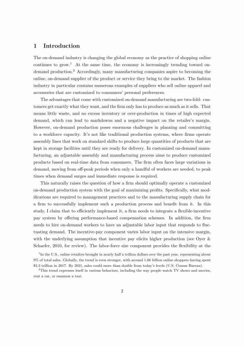
1 Introduction

The on-demand industry is changing the global economy as the practice of shopping online

continues to grow.1 At the same time, the economy is increasingly trending toward on-

demand production.2 Accordingly, many manufacturing companies aspire to becoming the

online, on-demand supplier of the product or service they bring to the market. The fashion

industry in particular contains numerous examples of suppliers who sell online apparel and

accessories that are customized to consumers’ personal preferences.

The advantages that come with customized on-demand manufacturing are two-fold: cus-

tomers get exactly what they want, and the firm only has to produce as much as it sells. That

means little waste, and no excess inventory or over-production in times of high expected

demand, which can lead to markdowns and a negative impact on the retailer’s margin.

However, on-demand production poses enormous challenges in planning and committing

to a workforce capacity. It’s not like traditional production systems, where firms operate

assembly lines that work on standard shifts to produce large quantities of products that are

kept in storage facilities until they are ready for delivery. In customized on-demand manu-

facturing, an adjustable assembly and manufacturing process aims to produce customized

products based on real-time data from consumers. The firm often faces large variations in

demand, moving from off-peak periods when only a handful of workers are needed, to peak

times when demand surges and immediate response is required.

This naturally raises the question of how a firm should optimally operate a customized

on-demand production system with the goal of maximizing profits. Specifically, what mod-

ifications are required to management practices and to the manufacturing supply chain for

a firm to successfully implement such a production process and benefit from it. In this

study, I claim that to efficiently implement it, a firm needs to integrate a flexible-incentive

pay system by offering performance-based compensation schemes. In addition, the firm

needs to hire on-demand workers to have an adjustable labor input that responds to fluc-

tuating demand. The incentive-pay component varies labor input on the intensive margin,

with the underlying assumption that incentive pay elicits higher production (see Oyer &

Schaefer, 2010, for review). The labor-force size component provides the flexibility at the

1In the U.S., online retailers brought in nearly half a trillion dollars over the past year, representing about

9% of total sales. Globally, the trend is even stronger, with around 1.66 billion online shoppers having spent

$2.3 trillion in 2017. By 2021, sales could more than double from today’s levels (U.S. Census Bureau).2This trend expresses itself in various behaviors, including the way people watch TV shows and movies,

rent a car, or summon a taxi.

2

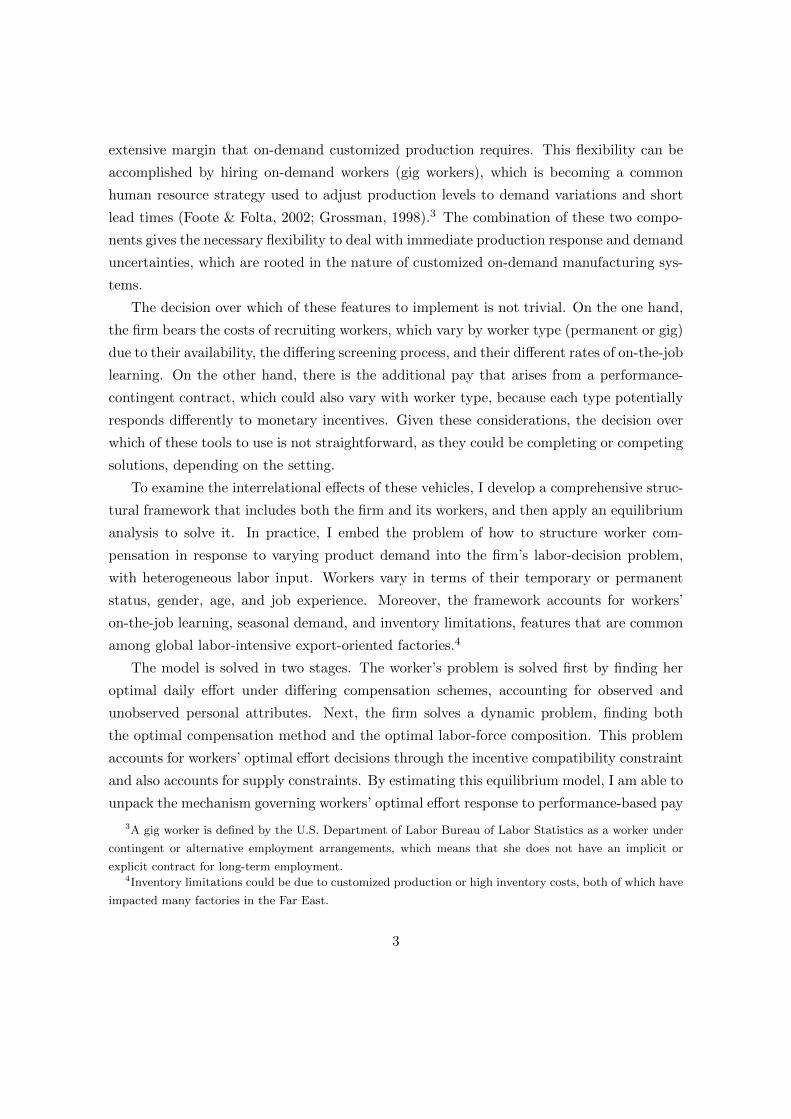
extensive margin that on-demand customized production requires. This flexibility can be

accomplished by hiring on-demand workers (gig workers), which is becoming a common

human resource strategy used to adjust production levels to demand variations and short

lead times (Foote & Folta, 2002; Grossman, 1998).3 The combination of these two compo-

nents gives the necessary flexibility to deal with immediate production response and demand

uncertainties, which are rooted in the nature of customized on-demand manufacturing sys-

tems.

The decision over which of these features to implement is not trivial. On the one hand,

the firm bears the costs of recruiting workers, which vary by worker type (permanent or gig)

due to their availability, the differing screening process, and their different rates of on-the-job

learning. On the other hand, there is the additional pay that arises from a performance-

contingent contract, which could also vary with worker type, because each type potentially

responds differently to monetary incentives. Given these considerations, the decision over

which of these tools to use is not straightforward, as they could be completing or competing

solutions, depending on the setting.

To examine the interrelational effects of these vehicles, I develop a comprehensive struc-

tural framework that includes both the firm and its workers, and then apply an equilibrium

analysis to solve it. In practice, I embed the problem of how to structure worker com-

pensation in response to varying product demand into the firm’s labor-decision problem,

with heterogeneous labor input. Workers vary in terms of their temporary or permanent

status, gender, age, and job experience. Moreover, the framework accounts for workers’

on-the-job learning, seasonal demand, and inventory limitations, features that are common

among global labor-intensive export-oriented factories.4

The model is solved in two stages. The worker’s problem is solved first by finding her

optimal daily effort under differing compensation schemes, accounting for observed and

unobserved personal attributes. Next, the firm solves a dynamic problem, finding both

the optimal compensation method and the optimal labor-force composition. This problem

accounts for workers’ optimal effort decisions through the incentive compatibility constraint

and also accounts for supply constraints. By estimating this equilibrium model, I am able to

unpack the mechanism governing workers’ optimal effort response to performance-based pay

3A gig worker is defined by the U.S. Department of Labor Bureau of Labor Statistics as a worker under

contingent or alternative employment arrangements, which means that she does not have an implicit or

explicit contract for long-term employment.4Inventory limitations could be due to customized production or high inventory costs, both of which have

impacted many factories in the Far East.

3

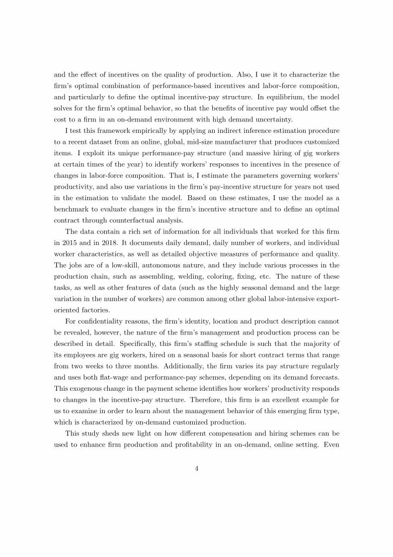
and the effect of incentives on the quality of production. Also, I use it to characterize the

firm’s optimal combination of performance-based incentives and labor-force composition,

and particularly to define the optimal incentive-pay structure. In equilibrium, the model

solves for the firm’s optimal behavior, so that the benefits of incentive pay would offset the

cost to a firm in an on-demand environment with high demand uncertainty.

I test this framework empirically by applying an indirect inference estimation procedure

to a recent dataset from an online, global, mid-size manufacturer that produces customized

items. I exploit its unique performance-pay structure (and massive hiring of gig workers

at certain times of the year) to identify workers’ responses to incentives in the presence of

changes in labor-force composition. That is, I estimate the parameters governing workers’

productivity, and also use variations in the firm’s pay-incentive structure for years not used

in the estimation to validate the model. Based on these estimates, I use the model as a

benchmark to evaluate changes in the firm’s incentive structure and to define an optimal

contract through counterfactual analysis.

The data contain a rich set of information for all individuals that worked for this firm

in 2015 and in 2018. It documents daily demand, daily number of workers, and individual

worker characteristics, as well as detailed objective measures of performance and quality.

The jobs are of a low-skill, autonomous nature, and they include various processes in the

production chain, such as assembling, welding, coloring, fixing, etc. The nature of these

tasks, as well as other features of data (such as the highly seasonal demand and the large

variation in the number of workers) are common among other global labor-intensive export-

oriented factories.

For confidentiality reasons, the firm’s identity, location and product description cannot

be revealed, however, the nature of the firm’s management and production process can be

described in detail. Specifically, this firm’s staffing schedule is such that the majority of

its employees are gig workers, hired on a seasonal basis for short contract terms that range

from two weeks to three months. Additionally, the firm varies its pay structure regularly

and uses both flat-wage and performance-pay schemes, depending on its demand forecasts.

This exogenous change in the payment scheme identifies how workers’ productivity responds

to changes in the incentive-pay structure. Therefore, this firm is an excellent example for

us to examine in order to learn about the management behavior of this emerging firm type,

which is characterized by on-demand customized production.

This study sheds new light on how different compensation and hiring schemes can be

used to enhance firm production and profitability in an on-demand, online setting. Even

4

though these types of practices are prevalent today, there is no previous study that incor-

porates these features into a unified framework and examines their interrelational effects on

firms’ optimal labor-management decisions.

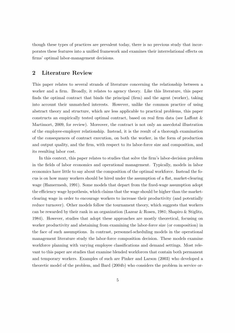
2 Literature Review

This paper relates to several strands of literature concerning the relationship between a

worker and a firm. Broadly, it relates to agency theory. Like this literature, this paper

finds the optimal contract that binds the principal (firm) and the agent (worker), taking

into account their unmatched interests. However, unlike the common practice of using

abstract theory and structure, which are less applicable to practical problems, this paper

constructs an empirically tested optimal contract, based on real firm data (see Laffont &

Martimort, 2009, for review). Moreover, the contract is not only an anecdotal illustration

of the employee-employer relationship. Instead, it is the result of a thorough examination

of the consequences of contract execution, on both the worker, in the form of production

and output quality, and the firm, with respect to its labor-force size and composition, and

its resulting labor cost.

In this context, this paper relates to studies that solve the firm’s labor-decision problem

in the fields of labor economics and operational management. Typically, models in labor

economics have little to say about the composition of the optimal workforce. Instead the fo-

cus is on how many workers should be hired under the assumption of a flat, market-clearing

wage (Hamermesh, 1991). Some models that depart from the fixed-wage assumption adopt

the efficiency wage hypothesis, which claims that the wage should be higher than the market-

clearing wage in order to encourage workers to increase their productivity (and potentially

reduce turnover). Other models follow the tournament theory, which suggests that workers

can be rewarded by their rank in an organization (Lazear & Rosen, 1981; Shapiro & Stiglitz,

1984). However, studies that adopt these approaches are mostly theoretical, focusing on

worker productivity and abstaining from examining the labor-force size (or composition) in

the face of such assumptions. In contrast, personnel-scheduling models in the operational

management literature study the labor-force composition decision. These models examine

workforce planning with varying employee classifications and demand settings. Most rele-

vant to this paper are studies that examine blended workforces that contain both permanent

and temporary workers. Examples of such are Pinker and Larson (2003) who developed a

theoretic model of the problem, and Bard (2004b) who considers the problem in service or-

5

ganizations, incorporating differences in employee skill levels as well as demand uncertainty.

A more recent paper by Dong and Ibrahim (2017) shows that the hiring decision depends

on the pool of gig workers, the operating costs, and customer demand. However, this strand

of literature is heavily theoretical, with applications and solutions based on simulations and

mathematical programming, and thus less relevant to practical problems.

This paper takes a unique stand, applying an empirical equilibrium approach that incor-

porates the workforce size and composition decisions with the decision on the nature of the

contract, as these aspects are intertwined. In doing so, it unpacks the firm’s “black box” as

viewed by labor economists, and expands the set of factors considered by operational man-

agement researchers by introducing the new and pertinent margin of labor-contract type into

the problem, and taking an empirical approach to finding the optimal labor-management

behavior.

Although the extensive operational management literature covers various factors that

affect firms’ hiring decisions, it usually overlooks the crucial feature of employees’ production

heterogeneity over time. In most models, there is an implied assumption that employees

are homogeneous in the sense that they reach their highest sustainable production capacity

immediately upon joining the firm. In practice, employees have different abilities, and

these abilities change over time. That is, employees learn on the job and, as a result, their

production ability increases over time. This feature is particularly important when hiring

on-demand workers, because these workers are hired for short-term work, when production

distortions are presumably at their peak. Thus, the consideration of such distortions is

critical, as it is costly and could affect hiring decisions. Stratman, Roth, and Gilland

(2004) identify this gap and build a theoretical model that takes into account dynamics

of workforce skill levels in the case of a blended workforce. At the core of the analysis,

there is a premise that temporary workers have relatively less skill, and therefore have

higher average production times, higher average defect rates associated with their assembly

activity, and lower rates of learning. These are strong assumptions that do not necessarily

hold in practice, and, in particular, will be shown not to hold in the framework used in this

paper. There is a need to build a model that captures the learning patterns exhibited in

the real data, which is one of the goals of this paper.

Finally, to complete the description of the relationship between a worker and a firm,

one should understand the linkage between production and contract types. At the core

of economists’ attention are two main questions relating to this concept: how workers

respond to a given set of incentives, and what the optimal set of incentives are that an

6

employer should provide. Many studies in personnel and labor economics have answered

the first question and established a positive relationship between incentives and productivity,

without distinguishing between worker types (see Oyer & Schaefer, 2010, for review). Papers

in operations management focus on gig workers and examine firms’ operational and pricing

decisions. Specifically, empirical studies focus on jobs of a self-scheduling nature performed

by independent providers, such as ride-hailing service drivers. Chen and Sheldon (2016)

show that dynamic wage schemes can lead drivers to work more hours by analyzing data

from 25 million rides. Hall et al. (2018) use differences in timing and city size, as well as

exogenous fare changes, to identify the impact of the fare on drivers’ hourly earnings.

... workers a This paper answers questions of a similar flavor with three major dif-

ferences. First, the job environment considered is in manufacturing, not service. Second,

workers are not self-scheduling but rather assigned to shifts by their manager. And last, the

workforce arrangement is such that both permanent workers and gig workers are present at

all times. Manufacturers no longer consider the practice of hiring gig workers in addition

to permanent workers a short-term solution. Instead, it has become a common human re-

source strategy used to adjust production to demand variation and short demand lead times

(Foote & Folta, 2002; Grossman, 1998). Yet, there has been little academic research aimed

at understanding the management practices applied to gig workers in such an environment,

particularly the role that incentive schemes play in this type of blended workforce. This

is surprising, because pay incentives are commonly instituted in gig-type jobs, where there

is no established relationship between the worker and the employer, and tasks are time-

sensitive. This paper fills the gap by identifying how different types of workers respond

to pay incentives, defining the firm’s optimal management behavior in such a setup, and

characterizing an optimal contract.

Apart from the distinction between worker types, the analysis also identifies the differ-

ence in response to incentives by gender. By doing so, this paper joins a pool of studies

that examine the effects of competition on performance by gender. In particular, a study

by Gneezy, Niederle, and Rustichini (2003) suggests that the observation of small numbers

of women in top positions is a result of men being more strongly motivated by competitive

incentives or more effective in competitive environments than women. Most studies that

examine this explanation show evidence to support it (Delfgaauw, Dur, Sol, & Verbeke,

2013; Jurajda & Munich, 2011; Ors, Palomino, & Peyrache, 2013). This paper, however,

presents evidence that does not align with this view, as the gender gap in response to in-

centives varies based on worker type. Specifically, female gig workers are on average more

7

productive than males under incentivepay, while the difference in response to incentives

between male and female permanent workers is not statistically different than zero.

With few exceptions, the majority of the empirical papers that examine the relationship

between incentives and productivity use reduced-form methods. The paper most similar

to this one is Shearer (2004), which also uses a comprehensive structural framework to

identify the underlying mechanism behind workers’ responses to incentives. This paper

goes beyond Shearer’s work by also modeling firms’ decisions in an equilibrium framework,

with the goal of linking productivity and profitability. Even though it is clear that firms

maximize discounted profits and not productivity, many studies tend to ignore this non-

trivial linkage. Freeman and Kleiner (2005) illustrate how incentives and profits are not

necessarily positively related, as they found that the abolition of performance pay reduced

productivity but increased profits as quality rose in the absence of production incentives.

The use of structural modeling to study the underlying mechanisms behind performance

incentives on both the worker and the firm sides enables assessment of the sensitivity of the

estimates to alterations in the economic environment, and thus enables us to make headway

in constructing the optimal contract as a counterfactual analysis.

3 Data and Settings

3.1 General

The recent micro-data used in this paper is from an online, global, mid-size manufacturer

that produces customized items. The data contain a rich set of information for all individuals

that worked for the firm in 2015 and in 2018. During these periods the management

adopted new compensation practices. Specifically, around the months of February 2015

and December 2018, the management deviated from its usual pay structure, a flat hourly

wage, and established a performance-pay scheme, with the goal of inducing productivity in

times of demand peak. The data from 2018 is utilized as the main data source throughout

the paper, as it includes a larger workforce and provides detailed information about the

quality of production and production score (which will be discussed in detail later). The

data from 2015 includes fewer workers and partial quality measures, and thus are used to

perform out-of-sample validation to test the assumptions of the model, and to realistically

compare its forecasting performance against other models.

Although the data provide information about all production process steps, the analysis

restricts attention to the assembly department for several reasons. First and foremost, this

8

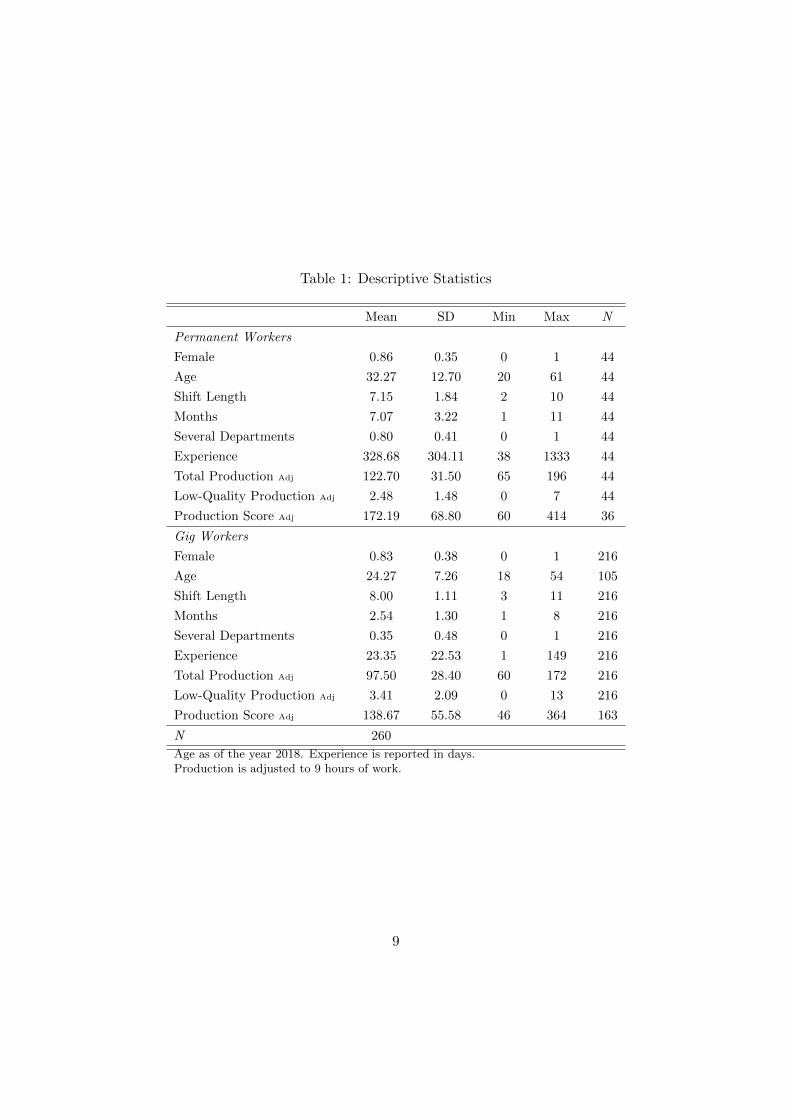
Table 1: Descriptive Statistics

Mean SD Min Max N

Permanent Workers

Female 0.86 0.35 0 1 44

Age 32.27 12.70 20 61 44

Shift Length 7.15 1.84 2 10 44

Months 7.07 3.22 1 11 44

Several Departments 0.80 0.41 0 1 44

Experience 328.68 304.11 38 1333 44

Total Production Adj 122.70 31.50 65 196 44

Low-Quality Production Adj 2.48 1.48 0 7 44

Production Score Adj 172.19 68.80 60 414 36

Gig Workers

Female 0.83 0.38 0 1 216

Age 24.27 7.26 18 54 105

Shift Length 8.00 1.11 3 11 216

Months 2.54 1.30 1 8 216

Several Departments 0.35 0.48 0 1 216

Experience 23.35 22.53 1 149 216

Total Production Adj 97.50 28.40 60 172 216

Low-Quality Production Adj 3.41 2.09 0 13 216

Production Score Adj 138.67 55.58 46 364 163

N 260

Age as of the year 2018. Experience is reported in days.Production is adjusted to 9 hours of work.

9

department is the only one along the production chain that is solely based on human-capital

labor and involves no machines or technology. This fact enables us to identify the trade-off

between labor-effort and quantity, which stands at the core of this paper, and eliminates

alternative trade-offs, such as labor-capital substitution. Second, the assembly department

is the largest in the plant as 95 percent of the output requires assembly. This fact makes

the total number of orders received in a given day a good proxy for workers’ workload.

Controlling for such features is crucial in an analysis that considers an unstable working

environment, where demand levels and workforce size vary on a daily basis. Lastly, the

assembly department is the last station the items pass through before reaching the quality-

assurance department, a fact that makes the quality measure most accurate, and prevents

records of false failures resulting.

3.2 Employment

The classification of workers into types – permanent or gig – is based on employment data

recorded by the firm’s personnel department. For each worker observed, there are records of

employment dates,5 which are used to infer whether a worker was hired as a gig worker with

a short-term contract or as a permanent worker with a long-term contract. By combining the

employment information with daily attendance records, I was able to generate an experience

measure that counts the number of days the worker actually attended work.6 Table 1 shows

that during the year of 2018, 216 (83 percent) of the 260 workers who worked in the assembly

department were gig workers. As expected, the average number of days of experience among

gig-workers is significantly lower than that of permanent workers. This is also true for the

number of months each type of worker is observed in the data.

The employment records contain information about the workers’ gender, and depending

on the worker’s type, the data also capture their ages. Originally, the personnel department

only recorded a worker’s date of birth if she was hired under a long-term contract. Once

we began collaborating, however, they started to record gig workers’ birthdates as well.

Thus, the dataset includes the ages of all permanent workers and the ages of gig workers

that were hired towards the end of 2018. A comparison of the gender composition of the

worker types, as presented in Table 1, reveals patterns that are similar. That is, females

are more attracted to assembly jobs irrespective of worker type, as the share of females

5In cases of repeated employment, all documented dates are considered.6For employees whose employment start date occurred prior to the beginning of the data, the number of

days of experience is approximated based on the observed data.

10

are 86 percent and 83 percent for permanent workers and gig workers, respectively. This

difference is not statistically significant. The statistics pertaining to the age of the workers

by type indicate an interesting pattern, and imply that the groups permanent workers

and gig workers are inherently different. That is, gig workers are on average eight years

younger than permanent workers, a difference that is statistically significant. Looking at

the descriptive characteristics creates an image of a typical gig worker – a young woman,

presumably a student, who wishes to fill the spaces in her schedule with non-binding work.

3.3 Production

The detailed production dataset was assembled from several sources. First, the total pro-

duction records were generated by a sophisticated monitoring system that documents daily

personal output for each worker at each workstation. Once an order is placed online, the

production process begins with the generation of a barcode for the ordered item. When a

worker starts to work on an item, she scans this barcode, an action that links the item to

herself and her workstation. Aggregation of this information generates a precise database

of workers’ daily production at each step in the production chain. This system was initially

installed for reasons other than the implementation of the performance-pay system, thus

its cost can be ignored when analyzing the trade-off between productivity and profitability.

Second, production quality measures are inferred from the quality-assurance department

records. For each item, this department’s records indicate whether it passed or failed a

quality check, and in the case of a failure, the record specifies the reason(s). Hence, as each

item is linked to all of the workers involved in its production, one can deduce the amount

of low-quality output generated by each worker. Lastly, each worker-day observation has

been matched with a shift-length record documented by the plant’s attendance system. I

use this data to adjust workers’ production by the number of hours worked, and thus create

a uniform and comparable production measure.

In addition to the production volume and quality, the data include records of production

score for each worker-day observation. The key difference between production score and

“regular” production is that the former takes into account the complexity associated with

assembling each item. This measure is used in the bonus-pay scheme, which is established

based on production-score. This adjustment eliminates the incentive of assembling only

items that can be finished quickly, as it does not pay workers merely based on production

quantities. Instead, it gives a higher weight for items with a higher score measure. In prac-

tice, the scoring menu was established during the year of 2018, and was finalized before the

11

implementation of the incentive scheme, towards the end of 2018. Thus, fewer observations

are included in the examination of the scheme as the analysis is restricted to the months of

October, November and December.

Table 1 summarizes the production information separately for permanent workers and

gig workers. The average shift length across all observations is 7.8 hours, a figure that is

very similar between worker types. Since shift length is determined by the manager and not

the worker, this is an expected outcome. Comparison between the average daily production

and score of each type, however, implies a dramatic difference in which permanent workers

are more productive than gig workers. Although this conclusion may seem intuitive, as it

is presumably assumed that permanent workers are more skilled and were more carefully

selected than gig workers, it is in fact misleading. Workers’ daily productivity is in fact

impacted by the demand and number of workers present in a given day. As both gig workers

and permanent workers are working at times under intrinsically different conditions, merely

comparing descriptive evidence yields an incomplete picture. In order to reliably compare

the productivity levels of permanent workers and gig workers, the demand, the number of

workers, and the offered incentive structure should all be taken into account, as is done

later in this paper.

3.4 Demand

The daily demand variable represents the sum of all orders placed online in a given day.

Figure 1 displays a time series of the average daily orders over the weeks of 2018. As

evident from the figure, demand is characterized by extreme seasonality around three annual

holidays – Valentine’s Day, Mother’s Day and Christmas, represented by gray lines, in this

order. The firm’s strict production policy is a key feature in explaining this demand pattern.

Within the plant there are up to four days of production, starting on the day the order is

placed and ending on the day the item is shipped, and outside the plant’s hands, the firm

guarantees its consumers the minimum possible shipment lead time, depending on where

the item is being shipped to. Combining this policy with having all products customized

to consumers’ preferences creates the seasonal demand pattern observed in the figure. The

demand peaks are as much as five times higher than the average volume in casual periods,

and they last from a week to two months. In fact, this pattern is not specific to the year of

2018, and is evident in the 2015 data as well, an observation that supports the assumption

that demand is predictable with high certainty. As these unusually intense and foreseeable

periods evoke the need to increase production, the firm uses two tools to prepare for it:

12

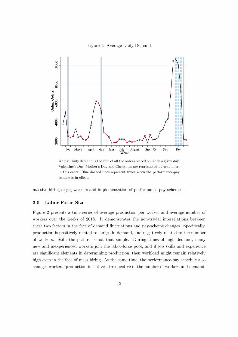
Figure 1: Average Daily Demand

Notes: Daily demand is the sum of all the orders placed online in a given day.

Valentine’s Day, Mother’s Day and Christmas are represented by gray lines,

in this order. Blue dashed lines represent times when the performance-pay

scheme is in effect.

massive hiring of gig workers and implementation of performance-pay schemes.

3.5 Labor-Force Size

Figure 2 presents a time series of average production per worker and average number of

workers over the weeks of 2018. It demonstrates the non-trivial interrelations between

these two factors in the face of demand fluctuations and pay-scheme changes. Specifically,

production is positively related to surges in demand, and negatively related to the number

of workers. Still, the picture is not that simple. During times of high demand, many

new and inexperienced workers join the labor-force pool, and if job skills and experience

are significant elements in determining production, then workload might remain relatively

high even in the face of mass hiring. At the same time, the performance-pay schedule also

changes workers’ production incentives, irrespective of the number of workers and demand.

13

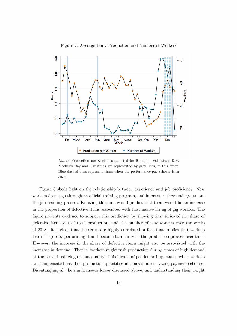
Figure 2: Average Daily Production and Number of Workers

Notes: Production per worker is adjusted for 9 hours. Valentine’s Day,

Mother’s Day and Christmas are represented by gray lines, in this order.

Blue dashed lines represent times when the performance-pay scheme is in

effect.

Figure 3 sheds light on the relationship between experience and job proficiency. New

workers do not go through an official training program, and in practice they undergo an on-

the-job training process. Knowing this, one would predict that there would be an increase

in the proportion of defective items associated with the massive hiring of gig workers. The

figure presents evidence to support this prediction by showing time series of the share of

defective items out of total production, and the number of new workers over the weeks

of 2018. It is clear that the series are highly correlated, a fact that implies that workers

learn the job by performing it and become familiar with the production process over time.

However, the increase in the share of defective items might also be associated with the

increases in demand. That is, workers might rush production during times of high demand

at the cost of reducing output quality. This idea is of particular importance when workers

are compensated based on production quantities in times of incentivizing payment schemes.

Disentangling all the simultaneous forces discussed above, and understanding their weight

14

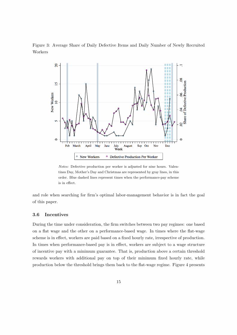
Figure 3: Average Share of Daily Defective Items and Daily Number of Newly Recruited

Workers

Notes: Defective production per worker is adjusted for nine hours. Valen-

tines Day, Mother’s Day and Christmas are represented by gray lines, in this

order. Blue dashed lines represent times when the performance-pay scheme

is in effect.

and role when searching for firm’s optimal labor-management behavior is in fact the goal

of this paper.

3.6 Incentives

During the time under consideration, the firm switches between two pay regimes: one based

on a flat wage and the other on a performance-based wage. In times where the flat-wage

scheme is in effect, workers are paid based on a fixed hourly rate, irrespective of production.

In times when performance-based pay is in effect, workers are subject to a wage structure

of incentive pay with a minimum guarantee. That is, production above a certain threshold

rewards workers with additional pay on top of their minimum fixed hourly rate, while

production below the threshold brings them back to the flat-wage regime. Figure 4 presents

15

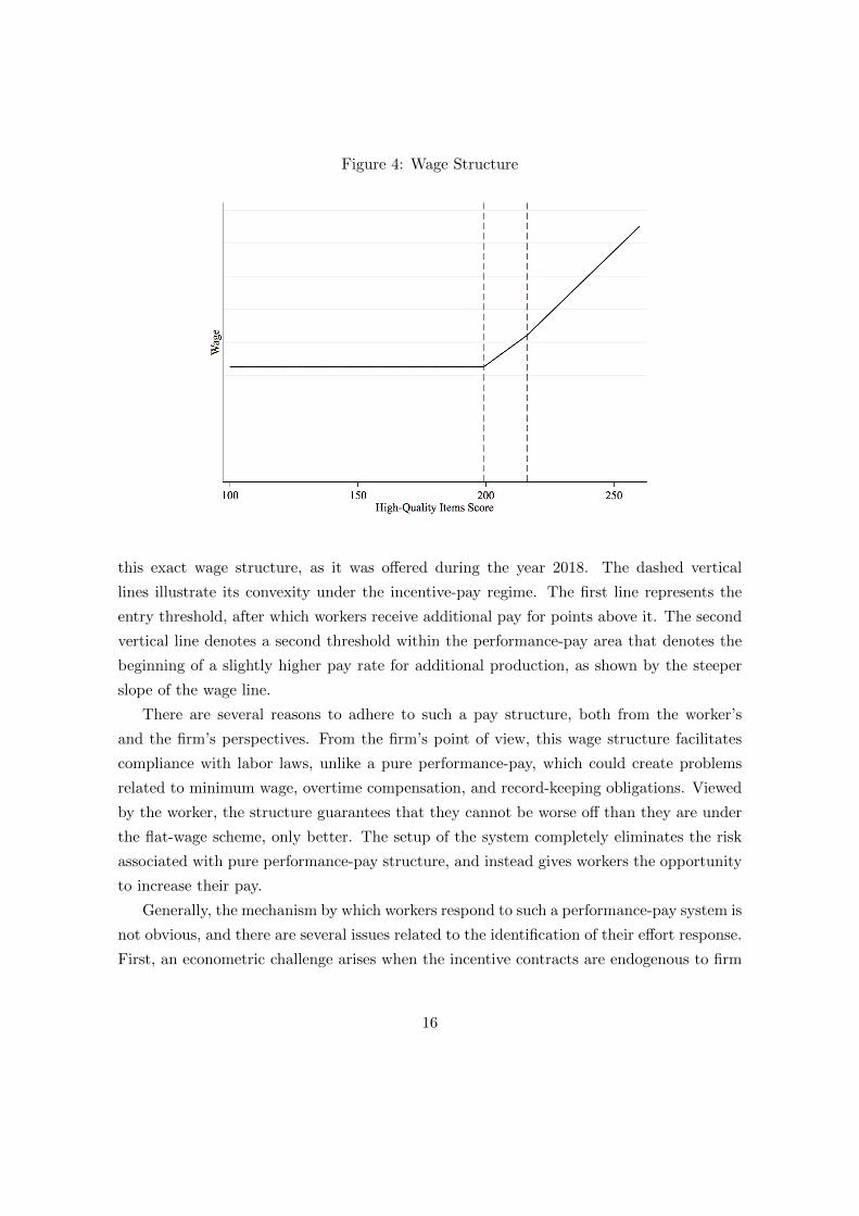
Figure 4: Wage Structure

this exact wage structure, as it was offered during the year 2018. The dashed vertical

lines illustrate its convexity under the incentive-pay regime. The first line represents the

entry threshold, after which workers receive additional pay for points above it. The second

vertical line denotes a second threshold within the performance-pay area that denotes the

beginning of a slightly higher pay rate for additional production, as shown by the steeper

slope of the wage line.

There are several reasons to adhere to such a pay structure, both from the worker’s

and the firm’s perspectives. From the firm’s point of view, this wage structure facilitates

compliance with labor laws, unlike a pure performance-pay, which could create problems

related to minimum wage, overtime compensation, and record-keeping obligations. Viewed

by the worker, the structure guarantees that they cannot be worse off than they are under

the flat-wage scheme, only better. The setup of the system completely eliminates the risk

associated with pure performance-pay structure, and instead gives workers the opportunity

to increase their pay.

Generally, the mechanism by which workers respond to such a performance-pay system is

not obvious, and there are several issues related to the identification of their effort response.

First, an econometric challenge arises when the incentive contracts are endogenous to firm

16

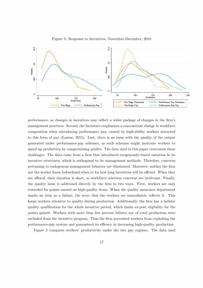
Figure 5: Response to Incentives, November-December, 2018

performance, as changes in incentives may reflect a wider package of changes in the firm’s

management practices. Second, the literature emphasizes a concomitant change in workforce

composition when introducing performance pay, caused by high-ability workers attracted

to this form of pay (Lazear, 2015). Last, there is an issue with the quality of the output

generated under performance-pay schemes, as such schemes might motivate workers to

speed up production by compromising quality. The data used in this paper overcomes these

challenges. The data come from a firm that introduced exogenously-timed variation in its

incentive structures, which is orthogonal to its management methods. Therefore, concerns

pertaining to endogenous management behavior are eliminated. Moreover, neither the firm

nor the worker know beforehand when or for how long incentives will be offered. When they

are offered, their duration is short, so workforce selection concerns are irrelevant. Finally,

the quality issue is addressed directly by the firm in two ways. First, workers are only

rewarded for points earned on high-quality items. When the quality assurance department

marks an item as a failure, the score that the workers see immediately reflects it. This

keeps workers attentive to quality during production. Additionally, the firm has a holistic

quality qualification for the whole incentive period, which limits ex-post eligibility for the

points gained. Workers with more than five percent failures out of total production were

excluded from the incentive program. Thus the firm prevented workers from exploiting the

performance-pay system and guaranteed its efficacy in increasing high-quality production.

Figure 5 compares workers’ productivity under the two pay regimes. The data used

17

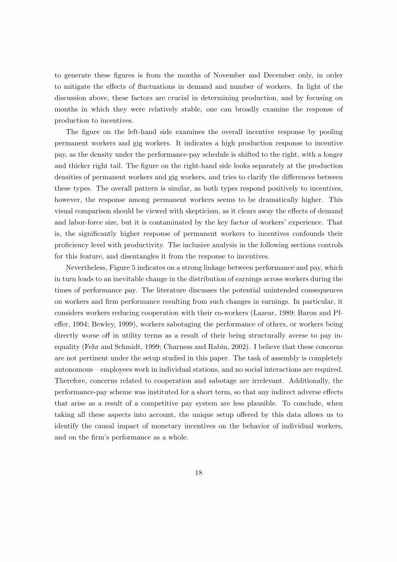
to generate these figures is from the months of November and December only, in order

to mitigate the effects of fluctuations in demand and number of workers. In light of the

discussion above, these factors are crucial in determining production, and by focusing on

months in which they were relatively stable, one can broadly examine the response of

production to incentives.

The figure on the left-hand side examines the overall incentive response by pooling

permanent workers and gig workers. It indicates a high production response to incentive

pay, as the density under the performance-pay schedule is shifted to the right, with a longer

and thicker right tail. The figure on the right-hand side looks separately at the production

densities of permanent workers and gig workers, and tries to clarify the differences between

these types. The overall pattern is similar, as both types respond positively to incentives,

however, the response among permanent workers seems to be dramatically higher. This

visual comparison should be viewed with skepticism, as it clears away the effects of demand

and labor-force size, but it is contaminated by the key factor of workers’ experience. That

is, the significantly higher response of permanent workers to incentives confounds their

proficiency level with productivity. The inclusive analysis in the following sections controls

for this feature, and disentangles it from the response to incentives.

Nevertheless, Figure 5 indicates on a strong linkage between performance and pay, which

in turn leads to an inevitable change in the distribution of earnings across workers during the

times of performance pay. The literature discusses the potential unintended consequences

on workers and firm performance resulting from such changes in earnings. In particular, it

considers workers reducing cooperation with their co-workers (Lazear, 1989; Baron and Pf-

effer, 1994; Bewley, 1999), workers sabotaging the performance of others, or workers being

directly worse off in utility terms as a result of their being structurally averse to pay in-

equality (Fehr and Schmidt, 1999; Charness and Rabin, 2002). I believe that these concerns

are not pertinent under the setup studied in this paper. The task of assembly is completely

autonomous – employees work in individual stations, and no social interactions are required.

Therefore, concerns related to cooperation and sabotage are irrelevant. Additionally, the

performance-pay scheme was instituted for a short term, so that any indirect adverse effects

that arise as a result of a competitive pay system are less plausible. To conclude, when

taking all these aspects into account, the unique setup offered by this data allows us to

identify the causal impact of monetary incentives on the behavior of individual workers,

and on the firm’s performance as a whole.

18

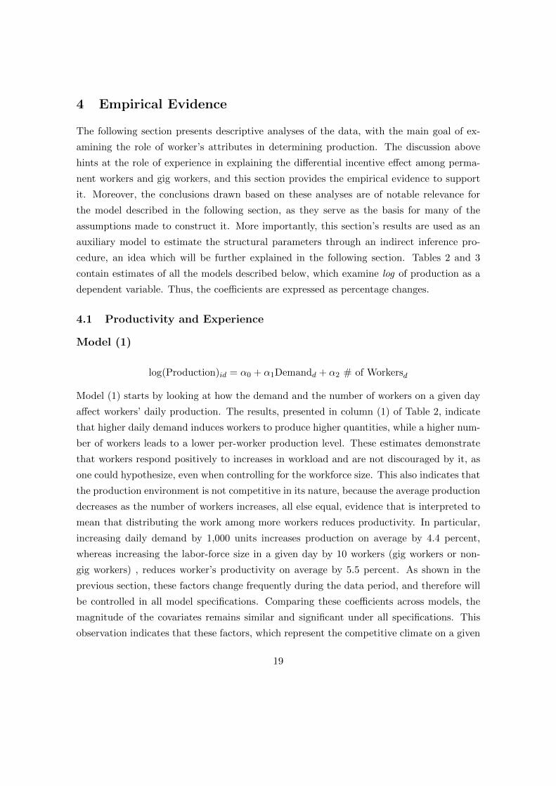
4 Empirical Evidence

The following section presents descriptive analyses of the data, with the main goal of ex-

amining the role of worker’s attributes in determining production. The discussion above

hints at the role of experience in explaining the differential incentive effect among perma-

nent workers and gig workers, and this section provides the empirical evidence to support

it. Moreover, the conclusions drawn based on these analyses are of notable relevance for

the model described in the following section, as they serve as the basis for many of the

assumptions made to construct it. More importantly, this section’s results are used as an

auxiliary model to estimate the structural parameters through an indirect inference pro-

cedure, an idea which will be further explained in the following section. Tables 2 and 3

contain estimates of all the models described below, which examine log of production as a

dependent variable. Thus, the coefficients are expressed as percentage changes.

4.1 Productivity and Experience

Model (1)

log(Production)id = α0 + α1Demandd + α2 # of Workersd

Model (1) starts by looking at how the demand and the number of workers on a given day

affect workers’ daily production. The results, presented in column (1) of Table 2, indicate

that higher daily demand induces workers to produce higher quantities, while a higher num-

ber of workers leads to a lower per-worker production level. These estimates demonstrate

that workers respond positively to increases in workload and are not discouraged by it, as

one could hypothesize, even when controlling for the workforce size. This also indicates that

the production environment is not competitive in its nature, because the average production

decreases as the number of workers increases, all else equal, evidence that is interpreted to

mean that distributing the work among more workers reduces productivity. In particular,

increasing daily demand by 1,000 units increases production on average by 4.4 percent,

whereas increasing the labor-force size in a given day by 10 workers (gig workers or non-

gig workers) , reduces worker’s productivity on average by 5.5 percent. As shown in the

previous section, these factors change frequently during the data period, and therefore will

be controlled in all model specifications. Comparing these coefficients across models, the

magnitude of the covariates remains similar and significant under all specifications. This

observation indicates that these factors, which represent the competitive climate on a given

19

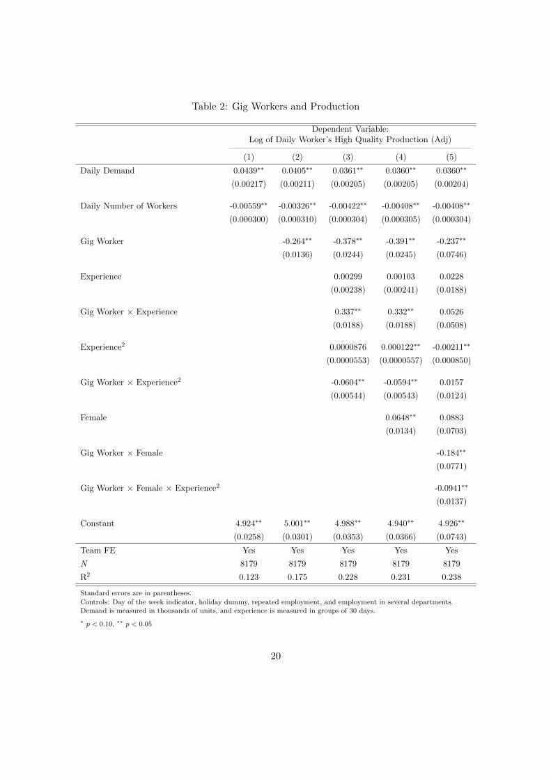
Table 2: Gig Workers and Production

Dependent Variable:Log of Daily Worker’s High Quality Production (Adj)

(1) (2) (3) (4) (5)

Daily Demand 0.0439∗∗ 0.0405∗∗ 0.0361∗∗ 0.0360∗∗ 0.0360∗∗

(0.00217) (0.00211) (0.00205) (0.00205) (0.00204)

Daily Number of Workers -0.00559∗∗ -0.00326∗∗ -0.00422∗∗ -0.00408∗∗ -0.00408∗∗

(0.000300) (0.000310) (0.000304) (0.000305) (0.000304)

Gig Worker -0.264∗∗ -0.378∗∗ -0.391∗∗ -0.237∗∗

(0.0136) (0.0244) (0.0245) (0.0746)

Experience 0.00299 0.00103 0.0228

(0.00238) (0.00241) (0.0188)

Gig Worker × Experience 0.337∗∗ 0.332∗∗ 0.0526

(0.0188) (0.0188) (0.0508)

Experience2 0.0000876 0.000122∗∗ -0.00211∗∗

(0.0000553) (0.0000557) (0.000850)

Gig Worker × Experience2 -0.0604∗∗ -0.0594∗∗ 0.0157

(0.00544) (0.00543) (0.0124)

Female 0.0648∗∗ 0.0883

(0.0134) (0.0703)

Gig Worker × Female -0.184∗∗

(0.0771)

Gig Worker × Female × Experience2 -0.0941∗∗

(0.0137)

Constant 4.924∗∗ 5.001∗∗ 4.988∗∗ 4.940∗∗ 4.926∗∗

(0.0258) (0.0301) (0.0353) (0.0366) (0.0743)

Team FE Yes Yes Yes Yes Yes

N 8179 8179 8179 8179 8179

R2 0.123 0.175 0.228 0.231 0.238

Standard errors are in parentheses.

Controls: Day of the week indicator, holiday dummy, repeated employment, and employment in several departments.Demand is measured in thousands of units, and experience is measured in groups of 30 days.

∗ p < 0.10, ∗∗ p < 0.05

20

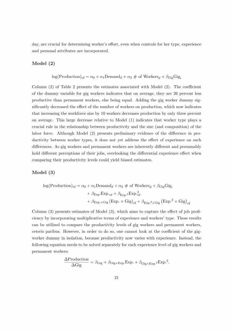
day, are crucial for determining worker’s effort, even when controls for her type, experience

and personal attributes are incorporated.

Model (2)

log(Production)id = α0 + α1Demandd + α2 # of Workersd + βGigGigi

Column (2) of Table 2 presents the estimates associated with Model (2). The coefficient

of the dummy variable for gig workers indicates that on average, they are 26 percent less

productive than permanent workers, else being equal. Adding the gig worker dummy sig-

nificantly decreased the effect of the number of workers on production, which now indicates

that increasing the workforce size by 10 workers decreases production by only three percent

on average. This large decrease relative to Model (1) indicates that worker type plays a

crucial rule in the relationship between productivity and the size (and composition) of the

labor force. Although Model (2) presents preliminary evidence of the difference in pro-

ductivity between worker types, it does not yet address the effect of experience on such

differences. As gig workers and permanent workers are inherently different and presumably

hold different perceptions of their jobs, overlooking the differential experience effect when

comparing their productivity levels could yield biased estimates.

Model (3)

log(Production)id = α0 + α1Demandd + α2 # of Workersd + βGigGigi

+ βExp.Exp.id + βExp.2Exp.2id

+ βExp.×Gig (Exp.×Gig)id + βExp.2×Gig

(Exp.2 ×Gig

)id

Column (3) presents estimates of Model (3), which aims to capture the effect of job profi-

ciency by incorporating multiplicative terms of experience and workers’ type. These results

can be utilized to compare the productivity levels of gig workers and permanent workers,

ceteris paribus. However, in order to do so, one cannot look at the coefficient of the gig-

worker dummy in isolation, because productivity now varies with experience. Instead, the

following equation needs to be solved separately for each experience level of gig workers and

permanent workers:

∆Production

∆Gig= βGig + βGig×Exp.Exp. + βGig×Exp.2Exp.2.

21

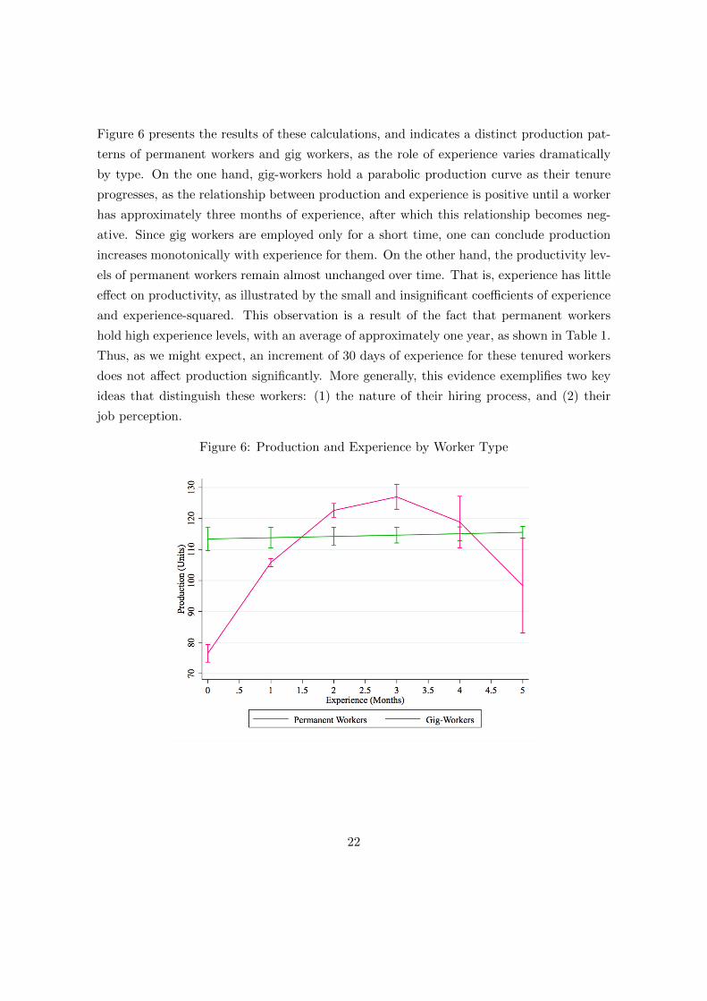
Figure 6 presents the results of these calculations, and indicates a distinct production pat-

terns of permanent workers and gig workers, as the role of experience varies dramatically

by type. On the one hand, gig-workers hold a parabolic production curve as their tenure

progresses, as the relationship between production and experience is positive until a worker

has approximately three months of experience, after which this relationship becomes neg-

ative. Since gig workers are employed only for a short time, one can conclude production

increases monotonically with experience for them. On the other hand, the productivity lev-

els of permanent workers remain almost unchanged over time. That is, experience has little

effect on productivity, as illustrated by the small and insignificant coefficients of experience

and experience-squared. This observation is a result of the fact that permanent workers

hold high experience levels, with an average of approximately one year, as shown in Table 1.

Thus, as we might expect, an increment of 30 days of experience for these tenured workers

does not affect production significantly. More generally, this evidence exemplifies two key

ideas that distinguish these workers: (1) the nature of their hiring process, and (2) their

job perception.

Figure 6: Production and Experience by Worker Type

22

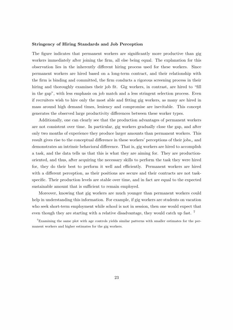
Stringency of Hiring Standards and Job Perception

The figure indicates that permanent workers are significantly more productive than gig

workers immediately after joining the firm, all else being equal. The explanation for this

observation lies in the inherently different hiring process used for these workers. Since

permanent workers are hired based on a long-term contract, and their relationship with

the firm is binding and committed, the firm conducts a rigorous screening process in their

hiring and thoroughly examines their job fit. Gig workers, in contrast, are hired to “fill

in the gap”, with less emphasis on job match and a less stringent selection process. Even

if recruiters wish to hire only the most able and fitting gig workers, as many are hired in

mass around high demand times, leniency and compromise are inevitable. This concept

generates the observed large productivity differences between these worker types.

Additionally, one can clearly see that the production advantages of permanent workers

are not consistent over time. In particular, gig workers gradually close the gap, and after

only two months of experience they produce larger amounts than permanent workers. This

result gives rise to the conceptual difference in these workers’ perceptions of their jobs,, and

demonstrates an intrinsic behavioral difference. That is, gig workers are hired to accomplish

a task, and the data tells us that this is what they are aiming for. They are production-

oriented, and thus, after acquiring the necessary skills to perform the task they were hired

for, they do their best to perform it well and efficiently. Permanent workers are hired

with a different perception, as their positions are secure and their contracts are not task-

specific. Their production levels are stable over time, and in fact are equal to the expected

sustainable amount that is sufficient to remain employed.

Moreover, knowing that gig workers are much younger than permanent workers could

help in understanding this information. For example, if gig workers are students on vacation

who seek short-term employment while school is not in session, then one would expect that

even though they are starting with a relative disadvantage, they would catch up fast. 7

7Examining the same plot with age controls yields similar patterns with smaller estimates for the per-

manent workers and higher estimates for the gig workers.

23

4.2 Gender and Performance of Gig Workers

Model (4)

log(Production)id = α0 + α1Demandd + α2 # of Workersd + βGigGigi

+ βExp.Exp.id + βExp.2Exp.2id

+ βExp.×Gig (Exp.×Gig)id + βExp.2×Gig

(Exp.2 ×Gig

)id

+ βFemaleFemalei + βFemale×Gig (Female×Gig)i

+ βFemale×Exp. (Female× Exp.)id + βFemale×Exp.2(Female× Exp.2

)id

+ βFemale×Exp.×Gig (Female× Exp.×Gig)id

+ βFemale×Exp.2×Gig

(Female× Exp.2 ×Gig

)id

Model (4) adds to the previous analysis by incorporating a dummy variable for gender,

as well as multiplicative terms of gender, worker’s type, and experience. The results pre-

sented in column(3) of Table 2 examine the aggregate gender effect, which indicates that

women are six percent more productive than men on average. To shed more light on the

gender differences between gig workers and non-gig workers, one should look at column

(4), which includes all of the interaction terms. The interpretation of the coefficients of

the dummy variables in the presence of these interactions is not straightforward, as both

gender and worker type are interacted with experience and experience-squared. A graphical

representation of the results is presented in Figure 7.

The figure examines the percentage change in productivity of females relative to males,

and indicates an interesting difference between worker types. Among gig-workers, the pro-

ductivity gap between females and males has a parabolic shape, with females being more

productive at almost all experience levels. Specifically, immediately after joining the firm

there is a 10-percent difference in favor of males, which flips to about five percent in favor

of females after 15 days of experience and climbs to 15 percent at 45 days of experience,

after which it decreases monotonically to zero. In contrast, among permanent workers the

pattern is different, as males are more productive than females at all experience levels,

however, this difference is not statistically significant. As the gender composition of gig

workers and permanent workers is similar, this result may suggest that female gig workers

hold different attitudes than their counterparts. In particular, it implies that female gig

workers are more competitive and production-oriented than male gig workers. Also, this

result could be attributed to young females being more committed to their jobs than males,

24

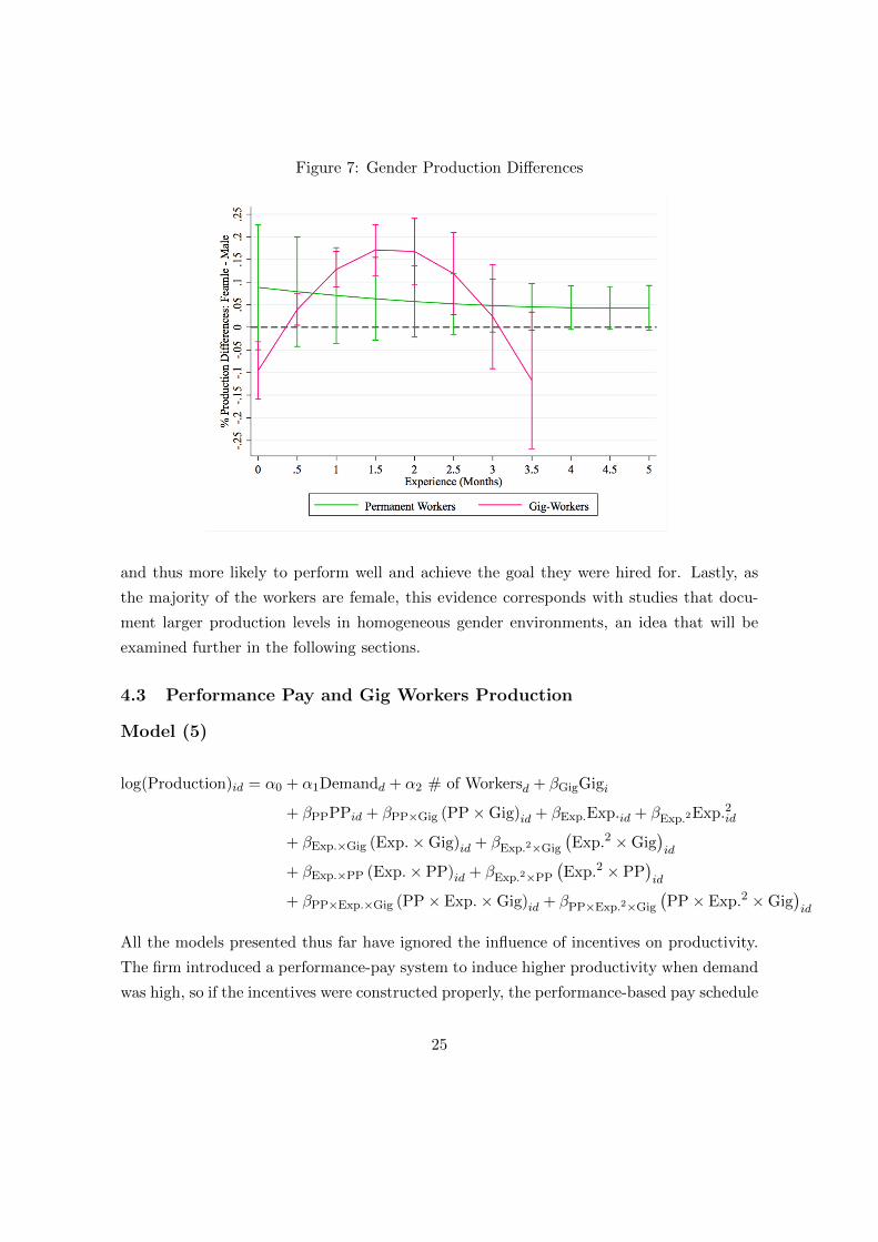
Figure 7: Gender Production Differences

and thus more likely to perform well and achieve the goal they were hired for. Lastly, as

the majority of the workers are female, this evidence corresponds with studies that docu-

ment larger production levels in homogeneous gender environments, an idea that will be

examined further in the following sections.

4.3 Performance Pay and Gig Workers Production

Model (5)

log(Production)id = α0 + α1Demandd + α2 # of Workersd + βGigGigi

+ βPPPPid + βPP×Gig (PP×Gig)id + βExp.Exp.id + βExp.2Exp.2id

+ βExp.×Gig (Exp.×Gig)id + βExp.2×Gig

(Exp.2 ×Gig

)id

+ βExp.×PP (Exp.× PP)id + βExp.2×PP

(Exp.2 × PP

)id

+ βPP×Exp.×Gig (PP× Exp.×Gig)id + βPP×Exp.2×Gig

(PP× Exp.2 ×Gig

)id

All the models presented thus far have ignored the influence of incentives on productivity.

The firm introduced a performance-pay system to induce higher productivity when demand

was high, so if the incentives were constructed properly, the performance-based pay schedule

25

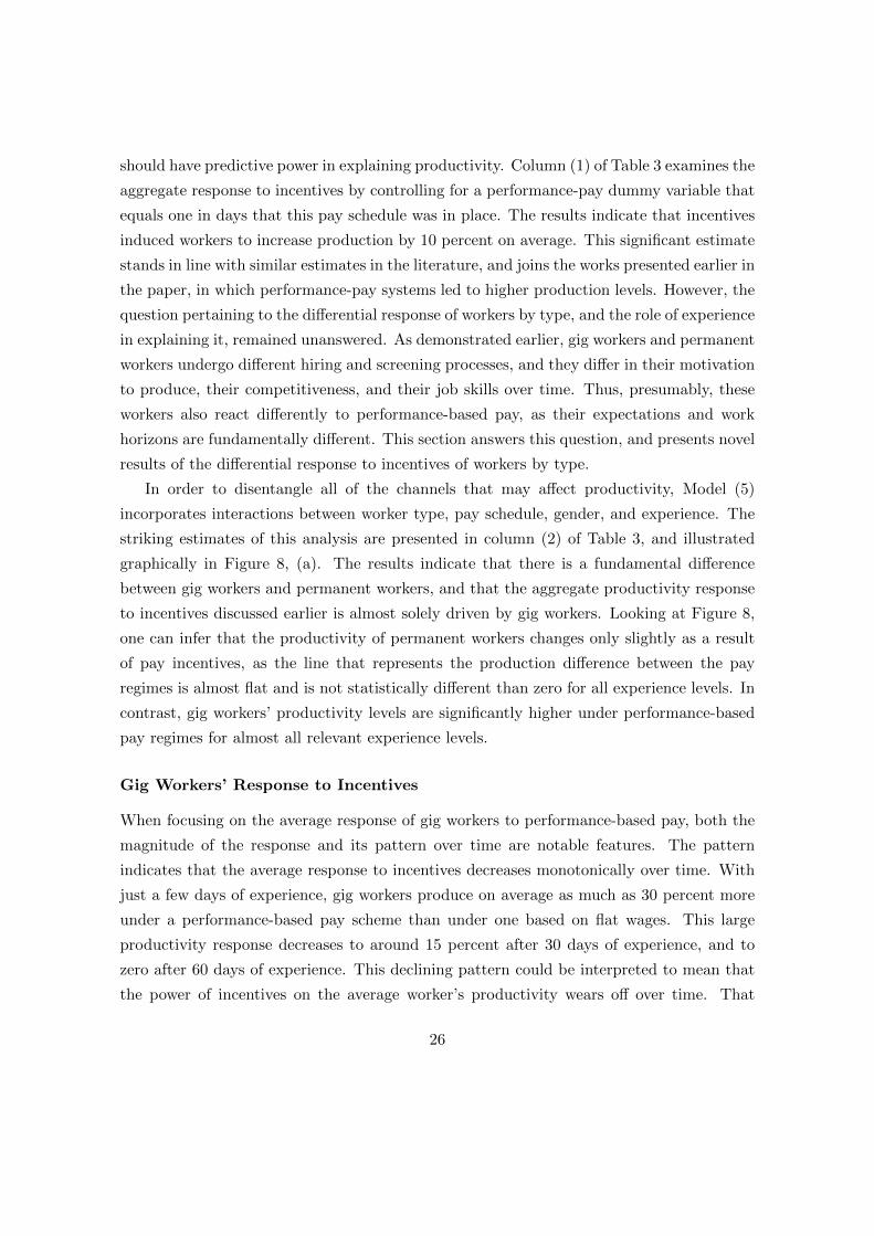
should have predictive power in explaining productivity. Column (1) of Table 3 examines the

aggregate response to incentives by controlling for a performance-pay dummy variable that

equals one in days that this pay schedule was in place. The results indicate that incentives

induced workers to increase production by 10 percent on average. This significant estimate

stands in line with similar estimates in the literature, and joins the works presented earlier in

the paper, in which performance-pay systems led to higher production levels. However, the

question pertaining to the differential response of workers by type, and the role of experience

in explaining it, remained unanswered. As demonstrated earlier, gig workers and permanent

workers undergo different hiring and screening processes, and they differ in their motivation

to produce, their competitiveness, and their job skills over time. Thus, presumably, these

workers also react differently to performance-based pay, as their expectations and work

horizons are fundamentally different. This section answers this question, and presents novel

results of the differential response to incentives of workers by type.

In order to disentangle all of the channels that may affect productivity, Model (5)

incorporates interactions between worker type, pay schedule, gender, and experience. The

striking estimates of this analysis are presented in column (2) of Table 3, and illustrated

graphically in Figure 8, (a). The results indicate that there is a fundamental difference

between gig workers and permanent workers, and that the aggregate productivity response

to incentives discussed earlier is almost solely driven by gig workers. Looking at Figure 8,

one can infer that the productivity of permanent workers changes only slightly as a result

of pay incentives, as the line that represents the production difference between the pay

regimes is almost flat and is not statistically different than zero for all experience levels. In

contrast, gig workers’ productivity levels are significantly higher under performance-based

pay regimes for almost all relevant experience levels.

Gig Workers’ Response to Incentives

When focusing on the average response of gig workers to performance-based pay, both the

magnitude of the response and its pattern over time are notable features. The pattern

indicates that the average response to incentives decreases monotonically over time. With

just a few days of experience, gig workers produce on average as much as 30 percent more

under a performance-based pay scheme than under one based on flat wages. This large

productivity response decreases to around 15 percent after 30 days of experience, and to

zero after 60 days of experience. This declining pattern could be interpreted to mean that

the power of incentives on the average worker’s productivity wears off over time. That

26

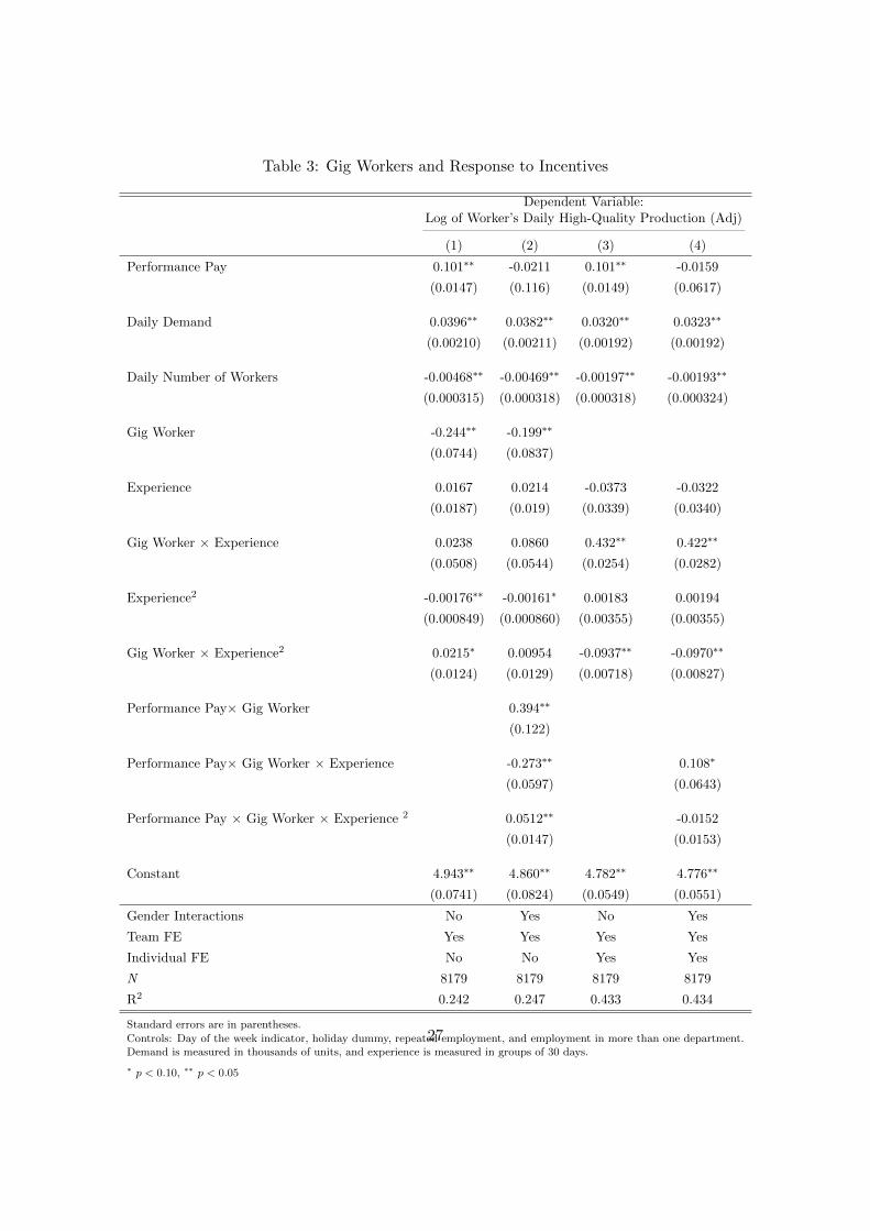
Table 3: Gig Workers and Response to Incentives

Dependent Variable:Log of Worker’s Daily High-Quality Production (Adj)

(1) (2) (3) (4)

Performance Pay 0.101∗∗ -0.0211 0.101∗∗ -0.0159

(0.0147) (0.116) (0.0149) (0.0617)

Daily Demand 0.0396∗∗ 0.0382∗∗ 0.0320∗∗ 0.0323∗∗

(0.00210) (0.00211) (0.00192) (0.00192)

Daily Number of Workers -0.00468∗∗ -0.00469∗∗ -0.00197∗∗ -0.00193∗∗

(0.000315) (0.000318) (0.000318) (0.000324)

Gig Worker -0.244∗∗ -0.199∗∗

(0.0744) (0.0837)

Experience 0.0167 0.0214 -0.0373 -0.0322

(0.0187) (0.019) (0.0339) (0.0340)

Gig Worker × Experience 0.0238 0.0860 0.432∗∗ 0.422∗∗

(0.0508) (0.0544) (0.0254) (0.0282)

Experience2 -0.00176∗∗ -0.00161∗ 0.00183 0.00194

(0.000849) (0.000860) (0.00355) (0.00355)

Gig Worker × Experience2 0.0215∗ 0.00954 -0.0937∗∗ -0.0970∗∗

(0.0124) (0.0129) (0.00718) (0.00827)

Performance Pay× Gig Worker 0.394∗∗

(0.122)

Performance Pay× Gig Worker × Experience -0.273∗∗ 0.108∗

(0.0597) (0.0643)

Performance Pay × Gig Worker × Experience 2 0.0512∗∗ -0.0152

(0.0147) (0.0153)

Constant 4.943∗∗ 4.860∗∗ 4.782∗∗ 4.776∗∗

(0.0741) (0.0824) (0.0549) (0.0551)

Gender Interactions No Yes No Yes

Team FE Yes Yes Yes Yes

Individual FE No No Yes Yes

N 8179 8179 8179 8179

R2 0.242 0.247 0.433 0.434

Standard errors are in parentheses.

Controls: Day of the week indicator, holiday dummy, repeated employment, and employment in more than one department.Demand is measured in thousands of units, and experience is measured in groups of 30 days.

∗ p < 0.10, ∗∗ p < 0.05

27

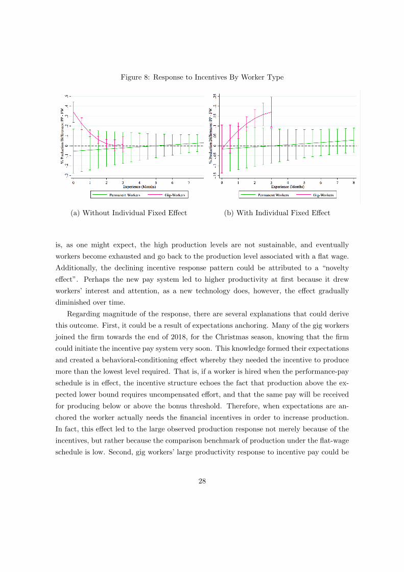
Figure 8: Response to Incentives By Worker Type

(a) Without Individual Fixed Effect (b) With Individual Fixed Effect

is, as one might expect, the high production levels are not sustainable, and eventually

workers become exhausted and go back to the production level associated with a flat wage.

Additionally, the declining incentive response pattern could be attributed to a “novelty

effect”. Perhaps the new pay system led to higher productivity at first because it drew

workers’ interest and attention, as a new technology does, however, the effect gradually

diminished over time.

Regarding magnitude of the response, there are several explanations that could derive

this outcome. First, it could be a result of expectations anchoring. Many of the gig workers

joined the firm towards the end of 2018, for the Christmas season, knowing that the firm

could initiate the incentive pay system very soon. This knowledge formed their expectations

and created a behavioral-conditioning effect whereby they needed the incentive to produce

more than the lowest level required. That is, if a worker is hired when the performance-pay

schedule is in effect, the incentive structure echoes the fact that production above the ex-

pected lower bound requires uncompensated effort, and that the same pay will be received

for producing below or above the bonus threshold. Therefore, when expectations are an-

chored the worker actually needs the financial incentives in order to increase production.

In fact, this effect led to the large observed production response not merely because of the

incentives, but rather because the comparison benchmark of production under the flat-wage

schedule is low. Second, gig workers’ large productivity response to incentive pay could be

28

explained by their marginal gains from incentives, which are conceptually different from

those of permanent workers. That is, when considering the expected job duration, the

marginal wage gain of $1 for a gig worker who works for a total of two weeks is dramat-

ically higher than that of a permanent worker who has already worked at the firm for a

year. Understanding that every additional unit of production could lead to a large relative

increase in wage is thus a potential channel that causes gig workers to increase production.

Lastly, as emphasized earlier, the higher production response of gig workers could be driven

by the fundamental difference between them and permanent workers. That is, gig workers

are young and ambitious, they are production-driven, motivated to fulfill the purpose they

were hired for, and desire to exploit as much gain as possible from their temporary position,

while permanent workers are less adventurous, seek stability, and thus remain at sustainable

production levels.

One unique feature of the data that has been overlooked so far is that many of the work-

ers are observed under both flat-wage and performance-pay systems. The associated data

enable an analysis of the each worker’s response to the incentive scheme, eliminating per-

sonal skills and attributes. Figure 8,(b) presents the results of this analysis. For permanent

workers, the figures indicate similar patterns when examining the average response or the

individual-specific response to incentives. For gig workers, however, a comparison between

the analyses is illuminating. The analysis with fixed effects reveals that the worker-specific

response to incentives is actually increasing with experience. Gig workers arrive at a relative

dis-advantage with respect to their job skills, but they were shown to learn the required

job skills quickly, and now the figure demonstrates that their acquired skills, combined with

their high ambition and motivation, lead to a significant monotone increase in response to

incentives over time.

5 Model

At the focus of this analysis stands a firm that wishes to satisfy its output demand opti-

mally with the objective of minimizing costs. The firm may choose to administer flat-wage

contracts, or to incentivize workers to increase their efforts by implementing a performance-

based pay system. In the latter scenario, the firm views workers’ effort endogenously, and

can potentially substitute labor quantity and effort. Therefore, in order to build a compre-

hensive framework of this problem, both the worker’s decision and the firm’s decision should

be closely analyzed. This section presents the model behind this framework and explains

29

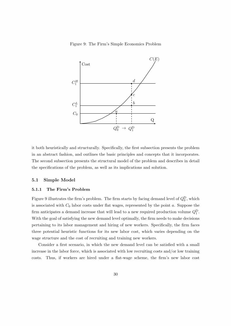
Figure 9: The Firm’s Simple Economics Problem

QD0

C0a

→ QD1

CL1

CH1

C(E)

b

c

d

Q

Cost

it both heuristically and structurally. Specifically, the first subsection presents the problem

in an abstract fashion, and outlines the basic principles and concepts that it incorporates.

The second subsection presents the structural model of the problem and describes in detail

the specifications of the problem, as well as its implications and solution.

5.1 Simple Model

5.1.1 The Firm’s Problem

Figure 9 illustrates the firm’s problem. The firm starts by facing demand level of QD0 , which

is associated with C0 labor costs under flat wages, represented by the point a. Suppose the

firm anticipates a demand increase that will lead to a new required production volume QD1 .

With the goal of satisfying the new demand level optimally, the firm needs to make decisions

pertaining to its labor management and hiring of new workers. Specifically, the firm faces

three potential heuristic functions for its new labor cost, which varies depending on the

wage structure and the cost of recruiting and training new workers.

Consider a first scenario, in which the new demand level can be satisfied with a small

increase in the labor force, which is associated with low recruiting costs and/or low training

costs. Thus, if workers are hired under a flat-wage scheme, the firm’s new labor cost

30

function is represented by CL1 . Consider another scenario, in which the firm needs to hire

many workers in order to meet the new demand level QD1 . Now, under a flat-wage scheme,

the firm faces a higher new labor cost function represented by CH1 . Under both scenarios,

the firm could decide to establish a performance-pay schedule whereby workers are paid

according to their measured productivity. In such case, as productivity depends on the

amount of effort a worker exerts, the firm faces a convex cost curve, represented by C(E),

where E stands for effort. The convexity of the function implies that under an incentivizing

payment structure, the firm’s labor costs are increasing with workers’ effort.

Having these options, the firm needs to make the optimal decision. Particularly, de-

pending on the degree of the effort-cost function convexity, and the costs associated with

recruiting and training new workers, the firm chooses between the new potential equilibria

b, c, and d. In the first scenario, it is optimal for the firm to be in b, which means that

the firm substitutes away effort for employment by hiring new workers with flat-wage con-

tracts. In the second scenario, the firm finds it optimal to choose c, because the increase in

cost associated with a larger labor force outweighs the increase in workers’ total pay when

incentive-pay contracts are used. Therefore, the firm will substitute away employment for

effort by instituting a performance-pay wage structure.

In practice, the curvature is a key feature in determining the attractiveness of the

equilibrium associated with the performance-pay option, and in fact, this is the factor

that determines the relationship between the new potential equilibria. Generous incentives

may induce higher productivity, but they result in a higher labor cost. Meager incentives

may not generate the desired increase in productivity. Thus, the optimal curvature is the

one that increases production while simultaneously keeping labor cost as low as possible.

A closer look at this factor and its implications is presented in the counterfactual analysis,

which constructs the optimal contract. Meanwhile, in the remainder of the model the

curvature is assumed to be given, so that the firm solves for the optimal number of workers

and payment system conditional on a particular incentive structure. This is because one

needs first to understand how workers respond to the offered incentives, and how the firm

optimizes based on such response, in order to construct the optimal incentive scheme.

5.1.2 Worker’s Problem

A worker needs to decide how much effort to exert under each compensation structure.

Under a flat-wage scheme, a rational worker finds it optimal to exert the minimal effort

level to produce the minimum required output amount, defined by Y (t). As illustrated by

31

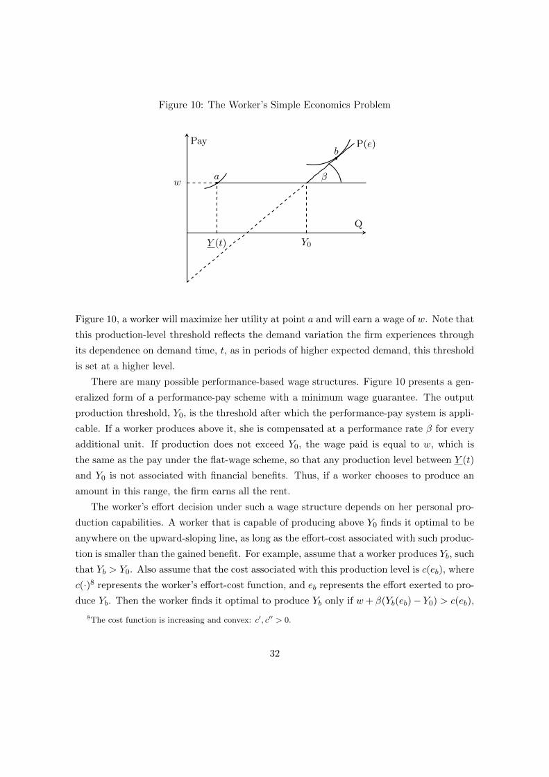
Figure 10: The Worker’s Simple Economics Problem

Y (t) Y0

w

P(e)

a

b

β

Q

Pay

Figure 10, a worker will maximize her utility at point a and will earn a wage of w. Note that

this production-level threshold reflects the demand variation the firm experiences through

its dependence on demand time, t, as in periods of higher expected demand, this threshold

is set at a higher level.

There are many possible performance-based wage structures. Figure 10 presents a gen-

eralized form of a performance-pay scheme with a minimum wage guarantee. The output

production threshold, Y0, is the threshold after which the performance-pay system is appli-

cable. If a worker produces above it, she is compensated at a performance rate β for every

additional unit. If production does not exceed Y0, the wage paid is equal to w, which is

the same as the pay under the flat-wage scheme, so that any production level between Y (t)

and Y0 is not associated with financial benefits. Thus, if a worker chooses to produce an

amount in this range, the firm earns all the rent.

The worker’s effort decision under such a wage structure depends on her personal pro-

duction capabilities. A worker that is capable of producing above Y0 finds it optimal to be

anywhere on the upward-sloping line, as long as the effort-cost associated with such produc-

tion is smaller than the gained benefit. For example, assume that a worker produces Yb, such

that Yb > Y0. Also assume that the cost associated with this production level is c(eb), where

c(·)8 represents the worker’s effort-cost function, and eb represents the effort exerted to pro-

duce Yb. Then the worker finds it optimal to produce Yb only if w+ β(Yb(eb)− Y0) > c(eb),

8The cost function is increasing and convex: c′, c′′ > 0.

32

which means that the production benefits outweigh the cost. A worker who is not capable

of producing above Y0, and chooses to produce anywhere between Y (t) and Y0, has chosen

a sub-optimal effort level, because the effort exerted to produce above Y (t) is uncompen-

sated. Hence, in this simplified model, optimal effort decisions when performance-based

pay is instituted occur at either the point a, as under the flat-wage scheme, or at any point

on the upward-sloping line, for example, the point b. In practice, the data tells us that

workers optimize by producing at a level between Y (t) and Y0. These production levels are

rationalized by considering workers’ inherent differences, an idea which is further discussed

in the next section.

5.2 Structural Model

5.2.1 The “New” Firm’s Problem

With the goal of constructing a model for the labor decision of a firm that sells on-demand

customized products, this model departs from the “traditional” one in several ways. First,

it stresses the fundamental difference between labor and capital. In the neoclassical model

of the labor market, the firm assumes that labor is hired as a factor of production and is

put to work like capital. That is, the firm chooses the optimal quantity of labor and capital

at the market-clearing wage and rental rate, respectively, given its production function.

However, there is one major difference between labor and capital that is ignored by this

assumption: The firm is free to use capital as it wishes, however, having hired a worker, it

faces a considerable restriction on the effort she actually exerts. Not only are there legal

restrictions, but the firm must usually obtain the willing cooperation of its workers in order

to make the best use of them. This idea is even more pronounced when hiring a gig worker,

as the interaction between her and the firm is occasional. For this reason, the paper focuses

on worker’s effort, and considers it as an input of production, instead of treating all laborers

as a uniform and homogeneous production factor.

Second, it redefines the extensive and intensive labor margins in a way that embodies

workers’ effort. The “traditional” simple firm problem focuses on determining the size of the

workforce. A more elaborate approach examines labor demand adjustment in the presence

of a trade-off between the number of workers hired and the amount of hours each employee

works. This trade-off defines the standard substitution of extensive and intensive labor

margins. This paper builds on this idea and analyzes the effort workers exert, instead of

hours worked, as a new labor-intensive margin.

33

The identification of effort is possible as workers’ production decision is observed under

varying compensation methods. This is in fact a key component of the model, as the firm

chooses an optimal pay method in addition to its conventional decision regarding its labor-

force size. In practice, the firm decides between a flat-wage schedule and a performance-

based payment scheme.9 By instituting incentive-based contracts, the firm takes advantage

of its workers’ heterogeneity (within a particular job) to elicit higher labor effort at cer-

tain times, with the underlying assumption that workers are endogenous in their innate

productive abilities, and therefore in their effort and output (Akerlof & Kranton, 2000).

When thinking about a performance-pay contract from the firm’s perspective, there is a

tension between productivity and profitability. The main advantage of such contracts is that

they not only improve labor productivity, but also increase labor welfare. However, a major

caveat of this statement is that firms maximize discounted profits, not productivity, and

performance-contingent contracts may increase productivity, but may not increase profit.

The two main factors that could cause a negative relationship between productivity and

profits in the face of performance-based contracts are quality reduction and the distribution

of earning gains. Performance-based pay could motivate workers to speed up production by

compromising quality, an idea which could explain the well-known phenomenon of “teaching

to the test”. This issue is of particular concern when output is measurable, but quality is

not, so that under incentive pay workers increase measured production at the expense of

unmeasured quality. This concept has been illustrated empirically in a study by Freeman

and Kleiner (2005), who show that the abolition of performance pay reduced productivity

but increased profits as quality rose in the absence of incentives. Holmstrom and Milgrom

(1991) have a similar theoretical finding in the context of a multi-tasking model where

incentive contracts can cause agents to under- or over-invest sub-optimally in different

tasks. For this reason, output quality is integrated as a factor of production into the “new”

firm’s problem, and as the “traditional” firm’s problem can answer questions such as how

increasing capital affects labor output, so does the new framework with respect to output

quality.

Additionally, the distribution of earning gains is a key aspect in linking productivity and

profitability. Assuming that performance-based pay leads to an increase in productivity and

consequently to earning gains, the firm is passing along some of these gains to its workforce

9Potential contracts are implicit, in the sense that workers need not be instantly rewarded for their per-

formance, but may earn a bonus, commission, or promotion at a future time in return for high performance.

Naturally, the structure of the incentive scheme depends on the job’s characteristics.

34

in the form of the additional compensation paid for their additional production. This

division of earning gains determines whether the increase in productivity was profitable or

not. The parameter that governs this allocation is the incentive rate. In fact, a major

challenge of constructing a performance-pay system lies in determining this rate. On the

one hand, setting it too high could lead to a scenario in which workers receive most of

the earnings gains, or even get a share that is larger than the earnings increment. In

such cases, productivity and profitability are negatively related. On the other hand, a rate

that is set too low could lead to there being no production response at all. The question

of which exact performance-pay contract to implement is a challenging one. There are

numerous potential contracts that might be offered and thus multiple possible outcomes

for productivity response. As mentioned above, the firm’s problem does not solve for the

optimal incentive rate parameter, instead, it takes the rate chosen by the firm as given.

Doing so allows me to construct a reliable model that describes workers’ response to the

existing incentives, and isolate it from other factors such as the competitive environment

and personal attributes. Only after the model is validated and estimated can one turn to

computing the optimal incentive structure. Thus, a thorough analysis of the performance

rate is applied in the counterfactual section, which solves for the optimal contract.

Last, the “new” type of firm is characterized by unorthodox labor arrangements, specifi-

cally, the hiring of gig workers. Even though it is a prevalent practice among manufacturers

today to hire gig workers to perform a specific task for a project or a season, it is rarely

examined in the Economics literature. As proven in the empirical analysis, gig workers and

permanent workers are inherently different in their learning abilities, motivation to produce,

and response to incentives. Therefore, decisions regarding the number of workers hired, and

the duration and nature of their contracts (gig or permanent), go hand in hand with the

decision on remuneration scheme. The “new” firm’s problem incorporates this key aspect

by considering not only a decision on the labor-force size, but also the decision regarding

its composition. To the best of my knowledge, this is the first research that applies such an

analysis in an empirical setup.

Model Details

The firm faces a dynamic problem in a calendar year, which is solved in is two phases. In

the first phase, the firm chooses the optimal number of workers, and in the second phase

it chooses its optimal compensation method. Starting in Phase 1, at the beginning of

every week, denoted by t, the firm considers two independent hypothetical scenarios, one

35

in which a flat-wage schedule (FW ) is instituted, and another in which a performance-

pay schedule (PP ) is in place. Then, under each regime, the firm solves for the optimal

workforce composition, considering both gig workers and permanent workers. The hiring

nature of each of these worker types is different. Gig workers are hired for a predetermined

short-term period, and therefore layoff decisions and costs associated with job termination

are irrelevant. Practically, the firm relies on the fact that the contract length is short and

known, and hence decides only on the number of new gig workers it wishes to hire. For

convenience reasons, I assume that the contract length is a week, and therefore, the number

of new gig workers hired at the beginning of time t, denoted by NGt, is equal to the total

number of gig workers at this period, Gt. That is, the law of motion governing the number

of gig workers in period t is

Gt = NGt,

and the labor costs associated with this group of workers is

RG ·NGt

where RG stands for the recruiting costs of gig workers.

The case with permanent workers is different. As they are hired based on a long-term

contract with an undetermined length, the firm needs to consider both their recruiting and

layoff costs. Then, based on these costs, the firm decides on the number of permanent

workers it wishes to hire or fire, given a natural job separation process. In particular,

a permanent worker might terminate her job for exogenous reasons with a separation rate

denoted by µ, or due to intentional layoffs implemented by the firm. Thus, the total number

of permanent workers at time t is equal to

Pt = (1− µ)Pt−1 − LPt +NPt

whereNPt denotes the number of new permanent workers hired and LPt denotes the number

of workers that were laid off at time t. In fact, the total number of permanent workers in

the previous period is the state variable of the dynamic problem, as it captures the past

information the firm needs in order to make an optimal decision. The costs associated with

this group of workers are equal to

RP ·NP t + LP · LPt

36

where RP stands for the recruiting costs of permanent workers, and LP represents the costs

associated with their job termination.

Another component to consider in the firm’s labor cost minimization problem are work-

ers’ wages. Under a flat-wage scheme, wages are fixed and independent of worker effort,

while under a performance-pay scheme, wage is a function of the effort level that maximizes

workers’ private payoff. In fact, worker effort is endogenously incorporated into the problem

through the incentive compatibility constraint

E∗zit = arg maxE

(Uit − Cit|z),

which stipulates that worker i in week t chooses an optimal effort E∗zit to maximize utility

Uit with associated effort costs Cit, for a given pay method z ∈ {FW,PP}. This is a crucial

factor of the problem, because it captures the idea that the firm has a comprehensive

understanding of its workers’ effort response to monetary incentives, which is necessary in

order to sustain and benefit from an incentive pay structure. Denote worker i’s wage at

time t by

Wit(E∗, z),

which is a function of the effort that the worker exerts and the pay method z ∈ {FW,PP},so that the total labor payments made by the firm at time t are

Gt+Pt∑i=1

E[Wit(E

∗, z)],

where expectation is taken over workers’ idiosyncratic heterogeneity, as explained below.

Worker effort also enters into the firm’s demand constraint, which promises that worker

production satisfies the demand volumes

Gt+Pt∑i=1

E[Yit(E

∗, z)]

= Dt,

where Yit denotes the production level of worker i at time t, and Dt denotes the demand the

firm expect to experience at time t. In the case of on-demand customized production, this

constraint is of high importance, as there is no inventory to rely on, and the firm operates

under strict production timing.

37

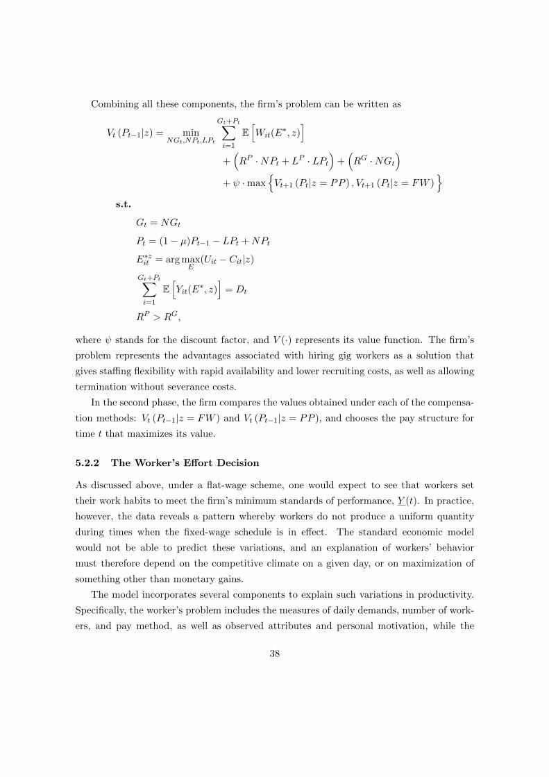
Combining all these components, the firm’s problem can be written as

Vt (Pt−1|z) = minNGt,NPt,LPt

Gt+Pt∑i=1

E[Wit(E

∗, z)]

+(RP ·NPt + LP · LPt

)+(RG ·NGt

)+ ψ ·max

{Vt+1 (Pt|z = PP ) , Vt+1 (Pt|z = FW )

}s.t.

Gt = NGt

Pt = (1− µ)Pt−1 − LPt +NPt

E∗zit = arg maxE

(Uit − Cit|z)

Gt+Pt∑i=1

E[Yit(E

∗, z)]

= Dt

RP > RG,

where ψ stands for the discount factor, and V (·) represents its value function. The firm’s

problem represents the advantages associated with hiring gig workers as a solution that

gives staffing flexibility with rapid availability and lower recruiting costs, as well as allowing

termination without severance costs.

In the second phase, the firm compares the values obtained under each of the compensa-

tion methods: Vt (Pt−1|z = FW ) and Vt (Pt−1|z = PP ), and chooses the pay structure for

time t that maximizes its value.

5.2.2 The Worker’s Effort Decision

As discussed above, under a flat-wage scheme, one would expect to see that workers set

their work habits to meet the firm’s minimum standards of performance, Y (t). In practice,

however, the data reveals a pattern whereby workers do not produce a uniform quantity

during times when the fixed-wage schedule is in effect. The standard economic model

would not be able to predict these variations, and an explanation of workers’ behavior

must therefore depend on the competitive climate on a given day, or on maximization of

something other than monetary gains.

The model incorporates several components to explain such variations in productivity.

Specifically, the worker’s problem includes the measures of daily demands, number of work-

ers, and pay method, as well as observed attributes and personal motivation, while the

38

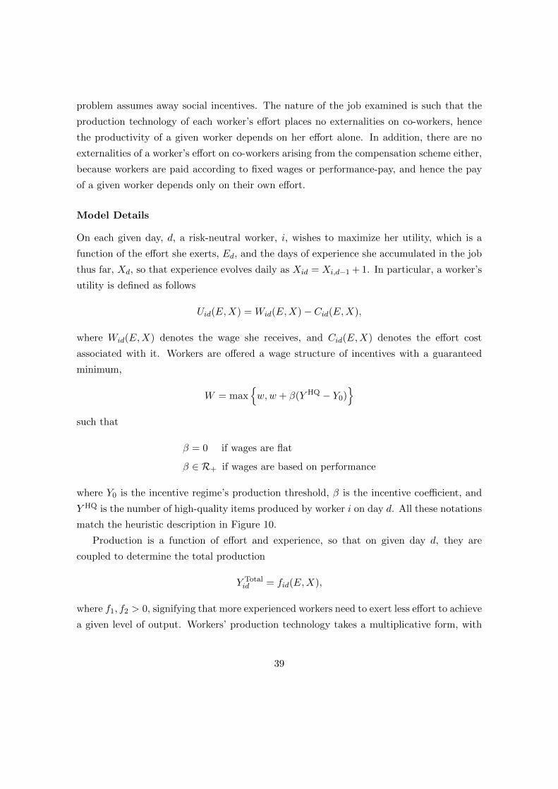
problem assumes away social incentives. The nature of the job examined is such that the

production technology of each worker’s effort places no externalities on co-workers, hence

the productivity of a given worker depends on her effort alone. In addition, there are no

externalities of a worker’s effort on co-workers arising from the compensation scheme either,

because workers are paid according to fixed wages or performance-pay, and hence the pay

of a given worker depends only on their own effort.

Model Details

On each given day, d, a risk-neutral worker, i, wishes to maximize her utility, which is a

function of the effort she exerts, Ed, and the days of experience she accumulated in the job

thus far, Xd, so that experience evolves daily as Xid = Xi,d−1 + 1. In particular, a worker’s

utility is defined as follows

Uid(E,X) = Wid(E,X)− Cid(E,X),

where Wid(E,X) denotes the wage she receives, and Cid(E,X) denotes the effort cost

associated with it. Workers are offered a wage structure of incentives with a guaranteed

minimum,

W = max{w,w + β(Y HQ − Y0)

}such that

β = 0 if wages are flat

β ∈ R+ if wages are based on performance

where Y0 is the incentive regime’s production threshold, β is the incentive coefficient, and

Y HQ is the number of high-quality items produced by worker i on day d. All these notations

match the heuristic description in Figure 10.

Production is a function of effort and experience, so that on given day d, they are

coupled to determine the total production

Y Totalid = fid(E,X),

where f1, f2 > 0, signifying that more experienced workers need to exert less effort to achieve

a given level of output. Workers’ production technology takes a multiplicative form, with

39

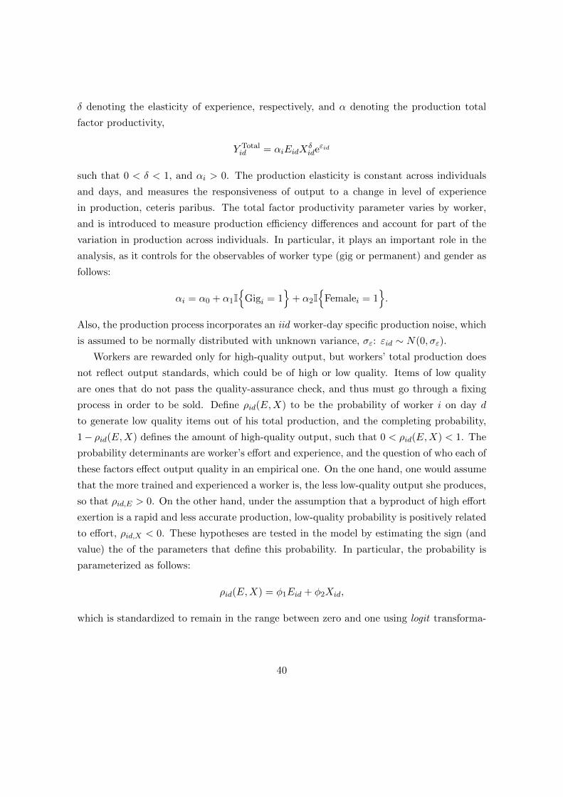
δ denoting the elasticity of experience, respectively, and α denoting the production total

factor productivity,

Y Totalid = αiEidX

δide

εid

such that 0 < δ < 1, and αi > 0. The production elasticity is constant across individuals

and days, and measures the responsiveness of output to a change in level of experience

in production, ceteris paribus. The total factor productivity parameter varies by worker,

and is introduced to measure production efficiency differences and account for part of the

variation in production across individuals. In particular, it plays an important role in the

analysis, as it controls for the observables of worker type (gig or permanent) and gender as

follows:

αi = α0 + α1I{

Gigi = 1}

+ α2I{

Femalei = 1}.

Also, the production process incorporates an iid worker-day specific production noise, which

is assumed to be normally distributed with unknown variance, σε: εid ∼ N(0, σε).

Workers are rewarded only for high-quality output, but workers’ total production does

not reflect output standards, which could be of high or low quality. Items of low quality

are ones that do not pass the quality-assurance check, and thus must go through a fixing

process in order to be sold. Define ρid(E,X) to be the probability of worker i on day d

to generate low quality items out of his total production, and the completing probability,

1− ρid(E,X) defines the amount of high-quality output, such that 0 < ρid(E,X) < 1. The

probability determinants are worker’s effort and experience, and the question of who each of

these factors effect output quality in an empirical one. On the one hand, one would assume

that the more trained and experienced a worker is, the less low-quality output she produces,

so that ρid,E > 0. On the other hand, under the assumption that a byproduct of high effort

exertion is a rapid and less accurate production, low-quality probability is positively related

to effort, ρid,X < 0. These hypotheses are tested in the model by estimating the sign (and

value) the of the parameters that define this probability. In particular, the probability is

parameterized as follows:

ρid(E,X) = φ1Eid + φ2Xid,

which is standardized to remain in the range between zero and one using logit transforma-

40

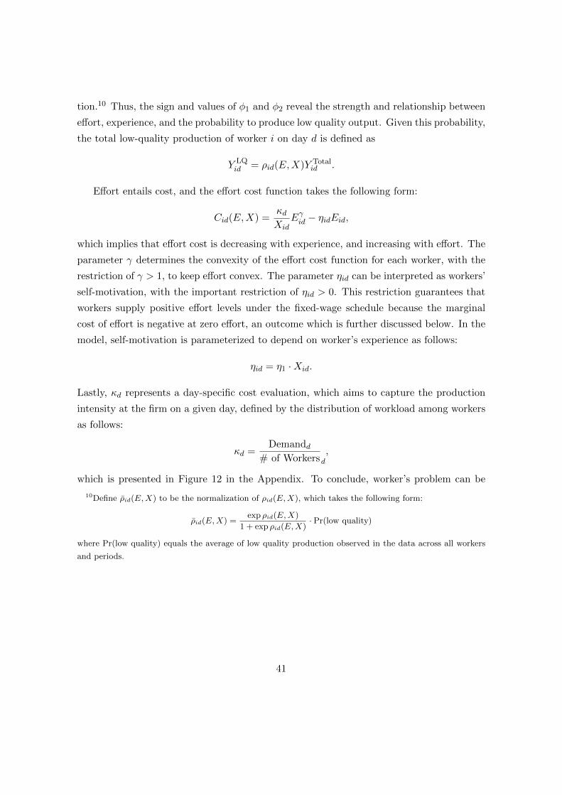
tion.10 Thus, the sign and values of φ1 and φ2 reveal the strength and relationship between

effort, experience, and the probability to produce low quality output. Given this probability,

the total low-quality production of worker i on day d is defined as

Y LQid = ρid(E,X)Y Total

id .

Effort entails cost, and the effort cost function takes the following form:

Cid(E,X) =κdXid

Eγid − ηidEid,

which implies that effort cost is decreasing with experience, and increasing with effort. The

parameter γ determines the convexity of the effort cost function for each worker, with the

restriction of γ > 1, to keep effort convex. The parameter ηid can be interpreted as workers’

self-motivation, with the important restriction of ηid > 0. This restriction guarantees that

workers supply positive effort levels under the fixed-wage schedule because the marginal

cost of effort is negative at zero effort, an outcome which is further discussed below. In the

model, self-motivation is parameterized to depend on worker’s experience as follows:

ηid = η1 ·Xid.

Lastly, κd represents a day-specific cost evaluation, which aims to capture the production

intensity at the firm on a given day, defined by the distribution of workload among workers

as follows:

κd =Demandd

# of Workersd,

which is presented in Figure 12 in the Appendix. To conclude, worker’s problem can be

10Define ρid(E,X) to be the normalization of ρid(E,X), which takes the following form:

ρid(E,X) =exp ρid(E,X)

1 + exp ρid(E,X)· Pr(low quality)

where Pr(low quality) equals the average of low quality production observed in the data across all workers

and periods.

41

written as

maxE

Wid(E,X)−(κdXid

Eγid − ηiEid)

s.t.

0 ≤ Eid ≤ 1

Wid(E,X) = max{w,w + β(Y HQ

id (E,X)− Y0)}

Y Totalid (E,X) = αEidX

δide

εid

Y HQid (E,X) =

[1− ρid(E,X)

]Y Totalid

E[Y HQid

]≥ Y (t),

where the last requirement states that expected production is as least as high as the mini-

mum required periodic production level, for d being a day in week t.

Note that effort is al latent variable that is not directly observed but are rather inferred

through the model’s solution. As such, in order for the problem to generate valuable

information, I restrict it to be between zero and one. Therefore, the solution of the worker’s

problem indicates on a relative effort exerted, given her attributed, the day-specific settings,

and shock realization.

5.3 Model Predictions and Implications

5.3.1 Effort Cost Function

Worker’s effort-cost function and parameters are constrained to satisfy several key features

of worker’s problem. First, consider worker’s effort in the flat-wage scenario. Given that

workers are guaranteed to receive their pay regardless of productivity level in this sce-

nario, and given that production entails a cost, we might reasonably expect that a utility-

maximizing agent will find it optimal to choose Eid = 0. The effort-cost production function

is constructed to preclude this possibility, as the marginal cost of effort is

Cid,E =κdXid

γEγ−1id − ηi,

which under no effort, is equal to

Cid,E

∣∣∣E=0

= −ηi,

42

and since ηi > 0, the marginal cost of effort is negative when no effort is exerted. This result

ensures that employees supply positive effort levels under a fixed wage. Moreover, the effort-

cost function is increasing with effort, Cid,E > 0, convex with respect to effort, Cid,EE > 0,

and (all other things being equal) more experienced workers face a lower marginal effort-

cost, Cid,EX < 0. While the second and third condition are satisfied by construction, the

first requires that

κdXid

γEγ−1id > ηi.

5.3.2 Optimal Effort

Flat Wage: β = 0

If the firm sets β = 0, then earnings are fixed and independent of performance, and thus it

is not the monetary incentive that leads workers to exert effort to produce above Y (t), but

rather their personal motivation. This factor plays a crucial role in the model, and ηi > 0

is in fact a necessary condition for positive production. This idea is presented clearly when

solving for the optimal effort level in the flat-wage scenario, denoted by E∗FWid , which yields

the following solution:

κdXid

γ(E∗FWid

)(γ−1)= ηid.

It shows that on day d, worker i will maximize her utility by choosing the effort level that

will equate her personal motivation to the marginal effort cost, given her experience, her

effort cost curvature, and the competitive climate on that given day. Also, the optimal

effort under the flat-wage scheme is decreasing with the competitive climate, and increasing

with experience and personal motivation. The optimal effort is increasing and concave with

effort-cost function curvature, which means that higher curvature is associated with higher

effort, but at a diminishing rate.

Performance Pay: β > 0

Under a performance-pay regime, workers choose their optimal effort, E∗PPid , to equate the

marginal benefit and the marginal costs of production, considering both monetary and

non-monetary incentives. This idea is clearly illustrated when examining the first-order

condition of the problem in the performance-pay scenario,

β[1− ρid

]αXδ

ideεidIPP + ηi =

κdXid

γ(E∗PPid

)(γ−1)+ βρid,Eα

(E∗PPid

)Xδide

εidIPP,

43

where ρid and ρid,E represent the probability and marginal probability of low-quality pro-

duction, respectively, and the indicator function equals one if a worker reaches the incentive

threshold, Y0, on days when the incentive scheme was in effect: IPP = I[Y HQid > Y0

]. If

IPP = 1, the left-hand-side represents the sum of the marginal monetary and non-monetary

benefits of production. That is, the marginal monetary benefits of producing above Y (t)

are represented by the product of the performance-rate β and the marginal productivity of

high-quality output, and the non-monetary benefits embodied by the personal motivation

parameter, ηid. The right-hand side is a sum of the marginal cost of production and the cost

of producing low-quality items above Y (t), as workers are not compensated for the produc-

tion of these items. If IPP = 0, then the optimal effort solution under the performance-pay

and flat-wage schemes coincide.

5.3.3 Participation Constraint

Gig workers are a temporary labor force that is leveraged by the firm during times of high

demand. Gig-worker jobs are characterized by high flexibility, with the most salient feature

being frequent transition. Because of this, it is reasonable to assume that these workers’

participation constraints are binding, and to assume that they are indifferent between this

current job and an alternative outside option. As the job is of a low-skill nature, this

assumption can be extended to permanent workers as well. Denote workers’ alternative

utility by u, and define the participation constraint by equating it to the utility under wage

flat-wage, that is

E[U(E∗FW

i , Xi)]

= u.

By writing this condition explicitly, one can identify the guaranteed wage level, w,

w = u+ E[C∗FWid

],

where C∗FWid denotes the effort cost under optimal effort in the fixed-wage payment schedule.

5.3.4 Indirect Utility

The indirect utility function under the flat-wage scheme is

V ∗FW = w − E[C∗FWid

],

44

and using the participation constraint result,one finds that workers’ maximum attainable

utility is equal to their outside option value

V ∗FW = u.

The indirect utility function under the performance-pay regime looks like this:

V ∗PP = w + β E[Y ∗HQ,PP − Y0

]IPP − E

[C∗PPid

],

and if the incentive threshold is reached, the result can be simplified using the participation

constraint, so that

V ∗PP = u+ β E[Y ∗HQ,PP − Y0

]− E

[C∗PPid − C∗FW

id

],

where Y ∗HQ,PP denotes the high-quality output generated under the optimal effort decision.

This result has several implications. First, it shows that workers’ maximal attainable

utility is equal to the monetary benefit of producing above Y0, and the cost for effort

exerted above what they would otherwise choose under the flat-wage regime, on top of the

outside option value, u. Also, the result indicates that utility is decreasing with the daily

competitive climate κd, increasing with personal motivation, ηi, and with the incentive rate,

β. In particular, this result distills the forces that stand behind the effort-decision problem

when incentives are available. Specifically, a worker chooses to exert effort greater than

that associated with her optimal decision under the flat-wage scheme only if the financial

benefit of doing so exceeds the effort costs associated with this benefit,

β E[Y ∗HQ,PP − Y0

]> E

[C∗PPid − C∗FW

id

], (1)

and when this is the case, workers are strictly better off under the performance-pay regime

V ∗PP > V ∗FW.

If production falls below the incentive threshold, so that IPP = 0, then the indirect utility

under performance-pay is given by

V ∗PP = u− E[C∗PPid − C∗FW

id

]where the second term must be equal to zero for the worker to accept this job. In particular,

the unique effort that satisfies this condition is E∗Fwid , so that the maximum attainable

utilities the flat-wage and performance-pay schemes are equal.

45

5.3.5 Expected Earnings

The expected earnings in the performance-pay scenario are higher than the expected earn-

ings in the flat-wage scenario only if a worker is capable of reaching Y0, and finds it optimal

to do so based on condition (1). From the worker’s perspective, the earnings when in-

centives are available should compensate her for the additional cost burden she incurs for

producing not above Y0, but rather above Y (t), which is the amount that promises mini-

mum wage. The following result illustrates the additional pay above w that should be given

to compensate a worker for her effort:

E(W |PP) = w + β E[Y ∗HQ,PP − Y0

].

6 Indirect Inference

I use indirect inference (Gourieroux, Monfort, & Renault, 1993), a simulation method, to

estimate the structural parameters. In practice, I focus on the empirical findings presented

in Section 4 as an auxiliary model to tightly link the structural parameters to the empirical

findings. This methodology is chosen over others, because it allows one to capture aspects

of the data upon which to base the estimation on, instead of selecting a set of moments (as

is typically done with the method of simulated moments).

In practice, the idea is to repeat simulations to find the data-generating parameters

that yields a mean of the estimates of Model (5) equal to the actual estimates obtained

from the data. First, I solve for the worker’s daily effort decision for a vector of possi-

ble values of structural parameters Θ = (α0, α1, α2, δ, η1, γ, φ1, φ2, σε), given the realiza-

tion of the idiosyncratic production shock, and a set of daily and personal observables.

Second, based on the solution and the set of chosen parameters I calculate the optimal

production. Then, based on this outcome I estimate the auxiliary model coefficients on

the simulated data, and obtain a vector of auxiliary parameters ψsim(Θ). The optimal

choice of Θ minimize the distance between the auxiliary parameters estimated on the ac-

tual data and the auxiliary parameters estimated on the simulated data. That is, I choose

Θ = (α0, α1, α2, δ, η1, γ, φ1, φ2, σε) such that

Θ = arg minΘ

(ψdata − ψsim(Θ)

)W(ψdata − ψsim(Θ)

)′where W is a symmetric and positive semi-definite weighting matrix.11

11W is estimated in two steps. At the first step it is set to be equal to the inverse of a diagonal matrix

46

7 Identification

The choice of the auxiliary parameters allows for rather transparent identification of the

structural parameters of the model. All parameters of the auxiliary model contribute to the

estimation of the structural parameters with varying contribution levels, depending on the

relationship between the auxiliary and structural parameters. To illustrate, Figure 11, which

obtained by simulation, outlines the relationship between a parameter of the structural

model and parameters of the auxiliary model with the largest identification contribution.

That is, it shows how a change in the value of the structural parameter vary the value of

the coefficients generated by the auxiliary model. For example, the parameters α1, and

α2, which define the contribution of workers’ type (gig or permanent) and gender to the

total factor productivity parameter of worker’s production function, are identified by the

parameters of Gig workers Dummy and Female Dummy from the auxiliary model.

8 Results

To be completed.

9 Counterfactual Analysis

To be completed.

10 Concluding Remarks

To be completed.

with the standard errors of the parameters of the auxiliary model on the main diagonal. The second step

calculates the variance-covariance matrix of the simulated auxiliary parameters, ψsim,

W =1

L

L∑l

(ψl

sim(σ1ε) − 1

L

L∑l

ψlsim(σ2

ε)

)·

(ψl

sim(σ1ε) − 1

L

L∑l

ψlsim(σ2

ε)

)′

where σjε, j = 1, 2 are different sets of L realizations of the idiosyncratic production shock, and L is equal

to 1000.

47

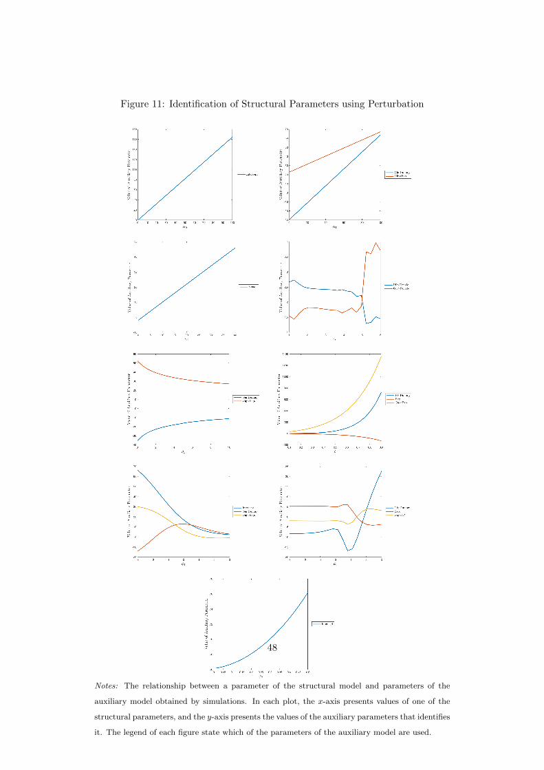
Figure 11: Identification of Structural Parameters using Perturbation

Notes: The relationship between a parameter of the structural model and parameters of the

auxiliary model obtained by simulations. In each plot, the x-axis presents values of one of the

structural parameters, and the y-axis presents the values of the auxiliary parameters that identifies

it. The legend of each figure state which of the parameters of the auxiliary model are used.

48

References

Akerlof, G. A., & Kranton, R. E. (2000). Economics and identity. The Quarterly Journal

of Economics, 115 (3), 715–753.

Allon, G., Cohen, M., & Sinchaisri, P. (2018). The impact of behavioral and economic

drivers on gig economy workers. Available at SSRN 3274628 .

Anderson, E. (1985). The salesperson as outside agent or employee: a transaction cost

analysis. Marketing science, 4 (3), 234–254.

Arrow, K. J. (1971). Insurance, risk and resource allocation. Essays in the theory of

risk-bearing , 134–143.

Baker, K. R. (1976). Workforce allocation in cyclical scheduling problems: A survey.

Journal of the Operational Research Society , 27 (1), 155–167.

Bandiera, O., Barankay, I., & Rasul, I. (2005). Social preferences and the response to

incentives: Evidence from personnel data. The Quarterly Journal of Economics,

120 (3), 917–962.

Bandiera, O., Barankay, I., & Rasul, I. (2007). Incentives for managers and inequality

among workers: Evidence from a firm-level experiment. The Quarterly Journal of

Economics, 122 (2), 729–773.

Bard, J. F. (2004a). Selecting the appropriate input data set when configuring a permanent

workforce. Computers & Industrial Engineering , 47 (4), 371–389.

Bard, J. F. (2004b). Staff scheduling in high volume service facilities with downgrading.

Iie Transactions, 36 (10), 985–997.

Bard, J. F., Binici, C., & desilva, A. H. (2003). Staff scheduling at the united states postal

service. Computers & Operations Research, 30 (5), 745–771.

Bard, J. F., Morton, D. P., & Wang, Y. M. (2007). Workforce planning at usps mail pro-

cessing and distribution centers using stochastic optimization. Annals of Operations

Research, 155 (1), 51–78.

Bard, J. F., & Purnomo, H. W. (2005). Short-term nurse scheduling in response to daily

fluctuations in supply and demand. Health Care Management Science, 8 (4), 315–324.

Billionnet, A. (1999). Integer programming to schedule a hierarchical workforce with

variable demands. European Journal of Operational Research, 114 (1), 105–114.

Brown, C. (1990). Firms’ choice of method of pay. ILR Review , 43 (3), 165–S.

Cachon, G. P., Daniels, K. M., & Lobel, R. (2017). The role of surge pricing on a service

platform with self-scheduling capacity. Manufacturing & Service Operations Manage-

49

ment , 19 (3), 368–384.

Conlon, E. J., & Parks, J. M. (1990). Effects of monitoring and tradition on compensation

arrangements: An experiment with principal-agent dyads. Academy of Management

Journal , 33 (3), 603–622.

Connelly, C. E., & Gallagher, D. G. (2004). Emerging trends in contingent work research.

Journal of management , 30 (6), 959–983.

Corominas, A., Lusa, A., & Pastor, R. (2004). Planning annualised hours with a finite set

of weekly working hours and joint holidays. Annals of Operations Research, 128 (1-4),

217–233.

DeFillippi, R. J., & Arthur, M. B. (1994). The boundaryless career: A competency-based

perspective. Journal of organizational behavior , 15 (4), 307–324.

Delfgaauw, J., Dur, R., Sol, J., & Verbeke, W. (2013). Tournament incentives in the field:

Gender differences in the workplace. Journal of Labor Economics, 31 (2), 305–326.

Dong, J., & Ibrahim, R. (2017). Flexible workers or full-time employees? on staffing systems

with a blended workforce (Tech. Rep.). Working paper.

Foote, D. A., & Folta, T. B. (2002). Temporary workers as real options. Human Resource

Management Review , 12 (4), 579–597.

Freeman, R. B., & Kleiner, M. M. (2005). The last american shoe manufacturers: Decreasing

productivity and increasing profits in the shift from piece rates to continuous flow

production. Industrial Relations: A Journal of Economy and Society , 44 (2), 307–

330.

Gabszewicz, J., & Turrini, A. (2000). Workers’ skills, product quality and industry equi-

librium. International journal of industrial organization, 18 (4), 575–593.

Gans, N., & Zhou, Y.-P. (2002). Managing learning and turnover in employee staffing.

Operations Research, 50 (6), 991–1006.

Gibbons, R. (2005). Incentives between firms (and within). Management science, 51 (1),

2–17.

Gillespie, P. (2017). Intuit: Gig economy is 34% of us workforce. CNN Money .

Gneezy, U., Niederle, M., & Rustichini, A. (2003). Performance in competitive environ-

ments: Gender differences. The Quarterly Journal of Economics, 118 (3), 1049–1074.

Gourieroux, C., Monfort, A., & Renault, E. (1993). Indirect inference. Journal of applied

econometrics, 8 (S1), S85–S118.

Grossman, R. J. (1998). Short-term workers raise long-term issues. HR Magazine, 43 (5),

80–89.

50

Hamermesh, D. S. (1991). Labor demand: what do we know? what don’t we know? (Tech.

Rep.). National Bureau of Economic Research.

Hamermesh, D. S., & Grant, J. (1979). Econometric studies of labor-labor substitution and

their implications for policy. Journal of Human Resources, 518–542.

Hojati, M., & Patil, A. S. (2011). An integer linear programming-based heuristic for

scheduling heterogeneous, part-time service employees. European Journal of Opera-

tional Research, 209 (1), 37–50.

Holmstrm, B., & Milgrom, P. (1991). Multitask principal-agent analyses: Incentive con-

tracts, asset ownership, and job design. JL Econ. & Org., 7 , 24.

Holmstrom, B., & Milgrom, P. (1987). Aggregation and linearity in the provision of in-

tertemporal incentives. Econometrica: Journal of the Econometric Society , 303–328.

Holmstrom, B., & Milgrom, P. (1994). The firm as an incentive system. The American

Economic Review , 972–991.

Ibrahim, R. (2018). Managing queueing systems where capacity is random and customers

are impatient. Production and Operations Management , 27 (2), 234–250.

Jarmon, R., Paulson, A. S., & Rebne, D. (1998). Contractor performance: How good

are contingent workers at the professional level? IEEE Transactions on Engineering

Management , 45 (1), 11–19.

Jensen, M. C., & Meckling, W. H. (1976). Theory of the firm: Managerial behavior, agency

costs and ownership structure. Journal of financial economics, 3 (4), 305–360.

Jurajda, S., & Munich, D. (2011). Gender gap in performance under competitive pressure:

Admissions to czech universities. American Economic Review , 101 (3), 514–18.

Katz, L. F., & Krueger, A. B. (2019). The rise and nature of alternative work arrangements

in the united states, 1995–2015. ILR Review , 72 (2), 382–416.

Kolisch, R., & Heimerl, C. (2012). An efficient metaheuristic for integrated scheduling and

staffing it projects based on a generalized minimum cost flow network. Naval Research

Logistics (NRL), 59 (2), 111–127.

Laffont, J.-J., & Martimort, D. (2009). The theory of incentives: the principal-agent model.

Princeton university press.

Lazear, E. P. (2000). Performance pay and productivity. American Economic Review ,

90 (5), 1346–1361.

Lazear, E. P. (2018). Compensation and incentives in the workplace. Journal of Economic

Perspectives, 32 (3), 195–214.

Lazear, E. P., & Rosen, S. (1981). Rank-order tournaments as optimum labor contracts.

51

Journal of political Economy , 89 (5), 841–864.

Li, Y., Chen, J., & Cai, X. (2007). An integrated staff-sizing approach considering feasibility

of scheduling decision. Annals of Operations Research, 155 (1), 361–390.

Manyika, J., Lund, S., Bughin, J., Robinson, K., Mischke, J., & Mahajan, D. (2016).

Independent work: Choice, necessity, and the gig economy. McKinsey Global Institute,

2016 , 1–16.

Marasco, A., & Romano, A. (2011). A mathematical model for the management of a service

center. Mathematical and Computer Modelling , 53 (9-10), 2005–2014.

Milner, J. M., & Pinker, E. J. (2001). Contingent labor contracting under demand and

supply uncertainty. Management Science, 47 (8), 1046–1062.

Misra, S., & Nair, H. S. (2011). A structural model of sales-force compensation dynamics:

Estimation and field implementation. Quantitative Marketing and Economics, 9 (3),

211–257.

Ors, E., Palomino, F., & Peyrache, E. (2013). Performance gender gap: does competition

matter? Journal of Labor Economics, 31 (3), 443–499.

Oyer, P., & Schaefer, S. (2010). Personnel economics: hiring and incentives (Tech. Rep.).

National Bureau of Economic Research.

Petriglieri, G., Ashford, S. J., & Wrzesniewski, A. (2019). Agony and ecstasy in the

gig economy: Cultivating holding environments for precarious and personalized work

identities. Administrative Science Quarterly , 64 (1), 124–170.

Pinker, E. J., & Larson, R. C. (2003). Optimizing the use of contingent labor when demand

is uncertain. European Journal of Operational Research, 144 (1), 39–55.

Polivka, A. E., & Nardone, T. (1989). On the definition of contingent work. Monthly Lab.

Rev., 112 , 9.

Robles, B. J., & McGee, M. (2016). Exploring online and offline informal work: findings

from the enterprising and informal work activities (eiwa) survey.

Ross, S. A. (1973). The economic theory of agency: The principal’s problem. The American

economic review , 63 (2), 134–139.

Shapiro, C., & Stiglitz, J. E. (1984). Equilibrium unemployment as a worker discipline

device. The American Economic Review , 74 (3), 433–444.

Shearer, B. (2004). Piece rates, fixed wages and incentives: Evidence from a field experi-

ment. The Review of Economic Studies, 71 (2), 513–534.

Stratman, J. K., Roth, A. V., & Gilland, W. G. (2004). The deployment of temporary

production workers in assembly operations: a case study of the hidden costs of learning

52

and forgetting. Journal of Operations Management , 21 (6), 689–707.

Syverson, C. (2011). What determines productivity? Journal of Economic literature,

49 (2), 326–65.

Techawiboonwong, A., Yenradee, P., & Das, S. K. (2006). A master scheduling model

with skilled and unskilled temporary workers. International Journal of Production

Economics, 103 (2), 798–809.

Thompson, G. M., & Goodale, J. C. (2006). Variable employee productivity in workforce

scheduling. European journal of operational research, 170 (2), 376–390.

Valls, V., Perez, A., & Quintanilla, S. (2009). Skilled workforce scheduling in service centres.

European Journal of Operational Research, 193 (3), 791–804.

Van den Bergh, J., Belien, J., De Bruecker, P., Demeulemeester, E., & De Boeck, L. (2013).

Personnel scheduling: A literature review. European journal of operational research,

226 (3), 367–385.

Wild, B., & Schneewei, C. (1993). Manpower capacity planning—a hierarchical approach.

International Journal of Production Economics, 30 , 95–106.

Wilson, R. (1968). The theory of syndicates. Econometrica: journal of the Econometric

Society , 119–132.

53

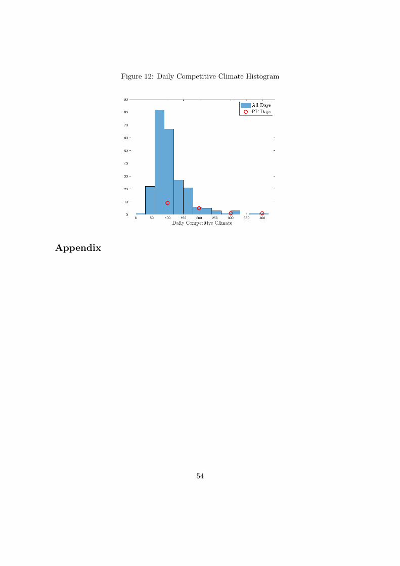
Figure 12: Daily Competitive Climate Histogram

Appendix

54