GIS - Taylor & Francis eBooks

GISA Computing Perspective

Second Edition

This page intentionally left blankThis page intentionally left blank

CRC PR ESSBoca Raton London New York Washington, D.C.

GISA Computing Perspective

Second Edition

Michael WorboysUniversity of Maine

USA

Matt DuckhamUniversity of Melbourne

Australia

CRC PressTaylor & Francis Group6000 Broken Sound Parkway NW, Suite 300Boca Raton, FL 33487-2742

© 2004 by Taylor & Francis Group, LLCCRC Press is an imprint of Taylor & Francis Group, an Informa business

No claim to original U.S. Government worksVersion Date: 20160421

International Standard Book Number-13: 978-0-203-48155-4 (eBook - PDF)

This book contains information obtained from authentic and highly regarded sources. Reasonable efforts have been made to publish reliable data and information, but the author and publisher cannot assume responsibility for the valid-ity of all materials or the consequences of their use. The authors and publishers have attempted to trace the copyright holders of all material reproduced in this publication and apologize to copyright holders if permission to publish in this form has not been obtained. If any copyright material has not been acknowledged please write and let us know so we may rectify in any future reprint.

Except as permitted under U.S. Copyright Law, no part of this book may be reprinted, reproduced, transmitted, or uti-lized in any form by any electronic, mechanical, or other means, now known or hereafter invented, including photocopy-ing, microfilming, and recording, or in any information storage or retrieval system, without written permission from the publishers.

For permission to photocopy or use material electronically from this work, please access www.copyright.com (http://www.copyright.com/) or contact the Copyright Clearance Center, Inc. (CCC), 222 Rosewood Drive, Danvers, MA 01923, 978-750-8400. CCC is a not-for-profit organization that provides licenses and registration for a variety of users. For organizations that have been granted a photocopy license by the CCC, a separate system of payment has been arranged.

Trademark Notice: Product or corporate names may be trademarks or registered trademarks, and are used only for identification and explanation without intent to infringe.

Visit the Taylor & Francis Web site athttp://www.taylorandfrancis.com

and the CRC Press Web site athttp://www.crcpress.com

http://www.copyright.com/

http://www.copyright.com/

http://www.taylorandfrancis.com

http://www.crcpress.com

http://www.copyright.com

To Helen,and to my parents, Rita and John

MD

To Moiraand to Bethan, Colin, Ruth, Sophie, Tom, and William

MW


Preface

Geographic information systems (GISs) are computer-based informationsystems that are used to capture, model, store, retrieve, share, manipu-late, analyze, and present geographically referenced data. This book isabout the technology, theories, models, and representations that surroundgeographic information and GISs. This study (itself often referred toas GIS or geographic information science) has emerged in the last twodecades as an exciting multi-disciplinary endeavor, spanning such areasas geography, cartography, remote sensing, image processing, environ-mental sciences, and computing science. The treatment in this text isunashamedly biased toward the computational aspects of GIS. Withincomputing science, GIS is a special interest of fields such as databases,graphics, systems engineering, and computational geometry, being notonly a challenging application area, but also providing foundational ques-tions for these disciplines.

The underlying question facing this multidisciplinary topic is “Whatis special about spatial information?” In this book, we attempt to provideanswers at several different levels: the conceptual and formal modelsneeded to understand spatial information; the representations and datastructures needed to support adequate performance in GISs; the special-purpose interfaces and architectures required to interact with and sharespatial information; and the importance of uncertainty and time in spatialinformation.

The task of computing practitioners in the field of GIS is to providethe application experts, whether geographers, planners, utility engineers,or environmental scientists, with a set of tools, based around digital com-puter technology, that will aid them in solving problems in their domains.These tools will include modeling constructs, data structures that willallow efficient storage and retrieval of data, and generic interfaces thatmay be customized for particular application domains.

The book inevitably reflects the interests and biases of its authors, inparticular emphasizing spatial information modeling and representation,as well as developing some of the more formal themes useful in under-standing GIS. We have tried to avoid detailed discussion of particular cur-rently fashionable systems, and concentrate instead upon the foundations

and general principles of the subject area. We have also tried to give anoverview of the field from the perspective of computing science.

Not every topic can be covered and we have deliberately neglectedtwo areas, leaving these to people expert in those domains. The first isthe historical background. The development of GIS has an interestinghistory, stretching back to the 1950s. Readers who wish to pursue thistopic will find an excellent introduction in Coppock and Rhind (1991),and more in-depth perspectives from many of the pioneers of GIS inForesman (1998). The other area that is given scant treatment is spatialanalysis, which requires specialized statistical techniques and is judgedto be specifically the province of the domain experts. Introductions tospatial analysis include Unwin (1981), Fotheringham et al. (2002), andO’Sullivan and Unwin (2002). The bibliographic notes in Chapter 1provide further references to texts on specific aspects of spatial analysis.

WHO SHOULD READ THIS BOOK

This book is intended for readers from any background who wish to learnsomething about the issues that GIS engenders for computing technology.The reader does not have to be a specialist computing scientist: the textdevelops the necessary background in specialist areas, such as databases,as it progresses. However, some knowledge of the basic componentsand functionality of a digital computer is essential for understanding theimportance of certain key issues in GIS. Where some aspect of generalcomputing bears a direct relevance to our development, the backgroundis given in the text. This book can be used as a teaching text, takingreaders through the main concepts by means of definitions, explications,and examples. However, the more advanced researcher is not neglected,and the book includes an extensive bibliography that readers can use tofollow up particular topics.

CHANGES TO THE SECOND EDITION

The second edition of this book was written with the aim of making thebook more accessible to a wider audience, at the same time as retainingthe core of tried and tested material. Chapters 1–6 have been extensivelyrevised, updated, and reformatted from the first edition, although in afast-moving high-technology area like GIS it was encouraging to findthat these fundamental aspects of GIS have remained largely unchanged.Chapters 7–10 present almost entirely new material, covering GIS ar-chitectures, GIS interfaces, uncertainty in geospatial information, andspatiotemporal information systems. The bibliography, index, and all thediagrams have also been completely revised.

In addition to the changes in content, we have tried to produce amore attractive and readable format for the book. The following sectioncontains more details on the formatting conventions used in this book andon the structure of the book. The spelling, grammar, and usage in second

edition has also changed, from British to American English. We hopethat this change will further improve the accessibility of this book to aninternational audience.

FORMATTING USED IN THIS BOOK

Several formatting conventions, new to the second edition, have been usedin this book. Material that is relevant to the main themes in the text, butnot essential to the reader, is included in gray inset boxes at the top ofa page. Typically insets contain more challenging material, and providesome background to each topic, as well as references and links, whichreaders may wish to pursue. A list of insets is included in the book’s frontmatter. Every chapter begins with a brief summary, outlining the majorideas in that chapter and highlighting some important terms introduced inthe chapter. At its close every chapter ends with itemized bibliographicnotes, providing some key references that readers can follow up. Thesection numbers alongside the bibliographic notes refer to the relevantsections in the main text.

Throughout this book, we have used margin text to allow rapid ref-erence to important terms. When an important term is first defined orintroduced, that term will appear in the margin. A corresponding entrycan be found in the index, with the page reference in bold typeface. Thisenables the reader to use the index rather like an extensive glossary ofterms used in this book. Each index term has at most one bold typefacepage reference, and a term can be rapidly located within a page by findingthe corresponding margin entry. In addition to normal- and bold-typefaceindex entries, those index entries that appear in italics refer to terms thatappear within a gray inset box.

STRUCTURE OF THIS BOOK

Figure 0.1 indicates the overall structure of interdependencies betweenchapters. Readers may find it helpful to refer to Figure 0.1 to tailor theiruse of this book to their own particular interests.

Chapter 1: Motivation and introduction to GIS; preparatory material ongeneral computing.

Chapters 2–3: Background material on general databases and for-malisms for spatial concepts.

Chapters 4–6: Exposition of the core material, forming a progressionfrom high-level conceptual models, through representations andalgorithms, to indexes and access methods that allow acceptableperformance.

Chapters 7–8: Discussion of the types of system architectures and userinterfaces needed for GIS.

Chapter 9: Introduction to spatial reasoning theory and techniques, withparticular focus on reasoning under uncertainty.

Chapter 10: Introduction to temporal and spatiotemporal informationsystems.

Figure 0.1:Relationshipsbetweenchapters

4. Models of

information

geospatial

5. Representation

and algorithms

6. Structures and

access methods

2. Fundamental

database

concepts

1. Introduction

3. Fundamental

spatial

concepts

7. Architectures

8. Interfaces

9. Spatial

reasoning

and uncertainty

10. Time

ONLINE RESOURCES

The website that accompanies this book can be found at:

http://worboys.duckham.org

The resources at this site are constantly under development, but in-clude resources such as sample exercises, lecture slides and notes, open-source computer code, sample material, useful links, errata, and contactinformation. We, the authors, welcome suggestions from readers as toresources that we should include on the website, or indeed any feed-back or comments on the book itself. We can be contacted on email [email protected]; other up-to-date contact information canbe found on the website.

http://worboys.duckham.org

mailto:[email protected]

Acknowledgments

The second edition of this book could never have been written withoutthose people who helped in completing the first edition. Consequently,the acknowledgments to the first edition are reproduced in their entiretybelow. We are indebted to many old and new faces who have contributedto the second edition. Lars Kulik provided invaluable assistance with boththe format and content of the book, reading and commenting on severalearly drafts. University of Maine graduate students in the Departmentof Spatial Information Science and Engineering provided very helpfulcomments on Chapters 8 and 9. The staff at CRC and Taylor & Francis,Randi Cohen, Matthew Gibbons, Samar Haddad, Sarah Kramer, andTony Moore, have been most patient and professional. Other help andcomments came from many quarters, including Jane Drummond, MaxEgenhofer, Jim Farrugia, Mike Goodchild, Lars Harrie, Chris Jones,David Mark, Jorg-Rudiger Sack, and Per Svensson. Helen Duckhamcommented on and corrected several early drafts. Moira Worboys greatlyassisted with the final draft.

Matt Duckham and Mike Worboys, 2003

ACKNOWLEDGMENTS TO THE FIRST EDITION

Many people have contributed to this book, either explicitly by perform-ing tasks such as reading drafts or contributing a diagram, or implicitlyby being part of the lively GIS community and so encouraging the authorto develop this material. Waldo Tobler, of Santa Barbara, California,contributed a diagram of an interesting travel-time structure for Chapter3 from his doctoral thesis, and cheerful encouragement. Also, from theNational Center for Geographic Information and Analysis (NCGIA) at theUniversity of California Santa Barbara, Mike Goodchild, Helen Coucle-lis, and Terry Smith provided a congenial environment for developingsome of the ideas leading to this book. Max Egenhofer, from anotherNCGIA site at the University of Maine, provided hospitality and a usefuldiscussion about the structure of the book. At Keele University, KeithMason and Andrew Lawrence provided invaluable help with some of theexample applications introduced in Chapter 1. Dick Newell of Smallworldhas generously provided Smallworld GIS as a research and teaching tool,

enabling me to develop and implement many ideas using a state-of-the-artsystem. Tigran Andjelic and Sonal Davda checked some of the technicalmaterial. Richard Steele from Taylor & Francis has been encouraging andpatient with my failure to meet deadlines. Mostly, I am indebted to mywife Moira for her invaluable assistance with the final draft, and for hermoral and practical support throughout this work.

Mike Worboys, 1995

Authors

Mike Worboys is a professor in the Department of Spatial InformationScience and Engineering, and at the National Center for GeographicInformation and Analysis (NCGIA), University of Maine, USA. He holdsa PhD in pure mathematics, and has worked for many years on com-putational aspects of geographic information. He is the author of thefirst edition of this book, editor of several collections, and serves on theeditorial boards of various international journals.

Matt Duckham is a lecturer in the Department of Geomatics at theUniversity of Melbourne, Australia. From 1999 to 2004, Matt worked asa postdoctoral researcher with Mike, first at the Department of ComputerScience, University of Keele, UK, where Mike was head of department,and subsequently at the NCGIA, Department of Spatial Information Sci-ence and Engineering, University of Maine, USA. Matt is an editor of thebook Foundations of Geographic Information Science.


List of Insets

GIS terminology . . . . . . . . . . . . . . . . . . . . . . . . 3Spatial data mining . . . . . . . . . . . . . . . . . . . . . . . 23CISC and RISC . . . . . . . . . . . . . . . . . . . . . . . . . 26Databases in a nutshell . . . . . . . . . . . . . . . . . . . . . 37ANSI/SPARC architecture . . . . . . . . . . . . . . . . . . . 40Alternative database architectures . . . . . . . . . . . . . . . 44Constructors . . . . . . . . . . . . . . . . . . . . . . . . . . . 77What is space? . . . . . . . . . . . . . . . . . . . . . . . . . . 84Diagonal triangulation . . . . . . . . . . . . . . . . . . . . . 89Russell’s paradox . . . . . . . . . . . . . . . . . . . . . . . . 92Topological spaces . . . . . . . . . . . . . . . . . . . . . . . 102Topological spaces (open and closed sets) . . . . . . . . . . . 105Brouwer’s fixed point theorem . . . . . . . . . . . . . . . . . 110Konigsberg bridge problem . . . . . . . . . . . . . . . . . . . 119Latitude and longitude . . . . . . . . . . . . . . . . . . . . . 125Jordan curve theorem . . . . . . . . . . . . . . . . . . . . . . 129Fiat and bona fide boundaries . . . . . . . . . . . . . . . . . . 134Object versus field . . . . . . . . . . . . . . . . . . . . . . . . 138Digital elevation models . . . . . . . . . . . . . . . . . . . . 143Object-based or object-oriented? . . . . . . . . . . . . . . . . 153Polynomial curves . . . . . . . . . . . . . . . . . . . . . . . . 156Geometric algorithms and computation . . . . . . . . . . . . . 170Alternative spatial object representations . . . . . . . . . . . . 186Regular tessellations . . . . . . . . . . . . . . . . . . . . . . 188Nested tessellations . . . . . . . . . . . . . . . . . . . . . . . 194Faster triangulation algorithms . . . . . . . . . . . . . . . . . 209NP-completeness . . . . . . . . . . . . . . . . . . . . . . . . 217Hashing . . . . . . . . . . . . . . . . . . . . . . . . . . . . . 225Indexes for complex spatial objects . . . . . . . . . . . . . . . 251Triangular point quadtree . . . . . . . . . . . . . . . . . . . . 256Hybrid GIS . . . . . . . . . . . . . . . . . . . . . . . . . . . 260XML . . . . . . . . . . . . . . . . . . . . . . . . . . . . . . . 265Parallel processing and Beowulf . . . . . . . . . . . . . . . . 269Mapping websites . . . . . . . . . . . . . . . . . . . . . . . . 270Web services . . . . . . . . . . . . . . . . . . . . . . . . . . 273

Mobile computing . . . . . . . . . . . . . . . . . . . . . . . . 279Combating wireless interference . . . . . . . . . . . . . . . . 283Websigns LOBS . . . . . . . . . . . . . . . . . . . . . . . . . 288Human senses . . . . . . . . . . . . . . . . . . . . . . . . . . 295Intuitive interfaces . . . . . . . . . . . . . . . . . . . . . . . . 298Metaphors . . . . . . . . . . . . . . . . . . . . . . . . . . . . 302Cartography cube . . . . . . . . . . . . . . . . . . . . . . . . 306Multimodal GIS . . . . . . . . . . . . . . . . . . . . . . . . . 313Immersive virtual reality . . . . . . . . . . . . . . . . . . . . 316Collaborative spatial decision making . . . . . . . . . . . . . 319Network errors . . . . . . . . . . . . . . . . . . . . . . . . . 330Errors of omission and commission . . . . . . . . . . . . . . . 333Statistical precision and accuracy . . . . . . . . . . . . . . . . 338Temporal references . . . . . . . . . . . . . . . . . . . . . . . 368Moving object databases . . . . . . . . . . . . . . . . . . . . 371Temporal metaphors . . . . . . . . . . . . . . . . . . . . . . . 373

List of Algorithms

Computing the counterclockwise sequence of arcs surroundingnode n . . . . . . . . . . . . . . . . . . . . . . . . . . . 183

Computing the clockwise sequence of arcs surrounding area X 184Greedy polygon triangulation algorithm . . . . . . . . . . . . 203Triangulation of a monotone polygon . . . . . . . . . . . . . . 204Divide-and-conquer Delaunay triangulation . . . . . . . . . . 207Zhang-Suen erosion algorithm for raster thinning . . . . . . . 210Breadth-first network traversal . . . . . . . . . . . . . . . . . 213Depth-first network traversal . . . . . . . . . . . . . . . . . . 214Dijkstra’s shortest path algorithm . . . . . . . . . . . . . . . . 215Binary search . . . . . . . . . . . . . . . . . . . . . . . . . . 224Point query linear search . . . . . . . . . . . . . . . . . . . . 231Range query linear search . . . . . . . . . . . . . . . . . . . . 231Quadtree complement algorithm (breadth-first traversal) . . . . 238Quadtree intersection algorithm (breadth-first traversal) . . . . 239Quadtree insert algorithm . . . . . . . . . . . . . . . . . . . . 2442D-tree insert algorithm . . . . . . . . . . . . . . . . . . . . . 2472D-tree range query algorithm . . . . . . . . . . . . . . . . . 247


Contents

1 Introduction 11.1 What is a GIS? . . . . . . . . . . . . . . . . . . . . . . 11.2 GIS functionality . . . . . . . . . . . . . . . . . . . . . 51.3 Data and databases . . . . . . . . . . . . . . . . . . . . 161.4 Hardware support . . . . . . . . . . . . . . . . . . . . . 24

2 Fundamental database concepts 352.1 Introduction to databases . . . . . . . . . . . . . . . . . 352.2 Relational databases . . . . . . . . . . . . . . . . . . . . 432.3 Database development . . . . . . . . . . . . . . . . . . 552.4 Object-orientation . . . . . . . . . . . . . . . . . . . . . 71

3 Fundamental spatial concepts 833.1 Euclidean space . . . . . . . . . . . . . . . . . . . . . . 843.2 Set-based geometry of space . . . . . . . . . . . . . . . 903.3 Topology of space . . . . . . . . . . . . . . . . . . . . . 993.4 Network spaces . . . . . . . . . . . . . . . . . . . . . . 1173.5 Metric spaces . . . . . . . . . . . . . . . . . . . . . . . 1233.6 Endnote on fractal geometry . . . . . . . . . . . . . . . 127

4 Models of geospatial information 1334.1 Modeling and ontology . . . . . . . . . . . . . . . . . . 1334.2 The modeling process . . . . . . . . . . . . . . . . . . . 1354.3 Field-based models . . . . . . . . . . . . . . . . . . . . 1404.4 Object-based models . . . . . . . . . . . . . . . . . . . 151

5 Representation and algorithms 1675.1 Computing with geospatial data . . . . . . . . . . . . . 1685.2 The discrete Euclidean plane . . . . . . . . . . . . . . . 1725.3 The spatial object domain . . . . . . . . . . . . . . . . . 1775.4 Representations of field-based models . . . . . . . . . . 1875.5 Fundamental geometric algorithms . . . . . . . . . . . . 1945.6 Vectorization and rasterization . . . . . . . . . . . . . . 2075.7 Network representation and algorithms . . . . . . . . . . 211

6 Structures and access methods 2216.1 General database structures and access methods . . . . . 2216.2 From one to two dimensions . . . . . . . . . . . . . . . 2296.3 Raster structures . . . . . . . . . . . . . . . . . . . . . . 2346.4 Point object structures . . . . . . . . . . . . . . . . . . . 2406.5 Linear objects . . . . . . . . . . . . . . . . . . . . . . . 2486.6 Collections of objects . . . . . . . . . . . . . . . . . . . 2506.7 Spherical data structures . . . . . . . . . . . . . . . . . 255

7 Architectures 2597.1 Hybrid, integrated, and composable architectures . . . . 2607.2 Syntactic and semantic heterogeneity . . . . . . . . . . . 2627.3 Distributed systems . . . . . . . . . . . . . . . . . . . . 2667.4 Distributed databases . . . . . . . . . . . . . . . . . . . 2737.5 Location-aware computing . . . . . . . . . . . . . . . . 278

8 Interfaces 2938.1 Human-computer interaction . . . . . . . . . . . . . . . 2938.2 Cartographic interfaces . . . . . . . . . . . . . . . . . . 3018.3 Geovisualization . . . . . . . . . . . . . . . . . . . . . 3058.4 Developing GIS interfaces . . . . . . . . . . . . . . . . 316

9 Spatial reasoning and uncertainty 3239.1 Formal aspects of spatial reasoning . . . . . . . . . . . . 3239.2 Information and uncertainty . . . . . . . . . . . . . . . 3289.3 Qualitative approaches to uncertainty . . . . . . . . . . . 3409.4 Quantitative approaches to uncertainty . . . . . . . . . . 3499.5 Applications of uncertainty in GIS . . . . . . . . . . . . 353

10 Time 35910.1 Introduction: “A brief history of time” . . . . . . . . . . 36010.2 Temporal information systems . . . . . . . . . . . . . . 36710.3 Spatiotemporal information systems . . . . . . . . . . . 37110.4 Indexes and queries . . . . . . . . . . . . . . . . . . . . 374

Appendix A: Cinema relational database example 383

Appendix B: Acronyms and abbreviations 387

Bibliography 391

Index 413

Introduction 1A geographic information system (GIS) is a special type of computer-based Summaryinformation system tailored to store, process, and manipulate geospatial data.This chapter sets the scene, describing what a GIS is and giving examples of whatit can do. At the heart of any GIS is the database, which organizes data in aform that is easy to store and retrieve. The chapter also describes some of thehardware technology surrounding GIS, including computer processors, storagedevices, user input/output devices, and computer networks.

“What makes GIS special?” Most people who work with geographicinformation systems have asked themselves this question at one time oranother. This chapter starts to answer the question by describing the fieldof GIS against the general background of computing and identifying whatdistinguishes geographic information systems from other informationsystems. First, we define the terms “information system” and “GIS,” andoutline the main components of a GIS (section 1.1). Then, in section 1.2,we look at some example applications that illustrate what a GIS can do,and provide a motivation for studying this topic. The most important tech-nology underlying GIS is the database system. Databases are introducedin section 1.3 along with an outline of the key features that are distinctivein geospatial databases. The chapter concludes with an overview of thebasic computing hardware common to all GISs (section 1.4).

1.1 WHAT IS A GIS?

A good starting point for defining a geographic information system, isto look at a general definition of an information system. An information information

systemsystem is an association of people, machines, data, and procedures work-ing together to collect, manage, and distribute information of importance

1

2 GIS: A COMPUTING PERSPECTIVE

to individuals or organizations. The term “organization” is meant herein a wide sense that includes corporations and governments as well asmore diffuse groupings, such as global colleges of scientists with commoninterests or a collection of people looking at the environmental impact ofa proposed new rail-link. The World Wide Web (WWW) is an exampleof an information system. The WWW comprises data (web pages) andmachines (web servers and web browsers), but also the many peopleacross the world who use the WWW and the procedures for maintaininginformation on the WWW.

A GIS is a special type of information system concerned with geo-graphically referenced data. Specifically:

A geographic information system is a computer-based in-geographicinformation

system formation system that enables capture, modeling, storage,retrieval, sharing, manipulation, analysis, and presentation ofgeographically referenced data.

In this book we use the term geospatial to mean “geographically refer-geospatial

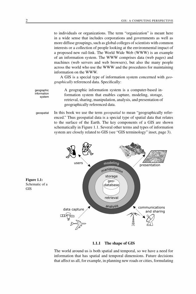
enced.” Thus geospatial data is a special type of spatial data that relatesto the surface of the Earth. The key components of a GIS are shownschematically in Figure 1.1. Several other terms and types of informationsystem are closely related to GIS (see “GIS terminology” inset, page 3).

Figure 1.1:Schematic of aGIS

data capture

presentation

communications

and sharing

users

analysis

geo-

database

storage

retrieval

modeling

manipulation

1.1.1 The shape of GIS

The world around us is both spatial and temporal, so we have a need forinformation that has spatial and temporal dimensions. Future decisionsthat affect us all, for example, in planning new roads or cities, formulating

INTRODUCTION 3

GIS terminology There are several terms in common use that are more or less synonymouswith GIS. A spatial information system (SIS) has the same functional components as a GIS,but may handle data that is referenced at a wider range of scales than simply geographic(for example, data on molecular configurations). A spatial database provides the databasefunctionality for a spatial information system. A geographic database (or geodatabase)provides the database functionality for a GIS. An image database is fundamentally differentfrom a spatial database or geodatabase in that the images have no structural interrelation-ships or topological features. For example, a database of brain-scan images may be termedan image database. Computer-aided design (CAD) has some elements in common with GIS,and historically some GIS software packages have developed from CAD software. UnlikeCAD, GIS software is used to manipulate data sets that are geographically referenced. Asa consequence, GIS software is usually used with larger data sets and more complex datamodels than CAD software. Conventionally, and in this book, the singular form of GIS maybe used to refer to “the field of GIS,” where no confusion is likely. While not synonymouswith GIS, the terms geographic information science (GIScience) and geoinformatics arerelevant to GIS as they are used to describe the systematic study of geographic informationand geographic information systems.

agricultural strategies, and locating mineral extraction sites, rely uponproperly collected, managed, distributed, analyzed, and presented spatialand temporal information. A GIS may be thought of as a tool that is able toassist us with these tasks. This tool relies on several underlying elements.In the remainder of this section we look in more detail at these differentelements, so describing the “shape” of GIS.

Database element At the heart of any GIS is the database. A database is database

a collection of data organized in such a way that a computer can efficientlystore and retrieve the data. Databases are introduced in Chapter 2. Animportant element of a database is the data model. Some applicationsrequire relatively simple data models. For example, in a library systemdata about books, users, reservations, and loans is structured in a clearway. Many applications, including most GIS applications, demand morecomplex data models (consider, for example, a model of global climate).One of the main issues addressed in this book is the provision of facilitiesfor handling these complex data models. Chapter 2 introduces somefundamental data modeling concepts, while Chapters 3 and 4 examinewhat makes geospatial data and geospatial data models special.

In this book we discuss how complex geospatial data models can berepresented in an information system. However, we do not discuss thesuitability of particular data models for particular application areas: thisis a topic for application domain experts. For example, a transportationgeography textbook should offer insights into whether a particular modelof transportation flow is appropriate for a particular application. We areonly concerned with providing the general facilities to represent geospa-tial data models, which might include models of transportation flow.


Data processing element Data models are stepping-stones to the ma-nipulation and processing of data. GIS software needs to have sufficientlycomplete functionality to provide the higher-level analysis and decisionsupport required within an application domain. For example, a GIS thatis used for utility applications will require network processing operations(optimal routing between nodes, connectivity checks, and so forth). AGIS for geological applications will require three-dimensional operations.Identifying and specifying a general set of primitive operations requiredby a generic GIS is a major concern of the book, covered primarily inChapter 5. Again, the discussion in this book does not address whetherspecific approaches to geospatial data analysis are suitable for particularapplications: those questions we leave to application domain experts.

Data storage and retrieval element Efficient storage and retrieval ofdata depend on not only properly structured data in the database toprovide satisfactory performance, but also optimized structures, repre-sentations, and algorithms for operating on data. Retrieval, operations,and performance raise many interesting questions for geospatial data andwill be a further main theme of this text (Chapter 6).

Data sharing element A GIS may comprise many different software andhardware components, such as geographic data servers, web browsers,and mobile computing devices. For example, in order to access real-timeinformation about the best route to drive home from work, allowing fortraffic jams, road works, and changing road conditions, several differentinformation system components must work together. An important char-acteristic of any GIS is the capability to share data between differentinformation systems, or between different components within a singleinformation system. Understanding and achieving data sharing are keytopics in this book, discussed under the general heading of system archi-tecture (Chapter 7).

Data presentation element Data within a GIS, and the operations per-formed upon that data, are not useful unless they can be communicated tothe people using that GIS. Many traditional information systems requireonly limited presentational forms, usually based around tables of data,numerical computation, and textual commentary. While these forms arealso required to support decision-making using a GIS, the geospatial na-ture of data in a GIS allows a whole new range of possibilities, includingcartographic (map-based) presentation as well as more exploratory formsof presentation. Presentation of the results of retrievals and analyses usinga GIS therefore takes us beyond the scope of most traditional databasesand is a further concern of this text (Chapter 8).

Spatial reasoning element To get the most from geospatial data, it isimportant that we are aware of and able to reason about its limitations.

INTRODUCTION 5

Accuracy, precision, and reliability are examples of terms we often usewhen talking about the limitations of data. Understanding such terms, andhow they affect the way we use a GIS to reason about geospatial data, isanother important topic in GIS, covered in Chapter 9.

Spatiotemporal element Finally, as stated above, the world is both spa-tial and temporal. Extending GIS to allow the storage and processing ofdynamic geospatial phenomena that change over time is a major topicfor current research. In the final chapter, we introduce the key models ofspatiotemporal phenomena, and show how the next generation of GIS isbeginning to move beyond static representations of the world around us.

1.1.2 Data and information

The structure of interrelationships between data and how data is collected,processed, used, and understood within an application forms the context context

for data. An understanding of the data model and of the limitations ofdata, discussed above, are elements of the context for data. Data only data

becomes useful, taking on value as information, within this context.For example, data about atmospheric conditions is recorded by me-

teorological stations across the world: there is likely to be one near yourecording right now. However, on its own the raw data from your nearestrecording station is unlikely to be useful to you. Useful information,such as a weather forecast that helps you decide if you need to carryan umbrella with you, is produced within the context of careful modelingand analysis of raw data from multiple sources (such as satellite imagery,data from other recording stations, and historical data). Accordingly,information can be defined as “data plus context”: information

information = data + context

We refine the concepts of data and information in later chapters(particularly Chapter 9), but this basic distinction between data and in-formation is needed throughout the book.

1.2 GIS FUNCTIONALITY

As highlighted above, a GIS is an information system that has somespecial characteristics. To demonstrate the range of capabilities andfunctionality of a GIS, seven example applications are described in thissection. These applications have been chosen for a region of England,familiarly called “The Potteries” due to its dominant eponymous indus-try. The Potteries comprise the six pottery towns of Burslem, Fenton,Hanley, Longton, Stoke, and Tunstall, along with the neighboring townof Newcastle-under-Lyme (see Figure 1.2). The Potteries region devel-oped rapidly during the English industrial revolution, local communitiesproducing ware of the highest standard (for example, from the potteriesof Wedgwood and Spode) from conditions of poverty and cramp. The


region’s landscape is scarred by the extraction of coal, ironstone, and clay.In the 20th century, the Potteries declined in prosperity although the areais now in a phase of regeneration.

Figure 1.2:The Potteriesregion

Tunstall

Burslem

Hanley

Newcastle-

under-Lyme

Stoke

Fenton

Longton

A34

A500

A500

M6

A53

A52

A50

A34

2 kms

Potteries

region

Town centers

Motorway

Main roads

A500

Built-up area

We emphasize that the example applications are here merely to showfunctionality, rather than serious descriptions of application areas. Forapplication-driven texts, see the bibliography at the end of the chapter.The final part of this section summarizes typical GIS functionality.

1.2.1 Resources inventory: A tourist information system

The Potteries, because of its past, has a locally important tourist industrybased upon the industrial heritage of the area. A GIS may be usedto support this, by drawing together data on cultural and recreationalfacilities within the region, and combining this data with details of localtransport infrastructure and hotel accommodation. Such an applicationis an example of a simple resource inventory. The power of almost anyresource

inventory information system lies in its ability to relate and combine data gatheredfrom disparate sources. This power is increased dramatically when thedata is geographically referenced, provided that the different sources ofgeospatial data are made compatible through some common spatial unit ortransformation process. Figure 1.3 shows the beginnings of such a system,including some of the local tourist attractions, the major road network,and built-up areas in the region.

INTRODUCTION 7

A34

A500

A500

M6

A53

A52

A50

A34

City Museum

Royal Doulton Pottery

Spode Pottery

Minton Pottery

Wedgwood

Visitor Centre

Coalport Pottery

Beswick

Pottery

Gladstone

Pottery

Museum

Park Hall

Country Park

Ford Green Hall

Westport Lake

Newcastle

Museum

New Victoria Theatre

Town centers

Motorway

Main roads

A500

Places of interest

Built-up area

Figure 1.3:Places ofinterest in thePotteries region

1.2.2 Network analysis: A tour of the Potteries

Network analysis is one of the cornerstones of GIS functionality. Applica- network analysis

tions of network analysis can be found in many areas, from transportationnetworks to the utilities. To provide a single simple example, we stay withthe tourist information example introduced above. The major potteries inthe Potteries area are famous worldwide. Many of these potteries offerfactory tours and have factory outlet stores. The problem is to provide aroute using the major road network, visiting each pottery (and the CityMuseum) only once, while minimizing the traveling time. The data setrequired is a travel-time network between the potteries: a partial exampleis given in Figure 1.4a.

The travel-time network in Figure 1.4a was derived from averagetimes on the main roads shown on the map. The network may then be usedas a basis for generating the required optimal route between Royal Doul-ton and the Wedgwood Visitor Centre, shown in Figure 1.4b. The routevisits the potteries in sequence: Royal Doulton, City Museum, Spode,Minton, Coalport, Gladstone, Beswick, Wedgwood. The specific networkanalysis technique required here is the traveling salesperson algorithm,which constructs a minimal weight route through a network that visitseach node at least once. The analysis could be dynamic, assigning weightsto the edges of the network and calculating optimal routes dependingupon changeable road conditions.


Figure 1.4:Travel networkbased upontravel times (inminutes) andoptimal route

City Museum


Spode Pottery

Minton Pottery

Wedgwood

Visitor Centre

Coalport Pottery

Beswick

PotteryGladstone

Pottery

Museum

15

128

5

20

7

9

27

5

5

30

35

7

a.

Travel time

network

b.

Optimal

route

City Museum


Spode Pottery

Minton Pottery

Wedgwood

Visitor Centre

Coalport Potterry

Beswick

PotteryGladstone

Pottery

Museum

INTRODUCTION 9

1.2.3 Distributed data: Navigating around the potteries

Much of the data used in a GIS is located in different formats at physicallyremote locations. A GIS needs to be able to overcome these barriers todata sharing. Continuing the tourist information example, the resourcesinventory and network analysis described above demand the sharing andanalysis of disparate geospatial data about the locations of places of inter-est, the transport infrastructure, and cultural, hospitality, and recreationalresources. These resources are commonly held by different organizationsat different locations. Base map data may be held in one place, such asby a national mapping agency. Data about transport infrastructure mightbe compiled by the local government or held by individual bus or traincompanies. The tourist information bureau will hold some data aboutthe local amenities, although more will often reside with the individualamenities themselves, such as museums or hotels.

Tourist

Service

Provider

Wireless

communication

Spatial

database

Network

analysisMuseum

information

To museum

Left at Post Office

Figure 1.5:Schematic viewof a distributedtouristinformationsystem

Figure 1.5 shows a schematic version of a distributed informationsystem that might be used as the basis of a Potteries tourist application.Before a tourist visiting the Potteries can receive navigation directionsand information about local attractions (for example, on their cell phoneor handheld computer), data from all these different sources must beintegrated, processed, and transmitted to the tourist. Since the tourist willnot usually be a GIS expert, these complex tasks would normally be doneon behalf of the tourist by some tourist service provider. The serviceprovider might gather all the information needed, either in advance ordynamically when requested, and perform the network analysis necessaryto find the best route for a particular user at a particular time and location.Although the information actually presented to a tourist at any moment intime may be simple (such as “turn left” indicators, Figure 1.5), the task ofintegrating data from different sources may be complex.


1.2.4 Terrain analysis: Siting an opencast coal mine

Terrain analysis is usually based upon data sets of topographic elevationsat point locations. Basic information about degree of slope and directionof slope (termed aspect) can be derived from such data sets. A more com-aspect

plex type of analysis, termed visibility analysis, concerns the visibilityvisibility analysis

between locations and the generation of a viewshed (a map of all thepoints visible from some location).

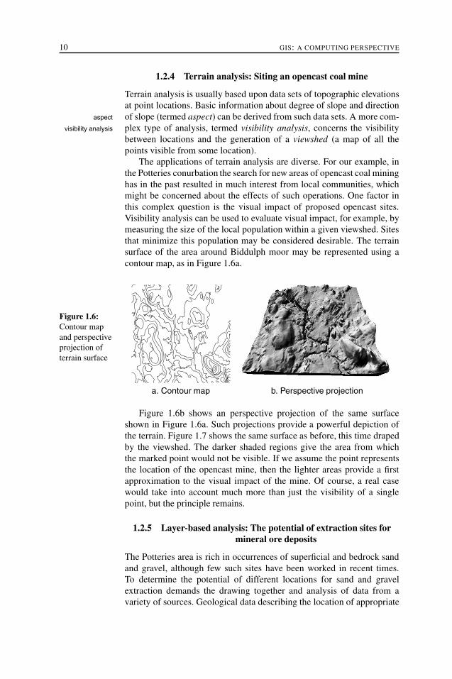
The applications of terrain analysis are diverse. For our example, inthe Potteries conurbation the search for new areas of opencast coal mininghas in the past resulted in much interest from local communities, whichmight be concerned about the effects of such operations. One factor inthis complex question is the visual impact of proposed opencast sites.Visibility analysis can be used to evaluate visual impact, for example, bymeasuring the size of the local population within a given viewshed. Sitesthat minimize this population may be considered desirable. The terrainsurface of the area around Biddulph moor may be represented using acontour map, as in Figure 1.6a.

Figure 1.6:Contour mapand perspectiveprojection ofterrain surface

a. Contour map b. Perspective projection

Figure 1.6b shows an perspective projection of the same surfaceshown in Figure 1.6a. Such projections provide a powerful depiction ofthe terrain. Figure 1.7 shows the same surface as before, this time drapedby the viewshed. The darker shaded regions give the area from whichthe marked point would not be visible. If we assume the point representsthe location of the opencast mine, then the lighter areas provide a firstapproximation to the visual impact of the mine. Of course, a real casewould take into account much more than just the visibility of a singlepoint, but the principle remains.

1.2.5 Layer-based analysis: The potential of extraction sites formineral ore deposits

The Potteries area is rich in occurrences of superficial and bedrock sandand gravel, although few such sites have been worked in recent times.To determine the potential of different locations for sand and gravelextraction demands the drawing together and analysis of data from avariety of sources. Geological data describing the location of appropriate

INTRODUCTION 11

Figure 1.7:Perspectiveprojection ofterrain surfacedraped withviewshed forthe markedpoint

deposits is, of course, needed. Other important considerations are localurban structure (e.g., urban overbuilding), water table level, transportationnetwork, land prices, and land zoning restrictions. Figure 1.8 shows asample of the available data overlaid on a single sheet, including dataon built-up areas, known sand and gravel deposits, and the major roadnetwork.

A34

A500

A500

M6

A52

A50

A34

Town centers

Motorway

Main roads

A500

Built-up area

Sand and gra-

vel deposits

Figure 1.8:Locations ofsand and graveldeposits in thePotteries region

Layer-based analysis results from posing a query such as: “Find alllocations that are within 0.5 km of a major road, not in a built-up area,and on a sand/gravel deposit.” Figure 1.9 illustrates the construction ofan answer to this question. The gray areas in Figure 1.9a show the regionwithin 0.5 km of a major road (not including the motorway), termed abuffer. The gray areas in Figure 1.9b indicate known sand and gravel


deposits, and in Figure 1.9c the shaded areas indicate locations that are notbuilt up. Figure 1.9d shows the overlay of the three other layers, and thusthe areas that satisfy our query. The analysis here is simplistic. A morerealistic exercise would take into account other factors, like the gradingof the deposit, land prices, and regional legislation. However, the exampledoes show some of the main functionality required of a GIS engaged inlayer-based analysis, including:

• The formation of areas containing locations within a given range ofa given set of features, termed buffering. Buffers are commonlybuffering

circular or rectangular around points, and corridors of constantwidth about lines and areas.

• The combination of one or more layers into a single layer that is theunion, intersection, difference, or other Boolean operation appliedto the input layers, termed Boolean overlay.Boolean overlay

Layer-based functionality is explored further in the context of field-based models and structures later in the book.

Figure 1.9:Layer-basedanalysis to sitea mineral oreextractionfacility

a. Road buffers b. Sand and gravel

c. Not built-up areas d. Overlay

1.2.6 Location analysis: Locating a clinic in the Potteries

Location problems have been solved in previous examples using terrainmodels (opencast mine example) and layer-based analysis (estimating the

INTRODUCTION 13

potential of sites for extracting sand and gravel). Our next example is thelocation of clinics in the Potteries area. A critical factor in the decisionto use a particular clinic is the time it takes to travel to it. To assess thiswe may construct the “neighborhood” of a clinic, based upon positions ofnearby clinics and travel times to the clinic. With this evidence, we canthen support decisions to relocate, close, or create a new clinic.

a. Clinics, with isochrones around one clinic

b. Proximal polygons

Figure 1.10:Potteriesclinics andtheir proximalpolygons

Figure 1.10 shows the idealized positions of clinics in the Potteriesregion. Assuming an “as the crow flies” travel time between points (i.e.,the time is directly related to the Euclidean distance between points),Figure 1.10a shows lines connecting locations that are equally far fromthe clinic in terms of travel time, termed isochrones. It is then possible isochrone


to partition the region into areas, each containing a single clinic, suchthat each area contains all the points that are nearest (in travel time) toits clinic, termed proximal polygons (see Figure 1.10b). Of course, weare making a simplistic assumption about travel time. If the road networkis accounted for in the travel-time analysis, then the isochrones will nolonger be circular and the areal partition will no longer be polygonal.This more general situation is discussed later in the book.

1.2.7 Spatiotemporal information: Thirty years in the Potteries

Geospatial data sometimes becomes equated with purely static data, thusneglecting the importance of change and time. In a temporal GIS, datais referenced to three kinds of dimensions: space, time, and attribute. Ourlast example suggests possibilities for a future dynamic GIS functionality,just beyond the reach of present systems. We return to the problem ofadding temporal dimensions in the final chapter.

The main period of industrial activity in the Potteries is long sincepast. The history of the region in the latter half of the 20th century hasbeen one of industrial decline. Figure 1.11 shows the Cobridge area of thePotteries, recorded in snapshot at two times: 1878 and 1924. It is clear thatas time has passed many changes have occurred, such as the extension ofresidential areas in the northwest and southeast of the map. Examples ofquestions that we may wish to ask of our spatiotemporal system include:

• Which streets have changed name in the period 1878–1924?

• Which streets have changed spatial reference in the period 1878–1924?

• In what year is the existence of the Cobridge Brick Works lastrecorded in the system?

• What is the spatial pattern of change in this region between 1878and 1924?

1.2.8 Summary of analysis and processing requirements

The examples of applications reviewed in this section demonstrate someof the specialized processing functionality that a GIS needs to provide,usually termed spatial analysis. Geospatial database functionality wasspatial analysis

illustrated with the resources inventory in section 1.2.1. Geospatial datais commonly presented using computer graphics, as shown in most ofthe figures in this section. However, we have seen that a GIS is morethan just a graphics database. A graphical system is concerned with themanipulation and presentation of screen-based graphical objects, whereasa GIS handles phenomena embedded in the geographic world and havingnot only geospatial dimensions but also structural placement in multidi-mensional geographic models. Some of the analytical processing require-ments that give a GIS its special flavor include:

INTRODUCTION 15

a. 1878

b. 1924

Figure 1.11:History of theCobridge area,recorded insnapshots attimes 1878 and1924 (Source:OrdnanceSurvey)

Geometric, topological, and set-oriented analyses: Most if not all geo-graphically referenced phenomena have geometric, topological,or set-oriented properties. Set-oriented properties include mem-bership conditions, Boolean relationships between collections ofelements, and handling of hierarchies (e.g., administrative areas).Topological operations include adjacency and connectivity rela-tionships. A geometric analysis of the clinics (section 1.2.6) pro-duced their proximal polygons. All these properties are key to aGIS and form a main theme of this book.

Field-based analysis: Many applications involve spatial fields, that is,variations of attributes over a region. The terrain in section 1.2.4is a variation of topographic elevation over an area. The gravel andsand deposits and built up areas of section 1.2.5 are variations of


other attributes. Fields may be discrete (a location is either built upor not) or continuous (e.g., topographic elevation). Fields may bescalar (variations of a scalar quantity and represented as a surface)scalar

or vector (variations of a vector quantity such as wind velocity).vector

Field operations include overlay (section 1.2.5), slope and aspectanalysis, path finding, flow analysis, and viewshed analysis (section1.2.4). Fields are discussed further throughout the text.

Network analysis: A network is a configuration of connections betweennodes. The maps of most metro systems are in network form, nodesrepresenting stations and edges being direct connections betweenstations. Networks may be directed, where edges are assigneddirections (e.g., in a representation of a one-way street system)or labeled, where edges are assigned numeric or non-numericattributes (e.g., travel-time along a rail link). Network operationsinclude connectivity analysis, path finding (trace-out from a singlenode and shortest path between two nodes), flow analysis, andproximity tracing (the network equivalent of proximal polygons).The Potteries tourist information system application (section 1.2.2)gives an example of a network traversal. Networks are consideredfurther in Chapter 3.

1.3 DATA AND DATABASES

Any information system can only be as good as its data. This sectionintroduces some of the main themes associated with databases and datamanagement. To support the database, there is a need for appropriate ca-pabilities for data capture, modeling, retrieval and analysis, presentation,and dissemination. An issue that arises throughout the book is the extrafunctionality that a geodatabase needs over and above the functionalityof a general-purpose database. This section provides an overview, but thetopic is taken up further in Chapter 2 and throughout the book.

1.3.1 Spatial data

First, a reminder of some data basics. Data stored in a computer system ismeasured in bits. Each bit records one of two possible states: 0 (off, false)bit

and 1 (on, true). Bits are amalgamated into bytes, each byte representingbyte

a single character. A character may be encoded using 7 bits with an extrabit used as an error check; thus each byte allows for 27 = 128 possiblecharacter combinations. This is enough for all the characters normallyused in the English language (this encoding is the basis of ASCII code).To represent all the characters found in other languages requires morebits. Two-byte characters allow for 216 = 65536 different charactercombinations (the basis for Unicode).

Geospatial data is traditionally divided into two great classes, rasterand vector. Traditionally, systems have tended to specialize in one or otherof these classes. Translation between them (rasterization for vector-to-rasterization

INTRODUCTION 17

raster and vectorization for raster-to-vector) has been a thorny problem, vectorization

to be taken up later in the book. Figure 1.12 shows raster and vector datarepresenting the same situation of a house, outbuilding, and pond next toa road.

Raster Vector

Figure 1.12:Raster andvector data

Raster data is structured as an array or grid of cells, referred to as raster

pixels. The three-dimensional equivalent is a three-dimensional array of pixels

cubic cells, called voxels. Each cell in a raster is addressed by its position voxels

in the array (row and column number). Rasters are able to represent a largerange of computable spatial objects. Thus, a point may be represented bya single cell, an arc by a sequence of neighboring cells and a connectedarea by a collection of contiguous cells. Rasters are natural structures touse in computers, because programming languages commonly supportarray handling and operations. However, a raster when stored in a rawstate with no compression can be extremely inefficient in terms of usageof computer storage. For example, a large uniform area with no specialcharacteristics may be stored as a large collection of cells, each holdingthe same value. We will consider efficient computational methods forraster handling in later chapters.

The other common paradigm for spatial data is the vector format.(This usage of the term “vector” is similar but not identical to “vector”in vector fields). A vector is a finite straight-line segment defined by vector

its end-points. The locations of end-points are given with respect tosome coordinatization of the plane or higher-dimensional space. Thediscretization of space into a grid of cells is not explicit as it is with theraster structure. However, it must exist implicitly in some form, becauseof the discrete nature of computer arithmetic. Vectors are an appropriaterepresentation for a wide range of spatial data. Thus, a point is justgiven as a coordinate. An arc is discretized as a sequence of straight-linesegments, each represented by a vector, and an area is defined in termsof its boundary, represented as a collection of vectors. The vector datarepresentation is inherently more efficient in its use of computer storagethan raster, because only points of interest need be stored. A disadvantageis that, at least in their crude form, vectors assume a hard-edged boundary


model of the world that does not always accord with our observations. Wereturn to these issues in later chapters.

1.3.2 Database as data store

A database is a repository of data that is logically related, but possiblyphysically distributed over several sites, and required to be accessed bymany applications and users. A database is created and maintained using ageneral-purpose piece of software called a database management system(DBMS). For a database to be useful it must be:DBMS

Reliable: A database must be able to offer a continual uninterrupted ser-vice when required by users, even if unexpected events occur, suchas power failures. For example, a database must be able to contendwith the situation where we deposit money into an automatic tellermachine (ATM) and the power fails before our balance has beenupdated.

Correct and consistent: Data items in the database should be correct andconsistent with each other. This has been a problem with older filesystems, when data held by one department contradicts data fromanother. While it is not possible to screen out all incorrect data, itis possible to control the problem to some extent, using integritychecking at input. Clearly, the more we know about the kinds ofdata that we expect, the more errors can be detected.

Technology proof : A database should evolve predictably, gracefully, andincrementally with each new technological development. Bothhardware and software continue to develop rapidly, as new pro-cessors, storage devices, software, and modeling techniques are in-vented. Database users should be insulated from the inner workingsof the database system. For example, when we check our balance atthe ATM, we do not really want to know that on the previous nightnew storage devices were introduced to support the database.

Secure: A database must allow different levels of authorized access andprevent unauthorized access. For example, we may be allowed toread our own, but no one else’s, bank balance (read access). Atthe same time we may not be allowed to change our bank balance(write access).

1.3.3 Data capture

The process of collecting data from observations of the physical envi-ronment is termed data capture. The primary source of data for a GIS isdata capture

from sensors that measure some feature of the geographic environment.Satellite imagery, for example, uses sensors to measure the electromag-netic radiation reflected or emitted from the Earth’s surface at different

INTRODUCTION 19

wavelengths. Surveyors use sensors to measure distances and anglesbetween features located on the Earth’s surface.

Sometimes humans are needed to convert the data produced by asensor into a form that an information system can use, such as when ahuman enters data using a keyboard. In most circumstances, however,data capture is automated, so that digital data from a sensor is fed directlyto an information system and, after processing, stored within a database.The variety of common digital sensors is steadily increasing, while theirsize and cost is steadily decreasing. As a result, GISs often need to storeand process sensor-based information from many different sources. Thedifferent types of sensor that exist for determining location are discussedin Chapter 7.

A secondary data capture stream for GISs is from a legacy data legacy data

source, such as paper maps. Maps combine the functions of data pre-sentation and data storage, functions that GISs keep separate. Convertinggeospatial data stored in a paper map into a form that can be storedin a GIS can be difficult and costly. Automatic conversions, such asscanning a map, cannot easily capture the complex structure of the map,and the results are more similar to an image database than a GIS. Manualconversions, for example, where humans trace the features of a map usinga digitizer (see section 1.4.4 and Figure 1.17), can capture more structure,but are time-consuming and laborious.

1.3.4 Data modeling

The choice of appropriate data model can be the critical factor for the data model

success or failure of an information system. In fact, the data model isthe key to the database idea. Data models function at all levels of theinformation system. The process of developing a database, or indeedany information system, is essentially a process of model building. Atthe highest level is the application domain model, which describes thecore requirements of users in a particular application domain, based onan initial study. At the next level, the conceptual computational modelprovides a means of communication between the user and the systemthat is independent of the details of the implementation. The process ofdeveloping a conceptual computational model focuses on questions ofwhat it is the system will do, termed system analysis. system analysis

The logical computational model is tailored to a particular type of im-plementation. The process of developing a logical computational modelfocuses on questions of how the system will implement the conceptualcomputational model, termed system design. Finally, the low-level physi- system design

cal computational model is the result of a process of programming andsystem implementation. It describes the actual software and hardware system

implementationapplication, including how data is processed and organized on a particulartype of machine.

The different stages and processes involved in system developmentare shown in Figure 1.13. The stages form a logical progression from


Figure 1.13:Modelingprocesses andthe stages ofsystemdevelopment

system

analysis

application

domain

application

domain

model

conceptual

computational

model

logical

computational

model

physical

computational

model

system

design

system

implementation

initial

study

application domain to actual implementation. This logical progressionis often referred to as the waterfall model of system development. Inwaterfall model

practice, system development is more cyclic (indicated in Figure 1.13with the dashed arrows), for example, with a new round of analysis anddesign following from a pilot implementation. The term system life-cyclesystem life-cycle

is therefore preferred to the waterfall model, because it emphasizes theevolutionary and iterative nature of system development.

The different stages of the system life-cycle form a bridge betweenthe human conception of the application domain and the computationalprocesses used in the information system. Without this structure, thesystem development process can become unmanageable. Typically, dis-regarding the system life-cycle leads to systems that are either difficult touse, because they neglect the human aspects of the information system,or inefficient, because they neglect the computational aspects.

Two important elements of the system life-cycle are not depictedin Figure 1.13, because they are not primarily modeling tasks. Sys-tem maintenance follows implementation, making ongoing changes andimprovements to a system in response to actual system usage. Systemdocumentation occurs throughout every stage of the system life-cycle,ensuring that adequate documentation accompanies the system.

1.3.5 Data retrieval and analysis

A key function of a database is the capability to rapidly and efficientlyretrieve and analyze information. To retrieve data from the database, wemay apply a filter, usually in the form of a logical expression, or query.query

INTRODUCTION 21

For example:

1. Retrieve names and addresses of all opencast coal mines in Staf-fordshire.

2. Retrieve names and addresses of all employees of WedgwoodPottery who earn more than half the sum earned by the managingdirector.

3. Retrieve the mean population of administrative districts in thePotteries area.

4. Retrieve the names of all patients at Stoke City General Hospitalwho are over the age of 60 and have been admitted on a previousoccasion.

Assuming that the first query accesses a national database and thatthe county in which a mine is located is given as part of its address, thenthe data may be retrieved by means of a simple look-up and match. Forthe second query, each employee’s salary would be retrieved along withthe salary of the managing director and a simple numerical comparisonmade. For the third, populations are retrieved and then a numericalcalculation is required. For the last, a more complex filter is required,including a check for multiple records for the same person.

There are spatial operators in the above queries. Thus, in the firstquery, whether a mine is in Staffordshire is a spatial question. However,it is assumed that the processing for this query needs no special spatialcomponent. In our example, there is no requirement to check whether amine is within the spatial boundary of the county of Staffordshire, becausethis information is given explicitly by textual means in the database. AGIS allows real geospatial processing to take place. For example, considerthe following two queries:

1. What locations in the Potteries satisfy the following set of condi-tions:

• less than the average price for land in the area;

• within 15 minutes drive of the motorway M6;

• having suitable geology for gravel extraction; and

• not subject to planning restrictions?

2. Is there any correlation between:

• the location of vehicle accidents (as recorded on a hospitaldatabase); and

• designated “accident black spots” for the area?

Satisfying such queries often requires the integration of both spatialand non-spatial information. The first of these examples is rather moreprescriptive than the second, specifying the type of relationship required.


The second example requires a more open-ended application of spatialanalysis techniques.

All of the above functionality is attractive and desirable, but will beuseless if not matched by commensurate performance. Computationalperformance is usually measured in terms of storage required and process-ing time. Storage and processing technology are continually advancing.However, not all computational performance problems can be solvedby using technology that is more advanced. Some problems, such asthe traveling salesperson problem mentioned in section 1.2.2, require somany calculations that in general it is not possible to compute an optimalsolution in a reasonable time.

Performance is an even bigger issue for a geodatabase than a general-purpose database. Spatial data is notoriously voluminous. In addition,spatial data is often hierarchically structured (a point being part of anarc, which is part of a polygon). We shall see that these structures presentproblems for traditional database technology. Although DBMSs are de-signed to handle multidimensional data, the dimensions are assumed in-dependent. However, geospatial data is often embedded in the Euclideanplane: special storage structures and access methods are required. Weshall return to the question of spatial data storage, access, and processinglater in the book.

1.3.6 Data presentation

Traditional general-purpose databases provide output in the form of textand numbers, usually in tabular form. A report generator is a standardfeature of a DBMS that allows data from a database to be laid out in aclear human-readable format. Many databases also have the capacity tooffer enhanced presentations, like charts and graphical displays, termedbusiness graphics.

In addition to these general presentation mechanisms, a GIS needs tooutput maps and map-based material. Map-based presentation is a highlydistinctive feature of a GIS compared with a general-purpose database.Indeed, the ability to produce hard copy maps automatically, termedautomated or digital cartography, was one of the primary reasons for thedigital

cartography initial development of GIS and remains an important function of someGIS software. A few DBMSs and GISs go further than business graphicsand maps, and provide tools to help users explore a data set and discoverrelationships and patterns embedded in their data, termed data miningdata mining

(see “Spatial data mining” inset, on the facing page). Questions of thekind “Here is a lot of data: is there anything significant or interestingabout it?” are prototypical for data mining. Systems that support datamining have usually highly flexible presentation capabilities, so that userscan interactively combine and re-express multidimensional data in manydifferent forms, including graphs, trees, and animations.

INTRODUCTION 23

Spatial data mining Data mining refers to the process of discovering valuable informationand meaningful patterns within large data sets. Data mining is particularly important forgeospatial data because this type of data is typically voluminous and a rich source ofpatterns. Data mining differs from basic database querying, in that users may not know whatinformation or patterns they are seeking in advance. The sorts of information and patternsthat can be discovered using data mining include association rules and clustering patterns.One common application of spatial data mining is customer relationship management(CRM). A CRM company might use data mining to discover if there is an associationbetween different types of retail outlet, perhaps based on data about credit or debit carduse. For example, if shortly after seeing a movie customers tend to eat out at restaurantsclose to the cinema, data mining should help reveal this pattern as a basis for specializedpromotions (such as “See a movie at the Regal cinema, get a free dessert at FriendlyJoe’s Pizza Restaurant!”). Data mining can also be used to discover clusters as a basis forclassification. As an example, an environmental agency might use data mining to discovergeospatially clustered patterns in the location of industrial pollution.

1.3.7 Data distribution

A centralized database system has the property that the data, the DBMS,and the hardware are all gathered together in a single computer system.Although the database may be located at a single site, that does notpreclude remote access to the database. Indeed, this is one of the guidingprinciples of a database: facilitating shared access to a data.

If all applications could use a centralized database, then the studyof databases would be a much simpler topic. However, as illustrated bythe examples of the tourist navigation and mineral extraction systems(sections 1.2.3 and 1.2.4 above), many applications require access to datafrom multiple databases connected by a digital communication network,termed a distributed database. There are natural reasons for data to bedistributed in this way. Data may be more appropriately associated withone site rather than another, allowing a greater degree of autonomy andeasier update and maintenance. For example, details of local weatherconditions may be more usefully held at a local site where local con-trol and integrity checks may be maintained. Another advantage of adistributed database is increased reliability; failure at one site will notmean failure of the entire system. Distributed databases may also offerimproved performance. In the example of the local weather conditionsdatabase, commonly occurring accesses to the local site from local userswill be more efficient. Performance will be weaker for those accesses toremote sites, but such accesses may be fewer.

The downside is that distributed databases have a more intricate struc-ture to support. For example, distributed databases must handle querieswhere the data is fragmented across sites, and maintain the consistency ofdata that is replicated across sites. Distributed geodatabases are one topiccovered in more detail in Chapter 7.


1.4 HARDWARE SUPPORT

The term hardware is used to refer to the physical components of ahardware

computer system, like computer chips and keyboards, while softwaresoftware

refers to instructions or programs executed by a computer system. Whilethe software needed for a GIS is highly specialized, the hardware used ina GIS is broadly the same as that used within general-purpose computersystems. This section discusses the structure and function of computerhardware, to the degree necessary for understanding of the role thatit plays in supporting GIS. We assume readers are already somewhatfamiliar with the architecture of a computer, so this section contains onlya brief overview of those components directly relevant to GIS. Moredetailed texts on hardware are referenced in the bibliographic notes.

1.4.1 Overall computer architecture

Despite the wide range of tasks required of computers, almost all contem-porary computers conform to the von Neumann architecture, developedvon Neumann

architecture by the Hungarian-born mathematician John von Neumann at PrincetonUniversity during the 1940s and 50s. According to the von Neumannarchitecture, a computer system can be thought of as comprising fourmajor subsystems, which are illustrated in Figure 1.14 and describedbelow.

Processing: Data processing consists of operations performed to com-bine and transform data. Complex data processing functions maybe reduced to a small set of primitive operations.

Storage: Data is held in storage so that it may be processed. This storagemay range from short term (held only long enough for the process-ing to take place) to long term (held in case of future processingneeds).

Control: The storage and processing functions must be controlled bythe computer, which must manage and allocate resources for theprocessing, storage, and movement of data.

Input/output: Computers must be able to accept data input and to out-put the results of processing operations. Two important classesof input/output are discussed in more detail in later chapters: in-put/output between humans and computers and input/output be-tween different computer systems, especially when mediated by adigital communication network.

In terms of components rather than functionality, the key computersystem components are the CPU (responsible for processing and control),memory devices (responsible for data storage), and input/output devices(such as human input/output devices and computer networks). Each ofthese components is considered in turn in the following sections.

INTRODUCTION 25

control

storage

processinginput/output Figure 1.14:The four majorfunctionalcomponents ofa computer

1.4.2 Processing and control

Processing of data in the computer hardware is handled by the centralprocessing unit (CPU). The CPU’s main function is to execute machine CPU

instructions, each of which performs a primitive computational operation.The CPU executes machine instructions by fetching data into specialregisters and then performing computer arithmetic upon them.

The CPU is itself made up of several subcomponents, most importantof which are the arithmetic/logic unit (ALU) and the control unit. The ALU

control unit is responsible for the control function, managing and allocat- control unit

ing resources. The ALU is responsible for the actual processing functions.

Control

Unit

ALU

CPUStorage

Fetc

hin

stru

ction Decode

instructio

nExecute

InstructionStore

resu

lt

Figure 1.15:The instructioncycle

Operations are performed upon data sequentially, by retrieving storeddata, executing the appropriate operation, and then returning the resultsto storage. The process of execution is known as the instruction cycle instruction cycle

(also termed the machine cycle or the fetch-execute cycle). The instructioncycle involves four steps, shown in Figure 1.15. The first step is for thecontrol unit to retrieve an instruction from storage. Next, the controlunit decodes the stored instruction to determine what operation mustbe performed. The control unit then passes this instruction to the ALU,which completes the actual task of executing the operation. Finally, theresults of the execution are returned to storage, ready to be retrievedfor a subsequent instruction cycle. Connectivity between the CPU andother components in the computer is provided by dedicated communi-cation wires, each called a bus. While almost all computers rely on the bus


CISC and RISC We usually think of hardware as completely separate from software:hardware is real computing objects you can touch, software is digital instructions anddata. However, the distinction is not always so clear-cut. The set of instructions supportedby a CPU (hardware) is a determining factor in the complexity of programs (software)running on that CPU. Most personal computers use a complex instruction set computer(CISC) architecture, such as that found in the Intel Pentium family of CPUs. In a CISCarchitecture, the CPU supports tens or even hundreds of instructions, so making softwaresimpler and cheaper to program. However, complex instructions are generally slower toexecute than simple instructions. A reduced instruction set computer (RISC) architecturesupports fewer instructions than a CISC architecture. RISC has the advantage of leadingto generally faster and cheaper CPUs with lower power consumption. Most small andmobile computing devices use a low-power RISC architecture, such as the ARM family ofCPUs. By making the hardware simpler, RISC architectures need more complex softwareto achieve the same tasks. CISC and RISC are good illustrations of why the distinctionbetween hardware and software can be blurred. In fact, the distinction between CISC andRISC is also becoming blurred, as the latest CISC CPUs incorporate many of the ideasdeveloped for RISC architectures, and new RISC CPUs use as many instructions as olderCISC architectures.

instruction cycle, computer processors differ in the types and range ofinstructions they implement (see “CISC and RISC” inset, on this page).

1.4.3 Storage devices

Digital data must be physically kept somewhere in the computer system.Storage devices differ in their capacity (how much data can be stored),performance (how quickly the data can be accessed), volatility (whetherstored data persists after power to the system is turned off), and price.Storage devices can be divided into two categories:

• Storage that can be directly manipulated by the CPU is termedprimary storage, and is usually based on semiconductor technol-primary storage

ogy. Primary storage is relatively expensive per stored bit, com-pared to secondary storage, and is generally volatile (stored data isvolatile

lost when the power to the storage device is turned off).

• Storage that can be accessed only indirectly by the CPU (viainput/output controllers) is termed secondary storage. Secondarysecondary

storage storage is usually based upon magnetic or optical technology. Sec-ondary storage is relatively cheaper than primary storage and isnormally non-volatile (stored data persists after the power to thestorage device is turned off).

Figure 1.16 shows some examples of common primary and secondarystorage devices. Primary storage generally provides faster access to datathan secondary storage. However, primary storage normally offers lowerdata storage capacity than secondary storage. The balance between pri-mary and secondary storage is critical to the day-to-day performance of

INTRODUCTION 27

ROM and CPU cache memory

(on board CPU)

RAM

Zip drive

(m )agnetic disk

CD drive

(o )ptical disk

Hard drive

(magnetic disk)

Primary storage

Secondary storage

Figure 1.16:Commonstorage devices

a GIS. In general, because of the large sizes of data sets, it is impracticalto handle all the data required by a GIS in primary storage. Therefore,efficient structuring of data files on secondary storage devices is animportant factor in GIS performance. Much effort and ingenuity has beenspent by computer scientists devising suitable data structures to ensuregood performance with spatial data. To understand the issues that arisewith such data structures, it is worth examining in more detail some ofthe properties of the typical primary and secondary storage technology.

Primary storage is directly accessible to the CPU. The CPU requiresits own local memory in the form of registers so that data may be operatedon by the ALU, and the control unit also requires some internal memory.Such register memory is the fastest and most expensive of all types, the register memory

speed of which must be comparable with instruction cycle times.Other types of primary storage are referred to as main memory. main memory

The most common main memory is random access memory (RAM), a RAM

misnomer because all main memory is randomly accessible (i.e., directlyaddressable). RAM is volatile, thus requiring a continuous power supply,and capable of both read and write access. RAM is used for holdingdata that is coming and going between the CPU and peripheral devices.Read-only memory (ROM) is non-volatile and contains data that is “hard- ROM

wired,” in the sense that it is written during the ROM chip manufactureand cannot subsequently be changed. ROM is therefore only useful forstoring permanent data, such as systems routines for often-used functions(for example, graphics functions in a GIS). Other types of ROM allowdata to be stored after manufacture. PROM (Programmable ROM) allowsthe writing of data to be done, once, after chip manufacture. EPROM(Erasable PROM) and EEPROM (Electrically EPROM) allow multiple


non-volatile writing and rewriting of data, although usually at the cost oflower data access speeds than RAM. Flash memory is a type of EEPROMflash memory

with relatively high speed data access, often used in small storage devicesand configurable mobile computing devices, like cell phones.

The most important form of secondary storage is the magnetic disk.A magnetic disk is coated with a thin layer of magnetic material. Thepolarization of minute regions of the disk can be accessed or changedby an electrical read/write head. A combination of disk rotation andmovement of the read/write head provides access to the entire surfaceof the disk. The disk itself rotates at several thousand RPM, so the timetaken to move the head, termed seek time, is the overriding factor in accessseek time

to data on a disk. Thus, there is an advantage in physically structuringthe data on the disk so as to minimize seek time as far as possible.The physical structure of geospatial data on a disk is a question that hasreceived attention from the computer science community. Optical storage,like CDs and DVDs, has a similar structure (rotating disk and read/writeheads), but uses laser technology to read and write from a photosensitive(rather than magnetic) disk.

Magnetic and optical disks read and write data by finding a specificblock of data on the disk based on a unique physical address, a processknown as direct access. After reaching the desired block, the data from thedirect access

block is scanned in sequence until the precise read/write location is found,a process known as sequential access. By analogy, when locating a bar ofsequential access

music on a CD we may go directly to the desired track (direct access) andthen scan through the music track for the specific bar (sequential access).The time taken to access data varies for direct access, while the time takenfor sequential access is dependent on how far through the sequence weneed to search. Continuing the musical analogy, the time taken to find thebar of music within a track will depend on how far the bar is from thebeginning of the music.

1.4.4 Human input/output devices

An array of different devices exists to enable humans to input data intocomputers and receive a computer’s output. One of the most commoninput devices is the keyboard (or keypad), used for entering numerical andtextual data. Pointing devices are a second common class of input devices.Unlike keyboards, which use fairly standard configurations of buttons(for example, the keypad buttons on a telephone), pointing devices comein many shapes and sizes. The mouse, touchpad, and stick pointer areexamples of pointing devices that can be found on many desktop orportable PCs, while joysticks and touch screens are also familiar pointingdevices.

One specialized type of pointing device that is of particular relevanceto GIS is the digitizer. A digitizer is a combination of a large flat tabletdigitizer

and a puck or stylus that can be moved across the tablet (see Figure1.17). Digitizers are needed for legacy data capture: converting geospatial

INTRODUCTION 29

information on paper maps into a digital form. A human operator placesthe map securely on the tablet and then uses the puck to trace out theshape of map features, such as the course of a river or the boundary of aan administrative district. As the puck moves across the tablet its positionis recorded by a computer. Other input devices can be used to input datain an audible form, such as a microphone used in combination with aspeech recognition system, or in a optical form, such as scanners used forconverting maps or pictures into digital images.

digitizing

tablet

map

puckFigure 1.17:Digitizingtablet

Output from the computer to a human user can be classified into twocategories: hard copy and soft copy. Hard copy output devices, such as hard copy

printers and plotters, produce output with some physical permanence. GIShas often been associated with expensive high-quality plotters, needed toproduce large format detailed paper maps. However, most GIS users relylargely or entirely on soft copy output devices, primarily the computerscreen or other video display unit (VDU). Soft copy output devices soft copy

produce output that is transient and intangible, like the image on a VDU.Sound from audio devices, such as speakers, is also a type of soft copyoutput. For GIS applications, the highly visual nature of human percep-tion and of geospatial information means that audio output is of lessimportance than visual display. Chapter 8 discusses human input/outputin more detail, including some examples of GIS applications where audiooutput is important.

1.4.5 Computer networks

Communication between computing devices connected by a networkhas become a fundamental part of most of today’s information systems,including GISs. Most communication networks are digital, meaning a digital

series of bits is transmitted using signal bursts at different intensitiescorresponding to the binary values 0 and 1 (Figure 1.18a). Older datacommunication technology sometimes uses analog signals, meaning the analog

signal strength can vary continuously like a sine wave (Figure 1.18b).There are a variety of techniques for encoding digital data within an

analog signal, including modulating (varying) the amplitude (intensity)


Figure 1.18:Digital andanalog signals

Binary digits (bits)

Signal

intensity

Time

0 1 0 1 ...

Signal

intensity

Time

a. Digital b. Analog

of the wave signal. An example of amplitude modulation for encodingdigital data within an analog signal is illustrated in Figure 1.19. Con-verting between digital and analog signals requires a device called amodem. Analog signals degrade more easily than digital signals, so mostmodem

remaining analog communication technology is being replaced by digitaltechnology.

Figure 1.19:Amplitudemodulationencodingdigital datawithin ananalog signal

Digital encoding

Signal

intensity

Time

0 1 0 1 ...

Irrespective of whether digital or analog signals are being transmit-ted, all communication networks use electromagnetic (EM) radiation topropagate signals. EM radiation can be thought of as a wave travelingthrough a medium. The frequency and wavelength of EM radiation affectits transmission properties. Frequency is the number of cycles a wavefrequency

completes per unit time, while the wavelength is the length of each cycle.wavelength

For a wave traveling at constant speed, such as EM radiation travelingthrough a vacuum, frequency is inversely proportional to wavelength (thatis to say, as wavelength increases frequency decreases).

EM radiation with shorter wavelengths, such as infrared and visiblelight, can carry more data than radiation with a longer wavelength, suchas microwaves and radio waves, because the shorter wavelengths allowthe signal bursts to be shorter. However, shorter wavelength EM signalsdegrade more quickly than longer wavelengths, and so are harder to useover longer distances. The range of wavelengths or frequencies availablefor data transmission is called the bandwidth. There is a clear relationshipbandwidth

between the bandwidth of a signal and the amount of data that can becarried by the signal: higher bandwidth means greater data transmissioncapacity.

INTRODUCTION 31

Figure 1.20 summarizes the magnetic spectrum and its data-transmission capabilities. Radio waves, microwaves, infrared, and visiblelight can all be used for computer networks. High-frequency ultraviolet,X-ray, and gamma ray EM radiation are not used for data transmission,because their high energies can be hazardous to the environment andhuman health.

Radiowaves

Micro-waves

Infra-red

Visiblelight

Ultra-violet

X-ray Gammarays

Longer wavelength

Lower frequency

Lower energy

Degrade more slowly

Can carry less information

Shorter wavelength

Higher frequency

Higher energy

Degrade more quickly

Can carry more information

Figure 1.20:Electromag-neticspectrum

Signals carried by EM radiation can be transmitted using differentmedia. The most common media used for data transmission are metal,normally copper, wires like those used in conventional phone lines andcoaxial computer network cables. Conventional telephone networks oftenhave low data transmission capacities, because they make inefficient useof the bandwidth available in the copper wires. Normal voice commu-nications require only a small frequency range for transmission, leavingmost of the available bandwidth unused. Digital communications usingthe telephone network often have to squeeze into the small bandwidthavailable for voice communications. Many telephone networks have nowbeen upgraded to make better use of bandwidth, and are able to transmitdigital data alongside voice communications, using frequencies that arenot needed for voice communications (termed digital subscriber line,DSL).

Increasingly, fiber-optic cables are replacing copper wire-based ca-bles. Fiber-optic cables use visible light to transmit data within fine glassfibers. Visible light offers greater bandwidth for data transmission thanradio waves, so fiber-optic cables can carry more data than copper cables.Additionally, fiber-optic cables are more reliable and less susceptible tointerference than copper wires.

Data transmission can also take place unguided through the Earth’satmosphere, termed wireless communication. Wireless communications wireless

normally use radio wave or microwave EM radiation to transmit data. Tocombat signal degradation and interference from environmental radiation,wireless signals must be relayed via antennas, either on the ground oron satellites. The shorter wavelengths of visible light and infrared make


these types of EM radiation less suitable for wireless communications.Using radio and microwave signals for wireless networks carries theadvantage that the low-frequency radiation can penetrate non-metallicobstacles, such as walls and floors, while visible light and infrared cannot.As a result, networks based on visible light and infrared signals areoften termed line-of-sight technology, although some diffuse optical andline-of-sight

infrared wireless networks have been developed that do not require adirect line of sight.

Most computers today are able to communicate with other computersvia a digital communication network, either using a connection-orientedor connectionless service. A connection-oriented service requires that aconnection-

oriented user’s computer must explicitly connect with a remote computer beforeany communication can occur. For example, to access a network via atelephone line, it is normally necessary to first dial up a remote computerto initiate the connection. A connectionless service allows computers toconnectionless

continually communicate with each other without the need to establishan explicit connection before communication begins. Most dedicateddata communication networks rely on connectionless services, and manytelephone networks are now beginning to offer connectionless services toreplace their older connection-oriented services.

Communication networks are distinguished according to the sizeof geographic area they cover. A local-area network (LAN) connectsLAN

groups of computers located within a small geographic area. A wide-areanetwork (WAN) connects groups of LANs together. The Internet is theWAN

largest WAN in existence, estimated in 2001 to connect more than 100million hosts.

From a GIS perspective, digital communications are radically alteringthe way people use geospatial information. Digital communications pro-mote sharing of geospatial information. Many companies and mappingagencies now offer a variety of geospatial information that can be down-loaded from the Internet. This in turn reduces the costs of data capture andanalysis for other organizations that use this data. Digital communicationsare also rapid. The speed of digital communications makes possiblecertain modes of computing, that would not otherwise be possible. Forexample, mobile GIS applications, like the tourist navigation systemdescribed in section 1.2.3, rely heavily on rapid digital communications.The topic of digital communications in GIS is examined in more detail inChapter 7.

BIBLIOGRAPHIC NOTES

1.1 There are now a great many general GIS textbooks, of whichonly a few examples are mentioned here. Longley et al. (2001)is an excellent introductory GIS textbook, which includes a thor-ough review of basic GIS functionality. Clarke (2002) is anotherpopular introductory-level GIS textbook. Jones (1997) empha-sizes the cartographic applications in GIS, while Burrough and

INTRODUCTION 33

McDonnell (1998) is aimed toward environmental applications.Affectionately known as the “Big Book,” Longley et al. (1999)is a more advanced two volume collection of chapters coveringmany aspects of GIS, both theory and applications. The firstedition of this book is still relevant and at the time of writingsome chapters are freely available online (Maguire et al., 1991).

1.2 Volume two of Longley et al. (1999) provides many examplesof specific applications of GIS. Examples of other application-oriented GIS texts include Clarke et al. (2001) (environmentalmodeling applications of GIS) and Miller and Shaw (2002)(transportation applications in GIS). The topic of spatial anal-ysis is introduced in Fotheringham et al. (2002) and O’Sullivanand Unwin (2002). Openshaw (1991) summarizes the methodsavailable for spatial analysis and suggests spatial analysis func-tionality relevant for GIS. Burrough and McDonnell (1998) andWeibel and Heller (1991) give overviews of visibility analysis.The inspiration for some of the example Potteries applicationswas provided by Phillips (1993).

1.3 Databases are the primary topic of the next chapter. Rigauxet al. (2001) and Shekhar and Chawla (2002) are two booksthat address GIS from a spatial databases perspective. Elmasriand Navathe (2003) is a more general databases textbook thatincludes a short section on GIS.

1.4 O’Leary and O’Leary (2003) and Williams et al. (2001) are ex-amples of very basic introductory texts on information systems,which contain chapters on hardware and computer networks.Thompson and Thompson (2002) is a slightly more advancedbook on PC hardware. Tannenbaum (2002) and Stallings (1999)cover both basic and more advanced networking topics.


Bibliography

Abadi, M. and Cardelli, L. (1996). A Theory of Objects. Berlin: Springer.

Abdelmoty, A., Williams, M., and Paton, N. W. (1993). Deduction anddeductive databases for geographic data handling. In Abel, D. andOoi, D. C. (Eds), Advances in Spatial Databases, pp. 443–464. Berlin:Springer.

Abel, D. J. and Mark, D. M. (1990). A comparative analysis of sometwo-dimensional orderings. International Journal of Geographical In-formation Systems, 4(1):21–31.

Abiteboul, S., Hull, R., and Vianu, V. (1995). Foundations of Databases.Reading, MA: Addison-Wesley.

Abowd, G., Mynatt, E. D., and Rodden, T. (2002). The human experience.Pervasive Computing, 1(1):48–57.

Abraham, T. and Roddick, J. F. (1999). Survey of spatiotemporaldatabases. GeoInformatica, 3:61–69.

ACM (2003). Association for computing machinery classic of the monthwebsite. http://www.acm.org/classics. Accessed 9 August 2003.

Ahlqvist, O., Keukelaar, J., and Oukbir, K. (2000). Rough classificationand accuracy assessment. International Journal of Geographic Infor-mation Science, 14:475–496.

Aho, A. V., Hopcroft, J. E., and Ullman, J. D. (1974). The Design andAnalysis of Computer Algorithms. Reading, MA: Addison-Wesley.

Akima, H. (1978). A method of bivariate interpolation and smooth sur-face fitting for irregularly distributed data points. ACM Transactionson Mathematical Software, 4(2):148–159.

Al Taha, K. K. (1992). Temporal Reasoning in Cadastral Systems. PhDthesis, University of Maine, Orono, ME.

Alchourron, C., Gardenfors, P., and Makinson, D. (1985). On the logicof theory change: Partial meet functions for contraction and revision.Journal of Symbolic Logic, 50:510–530.

Allen, J. F. (1983). Maintaining knowledge about temporal intervals.Communications of ACM, 26:832–843.

Allen, J. F. (1984). Towards a general theory of action and time. ArtificialIntelligence, 23:123–154.

391

http://www.acm.org/classics


Andany, J., Leonard, M., and Palisser, C. (1991). Management of schemaevolution in databases. In Proc. 17th International Conference on VeryLarge Data Bases (VLDB).

Armstrong, M. A. (1979). Basic Topology. Maidenhead, England:McGraw-Hill.

Barwise, J. and Etchemendy, J. (1999). Language, Proof, and Logic. NewYork: Seven Bridges.

Baumgart, B. (1975). A polyhedron representation for computer vision.In Proc. AFIPS National Conference 44, pp. 589–596.

Becker, B., Gschwind, S., Ohler, T., Seeger, B., and Widmayer, P.(1996). An asymptotically optimal multiversion B-tree. VLDB Journal,5(4):264–275.

Bentley, J. L. and Friedman, J. H. (1979). Data structures for rangesearching. ACM Computing Surveys, 11(4):397–409.

Beresford, A. and Stajano, F. (2003). Location privacy in pervasive com-puting. IEEE Pervasive Computing, 2(1):46–55.

Bertin, J. (1967). Semiologie Graphique. Paris: Mouton.

Bertolotto, M., De Floriani, L., and Marzano, P. (1994). An efficient rep-resentation for pyramidal terrain models. In Pissinou, N. and Makki,K. (Eds), Proc. Second ACM Workshop on Advances in Geographic In-formation Systems, pp. 129–136. Gaithersburg, MD: National Institutefor Standards and Technology.

Bezier, P. (1972). Numerical Control—Mathematics and Applications.London: Wiley. Translated from Emploi des Machines a Com-mande Numerique (1970), Masson et Cie: Paris, by Forrest, A. R. andPankhurst, A. F.

Blankenagel, G. and Guting, R. H. (1994). External segment trees. Algo-rithmica, 12:498–532.

Booch, G. (1993). Object-Oriented Analysis and Design with Applica-tions. Reading, MA: Addison-Wesley, 2nd edition.

Booch, G., Rumbaugh, J., and Jacobson, I. (1998). The Unified ModelingLanguage User Guide. Reading, MA: Addison-Wesley.

Bowyer, A. (1981). Computing Dirichlet tessellations. Computer Jour-nal, 24:162–166.

Brodie, M., Mylopoulos, J., and Schmidt, J. (Eds) (1984). On ConceptualModeling. Berlin: Springer.

Brookshear, J. G. (1989). Theory of Computation: Formal Languages,Automata, and Complexity. Redwood City, CA: Benjamin/Cummings.

Bryant, R. and Singerman, D. (1985). Foundations of the theory ofmaps on surfaces with boundaries. Quarterly Journal of Mathemat-ics, 36(2):17–41.

Bryant, V. (1985). Metric Spaces: Iteration and Application. Cambridge:Cambridge University Press.

BIBLIOGRAPHY 393

Burrough, P. (1981). Fractal dimension of landscapes and other environ-mental data. Nature, 294:240–242.

Burrough, P. and Frank, A. (1996). Geographic Objects with Indetermi-nate Boundaries. London: Taylor & Francis.

Burrough, P. A. and McDonnell, R. A. (1998). Principles of GeographicalInformation Systems. Oxford: Oxford University Press, 2nd edition.

Buttenfield, B. P. and McMaster, R. B. (Eds) (1991). Map Generalization:Making Rules for Knowledge Representation. London: Longman.

Camara, A. S. and Raper, J. (Eds) (1999). Spatial Multimedia and VirtualReality. London: Taylor & Francis.

Cardelli, L. and Wegner, P. (1985). On understanding types, data abstrac-tion, and polymorphism. ACM Computing Surveys, 17(4):480–521.

Chamberlin, D. and Boyce, R. (1974). SEQUEL: A structured Englishquery language. In Proc. ACM SIGMOD Conference, pp. 249–264.New York: ACM Press.

Charniak, E. (1991). Bayesian networks without tears. AI Magazine,91:50–63.

Chazelle, B. (1991). Triangulating a simple polygon in linear time. Dis-crete Computational Geometry, 6:485–524.

Chen, P. P.-S. (1976). The entity-relationship model—toward a unifiedview of data. ACM Transactions on Database Systems, 1(1):9–36.

Chess, D., Grosof, B., Harrison, C., Levine, D., Parris, C., and Tsudik, G.(1995). Itinerant agents for mobile computing. IEEE Personal Com-munications, 2(5):34–49.

Chicago Tribune (2001). Rental firm uses GPS in speeding fine. July 2nd,p9. Chicago, IL: Associated Press.

Chomicki, J. (1994). Temporal query languages: A survey. In Proc. 1stInternational Conference on Temporal Logic (ICTL’94).

Chomicki, J. and Revesz, P. (1997). Constraint-based interoperabilityof spatiotemporal databases. In Advances in Spatial Databases, vol-ume 1262 of Lecture Notes in Computer Science, pp. 142–161. Berlin:Springer.

Chorochronos Participants (1999). Chorochronos: A research network forspatiotemporal database systems. SIGMOD Record, 28(3):12–20.

Chrisman, N. (1975). Topological information systems for geographicrepresentation. In Proc. AUTOCARTO 2, pp. 346–351. Falls Church,VA: ASPRS/ACSM.

Chrisman, N. (1978). Concepts of space as a guide to cartographic datastructures. In Dutton, G. (Ed), Proc. First International AdvancedStudy Symposium on Topological Data Structures for Geographic In-formation Systems, pp. 1–19. Cambridge, MA: Harvard Laboratory forComputer Graphics and Spatial Analysis.

Chrisman, N. (1997). Exploring Geographic Information Systems. NewYork: John Wiley.


Chrisman, N. (1998). Rethinking levels of measurement in cartography.Cartography and GIS, 25(4):231–242.

Clarke, B. L. (1981). A calculus of individuals based on connection.Notre Dame Journal of Formal Logic, 22(3).

Clarke, B. L. (1985). Individuals and points. Notre Dame Journal ofFormal Logic, 26(1).

Clarke, K. C. (2002). Getting Started with GIS. Upper Saddle River, NJ:Prentice-Hall, 4th edition.

Clarke, K. C. and Battersby, S. E. (2001). The coordinate digit densityfunction and map information content analysis. In Proc. ACSM AnnualMeeting, Las Vegas, NV.

Clarke, K. C., Parks, B. O., and Crane, M. P. (Eds) (2001). Geographic In-formation Systems and Environmental Modeling. Upper Saddle River,NJ: Prentice-Hall.

Clements, P. (1996). From subroutine to subsystems: Component-basedsoftware development. In Brown, A. W. (Ed), Component Based Soft-ware Engineering, pp. 3–6. Los Alamitos, CA: IEEE Computer SocietyPress.

Cliff, A. D. and Ord, J. K. (1981). Spatial Processes, Models, and Appli-cations. London: Pion.

Coad, P. and Yourdon, E. (1991a). Object-Oriented Analysis. UpperSaddle River, NJ: Prentice-Hall/Yourdon Press.

Coad, P. and Yourdon, E. (1991b). Object-Oriented Design. Upper SaddleRiver, NJ: Prentice-Hall/Yourdon Press.

Codd, E. (1970). A relational model for large shared data banks. Com-munications of the ACM, 13(6):377–387.

Codd, E. (1979). Extending the relational database model to capture moremeaning. ACM Transactions on Database Systems, 4(4):397–434.

Cohn, A. G., Bennett, B., Gooday, J., and Gotts, N. M. (1997). Quali-tative spatial representation and reasoning with the region connectioncalculus. GeoInformatica, 1(3):275–316.

Cohn, A. G. and Hazarika, S. M. (2001). Qualitative spatial reasoning:An overview. Fundamenta Informaticae, 46(1–2).

Coleman, D. J. (1999). GIS in networked environments. In Longley, P.,Goodchild, M. F., Maguire, D. J., and Rhind, D. W. (Eds), Geograph-ical Information Systems, chapter 22. New York: John Wiley & Sons,2nd edition.

Comer, D. (1979). The ubiquitous B-tree. ACM Computing Surveys,11(2):121–137.

Connolly, T. and Begg, C. (1999). Database Systems: A Practical Ap-proach to Design, Implementation, and Management. Reading, MA:Addison-Wesley.

BIBLIOGRAPHY 395

Coppock, J. T. and Rhind, D. W. (1991). The history of GIS. In Maguire,D. J., Goodchild, M. F., and Rhind, D. W. (Eds), Geographical Infor-mation Systems, volume 1, pp. 21–43. Essex, England: Longman.

Couclelis, H. (1992). Beyond the raster-vector debate in GIS. In Frank,A. U., Campari, I., and Formentini, U. (Eds), Theories of Spatio-Temporal Reasoning in Geographic Space, volume 639 of LectureNotes in Computer Science, pp. 65–77. Berlin: Springer.

Coxeter, H. S. M. (1961). Introduction to Geometry. New York: Wiley.

Cui, Z., Cohn, A. G., and Randell, D. A. (1993). Qualitative and topo-logical relationships in spatial databases. In Abel, D. and Ooi, B. C.(Eds), Advances in Spatial Databases, Proc. SSD’93, volume 692 ofLecture Notes in Computer Science, pp. 296–315. Berlin: Springer.

Date, C. J. (2003). An Introduction to Database Systems. Reading, MA:Addison-Wesley, 8th edition.

David, B., Raynal, L., Schorter, G., and Mansart, V. (1993). GeO2: Whyobjects in a geographical DBMS? In Abel, D. and Ooi, B. C. (Eds),Advances in Spatial Databases, volume 692 of Lecture Notes in Com-puter Science, pp. 264–276. Berlin: Springer.

Davies, N., Cheverst, K., Mitchell, K., and Efrat, A. (2001). Using anddetermining location in a context-sensitive tour guide. IEEE Computer,34(8):35–41.

de Berg, M., van Kreveld, M., Overmars, M., and Schwarzkopf, O.(2000). Computational Geometry: Algorithms and Applications.Berlin: Springer, 2nd edition.

De Floriani, L. (1989). A pyramidal data structure for triangle-based sur-face description. IEEE Computer Graphics and Applications, 9(2):67–78.

De Floriani, L., Marzano, P., and Puppo, E. (1993). Spatial queries anddata models. In Frank, A. U. and Campari, I. U. (Eds), Spatial Infor-mation Theory, volume 716 of Lecture Notes in Computer Science, pp.113–138. Berlin: Springer.

De Floriani, L., Marzano, P., and Puppo, E. (1994). Hierarchical ter-rain models: Survey and formalization. In Proc. SAC’94, pp. 323–327,Phoenix, AR.

De Floriani, L. and Puppo, E. (1992). A hierarchical triangle-based modelfor terrain description. In Frank, A. U., Campari, I., and Formen-tini, U. (Eds), Theories of Spatio-Temporal Reasoning in GeographicSpace, volume 639 of Lecture Notes in Computer Science, pp. 236–251. Berlin: Springer.

Di Biase, D., MacEachren, A. M., Krygier, J., and Reeves, C. (1992).Animation and the role of map design in scientific visualization. Car-tography and Geographic Information Systems, 23(4):345–370.

Dijkstra, E. W. (1959). A note on two problems in connexion with graphs.Numerische Mathematik, (1):269–271.


Dirichlet, G. L. (1850). Uber die Reduction der positeven quadratischenFormen mit drei unbestimmten ganzen Zahlen. Journal fur die Reineund Angewandte Mathematik, 40:209–227.

Dix, A., Finlay, J., Abowd, G., and Beale, R. (1998). Human-ComputerInteraction. London: Prentice-Hall, 2nd edition.

Dodge, M. and Kitchin, R. (2002). Atlas of Cyberspace. Reading, MA:Addison-Wesley.

Douglas, D. (1990). It makes me so CROSS. In Peuquet, D. J. andMarble, D. F. (Eds), Introductory Readings in Geographic InformationSystems. London: Taylor & Francis. Reprinted from an unpublishedmanuscript, Harvard Laboratory for Computer Graphics and SpatialAnalysis, 1974.

Dretske, F. (1981). Knowledge and the Flow of Information. Cambridge,MA: MIT Press.

Duckham, M., Drummond, J. E., and Forrest, D. (2000). Assessmentof error in digital vector data using fractal geometry. InternationalJournal of Geographical Information Science, 14(1):67–84.

Duckham, M., Goodchild, M. F., and Worboys, M. F. (Eds) (2003). Foun-dations of Geographic Information Science. London: Taylor & Francis.

Duckham, M., Mason, K., Stell, J. G., and Worboys, M. F. (2001). Aformal approach to imperfection in geographic information. Computer,Environment, and Urban Systems, 25:89–103.

Duckham, M. and Worboys, M. F. (2001). Computational structure inthree-valued nearness relations. In Montello, D. R. (Ed), Spatial Infor-mation Theory: Foundations of Geographic Information Science, vol-ume 2205 of Lecture Notes in Computer Science, pp. 76–91. Berlin:Springer.

Dutton, G. H. (1984). Geodesic modeling of planetary relief. Carto-graphica, 21(2 & 3):188–207.

Dutton, G. H. (1989). Planetary modeling via hierarchical tessellation. InProc. AUTOCARTO 9, pp. 462–471. Baltimore, MD: ASPRS/ACSM.

Dutton, G. H. (1990). Locational properties of quaternary triangularmeshes. In Brassel, K. and Kishimoto, H. (Eds), Proc. 4th Interna-tional Symposium on Spatial Data Handling, pp. 901–910, Zurich.

Dutton, G. H. (1999). A Hierarchical Coordinate System for Geoprocess-ing and Cartography, volume 79 of Lecture Notes in Earth Sciences.Berlin: Springer.

Dwyer, R. A. (1987). A fast divide-and-conquer algorithm for construct-ing Delaunay triangulations. Algorithmica, 2:137–151.

Dykes, J. A. (1997). Exploring spatial data representations with dynamicgraphics. Computers and Geosciences, 23(4):345–370.

Egenhofer, M. and Kuhn, W. (1999). Interacting with geographic infor-mation. In Longley, P., Goodchild, M. F., Maguire, D. J., and Rhind,

BIBLIOGRAPHY 397

D. W. (Eds), Geographical Information Systems, chapter 28, pp. 401–412. New York: John Wiley & Sons, 2nd edition.

Egenhofer, M. J. (1989). A formal definition of binary topological re-lationships. In Litwin, W. and Schek, H.-J. (Eds), Proc. Third Inter-national Conference on Foundations of Data Organization and Algo-rithms (FODO), volume 367 of Lecture Notes in Computer Science,pp. 457–472. Berlin: Springer.

Egenhofer, M. J. (1991). Reasoning about binary topological relations.In Gunther, O. and Schek, H.-J. (Eds), Advances in Spatial Databases,Proc. SSD’91, volume 525 of Lecture Notes in Computer Science, pp.143–160. Berlin: Springer.

Egenhofer, M. J. and Frank, A. (1992). Object-oriented modeling for GIS.URISA Journal, 4:3–19.

Egenhofer, M. J., Frank, A. U., and Jackson, J. (1989). A topological datamodel for spatial databases. In Gunther, O. and Smith, T. (Eds), Designand Implementation of Large Spatial Databases, Proc. SSD’89, vol-ume 409 of Lecture Notes in Computer Science, pp. 189–211. Berlin:Springer.

Egenhofer, M. J. and Franzosa, R. D. (1991). Point-set topological spatialrelations. International Journal of Geographical Information Systems,5(2):161–176.

Egenhofer, M. J. and Franzosa, R. D. (1995). On the equivalence of topo-logical relations. International Journal of Geographical InformationSystems, 9(2):133–152.

Egenhofer, M. J. and Herring, J. R. (1990). A mathematical frameworkfor the definition of topological relationships. In Brassel, K. and Kishi-moto, H. (Eds), Proc. Fourth International Symposium on Spatial DataHandling, pp. 803–813, Zurich.

Egenhofer, M. J. and Herring, J. R. (1991). High-level spatial data struc-tures for GIS. In Maguire, D. J., Goodchild, M. F., and Rhind, D. W.(Eds), Geographical Information Systems, volume 1, pp. 227–237. Es-sex, England: Longman.

Egenhofer, M. J. and Kuhn, W. (1998). Beyond desktop GIS. In Proceed-ings GIS PlaNET, Lisbon.

Elmasri, R. E. and Navathe, S. B. (2003). Fundamentals of DatabaseSystems. Reading, MA: Addison-Wesley, 3rd edition.

Fabrikant, S. I. and Buttenfield, B. P. (2001). Formalizing spaces for in-formation access. Annals of the Association of American Geographers,91:263–280.

Faloutsos, C., Sellis, T., and Roussopoulos, N. (1987). Analysis of object-oriented spatial access methods. In Proc. 16th ACM SIGMOD Confer-ence, pp. 426–439. New York: ACM Press.

Fekete, G. and Davis, L. S. (1984). Property spheres: A new represen-tation for 3-D object recognition. In Proc. Workshop on ComputerVision: Representation and Control, pp. 176–186, Annapolis, MD.


Fernandez, R. N. and Rusinkiewicz, M. (1993). A conceptual design ofa soil database for a geographical information system. InternationalJournal of Geographical Information Systems, 7(6):525–539.

Finkel, R. A. and Bentley, J. L. (1974). Quad trees: A data structure forretrieval on composite keys. Acta Informatica, 4(1):1–9.

Fisher, P. F. (1994). Hearing the reliability in classified remotelysensed images. Cartography and Geographical Information Systems,21(1):31–36.

Fisher, P. F. (1999). Models of uncertainty in spatial data. In Longley, P.,Goodchild, M. F., Maguire, D. J., and Rhind, D. W. (Eds), Geograph-ical Information Systems, chapter 13. New York: John Wiley & Sons,2nd edition.

Fisher, P. F. and Orf, T. (1991). Investigation of the meaning of near andclose on a university campus. Computers, Environment, and UrbanSystems, 15:23–35.

Flanagan, N., Jennings, C., and Flanagan, C. (1994). Automatic GIS datacapture and conversion. In Worboys, M. F. (Ed), Innovations in GIS,pp. 25–38. London: Taylor & Francis.

Foley, J. D., van Dam, A., Feiner, S. K., and Hughes, J. F. (1995). Com-puter Graphics: Principles and Practice. Reading, MA: Addison-Wesley, 2nd edition.

Foresman, T. (Ed) (1998). The History of Geographic Information Sys-tems. Upper Saddle River, NJ: Prentice-Hall.

Forman, G. H. and Zahorjan, J. (1994). The challenges of mobile com-puting. IEEE Computer, 27(4):38–47.

Fortune, S. (1987). A sweepline algorithm for voronoi diagrams. Algo-rithmica, 2:153–174.

Fotheringham, A. S., Brunsdon, C., and Charlton, M. (2002). Geographi-cally Weighted Regression: The Analysis of Spatially Varying Relation-ships. New York: John Wiley.

Frank, A. and Barrera, R. (1989). The field-tree: A data structure forgeographic information systems. In Gunther, O. and Smith, T. (Eds),Design and Implementation of Large Spatial Databases, Proc. SSD’89,volume 409 of Lecture Notes in Computer Science, pp. 29–44. Berlin:Springer.

Freeman, J. (1975). The modeling of spatial relations. Computer Graph-ics and Image Processing, 4:156–171.

Freeston, M. (1989). A well-behaved file structure for the storage of spa-tial objects. In Gunther, O. and Smith, T. (Eds), Design and Imple-mentation of Large Spatial Databases, Proc. SSD’89, volume 409 ofLecture Notes in Computer Science, pp. 287–300. Berlin: Springer.

Freeston, M. (1993). Begriffsverzeichnis: A concept index. In Wor-boys, M. F. and Grundy, A. F. (Eds), Advances in Databases, Proc.11th British National Conference on Databases, BNCOD11, volume696 of Lecture Notes in Computer Science, pp. 1–22. Berlin: Springer.

BIBLIOGRAPHY 399

Freundschuh, S. and Egenhofer, M. (1997). Human conceptions ofspaces: Implications for GIS. Transactions in GIS, 2(4):361–375.

Fuchs, H., Abram, G. D., and Grant, E. D. (1983). Near real-time shadeddisplay of rigid objects. Computer Graphics, 17(3):65–72.

Fuchs, H., Kedem, Z. M., and Naylor, B. F. (1980). On visible surfacegeneration by a priori tree structures. Computer Graphics, 14(3):124–133.

Gabbay, D. and Hunter, A. (1991). Making inconsistencies respectable:Part 1—A logical framework for inconsistency in reasoning. In Jor-rand, P. and Keleman, J. (Eds), Foundations of Artificial IntelligenceResearch, volume 535 of Lecture Notes in Computer Science, pp. 19–32. Berlin: Springer.

Galton, A. (2000). Qualitative Spatial Change. Oxford: Oxford Univer-sity Press.

Galton, A. (2003). On the ontological status of geographical boundaries.In Duckham, M., Goodchild, M. F., and Worboys, M. F. (Eds), Founda-tions of Geographic Information Science, pp. 151–171. London: Taylor& Francis.

Gardenfors, P. and Rott, H. (1995). Belief revision. In Gabbay, D. M.,Hogger, C. J., and Robinson, J. A. (Eds), Handbook of Logic in Ar-tificial Intelligence and Logic Programming, volume 4, pp. 35–132.Oxford: Oxford University Press.

Garey, M. R., Johnson, D. S., Preparata, F. P., and Tarjan, R. E. (1978).Triangulating a simple polygon. Information Processing Letters,7:175–179.

Garlan, D. and Shaw, M. (1993). An introduction to software architec-ture. In Ambriola, V. and Tortora, G. (Eds), Advances in Software Engi-neering and Knowledge Engineering, volume 1. River Edge, NJ: WorldScientific Publishing.

Gatrell, A. C. (1991). Concepts of space and geographical data. InMaguire, D. J., Goodchild, M. F., and Rhind, D. W. (Eds), Geograph-ical Information Systems, volume 1, pp. 119–134. Essex, England:Longman.

Gaver, W. W. (1986). Auditory icons: Using sound in computer interfaces.Human-Computer Interaction, 2:167–177.

Giblin, P. J. (1977). Graphs, Surfaces, and Homology: An Introduction toAlgebraic Topology. London: Chapman & Hall.

Gold, C. (1994). Three approaches to automated topology, and how com-putational geometry helps. In Waugh, T. and Healey, R. G. (Eds), Ad-vances in GIS Research, Proc. SDH’94, pp. 145–158.

Gold, C. and Cormack, S. (1987). Spatially ordered networks and topo-graphic reconstructions. International Journal of Geographical Infor-mation Systems, 1:137–148.

Goodchild, M. F. (1988). Lakes on fractal surfaces: A null hypothesis forlake rich landscapes. Mathematical Geology, 20(6):615–629.


Goodchild, M. F. (1989). Tiling large geographical databases. In Gunther,O. and Smith, T. (Eds), Design and Implementation of Large SpatialDatabases, Proc. SSD’89, volume 409 of Lecture Notes in ComputerScience, pp. 137–146. Berlin: Springer.

Goodchild, M. F. (1991). Geographical data modeling. Computers andGeosciences, 18:400–408.

Goodchild, M. F. (1997). Towards a geography of geographic informa-tion in a digital world. Computers, Environment and Urban Systems,21(6):377–391.

Goodchild, M. F. and Proctor, J. (1997). Scale in a digital geographicworld. Geographical and Environmental Modelling, 1(1):5–23.

Goodchild, M. F. and Shiren, Y. (1992). A hierarchical data structurefor global geographical information systems. Graphical Models andImage Processing, 54(1):31–44.

Greene, D. and Yao, F. (1986). Finite resolution computational geome-try. In Proc. 27th IEEE Symposium on the Foundations of ComputerScience, pp. 143–152.

Guibas, L. and Stolfi, J. (1985). Primitives for the manipulation of generalsubdivisions and the computation of Voronoi diagrams. ACM Trans-actions on Graphics, 4(2):74–123.

Gunther, O. (1988). Efficient Structures for Geometric Data Management,volume 337 of Lecture Notes in Computer Science. Berlin: Springer.

Guptill, S. C. and Morrison, J. L. (Eds) (1995). Elements of Spatial DataQuality. Oxford: Pergamon Press.

Guting, R. H., Bohlen, M. H., Erwig, M., Jensen, C. S., Lorentzos, N. A.,Schneider, M., and Vazirgiannis, M. (2000). A foundation for repre-senting and querying moving objects. ACM Transactions on DatabaseSystems, 25(1):1–42.

Guting, R. H. and Schneider, M. (1995). Realm-based spatial data types:The ROSE algebra. VLDB Journal, 4(2):243–286.

Guttman, A. (1984). R-trees: A dynamic index structure for spatialsearching. In Proc. 13th ACM SIGMOD Conference, pp. 47–57. NewYork: ACM Press.

Hammer, M. M. and McLeod, D. J. (1981). Database description withSDM. ACM Transactions on Database Systems, 6(3):351–386.

Harary, F. (1969). Graph Theory. Reading, MA: Addison-Wesley.

Hein, J. L. (2003). Discrete Mathematics. Sudbury, MA: Jones & Bartlett,2nd edition.

Henle, M. (1979). A Combinatorial Introduction to Topology. San Fran-cisco, CA: Freeman.

Herring, J. (1991). The mathematical modeling of spatial and non-spatialinformation in geographic information systems. In Mark, D. M. andFrank, A. U. (Eds), Cognitive and Linguistic Aspects of GeographicSpace, pp. 313–350. Dordrecht, the Netherlands: Kluwer Academic.

BIBLIOGRAPHY 401

Higginbottom, J., Pianesi, F., and Varzi, A. (Eds) (2000). Speaking ofEvents. Oxford: Oxford University Press.

Hightower, J. and Boriello, G. (2001). Location systems for ubiquitouscomputing. IEEE Computer, 34(8):57–66.

Hoffmann, C. M. (1989). Geometric and Solid Modeling: An Introduc-tion. San Mateo, CA: Morgan Kaufmann.

Hornsby, K. and Egenhofer, M. (2000). Identity-based change: A founda-tion for spatio-temporal knowledge representation. International Jour-nal of Geographical Information Science, 14(3):207–224.

Hull, R. and King, R. (1987). Semantic data modeling: Survey, applica-tions, and research issues. ACM Computer Surveys, 19:201–260.

Hunter, A. (1997). Uncertainty in Information Systems: An Introductionto Techniques and Applications. New York: McGraw-Hill.

Hunter, A. (1998). Paraconsistent logics. In Besnard, P. and Hunter,A. (Eds), Handbook of Defeasible Reasoning and Uncertainty Man-agement Systems, volume 2, pp. 11–36. Dordrecht, the Netherlands:Kluwer.

Jankowski, P. and Nyerges, T. (2001). Geographic Information Systemsfor Group Decision Making. London: Taylor & Francis.

Jayawardena, D. P. W. and Worboys, M. F. (1995). The role of triangula-tion in spatial data handling. In Fisher, P. F. (Ed), Innovations in GIS,pp. 7–17. London: Taylor & Francis.

Joao, E. (1998). Causes and Consequences of Map Generalisation. Lon-don: Taylor & Francis.

Johnson, M. (1987). The Body in the Mind. Chicago: University ofChicago Press.

Jones, C. B. (1997). Geographical Information Systems and ComputerCartography. Reading, MA: Addison-Wesley.

Keefe, R. and Smith, P. (1996). Vagueness: A Reader. Cambridge, MA:MIT Press.

Kemp, K. K. (1992). Environmental modeling with GIS: A strategy fordealing with spatial continuity. In Proc. GIS/LIS Annual Conference,ASPRS and ACSM, pp. 397–406, Bethseda.

Knuth, D. (1973). The Art of Computer Programming: Sorting andSearching, volume 3. Reading, MA: Addison-Wesley.

Kollios, G. and Tsotras, V. J. (2002). Hashing methods for temporal data.IEEE Transactions on Data and Knowledge Engineering, 14(4):902–919.

Kriegel, H. P., Brinkhoff, T., and Schneider, R. (1993). Efficient spatialquery processing in geographic database systems. IEEE Data Engi-neering Bulletin, 6(3):10–15.

Krygier, J. (1994). Sound and geographic visualization. In MacEachren,A. M. and Taylor, D. R. F. (Eds), Visualization in Modern Cartography,pp. 1–12. Oxford: Pergamon.


Kuhn, W. and Frank, A. U. (1991). A formalization of metaphors andimage-schemas in user interfaces. In Mark, D. M. and Frank, A. U.(Eds), Cognitive and Linguistic Aspects of Geographic Space, pp. 419–434. Dordrecht, the Netherlands: Kluwer Academic.

Kuipers, B. (1978). Modeling spatial knowledge. Cognitive Science,2:129–153.

Kuipers, B. (1994). Qualitative Reasoning: Modeling and Simulationwith Incomplete Knowledge. Cambridge, MA: MIT Press.

Kuipers, B. (2000). The spatial semantic hierarchy. Artificial Intelligence,119:191–233.

Kumar, A., Tsotras, V. J., and Faloutsos, C. (1998). Designing accessmethods for bitemporal databases. IEEE Transactions on Data andKnowledge Engineering, 10(1):1–20.

Kurose, J. F. and Ross, K. W. (2002). Computer Networking: A Top-DownApproach Featuring the Internet. Reading, MA: Addison-Wesley, 2ndedition.

Lakoff, G. and Johnson, M. (1999). Philosophy in the Flesh: The Em-bodied Mind and Its Challenge to Western Thought. New York: BasicBooks.

Lam, N. S.-N. and De Cola, L. (Eds) (1993). Fractals in Geography.Upper Saddle River, NJ: Prentice-Hall.

Langran, G. (1992). Time in Geographic Information Systems. London:Taylor & Francis.

Lee, D.-T. and Schachter, B. J. (1980). Two algorithms for constructingthe Delaunay triangulation. International Journal of Computer andInformation Sciences, 9(3):219–242.

Lee, J. (1991). Analyses of visibility sites on topographic surfaces. Inter-national Journal of Geographical Information Systems, 1:413–429.

Lennes, N. J. (1911). Theorems on the simple finite polygon and polyhe-dron. American Journal of Mathematics, 33:37–62.

Lipschutz, S. (1997). Schaum’s Outline of Discrete Mathematics. NewYork: McGraw-Hill, 2nd edition.

Longley, P., Goodchild, M. F., Maguire, D. J., and Rhind, D. W. (Eds)(1999). Geographical Information Systems. New York: John Wiley &Sons, 2nd edition.

Longley, P. A., Goodchild, M. F., Maguire, D. J., and Rhind, D. W. (2001).Geographic Information Systems and Science. New York: John Wiley& Sons.

Lowen, R. (1996). Fuzzy Set Theory: Basic Concepts, Techniques, andBibliography. Dordrecht, the Netherlands: Kluwer Academic Publish-ers.

Luger, G. F. and Stubblefield, W. A. (1998). Artificial Intelligence: Struc-tures and Strategies for Complex Problem Solving. Reading, MA:Addison-Wesley, 3rd edition.

BIBLIOGRAPHY 403

MacEachren, A. (1994a). Time as a cartographic variable. In Hearnshaw,H. M. and Unwin, D. J. (Eds), Visualization in Geographical Informa-tion Systems, chapter 13, pp. 115–130. New York: John Wiley.

MacEachren, A. M. (1994b). Visualization in modern cartography: Set-ting the agenda. In MacEachren, A. M. and Taylor, D. R. F. (Eds),Visualization in Modern Cartography, pp. 1–12. Oxford: Pergamon.

MacEachren, A. M. (1995). How Maps Work. New York: Guilford Press.

MacEachren, A. M., Howard, D., von Wyss, M., Askov, D., andTaormino, T. (1993). Visualizing the health of Chesapeake Bay: An un-certain endeavor. In Proc. GIS/LIS, pp. 449–458. http://www.geovista.psu.edu/publications/RVIS/index.html, accessed 24 July 2003.

Mackinson, D. (1985). How to give it up: A survey of some formal aspectsof the logic of theory change. Synthese, 62:347–363.

Madsen, K. H. (1994). A guide to metaphorical design. Communicationsof the ACM, 37(12):57–62.

Maguire, D. J., Goodchild, M. F., and Rhind, D. W. (Eds) (1991). Geo-graphical Information Systems. Chicago: Longman, 1st edition. Somechapters available online from http://www.wiley.com/gis.

Mandelbrot, B. B. (1982). The Fractal Geometry of Nature. San Fran-cisco, CA: Freeman.

Manolopoulos, Y., Theodoridis, Y., and Tsotras, V. J. (1999). AdvancedDatabase Indexing. Dordrecht, the Netherlands: Kluwer AcademicPublishers.

Mark, D. M. (1979). Phenomenon-based data structuring and digital ter-rain modeling. Geo-Processing, 1:27–36.

Mark, D. M. (1989). Cognitive image-schemata for geographic informa-tion: Relations to users’ views and GIS interfaces. In Proc. GIS/LIS,volume 2, pp. 551–560. Falls Church, VA: ASPRS/ACSM.

Mark, D. M. and Frank, A. U. (1996). Experiential and formal models ofgeographic space. Environment and Planning B, 23:3–24.

Miller, C. L. and Laflamme, R. A. (1958). The digital terrain model—theory and application. Photogrammetric Engineering, 24(3):433–442.

Miller, H. J. and Shaw, S.-L. (2002). Geographic Information Systems forTransportation: Principles and Applications. Oxford: Oxford Univer-sity Press.

Moellering, H. (Ed) (1991). Spatial Database Transfer Standards: Cur-rent International Status. London: Elsevier.

Moellering, H. (Ed) (1997). Spatial Database Transfer Standards 2:Characteristics for Assessing Standards and Full Descriptions of theNational and International Standards in the World. London: Elsevier.

Monmonier, M. (1996). How to Lie with Maps. Chicago: University ofChicago Press, 2nd edition.

Monmonier, M. (2002). Spying with Maps: Surveillance Technologiesand the Future of Privacy. Chicago: University of Chicago Press.

http://www.geovista.psu.edu/publications/RVIS/index.html

http://www.geovista.psu.edu/publications/RVIS/index.html

http://www.wiley.com/gis


Montello, D. R. (1992). The geometry of environmental knowledge. InFrank, A. U., Campari, I., and Formentini, U. (Eds), Theories andMethods of Spatio-Temporal Reasoning in Geographic Space, vol-ume 639 of Lecture Notes in Computer Science, pp. 136–152. Berlin:Springer.

Montello, D. R. (1993). Scale and multiple psychologies of space. InFrank, A. U. and Campari, I. (Eds), Spatial Information Theory: A The-oretical Basis for GIS, volume 716 of Lecture Notes in Computer Sci-ence, pp. 312–321. Berlin: Springer.

Montello, D. R. (2003). Regions in geography. In Duckham, M., Good-child, M. F., and Worboys, M. F. (Eds), Foundations of GeographicInformation Science, pp. 173–189. London: Taylor & Francis.

Morehouse, S. (1990). The role of semantics in geographic data model-ing. In Brassel, K. and Kishimoto, H. (Eds), Proc. Fourth InternationalSymposium on Spatial Data Handling, pp. 689–700, Zurich.

Motro, A. and Smets, P. (1996). Uncertainty Management in InformationSystems: From Needs to Solutions. Boston: Kluwer.

Mourelatos, A. P. D. (1978). Events, processes, and states. Linguisticsand Philosophy, 2:415–434.

Munakata, T. (1998). Fundamentals of the New Artificial Intelligence:Beyond Traditional Paradigms. Berlin: Springer.

Musavi, M. T., Shirvaikar, M. V., Ramanathan, E., and Nekorei, A. R.(1988). A vision-based method to automate map processing. Interna-tional Journal of Pattern Recognition, 21(4):319–326.

Nelson, R. C. and Samet, H. (1986). A consistent hierarchical represen-tation for vector data. Computer Graphics, 20(4):197–206.

Nievergelt, J., Hinterberger, H., and Sevcik, K. C. (1984). The grid file:An adaptable, symmetric, multikey file structure. ACM Transactionson Database Systems, 9(1):38–71.

Norman, D. A. (1988). The Design of Everyday Things. New York:Doubleday.

Ohya, T., Iri, M., and Murota, K. (1984a). A fast Voronoi-diagram algo-rithm with quaternary tree bucketing. Information Processing Letters,18(4):227–231.

Ohya, T., Iri, M., and Murota, K. (1984b). Improvements of the incremen-tal method for the Voronoi diagram with computational comparisonsof various algorithms. Journal of the Operations Research Society ofJapan, 27:306–336.

Okabe, A., Boots, B., and Sugihara, K. (1992). Spatial tessellations: Con-cepts and Applications of Voronoi Diagrams. Chichester, England: Wi-ley.

O’Leary, T. J. and O’Leary, L. I. (2003). Computing Essentials. NewYork: McGraw-Hill.

BIBLIOGRAPHY 405

Onsrud, H. J., Johnson, J., and Lopez, X. (1994). Protecting personalprivacy in using geographic information systems. PhotogrammetricEngineering and Remote Sensing, 60(9):1083–1095.

Openshaw, S. (1991). Developing appropriate spatial analysis meth-ods for GIS. In Maguire, D. J., Goodchild, M. F., and Rhind, D. W.(Eds), Geographical Information Systems, volume 1, pp. 389–402. Es-sex, England: Longman.

O’Rourke, J. (1998). Computational Geometry in C. Cambridge, UK:Cambridge University Press, 2nd edition.

O’Sullivan, D. and Unwin, D. (2002). Geographic Information Analysis.New York: John Wiley & Sons.

Oszu, M. T. and Valduriez, P. (1999). Principles of Distributed DatabaseSystems. Upper Saddle River, NJ: Prentice-Hall, 2nd edition.

Otoo, E. J. and Zhu, H. (1993). Indexing on spherical surfaces usingsemi-quadcodes. In Abel, D. and Ooi, B. C. (Eds), Advances in SpatialDatabases, Proc. SSD’93, volume 692 of Lecture Notes in ComputerScience, pp. 510–529. Berlin: Springer.

Parsons, S. (1996). Current approaches to handling imperfect informationin data and knowledge bases. IEEE Transactions in Knowledge andData Engineering, 8(3):353–372.

Paton, N., Abdelmoty, A., and Williams, M. (1996). Programming spatialdatabases: A deductive object-oriented approach. In Parker, D. (Ed),Innovations in GIS 3, pp. 69–78. London: Taylor & Francis.

Pawlak, Z. (1982). Rough sets. International Journal of Computer andInformation Sciences, 11:341–356.

Pawlak, Z. (1995). Vagueness and uncertainty: A rough set perspective.Computational Intelligence, 11:227–232.

Peitgen, H.-O., Jurgens, H., and Saupe, D. (1992). Chaos and Fractals:New Frontiers of Science. Berlin: Springer.

Peterson, M. P. (1994). Spatial visualization through cartographic ani-mation: Theory and practice. In Proc. GIS/LIS, pp. 619–628. http://wwwsgi.ursus.maine.edu/gisweb/spatdb/gis-lis/gi94078.html, accessed24 July 2003.

Peucker, T. K. (1978). Data structures for digital terrain models: Discus-sion and comparison. In Harvard Papers on Geographic InformationSystems, number 5. Cambridge, MA: Harvard University Press.

Peucker, T. K., Fowler, R. J., Little, J. J., and Mark, D. M. (1978). Thetriangulated irregular network. In Proc. ASP Digital Terrain ModelsSymposium, pp. 516–540, Falls Church, VA.

Peuquet, D. J. (1984). A conceptual framework and comparison of spatialdata models. Cartographica, 21(4):66–113. Reproduced in Peuquetand Marble (1990).

Peuquet, D. J. (2001). Making space for time: Issues in space-time datarepresentation. GeoInformatica, 5:11–32.

http://wwwsgi.ursus.maine.edu/gisweb/spatdb/gis-lis/gi94078.html

http://wwwsgi.ursus.maine.edu/gisweb/spatdb/gis-lis/gi94078.html


Peuquet, D. J. and Marble, D. M. (Eds) (1990). Introductory Readings inGeographic Information Systems. London: Taylor & Francis.

Peuquet, D. J. and Zhan, C.-X. (1987). An algorithm to determine the di-rectional relationship between arbitrarily-shaped polygons in the plane.Pattern Recognition, 20:65–74.

Phillips, A. D. M. (1993). The Potteries: Continuity and Change in theStaffordshire Conurbation. Thrupp, UK: Sutton Publishing.

Pianesi, F. and Varzi, A. C. (1996). Events, topology, and temporal rela-tions. The Monist, 78:89–116.

Polidori, L., Chorowicz, J., and Guillande, R. (1991). Description of ter-rain as a fractal surface and application to digital elevation model qual-ity assessment. Photogrammetric Engineering and Remote Sensing,57(10):1329–1332.

Pradhan, S., Brignone, C., Cui, J.-H., McReynolds, A., and Smith, M. T.(2001). Websigns: Hyperlinking physical locations to the web. IEEEComputer, 34(8):42–48.

Preece, J., Rogers, Y., and Sharp, H. (2002). Interaction Design: BeyondHuman-Computer Interaction. New York: John Wiley & Sons.

Preparata, F. P. and Shamos, M. I. (1985). Computational Geometry: AnIntroduction. Berlin: Springer.

Priest, G. (2001). An Introduction to Non-Classical Logic. Cambridge,UK: Cambridge University Press.

Pullar, D. and Egenhofer, M. J. (1988). Towards formal definitions ofspatial relationships among spatial objects. In Proc. Third InternationalSymposium on Spatial Data Handling, pp. 225–242. Columbus, OH:International Geographical Union.

Ramakrishnan, R. and Gehrke, J. (2000). Database Management Systems,volume 2nd. New York: McGraw-Hill.

Randell, D. A., Cui, Z., and Cohn, A. G. (1992). A spatial logic basedon regions and connection. In Nebel, B., Rich, C., and Swartout, W.(Eds), Principles of Knowledge Representation and Reasoning: Proc.Third International Conference KR’92, pp. 165–176. San Mateo, CA:Morgan Kaufmann.

Rigaux, P., Scholl, M. O., and Voisard, A. (2001). Spatial Databases:With Application to GIS. San Mateo, CA: Morgan Kaufmann.

Ritter, G. X., Wilson, J., and Davidson, J. (1990). Image algebra: Anoverview. Computer Vision, Graphics, and Image Processing, 49:297–331.

Robinson, A. H., Morrison, J. L., Muehrcke, P. C., Kimerling, A. J., andGuptill, S. C. (1995). Elements of Cartography. New York: John Wiley& Sons, 6th edition.

Roddick, J. (1996). A survey of schema versioning issues for databasesystems. Information and Software Technology, 37(7):383–393.

BIBLIOGRAPHY 407

Rothermel, K. and Schwehm, M. (1999). Mobile agents. In Kent, A. andWilliams, J. G. (Eds), Encyclopedia for Computer Science and Tech-nology, volume 40, pp. 155–176. New York: Marcel Dekker.

Rumbaugh, J., Blaha, M., Premerlani, W., Eddy, F., and Lorenson, W.(1990). Object-Oriented Modeling and Design. Upper Saddle River,NJ: Prentice-Hall.

Russell, S. J. and Norvig, P. (2002). Artificial Intelligence: A ModernApproach. Upper Saddle River, NJ: Prentice-Hall, 2nd edition.

Samet, H. (1990a). Applications of Spatial Data Structures: ComputerGraphics, Image Processing, and GIS. Reading, MA: Addison-Wesley.

Samet, H. (1990b). The Design and Analysis of Spatial Data Structures.Reading, MA: Addison-Wesley.

Samet, H. (1995). Spatial data structures. In Kim, W. (Ed), ModernDatabase Systems, chapter 18, pp. 361–385. New York: ACM Press.

Samet, H. and Aref, W. G. (1995). Spatial data models and query pro-cessing. In Kim, W. (Ed), Modern Database Systems, chapter 17, pp.338–360. New York: ACM Press.

Samet, H. and Webber, R. E. (1985). Storing a collection of polygonsusing quadtrees. ACM Transactions on Graphics, 4(3):182–222.

Shafer, G. (1976). A Mathematical Theory of Evidence. Princeton, NJ:Princeton University Press.

Shamos, M. I. (1975). Geometric complexity. In Proc. Seventh AnnualACM Symposium on Theory of Computing, pp. 224–233.

Shamos, M. I. and Hoey, D. (1975). Closest point problems. In Proc.16th Annual IEEE Symposium on Foundations of Computer Science,pp. 151–162.

Shannon, C. and Weaver, W. (1949). Mathematical Theory of Communi-cation. Urbana, IL: University of Illinois Press. Republished 1963.

Shekhar, S. and Chawla, S. (2002). Spatial Databases: A Tour. UpperSaddle River, NJ: Prentice-Hall.

Sheth, A. and Larson, J. L. (1990). Federated databases: Architecturesand integration. ACM Computing Surveys, 22(3):183–236.

Shi, W., Goodchild, M. F., and Fisher, P. F. (Eds) (2002). Spatial DataQuality. London: Taylor & Francis.

Shneiderman, B. (1997). Designing the User Interface. Reading, MA:Addison-Wesley, 3rd edition.

Shoham, Y. (1988). Reasoning about Change. Cambridge, MA: MITPress.

Smith, B. (1995). On drawing lines on a map. In Frank, A. U. and Kuhn,W. (Eds), Spatial Information Theory: A Theoretical Basis for GIS,volume 988 of Lecture Notes in Computer Science. Berlin: Springer.

Smith, B. (1998). The basic tools of formal ontology. In Guarino, N. (Ed),Formal Ontology in Information Systems, pp. 19–28. Amsterdam: IOSPress.


Smith, B. and Varzi, A. C. (2000). Fiat and bona fide boundaries. Philos-ophy and Phenomenological Research, 60(2):401–420.

Smith, J. M. and Smith, D. C. P. (1977). Database abstractions: Aggre-gation and generalization. ACM Transactions on Database Systems,2(2):105–133.

Snodgrass, R. (Ed) (1995). The TSQL2 Temporal Query Language. Dor-drecht, the Netherlands: Kluwer Academic Publishers.

Sondheim, M., Gardels, K., and Buehler, K. (1999). GIS interoperability.In Longley, P., Goodchild, M. F., Maguire, D. J., and Rhind, D. W.(Eds), Geographical Information Systems, chapter 24. New York: JohnWiley & Sons, 2nd edition.

Sperber, D. and Wilson, D. (1995). Relevance: Communication and Cog-nition. Oxford: Blackwell, 2nd edition.

Spiegel, M. R., Schiller, J. J., and Srinivasan, R. A. (2000). Schaum’sOutline of Probability and Statistics. New York: McGraw-Hill, 2ndedition.

Spyns, P., Meersman, R., and Jarrar, M. (2002). Data modelling versusontology engineering. SIGMOD Record, 31(4):12–17.

Stallings, W. (1999). Data and Computer Communications. Upper SaddleRiver, NJ: Prentice-Hall, 6th edition.

Stevens, S. S. (1946). On the theory of scales and measurement. Science,103:677–680.

Stonebraker, M., Sellis, T., and Hanson, E. (1986). An analysis of ruleindexing implementations in data base systems. In Proc. First In-ternational Conference on Expert Database Systems, pp. 353–364,Charleston, SC.

Sutherland, W. A. (1975). Introduction to Metric and Topological Spaces.Oxford: Clarendon Press.

Szyperski, C. (2002). Component Software. Reading, MA: Addison-Wesley, 2nd edition.

Takayama, M. and Couclelis, H. (1997). Map dynamics integrating cel-lular automata and GIS through geo-algebra. International Journal ofGeographical Information Science, 11(1):73–91.

Tannenbaum, A. S. (2002). Computer Networks. Upper Saddle River, NJ:Prentice-Hall, 4th edition.

Tansel, A. U. and Tin, E. (1997). The expressing power of temporal re-lational query languages. IEEE Transactions of Data and KnowledgeEngineering, 9(1):120–134.

Tarjan, R. E. and Wyk, C. J. V. (1988). An O(n log log n)-time algo-rithm for triangulating a simple polygon. SIAM Journal of Computing,17:143–178.

Teorey, T. J., Yang, D., and Fry, J. P. (1986). Logical design methodologyfor relational databases. ACM Computing Surveys, 18(2):197–222.

BIBLIOGRAPHY 409

Theodoridis, Y. (2003). Ten benchmark database queries for location-based services. The Computer Journal, 46(5).

Thompson, R. B. and Thompson, B. F. (2002). PC Hardware in a Nut-shell. Sebastopol, CA: O’Reilly, 2nd edition.

Timpf, S. (2003). Geographic activity models. In Duckham, M., Good-child, M. F., and Worboys, M. F. (Eds), Foundations of GeographicInformation Science, pp. 241–254. London: Taylor & Francis.

Tobler, W. (1970). A computer movie simulating urban growth in theDetroit region. Economic Geography, 46(2):234–240.

Tobler, W. (1993). Non-isotropic geographic modeling. Technical Report93-1, National Center for Geographic Information and Analysis, SantaBarbara, CA. In Three Presentations on Geographical Analysis andModeling.

Tomlin, C. D. (1983). A map algebra. In Proc. Harvard Computer Graph-ics Conference, Cambridge, MA.

Tomlin, C. D. (1990). Geographic Information Systems and CartographicModeling. Upper Saddle River, NJ: Prentice-Hall.

Tomlin, C. D. (1991). Cartographic modeling. In Maguire, D. J., Good-child, M. F., and Rhind, D. W. (Eds), Geographical Information Sys-tems, volume 1, pp. 361–374. Essex, England: Longman.

Tsai, V. J. D. (1993). Delaunay triangulations in TIN creation: Anoverview and a linear-time algorithm. International Journal of Geo-graphical Information Systems, 7(6):501–524.

Unwin, D. J. (1981). Introductory Spatial Analysis. London: Methuen.

van Oosterom, P. J. M. (1993). Reactive Data Structures for GeographicInformation Systems. Oxford: Oxford University Press.

van Oosterom, P. J. M. (1999). Spatial access methods. In Longley, P.,Goodchild, M. F., Maguire, D. J., and Rhind, D. W. (Eds), Geograph-ical Information Systems, chapter 27. New York: John Wiley & Sons,2nd edition.

Vckovski, A. (1998). Interoperable and Distributed Processing in GIS.London: Taylor & Francis.

Voronoi, G. (1908). Nouvelles applications des parametres continus ala theorie des formes quadratiques, deuxieme memoire, recherches surles parallelloedres primitifs. Journal fur die Reine und AngewandteMathematik, 134:198–287.

Want, R., Hopper, A., Falcao, V., and Gibbons, J. (1992). The ActiveBadge location system. ACM Transactions on Information Systems,10(1):91–102.

Want, R. and Pering, T. (2003). New horizons for mobile computing.In Proc. First International Conference on Pervasive Computing andCommunications (PerCom ’03), pp. 3–8.

Ware, C. (2000). Information Visualization: Perception for Design. SanFrancisco: Morgan Kaufmann.


Warwick, K. (2000). Cyborg 1.0. Wired, 8(2).

Waugh, T. C. and Healey, R. (1987). The GEOVIEW design: A relationaldatabase approach to geographic data handling. International Journalof Geographical Information Systems, 1:101–118.

Wegner, P. (1996). Interoperability. ACM Computing Surveys, 28(1):285–287.

Weibel, R. and Heller, M. (1991). Digital terrain modeling. In Maguire,D. J., Goodchild, M. F., and Rhind, D. W. (Eds), Geographical Infor-mation Systems, volume 1, pp. 269–297. Essex, England: Longman.

Weibel, R. and Jones, C. B. (1998). Computational perspectives on mapgeneralization. Geoinformatica, 2(4):301–314.

Weiler, K. (1985). Edge-based data structures for solid modelingin curved-surface environments. Computer Graphics Applications,5(1):21–40.

Weiser, M. (1991). The computer for the twenty-first century. ScientificAmerican, pp. 94–104.

Werbach, K. (2000). Location-based computing: Wherever you go, thereyou are. Release 1.0, 18(6):1–26.

Wiederhold, G. (1992). Mediators in the architecture of future informa-tion systems. IEEE Computer, 25(3):38–49.

Williams, B. K., Sawyer, S. C., and Hutchinson-Clifford, S. (2001). UsingInformation Technology. New York: McGraw-Hill, 4th edition.

Williamson, T. (1994). Vagueness. London: Routledge.

Wolfson, O., Xu, B., Chamberlain, S., and Jiang, L. (1998). Moving ob-jects databases: Issues and solutions. In Proc. 10th International Con-ference on Scientific and Statistical Database Management, SSDBM98,pp. 111–122, Capri, Italy.

Wood, J. (2002). Java Programming for Spatial Scientists. London: Tay-lor & Francis.

Worboys, M. F. (1992). A generic model for planar geographic objects.International Journal of Geographical Information Systems, 6:353–372.

Worboys, M. F. (1994a). Object-oriented approaches to geo-referencedinformation. International Journal of Geographical Information Sys-tems, 8(4):385–399.

Worboys, M. F. (1994b). A unified model of spatial and temporal infor-mation. Computer Journal, 37(1):26–34.

Worboys, M. F. (1998a). Computation with imprecise geospatial data.Computers, Environment, and Urban Systems, 22(2):85–106.

Worboys, M. F. (1998b). Imprecision in finite resolution spatial data.Geoinformatica, 2(3):257–280.

Worboys, M. F. (2001). Nearness relations in environmental space. Inter-national Journal of Geographical Information Science, 15(7):633–651.

BIBLIOGRAPHY 411

Worboys, M. F. and Duckham, M. (2004). GIS: A Computing Perspective.Boca Raton, FL: CRC Press, 2nd edition.

Worboys, M. F., Hearnshaw, H. M., and Maguire, D. J. (1990). Object-oriented data modeling for spatial databases. International Journal ofGeographical Information Systems, 4:369–383.

Xia, Z.-G. and Clarke, K. C. (1997). Approaches to scaling of spatialdata in the geosciences. In Quattrochi, D. A. and Goodchild, M. F.(Eds), Scaling in Remote Sensing and GIS, pp. 309–360. Boca Raton,FL: CRC Lewis.

Zadeh, L. A. (1965). Fuzzy sets. Information and Control, 8:338–353.

Zadeh, L. A. (1988). Fuzzy logic. IEEE Computer, 21:83–93.

Zhang, T. Y. and Suen, C. Y. (1984). A fast parallel algorithm for thinningdigital patterns. Communications of the ACM, 27(3):236–239.

Zubin, D. (1989). Natural language understanding and referenceframes. In Mark, D., Frank, A., Egenhofer, M., Freundschuh, S., Mc-Granaghan, M., and White, R. M. (Eds), Languages of Spatial Rela-tions: Initiative 2 Specialist Meeting Report, pp. 13–16. Santa Barbara,CA: National Center for Geographic Information and Analysis.


Documents

GIS - Taylor & Francis eBooks