GLIDER: Gradient Landmark-Based Distributed Routing for Sensor Networks

Qing Fang∗ Jie Gao† Leonidas J. Guibas† Vin de Silva‡ Li Zhang§

∗ Department of Electrical Engineering, Stanford University. jqfang@stanford.edu† Department of Computer Science, Stanford University. {jgao,guibas}@cs.stanford.edu

‡ Department of Mathematics, Stanford University. silva@math.stanford.edu§ Information Dynamics Lab, HP Labs. l.zhang@hp.com

Abstract— We present Gradient Landmark-Based DistributedRouting (GLIDER), a novel naming/addressing scheme and as-sociated routing algorithm, for a network of wireless communi-cating nodes. We assume that the nodes are fixed (though theirgeographic locations are not necessarily known), and that eachnode can communicate wirelessly with some of its geographicneighbors—a common scenario in sensor networks. We developa protocol which in a preprocessing phase discovers the globaltopology of the sensor field and, as a byproduct, partitions thenodes into routable tiles—regions where the node placement issufficiently dense and regular that local greedy methods can workwell. Such global topology includes not just connectivity but alsohigher order topological features, such as the presence of holes.We address each node by the name of the tile containing it and aset of local coordinates derived from connectivity graph distancesbetween the node and certain landmark nodes associated withits own and neighboring tiles. We use the tile adjacency graphfor global route planning and the local coordinates for realizingactual inter- and intra-tile routes. We show that efficient load-balanced global routing can be implemented quite simply usingsuch a scheme.

Keywords: Graph theory, System Design, Combinatorics, Al-gebraic Topology, Topology Discovery, Landmark Routing

I. BACKGROUND

Techniques for routing information are central to all com-munication networks. Routing algorithms are intimately cou-pled to the way that nodes in the network are addressedor named. Such algorithms fall somewhere in the spectrumfrom proactive to reactive [15], according to the extent ofprecomputation done to facilitate route discovery. In stablenetworks with powerful nodes, such as the Internet, routingtables in special router nodes are proactively maintained andtake advantage of the hierarchical structure of IP addressesto enable route discovery. At the other end, in ad hoc sensorand communication networks, where topology changes are fre-quent and node hardware less powerful, reactive protocols thatdiscover a route on-demand become desirable. Unfortunately,in the absence of auxiliary data structures, reactive protocolssuch as AODV [12] or DSR [8], may resort to flooding thenetwork in order to discover the desired route.

In this paper we are primarily interested in routing onwireless sensor networks. Such networks are often deployedin settings where the nodes operate untethered; thus powerconservation becomes a serious concern and flooding is un-desirable. Early uses of sensor networks were primarily datacollection applications, requiring the one-time construction ofaggregation or broadcast trees. As the sophistication of sensor

network applications increases, however, there is more de-mand for point-to-point routing of information to support datacentric storage [14] and more complex database-like queriesand operations. Examples include multi-resolution storage,range searching, and the like. A survey of networking anddata storage techniques for sensor networks is given in [20].While the fragile link structure and meager node hardware ofsensor networks suggests the use of reactive routing protocols,the energy overhead of flooding for route discovery can besignificant and needs to be mitigated whenever possible.

One such situation is when the geographic locations ofsensor nodes are known. In that case, greedy geographicalrouting protocols can be used in which a packet starts atthe source node and is then successively relayed throughother nodes to its destination with as few intermediate statesas possible. At each step, the node currently holding thepacket simply forwards it to the node, among its one-hopcommunication neighbors, which is closest to the destination.Various meanings of ‘closest’ are possible. The presence ofholes in the sensor field can cause these greedy methods toget stuck in local minima; however, a variety of methodshave been proposed for overcoming this difficulty and guar-anteeing packet delivery, if at all possible. Probably the bestknown among these, GPSR [9] builds a planar subgraph ofthe connectivity graph and uses perimeter forwarding whengreedy forwarding gets stuck. The beauty of these geographicforwarding methods is that they compute routes that are oftenclose to the best possible, and do so with very little overheadin maintaining auxiliary routing structures. Effectively thelocation of a node becomes its name or address, and each nodeneeds only to know the locations of its neighbors and that ofthe destination in order to decide how to forward a packet.Euclidean coordinates encode the global state and hence suchalgorithms can operate effectively using information which ispurely local.

Although geographical location gives the nodes naturalnames and enables efficient routing, it is in many cases difficultor expensive to obtain accurately. GPS receivers can be costlyand lead to cumbersome node form factors; furthermore,they do not work indoors, or under heavy foliage, etc. Asa consequence, in most settings, it is only feasible to havea few nodes equipped with a GPS receiver. Various localiza-tion algorithms have been developed [16], [17] and must beinvoked to localize the rest of the nodes. In these methods,the geographic location of a set of anchor nodes is assumed

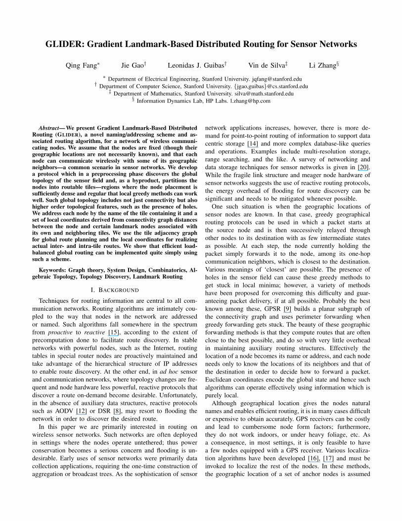
time: 0 time: 0

(i) (ii)

Fig. 1. Landmarks are shown by triangles. Sensor nodes are shown as small circles. The nodes are divided into tiles. The dark nodes are the boundaries ofthe tiles. (i) The landmark Voronoi complex; (ii) The combinatorial Delaunay triangulation.

to be known, either manually or through GPS. Other nodesdetermine their location by estimating their distances to threeor more of these anchors and then become anchors themselves;and so on. However, such localization algorithms are still quiteexpensive in terms of computation or communication, andoften insufficiently accurate. Unfortunately, these inaccuraciescan have deleterious effects on routing algorithms based onlocation information [18].

The idea of geographic forwarding is so compelling that anumber of authors have tried to use geographic coordinateseven when actual node locations are not available. The idea isto produce virtual node coordinates on which to use protocolssuch as GPSR. These are obtained by embedding the linkconnectivity graph of the nodes in the plane [10], [11], [13]so that nodes that can communicate directly are embeddednear each other and those that do not are further away.Unfortunately such global embeddings can be time-consumingto compute and may not reflect well the actual geometry of thenode layout. For example, in the presence of communicationobstacles (such as walls), nodes that are geographically closemay actually be distant in the communication graph. Also,when the actual node deployment is in 3-D, as in monitoringbuildings, forcing a 2-D layout will cause large distortions withthe consequence that the planarization required by GPSR andrelated protocols will necessarily ignore much of the actualconnectivity present.

II. TOPOLOGY-ENABLED ROUTING

We present a novel routing scheme, named GLIDER, that,like the virtual coordinate schemes above, depends only on

node connectivity and not on any knowledge of node posi-tions. The key idea is to divide the problem into a globalpreprocessing step and a local routing problem (for whichwe present a specific solution). In the preprocessing step wediscover the global topology of the sensor field. This givesus information about connected components and holes in thesensor field layout. In the process we partition the field intotiles. We regard these as having trivial topology, so that greedyforwarding methods based on local coordinates are likely towork well within each tile.

Our intuition is that, in many of the real-world situationswhere sensor networks may be deployed, the topologicalfeatures of the layout (e.g. holes) will be few and will mostlyreflect the underlying structure of the environment (e.g. obsta-cles). Moreover, this relatively simple global topology is likelyto remain stable: nodes may come and go, but such changes areunlikely to destroy or create large-scale topological features. Itfollows, if the global topology is stable, that we can afford tocarry out proactive routing at an abstract combinatorial level.These high-level routes can then be realized as actual paths inthe network by using reactive protocols.

For example, the node distribution shown in Figure 1 hasa large hole in the middle. If two nodes are situated onopposite sides of the hole, there are two ways of reachingone node from the other: clockwise and counter-clockwisearound the hole. This is a topological statement. Having madethe topological decision whether to go clockwise or counter-clockwise, we can use local decisions to select the specificpath on a node-by-node basis. In this way, we have brokenthe routing problem into two phases: a global planning phase,

in which the combinatorial structure of the path is determinedusing global information; and a local phase, in which thecombinatorial path is implemented as an actual sequence ofhops, selected using local greedy methods.

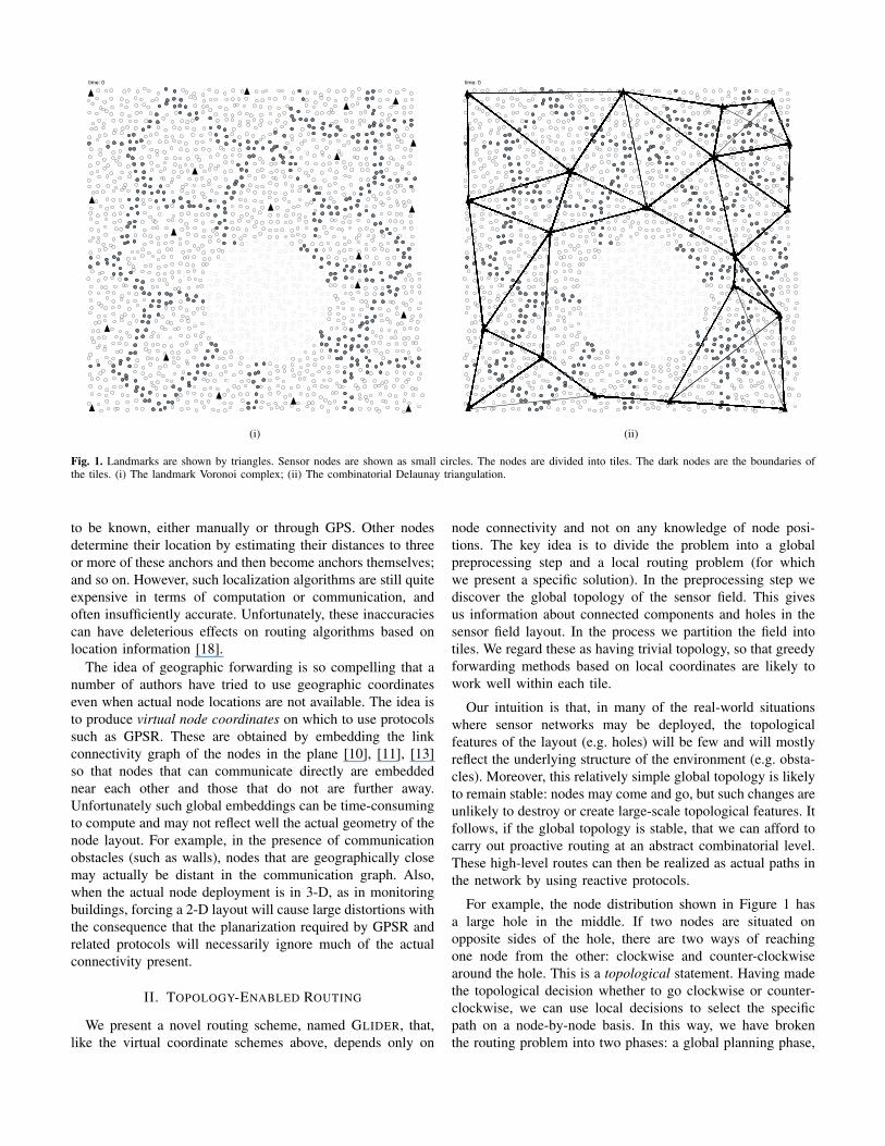
For this second phase, we define sets of local coordinatesthat depend only on the link connectivity of the nodes.Gradient descent on these coordinates will naturally followlocal geodesics of the layout. However, our procedure isless sensitive to sensor geometry than is classical geographicrouting. For example, suppose we have a collection of sensorsdensely deployed in two big rooms connected by a long narrowcorridor, as shown in Figure 2. The geometry of the sensorfield is curved, so greedy geographic routing between therooms will almost certainly fail if it is based directly on thecoordinate system implied by the diagram. On the other hand,the topology of this sensor field is fundamentally the same asthe topology of an array of sensors deployed densely insidea convex shape such as a disk. Our global-local scheme willthread the route through the corridor without difficulty. Thisworks because we limit the local greedy processes to certainregions (the tiles) whose topological structure is known tobe sufficiently nice. Our knowledge of the global networktopology allows our routing scheme to avoid some of the morecommon pitfalls and limitations of current global coordinate-based schemes; such as the limitation to two dimensions, or theneed to construct a planar graph to bypass local minima [9],[1], or the explicit discovery of holes [5].

Fig. 2. A narrow corridor connects two rooms. GLIDER discoversa route that goes through the corridor, following naturally definedgradients.

Both phases of our algorithm—global topology discoveryand local coordinates—are based on the selection of an ap-propriate subset of the nodes designated as landmarks. Weuse combinatorial Voronoi/Delaunay techniques to extract atopological complex whose vertices are the landmarks andwhose topology captures the topology of the underlying sensorfield. At the same time, we generate a set of local coordinates

for each node which are derived from the node’s link distancesto nearby landmarks. These coordinates are easy to generatesince they depend only on local information—we make noattempt to provide a global geometric embedding for the entirenetwork.

The idea of using landmarks for routing is of course notnew to the networking community. Tsuchiya [19] proposeda hierarchical landmark-based scheme for generating nodenames or addresses. Our use of landmarks for addressingand route generation is quite different—we use landmarks topartition the sensor field into geographically routable tiles.Recently, we became aware of another paper currently underreview that uses distances to landmarks as coordinates [7]and provides extensive simulation results. Our work differsin that we do not use all the landmarks to provide coordinatesfor all the nodes. It follows that our scheme scales betterto large networks. Moreover, we have a different methodfor generating the virtual local coordinate systems, which isguaranteed to route correctly in the continuous domain andwhich empirically works well in practice.

In a quite different subject area, nonlinear dimensionalityreduction (NLDR), landmarking techniques were introducedin [4] to simplify expensive calculations by using a sparseapproximate representation of the global geometry of a dataset. The goal in NLDR is to find explicit low-dimensionalcoordinates for viewing high-dimensional nonlinear data. Thelocal landmark coordinates used by GLIDER are closely relatedto the coordinate embedding functions derived in [4].

As an aside, it is somewhat unfortunate that the currentusage of the term topology discovery in the networking com-munity refers only to the discovery of local link relationshipsbetween nodes and to the lowest-order topological invariant,namely path connectivity. Our use of the term topology dis-covery in this paper refers more broadly to an understanding ofthe global topology of the sensor field in the sense of algebraictopology; for example, we consider higher order topologicalfeatures such as holes in 2-D, tunnels and voids in 3-D, andso on.

We note that in traditional algebraic topology the objectsof study are continuous spaces rather than discrete collectionsof points or nodes. That being so, when we talk about thetopology of a finite set of points sampled from an underlyingobject, we really mean the topology of the underlying objectitself. To recover this from the points alone, we can concep-tually transform the discrete cloud of points into a continuousspace by putting a small ball around each point, makingsure that the balls associated to nearby points have sufficientoverlap. From this one can build discrete structures, namelysimplicial complexes, that provably capture the topology ofthe underlying continuous object [2] under mild conditions.The same idea can be applied to the task of understanding thetopology of a field of communication nodes. However, the lackof positional information, the need to minimize computationalcosts, and the desire to perform topology estimation in adistributed way, all make the network case more challenging.

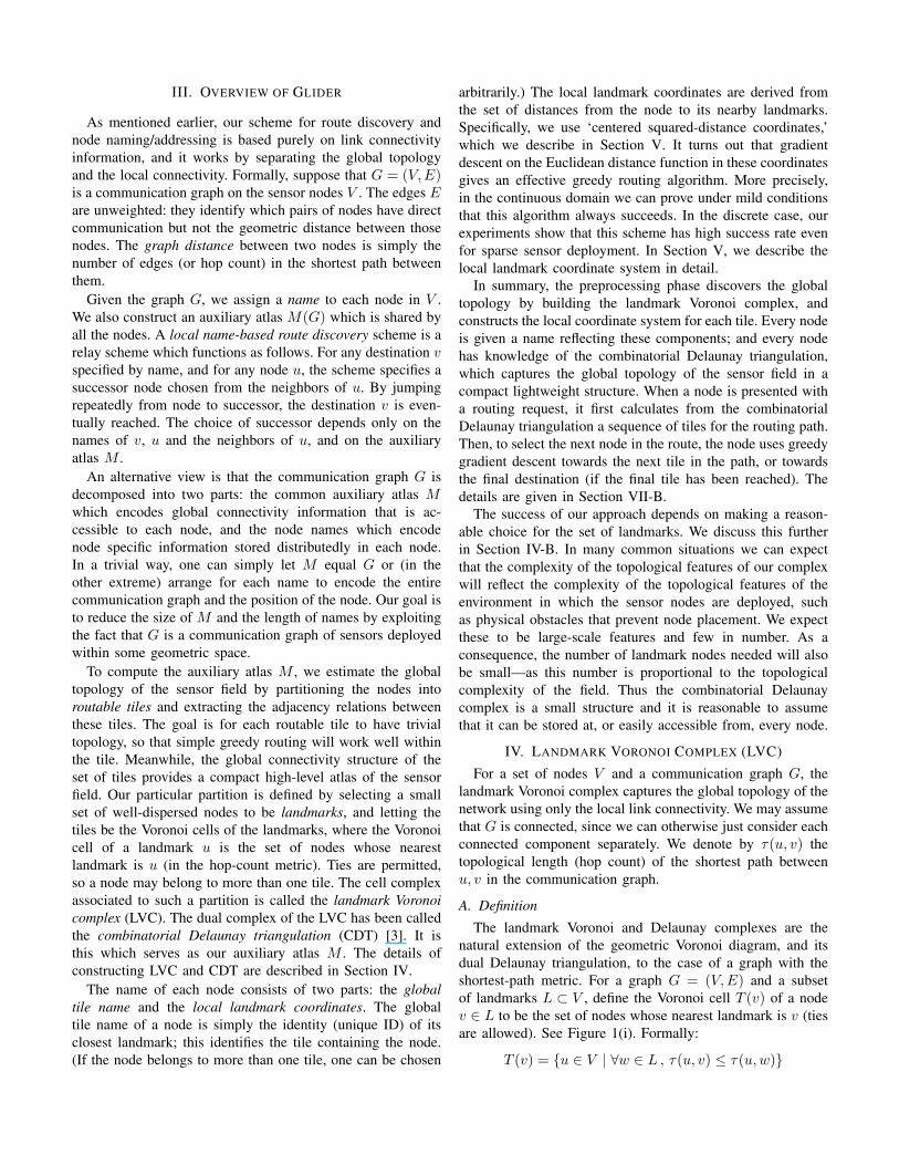
III. OVERVIEW OF GLIDER

As mentioned earlier, our scheme for route discovery andnode naming/addressing is based purely on link connectivityinformation, and it works by separating the global topologyand the local connectivity. Formally, suppose that G = (V,E)is a communication graph on the sensor nodes V . The edges Eare unweighted: they identify which pairs of nodes have directcommunication but not the geometric distance between thosenodes. The graph distance between two nodes is simply thenumber of edges (or hop count) in the shortest path betweenthem.

Given the graph G, we assign a name to each node in V .We also construct an auxiliary atlas M(G) which is shared byall the nodes. A local name-based route discovery scheme is arelay scheme which functions as follows. For any destination vspecified by name, and for any node u, the scheme specifies asuccessor node chosen from the neighbors of u. By jumpingrepeatedly from node to successor, the destination v is even-tually reached. The choice of successor depends only on thenames of v, u and the neighbors of u, and on the auxiliaryatlas M .

An alternative view is that the communication graph G isdecomposed into two parts: the common auxiliary atlas Mwhich encodes global connectivity information that is ac-cessible to each node, and the node names which encodenode specific information stored distributedly in each node.In a trivial way, one can simply let M equal G or (in theother extreme) arrange for each name to encode the entirecommunication graph and the position of the node. Our goal isto reduce the size of M and the length of names by exploitingthe fact that G is a communication graph of sensors deployedwithin some geometric space.

To compute the auxiliary atlas M , we estimate the globaltopology of the sensor field by partitioning the nodes intoroutable tiles and extracting the adjacency relations betweenthese tiles. The goal is for each routable tile to have trivialtopology, so that simple greedy routing will work well withinthe tile. Meanwhile, the global connectivity structure of theset of tiles provides a compact high-level atlas of the sensorfield. Our particular partition is defined by selecting a smallset of well-dispersed nodes to be landmarks, and letting thetiles be the Voronoi cells of the landmarks, where the Voronoicell of a landmark u is the set of nodes whose nearestlandmark is u (in the hop-count metric). Ties are permitted,so a node may belong to more than one tile. The cell complexassociated to such a partition is called the landmark Voronoicomplex (LVC). The dual complex of the LVC has been calledthe combinatorial Delaunay triangulation (CDT) [3]. It isthis which serves as our auxiliary atlas M . The details ofconstructing LVC and CDT are described in Section IV.

The name of each node consists of two parts: the globaltile name and the local landmark coordinates. The globaltile name of a node is simply the identity (unique ID) of itsclosest landmark; this identifies the tile containing the node.(If the node belongs to more than one tile, one can be chosen

arbitrarily.) The local landmark coordinates are derived fromthe set of distances from the node to its nearby landmarks.Specifically, we use ‘centered squared-distance coordinates,’which we describe in Section V. It turns out that gradientdescent on the Euclidean distance function in these coordinatesgives an effective greedy routing algorithm. More precisely,in the continuous domain we can prove under mild conditionsthat this algorithm always succeeds. In the discrete case, ourexperiments show that this scheme has high success rate evenfor sparse sensor deployment. In Section V, we describe thelocal landmark coordinate system in detail.

In summary, the preprocessing phase discovers the globaltopology by building the landmark Voronoi complex, andconstructs the local coordinate system for each tile. Every nodeis given a name reflecting these components; and every nodehas knowledge of the combinatorial Delaunay triangulation,which captures the global topology of the sensor field in acompact lightweight structure. When a node is presented witha routing request, it first calculates from the combinatorialDelaunay triangulation a sequence of tiles for the routing path.Then, to select the next node in the route, the node uses greedygradient descent towards the next tile in the path, or towardsthe final destination (if the final tile has been reached). Thedetails are given in Section VII-B.

The success of our approach depends on making a reason-able choice for the set of landmarks. We discuss this furtherin Section IV-B. In many common situations we can expectthat the complexity of the topological features of our complexwill reflect the complexity of the topological features of theenvironment in which the sensor nodes are deployed, suchas physical obstacles that prevent node placement. We expectthese to be large-scale features and few in number. As aconsequence, the number of landmark nodes needed will alsobe small—as this number is proportional to the topologicalcomplexity of the field. Thus the combinatorial Delaunaycomplex is a small structure and it is reasonable to assumethat it can be stored at, or easily accessible from, every node.

IV. LANDMARK VORONOI COMPLEX (LVC)

For a set of nodes V and a communication graph G, thelandmark Voronoi complex captures the global topology of thenetwork using only the local link connectivity. We may assumethat G is connected, since we can otherwise just consider eachconnected component separately. We denote by τ(u, v) thetopological length (hop count) of the shortest path betweenu, v in the communication graph.

A. Definition

The landmark Voronoi and Delaunay complexes are thenatural extension of the geometric Voronoi diagram, and itsdual Delaunay triangulation, to the case of a graph with theshortest-path metric. For a graph G = (V,E) and a subsetof landmarks L ⊂ V , define the Voronoi cell T (v) of a nodev ∈ L to be the set of nodes whose nearest landmark is v (tiesare allowed). See Figure 1(i). Formally:

T (v) = {u ∈ V | ∀w ∈ L , τ(u, v) ≤ τ(u,w)}

We note the following property of a Voronoi cell.

Lemma 1. For any node u ∈ T (v), the shortest path from u tov is completely contained in T (v).Proof. If the lemma were false, there would exist w �∈ T (v)on the shortest path from u to v. Since w �∈ T (v), there existsx ∈ L such that τ(w, x) < τ(w, v). Thus, τ(u, x) ≤ τ(u,w)+τ(w, x) < τ(u,w) + τ(w, v) = τ(u, v). This contradicts thehypothesis that u ∈ T (v); so the lemma must be true. �

One implication of this lemma is that the spanning graphon each Voronoi cell is connected. Thus, the Voronoi cellsof a set of landmarks provide a natural partitioning of thesensor field into connected tiles. A stronger requirement isthat the tiles have trivial topology in all dimensions (notjust connectivity). When the sensor field has large holes,we find that appropriately-chosen landmarks can effectivelyfragment the sensor field into subsets with simple topology.See Figure 1(i).

The Voronoi cells form the landmark Voronoi complex(LVC). Following [3], we use a dual combinatorial Delaunaytriangulation (CDT) to record the adjacency relation betweenVoronoi cells.1 For our purposes, the combinatorial Delaunaytriangulation D(L) is a modified dual of the LVC, defined asfollows. Write w ∼ w′ to mean that nodes w,w′ share an edgein G or are the same node. Then the vertices v1, . . . , vk spana simplex in D(L) if and only if there exist nodes w1, . . . , wk

such that wi ∈ T (vi) for all i and wi ∼ wj for all i, j.Under favorable conditions (a dense distribution of nodes,

reasonably simple topology, a small number of well-separatedlandmarks) suitable variations of the LVC and CDT complexessuccessfully capture the global topology of the communicationnetwork [3]. These constructions give us the potential to detectand exploit high-order topological characters of a sensor field.Having said that, in this paper we are mainly interested inthe connectivity graph D(L) of the landmarks, i.e. the 1-dimensional skeleton of CDT (Figure 1(ii)). The edge v1v2

belongs to D(L) iff there exist nodes w1, w2 with w1 ∼ w2

and wi ∈ T (vi) for i = 1, 2. The nodes wi are referred to aswitnesses to the edge v1v2.

For connectivity, we have the following easy result:

Theorem 2. If G is connected, then the combinatorial De-launay graph D(L) for any subset of landmarks L is alsoconnected.Proof. We must show that there is a path in D(L) betweenany pair of landmarks u, v. Since G is connected, there iscertainly a path from u to v within G. Let us suppose thispath visits nodes w0, w1, . . . , wk in sequence, where w0 = uand wk = v. Each node wi belongs to some Voronoi cellT (xi) where each xi ∈ L. We may assume that x0 = w0 = uand xk = wk = v. We claim that the sequence x0, x1, . . . , xk

represents a valid path in D(L) from u to v. Specifically, foreach 0 ≤ i < k, we claim that xi ∼ xi+1 in the graph D(L).

1Our definitions diverge slightly from the definitions in [3]. The problemin both cases is to ensure that CDT maintains the connectivity of the originalgraph; something that is not quite true with the natural definitions. We dealwith this in a different way than [3].

This is clear, since wi, wi+1 are witnesses for the edge xixi+1

in the case that xi �= xi+1. �The proof of Theorem 2 amounts to the stronger assertion

that every path in G can be ‘lifted’ to a path in D(L).Conversely, every path in D(L) can be realized as a path in G.This follows from the case of a single edge v1v2 ∈ D(L). Letw1, w2 be witnesses for v1v2. For each i the shortest pathfrom vi to wi lies entirely within T (vi), by Lemma 1. We canconcatenate these paths to obtain a path v1 . . . w1w2 . . . v2 in Gwhich lifts to the length-1 path v1v2 in D(L).

These last assertions provide strong corroboration of one ofthe main claims in this paper, which is that the CDT graph isan appropriate simplification of the communication graph Gfor determining a global routing strategy.

We summarize the main points of this section: For a set ofchosen landmark nodes, the Voronoi cells of the landmarksprovide a partitioning of the sensors. Each Voronoi cell isconnected and has ‘simple’ topology when the landmarksare well-chosen. The combinatorial Delaunay triangulationencodes adjacency information between Voronoi cells, andprovides a compact high-level atlas for the sensor field whichis suitable for global route-planning.

B. Landmark selection

While the definition and properties of LVC and CDT holdfor any subset of landmarks, careful selection of landmarks iscrucial for the effectiveness and efficiency of routing. SinceCDT serves as the auxiliary atlas provided to every node, itshould be as small as possible so that it can be replicated inthe network with minimal cost. On the other hand, we needenough landmarks to ensure that each Voronoi cell has simple(i.e. ‘hole-free’) topology. These are the two opposing goals.

The landmark selection problem bears some resemblance tothe sampling problem for mesh generation—we particularlydesire to have several landmarks lying close to topologicalfeatures, such as hole boundaries. Hand-picked landmarksare one option, since in many cases the presence of holesmay be known a priori to those deploying the network. Itis also possible to automatically discover hole-boundaries [6],or at any rate a few nodes on the boundary [13]. With suchinformation, we can arrange for nodes near the boundary tobe selected as landmarks with higher probability than interiornodes. In general we expect the number of landmarks to beproportional to the number of holes (or topological features) ofthe sensor domain. We are usually interested in domains witha small number of large holes, in which case the landmark setand hence the CDT complex will be small enough to distributeto the entire set of nodes.

V. LOCAL LANDMARK COORDINATES

Under ideal circumstances with well-chosen landmarks, thenodes in each cell of the landmark Voronoi complex will benicely distributed. By this we mean that the shortest-distancemetric in each tile approximates the metric in a finite sampleof a convex Euclidean region. One general strategy for routingon such network is to supply a coordinate system to the nodes,

and then perform greedy routing by forwarding packets toa neighbor which is closer to the destination according tothese coordinates. The use of the Euclidean coordinates ofthe sensors is one natural choice but these coordinates maybe difficult or expensive to obtain. Here we propose a virtualcoordinate system which is easy to compute, is guaranteed tobe free of local minima in the continuous plane, and which inpractice works well in the discrete case. These are the locallandmark coordinates. We first describe these coordinates incontinuous Euclidean space, and then extend the definitions tothe discrete case.

A. Continuous version

It is easiest to understand our coordinate system (we willdefine it shortly) in the continuous case. The goal is toconstruct a set of coordinate functions depending only onthe distances to some fixed set of landmark points, in such away that gradient descent on the distance function to a targetpoint always reaches the target successfully. In other words,the distance function should have no local minima other thanthe global minimum.

Let {ui} be a set of k landmarks in the plane. The naturalfirst guess is to assign to each point p the virtual coordinatevector A(p) = (|p − u1|, |p − u2|, . . . , |p − uk|), where|p − ui| is the Euclidean distance between p and ui. Thevirtual distance in this coordinate system between points p, qis then d(p, q) = |A(p)−A(q)|2 =

∑ki=1(|p−ui|−|q−ui|)2.

Given a destination q, the greedy routing algorithm operatesby gradient descent on this function with respect to p.

There are simple examples with three landmarks whichshow that this process can get stuck in local minima. One cando slightly better with the squared-distance vector B(p) =(|p−u1|2, |p−u2|2, . . . , |p−uk|2). It can be shown that thereare no local minima when 3 ≤ k ≤ 9 and when the destinationis inside the landmark convex hull. When k > 9 or whenthe destination is outside the convex hull, there is no suchguarantee. Figure 3(i) shows an example where the gradientflow can get trapped in a local minimum. For this reasonwe introduce centered landmark-distance coordinates C(p).The i-th coordinate is defined by [C(p)]i = [B(p)]i − B(p),where B(p) is the mean of the entries of B(p). The modifiedvirtual-distance function is then d(p, q) = |C(p)−C(q)|2. Theadvantage of this is made clear by the following lemma.

Lemma 3. In the continuous Euclidean plane, gradient descenton the function p �→ d(p, q) always converges to the target q,provided that there are at least three non-collinear landmarks.Proof. We can explicitly evaluate

[B(p)]i = |p|2 − 2p · ui + |ui|2 ,

and hence

[C(p)]i = −2p · (ui − u) + wi ,

where u = 1k

∑j uj and wi = |ui|2 − 1

k

∑j |uj |2.

The function p �→ C(p) is therefore an affine lineartransformation. Under the assumption that there are at least

three non-collinear landmarks, we now show that the mapis one-to-one. The idea is to find at least one point in theplane which is determined uniquely by its coordinates, becausethen (for an affine map) the same must be true for all pointsin the plane. The circumcenter of any three non-collinearlandmarks is such a point, since it is uniquely determinedby the property that the corresponding three coordinates areequal. This establishes that the map is one-to-one, in additionto being affine linear. It follows that gradient of the distancefunction is nowhere zero except at the destination itself. �

In k-dimensional Euclidean space, the minimum require-ment is k+1 landmarks not contained in any k−1-dimensionalaffine subspace. In other words, the affine span of the land-marks must be the entire k-space.

We note that the straight line path to the target is adescending trajectory for the distance function d. In generalit is not the path of steepest descent. Figure 3(ii) shows thesame configuration as in Figure 3(i), but with the distance totarget measured in the centered landmark-distance coordinates.In that case there is no local minimum.

B. Discrete version

In a graph setting, the discrete version of the greedyrouting algorithm uses hop counts to the landmarks as areplacement for Euclidean distances. In situations where thenodes are densely distributed, the minimum number of hops toa landmark is a fair approximation to the Euclidean distanceto that landmark.

For a set of landmarks {u1, u2, . . . , uk} and for any node p,let τ(p, ui) denote the graph distance (i.e. the minimal hopcount) between p and ui. Let τ(p) =

∑ki=1 τ(p, ui)2/k. We

then assign to p the centered virtual coordinate vector

C(p) = (τ(p, u1)2 − τ(p), . . . , τ(p, uk)2 − τ(p)) .

The centered virtual distance between two points p, q is thend(p, q) = |C(p) − C(q)|2 just as in the continuous Euclideancase. Given a destination q, our greedy routing algorithmchooses the neighbor r of p which minimizes d(r, q). Inother words, we move packets by greedy minimization ofthe Euclidean distance to the target, measured in the virtualcoordinate system. This algorithm is local and efficient sinceonly the virtual coordinates of the neighbor nodes are needed.

In the discrete version, we can no longer guarantee thatlocal minima do not exist. A packet may hit a node forwhich all the neighbor nodes have virtual distances furtheraway from the destination. However, when the nodes aredense enough, the shortest distance metric approximates theEuclidean metric closely enough to reduce the chance of localminima. Another cause of instability is the eccentricity of theaffine transformation in Lemma 3. When the landmarks arenearly collinear—e.g. when τ(u, v) + τ(v, w) ≈ τ(u,w) withthree landmarks u, v, w—the gradient field in the continuouscase is quite shallow in certain directions. This can be seenquite clearly in Figure 3(ii). Under these circumstances thediscrete approximation is more likely to suffer from localminima.

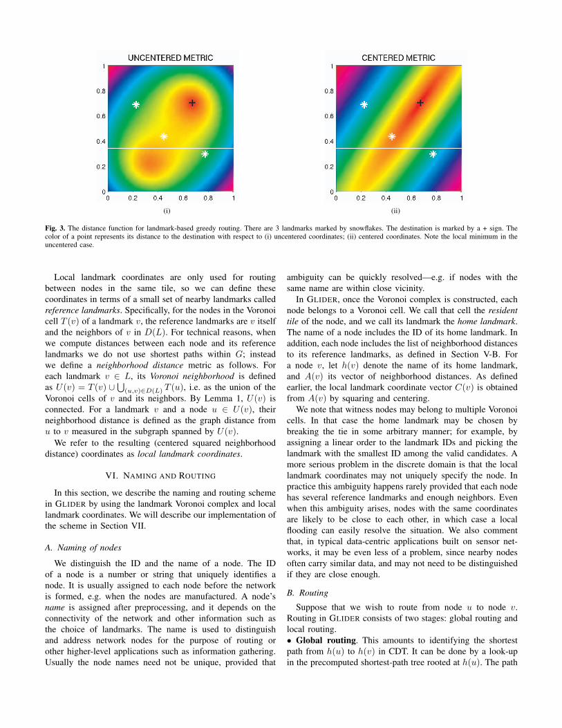
(i) (ii)

Fig. 3. The distance function for landmark-based greedy routing. There are 3 landmarks marked by snowflakes. The destination is marked by a + sign. Thecolor of a point represents its distance to the destination with respect to (i) uncentered coordinates; (ii) centered coordinates. Note the local minimum in theuncentered case.

Local landmark coordinates are only used for routingbetween nodes in the same tile, so we can define thesecoordinates in terms of a small set of nearby landmarks calledreference landmarks. Specifically, for the nodes in the Voronoicell T (v) of a landmark v, the reference landmarks are v itselfand the neighbors of v in D(L). For technical reasons, whenwe compute distances between each node and its referencelandmarks we do not use shortest paths within G; insteadwe define a neighborhood distance metric as follows. Foreach landmark v ∈ L, its Voronoi neighborhood is definedas U(v) = T (v) ∪ ⋃

(u,v)∈D(L) T (u), i.e. as the union of theVoronoi cells of v and its neighbors. By Lemma 1, U(v) isconnected. For a landmark v and a node u ∈ U(v), theirneighborhood distance is defined as the graph distance fromu to v measured in the subgraph spanned by U(v).

We refer to the resulting (centered squared neighborhooddistance) coordinates as local landmark coordinates.

VI. NAMING AND ROUTING

In this section, we describe the naming and routing schemein GLIDER by using the landmark Voronoi complex and locallandmark coordinates. We will describe our implementation ofthe scheme in Section VII.

A. Naming of nodes

We distinguish the ID and the name of a node. The IDof a node is a number or string that uniquely identifies anode. It is usually assigned to each node before the networkis formed, e.g. when the nodes are manufactured. A node’sname is assigned after preprocessing, and it depends on theconnectivity of the network and other information such asthe choice of landmarks. The name is used to distinguishand address network nodes for the purpose of routing orother higher-level applications such as information gathering.Usually the node names need not be unique, provided that

ambiguity can be quickly resolved—e.g. if nodes with thesame name are within close vicinity.

In GLIDER, once the Voronoi complex is constructed, eachnode belongs to a Voronoi cell. We call that cell the residenttile of the node, and we call its landmark the home landmark.The name of a node includes the ID of its home landmark. Inaddition, each node includes the list of neighborhood distancesto its reference landmarks, as defined in Section V-B. Fora node v, let h(v) denote the name of its home landmark,and A(v) its vector of neighborhood distances. As definedearlier, the local landmark coordinate vector C(v) is obtainedfrom A(v) by squaring and centering.

We note that witness nodes may belong to multiple Voronoicells. In that case the home landmark may be chosen bybreaking the tie in some arbitrary manner; for example, byassigning a linear order to the landmark IDs and picking thelandmark with the smallest ID among the valid candidates. Amore serious problem in the discrete domain is that the locallandmark coordinates may not uniquely specify the node. Inpractice this ambiguity happens rarely provided that each nodehas several reference landmarks and enough neighbors. Evenwhen this ambiguity arises, nodes with the same coordinatesare likely to be close to each other, in which case a localflooding can easily resolve the situation. We also commentthat, in typical data-centric applications built on sensor net-works, it may be even less of a problem, since nearby nodesoften carry similar data, and may not need to be distinguishedif they are close enough.

B. Routing

Suppose that we wish to route from node u to node v.Routing in GLIDER consists of two stages: global routing andlocal routing.• Global routing. This amounts to identifying the shortestpath from h(u) to h(v) in CDT. It can be done by a look-upin the precomputed shortest-path tree rooted at h(u). The path

provides a sequence of tiles for the journey; say T1, T2, . . . , Tk

where Ti = T (ui) for landmarks ui, with u1 = h(u), uk =h(v).• Local routing. Local routing consists of inter-tile routing,responsible for discovering path from tile Ti to Ti+1, and intra-tile routing, responsible for discovering the path towards vonce Tk is reached.

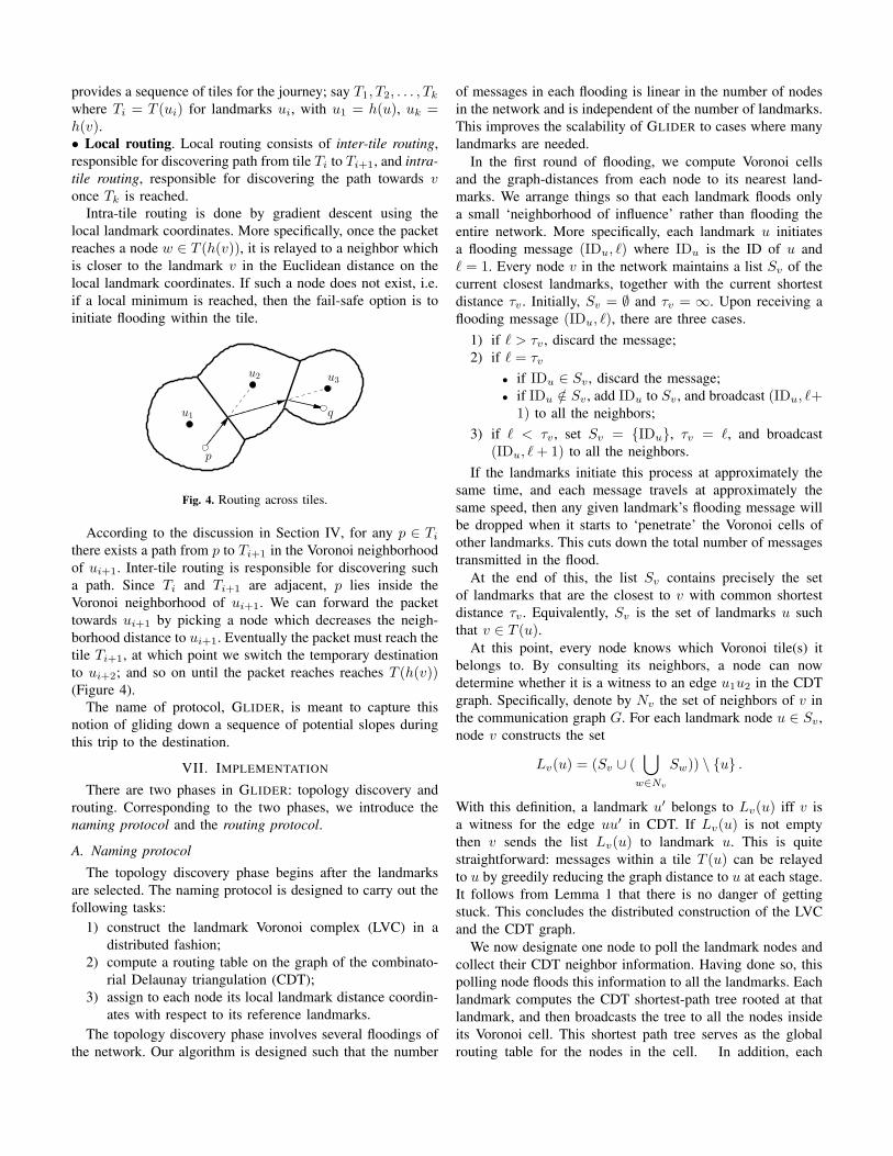
Intra-tile routing is done by gradient descent using thelocal landmark coordinates. More specifically, once the packetreaches a node w ∈ T (h(v)), it is relayed to a neighbor whichis closer to the landmark v in the Euclidean distance on thelocal landmark coordinates. If such a node does not exist, i.e.if a local minimum is reached, then the fail-safe option is toinitiate flooding within the tile.

u1

p

q

u2 u3

Fig. 4. Routing across tiles.

According to the discussion in Section IV, for any p ∈ Ti

there exists a path from p to Ti+1 in the Voronoi neighborhoodof ui+1. Inter-tile routing is responsible for discovering sucha path. Since Ti and Ti+1 are adjacent, p lies inside theVoronoi neighborhood of ui+1. We can forward the packettowards ui+1 by picking a node which decreases the neigh-borhood distance to ui+1. Eventually the packet must reach thetile Ti+1, at which point we switch the temporary destinationto ui+2; and so on until the packet reaches reaches T (h(v))(Figure 4).

The name of protocol, GLIDER, is meant to capture thisnotion of gliding down a sequence of potential slopes duringthis trip to the destination.

VII. IMPLEMENTATION

There are two phases in GLIDER: topology discovery androuting. Corresponding to the two phases, we introduce thenaming protocol and the routing protocol.

A. Naming protocol

The topology discovery phase begins after the landmarksare selected. The naming protocol is designed to carry out thefollowing tasks:

1) construct the landmark Voronoi complex (LVC) in adistributed fashion;

2) compute a routing table on the graph of the combinato-rial Delaunay triangulation (CDT);

3) assign to each node its local landmark distance coordin-ates with respect to its reference landmarks.

The topology discovery phase involves several floodings ofthe network. Our algorithm is designed such that the number

of messages in each flooding is linear in the number of nodesin the network and is independent of the number of landmarks.This improves the scalability of GLIDER to cases where manylandmarks are needed.

In the first round of flooding, we compute Voronoi cellsand the graph-distances from each node to its nearest land-marks. We arrange things so that each landmark floods onlya small ‘neighborhood of influence’ rather than flooding theentire network. More specifically, each landmark u initiatesa flooding message (IDu, �) where IDu is the ID of u and� = 1. Every node v in the network maintains a list Sv of thecurrent closest landmarks, together with the current shortestdistance τv . Initially, Sv = ∅ and τv = ∞. Upon receiving aflooding message (IDu, �), there are three cases.

1) if � > τv , discard the message;2) if � = τv

• if IDu ∈ Sv, discard the message;• if IDu /∈ Sv , add IDu to Sv , and broadcast (IDu, �+

1) to all the neighbors;

3) if � < τv , set Sv = {IDu}, τv = �, and broadcast(IDu, � + 1) to all the neighbors.

If the landmarks initiate this process at approximately thesame time, and each message travels at approximately thesame speed, then any given landmark’s flooding message willbe dropped when it starts to ‘penetrate’ the Voronoi cells ofother landmarks. This cuts down the total number of messagestransmitted in the flood.

At the end of this, the list Sv contains precisely the setof landmarks that are the closest to v with common shortestdistance τv . Equivalently, Sv is the set of landmarks u suchthat v ∈ T (u).

At this point, every node knows which Voronoi tile(s) itbelongs to. By consulting its neighbors, a node can nowdetermine whether it is a witness to an edge u1u2 in the CDTgraph. Specifically, denote by Nv the set of neighbors of v inthe communication graph G. For each landmark node u ∈ Sv,node v constructs the set

Lv(u) = (Sv ∪ (⋃

w∈Nv

Sw)) \ {u} .

With this definition, a landmark u′ belongs to Lv(u) iff v isa witness for the edge uu′ in CDT. If Lv(u) is not emptythen v sends the list Lv(u) to landmark u. This is quitestraightforward: messages within a tile T (u) can be relayedto u by greedily reducing the graph distance to u at each stage.It follows from Lemma 1 that there is no danger of gettingstuck. This concludes the distributed construction of the LVCand the CDT graph.

We now designate one node to poll the landmark nodes andcollect their CDT neighbor information. Having done so, thispolling node floods this information to all the landmarks. Eachlandmark computes the CDT shortest-path tree rooted at thatlandmark, and then broadcasts the tree to all the nodes insideits Voronoi cell. This shortest path tree serves as the globalrouting table for the nodes in the cell. In addition, each

node v knows the ID of its home landmark u and also of itsother reference landmarks, since these can be read off as theneighbors of u in the shortest-path tree.

The final stage is to compute, for every node v, the neigh-borhood distances between v and its reference landmarks. Thiscan be achieved by initiating a new flood from each land-mark u which is confined to U(u). Every node knows by nowwhether it belongs to U(u), so whenever the flooding messagereaches a node outside U(u) it is simply discarded. Once everynode v has obtained its vector A(v) of neighborhood distancesto its reference landmarks, the local coordinate vectors C(v)can be computed using the prescription in Section V-B.

B. Routing protocol

After successful completion of the naming protocol: (i) theglobal topology of the network is captured by the CDT graph;(ii) each node stores the CDT shortest-path tree rooted atits home landmark; (iii) each node stores the neighborhooddistances to its reference landmarks.

The GLIDER routing protocol runs on top of this infrastruc-ture. The header of a packet contains a ‘temporary destinationlandmark’ (TDL) bit together with a integer that saves theID of a temporary destination landmark. When a packet andthe name of its destination are received at a node v, thenode determines, by comparing names, whether the destinationbelongs to the same tile or a different tile. For the actualforwarding process—determining which node receives thepacket next—there are two scenarios to consider:

• Intra-tile routing. When the destination is inside the currenttile, GLIDER uses the greedy routing algorithm described inSection V-B. If all the neighbors of v are further away fromthe destination than v itself, flooding within the tile is usedto complete the delivery of the packet to the destination.Otherwise, v forwards the packet to a neighbor whose distanceto the destination is least among all neighbors of v.

• Inter-tile routing. If the destination is not in the currenttile, routing follows the method indicated in Section VI-B.The node v first checks whether the temporary destinationlandmark bit is set. If TDL is not set, or if TDL is set but theactual temporary destination landmark stored in the header isthe home landmark of v, then v consults its landmark routingtable to find the next tile ui+1 in a shortest-path route in CDTto the destination tile. Having done so, v sets TDL to TRUE

and saves the ID of ui+1 in the packet header.If TDL is set, and the indicated temporary destination ui

is not the home landmark of the current node v, then v greedilypicks any of its neighbors in U(ui) which is closer than vto ui in neighborhood distance. This is always possible sinceU(ui) is connected. When there are multiple such neighbors,we pick one randomly. This randomization achieves better loadbalancing without hurting the quality of the path.

C. Data structures

Landmarks are used as logical reference points in determin-ing nodes’ local coordinates. However, from the programming

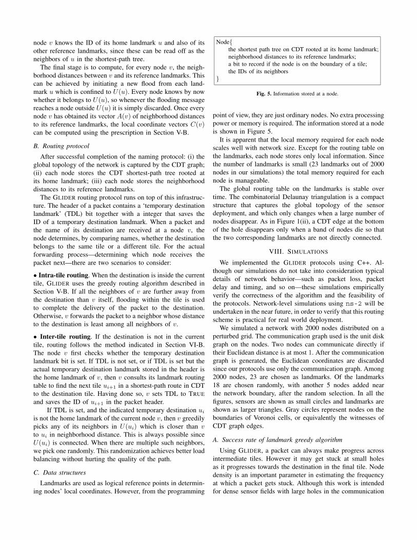
Node{the shortest path tree on CDT rooted at its home landmark;neighborhood distances to its reference landmarks;a bit to record if the node is on the boundary of a tile;the IDs of its neighbors

}

Fig. 5. Information stored at a node.

point of view, they are just ordinary nodes. No extra processingpower or memory is required. The information stored at a nodeis shown in Figure 5.

It is apparent that the local memory required for each nodescales well with network size. Except for the routing table onthe landmarks, each node stores only local information. Sincethe number of landmarks is small (23 landmarks out of 2000nodes in our simulations) the total memory required for eachnode is manageable.

The global routing table on the landmarks is stable overtime. The combinatorial Delaunay triangulation is a compactstructure that captures the global topology of the sensordeployment, and which only changes when a large number ofnodes disappear. As in Figure 1(ii), a CDT edge at the bottomof the hole disappears only when a band of nodes die so thatthe two corresponding landmarks are not directly connected.

VIII. SIMULATIONS

We implemented the GLIDER protocols using C++. Al-though our simulations do not take into consideration typicaldetails of network behavior—such as packet loss, packetdelay and timing, and so on—these simulations empiricallyverify the correctness of the algorithm and the feasibility ofthe protocols. Network-level simulations using ns-2 will beundertaken in the near future, in order to verify that this routingscheme is practical for real world deployment.

We simulated a network with 2000 nodes distributed on aperturbed grid. The communication graph used is the unit diskgraph on the nodes. Two nodes can communicate directly iftheir Euclidean distance is at most 1. After the communicationgraph is generated, the Euclidean coordinates are discardedsince our protocols use only the communication graph. Among2000 nodes, 23 are chosen as landmarks. Of the landmarks18 are chosen randomly, with another 5 nodes added nearthe network boundary, after the random selection. In all thefigures, sensors are shown as small circles and landmarks areshown as larger triangles. Gray circles represent nodes on theboundaries of Voronoi cells, or equivalently the witnesses ofCDT graph edges.

A. Success rate of landmark greedy algorithm

Using GLIDER, a packet can always make progress acrossintermediate tiles. However it may get stuck at small holesas it progresses towards the destination in the final tile. Nodedensity is an important parameter in estimating the frequencyat which a packet gets stuck. Although this work is intendedfor dense sensor fields with large holes in the communication

time: 0 time: 0

(i) (ii)

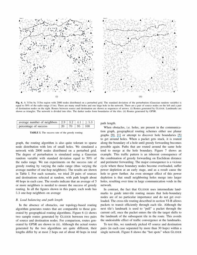
Fig. 6. A 315m by 315m region with 2000 nodes distributed on a perturbed grid. The standard deviation of the perturbation (Gaussian random variable) isequal to 50% of the radio range (11m). There are many small holes and one large hole in the network. There are a pair of source nodes on the left and a pairof destination nodes on the right. Routes between source and destination are shown as sequences of arrows. (i) Routes generated by GLIDER. Landmarks areshown as triangles. The network is divided into tiles. The darker nodes form boundaries of the tiles. (ii) Routes generated by GPSR.

average number of neighbors 2.9 3.2 4.1 ≥ 5.3percentage of success 20 70 95 100

TABLE I. The success rate of the greedy routing

graph, the routing algorithm is also quite tolerant to sparsenode distribution with lots of small holes. We simulated anetwork with 2000 nodes distributed on a perturbed grid.The degree of perturbation is simulated using a Gaussianrandom variable with standard deviation equal to 50% ofthe radio range. We ran experiments on the success rate ofgreedy routing by varying the radio range (thus varying theaverage number of one-hop neighbors). The results are shownin Table I. For each scenario, we tried 20 pairs of sourcesand destinations selected at random, with path length about40 hops in each case. The results indicate that an average of 5or more neighbors is needed to ensure the success of greedyrouting. In all the figures shown in this paper, each node has5.3 one-hop neighbors on average

B. Load balancing and path length

In the absence of obstacles, our topology-based routingalgorithm generates routes that are comparable to those gen-erated by geographical routing algorithms. Figure 6 (i) showstwo sample routes generated by GLIDER between two pairsof source and destination nodes. For comparison, routes gen-erated by GPSR are shown in (ii). Although the actual routesgenerated by the two algorithms are quite different, theirlengths differ by at most 2 hops out of about 40 hops in total

path length.When obstacles, i.e. holes, are present in the communica-

tion graph, geographical routing schemes either use planargraphs [9], [1] or attempt to discover hole boundaries [5]to get around holes. When a packet gets stuck, it is routedalong the boundary of a hole until greedy forwarding becomespossible again. Paths that are routed around the same holetend to merge at the hole boundary. Figure 7 shows anexample. This traffic pattern is an inherent consequence ofthe combination of greedy forwarding on Euclidean distanceand perimeter forwarding. The major consequence is a viciouscycle where these boundary nodes become overloaded, sufferpower depletion at an early stage, and as a result cause thehole to grow further. An even stronger effect of this powerdepletion is that small neighboring holes merge into largerholes, resulting over time in large communication voids in thenetwork.

In contrast, the fact that GLIDER uses intermediate land-marks to guide inter-tile routing means that hole-boundarynodes are of no particular importance and do not get over-loaded. The cross-tile routing described in section VI-B allowspackets to transit efficiently through each tile. Although thenext tile’s landmark is used to “pull” a packet through thecurrent cell, once the packet enters the tile the target shifts tothe landmark of the subsequent tile in the route. This avoidsthe undesirable effect of traffic convergence at the landmarks.

To test this, we randomly picked 45 source and destinationpairs (in each case separated by more than 30 hops) within asingle network. Figure 8 shows the “hot spots” when GLIDER

time: 0 time: 0

(i) (ii)

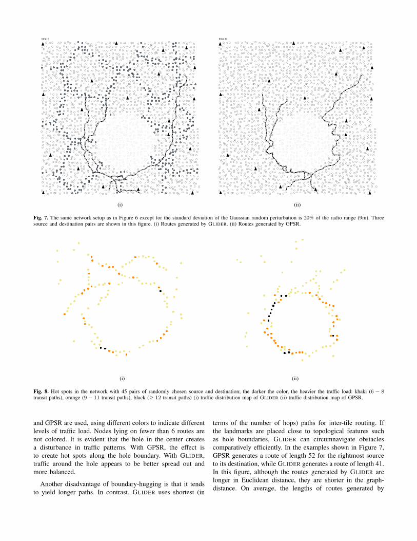
Fig. 7. The same network setup as in Figure 6 except for the standard deviation of the Gaussian random perturbation is 20% of the radio range (9m). Threesource and destination pairs are shown in this figure. (i) Routes generated by GLIDER. (ii) Routes generated by GPSR.

(i) (ii)

Fig. 8. Hot spots in the network with 45 pairs of randomly chosen source and destination; the darker the color, the heavier the traffic load: khaki (6 − 8transit paths), orange (9 − 11 transit paths), black (≥ 12 transit paths) (i) traffic distribution map of GLIDER (ii) traffic distribution map of GPSR.

and GPSR are used, using different colors to indicate differentlevels of traffic load. Nodes lying on fewer than 6 routes arenot colored. It is evident that the hole in the center createsa disturbance in traffic patterns. With GPSR, the effect isto create hot spots along the hole boundary. With GLIDER,traffic around the hole appears to be better spread out andmore balanced.

Another disadvantage of boundary-hugging is that it tendsto yield longer paths. In contrast, GLIDER uses shortest (in

terms of the number of hops) paths for inter-tile routing. Ifthe landmarks are placed close to topological features suchas hole boundaries, GLIDER can circumnavigate obstaclescomparatively efficiently. In the examples shown in Figure 7,GPSR generates a route of length 52 for the rightmost sourceto its destination, while GLIDER generates a route of length 41.In this figure, although the routes generated by GLIDER arelonger in Euclidean distance, they are shorter in the graph-distance. On average, the lengths of routes generated by

the two algorithms are comparable. For the 45 routes, theaverage path length generated by GPSR is 42.08. The averagepath length generated by GLIDER is 40.46. The major factorinfluencing path length in the case of GPSR is the geometricshape of the holes; in the case of GLIDER, it is the placementof the landmarks.

C. Discovery of routes under cases with difficult geometry

The landmark Voronoi complex succeeds in capturing thetopology of the network and discovering routes even in situa-tions that would be difficult for purely geometric approaches.In the scenario shown in Figure 2, two big rooms are connectedby a long narrow corridor. Landmarks are selected randomly.The routing path that goes from one room to the other throughthe corridor is correctly discovered by our routing algorithm.We do not actually need landmark nodes be placed in thecorridor itself. (Indeed, for randomly selected landmarks, theprobability of finding a landmark in the corridor is compar-atively small.) As long as the original network is connected,such connectivity is inherited by the combinatorial Delaunaytriangulation.

IX. SUMMARY AND FUTURE WORK

In this paper we propose a topology-based naming androuting structure that uses only the link connectivity of thenetwork. We do not use Euclidean coordinates—instead, weinvent a more robust local landmark coordinate system withineach tile, based on hop distances to nearby landmarks. Wepartition the network into tiles using the landmark Voronoicomplex so that within each tile local greedy routing usingour local coordinates can be expected to work well. We showthat the Voronoi landmark-based routing protocol generatesnatural and load-balanced routing paths. The algorithms andprotocols proposed in this paper work for sensor nodes in threedimensions as well—unlike other current geographic routingprotocols (in fact, which underlying space the network nodescome from matters little).

Although we currently only exploit the path connectivityinformation stored in the landmark Voronoi complex for ourrouting scheme, we believe that the higher order connectivityinformation we compute will prove useful in more complexapplications. An example may be loopy belief propagation andother probabilistic reasoning tasks that can benefit from a fullerunderstanding of the global topology of the sensor field.

It should be clear that this is only preliminary work onan approach to routing that leaves much to be explored.We still need to address important issues, such as the cri-teria and algorithms for landmark selection, potential multi-resolution LVC hierarchies for situations where a large numberof landmarks is required, as well as methods for handlingnetwork dynamics (node addition and failure). Additional localcoordinate systems also deserve to be explored, perhaps usingpartial or total information about the actual node positions orthe communication quality between nodes.

ACKNOWLEDGEMENT

The authors wish to thank John Hershberger for helpfulconversations. The authors also gratefully acknowledge thesupport of the DoD Multidisciplinary University ResearchInitiative (MURI) program administered by the Office of NavalResearch under Grant N00014-00-1-0637, NSF grants CCR-0204486 and CNS-0435111, and DARPA grant #30759.

REFERENCES

[1] P. Bose, P. Morin, I. Stojmenovic, and J. Urrutia. Routing withguaranteed delivery in ad hoc wireless networks. In 3rd Int. Work-shop on Discrete Algorithms and methods for mobile computing andcommunications (DialM ’99), pages 48–55, 1999.

[2] G. Carlsson, A. Collins, L. Guibas, and A. Zomorodian. Persistencebarcodes for shapes. In Symposium on Geometry Processing, 2004. toappear.

[3] G. Carlsson and V. de Silva. Topological approximation by smallsimplicial complexes, 2003. preprint.

[4] V. de Silva and J. B. Tenenbaum. Global versus local methods innonlinear dimensionality reduction, 2003.

[5] Q. Fang, J. Gao, and L. Guibas. Locating and bypassing routing holesin sensor networks. In IEEE INFOCOM, 2004.

[6] S. P. Fekete, A. Kroeller, D. Pfisterer, S. Fischer, and C. Buschmann.Neighborhood-based topology recognition in sensor networks. InAlgorithmic Aspects of Wireless Sensor Networks: First InternationalWorkshop (ALGOSENSOR), pages 123–136, 2004.

[7] R. Fonesca, S. Ratnasamy, J. Zhao, C. T. Ee, D. Culler, S. Shenker,and I. Stoica. Beacon vector routing: Scalable point-to-point routing inwireless sensornets, 2005.

[8] D. B. Johnson and D. A. Maltz. Dynamic source routing in ad hocwireless networks. In Imielinski and Korth, editors, Mobile Computing,volume 353. Kluwer Academic Publishers, 1996.

[9] B. Karp and H. Kung. GPSR: Greedy perimeter stateless routing forwireless networks. In Proc. of the ACM/IEEE International Conferenceon Mobile Computing and Networking (MobiCom), pages 243–254,2000.

[10] R. Nagpal, H. Shrobe, and J. Bachrach. Organizing a global coordinatesystem from local information on an ad hoc sensor network. In Proc. 2ndInternational Workshop on Information Processing in Sensor Networks(IPSN03), pages 333–348, Palo Alto, CA, April 2003. Springer.

[11] D. Niculescu and B. Nath. Ad hoc positioning system (APS). In IEEEGlobal Telecommunications Conference (GlobeCom), pages 2926–2931,2001.

[12] C. E. Perkins, E. M. Royer, and S. R. Das. Ad hoc on demand distancevector (AODV) routing, 1997.

[13] A. Rao, C. Papadimitriou, S. Shenker, and I. Stoica. Geographicrouting without location information. In Proceedings of the 9th annualinternational conference on Mobile computing and networking, pages96–108. ACM Press, 2003.

[14] S. Ratnasamy, B. Karp, L. Yin, F. Yu, D. Estrin, R. Govindan, andS. Shenker. GHT: A geographic hash table for data-centric storage.In First International Workshop on Sensor Networks and Applications,pages 78–87, 2002.

[15] E. M. Royer and C. Toh. A review of current routing protocols forad-hoc mobile wireless networks, April 1999.

[16] A. Savvides, C.-C. Han, and M. B. Strivastava. Dynamic fine-grainedlocalization in ad-hoc networks of sensors. In Proc. 7th Annual Inter-national Conference on Mobile Computing and Networking (MobiCom2001), pages 166–179, Rome, Italy, July 2001. ACM Press.

[17] A. Savvides and M. B. Strivastava. Distributed fine-grained localizationin ad-hoc networks. submitted to IEEE Trans. on Mobile Computing.

[18] K. Seada, A. Helmy, and R. Govindan. On the effect of localizationerrors on geographic face routing in sensor networks. In IPSN’04: Pro-ceedings of the third international symposium on Information processingin sensor networks, pages 71–80. ACM Press, 2004.

[19] P. F. Tsuchiya. The landmark hierarchy: a new hierarchy for routingin very large networks. In SIGCOMM ’88: Symposium proceedings onCommunications architectures and protocols, pages 35–42. ACM Press,1988.

[20] F. Zhao and L. Guibas. Wireless Sensor Networks: An InformationProcessing Approach. Elsevier/Morgan-Kaufmann, 2004.