Embed Size (px)
Citation preview
Universitätsdrucke GöttingenUniversitätsdrucke GöttingenISBN-13: 978-3-938616-93-2
Kapp
as/K
lein
n/Sl
obod
a (E
d.)
2nd
Göt
tinge
n G
IS a
nd R
emot
e Se
nsin
g D
ays
2006
Martin Kappas, Christoph Kleinn, and Branislav Sloboda (Ed.)
Global Change Issues in Developing and Emerging Countries
Proceedings of the 2nd Göttingen GIS and Remote Sensing Days 2006,
4th to 6th October, Göttingen, Germany
Remote sensing data and GIS methods provide powerful instruments for the assessment and modelling of environmental indicators of the earth system and its change at multiple scales. Change, in general, is a consequence of human activities and is apparent to us in terms of climate and land cover change.The present book addresses the up-to-date topic of change and is a compilation of scientific contributions related to mapping, monitoring and modelling “Global Change Issues in Developing and Emerging Countries”. It includes the condensed results of an international biennial conference on “GIS and Remote Sensing for Environmental Studies” that took place in Göttingen, Germany from 04th to 06th October 2006.


Martin Kappas, Christoph Kleinn, and Branislav Sloboda (Ed.)
Global Change Issues in Developing and Emerging Countries
Except where otherwise noted, this work is
licensed under a Creative Commons License

erschienen in der Reihe der Universitätsdrucke im Universitätsverlag Göttingen 2007

Martin Kappas, Christoph Kleinn, and Branislav Sloboda (Ed.)
Global Change Issues in Developing and Emerging Countries
Proceedings of the 2nd Göttingen GIS and Remote Sensing Days 2006, 4th to 6th October, Göttingen, Germany
Universitätsverlag Göttingen 2007

Bibliographische Information der Deutschen Nationalbibliothek
Die Deutsche Nationalbibliothek verzeichnet diese Publikation in der Deutschen Nationalbibliographie; detaillierte bibliographische Daten sind im Internet über <http://dnb.ddb.de> abrufbar.
This volume contains the proceedings of the 2nd Göttingen GIS and Remote Sensing Days which took place from 4th to 6th of October at the Georg-August-University Göttingen and have been organised by the Department of Cartography, GIS and Remote Sensing, the Institute of Forest Management and the Institute of Forest Biometry and Informatics. The conference was held under the main theme “Global Change Issues in Developing and Emerging Countries”. More information on GGRS 2006 at http://www.ggrs.uni-goettingen.de/index.php Address of the Editor: Prof. Dr. Martin Kappas Department of Cartography, GIS and Remote Sensing Goldschmidtstraße 5, D-37077 Göttingen [email protected], http://www.uni-goettingen.de/en/sh/36647.html
This work is protected by German Intellectual Property Right Law. It is also available as an Open Access version through the publisher’s homepage and the Online Catalo-gue of the State and University Library of Goettingen (http://www.sub.uni-goettingen.de). Users of the free online version are invited to read, download and distribute it under the licence agreement shown in the online version. Users may also print a small number for educational or private use. However they may not sell print versions of the online book. Cover Design: Margo Bargheer © 2007 Universitätsverlag Göttingen http://univerlag.uni-goettingen.de ISBN: 978-3-938616-93-2

PREFACE The 2nd Göttingen GIS & Remote Sensing Days (GGRS2006) was held at the University of Göttingen, Germany, from 4 to 6 October 2006, with the general theme „Global Change Issues in Developing and Emerging Countries“. The international conference was hosted by the the Institute of Geography (M. Kappas) and jointly organised with the Institute of Forest Biometrics and Applied Computer Science (B. Sloboda) as well as the Institute of Forest Management (C. Kleinn) of the University of Göttingen. First of all I like to mention that many colleagues who had visited the 1st GGRS in 2004 have also visited the 2nd GGRS, most notably I like to note Ján Tucek (Rector of the Technical University of Zvolen) and Ronald McRoberts (USDA Forest Service, St. Paul, Minnesota, USA), both members of the 1st GGRS conference committee. I am very happy to meet them and many other colleagues of the 1st GGRS again. I think this is a clear sign or indication of growing together, which will deepen the feeling of a “GGRS-family”. The persons in charge will promote the collaboration between the different universities and involved research centers. At the conference, more than 50 papers were presented.Particular attention was drawn to the protection of sites, to forestry, land degradation, environment/ecology applications. Based on the papers presented in these proceedings, it is clear that GIS and remote sensing, though not an overall methodology, is nvertheless a valuable tool in helping to tackle and solve many scientific, technical, social and especially environmental problems in developing and emerging countries and for mankind in general. I would like to thank all colleagues who have organised this event in Göttingen. To call by name: Johannes Broetz, Axel Buschmann, Stefan Erasmi, Susanne Feisthauer, Marion Hergarten, Catrin Kollatschny (GGRS-Office), Paul Magdon, Thorsten Mewes, Uwe Muuß, Sonja Rüdiger (GGRS-Office), Eva-Maria Schneider (Proceedings-Development), Rainer Schulz, Torsten Sprenger and Kai Walter. For those who could not attend (and this was sadly the case for many researchers from developing countries), I hope this volume provides a brief view of the research presented in Göttingen. Looking forward to meet you all at the next GGRS 2008 conference in Göttingen. Martin Kappas University of Göttingen
GGRS conference committee (left to right): Lubomir Scheer, Ján Tucek, Martin Kappas, Branislav Sloboda, Uwe Muuß, Brigitte Groneberg, Peter Holmgren, Ronald McRoberts, George Gertner, Christoph Kleinn

VII
TABLE OF CONTENTS
Session 1: Sustainable Development and Human Health D. Karthe, M. Kappas Modelling Malaria Transmission in a Rural Region in West Africa: A Case Study of Nouna District, Burkina Faso........................................................... 11 H. Storch, R. Eckert GIS-based Urban Sustainability Assessment................................................................ 17
Session 2: Image Processing Techniques H. H. Asadov, M. J. Kerimov Transitive - fuzzy principle for the optimization of information systems: application for remote-sensing systems ....................................................................... 29 A. Darvishi Boloorania, S. Erasmi, M. Kappas Rice field discrimination and classification with mutli-temporal SAR imagery...... 35 M. R. Mobasheri Uncertainties in the calculation of soil heat flux and sensible heat flux in SEBAL ........ 43 P. Surový, M. Fabrika, M. Daenner, R. Schulz, D. Lanwert, B. Sloboda Kartografer - a tool for supporting The management of forest landscape linking GIS and AN individual tree growth simulator................................................ 51
Session 3/5: Management of Forested Landscapes M. Fabrika Implementation of GIS and model SYBILA in a spatial decision support system for forest management ...................................................................................... 61 R. Haapanen, S. Tuominen Combination of remotely sensed data for forest resource assessment .................... 73 S. Hese, C. Schmullius, R. Gerlach The Siberian earth system science cluster (Sib-ess-c) ................................................. 83 D. Knorr, C. Schmullius Predictive vegetation mapping in Central Siberia using Earth Observation products......... 93 L. Scheer, R. Sitko Estimation of forest production employing IKONOS satellite data ................... 105 P. Surový, N. A. Ribeiro, L. Scheer, B. Sloboda Assessment of tree positions from aerial photos by combining three basic techniques: tree top searching, valley following and template matching .............. 115 N. Van Loi, M. Kappas, S. Erasmi GIS-based assessment of land potential for forestry use in Thua Thien Hue province, Central Vietnam ........................................................................................... 123 J.-S. Yim, P. Magdon, C. Kleinn, M.-Y. Shin Estimation of forest attributes by integrating satellite imagery and field plot data .... 131 J.-S. Yim, C. Kleinn, M.-Y. Shin, G.-S. Kong Mapping of forest cover types with satellite imagery and field plot data ............. 141
VIII
Session 4: Management of Agricultural and Agro-Forestry Landscapes A. Gleitsmann Ambiguity and boundary effects in land cover maps of a tropical mountainous landscape derived from high resolution satellite data ..................... 151 A. Hof Remote Sensing and GIS data requirements and data availability for land use / land cover change research in Sudano-Sahelian landscapes ................ 163 S. M. Tavakkoli, P. Lohmann, U. Soergel Multi-teomporal segement based classification of ASAR images of an agricultural area ................................................................................................... 175 Session 6: Dynamics of Urban and Peri-Urban Environments A. S. Almas, C. A. Rahim Sub-meter resolution satellite imagery and GIS techniques for improving the conventional urban administrative system ................................................................ 189 K. El Nabbout, M. Buchroithner, R. Sliuzas A new visualization tool for participatory urban planning: the case of Tripoli-Lebanon ........................................................................................ 199 Session 7: Land Use & Land Cover Change M. Ardiansyah, Widiatmaka Changes in soil oganic carbon related to land use change during two decades: a case study in the Boror district, West Java ............................................................. 209 M. S. Dafalla, M. A. Khiry, I. S. Ibrahim, E. Csaplovics Land cover change detection using high resolution satellite imagery in arid and semi arid areas of the northern Kordofan state , Sudan .......................... 217 S. Höhlig, R. Gloaguen, I. Niemeyer, H. Heilmeier Investigation of the influence of site factors on land use in the East Erzgebirge using remote sensing and statistics ................................................ 225 H. Özcan, Y. Yiğini, C. Akbulak, A. E. Erginal Monitoring and evaluation of land use changes and their effects on the environment in Kukale Plain (Troy)..................................................................... 233 P. A. Propastin, M. Kappas, N. R. Muratova Change detection of the Ili delta in the seven-stream land using multi-temporal remote sensing data ........................................................................... 239 D. Protic, B. Bajat Possibilities for improvement of the CORINE methodology for mapping the CORINE land cover classes ................................................................ 251
IX
Session 8/10: Watershed Management F. Bäse, J. Helmschrot, H. Müller Schmied, W. A. Flügel The impact of land use change on the hydrological dynamic of the semi arid Tsitsa catchment in South Africa ............................................................... 257 A. Bartsch, K. Scipal, P. Wolski, C. Pathe, D. Sabel, W. Wagner Microwave remote sensing of hydrology in southern Africa ................................. 269 A. M. Bhatti, S. Nasu, M. Takagi Assessment of suspended sediment concentration in surface water using remote sensing ..................................................................................................... 279 C. Feldkötter Use of remote sensing for monitoring of logging in the Mekong region – the Nam Theun logging surveys ................................................................................. 287 A. Görner, R. Gloaguen, M. Foltyn Remote sensing monitoring of lake level changes in eastern Africa ..................... 303 L. Halounová, M. Hanzlová, J. Horák, J. Unucka, D. Žídek, Z. Boukalová Remote sensing data and GIS tools for improvement of rainfall-runoff models in the Bělá river watershed in the northern Moravia ................................. 313 R. A. Petta, M. Meyer, R. F. Souza Lima GIS for the evaluation of nitrte water contamination and incidences of mortality in Natal (NE Brazil) ...................................................................................... 321
Session 9/11: Land Degradation and Desertification S. Bella, S. Szalai Drought vulnerability and drought changes of vulnerability in Hungary ............. 333 S. Hese, C. Schmullius OSCaR – oil spill contamination mapping in Russia using quickbird data ........ 339 R. A. Petta, M. Meyer, R. F. Souza Lima Geoprocessing applied to the evaluation of vulnerabilities and land degradation in areas of petroleum exploration ................................................ 351 P. A. Propastin, M. Kappas, S. Erasmi, N. R. Muratova Assessment of vegetation response to intra-annual patterns of climatic parameters in central Kazakhstan ................................................................ 361 P. A. Propastin, M. Kappas, S. Erasmi, N. R. Muratova Evaluation of land degradation in Kazakhstan and Middle Asia using multi-temporal NDVI and rainfall time-series .......................................................... 371
Other Applications A. E. Erginal, H. Özcan, M. Zeynel Öztürk Monitoring Shoreline Changes of the Kavak Delta (Saros Gulf - NW Turkey) Using GIS and Remote Sensing .................................................................................. 383 Á. Németh Dem based method for the determination of potential frost-risk territories ....... 393 Index of Authors ............................................................................................... 401

10
11
Modelling Malaria Transmission in a Rural Region in West Africa: A Case Study of Nouna District, Burkina
Faso
D. Karthea and M. Kappas a a Department of Geography, Georg-August-University, Göttingen, email:
ABSTRACT Malaria remains one of the most widespread and fatal infectious diseases in many countries of the developing world. Among other factors, the t1ransmission process is highly dependent on environmental parameters such as climate or vegetation which determine the habitat properties of the Anopheles mosquitoes which transmit the disease. One suitable tool to predict mosquito population dynamics and thus malaria transmission risks is the use of remote sensing data to monitor spatio-temporal variations of the environment in potential mosquito habitats. This article looks into the application of MODIS LST and NDVI data as input variables for malaria prediction at a regional scale. Keywords: Malaria, West Africa, Remote Sensing, Mosquito Habitats
1 INTRODUCTION Despite the efforts of numerous campaigns to eradicate or control malaria, 3.2 billion people live in malaria risk areas and an estimated 350–500 million clinical disease episodes occur annually [1]. Sub-Saharan Africa, where infections with the most serious malaria parasite (Plasmodium falciparum) dominate, bears the largest share of the global malaria burden. In West Africa alone, these infections are responsible for about 1 million deaths annually, mostly in children below the age of 5 [2].
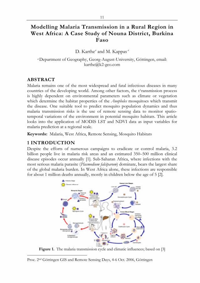
Figure 1. The malaria transmission cycle and climatic influences; based on [3]
Proc. 2nd Göttingen GIS and Remote Sensing Days, 4-6 Oct. 2006, Göttingen
12
Malaria is a vector-borne which is transmitted by Anopheles mosquitoes and caused by four protozoan parasites, P. vivax, P. ovale, P. malariae and P. falciparum. Female anopheline mosquitoes have to take blood meals prior to oviposition as they require proteins. During a blood meal from an infected person, a mosquito may ingest a parasite which then undergoes further development. After completion of the sporogonic cycle, infective forms of the malaria parasites (sporozoites) may be injected into a new human host. [3] This part of the transmission cycle depends on ecological factors such as the climate as they have an impact on mosquito reproduction, longevity and biting behavior. [2; 5]
2 MODELLING MALARIA RISK IN NOUNA DISTRICT, BURKINA FASO Field experience and laboratory studies have shown that various aspects of the malaria transmission cycle are influenced by ecological factors such as the climate. Nouna District, Burkina Faso has been identified as one region which is ideal for a case study on the environmental impacts on malaria transmission for several reasons: (1) it is an area of endemic malaria where malaria significantly contributes to the total disease burden; (2) there is a marked seasonality of the climate and malaria transmission; (3) an existing network of climate stations provide ground data; (4) the Centre de Récherche en Santé de Nouna (CRSN), in a cooperative effort with the Department of Tropical Hygiene, Heidelberg University, registers the time and locality of malaria cases of the study population. [4] Despite the complex interrelations between various ecological parameters and different aspects of malaria transmission, the survey of environmental variables through remote sensing may be one key to better understand the spatio-temporal pattern of malaria outbreaks. 2.1 MALARIA TRANSMISSION AND THE ENVIRONMENT The intensity of malaria transmission is linked to a large number of environmental parameters such as the climate, the terrain, the hydrography and the prevailing vegetation or land use in a region.
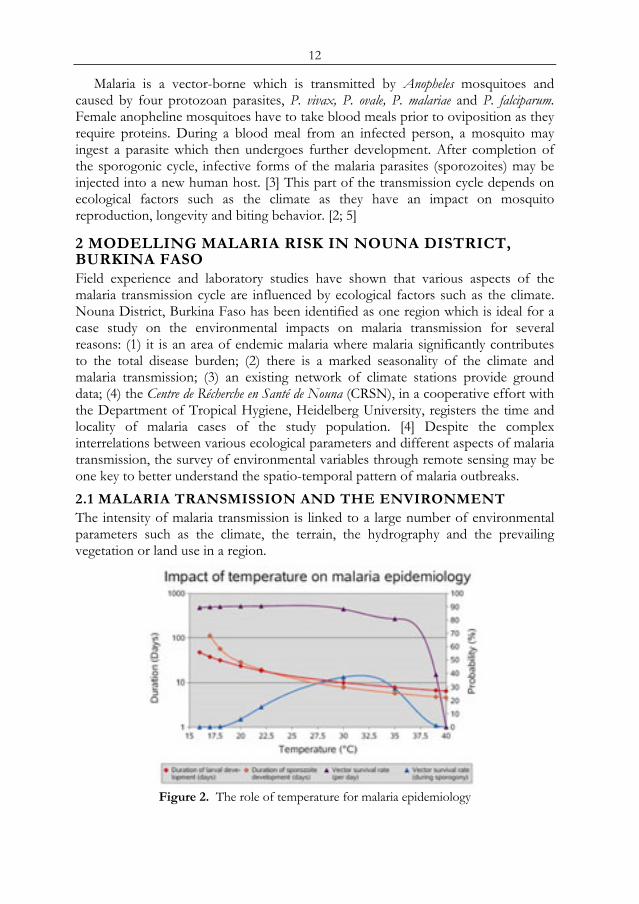
Figure 2. The role of temperature for malaria epidemiology
13
The effects of temperature on the reproduction, longevity and behavior of the mosquito vectors are a fine example for the complex interrelation between malaria transmission and the environment:
• At a temperature of 31°C the development from egg to adult takes around seven days, and considerably longer at lower temperatures (20 days at 20°C). Higher temperatures, unless accompanied by drought, result in even faster larval development [2; 5].
• The length of live of adult Anopheles varies somewhat between different species but much more due to environmental factors such as temperature, humidity and presence of natural enemies. When the mean temperature is over 35°C or the humidity less than 50%, the longevity of the mosquitos is drastically reduced [6].
• The period between one egg-laying and the next is called the gonotrophic cycle. The duration of the gonotrophic cycle is an important measure in malaria epidemiology as it determines the number of blood meals a female mosquito takes during her life. In the tropics one gonotrophic cycle typically lasts between two and four days. Low temperatures or adverse environmental conditions such as drought may lengthen this cycle considerably [5].
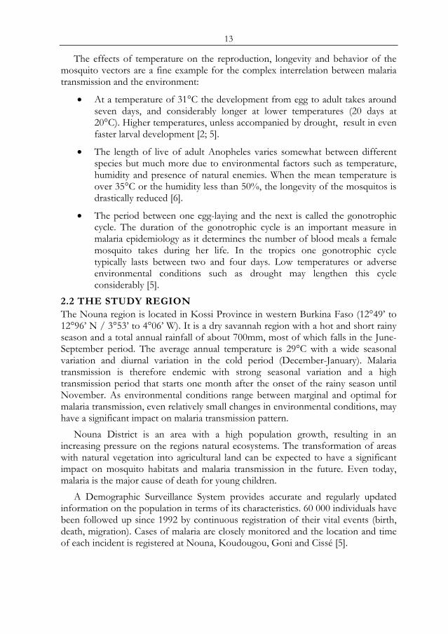
2.2 THE STUDY REGION The Nouna region is located in Kossi Province in western Burkina Faso (12°49’ to 12°96’ N / 3°53’ to 4°06’ W). It is a dry savannah region with a hot and short rainy season and a total annual rainfall of about 700mm, most of which falls in the June- September period. The average annual temperature is 29°C with a wide seasonal variation and diurnal variation in the cold period (December-January). Malaria transmission is therefore endemic with strong seasonal variation and a high transmission period that starts one month after the onset of the rainy season until November. As environmental conditions range between marginal and optimal for malaria transmission, even relatively small changes in environmental conditions, may have a significant impact on malaria transmission pattern.
Nouna District is an area with a high population growth, resulting in an increasing pressure on the regions natural ecosystems. The transformation of areas with natural vegetation into agricultural land can be expected to have a significant impact on mosquito habitats and malaria transmission in the future. Even today, malaria is the major cause of death for young children.
A Demographic Surveillance System provides accurate and regularly updated information on the population in terms of its characteristics. 60 000 individuals have been followed up since 1992 by continuous registration of their vital events (birth, death, migration). Cases of malaria are closely monitored and the location and time of each incident is registered at Nouna, Koudougou, Goni and Cissé [5].
14
Figure 3. Location and characteristics of main study sites
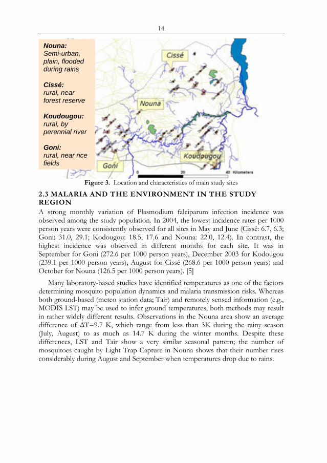
2.3 MALARIA AND THE ENVIRONMENT IN THE STUDY REGION A strong monthly variation of Plasmodium falciparum infection incidence was observed among the study population. In 2004, the lowest incidence rates per 1000 person years were consistently observed for all sites in May and June (Cissé: 6.7, 6.3; Goni: 31.0, 29.1; Kodougou: 18.5, 17.6 and Nouna: 22.0, 12.4). In contrast, the highest incidence was observed in different months for each site. It was in September for Goni (272.6 per 1000 person years), December 2003 for Kodougou (239.1 per 1000 person years), August for Cissé (268.6 per 1000 person years) and October for Nouna (126.5 per 1000 person years). [5]
Many laboratory-based studies have identified temperatures as one of the factors determining mosquito population dynamics and malaria transmission risks. Whereas both ground-based (meteo station data; Tair) and remotely sensed information (e.g., MODIS LST) may be used to infer ground temperatures, both methods may result in rather widely different results. Observations in the Nouna area show an average difference of ΔT=9.7 K, which range from less than 3K during the rainy season (July, August) to as much as 14.7 K during the winter months. Despite these differences, LST and Tair show a very similar seasonal pattern; the number of mosquitoes caught by Light Trap Capture in Nouna shows that their number rises considerably during August and September when temperatures drop due to rains.
Nouna: Semi-urban, plain, flooded during rains Cissé: rural, near forest reserve Koudougou: rural, by perennial river Goni: rural, near rice fields
15
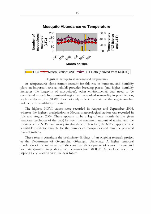
Mosquito Abundance vs Temperature
050
100150200
Jan
MarMay Ju
lSep Nov
Month of 2004
Num
ber o
f m
osqu
itoes
ca
ptur
ed
(LTC
)0.0
20.0
40.0
60.0
Tem
pera
ture
[°
C] (
Met
eo
and
LST)
LTC Meteo Station: AVG LST Data (derived from MODIS)
Figure 4. Mosquito abundance and temperatures As temperatures alone cannot account for this rise in numbers, and humidity
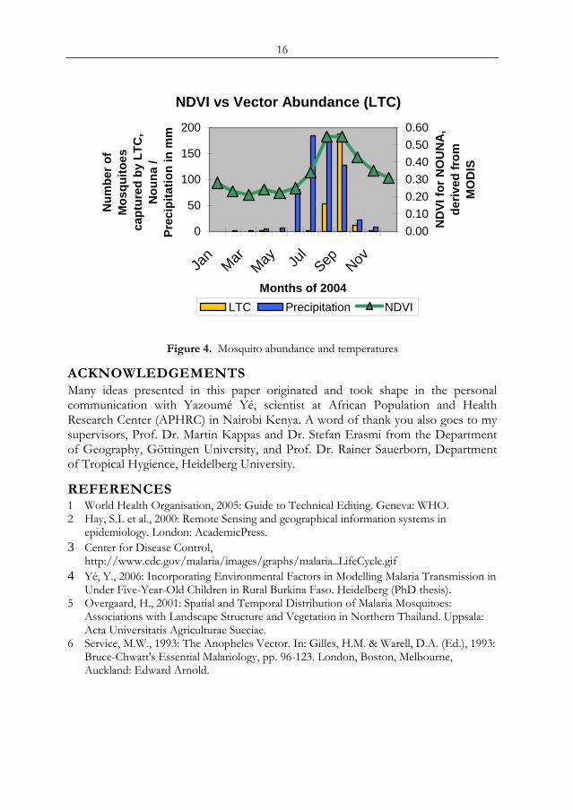
plays an important role as rainfall provides breeding places (and higher humidity increases the longevity of mosquitoes), other environmental data need to be considered as well. In a semi-arid region with a marked seasonality in precipitation, such as Nouna, the NDVI does not only reflect the state of the vegetation but indirectly the availability of water.
The highest NDVI values were recorded in August and September 2004, whereas the highest precipitation at Nouna meteorological station was recorded in July and August 2004. There appears to be a lag of one month (at the given temporal resolution of the data) between the maximum amount of rainfall and the maxima of the NDVI and mosquito abundance. Therefore, the NDVI appears to be a suitable predictor variable for the number of mosquitoes and thus the potential risks of malaria.
These results constitute the preliminary findings of an ongoing research project at the Department of Geography, Göttingen University. A higher temporal resolution of the individual variables and the development of a more robust and accurate algorithm to predict air temperatures from MODIS LST include two of the aspects to be worked on in the near future.
16
NDVI vs Vector Abundance (LTC)
0
50
100
150
200
Jan
MarMay Ju
lSep Nov
Months of 2004
Num
ber o
f M
osqu
itoes
ca
ptur
ed b
y LT
C,
Nou
na /
Prec
ipita
tion
in m
m
0.000.100.200.300.400.500.60
ND
VI fo
r NO
UN
A,
deriv
ed fr
om
MO
DIS
LTC Precipitation NDVI
Figure 4. Mosquito abundance and temperatures
ACKNOWLEDGEMENTS Many ideas presented in this paper originated and took shape in the personal communication with Yazoumé Yé, scientist at African Population and Health Research Center (APHRC) in Nairobi Kenya. A word of thank you also goes to my supervisors, Prof. Dr. Martin Kappas and Dr. Stefan Erasmi from the Department of Geography, Göttingen University, and Prof. Dr. Rainer Sauerborn, Department of Tropical Hygience, Heidelberg University.
REFERENCES 1 World Health Organisation, 2005: Guide to Technical Editing. Geneva: WHO. 2 Hay, S.I. et al., 2000: Remote Sensing and geographical information systems in
epidemiology. London: AcademicPress. 3 Center for Disease Control,
http://www.cdc.gov/malaria/images/graphs/malaria_LifeCycle.gif 4 Yé, Y., 2006: Incorporating Environmental Factors in Modelling Malaria Transmission in
Under Five-Year-Old Children in Rural Burkina Faso. Heidelberg (PhD thesis). 5 Overgaard, H., 2001: Spatial and Temporal Distribution of Malaria Mosquitoes:
Associations with Landscape Structure and Vegetation in Northern Thailand. Uppsala: Acta Universitatis Agriculturae Sueciae.
6 Service, M.W., 1993: The Anopheles Vector. In: Gilles, H.M. & Warell, D.A. (Ed.), 1993: Bruce-Chwatt's Essential Malariology, pp. 96-123. London, Boston, Melbourne, Auckland: Edward Arnold.
17
GIS-based Urban Sustainability Assessment
H. Storcha and R. Eckertb a BTU Cottbus, Department Environmental Planning, email: harry.storch@tu-
cottbus.de b BTU Cottbus, Department Urban Planning and Spatial Design, email:
ABSTRACT The paper presents significant initi2al experiences of an urban sustainability assessment research project of housing policies at the urban planning level in Ho Chi Minh City (HCMC), Vietnam. This research project is financed as part of the new research programme “Megacities of Tomorrow” by the German Federal Ministry of Education and Research (BMBF). The objective is to develop an integrated approach for the sustainable development of housing and settlement structures to balance urban growth and redevelopment in HCMC. A special focus will be laid on methodological issues of urban sustainability indicators and their spatial representation by multi-layered urban typologies for the evaluation of housing and settlement strategies. Keywords: GIS, Sustainability Assessment, Megacities, Urban Typologies.
1 INTRODUCTION - MEGACITY RESEARCH IN HCMC Megacities of tomorrow like Ho Chi Minh City (HCMC) offer exceptional opportunities to analyse both the impacts of large-scale environmental resource problems and institutional responses to these impacts, as well as urban planning and management strategies to overcome the limits and failures in the management of environmental resources.
The transition of the economic system of Vietnamese cities [1] has brought about major transformations in the physical and functional urban structures over the last decades. The development of the future megacity of HCMC has two interrelated perspectives: firstly urban growth, the evolving urban forms in the context of urbanisation, and secondly urban redevelopment within the inner urban area. HCMC covers 2,000 sq km, divided into 24 districts hosting an official population of more than 6 million. The inner city has an average population density of around 10,000 people per sq km. HCMC is undergoing a rapid urbanisation such that by 2020 the 17 inner city districts are expected to have a population of approximately 6 million, while the suburban area will have roughly 4 million residents. This rapid population and economic growth since the policy reform of Doi Moi has put a large and increasing stress on the water resources and environment in HCMC. The demand from industry and households surpassed the current distribution capacities. The water quality in underground sources and river courses is highly degraded due to many sources of pollution [16]. Proc. 2nd Göttingen GIS and Remote Sensing Days, 4-6 Oct. 2006, Göttingen
18
In HCMC, the public transport infrastructure can attract only around 10% of travel demand. The transportation infrastructure is poor and almost 90% of commuters use private forms of transport. The dominance of motorcycles and the weakness of public transport have resulted in increasing emissions from private urban transport activities. HCMC’s infrastructure is overloaded and is unable to meet the needs of people living in highly dense urban areas [17].
HCMC offers an appropriate setting for the analysis of many of the institutional forces and the urban dynamics that impact the interconnections between humans and their management of environmental resources in the megacities of today [9], because solutions seeking to make megacities work for those who are there and the migrants who will inevitably arrive are very uncommon [18]. The current urban transformation process requires that the urban planning system is based on a sound understanding of the housing and settlement development processes.
Quality of life, as access to basic housing needs and public services, and environmental quality are the determining factors in what a sustainable built-up environment is. However, there is need for a framework that will be able to support claims about housing needs in relation to the context of society and the physical and natural environment. The purpose of the research is to investigate the way in which housing needs and sustainability will be able to reinforce one another [11].
2 GIS-BASED SUSTAINABILITY ASSESSMENT The overall objective of the GIS-based sustainability indicator framework is to promote a better understanding of environmental and social impacts of planned settlement and housing developments in HCMC. Modern remote sensing (RS) and geo information (GI) techniques have had significant success in monitoring fast development processes in megacities [8]. The urban landscape is dominated by built environments that are physically distinguishable from the surrounding natural environment and therefore are readily identified through the use of remotely sensed image sources [6]. The framework needed, however, has to go beyond this simple identification of an urban environment and to integrate the variability of the built environment, which is associated with variability in human use patterns in settlement areas [7]. The key hypotheses are that different types of environmental and resource problems require particular kinds of management strategies to organise the obvious limits to growth of a pure, informal urbanisation process in metropolitan regions [12]. 2.1 CONFLICTING REQUIREMENTS OF SUSTAINABLE URBAN DEVELOPMENT To enable sustainable livelihoods for all within the bounds of the environmentally possible, the spatial planning aspects of sustainable urban development require the development of settlement and housing structures that facilitate equitable access to public resources and service opportunities and the efficient sharing of finite natural resources and agriculturally productive space in the metropolitan region. The social aspects of sustainable settlement and housing development primarily require providing people with opportunities for an acceptable quality of life. Planning strategies to ensure an acceptable quality of life are focused on the reduction of

19
environmental threats to human health that arise from insufficient urban sanitary infrastructure, inadequate provision of safe water, hazardous water and air pollution, and poor environment-related public services like the management of public transportation and of solid waste.
The environmental aspects of sustainable urban development of future megacities require a balance between protecting the natural environment and using its resources in a way that will allow the sustainable supporting of an acceptable quality of life for all urban residents. Environmental planning strategies are primarily concentrated on the reduction of impacts on natural resources and environmental systems of urban-based production, consumption and waste generation. Because these different principles of sustainability obviously have conflicting requirements [12], an integrated urban planning strategy will try to balance these different requirements. The resulting planning decisions need to be regularly monitored and assessed against agreed-upon urban sustainability indicators.
Because sustainable urban development holds these conflicting demands with different priorities in different regional contexts, it is not possible to define a general concept for sustainable human settlements. But urban-related sustainability indicator frameworks, like the Human Settlement Indicators of the Habitat Agenda, are creating an accepted normative framework based on human settlement-related indicators, defining urban sprawl and densification, and standards for basic needs, such as access to water and sanitation. 2.2 EFFICIENY INDICATORS FOR URBAN LAND USE PLANNING Settlement structure and its form of the built environment determine both the efficiency of resource uses and the quality of life of the inhabitants. Urban development planning of the last decades and the current discussion on sustainable spatial planning are characterised by two contrasting and conflicting urban planning models [4]. The 'network city' represents a car-based urban planning model and is in line with the global trends in urban development and the 'compact city' which represents an efficient use of resources such as land, energy, materials and time. The compact city model can assist in visualising a more sustainable urban form defined by two planning principles - densification and integration. The resulting dense and socially diverse urban structure lets social and economic activities overlap around well-defined centers of activity, generating focal points around which neighbourhoods can develop, thus reducing transportation needs.
Because efficiency indicators for residential land use can be easily used to contrast and separate the two competing urban development models of the current spatial planning discussion, the efficiency of regional and urban development structures is a real, measurable phenomenon with real implications for sustainability assessment (SA) procedures in urban planning. Densification is the most important efficiency indicator for urban land-use patterns, because it reduces sprawl. Further, the dense structure of the compact city provides the necessary economies of scale for an efficient infrastructure, and provisions for certain types of public urban services and an efficient use of finite natural resources. Urban planning strategies based on the compact city model with its efficient urban-related infrastructure and
20
service provision and protection of the natural environment promise to reduce the urban environmental footprint of megacities.
Yet in heavily under-serviced urban areas in developing countries, densification can be detrimental. In HCMC informal settlements are examples of areas of extremely high density living, but inadequate levels of service and infrastructure provision creating serious health problems and increased environmental impacts in these urban districts. In these under-serviced urban areas poverty reduction is the primary issue and the necessary establishment of acceptable living conditions induces an increase in resource consumption and energy production. Higher density is therefore not the only indicator for sustainable urban structures.
3 COMMON SPATIAL FRAMEWORK BASED ON URBAN TYPOLOGIES Sustainable urban development requires different strategies for different settlement types, because spatial planning concepts are very dependent on the particular local urban context. Different discipline-specific methodological approaches to the ‘urban environment’ require a commonly accepted spatial working basis, which can ensure that the resulting heterogeneous investigations can be trans-disciplinarily integrated by using an adequate spatially explicit classification. Therefore an ‘urban typology’ concept was developed and will be used as a practicable method to organise the spatial order of housing developments in HCMC.
Different settlement types will have different implications for achieving sustainability of settlement and housing structures. Settlement and housing types in HCMC are not uniform. Understanding these different types in HCMC therefore becomes crucial to the urban planning debate in this metropolitan region. Building HCMC-specific urban typologies should be centred on the interpretation of settlement types according their sustainability. To distinguish different settlement types it is important to define, based on sustainability indicators, the core information layers that can help to differentiate one settlement from another.
Because of the difficulties of separating settlement and housing typologies in HCMC they are used in an integrated manner to accept the complex nature and continued transformation of urban typologies in HCMC. It is therefore not the primary goal to develop a general definition of settlement and housing typologies in HCMC. Rather an analysis of the sustainability of urban typologies in a relatively representative model of different settlement and housing types is needed to assess the problems of different urban settlement and housing structures. Urban typologies can provide a tool for the structured and representative analysis of settlements in HCMC with its different components, of which housing is an important one.
The housing-related ‘urban typology’ provides a uniform methodological and spatial framework for the different tasks within the interdisciplinary network of the research project. Housing-related urban development decisions require a rational characterisation of urban structural landscapes according to environmental relevant features. The typology approach ensures that data integration of different sources (remotely sensed, field-based, survey-based and map-based) with their original
21
specific spatial/temporal resolutions and thematic contents can be operationally integrated in the GIS environment of the research project. 3.1 METHODOLOGY - DATA COLLECTION BASED ON HOUSING TYPOLOGIES In general, data on the housing typologies will be gathered by examining actual study sites within the metropolitan area of HCMC. Prior to the selection of these study sites, the kinds of housing development inherent to each typology were identified.
Four representative types, so called archetypes, of residential development were generally identified: Shop house (tube house with small lot wide) patterns, villas structures, condominium (mid-rise multiple family apartment buildings) and high-rise apartment blocks (up to 20 storeys high). Based on these four housing archetypes, each of these types was conceptually divided into two subtypes to generate the housing typologies with the exception of the shop house structure, which was divided into seven subtypes to reflect the broad variety of these predominant settlement structures occurring in the inner-districts of HCMC. The shop house is a building typology often found throughout Southeast Asia. They are mostly two to three storeys high and serve both shops on the ground floor and living quarters above. In HCMC, shop houses are located predominantly in the inner-city districts. The following building-specific indicators were used to define the final housing typologies: Height (storeys), block size and shape, structure of the street-network, built-up ratio, location in the metropolitan area, housing mix and mixture of usage (multi-functionality). Finally each housing typology is described by a unique combination of street block arrangement, land use mix, and density range (Tab. 1). These housing typologies are used to define the study sites for the data collection procedures.
Table 1. Study Sites, Housing Typologies. Hou-sing Typo-logy
Description Height (Storeys)
Block Size (Shape)
Street-Network
Built-up Ratio
Location Housing Mix (Types)
Mixture of Usage (Res/So/Com)
Shop house Type A Shop houses on
the border (street-orienta-ted) of a slum area
1-3 large irregular medium
Inner-City
medium medium (shops in the outside borders)
Type B Medium-sized blocks with a small inner connection only for pedestrians
2-4 medium regular high Inner-City
low high
Type C Small-sized blocks, every plot is connected to a street
2-3 small regular medium
Inner-City
low medium (basically residential use)
Type D High-density 2-8 small regular very Inner- medium high (basically
22
tourist area with hotels, restaurants, agencies in shop houses
high City commercial use, only some residential use)
Type E Redevelopment site with shop house typo-logy for middle- to high income groups
5 small regular high Inner-City, Redevelopment Area
low medium (sometimes residential use only)
Type F Orthogonal shop house pattern in the periphery
1-2 medium regular medium
Outer Districts
low medium
Type G Linear street-orientated sprawl
1-2 no blocks irregular
low Outer Districts
medium medium
Villas Structure Type A Mainly original
villa structure from the French influence
1-3 medium regular medium
Inner-City
medium medium-high
Type B Villa structure with an intense mix of other typologies
1-3 medium regular medium-high
Inner-City
rich medium-high
Condominium Type A High-density
linear apartment blocks
5-6 small regular high Inner-City
low (plug-in in shop house area)
medium (shops, services on ground floor)
Type B Medium-density apartment blocks with designed public space and partly occupied by slum buildings
5-6 large (linear row-structure)
irregular medium
Outer Districts
medium medium (shops, services on ground floor)
High-rise Type A High-rise
apartment buildings as plug-in in existing settlement structure
app. 20 small irregular high Inner-City
low low
Type B High-rise apartment buildings in the new development area Saigon-South
20-24 medium regular medium-high
New Development Area
low medium (shops, supermarkets on ground floor)

23
3.2 HOUSING TYPOLOGIES – SELECTION OF STUDY SITES Each study site represents one housing typology found within the settlement pattern of HCMC. First, these study sites were spatially defined through examination of satellite images and later verified by ground recognisance. Study sites were selected following three primary criteria: archetypical representation of the housing typology; conformance of the shape and size of the street block arrangement to the overarching archetype; and correlation to pre-existing statistical and spatial data sources. The final criterion was included to simplify the data collection process during the initial phase of the research programme, where all available data required for the multi-layered approach should only be aggregated to reflect the typology-driven accepted common spatial framework. Out of this process, a first requirement for thirteen study sites was realized (see table typology).
Up to four study sites are selected for each of the housing typologies. Each study site is selected to represent one housing typology found within the neighbourhood pattern on district level. The physical boundaries of the housing typologies are defined by street blocks. The study site is embedded within the surrounding urban fabric of the neighbourhood pattern. Data collected from the study sites for the representing housing typology will be used to formulate scores for sustainability based on the multi-layered approach. The neighbourhood pattern is represented as a puzzle, in which the separate housing typology pieces fit together to form the complete picture of settlement developments in HCMC.
4 TYPOLOGY BUILDING BASED ON SUSTAINABILITY INDICATORS There is a need to create urban typologies of the settlement structure of cities such as building/population density, housing types, spread of public services, commute times and other environment-related infrastructure issues. Such an urban typology of housing and settlement structures can take into consideration socio-economic information to determine the liveability and overall sustainability of these individual urban types. The proposed concept represents an interpretative method to integrate the physical aspect of housing developments with the socio-economic and environmental-related information of built-up areas (Tab. 2) based on the concept of urban typologies. The main purpose of urban typologies is to ensure that assessment of planning policies can be clarified and simplified by grouping residential areas and neighbourhoods with common characteristics and that could therefore have similar sustainability problems and environmental impacts. 4.1 INDICATOR-BASED MULTI-LAYERED URBAN TYPOLOGIES Because indicators used should reflect the housing-related sustainability issues that the urban typology is seeking to address, a layering of indicators is the most useful approach. It appears to be consensus that a useful urban typology must combine a range of different indicators. The selection of these indicators will directly influence the conclusions that can be drawn from the urban typology approach. The classification of settlement patterns and housing structures should be combined with an analysis of socio-economic, environmental and public service/infrastructure characteristics in order to provide a more accurate picture of current housing problems.
24
Certain core sustainability indicators specifically linked to urban settlement and housing structures have been identified by the analyses of international indicator programmes [13, 14] and critically assessed for their relevance to housing assessment in HCMC. The indicators used to formulate the urban typology are predominantly focused on housing structures and settlement pattern [5], with environmental capacity / sensitivity and socio-demographic and economic characteristics also being included. Therefore housing related typologies must be developed on the basis of criteria which reflect these additional socio-economic and environmental issues. This has led to a multi-layered typological approach (Tab. 2) in which urban typologies instrumental in highlighting the major aspects of sustainable urban development can be identified. The framing of these factors is based on a set of requirements drawn from international descriptions of the characteristics of a sustainable settlement as measured by the described indicator conceptions.
This multi-layered approach reflects that the livelihood of the neighbourhoods in general is dependent on the combined effect of a range of sustainability-related factors rather than the presence or absence of single aspects of urban sustainability. To assess the sustainability of urban settlement developments, four different layers must be analysed: physical structure, urban environmental land-use pattern [2], use (infrastructure services) patterns and the social system (Tab. 2).
Table 2. Multi-layered Urban Typologies based on Sustainability Indicators.
Layer 1 – Physical Structure Urban Settlement Planning
In urban areas, typologies are linked to housing developments
Housing related typologies reflect the regional knowledge of urban planners.
Indicators used to formulating the urban typology are predominantly focused on housing structures and settlement pattern.
Housing structures are detectable with high resolution remote sensing data.
Layer 2 - Urban Land Use Pattern Environmental Land Use Planning Linking land/vegetation-cover information to
housing typologies Environmentally-based urban administration
decisions require characterisation of urban landscapes according to urban land-cover and land-use types.
Integration of available data from different sources is possible (remotely sensed, field-based, and map-based).
Layer 3 – Use Pattern Public Infrastructure Services
25
Availability/quality of environmental-related infrastructure/services.
Assessing levels of infrastructure and service is important for the definition of settlement zones.
Definition of solutions for appropriate urban infrastructure development.
Sustainable management of urban services to improve the urban environment.
Integration of available data from official sources.
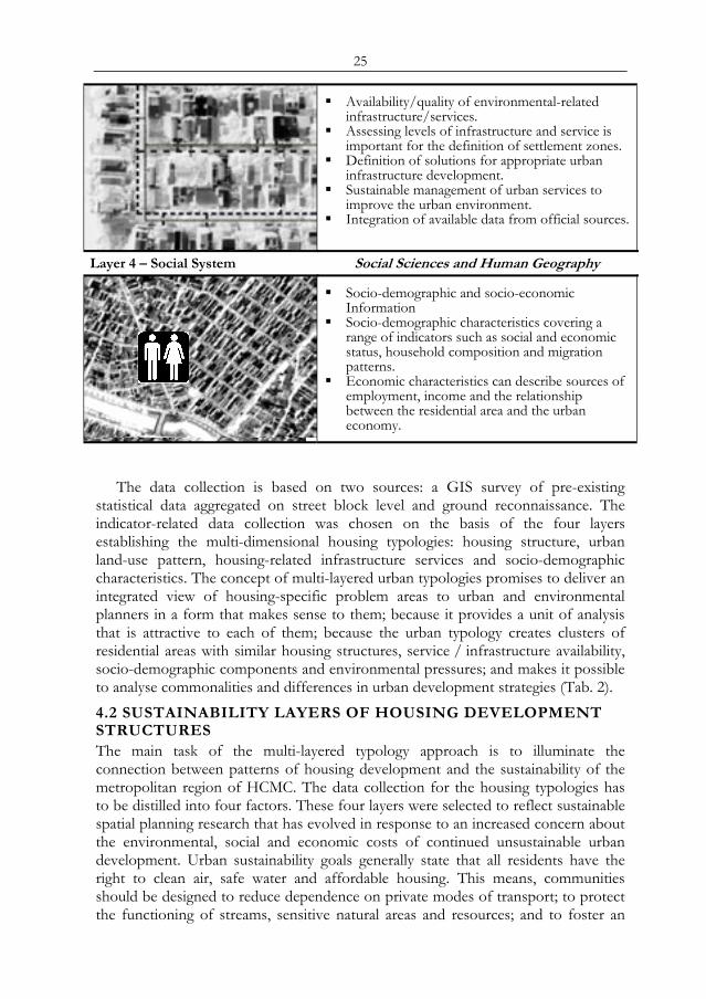
Layer 4 – Social System Social Sciences and Human Geography
Socio-demographic and socio-economic Information
Socio-demographic characteristics covering a range of indicators such as social and economic status, household composition and migration patterns.
Economic characteristics can describe sources of employment, income and the relationship between the residential area and the urban economy.
The data collection is based on two sources: a GIS survey of pre-existing
statistical data aggregated on street block level and ground reconnaissance. The indicator-related data collection was chosen on the basis of the four layers establishing the multi-dimensional housing typologies: housing structure, urban land-use pattern, housing-related infrastructure services and socio-demographic characteristics. The concept of multi-layered urban typologies promises to deliver an integrated view of housing-specific problem areas to urban and environmental planners in a form that makes sense to them; because it provides a unit of analysis that is attractive to each of them; because the urban typology creates clusters of residential areas with similar housing structures, service / infrastructure availability, socio-demographic components and environmental pressures; and makes it possible to analyse commonalities and differences in urban development strategies (Tab. 2). 4.2 SUSTAINABILITY LAYERS OF HOUSING DEVELOPMENT STRUCTURES The main task of the multi-layered typology approach is to illuminate the connection between patterns of housing development and the sustainability of the metropolitan region of HCMC. The data collection for the housing typologies has to be distilled into four factors. These four layers were selected to reflect sustainable spatial planning research that has evolved in response to an increased concern about the environmental, social and economic costs of continued unsustainable urban development. Urban sustainability goals generally state that all residents have the right to clean air, safe water and affordable housing. This means, communities should be designed to reduce dependence on private modes of transport; to protect the functioning of streams, sensitive natural areas and resources; and to foster an
26
acceptable quality of life for residents. The layered approach of housing typologies helps to indicate how successful each typology is in achieving these goals.
The mix of urban land uses, predominance of building types, density of development, and arrangement of street blocks describe a housing development pattern. Density and urban land use mix as well as the physical pattern of street blocks influence sustainability. The infiltration of rainwater is important to recharge groundwater. Infiltration also prevents flooding of housing areas, which occurs when large volumes of rainwater are conveyed to the canal and river network during storms. Soil sealing is a measure of how much of the area is in situ capable of infiltrating water. Areas with sealed soils are surfaces like streets, sidewalks and roofs that rain water cannot seep through. Areas with unsealed soils are surfaces like lawns, gardens, parks and lawns that rain water can infiltrate.
A fine-grained and diverse land use mix puts residents close to their daily needs including school, local shopping and, for some, work, while higher densities provide the residents required to support public infrastructure services and local shops. Housing mix describes what range of different housing types is available to residents. A good mix ensures that a wide range of household types can have their necessary housing needs accommodated in the neighbourhood. Affordability is different from housing mix and describes the cost of residing in the settlement pattern. Affordability measures what percentage of existing households could afford to purchase or rent a home or apartment in each settlement pattern and is broken down by different housing types.
These features are jointly influencing sustainability factors such as: commuting behaviour, housing affordability, the formation of social ties and job opportunities, and the efficiency of the use of land and natural environmental resources in general. A fine-grained urban land use mix places opportunities for employment close to residents. Higher density housing developments put enough residents in the neighbourhood to support public transit and local shops. A well interconnected arrangement of street blocks makes it easier to establish the necessary access to urban infrastructure services. In combination with higher population densities the cost of developing such urban infrastructure services are substantially lower.
Clearly, the structure and arrangement of housing areas are factors influencing urban sustainability. Recognition of this connection makes it possible to re-evaluate the housing development pattern as a fundamental determinant in the formation of urban sustainability, because, if replicated on multiple sites, the housing development pattern becomes an integral part of the urban fabric of HCMC. The sustainability of each housing development helps to determine the ultimate sustainability of the urban region. Urban sustainability is strongly influenced by the choices that are made about the housing types to build.
5 DISCUSSION AND CONCLUSIONS The concept of multi-layered urban typology looks at the housing development as a regional building block. Rather than examining the effects of housing developments on single aspects of sustainability independently, possible combinations of these aspects are explored. The goal of the data collection is to determine the relative
27
sustainability of each housing typology. Although all of the defined housing typologies are pre-existing in HCMC, the purpose of the multi-layered approach is to describe how each one would function as new developments in the metropolitan area of HCMC. The results of the investigation of multi-layered housing typologies will be applied in the Sustainability Assessment of new housing developments, where urban planning administrations may combine different housing typologies to explore the implications of the resulting settlement pattern on the creation of a sustainable urban development region.
This could help the urban planning system to act as an interface, connecting development strategies to produce a more sustainable approach to future settlement developments in the housing sector. The outcome of this research project will show whether a GIS-based sustainability assessment of urban developments fulfils only a technical role as a pure planning information system, or whether it might occupy a more central role in terms of sustainability assessment based on indicator-based modelling of form and function of defined urban typologies.
ACKNOWLEDGEMENTS The research project 'Sustainable Housing Policies for Megacities of Tomorrow. The Balance of Urban Growth and Redevelopment in Ho Chi Minh City' is financed as part of the new research programme 'Megacities of Tomorrow' by the German Federal Ministry of Education and Research (BMBF). The initial two-year phase of the project runs from 2005 to 2007. The research team is interdisciplinary, and consists of researchers in the areas of urban planning, geography, social sciences and environmental planning [3].
REFERENCES 1. Boothroyd, P. and Pham, X.N. (ed.) (2000): Socio-economic Renovation in Viet Nam.
The Origin, Evaluation, and Impact of Doi Moi, Institute of Southeast Asian Studies, Singapore.
2. Bouland P. and Hunhammar S. (1999): Ecosystem services in urban areas. Ecological Economics 29 (2), pp. 293-301.
3. BTU (Brandenburgische Technische Universität Cottbus) (2006): Megacities of Tomorrow Ho Chi Minh City/Vietnam. Sustainable Housing Policies for Megacities of Tomorrow. The Balance of Urban Growth and Redevelopment in Ho Chi Minh City. BMBF-Research Programme. Website: www.megacity-hcmc.org.
4. Ewing R, Pendall R, Chen D (2002) Measuring Sprawl and Its Impact. Smart Growth America. Website: www.smartgrowthamerica.org/sprawlindex/MeasuringSprawl.pdf
5. Flood, J. (1997): Urban and Housing Indicators. Urban Studies 34 (10), pp. 1635-1665. 6. Foresman, T., Pickett, S. and Zipperer, W. (1997): Methods for spatial and temporal land
use and land cover assessment for urban ecosystems and application in the greater Baltimore-Chesapeake region. Urban Ecosystems (1), pp. 201-216.
7. Harris, R.J. and Longley, P.A. (2001): Data-rich models of the urban environment: RS, GIS and 'lifestyles'. In: Halls. P. (ed.) Innovations in GIS 8: Spatial Information and the Environment. London: Taylor and Francis, pp. 53-76.
8. Herold, M., Hemphill J., Dietzel, C. and Clarke, K.C. (2005): Remote Sensing Derived Mapping to Support Urban Growth Theory. Proceedings URS2005 conference, Phoenix, Arizona, March 2005.

28
9. Lo, F-C. and Marcotullio P. J.(ed.) (2001): Globalization and the Sustainability of Cities in the Asia Pacific Region. New York: United Nations University Press.
10. Pauleit, S. and Duhme F. (2000): Assessing the environmental performance of land cover types for urban planning. Landscape and Urban Planning (52), pp. 1-20.
11. Satterthwaite, D. (1997): Sustainable cities or cities that contribute towards sustainable development? Urban Studies 34 (10), pp. 1667-1691.
12. Satterthwaite, D. (1999):The Links between Poverty and the Environment in Urban Areas of Africa, Asia and Latin America, United Nations Development Programme (UNDP) and the European Commission (EC), New York.
13. UN CSD (United Nations Commission for Sustainable Development) (2001). Indicators of Sustainable Development - CSD Theme Indicator Framework. Website: http://www.un.org/esa/sustdev/natlinfo/indicators/isdms2001/table_4.htm
14. UN Habitat (2004): Urban Indicators Guidelines. Monitoring the Habitat Agenda and the Millennium Development Goals. United Nations Human Settlement Programme, Aug. 2004, Nairobi: UN Habitat.
15. UNEP Grid Arendal (2006): Encyclopaedia of Urban Environment-Related Indicators. Website: http://www.ceroi.net/ind/indicat.htm
16. Van Duc, L., and Gupta, A. D. (2000). Water resources planning and management for lower Dong Nai River basin, Vietnam: Application of an integrated water management model. International Journal of Water Resources Development, 16(4), pp. 589-614.
17. Van Khoa, L. (2001): Air Quality Management in HO Chi Minh City. Department of Science, Technology and Environment. (DoSTE) of HCMC - Viet Nam. Website: http:/www.unescap.org/esd/environment/kitakyushu/urban_air/city_report/HoChiMinh2.pdf
18. Van Vliet, W. (2002): Cities in a globalizing world: from engines of growth to agents of change. Environment and Urbanization 14 (1), pp. 31-40.
29
TRANSITIVE – FUZZY PRINCIPLE FOR the OPTIMIZATION OF INFORMATION SYSTEMS
APPLICATION FOR REMOTE-SENSING SYSTEMS
H. H. Asadov and M. J. Kerimov
Azerbaijan National Aerospace Agency, AZ1106, Baku, Azerbaijan, Azadlig ave. 159, email: [email protected]
ABSTRACT It is shown that such different types of information systems as fuzzy control systems and remote sensing systems may be optimized using simil3ar procedures if both of them are attributed by some similar features of systems. The chosen single logarithmic weighted functional of effectiveness and universal limitation condition related to the distribution of the system’s major resource parameter during the whole work cycle makes it possible to find out the universal optimal regime of work for considered systems. The mathematical solution of optimization task is carried out using the multistage optimization principle previously suggested by the authors. Keywords: transitive systems, fuzzy systems, optimization, criterion of optimization, remote sensing systems
MAJOR COMMON FEATURES OF TRANSITIVE – FUZZY SYSTEMS There are many universal principles of optimization and control, which are successfully used in solution of various tasks. Suggested in this article the described transitive – fuzzy principle of optimization conceptually expresses the unity of definite and fuzzy systems and opens the new possibilities in formation of new single methods for analysis and synthesis of information systems considered as transitive definite or fuzzy systems (afterwards these systems will be called as transitive – fuzzy systems).
Major features of the formed class of transitive – fuzzy systems are following:
1. These systems are characterized with transitive parameters ( )xamii TTT ÷=0 to which the following is attributed:
(a) the function of membership ( )iTμμ = if the fuzzy system is considered;
(b) signal/noise ratio, if the definite system is considered. 2. We assume that these systems are characterized by some limiting resource
parameter, which is determined as follows: (a) for fuzzy systems:
Proc. 2nd Göttingen GIS and Remote Sensing Days, 4-6 Oct. 2006, Göttingen

30
( ) tsnocTdTMxamT
xamF == ∫0μ .
The parameter FM factually characterizes the fuzzy – resource of systems.
(b) for definite systems:
( ) tsnocTdTMxamT
D == ∫0η .
The parameter DM factually characterizes the correctness resource of a system.
3. The transitive – fuzzy systems are characterized by single logarithmic functional of effectiveness, which is determined as follows:
(a) for fuzzy systems:
( )[ ]
( )∑
∑
=
== n
jjxam
n
jjj
Fd
T
TTnlZ
1
1
μ
μ,
for discrete control regime, and
( )[ ]
( )∫
∫=
xam
xam
T
xam
T
Fa
dTT
dTTTnlZ
0
0
μ
μ (1)
(b) for analogous systems; the logarithmic functional of effectiveness is to be written as
( )[ ]
( )∑
∑
=
== n
jj
n
jij
ddT
TTnlZ
1
1
η
η,
for discrete control regime, and
( )[ ]
( )∫
∫=
xam
xam
T
T
ad
dTT
dTTTnlZ
0
0
η
η, (2)
in the analogous control. 4. The optimization of the systems of formed class of transitive-fuzzy systems,
i.e. optimization of functionals (1) and (2) should be carried out by single principle of optimization, which will be explained below.
31
OPTIMIZATION OF FUZZY CONTROL SYSTEM As the first example of realization of transitive – fuzzy principle of optimization we consider the classical structure of fuzzy information system for control [1] (fig. 1).
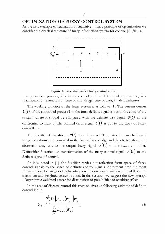
Figure 1. Base structure of fuzzy control system.
1 - controlled process; 2 - fuzzy controller; 3 - differential comparator; 4 - fuzzificator; 5 - extractor; 6 - base of knowledge, base of data; 7 – defuzzificator
The working principle of the fuzzy system is as follows [1]. The current output ( )tY of the controlled process 1 in the form definite signal is put to the entry of the
system, where it should be compared with the definite task signal ( )tg in the differential element 3. The formed error signal ( )te is put to the entry of fuzzy controller 2.
The fuzzifier 4 transforms ( )te to a fuzzy set. The extraction mechanism 5 using the information compiled in the base of knowledge and data 6, transform the aforesaid fuzzy sets to the output fuzzy signal ( )tU * of the fuzzy controller.
Defuzzifier 7 carries out transformation of the fuzzy control signal ( )tU * to the definite signal of control.
As it is noted in [1], the fuzzifier carries out reflection from space of fuzzy control signals to the space of definite control signals. At present time the most frequently used strategies of defuzzification are criterion of maximum, middle of the maximum and weighted center of zone. In this research we suggest the new strategy – logarithmic weighted center for distribution of possibilities of resulting effect.
In the case of discrete control this method gives us following estimate of definite control input:
( )[ ]
( )∑
∑
=
== n
jjxam
n
jjjxam
W
WWnlZ
1
10
μ
μ, (3)
3
4 5 7 1
6 2

32
where jW - carrier of value of control input under regular number
( )njj ,1= , upon which the function of membership reaches its maximal value ( )jxam Wμ .
The regular analog of the formula (3) can be written as follows:
( )
( )∫
∫=
xam
xam
W
xam
W
xam
r
dWW
dWWgolWZ
0
02
01
1
1
μ
μ. (4)
The ratio (4) may be considered as functional of effectiveness of the work of the fuzzy controller, and the following optimization task may be formulated: To find out the optimal function ( )Wxam 1
μ which brings the functional (4) to its maximal value. This mathematical task may be solved by help of new principle of optimization [2], consisting of in this case two steps: Step 1. Application of optimization principle of Gauss-Zaydel. Using of the first step of this principle allow us to formulate the following task of optimization: To find out the optimal function ( )Wxam 1
μ upon which the functional
( )∫=xamW
xam WdWgolWF0
2 1μ
reaches the maximal value, taking into consideration the following condition:
( ) tsnocWdWxamW
xam =∫0
1μ .
Step 2. In order to solve the optimization task, formulated in the Step 1, we transfer it to equivalent variation optimization task with limitation condition: To find out the conditional maximum of following functional
∫=xamW
xam WdgolWF0
21 1μ
with following limitation condition:
( ) tsnocWdWxamW
xam =∫0μ .
In order to solve this task we should compose the additional functional of optimization
33
( ) ( )dWWWdWgolWFxamxam W
xamxam
W
da ∫∫ +=00
21 11μλμ (6)
whereλ - Lagrange multiplier. Solution of this optimization task using method of Euler, gives us following
optimal function:
( ) 22
1xam
tpoxam WCWW =μ . (7)
It can be shown, that the second derivative of formula (6) taking into consideration of (5) is always negative, i.e. the chosen criterion of optimization is unimodal. Therefore, it is shown, that the fuzzy controller attributed with aforesaid common features of transitive – fuzzy systems may be characterized with optimal regime of the work.
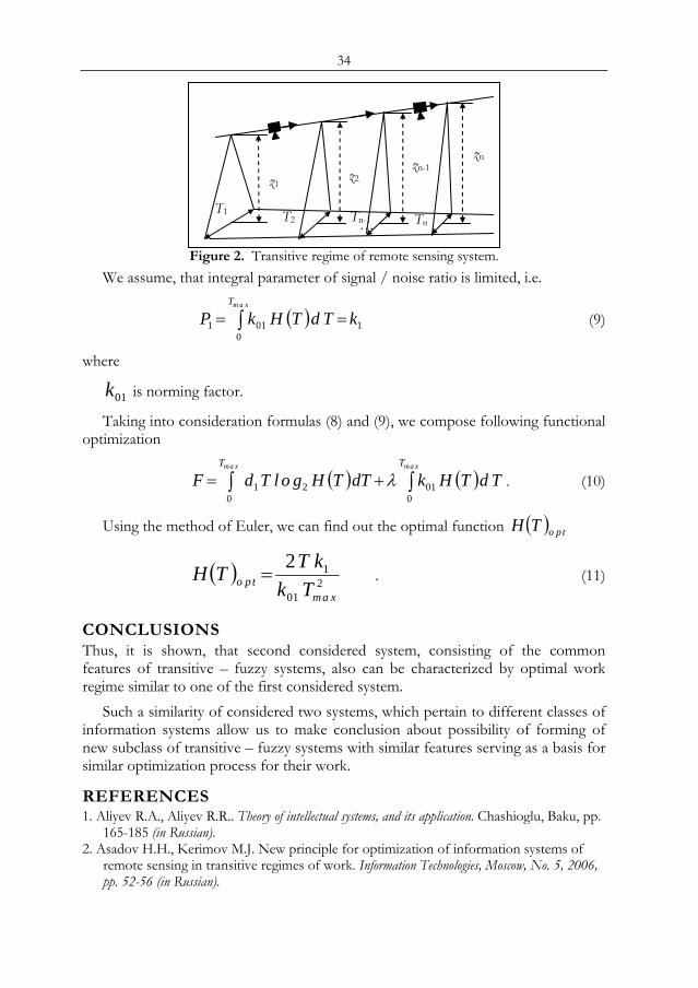
OPTIMIZATION OF TRANSITIVE REMOTE SENSING SYSTEM As the second example we consider the space remote sensing system installed in the space carrier, the height of the flight of which is changing monotonously.
The work regime of the carrier of remote sensing system is shown in the figure 2, where the photometer, installed in the carrier moving on inclined trajectory, carries out video recording with duration of lines ( )niTi ,1, = . The potential possible value of obtained measuring information is to be estimated on the basis of integrated value of logarithm of signal / noise ration, i.e.
( )∫=xamT
dTTHgolTdM0
21 (8)
where
( )TH -function of dependence of signal / noise ratio from time period of subcycle of measurements
T -duration of subcycle of measurement
1d -norming factor.
34
Figure 2. Transitive regime of remote sensing system.
We assume, that integral parameter of signal / noise ratio is limited, i.e.
( ) 10
011 kTdTHkPxamT
== ∫ (9)
where
01k is norming factor.
Taking into consideration formulas (8) and (9), we compose following functional optimization
( ) ( )∫ ∫+=xam xamT T
TdTHkdTTHgolTdF0 0
0121 λ . (10)
Using the method of Euler, we can find out the optimal function ( ) tpoTH
( ) 210
12
xamtpo Tk
kTTH = . (11)
CONCLUSIONS Thus, it is shown, that second considered system, consisting of the common features of transitive – fuzzy systems, also can be characterized by optimal work regime similar to one of the first considered system.
Such a similarity of considered two systems, which pertain to different classes of information systems allow us to make conclusion about possibility of forming of new subclass of transitive – fuzzy systems with similar features serving as a basis for similar optimization process for their work.
REFERENCES 1. Aliyev R.A., Aliyev R.R.. Theory of intellectual systems, and its application. Chashioglu, Baku, pp.
165-185 (in Russian). 2. Asadov H.H., Kerimov M.J. New principle for optimization of information systems of
remote sensing in transitive regimes of work. Information Technologies, Moscow, No. 5, 2006, pp. 52-56 (in Russian).
…Т1 Т2 Тn-1 Тn
z1 z2
zn-1 zn
35
RICE FIELD DISCRIMINATION AND CLASSIFICATION WITH MULTI-TEMPORAL SAR
IMAGERY
A. Darvishi Boloorania, b, S. Erasmia, M. Kappasa
a Dep. of Cartography, GIS & Remote Sensing4, Inst. of Geography, Goettingen University, Germany,
email: (adarvis, serasmi, mkappas)@uni-goettingen.de b Tarbiat Modares University, Tehran, Iran
ABSTRACT In general, rice is one of the most important crops in tropical areas, specifically in Southeast Asia. Due to many environmental and economical limitations in obtaining quantitative and qualitative information on agricultural crops in tropical areas, remotely sensed imagery can help us to obtain precise, up to date and reliable information. Temporal inconsistency in sowing, growing, harvesting and irrigation schemes requires the availability of multi-temporal satellite imagery. The frequent cloud cover in the tropics demands for the implementation of other than optical remote sensing imagery. Hence, satellite borne SAR data provide frequent observations for crop mapping at the regional level.
Therefore, main emphasis of this study was on the use of multi-temporal ENVISAT/ASAR satellite synthetic aperture radar (SAR) images for monitoring and temporal discrimination of fields under different rice cropping systems in Palolo Valley, Central Sulawesi, Indonesia. The utilized imagery were acquired in multi-polarimetric mode (HH, HV or VV, VH) from 4th February to 28th July 2004. Based on the objectives of the work, seven separate data sets were used which included Co-Polarized (HH, VV), Cross-Polarized (HV, VH), Mean Texture Co-Polarized, Mean Texture Cross-Polarized, Monthly Subtraction, Polarized Subtraction and Normalized Polarized Subtractions.
High resolution Quickbird/MS satellite imagery were used as ground truth and also for collecting training and validation samples for the purpose of classification and accuracy assessment. Final results show that co-polarized data yield the highest accuracy while normalized co-polarized data produced the worst accuracy. Keywords: Multi-Temporal Rice discrimination, SAR classification, ENVISAT/ASAR.
1 INTRODUCTION Rice as the second world basic food item accounts for 15% of the world’s total cultivated area [9]. In Asia, where 94% of the world’s rice is produced, rice is the main source of nutrition (35± 80% of the mean caloric intake) and a significant source of income [4]. Rice cropping in the Palolo Valley mostly depends on Proc. 2nd Göttingen GIS and Remote Sensing Days, 4-6 Oct. 2006, Göttingen
36
precipitation regimes, irrigation systems, and some socio-economical parameters. Therefore, the high diversity and somewhat irregularity of the rice cultivating systems demand the use of the multi-temporal images in monitoring, classification and discrimination of temporal growth regimes of rice crops. On the one hand, the accessibility of satellite imagery, obtained from different kind of sensors (microwave and optical), offer a good potential in remote sensing applications in monitoring and crop discriminations but on the other hand, one of the main limitations in the use of multi-spectral optical images is that the main rice producing areas are situated in the tropics. In this area, it is very difficult to ensure successful acquisitions with optical sensors because of the frequent cloud cover [9]. Therefore, the sun illumination and weather independency as well as cloud penetrative characteristics of SAR satellite images offer a good potential in this area of SAR applications. Because of the high amount of precipitation in tropical area there is no specific seasonality to planting rice [7]. Nevertheless, as a general rule for Indonesia the main paddy variety has a short cycle and permits at least two crops per year, one during the dry season (total mean rice crop duration 130 days from March to July-August) and another during the wet season which lasts usually 145 days from November to April [9]. Therefore, our data are considered as dry season in rice plantation timetable. More than the influence of seasonality phenomena in rice planting other phenomena like economical and social parameters have considerable effects in this area. These factors results in a diverse pattern of rice crop phenological stages at the same time. The temporal patterns can be assessed by the use of frequently available SAR satellite data. Based on the examination of the ability of multi-temporal, multi-polarized ASAR imagery in rice fields monitoring and usage of different ASAR derivative data sets in classification processes, the results of this work demonstrate the potential of SAR imagery for rice mapping and monitoring.
2 MATERIAL AND METHODS
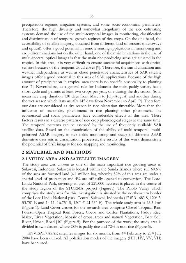
2.1 STUDY AREA AND SATELLITE IMAGERY The study area was chosen as one of the main important rice growing areas in Sulawesi, Indonesia. Sulawesi is located within the Sunda Islands where still 60.6% of the area are forested land (4.1 million ha), whereby 32% of this area are under a special level of protection and 4% are officially opened to conversion. The Lore-Lindu National Park, covering an area of 229.000 hectares is placed in the centre of the study region of the STORMA project (Figure1). The Palolo Valley which comprises the study area for this investigation is situated at the northeastern border of the Lore Lindu National park, Central Sulawesi, Indonesia (1° 8' 31.68" S, 120° 3' 53.78" E and 1° 11' 16.75" S, 120° 6' 21.63" E). The whole study area is 23.5 km² (Figure 1). Land Cover classes for the research area comprise Closed Tropical Rain Forest, Open Tropical Rain Forest, Cocoa and Coffee Plantations, Paddy Rice, Maize, River Vegetation, Mosaic of crops, trees and natural Vegetation, Bare Soil, River, Urban, Road [10] (Figure 5). For the purpose of the work, the study area is divided in two classes, where 28% is paddy rice and 72% is non-rice (Figure 5).
ENVISAT/ASAR satellites images for six month, from 4th February to 28th July 2004 have been utilized. All polarization modes of the imagery (HH, HV, VV, VH) have been used.
37
IndonesiaLore Lindu National park ASAR temporal color composite
Figure 1. The study area in three levels: country, province and study area.
2.2 SAR BACKSCATTER PROPERTIES IN RICE FIELDS The literature of SAR data analysis for rice field discrimination indicates that the
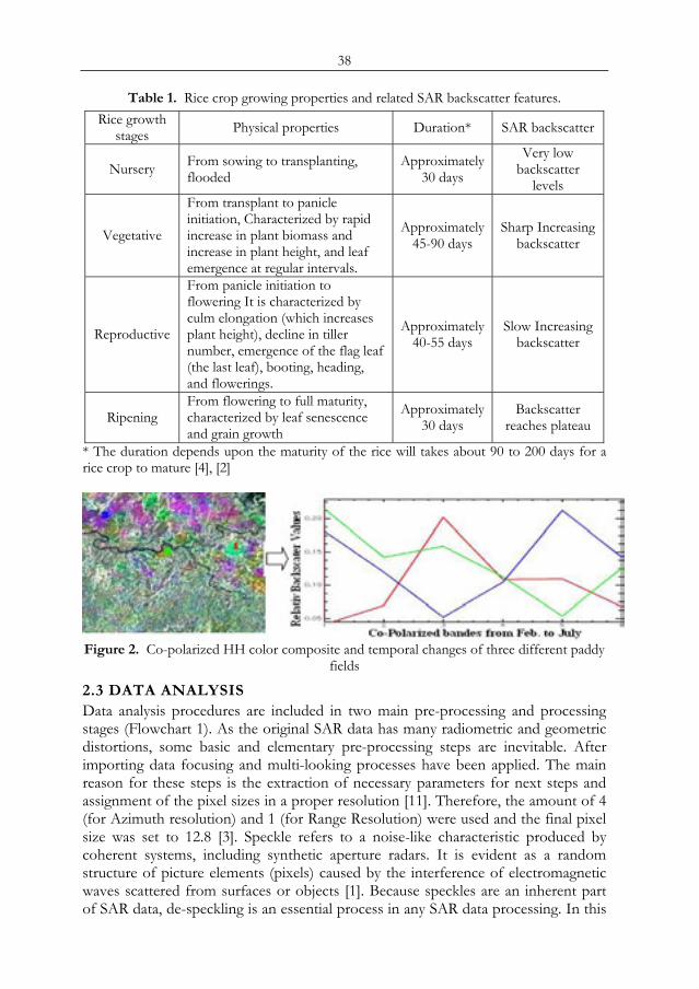
most important parameters which have been evaluated in relation to SAR application in rice crop mapping and monitoring can be categorized in two groups: rice crop parameters (temporal changes, phenology, biomass, rice height, water content etc) and SAR parameters (backscatter coefficient, polarization, incidence angle, etc) [6], [8], [9]. The main hypothesis of this work is based on the use of temporal changes of rice crops, variations in backscatter coefficients and diverse polarization parameters of multi-temporal SAR imagery. The rice growth phases can be split up into three stages: the vegetative of approximately 45 days, the reproductive stage of approximately 55 days and the ripening phase (approximately 45 days). Therefore, the rice growth duration depends upon the maturity of the rice being produced .Generally; it will take about 90 to 200 days for a rice crop to mature [4], [7] (Table 1).
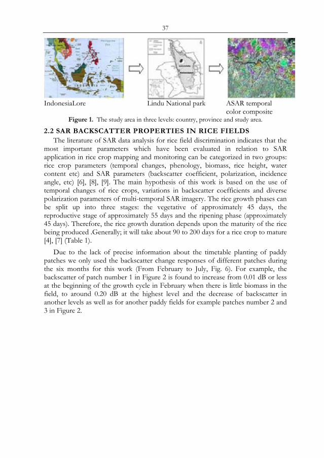
Due to the lack of precise information about the timetable planting of paddy patches we only used the backscatter change responses of different patches during the six months for this work (From February to July, Fig. 6). For example, the backscatter of patch number 1 in Figure 2 is found to increase from 0.01 dB or less at the beginning of the growth cycle in February when there is little biomass in the field, to around 0.20 dB at the highest level and the decrease of backscatter in another levels as well as for another paddy fields for example patches number 2 and 3 in Figure 2.
38
Table 1. Rice crop growing properties and related SAR backscatter features. Rice growth
stages Physical properties Duration* SAR backscatter
Nursery From sowing to transplanting, flooded
Approximately 30 days
Very low backscatter
levels
Vegetative
From transplant to panicle initiation, Characterized by rapid increase in plant biomass and increase in plant height, and leaf emergence at regular intervals.
Approximately 45-90 days
Sharp Increasing backscatter
Reproductive
From panicle initiation to flowering It is characterized by culm elongation (which increases plant height), decline in tiller number, emergence of the flag leaf (the last leaf), booting, heading, and flowerings.
Approximately 40-55 days
Slow Increasing backscatter
Ripening From flowering to full maturity, characterized by leaf senescence and grain growth
Approximately 30 days
Backscatter reaches plateau
* The duration depends upon the maturity of the rice will takes about 90 to 200 days for a rice crop to mature [4], [2]
Figure 2. Co-polarized HH color composite and temporal changes of three different paddy
fields
2.3 DATA ANALYSIS Data analysis procedures are included in two main pre-processing and processing stages (Flowchart 1). As the original SAR data has many radiometric and geometric distortions, some basic and elementary pre-processing steps are inevitable. After importing data focusing and multi-looking processes have been applied. The main reason for these steps is the extraction of necessary parameters for next steps and assignment of the pixel sizes in a proper resolution [11]. Therefore, the amount of 4 (for Azimuth resolution) and 1 (for Range Resolution) were used and the final pixel size was set to 12.8 [3]. Speckle refers to a noise-like characteristic produced by coherent systems, including synthetic aperture radars. It is evident as a random structure of picture elements (pixels) caused by the interference of electromagnetic waves scattered from surfaces or objects [1]. Because speckles are an inherent part of SAR data, de-speckling is an essential process in any SAR data processing. In this
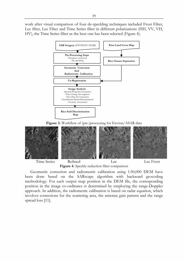
39
work after visual comparison of four de-speckling techniques included Frost Filter, Lee filter, Lee Filter and Time Series filter in different polarizations (HH, VV, VH, HV), the Time Series filter as the best one has been selected (Figure 4).
Figure 3. Workflow of (pre-)processing for Envisat/ASAR data
Time Series Refined Lee Lee Frost
Figure 4. Speckle reduction filter comparison Geometric correction and radiometric calibration using 1:50,000 DEM have
been done based on the SARscape algorithm with backward geocoding methodology. For each output map position in the DEM file, the corresponding position in the image co-ordinates is determined by employing the range-Doppler approach. In addition, the radiometric calibration is based on radar equation, which involves corrections for the scattering area, the antenna gain pattern and the range spread loss [11].
SAR Imagery (ENVISAT/ASAR) Prior Land Cover Map
Per-Processing Steps- Parameter extraction
- De-speckling
Geometric Correction And
Radiometric Calibration
Rice Classes Separation
Rice field Discrimination Map
Co-Registration
Image Analysis- Spectral Properties Extraction
- Time Change Investigation - New Data Set Extraction
- Classification-Based Discrimination - Accuracy Assessment
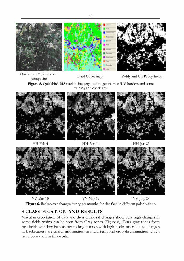
40
Quickbird/MS true color
composite Land Cover map Paddy and Un-Paddy fields
Figure 5. Quickbird/MS satellite imagery used to get the rice field borders and some training and check area
HH-Feb 4 HH-Apr 14 HH-Jun 23
VV-Mar 10 VV-May 19 VV-July 28
Figure 6. Backscatter changes during six months for rice field in different polarizations.
3 CLASSIFICATION AND RESULTS Visual interpretation of data and their temporal changes show very high changes in some fields which can be seen from Gray tones (Figure 6): Dark gray tones from rice fields with low backscatter to bright tones with high backscatter. These changes in backscatters are useful information in multi-temporal crop discrimination which have been used in this work.
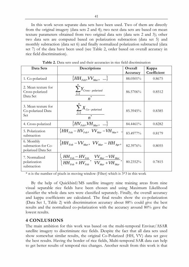
41
In this work seven separate data sets have been used. Two of them are directly from the original imagery (data sets 2 and 4); two next data sets are based on mean texture parameters obtained from two original data sets (data sets 2 and 3); other two data sets are computed based on polarization subtraction (data set 5) and monthly subtraction (data set 6) and finally normalized polarization subtracted (data set 7) of the data have been used (see Table 2, order based on overall accuracy in rice field discrimination).
Table 2. Data sets used and their accuracies in rice field discrimination Data Sets Descriptions Overall
Accuracy Kappa Coefficient
1. Co-polarized ...,, MarFeb VVHH 88.0501% 0.8675
2. Mean texture for Cross-polarized Data Set *
1
n
Yn
ipolarisedCross∑
=−
86.5706% 0.8512
3. Mean texture for Co-polarized Data Set *
1
n
Xn
ipolarisedCo∑
=−
85.3945% 0.8385
4. Cross-polarized ...,, MarFeb VHHV 84.4461% 0.8282
5. Polarization subtraction
..,, MarMarFebFeb VHVVHVHH −−
83.4977% 0.8179
6. Monthly subtraction for Co-polarized Data Set
,, AprMarMarFeb HHVVVVHH −−
82.3976% 0.8055
7. Normalized polarization subtraction ⎩
⎨⎧
+−
+− ,,
MarMar
MarMar
FebFeb
FebFeb
VHVVVHVV
HVHHHVHH
80.2352% 0.7815
* n is the number of pixels in moving window (Filter) which is 3*3 in this work
By the help of Quickbird/MS satellite imagery nine training areas from nine visual separable rice fields have been chosen and using Maximum Likelihood classifier the whole data sets were classified separately. Finally, the overall accuracy and kappa coefficients are calculated. The final results show the co-polarization (Data Set 1, Table 2) with discrimination accuracy about 88% could give the best results and the normalized co-polarization with the accuracy around 80% gave the lowest results.
4 CONLUSIONS The main ambition for this work was based on the multi-temporal Envisat/ASAR satellite imagery to discriminate rice fields. Despite the fact that all data sets used show somewhat similar results, the original Co-Polarized (HH, VV) data set gave the best results. Having the border of rice fields, Multi-temporal SAR data can help to get better results of temporal rice changes. Another result from this work is that
42
texture derivatives of polarized SAR data do not significantly improve the results for the discrimination of rice fields from other crops.
Multi-temporal SAR observations are able to characterize the phenological development of rice crops but for enhanced detection of growth stages and thus better mapping and monitoring of cropping systems, a higher temporal resolution would be desirable.
REFERENCES 1. ASAR Product Handbook, 2006, European Space Agency (ESA),
http://envisat.esa.int/handbooks/asar 2. C. Brouwer, K. Prins, M. Heibloem, 1989, Irrigation Water Management: Irrigation
Scheduling, Training manual no. 4. , FAO, http://www.fao.org. 3. Herrmann, David, 2006, Kartierung tropischer Kulturpflanzen und deren
Veränderung mit Hilfe multitemporaler und multipolarametrischer SAR-Satellitendaten (ENVISAT/ASAR) in Zentral-Sulawesi, Indonesien, Msc. thesis, Goettingen University.
4. International Rice Research Institute (IRRI), 2000, http://www.cgiar.org/irri/Riceweb/. 5. Kurosu, T. Fujita, M. and Chiba, K., 1997, The identification of rice fields using
multi-temporal ERS-1 C band SAR data, INT. J. REMOTE SENSING, vol. 18, no. 14, 2953± 2965.
6. Li, Y., Liao, Q., Li, X. Liao, S., CHI, G. and Peng, S., 2003, Towards an operational system for regional-scale rice yield estimation using a time-series of Radarsat ScanSAR images, INT. J. REMOTE SENSING, VOL. 24, NO. 21, 4207–4220.
7. Minas K., Frank J. Dent, Edward M. Herath, 2000, Bridging the rice yield gap in the Asia-Pacific region, FAO, http://www.fao.org.
8. Okomoto, K., Kawashima, H., 1999, Estimation of rice-planted area in the tropical zone using a combination of optical and microwave satellite sensor data, INT. J. REMOTE SENSING, vol. 20, no. 5, 1045± 1048.
9. Ribbes, F. and Le Toan T., 1999, Rice field mapping and monitoring with RADARSAT data, INT. J. REMOTE SENSING, vol. 20, no. 4, 745± 765.
10. Rohwer, Nina-Kathrin, 2006, Object oriented image analysis of high resolution satellite imagery: a land cover change analysis in the Palolo Valley, Central Sulawesi, Indonesia, based on Quickbird and IKONOS satellite data, Msc. thesis, Goettingen University.
11. SARscape User Guide, 2006, Sarmap homepages, http://www.sarmap.ch/SARscape_flyer.pdf.
43
UNCERTAINTIES IN THE CALCULATION OF SOIL HEAT FLUX AND SENSIBLE HEAT FLUX IN
SEBAL
M. R. Mobasheri Remote Sensing Department, Faculty of Geodesy and Geomatics, K. N. Toosi
University of Technology, Tehran, Iran, email: [email protected]
ABSTRACT Evapo-Transpiration (ET) is one of5 the most important components of the water balance, but also one of the most difficult to measure in time and space. Field techniques such as soil water balances and Bowen ratio or eddy covariance techniques are local ranging from point to field scale. The Surface Energy Balance Algorithm for Land (SEBAL) consists of 25 models that calculate ET and other energy balance components at the earth’s surface. SEBAL uses satellite image data in the visible, near-infrared, and thermal bands for the prediction of all energy components at each pixel in an image. The objective of this work was to assess validity of the applied model used for estimating soil heat flux and sensible heat flux by in situ measurements in the field while a satellite overpasses simultaneously the area. It is found that at the time of satellite overpass the sign of these two energy components was negative, i. e. more energy will be provided for ET. A comprehensive field work to validate SEBAL for the South-West of Iran was carried out. The LandSat 7ETM+ satellite images provided the instantaneous ET (ET_inst) at a resolution of 30m. These values showed more fluctuation with the suggested corrections. The assumption of taking cold pixel temperature equal to air temperature is not always a good idea and the time of satellite overpass should be taken as a critical factor for validity of this assumption. It is believed that more credit should be given to the soil temperature, air temperature and other atmospheric parameters in this model.
1 INTRODUCTION The SEBAL procedure consists of a series of algorithms that combine to solve the energy balance equation:
λET = Rn – G – H (1)
where λET is latent heat flux (the energy used to evaporate water), Rn is net radiation at the surface, G is soil heat flux, and H is sensible heat flux to the air. Other minor terms, such as energy absorbed by photosynthesis or advected horizontally, are relatively very small in value, and are ignored.
Each of the components on the right hand side of this equation will be calculated for each pixel. Rn is the sum of all incoming and outgoing short and long-wave energy components. Soil heat flux G is usually predicted using vegetation Proc. 2nd Göttingen GIS and Remote Sensing Days, 4-6 Oct. 2006, Göttingen
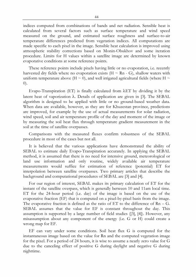
44
indices computed from combinations of bands and net radiation. Sensible heat is calculated from several factors such as surface temperature and wind speed measured on the ground, and estimated surface roughness and surface-to-air temperature differences predicted from vegetation indices. All computations are made specific to each pixel in the image. Sensible heat calculation is improved using atmospheric stability corrections based on Monin-Obukhov and some iteration procedure. Limits for H values within a satellite image are determined by known evaporative conditions at some reference points.
These reference points include pixels having little or no evaporation, i.e. recently harvested dry fields where no evaporation exists (H ~ Rn - G), shallow waters with uniform temperature above (H ~ 0), and well irrigated agricultural fields (where H ~ 0).
Evapo-Transpiration (ET) is finally calculated from λET by dividing it by the latent heat of vaporization λ. Details of application are given in [3]. The SEBAL algorithm is designed to be applied with little or no ground-based weather data. When data are available, however, as they are for Khuzestan province, predictions are improved, for example by the use of actual measurements for solar radiation, wind speed, soil and air temperature profile of the day and moment of the image or by measuring the soil heat flux through temperature gradient measurement in the soil at the time of satellite overpasses.
Comparisons with the measured fluxes confirm robustness of the SEBAL procedure in most of the cases but not all.
It is believed that the various applications have demonstrated the ability of SEBAL to estimate daily Evapo-Transpiration accurately. In applying the SEBAL method, it is assumed that there is no need for intensive ground, meteorological or land use information and only routine, widely available air temperature measurements would suffice for estimation of reference (potential) ET for interpolation between satellite overpasses. Two primary articles that describe the background and computational procedures of SEBAL are [3] and [4].
For our region of interest, SEBAL makes its primary calculation of ET for the instant of the satellite overpass, which is generally between 10 and 11am local time. ET for the 24-hour period (i.e. day) of the image is based on the use of the evaporative fraction (EF) that is computed on a pixel-by-pixel basis from the image. The evaporative fraction is defined as the ratio of ET to the difference of Rn – G. SEBAL assumes that the value for EF is constant throughout the day. This assumption is supported by a large number of field studies ([3], [4]). However, any misassumption about any component of the energy (i.e. G or H) could create a wrong map for EF.
EF can vary under some conditions. Soil heat flux G is computed for the instantaneous image based on the value for Rn and the computed vegetation image for the pixel. For a period of 24 hours, it is wise to assume a nearly zero value for G due to the canceling effect of positive G during daylight and negative G during nighttime.
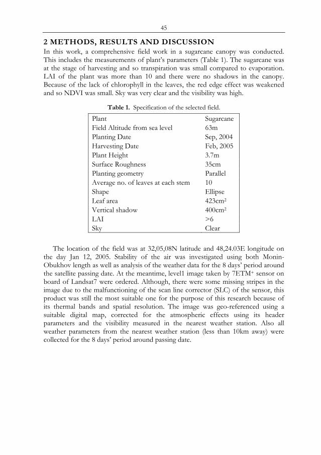
45
2 METHODS, RESULTS AND DISCUSSION In this work, a comprehensive field work in a sugarcane canopy was conducted. This includes the measurements of plant’s parameters (Table 1). The sugarcane was at the stage of harvesting and so transpiration was small compared to evaporation. LAI of the plant was more than 10 and there were no shadows in the canopy. Because of the lack of chlorophyll in the leaves, the red edge effect was weakened and so NDVI was small. Sky was very clear and the visibility was high.
Table 1. Specification of the selected field.
Plant Sugarcane Field Altitude from sea level 63m Planting Date Sep, 2004 Harvesting Date Feb, 2005 Plant Height 3.7m Surface Roughness 35cm Planting geometry Parallel Average no. of leaves at each stem 10 Shape Ellipse Leaf area 423cm2 Vertical shadow 400cm2 LAI >6 Sky Clear
The location of the field was at 32,05,08N latitude and 48,24.03E longitude on
the day Jan 12, 2005. Stability of the air was investigated using both Monin-Obukhov length as well as analysis of the weather data for the 8 days’ period around the satellite passing date. At the meantime, level1 image taken by 7ETM+ sensor on board of Landsat7 were ordered. Although, there were some missing stripes in the image due to the malfunctioning of the scan line corrector (SLC) of the sensor, this product was still the most suitable one for the purpose of this research because of its thermal bands and spatial resolution. The image was geo-referenced using a suitable digital map, corrected for the atmospheric effects using its header parameters and the visibility measured in the nearest weather station. Also all weather parameters from the nearest weather station (less than 10km away) were collected for the 8 days’ period around passing date.
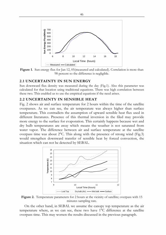
46
0100200300400500600700
6 8 10 12 14 16 18
Local Time (hours)
Sun
Ener
gy F
lux(
W/m
2)
Measured Calculated Figure 1. Sun energy flux for Jan 12, 05(measured and calculated). Correlation is more than
98 percent so the difference is negligible.
2.1 UNCERTAINTY IN SUN ENERGY Sun downward flux density was measured during the day (Fig.1). Also this parameter was calculated for that location using traditional equations. There was high correlation between these two. This enabled us to use the empirical equations if the need arises.
2.2 UNCERTAINTY IN SENSIBLE HEAT Fig. 2 shows air and surface temperature for 2 hours within the time of the satellite overpasses. As we can see, the air temperature was always higher than surface temperature. This contradicts the assumption of upward sensible heat flux used in different literatures. Presence of this thermal inversion in the filed may provide more energy to the surface for evaporation. This certainly happens because wet and dry bulb temperatures are away which means the weather is not saturated from water vapor. The difference between air and surface temperature at the satellite overpass time was about 2°C. This along with the presence of strong wind (Fig.3) would strengthen downward transfer of sensible heat by forced convection, the situation which can not be detected by SEBAL.
7
8
9
10
11
12
13
14
15
16
9 10 11 12Local Time (hours)
Tem
pera
ture
(C)
Leaf Top Dry bulb (Air) Wet bulb Surface
Figure 2. Temperature parameters for 2 hours at the vicinity of satellite; overpass with 15 minutes sampling rate.
On the other hand, in SEBAL we assume the canopy top temperature as the air temperature where, as we can see, these two have 1°C difference at the satellite overpass time. This may worsen the results discussed in the previous paragraph.
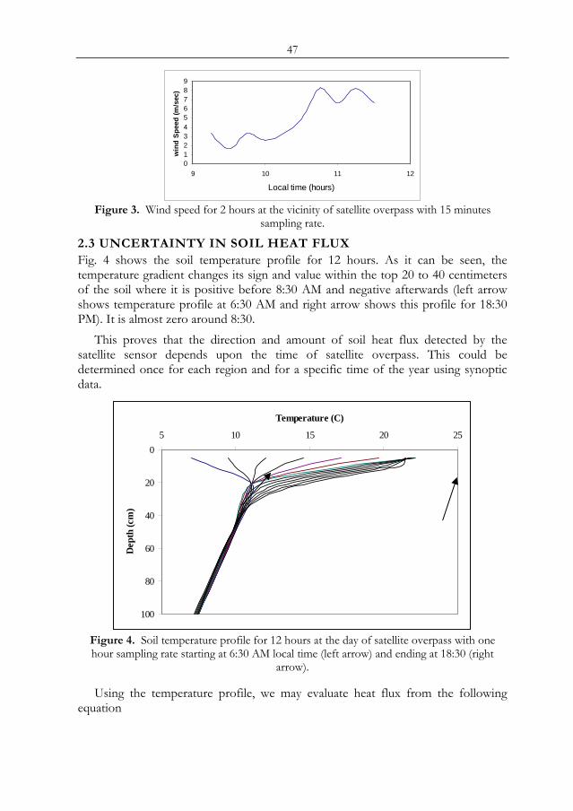
47
0123456789
9 10 11 12
Local time (hours) w
ind
Spee
d (m
/sec
)
Figure 3. Wind speed for 2 hours at the vicinity of satellite overpass with 15 minutes
sampling rate.
2.3 UNCERTAINTY IN SOIL HEAT FLUX Fig. 4 shows the soil temperature profile for 12 hours. As it can be seen, the temperature gradient changes its sign and value within the top 20 to 40 centimeters of the soil where it is positive before 8:30 AM and negative afterwards (left arrow shows temperature profile at 6:30 AM and right arrow shows this profile for 18:30 PM). It is almost zero around 8:30.
This proves that the direction and amount of soil heat flux detected by the satellite sensor depends upon the time of satellite overpass. This could be determined once for each region and for a specific time of the year using synoptic data.
0
20
40
60
80
100
5 10 15 20 25
Temperature (C)
Dep
th (c
m)
Figure 4. Soil temperature profile for 12 hours at the day of satellite overpass with one hour sampling rate starting at 6:30 AM local time (left arrow) and ending at 18:30 (right
arrow).
Using the temperature profile, we may evaluate heat flux from the following equation

48
dzdTkG −=
(2) where, k is the thermal conductivity of the soil and z is taken positive downward. For a fixed soil material, G depends on the temperature gradient which is a function of the climatic situation. The sign of G for our work was positive since the satellite passing time was around 10 to 10:30.
In SEBAL, G is the heat flux penetrating the surface. For the most part, G is the soil heat flux, since SEBAL is normally applied to land surfaces. However, lakes are part of the landscape, and water evaporates from their surface. Because the energy-balance dynamics of water bodies and soil are different, G needs to be treated differently for lakes than for soil. For soil surfaces, SEBAL assumes essentially no 24-hour heat carry-over for soil. Some portion of net radiation is stored in the soil as heat during the day, and that stored heat is then redirected during the night, resulting in a positive G during the day and a negative G at night.
Thus, SEBAL approximates the 24-hour G as zero for a land surface, although the instantaneous G at the time of image is not only zero but could be either positive or negative.
The problem with using zero as the 24-hour G-value for a deep, clear lake such as deeper part of Hoorol-azim and calmer portion of Karoon River is that solar energy is absorbed by the water column and stored and so the 24-hour G cannot be assumed to be zero. This is also approved by [1].
In equation (1), net radiation is the net radiant energy that the land surface actually receives and loses from or to the atmosphere. Usually Rn is positive during the day and negative at night. Some of the net energy is used to evaporate soil water, some energy is used to heat the air, and the rest of the net energy is stored in the ground (or a water body).
However, equation (2) cannot be applied to SEBAL because we do not usually know temperature profile within the soil. Therefore, for our work in Khuzestan the following empirical equation was used to estimate G [5]:
G/Rn=a*NDVI+b (3)
with a=-0.11 and b=0.15. This equation was a fit to the curve of G/Rn with respect to NDVI for different values of NDVI selected from the NDVI Image. Equation (3) gives a 0.04Rn value for G for the full cover canopy and a value of 0.15Rn for the bare soil as in agreement with the work of [2]. To compare the results of applying equation (3) and SEBAL model, Fig. 5 shows the image produced by these methods. As we can see Fig. 5b shows values for G almost twice as large as those in Fig. 5a calculated from equation (3) and SEBAL, respectively.
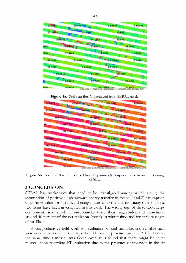
49
Figure 5a. Soil heat flux G produced from SEBAL model
Figure 5b. Soil heat flux G produced from Equation (3). Stripes are due to malfunctioning
of SLC.
3 CONCLUSION SEBAL has weaknesses that need to be investigated among which are 1) the assumption of positive G (downward energy transfer to the soil) and 2) assumption of positive value for H (upward energy transfer to the air) and many others. These two items have been investigated in this work. The wrong sign of these two energy components may result in uncertainties twice their magnitudes and sometimes around 40 percent of the net radiation (mostly in winter time and for early passages of satellite).
A comprehensive field work for evaluation of soil heat flux and sensible heat were conducted in the northern part of Khuzestan province on Jan 12, 05 where at the same time Landsat7 was flown over. It is found that there might be sever misevaluation regarding ET evaluation due to the presence of inversion in the air
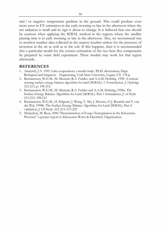
50
and / or negative temperature gradient in the ground. This could produce even more error in ET estimation in the early morning or late in the afternoon where the net radiation is small and its sign is about to change. It is believed that one should be cautious when applying the SEBAL method in the regions where the satellite passing time is in early morning or late in the afternoon. Also, we recommend one to monitor weather data collected in the nearest weather station for the presence of inversion in the air as well as in the soil. If this happens, then it is recommended that a particular model for the correct estimation of the two heat flux components be prepared by some field experiment. These models may work for that region afterwards.
REFERENCES 1. Amayreh, J.A. 1995. Lake evaporation: a model study. Ph.D. dissertation, Dept.
Biological and Irrigation Engineering, Utah State University, Logan, UT. 178 p. 2. Bastiaanssen, W.G.M., M. Menenti, R.A. Feddes, and A.A.M. Holtslag. 1998. A remote
sensing surface energy balance algorithm for land (SEBAL): 1. Formulation. J. Hydrology 212-213, p. 198-212.
3. Bastiaanssen, W.G.M., M. Menenti, R.A. Feddes and A.A.M. Holtslag, 1998a. The Surface Energy Balance Algorithm for Land (SEBAL): Part 1 formulation, J. of Hydr. 212-213: 198-212
4. Bastiaanssen, W.G.M., H. Pelgrum, J. Wang, Y. Ma, J. Moreno, G.J. Roerink and T. van der Wal, 1998b. The Surface Energy Balance Algorithm for Land (SEBAL): Part 2 validation, J. Of Hydr. 212-213: 213-229
5. Mobasheri, M. Reza, 2006.”Determination of Evapo-Transpiration in the Khuzestan Province” a project report to Khuzestan Water & Electricity Organization.
51
Kartografer - a tool for supporting The management of forest landscape linking GIS and AN individual tree
growth simulator
P. Surovýa, M. Fabrikaa, M. Daennerb, R. Schulzb, D. Lanwertb, B. Slobodab
a Department of Forest Management and Geodesy, Technical University in Zvolen, Slovak Republic, email: [email protected]
bInstitute of Forest Biometrics and Applied Computer Science, University of Goettingen
ABSTRACT The possibility of incorporating the indi6vidual tree growth simulator SIBYLA into GIS environment is demonstrated in this work. Two outputs of spatial information are provided by simulation: a productive one, wood production, and a non-productive one, biodiversity, are shown. Two scenarios were used for this study. Scenario one is a simulation of a whole non managed forest district where the production of wood, its dynamics and dynamics of other factors like biodiversity etc. can be observed. In the second scenario, a management concept for thinning was set. The concept is based on a target diameter where all trees above this diameter are removed in a 5 year interval. Different tree species have different target diameters. The same characteristics are evaluated and compared to the “non-managed” scenario. The simulation results are stored in a central map server where they can be queried for different data structures. The methodology of this data sharing technique through Deegree WMS is described.
1 INTRODUCTION Decisions can have a big influence on work productivity and final income during harvest. Therefore decision support is essential for proper management and efficiency of all parts of this process. Individual tree growth simulator SIBYLA reflects different climate and environment conditions. It is based on potential growth, modelled by curve, where the predicted value of growth for individual tree is always modified by a modifier. The potential curve depends on stand conditions: soil, climate, rain, etc… The modifier depends mostly on competition status of subject tree [11]. More trees in its neighbourhood and bigger these are, more the potential growth will be diminished.
SIBYLA can predict production under different management regimes like thinning interval, power of thinning, kind of thinning etc [10]. It means that user can set his management preferences and in real time see the results of prognosis; verify impact of his decision on production and also on other incomes of forest stand like biodiversity. The simulation for individual stand is quite quickly executed (in minutes) and results do not require a lot of disk space for storage. However, in forest practices, it is sometimes more useful to work with larger units than the forest Proc. 2nd Göttingen GIS and Remote Sensing Days, 4-6 Oct. 2006, Göttingen
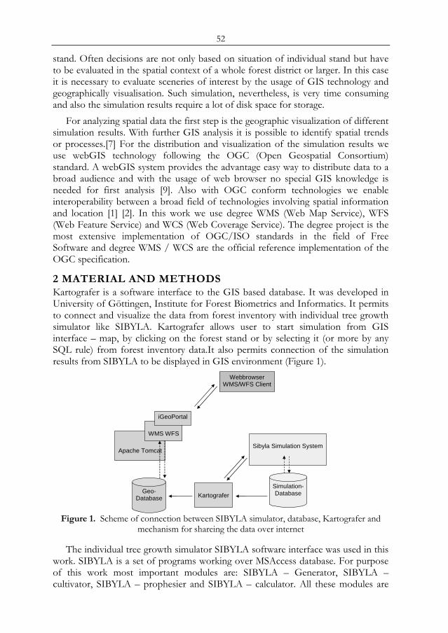
52
stand. Often decisions are not only based on situation of individual stand but have to be evaluated in the spatial context of a whole forest district or larger. In this case it is necessary to evaluate sceneries of interest by the usage of GIS technology and geographically visualisation. Such simulation, nevertheless, is very time consuming and also the simulation results require a lot of disk space for storage.
For analyzing spatial data the first step is the geographic visualization of different simulation results. With further GIS analysis it is possible to identify spatial trends or processes.[7] For the distribution and visualization of the simulation results we use webGIS technology following the OGC (Open Geospatial Consortium) standard. A webGIS system provides the advantage easy way to distribute data to a broad audience and with the usage of web browser no special GIS knowledge is needed for first analysis [9]. Also with OGC conform technologies we enable interoperability between a broad field of technologies involving spatial information and location [1] [2]. In this work we use degree WMS (Web Map Service), WFS (Web Feature Service) and WCS (Web Coverage Service). The degree project is the most extensive implementation of OGC/ISO standards in the field of Free Software and degree WMS / WCS are the official reference implementation of the OGC specification.
2 MATERIAL AND METHODS Kartografer is a software interface to the GIS based database. It was developed in University of Göttingen, Institute for Forest Biometrics and Informatics. It permits to connect and visualize the data from forest inventory with individual tree growth simulator like SIBYLA. Kartografer allows user to start simulation from GIS interface – map, by clicking on the forest stand or by selecting it (or more by any SQL rule) from forest inventory data.It also permits connection of the simulation results from SIBYLA to be displayed in GIS environment (Figure 1).
Sibyla Simulation System
Simulation-Database Geo-
Database
Apache Tomcat
WMS WFS
iGeoPortal
Kartografer
Webbrowser WMS/WFS Client
Figure 1. Scheme of connection between SIBYLA simulator, database, Kartografer and
mechanism for shareing the data over internet
The individual tree growth simulator SIBYLA software interface was used in this work. SIBYLA is a set of programs working over MSAccess database. For purpose of this work most important modules are: SIBYLA – Generator, SIBYLA – cultivator, SIBYLA – prophesier and SIBYLA – calculator. All these modules are
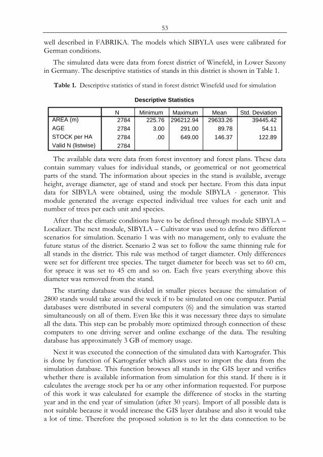
53
well described in FABRIKA. The models which SIBYLA uses were calibrated for German conditions.
The simulated data were data from forest district of Winefeld, in Lower Saxony in Germany. The descriptive statistics of stands in this district is shown in Table 1.
Table 1. Descriptive statistics of stand in forest district Winefeld used for simulation
Descriptive Statistics
2784 225.76 296212.94 29633.26 39445.422784 3.00 291.00 89.78 54.112784 .00 649.00 146.37 122.892784
AREA (m)AGESTOCK per HAValid N (listwise)
N Minimum Maximum Mean Std. Deviation
The available data were data from forest inventory and forest plans. These data
contain summary values for individual stands, or geometrical or not geometrical parts of the stand. The information about species in the stand is available, average height, average diameter, age of stand and stock per hectare. From this data input data for SIBYLA were obtained, using the module SIBYLA - generator. This module generated the average expected individual tree values for each unit and number of trees per each unit and species.
After that the climatic conditions have to be defined through module SIBYLA – Localizer. The next module, SIBYLA – Cultivator was used to define two different scenarios for simulation. Scenario 1 was with no management, only to evaluate the future status of the district. Scenario 2 was set to follow the same thinning rule for all stands in the district. This rule was method of target diameter. Only differences were set for different tree species. The target diameter for beech was set to 60 cm, for spruce it was set to 45 cm and so on. Each five years everything above this diameter was removed from the stand.
The starting database was divided in smaller pieces because the simulation of 2800 stands would take around the week if to be simulated on one computer. Partial databases were distributed in several computers (6) and the simulation was started simultaneously on all of them. Even like this it was necessary three days to simulate all the data. This step can be probably more optimized through connection of these computers to one driving server and online exchange of the data. The resulting database has approximately 3 GB of memory usage.
Next it was executed the connection of the simulated data with Kartografer. This is done by function of Kartografer which allows user to import the data from the simulation database. This function browses all stands in the GIS layer and verifies whether there is available information from simulation for this stand. If there is it calculates the average stock per ha or any other information requested. For purpose of this work it was calculated for example the difference of stocks in the starting year and in the end year of simulation (after 30 years). Import of all possible data is not suitable because it would increase the GIS layer database and also it would take a lot of time. Therefore the proposed solution is to let the data connection to be
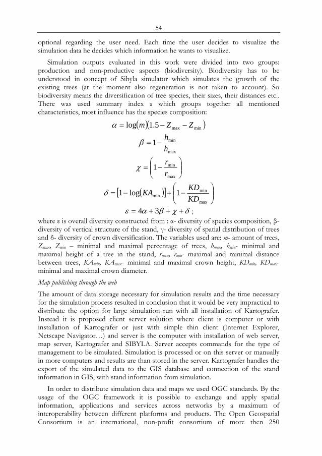
54
optional regarding the user need. Each time the user decides to visualize the simulation data he decides which information he wants to visualize.
Simulation outputs evaluated in this work were divided into two groups: production and non-productive aspects (biodiversity). Biodiversity has to be understood in concept of Sibyla simulator which simulates the growth of the existing trees (at the moment also regeneration is not taken to account). So biodiversity means the diversification of tree species, their sizes, their distances etc.. There was used summary index ε which groups together all mentioned characteristics, most influence has the species composition:
( )( )minmax5.1log ZZm −−=α
max
min1hh
−=β
⎟⎟⎠
⎞⎜⎜⎝
⎛−=
max
min1rr
χ
( )[ ] ⎟⎟⎠
⎞⎜⎜⎝
⎛−+−=
max
minmin 1log1
KDKD
KAδ
δχβαε +++= 34 ; where ε is overall diversity constructed from : α- diversity of species composition, β- diversity of vertical structure of the stand, γ- diversity of spatial distribution of trees and δ- diversity of crown diversification. The variables used are: m- amount of trees, Zmax, Zmin – minimal and maximal percentage of trees, hmax, hmin- minimal and maximal height of a tree in the stand, rmax, rmin- maximal and minimal distance between trees, KAmin, KAmax- minimal and maximal crown height, KDmin, KDmax- minimal and maximal crown diameter. Map publishing through the web The amount of data storage necessary for simulation results and the time necessary for the simulation process resulted in conclusion that it would be very impractical to distribute the option for large simulation run with all installation of Kartografer. Instead it is proposed client server solution where client is computer or with installation of Kartografer or just with simple thin client (Internet Explorer, Netscape Navigator…) and server is the computer with installation of web server, map server, Kartografer and SIBYLA. Server accepts commands for the type of management to be simulated. Simulation is processed or on this server or manually in more computers and results are than stored in the server. Kartografer handles the export of the simulated data to the GIS database and connection of the stand information in GIS, with stand information from simulation.
In order to distribute simulation data and maps we used OGC standards. By the usage of the OGC framework it is possible to exchange and apply spatial information, applications and services across networks by a maximum of interoperability between different platforms and products. The Open Geospatial Consortium is an international, non-profit consortium of more then 250
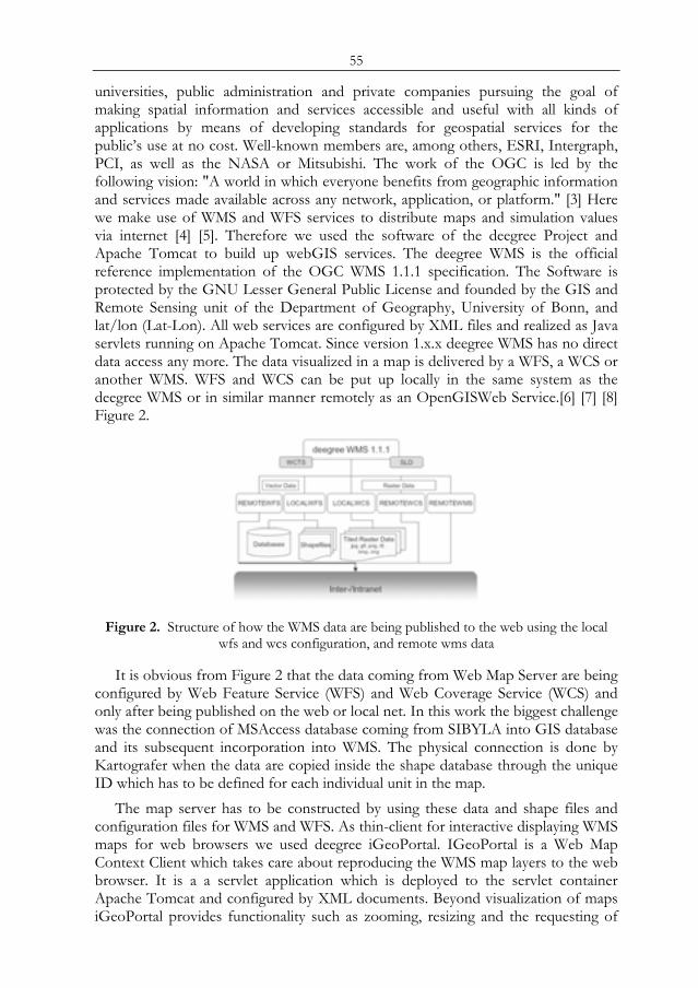
55
universities, public administration and private companies pursuing the goal of making spatial information and services accessible and useful with all kinds of applications by means of developing standards for geospatial services for the public’s use at no cost. Well-known members are, among others, ESRI, Intergraph, PCI, as well as the NASA or Mitsubishi. The work of the OGC is led by the following vision: "A world in which everyone benefits from geographic information and services made available across any network, application, or platform." [3] Here we make use of WMS and WFS services to distribute maps and simulation values via internet [4] [5]. Therefore we used the software of the deegree Project and Apache Tomcat to build up webGIS services. The deegree WMS is the official reference implementation of the OGC WMS 1.1.1 specification. The Software is protected by the GNU Lesser General Public License and founded by the GIS and Remote Sensing unit of the Department of Geography, University of Bonn, and lat/lon (Lat-Lon). All web services are configured by XML files and realized as Java servlets running on Apache Tomcat. Since version 1.x.x deegree WMS has no direct data access any more. The data visualized in a map is delivered by a WFS, a WCS or another WMS. WFS and WCS can be put up locally in the same system as the deegree WMS or in similar manner remotely as an OpenGISWeb Service.[6] [7] [8] Figure 2.
Figure 2. Structure of how the WMS data are being published to the web using the local
wfs and wcs configuration, and remote wms data
It is obvious from Figure 2 that the data coming from Web Map Server are being configured by Web Feature Service (WFS) and Web Coverage Service (WCS) and only after being published on the web or local net. In this work the biggest challenge was the connection of MSAccess database coming from SIBYLA into GIS database and its subsequent incorporation into WMS. The physical connection is done by Kartografer when the data are copied inside the shape database through the unique ID which has to be defined for each individual unit in the map.
The map server has to be constructed by using these data and shape files and configuration files for WMS and WFS. As thin-client for interactive displaying WMS maps for web browsers we used deegree iGeoPortal. IGeoPortal is a Web Map Context Client which takes care about reproducing the WMS map layers to the web browser. It is a a servlet application which is deployed to the servlet container Apache Tomcat and configured by XML documents. Beyond visualization of maps iGeoPortal provides functionality such as zooming, resizing and the requesting of
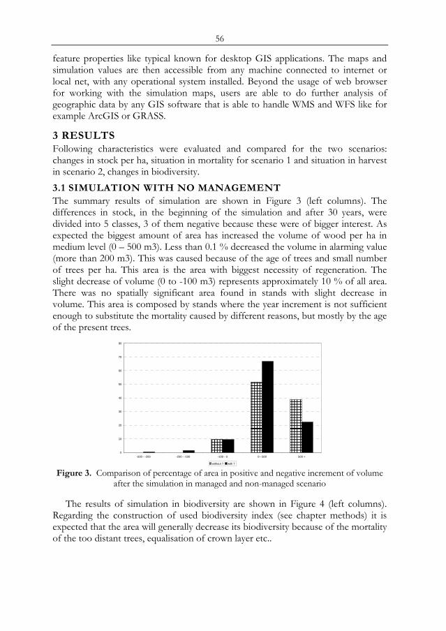
56
feature properties like typical known for desktop GIS applications. The maps and simulation values are then accessible from any machine connected to internet or local net, with any operational system installed. Beyond the usage of web browser for working with the simulation maps, users are able to do further analysis of geographic data by any GIS software that is able to handle WMS and WFS like for example ArcGIS or GRASS.
3 RESULTS Following characteristics were evaluated and compared for the two scenarios: changes in stock per ha, situation in mortality for scenario 1 and situation in harvest in scenario 2, changes in biodiversity. 3.1 SIMULATION WITH NO MANAGEMENT The summary results of simulation are shown in Figure 3 (left columns). The differences in stock, in the beginning of the simulation and after 30 years, were divided into 5 classes, 3 of them negative because these were of bigger interest. As expected the biggest amount of area has increased the volume of wood per ha in medium level (0 – 500 m3). Less than 0.1 % decreased the volume in alarming value (more than 200 m3). This was caused because of the age of trees and small number of trees per ha. This area is the area with biggest necessity of regeneration. The slight decrease of volume (0 to -100 m3) represents approximately 10 % of all area. There was no spatially significant area found in stands with slight decrease in volume. This area is composed by stands where the year increment is not sufficient enough to substitute the mortality caused by different reasons, but mostly by the age of the present trees.
0
10
20
30
40
50
60
70
80
-500 - -200 -200 - -100 -100 - 0 0 - 500 500 +
without T with T Figure 3. Comparison of percentage of area in positive and negative increment of volume
after the simulation in managed and non-managed scenario
The results of simulation in biodiversity are shown in Figure 4 (left columns). Regarding the construction of used biodiversity index (see chapter methods) it is expected that the area will generally decrease its biodiversity because of the mortality of the too distant trees, equalisation of crown layer etc..
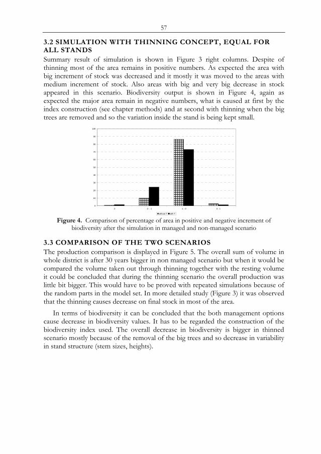
57
3.2 SIMULATION WITH THINNING CONCEPT, EQUAL FOR ALL STANDS Summary result of simulation is shown in Figure 3 right columns. Despite of thinning most of the area remains in positive numbers. As expected the area with big increment of stock was decreased and it mostly it was moved to the areas with medium increment of stock. Also areas with big and very big decrease in stock appeared in this scenario. Biodiversity output is shown in Figure 4, again as expected the major area remain in negative numbers, what is caused at first by the index construction (see chapter methods) and at second with thinning when the big trees are removed and so the variation inside the stand is being kept small.
0
10
20
30
40
50
60
70
80
90
100
-2 -2 - -1 -1 - 0 0 - 1
without T with T Figure 4. Comparison of percentage of area in positive and negative increment of
biodiversity after the simulation in managed and non-managed scenario
3.3 COMPARISON OF THE TWO SCENARIOS The production comparison is displayed in Figure 5. The overall sum of volume in whole district is after 30 years bigger in non managed scenario but when it would be compared the volume taken out through thinning together with the resting volume it could be concluded that during the thinning scenario the overall production was little bit bigger. This would have to be proved with repeated simulations because of the random parts in the model set. In more detailed study (Figure 3) it was observed that the thinning causes decrease on final stock in most of the area.
In terms of biodiversity it can be concluded that the both management options cause decrease in biodiversity values. It has to be regarded the construction of the biodiversity index used. The overall decrease in biodiversity is bigger in thinned scenario mostly because of the removal of the big trees and so decrease in variability in stand structure (stem sizes, heights).
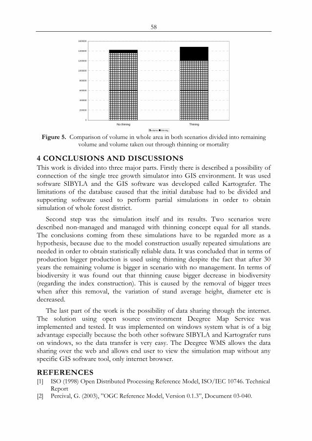
58
0
200000
400000
600000
800000
1000000
1200000
1400000
1600000
No thining Thining
volume thinning Figure 5. Comparison of volume in whole area in both scenarios divided into remaining
volume and volume taken out through thinning or mortality
4 CONCLUSIONS AND DISCUSSIONS This work is divided into three major parts. Firstly there is described a possibility of connection of the single tree growth simulator into GIS environment. It was used software SIBYLA and the GIS software was developed called Kartografer. The limitations of the database caused that the initial database had to be divided and supporting software used to perform partial simulations in order to obtain simulation of whole forest district.
Second step was the simulation itself and its results. Two scenarios were described non-managed and managed with thinning concept equal for all stands. The conclusions coming from these simulations have to be regarded more as a hypothesis, because due to the model construction usually repeated simulations are needed in order to obtain statistically reliable data. It was concluded that in terms of production bigger production is used using thinning despite the fact that after 30 years the remaining volume is bigger in scenario with no management. In terms of biodiversity it was found out that thinning cause bigger decrease in biodiversity (regarding the index construction). This is caused by the removal of bigger trees when after this removal, the variation of stand average height, diameter etc is decreased.
The last part of the work is the possibility of data sharing through the internet. The solution using open source environment Deegree Map Service was implemented and tested. It was implemented on windows system what is of a big advantage especially because the both other software SIBYLA and Kartografer runs on windows, so the data transfer is very easy. The Deegree WMS allows the data sharing over the web and allows end user to view the simulation map without any specific GIS software tool, only internet browser.
REFERENCES [1] ISO (1998) Open Distributed Processing Reference Model, ISO/IEC 10746. Technical
Report [2] Percival, G. (2003), ”OGC Reference Model, Version 0.1.3”, Document 03-040.

59
[3] OGC (2002) OGC Vision, Mission, Goals, Values. Open GIS Consortium, Inc., Technical Report
[4] WMS 1.1.0 (2002). OpenGIS® Web Map Service Implementation Specification. OpenGIS® Publicly Available Standard
[5] WFS 1.0.0 (2005). OpenGIS® Web Feature Service Implementation Specification. OpenGIS® Publicly Available Standard.
[6] lat/lon GmbH (2006), deegree Web Map Server, documentation included in the distribution
[7] lat/lon GmbH (2006), deegree Web Feature Service, documentation included in the distribution
[8] lat/lon GmbH (2006), deegree Web Coverage Service, documentation included in the distribution
[9] Mückschel, C et al. (2004): Web-basierte Informationssysteme in interdisziplinären Umweltforschungsprojekten – am Beispiel der beiden DFG-Sonderforschungsbereiche 299 (Giesen) und 552 (Göttingen/Kassel), Zeitschrift für Agrarinformatik 3, S. 46 - 55
[10] FABRIKA, M., ĎURSKÝ, J.: Risk management of forest ecosystems by dynamic model SIBYLA. Proceedings from IUFRO conference: „Sustainable Harvest Scenarios in Forest Management“, WP 4.04.10, Tále, Slovakia, August 25-27, 2004, s. 123-136
[11] HASENAUER, H., et al. (FABRIKA, M.): Sustainable Forest Management. Growth Models for Europe. Springer Berlin Heidelberg New York, 2006, 398 s, kapitola: FABRIKA, M., ĎURSKÝ, J.: Implementing Tree Growth Models in Slovakia, s.315-341.

60
61
Implementation of GIS and model Sybila in a Spatial Decision Support System for Forest Management
M. Fabrika Technical University in Zvolen, Faculty of Forestry, Slovakia, email:
ABSTRACT The paper deals with a proposal for a spatial decision support system for optimizing management strategies of forest treatments. A geographic inf7ormation system and the growth model SIBYLA are utilized for the above mentioned purposes.The model SIBYLA is an individual tree growth model developed in Slovakia. The model allows to generate the forest structure from forest inventory data, specify climatic and soil data, select a wide range of thinning concepts, execute growth prognoses, calculate stand output for production, ecology and economy, visualize output and analyze data in time series.The model SIBYLA is integrated into a GIS based information system called SIBYLA Cartographer. The system is connected to forest inventory data, forest spatial data (shape files) and other data sources (digital terrain model and satellite images). The system is prepared for being implemented in a spatial decision support system (SDSS). Connection is realized by a sub-model for decision-support called SIBYLA Analyst. A sub-model for the decision support system called SIBYLA Analyst is integrated directly into the SIBYLA model. The sub-models is based on knowledge base and production rules with fuzzy logic inferring principles. The knowledge base is composed of 3 criteria: production quality, quality of structure and level of economical yield. The criteria are evaluated by their aspects. The natural production is evaluated by the usage of production area, usage of increment power, quality level of production, and safeness of production. The ecological structure is evaluated by vertical tree species structure, type of horizontal mixture, and safeness of structure. The economical yield is evaluated by relative financial return. The aspects are estimated by quantifiers like for example: stand density, stand increment, assortment composition, height to diameter relation, species-profile index, index of Clark and Evans, total economy production, current economy increment, and bank interest rate. The quantifiers are the output from the growth prognosis for different management strategies. The unit SIBYLA Judge selects the optimal management concept from more variant prognoses. Keywords: growth modeling, multicriterial optimization, forest stand quality, optimal management concept
1 INTRODUCTION The tended forest management is complicated and integrated problem. We can’t solve its optimization only by simple algorithmic approaches. Usage of experience Proc. 2nd Göttingen GIS and Remote Sensing Days, 4-6 Oct. 2006, Göttingen

62
and practical knowledge from silviculture, forest management and forest economy is very important. Especially, the effect is very difficult to evaluate, because result of particular stand measure is not visible in a real time, but after a long period (number of decades). Besides, the effect depends on a set of measures into a forest ecosystem before and after. We must use adequate methods and instruments for a solution to the mentioned problem.
Knowledge base systems and expert systems are appropriated for a solution to the tasks with complicated structure and it is impossible to define algorithm. Because the processes are not distinct, we should prefer those ones, which support ambiguity, it means a level of plausibility for knowledge base and implementing engine. The systems, which use fuzzy logic, eventually heuristic methods on basis of artificial intelligence come under appropriate.
The solution to the stand tending optimization is not possible without prognostic or simulating models of forest growth and development. We can use wide range of models from traditional yield tables to complex individual tree growth simulators. We prefer models, which are flexible from the point of view starting status modeling (different vertical and horizontal stand structure, tree species mixture and age composition) and are sensible to different management measures (for example thinning) and different ecological site conditions.
The stand tending optimization is a process depending to not only a time, but the space too. This fact determines geographic information system as next tool appropriate for the optimization problem.
If we take mentioned analyze into consideration, the most optimal solution will be using of integrated tools. The spatial decision support systems (SDSS) have this character. They are the systems, which integrate geographic information system, knowledge base system or expert system and bank of methods, which supports a solution to the decision and optimization problems, into a compact system (CZERANKA IN DOLLINGER, STROBL, 1996).
The paper presents a proposal of usage the spatial decision support system (SDSS) on purpose to optimize the stand tending, which integrates productive, ecological and economical intentions. The proposal is submitted as methodical procedure and practical example is presented on real forest area. The work is a result of the scientific project VEGA Nr. 1047 (1/3531/06): Forest inventory and forecasting.
2 MODEL AND TOOLS Growth model SIBYLA SIBYLA is individual tree growth model developed in Slovakia (FABRIKA AND ĎURSKÝ 2005a). The model represents Slovakian growth conditions and management environment. The model needs individual tree data (diameters, heights, co-ordinates, crown parameters, and tree quality). Data can bee generated from current stand inventory data. The growth model depends on climatic and soil data (precipitation, temperatures, soil nutrient and moisture, etc.). Climatic and soil data can be generated from stand location and geomorphology (forest eco-region,
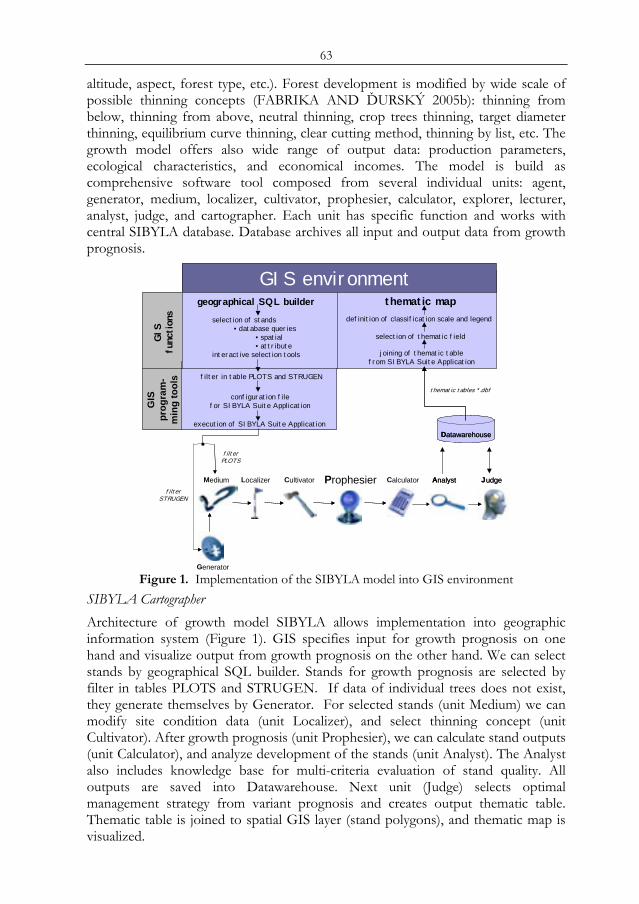
63
altitude, aspect, forest type, etc.). Forest development is modified by wide scale of possible thinning concepts (FABRIKA AND ĎURSKÝ 2005b): thinning from below, thinning from above, neutral thinning, crop trees thinning, target diameter thinning, equilibrium curve thinning, clear cutting method, thinning by list, etc. The growth model offers also wide range of output data: production parameters, ecological characteristics, and economical incomes. The model is build as comprehensive software tool composed from several individual units: agent, generator, medium, localizer, cultivator, prophesier, calculator, explorer, lecturer, analyst, judge, and cartographer. Each unit has specific function and works with central SIBYLA database. Database archives all input and output data from growth prognosis.
Medium
Generator
Localizer Cultivator Prophesier Calculator JudgeJudgeAnalystAnalyst
DatawarehouseDatawarehouse
GIS environment
GIS
func
tion
s
GIS
prog
ram
-m
ing
tool
s
geographical SQL builder thematic mapselection of stands
• database queries• spatial• attribute
interactive selection tools
filter in table PLOTS and STRUGEN
configuration filefor SIBYLA Suite Application
execution of SIBYLA Suite Application
filterPLOTS
filterSTRUGEN
definition of classification scale and legend
selection of thematic field
joining of thematic tablefrom SIBYLA Suite Application
thematic tables *.dbf
Figure 1. Implementation of the SIBYLA model into GIS environment
SIBYLA Cartographer Architecture of growth model SIBYLA allows implementation into geographic information system (Figure 1). GIS specifies input for growth prognosis on one hand and visualize output from growth prognosis on the other hand. We can select stands by geographical SQL builder. Stands for growth prognosis are selected by filter in tables PLOTS and STRUGEN. If data of individual trees does not exist, they generate themselves by Generator. For selected stands (unit Medium) we can modify site condition data (unit Localizer), and select thinning concept (unit Cultivator). After growth prognosis (unit Prophesier), we can calculate stand outputs (unit Calculator), and analyze development of the stands (unit Analyst). The Analyst also includes knowledge base for multi-criteria evaluation of stand quality. All outputs are saved into Datawarehouse. Next unit (Judge) selects optimal management strategy from variant prognosis and creates output thematic table. Thematic table is joined to spatial GIS layer (stand polygons), and thematic map is visualized.
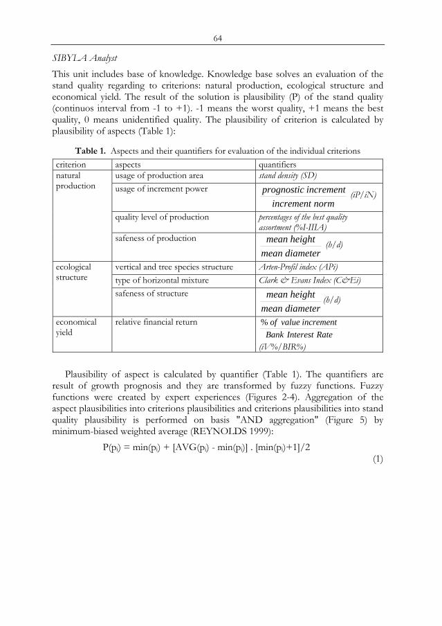
64
SIBYLA Analyst This unit includes base of knowledge. Knowledge base solves an evaluation of the stand quality regarding to criterions: natural production, ecological structure and economical yield. The result of the solution is plausibility (P) of the stand quality (continuos interval from -1 to +1). -1 means the worst quality, +1 means the best quality, 0 means unidentified quality. The plausibility of criterion is calculated by plausibility of aspects (Table 1):
Table 1. Aspects and their quantifiers for evaluation of the individual criterions criterion aspects quantifiers
usage of production area stand density (SD) usage of increment power
normincrementincrementprognostic (iP/iN)
quality level of production percentages of the best quality assortment (%I-IIIA)
natural production
safeness of production
diametermeanheightmean (h/d)
vertical and tree species structure Arten-Profil index (APi) type of horizontal mixture Clark & Evans Index (C&Ei)
ecological structure
safeness of structure
diametermeanheightmean (h/d)
economical yield
relative financial return RateInterestBank
incrementvalueof%
(iV%/BIR%)
Plausibility of aspect is calculated by quantifier (Table 1). The quantifiers are result of growth prognosis and they are transformed by fuzzy functions. Fuzzy functions were created by expert experiences (Figures 2-4). Aggregation of the aspect plausibilities into criterions plausibilities and criterions plausibilities into stand quality plausibility is performed on basis "AND aggregation" (Figure 5) by minimum-biased weighted average (REYNOLDS 1999):
P(pi) = min(pi) + [AVG(pi) - min(pi)] . [min(pi)+1]/2 (1)
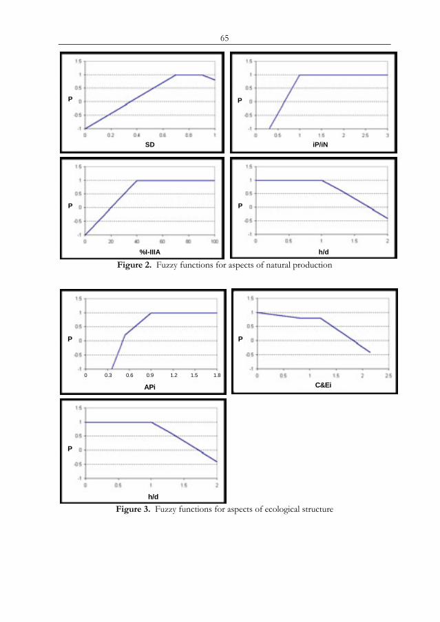
65
SDSD iP/iNiP/iN
%I-IIIA%I-IIIA h/dh/d
P
P
P
P
Figure 2. Fuzzy functions for aspects of natural production
h/dh/d
P
C&EiC&Ei
P P
APiAPi
0.90.60.30 1.2 1.5 1.8
Figure 3. Fuzzy functions for aspects of ecological structure
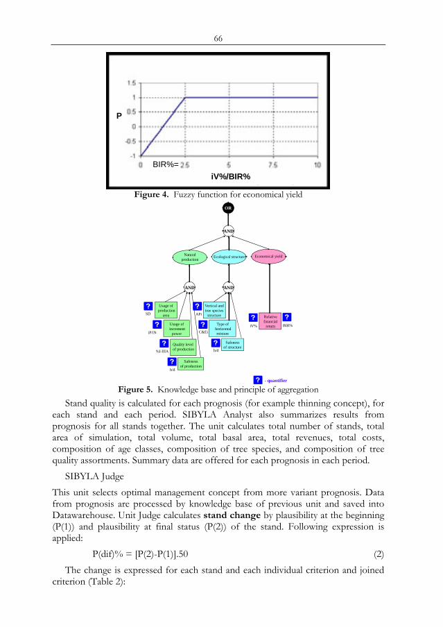
66
iV%/BIR%iV%/BIR%
P
BIR%=
Figure 4. Fuzzy function for economical yield
OR
AND
Naturalproduction
Ecological structure Economical yield
AND AND
Usage ofproduction
area
Usage ofincrement
power
Quality levelof production
Safenessof production
Vertical andtree species
structure
Type ofhorizontalmixture
Safenessof structure
Relativefinancial
return
SD
iP/iN
%I-IIIA
h/d
APi
C&Ei
h/d
iV% BIR%
- quantifier Figure 5. Knowledge base and principle of aggregation
Stand quality is calculated for each prognosis (for example thinning concept), for each stand and each period. SIBYLA Analyst also summarizes results from prognosis for all stands together. The unit calculates total number of stands, total area of simulation, total volume, total basal area, total revenues, total costs, composition of age classes, composition of tree species, and composition of tree quality assortments. Summary data are offered for each prognosis in each period.
SIBYLA Judge This unit selects optimal management concept from more variant prognosis. Data from prognosis are processed by knowledge base of previous unit and saved into Datawarehouse. Unit Judge calculates stand change by plausibility at the beginning (P(1)) and plausibility at final status (P(2)) of the stand. Following expression is applied:
P(dif)% = [P(2)-P(1)].50 (2) The change is expressed for each stand and each individual criterion and joined
criterion (Table 2):
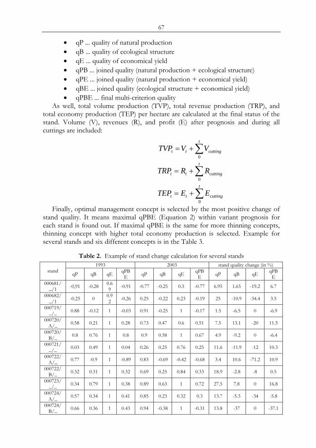
67
• qP ... quality of natural production • qB ... quality of ecological structure • qE ... quality of economical yield • qPB ... joined quality (natural production + ecological structure) • qPE ... joined quality (natural production + economical yield) • qBE ... joined quality (ecological structure + economical yield) • qPBE ... final multi-criterion quality
As well, total volume production (TVP), total revenue production (TRP), and total economy production (TEP) per hectare are calculated at the final status of the stand. Volume (V), revenues (R), and profit (E) after prognosis and during all cuttings are included:
∑+=t
cuttingtt VVTVP0
∑+=t
cuttingtt RRTRP0
∑+=t
cuttingtt EETEP0
Finally, optimal management concept is selected by the most positive change of stand quality. It means maximal qPBE (Equation 2) within variant prognosis for each stand is found out. If maximal qPBE is the same for more thinning concepts, thinning concept with higher total economy production is selected. Example for several stands and six different concepts is in the Table 3.
Table 2. Example of stand change calculation for several stands 1993 2003 stand quality change (in %)
stand qP qB qE qPBE qP qB qE qPB
E qP qB qE qPBE
000681/_/1 -0,91 -0.28 0.6
9 -0.91 -0.77 -0.25 0.3 -0.77 6.95 1.65 -19.2 6.7
000682/_/1 -0.25 0 0.9
2 -0.26 0.25 -0.22 0.23 -0.19 25 -10.9 -34.4 3.5
000719/_/_ 0.88 -0.12 1 -0.03 0.91 -0.25 1 -0.17 1.5 -6.5 0 -6.9
000720/A/_ 0.58 0.21 1 0.28 0.73 0.47 0.6 0.51 7.5 13.1 -20 11.5
000720/B/_ 0.8 0.76 1 0.8 0.9 0.58 1 0.67 4.9 -9.2 0 -6.4
000721/_/_ 0.03 0.49 1 0.04 0.26 0.25 0.76 0.25 11.6 -11.9 -12 10.3
000722/A/_ 0.77 -0.9 1 -0.89 0.83 -0.69 -0.42 -0.68 3.4 10.6 -71.2 10.9
000722/B/_ 0.32 0.31 1 0.32 0.69 0.25 0.84 0.33 18.9 -2.8 -8 0.5
000723/_/_ 0.34 0.79 1 0.38 0.89 0.63 1 0.72 27.5 7.8 0 16.8
000724/A/_ 0.57 0.34 1 0.41 0.85 0.23 0.32 0.3 13.7 -5.3 -34 -5.8
000724/B/_ 0.66 0.36 1 0.43 0.94 -0.38 1 -0.31 13.8 -37 0 -37.1
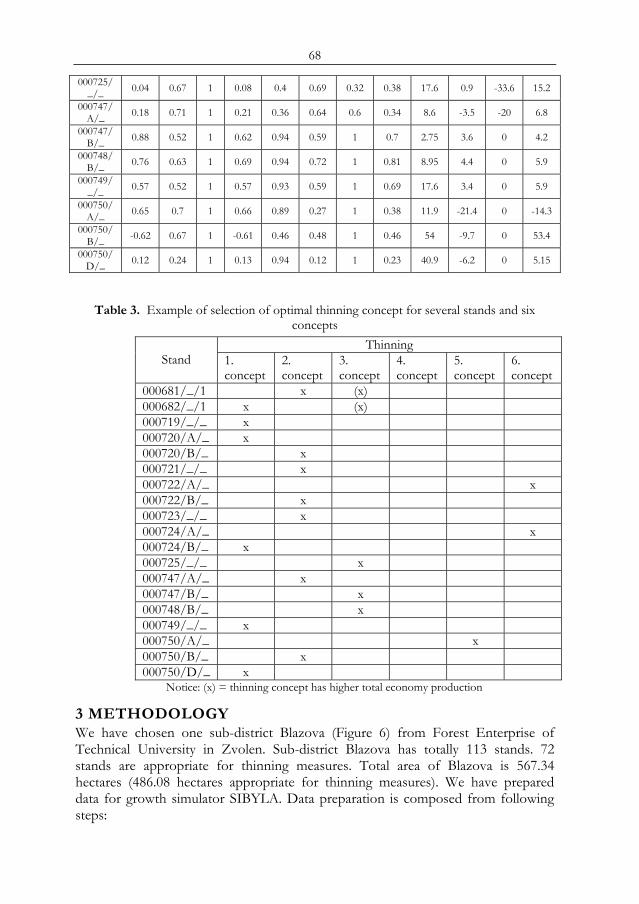
68
000725/_/_ 0.04 0.67 1 0.08 0.4 0.69 0.32 0.38 17.6 0.9 -33.6 15.2
000747/A/_ 0.18 0.71 1 0.21 0.36 0.64 0.6 0.34 8.6 -3.5 -20 6.8
000747/B/_ 0.88 0.52 1 0.62 0.94 0.59 1 0.7 2.75 3.6 0 4.2
000748/B/_ 0.76 0.63 1 0.69 0.94 0.72 1 0.81 8.95 4.4 0 5.9
000749/_/_ 0.57 0.52 1 0.57 0.93 0.59 1 0.69 17.6 3.4 0 5.9
000750/A/_ 0.65 0.7 1 0.66 0.89 0.27 1 0.38 11.9 -21.4 0 -14.3
000750/B/_ -0.62 0.67 1 -0.61 0.46 0.48 1 0.46 54 -9.7 0 53.4
000750/D/_ 0.12 0.24 1 0.13 0.94 0.12 1 0.23 40.9 -6.2 0 5.15
Table 3. Example of selection of optimal thinning concept for several stands and six concepts
Thinning Stand 1.
concept2. concept
3. concept
4. concept
5. concept
6. concept
000681/_/1 x (x) 000682/_/1 x (x) 000719/_/_ x 000720/A/_ x 000720/B/_ x 000721/_/_ x 000722/A/_ x 000722/B/_ x 000723/_/_ x 000724/A/_ x 000724/B/_ x 000725/_/_ x 000747/A/_ x 000747/B/_ x 000748/B/_ x 000749/_/_ x 000750/A/_ x 000750/B/_ x 000750/D/_ x
Notice: (x) = thinning concept has higher total economy production
3 METHODOLOGY We have chosen one sub-district Blazova (Figure 6) from Forest Enterprise of Technical University in Zvolen. Sub-district Blazova has totally 113 stands. 72 stands are appropriate for thinning measures. Total area of Blazova is 567.34 hectares (486.08 hectares appropriate for thinning measures). We have prepared data for growth simulator SIBYLA. Data preparation is composed from following steps:
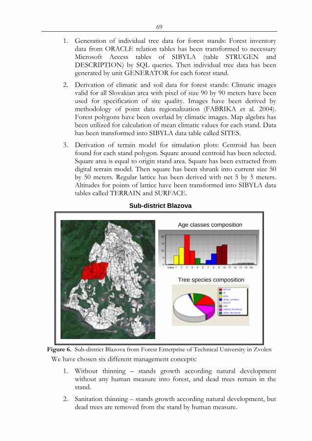
69
1. Generation of individual tree data for forest stands: Forest inventory data from ORACLE relation tables has been transformed to necessary Microsoft Access tables of SIBYLA (table STRUGEN and DESCRIPTION) by SQL queries. Then individual tree data has been generated by unit GENERATOR for each forest stand.
2. Derivation of climatic and soil data for forest stands: Climatic images valid for all Slovakian area with pixel of size 90 by 90 meters have been used for specification of site quality. Images have been derived by methodology of point data regionalization (FABRIKA et al. 2004). Forest polygons have been overlaid by climatic images. Map algebra has been utilized for calculation of mean climatic values for each stand. Data has been transformed into SIBYLA data table called SITES.
3. Derivation of terrain model for simulation plots: Centroid has been found for each stand polygon. Square around centroid has been selected. Square area is equal to origin stand area. Square has been extracted from digital terrain model. Then square has been shrunk into current size 50 by 50 meters. Regular lattice has been derived with net 5 by 5 meters. Altitudes for points of lattice have been transformed into SIBYLA data tables called TERRAIN and SURFACE.
sprucefirpineother conifersbeechoakvalued deciduosother deciduos
sprucefirpineother conifersbeechoakvalued deciduosother deciduos
Age classes composition
Tree species composition
Sub-district Blazova
Figure 6. Sub-district Blazova from Forest Enterprise of Technical University in Zvolen
We have chosen six different management concepts:
1. Without thinning – stands growth according natural development without any human measure into forest, and dead trees remain in the stand.
2. Sanitation thinning – stands growth according natural development, but dead trees are removed from the stand by human measure.
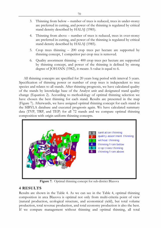
70
3. Thinning from below – number of trees is reduced, trees in under-storey are preferred in cutting, and power of the thinning is regulated by critical stand density described by HALAJ (1985).
4. Thinning from above – number of trees is reduced, trees in over-storey are preferred in cutting, and power of the thinning is regulated by critical stand density described by HALAJ (1985).
5. Crop trees thinning – 200 crop trees per hectare are supported by thinning concept, 1 competitor per crop tree is removed.
6. Quality assortment thinning – 400 crop trees per hectare are supported by thinning concept, and power of the thinning is defined by strong degree of JOHANN (1982), it means A-value is equal to 6.
All thinning concepts are specified for 20 years long period with interval 5 years.
Specification of thinning power or number of crop trees is independent to tree species and relates to all stands. After thinning prognosis, we have calculated quality of the stands by knowledge base of the Analyst unit and designated stand quality change (Equation 2). According to methodology of optimal thinning selection we have chosen the best thinning for each stand. Results are presented in the map (Figure 7). Afterwards, we have assigned optimal thinning concept for each stand in the SIBYLA database and executed prognosis again. We have calculated summary data (TVP, TRP, and TEP) for all 72 stands and we compare optimal thinning composition with origin uniform thinning concepts.
without thinningsanitation thinningquality assortment thinningwithout thinningthinning from belowcrop trees thinningthinning from above
sanitation thinningquality assortment thinningwithout thinningthinning from belowcrop trees thinningthinning from above
123456
11
1
11
1 1
11
2
2
2
2
2
33
3
33
33
3
3
4
45
5
5
5
6
6
6
6
66
6
Figure 7. Optimal thinning concept for sub-district Blazova
4 RESULTS Results are shown in the Table 4. As we can see in the Table 4, optimal thinning composition in area Blazova is optimal not only from multi-criteria point of view (natural production, ecological structure, and economical yield), but total volume production, total revenue production, and total economy production is also the best. If we compare management without thinning and optimal thinning, all total
71
productions are higher approximately 8 %. Difference in total economy production is 68 427 SKK per hectare. It is totally 33 260 996 SKK (898 946 EUR).
Table 4. Summary data of the specified thinning concepts thinning concept TVP TRP TEP TVP in % TRP in % TEP in %
without thinning 517 932 155 874 345 100 100 100 sanitation thinning 540 962 849 902 841 104 103 103 thinning from below 481 910 745 858 235 93 98 98 thinning from above 507 952 829 897 316 98 102 103 crop trees thinning 471 867 780 813 712 91 93 93 quality assortment thinning
501 921 399 864 915 97 99 99
optimal thinning 555 1 005 982
942 772 107 108 108
5 CONCLUSION The presented prototype of information system with SIBYLA growth model, knowledge base and GIS system represents power tool for evaluation of management impacts to forest. The system appreciates impacts in complex consideration regarding to productive, ecological and economical intentions. Quantification of changes during a long-time process in a real time performs scientific and mainly practical value of the system. This is not possible without such an instrument. The system allows experiment with various management procedures without any risk of ecosystem destruction, because it's only a computer model. Consequences and effects are immediately visible and are quantified. Therefore, the forest manager can consider quality of management measures with responsibility. The viewpoint is multifunctional and user can determine main management intentions, it means, whether he will optimise production, ecological stability, economical returns or integrated aspects. He can decide for the most optimal management concept and realise it on real stands.
ACKNOWLEDGEMENTS The paper is result of the scientific project VEGA Nr. 1047 (1/3531/06): Forest inventory and forecasting. Thanks to all colleagues participating at the project, mainly to Nadežda Pšidová.
REFERENCES 1 CZERANKA, M.: SDSS in Naturschutz und Landschaftspflege ? In: DOLLINGER, F. –
STROBL, J.: Angewandte Geographische Informationsverarbeitung VIII. Salzburger Geographische Materialien, Heft 24. Selbstverlag des Instituts für Geographie der Universität Salzburg, 1996.
2 FABRIKA, M., ĎURSKÝ, J.: Stromové rastové simulátory. EFRA (Tree Growth Simulators) -Vedecká agentúra pre ekológiu a lesníctvo (Ecological & Forestry Research Agency), Zvolen 2005, 112 p. (a)
3 FABRIKA, M., ĎURSKÝ, J.: Algorithms and software solution of thinning models for SIBYLA growth simulator. Journal of Forest Science, 51, 2005 (10), p.431-445 (b)

72
4 FABRIKA, M., ĎURSKÝ, J., PRETZSCH, H., SLOBODA, B.: Regionalisation of climatic values for ecological site classification using growth simulator SIBYLA with GIS. In: “Remote Sensing and Geographical Information Systems for Environmental Studies. Application in Forestry, Edited by KLEIN, CH., NIESCHULTZE, J. and SLOBODA, B., Band 138, 2005, Universität Göttingen, J.D. Sauerländer’s Verlag Frankfurt am main., p. 245-255
5 HALAJ, J.: Kritické zakmenenie porastov podľa nových rastových tabuliek (Critical stand density according new yield tables). Lesnícky časopis (Forestry Journal ), 31, č. 4, 1985, p. 267-276.
6 JOHANN, K.: Der „A-Wert“ – ein objektiver Parameter zur Bestimmung der Freistellungsstärke von Zentralbäumen. Ber. von der Jahrestagung der Sektion Ertragskunde im DVFFA in Weibersbrunn, 1982, p. 146-158.
7 REYNOLDS, K. M.: NetWeaver for EMDS user guide (version 1.0): a knowledge base development system. Gen. Tech. Rep. PNW-GTR-XX. Portland, OR: U.S. Department of Agriculture, Forest Service, Pacific Northwest Research Station, 1999, XX p.
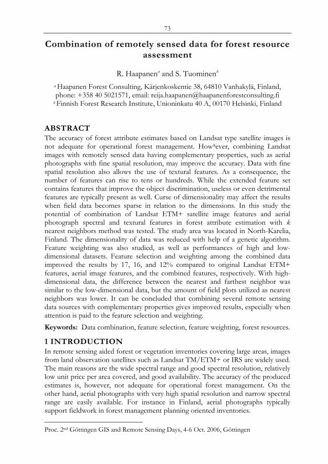
73
Combination of remotely sensed data for forest resource assessment
R. Haapanena and S. Tuominenb a Haapanen Forest Consulting, Kärjenkoskentie 38, 64810 Vanhakylä, Finland, phone: +358 40 5021571, email: [email protected]
b Finnish Forest Research Institute, Unioninkatu 40 A, 00170 Helsinki, Finland
ABSTRACT The accuracy of forest attribute estimates based on Landsat type satellite images is not adequate for operational forest management. How8ever, combining Landsat images with remotely sensed data having complementary properties, such as aerial photographs with fine spatial resolution, may improve the accuracy. Data with fine spatial resolution also allows the use of textural features. As a consequence, the number of features can rise to tens or hundreds. While the extended feature set contains features that improve the object discrimination, useless or even detrimental features are typically present as well. Curse of dimensionality may affect the results when field data becomes sparse in relation to the dimensions. In this study the potential of combination of Landsat ETM+ satellite image features and aerial photograph spectral and textural features in forest attribute estimation with k nearest neighbors method was tested. The study area was located in North-Karelia, Finland. The dimensionality of data was reduced with help of a genetic algorithm. Feature weighting was also studied, as well as performances of high and low-dimensional datasets. Feature selection and weighting among the combined data improved the results by 17, 16, and 12% compared to original Landsat ETM+ features, aerial image features, and the combined features, respectively. With high-dimensional data, the difference between the nearest and farthest neighbor was similar to the low-dimensional data, but the amount of field plots utilized as nearest neighbors was lower. It can be concluded that combining several remote sensing data sources with complementary properties gives improved results, especially when attention is paid to the feature selection and weighting. Keywords: Data combination, feature selection, feature weighting, forest resources.
1 INTRODUCTION In remote sensing aided forest or vegetation inventories covering large areas, images from land observation satellites such as Landsat TM/ETM+ or IRS are widely used. The main reasons are the wide spectral range and good spectral resolution, relatively low unit price per area covered, and good availability. The accuracy of the produced estimates is, however, not adequate for operational forest management. On the other hand, aerial photographs with very high spatial resolution and narrow spectral range are easily available. For instance in Finland, aerial photographs typically support fieldwork in forest management planning oriented inventories. Proc. 2nd Göttingen GIS and Remote Sensing Days, 4-6 Oct. 2006, Göttingen
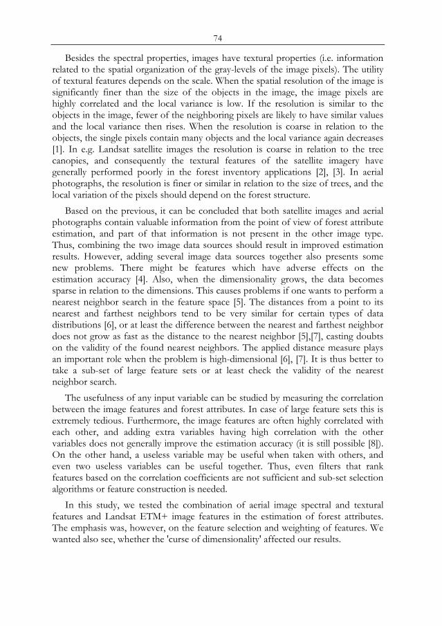
74
Besides the spectral properties, images have textural properties (i.e. information related to the spatial organization of the gray-levels of the image pixels). The utility of textural features depends on the scale. When the spatial resolution of the image is significantly finer than the size of the objects in the image, the image pixels are highly correlated and the local variance is low. If the resolution is similar to the objects in the image, fewer of the neighboring pixels are likely to have similar values and the local variance then rises. When the resolution is coarse in relation to the objects, the single pixels contain many objects and the local variance again decreases [1]. In e.g. Landsat satellite images the resolution is coarse in relation to the tree canopies, and consequently the textural features of the satellite imagery have generally performed poorly in the forest inventory applications [2], [3]. In aerial photographs, the resolution is finer or similar in relation to the size of trees, and the local variation of the pixels should depend on the forest structure.
Based on the previous, it can be concluded that both satellite images and aerial photographs contain valuable information from the point of view of forest attribute estimation, and part of that information is not present in the other image type. Thus, combining the two image data sources should result in improved estimation results. However, adding several image data sources together also presents some new problems. There might be features which have adverse effects on the estimation accuracy [4]. Also, when the dimensionality grows, the data becomes sparse in relation to the dimensions. This causes problems if one wants to perform a nearest neighbor search in the feature space [5]. The distances from a point to its nearest and farthest neighbors tend to be very similar for certain types of data distributions [6], or at least the difference between the nearest and farthest neighbor does not grow as fast as the distance to the nearest neighbor [5],[7], casting doubts on the validity of the found nearest neighbors. The applied distance measure plays an important role when the problem is high-dimensional [6], [7]. It is thus better to take a sub-set of large feature sets or at least check the validity of the nearest neighbor search.
The usefulness of any input variable can be studied by measuring the correlation between the image features and forest attributes. In case of large feature sets this is extremely tedious. Furthermore, the image features are often highly correlated with each other, and adding extra variables having high correlation with the other variables does not generally improve the estimation accuracy (it is still possible [8]). On the other hand, a useless variable may be useful when taken with others, and even two useless variables can be useful together. Thus, even filters that rank features based on the correlation coefficients are not sufficient and sub-set selection algorithms or feature construction is needed.
In this study, we tested the combination of aerial image spectral and textural features and Landsat ETM+ image features in the estimation of forest attributes. The emphasis was, however, on the feature selection and weighting of features. We wanted also see, whether the 'curse of dimensionality' affected our results.
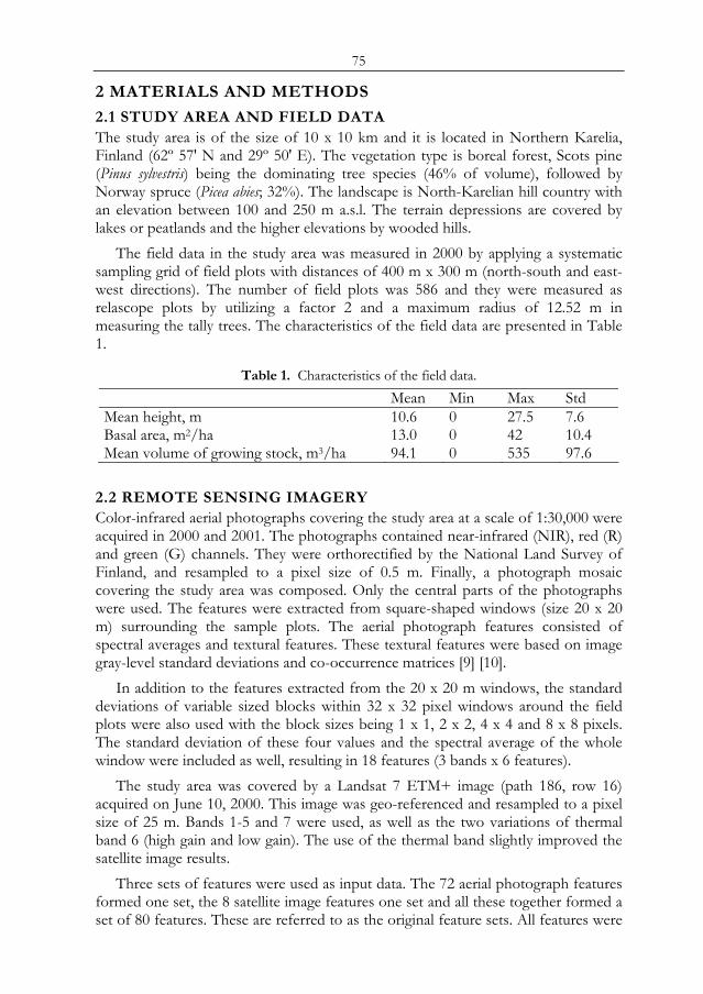
75
2 MATERIALS AND METHODS
2.1 STUDY AREA AND FIELD DATA The study area is of the size of 10 x 10 km and it is located in Northern Karelia, Finland (62º 57' N and 29º 50' E). The vegetation type is boreal forest, Scots pine (Pinus sylvestris) being the dominating tree species (46% of volume), followed by Norway spruce (Picea abies; 32%). The landscape is North-Karelian hill country with an elevation between 100 and 250 m a.s.l. The terrain depressions are covered by lakes or peatlands and the higher elevations by wooded hills.
The field data in the study area was measured in 2000 by applying a systematic sampling grid of field plots with distances of 400 m x 300 m (north-south and east-west directions). The number of field plots was 586 and they were measured as relascope plots by utilizing a factor 2 and a maximum radius of 12.52 m in measuring the tally trees. The characteristics of the field data are presented in Table 1.
Table 1. Characteristics of the field data. Mean Min Max Std Mean height, m 10.6 0 27.5 7.6 Basal area, m2/ha 13.0 0 42 10.4 Mean volume of growing stock, m3/ha 94.1 0 535 97.6
2.2 REMOTE SENSING IMAGERY Color-infrared aerial photographs covering the study area at a scale of 1:30,000 were acquired in 2000 and 2001. The photographs contained near-infrared (NIR), red (R) and green (G) channels. They were orthorectified by the National Land Survey of Finland, and resampled to a pixel size of 0.5 m. Finally, a photograph mosaic covering the study area was composed. Only the central parts of the photographs were used. The features were extracted from square-shaped windows (size 20 x 20 m) surrounding the sample plots. The aerial photograph features consisted of spectral averages and textural features. These textural features were based on image gray-level standard deviations and co-occurrence matrices [9] [10].
In addition to the features extracted from the 20 x 20 m windows, the standard deviations of variable sized blocks within 32 x 32 pixel windows around the field plots were also used with the block sizes being 1 x 1, 2 x 2, 4 x 4 and 8 x 8 pixels. The standard deviation of these four values and the spectral average of the whole window were included as well, resulting in 18 features (3 bands x 6 features).
The study area was covered by a Landsat 7 ETM+ image (path 186, row 16) acquired on June 10, 2000. This image was geo-referenced and resampled to a pixel size of 25 m. Bands 1-5 and 7 were used, as well as the two variations of thermal band 6 (high gain and low gain). The use of the thermal band slightly improved the satellite image results.
Three sets of features were used as input data. The 72 aerial photograph features formed one set, the 8 satellite image features one set and all these together formed a set of 80 features. These are referred to as the original feature sets. All features were
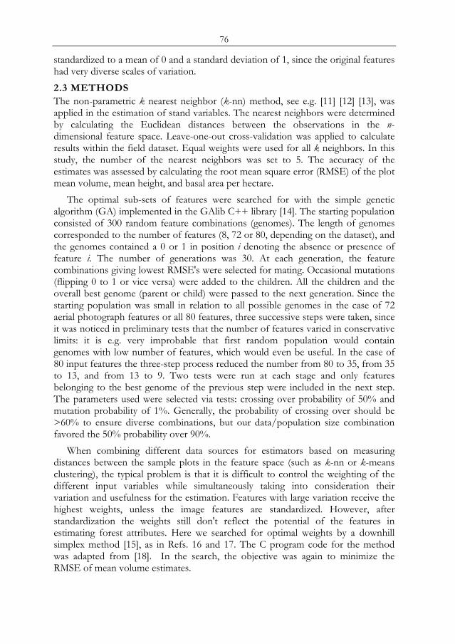
76
standardized to a mean of 0 and a standard deviation of 1, since the original features had very diverse scales of variation. 2.3 METHODS The non-parametric k nearest neighbor (k-nn) method, see e.g. [11] [12] [13], was applied in the estimation of stand variables. The nearest neighbors were determined by calculating the Euclidean distances between the observations in the n-dimensional feature space. Leave-one-out cross-validation was applied to calculate results within the field dataset. Equal weights were used for all k neighbors. In this study, the number of the nearest neighbors was set to 5. The accuracy of the estimates was assessed by calculating the root mean square error (RMSE) of the plot mean volume, mean height, and basal area per hectare.
The optimal sub-sets of features were searched for with the simple genetic algorithm (GA) implemented in the GAlib C++ library [14]. The starting population consisted of 300 random feature combinations (genomes). The length of genomes corresponded to the number of features (8, 72 or 80, depending on the dataset), and the genomes contained a 0 or 1 in position i denoting the absence or presence of feature i. The number of generations was 30. At each generation, the feature combinations giving lowest RMSE's were selected for mating. Occasional mutations (flipping 0 to 1 or vice versa) were added to the children. All the children and the overall best genome (parent or child) were passed to the next generation. Since the starting population was small in relation to all possible genomes in the case of 72 aerial photograph features or all 80 features, three successive steps were taken, since it was noticed in preliminary tests that the number of features varied in conservative limits: it is e.g. very improbable that first random population would contain genomes with low number of features, which would even be useful. In the case of 80 input features the three-step process reduced the number from 80 to 35, from 35 to 13, and from 13 to 9. Two tests were run at each stage and only features belonging to the best genome of the previous step were included in the next step. The parameters used were selected via tests: crossing over probability of 50% and mutation probability of 1%. Generally, the probability of crossing over should be >60% to ensure diverse combinations, but our data/population size combination favored the 50% probability over 90%.
When combining different data sources for estimators based on measuring distances between the sample plots in the feature space (such as k-nn or k-means clustering), the typical problem is that it is difficult to control the weighting of the different input variables while simultaneously taking into consideration their variation and usefulness for the estimation. Features with large variation receive the highest weights, unless the image features are standardized. However, after standardization the weights still don't reflect the potential of the features in estimating forest attributes. Here we searched for optimal weights by a downhill simplex method [15], as in Refs. 16 and 17. The C program code for the method was adapted from [18]. In the search, the objective was again to minimize the RMSE of mean volume estimates.
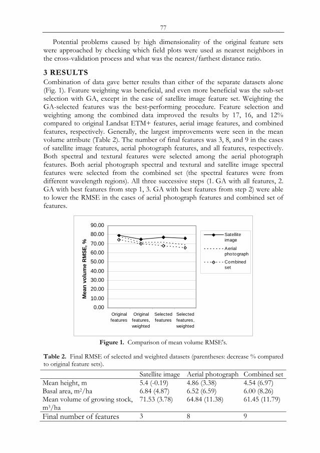
77
Potential problems caused by high dimensionality of the original feature sets were approached by checking which field plots were used as nearest neighbors in the cross-validation process and what was the nearest/farthest distance ratio.
3 RESULTS Combination of data gave better results than either of the separate datasets alone (Fig. 1). Feature weighting was beneficial, and even more beneficial was the sub-set selection with GA, except in the case of satellite image feature set. Weighting the GA-selected features was the best-performing procedure. Feature selection and weighting among the combined data improved the results by 17, 16, and 12% compared to original Landsat ETM+ features, aerial image features, and combined features, respectively. Generally, the largest improvements were seen in the mean volume attribute (Table 2). The number of final features was 3, 8, and 9 in the cases of satellite image features, aerial photograph features, and all features, respectively. Both spectral and textural features were selected among the aerial photograph features. Both aerial photograph spectral and textural and satellite image spectral features were selected from the combined set (the spectral features were from different wavelength regions). All three successive steps (1. GA with all features, 2. GA with best features from step 1, 3. GA with best features from step 2) were able to lower the RMSE in the cases of aerial photograph features and combined set of features.
0.0010.00
20.0030.0040.00
50.0060.0070.00
80.0090.00
Originalfeatures
Originalfeatures,weighted
Selectedfeatures
Selectedfeatures,weighted
Mea
n vo
lum
e R
MSE
, %
Satelliteimage
Aerialphotograph
Combinedset
Figure 1. Comparison of mean volume RMSE's.
Table 2. Final RMSE of selected and weighted datasets (parentheses: decrease % compared to original feature sets). Satellite image Aerial photograph Combined set Mean height, m 5.4 (-0.19) 4.86 (3.38) 4.54 (6.97) Basal area, m2/ha 6.84 (4.87) 6.52 (6.59) 6.00 (8.26) Mean volume of growing stock, m3/ha
71.53 (3.78) 64.84 (11.38) 61.45 (11.79)
Final number of features 3 8 9
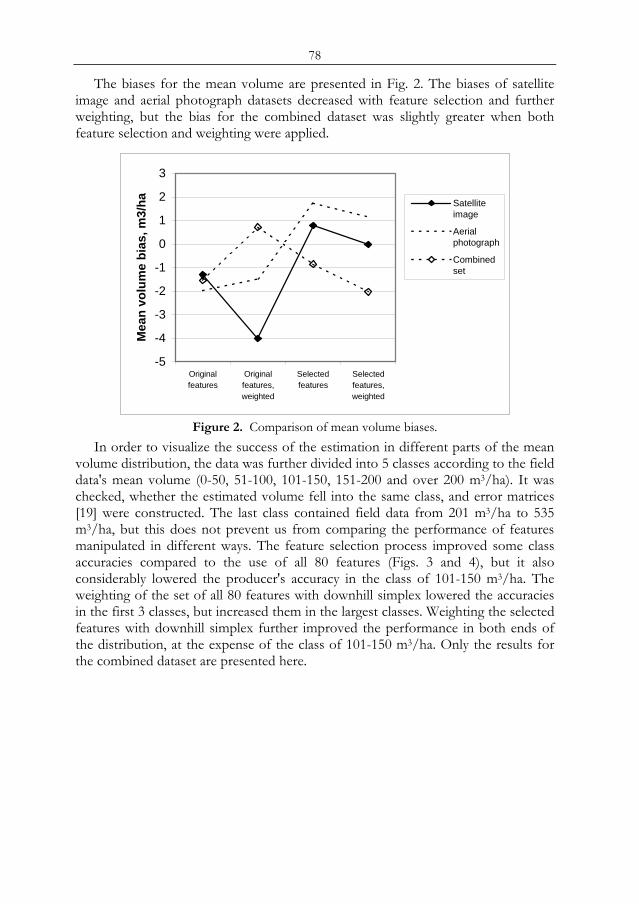
78
The biases for the mean volume are presented in Fig. 2. The biases of satellite image and aerial photograph datasets decreased with feature selection and further weighting, but the bias for the combined dataset was slightly greater when both feature selection and weighting were applied.
-5
-4
-3
-2
-1
0
1
2
3
Originalfeatures
Originalfeatures,weighted
Selectedfeatures
Selectedfeatures,weighted
Mea
n vo
lum
e bi
as, m
3/ha Satellite
image
Aerialphotograph
Combinedset
Figure 2. Comparison of mean volume biases.
In order to visualize the success of the estimation in different parts of the mean volume distribution, the data was further divided into 5 classes according to the field data's mean volume (0-50, 51-100, 101-150, 151-200 and over 200 m3/ha). It was checked, whether the estimated volume fell into the same class, and error matrices [19] were constructed. The last class contained field data from 201 m3/ha to 535 m3/ha, but this does not prevent us from comparing the performance of features manipulated in different ways. The feature selection process improved some class accuracies compared to the use of all 80 features (Figs. 3 and 4), but it also considerably lowered the producer's accuracy in the class of 101-150 m3/ha. The weighting of the set of all 80 features with downhill simplex lowered the accuracies in the first 3 classes, but increased them in the largest classes. Weighting the selected features with downhill simplex further improved the performance in both ends of the distribution, at the expense of the class of 101-150 m3/ha. Only the results for the combined dataset are presented here.
79
0.0
10.0
20.0
30.0
40.0
50.0
60.0
70.0
80.0
0-50 50-100 100-150 150-200 200-
Volume class, m3/ha
Prod
ucer
's a
ccur
acy,
%
Originalfeatures
Originalfeatures,weighted
Selectedfeatures
Selectedfeatures,weighted
Figure 3. Producer's accuracies in volume classes constructed of the continuous data. Thick
line: percentage of field plots in each class. Input: all 80 features.
0.010.020.030.040.050.060.070.080.090.0
100.0
0-50 50-100 100-150
150-200
200-
Volume class, m3/ha
Con
sum
er's
acc
urac
y, %
Originalfeatures
Originalfeatures,weighted
Selectedfeatures
Selectedfeatures,weighted
Figure 4. Consumer's accuracies in volume classes constructed of the continuous data.
Thick line: percentage of field plots in each class. Input: all 80 features.
The curse of dimensionality test results (Table 3) revealed no clear problems. If the nearest/farthest distance ratios approach 1, there is no distinction between data points. Here, however, the ratios were on average similar in both 9 and 80 dimensions. The nearest/farthest distance ratios were calculated using unstandardized features as well. There the ratios differed being on average 0.044 in the 9-dimensional case and 0.11 in the 80-dimensional case. Fewer of the field plots were selected as the closest neighbor when all 80 features were used. Furthermore, of the 5 nearest neighbors, on average 1.7 were common in the cases of 80 original features and selected 9 features. The first neighbor according to the 80 original
80
features was present within the 5 nearest neighbors based on the selected 9 features in 50% of the cases only. The first neighbors were close to the average in both cases, but the first neighbors according to the 9-dimensional case only (missing from the 80-dimensional case) were quite far from the average.
Table 3. Results of 'curse of dimensionality' tests. Original 80
features Selected 9 features
Field plots selected as the closest neighbor 329 376 Field plots selected as the farthest neighbor 3 6 Average volume of 1st neighbor, m3/ha 95.75 91.83 Average volume of 1st neighbor, those not present within other feature set's 1st neighbors, m3/ha
92.87 81.49
Nearest/farthest distance ratio, standardized features
0.10 0.11
Nearest/farthest distance ratio, unstandardized features
0.11 0.04
4 DISCUSSION AND CONCLUSIONS The results confirm those of Ref. 20: using a combination of a Landsat image and color-infrared aerial photographs gives more accurate estimates than those obtained using individual data sources. In Ref. 21 none or very little improvement was gained by combining high-altitude panchromatic aerial photographs and a Landsat image. This is explained by our results: in the case of combined dataset, spectral features were picked from both aerial photograph and satellite image (different wavelength regions). Thus, it was not the texture alone that brought the better results.
Sub-sets of features and/or feature weighting performed better than the original feature sets. There is, however, always the possibility of overfitting, when optimal features and weights are searched for within a specific dataset. These processes favor features that maximize of minimize the objective(s) defined in the objective function within the current data. There might be features that are useful for estimating the volumes of dominating stand types, but even detrimental for other stand types. This was analyzed by constructing error matrices of the data divided into 50 m3/ha volume classes. The classification of the largest volumes was more accurate in the approaches that incorporated a sub-set of features and/or feature weighting. In the case of the class containing the lowest volumes the variation of results was minor, while for the intermediate volume class the effect of feature selection and/or weighting was adverse. When the accuracies are compared to the proportion of field data in each class, it can be seen that the classes with largest amounts of data gained highest accuracies, at expense of the classes with smallest amounts of data. Furthermore, the improvement in results by feature selection and/or weighting was greatest in the case of mean volume, and smaller in the cases of height and basal area. The algorithms were instructed to minimize mean volume RMSE, and features or weights were selected accordingly. If the field data represents
81
the target area well and the interest lies on a few forest attributes, the overfitting is acceptable. In other cases, the objective criteria should also include other attributes, and include variables describing estimation success within size or age classes.
In order to test for possible effects caused by high dimensionality of the original data, it would be wise to check how often the 'real' nearest neighbors are selected in the Euclidian distance-based process within the cross-validation of field data. The problem is: how to define the real nearest neighbors, when forests vary along so many axes? How to weight e.g. volume, basal area, height, age, tree species distribution, stand structure, site type and soil class? Even though we didn't try to specify the real nearest neighbors in this study, it is clear that at least one of the two more closely examined feature sets did not catch those neighbors: on average, only 1.7 of the 5 nearest neighbors were the same. Further, fewer of the field plots were being selected as the 1st neighbor in the case of the 80-dimensional dataset than in the case of 9-dimensions. The neighbor search in high dimensional feature set resulted in more average data points. The convergence of nearest/farthest distance ratios towards 1 with increasing dimensionality, was not seen in the case of standardized data used in our study, but the additional test with unstandardized data revealed that a) there was clear difference between the high and low dimensions and b) the standardization had weakened the distinction between nearest and farthest neighbor in the 9-dimensional case, but had no effect on the 80-dimensional case.
It can be concluded that combining several remote sensing data sources with complementary properties gives improved results, especially when attention is paid to the feature selection and weighting. The quality of results based on large-dimensional datasets must, however, be evaluated even more carefully than in the case of traditional Landsat feature sets.
REFERENCES 1 Woodcock, C.E., and Strahler, A.H., 1987: The factor of scale in remote sensing. Remote Sensing of Environment 21, pp. 311-332. 2 Shang, D., and Waite, M-L., 1991: Utilization of textural and spectral features from Landsat TM imagery for stratifying forest sample plots. University of Helsinki, Department of Forest Mensuration and Management Research Notes 26. 3 Cohen, W.B., and Spies, T.A., 1992: Estimating structural attributes of Douglas-fir/western hemlock forest stands from Landsat and SPOT imagery. Remote Sensing of Environment 41, pp. 1-17. 4 McRoberts, R.E., Nelson, M.D., and Wendt, D.G., 2002: Stratified estimation of forest area using satellite imagery, inventory data, and the k-nearest neighbors technique. Remote Sensing of Environment 82, pp. 457-468. 5 Hinneburg, A., Aggarwal, C.C., and Keim, D.A., 2000: What is the nearest neighbor in high dimensional spaces? Proceedings of the 26th Very Large Data Bases (VLDB) Conference, September 10-14, Cairo, Egypt, pp. 506-515. 6 Beyer, K.S., Goldstein, J., Ramakrishnan, R., and Shaft, U., 1999: When Is "Nearest Neighbor" Meaningful? Proceedings of the 7th International Conference on Database Theory (ICDT), Jerusalem, Israel, January 10-12, pp. 217-235. 7 Aggarwal, C.C., Hinneburg, A., and Keim, D.A., 2001: On the surprising behavior of distance metrics in high dimensional space, Proceedings of the 8th International Conference on Database Theory (ICDT), London, UK, January 4-6, pp. 420–434.

82
8 Guyon, I., and Elisseeff, A., 2003: An introduction to variable and feature selection. Journal of Machine Learning Research 3, pp. 1157-1182. 9 Haralick, R.M., Shanmugan, K., and Dinstein, I., 1973: Textural features for image classification. IEEE Transactions on Systems, Man and Cybernetics. Vol. SMC-3, 6, pp. 610-621. 10 Haralick, R., 1979: Statistical and structural approaches to texture. Proc. IEEE 67(5), pp. 786-804. 11 Kilkki, P., and Päivinen, R., 1987: Reference sample plots to combine field measurements and satellite data in forest inventory. Department of Forest Mensuration and Management, University of Helsinki. Research notes 19, pp. 210- 215. 12 Muinonen, E., and Tokola, T., 1990: An application of remote sensing for communal forest inventory. Proceedings from SNS/IUFRO workshop: The usability of remote sensing for forest inventory and planning, 26-28 February 1990, Umeå, Sweden. Remote Sensing Laboratory, Swedish University of Agricultural Sciences, Report 4, pp. 35-42. 13 Tomppo, E., 1991: Satellite image-based national forest inventory of Finland. International archives of photogrammetry and remote sensing 28, pp. 419-424. 14 Wall, M., 1996: GAlib: A C++ Library of Genetic Algorithm Components Version 2.4 Documentation, revision B. Massachusetts Institute of Technology. 15 Nelder, J.A., and Mead, R., 1965: A simplex method for function minimization. Computer Journal 7, pp. 391-98. 16 Franco-Lopez, H., Ek, A.R., and Bauer, M.E., 2001: Estimation and mapping of forest density, volume and cover type using the k-nearest neighbors method. Remote Sensing of Environment 77, pp. 251 – 274. 17 Haapanen, R., Ek, A.R., Bauer, M.E., and Finley, A.O., 2004: Delineation of forest/nonforest land use classes using nearest neighbor methods. Remote Sensing of Environment 89, pp. 265-271. 18 Press, W.H., Teukolsky, S.A., Vetterling, W.T., and Flannery, B.P., 1999: Numerical recipes in C. The art of scientific computing, Second edition, Cambridge university press, UK. 19 Campbell, J.B., 2002: Introduction to remote sensing. Third edition. The Guilford Press, New York. 20 Tuominen, S., 2005: Hierarchical combination of data from satellite imagery and aerial photographs for multi-source forest inventory. Proceedings of ForestSat 2005, Borås May 31 - June 3. Rapport 8b. Swedish national board of forestry, pp. 26-30. 21 Tuominen, S., and Haakana, M., 2005: Landsat TM imagery and high altitude aerial photographs in estimation of forest characteristics. Silva Fennica 39(4), pp. 573-584.
83
the SiberiaN Earth System Science Cluster (Sib-ess-c)
S. Hese, C. Schmullius, R. Gerlach
Friedrich-Schiller University Jena, Institute of Geography, Department of Earth Observation, Löbdergraben 32, 07743 Jena, email: [email protected]
ABSTRACT This paper presents the concept of the 9Siberian Earth System Science Cluster currently being established at the University of Jena (Germany). SIB-ESS-C is the follow-on activity of the EU funded SIBERIA-II project (Multi-Sensor Concepts for Greenhouse Gas Accounting of Northern Eurasia). SIBERIA-II was a joint Russian-European remote sensing project that improved greenhouse gas accounting over a 300 million ha area in the central Siberian region. This area represents a significant part of the Earth’s boreal biome which plays a critical role in global climate change and has been defined as one of IGBP’s boreal transects representing a strong climate change hot spot in Northern Eurasia. The project lifetime was from January 2002 until December 2005.
In the initial phase of the SIB-ESS-C project, data sets and value-added products created within the SIBERIA-II project will form the basic set of products to be disseminated and extended. These products include regional maps of land cover, fire induced disturbances, phenology, snow depth, snow melt dates, onset and duration of freeze and thaw, LAI and others. Most of these Earth observation based products have been available for several years and cover the entire SIBERIA-II region. A major goal of SIB-ESS-C is to continue product generation for build up of time series for environmental monitoring and as input parameters for earth science models for a larger region. As research is advancing and new algorithms and data products are being developed, additional data sets of the extended region will be included. In order to provide a comprehensive spectrum of data sets for earth system research, various collaborations with other data providers and research organisations are planned. Keywords: SIB-ESS-C, Siberia-II, Landcover, DGVM, biosphere modelling, carbon accounting
INTRODUCTION With the recent advancements in information technology especially in the field of spatial data infrastructures new opportunities became available to the earth science community to efficiently share data, results and also applications over the World Wide Web using standards published by the World Wide Web Consortium (W3C®), the Open Geospatial Consortium (OGC™) or the International Organization for Standardization (ISO). Based on these technologies the Siberian Earth System Science Cluster (SIB-ESS-C) will be developed as a spatial data infrastructure for remote sensing product generation, data dissemination and scientific data analysis. Proc. 2nd Göttingen GIS and Remote Sensing Days, 4-6 Oct. 2006, Göttingen
84
SIB-ESS-C is the follow-on activity to the EU funded SIBERIA-II project (Multi-Sensor Concepts for Greenhouse Gas Accounting of Northern Eurasia, EVG2-2001-00008) [6][7][8][9]. SIBERIA-II was a joint Russian-European remote sensing project that improved greenhouse gas accounting over a 300 Million ha area in the central Siberian region. This area represents a significant part of the Earth’s boreal biome which plays a critical role in global climate change and has been defined as one of IGBP’s boreal transects representing a strong climate change hot spot in northern Eurasia. The overall objective of the SIBERIA-II project was to demonstrate the viability of full carbon accounting including greenhouse gases (GHG) on a regional basis using state-of-the-art environmental methods, biosphere modelling and advanced remote sensing technologies. The tools and systems which have been employed include a selected yet spectrally and temporally diverse set of 15 Earth observation datasets from 8 satellites, detailed GIS databases and some of the worlds most advanced Dynamic Global Vegetation Models (the Lund-Potsdam-Jena LPJ-DGVM and the Sheffield-DGVM) to account for fluxes between land and atmosphere.
The results showed that the Russian boreal forest is a carbon sink to increased CO2 in the atmosphere. However its sink capacity is smaller than earlier publications indicated. These results from [2] were calculated using a permafrost-enhanced version of LPJ, observed climate, and satellite-observed maps of forest composition and density and an embedded fire model. This enhanced LPJ process model represents realistically the ecosystem state in terms of area burned, vegetation productivity and biomass. Rising atmospheric CO2 content is found to be the main cause for the carbon sink. The capability however of the Russian boreal forest to compensate anthropogenic carbon emissions was found to be limited [2]. For the whole of Russia a moderate increase of forest biomass of 74TgC/a between 1983 and 1998 was calculated and this result agreed with inventory-based change calculations of 76TgC/a [5]. The carbon sink in the Russian forests between 1981 and 1999 was calculated with 131 TgC/a [2]. When considering the area of the forests the moderate contribution to the total terrestrial carbon sink indicates that the Russian forests have only a limited ability to offset the fossil fuel burning emissions in Eurasia.
These modelling results in SIBERIA-II demonstrated the importance to estimate the changes in carbon pools caused by climate change.
SIB-ESS-C will create the data basis to calculate related effects for a larger region of the Eurasian continent (compare with Figure 2) and will lead to more reliable sink/source estimations for carbon accounting. A lot of uncertainties are induced by forest fire probabilities based on climatically dependent fire ignition probabilities instead of actual fire ignitions. Other uncertainties include forest expansion and forest management practices.
In the initial phase of the SIB-ESS-C project, data sets and value-added products created within the SIBERIA-II project will form the basic set of products to be disseminated. These products include regional maps of land cover, fire induced disturbances, phenology, snow depth, snow melt date, onset and duration of freeze and thaw, LAI and others. Most of these products are available for several years and
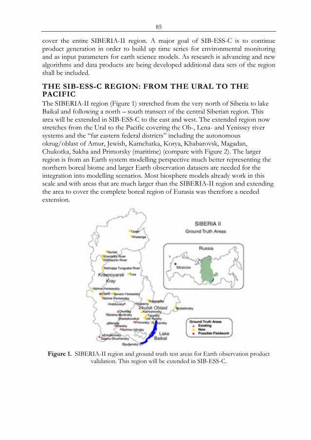
85
cover the entire SIBERIA-II region. A major goal of SIB-ESS-C is to continue product generation in order to build up time series for environmental monitoring and as input parameters for earth science models. As research is advancing and new algorithms and data products are being developed additional data sets of the region shall be included.
THE SIB-ESS-C REGION: FROM THE URAL TO THE PACIFIC The SIBERIA-II region (Figure 1) stretched from the very north of Siberia to lake Baikal and following a north – south transect of the central Siberian region. This area will be extended in SIB-ESS-C to the east and west. The extended region now stretches from the Ural to the Pacific covering the Ob-, Lena- and Yenissey river systems and the “far eastern federal districts” including the autonomous okrug/oblast of Amur, Jewish, Kamchatka, Korya, Khabarovsk, Magadan, Chukotka, Sakha and Primorsky (maritime) (compare with Figure 2). The larger region is from an Earth system modelling perspective much better representing the northern boreal biome and larger Earth observation datasets are needed for the integration into modelling scenarios. Most biosphere models already work in this scale and with areas that are much larger than the SIBERIA-II region and extending the area to cover the complete boreal region of Eurasia was therefore a needed extension.
Figure 1. SIBERIA-II region and ground truth test areas for Earth observation product
validation. This region will be extended in SIB-ESS-C.
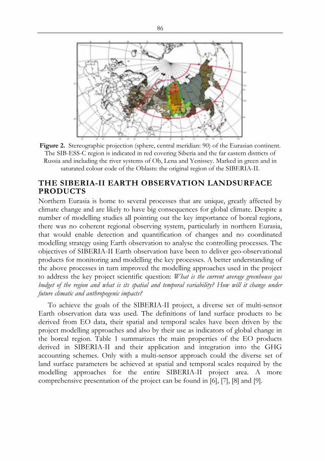
86
Figure 2. Stereographic projection (sphere, central meridian: 90) of the Eurasian continent.
The SIB-ESS-C region is indicated in red covering Siberia and the far eastern districts of Russia and including the river systems of Ob, Lena and Yenissey. Marked in green and in
saturated colour code of the Oblasts: the original region of the SIBERIA-II.
THE SIBERIA-II EARTH OBSERVATION LANDSURFACE PRODUCTS Northern Eurasia is home to several processes that are unique, greatly affected by climate change and are likely to have big consequences for global climate. Despite a number of modelling studies all pointing out the key importance of boreal regions, there was no coherent regional observing system, particularly in northern Eurasia, that would enable detection and quantification of changes and no coordinated modelling strategy using Earth observation to analyse the controlling processes. The objectives of SIBERIA-II Earth observation have been to deliver geo-observational products for monitoring and modelling the key processes. A better understanding of the above processes in turn improved the modelling approaches used in the project to address the key project scientific question: What is the current average greenhouse gas budget of the region and what is its spatial and temporal variability? How will it change under future climatic and anthropogenic impacts?
To achieve the goals of the SIBERIA-II project, a diverse set of multi-sensor Earth observation data was used. The definitions of land surface products to be derived from EO data, their spatial and temporal scales have been driven by the project modelling approaches and also by their use as indicators of global change in the boreal region. Table 1 summarizes the main properties of the EO products derived in SIBERIA-II and their application and integration into the GHG accounting schemes. Only with a multi-sensor approach could the diverse set of land surface parameters be achieved at spatial and temporal scales required by the modelling approaches for the entire SIBERIA-II project area. A more comprehensive presentation of the project can be found in [6], [7], [8] and [9].
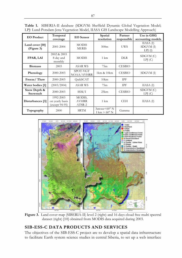
87
Table 1. SIBERIA-II database (SDGVM: Sheffield Dynamic Global Vegetation Model; LPJ: Lund-Potsdam-Jena Vegetation Model, IIASA GIS Landscape Modelling Approach)
EO Product Temporal coverage
EO Sensor Spatial
resolution Partner
responsibleUse in GHG
accounting models
Land cover [10] (Figure 3)
2001-2004 MODIS MERIS 500m UWS
IIASA (I) SDGVM (I)
LPJ (I)
FPAR, LAI 2002 & 2003
8 day and monthly
MODIS 1 km DLR SDGVM (C) LPJ (C)
Biomass 2003 ASAR WS 75m CESBIO
Phenology 2000-2003 SPOT-VGT NOAA/AVHRR 1km & 10km CESBIO SDGVM (I)
Freeze/ Thaw 2000-2003 QuikSCAT 10km IPF
Water bodies [1] (2003/2004) ASAR WS 75m IPF IIASA (I) Snow Depth &
Snowmelt 2000-2003 SSM/I 25km CESBIO SDGVM (C)
LPJ (C)
Disturbances [3]1992-2003
on yearly basis (except 94-95)
MODIS, AVHRR ATSR-2
1 km CEH IIASA (I)
Topography 2000 SRTM 3arcsec<60° N I km > 60° N Gamma -
Figure 3. Land cover map (SIBERIA-II) level 2 (right) and 16 days cloud free multi spectral
dataset (right) [10] obtained from MODIS data acquired during 2003.
SIB-ESS-C DATA PRODUCTS AND SERVICES The objectives of the SIB-ESS-C project are to develop a spatial data infrastructure to facilitate Earth system science studies in central Siberia, to set up a web interface
88
to provide access to data products created during the SIBERIA-II project, to continue remote sensing data acquisition and product generation to build up time series for a larger region in Eurasia and to integrate additional products from other projects as well as from external collaborators. The final stage of SIB-ESS-C will provide online geo-visualization and analysis tools (including a biosphere/Earth system modelling interface for registered users) for an integrated data analysis using the cluster processing structure and power provided with SIB-ESS-C. The overall structure of SIB-ESS-C will grow towards 16 - 32 processor nodes provinding enough processing power for complex modelling tasks using large area data sets.
Initial SIB-ESS-C datasets and products:
• SIBERIA-II metadata • SIBERIA-II "raw" satellite data - compare with table 1 • SIBERIA-II Earth observation products - compare with table 1 • IIASA's Landscape GIS for the SIBERIA-II region including forest
inventory information for approx. 70 test regions, • additional products from other FSU projects or external collaborators
SIB-ESS-C Services:
• Catalogue Service: providing meta data on products and procedures (search and find data),
• Coverage Service: providing direct access to datasets available from SIB-ESS-C (access and download data),
• Map Service: visualization of geographic datasets available from SIB-ESS-C,
• Analysis Service: advanced visualization tools for integrated data analysis (integration of multiple data sets, spatially and temporally),
• Customization Service: based on previous data analysis users should be enabled to retrieve customized data products according to their requirements,
• Processing Service: continuous EO-product generation, • Biosphere Modelling Service based on various datasets (final stage of the
SIB-ESS-C implementation)
THE SIB-ESS-C IMPLEMENTATION CONCEPT The overall design philosophy of SIB-ES-C follows two major principles:
i) adhere to standards to ensure interoperability and ii) implement free and open source software components whenever
possible. The architecture of SIB-ESS-C shall comprise OGC compliant components, e.g.
a Web Catalog Service for data discovery, a Web Coverage Service for data access, a Web Map Service for data viewing and in the future a Web Processing Service for on-demand product creation and triggering of biosphere modeling tasks.
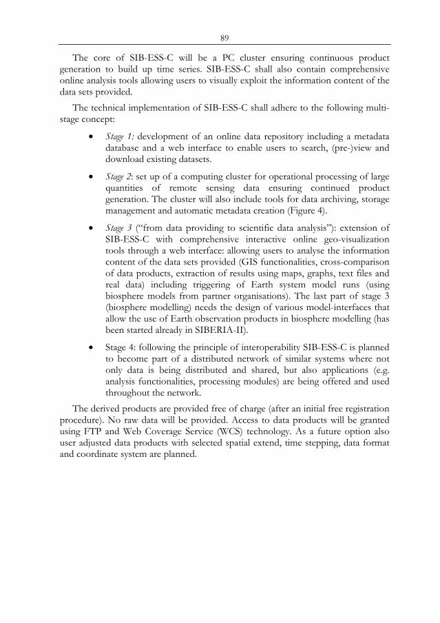
89
The core of SIB-ESS-C will be a PC cluster ensuring continuous product generation to build up time series. SIB-ESS-C shall also contain comprehensive online analysis tools allowing users to visually exploit the information content of the data sets provided.
The technical implementation of SIB-ESS-C shall adhere to the following multi-stage concept:
• Stage 1: development of an online data repository including a metadata database and a web interface to enable users to search, (pre-)view and download existing datasets.
• Stage 2: set up of a computing cluster for operational processing of large quantities of remote sensing data ensuring continued product generation. The cluster will also include tools for data archiving, storage management and automatic metadata creation (Figure 4).
• Stage 3 (“from data providing to scientific data analysis”): extension of SIB-ESS-C with comprehensive interactive online geo-visualization tools through a web interface: allowing users to analyse the information content of the data sets provided (GIS functionalities, cross-comparison of data products, extraction of results using maps, graphs, text files and real data) including triggering of Earth system model runs (using biosphere models from partner organisations). The last part of stage 3 (biosphere modelling) needs the design of various model-interfaces that allow the use of Earth observation products in biosphere modelling (has been started already in SIBERIA-II).
• Stage 4: following the principle of interoperability SIB-ESS-C is planned to become part of a distributed network of similar systems where not only data is being distributed and shared, but also applications (e.g. analysis functionalities, processing modules) are being offered and used throughout the network.
The derived products are provided free of charge (after an initial free registration procedure). No raw data will be provided. Access to data products will be granted using FTP and Web Coverage Service (WCS) technology. As a future option also user adjusted data products with selected spatial extend, time stepping, data format and coordinate system are planned.
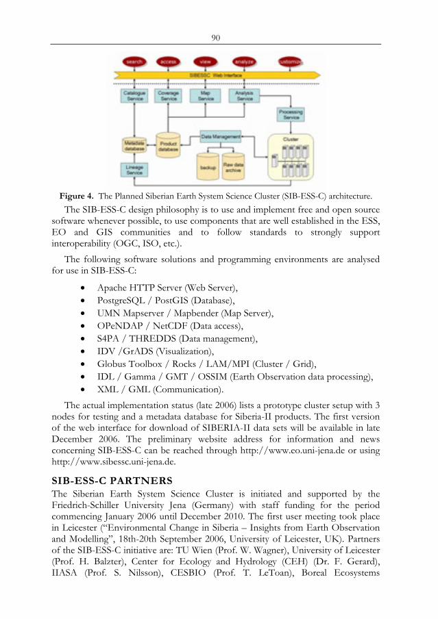
90
Figure 4. The Planned Siberian Earth System Science Cluster (SIB-ESS-C) architecture.
The SIB-ESS-C design philosophy is to use and implement free and open source software whenever possible, to use components that are well established in the ESS, EO and GIS communities and to follow standards to strongly support interoperability (OGC, ISO, etc.).
The following software solutions and programming environments are analysed for use in SIB-ESS-C:
• Apache HTTP Server (Web Server), • PostgreSQL / PostGIS (Database), • UMN Mapserver / Mapbender (Map Server), • OPeNDAP / NetCDF (Data access), • S4PA / THREDDS (Data management), • IDV /GrADS (Visualization), • Globus Toolbox / Rocks / LAM/MPI (Cluster / Grid), • IDL / Gamma / GMT / OSSIM (Earth Observation data processing), • XML / GML (Communication).
The actual implementation status (late 2006) lists a prototype cluster setup with 3 nodes for testing and a metadata database for Siberia-II products. The first version of the web interface for download of SIBERIA-II data sets will be available in late December 2006. The preliminary website address for information and news concerning SIB-ESS-C can be reached through http://www.eo.uni-jena.de or using http://www.sibessc.uni-jena.de.
SIB-ESS-C PARTNERS The Siberian Earth System Science Cluster is initiated and supported by the Friedrich-Schiller University Jena (Germany) with staff funding for the period commencing January 2006 until December 2010. The first user meeting took place in Leicester (“Environmental Change in Siberia – Insights from Earth Observation and Modelling”, 18th-20th September 2006, University of Leicester, UK). Partners of the SIB-ESS-C initiative are: TU Wien (Prof. W. Wagner), University of Leicester (Prof. H. Balzter), Center for Ecology and Hydrology (CEH) (Dr. F. Gerard), IIASA (Prof. S. Nilsson), CESBIO (Prof. T. LeToan), Boreal Ecosystems
91
Monitoring Laboratory / RAS (Dr. S. Bartalev), Sukachev Institute of Forest, RAS (Prof. E. Vaganov).
REFERENCES [1] Bartsch, A., Kidd, R., Pathe, C., Shvidenko, A. & W. Wagner 2004:
Identification of wetlands in central Siberia with ENVISAT ASAR WS data. Proceedings ENVISAT Symposium, Salzburg.
[2] Beer, C., W. Lucht, C. Schmullius, and A .Shvidenko 2006: Small net carbon dioxide uptake by Russian forests during 1981–1999, Geophys. Res. Lett., 33, L15403, doi:10.1029/2006 GL026919.
[3] George, C., C. Rowland, France Gerard and Heiko Balzter 2006: Retrospective mapping of burnt areas in Central Siberia using a modification of the normalised difference water index, Remote Sensing of Environment, Volume 104, Issue 3, 15 October 2006, Pages 346-359.
[4] Santoro, M., C.Schmullius, L.Eriksson, S.Hese 2002: The SIBERIA and SIBERIA-II projects: an overview, SPIE Crete, 2002.
[5] Shvidenko, A., and S. Nilsson 2003: Asynthesis of the impact of Russian forests on the global carbon budget for 1961–1998, Tellus, Ser. B, 55, 391–415.
[6] Schmullius, C., S. Hese, H. Balzter, W. Cramer, F. Gerard, R. Kidd, T. LeToan, W. Lucht, A. Luckman, I. McCallum, S. Nilsson, A. Petrocchi, S. Plummer, S. Quegan, A. Shvidenko, L. Skinner, S. Venevsky, S. Voigt, W. Wagner, U. Wegmüller, A. Wiesmann 2002: Sensor Systems and Data Products in SIBERIA-II – a Multi-Sensor Approach for Full Greenhouse Gas Accounting in Siberia, ForestSAT Conference 2002, Edinburgh, UK.
[7] Schmullius, C., S. Hese & SIBERIA-II Team 2002: SIBERIA-II: Sensor Systems and Data Products for Greenhouse Gas Accounting, S. Dech (Hersg.) Tagungsband 19. DFD Nutzerseminar, 15-16. Oktober 2002, S. 173-180.
[8] Schmullius, C., S. Hese, D. Knorr 2003: Siberia-II: A Multi-Sensor Approach for greenhouse Gas Accounting in Northern Eurasia, PGM (Petermanns Geographische Mitteilungen), 147, 2003/6.
[9] Schmullius, C., C. Beer, R. Gerlach, S. Hese, D. Knorr, M. Santoro, L. Skinner, A. Luckman 2005: SIBERIA-II - Multi-Sensor Land Cover Products for Greenhouse Gas Accounting of Northern Eurasia, ForestSAT Conference 2005, Conference Proceedings, Umea, Sweden.
[10] Skinner, L., and Luckman, A. 2004: Introducing a land cover map of Siberia derived from MERIS and MODIS data. Proceedings of IGARSS'04, Anchorage, 20-24 September, pp. 223-226.

92
93
Predictive vegetation mapping in Central Siberia using Earth Observation products
D. Knorr and C. Schmullius Friedrich-Schiller-University Jena, Institute for Geography, Department of Earth
Observation, email: [email protected]
ABSTRACT Traditionally, satellite-based ap10proaches of land cover classification over large areas rely on the use of input datasets from only one sensor (e.g. MODIS land cover, SPOT VGT for GLC2000 or AVHRR for IGBP) and the use of training areas. We developed an approach for the derivation of a land cover map over a 3 million km² study area in Central Siberia, which is based on the fusion of several independent satellite remote sensing products and a national soil map. Using special decision rules which rely upon landscape ecological regularities of the boreal study region, the vegetation classification could be enhanced down to species level. Such a depth of vegetation classification is needed for the regression based approach for terrestrial full carbon accounting at regional scale of the International Institute for Applied Systems Analysis (IIASA), Laxenburg, Austria. Keywords: rule based land cover classification, spatial modelling, predictive vegetation mapping.
1 INTRODUCTION The International Institute for Applied Systems Analysis (IIASA) developed as part of the EU-funded project SIBERIA-II (http://www.siberia2.uni-jena.de) a regression-based landscape ecosystem model which provides diagnostic predictions of carbon stocks and fluxes for the 3 Mio km² study region in Central Siberia [1]. In contrast to dynamic global vegetation models (DGVM), such as LPJ, which estimate net primary production (NPP) for plant functional types (PFT), the IIASA model differentiates between different vegetation classes and even tree species. Since major differences in vegetation cover are not depicted on any existing global land cover map [2], IIASA compiled a vegetation database with the necessary classification depth specifically for the regression-based carbon model. This database is represented by a GIS-based polygon vegetation map with an attributive database holding all information needed for full carbon accounting (FCA) of the terrestrial biota. It was compiled by Russian regional vegetation experts who manually identified and delineated homogenous vegetation polygons based on a variety of information sources, including in-situ measurements, forest inventory, soil and landscape maps and remote sensing data. Since this procedure is extremely labour and time consuming, and forest inventory is only conducted every 10 to 15 years, Proc. 2nd Göttingen GIS and Remote Sensing Days, 4-6 Oct. 2006, Göttingen
94
IIASA’s vegetation database is a static land cover description for the year 2003 only. A continuation for following years is not feasible.
Since vegetation is the most dynamic component of the terrestrial biosphere and therefore in the carbon cycle continuous observation is necessary. Only an automated method using consistent algorithms and continuous data retrieval would provide the needed temporal resolution for full carbon accounting.
The only cost effective source for spatially and temporally continuous data comes from Earth Observation. The problem of current global and continental land cover products is the insufficient vegetation classification for consideration of different rates of respiration and assimilation between different species.
To fulfil the requirements of the regression-based IIASA model, namely
• yearly information about vegetation distribution and disturbances, and
• detailed vegetation classification up to species level, we developed a method for vegetation classification based on a-priory knowledge about the study area and several satellite-derived datasets, including the SIBERIA-II land cover [3], digital elevation models (SRTM and GTOPO-30), MODIS Vegetation Continuous Field (VCF) products [4], the SIBERIA-II forest disturbance dataset [5], as well as a unique soil database provided by IIASA.
2 PREDICTIVE VEGETATION MAPPING Vegetation is the most influential and dynamic component of the terrestrial biosphere and represents the connection between the atmospheric and pedospheric carbon pools through photosynthesis and respiration. Therefore vegetation represents the most important driver in the greenhouse gas balance. Plant growth, species composition and distribution of vegetation communities are the result of different ecological site factors, such as the shape of relief, soil texture and, in higher latitudes, permafrost, which have all an impact on the distribution and availability of water, as well as elevation and slope aspect which influence temperature [6]. Additional influences on the ecosystem are natural and anthropogenic disturbances, such as fire, diseases, wind throw or logging, which change potential to actual vegetation cover. These relationships can be used for predictive vegetation mapping with Geographic Information Systems (GIS). When information about a region is difficult to obtain, because the study region is too large or inaccessible, relationships between vegetation distribution and mapped physical data (e.g. elevation, climate) can be used to predict vegetation composition across landscapes [7].
The use of topographic attributes (e.g. elevation, slope, aspect, curvature, topographic wetness index) derived from digital elevation models (DEMs) is among the most common variables employed in predictive vegetation mapping [7]. There are several studies [6], [7], [8] where elevation, slope, curvature and wetness index derived from DEMs have been used to map forest composition in mountainous regions.
Remote sensing data is often used as initial information about the distribution of vegetation patterns. One example for the application of GIS and remote sensing
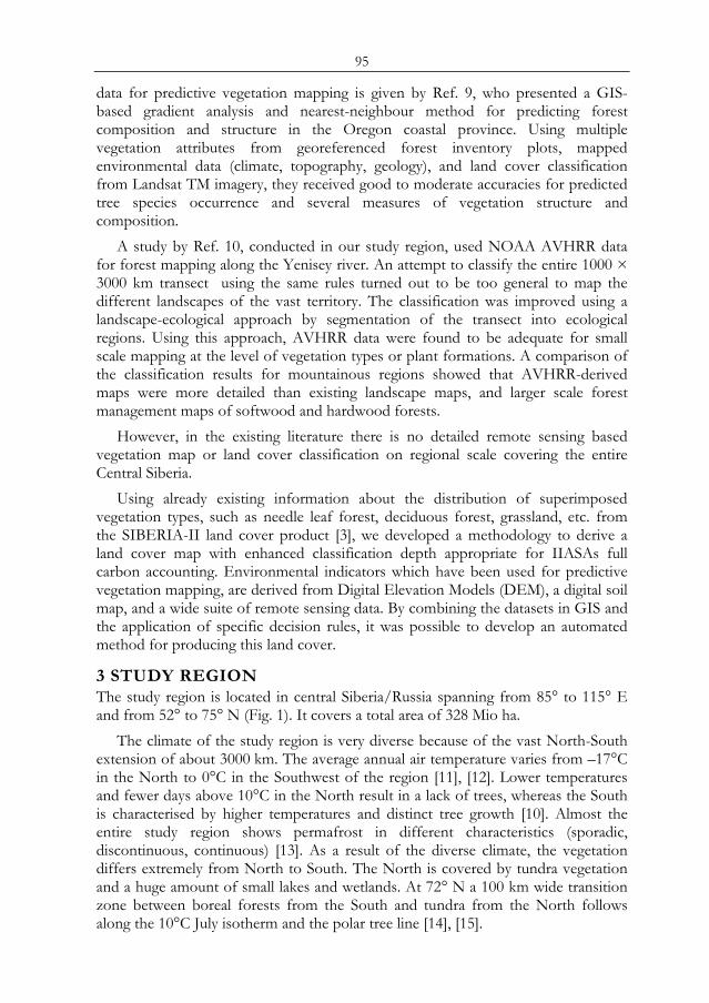
95
data for predictive vegetation mapping is given by Ref. 9, who presented a GIS-based gradient analysis and nearest-neighbour method for predicting forest composition and structure in the Oregon coastal province. Using multiple vegetation attributes from georeferenced forest inventory plots, mapped environmental data (climate, topography, geology), and land cover classification from Landsat TM imagery, they received good to moderate accuracies for predicted tree species occurrence and several measures of vegetation structure and composition.
A study by Ref. 10, conducted in our study region, used NOAA AVHRR data for forest mapping along the Yenisey river. An attempt to classify the entire 1000 × 3000 km transect using the same rules turned out to be too general to map the different landscapes of the vast territory. The classification was improved using a landscape-ecological approach by segmentation of the transect into ecological regions. Using this approach, AVHRR data were found to be adequate for small scale mapping at the level of vegetation types or plant formations. A comparison of the classification results for mountainous regions showed that AVHRR-derived maps were more detailed than existing landscape maps, and larger scale forest management maps of softwood and hardwood forests.
However, in the existing literature there is no detailed remote sensing based vegetation map or land cover classification on regional scale covering the entire Central Siberia.
Using already existing information about the distribution of superimposed vegetation types, such as needle leaf forest, deciduous forest, grassland, etc. from the SIBERIA-II land cover product [3], we developed a methodology to derive a land cover map with enhanced classification depth appropriate for IIASAs full carbon accounting. Environmental indicators which have been used for predictive vegetation mapping, are derived from Digital Elevation Models (DEM), a digital soil map, and a wide suite of remote sensing data. By combining the datasets in GIS and the application of specific decision rules, it was possible to develop an automated method for producing this land cover.
3 STUDY REGION The study region is located in central Siberia/Russia spanning from 85° to 115° E and from 52° to 75° N (Fig. 1). It covers a total area of 328 Mio ha.
The climate of the study region is very diverse because of the vast North-South extension of about 3000 km. The average annual air temperature varies from –17°C in the North to 0°C in the Southwest of the region [11], [12]. Lower temperatures and fewer days above 10°C in the North result in a lack of trees, whereas the South is characterised by higher temperatures and distinct tree growth [10]. Almost the entire study region shows permafrost in different characteristics (sporadic, discontinuous, continuous) [13]. As a result of the diverse climate, the vegetation differs extremely from North to South. The North is covered by tundra vegetation and a huge amount of small lakes and wetlands. At 72° N a 100 km wide transition zone between boreal forests from the South and tundra from the North follows along the 10°C July isotherm and the polar tree line [14], [15].
96
Figure 1. Location of study region in Russia and administrative regions.
Southwards of 72° N boreal forest (taiga) covers almost the entire study region. It consists to 85 % of coniferous species (pine, spruce, fir, larch and cedar) and to 13% of the deciduous broadleaved species birch and aspen. The differences in climate cause also a regional deviation in different taiga zones [13]. Forest tundra and sparse taiga cover the southern part of the North Siberian plain and the major part of the plateaus Putorana and Anabarskoe and are represented mainly by larch. Spruce occurs only in the extreme West and south-western parts [16], [17], [18]. The subzones of middle and southern taiga occupy the major part of the study region. Vegetation is represented by typical boreal forests, basically formed by larch and pine. The southern taiga of non-mountain regions is represented by pine, larch, and spruce-fir forests with admixtures of birch and aspen [12].
In the southern part of the Krasnoyarsk Kray and eastern part of the Republic Khakasia, enclosed by the high mountains of East and West Sayan, a relatively small area of steppe and forest steppe vegetation is located. Secondary deciduous forests, dominated by birch and aspen, as well as pine forest are common in the forest steppe region. Approximately two thirds of this area is transformed to agricultural land, mainly cultivated pastures and arable lands.
4 METHODOLOGY AND DATA SOURCES The process of producing a land cover map with enhanced vegetation classification was realised by post-classification of the already existing SIBERIA-II land cover map for the year 2003 [3], derived from MODIS 500 m data. The 16 classes of this product were successively broken down into more detailed classes which were adopted from IIASA’s vegetation map. The post-classification was based on the values of several independent input data sets and specifically developed decision rules which rely on landscape ecological regularities of the study region (e.g. altitudinal belts in mountains), and on information coming from the IIASA vegetation map and several digital forest inventory test sites.
Because of the different climatic conditions and vegetation zones, it was necessary to split the region into several smaller subregions and to develop different
97
rule sets for each of them. Seven eco-regions (“tundra and forest tundra”, “northern taiga”, “middle taiga”, “southern taiga”, “mountain middle taiga”, “mountain southern taiga”, “steppe and forest steppe”) have been separated based on bioclimatic and floristic criteria (see Fig. 1). Based on these eco-regions it was possible to check the SIBERIA-II land cover product for obvious misclassifications and to reclassify the relevant pixels after plausibility rules. For example, if pixels in the eco-region “tundra and forest tundra” are classified as agriculture, steppe or deciduous broadleaf forest, they are obviously misclassified. In such cases these pixels are assigned to new classes, which are more plausible for the specific eco-region. Since in all cases there is more than one possible class, the final assignment to one class followed in later classification steps using other input data sets.
Most of the pixels from 500 m resolution imagery contain a mixture of land cover types, which had significant implications if a hard classification is to be derived from such data sets [19]. We avoided this problem using the MODIS Vegetation Continuous Field (VCF) product [4] and applying a fuzzy classification system, which allows several land cover classes per pixel. To realise this, our land cover was also separated in three layers, namely a forest map, a map of non-forest vegetation classes and a map of unvegetated areas with the additional information of the percentage of each land cover class per pixel. So, also pixels with a lower percentage than 15% tree cover, which was used for the hard classification of forest in the SIBERIA-II land cover, can receive a specific tree species class in the forest layer. Every pixel with a minimum of 5% herbaceous cover appears in the non-forest layer of the continuous field land cover. All cells in all eco-regions, that have a VCF tree cover below 5% and a VCF barren ground cover more than 80% were assigned to the class “barren ground”, no matter to which initial class they belong. Only in the eco-region “tundra and forest tundra”, the threshold was set to 95%. In this eco-region pixels with a VCF barren ground value of 80 – 95% were assigned to the class “spotty tundra”. This tundra type consists mainly of bare rocks and soil with only some small patches of lichens and mosses [20], and appears in the study region only on the Taymir peninsula. The thresholds were chosen by comparison with the IIASA vegetation map.
Coming back to the above mentioned example of the misclassified pixels in the eco-region “tundra and forest tundra”, the MODIS VCF and appendant decision rules help to decide, if these pixels are “barren ground”, “larch forest” or “wetland/tundra”. In the latter case, further rules have to be applied for the decision between “wetland” or “tundra”.
The first set of decision rules for the refinement of the 16 initial land cover classes is related to the topographical location of the pixels in means of elevation. This information is derived from a digital elevation model (DEM) with 500 m spatial resolution, which is based on the Shuttle Radar Topography Mission (SRTM-3) DEM, available for the latitudes below 60° North and the GTOPO-30 DEM [21] for the areas above 60° N. There are two concepts behind the application of elevation. The first one is the altitudinal zonation of vegetation in mountains. The vegetation composition of the different altitudinal belts is taken from literature [16], [17], [22], [23], [24], [25], [26]. The second application scheme of elevation
98
information was applied in the non-mountainous regions, where it helped to separate subregions inside the eco-regions which have different tree species or types of wetlands. In this way it was possible to separate the lower West Siberian Lowlands from the higher Krasnoyarsk Kraj. For further separation of tree species and wetlands in the non-mountainous regions, information from a GIS-based soil database, provided by IIASA at a scale of 1:1 Mio was used.
Here, information about the soil texture helped to separate tree species. For wetland detection the soil map was used to produce a mask containing all polygons indicated as “peaty” soil types with a soil thickness more than 40 cm. All initial land cover classes besides the forest classes were assigned to specific wetland types if they coincide with this mask.
For the tundra eco-region another rule for wetland detection was applied. One problem is the vast amount of small and shallow lakes in this region, of which a huge part is not represented in the 500 m resolution of MODIS. Shallow lakes play an important role in wetland identification. Since the depth is often related to the size of those lakes, a high density of single permanently inundated basins below a size of 8 ha in the sub-arctic regions indicate tundra wetlands according to the Ramsar classification scheme [27]. The information about small permanent open water bodies was derived from ENVISAT ASAR Wide Swath data for the years 2003 and 2004 with a spatial resolution of 150 m [28]. To keep these lakes in the land cover with a resolution of 500 m these lakes and the land between them were aggregated to one polygon indicated as Ramsar wetland type Vt (tundra wetlands). To realise this a density analysis with a search radius of 50 km and a density threshold of 5000 m²/ km² of water surface area was performed by Ref. 27. For our product we combined the resulting polygon with the information from the soil database and classified all pixels as “tundra wetland”, which are located in this polygon and coincide with peaty soils thicker than 40 cm.
The last step in the classification process is the identification of disturbed areas. For this rule set the SIBERIA-II disturbance product [5] with information about the period 1992 to 2003 is used. All pixels, except of initial forest classes, which coincide with polygons of the disturbance map are assigned as “burnt area” if the MODIS VCF tree cover is lower than 5%. If it is higher than 5% it could mean that the vegetation cover changed due to disturbances after 2001, the year of the MODIS VCF. In such cases the year of the disturbances is applied: Only disturbances after 2001 lead to the class “burnt area”. Pixels which were not classified as forest in the initial SIBERIA-II land cover, but in our land cover because of the MODIS VCF value, and that were disturbed before 2001 receive the classes “birch”, “pine” or “larch” (depending on eco-region) as secondary forest after fire.
The stepwise fusion of input data sets and implementation of classification rules has been realised in ESRI’s (Environmental Systems Research Institute, Redlands/California) GIS ArcINFO and was automated using a routine written in ArcInfo Macro Language (AML).
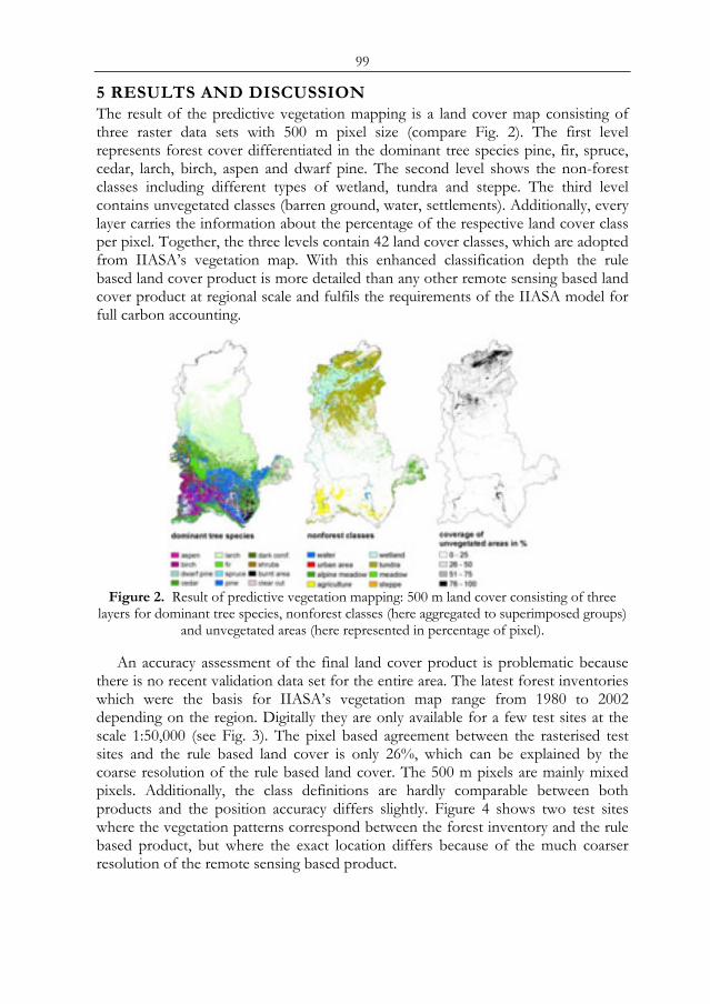
99
5 RESULTS AND DISCUSSION The result of the predictive vegetation mapping is a land cover map consisting of three raster data sets with 500 m pixel size (compare Fig. 2). The first level represents forest cover differentiated in the dominant tree species pine, fir, spruce, cedar, larch, birch, aspen and dwarf pine. The second level shows the non-forest classes including different types of wetland, tundra and steppe. The third level contains unvegetated classes (barren ground, water, settlements). Additionally, every layer carries the information about the percentage of the respective land cover class per pixel. Together, the three levels contain 42 land cover classes, which are adopted from IIASA’s vegetation map. With this enhanced classification depth the rule based land cover product is more detailed than any other remote sensing based land cover product at regional scale and fulfils the requirements of the IIASA model for full carbon accounting.
Figure 2. Result of predictive vegetation mapping: 500 m land cover consisting of three
layers for dominant tree species, nonforest classes (here aggregated to superimposed groups) and unvegetated areas (here represented in percentage of pixel).
An accuracy assessment of the final land cover product is problematic because there is no recent validation data set for the entire area. The latest forest inventories which were the basis for IIASA’s vegetation map range from 1980 to 2002 depending on the region. Digitally they are only available for a few test sites at the scale 1:50,000 (see Fig. 3). The pixel based agreement between the rasterised test sites and the rule based land cover is only 26%, which can be explained by the coarse resolution of the rule based land cover. The 500 m pixels are mainly mixed pixels. Additionally, the class definitions are hardly comparable between both products and the position accuracy differs slightly. Figure 4 shows two test sites where the vegetation patterns correspond between the forest inventory and the rule based product, but where the exact location differs because of the much coarser resolution of the remote sensing based product.
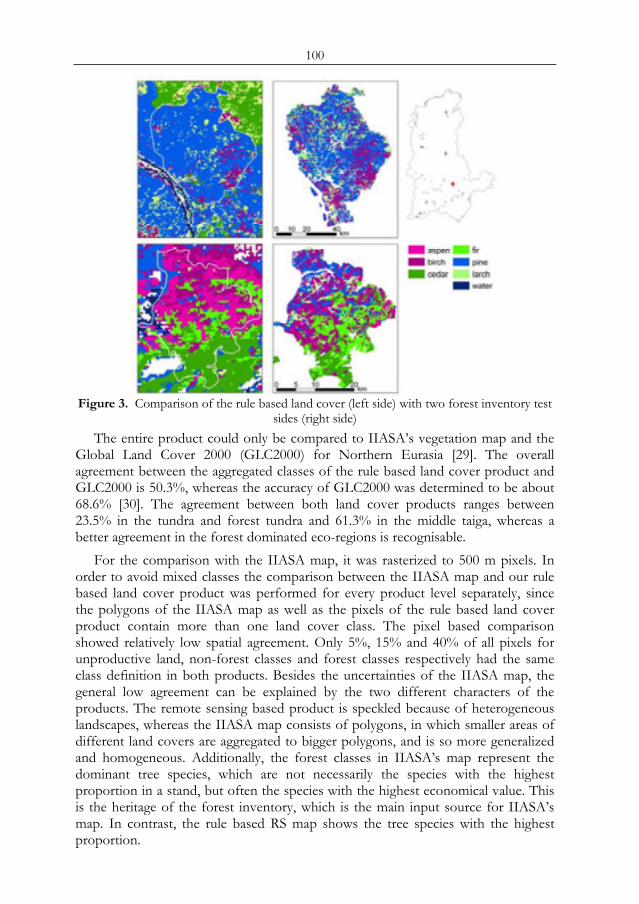
100
Figure 3. Comparison of the rule based land cover (left side) with two forest inventory test
sides (right side) The entire product could only be compared to IIASA’s vegetation map and the
Global Land Cover 2000 (GLC2000) for Northern Eurasia [29]. The overall agreement between the aggregated classes of the rule based land cover product and GLC2000 is 50.3%, whereas the accuracy of GLC2000 was determined to be about 68.6% [30]. The agreement between both land cover products ranges between 23.5% in the tundra and forest tundra and 61.3% in the middle taiga, whereas a better agreement in the forest dominated eco-regions is recognisable.
For the comparison with the IIASA map, it was rasterized to 500 m pixels. In order to avoid mixed classes the comparison between the IIASA map and our rule based land cover product was performed for every product level separately, since the polygons of the IIASA map as well as the pixels of the rule based land cover product contain more than one land cover class. The pixel based comparison showed relatively low spatial agreement. Only 5%, 15% and 40% of all pixels for unproductive land, non-forest classes and forest classes respectively had the same class definition in both products. Besides the uncertainties of the IIASA map, the general low agreement can be explained by the two different characters of the products. The remote sensing based product is speckled because of heterogeneous landscapes, whereas the IIASA map consists of polygons, in which smaller areas of different land covers are aggregated to bigger polygons, and is so more generalized and homogeneous. Additionally, the forest classes in IIASA’s map represent the dominant tree species, which are not necessarily the species with the highest proportion in a stand, but often the species with the highest economical value. This is the heritage of the forest inventory, which is the main input source for IIASA’s map. In contrast, the rule based RS map shows the tree species with the highest proportion.
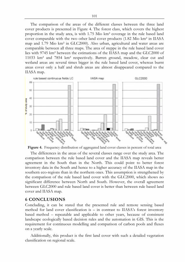
101
The comparison of the areas of the different classes between the three land cover products is presented in Figure 4. The forest class, which covers the highest proportion in the study area, is with 1.75 Mio km² coverage in the rule based land cover comparable with the two other land cover products (1.82 Mio km² in IIASA map and 1.79 Mio km² in GLC2000). Also urban, agricultural and water areas are comparable between all three maps. The area of steppe in the rule based land cover lies with 9745 km² between the estimations of the IIASA map and the GLC2000 of 11033 km² and 7854 km² respectively. Barren ground, meadow, clear cut and wetland areas are several times bigger in the rule based land cover, whereas burnt areas cover only a half and shrub areas are almost disappeared compared to the IIASA map.
Figure 4. Frequency distribution of aggregated land cover classes in percent of total area
The differences in the areas of the several classes range over the study area. The comparison between the rule based land cover and the IIASA map reveals better agreement in the South than in the North. This could point to better forest inventory data in the South and hence to a higher accuracy of the IIASA map in the southern eco-regions than in the northern ones. This assumption is strengthened by the comparison of the rule based land cover with the GLC2000, which shows no significant difference between North and South. However, the overall agreement between GLC2000 and rule based land cover is better than between rule based land cover and IIASA map.
6 CONCLUSIONS Concluding, it can be stated that the presented rule and remote sensing based method for land cover classification is – in contrast to IIASA’s forest inventory based method – repeatable and applicable to other years, because of consistent landscape ecologically based decision rules and the automation in GIS. This is the requirement for continuous modelling and comparison of carbon pools and fluxes on a yearly scale.
Additionally, this product is the first land cover with such a detailed vegetation classification on regional scale.
102
Uncertainties of this land cover product are expected to be reduced, with the forthcoming availability of the yearly MODIS VCF data for 2001 to 2005. The updating of the rule based land cover product for the following years is enabled by the availability of all other required remote sensing products in near future via the Siberian Earth System Science Cluster (SIB-ESS-C, http://www.sibessc.uni-jena.de).
ACKNOWLEDGMENTS The idea and methodology for this study has been developed during the Young
Scientists Summer Program at the International Institute for Applied System Analysis in 2005. Special thanks are directed to Anatoly Shvidenko and Ian McCallum.
REFERENCES 1 Shvindenko, A., Shepashenko D. Nilsson, S. & Bouloui, Y., accepted: Semi-empirical
Models for assessing biological productivity of Northern Eurasia forests. Ecological Modelling.
2 Walker, D.A., 2000: Hierarchical subdivition of arctic tundra based on vegetation response to climate, parent material and topography. Global Change Biology 8 (Suppl.1), pp. 19 – 34.
3 Skinner, L. and Luckman, A., 2003: Deriving Landcover Information over Siberia using MERIS and MODIS data. Proceedings of MERIS User Workshop, ESA-ESRIN, Frascati, 10-13 November, CD-ROM.
4 Hansen, M.C., DeFries, R.S., Townshend, J.R.G., Carroll, M., Dimiceli, C. and Sohlberg, R.A., 2003: Global Percent Tree Cover at a Spatial Resolution of 500 Meters: First Results of the MODIS Vegetation Continuous Field Algorithm. Earth Interactions 7 (10), pp. 1 – 15.
5 Georges, C. Rowland, C., Gerard, F. and Balzter, H., 2006: Retrospective mapping of burnt areas in Central Siberia using a modification of the normalised differenced water index. Remote Sensing of Enviroment 104 (3), pp. 346 – 359.
6 Pfeffer, K., Pebesma, E.J. and Burrough, P.A., 2003: Mapping alpine vegetation using vegetation observations and topographic attributes. Landscape ecology 18, pp. 759 – 776.
7 Vogiatzakis, I.N., 2003: GIS-based Modelling and Ecology: A Review of Tools and Methods.- Geographical Paper No. 170, Department of Geography, The University of Reading, Whiteknights (www.geog.reading.ac.uk/Research/Papers/GP170.pdf).
8 Bolstad, P.V., Swank, W. and Vose, J., 1998, Predicting Southern Appalachian overstory vegetation with digital terrain data. Landscape ecology 13, 271 -283.
9 Ohman, J. and Gregory, M., 2002: Predictive Mapping of forest composition and structure with direct gradient analysis and nearest- neighbor imputation in coastal Oregon, U.S.A. Canadian Journal of Forest Research 32, pp. 725 – 741.
10 Kharuk, V. I. , Ranson, K. J., Burenina, T. A. and Fedorova, E. V. , 2003: Mapping of Siberian forest landscapes along the Yenisey transect with AVHRR. International Journal of Remote Sensing 24, pp. 23-37.
11 Lucht, W., Schaphoff, S., Schröder, B. and Erbrecht, T., 2003, Trends in Regional Carbon Budget. unpublished deliverable 7000 A.2 of SIBERA-II project.
12 Rojkov, V.A., Gorshkova, M.A., Rukhovich, D.I., Kovaleva, P.V., Nilsson, S., Shvidenko, A. and McCallum, I., 2003, Deliverable 21 - Soil map and database, and Deliverable 22 - Accuracy assessment of soil map.- unpublished deliverables of Siberia-II project.

103
13 Walter, H. and Breckle, S.-W., 1994: Ökologie der Erde Band 3 – Spezielle Ökologie der gemäßigten Breiten und Arktischen Zonen Euro-Nordeurasiens. Gustav Fischer Verlag, Jena.
14 Grabherr, G., 1997: Farbatlas Ökosysteme der Erde. Ulmer, Stuttgart. 15 Schultz, J., 1995: The Ecozones of the World- The ecological divisions of the
Geosphere. Springer, Berlin. 16 Abaimov, A.P., Bondarev, A.I., Zyrjanova, O.A. and Shitova, S.A., 1987: Forests of
Krasnoyarsk polar area. Nauva, Novosibirsk, [in Russian]. 17 Zhukov, A.B., 1969: Forests of the USSR- Volume 4. Forests of Ural, Siberia and Far
East. Nauka, Moscow, [in Russian]. 18 Federal Forest Service of Russia, 1999: Forest Fund of Russia (state by 1.01.1998).
Moscow, [in Russian]. 19 George, C., Rowland, C., Roscher, M., Gerard, F. and Balzter, H., 2004: Description of
Scaling Approaches. unpublished deliverable 15 of SIBERIA-II project. 20 ielgolaski, F.E., 1997: Ecosystems of the World 3 – Polar and Alpine Tundra. Elsevier,
Amsterdam. 21 Distributed Active Archive Center, 2004: GTOPO30 Documentation.
http://edcdaac.usgs.gov/gtopo30/README.asp#h31 22 Buzikin, A.I., 1977: Forests of middle Priangare.- Nauva, Novisibirsk, [in Russian]. 23 Food and Agriculture Organisation (FAO), 2001: Global Forest resource Assessment
2000 – main report. FAO Forestry Paper 140, Rome. 24 Polykarpov, N.I., Chabanova, N.M. and Nazimova, D.I., 1986: Climate and mountain
forests of Southern Siberia.Nauva, Novosibirsk, [in Russian]. 25 Popov, L.V., 1982: Southern Taiga forests of middle Siberia. Irkutsk State University,
Irkutsk. 26 Semechkin, I.V. (Ed.), 1985: Cedar forests of Siberia. Wauka, Novosibirsk, [in Russian]. 27 Bartsch, A., Kidd, R., Pathe, C., Scipal, K. and Wagner, W., accepted: Satellite radar
imagery for monitoring inland wetlands in boreal and subarctic environments. Journal of Aquatic Conservation: Marine and Freshwater Ecosystems (radar special issue, INTECOL Wetlands conference 2004).
28 Bartsch, A., Pathe, C., Scipal, K. and Wagner, W., submitted: Detection of permanent open water surfaces in central Siberia with ENVISAT ASAR wide swath data with special emphasis on the estimation of methane fluxes from tundra wetlands.- Nordic Hydrology.
29 Bartalev, S.A., Belward, A.S., Erchov, D.V., Isaev, A.S., Bartholomé, E., Gond, V., Vogt, P., Achard, F., Zubkov, A.M., Mollicone, D., Savin, I.Yu, Fritz, S., Repina, G. and Hartley, A., 2003, The Land Cover Map for Northern Eurasia for the Year 2000. GLC2000 database, European Commission Joint Research Centre, 2003. http://www.gvm.jrc.it/glc2000.
30 Mayaux, P., Eva, H., Gallego, J., Strahler, A.H., Herold, M., Agrawal, S., Naumov, S., De Miranda, E.E., Di Bella, C.M., Ordoyne, C., Kopin, Y. and Roy, P.S., 2006: Validation of the global land cover 2000 map. IEEE Transactions on Geoscience and Remote Sensing, 44(7,1), pp. 1728- 1739.

104
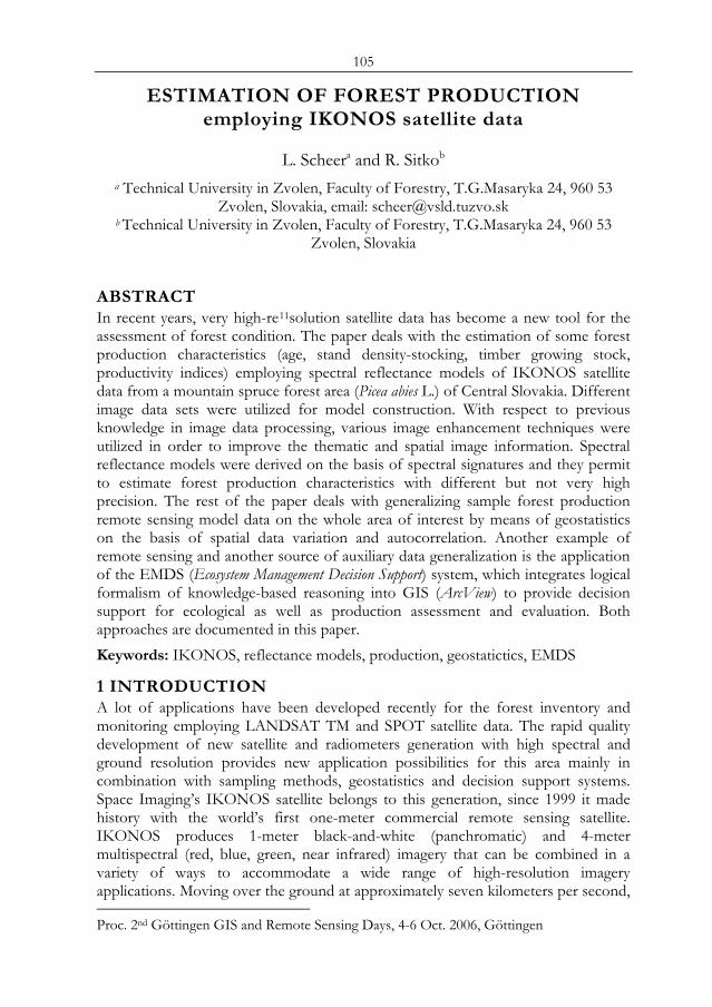
105
ESTIMATION OF FOREST PRODUCTION employing IKONOS satellite data
L. Scheera and R. Sitkob
a Technical University in Zvolen, Faculty of Forestry, T.G.Masaryka 24, 960 53 Zvolen, Slovakia, email: [email protected]
b Technical University in Zvolen, Faculty of Forestry, T.G.Masaryka 24, 960 53 Zvolen, Slovakia
ABSTRACT In recent years, very high-re11solution satellite data has become a new tool for the assessment of forest condition. The paper deals with the estimation of some forest production characteristics (age, stand density-stocking, timber growing stock, productivity indices) employing spectral reflectance models of IKONOS satellite data from a mountain spruce forest area (Picea abies L.) of Central Slovakia. Different image data sets were utilized for model construction. With respect to previous knowledge in image data processing, various image enhancement techniques were utilized in order to improve the thematic and spatial image information. Spectral reflectance models were derived on the basis of spectral signatures and they permit to estimate forest production characteristics with different but not very high precision. The rest of the paper deals with generalizing sample forest production remote sensing model data on the whole area of interest by means of geostatistics on the basis of spatial data variation and autocorrelation. Another example of remote sensing and another source of auxiliary data generalization is the application of the EMDS (Ecosystem Management Decision Support) system, which integrates logical formalism of knowledge-based reasoning into GIS (ArcView) to provide decision support for ecological as well as production assessment and evaluation. Both approaches are documented in this paper. Keywords: IKONOS, reflectance models, production, geostatictics, EMDS
1 INTRODUCTION A lot of applications have been developed recently for the forest inventory and monitoring employing LANDSAT TM and SPOT satellite data. The rapid quality development of new satellite and radiometers generation with high spectral and ground resolution provides new application possibilities for this area mainly in combination with sampling methods, geostatistics and decision support systems. Space Imaging’s IKONOS satellite belongs to this generation, since 1999 it made history with the world’s first one-meter commercial remote sensing satellite. IKONOS produces 1-meter black-and-white (panchromatic) and 4-meter multispectral (red, blue, green, near infrared) imagery that can be combined in a variety of ways to accommodate a wide range of high-resolution imagery applications. Moving over the ground at approximately seven kilometers per second, Proc. 2nd Göttingen GIS and Remote Sensing Days, 4-6 Oct. 2006, Göttingen
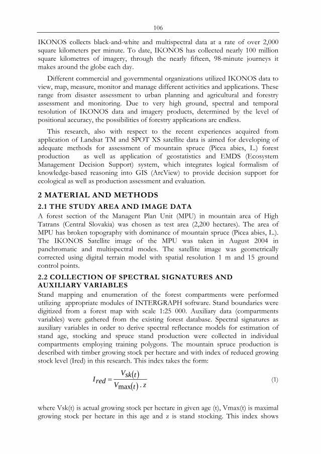
106
IKONOS collects black-and-white and multispectral data at a rate of over 2,000 square kilometers per minute. To date, IKONOS has collected nearly 100 million square kilometres of imagery, through the nearly fifteen, 98-minute journeys it makes around the globe each day.
Different commercial and governmental organizations utilized IKONOS data to view, map, measure, monitor and manage different activities and applications. These range from disaster assessment to urban planning and agricultural and forestry assessment and monitoring. Due to very high ground, spectral and temporal resolution of IKONOS data and imagery products, determined by the level of positional accuracy, the possibilities of forestry applications are endless.
This research, also with respect to the recent experiences acquired from application of Landsat TM and SPOT XS satellite data is aimed for developing of adequate methods for assessment of mountain spruce (Picea abies, L.) forest production as well as application of geostatistics and EMDS (Ecosystem Management Decision Support) system, which integrates logical formalism of knowledge-based reasoning into GIS (ArcView) to provide decision support for ecological as well as production assessment and evaluation.
2 MATERIAL AND METHODS
2.1 THE STUDY AREA AND IMAGE DATA A forest section of the Managent Plan Unit (MPU) in mountain area of High Tatrans (Central Slovakia) was chosen as test area (2,200 hectares). The area of MPU has broken topography with dominance of mountain spruce (Picea abies, L.). The IKONOS Satellite image of the MPU was taken in August 2004 in panchromatic and multispectral modes. The satellite image was geometrically corrected using digital terrain model with spatial resolution 1 m and 15 ground control points. 2.2 COLLECTION OF SPECTRAL SIGNATURES AND AUXILIARY VARIABLES Stand mapping and enumeration of the forest compartments were performed utilizing appropriate modules of INTERGRAPH software. Stand boundaries were digitized from a forest map with scale 1:25 000. Auxiliary data (compartments variables) were gathered from the existing forest database. Spectral signatures as auxiliary variables in order to derive spectral reflectance models for estimation of stand age, stocking and spruce stand production were collected in individual compartments employing training polygons. The mountain spruce production is described with timber growing stock per hectare and with index of reduced growing stock level (Ired) in this research. This index takes the form:
( )( ) ztVtskV
redI.max
= (1)
where Vsk(t) is actual growing stock per hectare in given age (t), Vmax(t) is maximal growing stock per hectare in this age and z is stand stocking. This index shows
107
production situation only with respect to site quality and also it takes stand stocking into account. Also another stand productivity indices (index of absolute growing stock level, index of relative growing stock level) were recently utilized in conjunction with Spot XS and Landsat TM satellite data for estimation of forest production [2]. However, results confirmed the most satisfactory relationship between the index of reduced growing stock level, therefore it was also apply in this research.
The ground data of the variables of interest (timber growing stock per hectare and stocking) were measured in single compartments and in combination with corresponding spectral signature were used in order to derive spectral regression models for the estimation of timber growing stock per hectare and Ired from satellite data. In addition to spectral signatures, the age of the forest compartment was employed as an auxiliary variable because it could be easily determined from previous forest management plans and could be projected to the current data.
3 RESULTS AND DISSCUSSION
3.1 REFLECTANCE MODELS FOR ESTIMATION OF FOREST PRODUCTION Spectral signatures for estimation of forest production were obtained from different original and enhanced image data. The topographic normalization, PCA analysis, HIS transformation and different spectral indices were utilized for original image data enhancement. With respect to recent knowledge with vegetation cover classification, image texture was also employed in enhancement approaches for forest production estimation. Mainly for estimation of stand density – stocking, was expected significant contribution of this image variable. The texture with different algorithms was analysed, which are based on evaluation of image spectral variation in various selected matrices 3x3, 5x5 or 7x7 pixels. Some of them are listed in Tab. 1. Totally more than 120 reflectance models were evaluated, simple and multiple, linear and exponential models. The parameters of the best spectral reflectance models for estimation of stand age, stocking, growing stock per hectare and Ired are listed in Tab.2. All models are significant (P=0.95); at simple regression correlation coefficients vary from 0.5 to 0.72, where the dependent forest variable is a function of its mean spectral signature of enhanced image data. With respect to previous knowledge, also transformed variable was introduced, which employs the ratio between the square of spectral signature and the age of the compartment.
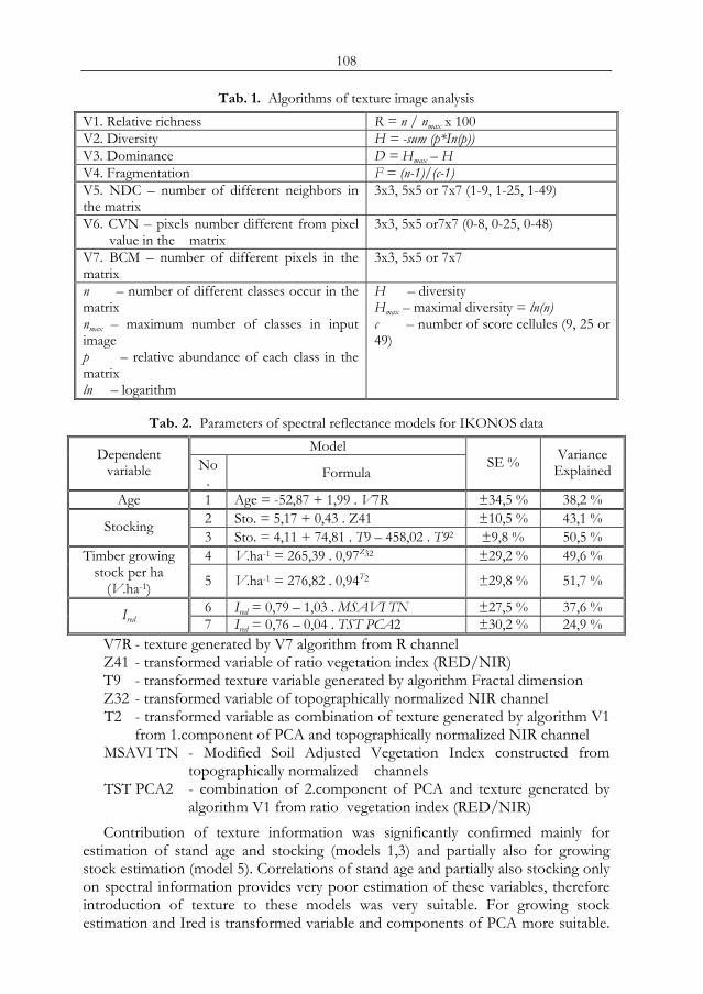
108
Tab. 1. Algorithms of texture image analysis V1. Relative richness R = n / nmax x 100 V2. Diversity H = -sum (p*In(p)) V3. Dominance D = Hmax – H V4. Fragmentation F = (n-1)/(c-1) V5. NDC – number of different neighbors in the matrix
3x3, 5x5 or 7x7 (1-9, 1-25, 1-49)
V6. CVN – pixels number different from pixel value in the matrix
3x3, 5x5 or7x7 (0-8, 0-25, 0-48)
V7. BCM – number of different pixels in the matrix
3x3, 5x5 or 7x7
n – number of different classes occur in the matrix nmax – maximum number of classes in input image
p – relative abundance of each class in the matrix ln – logarithm
H – diversity
Hmax – maximal diversity = ln(n) c – number of score cellules (9, 25 or 49)
Tab. 2. Parameters of spectral reflectance models for IKONOS data Model Dependent
variable No. Formula
SE % Variance Explained
Age 1 Age = -52,87 + 1,99 . V7R ±34,5 % 38,2 % 2 Sto. = 5,17 + 0,43 . Z41 ±10,5 % 43,1 % Stocking 3 Sto. = 4,11 + 74,81 . T9 – 458,02 . T92 ±9,8 % 50,5 % 4 V.ha-1 = 265,39 . 0,97Z32 ±29,2 % 49,6 % Timber growing
stock per ha (V.ha-1) 5 V.ha-1 = 276,82 . 0,94T2 ±29,8 % 51,7 %
6 Ired = 0,79 – 1,03 . MSAVI TN ±27,5 % 37,6 % Ired 7 Ired = 0,76 – 0,04 . TST PCA2 ±30,2 % 24,9 % V7R - texture generated by V7 algorithm from R channel Z41 - transformed variable of ratio vegetation index (RED/NIR) T9 - transformed texture variable generated by algorithm Fractal dimension Z32 - transformed variable of topographically normalized NIR channel T2 - transformed variable as combination of texture generated by algorithm V1
from 1.component of PCA and topographically normalized NIR channel MSAVI TN - Modified Soil Adjusted Vegetation Index constructed from
topographically normalized channels TST PCA2 - combination of 2.component of PCA and texture generated by
algorithm V1 from ratio vegetation index (RED/NIR) Contribution of texture information was significantly confirmed mainly for
estimation of stand age and stocking (models 1,3) and partially also for growing stock estimation (model 5). Correlations of stand age and partially also stocking only on spectral information provides very poor estimation of these variables, therefore introduction of texture to these models was very suitable. For growing stock estimation and Ired is transformed variable and components of PCA more suitable.
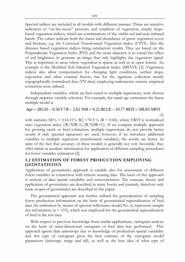
109
Spectral indices are included in all models with different manner. These are sensitive indicators of “on-the-scene” presence and condition of vegetation, mainly slope-based vegetation indices, which are combinations of the visible red and near infrared bands. The values indicate both the status and abundance of green vegetation cover and biomass, e.g. the Corrected Transformed Vegetation Index (CTVI). Also the distance based vegetation indices bring satisfactory results. They are based on the Perpendicular Vegetation Index (PVI) and the main objective is to cancel the effect of soil brightness to generate an image that only highlights the vegetation signal. This is important in areas where vegetation is sparse as well as in open forests. An example is the Modified Soil-Adjusted Vegetation Index (MSAVI) [1]. Vegetation indices also allow compensation for changing light conditions, surface slope, exposition and other external factors, but for the signature collection mostly topographically normalized data (TN data) employing radiometric statistic empirical correction were utilized.
Independent variables, which are best suited to multiple regressions, were chosen through stepwise variable selection. For example, for stand age estimation the linear multiple model is
NRVIREDBLUENIRRVAge 83.18877.1022.962.2756.081.285 +−+−−= (2)
with statistics SE% = ±14.11%, R2 =70.3 % (R = 0.84), where VRVI is normalized ratio vegetation index ((R/NIR-1)/(R/NIR+1)). If we compare multiple approach for growing stock or Ired estimation, multiple regressions do not provide better results if only spectral signatures are used; however, if we introduce additional variables to multiple regression (transformed variables), the results are better. In spite of the fact that accuracy of these models is generally not very favorable, they offer initial or auxiliary information for application of different sampling procedures for forest variables estimation [2]. 3.2 ESTIMATION OF FOREST PRODUCTION EMPLOYING GEOSTATISTICS Application of geostatistics approach is suitable also for assessment of different forest variables in connection with remote sensing data. The basis of this approach is analysis of data spatial variability and autocorrelation. The concept, theory and application of geostatistics are described in many books and journals, therefore only basic scopes of geostatistics are described in this paper.
The geostatistical approach was further utilised for generalization of sampling forest production information on the basis of geostatistical regionalization of Ired data. Its estimation by means of spectral reflectance model No. 6, represents sample dot information (n = 153), which was employed for the geostatistical regionalization of Ired in the test area.
With respect to previous knowledge from similar applications, variogram analysis on the basis of omni-directional variogram of Ired data was performed. This approach ignore data anisotropy due to knowledge of production spatial variability and this type of variogram gives the best estimate of the variogram model parameters (intercept, range and sill), as well as the best idea of what type of
110
variogram model should be fitted. From variogram analysis of Ired data and model fitting, the following conclusions can be summarized:
• The shape of experimental variogram has a typical character, the variance of Ired increases with the class distance (lag), variogram crosses the variance after 400 m, than is rather stable as well as number of pairs on all lags, which reflects the suitability of the parameter choice.
• An exponential covariance function was utilized for variogram fitting
( ) ⎥⎦
⎤⎢⎣
⎡⎟⎠⎞
⎜⎝⎛ −−=
ahCh
δγ exp1 , δ = 3 (3)
where range a = 580 m and sill (C) = 0.168. In the distance of 580 m (asymptotic sill) the covariance function reaches approximately 95% of the maximum.
The compatibility between the sample and model data was checked by the cross-validation. The experimental error and error forecast within the model for test and robust data are calculated in this procedure. Results of cross-validation are given in Table 3.
Tab. 3. Statistics of cross-validation for Ired Test data (Td), n = 153 Robust data (Rd), n = 148
Statistic Mean Variance Mean Variance
Error 0.00283 0.00339 0.00603 0.00155
Standardised error 0.02574 1.13919 0.09720 1.08566
Major conclusions of cross-validation can be summarized as follows:
• Estimation of Ired data employing an exponential variogram model is not biased, mean standard errors are not significantly different from zero for test as well as for robust data.
• Variance of standardized error of robust data is very close to 1, which means that experimental error is close to model error. Thus, we can consider applied model parameters as suitable and adequate. Some deviations from this optimum, with respect to variance of test data standardized error 1.13919; probably reflect the presence of outliers.
The standard kriging method with punctual calculation was employed for Ired regionalization over the test area. The results are visualized in the form of raster kriging map with X and Y mesh of sorting grid; x = 50 m, y = 100 m. A kriging map of Ired data is shown in Figure 1.
Additionally, the kriging standard deviation (δ) is produced in the process of the kriging, which gives important information about interpolation accuracy. It is possible to view the kriging error distribution as isolines over the test area. Smaller
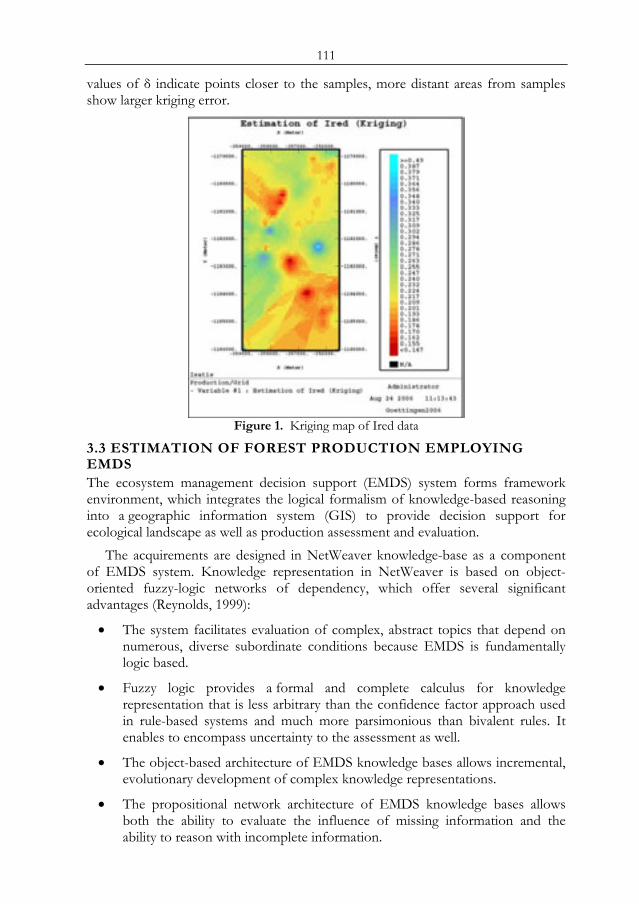
111
values of δ indicate points closer to the samples, more distant areas from samples show larger kriging error.
Figure 1. Kriging map of Ired data
3.3 ESTIMATION OF FOREST PRODUCTION EMPLOYING EMDS The ecosystem management decision support (EMDS) system forms framework environment, which integrates the logical formalism of knowledge-based reasoning into a geographic information system (GIS) to provide decision support for ecological landscape as well as production assessment and evaluation.
The acquirements are designed in NetWeaver knowledge-base as a component of EMDS system. Knowledge representation in NetWeaver is based on object-oriented fuzzy-logic networks of dependency, which offer several significant advantages (Reynolds, 1999):
• The system facilitates evaluation of complex, abstract topics that depend on numerous, diverse subordinate conditions because EMDS is fundamentally logic based.
• Fuzzy logic provides a formal and complete calculus for knowledge representation that is less arbitrary than the confidence factor approach used in rule-based systems and much more parsimonious than bivalent rules. It enables to encompass uncertainty to the assessment as well.
• The object-based architecture of EMDS knowledge bases allows incremental, evolutionary development of complex knowledge representations.
• The propositional network architecture of EMDS knowledge bases allows both the ability to evaluate the influence of missing information and the ability to reason with incomplete information.
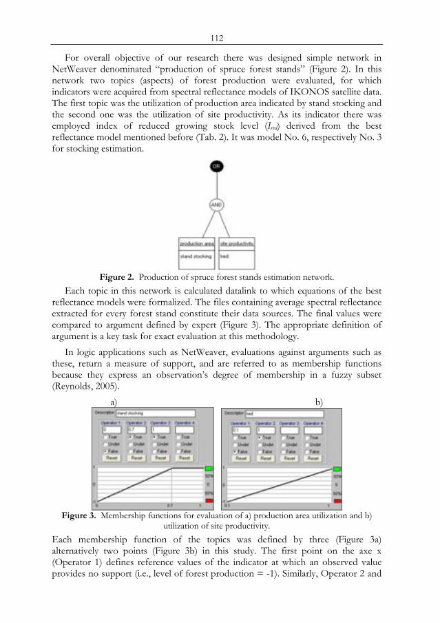
112
For overall objective of our research there was designed simple network in NetWeaver denominated “production of spruce forest stands” (Figure 2). In this network two topics (aspects) of forest production were evaluated, for which indicators were acquired from spectral reflectance models of IKONOS satellite data. The first topic was the utilization of production area indicated by stand stocking and the second one was the utilization of site productivity. As its indicator there was employed index of reduced growing stock level (Ired) derived from the best reflectance model mentioned before (Tab. 2). It was model No. 6, respectively No. 3 for stocking estimation.
Figure 2. Production of spruce forest stands estimation network.
Each topic in this network is calculated datalink to which equations of the best reflectance models were formalized. The files containing average spectral reflectance extracted for every forest stand constitute their data sources. The final values were compared to argument defined by expert (Figure 3). The appropriate definition of argument is a key task for exact evaluation at this methodology.
In logic applications such as NetWeaver, evaluations against arguments such as these, return a measure of support, and are referred to as membership functions because they express an observation’s degree of membership in a fuzzy subset (Reynolds, 2005).
a) b)
Figure 3. Membership functions for evaluation of a) production area utilization and b)
utilization of site productivity. Each membership function of the topics was defined by three (Figure 3a) alternatively two points (Figure 3b) in this study. The first point on the axe x (Operator 1) defines reference values of the indicator at which an observed value provides no support (i.e., level of forest production = -1). Similarly, Operator 2 and
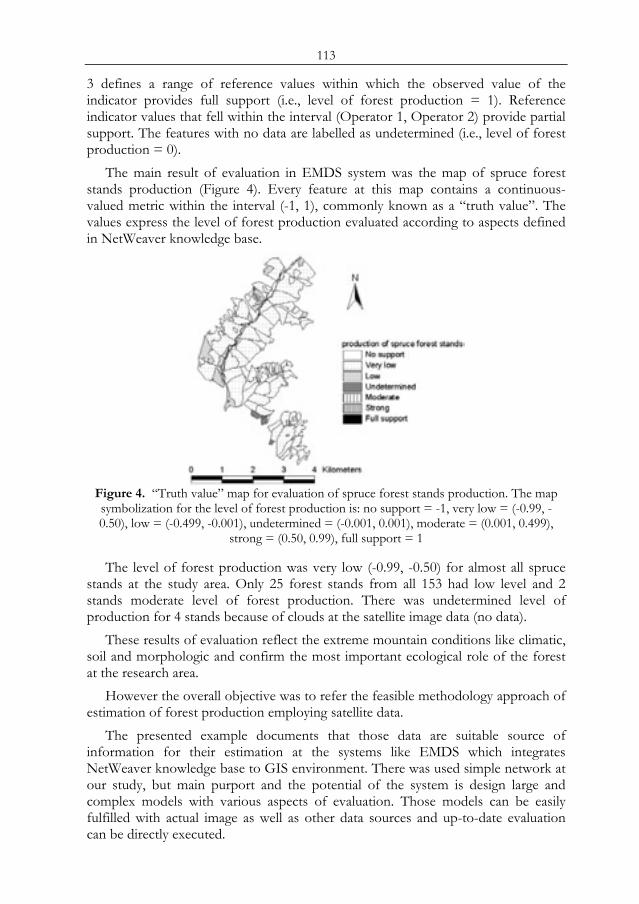
113
3 defines a range of reference values within which the observed value of the indicator provides full support (i.e., level of forest production = 1). Reference indicator values that fell within the interval (Operator 1, Operator 2) provide partial support. The features with no data are labelled as undetermined (i.e., level of forest production = 0).
The main result of evaluation in EMDS system was the map of spruce forest stands production (Figure 4). Every feature at this map contains a continuous-valued metric within the interval (-1, 1), commonly known as a “truth value”. The values express the level of forest production evaluated according to aspects defined in NetWeaver knowledge base.
Figure 4. “Truth value” map for evaluation of spruce forest stands production. The map symbolization for the level of forest production is: no support = -1, very low = (-0.99, -0.50), low = (-0.499, -0.001), undetermined = (-0.001, 0.001), moderate = (0.001, 0.499),
strong = (0.50, 0.99), full support = 1
The level of forest production was very low (-0.99, -0.50) for almost all spruce stands at the study area. Only 25 forest stands from all 153 had low level and 2 stands moderate level of forest production. There was undetermined level of production for 4 stands because of clouds at the satellite image data (no data).
These results of evaluation reflect the extreme mountain conditions like climatic, soil and morphologic and confirm the most important ecological role of the forest at the research area.
However the overall objective was to refer the feasible methodology approach of estimation of forest production employing satellite data.
The presented example documents that those data are suitable source of information for their estimation at the systems like EMDS which integrates NetWeaver knowledge base to GIS environment. There was used simple network at our study, but main purport and the potential of the system is design large and complex models with various aspects of evaluation. Those models can be easily fulfilled with actual image as well as other data sources and up-to-date evaluation can be directly executed.
114
4 CONCLUSION Forestry is a very important area for remote sensing application where different forestry variables are possible to estimate. Spectral reflectance models are good and acceptable basis for estimation of different forest variables, they offer initial information for application of different sampling methods, geostatistics approaches and decision support systems as well. With these methods we are able to generalize sample information to area of interest with known accuracy and sufficient efficiency. The advantages of geostatistics regionalization are mainly, that the spatial data variability and autocorrelation are taking into account and in comparison with standard interpolation methods we have information about the estimation error in the form of the kriging standard deviation. Another example of remote sensing and another sources auxiliary data generalization is application of EMDS. This approach integrates logical formalism of knowledge-based reasoning into GIS to provide decision support for ecological as well as production assessment and evaluation.
ACKNOWLEGEMENTS This study was funded by the Scientific Grant Agency, Ministry of Education of Slovak Republic, Project VEGA No. 1/3531/06. The authors want to acknowledge the support received from the Bundesministerium für Ernährung, Landwirtschaft und Forsten, Germany, for the financial support of German-Slovak research co-operation between Institut für Forsteinrichtung und Ertragskunde, Georg-August-Universität Göttingen and Department of Forest Management and Geodesy, Faculty of Forestry, Zvolen, where these tasks are also solved.
REFERENCES 1 Perry, Ch., R., Jr., Lautenschlager, L.,F., 1984: Functional Equivalence of Spectral
Vegetation Idices. Remote Sensing and the Environment 14, pp.169-182. 2 Reynolds, K., M., 1999: EMDS USER GUIDE (Version 2.0.): Knowledge – based
Decision Support for Ecological Assessment. Gen.Tech.Rep. PNW-GTR-XX. Portland, OR: U.S. Department of Agriculture, Forest Service, Pacific Northwest Research Station. 1999, 76p.
3 Reynolds, K., M. , Hessburg, P., F., 2005: Decision support for integrated landscape evaluation and restoration planning. Forest Ecology and Management 207 (2005), pp. 263–278
4 Scheer, Ľ., Akça, A., Feldkötter, Ch., 1997: Efficient Growing Stock Estimation from Satellite Data Employing Two-phased Sampling with Regression. Geo-Informations-Systeme. 10, No.3, pp.22-25.
5 Scheer, Ľ., Ďurský, J., 1998: Assessment of stand productivity employing satellite data. 6 Wackernagel, H., 1998: Multivariate geostatistics. Springer-Verlag, 291.
115
Assessment of tree positions from aerial photos by combining three basic techniques: tree top searching,
valley following and template matching
P. Surovýa, N. A. Ribeirob, L. Scheera, B. Slobodac
a Department of Forest Management and Geodesy, Technical University in Zvolen, Slovak Republic, email: [email protected]
b Departamento Fitotecnia Universidade de Évora, Portugal c Institute of Forest Biometrics and Applied Computer Science, University of
Goettingen
ABSTRACT In this work, a new method for tree identification is proposed. This method combines all three basic known techniques for the delineation12 of individual trees: tree top searching, valley-following and template-matching. The templates are based on shapes derived from photos using the tree-top technique together with the valley-following technique. Templates are then evaluated using so called certainty – probability that found shape is similar to known shape of crown, as by its form so by its dimensions. Implementation of this technique into software environment is described.
This method proved to be helpful especially for filtering small trees and improving estimation of the form of the crown area. Horizontal structure estimation was evaluated and significant improvement was found using the template filtering compared to the non filtered structure.
INTRODUCTION Agroforestry land in southern Portugal is the main producer of cork in the world. Various individual growth models demonstrated to be a reliable tool to support decisions for sustainable management of these lands (Ribeiro et al., 2003). Horizontal stand structure, or positions of individual trees, is very important input for these models as it describes the stand competition situation and resources availability of individual trees. The use of digital aerial images as alternative source of data has been a long time studied and several successes have been achieved.
There exist three basic approaches for delineation of individual tree crowns in image. The first technique is to find local maxima and consider this as a tree top. This approach was between others described in BLAZQUEZ (1989). Usually this technique, when used alone, suffers with a problem that the peak in the photo is not always individual pixel, so several peaks are found in one tree. Also the side branches can be considered as local maxima. This can be treated with filtering, smoothing etc. Proc. 2nd Göttingen GIS and Remote Sensing Days, 4-6 Oct. 2006, Göttingen

116
Second technique for delineation of individual trees is valley-following method described between other works of this author in Gougeon 1995. In this technique image is displayed as three-dimensional model where the tree tops appear to be peaks because of the highest value of grey and the delimiters appear to be valleys between these tops. The valleys are followed in order to create regions which are there considered to be trees. Drawback of this method is that sometimes the valleys are incomplete or interrupted and then two trees can be considered as one.
Third technique for delineation of individual trees is comparison with a template. It can be thought that all techniques are principally trying to repeat the human way of thinking by manual delineation of crown. In case of tree tops human observer also searches for the brightest points and mark them as trees. If he cannot decide he follows the delimiting valleys in order to delineate crown. In case of templates human sometimes mark a crown because it looks like a crown which is known to him. The template technique was developed and described in Pollock (1996) or later Larset et al. (1997). Templates in this works are defined as geometrical models or by other words as matrix of pixels which is usually moved over the image and in each position a correlation is evaluated. In this way, as also mentioned by authors, it is required to have all possible shapes of trees. All shapes and all possible sizes resolve to the enormous requirement on computational time. On the other hands if the method is successful it is possible to provide not only positions and sizes of individual crowns but also at the meantime it should be capable of recognizing the tree species.
MATERIALS AND METHODS In this work we propose a new approach to the template’s definition. As mentioned already in previous chapter, the different ways of crown delineation can be understood as different ways of imitation of human way of thinking or human knowledge. Therefore we propose a template as a joined knowledge about what can be a tree, regarding the image information and about what can be a tree regarding the ground truth information. Template philosophy The template and the shape are in this work not understood as two dimensional objects. There is processed construction of a curve which serves afterwards to evaluate the similarity between the found object and probable object - template. This process is shown in Figure 1. System starts to display over the chart (right) radius in each angle starting from clock number 3.
The construction of the curve shown in Figure 1 is only starting information for the subsequent analysis. Each point receives a value of certainty. This certainty is based on two sources or their mix (described later). This certainty is used for decision about the smoothing. One simple example of smoothing of the extremes is shown in Figure 2.
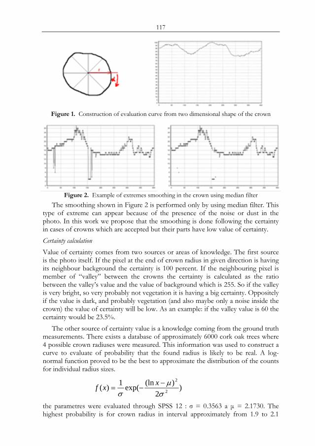
117
Figure 1. Construction of evaluation curve from two dimensional shape of the crown
Figure 2. Example of extremes smoothing in the crown using median filter
The smoothing shown in Figure 2 is performed only by using median filter. This type of extreme can appear because of the presence of the noise or dust in the photo. In this work we propose that the smoothing is done following the certainty in cases of crowns which are accepted but their parts have low value of certainty. Certainty calculation Value of certainty comes from two sources or areas of knowledge. The first source is the photo itself. If the pixel at the end of crown radius in given direction is having its neighbour background the certainty is 100 percent. If the neighbouring pixel is member of “valley” between the crowns the certainty is calculated as the ratio between the valley’s value and the value of background which is 255. So if the valley is very bright, so very probably not vegetation it is having a big certainty. Oppositely if the value is dark, and probably vegetation (and also maybe only a noise inside the crown) the value of certainty will be low. As an example: if the valley value is 60 the certainty would be 23.5%.
The other source of certainty value is a knowledge coming from the ground truth measurements. There exists a database of approximately 6000 cork oak trees where 4 possible crown radiuses were measured. This information was used to construct a curve to evaluate of probability that the found radius is likely to be real. A log-normal function proved to be the best to approximate the distribution of the counts for individual radius sizes.
)2
)(lnexp(1)( 2
2
σμ
σ−
−=xxf
the parametres were evaluated through SPSS 12 : σ = 0.3563 a μ = 2.1730. The highest probability is for crown radius in interval approximately from 1.9 to 2.1
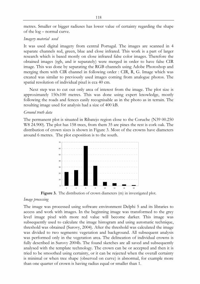
118
metres. Smaller or bigger radiuses has lower value of certainty regarding the shape of the log – normal curve. Imagery material used It was used digital imagery from central Portugal. The images are scanned in 4 separate channels red, green, blue and close infrared. This work is a part of larger research which is based mostly on close infrared false color images. Therefore the obtained images (rgb, and ir separately) were merged in order to have false CIR image. This was done by separating the RGB channels using Adobe Photoshop and merging them with CIR channel in following order : CIR, R, G. Image which was created was similar to previously used images coming from analogue photos. The spatial resolution of individual pixel is cca 40 cm.
Next step was to cut out only area of interest from the image. The plot size is approximately 150x100 metres. This was done using expert knowledge, mostly following the roads and fences easily recognisable as in the photo as in terrain. The resulting image used for analysis had a size of 400 kB. Ground truth data The permanent plot is situated in Ribatejo region close to the Coruche (N39 00.250 W8 24.900). The plot has 158 trees, from them 35 are pines the rest is cork oak. The distribution of crown sizes is shown in Figure 3. Most of the crowns have diameters around 6 metres. The plot exposition is to the south.
0
10
20
30
40
50
60
70
2 4 6 8 10 12 14 16 Figure 3. The distribution of crown diameters (m) in investigated plot.
Image processing The image was processed using software environment Delphi 5 and its libraries to access and work with images. In the beginning image was transformed to the grey level image pixel with more red value will become darker. This image was subsequently used to calculate the image histogram and using automatic technique, threshold was obtained (Surovy, 2004). After the threshold was calculated the image was divided to two segments: vegetation and background. All subsequent analysis was performed only in the vegetation area. The delineation of individual crowns is fully described in Surovy 2004b. The found sketches are all saved and subsequently analysed with the template technology. The crown can be or accepted and then it is tried to be smoothed using certainty, or it can be rejected when the overall certainty is minimal or when tree shape (observed on curve) is abnormal, for example more than one quarter of crown is having radius equal or smaller than 1.
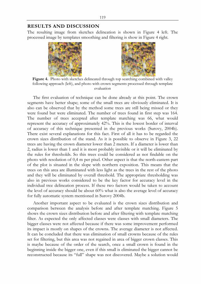
119
RESULTS AND DISCUSSION The resulting image from sketches delineation is shown in Figure 4 left. The processed image by templates smoothing and filtering is show in Figure 4 right.
Figure 4. Photo with sketches delineated through top searching combined with valley following approach (left), and photo with crown segments processed through template
evaluation
The first evaluation of technique can be done already at this point. The crown segments have better shape; some of the small trees are obviously eliminated. It is also can be observed that by the method some trees are still being missed or they were found but were eliminated. The number of trees found in first step was 164. The number of trees accepted after template matching was 66, what would represent the accuracy of approximately 42%. This is the lowest border of interval of accuracy of this technique presented in the previous works (Surovy, 2004b). There exist several explanations for this fact. First of all it has to be regarded the crown sizes distribution of the stand. As it is possible to observe in Figure 3, 22 trees are having the crown diameter lower than 2 meters. If a diameter is lower than 2, radius is lower than 1 and it is most probably invisible or it will be eliminated by the rules for thresholds. So this trees could be considered as not findable on the photo with resolution of 0,4 m per pixel. Other aspect is that the north-eastern part of the plot is situated in the slope with northern exposition. This means that the trees on this area are illuminated with less light as the trees in the rest of the photo and they will be eliminated by overall threshold. The appropriate thresholding was also in previous works considered to be the key factor for accuracy level in the individual tree delineation process. If these two factors would be taken to account the level of accuracy should be about 60% what is also the average level of accuracy for fully automatic system mentioned in Surovy 2004b.
Another important aspect to be evaluated is the crown sizes distribution and comparison between the analysis before and after template matching. Figure 5 shows the crown sizes distribution before and after filtering with template matching filter. As expected the only affected classes were classes with small diameters. The bigger classes were not affected because if there was some improvement performed its impact is mostly on shapes of the crowns. The average diameter is not affected. It can be concluded that there was elimination of small crowns because of the rules set for filtering, but this area was not regained in area of bigger crown classes. This is maybe because of the order of the search, once a small crown is found in the beginning inside the bigger one, even if this small is eliminated the bigger cannot be reconstructed because its “full” shape was not discovered. Maybe a solution would
120
be to repeat the simulation and increase the grey level of the area of these small crowns in order that these are not considered to be peaks of the trees.
0
10
20
30
40
50
60
70
80
90
2 4 6 8 10 12 14 0
10
20
30
40
50
60
70
80
90
2 4 6 8 10 12 14 Figure 5. The crown sizes distribution (left columns) compared to the real
distribution(right columns) for none filtered technique(left) and for the template matched technique (right)
In Figure 5 it can be also observed that the biggest tree (diameter 16m) was not found. This is the third aspect influencing the accuracy – the shape of the crown. It is knowns that this crown is not having compact surface and so it cannot be found as one tree using the technique of tree top and valleys. It does not have one peak, and the valleys are existing also inside the crown because of its irregularities. Valleys could be treated by proper smoothing what was also already described as the key factor for global accuracy. The use of smoothing is not a trivial task because smoothing with larger kernel causes the elimination of smaller valleys which are essential for delineation of smaller touching trees.
Figure 6. Comparison of pair correlation functions for different analysis from left: original stand, stand without filtering and filtered stand
Another important factor for accuracy evaluation is horizontal structure of found trees. Horizontal structure is key factor for competition description in the stand what is of a big importance for individual tree models. One of the possibilities how to evaluate the horizontal structure is the pair-correlation function (Stoyan, 1995) which was adapted in previous works. The pair correlation function evaluates presence of clustering and describes the situation in horizontal structure, especially whether this structure differs from random Poisson field. As it is possible to observe in figure 6, the non-filtered stand shows clustering in small distances (by what it also significantly differ from the original stand). This clustering is caused mostly by delineation of small trees inside the crowns of bigger ones, so all these points are found in close distances. After the application of the filter all this clusters are removed and the final curve show similar characteristics as the original one. The regular oscillation over the value 1, confirm that this point field can be considered as similar to the random Poisson field.
121
CONCLUSIONS In this work it is presented method for the delineation of individual trees by combination of three basic methods used for this task: tree top searching, valley following and template matching. The new approach is about the definition of templates where these are similarly to original works constructed as a known shape, but in this case the knowledge is sourced from two areas, one is the photo itself, other are the ground data. Both areas of knowledge are balanced by assignment of certainty to each point of the crown edge. Certainty is then used to decide about or the elimination of the crown at all, or about change of its shape to be more similar to the known or probable crown.
The results evaluation was divided into three areas: 1.) tree amount: the methodology decreases the accuracy in this variable when comparing to the methodology without filtering. But it is difficult to estimate only by a tree number whether the trees found are the real ground trees, or several trees are found in place of one big tree and small trees are not found. 2.) Crown sizes distribution: in this variable the impact of filtering by templates is only visible in small classes, because these are eliminated. It was concluded that the area decreased in this classes was not regained in bigger classes, because in bigger crowns the filter mostly improve shape of these crowns. 3.) The horizontal structure: evaluation was done by pair-correlation function and it can be concluded that the filtering had significantly positive impact on horizontal structure estimation.
REFERENCES Blazquez, C.H. (1989): Computer-based Image Analysis and Tree Counting with Aerial
Color Infrared Photograph. Journal of Imaging Technology 15(4): 163-168. Gougeon, F.A. (1995): A crown following approach to the automatic delineation of
individual tree crowns in high spatial resolution aerial images. Can. J. Remote Sens. 21(3): 274-284.
Larsen, M., Rudemo, M. (1997) Using Ray-Traced templates to Find Individual Trees in Aerial Photos. In: Frydrych, M., Parkkinen, J., Visa, A. editors, Proceedings of the 10th Scandinavian Conference on Image Analysis, vol. 2, p. 1007-1014, Lappeenranta, Finland.
Pollock, R.J. (1996) The Automatic recognition of Individual trees in Aerial Images of Forests Based on a Synthetic Tree Crown Image Model,UBCTechnical Report. Vancouver, Canada, June 1996
Ribeiro, N. A., Oliveira, A.C., Pretsch, H., Surový, P. (2003) Growth Simulation and sustainability of cork oak stands. Modelling Forest Systems. p,259-267. CABI Publishing, Wallingford, UK
Stoyan, D., Stoyan, H. (1995) Fractals, Random Shapes and Point Fields. Methods of Geometrical Statistics.J. Wiley & Sons, Chichester, New York, Brisbane, Toronto, Singapore
Surový, P., Ribeiro, N. A., Oliveira, A.C., Scheer, Ľ. (2004a): Detection of the vegetation from background in high resolution color remote sensed imagery. Journal of Forest Science, 50, 2004(4). pp: 161-170
Surový, P., Ribeiro, N. A., Oliveira, A.C., Scheer, Ľ. (2004b). Automated aerial imagery analysis system for individual tree identification in cork oak stands. Advances In Geoecology 37(2004): p.287-296

122
123
GIS-based assessment of land potential for forestry use in Thua Thien Hue province, Central Vietnam
N. Van Loi, M. Kappas, S. Erasmi Department of Cartography, GIS and Remote Sensing, Institute of Geography,
Goettingen University, Germany, Goldschmidtstr 5, 37077 Göttingen, email: [email protected], [email protected], serasmi@uni-
goettingen.de
ABSTRACT The main objective of ou13r work is the production of a land potential map for forestry production. Our method integrates remotely sensed data with the spatial analysis of geo-morphological, ecological and socio-economical data by GIS modelling to define potential areas and identify suitable sites for predetermined forest trees. The suitability of sites is related to individual tree requirements. The suitability assessment for each tree species was conducted using the method described in the FAO guidelines for land evaluation of forestry (FAO, 1984). The assessment process was partly modified for fitting particular tree conditions within Vietnam. The classification of forest and vegetation types is based on multi-date Landsat ETM+ data analysis and a broadly based field work. All derived data were integrated into GIS and a Linear Combination Method was used to define the land potential. The result is a comprehensible map that shows an area of 365,891ha suitable for forestry production. Furthermore, the entire area was divided into high potential, medium potential, low potential and very low potential sub-areas related to special tree requirements.
Cartography, IS and Remote Sensing department 1 INTRODUCTION Thua Thien Hue province is located in central Vietnam (Fig. 1). This province has a size of about 505 339 ha, of which more than three quarter is made up of mountainous and hilly land. The land itself and its soils are an important precondition for forest and downstreamed wood production. The forest soil as a main production parameter is classified into different soil types: Yellowish brown soils on old alluvia, yellowish red soils on acid magma rock, yellowish red soils on sandstone, yellowish red soils on metamorphic rocks, alluvial soils on river areas, humus soils and sand soils. Chemical analyses have shown that concentration of soil pH, organic matter, total nitrogen, available phosphorus and available potassium are very different between these soil types. At present, forestry management and local people are interested in terms of quality and quantity of forest and forest plantations to achive a sustainable management of tree species. Therefore, an comprehensive Proc. 2nd Göttingen GIS and Remote Sensing Days, 4-6 Oct. 2006, Göttingen
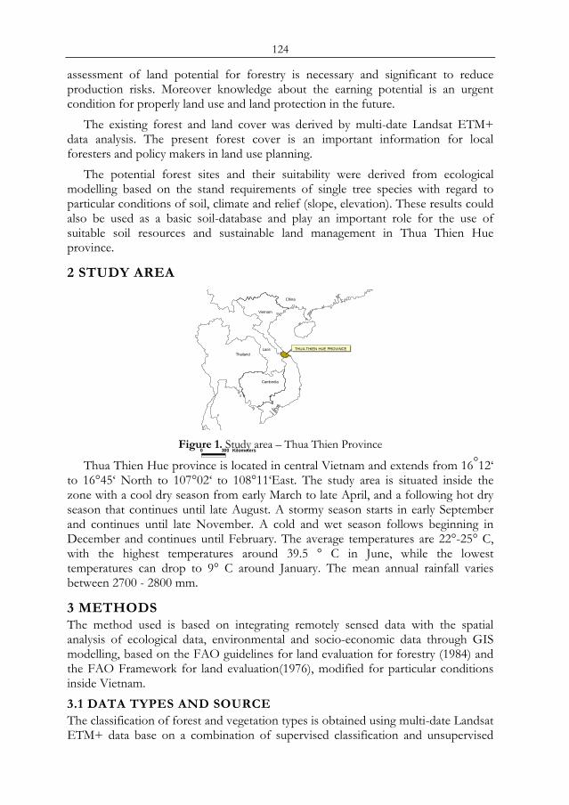
124
assessment of land potential for forestry is necessary and significant to reduce production risks. Moreover knowledge about the earning potential is an urgent condition for properly land use and land protection in the future.
The existing forest and land cover was derived by multi-date Landsat ETM+ data analysis. The present forest cover is an important information for local foresters and policy makers in land use planning.
The potential forest sites and their suitability were derived from ecological modelling based on the stand requirements of single tree species with regard to particular conditions of soil, climate and relief (slope, elevation). These results could also be used as a basic soil-database and play an important role for the use of suitable soil resources and sustainable land management in Thua Thien Hue province.
2 STUDY AREA
Figure 1. Study area – Thua Thien Province
Thua Thien Hue province is located in central Vietnam and extends from 16°12‘ to 16°45‘ North to 107°02‘ to 108°11‘East. The study area is situated inside the zone with a cool dry season from early March to late April, and a following hot dry season that continues until late August. A stormy season starts in early September and continues until late November. A cold and wet season follows beginning in December and continues until February. The average temperatures are 22°-25° C, with the highest temperatures around 39.5 ° C in June, while the lowest temperatures can drop to 9° C around January. The mean annual rainfall varies between 2700 - 2800 mm.
3 METHODS The method used is based on integrating remotely sensed data with the spatial analysis of ecological data, environmental and socio-economic data through GIS modelling, based on the FAO guidelines for land evaluation for forestry (1984) and the FAO Framework for land evaluation(1976), modified for particular conditions inside Vietnam. 3.1 DATA TYPES AND SOURCE The classification of forest and vegetation types is obtained using multi-date Landsat ETM+ data base on a combination of supervised classification and unsupervised
Vietnam
China
Laos
Cambodia
ThailandTHUA THIEN HUE PROVINCE
0 300 Kilometers
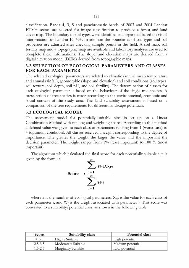
125
classification. Bands 4, 3, 5 and panchromatic bands of 2003 and 2004 Landsat ETM+ scenes are selected for image classification to produce a forest and land cover map. The boundary of soil types were identified and separated based on visual interpretation of Landsat ETM+. In addition the boundaries of soil types and soil properties are adjusted after checking sample points in the field. A soil map, soil fertility map and a topographic map are available and laboratory analyses are used to complete these informations. The slope, and elevation maps are derived from a digital elevation model (DEM) derived from topographic maps. 3.2 SELECTION OF ECOLOGICAL PARAMETERS AND CLASSES FOR EACH PARAMETER The selected ecological parameters are related to climatic (annual mean temperature and annual rainfall), geomorphic (slope and elevation) and soil conditions (soil types, soil texture, soil depth, soil pH, and soil fertility). The determination of classes for each ecological parameter is based on the behaviour of the single tree species. A preselection of tree species is made according to the environmental, economic and social context of the study area. The land suitability assessment is based on a comparison of the tree requirements for different landscape potentials. 3.3 ECOLOGICAL MODEL The assessment model for potentially suitable sites is set up on a Linear Combination Method with ranking and weighting scores. According to this method a defined value was given to each class of parameters ranking from 1 (worst case) to 4 (optimum condition). All classes received a weight corresponding to the degree of importance. The greater the weight the larger the value and the important the decision parameter. The weight ranges from 1% (least important) to 100 % (most important).
The algorithm which calculated the final score for each potentially suitable site is given by the formula:
where n is the number of ecological parameters, Xxyi is the value for each class of
each parameter i, and Wi is the weight associated with parameter i. This score was converted to a suitability/potential class, as shown in the following table:
Score Suitability class Potential class > 3.5 Highly Suitable High potential
2.5-3.5 Moderately Suitable Medium potential 1.5-2.5 Marginally Suitable Low potential
Score
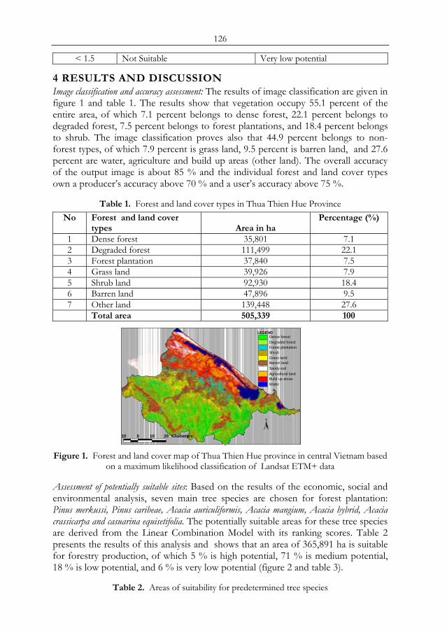
126
< 1.5 Not Suitable Very low potential
4 RESULTS AND DISCUSSION Image classification and accuracy assessment: The results of image classification are given in figure 1 and table 1. The results show that vegetation occupy 55.1 percent of the entire area, of which 7.1 percent belongs to dense forest, 22.1 percent belongs to degraded forest, 7.5 percent belongs to forest plantations, and 18.4 percent belongs to shrub. The image classification proves also that 44.9 percent belongs to non-forest types, of which 7.9 percent is grass land, 9.5 percent is barren land, and 27.6 percent are water, agriculture and build up areas (other land). The overall accuracy of the output image is about 85 % and the individual forest and land cover types own a producer’s accuracy above 70 % and a user’s accuracy above 75 %.
Table 1. Forest and land cover types in Thua Thien Hue Province No Forest and land cover
types Area in ha Percentage (%)
1 Dense forest 35,801 7.1 2 Degraded forest 111,499 22.1 3 Forest plantation 37,840 7.5 4 Grass land 39,926 7.9 5 Shrub land 92,930 18.4 6 Barren land 47,896 9.5 7 Other land 139,448 27.6 Total area 505,339 100
Figure 1. Forest and land cover map of Thua Thien Hue province in central Vietnam based on a maximum likelihood classification of Landsat ETM+ data
Assessment of potentially suitable sites: Based on the results of the economic, social and environmental analysis, seven main tree species are chosen for forest plantation: Pinus merkussi, Pinus caribeae, Acacia auriculiformis, Acacia mangium, Acacia hybrid, Acacia crassicarpa and casuarina equisetifolia. The potentially suitable areas for these tree species are derived from the Linear Combination Model with its ranking scores. Table 2 presents the results of this analysis and shows that an area of 365,891 ha is suitable for forestry production, of which 5 % is high potential, 71 % is medium potential, 18 % is low potential, and 6 % is very low potential (figure 2 and table 3).
Table 2. Areas of suitability for predetermined tree species
10 0 10 20 Kilometers
LEGEND
Barren land
Dense forest
Sandy soil
Degraded forestForest plantation
Grass land
Build up areasAgrisultural land
Shrub
Water
N
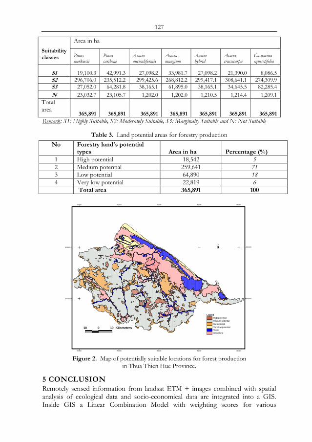
127
Area in ha Suitability classes Pinus
merkussi Pinus caribeae
Acacia auriculiformis
Acacia mangium
Acacia hybrid
Acacia crassicarpa
Casuarina equisetifolia
S1 19,100.3 42,991.3 27,098.2 33,981.7 27,098.2 21,390.0 8,086.5 S2 296,706.0 235,512.2 299,425.6 268,812.2 299,417.1 308,641.1 274,309.9 S3 27,052.0 64,281.8 38,165.1 61,895.0 38,165.1 34,645.5 82,285.4 N 23,032.7 23,105.7 1,202.0 1,202.0 1,210.5 1,214.4 1,209.1
Total area
365,891 365,891 365,891 365,891 365,891 365,891 365,891 Remark: S1: Highly Suitable, S2: Moderately Suitable, S3: Marginally Suitable and N: Not Suitable
Table 3. Land potential areas for forestry production No Forestry land's potential
types Area in ha Percentage (%) 1 High potential 18,542 5 2 Medium potential 259,641 71 3 Low potential 64,890 18 4 Very low potential 22,819 6 Total area 365,891 100
Hue cityHue city
Ca u h ai l ag oo nCa u h ai l ag oo n
Lan gc o l ago onLan gc o l ago on
10 0 10 Kilometers
LegendHigh potential
low potentialMedium potential
Other land
Very low potentialWater
N
720000
720000
750000
750000
780000
780000
810000
810000
840000
840000
1800000 1800000
1830000 1830000
Figure 2. Map of potentially suitable locations for forest production
in Thua Thien Hue Province.
5 CONCLUSION Remotely sensed information from landsat ETM + images combined with spatial analysis of ecological data and socio-economical data are integrated into a GIS. Inside GIS a Linear Combination Model with weighting scores for various
128
ecological-economical combinations was used to derive the land’s potential for forestry. This approach delivers a robust tool for land resources assessment and management.
The land suitability model for predetermined tree species will offer an efficient way to manage forest sites. Forest managers and local people get a revised decision system to find adapted locations for an optimized and sustainable forest development.
ACKNOWLEDGMENT Authors would like to thank the University of Marryland, USA; Forestry Faculty and Department of Soil Science of Hue University of Agriculture and Forestry; Department of Rural and Agricultural Development; Department of Science and Environment and Institute of Inventory and Planning, Thua Thien Hue province, Central Vietnam for providing satellite images, relevant maps and information.
REFERENCES Hopkin, L. D.: Method for Generating Land Suitability Maps. A Comparative Evaluation.
AIP journal. U.S.A.,Vol.14, pp. 386- 400, 1977 Jensen, J. R.: Remote Sensing of the Environment: An Earth Resource Perspective.
Prentice – Hall, New York, 1990. Estes, J. E.: Remote Sensing, Techniques for Environment Analysis. Santa Barbra,
California, 1974. FAO: Soil resources development and conservation, Framework for Land Evaluation.
FAO Soil bulletin 32, Rome, 1976. Dent, D., Young, A.: Soil Survey and Land Evaluation. Allen & Unwin, London, 1981 Congalton, R. G., Green, K.: Assessing the Accuracy of Remote Sensed Data. Lewis,
London -New York-Washington, 1999. FAO: Land Evaluation for Forestry. FAO Forestry paper 48, Rome, 1984 Burrough, P. A.: Principles of Geographic Information Systems for Land Resources
Assessment. Clarendon Press, Oxford, 1986. Lillesand, T. M., Kieper, R.: Remote Sensing and Image Interpretation, 3rd edition, New
York, 1994. Campbell, J. B.: Introduction to Remote Sensing. 3rd edition, New York, 2002. Chrisman, N. R.: The Accuracy of Map Overlayer. Introductory Reading in GIS. (edt. by)
Peuquet, D., Marble, D. F., Taylor and Francis, pp 308 Dent, D., Young, A.: Soil Survey and Land Evaluation. Allen & Unwin, London, 1981. Congalton, R. G., Green, K: Assessing the Accuracy of Remote Sensed Data. Lewis, London
-New York-Washington, 1999. FAO: 1980, ‘Land Evaluation for Development’, http://www.fao.org/docrep/u1980e
/u1980e00.htm FAO: 1993, ‘Guidelines for Land Use Planning’, FAO Development Series 1, Rome, Italy,
96 p.Kosmas, C. S., Danalatos, N. G. and Moustakas, N. K.: 1997, ‘The soils’, Hydrobiol. 351(1/3), 21–33.
Rossiter, D. G., VanWambeke, A. R.: 1989, ‘ALES: Automated Land Evaluation System’, ALES User’s Manual, Dept. of Agronomy, Cornell University, NY.
Davidson, D. A.: The Assessment of Land Resources: Achievements and New Challenges. Institute of Australian Geographers 2002.
Dela Rosa, D.: Soil Quality Evaluation and Mornitoring Based on Land Evaluation. Land degradation and development. 16: 551-559 (2005).
129
Rossiter, D. G.: Biophysical Models in Land Evaluation,”Land use and land over”(2003). EOLSS Publishers Co.LTD.(UK).
Torbick, N., Lusch, D., QI, J., Moore, N., Olson, J., GE, J.: Developing Land use/land Cover Parameterization for Climate Land Modelling in East Africa. International Journal of Remote Sensing, Vol. 27, Taylor and Francis, No. 19, 10 October 2006, 4227–4244.
Zhu, L., Tateishi, R.: Fusion of Multisensor Multitemporal Satellite Data for Land Cover Mapping. International Journal of Remote Sensing, Taylor and Francis. Vol. 27, No. 5, 10 March 2006, 903–918.
Amarsaikhan, D., Douglas, T. : Data Fusion and Multisource Image Classification. International Journal of Remote Sensing, Taylor and Francis VoL. 25, NO. 17, 10 September, 3529–3539.
Colditz, R. R., Wehrmann, T., Bachmann, M., Steinnocher,K., Schmidt, M., Strunz , G., Dech, S.: Influence of Image Fusion Approaches on Classification Accuracy: A Case Study. International Journal of Remote Sensing, Taylor and Francis.Vol. 27, No. 15, 10 August 2006, 3311–3335
Bojo Rquez -Tapia, L. A., Diasz-Mondrago, S., Ezcurra, N. E.: GIS-Based Approach for Participatory Decision Making and Land Suitability Assessment. International Journal of geographical information science Taylor and Francis. 2001, Vol. 15, No. 2, 129 – 151.
Yu, X., NG, C.: An Integrated Evaluation of Landscape Change Using Remote Sensing and Landscape Metrics: a case study of Panyu, Guangzhou. International Journal of Remote Sensing, Taylor and Francis. Vol. 27, No. 6, 20 March 2006, 1075–1092
Jeroen C. J., van den Bergh, M., Barendregt, A., Gilbert, A. J.: Spatial Ecological Economic Analysis for Wetland Management:Modelling and Scenario Evaluation of Land Use. Cambridge University Press. 2004.
Rahman, M. M., Csaplovics, E., Koch, B., Köhl, K.: Interpretation of Tropical Vegetation of Tropical Vegetation Using Landsat ETM +. Bangladesh Space Research and Remote Sensing Organization (SPARRSO), Agargaon, Sher-E-Bangla Nagar, Dhaka-1207, Bangladesh.
Ruiz, L. A., Sarria, A. F.: Analysis of Image Segmentation of Multisource Data in Mountain Environments. IAPRS, Vol. XXXIII, Amsterdam, 2000
Helmer, E. H., Brown, S., Cohen, W. B.: Mapping Montane Tropical Forest Successional Stage and Land Use with Multi-date Landsat Imagery. International Journal of Remote Sensing, Taylor and Francis 2000, Vol. 21, No. 11, 163–2183
Serwan M. J. BaBaN.: Mapping Land use/ cover Distribution on a Mountainous Tropical Island Using Remote Sensing and GIS. International Journal of Remote Sensing, Taylor and Francis 2001, Vol. 22, No. 10, 1909–1918

130
131
Estimation of Forest attributes by integrating Satellite Imagery and Field plot data
J.-S. Yima, P. Magdona, C. Kleinna, M.-Y. Shinb a Institute of Forest Management, Büsgenweg 5, D-37077 Göttingen, Eemail :
[email protected] b Department of Forest Resources, College of Forest Science, Kookmin University,
Korea
ABSTRACT Methodological research for fo14rest inventories focuses on sampling and remote sensing issues and the question on how to efficiently integrate both. The k Nearest Neighbor (kNN) technique is a nonparametric estimation approach that has been applied for estimation and classification of large areas. The technique is used to produce continuous digital information layers of forest attributes using sample based field inventory and satellite imagery as data source. The main aim of this study was to improve the estimation error for different reference windows; geographical horizontal reference areas (HRAs) and stratification by forest cover type, and feature weighting for estimating the growing stock with the kNN technique. In order to determine the optimal number of neighbor plots, the Root Mean Square Errors (RMSEs) and bias by the cross-validation method and a confusion matrix were evaluated. Data for this study was obtained from a pilot study of a new national forest inventory system in Korea.
For the sampling intensity in this study, a geographical HRA with a radius of 10km was found to be optimal for the estimation of growing stock. Stratification of reference plots by forest cover type improved the precision of estimation. As a consequence, the stratification window was considered a more efficient reference window than the HRAs in the cross-validation. The optimal value of k was selected such that the RMSE and bias of the estimates was minimized or stabilized, and that the overall accuracy was high. The RMSE decreased as k increased. A minimum value for RMSE was reached for a HRA of 10km radius and stratification. At a value of k=4 nearest neighbors for a HRA of 10km radius and at a value of k=6 nearest neighbors for stratification, the values for the RMSEs dropped and stabilized, and the biases were minimized. The RMSE and bias were 47.42, 0.42 m3/ha and 47.02, -0.09 m3/ha, respectively. However, the RMSEs for selected k values by reference window decreased by only 1% through feature weight optimization. With respect to the overall accuracy (OA), the reference window using a HRA of 10km radius was more accurate than the stratification approach for k < 8. The best OA (0.42) was found for k=5 nearest neighbors within a HRA of 10km radius. Keywords: k nearest neighbor estimation, growing stock, NFI, reference window, Landsat, Korea Proc. 2nd Göttingen GIS and Remote Sensing Days, 4-6 Oct. 2006, Göttingen

132
1 INTRODUCTION National Forest Inventories (NFIs) are carried out in many countries. The principal goal of NFIs is the provision of information which is relevant and required for national-level decision making and monitoring in forestry, and also in related sectors such as environmental studies, land use management and assessments of environmental impact etc. NFIs also provide data for sub-national geographical or political units and are an input to global forest assessments and other international processes in the context of sustainable management of natural resources. As forest resources are a complex object for an inventory, several information sources are utilized, among them field sampling and remote sensing. The methodological research for forest inventories focuses, therefore, widely on sampling and remote sensing issues and the question of how to efficiently combine them.
The k Nearest Neighbor (kNN) technique is a nonparametric estimation approach that can be used for estimation and classification over large areas. In the past decade, the kNN technique has been advanced for estimation of forest attributes and has now been operational in Finland’s NFI since 1990 [10]. The method uses the information of remote sensed data to interpolate the field-based inventory to produce continuous digital layers of forest attributes. Recently, to improve the accuracy of kNN technique, the consideration of horizontal and/or vertical reference boundaries and application of environmental stratifications for selecting of optimal k neighbors [2], [3], [4], [5], [13]. Also the method was applied with different weights for spectral data [1], [11]. The field sample data and satellite imagery or other ancillary data are combined so that for each field sample plot the corresponding to pixel values of the image are taken. For each pixel in the inventory area, the spectral distance is calculated to each field sample plot, and the distance weight of the pixel is given to the spectrally nearest sample plot, or it is divided between two or more nearest sample plots. The forest stand characteristics can then be computed with the distance weights of the field sample plots. The main aim of this study was to compare different reference windows for selecting reference plots to estimate growing stock with the kNN technique.
2 MATERIAL AND METHOD
2.1 STUDY AREA The study area, Yang-pyeong County, is located in the center of Korea, covering about 87,446 ha. The county is consisted of about 72%, or 63,242 ha of forests, whereas the area for farming is only 15%, or 13,494 ha, and others as 12%. The county is in the hill region, with elevation ranging from 20 to 1,157m above sea level with complex topographic conditions. The main tree species are Japanese red pine (Pinus densiflora), Korean pine (Pinus koraiensis), Japanese larch (Larix leptolepis), Mongolian oak (Quercus mongolica) and other broadleaved trees.
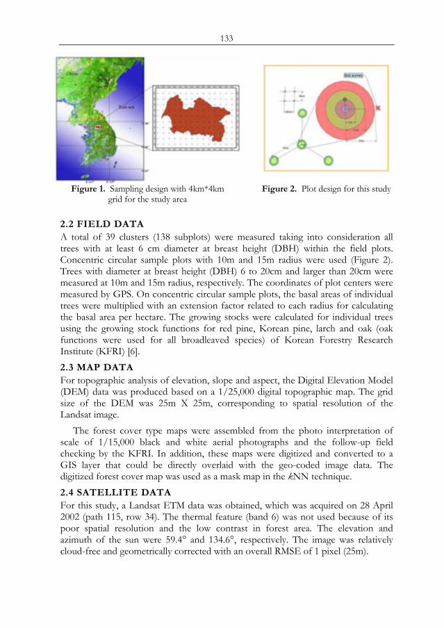
133
Figure 1. Sampling design with 4km*4km grid for the study area
Figure 2. Plot design for this study
2.2 FIELD DATA A total of 39 clusters (138 subplots) were measured taking into consideration all trees with at least 6 cm diameter at breast height (DBH) within the field plots. Concentric circular sample plots with 10m and 15m radius were used (Figure 2). Trees with diameter at breast height (DBH) 6 to 20cm and larger than 20cm were measured at 10m and 15m radius, respectively. The coordinates of plot centers were measured by GPS. On concentric circular sample plots, the basal areas of individual trees were multiplied with an extension factor related to each radius for calculating the basal area per hectare. The growing stocks were calculated for individual trees using the growing stock functions for red pine, Korean pine, larch and oak (oak functions were used for all broadleaved species) of Korean Forestry Research Institute (KFRI) [6]. 2.3 MAP DATA For topographic analysis of elevation, slope and aspect, the Digital Elevation Model (DEM) data was produced based on a 1/25,000 digital topographic map. The grid size of the DEM was 25m X 25m, corresponding to spatial resolution of the Landsat image.
The forest cover type maps were assembled from the photo interpretation of scale of 1/15,000 black and white aerial photographs and the follow-up field checking by the KFRI. In addition, these maps were digitized and converted to a GIS layer that could be directly overlaid with the geo-coded image data. The digitized forest cover map was used as a mask map in the kNN technique. 2.4 SATELLITE DATA For this study, a Landsat ETM data was obtained, which was acquired on 28 April 2002 (path 115, row 34). The thermal feature (band 6) was not used because of its poor spatial resolution and the low contrast in forest area. The elevation and azimuth of the sun were 59.4° and 134.6°, respectively. The image was relatively cloud-free and geometrically corrected with an overall RMSE of 1 pixel (25m).

134
2.5 KNN TECHNIQUE The kNN technique was used for estimating the forest attributes for target plots as unknown plots in the study area. The field sample plots are used as reference plots to estimate a value for each pixel and then as target plots to evaluate estimation error. The k nearest reference plots are those with the shortest distance in feature space to the target plot t. Distances between neighbors were computed using a Euclidean distance metric, where the weights, w, are set proportional to the inverse distance, d, between target pixel t and reference pixel r. A commonly used function for weighting distance is shown in Equation 1:
∑=
= k
r rt
rt
rt
d
dw1 ,
,
, 1
1
(1)
Once the distances among neighbors and their weights in the estimation were calculated, the kNN technique was applied to each pixel. The estimate of the variable value for the target pixel t is then expressed as the weighted sum of the reference pixel variable values. An estimated value tv for target pixel t is then estimated as:
∑=
∧
×=k
rrrtt vwv
1,
(2)
2.6 REFERENCE WINDOW The forest is covering a large area, and is located in mountainous ranges in Korea. The forest structure and character varies according to topography, soil and climate conditions. For this reason a reference window which is sensitive to those changes had to be applied. Two different windows for selecting reference plots were applied; horizontal reference areas and a stratification window by forest cover type. 2.6.1 Horizontal reference area (HRA) The relationship between growing stock and image features is depending on the site conditions may vary because of these changes. Too wide an HRA, that is, too large a value for the maximum distance, may lead to biased estimates. On the other hand, when field plot layout is sparse, a minimum distance is needed to include all the local variation of the forest variables in the field plots [4]. In this study, the study area is relatively small. We are divided the HRA into six areas from 10km to 60km radius. Close to the border of the study area, there are a lower number of field plots available. The RMSEs and biases of estimates were calculated with reference data depending on each HRA. 2.6.2 Stratification Several applications of stratification have been developed for obtaining better precision. Ancillary data can also be used either before classifier operations or post-classification. For stratification such information as site quality map [13], soil type map [4] and land use map [5] can be used. In this study, the field sample plot were
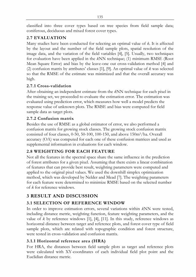
135
classified into three cover types based on tree species from field sample data; coniferous, deciduous and mixed forest cover types. 2.7 EVALUATION Many studies have been conducted for selecting an optimal value of k. It is affected by the layout and the number of the field sample plots, spatial resolution of the image data, and the variation of the field variables [4], [5]. Usually, two techniques for evaluation have been applied in the kNN technique; (1) minimum RMSE (Root Mean Square Error) and bias by the leave-one out cross-validation method [4] and (2) confusion matrix by attributes’ classes [1], [9]. An optimal value of k was selected so that the RMSE of the estimate was minimized and that the overall accuracy was high. 2.7.1 Cross-validation After obtaining an independent estimate from the kNN technique for each pixel in the training set, we proceeded to evaluate the estimation error. The estimation was evaluated using prediction error, which measures how well a model predicts the response value of unknown plots. The RMSE and bias were computed for field sample data as target plots. 2.7.2 Confusion matrix Besides the use of RMSE as a global estimator of error, we also performed a confusion matrix for growing stock classes. The growing stock confusion matrix consisted of four classes, 0-50, 50-100, 100-150, and above 150m3/ha. Overall accuracy (OA) was computed for each one of these confusion matrices and used as supplemental information in evaluations for each window. 2.8 WEIGHTING FOR EACH FEATURE Not all the features in the spectral space share the same influence in the prediction of forest attributes for a given pixel. Assuming that there exists a linear combination of features that can provide best result, weighting parameters were computed and applied to the original pixel values. We used the downhill simplex optimization method, which was developed by Nelder and Mead [7]. The weighting parameters for each feature were determined to minimize RMSE based on the selected number of k for reference windows.
3 RESULT AND DISCUSSION
3.1 SELECTION OF REFERENCE WINDOW In order to improve estimation errors, several variations within kNN were tested, including distance metric, weighting function, feature weighting parameters, and the value of k by reference windows [1], [4], [11]. In this study, reference windows as horizontal distance between target and reference plots, and forest cover type of field sample plots, which are related with topographic condition and forest structure, were tested in cross-validation and confusion matrix. 3.1.1 Horizontal reference area (HRA) For HRA, the distances between field sample plots as target and reference plots were calculated with XY-coordinates of each individual field plot point and the Euclidian distance metric.
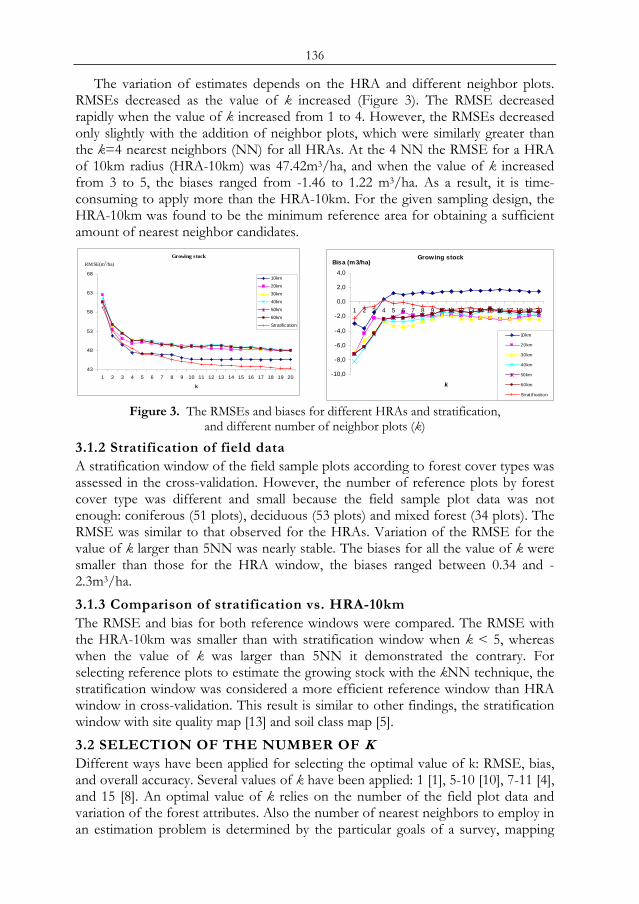
136
The variation of estimates depends on the HRA and different neighbor plots. RMSEs decreased as the value of k increased (Figure 3). The RMSE decreased rapidly when the value of k increased from 1 to 4. However, the RMSEs decreased only slightly with the addition of neighbor plots, which were similarly greater than the k=4 nearest neighbors (NN) for all HRAs. At the 4 NN the RMSE for a HRA of 10km radius (HRA-10km) was 47.42m3/ha, and when the value of k increased from 3 to 5, the biases ranged from -1.46 to 1.22 m3/ha. As a result, it is time-consuming to apply more than the HRA-10km. For the given sampling design, the HRA-10km was found to be the minimum reference area for obtaining a sufficient amount of nearest neighbor candidates.
Growing stock
43
48
53
58
63
68
1 2 3 4 5 6 7 8 9 10 11 12 13 14 15 16 17 18 19 20
k
RMSE(m3/ha)
10km
20km
30km
40km
50km
60km
Stratification
Growing stock
-10,0
-8,0
-6,0
-4,0
-2,0
0,0
2,0
4,0
1 2 3 4 5 6 7 8 9 10 11 12 13 14 15 16 17 18 19 20
k
Bisa (m3/ha)
10km
20km
30km
40km
50km
60km
Strat if ication Figure 3. The RMSEs and biases for different HRAs and stratification,
and different number of neighbor plots (k)
3.1.2 Stratification of field data A stratification window of the field sample plots according to forest cover types was assessed in the cross-validation. However, the number of reference plots by forest cover type was different and small because the field sample plot data was not enough: coniferous (51 plots), deciduous (53 plots) and mixed forest (34 plots). The RMSE was similar to that observed for the HRAs. Variation of the RMSE for the value of k larger than 5NN was nearly stable. The biases for all the value of k were smaller than those for the HRA window, the biases ranged between 0.34 and -2.3m3/ha. 3.1.3 Comparison of stratification vs. HRA-10km The RMSE and bias for both reference windows were compared. The RMSE with the HRA-10km was smaller than with stratification window when k < 5, whereas when the value of k was larger than 5NN it demonstrated the contrary. For selecting reference plots to estimate the growing stock with the kNN technique, the stratification window was considered a more efficient reference window than HRA window in cross-validation. This result is similar to other findings, the stratification window with site quality map [13] and soil class map [5]. 3.2 SELECTION OF THE NUMBER OF K Different ways have been applied for selecting the optimal value of k: RMSE, bias, and overall accuracy. Several values of k have been applied: 1 [1], 5-10 [10], 7-11 [4], and 15 [8]. An optimal value of k relies on the number of the field plot data and variation of the forest attributes. Also the number of nearest neighbors to employ in an estimation problem is determined by the particular goals of a survey, mapping
137
and global bias. Franco-Lopez et al. [1] demonstrated that when applying kNN technique, for map production using only the nearest neighbor plot, the estimator is unbiased and the range in variability of sample is largely preserved, while using more than one neighbor is appropriate to produce estimates of forest attributes over large areas. 3.2.1 Cross validation The RMSE normally decreases as k increases until a minimum RMSE is reached for the HRA-10km and stratification (Figure 3). A minimum RMSE may not be reached before k=20, which also depends on the number of field sample data. The RMSE varies from 45.54 to 60.56m3/ha and from 44.82 to 59.35m3/ha, respectively. A minimum RMSE was 45.54 m3/ha when k=18 for the HRA-10km, and 43.39 m3/ha when k=20 for the stratification. However, at the 4NN for the HRA-10km and at the 5NN for the stratification, the RMSEs showed little tendency to level off, the values were 47.42 and 47.05 m3/ha, and the difference to the minimum RMSE was approximately 4% and 8%, respectively. For selecting the value of k, the stability RMSE could be a more efficient method than the minimum RMSE. 3.2.2 Confusion matrix The overall accuracy (OA) in classification comparing the HRA-10km and stratification is shown in Figure 4. In other studies, there is an increase in the accuracy as the number of neighbors is increased. But the OAs for both reference windows were observed oscillating more or less around a trend in our study. The OA ranged from 0.35 to 0.42 and from 0.34 to 0.39, respectively. The results were much lower than other findings because the study area and the size of field plot data are relatively small. With respect to the OA, the HRA window was higher accurate than the stratification window, except for when k>7. The highest OA was identified as when k=5 with the HRA-10km, the estimated OA was 0.42. 3.3 WEIGHTING FOR EACH FEATURE Weighting parameters for each band were computed with the selected number of k=4 and 5 in cross validation. The calculated parameters were most similar because the correlation between forest attribute and spectral bands was low and spectral variability within a feature was low in our case.
With the weighting parameters for each band, the minimized RMSEs for both windows decreased approximately 1% through feature weight optimization (Table 1). This result is similar other studies with the same simplex optimization [1], [2]. On the other hand, a genetic algorithm approch for calculating weighting parameters performed noticeably better than the un-weighted kNN method [11].
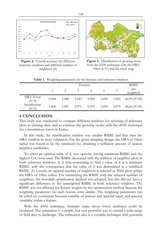
138
Overall accuracy (%)
25
27
29
31
33
35
37
39
41
43
45
1 2 3 4 5 6 7 8 9 10
k
HRA 10km
Fcover
Figure 4. Overall accuracy for different
reference windows and different number of neighbors (k)
Figure 5. Distribution of growing stock from the kNN technique with the HRA-
10km (k=5) and the mask map.
Table 1. Weighting parameters for the features and reference windows Features
1 2 3 4 5 7
RMSE (un-
weighted) HRA 10 km
(k=4) 0.944 1.088 1.043 0.984 1.056 1.065 46.99 (47.42)
Stratification (k=5) 1.006 1.087 0.971 0.979 1.059 0.975 46.66 (47.05)
4 CONCLUSION This study was conducted to compare different windows for selecting of reference plots in training data, and to estimate the growing stocks with the kNN technique for a mountinous forest in Korea.
In this study, the stratification window was smaller RMSE and bias than the HRA window in cross validation. For the given sampling design, the HRA of 10km radius was found to be the minimum for obtaining a sufficient amount of nearest neighbor candidates.
To select an optimal value of k, two options, having minimum RMSE and the highest OA, were used. The RMSE decreased with the addition of neighbor plots in both reference windows. It is time-consuming to find a value of k at a mininum RMSE, with the consequence that the value of k was determined at a stabilized RMSE. As a result, an optimal number of neighbors is selected as 5NN plots within the HRA of 10km radius. For minimizing the RMSE with the selected number of neighbors, the downhill optimization method was adopted, but this did not have a significant difference to the unweighted RMSE in both reference windows. The RMSE was not affected for feature weights by the optimization method because the weighting parameters for each feature were similar. The weighting parameters can be relied on correlation between variable of interest and spectral band, and spectral variabilty within a feature.
With the kNN technique, thematic maps about forest attributes could be produced. The estimation is a simple, but very powerful way to extend a wide range of field data to landscape. The estimation also is a versatile technique with potential
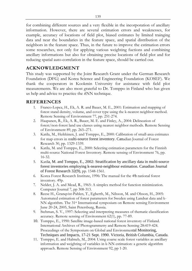
139
for combining different sources and a very flexible in the incorporation of ancillary information. However, there are several estimation errors and weaknesses, for example, accuracy of locations of field plot, biased estimates by limited trainging data and near the boundaries in the feature space, and spatial distribution of the neighbors in the feature space. Thus, in the future to improve the estimation errors some researches, not only for applying various weighting fuctions and combining ancillary informations but also for obtaining precise locations of field plot and for reducing spatial auto-correlation in the feature space, should be carried out.
ACKNOWLEDGMENT This study was supported by the Joint Research Grant under the German Research Foundation (DFG) and Korea Science and Engineering Foundation (KOSEF). We thank the cooperators in Kookmin University for assistance with field plot measurements. We are also most grateful to Dr. Tomppo in Finland who has given us help and advice to practice the kNN technique.
REFERENCES 1. Franco-Lopez, H., Ek, A. R. and Bauer, M. E., 2001: Estimation and mapping of
forest stand density, volume, and cover type using the k-nearest neighbor method. Remote Sensing of Environment 77, pp. 251-274.
2. Haapanen, R., Ek, A. R., Bauer, M. E. and Finley, A., 2004: Delineation of forest/non-forest land use classes using nearest neighbor methods. Remote Sensing of Environment 89, pp. 265–271.
3. Katila, M., Heikkinen, J. and Tomppo, E., 2000: Calibration of small-area estimates for map errors in multi-source forest inventory. Canadian Journal of Forest Research 30, pp. 1329-1339.
4. Katila, M. and Tomppo, E., 2000: Selecting estimation parameters for the Finnish multi-source National Forest Inventory. Remote sensing of Environment 76, pp. 16-32.
5. Katila, M. and Tomppo, E., 2002: Stratification by ancillary data in multi-source forest inventories employing k-nearest-neighbour estimation. Canadian Journal of Forest Research 32(9), pp. 1548-1561.
6. Korea Forest Research Institute, 1996: The manual for the 4th national forest inventory. 49p.
7. Nelder, J. A. and Mead, R., 1965: A simplex method for function minimization. Computer Journal 7, pp 308-313.
8. Reese H., Granqvist-Pahlen, T., Egberth, M., Nilsson, M. and Olsson, H., 2005: Automated estimation of forest parameters for Sweden using Landsat data and k-NN algorithm. The 31st International symposium on Remote sensing Environment June 20-24, 2005, Saint Petersburg, Russia.
9. Stehman, S. V., 1997: Selecting and interpreting measures of thematic classification accuracy. Remote sensing of Environment 62(1), pp. 77-89.
10. Tomppo, E., 1990: Satellite image-based national forest inventory of Finland. International Archives of Photogrammetry and Remote Sensing 28:419-424. Proceedings of the Symposium on Global and Environmental Monitoring, Techniques and Impacts, 17-21 Sept. 1990. Victoria, British Columbia, Canada.
11. Tomppo, E. and Halmeb, M., 2004: Using coarse scale forest variables as ancillary information and weighting of variables in k-NN estimation: a genetic algorithm approach. Remote Sensing of Environment 92, pp 1-20.

140
12. Tokola, T., 2000: The influence of field sample data location on growing stock volume estimation in Landsat TM-based forest inventory in eastern Finland. Remote sensing of environment 74(3), pp. 422-431.
13. Tokola, T. and Heikkilä, J., 1997: Improving satellite image based forest inventory by using a priori site quality information. Silva Fennica 31(1), pp. 67–78.
141
Mapping of forest cover types with satellite imagery and field plot data
J.-S. Yima, C. Kleinna, M.-Y. Shinb, G.-S. Kongc a Institute of Forest Management, Büsgenweg 5, D-37077 Göttingen, email :
[email protected] b Department of Forest Resources, College of Forest Science, Kookmin University,
Korea c Division of Forest Inventory, Korea Forest Research Institute, Korea
ABSTRACT Maps of forest cover types show impo15rtant baseline information for forest managers and forest politicians. In South Korea, a forest cover type map is produced at a 10-year interval from aerial photographs, an exercise which is linked to the field sampling of the national forest inventory (NFI). The objectives of this study were (I) to test the Minnaert correction for reducing topographic effects in the Landsat TM, (II) to draw a forest cover type map using field plot data available in the NFI and from Landsat TM, and (III) to compare the produced maps from aerial photographs and Landsat TM.
Minnaert constants (k) for each feature space were estimated with the Landsat TM and DEM data from field sample plot points. The calculated values of k ranged from 0.2402 to 0.5237, which implied that the topographic effect was not the same for all bands within Landsat. For forest cover type mapping, a pixel-wise classification by the maximum likelihood method was used. The pixel values obtained within Landsat from field sample points were then classified into three forest cover types based on linked field plot data. Most of the pixel values from mixed forest were overlapped in feature spaces with coniferous and broadleaved forests. The classified map was compared to the true forest cover map in the study area, which resulted from the third NFI. The error matrix was analyzed to evaluate accuracy of the classified map with the field sample plot and the digitized forest cover map, and the Chi-square goodness-of-fit was performed to compare distribution of forest cover types from the two maps. The accuracy was modest. User and producer accuracies were between 19 and 72%, and between 22 and 69%, respectively. The overall accuracy of classification achieved was 52%. The estimated kappa was 0.34. Conversely, the classification obtained from the two maps was done on statistical grounds using the Chi-square test. The result showed that there was no difference in the distributions of forest cover types between two maps. Keywords: forest cove type map, pixel-wise classification, topographic correction, NFI, Korea
1 INTRODUCTION Forests in South Korea cover an area of approximately 64,063km2, representing approximately 64% of the total land area, on the other hand the area for farming Proc. 2nd Göttingen GIS and Remote Sensing Days, 4-6 Oct. 2006, Göttingen
142
represents 20% and other land uses account for 16%. Forests cover a large area, and are mainly located in mountainous ranges.
There is a need for detailed maps providing the current status of forest cover types. Maps of forest cover types are important baseline information for forest managers and forest politicians. Forest cover type map shows relatively homogeneous forest stands or cover types, and has been produced from interpretation of aerial photographs, satellite imagery, and also field plots. It commonly includes information on the tree species, age class, diameter class, site and stocking level [10]. In Korea, the forest cover type maps are produced at 10-year intervals, from the interpretation of aerial photographs; the maps were corrected with field sample plots in the National Forest Inventory (NFI). Since the early 1970s, aerial photographs have been used to produce the forest cover type map in the NFI. However, the use of aerial photography is waning because the interpretation and processing is laborious, and aerial photography is often out of date. The ability to repeatedly obtain images, continuity of the obtained images, and their wide availability are some characteristics of digital satellite imagery that have contributed to the current development of remote sensing, image processing, and GIS technologies.
Recently, digital satellite data, for example Landsat TM, have been applied successfully to large-area applications [3]. Using satellite data, for classifying forest cover types has involved a supervised classification along with training data or reference data. A pixel-wise classification is used with field sample plots from NFIs. The basic idea is to combine the detailed reference data from the field sample data with remote sensing data and also digital maps. From the early 1990s, satellite image data have been applied to draw forest cover maps at the Korea Forest Research Institute (KFRI) and for some studies [1], [2]. Currently, research studies on remote sensing are increasing, particularly for forest area change monitoring in North Korea [7], and for forest health [8] and forest fire monitoring [17]. However, there has not been an attempt as yet to integrate satellite remote sensing to the NFI. The objectives of this study are (I) to test the Minnaert correction for reducing topographic effects in Landsat TM, (II) to draw a map of forest cover types using field plot data available in the NFI and from Landsat TM, and (III) to compare the produced maps from aerial photographs and Landsat TM.
2 MATERIAL
2.1 STUDY SITE The study area, Pyeong-chang County, is located in northeastern South Korea and covers an area of approximately 1,463 km2. The county lies between 37°16`N and 37°49`N parallels and 128°14`E and 128°46`E meridians. Approximately 84% (or 1,229 km2) of the land area of the county is occupied by forests; the area for farming is only 10% (or 152 km2) and that for other uses is 6% [9]. The county lies over a relatively hilly mountain range and the mean slope is approximately 20°. The altitude ranges from 210 to 1,570m and the average altitude is approximately 670m. The main tree species are Japanese red pine (Pinus densiflora), Korean pine (Pinus koraiensis), Japanese larch (Larix leptolepis), Mongolian oak (Quercus mongolica), and other broadleaved trees.
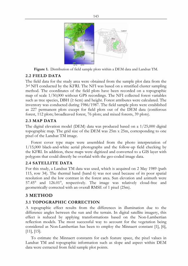
143
Figure 1. Distribution of field sample plots within a DEM data and Landsat TM.
2.2 FIELD DATA The field data for the study area were obtained from the sample plot data from the 3rd NFI conducted by the KFRI. The NFI was based on a stratified cluster sampling method. The coordinates of the field plots have been recorded on a topographic map of scale 1/50,000 without GPS recordings. The NFI collected forest variables such as tree species, DBH (≥ 6cm) and height. Forest attributes were calculated. The inventory was conducted during 1986/1987. The field sample plots were established as 227 permanent plots except for field plots out of the DEM data (coniferous forest, 112 plots; broadleaved forest, 76 plots; and mixed forests, 39 plots). 2.3 MAP DATA The digital elevation model (DEM) data was produced based on a 1/25,000 digital topographic map. The grid size of the DEM was 25m x 25m, corresponding to one pixel of the Landsat TM image.
Forest cover type maps were assembled from the photo interpretation of 1/15,000 black-and-white aerial photographs and the follow-up field checking by the KFRI. In addition, these maps were digitized and converted to a GIS layer with polygons that could directly be overlaid with the geo-coded image data. 2.4 SATELLITE DATA For this study, a Landsat TM data was used, which is acquired on 2 May 1989 (path 115, row 34). The thermal band (band 6) was not used because of its poor spatial resolution and the low contrast in the forest area. Sun elevation and azimuth were 57.45° and 126.01°, respectively. The image was relatively cloud-free and geometrically corrected with an overall RMSE of 1 pixel (25m).
3 METHOD
3.1 TOPOGRAPHIC CORRECTION A topographic effect results from the differences in illumination due to the difference angles between the sun and the terrain. In digital satellite imagery, this effect is reduced by applying transformations based on the Non-Lambertian reflection models. The most successful way to account for the vegetation being considered as Non-Lambertian has been to employ the Minnaert constant [1], [6], [11], [15].
To estimate the Minnaert constants for each feature space, the pixel values in Landsat TM and topographic information such as slope and aspect within DEM data were extracted from field sample plot points.
144
3.2 CLASSIFICATION To produce a classified image map, there are needs of clearer definitions of categories, e.g., forest and forest cover types within a forest. The classification categories are based upon a Manual of NFI by KFRI [10]. These categories are stocked land (coniferous-mixed forest, broadleaved-mixed forest and mixed forest), non-stocked land (cutover area, treeless land, denuded land, glass land and cultivated land), non-forest land and bare land. In this study, the first part of interpretation was the identification of forest areas from other land-cover classes. Further, the forest areas were classified into forest cover types (Table 1).
A pixel-wise classification by the maximum likelihood method was used along with the field sample plot data from the NFI. The basic concept is to combine the detailed reference data from the field sample data with remote sensing data and also digital map. The available field plot data for each forest stratum served as the training data.
Table 1. General description of forest cover types in Korea
Forest cover types Description
Forest (stocked land)
The forest has the above 30% of the crown cover area or
the above 1,200 seeding trees of coniferous or
the above 1,600 seeding trees of broadleaved, minimum area is 1 ha
Coniferous-mixed forest
The forest has the coniferous-mixed forest above 75% of the crown area or number of tree
Broadleaved-mixed forest
The forest has the broadleaved-mixed forest above 75% of the crown area or number of tree
Mixed forest The forest has the broadleaved tree or coniferous tree above 25% and below 75% of the crown area or number of tree
3.3 EVALUATION A produced image map based on the pixel-wise classification using Landsat TM was analyzed for evaluating the classification accuracy against forest cover types of field sample plots. This analysis allows an accuracy statement; the accuracy is defined in terms of the degree of misclassification and is calculated from a so-called confusion or error matrix [5], [14]. Further, the Kappa statistic is used as a measure of the classification accuracy [5]. The Kappa statistic incorporates the non-diagonal elements of the error matrix as a product of the row and column marginal [12]. 3.4 COMPARISON The produced image map was also compared against the true forest cover map (“digitized map”), which resulted from the third NFI with regard to the error matrix and Kappa statistic. Further, the comparison of the classification result from the two maps was done on statistical grounds using the Chi-square goodness-of-fit test. This test was preformed to determine the significance of the differences between them. The observed value used in this test was the number of points of forest cover
145
types on the digitized map, while the expected value was the number of points of forest cover types on the produced image map.
4 RESULT AND DISCUSSION
4.1 TOPOGRAPHIC CORRECTION The study area in this study covers hilly mountainous forest areas, as can be seen in Figure 2-a. The outcome is that the forest area classifications include various errors due to the topographic effect when satellite image applied. Lee and Yoon [11] tested three methods with the Landsat TM in mountainous forest areas: cosine, Minnaert constant, and band-ratio corrections. They found that the Minnaert correction method provided the most reliable result for reducing topographic effect.
The Minnaert constant k could be solved for each feature space in the TM data. The values of k were calculated and they ranged from 0.2402 to 0.5237, which implied that the topographic effect was not the same for all bands within the Landsat TM. When different bands were compared, band 7 showed the highest value of k. The largest range of difference was observed between bands 3 and 4. This was similar to other studies [1], [4], [11], [16]. With respect to the topographic effect on bands, Lee and Yoon [11] demonstrated that the near- and middle- infrared bands appeared to be more vulnerable to the topographic effect as compare to visible bands. After the Minnaert constants were derived, topographic correction was performed. A reduction in the topographic effect was visually apparent in a normalized image (Figure 2-b).
Figure 2. Comparison between row (a) and topographic normalized (b) image data (TM
4,3,2).
4.2 CLASSIFICATION The pixel-wise classification by the maximum likelihood method was applied for mapping forest cover types. The pixel values in the feature spaces were obtained from each field plot point, and then classified into three forest cover types based on linked field plot data. Figure 3 shows the mean of the pixel values for different forest cover types and bands. For bands 4 and 5, the difference in the forest cover types could be observed, whereas at other bands there existed little difference. The mean of the broadleaved-mixed forest (H) was the lowest for band 4, and it was the highest for band 5. Figure 4 illustrates the distribution of pixel values according to the forest cover types for bands 4 and 5. For classifying forest cover types, the difference in the pixel value between coniferous and broadleaved forests can be more clearly observed as compare to the mixed forest. Most of the pixel values from
(a) (b)
146
mixed forest were overlapped in the feature spaces with the coniferous and broadleaved forests.
253035404550556065707580859095
B1 B2 B3 B4 B5 B7
Band
Pixe
l val
ue
C
H
M
Figure 3. The mean of pixel values for different forest cover types and bands.
Figure 4. Distribution of pixel values by forest cover type for bands 4 and 5.
4.3 EVALUATION A classified image map (“classified map”) was produced through the pixel-wise classification by the maximum likelihood method using the Landsat TM. This map was analyzed for evaluating the classification accuracy with 227 field plot data within the DEM data (Table 2). The accuracy was modest. User and producer accuracies were between 22 and 65% and between 44 and 50%, respectively. The overall accuracy achieved was 47% and the estimated kappa was 0.2. With respect to classification based on satellite image data, Mayaux and Lambin [13] found that the forest cover was rather overestimated from coarse-resolution satellite data in regions where the forest cover was homogenous, and was rather underestimated in regions where the forest cover was fragmented. In our case, relatively homogenous forest covers, i.e., coniferous and broadleaved forests, were underestimated, while heterogeneous (mixed) forest cover was overestimated.
Table 2. Error matrix for assessing the classification accuracy of the classified forest cover map
Field plot Classification C H M
Total User’s accuracy
C 56 23 16 95 59 % H 13 34 5 52 65 % M 34 16 17 77 22 %
Classified map
Non-forest 9 3 7 13 Total 112 76 39 227
Producer’s accuracy 50 % 45 % 44 %
Overall accuracy 47 %
KHAT = 0.20
4.4 COMPARISON The classified map was compared with the digitized map by the error matrix and the Chi-square test. Table 4 presents the error matrix for the two maps. User and producer accuracies were between 19 and 72%, and between 22 and 69%, respectively. The overall accuracy achieved was 52% and the estimated kappa was 0.34. However, the mixed forest class was demonstrated the lowest accuracies; only
147
22% of the mixed forest areas were correctly identified as “mixed forest” and 19% in the study area and was identified as “mixed forest” on the classified map.
Table 4. Error matrix for assessing the classification accuracy with digitized and classified maps
Digitized map Classification
C H M Non-forest
Total User’s accuracy
C 427,180 165,943 149,863 70,262 813,248 52.5% H 119,859 410,158 119,805 30,782 680,604 60.3% M 204,737 108,274 81,496 34,240 428,747 19.0%
Classified map
Non-forest 82,466 20,079 16,076 307,314 425,935 72.2%
Total 834,242 704,454 367,240 442,598 2,348,534
Producer’s accuracy 51.2% 58.2% 22.2% 69.4%
Overall accuracy 52.2%
KHAT = 0.34
For mapping forest cover types, different minimum sizes were used for the areas. A minimum size of 1ha was used when the interpretation of aerial photographs was performed, while a minimum size of 0.0625 ha (which depends on a spatial resolution of satellite data) was used with the Landsat TM. For this reason, the coniferous and broadleaved forests on the digitized map were more separated as compared to that on the classified map; as a result, both the forests were classified as mixed forest on the classified map (Figure 5).
Figure 5. Comparison between digitized (a) and classified (b) forest cover maps for study
area. On the other hand, the comparison of the classification result from the maps
was done on statistical grounds using the Chi-square goodness-of-fit tests. To determine the significance of the differences in the forest cover types between two maps, we randomly selected 323 points. The null hypothesis of the test could be rejected. This result showed that there was no difference in the distributions of forest cover types between two maps.
(a) (b)
148
Table 5. The distribution of forest cover type for different maps and the result Chi-square test
Classification C H M Non-forest total
Digitized map 123 81 58 61 323 Classified map 96 87 70 70 323
Total 219 168 128 131 646 X2 ≈5.03, p ≈ 0.20 (not significant)
5 CONCLUSION Three conclusions may be drawn from this study: (1) Topographic effect over the mountainous forests can influence the natural spectral variability and is different for each feature space. Therefore, this study deals with a Minnaert correction method, which can be reduced. However, in the estimation of Minnaert constants from field sample plots, the size of sample plots was not enough to give reliable k estimates and variation within field sample plot data was to large. (2) For forest cover type mapping, a pixel-wise classification was applied. The pixel values obtained from the Landsat TM for each field plot point and they were then classified into three forest cover types based on linked field data. For the application of the pixel-wise classification, the location of the field sample plot was the main relational factor; however, the coordinates of field sample plot points from the 3rd NFI included location errors because the locations were marked on topographic maps without GPS recording. However if the global positioning system (GPS) is used for locating the field plot points, the errors should be reduced. (3) A minimum size of 1ha was used when the interpretation of aerial photographs was performed, while a minimum size of 0.0625ha was used with the Landsat TM. For this reason, the coniferous and broadleaved forests on the digitized map were more separated on the classified map. For obtaining the quality of the forest cover type classification results, above all, clearer and quantitative definitions are required to classify forest and non-forest areas and forest cover types within the forest areas. Further, the key to success is having sufficient field sample data to cover all the variations in topographic conditions and tree species for each cover type.
ACKNOWLEDGMENT This research was supported by the Joint Research Grant under the German Research Foundation (DFG) and Korea Science and Engineering Foundation (KOSEF). We thank the researcher in Korea Forest Research Institute for furnishing of field plot data and digitized forest cover maps.
REFERENCES 1. Cho, H. K., 2002: Untersuchungen über die Erfassung von Waldflächen und deren
Veränderungen mit Hilfe der Satellitenfernerkundung und segmentbasierter Klassifikation. Dissertation zur Georg-August-Universität Göttingen. 120p.
2. Chung, K. H., Lee,W. K., Lee, J. H., Kwon, K. H. and Lee, S. H., 2001: The classification of forest cover type using high resolution IKNOS satellite image. Journal of Korean Society Remote sensing 17(3), pp. 275-283.
3. Cihlar, J., Guindon, B., Beaubien, J., Latifovic, R., Peddle, D., Wulder, M., Fernandes, R. and Kerr, J., 2003: From need to product: a methodology for

149
completing a land cover map of Canada with Landsat data. Can. J. Remote Sensing 29(2), pp. 171-186.
4. Colby, J.D., 1991: Topographic normalization in rugged terrain. Photogrammertic Engineering and Remote sensing 45(9), pp. 1303-1309.
5. Congalton, R. G., 1991: A review of assessing the accuracy of classifications of remotely sensed data. Remote Sensing of Environment 37, pp. 35-46.
6. Itten, K. I., Meyer, P., Kellenberger, T., Leu, R., Bitter, P. and Seidel, K., 1992: Correction of the impact of topography and atmosphere on Landsat-TM forest mapping of Alpine regions. Remote sensing series vol. 18, 47p.
7. Kim, C. M. and Lee, S. H., 2001: The forest denude classification in North Korea used a satellite image at different period. Journal of Korean Forestry Society 87(2), pp. 168-169
8. Kim, J. B., Cho, M. H., Kim, I. H. and Kim, Y. G., 2003: A study on extraction of damaged area by Pine wood Nematode Using high resolution satellite images and GPS. Journal of Korean Forestry society 92(4), pp. 362-366.
9. Korea Forest Service, 2004: Statistical yearbook of Forestry. 434p. 10. Korea Forest Research Institute, 1996: The manual for the 4th national forest
inventory in Korea. 49p. 11. Lee, K. S. and Yoon, J. S., 1997: Radiometric correction of terrain effects for SPOT
and Landsat Thematic mapper imagery in mountainous forest area. Journal of the Korean society of Remote sensing 13(3) pp. 277-292.
12. Lillwsand, T. M., Kiefer, R. W. and Chipman, J. W., 2004: Remote sensing and image interpretation fifth. John Wiley & Sons, Inc. 763p.
13. Mayaux, P., and Lambin, E. F., 1995: Estimation of tropical forest area from coarse spatial resolution data: a two step correction function for proportional errors due to spatial aggregation. Remote Sensing of Environment 53, pp. 1–16.
14. Smits, P. S., Dellepiane, S. G. and Schowengerdt, R. A., 1999: Quality assessment of image classification algorithms for land-cover mapping: a review and a proposal for a cost-based approach. Int. J. Remote Sensing 20(8), pp. 1461-1486.
15. Toilet, P. M., Guindon, B. and Good enough, D. G.., 1982: On the slope-aspect correction of multi-spectral scanner data. Can. J. Remote sensing 8(2), pp. 84-106.
16. Tokola T., Sarkeala, J. and van der Linden, M., 2001: Use of topographic correction in Landsat TM-based forest interpretation in Nepal. Int. J. remote sensing 22(4), pp. 551–563.
17. Won, K. Y. and Im, J. H., 2001: Fire severity mapping using a single post fire Landsat 7-ETM imagery. Korean Journal of Remote Sensing 17(1), pp. 85-97.

150
151
AMBIGUITY AND BOUNDARY EFFECTS IN LAND COVER MAPS OF A TROPICAL MOUNTAINOUS
LANDSCAPE DERIVED FROM HIGH RESOLUTION SATELLITE DATA
A. Gleitsmanna a Institute of Geography, University of Göttingen, Goldschmidtstr. 5, 37077
Göttingen, email: [email protected]
ABSTRACT Mountainous tropical landscap16es where agriculturally used areas border on natural vegetation are often very fragmented and include many different types of land cover. In addition, the natural and semi-natural land cover types usually do not occur in discrete units, but with gradual transitions between them. In this study, high spatial resolution IKONOS data are used to map the vegetation of a protected mountain forest area and of the reserve’s buffer zone in the Dominican Republic’s Cordillera Central. Texture parameters calculated in 15 m × 15 m moving windows are used as input to the classification in addition to the 4 band multispectral information. Given the fragmented nature of the study area, the ‘hard’ classification accuracy is impaired by the fact that there are land cover ambiguities which tend to increase in the vicinity of land cover boundaries and in transitional areas. The spatial distribution of classification uncertainty is analyzed using the a posteriori probabilities of a maximum likelihood classification result. Areas of low a posteriori probability occur mostly along class boundaries. The classification accuracy in areas not close to class borders is compared to the accuracy values derived using reference points distributed over the whole study area, for classifications with and without texture parameters. It is shown that the texture parameters, although improving the overall classification accuracy, impair the accuracy in boundary regions. This is because pixels in the texture band contain information from the whole 15 m × 15 m window, a relatively large area compared to the 4 m resolution of the IKONOS multispectral bands. Classification ambiguities should be distinguished from absolute misclassifications. One way to do this is fuzzy accuracy assessment. The fuzzy accuracy is significantly higher than the ‘hard’ accuracy value. Keywords: High spatial resolution satellite data, Land cover mapping, Accuracy, Fuzzy, Boundary effects, Tropical mountain vegetation.
1 INTRODUCTION In mountainous tropical landscapes where agriculturally used areas border on remaining mountain forests and semi-natural vegetation types, the land cover pattern is typically very fragmented. Many different land cover types form a mosaic. Contiguous areas of one land cover type can be very small, like for example the Proc. 2nd Göttingen GIS and Remote Sensing Days, 4-6 Oct. 2006, Göttingen
152
narrow bands of riparian forest left in otherwise deforested areas, or the fields of small farms.
Low and medium resolution satellite data of such heterogeneous areas contain a large proportion of mixed pixels, preventing the accurate separation and mapping of land cover classes. Increasing the spatial resolution reduces the proportion of pixels on the boundary between class areas and would solve the problem for internally homogeneous land cover types with crisp boundaries. But land cover classes like agro-forestry or forest types start to appear internally heterogeneous when the resolution of the imagery is increased, with some pixels representing illuminated tree crowns, some understorey vegetation, others shadow areas and so on. This lack of spatial integration of the elements of the target classes poses a new problem for an automated per-pixel classification. The choice of data and the processing methods are then a compromise between trying to reduce the within-class variability (e.g. by spatial integration of small pixels) and trying to reduce edge effects in the form of pixels containing information about more than one target class [1].
A challenge in any classification of natural and semi-natural vegetation classes is the lack of crisp boundaries. Conventional ‘hard’ supervised classification techniques assume that the classes are exhausttively defined and mutually exclusive, so that each pixel belongs to one and only one of the pre-defined training classes. However, in the reality of land cover classification, and in particular in the classification of natural vegetation with remote sensing, there are several sources of uncertainty.
Firstly, there are ambiguities on the ground. Natural vegetation often does not occur in discrete spatial and thematic units. Instead, it may vary continuously according to environmental gradients, leading to gradual transitions between the defined classes (vegetation types) with broad areas of high ambiguity in the transition zones. Another source of uncertainty is the fragmentation of land cover types or environmental heterogeneity, i.e. the inclusion of small areas of one land cover type in another type [2]. There are also temporal continua, e.g. a secondary succession starting with a mainly herbaceous land cover, which develops first into a shrub-dominated land cover, then into a secondary forest and finally a mature forest. This entails that there are stages in the succession when the land cover is in a transitional stage between the defined land cover types of a classification scheme. In addition, some classes may contain common elements (two forest types could for example share a tree species or the same kind of understorey vegetation). If such similar classes occur adjacent to each other, the boundary between them will be more vague than for classes with larger differences in their definitions. Numerical thresholds in the definition of land cover classes (like percent crown cover) are idealisations of the natural world. If we define open forest as forest with a crown cover below 60 % and then encounter a forest area with around 60 % crown cover, it will be impossible to determine a definite boundary line between open and closed forest which all interpreters would exactly agree on.
Secondly, there are inherent uncertainties in the remotely sensed data which impede a direct, unambiguous link between the data and the type of the land cover. The limited spatial resolution leads to the possibility of class mixtures within one
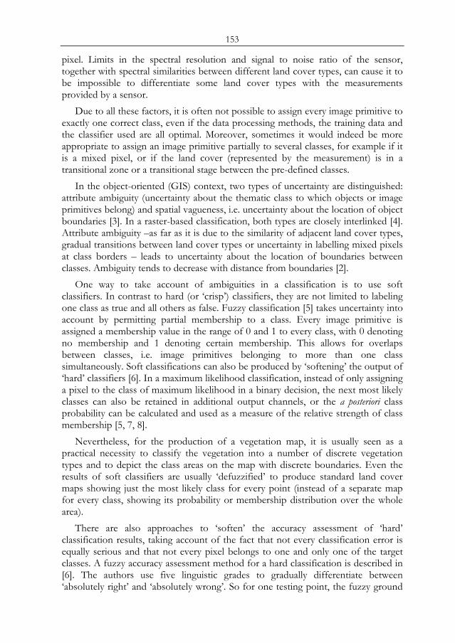
153
pixel. Limits in the spectral resolution and signal to noise ratio of the sensor, together with spectral similarities between different land cover types, can cause it to be impossible to differentiate some land cover types with the measurements provided by a sensor.
Due to all these factors, it is often not possible to assign every image primitive to exactly one correct class, even if the data processing methods, the training data and the classifier used are all optimal. Moreover, sometimes it would indeed be more appropriate to assign an image primitive partially to several classes, for example if it is a mixed pixel, or if the land cover (represented by the measurement) is in a transitional zone or a transitional stage between the pre-defined classes.
In the object-oriented (GIS) context, two types of uncertainty are distinguished: attribute ambiguity (uncertainty about the thematic class to which objects or image primitives belong) and spatial vagueness, i.e. uncertainty about the location of object boundaries [3]. In a raster-based classification, both types are closely interlinked [4]. Attribute ambiguity –as far as it is due to the similarity of adjacent land cover types, gradual transitions between land cover types or uncertainty in labelling mixed pixels at class borders – leads to uncertainty about the location of boundaries between classes. Ambiguity tends to decrease with distance from boundaries [2].
One way to take account of ambiguities in a classification is to use soft classifiers. In contrast to hard (or ‘crisp’) classifiers, they are not limited to labeling one class as true and all others as false. Fuzzy classification [5] takes uncertainty into account by permitting partial membership to a class. Every image primitive is assigned a membership value in the range of 0 and 1 to every class, with 0 denoting no membership and 1 denoting certain membership. This allows for overlaps between classes, i.e. image primitives belonging to more than one class simultaneously. Soft classifications can also be produced by ‘softening’ the output of ‘hard’ classifiers [6]. In a maximum likelihood classification, instead of only assigning a pixel to the class of maximum likelihood in a binary decision, the next most likely classes can also be retained in additional output channels, or the a posteriori class probability can be calculated and used as a measure of the relative strength of class membership [5, 7, 8].
Nevertheless, for the production of a vegetation map, it is usually seen as a practical necessity to classify the vegetation into a number of discrete vegetation types and to depict the class areas on the map with discrete boundaries. Even the results of soft classifiers are usually ‘defuzzified’ to produce standard land cover maps showing just the most likely class for every point (instead of a separate map for every class, showing its probability or membership distribution over the whole area).
There are also approaches to ‘soften’ the accuracy assessment of ‘hard’ classification results, taking account of the fact that not every classification error is equally serious and that not every pixel belongs to one and only one of the target classes. A fuzzy accuracy assessment method for a hard classification is described in [6]. The authors use five linguistic grades to gradually differentiate between ‘absolutely right’ and ‘absolutely wrong’. So for one testing point, the fuzzy ground
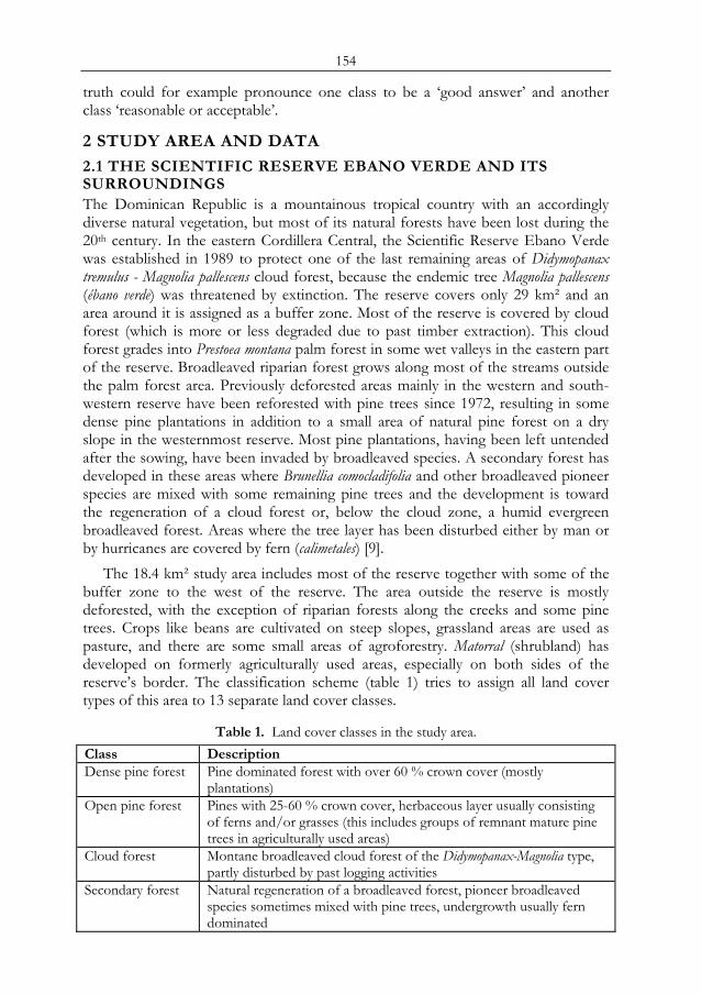
154
truth could for example pronounce one class to be a ‘good answer’ and another class ‘reasonable or acceptable’.
2 STUDY AREA AND DATA
2.1 THE SCIENTIFIC RESERVE EBANO VERDE AND ITS SURROUNDINGS The Dominican Republic is a mountainous tropical country with an accordingly diverse natural vegetation, but most of its natural forests have been lost during the 20th century. In the eastern Cordillera Central, the Scientific Reserve Ebano Verde was established in 1989 to protect one of the last remaining areas of Didymopanax tremulus - Magnolia pallescens cloud forest, because the endemic tree Magnolia pallescens (ébano verde) was threatened by extinction. The reserve covers only 29 km² and an area around it is assigned as a buffer zone. Most of the reserve is covered by cloud forest (which is more or less degraded due to past timber extraction). This cloud forest grades into Prestoea montana palm forest in some wet valleys in the eastern part of the reserve. Broadleaved riparian forest grows along most of the streams outside the palm forest area. Previously deforested areas mainly in the western and south-western reserve have been reforested with pine trees since 1972, resulting in some dense pine plantations in addition to a small area of natural pine forest on a dry slope in the westernmost reserve. Most pine plantations, having been left untended after the sowing, have been invaded by broadleaved species. A secondary forest has developed in these areas where Brunellia comocladifolia and other broadleaved pioneer species are mixed with some remaining pine trees and the development is toward the regeneration of a cloud forest or, below the cloud zone, a humid evergreen broadleaved forest. Areas where the tree layer has been disturbed either by man or by hurricanes are covered by fern (calimetales) [9].
The 18.4 km² study area includes most of the reserve together with some of the buffer zone to the west of the reserve. The area outside the reserve is mostly deforested, with the exception of riparian forests along the creeks and some pine trees. Crops like beans are cultivated on steep slopes, grassland areas are used as pasture, and there are some small areas of agroforestry. Matorral (shrubland) has developed on formerly agriculturally used areas, especially on both sides of the reserve’s border. The classification scheme (table 1) tries to assign all land cover types of this area to 13 separate land cover classes.
Table 1. Land cover classes in the study area. Class Description Dense pine forest Pine dominated forest with over 60 % crown cover (mostly
plantations) Open pine forest Pines with 25-60 % crown cover, herbaceous layer usually consisting
of ferns and/or grasses (this includes groups of remnant mature pine trees in agriculturally used areas)
Cloud forest Montane broadleaved cloud forest of the Didymopanax-Magnolia type, partly disturbed by past logging activities
Secondary forest Natural regeneration of a broadleaved forest, pioneer broadleaved species sometimes mixed with pine trees, undergrowth usually fern dominated
155
Palm dominated forest
Edaphic forest type dominated by the palm tree Prestoea montana
Broadleaved riparian forest
Evergreen broadleaved riparian forest (some small remains of non-riparian humid broadleaved forest are also assigned to this class)
Matorral) Areas with over 25 % shrub cover, besides ferns and grasses, tree crown cover below 25 % (in most cases no trees at all)
Calimetal Areas dominated by the fern Dicranopteris pectinata, sometimes with a proportion of other fern species, with no or very few emerging shrubs and trees
Agroforestry Crops (mostly coffee and bananas) with shade trees Grassland Herbaceous vegetation cover, mostly grasses, also ferns (but not
dominated by Dicranopteris pectinata), combined coverage of shrubs and trees below 25 %
Crops Cultivated agricultural areas, mostly beans, no shade trees Bare ground No or very sparse vegetation cover (roads, landslide scars, river bars,
agricultural areas with seasonal lack of vegetation cover) Water Open water (river)
2.1.1 Causes for ambiguities between the target classes The land cover of the study area is very heterogeneous with many gradual spatial transitions between the defined classes, for example between the classes cloud forest and palm dominated forest, where the proportion of palm trees in the cloud forest increases gradually, or between open pine forest and matorral. Temporal transitions (succession) occur between matorral and secondary forest and several other class pairs (Fig. 1). An example for the inclusion of small areas of one vegetation type within another type are the calimetal patches in the cloud forest and secondary forest. The fragmented land cover mosaic with many small contiguous class areas (e.g. narrow bands of riparian forest, small patches of agroforestry) leads to a high percentage of the total area being close to some class border. In medium resolution satellite data (like Landsat with 30 m spatial resolution) this would lead to a very high percentage of mixed pixels. 2.2 HIGH RESOLUTION SATELLITE DATA The remote sensing data used in this study was acquired on April 19, 2001 by the IKONOS-2 satellite. The IKONOS sensor records four channels of multispectral data (three in the visible and one in the near infrared) at 4 m resolution and one panchromatic channel at 1 m resolution. The high resolution of the data reduces the proportion of mixed pixels. On the other hand, the high resolution pixels fail to integrate the elements of some classes, particularly forest classes.
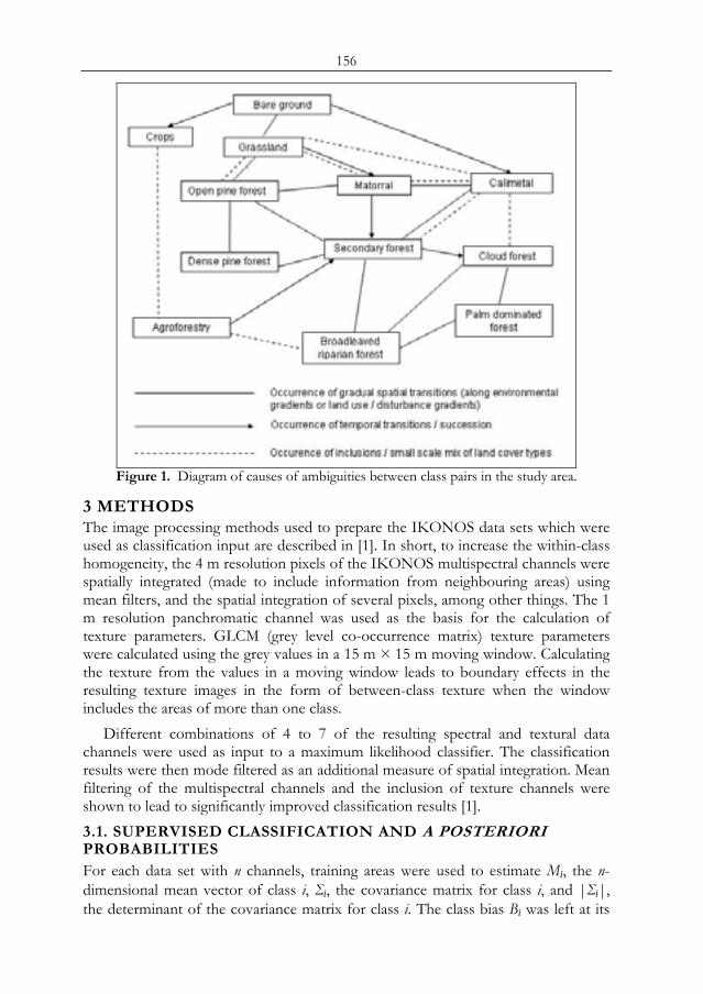
156
Figure 1. Diagram of causes of ambiguities between class pairs in the study area.
3 METHODS The image processing methods used to prepare the IKONOS data sets which were used as classification input are described in [1]. In short, to increase the within-class homogeneity, the 4 m resolution pixels of the IKONOS multispectral channels were spatially integrated (made to include information from neighbouring areas) using mean filters, and the spatial integration of several pixels, among other things. The 1 m resolution panchromatic channel was used as the basis for the calculation of texture parameters. GLCM (grey level co-occurrence matrix) texture parameters were calculated using the grey values in a 15 m × 15 m moving window. Calculating the texture from the values in a moving window leads to boundary effects in the resulting texture images in the form of between-class texture when the window includes the areas of more than one class.
Different combinations of 4 to 7 of the resulting spectral and textural data channels were used as input to a maximum likelihood classifier. The classification results were then mode filtered as an additional measure of spatial integration. Mean filtering of the multispectral channels and the inclusion of texture channels were shown to lead to significantly improved classification results [1]. 3.1. SUPERVISED CLASSIFICATION AND A POSTERIORI PROBABILITIES For each data set with n channels, training areas were used to estimate Mi, the n-dimensional mean vector of class i, Σi, the covariance matrix for class i, and |Σi|, the determinant of the covariance matrix for class i. The class bias Bi was left at its
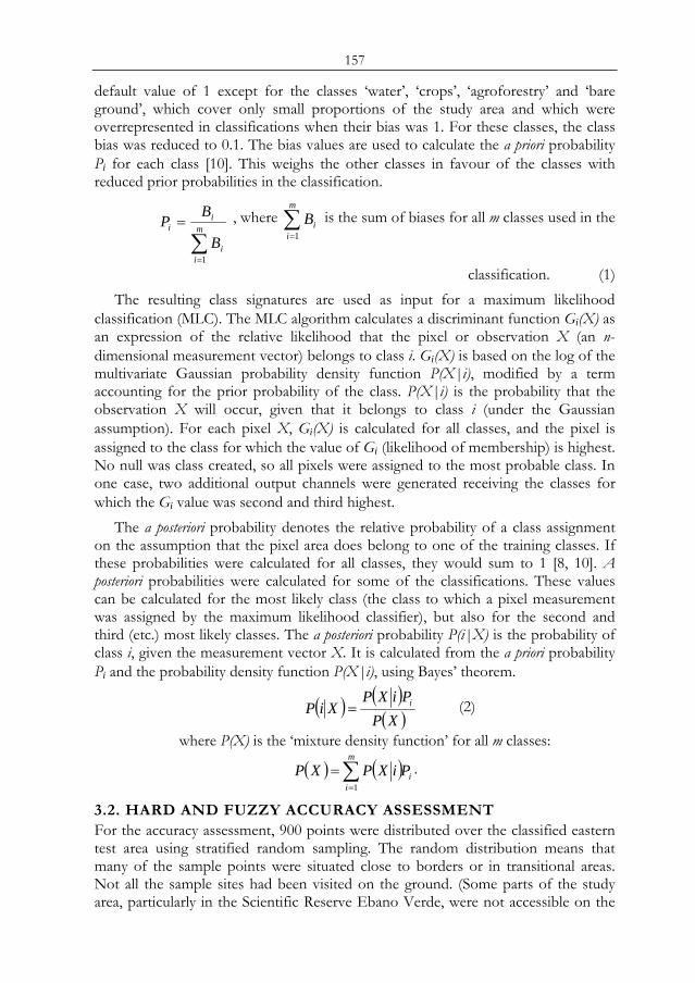
157
default value of 1 except for the classes ‘water’, ‘crops’, ‘agroforestry’ and ‘bare ground’, which cover only small proportions of the study area and which were overrepresented in classifications when their bias was 1. For these classes, the class bias was reduced to 0.1. The bias values are used to calculate the a priori probability Pi for each class [10]. This weighs the other classes in favour of the classes with reduced prior probabilities in the classification.
∑=
= m
ii
ii
B
BP
1
, where ∑=
m
iiB
1
is the sum of biases for all m classes used in the
classification. (1) The resulting class signatures are used as input for a maximum likelihood
classification (MLC). The MLC algorithm calculates a discriminant function Gi(X) as an expression of the relative likelihood that the pixel or observation X (an n-dimensional measurement vector) belongs to class i. Gi(X) is based on the log of the multivariate Gaussian probability density function P(X|i), modified by a term accounting for the prior probability of the class. P(X|i) is the probability that the observation X will occur, given that it belongs to class i (under the Gaussian assumption). For each pixel X, Gi(X) is calculated for all classes, and the pixel is assigned to the class for which the value of Gi (likelihood of membership) is highest. No null was class created, so all pixels were assigned to the most probable class. In one case, two additional output channels were generated receiving the classes for which the Gi value was second and third highest.
The a posteriori probability denotes the relative probability of a class assignment on the assumption that the pixel area does belong to one of the training classes. If these probabilities were calculated for all classes, they would sum to 1 [8, 10]. A posteriori probabilities were calculated for some of the classifications. These values can be calculated for the most likely class (the class to which a pixel measurement was assigned by the maximum likelihood classifier), but also for the second and third (etc.) most likely classes. The a posteriori probability P(i|X) is the probability of class i, given the measurement vector X. It is calculated from the a priori probability Pi and the probability density function P(X|i), using Bayes’ theorem.
( ) ( )( )XP
PiXPXiP i= (2)
where P(X) is the ‘mixture density function’ for all m classes:
( ) ( ) i
m
iPiXPXP ∑
=
=1
.
3.2. HARD AND FUZZY ACCURACY ASSESSMENT For the accuracy assessment, 900 points were distributed over the classified eastern test area using stratified random sampling. The random distribution means that many of the sample points were situated close to borders or in transitional areas. Not all the sample sites had been visited on the ground. (Some parts of the study area, particularly in the Scientific Reserve Ebano Verde, were not accessible on the
158
ground.) The land cover classes of 583 of these 900 sample points could be determined using a combination of the knowledge and data collected on the ground during field work and visual interpretation of the IKONOS image itself (using several channel combinations, including pan-sharpened, for the display) and of recent oblique and historical vertical aerial photographs.
For the ‘hard’ accuracy assessment, only one ‘correct’ class was assigned to each sample point, even if the point was located in a transitional area. If for example shrubs had started to grow in a grassland area, a decision was made to assign the sample point to either the grassland or the matorral class. For the classification of one data set, the reference sample for the accuracy assessment was ‘fuzzified’ by reassessing the pixels which had been labeled as misclassified in the hard accuracy assessment according to the linguistic scale presented in Ref. 6. For each reference point in the subset, all classes were assigned discrete levels of class membership between 1 and 5, according to the following description:
“(5) Absolutely right: No doubt about the match. Perfect. (4) Good answer: Would be happy to find this answer given on the map. (3) Reasonable or acceptable answer: Maybe not the best possible answer but it is
acceptable; this answer does not pose a problem to the user if it is seen on the map. (2) Understandable but wrong [...] (1) Absolutely wrong” [6]. Classes with scores of at least 3 (at least acceptable answers) were then counted
as ‘right’ for the reference point. This made it possible to calculate a fuzzy overall accuracy, i.e. the percentage of pixels for which the classified value matches at least one reference class with a score between 3 and 5. So instead of determining one ‘best’ class to every reference point, the fuzzy accuracy assessment makes it possible to count several classes as acceptable, e.g. both grassland and matorral in the rough grassland areas where small shrubs are starting to appear among the ferns and grasses, or both secondary forest and calimetal, if the testing point is located near the border of a calimetal patch within a secondary forest area. 3.3. ASSESSING THE CONTRIBUTION OF BOUNDARY EFFECTS ON CLASSIFICATION ACCURACY To test the amount of error introduced by mixed pixels and by edge effects in the texture data, all reference points closer than 12 m to a land cover boundary (as interpreted in the pan-sharpened IKONOS image) were deleted from the test sample, reducing it to 333 points. This should eliminate those testing pixels for which the texture values calculated in a 15 m × 15 m window are likely to be influenced by between-class texture. Accuracy assessments for the classification results obtained with different data sets (4 m resolution with and without texture parameters, low-pass filtered multispectral data, and resolution reduced to 12 m) were conducted with this set of reference points and the overall accuracies were compared to those produced with the complete set of 583 points.
4 RESULTS The best overall classification accuracy was achieved with a data set consisting of four 3×3 mode filtered IKONOS multispectral channels and three texture channels.
159
The 7×7 mode filtered classification result had a ‘hard’ classification accuracy of 70.4 %. 4.1. A POSTERIORI PROBABILITIES For the maximum likelihood classification of the above-mentioned spectral-textural dataset, the a posteriori probability of the most likely class (PP1) has a mean value of 0.77. The mean a posteriori probability for the second most likely class (PP2) is 0.15. The mean a posteriori probability for the third most likely class (PP3) is only 0.04. This indicates that, from the standpoint of a posteriori probabilities, there are usually no more than two classes for which assignments would be probable to a substantial degree.
If we look at the spatial distribution of PP1, a posteriori probabilities of 0.98 and more (white areas in figure 2) can be found in the core areas of classes, particularly in the contiguous cloud forest areas in the east of the study area, some pine plantations and in the river (because of the good spectral separability between water and other classes). The a posteriori probability is #0.66 for 31 % of the classified pixels. These low a posteriori probabilities occur mostly along class borders, in areas affected by spectrally mixed pixels and between-class texture effects and in areas of transition between different land cover types (i.e. chosen information classes) or with a small scale mix of land cover types.
A map display where only the classes of areas with a posteriori probabilities above 0.66 are depicted in colour while uncertain areas are left white does not necessarily give the user less information than a ‘complete’ map, because many of these white areas are obvious areas of boundary uncertainty.
As the a posteriori probability is not directly proportional to the Gaussian density function, there are a few cases (3 % of the pixels) where the a posteriori probability for the second most likely class (according to MLC) is higher than the a posteriori probability for the most likely class. This shows that the class to which a pixel was assigned by MLC does not in all cases have the highest a posteriori probability. The difference between the a posteriori probabilities of the two most likely classes could be used as another indicator of classification certainty. In a digital classification output (e.g. in a Geographic Information System), areas where ‘PP1 minus PP2’ is below a specified value could be annotated with a warning, offering information about the second most likely class (according to MLC) as an alternative class assignment.
160
Figure 2. A posteriori probability for the class assigned in a maximum likelihood
classification of the study area. Light areas indicate high a posteriori probabilities, dark grey areas indicate low a posteriori probabilities. Black areas are unclassified.
4.2. THE INFLUENCE OF BOUNDARY EFFECTS ON CLASSIFICATION ACCURACY When only testing points located more than 12 m from a land cover class boundary are retained while the others are eliminated, only 57 % of the original reference points (333 of 583) are left. This is an indicator of the high land cover diversity and heterogeneity of the landscape of the study area. Eliminating testing points close to boundaries from the accuracy assessment leads to markedly higher overall accuracies for all data sets (table 2). The smallest improvement was 5.5 % for the 4 m resolution multispectral data without any form of spatial integration. For spatially integrated data sets and data sets including texture channels, the boundary effects (as indicated by the difference in classification accuracy between the complete area and only areas away from boundaries) increases. In most cases of spatially integrated data sets, the difference to the overall accuracy values estimated with the full set of reference points was above 8 %. The overall accuracy estimated with the reduced set of reference points reached 79.0 % for the 5×5 mode filtered MLC result of the mean-filtered spectral-textural data set.
The fact that a disproportionate part of the errors occurs close to class boundaries demonstrates the detrimental effect of mixed pixels and other edge effects on classification accuracies. The results also indicate that such edge effects are relatively minor in the multispectral 4 m resolution data without spatial integration, while spatial integration and the inclusion of texture data augment the proportion of errors caused by edge effects. When texture parameters are part of the classified data set, the between-class texture caused by the texture calculation in 15 m × 15 m windows adds a major edge effect to the mixed spectral signal of the 4 m resolution multispectral pixels. However, the benefits of the inclusion of spatial information outweigh the disadvantage of increased edge effects considerably. So it
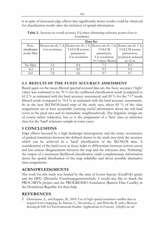
161
is in spite of increased edge effects that significantly better results could be observed for classification results after the inclusion of spatial information.
Table 2. Increase in overall accuracy [%] when eliminating reference points close to boundaries.
Data Set Post-
classification mode filter
Ikonos ms ch. 1-4, 4 m resolution
Ikonos ms ch. 1-4, 3 GLCM texture
parameters, 4 m resolution
Ikonos ms ch. 1-4, 3 GLCM
parameters, 4 m resolution,
3×3 mean filtered
Ikonos ms ch. 1-4, 3 GLCM texture
parameters, resolution reduced
to 12 m No filter 5.5 8.4 7.3 8.5
3x3 6.1 8.0 9.3 9.4 5x5 7.8 9.6 9.7 9.7
4.3. RESULTS OF THE FUZZY ACCURACY ASSESSMENT Based again on the mean-filtered spectral-textural data set, the fuzzy accuracy (‘right’ value) was estimated to be 76 % for the unfiltered classification result (compared to 61.2 % as estimated with the hard accuracy assessment) and 85 % for the 7×7 mode filtered result (compared to 70.4 % as estimated with the hard accuracy assessment). So in the best IKONOS-based map of the study area, about 85 % of the class assignments are at least acceptable (carrying useful information about the real land cover in the pixel area and its immediate neighbourhood). The linguistic ratings are of course rather subjective, but so is the assignment of a ‘best’ class as reference class for the ‘hard’ reference sample in some cases.
5 CONCLUSIONS Edge effects boosted by a high landscape heterogeneity and the many occurrences of gradual transitions between the defined classes in the study area limit the accuracy which can be achieved in a ‘hard’ classification of the IKONOS data. A consideration of the land cover as fuzzy helps to differentiate between serious errors and less serious disagreements between the map and the reference data. ‘Softening’ the output of a maximum likelihood classification yields complimentary information about the spatial distribution of the map reliability and about possible alternative class assignments.
ACKNOWLEDGMENTS The work for this study was funded by the state of Lower Saxony (GradFöG grant) and the DFG (Deutsche Forschungsgemeinschaft). I would also like to thank the PROCARYN project and the PROGRESSIO foundation (Ramón Elias Castillo) in the Dominican Republic for their help.
REFERENCES 1 Gleitsmann, A., and Kappas, M., 2005: Use of high spatial resolution satellite data in
tropical forest mapping. In: Kleinn, C., Nieschulze, J., and Sloboda, B. (eds.): Remote Sensing & GIS for Environmental Studies: Applications in Forestry. Schriften aus der
162
Forstlichen Fakultät der Universität Göttingen und der Niedersächsischen Forstlichen Versuchsanstalt 138, pp. 167-175.
2 Brown, D.G., 1998: Classification and boundary vagueness in mapping presettlement forest types. International Journal of Geographical Information Science 12 (2), pp. 105-129.
3 Cheng, T, Molenaar, M., and Lin, H., 2001: Formalizing fuzzy objects from uncertain classification results. International Journal of Geographical Information Science 15 (1), pp. 27-42.
4 Zhang, J., and Stuart, N., 2001: Fuzzy methods for categorical mapping with image-based land cover data. International Journal of Geographical Information Science 15 (2), pp. 175-195.
5 Ricotta, C., 2004: Evaluating the classification accuracy of fuzzy thematic maps with a simple parametric measure. International Journal of Remote Sensing 25 (11), pp. 2169-2176.
6 Woodcock, C.E., and Gopal, S., 2000: Fuzzy set theory and thematic maps: accuracy assessment and area estimation. International Journal of Geographical Information Science 14 (2), pp. 153-172.
7 Paola, J.D., and Schowengerdt, R.A. 1995: A detailed comparison of backpropagation neural network and maximum-likelihood classifiers for urban land use classification. IEEE Transactions on Geoscience and Remote Sensing 33 (4), pp. 981-995.
8 Palubinskas, G., Lucas, R.M., Foody, G.M., and Curran, P.J., 1995: An evaluation of fuzzy and texture-based classification approaches for mapping tropical forest classes from Landsat-TM data. International Journal of Remote Sensing 16 (4), pp. 747-759.
9 García, R., Mejía, M., and Zanoni, T., 1994: Composición floristica y principales asociaciones vegetales en la Reserva Científica Ebano Verde, Cordillera Central, República Dominicana. Moscosoa 10, pp. 86-130.
10 PCI, 2001: Xpace help system (softcopy), Version 9.1. Richmond Hill, Ontario.
163
Remote Sensing and GIS data requirements and data availability for land use / land cover change research in
Sudano-Sahelian landscapes
A. Hof Institute of Geography, Ruhr University Bochum, Universitaetsstrasse 150
D-44780 Bochum, email: [email protected]
ABSTRACT The paper addresses the rem17ote sensing and GIS data requirements for land use and land cover change research in the Sudano-Sahelian zone. It is argued that there is a gap of data and information to interlink local-scale studies and environmental information gathered at coarse spatial resolutions. The dearth of case studies actually using high spatial resolution remote sensing data points to the severe shortage of such data and the difficulties to derive biophysical information from even the higher spatial resolution imagery. The limited data availability is demonstrated for a case study area in northwest Nigeria. Monitoring of cropland expansion over 34 years was achieved with dry season data from multiple sensors. The dynamics of the grazed semi-natural vegetation lands cannot be analyzed retrospectively because the relevant remotely sensed data or thematic datasets are not available. A land cover classification was combined with in situ measurements of vegetation cover and productivity. The results show that cropland expansion and land degradation in the common access reserves have been overestimated. Available data are often not commensurate with the textbook requirements for change detection. Despite these difficulties, the scope of information that can be derived from the existing data is superior to coarse scale thematic land cover datasets. Case studies provide a spatial quantification of land cover dynamics at the local scale filling the gap of quantitative information on vegetation cover and current land use. Keywords: Sahel, degradation, land use, land cover, change detection, Landsat, data requirements.
1 INTRODUCTION It is undisputed that the use of satellite-based remote sensing and geographic information systems is pivotal for the development-related collection, assessment, and analysis of data at all scales. This applies to land use and land cover change research as well as to needs-driven approaches that focus on the inventory, assessment and mapping of relevant land attributes for planning and/or community-based natural resource management. However, the theoretical applicability of the tools is meaningless unless their feasibility in data-poor contexts like the Sudano-Sahelian zone can be demonstrated for applied research that is driven by a specific geographical context and the characteristics of change rather than by the available remote sensing data and algorithms. The objective of this Proc. 2nd Göttingen GIS and Remote Sensing Days, 4-6 Oct. 2006, Göttingen
164
paper is to assess the theoretical remote sensing and GIS data requirements for land use/land cover change research in Sudano-Sahelian landscapes and to discuss whether the available data are commensurate with those requirements. It is argued here that actual GIS and remote sensing data availability often makes it necessary to deviate from theoretical data requirements. Results from a case study from northwest Nigeria are summarised to demonstrate the scope of land use change information that can be derived from available GIS and remote sensing data. Finally, the paper discusses the importance of local-scale case studies in adverse geodata contexts and their transferability for improved understanding and projections of land cover and land use change in the Sudano-Sahelian zone.
2 LAND USE AND LAND COVER CHANGE IN THE SUDANO-SAHEL AND IMPLICATIONS FOR GIS & REMOTE SENSING APPLICATIONS The Sahel proper is the semiarid transition zone between the Sahara Desert to the north and the subhumid savannas to the south. In bioclimatic terms, the Sahel has come to include the Sudanian woodlands to the south of the Sahel proper and is situated approximately between 12° and 18° North. The Sudano-Sahelian zone is transitional between the Sub-Sahelian sector (550-750 mm) and the northern Sudanian sector which is bracketed by the 750 and 1000 mm isohyets of annual rainfall [1]. In the semi-arid Sudano-Sahelian zone, crops and livestock are of similar importance for livelihoods and agricultural production. Most households are now engaged in both cropping and livestock-keeping [2]. The competition for land between food and feed production is driven by demographic dynamics (human population growth, migration, shifts to a sedentary way of life) and livestock increase. A substantial transition from pastoral to agropastoral systems and reduction in fallow land is expected by 2050 [3]. 2.1 THE CHARACTERISTICS OF CHANGE The dominant theme of land use/land cover change in the Sudano-Sahel is agricultural expansion at the expense of woodland. Annual cropland expansion rates ranging from 3% to 5.8% (1961-1989) and 1.4% to 4.8% (1984-1997) were observed in local studies throughout the Sahelo-Sudanian zone [4]. The long-standing debate about human-induced land degradation in the Sahel is currently dominated by two interpretations of this land use and land cover change: the land degradation and the land use transition scenario.
The degradation scenario interlinks cropland expansion at the expense of rangelands with deforestation, and over-exploitation of woodland and rangeland. Increasing pressure on shrinking rangelands due to rising human and livestock populations is feared to threaten bioproductivity in the long run through unsustainable use of vegetation and soils [2],[5]. In contrast, the long-term land use transition scenario interprets changes in farming practices and natural resource management as responses of Sahelian peoples to intensifying environmental stress and climatic risk. One of the main characteristics of this change is the transition of uncultivated woodland to farmed parklands and, ultimately, intensive farming systems, through agricultural intensification of smallholder farming systems [6]. It has been reported that bioproductivity in terms of plant biomass (kg dry matter ha-1)
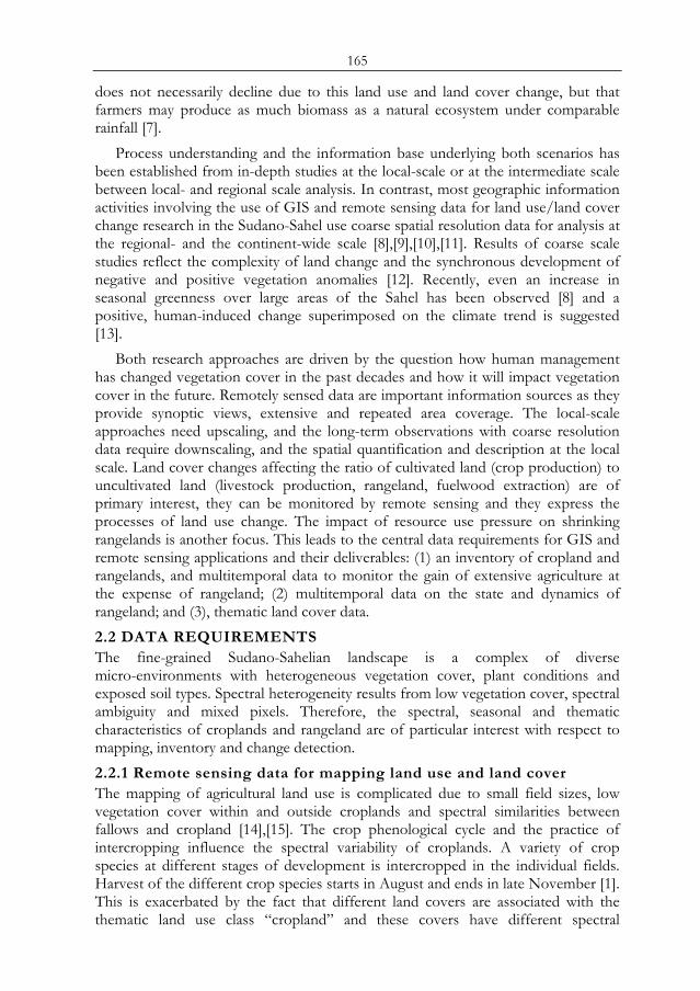
165
does not necessarily decline due to this land use and land cover change, but that farmers may produce as much biomass as a natural ecosystem under comparable rainfall [7].
Process understanding and the information base underlying both scenarios has been established from in-depth studies at the local-scale or at the intermediate scale between local- and regional scale analysis. In contrast, most geographic information activities involving the use of GIS and remote sensing data for land use/land cover change research in the Sudano-Sahel use coarse spatial resolution data for analysis at the regional- and the continent-wide scale [8],[9],[10],[11]. Results of coarse scale studies reflect the complexity of land change and the synchronous development of negative and positive vegetation anomalies [12]. Recently, even an increase in seasonal greenness over large areas of the Sahel has been observed [8] and a positive, human-induced change superimposed on the climate trend is suggested [13].
Both research approaches are driven by the question how human management has changed vegetation cover in the past decades and how it will impact vegetation cover in the future. Remotely sensed data are important information sources as they provide synoptic views, extensive and repeated area coverage. The local-scale approaches need upscaling, and the long-term observations with coarse resolution data require downscaling, and the spatial quantification and description at the local scale. Land cover changes affecting the ratio of cultivated land (crop production) to uncultivated land (livestock production, rangeland, fuelwood extraction) are of primary interest, they can be monitored by remote sensing and they express the processes of land use change. The impact of resource use pressure on shrinking rangelands is another focus. This leads to the central data requirements for GIS and remote sensing applications and their deliverables: (1) an inventory of cropland and rangelands, and multitemporal data to monitor the gain of extensive agriculture at the expense of rangeland; (2) multitemporal data on the state and dynamics of rangeland; and (3), thematic land cover data. 2.2 DATA REQUIREMENTS The fine-grained Sudano-Sahelian landscape is a complex of diverse micro-environments with heterogeneous vegetation cover, plant conditions and exposed soil types. Spectral heterogeneity results from low vegetation cover, spectral ambiguity and mixed pixels. Therefore, the spectral, seasonal and thematic characteristics of croplands and rangeland are of particular interest with respect to mapping, inventory and change detection. 2.2.1 Remote sensing data for mapping land use and land cover The mapping of agricultural land use is complicated due to small field sizes, low vegetation cover within and outside croplands and spectral similarities between fallows and cropland [14],[15]. The crop phenological cycle and the practice of intercropping influence the spectral variability of croplands. A variety of crop species at different stages of development is intercropped in the individual fields. Harvest of the different crop species starts in August and ends in late November [1]. This is exacerbated by the fact that different land covers are associated with the thematic land use class “cropland” and these covers have different spectral
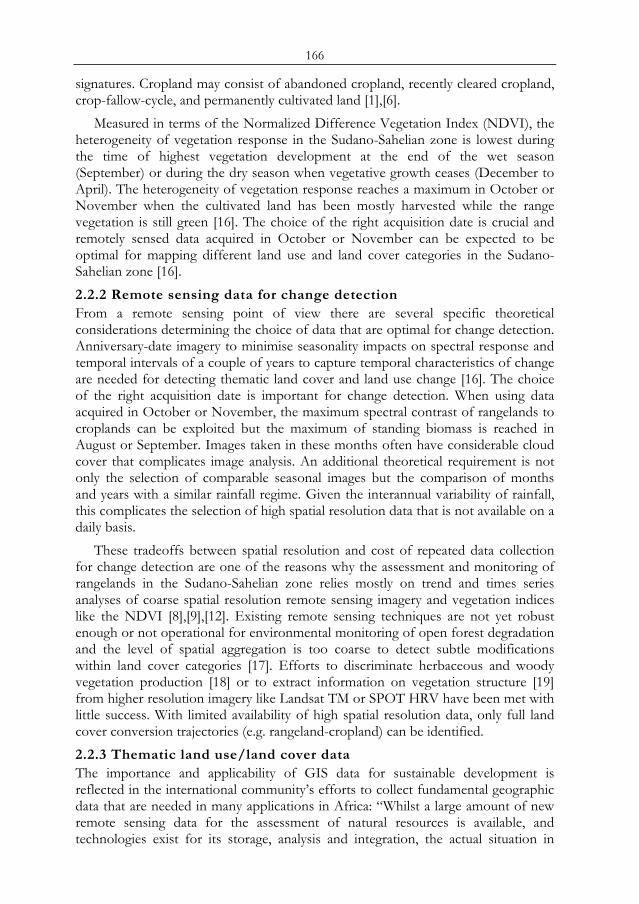
166
signatures. Cropland may consist of abandoned cropland, recently cleared cropland, crop-fallow-cycle, and permanently cultivated land [1],[6].
Measured in terms of the Normalized Difference Vegetation Index (NDVI), the heterogeneity of vegetation response in the Sudano-Sahelian zone is lowest during the time of highest vegetation development at the end of the wet season (September) or during the dry season when vegetative growth ceases (December to April). The heterogeneity of vegetation response reaches a maximum in October or November when the cultivated land has been mostly harvested while the range vegetation is still green [16]. The choice of the right acquisition date is crucial and remotely sensed data acquired in October or November can be expected to be optimal for mapping different land use and land cover categories in the Sudano-Sahelian zone [16]. 2.2.2 Remote sensing data for change detection From a remote sensing point of view there are several specific theoretical considerations determining the choice of data that are optimal for change detection. Anniversary-date imagery to minimise seasonality impacts on spectral response and temporal intervals of a couple of years to capture temporal characteristics of change are needed for detecting thematic land cover and land use change [16]. The choice of the right acquisition date is important for change detection. When using data acquired in October or November, the maximum spectral contrast of rangelands to croplands can be exploited but the maximum of standing biomass is reached in August or September. Images taken in these months often have considerable cloud cover that complicates image analysis. An additional theoretical requirement is not only the selection of comparable seasonal images but the comparison of months and years with a similar rainfall regime. Given the interannual variability of rainfall, this complicates the selection of high spatial resolution data that is not available on a daily basis.
These tradeoffs between spatial resolution and cost of repeated data collection for change detection are one of the reasons why the assessment and monitoring of rangelands in the Sudano-Sahelian zone relies mostly on trend and times series analyses of coarse spatial resolution remote sensing imagery and vegetation indices like the NDVI [8],[9],[12]. Existing remote sensing techniques are not yet robust enough or not operational for environmental monitoring of open forest degradation and the level of spatial aggregation is too coarse to detect subtle modifications within land cover categories [17]. Efforts to discriminate herbaceous and woody vegetation production [18] or to extract information on vegetation structure [19] from higher resolution imagery like Landsat TM or SPOT HRV have been met with little success. With limited availability of high spatial resolution data, only full land cover conversion trajectories (e.g. rangeland-cropland) can be identified. 2.2.3 Thematic land use/land cover data The importance and applicability of GIS data for sustainable development is reflected in the international community’s efforts to collect fundamental geographic data that are needed in many applications in Africa: “Whilst a large amount of new remote sensing data for the assessment of natural resources is available, and technologies exist for its storage, analysis and integration, the actual situation in
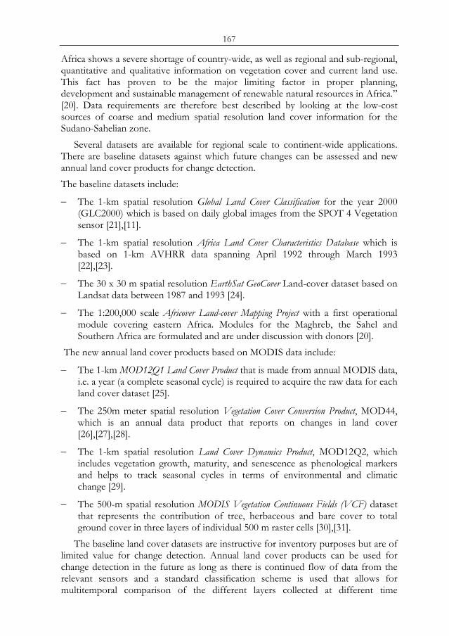
167
Africa shows a severe shortage of country-wide, as well as regional and sub-regional, quantitative and qualitative information on vegetation cover and current land use. This fact has proven to be the major limiting factor in proper planning, development and sustainable management of renewable natural resources in Africa.” [20]. Data requirements are therefore best described by looking at the low-cost sources of coarse and medium spatial resolution land cover information for the Sudano-Sahelian zone.
Several datasets are available for regional scale to continent-wide applications. There are baseline datasets against which future changes can be assessed and new annual land cover products for change detection. The baseline datasets include:
− The 1-km spatial resolution Global Land Cover Classification for the year 2000 (GLC2000) which is based on daily global images from the SPOT 4 Vegetation sensor [21],[11].
− The 1-km spatial resolution Africa Land Cover Characteristics Database which is based on 1-km AVHRR data spanning April 1992 through March 1993 [22],[23].
− The 30 x 30 m spatial resolution EarthSat GeoCover Land-cover dataset based on Landsat data between 1987 and 1993 [24].
− The 1:200,000 scale Africover Land-cover Mapping Project with a first operational module covering eastern Africa. Modules for the Maghreb, the Sahel and Southern Africa are formulated and are under discussion with donors [20].
The new annual land cover products based on MODIS data include:
− The 1-km MOD12Q1 Land Cover Product that is made from annual MODIS data, i.e. a year (a complete seasonal cycle) is required to acquire the raw data for each land cover dataset [25].
− The 250m meter spatial resolution Vegetation Cover Conversion Product, MOD44, which is an annual data product that reports on changes in land cover [26],[27],[28].
− The 1-km spatial resolution Land Cover Dynamics Product, MOD12Q2, which includes vegetation growth, maturity, and senescence as phenological markers and helps to track seasonal cycles in terms of environmental and climatic change [29].
− The 500-m spatial resolution MODIS Vegetation Continuous Fields (VCF) dataset that represents the contribution of tree, herbaceous and bare cover to total ground cover in three layers of individual 500 m raster cells [30],[31].
The baseline land cover datasets are instructive for inventory purposes but are of limited value for change detection. Annual land cover products can be used for change detection in the future as long as there is continued flow of data from the relevant sensors and a standard classification scheme is used that allows for multitemporal comparison of the different layers collected at different time
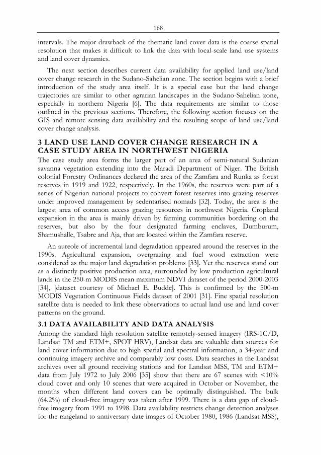
168
intervals. The major drawback of the thematic land cover data is the coarse spatial resolution that makes it difficult to link the data with local-scale land use systems and land cover dynamics.
The next section describes current data availability for applied land use/land cover change research in the Sudano-Sahelian zone. The section begins with a brief introduction of the study area itself. It is a special case but the land change trajectories are similar to other agrarian landscapes in the Sudano-Sahelian zone, especially in northern Nigeria [6]. The data requirements are similar to those outlined in the previous sections. Therefore, the following section focuses on the GIS and remote sensing data availability and the resulting scope of land use/land cover change analysis.
3 LAND USE LAND COVER CHANGE RESEARCH IN A CASE STUDY AREA IN NORTHWEST NIGERIA The case study area forms the larger part of an area of semi-natural Sudanian savanna vegetation extending into the Maradi Department of Niger. The British colonial Forestry Ordinances declared the area of the Zamfara and Runka as forest reserves in 1919 and 1922, respectively. In the 1960s, the reserves were part of a series of Nigerian national projects to convert forest reserves into grazing reserves under improved management by sedentarised nomads [32]. Today, the area is the largest area of common access grazing resources in northwest Nigeria. Cropland expansion in the area is mainly driven by farming communities bordering on the reserves, but also by the four designated farming enclaves, Dumburum, Shamushalle, Tsabre and Aja, that are located within the Zamfara reserve.
An aureole of incremental land degradation appeared around the reserves in the 1990s. Agricultural expansion, overgrazing and fuel wood extraction were considered as the major land degradation problems [33]. Yet the reserves stand out as a distinctly positive production area, surrounded by low production agricultural lands in the 250-m MODIS mean maximum NDVI dataset of the period 2000-2003 [34], [dataset courtesy of Michael E. Budde]. This is confirmed by the 500-m MODIS Vegetation Continuous Fields dataset of 2001 [31]. Fine spatial resolution satellite data is needed to link these observations to actual land use and land cover patterns on the ground. 3.1 DATA AVAILABILITY AND DATA ANALYSIS Among the standard high resolution satellite remotely-sensed imagery (IRS-1C/D, Landsat TM and ETM+, SPOT HRV), Landsat data are valuable data sources for land cover information due to high spatial and spectral information, a 34-year and continuing imagery archive and comparably low costs. Data searches in the Landsat archives over all ground receiving stations and for Landsat MSS, TM and ETM+ data from July 1972 to July 2006 [35] show that there are 67 scenes with <10% cloud cover and only 10 scenes that were acquired in October or November, the months when different land covers can be optimally distinguished. The bulk (64.2%) of cloud-free imagery was taken after 1999. There is a data gap of cloud-free imagery from 1991 to 1998. Data availability restricts change detection analyses for the rangeland to anniversary-date images of October 1980, 1986 (Landsat MSS),
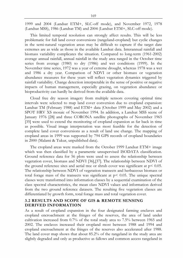
169
1999 and 2004 (Landsat ETM+, SLC-off mode), and November 1972, 1978 (Landsat MSS), 1986 (Landsat TM) and 2004 (Landsat ETM+, SLC-off mode).
This limited temporal resolution can strongly affect results. This will be less problematic for full land cover conversions (rangeland-cropland) but cyclic changes in the semi-natural vegetation areas may be difficult to capture if the target date extremes are as wide as those in the available Landsat data. Interannual rainfall and biomass variability complicates the situation. Compared to long-term (1961-2002) average annual rainfall, annual rainfall in the study area ranged in the October time series from average (1980) to dry (1986) and wet conditions (1999). In the November time series, 1972 was a year of extreme drought, whereas 1978 was a wet and 1986 a dry year. Comparison of NDVI or other biomass or vegetation abundance measures for these years will reflect vegetation dynamics triggered by rainfall variability. Change detection interpretable in the sense of positive or negative impacts of human management, especially grazing, on vegetation abundance or bioproductivity can hardly be derived from the available data.
Cloud free dry season imagery from multiple sensors covering optimal time intervals were selected to map land cover conversion due to cropland expansion: Landsat TM (February 1988) and ETM+ data (October 1999 and May 2002) and a SPOT HRV XS mosaic of November 1994. In addition, a Landsat MSS scene of January 1976 [28] and three CORONA satellite photographs of November 1965 [35] were used to extend the monitoring of cropland expansion as far back in time as possible. Visual image interpretation was most feasible for the detection of complete land cover conversions as a result of land use change. The mapping of cropland areas in 1999 was supported by 794 GPS records of cropland boundaries in 2000 (Malami & Tukur, unpublished data).
The cropland areas were masked from the October 1999 Landsat ETM+ image which was then classified by a parametric unsupervised ISODATA classification. Ground reference data for 56 plots were used to assess the relationship between vegetation cover, biomass and NDVI [36],[37]. The relationship between NDVI of the ground reference sites and aerial tree or shrub cover was significant at p< 0.05. The relationship between NDVI of vegetation transects and herbaceous biomass or total forage mass of the transects was significant at p< 0.05. The unique spectral classes were transformed into information classes by a sequential examination of the class spectral characteristics, the mean class NDVI values and information derived from the two ground reference datasets. The resulting five vegetation classes are differentiated by growth form, total forage mass and total vegetation cover. 3.2 RESULTS AND SCOPE OF GIS & REMOTE SENSING DERIVED INFORMATION As a result of cropland expansion in the four designated farming enclaves and cropland encroachment at the fringes of the reserves, the area of land under cultivation increased from 0.7% of the total study area to 7.5% between 1965 and 2002. The enclaves increased their cropland most between 1988 and 1994 and cropland encroachment at the fringes of the reserves also accelerated after 1988. The land cover map shows that about 85.2% of the rangeland in the study area are slightly degraded and only as productive as fallows and common access rangeland in
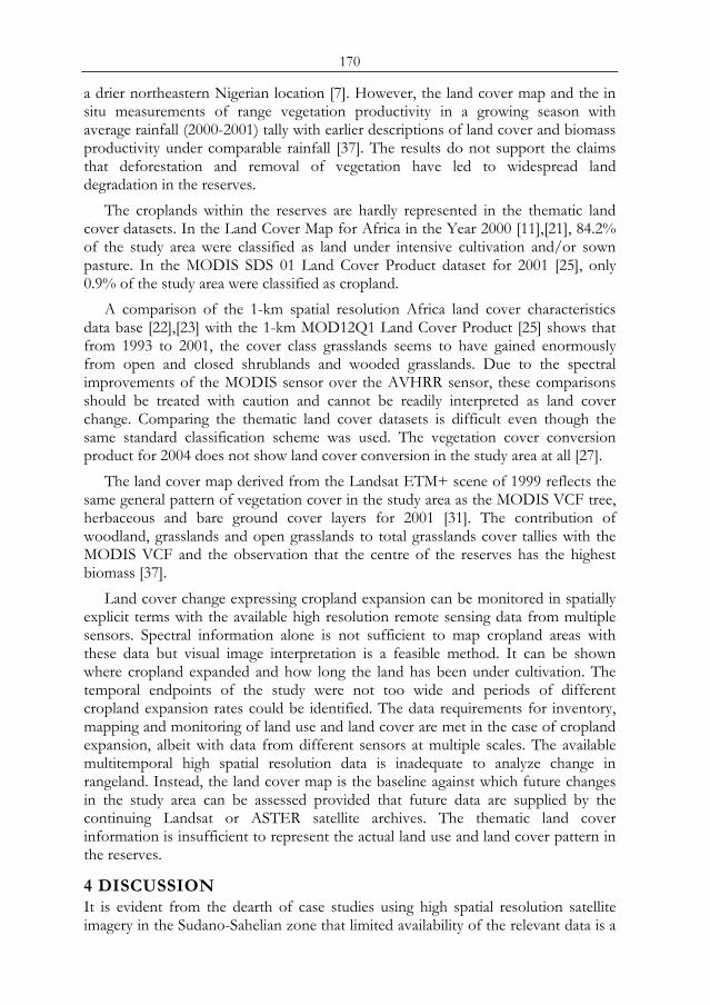
170
a drier northeastern Nigerian location [7]. However, the land cover map and the in situ measurements of range vegetation productivity in a growing season with average rainfall (2000-2001) tally with earlier descriptions of land cover and biomass productivity under comparable rainfall [37]. The results do not support the claims that deforestation and removal of vegetation have led to widespread land degradation in the reserves.
The croplands within the reserves are hardly represented in the thematic land cover datasets. In the Land Cover Map for Africa in the Year 2000 [11],[21], 84.2% of the study area were classified as land under intensive cultivation and/or sown pasture. In the MODIS SDS 01 Land Cover Product dataset for 2001 [25], only 0.9% of the study area were classified as cropland.
A comparison of the 1-km spatial resolution Africa land cover characteristics data base [22],[23] with the 1-km MOD12Q1 Land Cover Product [25] shows that from 1993 to 2001, the cover class grasslands seems to have gained enormously from open and closed shrublands and wooded grasslands. Due to the spectral improvements of the MODIS sensor over the AVHRR sensor, these comparisons should be treated with caution and cannot be readily interpreted as land cover change. Comparing the thematic land cover datasets is difficult even though the same standard classification scheme was used. The vegetation cover conversion product for 2004 does not show land cover conversion in the study area at all [27].
The land cover map derived from the Landsat ETM+ scene of 1999 reflects the same general pattern of vegetation cover in the study area as the MODIS VCF tree, herbaceous and bare ground cover layers for 2001 [31]. The contribution of woodland, grasslands and open grasslands to total grasslands cover tallies with the MODIS VCF and the observation that the centre of the reserves has the highest biomass [37].
Land cover change expressing cropland expansion can be monitored in spatially explicit terms with the available high resolution remote sensing data from multiple sensors. Spectral information alone is not sufficient to map cropland areas with these data but visual image interpretation is a feasible method. It can be shown where cropland expanded and how long the land has been under cultivation. The temporal endpoints of the study were not too wide and periods of different cropland expansion rates could be identified. The data requirements for inventory, mapping and monitoring of land use and land cover are met in the case of cropland expansion, albeit with data from different sensors at multiple scales. The available multitemporal high spatial resolution data is inadequate to analyze change in rangeland. Instead, the land cover map is the baseline against which future changes in the study area can be assessed provided that future data are supplied by the continuing Landsat or ASTER satellite archives. The thematic land cover information is insufficient to represent the actual land use and land cover pattern in the reserves.
4 DISCUSSION It is evident from the dearth of case studies using high spatial resolution satellite imagery in the Sudano-Sahelian zone that limited availability of the relevant data is a
171
general problem and not specific to the case study area. Coarse spatial resolution satellite data is not sufficient to map the highly fragmented Sudano-Sahelian landscapes but it is valuable to detect areas of increased or decreased vegetation productivity or hotspots of change. Fine spatial resolution data is required to link these observations to numerous anthropogenic impacts including agricultural expansion and maintenance of protected areas [38]. However, the current high spatial resolution sensors do not provide adequate temporal resolution to monitor this region that exhibits cloud cover throughout the growing season and photosynthetically mostly inactive vegetation cover for the rest of the year. Data fusion techniques that combine the higher spatial resolution data with the spectral resolution of coarse sensors exist. Yet including the temporal domain will be difficult unless the fused images are from the same date (phenological state). Another prerequisite is that the classes of interest can be distinguished even if their spectral characteristics change due to seasonal influences. For change detection or the mapping of land use and land cover in the Sudano-Sahelian zone, this limits the choice of data to the end of the growing season (October and November). Likewise, using spectral mixture analysis for quantifying vegetation abundance and change would be theoretically feasible, but such an analysis also requires scenes that are recorded at optimal and comparable phenological dates [39].
Due to its status as reserve, the case study area is less fragmented than the fine mosaic of semi-natural vegetation and farming prevailing in the Sudano-Sahelian zone. However, not even the discrete breaks in land use intensity within the reserves and between the reserves and the surrounding agricultural lands are reflected in the coarse spatial resolution thematic GIS land cover information. Comparing the results of satellite image interpretation and field research with thematic land cover datasets stresses the importance of high spatial resolution data to capture land use and land cover patterns in Sudano-Sahelian landscapes. The case study demonstrates that GIS and remote sensing data are scarce and often not commensurate with the analytical needs of land use/land cover change research. Therefore, the combination of in situ studies with satellite images and thematic land cover data at different scales is and remains important to provide a baseline against which future land use/cover changes can be assessed.
The results on cropland expansion, semi-natural land cover and vegetation productivity in the case study area show that like elsewhere in the Sudano-Sahelian zone, there are contradictory elements in diagnosing land degradation and attributing agency in the reserves [6]. In these adverse geodata contexts, case studies deliver current land cover information and help to fill the information gap between the local and the regional scale. Every case study runs a risk of being too specific and the transferability of the results is uncertain. However, rural land use systems in the Sudano-Sahelian zone are diverse. The results provided here and in the literature challenge simplistic degradation scenarios [6]. In conclusion, many more local-scale case studies like this are needed to account for the region’s diversity and to better inform the current land degradation debate that is flawed by a severe lack of the relevant quantitative and qualitative information on vegetation cover and current land use in the Sudano-Sahelian zone. GIS and remote sensing data are valuable sources for this purpose, but data at higher spatial and temporal resolution than

172
currently available are needed to advance from resource inventory studies that may indicate potential problems to trend relationships that could be closely linked with data on human management.
ACKNOWLEDGMENTS Funding for this research was supplied in part by the DG XII of the European Union under the INCO-DC project “Development of sustainable pastoral and agro-pastoral livelihood systems in West Africa” (Contract ERB IC18-CT98-0280).
REFERENCES 1 Mortimore, M., and Adams, W.M., 1999: Working the Sahel. Environment and Society in
Northern Nigeria. Routledge, London. 2 Hiernaux P., and Turner, M.D., 2002: The Influence of Farmer and Pastoralist
Management Practices on Desertification Processes in the Sahel. In: Reynolds, J.F., and Stafford-Smith, M.D. (ed.): Global Desertification: Do Humans Cause Deserts?, pp. 136-148. Dahlem University Press, Berlin.
3 FAO and World Bank, 2001: Farming Systems and Poverty. Improving Farmers’ Livelihoods in a Changing World. FAO and World Bank, Rome and Washington D.C..
4 Stéphenne, N., and Lambin, E.F., 2001: A dynamic simulation model of land-use changes in Sudano-sahelian countries of Africa (SALU). Agric. Ecosystems Environ., 85 (1-3), pp. 145-161.
5 Geist, H.J., and Lambin, E.F., 2004: Dynamic causal patterns of desertification. Bioscience, 54 (9), pp. 817-829.
6 Mortimore M., and Turner, B., 2005: Does the Sahelian smallholder's management of woodland, farm trees, rangeland support the hypothesis of human-induced desertification? J. Arid Environ., 63 (3), pp. 567-595.
7 Mortimore, M., Harris, F.M.A., and Turner, B., 1999: Implications of land use change for the production of plant biomass in densely populated Sahelo-Sudanian shrub-grasslands in north-east Nigeria. Global Ecol. Biogeogr., 8 (3-4), pp. 243-256.
8 Anyamba, A., and Tucker, C.J., 2005: Analysis of Sahelian vegetation dynamics using NOAA-AVHRR NDVI data from 1981-2003. J. Arid Environ., 63 (3), pp. 596-614.
9 Fuller, D.O., 1998: Trends in NDVI time series and their relation to rangeland and crop production in Senegal, 1987-1993. Int. J. Remote Sens., 19 (10), 2013-2018.
10 Lepers, E., Lambin, E.F., Janetos, A.C., DeFries, R.S., Achard, F., Ramankutty, N., and Scholes, R.J., 2005: A Synthesis of Information on Rapid Land-cover Change for the Period 1981-2000. Bioscience, 55 (2), pp. 115-124.
11 Mayaux, P., Bartholome, E. , Massart, M., and Belward, A.S., 2002: The Land Cover of Africa for the Year 2000. LUCC Newsletter No. 8, December 2002.
12 Li, J., Lewis, J., Rowland, J., Tappan, G., and Tieszen, L.L., 2004: Evaluation of land performance in Senegal using multi-temporal NDVI and rainfall series. J. Arid Environ., 59 (3), 463-480.
13 Herrmann, S.M., Anyamba, A., and Tucker, C.J., 2005: Recent trends in vegetation dynamics in the African Sahel and their relationship to climate. Global Environ Chang., 15 (4), 394-404.
14 Reenberg, A., 1994: Land-use Dynamics in the Sahelian Zone in Eastern Niger - Monitoring Change in Cultivation Strategies in Drought Prone Areas. J. Arid Environ., 27 (2), 179-192.
15 Turner, M.D. & Congalton, R.G., 1998: Classification of multi-temporal SPOT-XS satellite data for mapping rice fields on a West African floodplain. Int. J. Remote Sens., 19 (1), 21-41.
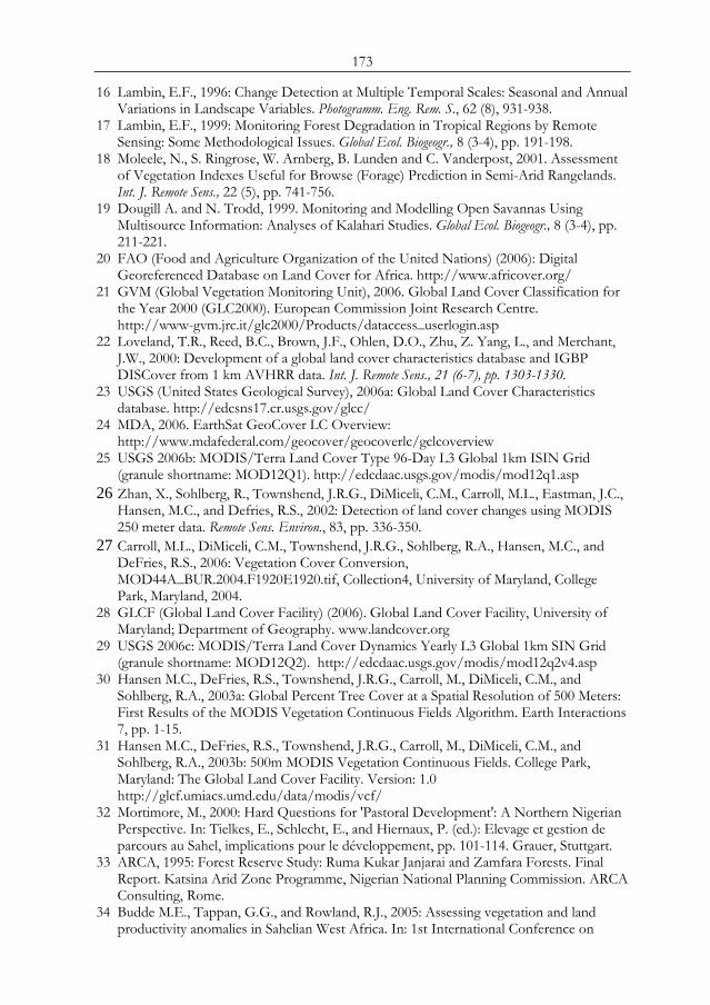
173
16 Lambin, E.F., 1996: Change Detection at Multiple Temporal Scales: Seasonal and Annual Variations in Landscape Variables. Photogramm. Eng. Rem. S., 62 (8), 931-938.
17 Lambin, E.F., 1999: Monitoring Forest Degradation in Tropical Regions by Remote Sensing: Some Methodological Issues. Global Ecol. Biogeogr., 8 (3-4), pp. 191-198.
18 Moleele, N., S. Ringrose, W. Arnberg, B. Lunden and C. Vanderpost, 2001. Assessment of Vegetation Indexes Useful for Browse (Forage) Prediction in Semi-Arid Rangelands. Int. J. Remote Sens., 22 (5), pp. 741-756.
19 Dougill A. and N. Trodd, 1999. Monitoring and Modelling Open Savannas Using Multisource Information: Analyses of Kalahari Studies. Global Ecol. Biogeogr., 8 (3-4), pp. 211-221.
20 FAO (Food and Agriculture Organization of the United Nations) (2006): Digital Georeferenced Database on Land Cover for Africa. http://www.africover.org/
21 GVM (Global Vegetation Monitoring Unit), 2006. Global Land Cover Classification for the Year 2000 (GLC2000). European Commission Joint Research Centre. http://www-gvm.jrc.it/glc2000/Products/dataccess_userlogin.asp
22 Loveland, T.R., Reed, B.C., Brown, J.F., Ohlen, D.O., Zhu, Z. Yang, L., and Merchant, J.W., 2000: Development of a global land cover characteristics database and IGBP DISCover from 1 km AVHRR data. Int. J. Remote Sens., 21 (6-7), pp. 1303-1330.
23 USGS (United States Geological Survey), 2006a: Global Land Cover Characteristics database. http://edcsns17.cr.usgs.gov/glcc/
24 MDA, 2006. EarthSat GeoCover LC Overview: http://www.mdafederal.com/geocover/geocoverlc/gclcoverview
25 USGS 2006b: MODIS/Terra Land Cover Type 96-Day L3 Global 1km ISIN Grid (granule shortname: MOD12Q1). http://edcdaac.usgs.gov/modis/mod12q1.asp
26 Zhan, X., Sohlberg, R., Townshend, J.R.G., DiMiceli, C.M., Carroll, M.L., Eastman, J.C., Hansen, M.C., and Defries, R.S., 2002: Detection of land cover changes using MODIS 250 meter data. Remote Sens. Environ., 83, pp. 336-350.
27 Carroll, M.L., DiMiceli, C.M., Townshend, J.R.G., Sohlberg, R.A., Hansen, M.C., and DeFries, R.S., 2006: Vegetation Cover Conversion, MOD44A_BUR.2004.F1920E1920.tif, Collection4, University of Maryland, College Park, Maryland, 2004.
28 GLCF (Global Land Cover Facility) (2006). Global Land Cover Facility, University of Maryland; Department of Geography. www.landcover.org
29 USGS 2006c: MODIS/Terra Land Cover Dynamics Yearly L3 Global 1km SIN Grid (granule shortname: MOD12Q2). http://edcdaac.usgs.gov/modis/mod12q2v4.asp
30 Hansen M.C., DeFries, R.S., Townshend, J.R.G., Carroll, M., DiMiceli, C.M., and Sohlberg, R.A., 2003a: Global Percent Tree Cover at a Spatial Resolution of 500 Meters: First Results of the MODIS Vegetation Continuous Fields Algorithm. Earth Interactions 7, pp. 1-15.
31 Hansen M.C., DeFries, R.S., Townshend, J.R.G., Carroll, M., DiMiceli, C.M., and Sohlberg, R.A., 2003b: 500m MODIS Vegetation Continuous Fields. College Park, Maryland: The Global Land Cover Facility. Version: 1.0 http://glcf.umiacs.umd.edu/data/modis/vcf/
32 Mortimore, M., 2000: Hard Questions for 'Pastoral Development': A Northern Nigerian Perspective. In: Tielkes, E., Schlecht, E., and Hiernaux, P. (ed.): Elevage et gestion de parcours au Sahel, implications pour le développement, pp. 101-114. Grauer, Stuttgart.
33 ARCA, 1995: Forest Reserve Study: Ruma Kukar Janjarai and Zamfara Forests. Final Report. Katsina Arid Zone Programme, Nigerian National Planning Commission. ARCA Consulting, Rome.
34 Budde M.E., Tappan, G.G., and Rowland, R.J., 2005: Assessing vegetation and land productivity anomalies in Sahelian West Africa. In: 1st International Conference on

174
Remote Sensing and Geoinformation Processing in the Assessment and Monitoring of Land Degradation and Desertification (RGLDD05), Trier, 7.-9. Sept, 2005. Abstract Book, pp. 115.
35 USGS 2006d: Earth Explorer. http://edcsns17.cr.usgs.gov/EarthExplorer/ 36 Küppers, K., 1998: Evaluation of the ligneous strata of the vegetation of Zamfara
Reserve, North-West Nigeria. In: Hoffmann, I. (ed.) Prospects of pastoralism in West Africa. Giessener Beiträge zur Entwicklungsforschung, Reihe I, Band 25, pp. 41-47. Tropeninstitut Justus Liebig Universität, Giessen, Germany.
37 Malami, B.S., 2005: Balancing Nutrients Supply and Requirements for Ruminants in Zamfara State, Nigeria. [unpublished] PhD thesis, Usmanu Danfodiyo University, Sokoto, Nigeria.
38 Budde, M.E., Tappan, G.G., Rowland, R.J., Lewis, J., and Tieszen, L.L., 2004: Assessing land cover performance in Senegal, West Africa using 1-km integrated NDVI and local variance analysis. J. Arid Environ., 59(3), pp. 481-498.
39 Hostert, P., Roeder. A., Hill. J., Udelhoven. T., and Tsiourlis, G., 2003: Retrospective studies of grazing-induced land degradation: a case study in central Crete, Greece. Int. J. Remote Sens., 24 (20), pp. 4019-4034.
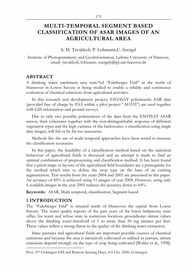
175
MULTI-TEMPORAL SEGMENT BASED CLASSIFICATION OF ASAR IMAGES OF AN
AGRICULTURAL AREA
S. M. Tavakkoli, P. Lohmann,U. Soergel Institute of Photogrammetry and GeoInformation, Leibniz University of Hanover,
email: (tavakkoli, lohmann, soergel)@ipi.uni-hanover.de
ABSTRACT A drinking water catchment area nam18ed “Fuhrberger Feld” in the north of Hannover in Lower Saxony is being studied to enable a reliable and continuous evaluation of chemical emissions from agricultural activities.
In this research and development project, ENVISAT polarimetric SAR data (provided free of charge by ESA within a pilot project “AO335”) are used together with GIS information and ground surveys.
Due to only two possible polarisations of the data from the ENVISAT ASAR sensor, their coherence together with the non-distinguishable response of different vegetation types and the high variance of the backscatter, a classification using single date images, will fail or be far too inaccurate.
Methods like the use of multi temporal approaches have been tested to increase the classification accuracies.
In this paper, the feasibility of a classification method based on the statistical behaviour of agricultural fields is discussed and an attempt is made to find an optimal combination of preprocessing and classification method. It has been found that a priori maps or layouts of the agricultural field boundaries are a prerequisite for the method which tries to define the crop type on the base of an existing segmentation. Test results from the years 2004 and 2005 are presented in this paper. An accuracy of 85% is achieved using 11 images of year 2004. However, using only 6 available images in the year 2005 reduces the accuracy down to 64%. Keywords: ASAR, Multi temporal, classification, Segment-based
1 INTRODUCTION The “Fuhrberger Feld” is situated north of Hannover the capital from Lower Saxony. The water quality reports of the past years of the lower SaSpaxony state office for water and refuse state in numerous locations groundwater nitrate values above the drinking water-threshold of 5 to more than 50 mg nitrates per liter. These values reflect a strong threat to the quality of the drinking water extraction.
Since pastures and agricultural fields are important possible sources of chemical emissions and because the area is intensively cultivated or utilised as pasture, nitrate emissions depend strongly on the type of crop being cultivated [Walter et al., 1998]. Proc. 2nd Göttingen GIS and Remote Sensing Days, 4-6 Oct. 2006, Göttingen
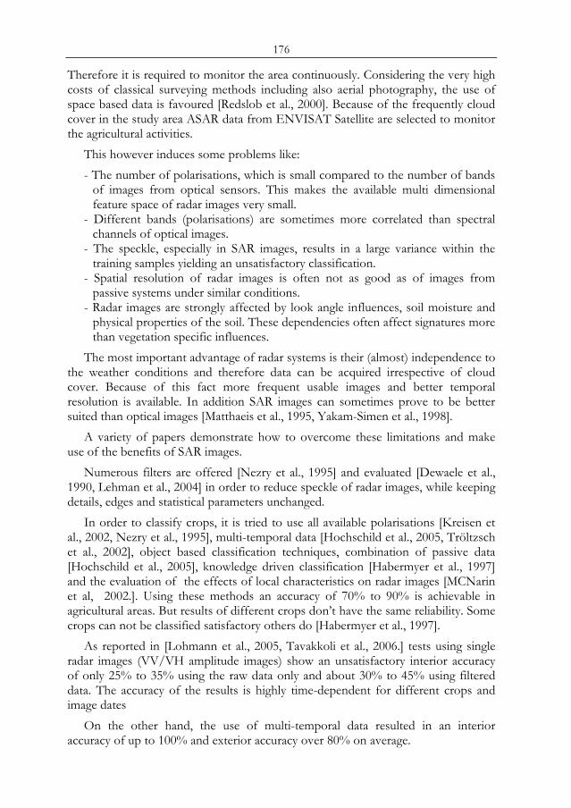
176
Therefore it is required to monitor the area continuously. Considering the very high costs of classical surveying methods including also aerial photography, the use of space based data is favoured [Redslob et al., 2000]. Because of the frequently cloud cover in the study area ASAR data from ENVISAT Satellite are selected to monitor the agricultural activities.
This however induces some problems like: - The number of polarisations, which is small compared to the number of bands
of images from optical sensors. This makes the available multi dimensional feature space of radar images very small.
- Different bands (polarisations) are sometimes more correlated than spectral channels of optical images.
- The speckle, especially in SAR images, results in a large variance within the training samples yielding an unsatisfactory classification.
- Spatial resolution of radar images is often not as good as of images from passive systems under similar conditions.
- Radar images are strongly affected by look angle influences, soil moisture and physical properties of the soil. These dependencies often affect signatures more than vegetation specific influences.
The most important advantage of radar systems is their (almost) independence to the weather conditions and therefore data can be acquired irrespective of cloud cover. Because of this fact more frequent usable images and better temporal resolution is available. In addition SAR images can sometimes prove to be better suited than optical images [Matthaeis et al., 1995, Yakam-Simen et al., 1998].
A variety of papers demonstrate how to overcome these limitations and make use of the benefits of SAR images.
Numerous filters are offered [Nezry et al., 1995] and evaluated [Dewaele et al., 1990, Lehman et al., 2004] in order to reduce speckle of radar images, while keeping details, edges and statistical parameters unchanged.
In order to classify crops, it is tried to use all available polarisations [Kreisen et al., 2002, Nezry et al., 1995], multi-temporal data [Hochschild et al., 2005, Tröltzsch et al., 2002], object based classification techniques, combination of passive data [Hochschild et al., 2005], knowledge driven classification [Habermyer et al., 1997] and the evaluation of the effects of local characteristics on radar images [MCNarin et al, 2002.]. Using these methods an accuracy of 70% to 90% is achievable in agricultural areas. But results of different crops don’t have the same reliability. Some crops can not be classified satisfactory others do [Habermyer et al., 1997].
As reported in [Lohmann et al., 2005, Tavakkoli et al., 2006.] tests using single radar images (VV/VH amplitude images) show an unsatisfactory interior accuracy of only 25% to 35% using the raw data only and about 30% to 45% using filtered data. The accuracy of the results is highly time-dependent for different crops and image dates
On the other hand, the use of multi-temporal data resulted in an interior accuracy of up to 100% and exterior accuracy over 80% on average.
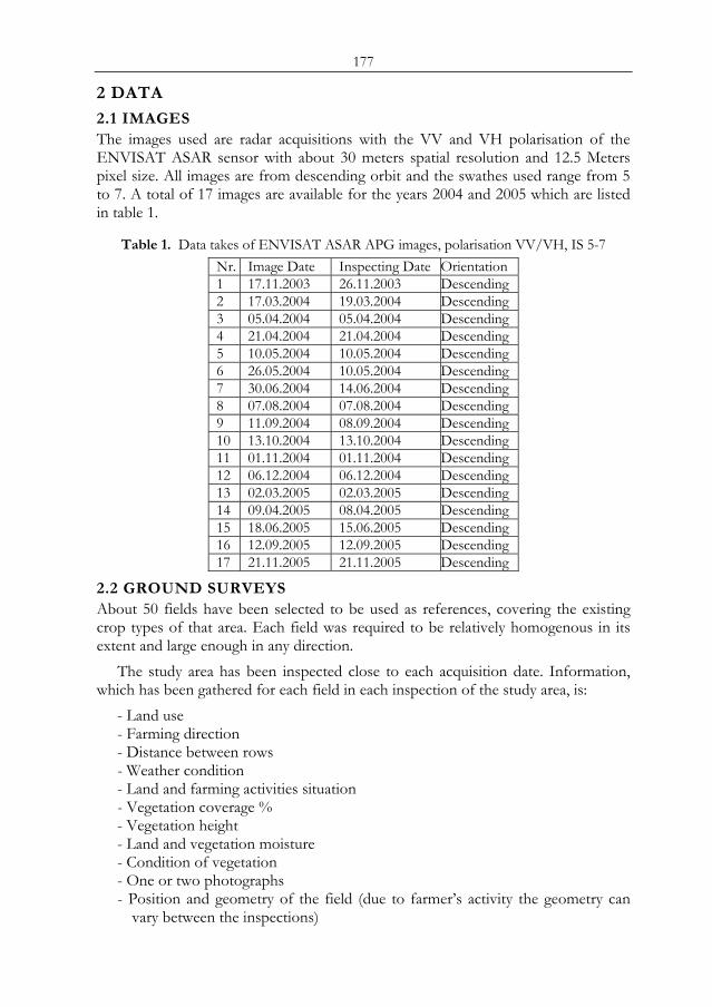
177
2 DATA
2.1 IMAGES The images used are radar acquisitions with the VV and VH polarisation of the ENVISAT ASAR sensor with about 30 meters spatial resolution and 12.5 Meters pixel size. All images are from descending orbit and the swathes used range from 5 to 7. A total of 17 images are available for the years 2004 and 2005 which are listed in table 1.
Table 1. Data takes of ENVISAT ASAR APG images, polarisation VV/VH, IS 5-7 Nr. Image Date Inspecting Date Orientation 1 17.11.2003 26.11.2003 Descending2 17.03.2004 19.03.2004 Descending3 05.04.2004 05.04.2004 Descending4 21.04.2004 21.04.2004 Descending5 10.05.2004 10.05.2004 Descending6 26.05.2004 10.05.2004 Descending7 30.06.2004 14.06.2004 Descending8 07.08.2004 07.08.2004 Descending9 11.09.2004 08.09.2004 Descending10 13.10.2004 13.10.2004 Descending11 01.11.2004 01.11.2004 Descending12 06.12.2004 06.12.2004 Descending13 02.03.2005 02.03.2005 Descending14 09.04.2005 08.04.2005 Descending15 18.06.2005 15.06.2005 Descending16 12.09.2005 12.09.2005 Descending17 21.11.2005 21.11.2005 Descending
2.2 GROUND SURVEYS About 50 fields have been selected to be used as references, covering the existing crop types of that area. Each field was required to be relatively homogenous in its extent and large enough in any direction.
The study area has been inspected close to each acquisition date. Information, which has been gathered for each field in each inspection of the study area, is:
- Land use - Farming direction - Distance between rows - Weather condition - Land and farming activities situation - Vegetation coverage % - Vegetation height - Land and vegetation moisture - Condition of vegetation - One or two photographs - Position and geometry of the field (due to farmer’s activity the geometry can
vary between the inspections)
178
2.3 MAP OF THE FIELDS It is necessary to create a separate layout map for each inspection, because the field borders are not always fixed and change frequently. Therefore, some fields may become too small to be used with respect to the resolution of the images and have to be eliminated, and other fields are added in order to keep record of the most important farming activities.
Considering the 30 meters spatial resolution, a 30 meter strip has been eliminated (buffered) from the boundary of each field to keep each training field as homogenous as possible and to eliminate mixed or unreliable pixels from the statistics. These maps then are used in the further processing.
3 PREPROCESSING Speckle in radar images reflect physical properties of microwaves together with instrumental errors and target properties. This means that the speckle may be a meaningful variable reflecting the behaviour of different surfaces. On the other hand it influences strongly the statistics of an image. Therefore the question arises, if the images should be filtered or if the speckle can be used to make fields more comparable for classification.
A Lee filter with a 7x7 kernel has been used as an example of a despeckle filter in order to investigate if despeckled images are better suited for the suggested method. The kernel size (7x7) has been chosen with respect to the resolution (30 meters) and pixel size (12.5 meters). Therefore a 7x7 filter on an image with 12.5 meters pixel size covers an area of 87.5x87.5 m2, which is comparable to a 3x3 kernel for the 30 meters resolution, and represents the smallest meaningful kernel size for this resolution.
4 CLASSIFICATION Considering the (almost) independence to the weather conditions, SAR data can be acquired irrespective of cloud cover. Because of this fact, more frequent usable images and therefore better temporal resolution and an extended feature space becomes available. Because of potential higher temporal resolution, SAR images sometimes are to be better suited than optical images as reported in de Matthaeis et al., 1995 and Yakam-Simen et al., 1998. 4.1 CLASSIFICATION OF SINGLE DATE IMAGES To test the ability of classical classification methods on single date ASAR images, we have tested different classification methods on two-band single date images. As result, only 20-30% of sample fields have been correctly classified using unfiltered images (interior accuracy). The interior accuracy of the classification of filtered images increased to 25-45% using sample fields, depending on the method of filtering and the date of acquisition. We did not find any important effect on the results concerning the classification method. [Lohmann et al., 2005].
It is noticeable that the accuracy of classification is strongly dependent on land use type and acquisition date, i.e. each crop can be recognised on some images better than on other images and on the other hand from each image some crops can be extracted better than other crops. As can be seen on Figure 1, some crops such
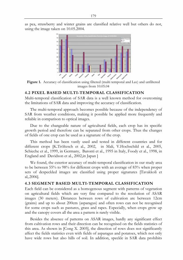
179
as pea, strawberry and winter grains are classified relative well but others do not, using the image taken on 10.05.2004.
Figure 1. Accuracy of classification using filtered (multi temporal and Lee) and unfiltered
images from 10.05.04
4.2 PIXEL BASED MULTI-TEMPORAL CLASSIFICATION Multi-temporal classification of SAR data is a well known method for overcoming the limitations of SAR data and improving the accuracy of classification.
The multi-temporal approach becomes possible because of the independency of SAR from weather conditions, making it possible be applied more frequently and reliable in comparison to optical images.
Due to the changeable nature of agricultural fields, each crop has its specific growth period and therefore can be separated from other crops. Thus the changes of fields of one crop can be used as a signature of the crop.
This method has been vastly used and tested in different countries and for different crops [K.Tröltzsch et al., 2002, in Mali, V.Hochschild et al., 2005, Schieche et al., 1999, in Germany, Baronti et al., 1995 in Italy, Foody et al., 1998, in England and Davidson et al., 2002,in Japan ]
We found, the exterior accuracy of multi-temporal classification in our study area to be between 55% to 98% for different crops with an average of 83% when proper sets of despeckled images are classified using proper signatures [Tavakkoli et al,.2006]. 4.3 SEGMENT BASED MULTI-TEMPORAL CLASSIFICATION Each field can be considered as a homogenous segment with patterns of vegetation on agricultural fields which are very fine compared to the resolution of ASAR images (30 meters). Distances between rows of cultivation are between 12cm (grains) and up to about 200cm (asparagus) and often rows can not be recognised for some crops such as pastures, grass and rapes. Especially, when crops grow up and the canopy covers all the area a pattern is rarely visible.
Besides the absence of patterns on ASAR images, hardly any significant effect from cultivation rows and their direction can be recognised on the fields statistics of this area. As shown in [Cong X. 2005], the direction of rows does not significantly affect the fields statistics even with fields of asparagus and potatoes, which not only have wide rows but also hills of soil. In addition, speckle in SAR data prohibits
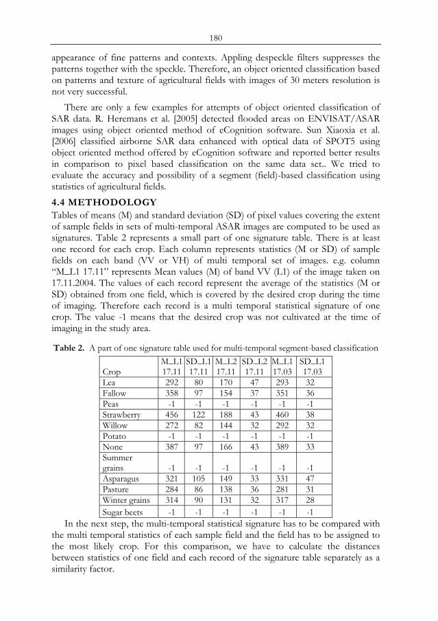
180
appearance of fine patterns and contexts. Appling despeckle filters suppresses the patterns together with the speckle. Therefore, an object oriented classification based on patterns and texture of agricultural fields with images of 30 meters resolution is not very successful.
There are only a few examples for attempts of object oriented classification of SAR data. R. Heremans et al. [2005] detected flooded areas on ENVISAT/ASAR images using object oriented method of eCognition software. Sun Xiaoxia et al. [2006] classified airborne SAR data enhanced with optical data of SPOT5 using object oriented method offered by eCognition software and reported better results in comparison to pixel based classification on the same data set.. We tried to evaluate the accuracy and possibility of a segment (field)-based classification using statistics of agricultural fields. 4.4 METHODOLOGY Tables of means (M) and standard deviation (SD) of pixel values covering the extent of sample fields in sets of multi-temporal ASAR images are computed to be used as signatures. Table 2 represents a small part of one signature table. There is at least one record for each crop. Each column represents statistics (M or SD) of sample fields on each band (VV or VH) of multi temporal set of images. e.g. column “M_L1 17.11” represents Mean values (M) of band VV (L1) of the image taken on 17.11.2004. The values of each record represent the average of the statistics (M or SD) obtained from one field, which is covered by the desired crop during the time of imaging. Therefore each record is a multi temporal statistical signature of one crop. The value -1 means that the desired crop was not cultivated at the time of imaging in the study area.
Table 2. A part of one signature table used for multi-temporal segment-based classification
Crop M_L117.11
SD_L117.11
M_L217.11
SD_L217.11
M_L117.03
SD_L1 17.03
Lea 292 80 170 47 293 32 Fallow 358 97 154 37 351 36 Peas -1 -1 -1 -1 -1 -1 Strawberry 456 122 188 43 460 38 Willow 272 82 144 32 292 32 Potato -1 -1 -1 -1 -1 -1 None 387 97 166 43 389 33 Summer grains -1 -1 -1 -1 -1 -1 Asparagus 321 105 149 33 331 47 Pasture 284 86 138 36 281 31 Winter grains 314 90 131 32 317 28 Sugar beets -1 -1 -1 -1 -1 -1
In the next step, the multi-temporal statistical signature has to be compared with the multi temporal statistics of each sample field and the field has to be assigned to the most likely crop. For this comparison, we have to calculate the distances between statistics of one field and each record of the signature table separately as a similarity factor.
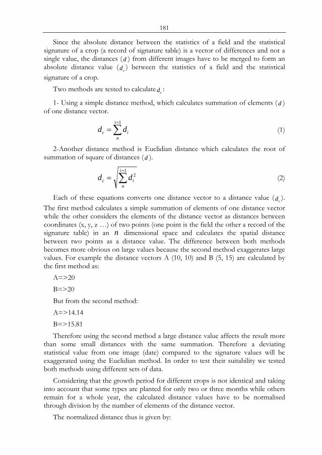
181
Since the absolute distance between the statistics of a field and the statistical signature of a crop (a record of signature table) is a vector of differences and not a single value, the distances ( d ) from different images have to be merged to form an absolute distance value (
cd ) between the statistics of a field and the statistical signature of a crop.
Two methods are tested to calculatecd :
1- Using a simple distance method, which calculates summation of elements ( d ) of one distance vector.
∑=
=1i
nic dd (1)
2-Another distance method is Euclidian distance which calculates the root of summation of square of distances ( d ).
∑=
=1
2i
nic dd (2)
Each of these equations converts one distance vector to a distance value (cd ).
The first method calculates a simple summation of elements of one distance vector while the other considers the elements of the distance vector as distances between coordinates (x, y, z …) of two points (one point is the field the other a record of the signature table) in an n dimensional space and calculates the spatial distance between two points as a distance value. The difference between both methods becomes more obvious on large values because the second method exaggerates large values. For example the distance vectors A (10, 10) and B (5, 15) are calculated by the first method as:
A=>20 B=>20 But from the second method: A=>14.14 B=>15.81 Therefore using the second method a large distance value affects the result more
than some small distances with the same summation. Therefore a deviating statistical value from one image (date) compared to the signature values will be exaggerated using the Euclidian method. In order to test their suitability we tested both methods using different sets of data.
Considering that the growth period for different crops is not identical and taking into account that some types are planted for only two or three months while others remain for a whole year, the calculated distance values have to be normalised through division by the number of elements of the distance vector.
The normalized distance thus is given by:
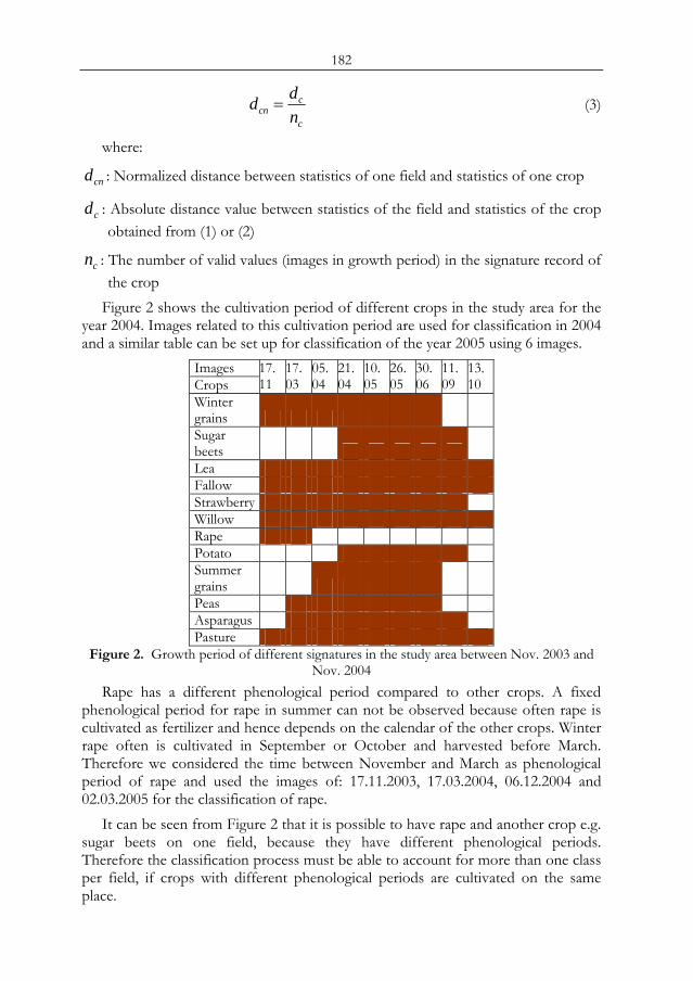
182
c
ccn n
dd = (3)
where:
cnd : Normalized distance between statistics of one field and statistics of one crop
cd : Absolute distance value between statistics of the field and statistics of the crop obtained from (1) or (2)
cn : The number of valid values (images in growth period) in the signature record of the crop
Figure 2 shows the cultivation period of different crops in the study area for the year 2004. Images related to this cultivation period are used for classification in 2004 and a similar table can be set up for classification of the year 2005 using 6 images.
Images Crops
17. 11
17. 03
05. 04
21. 04
10. 05
26. 05
30. 06
11. 09
13. 10
Winter grains Sugar beets Lea Fallow StrawberryWillow Rape Potato Summer grains Peas AsparagusPasture
Figure 2. Growth period of different signatures in the study area between Nov. 2003 and Nov. 2004
Rape has a different phenological period compared to other crops. A fixed phenological period for rape in summer can not be observed because often rape is cultivated as fertilizer and hence depends on the calendar of the other crops. Winter rape often is cultivated in September or October and harvested before March. Therefore we considered the time between November and March as phenological period of rape and used the images of: 17.11.2003, 17.03.2004, 06.12.2004 and 02.03.2005 for the classification of rape.
It can be seen from Figure 2 that it is possible to have rape and another crop e.g. sugar beets on one field, because they have different phenological periods. Therefore the classification process must be able to account for more than one class per field, if crops with different phenological periods are cultivated on the same place.
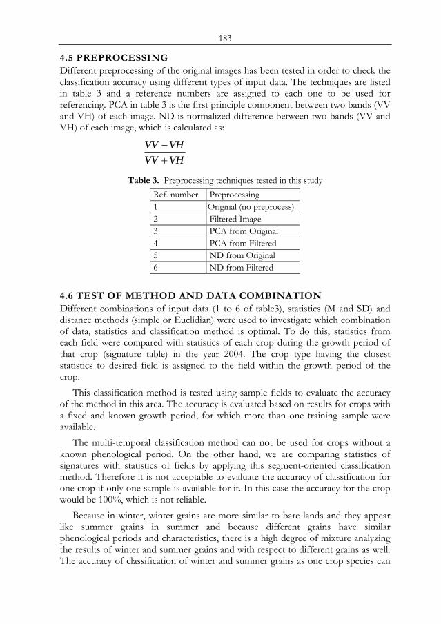
183
4.5 PREPROCESSING Different preprocessing of the original images has been tested in order to check the classification accuracy using different types of input data. The techniques are listed in table 3 and a reference numbers are assigned to each one to be used for referencing. PCA in table 3 is the first principle component between two bands (VV and VH) of each image. ND is normalized difference between two bands (VV and VH) of each image, which is calculated as:
VHVVVHVV
+−
Table 3. Preprocessing techniques tested in this study Ref. number Preprocessing 1 Original (no preprocess)2 Filtered Image 3 PCA from Original 4 PCA from Filtered 5 ND from Original 6 ND from Filtered
4.6 TEST OF METHOD AND DATA COMBINATION Different combinations of input data (1 to 6 of table3), statistics (M and SD) and distance methods (simple or Euclidian) were used to investigate which combination of data, statistics and classification method is optimal. To do this, statistics from each field were compared with statistics of each crop during the growth period of that crop (signature table) in the year 2004. The crop type having the closest statistics to desired field is assigned to the field within the growth period of the crop.
This classification method is tested using sample fields to evaluate the accuracy of the method in this area. The accuracy is evaluated based on results for crops with a fixed and known growth period, for which more than one training sample were available.
The multi-temporal classification method can not be used for crops without a known phenological period. On the other hand, we are comparing statistics of signatures with statistics of fields by applying this segment-oriented classification method. Therefore it is not acceptable to evaluate the accuracy of classification for one crop if only one sample is available for it. In this case the accuracy for the crop would be 100%, which is not reliable.
Because in winter, winter grains are more similar to bare lands and they appear like summer grains in summer and because different grains have similar phenological periods and characteristics, there is a high degree of mixture analyzing the results of winter and summer grains and with respect to different grains as well. The accuracy of classification of winter and summer grains as one crop species can
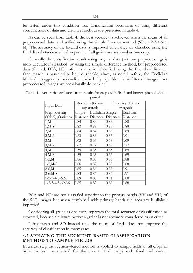
184
be tested under this condition too. Classification accuracies of using different combinations of data and distance methods are presented in table 4.
As can be seen from table 4, the best accuracy is achieved when the mean of all preprocessed data is classified using the simple distance method (SD, 1-2-3-4-5-6, M). The accuracy of the filtered data is improved when they are classified using the Euclidian distance method, especially if all grains are assumed as one crop.
Generally the classification result using original data (without preprocessing) is more accurate if classified by using the simple difference method, but preprocessed data (filtered, PCA, ND) often is superior classified using the Euclidian distance. One reason is assumed to be the speckle, since, as noted before, the Euclidian Method exaggerates anomalies caused by speckle in unfiltered images but preprocessed images are occasionally despeckled.
Table 4. Accuracies evaluated from results for crops with fixed and known phenological period
Input Data Accuracy (Grains separated)
Accuracy (Grains merged)
Preprocessing (Tab.5) ,Statistics
Simple Distance
Euclidian Distance
Simple Distance
Euclidian Distance
1,M 0.84 0.83 0.85 0.88 1,M-S 0.82 0.82 0.85 0.88 2,M 0.84 0.84 0.88 0.89 2,M-S 0.83 0.86 0.86 0.91 3,M 0.65 0.64 0.68 0.69 3,M-S 0.62 0.72 0.68 0.77 4,M 0.59 0.63 0.65 0.69 4,M-S 0.55 0.63 0.62 0.69 1-5,M 0.86 0.83 0.88 0.88 1-5,M-S 0.86 0.82 0.88 0.88 2-6,M 0.85 0.86 0.88 0.91 2-6,M-S 0.83 0.86 0.86 0.91 1-2-3-4-5-6,M 0.89 0.83 0.91 0.88 1-2-3-4-5-6,M-S 0.85 0.82 0.88 0.88
PCA and ND are not classified superior to the primary bands (VV and VH) of
the SAR images but when combined with primary bands the accuracy is slightly improved.
Considering all grains as one crop improves the total accuracy of classification as expected, because a mixture between grains is not anymore considered as an error.
Using mean and SD instead only the mean of fields does not improve the accuracy of classification in many cases. 4.7 APPLYING THE SEGMENT-BASED CLASSIFICATION METHOD TO SAMPLE FIELDS In a next step the segment-based method is applied to sample fields of all crops in order to test the method for the case that all crops with fixed and known
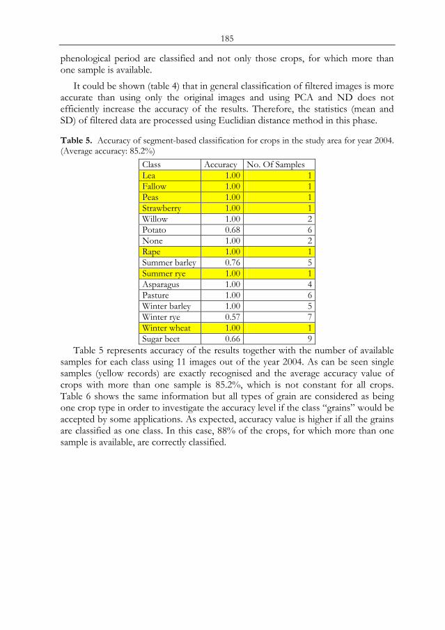
185
phenological period are classified and not only those crops, for which more than one sample is available.
It could be shown (table 4) that in general classification of filtered images is more accurate than using only the original images and using PCA and ND does not efficiently increase the accuracy of the results. Therefore, the statistics (mean and SD) of filtered data are processed using Euclidian distance method in this phase.
Table 5. Accuracy of segment-based classification for crops in the study area for year 2004. (Average accuracy: 85.2%)
Class Accuracy No. Of Samples Lea 1.00 1Fallow 1.00 1Peas 1.00 1Strawberry 1.00 1Willow 1.00 2Potato 0.68 6None 1.00 2Rape 1.00 1Summer barley 0.76 5Summer rye 1.00 1Asparagus 1.00 4Pasture 1.00 6Winter barley 1.00 5Winter rye 0.57 7Winter wheat 1.00 1Sugar beet 0.66 9
Table 5 represents accuracy of the results together with the number of available samples for each class using 11 images out of the year 2004. As can be seen single samples (yellow records) are exactly recognised and the average accuracy value of crops with more than one sample is 85.2%, which is not constant for all crops. Table 6 shows the same information but all types of grain are considered as being one crop type in order to investigate the accuracy level if the class “grains” would be accepted by some applications. As expected, accuracy value is higher if all the grains are classified as one class. In this case, 88% of the crops, for which more than one sample is available, are correctly classified.
186
Table 6. Accuracy of segment-based classification for crops in the study area when different grains are considered as one crop for year 2004. (Average accuracy: 88%)
Class Accuracy No. Of Samples Lea 1.00 1Fallow 1.00 1Peas 1.00 1Strawberry 1.00 1Willow 1.00 2Potato 0.68 6None 1.00 2Rape 1.00 1Asparagus 1.00 4pasture 1.00 6sugar beet 0.66 9Grains 0.82 19
Tables 7 and 8 show the accuracy and number of available samples for each class
using 6 images of the year 2005. The major difference between the classification of images of 2004 and 2005 is the number of available images. Only 6 images for the year 2005 are used which results in a poor average accuracy of 64% Another difference is that there are 3 fields of maize and 6 fields of rape which are well classified in the year 2005 but there were no Maize field and only one rape field in the year 2004. Table 8 shows the accuracy of results for the data of year 2005 with all grains classified as one crop. 75% of sample fields are correctly classified in this case. This shows an improvement of 11% in comparison to the values of table 7 (different grains separated); while there is only less than 3% difference between accuracy of the two representations of classification in the year 2004 (tables 5 and 6). This indicates a high value of mixture between different grains, which is caused by the small number of images for the year 2005.
Table 7. Accuracy of segment-based classification for crops in the study area for year 2005. (Average accuracy: 64%)
Class Accuracy No. of Samplespasture 0.81 5maize 1.00 3sugar beet 0.47 5Winter rye 0.36 9Fallow 1.00 1Winter barley 0.35 8Asparagus 0.44 4Summer barley 0.42 8Potato 0.71 4Willow 1.00 2Peas 1.00 1Lea 0.51 2Summer Wheat 1.00 1Summer oat 1.00 1Rape 1.00 6
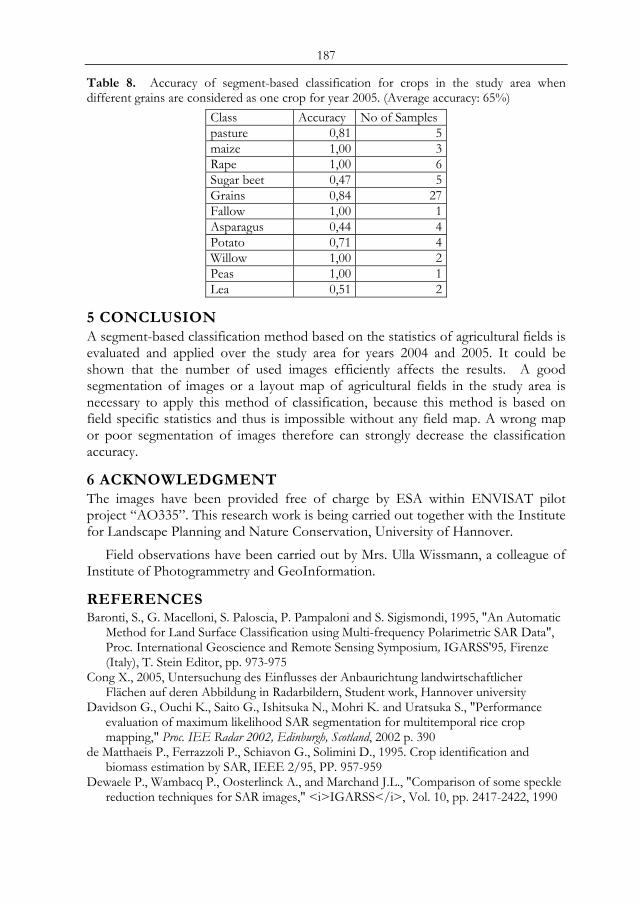
187
Table 8. Accuracy of segment-based classification for crops in the study area when different grains are considered as one crop for year 2005. (Average accuracy: 65%)
Class Accuracy No of Samplespasture 0,81 5maize 1,00 3Rape 1,00 6Sugar beet 0,47 5Grains 0,84 27Fallow 1,00 1Asparagus 0,44 4Potato 0,71 4Willow 1,00 2Peas 1,00 1Lea 0,51 2
5 CONCLUSION A segment-based classification method based on the statistics of agricultural fields is evaluated and applied over the study area for years 2004 and 2005. It could be shown that the number of used images efficiently affects the results. A good segmentation of images or a layout map of agricultural fields in the study area is necessary to apply this method of classification, because this method is based on field specific statistics and thus is impossible without any field map. A wrong map or poor segmentation of images therefore can strongly decrease the classification accuracy.
6 ACKNOWLEDGMENT The images have been provided free of charge by ESA within ENVISAT pilot project “AO335”. This research work is being carried out together with the Institute for Landscape Planning and Nature Conservation, University of Hannover.
Field observations have been carried out by Mrs. Ulla Wissmann, a colleague of Institute of Photogrammetry and GeoInformation.
REFERENCES Baronti, S., G. Macelloni, S. Paloscia, P. Pampaloni and S. Sigismondi, 1995, "An Automatic
Method for Land Surface Classification using Multi-frequency Polarimetric SAR Data", Proc. International Geoscience and Remote Sensing Symposium, IGARSS'95, Firenze (Italy), T. Stein Editor, pp. 973-975
Cong X., 2005, Untersuchung des Einflusses der Anbaurichtung landwirtschaftlicher Flächen auf deren Abbildung in Radarbildern, Student work, Hannover university
Davidson G., Ouchi K., Saito G., Ishitsuka N., Mohri K. and Uratsuka S., "Performance evaluation of maximum likelihood SAR segmentation for multitemporal rice crop mapping," Proc. IEE Radar 2002, Edinburgh, Scotland, 2002 p. 390
de Matthaeis P., Ferrazzoli P., Schiavon G., Solimini D., 1995. Crop identification and biomass estimation by SAR, IEEE 2/95, PP. 957-959
Dewaele P., Wambacq P., Oosterlinck A., and Marchand J.L., "Comparison of some speckle reduction techniques for SAR images," <i>IGARSS</i>, Vol. 10, pp. 2417-2422, 1990
188
Foody G.M., Curran P.J., Groom G.B., Munro D.C., 1988, Crop classification with multi-temporal X-Band SAR data, Proceedings of IGRASS ’88 Symposium’ Edinburgh, Scotland, 13-16 Sept. PP. 217-220.
Habermyer M., Schmullius C.C., 1997, Ein alguritmus zur Wissenbasierten Klassifikation multitemporaler Radar-fernerkundungsdaten, DGPF 5/1997, PP. 313-323.
Heremans R, Willekens A., Borghys D., Verbeeck B., Valckenborgh J., Acheroy M., Perneel C., 2005, Automatic detection of flooded areas on ENVISAT/ASAR images using object-oriented classification technique and an active contour algorithm, 31st ISRSE, Saint Petersburg.
Hochschild V., Weise C., Selsam P., 2005, Die Aktualisierung der digitalen Grundkarte Landwirtschaft in Thüringen mit Hilfe von Fernerkundungsdaten, DGPF 3/2005 PP. 201-208.
Kreisen A., 2002, Objektbasierte Klassifikation vollpolarimetrischer SAR-Daten, Dessertation, TU Berlin.
Lee, J.S., 1981: Speckle analysis and smoothing of Synthetic Aperture Radar Images, Comp. Graph. Image Process. Vol. 17, pp. 24-32, 1981
Lehman A., Jan. 2004, Vergeleichende Analyse von SAR speckle Filtern, dessertation, TU Berlin.
Lohmann, P., Tavakkoli, M.; Wissmann, U.: Environmental Mapping using ENVISAT ASAR Data: IntarchPhRS. Band XXXVI 1/W3. Hannover, 2005, 6 S., CD
McNarin H., Decker V., Murnaghan K., The sensitivity of C-Band polarimetric SAR to crop condition,
MCNarin H., Duguaby C., Brisco B., Pultz T.J., 2002, The effect of soil and crop residue characteristics on polarimetric radar response, Remote sensing of environment 80 (2002), PP. 308-320
Nezry E., Leysen M., De Grandi G.: "Speckle and scene spatial statistical estimators for SAR image filtering and texture analysis: Applications to agriculture, forestry and point targets detection", Proc. of SPIE, Vol.2584, pp. 1 10-120, Sept. 1995.
Redslob, M., 2000: Effektive Informationserhebung durch GIS-gestützte Radarfernerkundung - dargestellt am Beispiel des Niedersächsischen Moorschutzprogramms.
Schieche B., Erasmi S., Schrage T., Hurlemann P., 1999, Monitoring and registering of grassland and fallow fields with multitemporal ERS data within a district of Lower Saxony, Germany, IEEE 6/99, P 759.
Tavakkoli, S.M., Lohman P., 2006, MULTI-TEMPORAL CLASSIFICATION OF ASAR IMAGES IN AGRICULTURAL AREAS, ISPRS May 2006, Enschede.
Tröltzsch K., 2002, Untersuchung von Möglichkeiten zur Landnutzungsklassifikation anhand multitemporaler ERS-Daten, Dessertation, TU Dresden.
Walter, W., Scheffer, B., 1998: Ergebnisse langjähriger Lysimeter-, Drän- und Saugkerzen-Versuche zur Stickstoffauswaschung bei landbaulich genutzten Böden und Bedeutung für die Belastung des Grundwassers, Schriftenreihe des Inst. f. Verkehr und Stadtbauwesen, TU Braunschweig
Xiaoxia S., Jixian Z., Zhengjun L., Zheng Z., 2006, Classification From airborne SAR data enhanced by optical image using an object-oriented approach, ISPRS May 2006, Enschede.
Yakam-Simen F., Nezry E., Zagolski F., 1998, Early estimation of crop surfaces, and agricultural monitoring using RADARSAT data, Proceedings of the ADRO Final Symposium, 9 p., Montréal (Québec, Canada), 13-15 October 1998.
189
SUB-METER RESOLUTION SATELLITE IMAGERY AND GIS TECHNIQUES FOR IMPROVING THE CONVENTIONAL URBAN ADMINISTRATIVE
SYSTEM
A. S. Almas and C. A. Rahim Department of Space Science, University of the Punjab,
Quaid-e-Azam Campus, Lahore, Pakistan, email: [email protected]
ABSTRACT The present research effort aims at 19exploiting the techniques of Geographic Information Science (GIS) for the development and integration of digital thematic layers representing a portion of a relatively planned urban regime existing at the heart of Lahore Metropolis. The emphasis has been placed upon facilitating the urban administration on planning, management and monitoring of civic amenities by providing them digital geographic information in the form of editable and revisable digital maps of location, line and area features. Sub-meter resolution, pan-sharpened satellite imagery has been used as a planimetric reference and base map for delineation of road network, sketch maps for demarcation of water-supply network and physical survey of the area for locating fuel-stations, mosques, educational institutions, health centers, police stations, banks/ ATM facilities, markets, important buildings etc. In addition, census data has been acquired to digitize precincts of census units in order to compute the population density and analyze its relationship with reference to existing civic amenities. Conclusively, the integration of Remote Sensing and GIS techniques have been found useful in facilitating the urban administration towards better planning and management in comparison to the use of conventional methods already in practice. Keywords: GIS, Thematic layers, Resolution, Pan-sharpened, Remote Sensing
1 INTRODUCTION With the commercialization of very high resolution satellite imagery, the progress in Geographic Information System (GIS) has started to gain momentum at a much faster pace than ever as far as image-data input is concerned. In addition, rapid advancement in computer hardware and software systems has also played an obvious role in the overall development of geospatial technologies. The pace is continuing to pick up strength with the wide-spread advancement and exploitation of GIS techniques at both research and application levels. Development of Urban Information System (UIS) is one of the most significant application areas of GIS. Advanced countries are already the frontline users of geospatial technologies. The case of developing countries is different, their responsibilities are two-pronged, i.e., technical apprehension and subsequent implementation. The implementation is not a direct task; it entails complete computerization of the conventional procedures Proc. 2nd Göttingen GIS and Remote Sensing Days, 4-6 Oct. 2006, Göttingen
190
already in practice that further requires capacity building to achieve the tangible benefits of the modern cutting-edge GIS technologies.
Gulberg is relatively old planned settlement situated at the heart of lively city of Lahore, the provincial capital rich in cultural and historical aspects. The focus of research is the central portion of Gulberg that administratively falls in the Charge-34 (according to census,) and in UC 96 (according to city district Government). At city level, the hierarchical order of the census units is Charge, Circle and Block [1]. Union council is the block-based administrative unit of the city district government. The Metropolitan Development Authority of Lahore (LDA) has divided the Gulberg into Blocks those are different than the Census Blocks, while Water and Sanitation Authority has their own administrative divides called sub-divisions e.g., Gulberg sub-division for water supply and sewage. Hence, there are four different administrative precincts in which various organizations of the city administration work for the development, census, utilities and provision of amenities to the citizenry at large. The departments responsible for the provision of facilities involving communication, natural gas and electricity are besides the foregoing. All the departments are using their own hand-made sketch maps for carrying out their respective responsibilities. The graphical and alpha-numeric stuff is often un-sharable simply because graphical sketches are not made following any standard cartographic principles, resultantly, the planning and development activities fall prey to non-coordination and irregularity. Since, it is hard to revise the paper maps; the monitoring activities also get impeded. In a plan making process, better planning is achieved through better information, and better information necessarily flows from an information system [2]. If the dynamic information is made available to the responsible agencies of civic administration covering both geographic and associated alpha-numeric contexts, it would not only facilitate in entire management process but would also be helpful in easy revision of exiting resource. Geographical information systems (GISs) have emerged as a powerful tool for collecting and analyzing such planning information [3]; [4]; [5]. Geospatial techniques can be exploited in this regard to address such issues. [6] argues that one of the proposals for improving the quality of planning is an attempt to improve the understanding and analysis of the interrelated components of the urban development process in order to arrive at more appropriate priorities and sets of policies.
Resultantly, in addition to transforming the existing graphical and alpha-numeric data into context-sensitive geospatial layers, a context-sensitive GIS application software titled “Metro-Explore” has been developed that possesses the ability to display vector and raster layers of the Lahore district involving administrative precincts, physical features, infrastructure, utilities and water supply network. The software also offers the facility to carry out query-based geospatial analyses e.g. computing the shortest route and finding the nearest facility. The entire effort has resulted into a desktop GIS application that is not only useful for a common citizen but also facilitates urban-administrative agencies in the planning perspective. Instead of using conventional systems already in practice, the GIS offers state-of-the-art techniques to generate, modify and append geospatial information in a more flexible manner than the existing for addressing the matters of urban planning and management.
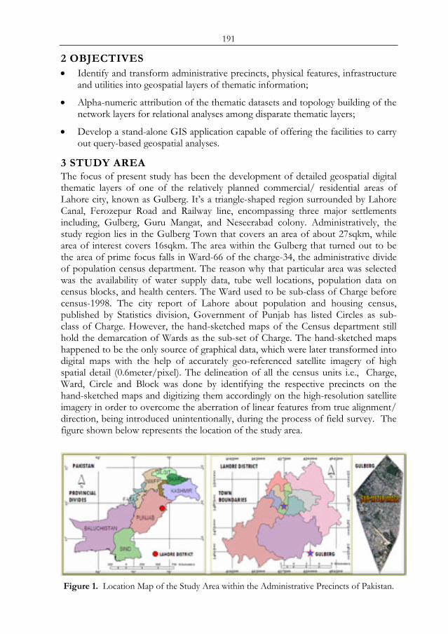
191
2 OBJECTIVES • Identify and transform administrative precincts, physical features, infrastructure
and utilities into geospatial layers of thematic information;
• Alpha-numeric attribution of the thematic datasets and topology building of the network layers for relational analyses among disparate thematic layers;
• Develop a stand-alone GIS application capable of offering the facilities to carry out query-based geospatial analyses.
3 STUDY AREA The focus of present study has been the development of detailed geospatial digital thematic layers of one of the relatively planned commercial/ residential areas of Lahore city, known as Gulberg. It’s a triangle-shaped region surrounded by Lahore Canal, Ferozepur Road and Railway line, encompassing three major settlements including, Gulberg, Guru Mangat, and Neseerabad colony. Administratively, the study region lies in the Gulberg Town that covers an area of about 27sqkm, while area of interest covers 16sqkm. The area within the Gulberg that turned out to be the area of prime focus falls in Ward-66 of the charge-34, the administrative divide of population census department. The reason why that particular area was selected was the availability of water supply data, tube well locations, population data on census blocks, and health centers. The Ward used to be sub-class of Charge before census-1998. The city report of Lahore about population and housing census, published by Statistics division, Government of Punjab has listed Circles as sub-class of Charge. However, the hand-sketched maps of the Census department still hold the demarcation of Wards as the sub-set of Charge. The hand-sketched maps happened to be the only source of graphical data, which were later transformed into digital maps with the help of accurately geo-referenced satellite imagery of high spatial detail (0.6meter/pixel). The delineation of all the census units i.e., Charge, Ward, Circle and Block was done by identifying the respective precincts on the hand-sketched maps and digitizing them accordingly on the high-resolution satellite imagery in order to overcome the aberration of linear features from true alignment/ direction, being introduced unintentionally, during the process of field survey. The figure shown below represents the location of the study area.
Figure 1. Location Map of the Study Area within the Administrative Precincts of Pakistan.

192
4 METHODOLOGY GIS is a computer-based information system that enables capturing, modeling, storage, retrieval, sharing, manipulation, analysis and presentation of geospatially referenced data [7]. In present research, the urban thematic layers were developed based on a common geographic coordinate system. Out of the entire spectrum of geographic features representing the study area, some of the most significant ones were selected, elaborating the focus of present research, and were converted into geospatial layers of thematic information. The administrative precincts and physical features those were developed into digital maps are listed below: 4.1 DISTRICT LEVEL Boundaries/ Precincts: District, Lahore Metropolis, Tehsil and Town Locations: Union Councils, Villages, Health Centers, Post Offices Linear Features: Major Roads, Water Channels, Canal 4.2 AREA OF INTEREST - GULBERG Boundaries/ Precincts: Residential Blocks, Census Precincts Locations: Hospitals, Post Office, Police Stations, Banks, ATM Sites, Tube wells Linear Features: Water Supply Network, Road Network
The information systems for urban planning include database management systems (DBMS), decision support system (DSS) and expert systems [8]. GIS alone plays a role of suggesting two-pronged solutions, data visualization component and the database one, hence facilitating in developing context-sensitive geospatial applications in the form of expert systems. Paper prints in the form of CAD sketches, maps of city district government, census layouts, locality maps from Lahore Development Authority (LDA), hand-sketches of Water and Sanitation Authority (WASA) have been the source of information for delineation of geospatial layers. For the sake of geographic precision and cartographic accuracy, very high resolution satellite imagery of QuickBirdTM satellite at 0.6meter spatial detail was also used. The sub-meter satellite imagery was used as a base map on which digitization was carried out by identifying the features on the paper maps and then delineating them on the imagery in order to establish geographic conformance between the actual features and their respective locations on the satellite imagery. This approach of digitization was followed because paper maps acquired from various city administrative organizations contained considerable distortions in scale, alignment and spatial distribution of physical features and precincts, that left no other choice than using the satellite imagery for precise demarcation and delineation of the features of interest. Once digitized in the forgoing manner, digitization of the remaining features lying within the precincts of district can be carried out with fair amount of spatial accuracy.
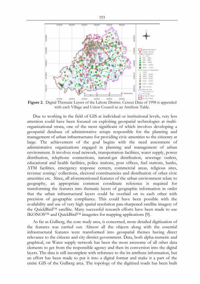
193
Figure 2. Digital Thematic Layers of the Lahore District. Census Data of 1998 is appended
with each Village and Union Council as an Attribute Table.
Due to working in the field of GIS at individual or institutional levels, very less attention could have been focused on exploiting geospatial technologies at multi-organizational strata, one of the most significant of which involves developing a geospatial database of administrative setups responsible for the planning and management of urban infrastructures for providing civic amenities to the citizenry at large. The achievement of the goal begins with the need assessment of administrative organizations engaged in planning and management of urban environment. It involves road network, transportation facilities, water supply, power distribution, telephone connections, natural-gas distribution, sewerage outlets, educational and health facilities, police stations, post offices, fuel stations, banks, ATM facilities, emergency response centers, commercial areas, religious sites, revenue zoning/ collections, electoral constituencies and distribution of other civic amenities etc. Since, all aforementioned features of the urban environment relate to geography, an appropriate common coordinate reference is required for transforming the features into thematic layers of geographic information in order that the urban infrastructural layers could be overlaid on to each other with precision of geographic compliance. This could have been possible with the availability and use of very high spatial resolution pan-sharpened satellite imagery of the QuickBirdTM satellite. Many successful research efforts have been made to use IKONOSTM and QuickBirdTM imageries for mapping applications [9].
As far as Gulberg, the core study area, is concerned, more detailed digitization of the features was carried out. Almost all the objects along with the essential infrastructural features were transformed into geospatial themes having direct relevance to the citizens and city district government. Data, both alpha-numeric and graphical, on Water supply network has been the most awesome of all other data elements to get from the responsible agency and then its conversion into the digital layers. The data is still incomplete with reference to the its attribute information, but an effort has been made to put it into a digital format and make it a part of the entire GIS of the Gulberg area. The topology of the digitized roads has been built
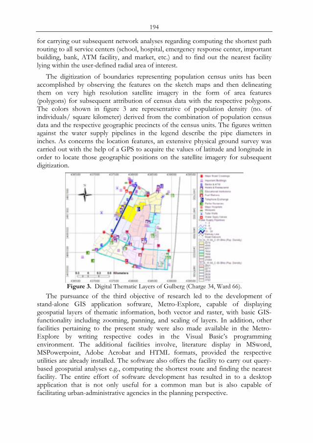
194
for carrying out subsequent network analyses regarding computing the shortest path routing to all service centers (school, hospital, emergency response center, important building, bank, ATM facility, and market, etc.) and to find out the nearest facility lying within the user-defined radial area of interest.
The digitization of boundaries representing population census units has been accomplished by observing the features on the sketch maps and then delineating them on very high resolution satellite imagery in the form of area features (polygons) for subsequent attribution of census data with the respective polygons. The colors shown in figure 3 are representative of population density (no. of individuals/ square kilometer) derived from the combination of population census data and the respective geographic precincts of the census units. The figures written against the water supply pipelines in the legend describe the pipe diameters in inches. As concerns the location features, an extensive physical ground survey was carried out with the help of a GPS to acquire the values of latitude and longitude in order to locate those geographic positions on the satellite imagery for subsequent digitization.
Figure 3. Digital Thematic Layers of Gulberg (Charge 34, Ward 66).
The pursuance of the third objective of research led to the development of stand-alone GIS application software, Metro-Explore, capable of displaying geospatial layers of thematic information, both vector and raster, with basic GIS-functionality including zooming, panning, and scaling of layers. In addition, other facilities pertaining to the present study were also made available in the Metro-Explore by writing respective codes in the Visual Basic’s programming environment. The additional facilities involve, literature display in MSword, MSPowerpoint, Adobe Acrobat and HTML formats, provided the respective utilities are already installed. The software also offers the facility to carry out query-based geospatial analyses e.g., computing the shortest route and finding the nearest facility. The entire effort of software development has resulted in to a desktop application that is not only useful for a common man but is also capable of facilitating urban-administrative agencies in the planning perspective.
195
The methodology conceived for the present study may not be unique regarding the implementation of standard procedures of RS/ GIS Processing, but in country like Pakistan, the GIS applications in the urban studies are very few, hence the focus has been placed to introduce modern tools of Geospatial technologies that can assist city administration to better plan and manage the urban environs in a broader scope of implementation. Recently, some studies to implement fundamental functions using geo-spatial imagery based on GIS have been carried out and tentatively tested [10]. The purpose of present research effort has been to facilitate the stakeholders of city administration to adopt modern techniques of geospatial sciences for planning new and managing the existing facilities/ amenities for the good of citizenry at large with the provision of data revisions on regular basis.
5 RESULTS AND DISCUSSION The achievement of first objective of the present research has resulted into development of more than 30 GIS-enabled thematic layers of geospatial information pertaining to Administrative boundaries, Linear/ curvilinear features, infrastructure, civic facilities, environmental themes and urban planning. The attribution of population census data with Villages and Union Councils at district level and down to the census blocks in the area of interest has proved very useful in making various analyses with reference to the spatial context. The analyses at district level reveal the following results:
Figure 4. Spatial Distribution of Villages with reference to Literacy Ratio, Population
density and Distance form the City center.
The information tabulated below demonstrates the out come of spatial-census analysis made for the rural part of Lahore district (262 total villages).
Table 1. Lahore District – Rural Regime: Statistical Comparison - Villages with Literacy Ratio ≥ 50% vs. ≤ 25%
Sr. No. Elements of Statistics
Literacy Ratio
(50 to 91) %
Literacy Ratio
(03 to 25) %1 No. of Villages with corresponding Literacy Ratio 29 45
LLLAAAHHHOOORRREEEMMMEEETTTRRROOOPPPOOOLLLIIISSS
196
2 Total Population (Both Male and Female) 239020 93378 3 Collective Area (square kilometers) 144 252 4 Population density (persons/ square kilometers) 1660 371 5 Total Number of Houses 31567 13455 6 Percentage of Houses (Brick/ Slum) 90/ 10 77/ 23 7 Percentage of Matriculated Population (Male/ Female) 10/ 5 2.1/ 0.4
8 Average Distance of Villages from City Center (Kilometers) 20km
>20km (>90% of
the Villages) At core study area level, another geospatial analysis has been carried out to
demonstrate area coverage of smallest population census unit, Block in Circles 05 and 01 of Ward 66 falling in precincts of Charge 34. the information listed below correspond to the results of spatial-census analysis made for circle 05 of Ward 66, Charge 34, Gulberg, Lahore. The Figure 2 depicts the spatial details of population census units.
Table 2. Population Census Data (1998) in combination with Geospatial Information – Prepared at Block Level (Smallest Census Unit) for Charge-34_Ward-66_Circle-05.
Census Unit
Census Code
Area (Sqkm
)
Population
(Male)
Population
(Female)
Household
Population Density
Population per
Household
Circle-05 703405 1.950 3028 2685 998 2930 5.72 Block-01 70340501 0.367 716 617 267 3632 5.00 Block-02 70340502 0.363 392 356 159 2061 2.50 Block-03 70340503 0.254 297 280 92 2271 6.27 Block-04 70340504 0.254 315 264 96 2271 6.03 Block-05 70340505 0.219 320 306 110 2858 5.70 Block-06 70340506 0.489 988 862 274 3783 6.75
The results shown in figure 3 and corresponding table 1 are indicative of
geographic location of villages in combination with the literacy ratio of their residents. The reason why the literacy ratio is moderate to high in about 10% of the total villages is their nearness to the city precincts and almost all the villages are connected to the city with major asphalt roads, so enjoying easy approach to the city. Moreover, the influence of the city lifestyle becomes more effective in the suburban areas as compared to the farther sites. Since, education imparts wisdom, the way of living also improves where literate population is residing. It can be observed that the percentage of Brick houses is much more in the villages with higher literacy ratio than the ones where literacy ratio is below average (less than 25%). On the contrary, villages with low literacy ratio are not only far from the urban area but also they have poor approach to the city due to small roads. They therefore, require more time and cost to reach city and such state of affairs causes one of the major constraints in getting them educated/ literate.
197
The GIS/ RS technologies give a clear picture of how the features exist and what types of facilities are available with their spatial distribution. In addition to the available graphical information, census data and sketch maps, digital high resolution imagery datasets provide amazing details of the earth surface [11].
Coming at the micro-level, GIS techniques have been exploited for the blocks (smallest census unit). The results listed in Table 2 clearly represent population with reference to the area coverage that gives population density. Such information can ultimately help city administration to watch the availability of basic amenities to the public. By simply looking at the layout (figure 3), it can be seen that the water supply pipelines with bigger diameter are passing through the areas those are relatively congested. Since, population of Lahore is growing very rapidly, the review of demand and supply of civic amenities becomes essential after every couple of years. Only GIS-Ready maps can offer the facility of rapid revision of both alpha-numeric and graphical information for timely provision of essential amenities. Analyzing short-term and long-term population trends is therefore an essential part of almost all cities’ Comprehensive Plan. Local and regional planners, developers, and politicians follow these trends closely in order to plan for new development and to manage urban growth [12].
The third objective of the present research has been achieved through developing a stand-alone GIS application, Metro-Explore, capable of not only displaying all the geospatial layers of thematic information but can also be used for carrying out query-based geospatial analysis. In addition to overlay management of the geospatial datasets following a common coordinate system. The basic analyses functions involve, accessibility to the feature of interest, location search, linear measurements, and attribute table editing etc.
6 CONCLUSION State of the art Geospatial technologies provide exceptional set of tools for transforming the spatial component of static data in to dynamic context-sensitive geospatial information upon which, various analysis could be carried out regarding type of urban features, distribution of facilities and coordinate-based measurements. The present research can be treated as a first comprehensive effort towards collection of urban-related data in the form of paper layouts, hand-made sketches, tabular data and its transformation into GIS-ready layers of spatial information. Very high-resolution satellite imagery has proved to be a data source of immense significance throughout the study. The current research effort has resulted in to the development of revisable/ editable atemporal (static) datasets pertaining to the MIS (Metropolitan Information System), the component of time is absent. The metropolitan Information System is still worth implementing provided the present revisable information be made dynamic by devising a procedure of updating it regularly based on agreed-upon time intervals to achieve the real improvement of the conventional urban administrative system.
ACKNOWLEDGMENTS The authors would like to thank the officials of city administration (Water and Sanitation Agency, City District Government, Lahore development Authority,

198
Traffic Engineering and Planning Authority, and Population Census Organization) for their prompt cooperation in providing pertinent datasets.
REFERENCES 1 Population Census Report 1998: Statistical Division, Government of Pakistan. 2 Calkins, H.W., 1972: An information system and monitoring framework for plan
implementation and the continuing planning process. Unpublished Ph.D. Thesis, University of Washington, Seattle, USA
3 Batty, M. 1993: Using Geographic Information Systems in Urban Planning and Policy-making. In GIS, Spatial Modeling and Policy Evaluation. (ed.) Nijkamp, F. Berlin, Springer-Verlag: 51-69.
4 Despotakis, V. K. Giaoutzi, M. & Nijkamp, P. 1993: Dynamic GIS Models for Regional Sustainable Development. In Geographical Information Systems, Spatial Modeling and Policy Evaluation. (ed.) Nijkamp, F. Berlin, Springer-Verlag: 235-261.
5 Pullar, D. & McDonald, G. 1999: Geographical Information Systems: A tool for planning. Australian Planner 36: 216-222.
6 Rakodi, C. 2001: Forget planning, put politics first? Priorities for urban management in developing countries. International Journal of Applied Earth Observation and Geoinformation, 3(3), 209-223.
7 Worboys M. and M. Dukhham, 2004: GIS: A Computing Perspective (pp.20), Second Edition, CRC Press.
8 Yeh, A. G-O (1999): Urban planning and GIS, In: Geographical Information System, Principal and Technical Issues, Eds. Longely P.A., Goodchild M.F., Maguire D.J., Rhind D.W., John Wiley and Sons, USA, Vol. 1.
9 Croitoru, A. Tao, V., Hu, Y., Xu, J. Wang, F. and Lenson, P., 2004: The rational function model: a unified 2D and 3D spatial data generation scheme. ASPRS annual Conference, 23-28 May, Denver, Colorado, 11 pages.
10 Lee, K. and S. K. Oh. 2003: Application of Quantitative Indices for Urban Environment Analysis in the Consideration of Remote Sensed Imagery: Accessibility and Connectivity. ACRS-ISRS 2003 Proceedings.
11 Carleer, A. P., Debeir, O., Wolff, E., 2005: Assessment of very high spatial resolution satellite image segmentations, Photogram-metric Engineering and Remote Sensing, in press.
12 Marc D. Barraclough. 2004: A Remote Sensing and GIS Investigation of Urban Growth and Development Patterns in the Metropolitan Region of Lexington-Fayette, Kentucky, Master’s Thesis, College of Arts and Sciences at, West Virginia University, USA.

199
A NEW VISUALIZATION TOOL FOR PARTICIPATORY URBAN PLANNING THE CASE OF TRIPOLI – LEBANON
K. El Nabbouta, M. Buchroithnera, R. Sliuzasb a Dresden University of Technology, Institute of Cartography, Dresden, Germany,
email: [email protected] ; [email protected]
b The International Institute for Geo-Information Science and Earth Observation (ITC), Enschede, the Netherlands, email: [email protected]
ABSTRACT The trends in the field of Urb20an Planning and Management are toward more strategic planning with an emphasis on collaborative planning. This changes the role of the planners from ‘only’ preparing a plan to being a coordinator, communicator and negotiator on different levels between the different stakeholders. Participatory urban planning processes require effective tools and means to facilitate communication between numerous stakeholders with often very heterogeneous backgrounds and interests. Visualization can provide useful support for participants to be effectively involved in the planning process.
Geo-Information Technology developments with the integration of Remote Sensing and GIS for use in spatial data management provides opportunities to develop several new visualization tools which can enhance stakeholder participation in urban planning. New visualization tools should have the advantage that they can be easily handled by the participant from different education levels and at the same time can be easy integrated into GIT. This is particularly important in developing countries where educational levels of residents and other stakeholders can vary considerably.
The paper will discuss the use of the Lenticular foil as a visualization tool for enhancing stakeholder participation in urban planning. The paper discusses the need for visualization tools, the production process and an assessment of its usability in the case study of Tripoli, the “second largest City in Lebanon” and the capital of North-Lebanon province. Keywords: Geo-Data Visualization, Lenticular Foil, Participatory, Tripoli, Urban Planning.
1 INTRODUCTION Geo-data visualization has been always one of the base tools in participatory urban planning to emphasise the role of stakeholders’ involvement in the planning process. The development in the field of geo-information technology in the last decades offered more opportunities and led to the development of new models like: Proc. 2nd Göttingen GIS and Remote Sensing Days, 4-6 Oct. 2006, Göttingen
200
Decision Support System (DSS), Planning Support System (PSS) which contributed highly to the parallel trend that has taken place around the same period in the field of urban planning. The recent development in urban planning has been its evolution from the rational planning model towards a more strategic planning process. This places a greater emphasis on the role of stakeholders in planning by means of a more collaborative and participatory approach than was previously found in the master planning process. The strategic planning process as more a collaborative planning process has important effects on the role of the planner, which shifts from a focus on technical issues such as the preparation \of master plans or zoning plans to be a moderator and facilitator between the different stakeholders [4],[7]. The development in urban planning process toward more participatory planning process is a component of the Governance Agenda of agencies such as the United Nation and the World Bank which is one of the most discussed topics at the public administration level. The issue of “Governance” will not be discussed in this paper since of this paper will focus mainly on the role of the Lenticular Foil technology or as Buchroithner refers to the “Lenticular Foil Display” (LFD) as new geo-data visualization tools and the role of this technology in participatory urban planning. However we see the use of this tool as a technological innovation that should be seen as being grounded in the drive for better urban governance. The evaluation of the LFD in the urban planning process was done in by an empirical case study on the metropolitan of Tripoli, Lebanon by interviewing 78 participants from different background, education level and experience in reading master plan maps.
2 CASE STUDY Tripoli is the second largest Lebanese city after the capital Beirut. During the crusaders time, the old town of Tripoli was destroyed and a new Tripoli was built by the Mamluk sultan al-Mansur Qalawun on a hill and around the citadel.
The city developed from an agricultural and harbor town to a city dominated by industry and commerce until the 1970th. With the beginning of the civil war in Lebanon the city development in Tripoli continued without any organization, coordination, green spaces and parks in the city center and the residential areas. The agricultural fields are rapidly vanishing due to the increasing urbanization.
The intensive urbanization and industrialization in the area of Tripoli between 1975 and 1991 occurred without the guidance of an operational master plan due to the civil war in Lebanon. Despite the civil war, the city development continued however and only in 2000 did the Directorate General for Urban Planning (DGUP) select a consultant firm to prepare a new master plan for Tripoli metropolitan. For the first time in the history of urban planning in Lebanon a democratic step was made that the Lebanese government agreed on establishing a committee from different institutions and the concerned municipalities to be involved in the 2000-2020 Master Plan preparation. However, the involvement of the local authorities and other stakeholders was unsuccessful due to a conflict between the planner and the stakeholders. This conflict, which could be not solved for more than 5 years, was caused by:
• the very technocratic and bureaucratic process,
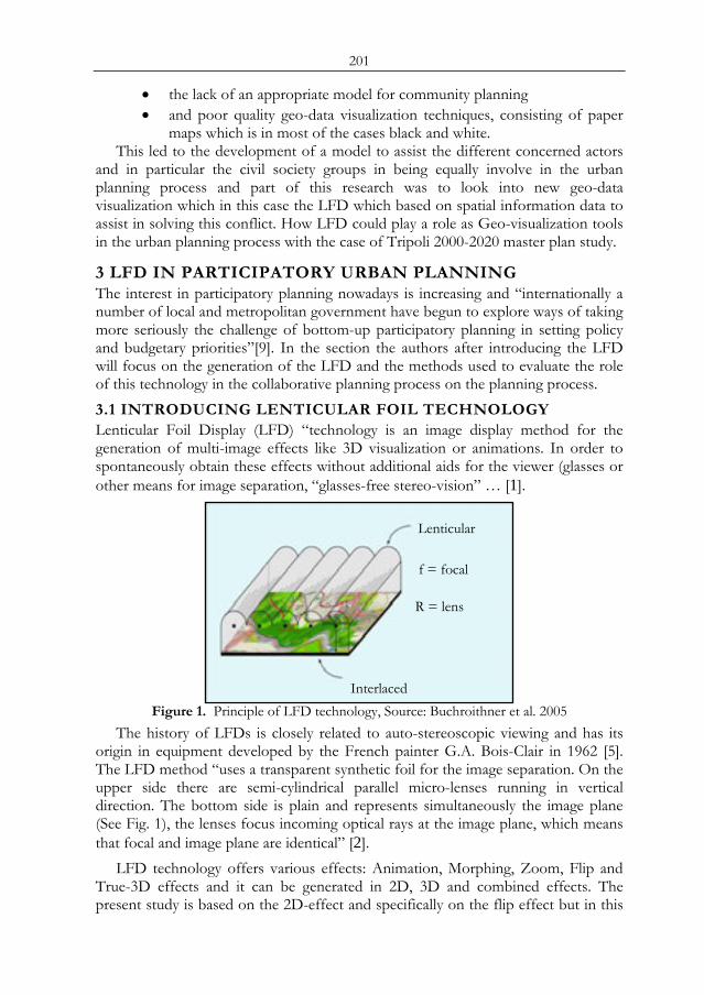
201
• the lack of an appropriate model for community planning • and poor quality geo-data visualization techniques, consisting of paper
maps which is in most of the cases black and white. This led to the development of a model to assist the different concerned actors
and in particular the civil society groups in being equally involve in the urban planning process and part of this research was to look into new geo-data visualization which in this case the LFD which based on spatial information data to assist in solving this conflict. How LFD could play a role as Geo-visualization tools in the urban planning process with the case of Tripoli 2000-2020 master plan study.
3 LFD IN PARTICIPATORY URBAN PLANNING The interest in participatory planning nowadays is increasing and “internationally a number of local and metropolitan government have begun to explore ways of taking more seriously the challenge of bottom-up participatory planning in setting policy and budgetary priorities”[9]. In the section the authors after introducing the LFD will focus on the generation of the LFD and the methods used to evaluate the role of this technology in the collaborative planning process on the planning process. 3.1 INTRODUCING LENTICULAR FOIL TECHNOLOGY Lenticular Foil Display (LFD) “technology is an image display method for the generation of multi-image effects like 3D visualization or animations. In order to spontaneously obtain these effects without additional aids for the viewer (glasses or other means for image separation, “glasses-free stereo-vision” … [1].
Figure 1. Principle of LFD technology, Source: Buchroithner et al. 2005
The history of LFDs is closely related to auto-stereoscopic viewing and has its origin in equipment developed by the French painter G.A. Bois-Clair in 1962 [5]. The LFD method “uses a transparent synthetic foil for the image separation. On the upper side there are semi-cylindrical parallel micro-lenses running in vertical direction. The bottom side is plain and represents simultaneously the image plane (See Fig. 1), the lenses focus incoming optical rays at the image plane, which means that focal and image plane are identical” [2].
LFD technology offers various effects: Animation, Morphing, Zoom, Flip and True-3D effects and it can be generated in 2D, 3D and combined effects. The present study is based on the 2D-effect and specifically on the flip effect but in this
Lenticular
Interlaced
f = focal
R = lens
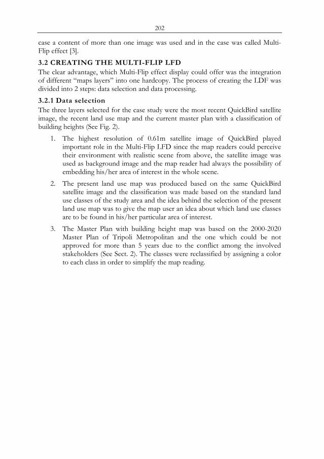
202
case a content of more than one image was used and in the case was called Multi-Flip effect [3]. 3.2 CREATING THE MULTI-FLIP LFD The clear advantage, which Multi-Flip effect display could offer was the integration of different “maps layers” into one hardcopy. The process of creating the LDF was divided into 2 steps: data selection and data processing. 3.2.1 Data selection The three layers selected for the case study were the most recent QuickBird satellite image, the recent land use map and the current master plan with a classification of building heights (See Fig. 2).
1. The highest resolution of 0.61m satellite image of QuickBird played important role in the Multi-Flip LFD since the map readers could perceive their environment with realistic scene from above, the satellite image was used as background image and the map reader had always the possibility of embedding his/her area of interest in the whole scene.
2. The present land use map was produced based on the same QuickBird satellite image and the classification was made based on the standard land use classes of the study area and the idea behind the selection of the present land use map was to give the map user an idea about which land use classes are to be found in his/her particular area of interest.
3. The Master Plan with building height map was based on the 2000-2020 Master Plan of Tripoli Metropolitan and the one which could be not approved for more than 5 years due to the conflict among the involved stakeholders (See Sect. 2). The classes were reclassified by assigning a color to each class in order to simplify the map reading.
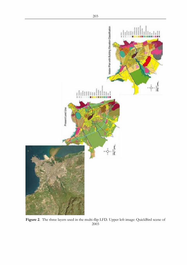
203
Figure 2. The three layers used in the multi-flip LFD. Upper left image: QuickBird scene of
2003

204
3.2.2 Data processing The data processing has been done in three steps: geo-data modeling, Flip creation and LFD hardcopy production.
1. Geo-data modeling was done by using ERDAS IMAGINE 8.7 to create the Background image by mosaic of three QuickBird scenes from 2003 and with the same quality and the off nadir angle in UTM projection. The reclassification of the Tripoli Master Plan with the building height classes was done in Autocad, same as for the Land use classification was created in Autocad by digitizing with visual interpretation and field check. The three layers were geo-referenced and exported all the three to FreeHand for Flip creation.
2. The Flip creation was done in Freehand since the Autocad data and the Satellite image could be imported with the same geo-reference and which is important issues in the image interlacing after the image interlacing the three scenes were send it to the printing process.
3. The LFD hardcopy production is done by printing the interlaced images and by laminating the Lenticular Foil over to get the Multi-flip LFD product as “three-in-one” hardcopy.
3.3 LFD IN PARTICIPATORY URBAN PLANNING After generating the Multi-Flip LFD it was necessary to evaluate this technologies applicability in participatory urban planning. The decision of the government to adopt the idea of public participation in the case of Tripoli was an very important step, even though the step was relatively late because the type of urban planning which is used in Lebanon still belong more to the rational planning model and need urgent update towards more open and inclusive planning approaches with more emphasis on public participation and collaboration” [6]. As it was mentioned in the beginning of the paper that several reasons led to the conflict among the stakeholders and one base issue was the selecting of the stakeholders as only expert in urban planning with the reason that the planning process is in technocratic process.
How Multi-Flip LFD could play a role in participatory urban planning and to get the different stakeholders more involved in the planning process as new geo-data visualization tool with the application in the case of Tripoli area?
The evaluation of the LFD was done by interviewing 78 stakeholders as part of interview questions which cover questions related to urban planning issues and participation issues as part of the research, in this paper only the part related to the LFD technology will be discussed.
The interviewees were from three different groups. A, B and C as summarized in Table 1, The division was done based on that Group A was the committee which was established to follow the planning process, Group B was supposed to be involved but the decision was rejected for political reason and that the urban planning process is more technocratic process. Group C was selected to cover as
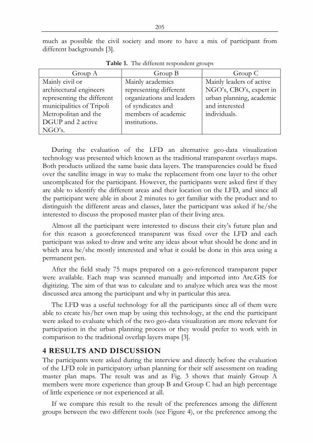
205
much as possible the civil society and more to have a mix of participant from different backgrounds [3].
Table 1. The different respondent groups Group A Group B Group C
Mainly civil or architectural engineers representing the different municipalities of Tripoli Metropolitan and the DGUP and 2 active NGO’s.
Mainly academics representing different organizations and leaders of syndicates and members of academic institutions.
Mainly leaders of active NGO’s, CBO’s, expert in urban planning, academic and interested individuals.
During the evaluation of the LFD an alternative geo-data visualization
technology was presented which known as the traditional transparent overlays maps. Both products utilized the same basic data layers. The transparencies could be fixed over the satellite image in way to make the replacement from one layer to the other uncomplicated for the participant. However, the participants were asked first if they are able to identify the different areas and their location on the LFD, and since all the participant were able in about 2 minutes to get familiar with the product and to distinguish the different areas and classes, later the participant was asked if he/she interested to discuss the proposed master plan of their living area.
Almost all the participant were interested to discuss their city’s future plan and for this reason a georeferenced transparent was fixed over the LFD and each participant was asked to draw and write any ideas about what should be done and in which area he/she mostly interested and what it could be done in this area using a permanent pen.
After the field study 75 maps prepared on a geo-referenced transparent paper were available. Each map was scanned manually and imported into Arc.GIS for digitizing. The aim of that was to calculate and to analyze which area was the most discussed area among the participant and why in particular this area.
The LFD was a useful technology for all the participants since all of them were able to create his/her own map by using this technology, at the end the participant were asked to evaluate which of the two geo-data visualization are more relevant for participation in the urban planning process or they would prefer to work with in comparison to the traditional overlap layers maps [3].
4 RESULTS AND DISCUSSION The participants were asked during the interview and directly before the evaluation of the LFD role in participatory urban planning for their self assessment on reading master plan maps. The result was and as Fig. 3 shows that mainly Group A members were more experience than group B and Group C had an high percentage of little experience or not experienced at all.
If we compare this result to the result of the preferences among the different groups between the two different tools (see Figure 4), or the preference among the
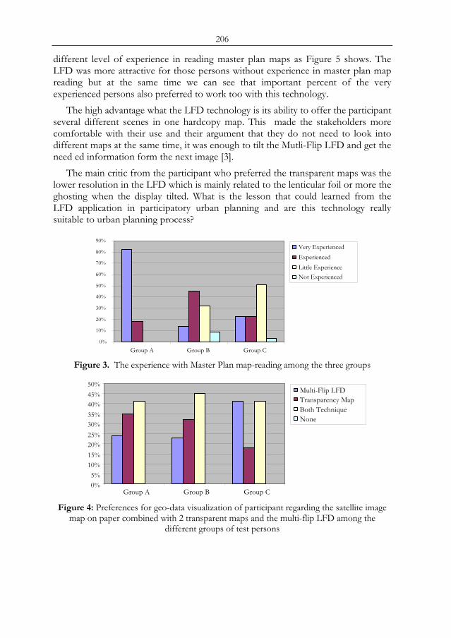
206
different level of experience in reading master plan maps as Figure 5 shows. The LFD was more attractive for those persons without experience in master plan map reading but at the same time we can see that important percent of the very experienced persons also preferred to work too with this technology.
The high advantage what the LFD technology is its ability to offer the participant several different scenes in one hardcopy map. This made the stakeholders more comfortable with their use and their argument that they do not need to look into different maps at the same time, it was enough to tilt the Mutli-Flip LFD and get the need ed information form the next image [3].
The main critic from the participant who preferred the transparent maps was the lower resolution in the LFD which is mainly related to the lenticular foil or more the ghosting when the display tilted. What is the lesson that could learned from the LFD application in participatory urban planning and are this technology really suitable to urban planning process?
Figure 3. The experience with Master Plan map-reading among the three groups
Figure 4: Preferences for geo-data visualization of participant regarding the satellite image
map on paper combined with 2 transparent maps and the multi-flip LFD among the different groups of test persons
0% 5%
10% 15% 20% 25% 30% 35% 40% 45% 50%
Group A Group B Group C
Multi-Flip LFD Transparency Map Both Technique None
0%
10%
20%
30%
40%
50%
60%
70%
80%
90%
Group A Group B Group C
Very ExperiencedExperiencedLittle ExperienceNot Experienced
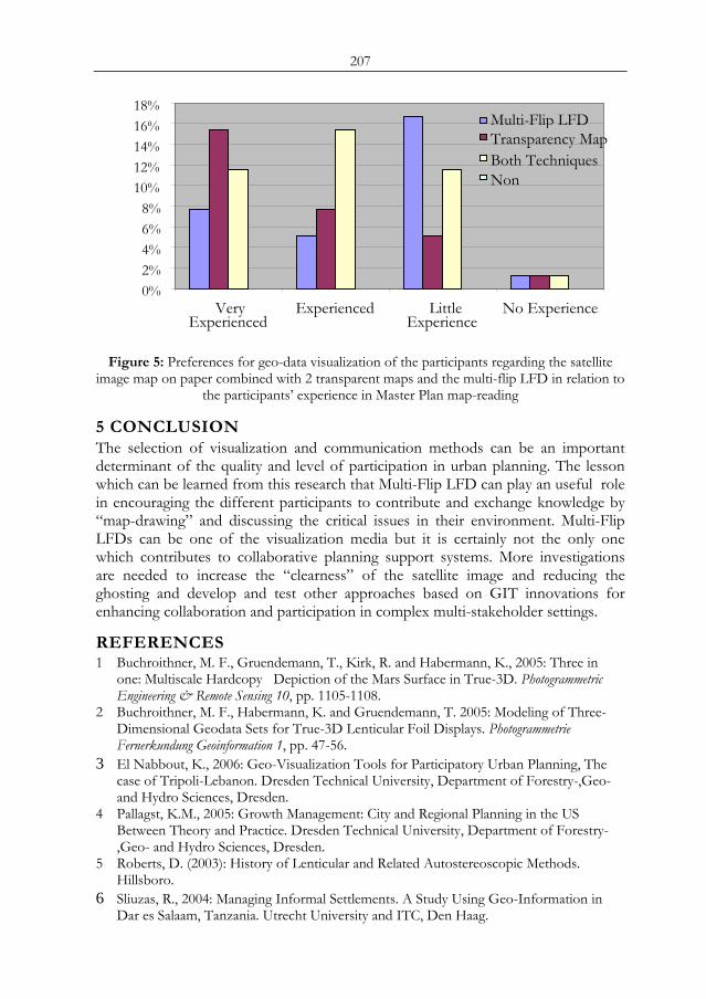
207
Figure 5: Preferences for geo-data visualization of the participants regarding the satellite image map on paper combined with 2 transparent maps and the multi-flip LFD in relation to
the participants’ experience in Master Plan map-reading
5 CONCLUSION The selection of visualization and communication methods can be an important determinant of the quality and level of participation in urban planning. The lesson which can be learned from this research that Multi-Flip LFD can play an useful role in encouraging the different participants to contribute and exchange knowledge by “map-drawing” and discussing the critical issues in their environment. Multi-Flip LFDs can be one of the visualization media but it is certainly not the only one which contributes to collaborative planning support systems. More investigations are needed to increase the “clearness” of the satellite image and reducing the ghosting and develop and test other approaches based on GIT innovations for enhancing collaboration and participation in complex multi-stakeholder settings.
REFERENCES 1 Buchroithner, M. F., Gruendemann, T., Kirk, R. and Habermann, K., 2005: Three in
one: Multiscale Hardcopy Depiction of the Mars Surface in True-3D. Photogrammetric Engineering & Remote Sensing 10, pp. 1105-1108.
2 Buchroithner, M. F., Habermann, K. and Gruendemann, T. 2005: Modeling of Three-Dimensional Geodata Sets for True-3D Lenticular Foil Displays. Photogrammetrie Fernerkundung Geoinformation 1, pp. 47-56.
3 El Nabbout, K., 2006: Geo-Visualization Tools for Participatory Urban Planning, The case of Tripoli-Lebanon. Dresden Technical University, Department of Forestry-,Geo- and Hydro Sciences, Dresden.
4 Pallagst, K.M., 2005: Growth Management: City and Regional Planning in the US Between Theory and Practice. Dresden Technical University, Department of Forestry-,Geo- and Hydro Sciences, Dresden.
5 Roberts, D. (2003): History of Lenticular and Related Autostereoscopic Methods. Hillsboro.
6 Sliuzas, R., 2004: Managing Informal Settlements. A Study Using Geo-Information in Dar es Salaam, Tanzania. Utrecht University and ITC, Den Haag.
0% 2% 4% 6% 8%
10% 12% 14% 16% 18%
VeryExperienced
Experienced LittleExperience
No Experience
Multi-Flip LFD Transparency Map Both Techniques Non

208
7 Steinberg, F., 2003: Strategic Urban Planning in Latin America: Experiences of Building and Managing the Future. Habitat International, pp. 1-25
8 Roberts, D. (2003): History of Lenticular and Related Autostereoscopic Methods. Hillsboro.
9 Wiseman, J., 2003: Engaging Citizens and Communities in Urban Planning: Learning from Recent Australian and International Experiments. Proc. State of Australian cities national Conference, Parramatta
209
CHANGES IN SOIL ORGANIC CARBON RELATED TO LAND USE CHANGE DURING TWO DECADES: A CASE STUDY IN THE BOGOR DISTRICT, WEST
JAVA
M. Ardiansyah and Widiatmaka Department of Soil Science and Land Resources, Faculty of Agriculture, Bogor Agricultural University, Jl. Meranti No. 1 Kampus IPB Darmaga Bogor 16680
Indonesia Phone: + 62 +251 629 360 Fax: + 62 +251 629 358
ABSTRACT Soil holds an important role in the gl21obal C cycle as it is the largest terrestrial C pool. On the other side, the soil organic carbon dynamic is affected significantly by land use and soil management practices. It has been reported that forest conversion and cultivated activities in dynamic land use change reduce soil organic carbon. Therefore, there is an important need to assess impacts of the land use and cover changes on changes of soil organic carbon. This study is directed to the temporal assessment of Bogor district as one of the most important districts in Indonesia. The SOC was obtained from soil inventory conducted in the period of 1980 to 1990, and soil analysis conducted in 2005. Land use and cover change was analyzed using Landsat imagery recorded on June 1989 and July 2003.
The objectives of the study were to detect the land and cover changes between 1989 and 2002 by using Landsat TM and Landsat ETM+ images, and to estimate soil organic carbon and its corresponding changes associated with land use and cover changes to the last 2 decades. On the basis of temporal classification of Landsat data, there are many changes of land use during the period of 1989 to 2002. The most important is that the forest cover and paddy field decreased by about 8% and 17% of the total area respectively, while bare land / settlement and croplands increased both by about 11%. During two decades, the land use and cover changes of Bogor district reduced the total SOC by 14.7% from 235 Mt in 1989 to 201 Mt. Keywords: land use and cover changes, soil organic carbon, soil organic matter, Bogor district
1 INTRODUCTION At the present, a major interest of global changes research is to understand further the role of soils in carbon emissions and sequestration. Through increases in organic matter, soils have been suggested as a potentially low cost means reduce atmospheric carbon dioxide emitted by anthropogenic sources. The United Nations Framework Convention on Climate Change (FCCC) have agreed to reduce global anthropogenic emissions of carbon in order stabilize concentration of CO2 in atmosphere at a level that will prevent disruptive changes in climate. This agreement Proc. 2nd Göttingen GIS and Remote Sensing Days, 4-6 Oct. 2006, Göttingen
210
requires industrialized countries to have reduce their emissions by 5–8% below 1990 levels by the period 2008–2012 [1, 2, 3]. The UNFCCC does not yet require commitments from developing countries, but recent decrease in the rates of deforestation in Asian Countries [4] may have already contributed to reduce emissions there [5].
Soil holds an important role in the global C cycle, as it is the largest terrestrial C pool. Soil can be a source (CO2, CH4 and N2O) or sink (CO2 and CH4) of green house gases, depending on land use and management [6, 7] World soils contain about 3.2 trillion tons of carbon. An estimated 2.5 trillion tons is in the form of soil organic carbon. This is the organic matter in the soil that makes it fertile. The remaining 0.7 trillion tons is soil inorganic carbon. In fact the soil carbon pool is two or three times the entire atmospheric pool as CO2 [8] and 2.5 to 3 times as much as that stored in plants [9, 10]. Thus, even a relatively small increase in soil carbon taken from the air could provide a significant reduction in atmospheric carbon. Moreover, since plants feed on carbon dioxide in the air, the primary way to store carbon in soil is to grow plants. Improved sustainable agriculture is the key to soil storage of carbon.
Soil organic content in soils and C flux from the soil significantly influenced by soil type, land use, and soil management practices [11, 12]. For a given soil, the greatest amount of organic matter generally accumulates in the topsoil under long-term undisturbed vegetation. It is well established that many forms of soil management can lead to changes in organic C concentrations, and the C contents of cropped and tilled soils are usually (but not always) lower than the equivalent soils under long-term grasslands or forest. The decline under more intensive forms of agriculture occur because there is increased loss of topsoil through erosion, decreased organic C return from plant residues, and enhanced breakdown of previously stabilized soil organic matter [13]. Land use and cover changes affect the amount of C stored terrestrial ecosystem. At the same time, changes in vegetation induce changes in the soil organic source. Recent analyses of land-use change have showed global terrestrial ecosystems to have been a net source of C (1.670.7 PgC yr-
1) during the 1980s [14]. In a comprehensive review of the effects of land-use changes on soil C stocks reported that the conversion of pasture to cropland reduces soil C stocks on average by 59% [15]. Therefore, the studying the effect of overall land use changes on distributed of SOC pools and C flux from the soils are important requirements for understanding the role of soils in the global C cycle.
The great attention of Indonesian decision makers, as well as research efforts on the study of the soil carbon cycle is not enough yet. There are no data available about the estimation of SOC, neither at national scale or at regional scale. The SOC storage in Indonesia soils had been in many small locations. The study area, Bogor district, is the district in Indonesia which is closer to the metropolitan city of Jakarta and industrial city of Bekasi. Since the last two decade the forest and the fertile agricultural areas (paddy field) have been attractive areas for new urban development. This accelerated rates of land use and cover change and urban development because of increased cultivation of land for crops and governmental changes in land use policy.
211
This study focused on the temporal assessment of Bogor district one of the most important districts in Indonesia. The objectives of the study was to detect the land and cover changes that have occurred between 1989 and 2002 by using Landsat TM and Landsat ETM+ images, and to estimate soil organic carbon and its corresponding changes associated with land use and cover changes in Bogor district to the last 2 decade.
2 MATERIALS AND METHODS
2.1 STUDY AREA The study area located in Bogor District in the province of West Java, facing the metropolitan city of Jakarta in the north, District of Bekasi in the east, and its south and west boundary is District of Cianjur and Banten respectively (Figure 1). There are several reasons in the choice of this study area. The first factor is the availability of archive data of Soil Organic Carbon (SOC). In 1968, a soil survey has been done, resulting in soil map of 1: 50.000 [16]. Moreover, as the study area close to Bogor Agricultural University, the soil of Bogor was also subject of many research of undergraduate student. In the period of 1980 – 1990, there are not less than 23 undergraduate theses with complete soil analysis including SOC, realized in dispersing part of the study area [17]. The second reason is the high dynamic of land-use change of this study area.
Figure 1. The study area of Bogor district
Total area of Bogor district is 316.432 Ha, which consist of 304.838 Ha of Bogor District, and 11.594 Ha of Bogor city towns. Considering this surface, Bogor District is one of the most extensive districts in Indonesia.
Monthly rainfall range between 161 to 435 mm. Areas with monthly rainfall <200 mm located in limited areas in the north-west, area with monthly rainfall between 200 to 300 mm spread over from west to east area. Here in after, areas with monthly rainfall between 300 to 400 mm located in the center and the south. Furthermore, areas with monthly rainfall >400 mm located Salak Mountain. Annual rainfall is almost in line with monthly rainfall that range from 1.926 to 5.218 mm.
Parent material consists mostly of rocks, i.e. rock of conglomerate and tuff sandstone or alluvium fan from the age of Pleistocene. The major soil order includes Ultisol, Inceptisol, Andisol and Entisol. 2.2 CALCULATION OF SOIL ORGANIC CARBON In this study, the SOC storage consists of the SOC storage for layer 0 – 20 cm and the SOC storage for layer 20 – 40 cm. Based on LULC changes detected from
Java Island
Bogor district
212
multitemporary remote sensing data, changes of soil organic matter (SOM) and bulk density (BD) estimated from soil inventory and research reports and soil sampling conducted on 2004, we calculated both of SOC storage for 1980/1990 and 2004.
The SOC storage of the study area is calculated by [18, 19]: SOCi = Ai x SOMi x Di x Bi x 10,000 x 0.58 (1)
where i is the LU type, SOCi the total soil organic carbon of LU type i (t), Ai is the area of LU type i (ha), SOMi is the average soil organic matter of LU type i (%), Di is the soil depth (m) of LU type i, and Bi is the average soil bulk density (Mg/m3) in LU type i.
The SOM in 1980-1990 was derived from soil inventory report and undergraduate thesis report, while the SOM in 2004 was analyzed from 148 soil samples. The soil samples are representative for bare land soil of upper layer (0 – 20 cm), bare land soil of lower layer (20-40 cm), vegetative soil of upper layer (0-20 cm) and vegetative soil of lower layer (20-40 cm). 2.3 REMOTE SENSING DATA PROCESSING The Landsat 5 TM and Landsat 7 ETM+, recorded on June 1989 and July 2002 respectively, were used to classify land use and cover in the Bogor District. The Landsat 7 ETM+ image was delivered in a geo-registered, UTM projection with 8-bit radiometric resolution to a WGS84 UTM36. Subsequently the Landsat 5 TM image was registered according to the geometry of the Landsat 7 ETM+ image. The consequent resampling was based on a nearest-neighbor algorithm, which takes the value of the pixel in the input image closest to the computed coordinate. This method is fast and does not alter the original pixel values. A first-order atmospheric correction was applied in order to account for path radiance. This correction was based on the dark pixel subtraction method.
Object oriented classification was performed to establish homogeneous areas within the images that are represented a land cover type or object class in study area, respectively. For this purpose image segmentation is carried out prior to image classification. The segmentation will subdivide an image into segments that correspond to objects based on spectral and or spatial information taken from the images. The result of the segmentation procedure is a mosaic of image objects per image layer that deliver the input data set for further classification issues. The classification of the segmented image layers is based on a fuzzy logic approach that allows complex object feature descriptions and uses membership functions (rule-sets) to conduct rules for the determination of the membership degree, i.e. the likelihood of a certain object to belong to an object class based on spectral and/or spatial attributes. Both Landsat data were segmented with a medium scale factor (scale=20). Consequently, the segmented images were classified into 5 categories.
3 RESULT AND DISCUSSION Two Landsat Images were used to analyze the land use and cover changes in the study area of Bogor District. To detect the changes between two images, classification of each image was performed. Using the object-oriented classification the images were classified into 5 land use categories: forest, plantation, crops, paddy
213
field and bare land/settlement. The classification results show that five land-use categories changed significantly in the study area during the 13-year period (Figure 1 and 2).
Specifically, the total area of bare land/settlement increased from 55,403 ha in 1989 to 91,851 ha in 2002, cropland increased from 70,470 ha in 1989 to 103,927 ha in 2002, and plantation increased from 28,434 ha in 1989 to 37,915 ha in 2002. In another side, forest area and paddy field area decreased by 24,975 ha and 54,406 ha in study area respectively (Table 1).
Figure 2. Distribution of land use and cover of Bogor district in 1989
Figure 3. Distribution of land use and cover of Bogor district in 2002
From Table 1 can be seen that the total forest area and paddy field of Bogor District decreased from 25.6% to 17.7% and 25.6% to 8.4% during the 1989–2002 period, which shows a transformation from forest areas and paddy field to another land uses. Conversely, the bare land / settlement areas, crops area, and plantation area increased from 17.5% to 29.0%, 22.3% to 32.8%, and 9.0% to 12.0% respectively. Later, some parts of these paddy field which were closer to the city and networks were transformed into bare land / settlement areas where area no vegetation was clearly seen. Significant increase of crops area occurred in the upper land and the flat area of Bogor district which were closer to land use type of forest and paddy field. These changes have caused residential development and population increases in the whole Bogor district as affected by economic and urban
214
expansion, and population increases of metropolitan city of Jakarta and Bekasi district.
Table 1. Area of land use and cover type of Bogor district in 1989 and 2002
Land Area of 1989 Land Area of 2002 Change of Area Land Use / Cover ha % Ha % ha %
Forest 81,045 25.6 56,070 17.7 -24,975 -7.9 Plantation 28,434 9.0 37,915 12.0 9,481 3.0 Crops 70,470 22.3 103,927 32.8 33,457 10.6 Paddy Field 81,075 25.6 26,669 8.4 -54,406 -17.2 Bare land/settlement 55,403 17.5 91,851 29.0 36,448 11.5
Changes in land use and cover lead to changes of biomass and its corresponding
carbon stocks. At the same time, land use and cover changes also affect the quantity and distribution of vegetation litter and soil organic inputting, which can induce changes in the soil organic matter and storage. Overall, as the vegetation cover was decreased, the soil organic matter also decreased (Table 2). Noticeably, the percent SOM was different in soil depth 0-20 cm and in soil depth 20-40 cm, where the percent SOM found in 0-20 cm was higher than found in 20-40 cm. Based on a research of soil characteristics [16, 17, 20] reported that approximately 45% of carbon was found in the top 25 cm. Therefore, the top 20 cm of the soil surface contains large part of the carbon of the horizon.
The SOC density measured on the basis of the SOM and soil bulk density differences among the land use/cover type. It decreased to the depth of 0–20 cm by 15.6% from 559 t/ha to 472 t/ha in the forest and by 11.3% from 483 t/ha to 428 t/ha in the crops, whereas SOC density in evergreen plantation and bare land did not change much. The same decreasing was arisen in SOC density to depth of 20–40 cm, here the decreasing in forest area is much more than found in 0-20 cm depth. When data from the average rates of five the land use transitions, and associated changes in SOC density were pooled for the total study area of 316,432 ha, the total SOC in the depth of 0-20 cm of 124 Mt in 1989 were estimated to decrease by 13.6.1% to 108 Mt in 2002, whereas the total SOC in the depth of 20-40 cm of 111 Mt in 1989 were estimated to decrease by 15.9% to 93 Mt in 2002. On average, land use and cover changes of Bogor district decreased the total SOC by 14.7% from 235 Mt in 1989 to 201 Mt in 2002. It indicates that in the study area occurred a small soil carbon emission during 2 decades as impact of land use and cover change. To make land use change may increase or stabilize the terrestrial carbon reserves, issues of reasonable land management and eco-environment protection should be addressed by local political and economic institutions in land use planning.
Table 2. Soil organic carbon among difference land use and cover type Land use/
Depth SOM (%)
BD (Mg/m
SOC storage (t/ha)
Total SOC storage (Mt)
215
cover (cm) 1980-1990
2004
3) 1980-1990 2004 1980-
1990 2004
0 - 20 3.71 3.13 1.3 559 472 45 26 Forest 20 -
40 3.36 2.31 1.3 507 348 41 20
0 - 20 3.20 2.84 1.3 483 428 14 16 Plantatio
n 20 - 40 3.20
2.84 1.3 483 428 14 16
0 - 20 2.27 2.25 1.3 342 339 24 35 Crops 20 -
40 2.10 1.96 1.3 317 296 22 31
0 - 20 2.34 2.34 1.3 353 353 29 9 Paddy
Field 20 - 40 1.79
1.79 1.3 270 270 22 7
0 - 20 1.52 1.46 1.3 229 220 13 20 Bare
Land 20 - 40 1.40
1.40 1.3 211 211 12 19
Sub total 0 - 20 124 108
20 - 40 111 93
Total 235 201
4 CONCLUSION In this study, remote sensing data has been shown as a potential technique for the study of land use changes and its corresponding soil carbon stocks. The total forest area and paddy field area decreased by 24,975 ha and 54,406 ha in study area respectively from 1989 to 2002. Changes in land use have produced severe losses in the soil carbon stocks in the study area. On average, conversion of forest and paddy field to crops and bare land / settlement in Bogor district decreased the total SOC by 14.7% from 235 Mt in 1989 to 201 Mt in 2002.
ACKNOWLEDGMENTS We gratefully acknowledge the financial supports from Osaka Gas Foundation of International Cultural Exchange (OGFICE), and Environmental Research Center, Bogor Agricultural University.
REFERENCES 1. IPCC. 1997a. Revised 1996 IPCC Guidelines for National Greenhouse Gas
Inventories Reporting Instructions (Volume 1). Houghton, J.T., L.G. Meira Filho, B. Lim,K. Treanton, I. Mamaty, Y. Bonduki, D.J. Griggs and B.A. Callender (Eds). Intergovernmental Panel on Climate Change.
2. IPCC. 1997b. Revised 1996 IPCC Guidelines for National Greenhouse Gas Inventories Workbook (Volume 2). Houghton, J.T., L.G. Meira Filho, B. Lim, K.

216
Treanton, I. Mamaty, Y. Bonduki, D.J. Griggs and B.A. Callender (Eds). Intergovernmental Panel on Climate Change.
3. IPCC. 1997c. Revised 1996 IPCC Guidelines for National Greenhouse Gas Inventories Reference Manual (Volume 3). Houghton, J.T., L.G. Meira Filho, B. Lim, K. Treanton, I. Mamaty, Y. Bonduki, D.J. Griggs and B.A. Callender (Eds). Intergovernmental Panel on Climate Change.
4. FAO. 1977. State of the world ‘s forest. FAO. Rome. 5. Houghton, R.A and J.L. Hackler. 2000. Emission of carbon from forestry and land
use change in tropical Asia. Global Change Biology (5):481-492. 6. Lal, R. 1995. Global soil erosion bywater and carbon dynamics. In: Soils and global
change. (eds. R. Lal, J. Kimble, E. Levine and B. A. Stewart) Advances in Soil Sciences, CRC Press, Boca Raton, FL, 131–142
7. Lal, R. 1999. Soil management and restoration for C sequestration to mitigate the accelerated greenhouse effect. Progr.Environ. Sci. 1, 307–326.
8. Davidson, E.A., Trumbore, S. E. and Amundson, R. 2000. Soil warming and organic carbon content. Nature 408, 789–790.
9. Post,W. M., T.H. Peng, W.R. Emanuel, A.W. King, V.H. Dale and D.L. Angelis 1990. The global carbon cycle. Am. Sci. 78, 310–326.
10. Houghton, R. A. and D.L. Skole. 1990. Carbon. In: The Earth as transformed by human action. (eds. B. L.Turner, W. C. Clark, Kates, R. W., J. F. Richards, J. T. Mathews and W. B. Meyer), Cambridge University Press, Cambridge, 393–408.
11. Batjes, N.H. 1996. Total carbon and nitrogen in soils of the world. Eur. J. Soil Sci. 47 : 151 – 163.
12. Post, W. M. and W.M. Kwon. 2000. Soil carbon sequestration and land-use change: processes and potential. Global Change Biol. 6, 317–327.
13. Reeves, J.B. 1997. Concatenation of near- and mid-infrared spectra to improve calibrations for determining forage composition. J. Agric. Food Chem. 45:1711-1714.
14. Houghton, R.A. 1995. Land-use change and the carbon cycle. Global Change Biology 1(4):275-287.
15. Guo LB, and R.M. Gifford. 2002. Soil carbon sequestration and land-use change: a meta analysis. Global Change Biology, 8, 345–360.
16. Atmosentono, H. 1968. Soil of Bogor and surrounding (in Indonesian). Soil Research Institute. Bogor.
17. Widiatmaka. 2005. Progress Report: Spatial dynamic of soil organic carbon related to land use change during 2 decades: A case study of Bogor area, West Java. Environmental Research Center, Bogor Agricultural University. Bogor
18. Wang, S., J. Xu, and C. Zhou. 2002. Using remote sensing to Estimate the change of carbon atorage: A case study in the Estuary of Yellow River delta. Int. J. Remote Sensing (23), 8: 1565–1580
19. Kilics., F. Evrendilek, S. Berberoglu and A. C. Demirkesen. 2006. Environmental monitoring of land use and land cover changes in a Mediterranean region of Turkey. Environmental Monitoring and Assessment 114: 157–168
20. Mazzarino, M.J., L. Oliva, A. Nunez, and A. Buffa. 1991. Nitrogen mineralization and soil fertility in the dry Chaco ecosystem (Argentina). Soil Sci. Soc. Am. J. 55, 515–522.
217
LAND COVER CHANGE DETECTION USING HIGH RESOLUTION SATELLITE IMAGERY IN
ARID AND SEMI-ARID AREAS OF THE NORTHERN KORDOFAN STATE, SUDAN
M. S. Dafallaa, c, M. A. Khiryb, c, I. S. Ibrahima, E. Csaplovicsc a Department of Soil Science and Environmental Studies, Faculty of Agriculture,
University of Khartoum, email: [email protected]; [email protected] b Department of Forest Management, Faculty of Forestry, University of Khartoum,
email: [email protected] c Department of Geosciences, University of Dresden, email: [email protected]
dresden.de
ABSTRACT Arid and semi-arid areas are char22acterized by scarce and fluctuating annual rainfall. Thus, these areas are affected by drought cycles. For better monitoring and evaluation of the status of vegetation cover and desertification studies, change detection is an essential step for a better understanding of the dynamics of vegetation changes in this ecosystem. Therefore, there is an urgent need for spatial change detection studies. This study is an attempt to use satellite imagery as a cheap multi-temporal tool. Northern Kordofan State is located at the centre of Sudan. Land uses are mixed forms of rain fed traditional agriculture, grazing and forestry. Subsets of geometrically and radiometrically corrected satellite images of Landsat ETM+ scenes 174/51 of 27.11.1999 and 16.01.2001 were used. Normalized Difference Vegetation Index (NDVI) and Tasseled Cap Transformation (TCT) for each subset were produced. Correlation coefficients of NDVI (1999 versus 2001) and TC components (1999 versus 2001) were calculated. Vegetated and non-vegetated areas were determined from NDVI (1999 and 2001). Visual on-screen interpretation was applied to analyze NDVI images assigning values of NDVI 99 in Red and of NDVI 01 in Green. The results showed a high correlation between NDVIs (1999 and 2001), greenness component (1999 and 2001) and brightness component (1999 and 2001). Furthermore, image classification of NDVI 99 and NDVI 01 for two classes, vegetated and non-vegetated areas, showed changes in the vegetation cover. The study showed that NDVI and TC can be used for change detection to support the development of management plans by supplying high-quality spatial information. Keywords: Sudan, NDVI, TCA.
INTRODUCTION Arid and semi-arid areas are characterized by patterns of fluctuated annual rainfall. Thus such areas are subjected to drought cycles during the precipitation deficit period that result in deterioration of the vegetation cover which may recover Proc. 2nd Göttingen GIS and Remote Sensing Days, 4-6 Oct. 2006, Göttingen
218
following a season with good precipitation [1, 2, 3]. However, some scientists claim that arid and semi-arid areas undergo systematic desertification in form of deterioration of vegetation cover that may trigger other types of land degradation processes. On the other hand, many studies showed that this was not the case. In contrast there was no systematic increase of desertification, and the rainfall pattern had pronounced effects on overall vegetation cover of the area [1, 2, 3].
For better monitoring and evaluation of status of vegetation cover and hence desertification studies, change detection is an essential step for a better understanding of dynamic of the vegetation change in these fragile ecosystems. Terrestrial conventional methods for change detection are expensive in term of money and time. Moreover, they lack spatial and integrated aspect, since they concentrate mainly on economic land uses such as agriculture, rangeland or forestry. Therefore, there is a critical need for spatial and overall change detection studies.
Remote sensing techniques for change detection are generally categorized into two types [4]: post and pre-classification techniques. The former one involves a thematic classification of the multi-temporal images and afterwards based on land use classes, the evaluation is carried out by applying change matrix. The latter adopts data transformation procedures of multi-temporal images such as Principal Component Analysis and Tasseled Cap Analysis, or arithmetic procedures such as image differencing and band ratios.
The vegetation indices are broadly divided into two basic categories: ratios and orthogonal indices. The ratio-based indices include the Ratio Vegetation Index (RVI) and the Normalized Difference Vegetation Index (NDVI). Orthogonal indices include Perpendicular Vegetation Index (PVI) and the Difference Vegetation Index (DVI). More recently a hybrid set of vegetation indices have emerged such as the Soil Adjusted Vegetation Index (SAVI).
Vegetation growth typically exhibits some type of annual cycle, with a period of low (or no) growth and a period of active growth and decline. This growth cycle is controlled by growth limiting factors, such as water availability, day length or temperature. Remote sensing is an accepted technique for resource assessment [5, 6, 7, 8]. A specific requirement in the seasonally arid regions of Africa is the capability to evaluate and predict the response of vegetation to climate variability. In this context remote sensing can provide an indirect measure of vegetation growth through calculation of vegetation indices [3, 7, 9, 10,]. NDVI is one of the most generally used indices for vegetation monitoring. It is calculated as the normalized ratio between visible red reflectance and near infrared reflectance. The main advantages of the use of the NDVI for monitoring vegetation are its simplicity of calculation and its high degree of correlation with a variety of vegetation parameters such as leaf area index [7].
Tasseled cap analysis (TCA) is a sensor-dependent linear transformation developed by Kauth and Thomas in order to describe the crop development in relation to soil background through its three components [11]. The component brightness highlights the higher brightness values from background soil, while the greenness refers to higher brightness values from active vegetation and wetness
219
highlights the higher brightness values from moist soils. TCA is used in the classification and change detection with emphasis on greenness components [4].
This study is an attempt to use satellite image as cheap and multi-temporal tool which can fulfill the above mentioned goal.
STUDY AREA Northern Kordofan State lies in the centre of the Sudan. Land uses are mixed forms of rainfed traditional agriculture, rangelands, and forestry. The major products are millet, sorghum, rosella, watermelon, gum arabic and animals such as sheep, camels, goats and cattle (Fig.1).
METHODOLOGY Subsets from geometrically and radiometrically corrected satellite imageries 174/51 ETM+ 27.11.1999 and 174/51 16.01.2001 were used. Normalize Difference Vegetation Index (NDVI) and Tasseled Cap Transformation (TCT) for each subset was produced. Correlation coefficients of NDVI (1999 versus 2001) and TC components (1999 versus 2001) were calculated. Vegetated and non-vegetated areas were determined from NDVI (1999 and 2001) through adoption of NDVI threshold values of 0.004 and 0.002 for 1999 and 2001, respectively. With aid of field work, which was carried out in November 2004, visual interpretation was carried out to interpret NDVI images which show NDVI 99 was in Red and NDVI 01 in Green.
RESULTS AND DISCUSSION NDVI 1999 and NDVI 2001 (fig.2) showed high correlation (r=0.53), which indicates slight change in the vegetated area. This pattern is also obvious from the high correlation between greenness component of TC 1999 and 2001 (r=0.60). Furthermore, brightness component of TC 1999 and 2001 showed high correlation (r=0.86) (Fig.3) as well. This can be attributed to the sparse nature of vegetation in this area and presence of sand which is characterized by high reflectance, i.e. high background reflectance. According to this high correlation, it is possible to interpret that there is no increase in non-vegetated area, and coupled with change in NDVI it could also be interpreted that the change in NDVI is a qualitative change rather than a quantitative one. This may be due to the nature of land use pattern, which is continuously changing from mixed woody grasses to traditional shifting rainfed agriculture through fallow land with or without grasses.
Visual interpretation of NDVI 99 and NDVI 01 (separately) for vegetated and non-vegetated areas with use of a threshold of 0.004 for 99 and 0.002 for 2001 showed that Jebel Ed Diar (Hill) and Khor Abu Habil (Wadi) vegetation cover is stable. However, the northern and southern parts of the study area showed a comparative decrease in vegetation cover. This may be due to different reasons in northern and southern parts (Fig.4 and Table 1). For the northern part this may be due to the difference in acquisition date, since the 1999 image was taken before harvest of crop (27th November) while the 2001 image was taken after the harvest (16th January). This decrease may also be due to increase in cropping area, which appears as bare land during this period. Moreover, it may also be due to change in
220
fallow/farm rotation. In the southern part it may be due primarily to an increase in of agricultural schemes that were distributed by the Northern Kordfan Goverment starting from 1999 and it compromise always with clearing of trees for agriculture. On the other hand tree cutting for production of charcoal, fuel wood and building material is widely practiced in this part. Moreover, the soil type of the southern part is clay with slow permeability and the plant cover is characterized by slow-recovering species.
Table 1. Vegetated and non-vegetated areas Status Area (ha) 1999 2001 Difference Vegetated 398916.36 36799.38 -362116.98 Non-vegetated 1183260.87 820540.55 362720.31
On the other hand, visual interpretation of overlay of NDVI 99 and 2001 in Red
and Green (Fig. 5) showed the same pattern as the above mentioned threshold method. The northern part of the study area, which is mainly sandy area, showed comparatively positive change. This may be due partially to high permeability of the soil, which helps in water conservation for dry period, and partially due to the type of vegetation which consists generally of tolerant species like Hashab (Acacia senegal), Seyal (Acacia toritlis), Sirih (Maerua crassifolia) and grasses. On the other hand this area is rehabilitated by the Forestry National Corporation (FNC) because of its significance for gum arabic production. Also this may be an indicator of increase in cropping area, since the traditional rainfed cultivation is widely practiced. However, the southern part of the study area, with higher rainfall than the northern part, showed no or negative changes (as mentioned above). The negative change may be attributed to continuous increase of rainfed mechanized agriculture, low permeability of the clay soil (locally known as gardud) and the plant species of this area which are perennial and need long time to recover such as Talh (Acacia seyal) and Kitir (Acacia melliferra). The contradiction between NDVI threshold analysis and direct visual overlay method may be attributed to the fact that the first one concentrates mainly on change in vegetated areas (positive NDVI range) while the second one shows the change in positive and negative range.
CONCLUSIONS This study showed that NDVI can be used as rule of thumb for change detection. This method help in minimizing the cost of field work and raises pre-knowledge about the dynamics of change.
REFERENCES [1] Ahlcrona, E. 1988. The impact of climate and Man on Land transformation in the
central Sudan, Lund University Press, 140 pp. [2] Hellden, U. 1988. Desertification monitoring: Is the desert encroaching?
Desertification control Bulletin 17: 8-12. [3] Herrmann, S.M., Anyamba, A. and Tucker, C.J. (2005). Exploring Relationship
between rainfall and Vegetation Dynamics in the Sahel using coarse Resolution satellite data. www.isprs.org/publications/ related/ISRSE/html/papers/293.pdf
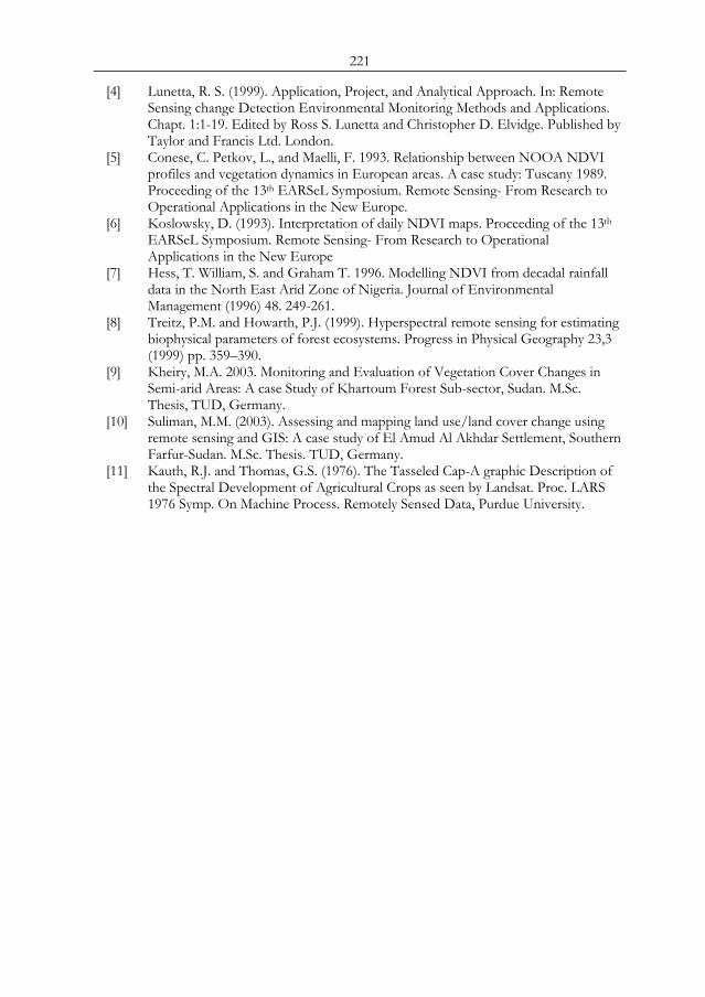
221
[4] Lunetta, R. S. (1999). Application, Project, and Analytical Approach. In: Remote Sensing change Detection Environmental Monitoring Methods and Applications. Chapt. 1:1-19. Edited by Ross S. Lunetta and Christopher D. Elvidge. Published by Taylor and Francis Ltd. London.
[5] Conese, C. Petkov, L., and Maelli, F. 1993. Relationship between NOOA NDVI profiles and vegetation dynamics in European areas. A case study: Tuscany 1989. Proceeding of the 13th EARSeL Symposium. Remote Sensing- From Research to Operational Applications in the New Europe.
[6] Koslowsky, D. (1993). Interpretation of daily NDVI maps. Proceeding of the 13th EARSeL Symposium. Remote Sensing- From Research to Operational Applications in the New Europe
[7] Hess, T. William, S. and Graham T. 1996. Modelling NDVI from decadal rainfall data in the North East Arid Zone of Nigeria. Journal of Environmental Management (1996) 48. 249-261.
[8] Treitz, P.M. and Howarth, P.J. (1999). Hyperspectral remote sensing for estimating biophysical parameters of forest ecosystems. Progress in Physical Geography 23,3 (1999) pp. 359–390.
[9] Kheiry, M.A. 2003. Monitoring and Evaluation of Vegetation Cover Changes in Semi-arid Areas: A case Study of Khartoum Forest Sub-sector, Sudan. M.Sc. Thesis, TUD, Germany.
[10] Suliman, M.M. (2003). Assessing and mapping land use/land cover change using remote sensing and GIS: A case study of El Amud Al Akhdar Settlement, Southern Farfur-Sudan. M.Sc. Thesis. TUD, Germany.
[11] Kauth, R.J. and Thomas, G.S. (1976). The Tasseled Cap-A graphic Description of the Spectral Development of Agricultural Crops as seen by Landsat. Proc. LARS 1976 Symp. On Machine Process. Remotely Sensed Data, Purdue University.
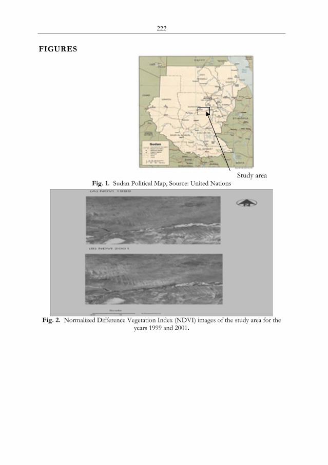
222
FIGURES
Study area Fig. 1. Sudan Political Map, Source: United Nations
Fig. 2. Normalized Difference Vegetation Index (NDVI) images of the study area for the
years 1999 and 2001.
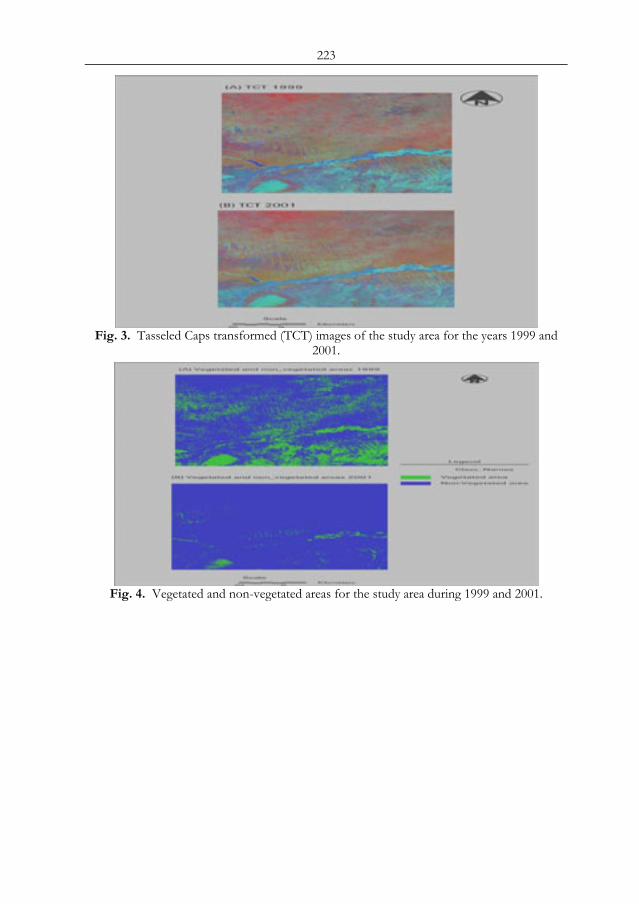
223
Fig. 3. Tasseled Caps transformed (TCT) images of the study area for the years 1999 and
2001.
Fig. 4. Vegetated and non-vegetated areas for the study area during 1999 and 2001.
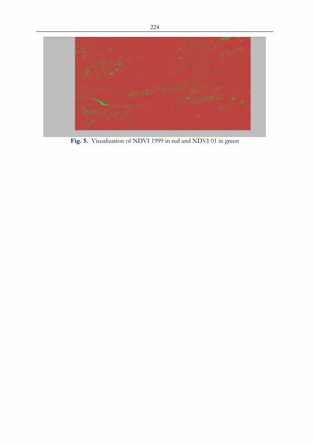
224
Fig. 5. Visualization of NDVI 1999 in red and NDVI 01 in green
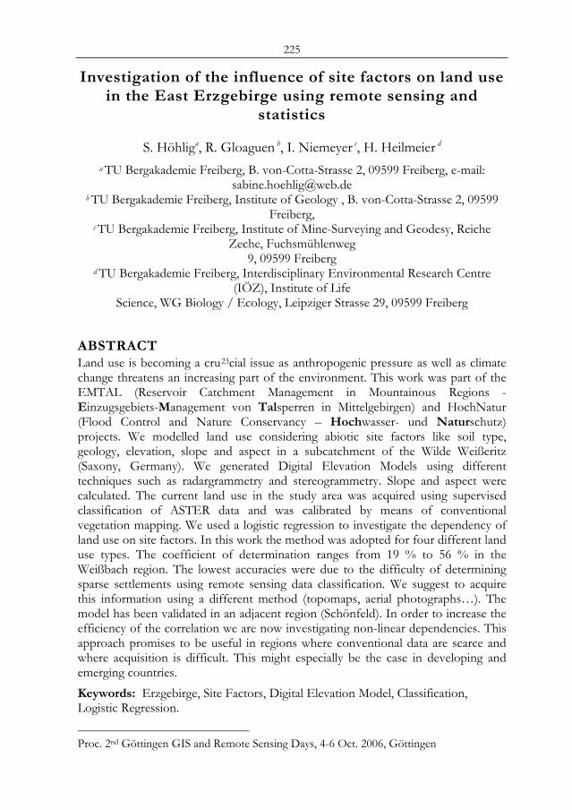
225
Investigation of the influence of site factors on land use in the East Erzgebirge using remote sensing and
statistics
S. Höhliga, R. Gloaguen b, I. Niemeyer c, H. Heilmeier d a TU Bergakademie Freiberg, B. von-Cotta-Strasse 2, 09599 Freiberg, e-mail:
[email protected] b TU Bergakademie Freiberg, Institute of Geology , B. von-Cotta-Strasse 2, 09599
Freiberg, c TU Bergakademie Freiberg, Institute of Mine-Surveying and Geodesy, Reiche
Zeche, Fuchsmühlenweg 9, 09599 Freiberg
d TU Bergakademie Freiberg, Interdisciplinary Environmental Research Centre (IÖZ), Institute of Life
Science, WG Biology / Ecology, Leipziger Strasse 29, 09599 Freiberg
ABSTRACT Land use is becoming a cru23cial issue as anthropogenic pressure as well as climate change threatens an increasing part of the environment. This work was part of the EMTAL (Reservoir Catchment Management in Mountainous Regions - Einzugsgebiets-Management von Talsperren in Mittelgebirgen) and HochNatur (Flood Control and Nature Conservancy – Hochwasser- und Naturschutz) projects. We modelled land use considering abiotic site factors like soil type, geology, elevation, slope and aspect in a subcatchment of the Wilde Weißeritz (Saxony, Germany). We generated Digital Elevation Models using different techniques such as radargrammetry and stereogrammetry. Slope and aspect were calculated. The current land use in the study area was acquired using supervised classification of ASTER data and was calibrated by means of conventional vegetation mapping. We used a logistic regression to investigate the dependency of land use on site factors. In this work the method was adopted for four different land use types. The coefficient of determination ranges from 19 % to 56 % in the Weißbach region. The lowest accuracies were due to the difficulty of determining sparse settlements using remote sensing data classification. We suggest to acquire this information using a different method (topomaps, aerial photographs…). The model has been validated in an adjacent region (Schönfeld). In order to increase the efficiency of the correlation we are now investigating non-linear dependencies. This approach promises to be useful in regions where conventional data are scarce and where acquisition is difficult. This might especially be the case in developing and emerging countries. Keywords: Erzgebirge, Site Factors, Digital Elevation Model, Classification, Logistic Regression.
Proc. 2nd Göttingen GIS and Remote Sensing Days, 4-6 Oct. 2006, Göttingen
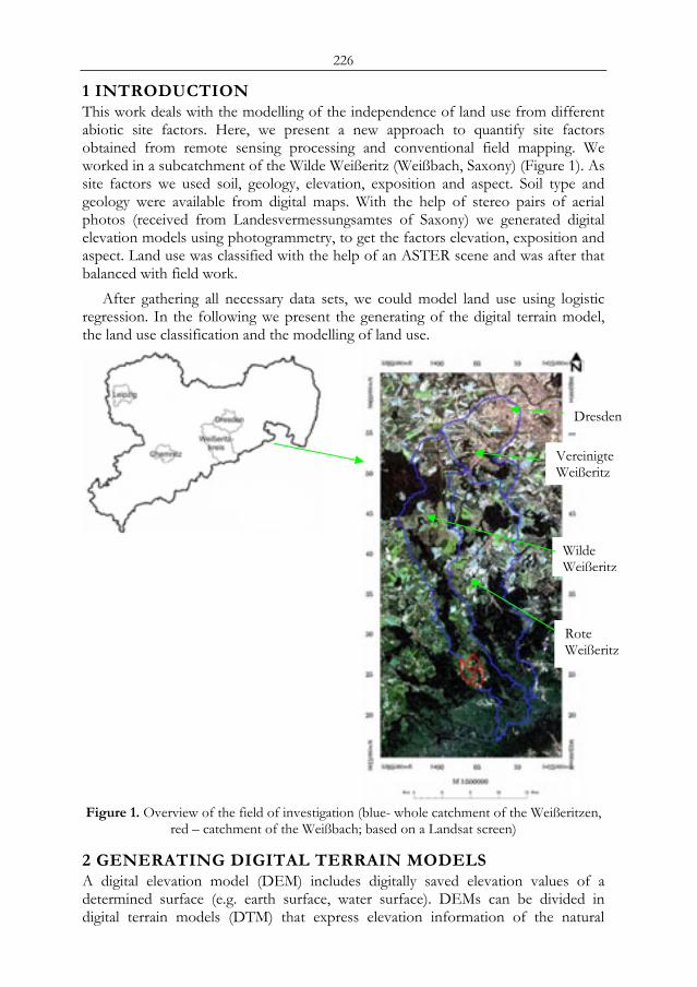
226
1 INTRODUCTION This work deals with the modelling of the independence of land use from different abiotic site factors. Here, we present a new approach to quantify site factors obtained from remote sensing processing and conventional field mapping. We worked in a subcatchment of the Wilde Weißeritz (Weißbach, Saxony) (Figure 1). As site factors we used soil, geology, elevation, exposition and aspect. Soil type and geology were available from digital maps. With the help of stereo pairs of aerial photos (received from Landesvermessungsamtes of Saxony) we generated digital elevation models using photogrammetry, to get the factors elevation, exposition and aspect. Land use was classified with the help of an ASTER scene and was after that balanced with field work.
After gathering all necessary data sets, we could model land use using logistic regression. In the following we present the generating of the digital terrain model, the land use classification and the modelling of land use.
Figure 1. Overview of the field of investigation (blue- whole catchment of the Weißeritzen,
red – catchment of the Weißbach; based on a Landsat screen)
2 GENERATING DIGITAL TERRAIN MODELS A digital elevation model (DEM) includes digitally saved elevation values of a determined surface (e.g. earth surface, water surface). DEMs can be divided in digital terrain models (DTM) that express elevation information of the natural
Dresden
Vereinigte Weißeritz
Wilde Weißeritz
Rote Weißeritz
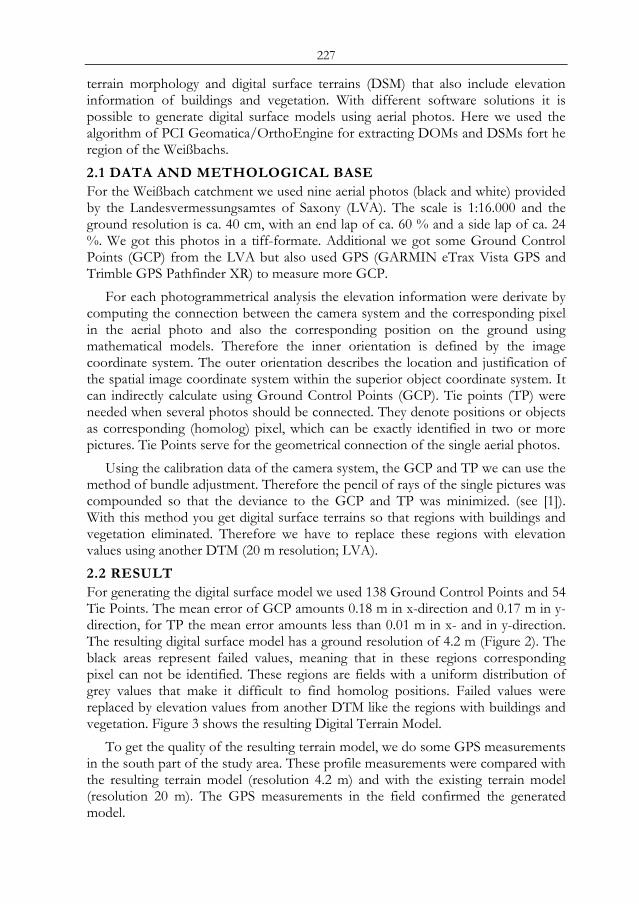
227
terrain morphology and digital surface terrains (DSM) that also include elevation information of buildings and vegetation. With different software solutions it is possible to generate digital surface models using aerial photos. Here we used the algorithm of PCI Geomatica/OrthoEngine for extracting DOMs and DSMs fort he region of the Weißbachs. 2.1 DATA AND METHOLOGICAL BASE For the Weißbach catchment we used nine aerial photos (black and white) provided by the Landesvermessungsamtes of Saxony (LVA). The scale is 1:16.000 and the ground resolution is ca. 40 cm, with an end lap of ca. 60 % and a side lap of ca. 24 %. We got this photos in a tiff-formate. Additional we got some Ground Control Points (GCP) from the LVA but also used GPS (GARMIN eTrax Vista GPS and Trimble GPS Pathfinder XR) to measure more GCP.
For each photogrammetrical analysis the elevation information were derivate by computing the connection between the camera system and the corresponding pixel in the aerial photo and also the corresponding position on the ground using mathematical models. Therefore the inner orientation is defined by the image coordinate system. The outer orientation describes the location and justification of the spatial image coordinate system within the superior object coordinate system. It can indirectly calculate using Ground Control Points (GCP). Tie points (TP) were needed when several photos should be connected. They denote positions or objects as corresponding (homolog) pixel, which can be exactly identified in two or more pictures. Tie Points serve for the geometrical connection of the single aerial photos.
Using the calibration data of the camera system, the GCP and TP we can use the method of bundle adjustment. Therefore the pencil of rays of the single pictures was compounded so that the deviance to the GCP and TP was minimized. (see [1]). With this method you get digital surface terrains so that regions with buildings and vegetation eliminated. Therefore we have to replace these regions with elevation values using another DTM (20 m resolution; LVA). 2.2 RESULT For generating the digital surface model we used 138 Ground Control Points and 54 Tie Points. The mean error of GCP amounts 0.18 m in x-direction and 0.17 m in y-direction, for TP the mean error amounts less than 0.01 m in x- and in y-direction. The resulting digital surface model has a ground resolution of 4.2 m (Figure 2). The black areas represent failed values, meaning that in these regions corresponding pixel can not be identified. These regions are fields with a uniform distribution of grey values that make it difficult to find homolog positions. Failed values were replaced by elevation values from another DTM like the regions with buildings and vegetation. Figure 3 shows the resulting Digital Terrain Model.
To get the quality of the resulting terrain model, we do some GPS measurements in the south part of the study area. These profile measurements were compared with the resulting terrain model (resolution 4.2 m) and with the existing terrain model (resolution 20 m). The GPS measurements in the field confirmed the generated model.
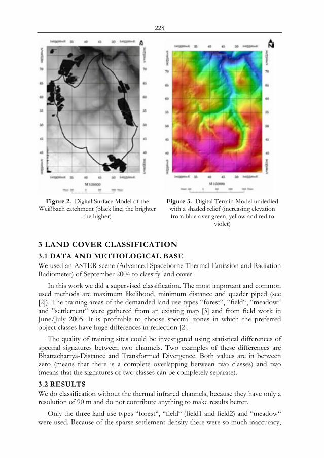
228
Figure 2. Digital Surface Model of the
Weißbach catchment (black line; the brighter the higher)
Figure 3. Digital Terrain Model underlied with a shaded relief (increasing elevation from blue over green, yellow and red to
violet)
3 LAND COVER CLASSIFICATION
3.1 DATA AND METHOLOGICAL BASE We used an ASTER scene (Advanced Spaceborne Thermal Emission and Radiation Radiometer) of September 2004 to classify land cover.
In this work we did a supervised classification. The most important and common used methods are maximum likelihood, minimum distance and quader piped (see [2]). The training areas of the demanded land use types “forest“, “field“, “meadow“ and ”settlement“ were gathered from an existing map [3] and from field work in June/July 2005. It is profitable to choose spectral zones in which the preferred object classes have huge differences in reflection [2].
The quality of training sites could be investigated using statistical differences of spectral signatures between two channels. Two examples of these differences are Bhattacharrya-Distance and Transformed Divergence. Both values are in between zero (means that there is a complete overlapping between two classes) and two (means that the signatures of two classes can be completely separate). 3.2 RESULTS We do classification without the thermal infrared channels, because they have only a resolution of 90 m and do not contribute anything to make results better.
Only the three land use types “forest“, “field“ (field1 and field2) and “meadow“ were used. Because of the sparse settlement density there were so much inaccuracy,
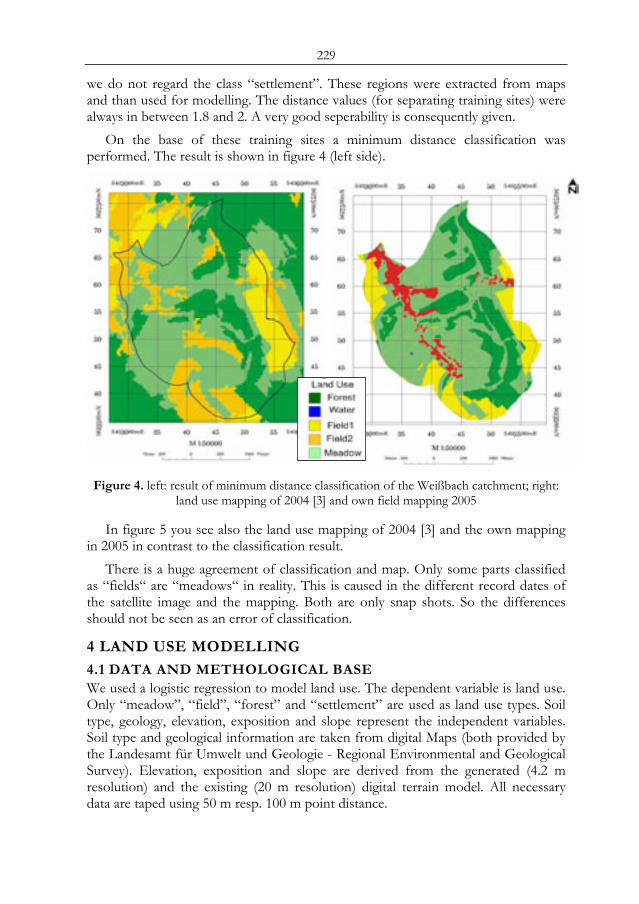
229
we do not regard the class “settlement”. These regions were extracted from maps and than used for modelling. The distance values (for separating training sites) were always in between 1.8 and 2. A very good seperability is consequently given.
On the base of these training sites a minimum distance classification was performed. The result is shown in figure 4 (left side).
Figure 4. left: result of minimum distance classification of the Weißbach catchment; right:
land use mapping of 2004 [3] and own field mapping 2005
In figure 5 you see also the land use mapping of 2004 [3] and the own mapping in 2005 in contrast to the classification result.
There is a huge agreement of classification and map. Only some parts classified as “fields“ are “meadows“ in reality. This is caused in the different record dates of the satellite image and the mapping. Both are only snap shots. So the differences should not be seen as an error of classification.
4 LAND USE MODELLING
4.1 DATA AND METHOLOGICAL BASE We used a logistic regression to model land use. The dependent variable is land use. Only “meadow”, “field”, “forest” and “settlement” are used as land use types. Soil type, geology, elevation, exposition and slope represent the independent variables. Soil type and geological information are taken from digital Maps (both provided by the Landesamt für Umwelt und Geologie - Regional Environmental and Geological Survey). Elevation, exposition and slope are derived from the generated (4.2 m resolution) and the existing (20 m resolution) digital terrain model. All necessary data are taped using 50 m resp. 100 m point distance.
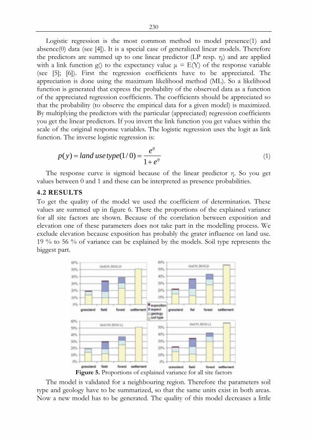
230
Logistic regression is the most common method to model presence(1) and absence(0) data (see [4]). It is a special case of generalized linear models. Therefore the predictors are summed up to one linear predictor (LP resp. ηi) and are applied with a link function g() to the expectancy value μ = E(Y) of the response variable (see [5]; [6]). First the regression coefficients have to be appreciated. The appreciation is done using the maximum likelihood method (ML). So a likelihood function is generated that express the probability of the observed data as a function of the appreciated regression coefficients. The coefficients should be appreciated so that the probability (to observe the empirical data for a given model) is maximized. By multiplying the predictors with the particular (appreciated) regression coefficients you get the linear predictors. If you invert the link function you get values within the scale of the original response variables. The logistic regression uses the logit as link function. The inverse logistic regression is:
η
η
eetypeuselandyp+
==1
)0/1()( (1)
The response curve is sigmoid because of the linear predictor η. So you get values between 0 and 1 and these can be interpreted as presence probabilities. 4.2 RESULTS To get the quality of the model we used the coefficient of determination. These values are summed up in figure 6. There the proportions of the explained variance for all site factors are shown. Because of the correlation between exposition and elevation one of these parameters does not take part in the modelling process. We exclude elevation because exposition has probably the grater influence on land use. 19 % to 56 % of variance can be explained by the models. Soil type represents the biggest part.
Figure 5. Proportions of explained variance for all site factors
The model is validated for a neighbouring region. Therefore the parameters soil type and geology have to be summarized, so that the same units exist in both areas. Now a new model has to be generated. The quality of this model decreases a little
231
bit because of the lost of information due to the summarizing of soil type and geology.
5 DISCUSSION AND PROSPECTUS For aerial photos with a scale of 1:10000, which were taken with a small picture camera (focal length 50 mm) [7] specifies the reachable accuracy in x, y and z direction with 0.5 to 3 m. We reached a resolution of 4.2 m, but we used photos with a smaller scale (1 : 16000) and the focal length of the used camera is 152 mm. By taking all these factors into account we are on a good level. An exact determination of the accuracy in z direction is not directly possible. Comparing the 20 m DTM (LVA) and the generated 4.2 m DTM, you can originate a metric resolution (elevation difference between the two DTM: mean difference -1.9 m, standard deviation ~ 2 m; complies with an external validation – [8]). The aerial photos were recorded early in the morning, so that the sun had a low elevation. Due to this fact there are many shadows, which decrease also the quality of the generated terrain model.
Land cover classification using satellite images is a common method. For Saxony there are no published data of land use observation using remote sensing. It was hard to classify settlement, because of the sparse settled study area and the maximum resolution of the used satellite scene (15m). A big and common problem is mixing pixels (see e.g. [9]). Differences to the mapping results are due to the fact that the satellite image is from September 2004 and the mapping was at the beginning of 2004 resp. in the middle of 2005. Land use is dynamic, that means there are different land use types on the same area in different years. This is the primarily explanation of the deviations for field and meadow. There are also variations within the year for one use type and that changes the spectral characteristics. The problems with the settlements may be improved using object-oriented classification. Due to the segmentation and the following classification based on that segmentation mixing pixels can be deleted. Also other features of the segments like form and texture can be applied for classification.
The method of land use modelling was used for the first time for four different land use types. The model quality reached 19 % up to 56 % and so is a really good result in biology. Also the transfer to a neighbouring area acquired nearly the same quality.
In order to increase the efficiency of the correlation we are now investigating non-linear dependencies. This approach promises to be useful in regions were conventional data are scarce and were acquisition is difficult. This might especially be the case in developing and emerging countries.
REFERENCES [1] Kraus, K., 1997: Photogrammetrie – Band 1: Grundlagen und Standardverfahren, 6th
edition, Ferd. Dümmlers Verlag Bonn [2] Albertz, J., 2001: Einführung in die Fernerkundung – Grundlagen der Interpretation von
Luft- und Satellitenbildern, 2nd edition, Wissenschaftliche Buchgesellschaft Darmstadt [3] Bianchin, S., 2004: Biotoptypenkartierung im Weißbachtal im Rahmen des HochNatur-
Projektes, unpublished manuscript, TU Bergakademie Freiberg
232
[4] Dormann, C. F.; Blaschke, T.; Lausch, A.; Schröder, B. & Söndgerath, D., 2004: Habitatmodelle – Methodik, Anwendung, Nutzen. Tagungsband zum Workshop vom 8. – 10. Oktober 2003 am UFZ Leipzig, UFZ-Berichte 9/2004
[5] Guisan, A.; Edwards, T.C.; J. & Hastie, T. (2002): Generalized linear and generalized additive models in studies of species distribution: setting the scene, Ecological Modelling 157: 89–100
[6] Schmid, C. (2002): Verallgemeinerte Lineare Modelle (http://www.uni-ulm.de/~cschmid/oldstat/se4_2.htm)
[7] Henry, J.-B.; Malet, J-P., Maquaire, O. & Grussenmeyer, P., 2002: The use of small-format and low-altitude aerial photos for realization of high-resolution DEMs in mountainous areas: application to the Super-Sauze Earthflow (Alpes-de-haute-provonce, Fran ce), Earth Surface Processes and Landforms 27: 1339 – 1350
[8] Kasser, M. & Egels, Y., 2002: Digital Photogrammetry, Taylor & Francis London, 350 S. [9] Lausch, A. & Biedermann, F. (2000): Analysis of temporal changes in the Lignite Mining
Region south of Leipzig using GIS and landscape metrics. – in: Clare, T. & Howard, D. (eds.) Quantitative approaches to landscape ecology, 6. – 10. September, Bangor, IALE (UK), S. 71 - 83
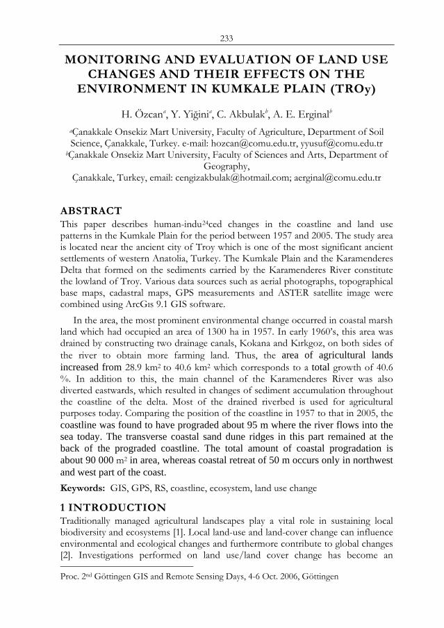
233
MONITORING AND EVALUATION OF LAND USE CHANGES AND THEIR EFFECTS ON THE
ENVIRONMENT IN KUMKALE PLAIN (TROy)
H. Özcana, Y. Yiğinia, C. Akbulakb, A. E. Erginalb aÇanakkale Onsekiz Mart University, Faculty of Agriculture, Department of Soil Science, Çanakkale, Turkey. e-mail: [email protected], [email protected]
bÇanakkale Onsekiz Mart University, Faculty of Sciences and Arts, Department of Geography,
Çanakkale, Turkey, email: [email protected]; [email protected]
ABSTRACT This paper describes human-indu24ced changes in the coastline and land use patterns in the Kumkale Plain for the period between 1957 and 2005. The study area is located near the ancient city of Troy which is one of the most significant ancient settlements of western Anatolia, Turkey. The Kumkale Plain and the Karamenderes Delta that formed on the sediments carried by the Karamenderes River constitute the lowland of Troy. Various data sources such as aerial photographs, topographical base maps, cadastral maps, GPS measurements and ASTER satellite image were combined using ArcGıs 9.1 GIS software.
In the area, the most prominent environmental change occurred in coastal marsh land which had occupied an area of 1300 ha in 1957. In early 1960’s, this area was drained by constructing two drainage canals, Kokana and Kırkgoz, on both sides of the river to obtain more farming land. Thus, the area of agricultural lands increased from 28.9 km2 to 40.6 km2 which corresponds to a total growth of 40.6 %. In addition to this, the main channel of the Karamenderes River was also diverted eastwards, which resulted in changes of sediment accumulation throughout the coastline of the delta. Most of the drained riverbed is used for agricultural purposes today. Comparing the position of the coastline in 1957 to that in 2005, the coastline was found to have prograded about 95 m where the river flows into the sea today. The transverse coastal sand dune ridges in this part remained at the back of the prograded coastline. The total amount of coastal progradation is about 90 000 m2 in area, whereas coastal retreat of 50 m occurs only in northwest and west part of the coast. Keywords: GIS, GPS, RS, coastline, ecosystem, land use change
1 INTRODUCTION Traditionally managed agricultural landscapes play a vital role in sustaining local biodiversity and ecosystems [1]. Local land-use and land-cover change can influence environmental and ecological changes and furthermore contribute to global changes [2]. Investigations performed on land use/land cover change has become an Proc. 2nd Göttingen GIS and Remote Sensing Days, 4-6 Oct. 2006, Göttingen
234
important aspect of global change, or global warming studies, since these changes form major factors for global change depending on their interactions with climate, ecosystem processes, biogeochemical cycles, biodiversity, and, even more important, human activities [3]. Land use change may involve either a shift to a different use or an expansion and intensification of an existing form [4].
It is well known that human-related land use and land cover change has many significant impacts on landscape and the global biosphere. Landscape fragmentation has brought significant impacts to wildlife species in a variety of ways [5]. Investigating landscape structure and its change is a prerequisite to the study of ecosystem functions and processes, sustainable resource management, and effective land use planning. Remote Sensing (RS) and Geographic Information Systems (GIS) have been commonly applied in identifying and analyzing land use and land cover change [6], [7], [8], in that landscape characteristics and changes on it can be practically quantified with these methods. Nowadays, RS has been used in combination with GIS and Global Positioning Systems (GPS) to assess land cover change more effectively than by RS data only [9, 10, 11]. Remote sensing (RS), GIS and GPS could be together applied in dynamic monitoring to assure basic data for planner and policy makers.
In the present work, human-accelerated coastline and land use changes between 1957 and 2005 in the Kumkale Plain were discussed. The study was carried out at three stages; i.e. (1) data collection and processing, (2) field surveys, (3) GIS and RS studies. Several field surveys were performed both to note geographical features and land use characteristics of the area and to confirm accuracy of GIS and RS data.
2 MATERIAL AND METHOD
2.1 STUDY AREA The study area is placed at a nearby place to the ancient city of Troia, which is one of the oldest and well-known archaeological sites in northwest Anatolia, Turkey (Figure 1). The Kumkale delta plain with an area of approximately 48.1 km2 is surrounded by a flat and slightly sloped low plateux area with elevations varying between 50-100 meters a.s.l. [12], [13]. Nearly 90 % of the lowland is lower than 10 m in altitude.
The Quaternary sediments carried by Karamenderes and Dumrek rivers form the youngest unit with top soil texture ranging from light to heavy [14]. The area consists entirely of farming parcels with sizes varying between 0.2 and 7.9 ha. As the main crops, wheat, cotton, tomato followed by corn, sunflower, alfalfa, pepper and rice are cultivated. The Marmara Transition (MRT) (from Mediterranean to Black Sea) [15] prevails in the area. The average annual rainfall is around 600 mm.
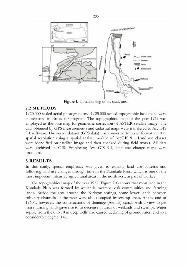
235
Figure 1. Location map of the study area.
2.2 METHODS 1/20.000-scaled aerial photograps and 1/25.000-scaled topographic base maps were coordinated in Erdas 9.0 program. The topographical map of the year 1972 was employed as the base map for geometric correction of ASTER satellite image. The data obtained by GPS measurements and cadastral maps were transfered to Arc GIS 9.1 software. The vector dataset (GPS data) was converted to raster format at 10 m spatial resolution using a spatial analyst module of ArcGIS 9.1. Land use classes were idendified on satellite image and then checked during field works. All data were archived in GIS. Employing Arc GIS 9.1, land use change maps were produced.
3 RESULTS In this study, special emphasize was given to existing land use patterns and following land use changes through time in the Kumkale Plain, which is one of the most important intensive agricultural areas in the northwestern part of Turkey.
The topographical map of the year 1957 (Figure 2A) shows that most land in the Kumkale Plain was formed by wetlands, swamps, oak communities and farming lands. Beside the area around the Kırkgoz springs, some lower lands between tributary channels of the river were also occupied by swamp areas. At the end of 1960’s, however, the constructions of drainage (Azmak) canals with a view to get more farming lands gave rise to to decrease in areas of wetlands and swamps. Water supply from the 6 to 10 m deep wells also caused declining of groundwater level to a considerable degree [14].
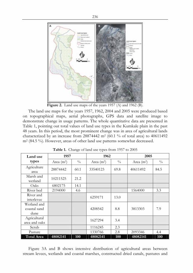
236
Figure 2. Land use maps of the years 1957 (A) and 1962 (B).
The land use maps for the years 1957, 1962, 2004 and 2005 were produced based on topographical maps, aerial photographs, GPS data and satellite image to demonstrate change in usage patterns. The whole quantitative data are presented in Table 1, pointing out total values of land use types in the Kumkale plain in the past 48 years. In this period, the most prominent change was in area of agricultural lands characterized by an increase from 28874442 m2 (60.1 % of total area) to 40611492 m2 (84.5 %). However, areas of other land use patterns somewhat decreased.
Table 1. Change of land use types from 1957 to 2005 1957 1962 2005 Land use
types Area (m2) % Area (m2) % Area (m2) % Agriculture
area 28874442 60.1 33540123 69.8 40611492 84.5
Marsh and wetland 10211525 21.2
Oaks 6802175 14.1 River bed 2194000 4.6 1564000 3.3 River and interlevee 6259171 13.0
Wetland and coastal sand
dune 4208542 8.8 3813303 7.9
Agricultural area and oaks 1627294 3.4
Scrub 1116245 2.3 Pasture 1330766 2.8 2093346 4.4
Total Area 48082141 100 48082141 100 48082141 100 Figure 3A and B shows intensive distribution of agricultural areas between
stream levees, wetlands and coastal marshes, constructed dried canals, pastures and
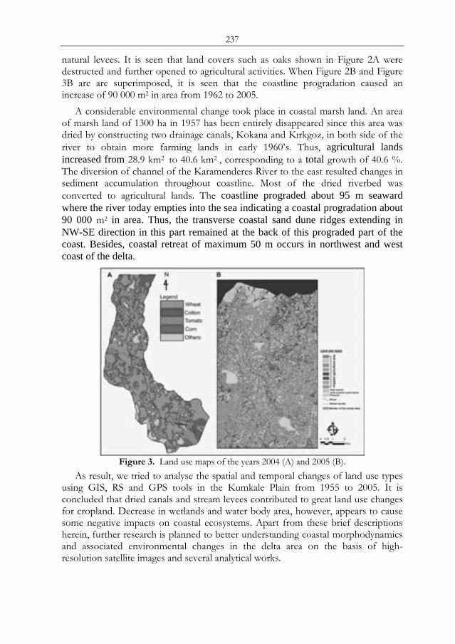
237
natural levees. It is seen that land covers such as oaks shown in Figure 2A were destructed and further opened to agricultural activities. When Figure 2B and Figure 3B are are superimposed, it is seen that the coastline progradation caused an increase of 90 000 m2 in area from 1962 to 2005.
A considerable environmental change took place in coastal marsh land. An area of marsh land of 1300 ha in 1957 has been entirely disappeared since this area was dried by constructing two drainage canals, Kokana and Kırkgoz, in both side of the river to obtain more farming lands in early 1960’s. Thus, agricultural lands increased from 28.9 km2 to 40.6 km2 , corresponding to a total growth of 40.6 %. The diversion of channel of the Karamenderes River to the east resulted changes in sediment accumulation throughout coastline. Most of the dried riverbed was converted to agricultural lands. The coastline prograded about 95 m seaward where the river today empties into the sea indicating a coastal progradation about 90 000 m2 in area. Thus, the transverse coastal sand dune ridges extending in NW-SE direction in this part remained at the back of this prograded part of the coast. Besides, coastal retreat of maximum 50 m occurs in northwest and west coast of the delta.
Figure 3. Land use maps of the years 2004 (A) and 2005 (B).
As result, we tried to analyse the spatial and temporal changes of land use types using GIS, RS and GPS tools in the Kumkale Plain from 1955 to 2005. It is concluded that dried canals and stream levees contributed to great land use changes for cropland. Decrease in wetlands and water body area, however, appears to cause some negative impacts on coastal ecosystems. Apart from these brief descriptions herein, further research is planned to better understanding coastal morphodynamics and associated environmental changes in the delta area on the basis of high-resolution satellite images and several analytical works.
238
REFERENCES 1. Turner, M.G., 1990. Landscape changes in nine rural counties in Georgia.
Photogramm. Eng. Rem. Sens. 56, 379–386. 2. Meyer, W.B., Turner II, B.L., 1991. Changes in Land Use and Land Cover: A
Global Perspective. Cambridge University Press, Cambridge. 3. L´opez, E., Bocco, G., Mendoza, M., Duhau, E., 2001. Predicting land-cover and
land-use change in the urban fringe: a case in Morelia city, Mexico. Landsc. Urban Plann. 55, 271– 285.
4. Matson, P. A,, Parton, W. J., Power, A. G. and Swift, M. J. 1997. Agricultural intensification and ecosystem properties. Science. 277(25): 504-509.
5. Egbert, S.L., Park, S., Price, K.P., Lee, Y.,Wu, J., Nellis, M.D., 2002. Using conservation reserve program maps derived from satellite imagery to characterize landscape structure. Comput. Electron. Agric. 37, 141–156.
6. Jensen, J.R., Cowen, D.C., 1999. Remote sensing of urban suburban infrastructure and socio-economic attributes. Photogramm. Eng. Rem. Sens. 65, 611–622.
7. Hathout, S., 2002. The use of GIS for monitoring and predicting urban growth in East and West St Paul, Winnipeg, Manitoba, Canada. J. Environ. Manag. 66, 229–238.
8. Eastman, J.R., Fulk, M., 1993. Long sequence time series evaluation using standardized principle components. Photogramm. Eng. Rem. Sens. 59, 991–996.
9. Jensen, J.R., 1996. Introductory Digital Image Processing: A Remote Sensing Perspective, second ed. Prentice Hall, Upper Saddle River, NJ.
10. Muller, D., Zeller, M., 2002. Land use dynamics in the central highlands of Vietnam: a spatial model combining village survey data with satellite imagery interpretation. Agric. Econ. 27, 333–354.
11. Jieying, X., Yanjun, S., Jingfeng, G., Ryutaro, T., Changyuan, T., Yanqing, L., Zhiying, H., 2006. Evaluating urban expansion and land use change in Shijiazhuang, China, by using GIS and remote sensing. Landscape and Urban Planning 75 (2006) 69–80
12. Bilgin, T., 1969. Biga Yarımadası güneybatı kısmının jeomorfolojisi. İ.Ü. Coğr. Enst. Yay. No:55, İstanbul.
13. Kayan, I., 2000. The water supply of Troia. Studia Troica, Verlag Philipp von Zabern, Mainz am Rhein, 135–144.
14. State Hydroulic Works (DSI), 1996. Karamenderes Project, Kumkale Plain irrigation and drainage survey and land classification report. Project no: 401. State Hydraulic Works, Turkey (in Turkish).
15. Turkes, M., 1996. Spatial and temporal analysis of annual rainfall variations in Turkey. International Journal of Climatology. 16: 1057-1076.
239
CHANGE DETECTION OF THE ILI DELTA IN THE SEVEN-STREAM LAND USING MULTI-
TEMPORAL REMOTE SENSING DATA
P. A. Propastina,b, M. Kappasa, N. R. Muratovab
a Department of Geography, Georg-August University Göttingen, Goldschmidtstr. 5, 37077, Göttingen, Germany, e-mail: [email protected]
b Laboratory of Remote Sensing and Image Analysis, Kazakh Academy of Science, Shevchenko Street, 15, 480040, Almaty, Kazakhstan, e-mail:
ABSTRACT The Ili delta is a sensitive ecosyst25em which existence fully depends on the runoff amount in the Ili River. Construction of a dam on the upper flow of the Ili sharply affected the natural hydrological regime of the Ili delta and changed its normal characteristics such as e.g. flooding the surface area and area of wetland. The purpose of the study is to monitor changes in the delta of the Ili River during 1970-2000 and to detect the disturbance and rehabilitation of this fragile ecosystem. High-resolution Landsat imagery from the years 1972, 1979, 1989, 1992 and 2000 were used for the detection of changes in the area of the Ili delta whereas a coarse resolution NOAA AVHRR multi-temporal dataset was used for monitoring biomass dynamic during 1982-2003. Areas covered by reed grass communities and water in the Ili delta were considered to be representative indicators for wetland changes in the Ili delta while the Normalized Difference Vegetation Index spatially averaged over the entire delta was taken to represent a general trend in biomass. Supervised classification of the Landsat imagery based on information extracted from topographic maps covered the entire delta and was checked up in the field. The results of classification were interpreted and tested for relationship with hydrological data. The delta NDVI displays significant intra-annual and inter-annual variability that was found to correlate with runoff of the Ili River and with the water level in the Balkhash Lake. A regression model established between NDVI and the water level was used for prediction of water level data which had been missing after 1993. Keywords: Ili River delta, wetland, change detection, anthropogenic impact
1 INTRODUCTION The largest inflow in Lake Balkhash is from the Ili River. The water of this river has been used in large scale irrigation since the 1960s. In autumn 1969, the Kapchagay dam was constructed on the upper flow of the Ili river. The Kapchagay Reservoir would expect to be a long-term benefit to the arid lands, but soon it was recognized that filling the Kapchagay reservoir would affect the water level in Lake Balkhash due to the retention of water in the reservoir. Because of the rapid decrease of Ili’s Proc. 2nd Göttingen GIS and Remote Sensing Days, 4-6 Oct. 2006, Göttingen
240
contributory between 1970 and 1985, the Lake Balkhash water volume decreased by 39 km3 and in 1987 the lake reached its lowest level for the last hundreds years, 340.5 m (Figure 1). Prior to damming of the Ili, the river's mean annual discharge to the lake was estimated to be around 15 km3, but a sequence of dry years in the early 1980s, the storage of water in the lake, evaporation losses and diversion of water for irrigation, reduced the delivery to about 8-9 km3/y. By 1986, the Kapchagay reservoir was still only half full [1, 2].
The construction of the Kapchagay Reservoir led to additional adverse effects in Lake Balkhash and its surrounding environments. The impacts include: (1) wetlands degradation of Lake Balkhash margins and of the Ili delta as well as of the Ili vallley; (2) rising salinities in Lake Balkhash; (3) dehydration of broad coastal areas and salinization of soils; (4) a decline in the value of the Balkhash fishery; and (5) an alteration of natural hydrological patterns. These impacts have been exacerbated by additional impacts from sources other than the Kapchagay reservoir, including an increase of grazing impact on the pastures in desert areas, in the Ili valley, and in the Ili delta, and a natural increase in the aridity of the Balkhash basin [3, 4].
A primary cause of the first three of these impacts was a fall in lake water level between 1970 and 1989. This fall of approximately 2 m was associated with a decrease in Lake Balkhash's surface area of 2610 km2. The impact of the fall in water level on wetlands associated with Lake Balkhash was profound. The reed grass thickets and reed swamps were of considerable significance; muskrat (introduced in 1935) provided a valuable harvest and in the Ili delta alone some 1.5 million muskrats were harvested annually (i.e. 80% of all muskrats harvested in Kazakhstan). For 1950-1960s, the area of wetlands in the Ili delta was estimated to be 500,000 ha. Annually, about 250,000 ha were flooded as the high water occurs. There were about 10,000 small lakes with area of > 1 ha [5]. The reed swamps of the deltas provided rich haymaking and pastures for livestock. All such values were significantly degraded by drying out of wetlands (Figure 2). The dehydration of Ili’s delta followed by a rapid decrease of its area from 11,000 km² in 1950-1960 to approximately 6,000 km² in 1985-1986. The extend of reed grass swamps dropped to one-half of its original area. By 1975, the desiccation of pastures led to livestock grazing in the tugay and the acceleration of the degradation of that habitat. Pastures in the Ili delta have been reduced to one-third of their original extent [4, 6].
In the mid 1980s, the public opinion had been alarmed from the approaching ecological disaster in the Balkhash Lake and its surrounding environments. The government of the Kazakh Soviet Republic undertook many efforts to change the ecological situation and diminish the consequences of the Balkhash disturbance. After stopping the filling the Kaptchagay Reservoir, the situation improved in 1988, when inputs into Balkhash from the eastern rivers were nearly 5.0 km3, and from all sources 19.4 km3. As a result, the Lake Balkhash water level rose by nearly 100 cm. The rise of the water level continued also after 1988 due to diminishing the cut of the Ili water and a general increase in precipitation in the Balkhash catchment. Unfortunately, the data of the water level from the last decade of 20 century are not available, probably, because of stopping the measurements after the collapse of the Soviet Union [6, 7]. There are a few studies from the Balkhash region carried out
241
during the last time; but according to the scarce reports and perception of the peoples living in this region, the rehabilitation of the Balkhash Lake and its wetlands has been also continued during the period 1993-2005.
The case of the Balkhash Lake, – the degradation of its surroundings due to human impact and then the rehabilitation of them, - is like a large experiment undertaken in the natural environment and has given an ideal chance to observe and analyse a change of a wetland ecosystem caused by anthropogenic impact. Taking into account a large area of the region to be studied (about 10,000 km²), use of remotely sensed data is of great importance. Multi-temporal satellite images include information of changes in land cover and land cover characteristics. Data from the Landsat satellite launched in 1972 and covering by its orbit the entire area of the Earth land surface have been widely used on various fields of geographical research on regional to local scale. Due to fine spatial resolution between 14.5 and 58 m, this data are devised to be most appropriate for studies of land cover change detection also in river deltas and see margin regions [8].
Figure 1. Fluctuations in water level in Lake Balkhash since the start of the measurements.
The dashed line (after 1993) presents the values predicted by a model developed in this study (for explanation see §4.2).
The Landsat data cover the period from 1972 to the current year but are available freely in Internet only with a low time sequence (some years). It means that change detection can be done only between the time points for which the data are available. Monitoring studies of inter-annual and intra-annual land cover change require data with finer temporal resolution (10-days, two-weeks, and month). Such data are available only from the satellite systems of coarse spatial resolution. One of these systems is the Advanced Very High Resolution Radiometer (AVHRR) launched by the National Oceanic and Atmospheric Administration (NOAA) in 1981. The data derived by the AVHRR have the 8-km resolution in nadir and are available with a time sequence of 1 week. The most recent studies of vegetation monitoring, drought detection, desertification etc. on global and regional scale have been used data from the AVHRR. Data from AVHRR has been successfully used also for change detection of climatically sensitive lakes [9]. Fusion of data with fine
242
and coarse resolution achieved very good results in many studies of change detection.
Figure 2. Change in the characteristics of Lake Balkhash during 1970-1989. This study objected to detect change in wetland in the delta of the Ili River over
the period 1972-2003. We based the study on monitoring two change indicators: (1) the area covered by reed grass and small lakes in the Ili delta; and (2) characteristics of biomass averaged over the entire delta. We also modelled relationships between these indicators and indicators of human impact associated with change in hydrological characteristics of the Ili River and the Balkhash Lake. Finally, we predicted missing values of the water level in the Balkhash Lake.
2 STUDY AREA The region of our investigation is situated in the southern part of Kazakhstan within the Balkhash lake basin between 44°00´ and 46°45´ north and 73°51´ and 78°13´ east (Figure 3). Lake Balkhash has a catchment of 501,000 km², a surface are of 15,730 km², and a volume of 87.7 km³. The main tributaries of the Balkhash Lake are the Ili River which enters from the south-west (and accounts for 78.2% of surface inflow); the Karatal River from the western slopes of Dzhungarskiy Alatau (15.1%); the Aksu River also from Dzhungarskiy Alatau (0.13%); and the Lepsy River from the same origin (5.4%). As the major influent, the Ili River, flows in at the south-western corner of the lake and has a mean annual runoff 15.6 km³. The delta of the Ili River is 120 km long, 100 km wide and occupies an area of about 10,000 km².
The climate in the area is highly continental, with low annual precipitation (under 150 mm) and severe daily and annual temperature variations. Winter air temperatures on dry clear days may fall as low as – 40° to – 50° C, while in the hottest month, July, the average air temperature is about 20° to 25°C. Eastern and north-eastern winds prevail throughout the year.
243
A spatial variability of hydrological factors in the study area predicts a diversity of soils and vegetation types. The areas of the recent Ili’s delta are covered by hydromorphic gley loamy soils. These soils have a thick turf horizon and are flooded every year from May to July. Thickets of reed grass cover the floodplains of the recent delta and are presented by such species as Calamagrostis pseudophragmites and Phragmites communis. Relief elevations in the delta and in the valley of the Ili river are covered by halophytic meadows and gallery forests (known here as tugay), the main species are Eleagnus angustifolia, Populus turanga, Hippophae rhamnoides and Tamarix-species. All space between the numerous streams and swamps where the ground water is low is occupied by sandy desert with barchan chains. The soil formation process here is still in its initial stage. Here, sand sagebrush and ephemeral-psammophytic shrub are dominating vegetation formations. The main species are Artemisia terrae albae, Artemisia songarica, Astragalus brachypus, Calligonum-species and Halocnemum strobilaceum. Woody species are presented by Haloxylon persicum and Haloxylon aphylum. Solonchaks are commonly located in relief depressions of the coastal zone as well as in the drying up areas of the Ili delta. A high groundwater table and a high evaporation of groundwater are two necessary factors for genesis of solonshaks. Commonly, they are vegetation free.
Figure 3. (left) Location of the study area on the map of Kazakhstan, (right) subset from a
Landsat TM mosaic.
3 DATA AND METHODS
3.1 LANDSAT DATASET The Landsat sensor was specifically designed for studies such as land cover mapping. Essentially, detection of changes in land cover involves the ability to quantify temporal differences using multi-temporal data sets. One of the major applications of remotely sensed data obtained from Earth Orbiting Satellites is change detection because of repetitive coverage, fine spatial resolution, and consistent image quality.
The Landsat satellite image data employed in this study were acquired in 1972, 1978, 1992, and 2001. Pre-processing of the Landsat dataset included common procedures of satellite data treatment such as radiometric and geometric correction,
244
rectification and co-registration of all images. The Landsat TM and Landsat ETM images from 1992 and 2001 were resamplied to the spatial resolution of 57 m in order to mach the Landsat MSS images. In addition, a set of topographic maps dated 1982 and covered the whole study area was used to compare with the analysed satellite images. In spite of large time gape between the image acquisitions, application of the Landsat dataset to change detection in the Ili delta is believed to be justifiable for two main reasons. Firstly, the years of image acquisition corresponded well to the main phases of environmental change in the Balkhash Lake and its surroundings: 1970-1986 is the phase of dehydration and degradation of wetland due to the reduce of Ili’s water runoff and the rapid drop in the water level in Lake Balkhash; 1987-1992 is the initial stage of situation improvement caused by the diminishing the cut off of the Ili’s water and a light increase in precipitation amount; since 1993-94 is the stage of rehabilitation the Balkhash Lake and its environment. Secondly, the intra-annual discrepancies between the images reflected different phenological phases of vegetation due to months of their acquisition (July-August) were expected to be fewer than the long-time differences caused by the general change in the Balkhash Lake environment. 3.2 NOAA AVHRR DATASET The AVHRR product commonly used for investigations of vegetation cover is the Normalized Difference Vegetation Index (NDVI). The vegetation absorbs a great part of incoming radiation in the visible portion of the spectrum (VIS=220-680 nm) and reaches maximum reflectance in the near-infrared channel (NIR=730-1100 nm). The NDVI, defined as ratio (NIR-VIS)/(NIR+VIS), represents the absorption of photosynthetic active radiation and hence is a measurement of the photosynthetic capacity of the canopy. Negative NDVI values indicate non-vegetated areas such as snow, ice, and water. Positive NDVI values indicate green, vegetated surfaces, and higher values indicate increase in green vegetation. The NDVI is established to be highly correlated to green-leaf density, absorbed fraction of photosynthetically active radiation and above-ground biomass and can be viewed as a proxy for photosynthetic capacity [10].
To monitor temporal variations in vegetation characteristics we used AVHRR NDVI dataset covering the period 1982-2003. The data, at 8-km spatial resolution, are originally processed as 10-day composites using the maximum value procedure to minimize effects of cloud contamination. For this research, we created monthly composites from three 10-day composites in any given month to further minimize the effects of clouds on the vegetation signal. These monthly NDVI data for consecutive seven months (April-October) were averaged to generate growing season NDVIs for each year. Additionally, we have calibrated the AVHRR NDVI data against three time invariant desert targets using a method described by [11]. 3.3 METHODS In this study, supervised classification technique was used to emphasize changes between areas covered by wetland in the Ili delta. The classification was executed for each date using regions of interest selected from topographic map and knowledge obtained during two field travels through the study region in 2004 and 2005. When performing the classification we concentrated on only two types of land cover: reed
245
grass and open water in the Ili delta. The resultants of classification were analysed and compared, areas covered by the cover classes mapped and measured. In order to prove relationship between change in land cover and change in human impact reflected by indicators of hydrological regime, the derived classification data were compared with the available hydrological data such as the water level in the Balkhash Lake, the runoff of the Ili River etc. Any associations between these factors and areas derived for reed grass and small water bodies in the Ili delta would indicate that land cover change is driven by human impact, namely by the cut off of the Ili’s water for filling the Kaptchagay Reservoir.
In order to monitor development of biomass at intra-annual and inter-annual time-scale over the study period, we generated two types of time series of AVHRR NDVI. As first, we averaged maximum values for every month from the growing season during the period 1981-2003, and secondly, we generated maximum growing season NDVI for every year. These datasets were spatially integrated over the entire area of the Ili delta. The first dataset was used for monitoring the dynamic of biomass within the growing season (April-October), whereas the second was utilized to determine the long-time (1981-2003) trend. We assumed that the trend in biomass of reed grass indicate the general environmental trend the Ili drainage basin and change in hydrological patterns over the study period, and, therefore, may be associated with the trend in human impact. This assumption was based on a hypotheses that both inter-annual and intra-annual dynamic of reed grass biomass is not controlled by the local precipitation but only by the water discharge in the system of the Ili River. To prove this hypothesis, we had analysed climate signal in the NDVI time-series. When this signal is presented in the NDVI dynamics, than the relationship between NDVI and precipitation must be statistically significant and strong. In order to test this relationship we computed linear regression models between corresponding NDVI and precipitation amount. Having tested this relationship both for within-season and inter-annual time series, we established regression models for NDVI and hydrological characteristics. Finally, we applied the regression model to calculate annual values of the water level in the Balkhash Lake that had been missing after 1993 because of measurement interruption.
4 RESULTS
4.1 CHANGES IN AREA OF THE ILI DELTA Four supervised classification images of 1972, 1978, 1992 and 2001 were obtained. In order to map extend of the reed grass thickets and water bodies in the Ili delta, four vector files were formed. These four vectors derived from satellite images were superimposed to detect the differences between each of the dates. Comparable analyses of area changes have been carried out and the areas covered by the land cover types at each date were measured and interpreted.
The classification results showed significant change between the years of image acquisition. A change of a high magnitude was to observe between the years 1972 and 1978. The classification results from these two images devised a sharp decrease in areas both of reed grass and small water bodies in the Ili delta. The area of reed grass reduced by about 40 % and so was also the area of small lakes. This dramatic
246
reduce of the extreme extend of the Ili delta had been caused by cut off of the Ili’s water for filling the Kaptchagay Reservoir. The years between 1970 and 1985 are associated with the highest level of the human impact on the hydrological regime of the Ili River. This impact was a driven force for the drop of the water level in the Balkhash Lake. After the cut off of the Ili’s water had been diminished at the end of 1980s, the water level begun to rise.
The classification results of the 1992 image revealed the first signs of situation improvement: the change in area of reed grass and small lakes was light positive. But this positive change is associated only with the northern section of the Ili delta, the southern delta continued to dry up. The classification image of 2001 devised a broad rehabilitation of the wetland in the Ili delta. The area covered by reed grass thickets was almost recovered to the area in 1972; positive changes are also associated with the area of small lakes. However, the southern part of the Ili delta is the only part which was not concerned by the process of rehabilitation. Visual comparison between the classification images from 1978 and 2001 devised identity in areas occupied by reed grass and small lakes. This can be explained by the fact that the patterns in hydrological regime had changed and the most runoff has transferred from the southern streams into the northern part of the delta system. Recent satellite based studies from this region reported about contemporary land degradation there [12]. It is impossible to know which of causes, human or natural, were responsible for that.
The results of area measurements were compared with the hydrological data in order to prove whether the change in hydrological regime had been a driven force for the changes in land cover. Figure 5 demonstrates a strong association between the change in land cover and the water level in the Balkhash Lake. In this case, the water level is considered to be an indicator of human impact on the ecosystem of the Balkhash region. 4.2 TRENDS IN BIOMASS AND THEIR EXPLANATORY FACTORS In order to prove how the change in hydrological regime has affected biomass trends in the Ili delta, we investigated intra-annual and inter-annual dynamics of spatially integrated NDVI and compared that with dynamic of climatic and hydrological factors. Mean monthly NDVI increased rapidly during the spring (April-May), peaked at the end of July-mid of August, and decreased during the autumn months. Precipitation showed two peaks, increasing from early April to early June and peaking in late May-early June, after that follows a rapid decrease, and then again a rapid increase till the next peak in mid of July. Minimum of precipitation occurs in August-September. Generally, precipitation is very scarcely in the study area (about 150 mm/year) and can not be a basis for the rich vegetation of reed grass thickets in the Ili delta. A further statistical analyse supported our suggestion. Having tried different time lag imposed to the NDVI data, we found no significant correlation with precipitation. On the contrary, the relationship between monthly NDVI and monthly runoff was very strong with a very high coefficient of determination, R² = 0.93. The intra-annual variability in NDVI is almost fully explained by the variability in runoff amount of the river system (Figure 6).
247
We suggested that not only intra-annual but also inter-annual dynamic in biomass may be associated with hydrological factors. In order to investigate this, we compared time series of growing season NDVI with time series of water level in the Balkhash Lake over the period 1981-1993. The association between these variables is strong (Figure 7, a). The regression analysis undertaken to model this relationship supported that. The change in water level explained about 80 % of inter-annual variance in NDVI (Figure 7, b). Using the derived equation between NDVI and water level in the Balkhash Lake, we were able to predict water level values which had been not available. The results of our prediction are showed as a dashed line in Figure 1.
0
10
20
30
40
1972
1978
1992
2001
Are
a, k
m²*
1000
Reed grassSmall lakes
340
341
342
343
1972
1978
1992
2001
Water level
Figure 5. Areas of reed grass and small lakes in the Ili delta (left) and water level in the
Balkhash Lake (right).
(a)
(b) Figure 6. (a) Mean monthly NDVI averaged over the Ili delta and mean monthly runoff (m³/s) in the system of the Ili River. (b) Scatter plot NDVI against runoff devises a strong
relationship between these variables. More than 90 % of variability in NDVI is explained by the variability in runoff (R² = 0.93).
248
(a)
(b) Figure 7. (a) Mean growing season NDVI averaged over the Ili delta and water level in the Balkhash Lake during 1981-1993. (b) Scatter plot between NDVI and the water level. The
relationship is statistically significant and strong with coefficient of determination R² = 0.80.
5 CONCLUSIONS Environmental changes have been determined in the delta of the Ili River using Landsat images acquired in 1972, 1978, 1992 and 2001 as well a dataset of NOAA AVHRR NDVI covering the period 1981-2003. Areas covered by reed grass and small lakes in the delta were considered to represent spatial indicators of land cover change. NDVI trends over the period 1981-2003 were proved to represent a temporal indicator of environmental change.
The most significant change is associated with the period between 1972 and 1978. The reed grass thickets reduced to about 60% of their previous area. The territory of small lakes in the Ili delta also revealed a strong decrease. For 1992, a slight increase in these characteristics has been observed. The results from 2001, exhibited the wide rehabilitation of the wetland environments in the Ili delta. A recover of reed grass area has been revealed for the most part of the Ili delta. This improvement did not concern the southern part of the delta. Here, the wetland environments remained devastated. It can be explained by a change in runoff distribution in the Ili’s system. Runoff transferred from the south to the north. These observations agree with results from other studies [12, 13]. The extreme extend of the Ili delta is highly dependent on such hydrological factors as water level in Lake Balkhash and the runoff amount of the Ili’s River. The rapid change in the delta extend observed during 1970-1980s was explained by the change in hydrological regime and explained by construction of the dam on the upper flow of the Ili. Comparison of indicators of land cover change with hydrological indicators
249
supported this assumption. There was a strong association of change in area occupied by reed grass and small lakes with water level in the Balkhash Lake.
Variability in biomass of reed grass thickets was also examined for dependence on hydrological factors such as runoff of the Ili and water level in Lake Balkhash. We found no correlation between temporal patterns in NDVI and precipitation whether for intra-annual or for inter-annual scale. On the contrary, strong relationship was found for NDVI and runoff amount as well for NDVI and water level. About 93 % of variance in inter-annual and 80 % in inter-annual NDVI dynamic were explained by variance in two hydrological factors. A model based on regression analysis helped us to predict the missing values of water level in the Balkhash Lake and complete the time series of this variable for the study period 1972-2003.
REFERENCES 1 Petr, T., 1992: Lake Balkhash. Kazakhstan. Int. J. Salt Lake Res., 1, pp. 21-46. 2 Tlenbekov, O. K. and Piven, E. N., 1993: Anthropogenic change in runoff of the rivers
in the Balkhash Lake basin. In: Tursunov, A. A. (ed.): Geographic problems of the Ili-Balkhash region, pp: 54-62. Almaty, Gylym,
3 Venus, B. G. and Pozdnyakova, G. V., 1991: Lake changes due to anthropogenic causes. In: D. V. Sevastjanov (ed.). History of Lake Sevan, Issyk-Kul, Balkhash, Zaisan, and Aral, pp. 169-172. Academiya Nauk, Leningrad, (in Russian).
4 Petr, T. and Mitrofanov, V. P., 1998: The impact on fish stocks of river regulation in Central Asia and Kazakhstan. Lakes & Reservoirs: Research and Management, 3, pp. 143-164.
5 Nikolayev, V. A., 1959: Delta of the Ili River and Bakanassy. Trudy Sektora Geographii AN KazSSR, 4, pp. 35-54.
6 Galperin R. I., 1993: Long-time variability of runoff of the rivers in the Balkhash Lake Basin. In: Tursunov A. A. (ed.): The Geographic Problems of Ili-Balkhash Region, pp. 63-71. Almaty, Gylym.
7 Piven E. N., 1990: Trends of runoff change for the rivers of the Ili-Balkhash Region. In: Natural Resources of the Ili-Balkhash Region. Almaty, Nauka, pp. 36-47.
8 Frihy, O. E., Dewidar, K. M, Hasr, S. M. and El Raey, M. M., 1998: Change detection of the north-east Nile Delta of Egypt: shoreline changes, Spit evolution, margin changes of Mangazal lagoon and its islands. Int. J. Remote Sensing, 19, pp. 1901-1912.
9 Harris, A. R., 1994: Time series remote sensing of a climatically sensitive lakes. Rem. Sensing Env., 50, pp. 83-100.
10 Tucker, C. J. & Sellers, P.J. 1986. Satellite remote sensing of primary production. Int. J. Remote Sensing 7, pp. 1395–1416.
11 Los S. O., 1993: Calibration Adjustment of the NOAA AVHRR Normalized Difference Vegetational Index Without Resource to Component Channel 1 and 2 Data. Int. J. Remote Sensing, 14, pp. 1907-1917.
12 Sultangasin, Y. M., Kurochkina, L. Y., Bomont, T. E., Archipkin, O. P, Muratova, N. R. and Terechov, A. G., 2002: Assessment of desertification processes in the Delta of the Ili River using remote sensing and GIS. In: Sultangasin, Y. M. (ed.): Space Research in Kazakhstan, pp. 232-240. Almaty.
13 Filonetz P. P., Omarov T. R. and T. A. Omarova. 1993. Recent conditions of little lakes in the Ili-Balkhash Basin. In: Tursunov A. A. (ed.): The Geographic Problems of Ili-Balkhash Region, pp. 90-101. Almaty, Gylym.

250
251
POSSIBILITIES FOR IMPROVEMENT OF THE CORINE METHODOLOGY FOR MAPPING THE
CORINE LAND COVER CLASSES
D. Protic and B. Bajat Institute for Geodesy, Faculty of Civil Engineering, University of Belgrade,
email: [email protected], [email protected]
26ABSTRACT Current establishment of the CORINE Land Cover 2000 database (CLC2000) for Serbia and Montenegro follows the standard CLC2000 methodology – computer assisted visual interpretation of satellite imagery supported with ancillary data and ground true knowledge. During the process of mapping the CLC classes, there is a strong individual influence of the interpreters on homogeneity and thematic accuracy of the database.
The progressive computer and image processing technology allows us to use advanced image processing techniques in order to improve the interpretation of satellite imagery with keeping the efficiency and expenses on the same level. In this paper, possibilities of using advanced image-processing algorithms for improvement of the CORINE methodology are being discussed.
1 INTRODUCTION In order to bring Serbia and Montenegro to the same line of activities as the rest of the European countries in relation to assessing the land cover resources, CORINE Land Cover 2000 (CLC2000) project in Serbia and Montenegro was implemented under the CARDS programme. The national team, led by private company Evrogeomatika d.o.o., included interpreters and image processing/GIS experts from Serbia (Evrogeomatika) and from Montenegro (Geological Survey of Montenegro). The project contains two segments: IMAGE2000 implies making orthorectified satellite image database as a main data source for land cover mapping while CLC2000 represent the activities connected to computer aided mapping of the land cover classes.
2 CORINE LAND COVER MAPPING METHODOLOGY The production of CLC2000 database follows standard CORINE methodology: computer-aided visual interpretation of satellite imagery supported with ancillary data (topographic maps, airborne imagery, thematic maps…) and field checking. The result should be a seamless vector dataset with the polygon topology. The main mapping parameters defined by the methodology: mapping scale (1:100,000), minimum mapping unit (25 ha) and minimum width of linear elements (100 meters) represent a trade-off between the costs of production and the details of land cover Proc. 2nd Göttingen GIS and Remote Sensing Days, 4-6 Oct. 2006, Göttingen
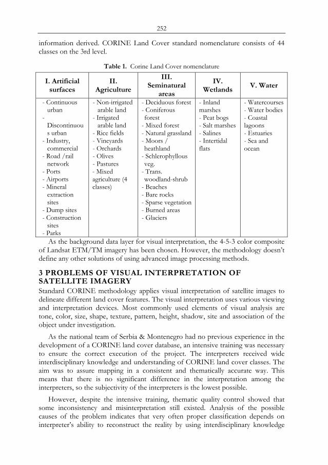
252
information derived. CORINE Land Cover standard nomenclature consists of 44 classes on the 3rd level.
Table 1. Corine Land Cover nomenclature
I. Artificial surfaces
II. Agriculture
III. Seminatural
areas
IV. Wetlands V. Water
- Continuous urban
- Discontinuous urban
- Industry, commercial
- Road /rail network
- Ports - Airports - Mineral
extraction sites
- Dump sites - Construction
sites - Parks
- Non-irrigated arable land
- Irrigated arable land
- Rice fields - Vineyards - Orchards - Olives - Pastures - Mixed agriculture (4 classes)
- Deciduous forest - Coniferous forest
- Mixed forest - Natural grassland - Moors / heathland
- Schlerophyllous veg.
- Trans. woodland-shrub
- Beaches - Bare rocks - Sparse vegetation - Burned areas - Glaciers
- Inland marshes - Peat bogs - Salt marshes - Salines - Intertidal flats
- Watercourses - Water bodies - Coastal lagoons - Estuaries - Sea and ocean
As the background data layer for visual interpretation, the 4-5-3 color composite of Landsat ETM/TM imagery has been chosen. However, the methodology doesn’t define any other solutions of using advanced image processing methods.
3 PROBLEMS OF VISUAL INTERPRETATION OF SATELLITE IMAGERY Standard CORINE methodology applies visual interpretation of satellite images to delineate different land cover features. The visual interpretation uses various viewing and interpretation devices. Most commonly used elements of visual analysis are tone, color, size, shape, texture, pattern, height, shadow, site and association of the object under investigation.
As the national team of Serbia & Montenegro had no previous experience in the development of a CORINE land cover database, an intensive training was necessary to ensure the correct execution of the project. The interpreters received wide interdisciplinary knowledge and understanding of CORINE land cover classes. The aim was to assure mapping in a consistent and thematically accurate way. This means that there is no significant difference in the interpretation among the interpreters, so the subjectivity of the interpreters is the lowest possible.
However, despite the intensive training, thematic quality control showed that some inconsistency and misinterpretation still existed. Analysis of the possible causes of the problem indicates that very often proper classification depends on interpreter’s ability to reconstruct the reality by using interdisciplinary knowledge
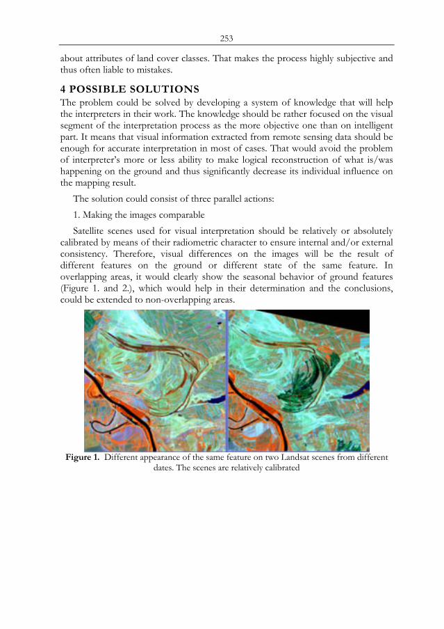
253
about attributes of land cover classes. That makes the process highly subjective and thus often liable to mistakes.
4 POSSIBLE SOLUTIONS The problem could be solved by developing a system of knowledge that will help the interpreters in their work. The knowledge should be rather focused on the visual segment of the interpretation process as the more objective one than on intelligent part. It means that visual information extracted from remote sensing data should be enough for accurate interpretation in most of cases. That would avoid the problem of interpreter’s more or less ability to make logical reconstruction of what is/was happening on the ground and thus significantly decrease its individual influence on the mapping result.
The solution could consist of three parallel actions: 1. Making the images comparable Satellite scenes used for visual interpretation should be relatively or absolutely
calibrated by means of their radiometric character to ensure internal and/or external consistency. Therefore, visual differences on the images will be the result of different features on the ground or different state of the same feature. In overlapping areas, it would clearly show the seasonal behavior of ground features (Figure 1. and 2.), which would help in their determination and the conclusions, could be extended to non-overlapping areas.
Figure 1. Different appearance of the same feature on two Landsat scenes from different
dates. The scenes are relatively calibrated
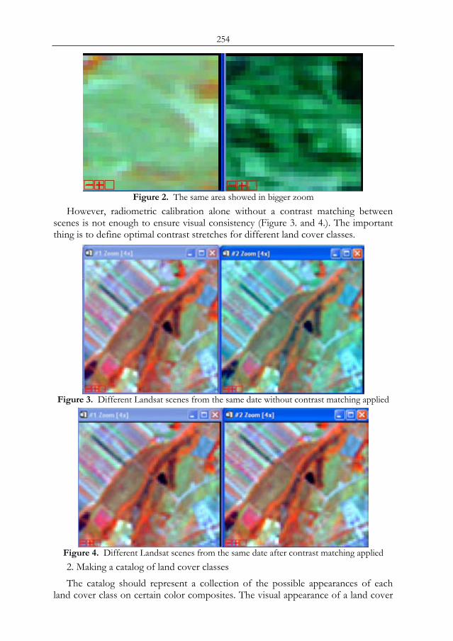
254
Figure 2. The same area showed in bigger zoom
However, radiometric calibration alone without a contrast matching between scenes is not enough to ensure visual consistency (Figure 3. and 4.). The important thing is to define optimal contrast stretches for different land cover classes.
Figure 3. Different Landsat scenes from the same date without contrast matching applied
Figure 4. Different Landsat scenes from the same date after contrast matching applied 2. Making a catalog of land cover classes The catalog should represent a collection of the possible appearances of each
land cover class on certain color composites. The visual appearance of a land cover
255
class could depend on the season, the character and the state of the ground features that the class is consisted of.
3. Application of other spectral transformations Involving other spectral transforms of remote sensing data like principal
component analysis or tasseled cap transformation could be beneficial in some cases. The optimal use, considering time and expenses, of such image processing methods should be defined for some “problematic” land cover classes where standard color composite is sometimes not enough for proper detection.
5 CONCLUSION Land cover maps have wide field of application in many disciplines. It is valuable information in many analytical processes, especially the ones with spatial dimension. Considering those facts it is clear that thematic accuracy of land cover maps are extremely important.
CORINE methodology for building the land cover database is based on extracting the necessary information from optical satellite imagery through a visual interpretation process. However, current methodology does not use all the benefits from optical remote sensing data and image processing techniques. It represents a trade-off between the costs of production and the details of land cover information derived. New technologies allow us now to improve thematic accuracy of the database. It could be accomplished through absolute/relative calibration of the images and application of optimal contrast stretch for each land cover class, making a catalog of the land cover classes and application of other spectral transformation in a fast and efficient way.
REFERENCES 1. Bossard, M., Feranec, J., Otahel, J., (2000) “CORINE Land Cover Technical Guide –
Addendum 2000”, Technical report No 40, EEA, Copenhagen 2. Protić, D., Nestorov, I. (2005) “Development of digital cartographic database for
managing of the environment and natural resources in the Republic of Serbia”, International Cartographic Conference-La Coruna 2005
3. Schowengerdt, R.A. (1997) “Remote sensing-models and methods for image processing”, Academic Press
4. Protić, D., (2006) “Possibilities of updating topographic maps by visual and automatic interpretation of remote sensing data INTERGEOEAST-Belgrade 2006
5. Harris, M.J. (2000) “Basic principles of Sustainable Development”, Global Development and Environment Institute – Working Paper 00-04
6. Buttner, G., Feranec, J., Jaffrain, G., (2000) “CORINE land cover update 2000”, Technical report No 89, EEA, Copenhagen
7. Protić, D., (2005-2006) “Technical reports on CORINE LC project in Serbia and Montenegro”, Evrogeomatika, Belgrade

256
257
THE IMPACT OF LAND USE CHANGE ON THE HYDROLOGICAL DYNAMIC OF THE SEMI ARID
TSITSA CATCHMENT IN SOUTH AFRICA
F. Bäse, J. Helmschrot, H. Müller Schmied, W.A. Flügel Department of Geoinformatics,27 Hydrology and Modelling, Institute of
Geography, Friedrich Schiller University, Löbdergraben 32, 07737 Jena, Germany, email: [email protected], [email protected],
[email protected], [email protected]
ABSTRACT In this study, GIS and remote sensing tools were combined with hydrological modelling to identify the impact of afforestation on basin hydrology in the Tsitsa basin, South Africa. Initially, hydrological characteristics such as long-term rainfall and temperature pattern as well as basin runoff dynamics were delineated analyzing available hydro-meteorological time series. Additionally, double mass plots of the runoff of the Tsitsa and its tributary Mooi were analysed in order to evaluate runoff dynamics with regard to spatio-temporal rainfall pattern. These efforts revealed a significant reduction of the Tsitsa runoff beginning in the 6th year after the first plantations. Furthermore, water balance was simulated using the process oriented, hydrological model JAMS/J2000 [1] to quantify the impact of these land use changes on runoff dynamics. Addressing the distributive concept of the J2000 model, the Tsitsa catchment has been divided into Hydrological Response Units (HRUs). Since a thorough hydrological system analysis has shown that slope, soil type, land use, geology and aspect are the hydrologically most relevant components, these input layers were used for a GIS-based overlay analysis to provide spatial model entities for the modelling. The model was parameterized using field data and literature values. Thus, it shows that GIS and remote sensing techniques provide proper methods and data for environmental modelling, particularly in large scale applications. Keywords: land use change, afforestation, hydrological modelling, HRU derivation, South Africa
1 INTRODUCTION Addressing the increasing demand on water for domestic, industrial, and agricultural use, prognostic hydrological modelling applications are required aiming to support and assess land management strategies and to analyze their impacts on the water balance, in particular in semiarid areas of South Africa. The north Eastern Cape Province is economically a less developed area in South Africa. For economic reasons, more than 60 000 ha of former grassland have been planted with pine and eucalypt species in the headwaters of the Umzimvubu catchment (19 845 km²) since 1989. Because little attention has been given regarding the effects of such land use Proc. 2nd Göttingen GIS and Remote Sensing Days, 4-6 Oct. 2006, Göttingen
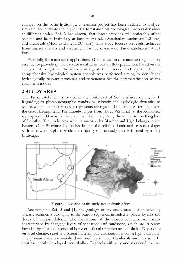
258
changes on the basin hydrology, a research project has been initiated to analyze, simulate, and evaluate the impact of afforestation on hydrological process dynamics at different scales. Ref. 2 has shown, that forest activities will noticeably affect wetland and basin hydrology at both microscale (Weatherley catchment: 1.2 km²) and mesoscale (Mooi catchment: 307 km²). This study focuses on results achieved from impact analysis and assessment for the macroscale Tsitsa catchment (4 281 km²).
Especially for macroscale applications, GIS analyses and remote sensing data are essential to provide spatial data for a sufficient stream flow prediction. Based on the analysis of long-term hydro-meteorological time series and spatial data, a comprehensive hydrological system analysis was performed aiming to identify the hydrologically relevant processes and parameters for the parameterization of the catchment model.
2 STUDY AREA The Tsitsa catchment is located in the south-east of South Africa, see Figure 1. Regarding its physio-geographic conditions, climatic and hydrologic dynamics as well as wetland characteristics, it represents the region of the south-eastern slopes of the Great Escarpment. The altitude ranges from about 782 m asl. at the Xonkonxa weir up to 2 700 m asl. at the catchment boundary along the border to the Kingdom of Lesotho. The study area with its major cities Maclear and Ugie belongs to the Eastern Cape Province. In the headwaters the relief is dominated by steep slopes with narrow floodplains while the majority of the study area is formed by a hilly landscape.
Figure 1. Location of the study area in South Africa.
According to Ref. 3 and [4], the geology of the study area is dominated by Triassic sediments belonging to the Karoo sequence, intruded in places by sills and dykes of Jurassic dolerite. The formations of the Karoo sequence are mainly characterized by changing layers of sandstone and mudstone, which are in places intruded by siltstone layers and horizons of coal or carbonaceous shales. Depending on local climate, relief and parent material, soil distribution shows a high variability. The plateau areas are mainly dominated by shallow Cambisols and Luvisols. In contrast, poorly developed, very shallow Regosols with very unconstrained textures
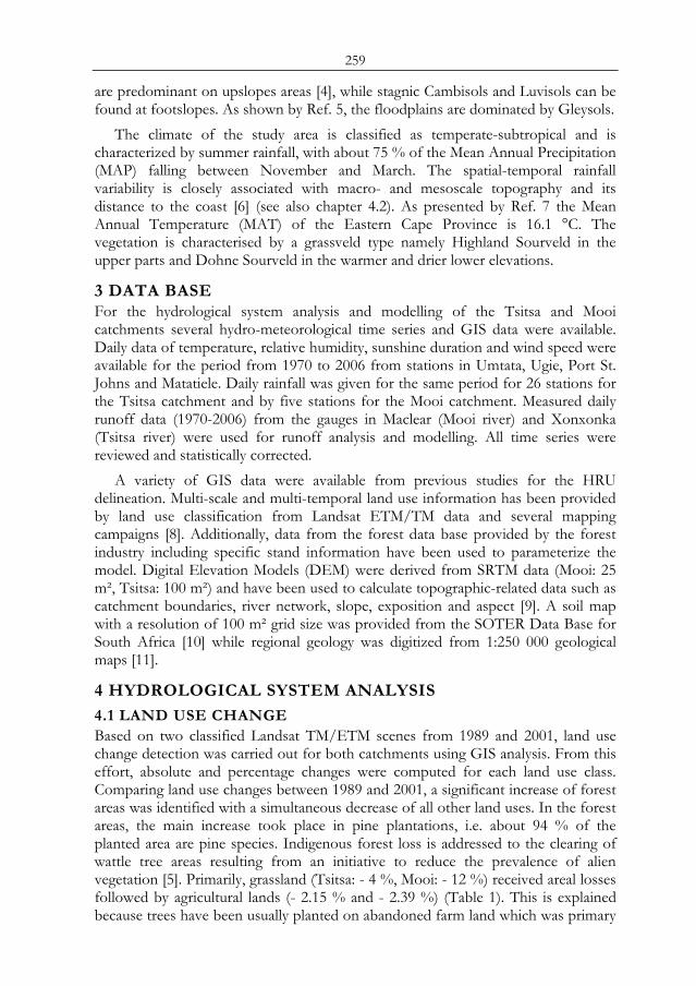
259
are predominant on upslopes areas [4], while stagnic Cambisols and Luvisols can be found at footslopes. As shown by Ref. 5, the floodplains are dominated by Gleysols.
The climate of the study area is classified as temperate-subtropical and is characterized by summer rainfall, with about 75 % of the Mean Annual Precipitation (MAP) falling between November and March. The spatial-temporal rainfall variability is closely associated with macro- and mesoscale topography and its distance to the coast [6] (see also chapter 4.2). As presented by Ref. 7 the Mean Annual Temperature (MAT) of the Eastern Cape Province is 16.1 °C. The vegetation is characterised by a grassveld type namely Highland Sourveld in the upper parts and Dohne Sourveld in the warmer and drier lower elevations.
3 DATA BASE For the hydrological system analysis and modelling of the Tsitsa and Mooi catchments several hydro-meteorological time series and GIS data were available. Daily data of temperature, relative humidity, sunshine duration and wind speed were available for the period from 1970 to 2006 from stations in Umtata, Ugie, Port St. Johns and Matatiele. Daily rainfall was given for the same period for 26 stations for the Tsitsa catchment and by five stations for the Mooi catchment. Measured daily runoff data (1970-2006) from the gauges in Maclear (Mooi river) and Xonxonka (Tsitsa river) were used for runoff analysis and modelling. All time series were reviewed and statistically corrected.
A variety of GIS data were available from previous studies for the HRU delineation. Multi-scale and multi-temporal land use information has been provided by land use classification from Landsat ETM/TM data and several mapping campaigns [8]. Additionally, data from the forest data base provided by the forest industry including specific stand information have been used to parameterize the model. Digital Elevation Models (DEM) were derived from SRTM data (Mooi: 25 m², Tsitsa: 100 m²) and have been used to calculate topographic-related data such as catchment boundaries, river network, slope, exposition and aspect [9]. A soil map with a resolution of 100 m² grid size was provided from the SOTER Data Base for South Africa [10] while regional geology was digitized from 1:250 000 geological maps [11].
4 HYDROLOGICAL SYSTEM ANALYSIS
4.1 LAND USE CHANGE Based on two classified Landsat TM/ETM scenes from 1989 and 2001, land use change detection was carried out for both catchments using GIS analysis. From this effort, absolute and percentage changes were computed for each land use class. Comparing land use changes between 1989 and 2001, a significant increase of forest areas was identified with a simultaneous decrease of all other land uses. In the forest areas, the main increase took place in pine plantations, i.e. about 94 % of the planted area are pine species. Indigenous forest loss is addressed to the clearing of wattle tree areas resulting from an initiative to reduce the prevalence of alien vegetation [5]. Primarily, grassland (Tsitsa: - 4 %, Mooi: - 12 %) received areal losses followed by agricultural lands (- 2.15 % and - 2.39 %) (Table 1). This is explained because trees have been usually planted on abandoned farm land which was primary
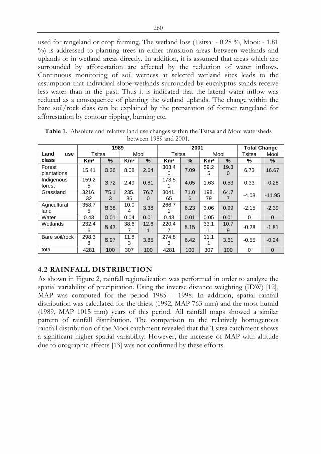
260
used for rangeland or crop farming. The wetland loss (Tsitsa: - 0.28 %, Mooi: - 1.81 %) is addressed to planting trees in either transition areas between wetlands and uplands or in wetland areas directly. In addition, it is assumed that areas which are surrounded by afforestation are affected by the reduction of water inflows. Continuous monitoring of soil wetness at selected wetland sites leads to the assumption that individual slope wetlands surrounded by eucalyptus stands receive less water than in the past. Thus it is indicated that the lateral water inflow was reduced as a consequence of planting the wetland uplands. The change within the bare soil/rock class can be explained by the preparation of former rangeland for afforestation by contour ripping, burning etc.
Table 1. Absolute and relative land use changes within the Tsitsa and Mooi watersheds between 1989 and 2001.
1989 2001 Total Change Tsitsa Mooi Tsitsa Mooi Tsitsa Mooi
Land use class Km² % Km² % Km² % Km² % % % Forest plantations 15.41 0.36 8.08 2.64 303.4
0 7.09 59.25
19.30 6.73 16.67
Indigenous forest
159.25 3.72 2.49 0.81 173.5
1 4.05 1.63 0.53 0.33 -0.28
Grassland 3216.32
75.13
235.85
76.70
3041.65
71.06
198.79
64.77 -4.08 -11.95
Agricultural land
358.75 8.38 10.0
4 3.38 266.71 6.23 3.06 0.99 -2.15 -2.39
Water 0.43 0.01 0.04 0.01 0.43 0.01 0.05 0.01 0 0 Wetlands 232.4
6 5.43 38.67
12.61
220.47 5.15 33.1
1 10.7
9 -0.28 -1.81
Bare soil/rock 298.38 6.97 11.8
3 3.85 274.83 6.42 11.1
1 3.61 -0.55 -0.24
total 4281 100 307 100 4281 100 307 100 0 0
4.2 RAINFALL DISTRIBUTION As shown in Figure 2, rainfall regionalization was performed in order to analyze the spatial variability of precipitation. Using the inverse distance weighting (IDW) [12], MAP was computed for the period 1985 – 1998. In addition, spatial rainfall distribution was calculated for the driest (1992, MAP 763 mm) and the most humid (1989, MAP 1015 mm) years of this period. All rainfall maps showed a similar pattern of rainfall distribution. The comparison to the relatively homogenous rainfall distribution of the Mooi catchment revealed that the Tsitsa catchment shows a significant higher spatial variability. However, the increase of MAP with altitude due to orographic effects [13] was not confirmed by these efforts.
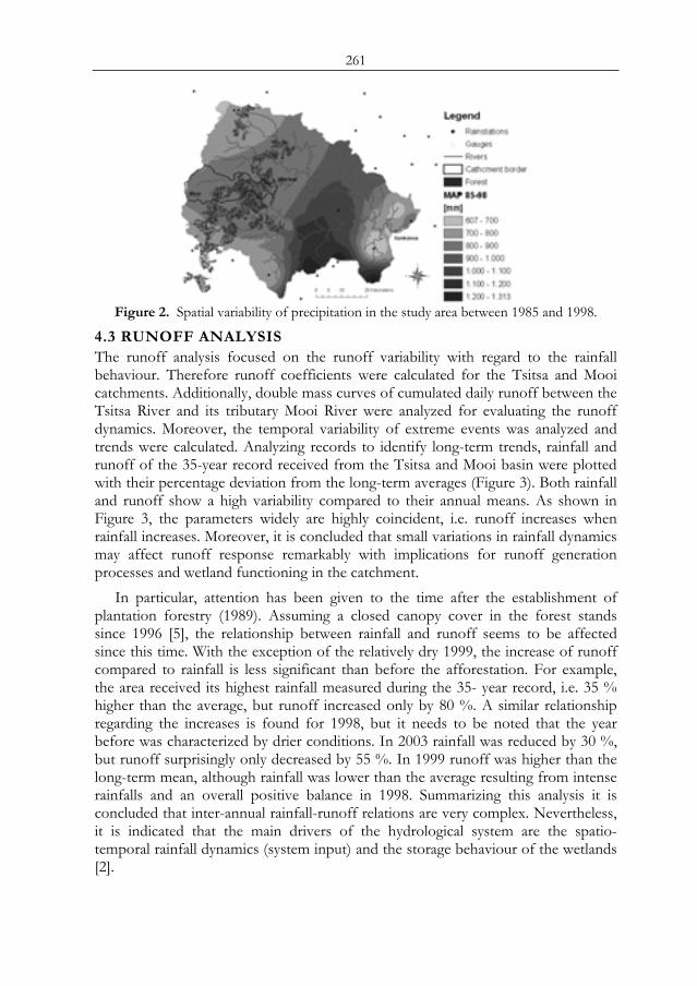
261
Figure 2. Spatial variability of precipitation in the study area between 1985 and 1998.
4.3 RUNOFF ANALYSIS The runoff analysis focused on the runoff variability with regard to the rainfall behaviour. Therefore runoff coefficients were calculated for the Tsitsa and Mooi catchments. Additionally, double mass curves of cumulated daily runoff between the Tsitsa River and its tributary Mooi River were analyzed for evaluating the runoff dynamics. Moreover, the temporal variability of extreme events was analyzed and trends were calculated. Analyzing records to identify long-term trends, rainfall and runoff of the 35-year record received from the Tsitsa and Mooi basin were plotted with their percentage deviation from the long-term averages (Figure 3). Both rainfall and runoff show a high variability compared to their annual means. As shown in Figure 3, the parameters widely are highly coincident, i.e. runoff increases when rainfall increases. Moreover, it is concluded that small variations in rainfall dynamics may affect runoff response remarkably with implications for runoff generation processes and wetland functioning in the catchment.
In particular, attention has been given to the time after the establishment of plantation forestry (1989). Assuming a closed canopy cover in the forest stands since 1996 [5], the relationship between rainfall and runoff seems to be affected since this time. With the exception of the relatively dry 1999, the increase of runoff compared to rainfall is less significant than before the afforestation. For example, the area received its highest rainfall measured during the 35- year record, i.e. 35 % higher than the average, but runoff increased only by 80 %. A similar relationship regarding the increases is found for 1998, but it needs to be noted that the year before was characterized by drier conditions. In 2003 rainfall was reduced by 30 %, but runoff surprisingly only decreased by 55 %. In 1999 runoff was higher than the long-term mean, although rainfall was lower than the average resulting from intense rainfalls and an overall positive balance in 1998. Summarizing this analysis it is concluded that inter-annual rainfall-runoff relations are very complex. Nevertheless, it is indicated that the main drivers of the hydrological system are the spatio-temporal rainfall dynamics (system input) and the storage behaviour of the wetlands [2].
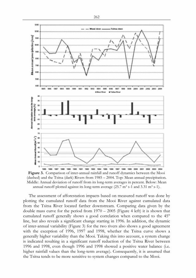
262
Figure 3. Comparison of inter-annual rainfall and runoff dynamics between the Mooi
(dashed) and the Tsitsa (dark) Rivers from 1985 – 2004. Top: Mean annual precipitation. Middle: Annual deviation of runoff from its long-term averages in percent. Below: Mean
annual runoff plotted against its long-term average (25.7 m³ s-1 and 3.31 m³ s-1).
The assessment of afforestation impacts based on measured runoff was done by plotting the cumulated runoff data from the Mooi River against cumulated data from the Tsitsa River located farther downstream. Comparing data given by the double mass curve for the period from 1970 – 2005 (Figure 4 left) it is shown that cumulated runoff generally shows a good correlation when compared to the 45° line, but also reveals a significant change starting in 1996. In addition, the dynamic of inter-annual variability (Figure 3) for the two rivers also shows a good agreement with the exception of 1996, 1997 and 1998, whether the Tsitsa curve shows a generally higher variability than the Mooi. Taking this into account, a system change is indicated resulting in a significant runoff reduction of the Tsitsa River between 1996 and 1998, even though 1996 and 1998 showed a positive water balance (i.e. higher rainfall values than the long-term average). Consequently, it is assumed that the Tsitsa tends to be more sensitive to system changes compared to the Mooi.
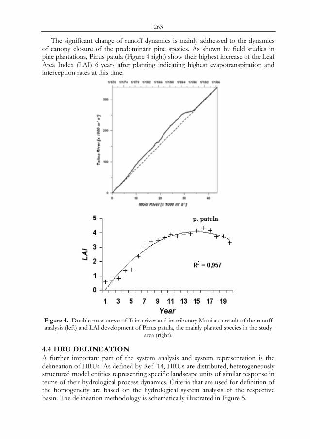
263
The significant change of runoff dynamics is mainly addressed to the dynamics of canopy closure of the predominant pine species. As shown by field studies in pine plantations, Pinus patula (Figure 4 right) show their highest increase of the Leaf Area Index (LAI) 6 years after planting indicating highest evapotranspiration and interception rates at this time.
Figure 4. Double mass curve of Tsitsa river and its tributary Mooi as a result of the runoff analysis (left) and LAI development of Pinus patula, the mainly planted species in the study
area (right).
4.4 HRU DELINEATION A further important part of the system analysis and system representation is the delineation of HRUs. As defined by Ref. 14, HRUs are distributed, heterogeneously structured model entities representing specific landscape units of similar response in terms of their hydrological process dynamics. Criteria that are used for definition of the homogeneity are based on the hydrological system analysis of the respective basin. The delineation methodology is schematically illustrated in Figure 5.
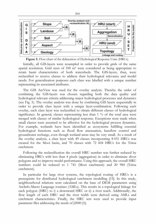
264
Figure 5. Flow-chart of the delineation of Hydrological Response Units (HRUs).
Initially, all GIS-layers were resampled in order to provide grids of the same spatial resolution. Grid sizes of 100 m² were considered as being appropriate to retain basin characteristics of both watersheds. The GIS-layers, than, were reclassified to receive classes to address their hydrological relevance and model needs. For generalization purposes each class was labelled with a unique number representing its associated attributes.
The GIS ArcView was used for the overlay analysis. Thereby the order of combining the GIS-layers was chosen regarding both the data quality and hydrological relevant criteria addressing major hydrological processes and dynamics (see Fig. 5). The overlay analysis was done by combining GIS layers sequentially in order to provide class layers with a unique layer-combination. Following each overlay, each class layer was reclassified to obtain different classes of hydrological significance. In general, classes representing less than 1 % of the total area were merged with classes of similar hydrological response. Exceptions were made when small classes were assumed to be affective for the hydrological process dynamics. For example, wetlands have been identified as ecosystems fulfilling essential hydrological functions such as flood flow attenuation, baseflow control and groundwater recharge, even though wetland areas may be very small. As a result of the overlay analysis, a class layer with 49 classes incorporating 8 031 HRUs was created for the Mooi basin, and 70 classes with 72 604 HRUs for the Tsitsa catchment.
Following the reclassification the overall HRU number was further reduced by eliminating HRUs with less than 4 pixels (aggregation) in order to eliminate sliver polygons and to improve model performance. Using this approach, the overall HRU numbers could be reduced to 1 741 (Mooi catchment) and 20 984 (Tsitsa catchment).
In particular for large river systems, the topological routing of HRUs is a prerequisite for distributed hydrological catchment modelling [15]. In this study, neighbourhood relations were calculated on the base of DEM parameters using ArcInfo-Macro Language routines (AMLs). This results in a topological linkage for each polygon (HRU) to i) a downward HRU or ii) a river reach. Additionally, the flow length of each HRU and the river width were derived using AMLs and catchment characteristics. Finally, the HRU sets were used to provide input parameter files addressing the needs of J2000 [1].
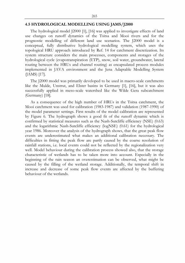
265
4.5 HYDROLOGICAL MODELLING USING JAMS/J2000
The hydrological model J2000 [1], [16] was applied to investigate effects of land use changes on runoff dynamics of the Tsitsa and Mooi rivers and for the prognostic modelling of different land use scenarios. The J2000 model is a conceptual, fully distributive hydrological modelling system, which uses the topological HRU approach introduced by Ref. 14 for catchment discretization. Its system structure considers the main processes, components and storages of the hydrological cycle (evapotranspiration (ETP), snow, soil water, groundwater, lateral routing between the HRUs and channel routing) as encapsulated process modules implemented in JAVA environment and the Jena Adaptable Modelling System (JAMS) [17].
The J2000 model was primarily developed to be used in macro-scale catchments like the Mulde, Unstrut, and Elster basins in Germany [1], [16], but it was also successfully applied in meso-scale watershed like the Wilde Gera subcatchment (Germany) [18].
As a consequence of the high number of HRUs in the Tsitsa catchment, the Mooi catchment was used for calibration (1983-1987) and validation (1987-1990) of the model parameter settings. First results of the model calibration are represented by Figure 6. The hydrograph shows a good fit of the runoff dynamic which is confirmed by statistical measures such as the Nash-Sutcliffe efficiency (NSE) (0.63) and the logarithmic Nash-Sutcliffe efficiency (logNSE) (0.61) for the hydrological year 1986. Moreover the analysis of the hydrograph shows, that the great peak flow events are underestimated what makes an additional calibration necessary. The difficulties in fitting the peak flow are partly caused by the coarse resolution of rainfall stations, i.e. local events could not be reflected by the regionalization very well. Model behaviour during the calibration process showed also, that the storage characteristic of wetlands has to be taken more into account. Especially in the beginning of the rain season an overestimation can be observed, what might be caused by the filling of the wetland storage. Additionally, the temporal shift in increase and decrease of some peak flow events are affected by the buffering behaviour of the wetlands.
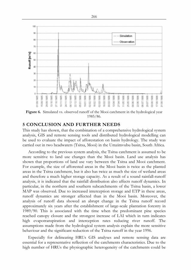
266
Figure 6. Simulated vs. observed runoff of the Mooi catchment in the hydrological year
1985/86.
5 CONCLUSION AND FURTHER NEEDS This study has shown, that the combination of a comprehensive hydrological system analysis, GIS and remote sensing tools and distributed hydrological modelling can be used to evaluate the impact of afforestation on basin hydrology. The study was carried out in two headwaters (Tsitsa, Mooi) in the Umzimvubu basin, South Africa.
According to the previous system analysis, the Tsitsa catchment is assumed to be more sensitive to land use changes than the Mooi basin. Land use analysis has shown that proportions of land use vary between the Tsitsa and Mooi catchment. For example, the size of afforested areas in the Mooi basin is twice as the planted areas in the Tsitsa catchment, but it also has twice as much the size of wetland areas and therefore a much higher storage capacity. As a result of a sound rainfall-runoff analysis, it is indicated that the rainfall distribution also affects runoff dynamics. In particular, in the northern and southern subcatchments of the Tsitsa basin, a lower MAP was observed. Due to increased interception storage and ETP in these areas, runoff dynamics are stronger affected than in the Mooi basin. Moreover, the analysis of runoff data showed an abrupt change in the Tsitsa runoff record approximately six years after the establishment of large-scale plantation forestry in 1989/90. This is associated with the time when the predominant pine species reached canopy closure and the strongest increase of LAI which in turn indicates high evapotranspiration and interception rates reducing river runoff. The assumptions made from the hydrological system analysis explain the more sensitive behaviour and the significant reduction of the Tsitsa runoff in the year 1996.
Especially for delineating HRUs GIS analyses and remote sensing data are essential for a representative reflection of the catchments characteristics. Due to the high number of HRUs the physiographic heterogeneity of the catchments could be
267
obtained. A first run of the parameterized subcatchment Mooi provided a good fit of the observed and simulated runoff dynamics. The result obtained by the first application of J2000 in semiarid areas on the southern hemisphere shows that the hydrological processes are well represented in the model. Since the parameter set used for the modelling of Mooi catchment provided reliable results, model parameters addressing the hydrological processes can be transferred to the Tsitsa catchment.
Further studies will focus on the validation and transferability of the model to the Tsitsa catchment as well as a quantitative assessment of the runoff behaviour after land use change. Additionally the analysis of different realistic land use scenarios and their effects to water resources are planed. Addressing the increasing water demand also different water management scenarios will be taken into account. Depending on further developments of JAMS/J2000 the display of the single runoff components for every single HRU and every time step will help to point out the most important areas for runoff and ground water generation.
ACKNOWLEDGMENTS The authors would like to thank the German Research Foundation (DFG) for
project funding. Acknowledgements are also given to Dr. P. Krause (FSU Jena), Dr. S. Lorentz (SBEEH, South Africa) and Mondi Forests Ltd. (South Africa) for scientific, data and logistical support.
REFERENCES 1 Krause, P., 2001: Das hydrologische Modellsystem J2000. Beschreibung und Anwendung
in großen Flußgebieten. In: Schriften des Forschungszentrums Jülich, 29. 2 Helmschrot, J., Lorentz, S., Flügel, W.A., 2005: Integrated wetland and landscape
modeling. A case study from the Eastern Cape Province, South Africa. In: Zerger, A., Argent, R.M. (eds.): MODSIM 2005 International Congress on Modelling and Simulation. Modelling and Simulation Society of Australia and New Zealand, pp. 1382-1388.
3 Karpeta, P., Johnson, M.R., 1979: The geology of the Umtata area. Explanation to the geological map, sheet 3128, scale 1:250 000. Geological Survey, Pretoria, 16 pp.
4 Herbert, M., 1997: Report on a site evaluation study of the estates Glen Cullen and Chillingly, Maclear District. Presentation of field data on topography, lithology, soils vegetation and climate from a sire transect survey, and discussion on findings and recommendations for optimal silvicultural operations for forestry production. Private Report prepared for North East Cape Forest, 88 pp. (unpubl.).
5 Helmschrot, J., 2006: An integrated, landscape-based approach to model the formation and hydrological functioning of wetlands in semiarid headwater catchments of the Umzimvubu River, South Africa. Friedrich-Schiller-Universität Jena, Dissertation, pp. 278.
6 Smakhtin, V.Y, Hughes, D.A., Creuse-Naudin, E., 1997: Regionalization of daily flow characteristics in part of the Eastern Cape, South Africa. Hydrological Sciences 42, pp. 919-936.
7 Schulze, R.E, 1997: South African Atlas of Agrohydrology and -Climatology. Water Research Commission, Pretoria, South Africa, WRC Report TT82/96, pp. 276.
8 Helmschrot, J., Flügel, W.A. 2002: Land use characterization and change detection analysis for hydrological model parameterisation of large scale afforested areas using remote sensing. Physics and Chemistry of the Earth 27: 711-718.
268
9 Dahlke, H., Helmschrot, J., Behrens, T., 2005: A GIS-based terrain analysis approach for inventory of wetland in the semi-arid headwaters of the Umzimvubu basin, South Africa. In: Erasmi, S., Cyffka, B., Kappas, M. 2005: Remote Sensing and GIS for Environmental Studies. Göttinger Geographische Abhandlungen 113, pp. 78-86.
10 Dijkshoorn, J.A., 2003: SOTER Data Base for South Africa (SOTERSAF). Technical Report, International Soil Reference and Information Centre. Wageningen,
11 Department of Mines, 1977: 1:250 000 Geological Series, 3128 Umtata, Pretoria. 12 Watson, D.F., Philip, G.M., 1985: A Refinement of Inverse Distance Weighted
Interpolation. In: Geo-Processing 2, pp. 315-327. 13 Forsyth, G.G., Versfeld, D.B., Chapman, R.A., Fowöes, B.K., 1997: The hydrological
implications of afforestation in the North-Eastern Cape. WRC Report No 511/1/97, Water Research Commission, Stellenbosch, pp. 134.
14 Flügel, W.A., 1995: Delineating hydrological response units (HRUs) by GIS analysis for regional hydrological modelling using MMS/PRMS in the drainage basin of the River Bröl, Germany. Hydrological Processes 9, pp. 423-436.
15 Staudenrausch, H., 2001: Untersuchungen zur hydrologischen Topologie von Landschaftsobjekten für die distributive Flussgebietsmodellierung. Friedrich-Schiller-Universität Jena. Dissertation.
16 Krause, P., 2002: Quantifying the impact of land use changes on the water balance of large catchments using the J2000 model. In: Physics and Chemistry of the Earth, 27, pp. 663-673.
17 Krause, P., Kralisch, S., 2005: The hydrological modelling system J2000 - knowledge core for JAMS. In: Zerger, A.; ARGENT, R.M. (ed.): MODSIM 2005 International Congress on Modelling and Simulation Modelling and Simulation Society of Australia and New Zealand, December 2005, pp. 676–682.
18 Bäse, F., 2005: Beurteilung der Parametersensitivität und der Vorhersagesicherheit am Beispiel des hydrologischen Modells J2000. Friedrich-Schiller-Universität Jena. Diplomarbeit, pp.86. (http://www.geogr.uni-jena.de/fileadmin/Geoinformatik/Lehre/Diplomarbeiten/DA_Baese.pdf).
269
Microwave remote sensing of hydrology in southern Africa
A. Bartscha, K. Scipala, P. Wolskib, C. Pathea, D. Sabela, W. Wagnera a Institute of Photogrammetry and Remote Sensing, Vienna University of
Technology, Gusshausstraße 27-29, 1040 Vienna, Austria, email: [email protected]
b Harry Oppenheimer Okavango Research Centre, private bag 285, Maun, Botswana
ABSTRACT ScanSAR systems such as ENV28ISATs ASAR Global Mode allow for monitoring of dynamic processes at medium resolution. Hence, they are especially useful for monitoring hydrologic processes such as soil moisture and inundation dynamics. In this paper, we present two studies which investigate the capabilities of ScanSAR ASAR Global Mode (1 km resolution) on the southern African subcontinent. One study focuses on the monitoring of the Okavango delta, Botswana. Temporal and spatial dynamics for the year 2005 have been investigated on approximately monthly time steps. The second study, SHARE, aims at enabling an operational soil moisture monitoring service for the region of the Southern African Development Community (SADC) by using ASAR Global Mode data in combination with ERS/METOP scatterometer data to build a synergistic 1 km soil moisture product. In this study, ASAR Global Mode data is used in two ways: Firstly, it is used directly to retrieve soil moisture information using a simple change detection algorithm; secondly, a scaling layer is defined which allows enhanced interpretation of coarse resolution (25 km) scatterometer data. Keywords: Southern Africa, satellite radar, soil moisture, wetlands, monitoring.
1 INTRODUCTION Radar signals are strongly dependent on hydrological conditions in addition to surface roughness and vegetation structure. Thus the analysis of radar time series allow the detection of environmental processes that are important for the functioning of terrestrial biota, in particular inundation dynamics, soil moisture and freeze-thaw changes. Results from a range of microwave sensors have shown a large potential for hydrological applications. For example, coarse resolution scatterometer data have been used successfully for global soil moisture monitoring [1]. Currently, our group at TU Wien develops algorithms foreseen to be implemented at EUMETSAT for operational Near Real Time (NRT) processing data from the METOP satellite series [2]. Beside scatterometers ScanSAR systems hold a large potential for the monitoring of hydrologic processes [3]. Systems such as ENVISATs ASAR Global Mode allow analyses on better spatial scale compared to scatterometers at the cost of reduced temporal resolution. In this paper we present two recent studies which investigate the capabilities of ScanSAR ASAR Global Proc. 2nd Göttingen GIS and Remote Sensing Days, 4-6 Oct. 2006, Göttingen
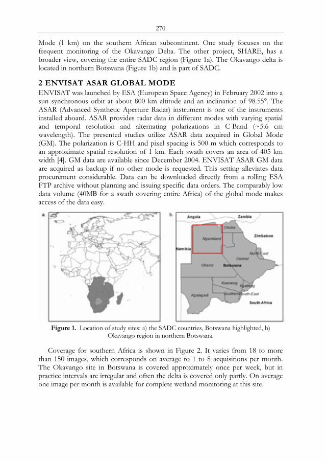
270
Mode (1 km) on the southern African subcontinent. One study focuses on the frequent monitoring of the Okavango Delta. The other project, SHARE, has a broader view, covering the entire SADC region (Figure 1a). The Okavango delta is located in northern Botswana (Figure 1b) and is part of SADC.
2 ENVISAT ASAR GLOBAL MODE ENVISAT was launched by ESA (European Space Agency) in February 2002 into a sun synchronous orbit at about 800 km altitude and an inclination of 98.55°. The ASAR (Advanced Synthetic Aperture Radar) instrument is one of the instruments installed aboard. ASAR provides radar data in different modes with varying spatial and temporal resolution and alternating polarizations in C-Band (~5.6 cm wavelength). The presented studies utilize ASAR data acquired in Global Mode (GM). The polarization is C-HH and pixel spacing is 500 m which corresponds to an approximate spatial resolution of 1 km. Each swath covers an area of 405 km width [4]. GM data are available since December 2004. ENVISAT ASAR GM data are acquired as backup if no other mode is requested. This setting alleviates data procurement considerable. Data can be downloaded directly from a rolling ESA FTP archive without planning and issuing specific data orders. The comparably low data volume (40MB for a swath covering entire Africa) of the global mode makes access of the data easy.
Figure 1. Location of study sites: a) the SADC countries, Botswana highlighted, b)
Okavango region in northern Botswana.
Coverage for southern Africa is shown in Figure 2. It varies from 18 to more than 150 images, which corresponds on average to 1 to 8 acquisitions per month. The Okavango site in Botswana is covered approximately once per week, but in practice intervals are irregular and often the delta is covered only partly. On average one image per month is available for complete wetland monitoring at this site.
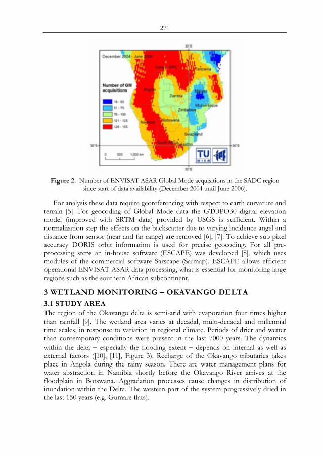
271
Figure 2. Number of ENVISAT ASAR Global Mode acquisitions in the SADC region
since start of data availability (December 2004 until June 2006).
For analysis these data require georeferencing with respect to earth curvature and terrain [5]. For geocoding of Global Mode data the GTOPO30 digital elevation model (improved with SRTM data) provided by USGS is sufficient. Within a normalization step the effects on the backscatter due to varying incidence angel and distance from sensor (near and far range) are removed [6], [7]. To achieve sub pixel accuracy DORIS orbit information is used for precise geocoding. For all pre-processing steps an in-house software (ESCAPE) was developed [8], which uses modules of the commercial software Sarscape (Sarmap). ESCAPE allows efficient operational ENVISAT ASAR data processing, what is essential for monitoring large regions such as the southern African subcontinent.
3 WETLAND MONITORING – OKAVANGO DELTA
3.1 STUDY AREA The region of the Okavango delta is semi-arid with evaporation four times higher than rainfall [9]. The wetland area varies at decadal, multi-decadal and millennial time scales, in response to variation in regional climate. Periods of drier and wetter than contemporary conditions were present in the last 7000 years. The dynamics within the delta − especially the flooding extent − depends on internal as well as external factors ([10], [11], Figure 3). Recharge of the Okavango tributaries takes place in Angola during the rainy season. There are water management plans for water abstraction in Namibia shortly before the Okavango River arrives at the floodplain in Botswana. Aggradation processes cause changes in distribution of inundation within the Delta. The western part of the system progressively dried in the last 150 years (e.g. Gumare flats).
272
3.2 RESULTS The 2005 flood in its maximum extent covered areas corresponding roughly to the regularly inundated zone. The largest expansion of the flood (the difference between annual maximum and annual minimum inundation extent) was observed in the SW part of the system, while in the NE part the flood expansion was smaller. Such behavior corresponds to the known differences in dynamics of inundation between these parts of the Delta.
The year 2005 was characterized by below average rainfall and inflow. The maximum wet area was, however, 6670 km² (Figure 4 and 5; excl. 300 km² of upper pan handle) larger than the 1985-2004 mean maximum inundation area (6280 km²). This reflects the influence of antecedent conditions on flooding in the Okavango Delta (Figure 3): flood of the preceding year 2004 was very large, reaching 10.000 km².
Figure 3. Internal and external factors influencing inundation patterns/wetland
maintenance in the Okavango delta.
Figure 4. Wet area in km² (note: not equal to inundated area especially during rain season) for each acquisition date 2005 within the delta (excluding upper pan handle, approximately.
300 km², see Figure 4).
273
Figure 5. Wet areas (blue) at end of rain season (April), first half dry season (May) and
maximum inundation (September). Grey – delta extent
4 ‘SHARE’ – ENHANCED SOIL MOISTURE MONITORING
4.1 THE PROJECT SHARE is a project funded within the framework of the ESA TIGER initiative. SHARE aims at enabling an operational soil moisture monitoring service for the region of the Southern African Development Community (SADC) by using ASAR Global Mode data and ERS/METOP scatterometer data. With its service it addresses today’s most severe obstacle in water resource management which is the lack of availability of reliable soil moisture information on a dynamic basis (weakly coverage or better). It is the aim of SHARE to develop an experimental medium resolution (1 km) soil moisture indicator solely based on ENVISAT GM data using a simple change detection algorithm. Additionally SHARE provides access to a coarse resolution (25 km) soil moisture product from ERS/METOP scatterometers together with a scaling layer (derived from ScanSAR data) which allows interpretation of the coarse resolution soil moisture product at 1 km resolution. 4.2 THE EXPERIMENTAL SOIL MOISTURE INDICATOR The experimental soil moisture indicator is a 1 km resolution soil moisture product based on a data driven change detection approach showing soil moisture changes of the topmost soil layer scaled between a low and a high backscatter limit. Change detection has been found to be a powerful tool for the retrieval of geophysical parameters from radar data [12]. Especially in practical applications it was found to be more useful than physical based retrievals. In several studies the potential of change detection has been outlined. For example, based on 32 ERS SAR images (C-band) acquired over the Orgeval watershed in France [13] developed a methodology for retrieving soil moisture. The algorithm was based on a selection of “sensitive targets”, for which vegetation and surface roughness effects can easily be estimated and removed if needed. The results of this study suggested that at the watershed scale the mean effect induced by different mixed roughness states is about constant during the year. Similar studies further demonstrated that change detection approaches for retrieving soil moisture at regional scales from C-band SAR time series can successfully account for surface roughness effects and to some extent for low vegetation cover [14], [15].
The foreseen method relates each radar backscatter measurement to a reference backscatter value. This reference value is derived from a pixel specific backscatter time series. In a first step, no roughness and vegetation correction is applied, as a
274
static influence of soil surface roughness and vegetation cover is assumed. We are well aware that this is a critical simplification as especially vegetation may exhibit a seasonal cycle. However, regarding from a time series perspective the sensitivity of C-band backscatter to soil moisture is much stronger than the sensitivity to changes in vegetation. The effect of vegetation growth on backscatter is even less strong in case of HH polarization, as used for ENVISAT ASAR GM mode, as for the VV polarized scatterometer data. Therefore, in a first step we neglect vegetation effects, which is the main reason for calling the ENVISAT ASAR GM products "experimental" soil moisture products. For a correct description of seasonal effects external data sets would be required in order to account for the multi incidence angle observations and for the noise and speckle effects inherent in the Global Mode backscatter observations. In contrast to vegetation, for surface roughness there is evidence that at the scale of Global Mode data temporal effects can be neglected. [16] found that at the scale of the watershed, field-specific roughness effects are averaged out for C-band ERS data. A similar observation was made by [17] who observed a high correlation between backscatter and soil moisture at catchment scale and a decrease in correlation at more detailed scales. 4.3 THE SCALING LAYER In 2002 TU Wien produced the first, global remotely sensed soil moisture dataset based on data acquired with the scatterometer on board of the European Satellites ERS-1 and ERS-2 [1]. Since the year 2002 the data have been distributed to about 100 users worldwide, which lead to the increasing acceptance of this technology and a growing number of research papers that investigate the quality and application potential of scatterometer soil moisture data. Amongst the first research users of the soil moisture products are meteorological services and research centres such as Met Office UK, Météo-France/CNRM and the European Centre for Medium Range Weather Forecasting (ECMWF). Currently, TU Wien is developing on behalf of EUMETSAT software for near-real-time processing of global ASCAT Level 2 surface soil moisture data in orbit geometry. It is planned to implement the operational system at EUMETSAT's central processing facility in Darmstadt, Germany, by 2008 in order to distribute the ASCAT Level 2 data over EUMETCast within 135 minutes after sensing.
To facilitate the use of this data in hydrologic applications such as flash flood forecasting, SHARE will develop a scaling layer. The scaling layer allows the interpretation of coarse resolution soil moisture information at 1 km resolution by identifying targets which have similar backscatter characteristics at local (observed with the ENVISAT ASAR Global Mode sensor) and regional (observed with the ERS/METOP scatterometers) scale. For these targets soil moisture trends observed in the coarse resolution product can be used instantaneously at 1 km scale.
The retrieval of the scaling layer is based on a well established concept in hydrologic sciences to describe the relation between local and regional soil moisture. This concept is known as "temporal stability" method and was introduced by [18] in 1985. Since then the method has for example been used by [19] and by [20] to describe the relation between local in-situ soil moisture data and regional soil moisture trends. In the SHARE project we envisage to apply this concept to
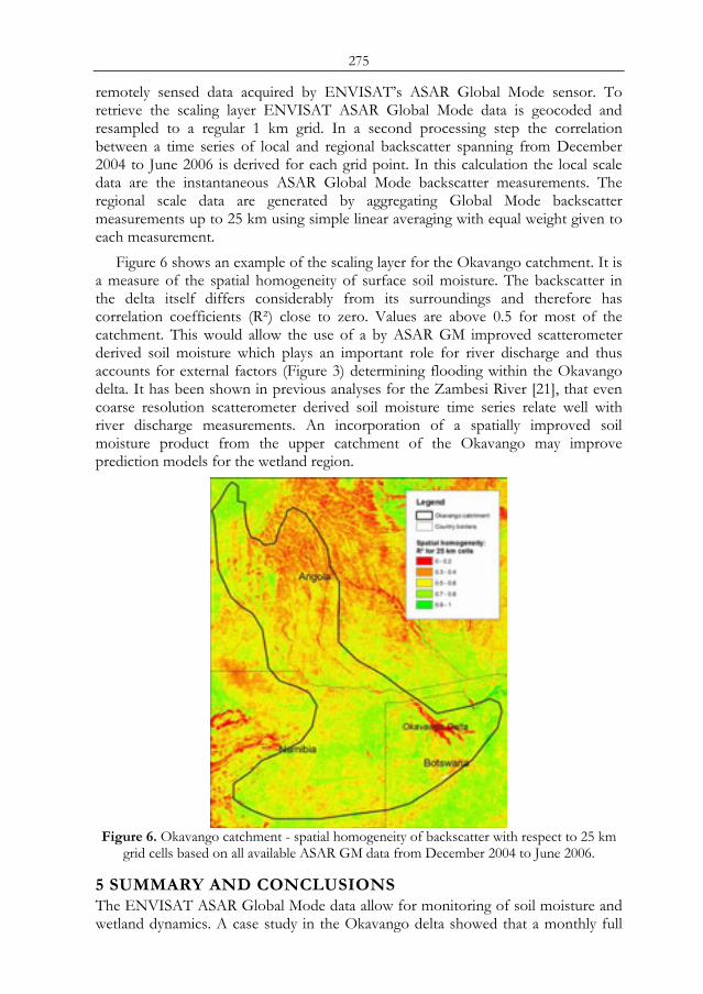
275
remotely sensed data acquired by ENVISAT’s ASAR Global Mode sensor. To retrieve the scaling layer ENVISAT ASAR Global Mode data is geocoded and resampled to a regular 1 km grid. In a second processing step the correlation between a time series of local and regional backscatter spanning from December 2004 to June 2006 is derived for each grid point. In this calculation the local scale data are the instantaneous ASAR Global Mode backscatter measurements. The regional scale data are generated by aggregating Global Mode backscatter measurements up to 25 km using simple linear averaging with equal weight given to each measurement.
Figure 6 shows an example of the scaling layer for the Okavango catchment. It is a measure of the spatial homogeneity of surface soil moisture. The backscatter in the delta itself differs considerably from its surroundings and therefore has correlation coefficients (R²) close to zero. Values are above 0.5 for most of the catchment. This would allow the use of a by ASAR GM improved scatterometer derived soil moisture which plays an important role for river discharge and thus accounts for external factors (Figure 3) determining flooding within the Okavango delta. It has been shown in previous analyses for the Zambesi River [21], that even coarse resolution scatterometer derived soil moisture time series relate well with river discharge measurements. An incorporation of a spatially improved soil moisture product from the upper catchment of the Okavango may improve prediction models for the wetland region.
Figure 6. Okavango catchment - spatial homogeneity of backscatter with respect to 25 km
grid cells based on all available ASAR GM data from December 2004 to June 2006.
5 SUMMARY AND CONCLUSIONS The ENVISAT ASAR Global Mode data allow for monitoring of soil moisture and wetland dynamics. A case study in the Okavango delta showed that a monthly full
276
coverage is possible for an area of this size (150 km x 150 km area of interest) and location. As the priority for certain ASAR modes vary, time steps are irregular. The entire available Global Mode data set (since December 2004) can be used to derive a scaling layer which is a measure of spatial heterogeneity of backscatter and thus soil moisture. It allows for improving coarse spatial but good temporal resolution relative soil moisture data which are derived from scatterometer measurements. Such a scaling layer has been created for the entire southern African subcontinent. It is anticipated to enable an operational soil moisture monitoring service for the SADC region. In case of the Okavango wetland area, it may contribute to an enhanced modeling of external factors of flooding dynamics.
ACKNOWLEDGMENTS The SHARE project is funded under the umbrella of the ESA TIGER initiative. The operational processing chain for ENVISAT ASAR data has been developed in conjunction with the MISAR project which has been funded by the Austrian Science Fund (FWF). The GTOPO30 DEM is available by courtesy of USGS.
REFERENCES 1 Wagner, W., Scipal, K., Pathe, C., Gerten, D., Lucht, W., and Rudolf, B., 2003:
Evaluation of the agreement between the first global remotely sensed soil moisture data with model and precipitation data. Journal of Geophysical Research – Atmospheres 108(D19), 4611.
2 Hasenauer, S., Wagner, W., Scipal, K., Naeimi, V., Bartalis, Z., 2006: Implementation of near real-time soil moisture products in the SAF network based on MetOp ASCAT data. Proceedings EUMETSAT Meteorological Satellite Conference, 12 - 16 June, Helsinki, Finland.
3 Wagner, W., Scipal, K., Bartsch, A., and Pathe, C., 2005: ENVISAT’s capabilities for Global Monitoring of the Hydrosphere. Proceedings IGARSS 25-26 June, Seoul.
4 Desnos, Y.-L., Buck, C., Guijarro, J., Suchail, J.-L., Torres, R., and Attema, E., 2000: ASAR- Envisat´s Advanced Synthetic Aperture Radar. Building on ERS Achievements towards Future Watch Missions. ESA Bulletin 102, pp. 91-100.
5 Meier, E., Frei, U., and Nüesch, D., 1993: Precise Terrain Corrected Geocoded Images. In: Schreier, G. (ed.): SAR geocoding: data and systems. Wichmann, Karlsruhe.
6 Roth, A., Craubner, A., and Hügel, T., 1993: Standard Geocoded Ellipsoid Corrected Images. In: Schreier, G. (ed.): SAR geocoding: data and systems. Wichmann, Karlsruhe.
7 van Zyl, J., Chapman, B., Dubois, P., and Shi, J., 1993: The effect of the topography on SAR calibration. IEEE Trans. Geoscience Rem. Sens. 31(5), pp. 1036-1043.
8 Pathe, C., and Wagner, W., 2004: Soil moisture estimation on a regional scale using ENVISAT ASAR wide swath images. Proceedings International Symposium on Retrieval of Bio- and Geophysical Parameters from SAR Dat for Land Applications, Innsbruck 16 -19 Nov.
9 Ringrose, S., Jellema, A., Hunstman-Mapila, P., Baker, L., and Brubaker, K., 2005: Use of remotely sensed data in the analysis of soil-vegetation changes along a drying gradient peripheral to the Okavango Delta, Botswana. International Journal of Remote Sensing 26 (19), pp. 4293-4319.
10 Gumbricht, T., Wolski, P., Frost, P., and McCarthy, T.S., 2004: Forecasting the spatial extent of the annual flood in the Okavango delta, Botswana. Journal of Hydrology 290, pp. 178-191.
11 Wolski, P., and Savenije, H.H.G., in press: Dynamics of floodplain-island groundwater flow in the Okavango Delta, Botswana. Journal of Hydrology.
12 Wagner, W., and Pathe, C., 2005: Has SAR failed in soil moisture retrieval? Proceedings ENVISAT & ERS Symposium, Salzburg, Austria, 6-10 September 2004.

277
13 Quesney, A., Hégarat-Mascle, S. L., Taconet, O., Vidal-Madjar, D., Wigneron, J. P., Loumagne, C., and Normand, M., 2000: Estimation of Watershed Soil Moisture Index from ERS/SAR Data. Remote Sensing of Environment 72, pp. 290-303.
14 Moran, M. S., Hymer, D. C., Qi, J. G. and Sano, E. E., 2000: Soil moisture evaluation using multi-temporal synthetic aperture radar (SAR) in semiarid rangeland. Agricultural and Forest Meteorology 105(1-3), pp. 69-80.
15 Oldak, A., Pachepsky, Y. A., Jackson, T. J., and Rawls, W. J., 2002: Statistical properties of soil moisture images revisited. Journal of Hydrology 255, pp. 12-24.
16 Cognard, A.-L., Loumagne, C., Normand, M., Olivier, P., Ottlé, C., Vidal-Madjar, D., Louahala, S., and Vidal, A., 1995: Evaluation of the ERS 1/synthetic aperture radar capacity to estimate surface soil moisture: two-year results over the Naizin watershed. Water Resources Research 31(4), pp. 975-982.
17 Alvarez-Mozos, J., Casali, J., Gonzalez-Audicana, M., and Verhoest, N. E. C., 2005: Correlation between ground measured soil moisture and RADARSAT-1 derived backscatter coefficient over an agricultural catchment of Navarre (North of Spain). Biosystems Engineering 92(1), pp. 119-133.
18 Vauchaud, G., d. Silans, A. P., Balabanis, P., and Vauclin, M., 1985: Temporal Stability of Spatially Measured Soil Water Probability Density Function. Soil Science Society of America 49, pp. 822-828.
19 Cosh, M. H., Jackson, T. J., Bindlish, R., and Prueger, J. H., 2004: Watershed scale temporal and spatial stability of soil moisture and its role in validating satellite estimates. Remote Sensing of Environment 92, pp. 427-435.
20 Martínez-Fernández, J., and Ceballos, A., 2005: Mean soil mositure estimation using temporal stability analysis. Journal of Hydrology 312, pp. 28-38.
21 Scipal, K., Scheffler, C., and Wagner, W., 2005. Soil Moisture Runoff Relation at the Catchment Scale as Observed with Coarse Resolution Microwave Remote Sensing. Hydrology and Earth System Sciences 2(2), pp. 417-448.

278
279
ASSESSMENT OF SUSPENDED SEDIMENT CONCENTRATION IN SURFACE WATER USING
REMOTE SENSING
A. M. Bhatti, S. Nasu, M. Takagi Department of Infrastructure Systems Engineering, Kochi University of
Technology, Tosayamada-cho, Kami-City, Kochi, 782-8502, Japan, email: [email protected]
ABSTRACT Remote sensing is an effect29ive tool for the assessment of suspended sediment in surface water. Experiments were conducted in the laboratory to investigate the spectral response of suspended sediments concentration, distribution and settling with time. A hyperspectral Field SpecPro FR Spectroradiometer was used to measure reflectance from the water in the electromagnetic spectrum region of 400 nm to 900 nm. Reflectance of water with varying concentration of clayey red soil ranging from 50 to 1000 mg/l was measured. Significant change in reflectance was observed for the same suspended sediment concentration (SSC) with time. However, the change of reflectance was more in visible domain. This paper analyses the relation between suspended sediment concentration and the reflectance. The near-infrared (NIR) wavelength was found to be optimum range for assessment of suspended sediment concentration in surface water. Keywords: Remote sensing, Suspended sediment assessment, Optimum range
1 INTRODUCTION High concentration of suspended sediment in water is a critical element in the economic feasibility of a project and could shorten the useful life of reservoirs & dams. It is estimated that approximately 1,100 km3 of sediments have been accumulated in the world’s reservoirs, taking up almost one fifth of the global reservoir storage capacity [1]. The reservoir resulting from the construction of a dam in a river is a site for the sedimentation of solid particles transported by the river, due to the decrease in the flow transport capacity. On the one hand, this sedimentation process has engineering consequences because it leads to a reduction of the storage capacity of the reservoir [2] and, hence, of its efficiency. It is important to incorporate sediment assessment as an integral part of water resources and environmental planning and management. The reason for success of remote sensing in such surveys is the strong positive relationship that exists between SSC and remotely sensed spectral reflectance.
Variations of sediment type (grain size and refractive index) and changing illumination conditions affect the reflectance signal of coastal waters and limit the accuracy of sediment-concentration estimations from remote-sensing measurements [3]. It is believed that the main differences between the two types of waters are Proc. 2nd Göttingen GIS and Remote Sensing Days, 4-6 Oct. 2006, Göttingen
280
located in the 0.4–0.7 m spectral range [4], where the turbid water has significantly larger reflectance than the clear water. This formed the basis for the detection of turbid water and SSC estimation algorithms. If the range of suspended sediments is between 0 and 50 mg/l, reflectance from almost any wavelength will be significantly related to suspended sediment concentrations [5]. As the range of suspended sediments increases to 200 mg/l or higher, curvilinear relationships have to be developed with reflectance in the longer wavelength. Significant relationships have been shown between suspended sediments and radiance or reflectance from spectral wave bands or combinations of wave bands on satellite sensors. Ritchie et al. [6] using in situ studies concluded that wavelengths between 700 and 800 nm were most useful for determining suspended sediments in surface waters.
Suspended sediments are the most common pollutant both in terms of weight and volume in surface waters of freshwater systems. Suspended sediments may serve as a surrogate contaminant in agricultural watersheds since phosphorus, insecticides, and metals adhere to fine sediment particles. Remote sensing is an effective tool for the assessment of suspended sediment in surface water. Numerous researchers have developed algorithms for the relationship between the concentration of suspended sediments and radiance or reflectance. A few studies have taken the next step and used these algorithms to estimate suspended sediments for another time or place [7]. The aim of the study was simply to investigate the relationship between suspended sediment concentration (SSC) and reflectance in a column of water. The objective was to understand the change in reflectance with SSC and change in reflectance for the same SSC with time.
2 METHODS The experiments were performed in Laboratory at Kochi University of Technology. The experiments were carried out in a black painted room to avoid extraneous reflectance. Field SpecPro FR Spectroradiometer (Analytical Devices, Inc., Boulder, CO) was used to collect the upwelling radiance from the water surface. This portable spectrometer combines three spectrometers to cover the wavelength range from 350 to 2500 nm. A photodiode array spectrometer is used to cover the 350 to 1000 nm spectral range (UV/VNIR), while two fast-scanning (0.1 sec) spectrometers provide coverage for the two wavelength ranges from 1001 to 1800 nm and 1801 to 2500 nm (SWIR 1 and SWIR 2). The sampling interval is 1.4 nm. Radiation input to the ASD FieldSpec FR spectrometers is through a fiber optic bundle, 5 meters in length. The fiber optic cable provides the ability to quickly and easily point the spectrometer field of view at different targets, especially when using the pistol grip. The spectroradiometer was calibrated in the laboratory before measuring water surface radiance. The warm up time, sensor height, cable flexure test and illumination angle was measured by making radiance measurements of reference panel in a black room. The reference plaque was a Labsphere white Spectralon of dimensions 12.5cm x 12.5cm.
The clayey red soil samples served as ingredient for sediment loading were collected from the central area of Okinawa Island (coordinates: 26º23´N and 127º73´E). Soil properties are closely related to geological and geomorphological components [8]. The soil sample was air dried and manually sieved to assure
281
uniform grain size. For this study, data from 400 to 900 nm was used because noise was pronounced at wavelength shorter that 400 nm and longer than 900 nm. The sensor was attached to the mechanical arm and positioned over the water at the height of 1 m. Radiance from the water surface with suspended sediments concentration (clayey red soil) ranging from 50 to 1000 mg/l was measured in a black coated water tank. The depth of water column was kept constant at 1 meter. The sediments were kept in suspension by manually stirring at regular intervals. In addition, radiance was measured for the same SSC without stirring after 1,2 and 3 minutes to investigate the effect of SSC distribution on reflectance value.
Reflectance was calculated as a simple ratio between target and reference panel using following equation:
)()()()(% λ
λλλ Cal
SLR ×=
where L(λ) is the radiance measured from the water surface, S(λ) is the radiance from the reference panel and Cal (λ) is the calibration factor for the reference panel. Using this method, all parameters that are multiplicative in nature, such as the spectral irradiance of the illumination source and the optical throughput of the field spectrometer, and present in both the spectral response of a reference sample and the target material, are mathematically eliminated.
3 RESULTS AND DISCUSSION
3.1 EQUIPMENT CALIBRATION The ASD FieldSpec FR spectroradimeter is calibrated in the laboratory to achieve maximum accuracy of radiance measurements. The calibration room was completely darkened, the only source of illumination was the halogen lamp. The instrument’s fiber optic probe is placed in a stationary position at a 45 degree angle to the Spectralon panel. The collection of accurate spectra requires an awareness of the influences of the various sources owing to sensitivity of the instrument. Instrument warm up time, field of view, illumination geometry, sensor height above the water surface and target characteristics must be considered for accurate measurements. The experimental design must be modified to account for the characteristics of the available instrumentation. Experiment was performed by making radiance measurement of reference panel with different warm up time. Sensitivity of spectroradiometer changes with temperature, and this is particularly significant when it is warming up. The measurements were made during instrument warm-up, after the spectrometer was turned on.
282
Figure 1. Reflectance measurement of reference panel with different warm up time after
the spectroradiometer was turned on, a: After 90 minute b: After 120 minute c: After 150 minute d: After 10 minute
Figure 2. Reflectance measurement of reference Panel with different sensor height above the water surface, a: 1.2 meter above the water surface b: 0.5 meter above the water surface
c: 1 meter above the water surface
Figure 3. Reflectance measurement of reference panel with different cable positions, a: one
twist in cable, b: zigzag cable, c: Straight cable d: many twist
Figure 4. Reflectance measurement of reference panel with different illumination angle; a: 60 degree b: 30
The warm up time of 150 minutes was selected and kept for all experiments (fig.1). Also, radiance measurement was taken with different sensor height above the water surface, different illumination angle with constant distance between the reference panel and the light source and different cable placements. Flexure of the cable effect the radiance measurement of the target by changing the signal level. Sensor height of 1 meter above the water surface was selected for all experiments (fig. 2), with straight fiber cable position (fig. 3), and illumination angle of 30 degree
0.94
0.95
0.96
0.97
0.98
0.99
1
400 500 600 700 800 900
Wavelength (nm)
Ref
lect
ance
Fig. 4 a
bc
0.93
0.94
0.95
0.96
0.97
0.98
0.99
1
400 500 600 700 800 900
Wavelength (nm)
Ref
lect
ance
Fig. abc
d
0.9400
0.9500
0.9600
0.9700
0.9800
0.9900
1.0000
400 500 600 700 800 900
Wavelength (nm)
Ref
lect
ance
d
c
a Fig. 1
b
0.94
0.95
0.96
0.97
0.98
0.99
1
400 500 600 700 800 900
Wavelength (nm)
Ref
lect
ance
Fig.
ba
c
283
(fig. 4) was kept during radiance measurement of water surface with varying suspended sediment concentration (SSC). 3.2 SUSPENDED SEDIMENT REFLECTANCE The reflectance spectra were computed for suspended sediment concentration ranging from 50mg/l to 1000 mg/l. The spectral shape is almost similar, however, the magnitude of reflectance increased with increase in SSC as depicted in figure 5. It is noted that reflectance value increased at all wavelengths above 500 nm with the increase in SSC. However from 700 to 900 the reflectance increased systematically with increase in SSC. A strong correlation exists between SSC and reflectance in the red and NIR region. In the present research work the bottom effect was not considered owing to already done research work. At a depth of 80 cm, the bright bottom signal is virtually non-existent when suspended sediment concentrations were above 100mg/l. At wavelengths between 740 and 900nm, bottom brightness has no impact due to the absorption of near-infrared energy by water [9].
Figure 5. Spectral reflectance of water with varying concentration of clayey red soil
The low reflectance value is due to the black coated inner walls of the tank, which absorb much of the incident light. Maximum reflectance is observed in the visible domain from about 550 to 700 nm followed by the second peak at 750 to 850 nm. High absorption is observed beyond 750nm in the near infra-red region. Increases in suspended sediment load lead to a shift in the reflectance spectral profile upwards. The results agreed with work done by the numerous researchers. 3.3 DISTRIBUTION OF SUSPENDED SEDIMENTS WITH DEPTH Assessment of suspended sediment in water bodies is based mainly on assumption of uniform distribution of suspended sediments along the depth. Most of the sediment which is eroded from the land surface is in the form of fine particles which are transported in water courses as a suspended load. These fine sediments account for the turbidity often observed in rivers and their natural fall velocity in water is as low that the natural turbulence maintains them in suspension. A small proportion of the sediment, perhaps around 10%, is courser material which is
0
0.04
0.08
0.12
0.16
0.2
400 500 600 700 800 900Wavelengt h (nm)
Refle
ctan
ce
Clean 50 100
1000
400 300 200
900 7000
284
transported as bed load. These sediments roll along the bed of the river or saltate (hop) close to the bed. Reservoirs act as settling basins for both types of sediment [10]. However, the distribution of sediments is not uniform and varies with depth depending on sediment characteristics, precipitation, run-off, temperature, water flow, and wind speed. Specular reflection from a wind-roughened water surface constitutes a serious problem in the interpretation of spectral data [11].
The objective to perform the experiment was to investigate the effect of non-uniform distribution of suspended sediment on remotely sensed data. Sediments were mixed in water uniformly by manually stirring the water sample for a few minutes. Spectral reflectance of water is measured for the constant amount of sediments immediately after the mixing of sediments. Also for the same concentration of suspended sediments the reflectance signals was measured with time without stirring the water sample.
Figure 6. Spectral reflectance of water with constant concentration of clayey red soil (500
mg/l) a: Spectral reflectance after manual mixing 500mg/l clayey red soil b: spectral reflectance after 1 minute c: Spectral reflectance after 2 minutes d: Spectral reflectance after
3 minutes
Suspended sediments settled with time in the water and reflectance value changed with the change in sediment distribution and caused error in accurate estimation of suspended sediments. With the time the reflectance value decreases for the same amount of sediments owing to settling of sediment with time. Sediment grain size is one of the major factors for the distribution of sediments. These results indicate that the sediment distribution with depth affects the reflectance values significantly.
4 BAND RATIO MODEL DEVELOPMENT Band ratio model was developed to investigate the relationship between suspended sediment and reflectance. This relationship is based on a simple reflectance ratio between near-infrared (825nm) and visible (560 nm) wavelengths. It was observed that strong correlation exists between SSC and the reflectance ratio of near-infrared
0
0.02
0.04
0.06
0.08
0.1
0.12
0.14
400 500 600 700 800 900
Wavelength (nm)
Ref
lect
ance
a
dc
Fig. 6
b
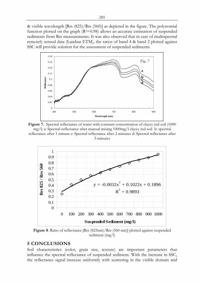
285
& visible wavelength [Rrs (825)/Rrs (560)] as depicted in the figure. The polynomial function plotted on the graph (R2=0.98) allows an accurate estimation of suspended sediments from Rrs measurements. It was also observed that in case of multispectral remotely sensed data (Landsat ETM), the ratios of band 4 & band 2 plotted against SSC will provide solution for the assessment of suspended sediments.
Figure 7. Spectral reflectance of water with constant concentration of clayey red soil (1000
mg/l) a: Spectral reflectance after manual mixing 1000mg/l clayey red soil b: spectral reflectance after 1 minute c: Spectral reflectance after 2 minutes d: Spectral reflectance after
3 minutes
y = -0.0032x2 + 0.1022x + 0.1896R2 = 0.9893
00.10.20.30.40.50.60.70.80.9
1
0 100 200 300 400 500 600 700 800 900 1000
Suspended Sediment (mg/l)
Rrs
825
/ R
rs 5
60
Figure 8. Ratio of reflectance [Rrs (825nm)/Rrs (560 nm)] plotted against suspended
sediment (mg/l)
5 CONCLUSIONS Soil characteristics (color, grain size, texture) are important parameters that influence the spectral reflectance of suspended sediment. With the increase in SSC, the reflectance signal increase uniformly with scattering in the visible domain and
0
0.02
0.04
0.06
0.08
0.1
0.12
0.14
0.16
0.18
400 500 600 700 800 900
Wavelength (nm)
Ref
lect
ance
a
d
Fig. 7
bc

286
absorption in the near-infrared domain. Hence, it was concluded that the visible domain is useful from qualitative point of view and near-infrared wavelength is useful for quantitative assessment. The optimum wavelength for measuring SSC is 750 nm to 900 nm. However, visible wavelength 525nm to 650nm is found to be optimum for characterizing and differentiating suspended sediments. Assessment of suspended sediment concentration is important for basic and applied field application. Effect of suspended sediments distribution on the spectral signatures in water bodies needs to be explored for future research.
ACKNOWLEDGMENTS The research work was financially supported by the Kochi University of Technology, Kochi Japan. The authors wish to acknowledge the financial assistance provided by the University. The assistance of all members of Nasu Lab is gratefully acknowledged.
REFERENCES 1 Mahmood K., 1987: Reservoir sedimentation: impact, extent and mitigation. World Bank
Technical Paper 71. 2 Graf H. W., 1983: The hydraulics of reservoir sedimentation. Water Power Dam
Construct. 35, 45–52. 3 D. Doxaran, Jean-M Froidefond & P. Castaing, 2003: Applied Optics-LP. Volume 42,
Issue 15, pp. 2623-2634. 4 Rong-Rong Li, Yoram J. Kaufman, Bo-Cai Gao, & Curtiss O. Davis, 2003: Remote
Sensing of Suspended Sediments and Shallow Coastal Waters. IEEE Transaction on Geoscience and Remote sensing. Vol. 41, No. 3 PP. 559.
5 Ritchie, J.C. & F.R. Schiebe, 2000: Remote Sensing in Hydrology and Water Management. Water Quality In: G.A. Schultz and E.T. Engman (eds.) Springer-Verlag, Berlin, Germany, pp. 287-303, 351-352.
6 Ritchie, J.C., Schiebe f. R., & Mchenary J. R., 1976: Remote sensing of suspended sediments in surface waters. Photogrammetric Engineering and Remote sensing, 42, 1539-1545.
7 Ritchie J.C. and C. M. Cooper, 1988: Comparison of Measured Suspended Sediment Concentration with Suspended Sediment Concentrations Estimated from Landsat MSS data. Int. Journal of Remote Sensing, Vol. 9, No. 3, pg. 379-387.
8 Buondonno,C., Leone, A. P., Ortolani, F., Pagliuca, S., & Tedeschi, P., 1989a: Rapportitra evoluzione geomorfologica e processi pedogenetici in aree significative della Campania. Bollettino della Societa, Geologica Italiana, 44, 41–51.
9 B. L. Tolk, L. Han & D. C. Rundquist, 2000: The impact of bottom brightness on spectral reflectance of suspended sediments. Int. j. remote sensing, 2000, vol. 21, No. 11, 2259–2268.
10 White W. R., 2005: World water storage in man-made reservoirs. Foundation for Water Research, FR/R0012, April 2005.
11 L. Han, D. C. Rundquist, 1998: The impact of a wind-roughened water surface on remote measurements of turbidity. Int. j. of remote sensing, 1998, vol. 19, no. 1, 195± 201.
287
USE OF REMOTE SENSING FOR MONITORING OF LOGGING IN THE MEKONG REGION – THE
NAM THEUN LOGGING SURVEYS
C. Feldkötter Deutsche Gesellschaft für Technische Zusammenarbeit (GTZ) GmbH, email:
ABSTRACT Remote sensing has long been a popular30 issue in development cooperation being considered as a means to monitor change processes. Yet, operational applications of remote sensing for monitoring purposes are comparatively rare. This is partly due to limitations of the methodology itself and constraints of access to digital technology. Yet, operational monitoring of natural resources degradation, especially logging, is of crucial importance in managing natural resources in developing countries. This paper introduces an approach to operational monitoring of logging based on a combination of high resolution Landsat and SPOT satellite images, simple remote sensing tools and visual interpretation, GPS, and ground / aerial surveillance. The approach has been practically applied and tested in two logging surveys in the catchment of the Nam Theun River in Lao PDR. Its application has demonstrably contributed to a significant reduction of logging activities, and has thus been considered a success by all involved parties. The success is attributed to two main factors, namely the use of appropriate technology, and integration with existing institutional processes. Questions remain as to whether the approach could be scaled up into broader application, which is currently being evaluated in a World Bank supported project in Lao PDR. Keywords: Logging, monitoring, remote sensing, visual interpretation, Lao PDR
1 INTRODUCTION Remote sensing has long been a popular issue in development cooperation in the forestry sector. It has been perceived to be capable of providing development actors with fast and reliable means to monitor change processes, such as forest resources degradation, and devise measures to steer these ([3], [4], [6]).
Yet, operational applications of remote sensing for monitoring purposes in developing and emerging countries, that contribute to devising actual measures on the ground, are comparatively rare. Among the few successful examples are the monitoring of deforestation in the Amazon [7] and monitoring activities in India [8]. Several approaches in the Mekong Basin, such as the Mekong River Commission’s Forest Cover Monitoring Project [6], do not appear to have fulfilled their intended purpose of influencing regional decision making processes. Proc. 2nd Göttingen GIS and Remote Sensing Days, 4-6 Oct. 2006, Göttingen
288
This is partly explained by the fact that remote sensing by itself is typically not considered sufficient as a stand alone tool for monitoring. To a large extent, this may be due to known limitations in the accuracy of conventional remote sensing based approaches, especially under conditions where boundaries between forest and other land cover types are fuzzy, as is frequently the case in the tropics. A few facts on area estimation using remote sensing may illustrate this: (a) Kleinn et al [19] found that for Costa Rica, forest cover figures anywhere within the range of below 20% to above 60% had been published in the 1970s to 90s, many of which were remote-sensing based. (b) Mather [18] reports similar issues in connection with the FAO Forest Resource Assessment process. (c) The Mekong River Commission [20] has reported similar findings, for instance that forest cover figures for the Lao PDR for a given reference date, published by different sources, ranged from 47 to over 80%.
Furthermore, conventional remote sensing based approaches often fail to reliably separate human-induced changes from natural changes. For instance, they often do not differentiate between natural phenomena (such as leaf shedding in a deciduous forest) and genuine human induced change ([4], [5]).
Limitations of technology as such are further compounded by the fact that in developing countries, access to remote sensing technology is often severely constrained, and capacities to use it are limited [21]. This has often lead to approaches, which were overambitious regarding the application of technology or the extent of spatial coverage, and which failed to deliver remote sensing results with practically usable information content on time. For instance, forest cover monitoring approaches were promoted, which used detailed wall to wall mapping [6]. These were typically too slow to deliver information based on which for instance strategic interventions against forest cover change could have been devised in a timely manner.
Yet, monitoring of forest cover change, especially in connection with illegal logging, is of crucial importance in managing natural resources in developing countries. Illegal logging, besides its immediate extractive character, typically creates the initial opening of previously undisturbed areas for unregulated exploitation of natural resources and encroachment, with resulting long term losses in natural resource capital for the national economy. This important role of monitoring, and particularly also of remote sensing, is strongly reflected in recent initiatives such as the Forest Law Enforcement, Governance and Trade (FLEGT) initiative of the European Union [17].
Monitoring must be able to support effective decision making and subsequent action, i.e. must enable effective measures against unwanted developments to be taken early on. In order to do so, monitoring must deliver a sufficiently reliable indication of where change occurs within a short time span of the change actually occurring. The challenge is thus to use remote sensing, which by itself is typically not sufficient to deliver this result, as part of integrated monitoring approaches to the best of its advantage. This can be achieved even in situations where access to technology or skills to use it are limited, as the case study on monitoring of logging in a developing country introduced in this paper will demonstrate.

289
2 CASE STUDY: THE NAM THEUN LOGGING SURVEYS This section introduces the logging surveys undertaken in the Nam Theun river basin of Lao PDR, first in May 2000 [1], and repeated in March 2002 [2]. 2.1 BACKGROUND The Nam Theun river basin, a remote area in the Lao PDR, is the site of a planned hydro-electric project, the 975 megawatt Nam Theun 2 Hydroelectric Dam. The geographical setting of the Nam Theun 2 project is outlined in Figure 1. It shows the planned hydro power project and its surroundings. Construction of the main dam at the north-western end of the inundation area will result in the flooding of parts of the Nakai / Nam Theun National Biodiversity Conservation Area (NBCA, a type of protected area that can roughly be described as Lao PDR’s equivalent of National Parks). The Nakai / Nam Theun NBCA is an area of utmost significance for biodiversity conservation. It is the largest remaining natural forest area in the remote Annamite mountain range that separates the Lao PDR and Vietnam.
In connection with implementation of the Nam Theun 2 project, funding from the World Bank was sought by the Government of the Lao PDR. In this context, agreements on compensation measures for the negative environmental impacts of the dam construction in general and for the loss of parts of the Nakai / Nam Theun NBCA in particular had been reached between the Government of the Lao PDR and the World Bank. These agreements, among other things, stipulated that: (a) An additional protected area (the “Extension” as shown in Figure 1), having a status similar to that of an NBCA, would be established. (b) Salvage logging would take place in the inundation area. (c) Both the Nakai / Nam Theun NBCA and the Extension would be fully protected from logging and road building.
In summary, the Government of the Lao PDR had made a clear commitment to the World Bank about prevention of logging during preparation and implementation of the Nam Theun 2 project.
Two independent bodies, who would act as independent monitors and advise on developments in connection with the progress of the Nam Theun 2 project, had already been in place since the 1990s: the Lao Government’s Panel of Environmental and Social Experts (PoE) and the World Bank’s International Advisory Group (IAG).
In early 2000, there were unconfirmed reports of logging taking place in areas that were, according to the existing agreements, designated as no-logging zones. In reaction to these reports, the 1st logging survey was launched in 2000, with the specific objective to conduct a rigorous field investigation of the Nam Theun 2 area and its surroundings in order to verify these reports, and to provide evidence, based on which corrective measures could be initiated if and as necessary. Furthermore, the logging survey was a continuation of ongoing efforts by the World Bank, the PoE and the IAG and to regularly monitor the status of the area. The 2nd logging survey in 2002 provided a follow up, in order to verify whether the corrective measures initiated after the 1st survey had the desired impact.
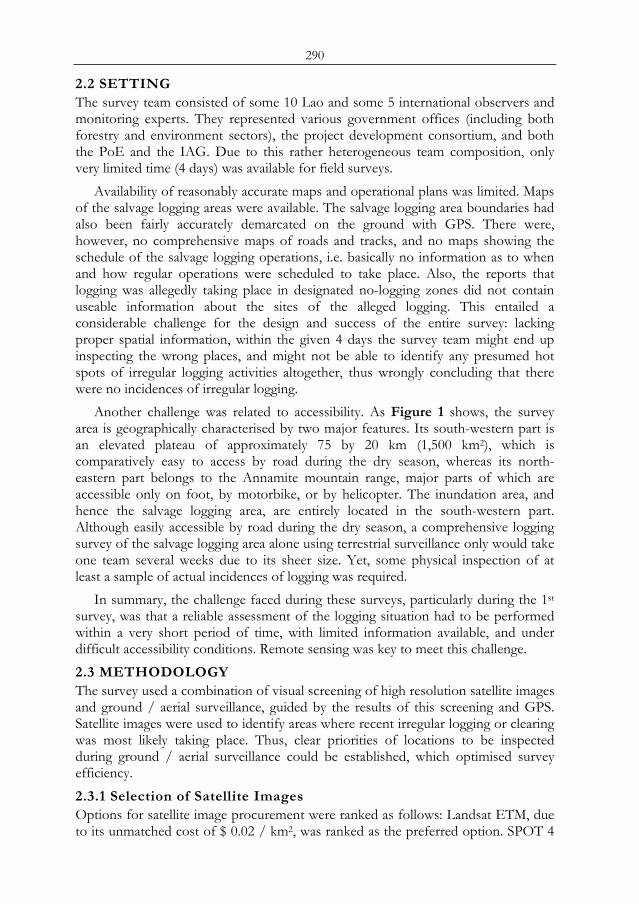
290
2.2 SETTING The survey team consisted of some 10 Lao and some 5 international observers and monitoring experts. They represented various government offices (including both forestry and environment sectors), the project development consortium, and both the PoE and the IAG. Due to this rather heterogeneous team composition, only very limited time (4 days) was available for field surveys.
Availability of reasonably accurate maps and operational plans was limited. Maps of the salvage logging areas were available. The salvage logging area boundaries had also been fairly accurately demarcated on the ground with GPS. There were, however, no comprehensive maps of roads and tracks, and no maps showing the schedule of the salvage logging operations, i.e. basically no information as to when and how regular operations were scheduled to take place. Also, the reports that logging was allegedly taking place in designated no-logging zones did not contain useable information about the sites of the alleged logging. This entailed a considerable challenge for the design and success of the entire survey: lacking proper spatial information, within the given 4 days the survey team might end up inspecting the wrong places, and might not be able to identify any presumed hot spots of irregular logging activities altogether, thus wrongly concluding that there were no incidences of irregular logging.
Another challenge was related to accessibility. As Figure 1 shows, the survey area is geographically characterised by two major features. Its south-western part is an elevated plateau of approximately 75 by 20 km (1,500 km2), which is comparatively easy to access by road during the dry season, whereas its north-eastern part belongs to the Annamite mountain range, major parts of which are accessible only on foot, by motorbike, or by helicopter. The inundation area, and hence the salvage logging area, are entirely located in the south-western part. Although easily accessible by road during the dry season, a comprehensive logging survey of the salvage logging area alone using terrestrial surveillance only would take one team several weeks due to its sheer size. Yet, some physical inspection of at least a sample of actual incidences of logging was required.
In summary, the challenge faced during these surveys, particularly during the 1st survey, was that a reliable assessment of the logging situation had to be performed within a very short period of time, with limited information available, and under difficult accessibility conditions. Remote sensing was key to meet this challenge. 2.3 METHODOLOGY The survey used a combination of visual screening of high resolution satellite images and ground / aerial surveillance, guided by the results of this screening and GPS. Satellite images were used to identify areas where recent irregular logging or clearing was most likely taking place. Thus, clear priorities of locations to be inspected during ground / aerial surveillance could be established, which optimised survey efficiency. 2.3.1 Selection of Satellite Images Options for satellite image procurement were ranked as follows: Landsat ETM, due to its unmatched cost of $ 0.02 / km2, was ranked as the preferred option. SPOT 4
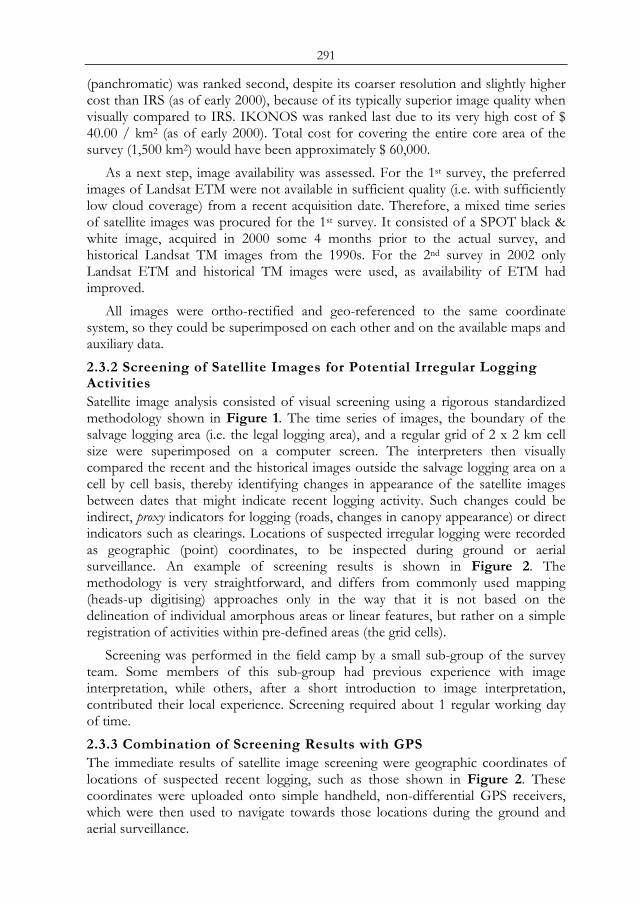
291
(panchromatic) was ranked second, despite its coarser resolution and slightly higher cost than IRS (as of early 2000), because of its typically superior image quality when visually compared to IRS. IKONOS was ranked last due to its very high cost of $ 40.00 / km2 (as of early 2000). Total cost for covering the entire core area of the survey (1,500 km2) would have been approximately $ 60,000.
As a next step, image availability was assessed. For the 1st survey, the preferred images of Landsat ETM were not available in sufficient quality (i.e. with sufficiently low cloud coverage) from a recent acquisition date. Therefore, a mixed time series of satellite images was procured for the 1st survey. It consisted of a SPOT black & white image, acquired in 2000 some 4 months prior to the actual survey, and historical Landsat TM images from the 1990s. For the 2nd survey in 2002 only Landsat ETM and historical TM images were used, as availability of ETM had improved.
All images were ortho-rectified and geo-referenced to the same coordinate system, so they could be superimposed on each other and on the available maps and auxiliary data. 2.3.2 Screening of Satellite Images for Potential Irregular Logging Activities Satellite image analysis consisted of visual screening using a rigorous standardized methodology shown in Figure 1. The time series of images, the boundary of the salvage logging area (i.e. the legal logging area), and a regular grid of 2 x 2 km cell size were superimposed on a computer screen. The interpreters then visually compared the recent and the historical images outside the salvage logging area on a cell by cell basis, thereby identifying changes in appearance of the satellite images between dates that might indicate recent logging activity. Such changes could be indirect, proxy indicators for logging (roads, changes in canopy appearance) or direct indicators such as clearings. Locations of suspected irregular logging were recorded as geographic (point) coordinates, to be inspected during ground or aerial surveillance. An example of screening results is shown in Figure 2. The methodology is very straightforward, and differs from commonly used mapping (heads-up digitising) approaches only in the way that it is not based on the delineation of individual amorphous areas or linear features, but rather on a simple registration of activities within pre-defined areas (the grid cells).
Screening was performed in the field camp by a small sub-group of the survey team. Some members of this sub-group had previous experience with image interpretation, while others, after a short introduction to image interpretation, contributed their local experience. Screening required about 1 regular working day of time. 2.3.3 Combination of Screening Results with GPS The immediate results of satellite image screening were geographic coordinates of locations of suspected recent logging, such as those shown in Figure 2. These coordinates were uploaded onto simple handheld, non-differential GPS receivers, which were then used to navigate towards those locations during the ground and aerial surveillance.
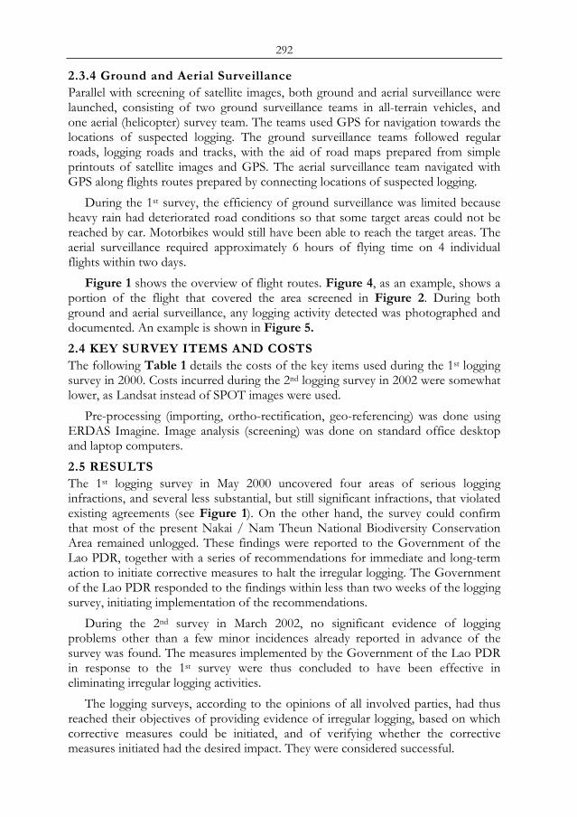
292
2.3.4 Ground and Aerial Surveillance Parallel with screening of satellite images, both ground and aerial surveillance were launched, consisting of two ground surveillance teams in all-terrain vehicles, and one aerial (helicopter) survey team. The teams used GPS for navigation towards the locations of suspected logging. The ground surveillance teams followed regular roads, logging roads and tracks, with the aid of road maps prepared from simple printouts of satellite images and GPS. The aerial surveillance team navigated with GPS along flights routes prepared by connecting locations of suspected logging.
During the 1st survey, the efficiency of ground surveillance was limited because heavy rain had deteriorated road conditions so that some target areas could not be reached by car. Motorbikes would still have been able to reach the target areas. The aerial surveillance required approximately 6 hours of flying time on 4 individual flights within two days.
Figure 1 shows the overview of flight routes. Figure 4, as an example, shows a portion of the flight that covered the area screened in Figure 2. During both ground and aerial surveillance, any logging activity detected was photographed and documented. An example is shown in Figure 5. 2.4 KEY SURVEY ITEMS AND COSTS The following Table 1 details the costs of the key items used during the 1st logging survey in 2000. Costs incurred during the 2nd logging survey in 2002 were somewhat lower, as Landsat instead of SPOT images were used.
Pre-processing (importing, ortho-rectification, geo-referencing) was done using ERDAS Imagine. Image analysis (screening) was done on standard office desktop and laptop computers. 2.5 RESULTS The 1st logging survey in May 2000 uncovered four areas of serious logging infractions, and several less substantial, but still significant infractions, that violated existing agreements (see Figure 1). On the other hand, the survey could confirm that most of the present Nakai / Nam Theun National Biodiversity Conservation Area remained unlogged. These findings were reported to the Government of the Lao PDR, together with a series of recommendations for immediate and long-term action to initiate corrective measures to halt the irregular logging. The Government of the Lao PDR responded to the findings within less than two weeks of the logging survey, initiating implementation of the recommendations.
During the 2nd survey in March 2002, no significant evidence of logging problems other than a few minor incidences already reported in advance of the survey was found. The measures implemented by the Government of the Lao PDR in response to the 1st survey were thus concluded to have been effective in eliminating irregular logging activities.
The logging surveys, according to the opinions of all involved parties, had thus reached their objectives of providing evidence of irregular logging, based on which corrective measures could be initiated, and of verifying whether the corrective measures initiated had the desired impact. They were considered successful.
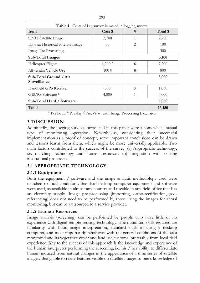
293
Table 1. Costs of key survey items of 1st logging survey. Item Cost $ # Total $
SPOT Satellite Image 2,700 1 2,700 Landsat Historical Satellite Image 50 2 100 Image Pre-Processing 300 Sub-Total Images 3,100
Helicopter Flights 1,200 A 6 7,200 All-terrain Vehicle Use 100 B 8 800 Sub-Total Ground / Air Surveillance
8,000
Handheld GPS Receiver 350 3 1,050 GIS/RS Software C 4,000 1 4,000 Sub-Total Hard / Software 5,050
Total 16,150 A Per hour. B Per day. C ArcView, with Image Processing Extension
3 DISCUSSION Admittedly, the logging surveys introduced in this paper were a somewhat unusual type of monitoring operation. Nevertheless, considering their successful implementation as a proof of concept, some important conclusions can be drawn and lessons learnt from them, which might be more universally applicable. Two main factors contributed to the success of the survey: (a) Appropriate technology, i.e. matching technology and human resources. (b) Integration with existing institutional processes. 3.1 APPROPRIATE TECHNOLOGY
3.1.1 Equipment Both the equipment / software and the image analysis methodology used were matched to local conditions. Standard desktop computer equipment and software were used, as available in almost any country and useable in any field office that has an electricity supply. Image pre-processing (importing, ortho-rectification, geo-referencing) does not need to be performed by those using the images for actual monitoring, but can be outsourced to a service provider. 3.1.2 Human Resources Image analysis (screening) can be performed by people who have little or no experience with digital remote sensing technology. The minimum skills required are familiarity with basic image interpretation, standard skills in using a desktop computer, and most importantly familiarity with the general conditions of the area monitored and its vegetative cover and land use customs, preferably from local field experience. Key to the success of this approach is the knowledge and experience of the human interpreter performing the screening, i.e. his / her ability to differentiate human induced from natural changes in the appearance of a time series of satellite images. Being able to relate features visible on satellite images to one’s knowledge of
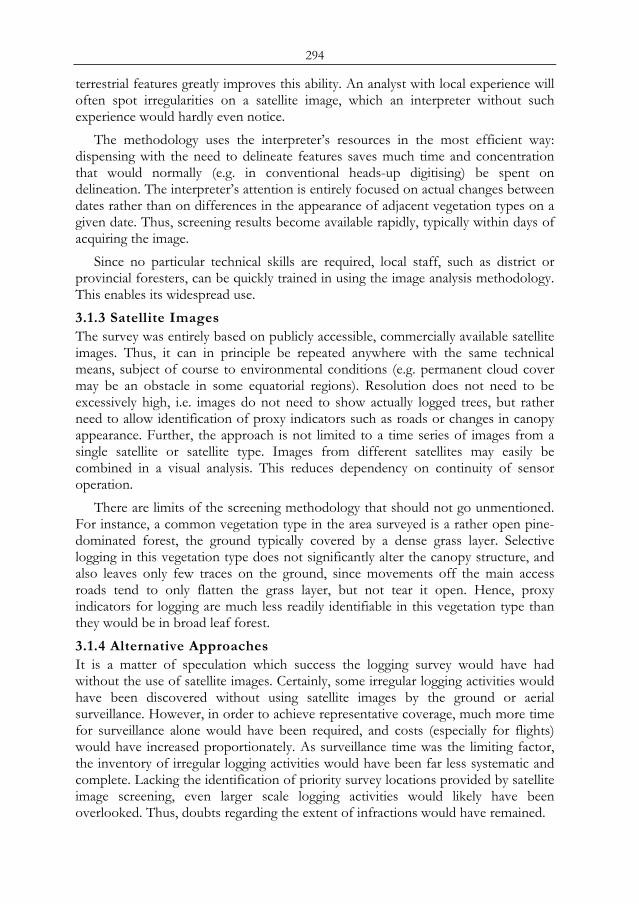
294
terrestrial features greatly improves this ability. An analyst with local experience will often spot irregularities on a satellite image, which an interpreter without such experience would hardly even notice.
The methodology uses the interpreter’s resources in the most efficient way: dispensing with the need to delineate features saves much time and concentration that would normally (e.g. in conventional heads-up digitising) be spent on delineation. The interpreter’s attention is entirely focused on actual changes between dates rather than on differences in the appearance of adjacent vegetation types on a given date. Thus, screening results become available rapidly, typically within days of acquiring the image.
Since no particular technical skills are required, local staff, such as district or provincial foresters, can be quickly trained in using the image analysis methodology. This enables its widespread use. 3.1.3 Satellite Images The survey was entirely based on publicly accessible, commercially available satellite images. Thus, it can in principle be repeated anywhere with the same technical means, subject of course to environmental conditions (e.g. permanent cloud cover may be an obstacle in some equatorial regions). Resolution does not need to be excessively high, i.e. images do not need to show actually logged trees, but rather need to allow identification of proxy indicators such as roads or changes in canopy appearance. Further, the approach is not limited to a time series of images from a single satellite or satellite type. Images from different satellites may easily be combined in a visual analysis. This reduces dependency on continuity of sensor operation.
There are limits of the screening methodology that should not go unmentioned. For instance, a common vegetation type in the area surveyed is a rather open pine-dominated forest, the ground typically covered by a dense grass layer. Selective logging in this vegetation type does not significantly alter the canopy structure, and also leaves only few traces on the ground, since movements off the main access roads tend to only flatten the grass layer, but not tear it open. Hence, proxy indicators for logging are much less readily identifiable in this vegetation type than they would be in broad leaf forest. 3.1.4 Alternative Approaches It is a matter of speculation which success the logging survey would have had without the use of satellite images. Certainly, some irregular logging activities would have been discovered without using satellite images by the ground or aerial surveillance. However, in order to achieve representative coverage, much more time for surveillance alone would have been required, and costs (especially for flights) would have increased proportionately. As surveillance time was the limiting factor, the inventory of irregular logging activities would have been far less systematic and complete. Lacking the identification of priority survey locations provided by satellite image screening, even larger scale logging activities would likely have been overlooked. Thus, doubts regarding the extent of infractions would have remained.

295
Substituting the aerial surveillance with very high resolution images, such as IKONOS, on which under certain circumstances actual logging might have been detectable, would have cost an estimated $ 60,000 (see also section 0.), not including additional image processing requirements due to limitations in image availability. Much of the area would not have been covered by recent images, thus giving a less comprehensive picture of the actual logging extent than the combination of high resolution images and ground /aerial surveillance. This emphasizes that the most appropriate images are not necessarily those with the highest resolution.
The use of a helicopter is a somewhat exceptional and expensive feature of this survey. However, use of aerial surveillance with light fixed wing aircraft in logging surveys is not uncommon ([9], [10]). Using such aircraft typically reduces the cost to some $ 500 – 600 per hour.
Finally, there is the option to use light off-road motorbikes instead of aerial surveillance or ground surveillance with all terrain vehicles. There is no place that can be reached with a logging truck but not with an off-road motorbike. This might be the preferred option if a combination of remote sensing and ground surveillance were used by government agencies for regular operational monitoring. 3.1.5 Summary: Appropriate Technology From a technical perspective, this case study presents an example of how, in a developing country, remote sensing can successfully be integrated into a monitoring process.
The key to success was to match available remote sensing resources and technology with human resources, and to focus remote sensing on what it can quickly and reliably deliver in connection with logging, i.e. a mere proxy indication of where logging is likely to occur as a result of rapid screening, instead of a quantification of its dimension or a delineation of the areas affected by it. This increased efficiency of the overall surveillance process, in a manner similar to the use of remote sensing in emergency situations.
For the approach presented here, satellite images of comparatively low resolution and cost are sufficient. They do not need to show actual logging, it is sufficient if they enable reliable identification of proxy indicators for logging. In most cases, these proxy indicators require confirmation through ground or aerial surveillance, so images are used to narrow down the choice of locations to be inspected in detail, and to establish priorities. Exceptions not requiring confirmation are clear-cuts, high-intensity selective logging in certain forest types (e.g. in evergreen or mixed deciduous forests), the construction of new roads or the re-opening of old roads. They constitute unquestionable evidence of activities on the ground clearly visible on satellite images. This approach may miss out on minor incidences of logging, but is highly likely to uncover really significant operations.
4 INSTITUTIONAL INTEGRATION Technological appropriateness was one key factor for the success of the survey. Institutional integration was an at least equally important factor.
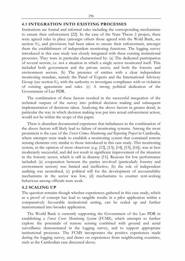
296
4.1 INTEGRATION INTO EXISTING PROCESSES Institutions are formal and informal rules including the corresponding mechanisms to ensure their enforcement [22]. In the case of the Nam Theun 2 project, there were agreed rules in place (amongst others those agreed with the Wold Bank, see section 0.), and provisions had been taken to ensure their enforcement, amongst them the establishment of independent monitoring functions. The logging survey introduced in this case study was closely integrated with these existing institutional processes. They were in particular characterised by: (a) The dedicated participation of several sectors, i.e. not a situation in which a single sector monitored itself. This included both government and the private sector, and both the forestry and environment sectors. (b) The presence of entities with a clear independent monitoring mandate, namely the Panel of Experts and the International Advisory Group (see section 0.), with the authority to investigate compliance with or violation of existing agreements and rules. (c) A strong political dedication of the Government of Lao PDR.
The combination of these factors resulted in the successful integration of the technical outputs of the survey into political decision making and subsequent implementation of decisions taken. Analysing the above factors in greater detail, in particular the way in which decision making was put into actual enforcement action, would not be within the scope of this paper.
There is abundant documented experience that imbalances in the combination of the above factors will likely lead to failure of monitoring systems. Among the most prominent is the case of the Forest Crimes Monitoring and Reporting Project in Cambodia, where attempts were made to establish a monitoring system that contained remote sensing elements very similar to those introduced in this case study. This monitoring system, in the opinion of most observers (e.g. [12], [13], [14], [15], [16]), was at best moderately successful, and did not result in significant improvement of the situation in the forestry sector, which is still in disarray [11]. Reasons for low performance included: (a) cooperation between the parties involved (particularly forestry and environment sectors) was limited and ineffective, (b) the role of independent auditing was neutralised, (c) political will for the development of accountability mechanisms in the sector was low, (d) mechanisms to counter rent-seeking behaviour among officials were weak. 4.2 SCALING UP The question remains though whether experiences gathered in this case study, which as a proof of concept has lead to tangible results in a pilot application within a comparatively favourable institutional setting, can be scaled up and further mainstreamed into broader application.
The World Bank is currently supporting the Government of the Lao PDR in establishing a Forest Cover Monitoring System (FCMS), which attempts to further explore the potentials of remote sensing combined with ground and aerial surveillance demonstrated in the logging survey, and to support appropriate institutional processes. The FCMS incorporates the positive experiences made during the logging survey, and draws on experiences from neighbouring countries, such as the Cambodian case discussed above.
297
The institutional design of the FCMS involves two major line agencies of the Government of the Lao PDR, namely the Ministry of Agriculture and Forestry and the Science, Technology and Environment Agency. They will jointly operate the FMCS and mutually audit their respective performance, i.e. detection efficiency. Such mutual audits are made possible by both institutions using exactly the same satellite image screening approach within the same reference frame (grid), as introduced in section 2.3. An additional design element is the regular performance of sample audits by an independent auditor, again based on the same reference frame. This independent auditing is expected to increase accountability of the line agencies involved for properly conducting the satellite image screening.
During preparation of the FCMS, the feasibility of scaling up the approach piloted in the logging survey has been assessed, considering parameters such as time consumption for satellite image screening and annual operating costs, both total and in relation to national annual log production. The results indicated that a monitoring system implemented in the 8 out of 18 provinces most heavily impacted by irregular logging could be operated with both a very reasonable time budget and at a cost of only the fraction of the value of total annual national log production. The average time required for screening one entire province would be 6 weeks (one interpreter, working 20 hours per week, using a reference frame for screening of 1 x 1 km). The annual operating cost of the monitoring system after end of the project was estimated at $ 285,000, which is equivalent to as little as 0.43 % of estimated overall national log production value (year 2001), or $ 0.65 per every m3 of logs produced.
According to the most recent progress reports by the project implementing the FMCS [23], the forest cover monitoring process from satellite images has been established in the Lao national forestry and environment administrations. Forestry administration personnel will detect changes from the images and report to provinces / districts for field surveillance, while environment administration personnel will evaluate their monitoring results. The process is based on visual change detection. Other more automated methods were trained and tested, but visual change detection still the most reliable under present circumstances. First results are expected in early 2007.
5 OUTLOOK Operational results from the recent scaling up of the monitoring approach in the Lao PDR are not available yet. Depending on the outcome of this first phase of scaling up, the monitoring approach might be further extended, perhaps also partly automated as skills in applying the remote sensing technology develop. Possible options for extension might include: (a) Simple multi-temporal change detection composites, e.g. of vegetation indices, to aid visual analysis. (b) Simple semi-automated analysis of these composites, to eliminate areas not requiring to be checked by visual analysis. (c) Extending the system to cover other land use or land cover changes, e.g. to monitor the rapidly expanding rubber tree or mining industries.
Remote sensing, which has so far often been the domain of specialists, will only realise its full potential if sensibly integrated in actual resources management
298
applications. This potential will continuously expand as high quality satellite images become more easily accessible and less expensive.
REFERENCES 1. The World Bank 2000: World Bank Logging Survey Mission: Technical Report. 2. The World Bank 2002: Second Logging Survey Mission: Technical Report.
Accessed 28 Sep 2006 at: http://lnweb18.worldbank.org/eap/eap.nsf/Attachments/SLSM/$File/secondloggingsurveymission.pdf
3. Meyer G., Panzer K.F. 1990. Regional renewable natural resources and land use inventory and monitoring. Report PN: 90.2098.3-03.120, Federal Republic of Germany-Interim Mekong Committee for Coordination of Investigations of the Lower Mekong Basin, GTZ, Eschborn, DE.
4. Stibig H.-J., Achard F., Fritz S. 2004: A new forest cover map of continental southeast Asia derived from SPOT-VEGETATION satellite imagery. Applied Vegetation Science 7: 153-162.
5. MRC / GTZ Forest Cover Monitoring Project (Stibig H.-J.) 1997: Technical Notes 2: Interpretation and Delineation from Satellite Images.
6. MRC / GTZ Forest Cover Monitoring Project (Panzer K.) 1999: Forest Cover Monitoring Project - Final Report.
7. DeFries R., Asner G., Achard F., Justice C., Laporte N., Price K., Small C., Townshend J. 2005: Monitoring Tropical Deforestation for Emerging Carbon Markets. In: Reduction of Tropical Deforestation and Climate Change Mitigation. Editors: Paulo Mountinho (IPAM) and Stephan Schwartzman (ED).
8. Forest Survey of India, 2001: State of Forest Report 2001. Ministry of Environment and Forest, Dehra Dun.
9. Global Witness 2005: A Guide to Independent Forest Monitoring. Accessed 07/08/2005 at: http://www. globalwitness.org/reports/download.php/00244.pdf
10. Global Forest Watch (Smith W., Ridder R.) 2001: Detecting Illegal Logging Using Remote Sensing: An Overview and Primer. Draft.
11. ITTO 2005: Status of Tropical Forest Management 2005. Summary Report. 12. Cambodia Independent Forest Sector Review 2004: The Forest Sector in
Cambodia. Part I: Policy Choices, issues and options. Accessed 29/09/2006 at: http://www.cambodia-forest-sector.net/docs/mainreport.pdf
13. Cambodia Independent Forest Sector Review (Miller F.) 2004: Regulatory mechanisms. Accessed 30/09/2006 at: http://www.cambodia forest-sector.net/docs/CIFSR%20Part%20II%20Chapt%2014%20Regulation.pdf
14. Brown D., Luttrell C. 2004: Review of Independent Forest Monitoring. Accessed 29/09/2006 at: http://www.odifpeg.org.uk/publications/reports/IFM%20Paper/IFM%20Final.pdf
15. Young D. 2005: Independent forest monitoring: A tool for social justice. Accessed 29/09/2006 at: http://www.policy-powertools.org/Tools/Ensuring/docs/ifm_tool_english.pdf
16. Verifor (Luttrell C., Brown D.) 2006: Country Case Study 4 The Experience of Independent Forest Monitoring In Cambodia Cecilia Luttrell and David Brown. Accessed 30/09/2006 at: http://www.verifor.org/ case_studies/Cambodia%20draft%200706.pdf

299
17. Commission of the European Communities 2003: Forest Law Enforcement, Governance and Trade (FLEGT). Proposal for an EU Action Plan. Accessed 30/09/2006 at: http://ec.europa.eu/comm/development/body/theme/forest/initiative/docs/Doc1-FLEGT_en.pdf
18. Mather A.S. 2005: Assessing the world's forests. Global Environmental Change 15 (2005), 267-280.
19. Kleinn C., Corrales L., Morales D. 2000: Forest Area in Costa Rica: A Comparative Study of Tropical Forest Cover Estimates over Time. Environmental Monitoring and Assessment 73 (2002), 17-40.
20. Mekong River Commission 2003: State of the Basin Report 2003. 21. GTZ 2001: Information and Communication Technologies for Development.
Present Situation, Perspectives and Potential Areas for German Technical Cooperation in Peru, Lao P.D.R., Vietnam, Tanzania and Uganda.
22. GTZ 2004: Natural Resources and Governance: Incentives for Sustainable Resource Use. Manual.
23. Sustainable Forestry and Rural Development Project Lao PDR (Jänne S.) 2006: Forest Cover Monitoring. End of Assignment Report.
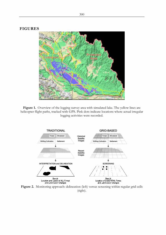
300
FIGURES
Figure 1. Overview of the logging survey area with simulated lake. The yellow lines are helicopter flight paths, tracked with GPS. Pink dots indicate locations where actual irregular
logging activities were recorded.
Figure 2. Monitoring approach: delineation (left) versus screening within regular grid cells
(right).
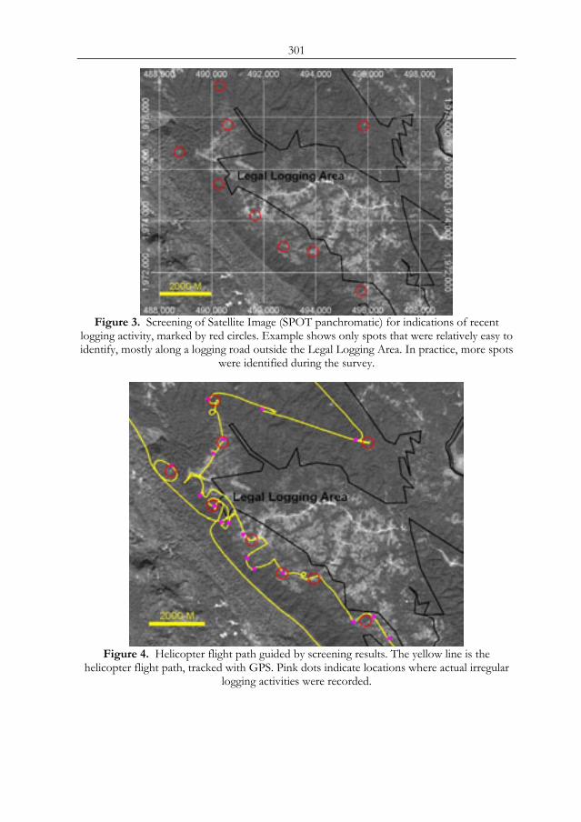
301
Figure 3. Screening of Satellite Image (SPOT panchromatic) for indications of recent
logging activity, marked by red circles. Example shows only spots that were relatively easy to identify, mostly along a logging road outside the Legal Logging Area. In practice, more spots
were identified during the survey.
Figure 4. Helicopter flight path guided by screening results. The yellow line is the
helicopter flight path, tracked with GPS. Pink dots indicate locations where actual irregular logging activities were recorded.
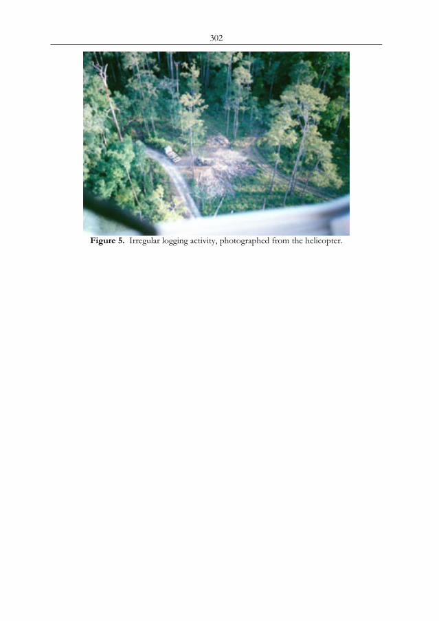
302
Figure 5. Irregular logging activity, photographed from the helicopter.
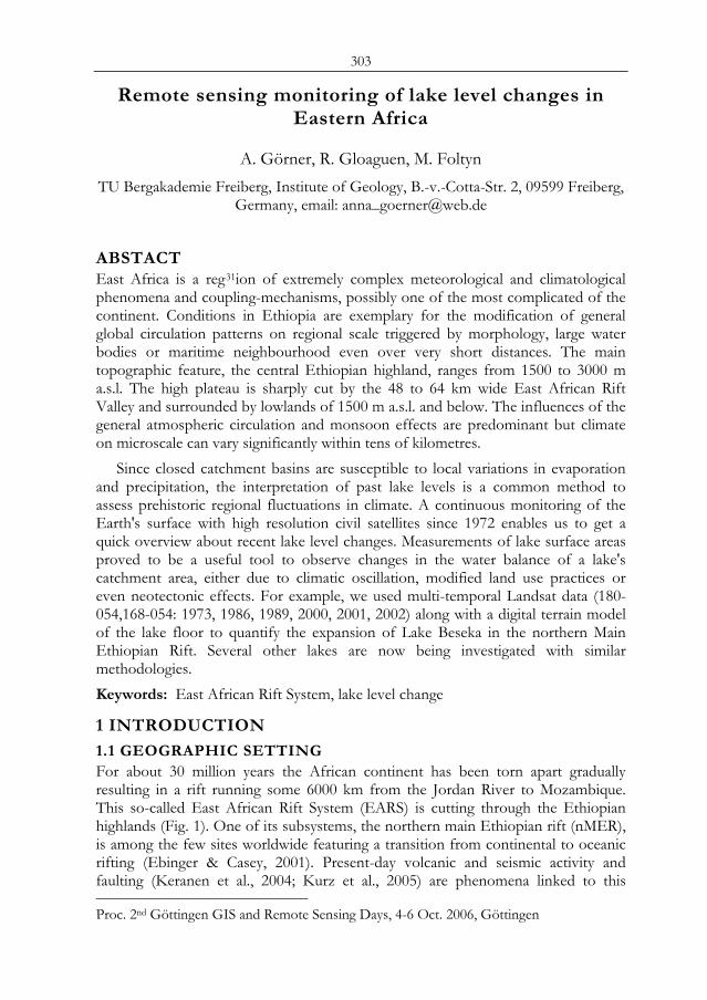
303
Remote sensing monitoring of lake level changes in Eastern Africa
A. Görner, R. Gloaguen, M. Foltyn TU Bergakademie Freiberg, Institute of Geology, B.-v.-Cotta-Str. 2, 09599 Freiberg,
Germany, email: [email protected]
ABSTACT East Africa is a reg31ion of extremely complex meteorological and climatological phenomena and coupling-mechanisms, possibly one of the most complicated of the continent. Conditions in Ethiopia are exemplary for the modification of general global circulation patterns on regional scale triggered by morphology, large water bodies or maritime neighbourhood even over very short distances. The main topographic feature, the central Ethiopian highland, ranges from 1500 to 3000 m a.s.l. The high plateau is sharply cut by the 48 to 64 km wide East African Rift Valley and surrounded by lowlands of 1500 m a.s.l. and below. The influences of the general atmospheric circulation and monsoon effects are predominant but climate on microscale can vary significantly within tens of kilometres.
Since closed catchment basins are susceptible to local variations in evaporation and precipitation, the interpretation of past lake levels is a common method to assess prehistoric regional fluctuations in climate. A continuous monitoring of the Earth's surface with high resolution civil satellites since 1972 enables us to get a quick overview about recent lake level changes. Measurements of lake surface areas proved to be a useful tool to observe changes in the water balance of a lake's catchment area, either due to climatic oscillation, modified land use practices or even neotectonic effects. For example, we used multi-temporal Landsat data (180-054,168-054: 1973, 1986, 1989, 2000, 2001, 2002) along with a digital terrain model of the lake floor to quantify the expansion of Lake Beseka in the northern Main Ethiopian Rift. Several other lakes are now being investigated with similar methodologies. Keywords: East African Rift System, lake level change
1 INTRODUCTION
1.1 GEOGRAPHIC SETTING For about 30 million years the African continent has been torn apart gradually resulting in a rift running some 6000 km from the Jordan River to Mozambique. This so-called East African Rift System (EARS) is cutting through the Ethiopian highlands (Fig. 1). One of its subsystems, the northern main Ethiopian rift (nMER), is among the few sites worldwide featuring a transition from continental to oceanic rifting (Ebinger & Casey, 2001). Present-day volcanic and seismic activity and faulting (Keranen et al., 2004; Kurz et al., 2005) are phenomena linked to this Proc. 2nd Göttingen GIS and Remote Sensing Days, 4-6 Oct. 2006, Göttingen
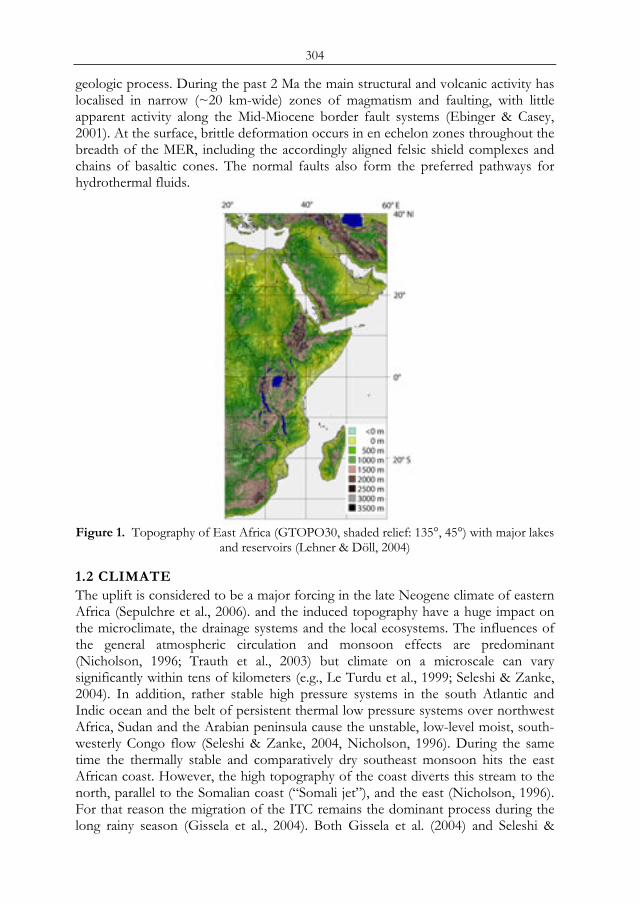
304
geologic process. During the past 2 Ma the main structural and volcanic activity has localised in narrow (~20 km-wide) zones of magmatism and faulting, with little apparent activity along the Mid-Miocene border fault systems (Ebinger & Casey, 2001). At the surface, brittle deformation occurs in en echelon zones throughout the breadth of the MER, including the accordingly aligned felsic shield complexes and chains of basaltic cones. The normal faults also form the preferred pathways for hydrothermal fluids.
Figure 1. Topography of East Africa (GTOPO30, shaded relief: 135°, 45°) with major lakes
and reservoirs (Lehner & Döll, 2004)
1.2 CLIMATE The uplift is considered to be a major forcing in the late Neogene climate of eastern Africa (Sepulchre et al., 2006). and the induced topography have a huge impact on the microclimate, the drainage systems and the local ecosystems. The influences of the general atmospheric circulation and monsoon effects are predominant (Nicholson, 1996; Trauth et al., 2003) but climate on a microscale can vary significantly within tens of kilometers (e.g., Le Turdu et al., 1999; Seleshi & Zanke, 2004). In addition, rather stable high pressure systems in the south Atlantic and Indic ocean and the belt of persistent thermal low pressure systems over northwest Africa, Sudan and the Arabian peninsula cause the unstable, low-level moist, south-westerly Congo flow (Seleshi & Zanke, 2004, Nicholson, 1996). During the same time the thermally stable and comparatively dry southeast monsoon hits the east African coast. However, the high topography of the coast diverts this stream to the north, parallel to the Somalian coast (“Somali jet”), and the east (Nicholson, 1996). For that reason the migration of the ITC remains the dominant process during the long rainy season (Gissela et al., 2004). Both Gissela et al. (2004) and Seleshi &
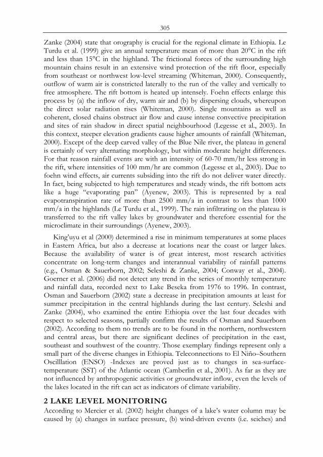
305
Zanke (2004) state that orography is crucial for the regional climate in Ethiopia. Le Turdu et al. (1999) give an annual temperature mean of more than 20°C in the rift and less than 15°C in the highland. The frictional forces of the surrounding high mountain chains result in an extensive wind protection of the rift floor, especially from southeast or northwest low-level streaming (Whiteman, 2000). Consequently, outflow of warm air is constricted laterally to the run of the valley and vertically to free atmosphere. The rift bottom is heated up intensely. Foehn effects enlarge this process by (a) the inflow of dry, warm air and (b) by dispersing clouds, whereupon the direct solar radiation rises (Whiteman, 2000). Single mountains as well as coherent, closed chains obstruct air flow and cause intense convective precipitation and sites of rain shadow in direct spatial neighbourhood (Legesse et al., 2003). In this context, steeper elevation gradients cause higher amounts of rainfall (Whiteman, 2000). Except of the deep carved valley of the Blue Nile river, the plateau in general is certainly of very alternating morphology, but within moderate height differences. For that reason rainfall events are with an intensity of 60-70 mm/hr less strong in the rift, where intensities of 100 mm/hr are common (Legesse et al., 2003). Due to foehn wind effects, air currents subsiding into the rift do not deliver water directly. In fact, being subjected to high temperatures and steady winds, the rift bottom acts like a huge “evaporating pan” (Ayenew, 2003). This is represented by a real evapotranspiration rate of more than 2500 mm/a in contrast to less than 1000 mm/a in the highlands (Le Turdu et al., 1999). The rain infiltrating on the plateau is transferred to the rift valley lakes by groundwater and therefore essential for the microclimate in their surroundings (Ayenew, 2003).
King’uyu et al (2000) determined a rise in minimum temperatures at some places in Eastern Africa, but also a decrease at locations near the coast or larger lakes. Because the availability of water is of great interest, most research activities concentrate on long-term changes and interannual variability of rainfall patterns (e.g., Osman & Sauerborn, 2002; Seleshi & Zanke, 2004; Conway et al., 2004). Goerner et al. (2006) did not detect any trend in the series of monthly temperature and rainfall data, recorded next to Lake Beseka from 1976 to 1996. In contrast, Osman and Sauerborn (2002) state a decrease in precipitation amounts at least for summer precipitation in the central highlands during the last century. Seleshi and Zanke (2004), who examined the entire Ethiopia over the last four decades with respect to selected seasons, partially confirm the results of Osman and Sauerborn (2002). According to them no trends are to be found in the northern, northwestern and central areas, but there are significant declines of precipitation in the east, southeast and southwest of the country. Those exemplary findings represent only a small part of the diverse changes in Ethiopia. Teleconnections to El Niño–Southern Oscilllation (ENSO) -Indexes are proved just as to changes in sea-surface-temperature (SST) of the Atlantic ocean (Camberlin et al., 2001). As far as they are not influenced by anthropogenic activities or groundwater inflow, even the levels of the lakes located in the rift can act as indicators of climate variability.
2 LAKE LEVEL MONITORING According to Mercier et al. (2002) height changes of a lake’s water column may be caused by (a) changes in surface pressure, (b) wind-driven events (i.e. seiches) and
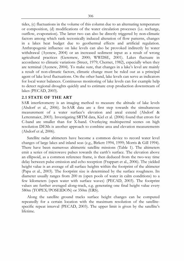
306
tides, (c) fluctuations in the volume of this column due to an alternating temperature or composition, (d) modifications of the water circulation processes (i.e. recharge, outflow, evaporation). The latter two can also be directly triggered by non-climatic factors among which rank tectonically induced alteration of flow patterns, changes in a lakes heat budget due to geothermal effects and artificial regulation. Anthropogenic influence on lake levels can also be provoked indirectly by water withdrawal (Ayenew, 2004) or an increased sediment input as a result of wrong agricultural practices (Geremew, 2000; WWDSE, 2001). Lakes fluctuate in accordance to climatic variations (Street, 1979; Chernet, 1982), especially when they are terminal (Ayenew, 2004). To make sure, that changes in a lake’s level are mainly a result of non-climatic factors, climatic change must be ruled out as a principal agent of lake level fluctuations. On the other hand, lake levels can serve as indicators for local water balances. Continuous monitoring of lake levels can for example help to detect regional droughts quickly and to estimate crop production downstream of lakes (PECAD, 2003). 2.1 STATE OF THE ART SAR interferometry is an imaging method to measure the altitude of lake levels (Alsdorf et al., 2006). In-SAR data are a first step towards the simultaneous measurement of a water surface’s elevation and areal extend (Alsdorf & Lettenmaier, 2003). Investigating SRTM data, Kiel et al. (2006) found that errors for C-band are smaller than for X-band. Overlaying multispectral scenes on high resolution DEMs is another approach to combine area and elevation measurements (Alsdorf et al, 2006).
Satellite radar altimeters have become a common device to record water level changes of large lakes and inland seas (e.g., Birkett 1994, 1999; Morris & Gill 1994). There have been numerous altimetric satellite missions (Table 1). The altimeters emit a series of microwave pulses towards the earth’s surface. The elevation above an ellipsoid, as a common reference frame, is then deduced from the two-way time delay between pulse emission and echo reception (Frappart et al., 2006). The yielded height value is an average of all surface heights within the footprint of the altimeter (Papa et al., 2003). The footprint size is determined by the surface roughness. Its diameter usually ranges from 200 m (open pools of water in calm conditions) to a few kilometers (open water with surface waves) (PECAD, 2003). The footprint values are further averaged along-track, e.g. generating one final height value every 580m (TOPEX/POSEIDON) or 350m (ERS).
Along the satellite ground tracks surface height changes can be computed repeatedly for a certain location with the maximum resolution of the satellite-specific repeat interval (PECAD, 2003). The upper limit is given by the satellite’s lifetime.

307
Table 1. Altimetric satellite missions (modified from PECAD, 2003; Alsdorf, 2006) *) failure of on-board storage, radar altimeter keeps working
Mission operation repeat comments past missions Seasat 1978 17 days Geosat 1986-1989 17 days ERS-1 1991-1996 35 days ERS-2 1995-2003* 35 days on-going missions TOPEX/Poseidon launch 1992 10 days new orbit in 2002 Geosat Follow-on (GFO)
launch 2001 17 days
ENVISAT (RA-2, MWR) launch 2002 35 days JASON-1 launch 2002 10 days Follow-on to T/P; 2-3 days latency
period ICESat (GLAS) launch 2003 183 days LIDAR, diameter footprint ca. 70 m
Time of day, weather, or canopy cover do not limit the successful application of
satellite altimetry for lakes. The results allow submonthly, seasonal or interannual monitoring of lake level changes. Satellite altimetry can supply elevation data even if conventional gauge records are not available. However, there are several limitations to the technique. The instruments are primarily designed to operate over homogenous surfaces, i.e. oceans and ice-sheets. Highly undulating or complex topography may result in non-interpretable or lost data. The aggregation of data presents the main difference to traditional gauge measurements that are taken at specific points. The elevation accuracy is primarily influenced by knowledge of the satellite orbit, the distance between antenna and target, the geophysical range corrections and the size and type of the target. Height variations obtained from the TOPEX/POSEIDON mission have an accuracy of 3-4cm RMS for the largest lakes (e.g., Lake Ontario), ~5cm-10cm RMS for smaller lakes (100km2), and tens of centimetres for rivers, wetlands and floodplains. The Instrument footprint size, the telemetry/data rates, the surrounding topography, and as well the target-tracking method used determine the minimum target size (PECAD, 2003). 2.2 EXAMPLE OF A RIFT LAKE When it comes to the investigations of lake level changes spanning over several decades, satellite altimetry is of little use. For such long time series we need to get back to Landsat data, which are available since 1972. The currently operating satellite altimetry missions can also not be considered for research on lakes smaller than the footprint area of the altimeter, or for lakes away from the altimeter ground tracks. The endorheic Lake Beseka, located in the nMER (Fig. 2), falls into this category of water bodies. We investigated its fast water level rise with an area-measuring approach. For the past decades, the alkaline (pH = 9.5) and saline (electrical conductivity: 6.3 mS/cm) Lake Beseka has undergone a major water level increase, threatening an important road and railway and partially flooding and salinising the Abadir Farm (e.g. Ayenew, 2004). The Koka dam was constructed 152
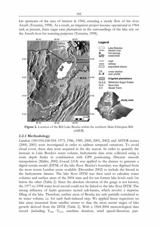
308
km upstream of the area of interest in 1960, ensuring a steady flow of the river Awash (Tessema, 1998). As a result, an irrigation project became operational in 1964 and, at present, three sugar cane plantations in the surroundings of the lake rely on the Awash river for watering purposes (Tessema, 1998).
Figure 2. Location of the Rift Lake Beseka within the northern Main Ethiopian Rift
(nMER)
2.2.1 Methodology Landsat (180-054,168-054: 1973, 1986, 1989, 2000, 2001, 2002) and ASTER scenes (2000, 2001) were investigated in order to address temporal variations. To avoid cloud cover, these data were acquired in the dry season. In order to quantify the increase in Lake Beseka's water volume, bathymetric data were collected using a sonic depth finder in combination with GPS positioning. Discrete smooth interpolation (Mallet, 2002; Gocad 2.0.8) was applied to the dataset to generate a digital terrain model (DTM) of the lake floor. Beseka’s boundary was digitised from the most recent Landsat scene available (December 2002) to include the littoral in the bathymetric dataset. The lake floor DTM was then used to calculate water volumes and surface areas of the 2004 state and for ten former lake levels each 1m below the other (Table 2). Since the absolute elevation of the gauge is not known, the 1977-to-1998 water level record could not be linked to the lake floor DTM. The strong influence of faults generates nested sub-basins, which involve a stepwise filling of the lake. Therefore, surface areas of Beseka are only partially correlated to its water volume, i.e. for each fault-induced step. We applied linear regression on lake areas measured from satellite scenes to date the most recent stages of lake growth derived from the DTM (Table 2). With a 1964-2004 meteorological data record (including Tmin, Tmax, sunshine duration, wind speed/direction, pan-
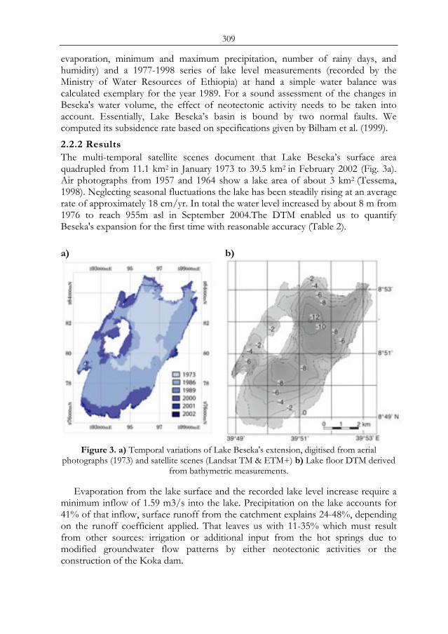
309
evaporation, minimum and maximum precipitation, number of rainy days, and humidity) and a 1977-1998 series of lake level measurements (recorded by the Ministry of Water Resources of Ethiopia) at hand a simple water balance was calculated exemplary for the year 1989. For a sound assessment of the changes in Beseka's water volume, the effect of neotectonic activity needs to be taken into account. Essentially, Lake Beseka’s basin is bound by two normal faults. We computed its subsidence rate based on specifications given by Bilham et al. (1999). 2.2.2 Results The multi-temporal satellite scenes document that Lake Beseka’s surface area quadrupled from 11.1 km2 in January 1973 to 39.5 km2 in February 2002 (Fig. 3a). Air photographs from 1957 and 1964 show a lake area of about 3 km2 (Tessema, 1998). Neglecting seasonal fluctuations the lake has been steadily rising at an average rate of approximately 18 cm/yr. In total the water level increased by about 8 m from 1976 to reach 955m asl in September 2004.The DTM enabled us to quantify Beseka's expansion for the first time with reasonable accuracy (Table 2). a) b)
Figure 3. a) Temporal variations of Lake Beseka's extension, digitised from aerial
photographs (1973) and satellite scenes (Landsat TM & ETM+) b) Lake floor DTM derived from bathymetric measurements.
Evaporation from the lake surface and the recorded lake level increase require a minimum inflow of 1.59 m3/s into the lake. Precipitation on the lake accounts for 41% of that inflow, surface runoff from the catchment explains 24-48%, depending on the runoff coefficient applied. That leaves us with 11-35% which must result from other sources: irrigation or additional input from the hot springs due to modified groundwater flow patterns by either neotectonic activities or the construction of the Koka dam.
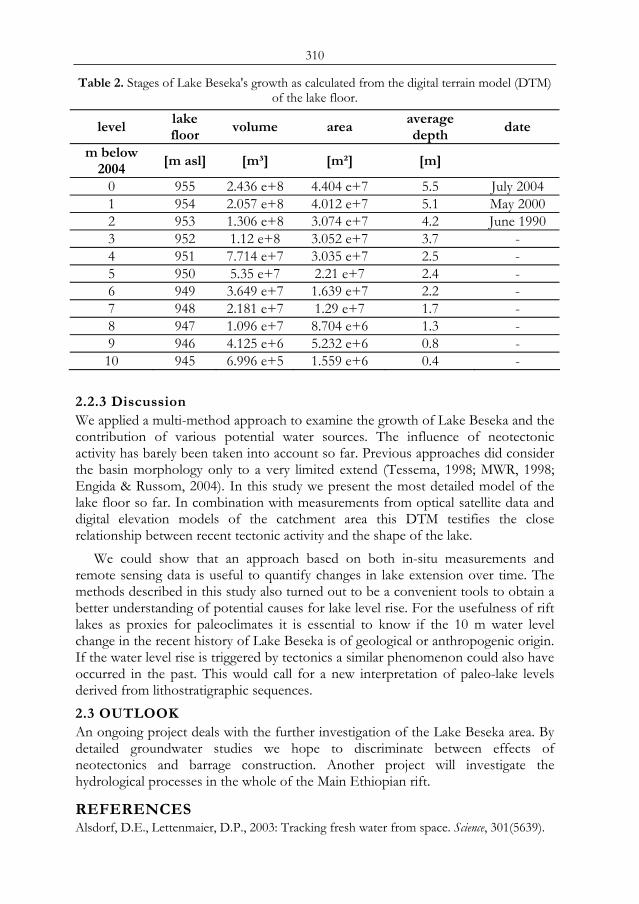
310
Table 2. Stages of Lake Beseka's growth as calculated from the digital terrain model (DTM) of the lake floor.
level lake floor
volume area average depth
date
m below 2004
[m asl] [m³] [m²] [m] 0 955 2.436 e+8 4.404 e+7 5.5 July 2004 1 954 2.057 e+8 4.012 e+7 5.1 May 2000 2 953 1.306 e+8 3.074 e+7 4.2 June 1990 3 952 1.12 e+8 3.052 e+7 3.7 - 4 951 7.714 e+7 3.035 e+7 2.5 - 5 950 5.35 e+7 2.21 e+7 2.4 - 6 949 3.649 e+7 1.639 e+7 2.2 - 7 948 2.181 e+7 1.29 e+7 1.7 - 8 947 1.096 e+7 8.704 e+6 1.3 - 9 946 4.125 e+6 5.232 e+6 0.8 - 10 945 6.996 e+5 1.559 e+6 0.4 -
2.2.3 Discussion We applied a multi-method approach to examine the growth of Lake Beseka and the contribution of various potential water sources. The influence of neotectonic activity has barely been taken into account so far. Previous approaches did consider the basin morphology only to a very limited extend (Tessema, 1998; MWR, 1998; Engida & Russom, 2004). In this study we present the most detailed model of the lake floor so far. In combination with measurements from optical satellite data and digital elevation models of the catchment area this DTM testifies the close relationship between recent tectonic activity and the shape of the lake.
We could show that an approach based on both in-situ measurements and remote sensing data is useful to quantify changes in lake extension over time. The methods described in this study also turned out to be a convenient tools to obtain a better understanding of potential causes for lake level rise. For the usefulness of rift lakes as proxies for paleoclimates it is essential to know if the 10 m water level change in the recent history of Lake Beseka is of geological or anthropogenic origin. If the water level rise is triggered by tectonics a similar phenomenon could also have occurred in the past. This would call for a new interpretation of paleo-lake levels derived from lithostratigraphic sequences. 2.3 OUTLOOK An ongoing project deals with the further investigation of the Lake Beseka area. By detailed groundwater studies we hope to discriminate between effects of neotectonics and barrage construction. Another project will investigate the hydrological processes in the whole of the Main Ethiopian rift.
REFERENCES Alsdorf, D.E., Lettenmaier, D.P., 2003: Tracking fresh water from space. Science, 301(5639).
311
Alsdorf. D.E., Rodríguez, E., Lettenmaier, D.P., 2006 (submitted): Measuring surface water from space. Reviews of Geophysics.
Ayenew, T., 2003: Environmental isotope-based integrated hydrogeological study of some Ethiopian rift lakes. J Radioanal Nucl Ch, 257(1), pp. 11–16.
Ayenew, T. (2004): Environmental implications of changes in the levels of lakes in the Ethiopian Rift since 1970. Regional Environmental Change, 4, pp. 192-204.
Bilham, R., Bendick, R., Larson, K., Mohr, P., Braun, J., Tesfaye, S., Asfaw, L., 1999: Secular and tidal strain across the Main Ethiopian Rift. Geophysical Research Letters, 26, pp. 2789–2792.
Birkett, C.M., 1994: Radar altimetry - A new concept in monitoring global lake level changes. Eos Trans. AGU, 75(24), pp. 273–275.
Birkett, C., Murtugudde, R. and Allan, T., 1999: Indian Ocean climate event brings floods to East Africa's lakes and the Sudd Marsh. Geophysical Research Letters, 26(8), pp. 1031–1034.
Camberlin, P., Janicot, S., Poccard, I., 2001: Seasonality and atmospheric dynamics of the teleconnections between African rainfall and tropical sea-surface temperature: Atlantic vs. ENSO. International Journal of Climatology, 21, pp. 973–1005.
Conway, D., Mould, C., Bewket, W., 2004: Over one century of rainfall and temperature observations in Addis Ababa, Ethiopia. International Journal of Climatoloty, 24, pp. 77 – 91.
Ebinger, C.J., Casey, M., 2001: Continental breakup in magmatic provinces: An Ethiopian example. Geology, 29, pp. 527–530.
Engida, Z.A., Russom, G.E., 2004: Determination for the Cause of Rising Water levels in Lake Beseka and design of remedial measure. Ethiopian Engineers Association Journal, august issue.
Frappart, F., Calmant, S., Cauhopé, M., Seyler, F., Cazenave, A., 2006: Preliminary results of ENVISAT RA-2-derived water levels validation over the Amazon basin, Remote Sensing of Environment, 100( 2), pp. 252-264.
Geremew, Z., 2000: Engineering geological investigation and lake level changes in the Awassa Basin. MSc thesis, Department of Geology and Geophysics, Addis Ababa University, Addis Ababa, Ethiopia, 185.
Gissela, T., Black, E., Grimes, D.I.F., Slingo, J.M., 2004: Seasonal forecasting of the Ethiopian summer rains. International Journal of Climatology, 24, pp. 1345–1358.
Goerner, A., Jolie, E., Gloaguen, R.: Non-climatic growth of the saline Lake Beseka, Main Ethiopian Rift, submitted to J. Arid Env., May 2006
Keranen, K., Klemperer, S., Gloaguen, R. and EAGLE Working Group, 2004: Imaging a proto-ridge axis in the Main Ethiopian rift. Geology, 39, pp. 949-952.
Kiel, B.a , Alsdorf, D.a , LeFavour, G.B., 2006: Capability of SRTM C- and X-band DEM data to measure water elevations in Ohio and the Amazon. Photogrammetric Engineering and Remote Sensing, 72(3), pp. 313-320.
King’uyu, S.M., Ogallo, L.A, Anyamba, E.K., 2000: Recent trends of minimum and maximum surface temperatures over eastern Africa. Journal of Climate, 13, pp. 2876–2886.
Kurz, T., Gloaguen, R., Ebinger, C., Casey, M., Abebe, B., 2005 (accepted): Deformation distribution and type in the Main Ethiopian Rift (MER); a remote sensing study, Journal of African Earth Sciences.
Legesse, D., Vallet-Coulomb, C., Gasse, F., 2003: Hydrological response of a catchment to climate and land use changes in Tropical Africa: case study South Central Ethiopia. Journal of Hydrology, 275, pp. 67–85
Lehner, B. and Döll, P., 2004: Development and validation of a global database of lakes, reservoirs and wetlands. Journal of Hydrology 296(1-4), pp. 1-22.

312
Le Turdu, C., Tiercelin, J-J., Gibert, E., Travi, Y., Lezzar, K-E., Richert, J-P., Massault, M., Gasse, F., Bonnefille, R., Decorbert, M., Gensous, B., Jeudy, V., Tamrat, E., Mohammed, M.U., Martens, K., Atnafu, B., Chernet, T., Williamson, D., Taieb, M., 1999: The Ziway-Shala lake basin system, main Ethiopian Rift; influence of volcanism, tectonics, and climatic forcing on basin formation and sedimentation. Palaeogeography, Palaeoclimatology, Palaeoecology, 150(3-4), pp. 135-177.
Mallet, J.-L., 2002: Geomodelling. Oxford University Press. Mercier, F., Cazenave, A., Maheu, C., 2002: Interannual lake level fluctuations (1993-1999) in
Aftica from Topex/Poseidon: connections with ocean-atmosphere interactions over the Indian Ocean. Global and Planetary Changes, 32, pp. 141-163.
Morris, C.S. and Gill, S.K., 1994a: Variation of Great Lakes water levels derived from Geosat altimetry. Water Resour. Res., 30(4), pp. 1009–1017.
Morris, C.S. and Gill, S.K., 1994b: Evaluation of the TOPEX/POSEIDON altimeter system over the Great Lakes. J. Geophys. Res., 99(C12), pp. 24,527–24,539.
MWR, 1998: Study of Lake Beseka (Inception Report, Vol. 1). Ministry of Water Resources, Addis Ababa, Ethiopia.
Nicholson, S.E. 1996: A review of climate dynamics and climate variability in Eastern Africa, in: T.C. Johnson, E.O. Odada (Eds.), The Limnology, Climatology and Paleoclimatology of the East African Lakes, The International Decade for the East African Lakes (IDEAL), pp. 25-56. Gordon and Breach, Newark, NJ.
Osman, M., Sauerborn, P., 2002: A preliminary assessment of characteristics and long-term variability of rainfall in Ethiopia – Basis for sustainable land use and resource management. Conference on Agricultural Research for Development, Deutscher Tropentag Witzenhausen, October 9-11, 2002.
Papa, F., Legrésy, B., Rémy, F., 2003: Use of the Topex – Poseidon dual-frequency radar altimeter over land surfaces. Remote Sensing of Environment, 87, pp. 136-147.
PECAD (Production Estimates and Crop Assessment Division, Foreign Agricultural Service, U.S. Department of Agriculture), 2004: Near-Real Time Monitoring of Lake and Reservoir Surface Elevations. URL: http://bigquill.gsfc.nasa.gov
Seleshi, Y., Zanke, U., 2004: Recent changes in rainfall and rainy days in Ethiopia. International Journal of Climatology, 24, pp. 973-983.
Sepulchre, P, Ramstein, G, Fluteau, F, Schuster, M, Tiercelin, JJ, Brunet, M, 2006: Tectonic uplift and Eastern Africa aridification. Science, 313(5792), pp. 1419-1423.
Tessema, Z., 1998: Hydrochemical and water balance approach in the study of high water level rise of Lake Beseka. MSc. Thesis, University of Birmingham, UK.
Trauth, M.H., Deino, A.L., Bergner, A.G.N., Strecker, M.R., 2003: East African climate change and orbital forcing during the last 175 kyr BP. Earth Planet Sci Lett 206, pp. 297-313.
Whitemann, C.D., 2000: Mountain Meteorology – Fundamentals and applications. Oxford University Press.
WWDSE (2001): The study of Lake Awassa level rise (Main Report, Vol II). Unpublished report of Water Works Design and Supervision Enterprise, Addis Ababa, Ethiopia, 291.
313
Remote sensing data and GIS tools for the improvement of rainfall-runoff models in the Bělá River watershed in
the northern Moravia
L. Halounováa, M. Hanzlováb, J. Horákb, J. Unuckab, D. Žídekc, Z. Boukalovád
a Faculty of Civil Engineering, CTU Prague, Thákurova 7, 166 29 Prague 6, email: [email protected]
b Institute of geoinformatics, University of Mining - TU Ostrava c Czech Hydrometeorological Institute Ostrava
d Cross Czech a.s., Prague
ABSTRACT ERS-2 radar data and S32POT data are used together with rainfall estimation from radar measurements and historical records of rainfall measurements to verify suitability of linking and combining individual models in the watershed. The meteorological data are processed by stochastic and geostatistic methods. The Quasi 2D hydrological model HELP, a snow melting model (degree/day) and a local hydro-geological model are used. Changes in remote sensing data are compared to the meteorological data and calibrated for the relation - precipitations and changes before and after the rainfall in remote sensing data in individual parts of the watershed – in optical and microwave wavebands. The watershed covers an area between the Jeseníky Mountain and the frontier with Poland. Keywords: rainfall-runoff, model, ERS-2, ETM+, SPOT, object-oriented classification.
1 INTRODUCTION Storm water with high water volume and following floods, they are not new events in the human history, but it seems that their occurrence is now more often in previously safe regions. There are several reasons of the situation. Present land cover having worse ratio in pervious/impervious surface, unsuitable vegetation cover and other phenomena deteriorate the surface runoff.
The Czech Republic being called the roof of Europe is a place where many rivers have their springs. Catchments of these watercourse upper parts have difficult positions in the flood warning system. The warning system is usually late due to small distances of the water runoff and therefore due to the short time for warning. To solve the problem, rainfall forecasts and following surface and underground runoff modeling could allow to bring new information concerning the potential flood occurrence.
The project of the Czech Grant Agency called „Application of geoinformation technologies to improve rainfall-runoff relations“ is focused on modeling situations combining storm water forecast, water surface runoff and ground water flow. Proc. 2nd Göttingen GIS and Remote Sensing Days, 4-6 Oct. 2006, Göttingen
314
Land cover in the Czech Republic like in other European countries has been changing and usually by the more dangerous way from pervious to the impervious surfaces or even from forest pervious surfaces to impervious ones. The pervious forest surface preserves and delays a substantial part of the precipitation water volume and therefore the runoff has a lower, longer, and less dangerous curve of the discharge. The delay prolongs the time of the runoff that is also smaller due to the seepage. Thus the water capacity of the underground layer is another important phenomenon of the potential flood situation even though unchangeable within the human power. The knowledge of the underground layer perviousness and water capacity is a function of the soil layer type, layer thickness, soil moisture and of the underground water level.
One part of the project is dealing with effective proposal of remote sensing data classifications – satellite or aerial. Classification means the classification related to the soil type, soil water capacity, soil moisture and its changes detectable from radar/optical data, vegetation cover, forest cover etc. Impact of proposed changes of the land cover and resulting hydrological situation compared to the present watercourse discharge impact will be studied to improve the nowadays runoff state. Land cover data have been determined from the Landsat data; two additional land cover classification will be performed from two SPOT scenes – in 2000 and 2004 shortly after the flood event. ERS-2 data covering the region with 36 days revisiting will be used first of all as a knowledge base for the moisture detection and then as a moisture change detection.
Microwave radiation is sensitive to the surface roughness and surface moisture. However, the direct relation between measured values of the image data and moisture percentage is unknown and will be studied in the project framework [5], [6].
The project is a joint work of hydrologists, hydro geologists, remote sensing specialists, and geoinformation specialists.
2 STUDY AREA The Bělá River watershed is a catchment of the Bělá River upper part starting at the river spring and continuing up to the frontier with Poland in the Jeseníky Mountains in the northern Moravia – north eastern Czech Republic (see Fig. 1).
The catchment seriously suffered from the 1997 European flood. The flood caused deterioration of the sewer network capacity due to sediments in the system, hydro geological borehole sedimentation, etc.
The Bělá River watershed is composed from forests, agricultural, urban areas, and water surfaces. Figure 2 shows the land cover (CORINE land cover = CLC) made in the 2000 CORINE project in the Czech Republic and the ETM+ classification from 2000 and 2002. The classes´ nomenclature is the same as in the 1990 CORINE project [1].
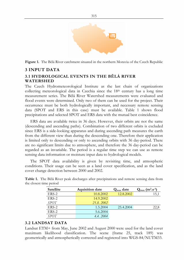
315
Figure 1. The Bělá River catchment situated in the northern Moravia of the Czech Republic
3 INPUT DATA
3.1 HYDROLOGICAL EVENTS IN THE BĚLÁ RIVER WATERSHED The Czech Hydrometeorological Institute as the last chain of organizations collecting meteorological data in Czechia since the 18th century has a long time measurement series. The Bělá River Watershed measurements were evaluated and flood events were determined. Only two of them can be used for the project. Their occurrence must be both hydrologically important, and necessary remote sensing data (SPOT and ERS in this case) must be available. Table 1 shows flood precipitations and selected SPOT and ERS data with the mutual best coincidence.
ERS data are available twice in 36 days. However, their orbits are not the same (descending and ascending paths). Combination of two different orbits is excluded since ERS is a side-looking apparatus and during ascending path measures the earth from the different view than during the descending one. Therefore their application is limited only to descending or only to ascending orbits with 36 day-period. There are no significant limits due to atmosphere, and therefore the 36 day-period can be regarded as an invariable. The period is a regular time step we can use as remote sensing data information or moisture input data to hydrological models.
The SPOT data availability is given by revisiting time, and atmospheric conditions. Their usage can be seen as a land cover specification, and as the land cover change detection between 2000 and 2002.
Table 1. The Bělá River peak discharges after precipitations and remote sensing data from the closest time period
Satellite Aquisition date Qmax date Qmax (m3.s-1) ERS-2 10.8.2002 12.8.2002 15,1 ERS-2 14.9.2002SPOT 21.8. 2002ERS-2 1.5.2004 25.4.2004 22,8 ERS-2 5.6.2004SPOT 4.4. 2004
3.2 LANDSAT DATA Landsat ETM+ from May, June 2002 and August 2000 were used for the land cover maximum likelihood classification. The scene (frame 25, track 189) was geometrically and atmospherically corrected and registered into WGS-84/NUTM33.
316
3.3 SPOT DATA SPOT data classification is performed individually for 2002 and 2004 years. Object-oriented classification implemented in the eCognition software yields classification of segments – groups of pixels. Segmentation is a sensitive tool that is controlled by the operator and by 3 input values – scale as the color/shape heterogeneity, and shape heterogeneity is further controlled by the compactness/smoothness ratio Sum of shape and color heterogeneity is equal to 1, the same as the compactness and smoothness sum [3]. Segmentation shapes are controlled visually and the final ones can be exported to GIS. Results of two segmentations and two classifications will be processed by overlaying in GIS. The GIS evaluation will bring information about land cover of individual dates and their overlay will show land cover changes between years. These changes may be a significant source of the landscape water capacity improvement/deterioration if there are more woodland and other pervious areas with vegetation, or if there are larger urbanized areas. 3.4 ERS-2 Land use/land cover classification of radar data is a very complex and difficult task especially for one scene. Two scenes comprise temporal signatures allowing improvement of classifications. Classifications of ERS data are focused on change classifications. Radar data are data with “pepper and salt” appearance. It means that neighboring values within one homogenous class have very different values due to the microwave intensity signal measurement. The fact will be compressed by the image filtration (median, Gaussian) and by the segment classification unlike usually used pixel per pixel classifications [4]. The classification will be performed always for the radar image pairs (before and after the peak discharge in 2002, or for two images after the peak discharge in 2004. 3.5 GEOLOGICAL AND SOIL DATA The upper soil layer quality is derived from soil qualitatively homogenous unit maps available at the Research Institute of the Soil Protection. The hydro geological conditions are mapped in hydro geological maps of the Czech Geological Institute, and are combined with the large borehole database (about 6000 boreholes of the Czech Republic) of the Czech Geological Archive – GEOFOND.
4 METHODOLOGY
4.1 HYDROLOGICAL MODELS The Czech Hydrometeorological Institute and Management Institutes of River Watersheds have been using various hydrodynamic models. There are rainfall-runoff models with three-dimensional non-stationary models of flow, or quasi two-dimensional models of flow for small watercourses. The model input data are precipitations derived either from rainfall measurements or from meteorological radar forecasts. To calculate discharge in the watercourse and in case of a flood flow in the surrounding river basin, it is necessary to know the river basin surface roughness (to determine roughness coefficients) and therefore surface types; the water basin surface slope is also necessary. Certain models take into account also infiltration, evapotranspiration or hypodermic outflow. All calculation is performed by numerical methods with the water catchment discretization. The discretization
317
should characterize the main distinct parts of the water basins – homogenous slopes, surface roughness, river crossection shapes, etc. The above mentioned models reflecting reality are the most objective ones and their calibration is advantageous due to the “open modeling system”. The World Meteorological Organization summarizes all model types into 4 groups [1]: o black box models – with very low quality for calibration due to relatively
unknown methodology o conceptual models - based on unrealistic repetition phenomena o stochastic models – using statistic approach – which is again very unrealistic due
to changing conditions in water basins and relatively short evaluated and processed rain data series
o hydrodynamic models – describing reality in the best way and allowing users operational calibration; that is why they are widely used for many watercourses (the Elbe River, the Vltava River, the Ohře River, etc.) in the Czech Republic. The dimensionality of hydrodynamic models depends upon the watercourse types and calculation demands. If floods are being modeled, three-dimensional models describe the situation in the most realistic way – the flow in the river bed differs significantly from the inundation flow and should be modeled in three dimensions and as non-stationary.
4.2 HYDROLOGICAL MODELING Hydrological calibrated models for two significant flood situations (Table 1) in the Bělá River are prepared where the model consists of the rainfall forecast from the meteorological radar, and the HELP model for the surface water flow. Surface data from remote sensing data are processed for the whole watershed and allow to determine roughness coefficients of the land cover classes. These values are input data to the model of flow. ERS-2 data will enable us to study soil moisture in the upper soil layer for the future determination of immediate soil moisture as the soil layer water capacity information.
The SPOT data yield the most accurate (the historically closest) land cover information. The process of calibration will be calculated iteratively to determine reliably soil layer water capacity, evapotranspiration and roughness coefficients.
5 RESULTS The project is in the first phase and therefore necessary data have been collected, the first land cover of the CORINE data was processed and the first land cover from ETM+ (Landsat) was performed. Hydrological model of two hydrological events (Table 1) was calibrated.
The CORINE classification has three level hierarchy. The 1st level of the CORINE project is valid for scales smaller than 1:1 000 000 and comprises 5 classes. The 2nd level is defined for 1:500 000 to 1:1 000 000 scales comprising 15 classes where 13 of them occur in the Czech Republic. The 3rd level is divided into 44 classes and 28 of them are in the Czech Republic. The following Table 2 and Figure 2 comprehend classes occurring in the Bělá River catchment [2].
318
Figure 2 compares two classifications – the 2000 CORINE classification and the ETM+ one.
Table 2. 3 level CORINE classes. Grey cells contain classes of the Landsat ETM+ data classification made for the project and therefore there are agreements between CORINE and remote sensing data. 1st level 2nd level 3rd level
1.1 Residential areas 1.1.1 Town continuous zones
1.2 Industrial and business zones, traffic network
1.2.1 Industrial and business zones
1.3 Mines, dumps, building sites
1.3.1 Mineral exploitation sites
1. URBAN AREAS (1)
1.4 Artificial areas with non-agricultural vegetation
1.4.2 Sport and leisure facilities
2.1 Arable land 2.1.1 Arable non-irrigated land
2.3 Pastures (2.1) 2.3.1 Meadows
2. AGRICULTURE AREAS (2)
2.4 Various agricultural areas (2.2, 2.3, 2.4)
2.4.3 Land principally occupied by agriculture with significant areas of natural vegetation 3.1.1 Deciduous forests (3.1) 3.1.2 Coniferous forests (3.2)
3.1 Forests
3.1.3 Mixed forests (3.3) 3.2.2 Moors and heather, shrubs (4)
3. FORESTS AND HALF NATURAL AREAS
3.2 Areas with shrub and grass vegetation
3.2.4 Transitional woodland - shrubs
4. HUMID AREAS 4.1 Inland humid areas 4.1.2 Peat-bog (5)
6 FUTURE WORK The project will continue in further calibrations of the whole rainfall-runoff model where the soil moisture will be related to the ERS-2 data processing, surface roughness coefficients and other parts of the model will be calibrated. Evapotranspiration and hydro geological models will be included.
7 CONCLUSION Watershed rainfall-runoff modeling is a complex task where remote sensing data “market” is not yet really sufficient. One month or worse time difference is quite a long period for accurate hydrological modeling – for remote sensing data updating. However, these models can be regarded as a training period for the future situation being now in meteorology, in our case in the rainfall forecast part and in watercourse level measurements - with several hours’ remote sensing data updating in small areas.
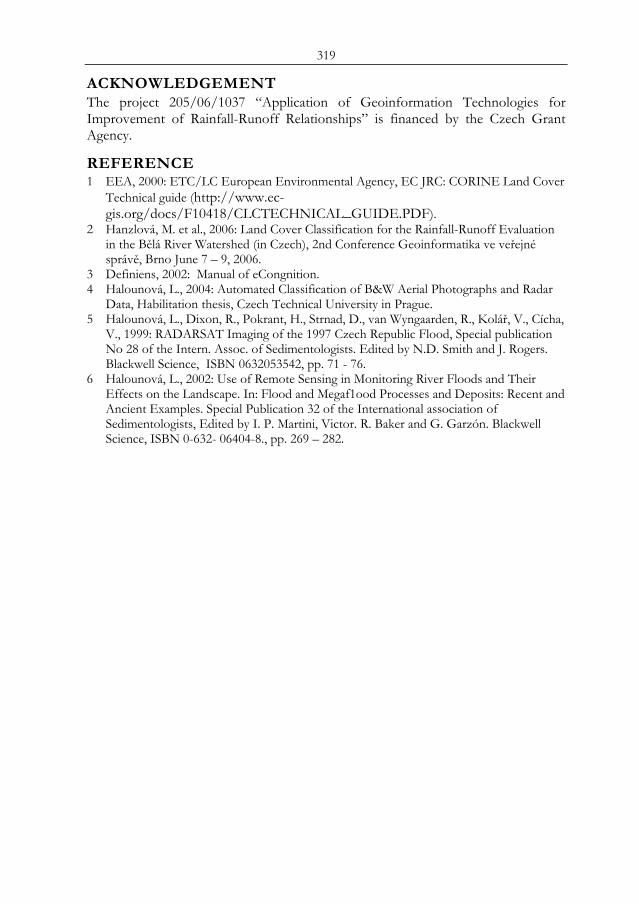
319
ACKNOWLEDGEMENT The project 205/06/1037 “Application of Geoinformation Technologies for Improvement of Rainfall-Runoff Relationships” is financed by the Czech Grant Agency.
REFERENCE 1 EEA, 2000: ETC/LC European Environmental Agency, EC JRC: CORINE Land Cover
Technical guide (http://www.ec-gis.org/docs/F10418/CLCTECHNICAL_GUIDE.PDF).
2 Hanzlová, M. et al., 2006: Land Cover Classification for the Rainfall-Runoff Evaluation in the Bělá River Watershed (in Czech), 2nd Conference Geoinformatika ve veřejné správě, Brno June 7 – 9, 2006.
3 Definiens, 2002: Manual of eCongnition. 4 Halounová, L., 2004: Automated Classification of B&W Aerial Photographs and Radar
Data, Habilitation thesis, Czech Technical University in Prague. 5 Halounová, L., Dixon, R., Pokrant, H., Strnad, D., van Wyngaarden, R., Kolář, V., Cícha,
V., 1999: RADARSAT Imaging of the 1997 Czech Republic Flood, Special publication No 28 of the Intern. Assoc. of Sedimentologists. Edited by N.D. Smith and J. Rogers. Blackwell Science, ISBN 0632053542, pp. 71 - 76.
6 Halounová, L., 2002: Use of Remote Sensing in Monitoring River Floods and Their Effects on the Landscape. In: Flood and Megaf1ood Processes and Deposits: Recent and Ancient Examples. Special Publication 32 of the International association of Sedimentologists, Edited by I. P. Martini, Victor. R. Baker and G. Garzón. Blackwell Science, ISBN 0-632- 06404-8., pp. 269 – 282.
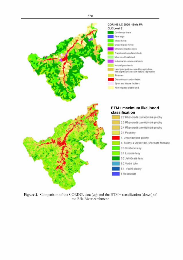
320
Figure 2. Comparison of the CORINE data (up) and the ETM+ classification (down) of
the Bělá River catchment
ETM+ maximum likelihood classification
321
GIS FOR the EVALUATION OF NITRATE WATER CONTAMINATION AND INCIDENCE OF
MORTALITY IN NATAL (NE Brazil)
R. A. Pettaa, M. Meyerb, R. F. Souza Limaa, a Geology Dept - Federal University of Rio Grande do Note, Brazil, email:
[email protected] b Rheinisch-Westfälische Technische Hochschule (RWTH), email: m.meyer@rwth-
aachen.de
ABSTRACT Neoplasia related to sanita33tion is a great challenge for public health due to increasing mortality rates where sanitation and water pollution may represent sources or causes of emerging difficulties. In that sense, this work presents a spatial analysis of the incidence of endemism caused by the lack of sanitation associating parameters related to the quality of water in Natal (Brazil). A Geographic Information System was used with the purpose of analyzing the situation of neoplasia in the area of Natal and establishing a database with information on areas of incidence, sanitation and quality of water resources within the period from 1998 to 2002. Several sources of pollutants were punctually registered which include sewers, gas stations, cemeteries, factories, industrial dejections and sewages.The data treatment was accomplished by statistical spatial analysis presenting results through absolute values, percentages and averages. With this data, a cartographic basis was generated, and a scale from one to six (06) classifications was assigned from low to high concentration of pollutants and water quality. The epidemic data were also crossed with data of water quality and other environmental data, making it possible to accomplish an analysis of the current context of the hydro system of Natal. The mainly studied diseases related to the ingestion of polluted water were stomach and intestinal cancer, cholera, dysentery ameba, bacillary dysentery, typhoid fever and paratyphoid, gastroenteritis, giardiasis, infectious hepatitis, leptospirosis, infantile paralysis and salmonellas. Other diseases acquired by contact with polluted water were scabies, trachoma, vermins and schistosomiasis. Diseases, which are spread by insects that grow in the water, like primness, yellow fever, filariose and malaria are not subject to this work in specific. As a final product, in agreement with the already available data, a map of incidence areas of mortality cases was elaborated. Keywords: Public health, System of Geographical Information, Environmental Administration, Hydro Resources.
INTRODUCTION The city of Natal has been going by a process of strong growth disorganized on these last 15 years. Formerly when a tourist or resident opened the faucet of his residence, of the hotel or of the lodging, could expect water with quality of mineral Proc. 2nd Göttingen GIS and Remote Sensing Days, 4-6 Oct. 2006, Göttingen
322
water. Today, the situation is very different. Since the beginning of last century, the whole sewer produced in the city (only 17% cleaned up) it is thrown 'in natura' in Rio Potengi, or then it is stored in septic tanks and "drains" of the back yards of the houses, with percolation affecting directly the underground water, from where are captured more than 70% of the water that supplies the city. Could be added to this fact the impermeability of the soil and the asphalt covering that transfer a good part of the rain water that could recharge of the aquifer, to be drained for the sea. There is no control of the number of sewages and existent clandestine wells in the city, however the estimate is that, every year, just the capital of Rio Grande do Norte drops about 42 million cubic meters of sewer in that immense natural filter, denominated Dunas/Barreiras Aquifer System, however there are indications that that number can be very larger.
The direct consequence of that behavior makes the underground water reservoir receive more sewers and less water every year, and it can be measured by the several studies accomplished by the Federal University of Rio Grande do Norte (UFRN), by NGOs and even for the Company of Waters and Sewers of Rio Grande do Norte (CAERN). Today, the Dunas/Barreiras Aquifer (main ground water reservoir) is almost totally polluted. In some capitation well points, the amount of nitrate (a sub-product of the contamination for fecal collyphorm) get the level of 100ppm. In other words, it is clearly above the 45 ppm considered acceptable for the World Health Organization (WHO).
Several studies and discussions exist about reception, effluents, quality and contamination of the water in Natal, however this subject that we will discuss here is pioneering in this area of linking the statistics of distribution of diseases transmitted for hydro agent and the quality of the waters of this area.
Our proposal intends to demonstrate the application of a System of Geographical Information - SIG, working as a support tool, that makes possible complementally actions of the monitoring programs and administration of the quality of the water and of the resources of environmental sanitation, allowing the information to be analyzed of form geo-referenced in the geographical space, with a degree of precision almost always satisfactory, making it a viable alternative, easy to implement and positive for plans involving events of this type.
Starting from the data, several interrelated layers were built, that allow to integrate the special information involving the database (Fig 01):
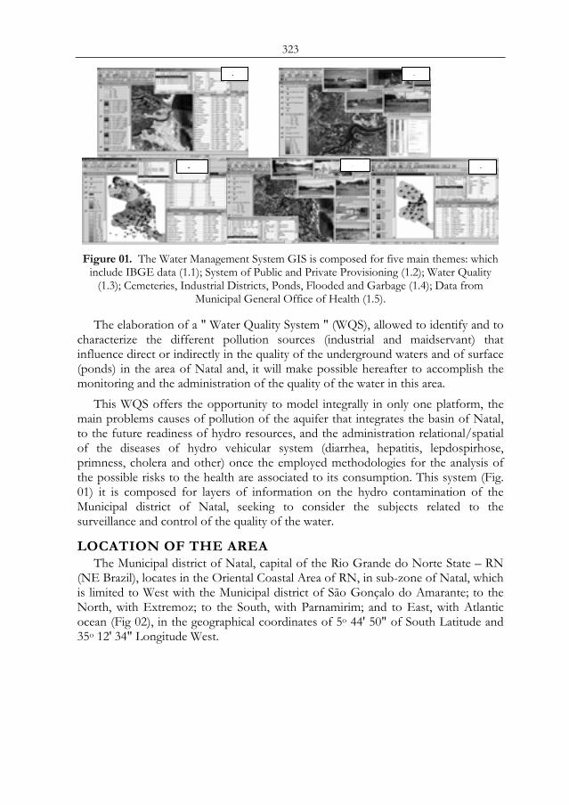
323
Figure 01. The Water Management System GIS is composed for five main themes: which
include IBGE data (1.1); System of Public and Private Provisioning (1.2); Water Quality (1.3); Cemeteries, Industrial Districts, Ponds, Flooded and Garbage (1.4); Data from
Municipal General Office of Health (1.5).
The elaboration of a " Water Quality System " (WQS), allowed to identify and to characterize the different pollution sources (industrial and maidservant) that influence direct or indirectly in the quality of the underground waters and of surface (ponds) in the area of Natal and, it will make possible hereafter to accomplish the monitoring and the administration of the quality of the water in this area.
This WQS offers the opportunity to model integrally in only one platform, the main problems causes of pollution of the aquifer that integrates the basin of Natal, to the future readiness of hydro resources, and the administration relational/spatial of the diseases of hydro vehicular system (diarrhea, hepatitis, lepdospirhose, primness, cholera and other) once the employed methodologies for the analysis of the possible risks to the health are associated to its consumption. This system (Fig. 01) it is composed for layers of information on the hydro contamination of the Municipal district of Natal, seeking to consider the subjects related to the surveillance and control of the quality of the water.
LOCATION OF THE AREA The Municipal district of Natal, capital of the Rio Grande do Norte State – RN
(NE Brazil), locates in the Oriental Coastal Area of RN, in sub-zone of Natal, which is limited to West with the Municipal district of São Gonçalo do Amarante; to the North, with Extremoz; to the South, with Parnamirim; and to East, with Atlantic ocean (Fig 02), in the geographical coordinates of 5o 44' 50" of South Latitude and 35o 12' 34" Longitude West.
1 1
1 1 1
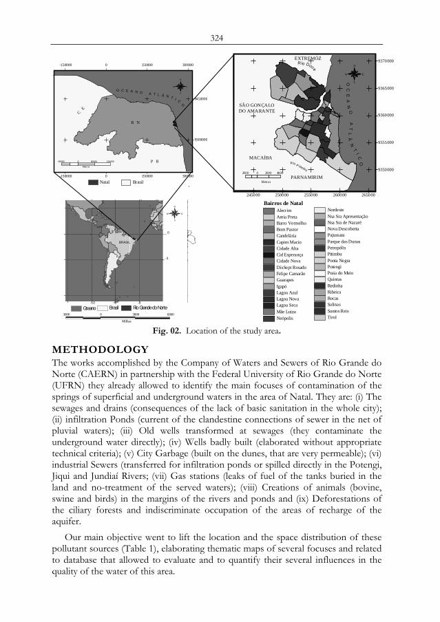
324
Fig. 02. Location of the study area.
METHODOLOGY The works accomplished by the Company of Waters and Sewers of Rio Grande do Norte (CAERN) in partnership with the Federal University of Rio Grande do Norte (UFRN) they already allowed to identify the main focuses of contamination of the springs of superficial and underground waters in the area of Natal. They are: (i) The sewages and drains (consequences of the lack of basic sanitation in the whole city); (ii) infiltration Ponds (current of the clandestine connections of sewer in the net of pluvial waters); (iii) Old wells transformed at sewages (they contaminate the underground water directly); (iv) Wells badly built (elaborated without appropriate technical criteria); (v) City Garbage (built on the dunes, that are very permeable); (vi) industrial Sewers (transferred for infiltration ponds or spilled directly in the Potengi, Jiqui and Jundiaí Rivers; (vii) Gas stations (leaks of fuel of the tanks buried in the land and no-treatment of the served waters); (viii) Creations of animals (bovine, swine and birds) in the margins of the rivers and ponds and (ix) Deforestations of the ciliary forests and indiscriminate occupation of the areas of recharge of the aquifer.
Our main objective went to lift the location and the space distribution of these pollutant sources (Table 1), elaborating thematic maps of several focuses and related to database that allowed to evaluate and to quantify their several influences in the quality of the water of this area.
N
EW
S
Brasil Rio Grande do NorteOceano
__ 0
__ -3
-6 -3-10
BRASIL
3000 0 3000 6000
Milhas
EXTREMÓZ
MACAÍBA
PARNAMIRIM
SÃO GONÇALODO AMARANTE
9370000
9365000
9360000
9355000
9350000
265000260000255000250000245000
N
EW
S
2000 0 2000 4000
Metros
Rio P itimbu
Rio Doce
OC
EA
NO
A
TL
ÂN
TI
COP B
C E
R N
O C E A N O A T L Â N T I C O
-150000
-150000
0
0
150000
150000
300000
300000
9300000
9450000
60000 0 60000 120000
Metros
N
EW
S
BrasilNatal
TirolSantos ReisSalinasRocasRibeiraRedinhaQuintasPraia do MeioPotengiPonta NegraPitimbuPetropólisParque das DunasPajussaraNova DescobertaNsa Sra de NazaréNsa Sra ApresentaçãoNordeste
NeópolisMãe LuizaLagoa SecaLagoa NovaLagoa AzulIgapóGuarapesFelipe CamarãoDixSept RosadoCidade NovaCid EsperançaCidade AltaCapim MacioCandeláriaBom PastorBarro VermelhoAreia PretaAlecrim
Bairros de Natal
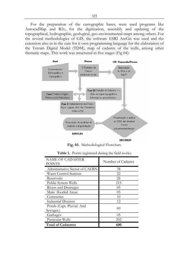
325
For the preparation of the cartographic bases, were used programs like AutocadMap and R2v, for the digitization, assembly and updating of the topographical, hydrographic, geological, geo-environmental maps among others. For the several methodologies of GIS, the software ESRI ArcGis was used and the extension also as in the case for it own programming language for the elaboration of the Terrain Digital Model (TDM), map of cadastre of the wells, among other thematic maps. This work was structured in five stages (Fig 04):
Fig. 03. Methodological Flowchart.
Table 1. Points registered during the field works.
NAME OF CADASTER POINTS Number of Cadaster
Administrative Sector of CAERN 38 Water Control Stations 22 Reservoirs 26 Public System Wells 215 Rivers and Drainages 05 Main flooded Areas 05 Cemeteries 10 Industrial Districts 12 Ponds (Capt. Pluvial. And Sewages.) 60
Garbages 05 Particular Wells 202 Total of Cadastres 600

326
NATURAL RESOURCES: The map of the blocks and lots of Natal in the scale of 1:2.000 were obtained on the CAERN. For the mapping of the hydro resources composed by rivers, streams, dams, ponds, dams, wells, publics and matters, images of Ikonos and Spot satellite were used. The composed data in this theme were: geological, geomorphologic, land use, physical environment, areas of environmental protection, and infrastructure & topographical maps. SANITARY DISTRICTS: The outlines of the sanitary districts sections of the municipal district of Natal was transcribed visually starting from the base data of IBGE, for plants in the scale of 1:10.000 and 1:2.000 obtained from IDEMA/RN and CAERN. To these sections data were associated on sanitation, provisioning and population contained in the Demographic Census of year 2.000. The layers of the sanitary exhaustion were classified by permanent private homes, general net of sewer or pluvial, septic tank, for rudimentary sewage, ditches, river, lake or sea, or other canal type, and also if had or no bathroom or sanitarium. The forms of water supply were classified in agreement with the permanent private homes under the users' of the general net total; well or nascent; another form of provisioning and no channeled (Fig 1.1). PUBLIC SYSTEM AND PECULIAR OF WATER SUPPLY: This theme was implemented starting from digital maps in the scale 1:2.000, obeying the map base of CAERN, involving the identification of the offices, of the reservoirs, public and private wells, treatment elevator stations, and their respective alphanumeric data, as well as photos of the referred point, locate by GPS and visualization of the scanner profiles (in the case of the wells) (Fig. 1.2). In this theme they were incorporate the information of analyses in the concentrations of nitrate and the layer in 3D of the no-saturated underground water level. INDUSTRIAL DISTRICTS, PUBLIC AND PRIVATE CEMETERIES, PONDS, FLOODED AREAS AND GARBAGES: The used routine went to the same that the previous, the same scale (1:2.000), the points were obtained in field through the use of GPS. The images, and the implemented alphanumeric data are referring to each point and complementally information of the same get in the field. (Fig 1.4). GOVERNMENTAL SYSTEM OF HEALTH: In this layer were implemented the data about the incidence of diseases linked to the sanitation in the neighborhoods of the municipal district, exposing its existent situation for crossing of the data with the hydro resources, industrial districts, cemeteries and garbage. The data are willing in the theme in several ways, all regarding the years from 1998 to 2001 (Fig 1.5). QUALITY OF THE WATER: Data were associated with the acceptable pattern in agreement with the world patterns as World Health Organization (WHO), and Brazilian patterns as CONAMA, CAERN and SERHID, in the sense that each point has it located space positioning and plotted as permanent point of monitoring in chart with scale 1:2.000 supplying the maps of CAERN (Fig. 1.3).
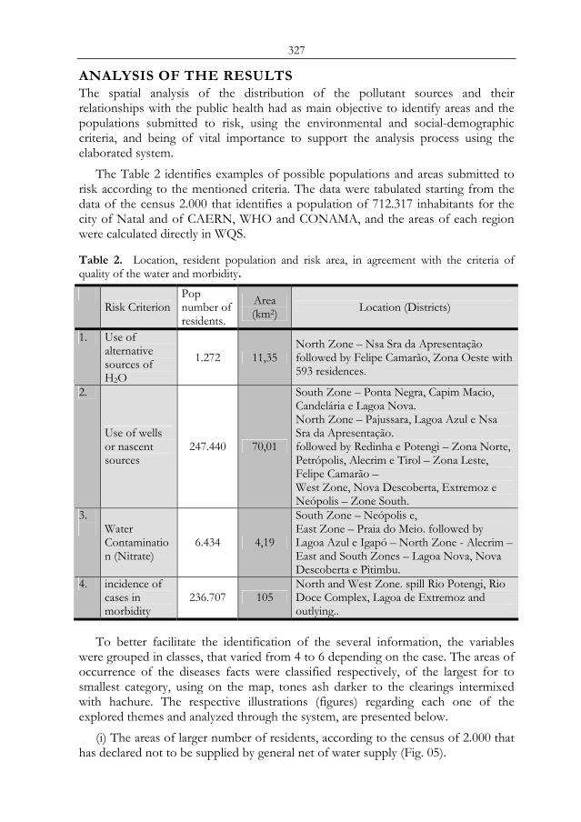
327
ANALYSIS OF THE RESULTS The spatial analysis of the distribution of the pollutant sources and their relationships with the public health had as main objective to identify areas and the populations submitted to risk, using the environmental and social-demographic criteria, and being of vital importance to support the analysis process using the elaborated system.
The Table 2 identifies examples of possible populations and areas submitted to risk according to the mentioned criteria. The data were tabulated starting from the data of the census 2.000 that identifies a population of 712.317 inhabitants for the city of Natal and of CAERN, WHO and CONAMA, and the areas of each region were calculated directly in WQS.
Table 2. Location, resident population and risk area, in agreement with the criteria of quality of the water and morbidity.
Risk Criterion
Pop number of residents.
Area (km2) Location (Districts)
1. Use of alternative sources of H2O
1.272 11,35 North Zone – Nsa Sra da Apresentação followed by Felipe Camarão, Zona Oeste with 593 residences.
2.
Use of wells or nascent sources
247.440 70,01
South Zone – Ponta Negra, Capim Macio, Candelária e Lagoa Nova. North Zone – Pajussara, Lagoa Azul e Nsa Sra da Apresentação. followed by Redinha e Potengi – Zona Norte, Petrópolis, Alecrim e Tirol – Zona Leste, Felipe Camarão – West Zone, Nova Descoberta, Extremoz e Neópolis – Zone South.
3. Water
Contamination (Nitrate)
6.434 4,19
South Zone – Neópolis e, East Zone – Praia do Meio. followed by Lagoa Azul e Igapó – North Zone - Alecrim –East and South Zones – Lagoa Nova, Nova Descoberta e Pitimbu.
4. incidence of cases in morbidity
236.707 105 North and West Zone. spill Rio Potengi, Rio Doce Complex, Lagoa de Extremoz and outlying..
To better facilitate the identification of the several information, the variables
were grouped in classes, that varied from 4 to 6 depending on the case. The areas of occurrence of the diseases facts were classified respectively, of the largest for to smallest category, using on the map, tones ash darker to the clearings intermixed with hachure. The respective illustrations (figures) regarding each one of the explored themes and analyzed through the system, are presented below.
(i) The areas of larger number of residents, according to the census of 2.000 that has declared not to be supplied by general net of water supply (Fig. 05).
328
(ii) The areas of larger concentration in septic and/or rudimentary tanks and larger number of wells were marked on the map, and depending of the growing population of these districts it is possible that there a strict relation with the contamination of the aquifer. These were identified in agreement with the base of data of the census section that has answered to this criterion (Fig. 06).
(iii) The areas nearly of the wells with concentration of the ion Nitrate that present tenors above 40 mg/l., superior to the acceptable index for CONAMA and WHO. The tenors were located through buffers of 0,5 km surrounding the arches that represent the whole net of water provisioning for each well (Fig 07).
(iv) The areas of larger incidence, for all of the cases of morbidity, in tones ash darkness. In this case it was associated to the probable hydro net. The areas were identified through the base of data of Districtal Public Health dates (Fig. 08).
Table 2 presents the criteria that were used, in way to allow the identification of partner-space groups subject to risks to the health associated to the resources of provisioning of sanitation. The use of alternative sources of water supply through small local springs (criterion 1) in the figure 5, or the use wells or nascent in areas of larger concentration in septic tanks and/or rudimentary (criterion 2) visualized in the figure 6, they can present risks for significant portions of the population (about 35%), located in the areas North and South of the municipal district and concentrate the most several economical classes. The tenors in the concentrations of nitrate are distributed by the whole municipal district, as display the stains of the obtained starting from data of all of the wells (figure 7). They were associated with those tenors (criterion 3) for the cases of mortality in stomach and intestinal cancer and it can be observed that the population under risk (less than 2%), is concentrate at the South area and East.
The location of the resident population and risk area for the incidences of the cases of morbidity (criterion 4) according to obtained data of the Secretary Municipal of Health they can be visualized in the figure 8. It includes a great part of the population under risk, acting more than 30% of the residents' total population in the municipal district. The areas of incidences of the cases of morbidity are concentrated in the surround area of the Potengi River, Rio Doce and Pond of Extremoz and outlying of the North and West Area, which represent a mesh diversified hydro.
CONCLUSIONS With this research it was intended to implement a digital hydro-cartographic base of the area of Natal, with reliable data and that could rescued the largest number of possible information, because only a extensive and systematic monitoring, settling down techniques of control of the pollutant sources and the identification of the risks to the human health related to the non service of the pattern of potability of the water, it will allow precautions to be taken and settle down politics of control of the patterns of the quality of the waters.
All the wells of the public system of provisioning were registered, besides the closed and the one that are not in operation, as well as the water stations and the reservoirs. Also the ponds of reception of pluvial waters and of treatment of sewers
329
considered important its maintenance in the existent place due to the intrusion of the saline wedge in the underground water. On this sense the WQS GIS gives opportunity to model integrally in only one platform, the main problems causes of pollution of the Dunas/Barreiras aquifer, with focus to the problems of the binomial "water & health", as well as of creating simulations seeking to identify risk areas, as well as evaluating the relationships of quality of the water with the public health, to generate of new maps thematic identification of problematic areas with epidemic focuses, that can notice problems related to the bad quality of the water.
The main sources of pollutants were registered, be through sewers, industrial dejections or sewages. Also as final product in agreement with the data already existent, a map was produced in 3-D (three dimensions) of the profile of the aquifer in sub-surface, starting from the crossing of the data of the static level of each well added to the topographical data, making possible to visualize the level no saturated and it recharge relationship with the lease of the main potential sources of contamination of the aquifer, through rivers, streams, reservoirs, ponds of stabilization that receive industrial dejections among other, wells, garbage, cemeteries, finally, resources that interact with the Duna/Barreiras aquifer system.
On this view point it can be evaluated that the area of Natal lacks an intensive management in a lot of areas, mainly in those located in area of recharge of the aquifer as well as, with urgency, an appropriate sanitation to avoid the pollution. It was also verified the need of an intensive politics of sanitation in vulnerable areas the pollution, where the researches should come accompanied of other actions, as the finalization of the collection system and sewer treatment in the whole city, the creation of a politics and to of laws that make possible a better recharge of the aquifer, the cadastre of the existent wells, the prohibition of the construction of new wells and, mainly, the creation of a fiscal equip for manager the use of the hydro resources
REFERENCES Araújo, L. P.; Petta, R. A.; Duarte, C. R.. (2005) Sistema de informações geográficas aplicado
à análise das relações da qualidade da água e risco em saúde pública no município de Natal (RN). Geociências,. v. 24, n. 1, p. 55-66, 2005
Barcellos, C. e Pina, M. de F. 1998. Análise de risco em saúde utilizando GIS: o caso do abastecimento de água no Rio de Janeiro. Revista FatorGis, São Paulo e no site URL: http://www.procc.fiocruz.br/~barcello/
Carvalho Jr. E. R. 2001. Contaminação das águas subterrâneas por nitrato e sua relação com a estrutura hidrogeológica nos bairros de Pirangi e Ponta Negra, Natal/RN. Deptº Geologia, Universidade Federal do Rio Grande do Norte, Natal, dissertação de mestrado, 170p.
ESRI – Environmental systems research institute. 1996. Using arc view GIS. Manual, 350p. Goodchild M. F. 1991. Spacial analysis with GIS: Problems and prospects GIS/LIS. The
Inforum Atlanta. 40-48p. Mineiro F. 2001. Relatório sobre a qualidade da água na cidade do Natal. Natal, 2 ed. Natal
p.19. Ministério da Saúde – RIPSA, 2000. Conceitos básicos de sistemas de informação geográfica
e cartografia aplicados à saúde. Ed. Organização Panamericana da Saúde – Representação no Brasil. Brasília – DF, p. 124, ilus. www.fiocruz.br.
330
FIGURES
Fig. 04. Areas in agreement with number of residents no supplied by the general net of water supply, according to the 2.000 census. Larger concentration was identified in dark
hachure of gray tone.
Fig. 05. Areas of larger concentration in septic tanks and/or rudimentary and larger
number of wells. These were identified in agreement with the base of data of the census section that has answered to this criterion. The hachure of dark gray tone shows the
neighborhoods under risk in relation to the quality of the water.
No District Water Supply
Concentration of septic and/or rudimentary
tanks and larger number of wells.
331
Fig. 06. Contamination for nitrate in the public and private wells in Natal. The space
analysis used the technique of buffers in a ray of 500 m starting from the positions of the wells with tenors of nitrate above the acceptable levels for the organs CONAMA/WHO.
Those data were crossed with the mortality data in stomach and intestinal cancers.
Fig. 07. Areas of larger incidence of the cases of morbidity, for all of the studied cases, in
hachure of dark gray tone. In this case it has associated the hydro net information.
A f I fl (500 ) WHO
T l h d

332
333
Drought Vulnerability and drought Changes of Vulnerability in Hungary
S. Bellaa,b and S. Szalaia a Hungarian Meteorological Service, H-1024 Budapest, Kitaibel Pál út 1. email:
[email protected] b Department of Physical Geography, Eötvös University, Pázmány P. sétány 1/c; H
– 1117 Budapest, Hungary
ABSTRACT Drought is one of the ma34in characteristics of Hungary. It occurred often in the past, it also occurs nowadays, and it will probably occur in the future as well. Many important areas of life are affected such as economy, agriculture, ecosystem, society etc.. Values of the damages caused become greater and greater. Among natural catastrophes, drought occupies a top place regarding both the affected land and the number of people in Hungary as well as in other counties. Determination of drought vulnerability of Somogy County was already carried out in our previous work. Values of the weighting factors were refined and integrated in order to be able to conduct examinations on a national level. Drought vulnerability was examined in three countries (Somogy, Baranya, Tolna), in the southern part of Hungary with the advanced tools. Besides the natural parameters, we examined the effects on land of eventual change of some parameters (e.g. precipitation, groundwater). We used GIS software (ArcView + Spatial Analyst, and Surfer). The results obtained can improve the efficiency of drought prevention. Therefore, the drought vulnerability-map is a valuable factor for sustainable development. Keywords: drought, vulnerability, changes, GIS, vulnerability map
1 INTRODUCTION The drought has an important influence not only in the agriculture and production of plants but also animals (domestic and wild), plants and human beings. It means that the damages influence uncultivated lands, nature reservations beside the agriculture, and also the human society (all parts of it). Consequently the harmful impacts of the drought must be known globally.
In order to be able to fight effectively against drought, we have to make a suitable examination. Maybe the most important task is the systematical collection, processing, and analysis of data. It is important that the society be aware of the importance of understanding the behaviour of drought. Intervention is needed not only when the event is going on. Setting up drought plans to county lands may contribute to the reduction of the impact of drought. Proc. 2nd Göttingen GIS and Remote Sensing Days, 4-6 Oct. 2006, Göttingen
334
Climate is one of the main determinative factors of social and economic relations of mankind. Economy is “built up” on its average, or a certain standard deviation of climatological elements.
It is not well prepared for a phenomenon, which is too different from the above-mentioned standard deviation. Accordingly, this phenomenon can lead to various losses. Vulnerability studies are important, because the same severity of natural hazards (e.g. drought, frost) could have different impacts depending on the natural and socio-economical factors [1]. We have to notice, that preparations for extreme events require huge costs, and because of saving behaviours these projects, part of project are not finalized. Both extremities of the precipitation cause serious problems. Too much precipitation causes floods, while too little leads to drought.
2 METHOD Bella et al [2] have set up a method for measuring drought vulnerability. They considered Somogy County as sample area. According to its results, lessons (refinement of weight factors, adding new data in the model) they constructed the drought vulnerability map of Southern Transdanubium. We provide a short description below. 2.1 SOIL PARAMETERS Soil data were obtained from AGROTOPO database of the Research Institute of Soil Science and Agrochemistry of Hungarian Academy of Science. The hardest part of the examination was the determination of the weight factors of soil data. We used data regarding soil texture, organic content, topsoil thickness, mineral content, type of rocks and water management. Mineral content Minerals have important role for the soil and rocks. They determine the number and proportion of chemical elements, the physical and chemical behaviour of the substance, and the impact on living organisms. Land classification is a function of claim minerals. The claim minerals are the most important class of the mineral parts of the soil. The nutriments and water management of soil depend on the claim minerals quality and quantity. Soil texture Soil texture is the integrated determinant of the scale distribution of the organic and mineral components of the soil. It indicates the quantity and distribution of different particle size of mechanical content. Similar to the mechanical content the soil texture is very stable in time. It determines the physical features, affects the mechanical ones of the soil (plasticity), absorption capability, chemical, physical features. 2.2 WATER MANAGEMENT Water management was considered according to the sinkhole capacity, permeability and water storage capacity. Sinkhole capacity
335
Sinkhole capacity is indicated by the amount of water that seeps into the soil per unit of time. Because the infiltration is made up of two parts (pores full of air filled up with water + water conduction toward deeply soil layers) the sinkhole capacity is always bigger – especially in case of dry soil -, than the water leading capacity [3]. Permeability Permeability is measured by the amount of water that passes through the cross section of the saturated soil per unit of time. Permeability of the whole section is determined by the value of the worst layer. The distance of this layer from the surface is very important. If the bad water leading capacity layer is just 40-50 cm under the surface, it can swell the water to the upper layers during heavy rains, which can cause surface runoff. It can be said, that the upper layers of the soil (10-20 cm) – i.e. the ploughed layer - have the crucial role in water leading capacity ([4]). Water storage capacity Water storage capacity of soil makes it possible to plants to be able to satisfy their continuous water demand from the very unsystematical (very often its temporal and spatial distribution is pettish) precipitation activity during their growth periods. The same meteorological situation leads to different ecological outcomes (in crops and yield) on different soils, as the record of the most recent past shows. There were a lot of cases to it in the past. It is understandable that years of drought overvalue the importance of the soil, and shows that the soil is the biggest natural water storage in Hungary. 2.3 TOPSOIL THICKNESS This layer is important for plants, agriculture, because these get the water and the necessary nutritive from it. 2.4 ORGANIC CONTENT Organic content plays a very important role (considering both quality and quantity) in the development of soil fertility. The organic content of the soil - humus – is not a uniform substratum. It is a mixture of many organic components with different chemical contents, and physical behaviour. We classified it according to the total amounts per hectare. 2.5 TYPE OF ROCK Rocks give basic sources for soil formation. Its physical properties, chemical, mineral content affects the soil parameters. 2.6 PRECIPITATION Precipitation has a very important role – with respect to climate - in drought development. Therefore we first processed the precipitation data. We used long time series of 53 rain gauge stations, which are in Somogy, Baranya and Tolna County belonging to the Hungarian Meteorological Service. The precipitation data were homogenized with MASH [5].
For the determination of drought vulnerability, we used the spatial averages of the long-term data in the given territory. We chose a period, that is long enough for climatological research, and in which there was no change in the measuring network.
336
We made precipitation maps to three such time intervals, namely: 1951-1980, 1961-1990 and 1971-2000. We made the interpolation with kriging method. According to the tree thirty years periods the big annual amounts of precipitation (>700 mm) lands decreased substantially in the SW part of the region. 2.7 GROUNDWATER The groundwater data were obtained from the archives of hydrological data of VITUKI (Water Resources Research Centre), and from hydrographical yearbooks. We examined the following periods: 1951-1980, 1961-1990, 1971-2000. Since 1971 much more stations have measured groundwater than between 1951-1971.
The interpolation was kriging, too. Decrease of groundwater is demonstrable; the most significant occurrence is in Belső-Somogy. Opposite process can be observed in Nagyberek. 2.8 LAND USE Land use data were obtained from 1:100.000 CORINE (1994) Land Cover database, of the Institution of Survey and Remote Sensing (FÖMI). The land use categories [6] were simplified significantly (five categories).
2.9 SLOPE, ASPECT We used the Digital Terrain Model made by the Cartographer Service of the Hungarian Defence Ministry (DDM-100) to represent surface elevation information of the territory. Regarding the aspect we took into account the four main points of the compass, and plain lands were treated separately. The aspect’s categories are those used in the physical geography.
Fig. 1 represents the flowchart of determination of drought vulnerability. We made our maps with a similar method in our previous works but then we used an extra weighting and reclassifying method. We will see later that there is no significant difference between these results.
We supposed in the examination, that except for precipitation and groundwater data, other parameters are constants. This is true acceptable, but if we would like to examine a longer period, change of land use must be considered, too, and there may be changes in the soils too. Considering these is not easy, because the old maps are available only in papers based, analogue format. If we liked to use them, we would have to perform a difficult digitalisation process.
Fig. 2 and 3 are tendency maps. We made the region’s drought vulnerability map according to the precipitation and groundwater data of 1951-1980. The same method was used for 1961-1990, 1971-2000. After it from the map of 1951-1980 we “subtract” the other two maps, which were made based on the other two thirty years averages. This way, we can see the changes of vulnerability.
The situation turned more unfavourable on the lands of Belső-Somogy, Baranyai-dombság, Southen parts of Lake Balaton, Southern Mezőföld, and other territories of the region (Fig. 2.). These lands were placed into worse categories of the 5-class scale. Beside worse lands (signed by red colour) there are better ones (signed by blue), but they are much smaller.
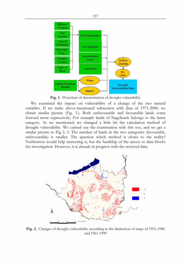
337
Fig. 1. Flowchart of determination of drought vulnerability
We examined the impact on vulnerability of a change of the two natural variables. If we make above-mentioned subsection with data of 1971-2000, we obtain similar picture (Fig. 3.). Both unfavourable and favourable lands come forward more expressively. For example lands of Nagyberek belongs to the latter category. As we mentioned, we changed a little bit the calculation method of drought vulnerability. We carried out the examination with this too, and we get a similar picture to Fig 2.-3. The number of lands in the two categories (favourable, unfavourable) is smaller. The question which method is closes to the reality? Verification would help answering it, but the hardship of the access to data blocks the investigation. However, it is already in progress with the received data.
Fig. 2. Changes of drought vulnerability according to the distinction of maps of 1951-1980
and 1961-1990
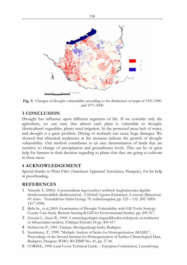
338
Fig. 3. Changes of drought vulnerability according to the distinction of maps of 1951-1980
and 1971-2000
3 CONCLUSION Drought has influence upon different segments of life. If we consider only the agriculture, we can state that almost each plant is vulnerable to drought. Horticultural vegetables, plants need irrigation. In the protected areas lack of water, and drought is a great problem. Drying of wetlands can cause huge damages. We showed that climatical tendencies at the moment indicate the growth of drought vulnerability. Our method contributes to an easy determination of lands that are sensitive to change of precipitation and groundwater levels. This can be of great help for farmers in their decision regarding to plants that they are going to cultivate in these areas.
4 ACKNOWLEDGEMENT Special thanks to Péter Fákó (American Appraisal Associates, Hungary), for his help in proofreading.
REFERENCES 1 Németh Á. (2006): A potenciálisan fagyveszélyes területek meghatározása digitális
domborzatmodellek alkalmazásával. A Miskolci Egyetem Közleményei; A sorozat (Bányászat) 69. kötet - Tiszteletkötet Hahn György 70. születésnapjára; pp. 125 – 132. (HU ISSN 1417-5398)
2 Bella Sz., et al.,2005: Examination of Drought Vulnerability with GIS Tools: Somogy County Case Study, Remote Sensing & GIS for Environmental Studies, pp. 209-217.
3 Góczán L., Kazó B., 1969: A mérnökgeológiai-vízgazdálkodási térképezés új módszerei és felhasználási területei. Földrajzi Értesítő 18 pp. 409-417.
4 Stefanovits P., 1981: Talajtan, Mezőgazdasági kiadó, Budapest 5 Szentimrey, T., 1999: ”Multiple Analysis of Series for Homogenization (MASH)”,
Proceedings of the Second Seminar for Homogenization of Surface Climatological Data, Budapest, Hungary; WMO, WCDMP-No. 41, pp. 27-46.
6 CORINE, 1994: Land Cover Technical Guide. – European Commission, Luxembourg
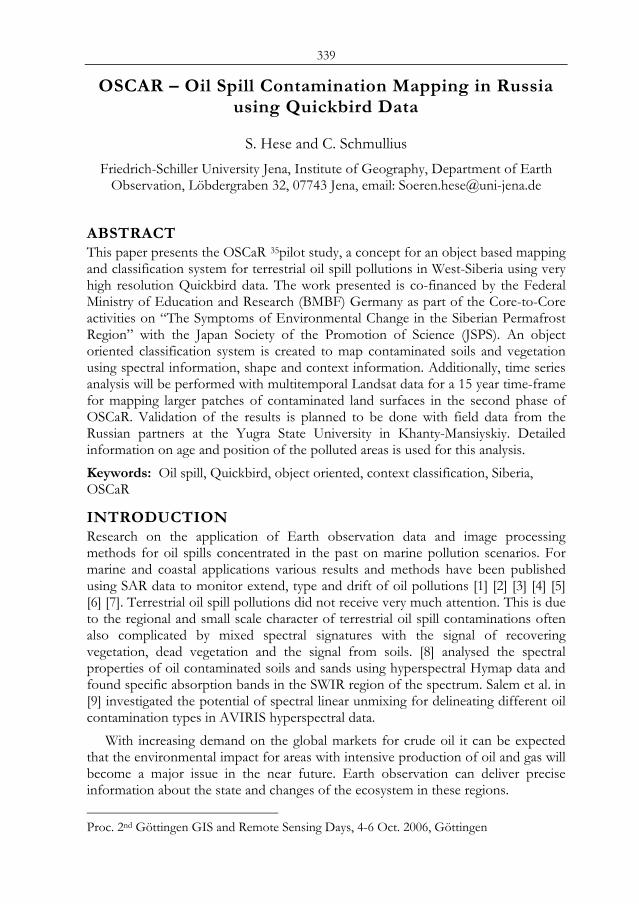
339
OSCAR – Oil Spill Contamination Mapping in Russia using Quickbird Data
S. Hese and C. Schmullius
Friedrich-Schiller University Jena, Institute of Geography, Department of Earth Observation, Löbdergraben 32, 07743 Jena, email: [email protected]
ABSTRACT This paper presents the OSCaR 35pilot study, a concept for an object based mapping and classification system for terrestrial oil spill pollutions in West-Siberia using very high resolution Quickbird data. The work presented is co-financed by the Federal Ministry of Education and Research (BMBF) Germany as part of the Core-to-Core activities on “The Symptoms of Environmental Change in the Siberian Permafrost Region” with the Japan Society of the Promotion of Science (JSPS). An object oriented classification system is created to map contaminated soils and vegetation using spectral information, shape and context information. Additionally, time series analysis will be performed with multitemporal Landsat data for a 15 year time-frame for mapping larger patches of contaminated land surfaces in the second phase of OSCaR. Validation of the results is planned to be done with field data from the Russian partners at the Yugra State University in Khanty-Mansiyskiy. Detailed information on age and position of the polluted areas is used for this analysis. Keywords: Oil spill, Quickbird, object oriented, context classification, Siberia, OSCaR
INTRODUCTION Research on the application of Earth observation data and image processing methods for oil spills concentrated in the past on marine pollution scenarios. For marine and coastal applications various results and methods have been published using SAR data to monitor extend, type and drift of oil pollutions [1] [2] [3] [4] [5] [6] [7]. Terrestrial oil spill pollutions did not receive very much attention. This is due to the regional and small scale character of terrestrial oil spill contaminations often also complicated by mixed spectral signatures with the signal of recovering vegetation, dead vegetation and the signal from soils. [8] analysed the spectral properties of oil contaminated soils and sands using hyperspectral Hymap data and found specific absorption bands in the SWIR region of the spectrum. Salem et al. in [9] investigated the potential of spectral linear unmixing for delineating different oil contamination types in AVIRIS hyperspectral data.
With increasing demand on the global markets for crude oil it can be expected that the environmental impact for areas with intensive production of oil and gas will become a major issue in the near future. Earth observation can deliver precise information about the state and changes of the ecosystem in these regions. Proc. 2nd Göttingen GIS and Remote Sensing Days, 4-6 Oct. 2006, Göttingen
340
For the detection of hydrocarbons hyperspectral data has been reported to be very useful. The only system with appropriate geometrical resolution at the time of writing is the Hyperion system with 30 meters spatial resolution and 220 bands with 10 nm band widths [10]. Calibration of this data is however problematic as the spectral ground measurements in West-Siberia are not easily obtainable. Data with very high spatial resolution is available and covers the visible and near infrared domain of the spectrum with 0.6 to 2.5 m spatial resolution. For the analysis of terrestrial oil contamination and the detection of specific materials a combination of both data types would be desirable to determine the mixed pixel content of the hyperspectral signal.
The presented work of the OSCaR project concentrates on spatial high resolution data in combination with time series analysis to detect contaminations and to precisely date the oil spill events. The methods utilised concentrate on object oriented image processing techniques and will be combined with time series analysis in the future.
The Khanty-Mansiyskiy area in West Siberia is one of the most important territories for the Russian oil and gas production with 58% of the total Russian oil production and being on the 3rd place with its national gas production. Large areas are oil and waste water polluted from pipeline leakages with heavy direct impact on underground and surface water quality, ecological conditions and quality of living (Figure 1). The region is largely covered by taiga and tundra forest with subarctic to continental climate and areas of permafrost with annual precipitation between 400 to 500 mm. The area has low nutrient peat based soils with long biological recovery times and includes important habitats for endangered fauna. Due to low evaporation and low temperatures, lack of drainage and small infiltrations rates large wetlands are formed. Thermokarst occurs due to melting ground ice (Pattern Ground) and thaw lakes and thermokarst pits can occur. The geological structure of the West Siberian basin is dominated by lower cretaceous and jurassic sections. The oil and gas resources are found in stratigraphic and structural traps that extend into the Kara Sea region.
Population is concentrated in a number of urban and industrial areas, which have developed over the last half century due to a strong immigration. The region has compared with the Russian average low health rates often related to the environmental quality of living with a potential (suspected) relationship with a “higher than average” [11] level of diseases. The number of indigenous people of West Siberia based on traditional family structured hunting, reindeer herding, fishing and nomadic lifestyle (Khants, Mansis, Nenets) has been severely reduced since the 1950s [11]. The Russian Federation belongs to the top 5 energy producers with Germany and other European countries being the major importers. West Siberia is the oldest oil and gas region mainly exploited by Russian privatised companies (LUKoil, Surneftegaz, Yukos, Sidanko, Tatneft, Tyumen Oil (TNK)).
According to the IWACO Report the privatisation has transferred the responsibility for past and current environmental impacts from the government to the oil companies exploiting the fields. The governmental authorities remain however responsible for monitoring and enforcement of environmental legislation
341
and developing strategies for the energy sector. The IWACO Report states that about 700 000 to 840 000 hectares in West Siberia are oil polluted – a much larger area than indicated by the government or oil company statistics.
Figure 1. Oil spill polluted forest and tundra areas in the Samotlor oil field, West Siberia (S.
Cejchan, BFH Hamburg).
The major environmental and social impacts come from activities like: 1. pipeline breaks, spills, and pipeline accident, 2. deposition of oily muds, drilling and production wastes, 3. chemical waste disposal and leaking storages, 4. surface water pollution in water bodies around oil fields, 5. emissions of hydrocarbons and greenhouse gases from flaring and
venting of gases and oily waste burning and 6. inadequate emergency planning and under-developed awareness of
environmental impact and remediation measures. In the Khanty Mansiysk district more than 62000 oil wells have been drilled and
according to sources from the IWACO report [11] 64000 km of pipelines have been constructed.
The magnitude of the oils spills is very difficult to calculate. Accurate data on numbers is very hard to obtain. According to different sources about 2% of the total
342
oil quantity produced is spilled into the tundra. The average oil spill loses about 2 tons of oil and covers about 1000 sqm.
THE OSCAR PILOT STUDY (OIL SPILL CONTAMINATION MAPPING IN RUSSIA) The OSCaR (OilSpill Contamination mapping in Russia) pilot study project was initiated in 2005 as part of BMBF financed permafrost degradation proposal preparation meetings in Russia (Challenges of Permafrost Degradation of Siberian Soils to Science and Technology) and Core2Core activities with the Japanese JSPS programme in 2005.
The German Ministry for Education and Science co-financed OSCaR with funding for Earth observation data of the Khanty Mansiysk area (Landsat and Quickbird data). The main goal of OSCaR is to test very high resolution multispectral data for oil spill contamination mapping with advanced image processing algorithms. The methodological focus is on spatial high resolution data analysis. Object oriented image analysis has been carried out to link the spectral characteristics of oil spill objects to secondary image object features that have a contextual relation to oil spills (infrastructure, drilling platforms, pipelines, waste water reservoirs or drilling mud reservoirs). Post classification analysis of specific objects has to be performed to identify the structural identity of oil spills and the related objects.
In a second stage the development of the region is analysed using multi temporal data with lower spatial but with very high temporal resolution. Changes will be mapped starting in the early 80s and with 2-3 year steps until 2005. The main interests are 1. to identify area and position of larger oil spills and 2. to map changes in industrial structures and infrastructure (increase of oil wells, construction of new pipelines etc.) Identification of oil spills in multitemporal data is important for dating of spill events and large oil pipeline leakages.
DATA For the OSCaR project very high resolution Quickbird data was selected covering an approximate 20x16 km subset of a region in the Khanty Mansiysk area north of Surgut in West Siberia. A full “Basic Set” Quickbird data take was ordered from the archive from 2004 (acquisition date 2004-09-27) including the full resolution multispectral information (2.72 m) and a panchromatic data layer with 0.68 meter spatial resolution (Table 1). The data was imported and georeferenced using the RPCs provided by Digital Globe without ortho correction.
Table 1. Quickbird data Quickbird data Digital Globe Date 2004 09 27 Cloud Cover 1 % Catalog ID 101001000348E202 Resolution 0.68 / 2.72 meters Off-Nadir 19 degrees
343
The data was interpolated to the appropriate resolution with a bilinear interpolation to UTM 43 (WGS84) in 16 Bit radiometric resolution (NN interpolation was not performed as no pixel based analysis is planned and smooth object geometry is priority).
Landsat ETM+ and Landsat TM5 data was ordered for the path/row sets 156/17 and 157/17 with a temporal coverage for the years 1987, 1988, 1990, 1995, 2000, 2001 and 2003. Ground information was provided by the Russian partners from the Yugra State University in Khanty-Mansiyskiy. Digital maps with indicated dates and extend of oil spill events and digitized information about infrastructure and the position of oil wells.
Figure 2. Landsat subset (left), Quickbird data set (right) from 27. September 2004, overlay with oil contaminated ground truth information layer, infrastructure layer with positions of
oil wells (Kusts) and pipelines, RGB with Quickbird channels 4-3-2.
METHODS The object-based strategy for data classification [12] [13] uses as a first stage a segmentation into different scales of image object primitives according to spatial and spectral features. The segmentation is a bottom up region merging technique starting with one pixel sized objects. In numerous subsequent steps smaller objects are merged into bigger objects (pair wise clustering) minimizing the weighted heterogeneity of resulting objects using the size and a parameter of heterogeneity (local optimization procedure) [13]. This concept has the advantage to account for contextual information using image objects instead of the pixel based concept used frequently as the basic element in Earth observation image analysis. In a second stage rule-based decisions can be used to classify the multi scale image objects. Class based feature definitions (integrating a post classification analysis) are possible as well as the inheritance of class descriptions to form a class hierarchy. Image processing tasks can be performed using vector shape and vector characteristics. This increases the flexibility of the image processing concept and integrates GIS-like data queries in an attribute database directly into the image processing and analysis
344
approach. New attributes (like object shape or structural characteristics, e.g. distance to other objects) can be used.
Object based image analysis has been used since 1999 for different approaches and in different remote sensing disciplines. Various approaches applied object oriented methods to urban applications [14], biotope classification [15] and forest applications [16] [17] [18] [19].
Advantages over pixel-based approaches have been published mainly using very high resolution airborne or orbital Earth observation data. The primary advantage of reducing the spectral variability in very high spatial resolution data sets (spatial resolution better 5 m) is however only one aspect of object oriented image analysis.
In this work object oriented image analysis has been carried out to link the spectral characteristics of oil spill objects to secondary image object features that have a contextual relation to oil spills (e.g. infrastructure objects, oil well objects, pipeline objects and waste water reservoir objects or drilling mud reservoir objects). The classification of these secondary objects is done in different segmentation scales. Post classification analysis of specific objects has to be performed to identify the structural identity of oil spills and related objects.
The dataset is segmented into three different layers with segments scales. A hierarchical class description is build that classifies water bodies and vegetation
cover types in the finest level and infrastructure, roads and industrial sites in the coarser segmentation levels. Road objects and industrial classes are differentiated with object shape features and with spectral characteristics. Oil contaminated areas are mapped with a thresholding of NDVI calculations into four different vegetation sub classes ranging from healthy vegetation to heavily polluted vegetation. The correlation between NDVI and oil spills is based on the reduced amount of healthy vegetation on oil contaminated soils. This is clearly visible in the NIR with a reduced amount of reflectance in polluted areas. Water bodies and non-vegetated areas have been masked out to avoid the overlap with non-vegetated areas through inverted expressions (Figure 3).
To increase the accuracy of the classification class related feature sets are designed that introduce distance in relation to the class infrastructure and industrial area as a characteristic object property of oil spill objects. Oil polluted areas therefore are only classified in a defined distance (buffer) to road networks, oil production platforms or other industrial areas (Figure 4 and class description shown in Figure 6).
A typical example of oil polluted vegetation in direct neighbourhood of oil wells is shown in Figure 5.
In a second stage in OSCaR the regional changes will be analysed using multi temporal data with lower spatial resolution but with high temporal resolution. The changes will be mapped starting in the early 80s and with 2-3 year steps until 2004. The main interests are 1. mapping of changes in industrial object structures and infrastructure (increase of oil wells, construction of new pipelines etc.) and 2. dating and identification of areas with large oil spills.
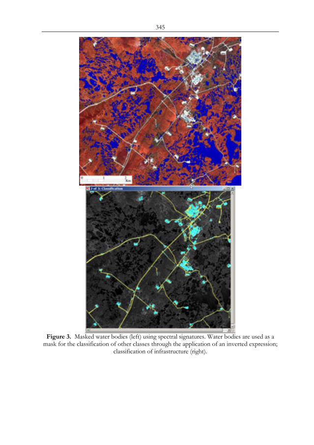
345
Figure 3. Masked water bodies (left) using spectral signatures. Water bodies are used as a
mask for the classification of other classes through the application of an inverted expression; classification of infrastructure (right).
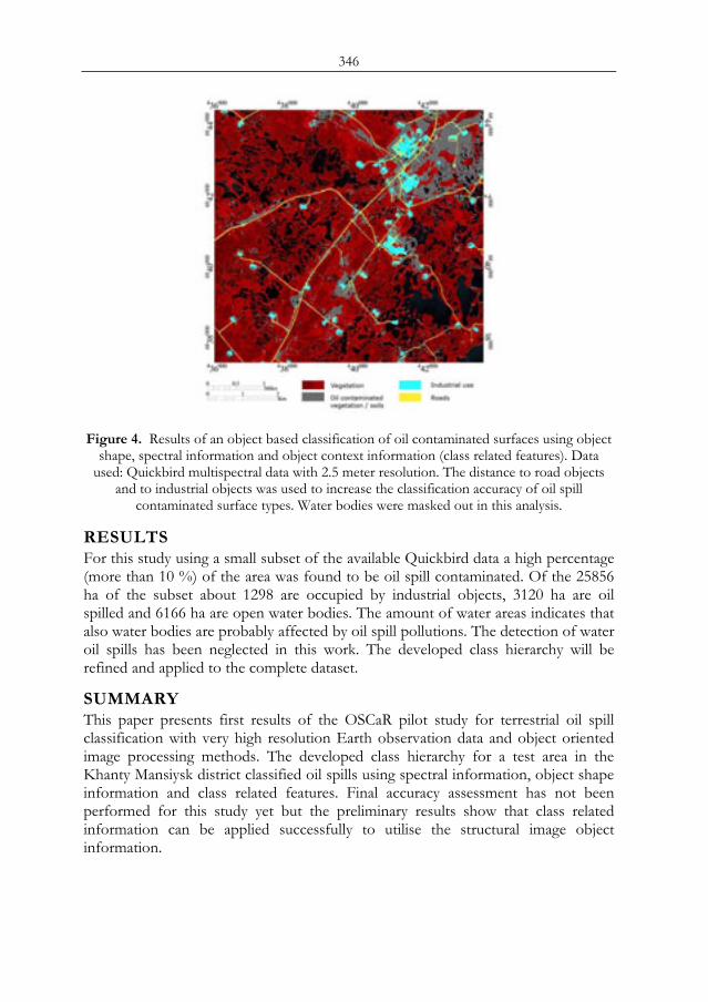
346
Figure 4. Results of an object based classification of oil contaminated surfaces using object shape, spectral information and object context information (class related features). Data
used: Quickbird multispectral data with 2.5 meter resolution. The distance to road objects and to industrial objects was used to increase the classification accuracy of oil spill
contaminated surface types. Water bodies were masked out in this analysis.
RESULTS For this study using a small subset of the available Quickbird data a high percentage (more than 10 %) of the area was found to be oil spill contaminated. Of the 25856 ha of the subset about 1298 are occupied by industrial objects, 3120 ha are oil spilled and 6166 ha are open water bodies. The amount of water areas indicates that also water bodies are probably affected by oil spill pollutions. The detection of water oil spills has been neglected in this work. The developed class hierarchy will be refined and applied to the complete dataset.
SUMMARY This paper presents first results of the OSCaR pilot study for terrestrial oil spill classification with very high resolution Earth observation data and object oriented image processing methods. The developed class hierarchy for a test area in the Khanty Mansiysk district classified oil spills using spectral information, object shape information and class related features. Final accuracy assessment has not been performed for this study yet but the preliminary results show that class related information can be applied successfully to utilise the structural image object information.
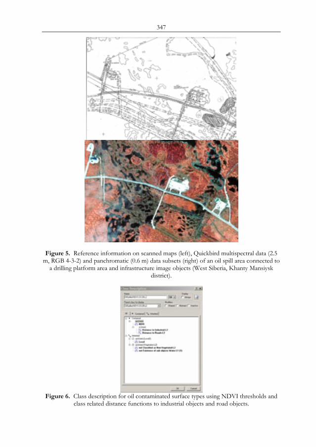
347
Figure 5. Reference information on scanned maps (left), Quickbird multispectral data (2.5 m, RGB 4-3-2) and panchromatic (0.6 m) data subsets (right) of an oil spill area connected to
a drilling platform area and infrastructure image objects (West Siberia, Khanty Mansiysk district).
Figure 6. Class description for oil contaminated surface types using NDVI thresholds and
class related distance functions to industrial objects and road objects.
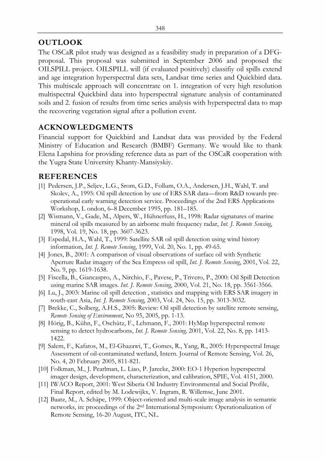
348
OUTLOOK The OSCaR pilot study was designed as a feasibility study in preparation of a DFG-proposal. This proposal was submitted in September 2006 and proposed the OILSPILL project. OILSPILL will (if evaluated positively) classifiy oil spills extend and age integration hyperspectral data sets, Landsat time series and Quickbird data. This multiscale approach will concentrate on 1. integration of very high resolution multispectral Quickbird data into hyperspectral signature analysis of contaminated soils and 2. fusion of results from time series analysis with hyperspectral data to map the recovering vegetation signal after a pollution event.
ACKNOWLEDGMENTS Financial support for Quickbird and Landsat data was provided by the Federal Ministry of Education and Research (BMBF) Germany. We would like to thank Elena Lapshina for providing reference data as part of the OSCaR cooperation with the Yugra State University Khanty-Mansiyskiy.
REFERENCES [1] Pedersen, J.P., Seljev, L.G., Srom, G.D., Follum, O.A., Andersen, J.H., Wahl, T. and
Skolev, A., 1995: Oil spill detection by use of ERS SAR data—from R&D towards pre-operational early warning detection service. Proceedings of the 2nd ERS Applications Workshop, L ondon, 6–8 December 1995, pp. 181–185.
[2] Wismann, V., Gade, M., Alpers, W., Hühnerfuss, H., 1998: Radar signatures of marine mineral oil spills measured by an airborne multi frequency radar, Int. J. Remote Sensing, 1998, Vol. 19, No. 18, pp. 3607-3623.
[3] Espedal, H.A., Wahl, T., 1999: Satellite SAR oil spill detection using wind history information, Int. J. Remote Sensing, 1999, Vol. 20, No. 1, pp. 49-65.
[4] Jones, B., 2001: A comparison of visual observations of surface oil with Synthetic Aperture Radar imagery of the Sea Empress oil spill, Int. J. Remote Sensing, 2001, Vol. 22, No. 9, pp. 1619-1638.
[5] Fiscella, B., Giancaspro, A., Nirchio, F., Pavese, P., Trivero, P., 2000: Oil Spill Detection using marine SAR images. Int. J. Remote Sensing, 2000, Vol. 21, No. 18, pp. 3561-3566.
[6] Lu, J., 2003: Marine oil spill detection , statistics and mapping with ERS SAR imagery in south-east Asia, Int. J. Remote Sensing, 2003, Vol. 24, No. 15, pp. 3013-3032.
[7] Brekke, C., Solberg, A.H.S., 2005: Review: Oil spill detection by satellite remote sensing, Remote Sensing of Environment, No 95, 2005, pp. 1-13.
[8] Hörig, B., Kühn, F., Oschütz, F., Lehmann, F., 2001: HyMap hyperspectral remote sensing to detect hydrocarbons, Int. J. Remote Sensing, 2001, Vol. 22, No. 8, pp. 1413-1422.
[9] Salem, F., Kafatos, M., El-Ghazawi, T., Gomes, R., Yang, R., 2005: Hyperspectral Image Assessment of oil-contaminated wetland, Intern. Journal of Remote Sensing, Vol. 26, No. 4, 20 February 2005, 811-821.
[10] Folkman, M., J. Pearlman, L. Liao, P. Jarecke, 2000: EO-1 Hyperion hyperspectral imager design, development, characterization, and calibration, SPIE, Vol. 4151, 2000.
[11] IWACO Report, 2001: West Siberia Oil Industry Environmental and Social Profile, Final Report, edited by M. Lodewijkx, V. Ingram, R. Willemse, June 2001.
[12] Baatz, M., A. Schäpe, 1999: Object-oriented and multi-scale image analysis in semantic networks, in: proceedings of the 2nd International Symposium: Operationalization of Remote Sensing, 16-20 August, ITC, NL.
349
[13] Benz, U.C., P. Hofmann, G. Willhauck, I. Langenfelder, M. Heynen, 2004: Multi-resolution, object-oriented fuzzy analysis of remote sensing data for GIS-ready information, ISPRS Journal of Photogrammetry and Remote Sensing, 58 (2004), 239-258.
[14] Damm, A., P. Hostert, S. Schiefer, 2005: Investigating Urban Railway Corridors with Geometric High Resolution Satellite Data, Urban Remote Sensing 2005, Berlin Adlershof.
[15] Leser, C., 2002: Operationelle Biotoptypenkartierung mit HRSC-Daten – Probleme und Lösungsansätze. In: Blaschke, T. (Hrsg.): GIS und Fernerkundung: Neue Sensoren – Innovative Methoden. Wichmann Verlag, Heidelberg: 88-97.
[16] Mitri, G.H. & I. Gitas, 2002: The development of an object-oriented classification model for operational burned area mapping on the Mediterranean island of Thasos using LANDSAT TM images, in Viegas X. (ed.) Forest Fire Research & Wildland Fire Safety, 2002 Millpress, Rotterdam, ISBN 90-77017-72-0.
[17] Flanders, D., M. Hall-beyer & J. Pereverzoff, 2003: Preliminary evaluation of eCognition object-based software for cut block delineation and feature extraction. In: Canadian Journal of Remote Sensing, Vol. 29, No. 4, pp. 441–452, August 2003.
[18] Hese, S., Schmullius, C., 2005: Forest Cover Change in Siberia - Results from the Siberia-II Project, International Conference on Remote Sensing of Environment, Conference Proceedings, St. Petersburg, Russia.
[19] Chubey, M., S. Franklin and M. Wulder, 2006: Object-based Analysis of Ikonos-2 Imagery for Extraction of Forest Inventory Parameters. PE & RS, April 2006.

350
351
GEOPROCESSING APPLIED TO THE EVALUATION OF VULNERABILITIES AND LAND
DEGRADATION IN AREAS OF PETROLEUM EXPLORATION
R. A. Pettaa, M. Meyerb, R. F. Souza Limaa a Depto Geologia Universidade Federal do Rio Gde do Norte (UFRN), Campus
Universitário CP: 59.970-072 Natal (RN/Brazil), email: [email protected]
b Rheinisch-Westfälische Technische Hochschule (RWTH) Aachen, email: [email protected]
ABSTRACT This investigation is focused 36on the evaluation of land degradation and environmental and natural vulnerability for petroleum spills in the Canto do Amaro oil field area, located in the Potiguar Basin - Rio Grande do Norte - Brazil, using a Geographic Information System (GIS) associated to an environmental and socioeconomic database. The final objective is to subsidize the thematic cartographic basis for the elaboration of contingency plans in case of disasters in areas of petroleum exploration activities. The region is characterized by an intense intervention of anthropogenic activities, existence of more than 1.700 oil wells, dutes, storage and transport structures of gas and oil, ponds for stabilization and treatment of dejects, pumping and collecting stations besides a marine salt industry and wide areas with activities of shrimp farms. The study has the starting focal point on the geo-environmental monitoring of land degradation through the analysis of georeferenciated multi-temporal images of orbital sensors Spot (2000 to 2004) and Ikonos (2003), and aerial photos of low altitude. The methodology involved mapping of the natural resources of the area using the sensor products that were classified through techniques of digital image processing (DIP) associated to traditional techniques of field mapping for the production of thematic index maps in detail (1:25.000) and semi-detail (1:50.000) scales, containing information about geology, geomorfology, pedology, vegetation, land use and occupation, and environmental vulnerability to the occupation, as well as to petroliferous exploratory activity, seeking to determine which areas are more susceptible to degradation. Keywords: Environmental Vulnerability; GIS; remote sensing.
INTRODUCTION The Potiguar Basin – main area of petroleum exploration in Rio Grande do Norte State (Brazil) - is an area where in the last two decades Petrobrás (oil Brazilian company) increased considerably their exploratory activities, being the first national field producer of oil in land, and second if considered the production in land and sea. Proc. 2nd Göttingen GIS and Remote Sensing Days, 4-6 Oct. 2006, Göttingen
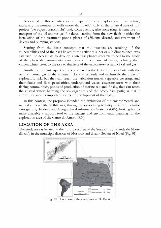
352
Associated to this activities was an expansion of all exploration infrastructure, increasing the number of wells (more than 3.600), only in the physical area of this project (www.petrobras.com.br) and, consequently, also increasing, it structure of transport of the oil and/or gas for dutes, starting from the new fields, besides the installation of the treatment ponds, places of effluents discard, and treatment of dejects and pumping stations.
Starting from the basic concepts that the disasters are resulting of the vulnerabilities and of the risks linked to the activities super or sub dimensioned, was establish the necessitate to develop a interdisciplinary research turned to the study of the physical-environmental conditions of the main risk areas, defining their vulnerabilities front to the risk to disasters of the exploratory system of oil and gas.
Another important aspect to be considered is the fact of the accidents with the oil and natural gas in the continent don't affect only and exclusively the areas of exploratory risk, but they can reach the habitation nuclei, vegetable coverings and their fauna and flora peculiarities, underground water, estuarine areas with their fishing communities, ponds of production of marine salt and, finally, they can reach the coastal waters harming the sea organism and the ecotourism potiguar that it constitutes another important source of development of the State.
In this context, the proposal intended the evaluation of the environmental and natural vulnerability of this area, through geoprocessing techniques as the thematic cartography, database and Geographical information Systems (GIS), looking for to make available a support tool to the strategy and environmental planning for the exploration area of the Canto do Amaro (RN).
LOCATION OF THE AREA The study area is located in the northwest area of the State of Rio Grande do Norte (Brazil), in the municipal districts of Mossoró and distant 260km of Natal (Fig. 01).
Fig. 01. Location of the study area – NE Brazil.
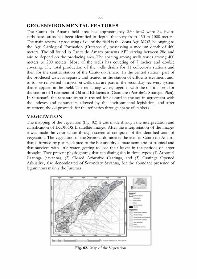
353
GEO-ENVIRONMENTAL FEATURES The Canto do Amaro field area has approximately 250 km2 were 32 hydro carbonates areas has been identified in depths that vary from 450 to 1000 meters. The main reservoir producing of oil of the field is the Zona Açu-MO2, belonging to the Açu Geological Formation (Cretaceous), possessing a medium depth of 460 meters. The oil found in Canto do Amaro presents API varying between 28o and 44o to depend on the producing area. The spacing among wells varies among 400 meters to 200 meters. Most of the wells has covering of 7 inches and double covering. The total production of the wells drains for 11 collector’s stations and then for the central station of the Canto do Amaro. In the central station, part of the produced water is separate and treated in the station of effluents treatment and, to follow reinserted in injection wells that are part of the secondary recovery system that is applied in the Field. The remaining water, together with the oil, it is sent for the station of Treatment of Oil and Effluents in Guamaré (Petrobrás Strategic Plan). In Guamaré, the separate water is treated for discard in the sea in agreement with the indexes and parameters allowed by the environmental legislation, and after treatment, the oil proceeds for the refineries through shape oil tankers.
VEGETATION The mapping of the vegetation (Fig. 02) it was made through the interpretation and classification of IKONOS II satellite images. After the interpretation of the images it was made the vetorization through screen of computer of the identified units of vegetation. The vegetation of the Savanna dominates the area of Canto do Amaro, that is formed by plants adapted to the hot and dry climate semi-arid or tropical and that survives with little water, getting to lose their leaves in the periods of larger drought. They present physiognomy that can distinguish in three types: (1) Arboreal Caatinga (savanna), (2) Closed Arbustive Caatinga, and (3) Caatinga Opened Arbustive, also denominated of Secondary Savanna, for the abundant presence of leguminous mainly the Juremas.
Fig. 02. Map of the Vegetation
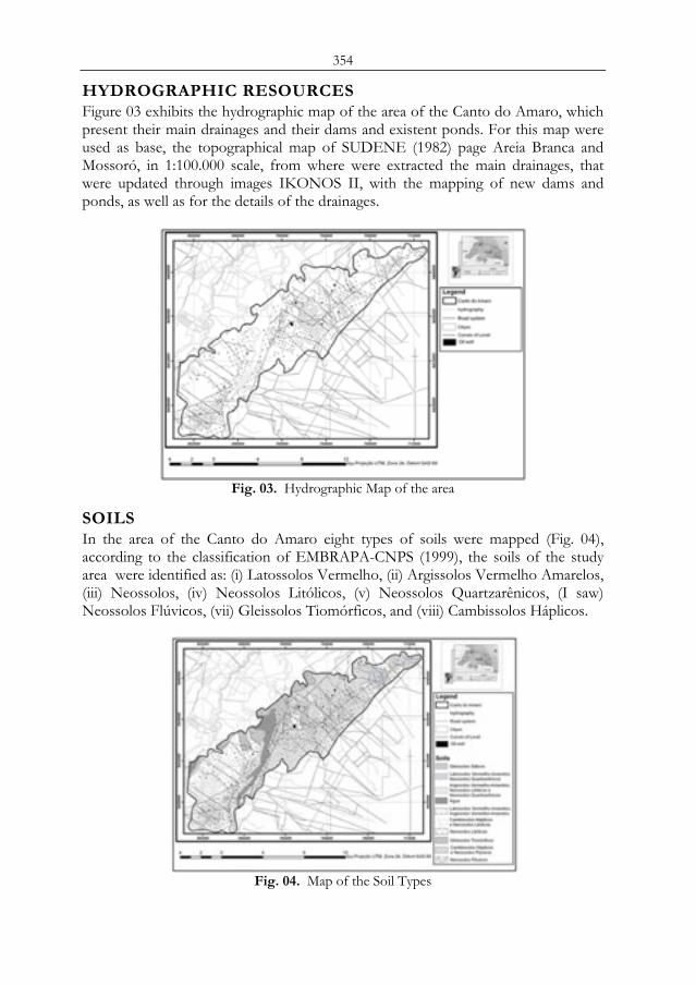
354
HYDROGRAPHIC RESOURCES Figure 03 exhibits the hydrographic map of the area of the Canto do Amaro, which present their main drainages and their dams and existent ponds. For this map were used as base, the topographical map of SUDENE (1982) page Areia Branca and Mossoró, in 1:100.000 scale, from where were extracted the main drainages, that were updated through images IKONOS II, with the mapping of new dams and ponds, as well as for the details of the drainages.
Fig. 03. Hydrographic Map of the area
SOILS In the area of the Canto do Amaro eight types of soils were mapped (Fig. 04), according to the classification of EMBRAPA-CNPS (1999), the soils of the study area were identified as: (i) Latossolos Vermelho, (ii) Argissolos Vermelho Amarelos, (iii) Neossolos, (iv) Neossolos Litólicos, (v) Neossolos Quartzarênicos, (I saw) Neossolos Flúvicos, (vii) Gleissolos Tiomórficos, and (viii) Cambissolos Háplicos.
Fig. 04. Map of the Soil Types
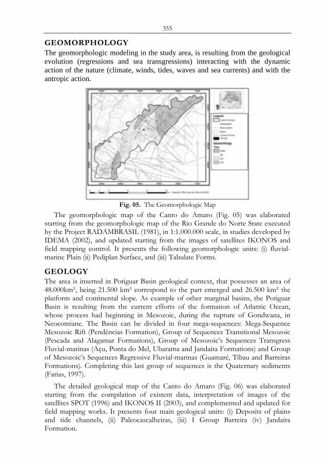
355
GEOMORPHOLOGY The geomorphologic modeling in the study area, is resulting from the geological evolution (regressions and sea transgressions) interacting with the dynamic action of the nature (climate, winds, tides, waves and sea currents) and with the antropic action.
Fig. 05. The Geomorphologic Map
The geomorphologic map of the Canto do Amaro (Fig. 05) was elaborated starting from the geomorphologic map of the Rio Grande do Norte State executed by the Project RADAMBRASIL (1981), in 1:1.000.000 scale, in studies developed by IDEMA (2002), and updated starting from the images of satellites IKONOS and field mapping control. It presents the following geomorphologic units: (i) fluvial-marine Plain (ii) Pediplan Surface, and (iii) Tabulate Forms.
GEOLOGY The area is inserted in Potiguar Basin geological context, that possesses an area of 48.000km², being 21.500 km² correspond to the part emerged and 26.500 km² the platform and continental slope. As example of other marginal basins, the Potiguar Basin is resulting from the current efforts of the formation of Atlantic Ocean, whose process had beginning in Mesozoic, during the rupture of Gondwana, in Neocomiane. The Basin can be divided in four mega-sequences: Mega-Sequence Mesozoic Rift (Pendências Formation), Group of Sequences Transitional Mesozoic (Pescada and Alagamar Formations), Group of Mesozoic’s Sequences Transgress Fluvial-marinas (Açu, Ponta do Mel, Ubarama and Jandaíra Formations) and Group of Mesozoic’s Sequences Regressive Fluvial-marinas (Guamaré, Tibau and Barreiras Formations). Completing this last group of sequences is the Quaternary sediments (Farias, 1997).
The detailed geological map of the Canto do Amaro (Fig. 06) was elaborated starting from the compilation of existent data, interpretation of images of the satellites SPOT (1996) and IKONOS II (2003), and complemented and updated for field mapping works. It presents four main geological units: (i) Deposits of plains and tide channels, (ii) Paleocascalheiras, (iii) I Group Barreira (iv) Jandaíra Formation.
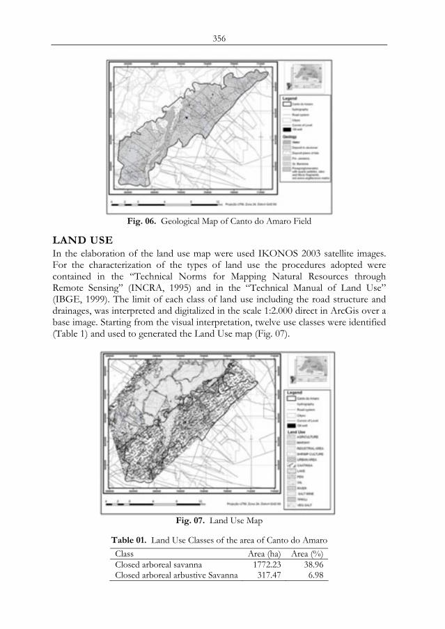
356
Fig. 06. Geological Map of Canto do Amaro Field
LAND USE In the elaboration of the land use map were used IKONOS 2003 satellite images. For the characterization of the types of land use the procedures adopted were contained in the “Technical Norms for Mapping Natural Resources through Remote Sensing” (INCRA, 1995) and in the “Technical Manual of Land Use” (IBGE, 1999). The limit of each class of land use including the road structure and drainages, was interpreted and digitalized in the scale 1:2.000 direct in ArcGis over a base image. Starting from the visual interpretation, twelve use classes were identified (Table 1) and used to generated the Land Use map (Fig. 07).
Fig. 07. Land Use Map
Table 01. Land Use Classes of the area of Canto do Amaro Class Area (ha) Area (%)Closed arboreal savanna 1772.23 38.96Closed arboreal arbustive Savanna 317.47 6.98
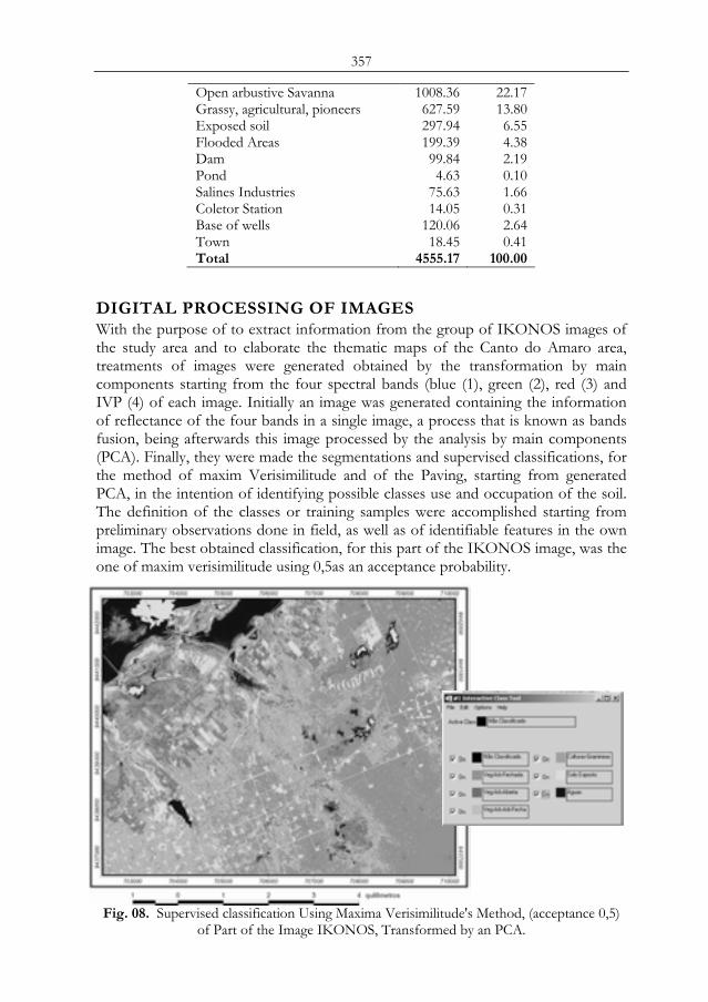
357
Open arbustive Savanna 1008.36 22.17Grassy, agricultural, pioneers 627.59 13.80Exposed soil 297.94 6.55Flooded Areas 199.39 4.38Dam 99.84 2.19Pond 4.63 0.10Salines Industries 75.63 1.66Coletor Station 14.05 0.31Base of wells 120.06 2.64Town 18.45 0.41Total 4555.17 100.00
DIGITAL PROCESSING OF IMAGES With the purpose of to extract information from the group of IKONOS images of the study area and to elaborate the thematic maps of the Canto do Amaro area, treatments of images were generated obtained by the transformation by main components starting from the four spectral bands (blue (1), green (2), red (3) and IVP (4) of each image. Initially an image was generated containing the information of reflectance of the four bands in a single image, a process that is known as bands fusion, being afterwards this image processed by the analysis by main components (PCA). Finally, they were made the segmentations and supervised classifications, for the method of maxim Verisimilitude and of the Paving, starting from generated PCA, in the intention of identifying possible classes use and occupation of the soil. The definition of the classes or training samples were accomplished starting from preliminary observations done in field, as well as of identifiable features in the own image. The best obtained classification, for this part of the IKONOS image, was the one of maxim verisimilitude using 0,5as an acceptance probability.
Fig. 08. Supervised classification Using Maxima Verisimilitude's Method, (acceptance 0,5) of Part of the Image IKONOS, Transformed by an PCA.
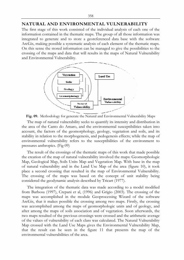
358
NATURAL AND ENVIRONMENTAL VULNERABILITY The first stage of this work consisted of the individual analysis of each one of the information contained in the thematic maps. The group of all those information was integrated to generate and to store a georeferenced data base with the software ArcGis, making possible a systematic analysis of each element of the thematic maps. On this sense the stored information can be managed to give the possibilities to the crossing of the maps and data that will results in the maps of Natural Vulnerability and Environmental Vulnerability.
Fig. 09. Methodology for generate the Natural and Environmental Vulnerability Maps The map of natural vulnerability seeks to quantify its intensity and distribution in
the area of the Canto do Amaro, and the environmental susceptibilities taken into account, the factors of the geomorphology, geology, vegetation and soils, and its stability in relation to the morphogenesis, and pedogenesis effects; while the map of environmental vulnerability refers to the susceptibilities of the environment to pressures anthropics. (Fig 09)
The result of the crossings of the thematic maps of this work that made possible the creation of the map of natural vulnerability involved the maps: Geomorphologic Map, Geological Map, Soils Units Map and Vegetation Map. With base in the map of natural vulnerability and in the Land Use Map of the area (figure 10), it took place a second crossing that resulted in the map of Environmental Vulnerability. The crossing of the maps was based on the concept of unit stability being considered the geodynamic analysis described by Tricart (1977).
The integration of the thematic data was made according to a model modified from Barbosa (1997), Crepani et al, (1996) and Grigio (2003). The crossing of the maps was accomplished in the module Geoprocessing Wizard of the software ArcGis, that it makes possible the crossing among two maps. Firstly, the crossing was accomplished among the maps of geomorphologic units and of geology, and after among the maps of soils association and of vegetation. Soon afterwards, the two maps resulted of the previous crossings were crossed and the arithmetic average of the values of vulnerability of each class was calculated. The Natural Vulnerability Map crossed with the Land Use Maps gives the Environmental Vulnerability Map, that the result can be seen in the figure 11 that presents the map of the environmental vulnerabilities of the area.
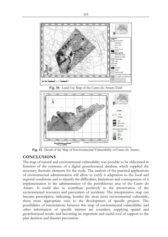
359
Fig. 10. Land Use Map of the Canto do Amaro Field
Fig. 11. Detail of the Map of Environmental Vulnerability of Canto do Amaro
CONCLUSIONS The map of natural and environmental vulnerability was possible to be elaborated in function of the existence of a digital georeferenced database which supplied the necessary thematic elements for the study. The analysis of the practical applications of environmental administration will allow to verify it adaptation to the local and regional conditions and to identify the difficulties, limitations and consequences of it implementation in the administration of the petroliferous area of the Canto do Amaro. It could also to contribute positively to the preservation of the environmental resources and prevention of accidents. The interpretative map can become prescriptive, indicating, besides the areas most environmental vulnerable, those more appropriate ones to the development of specific projects. The possibilities of interrelations between this map of environmental vulnerability and other information of specific interest are countless, supplying spatial and georeferenced results and becoming an important and useful tool of support to the plan decision and disaster prevention.

360
REFERENCES Barbosa, C. C. F. 1997. Álgebra de mapas e suas aplicações em Sensoriamento Remoto e
Geoprocessamento. Programa de Pós-graduação em Sensoriamento Remoto. Instituto Nacional de Pesquisas Espaciais, São Paulo, Dissertação de Mestrado, 126p.
Crepani, E.; Medeiros, J.S.; Azevedo, L.G.; Duarte, V.; Hernandez, P.; Florenzano, T. 1996. Curso de Sensoriamento Remoto Aplicado ao Zoneamento Ecológico-Econômico. INPE - Instituto Nacional de Pesquisas Espaciais, São José dos Campos.
Crosta, A. P. 1992 – Processamento Digital de Imagens de Sensoriamento Remoto – UNICAMP 164 pgs.
Embrapa-CNPS. 1999 Centro Nacional de Pesquisa de Solos (Rio de Janeiro, RJ). Sistema brasileiro de classificação de solos. Brasília: Embrapa-SPI; Rio de Janeiro: Embrapa-CNPS, 412 p., il.
Farias, P. R. C. 1997. Geologia de superfície da área de detalhe de Macau-RN. Relatório Final. Petrobras/Gexp/Gelab, Relatório Interno, 76 p
Grigio, A. M. 2003. Aplicação do Sensoriamento Remoto e Sistemas de Informação Geográfica na Determinação da Vulnerabilidade Natural e Ambiental do Município de Guamaré (RN): Simulação de Risco ás Atividades da Industria Petrolífera. Centro de Ciências Exatas e da Terra. Programa de Pós Graduação em Geodinâmica e Geofísica. Universidade Federal do Rio Grande do Norte. Dissertação de Mestrado. 222p.
Ibge, 1999. Manual Técnico de Uso da Terra. Série Manuais Técnicos em Geociências, Número 07, 58p.
Idema. 2002. Diagnóstico e vulnerabilidade ambiental dos estuários do litoral norte e seus entornos. Instituto de Desenvolvimento Econômico e Meio Ambiente - IDEMA. Projeto de Zoneamento Ecológico-Econômico dos estuários do Estado do Rio Grande do Norte e dos seus entornos, Sugerco/Idema. Relatório Final. Natal.
Incra, 1995. Normas técnicas para mapeamento de recursos naturais através de sensoriamento remoto. Incra/Pnud. Brasília, 56p.
Plano Estratégico Petrobrás 2015 - http://www2.petrobras.com.br/ri/port/Apresentacoes Eventos/ConfTelefonicas/pdf/Plano_Estrategico_2015_FINAL_1506.pdf
Radambrasil. 1981. Levantamento de Recursos Naturais. Ministério das Minas e Energia, 23, Folha SD-24-25/ Jaguaribe -Natal.
Rizzini, C. T. 1997. Tratado de fitogeografia do Brasil: aspectos ecológicos, sociológicos e florísticos. Rio de Janeiro: Âmbito Cultural Edições Ltda., 2o ed., p. 521.
Tricart, J. 1977. Ecodinâmica. Rio de Janeiro: IBGE-SUPREN. (Recursos Naturais e Meio Ambiente).
361
ASSESSMENT OF VEGETATION RESPONSE TO INTRA-ANNUAL PATTERNS OF CLIMATIC PARAMETERS IN CENTRAL KAZAKHSTAN
P. A. Propastina, M. Kappasa, S. Erasmia, N. R. Muratovab a Department of Geography, Georg-August University Göttingen, Goldschmidtstr.
5, 37077, Göttingen, Germany, e-mail: [email protected] b Laboratory of Remote Sensing and Image Analysis, Kazakh Academy of Science,
Shevchenko Street, 15, 480040, Almaty, Kazakhstan, e-mail: [email protected]
ABSTRACT We combined the NOAA/37AVHRR NDVI dataset and records collected from climate stations to analyse within-season temporal relationships between NDVI and two eco-climatic parameters (precipitation and temperature) in an arid region of Central Kazakhstan. An assessment of within-season relationships based on 10-day values of NDVI and climatic parameters during the growing season (April-October) was performed for each pixel as well as for the aggregated areas representing different land cover types. The strength of the relationship was estimated by calculating correlations between NDVI and the climatic parameters for each year of the period 1985-2001. The results indicate that a strong significant positive correlation exists between NDVI and the explanatory climatic parameters within the growing season. Temperature was the leading climatic factor controlling intra-annual NDVI dynamics. The correlation coefficients between NDVI-rainfall and NDVI-temperature exhibit a clear structure in terms of spatial distribution. The results indicate that the response of vegetation to climatic factors increases in the sequence from shrubs and desert vegetation to semi-desert, short grassland and to steppe vegetation. Keywords: NDVI, Climate, Vegetation Response, Correlation Analysis.
1 INTRODUCTION Satellite derived Normalized Difference Vegetation Index (NDVI) is a very convenient tool for monitoring terrestrial ecosystems at all scales from global to local. It enables regular detection of seasonal and inter-annual changes in vegetation activity. Since the early 1980th many studies of vegetation distribution and vegetation conditions at both global and regional scales were based on the use of time-series data of the Advanced Very High Resolution Radiometer (AVHRR) sensor launched by the National Oceanic and Atmospheric Agency (NOAA). AVHRR derived NDVI data have been successfully used for monitoring vegetation activity and environmental changes at regional and global scales [1, 2, 3], detection of droughts [4], desertification and land degradation studies [5]. Proc. 2nd Göttingen GIS and Remote Sensing Days, 4-6 Oct. 2006, Göttingen
362
The investigation of the relations between vegetation pattern and its explanatory factors is an object of applications of NDVI. Temporal and spatial correlations between NDVI and climatic factors are investigated in many research works. Particularly good correlation in the arid regions, both spatially and temporally, are documented based on NDVI and rainfall [6, 7, 8]. The relationship between NDVI and temperature is also reported to be significant, but weaker [9, 10]. Numerous studies have suggested a linear relationship between NDVI and climate predictors. However, the relationship is linear only in a limited range of rainfall conditions. The upper thresholds for the linear relationship between NDVI and rainfall were reported to be approximately 500 mm/yr for semi-arid Botswana [11], 700-800 mm/yr for Senegal [12], and 500-700 mm/yr for China [8]. Above these limits, NDVI increases with rainfall only at a slower rate.
The response of NDVI to rainfall and temperature depends on vegetation types and varies by geographical region [11]. Woodland and forest vegetation shows a lower correlation between NDVI and climate factors. Shrubs and desert vegetation patterns are reported to higher correlate with temporal and spatial variations of climate factors. Vegetation patterns in steppe grassland and savannah reveal the highest correlation with rainfall and temperature [8, 9, 12].
The goal of the study is to analyse the seasonal variations of vegetation activity in the region of Central Kazakhstan, and to explore relationships with corresponding variations in rainfall and temperature. Our research is based on NDVI data that have been retrieved from Advanced Very High Resolution Radiometer (AVHRR) and a gridded climatology dataset calculated from the records of climate stations from the study area.
2 STUDY AREA The study area is located in the middle part of Kazakhstan between 46 and 50° northern latitude and 72° and 75° eastern longitude. The climate of the region is dry, cold and high continental. Average annual precipitation is above 250-300 mm per year in the north of the study area, and below 150 mm in the south. The most part of precipitation falls during warm period from March to October. The temperature amplitude is relative high: average January temperature is below –12° C and average July temperature is about 26-28° C.
The south of the study region is vegetated by sagebrush and perennial saltwort associations. Dominating vegetation species here are Artemisia terrae-albae, Artemisia pauciflora, Anabasis salsa, Salsola orientalis. The northern section of the study region is occupied by steppe vegetation, where dominate short grassland species such as Festuca sulcata, Stipa capillata and Stipa lessingiana. The semi-desert vegetation complex occupying the mid of the study area represents a complex combination of real steppe turf grasses and semi-shrubs with halophytes.
3 DATA AND METHODS
3.1 NOAA AVHRR NDVI DATA SET We used 10-day maximum NDVI composites of the AVHRR sensor with a spatial resolution of 8 km. The data cover the period of growing season (April-October)
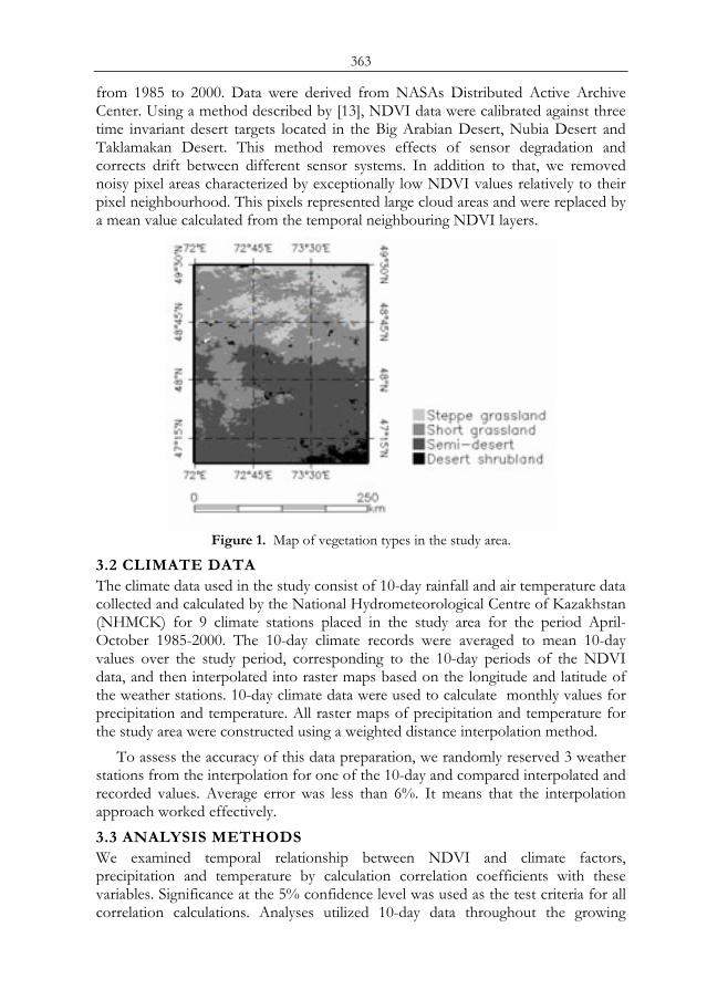
363
from 1985 to 2000. Data were derived from NASAs Distributed Active Archive Center. Using a method described by [13], NDVI data were calibrated against three time invariant desert targets located in the Big Arabian Desert, Nubia Desert and Taklamakan Desert. This method removes effects of sensor degradation and corrects drift between different sensor systems. In addition to that, we removed noisy pixel areas characterized by exceptionally low NDVI values relatively to their pixel neighbourhood. This pixels represented large cloud areas and were replaced by a mean value calculated from the temporal neighbouring NDVI layers.
Figure 1. Map of vegetation types in the study area.
3.2 CLIMATE DATA The climate data used in the study consist of 10-day rainfall and air temperature data collected and calculated by the National Hydrometeorological Centre of Kazakhstan (NHMCK) for 9 climate stations placed in the study area for the period April-October 1985-2000. The 10-day climate records were averaged to mean 10-day values over the study period, corresponding to the 10-day periods of the NDVI data, and then interpolated into raster maps based on the longitude and latitude of the weather stations. 10-day climate data were used to calculate monthly values for precipitation and temperature. All raster maps of precipitation and temperature for the study area were constructed using a weighted distance interpolation method.
To assess the accuracy of this data preparation, we randomly reserved 3 weather stations from the interpolation for one of the 10-day and compared interpolated and recorded values. Average error was less than 6%. It means that the interpolation approach worked effectively. 3.3 ANALYSIS METHODS We examined temporal relationship between NDVI and climate factors, precipitation and temperature by calculation correlation coefficients with these variables. Significance at the 5% confidence level was used as the test criteria for all correlation calculations. Analyses utilized 10-day data throughout the growing
364
season (April-October). There is a time lag between precipitation events and the response of vegetation to such events. The time interval can vary from 1 to 12 weeks depending on vegetation type [9, 11, 1]. Therefore, correlation analyses of NDVI-precipitation relationship wwas performed using the variables in two ways. First, correlation coefficients were calculated between the time-series of NDVI and precipitation over the same period (synchronous analysis). Second, correlation analysis was conducted with time lags being imposed to NDVI variable. In order to account for time lag, we calculated NDVI-rainfall correlation coefficients using time lags of 1-9 weeks.
The objectivities of the study implemented to obtain results at three different scales: spatially averaged over the entire region, spatially averaged over every vegetation type, and at per-pixel scale.
4 RESULTS
4.1 GENERAL TRENDS IN NDVI, PRECIPITATION AND TEMPERATURE Figure 2 illustrates the within-season cycles of NDVI and climate factors averaged over the entire study region. 16-year average of 10-day NDVI values (1985-2001) increased rapidly during the spring (early April-mid-May), peaked during the summer months (mid-May-early July), and decreased during August-September-October. Precipitation showed two peaks, increasing from early April to early June and peaking in late May-early June, after that follows a rapid decrease, and then again a rapid increase till the next peak in mid-July. Minimum of precipitation occurs in August-September. The duration of the growing season is approximately from April to October. The growth of vegetation begins in the time between the second and the third decade of April, approximately 1 decade after temperature value had risen above zero. The curve of temperature displays a very symmetric form with a peak value in mid-July-early August. Generally, temperature rises during the months April-July, and then gradually decreases during August-October.
There is a discrepancy of the time of greening up and peaking between different vegetation types which are distributed in the study area. NDVI curves for desert shrubland showed a peaking time in May, while the curves for short grassland and steppe grassland peak later, in the late June or July. The peaking time for semi-desert vegetation occurs approximately in the early and mid June, but this depends highly on local conditions, namely on the balance between grasses and shrubs in the vegetation communities of semi-desert.
365
Figure 2. NDVI, precipitation and temperature for each 10-day period of the growing
season (spatially averaged over the entire region).
Reasons for a large discrepancy in NDVI temporal patterns of individual land-cover types is a significant difference in moisture and temperature conditions over the territory of the study area and differential responses of vegetation cover to summer climate conditions such as responsiveness to precipitation or limitations from high temperatures. In the next section we investigate the influence of climatic predictors on vegetation development during the phenological cycle. We carried out a detailed investigation of temporal relationships between NDVI and eco-climatic parameters during the growing season and highlighted how this relationship changes in the space over the study area. 4.2 NDVI-PRECIPITATION RELATIONSHIP Correlation coefficients between NDVI and precipitation are high in specific combinations of time duration and lag. The rainfall lag periods varied up to four 10-day periods. This indicates the time period for which an influence of rainfall on NDVI is the strongest. The results indicated that the rainfall time lag increases with a general increase of grass species in vegetation cover. The imposed time lag continually increases from desert shrubland, over semi-desert, to short grassland, and to steppe grassland (Figure 3).
Figure 3 indicates that the best correlation between 10-day NDVI and precipitation is achieved for desert shrubland by imposing no time lag, for semi-desert by imposing a time lag of 1-2, for short grassland and steppe grassland by a time lag of 3-4.
In terms of the strength of the NDVI-precipitation relationship, it gradually increases from desert shrubland, to semi-desert, to short grassland and to steppe vegetation, with a maximum value of correlation coefficient of 0.49, 0.54, 0.58 and 0.67, respectively. Vegetation cover of irrigated cropland and tundra exhibits only weak response to precipitation. This seems to be best explained by the diversity that exists between the different vegetation species associated with each vegetation type. The results of this analysis are in agreement with the research results obtained by others for dry regions [9, 11]. In accordance with the results, higher correlation
366
coefficients between NDVI and precipitation are observed in landscapes with natural grassland vegetation cover. Correlations are getting weaker with a decrease of grasses in the vegetation cover.
0
0,2
0,4
0,6
0,8
0 1 2 3 4 5 6Time lag (10-day units)
Cor
rela
tion
coef
ficie
ntSteppe Short grasslandSemi-desertDesert shrubland
Figure 3. Dependence of correlation coefficient between 10-day NDVI and precipitation
on time lag imposed.
4.3 NDVI-TEMPERATURE RELATIONSHIP The calculated NDVI-temperature correlation coefficients indicate that there is a significant relationship between NDVI and temperature for all vegetation types. 10-day NDVI was strongly correlated with temperature indices of the same period. We found no time lag in any vegetation type. The value of correlation coefficient between NDVI and temperature was 0.63, 0.70, 0.76 and 0.84, for desert shrubland, semi-desert, short grassland and steppe grassland, respectively.
Temperature often serves as an indirect measure of available energy for plant growth. Above a certain base temperature, a plant’s rate of growth is found to be proportional to temperature. From Figure 4 we can see that for all vegetation types, within-season NDVI-temperature correlation coefficient was higher than that obtained for NDVI-precipitation. This agrees with the results reported [8] for China and by [14] for Nebraska, U.S.A. 4.4 SPATIAL PATTERN IN NDVI-CLIMATE RELATIONSHIP The results of this study show that 70.52% and 94.90% of all pixels exhibited significant positive correlation (r > 0.48) between 10-day time-series of NDVI-rainfall and NDVI-temperature, respectively. The pixels with high correlation coefficients (r > 0.70) are mainly distributed in the north, south-west and east portion of the study area (Figure 6). The total area of pixels varied substantially by land-cover type and increases in order from desert shrubland, to semi-desert, to short grassland and to steppe.
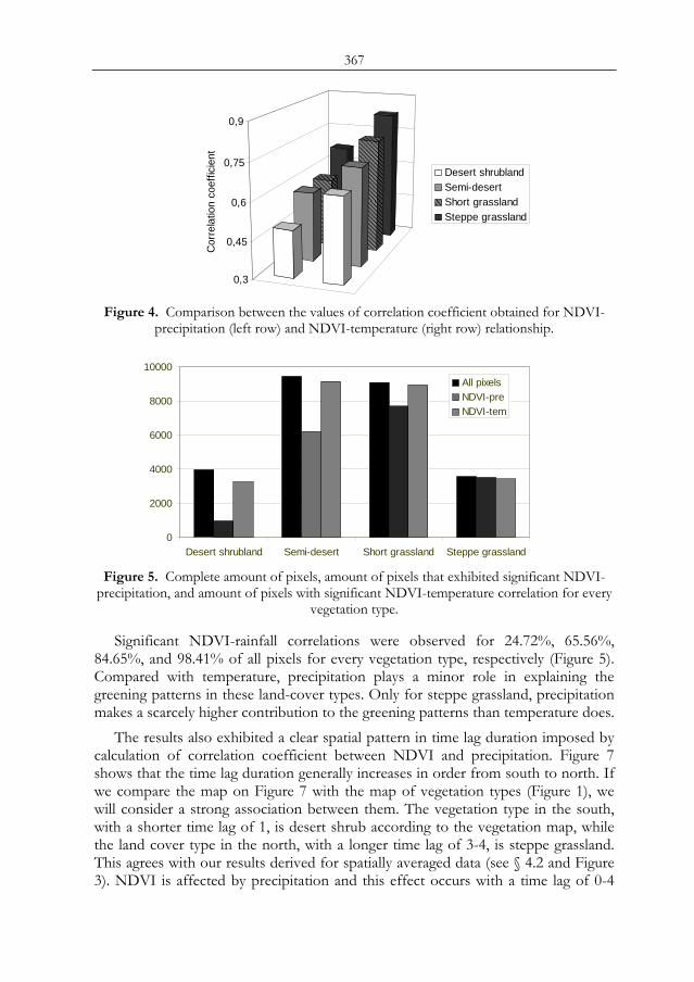
367
0,3
0,45
0,6
0,75
0,9
Cor
rela
tion
coef
ficie
nt
Desert shrublandSemi-desertShort grasslandSteppe grassland
Figure 4. Comparison between the values of correlation coefficient obtained for NDVI-
precipitation (left row) and NDVI-temperature (right row) relationship.
0
2000
4000
6000
8000
10000
Desert shrubland Semi-desert Short grassland Steppe grassland
All pixelsNDVI-preNDVI-tem
Figure 5. Complete amount of pixels, amount of pixels that exhibited significant NDVI-
precipitation, and amount of pixels with significant NDVI-temperature correlation for every vegetation type.
Significant NDVI-rainfall correlations were observed for 24.72%, 65.56%, 84.65%, and 98.41% of all pixels for every vegetation type, respectively (Figure 5). Compared with temperature, precipitation plays a minor role in explaining the greening patterns in these land-cover types. Only for steppe grassland, precipitation makes a scarcely higher contribution to the greening patterns than temperature does.
The results also exhibited a clear spatial pattern in time lag duration imposed by calculation of correlation coefficient between NDVI and precipitation. Figure 7 shows that the time lag duration generally increases in order from south to north. If we compare the map on Figure 7 with the map of vegetation types (Figure 1), we will consider a strong association between them. The vegetation type in the south, with a shorter time lag of 1, is desert shrub according to the vegetation map, while the land cover type in the north, with a longer time lag of 3-4, is steppe grassland. This agrees with our results derived for spatially averaged data (see § 4.2 and Figure 3). NDVI is affected by precipitation and this effect occurs with a time lag of 0-4
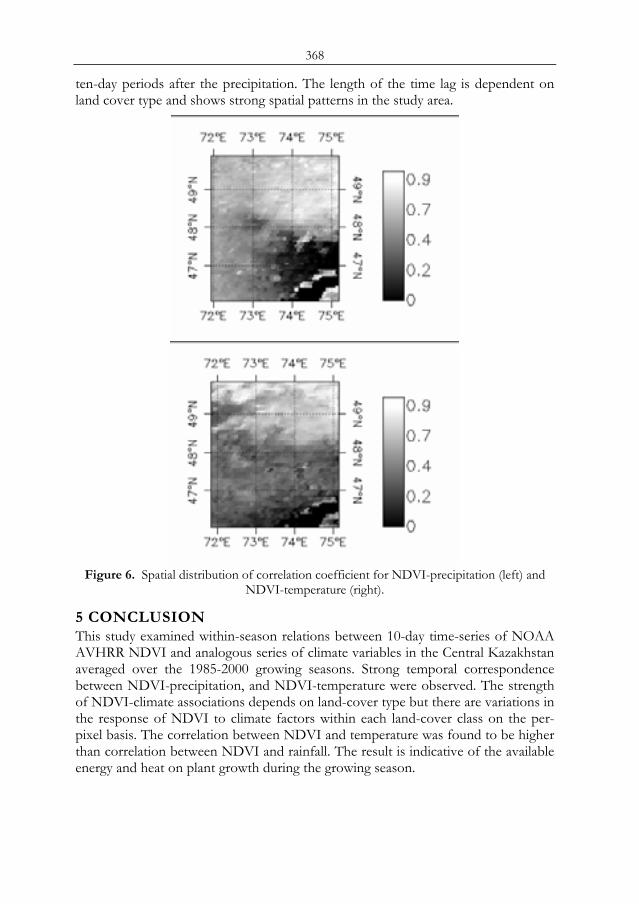
368
ten-day periods after the precipitation. The length of the time lag is dependent on land cover type and shows strong spatial patterns in the study area.
Figure 6. Spatial distribution of correlation coefficient for NDVI-precipitation (left) and
NDVI-temperature (right).
5 CONCLUSION This study examined within-season relations between 10-day time-series of NOAA AVHRR NDVI and analogous series of climate variables in the Central Kazakhstan averaged over the 1985-2000 growing seasons. Strong temporal correspondence between NDVI-precipitation, and NDVI-temperature were observed. The strength of NDVI-climate associations depends on land-cover type but there are variations in the response of NDVI to climate factors within each land-cover class on the per-pixel basis. The correlation between NDVI and temperature was found to be higher than correlation between NDVI and rainfall. The result is indicative of the available energy and heat on plant growth during the growing season.
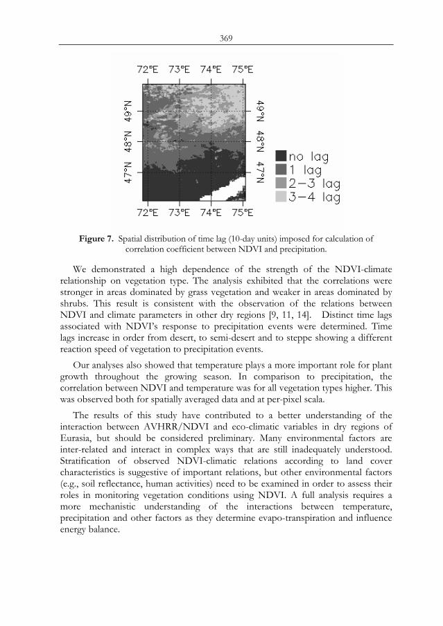
369
Figure 7. Spatial distribution of time lag (10-day units) imposed for calculation of
correlation coefficient between NDVI and precipitation.
We demonstrated a high dependence of the strength of the NDVI-climate relationship on vegetation type. The analysis exhibited that the correlations were stronger in areas dominated by grass vegetation and weaker in areas dominated by shrubs. This result is consistent with the observation of the relations between NDVI and climate parameters in other dry regions [9, 11, 14]. Distinct time lags associated with NDVI’s response to precipitation events were determined. Time lags increase in order from desert, to semi-desert and to steppe showing a different reaction speed of vegetation to precipitation events.
Our analyses also showed that temperature plays a more important role for plant growth throughout the growing season. In comparison to precipitation, the correlation between NDVI and temperature was for all vegetation types higher. This was observed both for spatially averaged data and at per-pixel scala.
The results of this study have contributed to a better understanding of the interaction between AVHRR/NDVI and eco-climatic variables in dry regions of Eurasia, but should be considered preliminary. Many environmental factors are inter-related and interact in complex ways that are still inadequately understood. Stratification of observed NDVI-climatic relations according to land cover characteristics is suggestive of important relations, but other environmental factors (e.g., soil reflectance, human activities) need to be examined in order to assess their roles in monitoring vegetation conditions using NDVI. A full analysis requires a more mechanistic understanding of the interactions between temperature, precipitation and other factors as they determine evapo-transpiration and influence energy balance.

370
REFERENCES 1 Tateishi, R. & Ebata, M. 2004. Analysis of phenological change patterns using 1982-2000
Advanced Very High Resolution Radiometer (AVHRR) data. Int. J. Remote Sensing, 25: 2287-2300.
2 Kowabata A., Ichi K. & Yamaguchi Y. 2001. Global Monitoring of Inter-annual Changes in Vegetation Activities Using NDVI and its Relationship to Temperature and Precipitation. Int. J. Remote Sensing, 22: 1377-1382.
3 Tucker C. J., Slayback D. A., Pinzon J. E., Los S. O., Muneni R. B. & Taylor M. G. 2001. Higher northern latitude Normalized Difference Vegetation Index and growing season trends from 1982 to 1999. Int. J. Biometeorol., 45: 184-190.
4 Kogan, F. N. 1997. Global drought watch from space. Bulletin of the American Meteorological Society, 78: 621-636.
5 Evans J. & R. Geerken. 2004. Discrimination between climate and humane-induced dryland degradation. J. of Arid Environment, 57: 535-554.
6 Richard Y. & Poccard I. 1998. A statistical study of NDVI sensitivity to seasonal and inter-annual rainfall variations in southern Africa. Int. J. Remote Sensing, 19: 2907-2920.
7 Schultz P. A. & Halpert M. S. 1995. Global Analysis of the Relationships Among a Vegetation index, Precipitation and Land Surface Temperature. Int. J. Remote Sensing, 16: 2755-2776.
8 Li B., Tao S. & Dawson R. W. 2002. Relation between AVHRR NDVI and ecoclimatic parameters in China. Int. J. Remote Sensing, 23: 989-999.
9 Wang J., Price K. P. & Rich P. M. 2001. Spatial patterns of NDVI in response to precipitation and temperature in the central Great Plains. Int. J. of Remote Sensing, 22: 3827-3844.
10 Wang J., Rich P. M. & Price K. P. 2003. Temporal responses of NDVI to precipitation and temperature in the central Great Plains, USA. Int. J. of Remote Sensing, 24: 2345-2364.
11 Nicholson, S. E. & Farrar, T. J. 1994. The influence of soil type on the relationships between NDVI, rainfall and soil moisture in Semiarid Botswana. I. NDVI response to rainfall. Remote Sensing of Environment, 50: 107-120.
12 Li J., Lewis J., Rowland J., Tappan G., Tieszen L., 2004. Evaluation of land performance in Senegal using multi-temporal NDVI and rainfall series. J. of Arid Environments, 59: 463-480.
13 Los S. O. 1993. Calibration Adjustment of the NOAA AVHRR Normalized Difference Vegetational Index Without Resource to Component Channel 1 and 2 Data. Int. J. Remote Sensing, 14:1907-1917.
14 Yang L., Wylie B., Tieszen L.L., Reed B. C., 1998. An analysis of relationships among climate forcing and time-integrated NDVI of grasslands over the U.S. Northern and Central Great Plains. Remote Sensing of the Environment 65, 25–37.
371
EVALUATION OF LAND DEGRADATION IN KAZAKHSTAN AND MIDDLE ASIA USING MULTI-TEMPORAL NDVI AND RAINFALL TIME-SERIES
P. A. Propastina, M. Kappasa, S. Erasmia, N. R. Muratovab a Department of Geography, Georg-August-University Göttingen, Goldschmidtstr.
5, 37077, Göttingen, Germany, email: [email protected] b Laboratory of Remote Sensing and Image Analysis, Kazakh Academy of Science,
Shevchenko Street, 15, 480040, Almaty, Kazakhstan, email: [email protected]
ABSTRACT The primary objective o38f this study was to assess dry land degradation in Kazakhstan and Middle Asia based on time series of rainfall data and normalized difference vegetation index (NDVI) from NOAA AVHRR for the period 1981-1998. Normalized Difference Vegetation Index (NDVI) is generally recognized as a good indicator of terrestrial vegetation productivity. In arid, semi-arid and sub-humid regions rainfall is proved to have a dominant role in determining vegetation growth and in predicting trends in vegetation activity over time. Therefore, changes in vegetation cover imposed by human influences are difficult to identify. We applied regression analysis between the growing season NDVI and rainfall time-series to identify the climatic component in the vegetation change over the period 1981-2000. In order to verify the human-induced influence on the vegetation cover, the climatic component was removed from the NDVI time-series. For a given value of rainfall, a value of NDVI was obtained for every pixel and for each year from individual regression equation. This value was considered to reveal the climatic component. Deviations in NDVI from obtained NDVI values expressed in the regression residuals were computed at pixel-by-pixel basis for each year. A range of the standard error of the estimation (SEE) was obtained and the residuals outlying of the SEE are interpreted as human-induced. Negative outliers indicate those pixels that have low NDVI values and high precipitation for the local area and represent ground areas with a decreasing amount of vegetation due to anthropogenic impact. We combined the negative outliers for the entire time-series 1981-2000 and calculated the running sum of the outliers for the 20-year period. Pixels with a large running sum of negative outliers are considered to represent ground areas undergoing land degradation. Keywords: Central Asia, Land degradation; NDVI, Rainfall, Regression analysis, Vegetation activity trend
1 INTRODUCTION Desertification refers to land degradation at arid, semi-arid and dry sub-humid areas and has been seen as one of the major environmental problems in large parts of the Proc. 2nd Göttingen GIS and Remote Sensing Days, 4-6 Oct. 2006, Göttingen
372
land surface. Desertification is considered the result of a series of complex natural, mainly climatic, and anthropogenic processes that leads to gradual environmental degradation or loss of the lands biological and economical productivity. The processes leading to desertification manifest in all compartments of ecosystems and are divided into the follows groups: vegetative, biological, chemical, hydrological, and morpho-dynamical.
Common approaches to assess desertification demand measurements of different indicators which usually describe one or more aspects of desertification and provide data on threshold levels, status and evolution of relevant processes. Degradation of vegetation cover is one of the most important desertification indicator and can be monitored using satellite imagery. Satellite derived Normalized Difference Vegetation Index (NDVI) is a convenient tool for monitoring of vegetation cover at all scales from global to local. It enables regular detection of seasonal and inter-annual changes in vegetation activity. The NDVI has successfully served as a vegetation indicator in many studies on desertification [1, 2]. These and other similar studies are motivated by the appropriation of NDVI for the analysis of vegetation cover at a wide range of spatial scales.
According to recent studies, precipitation has a strong effect on the inter-annual variability of vegetation activity especially in dry regions [3, 4, 5, 6]. It is likely that any trend in NDVI may reflect trend in precipitation amount over the time. For example, the contemporary greening patterns in the Sahel are supported to be driving by an increasing trend in rainfall [7, 8]. Existence of high correlation between inter-annual vegetation activity and precipitation has been used to detect areas of land degradation and desertification in the Near East and in Senegal [9, 10].
Kazakhstan and the other republics of the former Soviet Union in Central Asia (Uzbekistan, Turkmenistan, Kyrgyzstan and Tajikistan) comprise more than 6.5 million km² of territory and according to UNCCD (2000) are associated with the regions threatened by extensive desertification. But the assessment of area affected and desertification grade remains controversial. According to research works published during and after the Soviet Era by Russian and national scientists, the region of Central Asia is strongly affected by desertification hazard, up to 60% of the entire area were already degraded. Vegetation degradation and wind erosion were reported to be the most important types of desertification in the arid pastoral areas whereas soil salinization occurs in irrigated areas [11]. On the contrary, investigations carried out by scientists from the western countries found no catastrophic extend of desertification processes throughout the region, and even reported about very good conditions of pastoral lands. [12] described the pastures in Kazakhstan as “rather ungrazed than overgrazed”. [13] found improvement of vegetation cover during 1990s also in irrigated lands. Therefore, there is a great demand for a new assessment of desertification in Central Asia at regional and national scales, in order to re-examine the previous studies from the innovative view.
The objective of this study is to assess the area of degradation of vegetation cover in the former soviet republics of Central Asia. The assessment is based on synchronous monitoring of two indicators: vegetation and climate. The study
373
utilized remotely sensed derived greenness index (NDVI) and precipitation data obtained from a global climate dataset. For the study, we examined the trends in vegetation activity and precipitation over 1981-2000 and modelled interrelationships between these variables. The developed monitoring system enabled us to discriminate between two major causes of degradation: climatic or anthropogenic. Degraded areas were measured and mapped.
2 DATA AND METHODS
2.1 NOAA AVHRR NDVI We used the Normalized Difference Vegetation Index (NDVI) derived by NOAA Advanced Very High Resolution Radiometer (AVHRR) launched by the National Oceanic and Atmospheric Administration (NOAA). The NDVI, defined as ratio (NIR-VIS)/(NIR+VIS), represents the absorption of photosynthetic active radiation and is established as a precise measurement of the photosynthetic capacity of the canopy. Negative NDVI values indicate non-vegetated areas such as snow, ice, and water. Positive NDVI values indicate green, vegetated surfaces, and higher values indicate an increase in green vegetation.
Figure 1. Land-cover distribution in Kazakhstan and the Middle Asia based on the USGS
land-cover map. Global Inventory Monitoring and Modelling System (GIMMS) NDVI dataset is
a derivate from the NOAA AVHRR data and is freely available in Internet. We used GIMMS NDVI for the entire study region and for the period of 1981-2000. The GIMMS dataset was already pre-processed for radiometric and atmospheric corrections, calibration for sensor differences and orbital drift. The data, at 8-km spatial resolution, are originally processed as 15-day composites using the maximum value procedure to minimize effects of cloud contamination [14]. These original data were averaged to generate a mean growing-season NDVI for each year. 2.2 CLIMATE DATASET A global data set of precipitation was used. This grid raster data are interpolated from climate station records and have a spatial resolution of 0.5°. The data are available from the Climatic Research Unit (CRU), School of Environmental Sciences, University of East Anglia (http://www.cru.uea.ac.uk/). The monthly
374
precipitation and temperature data were resampled to 8-km resolution to match the 8-km NDVI dataset. 2.3 METHODS We generated time series of mean growing season NDVI and time-series of total precipitation over the growing season (April-October) comprising every year from the period 1981-1998. Our assumption that trends in NDVI can serve as a good indicator of inter-annual changes in green vegetation productivity is supported in the literature. Recent investigations of trends in NOAA AVHRR NDVI at global and regional scales exposed significant changes in vegetation activity throughout the land surface [15, 16]. Previous studies have shown a strong relationship between interannual changes in vegetation activity and precipitation [3, 4, 5]. It is clear that climate signal in NDVI time series must be very strong. Climate should have a substantial control on NDVI through annual precipitation. This control, however, should be predictable in every point of the study area where the relationship between NDVI and climate change are statistically significant. Identification and quantification of climate signal should help to discriminate between two major factors of desertification, climatic and anthropogenic. Some examples of dealing with climatic signal and discrimination between human-induced and climate-induced degradation have been presented in the recent literature [9, 10].
In order to detect human-induced degradation of vegetation cover, the effect of climate must be removed from trends in vegetation activity. After the climate signal had been removed, changes remaining in NDVI time series may be associated with anthropogenic factor. If these changes are positive, one may speak about improvement of vegetation cover due to changes in land use and agricultural practices. If these changes are negative, in that case vegetation cover is degrading due to human influence. A framework of decision making is shown in Figure 2.
In this study, a detection of anthropogenic factors in degradation or rehabilitation processes was carried out as follows. First, we calculated linear regression between NDVI and rainfall time-series to identify the climatic component in the vegetation change over the period 1981-2000. For a given value of rainfall, a value of NDVI predicted by the regression, abbreviated as predNDVI , was obtained for every pixel and for each year, this value was considered to reveal the climatic component. The observed NDVI, abbreviated as obsNDVI , may show deviations from the regression line. We suggested that positive deviations indicate better response of vegetation to climate while negative deviations indicate worse response. Deviations in obsNDVI from predNDVI expressed in the regression residuals were computed at pixel-by-pixel basis for every year. A range of the standard error of the estimate (SEE) was obtained and the residuals, laying out of the SEE are interpreted as human-induced. Negative outliers indicate those pixels that have low NDVI values and high precipitation for the local area and represent ground areas with decreasing amount of vegetation due to anthropogenic impact.
We combined the negative outliers for the entire time-series 1981-2000 and calculated running sum of the outliers for the 20-year period. Pixels with a large
375
running sum of negative outliers are considered to represent ground areas undergoing land degradation.
Figure 2. Framework for decision making by detection of human-induced degradation.
3 RESULTS 3.1 IDENTIFICATION OF THE CLIMATIC SIGNAL Spatial distribution of trends in growing season NDVI from 1981 to 2000 is shown in Figure 3 (left). In the north and the south of the study area upwards trends were found broadly from the west border to the east. Especially high increases in NDVI are associated with areas covered by forest vegetation and located in the mountainous regions of the south. On the other hand, NDVI decreased in some areas located in the central part, especially between the Caspian Sea and the Aral Sea, as well between the Aral Sea and the Balkhash Lake. Over the entire study region, the results of our calculations show that about 25% of all vegetated pixels for the growing season exhibited statistically significant upward trends over the study period, and 9.72% of all pixels exhibited significant downward trends.
Several previous studies have shown a positive relationship between NDVI and rainfall []. In the precipitation-dependent areas such as Central Asia, the change in NDVI is assumed to be affected by the occurrence of precipitation. Figure 3 (right) displays trends in growing season rainfall over the study period. The pattern of vegetation and rainfall trends may suggest a positive link in some areas but not consistently. It seemed important to test several different precipitation accumulation periods in order to find an optimum correlation with time series of NDVI. Hence correlations were calculated for many different combinations of precipitation accumulation (growing season, summer, spring-summer etc.).
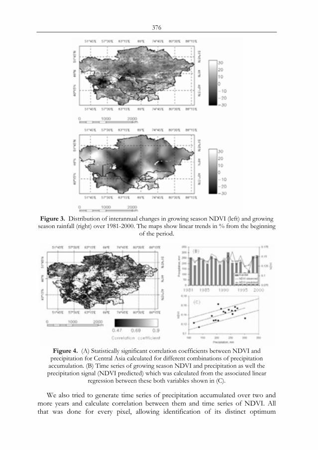
376
Figure 3. Distribution of interannual changes in growing season NDVI (left) and growing
season rainfall (right) over 1981-2000. The maps show linear trends in % from the beginning of the period.
Figure 4. (A) Statistically significant correlation coefficients between NDVI and
precipitation for Central Asia calculated for different combinations of precipitation accumulation. (B) Time series of growing season NDVI and precipitation as well the precipitation signal (NDVI predicted) which was calculated from the associated linear
regression between these both variables shown in (C).
We also tried to generate time series of precipitation accumulated over two and more years and calculate correlation between them and time series of NDVI. All that was done for every pixel, allowing identification of its distinct optimum
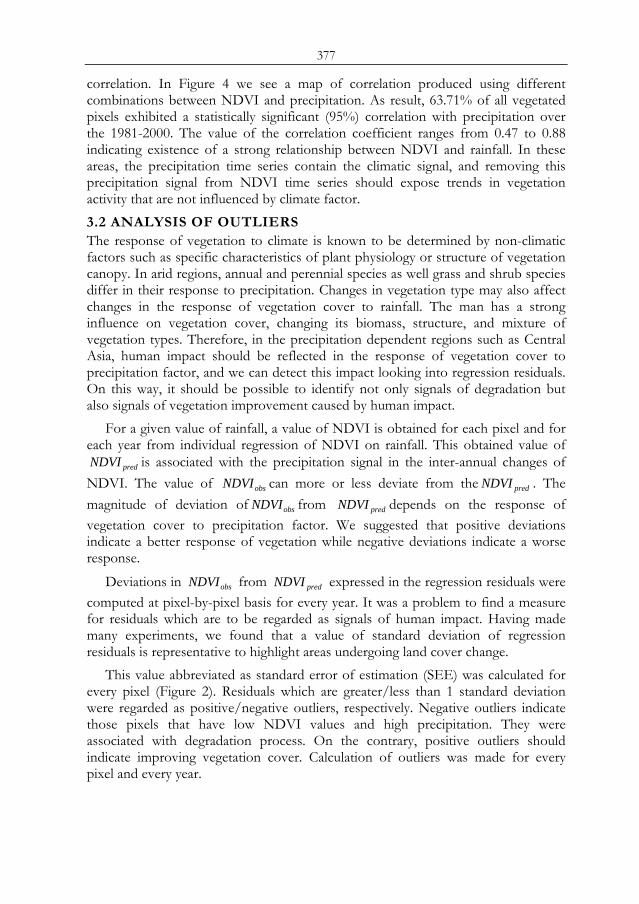
377
correlation. In Figure 4 we see a map of correlation produced using different combinations between NDVI and precipitation. As result, 63.71% of all vegetated pixels exhibited a statistically significant (95%) correlation with precipitation over the 1981-2000. The value of the correlation coefficient ranges from 0.47 to 0.88 indicating existence of a strong relationship between NDVI and rainfall. In these areas, the precipitation time series contain the climatic signal, and removing this precipitation signal from NDVI time series should expose trends in vegetation activity that are not influenced by climate factor. 3.2 ANALYSIS OF OUTLIERS The response of vegetation to climate is known to be determined by non-climatic factors such as specific characteristics of plant physiology or structure of vegetation canopy. In arid regions, annual and perennial species as well grass and shrub species differ in their response to precipitation. Changes in vegetation type may also affect changes in the response of vegetation cover to rainfall. The man has a strong influence on vegetation cover, changing its biomass, structure, and mixture of vegetation types. Therefore, in the precipitation dependent regions such as Central Asia, human impact should be reflected in the response of vegetation cover to precipitation factor, and we can detect this impact looking into regression residuals. On this way, it should be possible to identify not only signals of degradation but also signals of vegetation improvement caused by human impact.
For a given value of rainfall, a value of NDVI is obtained for each pixel and for each year from individual regression of NDVI on rainfall. This obtained value of
predNDVI is associated with the precipitation signal in the inter-annual changes of NDVI. The value of obsNDVI can more or less deviate from the predNDVI . The magnitude of deviation of obsNDVI from predNDVI depends on the response of vegetation cover to precipitation factor. We suggested that positive deviations indicate a better response of vegetation while negative deviations indicate a worse response.
Deviations in obsNDVI from predNDVI expressed in the regression residuals were computed at pixel-by-pixel basis for every year. It was a problem to find a measure for residuals which are to be regarded as signals of human impact. Having made many experiments, we found that a value of standard deviation of regression residuals is representative to highlight areas undergoing land cover change.
This value abbreviated as standard error of estimation (SEE) was calculated for every pixel (Figure 2). Residuals which are greater/less than 1 standard deviation were regarded as positive/negative outliers, respectively. Negative outliers indicate those pixels that have low NDVI values and high precipitation. They were associated with degradation process. On the contrary, positive outliers should indicate improving vegetation cover. Calculation of outliers was made for every pixel and every year.
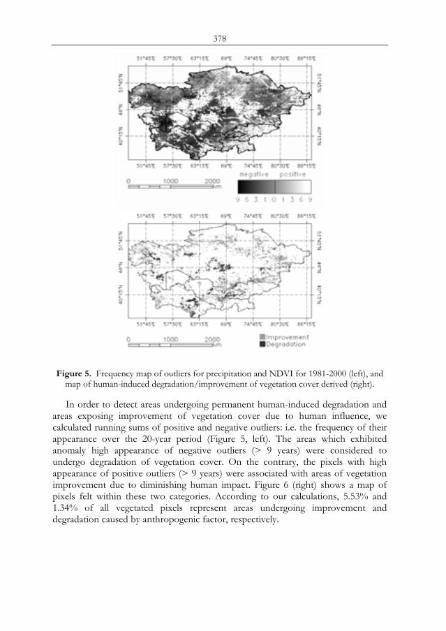
378
Figure 5. Frequency map of outliers for precipitation and NDVI for 1981-2000 (left), and
map of human-induced degradation/improvement of vegetation cover derived (right).
In order to detect areas undergoing permanent human-induced degradation and areas exposing improvement of vegetation cover due to human influence, we calculated running sums of positive and negative outliers: i.e. the frequency of their appearance over the 20-year period (Figure 5, left). The areas which exhibited anomaly high appearance of negative outliers (> 9 years) were considered to undergo degradation of vegetation cover. On the contrary, the pixels with high appearance of positive outliers (> 9 years) were associated with areas of vegetation improvement due to diminishing human impact. Figure 6 (right) shows a map of pixels felt within these two categories. According to our calculations, 5.53% and 1.34% of all vegetated pixels represent areas undergoing improvement and degradation caused by anthropogenic factor, respectively.
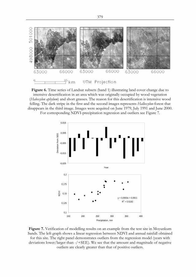
379
Figure 6. Time series of Landsat subsets (band 1) illustrating land cover change due to intensive desertification in an area which was originally occupied by wood vegetation
(Haloxylon aphylum) and short grasses. The reason for this desertification is intensive wood felling. The dark stripe in the first and the second images represents Halloxylon-forest that
disappears in the third image. Images were acquired on June 1979, July 1991 and June 2000. For corresponding NDVI-precipitation regression and outliers see Figure 7.
-0,025
-0,015
-0,005
0,005
0,015
1
Year
Dev
iatio
n fro
m S
EE
y = 0,0003x + 0,0911R2 = 0,5182
0,1
0,125
0,15
0,175
0,2
150 200 250 300 350 400
Precipitation, mm
ND
VI
Figure 7. Verification of modelling results on an example from the test site in Moyunkum Sands. The left graph shows a linear regression between NDVI and annual rainfall obtained
for this site. The right panel demonstrates outliers from the regression model (years with deviations lower/larger than -/+SEE). We see that the amount and magnitude of negative
outliers are clearly greater than that of positive outliers.
380
3.3 VERIFICATION OF MODEL RESULTS Verification of identified trends in degradation/improvement of vegetation cover was made by field surveys and/or analysis of satellite imagery of fine resolution. Because of a large dimension of the study area (about 6 Mio. Km²), we were physically not able to travel to all areas identified as degrading/improving or analyse all corresponding satellite images. We have concentrated on a number of test sites located in desert, semi-desert and steppe zone in the central part of Kazakhstan. In this paper, we refer to only one brilliant example from a test site in the water catchment of the Balkhash Lake.
This test site is located in the southern part of the Moyunkum Sands, a sand desert in the south-east of Kazakhstan. Originally, the area was covered by woody and grass vegetation, the Haloxylon-forest extends from south-west to north-east as a broad stripe with a width from 10 to 25 km (Figure 6). Because of a lower reflectance in blue spectrum, the areas occupied by Haloxylon thickets occurs deep dark in the 1 channel of Landsat and can be easy identified and mapped. On the Landsat image from 1990, many light areas, especially in the western part, occurred within the contour of Haloxylon’s stripe. On the third Landsat image shouted in year 2000, the light areas widespread over the significant part of the image associated with Haloxylon occurrence. Field surveys in this region in 2004 and 2005 as well as reports from local officials verified a clear signs of massive destruction of vegetation cover caused by intensive wood felling. Wide areas of the Haloxylon-forest are already completely cut out; at many places the wood cutting continues intensive at the present time. As a result of wood cutting, surfaces with only thin, rare vegetation cover composed by dwarf shrubs and ephemerals were formed among overgrown sands on many places. When these areas are grazed, they easy get trampled by livestock. After that, bare sand surfaces and even mobile forms of sand such as barkhan chains and barkhan ridges appeared. The destruction of vegetation cover, a decrease of biomass and higher rates of soil loss in this region resulted in a drastic decrease of vegetation response to precipitation over the period 1981-2000. That is reflected in the outliers from the regression model (Figure 7).
4 CONCLUSIONS This study investigated the response of vegetation cover to inter-annual changes in precipitation in Central Asia. We found that 63.71% of all vegetated pixels exhibited statistically significant correlation between time series of NDVI and time series of precipitation over the period 1981-2000. The signal of precipitation had been understood as climatic signal in these areas and was used to discriminate between climate-induced and human-induced change in vegetation activity. To do this, we calculated outliers from the regression models at the per-pixel basis for every year, +/- 1 standard deviation of regression residuals was established as a measure for outliers. These outliers were supposed to represent the signal of anthropogenic factor in the inter-annual changes of NDVI. Pixels with high appearance of outliers (> 9 years) were regarded to be anomalous. According to our measurements, 5.53% and 1.34% of all vegetated pixels demonstrated positive or negative outliers’ anomaly, respectively. These areas were mapped as areas of human-induced improvement or degradation of vegetation cover. Results of the modelling were
381
validated by test of statistical significance and by comparison with the data from the remote sensing systems of fine resolution and trips to key field sites.
REFERENCES 1 Wessels, K. J., Prince, S. D., Frost, P. E. and D. Van Zyl. 2004. Assessing the effects of
human-induced land degradation in the former homelands of northern South Africa with a 1-km AVHRR NDVI time-series. Remote Sensing of the Environment, 91: 47-67.
2 Symeonakis, E. and Drake, N. 2004. Monitoring desertification and land degradation over sub-Saharan Africa. Int. J. Remote Sensing, 25: 573-592.
3 Yang L., Wylie B., Tieszen L.L., Reed B. C., 1998. An analysis of relationships among climate forcing and time-integrated NDVI of grasslands over the U.S. Northern and Central Great Plains. Remote Sensing of the Environment 65, 25–37.
4 Richard Y. & Poccard I. 1998. A statistical study of NDVI sensitivity to seasonal and inter-annual rainfall variations in southern Africa. Int. J. Remote Sensing, 19: 2907-2920.
5 Wang J., Rich P. M. & Price K. P. 2003. Temporal responses of NDVI to precipitation and temperature in the central Great Plains, USA. Int. J. of Remote Sensing, 24: 2345-2364.
6 Li B., Tao S. & Dawson R. W. 2002. Relation between AVHRR NDVI and ecoclimatic parameters in China. Int. J. Remote Sensing, 23: 989-999.
7 Anyamba, A. & Tucker, C. J. 2005. Analysis of Sahelian vegetation dynamics using NOAA-AVHRR NDVI data from 1981-2003. J. of Arid Environments, 63: 596-614.
8 Olsson, L., Eklundh, L. & Ardo, J. 2005. A recent greening of the Sahel – trends, patterns and potential causes. J. of Arid Envirinments, 63: 556-566.
9 Evans J. & R. Geerken. 2004. Discrimination between climate and humane-induced dryland degradation. J. of Arid Environments, 57: 535-554.
10 Li J., Lewis J., Rowland J., Tappan G., Tieszen L., 2004. Evaluation of land performance in Senegal using multi-temporal NDVI and rainfall series. J. of Arid Environments, 59: 463-480.
11 Kharin, N. G., Tateishi, R. & Harahsheh, H. 1999. Degradation of the dryland of Asia. Japan: Chiba University.
12 Robinson, S., Milner-Gulland, E. L. & Alimaev, I. 2002. Rangeland degradation in Kazakhstan during the Soviet-era: re-examining the evidence. J. of Arid Environments, 53: 419-439.
13 DeBeurs, K. M. & Henebry, G. M. 2004. Land surface phenology, climatic variation, and institutional change: analysing agricultural land cover change in Kazakhstan. Remote Sensing of Environment, 89: 497-509.
14 Holben, B. N. 1986. Characteristics of maximum-value composite images from temporal AVHRR data. Int. J. Remote Sensing, 7:1417-1434.
15 Xiao J. & Moody A. 2004. Trends in vegetation activity and their climatic correlates: chin 1982 to 1998. Int. J. Remote Sensing, 20: 5669-5689.
16 Kowabata A., Ichi K. & Yamaguchi Y. 2001. Global Monitoring of Inter-annual Changes in Vegetation Activities Using NDVI and its Relationship to Temperature and Precipitation. Int. J. Remote Sensing, 22: 1377-1382.

382
383
MONITORING SHORELINE CHANGES OF THE KAVAK DELTA (SAROS GULF-NW TURKEY) USING
GIS AND Remote Sensing
A. E. Erginala, H. Özcanb, M. Zeynel Öztürkc a Çanakkale Onsekiz Mart University, Faculty of Sciences and Arts, Department of
Geography, Çanakkale, Turkey, email: [email protected]
b Çanakkale Onsekiz Mart University, Faculty of Agriculture, Department of Soil Science,
Çanakkale, Turkey, email: [email protected] c Çanakkale Onsekiz Mart University, Institute of Social Sciences, Çanakkale,
Turkey, email: [email protected]
ABSTRACT This paper discusses shoreli39ne changes throughout the Kavak Delta for the period from 1962 to 2006. To detect the position changes of the shoreline, different data sources such as aerial photographs, 1/25000-scaled topographical base maps, Landsat ETM satellite images, Global Positioning System (GPS) data were combined. Our preliminary results reveal that marked changes occurred particularly along the northern coastal section of the delta. Related to the transport of abundant sediment input by longshore currents from north to south, the northern shoreline of the delta prograded about 330 m seaward in the last 44 years corresponding to an increase by 1.182 km2 in area of the delta. Local coastal retreat of about 40 m (14.640 m2) was also determined in this part. The southern shoreline, however, has undergone a rapid coastal retreat reaching 62 m because of the construction of two small-size water reservoirs in the middle and upper reaches of the Kavak Creek. Based on our preliminary results, we consider that the Kavak Delta is vulnerable to the variations in sediment supply. Keywords: Shoreline Change, GIS, RS, GPS, Aerial Photograph, Kavak Delta, NW Turkey.
1 INTRODUCTION Defined as “the subarial and submerged contiguous sediment mass deposited in a body of water, such as sea or lake, primarily by the action of a river” [1], deltas are amongst the important elements of coastal landscapes. As mostly emphasized, the present-day deltas have been formed after increased sea-level during the post-Pleistocene times [2] or post-glacial sea-level rise [3].
Deltaic environments are shaped by combined effects of many natural dynamic variables, such as the amount of sediment load carried by streams, coastal currents, Proc. 2nd Göttingen GIS and Remote Sensing Days, 4-6 Oct. 2006, Göttingen
384
tidal range, sea bottom topography, climatic parameters, and are commonly interrupted by man-made coastal defense structures. As dynamic coastal systems reflecting changes in interactions between land-based fluvial and see/ocean-based natural agents, deltas are of prime significance for both better understanding the value of soil erosion within upland drainage basins and for assessment of past and contemporary morpho-climatic, tectonic and eustatic variations of global scale.
Rapid progradation of deltas are associated with increase in sediment load where soil erosion is accelerated by human activities, such as deforestation, mining works etc. [4], [5]. These conditions, particularly changes in river regimes, gave rise to the growth of numerous deltas of the world over the past 2000 years [6]. Several examples, on the other hand, showed that shoreline retreat in deltaic environments results chiefly from sediment trapping in water reservoirs constructed in catchment areas, which affect land-ocean sediment fluxes in modern deltaic environments [7], [8], and [9]. Recent attempts on the basis of GIS and satellite images for monitoring purposes have shown that GIS and Remote Sensing techniques provide great advantages in mathematically-defined accurate detection and monitoring of shoreline changes in time and space [10], [11].
As a mountainous country with a total land of 780.580 sq km and an average elevation of 1032 m a.s.l, Turkey is surrounded by the Black Sea in the north, the Mediterranean Sea in the south and the Aegean Sea in the west. It has 8333 kilometers of coastline. The present geomorphologic features of Turkey including coastal landforms were defined by new vertical crustal deformations, i.e. neotectonics, which followed the Alpine orogenic state [12].
In the present work, an example of rapidly prograding type of deltas was discussed in the northwestern part of Turkey. The Kavak delta is rather small in size when compared with those explained above. However, it has been subjected to considerable changes in the past 44 years. Special emphasis was given to shoreline changes throughout the Kavak Delta coast. In addition to this, the prominent geomorphic features in the area, such as development and migration of coastal sand dunes and long-term variations in areas of lagoons are also discussed. To clarify changes in position of the shoreline, different data sources, such as aerial photographs, topographical base maps, satellite images, GPS measurements were used.
2 STUDY AREA The Kavak Delta covering an area of 21.355 sq km lies within latitudes 40°39'24'' N to 40°35'01'' N and longitudes 26°47'57'' E to 26°52'12'' E in the eastern end of the Saros Gulf in the northern Aegean Sea, northwest Turkey (Figure 1). It was formed on sediments carried by the Kavak River that discharges into the Saros Gulf. The river with a total drainage area of 783.36 sq km and a drainage length of 590 km is about 64 km long. The river and its several tributaries originate from Mt Korudag (674 m) to the north and and Mt Ganos to the northeast (Figure 2). When including the other stream catchments supplying abundant sediment load from the north, the total drainage area of the delta reaches approximately 845 sq km.
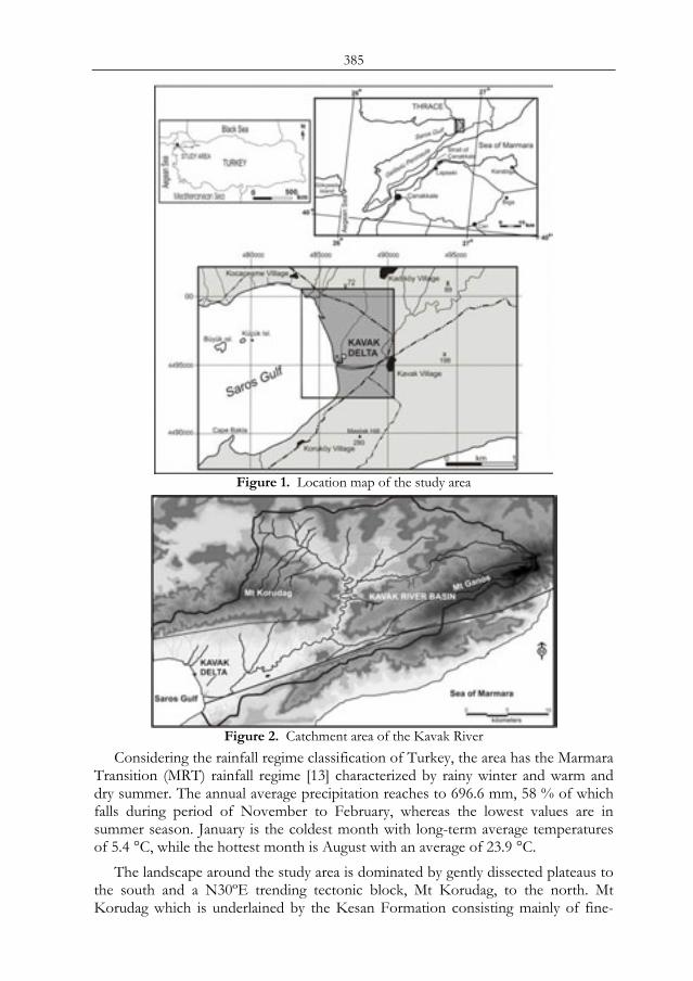
385
Figure 1. Location map of the study area
Figure 2. Catchment area of the Kavak River
Considering the rainfall regime classification of Turkey, the area has the Marmara Transition (MRT) rainfall regime [13] characterized by rainy winter and warm and dry summer. The annual average precipitation reaches to 696.6 mm, 58 % of which falls during period of November to February, whereas the lowest values are in summer season. January is the coldest month with long-term average temperatures of 5.4 °C, while the hottest month is August with an average of 23.9 °C.
The landscape around the study area is dominated by gently dissected plateaus to the south and a N30ºE trending tectonic block, Mt Korudag, to the north. Mt Korudag which is underlained by the Kesan Formation consisting mainly of fine-
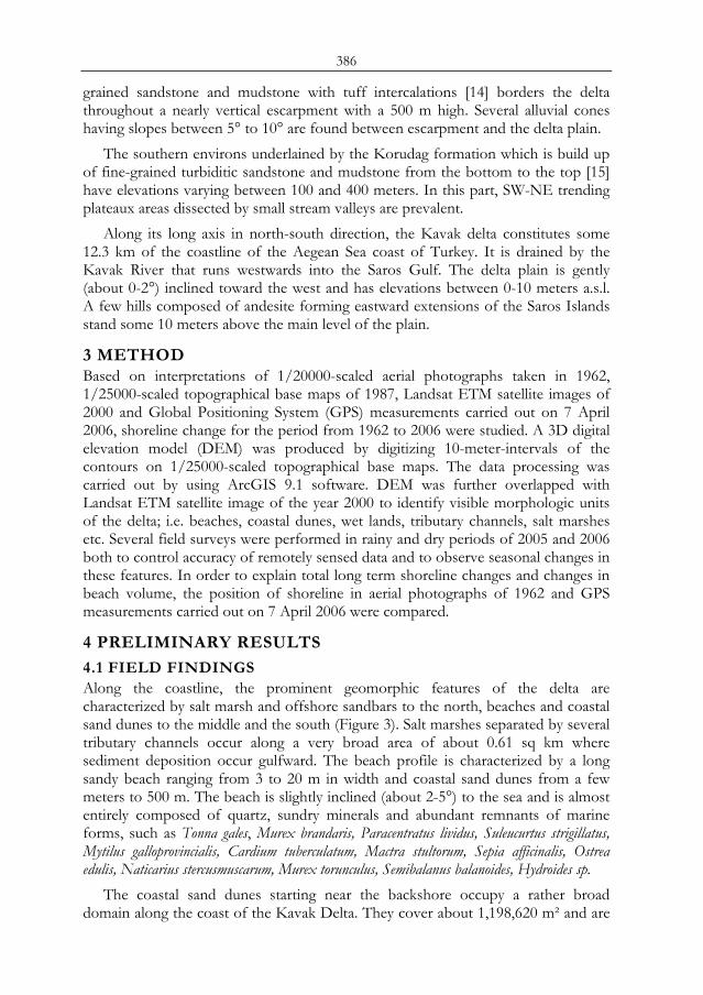
386
grained sandstone and mudstone with tuff intercalations [14] borders the delta throughout a nearly vertical escarpment with a 500 m high. Several alluvial cones having slopes between 5° to 10° are found between escarpment and the delta plain.
The southern environs underlained by the Korudag formation which is build up of fine-grained turbiditic sandstone and mudstone from the bottom to the top [15] have elevations varying between 100 and 400 meters. In this part, SW-NE trending plateaux areas dissected by small stream valleys are prevalent.
Along its long axis in north-south direction, the Kavak delta constitutes some 12.3 km of the coastline of the Aegean Sea coast of Turkey. It is drained by the Kavak River that runs westwards into the Saros Gulf. The delta plain is gently (about 0-2°) inclined toward the west and has elevations between 0-10 meters a.s.l. A few hills composed of andesite forming eastward extensions of the Saros Islands stand some 10 meters above the main level of the plain.
3 METHOD Based on interpretations of 1/20000-scaled aerial photographs taken in 1962, 1/25000-scaled topographical base maps of 1987, Landsat ETM satellite images of 2000 and Global Positioning System (GPS) measurements carried out on 7 April 2006, shoreline change for the period from 1962 to 2006 were studied. A 3D digital elevation model (DEM) was produced by digitizing 10-meter-intervals of the contours on 1/25000-scaled topographical base maps. The data processing was carried out by using ArcGIS 9.1 software. DEM was further overlapped with Landsat ETM satellite image of the year 2000 to identify visible morphologic units of the delta; i.e. beaches, coastal dunes, wet lands, tributary channels, salt marshes etc. Several field surveys were performed in rainy and dry periods of 2005 and 2006 both to control accuracy of remotely sensed data and to observe seasonal changes in these features. In order to explain total long term shoreline changes and changes in beach volume, the position of shoreline in aerial photographs of 1962 and GPS measurements carried out on 7 April 2006 were compared.
4 PRELIMINARY RESULTS
4.1 FIELD FINDINGS Along the coastline, the prominent geomorphic features of the delta are characterized by salt marsh and offshore sandbars to the north, beaches and coastal sand dunes to the middle and the south (Figure 3). Salt marshes separated by several tributary channels occur along a very broad area of about 0.61 sq km where sediment deposition occur gulfward. The beach profile is characterized by a long sandy beach ranging from 3 to 20 m in width and coastal sand dunes from a few meters to 500 m. The beach is slightly inclined (about 2-5°) to the sea and is almost entirely composed of quartz, sundry minerals and abundant remnants of marine forms, such as Tonna gales, Murex brandaris, Paracentratus lividus, Suleucurtus strigillatus, Mytilus galloprovincialis, Cardium tuberculatum, Mactra stultorum, Sepia afficinalis, Ostrea edulis, Naticarius stercusmuscarum, Murex torunculus, Semibalanus balanoides, Hydroides sp.
The coastal sand dunes starting near the backshore occupy a rather broad domain along the coast of the Kavak Delta. They cover about 1,198,620 m² and are
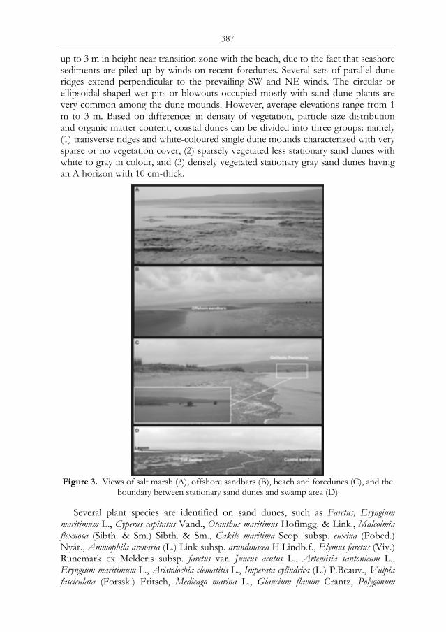
387
up to 3 m in height near transition zone with the beach, due to the fact that seashore sediments are piled up by winds on recent foredunes. Several sets of parallel dune ridges extend perpendicular to the prevailing SW and NE winds. The circular or ellipsoidal-shaped wet pits or blowouts occupied mostly with sand dune plants are very common among the dune mounds. However, average elevations range from 1 m to 3 m. Based on differences in density of vegetation, particle size distribution and organic matter content, coastal dunes can be divided into three groups: namely (1) transverse ridges and white-coloured single dune mounds characterized with very sparse or no vegetation cover, (2) sparsely vegetated less stationary sand dunes with white to gray in colour, and (3) densely vegetated stationary gray sand dunes having an A horizon with 10 cm-thick.
Figure 3. Views of salt marsh (A), offshore sandbars (B), beach and foredunes (C), and the
boundary between stationary sand dunes and swamp area (D)
Several plant species are identified on sand dunes, such as Farctus, Eryngium maritimum L., Cyperus capitatus Vand., Otanthus maritimus Hofimgg. & Link., Malcolmia flexuosa (Sibth. & Sm.) Sibth. & Sm., Cakile maritima Scop. subsp. euxina (Pobed.) Nyár., Ammophila arenaria (L.) Link subsp. arundinacea H.Lindb.f., Elymus farctus (Viv.) Runemark ex Melderis subsp. farctus var. Juncus acutus L., Artemisia santonicum L., Eryngium maritimum L., Aristolochia clematitis L., Imperata cylindrica (L.) P.Beauv., Vulpia fasciculata (Forssk.) Fritsch, Medicago marina L., Glaucium flavum Crantz, Polygonum
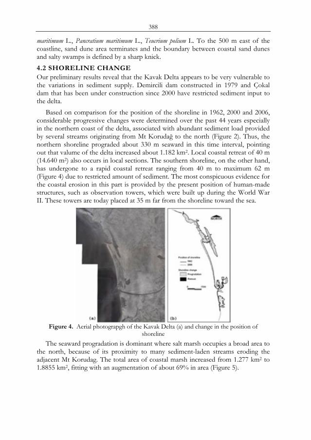
388
maritimum L., Pancratium maritimum L., Teucrium polium L. To the 500 m east of the coastline, sand dune area terminates and the boundary between coastal sand dunes and salty swamps is defined by a sharp knick. 4.2 SHORELINE CHANGE Our preliminary results reveal that the Kavak Delta appears to be very vulnerable to the variations in sediment supply. Demircili dam constructed in 1979 and Çokal dam that has been under construction since 2000 have restricted sediment input to the delta.
Based on comparison for the position of the shoreline in 1962, 2000 and 2006, considerable progressive changes were determined over the past 44 years especially in the northern coast of the delta, associated with abundant sediment load provided by several streams originating from Mt Korudağ to the north (Figure 2). Thus, the northern shoreline prograded about 330 m seaward in this time interval, pointing out that valume of the delta increased about 1.182 km2. Local coastal retreat of 40 m (14.640 m2) also occurs in local sections. The southern shoreline, on the other hand, has undergone to a rapid coastal retreat ranging from 40 m to maximum 62 m (Figure 4) due to restricted amount of sediment. The most conspicuous evidence for the coastal erosion in this part is provided by the present position of human-made structures, such as observation towers, which were built up during the World War II. These towers are today placed at 35 m far from the shoreline toward the sea.
Figure 4. Aerial photograpgh of the Kavak Delta (a) and change in the position of
shoreline The seaward progradation is dominant where salt marsh occupies a broad area to
the north, because of its proximity to many sediment-laden streams eroding the adjacent Mt Korudag. The total area of coastal marsh increased from 1.277 km2 to 1.8855 km2, fitting with an augmentation of about 69% in area (Figure 5).
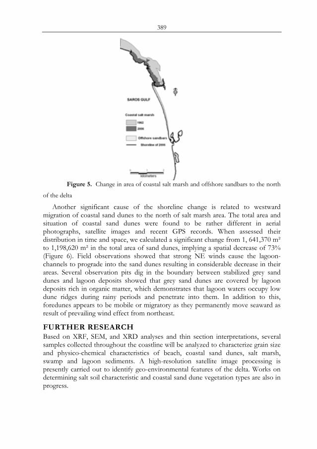
389
Figure 5. Change in area of coastal salt marsh and offshore sandbars to the north
of the delta
Another significant cause of the shoreline change is related to westward migration of coastal sand dunes to the north of salt marsh area. The total area and situation of coastal sand dunes were found to be rather different in aerial photographs, satellite images and recent GPS records. When assessed their distribution in time and space, we calculated a significant change from 1, 641,370 m² to 1,198,620 m² in the total area of sand dunes, implying a spatial decrease of 73% (Figure 6). Field observations showed that strong NE winds cause the lagoon-channels to prograde into the sand dunes resulting in considerable decrease in their areas. Several observation pits dig in the boundary between stabilized grey sand dunes and lagoon deposits showed that grey sand dunes are covered by lagoon deposits rich in organic matter, which demonstrates that lagoon waters occupy low dune ridges during rainy periods and penetrate into them. In addition to this, foredunes appears to be mobile or migratory as they permanently move seaward as result of prevailing wind effect from northeast.
FURTHER RESEARCH Based on XRF, SEM, and XRD analyses and thin section interpretations, several samples collected throughout the coastline will be analyzed to characterize grain size and physico-chemical characteristics of beach, coastal sand dunes, salt marsh, swamp and lagoon sediments. A high-resolution satellite image processing is presently carried out to identify geo-environmental features of the delta. Works on determining salt soil characteristic and coastal sand dune vegetation types are also in progress.
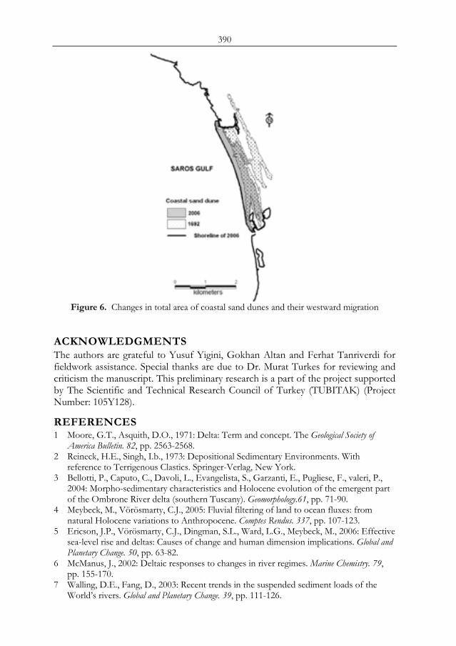
390
Figure 6. Changes in total area of coastal sand dunes and their westward migration
ACKNOWLEDGMENTS The authors are grateful to Yusuf Yigini, Gokhan Altan and Ferhat Tanriverdi for fieldwork assistance. Special thanks are due to Dr. Murat Turkes for reviewing and criticism the manuscript. This preliminary research is a part of the project supported by The Scientific and Technical Research Council of Turkey (TUBITAK) (Project Number: 105Y128).
REFERENCES 1 Moore, G.T., Asquith, D.O., 1971: Delta: Term and concept. The Geological Society of
America Bulletin. 82, pp. 2563-2568. 2 Reineck, H.E., Singh, I.b., 1973: Depositional Sedimentary Environments. With
reference to Terrigenous Clastics. Springer-Verlag, New York. 3 Bellotti, P., Caputo, C., Davoli, L., Evangelista, S., Garzanti, E., Pugliese, F., valeri, P.,
2004: Morpho-sedimentary characteristics and Holocene evolution of the emergent part of the Ombrone River delta (southern Tuscany). Geomorphology.61, pp. 71-90.
4 Meybeck, M., Vörösmarty, C.J., 2005: Fluvial filtering of land to ocean fluxes: from natural Holocene variations to Anthropocene. Comptes Rendus. 337, pp. 107-123.
5 Ericson, J.P., Vörösmarty, C.J., Dingman, S.L., Ward, L.G., Meybeck, M., 2006: Effective sea-level rise and deltas: Causes of change and human dimension implications. Global and Planetary Change. 50, pp. 63-82.
6 McManus, J., 2002: Deltaic responses to changes in river regimes. Marine Chemistry. 79, pp. 155-170.
7 Walling, D.E., Fang, D., 2003: Recent trends in the suspended sediment loads of the World’s rivers. Global and Planetary Change. 39, pp. 111-126.

391
8 Vörösmarty, C.V., Meybeck, M., Fekete, B., Sharma, K., Green, P., Syvitski, J., 2003: Anthropogenic sediment retention: major global impact from registered river impoundments. Global and Planetary Change. 39, pp. 169-190.
9 Williams, G.P., Wolman, M.G., 1984: Downstream effects of dams on alluvial rivers. U.S. Geological Survey Professional Paper 1286, 1 – 61 (Washington, D.C.).
10 Blodget, H.W., Taylor, P.T., Roark, J.H., 1991: Shoreline change along the Rosetta-Nile promontory. Monitoring with satellite observations. Marine Geology. 99, pp. 67-77.
11 White, K., El Asmar, H.M., 1999: Monitoring changing position of coastlines using Thematic Mapper imagery, an example from the Nile Delta. Geomorphology. 29, pp. 93-105.
12 Erinc, S., 1976: Geomorphological evidence of neo-tectonics in Turkey. Review of the Geographical Institute of the University of Istanbul. 15, pp. 37-41.
13 Turkes, M., 1996: Spatial and temporal analysis of annual rainfall variations in Turkey International Journal of Climatology. 16, pp.1057-1076.
14 Gokcen, L.S., 1967: Eocene-Oligocene sedimentation in Kesan Area, Trace of Southwest Turkey. Bulletin of the Mineral Research and Exploration Institute of Turkey. 69, pp. 1-10 (in Turkish).
15 Kellog, H.E, 1973: Geology and petroleum prospects Gulf of Saros and vicinity southwestern Trace: Ashland Oil of Turkey, Inc. National Oil &,Natural Gas Company of Turkiye (unpublished report).

392
393
DEM based method for The determination of potential frost-risk territories
Á. Németha, b a Climatology Division, Hungarian Meteorological Service; Kitaibel P. u. 1, H-1024
Budapest, Hungary; email: [email protected]
b Dept. of Physical Geography and Environmental Sciences, University of Miskolc, H-3515 Miskolc-Egyetemváros, Hungary
ABSTRACT Nowadays, more and more hypoth40eses come out that the frost-risk decreases in Hungary and the importance of late spring frosts become negligible on account of the global climate change. But the result of climate data processing opposes this idea. According to the measurements of the Hungarian Meteorological Service, the frost frequency and intensity increased significantly in the last decades (mainly in April). The day of the last frost is pushed later and later in time. This tendency is very dangerous at the beginning of the growing season. These results flashed that it is very important to determine potential frost-risk lands.
Determination of potential frost-risk territories practically means the determination of cold air lakes. The method is based on the 90m-resolution SRTM (Shuttle Radar Topography Mission) digital elevation model and on primary and secondary terrain parameters. We used the SAGA (System for Automated Geo-scientific Analysis) and DIGEM (Digitales Gelände-Modell) software to produce input parameters, ArcView 3.2 and AV Spatial Analyst software to create raster-category maps and spatial analysis and the SURFER 8 software for visualization. We applied this method on the Southern-Balaton Winery (Hungary) as a sample area. The verification was done with satellite remote sensing techniques (using land surface temperature data which was calculated from NOAA-AVHRR images). Keywords: potential frost-risk, SRTM, GIS.
1 INTRODUCTION Frosts (measured at two meters as well as frost above the ground) are harmful phenomena for plants. The sensitivity of plants to temperatures below zero is different in different periods of their growth. In Hungary’s climate one can expect frost damages to occur in three seasons. In spring and fall air with temperature not much below the freezing-point causes losses to farmers, as in winter, the extreme cold weather can be damaging. In the Southern, warmest part of Hungary the frost free period is between 195 – 200 days. This period is 180 – 195 days in most parts of Hungary, but in the higher mountain areas it decreases below 180 days. Frost above the ground can even occur in the beginning of June (this is very rare), and in Proc. 2nd Göttingen GIS and Remote Sensing Days, 4-6 Oct. 2006, Göttingen
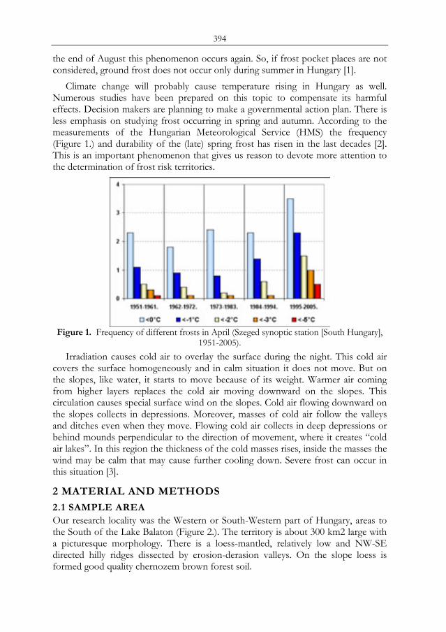
394
the end of August this phenomenon occurs again. So, if frost pocket places are not considered, ground frost does not occur only during summer in Hungary [1].
Climate change will probably cause temperature rising in Hungary as well. Numerous studies have been prepared on this topic to compensate its harmful effects. Decision makers are planning to make a governmental action plan. There is less emphasis on studying frost occurring in spring and autumn. According to the measurements of the Hungarian Meteorological Service (HMS) the frequency (Figure 1.) and durability of the (late) spring frost has risen in the last decades [2]. This is an important phenomenon that gives us reason to devote more attention to the determination of frost risk territories.
Figure 1. Frequency of different frosts in April (Szeged synoptic station [South Hungary],
1951-2005). Irradiation causes cold air to overlay the surface during the night. This cold air
covers the surface homogeneously and in calm situation it does not move. But on the slopes, like water, it starts to move because of its weight. Warmer air coming from higher layers replaces the cold air moving downward on the slopes. This circulation causes special surface wind on the slopes. Cold air flowing downward on the slopes collects in depressions. Moreover, masses of cold air follow the valleys and ditches even when they move. Flowing cold air collects in deep depressions or behind mounds perpendicular to the direction of movement, where it creates “cold air lakes”. In this region the thickness of the cold masses rises, inside the masses the wind may be calm that may cause further cooling down. Severe frost can occur in this situation [3].
2 MATERIAL AND METHODS
2.1 SAMPLE AREA Our research locality was the Western or South-Western part of Hungary, areas to the South of the Lake Balaton (Figure 2.). The territory is about 300 km2 large with a picturesque morphology. There is a loess-mantled, relatively low and NW-SE directed hilly ridges dissected by erosion-derasion valleys. On the slope loess is formed good quality chernozem brown forest soil.
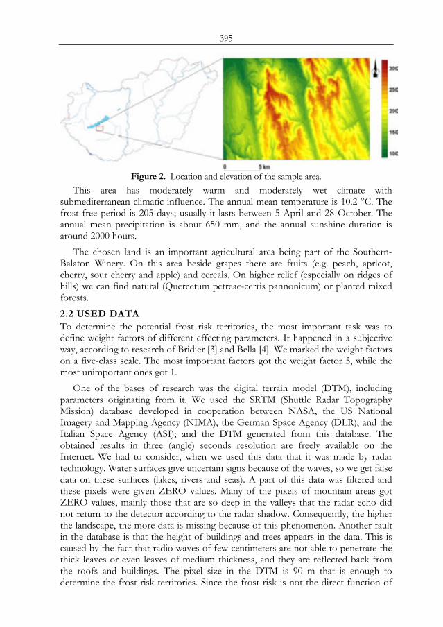
395
Figure 2. Location and elevation of the sample area.
This area has moderately warm and moderately wet climate with submediterranean climatic influence. The annual mean temperature is 10.2 °C. The frost free period is 205 days; usually it lasts between 5 April and 28 October. The annual mean precipitation is about 650 mm, and the annual sunshine duration is around 2000 hours.
The chosen land is an important agricultural area being part of the Southern-Balaton Winery. On this area beside grapes there are fruits (e.g. peach, apricot, cherry, sour cherry and apple) and cereals. On higher relief (especially on ridges of hills) we can find natural (Quercetum petreae-cerris pannonicum) or planted mixed forests. 2.2 USED DATA To determine the potential frost risk territories, the most important task was to define weight factors of different effecting parameters. It happened in a subjective way, according to research of Bridier [3] and Bella [4]. We marked the weight factors on a five-class scale. The most important factors got the weight factor 5, while the most unimportant ones got 1.
One of the bases of research was the digital terrain model (DTM), including parameters originating from it. We used the SRTM (Shuttle Radar Topography Mission) database developed in cooperation between NASA, the US National Imagery and Mapping Agency (NIMA), the German Space Agency (DLR), and the Italian Space Agency (ASI); and the DTM generated from this database. The obtained results in three (angle) seconds resolution are freely available on the Internet. We had to consider, when we used this data that it was made by radar technology. Water surfaces give uncertain signs because of the waves, so we get false data on these surfaces (lakes, rivers and seas). A part of this data was filtered and these pixels were given ZERO values. Many of the pixels of mountain areas got ZERO values, mainly those that are so deep in the valleys that the radar echo did not return to the detector according to the radar shadow. Consequently, the higher the landscape, the more data is missing because of this phenomenon. Another fault in the database is that the height of buildings and trees appears in the data. This is caused by the fact that radio waves of few centimeters are not able to penetrate the thick leaves or even leaves of medium thickness, and they are reflected back from the roofs and buildings. The pixel size in the DTM is 90 m that is enough to determine the frost risk territories. Since the frost risk is not the direct function of
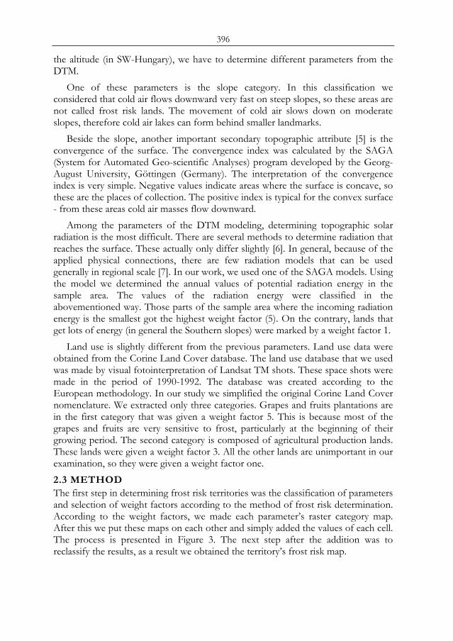
396
the altitude (in SW-Hungary), we have to determine different parameters from the DTM.
One of these parameters is the slope category. In this classification we considered that cold air flows downward very fast on steep slopes, so these areas are not called frost risk lands. The movement of cold air slows down on moderate slopes, therefore cold air lakes can form behind smaller landmarks.
Beside the slope, another important secondary topographic attribute [5] is the convergence of the surface. The convergence index was calculated by the SAGA (System for Automated Geo-scientific Analyses) program developed by the Georg-August University, Göttingen (Germany). The interpretation of the convergence index is very simple. Negative values indicate areas where the surface is concave, so these are the places of collection. The positive index is typical for the convex surface - from these areas cold air masses flow downward.
Among the parameters of the DTM modeling, determining topographic solar radiation is the most difficult. There are several methods to determine radiation that reaches the surface. These actually only differ slightly [6]. In general, because of the applied physical connections, there are few radiation models that can be used generally in regional scale [7]. In our work, we used one of the SAGA models. Using the model we determined the annual values of potential radiation energy in the sample area. The values of the radiation energy were classified in the abovementioned way. Those parts of the sample area where the incoming radiation energy is the smallest got the highest weight factor (5). On the contrary, lands that get lots of energy (in general the Southern slopes) were marked by a weight factor 1.
Land use is slightly different from the previous parameters. Land use data were obtained from the Corine Land Cover database. The land use database that we used was made by visual fotointerpretation of Landsat TM shots. These space shots were made in the period of 1990-1992. The database was created according to the European methodology. In our study we simplified the original Corine Land Cover nomenclature. We extracted only three categories. Grapes and fruits plantations are in the first category that was given a weight factor 5. This is because most of the grapes and fruits are very sensitive to frost, particularly at the beginning of their growing period. The second category is composed of agricultural production lands. These lands were given a weight factor 3. All the other lands are unimportant in our examination, so they were given a weight factor one. 2.3 METHOD The first step in determining frost risk territories was the classification of parameters and selection of weight factors according to the method of frost risk determination. According to the weight factors, we made each parameter’s raster category map. After this we put these maps on each other and simply added the values of each cell. The process is presented in Figure 3. The next step after the addition was to reclassify the results, as a result we obtained the territory’s frost risk map.
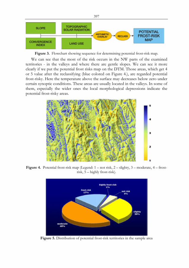
397
Figure 3. Flowchart showing sequence for determining potential frost-risk map.
We can see that the most of the risk occurs in the NW parts of the examined territories - in the valleys and where there are gentle slopes. We can see it more clearly if we put the potential frost risks map on the DTM. Those areas, which get 4 or 5 value after the reclassifying (blue colored on Figure 4.), are regarded potential frost-risky. Here the temperature above the surface may decreases below zero under certain synoptic conditions. These areas are usually located in the valleys. In some of them, especially the wider ones the local morphological depressions indicate the potential frost-risky areas.
Figure 4. Potential frost-risk map (Legend: 1 – not risk, 2 – slighty, 3 – moderate, 4 – frost-
risk, 5 – highly frost-risk).
Figure 5. Distribution of potential frost-risk territories in the sample area
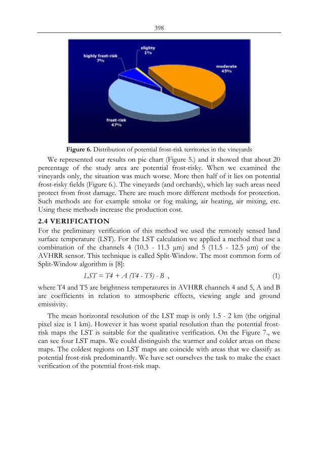
398
Figure 6. Distribution of potential frost-risk territories in the vineyards
We represented our results on pie chart (Figure 5.) and it showed that about 20 percentage of the study area are potential frost-risky. When we examined the vineyards only, the situation was much worse. More then half of it lies on potential frost-risky fields (Figure 6.). The vineyards (and orchards), which lay such areas need protect from frost damage. There are much more different methods for protection. Such methods are for example smoke or fog making, air heating, air mixing, etc. Using these methods increase the production cost. 2.4 VERIFICATION For the preliminary verification of this method we used the remotely sensed land surface temperature (LST). For the LST calculation we applied a method that use a combination of the channels 4 (10.3 - 11.3 μm) and 5 (11.5 - 12.5 μm) of the AVHRR sensor. This technique is called Split-Window. The most common form of Split-Window algorithm is [8]:
LST = T4 + A (T4 - T5) - B , (1) where T4 and T5 are brightness temperatures in AVHRR channels 4 and 5, A and B are coefficients in relation to atmospheric effects, viewing angle and ground emissivity.
The mean horizontal resolution of the LST map is only 1.5 - 2 km (the original pixel size is 1 km). However it has worst spatial resolution than the potential frost-risk maps the LST is suitable for the qualitative verification. On the Figure 7., we can see four LST maps. We could distinguish the warmer and colder areas on these maps. The coldest regions on LST maps are coincide with areas that we classify as potential frost-risk predominantly. We have set ourselves the task to make the exact verification of the potential frost-risk map.
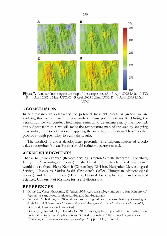
399
Figure 7. Land surface temperature map of the sample area (A – 3 April 2005 1.49am UTC;
B – 4 April 2005 1.34am UTC; C – 5 April 2005 1.26am UTC; D – 6 April 2005 1.15am UTC)
3 CONCLUSION In our research we determined the potential frost risk areas. At present we are verifying this method, so this paper only contains preliminary results. During the verification we will conduct field measurements to determine exactly the frost-risk areas. Apart from this, we will make the temperature map of the area by analysing meteorological network data with applying the suitable interpolation. These together provide enough possibility to verify the results.
The method is under development presently. The implementation of albedo values determined by satellite data would refine the current model.
ACKNOWLEDGMENTS Thanks to Ildikó Szenyán (Remote Sensing Division Satellite Research Laboratory, Hungarian Meteorological Service) for the LST data. For the climatic data analysis I would like to thank Elena Kalmár (Climatology Division, Hungarian Meteorological Service). Thanks to Sándor Szalai (President’s Office, Hungarian Meteorological Service) and Endre Dobos (Dept. of Physical Geography and Environmental Sciences, University of Miskolc) for useful discussions.
REFERENCES 1 Botos, L., Varga-Haszonits, Z. (eds.), 1974: Agroclimatology and cultivation. Ministry of
Agriculture and Food, Budapest, Hungary (in Hungarian) 2 Németh, Á., Kalmár, E., 2006: Winter and spring cold extremes in Hungary. Proceeding of
VAHAVA (Weather and Climate, Effects and Arrangements) Final Conference, 9 March 2006, Budapest, Hungary (in Hungarian)
3 Bridier, S., Quénol, H., Beltrando, G., 2004: Cartographie du potentiel de refroidissement en situation radiative. Application au terroir des Fonds de Sillery dans le vignoble de Champagne. Revue internationale de géomatique 14, pp. 1–14. (in French)
400
4 Bella, Sz., Szalai, S. 2006: Drought vulnerability of South Transdanubia, changing of drought vulnerability. Proceedings of the 3rd MFK Conference, 6-7 September 2006, Budapest, Hungary (in Hungarian) [ISBN 963-9545-12-0]
5 Wilson, J. P., Gallant, J. C., 2000: Secondary Topographic Attributes. In: Wilson, J. P., Gallant, J. C. (eds.): Terrain Analysis: Principles and Applications, pp. 87 – 131. John Wiley and Sons Inc.
6 Kang, S., Kim, S., Lee, D., 2002: Spatial and temporal patterns of solar radiation based on topography and air temperature. Canadian Journal of Forest Resources 32, pp. 487 – 497.
7 Németh, Á., 2004: Modelling of topographic solar radiation using digital elevation models. Proceedings of HUNDEM Conference, University of Miskolc, Hungary (in Hungarian)
8 Beik, F., Saradjian, M. R., 2003: Emissivity determination for Land Surface Temperature estimation of Iran using AVHRR Thermal Infrared Data. Proceedings of Map Asia Conference, 13-15 October 2003, Kuala Lumpur, Malaysia
401
Index of Authors Author’s name Page(s) Author’s name Page(s) Akbulak, C. .......................................233 Almas, A. S........................................189 Ardiansyah, M. .................................209 Asadov, H. H......................................29 Bajat, B. .............................................251 Bartsch, A..........................................269 Bäse, F. ..............................................257 Bella, S. ..............................................333 Bhatti, A. M. .....................................279 Boukalová, Z. ...................................313 Buchroithner, M...............................199 Csaplovics, E. ...................................217 Daenner, M. ........................................51 Dafalla, M. S. ....................................217 Darvishi Boloorani, A. ......................35 Eckert, R. ............................................17 El Nabbout, K..................................199 Erasmi, S. ..................35, 123, 361, 371 Erginal, A. E. ...........................233, 383 Fabrika, M. ................................... 51, 61 Feldkötter, C.....................................287 Flügel, W. A. .....................................257 Foltyn, M...........................................303 Gerlach, R. ..........................................83 Gleitsmann, A. .................................151 Gloaguen, R. ............................225, 303 Görner, A. .........................................303 Haapanen, R. ......................................73 Halounová, L. ...................................313 Hanzlová, M. ....................................313 Heilmeier, H. ....................................225 Helmschrot, J....................................257 Hese, S. ....................................... 83, 339 Hof, A................................................163 Höhlig, S............................................225 Horák, J. ............................................313 Ibrahim, I. S. .....................................217 Kappas, M........ 35, 123, 239, 361, 371 Karthe, D. ...........................................11 Kerimov, M. J.....................................29 Khiry, M. A. ......................................217 Kleinn, C. .................................131, 141 Knorr, D..............................................93 Kong, G.-S. .......................................141
Lanwert, L. ......................................... 51 Lohmann, P...................................... 175 Magdon, P. ....................................... 131 Meyer, M.................................. 321, 351 Mobasheri, M. R. ............................... 43 Müller Schmied, H. ......................... 257 Muratova, N. R. ..............239, 361, 371 Nasu, S. ............................................. 279 Németh, A. ....................................... 393 Niemeyer, I....................................... 225 Özcan, H.................................. 233, 383 Pathe, C............................................. 269 Petta, R. A................................ 321, 351 Propastin, P. A................239, 361, 371 Protic, D. .......................................... 251 Rahim, C. A...................................... 189 Ribeiro, N. A.................................... 115 Sabel, D............................................. 269 Scheer, L. ................................. 105, 115 Schmullius, C. ..................... 83, 93, 339 Schulz, R. ............................................ 51 Scipal, K. ........................................... 269 Shin, M.-Y................................ 131, 141 Sitko, R.............................................. 105 Sliuzas, R........................................... 199 Sloboda, B. .................................51, 115 Soergel, U. ........................................ 175 Souza Lima, R. F. ................... 321, 351 Storch, H............................................. 17 Surový, P.....................................51, 115 Szalai, S.............................................. 333 Takagi, M. ......................................... 279 Tavakkoli, S. M. ............................... 175 Tuominen, S. ...................................... 73 Unucka, J. ......................................... 313 Van Loi, N........................................ 123 Wagner, W........................................ 269 Widiatmaka....................................... 209 Wolski, P........................................... 269 Yiğini, Y. ........................................... 233 Yim, J.-S. .................................. 131, 141 Zeynel Öztürk, M............................ 383 Žídek, D............................................ 313

402


Universitätsdrucke GöttingenUniversitätsdrucke GöttingenISBN-13: 978-3-938616-93-2
Kapp
as/K
lein
n/Sl
obod
a (E
d.)
2nd
Göt
tinge
n G
IS a
nd R
emot
e Se
nsin
g D
ays
2006
Martin Kappas, Christoph Kleinn, and Branislav Sloboda (Ed.)
Global Change Issues in Developing and Emerging Countries
Proceedings of the 2nd Göttingen GIS and Remote Sensing Days 2006,
4th to 6th October, Göttingen, Germany
Remote sensing data and GIS methods provide powerful instruments for the assessment and modelling of environmental indicators of the earth system and its change at multiple scales. Change, in general, is a consequence of human activities and is apparent to us in terms of climate and land cover change.The present book addresses the up-to-date topic of change and is a compilation of scientific contributions related to mapping, monitoring and modelling “Global Change Issues in Developing and Emerging Countries”. It includes the condensed results of an international biennial conference on “GIS and Remote Sensing for Environmental Studies” that took place in Göttingen, Germany from 04th to 06th October 2006.


