Global Tomography of Seismic Anisotropy and Interpretations

JOURNAL OF GEOPHYSICAL RESEARCH, VOL. 96, NO. B12, PAGES 20,337-20,351, NOVEMBER 10, 1991

Global Upper Mantle Tomography of Seismic Velocities and Anisotropies

JEAN-PAUL MONTAGNER

Laboratoire de Sismologie, Institut de Physique du Globe, Paris, France

TosI-imo TANIMOTO

Seismological Laboratory, California Institute of Technology, Pasadena

A data set of 2600 paths for Rayleigh waves and 2170 paths for Love waves enabled us to retrieve three-dimensional distributions of different seismic parameters. Shallow layer corrections have been carefully performed on phase velocity data before regionalization and inversion at depth. The different seismic parameters include the five parameters of a radially anisotropic medium and the eight azimuthal anisotropic parameters as defined by Montagner and Nataf. It is found that the lateral heterogeneities of velocities and anisotropies in the upper mantle are dominated down to 250-30 km by plate tectonics with slow velocities below ridges, high velocities below continents and a velocity increasing with the age of the seafloor. Anisotropy is present in this whole depth range and the directions of maximum velocities are in good agreement with absolute plate velocities. Below 300 km, there is a sharp decreasing of the amplitude of lateral heterogeneities of seismic velocities and anisotropies. Below 450 km, lateral heterogeneities display a degree 2 and to a less extent a degree 6 pattem. Therefore, between 250 km and 450 km, there is a transition region where vertical circulation of matter is possible as shown by sub- ducted slabs and "plumes" of slow velocities but which probably separates two types of convection. The first one is closely related to plate tectonics and to the distribution of continents. The second one dominates below 450 km and is characterized by two downgoing and two upgoing flOWS.

INTRODUCTION

The first generation of tomographic models of the upper mantle [Woodhouse and Dziewonski, 1984; Nakan- ishi and Anderson, 1984; Nataf et al., 1984, 1986] used the simple parameterization of a transversely isotropic medium with a vertical symmetry axis. This simple case of radial anisotropy was invoked in order to remove the discrepancy between Love wave and Rayleigh data in an isotropic medium [Anderson, 1966; Aki, 1968]. But this parameterization is unable to explain the azimuthal anisotropy. However, regional investigations in the Pacific Ocean [Forsyth, 1975; Schlue and Knopoff, 1977; Yu and Mitchell, 1979; Montagner and Jobert, 1983; Anderson and Regan, 1983; Suetsugu and Nakanishi, 1987; Nishimura and Forsyth, 1988, 1989; Zhang and Tani- moto, 1989] or in the Indian Ocean [Montagner, 1986a,b; Montagner and Jobert, 1988] have demonstrated that the introduction of azimuthal anisotropy makes easier the explanation of data. Tanimoto and Anderson [1984, 1985] provided the first maps of azimuthal anisotropy on a global scale, at different periods. Montagner and Nataf [1986, 1988] have presented a method for inverting at the same time the two kinds of observable anisotropy, i.e., the radial anisotropy, obtained from the simultaneous inversion of Rayleigh and Love waves, and the azimuthal

Copyright 1991 by the American Geophysical Union.

Paper number 9 lIB01890 0148-0227/91/9 lIB-01890505.00

anisotropy directly derived from the regionalization of phase or group dispersion curves. This technique coined "vectorial tomography" has been applied by Montagner and Jobert [1988] to data in the Indian Ocean, by Hadiouche et al. [1989] to data in Africa, and by Moc- quet et al. [1989] to data in the Atlantic Ocean.

In this paper, we pursue the investigation of anisotropy in the upper mantle on a global scale. In a previous paper [Montagner and Tanimoto, 1990; hereafter referred as MT], Rayleigh and Love wave phase velocities in the period range of 70-250 s, were regionalized in terms of different azimuthal terms. It has been discovered that

Love wave phase velocities are in good agreement in the whole period range with surface tectonics. Only a small decrease of the amplitude of anomalies with period is observed. For Rayleigh waves, the agreement between local phase velocities and surface tectonics is good at the shortest periods and degrades as period increases. When a spherical harmonics expansion is performed on phase velocities distributions, it tums out that at periods longer than 200 s the most important degree is degree 2 and the second is degree 6, when compared to a regular decrease of the power spectrum with angular order 1. The result for degree 2 corroborates the previous findings by Mas- ters et al. [1982] and Romanowicz et al. [1987]. How- ever, Masters et al. [1982] locate this large degree 2 in the transition region. Kawakatsu [1983], Nakanishi and Anderson [1984], and Tanimoto [1984] using different approaches make it shallower. And recent independent results obtained by Romanowicz [1990] and Roult et al.

20,337

20,338 MONTAGNER AND TANIMOTO: GLOBAL ANISOTROPY TOMOGRAPHY

[1990] from GEOSCOPE data confirm this second interpretation. Degree 6 is the second most important degree, and one can wonder whether it is related to the hotspot distribution [Richards and Hager, 1988]. The azimuthal anisotropy of Rayleigh waves is found to be qualitatively in agreement with plate velocities. Its amplitude is more or less constant up to 130 s and its maximum value is around 1.4%. It decreases with increasing period and becomes very small at very long period (200- 250 s).

In this second paper, we present the simultaneous inversion at depth of the different azimuthal distributions presented in MT. And the questions that we would like to address are the following:

What is the depth extent of continents and anisotropy? What are the implications for the upper mantle convection? At which depth do degree 2 and degree 6 become prominent?

DATA PROCESSING

The data are composed of Global Digital Seismo- graph Network (GDSN) and GEOSCOPE [Romanowicz et al., 1984] three-component records. Their selection has been presented in MT. In order to resolve at the same time, the odd and even orders of lateral heterogeneities, only R•, R 2, G• and G 2 trains were considered. The phase velocity dispersion curve is computed along each path by comparing data to synthetic seismograms. It is also assumed that the approximation of geometrical optics is valid and that the phase slowness between an epicenter and a station is the average of the local phase slownesses along the great circle path connecting the two points. According to Smith and Dahlen [1973] a general slight elastic anisotropy gives rise to an azimuthal dependence of the local phase or group velocities of Love and Rayleigh waves of the form

V (co,•)-V0(co,W)=A 0(co)+A •(co)cos2•+A 2(co)sin 2el

+A 3(co)cos 4el+A 4(co)sin 4•, (1)

where •t' is the azimuth along the path.

Montagner and Natal [1986] showed that the 0-• term corresponds to the average over all azimuths and involves five independent parameters, A, C, F, L, and N, which express the equivalent transverse isotropic medium with vertical symmetry axis. The other azimuthal terms (2-• and 4-•) depend on four groups of 2 parameters, B, G, H, and E describing the azimuthal variation of A, L, F, and N respectively. This approach has been later on justified asymptotically, for a spherical Earth, by Tanimow [1986c] and Romanowicz and Snieder [1988]. The phase velocity dispersion curves have been regionalized according to a new tomographic technique described in MT.

The data used for this second paper are the phase velocity distributions at different periods. In MT, the most general case for which the 0-•, 2-•, and 4-• have been inverted for was considered. Notwithstanding some trade-off between the different azimuthal terms, it

has been found that the azimuthal anisotropy is significant. However, data do not have the resolving power for inverting for the five azimuthal distributions at a given period with the required spatial resolution. More- over, Montagner and Nataf [1986] and Montagner and Anderson [1989a] showed that the Rayleigh 4-W term and the Love 2-• term are small, when calculated from realistic petrological models. For the inversion at depth, we will only consider the 0-W and 2-W distributions for Rayleigh waves and the 0-• and 4-• distributions for Love waves. Different resolution tests in MT have

shown that the azimuthal anisotropy is significant. The covariance fonction after inversion can be derived from

the relation (5a) of MT. However, the understanding of the existence of the 2-W term for Love waves deserves

to be addressed in the future.

The problem of the resolution and of errors is an important issue. But it has been extensively discussed in different previous papers. As far as the regionalization is concerned, Montagner [1986a,b], and Montagner and Jobert [1988] (for the Indian Ocean) have carefully investigated the problem of errors and resolution and have shown error maps and resolution maps as derived from the algorithm of Tarantola and Valette [1982]. These papers have clearly demonstrated that as far as the azimuthal coverage is good (and it is actually better in this global study than in the investigation of the Indian Ocean; see Figure 2 of MT) the trade-off between the constant term (0-•P term) with azimuthal terms (2-W term mainly) is weak.

For the inversion at depth, the technique derived from the algorithm of Tarantola and Valette [1982] has been extensively described and widely used for the first time by Montagner and Jobert [1981], then by Nataf et al. [1986], Nishimura and Forsyth, [1989]. The final covariance function of the regionalization is used as the "data" covariance function in this second inversion. The

error bars and the resolution are the same as in the inver-

sion of Nataf et al. [1986], inasmuch as the same period range is spanned by our fundamental mode data. They show that S wave related parameters (SV velocity and •=N/L) are the best resolved. That means that in our inversion scheme, the anisotropic parameters Gc and Gs which have the same kernels as L=pVs2v are correctly resolved down to a depth of 500 km according to the previous resolution experiments of Montagner and Jobert [1981] and Nataf et al. [1986]. On the other hand, the inversion has been slightly enhanced, because we have introduced realistic correlations in the covariance func-

tion of parameters inferred from petrological considera- tions [Montagner and Anderson 1989a,b].

SHALLOW LAYER CORRECTIONS

Surface waves are sensitive to shallow structure

even at long periods [Dziewonski, 1971; Montagner and Jobert, 1981]. In order to prevent deep structure from being contaminated by shallow layer heterogeneities, corrections must be applied. So far, only linear perturba-

MONTAGNER AND TANIMOTO: GLOBAL ANISOTROPY TOMOGRAPHY 20,339

Sph. Harm Exp. 0-15 MOH0

SYNTHETIC Spher. Harm Exp 0-15 BATHY

Fig. 1. Spherical harmonic expansions up to degree '[5 of the crustal thickness, bathymetry + topography.

POWER

0.020 0.018

0.016

0.014 -

0.012 -

0.010 -

0.008

0.006

O. 004 - :ocS

0.002

a) i õ 6 7 8 9 10 1! 1• 13 14 15 16 17 Ill 19 •0

ANGULAR ORDER

0.020

POWER

0.018

0.016

0.014

0.012

0.008

0.006

0.004

0.002

AN U ORDER

Fig. 2. Power spectra of lateral heterogeneities of phase velocities (a) before and (b) after shallow layer corrections.

20,340 MONTAGNER AND TANIMOTO: GLOBAL ANISOTROPY TOMOGRAPIIY

tion corrections were applied to global tomographic models [Woodhouse and Dziewonski, 1984; Nataf et al., 1984, 1986; Tanimoto, 1986a,b]. However, Montagner and Jobert [1988] showed that shallow layer effect is non linear and that part of this nonlinearity can be taken into account by directly correcting for the structural difference between continent and ocean. The correction

VARIANCE OF DATA BEFORE AND AFTER SHALLOW LAYER CORRECTIONS

1•0 1•0 2(•0 250 period

Fig. 3. Variance of data before (solid curve) and after shallow layer corrections (dashed line).

is decomposed into two parts, a non linear one and a linear one. In order to correct a dispersion velocity datum Va, the total correction can be obtained at a given period by the relation

3 R

Vcor--Vd-i=•lldS (M )•i (M )[(Vi-Vref ) vl av

+• V•(M) ah•-• -(h•(M)-h'•)l' (2) k=l

where 8i (M) is a tectonic distribution, depending on the region at the running point M (continental, intermediate or oceanic). V,,i is the reference velocity of the intermediate model, hak is the depth of the k- th discontinuity of the local reference model 8(M), hk(M) is the actual depth of the discontinuity at point M, and Vco• is the corrected dispersion velocity datum.

The effects of topography, bathymetry, sediments, and crustal thicknesses have been taken into account.

Figure 1 presents the maps of the spherical harmonic expansion up to degree 15 of the crustal thickness, bathymetry, and topography. The crustal thickness distribution comes from a compilation by Soller et al. [1981]. When

a RAYLEIGH 0+a PSII

AMAX- 2.240 = LONGITUDE •.0 60 00 120.00 180.00 240 00 300.00 36•.00 • 1' I ' I I

.......

0. {$0.[1(] 1 •(1.(]0 11](].(](! a4 (].(10

0+2 PSI isolines=O.b% T=100.000000

Fig. 4. Phase velocity distributions at different periods (a) T=100s; (b) T=250 s for Rayleigh waves in a 0+2 ß terms regionalization. (Bottom) Azimuthally averaged phase velocity distribution (0- ß term). (Top) 2-• term azimuthal anisotropy. The length of the line is normalized by the maximum value of anisotropy AMAX.

MONTAGNER AND TANIMOTO: GLOBAL ANISOTROPY TOMOGRAPIIY 20,341

no data were available, crustal thickness is predicted according to the tectonic setting. It can be noted that the average crustal thickness used in this study is 20.7 km. This value is very close to the average between an oceanic crust (=12 km) and a continental crust (=33 km) for an Earth covered by 60% oceans, and smaller than the value (24.4 km) used in the preliminary reference Earth model (PREM model). Figure 2 presents the power spectra of the lateral heterogeneities obtained without any corrections. As it can be seen, the power spectrum decreases slowly as period increases. When compared to the power spectrum of phase velocity anomalies, the power spectrum of shallow layer corrections is shown to be as large as lateral heterogeneities themselves, when no shallow layer effect is taken into account. It can also be seen that shallow layer corrections tend to increase the amplitude of lateral heterogeneities.

It is quite important to correct for shallow layer effect before regionalization. As a matter of fact, when phase velocity data are regionalized, our experience showed us that the location of anomalies is robust but

not its amplitude (MT). Therefore it does not make sense to correct regionalized phase velocities. A better

approach is to directly correct data and then to regional- ize phase velocities.

PHASE VELOCiTY DISTRIBU•ONS

After correcting for shallow layer corrections, new data sets (called DATARC and DATALC in figures) are obtained. The variance of the new data is increased with

respect to the rough data as shown in Figure 3. This can be easily understood. Continents display a thick crust (at least 30 km). The crust of any average model has a thinner crust than a continental crust. The crust presents slow velocities. Therefore corrections applied for elim- inating the lateral differences, mainly between continents and oceans, will tend to increase continental velocities. The effect is opposite for young oceans, characterized by a thin crust and shallow bathymetry. For old oceans, the effects of a deep ocean and an oceanic crust have a ten- dency to cancel out.

The regionalization results after shallow layer corrections are presented in Figure 4 for Rayleigh waves and in Figure 5 for Love waves at two different periods. The 0- and 2-q • azimuthal terms have been retrieved for

Rayleigh waves and the 0- and 4-q • terms for Love

RAYLEIGH 0+2 PSI

AMAX- 0.820 LONGITUDE

•o•. •o.oo •7o.oo 7o.oo z,4o.oo :•,oo.oo :•fi•.oo

0. 6•0.00 120.00 180.00 ',() N C- I'I' r,; .,, t"

0+2 PSI isolines=0.25% Rayleigh

_ :'; .... > :::'.: ß

T=250.000000

Fig. 4. (continued)


a

LOVE O+4 PSI

AMAX- 180 LONGITUDE •

60.00 120.00 180.00 240.00 300.00 36•.00

0. 6O.0O 120.00 180.()() 24 0.00 30().00

LONGITtJDE

0+4 PSI isolines=0.5% T=100.000000

3 [• (1. (1 (}

Fig. 5. Same as Fig. 4 for Love waves at two different periods (a) 100 s and (b) 200 s in a 0+4 •P regionalization.

waves. Though shallow layer effect is very large, it does not affect the location of anomalies as displayed in MT. The correlation with surface tectonics is even enhanced

at periods smaller than 100 s. Different experiments of regionalization have been

performed on this corrected data set. For instance, we did the same experiment as in MT by inverting for the 0+2+4• azimuthal terms. A nice consequence is that the 2-• azimuthal anisotropy for Love waves is decreased, whereas the 2-• term for Rayleigh waves is increased in a 0+2+4• inversion. For instance, at a period of 250 s, the average for the 2-• Rayleigh term is 0.0017 before shallow layer corrections and 0.0024 after; for the 4-• term, it is slightly decreased from 0.0021 to 0.0019.

TOMOGRAPHIC TECHNIQUE

At this stage, we have six distributions at different periods, three for Rayleigh waves (0+2-•P terms) and 3 for Love waves (0+4-• terms). These distributions can be inverted at depth, and the technique was extensively described by Montagner and Jobert [1981] and extended to the completely anisotropic case by Montagner and Nataf [1988]. The different azimuthal terms A0, A •, A 2,

A 3, and A 4 depend on three-dimensional parameters, which are assumed to be independent. Let us recall the different parameters present in the different azimuthal terms and which can be related to elastic moduli Cij [Montagner and Nataf, 1986; Tanimoto, 1986b]. Tani- moto, [1986c] showed that this approach is justified and that the same combinations arise in a spherical Earth for the asymptotic azimuthal dependence of the eigenfrequency shift. The corresponding kernels are detailed, and their variation at depth was plotted by Montagner and Nataf [1986].

Constant term (0•P azimuthal term) (/to)

A = QVp2H = -•-(Cl1+C22)+ C12+•C66 C = OV/v-' C33

F = •-(C13+C23) (3a) 1

L = pVs2v = •-(C44+C55 ) 1 1

N = pVs2H = •-(C11+C22)-•-C 1

2+--C66


b [,OVE 0+4-

AMAX= 1.750 LONGITUDE •

60.00 120.00 180.00 240.00 300.00 3 .00

0. fi0.00 1 ;•0.[), e] 180.00

LONG ITU D

0+4 PSI isolines=0.5% T=200.000000

Fig.5 (continued)

2•P azimuthal term

('41) cos2•P

B c - • (C l l-C 22) Go- •-(C 55-C44) H•- •--(C 13-C23)

(,42) sin2•P

Bs= C 16+C26

Gs= C 54

It•= C36

(3b)

4 •P-azimuthal term:

(A3) cos4•P

E•- (Cl1+C22)-•-C12--•-C66

sin4•P 1

Es--•(C 16-C26) (3½) where indices 1 and 2 refer to horizontal coordinates (1, north direction) and index 3 refers to vertical coordinate. p is the density, Vm/,V•,v are horizontal and vertical P wave velocities respectively, and Vsu ,Vsv horizontal and vertical S wave velocities.

Therefore, in the most general case for a slight anisotropy, 13 combinations of elastic moduli are

necessary to describe the total effect of anisotropy on seismic surface waves. That means that from a theoreti-

cal point of view, seismic surface waves have the ability for providing 13 tomographic models. However, from a practical point of view, data do not have the resolving power for inverting for so many parameters. Montagner and Anderson [1989a] proposed to use constraints from petrology in order to reduce the parameter space. Actu- ally, they found out that some of these parameters display large correlations independent of the petrological model used. Two extreme models were used to derive

these correlations, the pyrolite model [Ringwood, 1975] and the piclogite model [Anderson and Bass, 1984, 1986; Bass and Anderson, 1984]. In the inversion process, the smallest correlations between parameters of both models are kept. This approach was already followed by Mon- tagner and Anderson [1989b] to derive an average reference Earth model. Montagner and Anderson [1989b] proposed different models which satisfactorily explain their data set of normal mode eigenfrequencies. Among these models, they preferred a model called ACY400, with radial anisotropy down to 400 km. We have chosen this model as the starting model of our inversion at depth.


DEPTH - 100km

DEPTH=•O-Okrn

a

DEPTH =370km

c

DE PTH -'440k rn

cl

Plate 1. Vsv wave velocity distributions at different depths. (a) 100 km, (b) 200 km, (c) 370 km, (d) 440 km. The color scale is reported at the bottom of the figure. Two horizontal cross sections are also presented at (e) 30øN and (f) 20 ø S.

MONTAGNER AND TANIMOTO: GLOBAL ANISOTROPY TOMOGRAPItY 20,345

E • CROSS-SECTION OF VSV VELOCITIES AT 3ON.

6O

120

2OO

30:0-

400-

500 j DEPTtt

e

60

120-

aO0-

4,00

5(10

DEPTH (KM)

CROSS-SECTION OF VSV VELOCITIES AT -20S.

--3. ---1. -0.3 -0.1 0.1 0.3 1. 3. F.

Plate I. (continued)


Other reference models were also considered such as model 1066a [Gilbert and Dziewonski, 1975] and the PREM model [Dziewonski and Anderson, 1981] but it turns out that it is not a good average model, especially for Love waves [Montagner and Anderson, 1989a]. At a given point, the inversion technique of the different phase velocity azimuthal terms was extensively discussed by Montagner and Jobert [1981] and Nataf et al. [1986] and extended to the anisotropic case by Montagner [1986a]. It is based on the algorithm of Tarantola and Valette [1982] and makes it possible to take account in the inversion process of the data and parameters errors and their possible correlations. In that case, the "data" are the local phase velocity dispersion curves, and the corresponding error is the diagonal term of the final covariance function (see Montagner [1986a] for more detail).

The results of the inversion are presented in Plate 1 for Vsv, Plate 2 for •=(N-L)/L and Figure 6 for G, which expresses the azimuthal variation of SV wave velocity. Naturally, it could have been possible to present results for P wave velocities and anisotropies (•, Be, Bs), F and related anisotropies (•1, He, Hs), but we present results for $ wave related parameters which are sensitive to deeper structure than P wave. Moreover, the variations at depth of other parameters are roughly related as parameters are correlated. A last step was proposed by Montagner and Nataf [1988] in order to explain the different anisotropic parameters. By assuming a simple orthotropic (or hexagonal) model, i.e., which possesses a symmetry axis characterized by an azimuth ß and a vertical angle O, it is possible to explain very simply the different azimuthal terms. However, in this paper, we present results that naturally derive from seismological observations, and no interpretation of anisotropy by assuming symmetry properties will be attempted.

DISCUSSION

The tomographic results consist of different tomographic models, two scalar models, the Vsv model and the radial SV anisotropy • model and "tensorial" models (actually vectorial) models which express the azimuthal variations of Vsv and Vs•. We successively present these models, and afterwards the corresponding distributions are expanded in spherical harmonics. Some conse- quences for our knowledge of upper mantle convection will be outlined.

S Wave Velocity Model

Plate 1 shows the distributions of SV velocity at different depths. At shallow depths (100 km, Plate l a), it can be observed a very good correlation with surface tectonics: all ridges are slow, all shields are fast; back arc areas and tectonic areas are also slow. An increase of

velocity with the age of the seafloor is also observed. Generally, plate boundaries are slow.

At a depth of 200 km (Plate lb), the same features still hold, except that slow ridges are hardly visible, and back arc regions are not more systematically slow. At a depth of 370 km (Plate l c), a sharp decrease in the amplitude of anomalies can be observed. The correlation with surface tectonics is more and more fuzzy. How- ever, continents are still fast, but slow ridges and back arc regions are not more visible. Fast ridges are offset with respect to their surface signature. At larger depths (440 km, Plate l d), the most prominent feature is the fast velocity anomalies in the western Pacific, along the Alpine-Himalayan belt and beneath the Atlantic Ocean. It is important to note the sharp decrease of anomalies as depth increases. Most of the anomalies are located in the upper 300 km.

These different features were already displayed by previous tomographic models [Woodhouse and Dziewon- ski, 1984; Nataf et al., 1984, 1986; Tanimoto, 1986b, 1988, 1990] but due to the increased number of paths, we have improved the lateral resolution by a factor of 2 with respect to these previous models. The agreement with these models is very good down to 300 km where the correlation with surface tectonics is excellent. But at

larger depths (below 450 km), the importance of degrees 2 and 6 is magnified in our model. This feature, however, is strongly dependent on shallow layer corrections which are important even at long period.

Radial Anisotropy

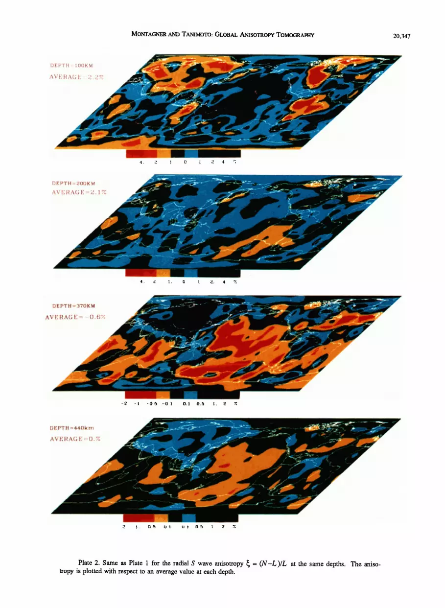
The radial anisotropy (i.e., transverse isotropy with vertical symmetry axis) is characterized by three addi- tional parameters, namely, O) = (A-C)/A, • = (N-L )/L and •! = F/(A-2L). In Plate 2, we only present the results for • at different depths. Plate 2a shows the radial $ wave anisotropy at 100 km of depth. A large dissymmetry is visible between oceans and continents. The anisotropy is rather uniform (around 3-4%) below oceans and is small (smaller than 2%) below continents. Down to 250 km, the anisotropy decreases slowly but sharply between 250 and 350 km to become small at larger depths. It can be noted that it is not negligible below old continents at 370 and 444 km, which could be related to a larger strain field below the root of continents.

On a global scale, our results can be compared to the only available model of Nataf et al. [1986]. We find a smaller radial anisotropy than their's, and it is found very small below 300-400 km, whereas it is more distri- buted in the whole upper mantle of Nataf et al. [1986].

S Wave Azimuthal Anisotropy

The azimuthal anisotropy is characterized by eight parameters. However, as we only regionalized for the 2- •F Rayleigh and the 4-•F Love term, only four among these parameters are well resolved. In order to be con- sistent with previous Plates 1 and 2, we only plotted the S wave azimuthal anisotropy, defined by Gc and Gs (or


I.)EPTtt = 100KM

i.•V E I[•A{..; E -----' 2.2?;

DE PTH =•00K'M

AVE RAG E =,•. 1 •,

DEPTH=370KM

DEPT!t =440kin

AVE RAG E=O.•

Plate 2. Same as Plate 1 for the radial S wave mtisotropy • = (N-L)/L at the same depths. The anisotropy is plotted with respect to an average value at each depth.


AMAX = 6.260 • LONG ITU DE -0. õ(1.00 120.00 180.0(I 240.00 300.0()

O. 60.00 120.00 180.00 240.00 300.00 380.00 LONGITUDE

depth = •O(]k m

AMAX-- 3.830 • LONGITUDE

. 60.00 120.00 180.00 240.00 300.00

.......

, , •'---'---'-' ' 'i ..... '• ...... '• ...... • O. 60.00 120.00 180.00 240.00 300.00 360.00

LONGITUDE

depth- 370kin AMAX- 0.930

LONGITUDE 60.00 120.00 180.00 240.00 •-0. 300.00

.... i ..... i ..... i .... i ' 0. 60.00 240.00 300.00 120.00 180.00

LONGITUDE 360.00

depth- 444 km AMAX- 0.410

• LONGITUDE •0. 60.(10 120.00 180.00 240.00 300.00

I!. !ill.(Ill I •(I.(11) I ]11.()• •41).1)1) ]•.• : •.•

1,(}• (; I'I'•

G and its azimuth •PG). The same observations as for Vsv and • are still valid (Figure 6) . Azimuthal anisotropy is significant down to 250-300 km and becomes small below. We note a good correlation between plate tectonics velocities and directions of maximum G. It is even better at 300 km than at 100 km.

As no global model of azimuthal anisotropy is available so far, our results for azimuthal anisotropy can only be compared to a few regional models, in the Indian Ocean [Montagner and Jobeft, 1988], in Africa [Hadiouche et al., 1989] and in the Pacific Ocean [Nishimura and Forsyth, 1989]. In the Indian Ocean, our map at a depth of 100 km presents the same features as the one at 58 km of Montagner and Jobert [1988] and the best agreement is found at 200 km where maps of azimuthal anisotropy look like plate motion direction map [Minster and Jordan, 1978]. In Africa, we find, as did Hadiouche et al. [1989], in southern Africa a surprising NW-SE direction (not related to absolute plate motion), in northern Africa a N-S direction and in Eastern Africa a direction perpendicular to the opening direction of Red Sea. Therefore, the agreement between that regional model and our global model is very good. In the Pacific Ocean, we find, as did Nishimura and

Forsyth, [1989] that the directions of maximum velocity are related to fossil seafloor spreading at 100 km of depth for old ocean but to the present plate motion at a depth of 200 km. At depths larger than 350-400 km, the anisotropic parameter G becomes very small and is not well resolved. Therefore, the comparison between our model and regional models is qualitatively good, but we note that there can be some disagreement on the location at depth of this kind of anisotropy.

Spherical Harmonic Expansion

The tomographic models were derived from a technique which does not need any basis of functions (see Montagner [1986a] for the philosophy of the method). This approach is preferable because only the first and second trains of surface waves have been used. However, it is possible to calculate spherical harmonic expansion of the different distributions presented in the previous sections (which must be seen as a by-product of our tomographic technique).

A spherical harmonic expansion for Vsv is presented in Figure 7. The spherical harmonic expansion of noncorrected phase velocities distributions displayed a difference between intermediate long period surface waves (70-180 s) and long period (>180 s) surface waves (MT). The first ones display a rather regular decreasing with order, whereas long-period expansion presents two secondary maxima, one for degree 2 and the second one for degree 6. Shallow layer corrections by increasing odd order terms tend to hide even orders (Figure 2). The

Fig. 6. S wave azimuthal anisotropy (G parameter expressed in gigapascals see text) at the same depths as previously.

MONTAGNER AND TANIMOTO: GLOBAL ANISOTROPY TOMOGRAPItY 20,349

VSV (DATAB4v) 11•t/10 100km

POWER

0.34,0

0.240

0.0•0

ORDER

Fig. 7. Spherical harmonic expansion of Vsv distribution at different depths.

spherical harmonic expansion at different depths displays again a distinction between shallow structure down to 400 km and deep structure (below 400 km) which again exhibits the predominance of degrees 2 and 6 when compared to a regular decrease of the power spectrum with angular order. It must be stressed that the importance of degree 2 with respect to other degrees is highly dependent on the magnitude of shallow layer corrections. If no shallow layer correction is taken into account, degree 2 becomes predominant as shallow as 350 km. When shallow layer corrections are accounted for, it is only true below 450-500 km. This can be easily understood, as long as we bear in mind that shallow layer corrections tend to increase odd orders much more than even orders.

That is also the reason why degree 6 is not as prominent as in MT after shallow layer corrections. However, it still comes up at depths larger than 500 km. A complete comparison of the geographical distributions of these different degrees with other geophysical data is presently under investigation (J.P. Montagner and B. Romanowicz, manuscript in preparation, 1991).

Convection Model

Our results makes it possible to define two zones inside the upper mantle:

Down to 300-350 km, the convection pattern is completely dominated by plate tectonics and the distribution of oceans and continents.

Below 400-500 km, the convection is more dominated by a degree 2 and degree 6 pattern.

Figure 8 shows what representation we may have of the convection in the upper mantle from our results. Therefore a new layering is proposed for the upper mantle. This layering does not mean that there is no circulation of matter between the upper and the lower zone. It only means that a secondary convection probably occurs in the first 300 km according to a scheme described by

60

120 •

.

plate tectonics layer

transition layer

degree 2 and 6 pattern

KM

Fig. 8. Schematic convection in the upper mantle as inferred from our results. Hashed zones correspond to continents.

20,350 MONTAGNER AND TANIMOTO: GLOBAL ANISOTROPY TOMOGRAFIIY

Robinson and Parsons [1988]. The cross sections at 30øN show that slabs go through separation between the two zones. On the other hand, the boundary between them is rather fuzzy, and the resolution at depth is too poor to associate the boundary between the two zones to the 400-km discontinuity.

Other parameterizations and other reference models (with or without radial anisotropy) were checked. As a starting model, the PREM model [Dziewonski and Ander- son, 1981] was also considered. It tums out that it does not fit very well the averaged phase velocities. We also attempt to explain data by a transverse isotropic with vertical symmetry axis, as previously attempted Nataf et al. [1984, 1986]. It does not change the global features of the results, only the amplitude which tends to increase.

CONCLUSIONS

A global tomographic model is proposed for the upper mantle. It displays a vertical layering into three zones. A first zone down to about 300 km, primarily dominated by plate tectonics and the distribution of continents, with a rather regular decreasing of the power of heterogeneities with the order of spherical harmonic expansion, also characterized by a significant anisotropy. The second zone between 300 and 450 km shows the

transition toward a zone characterized by large degrees 2 and 6 (compared to a regular decrease of power spectrum with angular order) which corresponds to a simple convection pattern with two downgoing and upgoing flows. The amplitude of lateral heterogeneities of velocities and anisotropies is small compared to the ones in the first zone.

Acknowledgments. The GEOSCOPE data used in this study were made available to us by courtesy of Barbara Romanowicz at the Institut de Physique du Globe The authors wish to thank Claude Allhgre, Don Anderson, Henri-Claude Nataf, Barbara Romanowicz, Nelly Jobert, Philippe Lognonnd, Genevihve Roult, Annie Souriau, and Anny Cazenave for fruit- ful discussions and suggestions. This research was conducted under the sponsorship of INSU grant "ASP GEOSCOPE 1989" and parfly supported by National Science Foundation grant EAR8803603. The three-dimensional models of seismic velo-

city and anisotropy parameters, and shallow layer corrections are available upon request to Jean-Paul Montagner (I.P.G. Paris). Contribution IPGP 1149. Contribution 4918 of the Division of Geological and Planetary Sciences, California Insti- tute of Technology.

REFERENCES

Aki, K., Seismological evidences for the existence of soft thin layers in the upper mantle under Japan, J. Geophys. Res., 73, 585- 594, 1968.

Anderson, D. L., Recent evidence concerning the structure and composition Earth's mantle, Phys. Chern. Earth, 6, 1-131, 1966.

Anderson, D.L., and J.D. Bass, Mineralogy and composition of the upper mantle, Geophys. Res. Lett., 11, 637-640, 1984.

Anderson, D.L., and J.D. Bass, Transition region of the Earth's upper mantle Nature, 320, 321-328, 1986.

Anderson, D.L., and J. Regan, Upper mantle anisotropy and the oceanic lithosphere, Geophys. Res. Lett., 10, 841-844, 1983.

Bass, J.D., and D.L. Anderson, Composition of the upper mantle: Geophysical tests of two petrological models, Geo- phys. Res. Lett., 11, 237-240, 1984.

Dziewonski, A.M., Upper mantle models from "pure-path" dispersion data, J. Geophys. Res., 76, 2587-2601, 1971.

Dziewonski, A.M., and D.L. Anderson, Preliminary reference Earth model, Phys. Earth Planet. Inter., 25, 297-356, 1981.

Forsyth, D.W., The early structural evolution and anisotropy of the oceanic upper mantle, Geophys. J. R. Astron. Soc., 43, 103-162, 1975.

Gilbert, F., and A.M. Dziewonski, An application of normal mode theory to the retrieval of structural parameters and source mechanics from seismic spectra, Philos. Trans. R. Soc. London, Ser. A, 278, 187-269, 1975.

Hadiouche, O., N. Jobert and J.P. Montagner, Anisotropy of the African continent inferred from surface waves, Phys. Earth Planet. Inter., 58, 61-81, 1989.

Kawakatsu, H., Can 'pure-path' models explain free oscillation data, Geophys. Res. Lett., 10, 186-189, 1983.

Masters, G., T.H. Jordan, P.G. Silver, and F. Gilbert, Aspheri- cal Earth structure from fundamental spheroidal-mode data, Nature, 298, 609-613, 1982.

Minster, J.B., and T.H. Jordan, Present day plate motions, J. Geophys. Res., 83, 5331-5354, 1978.

Mocquet, A., B. Romanowicz, and J.P. Montagner, Three- dimensional structure of the upper mantle beneath the Atlantic Ocean inferred from long-period Rayleigh waves, 1, Group and phase velocity distributions, J. Geo- phys. Res., 94, 7449-7468, 1989.

Montagner, J.P., Regional three-dimensional structures using long-period surface waves, Ann. Geophys. Ser. B, 4, 283-294, 1986a.

Montagner, J.P., Etude du manteau su•eur • partir des ondes de surface sismiques, thb•se d'•at, Univ. Pierre and Marie Curie, Paris, 1986b.

Montagner, J.P., and D.L. Anderson, Petrological constraints on seismic anisotropy, Phys. Earth Planet. Inter., 54, 82- 105, 1989a.

Montagner, J.P., and D.L. Anderson, Constrained reference mantle model, Phys. Earth Planet. Inter., 58, 205-227, 1989b.

Montagner, J.P., and N. Jobert, Investigation of upper mantle structure under young regions of the south-east Pacific using long period Rayleigh waves, Phys. Earth Planet. Inter., 27, 206-222, 1981.

Montagner, J.P., and N. Jobert, Variation with age of the deep structure of the Pacific Ocean inferred from very long- period Rayleigh wave dispersion, Geophys. Res. Lett., 10, 273-276, 1983.

Montagner, J.P., and N. Jobert, Vectorial tomography, 11, Appli- cation to the Indian Ocean, Geophys. J. R. Astron. Soc., 94, 309-344, 1988.

MONTAGNER AND TANIMOTO: GLOBAL ANISOTROPY TOMOGRAPIIY 20,351

Montagner, J.P., and H.C. Nataf, A simple method for inverting the azimuthal anisotropy of surface waves, J. Geophys. Res., 91, 511-520, 1986.

Montagner, J.P., and H.C. Nataf, Vectorira tomography, I, Theory, Geophys. J. R. Astron. Soc., 94, 295-307, 1988.

Montagner, J.P., and T. Tanimoto, Global anisotropy in the upper manfie inferred from the regionalization of the phase velocities, J. Geophys. Res., 95, 4797-4819, 1990.

Nakanishi, I., and D.L. Anderson, Measurements of mantle wave velocities and inversion for lateral heterogeneities and anisotropy, Part II, Analysis by the single station method, Geophys. J. R. Astron. Soc., 78, 573-617, 1984.

Nataf, H.C., I. Nakanishi, and D.L. Anderson, Anisotropy and shear-velocity heterogeneities in the upper mantle, Geoo phys. Res. Lett., 11, 109-112, 1984.

Nataf, H.C., I. Nakanishi, and D.L. Anderson, Measurements of mantle wave velocities and inversion for lateral hetero-

geneities and anisotropy, 3, Inversion, J. Geophys. Res., 91, 7261-7307, 1986.

Nishimura, C., and D.W. Forsyth, Rayleigh wave phase velocities in the Pacific with implications for azimuthal anisotropy and lateral heterogeneities, Geophys. J., 94, 479- 501, 1988.

Nishimura, C., and D.W. Forsyth, The anisotropic structure of the upper manfie in the Pacific Ocean, Geophys. J., 96, 203-229, 1989.

Richards, M.A., and B.H. Hager, The Earth's geoid and the large-scale structure of mantle convection, in The Physics of the Planets, edited by S.K. Runcorn, pp. 247-271, John Wiley, New-York, 1988.

Ringwood, A.E., Composition and petrology of the Earth's mantle, McGraw-Hill, New-York, 618pp., 1975.

Robinson, E.M., and B. Parsons, Effect of a shallow low- viscosity zone on small-scale instabilities under the cool- ing oceanic plates, J. Geophys. Res., 93, 3469-3479, 1988.

Romanowicz, B., The upper mantle degree 2: Constraints and inferences on attenuation tomography from global mantle wave measurements, J. Geophys. Res., 95, 11,051- 11,071, 1990.

Romanowicz, B., and R. Snieder, A new formalism for the

effect of lateral heterogeneity on normal modes and surface waves, H, General anisotropic perturbation, Geoo phys. J., 93, 91-99, 1988.

Romanowicz, B., M. Cara, J.F. Fels, and D. Rouland, GEO-

SCOPE: A French initiative on long-period three- component global seismic networks, Eos Trans. AGU, 65, 753-756, 1984.

Romanowicz B., G. Roult, and T. Kohl, The upper mantle degree two pattern: constraints from GEOSCOPE fundamental spheroidal mode eigenfrequency and attenuation measurements, Geophys. Res. Lett., 14, 1219-1222, 1987.

Roult, G., B. Romanowicz, and J.P. Montagner, 3D upper mantle shear velocity and attenuation from fundamental mode free oscillation data, Geophys. J., 101, 61-80, 1990.

Schlue, J.W., and L. Knopoff, Shear-wave polarization anisotropy in the Pacific Ocean, Geophys. J. R. Astron. Soc., 49, 145-165, 1977.

Smith, M.L., and F.A. Dahlen, The azimuthal dependence of

Love and Rayleigh wave propagation in a slightly anisotropic medium, J. Geophys. Res., 78, 3321-3333, 1973.

Sollet, D.R., R.D, Ray, and R.D. Brown, A global crustal thickness map, Phoenix Corp., McLean, Virginia, 1981.

Suetsugu D., and I. Nakanishi, Regional and azimuthal dependence of phase velocities of mantle Rayleigh waves in the Pacific Ocean, Phys. Earth Planet. Inter., 47, 230- 245, 1987.

Tanimoto, T., Waveform inversion of mantle Love waves: The

Born seismogram approach, Geophys. J. R. Astron. Soc., 78, 641-660, 1984.

Tanimoto, T., The Backus-Gilbert approach to the 3-D structure in the upper mantle, I, Lateral variation of surface wave phase velocity with its error and resolution, Geophys. J. R. Astron. Soc., 82, 105-123, 1986a.

Tanimoto, T., The Backus-Gilbert approach to the 3-D structure in the upper mantle, II, SH and SV velocity, Geophys. J. R. Astron. Soc., 84, 49-69, 1986b.

Tanimoto, T., Free oscillations in a slightly anisotropic Earth, Geophys. J. R. Astron. Soc., 87, 493-517, 1986c.

Tanimoto, T., The 3D shear wave structure in the mantle by overtone waveform inversion, II, Inversion of X waves, R

waves and G waves, Geophys. J. R. Astron. Soc., 93, 321-333, 1988.

Tanimoto, T., Long wavelength S wave velocity Structure throughout the mantle, Geophys. J. lnt., 100, 327-336, 1990.

Tanimoto, T., and D.L. Anderson, Mapping convection in the mantle, Geophys. Res. Lett., 11, 287-290, 1984.

Tanimoto, T., and D.L. Anderson, Lateral heterogeneity and azimuthal anisotropy of the upper mantle: Love and Ray- leigh waves 100-250 s, J. Geophys. Res., 90, 1842-1858, 1985.

Tarantola, A., and B. Valette, Generalized nonlinear inverse

problems solved using the least squares criterion, Rev. Geophys., 20, 219-232, 1982.

Woodhouse, J.H., and A.M. Dziewonski, Mapping the upper mantle: Three-dimensional modelling of Earth structure by inversion of seismic waveform, J. Geophys. Res., 89, 5953-5986, 1984.

Yu, G.K., and B.J. Mitchell, Regionalized shear velocity models of the Pacific upper mantle from observed Love and Ray- leigh wave dispersion, Geophys. J. R. Astron. Soc., 57, 311-341, 1979.

Zhang, Y.S., and T. Tanimoto, Three-dimensionai modeling of upper mantle structure under the Pacific Ocean and sur- rounding area, Geophys. J. Int., 98, 255-269, 1989.

J.P. Montagner, Laboratoire de Sismologie, Institut de Physique du Globe, 4, Place Jussieu, 75252, Paris Cedex 05, France.

T. Tanimoto, Seismological Laboratory 252-21, Califor- nia Institute of Technology, Pasadena, CA 91125.

(Received, October 15, 1990; revised July 9, 1991;

accepted July 12, 1991)

Documents

Global Tomography of Seismic Anisotropy and Interpretations