Running head: UA/SA of a food web bioaccumulation model 1

2

3

4

5

6

7

8

9

10

11

12

Corresponding author: 13

Stefano Ciavatta 14

Department of Physical-Chemistry, University of Venice, 15

Dorsoduro 2137, 16

30123 Venice, Italy 17

Phone: +39 041 234 8632 18

Fax: +39 041 234 8594 19

e-mail: ciavatta@unive.it 20

Word count (text and references only): 9398 21

GLOBAL UNCERTAINTY AND SENSITIVITY ANALYSIS OF A FOOD WEB 22

BIOACCUMULATION MODEL 23

24

Stefano Ciavatta†,‡*, Tomas Lovato§, Marco Ratto|| and Roberto Pastres‡ 25

26

†EuroMediterranean Centre for Climate Change (CMCC) c/o Consorzio Venezia Ricerche, 27

Via della Libertà 12, 30175 Venezia, Italy 28

‡ Dept. of Physical-Chemistry, University of Venice, Dorsoduro 2137, 30123 Venezia, Italy 29

§ Dept. of Environmental Sciences, University of Venice, Dorsoduro 2137, 30123 Venezia, 30

Italy 31

|| European Commission, Joint Research Centre, TP361 Via Fermi 1, 21027 Ispra (VA), Italy 32

* Corresponding author: 33

Stefano Ciavatta 34

Dept. of Physical-Chemistry, University of Venice, 35

Dorsoduro 2137, 36

30123 Venezia, Italy 37

Phone: 0039 041 234 8632 38

Fax: 0039 041 234 8594 39

e-mail: ciavatta@unive.it 40

Abstract 41

42

A global Uncertainty and Sensitivity Analysis (UA/SA) of a state of the art food web 43

bioaccumulation model was carried out. We used an efficient screening analysis technique to 44

identify the subset of the most relevant input factors among the whole set of 227 model 45

parameters. A quantitative UA/SA was then applied to this subset, in order to rank the 46

parameters and to partition the model output variance among them, by means of a non-linear 47

regression of the outcomes of one thousand Monte Carlo simulations. The concentrations of 48

four representative persistent organic pollutants (POPs) in two representative species of the 49

coastal marine food-web of the Lagoon of Venice, Italy, were taken as model outputs. 50

The screening analysis showed that the ranking was remarkably different in relation to the 51

species and chemical being considered. The subsequent Monte Carlo based quantitative 52

analysis showed that the relationships among some of the parameters and the model outputs is 53

non linear. The non linear regression showed that the fraction of output variance accounted 54

for by each parameter strongly depends upon the range of the octanol/water partition 55

coefficient (KOW) values which are being considered. In fact, for the low hydrophobic 56

chemicals, the main sources of model uncertainty were the parameters related to the 57

respiratory bioaccumulation, while, for the more hydrophobic chemicals, KOW and other 58

parameters related to the dietary uptake explained the largest fractions of the variance of the 59

organism concentrations of the chemicals. 60

The analysis pointed out that efforts are still needed for reducing uncertainty of model 61

parameters to get reliable results from the application of food web bioaccumulation models. 62

63

Key words: 64

non linear analysis, persistent organic pollutants, coastal food web, Lagoon of Venice 65

66

INTRODUCTION 67

Food-web bioaccumulation in aquatic systems represents a relevant issue in environmental 68

toxicology and risk assessment and, more recently, a focus of regulatory efforts, because of 69

the risks that persistent organic pollutants (POPs) may pose to humans and environment [1]. 70

Modelling tools of increasing complexity have been proposed since the 1970s for the 71

quantitative assessments of the concentration of chemicals in the environment and in the 72

organisms and at present, food web bioaccumulation models are regarded as reliable research 73

and management tools [2,3]. 74

These models allow one to take into account the contaminant migration and 75

biomagnification through the food web, due to the feeding habits of the most important 76

species. They usually include a large number of parameters, which are determined by means 77

of either complex laboratory, site-specific measurements or empirical relationships and 78

therefore are inherently uncertain, leading to uncertainties in estimates of chemical 79

concentrations in the target species[2,3]. 80

Thus, Uncertainty and Sensitivity analyses (UA/SA) of model outputs with respect to the 81

model parameters has become a quite common practice in evaluating the uncertainty in the 82

response of food web bioaccumulation models and both local and global analysis have been 83

applied [4]. Local methods are based on the assumption of a linear relationship among the 84

model parameters and model outputs [5-7]. In the context of bioaccumulation modelling In 85

most applications, they have been applied by changing the nominal values of the model 86

parameters one-at-a-time, by a small fixed amount, and computing the corresponding changes 87

of the model output (see for example [8-10]). Global UA/SA methods allow one to assess the 88

overall uncertainty in the model output, due to the simultaneous variation of the model 89

parameters (or "input factors") within their whole range of variability, accordingly to their 90

probability density functions (pdfs) [7]. MacLeod et al. [4] pointed out that the global “Monte 91

Carlo approach is virtually synonymous with uncertainty analysis in the field of chemical fate 92

assessment“ [4], since its application in Gobas [11] up to the recent work of Nfon and 93

Cousins [12]. Nevertheless, the Monte Carlo approach to UA/SA may pose difficulties, due to 94

both the very high number of model parameters and to the lack of knowledge about the pdfs 95

of the parameters [4]. In order to overcome these difficulties, MacLeod et al. [4] propose a 96

methodological approach were a local sensitivity screening method – based on a linear 97

approximation of the model equations by means of a Taylor series expansion - is applied in 98

order to identify the few most relevant parameters to be eventually included in a subsequent 99

UA. The variance of the output of the Monte Carlo trials is then usually partitioned among the 100

input factors by using linear methods, such as the rank correlation coefficients technique [4, 101

12]. Saloranta et al. [13] proposed to carry out UA/SA using an alternative global method, 102

namely the Fourier Amplitude Sensitivity Test, which was applied for evaluating the 103

sensitivity and the uncertainty of the bioaccumulation model proposed by Gobas in 1993 [11], 104

with respect to 15 arbitrarily pre-selected model parameters. 105

The aim of the present paper is to estimate the uncertainty of the state-of-the-art Arnot and 106

Gobas food web bioaccumulation model [14] associated to the uncertainty in the model 107

parameters and to partition the model output variance among them. To this aim, we propose 108

the application of a global UA/SA approach which accounts for the non linear relationships 109

among the parameters and the model outputs. Thus, we identified the subset of the most 110

relevant parameters by means of a preliminary screening analysis conducted by means of the 111

Morris method [15], as improved by Campolongo et al. [16]. The ranking and the contribution 112

of these parameters to the output variance were subsequently estimated by fitting a non linear 113

"State Dependent" regression model [17] to a Monte Carlo input-output sample, accordingly 114

to the UA/SA method proposed by Ratto et al. [18]. We selected as model outputs the 115

concentrations of four representative POPs, ranging from low up to very hydrophobic 116

chemicals, in two important species of a coastal marine food-web in the Lagoon of Venice, 117

Italy. In order to untie the UA/SA from site specific conditions, the model forcing functions 118

were kept constant to values representative of a temperate lagoon and the pdfs of the model 119

parameters were defined on the basis of a literature review. 120

121

METHODS 122

123

The model 124

125

The model analyzed in the present paper is the food web bioaccumulation model proposed 126

by Arnot and Gobas [14] and updated in Gobas and Arnot [2]. 127

The model mass-balance equation is based on the steady state assumption of a time 128

invariant concentration of the chemical in the species i of the food web [8]: 129

[ ] [ ]MGEiDDSWDPOWDiB kkkkCkCmCmkC +++⋅+⋅+⋅⋅= 2,,,01, /)( (1) 130

In Equation 1, CB,i (g/kg), CWD,O (g/L), CWD,S (g/L) and CD,i (g/kg) are the dissolved 131

concentrations of the chemical in the species i, in the water column, in the sediment 132

associated pore water and in the diet, respectively, while mO and mP are the fractions of the 133

respiratory ventilation that involve the overlying and pore water and 134

SWDPOWDWR CmCmC ,,0 ⋅+⋅= can be defined as the overall freely dissolved chemical 135

concentration in the water involved in the respiratory ventilation (g/L). The remaining 136

parameters characterize the uptake and loss routes, namely: k1 (L/kgּd) and kD (kg/kgּ d) are 137

the clearance rates through respiration and diet, while the terms k2, kE, kG and kM (d-1) 138

represent the loss rates for respiration, excretion, growth dilution and biotransformation, 139

respectively. In this application, as in [2, 14], the parameter kM was set to zero since we 140

considered non metabolized chemicals. 141

The model parameters are listed in Table 1, while the environmental model forcings are 142

listed in Table 2. Coherently with the original model formulation [14], the freely dissolved 143

concentration CWD,O in Equation 1 was estimated on the basis of the partitioning equilibrium 144

between the particulate and dissolved organic carbon (POC and DOC, respectively) and the 145

total concentration in water [2, 14]: 146

)1(

,,

DOCOWDOCPOCOWPOC

OWTOWD KK

CC

χαχα ++= (2) 147

where CWT,O is the total concentration of the chemical in the water (g/L), KOW is the octanol-148

water partitioning constant of the chemical, χPOC and χDOC are the POC and DOC 149

concentrations in water (kg/L) while αPOC and αDOC are dimensionless constants describing 150

the similarity in phase partitioning of POC and DOC, respectively, in relation to that of 151

octanol. 152

The concentrations in the pore water and in the water column were not assumed to be in 153

equilibrium. The freely dissolved concentration in pore water CWD,S in Equation 1 was 154

estimated from the concentration of the chemical in the sediment, by using the partitioning 155

equation proposed by Gobas and MacLean [19]: 156

,sOWOCs

sSWD KOC

CC

δα= (3) 157

where Cs is the chemical concentration in the sediment (g/kg), OCs and δs are, respectively, 158

the organic carbon fraction in the sediment and the sediment density, αOC is a constant which 159

represents the ratio between the sorption capacity of the organic carbon and that of octanol. 160

The dependence of KOW on water temperature, an environmental model forcing, was here 161

represented by means of the Van’t Hoff equation, as recently proposed in Gewurtz et al [10] 162

and Nfon and Cousins [12]: 163

−⋅

∆+=

w

OWOWwOW TR

KLogTKLog1

15.298

1

)10ln(

H )( 25, (4) 164

where Tw is the water temperature (K), KOW,25 is the value of the octanol-water partitioning 165

constant at TW =298.15K, R is the universal gas constant and ∆HOW is the internal enthalpy of 166

phase transfer of the chemical between octanol and water (J K-1 mol-1). 167

Accordingly to Equations 1 to 4, the fate of a contaminant is driven by its physical-168

chemical properties, characterized by the parameters X1 - X5 in Table 1, and by the 169

environmental forcing functions OCs, POC and DOC. Two more physical-chemical 170

parameters, X6=β and X7=βa in Table 1, characterize the partitioning of chemicals among 171

octanol/non-lipid organic matter and octanol/non-lipid organic carbon in heterotrophic and 172

autotrophic species, respectively. 173

In the Arnot and Gobas model (1), several other equations describe the physiological and 174

ecological processes driving the route of the contaminant throughout the organisms of the 175

site-specific food-web, in relation to the biological and dietary characteristics of the particular 176

species or trophic compartment [14]. These equations are characterized by the species-177

specific parameters - or compartment-specific parameters - from X8 to X23 in Table 1. In the 178

present paper, however, the dilution rate for heterotrophic species growth, kg (d-1) in Equation 179

1, was computed by means of: 180

-0.2i

20)-(T )w(1000(1.113)0.00586 w ⋅⋅⋅=gk (5) 181

as recently proposed in [2,10], where Tw is the water temperature and wi is the weight of the 182

organism (kg). For autotrophic species i, kg needs to be parameterized – parameter X21,i= kg,i 183

in Table 1 – and defined on the basis of site-specific measurements [14]. 184

Not all the species-specific parameters are independent. In particular, the values of the 185

water fraction in the heterotrophic species i (νw,i) are calculated as a function of the lipid (νl,i) 186

and nonlipid organic matter (νn,i) fractions in organisms [2]: 187

νw,i=1-(νl,i+νn,i) (6a) 188

while for autotrophic species the nonlipid organic carbon (νn’,i) fraction is considered: 189

νw,i=1-(νl,i+νn',i) (6b) 190

Moreover, the sum of the fractions of dietary preference of species i (pi,j, where species j is 191

a prey of species i) must equal 1. Thus, one of the dietary preference fractions, say pi,J, is fully 192

dependent and can be calculated from the remaining fractions: 193

∑−=in

jjiJi pp ,, 1 (7) 194

where ni is the number of preys of species i; we assumed, for each species i, the diet 195

preferences pi,j with the highest values as the dependent diet preference pi,J. 196

Finally, for the benthic species i, the fraction of the respiratory ventilation mO,i that 197

involves overlying water depends upon the pore water fractions mO,i [14]: 198

iPiO mm ,, 1−= (8) 199

while the value mO,i was set equal to one for the species that normally have no direct contact 200

with the pore water [14]. 201

202

The screening method 203

204

The screening technique adopted in the present work for the preliminary ranking of the 205

parameters Xi listed in Table 1, which are also named "input factors" in the framework of 206

UA/SA [5], is the improved version of the Morris method [15], proposed in Campolongo et 207

al. [16]. The key idea of this method, exemplified in is to average "Elementary Effects", 208

resembling "derivatives", over the space of values of the input factors, which is approximated 209

by a grid of p levels. In the example shown in Figure 1, the parallelepiped represents the 210

space of k=3 input factors, whose marginal distribution are subdivided into p=4 levels. 211

The Elementary Effects (EEs) are defined as 212

( ) ( )ji

jjjjjji

jjjjj

ikkiii

xxxYxxxxxxYEE

∆−∆+

= +−,...,,...,,,...,

211121 (9) 213

where, for the factor iX of the p-level grid, an incremental ratio of the model output Y is 214

computed with respect to an increment ji∆ of the value j

ix . By incrementing each factor in 215

random sequence, one obtains a "trajectory" j in the factor space (the black arrows in Figure 216

1), whose (k+1) nodes represent sets of parameter values used to run the model and to 217

compute k values of EEs. A number of j=1,2, ..., r trajectories can be built by randomly 218

selecting r starting grid points (a second trajectory is represented in grey in Figure 1), leading 219

for each input factor to a sample of r EEs evaluated at different points within the whole range 220

of variability of the factor. 221

This sample of EEs allows one to estimate various sensitivity measures, such as the 222

average or the standard deviation [15]: 223

∑

∑

=

=

−=

=

rj i

jii

rj

jii

EE

EE

122

1

])[( µσ

µ, (10) 224

However, as suggested in [16], we used as sensitivity index the average of the absolute 225

values of the elementary effects: 226

∑ == rj

jii EE1

* ||µ (11) 227

where r is the sample size for each factor, usually of the order of 10 [16], for an overall 228

computational cost of )1( +kr model runs. Thus, despite the single jiEE in Equation 8 are 229

‘local’ incremental ratios, the sensitivity index *µ is estimated by averaging several jiEE 230

computed at different points sampled in the whole input space. Therefore, this method can be 231

regarded as a "global" screening technique and allows one to perform a reliable screening for 232

highly non linear models, while local derivative-based methods can not. It has a number of 233

advantages –in terms of lower computational costs, numbers of assumptions and reliability of 234

the results - with respect to other screening methods which are widely accepted in the 235

literature, as demonstrated in [5-7, 16]. In particular, Campolongo et al. [16] compared the 236

sensitivity *µ with a quantitative variance-based measures and demonstrated that µ* is a 237

good proxy of the total sensitivity index ST, which is a measure of the overall effect of a 238

factor on the output (inclusive of interactions) and corresponds to the expected variance of the 239

model output Y that is left when all factors are fixed except Xi. Moreover, Saltelli et al. [7] 240

showed that *µ is particularly suitable for screening purposes because it is rather resilient 241

against type II errors, meaning that, if a factor is found as non-influential by *µ , it is unlikely 242

to be found as influential by applying any other sensitivity measure. Finally, in contrast to µ 243

in Equation 10, the sensitivity index *µ has the advantage that it can be adjusted to provide 244

the overall sensitivity of subsets of input factors (see [16] for details). The last property 245

allowed us to collect the constrained input factors in Equation 1 into groups - such as the ones 246

on the right sides of Equations 7 and 8 - and to evaluate their overall index *µ through the 247

stochastic variations of the single factors but still respecting their mathematical relationships. 248

The cost of grouping factors is the loss of information on the relative importance of the 249

factors belonging to the same group [16]. 250

The routines to carry out the Morris screening analysis are coded in the freely available 251

computer program SimLab [20]. 252

253

The Monte Carlo analysis and the variance partition method 254

255

A Monte Carlo sampling-based analysis [7] was employed in order to explore the 256

relationship between the Equation 1 output and the subset of i=1,2,..., m input factors selected 257

on the basis of the results of the screening sensitivity analysis and collected in an m 258

dimensional input factor vector, X=(X1,..., Xm). 259

A crude Monte Carlo sampling scheme [7] was used to generate a number of t=1,2, ..., N 260

realizations of the input factor vector, and the input-output relationship was represented by 261

means of a multiple regression model, accordingly to the method proposed by Ratto et al. 262

[18]: 263

t

m

itiit eXffy ++= ∑

=1,0 )( ),0( 2σNet = (12a) 264

where: 265

tititii XbXf ,,, )( = (12b) 266

In Equation 12, yt, t=1,2., ... N, represents the tth Monte Carlo output corresponding to the 267

input factor sample Xt=(X1,t, ..., Xm,t); et represents a Gaussian stochastic variable with mean 0 268

and variance σ; and bi,t, i=1,2,..m, is the regression coefficient i, whose value is related to the 269

tth sample of the input factor vector i: )( ,tiii Xbb = . They are collected in the parameter vector 270

bt=(b1,t,..., bm,t). The functional terms )( ,tiii Xff = in Equation 12 are a non linear functions 271

with respect the input factors, due to the dependency of bi,t, upon Xi,t: ( ) titiii XXbf ,, ⋅= . The 272

regression model in Equation 12 was proposed in the framework of time series and system 273

analysis [17], and it is also named "State Dependent Regression" (SDR) model, because it is a 274

function of the "State Dependent Parameters" (SDPs) )( ,tiii Xbb = . 275

Accordingly to [18], the portion Vi of the variance of the model output y explained by each 276

single input Xi was calculated as the ratio of the variance of the associated term fi and the 277

variance of the model output: 278

)var(

)var(

y

fV i

i = (13) 279

where var stands for variance. The variance Vi in Equation 13, represent also an estimator of 280

the main effect sensitivity measure Si of the of the input Xi with respect to the model output, 281

and thus they were used to rank the relevance of the parameters of the model in Equation 1 282

[18]. 283

In order to calculate Vi in Equation 13, one needs to estimate the SDPs bi,t which, 284

accordingly to Equation 12, define the functional terms fi. Coherently with [18], we assumed 285

that bi,t are stochastic variables whose values are defined by an integrated random walk model 286

[17], allowing one to rewrite the regression model (12) in the following State-Space form: 287

tttt ey +⋅= bX ),0( 2σNet = (Observation Equation) (14a) 288

1,1,, −− += tititi dbb (State Equations) (14b) 289

tititi dd ,1,, η+= − ),0( 2, ,ti

Nti ηση = (14c) 290

where di,t ,i=1,2,...,m and t=1,2,...,N, are random variables which provide the stochastic 291

stimulus for the changes of the regression parameters bi,t, through the Gaussian stochastic 292

variables ηi,t, which has mean 0 and variance 2

,tiησ . The variables ηi,t are assumed 293

independent of each other and independent of et [17,18]. Referring for details to [18], the 294

sequence of bi,t values in Equation 14 is estimated by using a recursive estimation approach. 295

This approach requires that the input output data matrix is iteratively sorted along the 296

coordinate of each input factor Xi, and that the ty values are processed one-at-a-time and in 297

turn with respect to each sorted input factor, leading to a corresponding series of optimal bi,t 298

estimates. Coherently with [18], the recursive Kalman Filter and an associated Fixed Interval 299

Smoothing algorithm were used to obtain smoothed least square recursive estimates of bi,t, on 300

the basis of maximum likelihood estimates of the hyperparameters σ and ti ,ησ in Equation 14 301

(see [17] for details). The SDP analysis was carried out by using the freely available computer 302

program SS-ANOVA-R [21]. 303

The SDP approach presented here is equivalent to a smoothing spline analysis of variance 304

(ANOVA) model, with the advantage of the recursive algorithms, which avoid matrix 305

inversions that are computationally demanding [22,23]. Moreover, it is worth highlighting 306

that Equation (12) represents a classical Multiple Linear Regression model (MLR model), if 307

the values of the regression coefficients bi are set constant. A MLR model can been exploited 308

to estimate the portion )var(/)var(22, yXbV iiiil =≈ β of the variance of the model output y 309

explained by each single input Xi [7], where var indicates the variance, bi are the constant 310

regression coefficients estimated by using least square methods and βi are their standardized 311

values. Nevertheless, the above linear estimate Vl,i are reliable if the coefficient of 312

determination R2 of the MLR model is close to unity, that means, if the relationship between 313

the Monte Carlo output y and the factors Xi is quasi linear [7]. Differently, the fraction of 314

variance estimates given by Equation 13 allows one to partition the output variance despite 315

non linear relationships, because the latest are fitted by means of the non linear functional 316

terms fi obtained in the SDR estimation, as we show in the present paper, also through a 317

comparison of the output variance explained by SDR and MLR models. 318

Finally, it is worth highlighting that Monte Carlo based UA/SA - regardless the choice of 319

applying a SDR or a MLR model for the parameter ranking and variance partitioning - is 320

remarkably advantaged by the pre-selection of the input factor by means of the Morris 321

screening analysis. The latest, in fact, allows one to optimize the computational efficiency of 322

the analysis, reducing the number of input factors and thus of required Monte Carlo 323

simulation necessary for carrying out statistically significative regression analysis. But, even 324

more important, it completes the overall UA/SA approach because it allows one to identify 325

the input factors which have negligible effects on the model output, on the basis of a reliable 326

measure of total sensitivity, which currently can not be reliably provided by any 327

metamodelling technique, neither by SDR or MLR models [18]. 328

329

Set up of the analysis 330

331

In order to carry out the UA/SA of the model Equation 1 with respect to the input factors 332

in Table 1, we considered four representative POPs: lindane and three polychlorinated 333

biphenyls (PCB) congeners PCB 15, PCB 101 and PCB 194. As one can see in Table 1, the 334

literature values of the octanol-water coefficients of these chemicals span the range from ∼3.8 335

(lindane) up to ∼8.7 (PCB 194) and, thus, they represent POPs ranging from low hydrophobic 336

up to very hydrophobic, accordingly to a classification used in [1]. 337

Equation 1 was adapted to represent the bioaccumulation of the above chemicals through a 338

coastal food web in the temperate zone, that is the one for the Lagoon of Venice presented in 339

[24,25] and summarized in Tables S.1 and S.2 [SETAC Supplemental Data Archive, Item 340

XXX]. In particular, we selected as model output the concentrations of the four POPs in two 341

key species of the food web, which are the filter-feeder clam Tapes philippinarum and the top 342

predator fish Zosterissesor ophiocephalus. 343

The choice of this food web, lead to include in the model 227 input factors, and the UA/SA 344

required to specify the pdfs of each of them. Accordingly to the objectives of the present 345

work, uniform probability distributions among minimum-maximum ranges were assumed for 346

all the factors, as in [12,13]. The reference values and the minimum-maximum ranges were 347

defined on the basis of a literature review – see Table 1 and Tables S.1 and S.2 [SETAC 348

Supplemental Data Archive, Item XXX]. When the literature ranges were not available, a 349

minimum-maximum range of ±30% of the reference value was arbitrarily assumed. An 350

exception was done for the input factors εl,i and σi - which indicate fractions - when they have 351

a value, say l, in the range 0.77<l<1. In these cases, the ranges were set equal to l ± (1-l), that 352

means less than 30%, in order to avoid the random selection of fraction values greater than 1 353

from the pdfs in the UA/SA. 354

The environmental forcing functions were not included in the UA/SA and their values 355

were kept constant and equal to the values shown in the last column of Table 2, defined on the 356

basis of data collected in the Lagoon of Venice [26]. Moreover, the set of input factors does 357

not include neither the diet preference fractions pi,j equal to 1 - because that means that the 358

species j is the unique prey of species i -, nor the model parameters νw,i and pi,J, because their 359

values are determined by the constrained input factors at the right hand sides of Equations 6 360

and 7. These latest constrained factors were collected into two groups for each of the species, 361

leading to 41 groups collecting altogether 119 factors, among the total number of 227, and the 362

remaining (227-119)=108 factors represented single factor groups. Thus, a total number of 363

k=108+41=149 groups were the object of the screening sensitivity analysis. The number of 364

levels chosen for each factor was p = 4, meaning that the grid over which the elementary 365

effects are computed was constructed by dividing each marginal distribution into four levels. 366

The number of trajectories was r=10, leading to N= r (k+1) = 1500 required model 367

executions. 368

Finally, the input factors with the highest values of the sensitivity indexes µ* with respect 369

any of the model outputs obtained in the screening analysis, were selected to be included in 370

the Monte Carlo based UA/SA. This choice leads to define the same set of factors to be 371

investigated in the quantitative UA/SA, regardless the model output being considered, 372

allowing one the quantitative inter-comparison of the relevance of a model parameter with 373

respect different species and chemicals. In the absence of a theoretical threshold for the µ* 374

values of non-relevant factors [16], a subjective practical threshold was defined with respect 375

to each output, in correspondence of a plateau in the µ* values ordered in a descending 376

sequences, as in the practical case studies presented in [16]. 377

378

RESULTS 379

380

Screening Sensitivity analysis 381

382

The results of the application of the Morris method with respect each model output, are 383

synthesized in the first eight rows of Table 3, which lists the input factors with the sensitivity 384

indices *iµ above the selection thresholds, whose values are indicated in Tables S.3 and S.4 385

[SETAC Supplemental Data Archive, Item XXX]. As one can see in the Table 3, the input 386

factor ranking is a function of the species and chemical being considered. Moreover, in 387

general, sets including just few factors emerged as relevant with respect the chemical 388

concentrations in Zosterisessor ophiocephalus, due to the fact that the sequences of *iµ values 389

quickly dropped to low plateau values (see Tables S.3 and S.4 in [SETAC Supplemental Data 390

Archive, Item XXX]). Differently, when Tapes philippinarum is considered, the *iµ values 391

drop slower and thus larger sets of input factors ranked the highest positions with *iµ values 392

remarkably higher with respect the assumed plateau thresholds. 393

The lower part of Table 3 orders the parameters which appeared at least once in the upper 394

part. Thus, these parameters represent the set of factors which were found to be relevant for, 395

at least, one of the outputs and this set was thus investigated in the subsequent UA/SA. It 396

includes sixteen factors, six of which are physical-chemical parameters, while the remaining 397

ten are species-specific parameters. 398

399

Monte Carlo analysis and variance decomposition 400

401

The results of the UA of the model output with respect to the input factors listed in the last 402

rows of Table 3, are summarized in Table 4, which presents the mean values, the standard 403

deviation and the coefficient of variation (CV) of each model output. Table 4 shows that the 404

coefficient of variations -and thus the model uncertainty - were markedly different with 405

respect to the different species and chemicals, ranging from 25% up to 119% for, respectively, 406

lindane and PCB 194 in Zosterisessor ophiocephalus. The mean concentrations and the 407

standard deviations are, in general, remarkably higher for the fish, with the only exception of 408

lindane, whose mean concentrations and standard deviations are of the same order of 409

magnitude with respect to the two species. The CVs are maxima when the very hydrophobic 410

PCB 194 is considered, and their values are comparable when the hydrophobic PCB 15 and 411

PCB 101 are considered. In fact, the CVs of both chemicals are equal to ∼40% and ∼60% for, 412

respectively, the clam and the fish. The CV of the low hydrophobic lindane is relatively low 413

with respect to the fish, but it assumes an intermediate value of ∼50% when the clam is 414

considered. 415

The results of the UA/SA based on the State Dependent Regression (SDR) model in 416

Equation 11 are presented in Table 5 and synthesized graphically in Figure 2. The Table 417

shows the fractions of variance Vi - see Equation 13 - explained by all the input factors while 418

the figure represents the fractions explained by just the most relevant ones. Table 5 reports 419

also the factor rankings based on the Vi values, and in the last row, we compare the sums 420

sum(Vi) - which furnish overall output variance explained by the SDR model - with the 421

fraction of output of variance explainable by fitting MLR models to the Monte Carlo input-422

output samples, sum(Vl,i). The latest sums were calculated on the basis of the Vl,i values 423

reported in Table S.5 [SETAC Supplemental Data Archive, Item XXX]. As one can see, the 424

values of sum(Vi) are higher than 90%, and resulted in all the cases higher than sum(Vl,i), in 425

particular for PCB 101 in both the species (sum(Vl,i) ∼ 60%), for lindane in the clam and PCB 426

194 in the fish, highlighting a significant degree of non-linearity in the model, which can not 427

be accounted for by the MLR model. 428

Table 5 and Figure 2 show differences in the factor ranking with respect to the species and 429

chemicals. Remarkably, the octanol water partition coefficient at 25°C (KOW,25) is the most 430

relevant parameter, ranked first, for most of the outputs, but the Vi values of this factor are 431

highly variable, ranging from 50% (PCB 101 concentration in the clam) up to 96% (PCB 194 432

in the fish). The octanol-carbon proportionality constant (αOC) and the lipid fraction (νl) 433

explain the major part of the uncertainty in the estimated bioaccumulation of lindane, 434

respectively, in the clam (Vi=71%) and in the fish (Vi=50%), while in these two cases Log 435

KOW,25 ranks just 6th (Vi=0.6%) and second (Vi=38%). The nonlipid organic matter-octanol 436

proportionality constant (β) tends to be quite relevant for the estimated chemical 437

concentrations in the clam and, in particular, this factor ranks second and explains ∼10% of 438

the variance of the less hydrophobic lindane and PCB 15. The fraction of the respiratory 439

ventilation which involves pore water (mp) is also important for the estimated 440

bioaccumulation of lindane in the clam, ranking third and explaining 7% of the variance. For 441

both the species, the lipid content of the organism are more important for the less hydrophobic 442

chemicals, while the parameters related to the bioavailability of the chemicals in the water 443

column (αPOC and αDOC in the partition Equation 2) tend to be more relevant with respect to 444

the two more hydrophobic ones- ranking second or third - and, in particular, αDOC explains 445

Vi=25% the variance of PCB 101 in the clam. Finally, it is worth noting that the internal 446

enthalpy ∆HOW and the diet fractions pi,j resulted among the less important factors in 447

determining the uncertainty in the outputs, since they ranked the last positions, with a 448

maximum contribute of 1.4% given by the diet fraction of the fish's prey Micro-Meio benthos 449

(pZo,MiMeb) to the uncertainty in the concentration of PCB 101 in Zosterisessor ophiocephalus. 450

451

DISCUSSION 452

453

The UA/SA approach we have adopted in the present paper allowed to us to partition the 454

variance of the outputs of the Arnot and Gobas model with respect to the most important 455

model parameters. The results showed that the model uncertainty and the parameter ranking 456

are strongly dependent upon the model output which is considered. Thus, for example, the 457

uncertainty in the estimated bioaccumulation was found to be intermediate for lindane in the 458

clam and very high for PCB 194 in the fish (Table 4), due mainly, respectively, to the 459

uncertainty in the organic carbon/octanol constant αOC and in the octanol/water partition 460

coefficient Log KOW,25 (Table 5 and Figure 2). Such differences are related to the physical-461

chemical properties of the chemicals and to the trophic level of the target species, which 462

imply that different uptake and loss processes - and thus model parameters - are involved as 463

main drivers of the estimated POP bioaccumulation. However, the results were, evidently, 464

influenced also by our methodological approach to the UA/SA. In particular, by our 465

assumptions upon the partial distribution functions (pdfs) of the factors, by our choice of 466

preferring global non linear methods to local linear ones, and by the criteria adopted to select 467

the set of input factors investigated in the UA/SA, on the basis of the screening results. In the 468

following, these methodological key points are firstly deepened before discussing the model 469

uncertainty and the variance partitioning among the factors in relation to the equations in the 470

Arnot and Gobas model (1). 471

472

The pdfs of the input factors 473

474

The definition of the probability density functions (pdfs) of the input factors is a critical 475

step in carrying out the UA/SA analysis of a model. In fact, factors characterized by the same 476

sensitivity indexes contribute to the output uncertainty in a measure somehow depending 477

upon their assumed variability. 478

In the application presented in this paper, we made some arbitrary assumptions with 479

respect the pdfs of the factors in Table 1, because their shapes and ranges are not univocally 480

defined in the literature (see for example the different pdfs assumed in [2,4,12,13]). Since the 481

theoretical applicability of both the Morris method and the SDR model does not rely on the 482

choice of any particular pdf, we assumed independent uniform distributions for of all the input 483

factors, like for example in [12,13], because two main reasons made this choice preferable to 484

others in the present application. First, using independent inputs makes the variance 485

decomposition unique, while assuming dependencies among input factors implies infinite 486

possible variance decomposition schemes, thus making the interpretation of the sensitivity 487

analysis results much more problematic (see for example Saltelli et al. [6] for a discussion of 488

the use of independent inputs in sensitivity also in the presence of dependency among input 489

factors). Second, using uniform distributions, as in [12,13], makes the UA/SA less prone to 490

possible mis-specified pdf’s, because it avoids to estimate the sensitivity index µ* and Vi on 491

the basis of random factor samples that are wrongly ‘too dense’ in some part of the 492

uncertainty space and ‘too sparse’ in some other regions of the space. 493

On the other hand, the ranges of the uniform distributions were set equal to the minimum-494

maximum ranges found in the literature and, in most instances, are consistent with those 495

applied in other UA/SA of bioaccumulation models (see for example [13]). As pointed out in 496

the Methods, when ranges were not available, we decided to set a range of ±30% the nominal 497

values for most of the species-specific parameters, which is lower than the 50% used in 498

Saloranta et al [13] and higher than the 10% applied in Nfon and Cousins [12]. This choice 499

aims at setting ranges of comparable size with respect to most of the input factors. In this way, 500

the ranks given by the screening sensitivity analysis are more likely to be determined by the 501

relevance of the factors rather than by differences in their ranges of variability. However, our 502

assumption does not remarkably affect the outcome of the screening step. In fact, in order to 503

check the robustness of the results, we repeated the screening analysis assuming a ±50% 504

range, as in Saloranta et al [13], for the species-specific parameters. The result, presented in 505

Table S.6 and S.7 [SETAC Supplemental Data Archive, Item XXX], showed that, despite the 506

variations in the µ* values, the parameters in Table 3 still ranked the highest positions with 507

respect the different model outputs and the parameters in the lower part of Table 3 would 508

have been again selected as input factors of the quantitative UA/SA on the basis of the same 509

threshold values. 510

511

Robustness of the screening analysis 512

513

The set of parameters in Table 3 were identified on the basis of the screening results and 514

defining arbitrary thresholds for the sensitivity measure µ*. In order to confirm that none 515

relevant model parameter was indeed classified as negligible and excluded from the 516

quantitative UA/SA, we performed a Monte Carlo experiment where all the model parameters 517

in Table 1, besides the sub set in Table 3, were uniformly sampled in their minimum-518

maximum ranges defined in Table 1. As a result of one thousand runs, the mean values and 519

standard deviations of the model outputs- presented in Table S.8 [SETAC Supplemental Data 520

Archive, Item XXX]- were found to be almost equal to those shown in Table 4. It was thus 521

proved that the few model parameters identified in Table 3 are by far more relevant than all 522

the remaining model parameters altogether in determining the model output variability. 523

524

Linear vs. non linear global methods 525

526

From the results in Table 5, one can infer that the relationships among some of the factors 527

and the model outputs were remarkably non-linear. In fact, the SDR models explained larger 528

fractions of the output variance with respect to the MLR models. An example of a non linear 529

relationship between an input factor and the model output is shown in Figure 3, where CB,i in 530

Equation 1 is plotted as a function of LogKOW values from 3 up to 9, which include the ranges 531

of variability of the octanol/water coefficient at 25°C (LogKOW,25) of the four chemicals 532

included in the UA/SA. One can see that CB in both the target species has a non linear bell-533

shape in the range of variability of PCB 101 or an exponential-like decrease in the range of 534

variability of PCB 194. As a consequence, the application of global and non linear methods in 535

the screening step and in the quantitative UA/SA avoids misleading parameter rankings and 536

variance partitions which could result from the application of local linear methods. 537

Thus, in the screening step, a local sensitivity index, such as the widely applied local 538

standardized sensitivities si, (see for example [9]) could have lead to classify the factor Log 539

KOW,25 of PCB 101 as a negligible one, if one had chosen a nominal values in the 540

neighborhood of the local maximum at Mx = Log KOW ∼ 6.6, evident in Figure 3. For 541

example, by changing by ∆x=0.6 (∼10%) a nominal value of x=6.35 and by evaluating the 542

corresponding fluctuations ∆yi in the estimated concentrations y of PCB 101 in Z. 543

ophiocephalus, one obtains 01.0)/()/( =⋅∆∆= iiiii yxxys and such an almost null value of 544

the sensitivity measure could lead one to classify the factor Log KOW,25 as negligible. This 545

misleading conclusion is avoided by using the Morris methods and the sensitivity index µ*, 546

which accounts for the absolute values of Elementary Effects calculated across the whole 547

range of variability of the parameter, leading to classify Log KOW,25 as the most important 548

parameter for the estimated bioaccumulation of PCB 101 in both the target species (Table 3). 549

Analogous considerations holds for any POPs of which the ranges of Log KOW,25 values 550

include the critical point Mx ∼6.6, such as, for example, PCB 105 and PCB 155 [27]. 551

On the other hand, as far as the Monte Carlo based UA/SA is concerned, Table 5 clearly 552

shows that the non linear SDR models explain larger fractions of the output variance with 553

respect to linear regression models. Thus, the relevant degree of non-linearity in the model 554

makes the MLR model inadequate for partitioning the variance of the model output. Thus, for 555

example, the better performances of the SDR models highlighted in Table 5 with respect to 556

the cases of the lindane concentration in the clam or the PCB 101 concentrations in the fish 557

were mainly due to the non linear effects of, respectively, X3=αOC and X1=KOW,25. In fact, in 558

Figure 4 one can see that, in both the cases, the non linear functions fi of the SDR models fit 559

much better the outputs of the Monte Carlo simulations if compared with the straight lines 560

bi⋅X i estimated by the MLR models. Consequently, the values of the variance fractions Vl,i 561

given for the above two factors by the linear model (Vl,3=58% and Vl,1=28% in Table S.5 562

[SETAC Supplemental Data Archive, Item XXX]) underestimate the fractions of explained 563

variance provided by the SDR model (Vl,3=71% and Vl,1=52% in Table 5). On the other hand, 564

when the coefficient of determination of the MLR models are close to one, the performances 565

of the linear regression compares well with those of the SDR model - as in the cases of the 566

results for the concentrations of PCB 15 in the clam or of lindane in the fish, in Table 5 and 567

Table S.5 [SETAC Supplemental Data Archive, Item XXX]. 568

569

The factor rankings in relation to the bioaccumulation processes 570

571

The results presented in Figure 2 and in Tables 4 and 5 show that the uncertainty in the 572

model output and the variance partitioning depend upon the trophic level of the species and 573

the hydrophobicity of the POP under investigation, which determine the relevance of the 574

different chemical uptake and loss routes. Thus, in the following, the factor rankings are 575

interpreted in relation to the equations and parameterizations of the bioaccumulation 576

processes in Equation (1), gathering insights into the performances of Arnot and Gobas 577

model. To this aim, we refer also to the graphs of Figures 5, 6 and 7, which show, 578

respectively, the uptake and loss rates, the functional expressions defining the uptake rates, 579

and the water concentrations of the chemical as functions of KOW. For the sake of clarity, in 580

the following we discuss separately low (Log KOW<5) and very hydrophobic (Log KOW>5) 581

chemicals. 582

Low hydrophobic chemicals. As one can see in Figure 5, the respiratory uptake is the main 583

inflow route of chemicals in the range Log KOW<5, which include lindane. This uptake is 584

counterbalanced by the high respiratory elimination rate, which keeps the lindane 585

concentration in the target species to the relatively low values shown in Table 4. Since the 586

respiratory route is highly relevant for low hydrophobic chemicals, the input factors related to 587

the POP bioavailability in the water (αOC), to its flux through the respiratory areas (mp), and 588

to its sorption by the organic matter (β and νl,i) rank high positions in Table 5 when the 589

lindane concentrations in the organisms are considered. 590

As far as differences among species are concerned, Figure 6 shows that the respiratory 591

uptake is higher for the clam due to both the higher values of the clearance rate constant k1 592

and to the higher chemical concentrations CWR in the water involved in the respiration, which 593

is in turn due to the high chemical concentrations in the pore water fraction (CWD,S in Figure 594

7). As a consequence, in Table 5, the factors αOC and mp, which respectively drive the 595

sediment/pore water partitioning of the POPs (see Equation 3) and quantify the pore water 596

fraction filtered by the clam (see Equation 1), rank the highest positions when the lindane 597

concentration in Tapes philippinarum is considered, explaining altogether ∼80% of the model 598

output variance. On the other hand, the relatively low rank of the factors characterizing the 599

bioavailability in the overlay water involved in respiration (αDOC and αPOC in Equation 2), 600

with respect to αOC, is mainly due to our choice of setting CS>>CWT,O in Table 2, which leads 601

the bioavailable concentrations in the overlay water (CWD,O in Figure 7) to be a negligible 602

source of chemical with respect to CWD,S when Log KOW< 5. 603

Accordingly to the Arnot and Gobas model, the chemical in the water entering the 604

respiratory area of the species is then sorbed by the organism in a measure which is 605

proportional to the coefficient iwOWinOWilBW KKkkK ,,,21 / νβνν +⋅⋅+⋅== [14]. Thus, the 606

lipid fraction νl,i and the nonlipid organic matter-octanol proportionality constant β become 607

critical parameters for the respiratory absorption of lindane and thus they rank, respectively, 608

first and second positions for, respectively, the relatively "fat" fish and the "thin" clam. This 609

outcome is in agreement with the indications given in Arnot and Gobas [14] and deBruyn and 610

Gobas [29], which highlights that further accurate estimates of β are particularly relevant for 611

reliable estimates of POPs bioaccumulation in species which lipid fraction is less than ∼5% 612

the dry-weight organic content (as Tapes philippinarum), since in these cases the sorptive 613

capacity can be dominated by the contribution from proteins rather than from lipids [29]. 614

Finally, the relatively high relevance of Log KOW,25 for lindane bioaccumulation in the fish is 615

partially due to its influence on KBW and on k1, the latest being proportional to the gill 616

chemical uptake 1)/15585.1( −+= OWW KE , whose slope reaches its maximum with respect to 617

Log KOW in the range Log KOW< 5. Nevertheless, the relevance of Log KOW,25 is also due to 618

its influence on the diet uptake rate, which, for the fish, is not negligible neither in the range 619

of low hydrophobic chemicals, as one can see in Figure 5. 620

Very hydrophobic chemicals. In the range of Log KOW>5, which include the three PCB 621

congeners we investigated, the relevance of the dietary uptake become comparable or much 622

higher with respect to the respiration uptake, in the cases of, respectively, the clam and the 623

fish, as one can see in Figure 5. Moreover, the diet uptake is quantitatively more relevant for 624

Zosterisessor ophiocephalus, due to the higher chemical concentrations in its diet, as shown 625

in Figure 6 by the relevant differences of the CD values for the two species, coherently with 626

the conceptual model of biomagnification of hydrophobic chemicals at the highest trophic 627

positions [1]. 628

Thus, on one hand, some of the input factors related to the respiratory route still explain 629

large fractions of the outputs for the clam, such β and αPOC and αDOC, which, in the range Log 630

KOW >5, have the main influence on CWR due to the relevance of CWD,O, as one can see in 631

Figure 7. On the other hand, the input factors more directly involved in the equations of the 632

dietary uptake (such as Log KOW,25, εl,i or σTp) increase their ranking positions when 633

considering the hydrophobic chemicals, with respect to both the species. 634

In particular, in Table 5, Log KOW,25 resulted by far the most relevant parameter with 635

respect to the three PCBs, explaining more than 50% of the variance of their concentrations in 636

the target species. Thus, it is worth noting that KOW directly influence the dietary route 637

accordingly to a lipid-water two-phase resistance model 17 )0.2100.3( −− +⋅⋅= OWD KE , which 638

enters in the formulations of the fecal elimination rate constant kE (see Figure 5) and of the 639

clearance rate constant kD (see Figure 6). This function has the highest slope with respect to 640

Log KOW when 5 > Log KOW > 8, leading to the high sensitivity of the dietary route and thus 641

of the PCB 15 and PCB 101 outputs with respect to Log KOW,25. Differently, the relevance of 642

this factor upon the model output was only secondarily determined by the influence of KOW 643

on the partition coefficient of the chemicals between the intestinal content and the organism 644

(KGB, [14]), since the function KGB has an almost constant plateau value with respect to Log 645

KOW, when considering hydrophobic chemicals. Finally, in the range Log KOW > 8, which 646

includes PCB 194, the estimated POP concentrations in the water rapidly drop to negligible 647

values, as one can see in Figure 7, coherently with the conceptual model of binding the more 648

hydrophobic chemicals to sediment and suspended organic matter [14,28]. However, 649

fluctuations of the Log KOW,25 value may lead, also in this case, to relevant changes in the 650

bioavailable water concentrations and in the estimated bioaccumulation, as highlighted by the 651

large fraction of variance explained by this factor in Table 5 and by the high uncertainty of the 652

estimated PCB 194 concentrations in the target species in Table 4. These results stress the 653

well known relevance of accurate KOW estimates for reliable applications of food web 654

bioaccumulation models (see for example the discussion in [39]), and, in particular, they 655

highlight that the model accuracy may become critical when very hydrophobic chemicals 656

characterized by uncertain KOW,25 values are considered. 657

658

CONCLUSIONS 659

660

A methodological approach for carrying out global UA/SA of food web bioaccumulation 661

models with respect the model parameters was proposed. The approach was then applied to 662

the analysis of a state of the art model and to a coastal marine food web, leading to the 663

quantitative estimation of the most relevant sources of model uncertainties, with respect to 664

eight representative outputs. 665

The use of this approach is suggested because it allows one to deal with large numbers of 666

model parameters, characterized by huge ranges of uncertainty, which may lead the model to 667

non-linear responses. In fact, it consists in a preliminary screening analysis aimed to select the 668

most relevant model parameters on the basis of a sensitivity index calculated by exploring 669

their whole range of variability. The selected parameters are then included as input factors in 670

a subsequent Monte Carlo based quantitative UA/SA. The screening and quantitative analysis 671

are carried out by means of two global methods - the refined Morris method and the State 672

Dependent Regression of the Monte Carlo input-output sample - not yet applied in the 673

framework of food web bioaccumulation modelling. These methods were proved to be 674

preferable to classical local and linear methods in the applications described in the present 675

paper. 676

Such applications provided valuable insights into the performances of the Arnot and Gobas 677

model, which is widely applied in the framework of risk assessments and regulatory efforts. 678

In particular, the analysis lead to the identification of the negligible model parameters, whose 679

values could be fixed to any value within their ranges of variability without influencing 680

significantly the model outputs. The modeller could even consider either to eliminate or to 681

simplify the parts of the model where these parameters are involved. This is the case, for 682

example, of the Van't Hoff Equation 4, due to the low relevance of the enthalpy of phase 683

transfer ∆HOW. On the other hand, the UA/SA indicated those factors which need to be further 684

investigated and correctly specified for reliable model applications, such as for example the 685

nonlipid organic matter-octanol proportionality constant β, or the lipid content of organisms 686

νl, or the fraction of pore water involved in respiratory uptake mp, which for low hydrophobic 687

chemicals can be more relevant than Log KOW,25 in determining the model output uncertainty. 688

Coherently with the objectives of the paper, the UA/SA focused on the model parameters 689

rather then on the model environmental forcing functions, such as the POP concentration in 690

the sediment or the water temperature. These forcings, in practical model applications, can 691

contribute considerably to the variability of the model predictions (see for example the 692

analysis in Nfon and Cousins [12] for the Baltic sea), and thus our estimates of model 693

uncertainty can not be compared the actual variability of the estimates of POPs 694

concentrations in the species in the Lagoon of Venice, for example those presented in 695

Micheletti et al [25]. But the extension of the global UA/SA approach to account also for the 696

environmental forcings is straightforward, once their pdfs are specified on the basis of site 697

specific data. Thus, in the framework of ongoing research, the approach is being applied to 698

compare the relevance of water temperature fluctuations in determining the output variability, 699

with respect to the relevance of the actual uncertainty in the model parameters. In fact, we 700

retain such preliminary analysis mandatory for reliable modelling assessments of the 701

consequences of future climatic scenarios upon the POP bioaccumulation in coastal food 702

webs. 703

704

Acknowledgement – The authors thank CMCC for partially founding the present work and 705

Ministero delle Infrastrutture-Magistrato alle Acque di Venezia for making data and technical 706

reports available. 707

708

REFERENCES 709

710

1. Kelly BC, Ikonomou MG, Blair JD, Morin AE, Gobas FAPC. 2007. Food web–711

specific biomagnification of persistent organic pollutants. Science 317:236 – 239. 712

2. Arnot JA, Gobas FAPC. 2006. A review of bioconcentration factor (BCF) and 713

bioaccumulation factor (BAF) assessments for organic chemicals in aquatic 714

organisms. Environ Rev 14:257-297. 715

3. Mackay D, Fraser A. 2000. Bioaccumulation of persistent organic chemicals: 716

Mechanisms and models. Environ Pollut 110:375–391 717

4. MacLeod M, Fraser AJ, Mackay D. 2002. Evaluating and expressing the propagation 718

of uncertainty in chemical fate and bioaccumulation models. Environ Toxicol Chem 719

21:700-709. 720

5. Saltelli A, Chan K, Scott M, eds. 2000. Handbook of Sensitivity Analysis. John Wiley 721

& Sons, New York, USA. 722

6. Saltelli A, Tarantola S, Campolongo F, Ratto M. 2004. Sensitivity analysis in practice. 723

A guide to assessing scientific models. John Wiley & Sons, New York, USA. 724

7. Saltelli A, Ratto M, Andres T, Campolongo F, Cariboni J, Gatelli D, Saisana M, 725

Tarantola, S. 2008. Global Sensitivity Analysis, The Primer, Wiley & Sons, 726

Chichester, UK. 727

8.- Morrison HA, Gobas FAPC, Lazar R, Whittle DM, Haffner GD. 1997. Development 728

and verification of a benthic/pelagic food web bioaccumulation model for PCB 729

congeners in Western Lake Erie. Environ Sci Technol 31:3267-3273. 730

9. Burkhard LP. Comparison of two models for predicting bioaccumulation of 731

hydrophobic organic chemicals in a Great Lakes food web. 1998. Environ Toxicol 732

Chem, 17:383-393. 733

10. Gewurtz SB, Lposa R, Gandhi N, Guttorm C, Evenset A, Gregor D, Diamond ML. 734

2006. A comparison of contaminant dynamics in arctic and temperate fish: A 735

modelling approach. Chemosphere 63:1328-1341. 736

11. Gobas FAPC. 1993. A model for predicting the bioaccumulation of hydrophobic 737

organic chemicals in aquatic food webs: Application to Lake Ontario. Ecol Model 738

69:1–17. 739

12. Nfon E, Cousins IT. 2007. Modelling bioaccumulation in a Baltic food web. Environ 740

Pollut 148: 73-82. 741

13. Saloranta TM, Andersen T, Naes K. 2006. Flow of dioxins and furans in coastal food 742

webs: inverse modeling, sensitivity analysis, and applications of linear system theory. 743

Environ Toxicol Chem 25:253-264. 744

14. Arnot JA, Gobas FAPC. 2004. A food web bioaccumulation model for organic 745

chemicals in aquatic ecosystems. Environ Toxicol Chem 23:2343-2355. 746

15. Morris MD. 1991. Factorial sampling plans for preliminary computational 747

experiments. Technometrics 33:161-174. 748

16. Campolongo F, Cariboni J, Saltelli A. 2007. An effective screening design for 749

sensitivity analysis of large models. Environmental Modelling & Software 22:1509-750

1518. 751

17. Young, PC. 2000. Stochastic, dynamical modelling and signal processing: Time 752

variable and state dependent parameter estimation. In: Fitzgerald WJ, Smith RL, 753

Walden AT, Young PC, eds, Nonlinear and Nonstationary Signal Processing, 754

Cambridge University Press, Cambridge, USA, pp 74-114. 755

18. Ratto M, Pagano A, Young P. 2007. State dependent parameter meta-modelling and 756

sensitivity analysis. Computer Physics Communications 177:863-876. 757

19. Gobas FAPC, Maclean LG. 2003. Sediment–water distribution of organic 758

contaminants in aquatic ecosystems: The role of organic carbon mineralization. 759

Environ Sci Technol 37:735–741. 760

20. SimLab. Joint Research Centre (European Commission), Ispra, Italy. 761

http://simlab.jrc.ec.europa.eu 762

21. SS-ANOVA-R. 2007. Joint Research Centre (European Commission), Ispra, Italy. 763

http://eemc.jrc.ec.europa.eu/softwareSS-ANOVA-R-Dowload.htm. 764

22. Wahba G. 1990. Spline Models for Observational Data. In Series in Applied 765

Mathematics, Vol 59. Society for Industrial and Applied Mathematics. Philadelphia, 766

USA. 767

23. Gu C. 2002. Smoothing Spline ANOVA Models. Springer, New York, USA. 768

24. Libralato S, Pastres R, Pranovi F, Raicevich S, Granzotto A, Giovanardi , Torricelli P. 769

2002. Comparison between the energy flow networks of two habitats in the Venice 770

Lagoon. Mar Ecol 23:228–236 771

25. Micheletti C, Lovato T, Critto A, Pastres R, Marcomini A. Spatially distributed 772

Ecological risk for fish of a coastal food web exposed to dioxins. Environ Toxicol 773

Chem 27:1217-1225. 774

26. Penna G, Barbanti A, Bernstein AG, Boato S, Casarin R, Ferrari G, Montobbio L, 775

Parati P, Piva MG, Vazzoler M. 2007. Institutional monitoring of the Venice Lagoon, 776

its watershed and coastal waters: a continuous updating of their ecological quality. In 777

Fletcher CA, Spencer DC, eds, Flooding and Environmental Challenges for Venice 778

and its Lagoon. State of Knowledge. Cambridge University, Cambridge, United 779

Kingdom, pp 517-528. 780

27. Li N, Wania F, Lei YD, Daly GL. 2003. A comprehensive and critical compilation, 781

evaluation, and selection of physical-chemical property data for selected 782

Polychlorinated Biphenyls. J Phys Chem Ref Data 32:1545-1590. 783

28. Erickson RJ, MacKim JM. 1990. A model for exchange of organic chemicals at fish 784

gills: flow and diffusion limitations. Aquat Toxicol 18: 175-198. 785

29. deBruyn AMH, Gobas FAPC. 2007. The sorptive capacity of animal protein. Environ 786

Toxicol Chem 26:1803-1808. 787

30 Paschke A, Schüürmann G. 1998. Ocatanol/water-partitioning of four HCH isomers at 788

5, 25 and 45 °C. Fresenius Envir Bull 7:258-263. 789

31 Paschke A, Popp P, Schüürmann G. 1998. Water solubility and octanol/water-790

partitioning of hydrophobic chlorinated organic substances determined by using 791

SPME/GC. Fresenius J Anal Chem 360: 52-57. 792

32 Paschke A, Schüürmann G. 2000. Concentration dependence of the octanol/water 793

partition coefficients of the Hexachlorocyclohexane isomers at 25°C. Chem Eng 794

Technol 23: 666-670. 795

33 Harner T, Bidleman TF, Jantunen LMM, MacKay D. 2001. Soil-air exchange model 796

of persistent pesticides in the United States cotton belt. Environ Toxicol Chem 797

20:1612-1621. 798

34 MacKay D, Shiu WY, Ma KC. 1997. Illustrated handbook of physical-chemical 799

properties and environmental fate for organic chemicals. Volume V Pesticide 800

Chemicals. Lewis Publishers, New York, USA. 801

35 Ruelle P, Kesselring UW. 1998. The hydrophobic effect. 3. A key ingredient in 802

predicting n-octanol-water partition coefficient. Journal of Pharmaceutical Sciences 803

87:1015-1024 804

36 Paassivirta J, Sinkkonen S., Mikkelson P, Rantio T, Wania F. 1999. Estimation of 805

vapour pressures, solubilities and Henry's law constants of selected persistent organic 806

pollutants as function of temperature. Chemosphere 39:811-832 807

37 Seth R, Mackay D, Muncke J. 1999. Estimating the organic carbon partition 808

coefficient and its variability for hydrophobic chemicals. Environ Sci Technol 809

33:2390–2394. 810

38. Burkhard LP. 2000. Estimating dissolved organic carbon partition coefficients for 811

nonionic organic chemicals. Environ Sci Technol 34:4663–4668. 812

39. Rebecca R. 2002. The KOW Controversy. Environ Sci Technol, 36:411A-413A.813

Figure 1 Graphical representation of the Morris sampling strategy in a three dimensional input 814

factor space which define the ranges of variability of k=3 input factors Xi (i=1,...,k) 815

subdivided into a grid of four levels (p=4). The trajectory j (j=1, 2, ...,r), represented by the 816

black arrows, connect a sequence of grid points which differ in one of coordinates by the 817

quantity ji∆ . The grey arrows represent a second trajectory drawn by changing the starting 818

grid point and the sequence of the factor variations. 819

820

Figure 2 Fractions of the variance of the concentrations of lindane and of three 821

polychlorinated biphenyls (PCB) congeners in i=Tapes philippinarum, Zosterisessor 822

ophiocephalus explained by the input factors included in the quantitative UA/SA. 823

824

Figure 3 Estimated organism concentration (CB) of persistent organic pollutants in i=Tapes 825

philippinarum, Zosterisessor ophiocephalus as a function of Log KOW values in the range 826

from 3 up to 9, which includes the ranges of variability of lindane and of three 827

polychlorinated biphenyls (PCB) congeners accounted for in the UA/SA. 828

829

Figure 4 Scatter-plots of the lindane concentrations in Tapes philippinarum (CTp) and of the 830

polychlorinated biphenyls (PCB) congener PCB 101 in Zosterisessor ophiocephalus (CZp) 831

versus the values of, respectively, the organic carbon – octanol proportionality constant (αOC) 832

and the octanol-water partition coefficient at 25°C (Log KOW,25), obtained by the Monte Carlo 833

runs. The values of the corresponding state dependent regression functions fi are represented 834

by means of continuous black lines and the linear regression functions bi⋅X i by means of 835

dashed lines 836

837

Figure 5 Estimated values of the respiratory uptake (k1⋅CWR), dietary uptake (kD⋅CD), 838

respiratory elimination rate (k2), excretion elimination rate (kE) and loss rate due to growth 839

dilution (kG) for Tapes philippinarum (graphs A and C) and Zosterisessor ophiocephalus 840

(graphs B and D) versus Log KOW. 841

842

Figure 6 Estimated values of the respiratory clearance rate (k1), chemical concentration ⋅in the 843

respired water (CWR), dietary clearance rate (kD) and chemical concentration ⋅in the prey items 844

(⋅CD) of Tapes philippinarum and Zosterisessor ophiocephalus versus Log KOW values in the 845

range from 3 up to 9. 846

847

Figure 7 Estimated values of the freely dissolved concentrations in pore water (CWD,S) and in 848

the water column (CWD,O) versus Log KOW values in the range from 3 up to 9 estimated by 849

means of the partitioning Equations 2 and 3. 850

851

(x1j,x2

j+∆2j, x3

j)x2

x3

(x1j +∆1

j,x2j+∆2

j, x3j)

(x1j +∆1

j,x2j+∆2

j, x3j+∆3

j)

x1

(x1j,x2

j, x3j) (x1

j,x2j+∆2

j, x3j)

x2

x3

(x1j +∆1

j,x2j+∆2

j, x3j)

(x1j +∆1

j,x2j+∆2

j, x3j+∆3

j)

x1

(x1j,x2

j, x3j)

852

853

854

Figure 1 855

856

857

Figure 2 858

859

860

Figure 3 861

862

Figure 4 863

864

865

866

867

Figure 5 868

869

870

871

872

Figure 6 873

874

875

876

Figure 7 877

878

879

Table 1 Summary of the input factors accounted for in the UA/SA analysis, units, range and 880

reference values and their sources. 881

882

883

Definition Input factor Units Range Reference

value (r.v.)

Octanol-water partition

coefficient at 25°C

X1=

Log KOW,25 unitless

lindane: 3.7-3.9 a

PCB 15: 4.8-5.5 b

PCB 101: 5.9-7.6 b

PCB 194: 7.6-8.7 b

3.8 1

5.17 1

6.8 1

8.15 1

Internal enthalpy of phase

transfer octanol-water

X2=∆HOW J K-1 mol-

1

lindane: 9.88-10.92 2

PCB 15: 19.95-20.5 2

PCB 101: 22.8-25.2 2

PCB 194: 25.65-

28.35 2

10.4 c

21 b

24 b

27 b

Organic carbon – octanol

proportionality constant

X3=αOC unitless 0.14-0.89 3 0.35d

Dissolved organic carbon –

octanol proportionality

constant

X4=αDOC unitless 0.004-1.6 4 0.08e

Particulate organic carbon –

octanol proportionality

constant

X5=αPOC unitless 0.14-0.89 5 0.35f

Nonlipid organic matter-

octanol proportionality

constant

X6=β unitless 0.0105-0.0595 6 0.035f

Nonlipid organic carbon-

octanol proportionality

constant

X7=βa unitless 0.14-0.89 7 0.35f

Weight of species i X8,i=wi kg Table A in Appendix

Lipid fraction of species i X9,i=νl,i kg /kg Table A in Appendix

Nonlipid organic matter

fraction of heterotrophic

X10,i=νn,i kg /kg 0.14-0.26 8 0.20d

species i

Nonlipid organic carbon

fraction of autotrophic

species i

X11,i=νn’,i kg /kg 0.14-0.25 8 0.195d

Water fraction of species i X12,i=νw,i kg /kg Eq. (8)

Dietary absorption

efficiency of lipid for

heterotrophic species i

X13,i=εl,i %

plankton 0.50-0.94 8

invertebrates 0.53-

0.988

fishes 0.84-1.00 9

0.72 d

0.92 d

0.72 d

Dietary absorption

efficiency of nonlipid

organic matter for

heterotrophic species i

X14,i=εn,i %

plankton 0.50-0.94 8

invertebrates 0.53-

0.988

fishes 0.42-0.78 8

0.72 d

0.75 d

0.60 d

Dietary absorption

efficiency of water for

heterotrophic species i

X15,i=εw,i % 0.35-0.65 8 0.50 h

Fraction of dietary

preference of species i with

respect species j

X16,i=pi,j % Table B in Appendix

Weight of sediment/detritus X17,i=ws kg 1.8-3.3 8 2.57 h

Lipid fraction in

sediment/detritus

X18,i=νl,s % 0.0035-0.0065 8 0.005 h

Nonlipid organic fraction in

sediment/detritus

X19,i=νn,s % 0.028-0.052 8 0.04 h

Water fraction in

sediment/detritus

X20,i=νw,s % 0.24-0.45 8 0.345 h

Growth rate of autotrophic

species i

X21,i=kg,i d-1 0.056-0.0.104 8 0.08 d

Fraction of the respiratory

ventilation of the benthic

species i which involve

pore water.

X22,i=mp,i % 0.035-0.065 8 0.05 d

Scavenging efficiency of

particles for filter-feeding

X23,i=σi % 0.80-1.00 9 0.90 10

species i

a Range of lindane KOW values at 25 °C in: Paschke and Schüürmann [30], Paschke et al. [31],

Paschke and Schüürmann [32], Harner et al [33], MacKay et al. [34], Ruelle and Kesselring

[35], Paassivirta et al. [36] b Li et al [27]; c Paschke and Schüürmann [30]; d Seth et al. [37]; e Burkhard [38]; fArnot and

Gobas [14]; g Gewurtz et al. [10]; hMicheletti et al [25] 1 Reference value defined as the central value of the literature range; 2 Range defined as ±5% the r.v. 3 Calculated by considering a variation by a factor 2.5 in either direction for the regression

Koc=0.35 Kow [37]; 4 Calculated by considering a 95% confidence limit of a factor 20 in either direction for the

regression KDOC=0.08 Kow [38]; 5 Calculated in analogy with respect αDOC as suggested by Arnot and Gobas [14] 6 Range defined as ±70% the r.v. value, same order of variability of αOC and αPOC; 7 Range defined equal to the range of αOC due to the analogy among the two parameters [14]; 8 Range defined arbitrarily in the present work as ±30% the r.v.; 9 Range defined as 2 x (1-r.v.); 10 Reference value changed in the present work from 1 in [25] to 0.9 in order to include the

parameter among the input factors of the UA/SA

Table 2. Environmental forcing functions of the food web bioaccumulation model. The 884

reference values compares to the values found in the Lagoon of Venice [26]. 885

886

Environmental forcing Label Unit Reference Value

Total chemical concentration in overlay water CWT,O g/L 1E-11 1

Chemical concentration in sediment Cs g/kg 1E-7 1

Organic carbon fraction in sediment OCs % 0.032

Sediment density δs kg/L 1.67

Concentration of suspended solids in water Css g/L 3.1E-5

Particulate organic carbon concentration in water χPOC kg/L 1.0E-6

Dissolved organic carbon concentration in water χDOC kg/L 1.0E-6

Water temperature T °C 17.5

Dissolved oxygen concentration 2 Cox mgO2/L 8.1

1 The concentrations of the four chemicals were set equal to a single arbitrary value for

comparison purposes.

Table 3. The most important input factors identified by the screening sensitivity analysis with 887

respect the target species i=Tapes philippinarum (Tp), Zosterisessor ophiocephalus (Zo). The 888

diet fractions pi,j refer to the target species' preys j=Phytoplankton (Fp), Bacterioplankton 889

(Bp), Zooplankton (Zp), Micro-Meiobenthos (MiMeB), Macrobenthos omnivorous filter-890

feeder (MaBoff), Macrobenthos omnivorous mixed-feeder (MaBomf), Carcinus 891

mediterraneus (Cm), Atherina boyeri (Ab). 892

893

Model output CB,i Input Factors

lindane in Tp αOC, νl,Tp/νn,Tp, β mP,Tp, LogKOW,25, σTp, pTp,j, ∆HOW, αDOC

PCB 15 in Tp LogKOW,25, νl,Tp/νn,Tp, β, αDOC, αOC, αPOC, σTp, mp,Tp

PCB 101 in Tp LogKOW,25, αDOC, αPOC, νl,Tp/νn,Tp, β, σTp, pTp,j, εl,Tp

PCB 194 in Tp LogKOW,25, αDOC, αPOC, σTp, wTp

lindane in Zo νl,Zo/νn,Zo, Log KOW,25, αOC, β

PCB 15 in Zo LogKOW,25, νl,Zo/νn,Zo, εn,Zo, αDOC, β

PCB 101 in Zo LogKOW,25, αDOC, εn,Zo, αPOC

PCB 194 in Zo LogKOW,25, αDOC, αPOC

Subset included in the Monte Carlo based UA/SA

Physical – chemical input factors

Log KOW,25 ∆HOW αOC αDOC αPOC β

Species-specific input factors

wi νl,i νn,i εl,i εn,i (for Tp and Zo)

pTp,Fp pTp,Bp pTp,Zp σTp mp,Tp (for Tp)

pZo,MiMeb pZo,MaBoff pZo,MaBomf pZo,Cm pZo,Ab (for Zo)

894

895

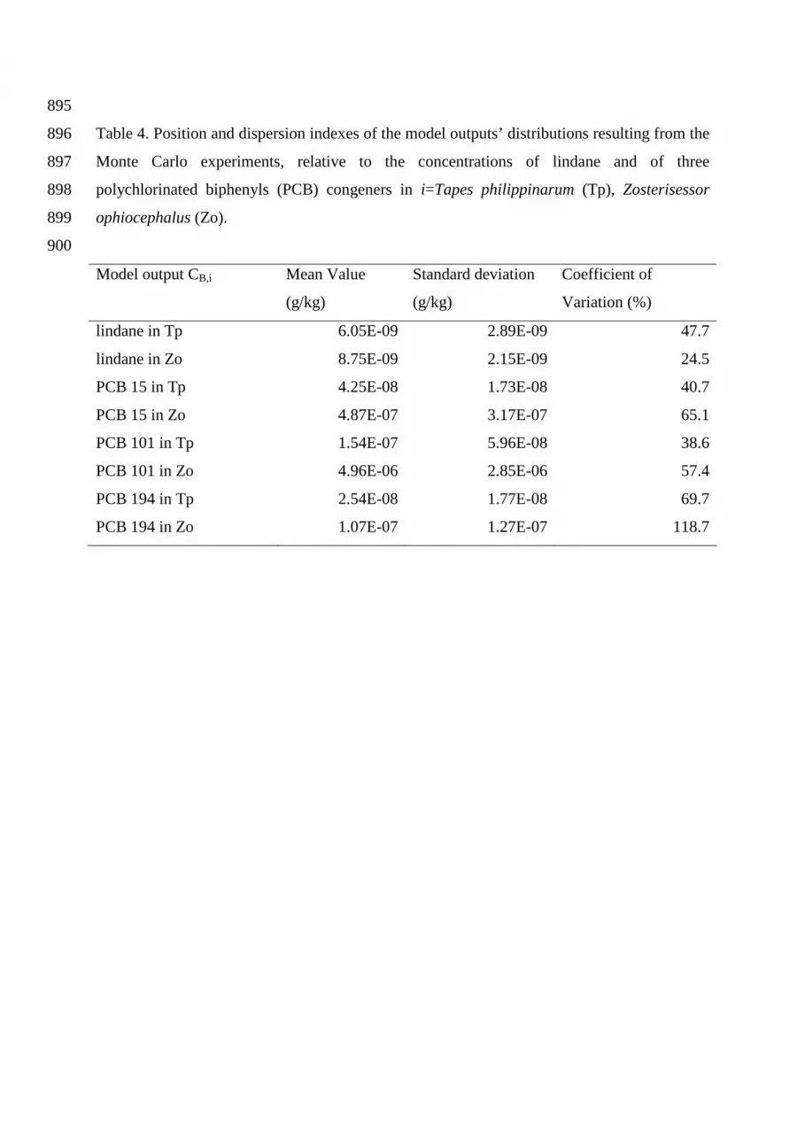
Table 4. Position and dispersion indexes of the model outputs’ distributions resulting from the 896

Monte Carlo experiments, relative to the concentrations of lindane and of three 897

polychlorinated biphenyls (PCB) congeners in i=Tapes philippinarum (Tp), Zosterisessor 898

ophiocephalus (Zo). 899

900

Model output CB,i Mean Value

(g/kg)

Standard deviation

(g/kg)

Coefficient of

Variation (%)

lindane in Tp 6.05E-09 2.89E-09 47.7

lindane in Zo 8.75E-09 2.15E-09 24.5

PCB 15 in Tp 4.25E-08 1.73E-08 40.7

PCB 15 in Zo 4.87E-07 3.17E-07 65.1

PCB 101 in Tp 1.54E-07 5.96E-08 38.6

PCB 101 in Zo 4.96E-06 2.85E-06 57.4

PCB 194 in Tp 2.54E-08 1.77E-08 69.7

PCB 194 in Zo 1.07E-07 1.27E-07 118.7

Table 5 Values of the fractions of variance explained by the input factors (Vi) and correspondent factors' rank obtained by means of the state 901

dependent regression (SDR) model, with respect the estimated concentrations of lindane and of three polychlorinated biphenyls (PCB) congeners in 902

i=Tapes philippinarum (Tp), Zosterisessor ophiocephalus (Zo). The diet fractions pi,j refer to the target species' preys j=Phytoplankton (Fp), 903

Bacterioplankton (Bp), Zooplankton (Zp), Micro-Meiobenthos (MiMeB), Macrobenthos omnivorous filter-feeder (MaBoff), ), Macrobenthos 904

omnivorous mixed-feeder (MaBomf), Carcinus mediterraneus (Cm), Atherina boyeri (Ab). In the last row, sum (Vi) and sum (Vl,i) are the total 905

fraction of variance explained by, respectively, the SDR model and the multiple linear regression (MLR) model. 906

907

Tapes philippinarum Zosterisessor ophiocephalus

Input Factor lindane PCB 15 PCB 101 PCB 194 Input Factor lindane PCB 15 PCB 101 PCB 194

rank Vi (%) rank Vi (%) rank Vi (%) rank Vi (%) rank Vi (%) rank Vi (%) rank Vi (%) rank Vi (%)

LogKOW,25 6 0.6 1 69.9 1 52.2 1 84.9 LogKOW,25 2 38.4 1 86.0 1 79.9 1 96.3

∆HOW 14 1.E-3 12 8.E-3 12 2.3.E-2 8 8.E-3 ∆HOW 12 8.E-3 10 0.11 14 6.E-3 7 1.3.E-2

αOC 1 71.4 6 2.00 13 2.0.E-2 14 1.1.E-3 αOC 3 5.8 9 0.12 16 1.E-4 16 6.E-6

αDOC 10 6.E-3 5 2.05 2 25.1 2 6.6 αDOC 8 2.1.E-2 3 1.4 2 6.9 2 1.3

αPOC 11 3.1.E-3 7 0.3 3 6.4 3 1.7 αPOC 14 3.E-4 7 0.20 4 2.0 3 0.4

β 2 9.1 2 12.3 4 6.2 7 3.7.E-2 β 4 2.8 5 0.7 9 3.E-2 10 5.E-3

νl,Tp 4 5.1 3 7.5 5 2.9 15 1.E-4 νl,Zo 1 44.9 2 4.4 5 1.5 4 5.E-2

νn,Tp 5 1.4 4 2.2 6 0.8 10 5.1.E-3 νn,Zo 5 0.2 13 1.E-2 11 1.E-2 14 1.E-3

εl,Tp 7 5.E-2 16 9.E-5 7 0.7 6 4.4.E-2 εl,Zo 11 1.E-2 4 0.9 3 3.8 5 3.E-2

εn,Tp 12 2.9.E-3 14 6.E-4 10 3.3.E-2 16 3.E-5 εn,Zo 7 2.4.E-2 8 0.19 7 0.4 9 6.E-3

wTp 16 7.E-5 13 6.E-3 15 3.E-4 5 0.2 wZo 6 3.E-2 11 0.1 15 1.E-4 15 4.E-4

pTp,Fp 15 7.E-4 15 1.E-4 14 1.E-3 12 2.7.E-3 pZo,MiMeb 16 3.E-7 6 0.4 6 1.4 6 1.3.E-2

pTp,Bp 8 2.E-2 10 2.E-2 16 2.E-4 9 5.5.E-3 pZo,MaBoff 9 1.7.E-2 12 2.E-2 8 0.2 8 7.E-3

pTp,Zp 13 2.E-3 11 1.E-2 8 0.52 11 3.0.E-3 pZo,MaBomf 10 1.3.E-2 14 2.1.E-3 13 7.E-3 13 3.8.E-3

σTp 9 1.E-2 8 0.09 9 0.46 4 0.4 pZo,Cm 13 4.E-3 15 1.8.E-3 10 2.E-2 12 3.9.E-3

mp,Tp 3 7.4 9 0.06 11 2.8.E-2 13 1.5.E-3 pZo,Ab 15 9.E-5 16 1.6.E-3 12 8.E-3 11 4.3.E-3

sum (Vi)

(sum (Vl,i))

95.1

(82)

96.6

(94)

95.4

(59)

94.0

(88)

sum (Vi)

(sum (Vl,i))

92.3

(91)

94.4

(87)

96.2

(61)

98.1

(75)

908

SETAC - SUPPLEMENTAL DATA ARCHIVE 909

Table S.1. Trophic compartments included in the food web of the Lagoon of Venice [24,25] 910

exploited to carry out the UA/SA of the Arnot and Gobas model [14] and corresponding 911

nominal values of the organism wet weights (wi), of the lipid fractions (νn,i) and nonlipid 912

organic matter (νn,i).The range of variability of these factors were set equal to ±30% the 913

nominal values. 914

915

Trophic

level

Compartment Label wi

(kg)

νl,i(kg/kg) νn,i(kg/kg)

Sediment/Detritus SD 2.57 5.0E-3 0.04

Phytoplankton Fp 3.2E-

3

5.0E-3 0.195*

Phytobentos Fb 6.5E-

12

5.0E-3 0.2*

Bacterioplankton Bp 3.0E-

5

5.0E-2 0.2

Plankton

Zooplankton Zp 3.4E-

5

5.0E-2 0.2

Micro-Meio benthos MiMeB 1.0E-

4

1.4E-2 0.2

Macrobenthos detritivorous MaBd 3.2E-

4

1.4E-2 0.2

Macrobenthos erbivorous/detritivorous MaBhd 2.5E-

5

1.4E-2 0.2

Macrobenthos omnivorous filter-feeder MaBoff 6.7E-

3

1.2E-2 0.2

Tapes philippinarum juveniles TpJ 1.0E-

3

1.3E-2 0.2

Tapes philippinarum Tp 7.0E-

3

1.3E-2 0.2

Macrobenthos omnivorous mixed-feeder MaBomf 1.4E-

3

2.6E-2 0.2

Benthos

Carcinus mediterraneus Cm 1.0E-

2

5.0E-2 0.2

Macrobenthos omnivorous predator MaBop 1.6E-

3

5.0E-2 0.2

Chelon labrosus juveniles ClJ 1.7E-

2

6.8E-2 0.2

Chelon labrosus Cl 2.7E-

2

6.8E-2 0.2

Atherina boyeri Ab 3.2E-

3

9.6E-2 0.2

Zosterisessor ophiocephalus Zo 1.6E-

1

1.0E-1 0.2

Nekton carnivorous benthic feeder Ncarbf 8.2E-

2

8.0E-2 0.2

Sparus aurata juveniles SaJ 4.3E-

2

9.7E-2 0.2

Sparus aurata Sa 1.3E-

1

9.7E-2 0.2

Dicentrarcus labrax juveniles DlJ 4.0E-

2

1.3E-1 0.2

Fish

Dicentrarcus labrax Dl 2.5E-

1

1.3E-1 0.2

* Nonlipid organic carbon fraction of autotrophic species (νn',i; kg/kg)

916

Table S.2. Dietary preference matrix for the trophic web of the Lagoon of Venice [24,25], relative to Phytoplankton (Fp), Phytobentos (Fb),

Bacterioplankton (Bp),Zooplankton (Zp), Micro-Meiobenthos (MiMeB), Macrobenthos detritivorous (MaBd), Macrobenthos

erbivorous/detritivorous (MaBhd), Macrobenthos omnivorous filter-feeder (MaBoff), Tapes philippinarum juveniles (TpJ), Tapes philippinarum

(Tp), Macrobenthos omnivorous mixed-feeder (MaBomf), Carcinus mediterraneus (Cm), Macrobenthos omnivorous predator (MaBop), Chelon

labrosus juveniles (ClJ), Chelon labrosus (Cl), Atherina boyeri (Ab), Zosterisessor ophiocephalus (Zo), Nekton carnivorous benthic feeder

(Ncarbf), Sparus aurata juveniles (SaJ), Sparus aurata (Sa), Dicentrarcus labrax juveniles (DlJ), Dicentrarcus labrax (Dl).

Pre

dato

r/

Pre

y

SD

Fp

Fb

Bp

Zp

MiM

eB

MaB

d

MaB

hd

MaB

off

TpJ

Tp

MaB

omf

Cm

MaB

op

ClJ

Cl

Ab

Zo

Nca

rbf

SaJ

Sa

DlJ

Dl

Fp

Fb

Bp 1**

Zp .5* .3 .2

MiMeB .99* .01

MaBd .66* .34

MaBhd .1 .9*

MaBoff .2 .5 .06 .24*

TpJ .52* .2 .22 .06

Tp .83* .075 .085 .01

MaBom

f .34* .25 .05 .23 .09 .04

Cm .25* .15 .2 .1 .04 .06 .1 .1

MaBop .25* .2 .04 .2 .16 .15

ClJ .69* .31

Cl .45* .11 .32 .12

Ab .38* .12 .28 .15 .01 .06

Zo .08 .44* .12 .23 .01 .12

Ncarbf .04 .41* .18 .15 .15 .01 .06

SaJ .52* .24 .12 .12

Sa .2 .22 .26* .21 .09 .005 .005 .005 .005

DlJ .12 .48* .18 .16 .01 .05

Dl .03 .05 .1 .52* .05 .05 .05 .08 .07

* Dependent input factor in the UA/SA analysis: the value is calculated as the difference between 1 and the sum of the other diet fractions relative

prey i

** Parameter not included among the input factors in the UA/SA

Table S.3 The first twenty highest values of the sensitivity index µ* estimated by means of the

Morris screening analysis with respect to the concentrations of lindane and three polychlorinated

biphenyls (PCBs) in Tapes philippinarum (Tp). Some of the input factors are relative to

Phytoplankton (Fp), Phytobentos (Fb), Bacterioplankton (Bp),Zooplankton (Zp). The symbol †

highlight the first µ* value of each sequence which is below to the corresponding threshold value in

the last row.

Rank lindane PCB 15 PCB 101 PCB 194

Factor µ* Factor µ* Factor µ* Factor µ*

1 αOC 6.5Ε−9 LogKOW,25 3.6Ε−8 LogKOW,25 1.12E-07 LogKOW,25 3.7Ε−8

2 νl,Tp/νn,Tp 2.5Ε−9 νl,Tp/νn,Tp 1.7Ε−8 αDOC 7.67E-08 αDOC 1.0Ε−8

3 β 2.5Ε−9 β 1.4Ε−8 αPOC 5.11E-08 αPOC 6.6Ε−9

4 mTp 2.2Ε−9 αDOC 6.1Ε−9 νl,Tp/νn,Tp 3.91E-08 σTp 1.9Ε−9

5 LogKOW,25 5.7Ε-10 αOC 4.4Ε−9 β 3.71E-08 wTp 1.4Ε−9

6 σTp 5.2Ε-11 αPOC 4.3Ε−9 σTp 1.55E-08 νl,Tp/νn,Tp 6.2Ε-10†

7 pTp 1.7Ε-11 σTp 1.6Ε−9 pTp 1.48E-08 ∆HOW 5.1Ε-10

8 ∆HOW 1.2Ε-11 mTp 1.0Ε−9 εl,Tp 1.23E-08 pTp 4.6Ε-10

9 αDOC 1.0Ε-11 νn,Bp 4.8Ε-10† νn,Bp 8.7E-09† β 4.5Ε-10

10 αPOC 5.4Ε-12† ∆HOW 4.6Ε-10 wTp 5.49E-09 εl,Tp 4.2Ε-10

11 εl,Tp 2.1Ε-12 εl,Tp 3.8Ε-10 νl,s 5.04E-09 αOC 2.7Ε-10

12 βa 1.1Ε-12 pTp 2.8Ε-10 εn,Tp 3.46E-09 mTp 1.5Ε-10

13 νn,Bp 8.2Ε-13 βa 2.0Ε-10 εl,Bp 3.12E-09 νl,s 1.3Ε-10

14 νl,s 6.9Ε-13 kgFp 1.4Ε-10 αOC 2.74E-09 εn,Tp 1.0Ε-10

15 εn,Tp 5.0Ε-13 νl,s 1.1Ε-10 νn,s 1.24E-09 εl,Bp 3.9Ε-11

16 νn',Fp 4.0Ε-13 εn,Tp 1.0Ε-10 νn,Zp 1.09E-09 νn,s 3.7Ε-11

17 wTp 3.2Ε-13 νn',Fp 7.9Ε-11 εn,Bp 9.76E-10 νn,Bp 2.6Ε-11

18 kgFp 2.7Ε-13 wTp 7.3Ε-11 mTp 9.12E-10 pZp 1.8Ε-11

19 νn,s 1.9Ε-13 νn,s 4.0Ε-11 pZp 8.8E-10 wBp 8.2Ε-12

20 νn,Zp 7.4Ε-14 wBp 3.7Ε-11 ∆HOW 7.88E-10 εn,Bp 5.6Ε-12

Thresholds 1.0E-11 1.0E-9 1.0E-8 1.0E-9

Table S.4 The first twenty highest values of the sensitivity index µ* estimated by means of the

Morris screening analysis with respect to the concentrations of lindane and three polychlorinated

biphenyls (PCBs) in Zosterisessor ophiocephalus (Tp). Some of the input factors are relative to

Zooplankton (Zp), Micro-Meiobenthos(MiMeB), Macrobenthos detritivorous (MaBd),

Macrobenthos omnivorous filter-feeder (MaBoff), Macrobenthos omnivorous mixed-feeder

(MaBomf) and Atherina boyeri (Ab). The symbol † highlight the first µ* value of each sequence

which is below to the corresponding threshold value in the last row.

Rank lindane PCB 15 PCB 101 PCB 194

Factor µ* Factor µ* Factor µ* Factor µ*

1 νl,Zo /νn,Zo 3.7Ε−9 LogKOW,25 7.1Ε−7 LogKOW,25 6.2Ε−6 LogKOW,25 2.5Ε−7

2 Log KOW,25 3.1Ε−9 νl,Zo /νn,Zo 1.4Ε−7 αDOC 1.7Ε−6 αDOC 3.1Ε−8

3 αOC 9.7Ε-10 εn,Zo 7.2Ε−8 εn,Zo 1.2Ε−6 αPOC 1.7Ε−8

4 β 9.1Ε-10 αDOC 6.8Ε−8 αPOC 1.2Ε−6 εn,Zo 9.4Ε−9†

5 νn,MaBa 1.7Ε-10† β 6.0Ε−8 νl,Zo /νn,Zo 8.1Ε−7† νn,MaBd 5.7Ε−9

6 mMaBd 1.6Ε-10 νn,Αb 4.1Ε−8† pZo 7.0Ε−7 νl,Zo /νn,Zo 5.6Ε−9

7 νn,MaBomf 1.6Ε-10 εw,Zo 3.5Ε−8 εw,Zo 6.7Ε−7 ∆HOW 4.1Ε−9

8 mMaBomf 1.5Ε-10 pZo 3.3Ε−8 εn,Αb 4.7Ε−7 νl,s 4.0Ε−9

9 wZo 9.8Ε-11 αPOC 3.3Ε−8 β 4.4Ε−7 pZo 3.7Ε−9

10 ∆HOW 6.7Ε-11 αOC 2.8Ε−8 νn,MaBd 4.1Ε−7 εl,MaBd 3.5Ε−9

11 pZo 5.9Ε-11 νn,MaBomf 2.1Ε−8 νn,MiMeB 3.2Ε−7 εw,Zo 3.5Ε−9

12 αDOC 5.7Ε-11 νn,MaBd 2.0Ε−8 εl,MaBe 3.2Ε−7 pMaBomf 3.3Ε−9

13 εn,Zo 5.4Ε-11 wZo 1.6Ε−8 εl,MiMeB 3.2Ε−7 pMaBd 2.4Ε−9

14 νn,Αb 4.6Ε-11 εn,Αb 1.4Ε−8 νn,Zp 3.1Ε−7 wZo 1.6Ε−9

15 mMaBoff 4.1Ε-11 νn,MaBoff 1.1Ε−8 νl,s 3.0Ε−7 νn,MiMeB 1.5Ε−9

16 mMiMeB 3.2Ε-11 ∆HOW 9.6Ε−9 pZp 2.6Ε−7 εn,MaBd 1.4Ε−9

17 νn,MiMeB 2.9Ε-11 νn,MiMeB 8.3Ε−9 pMaBd,i 2.6Ε−7 εl,MiMeB 1.2Ε−9

18 νn,MaBoff 2.7Ε-11 νn,Zp 8.0Ε−9 νn,MaBomf 2.0Ε−7 νn,MaBomf 1.2Ε−9

19 αPOC 2.6Ε-11 wMaBomf 6.2Ε−9 εl,MaBomf 1.8Ε−7 εn,Αb 1.0Ε−9

20 εw,Zo 2.3Ε-11 ba 6.1Ε−9 εw,Αb 1.7Ε−7 εl,MaBomf 9.3Ε-10

Thresholds 5.0E-10 5.0E-8 1.0E-6 1.0E-8

Table S.5 Values of the fractions of variance explained by the input factors (Vl,i) and correspondent factors' rank obtained by means of the multiple

linear regression (MLR) model, with respect the estimated concentrations of lindane and of three polychlorinated biphenyls (PCB) congeners in

i=Tapes philippinarum (Tp), Zosterisessor ophiocephalus (Zo). The diet fractions pi,j refer to the target species' preys j=Phytoplankton (Fp),

Bacterioplankton (Bp), Zooplankton (Zp), Micro-Meiobenthos (MiMeB), Macrobenthos omnivorous filter-feeder (MaBoff), Macrobenthos

omnivorous mixed-feeder (MaBomf), Carcinus mediterraneus (Cm), Atherina boyeri (Ab). In the last row, sum (Vl,i) is the total fraction of variance

explained by the MLR models.

Tapes philippinarum Zosterisessor ophiocephalus

Input Factor lindane PCB 15 PCB 101 PCB 194 Input Factor lindane PCB 15 PCB 101 PCB 194

rank Vl,i (%) rank Vl,i (%) rank Vl,i (%) rank Vl,i (%) rank Vl,i (%) rank Vl,i (%) rank Vl,i (%) rank Vl,i (%)

LogKOW,25 6 0.39 1 68.55 1 22.78 1 80.01 LogKOW,25 2 38.14 1 78.57 1 46.19 1 73.92

∆HOW 13 0.01 12 0.01 11 0.04 6 0.03 ∆HOW 10 0.00 12 0.05 11 0.05 9 0.02

αOC 1 58.38 6 1.59 14 0.01 10 0.01 αOC 3 4.63 8 0.23 15 0.00 7 0.03

αDOC 14 0.01 4 2.11 2 18.76 2 5.38 αDOC 7 0.03 3 1.29 2 4.91 2 0.48

αPOC 9 0.04 7 0.27 3 7.03 3 1.54 αPOC 15 0.00 7 0.28 4 2.61 3 0.31

β 2 8.50 2 12.17 4 5.25 7 0.02 β 4 2.54 5 0.52 9 0.16 16 0.00

νl,Tp 4 5.31 3 7.00 5 3.32 14 0.00 νl,Zo 1 45.48 2 4.40 5 1.45 8 0.02

νn,Tp 5 1.53 5 2.10 6 1.27 8 0.02 νn,Zo 5 0.27 13 0.03 8 0.18 12 0.01

εl,Tp 7 0.15 16 0.00 8 0.34 16 0.00 εl,Zo 11 0.00 4 0.87 3 3.91 10 0.01

εn,Tp 8 0.06 14 0.00 12 0.01 13 0.00 εn,Zo 9 0.01 9 0.14 7 0.57 4 0.08

wTp 16 0.00 15 0.00 13 0.01 5 0.23 wZo 6 0.03 10 0.12 13 0.01 5 0.05

pTp,Fp 15 0.00 11 0.01 15 0.00 11 0.01 pZo,MiMeb 13 0.00 15 0.00 16 0.00 6 0.04

pTp,Bp 10 0.03 10 0.01 7 0.35 9 0.02 pZo,MaBoff 12 0.00 16 0.00 10 0.08 11 0.01

pTp,Zp 11 0.01 13 0.00 16 0.00 12 0.00 pZo,MaBomf 8 0.03 11 0.06 12 0.04 13 0.00

σTp 12 0.01 8 0.11 9 0.15 4 0.44 pZo,Cm 14 0.00 14 0.00 14 0.01 15 0.00

mp,Tp 3 7.24 9 0.06 10 0.05 15 0.00 pZo,Ab 16 0.00 6 0.38 6 0.59 14 0.00

sum (Vl,i) 81.7 94.0 59.4 87.7 sum (Vl,i) 91.2 86.9 60.8 75.0

54

Table S.6 The first twenty highest values of the sensitivity index µ* estimated by means of 1

the Morris screening analysis when the ranges of variability of the species specific input 2

factor were increased to 50% the reference values, with exception of the factors εl,i and εn,i 3

higher than 0.67 which were kept to ±30%. The model outputs are the concentrations of 4

lindane and three polychlorinated biphenyls (PCBs) in Tapes philippinarum (Tp). Some of the 5

input factors are relative to Phytoplankton (Fp), Phytobenthos (Fb), Bacterioplankton 6

(Bp),Zooplankton (Zp). The symbol † highlight the first µ* value of each sequence which is 7

below to the corresponding threshold value in the last row. 8

Rank lindane PCB 15 PCB 101 PCB 194

Factor µ* Factor µ* Factor µ* Factor µ*

1 αOC 5.7E-09 LogKOW,25 3.9E-08 LogKOW,25 9.0E-08 LogKOW,25 3.5E-08

2 mTp 3.4E-09 νn,Tp 2.0E-08 αDOC 8.5E-08 αDOC 5.9E-09

3 νl,Tp/νn,Tp 3.4E-09 β 1.7E-08 αPOC 4.6E-08 αPOC 4.1E-09

4 β 2.0E-09 αOC 6.6E-09 β 3.8E-08 wTp 3.0E-09

5 LogKOW,25 5.6E-10 αDOC 5.6E-09 νl,Tp/νn,Tp 3.5E-08 σTp 2.4E-09

6 σTp 4.3E-11 mTp 3.5E-09 σTp 1.5E-08 νl,Tp/νn,Tp 1.5E-09

7 pTp 2.6E-11 αPOC 3.2E-09 pTp 1.2E-08 pTp 1.1E-09

8 ∆HOW 1.3E-11 σTp 1.4E-09 νn,Bp 8.7E-09† εl,Tp 7.4E-10†

9 αDOC 1.2E-11 νn,Bp 8.3E-10† νl,s 8.0E-09 ∆HOW 5.0E-10

10 αPOC 5.0E-12† pTp 7.3E-10 εl,Tp 6.9E-09 β 4.9E-10

11 εl,Tp 2.3E-12 ∆HOW 5.1E-10 wTp 6.4E-09 νl,s 3.3E-10

12 νl,s 1.8E-12 εl,Tp 4.9E-10 εn,Tp 3.3E-09 mTp 2.4E-10

13 νn,BB 1.2E-12 νl,s 2.2E-10 εl,Bp 2.7E-09 αOC 1.7E-10

14 βa 1.0E-12 βa 1.9E-10 αOC 2.4E-09 εn,Tp 1.2E-10

15 εn,Tp 9.3E-13 νn',Fp 1.5E-10 νn,s 2.4E-09 νn,Bp 7.1E-11

16 νn',Fp 5.8E-13 kgFp 1.4E-10 νn,Zp 2.1E-09 εl,Bp 6.7E-11

17 wTp 4.7E-13 εn,Tp 1.4E-10 kgFp 1.8E-09 νn,s 6.0E-11

18 νn,s 2.8E-13 vl,Zp 1.0E-10 pZp 1.5E-09 pZp 2.1E-11

19 kgFp 2.6E-13 νn,s 8.6E-11 ∆HOW 1.1E-09 νn,Zp 1.9E-11

20 νn,Zp 1.3E-13 wTp 6.95E-11 wBB 1.1E-09 wBp 1.3E-11

Thresholds 1.0E-11 1.0E-9 1.0E-8 1.0E-9

55

Table S.7 The first twenty highest values of the sensitivity index µ* estimated by means of 9

the Morris screening analysis when the ranges of variability of the species specific input 10

factor were increased to 50% the reference values, with exception of the factors εl,i and εn,i 11

higher than 0.67 which were kept to ±30%. The model outputs are the concentrations of 12

lindane and three polychlorinated biphenyls (PCBs) in Zosterisessor ophiocephalus (Tp). 13

Some of the input factors are relative to Zooplankton (Zp), Micro-Meiobenthos(MiMeB), 14

Macrobenthos detritivorous (MaBd), Macrobenthos omnivorous filter-feeder (MaBoff), 15

Macrobenthos omnivorous mixed-feeder (MaBomf) and Atherina boyeri (Ab). The symbol † 16

highlight the first µ* value of each sequence which is below to the corresponding threshold 17

value in the last row. 18

Rank lindane PCB 15 PCB 101 PCB 194

Factor µ* Factor µ* Factor µ* Factor µ*

1 νl,Zo /νn,Zo 6.1E-09 LogKOW,25 5.6E-07 LogKOW,25 5.1E-06 LogKOW,25 2.4E-07

2 Log KOW,25 3.4E-09 νl,Zo /νn,Zo 2.8E-07 αDOC 1.6E-06 αDOC 3.4E-08

3 αOC 1.1E-09 pZo 6.1E-08 νl,Zo /νn,Zo 1.5E-06 νl,Zo /νn,Zo 1.1E-08

4 β 8.5E-10 νn,MaBomf 4.9E-08† εn,Zo 1.0E-06 αPOC 1.1E-08

5 νn,MaBa 3.1E-10† νn,Αb 4.8E-08 εw,Zo 8.6E-07† νn,MaBd 5.3E-09†

6 mMaBd 3.0E-10 νn,MaBd 4.6E-08 αPOC 7.9E-07 pZo 5.0E-09

7 mMaBomf 2.8E-10 β 4.4E-08 pZo 7.1E-07 ∆HOW 4.6E-09

8 νn,MaBomf 2.4E-10 αDOC 4.1E-08 νn,Zp 5.6E-07 νl,s 3.7E-09

9 wZo 2.0E-10 εn,Zo 3.8E-08 νn,MaBd 5.0E-07 εw,Zo 3.2E-09

10 pZo 1.3E-10 εw,Zo 2.8E-08 νn,Αb 4.9E-07 β 2.9E-09

11 mMaBoff 9.1E-11 νn,Zp 2.2E-08 εn,Ab 4.6E-07 νn,MiMeB 2.7E-09

12 νn,Αb 8.9E-11 αOC 1.9E-08 νl,s 4.0E-07 pMaBomf 2.6E-09

13 νn,MiMeB 7.4E-11 wZo 1.8E-08 εw,Αb 3.8E-07 εl,MiMeB 2.2E-09

14 αDOC 7.2E-11 αPOC 1.6E-08 pMaBd,i 3.3E-07 νn,s 1.6E-09

15 ∆HOW 6.8E-11 νn,MiMeB 1.2E-08 pMaBomf 2.9E-07 wZo 1.6E-09

16 εn,Zo 6.7E-11 εw,Ab 1.1E-08 pZp 2.7E-07 εl,MaBd 1.6E-09

17 νn,MaBoff 6.3E-11 νn,MaBoff 9.9E-09 εl,MaBd 2.7E-07 wMaBd 1.6E-09

18 mMiMeB 5.4E-11 wAb 8.2E-09 pAb 2.6E-07 pZp 1.5E-09

19 εw,Zo 3.9E-11 ∆HOW 7.2E-09 vn,MaBomf 2.4E-07 pMaBd 1.5E-09

20 αPOC 2.9E-11 νn,MaBoff 6.7E-09 β 2.4E-07 εn,Zo 1.5E-09

56

Thresholds 5.0E-10 5.0E-8 1.0E-6 1.0E-8

57

19

Table S.8. Position and dispersion indexes of the model outputs’ distributions resulting from 20

the Monte Carlo experiments where all the 227 model parameters were randomly sampled. 21

The indexes are relative to the concentrations of lindane and of three polychlorinated 22

biphenyls (PCB) congeners in Tapes philippinarum (Tp) and Zosterisessor ophiocephalus 23

(Zo). 24

25

Model output Cb Mean Value

(g/kg)

Standard deviation

(g/kg)

Coefficient of

Variation (%)

lindane in Tp 6.05E-09 2.89E-09 47.7

lindane in Zo 8.75E-09 2.15E-09 24.5

PCB 15 in Tp 4.25E-08 1.72E-08 40.6

PCB 15 in Zo 4.87E-07 3.23E-07 66.3

PCB 101 in Tp 1.55E-07 6.00E-08 38.8

PCB 101 in Zo 4.97E-06 2.91E-06 58.5

PCB 194 in Tp 2.54E-08 1.77E-08 69.7

PCB 194 in Zo 1.07E-07 1.26E-07 118.5

26