jrofor­

ential

larket­

lrtant

)duct

y the

Larry D. Godsey University of Missouri, Columbia, MO

D. Evan Mercer USDA Forest Service, Southern Res. Stn., Re~earch Triangle Park, NC

Robert K. Grala Stephen C. Grado Mississippi State University, Mississippi State, MS

Janaki R.R. Alavalapati University of Florida, Gainesville, FL

Agroforestry Economics and Policy Essentia lly every living thing on Earth has applied the basic concepts of economics. That is, every living thing has had to use a limited set of resources to meet a minimum set of needs or wants. Although the study of economics is often confused with the study of markets or finance, economics is simply a social science that studies the choices people make. As a social science, economics is the study of human motivations. Or, as Landsburg (1993) put it, Umost of economics can be summarized in four words: 'People respond to incentives'." Those incentives reflect the value of the trade-offs made between a limited set of resources and an unlimited set of wants, needs, and desires.

It is true that the concepts of money and price are often used as proxy values for economic decisions, but markets don't always reflect the true value of natural resource benefits and prices do not indicate the actual cost of the services provided by natural pro­cesses (Sagoff, 2004). Remember the last time you drove through the countryside on a nice autumn day and admired the beautiful colors. How much did you have to pay for this ben­efit? If you paid nothing, does that mean that it has no value?

Economics characterize the mental calculus of a decision maker, whether a private land­owner or a policymaker. In particular, economic models are abstract representations of the real world useful for hypothesis generation, forecasting, policy analysis, and decision­making (Buongiorno and Gilles, 2003). Alavalapati and Mercer (2004) recently discussed diverse economic models and their applications to agroforestry (Table 12-1). Some are designed to assess simple cost and benefits of outputs and inputs for which markets are fairly established, while others are amenable to a variety of environmental services and damages for which there are no established markets. Furthermore, some methodologies are more appropriate for assessing issues at a farm or household level, and others are applicable at regional and national scales.

The goal of this chapter is to present the concepts ofeconomics and explain how it applies to natural resource management decisions so that students with limited backgrounds in economics may still understand the issues faced by decision makers. This chapter dis­cusses many of the tools used by economists to measure and determine how choices are made at both the micro- (individual) and the macro- (aggregate) level. financial concepts are the basis for many of the tools that economists use to measure market- and nonmarket­based values at the individual level. These tools include benefit-cost, discounted cash flow, and willingness-to-pay analysis. The appendices provide an overview of several basic eco­nomic concepts (interest rates, compounding versus discounting, and inflation) that form

North American Agroforestry: An Integrated Science and Practice, 2nd edition, H.E. Garrett (ed.) Copyright © 2009. American Society of Agronomy, 677 S. Segoe Rd., Madison, WI 53711, USA.

315

t Source: A revised version adapted from Alavalapati and Mercer (2004).

Table 12-1. Economic methodologies commonly applied to assess agroforestry systems.t and cattle p systems (Cha will include s

Whole-far line to accom limited resou attainment 0

whole-farm complicated, ber of farm en all of the far describes ho production as (Doye, 2007). the summary ing outlined f from selling income gener 1992). A whol mine the net it will be afie prices, and ex several alter owners can u potential and institutions (S

Enterprise B An enterprise nues associate and explains in the product' As with whole also vary in f provided. Mo on revenues g~

costs such as H labor, machin~ overhead (Do~

.hon, these b~

prices per uni analyses (Sma! can be used in ing. Most COffil

the most praHl mine if current be replaced W

such as agrofor

Partial Budgf A partial bud! change in the f of farm produ instead of devel enterprise budl those costs and To determine t

of agroforestry practices as well as the entire farm production.

Farm Budgeting for Agroforestry Alternatives

The process of financially determining the most effective farm operations is not an easy task. Increasing production costs and changing demands for farm products require continuous reevaluation of farm management objectives and adjustments of farm production to make it profitable. Possible adjustments might include lowering farm production costs, improving pro­duction technology, and introducing new farm operations such as agroforestry practices. These changes can have a significant impact on the financial viability of the entire farm. Thus, such enterprises have to be well planned and eXi;lm­ined from a financial perspective to ensure that only alternatives improving overall profitabil­ity are implemented. This requires a consistent examination of short- and long-term financial effects of proposed changes in farm management. Farm budgeting is a method used to evaluate the attainment of farm financial goals by comparing revenues and costs associated with farm produc­tion. There are several types of farm budgeting, and we briefly discuss three: whole-farm, enter­prise, and partial budgeting.

Whole-Farm Budgeting A whole-farm budget is a snapshot describing the entire production on the farm. It identifies indi­vidual farm components called enterprises and shows how they contribute to the overall profit generated by farm production (Doye, 2007). A farm enterprise consists of any type of farm pro­duction such as corn, soybeans, wheat, tomatoes,

Nature, Scope, and Scale of the Issue for Investigation

Estimate the profitability of a farm or enterprise by calculating indicators such as net present values (NPV), benefit/cost ratio (BCR), and internal rate of return (lRR).

Incorporate probabilities of events occurring and estimate the expected profitability of agroforestry.

Assess the profitability at a farm or regional level from both the individual and society perspective (similar to farm budget models, but also includes market failures).

Optimization models to estimate land expectation values assuming that the land will be used for agroforestry (the best possible productive use) in perpetuity.

Estimate optimum resource allocation subject to various constraints faced by the decision maker.

Estimate the relationships among variables under investigation for forecasting, policy analysis, and decision making.

Stated and revealed preference models to estimate values for environmental goods and services such as reducing soil erosion, improving water quality, and carbon sequestration (examples include hedonic and contingent valuation models).

Estimate changes in income, employment, and price levels at regional or national level, in response to a policy or program change and explicitly incorporate intersectoral linkages.

Economic Approach/Model

Linear and nonlinear programming models

Nonmarket valuation models

Econometric models

Enterprise/farm budget models

Faustmann and Hartmann models

Regional economic models

Policy analysis matrix (PAM) models

Risk assessment models

the basis for the financial analysis described below. To give a flavor of how the tools of eco­nomics can be used to analyze agroforestry, in the next sections we describe and provide exam­ples of using two of the approaches in Table 12-1, enterprise/farm budget models and nonmar­ket valuation models. These are followed by an overview of policies and incentives to encourage landowners to adopt agroforestry systems.

Budgeting and Valuation in an Agroforestry Context

Agroforestry practices usually constitute part of a larger farm system that includes various oper­ations in which agricultural production (annual crops and/or livestock) is combined with trees. They provide numerous market and nonmarket benefits that not only improve sustainability of the farm (Young, 1989) but also can lead to sig­nificant increases in monetary returns (Gordon and Newman, 1997). However, implementa­tion of agroforestry alternatives as well as other farm practices is often constrained by available resources such as land, financial capital, equip­ment, production technology, and labor (Kurtz, 2000). Farmers and landowners allocate these limited resources in a way that allows them to attain their objectives in the most efficient man­ner. When the objective is to maximize financial returns on farm production, this implies that you are comparing costs and returns, and selecting, from a financial perspective, the most promising practices (Alavalapati and Mercer, 2004; Kurtz, 2000). In this section, we describe methods and tools commonly used to assess financial viability

316 Godsey, Mercer, Grala, Grado, Alavalapati

I

ch as net IRR).

,fitability of

nd society res).

, land will

'y the

ng, policy

,I goods lCbon s).

,tionaI level, sectoral

1e entire

~s

ling the an easy

:hanging ntinuous ,bjectives , make it

include V"ing pro­ew farm ·s. These , on the us, such Id eX;1ffi­

ure that rofitabil­nsistent inancial gement. late the 1paring produc­igeting, I, enter­

ng the ~s indi­es and profit

107). A mpro­llatoes,

agroforestry economics and policy

and cattle production, as well as agroforestry systems (Chase, 2006). Therefore, a typical farm will include several enterprises.

Whole-farm budgeting serves as a guide­line to accomplish the owner's objectives, given limited resources, and monitor progress in the attainment of these objectives (Doye, 2007). A whole-farm budget can be fairly extensive and complicated, depending on farm size and num­ber of farm enterprises involved. Typically, it lists all of the farm's physical and financial assets and describes how they are allocated to whole farm production as well as particular farm enterprises (Doye, 2007). The pivotal part of the budget is the summary of costs associated with conduct­ing outlined farm operations, expected revenues from selling farm products, and estimated net income generated by the entire farm (Smathers, 1992). A whole-farm budget can be used to deter­mine the net value of farm production and how it will be affected by changes in costs, products prices, and expected crop yields. By comparing several alternative management plans, land­owners can use this budget to determine farm potential and negotiate financing from lending institutions (Smathers, 1992).

Enterprise Budgeting An enterprise budget describes costs and reve­nues associated with a specific farm enterprise and explains how farm resources are allocated in the production of farm products (Chase, 2006). As with whole-farm budgets, enterprise budgets also vary in format and amount of information provided. Most often they include information on revenues generated from the enterprise and costs such as planting, fertilizing, weed control, labor, machinery, land and building costs, and overhead (Doye, 2007; Smathers, 1992). In addi­tion, these budgets often include break-even prices per unit of production and sensitivity analyses (Smathers, 1992). Enterprise budgets can be used in several ways to aid decision mak­ing. Most commonly, they are used to identify the most profitable farm enterprises and deter­mine if current crop or livestock operations can be replaced with more profitable alternatives, such as agroforestry (Chase, 2006).

Partial Budgeting A partial budget is used in situations where change in the farm operation only affects a part of farm production (Lessley et aI., 1991). Thus, instead of developing an extensive whole-farm or enterprise budget, it is possible to examine only those costs and revenues affected by the change. To determine the net outcome of the proposed

change it is necessary to identify associated positive and negative effects as outlined by the partial budget methodology. Increased revenues and reduced costs resulting from the change are considered as positive effects, whereas lost or decreased revenues and increased costs as neg­ative effects. If positive effects exceed negative ones, overall farm income increases. In contrast, if negative effects are larger than positive ones, farm income will decrease (Doye, 2007).

Consider Chase et a1.'s (2006) example of a situation where a farmer considers switching from organic soybean production to organic corn production on 16 ha of farmland. Cur­rent revenue associated with organic soybean production on this parcel of land is $20,160.00, whereas the cost is $3,150.00. If the land is shifted to organic corn production, it is expected that it will generate revenue of $27,000.00 at a cost of $6,530.00. The positive effects in this case include increased revenue of $27,000.00 generated from corn production and reduced costs of $3,150.00, amounting to a total of $30,150.00. The reduced cost of $3,150.00 is considered a positive effect because it is associated with soybean production. Since soybeans will be replaced with corn this cost won't be incurred again and thus represents additional savings. The negative effects include lost income of $20,160.00 and increased costs of $6,530.00 totaling $26,690.00. Again, since soy­beans won't be cultivated, lost soybean revenue has to be accounted for as a negative effect. Simi­larly, the cost associated with corn production is considered as a new cost and consequently also a negative effect. The net outcome of the proposed change from organic soybeans to organic corn production equals $3,460.00 (positive effects ­negative effects = $30,150.00 - $26,690.00). This value represents an amount by which over­all farm income will increase if organic corn production is implemented versus organic soy­bean production.

Effect of Time on the Value of Agroforestry Practices

A common feature of agroforestry alternatives is that they involve long investment periods (often more than a decade), which require special approaches in financial evaluation. Comparing revenues and costs simply as they appear is mis­leading and will lead to an incorrect decision on the financial viability of an agroforestry alterna­tive. \Ve can't just subtract costs from revenues to determine if the investment is profitable because with such long investment periods, time becomes a cost itself and needs to be properly accounted for in the analysis.

317

Imagine a situation in which you have been offered $2,000.00 and are given an option to cash it in today or receive the same amount after 5 yr. The choice for most people would be simple­they would prefer to receive the money now. Why? One reason is that there are numerous investment opportunities available that can gen­erate additional income during that 5-yr period. So, why wait so long to receive the same amount of money if you can deposit it, for example, in a bank account or in~est in the stock market and collect a much larger sum after 5 yr? For instance, if you deposit $2,000.00 into a savings account that pays an annual interest rate of 4%, after 5 yr you will be able to withdraw $2,433.31 (see Appendices 12-1 and 12-2 for details on how to calculate this value). You gain an additional $433.31 by investing now and cashing in after 5 yr instead of doing so today. Others might have different investment opportunities available to them (such as agroforestry) and consequently will earn more or less than $433.31.

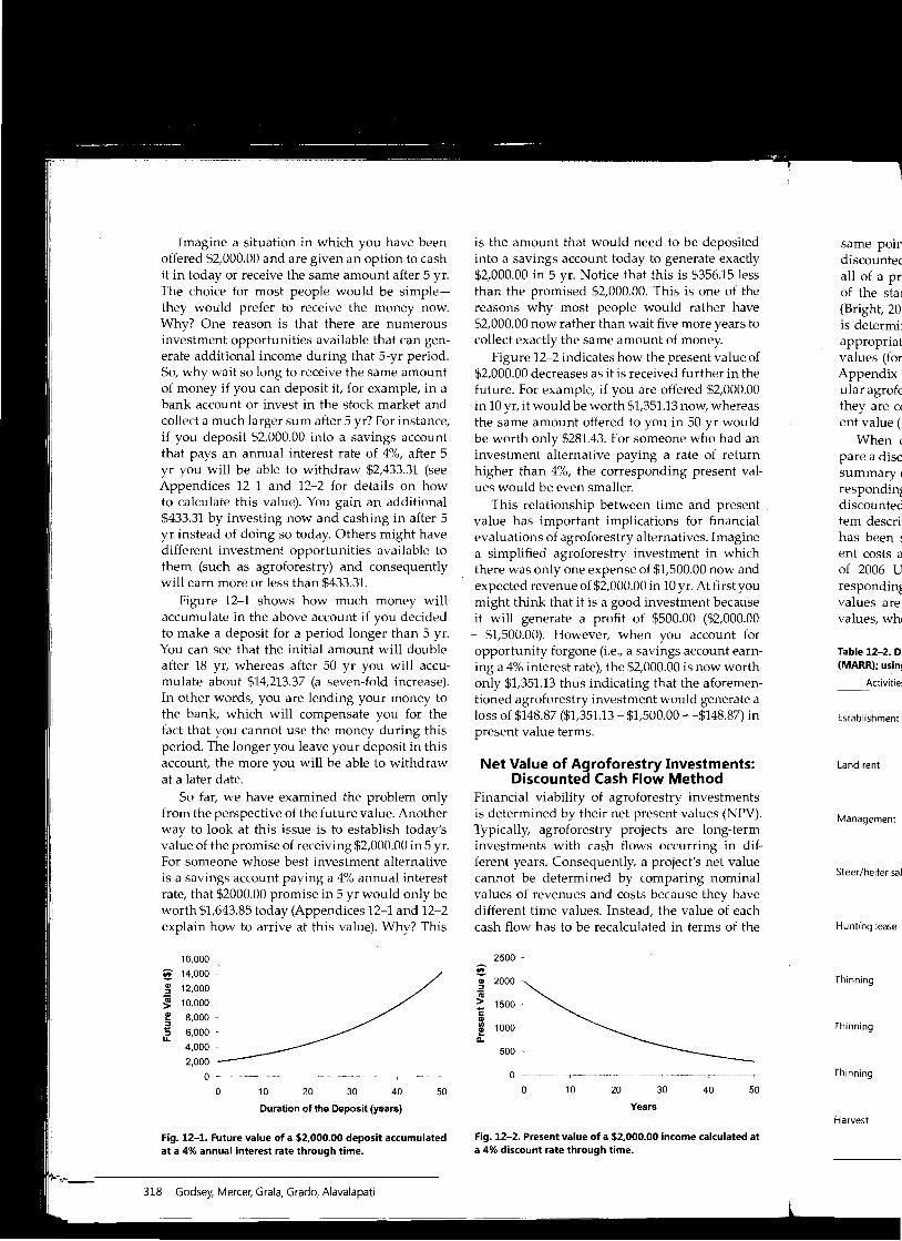
Figure 12-1 shows how much money will accumulate in the above account if you decided to make a deposit for a period longer than 5 yr. You can see that the initial amount will double after 18 yr, whereas after 50 yr you will accu­mulate about $14,213.37 (a seven-fold increase). In other words, you are lending your money to the bank, which will compensate you for the fact that you cannot use the money during this period. The longer you leave your deposit in this account, the more you will be able to withdraw at a later date.

So far, we have examined the problem only from the perspective of the future value. Another way to look at this issue is to establish today's value of the promise of receiving $2,000.00 in 5 yr. For someone whose best investment alternative is a savings account paying a 4% annual interest rate, that $2000.00 promise in 5 yr would only be worth $1,643.85 today (Appendices 12-1 and 12-2 explain how to arrive at this value). Why? This

16,000

~ 14.000

~ 12,000

~ 10,000

l!! 8,000

:;" 6,000 u.

4,000

2,000 o -,-.~.. _-- " -.-~.~~-..-~.•..."..... "~'~~--"--,

o 10 20 30 40 50

Duration of the Deposit (years)

Fig. 12-1. Future value of a $2.000.00 deposit accumulated at a 4% annual interest rate through time.

is the amount that would need to be deposited into a savings account today to generate exactly $2,000.00 in 5 yr. Notice that this is $356.15 less than the promised $2,000.00. This is one of the reasons why most people would rather have $2,000.00 now rather than wait five more years to collect exactly the same amount of money.

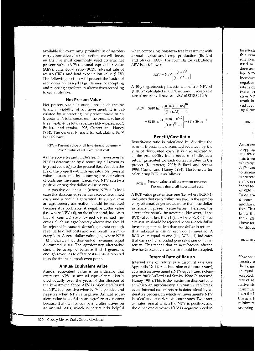
Figure 12-2 indicates how the present value of $2,000.00 decreases as it is received further in the future. For example, if you are offered $2,000.00 in 10 yr, it would be worth $1,351.13 now, whereas the same amount offered to you in 50 yr would be worth only $281.43. For someone who had an investment alternative paying a rate of return higher than 4%, the corresponding present val­ues would be even smaller.

This relationship between time and present value has important implications for financial evaluations of agroforestry alternatives. Imagine a simplified agroforestry investment in which there was only one expense of $1,500.00 now and expected revenue of $2,000.00 in 10 yr. At first you might think that it is a good investment because it will generate a profit of $500.00 ($2,000.00

- $1,500.00). However, when you account for opportunity forgone (Le., a savings account earn­ing a 4% interest rate), the $2,000.00 is now worth only $1,351.13 thus indicating that the aforemen­tioned agroforestry investment would generate a loss of $148.87 ($1,351.13 - $1,500.00 = -$148.87) in present value terms.

Net Value of Agroforestry Investments: Discounted Cash Flow Method

Financial viability of agroforestry investments is determined by their net present values (NPV). Typically, agroforestry projects are long-term investments with cash flows occurring in dif­ferent years. Consequently, a project's net value cannot be determined by comparing nominal values of revenues and costs because they have different time values. Instead, the value of each cash flow has to be recalculated in terms of the

2500

.. 2000

" ~ 1500_

i c

1000 lL

500 ­

o 10 20 30 40 50

Years

Fig. 12-2. Present value of a $2.000.00 income calculated at a 4% discount rate through time.

same poin discountec all of apr' of the stm (Bright, 201 is determil appropriat values (for Appendix' ular agrofc they are c( ent value (

When ( pare a disc summary ( respondinl discounted tem descril has been ~

ent costs a of 2006 U respondin~

values are values, whl

Table 12-2. Di (MARR); usin!

Activitie'

Establishment

Land rent

Management

Steer/heifer sal

Hunting lease

Thinning

Thinning

Thinning

Harvest

318 Godsey, Mercer, Grala, Grado, Alavalapati

~d to be deposited to generate exactly this is $356.15 less This is one of the muld rather have t five more years to ntofmoney. he present value of ~ived further in the e offered $2,000.00 51.13now, whereas 'au in 50 yr would neone who had an g a rate of return ,nding present val­

time and present tions for financial ernatives. Imagine 'estment in which .$1,500.00 now and in 10 yr. At first you nvestment because $500.00 ($2,000.00

you account for vings account earn­00.00 is now worth that the aforemen­It would generate a ~o.oo = -$148.87) in

'Y Investments: w Method estry investments sent values (NPV). 2ts are long-term occurring in dif­

project's net value mparing nominal Jecause they have the value of each ~d in terms of the

30 40 50

I income calculated at

_ag;;;;;.r_o_f_o_re_s_t_rY,---e_co_no_m_ic_s_a_n_d---,-p_o_lic--,Y -::~,_,;

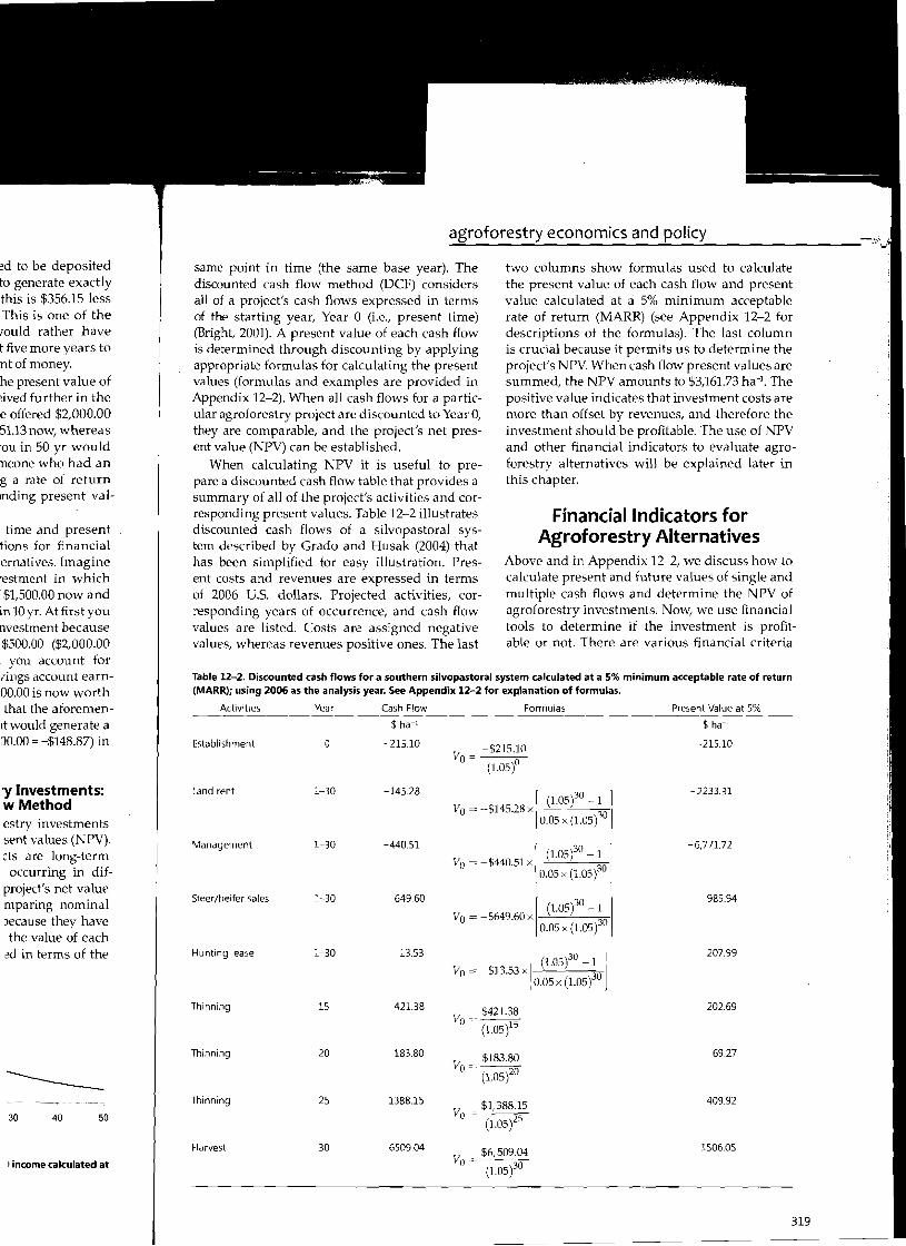
same point in time (the same base year). The two columns show formulas used to calculate discounted cash flow method (DCF) considcrs the present value of each cash flow and present all of a project's cash flows expressed in terms value calculated at a 5% minimum acceptable of the starting year, Year 0 (i.e., present time) rate of return (MARR) (see Appendix 12-2 for (Bright, 2001). A present value of each cash flow descriptions of the formulas). The last column is determined through discounting by applying is crucial because it permits us to determine the appropriate formulas for calculating the present project's NPV. When cash flow present values are values (formulas and examples are provided in summed, the NPV amounts to $3,161.73 ha-1

• The Appendix 12-2). When all cash flows for a partic­ positive value indicates that investment costs are ular agroforestry project are discounted to Year 0, more than offset by revenues, and therefore the they are comparable, and the project's net pres­ investment should be profitable. The use of NPV ent value (NPV) can be established. and other financial indicators to evaluate agro­

When calculating NPV it is useful to pre­ forestry alternatives will be explained later in pare a discounted cash flow table that provides a this chapter. summary of all of the project's activities and cor­responding present values. Table 12-2 illustrates Financial Indicators for discounted cash flows of a silvopastoral sys­ Agroforestry Alternatives tcm described by Grado and Husak (2004) that has been simplified for easy illustration. Pres­ Above and in AppendiX 12-2, we discuss how to ent costs and revenues are expressed in terms calculate present and future values of single and of 2006 U.S. dollars. Projected activities, cor­ multiple cash flows and determine the NPV of responding years of occurrence, and cash flow agroforestry investments. Now, we use financial values are listed. Costs are assigned negative tools to determine if the investment is profit­values, whereas revenues positive ones. The last able or not. There are various financial criteria

Table 12-2. Discounted cash flows for a southern silvopastoral system calculated at a 5% minimum acceptable rate of return (MARR); using 2006 as the analysis year. See Appendix 12-2 for explanation of formulas.

Activities Year Cash Flow Formulas Present Value at 5%

$~~ $~~

Establishment o -215.10 -215.10V = -$215.10 o

(1.05)0

Land rent 1-30 -145.28 -2233.31 (1.05)30 -1 1

Vo = -$145.28 x 30

f 0.05 x (1.05)

Management 1-30 -440.51 -6,771.72 (1.05)30 - 1 ]

Vo = -$440.51 x 30 [0.05 x (1.05)

Steer/heifer sales 1-30 649.60 985.94 (1.05)30 -1 1

Vo = -S649.60x 30 0.05 x (1.05) I

Hunting lease 1-30 13.53 207.99

l(1.05)30 -1 j

Vo = -$13.53 x 30 0.05 x (1.05)

Thinning 15 421.38 202.69

Thinning 20 183.80 69.27

Thinning 25 1388.15 409.92V = $1,388.15

o (1.05)25

Harvest 30 6509.04 1506.05V = $6,509.04

o (1.05)30

319

I

available for examining profitability of agrofor­estry alternatives. In this section, we will focus on the five most commonly used criteria: net present value (NPV), annual equivalent value (AEV), benefit/cost ratio (BCR), internal rate of return (IRR), and land expectation value (LEV). The following section will present the basics of each criterion, as well as guidelines for accepting and rejecting agroforestry alternatives according to each criterion.

Net Present Value Net present value is often used to determine financial viability of an investment. It is cal­culated by subtracting the present value of an investment's total costs from the present value of the investment's total revenues (Klemperer, 2003; Bullard and Straka, 1998; Gunter and Haney, 1984). The general formula for calculating NPV is as follows:

NPV = Present value of all investment revenues ­Present value of all investment costs

As the above formula indicates, an investment's NPV is determined by discounting all revenues (R,,) and costs (C) to the present (Le., Year 0 in the life of the project) with interest rate i. Net present value is calculated by summing present values of costs and revenues. Calculated NPV can be a positive or negative dollar value or zero.

A positive dollar value (where NPV > 0) indi­cates that discounted revenues exceed discounted costs and a profit is generated. In such a case, an agroforestry alternative should be accepted because it is profitable. A negative dollar value (Le., where NPV < 0), on the other hand, indicates that discounted costs exceed discounted rev­enues. Such an agroforestry alternative should be rejected because it doesn't generate enough revenue to offset costs and will result in a mon­etary loss. A zero dollar value (i.e., where NPV

= 0) indicates that discounted revenues equal discounted costs. The agroforestry alternative should be accepted because it still generates enough revenues to offset costs-this is referred to as the financial break-even point.

Annual Equivalent Value Annual equivalent value is an indicator that expresses NPV in annual equivalents distrib­uted equally over the years of the lifespan of the investment. Since AEV is calculated based on NPY, it is positive when NPV is positive and negative when NPV is negative. Annual equiv­alent value is useful in an agroforestry context because it allows for comparing alternatives on an annual basis, which is particularly helpful

320 Godsey, Mercer, Grala, Grado, Alavalapati

when comparing long-term tree investment with annual agricultural crop production (Bullard and Straka, 1998). The formula for calculating AEV is as follows:

AEV = NPvl i(l + it j ,(1+ it-1

A lO-yr agroforestry investment with a NPV of $910 ha-1 calculated at an 8% minimum acceptable rate of return will have an AEV of $118.89 ha- l

:

AE V = $910 ha -1[ 0.08 (1 + 0.08)10 jl

I (1 + 0.08iO -1

0 08(1 08)10 1 = $910 ha-1 ' ;0 = $118.89 ha-1

[ (1.08) -1

Benefit/Cost Ratio Benefit/cost ratio is calculated by dividing the sum of investment discounted revenues by the sum of discounted costs. It is also referred to as the profitability index because it indicates a return generated for each dollar invested in the project (Klemperer, 2003; Bullard and Straka, 1998; Gunter and Haney, 1984). The formula for calculating BCR is as follows:

BCR = Present value of all investment revenues Present value of all investment costs

A BCR value greater than one (Le., where BCR > 1) indicates that each dollar invested in the agrofor­estry alternative generates more than one dollar in return in present value terms. Therefore, the alternative should be accepted. However, if the BCR value is less than 1 (i.e., where BCR < 1), the alternative should be rejected because each dollar invested generates less than one dollar in return­this indicates a loss on each dollar invested. A BCR value equal to one (i.e., BCR = 1) indicates that each dollar invested generates one dollar in return. This means that an agroforestry alterna­tive has broken even and also should be accepted.

Internal Rate of Return Internal rate of return is a discount rate (see Appendix 12-1 for a discussion of discount rates), at which an investment's NPV equals zero (Klem­perer, 2003; Bullard and Straka, 1998; Gunter and Haney, 1984). This is the maximum discount rate at which an agroforestry alternative can break even. Internal rate of return is determined by an iterative process, in which an investment's NPV is calculated at various discount rates. Two inter­est rates, one at which the NPV is positive, and the other one at which NPV is negative, need to

be selecte this itera relationsl used to decrease~

late NPV increasec negative rate is de two discc ative NP' result in and it cal ing form\

IRR=

As an exa cropping at a 6% d this inves whereby NPVwas to increas is increas ha-1• Com increased of $130 ho To deterrr discount another d tive. This know tha than 12%. above for for this a~

IRR = 100/.

How can , forestry G

the farme or equal accepted. rate of re native sh minimurr than the I financial]. minimum cropping

I

'estment with tion (Bullard )r calculating

'ith a NPV of :lm acceptable 118.89 ha~l:

118.89 ha- 1

dividing the venues by the ,0 referred to it indicates a

wested in the j and Straka, Ie formula for

~nt revenues

nent costs

",here BCR > 1) in the agrofor~

1an one dollar Therefore, the owever, if the ~ BCR < 1), the Ise each dollar liar in return­1r invested. A = 1) indicates

; one dollar in Irestry alterna~

Id be accepted.

un )lint rate (see iiscount rates), lIs zero (Klem~

)8; Gunter and l discount rate ive can break ~rmined by an ~stment's NPV ltes. Two inter~

, positive, and ;ative, need to

agroforestry economics and policy

be selected to calculate IRK The reason for using this iterative process is that there is an inverse relationship between NPV and the discount rate used to calculate NPY. More specifically, NPV decreases as the discount rate used to calcu~

late NPV increases. When the discount rate is increased sufficiently high, the NPV will become negative (the opposite will hold if the discount rate is decreased). This means that between the two discount rates (resulting in positive and neg~

ative NPVs, respectively) there is one that will result in an NPV equal to zero. This is the IRR and it can be approximated by using the follow~

ing formula (Bright, 2001):

Discount rate resulting IRR=

in negative NPV

Difference between Positive NPV 1 + [ x Jdiscount rates Incremental NPV

As an example, we calculate an IRR for an alley cropping system that generates a NPV of $650 ha~l

at a 6% discount rate. To determine the IRR for this investment, we need to find a rate of return whereby the NPV will become negative. Since NPV was positive at 6%, this means that we need to increase the discount rate. If the discount rate is increased to 8%, NPV is still positive at $320 ha~l. Consequently, the discount rate needs to be increased even further. At 10%, it generates NPV of $130 hal, but at 12% NPV drops to -$28 ha~l.

To determine IRR, we need to select the highest discount rate at which NPV is still positive and another discount rate where NPV becomes nega~

tive. This is 10 and 12%, respectively. Now, we know that IRR is greater than 10% but smaller than 12%. By inserting this information into the above formula we can approximate that the IRR for this agroforestry alternative is 11.65%:

1 IRR=lO%+ 2%x ~ $130ha- ) =11.65%

$130 ha-1 + $28 ha-1

How can the IRR be used to determine if an agro~

forestry alternative is financially acceptable? If the farmer's acceptable rate of return is smaller or equal to the IRR, the alternative should be accepted. However, if the minimum acceptable rate of return is greater than the IRR, the alter~

native should be rejected. This is because the minimum acceptable rate of return that is higher than the IRR will result in a negative NPV, and a financial loss for the agroforestry alternative. If the minimum acceptable rate of return for the alley cropping system mentioned above is 6%, then it

would be a good investment because the actual IRR is well above that acceptable rate. In fact, this alley cropping system would break even at a mini~

mum acceptable rate of return as high as 11.65%.

Table 12-3 gives a summary of the how the indi­cators of NPV; IRR, and BCR can be used to assist in the decision making process. The landowner should accept investments with NPVs greater than or equal to 0, a BCR that is greater than or equal to 1, and an IRR that is greater than or equal to the mini~

mum acceptable rate of return.

Land Expectation Value Land expectation value (LEV) is a financial tool used to estimate land value based on all expected future costs and revenues generated from the use of this land. The LEV (known also as the Faustmann formula) has been used pri­marily to calculate the value of land parcels for which timber production was determined to be the best land use. Its major assumption is that timber production will be continued on a partic­ular parcel of land in perpetuity under the same management regime (Klemperer, 2003; Bullard and Straka, 1998). However, the LEV can also be used to establish the value of a specific land par­cel based on costs and revenues associated with both tree and agricultural production. In this case, the LEV is interpreted as the maximum amount of money a landowner can pay for the land and still earn the minimum acceptable rate of the return on an agroforestry investment.

The LEV can be computed in several ways. We calculate LEV for the silvopastoral system pre­sented in Table 12-2 based on its NPV of $3,161.73 ha~J. However, this NPV already includes land rent, whereas the LEV calculates land value based on future costs and returns. Therefore, we need to exclude land payments that occur during the investment period. When they are removed from the analysis, the recalculated NPV is $5,395.04 ha- l

• Now, we are ready to calculate LEV by using the following formula:

NPV(l+i)tLEV = ----'---'----'-­

(1 + ii-1

$5,395.04 ha-1 x (1.05)30

(1.05)30 -1

= $7,019.10 ha-1

Table 12-3. Guidelines for accepting or rejecting agrofor­estry alternatives according to net present value (NPVI, benefit/cost ratio (BCR), and internal rate of return (IRR).

Decisio:n~~ru~le=-- _

Accept the investment NPV;, 0 BCR;, 1 MARRt ~ IRR

Reject the investment NPV < 0 BCR < 1 MARR> IRR

t Minimum acceptable rate of return.

321

perspective, generally termed private profitability, can be different from that of a social perspective, often referred to as social profitability. The exclu­sion or inclusion of social benefits and costs and nonmarket goods and services (e.g., biodiversity and carbon sequestration), also known as exter­nalities, largely differentiates the private and social profitability.

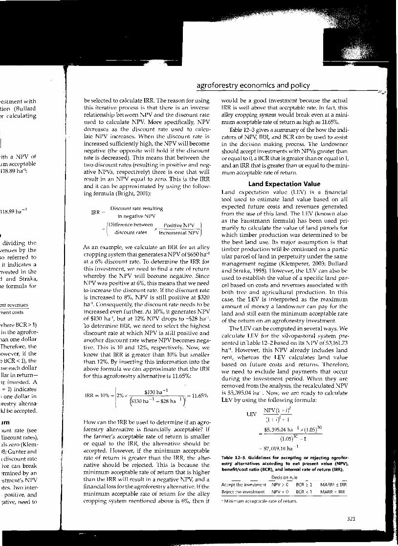
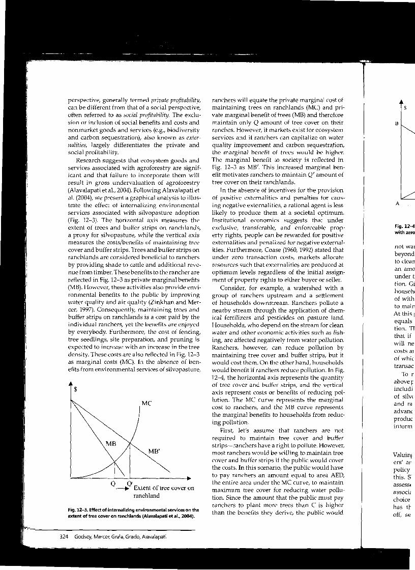
Research suggests that ecosystem goods and services associated with agroforestry are signif­icant and that failure to incorporate them will result in gross undervaluation of agroforestry (Alavalapati et al., 2004). Following Alavalapati et al. (2004), we present a graphical analysis to illus­trate the effect of internalizing environmental services associated with silvopasture adoption (Fig. 12-3). The horizontal axis measures the extent of trees and buffer strips on ranchlands, a proxy for silvopasture, while the vertical axis measures the costs/benefits of maintaining tree cover and buffer strips. Trees and buffer strips on ranchlands are considered beneficial to ranchers by providing shade to cattle and additional reve­nue from timber. Thesebenefits to the rancher are reflected in Fig. 12-3 as private marginal benefits (MB). However, these activities also provide envi­ronmental benefits to the public by improving water quality and air quality (Zinkhan and Mer­cer, 1997). Consequently, maintaining trees and buffer strips on ranchlands is a cost paid by the individual ranchers, yet the benefits are enjoyed by everybody. Furthermore, the cost of fencing, tree seedlings, site preparation, and pruning is expected to increase with an increase in the tree density. These costs are also reflected in Fig. 12-3 as marginal costs (MC). In the absence of ben­efits from environmental services of silvopasture,

$

Me

MB'

Q Q' -.. Extent of tree cover on

ranchland

Fig. 12-3. Effect of internalizing environmental services on the extent of tree cover on ranchlands (Alavalapati et aI., 2004).

324 Godsey, Mercer, Grala, Grado, Alavalapati

ranchers will equate the private marginal cost of maintaining trees on ranchlands (MC) and pri­vate marginal benefit of trees (MB) and therefore maintain only Q amount of tree cover on their ranches. However, if markets exist for ecosystem services and if ranchers can capitalize on water quality improvement and carbon sequestration, the marginal benefit of trees would be higher. The marginal benefit to society is reflected in Fig. 12-3 as MB'. This increased marginal ben­efit motivates ranchers to maintain Q' amount of tree cover on their ranchlands.

In the absence of incentives for the provision of positive externalities and penalties for caus­ing negative externalities, a rational agent is less likely to produce them at a societal optimum. Institutional economics suggests that under exclusive, transferable, and enforceable prop­erty rights, people can be rewarded for positive externalities and penalized for negative external­ities. Furthermore, Coase (1960, 1992) stated that under zero transaction costs, markets allocate resources such that externalities are produced at optimum levels regardless of the initial assign­ment of property rights to either buyer or seller.

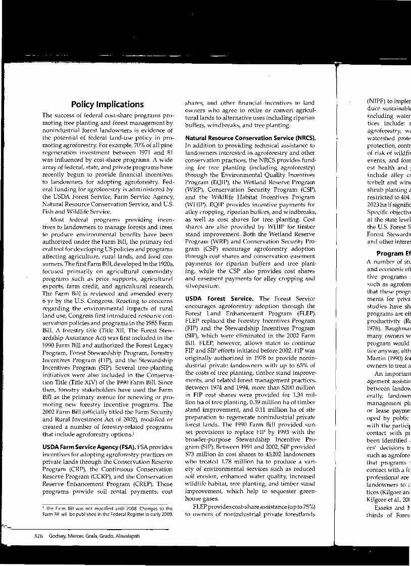
Consider, for example, a watershed with a group of ranchers upstream and a settlement of households downstream. Ranchers pollute a nearby stream through the application of chem­ical fertilizers and pesticides on pasture land. Households, who depend on the stream for clean water and other economic activities such as fish­ing, are affected negatively from water pollution. Ranchers, however, can reduce pollution by maintaining tree cover and buffer strips, but it would cost them. On the other hand, households would benefit if ranchers reduce pollution. In Fig. 12-4, the horizontal axis represents the quantity of tree cover and buffer strips, and the vertical axis represent costs or benefits of reducing pol­lution. The MC curve represents the marginal cost to ranchers, and the MB curve represents the marginal benefits to households from reduc­ing pollution.

First, let's assume that ranchers are not required to maintain tree cover and buffer strips-ranchers have a right to pollute. However, most ranchers would be willing to maintain tree cover and buffer strips if the public would cover the costs. In this scenario, the public would have to pay ranchers an amount equal to area AED, the entire area under the MC curve, to maintain maximum tree cover for reducing water pollu­tion. Since the amount that the public must pay ranchers to plant more trees than C is higher than the benefits they derive, the public would

$

B

A

Fig. 12-4 with zero

not wal beyond to clean an amo under t tion. Gi househ, of with to maill At this] equals tion. Tl that if will ne costs al of whic transac

To r abovef includi of silv( and ra advanc produc inform

Valuin) ers' an policy this. S asseSSl associ, choice has tr off, se

Policy Implications The success of federal cost-share programs pro­moting tree planting and forest management by nonindustrial forest landowners is evidence of the potential of federal land-use policy in pro­moting agroforestry. For example, 70% of all pine regeneration investment between 1971 and 81 was influenced by cost-share programs. A wide array of federal, state, and private programs have recently begun to provide financial incentives to landowners for adopting agroforestry. Fed­eral funding for agroforestry is administered by the USDA Forest Service, Farm Service Agency, Natural Resource Conservation Service, and U.S. Fish and Wildlife Service.

Most federal programs providing incen­tives to landowners to manage forests and trees to produce environmental benefits have been authorized under the Farm Bill, the primary fed­eral tool for developing US policies and programs affecting agriculture, rural lands, and food con­sumers. The first Farm Bill, developed in the 1920s, focused primarily on agricultural commodity programs such as price supports, agricultural exports, farm credit, and agricultural research. The Farm Bill is reviewed and amended every 6 yr by the U.S. Congress. Reacting to concerns regarding the environmental impacts of rural land use, Congress first introduced resource con­servation policies and programs in the 1985 Farm Bill. A forestry title (Title XII, The Forest Stew­ardship Assistance Act) was first included in the 1990 Farm Bill and authorized the Forest Legacy Program, Forest Stewardship Program, Forestry Incentives Program (FIP), and the Stewardship Incentives Program (SIP). Several tree-planting initiatives were also included in the Conserva­tion Title (Title XIV) of the 1990 Farm Bill. Since then, forestry stakeholders have used the Farm Bill as the primary avenue for renewing or pro­moting new forestry incentive programs. The 2002 Farm Bill (officially titled the Farm Security and Rural Investment Act of 2002), modified or created a number of forestry-related programs that include agroforestry options.1

USDA Farm Service Agency (FSA). FSA provides incentives for adopting agroforestry practices on private lands through the Conservation Reserve Program (CRP), the Continuous Conservation Reserve Program (CCRP), and the Conservation Reserve Enhancement Program (CREP). These programs provide soil rental payments, cost

1 The Farm Bill was not modified until 2008. Changes to the Farm Bill will be published in the Federal Register in early 2009.

,,...

326 Godsey, Mercer, Grala, Grado, Alavalapati

shares, and other financial incentives to land owners who agree to retire or convert agricul­turallands to alternative uses including riparian buffers, windbreaks, and tree planting.

Natural Resource Conservation Service (NRCS). In addition to providing technical assistance to landowners interested in agroforestry and other conservation practices, the NRCS provides fund­ing for tree planting (including agroforestry) through the Environmental Quality Incentives Program (EQIP), the Wetland Reserve Program (WRP), Conservation Security Program (CSP), and the Wildlife Habitat Incentives Program (WHIP). EQIP provides incentive payments for alley cropping, riparian buffers, and windbreaks, as well as cost shares for tree planting. Cost shares are also provided by WHIP for timber stand improvement. Both the Wetland Reserve Program (WRP) and Conservation Security Pro­gram (CSP) encourage agroforestry adoption through cost shares and conservation easement payments for riparian buffers and tree plant­ing, while the CSP also provides cost shares and easement payments for alley cropping and silvopasture.

USDA Forest Service. The Forest Service encourages agroforestry adoption through the Forest Land Enhancement Program (FLEP). FLEP replaced the Forestry Incentives Program (FIP) and the Stewardship Incentives Program (SIP), which were eliminated in the 2002 Farm Bill. FLEP, however, allows states to continue FIP and SIP efforts initiated before 2002. FIP was originally authorized in 1978 to provide nonin­dustrial private landowners with up to 65% of the costs of tree planting, timber stand improve­ments, and related forest management practices. Between 1974 and 1994, more than $200 million in FIP cost shares were provided for 1.34 mil­lion ha of tree planting, 0.59 million ha of timber stand improvement, and 0.11 million ha of site preparation to regenerate nonindustrial private forest lands. The 1990 Farm Bill provided sun­set provisions to replace FIP by 1995 with the broader-purpose Stewardship Incentive Pro­gram (SIP). Between 1991 and 2002, SIP provided $73 million in cost shares to 45,102 landowners who treated 1.78 million ha to produce a vari­ety of environmental services such as reduced soil erosion, enhanced water quality, increased wildlife habitat, tree planting, and timber stand improvement, which help to sequester green­house gases.

FLEP provides cost-share assistance (up to 75%) to owners of nonindustrial private forestlands

(NIPF) to implen duce sustainablE including water tices include: a agroforestry, We watershed prote protection, contr of risk of wildfir events, and fore est health and I include alley cr terbelt and wine shrub planting a restricted to 404.1 2023 ha if signific Specific objectivl at the state level the U.S. Forest S< Forest Stewards and other intere~

Program Ef A number of stu and economic eH tive programs j

such as agrofore that these progn ments for prival studies have sh, programs are eH productiVity (Re 1976). Baughmal many owners w program would tice anyway, alth Martin (1990) f01 owners to treat a

An important agement assistaI between landoVl erally, landown management ph or lease payme: oped by public with the particil contact with pI been identified , ers' decisions t< such as agrofore that programs contact with a fe professional are landowners to e tices (Kilgore ani Kilgore et aI., 20(

Esseks and ~

thirds of Fores

agroforestry economics and policy

oland agricul­iparian

NRCS). mce to i other s fund­,restry) mtives ogram

(CSP), ogram nts for breaks, ;. Cost timber eserve ty Pro­option ement plant­

shares 19 and

ervice ;h the FLEP). )gram )gram Farm

1tinue Pwas nonin­5% of prove­ctices. lillion 4 mil­imber )f site rivate i sun­h the

Pro­vided Nners

vari­iuced eased stand green­

)75%) lands

(NIPF) to implement a management plan to pro­duce sustainable public environmental benefits including water from forests. Acceptable prac­tices include: afforestation and reforestation, agroforestry, water quality improvement and watershed protection, fish and wildlife habitat protection, control of invasive species, reduction of risk of wildfire and restoration from wildfire events, and forest management to improve for­est health and growth. Agroforestry practices include alley cropping, riparian buffers, shel­terbelt and windbreak establishment, and tree/ shrub planting and pruning. Each landowner is restricted to 404.6 ha, which may be increased to 2023 ha if significant public benefits are produced. Specific objectives and practices are determined at the state level through partnerships between the U.S. Forest Service, the State Foresters, State Forest Stewardship Coordinating Committees, and other interested stakeholders.

Program Effectiveness and Barriers A number of studies have examined the social and economic efficiency of public financial incen­tive programs for private forest investments such as agroforestry. One hypothesis has been that these programs substitute government pay­ments for private capital investments. Several studies have shown that cost-share assistance programs are effective in improving forest land productivity (Royer and Moulton, 1987; Mills, 1976). Baughman (2002), however, found that many owners who participated in an incentive program would have done the supported prac­tice anyway, although Royer (1987) and Bliss and Martin (1990) found that the incentives enabled owners to treat additional hectares.

An important aspect of cost-share and man­agement assistance programs is the interaction between landowners and land managers. Gen­erally, landowners are required to develop management plans before receiving cost-share or lease payments. Plans are generally devel­oped by public or private professionals, often with the participation of the landowner. Direct contact with professional land managers has been identified as a leading factor in landown­ers' decisions to adopt conservation practices such as agroforestry. Several studies have found that programs that put landowners in direct contact with a forester or other natural resource professional are most influential in encouraging landowners to adopt sustainable forestry prac­tices (Kilgore and Blinn, 2004; Greene et aI., 2005; Kilgore et aI., 2007).

Esseks and Moulton (2000) found that two­thirds of Forest Stewardship Program (FSP)

participants had never had contact with a pro­fessional forester before developing the required management plan. A similar number began managing their land for multiple purposes and using new practices due to the FSP. In addi­tion, participation in FSP prompted owners to spend an average of $2,767 of their own funds for forest management activities. Interestingly, without their involvement in FSP and receiv­ing cost-share assistance, nearly two-thirds of par.ticipating owners said they would not have made the expenditures.

Funding has been established as a crucial bar­rier in promoting sustainable land use practices such as agroforestry. In a Congressional hearing reviewing the FLEP before the House Committee on Agriculture in July 2004, Charles W. Sten­holm, a representative from Texas lamented that

"states are facing requests for assistance that far exceeds the funding that is available." This con­cern is consistent with evidence from Florida: in 2003, 150 of 206 applications for FLEP funding were denied; in 2004 (a small amount of money was left over from 2003), 231 of 347 applications were denied; and in 2005, 187 of 429 applications were denied. Conversely, incentive programs may have the unintended effect of discouraging timely investments. In some instances, landown­ers have delayed investments until cost-share program funding was available (Haines, 1995).

Summary Agroforestry is a way for landowners to manage scarce natural resources that balances environ­mental stewardship, financial feasibility, and social responsibility. Because it is a balance of these three objectives, it requires the landowner to make complex decisions. Economic analysis uses a set of tools that can identify the tradeoffs that are made in the decision process. This chap­ter gave a broad overview of the decision tools that economist.s use, including budgeting meth­ods, financial methods, and nonmarket valuation methods. Real-world applications of these meth­ods illustrate the applicability and importance to the decision process.

Governmental policies have an impact on land management decisions. Management of privately owned natural resources can have an impact on society in both positive and negative· ways. Therefore, land management policies have been developed that provide financial incen­tives for land use practices, such as agroforestry, that protect, conserve, and improve the natural resource base.

327

I