GR Calculations in Mathematica

General Relativistic Calculations in

Mathematica

By George E. Hrabovsky

What I Will Cover0000 What is xAct?0000 What Do We Do Next?0000 Contraction0000 Covariant Derivatives0000 The Second Bianchi Identity0000 Perturbative GR

2 GRCalcs.nb

What is xAct?

This is a very complete system for doing tensor analysis in the Mathematica system.

All you need do is open the system:<< xAct`xTensor`

------------------------------------------------------------

Package xAct`xPerm` version 1.2.2, {2014, 9, 28}

CopyRight (C) 2003-2014, Jose M. Martin-Garcia, under the General Public License.

Connecting to external MinGW executable...

Connection established.

------------------------------------------------------------

Package xAct`xTensor` version 1.1.1, {2014, 9, 28}

CopyRight (C) 2002-2014, Jose M. Martin-Garcia, under the General Public License.

------------------------------------------------------------

These packages come with ABSOLUTELY NO WARRANTY; for details typeDisclaimer[]. This is free software, and you are welcome to redistributeit under certain conditions. See the General Public License for details.

------------------------------------------------------------

GRCalcs.nb 3

What Do We Do Next?

Now that we have started things up, there are some things we need to do.

1. We need to define the underlying manifold we are working in. We do this with the

DefManifold command: DefManifold[M, dim, {a, b, c,...}] defines M to be an n‐dimensional

differentiable manifold with dimension dim (a positive integer or a constant symbol) and

tensor abstract indices a, b, c, ... . DefManifold[M, {M1, ..., Mm}, {a, b, c,...}] defines M to be the

product manifold of previously defined manifolds M1 ... Mm. For backward compatibility dim

can be a list of positive integers, whose length is interpreted as the dimension of the defined

manifold. Here we define a four‐dimensional manifold having the indices

a, b, c, d, e, f , g, h, i, j, k, l:

DefManifold[M, 4, {a, b, c, d, e, f, g, h, i, j, k, l}]

** DefManifold: Defining manifold M.

** DefVBundle: Defining vbundle TangentM.

In defining the manifold, we have also defined the vector bundle called TangentM,

π : TM → M. This is where our tensors will be.

4 GRCalcs.nb

2. We need to define the metric using the DefMetric command: DefMetric[signdet, metric[‐a,‐b],

covd, covdsymbol] defines metric[‐a, ‐b] with signdet 1 or ‐1 and associates the covariant

derivative covd[‐a] to it. Note that we have the convention [‐a] has a as the subscript, and [a]

has it as the superscript.

DefMetric[-1, metric[-i, -j], cd, {";", "∇"}, PrintAs → "g"]

** DefTensor: Defining symmetric metric tensor metric[-i, -j].

** DefTensor: Defining antisymmetric tensor epsilonmetric[-a, -b, -c, -d].

** DefTensor: Defining tetrametric Tetrametric[-a, -b, -c, -d].

** DefTensor: Defining tetrametric Tetrametric†[-a, -b, -c, -d].

** DefCovD: Defining covariant derivative cd[-i].

** DefTensor: Defining vanishing torsion tensor Torsioncd[a, -b, -c].

** DefTensor: Defining symmetric Christoffel tensor Christoffelcd[a, -b, -c].

** DefTensor: Defining Riemann tensor Riemanncd[-a, -b, -c, -d].

** DefTensor: Defining symmetric Ricci tensor Riccicd[-a, -b].

** DefCovD: Contractions of Riemann automatically replaced by Ricci.

** DefTensor: Defining Ricci scalar RicciScalarcd[].

** DefCovD: Contractions of Ricci automatically replaced by RicciScalar.

** DefTensor: Defining symmetric Einstein tensor Einsteincd[-a, -b].

** DefTensor: Defining Weyl tensor Weylcd[-a, -b, -c, -d].

** DefTensor: Defining symmetric TFRicci tensor TFRiccicd[-a, -b].

** DefTensor: Defining Kretschmann scalar Kretschmanncd[].

** DefCovD: Computing RiemannToWeylRules for dim 4

** DefCovD: Computing RicciToTFRicci for dim 4

** DefCovD: Computing RicciToEinsteinRules for dim 4

** DefTensor: Defining weight +2 density Detmetric[]. Determinant.

GRCalcs.nb 5

3. We can define tensors using the DefTensor command: DefTensor[T[‐a, b, c, ...], {M1, ...}]

defines T to be a tensor field on manifolds and parameters M1,... and the base manifolds

associated to the vector bundles of its indices. DefTensor[T[‐a, b, c, ...], {M1, ...}, symmetry]

defines a tensor with symmetry given by a generating set or strong generating set of the

associated permutation group. In fact we can define any order of tensor just by specifying the

indices. A scalar has no indices so we can define the scalar

DefTensor[s[], M]

** DefTensor: Defining tensor s[].

s

s

a tangent vector

DefTensor[tv[i], M]

** DefTensor: Defining tensor tv[i].

tv[i]

tvi

6 GRCalcs.nb

a covector

DefTensor[cv[-i], M]

** DefTensor: Defining tensor cv[-i].

cv[-i]

cvi

and so on.

GRCalcs.nb 7

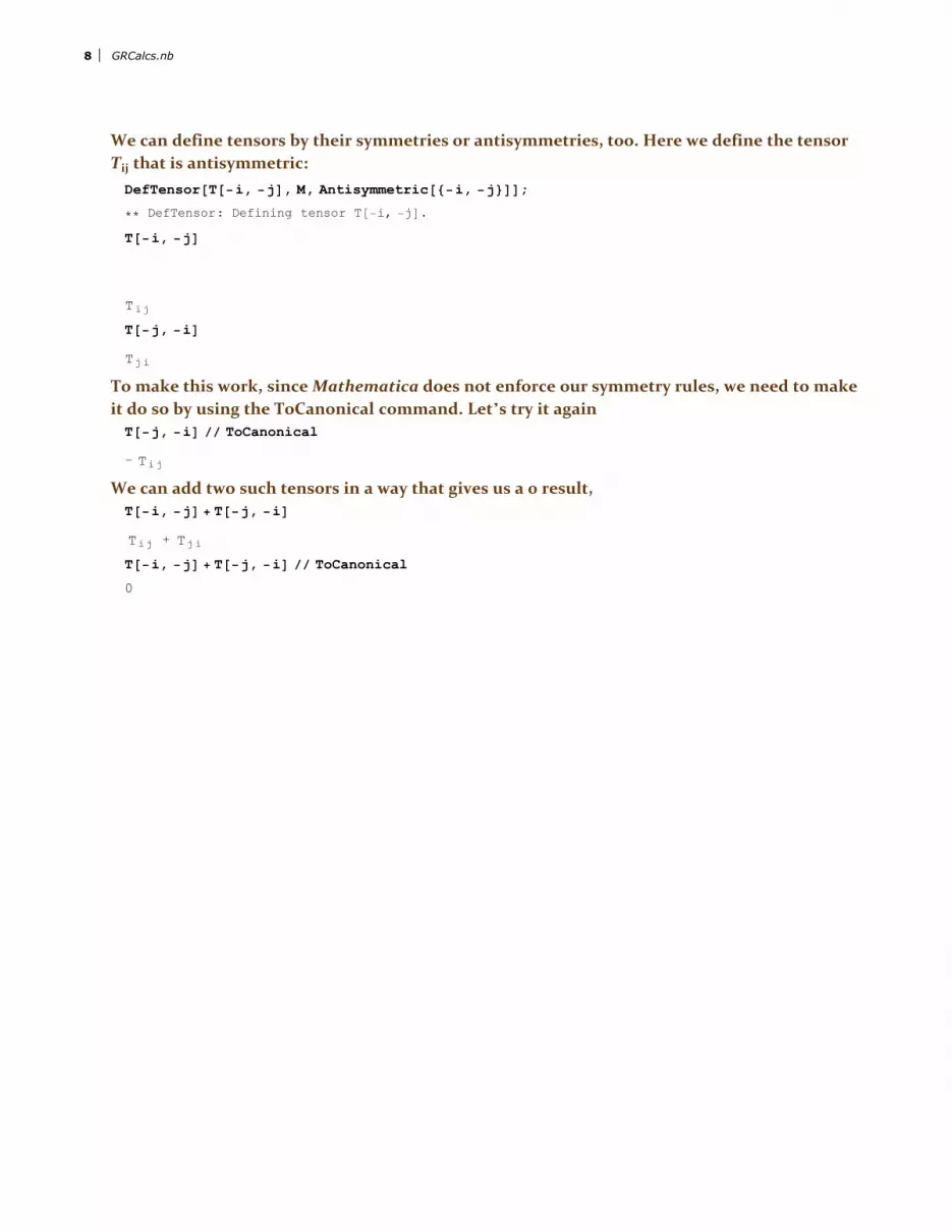
We can define tensors by their symmetries or antisymmetries, too. Here we define the tensor

Tij that is antisymmetric:

DefTensor[T[-i, -j], M, Antisymmetric[{-i, -j}]];

** DefTensor: Defining tensor T[-i, -j].

T[-i, -j]

Tij

T[-j, -i]

Tji

To make this work, since Mathematica does not enforce our symmetry rules, we need to make

it do so by using the ToCanonical command. Let’s try it again

T[-j, -i] // ToCanonical

- Tij

We can add two such tensors in a way that gives us a 0 result,

T[-i, -j] + T[-j, -i]

Tij + Tji

T[-i, -j] + T[-j, -i] // ToCanonical

0

8 GRCalcs.nb

Contraction

We can do some operations. Let’s say we have the Riemann tensor Rijkl and we want to

contract it using the metric gik. we use the ContractMetric command,metric[i, k] Riemanncd[-i, -j, -k, -l] // ContractMetric

R[∇]jl

Mathematica also understands that this is the Ricci tensor, Rjl,

metric[i, k] Riemanncd[-i, -j, -k, -l] // ContractMetric // InputForm

Riccicd[-j, -l]

Contracting it again gives us the Ricci scalar,metric[j, l] Riccicd[-j, -l] // ContractMetric // InputForm

RicciScalarcd[]

GRCalcs.nb 9

Covariant Derivatives

The covariant derivative of our tensor, ∇iTjl, is input

cd[-i][T[-j, -l]]

∇iTjl

If we have multiple covariant derivatives, we would enter them as follows, where @ is the

Map command:cd[-a]@cd[-b]@cd[-c]@T[-d, -e] // ToCanonical

∇a∇b∇cTde

To evaluate this we use the command SortCovDscd[-a]@cd[-b]@cd[-c]@T[-d, -e] // ToCanonical // SortCovDs

- R[∇] l$1032cbe ∇aTdl$1032 - R[∇] l$1032

cbd ∇aTl$1032e -

Tl$1030e ∇bR[∇]l$1030

cad - Tdl$1030 ∇bR[∇] l$1030cae - R[∇] l$1030

cae ∇bTdl$1030 -

R[∇] l$1030cad ∇bTl$1030e - R[∇] l$1028

bae ∇cTdl$1028 - R[∇] l$1028bad ∇cTl$1028e +

∇c∇b∇aTde - R[∇] l$1028bac ∇l$1028Tde - R[∇] l$1032

cba ∇l$1032Tde

10 GRCalcs.nb

This is correct, but too difficult to interpret, we add the command ScreenDollarIndices to

put it into a lnaguage we can read instead of just the computer reading itcd[-a]@cd[-b]@cd[-c]@T[-d, -e] // ToCanonical // SortCovDs // ScreenDollarIndices

- R[∇] fcbe ∇aTdf - R[∇] f

cbd ∇aTfe - Tfe ∇bR[∇]f

cad -

Tdf ∇bR[∇] fcae - R[∇] f

cae ∇bTdf - R[∇] fcad ∇bTfe - R[∇] f

bae ∇cTdf -

R[∇] fbad ∇cTfe + ∇c∇b∇aTde - R[∇] f

bac ∇fTde - R[∇] fcba ∇fTde

Instead of having to write all of this all of the time we make a session‐wide command$PrePrint = ScreenDollarIndices;

cd[-a]@cd[-b]@cd[-c]@T[-d, -e] // ToCanonical // SortCovDs

- R[∇] fcbe ∇aTdf - R[∇] f

cbd ∇aTfe - Tfe ∇bR[∇]f

cad -

Tdf ∇bR[∇] fcae - R[∇] f

cae ∇bTdf - R[∇] fcad ∇bTfe - R[∇] f

bae ∇cTdf -

R[∇] fbad ∇cTfe + ∇c∇b∇aTde - R[∇] f

bac ∇fTde - R[∇] fcba ∇fTde

GRCalcs.nb 11

The Second Bianchi Identity

Here we seek to reproduce the Second Bianchi identity. We redefine our covariant

derivativeDefCovD[CD[-a], {";", "∇"}]

** DefCovD: Defining covariant derivative CD[-a].

** DefTensor: Defining vanishing torsion tensor TorsionCD[a, -b, -c].

** DefTensor: Defining symmetric Christoffel tensor ChristoffelCD[a, -b, -c].

** DefTensor: Defining Riemann tensorRiemannCD[-a, -b, -c, d]. Antisymmetric only in the first pair.

** DefTensor: Defining non-symmetric Ricci tensor RicciCD[-a, -b].

** DefCovD: Contractions of Riemann automatically replaced by Ricci.

We begin by establishing a termterm1 = Antisymmetrize[CD[-e][ RiemannCD[-c, -d, -b, a] ], {-c, -d, -e} ]

1

6∇cR[∇]

adeb - ∇cR[∇]

aedb - ∇dR[∇]

aceb + ∇dR[∇]

aecb + ∇eR[∇]

acdb - ∇eR[∇]

adcb

We sum these,bianchi2 = 3 term1 // ToCanonical

∇cR[∇]a

deb - ∇dR[∇]a

ceb + ∇eR[∇]a

cdb

12 GRCalcs.nb

We expand the covariant derivatives in Christoffel symbols:exp1 = bianchi2 // CovDToChristoffel

Γ[∇]aef R[∇] f

cdb - Γ[∇]feb R[∇] a

cdf - Γ[∇]adf R[∇] f

ceb +

Γ[∇]fdb R[∇] a

cef + Γ[∇]fde R[∇] a

cfb - Γ[∇]fed R[∇] a

cfb +

Γ[∇]acf R[∇] f

deb - Γ[∇]fcb R[∇] a

def - Γ[∇]fce R[∇] a

dfb - Γ[∇]fec R[∇] a

fdb -

Γ[∇]fcd R[∇] a

feb + Γ[∇]fdc R[∇] a

feb + ∂cR[∇]a

deb - ∂dR[∇]a

ceb + ∂eR[∇]a

cdb

GRCalcs.nb 13

We expand the Riemann tensors in Christoffel symbolsexp2 = exp1 // RiemannToChristoffel

- Γ[∇]feb ∂cΓ[∇]

adf + Γ[∇]

fdb ∂cΓ[∇]

aef + Γ[∇]

aef ∂cΓ[∇]

fdb -

Γ[∇]adf ∂cΓ[∇]

feb - ∂c∂dΓ[∇]

aeb + ∂c∂eΓ[∇]

adb + Γ[∇]

feb ∂dΓ[∇]

acf -

Γ[∇]feb Γ[∇]

adg Γ[∇]

gcf - Γ[∇]

acg Γ[∇]

gdf - ∂cΓ[∇]

adf + ∂dΓ[∇]

acf -

Γ[∇]fcb ∂dΓ[∇]

aef - Γ[∇]

aef ∂dΓ[∇]

fcb +

Γ[∇]aef Γ[∇]

fdg Γ[∇]

gcb - Γ[∇]

fcg Γ[∇]

gdb - ∂cΓ[∇]

fdb + ∂dΓ[∇]

fcb +

Γ[∇]acf ∂dΓ[∇]

feb + ∂d∂cΓ[∇]

aeb - ∂d∂eΓ[∇]

acb - Γ[∇]

fdb ∂eΓ[∇]

acf +

Γ[∇]fdb Γ[∇]

aeg Γ[∇]

gcf - Γ[∇]

acg Γ[∇]

gef - ∂cΓ[∇]

aef + ∂eΓ[∇]

acf +

Γ[∇]fcb ∂eΓ[∇]

adf - Γ[∇]

fcb

Γ[∇]aeg Γ[∇]

gdf - Γ[∇]

adg Γ[∇]

gef - ∂dΓ[∇]

aef + ∂eΓ[∇]

adf + Γ[∇]

adf ∂eΓ[∇]

fcb -

Γ[∇]adf Γ[∇]

feg Γ[∇]

gcb - Γ[∇]

fcg Γ[∇]

geb - ∂cΓ[∇]

feb + ∂eΓ[∇]

fcb -

Γ[∇]acf ∂eΓ[∇]

fdb +

Γ[∇]acf Γ[∇]

feg Γ[∇]

gdb - Γ[∇]

fdg Γ[∇]

geb - ∂dΓ[∇]

feb + ∂eΓ[∇]

fdb - ∂e∂cΓ[∇]

adb +

∂e∂dΓ[∇]acb + Γ[∇]

fde Γ[∇]

afg Γ[∇]

gcb - Γ[∇]

acg Γ[∇]

gfb - ∂cΓ[∇]

afb + ∂fΓ[∇]

acb -

Γ[∇]fed Γ[∇]

afg Γ[∇]

gcb - Γ[∇]

acg Γ[∇]

gfb - ∂cΓ[∇]

afb + ∂fΓ[∇]

acb -

Γ[∇]fec - Γ[∇]

afg Γ[∇]

gdb + Γ[∇]

adg Γ[∇]

gfb + ∂dΓ[∇]

afb - ∂fΓ[∇]

adb -

Γ[∇]fce Γ[∇]

afg Γ[∇]

gdb - Γ[∇]

adg Γ[∇]

gfb - ∂dΓ[∇]

afb + ∂fΓ[∇]

adb -

Γ[∇]fcd - Γ[∇]

afg Γ[∇]

geb + Γ[∇]

aeg Γ[∇]

gfb + ∂eΓ[∇]

afb - ∂fΓ[∇]

aeb +

Γ[∇]fdc - Γ[∇]

afg Γ[∇]

geb + Γ[∇]

aeg Γ[∇]

gfb + ∂eΓ[∇]

afb - ∂fΓ[∇]

aeb

14 GRCalcs.nb

We canonicalize this to enforce symmetries and antisymmetries,exp3 = exp2 // ToCanonical

0

Which is what we expected.

∇cR[∇]abde +∇dR[∇]

abec +∇eR[∇]

abcd = 0

GRCalcs.nb 15

Perturbative GR

We begin this by opening the perturbative package:<< xAct`xPert

Get::noopen : Cannot open xAct`xPert.

$Failed

16 GRCalcs.nb

We must first establish our metric perturbation, this is because the metric is a vacuum

metric; thus all small perturbations are gravitational waves. We define the metric perturba‐

tion using the DefMetricPerturbation[the existing metric, name of the perturbation, pertur‐

bation parameter]DefMetricPerturbation[metric, pert, ϵ]

** DefParameter: Defining parameter ϵ.

** DefTensor: Defining tensor pert[LI[order], -a, -b].

We can tell Mathematica to write the perturbation using the traditional notation h,PrintAs[pert] ^= "h";

A second‐order perturbation in the metric is then writtenpert[LI[2], -a, -b]

h2ab

So the first‐order perturbation of the metric gab isPerturbation[metric[-a, -b], 1]

h1ab

GRCalcs.nb 17

for gab we have,Perturbation[metric[a, b], 1]

△gab

What? What is Δ? It turns out that Mathematica does not know how to perform a perturba‐

tion on the inverse metric. We need to use the ExpandPerturbation command,Perturbation[metric[a, b], 1] // ExpandPerturbation

- h1ab

This is not too impressive, let’s try a fourth‐order perturbationPerturbation[metric[a, b], 4] // ExpandPerturbation

24 h1ac h1 dc h1 e

d h1 be - 12 h1 d

c h1 bd h2ac + 6 h2ac h2 b

c -

12 h1ac h1 bd h2 d

c - 12 h1ac h1 dc h2 b

d + 4 h1 bc h3ac + 4 h1ac h3 b

c - h4ab

Let’s examine the third‐order perturbed metricPerturbed[metric[-a, -b], 3]

gab + ϵ h1ab +

1

2ϵ2 h2

ab +1

6ϵ3 h3

ab

18 GRCalcs.nb

and the inverse metricPerturbed[metric[a, b], 3] // ExpandPerturbation

gab - ϵ h1ab +1

2ϵ2 2 h1ac h1 b

c - h2ab +

1

6ϵ3 -6 h1ac h1 d

c h1 bd + 3 h1 b

f h2af + 3 h1ae h2 be - h3ab

Jolyon Bloomfield [5] produced a method of extracting only the first‐order terms of the

expansion, since ϵ is assumed to be small, where we can write the metric as the sum of a

linearized metric and a perturbed metric, gab = g0ab + hab we adapt it for our use

firstorderonly = pert[LI[n_], __] ⧴ 0 /; n > 1;

Perturbed[metric[-a, -b], 3] /. firstorderonly

gab + ϵ h1ab

Given an action we can derive an equation of motion. First we need to establish our scalar

field,DefTensor[sf[], M, PrintAs → "ϕ"]

** DefTensor: Defining tensor sf[].

GRCalcs.nb 19

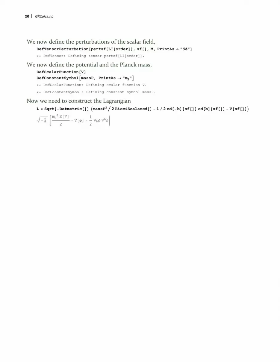
We now define the perturbations of the scalar field,DefTensorPerturbation[pertsf[LI[order]], sf[], M, PrintAs → "δϕ"]

** DefTensor: Defining tensor pertsf[LI[order]].

We now define the potential and the Planck mass,DefScalarFunction[V]

DefConstantSymbolmassP, PrintAs → "mp"

** DefScalarFunction: Defining scalar function V.

** DefConstantSymbol: Defining constant symbol massP.

Now we need to construct the Lagrangian

L = Sqrt[-Detmetric[]] massP2 2 RicciScalarcd[] - 1 / 2 cd[-b][sf[]] cd[b][sf[]] - V[sf[]]

-g mp2 R[∇]

2- V[ϕ] -

1

2∇bϕ ∇bϕ

20 GRCalcs.nb

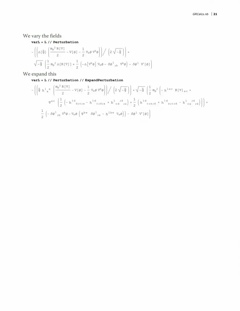
We vary the fieldsvarL = L // Perturbation

- △[g]

mp2 R[∇]

2- V[ϕ] -

1

2∇bϕ ∇bϕ 2 -g

+

-g 1

2mp2 △[R[∇]] +

1

2-△∇bϕ ∇bϕ - δϕ

1;b ∇bϕ - δϕ1 V′[ϕ]

We expand thisvarL = L // Perturbation // ExpandPerturbation

- gh1 a

a

mp2 R[∇]

2- V[ϕ] -

1

2∇bϕ ∇bϕ 2 -g

+ -g

1

2mp2 - h1ac R[∇]ac +

gac1

2- h

1dd;c;a - h

1dc;d;a + h

1 ;dcd ;a +

1

2 h

1dc;a;d + h

1da;c;d - h

1 ;dca ;d +

1

2- δϕ

1;b ∇bϕ - ∇bϕ gbe δϕ

1;e - h1be ∇eϕ - δϕ1 V′[ϕ]

GRCalcs.nb 21

We perform the metric contractionsvarL = L // Perturbation // ExpandPerturbation // ContractMetric

-1

2mp2 -g

h1ab R[∇]ab +

1

4mp2 -g

h1 a

a R[∇] -1

2-g

h1 aa V[ϕ] -

1

4mp2 -g

h1b ;a

b ;a -1

4mp2 -g

h1ba

;b;a +1

4mp2 -g

h1a ;b

b ;a +

1

2-g

h1ba ∇aϕ ∇bϕ +1

2mp2 -g

h1ba

;a;b -1

4mp2 -g

h1a ;b

a ;b -

1

2-g

∇bϕ δϕ1;b

-1

2-g

δϕ1;b ∇bϕ -

1

4-g

h1 aa ∇bϕ ∇bϕ - -g

δϕ1 V′[ϕ]

? RicciTo*

xAct`xTensor`

RicciToEinstein RicciToTFRicci

RicciToEinstein[expr, covd] expands expr expressing all Ricci tensors of covd in terms of the Einstein and RicciScalar tensors

of covd. If the second argument is a list of covariant derivatives the command is applied sequentially on expr. RicciToEinstein[expr] expands all Ricci tensors.

Then we enforce the symmetriesvarL = L // Perturbation // ExpandPerturbation // ContractMetric // ToCanonical

-1

2mp2 -g

h1ba R[∇]ba +

1

4mp2 -g

h1b

b R[∇] -

1

2-g

h1bb V[ϕ] -

1

2mp2 -g

h1b ;a

b ;a +1

2mp2 -g

h1ba

;b;a -

-g

∇bϕ δϕ1;b

+1

2-g

h1ba ∇aϕ ∇bϕ -

1

4-g

h1aa ∇bϕ ∇bϕ - -g

δϕ1 V′[ϕ]

22 GRCalcs.nb

The scalar equation of motion is then found by taking the variational derivatives of the

scalar field and set them equal to 00 == VarD[pertsf[LI[1]], cd][varL] / Sqrt[-Detmetric[]]

0 ⩵1

-g

δ1

1 -g

∇a∇aϕ - δ

11 -g

V′[ϕ]

we enforce the Kronecker delta0 == VarD[pertsf[LI[1]], cd][varL] / Sqrt[-Detmetric[]] /. delta[-LI[1], LI[1]] → 1

0 ⩵-g

∇a∇aϕ - -g

V′[ϕ]

-g

We canonicalize it0 == VarD[pertsf[LI[1]], cd][varL] / Sqrt[-Detmetric[]] /.

delta[-LI[1], LI[1]] → 1 // ToCanonical

0 ⩵ ∇a∇aϕ - V′[ϕ]

There we have it.

GRCalcs.nb 23

We can get the tensor equation of motion,vartf = 2 (-VarD[pert[LI[1], a, b], cd][varL] / Sqrt[-Detmetric[]])

1

-g

21

2mp2 δ

11 -g

R[∇]ab -

1

4mp2 δ

11 -g

gab R[∇] +

1

2δ

11 -g

gab V[ϕ] +

1

4δ

11 -g

gab ∇cϕ ∇cϕ -

1

2δ

11 -g

gac gbd ∇cϕ ∇dϕ

This is a mess, so we begin enforcing the Kronecker deltasvartf =

2 (-VarD[pert[LI[1], a, b], cd][varL] / Sqrt[-Detmetric[]] /. delta[-LI[1], LI[1]] → 1)

1

-g

21

2mp2 -g

R[∇]ab -

1

4mp2 -g

gab R[∇] +

1

2-g

gab V[ϕ] +1

4-g

gab ∇cϕ ∇cϕ -1

2-g

gac gbd ∇cϕ ∇dϕ

24 GRCalcs.nb

We now expand by expressing all Ricci tensors of covariant derivatives in terms of Einstein

tensors and Ricci scalarsvartf =

2 (-VarD[pert[LI[1], a, b], cd][varL] / Sqrt[-Detmetric[]] /. delta[-LI[1], LI[1]] → 1 //

SeparateMetric[metric] // RicciToEinstein)

1

-g

2 -1

4mp2 -g

gab R[∇] +

1

2mp2 -g

G[∇]ab +

1

2gba R[∇] +

1

2-g

gab V[ϕ] -1

2-g

∇aϕ ∇bϕ +1

4-g

gab gcd ∇cϕ ∇dϕ

We expand thisvartf =


SeparateMetric[metric] // RicciToEinstein) // Expand

mp2 G[∇]ab -1

2mp2 gab R[∇] +

1

2mp2 gba R[∇] + gab V[ϕ] - ∇aϕ ∇bϕ +

1

2gab gcd ∇cϕ ∇dϕ

GRCalcs.nb 25

Then we enforce the symmetries,vartf =


SeparateMetric[metric] // RicciToEinstein) //

Expand // ContractMetric // ToCanonical

mp2 G[∇]ab + gab V[ϕ] - ∇aϕ ∇bϕ +1

2gab ∇cϕ ∇cϕ

We set this equal to 0,0 ⩵ vartf

0 ⩵ mp2 G[∇]ab + gab V[ϕ] - ∇aϕ ∇bϕ +1

2gab ∇cϕ ∇cϕ

Here we get the conservation of energyeterm = IndexCollect[cd[a]@vartf // ToCanonical, CD[-b][sf[]]] // Simplify

∇bϕ (-∇a∇aϕ + V′[ϕ])

26 GRCalcs.nb

then0 ⩵ eterm

0 ⩵ ∇bϕ (-∇a∇aϕ + V′[ϕ])

this is degenerate with the scalar equation of motion0 ⩵ ∇a∇

aϕ - V′[ϕ]

GRCalcs.nb 27

Bibliography

[1] M. Nakahara, (2003), Geometry, Topology, and Physics, 2nd Edition, Taylor and Francis

Group.

[2] Theodore Frankel, (2012), The Geometry of Physics, 3rd Edition, Cambridge University

Press

[3] Jose M. Martin‐Garcia, (2009), xAct Intro

[4] B. F. Schutz, (1984), The Use of Perturbation and Approximation Methods in General

Relativity. In: Relativistic Astrophysics and Cosmology: Proceedings of the GIFT Interna‐

tional Seminar on Theoretical Physics, (Eds.) Fustero, Xavier; Verdaguer, Enric; Singapore:

World Scientific 35‐98 (1984)

[5] Jolyon Bloomfield, (2013), xAct Tutorial

xAct can be found at the website: http://www.xact.es/index.html

28 GRCalcs.nb

Thank You for Attending!

GRCalcs.nb 29

Documents

GR Calculations in Mathematica