Accepted Manuscript

Title: Gravity and magnetic data inversion for 3D topographyof the Moho discontinuity in the northern Red Sea area, Egypt

Authors: Ilya Prutkin, Ahmed Saleh

PII: S0264-3707(08)00091-4DOI: doi:10.1016/j.jog.2008.12.001Reference: GEOD 871

To appear in: Journal of Geodynamics

Received date: 2-9-2008Revised date: 28-11-2008Accepted date: 5-12-2008

Please cite this article as: Prutkin, I., Saleh, A., Gravity and magnetic data inversion for3D topography of the Moho discontinuity in the northern Red Sea area, Egypt, Journalof Geodynamics (2008), doi:10.1016/j.jog.2008.12.001

This is a PDF file of an unedited manuscript that has been accepted for publication.As a service to our customers we are providing this early version of the manuscript.The manuscript will undergo copyediting, typesetting, and review of the resulting proofbefore it is published in its final form. Please note that during the production processerrors may be discovered which could affect the content, and all legal disclaimers thatapply to the journal pertain.

peer

-005

3189

6, v

ersi

on 1

- 4

Nov

201

0Author manuscript, published in "Journal of Geodynamics 47, 5 (2009) 237"

DOI : 10.1016/j.jog.2008.12.001

Page 1 of 19

Accep

ted

Man

uscr

ipt

Gravity and magnetic data inversion for 3D

topography of the Moho discontinuity in the

northern Red Sea area, Egypt

Ilya Prutkin a,∗, Ahmed Saleh b

aDelft University of Technology, Netherlands

bNational Research Institute of Astronomy and Geophysics, Helwan, Cairo, Egypt

Abstract

The main goal of our study is to investigate 3D topography of the Moho bound-ary for the area of the northern Red Sea including Gulf of Suez and Gulf of Aqaba.For potential field data inversion we apply a new method of local corrections. Themethod is efficient and does not require trial-and-error forward modeling. To sepa-rate sources of gravity and magnetic field in depth, a method is suggested, based onupward and downward continuation. Both new methods are applied to isolate thecontribution of the Moho interface to the total field and to find its 3D topography.At the first stage, we separate near–surface and deeper sources. According to theobtained field of shallow sources a model of the horizontal layer above the depth of7 km is suggested, which includes a density interface between light sediments andcrystalline basement. Its depressions and uplifts correspond to known geologicalstructures. At the next stage, we isolate the effect of very deep sources (below 100km) and sources outside the area of investigation. After subtracting this field fromthe total effect of deeper sources, we obtain the contribution of the Moho interface.We make inversion separately for the area of rifts (Red Sea, Gulf of Suez and Gulf ofAqaba) and for the rest of the area. In the rift area we look for the upper boundaryof low–density, heated anomalous upper mantle. In the rest of the area the field issatisfied by means of topography for the interface between lower crust and normalupper mantle. Both algorithms are applied also to the magnetic field. The magneticmodel of the Moho boundary is in agreement with the gravitational one.

Key words: 3D gravity and magnetic data inversion, Moho boundary,Computational methods: potential fields, Contact surface topography, NorthernRed Sea

∗ Corresponding author. Tel.: +31 1527 87394; Fax: +31 1527 82348.Email address: I.Prutkin@tudelft.nl (Ilya Prutkin).

Preprint submitted to Elsevier 28 November 2008

* Manuscriptpe

er-0

0531

896,

ver

sion

1 -

4 N

ov 2

010

Page 2 of 19

Accep

ted

Man

uscr

ipt

1 Introduction

The Red Sea is considered to be a typical example of a newly formed ocean.Therefore, since the discovery of plate tectonics, a great number of studiesdiscussed its evolution as a key to the understanding of continental riftingand the initiation of sea floor spreading (Drake and Girdler, 1964; Tramontiniand Davies, 1969; Makris et al., 1983; Gaulier et al., 1988; Meshref, 1990).The northern part of the Red Sea appears to be characterized by oceanic typecrust, lying at a mean depth of 7 to 8 km, whereas the Moho is at a meandepth of 10 to 13 km, and at 32 km closest to the coastline (Gaulier et al.,1988; Makris et al., 1991; Rihm et al., 1991). In the Gulf of Suez, the top of thecrust is at a depth of 5 km. The Moho is found at a relatively shallow depth of18 to 20 km and at a mean depth of 30 to 35 km both under southern Sinai andEastern Desert plateaus (Gaulier et al., 1988; Saleh et al., 2006). Refractiondata indicate the Moho depth of 35 to 40 km in the areas not affected bythe rifting event (Ginzburg et al., 1981; Makris et al., 1983; Gettings et al.,1986; El-Isa et al., 1987). The anomalous nature of the upper mantle (8.0km/s) and the thinning of the crust beneath the northern Red Sea rift arewell known from the results of seismic and gravity studies. The density valuesof the different geological sedimentary units and the megastructures (the crustand the upper mantle) of the present study are based on the P-wave velocitydistribution in the northern Red Sea and the Gulf of Suez (Gaulier et al.,1988).

Our goal is to retrieve the 3D geometry of the Moho interface for the northernRed Sea area by means of two new algorithms for gravity and magnetic data in-version and for separating sources in depth. Till now the usual approach to find3D topography of a contact surface is forward gravity modeling. One changesan initial model in interactive way to diminish gravity residuals. Recently thisapproach has been applied, for instance, to study a geological structure of thenorthern Red Sea area in Saleh et al. (2006) using the package IGMAS (Gotzeand Lahmeyer, 1988) for interactive gravity modeling. The disadvantages ofthe forward modeling approach are following. One changes the model of thegeological section from one profile to another, but changes in one vertical sec-tion influence the gravity field along other profiles. Each section takes intoaccount a lot of geological and seismic a priori information, but the numberof parameters, per section, is much larger, than the number of profile obser-vations, it is not reasonable from the viewpoint of stability. The problems ofnon-uniqueness and instability of gravity data inversion are not likely to besolved by a forward modeling approach.

A different approach is applied by Tirel et al. (2004) to obtain the Moho to-pography to the north of Crete, the linearized inverse problem is solved bymeans of the Fourier Transform (Parker, 1972; Oldenburg, 1974). In our inves-

2

peer

-005

3189

6, v

ersi

on 1

- 4

Nov

201

0

Page 3 of 19

Accep

ted

Man

uscr

ipt

tigation we use quite a different procedure. We solve an integral equation for afunction determining geometry of an unknown contact surface. The kernel ofthis equation, evaluating the gravitational effect of a contact surface, dependsin a nonlinear way on the sought function. The 3D inverse problem is solvedin a full (nonlinear) statement by means of the method of local corrections(Prutkin, 1983, 1986) without any linearization. This method does not makeuse of nonlinear minimization, which reduces the computer calculation time byan order of magnitude. The local corrections method takes the non-uniquenessand instability of the inverse problem into account.

Our method of inversion is of the same type, as the method of Cordell andHenderson (1968). A solution is calculated from gravity data automatically bysuccessive approximations, without a time-consuming trial-and-error process.Like in the algorithm of Cordell and Henderson (1968), density contrast andthe position of a horizontal reference plane should be specified to obtain aunique solution. We apply a different approach to form a successive approx-imation. Moreover, we take into account instability of the inverse problemby means of a sort of regularization. We have mentioned only a few differentapproaches for gravity data inversion. A detailed overview of the literatureon the potential field inverse problem can be found in Blakely (1995). In thealgorithm of Cordell and Henderson (1968) density contrast is assumed to beuniform. In our approach it can be different in every point; an elementarycolumn is not homogeneous in the vertical direction above and below the un-known contact surface; moreover, we apply the method of local correctionsboth for gravity and magnetic data inversion.

The paper is organized as follows: we present new mathematical algorithmsfor isolating sources in depth and for 3D gravity and magnetic data inversion,and then both algorithms are applied to the northern Red Sea area to extractthe effect of the Moho interface and to find its 3D topography. We start withour mathematical theory; it is presented in the first section. As a preliminarypre–processing of gravity and magnetic observations, the new algorithm is sug-gested to extract the effect of the contact surface sought. The main idea of thealgorithm is to eliminate sources from the Earth’s surface up to a prescribeddepth by means of upward and downward continuation. In the same section2, the method of local corrections applied to a 3D contact surface topographyrecovery is described. Next, we start with application of our algorithms for thenorthern Red Sea area. In section 3 we separate sources of the gravitationalfield into shallow and deeper ones and construct a model of the near–surfacelayer. Then we isolate the gravitational effect of the Moho interface and findits 3D topography. In section 4 we make the same based on magnetic data.Section 5 contains the main conclusions of our study.

3

peer

-005

3189

6, v

ersi

on 1

- 4

Nov

201

0

Page 4 of 19

Accep

ted

Man

uscr

ipt

2 Mathematical theory

The main purpose of the algorithm to separate sources in depth is to findthe part of the observed field, which is harmonic above a given depth h. Wecan treat this function as an effect of the half–space below the depth h. Tofind such a function means to eliminate all sources located in the horizontallayer from the Earth surface up to a prescribed depth. The algorithm allowsto separate the effects of shallow and deeper objects and to extract the gravitysignal of sources located in horizontal layer between given depths h1 and h2.

The algorithm is based on upward and downward continuation (Vasin, Prutkinand Timerkhanova, 1996; Martyshko and Prutkin, 2003). There are two prob-lems to be solved. Firstly, we continue the data upward to the height h todiminish the influence of the sources in the near–surface layer. This operationcauses the main errors in the vicinity of the boundary of the area. To reducethem we need some model of the regional field to subtract it from the observedfield prior to upward continuation. Secondly, we continue the obtained func-tion downward to the depth h, i.e. to the distance 2h in downward direction.The problem of downward continuation is a linear ill–posed inverse problem,therefore we must use some regularization.

The function, which we treat as a regional field, is assumed to be harmonicin the area (in two–dimensional sense) and to have the same values at theboundary of the area, as the observed field:

∆2f = ∂2f∂x2 + ∂2f

∂y2 = 0 within area S

f = ∆g on its boundary ∂S(1)

If we subtract the values of this function, the residual field will be equal tozero at the boundary of the area, therefore no errors are introduced, whenwe integrate the residual field while upward continuation along the restrictedarea. According to the properties of harmonic functions, this function has noextremum within the area, so we create no false anomalies. Besides, as it isknown from calculus of variations (Gelfand and Fomin, 2000), a solution ofthe problem (1) provides a minimum of the following functional:

J(f) =∫∫

S

∂f

∂x

2

+

∂f

∂y

2

dx dy −→ min, (2)

therefore, we obtain the smoothest possible function with given values on theboundary. All these properties allow us to regard this function as a model ofthe regional field.

4

peer

-005

3189

6, v

ersi

on 1

- 4

Nov

201

0

Page 5 of 19

Accep

ted

Man

uscr

ipt

After subtracting the suggested model of the regional field we make upwardcontinuation of the residual field by means of the following formula:

1

2π

∫∫

h

((x − x′)2 + (y − y′)2 + h2)3/2U(x, y, 0) dxdy = U(x′, y′, h) (3)

The formula (3) gives a solution of the Dirichlet problem: to find a harmonicfunction in the upper half–space with given values on the boundary (on theplane z = 0).

At the second step we continue the obtained function downward to the depthh, i.e. to the distance 2h in downward direction. To do this, we apply a formulasimilar to (3):

1

2π

∫∫

h1

((x − x′)2 + (y − y′)2 + h21)

3/2U(x, y,−h) dxdy = U(x′, y′, h) , (4)

where h1 = 2h. Formula (4) provides a function, which is harmonic in a half–space above the plane z = −h. But this time we treat the formula as anintegral equation: the right hand is given, and we have to find the unknownfunction U(x, y,−h).

Although the influence of shallow sources is diminished after upward contin-uation, the rest of them is still presented in the field, so we make downwardcontinuation through the sources. It should be emphasized, that the problemof downward continuation is a linear ill–posed inverse problem, therefore wemust use some regularization. Since the integral operator A in (4) is self–adjoint and positive, we apply the Lavrent’ev’s approach (Lavrent’ev et al.,1986). If we write (4) in the following form: Au = uh, u is an unknown field onthe level z = −h, uh is the obtained field on the height h, then the Lavrent’ev’sregularization gives: (A + αI)u = uh , where I is identity operator, α – a reg-ularizing parameter. Therefore, after discretization no matrix multiplicationis required.

At last we calculate the field on the Earth’s surface z = 0 using a formula,similar to (3). We obtain a part of the field, which is harmonic up to the depthh, so we could treat it as an effect from the deeper sources.

To evaluate the gravitational effect of a contact surface, we consider a followingmodel of a two–layer gravitational medium in 3D space. The model consistsof two layers of a constant density σ1 and σ2, separated by the surface S.Suppose that, in the Cartesian coordinate system, the plane xOy coincideswith the Earth surface, and the axis z is directed downward. The upper layer

5

peer

-005

3189

6, v

ersi

on 1

- 4

Nov

201

0

Page 6 of 19

Accep

ted

Man

uscr

ipt

is bounded above by the horizontal plane z = h−, h− > 0, and below by thesurface S; the lower layer is bounded above by the surface S and below by theplane z = h+; at z < h− and z > h+ masses are absent. The unknown contactsurface is determined by the equation z = z(x, y). It is assumed that z(x, y)is a single–valued limited function, and that for a certain H

lim|x|→∞|y|→∞

|z(x, y) − H| = 0, (5)

i.e., the surface S has a horizontal asymptotic plane z = H . If we subtractthe effects of two Bouguer plates, we find, that the field of our two–layermodel accurate to a constant term is the field of masses contained betweenthe surface S and the plane z = H , with a density ±∆σ, where ∆σ = σ2 − σ1

is the density contrast at the contact surface. The field of such an object isevaluated by the formula

∆g(x′, y′, 0) = G ∆σ

∞∫

−∞

∞∫

−∞

1√

(x − x′)2 + (y − y′)2 + z2(x, y)

−1

√

(x − x′)2 + (y − y′)2 + H2

dx dy, (6)

where G is the gravitational constant. We can regard formula (6) as a nonlinearintegral equation of the 1st kind with respect to the unknown function z(x, y).Suppose that the field at the Earth surface is given on a rectangular gridxi, yj. We divide a volume between the surface S and the plane z = H into anumber of elementary prisms, for each prism the projection of its center ontothe plane xOy coincides with some observation point. The mean heights ofthe prisms are taken as unknown parameters. Their number equals exactly tothe number of observations N . Denote by K(x′, y′, x, y, z(x, y)) the integrandin (6). This expression was refered in (Snopek and Casten, 2006) as the gravityattraction of a linear, vertical mass. It has been suggested there to apply itas an approximation of the exact fomula for the prism gravity. It means, thatwhile discretizing (6) by numerical integration we use one–point cubatureformula for each elementary prism, which gives

c G ∆σ∑

i

∑

j

Ki0j0(zij) = Ui0j0 , (7)

where c is the weight of the cubature formula, zij = z(xi, yj), and

6

peer

-005

3189

6, v

ersi

on 1

- 4

Nov

201

0

Page 7 of 19

Accep

ted

Man

uscr

ipt

Ui0j0 = ∆g(xi0, yj0, 0) , Ki0j0(zij) = K(xi0 , yj0, xi, yj, zij).

To increase the accuracy one could apply for discretisation (6) Gauss cuba-ture, in this case each term in (7) will be substituted by several similar ones,corresponding to the same zij .

Our goal is to develope an iterative procedure for solving the system of non-linear equations (7). Suppose that zn

ij are the values of the unknown functionobtained at the n-th step. For the corresponding solution of the direct problemwe introduce the notation

Uni0j0 = c G ∆σ

∑

i

∑

j

Ki0j0(znij). (8)

The method of local corrections is based on the fact that the variation ofthe field at a certain point is affected mostly by the variation of the part ofthe object boundary closest to this point. At each step we try to reduce thedifference between the given and the approximate values of the field at a givennode solely by modifying the value of the unknown function at that node. Ifthe value of the unknown function in one point only has been changed, thenthe sum in (8) for the next iteration differs only in one term. Assuming thatin the chosen node Un+1

ij = Uij and subtracting (8) from the similar equalitycorresponding to the (n + 1)-th step, we obtain the fundamental equation tofind the next approximation (Prutkin, 1986):

G ∆σ(

Kij(zn+1

ij ) − Kij(znij)

)

= α(

Uij − Unij

)

. (9)

The coefficient α in the right hand of (9) is introduced to slow down the changeof the model.

It turns out that, in the case of a contact surface, Eq. (9) can be converted toa very simple form. Indeed, considering Eq. (6), we have

Kij(znij) = 1/zn

ij − 1/H (10)

Using (10), we rewrite Eq. (9) as

G ∆σ(

1/zn+1ij − 1/zn

ij))

= α(

Uij − Unij

)

and finally

7

peer

-005

3189

6, v

ersi

on 1

- 4

Nov

201

0

Page 8 of 19

Accep

ted

Man

uscr

ipt

zn+1

ij =zn

ij

1 + αsznij

(

Uij − Unij

) , (11)

where s = (G∆σ)−1. According to (11), several arithmetic operations aresufficient to obtain the next successive approximation at each point of thegrid. We have to store only the vector of unknowns of the same length N asthe length of the observations vector. The full (nonlinear) inverse problem issolved without any linearization, and we don’t need to store some matrix ofthe size N × N .

It is known, that for the fixed values of the density contrast ∆σ and thedepth to the asymptotic plane H , a solution of the inverse problem for acontact surface is unique. In the same time, taking different values of theseparameters, one could obtain different solutions causing the same gravity field.In (Prutkin, 1986), a family of contact surfaces is presented, which generatewith different values of ∆σ and H the same field, as a point source.

Eq. (6) is an integral equation of the 1st kind, this problem is ill–posed andrequires regularization. Diminishing the coefficient α in (11), we can preventhighly oscillating solutions, therefore, this factor is really similar to a regu-larization parameter. The choice of the regularization parameter decides howwell the solution fits the data. To find a suitable regularization parameter, weuse the method of residuals (Lavrent’ev et al., 1986), which exploits informa-tion about data noise: we look for the smoothest possible solution, which fieldapproximates the given data with the same accuracy as the data noise level.

Due to the fact that our approach to inversion is local, we could take a differentvalue of the density contrast at each grid point. One should include a functionof two variables ∆σ(x, y) into the integrand of Eq. (6), then use factors ∆σij =∆σ(xi, yj) in the left hand of (7) and substitute the coefficient s in (11) bysij = (G∆σij)

−1. The same is valid for the depth to the asymptotic planeH . Sometimes it is reasonable, to divide the whole area into subareas and touse different values of H and ∆σ for each one. Within the method of localcorrections it is also possible, which is demonstrated in the next section.

3 Gravity data inversion

A considerable amount of gravity data is now available to unravel the grosscrustal structure of the Red Sea region. In order to investigate the structureof the northern Red Sea rift and Gulf of Suez, a new Bouguer gravity anomalymap has been prepared. It utilizes all available gravity data: Bouguer grav-ity data of the Egyptian General Petroleum Company published as a set of

8

peer

-005

3189

6, v

ersi

on 1

- 4

Nov

201

0

Page 9 of 19

Accep

ted

Man

uscr

ipt

Bouguer maps of Egypt at 1:500,000 scale in 1980; gravity surveys of the Gulfof Suez, Sinai and the Eastern Desert conducted by the Sahara PetroleumCompany (SAPETCO) and PHILIPS Company between 1954 and 1958; ma-rine gravity data in the northern Red Sea measured by the research vessel”Robert D. Conrad” to the north of 26 N in 1984. All the data of these sur-veys were compiled, classified and ranked according to instrument sensitivityand measurement density. More details on how the Bouguer map was compiledcan be found in (Saleh et al., 2006). The resulting Bouguer map is shown inFig. 1.

Fig. 1.

The calculated Bouguer gravity anomaly is reduced to sea level and correctedfor mass effects of topography with the standard density of reduction 2670kg/m3. The general trend of the Bouguer gravity anomalies is northwest–southeast. The anomaly increases in magnitude with a decrease in the reliefof the topography and attains its maximum of +95 mGal along the axis ofthe Red Sea rift floor.

The main goal of our investigation is to extract the gravity signal from theMoho boundary and to find its 3D topography. At the first stage, we separatenear–surface and deeper sources by means of the algorithm of upward anddownward continuation described in section 2. Gravitational effects of shallowand deeper sources are shown in Fig. 2.

Fig. 2.

According to the obtained field of shallow sources a model of the horizontallayer above the depth of 7 km is found using the method of local correctionsfrom section 2, which includes a generalized density interface between lightsediments with a mean density value of 2300 kg/m3 and crystalline basementwith density of 2750 kg/m3. Its depressions and uplifts correspond to knowngeological structures. We present in Fig. 3 a position of the obtained contactsurface along a profile 28 of northern latitude. Presented is a depression of thelight material, then an uplift of dense rocks near Gebel El Zeit, a depressionof the light (sedimentary) material below the Gulf of Suez, an uplift of densematerial below Sinai Peninsula, a depression below the Gulf of Aqaba, thenan uplift of dense rocks near the coast of Saudi Arabia.

Fig. 3.

At the next stage, we isolate the effect of very deep sources (below 100 km)and sources outside the area of investigation. We apply again the algorithmdescribed in section 2. This time the part of the residual field has been found,which is harmonic above the depth of 100 km. A possible source of the positiveanomaly could be an uplift of astenosphere. After subtracting this field from

9

peer

-005

3189

6, v

ersi

on 1

- 4

Nov

201

0

Page 10 of 19

Accep

ted

Man

uscr

ipt

the total effect of deeper sources shown in Fig. 2, we obtain the contributionof the Moho interface. The gravitational signal from the half–space below 100km and the effect of the Moho boundary are presented in Fig. 4.

Fig. 4.

Using the obtained residual field as a given data, we solve the inverse problemfor a 3D topography of the Moho boundary. The method of local correctionsis applied, which is described in section 2.

We make inversion separately for the area of rifts (Red Sea, Gulf of Suezand Gulf of Aqaba) and for the rest of the area. In the rift area we look forthe upper boundary of the low–density, heated anomalous upper mantle withdensity of 3100 kg/m3. We assume that the ambient medium has a horizontallylayered structure, it consists of the layer with density 2750 kg/m3 above thedepth of 20 km, the layer with density 2900 kg/m3 between 20 and 30 kmand the layer with density 3250 kg/m3 below 30 km. If the upper boundaryof the anomalous mantle intersects both mentioned layers, it has a densitycontrast with the ambient medium of 350 kg/m3 above the depth of 20 km,200 kg/m3 between 20 and 30 km and -150 kg/m3 below 30 km. The depth tothe asymptotic plane H (see section 2) equals to 50 km. The found topographyis shown in Fig. 5, the altitude above the depth of 30 km is presented, +17km means the depth to the density interface of 30 - 17 = 13 km, +2 km - thedepth of 30 - 2 = 28 km.

In the rest of the area the field is satisfied by means of a topography forthe interface between material with density 2900 kg/m3 (lower crust) and3250 kg/m3 (normal upper mantle). Density contrast amounts 350 kg/m3, thedepth to the asymptotic plane is equal to 30 km. The obtained 3D topographyis also presented in Fig. 5, again variations relative the depth of 30 km areshown.

Fig. 5.

We note that the density contrast ∆σ and the depth to the asymptotic plane Hare different in different subareas and the ambient medium is not homogeneousin the vertical direction above and below the unknown contact surface, whichis possible within the method of local corrections.

The amplitude of the residual field is less than 2 mGal. The main features ofthe obtained topography are quite in agreement with seismic information andresults of previous gravity modeling (Saleh et al., 2006).

10

peer

-005

3189

6, v

ersi

on 1

- 4

Nov

201

0

Page 11 of 19

Accep

ted

Man

uscr

ipt

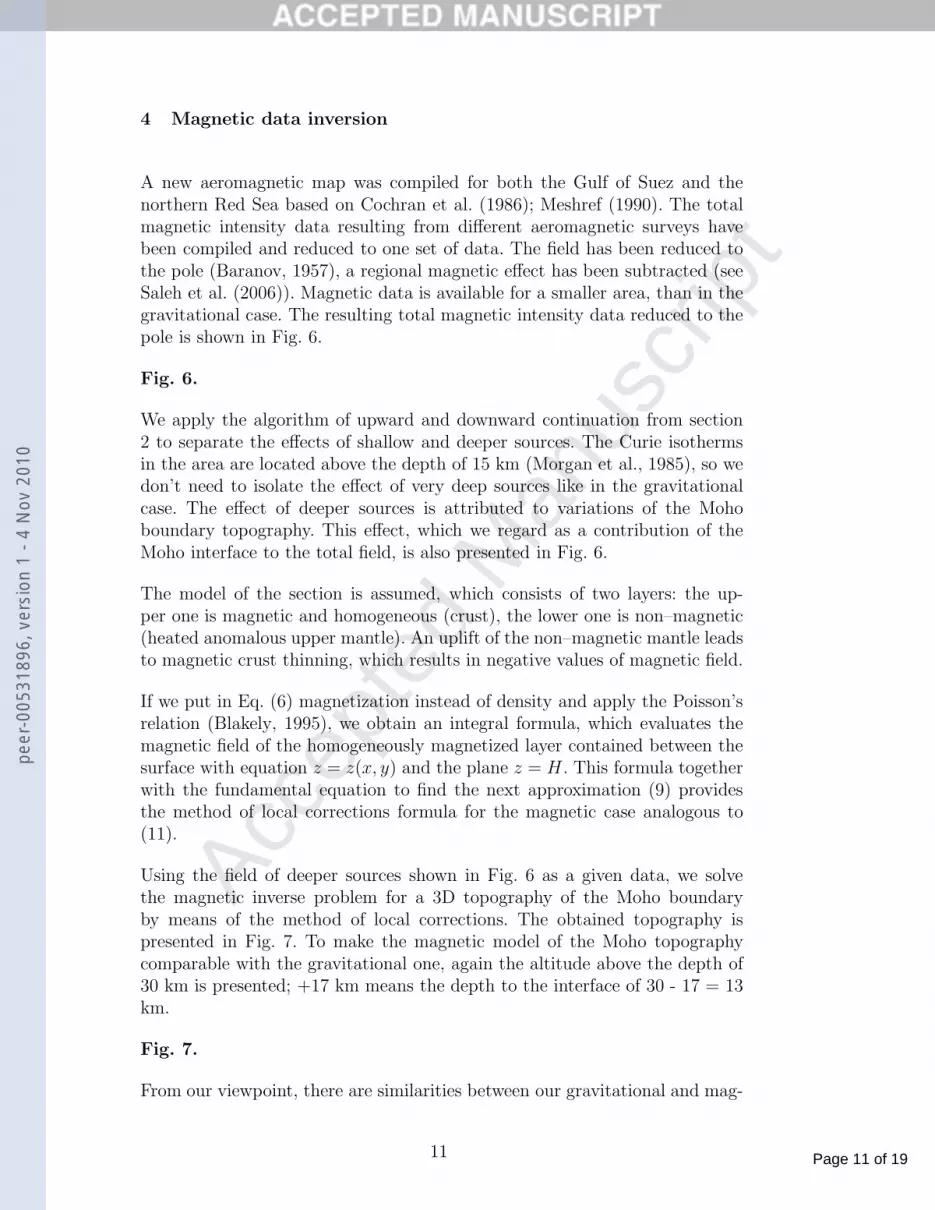
4 Magnetic data inversion

A new aeromagnetic map was compiled for both the Gulf of Suez and thenorthern Red Sea based on Cochran et al. (1986); Meshref (1990). The totalmagnetic intensity data resulting from different aeromagnetic surveys havebeen compiled and reduced to one set of data. The field has been reduced tothe pole (Baranov, 1957), a regional magnetic effect has been subtracted (seeSaleh et al. (2006)). Magnetic data is available for a smaller area, than in thegravitational case. The resulting total magnetic intensity data reduced to thepole is shown in Fig. 6.

Fig. 6.

We apply the algorithm of upward and downward continuation from section2 to separate the effects of shallow and deeper sources. The Curie isothermsin the area are located above the depth of 15 km (Morgan et al., 1985), so wedon’t need to isolate the effect of very deep sources like in the gravitationalcase. The effect of deeper sources is attributed to variations of the Mohoboundary topography. This effect, which we regard as a contribution of theMoho interface to the total field, is also presented in Fig. 6.

The model of the section is assumed, which consists of two layers: the up-per one is magnetic and homogeneous (crust), the lower one is non–magnetic(heated anomalous upper mantle). An uplift of the non–magnetic mantle leadsto magnetic crust thinning, which results in negative values of magnetic field.

If we put in Eq. (6) magnetization instead of density and apply the Poisson’srelation (Blakely, 1995), we obtain an integral formula, which evaluates themagnetic field of the homogeneously magnetized layer contained between thesurface with equation z = z(x, y) and the plane z = H . This formula togetherwith the fundamental equation to find the next approximation (9) providesthe method of local corrections formula for the magnetic case analogous to(11).

Using the field of deeper sources shown in Fig. 6 as a given data, we solvethe magnetic inverse problem for a 3D topography of the Moho boundaryby means of the method of local corrections. The obtained topography ispresented in Fig. 7. To make the magnetic model of the Moho topographycomparable with the gravitational one, again the altitude above the depth of30 km is presented; +17 km means the depth to the interface of 30 - 17 = 13km.

Fig. 7.

From our viewpoint, there are similarities between our gravitational and mag-

11

peer

-005

3189

6, v

ersi

on 1

- 4

Nov

201

0

Page 12 of 19

Accep

ted

Man

uscr

ipt

netic models of the Moho interface.

Both models agree well with the P-wave velocity distribution in the northernRed Sea and the Gulf of Suez (Gaulier et al., 1988). The gravitational modelis also supported by refraction data in the areas not affected by the riftingevent (Makris et al., 1983; El-Isa et al., 1987). The Moho topography magneticmodel shows a poor flattening especially in the eastern region (e.g., Gaulieret al. (1988); Saleh et al. (2006)). The present results are in good agreementwith the geothermal gradient values in the Red Sea (Cochran et al., 1986). Therelatively low density of the anomalous upper mantle (3100 kg/m3) of the RedSea rift, as deduced from the gravity modeling, indicates the possible presenceof partial melting in the upper mantle. The size of the area of anomalousupper mantle suggests that a large scale asthenospheric upwelling might beresponsible for the subsequent rifting of the Red Sea. As a possible resultof pressure release and convection heat, indicating a more advanced stage ofrifting taking place in the northern part of Red Sea rift (which is interpreted asevidence for updoming due to the sea floor spreading in the central Red Sea),the crust becomes more oceanic in its nature. These results, which have beenconstrained by seismic measurements and confirmed by gravity and magneticmodeling, are in agreement with Cochrans concept of the northern part of theRed Sea (Cochran and Martinez, 1988; Saleh et al., 2006).

5 Summary and conclusions

Two new algorithms have been suggested to extract the signal from a contactsurface and to find its 3D geometry. Both algorithms are applied to gravityand magnetic data for the area of the northern Red Sea including Gulf of Suezand Gulf of Aqaba to recover the Moho boundary topography. The followingconclusions are drawn:

(1) A new algorithm has been suggested to eliminate potential field sourcesfrom the Earth’s surface to a prescribed depth h, based on upward anddownward continuation. The solution of the 2D Dirichlet problem canbe used as a model of the regional field. Subtracting the regional fieldfrom the observations prior to upward continuation allows integrationof gravity data in the restricted area, while ignoring any informationbeyond the area of investigation. Downward continuation provides thepart of the field, which is harmonic above the depth h. The propertiesof the integral operator give an opportunity to implement Lavrent’ev’sregularization and to get rid of matrix multiplication. The algorithm hasbeen successfully applied to separate the effects of shallow and deepersources of gravity and magnetic field for the northern Red Sea area.

(2) The method of local corrections is developed to recover 3D topography

12

peer

-005

3189

6, v

ersi

on 1

- 4

Nov

201

0

Page 13 of 19

Accep

ted

Man

uscr

ipt

of a contact surface. The method offers a simple and effective procedurefor solving the nonlinear inverse problem without any linearization. Thismethod does not make use of nonlinear minimization, which reduces thecomputer calculation time by an order of magnitude. We solve an integralequation for the function determining topography. We take into accountinstability of the inverse problem by means of a sort of regularization.The method of local corrections is applied for both gravity and magneticdata inversion to retrieve the 3D topography of the upper boundary ofthe heated anomalous mantle for the Red Sea rift area.

(3) The gravitational and magnetic models of the Moho interface are obtainedautomatically without interactive forward modeling which dramaticallydiminishes the time expenditure. Both models are in agreement withseismic information and results of previous gravity modeling. There aresimilarities between the obtained gravitational and magnetic models ofthe Moho boundary. The uplift of the dense mantle and the thinning ofthe magnetic crust can explain low–frequency part of both gravity andmagnetic field attributed to the Moho interface.

Acknowledgments

We would like to express our gratitude to the General Petroleum Company,Cairo, for utilizing the Bouger gravity data. Also, we would like to thank M.Hussain, Institute of Petroleum Research, for his encouragement and providingmagnetic data.

References

Baranov, W., 1957. A new method for interpretation of aeromagnetic maps:pseudo–gravimetric anomalies. Geophysics 22, 359–383.

Blakely, R.J., 1995. Potential Theory in Gravity and Magnetic Applications.Cambridge University Press, Cambridge, 441 pp.

Cochran, J.R., Martinez, F., Steckler, M.S., Hobart, M.A., 1986. Conrad deep:a new northern Red Sea deep. Origin and implications of continental rifting.Earth Planet Sci. Lett. 78, 18–32.

Cochran, J.R., Martinez, F., 1988. Evidence from the northern Red Sea on thetransition from continental to oceanic rifting. Tectonophysics 153, 25–53.

Cordell, L., Henderson, R.G., 1968. Iterative three–dimensional solution ofgravity anomaly data using a digital computer. Geophysics 33, 596–601.

Drake, C.L., Girdler, R.W., 1964. A geophysical study of the Red Sea. Geo-phys. J. R. Astron. Soc. 8, 473–495.

El-Isa, Z., Mechie, J., Prodehl, C., Makris, J., Rihm, R., 1987. A crustal struc-

13

peer

-005

3189

6, v

ersi

on 1

- 4

Nov

201

0

Page 14 of 19

Accep

ted

Man

uscr

ipt

ture study of Jordan derived from seismic refraction data. Tectonophysics138, 235–253.

Gaulier, J.M., Le Pichon, X., Lyberis, N., Avedik, F., Geli, L., Moretti, I.,Deschamps, A., Salah, H., 1988. Seismic study of the crust of the northernRed Sea and Gulf of Suez. Tectonophysics 153, 55–88.

Gelfand, I.M., Fomin, S.V., 2000. Calculus of Variations. Dover Publications,New York, 240 pp.

Gettings, M.E., Blank Jr., H.R., Mooney, W.D., Healy, J.H., 1986. Crustalstructure of southwestern Saudi Arabia. J. Geophys. Res. 91(B6), 6491–6512.

Ginzburg, A., Makris, J., Fuchs, K., Prodehl, C., 1981. The structure of thecrust and upper mantle in the Dead Sea rift. Tectonophysics 80, 109–119.

Gotze, H.-J., Lahmeyer, B., 1988. Application of three-dimensional interactivemodelling in gravity and magnetics. Geophysics 53, 1096–1108.

Lavrent’ev, M.M., Romanov, V.G., Shishatskii, S.P., 1986. Ill-Posed Problemsof Mathematical Physics and Analysis. Translations of Math. Monographs,v. 64, published by Amer. Math. Soc., Providence, 290 pp.

Makris, J., Allam, A., Moktar, T., Basahel, A., Dehghani, G.A., Bazari, M.,1983. Crustal structure at the northwestern region of the Arabian shieldand its transition to the Red Sea. Bull. Fac. Earth Sci. K. Abdulaziz Univ.6, 435–447.

Makris, J., Henke, C.H., Egloff, F., Akamaluk, T., 1991. The gravity field ofthe Red Sea and East Africa. Tectonophysics 198, 369–381.

Martyshko, P.S., Prutkin, I.L., 2003. Technology of depth distribution of grav-ity field sources. Geophys. J. 25 (3), 159–168. (In Russian).

Meshref, W.M., 1990. Tectonic framework. In: Said, R. (Ed.), The geology ofEgypt. A.A. Balkema, Rotterdam, p.p. 113–155.

Morgan, P., Boulos, F.K., Hennin, S.F., El-Sherif, A.A., El Sayed, A.A., Basta,N.Z., Melek, Y.S., 1985. Heat flow in Eastern Egypt: the thermal signatureof continental breakup. J. Geodyn. 4, 107–131.

Oldenburg, D., 1974. The inversion and interpretation of gravity anomalies.Geophysics 39, 526–536.

Parker, R., 1972. The rapid calculation of potential anomalies. GeophysicalJournal of the Royal Astronomical Society 31, 447–455.

Prutkin, I.L., 1983. Approximate solution of three–dimensional gravimetricand magnetometric inverse problems by the method of local corrections.Izvestiya. Physics of the Solid Earth 19 (1), 38–41.

Prutkin, I.L., 1986. The solution of three–dimensional inverse gravimetricproblem in the class of contact surfaces by the method of local corrections.Izvestiya. Physics of the Solid Earth 22 (1), 49–55.

Rihm, R., Makris, J., Moller, L., 1991. Seismic survey in the northern RedSea: asymmetric crustal structure. Tectonophysics 198, 279–295.

Saleh, S., Jahr, T., Jentzsch, G., Saleh, A., Abou Ashour, N.M., 2006. Crustalevaluation of the northern Red Sea rift and Gulf of Suez, Egypt from geo-physical data: 3-dimensional modeling. J. African Earth Sci. 45, 257–278.

14

peer

-005

3189

6, v

ersi

on 1

- 4

Nov

201

0

Page 15 of 19

Accep

ted

Man

uscr

ipt

Snopek, K., Casten, U., 2006. 3GRAINS: 3D Gravity Interpretation Softwareand its application to density modeling of the Hellenic subduction zone.Computers & Geosciences 32 (5), 592–603.

Tirel, C., Gueydan, F., Tiberi, C., Brun, J.-P., 2004. Aegean crustal thick-ness inferred from gravity inversion. Geodynamical implications. Earth andPlanetary Science Letters 228, 267–280.

Tramontini, C., Davies, D., 1969. A seismic refraction survey in the Red Sea.Geophys. J. R. Astron. Soc. 17, 2225–2241.

Vasin, V.V., Prutkin, I.L., Timerkhanova, L.Yu., 1996. Retrieval of a Three-Dimensional Relief of Geological Boundary from Gravity Data. Izvestiya.Physics of the Solid Earth 32 (11), 901–905.

15

peer

-005

3189

6, v

ersi

on 1

- 4

Nov

201

0

Page 16 of 19

Accep

ted

Man

uscr

ipt

25

26

27

28

29

30

Latit

ude

32 33 34 35 36

Longitude

-80

-70-70

-60

-60

-60

-60

-50

-50

-50

-40

-40

-40

-40

-40

-40

-30

-30

-30

-30

-30-20

-20

-20

-20

-20

-10

-10

-10

0

0

10

10

20

20

30

30

40

40

50

50

60

60

70

70

80

-90 -80 -70 -60 -50 -40 -30 -20 -10 0 10 20 30 40 50 60 70 80 90 100

mGal

Fig. 1. Bouguer gravity anomaly for Red Sea and surrounding region. Contour in-terval is 10 mGal. Data are corrected for mass effects of topography using reductiondensity of 2670 kg/m3.

16

peer

-005

3189

6, v

ersi

on 1

- 4

Nov

201

0

Page 17 of 19

Accep

ted

Man

uscr

ipt

25

26

27

28

29

30

Latit

ude

32 33 34 35 36

Longitude

-20

-20

-10

-10

-10

-10

-10

-10

-10

0

0

0

0

0

0

0

0

0

0

00

0

0

0

0

0

0

0

0

0

10

10

10

10

10

10

10

1010

20

-30 -20 -10 0 10 20 30 40

mGal

25

26

27

28

29

30

Latit

ude

32 33 34 35 36

Longitude

-75

-70

-65 -6

0

-60

-55

-50

-45-45

-40

-40

-35

-35

-35

-35

-30

-30

-30

-30

-25

-25

-20

-20

-15

-15

-10

-10

-5

-5

0

0

5

5

10

1015

15

20

20

25

25

30

30

35

35

40

40

45

45

50

50

55

55

60

60

65

70

75

-90 -80 -70 -60 -50 -40 -30 -20 -10 0 10 20 30 40 50 60 70 80 90 100

mGal

Fig. 2. Gravitational effects of shallow (left) and deeper (right) sources separatedby means of algorithm of upward and downward continuation from section 2.

-2.5

-2

-1.5

-1

-0.5

0

32 32.5 33 33.5 34 34.5 35 35.5 36

km

Longitude

Fig. 3. Position of generalized density interface between light sediments with meandensity value of 2300 kg/m3 and crystalline basement with density of 2750 kg/m3

along profile 28 N.

17

peer

-005

3189

6, v

ersi

on 1

- 4

Nov

201

0

Page 18 of 19

Accep

ted

Man

uscr

ipt

25

26

27

28

29

30

Latit

ude

32 33 34 35 36

Longitude

-50

-45

-40

-40

-35-3

5

-30

-30

-25

-25

-20

-20

-15

-15

-10

-10

-5

-5

05

10 15

15

20 25 3035

40

45

-90 -80 -70 -60 -50 -40 -30 -20 -10 0 10 20 30 40 50 60 70 80 90 100

mGal

25

26

27

28

29

30

Latit

ude

32 33 34 35 36

Longitude

-50 -40 -30 -20 -10 0 10 20 30 40 50

mGal

Fig. 4. Gravitational effects of very deep sources (below 100 km) and sources outsidearea of investigation (left) and contribution of Moho interface (right).

26

27

28

29

Latit

ude

33 34 35

Longitude

5

5

5

5

5

6

6

6

6 6

7

7

7

7

7

8

8

8

8

9

9

10

1011

11

11

11

12

12

12

12

13

13

13

14

14

14

15

15

16

0 2 4 6 8 10 12 14 16 18 20

km

26

27

28

29

Latit

ude

33 34 35

Longitude

-2

0

0

2

2

2

4

4 4

4

-4 -2 0 2 4 6 8 10

km

Fig. 5. Gravitational model of Moho topography within rift area (left) and for restof region (right). It represents upper boundary of heated anomalous mantle withdensity 3100 kg/m3 for rift area and interface between lower crust (density 2900kg/m3) and normal upper mantle (density 3250 kg/m3) for rest of region.

18

peer

-005

3189

6, v

ersi

on 1

- 4

Nov

201

0

Page 19 of 19

Accep

ted

Man

uscr

ipt

26

27

28

29

30

Latit

ude

32 33 34 35 36

Longitude

-100 0 100 200 300 400 500 600 700 800 900 1000

nT

26

27

28

29

30

Latit

ude

32 33 34 35 36

Longitude

250

250

300

350

350

400

400

400

450

450

450

500

500

500

550

550

550

550

100 150 200 250 300 350 400 450 500 550 600

nT

Fig. 6. Total magnetic intensity data reduced to pole (left) and magnetic field ofdeeper sources (right) obtained using algorithm of upward and downward continu-ation.

26

27

28

29

30

Latit

ude

32 33 34 35 36

Longitude

9

10

10

10

11

11

11

12

12

12

13

13

13

14

1415

15

16

16

17

8 9 10 11 12 13 14 15 16 17 18

km

Fig. 7. Magnetic model of the Moho topography. It is obtained using method oflocal corrections from section 2 and represents interface between magnetic crustand non–magnetic anomalous upper mantle.

19

peer

-005

3189

6, v

ersi

on 1

- 4

Nov

201

0