Green Energy and Technology

Green Energy and Technology

For further volumes:http://www.springer.com/series/8059

http://www.springer.com/series/8059

Djamila Rekioua • Ernest Matagne

Optimization of PhotovoltaicPower Systems

Modelization, Simulation and Control

123

Djamila RekiouaLT.I.I LaboratoryUniversity of BejaiaRoute de Terga Ouzemour06000 BejaiaAlgeriae-mail: [email protected]

Ernest MatagneUniversité Catholique de LouvainPlace de I’Université 11348 Louvain-la-NeuveBelgium

ISSN 1865-3529 e-ISSN 1865-3537ISBN 978-1-4471-2348-4 e-ISBN 978-1-4471-2403-0DOI 10.1007/978-1-4471-2403-0Springer London Dordrecht Heidelberg New York

British Library Cataloguing in Publication DataA catalogue record for this book is available from the British Library

Library of Congress Control Number: 2011942409

� Springer-Verlag London Limited 2012Apart from any fair dealing for the purposes of research or private study, or criticism or review, aspermitted under the Copyright, Designs and Patents Act 1988, this publication may only be reproduced,stored or transmitted, in any form or by any means, with the prior permission in writing of thepublishers, or in the case of reprographic reproduction in accordance with the terms of licenses issuedby the Copyright Licensing Agency. Enquiries concerning reproduction outside those terms should besent to the publishers.The use of registered names, trademarks, etc., in this publication does not imply, even in the absence ofa specific statement, that such names are exempt from the relevant laws and regulations and thereforefree for general use.The publisher makes no representation, express or implied, with regard to the accuracy of theinformation contained in this book and cannot accept any legal responsibility or liability for any errorsor omissions that may be made.

Printed on acid-free paper

Springer is part of Springer Science+Business Media (www.springer.com)

Additional material to this book can be downloaded from http://extra.springer.com

http://dx.doi.org/http://extra.springer.com

Introduction

Solar energy which is free and abundant in most parts of the world has proven tobe an economical source of energy in many applications. The energy that the Earthreceives from the Sun is so enormous and so lasting that the total energy consumedannually by the entire world is supplied in as short a time as half an hour. The sunis a clean and renewable energy source, which produces neither green-house effectgas nor toxic waste through its utilization.

Photovoltaic (PV) is a technology in which radiant energy from the sun isconverted to direct current (DC) electricity. The most important advantages ofphotovoltaic systems are:

– The photovoltaic processes are completely solid state and self contained.– There are no moving parts and no materials consumed or emitted.– They are non-polluting emissions.– They require no connection to an existing power source or fuel supply.– They may be combined with other power sources to increase system reliability.– They can withstand severe weather conditions, including cloudy weather.– They consume no fossil fuels - their fuel is abundant and free.– They can be installed and upgraded as modular building blocks; more photo-

voltaic modules may be added as power demand increases.

The watt peak power price is considerably decreased since the seventies. Thisleads to a large-scale application of photovoltaic systems in several promisingareas. Compared with conventional fossil energy sources, small scale stand-alonephotovoltaic (PV) systems are the best option for many remote applications aroundthe world. Small-scale Stand-alone photovoltaic (PV) systems now provide powerfor hundreds of thousands of installations throughout the world. They have thepotential to be used in millions more, particularly in developing countries wheretwo billion people still do not have access to electricity.

v

Aims of the Book

Many books currently on the market are based around discussion of the solar cellas semiconductor devices rather than as a system to be modeled and applied toreal-world problems.

The main objective of this book is to enable all students including graduationand post graduation, especially in the field of electrical engineering, to quicklyunderstand the concepts of photovoltaic systems, provide models, control andoptimization of some stand alone photovoltaic applications, such as ruralelectrification, pumping and desalination. Mathematical models are given foreach system and a corresponding example under MATLABTM/SIMULINKTM

package is given at the end of each section. The book is accompanied by SpringersExtras available online containing each application scheme for an eventualimplementation under DSPACE package. Some electrical machine controlapproaches, such as vector control and direct torque control are introduced indifferent drive systems used. Furthermore, in order to optimize the photovoltaicarray operation, intelligent techniques are developed. By writing this book, wecomplete the existing knowledge in the field of photovoltaic and the reader willlearn how to make the modeling and the optimization of the most used stand alonephotovoltaic applications by applying different control strategies.

How the Book is Organized?

The book is organized through seven chapters. The first chapter is intended as anintroduction to the subject. It defines the photovoltaic process, introduces the mainmeteorological elements, the solar irradiance and presents an overview of PVsystems (stand alone systems and grid connected systems). This chapter alsoincludes pre-sizing and maintenance of PV systems.

Chapter 2 focuses on an explicit modeling of solar irradiance and cells.Different models describing the operation and the behavior of the photovoltaicgenerator are presented. Some programs are given under MATLABTM/SIMU-LINKTM.

Chapter 3 is devoted to power electronics modeling. The different structures ofconverters used in PV systems are presented.

In Chap. 4, a detailed review on the most used algorithms to track the maximumpower point is presented. Some simple MATLABTM/SIMULINKTM examples aregiven.

In Chap. 5, a description and modeling of the storage device is showed. Thestudy describes a usual battery bank and provides an explicit modeling andexperimental scheme of the lead-acid battery.

Chapter 6 fulfils these tasks for a photovoltaic pumping system based on bothDC and AC machines. Each component is modeled individually before connectingsubsystems for simulation. Several control algorithms such as scalar, vector and

vi Introduction

http://dx.doi.org/10.1007/978-1-4471-2403-0_2

http://dx.doi.org/10.1007/978-1-4471-2403-0_3

http://dx.doi.org/10.1007/978-1-4471-2403-0_4

http://dx.doi.org/10.1007/978-1-4471-2403-0_5

http://dx.doi.org/10.1007/978-1-4471-2403-0_6

direct torque control are well described. In addition, classic optimization algo-rithms are applied and an analysis of economic feasibility of PV pumping systemin comparison with systems using diesel generators is presented. This chapterincludes also environmental aspects of PV power pumping system.

The Chap. 7 is devoted to hybrid photovoltaic systems. The chapter describesthe different configurations and the different combinations of hybrid PV systems.Different synoptic schemes and simulation applications are also presented.

Introduction vii

http://dx.doi.org/10.1007/978-1-4471-2403-0_7

Contents

1 Photovoltaic Applications Overview . . . . . . . . . . . . . . . . . . . . . . . 11.1 Photovoltaic Definitions . . . . . . . . . . . . . . . . . . . . . . . . . . . . . 3

1.1.1 Irradiance and Solar Radiation . . . . . . . . . . . . . . . . . . 31.1.2 Photovoltaic Cells Technologies . . . . . . . . . . . . . . . . . 41.1.3 Photovoltaic Cells and Photovoltaic Modules . . . . . . . . 6

1.2 Introduction to PV Systems . . . . . . . . . . . . . . . . . . . . . . . . . . 121.2.1 Stand Alone PV Systems . . . . . . . . . . . . . . . . . . . . . . 131.2.2 Grid-Connected PV Systems . . . . . . . . . . . . . . . . . . . . 17

1.3 System Pre-Sizing . . . . . . . . . . . . . . . . . . . . . . . . . . . . . . . . . 181.3.1 Determination of Load Profile. . . . . . . . . . . . . . . . . . . 181.3.2 Analysis of Solar Radiation . . . . . . . . . . . . . . . . . . . . 191.3.3 Calculation of Photovoltaic Energy . . . . . . . . . . . . . . . 191.3.4 Size of PV . . . . . . . . . . . . . . . . . . . . . . . . . . . . . . . . 191.3.5 Size of Battery Bank . . . . . . . . . . . . . . . . . . . . . . . . . 201.3.6 Inverter Size . . . . . . . . . . . . . . . . . . . . . . . . . . . . . . . 211.3.7 Sizing of DC Wiring . . . . . . . . . . . . . . . . . . . . . . . . . 231.3.8 Sizing of AC Cables . . . . . . . . . . . . . . . . . . . . . . . . . 251.3.9 Sizing of DC Fuses . . . . . . . . . . . . . . . . . . . . . . . . . . 26

1.4 Feasibility of Photovoltaic Systems . . . . . . . . . . . . . . . . . . . . . 261.4.1 Estimating the Size of a Photovoltaic System . . . . . . . . 271.4.2 Estimating of PV System Costs . . . . . . . . . . . . . . . . . . 27

1.5 Maintenance of Photovoltaic Systems . . . . . . . . . . . . . . . . . . . 281.5.1 Panels Cleaning. . . . . . . . . . . . . . . . . . . . . . . . . . . . . 291.5.2 Verification of Supports . . . . . . . . . . . . . . . . . . . . . . . 291.5.3 Regular Maintenance of Batteries . . . . . . . . . . . . . . . . 291.5.4 Inverters Control . . . . . . . . . . . . . . . . . . . . . . . . . . . . 29

2 Modeling of Solar Irradiance and Cells . . . . . . . . . . . . . . . . . . . . 312.1 Irradiance Modeling. . . . . . . . . . . . . . . . . . . . . . . . . . . . . . . . 34

2.1.1 Principles and First Simplifying Assumption. . . . . . . . . 34

ix

http://dx.doi.org/10.1007/978-1-4471-2403-0_1

http://dx.doi.org/10.1007/978-1-4471-2403-0_1

http://dx.doi.org/10.1007/978-1-4471-2403-0_1#Sec1


















































http://dx.doi.org/10.1007/978-1-4471-2403-0_2

http://dx.doi.org/10.1007/978-1-4471-2403-0_2





2.1.2 Sky and Ground Radiance Modeling . . . . . . . . . . . . . . 382.1.3 Use of an Atmospheric Model. . . . . . . . . . . . . . . . . . . 41

2.2 PV Array Modeling . . . . . . . . . . . . . . . . . . . . . . . . . . . . . . . . 532.2.1 Ideal Model . . . . . . . . . . . . . . . . . . . . . . . . . . . . . . . 542.2.2 Two Diode PV Array Models . . . . . . . . . . . . . . . . . . . 802.2.3 Power Models . . . . . . . . . . . . . . . . . . . . . . . . . . . . . . 802.2.4 General Remarks on PV Arrays Models . . . . . . . . . . . . 85

3 Power Electronics Modeling . . . . . . . . . . . . . . . . . . . . . . . . . . . . . 893.1 The Origin of Power Losses in Power Electronic Converters . . . 91

3.1.1 Power Electronics Fundamentals . . . . . . . . . . . . . . . . . 913.1.2 Methods of Elementary Losses Modeling . . . . . . . . . . . 923.1.3 The Most Used Power Semiconductors . . . . . . . . . . . . 943.1.4 Particularities of the Semiconductors From

the Losses Point of View . . . . . . . . . . . . . . . . . . . . . . 953.2 The Structures of Converters and the Influence

on Their Efficiencies . . . . . . . . . . . . . . . . . . . . . . . . . . . . . . . 953.2.1 Direct Connection to a DC Bus. . . . . . . . . . . . . . . . . . 963.2.2 DC/DC Conversion . . . . . . . . . . . . . . . . . . . . . . . . . . 963.2.3 DC/AC Conversion . . . . . . . . . . . . . . . . . . . . . . . . . . 99

3.3 Empirical Modeling of the Converters . . . . . . . . . . . . . . . . . . . 1053.3.1 Case of Constant Voltage . . . . . . . . . . . . . . . . . . . . . . 1053.3.2 Case of Variable Input Voltage . . . . . . . . . . . . . . . . . . 1063.3.3 Note on Experimental Losses Determination. . . . . . . . . 107

3.4 Circuit Modeling . . . . . . . . . . . . . . . . . . . . . . . . . . . . . . . . . . 1073.5 Note on the Nominal Power Choice. . . . . . . . . . . . . . . . . . . . . 1083.6 Multi-Agent Systems for the Control of Distributed

Energy Systems. . . . . . . . . . . . . . . . . . . . . . . . . . . . . . . . . . . 1083.6.1 Multi-Agent Systems . . . . . . . . . . . . . . . . . . . . . . . . . 1093.6.2 Multi-Agent System in Power Systems. . . . . . . . . . . . . 1103.6.3 Distributed Power Systems . . . . . . . . . . . . . . . . . . . . . 1103.6.4 Control Systems for Inverters . . . . . . . . . . . . . . . . . . . 1113.6.5 Application . . . . . . . . . . . . . . . . . . . . . . . . . . . . . . . . 111

3.7 Conclusion . . . . . . . . . . . . . . . . . . . . . . . . . . . . . . . . . . . . . . 111

4 Optimized Use of PV Arrays . . . . . . . . . . . . . . . . . . . . . . . . . . . . 1134.1 Introduction to Optimization Algorithms . . . . . . . . . . . . . . . . . 1144.2 Maximum Power Point Tracker Algorithms . . . . . . . . . . . . . . . 115

4.2.1 Perturb and Observe Technique. . . . . . . . . . . . . . . . . . 1184.2.2 Modified P&O Method . . . . . . . . . . . . . . . . . . . . . . . 1194.2.3 Incremental Conductance Technique . . . . . . . . . . . . . . 1204.2.4 Modified INC . . . . . . . . . . . . . . . . . . . . . . . . . . . . . . 1244.2.5 Hill Climbing Control . . . . . . . . . . . . . . . . . . . . . . . . 124

x Contents















http://dx.doi.org/10.1007/978-1-4471-2403-0_3

http://dx.doi.org/10.1007/978-1-4471-2403-0_3
















































http://dx.doi.org/10.1007/978-1-4471-2403-0_4

http://dx.doi.org/10.1007/978-1-4471-2403-0_4



http://dx.doi.org/10.1007/978-1-4471-2403-0_#Sec2

http://dx.doi.org/10.1007/978-1-4471-2403-0_#Sec2











4.2.6 MPPT Controls Based on Relationsof Proportionality . . . . . . . . . . . . . . . . . . . . . . . . . . . 125

4.2.7 Curve-Fitting Method. . . . . . . . . . . . . . . . . . . . . . . . . 1284.2.8 Look-Up Table Method . . . . . . . . . . . . . . . . . . . . . . . 1294.2.9 Sliding Mode Control. . . . . . . . . . . . . . . . . . . . . . . . . 1294.2.10 Method of Parasitic Capacitance Model . . . . . . . . . . . . 1344.2.11 Fuzzy Logic Technique . . . . . . . . . . . . . . . . . . . . . . . 1344.2.12 Artificial Neural Networks . . . . . . . . . . . . . . . . . . . . . 1394.2.13 Neuro-Fuzzy Method . . . . . . . . . . . . . . . . . . . . . . . . . 1414.2.14 Genetic Algorithms . . . . . . . . . . . . . . . . . . . . . . . . . . 144

4.3 Efficiency of a MPPT Algorithm. . . . . . . . . . . . . . . . . . . . . . . 1454.4 Comparison of Different Algorithms . . . . . . . . . . . . . . . . . . . . 145

5 Modeling of Storage Systems . . . . . . . . . . . . . . . . . . . . . . . . . . . . 1495.1 Description of Different Storage Systems . . . . . . . . . . . . . . . . . 150

5.1.1 Battery Bank Systems . . . . . . . . . . . . . . . . . . . . . . . . 1505.1.2 Battery Bank Model. . . . . . . . . . . . . . . . . . . . . . . . . . 1585.1.3 Equivalent Circuit Battery Models . . . . . . . . . . . . . . . . 1625.1.4 Traction Model . . . . . . . . . . . . . . . . . . . . . . . . . . . . . 1705.1.5 Application: CIEMAT Model . . . . . . . . . . . . . . . . . . . 170

6 Photovoltaic Pumping Systems . . . . . . . . . . . . . . . . . . . . . . . . . . . 1816.1 PV Pumping Systems Based on DC Machines . . . . . . . . . . . . . 182

6.1.1 Description . . . . . . . . . . . . . . . . . . . . . . . . . . . . . . . . 1826.1.2 System Modeling. . . . . . . . . . . . . . . . . . . . . . . . . . . . 1836.1.3 Application . . . . . . . . . . . . . . . . . . . . . . . . . . . . . . . . 188

6.2 PV Pumping Systems Based on AC Motor . . . . . . . . . . . . . . . . 1896.2.1 Description . . . . . . . . . . . . . . . . . . . . . . . . . . . . . . . . 1896.2.2 System Modeling. . . . . . . . . . . . . . . . . . . . . . . . . . . . 1916.2.3 Scalar Control of the PV System. . . . . . . . . . . . . . . . . 1996.2.4 Vector Control of the PV System Based

on Induction Machine . . . . . . . . . . . . . . . . . . . . . . . . 2036.2.5 DTC Control of the PV System. . . . . . . . . . . . . . . . . . 204

6.3 Maximum Power Point Tracking for Solar Water Pump. . . . . . . 2106.3.1 With DC Machine . . . . . . . . . . . . . . . . . . . . . . . . . . . 2106.3.2 With AC Machine . . . . . . . . . . . . . . . . . . . . . . . . . . . 211

6.4 Economic Study . . . . . . . . . . . . . . . . . . . . . . . . . . . . . . . . . . 2116.4.1 Estimation of the Water Pumping Energy Demand . . . . 2126.4.2 Life Cycle Cost (LCC) Calculations . . . . . . . . . . . . . . 2136.4.3 Environmental Aspects of PV Power Systems. . . . . . . . 216

7 Hybrid Photovoltaic Systems . . . . . . . . . . . . . . . . . . . . . . . . . . . . 2237.1 Advantages and Disadvantages of a Hybrid System. . . . . . . . . . 225

7.1.1 Advantages of Hybrid System . . . . . . . . . . . . . . . . . . . 2257.1.2 Disadvantages of a Hybrid System . . . . . . . . . . . . . . . 226

Contents xi
























http://dx.doi.org/10.1007/978-1-4471-2403-0_5

http://dx.doi.org/10.1007/978-1-4471-2403-0_5













http://dx.doi.org/10.1007/978-1-4471-2403-0_6

http://dx.doi.org/10.1007/978-1-4471-2403-0_6




































http://dx.doi.org/10.1007/978-1-4471-2403-0_7

http://dx.doi.org/10.1007/978-1-4471-2403-0_7







7.2 Configuration of Hybrid Systems . . . . . . . . . . . . . . . . . . . . . . 2267.2.1 Architecture of DC Bus . . . . . . . . . . . . . . . . . . . . . . . 2267.2.2 Architecture of AC Bus . . . . . . . . . . . . . . . . . . . . . . . 2267.2.3 Architecture of DC/AC Bus . . . . . . . . . . . . . . . . . . . . 2287.2.4 Classifications of Hybrid Energy Systems . . . . . . . . . . 229

7.3 The Different Combinations of Hybrid Systems . . . . . . . . . . . . 2307.3.1 Hybrid Photovoltaic/Diesel Generator Systems . . . . . . . 2307.3.2 Hybrid Wind/Photovoltaic/Diesel Generator System . . . 2327.3.3 Hybrid Wind/Photovoltaic System . . . . . . . . . . . . . . . . 2437.3.4 Hybrid Photovoltaic/Wind//Hydro/Diesel System. . . . . . 2547.3.5 Hybrid Photovoltaic-Fuel Cell System . . . . . . . . . . . . . 2547.3.6 Hybrid Photovoltaic-Battery-Fuel Cell System . . . . . . . 2567.3.7 Hybrid Photovoltaic-Electrolyser-Fuel Cell System . . . . 2577.3.8 Hybrid Photovoltaic/Wind/Fuel Cell System . . . . . . . . . 273

References . . . . . . . . . . . . . . . . . . . . . . . . . . . . . . . . . . . . . . . . . . . . 275

xii Contents





























Chapter 1Photovoltaic Applications Overview

SymbolsApv Solar cell surface (m2)b Coefficient equal to

ffiffiffi

3p

in 3-phase and equal to 2 in singlephase lines

c Velocity of light (m/s)Cbatt,u Capacity of a battery unit (Ah)Cbatt,min Minimum capacity of the battery bank (Ah)cos(u) Power factor (u is the phase shift between AC current and

voltage)DOD Depth of dischargeEi Energy dissipated by Joule losses in the conductor iEL Total energy produced by the photovoltaic generator which

supplies the loadEL,m Monthly energy required by the loadEL Annual mean of the monthly load power consumptionEpv The electrical energy produced by a photovoltaic generatorEpv,m Monthly energy produced by the system per unit area (kW h/m2)Epv Annual mean of the monthly PV contribution (kWh/m2)fb Fraction of the energy which passes through the batteriesFF Fill factorff Fraction of load supplied by the photovoltaic energyFT Temperature factorG Solar global irradiance (W/m2)h Plank’s constantI0 Saturation current of the diodeId Diode-current (A)Ii (quadratic) Mean current of conductor i (A)

D. Rekioua and E. Matagne, Optimization of Photovoltaic Power Systems,Green Energy and Technology, DOI: 10.1007/978-1-4471-2403-0_1,� Springer-Verlag London Limited 2012

1

Imax Maximum current (A)Imax Maximum current when panels are in parallel (A)Impp Current at maximum power point (A)Iph Light-generated current (A)Ipv Output-terminal current (A)IRsh Shunt-leakage current (A)Isc-Tjref Short-circuit current at the reference temperature (A)L1 Length of cable (m)l c Cable length (m)Nbatt Number of batteries to be usedNj Days of autonomy (backup days)Nmaximalpv serial Maximal number of photovoltaic modules in seriesNminimalpv serial Minimum number of photovoltaic modules in seriesNpv Number of photovoltaic generatorsNpv-serial Maximum number of photovoltaic modules in seriesRi Resistance of conductor I (X)Rserial Serial resistance (X)Rsh Shunt resistance (X)S Cable section (m2)S1 Conductor section (mm2)Tdur Considered time duration (in hours is the energy

is expressed in Wh)Tj Temperature cells (�K)Tjref Reference temperature of the PV cell (�K)Ubatt Battery voltage (V)Vmax Maximum admissible input voltage (V)Vmpp Voltage at maximum power point (V)Vn Rated voltage (V)Voc-Tjref Open-circuit voltage at the reference temperature (V)asc Relative temperature coefficient of short-circuit current (/�K) as

found from the data sheetboc Relative voltage temperature coefficient (/�K) as found from the

data sheetcMPP Relative MPP power temperature coefficient (/�K) as found from

the data sheetDV Voltage drop (V)e Admissible voltage dropg1 Efficiency of the PV panelg2 Efficiency due to the junction temperatureg3 Efficiency due to the power losses by Joule effect in the cablesg4 Efficiency due to losses in the inverterg5 Efficiency is related to the maximum power point tracking

2 1 Photovoltaic Applications Overview

gbatt the battery energy efficiencyk Wavelengthkc Reactance of conductor (X/m)qc Resistivity of the cable (X. m)q1 Resistivity of the conductive material (copper or aluminum)

1.1 Photovoltaic Definitions

Photovoltaic is the direct conversion of light into electricity. It uses materialswhich absorb photons of lights and release electrons charges. It can be used formaking electric generators. The basic element of these generators is named a PVcell.

1.1.1 Irradiance and Solar Radiation

Irradiance is an instantaneous quantity describing the flux of solar radiationincident on a surface (kW/m2). The density of power radiation from the sun at theouter atmosphere is 1.373 kW/m2 [1], but only a peak density of 1 kW/m2 is thefinal incident sunlight on earth’s surface. Irradiation measures solar radiationenergy received on a given surface area in a given time. It is the time integral ofirradiance. For example, daily irradiation can be given into kWh/m2 per day.Insolation is another name for irradiation. Referring to a standard irradiance of1000 W/m2, insolation is usually given in hours. Figure 1.1. gives the relationbetween irradiance and insolation.

Solar radiation consists of photons carrying energy Eph which is given by thefollowing equation:

Eph ¼ hc

kð1:1Þ

where k is the wavelength, h Plank’s constant and c is the velocity of light.Global radiation comprises three components:

– direct solar radiation: The sun radiation received directly from the sun.– diffuse radiation scattered by the atmosphere and clouds.– reflected radiation from the ground.

The measurements of solar irradiance are taken using either a pyranometer forglobal radiation or a pyrheliometer for direct radiation. The integral of solarirradiance over a time period is solar irradiation.

1 Photovoltaic Applications Overview 3

1.1.2 Photovoltaic Cells Technologies

The basic element of a photovoltaic system (PV) is solar cells which convert thesunlight energy directly to direct current. A typical solar cell consists of a PNjunction formed in a semi-conductor material similar to a diode. Semi-conductormaterial most widely used in solar cells is silicon. Each material gives differentefficiency and has different cost. There are several types of solar material cells:

• monocrystalline silicon (c-Si)

It is the widely available cell material. Fig. 1.2Its efficiency is limited due to several factors. The highest efficiency of silicon

solar cell is around 23%, by some other semi-conductor materials up to 30%,which is dependent on wavelength and semiconductor material.

We give in Fig. 1.3 the efficiency development of crystalline silicon from 1977to 2010 [2].

• polycrystalline cells

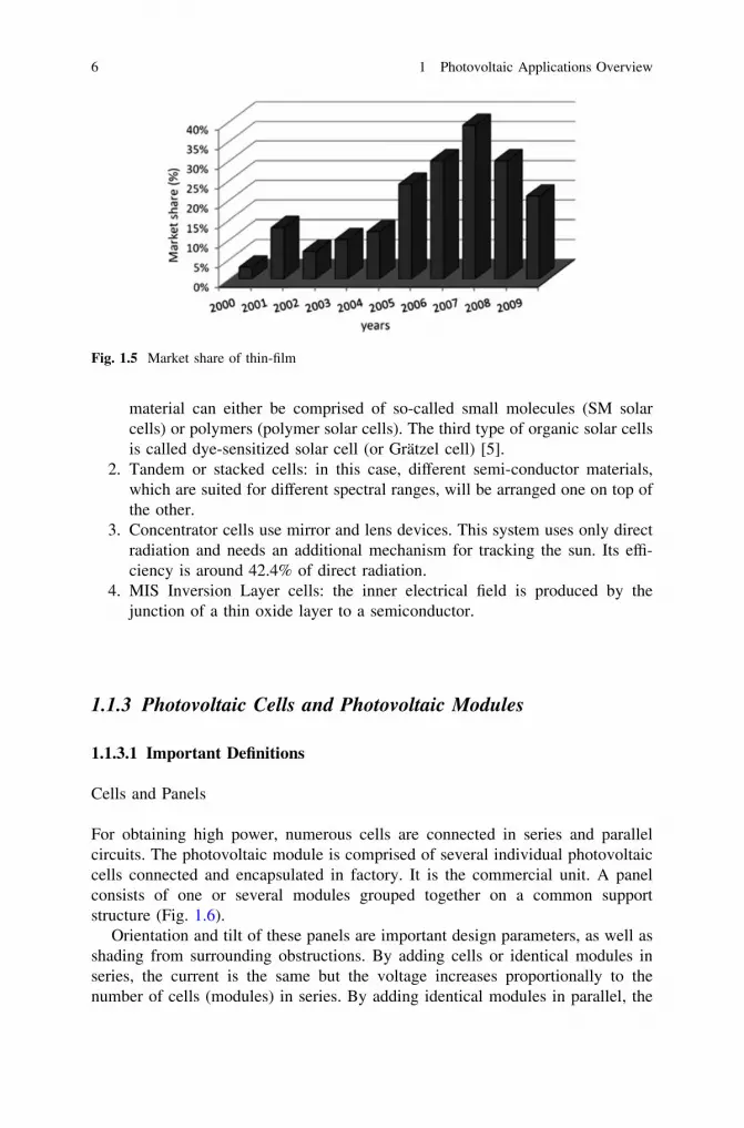
It is also called polysilicon. In this case, the molten silicon is cast into ingots.Then it forms multiple crystals. These cells have slightly lower conversion effi-ciency compared to the single crystal cells. Monocrystalline and polycrystallinesilicon modules are highly reliable for outdoor power applications. The marketshare of crystalline silicon is represented in Fig. 1.4 [3].

• Thin films

Thin-film solar cell (TFSC), also called a thin-film photovoltaic cell (TFPV), isa solar cell made by thin film materials with a few lm or less in thickness. Thin-film solar cells usually used are [4]:

1. Amorphous silicon (a-Si) and other thin-film silicon (TF-Si). The efficiency ofamorphous solar cells is typically between 10 and 13%. Their lifetime is shorterthan the lifetime of crystalline cells.

2. Cadmium Telluride (CdTe) which is a crystalline compound formed fromcadmium and tellurium and its efficiency is around 15%.

3. Copper indium gallium selenide (CIS or CIGS) is composed of copper, indium,gallium and selenium. Its efficiency is around 16.71%.

Fig. 1.1 Solar irradiance andinsolation


4. Dye-sensitized solar cell (DSC) is formed by a photo-sensitized anode and anelectrolyte. Its efficiency is around 11.1%.

Thin-film cells cost less than crystalline cells. The market share of thin films isrepresented in Fig. 1.5 [3].

• Other new technologies:

1. Organic solar cells (OSC) are made of thin layers of organic materials. Threedifferent types of organic solar cells are known: the organic semiconducting

Contact N_semiconductor

PN junction

P_semiconductor

Anti-reflection film

+-

Fig. 1.2 Monocrystallinesilicon cell [2]

Fig. 1.3 Efficiency development of crystalline silicon

Fig. 1.4 Market share of crystalline silicon

1.1 Photovoltaic Definitions 5

material can either be comprised of so-called small molecules (SM solarcells) or polymers (polymer solar cells). The third type of organic solar cellsis called dye-sensitized solar cell (or Grätzel cell) [5].

2. Tandem or stacked cells: in this case, different semi-conductor materials,which are suited for different spectral ranges, will be arranged one on top ofthe other.

3. Concentrator cells use mirror and lens devices. This system uses only directradiation and needs an additional mechanism for tracking the sun. Its effi-ciency is around 42.4% of direct radiation.

4. MIS Inversion Layer cells: the inner electrical field is produced by thejunction of a thin oxide layer to a semiconductor.

1.1.3 Photovoltaic Cells and Photovoltaic Modules

1.1.3.1 Important Definitions

Cells and Panels

For obtaining high power, numerous cells are connected in series and parallelcircuits. The photovoltaic module is comprised of several individual photovoltaiccells connected and encapsulated in factory. It is the commercial unit. A panelconsists of one or several modules grouped together on a common supportstructure (Fig. 1.6).

Orientation and tilt of these panels are important design parameters, as well asshading from surrounding obstructions. By adding cells or identical modules inseries, the current is the same but the voltage increases proportionally to thenumber of cells (modules) in series. By adding identical modules in parallel, the

Fig. 1.5 Market share of thin-film


voltage is equal to the voltage of each module and the intensity increases with thenumber of modules in parallel (Fig. 1.7, Fig. 1.8).

Current Versus Voltage Characteristic

All other quantities being constant, the current IPV supplied by a photovoltaic celldepends on the voltage VPV at its terminals. The graph of that characteristic hastypically the form shown in Fig. 1.9. The current decreases as the voltage isincreasing, and the curve concavity is directed to the bottom.

Open Circuit Voltage and Short Circuit Current

Open circuit voltage and short circuit current are two parameters widely used fordescribing the cell electrical performance (Fig. 1.9). The short circuit current Isc ismeasured by shorting the output terminals. It is the current at zero voltage(Vpv = 0). The open circuit voltage is the voltage at zero current (Ipv = 0).

The values of Isc and Voc obtained in standard conditions are named Isc-ref andVoc-ref. Those values are given in the datasheet of the cell or module.

Maximum Power Point

The power supplied by a photovoltaic generator is

Ppv ¼ VpvIpv ð1:2Þ

This power is positive for the part of the IPV-VPV curve included between theopen-circuit point and the short-circuit point, thus for values of VPV satisfying thecondition

0 \ Vpv\ Voc ð1:3Þ

Fig. 1.6 Efficiency development of concentrator cells [4]


Fig. 1.7 Efficiency of different material cells in laboratory [2]

+

-

+

-

Fig. 1.8 Cells, photovoltaic module and panel [44]

ocV

scI

pvI

pvV

Fig. 1.9 Typical form ofIPV-VPV characteristic


Outside the interval defined by Eq. 1.3, the power Ppv is negative: the PVdevice receives the power from the external electric circuit. This case is notconsidered here.

The power PPV is null when VPV = 0 (short-circuit point) by Eq. 1.2. Similarly,the power Ppv is null when Vpv = Voc (open-circuit point) since, then Ipv = 0 andthus, by Eq. 1.2, Ppv is also null. Then, in the interval defined by Eq. 1.3, PPV

reaches a maximum value. This arrives at a point named Maximum Power Point(MPP). The corresponding values of Vpv and Ipv are named respectively VMPP andIMPP (Fig. 1.10). At that point P(VMPP, IMPP), the power Ppv supplied by thephotovoltaic generator is maximum and denoted PMPP. We have:

PMPP ¼ VMPPIMPP ð1:4Þ

In standard conditions, the quantities PMPP, VMPP and IMPP take respectively thevalues PMPP-ref

, IMPP-ref and VMPP–ref.

The MPP is reached when

0 ¼ o PPV

o VPV

ð1:5Þ

i.e., owing to Eq. 1.2,

0 ¼ o ðVpv IpvÞo Vpv

¼ Ipv þ Vpv

o Ipv

o Vpv

ð1:6Þ

or equivalently,

� o Vpv

o Ipv

¼ Vpv

Ipv

ð1:7Þ

The left member of Eq. 1.7 is the incremental internal resistance of the PVgenerator (the minus sign is due to the choice for that device of the generatorreference directions). The right member is the apparent resistance of the load.Thus, one can consider Eq. 1.7 as the equation defining the resistance adaptationof the load the internal resistance of the PV generator.

MPPV ocV

PMPPI

scI

pvI

pvV

Fig. 1.10 Current versusvoltage Ipv-Vpvcharacteristic for a solar cell


Efficiency

The conversion efficiency of a PV module is the proportion of received sunlightenergy that the module converts to electrical energy. It is defined as the ratiobetween the solar module output and incident light power.

g1 ¼Pout

Pin

¼Vpv:Ipv

Apv:Gð1:8Þ

where Apv is the solar module surface and G the irradiance.In fact, the true efficiency of the PV panel is given by:

gpv ¼ g1:g2:g3:g4:g5 ð1:9Þ

where g1 is the efficiency of the PV panel above calculated (Eq. 1.8),g2 is due to the junction temperature increase since a part of received solar flux

is not converted in electric power but dissipated as heat inside the module. Thetemperature increase is higher in case of poor ventilation of the photovoltaicmodules 0:8hg2h0:9ð Þ:

g3 is due to the power losses by Joule effect in the cables. In order to reducethose losses, the cable section is sized versus to a voltage drop in the cablesg3 � 0:98ð Þ:

g4 is due to losses in the inverter g4 � 0:95ð Þg5 is related to the maximum power point tracking. If the losses of the converter

which carries that tracking are included in g4, then g5 takes into account only theimperfections of the maximum power point traking (g5 & 0.98). g5 is lower if ittakes also into account the losses of the tracking converter (g5 & 0.95). Finally, ifthere is none maximum power point tracking, g5 takes into account the conse-quence of that lack (g5 & 0.8).

Fill Factor

It describes how square the Ipv-Vpv curve is. The fill factor is defined as follows

FF ¼ PMPP

Voc � Isc

¼ VMPP:IMPP

Voc � Isc

ð1:10Þ

1.1.3.2 Characteristic Curves of Solar Cells

The electrical characteristic of the PV cell is generally represented by the currentversus voltage (Ipv-Vpv) curve and power versus voltage (Ppv-Ipv) for differentconditions.


Irradiance Effect

Figure 1.11 shows the current–voltage characteristics Ipv-Vpv and power–voltagePpv-Vpv of the PV cell for different levels of radiation. We note that the current Isc

increases quasi linearly with irradiance and that the voltage Voc increases slightly.Then, the maximum electric power PMPP increases faster than the irradiance, i.e.the efficiency is better for high irradiance.

The reference conditions are generally chosen with an irradiance of 1,000 W/m2. In practice, the irradiance on PV without light concentration is lower, and thusthe efficiency is lower than its rated value.

Temperature Effect

When the internal temperature Tj increases, the short circuit current Isc increasesslightly due to better absorption of light (as an effect of the gap energy decreasewith temperature) but the open-circuit voltage strongly decreases with tempera-ture. The maximum electric power also strongly decreases with temperature(Fig. 1.12).

Cur

rent

(A

)

1000W/m2

400W/m2

800W/m2

600W/m2

Voltage (V) Voltage (V)

1000W/m2

800W/m2

600W/m2

400W/m2Pow

er (

W)

Fig. 1.11 Irradiance effect on electrical characteristic

Voltage (V)Voltage (V)

Cur

rent

(A

)

Pow

er (

W)

T = 0o Cj

T = 25o

Cj

T = 50o

Cj

T = 75o

Cj

T = 0o Cj

T = 25o

Cj

T = 50o

Cj

T = 75o

Cj

Fig. 1.12 Temperature effect on electrical characteristic [31]


The standard conditions are generally chosen for a value of internal temperatureTj equal to 25�C. Under sunshine, the internal temperature is often higher and thusthe efficiency lower.

The short-circuit current Isc can be calculated at a given temperature Tj, forsmall temperature variation, by:

DT¼Tj � Tjref : ð1:11Þ

Isc ¼ Isc�Tjref1þ asc:DT½ � ð1:12aÞ

where asc is the relative temperature coefficient of short-circuit current (/�K) asfound from the data sheet, Tjref is the reference temperature of the PV cell (�K),Isc-Tjref is the short-circuit current at the reference temperature.

Similarly, the open-circuit voltage, for small temperature variations can be alsoexpressed as:

Voc ¼ Voc�Tjref1þ boc:DT½ � ð1:12bÞ

where Voc-Tjref is the open-circuit voltage at the reference temperature and boc isthe relative temperature coefficient of that voltage (/�K) as found from the datasheet.

Often, datasheet also gives the temperature coefficient of PMPP:

PMPP¼ P

MPP�Tjref1þ c

MPP:DT

� �

ð1:12cÞ

where PMPP-Tjref is the maximum power at the reference temperature, cMPP is therelative maximum power temperature coefficient (/�K) as found from the data sheet.

Note on Spectral Effect

White light can be considered as a sum of radiations with different wave length(colors). The efficiency of PV generators is not the same for each wave length. Forthat reason, the standard conditions used for cells and modules rating include aconstraint on the light spectrum. The standard spectrum commonly used is that onenamed AM 1.5. As a consequence, the PV cells and modules are sometimesoptimized for that standard spectrum. In real condition, the light spectrum can bedifferent, and that has also an effect on the PV efficiency.

1.2 Introduction to PV Systems

A PV system converts sunlight into electricity. A PV system contains differentcomponents including cells, electrical connections, mechanical mounting and away to convert the electrical output. The electricity generated can be kept in astandalone system, stored in batteries or can feed a greater electricity power grid. It


is interesting to include electrical conditioning equipment. This one ensures the PVsystem to operate under optimum conditions. In this case, we use special equip-ment to follow the maximum power of the array. This equipment is known asmaximum power point tracking (see Chap. 4).

1.2.1 Stand Alone PV Systems

1.2.1.1 Direct-Coupled PV System

Stand-alone PV systems are designed to operate independent of the electric utilitygrid, and are generally designed and sized to supply certain DC and/or AC elec-trical loads. The simplest type of stand-alone PV system is a direct-coupled sys-tem, where the DC output of a PV module is directly connected to a DC load(Fig. 1.13).

In direct-coupled systems, the load only operates during sunlight hours. Thecommon applications for this system are such as ventilation fans, water pumps andsmall circulation pumps for solar thermal water heating systems.

1.2.1.2 Stand-Alone PV System with Battery Storage Powering DCand AC Loads

In standalone PV applications, electrical power is required from the system duringnight or hours of darkness. Thus the storage must be added to the system. Gen-erally, batteries are used for energy storage. Several types of batteries can be usedsuch as lead-acid, nickel–cadmium, lithium zinc bromide, zinc chloride, sodiumsulfur, nickel-hydrogen, redox and vanadium batteries. Different factors are con-sidered in the selection of batteries for PV application (see Chap. 5). The inverteruses an internal frequency generator to obtain the correct output frequency (seeChap. 3).

A charge controller must keep the battery at the highest possible state whileprotecting it from overloaded by the photovoltaic generator and from over-dis-charge by loads. There are several types of charge controller [6]

• Shunt controller: the function is to regulate the charging of battery. This con-troller is basically connected in parallel with array and battery [2].

• Series controller: this controller is commonly used in small PV system andconnected in series between PV array and battery.

• Tracking controller: This controller tracks the maximum power point of PVarray (see Chap. 4).

PV array DC load

Fig. 1.13 Direct-coupled PVsystem

1.2 Introduction to PV Systems 13

http://dx.doi.org/10.1007/978-1-4471-2403-0_4

http://dx.doi.org/10.1007/978-1-4471-2403-0_4

http://dx.doi.org/10.1007/978-1-4471-2403-0_5

http://dx.doi.org/10.1007/978-1-4471-2403-0_5

http://dx.doi.org/10.1007/978-1-4471-2403-0_3

http://dx.doi.org/10.1007/978-1-4471-2403-0_3

http://dx.doi.org/10.1007/978-1-4471-2403-0_4

http://dx.doi.org/10.1007/978-1-4471-2403-0_4

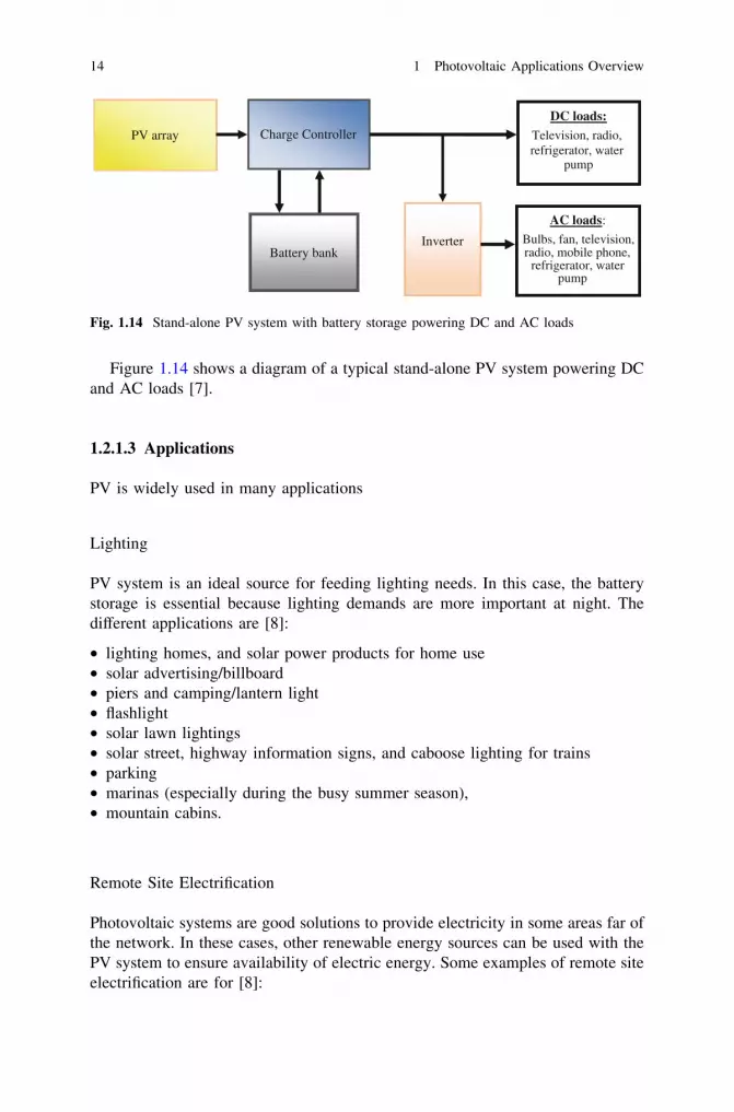
Figure 1.14 shows a diagram of a typical stand-alone PV system powering DCand AC loads [7].

1.2.1.3 Applications

PV is widely used in many applications

Lighting

PV system is an ideal source for feeding lighting needs. In this case, the batterystorage is essential because lighting demands are more important at night. Thedifferent applications are [8]:

• lighting homes, and solar power products for home use• solar advertising/billboard• piers and camping/lantern light• flashlight• solar lawn lightings• solar street, highway information signs, and caboose lighting for trains• parking• marinas (especially during the busy summer season),• mountain cabins.

Remote Site Electrification

Photovoltaic systems are good solutions to provide electricity in some areas far ofthe network. In these cases, other renewable energy sources can be used with thePV system to ensure availability of electric energy. Some examples of remote siteelectrification are for [8]:

Inverter

AC loads:

Bulbs, fan, television,radio, mobile phone,

refrigerator, waterpump

PV array

DC loads:Television, radio, refrigerator, water

pump

Charge Controller

Battery bank

Fig. 1.14 Stand-alone PV system with battery storage powering DC and AC loads


• rural homes,• water supply in rural areas,• parks,• mountain cabins,• remote farms• island electrification,• mobile clinics for remote rural areas,• solar highway,• facilities at public beaches,• campgrounds,• military installations.

Communications

Some examples of communications are:

• radio telephone equipment,• radio,• television,• telecommunication systems,• military usage for telecommunications,• relay towers or repeater stations,• portable computer systems,• highway callboxes,• fire lookout tower.

Remote Monitoring

Some examples of remote monitoring

• power source monitoring,• meteorological measurement systems,• highway/traffic conditions,• structural conditions,• seismic recording,• irrigation control,• scientific research in remote locations.

Water Pumping and Control

These systems may be either:


• direct systems supplying water only when the sunlight is sufficient,• pumping water to an elevated storage tower during sunny hours to provide

available water at any time.

PV powered water pumping is used to provide water for

• campgrounds,• irrigation,• remote village water supplies,• livestock watering

Charging Vehicle Batteries

PV systems may be used to

• directly charge vehicle batteries,• or to provide a ‘‘trickle charge’’ for maintaining a high battery state of charge on

little-used vehicles.

Some examples are:

• fire-fighting and snow removal• equipment and agricultural machines such as tractors or harvesters• direct charging is useful for boats and recreational vehicles• solar stations may be dedicated to charging electric vehicles.

Refrigeration

PV systems are excellent for remote or mobile storage of medicines and vaccines.

Consumer Products

There is a variety of consumer products. PV is used to power

• small DC appliances for recreational vehicles,• watches,• lanterns,• calculators,• radios,• televisions,• flashlights,• outdoor lights,


• security systems,• gate openers.

1.2.1.4 Advantages of Stand-Alone PV System

The most important advantages of PV system are [8]:

• The reliable supply of the load with electricity during operating time,• a long lifetime,• expenses for maintenance must be low.

1.2.2 Grid-Connected PV Systems

Utility-interactive PV power systems mounted on residential and commercialbuildings are likely to become important source of electric generation. Grid-connected PV systems offer the opportunity to generate significant quantities ofhigh-grade energy near the consumption point, avoiding transmission and distri-bution losses. These systems operate in parallel with existing electricity grids,allowing exchange of electricity to and from the grid. Grid-connected PV systemcan be subdivided into two systems:

• Decentralized grid-connected PV systems• Central grid-connected PV systems.

1.2.2.1 Decentralized Grid-Connected PV Systems

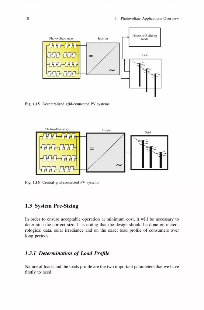
In these systems, energy storage is not necessary because solar radiation providespower in the houses and if there is surplus energy it can be injected into the grid(Fig. 1.15). In this case, the inverter must integrate harmoniously with the energy(voltage and frequency) provided by the grid.

During night or at instants when the PV power is inadequate, the grid can beused as a storage system and will feed the houses.

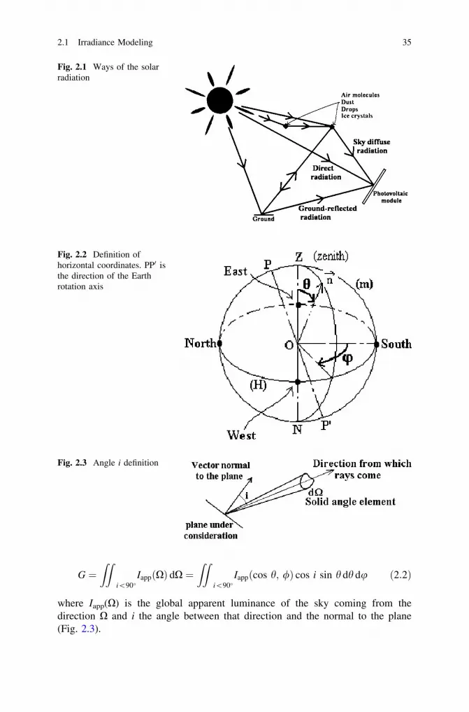
1.2.2.2 Central Grid-Connected PV Systems

It is a central photovoltaic power station and it is installed to systems up to theMW range. With this system, we can obtain medium or high voltage grid(Fig. 1.16).


1.3 System Pre-Sizing

In order to ensure acceptable operation at minimum cost, it will be necessary todetermine the correct size. It is noting that the design should be done on meteo-rological data, solar irradiance and on the exact load profile of consumers overlong periods.

1.3.1 Determination of Load Profile

Nature of loads and the loads profile are the two important parameters that we havefirstly to need.

=

InverterPhotovoltaic arrayGrid

Fig. 1.16 Central grid-connected PV systems

= Grid

InverterHouse or Building

loadsPhotovoltaic array

Fig. 1.15 Decentralized grid-connected PV systems


1.3.2 Analysis of Solar Radiation

We have to need information on latitude and longitude, on weather data and on thedifferent constraints on installation system.

1.3.3 Calculation of Photovoltaic Energy

The energy produced by a photovoltaic generator is estimated using data from theglobal irradiation on an inclined plane, ambient temperature and the data sheet ofthe photovoltaic module given by the manufacturer. The electrical energy pro-duced by a photovoltaic generator is given by:

Epv ¼ gpv Apv G ½1: � fb þ fb gbatt� ð1:13Þ

where fb is the fraction of the energy which passes through the batteries and gbatt

the battery energy efficiency (gbatt & 0.8)

1.3.4 Size of PV

1.3.4.1 First Method

The monthly energy produced by the system per unit area is denoted: Epv,m (kWh/m2) and EL,m is the monthly energy required by the load (where m = 1,2,…, 12represents the month of the year.). The minimum surface of the generator neededto ensure full (100%) coverage load (EL) is expressed by [9]:

Apv ¼ maxm

EL;m

Epv;mð1:14Þ

Surface larger than Eq. 1.14 can be needed for taking into account the limitedsize of the batteries or for including a security factor.

For systems including a grid connection or alternative energy sources, thesizing can be achieved on annual basis.

The total energy produced by the photovoltaic generator which supplies theload can be expressed by:

EL ¼ Epv:Apv ð1:15Þ

The calculation of the photovoltaic generator size (Apv) is established from theannual mean of the monthly contribution Epv

� �

: The load is represented by the

average annual monthly EL:

1.3 System Pre-Sizing 19

Apv ¼ ff :EL

Epv

ð1:16Þ

where ff is the fraction of load supplied by the photovoltaic energy.The number of photovoltaic generator is calculated using the surface of the

system unit Apv,u taking the entire value:

Npv ¼ ENTApv

Apv;u

� �

þ 1 ð1:17Þ

1.3.4.2 Second Method (see Sect. 1.3.6)

1.3.5 Size of Battery Bank

Always, before tackling the calculations, we start by identifying:

• the electricity usage per day• number of days of autonomy• depth of discharge limit• ambient temperature at battery bank.

1.3.5.1 Electrical Usage

Firstly, we have to know the amount of energy we will be consuming per dayEL,max (Wh/day).

1.3.5.2 Number of Autonomy Days

In the second step, we have to identify days of autonomy Nj (backup days). Wemultiply EL,max by this factor Nj.

RES ¼ El;max:Nj ð1:18Þ

1.3.5.3 Depth of Discharge Limit

We have to identify depth of discharge (DOD) and convert it to a decimal value.Divide Eq. 1.18 by this value (DOD).

ANT ¼ RESDOD

¼ El;max:Nj

DODð1:19Þ


1.3.5.4 Ambient Temperature at Battery Bank

We have to derate battery bank for ambient temperature effect. We have to selectthe multiplier corresponding to the lowest average temperature that batteries willbe exposed to. This multiplier depends on the battery type (Table 1.1 gives anexample of such data).

We multiply Eq. 1.19 by this factor (FT). And then we obtain the minimumcapacity of battery bank (Wh).

Cbatt;minðWhÞ ¼ ANT � FTNm � gbatt

ð1:20Þ

Finally we divide the minimum capacity of battery bank by battery voltage Vbatt

and we obtain the minimum capacity (Ah) of the battery bank.

Cbatt;minðA:hÞ ¼Cbatt;minðW : hÞ

Ubatt

ð1:21Þ

The battery capacity of storage can be written as:

Cbatt;minðA:hÞ ¼EL;max:Nj:FT

Ubatt:DOD:Nm:gbatt

ð1:22Þ

where Ubatt is the battery voltage, DOD is the depth of discharge, gbatt is the batteryefficiency, NM is the number of days in the month which has the maximum energyconsumed.

The number of batteries to be used is determined from the capacity of a batteryunit Cbatt,u is given by:

Nbatt ¼ ENTCbatt;min

Cbatt;u

� �

ð1:23Þ

1.3.6 Inverter Size

The selection and number of inverters is based on three criteria: the voltagecompatibility, the current compatibility and the power compatibility. From these

Table 1.1 Factor FTcalculation [10]

Temperature (�C) Temperature (�F) Factor (FT)

+26 80+ 1.00+21 70 1.04+15 60 1.11+10 50 1.19+4 40 1.30-1 30 1.40-6 20 1.59


three criteria, the design of inverters will impose how to wire the photovoltaicmodules together

1.3.6.1 Voltage Compatibility

Maximum Admissible Input Voltage Vmax

An inverter is characterized by a maximum admissible input voltage Vmax. If thevoltage delivered by the PV is greater than Vmax, the inverter will be damaged.Exceeding the value Vmax for the input voltage is also the only cause damaging theinverter. Moreover, as the PV voltages in series are added, the value of Vmax willtherefore determine the maximum number of modules in series. This will obvi-ously depend on the voltage delivered by the photovoltaic modules. We willconsider that the voltage delivered by a PV is its open circuit voltage Voc. Thus, themaximum number of photovoltaic modules in series is calculated by the followingsimple equation:

Npv serial ¼ ENTVmax

Voc � 1:15

� �

ð1:24Þ

The coefficient 1.15 is a safety factor.

Maximum Power Point Tracking Voltage Range

We can also calculate the minimum and maximum number of photovoltaicmodules in series according to the Maximum Power Point Tracking (MPPT)voltage. Indeed, the inverter must at all times track their maximum power mod-ules. The MPPT system works only for a range of input voltage inverter defined bythe manufacturer and specified on the inverter datasheet. When the input voltage ofthe inverter DC side is less than the MPPT minimum voltage, the invertercontinues to operate but provides the power corresponding to the minimum voltageMPPT. We must therefore ensure that the voltage delivered by the PV system is inthe range of the inverter voltage MPPT which it is connected. If this is not the case,there will be no damage to the inverter, but only a loss of power.

The minimum and maximum number of photovoltaic modules in series iscalculated by the following equation [9]:

Nminimalpv serial¼ ENT

Vmpp;min

Vmpp � 0:85

� �

ð1:25Þ

Nmaximalpv serial¼ ENT

Vmpp;max

Vmpp � 1:15

� �

ð1:26Þ


The coefficient 1.15 is a coefficient of increase to calculate the MPP voltage at-20�C.

The coefficient 0.85 is a reduction factor to calculate the MPP voltage at 70�C.

1.3.6.2 Compatibility with Current

As currents are added when panels are in parallel, the value of the current Imax willdetermine the maximum number of parallel panels. This will obviously depend onthe current delivered by a PV system. In the design sizing, it is assumed that thecurrent delivered by a PV system is equal to the short-circuit current (Isc) given onthe datasheet. The maximum number of panels in parallel is calculated by thefollowing equation:

Npv parallel ¼ ENTImax

I�sc1:25

� �

ð1:27Þ

The coefficient 1.25 is a safety factor.

1.3.6.3 Compatibility in Power

The value of the maximum power input of the inverter will limit the number ofpanels connected. Indeed, we must ensure that the power of a PV system does notexceed the maximum allowable power. As the power delivered by the PV systemvaries with radiation and temperature, we can consider for the sizing that thecalculated power is less than the maximum allowable power by the inverter.Ideally, the power delivered by the PV system must be substantially equal to themaximum allowable power inverter.

1.3.7 Sizing of DC Wiring

The array cabling ensures that energy produced by PV array is transferred effi-ciently to the load. In theory, connections are made up of perfect current con-ductors with a zero resistance. In practice, a conductor is not perfect. It works likea resistance (Fig. 1.17).

The resistance of an electric conductor is very low but not zero. We have thefollowing expression:

R ¼ q � lcS

ð1:28Þ


with lc the conductor length (m), S the cross-section area (m2), qc (X. m) theresistivity of the cable. It depends on the material [11]:

The conductor resistance, defined above, will cause a potential drop betweenconductor input and the conductor output. We have:

U ¼ VA � VB ¼ R:I

Thus, if the conductor is perfect, we have:

R ¼ 0

U ¼ 0

Then:

VA ¼ VB

But as R [ 0 for a non-perfect conductor, we haveVAiVB this corresponds to apotential drop. Table 1.2

The voltage drop in a DC conductor is related to power losses. We have:

EJ;i ¼ Ri:I2i :Tdur ð1:29Þ

where Ei is the energy dissipated by Joule losses in the conductor i, Ri and Ii are theresistance and the (quadratic) mean current of that conductor and Tdur the con-sidered time duration (in hours is the energy is expressed in Wh). Of course, thetotal Joule losses of the DC cabling are, replacing each Ri by its value fromEq. 1.28:

EJ ¼X

i

qcLi

SiI2i Tdur ¼ qc Tdur

X

i

Li

SiI2i ð1:30Þ

It is easy to proof that, in order to low the losses for a given conductor volume,we have to keep for all conductors the same ratio

kc ¼Si

Iið1:31Þ

I

VA VB

R

A B

Fig. 1.17 Modeling of acable [11]

Table 1.2 Materialresistivity

qc (X.m) Material

2.7 9 10-8 Aluminum cable1.7 9 10-8 Copper cable1.6 9 10-8 Silver cable


Thus, the Joule losses in the DC cabling are

EJ ¼q T

kc

X

i

Li Ii ð1:32Þ

In practice, we limit the DC cabling losses to a fraction e of the energy pro-duced Npv Epv (e & …1% … 3%). Thus, we find from Eq. 1.32:

kc ¼qc Tdur

EJ

X

i

Li Ii ¼qc Tdur

e Npv Epv

X

i

Li Ii ð1:33Þ

Finally, we obtain from Eq. 1.31 the minimum section of each conductor

Si ¼ kc Ii ð1:34Þ

Of course, the security rules in force in the concerned country need also to berespected.

1.3.8 Sizing of AC Cables

The voltage drop in an AC electrical circuit is calculated as follows:

DV ¼ b qc1:L1

S1: cos /þ kc:L1: sin /

:Imax ð1:35Þ

where DV is the voltage drop. In the three-phase case, currents are expressed asline currents and voltages are expressed as line-to-line voltages. b a coefficientequal to

ffiffiffi

3p

in 3-phase and equal to 2 in single phase, qc1is the resistivity of theconductive material (copper or aluminum), L1 is the length of line (m), S1 is theconductor section (mm2), cos(u) is the power factor (u is the phase shift betweencurrent and voltage AC), Imax is the maximum current and kc is the reactance ofconductor (X/m).

The reactance of the conductors, denoted kc, depends on the arrangement ofconductors between them.

In the case of photovoltaic systems, the power factor cos(u) is currently oftenequal to unity. This means that sin(u) = 0. Therefore, the second term of theEq. 1.35 is zero, whatever the value of the reactance. Thus, it is not necessary toknow the reactance of the conductors to calculate the voltage drop on the AC side.It can be calculated as follows:

DV ¼ b q:L1

S1: cos /

:Imax ð1:36Þ

We have


e ¼ DV

Vnð1:37Þ

where Vn is the rated voltageThus

S1 ¼ b q1:L1

e: cos /

:Imax

Vnð1:38Þ

with e & 0.01. Of course, the security rules in force in the concerned country needalso to be respected.

1.3.9 Sizing of DC Fuses

In a photovoltaic system, fuses have to protect the photovoltaic modules againstthe risk of overload. The information needed to define a good protection againstover current by fuses is:

• Npv-Serial Serial number of modules: in a photovoltaic system, panels are con-nected in series to obtain the desired DC voltage.

• Npv-parallel, the number of PV in parallel: Up to three panels in parallel (Npv-

parallel B 3), protection against overcurrent is not necessary. From four panels inparallel (Npv-parallel C 4), the over current, can heat the cables and damagephotovoltaic panel. It must be eliminated with a fuse placed at each panel.

• Isc, the current short-circuit (under standard test conditions STC).• The fuse rating current should be between 1.5 and 2 times the current Isc.• Voc, the open circuit voltage (under standard test conditions STC).

The operating voltage of a fuse should be 1.15 times the open circuit voltage(1.15 9 Vco 9 Npv-Serial).

Generally, fuses and switching equipment should be rated for DC operation.

1.4 Feasibility of Photovoltaic Systems

We can make an application of the typical stand-alone PV system powering DCand AC loads represented in Fig. 1.14. We represent it in the following figure(Fig. 1.18.)


1.4.1 Estimating the Size of a Photovoltaic System

A load includes anything that uses electricity from the power source (televisions,radios or batteries). Then, you must determine the daily amount of sunlight in yourregion. And finally we will determine PV array size (see Sect. 1.3.4) and batterybank size (see Sect. 1.3.5). The following flowchart will explain how to estimatethe size of a PV array and battery bank. Fig. 1.19

1.4.2 Estimating of PV System Costs

When we will buy modules, verify that the modules meet electrical safety stan-dards, and long-term warranties. Generally, in PV systems we use flooded leadacid batteries (see Chap. 5). We have to use an inverter which is needed to convertto AC power (see Chap. 3). Besides PV modules and batteries, complete PVsystems also use wire, switches, fuses and connectors. Generally, we use a factorof 20% to cover balance of system costs [12] (Fig. 1.20).

Fig. 1.18 Schematic diagram

1.4 Feasibility of Photovoltaic Systems 27

http://dx.doi.org/10.1007/978-1-4471-2403-0_5

http://dx.doi.org/10.1007/978-1-4471-2403-0_5

http://dx.doi.org/10.1007/978-1-4471-2403-0_3

http://dx.doi.org/10.1007/978-1-4471-2403-0_3

1.5 Maintenance of Photovoltaic Systems

Generally, a PV system requires little maintenance, but is important sometimes toclean panels. It is also necessary to control electrical connections to eliminate theproblem of corrosion. And finally, the battery bank needs regular maintenance.

Determine LoadWe will need to estimate all the different loads in the house on a typical

day and sum them.

Determine Available SunlightWe have to calculate the sunshine available for the panels on an average day during the

worst month of the year. It is called the insolation value.

Determine PV Array SizeThe size of the array is determined by the daily energy requirement

divided by the sun-hours per day

Determine Battery Bank Size.

Fig. 1.19 Flowchart of estimating the size of a PV [11]

Estimate PV array cost.

Estimate battery bank cost

Estimate inverter cost.

Estimate balance of system cost.

Fig. 1.20 Flowchart ofestimating of PV system costs[11]


1.5.1 Panels Cleaning

We have to wash PV array, when there is a noticeable buildup of soiling deposits.But in desert area, there is dust on the modules. In this case, it is necessary to cleanmore frequently. Generally we use with ambient-temperature de-mineralizedcleaning solution, to prevent any glass-shock or hard-water spots. We have also toclean dust and dirt from the electrical combiner box and from the DC-to-ACinverter(s)

1.5.2 Verification of Supports

We have to verify periodically the system with all its supports. Also, it is importantto verify if the system performances are close to the previous ones.

1.5.3 Regular Maintenance of Batteries

We have to control batteries for any imperfection, especially corrosion or leakageand if necessary adding electrolyte and equalizing charging.

1.5.4 Inverters Control

We have only to verify if the inverter is properly matched to the panels.

1.5 Maintenance of Photovoltaic Systems 29

Chapter 2Modeling of Solar Irradiance and Cells

SymbolsA Diode ideality factorC(N) Distance correctionCT Civil timedX Elementary solid angleE Normal irradiance of a beam radiationEt Time equationfcirc The circumsolar fractionG Global irradiance on a plane (W/m2)Gref Reference irradiance (1000 W/m2)g Asymmetry factor of the phase function P(H)gh Asymmetry factor of the hemispherical phase functionGMT Greenwich Mean TimeH_ Global irradiance on a horizontal surfaceHA Sun hour angleh Apparent Sun elevationhastr Astronomic (real) sun elevationHd Direct irradianceHd0 Directional irradianceHd0- Directional irradiance on a horizontal surfaceHd0n Directional Sun irradiance on a plane perpendicular to the Sun

beamHdn Direct Sun irradiance on a plane perpendicular to Sun beamH*dn Value of Hdn by sunshine timeHe

dnk Normal direct irradiance outside the atmosphere for wave lengthk

Hedn Normal direct irradiance outside the atmosphere

He0 Solar constant

Hs Diffuse (scattered) irradiance


31

Hsg Hemispherical irradiance coming from groundHsh Hemispherical irradianceHsh sky Hemispherical irradiance coming from the skyHsh sky- Hemispherical irradiance on a horizontal surface coming from the

skyI0 Reverse saturation current of a diode (A)Iapp(X) Global apparent radiance of the sky coming from the direction XId Current shunted through the intrinsic diodeIs app hem Hemispherical diffuse apparent radiance of the skyIph PhotocurrentIRsh Current of the shunt resistanceIsc Short-circuit currentIsc-tjref Short-circuit current at rated temperaturei Angle between a direction X and the normal to a planeJ(l, u) Radiance source due to multiple scatteringJ0(l,u) Radiance source due to first scatteringk Extinction coefficient in atmospheric modelK Boltzman constant (K = 1.381910-23 J/K) in cell modelk0 Directional extinction coefficientkk dm Elementary relative extinction coefficient at wave length kk0 (m) Value of k corresponding to the standard atmosphere(lat) North latitude of the place(long) East longitude of the placem Relative (without physical dimension) Air Massm0 Absolute air massm0z ref Absolute air mass of a standard atmosphere in the vertical

direction (between TOA and the sea level)MST Local mean solar timeN Number of the day of the yearP(H) So-called phase functionP1, P2 and P3 Constant parametersp Atmospheric pressure in hPa (mbars)p0 Pressure used in the definition of the standard atmosphere

(p0 = 1013.25 hPa)psea level Pressure at the sea levelq Quantum of charge (1.602910-19 C)Rloc Local ground albedo (the fraction of the light received by the

ground which is reflected)Rreg Regional soil albedoRs Series resistanceRsh Shunt resistanceRST Real solar time at the placeSTC Standard conditionsT Temperature

32 2 Modeling of Solar Irradiance and Cells

Tj Junction temperatureTj ref Reference temperatureTLinke Linke turbidity factorTD Time difference (which is defined for each country, with in some

countries a seasonal change)TOA Top of AtmosphereUT Universal TimeVpv Voltage across the PV cellz Altitudeasc Temperature coefficient of short-circuit current found from the

datasheet (absolute or relative)boc Temperature coefficient of open-circuit voltage found from the

datasheet (absolute or relative)c1 and c2 Coefficientsd DeclinationH Angle between the incident and scattered lighth0 Apparent Sun zenithal angleh0 astr Astronomic (real) Sun zenithal angle u0

hp Inclination of a planek Wave lengthl, l0, lp Cosines of the corresponding zenithal anglesu Azimuthu0 Sun azimuthup Orientation of a planex Ratio of the scattering coefficient to the sum of the scattering and

absorption coefficientsx0 The ratio of the hemispherical scattering coefficient to the sum of

the hemispherical scattering and absorption coefficients-0;-1;-2 Coefficients of the decomposition of Ih in Legendre polynomials

In order to obtain a realistic view of the behavior of a photovoltaic system, it isnecessary to achieve computer simulations. For that purpose, the most importantdata is the light irradiance of the photovoltaic array at a small time scale (someminutes) during a significant duration (one year or more). Unfortunately, completeexperimental data (irradiance for all module inclination and orientation) are neveravailable. For example, the only available measurement result is often hourly ordaily global irradiance on a horizontal plane. Sky modeling is thus necessary inorder to deduce from the available partial data, a realistic estimation of the moduleirradiance and some spectral characteristics of that irradiance. Of course, that firstresult is useful only in conjunction with a model of the photovoltaic modules, inorder to deduce from it the electrical power generation for varying irradiance,spectrum, and temperature.

When one is concerned by optimization of a system, it is important to usemodels well suited in order to achieve the performance evaluation of each tested

2 Modeling of Solar Irradiance and Cells 33

configuration in a short time, and so to have the possibility of comparing a largenumber of possibilities. The first part of this chapter is devoted to irradiationestimation using simplified sky or atmosphere models. The second part is devotedto module modeling.

2.1 Irradiance Modeling

2.1.1 Principles and First Simplifying Assumption

2.1.1.1 Sun Light Travel

In order to reach photovoltaic modules, sunlight must go through the atmosphere,where it is subject to absorption and scattering. A part of sunlight reaches themodule without undergoing these phenomena: it is named the direct radiation.During its travel through atmosphere, a part of the light is scattered by air mol-ecules, aerosols (dust), water drops or ice crystals, and also by the ground surface.That light has still a chance to arrive on the photovoltaic module after one orseveral scatterings. That part of module irradiation is named the diffuse fraction.By clear sky, the main part of irradiance is the direct one. By overcast sky, globalirradiation is lower and the diffuse to global ratio is higher. So, the light whichreaches a photovoltaic module can come from Sun by a variety of ways, asschematically shown on Fig. 2.1.

In this chapter, we do not consider the infrared radiation coming from theatmosphere, since this one has wavelengths too larger for inducing photovoltaicgeneration. However, we consider ‘‘light’’ as also the infrared radiation comingfrom Sun, because the part of that radiation which is not stopped by atmospherehas wavelengths able to cause photovoltaic effect.

2.1.1.2 Angles Definition

In order to correctly describe the different directions, we define a sphericalcoordinate system called horizontal coordinates, as shown in Fig. 2.2, where ZN isthe local vertical.

Then, any direction X can be specified by the two angles h and u. In particular,the normal to the receiving plane can be specified by hp and up, which arerespectively the inclination of the plane and its orientation.

A solid angle is defined as the surface intersected by a cone on a unit radiussphere centered on its top. In spherical coordinate, the elementary solid angle is

dX ¼ sin h dh du ð2:1Þ

and is expressed in steradians (sr) if h and u are expressed in radians (rad).Defining global irradiance G on a plane as the power received from light by unit

area, we have then


G ¼ZZ

i\90�IappðXÞ dX ¼

ZZ

i\90�Iappðcos h; /Þ cos i sin h dh du ð2:2Þ

where Iapp(X) is the global apparent luminance of the sky coming from thedirection X and i the angle between that direction and the normal to the plane(Fig. 2.3).

Fig. 2.2 Definition ofhorizontal coordinates. PP0 isthe direction of the Earthrotation axis

Fig. 2.1 Ways of the solarradiation

Fig. 2.3 Angle i definition

2.1 Irradiance Modeling 35

The spherical geometry allows to compute the angle i by

cos i ¼ cos h cos hp þ sin h sin hp cos ðu� upÞ ð2:3Þ

2.1.1.3 Sun Position Computation

The Sun position is defined by angles h0 and u0, respectively the Sun zenithalangle and the Sun azimuth. Instead of h0, we often use angle

h ¼ p2� h0 ð2:4Þ

named Sun elevation. h is the angle between the sun direction and the horizontalplane.

Sun position is in practice never measured, since it is easy to compute itknowing date and time, longitude and latitude of the place, and some astronomicdata. The computation is made easier in a coordinates system different fromFig. 2.2, namely the equatorial coordinates. These ones are defined as shown atFig. 2.4, where (m) is the local meridian as defined on Fig. 2.2.

In that system, the coordinates are angles d and HA, called respectively thedeclination and the hour angle. Sun declination and hour angle can be computedwith a very large accuracy by astronomical methods. Simplified computationmethods without significant error for the present purpose can be found in theliterature. An example of such code is given in [13].

If some degrees inaccuracy is acceptable, we can use the following formulae[14]. Sun declination is obtained as

sin dðNÞ ¼ 0:398 sin2 p365

N � 82þ 2 sin2 p ðN � 2Þ

365

� ��

ð2:5Þ

Fig. 2.4 Equatorialcoordinates definition


where N is the number of the day of the yearIn order to obtain the hour angle H, the following operations are leaded starting

with the civil time CT in hours

(a) UT (Universal Time) or GMT (Greenwich Mean Time) is obtained by sub-tracting from CT the time difference TD (which is defined for each country,with in some countries a seasonal change).

UT ¼ CT� TD ð2:6Þ

(b) Using the east longitude of the place, we obtain the local mean solar time ofthe place by

MST ¼ UTþ ðlongÞ15

ð2:7Þ

where (long) is the east longitude of the place expressed in �, MST and UTbeing in hours.

(c) Then, the real solar time at the place is obtained using the equation

RST ¼ MSTþ Et ð2:8aÞ

where Et is the time equation, which take into account the fact that the rotationspeed of the Earth around Sun is not uniform. We have approximately, inhours,

EtðNÞ ¼1

60½9:87 sin ð2N 0Þ � 7:53 cos ðN 0Þ � 1:5 sin ðN 0Þ� ð2:8bÞ

with

N 0 ¼ 2p ðN � 81Þ365

ð2:8cÞ

(d) The hour angle is linked to the real solar time by the relation

HA ¼ p12ðRST� 12Þ ð2:9Þ

Once the angles d and HA are known, we can compute the angles h0 astr or hastr

and u0 by a change of coordinates:

sin hastr ¼ cos HA cos d cos ðlatÞ þ sin d sin ðlatÞ ð2:10aÞ

cos u0 cos hastr ¼ cos HA cos d sin ðlatÞ � sin d cos ðlatÞ ð2:10bÞ

sin u0 cos hastr ¼ sin HA cos ðdÞ ð2:10cÞ

where (lat) is the north latitude.


It is to be noticed that the determination of u0 without ambiguity is possibleonly using all the two Eqs. 2.10b and 2.10c.

The apparent Sun zenithal angle h0 is approximately equal to the astronomicalangle h0 astr: a small difference occurs due to the atmospheric refraction. In pho-tovoltaic studies, we assume frequently

h0 � hastr or; equivalently; h � hastr ð2:11aÞ

None correction to Eq. 2.11a is useful for small zenithal angle (Sun elevationnear to 90�). For larger zenithal angles (Sun elevation near to 0�), the enhancedSaemundsson formula [15] is a little bit better:

h � hastr þp

1010283:15

273:15þ T

1:0260

cotg hastr þ10:3

hastr þ 5:14

� �

for� 2�\hastr\89�ð2:11bÞ

where p is the atmospheric pressure in hPa (mbars) and T the temperature in �C,h and hastr being expressed in degrees.

Of course, the formulae are not relevant when hastr \ -2� since it is thencertainly the night.

Taking into account the sun radius, sunrise or sunset arrives when

h � �0:27�: ð2:12Þ

2.1.2 Sky and Ground Radiance Modeling

The global irradiance Eq. 2.2 can be split is two parts: direct irradiance and diffuseirradiance

G ¼ Hd þ Hs ð2:13Þ

where the index ‘‘d’’ stands for ‘‘direct’’ and the index ‘‘s’’ for ‘‘scattered’’(diffuse).

2.1.2.1 Direct Radiation

Direct Sun radiation (also named beam radiation) is assumed coming from a pointat the Sun disk center. The direct radiance is thus a Dirac delta on the point ofcoordinate h0 (or h) and u0. Then, the corresponding part of Eq. 2.2 reduces to

Hd ¼ 0 if cos i\0 ð2:14aÞ

Hd ¼ Hdn cos i if cos i [ 0 ði\90�Þ ð2:14bÞ


where the index ‘‘n’’ is for ‘‘normal’’ and, thus, Hdn is the direct Sun irradiance ona plane perpendicular to Sun beam. i is the incidence angle of direct radiation onthe plane. It is easy to compute that incidence angle i, using the particular case ofEq. 2.3 where h = h0,

cos i ¼ cos h0 cos hp þ sin h0 sin hp cosðu0 � upÞ¼ sin h cos hp þ cos h sin hp cos ðu0 � upÞ

ð2:15Þ

So, using twice (2.14), it is sufficient to have only one measurement of directradiation on one irradiated plane to compute Hdn and thus the value of Hd on anyplane.

When the sky is uniform (clear or uniformly cloudy), Hdn is a smooth functionof time. However, in case of incomplete cover by thick clouds, Hdn experiencesquick changes between a value H*dn for sunshine time and nearly 0 when there is acloud in front of Sun. In that case, we speak about ‘‘bimodal state’’.

A related notion is the sunshine duration. The sunshine duration is the time forwhich Hdn [ 120 W. Thus, if H*dn [ 120 W, the ratio between the sunshineduration and the time of recording is equal to the probability to have Hdn = H*dn

at a particular time. That probability is also approximately equal to the comple-ment to unity of the cloud cover (in per unit)

2.1.2.2 Circumsolar Diffuse Radiation

Restraining the Eq. 2.2 to the diffuse part, we have

Hs ¼ZZ

i\90�Is appðXÞdX ¼

ZZ

i\90�Is appðcos h;uÞ cos i sin h dh du ð2:16Þ

Searching for a simplified expression of Is app (cos h, u), a common approxi-mation [16] is to split that function of two coordinates in a sum of two function ofonly one coordinate, namely a circumsolar part and an hemispherical part:

Is app ¼ Is app circðHÞ þ Is app hemðhÞ ð2:17Þ

where the circumsolar part is function only of the angle between the Sun directionand the observation direction, and the hemispheric part is only function of h. Thatsplitting comes from the common observation that the radiance of the part of thesky which is near to the Sun is higher than the other parts of the sky. Angle H issimply

cos H ¼ cos h cos h0 þ sin h sin h0 cosðu� u0Þ ð2:18Þ

For the irradiance computation, usually, we do not use Eq. 2.18, but we con-sider that all the circumsolar part comes from the Sun disk center. Then, directirradiance and circumsolar irradiance can be treated as a whole, which is named‘‘directional’’ ‘‘irradiance’’. We use the index ‘‘d’’’ for ‘‘directional’’. We obtain


for the directional component an expression very similar to that obtained for directcomponent (2.14):

Hd0 ¼ 0 if cos i\0 ð2:19aÞ

Hd0 ¼ Hd0n cos i if cos i [ 0 ði\90�Þ ð2:19bÞ

As the radiance Is app hem depends only of h, it is clear that the correspondingirradiance depends only of the plane inclination hp. We have then

G ¼ Hd0n cos iþ Hsh ðhpÞ ð2:20Þ

That partition can give a good approximation of real irradiance, as it is shown atFig. 2.5, which uses global irradiance experimental data from the literature [17]versus inclination for different orientations at a fixed time (clear sky, Davis Cal-ifornia, h0 = 90–34� = 56�).

From Eq. 2.20, it is obvious that, in order to compute the directional part ofirradiation, it is sufficient to have two experimental values of global irradiance ontwo planes of same inclination hp but different orientations up provided they aredissymmetric with regard to Sun azimuth u0. However, it remains useful to splitthe directional irradiance into direct and circumsolar irradiances since only thedirect component is submitted to bimodal state.

An important particular case of Eq. 2.20 is the irradiance on the horizontalplane, which is often measured in meteorological stations. In that case, followingEq. 2.15 for hp = 0, we have cos i = sin h and thus Eq. 2.20 becomes:

G� ¼ Hd0n sin hþ Hsh� ð2:21Þ

2.1.2.3 Ground Diffuse Radiation

The next step in our analysis is to split the hemispherical irradiance into a partcoming from the sky and a part coming from ground.

Hsh ¼ Hsh sky þ Hsg ð2:22Þ

Fig. 2.5 Total irradiance ona surface in function of theinclination for differentorientations. * areexperimental values [17],curves are computed byEq. 2.20 with Hd0n and Hsh

fitted for the bestapproximation


This ground radiance is often assumed to be isotropic, and thus purely hemi-spherical. For that reason, we have omitted the index ‘‘h ’’ in the last term ofEq. 2.22. Then, reducing the integral Eq. 2.2 to the ground diffuse radiation, wecan show that the corresponding irradiance is

Hsg ¼ Rloc G�1� cos hp

2ð2:23Þ

where Rloc is the local ground albedo (the fraction of the light received by theground which is reflected).

In the expression Eq. 2.23, the value of G- is given by (2.21). It shall benoticed that the ground diffuse irradiance does not contribute to Hs h-.

G� ¼ Hd0� þ Hsh sky� ð2:24Þ

2.1.2.4 Sky Hemispherical Diffuse Irradiance

It remains for achieving the analysis to give an expression for the sky hemi-spherical diffuse irradiance Hsh sky(hp). The simplest assumption is that the skyhemispherical irradiance results from an isotropic radiance. Then, the corre-sponding part of Eq. 2.2 leads to the expression

Hsh sky ¼ Hsi ¼ Hsi�1þ cosðhpÞ

2ð2:25Þ

where the index ‘‘i’’ stands for ‘‘isotropic sky’’ and thus implicitly hemispherical.In that case, the full description of irradiance as a function of the inclination and

orientation of a plane is obtained using only three parameters: Hd0n, Hsi- and Rloc.If Rloc is known, the two irradiance measurement requested at Sect. 2.1.2.2. aresufficient in order to identify that function.

Unfortunately, the sky isotropy assumption is contrary to the common obser-vation that the part of the sky near to the horizon is often clearer than the otherparts of the sky. So, different authors have introduced empirical additional terms,the most known being the horizon circle diffuse irradiance. We shall not considersuch terms in that book because we prefer obtain the expression of Hsh sky from aphysical analysis of atmosphere, which is achieved below.

2.1.3 Use of an Atmospheric Model

In many cases, the available experimental irradiance data are insufficient, because

• they do not allow computing the irradiance on the considered plane using themethods described in 2.1.2,


• a best approximation of Hsh sky than Eq. 2.25 is required and the number ofirradiance measurements is insufficient for that,

• they are given as mean values on too large time intervals,• information on spectral characteristics is needed but not available.

In particular, we stress the fact that average values of irradiance are not suitedfor direct use in photovoltaic studies since

• the power generation of photovoltaic modules is not proportional to irradiance,• for the systems simulations, the energy production timing is of importance.

Then, atmospheric modeling can be used to extend in a realistic way theavailable experimental data.

2.1.3.1 Air Mass Notion

As the air density increases from 0 at the TOA (top of atmosphere) to its value atthe ground level, the air influence on a light ray is more important at low altitude.For that reason, it is useful to use as coordinate not the distance l covered by thelight ray but the Air Mass

m0 ¼def

Z

q dl ð2:26Þ

The use of Air Mass in the equation is related to the assumptions that

• the air molecules and particles act on light individually,• their effect is independent of temperature.

Besides being not totally exact, these assumptions are acceptable for ourpurpose.

A particular case of Eq. 2.26 is the case of a vertical ray. We define m0z ref asthe Air Mass of a standard atmosphere in the vertical direction between TOA andthe sea level. Then, we can use instead of absolute Air Mass Eq. 2.26 a relative(without physical dimension) Air Mass

m ¼def

m0

m0z ref

ð2:27Þ

Vertical Air Mass mz is strongly related to the atmospheric pressure. Assumingthat the gravitational field g is constant in the entire atmosphere (g & 9.81 m/s2),vertical Air Mass is given by

mz ¼p

p0ð2:28Þ


where p0 is the pressure used in the definition of the standard atmosphere(p0 = 1013.25 hPa).

If one knows the pressure at the sea level, we can find the pressure at an altitudez (in km) using the formula [14]

p ¼ psea level ð0:89Þz for z \3 km ð2:29Þ

Light can be considered as the sum of electromagnetic radiations with differentwave length k. Visible light has a spectrum going from k = 400 nm (violet) untilk = 800 nm (red) (1 nm = 10-9 m). Sun radiation includes UV (ultraviolet) ofshorter wave lengths and IR (infrared) of longer wave length. Some solar modulesare able to get energy even from invisible Sun radiation.

When a beam of light crosses an air volume, its energy is lowered by absorptionand diffusion phenomena. The elementary relative lowering is given by theproduct kk dm, where dm is the elementary relative Air Mass in the beam directionand where kk is a coefficient named ‘‘extinction coefficient’’. kk is function only ofk and of the atmosphere composition. Figure 2.6 gives an illustration of thatphenomenon.

2.1.3.2 Direct Radiation

Direct radiation, also called ‘‘beam radiation’’, is considered as coming from thedirection computed at 2.2.1.3.

It experiences an Air Mass m which is given, assuming the atmosphere planeand without refraction, by:

m � mz

cosðh0Þ¼ mz

sin h� mz

sin hastr

ð2:30Þ

If we consider the atmospheric refraction, the way followed by the beamradiation is lightly curved. We can take that fact into account replacing Eq. 2.30by a best approximation, such as the Kasten formula [14]

m � mz1

sin hþ 9:40 10�4ðsin hþ 0:0678Þ�1:253 ð2:31Þ

The direct radiation is characterized by its normal irradiance Hdn, as inSect. 2.1.2.1. The extinction mechanism of Fig. 2.6 leads thus to the equation:

Fig. 2.6 Definition of theextinction coefficient


dHdnk ¼ �kkHdnkdm ð2:32Þ

Assuming the atmosphere uniform, the solution of Eq. 2.32 is simply

Hdnk ¼ Hednk e�kkm ð2:33Þ

where Hednk is the normal irradiance outside the atmosphere (at the TOA)

Integrating on all the wave length, we obtain the total normal irradiance outsidethe atmosphere

Hedn ¼

Z

Hednk dk ð2:34Þ

When the Sun–Earth distance is equal to its mean value (1 astronomical unit), thevalue of He

dn is called the ‘‘solar constant’’ He0 The value of that last one is

approximately He0 ¼ 1361 W=m2 [18]. Similarly, the mean values of the He

dnkcanbe found in the literature [19].

However, the Sun irradiation received at TOA varies during a year due to thevariation of Sun–Earth distance. So, He

dn and Hednk have to be deduced from their

mean values using a distance correction

CðNÞ � 1þ 0:034 cos2p365ðN � 2Þ

� �

ð2:35Þ

where N is the number of the day of the year.For each wave length, kk can be decomposed in a sum. Each term of the sum

take into account the effect of one atmospheric component. In fact, we can con-sider as only one component the set of all constant gas (N2, O2, .. CO2). Variablegases are the water vapor H2O, ozone O3 and sometime NO2. We have also to takeinto consideration the aerosol content (dust) and the water condensed in drops or inice crystals (clouds).

For simplified computation, we prefer to replace the infinite sum Eq. 2.34 by afinite one:

Hdn ¼ Hedn

X

i

ai e�kim withX

i

ai\1 ð2:36Þ

For terrestrial applications, the sum of the coefficients ai can be lower than unitysince some wave length are so strongly absorbed in the atmosphere that they donot contribute to the irradiance at the ground level.

The decomposition Eq. 2.36 can maintain information on the light spectrum.For that, the spectrum can be divided in bands of wave length, each band corre-sponding to one or several exponential terms.

On the other hand, for a very simplified computation, we can use only oneexponential for the entire spectrum. In that case, it is convenient to admit that theextinction factor k is a function of m. A classical method is to use


kðmÞ ¼ k0ðmÞTLinke ð2:37Þ

where k0 (m) is the value corresponding to the standard atmosphere. TLinke is theLinke turbidity factor, which is a characteristic of the state of the atmosphere.Once k0(m) has been determined by computation, one measurement of the directirradiation is sufficient in order to compute TLinke. Historically, several approxi-mations of k0(m) have been proposed and lead to different value of TLinke. Thus,old experimental values of TLinke can need revision. Kasten [48] has given in 1996an accurate expression:

k0ðmÞ ¼1

6:6296þ 1:7513 m� 0:1202 m2 þ 0:0065 m3 � 0:00013 m4

for 1\m\20ð2:38aÞ

For higher values of m, one can use [49]

k0ðmÞ ¼1

10:4þ 0:718 mfor m [ 20 ð2:38bÞ

Contrary to the irradiance, the value of TLinke depends only on little of the Sunelevation. Then, assuming that the meteorological conditions are constant during atime period, if one knows the experimental mean value of Hdn during that period, itis possible to search the value of TLinke which is constant on that period and which,by computation, leads to the same mean value of Hdn. Using that value of TLinke,it is then possible to compute at each time the value of Hdn. Of course, if one is in

bimodal mode, that computation has to be adapted taking into account the sunshineduration. For photovoltaic computation, it is better to use H*dn with a sunshineprobability in place of a smoothed value of Hdn for the above mentioned reasons.For the systems simulations where the energy production timing is of importance,it is possible to generate realistic variations of the direct irradiation at small timescale using the method of Markov chains.

2.1.3.3 Generalities About the Diffuse Radiation

In the following, we use the variables:

l ¼ cos h; l0 ¼ cos h0; lp ¼ cos hp. . . ð2:39Þ

Behind the considered functions are wave length dependent, we shall makeabstraction of the subscript ‘‘k’’, hoping that the formulae could be use forbroadband calculations.

The diffuse light is described at each point of the atmosphere by the radianceI(h, u) going to the direction (h, u). The apparent sky and ground radiances arethen related to I(h, u) by:

Is appðl;uÞ ¼ Ið�l;uþ pÞ ð2:40Þ


When an unpolarized parallel beam of normal irradiance E crosses an ele-mentary volume of thickness dm (given in relative Air Mass), the increase ofscattered radiance is given by the equation

dIðHÞ ¼ k x4 p

PðHÞE dm ð2:41Þ

where x is the ratio of the scattering coefficient to the sum of the scattering andabsorption coefficients, H is the angle between the incident and scattered light andP(H) is the so-called phase function. The phase function is normalized in such away that [20]

14p

Z

4p

PðHÞdX ¼ 12

Z

p

0

PðHÞ sin HdH ¼ 1 ð2:42Þ

where dX is the elementary solid angleIn presence of aerosols or water drops, the phase function is very complicated

and, even when long numerical computations are achieved, we use for radiativetransfer computations approximations of this function which depend only of a fewparameters, the most important of them being the asymmetry factor defined as

g ¼ 14p

Z

4p

PðHÞ cosðHÞdX ¼ 12

Z

p

0

PðHÞ cosðHÞ sinðHÞdðHÞ ð2:43Þ

From the above definitions, it can be proved that, in a plane atmosphere, thediffuse radiance I(l, u) obeys to the equation

ldIðl;uÞ

dmz¼ kIðl;uÞ � Jðl;uÞ � J0ðl;uÞ ð2:44Þ

where J(l, u) is the source due to multiple scattering and J0(l, u) is the source dueto first scattering.

The source due to multiple scattering is given by the equation

Jðl;uÞ ¼ kx4p

Z

2p

0

Z

1

�1

Iðl0;u0ÞPðcos HÞdl0du0 ð2:45Þ

with

cos H ¼ ll0 þffiffiffiffiffiffiffiffiffiffiffiffiffi

1� l2p ffiffiffiffiffiffiffiffiffiffiffiffiffiffi

1� l02p

cosðu� u0Þ ð2:46Þ

On the other hand, the primary source of diffuse radiation is

J0ðl;uÞ ¼kx4p

H0Pð� cos H0Þe�kmz=l0 ð2:47Þ


with

cosðH0Þ ¼ ll0 þffiffiffiffiffiffiffiffiffiffiffiffiffi

1� l2p

ffiffiffiffiffiffiffiffiffiffiffiffiffi

1� l20

q

cosðu� u0Þ ð2:48Þ

where h0 and u0 are the coordinates of the Sun and l0 is defined by Eq. 2.39.The equation system Eqs. 2.44–2.48 is very difficult to solve. Currently, an

accurate solution of these equations can be obtained only by using time-consumingnumerical calculations. Numerous empirical models have been developed.Reviews of these models can be found in the literature [21, 22]. Such models usefunctions whose numerous parameters are to be extracted from experimental data.They can thus be geography or climate dependent and present unpredictablelimitations. In the following, we describe a realistic simplified model using only asdata a few atmospheric parameters with well defined physical signification.

2.1.3.4 d-Approximation and Circumsolar Component

The d-approximation [35] consist to assume that a fraction fcirc of the scatteredlight keeps the direction of the incident light, let’s be

PðHÞ ¼ 2 fcircdð1� cos HÞ þ ð1� fcircÞPhðHÞ ð2:49Þ

where the first term is a Dirac deltaWe consider then that the circumsolar component is due to the first term and has

then exactly the same direction as the direct rays. On the other hand, the residualphase function Ph(H) shall be related to hemispherical diffuse radiation. Using thesubscript d0 for the directional irradiance (direct ? circumsolar), we obtain anequation similar to Eq. 2.33:

Hd0n ¼ Hedne�k0m ð2:50Þ

where k0 is the directional extinction coefficient and

k0 ¼ kð1� x fcircÞ ð2:51Þ

If necessary, the circumsolar component can be obtained as the differencebetween Eqs. 2.50 and 2.33.

2.1.3.5 Equations for Hemispherical Component

We obtain equations for the residual diffuse radiance Ih (l, u) by replacing inEqs. 2.44, 2.45 and 2.47 k by k0 and x by:

x0 ¼ ð1� fcircÞx1� x fcirc

ð2:52Þ


Defining Ih (l) as the mean value of Ih (l, u) on –p\ u\p, the equation for Ih

(l) is obtained by replacing in the corresponding part of Eq. 2.44 I, J and J0 bytheir mean values on u. We get [24]:

ldIhðmz; lÞ

dmz¼ k0Ihðmz; lÞ �

k0x0

2

Z

1

�1

Ihðmz; l0ÞPhðl; l0Þdl0

� k0x0

4pPhðl;�l0ÞH0e�k0mz=l0 ð2:53Þ

where

Phðl; l0Þ ¼ 12p

Z

2p

0

PhðHÞ du ð2:54Þ

The approximation is to consider that Ih (mz, l, u) can be identified with Ih (mz,l), and thus considered as a hemispherical radiance.

There are some approximate solutions of the Eq. 2.53. The most known arecalled two-stream approximations. In those methods, the variables are the upwardand downward hemispherical diffuse irradiation:

Hþh ðmzÞ ¼ 2pZ

1

0

Ihðmz; lÞl dl ð2:55aÞ

and

H�h ðmzÞ ¼ 2pZ

1

0

Ihðmz;�lÞl dl ð2:55bÞ

Hh+ and Hh

- are the only variables of the differential system if we use anapproximation of Ih(l) completely determined by Hh

+ and Hh-. That approximation

can thus have only two freedom degrees.

2.1.3.6 Spherical Harmonics Decomposition

The function Ih(mZ, l) can be decomposed in Legendre polynomial series. The firstLegendre polynomials are

P0ðlÞ ¼ 1 P1ðlÞ ¼ l P2ðlÞ ¼12ð3l2 � 1Þ ð2:56Þ


These polynomials obey the orthogonallity condition

2iþ 12

Z

1

�1

PiðlÞPjðlÞdl ¼ dij ð2:57Þ

And the recurrence formula [37]

ð2iþ 1Þl PiðlÞ ¼ ðiþ 1ÞPiþ1ðlÞ þ i Pi�1ðlÞ ð2:58Þ

We can consider decompositions

Ihðmz; lÞ ¼ I0ðmzÞP0ðlÞ þ 3 I1ðmzÞP1ðlÞ þ 5 I2ðmzÞP2ðlÞ þ � � � ð2:59Þ

and

PhðlÞ ¼ -0P0ðlÞ þ -1P1ðlÞ þ -2P2ðlÞ þ � � � � � � ð2:60Þ

The Legendre polynomials have the property [25]:

12p

Z

2p

0

Piðcos HÞdu ¼ PiðlÞPiðl0Þ ð2:61Þ

Using this property and Eqs. 2.56, 2.57, 2.53 can be decomposed as:

ðiþ 1Þ ddmz

Iiþ1 þ id

dmzIi�1

� �

¼ k0ð2iþ 1ÞIi � k0x0-iIi

� k0x0-i

4pPið�l0ÞH0e�k0mz=l0 ð2:62Þ

Applying the analog of Eqs. 2.42 and 2.43. for Ph(l), we have always [24]

-0 ¼ 1 -1 ¼ 3 gh ð2:63aÞ

and, by reference to the Henyey-Greenstein phase function, there is a reason [23]to take

-2 ¼ 0 ð2:63bÞ

We assume that -i ¼ 0 for all ii1. In the particular case where gh = 0, thehemispherical diffusion is isotropic, i.e. Ph(l) = 1. In that case, the identificationof that Ih (mz, l, u) with Ih (mz, l) is exact, and thus also the hemisphericalhypothesis.

In order to obtain a system of two differential equations, the decomposition ofEq. 2.59 can only involve two degrees of freedom. The Eddington approximationconsists to keep only the first two terms of Eq. 2.59. However, empirical inves-tigations [16] and accurate numerical solutions [26] show that an approximation ofthe first degree in l is not sufficient for a correct modeling of the hemisphericalradiance.


2.1.3.7 Taking into Account the Second Order Term

The following analysis is equivalent to the method developed in [27]. Thatapproach is to consider the three first terms of the series Eq. 2.59 with an addi-tional condition in order to keep only two freedom degrees. Equation 2.62 yields[28]:

dI1

dmz¼ a0k0I0 � b0k0H0e�k0mz=l0 ð2:64aÞ

2dI2

dmzþ dI0

dmz¼ a1k0I1 � b1k0H0e�k0mz=l0 ð2:64bÞ

and, assuming I3 = 0,

2dI1

dmz¼ a2k0I2 � b2k0H0e�k0mz=l0 ð2:64cÞ

where

ai ¼ ð2iþ 1Þ � x0-i ð2:65aÞ

and

bi ¼1

4px0-iPið�l0Þ ð2:65bÞ

Comparing Eqs. 2.64a and 2.64c, we see that the system is degenerated and canonly have a solution if

I2 ¼ c1I0 þ c2H0e�k0mz=l0 ð2:66aÞ

with

c1 ¼ 2a0

a2and c2 ¼

b2 � 2b0

a2ð2:66bÞ

Constraint Eq. 2.66 allows for replacing Eq. 2.64b by

dI0

dmz¼ a01I1 � b01H0e

�k0mz=l0 ð2:67Þ

where

a01 ¼a1

1þ 2c1and b01 ¼

b1 � 2c2=l0

1þ 2c1ð2:68Þ

The system Eqs. 2.64a and 2.67 is easy to solve. Its solution, completed withEq. 2.66, is of the form


I0 ¼ffiffiffiffiffi

a01

q

c1ekk0mz þ

ffiffiffiffiffi

a01

q

c2e�kk0mz þ c3H0e

�k0mz=l0 ð2:69aÞ

I1 ¼ffiffiffiffiffi

a0p

c1ekk0mz � ffiffiffiffiffi

a0p

c2e�kk0mz þ c4H0e

�k0mz=l0 ð2:69bÞ

I2 ¼ c1

ffiffiffiffiffi

a01

q

c1eks0 þ c1

ffiffiffiffiffi

a01

q

c2e�ks0 þ ðc1c3 þ c2ÞH0e�s0=l0 ð2:69cÞ

where

k ¼ffiffiffiffiffiffiffiffiffi

a0a01

q

ð2:70Þ

c3 ¼l0ðb01 � a01b0l0Þ

1� a0a01l20

ð2:71aÞ

and

c4 ¼l0ðb0 � a0 b01l0Þ

1� a0a01l20

ð2:71bÞ

The coefficients c1 and c2 are to be determined using boundary conditions. Forthat, we use the upward and downward horizontal irradiance Eq. 2.55 whoseexpression is [28], by assuming coefficient I3 and the next ones equal to 0:

Hþh ¼ p I0 þ 2I1 þ54

I2

� �

ð2:72aÞ

and

H�h ¼ p I0 � 2I1 þ54

I2

� �

ð2:72bÞ

Thus, introducing Eq. 2.69 into Eq. 2.72,

H�h ¼pffiffiffiffiffi

a01

q

1þ54

c1

� �

�2ffiffiffiffiffi

a0p

� �

ekk0mzc1þpffiffiffiffiffi

a01

q

1þ54

c1

� �

�2ffiffiffiffiffi

a0p

� �

e�kk0mzc2

þp 1þ54

c1

� �

c3þ54

c2�2c4

� �

H0e�k0mz=l0 ð2:73Þ

The boundary conditions are then

H�h ¼ 0 at the TOA ðmz ¼ 0Þ ð2:74aÞ

Hþh ¼ RregðH�h þ Hd0nl0Þ at the ground level ðmz ¼ mz sfcÞ ð2:74bÞ

where Rreg is the regional soil albedo.


There results a linear system of two equations in c1 and c2, which can thus becomputed. Then, the expression Eq. 2.59 is completely determined. IntegratingEq. 2.59 similarly to Eq. 2.2, we obtain hemispherical irradiance on any plane. Byexample, considering the case of Fig. 2.5, we obtain good results usingk0 mz = 0.220, x0 = 0.4141 gh = 0 and Rreg = 0.2779, behind the fact that thenumber of freedom degrees is much smaller.

Figure 2.7 shows the corresponding radiance as a function of the zenith angle.We can see that this second order approximation is not realistic since it leads tonegative values of the radiance. In fact, the function Ih(s0,l) thus obtained is asmooth function unable to correctly describe the directional properties of radiancenear the ground level, because at that boundary the sky and soil radiances do nothave the same form.

2.1.3.8 Enhanced Approximation for Hemispherical Radiance

Although the second order model do not lead to realistic values of the radiance, itseems to give an acceptable approximation of the global state of radiation (seeFig. 2.5). Another advantage of that second order model is that the solutionincludes only three exponentials functions of mz:

ekk0mz e�kk0mz e�k0mz=l0 ð2:75Þ

Then, if we assume that the second term of Eq. 2.53 can be computed using thatmodel, Eq. 2.53 becomes very simple and can be solved analytically for l \ 0.That enhanced solution contains only one more exponential, that is to say

ek0mz=l ð2:76Þ

Fig. 2.7 Hemisphericalradiance computed by thepresent model (with k0

mz = 0.220 x0 = 0.4141,gh = 0 and Rreg = 0.2779)


with that enhanced model, new parameter identification has been needed in orderto keep the good correspondence of Fig. 2.5. We obtain then x0 = 0.288 andRreg = 0.302. The result is shown at Fig. 2.8 assuming that the soil radiance isisotropic and that Rloc = Rreg

The present model can take into account the fact that sky brightness is oftenhigher near the horizon. In addition to the soil albedos Rreg and Rloc, it makes useof only three atmospheric parameters with well defined physical significance:k0, x0 and gh. So, a few number of global irradiance measurements on tiltedsurfaces is sufficient to determine those parameters. Further investigations areneeded to obtain the value of gh in function of k0 and x0, and even a relationbetween k0 and x0, in order to reduce the number of measurements needed for thedetermination of the model.

2.2 PV Array Modeling

In literature, there are several mathematical models that describe the operation andbehavior of the photovoltaic generator. For example, Borowy and Salameh [29]have given a simplified model, with which the maximum power output can becalculated for a module once photovoltaic solar irradiance on the photovoltaicmodule and the temperature is found, and Jones and Underwood [30] also intro-duced a simplified model of the maximum power output which has a reciprocalrelationship with the temperature module and logarithmic relationship with thesolar radiation absorbed by the photovoltaic module. In addition, Jones andUnderwood have given the thermal model of the temperature module photovoltaicthrough the evaluation of many factors. These models differ in the calculationprocedure, accuracy and the number of parameters involved in the calculation ofthe current–voltage characteristic.

Fig. 2.8 Hemisphericalradiance computed by thesecond ordre model and theenhanced model (with k0

mz = 0.220 x0 = 0.288,gh = 0 andRloc = Rreg = 0.302)


2.2.1 Ideal Model

The simplified equivalent circuit of a solar cell consists of a diode and a currentsource connected in parallel (Fig. 2.9). The current source produces the photo-current Iph, which is directly proportional to solar irradiance G. The two keyparameters often used to characterize a PV cell are its short-circuit current and itsopen-circuit voltage which are provided by the manufacturer’s data sheet. Theequation of the current voltage Ipv–Vpv simplified equivalent circuit is derivedfrom Kirchhoff’s law.

We have

Ipv ¼ Iph � Id ð2:77Þ

where

Id ¼ I0 eq

Vpv

AKTj � 1

2

6

6

4

3

7

7

5

ð2:78Þ

Thus

Ipv ¼ Iph � I0 eq

Vpv

AKTj � 1

2

6

6

4

3

7

7

5

ð2:79Þ

with Iph (A) is the photocurrent that is equal to short-circuit current, I0 (A) is thereverse saturation current of the diode, q is the electron charge (1.602910-19 C),K Botzman’s constant (1.381910-23 J/K), A is diode ideality factor, Tj is junctiontemperature of the panels (�K), Id is the current shunted through the intrinsic diode,Vpv is the voltage across the PV cell.

Ipv ¼ Isc � I0 eq

Vpv

AKTj � 1

2

6

6

4

3

7

7

5

ð2:80Þ

We can determine the reverse saturation current I0 by setting Ipv=0 (case whenno output current).

Ipv ¼ 0

Vpv ¼ Voc

0 ¼ Iph � I0 eq

Vocð ÞAKTj � 1

2

6

4

3

7

5

ð2:81Þ


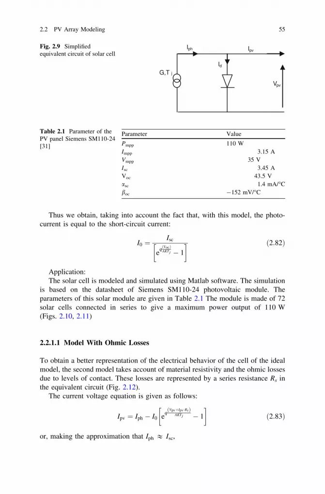
Thus we obtain, taking into account the fact that, with this model, the photo-current is equal to the short-circuit current:

I0 ¼Isc

eq Vocð Þ

AKTj � 1

� � ð2:82Þ

Application:The solar cell is modeled and simulated using Matlab software. The simulation

is based on the datasheet of Siemens SM110-24 photovoltaic module. Theparameters of this solar module are given in Table 2.1 The module is made of 72solar cells connected in series to give a maximum power output of 110 W(Figs. 2.10, 2.11)

2.2.1.1 Model With Ohmic Losses

To obtain a better representation of the electrical behavior of the cell of the idealmodel, the second model takes account of material resistivity and the ohmic lossesdue to levels of contact. These losses are represented by a series resistance Rs inthe equivalent circuit (Fig. 2.12).

The current voltage equation is given as follows:

Ipv ¼ Iph � I0 eq

VpvþIpv �Rsð ÞAKTj � 1

� �

ð2:83Þ

or, making the approximation that Iph & Isc,

Table 2.1 Parameter of thePV panel Siemens SM110-24[31]

Parameter Value

Pmpp 110 WImpp 3.15 AVmpp 35 VIsc 3.45 AVoc 43.5 Vasc 1.4 mA/�Cboc -152 mV/�C

G,T j

Iph Ipv

Id

Vpv

Fig. 2.9 Simplifiedequivalent circuit of solar cell

2.2 PV Array Modeling 55

Ipv ¼ Isc � I0 eq

VpvþIpv �Rsð ÞAKTj � 1

� �

ð2:84Þ

The short-circuit Isc can be calculated at a given temperature Tj:

Isc�Gref ¼ Isc�ref 1þ asc � DT½ � ð2:85Þ

DT ¼ Tj � Tjref ð2:86Þ

Fig. 2.10 Example of PVarray structure

Fig. 2.11 Bloc diagram ofideal model [195]


where Isc-ref is measured under irradiance Gref = 1000 W/m2 and Tj-ref = 25�Cand is given on the datasheet, ascis the temperature coefficient of short-current(/�K) and found on the data sheet, Tjref is the reference temperature of the PV cell(�K), Tj is the junction temperature (�K).

The short-current generated at any other irradiance G (W/m2) can be obtainedby:

Isc�G ¼ Isc�Gref

G

Gref

ð2:87Þ

Applying Eq. 2.84 to the case where Ipv = 0 (open-circuit case), one sees thatthe reverse saturation current at a reference temperature (Tjref) is given by:

I0�Tjref ¼Isc�Tjref

eq

Voc�Tjrefð ÞAKT jref � 1

" #ð2:88Þ

Defining

Vth�Tjref ¼A � K � Tjref

qð2:89Þ

one can write Eq. 2.88 in the form:

I0�Tjref ¼Isc�Tjref

eVoc�TjrefVth�Tjref � 1

� � ð2:90Þ

The reverse saturation current at any other temperature Tj (�K) can be obtainedby:

I0 ¼ I0�Tjref � exp�q � Eg

A�K1Tj� 1

Tjref

!" #

� Tj

Tjref

� �3A

ð2:91Þ

Fig. 2.12 Simplifiedequivalent circuit of solar cellwith Rs


Ipv ¼G

Gref

� Isc�ref � 1þ asc � Tj � Tref

� �

� Isc�ref

exp q � Voc�ref

A�K�Tj�ref� 1

� � exp�q � Eg

A�K1Tj� 1

Tjref

!" #

� Tj

Tjref

� �3A

0

@

1

A

exp q �Vpv þ Rs � Ipv

A � K � Tj

� �

� 1

� �

ð2:92Þ

where Eg represents the gap energy.The simple relationship of power for a photovoltaic module is

Ppv¼Ipv �Vpv

¼(

G

Gref

�Isc � 1þasc � Tj�Tref

� �

� Isc�ref

exp q� Voc�ref

A�K�Tj�ref�1

�� exp�q� Eg

A�K1Tj� 1

Tjref

!" #

� Tj

Tjref

� �3A

0

@

1

A exp q�VpvþRs �Ipv

A�K �Tj

� �

�1

� �

)

�Vpv

ð2:93Þ

Neglecting the term ‘‘-1’’ added to the exponential in Eq. 2.84, the value of Rs

can be obtained by

Rs ¼ �dVpv

dIpv

�

�

�

�

Vpv¼Voc

� 1w

w ¼ q � Isc

A � K � Tj

ð2:94Þ

The first term of Eq. 2.94 ð�dVpv=dIpvjVpv¼VocÞ can be determined either by

experimental or by measures of Ipv–Vpv characteristic of the manufacturer (data-sheets). Eq. 2.84 can be solved using Matlab/simulink or writing a function inMatlab. We can for example Newton’s method which is described as [32]:

xnþ1 ¼ xn �f ðxnÞf 0ðxnÞ

ð2:95Þ

with f ðxnÞis the function, f 0ðxnÞ is the derivate of the function.We have

f ðxnÞ ¼ 0

xn is the first valuexnþ1 is the next valueWe obtain


f ðIpvÞ ¼ Isc � Ipv � I0 eqðVpvþIpv �RsÞ

AKTj � 1

� �

¼ 0 ð2:96Þ

and then

Ipv nþ1 ¼ Ipv n �Isc � Ipv � I0 e

qVpvþIpv :Rsð Þ

AKTj � 1

� �

�1� I0 � qA�K�Tj

� Rs � eqðVpvþIpv�RsÞ=ðA�K�TjÞð2:97Þ

Defining

Vth ¼A � K � Tj

qð2:98aÞ

we obtain

Ipvnþ1¼ Ipvn

�Isc � Ipv � I0 e

VpvþIpv :Rsð ÞVth � 1

� �

�1� I0 � RsVth� eðVpvþIpv�RsÞ=ðVthÞ

ð2:98bÞ

The resolution under Matlab/simulink is given in Figs. 2.13 and 2.14.

2.2.1.2 Other One Exponential PV Array Models

In the equations of models above described (Sects. 2.2.1 and 2.2.2), there is onlyone exponential function. In this section, we present and explain four commonlyused models which exhibit the same property.

Fig. 2.13 Bloc diagram of model with ohmic losses


2.2.1.3 Model No. 1

The first model studied in this section is defined, as one of these Sects. 2.2.1 and2.2.2, by an equivalent circuit. This one consists of a single diode for the phe-nomena of cell polarization and two resistors (series and shunt) for the losses(Fig. 2.15). It can thus be named ‘‘one diode model’’. This model is used bymanufacturers by giving the technical characteristics of their solar cells (datasheets).

Ipv(Vpv) characteristic of this model is given by the following equation [33]:

Ipv ¼ Iph � Id � IRsh ð2:99Þ

or, developing the terms Id and IRsh:

Ipv ¼ Iph � I0 expqðVpv þ Rs � IpvÞ

Ns�cellKTj

� �

� 1

� �

� Vpv þ Rs � Ipv

Rsh

ð2:100Þ

There are different methods to solve Eq. 2.100 resulting in different approxi-mation mathematical models. The different mathematical models generally includeparameters that are provided by photovoltaic modules manufacturers. For this,several methods have been proposed in the literature to determine different

Fig. 2.14 PV subsystem bloc diagram of model with ohmic losses [195]

G

Tj

IphIpv

Id IRsh

Rsh

Rs

Vpv

Fig. 2.15 Simplifiedequivalent circuit of solar cell


parameters. Wolf and Rauschenbach [34] suggest that the current–voltage char-acteristics of photovoltaic cells can be determined by three different methods. Thethree characteristics that results are the photovoltaic output characteristic, the pnjunction characteristic, and the rectifier forward characteristic. These methods givedifferent results because of the effects of the cell internal series resistance. In Ref.[35], authors propose simple approximate analytical expressions for calculating thevalues of current and voltage at the maximum power point and the fill factor of asolar cell. While in reference [36], authors use dynamic measurements for inte-gration procedures based on computation of the area under the current–voltagecurves.

Recent methods [37] have applied to extract the intrinsic and extrinsic modelparameters of illuminated solar cells containing parasitic series resistance andshunt conductance. The approach is based on calculating the Co-content function(CC) from the exact explicit analytical solutions of the illuminated current–voltage(Ipv–Vpv) characteristics. The resulting CC is expressed as a purely algebraicfunction of current and voltage from whose coefficients the intrinsic and extrinsicmodel parameters are then readily determined by bidimensional fitting. Ref [33]proposes an accurate method using Lambert W-function to study differentparameters of organic solar cells. The method proposed by [38] uses separatefitting in two different zones in the Ipv–Vpv curve. In the first one, near short circuit,current fitting is used because the error in current dominates. In the second one,near open-circuit, voltage fitting is used because this is the dominant error. Themethod overcomes some drawbacks of common procedures: voltage errors areproperly managed and no accurate initial guesses for the parameters are needed.This approach is a combination of lateral and vertical optimization to extract theparameters of an illuminated solar cell.

The suggested technique in Ref [35] deals with the extraction of bias inde-pendent parameters. It is based on the current–voltage (Ipv–Vpv) characteristics andthe voltage-dependent differential slope a = d(ln I)/d(lnV) in order to extract therelevant device parameters of the nonideal Schottky barrier, p-n and p-i-n diodes.

In Ref [39], authors propose an approach for photovoltaic (PV) sources mod-eling based on robust least squares linear regression (LSR) parameter identificationmethod. The parameter extraction is performed starting by the consideration of thetemperature and MPPs voltage and current measured values distributions versussolar irradiance. Such distributions show a data placement along a straight line thatsuggests the possibility to obtain such data by a linear least squares (LSR) [39]. InRef [40], authors present a method to determine the five solar cell parameters ofthe single diode lumped circuit model. These parameters are usually the saturationcurrent, the series resistance, the ideality factor, the shunt conductance and thephotocurrent. The method includes the presentation of the standard Ipv = f (Vpv)function as Vpv = f (Ipv) and the determination of the factors of this function thatprovide the calculation of the illuminated solar cell parameters [40–41].

• The simplified model with four parameters ðIph; I0;Rs; aÞ


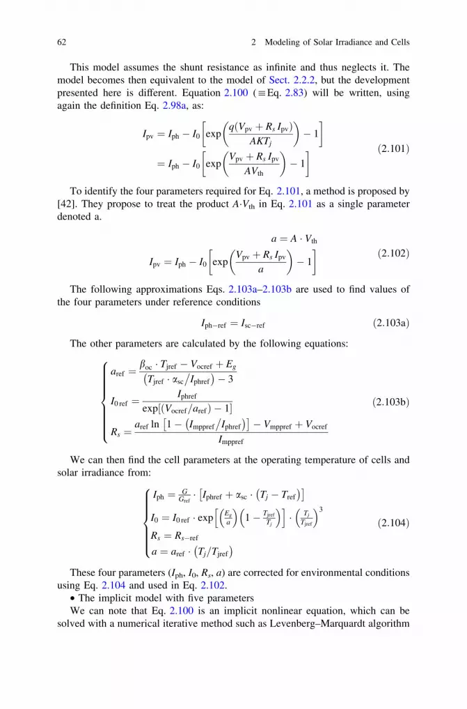
This model assumes the shunt resistance as infinite and thus neglects it. Themodel becomes then equivalent to the model of Sect. 2.2.2, but the developmentpresented here is different. Equation 2.100 (:Eq. 2.83) will be written, usingagain the definition Eq. 2.98a, as:

Ipv ¼ Iph � I0 expqðVpv þ Rs IpvÞ

AKTj

� �

� 1

� �

¼ Iph � I0 expVpv þ Rs Ipv

AVth

� �

� 1

� � ð2:101Þ

To identify the four parameters required for Eq. 2.101, a method is proposed by[42]. They propose to treat the product A�Vth in Eq. 2.101 as a single parameterdenoted a.

a ¼ A � Vth

Ipv ¼ Iph � I0 expVpv þ Rs Ipv

a

� �

� 1

� � ð2:102Þ

The following approximations Eqs. 2.103a–2.103b are used to find values ofthe four parameters under reference conditions

Iph�ref ¼ Isc�ref ð2:103aÞ

The other parameters are calculated by the following equations:

aref ¼boc � Tjref � Vocref þ Eg

Tjref � asc

�

Iphref

� 3

I0 ref ¼Iphref

exp Vocref=arefð Þ � 1½ �

Rs ¼aref ln 1� Imppref

�

Iphref

� �

� Vmppref þ Vocref

Imppref

8

>

>

>

>

>

>

>

<

>

>

>

>

>

>

>

:

ð2:103bÞ

We can then find the cell parameters at the operating temperature of cells andsolar irradiance from:

Iph ¼ GGref� Iphref þ asc � Tj � Tref

� �

I0 ¼ I0 ref � expEg

a

�

1� Tjref

Tj

�h i

� Tj

Tjref

�3

Rs ¼ Rs�ref

a ¼ aref � Tj=Tjref

8

>

>

>

>

>

<

>

>

>

>

>

:

ð2:104Þ

These four parameters (Iph, I0, Rs, a) are corrected for environmental conditionsusing Eq. 2.104 and used in Eq. 2.102.

• The implicit model with five parametersWe can note that Eq. 2.100 is an implicit nonlinear equation, which can be

solved with a numerical iterative method such as Levenberg–Marquardt algorithm


which requires a close approximation of initial parameter values to attain con-vergence. Different analytical methods can be used to extract parameters.

1. Proposed analytical methodThe five parameters IL, I0, Rs, Rsh, and A are calculated at a particular tem-

perature and solar-irradiance level from the limiting conditions of Voc, Isc, Vmpp,Impp and using the following definitions of Rso and Rsho. Ipv(ipv) characteristic ofthis model is given by Eq. 2.100. rewritten using again definition Eq. 2.98a:

Ipv ¼ Iph � I0 expVpv þ Rs Ipv

AVth

� �

� 1

� �

� Vpv þ Rs Ipv

Rsh

ð2:105Þ

For Vpv = Voc, Ipv = 0, we have:

0 ¼ Iph � I0 expVoc

AVth

� �

� 1

� �

� Voc

Rsh

ð2:106Þ

For Vpv = 0, Ipv = Isc, we have:

Isc ¼ Iph � I0 expIscRs

AVth

� �

� 1

� �

� IscRs

Rsh

ð2:107Þ

Replacing Iph in Eq. 2.107 by its value extracted from Eq. 2.106, we have:

Isc ¼ I0 expVoc

AVth

� 1

� �

þ Voc

Rsh

� I0 expIscRs

AVth

� �

� 1

� �

� IscRs

Rsh

ð2:108Þ

Isc ¼ I0 expVoc

AVth

� expIscRs

AVth

� �

þ Voc

Rsh

� IscRs

Rsh

ð2:109Þ

Thus

I0 expVoc

AVth

� expIscRs

AVth

� �

þ Voc

Rsh

� Isc 1þ Rs

Rsh

� �

¼ 0 ð2:110Þ

We derive Eq. 2.105 with respect to the current:

1 ¼ �I0dVpv

dIpv

1AVth

þ Rs

AVth

� �

expVpv þ IpvRs

AVth

� 1Rsh

dVpv

dIpv

� Rs

Rsh

¼ � I0

AVth

expVpv þ IpvRs

AVth

dVpv

dIpv

� I0Rs

AVth

expVpv þ IpvRs

AVth

� 1Rsh

dVpv

dIpv

� Rs

Rsh

ð2:111Þ

� dVpv

dIpv

I0

AVth

expVpv þ IpvRs

AVth

þ 1Rsh

� �

� I0Rs

AVth

expVpv þ IpvRs

AVth

� Rs

Rsh

� 1 ¼ 0

ð2:112Þ

For Vpv = Voc we define


dVpv

dIpv

� �

Vpv¼VOC

¼ �Rs0 ð2:113Þ

Replacing Eq. 2.113 in Eq. 2.112, we find

Rs0I0

AVth

expVoc

AVth

þ 1Rsh

� �

� I0Rs

AVth

expVoc

AVth

� Rs

Rsh

� 1 ¼ 0

Rs0 � Rsð Þ I0

AVth

expVoc

AVth

þ 1Rsh

� �

� 1 ¼ 0

ð2:114Þ

For Ipv = Isc, we define:

dVpv

dIpv

� �

Ipv¼ISC

¼ �Rsh0 ð2:115Þ

Replacing Eq. 2.115 in Eq. 2.112 we find:

Rsh0

I0

AVth

expIscRs

AVth

þ 1Rsh

� �

� I0Rs

AVth

expIscRs

AVth

� Rs

Rsh

� 1 ¼ 0

Rsh0�RSð Þ I0

AVth

expIscRs

AVth

þ 1Rsh

� �

� 1 ¼ 0

ð2:116Þ

Dividing Eq. 2.116 by (Rsh0-Rs), we find

1Rsh

� 1Rsh0�Rs

þ I0

AVth

expIscRs

AVth

¼ 0 ð2:117Þ

At maximum power point, we have

Impp ¼ Iph � I0 expVmpp þ ImppRs

AVth

� 1

� �

� Vmpp þ ImppRs

Rsh

ð2:118Þ

From Eq. 2.106, we obtain

Iph ¼ I0 expVoc

AVth

� 1

� �

þ Voc

Rsh

ð2:119Þ

Substituting Eq. 2.119 into Eq. 2.118, we get

Impp ¼ I0 expVoc

AVth

� 1

� �

þ Voc

Rsh

� I0 expVmpp þ ImppRs

AVth

� 1

� �

� Vmpp þ ImppRs

Rsh

ð2:120Þ

I0 expVoc

AVth

þ Voc � Vmpp

Rsh

� I0 þ Impp

Rs

Rsh

� �

� I0 expVmpp þ ImppRs

AVth

¼ 0 ð2:121Þ

Kennerud and Charles showed that the four parameters A, Rs, I0, and Rsh can bedetermined by the Newton-Raphson solving simultaneous nonlinear equations


Eqs. 2.110, 2.114, 2.117 and 2.121. However, this method requires long calcula-tions and initial conditions for strict convergence hence, it is difficult to determinethese parameters. So it is necessary to have analytical expressions for determiningthese parameters directly.

As Rsh [ [ Rs, we assume for the parameters determination that

1þ Rs=Rsh � 1

In Eq. 2.110, we assume also:

expVoc

AVth

ii expIscRs

AVth

In Eq. 2.114, we assume:

I0

AVth

expVoc

AVth

ii 1RSh

Finally, in Eq. 2.117, we assume: I0AVth

expVpvþIpvRserial

AVthhh10% of the remaining

terms.With these simplifications, we get from Eqs. 2.110, 2.114, 2.117 and 2.121:

I0 expVoc

AVth

� Isc þVoc

Rsh

¼ 0 ð2:122Þ

Rs0 � RSð Þ I0

AVth

expVoc

AVth

� 1 ¼ 0 ð2:123Þ

Rsh ¼ Rsh0 ð2:124Þ

I0 expVoc

AVth

þ Voc � Vmpp

Rsh

� Impp � I0 expVmpp þ Impp � Rs

AVth

¼ 0 ð2:125Þ

From these last four equations, we obtain an analytic expression of A. For that,from Eq. 2.122, we have:

I0 ¼ Isc �Voc

Rsh

� �

exp � Voc

AVth

� �

ð2:126Þ

From Eq. 2.123, we have

Rs0 � Rs ¼1

I0AVth

exp Voc

AVth

Rs ¼ Rs0 �1

I0AVth

exp Voc

AVth

¼ Rs0 �1

1AVth

Isc � Voc

Rsh

�

ð2:127Þ


Substituting Eq. 2.126 into Eq. 2.125, we obtain:

Isc �Voc

Rsh

þ Voc � Vmpp

Rsh

� Impp ¼ I0 expVmpp þ Impp � Rs

AVth

Isc �Vmpp

Rsh

� Impp ¼ Isc �Voc

Rsh

� �

exp � Voc

AVth

þ Vmpp þ Impp � Rs

AVth

� �

or, substituting Eq. 2.127 in that equation:

Isc � Vmpp

Rsh� Impp

Isc � Voc

Rsh

¼ exp�Voc þ Vmpp þ ImppRs0 � Impp�A�Vth

Isc�Voc=Rsh

AVth

!

lnIsc � Vmpp

Rsh� Impp

Isc � Voc

Rsh

!

¼ �Voc þ Vmpp þ ImppRs0

AVth

� Impp

Isc � Voc

Rsh

Finally, we obtain the expression of A

A ¼ Vmpp þ ImppRs0 � Voc

Vth ln Isc � Vmpp

Rsh� Impp

�

� ln Isc � Voc

Rsh

�

þ Impp

Isc�VocRsh

� �� ð2:128Þ

and I0, Rs and Iph are obtained by

I0 ¼ Isc �Voc

Rsh

� �

exp � Voc

AVth

� �

Rs ¼ Rs0 �AVth

I0exp � Voc

AVth

� �

Iph ¼ Isc 1þ Rs

RSh

� �

þ I0 expIscRs

AVth

� 1

� �

8

>

>

>

>

>

>

>

<

>

>

>

>

>

>

>

:

ð2:129Þ

Once these parameters (A, Iph, Rs, and I0) are determined, the Ipv–Vpv charac-teristic will be calculated by Eq. 2.100 using the Newton Raphson method.

2. Second method (Method of Pi constants)The model can be enhanced by releasing the constraint of linearity between the

photocurrent Iph and the irradiance G. For that, we make choice of an expressionfor Iph with a term quadratic in G:

Iph ¼ P1 � G � ½1þ P2 � ðG� GrefÞ þ P3 � ðTj � TrefÞ� ð2:130Þ

where G is irradiance on the panel plane (W/m2); Gref corresponds to the referenceirradiance of 1000 W/m2 and Tjref to the reference panel temperature of 25�C. P1,P2 and P3 are constant parameters.


The polarization current Id of junction PN, is given by the expression:

Id ¼ I0 � expq � ðVpv þ Rs � IpvÞA � Ns�cell � K � Tj

� �

� 1

� �

ð2:131Þ

I0 ¼ P4 � T3j � exp � Eg

K � Tj

� �

ð2:132Þ

where I0 (A) is the saturation current, q is the elementary charge, K Botzman’sconstant, A ideality factor of the junction, Tj junction temperature of the panels(�K), Rs and Rsh (X) are resistors (series and shunt) and ns the number of cells inseries.

The shunt current is given by:

IRsh ¼Vpv þ Rs � Ipv

Rsh

ð2:133Þ

Thus

Ipv ¼ P1 � G � 1þ P2 � G� Grefð Þ þ P3 � Tj � Tref

� �

� P4 � T3j � exp � Eg

K � Tj

� �

� exp q �Vpv þ Rs � Ipv

A � ns � K � Tj

� �

� 1

� �

�Vpv þ Rs � Ipv

Rsh

ð2:134Þ

Different methods exist to determine the constant parameters P1, P2, P3, and P4.• First approachWe determine the seven constant parameters P1, P2, P3, P4, the coefficient

A and the resistance Rs and Rsh of PV model with a numerical resolution and theuse of data sheets PV panels. Parameters commonly provided by module manu-facturers are values of short-circuit current Isc, the open-circuit voltage Voc and thepoint of optimum power (Impp, Vmpp). We determine the system of nonlinearequation as follows:

IpvðVocÞ ¼ 0

Ipvð0Þ ¼ Isc

IpvðVmppÞ ¼ Impp

dPpv

dVpv

�

�

�

�

P¼Pmpp

¼ Impp þdIpv

dVpv

�

�

�

�

I¼Impp

V¼Vmpp

¼ 0

8

>

>

>

>

>

>

<

>

>

>

>

>

>

:

ð2:135Þ

In order to determine all the seven parameters, three additional equations areneeded. In order to determine P2, points with different irradiance are necessary.Similarly, in order to determine P3, points with different temperatures are needed.

The system resolution of the nonlinear Eq. 2.135 is done by running thefunction ‘fsolve’ contained in toolboxes of Matlab which is based on the leastsquares method (Fig. 2.16).


• Second approachTo determine the parameters of the panels (Pi, Rs, Rsh), we developed a method

based on optimization techniques to find the extrema for the function indicated. Itsprinciple is simple; it consists in the first step to define an objective function,called a criterion. This criterion E depends on a set of parameters grouped in avector p. This objective function is the error between the practical results and thoseof the simulation. It is given by:

Beginning

Write the program executing the statement of nonlinear Eq.2.134

Introduction of initial conditions

[ ]shserial4321o RRAPPPPX =

Resolution of )X(F by the function:

)X),X(F(fsolvea o=

Convergence Test:

ε≈)(aF ?

[ ]shserial4321 RRAPPPP)i(Xa ==

End

No

Yes

Fig. 2.16 Flowchart of resolution with parameters Pi


EðpÞ ¼ Ipv� exp � Ipv�sim

Ipv� exp

ð2:136Þ

with Ipv-sim is calculated from Eq. 2.134 for the model with a diode, using a widerange of variation of the illumination received by the photovoltaic panel, p con-tains various parameters to determine (P1, P2, P3, P4, A, Rs, Rsh). We use the least

Begining

Introduction Ipv(Vpv) characteristics

Value of i

Experimental values of Ipvi-exp and Vpvi-exp

Calcul of Ipvi-sim (Eq 2.100)

Calcul of Ei

I=i-1

Maximiser Ei

Yes

Noi

Display Pi parameters

End

Fig. 2.17 Flowchart to determine the parameters of the panels (Pi, Rs, Rsh)


squares method to find the value of P that minimizes the function R (E(p))2. Wepresent the proposed flowchart (Figs. 2.17, 2.18, 2.19).

Application in Matlab/simulink (see CD program-model 1)The simulated current–voltage (Ipv–Vpv) characteristic and power-voltage (Ppv–

Vpv) of the PV Module is shown in Fig. 2.20. The characteristic is obtained at aconstant level of irradiance and by maintaining a constant cell temperature.

The variation in both the Ipv–Vpv and Ppv–Vpv characteristics with irradiancelevel are simulated and the results are shown in Fig. 2.21.

Fig. 2.18 Bloc diagram of the PV model [195]

Fig. 2.19 PV subsystem model [195]


Fig. 2.20 Characteristics Ipv = f (Vpv) and Ppv = f (Vpv) in STC conditions

Fig. 2.21 Effects of solar irradiance changing

Fig. 2.22 Effects of temperature changing


The simulated Ipv–Vpv and Ppv–Vpv characteristics of the solar cell at differentcell temperatures are shown in Fig. 2.22.

We make validation through the following experimental bench: We can use themethod of resistance variation or the charging and discharging capacitor method.First, we measure the irradiation after we close the switch K1. The capacitorcharges, we measure the different values of current and voltage panel. To dischargethe capacitor, we open the switch K1 and close K2 (Figs. 2.23, 2.24, 2.25, 2.26).

2.2.1.4 Model No. 2

The second model here presented has no physical meaning, but is characterized bya very simple resolution. It requires only four parameters namely Isc, Voc, Vmp, andImp. The form of the Ipv–Vpv characteristic of this model is loosely based on that ofModel No. 1, that is to say:

Fig. 2.23 Experimental bench [9]

Fig. 2.24 Comparison of experimental results with simulation ones [195]


Ipv ¼ Isc 1� C1 expVpv

C2 � Voc

� �

� 1

� ��

ð2:137Þ

That equation fits exactly the short-circuit point.The open-circuit and maximum power points are approximately restituted with:

C2 ¼Vmpp

Voc

�

� 1

ln 1� Impp

Isc

�

C1 ¼ 1� Impp

Isc

� �

exp � Vmpp

C2 � Voc

� �

ð2:138Þ

The simple relationship of power for a photovoltaic module is

Fig. 2.25 Bloc diagram of Model No. 2 [195]

Fig. 2.26 PV subsystem (Model No. 2) [195]


Ppv ¼ Isc 1� C1 expVpv

C2 � Voc

� �

� 1

� ��

� Vpv ð2:139Þ

The constant parameters can be determined directly by Eq. 2.138.Application in Matlab/simulink(see CD program-model2)Figure 2.27 below shows the characteristic power/voltage and current/voltage

obtained under the STC conditions (Standard Test Condition G = 1000 W/m2,Tj = 25�C)

The Figs. 2.28, 2.29 and 2.30 show the influence of irradiance G and temper-ature Tj on the electrical characteristics.

2.2.1.5 Model No. 3

The third model offers one more freedom degree than Model No. 2. The PV arraycurrent Ipv obeys to the expression:

Fig. 2.27 Characteristics Ipv = f (Vpv) and Ppv = f (Vpv) under the STC conditions (Model No. 2)

Fig. 2.28 Effects of irradiance changing (Model No. 2)


Ipv ¼ Isc � f1� C1½expðC2VmpvÞ � 1�g ð2:140Þ

All the three rated points are exactly fitted if the coefficients C1, C2 andm verify:

C2 ¼C4

Vmoc

C3 ¼ lnIscð1þ C1Þ � Impp

C1Isc

� �

C4 ¼ ln1þ C1

C1

� �

m ¼ln

C3C4

h i

lnVmpp

Voc

h i

Fig. 2.29 Effect of temperature changing (model No. 2)

Fig. 2.30 Effects of irradiance and temperature changing (model No. 2)


with Vmpp voltage at maximum power point; Voc open-circuit voltage; Impp currentat maximum power point; Isc short-circuit current. The parameters determination isachieved with the arbitrary condition

C1 ¼ 0:01175

Equation 2.140 is only applicable at one particular irradiance level G and celltemperature Tj, at standard test conditions (STC) (G = 1000 W/m2, Tj = 25�C).When irradiance and temperature vary, the parameters change according to thefollowing equations:

DTj ¼ Tj � Tjref

DIpv ¼ asc

G

Gref

� �

DTj þG

Gref

� 1

� �

Isc;ref

DVpv ¼ �bocDTj � RsDIpv

ð2:141Þ

where asc is the current temperature coefficient and boc the voltage temperaturecoefficient.

The new values of the photovoltaic voltage and the current are given by

Vpv; new ¼ Vpv þ DVpv

Ipv; new ¼ Ipv þ DIpv

ð2:142Þ

The simple relationship of power for a photovoltaic module is (Fig. 2.31)

Ppv ¼ Iscf1� C1 expðC2VmpvÞ � 1

h i

g � Vpv ð2:143ÞApplication under Matlab/simulink (see CD program-model 3)The Fig. 2.32 shows the characteristic power/voltage and current/voltage

obtained under the STC conditions (Figs. 2.33, 2.34, 2.35).We make validation through the experimental bench given in Fig. 2.26. We

obtain the following results (Fig. 2.36) comparing to the simulation ones.

2.2.1.6 Model No. 4

The fourth model is based on references [39, 40] and [43]. The advantage of thismodel is that it can be established using only standard data for the module andcells, provided by the manufacturer (data sheets). This model is simple, because itis independent of the saturation current I0. The current delivered by the solarmodule (Ipv) in any conditions is given by

Ipv ¼ Isc�pv � 1� expVpv � Voc�pv þ Rs�pv � Ipv

A � Vth�pv

� �

� exp�Voc�pv

A � Vth�pv

� ��

ð2:144Þ


Fig. 2.32 Characteristics Ipv = f (Vpv) and Ppv = f (Vpv) under the STC conditions(Model No. 3)[195]

Fig. 2.31 Bloc diagram of Model No. 3 [195]


Fig. 2.33 Effects of solar irradiance changing (Model No. 3) [195]

Fig. 2.34 Effects of temperature changing (Model No. 3) [195]

0 5 10 15 20 25 30 35 40 45 500

0.5

1

1.5

2

2.5

3

3.5

4

4.5

5

G=900W/m², Tc=35°C

G=650W/m², Tc=33°C

G=450W/m², Tc=25°C

0 5 10 15 20 25 30 35 40 45 500

20

40

60

80

100

120

G=900W/m², Tc=35°C

G=650W/m², Tc=33°C

G=450W/m², Tc=25°C

Pow

er(W

)

Voltage(V)

Cur

rent

(A)

Voltage(V)

Fig. 2.35 Characteristics Ipv = f (Vpv) and Ppv = f (Vpv) (Model No. 3) [195]


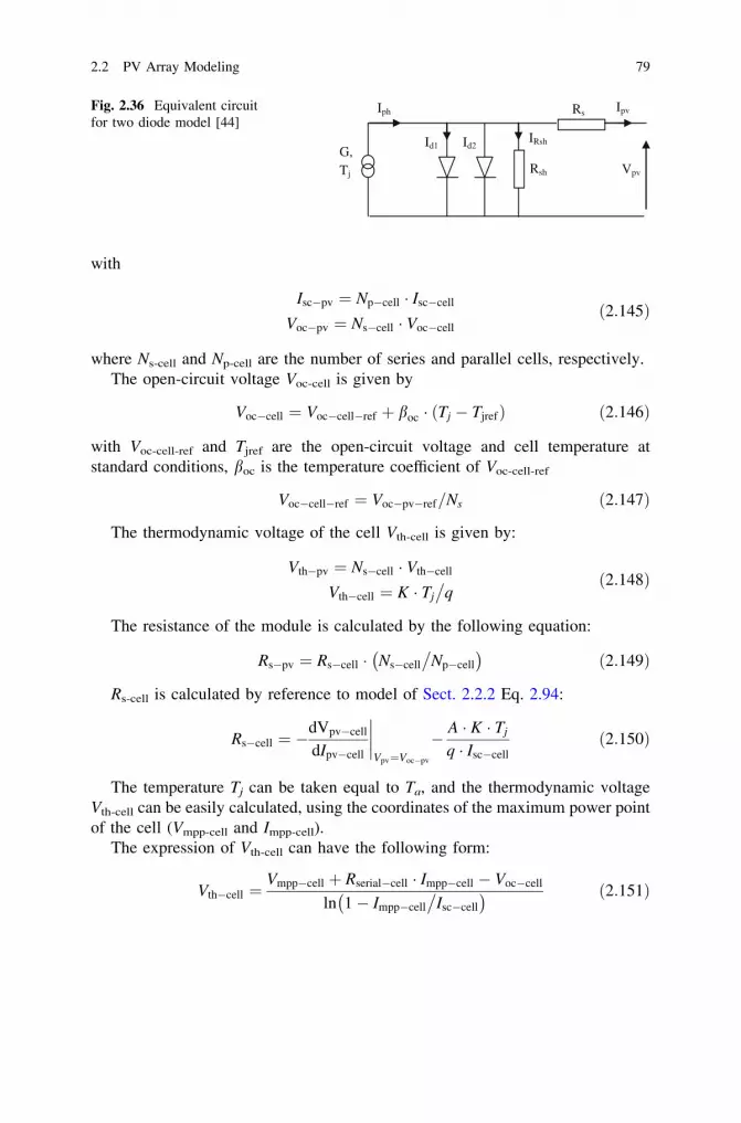
with

Isc�pv ¼ Np�cell � Isc�cell

Voc�pv ¼ Ns�cell � Voc�cell

ð2:145Þ

where Ns-cell and Np-cell are the number of series and parallel cells, respectively.The open-circuit voltage Voc-cell is given by

Voc�cell ¼ Voc�cell�ref þ boc � ðTj � TjrefÞ ð2:146Þ

with Voc-cell-ref and Tjref are the open-circuit voltage and cell temperature atstandard conditions, boc is the temperature coefficient of Voc-cell-ref

Voc�cell�ref ¼ Voc�pv�ref=Ns ð2:147Þ

The thermodynamic voltage of the cell Vth-cell is given by:

Vth�pv ¼ Ns�cell � Vth�cell

Vth�cell ¼ K � Tj

�

qð2:148Þ

The resistance of the module is calculated by the following equation:

Rs�pv ¼ Rs�cell � Ns�cell

�

Np�cell

ð2:149Þ

Rs-cell is calculated by reference to model of Sect. 2.2.2 Eq. 2.94:

Rs�cell ¼ �dVpv�cell

dIpv�cell

�

�

�

�

Vpv¼Voc�pv

� A � K � Tj

q � Isc�cell

ð2:150Þ

The temperature Tj can be taken equal to Ta, and the thermodynamic voltageVth-cell can be easily calculated, using the coordinates of the maximum power pointof the cell (Vmpp-cell and Impp-cell).

The expression of Vth-cell can have the following form:

Vth�cell ¼Vmpp�cell þ Rserial�cell � Impp�cell � Voc�cell

ln 1� Impp�cell

�

Isc�cell

ð2:151Þ

G,Tj

Iph Ipv

Id1IRsh

Rsh

Rs

Vpv

Id2

Fig. 2.36 Equivalent circuitfor two diode model [44]


2.2.2 Two Diode PV Array Models

The ‘‘two diodes’’ model uses an equivalent circuit and takes into account themechanism of electric transport of charges inside the cell. In this model, the twodiodes represent the PN junction polarization phenomena. These diodes representthe recombination of the minority carriers, which are located both at the surface ofthe material and within the volume of the material (Fig. 2.36).

The following equation is then obtained:

Ipv ¼ Iph � ðId2 þ Id2Þ � IRsh ð2:152Þ

with Iph and IRsh maintaining the same expressions as above Eqs. 2.130 and 2.133.For the recombination currents, we have:

Id1 ¼ I01 � expq�ðVpvþRs�IpvÞA�Ns�cell�K�Tj

�

� 1h i

Id2 ¼ I02 � expq�ðVpvþRs�IpvÞ2�A�Ns�cell�K�Tj

�

� 1h i

8

<

:

ð2:153Þ

The saturation currents are written as:

I01 ¼ P4 � T3j � exp

�Eg

k�Tj

�

I02 ¼ P5 � T3j � exp

�Eg

2�k�Tj

�

8

<

:

ð2:154Þ

with Ns is the number of cells in branched series.The final equation of the model is thereby written as (Figs. 2.37, 2.38):

Ipv ¼ P1 � G � 1þ P2 � G� Grefð Þ þ P3 � Tj � Tref

� �

�Vpv þ Rs � Ipv

Rsh

� P4 � T3j � exp

�Eg

k � Tj

� �

� exp q � Vpv þ Rs � Ipv

A � Ns�cell � K � Tj

� �

� 1

� �

� P5 � T3j � exp

�Eg

2 � k � Tj

� �

� exp q � Vpv þ Rs � Ipv

2 � A � Ns�cell � K � Tj

� �

� 1

� �

ð2:155Þ

Application under Matlab/simulink(see CD program-modele2D)We make validation through the experimental bench given in Fig. 2.25. We

obtain the following results (Fig. 2.39) comparing to the simulation ones.

2.2.3 Power Models

2.2.3.1 Model No. 1: Polynomial Model

This model can give the same power of solar modules operating at MPP (Maxi-mum Power Point). It is intended to polycrystalline silicon technology. Themaximum power Ppvmax can be given by [44] (Figs. 2.40, 2.41, 2.42):


Ppv�max ¼ K1 � ð1þ K2ðTj � TjrefÞÞ:ðK3 þ GÞ ð2:156Þ

where K1, K2, and K3 are constants to be determined (data sheets)We can obtain the maximum power for a given irradiance G and panel tem-

perature Tj with only three constant parameters and then solve a simple equationEq. 2.156.

Fig. 2.38 Characteristics Ipv = f (Vpv) and Ppv = f (Vpv) simulation results (two diode model)[195]

Fig. 2.37 Block diagram of two diode model [195]


The identification parameter was carried from the maxima characteristic volt-age/power panels with experimental measurements performed on site. Actualvalues used for several surveys covering a wide range of variation of sunshineactions were taken as:

• K1 between 0.095 and 0.105 for a panel represents the dispersion characteristicsof the panels.

• K2 = -0.47%/�C drift in temperature of the panels.• a parameter (K3) added to the characteristic of the manufacturer, to obtain

results much more satisfying:

Application under Matlab (see CD program Power model 1)For this model, the optimization is given only on the maximum power. It is

possible to represent the curves corresponding to the variations of the maximumpower for different days in the year (summer, spring, winter).

2.2.3.2 Model No. 2

The following benchmark model can determine the maximum power provided by aPV module for given irradiance and temperature with only four constant param-eters to determine a, b, c, and d. These parameters are obtained solving a simpleequation system for a resulting set of measurement points sufficiently extended[30]. We have

Ppv�max ¼ ða � Gþ bÞ � Tj þ c � Gþ d ð2:157Þ

where Ppv-max is the maximum power output and where a, b, c, and d are positiveconstants which can be obtained experimentally.

Application under Matlab (see CD program Power model 2)

Fig. 2.39 Characteristics Ipv = f (Vpv) and Ppv = f (Vpv) comparison of experimental resultswith simulation ones(two diode model)


Fig. 2.41 Variations ofpower (Model No. 3) [195]

Fig. 2.42 Variations ofpower (Model No. 4) [195]

Time (hours)

07h 08h 09h 10h 11h 12h 13h 14h 15h 16h 17h 18h 19h0

10

20

30

40

50

60

70

80

90

100

Pow

er (

W)

journée d'étéjournée de printempsjournée d'hiver

Summer daySpring dayWinter day

Summer day

Spring day

Winter day

Fig. 2.40 Variations of power for different days of the year (Model No. 1) [9]


2.2.3.3 Model No. 3

The energy produced by a photovoltaic generator is estimated from the data theglobal irradiation on inclined plane, the ambient temperature data manufacturer forthe PV module used. The power output of PV array can be calculated from thefollowing equation [1]:

Ppv�max ¼ gpv:Apv � Nm � G ð2:158Þ

where Apv is the total area of the photovoltaic generator and ggen the efficiency ofthe photovoltaic generator.

gpv ¼ gr � gpc 1� ascðTj � TjrefÞ� �

ð2:159Þ

where G is a solar radiation on tilted plane module, gr is the reference efficiency ofthe photovoltaic generator, gpc is the power conditioning efficiency which is equalto 1 if a perfect maximum power tracker (MPPT) is used, asc is the temperaturecoefficient of short-current (/�K) as found on the datasheet, Tj is cell temperatureand Tjref is the reference cell temperature.

Application under Matlab (see CD program Power model 3)

2.2.3.4 Model No. 4

Jones and Underwood developed the following practical model in 2002 for theproduction of optimal output power of a photovoltaic module [30, 45]:

Ppv�max ¼ FF � Isc �G

Gref

� �

� Voc �lnðP1 � GÞ

lnðP1 � GrefÞ:Tjref

Tj

� �

ð2:160Þ

where P1 is a constant coefficient, which can be calculated by the followingformula:

P1 ¼Isc

Gð2:161Þ

FF is the Filling factor.

FF ¼ Ppv max

Voc � Isc

¼ Vmpp Impp

Voc Isc

with Ppv-max the maximum power under STC conditions.Application under Matlab (see CD program Power model 4)


2.2.4 General Remarks on PV Arrays Models

2.2.4.1 The Forgotten Equation

Some of the above described model use for the parameters identification the valuesof Vmpp and Impp. However, only one of them (see Eq. 2.135) makes use of the factthat the point (Vmpp, Impp) is the point at maximum power. And yet, for that point,it is easy to prove (see Eq. 1.7) that, whatever the used model may be,

dIpv

dVpv

�

�

�

�Vpv ¼ Vmpp¼ � Impp

Vmpp

ð2:162Þ

That additional equation allows determining one more parameter using the nom-inal values of a photovoltaic cell or module.

2.2.4.2 General Structure and Consequences

All the models above described which are based on an equivalent circuit have thesame general structure shown at Fig. 2.43.

The above described models differ only due to the nature of the nonlinearelement J in parallel on the current source Iph. Following the complexity of themodel, that element can be formed with a variable number of ideal elements: oneor two diodes and sometime a resistance Rsh.

The consequence of that general structure is that all the characteristics Ipv–Vpv

corresponding to the same junction temperature but different irradiance can beobtained by translation of one of them [13]. The translation has a vertical com-ponent DIph and a horizontal component –Rs DIph. It is then possible to deduce thevalue of Rs from the Ipv–Vpv characteristics without reference to one particularmodel. That method is thus an interesting alternative to Eqs. 2.94, 2.103b and2.129 for determining the series resistance Rs. It has the additional advantage toconsider globally the characteristics and not one particular point.

With the general structure of Fig. 2.43, we have, for a variation of Vpv

Fig. 2.43 General equivalentcircuit for PV cell or modulemodeling


http://dx.doi.org/10.1007/978-1-4471-2403-0_1

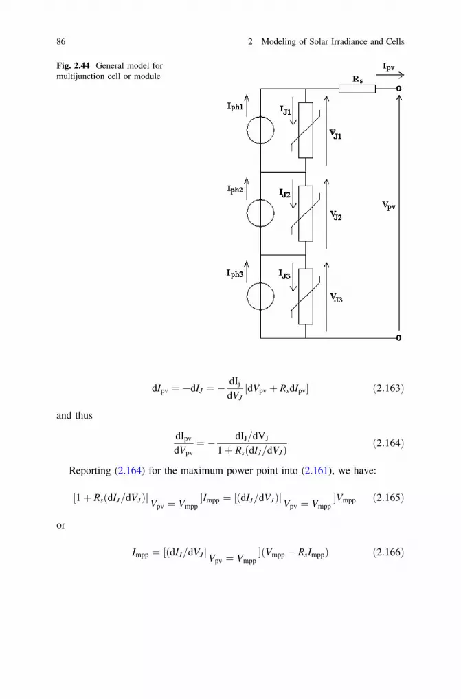
dIpv ¼ �dIJ ¼ �dIj

dVJ½dVpv þ RsdIpv� ð2:163Þ

and thus

dIpv

dVpv

¼ � dIJ=dVJ

1þ RsðdIJ=dVJÞð2:164Þ

Reporting (2.164) for the maximum power point into (2.161), we have:

½1þ RsðdIJ=dVJÞjVpv ¼ Vmpp�Impp ¼ ½ðdIJ=dVJÞjVpv ¼ Vmpp

�Vmpp ð2:165Þ

or

Impp ¼ ½ðdIJ=dVJ jVpv ¼ Vmpp�ðVmpp � RsImppÞ ð2:166Þ

Fig. 2.44 General model formultijunction cell or module


2.2.4.3 Partial Linearity of the Models

Starting with the values of open-circuit voltage, maximum power current andvoltage, and short-circuit current, we obtain in all case a system of four equations(three equations for the three nominal points and Eq. 2.165). That system is linearin Iph, 1/Rsh, Id1 and Id2. Then, no approximation formula is necessary for deter-mining that parameters. The only parameters which arrive in the equations systemin a nonlinear way are Rs and the non ideality factor A. If one uses the two diodesmodel, the simplest way is to assume that the factor A is unity. Then, beside Rs

which has to be determined by another way, all the parameters of the model aredetermined using the three nominal points.

2.2.4.4 Remark About the Multijunction Cells

All the above mentioned models are suited for single junction cells. In case ofmultijunction cells, the model of each cell corresponds to the series connection oftwo or three circuits with the structure of Fig. 2.43, but with different parameters.Summing all the Rs resistance in only one, we obtain the general model ofFig. 2.44. Of course, that model contains many too parameters. However, if themanufacturer has well equilibrated the junctions for the standard spectrum, wehave (for standard spectrum only) equality of the three current sources. In only thatcase we can combine the three nonlinear elements of Fig. 2.44 and retrieve thesimpler structure of Fig. 2.43.


Chapter 3Power Electronics Modeling

Symbols\g[ Mean value of a quantity gC Value of a capacitanceCpv Input capacitance of a converter connected to photovoltaic arrayf Internal frequency of the converteri Instantaneous value of a currentI Rms value of the currentk Ratio between input and output voltages of a converterkoff, kon Constants used for commutation losses estimationL Value of an inductancep Instantaneous value of a powerP Active power (mean power on a period)Pcap Mean power dissipated during commutations due to stray capacitancesPind Mean power dissipated during commutations due to stray inductancesploss Instantaneous value of a power dissipated as heatPloss Mean value of a power dissipated as heatPnom Nominal power of the converterPon Mean power of commutation losses related to transient from OFF to ON

statesPoff Mean power of commutation losses related to transient from ON to OFF

statesPQ Mean power of commutation losses related to recovery charge of nearby

componentsQ Value of an electric chargeRdiff Differential resistanceT Internal period of the converterton Time of variation of electrical quantities when going from OFF to ON

states


89

toff Time of variation of electrical quantities when going from ON to OFFstates

u Instantaneous value of a voltageUin Input voltage of a converterUin nom Nominal input voltage of a converterUthr Threshold voltagea Duty cycle of a convertergeur European efficiency.gx efficiency for an operating point at x percent of its nominal power

Photovoltaic generators are almost always associated with some control and powerelectronics. Even in the case of a direct connection between a solar array and abattery, a non-return diode is needed. Generally, more complex power electronicconverters are needed in order to adapt the electrical frequency and voltage level tothe planned use. In addition, the rational use of photovoltaic generators is possibleonly in association with power electronic converters in order to adjust the voltageof the photovoltaic array to the maximum power point independently of the outputvoltage of the system. Power electronic converters associated to photovoltaicgenerators have to verify constraints on quality of energy supplied (low level ofharmonics), electromagnetic perturbations (low level of EMC) and security. Forinstance, for photovoltaic generators connected to the AC mains, automaticdisconnection from the grid in case of grid islanding is required.

Once those constraints are satisfied, we can look to the properties that have aninfluence on the energy production of the whole system, i.e. the ability to track theMPPT and the power losses or, equivalently, the efficiency of the power electronicconverter.

As windmill systems, photovoltaic systems are fluctuating energy suppliers.The first consequence is that the velocity of the MPPT is important, but above all,these systems work during the most of the time at power levels very lower thantheir rated power. Thus, the rated efficiency of the power electronic converter isnot relevant.

In some cases, the only goal is to maximize the total energy supplied on a largetime interval (one year…). Then, we can achieve the design using a weightedaverage value of the efficiency. However, in many cases, it is necessary to studythe time evolution of the working point of the system. It is for example the casewhen we want to evaluate a risk of energy lack, or if the energy price varies duringthe time. Then, we have to know the efficiency as a function of the operating point(converted power, input and output voltage …). This is the main subject of thischapter.

90 3 Power Electronics Modeling

3.1 The Origin of Power Losses in Power Electronic Converters

3.1.1 Power Electronics Fundamentals

Power electronic converters are made up of power semiconductors switches (diodes,transistors….) and passive components. Passive components are mainly inductive(inductors, transformers, coupled inductors) or capacitive (capacitors). In non-reactive components (semiconductors, resistors), the power dissipated as heat insidethe components is equal to its instantaneous electric power

ploss ¼ ui ð3:1Þ

where u is the voltage and i the current of the component.A semiconductor acting as a switch has only two states, the ON state and the

OFF state. The transitions from one state to the other one are achieved in short timesnamed commutations. This use of semiconductors allows the reduction of theirlosses. Indeed, in the ON state, a significant current i can flow through the com-ponent, while the voltage u is low. The power (Eq. 3.1) dissipated during con-duction intervals is thus low. It is referred as the ‘‘conduction losses’’. Similarly, inthe OFF state, the voltage u across the component can take significant values, whilethe current which is flowing through it remains very small, so that the power (Eq.3.1) dissipated in the component is generally negligible in OFF state.

The structure of the power converter must take into account the characteristicsof the external circuits connected to its input and output ports. For example,a battery appears as a voltage source, and so it is not acceptable to short circuit it.Moreover, the use of the semiconductors as switches is associated to strongvariations of the currents and voltages inside the converter. Generally, thesevariations are not acceptable for the circuits connected at the input and output portsof the converter. For example, solar modules give all the possible power only attheir maximum power point (MPP). So, the converter may not induce significantvariations of current and voltage into the solar array. In order to satisfy the above-mentioned constraints, power electronic converter includes, in addition to semi-conductors, reactive (inductive and capacitive) components for filtering purpose.These components are not the ideal lossless elements of the circuit theory: they areprone to power losses. For example, the equivalent circuit of the inductivecomponent includes always a ‘‘parasitic’’ series resistance which generates con-duction losses. There are also magnetic losses in inductive components andleakage losses in capacitors.

There is also another type of losses due to the fact that the commutations of asemiconductor switch (transition from one state to the other one) are neverinstantaneous: during a short time interval, u and i take simultaneously significantvalues, so that a given energy amount is lost at each commutation. There is thus, inaddition to the conduction losses, commutation losses which are proportional tothe internal frequency of the converter.

3.1 The Origin of Power Losses in Power Electronic Converters 91

Today, most of power electronic converters are switching converters, i.e.converters in which the switching frequency of the semiconductor switches ismuch higher than the frequency found at the input and output ports of theconverter (0 Hz for a port connected to a DC circuit, 50 or 60 Hz for a portconnected to the AC mains).

According to the power rating of a converter, the switching frequency may rangefrom several kHz for high to medium power converters to more than 1 MHz for verylow power converters. The use of a high switching frequency makes easier thefiltering of the current and voltage ripples generated at the switching frequency at theinput and output of the converter. Moreover, as the energy which has to be storedinside the passive components is lower when the internal frequency is high, thefrequency increase allows reducing the size and the cost of the passive components.

Unfortunately, an increase of the switching frequency increases the commu-tation losses, so the choice of this frequency results from a compromise which ismainly ruled by the switching speed of the semiconductors. As the commutationlosses are lower when the components can commute faster, the optimal switchingfrequencies grow more and more as the semiconductor performances areimproved.

Finally, it is necessary to mention the power consumption of auxiliary circuits(drivers of the power switches, sensors, control and communication electronics).

3.1.2 Methods of Elementary Losses Modeling

In the case of a component which includes in its equivalent circuit a constant seriesresistance R, the power dissipation related to that resistance is simply

p ¼ R:i2 ð3:2Þ

Fig. 3.1 I-U curve for atypical power diode


And, thus the mean dissipated power during a switching cycle is

P ¼ R:I2 ð3:3Þ

where I is the rms value of the current flowing through the semiconductor duringthat cycle.

Many semiconductors in ON state exhibit a non-linear current–voltagecharacteristic, as shown in Fig. 3.1.

In that case, we consider often an approximate characteristic of the form

u ¼ Uthr þ Rdiff :I ð3:4Þ

where Rdiff is named ‘‘differential resistance’’ and Uthr is named ‘‘thresholdVoltage’’. In that case, it is easily found that the mean power related to con-duction losses during a cycle is, assuming that the current i can only have thepositive sign

P ¼ Uthr:hii þ RdiffI2 ð3:5Þ

where \ i [ is the mean value of the current i during that cycle.In the commutation losses of a semiconductor, we find a term proportional to

the time ton (time for going from the OFF-state to the ON-state). Noting u1 thevoltage just before that commutation and i1 the current just after it, we have:

Pon ¼ kon:u1:i1:ton:f ð3:6Þ

where f is the internal frequency of the converter and kon a constant.Similarly, we have a term proportional to the time toff (time for going from the

ON-state to the OFF-state). Noting i2 the current just before that commutation andu2 the current just after it, we find:

Poff ¼ koff :u2:i2:toff :f ð3:7Þ

Using approximate time dependence of the quantities (linear commutation), onefinds for kon and koff values in the range 0.2–0.5.

The commutation losses (Eq. 3.6) and (Eq. 3.7) can be reduced using shortercommutation times but one is limited in that way by the intrinsic limitations of thecomponent or when the maximum values of voltage and current reached during thetransient become too high for the components.

There is also commutation losses linked to the stray elements. So, if there isa stray inductance L in series with the commuting element (due to its con-nections, including the connection inside its packaging), we have power dissi-pation corresponding to the transfer of the inductance energy to the switch at itsturnoff.

Pind ¼12:L:i2

2:f ð3:8Þ


Similarly, if there is a stray capacitance C in parallel on a switch, it causespower dissipation corresponding to the transfer of the capacitance energy to theswitch at its turnon.

Pcap ¼12

Cu12 f ð3:9Þ

Finally, if there is in parallel on the component a source able to supply anelectric charge Q under the voltage u1, it causes power dissipation

PQ ¼ u1:Q:f ð3:10Þ

Magnetic losses in inductive components can be classified into two types.Hysteresis losses are proportional to the frequency f but they are growing

function of the flux variation. The flux variation is approximately equal to u/f, sofor a given frequency, they are growing with u. Eddy current losses are propor-tional to the frequency square f 2 and to the square of the flux, so they depend onlyof the square of the voltage.

3.1.3 The Most Used Power Semiconductors

The symbols of some power semiconductors with the name of their connectionsare shown in Fig. 3.2.

Diode (Fig. 3.2a) is not controllable. It becomes conducting when a smallvoltage is applied in the conduction direction otherwise it becomes blocking.

Thyristor (Fig. 3.2b) is only half controllable. It becomes conducting only if thevoltage between anode and cathode is positive and if a current pulse is applied ongate. It becomes blocking when the current tends to zero.

Other semiconductors of the Fig. 3.2 are fully controllable. Bipolar transistor(Fig. 3.2c) is conducting only if a base current is continuously applied. MosFettransistor (Fig. 3.2d) and IGBT (Fig. 3.2e) are in conduction only if a positive gatevoltage is applied.

Fig. 3.2 Symbol of somepower semiconductors.a Diode. b Thyristor.c bipolar transistor. d MosFettransistor. e IGBT. Arrowshows the current directionwhen the semiconductor isconducting


3.1.4 Particularities of the Semiconductors From the LossesPoint of View

Diode (Fig. 3.2a) exhibits a significant threshold voltage. So, in the expression(Eq. 3.5) of losses, the first term must be considered. The drawback is especiallypenalizing in case of low voltage converters. At low voltage, it can be reducedusing Schottky diodes. Another possibility is to replace diodes by MosFet at theprice of additional command circuits.

Thyristor (Fig. 3.2b), bipolar transistor (Fig. 3.2c) and IGBT (Fig. 3.2e) alsoexhibit a threshold voltage, but often lower than the threshold voltage of a diode.

Bipolar transistor (Fig. 3.2c) remains conducting only as long as a base currentis applied. This requires a circuit which is able to supply that current. It is thusnecessary in the energy balance to take into account the power consumption of thatcircuit, in addition to conduction losses.

MOSFET transistor (Fig. 3.2d) is controlled by gate voltage. At standstill thatvoltage can be maintained without current consumption. So, the control circuitconsumes energy only during the commutations. The MosFet can commute veryfast, then reducing the commutations losses (Eq. 3.6) and (Eq. 3.7). Moreover, itpresents no threshold voltage. It is thus possible to reduce the conduction losses byparalleling several MOSFET or, equivalently, using overrated MOSFET. As arough estimate, IGBT behaves like the bipolar transistor for the main circuit, but asthe MosFet for the command circuit.

3.2 The Structures of Converters and the Influenceon Their Efficiencies

Inside this section, we shall use the symbol of Fig. 3.3 for any of the fullycontrolled power switch, i.e. bipolar transistor (Fig. 3.2c), MOSFET transistor(Fig. 3.2d) or IGBT (Fig. 3.2e).

In the following examples, the command of these semiconductors is a periodicdigital signal whose period is T = 1/f, f being the internal frequency of theconverter. The duty cycle a of that signal, as shown in Fig. 3.3, is the ratio betweenthe duration a T in the state ‘‘on’’ and the entire period T. We do not give here adetailed description of quantities time evolution: interested readers can find suchan analysis in classical power electronics textbooks such as [50, 51].

Fig. 3.3 Generic symbolfor any of the fully controlledpower switches


The choice of the internal frequency f results from a compromise. In one hand, ahigh frequency f allows for an easier filtering of the harmonics at input and output,and thus lowers losses in passive components. On the other hand, commutationlosses (and command losses in case of MosFet or IGBT) increase proportionally tothat frequency. It thus exists an optimum frequency. This optimum can depend onthe working point, but, for practical reasons, designers often opt for a fixedfrequency.

3.2.1 Direct Connection to a DC Bus

The simplest interface between a photovoltaic array and a constant voltage DC bus(for example a battery) is to use only one diode (Fig. 3.4).

This circuit has little losses, but, as it is not controlled, the voltage of the PV isfixed. As the optimum voltage value is temperature and irradiation dependent, theuse of PV is often far away from the optimum point, and PV cannot supply currentwhen its open-circuit voltage is lower than the DC bus voltage. As that interfacehas no command possibility, it is often completed by a circuit which can short-circuit or disconnect the PV array when the battery and the load are not able toabsorb all the available power.

3.2.2 DC/DC Conversion

3.2.2.1 Transformerless DC/DC Converters

The simplest controllable converters are made of only one transistor, one diodeand one inductor as main components. When the input of the converter is the PVarray, the best efficiency can be obtained with the boost converter (Fig. 3.5).

For the boost converter, when the duty ratio a goes from 0 to 1, ratio k betweeninput and output voltages goes from 1 to 0. So, it is possible to obtain energyproduction even for low irradiance (for example at sunrise and sunset). The designmust be done in a way that the open-circuit voltage of the PV remains most of thetime lower than the DC bus voltage. However, in order to obtain a good efficiency,the input and output voltage levels cannot be too different. Indeed, considering the

Fig. 3.4 Direct connectionof a PV array to a DC bus


input and output current and voltage, the sizing is governed by the product of thebigger voltage by the bigger current. A big value of the ratio k leads to oversizedconverter, and then lower efficiency. For that reason, the output voltage is not toolarge and one can admit that, occasionally, the optimum PV voltage becomeshigher than the output voltage. When that case occurs, the converter reduces todirect connection (Fig. 3.4) but it remains possible to short-circuit the PV ifnecessary by keeping the transistor ‘‘on’’.

The fact that the inductor is in series with input is interesting because itmaintains constant the current value during the period T, which is suitable tomaintain continuously PV voltage at its optimum value.

In some cases, the PV optimum voltage is most of time higher than the DC busvoltage. It is often the case with a 12 V battery and commercial PV modules. Insuch a case, the buck converter (Fig. 3.6) can be interesting.

However, with the buck converter, when the duty ratio a goes from 0 to 1, ratiok between input and output voltages goes from 1 to ?. So, it is not possible toobtain energy production when open voltage of the PV is low (for example atsunrise and at sunset). The buck-boost converter (Fig. 3.7) does not have thatdrawback because it allows for using all the values of k between 0 and ?.However, efficiency of the buck-boost converter is slightly lower then the effi-ciencies of boost or buck converters because, in the buck-boost converter, all theenergy carried from input to output is transiently stored inside the inductor. Theinput current of the buck converter and of the buck-boost converter is chopped, sothat in the case of using PV, filtering by a capacitor in parallel on the input isnecessary.

3.2.2.2 DC/DC Converters with Transformer

As above mentioned, the efficiency of the DC/DC converters of the Sect. 3.3.2.1 islowered if the input and output voltage are at very different levels. In that case,

Fig. 3.5 Power componentsof the boost converter

Fig. 3.6 Buck converter

3.2 The Structures of Converters and the Influence on Their Efficiencies 97

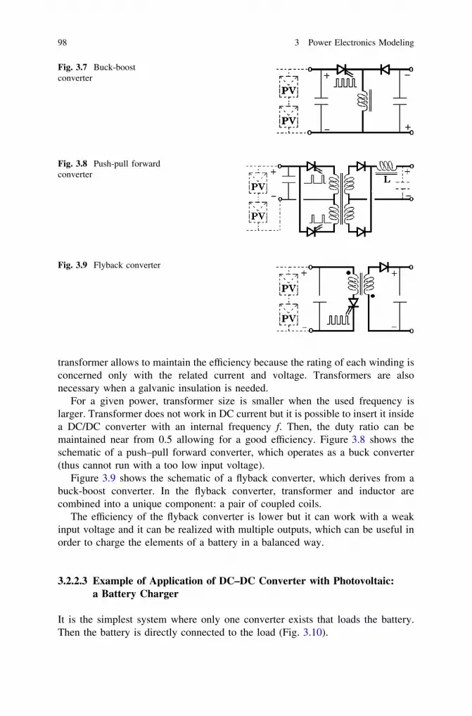
transformer allows to maintain the efficiency because the rating of each winding isconcerned only with the related current and voltage. Transformers are alsonecessary when a galvanic insulation is needed.

For a given power, transformer size is smaller when the used frequency islarger. Transformer does not work in DC current but it is possible to insert it insidea DC/DC converter with an internal frequency f. Then, the duty ratio can bemaintained near from 0.5 allowing for a good efficiency. Figure 3.8 shows theschematic of a push–pull forward converter, which operates as a buck converter(thus cannot run with a too low input voltage).

Figure 3.9 shows the schematic of a flyback converter, which derives from abuck-boost converter. In the flyback converter, transformer and inductor arecombined into a unique component: a pair of coupled coils.

The efficiency of the flyback converter is lower but it can work with a weakinput voltage and it can be realized with multiple outputs, which can be useful inorder to charge the elements of a battery in a balanced way.

3.2.2.3 Example of Application of DC–DC Converter with Photovoltaic:a Battery Charger

It is the simplest system where only one converter exists that loads the battery.Then the battery is directly connected to the load (Fig. 3.10).

Fig. 3.7 Buck-boostconverter

Fig. 3.8 Push-pull forwardconverter

Fig. 3.9 Flyback converter


The function of the battery charger is providing energy to a battery bank undercontrolled voltage and current, in order to improve the service lifetime of thebattery bank. We consider as example the circuit of Fig. 3.6 (buck converter). Tomodel the battery charger, we use the equivalent circuit of Fig. 3.11.

As long as the battery is not fully charged, the control circuit act on the switchesof DC/DC converter in order to maximize the battery current. However, it canestimate the charge of the battery using measurements of battery voltage, currentand often temperature and current integral. It can thus limit the battery current if itsvalue is too large considering the battery state of charge. Often, the control circuitcan also acts on a relay in order to disconnect the load when the battery is toodischarged. In theory, a model of the battery is needed in order to estimate thebattery state of charge. Several control circuits include a fuzzy logic controllerwhich can determinate implicitly such a model after some cycles of charge.

3.2.3 DC/AC Conversion

3.2.3.1 Converters Topologies

DC/AC Converters (Single Stage Inverters)

When the power generated is transmitted to the public network, or used by ACdevices, it is necessary to use a DC/AC converter. The most popular is the voltageinverter, whose schematic is given at Fig. 3.12 (single phase inverter) or atFig. 3.13 (three phase inverter).

Fig. 3.10 Simple dc system

Fig. 3.11 Simplified modelof the battery charger


In order to avoid harmonics injection on the AC grid, output filtering is needed.For making that filtering with small reactance, it is necessary to use a highswitching frequency, which induces significant commutation losses. On the otherhand, the inverter does not provide galvanic insulation. Input voltage of thevoltage inverter must be higher than the peak value of the AC voltage, i.e. 315 Vin case of single phase 230 Vrms and 566 V in case of three phases 400 Vrms. Thus,if the output is connected to the public grid and the input to photovoltaic array, thisone must deliver a high voltage that is possible only for a series connection ofmany solar modules and leave only few possibilities MPPT. Moreover, in the caseof a single phase inverter, input current is modulated to twice the grid frequency;in that case, if the input is connected to a PV array, use of a capacitor CPV of largevalue in parallel to the input is needed in order to maintain the PV current at theoptimum value of the current. In the following, inverters shall be schematized as inFig. 3.14, as well as in case of single stage inverter of the Figs. 3.12 and 3.13 thanin case of more complex ones.

Complex DC/AC Converters (Multistage Inverters)

The drawbacks mentioned at the DC/AC convertors (Single stage inverters) can beavoided adding to the inverter other conversion stages. In fact, what is named

Fig. 3.12 Single phasevoltage inverter

Fig. 3.13 Three phase voltage inverter

Fig. 3.14 Single stageInverter


commercially ‘‘solar inverter’’ often includes several power electronic converters.As a first example, we can have a dual-stage inverter (Fig. 3.15). This topologyconsists of a DC–DC converter which is used for the MPPT, and a DC–AC inverter.The control signals applied to the power switches of the final stage can then be 180or 120� conduction at the grid frequency (50 or 60 Hz). Then, commutation lossesof the inverter are very low. This is possible without strong oversize output filter ifthe output from the DC–DC converter is modulated to follow a rectified sine wave.

Another example of double stage inverter is given in Fig. 3.16.In the Fig. 3.16, the DC link between the DC–DC converter which carries out

the MPPT and the inverter is fitted with a capacitor Clink. Then, it is no longerpossible for modulating the DC link voltage to follow a rectified sine wave. ButClink is used for energy storage in order to cover the power fluctuations peculiar tosingle phase AC grid. It is best suited for that use that the input capacitor CPV

because larger voltage fluctuations are acceptable on Clink. Cpv can then bestrongly reduced.

Insertion of a Transformer

In some cases, galvanic insulation is required for security reasons, or in order to allowgrounding of the photovoltaic array, which is necessary with some photovoltaictechnologies. Then, the insertion of a transformer inside the converter is needed.Another case where a transformer is requested is when voltage level of the DC inputand AC output are very different. Then, the use of a transformer allows keeping in theconverters duty cycles compatible with good efficiency. The simplest topologyincluding a transformer consists to insert a low frequency transformer (LFT) betweenthe output of the converter and the AC grid, as shown in Fig. 3.17.

Unfortunately, at low frequency, transformers are big, heavy and costly. Analternative is to include the transformer inside the DC link of Fig. 3.16. Astransformer does not work in DC, it is necessary to insert it between a DC–AC andan AC–DC converter. It is then possible to use a transformer operating at highfrequency (HFT). This leads to the general configuration described at Fig. 3.18.

Fig. 3.15 Example ofdouble-stage inverter

Fig. 3.16 Dual stage inverter


Another solution is to use as input stage a DC/DC converter with transformer,for example the converter of Fig. 3.8 or Fig. 3.9. Figure 3.19 shows a schematicwhere the input DC/DC converter is boost modified in order to include atransformer.

Multi-Input DC/AC Converters

When the optimum working points of the modules are not all the same ones, forexample in case of partial shade, it can be interesting to split the PV array in

Fig. 3.17 Inverter with LFT

Fig. 3.18 Inverter with HFT

Fig. 3.19 Example of complex ‘‘solar inverter’’ topology

Fig. 3.20 Multi-inputinverter


several subarrays, each of that subarray being fitted with its own converter andMPPT. We can also have a multi-input inverter (Fig. 3.20). This topology consistsof two DC–DC converters connected to the DC link of a common DC–ACinverter.

In that case, we can use several stages of the conversion: only the first stage isown to each subarray and subsequent stages are common. So, we can use at firststage a simple circuit such as a transformerless boost (Fig. 3.5) in order to keep agood efficiency in spite of the reduced power. Figure 3.21 shows a circuit made ofseveral boosts, a common fixed duty factor push–pull converter in order to adaptthe voltage level and to provide galvanic insulation, a storage capacitor and finallyan inverter.

An important aspect of multi-input inverters is that they can control severaldifferent energy sources, for example several photovoltaic subarrays and one windturbine generator.

3.2.3.2 Systems Configurations

In general, three types of configurations have been identified:

Central Plant Inverter

The past technology is the central plant inverter, and it was based on centralizedinverters that interfaced a large number of PV modules to the grid. The PVmodules were divided into series connections (called a string).These ones werethen connected in parallel, through string diodes, in order to reach high powerlevels (Fig. 3.22).

String Inverters and AC-Modules

The present technology consists of the string inverters and the AC modules. Thestring inverter is a reduced version of the centralized inverter, where a single stringof PV modules is connected to the inverter (Fig. 3.23). The present solutions use

Fig. 3.21 Example of complex ‘‘solar inverter’’ with several independent inputs


self-commutated DC–AC inverters, by means of IGBTs or MOSFETs, involvinghigh power quality in compliance with the standards.

At the limit case, it is possible to associate a DC/AC converter with eachmodule, which can then be called AC-modules (Fig. 3.24). This solution has theadvantage of being totally modular. It is an interesting solution when the photo-voltaic array is subject to complex shadows, since each module can always be usedat its optimal power. However, the DC/AC converters are complex since there is alarge difference in the input and output voltage levels, and their nominal power islow since each of them controls only one module. Their efficiency is thus relativelylow.

Multi-String Inverter

In the multi-string inverter several strings are interfaced with their own DC–DCconverter to a common DC–AC inverter (Fig. 3.25). It is an advantage comparedwith the centralized system, since every string can be controlled individually. It isalso an advantage compared with string inverters and AC modules, since the partof the converter which is critical from the losses point of view is an only DC/ACinverter, which has a higher power and thus a better efficiency.

The choice of appropriate configuration must be motivated by the use condi-tions imposed by the environment and situation.

Fig. 3.22 Central plantinverter

Fig. 3.23 String inverter


3.3 Empirical Modeling of the Converters

If we admit that the voltage and current on the components are proportional to thevoltage and currents at the ports of the converter, we conclude that, at view of thedeveloped expressions above, at fixed internal frequency f, the losses are a sum ofterms of the first and second order in the input and output current and voltage, plusa constant term due to the auxiliary circuits. This remark furnishes a help toidentify the expression of the losses using data of the manufacturer or otherexperimental measurements.

The data of the manufacturer are usually expressed in form of efficiency. It isthen possible to obtain losses using the relation between efficiency g, loss powerPloss and output power P

Ploss ¼1g� 1

� �

P ð3:11Þ

.

3.3.1 Case of Constant Voltage

In some cases, the converter operates with a constant voltage as well as at the inputand the output. This is for instance the case of a DC to AC converter connected

Fig. 3.24 AC modules

Fig. 3.25 Multi-string inverter

3.3 Empirical Modeling of the Converters 105

between a DC link and the public distribution network. In such a case, only thedependence with the currents has to be identified. As the power electronic con-verters exhibit often a very good efficiency, we assume that the power is the sameat the input than at the output. At fixed voltage (and fixed power factor in case ofAC output), the current is proportional to the power, so that it is sufficient toidentify the three coefficients of a second-order polynomial

Ploss ¼ Aþ BPþ CP2 ð3:12Þ

.In order to determine the three coefficients of Eq. 3.12, it is necessary to have

at one’s disposal three data. Manufacturer usually provides value of the effi-ciency at nominal power. A second data is the so named ‘‘European efficiency’’.It is a mean value of the efficiency at several values of the power. The‘‘European efficiency’’ is added for the fact that solar systems work most of thetime at lower power than their nominal power. It is a weighted average onefficiencies related to a histogram of solar irradiation at temperate latitude on anannual basis. Calling Pnom the nominal power of the converter and gx its effi-ciency for an operating point at x percent of its nominal power, European effi-ciency is defined as

geur ¼ 0:03g5 þ 0:06g10 þ 0:13g20 þ 0:10g30 þ 0:48g50 þ 0:20g100 ð3:13Þ

Knowledge of the nominal and European efficiencies is not sufficient in order todetermine the three coefficients A, B and C of Eq. 3.12. If an additional operatingpoint is not available, we have to put an arbitrary constraints, for example B = 0,for computing the values of these coefficients.

3.3.2 Case of Variable Input Voltage

Practically, output voltage of converter is approximately fixed because it is usuallyeither the public grid voltage, either a battery voltage.

However, when the input of the converter is connected to PV array, its voltagecan vary because optimal working point of photovoltaic modules depends ontemperature and solar irradiation. So, it should be useful to take into considerationthe variation of losses in function of input voltage.

For a given power P, a variation of input voltage causes a variation of inputcurrent because the power is the product of current and voltage. On that consid-eration, using also the introductory remark of this section, one could split the termsof (Eq. 3.12) setting


Ploss ¼ A1 þ A2Uin

Uin nom

þ A3Uin

Uin nom

� �2

þ B1 þ B2Uin nom

Uin

� �

P

þ C1 þ C2Uin nom

Uin

þ C3Uin nom

Uin

� �2" #

P2 ð3:14Þ

.Unfortunately, manufacturer data are usually insufficient in order to determine

all the coefficients of (Eq. 3.14). When manufacturer gives values of efficiency forseveral input voltages, it is generally for different configurations of the converterobtained by changing the turn numbers of transformer windings, so obtainingseveral and different values of the nominal input voltage. Then, there are as manydifferent expressions of losses as different configurations, but often the data foreach configuration describe the losses only for the nominal input voltage of thatconfiguration.

3.3.3 Note on Experimental Losses Determination

Even if we have the converter at one’s disposal, measuring losses of that converteris difficult because, as the efficiency is always good, obtaining the losses bysubtraction between measured input and output powers leads to inaccuracybecause it is the difference between two similar values. Thus, it should benecessary to measure input and output powers with a very high accuracy. Anotherapproach is to measure the heat generated by calorimetric methods.

3.4 Circuit Modeling

During the conception of a converter, a circuit model is needed in order to obtainperformance evaluation of device which does not exist. Then, it is possible tooptimize the device for a particular use, on basis of realistic working conditions.Even if the converter exists, it can be useful to achieve an analysis of its working atview of the difficulties noticed in Sect. 3.1. For obtaining a losses expression, ofcourse, it is possible to complete by this way the manufacturer data only if oneknows the structure (see Sect. 3.2) of the converter and the references of all powercomponents used, as well as the command strategy. Analysis of a power electroniccircuit can be achieved by specialized software using sophisticated model of eachcomponent, and losses can then be accurately computed. Another approach, bestfitted for optimization, is to compute the time evolution of quantities analytically,using for that approximated models. Then, an approximate value of losses isobtained as explained in Sect. 3.1.2.

3.3 Empirical Modeling of the Converters 107

3.5 Note on the Nominal Power Choice

The choice of the converters nominal power is an important aspect of optimization.Indeed, a too large value of the nominal power reduces the ratio between real andnominal powers, and thus the mean efficiency of the converter. On the other hand,for an optimum sizing, it can arrive during limited time that the optimum power ofthe PV array goes beyond the converter nominal power. In that case, it is importantfor the protection of the converter to saturate, even if then a part of the availableenergy is not exploited. This case arrives in particular with amorphous siliconpanels, which can produce during the period just after they enter service up to 25%(in the case of single junction) more than their nominal power [52].

3.6 Multi-Agent Systems for the Control of DistributedEnergy Systems

In order to handle inherent uncertainties of renewable sources, it is necessary todesign controllers able to implement the interface between the grid and therenewable energy systems. The controller must be capable of intelligent andsuitable responses to changing environments. In the next generation of gridconnected renewable energy systems, the inverters will be the core enablingtechnologies for the growth of large-scale energy systems. These more intelligentinverters with advanced control features will improve the performance andcontrollability of future renewable energy systems. The inverter is the intelligentdevice of the energy conversion system. It has the capability of sensing and storinga wide variety of environmental conditions. By reacting to these changing con-ditions, the inverter will improve the system’s health. Furthermore, the invertercan be used in a distributed control system by taking advantage of the imple-mented intelligent algorithms and the communication ability of the inverter. Thisfeature will increase the penetration of renewable energy systems by facilitatingtheir connection to the conventional electrical grid. The use of intelligent inverterswill increase the reliability of renewable energy systems by improving the qualityof the power transferred to the grid. In renewable energy distributed energysystems, the inverters enable renewable energy systems to ride through grid dis-turbances, operate in islanded or micro-grid modes. Due to environmentalawareness, renewable energy penetration in power generation and distribution iscontinuously increasing. This causes many problems when the distributedrenewable systems are connected to the main conventional grid.

Many researches had been conducted on distributed energy systems. Thescientific community addressed many issues including technical, environmentaland economic issues. Centralized control systems may be able to solve a givenproblem using powerful computational tools. However, as the complexity of theenergy systems increases, computational and communications overheads


become a significant problem. To get ride through these issues, decentralizedcontrol is an ideal solution because data are locally processed and only theresults are transferred, computation time and communications are considerablyreduced.

3.6.1 Multi-Agent Systems

Agent-based systems technology has generated lots of interest in recent yearsbecause of its promise as a new paradigm for conceptualizing, designing andimplementing power control systems. This is particularly attractive for powersystems that operate in open and distributed environments.

In order to explore the potential benefits of MAS to power generation anddistribution systems, the concepts associated with multi-agent technology need tobe described. First, the concept of agent needs to be described. Second, somecritical notions in MAS are presented below.

3.6.1.1 Definition of an Agent

The agent concept was defined first from computer engineering. The computerscience researchers have proposed several definitions of what an agent is [53–56].Agents are typically defined to have the following traits:

• Autonomy (they operate without human intervention).• Cooperation (they interact with other agents).• Reactivity (they perceive and react to their environment).• Pro-activeness (they have goal-oriented behavior). [56]:‘‘a software (or hardware)

entity that is situated in some environment and is able to autonomously react tochanges in that environment’’. While similar to objects, agents are distinguishedfrom existing software and hardware, thanks to their cooperation and pro-activeness properties.

3.6.1.2 Definition of a Multi-Agent System

If a problem is particularly large or complex, then the best way it can be handledis to use a number of agents that are specialized at solving a specific problemaspect [57, 58]. According to Wooldridge’s definition, agents must have theability to communicate with each other. A multi-agent system is a combinationof several agents working in collaboration to achieve the overall assigned goal ofthe system.

3.6 Multi-Agent Systems for the Control of Distributed Energy Systems 109

3.6.2 Multi-Agent System in Power Systems

Power system control is currently performed by a central SCADA (SupervisoryControl and Data Acquisition System) system in combination with smaller localSCADA systems. The control methods based on SCADA technology are nolonger efficient as power systems are increasing in complexity, requiring largeamounts of data transfers and computations. However, there is actually agrowing trend toward the application of MAS for the control of power systems.The justification of the use of MAS is their ability to be flexible, extensible andfault tolerant [59]. Mc Arthur stated that the MAS systems have been used intwo ways: first, as a method to build flexible and extensible power systems,second as a modeling method. Furthermore, four main applications of MAS havebeen identified [59]:

• Monitoring and diagnostics.• Protection.• Modeling and simulation.• Distributed control.

3.6.3 Distributed Power Systems

Alternative energy production using distributed energy resources attracts growinginterest due to their potential benefits to provide reliable, efficient, environmentallyfriendly and sustainable energy from renewable sources. However, as the degree ofpenetration increases, the interconnection of distributed energy resources with themain grid involves many problems. The main issues that can affect the quality ofsupply, include:

• Equipment and public safety.• Stability.• Synchronism.• Reactive power compensation.• Harmonic injection.• Central control.• Market organization.

.To address the different issues, the research community has conducted many

researchers. It is clear that the distributed nature of this energy production systemrequires a distributed and autonomous control system.


3.6.4 Control Systems for Inverters

Most distributed energy resources are not suitable for direct power transfer to theelectrical grid due to the characteristics of the energy produced. Therefore,power electronic interfaces (inverter or converter) and their control systems arerequired for interfacing the distributed energy resources with the electric grid.The importance of the inverter is increased because its role has two importantaspects. First, it extracts and manages the maximum power from the source.Second, it conditions the input power in order to deliver clean and compliantpower to the grid.

3.6.5 Application

In this work, the MAS is intended to be used to build a flexible and extensiblecontrol system based on control units interconnected with inverters serving aspower interfaces. Figure 3.26 illustrates the concept of the control method to beused in this work.

3.7 Conclusion

As power losses inside the electronic converters are dependent from the operationconditions, there is a necessity for evaluating these losses to have more infor-mation than for electronic converters classically used. Specific design is suitable inorder to keep acceptable efficiency even during the frequent periods where thereceived power is weak, and more sophisticated modeling is required in order toevaluate the converters influence on solar systems performances. Solar systemsdesign must also take into account the electric grid behavior, and this one is calledto become more interactive with the growing of distributed energy resources.

Fig. 3.26 Schematicdiagram of distributed controlfor distributed energysystems

3.6 Multi-Agent Systems for the Control of Distributed Energy Systems 111

Chapter 4Optimized Use of PV Arrays

Symbolsa, b, c and d Coefficients determined by the sampling values of the photovoltaic

voltage VPV

BN Big negativeBP Big positivedPpv

dVpv

Derivative of PV power by the voltage

IL Inductance currentk1 A constant of proportionality (0:71hk1h0:78)k2 A factor which depends on the current PV (0:78hk2h0:92)KG A proportional gainkc A positive scaling constantMN Means negativeMP Means positiveRpv Equivalent load connect to the PVSN Small negativeSP Small positiveVopt Optimal voltage which gives maximum powerZ Zeroa Duty cycleaeq Equivalent duty cycleDPpv Power variation between two operating pointsDVpv Voltage variation between two operating points.

The source of photovoltaic electrical energy is the solar cell. Commercial solarcells reach maximum conversion efficiencies of 20–21%, while an efficiency of25% may be achieved in laboratory [62]. The overall efficiency of a module rangesfrom 15 to 17% [62]. Under real operating conditions, a lower efficiency than the


113

nominal efficiency could be observed [73]. PV arrays must be installed so that theymaximize the amount of direct exposure to the sun. That usually means placementin an area clear of shading, in a southward direction and at an angle equal to thelatitude of the location. The power provided by the PV array varies with solarirradiance and temperature, since these parameters influence the I–V characteris-tics of solar cells. In order to optimize the energy transfer from the PV array to theload, it is necessary to force the working point to be at the maximum power point(MPP) [31, 63].

4.1 Introduction to Optimization Algorithms

Photovoltaic energy has increased interest in electrical power applications, since itis considered as an essentially inexhaustible and broadly available energyresource. However, the output power induced in the photovoltaic modules dependson solar irradiance and temperature of the solar cells. Therefore, to maximize theefficiency of the renewable energy system, it is necessary to track the maximumpower point of the PV array. The PV array has a unique operating point that cansupply maximum power to the load. This point is called the maximum power point(MPP). The locus of this point has a nonlinear variation with solar irradiance andthe cell temperature. Thus, in order to operate the PV array at its MPP, the PVsystem must contain a maximum power point tracking (MPPT) controller. Fig. 4.1

The maximum power point (MPP) is obtained when the derivative of PV powerby the voltage (dPpv/dVpv) is zero. Basically, to achieve the maximum power pointof operation, the generator voltage Vpv is regulated so that it increases when theslope dPpv/dVpv is positive and it decreases when the slope dPpv/dVpv is negative.A control which provides continuous extraction of maximum power point isgiven by:

Vopt ¼ KG �Z

dPpv

dVpv

dt � KG�Z

DPpv

DVpv

dt ð4:1Þ

MPPIpvmax

Vpvmax

Ipv(A)

Vpv(V)

MPPPpvmax

Vpvmax

Ppv(A)

Vpv(V)

Fig. 4.1 Ipv-Vpv and Ppv-Vpv curves [9]

114 4 Optimized Use of PV Arrays

where Voptis the optimal voltage which gives maximum power, KG is a propor-tional gain, DPpvis power variation between two operating points and DVpv isvoltage variation between two operating points.

The following figure shows the curve power–voltage (Fig. 4.2).Consider the system operating at A, B and C points in Fig. 4.2. Table 4.1

indicates the control signal which will result in each case.The control block diagram is shown in Figs. 4.3, 4.4.

4.2 Maximum Power Point Tracker Algorithms

By definition [64], an maximum power point tracking (MPPT) control combined toa DC/DC converter allows a photovoltaic generator to produce the maximumcontinuous power, whatever the metrological conditions (irradiance, temperature).

C Ppvmax

Vpvmax

Ppv(A)

Vpv(V)

A

B

Fig. 4.2 Power–voltagecharacteristic of aphotovoltaic cell

Table 4.1 Control action for different operating points of the power–voltage characteristic of aphotovoltaic generator

Operating point DVpv DPpvDPpv

DVpv

Control action

A i0 i0 i0 Increase Vpv

h0 h0 i0 Increase Vpv

B i0 h0 h0 decrease Vpv

h0 i0 h0 decrease Vpv

C i0 0h0 No change 0 No change

pv

pv

V

P

ΔΔ

ΔPpv

ΔVpvP.I

Vopt

Fig. 4.3 MPPT control scheme and voltage regulation of VPV

4.1 Introduction to Optimization Algorithms 115

This control places the system at maximum operating point (Vopt, Iopt). The firstsystem with MPPT was introduced in 1968 for a space system [65]. Over the years,several MPPT algorithms have been developed and widely adapted to determinethe maximum power point [31, 66, 67]. The control technique the most usedconsist to act on the duty cycle automatically to place the generator at its optimalvalue whatever the variations of the metrological conditions or sudden changes inloads which can occur at any time. The main components of the MPPT circuit areits power stage and the controller. The two configurations of MPPT scheme arerepresented in Figs. 4.5 and 4.6.

In Fig. 4.5 the power stage input voltage Vpv and current Ipv are used by thecontroller for the purpose of MPP tracking. In this case, the power stage controlparameter a is continuously turned until the PV array is loaded at its MPP.

Many methods have been developed to determine the maximum power point(MPP). In Ref. [68], to track MPP, a look-up table on a microcomputer isemployed. It is based on the use of a database that includes parameters and datasuch as typical curves of the PV generator for different irradiances and tempera-tures. In Ref. [69], curve-fitting method is used, where the nonlinear characteristicof PV generator is modeled using mathematical equations or numerical approxi-mations. These two algorithms have as disadvantage that they may require a large

0 10 20 30 400

1

2

3

4

V p v (V )

Ipv

(A)

0 10 20 30 400

30

60

90

120

V pv (V )

Pp

v (W

)

Fig. 4.4 Ipv(Vpv) and Ppv(Vpv) characteristics [9]

0 5 10 15 20 25 30 35 40 45 500

0.5

1

1.5

2

2.5

3

3.5

4

Vpv (V)

I pv

(A)

MPPT power stage

Control

Duty cycle

DC Load Irradiance

Temperature

Fig. 4.5 MPPT control via input parameters


memory capacity, for calculation of the mathematical formulations and for storageof the data. Open-circuit voltage photovoltaic generator method is employed inRef. [70], it approximates linearly the voltage of PV generator at the MPP to itsopen-circuit voltage and a linear dependency between the current at the MPP andthe short-circuit current for the short-circuit photovoltaic generator method pre-sented in Ref. [71]. These methods are apparently simple and economical, but theyare not able to adapt to changeable environmental conditions. Santos et al. presentperturb and observe (P&O) method which is based on iterative algorithms to trackcontinuously the MPP through the current and voltage measurement of the PVmodule. Most control schemes use the P&O technique because it is easy toimplement [73–76] but the oscillation problem is unavoidable. Conductanceincremental method presented in Ref. [76] requires complex control circuit. Thetwo last strategies have some disadvantages such as high cost, difficulty, com-plexity and instability.

Intelligent based control schemes MPPT have been introduced (fuzzy logic,neural network) [76–84]. The fuzzy logic controllers (FLC) are used very suc-cessfully in the implementation for MPP searching. The fuzzy controller improvescontrol robustness, it does not need exact mathematical models, it can handle non-linearity and this control gives robust performance under parameters and loadvariation. The inputs of a MPPT fuzzy logic controller are usually an error E andan error variation DE [76–78]. This method is simple, permits to control thevoltage of the PV generator whatever the variation of weather condition in order toobtain the maximum power.

Irradiance

Temperature

0 5 10 15 20 25 30 35 40 45 500

0.5

1

1.5

2

2.5

3

3.5

4

Vpv (V)

I pv

(A)

MPPT Power Stage

Control

Duty

cycle

Load

Fig. 4.6 MPPT control via output parameters

Perturb & Observe Technique

Fig. 4.7 Block diagram ofPerturb and Observe method

4.2 Maximum Power Point Tracker Algorithms 117

4.2.1 Perturb and Observe Technique

This is the most widely used method [63, 66, 72, 75, 85]. A feedback loop and fewmeasures are needed. The bloc diagram of the P&O method is given in Fig. 4.7.The panel voltage is deliberately perturbed (increased or decreased) then thepower is compared to the power obtained before to disturbance. Specifically, if thepower panel is increased due to the disturbance, the following disturbance will bemade in the same direction. And if the power decreases, the new perturbation ismade in the opposite direction. A flowchart of this method is shown in Fig. 4.8.

Beginning

Mesure Vpv(t1),Ipv(t1)


Increase VoltageDecrease Voltage

Fig. 4.8 Flowchart of Perturb and Observe method


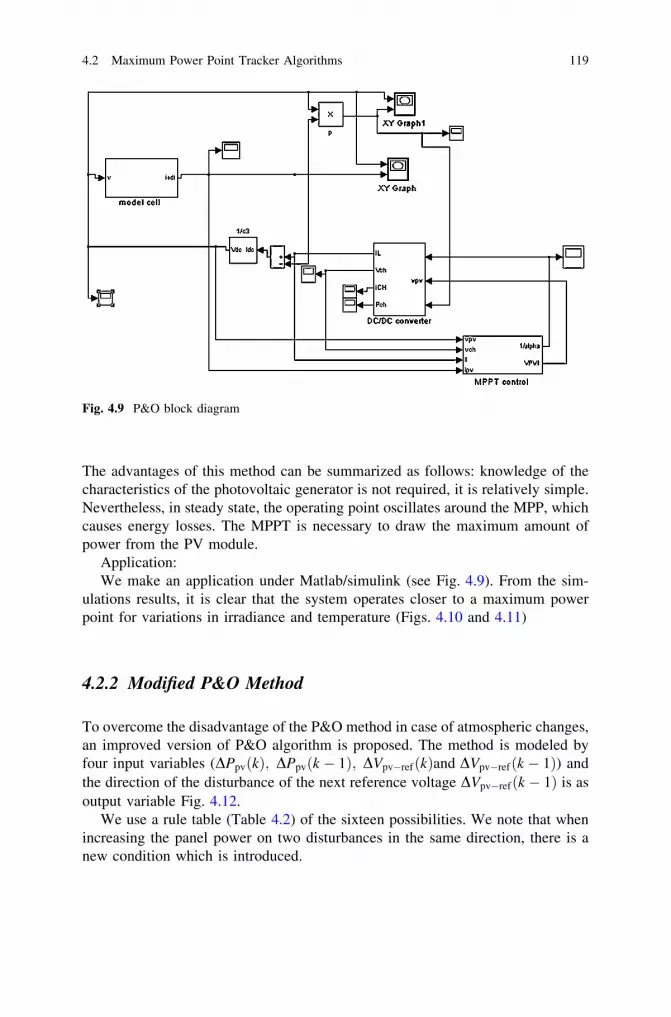
The advantages of this method can be summarized as follows: knowledge of thecharacteristics of the photovoltaic generator is not required, it is relatively simple.Nevertheless, in steady state, the operating point oscillates around the MPP, whichcauses energy losses. The MPPT is necessary to draw the maximum amount ofpower from the PV module.

Application:We make an application under Matlab/simulink (see Fig. 4.9). From the sim-

ulations results, it is clear that the system operates closer to a maximum powerpoint for variations in irradiance and temperature (Figs. 4.10 and 4.11)

4.2.2 Modified P&O Method

To overcome the disadvantage of the P&O method in case of atmospheric changes,an improved version of P&O algorithm is proposed. The method is modeled byfour input variables (DPpvðkÞ; DPpvðk � 1Þ; DVpv�refðkÞand DVpv�refðk � 1Þ) andthe direction of the disturbance of the next reference voltage DVpv�refðk � 1Þ is asoutput variable Fig. 4.12.

We use a rule table (Table 4.2) of the sixteen possibilities. We note that whenincreasing the panel power on two disturbances in the same direction, there is anew condition which is introduced.

Fig. 4.9 P&O block diagram


4.2.3 Incremental Conductance Technique

This method focuses directly on power variations. The output current and voltageof the photovoltaic panel are used to calculate the conductance and the incrementalconductance. Its principle is to compare the conductance (GG ¼ Ipv=Vpv) andincremental conductance (DGG ¼ dIpv=dVpv) and to decide when to increase or todecrease the PV voltage to reach the MPP where the derivative of the power isequal to zero (dPpv=dVpv ¼ 0). The incremental conductance method is oftenconsidered effective to search efficiently the maximum power point [66, 86].However the algorithm to implement is often complex and requires a high cal-culation capacity, which increases the system control period. The output power ofPV array can be given as:

Fig. 4.10 Current–voltagecharacteristic of a PV modulefor different irradiances

Fig. 4.11 Power-voltagecharacteristic of a PV modulefor different irradiances


Ppv ¼ Vpv � Ipv

dPpv

dVpv

¼d Vpv � Ipv

� �

dVpv

¼ Ipvþ Vpv �dIpv

dVpv

1Vpv

� dPpv

dVpv

¼ Ipv

Vpv

þ dIpv

dVpv

ð4:2Þ

By defining PV conductance and incremental conductance, yields,

GG ¼ Ipv

Vpv

DGG ¼ � dIpv

dVpv

8

>

>

<

>

>

:

ð4:3Þ

We obtain:

1Vpv

� dPpv

dVpv

¼ GG� DGG ð4:4Þ

Modified P&O method

)k(Ppv

)1k(Ppv

)k(V refpv

)1k(V refpv

)1k(V refpv

Fig. 4.12 Modified P&O modelisation [88]

0dV

dP

pv

pv

Ppvmax

Vpvmax

Ppv(A)

Vpv(V)

0dV

dP

pv

pv

0dV

dP

pv

pv

PPM

Fig. 4.13 Operating point

according to the sign of dPpv

dVpv

on the power characteristic[9]

Incremental Conductance Technique

Fig. 4.14 Block diagram ofincremental conductancemethod [9]


Equation 4.4 explains that the operating voltage is below the voltage at themaximum power point if the conductance is larger than the incremental conduc-tance, and vice versa. Thus, the task of this algorithm is to track the voltageoperating point at which conductance is equal to incremental conductance. Hence,

dPpv

dVpv

¼ 0Ipv

Vpv

¼ � dIpv

dVpv

GG ¼ DGG ð4:5Þ

dPpv

dVpv

[ 0Ipv

Vpv

[ � dIpv

dVpv

GG [ DGG ð4:6Þ

dPpv

dVpv

\ 0Ipv

Vpv

\ � dIpv

dVpv

GG \ DGG ð4:7Þ

In turn, Eqs. 4.6 and 4.7 are used to determine the direction in which aperturbation must occur to shift the operating point toward the MPP, and theperturbation is repeated until Eq. 4.5 is satisfied. Once the MPP is reached, theMPPT continues to operate at this point until a change in current is measuredwhich will correlate to a change in irradiance on the array Fig. 4.13.

The relationship between voltage and current, for the one-exponential model, isgiven by the following equation:

Ipv ¼ Iph � Is expqðVpv þ RsIpvÞ

AKTj

� �

� 1

� �

� Vpv þ RsIpv

Rsh

ð4:8Þ

For an optimal Eq. 4.8, it follows that the derivative of current can be expressedby [87, 88]:

Table 4.2 Rule table of modified P&O

DVpv�refðk � 1Þ DPpvðk � 1Þ DVpvðkÞ DPpvðkÞ System state DVpv�refðk � 1Þh0 h0 h0 h0 Invalid i0h0 h0 h0 i Invalid i0h0 h0 i h0 Decreasing of G h0h0 h0 i0 i0 VpvhVmpp i0h0 i0 h0 h0 Vpv � Vmpp i0h0 i0 h0 i0 New condition i0h0 i0 i0 h0 VpviVmpp h0h0 i0 i0 i0 Increasing of G h0i0 h0 h0 h0 Decreasing of G i0i0 h0 h0 i0 VpviVmpp h0i0 h0 i0 h0 Invalid h0i0 h0 i0 i0 Invalid h0i0 i0 h0 h0 VpvhVmpp i0i0 i0 h0 i0 Increasing of G i0i0 i0 i0 h0 Vpv � Vmpp h0i0 i0 i0 i0 New condition h0


dIpv

dVpv

¼ � Rs þqIs

AkTjexp

qðVpv þ RsIpvÞAKTj

� �

þ 1Rsh

� ��1 !�1

ð4:9Þ

dIpv

dVpv

¼ � 1

Rs þ1

qIs

AkTjexp

qðVpvþRsIpvÞAKTj

� �

þ 1Rsh

0

@

1

A

ð4:10Þ

The block diagram of Incremental Conductance method is the same as that ofPerturb & Observe method Fig. 4.14.

Figure 4.15 shows the flowchart of this method.

Beginning


Vref(t3)=Vref(t2)- CVref(t3)=Vref(t2)+C

Yes


Yes

No

0dIpv

pv

pv

pv

pv

V

I

dV

dI

0dVpv

YesYes

No

pv

pv

pv

pv

V

I

dV

dI

pv

pv

pv

pv

V

I

dV

dI Yes

Vref(t3)=Vref(t2)-C

No

Vref(t3)=Vref(t2)+C

No

)t(I)t(IdI 1pv2pvpv

)t(V)t(VdV 1pv2pvpv

Fig. 4.15 Flowchart of the incremental conductance method


4.2.4 Modified INC

Incremental Conductance (INC) method is simple and easy to implement and itstracking efficiency is very high. It is able to tell whether the current working pointis at the MPP or not, in case of ideal conditions. But in the measurements, theoperating point could oscillate around the MPP. In the modified INC method, weadded the part which monitors the maximum and minimum values of the poweroscillations on the PV side. These values can be used to find out how close thecurrent operating point is to the MPP, thereby slowing down the increment ofthe reference, in order not to cross the MPP [113].

4.2.5 Hill Climbing Control

This method consists to climb the operating point along the generator character-istic to a maximum. It is based on the relationship between the power panel and thevalue of the duty ratio applied to the static converter. Mathematically the PPM is

reached when dPpv

da is forced to zero by the control Fig. 4.16.Periodically, the power Ppv(t2) is compared to the previous value Ppv (t1).

Depending on the outcome of the comparison, we increase or decrease the dutycycle a. Once the PPM point reached, the system oscillates around it indefinitely.The advantage of this method is that it is simple to implement. But there areoscillations around the MPP in steady state and a loss of research of the MPP whenclimatic conditions change rapidly.

The flowchart of this algorithm is given in Fig. 4.17.

0d

dPpv

Ppvmax

max

Ppv(A)

0d

dPpv

0d

dPpv

PPM

Fig. 4.16 Relationshipbetween power and the dutyratio a [9]


4.2.6 MPPT Controls Based on Relations of Proportionality

These methods are based on proportional relationships between parameters ofoptimal maximum power point (Iopt, Vopt) and the characteristic parameters of thepanel (Isc, Voc).

4.2.6.1 Constant Reference Voltage Algorithm

The simplest technique to maintain the operation of the PV system near themaximum power point is to control the voltage measured at the PV generator, to its

Beginning

Measure Vpv(t1),Ipv(t1)

)t(P)t(P

)t()t(

1pv2pv

12

Measure Vpv(t2),Ipv(t2)

Yes

No

)t(P)t(P 1pv2pv

)t(P)t(P 1pv2pv

No

Yes

)t(I).t(V)t(P 2pv2pv2pv

)t(I).t(V)t(P 1pv1pv1pv

)t(P)t(P

)t()t(

1pv2pv

12

Fig. 4.17 Flowchart of theHill climbing control


reference voltage corresponding to the optimum voltage [89]. This methodassumes that the variation of the optimum voltage to climatic factors variations(irradiance, temperature) is negligible as shown in Fig. 4.18a. However, when thejunction temperature of the PV cell varies as shown in Fig. 4.18b, the optimumvoltage will be not constant. This method uses a single control loop and iswell suited for applications where climatic conditions are stable, such as spacesatellites [90].

4.2.6.2 Open-Circuit Voltage Photovoltaic Generator Method

It is a very simple method. It consists on comparing the panel voltage Vpv with areference voltage corresponding to an optimal voltage Vopt. The voltage error isthen used to adjust the duty ratio of the static converter. The reference voltage isobtained by the following equation:

Vopt ¼ k1:Vco ð4:11Þ

with k1 as a constant of proportionality (0:71hk1h0:78).Once k1 is known, Vopt can be computed using Eq. 4.11.

Voltage (V)

1maxpV

Pow

er (

W)

Voltage (V)

2maxpV 3maxpVmaxpV

Pow

er (

W)

(a) (b)

Fig. 4.18 Power–voltage characteristic Ppv(Vpv) of PV generator a-Variable irradiance, constanttemperature b-Variable temperature, constant irradiance

Open circuit voltage algorithmVco

Vopt

Fig. 4.19 Block diagram ofopen circuit voltage method[9]


This requires that the system performs the measurement of the voltage Vco foreach time period. Then we obtain directly the reference voltage which is theoptimum voltage. Although this method is simple, it is difficult to choose anoptimal value of k1 [66, 91] Fig. 4.19.

4.2.6.3 Optimal Voltage with Temperature Compensation

We generate the reference voltage by adding a unique cell junction which iselectrically independent of the PV system and having an electrical characteristicidentical to the cells of the PV generator [68] Fig. 4.20.

The open-circuit voltage Voc varies with the cell temperature Tj, and the short-circuit current Isc is directly proportional to the irradiance level G. It can bedescribed through the following equation:

Temperature compensation method

Vpv Vopt

Tj

Fig. 4.20 Block diagram ofTemperature compensationmethod [9]

Short circuit current algorithm

Vpv

Isc

IoptVopt PI regulator

Fig. 4.21 Block diagram of Short circuit current method [9]

Irradiance

Temperature

0 5 10 15 20 25 30 35 40 45 500

0.5

1

1.5

2

2.5

3

3.5

4

Vpv (V)

I pv

(A)

MPPT powerstage

Sliding MPPT

Controller

Duty cycle

IL

Vpv V0

Fig. 4.22 Sliding maximum power point tracker for a photovoltaic system [9]


Voc ¼ Voc�STC þdVoc

dTTj � Tj�STC

� �

ð4:12Þ

where Voc�STCis the open-circuit voltage under Standard Test Conditions (V),dVoc=dT is the temperature coefficient (V/K), and Tj�STC is the cell temperatureunder STC(�K).

4.2.6.4 Short-Circuit Current Photovoltaic Generator Method

This method is based on knowledge of the linear relationship between current andoptimal Iopt and the short-circuit current Isc.

Iopt ¼ k2 � Isc ð4:13Þ

with k2 a factor which depends on the current PV (0:78hk2h0:92).According to Eq. 4.12, the current Iopt can be determined by measuring the

current Isc. In this method the temperature does not affect the coefficient k2, and weneed only a single sensor. The implementation is easy but the accuracy of thiscontrol is weak due to the estimation of Iopt [71] Fig. 4.21.

4.2.7 Curve-Fitting Method

The nonlinear characteristic of the photovoltaic generator can be modeledusing mathematical equations or numerical approximations [69], However, their

VC CE

iLIload

RLoad

L

S=1

VdcCdc

S=0Fig. 4.23 DC–DC converter[97]

Ppvmax

Vpvmax

Ppv(A)

Vpv(V)

MPP

α decrease

α increase

0<σ 0>σ

Fig. 4.24 Operating pointaccording to the sign of r[97]


resolution is very difficult by conventional digital controls. Therefore, theirapplication does not seem appropriate for research of the MPP. Nevertheless, otherapproaches based on this model are used in [66], [96]. In the last reference,Eq. 4.14 represents the characteristic Ppv (VPV) of a photovoltaic generator, where(a, b, c and d) are coefficients determined by the sampling values of the photo-voltaic voltage VPV, current ipv and power Ppv.The optimum voltage whichcorresponds to the maximum power is obtained by Eq. 4.15.

Ppv ¼ a � V3pvþ b � V2

PVþ c

P� V

PVþ d ð4:14Þ

Vopt ¼�b þ

ffiffiffiffiffiffiffiffiffiffiffiffiffiffiffiffiffiffiffiffiffi

b2 � 3 a cp

3 að4:15Þ

The disadvantage of this method is that the numerical approximations used arenot valid during the meteorological conditions variations. It requires large memorystorage for the calculation of mathematical formulas.

4.2.8 Look-Up Table Method

In this method, the measured values of voltage and photovoltaic current arecompared to those stored in the control system, which corresponds to those in theoptimal operating conditions under real conditions [68]. This algorithm requires alarge memory capacity for data storage and parameters should be adjustedaccording to the solar panel used. In addition, it is difficult to record and store allpossible conditions of system operation.

4.2.9 Sliding Mode Control

4.2.9.1 Control Design of Sliding Mode

The advantages of sliding mode control are various and important: high precision,good stability, simplicity, invariance, robustness etc… This allows it to beparticularly suitable for systems with imprecise model. Often it is better to specifythe system dynamics during the convergence mode. In this case, the controllerstructure has two parts, one represents the dynamics during the sliding mode andthe other represents the discontinuous system dynamics during the convergencemode.

The design of the control can be obtained in three important steps and each stepis dependent on another one:

• The choice of surface.


For a system defined by the following equation, the vector of surface has thesame dimension as the control vector (u).

x� ¼ A x; tð Þ � xþ B x; tð Þ � u ð4:16Þ

We find in the literature different forms of the sliding surface and each surfacehas better performance for a given application. In general, we choose a nonlinearsurface. The nonlinear form is a function of the error on the controlled variable (x),it is given by:

SðxÞ ¼ o

otþ kx

� �r�1

�e xð Þ ð4:17Þ

where e xð Þ ¼ x� x is the difference between the controlled variable x and itsreference x ; kx is a positive constant, r is the number of times to derive thesurface to obtain the control, x is the controlled variable.

The purpose of the control is to maintain the surface to zero. This one is a lineardifferential equation with a unique solution e xð Þ ¼ 0 for a suitable choice ofparameter kx with respect to the convergence condition.

• The establishment of the invariance conditions.

The conditions of invariance and convergence criteria have different dynamicsthat allow the system to converge to the sliding surface and stay there regardless ofthe disturbance: There are two considerations to ensure the convergence mode.

• The discrete function switching.

This is the first convergence condition. We have to give to the surface adynamic converging to zero. It is given by:

S�

xð Þ � 0 si S xð Þ � 0

S�

xð Þ � 0 si S xð Þ � 0

8

<

:

ð4:18Þ

It can be written as:

S�

xð Þ � S xð Þ � 0 ð4:19Þ

• Lyapunov function:

The Lyapunov function is a positive scalar function for the state variables of thesystem. The idea is to choose a scalar function to ensure the attraction of thevariable to be controlled to its reference value.


We define the Lyapunov function as follows:

V xð Þ ¼ 12� S2 xð Þ ð4:20Þ

The derivative of this function is:

V�

xð Þ ¼ S xð Þ � S�

xð Þ ð4:21Þ

The function will decrease, if its derivative is negative. This is checked only ifthe condition (Eq. 4.19) is verified.

• Determination of the control law.

The structure of a sliding mode controller consists of two parts. The first oneconcerns the exact linearization ueq

� �

and the second one concerns the stabilizationunð Þ:

u ¼ ueq þ un ð4:22Þ

where ueq corresponds to the control. It serves to maintain the variable control onthe sliding surface. unis the discrete control determined to check the convergencecondition (Eq.4.19).

We consider a system defined in state space by Eq. 4.16, and we have to findanalogical expression of the control (u).

S�

xð Þ ¼ oS

ot¼ oS

ox� ox

otð4:23Þ

Substituting Eq. 4.16 and Eq. 4.22 in Eq. 4.23, we obtain:

S�

xð Þ ¼ oS

ox� A x; tð Þ þ B x; tð Þ � ueq

� �

þ oS

ox� B x; tð Þ � un ð4:24Þ

We deduce the expression of the equivalent control:

ueq ¼ �oS

o t� B x; tð Þ

� ��1

� oS

o t� A x; tð Þ ð4:25Þ

For the equivalent control can take a finite value, it must:

oS

ox� B x; tð Þ 6¼ 0 ð4:26Þ

In the convergence mode and replacing the equivalent command by itsexpression in Eq. 4.24, we find the new expression of the surface derivative:

S�

x; tð Þ ¼ oS

ox� B x; tð Þ � un ð4:27Þ


And the condition expressed by Eq. 4.19 becomes:

S x; tð Þ � oS

ox� B x; tð Þ � un � 0 ð4:28Þ

The simplest form that can take the discrete control is as follows:

un ¼ ks � sign S x; tð Þð Þ ð4:29Þ

where the sign of ks must be different from that of oS=ox � B x; tð Þ:

4.2.9.2 A Sliding Maximum Power Point Tracker for a PhotovoltaicSystem

In sliding mode controller, the control circuit adjusts the duty cycle of the switchcontrol waveform for maximum power point tracking as a function of theevolution of the power input at the DC/DC converter. In this control system, it isnecessary to measure the PV array output power and to change the duty cycle ofthe DC/DC converter control signal [97–101] (Figs. 4.22, 4.23).

The system can be written in two sets of state equations depending on theposition of switch S.

diL

dt¼ 1

LVdc � VCð1� SÞ½ � ð4:30Þ

dVC

dt¼ 1

CiLð1� SÞ � iload½ � ð4:31Þ

We introduce the concept of the approaching control [100]. We select thesliding surface as:

dPpv

dIpv

¼ 0 ð4:32Þ

dPpv

dIpv

¼dðRpv:I2

pvÞdIpv

¼ 0 ð4:33Þ

dPpv

dIpv

¼dðRpv:I2

pvÞdIpv

¼ 2:Ipv:Rpv þ I2pv

dRpv

dIpv

¼ 0 ð4:34Þ

dPpv

dIpv

¼ Ipvð2:Rpv þ Ipv

dRpv

dIpv

Þ ¼ 0 ð4:35Þ

where Rpv ¼ Vpv

Ipvis the equivalent load connect to the PV,

with Ipv ¼ IL:


The non-trivial solution of Eq. 4.35 is:

2:Rpv þ Ipv

dRpv

dIpv

¼ 0 ð4:36Þ

The sliding surface is given as:

r¼D 2:Rpv þ ILdRpv

dILð4:37Þ

We have to observe the duty cyclea. Its control can be chosen as:

a ¼ aþ Da if ri0

a ¼ a� Da if rh0

Equations 4.30 and 4.31 can be replaced by an averaged set summing theirexpressions for S = 0, weighted by 1-a, and their expressions for S = 1,weighted by a. Then, the result can be written in general form of the nonlinear timeinvariant system.

X�¼ f ðXÞ þ gðXÞ � a ð4:38Þ

The equivalent control aeq is determined from the following condition [100]:

r� ¼ dr

dX

T

:X�¼ 0 ð4:39Þ

r� ¼ dr

dX

T

f ðXÞ þ gðXÞ:aeq

� �

¼ 0 ð4:40Þ

We obtain the equivalent control aeq :

aeq ¼ �

drdX

T

�f ðXÞ

drdX

T

�gðXÞ¼ 1� Vpv

VCð4:41Þ

The equivalent duty cycle must lie in 0 h aeq h1:The real control signal a is proposed as [100]:

a ¼ 1 if aeq þ kcr 1

a ¼ aeq þ kcr if 0haeq þ kcrh1

a ¼ 0 if aeq þ kcr 0

where the control saturate if aeq þ kcr is out of range, where kc is a positive scalingconstant Fig. 4.24.


4.2.10 Method of Parasitic Capacitance Model

The algorithm of the parasitic capacitance (Parasitic Capacitance MPPT) is similarto that of the incremental conductance (INC-MPPT) except that the effect ofparasitic capacitance (CP), which models the storage charges in the p-n solar cellsjunctions and stray capacitance, is included. A capacitance Cp is added in parallelon the terminals of the previous models. The current in that capacitance isIpc(t) = CP.dVpv/dt, so that the observed current Iobs is expressed by [102–103]:

Iobs ¼ Ipv � Ipc

¼ Iph � IS expVpv þ Rs Ipv

� �

A Vth

� �

� 1

� Vpv þ Rs Ipv

RSh

� �

� CPdVpv

dt

¼ FðVpvÞ � CPdVpv

dtð4:42Þ

Equation 4.42 shows the first component (Ipv) is function of the voltageF(V) and the second one relates to the current in the parasitic capacitance. Usingthis notation, the incremental conductance of the solar panel (Cp not included) canbe defined as the ratio dF(Vpv)/dVpv and the instantaneous conductance can bedefined as the ratio F(Vpv)/Vpv. The MPP is obtained when dPpv/dVpv = 0. Mul-tiplying Eq. 4.42 by the panel voltage (Vpv) for electric power, and then differ-entiating the result, the equation of electric power at MPP is obtained and can beexpressed as [104]:

dFðVpvÞdVpv

þ FðVpvÞVpv

¼ dIobs

dVpv

þ Iobs

Vpv

þ Cp

V�

pv

Vpv

þV��

pv

V�

pv

0

B

@

1

C

A

¼ 0 ð4:43Þ

The three terms of Eq. 4.43 represent the negative of the observed incrementalconductance, the observed instantaneous conductance and the correction for par-asitic capacitance. The first and second derivatives of the voltage of the panel takeinto account the ripple effect generated by power electronic converter. This ripplecan then be used as voltage variation allowing MPPT. Note that if CP is zero,Eq. 4.43 simplifies and becomes the one used for the incremental conductancealgorithm.

4.2.11 Fuzzy Logic Technique

In recent years, fuzzy logic controllers (FLC) are widely used for finding the MPP[76, 77, 79, 80, 83, 85, 92, 93, 94]. The inputs of fuzzy controller are error and itsvariations; the output is the duty ratio of DC/DC converter or its variation. Thefuzzy controller introduced in [77, 78, 92] uses dPpv/dIpv and its variation


D(dPpv/dIpv) as inputs, calculates the duty ratio of the MPPT converter in the firstreference and the variation of this one in the last two references. While the fuzzycontroller in [80] considers the variation of duty cycle as output, it replaces dPpv/dIpv by photovoltaic panel power variations. The fuzzy controller developed in[77] is inadequate when operating conditions vary widely. The adaptive fuzzycontroller and hybrid fuzzy controller [92–93] that exploits the characteristics ofthe fuzzy controller and the theory of neural networks are complex and require alarge computing capacity.

The theory of fuzzy logic is used to address the problem of oscillation of theperturbation and observation method (P&O). The proposed fuzzy controlleroptimizes the amplitude of the disturbance to minimize the oscillations and for aquick response without oscillations. The inputs used to generate the optimalvoltage which corresponds to the maximum power are the photovoltaic powervariation (DPpv) and the variation of the photovoltaic voltage (DVpv). As output,the fuzzy controller determines the optimum increment to be added to the oper-ating voltage to extract the maximum power MPP. In contrast to the Perturb andObserve (P & O) method which uses a constant disturbance to determine theoperating voltage, it produces the oscillation of the operating point around theMPP in steady state.

4.2.11.1 The Fuzzy MPPT Controller

Fuzzy logic controller is introduced to determine the operating point corre-sponding to maximum power for irradiance and temperature levels. In this case,inputs of the fuzzy logic controller are power variation (DPpv) and voltage vari-ation (DVpv). The output is reference voltage variation (DVpv, ref). In order toconverge toward the optimal point, rules are relatively simple to establish. Theserules depend on the variations of power DPpv and voltage DVpv. In accordancewith Table 4.3, if the power (Ppv) increased, the operating point should beincreased as well. However, if the power (Ppv) decreased, the voltage (Vpv,ref)should do the same.

From these linguistic rules, the MPPT algorithm contains measurement ofvariation of photovoltaic power DPpv and variation of photovoltaic voltage DVpv

and proposes a variation of the voltage reference DVpv, ref according to Eq. 4.44.

DPpv ¼ PpvðkÞ � Ppvðk � 1Þpv ¼ VpvðkÞ � Vpvðk � 1ÞVpv�refðkÞ ¼ Vpvðk � 1Þ þ DVpv�refðkÞ

8

>

<

>

:

ð4:44Þ

where Ppv(k) and Vpv(k) are the power and voltage of the photovoltaic generator atsampled times (k), and Vpv,ref (k) the instant of reference voltage. Figure. 4.25gives an example of a track in the Ppv(Vpv) plan for a constant irradiance andtemperature.


The power variation (DPpv) is either in the positive direction or in the negativeone. The value of DPpv can also be small or on the contrary large. This controlallows the research of the optimum point while being based on the expertobservations. From these judgments, the reference photovoltaic voltage Vpv,ref isincreased or decreased in a small or large way in the direction which makes itpossible to increase the power Ppv.

If a great increase in the voltage Vpv involves a great increase in the power Ppv,we continue to strongly increase the reference voltage Vpv, ref (point A to point Bor point B to point C). If a great increase in the voltage Vpv involves a reduction inthe power Ppv (point C to point D), we decrease the reference voltage Vpv, ref toobtain a fast increase in the power Ppv. If a reduction in the voltage Vpv involves aweak increase in the power Ppv then we get closer to the optimal reference voltagewhich is the beginning of stabilization.

When irradiance and temperature vary, the same types of rules are applied totrack the maximum power point. The structure of fuzzy logic controller is shown inFig. 4.26.

As explained previously, the MPPT technique takes measurement of PV volt-age and current, and then uses FLC to calculate the reference voltage (Vpv, ref).Then, there is another control loop where proportional and integral (PI) controller

Table 4.3 Fuzzy rule table [63]

DPpv

DVpv BN MN SN Z SP MP BP

BN BP BP MP Z MN BN BNMN BP MP SP Z SN MN BNSN MP SP SP Z SN SN MNZ BN MN SN Z SP MP BPSP MN SN SN Z SP SP MPMP BN MN SN Z SP MP BPBP BN BN MN Z MP BP BP

Vpv (V)

P pv(w

)

A

EPmpp

Vmpp

B

C D

Fig. 4.25 Principle ofoperation of the MPPT fuzzycontroller [9]


regulates the input voltage of converter. Its task is to minimize error betweenVpv,ref and the measured voltage (Vpv,m). The PI loop operates with a much fasterrate and provides fast response and overall system stability [87]. The fuzzy logiccontroller block includes three functional blocks: fuzzification, fuzzy rule algo-rithm and defuzzification. Fuzzy logic controller (FLC) inputs can be measuredor computed from the voltage and current of solar panel. Figure 4.27 shows themembership functions of input and output variables in which membershipfunctions of input variables DPpv and DVpv are triangular and has seven fuzzysubsets. Seven fuzzy subsets are considered for membership functions of theoutput variable DVpv, ref. These input and output variables are expressed in termsof linguistic variables (such as BN (big negative), MN (means negative), SN(small negative), Z (zero), SP (small positive), MP (means positive), and BP (bigpositive)).

The control rules are indicated in Table 4.3 with DPpv and DVpv as inputs andDVpv, ref as the output. The fuzzy inference is carried out by using Sugeno’smethod [88], and the defuzzification uses the center of gravity to compute theoutput of this FLC which is the variation of reference voltage (DVpv,ref).

Fig. 4.26 Structure of MPPT fuzzy controller


4.2.11.2 Application Under Matlab/Simulink

We make application under Matlab/Simulink and we present simulation resultsunder the following operating conditions:

• Irradiance level G is changed from 900 to 450 W/m2 and temperature Tj ischanged from 35 to 25�C.

• Temperature (Tj) is changed from 10 to 50�C for constant irradiance of 1000 W/m2 Fig. 4.28.

The PV characteristics using MPPT control with FLC and the theoretical PVarray characteristic are illustrated in Fig. 4.29 for change in irradiance level andtemperature. In Fig. 4.29a, b we can see the power-voltage characteristic andpower-current characteristic respectively. For G = 900 W/m2 and Tj = 35�C themaximum power point corresponds to the values of voltage and current (35.95 V,2.74 A). The decrease of the irradiance implies a decrease of the PV power,therefore, the maximum power point moves to join the maximum point corre-sponding to this irradiance, and we can have the corresponding voltage and currentvalue in Fig. 4.29c. In Fig. 4.30, we present PV array characteristics for change intemperature (Tj) at constant irradiance. The open-circuit voltage (Voc) decreases

BN MN SP BPZ

1 0 1

µ( ΔVpv,ref)

SN MP

2/31/31/32/3 ΔVpv,ref

ΔPpv, ΔVpv

BN MN SP BPZ

1 0 1

µ(ΔPpv)

SN MP

2/3 1/3 1/3 2/3

1

0

Fig. 4.27 Membership functions of DPpv, DVpv and of DVpv, ref


when temperature increases, the maximum power point changes according to thevariation of temperature. It is clear that the operating point of this system operatescloser to a maximum power point for variations in irradiance and temperature.

The simulation results show the robustness of the FLC for variation in envi-ronmental conditions, the PV system is always operating at the maximal powerpoint.

4.2.12 Artificial Neural Networks

4.2.12.1 Definition of ANN

Artificial neural networks (ANN) are electronic models based on the neuralstructure of the brain. This function permits ANNs to be used in the design ofadaptive and intelligent systems since they are able to solve problems fromprevious examples. ANN models involve the creation of massively parallelednetworks composed mostly of nonlinear elements known as neurons. Each modelinvolves the training of the paralleled networks to solve specific problem [105].ANNs consist of neurons in layers, where the activations of the input layer are setby an external parameter. Generally, networks contain three layers—input, hiddenand output. The input layer receives data usually from an external source while theoutput layer sends information to an external device. There may be one or morehidden layers between the input and output layers. The back-propagation methodis the common type of learning algorithm [105].

4.2.12.2 MPPT Using Artificial Neural Networks

In photovoltaic systems, the input variables can be PV array parameters such asopen-circuit voltage (VOC) and short-circuit current (ISC), atmospheric data-likeirradiance (G) and temperature (Tj), or any combination of these. Ramaprabha R

Fig. 4.28 Membership function plots in Matlab [9]



ad Mathur. B. L propose an ANN algorithm with three layers (input layer, hiddenlayer and output layer). In this case, the block diagram producing maximum powerand voltage is given in Fig. 4.31. We have two input neurons, hidden layers andtwo output neurons. The method used is the back-propagation algorithm (BPA).

In Ref. [107], authors present the ANN block diagram with three input neurons(irradiance, temperature and array voltage). The output neurons are maximumcurrent, maximum voltage and current load. The hidden layer in PBA algorithmconsists of four neurons (H1, H2, H3 and H4) Fig. 4.32.

The proposed architecture of the back-propagation algorithm (BPA) is given asFig. 4.33.

4.2.13 Neuro-Fuzzy Method

4.2.13.1 Definition

The classic cycle of development of a neuro-fuzzy model can be separated intoseven stages [110]:

1. data collection,2. data analysis,3. separate databases,4. the choice of a neural network,5. formatting data,6. learning.

A typical architecture of a neuro-fuzzy network is shown in Fig. 4.34 Fig. 4.35.It has a single input variable and five membership functions MF [111].

4.2.13.2 MPPT Using Neuro-Fuzzy Network

The neuro-fuzzy controller has two inputs (e and De) and a single output (a),where: e represents the error and De the error variation. The two input variablesgenerate action control and adjust the duty cycle a to be applied to the DC–DCconverter so as to ensure the adaptation of the power supplied by the GPV. Thiscontroller allows automatic generation of fuzzy rules based on the Sugeno infer-ence model [108–109]. The block diagram of a photovoltaic system with a MPPT

Fig. 4.29 Simulation results of fuzzy logic controller versus theoretical PV array characteristic,irradiance level G is changed from 900 to 450 W/m2 and temperature Tc is changed from 35 to25�C. (a): Ppv(Vpv), (b):Ppv (Ipv), (c):Ipv (Vpv) a. Power-voltage characteristic of a PV module fordifferent irradiance. b. Power-current characteristic of a PV module for different irradiance. c.Current–voltage characteristic of a PV module for different irradiance

b


0 5 10 15 20 25 30 35 40 45 500

20

40

60

80

100

120

V pv (V )

Ppv

(W

)

10°C

25°C

50°C

0 0.5 1 1.5 2 2.5 3 3.5 4 4.5 50

20

40

60

80

100

120

Ipv (A )

Ppv

(W

)

10°C

25°C

50°C

0 5 10 15 20 25 30 35 40 45 500

0.5

1

1.5

2

2.5

3

3.5

4

4.5

5

V pv (v)

Ipv

(A)

10°C

25°C

50°C

(a)

(b)

(c)


Fig. 4.30 Simulation results of fuzzy logic controller versus theoretical PV array characteristic,temperature Tj is changed from 10 to 50�C at constant irradiance (1000 W/m2). (a): Ppv(Vpv),(b):Ppv (Ipv), (c):Ipv (Vpv) a. Power-voltage characteristic of a PV module for differenttemperatures. b. Power-current characteristic of a PV module for different temperatures. c.Current-voltage characteristic of a PV module for different temperatures [31]

b

ANN algorithm

Irradiance G

Temperature Tj

Maximum current Imax

Maximum Voltage Vmax

Array voltage Voc

Load current Iload

Maximum

Power Pmax

Fig. 4.32 ANN block diagram with three input layers [106]

Voc

Tj

G

Vmax

Imax

Iload

H1

H2

H3

H4

X1

X2

X3

Y1

Y2

Y3

W34V41

W34

W11V11Fig. 4.33 Architecture of thePBA algorithm

Input Output

MF input MF outputRuleFig. 4.34 Structure ofNeuro-Fuzzy Model [111]

ANN algorithm

Irradiance G

Temperature Tj

Maximum Power Pmax

Maximum Voltage Vmax

Fig. 4.31 ANN blockdiagram with two inputneurons


control network-based neuro-fuzzy is represented in Fig 4.36.The main advantageof this algorithm comparing to a conventional single ANN algorithm is the distinctgeneralization ability [110].

4.2.14 Genetic Algorithms

Genetic algorithms (GA) are stochastic optimization algorithms based on mech-anisms of natural selection and genetics. Its operation is extremely simple. It startswith an initial population which is encoded for the model of problem by somemethods Fig. 4.37.

Start


Ppv(t1)=Vpv(t1)*Ipv(t1)


Ppv(t2)=Vpv(t2)*Ipv(t2)

CalculateVpv=Vpv(t2)-Vpv(t1)Ipv=Ipv(t2)-Ipv(t1)

Ppv=Ppv(t2)-Ppv(t1)

Vpv-ref=Vopt-ANN

Ipv-ref=Iopt-ANN

Yes

No

0dV

dP

pv

pv =

Fig. 4.35 Flowchart of Neuro-Fuzzy Model [111]


4.3 Efficiency of a MPPT Algorithm

Efficiency gMPPTis the most important parameter of an MPPT algorithm. Thisvalue is calculated as

gMPPT ¼R t

0 Ppv�maxðtÞdtR t

0 Ppv�MPPTðtÞdtð4:45Þ

where PPV�MPPT represents the output power of PV system with MPPT, andPpv�max is the output power at true maximum power point.

4.4 Comparison of Different Algorithms

Hill climbing and P&O methods are different ways but based on the same fun-damental method. Hill climbing involves a perturbation in the duty ratio a of thepower converter while P&O makes a perturbation in the operating voltage of the

Fig. 4.36 Photovoltaic system with MPPT control by neuro-fuzzy networks

4.3 Efficiency of a MPPT Algorithm 145

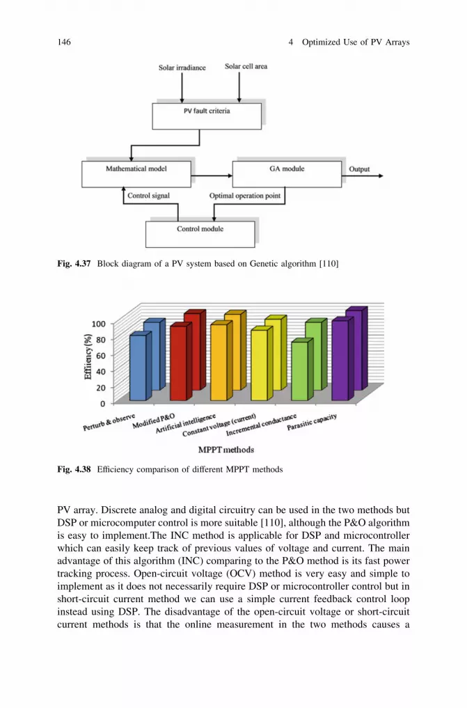
PV array. Discrete analog and digital circuitry can be used in the two methods butDSP or microcomputer control is more suitable [110], although the P&O algorithmis easy to implement.The INC method is applicable for DSP and microcontrollerwhich can easily keep track of previous values of voltage and current. The mainadvantage of this algorithm (INC) comparing to the P&O method is its fast powertracking process. Open-circuit voltage (OCV) method is very easy and simple toimplement as it does not necessarily require DSP or microcontroller control but inshort-circuit current method we can use a simple current feedback control loopinstead using DSP. The disadvantage of the open-circuit voltage or short-circuitcurrent methods is that the online measurement in the two methods causes a

Fig. 4.37 Block diagram of a PV system based on Genetic algorithm [110]

Fig. 4.38 Efficiency comparison of different MPPT methods


reduction in output. The disadvantage of parasitic capacitance algorithm is that theparasitic capacitance is very small in each module. It will be interesting only inlarge PV arrays, where several module strings are connected in parallel. Thedisadvantage of intelligent techniques such as fuzzy controller, Neural networks,Neuro-Fuzzy and Genetic algorithms is the high cost of their implementation withcomplex algorithms that usually need a DSP. Others algorithms of MPPT are usedby different authors such as the Delta-adaptive method, the Ripple correlationcontrol (RCC), current sweep method, Load Current or Load Voltage Maximi-zation and dP/dV or dP/dI Feedback Control [55]. We make a comparison betweensome important methods. We represent their minimum and maximum efficiencyvalue in Fig. 4.38.

4.4 Comparison of Different Algorithms 147

Chapter 5Modeling of Storage Systems

SymbolsC Capacity according to Peukert, at a one-ampere discharge rate (A�h)C0 Capacitance of the parallel platesC1 and C2 Capacities of the battery at different discharge-rate statesC10 10-h capacityDc and Dd Diodes which are in series with Rc and Rd, respectivelyEb Open-circuit voltage of the battery chargedEm Main branch electromotive force of the batteryEt Battery terminal voltageIbatt Discharge currentkEb and kR Coefficients that can be calculated experimentallyKi Polarization resistancen Peukert constantR0 Initial battery internal resistance calculated when the battery is full

chargedRbatt Internal (ohmic) resistance of the batteryRc and Rd Internal resistances associated respectively with the charging and

discharging process of the batteryR0 Nonlinear resistance contributed by the contact resistance of plate to

electrolyteQ Accumulated ampere-hours divided by full battery capacitySOC State of chargeti Time to discharge at current IUbatt Terminal voltage of the batteryVoc Open-circuit voltage of a battery cell when fully chargedZm Internal impedance of the batteryBattery is generally needed when PV array cannot be functional as at night or on acloudy day. The major functions of a storage battery in a PV system are:


149

• energy storage capacity and autonomy• voltage and current stabilization• supply surge currents

Indeed, battery is necessary to store electrical energy that is produced by the PVarray as well as to supply energy to electrical loads. It can supply power toelectrical loads at stable voltages and currents, and it can supply surge or high peakoperating currents to electrical loads or appliances.

5.1 Description of Different Storage Systems

Cell is the basic electrochemical unit used to generate electrical energy from storedchemical energy or to store electrical energy in the form of chemical energy.It consists of a positive and a negative electrode in a container filled with anelectrolyte which provides the essential ionic conductivity between the positiveand negative electrodes of a cell. A separator which is an ion-permeable, elec-tronically non-conductive material or spacer prevents short-circuiting of thepositive and negative electrodes of the cell.

The desired battery is obtained when two or more cells are connected in anappropriate series/parallel arrangement to obtain the required operating voltageand capacity for a certain load (Fig. 5.1).

5.1.1 Battery Bank systems

In the market, there are many different types of batteries and most of them aresubject to further research and development. In PV systems, several types ofbatteries can be used: nickel-cadmium (NiCd), Nickel-Zinc (Ni-Zn), lead acid etc.Nevertheless it must have some important properties as high charge-dischargeefficiency, low self-discharge, and long life under cyclic charging and discharging.

5.1.1.1 Nickel-Cadmium (NiCd) Batteries

The NiCd batteries are commonly known as relatively cheap and robust. Thepositive nickel electrode is a nickel hydroxide/nickel oxyhydroxide (Ni(OH)2/NiOOH) compound, while the negative cadmium electrode consists of metalliccadmium (Cd) and cadmium hydroxide (Cd(OH)2). The electrolyte is an aqueoussolution of potassium hydroxide (KOH). It is based on the following redoxreaction [114]

150 5 Modeling of Storage Systems

NiOOH þ H20þ e��!

discharge

�charge

Ni(OH)2 þ OH� ð5:1Þ

1=2ð ÞCdþ OH��!

discharge

�charge

1=2ð ÞCdðOHÞ2 þ e� ð5:2Þ

The overall reaction is

NiOOH þ 1=2ð ÞCdþ H20�!

discharge

�charge

NiðOHÞ2 þ 1=2ð ÞCdðOHÞ2 ð5:3Þ

Compared to lead acid batteries which are probably the most commonly usedbatteries in photovoltaic applications, nickel-cadmium batteries can be, in somephotovoltaic systems, cost-effective on a life cycle/cost profitable basis.

5.1.1.2 Nickel-Hydrogen Batteries

Nickel-Hydrogen battery has some advantages as long cycle, resistance to over-charge and good energy density, but it has high cost, high cell pressure and lowvolumetric energy density. It is generally used in space applications and com-munication satellites [2].

At the nickel electrode, we have:

NiOOHþ H2Oþ e��!

discharge

�charge

NiðOHÞ2 þ OH� ð5:4Þ

Negative platePositive plate

-+

Electrolyte

Case

GridGrid Separator

Fig. 5.1 Battery cellcomposition [10]

5.1 Description of Different Storage Systems 151

At the hydrogen electrode, we have:

OH� þ 1=2ð ÞH2�!

discharge

�charge

H2Oþ e� ð5:5Þ

And the global reaction is

NiOOHþ 1=2ð ÞH2�!

discharge

�charge

NiðOHÞ2 ð5:6Þ

5.1.1.3 Nickel-Metal Hydride Batteries

Nickel-Metal Hydride batteries are used generally commercial consumer product.Its disadvantages are high self-discharge and failure leading to high pressure [115].

At the positive electrode, we have

NiOOHþ H2Oþ e��!

discharge

�charge

NiðOHÞ2 þ OH� ð5:7Þ

At the negative electrode, we have

MðHÞ þ OH��!

discharge

�charge

Mþ H2Oþ e� ð5:8Þ

And the global reaction is

NiOOH þMðHÞ �!discharge

�charge

NiðOHÞ2 þM ð5:9Þ

5.1.1.4 Nickel-Zinc batteries

The positive electrode is the nickel oxide but the negative electrode is composed ofzinc metal. In addition to better environmental quality, this type of battery has ahigh energy density (25% higher than nickel-cadmium). Its operation is based onthe following redox reaction [115]:


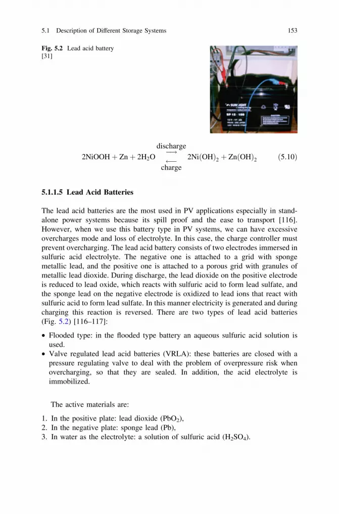
2NiOOHþ Znþ 2H2O�!

discharge

�charge

2NiðOHÞ2 þ ZnðOHÞ2 ð5:10Þ

5.1.1.5 Lead Acid Batteries

The lead acid batteries are the most used in PV applications especially in stand-alone power systems because its spill proof and the ease to transport [116].However, when we use this battery type in PV systems, we can have excessiveovercharges mode and loss of electrolyte. In this case, the charge controller mustprevent overcharging. The lead acid battery consists of two electrodes immersed insulfuric acid electrolyte. The negative one is attached to a grid with spongemetallic lead, and the positive one is attached to a porous grid with granules ofmetallic lead dioxide. During discharge, the lead dioxide on the positive electrodeis reduced to lead oxide, which reacts with sulfuric acid to form lead sulfate, andthe sponge lead on the negative electrode is oxidized to lead ions that react withsulfuric acid to form lead sulfate. In this manner electricity is generated and duringcharging this reaction is reversed. There are two types of lead acid batteries(Fig. 5.2) [116–117]:

• Flooded type: in the flooded type battery an aqueous sulfuric acid solution isused.

• Valve regulated lead acid batteries (VRLA): these batteries are closed with apressure regulating valve to deal with the problem of overpressure risk whenovercharging, so that they are sealed. In addition, the acid electrolyte isimmobilized.

The active materials are:

1. In the positive plate: lead dioxide (PbO2),2. In the negative plate: sponge lead (Pb),3. In water as the electrolyte: a solution of sulfuric acid (H2SO4).

Fig. 5.2 Lead acid battery[31]


The battery model has two modes of operation: charge and discharge. Thebattery is in charge mode when the current into the battery is positive, and dis-charge mode when the current is negative.

It is based on the following reversible chemical reaction:

Anode : Pbþ H2SO4�!

discharge

�charge

PbSO4 þ 2Hþ þ 2e� ð5:11Þ

Cathode PbO2 þ H2SO4 þ 2e��!

discharge

�charge

PbSO4 þ 2OH� ð5:12Þ

Overallreaction Pbþ PbO2 þ 2H2SO4�!

discharge

�charge

2PbSO4 þ 2H2O ð5:13Þ

In this chemical reaction, we obtain the ideal proportions by weight of thereactants to provide capacity at lowest mass when the quantity of PbO2, lead andsulfuric acid would be simultaneously reduced to zero. There must be an excess ofnegative active material (Pb) in the negative plate to extend the life cycle and wetlife, and an excess of sulfuric acid in the electrolyte in most cells to maintainadequate acidity for long life and low internal resistance (Fig. 5.3).

5.1.1.6 Sodium-Sulfur (NaS) Batteries

In a sodium-sulfur battery, sodium and sulfur are in liquid form and are theelectrodes, sodium being the cathode and sulfur being the anode [118]. They areseparated by alumina which has the role of electrolyte. This one allows only thepositive sodium ions to go through it and combine with the sulfur to form sodiumpolysulfide. This type of battery has a high energy density, high efficiency ofcharge/discharge (89–92%) long cycle life and it is fabricated from inexpensivematerials (Fig. 5.4).

The cell reaction is written as:

2Naþ x:S�!

discharge

�charge

Na2Sx ð5:14Þ


Fig. 5.4 Soduim sulfur cell[118]

Lea

d ac

id

PbO

2

using

- +

Separator

Discharging

Charging

2 e- 2 e-

2−4SO

+H

+H

2−4SO

2−O

+H

Lea

d ac

id

PbO

2

PV

- +

Separator

2 e- 2 e-

2−4SO

+H

+H

2−4SO

2−O

+H

Fig. 5.3 Operation principle of a lead acid battery [117]


5.1.1.7 Sodium-Metal Chloride Batteries

Sodium-Metal Chloride Battery is also known as ZEBRA (zero emission batteryresearch activity) battery and it is a system operating at around 270–350�C [119,120]. The chemical reaction in the battery converts sodium chloride and nickel tonickel chloride and sodium during the charging phase. During discharge, thereaction is reversed. Each cell is enclosed in a robust steel case. A ZEBRA batteryis designed for a 2 h discharge with peak power capability as required [119–122].The normal operation can be written as:

2NaClþ Ni�!

charge

�discharge

NiCl2 þ 2Na ð5:15Þ

Zebra battery has some proprieties [122] (Table 5.1):For applications, ZEBRA batteries are well suited for pure electric cars, vans

and buses as well as for hybrid cars, hybrid vans and hybrid buses, and can be usedin stationary systems such as telecom back-up power and regenerative energysupply by photovoltaic or wind generators [122].

5.1.1.8 Lithium-ion (Li-ion) batteries

The operation of Li-ion batteries is based on the transfer of lithium ions from thepositive electrode to the negative electrode while charging and vice versa whiledischarging [123, 124]. The positive electrode of a Li-ion battery consists of one ofa number of lithium metal oxides, which can store lithium ions and the negativeelectrode of a Li-ion battery is a carbon electrode. The electrolyte is made up oflithium salts dissolved in organic carbonates.

At the positive electrode we have:

XLiþ þ Li1�XCoO2 þ Xe��!

discharge

�charge

LiCoO2 ð5:16Þ

Table 5.1 Zebra battery properties [122]

Specific energy 120 Wh/kgSpecific power [150 W/kgDischarge rate [45 minMean discharge rate 2 h or longerCycle life 1000 cyclesCost materials LowTechnology recommended for large capacity batteries ([8–40 KWh)


At the negative electrode:

LiXC�!

discharge

�charge

XLiþ þ Cþ Xe� ð5:17Þ

5.1.1.9 Lithium-Ion Polymer Batteries

The major difference with Li-ion batteries is that the electrolyte consists of a solidion-conducting polymer material [125]. The polymer electrolyte also serves as aseparator. The advantage of this architecture is related to the absence of liquid inthe battery which increases the energy density, the safety and life.

The overall reaction during charging and discharging of the considered Li-ionbattery, in which Li+ ions are involved, is given by [126]:

LiCoO2 þ C6�!

charge

�discharge

CoO2 þ LiC6 ð5:18Þ

The Li+ ions move from the LiCoO2 electrode to the graphite electrode duringcharging. They move in the other direction during discharging. Lithium-ionPolymer batteries are being developed as energy storage system for differentapplications (satellites, space shuttle…).

5.1.1.10 Li-Metal Batteries

The biggest advantage of storing lithium in its metallic form, instead of its ionicform surrounded by carbon atoms in the maximum ratio of 1:6, is a gain in energydensity and specific energy [127–129]. However, the use of metallic lithiumintroduces the severe problem of its very high reactivity (Table 5.2).

5.1.1.11 Comparison of Different Batteries

We give some typical numbers of characteristics of different types of batteries(Table 5.3).

Sodium nickel chloride battery or ZEBRA battery has a relatively high energydensity and no electric self-discharge but belongs to the high-temperature batteriesclass. It can provide new levels of performance, capability, safety and cost-effectiveness and it is ideal for surface ships, submersibles submarines applica-tions, and electric vehicles [118, 130].

NiCd batteries are among the hardest batteries to charge. While with lithium ionand lead acid batteries you can control overcharge by just setting a maximum


charge voltage, the nickel-based batteries do not have a ‘‘float charge’’ voltage.So the charging is based on forcing current through the battery. We can alsoremark that NiCd batteries are lighter and as efficient and reliable as lead acidbatteries.

NaS battery has fast response in charging and discharging performances, andthen can be applicable for absorbing fluctuations in photovoltaic systems [6].

Lithium-ion (Li-ion) batteries have become very popular due to their highenergy density, longevity and their good performance even when temperatures arelow. Their disadvantage is the relatively expensive surveillance measures whichhave to control the cell in order to avoid explosion if they get too hot.

The best batteries used in PV systems are lead acid batteries, captive electrolytelead acid (VRLA) and nickel-cadmium (NiCd). These batteries must have certainessential properties [131]:

• Low self-discharge• High charge-discharge efficiency• Long life under cyclic charging and discharging• Ease of transport• Low maintenance

5.1.2 Battery Bank Model

Different mathematical models exist to predict the performance of batteries. Noneof these models is completely accurate and the factors that affect battery perfor-mance are [132–133]:

• State of charge• Battery storage capacity

Table 5.2 Comparison of different Li-ion batteries [114]

Cathodematerials

Lithium cobaltoxide (LiCoO2)

Lithium manganeseoxide (LiMn2O4)

New material(Li(NiCoMn)O2)

Lithium ironphosphate(LiFePO4)

Working voltage(V)

3.7 3.8 3.6 3.2

Chargeterminationvoltage (V)

4.25 4.35 4.3 4.2

Overchargetolerance (V)

0.1 0.1 0.2 0.7

Cycle life(cycles)

400 300 400 1000

Energy density(Wh.kg)

180 100 170 130


Tab

le5.

3C

ompa

riso

nof

diff

eren

tba

tter

ies

[118

]

Bat

teri

esL

ead

acid

NiC

dN

iZn

Li/

ion

Li/

poly

mer

Sod

ium

nick

elch

lori

de(N

a-N

iCl 2

)N

AS

Ene

rgy/

wei

ght

(Wh/

kg)

40–5

060

–75

50–6

015

0–20

015

0–20

012

515

0–24

0C

ell

volt

age

(V)

21.

251.

53.

73.

72.

58&

2V

olta

geat

the

end

ofdi

scha

rge

slow

/fas

t(V

)1.

8–1.

651.

09/0

.71.

62.

75/1

.45

/1.

581.

74–2

.076

Cyc

lenu

mbe

r60

0–15

0080

0–25

0050

0–10

0050

0–10

0010

0–10

.000

1000

–250

025

00O

pera

ting

tem

pera

ture

(�C

)0–

450–

5050

Am

bien

tA

mbi

ent

270–

350

300

Cha

rgin

gti

me

(h)

5–20

10–1

51.

51–

21–

52

8E

ffici

ency

(%)

65–8

570

–80

65–8

085

–95

90–9

590

89–9

2


• Rate of charge/discharge• Environmental temperature• Age/Shelf life

5.1.2.1 Electrochemical Battery Models

The simplest models are based solely on electrochemistry. These models canpredict energy storage but they are neither able to model phenomena such as thetime rate of change of voltage under load nor do they include temperature and ageeffects.

5.1.2.2 Peukert Equation

A cell is characterized by its capacity. It is an amount of electricity, expressed inAh, and that it is able to return after a full charge, and discharged at a constantcurrent. This capacity varies depending on several factors, such as the intensity ofdischarge, temperature and electrolyte concentration.

The Peukert equation (5.19) is an empirical formula which approximates howthe available capacity of a battery changes according to the rate of discharge[129–134].

Inbatt:t ¼ C ð5:19Þ

where Ibatt is the discharge current, n the Peukert constant, t the time to dischargeat current Ibatt and C is the capacity according to Peukert, at a one-ampere dis-charge rate, expressed in A�h.

The Peukert constant increases with age for any of the battery types (Table 5.4).Equation 5.19 shows that at higher currents, there is less available capacity in

the battery. The Peukert constant is directly related to the internal resistance of thebattery, and indicates how well a battery performs under continuous heavycurrents.

We can relate the capacity at one discharge rate to another combination ofcapacity and discharge rate. Then we obtain:

C1 ¼ C2:Ibatt2

Ibatt1

� �n�1

ð5:20Þ

Table 5.4 Peukert constant

AGMbatteries

Gelbatteries

Floodedbatteries

Typical lead acidbatteries

Lithium-ionbatteries

1.05–1.15 1.1–1.25 1.2–1.6 1.35 1.1


where C1 and C2 are capacities of the battery at different discharge-rate states.The state of charge (SOC) at a constant discharge rate can be obtained by the

following equation:

SOCðtÞ ¼ 1� Ibatt

C

� �

� t ð5:21Þ

The current is continuously variable over time. We consider the constant currentbetween two calculation steps. Then we can determine the expression of thechange in charge state of the cell at time tk:

DSOCðtkÞ ¼Ibatt k

C1:

Ibatt k

Ibatt 1

� �n�1

�Dt ð5:22Þ

This approach also takes into account the phases of recharging the battery. Indeed,if the current in the cell becomes negative, its state of charge increases. Ultimately,cell state of charge is expressed by:

SOCðtkÞ ¼ SOCðtk�1Þ þ DSOCðtkÞ ð5:23Þ

5.1.2.3 Shepherd Model Equation

The model describes the electrochemical behavior of the battery directly in termsof voltage and current. It is often used in conjunction with the Peukert equation toobtain battery voltage and state of charge given power draw variations [135]:

Et ¼ Ec � KiQ� Rbatt Ibatt ð5:24Þ

where Et is the battery terminal voltage, Ec a constant potential, Ki a polarizationcoefficient and Rbatt the internal (ohmic) resistance of the battery. We have

Rbatt ¼ R0 þ KR1

1� Qð5:25Þ

with KR the electrolyte resistance at full charge and Q the accumulated ampere-hours divided by full battery capacity. The residual resistance R0 is thus given by

R0 ¼ R0 þ KR

with R0 the initial battery resistance at full charge (Q = 0).The open-circuit voltage or no-load battery terminal voltage for this model is

simply:

Eoc ¼ E0 � KiQ ð5:26Þ

The determination of the Shepherd model parameters is based on constantcurrent discharges at low current levels.


5.1.2.4 Unnewehr Universal Model

Unnewehr and Nasar [136] suggest simplifying the Shepherd equations byreplacing (5.25) with

Rbatt ¼ R0 � KRQ ð5:27Þ

where R0 is the total internal resistance of a fully charged battery.With all models which consider a linear variation of the voltage Et versus the

current, as are Shepherd and Unnewehr models, we can calculate the current for agiven power P during discharge as:

Ibatt ¼Eoc �

ffiffiffiffiffiffiffiffiffiffiffiffiffiffiffiffiffiffiffiffiffiffiffiffiffiffiffiffiffiffiffiffiffi

E2oc � 4 � Rbatt � P

p

2 � Rbatt

ð5:28Þ

and during charge as:

Ibatt ¼�Eoc þ

ffiffiffiffiffiffiffiffiffiffiffiffiffiffiffiffiffiffiffiffiffiffiffiffiffiffi

E2oc þ 4RbattP

p

2Rbatt

During discharge, the maximum power Pmax can be calculated as:

Pmax ¼E2

oc

4 � Rbatt

ð5:29Þ

5.1.3 Equivalent Circuit Battery Models

These models are modeling the batteries in the shape of electronic circuits. Thereare many models proposed by different scientists.

5.1.3.1 Ideal Model of Battery

In an ideal model, the battery is represented by a single voltage source and theother internal parameters are ignored [127] (Fig. 5.5).

UbattEb+-

Fig. 5.5 Ideal model ofbattery [127]


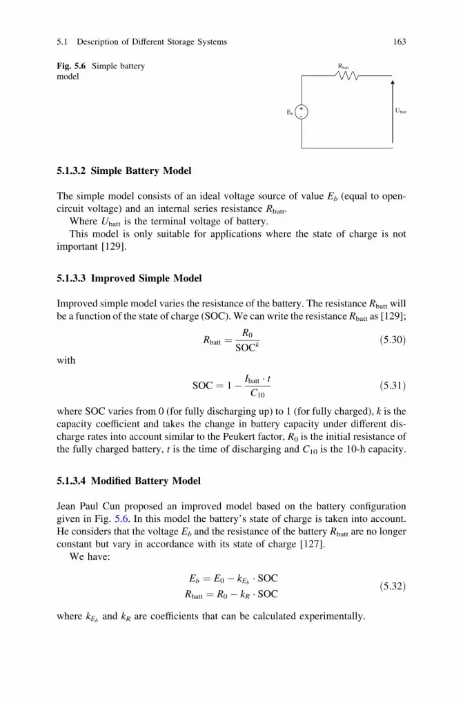
5.1.3.2 Simple Battery Model

The simple model consists of an ideal voltage source of value Eb (equal to open-circuit voltage) and an internal series resistance Rbatt.

Where Ubatt is the terminal voltage of battery.This model is only suitable for applications where the state of charge is not

important [129].

5.1.3.3 Improved Simple Model

Improved simple model varies the resistance of the battery. The resistance Rbatt willbe a function of the state of charge (SOC). We can write the resistance Rbatt as [129];

Rbatt ¼R0

SOCk ð5:30Þ

with

SOC ¼ 1� Ibatt � tC10

ð5:31Þ

where SOC varies from 0 (for fully discharging up) to 1 (for fully charged), k is thecapacity coefficient and takes the change in battery capacity under different dis-charge rates into account similar to the Peukert factor, R0 is the initial resistance ofthe fully charged battery, t is the time of discharging and C10 is the 10-h capacity.

5.1.3.4 Modified Battery Model

Jean Paul Cun proposed an improved model based on the battery configurationgiven in Fig. 5.6. In this model the battery’s state of charge is taken into account.He considers that the voltage Eb and the resistance of the battery Rbatt are no longerconstant but vary in accordance with its state of charge [127].

We have:

Eb ¼ E0 � kEb � SOC

Rbatt ¼ R0 � kR � SOCð5:32Þ

where kEb and kR are coefficients that can be calculated experimentally.

Ubatt

Rbatt

Eb+-

Fig. 5.6 Simple batterymodel


5.1.3.5 Thevenin Battery Model

Thevenin battery model is a basic model, and consists of an ideal no-load voltage(E0), an internal resistance (Rbatt), a capacitance C0 and an overvoltage resistanceRNL [137] (Fig. 5.7).

C0 is the capacitance of the parallel plates and RNL is the nonlinear resistancecontributed by the contact resistance of plate to electrolyte.

The disadvantage of this model is that all the parameters are assumed to beconstant but in reality these parameters change with temperature and batteryconditions.

A new approach to evaluate batteries is a modified Thevenin model [133]. Theelectrical equivalent of the proposed model is shown in Fig. 5.8, where E-batteryis a simple DC voltage source designating the voltage in the battery cells,E-polarization represents the polarization effects due to the availability of activematerials in the battery, E-temperature represents the effect of temperature on thebattery terminal voltage and Rbatt is the battery internal impedance, the value ofwhich depends primarily on the relation between cell voltage and state of charge(SOC) of the battery.

Voltage–sensor–current is basically a voltage source with a value of 0 V. It isused to record the value of battery current.

Thus, this model is comparatively more precise and can be extended for usewith NiCd and Li-ion batteries [133]. Only a few modifications need to be carried

Ubatt

C0

RNL

Rb

E0+-

Fig. 5.7 Thevenin battery model [137]

Rbatt

Voltage-sensor-current

+-

E-temperature

+-

E-polarisation

+-

E-battery

+-

-+

Fig. 5.8 Modified Thevenin model


out in order to vary the parameters, such as state of charge, current density andtemperature.

5.1.3.6 Linear Dynamic Model

An improved variant of the Thevenin model is a linear electrical battery model[138]. It models the behavior of the battery during overvoltage and self-dischargeof the battery. This model is more accurate than the Thevenin model but it stilldoes not consider the change of the value of parameters according to differentoperating conditions (Fig. 5.9).

5.1.3.7 Nonlinear Dynamic Model

The nonlinear dynamic model takes into account the variation of differentparameters with state of charge of the battery, temperature and discharge rate(Fig. 5.10).

The circuit is composed of two sections:

• The battery open-circuit voltage which is represented by a controlled dc voltagesource and its magnitude is changed by state of charge and temperature,

• Internal resistance which is modeled by Rc and Rd representing charging anddischarging resistances, respectively. The value of these resistances is changedby the state of charge and temperature as well.

The model is nonlinear in the sense that the elements Voc, Rd and Rc are notconstants but are modeled as a function of state of charge and temperature. Only

Ubatt

C1

R2

C2 C3

C0

E0+

-

R3

R1

Rp

Fig. 5.9 Linear dynamicmodel [137]

Voc(SOC,T)+-

C 1

Rd(SOC,T)

R c(SOC,T)

Fig. 5.10 Battery nonlinearmodel [137]


C1 has been considered constant although it is changing with state of charge but itschange is not significant [139, 140].

5.1.3.8 Resistive Thevenin Battery Model

The resistive Thevenin battery model assumes the following [141]:

• The electrodes are made of porous materials.• The electrolytic resistance is constant throughout discharge.• The discharge occurs at constant current.• Polarization is a linear function of the active material current density.

The circuit model for the resistive Thevenin battery is shown in Fig. 5.11,where Rc and Rd are internal resistances associated with the charging and dis-charging process of the battery, respectively, and Dc and Dd are diodes which arein series with Rc and Rd, respectively and have no physical significance in thebattery. It implies that during charging or discharging only one of the resistancesRc or Rd will be used because when one diode is forward biased the other will bereverse biased.

5.1.3.9 Other Models

Modified Thevenin Equivalent Battery Model

A simple dynamic battery model is shown in Fig. 5.12 [141]. The dynamicequations of the circuit model for discharging and charging are given by:

dVp

dt¼ � Vp

Rd � Cpþ Ubatt

Rd � Cp� Ibatt

Cpif Vp�Eb ð5:33aÞ

and

dVp

dt¼ � Vp

Rd � Cpþ Ubatt

RC � Cp� Ibatt

Cpif Vp�Eb ð5:33bÞ

E0+- Rc

Rd

Ubatt

Dd

Dc

Fig. 5.11 Thevenin resistivemodel


with

Ibatt ¼Vp � Ubatt

Rbatt

Model From a Series Experimental Test

The following model is developed from a series of experimental tests performedthrough examination of the graphic plots of the experimental data, and manu-facturer’s specifications. This is the simplest model that meets most requirementsfor a good battery model. It contains most nonlinear characteristics as well asdependence on the state of charge [141] (Fig. 5.13).

C1dVC1

dt¼ �Ibatt �

VC1

R00if VC1� 0 ð5:34aÞ

and

C1dVC1

dt¼ �Ibatt �

VC1

R0if VC1� 0 ð5:34bÞ

Eb

Rd

UbattCp VpRc

IbattRbatt

Fig. 5.12 Modified Thevenin equivalent battery model

Cp

Rd

UbattRp VOC

R’

Rc R"

Ibatt

C1

VC1

Fig. 5.13 Model from a series experimental test [137]


We obtain during charge:

Ubatt ¼ Voc � Rc Ibatt þ VC1 ð5:35aÞ

and during discharge,

Ubatt ¼ Voc � Rd Ibatt þ VC1 ð5:35bÞ

where ideal diodes are chosen strictly for directional purposes, and are required todifferentiate between internal and overvoltage resistances for the charge and thedischarge.

Dynamical Model

An empirical mathematical model is developed for lead acid traction battery [143]:

Vbatt ¼ Voc � Rbatt � Ibatt �K

SOCIbatt ð5:36Þ

where Voc is the open-circuit voltage, Ibatt is the discharge current, K a constant,typically 0.1 ohm and K=SOC represents the part of internal resistance which isSOC dependent.

Dynamic Model of Third-Order

The equivalent network of the following model of the battery is described by theFig. 5.14 [142], where Em in this the main branch is the electromotive force of thebattery and Zm is the main part of the internal impedance of the battery. Thisimpedance Zm can be approximated by two R–C blocks.

When a battery is being charged, a part of the electrical energy received isconverted into other forms of energy such as water electrolysis. Because of this, aparasitic branch is added in the model. This part is used only when the battery isbeing charged.

IpðVPNÞ stands for the expression of simple resistor Rp because the nonlinearcharacter of the parasitic branch is taken in account by the threshold voltage Ep.

R0

Em Ep

ZpZm

Im

Ip

+-

+-

Fig. 5.14 Battery equivalentnetwork


An equivalent network is represented in Fig. 5.15. This model is constituted by:

• An electrical equivalent with two R–C blocks and an algebraic parasitic branch.• Algorithms for calculating the state of charge and internal (electrolyte)

temperature.• Equations for computation of the elements of the equivalent network as func-

tions of state of charge and temperature.

C1, R1 and R2 are the elements of Zm.

Dynamic Model of Fourth Order

Giglioi [143] proposed a dynamic model which is an accurate and sophisticatedmodel. It consists of two parts:

• Current Ip flowing through RP (electrolyte reaction), Rd (ohmic effect) and itsassociated leakage capacitance Cd, and waste of energy Rw and its associatedleakage capacitance CW;

• Current Is flowing through Rs (self-discharge) (Fig. 5.16).

This model is accurate but it has some drawbacks:

• It requires a longer time for computation due to the high order system.• Modeling process is complicated because it involves a lot of empirical data.

+-

Em

Ibatt

R1

C1

R2

I (V )p p

R0IpIm

I1

Fig. 5.15 Third-orderbattery model

Ubatt

RW

+- +

-

Rd Rp Rs

Es

CW

Cd

Eb

Is

Ip

Fig. 5.16 Dynamic model offourth order [143]


5.1.4 Traction Model

A mathematical model is used for a traction lead acid battery (Fig. 5.17) [127].This model is used primarily in applications of electric and hybrid vehicles; itconsists of the EMF Eb in series with a resistance Rbatt and a capacitor (Q/K).

Vbatt ¼ Eb � Rbatt � Ibatt � K

Z

Ibatt

Q

� �

dt ð5:37Þ

with Vbatt terminal voltage of the battery, Eb zero-current voltage of the battery

charged and K constant which depends on the battery.R

Ibatt

Q

� �

dt indicates the state

of battery discharge, Q being the battery capacity (Ah).

5.1.5 Application: CIEMAT Model

The advantage of the battery models developed by CIEMAT is their ability to copewith a wider range of lead acid batteries and requires few manufacturers’ datatechnological parameters [129, 144, 145]. This model is based on the electricalscheme of Fig. 5.18, the battery is then described by two elements, a voltagesource Eb and an internal resistance Rb, of which characteristics depend on anumber of parameters (temperature and charge state).

For a number of nb cells, the voltage equation is:

Ubatt ¼ nb � Eb � nb � Rbatt � Ibatt ð5:38Þ

+-

Vbatt

Q/K

Rbatt

Eb

Fig. 5.17 Model traction

Ubatt

n .Rbatt

n .Ebb

b

+-

IbattFig. 5.18 Equivalent circuitof a battery of nb elements


5.1.5.1 Capacitor Model

To highlight the physical phenomena that govern the operation of the storagesystem, the capacity should take into account the temperature. Therefore, wepropose the model of capacity, giving the amount of energy that can be returnedaccording to the mean discharge current, it is given by Eq. 5.39 The capacitymodel is established from the expression of the current I10, which corresponds tothe operating speed to C10, where DT is the heating of the accumulator (assumedidentical for all elements) over an ambient temperature which is equal to 25�C[146].

Cbatt

C10¼ 1:67

1þ 0:67 II10

� �0:9 1þ 0:005DTð Þ ð5:39Þ

The capacity Cbatt is used as a reference for determining the state of batterycharge.

SOC ¼ 1� Q

Cbatt

ð5:40Þ

with

Q ¼ Ibatt � t ð5:41Þ

t is the discharging time with a current Ibatt.

5.1.5.2 Charge Voltage Equation

Expression of the battery voltage is function of the internal components of thebattery depending on the electromotive force and the internal resistance.

Vbatt�charge ¼ nb 2:þ 0:16 � SOC½ � þ nb:Ibatt

C10

6

1þ I1:3batt

þ 0:27

SOC1:5 þ 0:002

� �

� 1� 0:007:DTð Þ ð5:42Þ

where nb is the cells number, DT is the temperature variation

DT ¼ T � 25

and C10 is the rated capacity (I10)


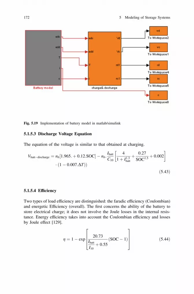
5.1.5.3 Discharge Voltage Equation

The equation of the voltage is similar to that obtained at charging.

Vbatt�discharge ¼ nb 1:965:þ 0:12:SOC½ � � nb:Ibatt

C10

4

1þ I1:3batt

þ 0:27

SOC1:5 þ 0:002

� �

� 1� 0:007:DTÞð Þð5:43Þ

5.1.5.4 Efficiency

Two types of load efficiency are distinguished: the faradic efficiency (Coulombian)and energetic Efficiency (overall). The first concerns the ability of the battery tostore electrical charge; it does not involve the Joule losses in the internal resis-tance. Energy efficiency takes into account the Coulombian efficiency and lossesby Joule effect [129].

g ¼ 1� exp20:73

Ibatt

I10þ 0:55

SOC� 1ð Þ

2

6

6

4

3

7

7

5

ð5:44Þ

Fig. 5.19 Implementation of battery model in matlab/simulink


5.1.5.5 Temperature Effects

We make application under Matlab/Simulink (Fig. 5.19).

Temperature Influence on Battery Capacity

The battery temperature affects the storage capacity. The capacity increases withthe temperature of the element (Fig. 5.20). This is explained partly by theincreased diffusion coefficient of sulfuric acid solutions, on the other hand by thedecrease in resistivity of the electrolyte at commonly used concentrations.

Fig. 5.20 Temperatureinfluence on battery capacity

Fig. 5.21 Temperatureinfluence on state of charge


Temperature Influence on State of Charge

The charging (or discharging) is used to express the relationship between thenominal capacity of a battery and the charge (or discharge) current. Figures 5.21and 5.22 show the evolution of the state of charge and the discharge state (DOD)according to battery capacity, respectively.

DOD ¼ 1� SOC ð5:45Þ

Temperature Influence on Battery Voltage

The curves of the battery voltage (Figs. 5.23, 5.24) are influenced by temperaturebecause voltage is a function of SOC, the charge and discharge time, temperatureand current.

Influence of Charge and Discharge Time on the State of the Battery

The influence of charge time on the state of the battery is shown in Figs. 5.25 and5.26

In the case of the charge, more charge time decreases, and more the batterycharge state is close to 1. And in the case of discharge, more the discharge time isimportant more the discharge state reached its maximum value.

Influence of Charge Time and Discharge Time on the Battery Voltage

For both charge and discharge, the evolution of the voltage is directly proportionalto the time of charge and discharge (Figs. 5.27, 5.28).

Fig. 5.22 Influence oftemperature on the dischargestate


Fig. 5.25 Effect of time onthe state of discharge (DOD)

Fig. 5.23 Influence oftemperature on the dischargevoltage

Fig. 5.24 Influence oftemperature on the chargevoltage


Fig. 5.26 Effect of time onthe state of charge (SOC)

Fig. 5.27 Influence of timeon the charge voltage [195]

Fig. 5.28 Influence of timeon the discharge voltage[195]


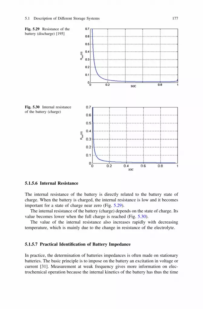
5.1.5.6 Internal Resistance

The internal resistance of the battery is directly related to the battery state ofcharge. When the battery is charged, the internal resistance is low and it becomesimportant for a state of charge near zero (Fig. 5.29).

The internal resistance of the battery (charge) depends on the state of charge. Itsvalue becomes lower when the full charge is reached (Fig. 5.30).

The value of the internal resistance also increases rapidly with decreasingtemperature, which is mainly due to the change in resistance of the electrolyte.

5.1.5.7 Practical Identification of Battery Impedance

In practice, the determination of batteries impedances is often made on stationarybatteries. The basic principle is to impose on the battery an excitation in voltage orcurrent [31]. Measurement at weak frequency gives more information on elec-trochemical operation because the internal kinetics of the battery has thus the time

Fig. 5.29 Resistance of thebattery (discharge) [195]

Fig. 5.30 Internal resistanceof the battery (charge)


to react to the imposed disturbance. In order to determine the internal impedanceof the battery (12 V, 100 Ah) for one state of charge of the battery, we super-impose an alternate sinusoidal signal of 50 Hz frequency to the continuouscomponent of the battery. We made application with a system of storage which iscomposed of two lead acid batteries of 12 V, 92 Ah inter connected in series tohave 24 V. We close the battery on a circuit including a rheostat for the currentlimitation (15.8X, 10 A), a shunt (250 V, 10 A) allowing to measure the circu-lating current in the circuit and a source of alternating voltage (0–36 V, 20 A). Themeasurement system is developed (Fig. 5.31).

We measure two voltages using an oscilloscope: the voltage at the shunt ter-minals which is a direct picture of the current circulating in the circuit and the

Fig. 5.31 Circuit measurement of battery impedances

Fig. 5.32 Measured signals S1 current and S2 voltage


voltage at the battery terminals. The ratio of these two voltages and their phaseangle provides the absolute value of the internal impedance of the battery.

Measures are carried out by a digital oscilloscope, Tektronix TDS3032,300 MHz with two channels, which makes the acquisition of signals possible, thento transfer them to a computer for analysis. The mass is common to both measuresof voltage. The signal (V1) permits to measure the battery voltage and the signal(V2) the current. Figure 5.32 presents the signals recovered by Excel. The signal(S1) is a direct image of the AC current of measurement (conversion factor:50 V = 1A) while the second signal represents the resulting voltage on the bat-tery’s terminals.

The battery behaves as complex impedance Zbatt containing a resistance Rbatt

and a reactance Xbatt to this disturbance.

Zbatt ¼ Rbatt � jXbatt ð5:46Þ

The module of the complex impedance is thus well defined by the ratio of theabsolute values of the two signals. We deduce the dephasing by the temporaldifference between the two signals with the passage by zero.

Zbattj j ¼ Vbatt=Ibatt ð5:47Þ

Knowing the module of Zbatt and its dephasing, we can thus deduce the real partRbatt and imaginary Xbatt of the impedance for this state of charge, these valueschanges according to the latter.


Chapter 6Photovoltaic Pumping Systems

Symbolsa(h), b(h), c(h), d(h) Coefficients corresponding to the working total headai, bi, ci and di Constants which depend on the type of solar pumping

systemCi ith calculated valueh Total headhh p.u Fundamental voltage valueia Armature current(Isd Isq) (d, q) Components of the stator currentiF Field currentJ Rotor and load moment of inertiaJmotAC Inertia of the AC motorKh Harmonics to be minimizedKm Constant related to the design of the machineLF Field winding inductanceLa Armature winding inductanceMi ith measured valuen Number of measurementsP9 Electrical power input of the motor pumpp Pole pair number of the AC machineRa Armature resistanceRF þ Radj Total field resistanceRm Core loss resistance (X)Rs Stator resistance per phase (X)Rr Equivalent rotor resistance per phase (X)TL Load torquev Terminal voltageVa, Vb and Vc Phase voltagesVs rms Motor voltage (V)


181

(Vsd, Vsq) (d, q) Components of the stator voltageXm Magnetizing reactance (X)Xs Stator leakage reactance (X)Xr Equivalent rotor leakage reactance (X)r Leakage coefficient/ Flux per pole(/sd, /sq) (d, q) Components of the stator fluxx Rotational speed of the rotorxrAC AC motor velocity angularxs Angular frequency of the supply (rd/s)

Photovoltaic pumping has become one of the most promising fields in photovoltaicapplications. To achieve the most reliable and economical operation, moreattention is paid to their design and their optimal use. Depending upon the intendedapplication, the pumping system can be selected from surface, submersible orfloating pump types [147]. Submersible pumps remain underwater, surface pumpsare mounted at water level at the vicinity of the well or, in the case of a floatingpump, on top of the water. Pumps can be classified according to their operatingmodes. Mainly there are centrifugal and positive displacement pumps [147]. In thecentrifugal pump, the rotation of an impeller forces water into the pipe. The watervelocity and pressure depend on the available mechanical power at the rotatingimpeller and the total head. The displacement pump uses a piston or a screw tocontrol the water flow. Compared to the centrifugal pump, the positive displace-ment pump presents a better efficiency under low power conditions.

The water pumps may be driven by DC or AC motors. The earlier PV pumpingsystems were principally based on DC motors [148]. The DC motors present thedrawback of maintenance expenses due to frequent brush replacements [149].Brushless permanent magnet DC motors have been introduced in some systemsPhotovoltaic array [150]. Recent developments in induction motor technologymade this option attractive among the AC motors-based pumping setups. Theinduction motor is more robust, requires much less maintenance and is available atlower costs than DC motors [149, 150].

6.1 PV Pumping Systems Based on DC Machines

6.1.1 Description

Photovoltaic water pumping systems generally consist of a PV array, a motorpump subsystem, a controller and a tank. The motor pump subsystem includes a

182 6 Photovoltaic Pumping Systems

DC motor and a centrifugal pump. There are two configurations of PV pumpingsystems based on DC motor. In the first system (Fig. 6.2), the motor could beconnected directly to the PV generator. For allowing operation of the pumpingsystem at maximum power, the motor controller has to be able to perform thetracking of the MPP.

The second system comprises PV array feeding a DC motor via a DC–DCconverter which may perform the MPPT (Fig. 6.3).

6.1.2 System Modeling

6.1.2.1 DC Machine Model

DC motors are electrical machines which consume DC electrical power andproduce mechanical power. In shunt machines, the field circuit is connected inparallel with the armature circuit while DC series machines have their field circuit

Controller

DC/DC

DC/AC

Battery

DC Pump

DC motor

AC Pump

AC motor

Fig. 6.1 General configuration of a photovoltaic pumping system [62]

DCMotor

Photovoltaic arrayFig. 6.2 Photovoltaic systemloaded by DC motor

6.1 PV Pumping Systems Based on DC Machines 183

in series with the armature where both field and armature currents are identical.Permanent magnet machines, on the other hand, have only one circuit (armaturewinding) and the flux generated by the magnets is constant.

DC Shunt Motor

The equivalent circuit of DC Shunt motor is shown in Fig. 6.4. Adjustable resistorRadj is connected in series with the field circuit for speed control.

The dynamical model of DC shunt motor can be written as

LFdiF

dt¼ V � ðRF þ RadjÞiF ð6:1Þ

Ladiadt¼ V � Raia � Km/x ð6:2Þ

Jdxdt¼ Km/ia � TL ð6:3Þ

DC/DC

converter

Duty ratio

DCMotor

Photovoltaic array

Fig. 6.3 Photovoltaic system loaded by DC motor via DC–DC buck-boost converter

Ra La

RF

Radj

LF

+

-

VEA

ia iL

IF

Fig. 6.4 Equivalent circuitof DC Shunt motor


with LF as the field winding inductance, iF field current, V terminal voltage andRF þ Radj total field resistance, La armature winding inductance, ia armature cur-rent, Ra armature resistance, Km constant related to the design of the machine, /flux per pole, x rotational speed of the motor, J rotor and load moment of inertiaand TL load torque.

DC Series Motor

The equivalent circuit of DC series motor is shown in Fig. 6.5. The field circuit isconnected in series with the armature and then the armature and field currents areidentical.

The nonlinear dynamical mathematical model is given by:

ðLF þ LaÞdia

dt¼ VT � ðRa þ RFÞia � Km/x ð6:4Þ

Jdxdt¼ Km/ia � TL ð6:5Þ

Permanent Magnet DC Motor (PMSM)

Due to the absence of the field current and field winding, permanent magnetmachines exhibit high efficiency in operation, simple and robust structure inconstruction and high power to weight ratio. The attractiveness of permanentmagnet machines is further enhanced by the availability of high-energy rare earthpermanent magnet materials like SmCo and NdFeB. However, the speed control ofpermanent magnet DC motor via changing the field current is not possible. Then,MPPT is possible only using a DC–DC converter as in Fig. 6.3.

The dynamical model can be written as:

Ladiadt¼ V � Raia � Km:/x ð6:6Þ

Ra La RF LF

+

-

VEA

ia

Fig. 6.5 Equivalent circuitof DC series motor


Jdxdt¼ K:/:ia � TL ð6:7Þ

6.1.2.2 Centrifugal Pump Model

Description

In the centrifugal pump, the rotation of an impeller forces water into the pipe.The water velocity and pressure depend on the available mechanical power at therotating impeller and the total head. A centrifugal pump commonly requires asingle quadrant drive.

Pump Model

There are still many obstacles inhibiting a larger implementation of PV pumpingsystems [149]. Among these problems is the lack of accurate tools for the

Ra La

+

-

VEA

iaFig. 6.6 Equivalent circuitof PMSM

Fig. 6.7 Pump model


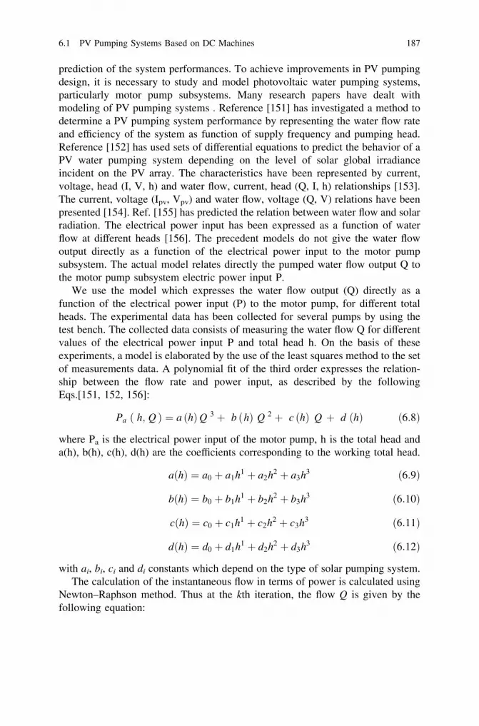
prediction of the system performances. To achieve improvements in PV pumpingdesign, it is necessary to study and model photovoltaic water pumping systems,particularly motor pump subsystems. Many research papers have dealt withmodeling of PV pumping systems . Reference [151] has investigated a method todetermine a PV pumping system performance by representing the water flow rateand efficiency of the system as function of supply frequency and pumping head.Reference [152] has used sets of differential equations to predict the behavior of aPV water pumping system depending on the level of solar global irradianceincident on the PV array. The characteristics have been represented by current,voltage, head (I, V, h) and water flow, current, head (Q, I, h) relationships [153].The current, voltage (Ipv, Vpv) and water flow, voltage (Q, V) relations have beenpresented [154]. Ref. [155] has predicted the relation between water flow and solarradiation. The electrical power input has been expressed as a function of waterflow at different heads [156]. The precedent models do not give the water flowoutput directly as a function of the electrical power input to the motor pumpsubsystem. The actual model relates directly the pumped water flow output Q tothe motor pump subsystem electric power input P.

We use the model which expresses the water flow output (Q) directly as afunction of the electrical power input (P) to the motor pump, for different totalheads. The experimental data has been collected for several pumps by using thetest bench. The collected data consists of measuring the water flow Q for differentvalues of the electrical power input P and total head h. On the basis of theseexperiments, a model is elaborated by the use of the least squares method to the setof measurements data. A polynomial fit of the third order expresses the relation-ship between the flow rate and power input, as described by the followingEqs.[151, 152, 156]:

Pa ð h; Q Þ ¼ a ðhÞQ 3 þ b ðhÞ Q 2 þ c ðhÞ Q þ d ðhÞ ð6:8Þ

where Pa is the electrical power input of the motor pump, h is the total head anda(h), b(h), c(h), d(h) are the coefficients corresponding to the working total head.

aðhÞ ¼ a0 þ a1h1 þ a2h2 þ a3h3 ð6:9Þ

bðhÞ ¼ b0 þ b1h1 þ b2h2 þ b3h3 ð6:10Þ

cðhÞ ¼ c0 þ c1h1 þ c2h2 þ c3h3 ð6:11Þ

dðhÞ ¼ d0 þ d1h1 þ d2h2 þ d3h3 ð6:12Þ

with ai, bi, ci and di constants which depend on the type of solar pumping system.The calculation of the instantaneous flow in terms of power is calculated using

Newton–Raphson method. Thus at the kth iteration, the flow Q is given by thefollowing equation:


For Pa [ 0:

Qk ¼ Qk�1 �FðQk�1Þ

F 0ðQk�1Þð6:13Þ

with

FðQk�1Þ ¼ a Q 3k�1þb Q 2

k�1þc Qk�1 þ d � Pa ð6:14Þ

where F0(Qk-1) is the derivative of the function F(Qk-1).Validation of the presented motor pump subsystem model is performed at

different heads and input powers by comparing the measured water flow rates withthe simulation results. The comparison uses the root mean square error (RMSE)and mean bias error (MBE) indicators; these coefficients are defined by Eqs. 15and 16 as

RMSE ¼Pn

i¼1 Ci �Mið Þ2Pn

i¼1 M2i

" # 0:5

� 100 ð6:15Þ

MBE ¼Pn

i¼1Mi�Cij j

Mi

h i

n

2

4

3

5 � 100 ð6:16Þ

where n is the number of measurements, Ci the ith calculated value and Mi the ithmeasured value.

6.1.3 Application

The experiments are carried out using the pump testing system at the Centre ofDevelopment of Renewable Energies located in Algiers-Algeria [60]. The maincomponents of the test facility consist of 30 mono-crystalline PV modules with atotal peak power of 2.2 kWp, several pumps, a water tank, an air/water regulatedpressure vessel, an air compressor, a piping system and measuring devices.A motor operated valve is used to set the water head between 0 and 120 m withflow rates ranging between 0 and 30 m3 per hour.

We present the experiments conducted for two centrifugal pumps C1 (400 W)and C2 (1000 W). The water flow Q and electric power input P values are loggedat different total heads, for the tested pumps C1 and C2. Examples of Q–P curvesare shown in Figs. 6.8, and 6.9 and the results concerning the RMSE and MBEindicators are given in Figs. 6.10,and 6.11. Good agreement between experimentaland calculated data is seen in Figs. 6.8, 6.9, 6.10, 6.11. The low values of theRMSE and MBE validate the present model.


6.2 PV Pumping Systems Based on AC Motor

6.2.1 Description

Photovoltaic water pumping systems based on induction machine consist of a PVarray, a motor pump subsystem, a controller and a tank (Fig. 6.12). The motorpump subsystem includes a motor, a pump and a power converter.

The controller is an electronic interface between the photovoltaic array and themotor pump subsystem. In the case of AC motor use, an inverter may be includedin the controller [158]. Usually a tank is commonly employed for water storage.The principle is to store water rather than electricity in batteries, thereby reducingthe cost and complexity of the system.

Fig. 6.8 Q–P characteristicsfor C1 at heads: 6, 12, 18,26 m [62]

Fig. 6.9 Q–P characteristicsfor C2 at heads: 35, 40, 45,50, 55, 60 m [62]

6.2 PV Pumping Systems Based on AC Motor 189

Fig. 6.10 RMSE and MBE results for the centrifugal pumps C1 [62]

Fig. 6.11 RMSE and MBE results for the centrifugal pumps C2 [62]

VSI

Inverter

IM

PV array

C

Pump

Fig. 6.12 Block diagram of PV pumping based on induction machine


6.2.2 System Modeling

6.2.2.1 The d–q Induction Motor Model

We use an induction motor which is modeled using voltage and flux equationsreferred in a general normalized stator frame [157]:

– Stator voltage equations:

Vds ¼ RSIds þdUds

dt

Vqs ¼ RSIqs þdUqs

dt

8

>

<

>

:

ð6:17Þ

where (Ids Iqs), (Vds, Vqs) and (Uds, Uqs) are the (d, q) components of the statorcurrent, voltage and flux, Rs is the stator resistance.

– Rotor voltage equations:

0 ¼ Vdr ¼ RrIdr þdUdr

dtþ p xrAC:Uqr

0 ¼ Vqr ¼ RrIqr þdUqr

dt� p xrACUdr

8

>

<

>

:

ð6:18Þ

where Idr, Iqr are (d, q) rotor current, Udr, Uqr are (d, q) rotor flux, Rr is the rotorresistance.

We obtain the following mathematical model:

dids

dtdiqs

dtdidr

dtdiqr

dt

2

6

6

6

6

6

6

6

6

6

6

4

3

7

7

7

7

7

7

7

7

7

7

5

¼ 1r

�Rs

Ls

p �xrAC � L2m

Ls � Lr

Lm:Rr

Lsr

p �xrAC � Lm

Ls

�p �xrAC � L2m

Lsr�Rs

Ls

p �xrAC � Lm

Ls

Lm:Rr

Ls � LrLm:Rs

Ls � Lr�p �xrAC � Lm

Lr�Rr

Lr�p:xrAC

p �xrAC � Lm

Lr

Lm:Rs

Ls � Lrp:xrAC �Rr

Lr

2

6

6

6

6

6

6

6

6

6

6

4

3

7

7

7

7

7

7

7

7

7

7

5

:

ids

iqs

idr

iqr

2

6

6

6

4

3

7

7

7

5

þ 1r

1Ls

00 1

Ls

� LmLs:Lr

0

0 � LmLs:Lr

2

6

6

6

4

3

7

7

7

5

:vds

vqs

� �

ð6:19Þ


with Lm as the magnetizing inductance of the motor and Ls and Lr are the statorand rotor inductances and

r ¼ 1 � L2m

Ls Lr

– Mechanical equation:

TemAC � TLoad ¼ JmotAC:dxr AC

dtð6:20Þ

with xrAC as the AC motor angular velocity and JmotAC the inertia of the ACmotor.

The electromagnetic torque can be written as:

TemAC ¼ p:ð/ds:iqs � /qs:idsÞ ð6:21Þ

where p is the pole pair number of the AC machine

Uds ¼ Ls:ids þ Lm:idr

Uqs ¼ Ls:iqs þ Lm:iqr

The modelisation is made under Matlab/Simulink (Fig. 6.13).

Fig. 6.13 Motor block diagram


6.2.2.2 The d-q Synchronous Motor Model

Using the normalized (d-q) rotating reference frame, with id andiq as the(d, q) stator currents, the machine model based on Park’s d-q components isdescribed by the following equations [159]:

Vds ¼ RSIds � LqxrAC:Iqs þ LddIds

dt

Vqs ¼ RSIqs þ LdxrAC:Ids þ LqdIqs

dt þ xrAC/f

ð6:22Þ

with Rs as the armature winding, Ld and Lq are d and q axial inductances, Uf theinterlinkage magnetic flux, Vd and Vq the d and q axial voltages, ids and iqs thed and q axial currents and xrAC the angular velocity of rotor.

The mechanical equation is given as:

JdXrAC

dt¼ TemAC � TL ð6:23Þ

where

TemAC ¼ pð/f Iqs þ ðLd � LqÞIdsIqsÞ ð6:24Þ

with J as the rotor inertia moment, TL the load torque and p pole the pair number.

6.2.2.3 Displacement Pump

Description

The displacement pump uses a piston or a screw to control the water flow.As compared to the centrifugal pump, the positive displacement pump presents abetter efficiency under low power conditions.

Pump Model

We use the same model as above (see Section ‘‘Pump model’’).

6.2.2.4 Application

The experiments are carried out using the pump testing system at the Centre ofDevelopment of Renewable Energies located in Algiers-Algeria [62]. We presentthe experiments conducted for the displacement pump D1. The water flow Q andelectric power input P values are logged at different total heads, for the testedpump D1.


Examples of Q–P curves are shown in Fig. 6.15 and the results concerning theRMSE and MBE indicators are given in Fig. 6.16. Good agreement betweenexperimental and calculated data is seen in Fig. 6.15. The low values of the RMSEand MBE validate the present model (Fig. 6.16).

6.2.2.5 Voltage Source Inverter Model

Natural PWM Strategy

A natural PWM strategy is used to drive the full bridge DC–AC inverter with amodulation index m and the ratio between the frequencies of the carrier andmodulating waveforms r.

The capacitor across the inverter input terminals as shown in Fig. 6.12, servesto smooth the output voltage of the DC source and to reduce the source impedance.

Fig. 6.15 Q–P curves forpump D1 at head: 45, 55, 65,75, 80 m [62]

Fig. 6.14 Example ofdisplacement pump


The three-phase inverter consists of three legs, one for each phase. It is assumedthat the switches and diodes are ideal devices. The control signals are generated bymodulating three low frequency sinusoidal (va, vb, vc) with a common high

Fig. 6.16 RMSE and MBE results for the centrifugal pumps D1 [62]

Switching logicCarrier wave Comparators

+

-

+

-

+

-

va

vb

vc

Vp

Fig. 6.17 Sinusoidal PWM strategy and voltage waveforms


frequency triangular carrier wave (Vp). The switching instants are determined bythe crossover of the two waveforms.

Harmonic Elimination PWM Strategy

The undesirable harmonics of a square wave can be eliminated and the funda-mental voltage component can be controlled as well by what is known as theharmonic elimination method. In this method, notches are created in the squarewave at predetermined angles (Fig. 6.19). It can be shown that the notch anglescan be controlled to eliminate certain harmonic components and control the fun-damental voltage [158].

Fig. 6.18 Subsystem of an IM fed by an MLI inverter

Fig. 6.19 Optimized P.W.M signal


The Fourier series development of a control signal C1(xt) is:

C1ðxtÞ ¼ a0 þX

1

n¼1

an: cosðn:hÞþX

1

n¼1

bn:sinðn:hÞ ð6:25Þ

where

a0 ¼ 0

an ¼2p:

Z

p2

�p2

C1ðhÞ:cosðnhÞdðhÞ

bn ¼2p:

Z

p2

�p2

C1ðhÞ:sinðnhÞdðhÞ

h ¼ x:t

2

6

6

6

6

6

6

6

6

6

6

6

6

6

6

4

3

7

7

7

7

7

7

7

7

7

7

7

7

7

7

5

ð6:26Þ

In a quarter-cycle symmetrical waveform, only the sine odd harmonics exist.Therefore, the coefficients are given by:

an ¼ 0

bn ¼4p:

Z

p2

0

C1ðhÞ �12

� �

: sinðnhÞ:dðhÞ

2

6

6

6

4

3

7

7

7

5

ð6:27Þ

Then, the following system of transcendental equations is obtained:

Fig. 6.20 Angles notches for different harmonic ranks


12� cosðh1Þ þ cosðh2Þ � cosðh3Þ þ . . .. . .. . .þ cosðhnÞ ¼ hh

12� cos 5ðh1Þ þ cos 5ðh2Þ � cos 5ðh3Þ þ . . .. . .þ cos 5ðhnÞ ¼ 0


12� cos 11ðh1Þ þ cos 11ðh2Þ � cos 11ðh3Þ þ . . .þ cos 11ðhnÞ ¼ 0


. . .. . .. . .. . .. . .. . .. . .. . .. . .. . .. . .. . .. . .. . .. . .. . .. . .. . .. . .. . .. . .. . .. . .. . .

12� cos jðh1Þ þ cos jðh2Þ � cos jðh3Þ þ . . .. . .þ cos jðhnÞ ¼ 0

2

6

6

6

6

6

6

6

6

6

6

6

6

6

6

6

6

6

6

6

6

4

3

7

7

7

7

7

7

7

7

7

7

7

7

7

7

7

7

7

7

7

7

5

ð6:28Þ

where hh is p.u. fundamental voltage value.This system of nonlinear transcendental equations is solved employing an

algorithm written in language Matlab, h1, h2…. hn are then determined (Table 6.1).

– Application:

An application is made on AC motor supplied from a voltage source inverter.The machine is controlled using a position sensor which produces the invertercontrol signals. This sensor is fixed on to the rotor shaft and allows for supplyfrequency setting to the value of the rotor frequency. Simulation and experimentalresults are presented in Fig. 6.21 [159].

Pondered Harmonic Minimization Strategy

We can use another alternative where performance indexes are considered. Thisapproach is to define a performance index related to the undesirable effects of theharmonics and to select the switching angles so that the fundamental voltage iscontrolled and the performance index is minimized. This is called a distortion

Table 6.1 Angles Notches for 5, 7, 11 … 31th harmonics[157]

Rank h1 h2 h3 h4 h5 h6 h7 h8 h9 h10

5 12.005,7 16.25 22.055,7,11 8.74 24.39 27.755,7,11,13 10.54 10.09 30.90 32.865,7,11,13,17 6.79 17.30 21.03 34.67 35.995,7,11,13,17,19 7.80 12.67 23.08 25.62 38.11 38.995,7,11,13,17,19,23,25 6.19 10.45 18.40 21.04 30.49 32.85 42.43 42.905,7,11,13,17,19,23,25,

29,315.13 8.90 15.29 17.88 25.39 26.98 35.40 36.22 45.33 45.61


minimization PWM technique. In this method, the total harmonic voltage distor-tion factor (THD) is minimized. The minimization of this quantity and the controlof the fundamental are achieved by an appropriate positioning of the switchingangles. Considering that higher harmonics are easier to filter, we take into accountharmonics until nth with a weigh decreasing with frequency. The THD perfor-mance factor is then defined as:

THD ¼

ffiffiffiffiffiffiffiffiffiffiffiffiffiffiffiffiffiffiffiffiffiffiffiffi

X

n

kh6¼1

Vkh

kh

� �2v

u

u

t ð6:29Þ

6.2.3 Scalar Control of the PV System

The steady-state performance of an induction motor is modeled using the con-ventional equivalent circuit of Fig. 6.22, where Vs is the rms phase motor voltage(V), Rs the stator resistance per phase (X), Rr the equivalent rotor resistance perphase (X), Rm the core loss resistance (X), Xs = xs (Ls – Lm) the stator leakagereactance (X), Xr = xs ( Lr – Lm) the equivalent rotor leakage reactance (X),

Fig. 6.21 Simulation and experimental results in the case of 5, 7, 11 and 13th harmonicselimination


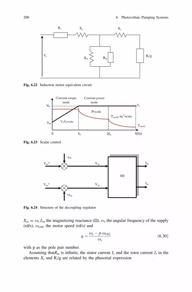
Xm = xs Lm the magnetizing reactance (X), xs the angular frequency of the supply(rd/s), xrAC the motor speed (rd/s) and

g ¼ xs � p:xrAC

xsð6:30Þ

with p as the pole pair number.Assuming thatRm is infinite, the stator current Is and the rotor current Ir in the

elements Xr and Rr/g are related by the phasorial expression

Rs

Vs

Xs Xr

Rr/g

Fig. 6.22 Induction motor equivalent circuit

Constant power mode

Constant torquemode

Vs/fs=cste

TemAC. s2=cste

P=cste

Vs

TemAC

Fig. 6.23 Scalar control

Iqs

Ids

-eds

+eqs

Vqs*

Vds*

Vqs

Vds

IM

Fig. 6.24 Structure of the decoupling regulator


�Is ¼ �Ir þðRr=g þ j XsÞ�Ir

j Xm¼ Rr=g þ j Lr xs

j Lm xs

�Ir

It is then easy to compute Ir as a function of Vs. One obtains

�Ir ¼j xs Lm Vs

RsRr=g � x2s ðLrLs � L2

mÞ þ jxsðRrLs=g þ RsLrÞ

The expression of electromagnetic torque can be written as:

Tem AC ¼ 3Rr

gI2r = ðxs=pÞ

or

VSI

Inverter

IM

PV array

Pump

ref

Iqs

Ids

+eqs

eds

Vds*

Vqs*

Ids

PI

r

qs

r

mI

T

L

PI

*

*

r

qs

r

mI

T

L

mL

1

p

s s

rAC

TemAC* Iqs*

Fig. 6.25 Block diagram of indirect vector control


TemAC ¼ 3p:V2s

Rr

gxsL

2m

RrRs

g� x2

s : LsLr � L2m

� �

� �2

þx2s

RrLs

gþ RsLr

� �2 ð6:31Þ

Power converted in mechanical power, stator current and stator power will be:

Pconv ¼ 3Rr

gI2r ð1� gÞ ð6:32Þ

Is ¼ 1 þ Rr=g þ jðLr � LmÞxs

j Lm xs

Ir ¼Rr=g þ j Lr xs

j Lm xs

Ir ð6:33Þ

Ps ¼ Pconv þ Pjr þ Pjs ð6:34Þ

From the previous equations, we obtain the total power absorbed by the stator:

Ps ¼ 3Rr

gþ Rs

ðRr=gÞ2 þ L2r x

2s

L2mx2

s

" #

I2r

erreur

w

Isa1

Q

Ce

t

omega

isq

isd

ws

fird_est

teta

flux estimation

firef

fcon

usd

usq

ws

vsd*

vsq*

decouplage1

id

iq

teta

ia

ib

ic

omega

Q

Cr

Pump

Pmax_Wref

PI

PI omega

PI

PI flux

PI

PI Iq

PI

PI Id

E

Vd_ref

Vq_ref

teta

Vd

Vq

Ond1

MATLABFunction

MATLAB Fcn Is3

Is2

Is1

Is

Vds

Vqs

ws

Cr

Ids

Iqs

Ce

Omega

IM

E

Cr

fird_est

ws

teta

omega

[isd]

[ws]

[omega]

[fird]

[isq]

[isq]

[teta]

[omega]

[ws]

[E]

[Cr]

[teta]

[isd]

From11

[omega]

[fird_est]

Signal 2

Signal 3

Eclairement1

Demux25

Constant1

Clock

Fig. 6.26 Vector control of the PV pumping system based on induction machine


or, according to speed:

Ps ¼ 3 k2 ðxs � p xr ACÞxs

RrLsLr

�2 þ RsR2

r þ L2r ðxs � p xr ACÞ2

L2s x

2s

�

2

6

4

3

7

5

V2s ð6:35Þ

with

k2 ¼ L2s R2

r

½Rr Rs � g x2s ðLrLs � L2

mÞ�2 þ x2

s ½RrLs þ g RsLr�2

Generally, in variable speed drives, motor air-gap flux is maintained constant atall frequencies so that the motor can deliver a constant torque. This will occur ifthe Vs /fs ratio (or Vs /xs) is kept constant at its nominal value. To compensate thevoltage drop due to stator resistance effect at low frequencies, a boost voltage Vs0

is added to phase voltages. For aerodynamic loads, the stator voltage as function offrequency is given by

For 0� f � fN Vs ¼ Vs0 þ x:fs

For f � fN Vs ¼ VN

where x = (VN –Vs0)/fN is the slope of the linear part.

6.2.4 Vector Control of the PV System Basedon Induction Machine

We oriented the rotoric flux /r along the direct axis

Udr ¼ Ur

Uqr ¼ 0

(

ð6:36Þ

We obtain

Vds ¼ RsIds þ rLsdIds

dtþ Lm

Lr

dUr

dt� xs:rLs:Iqs

Vqs ¼ RsIqs þ rLsdIqs

dtþ xs

Lm

LrUr þ xs:rLs:Ids

xrAC ¼Lm

Tr

Iqs

Ur

TemAC ¼ pLm

LrðUr:IqsÞ

8

>

>

>

>

>

>

>

>

>

>

>

<

>

>

>

>

>

>

>

>

>

>

>

:

ð6:37Þ


The new control is as follows:

Vds� ¼ Rs þ s:rLsð ÞIds ¼ Vds þ xs:rLs:Iqs ¼ Vds þ eds

Vqs� ¼ Rs þ s:rLsð ÞIqs ¼ Vqs � xsLm

LrUr þ xs:rLs:Ids

� �

¼ Vqs � eqs

8

>

<

>

:

ð6:38Þ

with r as the leakage coefficient:

r ¼ 1 � L2m

Ls Lr

The structure of the indirect vector control is given byThe pump torque and speed are set in relation in the following equation [160]:

TemAC ¼ KP:x2rAC ð6:40Þ

where KP is the pump constant.Thus, the mechanical output power of induction motor is given by:

Pmec ¼ KP:x3rAC ð6:41Þ

Neglecting inverter and motor losses, from energy conservation (Pin = -Pout = Ppv) the angular speed is:

xrAC ¼ 3

ffiffiffiffiffiffiffi

Ppv

KP

r

ð6:42Þ

The mechanical torque of induction motor pump can be written as:

TemAC ¼ 3ffiffiffiffiffiffiffiffiffiffiffiffiffiffi

KP:P2pv

q

ð6:43Þ

6.2.5 DTC Control of the PV System

6.2.5.1 DTC Principles

Direct torque control (DTC) of induction machines (IM) is a powerful controlmethod for motor drives. Featuring a direct control of the stator flux and torqueinstead of the conventional current control technique, it provides a systematicsolution to improve the operating characteristics of the motor and the voltageinverter source [147, 148]. In principle, the DTC method is based mainly oninstantaneous space vector theory. By optimal selection of the space voltagevectors in each sampling period,the DTC achieves effective control of the statorflux and torque [148]. Consequently, the number of space voltage vectors andswitching frequency directly influence the performance of DTC control system.


For a prefixed switching strategy, the drive operation, in terms of torque, switchingfrequency and torque response, is quite different at low and high speeds.

6.2.5.2 DTC Structure

A configuration of the DTC scheme is represented in Fig. 6.27. In this system theinstantaneous values of flux and torque can be calculated from stator variables andmechanical speed or using only stator variables. Stator flux and torque can becontrolled directly and independently by properly selecting the inverter switchingconfigurations. With a three-phase voltage source inverter, six non-zero voltagevectors and two zero-voltage vectors can be applied to the machine terminals.

The stator flux can be estimated using measured current and voltage vectors[161]:

/sðtÞ ¼Z

t

0

ðVs � RsisÞdt ð6:44Þ

β

Torque and stator flux calculation

).(pTem A C

t

0

ssss (0))dtiR(V(t)

+

+

Fig. 6.27 Block diagram of the conventional direct torque control of induction motor drives

Table 6.2 Switching table for the conventional DTC

ET EU N

1 2 3 4 5 6

ET = 1 EU = 1 V2(110) V3(010) V4(011) V5(001) V6(101) V1(100)EU = 0 V6(101) V1(100) V2(110) V3(010) V4(011) V5(001)

ET = 0 EU = 1 V3(010) V4(011) V5(001) V6(101) V1(100) V2(110)EU = 0 V5(001) V6(101) V1(100) V2(110) V3(010) V4(011)


Since stator resistance Rs is is relatively small, the voltage drop Rs.is might beneglected ðVs RsisÞ; we obtain:

/sðtÞ ¼ Vs:T þ /sð0Þ ð6:45Þ

/sð0Þ is the stator flux initial value at the switching time and T the samplingperiod in which the voltage vector is applied to stator windings.

It is clear that stator flux directly depends on the space voltage vector Vs and thesystem sampling period T.

The stator voltage vector Vs is selected using Table 6.2., where signs of torqueand flux errors ET and EU are determined with a zero hysteresis band (Fig. 6.27).

ET ¼ Teref � TemAC ð6:46Þ

Eu ¼ /sref � /s ð6:47Þ

where

/s ¼ffiffiffiffiffiffiffiffiffiffiffiffiffiffiffiffiffiffiffiffiffiffiffiffiffiffiffiffiffiffiffi

ð/saÞ2 þ ð/sbÞ2q

ð6:48ÞTable 6.2. shows the associated inverter switching states of the conventional

direct torque control strategy.The definition of flux sector and inverter voltagevectors are shown in Fig. 28, where the stator flux vector is rotating with a speedof xrAC. For each possible switching configuration, the output voltages can berepresented in terms of space vector, according to the following equation:

VS ¼ VSa þ jVSb ¼ffiffiffi

23

r

Va þ Vb exp j2p3

� �

þ Vc exp j4p3

� ��

ð6:49Þ

where Va, Vb and Vc are voltage phases.

V0 (000)

V7 (111)

V1 (100)

V2 (110)V3 (010)

V4 (011)

V5 (001) V6 (101)

s(t)

Fig. 6.28 Movement of theinverter voltage in the space-vector plane


6.2.5.3 Application to Induction Motor

The DTC control applied to the induction motor is simulated through MatlabSimulink. The simulation model of the induction motor is given in Fig. 6.29.

The simulation diagram of the stator flow control stator is illustrated inFig. 6.30. The control signal flow (fx_con) is generated by a comparator with

teta rot

vc

va

vb

[source

id

iq

teta

ia

ib

ic

[T32][P(teta)]2

id

iq

teta

ia

ib

ic

[T32][P(teta)]1

va

vb

vc

vq

vd

[P(-teta)][T32]t

Wr 1

Wr

Wm

Mux

Mux

Iabc 2

Iabc 1

Vsq

Vsd

Vrd

Vrq

Tr

Wm

Wr

teta rot

Isd

Isq

TemAC

Ird

Irq

IM

30/pi

Cem

Source

Park transformation

3-----2Induction

motor

Inverse Park transformation

2-----3

ias

ibs

ics

Ids

Iqs

rAC

Vds

Vqs

vas

vbs

vcs

Fig. 6.29 Simulation diagram of induction motor

Fig. 6.30 Simulation diagram of stator flux control


hysteresis, after estimating the vector flux and compares the flow module to itsreference value.

Fig. 6.32. shows the block diagram of the overall system.Some simulation results are presented.

Fig. 6.31 Simulation diagram of the electromagnetic torque control

Control signals

Inverter Induction motor

Calcul of estimated flux andTorque

vas

vbs

vcs

rAC

Ids

Iqs

Vs

Sa

Sb

Sc

fx-est

Tq_est

Vdc

Fig. 6.32 Simulation diagram of the overall structure of the DTC control


6.2.5.4 DTC of IM Fed by a PV Generator

Description of the Global System

The block diagram is given in Fig. 6.34.

Application Under Matlab/Simulink

We make an application (Fig. 6.35) under Matlab/simulink. Some simulationresults are presented in (Fig. 6.36).

1000 tr/mn/div

Speed

Torque

Reference Torque

Fig. 6.33 Evolution of the torque, speed, stator current and stator flux with a speed reference


6.3 Maximum Power Point Tracking for Solar Water Pump

6.3.1 With DC Machine

Figure 6.37 shows the maximum power tracking system with DC/DC converter.The system consists of a PV array, a DC to DC boost converter with MPPT and theDC motor coupled to a centrifugal pump.

Control signals

Inverter Induction motor

Calcul of estimated flux and Torque

vas

vbs

vcs

rAC

Ids

Iqs

Vs

Sa

Sb

Sc

fx-est

Tq_est

Vdc

Tj

G

0 5 10 15 20 25 30 35 40 45 50

0

0.5

1

1.5

2

2.5

3

3.5

4

Vpv (V)

I pv

(A)

Vmpp

Calcul of current inverter

ias

ibs

ics

Iinv

Fig. 6.34 Simulation of direct torque control of the induction generator fed by PV generator


6.3.2 With AC Machine

Figure 6.38 illustrates the maximum power tracking system for three-phase ACmotors.

6.4 Economic Study

This section presents an analysis of the economic feasibility of the PV pumpingsystem in comparison with systems using diesel generators. The economic studyconsists of determining first the capital cost for the PV system and diesel alter-native and then calculating the life cycle costs. The life cycle cost uses a com-bination of costs to measure the cost effectiveness of a specific pumping system.The study below is only a rough estimation because it uses relations with verysimplified formulae and keeps between mean values relations obtained forinstantaneous values. It is however valuable for fast comparison between differentdesigns.

Inverter

bsi

asi

Switching tableflux & torque Controllers

NemACT

I

emACT

Flux & torque Estimators

dcV

dcV

dcV

qsds vv ,

qsds ii ,

asbs

cs

as

bs

cs

dcV

IM

pump

Fig. 6.35 Studied system

6.3 Maximum Power Point Tracking for Solar Water Pump 211

6.4.1 Estimation of the Water Pumping Energy Demand

The required electric energy Ea that is to be delivered by either the PV or the dieselsystem is determined by:

Ea ¼ Pa ts ð6:50Þ

Fig. 6.36 Simulation results obtained from the PV generator according to the variation inirradiance

G

Tj

0 5 10 15 20 25 30 35 40 45 500

0.5

1

1.5

2

2.5

3

3.5

4

Vpv (V)

I pv

(A)

MPPT Power Stage

&

DC/DC converter

Fig. 6.37 Maximum power point tracking with DC motor


where Pa is the average electrical input power and ts is the average working time.The necessary energy to be delivered by a PV generator taking into account the

mismatch factor is calculated as follows:

Epv ¼ F Ea ð6:51Þ

where F is the mismatch factor.The peak power of the PV generator is given by:

Ppv ¼ Epv

Gref G ð6:52Þ

where Gref is the peak solar irradiance intensity (1 kW/m2) and G is the annualaverage of solar irradiance on a horizontal surface.

The water flow Q is calculated by the corresponding daily pumped watervolume V is given by:

V ¼ Q ts ð6:53Þ

6.4.2 Life Cycle Cost (LCC) Calculations

The LCC analysis uses a combination of the initial capital cost, operation,maintenance costs and replacement costs with economic assumptions. The lifecycle cost calculates the present worth of all expenses expected to occur over thelife cycle of the system by using the following equation [153]:

LCC ¼ C þ M þ R ð6:54Þ

where C is the capital cost ($), M is the sum of all operation and maintenance costs($), R is the sum of all equipment replacements costs ($).

G

Tj

0 5 10 15 20 25 30 35 40 45 500

0.5

1

1.5

2

2.5

3

3.5

4

Vpv (V)

I pv

(A)

MPPT PowerStage

&DC/DC

converter

Inverter

Fig. 6.38 Maximum Power Point Tracking with AC motor

6.4 Economic Study 213

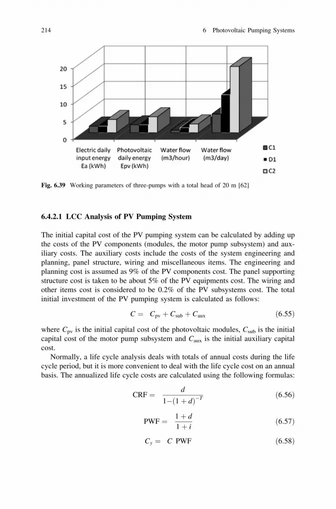
6.4.2.1 LCC Analysis of PV Pumping System

The initial capital cost of the PV pumping system can be calculated by adding upthe costs of the PV components (modules, the motor pump subsystem) and aux-iliary costs. The auxiliary costs include the costs of the system engineering andplanning, panel structure, wiring and miscellaneous items. The engineering andplanning cost is assumed as 9% of the PV components cost. The panel supportingstructure cost is taken to be about 5% of the PV equipments cost. The wiring andother items cost is considered to be 0.2% of the PV subsystems cost. The totalinitial investment of the PV pumping system is calculated as follows:

C ¼ Cpv þ Csub þ Caux ð6:55Þ

where Cpv is the initial capital cost of the photovoltaic modules, Csub is the initialcapital cost of the motor pump subsystem and Caux is the initial auxiliary capitalcost.

Normally, a life cycle analysis deals with totals of annual costs during the lifecycle period, but it is more convenient to deal with the life cycle cost on an annualbasis. The annualized life cycle costs are calculated using the following formulas:

CRF ¼ d

1� 1þ dð Þ�T ð6:56Þ

PWF ¼ 1þ d

1þ ið6:57Þ

Cy ¼ C PWF ð6:58Þ

Fig. 6.39 Working parameters of three-pumps with a total head of 20 m [62]


Ck ¼ Rk PWF ð6:59Þ

Ry ¼X

k

Ck ð6:60Þ

Ay ¼ Cy þMy þ Ry ð6:61Þ

where CRF is the capital recovery factor, d is the discount rate, T is the lifetimeperiod, PWF is the present worth factor, i is the interest rate, Cy is the annualizedcapital cost, Ck is the present worth of replacement at year k, Rk is the cost ofreplacement of a system component at year k, Ry is the present worth of allreplacements incurred during the lifetime T, My is the yearly operating and Ay isannualized life cycle cost.

6.4.2.2 LCC Analysis of Diesel Pumping System

Usually, diesel generators are oversized as compared to the power needs of waterpumping systems [153]. In Algeria, the available diesel generators are rated at5 kW or larger resulting in high investment cost, operating cost, maintenance andreplacement costs. These costs are added up to the diesel fuel cost to calculate thetotal life cycle cost. To produce the electric energy Ea determined, it is necessaryto use a fuel volume Vd. This volume as calculated by Eq. 6.2, depends on effi-ciency gd of the diesel generator and the heating value kd of the fuel. The averageefficiency gd of various generators varies between 0.299 and 0.353 as reportedby [163].

Vd ¼ Ea

gd kdð6:62Þ

where gd is the diesel generator energy conversion efficiency and kd is the heatingvalue of diesel.

The annual cost for diesel fuel consumption is found by:

Af ¼ Ndays Fd Vd ð6:63Þ

where Fd is the actual diesel price;Ndays Number of days (365 days).

6.4.2.3 Pumped Water Cost

The cost of m3 of the pumped water Cw by PV and diesel system pumping systemsis calculated, using the cost annuity method based on the LCC analysis byEq. 6.64:


Cw ¼Ay

Ndays Vð6:64Þ

where Ay is the annualized cost of the considered PV or diesel pumping system andV is the daily pumped water.

6.4.3 Environmental Aspects of PV Power Systems

6.4.3.1 Introduction

Generally, PV systems do not emit substances that may damage human health orthe environment. PV systems do not produce any noise, toxic gas emissions orgreenhouse gases. In fact, PV systems can lead to significant emission reductions.

6.4.3.2 Water Pumping Planning and Evaluation of Carbon DioxideReduction

The reduction of CO2 emissions is estimated in the case of photovoltaic pumpingfacilities installed instead of diesel pumping systems.

Water Planning

For water planning, the available electrical power input is assumed to be knownand the working conditions are specified (type of pumps, pumping heads, averageworking time). Using Eq. 6.65 with the average values, the average water quantityis calculated by

Qa ¼ a ðhaÞP3a þ b ðhaÞ P2

a þ c ðhaÞ Pa þ d ðhaÞ ð6:65Þ

where Qa is the average water flow (m3 per hour), Pa is the average electricalpower input to the motor pump (W) and a(ha), b(ha), c(ha), d(ha) are coefficientscorresponding to the working head ha.

The number N of pumps needed to deliver a fixed water volume Qw is simplyexpressed by:

N ¼ Qw

Ndays Qatað6:66Þ

where N is the number of pumps, Qw is the average water production objective(m3 per year) and ta is the average working time (hours).


Evaluation of CO2 Savings

The greenhouse gas emissions from Arab countries was 986 million tons in 1999[162]. The main component of these gases is CO2 [162]. Electric energy in remoteAlgerian locations is usually produced by means of diesel generators [163]. Thecarbon dioxide emissions are expected to increase due to population growth andeconomical development. To limit CO2 emissions, it is necessary to encourage thedevelopment of water pumping systems powered by photovoltaic energy. Themethod used in this work compares between the PV water pumping systems withdiesel-based generators water installations in Algerian remote locations. Thecalculation of the savings is carried out as follows:

First, the total electrical energy needed by N pumps in a PV system is given by:

Ew ¼ N Pata ð6:67Þ

where EW is the total electrical energy (kWh), N is the number of pumps, Pa is theaverage power input of a pump (W) and ta is the average working time of a pump(hours).

The second step is to find the quantity of diesel fuel that is necessary to providethe same electric energy Ew by using Eq. 6.67. In the third step, the exhaustsvolume Vc of carbon dioxide is calculated by the following relation:

Vc ¼ kc Vd ð6:68Þ

where Vd is the consumption of the diesel fuel and kc is the carbon dioxide weightequivalent for the diesel fuel [164].

By combining Eqs. 6.67 and 6.68, the volume of carbon dioxide reductions Vc

is expressed as a function of the average pump power, average working time andnumber of pumps, as follows:

Vc ¼kc

gd kdNPata ð6:69Þ

where Pa is the average power of a pump (W), ta is the average working time of apump (hours), gd is the diesel generator energy conversion efficiency and kd is theheating value of diesel.

Application

In Algeria the total peak power of the installed pumping systems is not preciselyknown. Nevertheless, according to the Ministry of Energy and Mines, the reportedpeak power of the installed water pumping sets is around 54 kW [165]. Thiscorresponds approximately to only 54 water pumps systems, showing that muchfurther developments may be achieved. Installing much more photovoltaic pow-ered water sets is encouraged by the recent governmental policy in the domain of


renewable energies. The Algerian government stated that 10% of the electricenergy in 2020 is to be provided by renewable energies sources. Increasing thenumber of water pumping systems is an interesting way in order to reach theabove-mentioned 20% objective. In this context, raising the peak power ofinstalled PV water systems from 54 kW to 1 MW, corresponding to 1000 pumpsof C2 type, is possible and constitutes a reasonable goal. Not only will satisfy thischoice the water demands in remote locations and improve the life of isolatedpopulations, but it also alleviates the negative impact of diesel sets ups on theclimate. For the case of 1000 pumps of type C2, working at the average conditionsof a power input equal to 950 W and during 5 h a day, the carbon dioxide exhaustsreductions are evaluated by Eq.6.23 and attain the amount of 4.2 ton/year. Thisshows that larger amounts of carbon gas emissions might be avoided by anextended application of PV systems in the water pumping field. There is a vastpotential for the diffusion of the PV pumping technology in Algeria, not only fordrinking water applications but for irrigation as well. The potential number of PVpumping systems is estimated at about 13,300 to provide 40 l/day per person tosatisfy the drinking water demand of the 2.66 million inhabitants living in theremote regions of Algeria [60].

The case study considers PV and diesel pumping facilities using pumpsC1(400 W), C2(1000 W) and D1(400 W), assuming for the three systems that thetotal head is 20 m and an average daily working time ts equal to 7.5 h.

C1 and C2 are centrifugal pumps and D1 a positive displacement pump. Theaverage electrical input power Pa is supposed to be equal to 250 W for pumps C1

and D1, and equal to 500 W for pump C2. Figure 6.40 presents the workingparameters and the size of the PV array for the three pumps C1, C2 and D1.

For C1, D1 and C2, the corresponding volumes of daily pumped water at thespecified conditions are respectively equal to about 5, 19 and 11 m3. Assuming a

Fig. 6.40 Economic assumptions for three different pumps (C1, D1, C2)


Fig. 6.41 Total initial investment costs of the PV systems ($)

Fig. 6.42 Total initial investment costs of the Diesel systems ($)

Fig. 6.43 Annuity and water cost calculations for the PV systems ($)


daily demand of 40 liters per person, the calculated pumped water will respectivelysatisfy the needs of 125, 275 and 475 people.

For example, we present in Fig. 6.40. economic assumptions for three differentpumps (C1, C2 and D1).

The equipment costs provided by local retailers are represented in Fig. 6.41. forthe three systems based on pumps C1, C2 and D1.The maintenance cost is con-sidered to be 2% of the total investment costs. The lifetime of the PV modules isassumed to be 20 years, so this period is chosen for the LCC analysis. The lifetimeof the motor pump subsystems is assumed to be 8 years, due to the hard workingconditions in the major parts of the country. These subsystems should be replacedto match the lifetime of the PV generator and their replacement costs must beconsidered.

The total initial costs of diesel systems are presented in Fig. 6.42.

Fig. 6.44 Annuity and water cost calculations for diesel systems ($)

Fig. 6.45 Water produced by 1000 pumps of type C2 with an average working time of 5 h, aninput power of 950 W at different heads


For the diesel pumping system, the initial capital cost includes the dieselgenerator and the motor pump subsystem. The annual fuel cost Af and the main-tenance cost is assumed to be equal to 10% of the diesel generator cost.Replacements of the diesel generator and motor pump subsystem are assumed tooccur after equal lifetimes of 8 years.

As expected, the calculated cost of initial investment for PV systems is higherthan the initial cost of systems based on diesel generators. But on an annual basis,PV systems are more economical than diesel systems. The cost of water pumpedby a photovoltaic system is lower than that pumped by a facility based on a dieselgenerator. We present in Fig. 6.45 the results of calculations corresponding to1000 C2 pumps, working 5 h per day with a power input of 950 W for each one. Ateach total head, the required energy to cover between 0.14 and 0.66% of theAlgerian drinking water consumption (in 2000), is approximately 4.8 MWh [60].

In Fig. 6.45, Qw is also expressed as a ratio of the PV pumped water to thewithdrawals (1.339109 m3) in 2000 [62].


Chapter 7Hybrid Photovoltaic Systems

Symbolsa1, a2 and a3 ConstantsApv Total area of the photovoltaic generatorb1, b2, b3 and b4 Constantsc Load consumptionC�O2 Oxygen concentration in the cathode area (mol/cm3)Cp Heat capacity of gas (kJ/�K)Cpðk; bÞ Power coefficientDOD Depth of dischargeE Tolerance predefinedENernst Cell thermodynamic potential associated to reversible voltage

(V)f Fraction of load supplied by the photovoltaic energyF Faraday constant (C/mol)fcomp Compressor molar flow (mol/s)FH2ð Þpurg Purge flow system if the anode compartment is not closed

Fmass Compressor mass flow (g/s)Fmolar Molar flow of the compressor (mol/s)Fref Molar flow reference in the valve (mol/s)Fsteam Corresponds to the amount of steam supplied by the

humidification system (mol/s)Fvalve Molar flow through the valve (mol/s)Gin Solar irradiance on an inclined planeGx Overall gear ratioIbatt Battery currentids and iqs d and q axial currentIload Load currentIpac Current in the battery (A)Ka and Kb Constants to be determined


223

Kopt Coefficient which depends on the ratio of tip speed and optimalpower coefficient maximum

Ld and Lq d and q axial inductanceM Molar mass of the airMH2O Molar molecular weight of water (g/mol)ncath Moles number in the cathode compartment (mol)nH2 Number of hydrogen moles in the compartment (mol)nH2Oð Þsteam Number of water steam moles in the compartment (mol)

Ncell Number of cells in the stackNj Number of days of autonomyPatm Atmospheric pressure (output pressure)Pch Power required by the loadPcath Pressure in the cathode compartment (Pa)PH2 tð Þ Hydrogen partial pressurePpv Power supplied by the photovoltaic generatorPrequired Total required powerPwind Wind powerR Molar gas constant (J/K/mol)Rs Stator winding resistanceRc Contact resistance equivalent of the electrodes (X)Scell Cell active area (m2)Sopen Maximum opening of the valve m2ð ÞStO2 Ratio of the stoichiometryTe Temperature input (�K)Tpac Cell temperature (K)Tj Temperature of photovoltaic cellsTpac Absolute operating temperature of the stack (�K)Ts Output temperature (K)Ubatt Battery voltageUact Activation losses (V)Uconc Loss of concentration (V)Uohm Ohmic losses (V)v Volume of fuel consumedVanod Anode volume of compartment m3ð ÞVcath Volume of the cathode compartment m3ð ÞVds and Vqs d and q axial voltageVpac Unit cell voltage (V)Vwind Wind velocityXH2ð Þanod Molar fraction of hydrogen in the compartment

(XO2)air Molar fraction of oxygen in the air(XO2)valve Molar fraction of oxygen in the valveXsteam Mole fraction of water vapor in the humidification systemb Pitch angle controlc Polytropic exponent

224 7 Hybrid Photovoltaic Systems

DP Power excess valueggen Photovoltaic generator efficiencygis Isentropic efficiencygr Reference efficiency of the photovoltaic generatork Tip speed ratioq Air densityqe Gas density (kg/m3)xflow Control bandwidth (rad/s)Xr AC Angular velocity of rotorXt Turbine angular velocity

Hybrid power systems (HPS) combine two or more sources of renewable energy asone or more conventional energy sources [167–169]. The renewable energysources such as photovoltaic and wind do not deliver a constant power, but due totheir complementarities their combination provides a more continuous electricaloutput. Hybrid power systems are generally independent of large interconnectednetworks and are often used in remote areas [170, 171]. The purpose of a hybridpower system is to produce as much energy from renewable energy sources toensure the load demand. In addition to sources of energy, a hybrid system may alsoincorporate a DC or AC distribution system, a storage system, converters, filtersand an option to load management or supervision system. All these componentscan be connected in different architectures. The renewable energy sources can beconnected to the DC bus depending on the size of the system. The power deliveredby HPS can vary from a few watts for domestic applications up to a few megawattsfor systems used in the electrification of small villages. Thus, the hybrid systemsused for applications with very low power (under 5 kW) generally feed DC loads.Larger systems, with power greater than 100 kW, connected to an AC bus, aredesigned to be connected to large interconnected networks [172]. Hybrid systemsare characterized by several different sources, several different loads, severalstorage elements and several forms of energy (electrical, thermal).

7.1 Advantages and Disadvantages of a Hybrid System

7.1.1 Advantages of Hybrid System

The most important advantages of hybrid power systems are:

• Not dependent on one source of energy.• Simple to use.

7 Hybrid Photovoltaic Systems 225

• Efficiency, low life cycle cost of the components.• Lower needs for storage.

7.1.2 Disadvantages of a Hybrid System

We can resume some disadvantages of hybrid power systems as:

• More complex than single-source systems.• High capital cost compared to diesel generators.

7.2 Configuration of Hybrid Systems

Photovoltaic and wind generators in a hybrid system can be connected in threeconfigurations, DC bus architecture, AC bus architecture and DC–AC bus archi-tecture [172, 173].

7.2.1 Architecture of DC Bus

In the hybrid system presented in Fig. 7.1, the power supplied by each source iscentralized on a DC bus. Thus, generators which provide AC power have to beconnected first to a rectifier in order to obtain DC power. The inverter shouldsupply the alternating loads from the DC bus and must follow the set point for theamplitude and frequency [174]. The batteries are sized to supply peak loads.The advantage of this topology is the simplicity of operation and the load demandis satisfied without interruption even when the generators are unable to provide theload demand.

7.2.2 Architecture of AC Bus

In AC bus topology, all components of the HPS are related to AC loads, as shownin Fig. 7.2. This configuration provides superior performance compared to theprevious configuration, since each converter can supply the load independently andsimultaneously with other converters [173]. This provides flexibility for the energysources which fed the load demand. In the case of low load demand, all generatorand storage systems are in stand-by except for example the photovoltaic generatorto cover the load demand. However, during heavy load demands or during peak


≈

≈

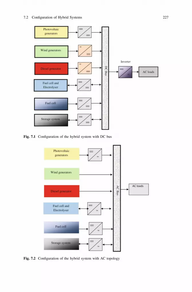
AC

Bus

Photovoltaic generators

Wind generators

Diesel generator

Storage system

Fuel cell and Electrolyser

Fuel cell

≈

≈

Fig. 7.2 Configuration of the hybrid system with AC topology


Wind generators

Diesel generator

Storage system

DC

Bus

≈

≈

≈

Inverte


Fuel cell

AC loads

Fig. 7.1 Configuration of the hybrid system with DC bus

7.2 Configuration of Hybrid Systems 227

hours, generators and storage units operate in parallel to cover the load demand.The realization of this system is relatively complicated because parallel operationrequires synchronization of each output voltages with the charge voltages [172].This topology has several advantages compared to the DC coupled topology suchas higher overall efficiency, smaller sizes of the power conditioning unit whilekeeping a high level of energy availability, and optimal operation of the dieselgenerator due to reducing its operating time and consequently its maintenance cost[173].

7.2.3 Architecture of DC/AC Bus

The configuration of DC and AC bus is shown in Fig. 7.3 [170]. It has superiorperformance compared to the previous configurations. In this case, renewableenergy and diesel generators can power a portion of the load directly to AC, whichcan increase system performance and reduce power rating of the diesel generatorand the inverter. The diesel generator and the inverter can operate independently orin parallel by synchronizing their output voltages. Converters located between twobuses (rectifier and inverter) can be replaced by a bidirectional converter which,

≈

DC

Bus

PV generators

Wind generators

Diesel generator

Storage system AC

Bus

≈

≈

≈


Fuel cell

AC loads

Fig. 7.3 Configuration of the hybrid system with DC and AC buses


in normal operation, performs the conversion DC/AC (inverter operation). Whenthere is a surplus of energy from the diesel generator, it can also charge batteries(operating as a rectifier). The bidirectional inverter can supply the peak load whenthe diesel generator is overloaded.

The advantages of this configuration are:

• The diesel generator and the inverter can operate independently or in parallel.When the load level is low, one or the other can generate the necessary energy.However, both sources can operate in parallel during peak load.

• The possibility of reducing the nominal power of the diesel generator and theinverter without affecting the system ability to supply peak loads.

The disadvantages of this configuration are:

• The implementation of this system is relatively complicated because of theparallel operation (the inverter should be able to operate autonomously and tooperate with synchronization of its output voltages with output voltages of dieselgenerator).

7.2.4 Classifications of Hybrid Energy Systems

The power delivered by hybrid systems can vary from a few watts for domesticapplications up to a few megawatts for systems used in the electrification of smallislands [167]. For hybrid systems with power below 100 kW, the configurationwith AC and DC bus, with battery storage, is the most used. The storage systemuses a high number of batteries to be able to cover the average load for severaldays. This type of hybrid system uses small renewable energy sources connected tothe DC bus. Another possibility is to convert the direct-current power into analternating-current one by using inverters. Hybrid systems used for applicationswith very low power (below 5 kW) supply generally DC loads (Table 7.1).

Table 7.1 Classification of hybrid systems by power range [194]

Power of hybridsystem (kW)

Applications

Low power \5 Autonomous system: telecommunication stations, pumping water, otherisolated applications.

Average power10–250

Micro isolated systems: feeding a remote village, rural…

High power [500 Large isolated systems (Islands)

7.2 Configuration of Hybrid Systems 229

7.3 The Different Combinations of Hybrid Systems

7.3.1 Hybrid Photovoltaic/Diesel Generator Systems

Systems based on a combination of photovoltaic generators and Diesel generatorsmay also include energy storage such as battery. Photovoltaic panels and gener-ators are highly complementary to each other. Photovoltaic systems do not causefuel consumption and costs are maintained generally low. Diesel generators causecosts of operating [176], but can produce energy demand. The combination ofenergy sources allows the continuous cover of energy demand (electric powergeneration using photovoltaic generators when the weather is sunny and Dieselgenerators when weather is dark). However, energy production is not entirelyrenewable and for applications in remote sites, transportation and fuel costs andthe environmental costs are high [176].

We present in Fig. 7.4 the block diagram of the hybrid system model.During the day, the inverter converts DC power from the solar PV into AC

power for the load. The extra power produced is stored in battery system. Duringthe night, the inverter converts DC power from the battery into AC power for theload. The battery will supply the load to its maximum discharge level. When thebattery reaches its maximum discharge level, the diesel generator serves the loadand charges the battery. The controller unit manages the load demand and theenergy supplied.

7.3.1.1 Photovoltaic Generator Model

See Chap. 2.

7.3.1.2 Diesel Generator Model

Diesel generators can boost up the electricity supply during sudden increase inenergy demand or when the batteries, capacity decreases and thus for not facingsupply interruption. The generator is characterized by its efficiency defined as theratio of the electrical power supplied to the equivalent energy of the fuel used toproduce it. The fuel consumption of a generator can be characterized by quantitiescorresponding to different points of motor operation. The diesel generator can bemodeled by a polynomial of first or second order [177, 178] such as Eq. 7.1.

v ¼ a � p2 þ b � pþ c ð7:1Þ

where p is the electric power, a, b and c are constants and v is the volume of fuelconsumed.


http://dx.doi.org/10.1007/978-1-4471-2403-0_2

http://dx.doi.org/10.1007/978-1-4471-2403-0_2

The curve cuts the y-axis in v = c, which corresponds to no-load operation. Theslope of the line (b) represents the increase in consumption with the load, but nearthe nominal operating point, the increase in consumption is not linear. This is dueto the influence of Diesel motor efficiency. Making measurements, we have madeit possible to fit the values of the parameters a, b and c.

7.3.1.3 Control Strategy of Diesel Generator

There are several strategies for controlling the power delivered by the generator.We present two strategies:

(a) Strategy 1

The generator starts if Vbatt B Vmin. and feeds only the battery.The generator stops if Vbat = Vnom.

(b) Strategy 2

It is to supply a portion of the load by the generator if:

DP ¼ Pch � Ppv� e ð7:2Þ

where Pch is the power required by the load, Ppv is the power supplied by thephotovoltaic generator, e is the tolerance predefined and DP is the power excessvalue.

DC/DC

Irradiance

TemperaturePV

pannels

Battery charger

DC/AC

Battery

Dieselgenerator 3 ∼

Fig. 7.4 Block diagram of the hybrid photovoltaic/diesel generator system

7.3 The Different Combinations of Hybrid Systems 231

7.3.1.4 Sizing of Diesel Generator

The Diesel generator is used in hybrid energy systems as backup power in the casewhere the weather conditions are unfavorable for a while. It must supply the loadduring this period. The power of the generator is given by [180]

PG ¼Pch

NG

ð7:3Þ

where NG is the number of identical generators.

7.3.2 Hybrid Wind/Photovoltaic/Diesel Generator System

Hybrid PV/wind/Diesel generator systems are well suited for decentralized pro-duction of electricity, and can contribute to solving the problem of connecting tothe electrical power networks (cases of isolated sites) [167, 168]. The initial data inthe implementation of such a system of production from renewable sources ofenergy like any other energy system is the demand, which will be determined bycomparing the load to be supplied. This request must be estimated as accurately aspossible both from a point of view of energy balance and of power temporaldistribution, even if its random nature often makes this a difficult task. Adding agenerator to a system of renewable energy production may on the one handincrease the reliability of power system loads and on the other hand reducesignificantly the cost of electricity, producing a significant decrease of the size ofthe storage system [170, 181, 182].

Reference [169] proposed that there are multiple types of electrical circuitarchitectures which could be used depending on people needs and site capabilities.In the first architecture (Fig. 7.5), the generators and the battery are all installed inone place and are connected to a main AC bus bar before being connected to thegrid. The power delivered by all the energy conversion systems and the battery isfed to the grid through a single point. In this case, the power produced by the PVsystem and the battery is converted into AC before being connected to the mainAC bus. This system is called a centralized AC bus architecture.

The energy conversion systems can also be connected to the grid in anothermanner (Fig. 7.6). This system is called a decentralized AC bus architecture.The power sources in this case do not need to be connected to one main bus bar.The power generated by each source is conditioned separately to be identical tothat required by the grid.

The third architecture uses a main centralized DC bus bar (Fig. 7.7). The energyconversion systems producing AC power (wind energy converter and the dieselgenerator) deliver their power to rectifiers in order to convert it into DC and then itis delivered to the main DC bus bar. A main inverter feeds the AC grid from thismain DC bus.


7.3.2.1 Wind Generator System

Wind Turbine

The total kinetic power of the wind through a wind disc of radius R is given by[183]:

Pwind ¼12

qp R2 V3wind ð7:4Þ

where q represents the air density and Vwind the wind velocity (Fig. 7.8).A wind turbine can only convert just a certain percentage of the captured wind

power. This percentage is represented by CPðk; bÞ where b is the pitch angle ofspecific wind turbine blades and k is the ratio between the turbine angular velocityXt and the wind speed vwind: This ratio is called the tip speed ratio.

k ¼ R � Xt

vwind

ð7:5Þ

with

Gearbox

Pload

Rectifier/Inverter

DC/AC

AC

bus

Pwind

Ppv

Pg

Diesel 3 ∼

DC/ACBattery

Backup System

Fig. 7.5 Centralized AC bus architecture


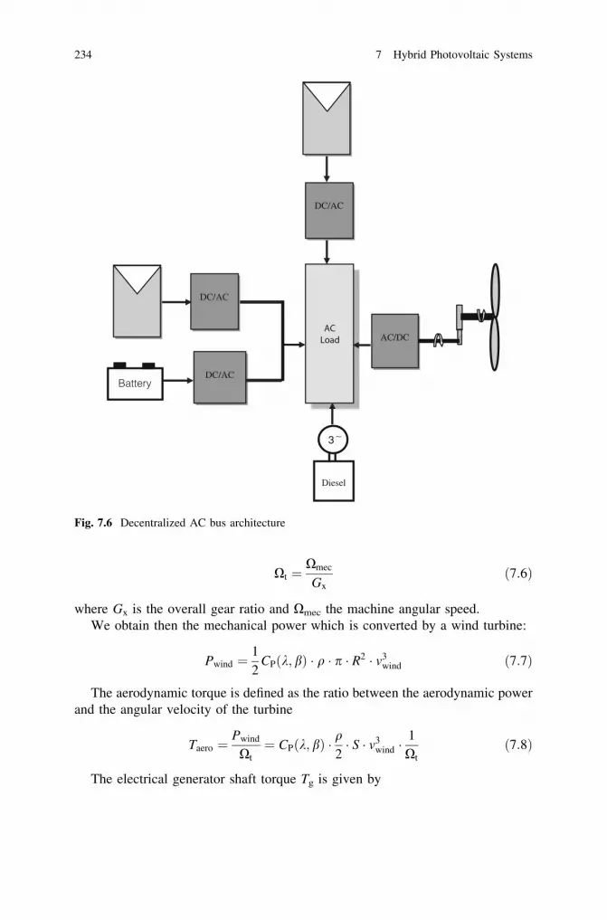
Xt ¼Xmec

Gx

ð7:6Þ

where Gx is the overall gear ratio and Xmec the machine angular speed.We obtain then the mechanical power which is converted by a wind turbine:

Pwind ¼12

CPðk; bÞ � q � p � R2 � v3wind ð7:7Þ

The aerodynamic torque is defined as the ratio between the aerodynamic powerand the angular velocity of the turbine

Taero ¼Pwind

Xt

¼ CPðk; bÞ �q2� S � v3

wind �1Xt

ð7:8Þ

The electrical generator shaft torque Tg is given by

DC/AC

DC/AC

Diesel

3 ∼

DC/ACBattery

AC/DC

Fig. 7.6 Decentralized AC bus architecture


Tg ¼Taero

Gx

ð7:9Þ

The mechanical speed evolution is determined from the total torque Tmec

applied to the electrical generator rotor

AC/DC

Gearbox

DC/DC

DC

bus

Pwind

Ppv

Backup System

Diesel 3 ∼ AC/DC

DC/AC

Battery

Fig. 7.7 Centralized DC bus architecture

mecΩ

R

turbineΩ

Turbine

Gearbox

Vwind

Fig. 7.8 Wind turbine [185]


JdXmec

dt¼ Tmec ð7:10Þ

Tmec ¼ Tg � TemAC � Tvisq ð7:11Þ

where J is the effective inertia of rotor, TemAV is the electromechanical torque ofthe machine and Tvisq the resistant torque due to frictions. This torque is modeledby a coefficient of viscous friction f:

Tvisq ¼ f Xmec ð7:12Þ

The peak power for each wind speed occurs at the point where CPðk; bÞ ismaximized. To maximize the generated power, it is therefore desirable for theelectrical generator to have a power characteristic that will follow the maximumCp�max line. The action of the speed corrector must control the mechanical speedXmec in order to get a speed reference Xmec� ref : The simplified block diagram isgiven in Fig. 7.9.

Electrical Generators

• Induction generators (IG)

Induction machines are largely used in the field of wind energy conversion. Forstandalone operations, the squirrel induction machine is preferred because it isrobust, needs little maintenance and does not need an auxiliary supply for mag-netizing it. The simplest way to use it as an autonomous generator consists inconnecting its stator windings to a capacitor bank in parallel to the load. Theremaining magnetic flux, added to the magnetizing current through the capacitorbank yields the built up of the electromotive force and its increase to a usefulvalue. This approach is very cheap and is well adapted to convert the wind energyinto an electrical one for isolated areas or areas faraway from the distribution grid

xG

1

xG

1 1

J .p f

Turbine Gearbox

β

wind

wind

turbine

v

.R Ω =λ

t

3windP

1.v.S.

2).,(C

Ωρβλ

Fig. 7.9 Simplified block diagram


[184]. However, the magnitude of the stator voltage and frequency are verysensitive to both speed and load values. The used model for the induction machineis expressed in d – q frames (see Sect. 6.2.2.1)

• Doubly fed induction generator (DFIG)

The application of the doubly fed induction generator (DFIG) in the modernwind turbine becomes an imposing reality, by its offered performances. Generally,if a wind turbine contains the DFIG, the stator is connected directly to the grid; therotor is connected to the grid by means of a static converter. Modern high-powerwind turbines are equipped with adjustable speed generators; the constraints on thestatic converter will be decreased, which leads to the reduction in the size and costof the converter. The energy storage system associated to a grid connected variablespeed wind generation scheme using a DFIG is investigated [185]. By choosing ageneral d–q reference frame, stator voltages and fluxes can be rewritten as follows:

Vsd ¼ Rs � Isd � xs � Usq þdUsd

dt

Vsq ¼ RsIsq þ xs � Usd þdUsq

dt

Vrd ¼ Rr � Ird � xr � Urq þdUrsd

dt

Vrq ¼ Rr � Irq þ xr � Urd þdUrq

dt

ð7:13Þ

with

Usd ¼ Ls � Isd þ LmIrd

Usq ¼ Ls � Isq þ Lm � Irq

Urd ¼ Lm � Isd þ Lr � Ird

Urq ¼ Lm � Isq þ Lr � Irq

ð7:14Þ

• Permanent magnet synchronous generator (PMSG) (see Sect. 6.3.2.2).

Control of Wind Generator System with IG

We propose to present two strategies to control the DC voltage of an autonomousinduction generator connected to a rectifier when the input speed varies.The control strategies are based on the choice of the reference frame orientation.The d–q frame must be chosen in order to maintain the d-axis always along the


http://dx.doi.org/10.1007/978-1-4471-2403-0_6

http://dx.doi.org/10.1007/978-1-4471-2403-0_6

http://dx.doi.org/10.1007/978-1-4471-2403-0_6

http://dx.doi.org/10.1007/978-1-4471-2403-0_6

rotor flux. This choice implies an important simplification in the elaboration of thecontrol. Normally, the saturation effect, as well as the cross magnetizing effect,must be taken into account in the model of the induction generator. This obviouslycomplicates the model as it can be seen through electrical equations. Then, themachine control can seem to be difficult. However, when the flux is controlled tobe constant, the model of the induction generator can be considered as a linear one.The inductance values, constant, depend on the given flux but there is no morecross magnetizing effect which has to be considered. Besides, the variations whichcan occur around the reference value of the flux can be considered as negligible.The operating of the machine can then be considered practically linear. Theelectrical equations of the induction machine are given in Eq. 7.13 [184].

As Urd ¼ Ur and Urq ¼ 0; this implies that the expressions of the flux Ur andits derivative take the forms:

dUr

dt¼ �Rr � Ird

Ur ¼ �Rr � Irq

xr

ð7:15Þ

Moreover, the rotor currents can be expressed in the following way:

Ird ¼Ur � Lm � Isd

Lr

Irq ¼ � Lm � Isq

Lr

ð7:16Þ

Indeed, by introducing the leakage flux coefficient we obtain:

Vsd ¼ Rs � Isd þ r � Ls �dIsd

dt� xs � r � Ls � Isq þ Lm �

dUr

dt

Vsq ¼ Rs � Isq þ r � Ls �dIsq

dtþ xs � r � Ls � Isd þ xs � Lm

ð7:17Þ

Finally, as the chosen frame implies Urq ¼ 0; the expression of the electro-magnetic torque becomes:

TemAC ¼ p � Lm

Lr

� Ur � Isq ð7:18Þ

We can write the rotor flux as a function of the current isd and the rotor timeconstant Tr = Lr/Rr

Ur ¼Lm

1 þ Tr � sisd ð7:19Þ

where s represents the derivative operator


Thus, we can obtain:

xr ¼Lm Isq

Tr � Ur

ð7:20Þ

By controlling the flux Urd-ref at a wished value, it is possible to determine themagnetizing inductance Lm for the saturation level. This is given by the followingequation [184]:

Lm �Ur�ref

imd

¼ffiffiffi

23

r

Ur�ref

imj jð7:21Þ

The intersection between the characteristic Lm Imj jð Þ and the curve described byEq. 7.19 makes it possible to determine the value of Lm to use in the control. Then,the rotor flux in the machine is adjustable by Isd.The electromagnetic torque can becontrolled by Isq:

The strategies proposed are relatively close. The first is classical with a constantUrd-ref. The second is based on a rotor flux reference value obtained from thefollowing relation:

Ur� re0f ¼x

xrat

Urd� rat ð7:22Þ

where Urd - rat and xrat are the rated values of the rotor flux and the rotation speedrespectively.

Control of Hybrid Wind/Photovoltaic/Diesel Generator System

The monitoring equipment includes data loggers, wind speed and direction sen-sors, ambient and battery temperature sensors, and various AC and DC current/voltage/power sensors. The purposes for using monitoring systems are to [186]

• Determine the components and system efficiencies• Verify the proper system functioning• Provide system trouble shooting• Detect and analyze significant load changes• Calculate the actual cost of utilized energy.

We propose a control system of the hybrid PV/wind/Diesel system [187]. It isbased on the overall energy balance equation.

Pdiesel ¼ Pload � Pwind � Ppv þ DP� P ð7:23Þ

where Pdiesel is the power delivered from the Diesel generator(s), PLoad is thepower required by the load, PWind is the power delivered from the wind turbine,


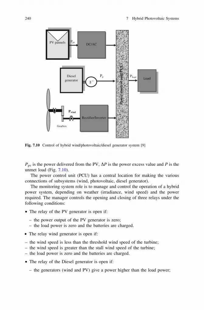
Ppv is the power delivered from the PV, DP is the power excess value and P is theunmet load (Fig. 7.10).

The power control unit (PCU) has a central location for making the variousconnections of subsystems (wind, photovoltaic, diesel generator).

The monitoring system role is to manage and control the operation of a hybridpower system, depending on weather (irradiance, wind speed) and the powerrequired. The manager controls the opening and closing of three relays under thefollowing conditions:

• The relay of the PV generator is open if:

– the power output of the PV generator is zero;– the load power is zero and the batteries are charged.

• The relay wind generator is open if:

– the wind speed is less than the threshold wind speed of the turbine;– the wind speed is greater than the stall wind speed of the turbine;– the load power is zero and the batteries are charged.

• The relay of the Diesel generator is open if:

– the generators (wind and PV) give a power higher than the load power;

Pload

Rectifier/Inverter

Pg

Gearbox

DC/AC

Pow

er c

ontr

ol u

nit(

PC

U)

Pwind

pvP

Dieselgenerator ∼

PV pannels

Fig. 7.10 Control of hybrid wind/photovoltaic/diesel generator system [9]


– the load power is zero and the batteries are charged.

And the closure of this relay is when the battery state of charge reaches theminimum level.

From these conditions, we find that the monitoring system includes 06 inputs,03 outputs and 06 tests.

• The input variables are:

– The irradiance (G)– The wind Speed(Vwind)– The power of PV generator(Ppv)– The wind power generator(Pwind)– The load power (Pload)– The battery voltage(Vbatt)

• The output variables are:

– Tpv the relay control signal of PV generator– Twind the relay control signal of wind generator– Tdiesel the relay control signal of Diesel generator

• The different tests are:

– Test on the PV power Ppv = 0 or G = 0 (()A)– Test on the wind speed (()B)– Test on the load power Pload = 0(()C)– Test on PV and wind power Ppv ? Pwind C Pload (()D)– Test on voltage battery Vbatt B Vmin (()E)– Test on voltage battery Vbatt C Vmax (()F).

From the number of tests, we determined the number of possible combinationsthat we calculated using the following equation:

X ¼ 2n ð7:24Þ

where X is the number of possible combinations and n the number of inputs.Table 7.2 summarizes the 64 combinations. According to the table we see that

the number of possible combinations is reduced to 36. The logical equations aredetermined and give the control signals of the relays from each source (Figs. 7.11,7.12, 7.13):

Tpv ¼ ðE � F þ E � FÞðA � Dþ A � B � C � Dþ A � B � C � D � E � FÞTwind ¼ ðE � F þ E � FÞðB � Dþ A � B � C � Dþ A � B � C � D � E � FÞ

Tdiesel ¼ ðE � F�DÞðA � Bþ A � B � C þ A � B � CÞð7:25Þ


Table 7.2 The different combinations

A B C D E F Tpv Twind Tdiesel

1 1 1 1 1 1 * * *1 1 1 1 1 0 0 0 11 1 1 1 0 1 0 0 01 1 1 1 0 0 0 0 01 1 1 0 1 1 * * *1 1 1 0 1 0 0 0 11 1 1 0 0 1 0 0 01 1 1 0 0 0 0 0 01 1 0 1 1 1 * * *1 1 0 1 1 0 * * *1 1 0 1 0 1 * * *1 1 0 1 0 0 * * *1 1 0 0 1 1 * * *1 1 0 0 1 0 0 0 11 1 0 0 0 1 0 0 01 1 0 0 0 0 0 0 01 0 1 1 1 1 * * *1 0 1 1 1 0 0 1 01 0 1 1 0 1 0 0 01 0 1 1 0 0 0 1 01 0 1 0 1 1 * * *1 0 1 0 1 0 * * *1 0 1 0 0 1 * * *1 0 1 0 0 0 * * *1 0 0 1 1 1 * * *1 0 0 1 1 0 0 1 01 0 0 1 0 1 0 0 01 0 0 1 0 0 0 1 01 0 0 0 1 1 * * *1 0 0 0 1 0 0 1 11 0 0 0 0 1 0 1 01 0 0 0 0 0 0 1 00 1 1 1 1 1 * * *0 1 1 1 1 0 1 0 00 1 1 1 0 1 0 0 00 1 1 1 0 0 1 0 00 1 1 0 1 1 * * *0 1 1 0 1 0 * * *0 1 1 0 0 1 * * *0 1 1 0 0 0 * * *0 1 0 1 1 1 * * *0 1 0 1 1 0 1 0 00 1 0 1 0 1 0 0 00 1 0 1 0 0 1 0 00 1 0 0 1 1 * * *

(continued)


Application of Hybrid Wind/Photovoltaic/Diesel Generator System

Wind/Photovoltaic/Diesel systems can be used for desalination of sea water [188].Different distinct approaches to Wind/Photovoltaic/Diesel exist, each with its ownarchitecture. Generally, these systems are used to supply village power.

7.3.3 Hybrid Wind/Photovoltaic System

The optimization of wind and photovoltaic energy with electrochemical storage(batteries) depends on many economic models of each system separately (wind and

Table 7.2 (continued)

A B C D E F Tpv Twind Tdiesel

0 1 0 0 1 0 1 0 10 1 0 0 0 1 1 0 00 1 0 0 0 0 1 0 00 0 1 1 1 1 * * *0 0 1 1 1 0 1 1 00 0 1 1 0 1 0 0 00 0 1 1 0 0 1 1 00 0 1 0 1 1 * * *0 0 1 0 1 0 * * *0 0 1 0 0 1 * * *0 0 1 0 0 0 * * *0 0 0 1 1 1 * * *0 0 0 1 1 0 1 1 00 0 0 1 0 1 0 0 00 0 0 1 0 0 1 1 00 0 0 0 1 1 * * *0 0 0 0 1 0 1 1 10 0 0 0 0 1 0 0 00 0 0 0 0 0 1 1 0

Supervisor

A

B

C

D

E

F

Tpv

Twind

Tdiesel

Fig. 7.11 Supervisor ofhybrid wind/photovoltaic/diesel generator system


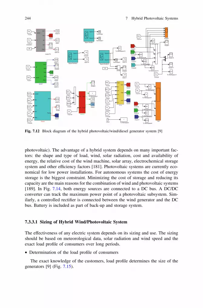
photovoltaic). The advantage of a hybrid system depends on many important fac-tors: the shape and type of load, wind, solar radiation, cost and availability ofenergy, the relative cost of the wind machine, solar array, electrochemical storagesystem and other efficiency factors [181]. Photovoltaic systems are currently eco-nomical for low power installations. For autonomous systems the cost of energystorage is the biggest constraint. Minimizing the cost of storage and reducing itscapacity are the main reasons for the combination of wind and photovoltaic systems[189]. In Fig. 7.14, both energy sources are connected to a DC bus. A DC/DCconverter can track the maximum power point of a photovoltaic subsystem. Sim-ilarly, a controlled rectifier is connected between the wind generator and the DCbus. Battery is included as part of back-up and storage system.

7.3.3.1 Sizing of Hybrid Wind/Photovoltaic System

The effectiveness of any electric system depends on its sizing and use. The sizingshould be based on meteorological data, solar radiation and wind speed and theexact load profile of consumers over long periods.

• Determination of the load profile of consumers

The exact knowledge of the customers, load profile determines the size of thegenerators [9] (Fig. 7.15).

model PV

insolation

control

E

T

Ipv1

Ppv

Ipv

Vpv

Ppv1

In3

iCH

vbat

P bat

battery

Vs2

pgrop

To Workspace9

peol

To Workspace8

ppv

To Workspace7

w

To Workspace6

es

To Workspace5

tgroup

To Workspace4

teol

To Workspace3

tpv

To Workspace2

es1

To Workspace12

pch

To Workspace11

pbat

To Workspace10

v

To Workspace1

t

To Workspace

Terminator2

Terminator1

Terminator

Signal 2

Signal 3

Signal Builder3

Signal 2

Signal 3

Signal Builder2

Signal 2

Signal 3

Signal Builder1

Scope7

Scope6

Scope5

Scope3

Scope2

Scope17

Scope16

Scope1

Scope

Vbat

Ipv

Ieol

Vw

Ej

Ich

Out1

Out2

Out3

PCU

wr

control

Out1

Veol

Peol

Ieol

Peol1

MSAP

[Pgrop]

Goto9

[Peol]

Goto8

[Ppv]

Goto7

Tgrop

Goto6

Tpv

Goto5

Teol

Goto4

Pbat

Goto3

Es

Goto20

[Ieol1]

Goto2

Vw

Goto19

[Ppv1]

Goto18

[Ieol]

Goto17

[Ipv]

Goto16

Pch

Goto15

[Igrop]

Goto14

[Peol1]

Goto12

Ich

Goto11

Vbat

Goto10

[Ipv1]

Goto1

Vbat

From9

Tpv

From8

Teol

From7

[Ieol1]

From6

[Igrop]

From5

[Ieol]

From4

Pch

From30

[Ppv1]

From3

Pbat

From29

Ich

From28

[Pgrop]

From27

[Ibat]

From26

Ich

From25

Es

From24

[Peol]

From23

Tgrop

From22

[Ieol]

From21

[Ipv]

From20

[Ipv1]

From2

Vw

From19

Ich

From18

Tgrop

From17

Teol

From16

Tpv

From15

Vbat

From14

Vw

From13

Es

From12

Vw

From11

Es

From10

[Ipv]

From1

Divide

control

Ppv

Peol

Pch

Pbat

Out1

Pgroup

Diesel

25

24

Clock

Fig. 7.12 Block diagram of the hybrid photovoltaic/wind/diesel generator system [9]


• Analysis of solar and wind energy potential

We make applications in Bejaia (Algeria) which is a coastal region. The curvein Fig. 7.16 is the superposition of two characteristics (wind speed and radiation),and shows their complementarity; we can say that the coupling of a photovoltaicsystem and wind is very interesting for electricity production throughout the year.

• Photovoltaic energy calculation:

Fig. 7.13 Simulation results of hybrid wind/photovoltaic/diesel generator system


wI

sIpvI

DC

DC

DC

ACchI

battI

AC

DC

Photovoltaicpanels

Battery

Fig. 7.14 Hybrid wind/photovoltaic system

Hours0 4 8 12 16 20

0

50

100

150

200

250

300

350

400

Ene

rgy

(Wh/

day )

Fig. 7.15 Daily consumption profile of a rural house [9]

H(k

Wh/

m2 .d

ay)

V win

d(m

/s)

Month

Jan Feb Mar Apr May Jun July Aug Sept Nov Dec3,4

3,5

3,6

3,7

3,8

3,9

4

4,1

4,2

4,3

4,4

0

1

2

3

4

5

6

7

8

Vwind (m/s)

H (kWh/m2.day)

Fig. 7.16 Monthly average global radiation and wind speed monthly average of Bejaia (Algeria)site from 1998 to 2007


The energy produced by a photovoltaic generator per unit area is estimatedusing data from the global irradiance on an inclined plane, ambient temperatureand the data sheet for the used photovoltaic panel.

The electrical energy produced per unit area by a photovoltaic generator isgiven by:

DEpv ¼ gpv:G Dt ð7:26Þ

where G is a solar radiation on tilted plane module and gpv the efficiency of thephotovoltaic generator:

gpv ¼ gr�pv:gpc 1� ascðTj � TjrefÞ� �

ð7:27Þ

with gr�pv the efficiency of the photovoltaic generator (power electronic converterincluded) and gpc the power conditioning efficiency which is equal to one if aperfect maximum power tracker (MPPT) is used. asc is the temperature coefficientof short-current (A/�K) as found on the data sheet, Tj the cell temperature and Tjref

the reference cell temperature. We put the emphasis on the fact that gr�pv is not aconstant, but depends on the climatic conditions (temperature, irradiance…).

• Wind energy calculation

The power contained in the form of kinetic energy per unit area in the wind isexpressed by:

Pwind ¼12� q � v3

wind gwind ð7:28Þ

with gwind the efficiency of the photovoltaic generator (power electronic converterand power conditioning efficiency included).

The energy produced by wind generator is expressed by:

DEwind ¼ Pwind � Dt ð7:29Þ

• Pre-sizing of photovoltaic and wind systems:

The monthly energy produced by the system per unit of area is denoted Epv,m

(kWh/m2) for photovoltaic energy and Ewind,m (kWh/m2) for wind energy and EL,m

represents the energy required by load every month (where m = 1, 2,…,12 rep-resents the month of the year). One has:

Epv;m ¼X

month m

DEpv ð7:30aÞ


Ewind;m ¼X

month m

DEwind ð7:30bÞ

and

EL;m ¼X

month m

DEL ð7:31Þ

Pre-sizing is sometimes based on the worst month of the year. Then, the totalarea of the photovoltaic generator Apv and the total area of the wind generator Swind

are chosen in such a way that

EL;worth m ¼ Epv;worth m � Apv þ Ewind;worst m � Swind ð7:32Þ

One can introduce the parameter f which is the fraction of load supplied by thephotovoltaic energy, (1 - f) being the fraction of load supplied by the windenergy. Then:

f = 1 indicates that the entire load is supplied by the photovoltaic source.f = 0 indicates that the entire load is powered by the wind source.Using f, one has

Apv ¼f EL;worst m

Epv;worst m

ð7:33aÞ

Swind ¼ð1� f Þ EL;worst m

Ewind; worst m

ð7:33bÞ

The pre-sizing is also often based on a monthly annual average [169, 190]. Thecalculation of the size of wind generator and photovoltaic (Apv and Swind) isestablished from the annual average values of each monthly contributionEpv and Ewind

� �

: The load is represented by the monthly annual average EL:

Apv ¼ f � EL

Epv

Swind ¼ ð1� f Þ � EL

Ewind

ð7:34Þ

The number of photovoltaic and wind generators to consider, is calculatedaccording to the area of the system unit taking the integer value of the ratio byexcess.

Npv ¼ ENTApv

Apv;u

� �

Nwind ¼ ENTSwind

Swind;u

� � ð7:35Þ

• Batteries pre-sizing (see Sect. 1.3.5).


http://dx.doi.org/10.1007/978-1-4471-2403-0_1

http://dx.doi.org/10.1007/978-1-4471-2403-0_1

7.3.3.2 Application

ELmax ¼ 121;52kWh; Ubatt ¼ 12V ;

Nm ¼ 31days Nj ¼ 2 gbatt ¼ 0:94

Figures 7.17 and 7.18 show respectively photovoltaic panels and wind turbinesarea and the obtained number to install according to the fraction of the load ( f ) seeEq. 1.22.

Cbatt ¼121; 52 :1000

0; 9 : 12 : 0; 8 : 31: 2 ¼ 907; 407Ah

The number of batteries is determined from the capacity (Cbatt, u = 92 Ah)taking the integer value of the ratio by excess.

Fig. 7.17 Areas of photovoltaic panels and wind turbines

Fig. 7.18 Number of photovoltaic panels and wind turbines as a function of the fraction of theload


http://dx.doi.org/10.1007/978-1-4471-2403-0_1

Nbatt ¼ ENTCbatt

Cbatt;u

� �

¼ ENT907; 407

92

� �

¼ 10

We will use ten batteries of 92 Ah capacity.

7.3.3.3 Control of Hybrid Photovoltaic/Wind System

Managing energy sources (photovoltaic and wind) is provided by a supervisor. Forthe design of the supervisor, it was decided that the photovoltaic subsystem wouldbe the main generator, while the wind generator subsystem would be comple-mentary. This choice is motivated by the design already made based on themonthly averages annual site rating. However, the supervisor applications extendto considering the wind subsystem as the main generator and the photovoltaicsubsystem would be complementary.

Three operating modes are possible to determine the ability of the hybridsystem to supply the total power required (the power load and the power requiredto charge the batteries) on the basis of atmospheric conditions (irradiance, tem-perature and wind speed). This supervisor is essential to effectively control energysubsystems (photovoltaic, wind). We can have three cases [9, 191]:

• Case 1:

This mode corresponds to the periods where photovoltaic power is sufficient forsupplying the load demand. However, the PV generator must provide the totalpower while the wind subsystem is supposed stopped and the batteries arecharging. This situation is maintained while the power required by the load doesnot exceed the maximum PV power. Beyond this limit, the supervisor switches inCase 2 and activates the wind generator. In this case, the objective of the photo-voltaic system is under power control according to this reference:

Pref1 S ¼ Prequired ¼ Vbatt � ðIload þ IbattÞ ð7:36Þ

with Iload the load current, Ibatt the battery current, and Prequired the total requiredpower.

• Case 2:

In this case, the photovoltaic system generates the maximum power (operatingat maximum power point (MPPTw = 1) and the wind system is controlled toproduce a reference power. This one is the power required to complete the powerproduced by the photovoltaic generator at the same time supplying the total powerload. It should be noted that in cases 1 and 2, batteries are not used to produce loadpower, instead they become a part of the power required. Once the maximum


production limit of the hybrid system is reached or exceeded by any powerdemand, the system switches in the Case 3.

In cases 2 and 3, the PV system produces maximum power at MPPT operation.Different algorithms can be used to extract the maximum power (see Chap. 4). Thereference power is given by (Figs. 7.19, 7.20):

Pref2 S ¼ Poptpv ¼ Popt

s ¼ Voptpv � Iopt

pv ð7:37Þ

The wind system starts its operation when the PV power is insufficient to supplythe total power required. The supervisor controls the wind system by power control

0 5 10 15 20 25 30 35 40 450

20

40

60

80

100

120

A B

C

Ps_ref1

Ppv,opt

P pv (W

)

Vpv(V)

Fig. 7.20 Characteristic PPV(VPV) panel with photovoltaic power Reference Pref_S produced(Case 2)

0 5 10 15 20 25 30 35 40 450

1

2

3

4

A

B

C Pmpp,s

Pref_s

I pv (

A)

Vpv(V)

Fig. 7.19 Characteristic IPV(VPV) panel with photovoltaic power Reference Pref_s produced [9]


http://dx.doi.org/10.1007/978-1-4471-2403-0_4

http://dx.doi.org/10.1007/978-1-4471-2403-0_4

or by power operation. The objective in case 2 is to produce the additional powerto supply the total power applied. The wind power reference is given by:

Pref1 w ¼ Prequired � Popts ¼ Vbatt � ðIload þ Ibatt � IsÞ ð7:38Þ

When the contribution of wind power subsystem is no longer sufficient tosupply the total power required the supervisor switches in Case 3. The objective ofthis subsystem is the generation of maximum power extraction.

• Case 3

In this case, the two photovoltaic and wind generator provide maximum power(operating at MPPT). In addition, to supply the load demand, the batteries arecharged or discharged. At discharge, Case 3 is maintained as long as the availableenergy levels of the batteries is sufficient to complete the load demand, after that,the load must be disconnected to charge the batteries. The wind system producesmaximum power MPPT, the reference power is given by:

Pref2 w ¼ Poptw ¼ Kopt � X3

opt ð7:39Þ

with Kopt a coefficient which depends on the ratio of tip speed and optimal powercoefficient.

We note in Fig. 7.21 the intersection of PW(X) characteristic with referencePref2_W(X) (point C0) which corresponds to the maximum power point for a par-ticular value of wind speed. As for the operation of photovoltaic system, weremark that two operating points can develop the same reference power (point A0

and B0). Operation on the right side of the point of maximum power requires asystem of power control [191]. The operating point (A0) would be the mostappropriate. The reference angular velocity which corresponds to the operatingMPPT is given by:

Xref ¼ Xopt ¼ffiffiffiffiffiffiffiffiffiffiffiffiffiffi

Pref2�w

Kopt

3

s

ð7:40Þ

Then the supervisor decides the case (1 or 2/3) by comparing the measuredmechanical speed with the reference speed.

If X \ Xopt; case 1 Pw ¼ Pref1 w

If X ¼ Xopt; case 2/3 Pw ¼ Pref2 w ¼ Poptw

ð7:41Þ

A description of operating cases is shown in Fig. 7.22.


7.3.3.4 Application of the Control of Hybrid Photovoltaic/Wind System

We make an application with a hybrid wind/photovoltaic system. It comprises tenphotovoltaic panels of 110 W each one (five panels in series in parallel with the fiveother), a parallel chopper (boost), ten lead acid batteries (12 V, 92 Ah)connected in series and a wind Turbine 600 W with a permanent magnet syn-chronous generator, a PWM rectifier connected to the battery bank and a load thatrepresents a house with a total load of 3920 Wh/day. The application is made underMatab/Simulink. We note from these results that the controller manages the systemfunctions described above [9] (Figs. 7.23, 7.24, 7.25, 7.26, 7.27, 7.28, 7.29).

0 5 10 15 20 25 30 35 400

100

200

300

400

500

600

700

P éol

(W)

Ω (rd/s)

Fig. 7.21 Characteristic PW(X) with photovoltaic power Reference Pref_pv produced (Case 3)

CASE 1

(MPPTpv=0, MPPTw=0)

1. PV system:control power

2. Wind System:stopped

3. Batteries:in charge

CASE 3

(MPPTpv=1, MPPTw=1)

1. PV system:operating at maximum

power

2. Wind System:operating at maximum

3. Batteries:in charge or in

discharge

CASE 2

(MPPTpv=1, MPPTw=0)

1. PV system:operating at maximum

power

2. Wind System:control power

3. Batteries:in charge

Fig. 7.22 Description of operating cases


7.3.4 Hybrid Photovoltaic/Wind//Hydro/Diesel System

These systems consist of micro-hydro, solar, wind and Diesel generator andbattery as back-up (Fig. 7.30) [192].

7.3.5 Hybrid Photovoltaic-Fuel Cell System

The role of a hybrid (fuel cell-PV) system is the production of electricity withoutinterruption in remote areas. It consists generally of a photovoltaic generator (PV),an alkaline water electrolyser, a storage gas tank, a proton exchange membranefuel cell (PEMFC) and PCU to manage the system operation of the hybrid system.A PEMFC can be described as two electrodes (anode and cathode) separated by asolid membrane. Energy is produced by a PV generator to supply a user load.Whenever there is enough solar radiation, the user load can be powered totally bythe PV energy. During periods of low solar radiation, auxiliary electricity isrequired. An alkaline high pressure water electrolyser is powered by the excessenergy from the PV generator to produce hydrogen and oxygen at a maximumpressure. A PEMFC is used to keep the system reliability at the same level as forthe conventional system while decreasing the environmental impact of the wholesystem. The PEMFC consumes gases which are produced by an electrolyser tosupply the user load demand when the PV generator energy is deficient; it works asan auxiliary generator. Power conditioning units dispatch the energy between thecomponents of the system.

(a) (b)Summer day Winter day

0 4 8 12 16 200

200

400

600

800

1000

t(h)

G (

W/m

²)

0 4 8 12 16 200

200

400

600

800

1000

t (h)

G (

W/m

²)Fig. 7.23 Irradiance (G) for a day. a Summer day. b Winter day [9]


VW

(m/s

)

VW

(m/s

)

0 4 8 12 16 200

3

6

9

12

15

t (h)

0 4 8 12 16 200

3

6

9

12

15

t(h)

0 4 8 12 16 200

3

6

9

12

15

t (h)

Vv

(m

/s)

0 4 8 12 16 200

3

6

9

12

15

t(h)

Summer day Winter day (a) (b)

Fig. 7.24 Profile of wind speed (Vw) for a day. a Summer day. b Winter day

0 4 8 12 16 200

200

400

600

800

1000

1200

t (h) t (h)

Ppv

_max

,P

,

ref_

s ( W

)

Ppv

max

,Pre

f_s

( W)

Ppv_max

P ref_s P ref_s

0 4 8 12 16 200

200

400

600

800

1000

1200

Ppv_max

Summer day Winter day(a) (b)

Fig. 7.25 Photovoltaic power output, maximum (Ppv_max) and reference power (Pref_s).a Summer day. b Winter day


7.3.6 Hybrid Photovoltaic-Battery-Fuel Cell System

In this configuration (Fig. 7.31), the fuel cell system is used as a back-up gener-ator, when the batteries reach the minimum allowable charging level and the loadexceeds the power produced by the PV generator. The advantages of this systemare in general the same as for a Photovoltaic-Battery-Diesel hybrid system withregard to the PV generator size and batteries, availability. It is noted that the fuelcell system needs more time to provide the rated power and the output should onlybe increased slowly after startup. The increasing operating temperature whichoccurs during operation improves the efficiency of a fuel cell significantly [173].

Summer day Winter day

0 4 8 12 16 200

50

100

150

200

t(h)

P w,m

axP

ref_

w(W

)

Pw,max

P ref_w

0 4 8 12 16 200

100

200

300

400

t (h)

Pw,max

P ref_w

,

P w,m

axP

ref_

w(W

),

(a) (b)

Fig. 7.26 Wind power output, maximum (Pw_max) and its reference (Pref_w). a Summer day. bWinter day

Summer day Winter day

0 4 8 12 16 200

100

200

300

400

500

600

t (h)

Pre

f_w

+ P

ref_

s , P

tot( W

)

Pre

f_w

+ P

ref_

s , P

tot( W

)

Ptot

P ref_w+ Pref_s

0 4 8 12 16 200

100

200

300

400

500

600

t(h)

Ptot

P ref_w+ Pref_s

(b)(a)

Fig. 7.27 Total power required and power output (Pref_s, Pref_w). a Summer day. b Winter day


7.3.7 Hybrid Photovoltaic-Electrolyser-Fuel Cell System

In some applications, another source of energy is necessary to realize energystorage. In this system, the excess energy is stored in the form of compressedhydrogen via conversion through the electrolyser. The fuel cell is used to producepower if the load power exceeds that produced from the PV generator. It can alsofunction as an emergency generator, if the PV generator system fails [173](Fig. 7.32).

(a) Summer day (b) Winter day

0 4 8 12 16 200

100

200

300

400

500

600

t (h)

Pba

tt(W

)

0 4 8 12 16 200

100

200

300

400

500

600

t(h)

Pba

tt(W

)Fig. 7.28 Power supplied by batteries. a Summer day. b Winter day

0 4 8 12 16 200

100

200

300

400

500

600

t(h)

Pre

f_w

+ P

ref _

s ,

Pto

t, P

batt

(W)

Ptot

P ref_w+ Pref_s

Pbatt

0 4 8 12 16 200

100

200

300

400

500

600

t(h)

Pre

f_w

+ P

ref _

s ,

Pto

t, P

bat

(W)

Ptot

P ref_w+ Pref_sPbatt

(a) Summer day (b) Winter day

Fig. 7.29 Total power required, power output (Pw ? Ps) and power supplied by batteries.a Summer day. b Winter day


DC

DC

AC

DC

AC loadMicro-hydro

Battery

Photovoltaic panels

Gearbox

Diesel generator

3

Fig. 7.30 Description of hybrid photovoltaic/wind//hydro/diesel system

AC

DC

AC load

Photovoltaicpanels

Fuel cell stack

Hydrogen consumption

wI

sIpvI

DC

DC

DC

DCchI

battIDC load

Battery

Fig. 7.31 Description of a hybrid photovoltaic-battery-fuel cell


7.3.7.1 Different Topologies of Hybrid Photovoltaic-Electrolyser-FuelCell System

Different topologies are competing for an optimal design of the Hybrid Photo-voltaic-Electrolyser-Fuel cell System. These topologies are DC and AC coupledsystems. The PV generator supply DC voltage to the electrolyser. The AC invertermust also supply DC voltage range of electrochemical components. To obtaincorrectly the direct coupling of the component, the maximum power point voltageof the PV generator must be equal to the maximum voltage of the fuel cellcomponent and the rated voltage of the electrolyser component [173] (Fig. 7.33).

In this case, the connection between the components and user demand isestablished through power conditioning unit. It keeps the DC bus voltage almostconstant in the event of bus power interruptions (Fig. 7.34).

Components of the hybrid system with AC coupled are connected directly tothe AC bus. The inverters can keep the output frequency and voltage stable andallow the energy surplus to flow backwards to be stored into the hydrogen sub-system. This configuration has numerous advantages such as: expandability, utilitygrid, compatibility, cost reduction, and simple design and installation [173](Fig. 7.35).

Water(H2O)

Oxygen (O2) Oxygen (O2) or Air

Power conditioning unit

Energy Storage (Battery)


Energy

Hydrogen

Water

Oxygen

loads

Electrolyser Fuel cellHydrogen storingunit

Fig. 7.32 Description of a hybrid photovoltaic-Electrolyzer-fuel cell System [193]


7.3.7.2 Modeling of Hybrid System

Modeling PV

See Chap. 2.

Fuel cell

Hydrogen storing unit

Electrolyser

DC

Bus

InverterOxygen

Hydrogen

Hydrogen

Air

Water

AC loads

Fig. 7.34 Description of a hybrid photovoltaic-Electrolyzer-fuel cell system with DC indirectcoupling

Fuel cell


ElectrolyserAC loads

DC

Bus

InverterOxygen

Hydrogen

Hydrogen

air

Water

Fig. 7.33 Description of a hybrid photovoltaic-Electrolyzer-fuel cell system with DC directcoupling


http://dx.doi.org/10.1007/978-1-4471-2403-0_2

http://dx.doi.org/10.1007/978-1-4471-2403-0_2

Modeling of Fuel Cell PEMFC

It is necessary to define the different circuits of a fuel cell system to simplify themodeling and control of each circuit. The cell system is composed of the heart cellassociated with all necessary ancillaries to the operation of a fuel cell in anembedded application. Figure 7.36 shows all the functions present in a fuel cellsystem [193].

• Moto-compressor model

The Moto-compressor is composed of an air compressor and an electricalmachine. Generally, it is a permanent magnet motor (PMSM).

– Air Compressor model

An air compressor supplies directly each stack, and the flow is regulatedthrough its rotational speed. The compressors used in such applications are vol-umetric type because they can easily control the outflow. These types of com-pressors are classified into two categories: reciprocating compressors and rotarycompressors. In fuel cell applications, it is the twin-screw rotary compressor typeswhich are used because they do not require lubrication. The inputs of the com-pressor model are rotating speed x and discharge pressure Ps (imposed by thepressure control). The outputs are the mass flow Fmass and torque compression

Fuel cell

Electrolyser

AC

Bu

sOxygen

Hydrogen

Hydrogen

air

Water

AC loads


Fig. 7.35 Description of a hybrid photovoltaic-Electrolyzer-fuel cell system with AC coupled[193]


Ccomp. Another useful parameter for the operation of the stack is the gas tem-perature at the output of the compressor Ts (Fig. 7.37).

The mass flow Fmass is calculated easily with the compressor cylinder Cyl,speed x and density of the gas qe: In the ideal case [193]:

Fig. 7.37 Compressor model

cath

ode

Ano

de

Input air

Moto-compressor

Electric circuit

Hydrogen

Fan

pump

Output air

Tank

Out of hydrogen

regulator

Recirculation

To electric circuit

To electric circuit

Control of input/output Temperature

Electric circuit

Humid Air

Liquid Water

HydrogenCooling

Fig. 7.36 Diagram of a PEMFC


Fmass ¼ qeCyl

x2p

ð7:42Þ

with Fmass as mass flow compressor (g/s), Fmolar the Molar flow of the compressor(mol/s), and qe Gas density (kg/m3).

In the case of a real compressor, we must take into account a leakage rate. Thisis summarized by involving volumetric efficiency gv (P, x).

Fmolar ¼ps

RTs

Cyl

x2p

gv P;xð Þ ð7:43Þ

with Ts a is the output temperature (K �) and P a the compression ratio.The cylinder is chosen so that the maximum molar flow rate charged by the cell

is reached for the rated rotation speed.We have [193]

Wis ¼ Cylp1ce

Z

e

s

dp

p1=c¼ peCyl

c1� c

Pc�1c � 1

�

ð7:44Þ

with c polytropic exponent (for air c = 1.4) and pe the input pressure.The compression power is deduced as:

pcomp is ¼ FmassCpTe Pc�1c � 1

�

ð7:45Þ

with Cp as Heat capacity of gases (kJ/K) and Te: Temperature input (K �).The various losses are taken into account by introducing an isentropic efficiency

of compression. It is defined by:

gis P;xð Þ ¼ pcomp is

pcomp required

ð7:46Þ

The actual power required for compression is:

pcomp required ¼FmassCpTe

gis P;xð Þ Pc�1c � 1

�

ð7:47Þ

and compressor torque is given by

Ccomp ¼pcomp required

xð7:48Þ

with gis isentropic efficiency.

– Modeling of the cathode compartment

Considering the ideal gas law, we can write:


Pcath ¼RTPEMFC

Vcath

ncath ð7:49Þ

The cathode pressure is directly dependent on the moles number of gascontained in the cathode compartment (Fig. 7.38).

We can write [193]

dncathðtÞdt

¼ FcompðtÞ þ FsteamðtÞ � FO2consðtÞ � FvalveðtÞ ð7:50Þ

with

FsteamðtÞ ¼Xsteam PsteamðtÞ; TPEMFCðtÞð Þ

1� Xsteam PcathðtÞ; TPEMFCðtÞð ÞFcompðtÞ

Xsteam PcathðtÞ; TPEMFCðtÞð Þ ¼ Psat TPEMFCðtÞð ÞPcathðtÞ

FO2consðtÞ ¼Ncell

4FIPEMFCðtÞ

Fvalve ¼ % Sopen

ffiffiffiffiffiffiffiffiffiffiffiffiffiffiffiffiffiffiffiffiffiffiffiffiffiffiffiffiffiffiffiffiffiffiffiffiffiffiffiffiffiffiffiffiffiffiffiffiffiffiffiffiffiffiffiffiffiffiffiffiffiffiffiffiffiffiffiffiffiffiffiffiffiffiffiffiffiffiffiffi

2P2cath

MRTPEMFC

cc� 1

Patm

Pcath

� 2c

� Patm

Pcath

�

cþ1c

" #

v

u

u

t

with Sopen as the maximum opening of the valve (m2).The initial condition of operation is:

n0 ¼PatmVcath

RTpac

dPcath tð Þdt

¼ RTPEMFCðtÞVcath

1þ Xsteam PcatðtÞ; TPEMFCðtÞð Þ1� XSteam PcathðtÞ; TPEMFCðtÞð Þ

�

FcompðtÞ � FvalveðtÞ � FO2consðtÞ�

ð7:51Þ

By simplifying the equation we obtain:

dPcath

dt¼ RTPEMFC10�5

Vcath

1þ Xsteam

1� Xsteam

�

Fcomp � Fvalve �Ncell

4FIPEMFC

� � �

ð7:52Þ

with P0 = Patm as the initial condition.

cath

ode

Ano

de

Fcomp

Fsteam

Fvalve

Fig. 7.38 Cathode model


We represent the compressor molar flow rate (mol/s) by the following sim-plified expression in Laplace space:

F pð Þ ¼ Fcomp pð ÞFref pð Þ ¼

1

1þ 1xflow

p �2 ð7:53Þ

with xflow as control bandwidth (50 rad/s), ncath moles number in the cathodecompartment (mol), Pcath pressure in the cathode compartment (Pa), TPEMFC celltemperature (K), Vcath volume of the cathode compartment (m3), R molar gasconstant: 8.13 J/K/mol, F Faraday constant: 96,485 C/mol, Fcomp molar flowcompressor (mol/s) and M molar mass of the air (M = 0.029 g/mol).

Oxygen molar flow is modeled as

FO2ðtÞ ¼ XO2ð Þair�FcompðtÞ � FO2consðtÞ � XO2ð ÞvalveFvalveðtÞ ð7:54Þ

with

FO2consðtÞ ¼Ncell

4Fsteam

IPEMFCðtÞ

FðpÞ ¼ FcompðpÞFrefðtÞ

¼ 1

1þ 1xflow

p �2

with (XO2)air as molar fraction of oxygen in the air (21%), (Xo2)valve as molarfraction of oxygen in the valve, Ncell number of cells in the stack, IPEMFC current inthe cells (A), Fvalve molar flow through the valve (mol/s), Fsteam corresponds to thesteam amount supplied by the humidification system (mol/s), Xsteam mole fractionof water vapor in the humidification system, Fref molar flow reference in the valve(mol/s)

– Determination of XO2ð ÞvalveFvalveðpÞ

To simplify the model, we can take this constant value

XO2ð ÞvalveFvalveðpÞ ¼ ðstO2 � 1ÞFO2cons pð Þ ¼ stO2 � 1ð ÞNcell

4FIPEMFCðpÞ ð7:55Þ

with StO2 ratio of the stoichiometry (equal to 1.6),If we replace all in the equation we obtain:

FO2ðpÞ ¼ XO2ð ÞairF pð ÞFrefðpÞ �Ncell

4FI

PEMFCpð Þ � stO2 � 1ð ÞNcell

4FIPEMFCðpÞ ð7:56Þ

We can write:


FO2 pð ÞFref pð Þ ¼ XO2ð Þair F pð Þ � 1ð Þ

The number of oxygen moles is given by:

nO2pð Þ ¼ 1

NcellpFO2 pð Þ ð7:57Þ

with

nO2½ �init¼ PcathVcath

RTPEMFC

XO2½ �init

The total number of moles in the cathode compartment is

ncath ¼PcathVcath

RTPEMFC

ð7:58Þ

The partial oxygen pressure is given by

PO2ðpÞ ¼ nO2

ðpÞncath

PinðpÞ ð7:59Þ

The term Pin shows the pressure evolution within the cathode compartment.

PinðpÞ ¼ Pcath � KinFcompðpÞ

with

KinðtÞ ¼ KaFcompðtÞ þ Kb

Ka and Kb are constants to be determined [193]

• Anodic compartment modeling

We have to determine the partial hydrogen pressure at the membrane and thehydrogen flow within the compartment. The number of steam moles is given by[193]:

nH2Oð Þsteam¼PH2Osat T

PEMFCð ÞVanod

RTPEMFC

ð7:60Þ

with

PH2Osatð Þ TPEMFCð Þ ¼ e

23:1961� 3816:44TPEMFC�46:13

The number of hydrogen moles is given by:


nH2 tð Þ ¼ Vanod

RTPEMFC

PH2 tð Þ

Panod tð Þ ¼nH2 tð Þ þ nH2Oð Þsteam

� �

RTPEMFC

Vanod

ð7:61Þ

with PH2 tð Þ the partial hydrogen pressure in the compartment,Vanod anode volume of compartment (m3),nH2

number of hydrogen moles of in the compartment (mol),nH2Oð Þsteam number of water steam moles in the compartment (mol)

From these expressions, we can determine the partial hydrogen pressure:

PH2 tð Þ ¼ Panod tð Þ � PH2Osat TPEMFCð Þ ð7:62Þ

We have the following equations which can calculate the hydrogen flowFH2ð Þconsconsumed by the chemical redox reaction [193]:

FH2 tð Þ ¼ FH2ð Þcons� FH2ð Þpurg tð Þ

FH2ð Þcons¼NcellIPEMFC

tð Þ2F

ð7:63Þ

with FH2ð Þpurg the purge flow system if the anode compartment is not closed

The purge is a valve and we can model the flow through the followingexpression:

Fvanneð Þanod¼ %Sopen

ffiffiffiffiffiffiffiffiffiffiffiffiffiffiffiffiffiffiffiffiffiffiffiffiffiffiffiffiffiffiffiffiffiffiffiffiffiffiffiffiffiffiffiffiffiffiffiffiffiffiffiffiffiffiffiffiffiffiffiffiffiffiffiffiffiffiffiffiffiffiffiffiffiffiffiffiffiffiffiffiffiffiffiffiffi

2P2anod

MH2ORTPEMFC

cc� 1

Patm

Panod

� 2c

� Patm

Panod

�

cþ1c

" #

v

u

u

t ð7:64Þ

with Patm atmospheric pressure (output pressure) constant at 1:013times; 105Pa,MH2Omolar molecular weight of water (0,018 g/mol)

We can therefore determine FH2ð Þpurg by

FH2ð Þpurg¼ XH2ð Þanod Fvalveð Þanod ð7:65Þ

with

XH2ð Þanod¼ 1� Xsteam

Xsteam ¼PH2Osat Tpac

� �

Panod

XH2ð Þanod is the molar fraction of hydrogen in the compartment.

PH2in tð Þ ¼ Panod tð Þ � PH2Osat TPEMFCð Þ ð7:66Þ

– Electrical model of the fuel cell


The cell voltage VPEMFC is lower than the theoretical voltage ENerst due tovarious irreversible loss mechanisms. These losses, which are often called polar-ization or over-voltage losses, originate primarily from three sources: activationovervoltage Uact; concentration or diffusion over-voltage Uconc and resistive orohmic over-voltage Uohm [173] (Fig. 7.39).

VPEMFC ¼ ENernst þ Uact � Uohm � Uconc ð7:67Þ

where VPEMFC A unit cell voltage (Volt), ENernst is the Nernst voltage (Volt), Uohm

resistive or ohmic over-voltage (volt)

Uohm¼Ipac

Scell

181:6 1þ0:03 IPEMFC

Scell

�

þ0:06 T303

� �2 IPEMFC

Scell

�2:5� �

k�0:634�3 IPEMFC

Scell

�h i

exp 4:18 T�303T

� ��

�IPEMFCþScell �Rc

0

B

B

@

1

C

C

A

ð7:68Þ

VPEMFC

Uohm

Ucon

ENerst+-

Uact +

-

load

IPEMFCFig. 7.39 Electricalrepresentation of a PEMFC

C Vbus

IloadIL

RLoad

L D

SVPEMFCPEMFC

ICIPEMFC

Fig. 7.40 Diagram of thefuel cell associated withconverter [193]


Fig. 7.41 Voltage/currentdensity characteristic of aPEMFC at T = 25�C [193]

Fig. 7.42 Power density/current density characteristicof a PEMFC at T = 25�C[193]

Fig. 7.43 Evolution of thecell output voltage [193]

Fig. 7.44 Evolution of thecurrent of the cell [193]


with Uconc concentration or diffusion over-voltage (volt), Uact activation over-voltage (volt)

Uact ¼ b1 þ b2 � TPEMFC þ b3 � TPEMFC � ln j � 5 � 10�3� �

þ b4 � TPEMFC � ln C�O2

Fig. 7.45 Evolution of thecell power

Load (house,..)AC

DCPower management

unit

Fuel cell stack

Storageoxygen

hydrogen

Photovoltaicpanels

Fig. 7.46 Power management


with C�O2as the oxygen concentration in the cathode area (mol/cm3), b1, b2, b3 and

b4 are constants, Scell cell active area (m2) and Rc as contact resistance equivalentof the electrodes (X)

Uconc ¼ �B ln 1� j

jmax

�

ð7:69Þ

The expression of the Nernst equation according to JC Amphlett is given by:

ENernst ¼ a1 þ a2 � TPEMFC � 298:15ð Þ þ a3 � TPEMFC � 0:5 � ln P�O2þ ln P�H2

�

ð7:70Þ

with TPEMFC absolute operating temperature of the stack (K), a1, a2 and a3 areconstants

Load

DC/DCPV pannels

Fuel cell DC/DC

Electrolyser DC/DCH2O

AC/DC

Gearbox

Pwind

DC/AC

H2 O2

Fig. 7.47 Hybrid wind/Photovoltaic/fuel cell configuration


– Association-fuel cell converter– Application:

We make application under Matlab/simulink (Figs. 7.40, 7.41, 7.42, 7.43, 7.44,7.45).

Note in this figure that the shape of the power curve follows well the profile ofthe current.

7.3.7.3 Power Management

Power management unit (PMU) allows the coordination between different energysources such as PV panels electrolyzes and fuel cells (Fig. 7.46).

Generally, PV subsystem works as a primary source, converting solar irradia-tion into electricity that is given to a DC bus. The second working subsystem is theelectrolyser which produces hydrogen and oxygen from water as a result of anelectrochemical process. When there is an excess of solar generation available, theelectrolyser is turned on to begin producing Hydrogen which is sent to a storagetank. The produced Hydrogen is used by the third working subsystem (the fuel cellstack) which produces electrical energy to supply the DC bus.

Fig. 7.48 Solar-wind-hydrogen energy cycle


7.3.8 Hybrid Photovoltaic/Wind/Fuel Cell System

The necessary changes in our energy supply system can be accomplished if we usea hybrid system with solar, wind and fuel cell energies. Generally, the overallsystem comprises a wind subsystem with an AC/DC rectifier to connect the windgenerator to the DC bus. It is also consists of a PV subsystem connected to the DCbus via a filter and DC/DC converter. The excess energy is stored as electrolytichydrogen through an electrolyser and we use a fuel cell to generate electricityduring low irradiance and low wind speed (Fig. 7.47).

In fact, when supply and demand do not coincide we need a convenient way toboth store and transport renewable energy. This is where hydrogen comes into playas a storage and transport medium. When excess electric energy from wind andsolar energy is stored in hydrogen and then converted back to electricity we have asolar-wind hydrogen energy cycle. Electrolysers use wind and solar excess elec-tricity to split water into oxygen and hydrogen. When we need electricity the gasesare fed into a fuel cell which converts the chemical energy of the hydrogen (andoxygen) into electricity, water and heat (Fig. 7.48).


References

1. Patel MR (1999) Wind and solar power systems. By CRC Press LLC, Boca Raton2. http://www.pvresources.com/knowledge/basic-knowledge/photovoltaics.html3. http://www.eia.doe.gov/cneaf/solar.renewables/page/solarreport/solarpv.html4. http://en.wikipedia.org/wiki/solar_cell5. http://www.iapp.de/iapp/agruppen/osol/?research:organic_solar_cells:basics_of_osc6. Siti NBM (2010) Simulation design of a stand-alone photovoltaic (PV) inverter, a report

submitted in partial fulfillment of the requirements for the award of the degree of bachelorof electrical engineering, faculty of electrical engineering, University Technology Malaysia

7. http://www.fsec.ucf.edu/en/consumer/solar_electricity/basics/types_of_pv.htm8. Photovoltaic applications solar center information. http://www.ncsc.ncsu.edu/include/_

upload/…/pvapplication.pdf9. Lalouni S (2009) Study and control of hybrid electric wind power—photovoltaic, PHD in

Science. University of Bejaia, Algeria10. http://www.altestore.com/howto/how-to-size-a-battery-bank/a94/11. http://www.photovoltaique.guidenr.fr /cours_photovoltaique_2011/cours_photovoltaique.php12. Feasibility of photovoltaic systems, renewable energy, fact sheet no 19. http://

www.infinitepower.org/pdf/factsheet-24.pdf13. Matagne E, Photovoltaic Solar Energy (in french:Energie solaire photovoltaïque). http://

perso.uclouvain.be/ernest.matagne/SOLAIRE/INDEX.HTM14. Capderou M (1987) Solar Atlas of Algeria (in french: Atlas Solaire de l’Algérie), 1(1, 2):

Theoretical and experimental models, Office of University Publications, Algeria15. Meeus J (1991) Astronomical algorithms, Willmann-Bell, Richmond, Virginia (in french:

Météorologie et energies renouvelable)16. Gueymard C (1984) Physical modeling of solar radiation received by tritled surfaces with

respect to aerosol anisotropic effect, symposium of meteorology and renewable energy,p 303

17. Temps RC, Coulson KL (1977) Solar radiation incident upon slopes of differentorientations. Solar Energy 19:179

18. NASA, solar dynamics observatory: The ‘Variable Sun’ Mission. http://science.nasa.gov/science-news/science-at-nasa/2010/05feb_sdo/ (consulted 08/04/2011)

19. Gueymard C (1995) SMARTS2 a simple model of the atmospheric radiative tranfer ofsunshine: algorithms and performance assessment, Florida Solar Energy Center

20. Jacobson MZ (2005) Fundamentals of atmospheric modeling, 2nd edn. CambridgeUniversity Press, Cambridge

D. Rekioua and E. Matagne, Optimization of Photovoltaic Power Systems,Green Energy and Technology, DOI: 10.1007/978-1-4471-2403-0,� Springer-Verlag London Limited 2012

275

http://www.pvresources.com/knowledge/basic-knowledge/photovoltaics.html

http://www.eia.doe.gov/cneaf/solar.renewables/page/solarreport/solarpv.html

http://en.wikipedia.org/wiki/solar_cell

http://www.iapp.de/iapp/agruppen/osol/?research:organic_solar_cells:basics_of_osc

http://www.fsec.ucf.edu/en/consumer/solar_electricity/basics/types_of_pv.htm

http://www.ncsc.ncsu.edu/include/_upload/…/pvapplication.pdf

http://www.ncsc.ncsu.edu/include/_upload/…/pvapplication.pdf

http://www.altestore.com/howto/how-to-size-a-battery-bank/a94/

http://www.photovoltaique.guidenr.fr/cours_photovoltaique_2011/cours_photovoltaique.php

http://www.infinitepower.org/pdf/factsheet-24.pdf

http://www.infinitepower.org/pdf/factsheet-24.pdf

http://perso.uclouvain.be/ernest.matagne/SOLAIRE/INDEX.HTM

http://perso.uclouvain.be/ernest.matagne/SOLAIRE/INDEX.HTM

http://science.nasa.gov/science-news/science-at-nasa/2010/05feb_sdo/

http://science.nasa.gov/science-news/science-at-nasa/2010/05feb_sdo/

21. Notton G, Cristofari Ch, Muselli M, Poggi Ph, Heraud N (2006) Hourly solar irradiationsestimation: from horizontal measurements to inclined data, First international symposiumon environment identities and mediterranean area, ISEIMA’06, Ajaccio, p 234

22. Loutzenhiser PG, Manz H, Felsmann C, Strachan PA, Frank T, Maxwell GM (2007)Empirical validation of models to compute solar irradiance on inclined surfaces for buildingenergy simulation. Solar Energy 81:254

23. Joseph JH, Wiscombe WJ, Weinman JA (1976) The delta-eddington approximation forradiative flux transfer. J Atm Sci 33:2452

24. Jimenez-Aquino JI, Varela JR (2005) Two Stream approximation to radiative transferequation: an alternative method of solution. Revista Mexicana de Fisica 51(1):82

25. Abramowitz M, Stegun IA (1965) Hanbook of mathematical functions, 3th edn. UnitedStates Department of Commerce, Washington

26. Yang J, Qiu J (1992) An easy algorithm for solving radiative transfer equation in clearatmosphere. Adv Atm Sci 9(4):483

27. Matagne E (2011) Enhanced d-two-stream approximation model of diffuse solar radiationand its application to computation of solar irradiation on tilted surface, analog integratedcircuits and signal processing, Online FirstTM, 24 March

28. Li J, Ramaswamy V (1996) Four-stream spherical harmonic expansion approximation forsolar radiative transfer. J Atm Sci 53(8):1174

29. Borowy B, Salameh Z (1996) Methodology for the optimally sizing the combination of abattery bank and PV array in a wind/PV hybrid system. IEEE Trans Energy Convers11(2):367

30. Jones CP (2002) Underwood a modeling method for building-integrated PV systems. SolarEnergy 70(4):349

31. Lalouni S, Rekioua D, Rekioua T, Matagne E (2009) Fuzzy logic control of standalonephotovoltaic system with battery storage. J Power Sources 193(2):899

32. Akihiro O (2005) Design and simulation of photovoltaic water pumping system. Master ofscience in electrical engineering, faculty of California polytechnic state university, San LuisObispo

33. Laplaze D, Youm I (1985) Solar cells 14:16734. Wolf M, Rauschenbach H (1963) Adv Energy Convers 3:45535. Charles JP, Abdelkrim M, Muoy, Mialhe P (1981) Solar cells 4:16936. Agrawal SK, Muralidharam R, Agrawala AYH, Tewary VK, Jain SC (1981) J Phys 14:163437. Cabestany J, Castaner L (1983) Rev Phys Appl 18:56538. Warashina M, Ushirokawa A (1980) J App Phys 19:17939. Ouennoughi Z, Chegaar M (1999) Solid-state electron, a simple method for extracting solar

cell parameters using the conductance method. Solid-State Electron 43:198540. Chegaar M, Ouennoughi Z, Hoffmann A (2001) A new method for evaluating illuminated

solar cell parameters. Solid-State Electron 45:29341. Miahle P, Khoury A, Charles JP (1984) Phys Status Solid (A) 83:403–40942. Walker GR (2001) Evaluating MPPT converter topologies using a Matlab PV model.

J Electr Electron Eng 21(1):4943. Aberle AG, Wenham SR, Green MA (1993) In: 23th IEEE photovoltaic specialist

conference, p 13344. Gergaud B, Multon B, Ben Ahmed H (2002) Analysis and experimental validation of

various photovoltaic system models. In: Proceedings of the 7th internationalELECTRIMACS’2002 congress, Montréal

45. Markvard T (2000) Solar electricity, 2nd edn. Willey, New York46. Rekinger M, Matagne E, El Bachtiri R, Chenni R (2007) A model of solar cell with thermal

effect determined on the basis of nominal values. In: Proceedings of days of futureelectrical—EF’2007. Toulouse

47. Caprasse Q, Matagne E (2008) A model of two-exponential solar cell prepared on the basisof nominal values. In: Proceedings of the conference CEE’08. Batna

276 References

48. Kasten F (1999) The linke turbidity factor based on improved values of the integralRayleigh optical thickness. Solar Energy 56(3):239–244

49. Suri M, Hofierka J (2004) A new GIS-based solar radiation model its application tophotovoltaic assessments. Trans GIS 8(2):175–190

50. Kassakian JG, Schlecht MF, Verghese GC (1991) Principles of power electronics. Addison-Wesley, Boston

51. Mohan N, Undeland TM, Robbins WP (1989) Power electronics: converters, applicationsand design. Wiley, New York

52. Kjaer SB, Pedersen JK, Blaabjerg F (2005) A review of single-phase grid-connectedinverters for photovoltaic modules. IEEE Trans Ind Appl 41(5):1292–1306

53. Labouret A, Villoz M (2010) Solar photovoltaic energy. The institution of Engineering andTechnology, London, (translated from French, Energie solaire photovoltaïque, 4e éd,Dunod, 2009)

54. Russell R, Norvig P (1995) Artificial intelligence: a modern approach. Prentice-Hall,Englewood Cliffs

55. Maes P (1995) Artificial life meets entertainment: life-like autonomous agents. CommunACM 38(11):108

56. Foner LN (1997) Entairtaining agents: a sociological case study. In: Proceedings of the 1stinternational conference Auton agents

57. Wooldridge M (1999) Intelligent agents. In: Weiss G (ed) Multi-agent systems. MIT Press,Cambridge

58. Sycara K (1998) Multiagent systems. AI Mag 19(2):79, August (1987)59. Deloach SA, Wood MF, Sparkman CH (2001) Multiagent systems engineering. Int J Softw

Eng Knowl Eng 11(3):231–25860. McArthur SDJ, Davidson EM , Catterson VM, Dimeas A, Hatziargyriou N, Ponci F,

Funabashi T (2007) Challenges. IEEE Transac Power Syst 22(4):174361. Nema S, Nema RK, Agnihotri G (2011) Inverter topologies and control structure in

photovoltaic applications: a review. J renew sustain energy 3:01270162. Ould-Amrouche S, Rekioua D, Hamidat A (2010) Modeling photovoltaic water pumping

systems and evaluation of their CO2 emissions mitigation potential. Appl Energy87:3451–3459

63. Salameh Z, Taylor D (1990) Set-up maximum power point tracker for photovoltaic arrays.Solar Energy 44(1):57

64. Zhou S, Kang L, Sun J, Guo G, Cheng B, Cao B, Tang Y (2010) A novel maximum powerpoint tracking algorithms for stand-alone photovoltaic system. Int J Control Autom Syst8(6):1364

65. Yazdani A (2009) A control methodology and characterization of dynamics for aphotovoltaic (PV) system interfaced with a distribution network. IEEE Trans Power Deliv24(3):1538

66. Salas V, Olias E, Barrado A, Lazaro A (2006) Review of the maximum power pointtracking algorithms for stand-alone photovoltaic systems. Solar Energy Mat Solar Cells90(11):1555

67. Hurng-Liahng Jou, Wen-Jung Chiang, Jinn-Chang Wu (2007) A novel maximum powerpoint tracking method for the photovoltaic system, conference international PEDS, p 619

68. Ibrahim HE.-SA, Houssiny FF, El-Din HMZ, El-Shibini MA (1999) Microcomputercontrolled buck regulator for maximum power point tracker for DC pumping systemoperates from photovoltaic system. Fuzzy systems conference FUZZ-IEEE’99, p 406

69. Nishioka K, Sakitani N, Kurobe K, Yamamoto Y, Ishikawa Y, Uraoka Y, Fuyuki T (2003)Analysis of the temperature characteristics in polycrystalline Si solar cells using modifiedequivalent circuit model. J Appl Phys 42:7175

70. Masoum MAS, Dehbonei H (1999) Design, construction and testing of a voltage-basedmaximum power point tracker (VMPPT) for small satellite power supply. In: 13th annualAIAA/USU conference, Small Satellite

References 277

71. Noguchi T, Togashi S, Nakamoto R (2000) Short-current pulse-based adaptive maximumpower point tracking for a photovoltaic power generation system. In: Proceedings of the2000 IEEE international symposium on ISIE vol 1, p 157

72. Santos LJL, Antunes F, Chehab A, Cruz C (2006) A maximum power point tracker for PVsystems using a high performance boost converter. Solar Energy 80(7):772

73. Krauter SCW (2006) Solar electric power generation-photovoltaic energy systems.Springer, New York

74. Al-Atrash H, Batarseh I, Rustom K (2005) Statistical modelling of DSP-based hill-climbingMPPT algorithms in noisy environments, Applied Power Electronics Conf Exposition,APEC’05 IEEE, vol 3, p 1773

75. Jiang J-A, Huang T-L, Hsiao Y-T, Chen C-H (2005) Maximum power tracking forphotovoltaic power systems. Tamkang J Sci Eng 8(2):147

76. Won C-Y, Kim DH, Kim SC, Kim WS, Kim H-S (1994) A new maximum power pointtracker of photovoltaic arrays using fuzzy controller. In: 25th annual IEEE powerelectronics specialists conference, vol 396

77. Patcharaprakiti N, Premrudeepreechacharn S, Sriuthaisiriwong Y (2005) Maximum powerpoint tracking using adaptive fuzzy logic control for grid connected photovoltaic system.Renew Energy 30(11):1771

78. Masoum MAS, Sarvi M (2002) Design, simulation and construction of a new fuzzy-basedmaximum power point tracker for photovoltaic applications, Australian universities powerengineering conference, AUPEC, pp 1–6

79. Altas IH, Sharaf AM (2008) A novel maximum power fuzzy logic controller forphotovoltaic solar energy systems. Renew Energy 33(3):388–399

80. Gounden NA, Peter SA, Nallandula H, Krithiga S (2009) Fuzzy logic controller with MPPTusing line-commutated inverter for three-phase grid connected photovoltaic systems. RenewEnergy 34(3):909–915

81. Cheikh MSA, Larbes C, Kebir GFT, Zerguerras A (2007) Maximum power point trackingusing a fuzzy logic control scheme. Renew Energies Rev 10(3):387–395

82. Taherbaneh M, Ghafori fard H, Rezaie AH, Karbasian S (2007) Combination of fuzzmaximum power point tracker and sun traker for deployable solar panels in photovoltaicsystems, Fuzzy systems conference FUZZ-IEEE, pp 23–36

83. Veerachary M, Senjyu T, Uezato K (2003) Neural-network-based maximum-power-pointtracking of coupled inductor interleaved-boost-converter-supplied PV system using fuzzycontroller. IEEE Trans Ind Electron 50:749–758

84. Simoes MG, Franceschetti NN (1999) Fuzzy optimization based control of a solar array.IEEE Proc Electr Power Appl 146(5):552–558

85. Hua Ch, Lin J, Shen Ch (1998) Implementation of a DSP-controlled PV system with peakpower tracking. IEEE Trans Ind Electron 45(1):99

86. Liu F, Duan S, Liu F, Liu B, Kang Y (2008) A variable step size INC MPPT method for PVsystems. IEEE Trans Ind Electron 55(7):2622–2628

87. Hohm DP, Ropp ME (2003) Comparative study of maximum power point trackingalgorithms. Prog Photovolt: Res Appl 11:47–62

88. Enrique JM, Duran E, Sidrach-de-Cardona M, Andujar JM (2007) Theoretical assessment ofthe maximum power point tracking efficiency of photovoltaic facilities with differentconverter topologies. Solar Energy 81:31–38

89. Murray Thomson A (2003) Reverse-osmosis desalination of seawater powered byphotovoltaics without batteries, Thesis Doctorat, University of Loughborough, UK

90. Yu GJ, Jung YS, Choi JY, Choy I, Song JH Kim GS (2002) A novel two-mode MPPTcontrol algorithm based on comparative study of existing algorithms. In: Proceedingsphotovoltaic specialists conference, pp 1531–1534

91. Masoum MAS, Dehbonei H, Fuchs EF (2002) Theoretical and experimental analyses ofphotovoltaic systems with voltage and current-based maximum power point tracking. IEEETrans Energy Convers 17(4):514–522

278 References

92. Kottas TL, Boutalis YS, Karlis AD (2006) New maximum power point tracker for PV arraysusing fuzzy controller in close cooperation with fuzzy cognitive networks. IEEE TransEnergy Convers 21(3):793–803

93. Hiyama T, Kouzuma S, Imakubo T, Ortmeyer TH (1995) Evaluation of neural networkbased real time maximum power tracking controller for PV system. IEEE Trans EnergyConvers 10(3):543–548

94. Gao D, Jin Z, Lu Q (2008) Energy management strategy based on fuzzy logic for a fuel cellhybrid bus. J Power Sources 85(1):311–317

95. Chaabene M, Ammar MB, Elhajjaji A (2007) Fuzzy approach for optimal energy-management of a domestic photovoltaic panel. Appl Energy 84:992–1001

96. Hamdy MA (1994) A new model for the current-voltage output characteristics ofphotovoltaic modules. J Power Sources 50(1):11–20

97. Arteaga Orozco MI, Vázquez JR, Salmerón P, Pérez A (2009) A sliding maximum powerpoint tracker for a photovoltaic system, 11th Spanish Portuguese conference on electricalengineering (11CHLIE). http://www.aedie.org/11chlie-papers/…/212-arteaga-summary.pdf

98. Ya-Ting Lee, Chian-Song Chiu, Chih-Teng Shen (2010) Adaptive fuzzy terminal slidingmode control of DC–DC buck converters via PSOC, IEEE international conference oncontrol applications part of 2010 IEEE multi-conference on systems and control,Yokohama, Japan, 8–10 Sept

99. Juan José Negroni, Domingo Biel Francesc, Guinjoan Carlos Meza (2010) Energy-balanceand sliding mode control strategies of a cascade H-bridge multilevel converter for grid-connected PV systems international conference on industrial technology ICIT2010, 14–17Mar, Chile

100. Chen-ChiChu, Chieh-LiChen (2009) Robust maximum power point tracking method forphotovoltaic cells: a sliding mode control approach. Solar Energy 83:1370–1378

101 Ellouze M, Gamoudi R, Mami A (2010) Sliding mode control applied to a photovoltaicwater-pumping system. Int J Phys Sci 5(4):334–344. http://www.academicjournals.org/IJPS

102. Hohm DP, Ropp ME (2003) Comparative study of maximum power point trackingalgorithms. Progress in photovoltaic, research and applications 11:47–62

103. Tan CW, Green C (2005) An improved maximum power point tracking algorithm withcurrent-mode control for photovoltaic applications, The sixth international conference onpower electronics and drive IEEE PEDS, Malaysia, pp 5–14

104. Chaudhari VA (2005) Automatic peak power tracker for solar bv modules using dspacersoftware, thesis of the master of technology in energy, Maulana Azad National Institute ofTechnology (Deemed University)

105. Hassoun MH (1995) Fundamentals of artificial neural networks. The MIT Press, Cambridge106. Ramaprabha R, Mathur BL (2011) Intelligent controller based maximum power point

tracking for solar PV system. Int J Comput Appl 12(10):0975–8887107. Kamath HR (2008) Modelling of photovoltaic array and maximum power point tracker

using ANN. Int J Electr Syst 4(3):1–5108. Mellit A, Kalogirou SA (2011) ANFIS-based modelling for photovoltaic power supply

system: a case study. Renew Energy 36(1):250–258109. Belhachat F, Larbes C, Barazane L, Kharzi S (2007) Neuro-fuzzy control of a chopper

MPPT, 4th international conference on computar integrated manufacturing CIP’2007, 3–4Nov 2007

110. Chaouachi A., Kamel RM, Nagasaka K (2010) MPPT operation for PV grid-connectedsystem using RBFNN and fuzzy classification, vol 65, World Academy of Science,Engineering and Technology

111. Larbes C, Cheikh SMA, Obeidi T, Zerguerras A (2009) Genetic algorithms optimized fuzzylogic control for the maximum power point tracking in photovoltaic system. Renew Energy34(10):2093–2100

112. Moubayed N, El-Ali A, Outbib R (2009) A comparison of two MPPT techniques for PVsystem. WSEAS Trans Environ Dev 5(12):1–10

References 279

www.aedie.org/11chlie-papers/…/212-arteaga-summary.pdf

http://www.academicjournals.org/IJPS

113. Wu L, Zhao Z, Liu J (2007) A single-stage three-phase grid-connected photovoltaic systemwith modified MPPT method and reactive power compensation. IEEE Trans EnergyConvers 22(4):881–886

114. Comparison of Different Battery Technologies (2006) General electronics battery co., ltd.pp 1–4. www.tradekorea.com/product/file/download.mvc;…TK

115. Doris L, Britton Thomas B (2000) Miller battery fundamentals and operations-batteries fordummies—April

116. Linden D (2002) Handbook of batteries and fuel cells, 3rd edn. Mcgraw-Hill, New York117. Divya KC, Stergaard J (2009) Battery energy storage technology for power systems—an

overview. Electr Power Syst Res 79:511–520118. Hussien ZF, Cheung LW, Siam MFM, Ismail AB (2007) Modeling of Sodium Sulfur

Battery For Power System Applications 9(2):66–72. (http://fke.utm.my/elektrik)119. London Research International Ltd (2010) Survey of Energy Storage Options in Europe,

Report � London Research International Ltd, London, March 2010120. Vaillant JR (1978) Uses and promises of solar energy, 2nd edn121. Piemontesi M, Dustmann C, Energy storage systems for ups and energy management at

consumer level. (www.battcon.com/papersfinal2010/piemontesipaper2010final_5.pdf122. Manzoni R, Metzger M, Crugnola G (2008) Zebra electric energy storage system: From

R&D to Market, Presented at HTE hi.tech.expo—Milan, 25–28 Nov123. Rouault H, Blach D (2004) The electricity storage: the batteries, vol 44, Clefs CEA124. Saisset R (2004) Study contribution systemic including electrochemical energy devices.

PHD thesis INP Toulouse specialty electrical engineering. April 2004125. Sabonnadière JC (2007) New energy technologies and storage technology decarbonizing,

Edition Dunod126. Hendrik Johannes Bergveld (2001) Battery Management Systems Design by Modeling.

Thesis University Press Facilities, Eindhoven (doc.utwente.nl/41435/)127. Lalouni S (2005) Optimizing the quality of electrical energy in the case of a battery charger.

Thesis of Master University of Bejaia128. Hladik J (1977) Storage batteries, first edition: 1st Quarter, Presses Universities France129. Achaibou N, Haddadi M, Malek A (2008) Lead acid batteries simulation including

experimental validation. J Power Sources 185:1484–1491130. http://www.rollsroyce.com/marine/products/electrical_power_systems/storage/index.jsp131. Dûrr M (2006) Dynamic model of a lead acid battery for use in a domestic fuel cell system.

J Power Sources 161:1400–1411132. Achaibou N (1999) Introduction to study storage system in a photovoltaic system. J Renew

Energy CDER, pp 1–6133. Zoroofi S (2008) Modeling and simulation of vehicular power systems. Thesis of Master,

University of Technology Chalmers134. Marquet A (2003) Storage of electricity in electric systems, Engineering techniques D4 030135. Francois CJ (1997/1998) Modeling the art of charge electric vehicle batteries, University of

Liege Faculty of Applied Sciences Degree Legal Electricians Civil Engineer136. Multon B, Ahmed HB, Bernar N, Kerzreho C (2007) The inertial storage electromechanics.

3EI J 48:18–29137. Salameh ZM, Casacca MA, Lynch WAA (1992) Mathematical model for lead-acid

batteries. IEEE Trans Energy Convers 7(1):93–98138. EA Technology (2004) Review of electrical energy storage technologies and systems and of

their potential for the UK, pp 1–34. http://www.wearemichigan.com/JobsAndEnergy/documents/file15185.pdf

139. Kosin L, Usach F (1995) Electric characteristics of lead battery. Russ J Appl Chem143(3):1–4

140. Labbé J (2006) Electrolytic Hydrogen as a storage of electricity for Photovoltaic SystemsInsulated. PhD thesis, School of Mines Paris, Specialty Energetic

280 References

http://www.tradekorea.com/product/file/download.mvc;…TK

http://fke.utm.my/elektrik

http://www.battcon.com/papersfinal2010/piemontesipaper2010final_5.pdf

http://www.rollsroyce.com/marine/products/electrical_power_systems/storage/index.jsp

www.wearemichigan.com/JobsAndEnergy/documents/file15185.pdf

www.wearemichigan.com/JobsAndEnergy/documents/file15185.pdf

141. Francisco M, Longatt G (2006) Circuit based battery models: a review, 2do CongresoIberoamericano De Estudiantes De Ingeniería Eléctrica (II CIBELEC 2006) pp 1–5

142. Chan HM, Stutanto D (2000) A new battery model for use with battery energy storagesystems and electric vehicles power system. IEEE Power Eng Soc Winter Meet 1:470–475

143. Ceraolo M (2000) Dynamical models of lead-acid batteries. IEEE Trans Power Syst15:1184–1190

144. Gergaud O, Robins G, Multon B, Ben Ahmed H (2003) Energy modeling of a lead-Acidbattery within hybrid wind photovoltaic system, EPE’03 Toulouse, France, pp 1–10. http://www.bretagne.ens-cachan.fr/…/EnergiesRenouv/LeadAcidBattery_Gergaud_EPE2003.pdf

145. Ould Mohamed Yahia A, Ould Mhmoud A, Youm I (2007) On modeling integrated storagesystem in a hybrid system (PV / Wind / Diesel). Renew Energy J 10(2):205–214

146. www.Stielec.Ac-Aix-Marseille.Fr/…2009/Stockage_2009.Pdf147. Meah K, Fletcher S, Ula S (2008) Solar photovoltaic water pumping for remote locations.

Renew Sustain Energy Rev 12(2):472–487148. Vongmanee V (2002) The vector control inverter for a PV motor drive system implemented

by a single chip DSP controller ADMC331. In: Proceedings of IEEE Asia Pacificconference on circuits and systems, p 447

149. Betka A, Moussi A (2004) Performance optimization of a photovoltaic induction motorpumping system. Renew Energy 29(14):2167

150. Odeh I, Yohanis YG, Norton B (2006) Influence of pumping head, insolation and PV arraysize on PV water pumping system performance. Solar Energy 80(1):51–64

151. Daud AK, Mahmoud MM (2005) Solar powered induction motor-driven water pumpoperating on a desert well, simulation and field tests. Renew Energy 30(5):701–714

152. Badescu V (2003) Time dependent model of a complex PV water pumping system. RenewEnergy 28(4):543–560

153. Ghoneim AA (2006) Design optimization of photovoltaic powered water pumping system.Energy Convers Manag 47(11–12):1449–1463

154. Hadj Arab A, Benghanem M, Chenlo F (2006) Motor—pump system modelization. RenewEnergy 31(7):905–913

155. Amer EH, Younes MA (2006) Estimating the monthly discharge of a photovoltaic waterpumping system: model verification. Energy Convers Manag 47(15–16):2092–2102

156. Hamidat A, Benyoucef B (2008) Mathematic models of photovoltaic motor—pumpsystems. Renew Energy 33(5):933–942

157. Rekioua D, Rekioua T, Laporte B, Benmahammed K (2001) Design of a position sensor fortorque ripple minimization of VSI fed self synchronous machine. Int J Electron 88(7)

158. Bose BK (1986) Power electronics and variable frequency drives: technology andapplications, Wiley-IEEE Press, New York

159. Rekioua T, Rekioua D, Laporte B, Benmahammed K (2001) Optimization and minimizationof torque ripple in AC machines supplied by VSI. J Eur Trans Electr Power (ETEP),Germany, Edition Verlag 11(5)

160. Vongmanee V (2002b) the vector control inverter for a pv motor drive system implementedby a single chip DSP controller ADMC331, APCCAS. Denpasar, Bali-Indonesia

161. Abdelli R, Rekioua D, Rekioua T (2011) Performances improvements and torque rippleminimization for VSI fed induction machine with direct control torque 50(2):213–219

162. Chedid R , Chaaban F (2003) Renewable-energy developments in Arab countries: a regionalperspective. Appl Energy 74(1–2):211–220

163. Saheb-Koussa D, Haddadi M, Belhamel M (2009) Economic and technical study of a hybridsystem (wind-photovoltaic-diesel) for rural electrification in Algeria. Appl Energy86(7–8):1024–1030

164. Department for Environment, Food and Rural Affairs (2005) Guidelines for companyreporting on greenhouse gas emissions, annex 1: fuel conversion factors. http://www.archive.defra.gov.uk/environment/business/envrp/pdf/envrpgasannexes.pdf AccessedDec 2008

References 281

www.bretagne.ens-cachan.fr/…/EnergiesRenouv/LeadAcidBattery_Gergaud_EPE2003.pdf

www.bretagne.ens-cachan.fr/…/EnergiesRenouv/LeadAcidBattery_Gergaud_EPE2003.pdf

http://www.Stielec.Ac-Aix-Marseille.Fr/…2009/Stockage_2009.Pdf

http://www.defra.gov.uk/environment/business/envrp/pdf/envrpgasannexes.pdf

http://www.defra.gov.uk/environment/business/envrp/pdf/envrpgasannexes.pdf

165. Ministère de l’Energie et des Mines. Bilan général des réalisations. \http:// www.mem-algeria.org/fr/enr/energiesolaire/Bilan_generale.htm[ Accessed 5 May 2009

166. Boudghene SA (2006) Overview and perspectives of the Algerian renewable energyprogram. In: Proceedings of National Symposium on Solar Energy CNESOL 06, Bejaia,Algeria, pp 93–99

167. Mcgowan JG, Manwell JF (1999) Hybrid/PV/Diesel system experiences. Rev RenewEnergy 16:928–933

168. Belhamel M, Moussa, S Kaabeche A (2002) Production of electricity by means of a hybridsystem (Wind-Photovoltaic-Diesel), (traducted from french: Production d’Electricité auMoyen d’un Système Hybride (Eolien- Photovoltaïque -Diesel)). Renew Energy J 49–54

169. El Khadimi A, Bachir L, Zeroual A (2004) Sizing optimization and techno-economic energysystem hybrid photovoltaic - wind with storage system. Renew Energy J 7:73–83

170. Koussa DAlem, M, Belhamel M (2002) Hybrid system (Wind, Solar) for the power supplyfor a load for household. J Renew Energy 1–8

171. Kaldellisa JK, Kavadiasa KA, Koronakis PS (2007) Comparing wind and photovoltaicstand-alone power systems used for the electrification of remote consumers. Renew SustainEnergy Rev 11:57–77

172. Vechiu I (2005) Modelling and analysis of integration of renewable energy In anautonomous network. Ph. D. thesis, University of Havre, France

173. Abou El-Maaty Metwally Metwally Aly Abd El-Aal (2005) Modeling and simulation of aphotovoltaic fuel cell hybrid system. A Dissertation in Candidacy For The Degree OfDoctor in Engineering (Dr.-Ing.), Faculty of Electrical Engineering, University of Kassel,Germany

174. Leclerc L (2004) Inertial Storage Contribution From wind turbines in an electrical networkin order to ensure system services. Ph. D. thesis, University of Lille

175. Kato N, Kurozumi K, Susuki N, Muroyama S (2001) Hybrid power supply systemcomposed of photovoltaic and fuel cell systems, conférence INTELEC, pp 631–635

176. Mirecki A (2005) Comparative study chain of energy conversion dedicated to a small windturbine, PhD from the Institute National Polytechnique de Toulouse, France

177. Kaller R, Allenbach JM (1995) Electric Traction 1. Polytechnic and university pressesRomande, Lausanne

178. EL Mokadem M, Nichita C, Barkat G, Dakyo B (2002) Control strategy for stand alonewind-diesel hybrid system using a speed model. In: 7th International ELECTRIMACSCongress, Montréal

179. Jurado F, Saenz R (2002) Neuro-Fuzzy control for autonomous wind-diesel systems usingbiomass. Renew Energy 27:39–56

180. Pouria P (1983) Emergency generator, technical engineering (translated from french:Groupes électrogènes de secours, techniques de l’ingenieur), D 505

181. Muljadi E, Buterfield CP (1999) Pitch controlled variable speed wind turbine generation.IEEE industry applications, society annual meeting, Phoenix, Arizona, 2–7 Oct 1999

182. Saheb–Koussa D, Belhamel M, Benferhat K (2007) Electrify isolated by a hybrid system ofrenewable energy sources. International conference on renewable energies ICRE’07, pp 1–6

183. Chang L (2002) Systems Conversion of wind energy. IEEE Can Rev, summer, pp 1–5184. Idjdarene K, Rekioua D, Rekioua T, Tounzi A (2007) Control strategies for an autonomous

induction generator taking the saturation effect into account, 12th European conference onpower electronics and applications (EPE’2007), Aalborg, Denmark, 2–5 Sept 2007, pp 1–6

185. Taraft S, Rekioua D, Aouzellag D (2010) Control of electric power of a wind generatorbased on the wound rotor machine connected to the grid, conference ICEEA10, Bejaia(Algeria), 2–3 Nov 2010

186. Gevorgian V, Touryan K, Bezrukikh P, Karghiev V, Bezrukikh P (1999) Wind-DieselHybrid Systems For Russia’s Northern Territories;Presented at Windpower ’99, Burlington,Vermont, 20–23 June 1999

282 References

http://www.mem-algeria.org/fr/enr/energiesolaire/Bilan_generale.htm

http://www.mem-algeria.org/fr/enr/energiesolaire/Bilan_generale.htm

187. Manwell JF, Mcgowan JG, Abdulwahid U (2000) Simplified Performance Model for HybridWind Diesel Systems, Renewable energy: the energy for the 21st century, World renewableenergy congress N�6, Brighton , ROYAUME-UNI, pp 1183–1188

188. Lysen EH (2000) hybrid technology. http://climatetechwiki.org/technology/hybrid-technology

189. Prasad AR, Natarajan E (2006) Optimization of integrated photovoltaic-wind powergeneration systems with battery storage. Energy 31:1943–1954

190. Diaf S, Haddadi M, Belhamel M (2006) Techno Economic Analysis of a hybrid system(Photovoltaic / Wind) Independent Website for The Adrar. Renew Energy J 9(3):127–134

191. Dali M, Belhadj J, Roboam X, Blaquiere JM (2007) Control and energy management of awind-photovoltaic hybrid system, 12th European conference on power electronics andapplications (EPE’2007), Aalborg, Denmark, 02–05 September, pp 1–10

192. Ab Razak J, Sopian K, Ali Y, Alghoul MA, Zaharim A, Ahmad I (2009) Optimization ofPV-Wind-Hydro-Diesel Hybrid System By Minimizing Excess Capacity. European J SciRes 25(4):663–671

193. Bettar N (2008) Study and Modeling of a PEM Fuel Cell. Master’s thesis, University ofBejaia, Algeria

194. Rezkallah M Improving quality of energy independent network provided: wind-dieselhybrid, master in electrical engineering, Montréal, 3 May 2010

195. Simulink: dynamic system simulation for Matlab-using Simulink. The MathWorks, Inc.Copyright 1984–2002. Release 13.

References 283

http://climatetechwiki.org/technology/hybrid-technology

http://climatetechwiki.org/technology/hybrid-technology

Documents

Green Energy and Technology