Embed Size (px)
Citation preview

Green Functions and Radiation
Reaction From a Spacetime
Perspective
by
Barry Wardell
A dissertation submitted to University College Dublin
in partial fulfilment of the requirements for the degree of
Philosophiae Doctor
in the College of Engineering, Mathematical and Physical Sciences
January 20, 2012
Complex and Adaptive Systems Laboratory
and
School of Mathematical Sciences
University College Dublin
Supervisor: Professor Adrian C. Ottewill
Head of Department: Dr. Mıcheal O Searcoid

Abstract
Accurate modelling of gravitational wave emission by extreme mass ratio inspirals
is essential for their detection by LISA, the proposed space-based gravitational wave
detector. A leading perturbative approach involves the calculation of the self-force
acting upon the smaller orbital body. In this thesis, we present methods for calcu-
lating the self-force which are motivated by a desire to gain a deep understanding
of the self-force and the effect that the geometry of spacetime has on it.
The basis of this work is the first full application of the Poisson-Wiseman-
Anderson method of ‘matched expansions’ to compute the self-force acting on a
point particle moving in a curved spacetime. The method employs two expansions
for the Green function which are respectively valid in the ‘quasilocal’ and ‘distant
past’ regimes, and which are matched together within the normal neighborhood.
Building on a fundamental insight due to Avramidi, we provide a system of
transport equations for determining key fundamental bi-tensors, including the tail-
term, V (x, x′), appearing in the Hadamard form of the Green function. These
bitensors are central to a broad range of problems from radiation reaction and
the self-force to quantum field theory in curved spacetime and quantum gravity.
Using their transport equations, we show how the quasilocal Green function may be
computed throughout the normal neighborhood both numerically and as a covariant
Taylor series expansion. These calculations are carried out for several black hole
spacetimes.
Finally, we present a complete application of the method of matched expansions.
The calculation is performed in a static region of the spherically symmetric Nariai
spacetime (dS2 × S2), where the matched expansion method is applied to compute
the scalar self-force acting on a static particle. We find that the matched expan-
sion method provides insight into the non-local properties of the self-force. The
Green function in Schwarzschild spacetime is expected to share certain key features
with Nariai. In this way, the Nariai spacetime provides a fertile testing ground for
developing insight into the non-local part of the self-force on black hole spacetimes.

Acknowledgments
I would like to thank my supervisor, Adrian Ottewill, for his endless support and
encouragement. I would also like to thank the other members of staff and students of
the School of Mathematical Sciences and CASL. In particular, Marc Casals and Sam
Dolan deserve a special mention for all the help they have given me with my research,
as does Kirill Ignatiev for helping with the derivation of some tricky formulæ.
Several researchers have generously given me their time through the years. Paul
Anderson, Ardeshir Eftekharzadeh and Warren Anderson gave valuable time and
effort to resolving some issues that arose during this work. Correspondences with
Antoine Folacci have always been helpful and informative. Brien Nolan has given key
insights, in particular with regard to analytic calculations in the Nariai spacetime.
Also my appreciation to the many others from the Capra meetings for numerous
interesting conversations.
Finally I would like to thank my family, all my friends and my girlfriend Sinead
for all their support.
This research was financially supported by the Irish Research Council for Science,
Engineering and Technology: funded by the National Development Plan.
i

Contents
Overview 1
1 Introduction 7
1.1 A Brief Review of Green functions, Bitensors and Covariant Expansions 7
1.1.1 Classical Green functions . . . . . . . . . . . . . . . . . . . . . 7
1.1.2 The quantum theory . . . . . . . . . . . . . . . . . . . . . . . 10
1.1.3 Bi-tensors and Covariant Expansions . . . . . . . . . . . . . . 14
1.2 Black Hole Spacetimes . . . . . . . . . . . . . . . . . . . . . . . . . . 16
1.2.1 Spherically Symmetric Spacetimes . . . . . . . . . . . . . . . . 17
1.2.2 Axially Symmetric Spacetimes . . . . . . . . . . . . . . . . . . 20
1.2.3 Kerr-Newman . . . . . . . . . . . . . . . . . . . . . . . . . . . 21
1.3 The Nariai Spacetime . . . . . . . . . . . . . . . . . . . . . . . . . . . 22
1.3.1 Poschl-Teller Potential and Nariai Spacetime . . . . . . . . . . 23
1.3.2 Nariai spacetime . . . . . . . . . . . . . . . . . . . . . . . . . 26
1.3.3 Geodesics on Nariai spacetime . . . . . . . . . . . . . . . . . . 28
1.3.4 Hadamard Green Function: Exact solution . . . . . . . . . . . 30
2 The Scalar Self-force and Equations of Motion 34
2.1 MiSaTaQuWa Equation for the Self-force . . . . . . . . . . . . . . . . 35
2.2 The Method of Matched Expansions . . . . . . . . . . . . . . . . . . 37
2.2.1 The Static Particle . . . . . . . . . . . . . . . . . . . . . . . . 41
2.3 Quasilocal Contribution: Geodesic Motion . . . . . . . . . . . . . . . 44
2.3.1 Covariant Calculation . . . . . . . . . . . . . . . . . . . . . . 46
ii

2.3.2 Simplification of the quasilocal self-force for massless fields in
vacuum spacetimes . . . . . . . . . . . . . . . . . . . . . . . . 50
2.4 Quasi-local Contribution: Non-geodesic Motion . . . . . . . . . . . . 51
2.5 Static Particle in a stationary spacetime . . . . . . . . . . . . . . . . 55
3 Coordinate Expansion of Hadamard Green Function 59
3.1 Hadamard-WKB Calculation of the
Green Function . . . . . . . . . . . . . . . . . . . . . . . . . . . . . . 61
3.2 Convergence of the Series . . . . . . . . . . . . . . . . . . . . . . . . . 72
3.2.1 Tests for Estimating the Radius of Convergence . . . . . . . . 73
3.2.2 Nariai Spacetime . . . . . . . . . . . . . . . . . . . . . . . . . 76
3.2.3 Schwarzschild Spacetime . . . . . . . . . . . . . . . . . . . . . 80
3.3 Extending the Domain of Series Using Pade Approximants . . . . . . 83
3.3.1 Nariai spacetime . . . . . . . . . . . . . . . . . . . . . . . . . 85
3.3.2 Schwarzschild spacetime . . . . . . . . . . . . . . . . . . . . . 88
3.3.3 Convergence of the Pade Sequence . . . . . . . . . . . . . . . 89
4 Transport Equation Approach to Calculations of Green functions
and DeWitt coefficients 93
4.1 Introduction . . . . . . . . . . . . . . . . . . . . . . . . . . . . . . . . 93
4.2 Avramidi Approach to Covariant Expansion Calculations . . . . . . . 96
4.2.1 Transport equation for ξa′
b′ . . . . . . . . . . . . . . . . . . . . 98
4.2.2 Transport equation for ηab′ . . . . . . . . . . . . . . . . . . . . 98
4.2.3 Transport equation for γa′
b . . . . . . . . . . . . . . . . . . . . 99
4.2.4 Equation for λab . . . . . . . . . . . . . . . . . . . . . . . . . . 99
4.2.5 Transport equation for σa′
b′c′ . . . . . . . . . . . . . . . . . . . 100
4.2.6 Transport equation for σab′c′ . . . . . . . . . . . . . . . . . . . 100
4.2.7 Transport equation for σa′
b′c′d′ . . . . . . . . . . . . . . . . . . 100
4.2.8 Transport equation for σab′c′d′ . . . . . . . . . . . . . . . . . . 101
4.2.9 Transport equation for g ba′ . . . . . . . . . . . . . . . . . . . . 101
iii

4.2.10 Transport equation for gab′;c′ . . . . . . . . . . . . . . . . . . . 101
4.2.11 Transport equation for gab′;c . . . . . . . . . . . . . . . . . . . 101
4.2.12 Transport equation for g b′
a ;c′d′ . . . . . . . . . . . . . . . . . . 102
4.2.13 Transport equation for ζ = ln ∆1/2 . . . . . . . . . . . . . . . 102
4.2.14 Transport equation for the Van Vleck determinant, ∆1/2 . . . 103
4.2.15 Equation for ∆−1/2D(∆1/2) . . . . . . . . . . . . . . . . . . . 103
4.2.16 Equation for ∆−1/2D′(∆1/2) . . . . . . . . . . . . . . . . . . . 103
4.2.17 Equation for ∇a′∆ . . . . . . . . . . . . . . . . . . . . . . . . 104
4.2.18 Equation for ′∆ . . . . . . . . . . . . . . . . . . . . . . . . . 104
4.2.19 Equation for ′∆1/2 . . . . . . . . . . . . . . . . . . . . . . . 105
4.2.20 Transport equation for V0 . . . . . . . . . . . . . . . . . . . . 105
4.2.21 Transport equations for Vr . . . . . . . . . . . . . . . . . . . . 105
4.3 Semi-recursive Approach to Covariant
Expansions . . . . . . . . . . . . . . . . . . . . . . . . . . . . . . . . 108
4.3.1 Recursion relation for coefficients of the covariant
expansion of γa′
b . . . . . . . . . . . . . . . . . . . . . . . . . . 110
4.3.2 Recursion relation for coefficients of the covariant
expansion of ηab′ . . . . . . . . . . . . . . . . . . . . . . . . . . 111
4.3.3 Recursion relation for coefficients of the covariant
expansion of ξa′
b′ . . . . . . . . . . . . . . . . . . . . . . . . . . 111
4.3.4 Recursion relation for coefficients of the covariant
expansion of λab . . . . . . . . . . . . . . . . . . . . . . . . . . 111
4.3.5 Recursion relation for coefficients of the covariant
expansion of Aabc . . . . . . . . . . . . . . . . . . . . . . . . . 112
4.3.6 Recursion relation for coefficients of the covariant
expansion of Babc . . . . . . . . . . . . . . . . . . . . . . . . . 113
4.3.7 Covariant expansion of ζ . . . . . . . . . . . . . . . . . . . . . 113
4.3.8 Recursion relation for ∆1/2 . . . . . . . . . . . . . . . . . . . . 113
4.3.9 Recursion relation for ∆−1/2 . . . . . . . . . . . . . . . . . . . 114
iv

4.3.10 Covariant expansion of τ . . . . . . . . . . . . . . . . . . . . . 114
4.3.11 Covariant expansion of τ ′ . . . . . . . . . . . . . . . . . . . . 114
4.3.12 Covariant expansion of covariant derivative at x′ of a bi-scalar 114
4.3.13 Covariant expansion of d’Alembertian at x′ of a
bi-scalar . . . . . . . . . . . . . . . . . . . . . . . . . . . . . . 115
4.3.14 Covariant expansion of ∇a∆1/2 . . . . . . . . . . . . . . . . . 115
4.3.15 Covariant expansion of ′∆1/2 . . . . . . . . . . . . . . . . . . 116
4.3.16 Covariant expansion of V0 . . . . . . . . . . . . . . . . . . . . 116
4.3.17 Covariant expansion of Vr . . . . . . . . . . . . . . . . . . . . 116
4.3.18 Results . . . . . . . . . . . . . . . . . . . . . . . . . . . . . . . 116
4.4 Numerical Solution of Transport Equations . . . . . . . . . . . . . . . 117
4.4.1 Initial Conditions . . . . . . . . . . . . . . . . . . . . . . . . . 119
4.4.2 Results . . . . . . . . . . . . . . . . . . . . . . . . . . . . . . . 119
5 Quasilocal Self-force in Black Hole Spacetimes 130
5.1 Geodesic Motion . . . . . . . . . . . . . . . . . . . . . . . . . . . . . 130
5.1.1 Schwarzschild Space-time . . . . . . . . . . . . . . . . . . . . . 131
5.1.2 Kerr Space-time . . . . . . . . . . . . . . . . . . . . . . . . . . 137
5.1.3 Coordinate Calculation . . . . . . . . . . . . . . . . . . . . . . 146
5.1.4 Radial Geodesic: Infall from rest . . . . . . . . . . . . . . . . 149
5.2 Quasi-local Self-force: Non-Geodesic Motion . . . . . . . . . . . . . . 150
5.2.1 Static Particle in Reissner-Nordstrom
spacetime . . . . . . . . . . . . . . . . . . . . . . . . . . . . . 151
5.2.2 Static Particle in Kerr-Newman spacetime . . . . . . . . . . . 152
5.2.3 Coordinate Calculation . . . . . . . . . . . . . . . . . . . . . . 157
6 The Scalar Self-force in Nariai Spacetime 158
6.1 The Scalar Green Function . . . . . . . . . . . . . . . . . . . . . . . . 159
6.1.1 Retarded Green function as a Mode Sum . . . . . . . . . . . . 159
6.1.2 Distant Past Green Function: The Quasinormal Mode Sum * . 163
v

6.1.3 Quasilocal Green Function: Hadamard-WKB Expansion . . . 170
6.2 Singular Structure of the Green Function . . . . . . . . . . . . . . . . 171
6.2.1 Singularities of the Green function: Large-l Asymptotics * . . 172
6.2.2 Watson Transform and Poisson Sum * . . . . . . . . . . . . . 175
6.2.3 Watson Transform: Computing the Series * . . . . . . . . . . 177
6.2.4 The Poisson sum formula: Singularities and
Asymptotics * . . . . . . . . . . . . . . . . . . . . . . . . . . . 178
6.2.5 Hadamard Approximation and the Van Vleck
Determinant . . . . . . . . . . . . . . . . . . . . . . . . . . . . 184
6.3 Summary . . . . . . . . . . . . . . . . . . . . . . . . . . . . . . . . . 188
6.4 Self-Force on the Static Particle . . . . . . . . . . . . . . . . . . . . . 191
6.4.1 Static Green Function Approach . . . . . . . . . . . . . . . . . 191
6.4.2 Matched Expansions for Static Particle . . . . . . . . . . . . . 194
6.4.3 Numerical Methods for Computing Mode Sums * . . . . . . . 196
6.5 Results . . . . . . . . . . . . . . . . . . . . . . . . . . . . . . . . . . . 197
6.5.1 The Green Function Near Infinity from Quasinormal Mode
Sums * . . . . . . . . . . . . . . . . . . . . . . . . . . . . . . . 198
6.5.2 Asymptotics and Singular Structure * . . . . . . . . . . . . . . 200
6.5.3 Matched Expansions: Quasilocal and Distant Past . . . . . . . 203
6.5.4 The Self-Force on a Static Particle . . . . . . . . . . . . . . . 206
Discussion 214
A Odd Order Series Coefficients of Symmetric Bi-scalars 223
A.1 Covariant Series . . . . . . . . . . . . . . . . . . . . . . . . . . . . . . 223
A.2 Odd Order Coordinate Series Coefficients of Symmetric Bi-scalars . . 224
B Vacuum expressions for the DeWitt Coefficients 226
C Pade Approximants and Convergence Properties of Series 229
D Massive Scalar Field in Nariai 233
vi

E Large-λ Asymptotics of the Hypergeometric 2F1 function * 239
F Poisson Sum Asymptotics * 241
G Green function on T × S2 * 244
vii
List of Figures
1.1 Derivative of σ(x, x′) . . . . . . . . . . . . . . . . . . . . . . . . . . . 14
1.2 Schwarzschild light cone . . . . . . . . . . . . . . . . . . . . . . . . . 19
1.3 Effective Potentials for Schwarzschild and Poschl-Teller radial wave
equations . . . . . . . . . . . . . . . . . . . . . . . . . . . . . . . . . 24
1.4 Penrose diagram for the Nariai spacetime . . . . . . . . . . . . . . . . 28
2.1 Method of matched expansions . . . . . . . . . . . . . . . . . . . . . 38
2.2 Orbiting null geodesics on the Schwarzschild spacetime . . . . . . . . 42
2.3 Worldline of a static particle . . . . . . . . . . . . . . . . . . . . . . . 52
3.1 Contour integral . . . . . . . . . . . . . . . . . . . . . . . . . . . . . . 70
3.2 Radius of convergence of Taylor series as a function of the order for
the Nariai spacetime . . . . . . . . . . . . . . . . . . . . . . . . . . . 78
3.3 Radius of convergence of Taylor series as a function of radial position
for the Nariai spacetime . . . . . . . . . . . . . . . . . . . . . . . . . 79
3.4 Relative truncation error in Nariai spacetime . . . . . . . . . . . . . . 80
3.5 Radius of convergence of Taylor series as a function of the order for
the Schwarzschild spacetime . . . . . . . . . . . . . . . . . . . . . . . 81
3.6 Radius of convergence of Taylor series as a function of radial position
for the Schwarzschild spacetime . . . . . . . . . . . . . . . . . . . . . 82
3.7 Radius of convergence of Taylor series as a function of the order for
a circular geodesic in Schwarzschild spacetime . . . . . . . . . . . . . 82
3.8 Radius of convergence of Taylor series as a function of radial position
for a circular geodesic in Schwarzschild spacetime . . . . . . . . . . . 83
viii

3.9 Comparing Pade approximant and coordinate Taylor series . . . . . . 86
3.10 Relative Error in Improved vs Regular Pade Approximant. . . . . . . 88
3.11 Comparing Pade to Taylor series for Schwarzschild . . . . . . . . . . 88
3.12 Convergence of the Taylor and Pade Sequences in Nariai . . . . . . . 91
3.13 Convergence of the Taylor and Pade sequences in Schwarzschild . . . 92
4.1 Comparison of numerical and exact analytic calculations of ∆1/2 . . . 121
4.2 Comparison of numerical and exact analytic calculations of V0 . . . . 122
4.3 ∆1/2 along the light-cone in Schwarzschild spacetime (I) . . . . . . . . 124
4.4 ∆1/2 along the light-cone in Schwarzschild spacetime (II) . . . . . . . 125
4.5 V (x, x′) along the light-cone in Schwarzschild spacetime (I). . . . . . 126
4.6 V (x, x′) along the light-cone in Schwarzschild spacetime (II). . . . . . 127
4.7 V0(x, x′) and ∆1/2 along the timelike circular orbit in Schwarzschild . 128
6.1 Penrose diagrams for IN and UP radial solutions. . . . . . . . . . . . 162
6.2 Contour Integrals . . . . . . . . . . . . . . . . . . . . . . . . . . . . . 165
6.3 The Watson Transform . . . . . . . . . . . . . . . . . . . . . . . . . . 176
6.4 Singularities of the ‘fundamental mode’ Green function (6.35) near
the caustic at 2π and ρ = ρ′ → +1 . . . . . . . . . . . . . . . . . . . 183
6.5 Distant Past Green Function for spatially-coincident points near in-
finity (ρ = ρ′ → 1, γ = 0) . . . . . . . . . . . . . . . . . . . . . . . . . 199
6.6 Distant Past Green Function near spatial infinity (ρ = ρ′ → 1) for
points separated by angle γ = π/2 . . . . . . . . . . . . . . . . . . . . 200
6.7 Green function near the singularity arising from a null geodesic pass-
ing through an angle ∆φ = 3π/2 and with ρ = ρ′ → 1 . . . . . . . . . 201
6.8 Singularities of the ‘Fundamental Mode’ Green function compared
with asymptotics from the Poisson sum . . . . . . . . . . . . . . . . . 202
6.9 Singularities of ‘Fundamental Mode’ approximation . . . . . . . . . . 204
6.10 Matching of the quasilocal and distant past Green functions (I) . . . 205
6.11 Matching of the quasilocal and distant past Green functions (II) . . . 207
ix

6.12 Error in Matching the Quasilocal and Distant Past Green Functions. 208
6.13 ‘Partial Field’ Generated by a Static Particle at ρ = 0.5 . . . . . . . . 210
6.14 Illustration of the matching calculation of the self-force for ξ = 1/6
on a static particle at ρ = ρ′ = 0.5 . . . . . . . . . . . . . . . . . . . . 211
6.15 The Tail Field Generated by the Static Particle . . . . . . . . . . . . 212
6.16 The Radial Self-Force on the Static Particle . . . . . . . . . . . . . . 213
Kerr light cone . . . . . . . . . . . . . . . . . . . . . . . . . . . . . . . . . 222
C.1 Circle of convergence of the Taylor series of 1/(1 + x2) . . . . . . . . 230
C.2 Series expansion of 1/(1 + x2) . . . . . . . . . . . . . . . . . . . . . . 231
C.3 Series expansion of ln(1 + x)/x . . . . . . . . . . . . . . . . . . . . . 232
x

List of Tables
4.1 Calculation performance of our semi-recursive implementation of the
Avramidi method for computing the coincident (diagonal) DeWitt
coefficients, ak. . . . . . . . . . . . . . . . . . . . . . . . . . . . . . . 117
4.2 Calculation performance of the Avramidi method for computing the
covariant series expansion of V0. . . . . . . . . . . . . . . . . . . . . . 118
4.3 Initial conditions for tensors used in the numerical calculation of V0. . 120
4.4 Initial conditions (ICs) for transport equations required for the nu-
merical calculation of V0. . . . . . . . . . . . . . . . . . . . . . . . . . 129
xi

Overview
The last decade has seen a surge of interest in the nascent field of gravitational wave
astronomy. Gravitational waves – propagating ripples in spacetime – are generated
by some of the most violent processes in the known universe, such as supernovae,
black hole mergers and galaxy collisions. These powerful processes are often hidden
from the view of ‘traditional’ electromagnetic-wave telescopes behind shrouds of dust
and radiation. On the other hand, gravitational waves are not strongly absorbed or
scattered by intervening matter, and carry information about the dynamics at the
heart of such processes. The prospects seem good for direct detection of gravitational
waves in the near future. The interest in gravitational wave astronomy has been
increasingly spurred on by the recent and upcoming construction of both ground and
space based gravitational wave observatories. A number of ground-based detectors
(such as LIGO [1], VIRGO [2] and GEO600 [3]) are now in the data collection phase.
Gravitational wave astronomy will enter a new era with the launch of the first
space-based observatory: the Laser Interferometer Space Antenna (LISA) [4]. It
is hoped that this joint NASA/ESA mission, presently in the design and planning
phase, will be launched within a decade. It will be preceded by a pathfinder mission,
due for launch in 2010 [5]. The primary difference between ground and space based
detectors is the frequency band in which they operate. Environmental effects such
as seismic noise mean that ground based detectors are only capable of making ob-
servations above 1Hz. Space based detectors have the benefit of not being affected
by this large amount of low frequency noise, so are free to explore much lower fre-
quency bands, where a considerable number of interesting gravitational wave sources
1

Overview
are expected to be found. The LISA mission will detect gravitational waves in the
frequency band 0.1-0.0001Hz.
Data analysis methods such as matched filtering may be applied to improve the
sensitivity of detectors by separating the weak GW signals from a noisy background
[6]. To improve the effectiveness of this data analysis, it is necessary to have accurate
predictions of the waveforms of the gravitational radiation emitted by candidate
sources. As an essential prerequisite to the creation of accurate templates for the
gravitational wave emission of such sources, it is necessary to develop a theoretical
model of the system.
Black hole binary systems are a key target for gravitational wave (GW) obser-
vatories worldwide. Breakthroughs in numerical relativity [7] in the last five years
have led to a rapid advance in the theoretical modelling of comparable-mass binaries,
where the partners are of similar mass. Progress in numerical relativity continues
apace [8].
One of the primary targets for the LISA mission are the so-called Extreme Mass
Ratio Inspirals (EMRIs): compact binaries in which one partner (mass M) is sig-
nificantly more massive than the other (mass m). EMRIs with mass ratios of
µ ≡ m/M & 10−9 are possible, for example for a solar-mass black hole orbiting
a supermassive black hole [9]. Those with µ ∼ 10−7 − 10−5 are expected to be
detectable by LISA out to Gpc distances [10]. Mass ratios of up to m/M ∼ 1/10
have been studied by numerical relativists [8]; smaller ratios are presently beyond
the scope of numerical relativity due to the existence of two distinct and dissimilar
length scales in the system. Perturbative approaches seem more likely to succeed in
the extreme-mass regime.
EMRI systems may be perturbatively modelled by making the approximation
that the smaller mass is travelling in the background spacetime of the larger mass.
The compact nature of the smaller mass means that it will distort the curvature of
the spacetime in which it is moving to a non-negligible extent. As a result, it does
not exactly follow a geodesic of the background spacetime generated by the larger
2
Overview
mass, M , but rather, it follows a geodesic of a total effective spacetime generated
by both the larger mass and a regularized perturbation from the smaller mass [11].
However, if the mass ratio is extreme, the deviation of the smaller body’s motion
from the background geodesic will be (locally) small and may be interpreted as
arising from a self-force, created by the smaller mass m interacting with its own
gravitational field. To leading order, the self-force acceleration is proportional to
m. The computation of this self-force is of fundamental importance to the accurate
calculation of the orbital evolution of such EMRI systems and hence to the prediction
of the gravitational radiation waveform. Unfortunately, finding the instantaneous
self-force in a curved spacetime is not at all straightforward; it turns out to depend
on the entire past history of the smaller mass, m.
In this thesis, we focus primarily not on the gravitational self-force described thus
far, but rather on the analogous scalar self-force. Instead of considering a smaller
mass, m, to be generating a gravitational field, we consider a point particle with
scalar charge, q. This charge couples to a massless scalar field which is then the
cause of the self-force. Otherwise, we leave the problem exactly as posed above.
The idea of a self-force has a long history in physics. In the late 19th century
it was well-known that a charge undergoing an acceleration in flat spacetime will
generate electromagnetic radiation, and will feel a corresponding radiation reaction.
The self-acceleration of a charged point particle in flat spacetime is given by the well-
known Abraham-Lorentz-Dirac formula [12]. Radiation reaction implies that the
‘classical’ model of the atom (a point-particle electron orbiting a compact nucleus) is
unstable. The observed stability of the atom remained a puzzle for many years, and
provided a key motivation for the development of quantum mechanics. In the 1960s,
DeWitt and Brehme [13] derived for the first time a formula for the self-force acting
on an electrically-charged point particle in a curved background, and a correction
was later provided by Hobbs [14]. More recently, this expression was recovered by
Quinn and Wald [15] and in a rigorous derivation by Gralla, Harte and Wald [16].
The gravitational self-force acting on a point mass was found in 1997 by two groups
3

Overview
working concurrently and independently: Mino, Sasaki and Tanaka [17] and Quinn
and Wald [15]. A subsequent derivation using matched asymptotic expansions was
given by Poisson [18]. Recent developments have put the gravitational self-force
on a thoroughly firm footing through a rigorous treatment by Gralla and Wald
[19]. For the case of a minimally-coupled scalar charge, Quinn used a adaptation of
the axiomatic approach of Ref. [15] to derive an expression for the scalar self-force
[20]. Many of these developments are summarized in 2004/05 reviews by Poisson
[18] (where the scalar case was extended to cater for non-minimal coupling) and
Detweiler [21]. In the subsequent period, a range of complementary approaches to
the self-force problem have been developed [22, 23, 24, 25, 26].
The organization of this thesis is as follows. In Chapter 1 we introduce the
concept of a bi-tensor and define some useful quantities such as the world function,
the Van Vleck determinant and the bi-tensor of parallel transport. We also introduce
the scalar Green function and its expression within the normal neighborhood in the
Hadamard form. Finally, we introduce several black hole spacetimes which are of
particular interest for self-force calculations.
In Chapter 2, we discuss the scalar self-force and the equations of motion of a
scalar charge moving in a curved background spacetime. We also introduce the MiS-
aTaQuWa equation for the self-force and present the method of matched expansions
as a way of evaluating it. This leads to a derivation of the quasilocal self-force, the
contribution to the self-force from the recent past of the particle. We consider cases
of both geodesic and non-geodesic motion.
In Chapter 3 we describe a coordinate expansion approach to the calculation of
the scalar Green function within the quasilocal region. Using a high-order coordinate
Taylor series representation, valid in spherically symmetric spacetimes, we show that
the expansion is valid throughout a significant portion of the normal neighborhood.
Applying the method of Pade approximants, we show that the domain of the series
representation may be extended beyond its radius of convergence to within a short
distance of the normal neighborhood boundary.
4

Overview
The coordinate approach of Chapter 3 is limited to spherically symmetric space-
times. This precludes its application to the most astrophysically relevant spacetime,
the Kerr black hole. We present a solution to this problem in Chapter 4, where we
derive a system of transport equations allowing us to compute the Green function
for a general spacetime in a totally covariant way. These transport equations may
be solved either numerically or as a covariant series. We investigate both methods
and present some results for specific spacetimes.
These results are applied, in Chapter 5, to the calculation of the quasilocal self-
force. We study a range of examples of both geodesic and non-geodesic motion
in several spacetimes. We compare our results with other results achieved using
alternative methods.
Finally, in Chapter 6, we combine the quasilocal results with calculations of
the contribution to the self-force from the ‘distant past’ to produce an example
application of the method of matched expansions. We conduct our calculation in
the Nariai spacetime and consider as a specific example the case of a static particle -
a particle with fixed spatial coordinates. This toy model yields considerable insight
into the self-force and the effect that the geometry of spacetime has on it.
Some portions of this thesis were done in collaboration with Marc Casals, Sam
Dolan and Adrian Ottewill. For the sake of clarity and a coherent presentation of
the matched expansions method, that work is included here in full, with sections for
which I was not a primary contributor indicated by an asterisk (∗). Additionally, it
should be noted that many of the results presented here have previously appeared
in journal articles by the authors [27, 28, 29, 30, 31].
Throughout this thesis, we use units in which G = c = 1 and adopt curvature
conventions of [32], including the metric signature convention − + ++. We de-
note symmetrization of indices using brackets (e.g. (ab)), anti-symmetrization using
square brackets (eg. [ab]) and exclude indices from symmetrization by surrounding
them by vertical bars (e.g. (a|b|c)). Roman letters are used for free indices and
Greek letters for indices summed over all spacetime dimensions. The Roman letters
5

Overview
i, j, k, l are used for indices over spatial dimensions only.
6

Chapter 1
Introduction
1.1 A Brief Review of Green functions, Bitensors
and Covariant Expansions
1.1.1 Classical Green functions
We take an arbitrary field ϕA(x) where A denotes the spinorial/tensorial index ap-
propriate to the field, and consider wave operators which are second order partial
differential operators of the form [33]
DAB = δAB(−m2) + PAB (1.1)
where = gαβ∇α∇β, gαβ is the (contravariant) metric tensor and ∇α is the covari-
ant derivative defined by a connection AABα: ∇αϕA = ∂αϕ
A + AABαϕB, m is the
mass of the field and PAB(x) is a possible potential term.
In the classical theory of wave propagation in curved spacetime, a fundamental
object is the retarded Green function, GretBC′ (x, x
′), where x′ is a spacetime point
in the causal past of the spacetime field point, x. The retarded Green function is a
solution of the inhomogeneous wave equation,
DABGretBC′ (x, x
′) = −4πδAC′δ (x, x′) , (1.2)
7

1.1. A Brief Review of Green functions, Bitensors andCovariant Expansions
with support on and within the past light-cone of the field point. (The factor of 4π
is a matter of convention, our choice here is consistent with Ref. [18].) Finding the
retarded Green function globally can be extremely hard. However, provided x and
x′ are sufficiently close (within a normal neighborhood1), we can use the Hadamard
form for the retarded Green function solution [34, 35], which in 4 spacetime dimen-
sions takes the form
GretAB′ (x, x
′) = θ− (x, x′)UA
B′ (x, x′) δ (σ (x, x′))− V A
B′ (x, x′) θ (−σ (x, x′))
,
(1.3)
where θ− (x, x′) is analogous to the Heaviside step-function, being 1 when x′ is in
the causal past of x, and 0 otherwise, δ (x, x′) is the covariant form of the Dirac
delta function, UAB′ (x, x′) and V AB′ (x, x′) are symmetric bi-spinors/tensors and
are regular for x′ → x. The bi-scalar σ (x, x′) is the Synge [18] world function,
which is equal to one half of the squared geodesic distance between x and x′. The
first term, involving UAB′ (x, x
′), in Eq. (1.3) represents the direct part of the Green
function while the second term, involving V AB′ (x, x
′), is known as the tail part
of the Green function. This tail term represents back-scattering off the spacetime
geometry and is, for example, responsible for the quasilocal contribution to the
self-force.
Within the Hadamard approach, the symmetric bi-scalar V AB′ (x, x′) is expressed
in terms of a formal expansion in increasing powers of σ [36]:
V AB′ (x, x′) =∞∑
r=0
VrAB′ (x, x′)σr (x, x′) (1.4)
The coefficients UAB′ and VrAB′ are determined by imposing the wave equation,
using the identity σασα = 2σ = σα′σ
α′ , and setting the coefficient of each manifest
1More precisely, the Hadamard parametrix used in the quasilocal region requires that x andx′ lie within a causal domain – a convex normal neighborhood with causality condition attached.This effectively requires that x and x′ be connected by a unique non-spacelike geodesic whichstays within the causal domain. However, as we expect the term normal neighborhood to be morefamiliar to the reader, we will use it throughout this thesis, with implied assumptions of convexityand a causality condition.
8

1.1. A Brief Review of Green functions, Bitensors andCovariant Expansions
power of σ equal to zero. Since V AB′ is symmetric for self-adjoint wave operators
we are free to apply the wave equation either at x or at x′; here we choose to apply
it at x′. We find that UAB′ (x, x′) = ∆1/2 (x, x′) gAB′(x, x′), where ∆ (x, x′) is the
Van Vleck-Morette determinant defined as [18]
∆ (x, x′) =− [−g (x)]−1/2 det (−σαβ′ (x, x′)) [−g (x′)]−1/2
= det(−gα′α (x, x′)σαν′ (x, x
′))
(1.5)
with gα′α (x, x′) being the bi-vector of parallel transport (defined fully below) and
where gAB′
is the bi-tensor of parallel transport appropriate to the tensorial nature
of the field, eg.
gAB′=
1 (scalar)
gab′
(electromagnetic)
ga′(agb)b
′(gravitational).
(1.6)
In making the identification (1.5), we have used the transport equation for the Van
Vleck-Morette determinant:
σα∇α ln ∆ = (4−σ). (1.7)
The coefficients V AB′r (x, x′) satisfy the recursion relations
σα′(∆−1/2V AB′
r );α′ + (r + 1) ∆−1/2V AB′
r +1
2r∆−1/2DB′C′V AC′
r−1 = 0 (1.8a)
for r ∈ N along with the ‘initial condition’
σα′(∆−1/2V AB′
0 );α′ + ∆−1/2V AB′
0 +1
2∆−1/2DB′C′(∆1/2gAC
′) = 0. (1.8b)
These are transport equations which may be solved in principle within a normal
neighborhood by direct integration along the geodesic from x to x′. The complication
is that the calculation of V AB′r requires the calculation of second derivatives of V AB′
r−1
9

1.1. A Brief Review of Green functions, Bitensors andCovariant Expansions
in directions off the geodesic; we address this issue below.
Finally we note that the Hadamard expansion is an ansatz not a Taylor series.
For example, in deSitter spacetime for a conformally invariant scalar theory all the
Vr’s are non-zero while V ≡ 0.
1.1.2 The quantum theory
In curved spacetime a fundamental object of interest is the Feynman Green function
defined for a quantum field ϕA(x) in the state |Ψ〉 by
GAB′
f (x, x′) = iT[〈Ψ|ϕA(x)ϕB
′(x′)|Ψ〉
].
where T denotes time-ordering. The Feynman Green function may be related to
the advanced and retarded Green functions of the classical theory by the covariant
commutation relations [37]
GfAB′(x, x′) =
1
8π
(GAB′
adv (x, x′) +GAB′
ret (x, x′))
+i
2〈Ψ|ϕA(x)ϕB
′(x′) + ϕB
′(x′)ϕA(x)|Ψ〉. (1.9)
The anticommutator function 〈Ψ|ϕA(x)ϕB′(x′) + ϕB
′(x′)ϕA(x)|Ψ〉 clearly satisfies
the homogeneous wave equation so that the Feynman Green function satisfies the
equation
DABGfBC′ (x, x
′) = −δAC′δ(x, x′).
Using the proper-time formalism [37], the identity
i
∞∫
0
ds e−εs exp(isx) = − 1
x+ iε, (ε > 0),
allows the causal properties of the Feynman function to be encapsulated in the
10

1.1. A Brief Review of Green functions, Bitensors andCovariant Expansions
formal expression
GfAC′ (x, x
′) = i
∞∫
0
ds e−εs exp(isD)ABδBC′δ(x, x
′)
where the limit ε→ 0+ is understood. The integrand
KAC′(x, x
′; s) = exp(isD)ABδBC′δ(x, x
′) (1.10)
clearly satisfies the Schrodinger/heat equation
1
i
∂KAC′
∂s(x, x′; s) = DABKB
C′(x, x′; s) (1.11)
together with the initial condition KAB′(x, x
′; 0) = δAB′(x, x′). The trivial way in
which the mass m enters these equations allows it to be eliminated through the
prescription
KAC′(x, x
′; s) = e−im2sK0
AC′(x, x
′; s), (1.12)
with the massless heat kernel satisfying the equation
1
i
∂K0AC′
∂s(x, x′; s) = (δAB+ PA
B)K0BC′(x, x
′; s) (1.13)
together with the ‘initial condition’ K0AB′(x, x
′; 0) = δAB′δ(x, x′).
In 4-dimensional Minkowski spacetime without potential, the massless heat ker-
nel is readily obtained as
K0AB′(x, x
′; s) =1
(4πs)2exp
(− σ
2is
)δAB′ (flat spacetime). (1.14)
This motivates the ansatz [37] that in general the massless heat kernel allows the
11

1.1. A Brief Review of Green functions, Bitensors andCovariant Expansions
representation
K0AB′(x, x
′; s) ∼ 1
(4πs)2exp
(− σ
2is
)∆1/2 (x, x′) ΩA
B′(x, x′; s) , (1.15)
where ΩAB′(x, x
′; s) possesses the following asymptotic expansion as s→ 0+:
ΩAB′(x, x
′; s) ∼∞∑
r=0
aAr B′(x, x′)(is)r , (1.16)
with a0AB′(x, x) = δAB′ and ar
AB′(x, x
′) has dimension (length)−2r. The inclusion
of the explicit factor of ∆1/2 is simply a matter of convention; by including it we are
following DeWitt, but many authors, including Decanini and Folacci [36], choose
instead to include it in the series coefficients
ArAB′(x, x
′) = ∆1/2arAB′(x, x
′). (1.17)
It is clearly trivial to convert between the two conventions and, in any case, the
coincidence limits agree.
Now, requiring our expansion to satisfy Eq. (1.13) and using the symmetry of
ΩAB′(x, x
′; s) to allow operators to act at x′, we find that ΩAB′(x, x
′; s) must satisfy
1
i
∂ΩAB′
∂s+
1
isσα′ΩAB′
;α′ = ∆−1/2(δB′C′+ PB′
C′)(
∆1/2ΩAC′(x, x′; s)).
Inserting the expansion Eq. (1.16), the coefficients aAB′
n (x, x′) satisfy the recursion
relations
σα′a AB′
r+1 ;α′ + (r + 1) a AB′
r+1 −∆−1/2(δB′C′+ PB′
C′)(
∆1/2arAC′)
= 0 (1.18a)
for n ∈ N along with the ‘initial condition’
σα′a0AB′
;α′ = 0, (1.18b)
12

1.1. A Brief Review of Green functions, Bitensors andCovariant Expansions
with the implicit requirement that they be regular as x′ → x.
Comparing (1.8) and (1.18), one can see that the Hadamard and (mass indepen-
dent) DeWitt2 coefficients are related for a theory of mass m by
VrAB′(x, x
′) =∆1/2 (x, x′)
2r+1r!
r+1∑
k=0
(−1)k(m2)r−k+1
(r − k + 1)!ak
AB′(x, x
′) (1.19)
with inverse
ar+1AB′(x, x
′) = ∆−1/2
r∑
k=0
(−2)k+1 k!
(r − k)!(m2)r−kVk
AB′(x, x
′) +(m2)r+1
(r + 1)!. (1.20)
In particular,
V (m2=0)r
AB′(x, x
′) =∆1/2 (x, x′)
2r+1r!(−1)r+1ar+1
AB′(x, x
′). (1.21)
These relations enable us to relate the ‘tail term’ of the massive theory to that
of massless theory by
V (x, x′)AB′ =
∞∑
r=0
V (m2=0)r
AB′(x, x
′)(2σ)r r!Jr
((−2m2σ)1/2
)
(−2m2σ)r/2+m2∆1/2J1
((−2m2σ)1/2
)
(−2m2σ)1/2δAB′ ,
(1.22)
where Jr(x) are Bessel functions of the first kind. This last expression is obtained
by using (1.21) in (1.19), substituting the result into (1.4) and interchanging the
order of summation (upon doing so, the sum over k yields the Bessel functions).
2The Hadamard and DeWitt coefficients also appear in the literature under several other guises.They may be called DeWitt, Gilkey, Heat Kernel, Minakshisundaram, Schwinger or Seeley coeffi-cients, or any combination thereof (yielding acronyms such as DWSC, DWSG and HDMS). In thecoincidence limit, it has been proposed that they be called Hadamard-Minakshisundaram-DeWitt(HaMiDeW) [38] coefficients. For the remainder of this thesis, we will refer to them as eitherDeWitt (for the coefficients ak
AB′) or Hadamard (for the coefficients Vr
AB′) coefficients.
13

1.1. A Brief Review of Green functions, Bitensors andCovariant Expansions
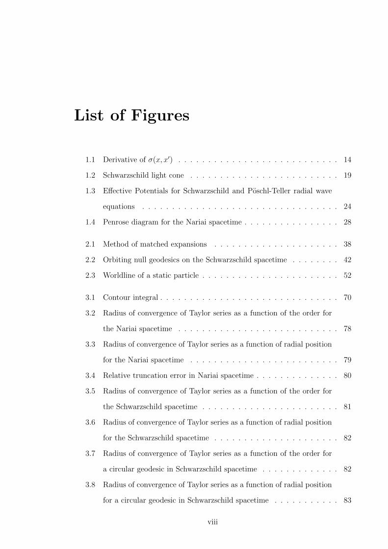
Figure 1.1: Derivatives of σ(x, x′) at x (left) and at x′ (right).
1.1.3 Bi-tensors and Covariant Expansions
The Synge world-function, σ(x, x′), is a bi-scalar, i.e. a scalar at x and at x′ defined
to be equal to half the square of the geodesic distance between the two points. The
world-function may be defined by the fundamental identity
σασα = 2σ = σα′σ
α′ , (1.23)
together with the boundary condition limx′→x
σ(x, x′) = 0 and limx′→x
σab(x, x′) = gab(x).
Here we indicate derivatives at the (un-)primed point by (un-)primed indices:
σa ≡ ∇aσ σa ≡ ∇aσ σa′ ≡ ∇a′σ σa′ ≡ ∇a′σ. (1.24)
σa is a vector at x of length equal to the geodesic distance between x and x′, tangent
to the geodesic at x and oriented in the direction x′ → x while σa′
is a vector at x′
of length equal to the geodesic distance between x and x′, tangent to the geodesic
at x′ and oriented in the opposite direction (see Fig. 1.1).
The covariant derivatives of σ may be written as
σa(x, x′) = (s− s′)ua σa′(x, x′) = (s′ − s)ua′ (1.25)
where s is an affine parameter and ua is tangent to the geodesic. For time-like
geodesics, s may be taken as the proper time along the geodesic while ua is the
14

1.1. A Brief Review of Green functions, Bitensors andCovariant Expansions
4-velocity of the particle and
σ(x, x′) = −1
2(s− s′)2. (1.26)
For null geodesics, ua is null and σ(x, x′) = 0.
Another bi-tensor of frequent interest is the bi-vector of parallel transport, gab′
defined by the equation
gab′;ασα = 0 = gab′;α′σ
α′ (1.27)
with initial condition limx′→x
gab′(x, x′) = gab(x). From the definition of a geodesic it
follows that
gaα′σα′ = −σa and gαa′σ
α = −σa′ (1.28)
Given a bi-tensor Ta at x, the parallel displacement bi-vector allows us write Ta
as a bi-tensor at x′, obtained by parallel transporting Ta along the geodesic from x
to x′ and vice-versa,
Tαgαa′ = Ta′ Tα′g
α′
a = Ta. (1.29)
Any sufficiently smooth bi-tensor Ta1···ama′1···a′n may be expanded in a local co-
variant Taylor series about the point x:
Ta1···ama′1···a′n(x, x′) =∞∑
k=0
1
n!ta1···ama′1···a′n α1···αk(x)σα1 · · ·σαk (1.30)
where the ta1···ama′1···a′n α1···αk are the coefficients of the series and are local tensors at
x. Similarly, we can also expand about x′:
Ta1···ama′1···a′n(x, x′) =∞∑
k=0
1
n!ta1···ama′1···a′n α′1···α′k(x
′)σα′1 · · ·σα′k (1.31)
For many fundamental bi-tensors, one would typically use the DeWitt approach
[13] to determine the coefficients in these expansions as follows:
1. Take covariant derivatives of the defining equation for the bi-tensor (the num-
15

1.2. Black Hole Spacetimes
ber of derivatives required depends on the order of the term to be found).
2. Replace all known terms with their coincidence limit, x→ x′.
3. Sort covariant derivatives, introducing Riemann tensor terms in the process.
4. Take the coincidence limit x′ → x of the result.
This method allows all coefficients to be determined recursively in terms of lower
order coefficients and Riemann tensor polynomials. Although this method proves
effective for determining the lowest few order terms by hand [39, 40] and can be
readily implemented in software [41], it does not scale well with the order of the
term considered and it is not long before the computation time required to calculate
the next term is prohibitively large. This issue can be understood from the fact
that the calculation yields extremely large intermediate expressions which simplify
tremendously in the end. The fact that the final expressions are so short relative
to these intermediate expressions suggests that the algorithm is lacking efficiency.
It is therefore desirable to find an alternative approach which is more efficient and
better suited to implementation in software. In Chapter 4, we will describe one such
approach which proves to be highly efficient.
1.2 Black Hole Spacetimes
From astrophysical considerations, EMRI systems are expected to consist of either
static, spherically symmetric black holes, or, more likely, axially symmetric spinning
black holes. In this section, we will introduce some black hole spacetimes which are
of particular interest for self-force calculations.
16

1.2. Black Hole Spacetimes
1.2.1 Spherically Symmetric Spacetimes
Schwarzschild
The Schwarzschild spacetime represents a static, spherically symmetric black hole
parametrized by a single quantity, its mass, M . It has a line element given by
ds2 = −(
1− 2M
r
)dt2+
(1− 2M
r
)−1
dr2+r2dΩ22, dΩ2
2 = dθ2+sin2 θdφ2. (1.32)
Schwarzschild is a vacuum spacetime, having vanishing Ricci tensor and scalar.
The equations governing the geodesics in Schwarzschild spacetime can be derived
from the Lagrangian [42, 43],
L =1
2
[−t2
(1− 2M
r
)+ r2
(1− 2M
r
)−1
+ r2θ2 + (r2 sin2 θ)φ2
], (1.33)
where the overdot indicates differentiation with respect to s and where L = −1 for
timelike geodesics and L = 0 for null geodesics. Since the spacetime is spherically
symmetric, without loss of generality, we can set θ = π/2 and θ = 0. The geodesics
are then parametrized by two constants of the motion
e = t
(1− 2M
r
)(1.34)
and
l = r2φ, (1.35)
corresponding to the energy per unit mass and angular momentum per unit mass,
17

1.2. Black Hole Spacetimes
respectively. Using this parametrization, the geodesic equations are:
t =e(
1− 2Mr
) (1.36a)
r =±√e2 −
(1− 2M
r
)(ε+
l2
r2
)(1.36b)
φ =l
r2, (1.36c)
where ε = 1 for timelike geodesics, ε = 0 for null geodesics and the sign of the square
root in the radial equation is chosen dependent on whether the radial motion is
inwards or outwards. For the purposes of numerically solving the geodesic equations,
this sign choice is troublesome and it proves better to work with the second order
version of the radial equation3,
r =l2(r − 3M)
r4− Mε
r2, (1.37)
which is independent of whether the geodesic is moving inwards or outwards in the
radial direction. We also point out that it is highly advantageous in a numerical
integration (particularly in the case of elliptical orbits) to make use of an algorithm
incorporating adaptive step-sizing. Furthermore, algorithms which make use of the
Jacobian (such as Burlisch-Stoer) perform orders of magnitude better than those
that do not.
There is a null circular orbit at r = 3M . This means that null geodesics which
come close to this orbit may circle the black hole one or more times before going
out to infinity. As a result, we find that the light cone in Schwarzschild is self-
intersecting (see Fig. 1.24), resulting in caustics, points where neighboring geodesics
converge, at the antipodal points (i.e. at an angle π, equivalently the opposite side
of the black hole).
3In practise, Eq. (1.37) can be numerically solved by writing it as a pair of coupled first orderequations for r and r.
4This figure is inspired by one previously produced by Perlick [44].
18

1.2. Black Hole Spacetimes
Figure 1.2: The light cone in Schwarzschild spacetime is self-intersecting. Geodesicsinitially moving in different directions will re-intersect at a later time. The sphericalsymmetry of Schwarzschild means that an infinite number of geodesics intersectat a caustic. These caustics appear in the image as the points where the coneintersects itself. The Hadamard form for the Green function is valid for pointsseparated along a geodesic, provided there is no other geodesic also connecting thosepoints (i.e. within a normal neighborhood). In this light-cone diagram, the normalneighborhood for geodesics emanating from the vertex of the cone is the interiorof the cone (and including the cone itself), excluding the region in the middle-leftbounded by the null geodesics which have already passed through a caustic.
19

1.2. Black Hole Spacetimes
Reissner-Nordstrom
The Schwarzschild spacetime may be generalized to allow the black hole to have a
charge, Q, resulting the Reissner-Nordstrom spacetime, with line element
ds2 = −(
1− 2M
r+Q2
r2
)dt2 +
(1− 2M
r+Q2
r2
)−1
dr2 + r2dΩ22. (1.38)
Reissner-Nordstrom has a vanishing Ricci scalar, but non-vanishing Ricci tensor.
This property will prove useful in calculating the self-force for non-geodesic motion in
Chapter 5. We will see that it highlights the difference made by the non-geodesicity
of the motion at a lower order than a spacetime with vanishing Ricci tensor would.
1.2.2 Axially Symmetric Spacetimes
Kerr
The spacetime of a spinning black hole is given by the Kerr metric. In Boyer-
Lindquist coordinates, its line-element is
ds2 = −(
1− 2Mr
Σ
)dt2 − 4aMr sin2 θ
Σdtdφ+
Σ
∆dr2
+ Σdθ2 +
(∆ +
2Mr(r2 + a2)
Σ
)sin2 θdφ2 (1.39)
where
Σ = r2 + a2 cos2 θ (1.40)
∆ = r2 − 2Mr + a2 (1.41)
and the black hole is parametrized by two quantities: its mass, M , and its angular
momentum per unit mass, a. In analogy to the Schwarzschild case, geodesics of the
Kerr spacetime can be parametrized by constants of the motion. In addition to two
constants e and l, which are analogous to those of Schwarzschild, the geodesics of
Kerr have a third constant of the motion, the Carter constant [45]. In the cases
20

1.2. Black Hole Spacetimes
studied in this thesis, however, for simplicity we will restrict ourselves to motion in
the equatorial plane (by the symmetry of the spacetime, this motion will remain in
the equatorial plane) and will only be concerned with the constants e and l.
The equations governing the timelike geodesics in the equatorial plane may be
written in terms of these two constants [42, 43]:
t =1
∆
[(r2 + a2 +
2Ma2
r
)e− 2Ma
rl
](1.42a)
φ =1
∆
[(1− 2M
r
)l +
2Ma
re
](1.42b)
r2 = e2 − 1− 2Veff(r, e, l), (1.42c)
where Veff(r, e, l) is an effective potential given by
Veff(r, e, l) = −Mr
+l2 − a2 (e2 − 1)
2r2− M (l − ae)2
r3. (1.43)
For null geodesics, the radial equation takes a different form and depends on the
impact parameter, b = |l/e|, and on whether the orbit is with or against the rotation
of the black hole (determined by l ≡ sign(l)) [42, 43]:
r2 = e2 −Weff(r, b, l), (1.44)
where Weff(r, b, σ) is an effective potential given by
Weff(r, b, σ) =1
r2
[1−
(ab
)2
− 2M
r
(1− l a
b
)2]. (1.45)
1.2.3 Kerr-Newman
As was the case with Schwarzschild, the Kerr spacetime may be generalized to allow
the black hole to have a charge, giving the Kerr-Newman spacetime. In Boyer-
21

1.3. The Nariai Spacetime
Linquist coordinates, the Kerr-Newman metric is [46]:
ds2 = −∆− a2 + z2
ρ2dt2 +
2(∆− r2 − a2)(a2 − z2)
aρ2dtdφ+
ρ2
∆dr2
+ ρ2dθ2 +a2 − z2
a2ρ2
((a2 + r2)2 −∆(a2 − z2)
)dφ2, (1.46)
where ∆ = r2 − 2Mr + a2 + Q2, ρ2 = r2 + a2 cos2 θ and z = a cos θ. Here, Q is the
charge per unit mass of the black hole. Like Reissner-Nordstrom, the Kerr-Newman
spacetime has vanishing Ricci scalar, but non-vanishing Ricci tensor, which again
will prove useful in Chapter 5.
1.3 The Nariai Spacetime
The spacetimes of greatest astrophysical interest are undoubtedly Schwarzschild and
Kerr. However, in developing new methods and techniques, it can also prove useful
to consider other, simpler spacetimes. One such example is the product spacetime
dS2 × S2, (1.47)
called the Nariai spacetime (the line element will be given later, in Eq. (1.55)). The
deSitter−2 subspace, dS2 is a 2-hyperboloid, while the S2 subspace is a 2-sphere.
Nariai is not a black hole spacetime and so may appear at first to be of little interest
for astrophysical self-force calculations. On the contrary, as will be discussed in this
section, Nariai is very useful as a toy model spacetime, giving fundamental insight
into self-force calculations on the Schwarzschild spacetime. We begin this section
with some motivation for this use of Nariai as a toy model for Schwarzschild.
To evaluate the retarded Green function (2.11) we require solutions to the homo-
geneous scalar field equation on the appropriate curved background. In the absence
of sources, the scalar field equation (2.1) is
1√−g ∂µ(√−ggµν∂νΦ
)− ξRΦ = 0, (1.48)
22

1.3. The Nariai Spacetime
where ξ is the curvature coupling constant. For the Schwarzschild spacetime, the
line element is given by (1.32). We decompose the field in the usual way,
Φ(x) =
∫ ∞
−∞dωS
+∞∑
l=0
+l∑
m=−l
clmωSΦlmωS(x) (1.49)
where
ΦlmωS(x) =u
(S)lωS
(r)
rYlm(θ, φ)e−iωStS , (1.50)
and where Ylm(θ, φ) are the spherical harmonics, clmωS are the coefficients in the
mode decomposition, and the radial function u(S)lωS
(r) satisfies the radial equation
[d2
dr2∗
+ ω2S − V (S)
l (r)
]u
(S)lωS
(r) = 0 (1.51)
with an effective potential
V(S)l (r) = fS(r)
(l(l + 1)
r2+
2M
r3
). (1.52)
where fS(r) = 1− 2M/r. Here r∗ is a tortoise (Regge-Wheeler) coordinate, defined
by
dr∗dr
= f−1S (r) ⇒ r∗ = r + 2M ln(r/2M − 1)− (3M − 2M ln 2). (1.53)
The outer region r ∈ (2M,+∞) of the Schwarzschild black hole is now covered
by r∗ ∈ (−∞,+∞). Note that we have chosen the integration constant for our
convenience so that, in the high-l limit, the peak of the potential barrier (at r = 3M)
coincides with r∗ = 0.
1.3.1 Poschl-Teller Potential and Nariai Spacetime
Unfortunately, to the best of our knowledge, closed-form solutions to (1.51) with
potential (1.52) are not known. However, there is a closely-related potential for
23

1.3. The Nariai Spacetime
0
0.5
1
1.5
2
2.5
3
3.5
4
4.5
-20 -15 -10 -5 0 5 10 15 20Ef
fect
ive P
oten
tial
Radial Coordinate r* / M
Comparison of Effective Potentials for Schwarzschild and Nariai Spacetimes
l = 10
Schwarzschild potentialPoschl-Teller potential
Figure 1.3: Effective Potentials for Schwarzschild (1.52) and Poschl-Teller (1.54) ra-dial wave equations. Note that here the Schwarzschild tortoise coordinate is definedin (1.53) so that the peak is near r∗ = 0. The constants in (1.54) are V0 = l(l + 1),
r(0)∗ = 0 and α = 1/(
√27M).
which exact solutions are available: the so-called Poschl-Teller potential [47],
V(PT )l (r∗) =
α2V0
cosh2(α(r∗ − r(0)∗ ))
(1.54)
where α, V0 and r(0)∗ are constants (V0 may depend on l). Unlike the Schwarzschild
potential, the Poschl-Teller potential is symmetric about r(0)∗ , and decays exponen-
tially in the limit r∗ → ∞. Yet, like the Schwarzschild potential, it has a single
peak, and with appropriate choice of constants, the Poschl-Teller potential can be
made to fit the Schwarzschild potential in the vicinity of this peak (see Fig. 1.3).
In the Schwarzschild spacetime, the peak of the potential barrier is associated with
the unstable photon orbit at r = 3M . This photon orbit may lead to singularities in
the Green function. Hence by building a toy model which includes an unstable null
orbit, we hope to capture the essential features of the distant past Green function.
Authors have found that the Poschl-Teller potential is a useful model for exploring
(some of the) properties of the Schwarzschild solution, for example the quasinormal
mode frequency spectrum [48, 49].
An obvious question follows: is there a spacetime on which the scalar field equa-
tion reduces to a radial wave equation with a Poschl-Teller potential? The answer
24
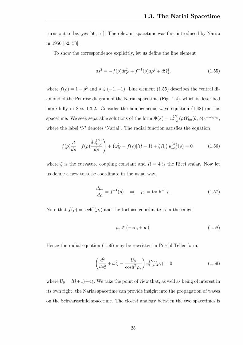
1.3. The Nariai Spacetime
turns out to be: yes [50, 51]! The relevant spacetime was first introduced by Nariai
in 1950 [52, 53].
To show the correspondence explicitly, let us define the line element
ds2 = −f(ρ)dt2N + f−1(ρ)dρ2 + dΩ22, (1.55)
where f(ρ) = 1− ρ2 and ρ ∈ (−1,+1). Line element (1.55) describes the central di-
amond of the Penrose diagram of the Nariai spacetime (Fig. 1.4), which is described
more fully in Sec. 1.3.2. Consider the homogeneous wave equation (1.48) on this
spacetime. We seek separable solutions of the form Φ(x) = u(N)lωN
(ρ)Ylm(θ, φ)e−iωN tN ,
where the label ‘N’ denotes ‘Nariai’. The radial function satisfies the equation
f(ρ)d
dρ
(f(ρ)
du(N)lωN
dρ
)+(ω2N − f(ρ)[l(l + 1) + ξR]
)u
(N)lωN
(ρ) = 0 (1.56)
where ξ is the curvature coupling constant and R = 4 is the Ricci scalar. Now let
us define a new tortoise coordinate in the usual way,
dρ∗dρ
= f−1(ρ) ⇒ ρ∗ = tanh−1 ρ. (1.57)
Note that f(ρ) = sech2(ρ∗) and the tortoise coordinate is in the range
ρ∗ ∈ (−∞,+∞). (1.58)
Hence the radial equation (1.56) may be rewritten in Poschl-Teller form,
(d2
dρ2∗
+ ω2N −
U0
cosh2 ρ∗
)u
(N)lωN
(ρ∗) = 0 (1.59)
where U0 = l(l+1)+4ξ. We take the point of view that, as well as being of interest in
its own right, the Nariai spacetime can provide insight into the propagation of waves
on the Schwarzschild spacetime. The closest analogy between the two spacetimes is
25

1.3. The Nariai Spacetime
found by making the associations
ρ∗ αr∗, tN αtS, ωN ωS/α where α = 1/(√
27M). (1.60)
Fig. 1.3 shows the corresponding match between the potential barriers V(S)l (r∗) and
V(PT )l (ρ∗). In the following sections, we drop the label ‘N’, so that t ≡ tN and
ω ≡ ωN .
The solutions of Eq. (1.59) are presented in Sec. 6.1.1. First, though, we consider
the Nariai spacetime in more detail.
1.3.2 Nariai spacetime
The Nariai spacetime [52, 53] may be constructed from an embedding in a 6-
dimensional Minkowski space
ds2 = −dZ20 +
5∑
i=1
dZ2i (1.61)
of a 4-D surface determined by the two constraints,
− Z20 + Z2
1 + Z22 = a2, Z2
3 + Z24 + Z2
5 = a2, where a > 0, (1.62)
corresponding to a hyperboloid and a sphere, respectively. The entire manifold is
covered by the coordinates T , ψ, θ, φ defined via
Z0 = a sinh
(Ta
), Z1 = a cosh
(Ta
)cosψ, Z2 = a cosh
(Ta
)sinψ,
(1.63)
Z3 = a sin θ cosφ, Z4 = a sin θ sinφ, Z5 = a cos θ, (1.64)
with T ∈ (−∞,+∞), ψ ∈ [0, 2π), θ ∈ [0, π], φ ∈ [0, 2π). The line-element is given
by
ds2 = −dT 2 + a2 cosh2
(Ta
)dψ2 + a2dΩ2
2. (1.65)
26

1.3. The Nariai Spacetime
From this line-element one can see that the spacetime has the following features:
(1) it has geometry dS2 × S2 and topology R × S1 × S2 (the radius of the 1-sphere
diminishes with time down to a value a at T = 0 and then increases monotonically
with time T , whereas the 2-spheres have constant radius a), (2) it is symmetric (ie,
Rµνρσ;τ = 0), with Rµν = Λgµν , and constant Ricci scalar, R = 4Λ, where Λ = 1/a2
is the value of the cosmological constant, (3) it is spherically symmetric (though not
isotropic), homogeneous and locally (not globally) static, (4) its conformal structure
can be obtained by noting the Kruskal-like coordinates defined via U = −(1 −
ΛUV )(Z0 +Z1)/2, V = −(1−ΛUV )(Z0−Z1)/2, for which the line-element is then
ds2 = − 4dUdV
(1− ΛUV )2 + dΩ22. (1.66)
Its two-dimensional conformal Penrose diagram is shown in Fig. 1.4 (see, e.g., [54]),
where we have defined the conformal time ζ ≡ 2 exp (T /a) ∈ (0, π). Its Penrose
diagram differs from that of de Sitter spacetime in that here each point represents a
2-sphere of constant radius; note also that the corresponding angular coordinate ψ
in de Sitter spacetime has a different range, ψ ∈ [0, π), as corresponds to its R× S3
topology. Past and future timelike infinity i± coincide with past and future null
infinity I±, respectively, and they are all spacelike hypersurfaces. A consequence of
the latter fact is the existence of ‘past/future (cosmological) event horizons’ [55, 56,
54]: not all events in the spacetime will be influentiable/observable by a geodesic
observer; the boundary of the future/past of the worldline of the observer is its
past/future (cosmological) event horizon.
In this thesis, we consider the static region of the Nariai spacetime which is
covered by the coordinates t, ρ, θ, φ, where ρ ≡ a tanh(ρ∗/a) ∈ (−a,+a), ρ∗ ≡ (v−
u)/2 ∈ (−∞,+∞), t ≡ (v + u)/2 ∈ (−∞,+∞) and the null coordinates u, v are
given via U = ae−u/a, V = −aev/a. This coordinate system, t, ρ, θ, φ, covers the
diamond-shaped region in the Penrose diagram (Fig. 1.4) around the hypersurface,
say, ψ = π (because of homogeneity we could choose any other ψ = constant
hypersurface). We denote by H−± the past cosmological event horizon at ρ = ±a of
27

1.3. The Nariai Spacetime
H−−
ρ=−a
(U=0)
ρ=−a
(U=0)
H+
+
ρ=+a(U
=+∞)
ρ=+a(U
=+∞)
H +−ρ= −a(V
=0)
H −+
ρ=+a(V
= −∞)
ρ= −a(V
=0)
ρ=+a(V
= −∞)
ρ = 0ψ = π
ρ=
0(UV
=−
1Λ)
ψ=
0
ρ=
0(UV
=−
1Λ)
ψ=
2π
I+ = i+ (t =∞, ρ =∞;UV = 1Λ ) I+ = i+ (t =∞, ρ = −∞;UV = 1
Λ )
I− = i− (t = −∞, ρ = −∞;UV = 1Λ )I− = i− (t = −∞, ρ =∞;UV = 1
Λ )
Figure 1.4: Penrose diagram for the Nariai spacetime in coordinates (ψ, ζ). Thehypersurfaces ψ = 0 and ψ = 2π are identified. Past/future timelike infinity i−/+ co-incides with past/future null infinity I−/+, and they are all spacelike hypersurfaces.Thus, there exist observer-dependent past and future cosmological event-horizons,here marked as H±± for an observer along ψ = π.
an observer moving along ψ = π; similarly, H+± will denote its future cosmological
event horizon at ρ = ±a. Interestingly, Ginsparg and Perry [57] showed that this
static region is obtained from the Schwarzschild-deSitter black hole spacetime as
a particular limiting procedure in which the event and cosmological horizons of
Schwarzschild-deSitter coincide (see also [58, 59, 60, 61]).
Note that there are three hypersurfaces ρ = 0, only two of which (those corre-
sponding to ψ = 0 and 2π) are identified (the one corresponding to ψ = π is not).
Without loss of generality, we will take Λ = 1 = a. The line-element corresponding
to this static coordinate system is given in (1.55).
1.3.3 Geodesics on Nariai spacetime
Let us now consider geodesics on the Nariai spacetime. Our chief motivation is to
find the orbiting geodesics, the analogous rays to those shown in Fig. 2.2 for the
Schwarzschild spacetime. We wish to find the coordinate times t− t′ for which two
28

1.3. The Nariai Spacetime
angularly-separated points at the same ‘radius’, ρ, (the quotes indicate the fact that
the area of the 2-spheres does not depend on ρ) may be connected by a null geodesic.
We expect the Green function to be singular at these times.
We will assume that particle motion takes place within the central diamond of the
Penrose diagram in Fig. 1.4; that is, the region −1 < ρ < 1 (notwithstanding the fact
that timelike geodesics may pass through the future horizons H++ and H+
− in finite
proper time). Without loss of generality, let us consider motion in the equatorial
plane (θ = π/2) described by the world line zµ(λ) = [t(λ), ρ(λ), π/2, φ(λ)] with
tangent vector uµ = [t, ρ, 0, φ], where the overdot denotes differentiation with respect
to an affine parameter λ. Symmetry implies two constants of motion, k = f(ρ)t and
h = φ. The radial equation is ρ = ±H(ρ2 − ρ20)1/2 where ρ0 =
√1− k2/H2 is
the closest approach point and H2 = h2 + κm20. Here, m0 is the scaling of the
affine parameter (which is equal to the particle’s rest mass in the case of a massive
particle following a timelike geodesic) and κ = +1 for timelike geodesics, κ = 0
for null geodesics, and κ = −1 for spacelike geodesics. We still have the freedom
to rescale the affine parameter, λ, by choosing a value for m0. It is conventional
to rescale so that λ corresponds to proper time or distance, that is, set m0 = 1.
Instead, we will rescale so that λ = φ, that is, we set h = 1.
Let us consider a geodesic that starts at ρ = ρ1, φ = 0 which returns to ‘radius’
ρ = ρ1 after passing through an angle of ∆φ (N.B. ∆φ is unbounded, ∆φ ∈ [0,+∞).
In some cases we will refer to the bounded minimal angular distance, γ ∈ [0, π]).
The geodesic distance in this case is s = −κ(H2 − 1)1/2∆φ. It is straightforward to
show that
ρ(φ) = ρ1cosh (Hφ−H∆φ/2)
cosh (H∆φ/2), (1.67)
hence the radius of closest approach, ρ0, is
ρ0 = ρ1sech(H∆φ/2). (1.68)
29

1.3. The Nariai Spacetime
The coordinate time ∆t1 it takes to go from ρ = ρ1, φ = 0 to ρ = ρ1, φ = ∆φ is
∆t1 = 2ρ∗1 + ln
(ρ1 − ρ2
0 +√
(1− ρ20)(ρ2
1 − ρ20)
ρ1 + ρ20 −
√(1− ρ2
0)(ρ21 − ρ2
0)
)(1.69)
where ρ∗1 = tanh−1(ρ1). Substituting (1.68) into (1.69) yields ∆t1 as a function of
the angle ∆φ,
∆t1 = 2ρ∗1 + ln
1− ρ1sech2(H∆φ/2) + tanh(H∆φ/2)
√1− ρ2
1sech2(H∆φ/2)
1 + ρ1sech2(H∆φ/2)− tanh(H∆φ/2)√
1− ρ21sech2(H∆φ/2)
.
(1.70)
This takes a particularly simple form as ρ1 → 1,
∆t1 ∼ 2ρ∗1 + ln(sinh2(H∆φ/2)
), for ρ1 → 1. (1.71)
As ∆φ→∞, the geodesic coordinate time increases linearly with the orbital angle
∆φ
∆t1 ∼ 2ρ∗1 +H∆φ, for ∆φ→∞, ρ1 → 1. (1.72)
In other words, for fixed spatial points near ρ = 1, the geodesic coordinate times ∆t1
are very nearly periodic, with period 2πH. Results (1.67), (1.70), (1.71) and (1.72)
will prove useful when we come to consider the singularities of the Green function
in Secs. 6.2.4 and 6.2.5.
1.3.4 Hadamard Green Function: Exact solution
With Nariai being a highly symmetric product spacetime, it is not surprising that
analytic expressions for many functions of the affine length can be found. The
spacetime can be separated almost entirely into its two constituent subspaces, with
each subspace then being treated independently. The world function, σ, for the total
spacetime then separates into a component from the dS2 part, λ, and a component
30

1.3. The Nariai Spacetime
from the S2 part, γ, [62]
σ = σ + σ = −1
2λ2 +
1
2γ2. (1.73)
where we use the convention that ˆ denotes a quantity in the dS2 part and ˜ denotes
a quantity in the S2 part. Each of these components remains symmetric in x and
x′. As a result, the connection coefficients, metric and wave operator also separate,
Γabc =
Γabc
0
0 Γabc
, gab =
gab 0
0 gab
, =+ . (1.74)
Furthermore, we have an independent defining equation, (1.26), for each component
of the world function
σασα = 2σ σασα = 2σ. (1.75)
Finally, it is shown in Ref. [62] that the affine parameter can be written in analytic
form for each subspace:
γ = cos−1 [cos (φ− φ′) sin θ sin θ′ + cos θ cos θ′] (1.76a)
λ = cosh−1
[√(1− ρ2)(1− ρ′2) cosh (t− t′) + ρρ′
]. (1.76b)
For null geodesics, given the choice of affine parameter given in Sec. 1.3.3 and since
σ = 0, we find that both affine parameters are equal to φ (the angle coordinate on
S2):
γ = φ λ = φ, (1.77)
and the tangent vectors are
uθ = 1 uφ = −1 uρ = λ,ρ ut = λ,t . (1.78)
31
1.3. The Nariai Spacetime
In this case, we can view null geodesic motion in the full spacetime as consisting of
a spacelike geodesic in the S2 subspace and a timelike geodesic in the dS2 subspace.
Without loss of generality, we restrict geodesics to the plane θ = π/2. For geodesics
outside the θ = π/2 plane, one simply rotates the coordinates so that the geodesics
are in the plane.
Both subspaces are maximally symmetric, so we may now apply the results of
[63] to find analytic expressions for λ = − cothλ, γ = cotλ, gab′ , σab, σab′ and
their derivatives (it is also straightforward to calculate derivatives of σ without the
use of Ref. [63] by covariantly differentiating Eq. (1.73) and making use of (1.76)).
This yields
gab′ = −sinhλ
λσab′ −
(sinhλ
λ− 1
)λ,ρλ,ρ′ g
ρρ′ (1.79a)
gab′ = δa
b′ (1.79b)
gab′;c′ = − tanhλ
2(gc′b′ua + gc′aub′) (1.79c)
gab′;c′ = − tanγ
2(gc′b′ua + gc′aub′) (1.79d)
σa′b′ = −(λ,a′λ,b′ + λλ,a′b′ − Γα
′
a′b′λ,α′)
(1.79e)
σab′ = − (λ,aλ,b′ + λλ,ab′) (1.79f)
σ = 1 + λ cothλ (1.79g)
σ = 1 + γ cot γ (1.79h)
σa′b′ =(γ,a′γ,b′ + γγ,a′b′ − Γα
′
a′b′γ,α′)
(1.79i)
σab′ = (γ,aγ,b′ + γγ,ab′) (1.79j)
∆1/2 =√λ sinhλ (1.79k)
∆1/2 =√γ sin γ (1.79l)
σa′b′c′ = (σa′b′);c′ (1.79m)
σa′b′c′ = (σa′b′);c′ (1.79n)
σa′b′c′d′ = (σa′b′);c′d′ (1.79o)
σa′b′c′d′ = (σa′b′);c′d′ (1.79p)
32

1.3. The Nariai Spacetime
∆1/2 = ∆1/2 + ∆1/2
=1
2
(4− coth2 λ+ cot2 γ
)√
γ
sin γ
λ
sinhλ(1.79q)
and, for null geodesics,
V0 = −1
8(2λ+ cothλ− cotλ) (sinhλ sinλ)−1/2 . (1.79r)
These expressions allow us to compute all of these quantities exactly and will
prove useful as a check on alternative methods for calculating the Green function.
In particular, analytic expressions for these quantities were invaluable as a way of
verifying our numerical code described in Sec. 4.4.
33

Chapter 2
The Scalar Self-force and
Equations of Motion
The idea of a self-force has a long history in physics. Derivations of expressions
for the scalar, electromagnetic and scalar self-force have been given by several re-
searchers [13, 15, 17, 20, 22, 23, 19, 24, 25, 26]. In this thesis, we restrict our
attention to the simplest case: a point-like scalar charge q of mass m coupled to
a massless scalar field Φ(x) moving on a curved background geometry. The scalar
field Φ(x) satisfies the field equation
(− ξR) Φ(x) = −4πρ(x) (2.1)
where is the d’Alembertian on the curved background created by, e.g. a black
hole of mass M , R is the Ricci scalar, and ξ is the coupling to the scalar curvature.
The charge density, ρ, of the point particle is
ρ(x) =
∫
γ
qδ4(xµ − zµ(τ))√−g dτ (2.2)
where z(τ) describes the worldline γ of the particle with proper time τ , gµν is the
background metric, g = det(gµν), and δ4(·) is the four-dimensional Dirac distribu-
tion. The scalar field propagates along and within the null cone, while the particle
34

2.1. MiSaTaQuWa Equation for the Self-force
itself will (approximately) follow a time-like geodesic of the background. As a result
the particle may ‘feel’ its own field. In this sense, the field is seen to exert a radiation
reaction on the particle, creating a self-force [20]
f selfµ = q∇µΦR (2.3)
which leads to the equations of motion for the scalar particle
maµ = (gµν + uµuν)f selfν = q(gµν + uµuν)∇νΦR (2.4)
where uµ is the particle’s four-velocity, aµ is its four-acceleration and ΦR is the
radiative part of the field. Identifying the correct radiative field (which is regular
at the particle’s position) is the essential step in the derivation of the self-force [18].
Note that the projection operator gµν + uµuν has been applied here to ensure that
uµaµ = 0. The mass, m, appearing in (2.4) is the ‘dynamical’ (and renormalized)
particle’s mass, which in the scalar case is not necessarily a constant of motion [20].
Rather, it evolves according to
dm
dτ= −quµ∇µΦR. (2.5)
In other words, a scalar particle may radiate away its mass through the emission of
monopolar waves.
2.1 MiSaTaQuWa Equation for the Self-force
A leading method for computing the derivative of the radiative field, ∇νΦR, and
hence the self-force, is based on mode sum regularization (MSR). The MSR approach
was developed by Barack, Ori and collaborators [64, 65, 66, 67] and Detweiler and
coworkers [68, 21, 69]. The method has been applied to the Schwarzschild spacetime
to compute, for example, the gravitational self-force for circular orbits [67] and the
scalar self-force for eccentric orbits [70]. The application to Kerr is in progress
35

2.1. MiSaTaQuWa Equation for the Self-force
[71, 72]. It was recently shown [73] that the gravitational self-force computed in the
Lorenz gauge is in agreement with that found in the Regge-Wheeler gauge [68, 21].
Further gauge-independent comparisons, and comparison with the predictions of
Post-Newtonian theory [74, 75] are presently under consideration [76].
One drawback of the MSR method is that it gives relatively little geometric
insight into the physical origin of the self-force. Other methods [77, 78, 79, 80],
based on the MiSaTaQuWa equation first derived by DeWitt and Brehme in the
1960’s, rely on an expression for the derivative of the radiative field involving the
integral of the retarded Green function over the entire past worldline of the particle1,
∇µΦR (z(τ)) =(
1
2m2
field −1
12(1− 6ξ)R
)quµ + q(gµν + uµuν)
(1
3aν +
1
6Rν
λuλ
)+ Φtail
µ (z(τ)) .
(2.6)
Here, Rνλ is the Ricci tensor of the background metric, mfield is the field mass and
aν is the derivative with respect to proper time of the four-acceleration aν = duν
dτ.
The first two sets of terms are evaluated locally [15, 20, 18] without posing any
real difficulty. The task is therefore to elucidate the final, non-local term, Φtailµ , the
so-called tail integral,
Φtailµ (z(τ)) = q lim
ε→0+
∫ τ−ε
−∞∇µGret(z(τ), z(τ ′))dτ ′ (2.7)
where Gret(x, x′) is the retarded scalar Green function and the limiting feature at
the upper limit of integration avoids the singular nature of the Green function at
the point x = x′. Note that the tail integral depends on the entire past history
of the particle’s motion. The calculation of the Green function poses a formidable
challenge and is the main obstacle to progress.
The Green function would normally be evaluated using a mode-sum approach.
1Note that we include here the field mass, mfield, for the sake of generality. In the self-forcecalculations considered in this thesis, we will be considering massless fields, i.e. setting mfield = 0.
36

2.2. The Method of Matched Expansions
One would calculate a sufficient number of the modes and sum them up to obtain the
Green function solution and hence the self-force. However, the limiting feature in the
upper limit of integration causes great difficulties for this method. As ε decreases, it
is necessary to take an increasing number of modes to obtain an accurate solution.
When ε tends towards 0, the number of modes required becomes infinite and it is no
longer possible to accurately compute the integral. A novel solution to this problem,
based on matched expansions, was suggested by Poisson and Wiseman in 1998 [81].
Their idea was to compute the self-force by matching together two independent
expansions for the Green function, valid in ‘quasilocal’ and ‘distant past’ regimes.
This suggestion was analyzed by Anderson and Wiseman [79], who concluded in
2005 that “this approach remains, in our opinion, in the category of ‘promising
but possessing some technical challenges’.” The present thesis represents the first
practical implementation of this method.
2.2 The Method of Matched Expansions
We now briefly outline the Poisson-Wiseman-Anderson method of ‘matched expan-
sions’ [81, 79]. The tail integral (2.7) may be split into so-called quasilocal (QL) and
distant past (DP) parts, as shown in Fig. 2.1. That is,
Φtailµ (z(τ)) = Φ(QL)
µ (z(τ)) + Φ(DP)µ (z(τ))
= q limε→0+
∫ τ−ε
τ−∆τ
∇µGret(z(τ), z(τ ′))dτ ′ (2.8)
+ q
∫ τ−∆τ
−∞∇µGret(z(τ), z(τ ′))dτ ′ (2.9)
where τ −∆τ is the matching time, with ∆τ being a free parameter in the method
(see Fig. 2.1).
The QL and DP parts may be evaluated separately using independent methods.
In particular, if we choose ∆τ to be sufficiently small so that z(τ) and z(τ − ∆τ)
are within a normal neighborhood (see footnote 1) [35], then the QL part may be
37

2.2. The Method of Matched Expansions
Worldline of the particle
Current location of the particle - z(τ)
Matching point - z(τ -Δτ)
q2
! !
!!!!
!aGretd!"
Quasilocal integral back Δτ along the worldline
q2
! !!!!
!"!aGretd!
#
Integral outside quasilocal region
Boundary of normal neighborhood where Hadamard parametrix is valid
Figure 2.1: In the method of matched expansions, the tail integral is split into quasilo-cal (QL) and distant past (DP) parts.
evaluated by expressing the Green function in the Hadamard parametrix [34]. In
other words, if z(τ) and z(τ−∆τ) are connected by a unique non-spacelike geodesic,
then the QL integral is simply
q−1Φ(QL)µ (z(τ)) = − lim
ε→0+
∫ τ−ε
τ−∆τ
∇µV (z(τ), z(τ ′))dτ ′ , (2.10)
where V (x, x′) is a smooth, symmetric bi-scalar describing the propagation of radi-
ation within the light cone (see Sec. 6.1.3 for full details). Methods for evaluating
the Hadamard Green function will be discussed in the Chapters 3, 4 and 5. The
approach ultimately yields an expression for the QL self force in terms of the sep-
aration of the points x and x′. In Sec. 6.1.3 we apply these methods to determine
the quasilocal Green function, as required for a matched expansion calculation of
the self-force in the Nariai spacetime.
Evaluating the contribution to the Green function from the ‘distant past’ is a
greater challenge. One possibility is to decompose the Green function into a sum over
angular modes and an integral over frequency. In a spherically symmetric spacetime,
the ‘retarded’ Green function may be defined in terms of a Laplace integral transform
38

2.2. The Method of Matched Expansions
and an angular l-mode decomposition as follows,
Gret(x, x′) =
1
2π
∫ +∞+ic
−∞+ic
dωe−iω(t−t′)+∞∑
l=0
(2l + 1)Pl(cos γ)glω(r, r′). (2.11)
Here c is a positive constant, t and r are appropriate time and radial coordinates,
and cos γ = cos θ cos θ′ + sin θ sin θ′ cos(φ − φ′), where γ is the angle between the
spacetime points x and x′. The radial Green function glω(r, r′) may be constructed
from two linearly-independent solutions of a radial equation. Since the DP Green
function does not need to be extended to coincidence (τ ′ → τ), the mode sum does
not require regularization (though it may still be regularized if desired). However,
Anderson and Wiseman [79] found the convergence of the mode sum to be poor,
noting that going from 10 modes to 100 increased the accuracy by only a factor of
three.
In Chapter 6, we explore a new method for evaluating the ‘distant past ’ contri-
bution, based on an expansion in so-called quasinormal modes. The integral over
frequency in equation (2.11) may be evaluated by deforming the contour in the com-
plex plane [82, 83]. This is shown in Fig. 6.2. In the Schwarzschild case there arise
three distinct contributions to the Green function, from the three sections of the
frequency integral in (2.11):
1. An integral along high-frequency arcs, which leads to a prompt response. An-
dersson [83] has shown that this is 0 for black hole spacetimes at sufficiently
late times.
2. A ‘quasinormal mode sum’, arising from the residues of poles in the lower half-
plane of complex frequency ω. This contribution leads to a damped ringing,
characteristic of the black hole.
3. An integral along a branch cut, which leads to a power-law tail (among possible
other features).
The three parts (1–3) are commonly supposed to dominate the scattered signal at
early, intermediate and late times, respectively [82, 83]. (This may be slightly mis-
39

2.2. The Method of Matched Expansions
leading, however; Leaver [82] notes that, in addition, the branch cut integral (part
3) “contributes heavily to the initial burst of radiation”). In Chapter 6, we investi-
gate an alternative spacetime, introduced by Nariai in 1950 [52, 53] and discussed
in Sec. 1.3, in which the power-law tail (part 3) is absent. We demonstrate that,
on the Nariai spacetime, at suitably ‘late times’, the distant past Green function
may be written as a sum over quasinormal modes (defined in Sec. 6.1.2). We use
the sum to compute the Green function, the tail field and the self-force for a static
particle.
A key question to be addressed in this work is the following: how much of the self-
force arises from the quasilocal region, and how much from the distant past? If the
Green function falls off fast enough then only the QL integral would be needed, and,
since the QL integral is restricted to the normal neighborhood, only the Hadamard
parametrix is required. Unfortunately this is not necessarily the case; Anderson
and Wiseman [79] note that there are simple situations in which the DP integral in
(2.11) gives the dominant contribution to the self-force.
Using the methods presented in Chapter 6, we are able to compute the retarded
Green function and the integrand of Eq. (2.7) as a function of time along the past
worldline. We will show that the DP contribution cannot be neglected. In particular,
we find that the Green function and the integrand of Eq. (2.7) is singular whenever
the two points zµ(τ) and zµ(τ ′) are connected by a null geodesic and that the
singular form of the Green function changes every time a null geodesic passes through
a caustic. On a spherically-symmetric spacetime, caustics occur at the antipodal
points.
On Schwarzschild spacetime, the presence of an unstable photon orbit at r = 3M
implies that a null geodesic originating on a timelike worldline may later re-intersect
the timelike worldline, by orbiting around the black hole. Hence the effect of caustics
may be significant. For example, Fig. 2.2 shows orbiting null geodesics on the
Schwarzschild spacetime which intersect timelike circular orbits of various radii. We
believe that understanding the singular behavior of the integrand of Eq. (2.7) is a
40
2.2. The Method of Matched Expansions
crucial step in understanding the origin of the non-local part of the self-force. As
we shall see in Chapter 6, the Nariai spacetime proves a fertile testing ground.
2.2.1 The Static Particle
Before continuing, we will briefly review the extensive literature that has studied the
specific case of the self-force on a static particle. This will be of use in subsequent
sections and chapters.
A static particle – a particle with constant spatial coordinates – has been the fo-
cus of several scalar self-force calculations, in particular for the Schwarzschild space-
time [84, 77, 85, 79, 78, 86, 27]. Although a static particle may not be a particularly
physical case, it is frequently chosen because it involves relatively straightforward
calculations and has an exact solution for the Schwarzschild spacetime. It there-
fore provides a good testing ground for new approaches to the calculation of the
self-force.
Smith and Will [84] calculated the self-force on a static electric charge in the
Schwarzschild background and found it to be non-zero. In [77], Wiseman considered
the analogous case of a static scalar charge in the case of minimal-coupling (i.e., ξ =
0) in Schwarzschild. Using isotropic coordinates, he managed to sum the Hadamard
series for the Green function in the static case (i.e., the “Helmholtz”-like equation
in Schwarzschild with zero-frequency, ω = 0) and thus obtain in closed form the
field created by the static charge in the scalar and also electrostatic (already found
in [87, 88] using a different method) cases. He then found the self-force to be zero
in the scalar, minimally-coupled case.
In [86], the calculation of the self-force on a static scalar charge in Schwarzschild
is extended to the case of non-minimal coupling (ξ 6= 0) and is found to be zero as
well. The fact that the value of the scalar self-force in Schwarzschild is the same
(zero) independently of the value of the coupling constant is in agreement with
the Quinn-Wald axioms [15, 20]: their method relies only on the field equations,
and these are independent of the coupling constant in a Ricci-flat spacetime such
41

2.2. The Method of Matched Expansions
-10
-5
0
5
10
-10 -5 0 5 10
R = 6M
x
x1
x2x3
Orbit of small black holeNull geodesic (1)Null geodesic (2)Null geodesic (3)
r = 3M, circular photon orbit
10
5
0
5
10
10 5 0 5 10
R = 6M -10
-5
0
5
10
-10 -5 0 5 10
R = 8M 10
5
0
5
10
10 5 0 5 10
R = 8M
-10
-5
0
5
10
-10 -5 0 5 10
R = 10M 10
5
0
5
10
10 5 0 5 10
R = 10M -10
-5
0
5
10
-10 -5 0 5 10
R = 12M 10
5
0
5
10
10 5 0 5 10
R = 12M
Figure 2.2: Orbiting null geodesics on the Schwarzschild spacetime that intersecttimelike circular orbits of various radii R = 6M , 8M , 10M and 12M . The nullgeodesics are shown as dotted (coloured) lines, and the timelike circular orbit isshown as a solid (black) line. The spacetime point x is connected to x1, x2, etc. bynull geodesics, as well as by the timelike circular geodesic. The Green function issingular when x′ = x1, x2, etc. Note that between R = 6M and R = 8M theordering of the points x2 and x3 becomes reversed.
42

2.2. The Method of Matched Expansions
as Schwarzschild. The calculation (without using the Quinn-Wald axioms) is by
no means trivial, however, since the effect of the coupling constant might be felt
through the stress-energy tensor (in fact, [86] corrected a previous result in [89, 90],
where the self-force had been incorrectly found to be non-zero). Rosenthal [85]
has also considered the case of a static particle in Schwarzschild and used it as an
example application of the massive field approach [91] to self-force calculations (in
Appendix D, we apply this method to the Nariai case).
On the other hand, using the conformal invariance of Maxwell’s equations,
Hobbs [92] showed that, in a conformally-flat spacetime, the ‘tail’ contribution (2.7)
to the self-force on an electric charge (on any motion, static or not) is zero. The only
possible contribution to the self-force might then come from the local Ricci terms,
which are zero in cases of physical interest such as in the de Sitter universe.
One would expect the ‘tail’ contribution to the scalar self-force to also be zero for
a charge undergoing any motion in a conformally-flat 4-D spacetime with conformal-
coupling (i.e., ξ = 1/6). In a recent article [93], it was further argued using
Hobbs’ result that the self-force should be zero for a static charge (where the time-
independence effectively reduces the problem to a 3-D spatial one), in a spacetime
such that its 3-D spatial section is conformally-flat and with conformal-coupling in
3-D (i.e., ξ = 1/8). Indeed, they showed that the scalar self-force on a massless
static particle in a wormhole spacetime (with non-zero Ricci scalar and where the
3-D spatial section is conformally-flat) is equal to zero at ξ = 1/8 and it actually
changes sign at this 3-D conformal value. [Note that in this case the local contri-
bution to the self-force is exactly zero, so there may only be a ‘tail’ contribution -
if any]. It is not completely clear to us, however, that the argument that the ‘tail’
contribution to the self-force is zero due to the conformality of the physical system
carries through intact from a 4-D spacetime to its 3-D spatial section - Note that,
from the Hadamard form in 3-D [34, 36], the corresponding Green function (the so-
called ‘scalarstatic’ or ‘electrostatic’ Green function) never (regardless of whether
there is conformality or not) possesses a ‘tail’ part V (x, x′), and the self-force is
43

2.3. Quasilocal Contribution: Geodesic Motion
calculated from this static Green function, not via Eqs.(2.3) and (2.6), but rather
via, e.g., Eq.(6.95) of Chapter 6.
In Chapter 6, we study the self-force on a static particle in Nariai spacetime. The
Nariai spacetime, not being Ricci-flat and being conformal to a wormhole spacetime
(and so with a conformally-flat 3-D spatial section), suggests a very interesting
playground for calculating the self-force: What role does the coupling constant ξ
play? Do particular values such as ξ = 1/6 (4-D conformal-coupling) and ξ = 1/8
(3-D conformal-coupling, so a particular value in the case of a static charge) yield
‘particular’ values (namely, zero) for the self-force? Are the Quinn-Wald axioms
satisfied?
2.3 Quasilocal Contribution: Geodesic Motion
Within the quasilocal region, where x and x′ are within a normal neighborhood 2 ,
we can use the scalar version of the Hadamard form, (1.3), for the retarded Green
function,
Gret (x, x′) = θ− (x, x′) U (x, x′) δ (σ (x, x′))− V (x, x′) θ (−σ (x, x′)) (2.12)
where θ− (x, x′) is analogous to the Heaviside step-function (i.e. 1 when x′ is in the
causal past of x, 0 otherwise), δ (x, x′) is the standard Dirac delta function, U (x, x′)
and V (x, x′) are symmetric bi-scalars having the benefit that they are regular for
x′ → x and σ (x, x′) is the Synge [94, 18, 37] world function, defined in Sec. 1.1.3.
The first term (involving U (x, x′)) in Eq. (2.12) is the direct part of the Green
function and does not contribute to the self-force. This can be understood by the
fact that the presence of δ (σ (x, x′)) in the direct part of Gret means that it is only
non-zero on the past light-cone of the particle. However, since the quasilocal integral
in Eq. (2.8) is totally internal to the past light-cone, this term does not contribute
2Anderson and Wiseman [79] have calculated some explicit values for the normal neighborhoodboundary for a particle following a circular geodesic in Schwarzschild spacetime. These valuesplace an upper bound estimation on the geodesic distance in the past at which we can place thematching point ∆τ .
44

2.3. Quasilocal Contribution: Geodesic Motion
to the integral. The second term in Eq. (2.12), the tail part of the Green function,
is responsible for the self-force. Its calculation is therefore the primary focus in any
calculation of the quasilocal self-force.
We can now substitute Eq. (2.12) into Eq. (2.10) to obtain the final form of the
quasilocal self-force:
faQL(z(τ)) = limε→0
q2
∫ τ−ε
τ−∆τ
∇aGret (z(τ), z(τ ′)) dτ ′. (2.13)
Note that it is no longer necessary to take the limit since V (x, x′) is regular every-
where.
Unlike the cases of electromagnetic and gravitational fields, where the four-
acceleration is exactly equal to the self-force divided by the mass, there is one
further step required in order to obtain the equations of motion in the presence of a
scalar field. In this case, the self-force contains two components, one related to the
four-acceleration, the other related to the change in mass:
faQL =dm
dτua +maa (2.14)
The 4-acceleration is always orthogonal to the 4-velocity, so in order to obtain
it from the self-force, we take the projection of fa orthogonal to ua:
maa = P aβ f
β (2.15)
where
P ba = δba + uau
b (2.16)
is the projection orthogonal to uα. The remaining component of the self-force (which
is tangent to the 4-velocity) is simply the rate of change of the mass:
dm
dτ= −fαuα (2.17)
45

2.3. Quasilocal Contribution: Geodesic Motion
2.3.1 Covariant Calculation
The calculation of V (x, x′) was previously discussed in Sec. 1.1.1 in the general (not
necessarily scalar) case. In this section, we repeat the calculation in the particular
case of a scalar field. The symmetric bi-scalar V (x, x′) is expressed in terms of an
expansion in increasing powers of σ [36]:
V (x, x′) =∞∑
n=0
Vn (x, x′)σn (x, x′) (2.18)
Substituting the expansion (2.18) into the wave equation, Eq. (1.2), using the iden-
tity σασα = 2σ and explicitly setting the coefficient of each manifest power of σ
equal to zero, we find (in 4-dimensional spacetime) that the coefficients Vn (x, x′)
satisfy the scalar version of the recursion relations, (1.8),
(n+ 1) (2n+ 4)Vn+1 + 2 (n+ 1)Vn+1;µσµ
− 2 (n+ 1)Vn+1∆−1/2∆1/2
;µσµ +
(x −m2 − ξR
)Vn = 0 for n ∈ N (2.19)
along with the initial conditions
2V0 + 2V0;µσµ − 2V0∆−1/2∆
1/2;µσ
µ +(x −m2 − ξR
)U0 = 0 (2.20a)
U0 = ∆1/2 (2.20b)
The quantity ∆ (x, x′) is the Van Vleck-Morette defined in Sec. 1.1.3.
It is important to note that the Hadamard expansion is not a Taylor series
and is not unique. Indeed, in Appendix B we show how, under the assumption of a
massless field on a vacuum background spacetime, the terms from V0 and V1 conspire
to cancel to third order when combined to form V . Such cancellation is also seen,
for example, in deSitter spacetime, where for a conformally invariant theory all the
Vn’s are non-zero while V ≡ 0.
In order to solve the recursion relations (2.19) and (2.20) for the coefficients
Vn (x, x′), it is convenient to first write Vn (x, x′) in terms of its covariant Taylor
46

2.3. Quasilocal Contribution: Geodesic Motion
series expansion about x = x′:
Vn (x, x′) =∞∑
p=0
(−1)p
p!vn(p) (x, x′) , (2.21)
where the vn(p) are bi-scalars of the form
vn(p) (x, x′) = vn α1...αp(x)σα1 (x, x′) . . . σαp (x, x′) . (2.22)
Decanini and Folacci [36] calculated expressions for these vn(p) up to O (σ2),
or equivalently O (∆τ 4), where ∆τ is the magnitude of the proper time separation
between x and x′. In Chapter 4, we show how this calculation may be implemented in
computer algebra to calculate the expansions to O (∆τ 20) and beyond. In Appendix
A.1, we show how, using the symmetry of the Green function in x and x′ an even
order covariant series expansion may be extended by one further order in the proper
time separation of the points, ∆τ , or equivalently one half order in σ (x, x′).
We now turn to the evaluation of the self-force. We could calculate the self-force
given this form for Vn (x, x′), however, it proves easier to work with the full V (x, x′)
expressed in the form of a covariant Taylor expansion, i.e. an expansion in increasing
powers of σa:
V (x, x′) =∞∑
p=0
(−1)p
p!vα1...αp(x)σα1 (x, x′) . . . σαp (x, x′) (2.23)
Explicit expressions for the va1...ap(x), can then be easily obtained order by order by
combining the relevant vn a1...ap , as described in Appendix B.
Substituting Eq. (2.23) into Eq. (2.13), taking the covariant derivative and noting
that the va1...ap are symmetric under exchange of all indices, a1, . . . , ap, we obtain
47

2.3. Quasilocal Contribution: Geodesic Motion
an expression for the quasilocal self-force in terms of va1...ap , σ and their derivatives:
faQL = −q2
∫ τ
τ−∆τ
[v;a − v ;a
β σβ − vβσβa +2
2!vβγσ
βaσγ +1
2v ;aβγ σβσγ
− 3
3!vβγδσ
βaσγσδ − 1
3!v ;aβγδ σβσγσδ +
4
4!vβγδεσ
βaσγσδσε
+1
4!v ;aβγδε σβσγσδσε − 5
5!vβγδεζσ
βaσγσδσεσζ +O(σ5/2
) ]dτ ′ (2.24)
Now, by definition, for a time-like geodesic,
σ = −1
2(τ − τ ′)2
(2.25a)
σa = − (τ − τ ′)ua (2.25b)
where ua is the 4-velocity of the particle. We may also write σab in terms of a
covariant Taylor series expansion [13, 18, 36],
σab = gab − 1
3Ra b
α βσασβ +
1
12Ra b
α β;γσασβσγ
−[
1
60Ra b
α β;γδ +1
45Ra
αρβRρ bγ δ
]σασβσγσδ +O
[(σa)5] (2.26)
Substituting Eqs. (2.25a), (2.25b) and (2.26) into Eq. (2.24), the integrand be-
comes an expansion in powers of the proper time, τ − τ ′:
faQL = −q2
∫ τ
τ−∆τ
[Aa(τ − τ ′)0
+Ba(τ − τ ′)1+ Ca(τ − τ ′)2
+Da(τ − τ ′)3+ Ea(τ − τ ′)4
+O(
(τ − τ ′)5) ]dτ ′, (2.27)
48

2.3. Quasilocal Contribution: Geodesic Motion
where
Aa = v;a − vβgβa (2.28a)
Ba = v ;aβ uβ − vβγgβauγ (2.28b)
Ca =1
3vβR
β aγ δu
γuδ +1
2v ;aβγ uβuγ − 1
2vβγδg
βauγuδ (2.28c)
Da =1
12vβR
β aγ δ;εu
γuδuε +1
3vβγR
β aδ εu
γuδuε +1
6v ;aβγδ uβuγuδ
−1
6vβγδεg
βauγuδuε (2.28d)
Ea = vβ
(1
60Rβ a
γ δ;εζ +1
45Rβ
γρδRρ aε ζ
)uγuδuεuζ
+1
12vβγR
β aδ ε;ζu
γuδuεuζ +1
6vβγδR
β aε ζu
γuδuεuζ
+1
24v ;aβγδε uβuγuδuε − 1
24vβγδεζg
βauγuδuεuζ . (2.28e)
The coefficients of the powers of τ−τ ′ are all local quantities at x, but the integral is
in terms of the primed coordinates, x′, so the coefficients may be treated as constants
while performing the integration. The result is that we only have to perform a trivial
integral of powers of τ − τ ′. Performing the integration gives us our final result, the
quasilocal part of the self force in terms of an expansion in powers of the matching
point, ∆τ :
faQL = −q2
(Aa∆τ 1 +
1
2Ba∆τ 2 +
1
3Ca∆τ 3 +
1
4Da∆τ 4 +
1
5Ea∆τ 5 +O
(∆τ 6
)).
(2.29)
It is possible to simplify Eqs. (2.28a) - (2.28e) further by using the results
of Appendix A.1 to rewrite all the odd order va1...ap terms in terms of the lower
order even terms. It is then straightforward to substitute in for the va1...ap to get
an expression for the quasilocal self-force in terms of only the scalar charge, field
mass, coupling to the scalar background, 4-velocity, and products of Riemann tensor
components of the background spacetime. However, we choose not to do so here as
that would result in excessively lengthy expressions. Instead, we direct the reader to
Chapter 4 and Ref. [36] for general expressions for the vn a1...ap for a scalar field and
to Appendix B, where we give the expressions for the vn a1...ap for massless scalar
49
2.3. Quasilocal Contribution: Geodesic Motion
fields in vacuum spacetimes up to the orders required.
Once an expression has been obtained for the self-force using this method, it is
straightforward to use Eqs. (2.15) - (2.17) to obtain the equations of motion.
2.3.2 Simplification of the quasilocal self-force for massless
fields in vacuum spacetimes
Eq. (2.29) is valid for any geodesic motion and any scalar field (massless or massive)
in any background spacetime. At first it may appear that this result is quite difficult
to work with due to the length of the expressions for the vn a1...ap . However, if we
make the two assumptions that:
1. The scalar field is massless (mfield = 0),
2. The background spacetime is a vacuum spacetime (Rαβ = 0 = R),
then the majority of these terms vanish and we are left with the much more man-
ageable expressions for the vn a1...ap given in Appendix B for a massless field in a
vacuum spacetime up to O(σ5/2
). We can see immediately from these expressions
that all terms involving vα, vαβ and vαβγ identically vanish. That leaves expressions
involving only vαβγδ and vαβγδε and higher order terms. However, Eq. (A.4) gives
us a relation which allows us to express any odd order term (in this case, vαβγδζ) in
terms of the lower even order terms. This, along with the fact that va1...ap is totally
symmetric, leads to a vastly simplified expression for the quasilocal self-force on a
scalar particle following a geodesic in a vacuum background spacetime:
faQL =
q2gβa[
1
4!vβγδεu
γuδuε∆τ 4 − 1
5!
(1
2vγδεζ;β − 2vβγδε;ζ
)uγuδuεuζ∆τ 5 +O
(∆τ 6
)]
(2.30)
We see that a large number of terms in (2.29) either identically vanish or cancel
each other out. In fact, at the first three orders in ∆τ , we get no contribution to the
50

2.4. Quasi-local Contribution: Non-geodesic Motion
quasilocal self-force whatsoever. Additionally, our fourth and fifth order coefficients
take on a much simpler form than the general case given in Eqs. (2.28d) and (2.28e).
2.4 Quasi-local Contribution: Non-geodesic Mo-
tion
In the previous section, we gave an expression for the scalar self-force on a scalar
charge travelling on a curved background spacetime. However, this expression was
only valid provided the particle’s path was that of a geodesic of the background
spacetime. With some additional care, this result can be extended relatively easily
to allow for non-geodesic particle motion. The calculation remains largely the same
as for geodesic motion, so we will focus here here on the differences caused by the
non-geodesicity of the motion. As before, we are primarily concerned with the
non-local component of the self-force, (2.8). In the most frequently studied cases
of geodesic motion (aa = 0, a = 0) in Ricci-flat spacetimes (Rab = 0, R = 0) and
without field mass (mfield = 0), the local terms of Eq. (2.6) are all identically zero and
the full self-force is given by the non-local component. However, for non-geodesic
motion, the 4-acceleration will always be non-zero so there will always be some local
terms to consider when calculating the self-force.
As before, we focus on the quasilocal contribution, (2.10), using the Hadamard
form, (2.12), and leave the remaining ‘distant past’ contribution to be computed by
other means. We now expand V (x, x′) in two ways. First, we express it in the form
of a covariant Taylor series expansion as given in Eq. (2.23). In the previous section,
we were able to use this expression for V (x, x′) to compute the self-force for geodesic
motion. Unfortunately, things are less straightforward when non-geodesic motion is
allowed for. The problem arises as a result of the presence of σa in this expression.
As demonstrated in Fig. (2.3), it encodes the proper time, τg, along a geodesic of
the background spacetime, defined through σaσa = −τg2. However, the integral in
Eq. (2.10) is along the world line of the particle. In the previous case of geodesic
51

2.4. Quasi-local Contribution: Non-geodesic Motion
Figure 2.3: The worldline of a static particle (xi = constant) in Schwarzschildspacetime is not a geodesic, so the geodesic proper time, τg, and the particle propertime, τ , are not the same. The integral in Eq. (2.13) is along the particle worldline(black), while σa is along the time-like geodesic (red).
motion, this was not a problem as in that case τg is a natural parameter along the
world line. For non-geodesic motion, this is no longer the case. To proceed with
the calculation using this expansion of V (x, x′) would require us to first express the
geodesic proper time τg in terms of the integration variable, i.e. the particle’s proper
time τ . This is a non-trivial task for general motion in general spacetimes.
An easier resolution of this problem comes from expressing V (x, x′) in a second
form, as a non-covariant Taylor series expansion in the coordinate separation of the
points, ∆xa:
V (x, x′) =∞∑
p=0
(−1)p
p!vα1...αp(x)∆xα1 . . .∆xαp (2.31)
where ∆xα = xα − xα′ and the quantities vα1...αp(x) may be expressed in terms of
combinations of the (known) quantities vα1...αp(x) as follows.
First, the world function σ (x, x′) is expressed in terms of an expansion in powers
52

2.4. Quasi-local Contribution: Non-geodesic Motion
of the coordinate separation of x and x′, ∆xα:
σ =1
2gαβ∆xα∆xβ + Aαβγ∆x
α∆xβ∆xγ +Bαβγδ∆xα∆xβ∆xγ∆xδ
+ Cαβγδε∆xα∆xβ∆xγ∆xδ∆xε + . . . (2.32)
where the coefficients Aαβγ, Bαβγδ, Cαβγδε, . . . are to be determined. Differentiating
Eq. (2.32), the coordinate expansion of the derivative of σ is:
σa = gaα∆xα + (1
2gαβ,a + 3Aaαβ)∆xα∆xβ + (Aαβγ,a + 4Baαβγ)∆x
α∆xβ∆xγ
+ (Bαβγδ,a + 5Caαβγδ)∆xα∆xβ∆xγ∆xδ + . . . . (2.33)
Substituting expansions (2.32) and (2.33) into the defining relationship
2σ = σασα (2.34)
and equating powers of ∆xα, we get expressions for each coefficient in terms of the
lower order coefficients. The lowest terms are given by:
Aabc = −1
4g(ab,c) (2.35a)
Babcd = −1
3
[A(abc,d) + gαβ
(1
8g(ab,|α|gcd),β +
3
2g(ab,|α|A|β|cd)
+9
2Aα(abA|β|cd)
)](2.35b)
Cabcde = −1
4
[B(abcd,e) + gαβ
(12Aα(abB|β|cde) + 3Aα(abAcde),β
+ 2g(ab|,α|B|β|cde) +1
2A(abc|,α|gde),β
)](2.35c)
This procedure may be easily extended to higher orders using a computer algebra
package.
Next, we obtain a relation between the known coefficients of the covariant ex-
pansion, Eq. (2.23), and those of the coordinate expansion, Eq. (2.31), by first
substituting Eq. (2.33) into Eq. (2.23) and then equating the two expansions. In
53

2.4. Quasi-local Contribution: Non-geodesic Motion
this way we find the following expressions for the vα1...αp(x) in terms of the vα1...αp(x):
v = v (2.36a)
va = va (2.36b)
vab = vab + vαΓαab (2.36c)
vabc = vabc + 3v(a|α|Γαbc) + 6vα
(A
,α(abc) + 4Bα
abc
)(2.36d)
vabcd = vabcd + 6vα(abΓαcd) + 12vαβ
(1
4Γα(abΓ
βcd) + 2g
α(a A
,βbcd) + 8g
α(a B
βbcd)
)
−24vα
(B
,α(abcd) + 5Cα
(abcd)
)(2.36e)
vabcde =1
2v,(abcde) −
5
2v(ab,cde) +
5
2v(abcd,e) (2.36f)
where the Γαab are the Christoffel symbols of the second kind. We note here the
presence of the Christoffel symbols in the relation between the covariant and coor-
dinate expansions. In the case of a static particle (i.e. purely time separation of
the points), these take on a particularly clear form by being directly related to the
4-acceleration of the particle. In particular, the leading order at which this effect
appears is given in Eq. (2.36c), which in this case becomes:
vtt = vtt + vαΓαtt = vtt + 3vαaα (2.37)
where aα is 4-acceleration of the particle.
Although vabcde could alternatively be given in terms of the vα1...αp(x), we have
found that the expression we give proves easier to work with. It is found by taking
five symmetrized partial derivatives of the equation
V (x, x′) = V (x′, x) (2.38)
and then taking taking the coincidence limit x′ → x. It is a special case of the
general result, Eq. (A.4), of Appendix A.1.
54
2.5. Static Particle in a stationary spacetime
Now, we simply substitute expansion (2.31) into Eq. (2.13) and, since V (x, x′)
is a scalar, take a partial rather than covariant derivative to get an easily evaluated
expression for the self-force (in this case, it is most natural to work with an expression
for the self-force in covariant rather than contravariant form):
fQLa = −q2
∫ τ
τ−∆τ
[v,a − va − (vα,a − vαa) ∆xα +
1
2(vαβ,a − vαβa) ∆xα∆xβ
− 1
3!(vαβγ,a − vαβγa) ∆xα∆xβ∆xγ +
1
4!(vαβγδ,a − vαβγδa) ∆xα∆xβ∆xγ∆xδ
+O(∆x5
) ]dτ ′ (2.39)
Finally, we obtain the equations of motion by projecting orthogonal and perpen-
dicular to the particle 4-velocity, as in Sec. 2.3. This expression may be evaluated for
a specific particle path in a specific spacetime by writing the coordinate separations
∆xα in terms of the particle proper time separation (τ − τ ′). Specific examples of
such an evaluation are given in Chapter 5.
2.5 Static Particle in a stationary spacetime
The expression for the quasilocal contribution to the self-force given in Eq. (2.39)
(and the subsequent equations of motion) take on a significantly simple form if the
spacetime is assumed to be stationary and if we assume the spatial coordinate of
the particle to be fixed. Stationarity allows us to introduce coordinates (t, xi) such
that the metric tensor components, gab are all independent of the time coordinate.
In addition, for a static particle, xi = constant, and only the time component of the
contravariant 4-velocity, ut, is non-zero. These conditions hold, of course, for the
case of a particle held at rest in Schwarzschild spacetime which has already received
much attention in the literature [79, 77].
Since the spatial coordinates of the particle are held fixed, the points x and
x′ are now only separated in the time direction. Furthermore, in this case it is
straightforward to relate the time coordinate to the proper time along the particle’s
55

2.5. Static Particle in a stationary spacetime
world line. As a result we can rewrite the coordinate separation of the points x and
x′ in terms of the proper time separation:
∆xt = ∆t = ut(τ − τ ′) =1√−gtt
(τ − τ ′), ∆xi = 0. (2.40)
Substituting this into Eq. (2.39) and performing the straightforward integral of
powers of (τ − τ ′) gives
fQLa = −q2
[(v,a − va) ∆τ − 1
2!(vt,a − vta)ut∆τ 2 +
1
3!(vtt,a − vtta) (ut)2∆τ 3
− 1
4!(vttt,a − vttta) (ut)3∆τ 4 +
1
5!(vtttt,a − vtttta) (ut)4∆τ 5 +O
(∆τ 6
) ](2.41)
We can now use Eq. (2.36f) for vabcde, along with the analogous equations for va
and vabc,
va =1
2v,a (2.42)
vabc = −1
4v,(abc) +
3
2v(ab,c) (2.43)
to eliminate several terms in this expression. While this did not previously prove
particularly beneficial in the general case, the fact that partial derivatives with re-
spect to t of these fundamentally geometric objects vanish in a stationary spacetime
means that many of the extra terms introduced by the substitution will also vanish.
Indeed it is easy to see from Eq. (A.2) that (in this case of purely time separated
points) any term of order 2k + 1 can be related to the order 2k term:
v tt...tt︸︷︷︸2k
b =1
2v tt...tt︸︷︷︸
2k
,b (2.44)
56

2.5. Static Particle in a stationary spacetime
As a result, Eq. (2.41) may be taken to arbitrary order to give:
fQLa =− q2
[1
2
∞∑
k=0
1
(2k + 1)!v tt...tt︸︷︷︸
2k
,a∆τ2k+1(ut)2k (2.45)
+∞∑
k=1
1
(2k)!v tt...tt︸︷︷︸
2k−1
a∆τ2k(ut)2k−1
](2.46)
To proceed further, we benefit from differentiating between the time and spatial
components:
fQLt =− q2
[ ∞∑
k=1
1
(2k)!v tt...tt︸︷︷︸
2k
∆τ 2k(ut)2k−1]
(2.47)
fQLi =− q2
[1
2
∞∑
k=0
1
(2k + 1)!v tt...tt︸︷︷︸
2k
,i∆τ2k+1(ut)2k (2.48)
+∞∑
k=1
1
(2k)!v tt...tt︸︷︷︸
2k−1
i∆τ2k(ut)2k−1
](2.49)
From this, it is clear that the t component of the quasilocal self-force only appears
at even orders in ∆τ , while the spatial components may appear at both even and
odd orders (this is consistent with one’s physical intuition: the fact that there is an
odd power of ut in fQLt means that it is odd overall, as might be expected given its
role in determining energy balance). Note, however, that for a static spacetime - i.e.
imposing time reversal invariance in addition to stationarity - the second term in
Eq. (2.48) will vanish since each of the vt...ti must be zero in that case (as we have
an odd number of t’s). As a result, in a static spacetime, the spatial component of
the quasilocal self-force will only appear at odd orders in ∆τ .
By Eq. (2.17) and the fact that only the time component of the contravariant
4-velocity is non-zero, we can now rewrite the rate of change of the particle’s mass
as:
dm
dτ= −fαuα = −ftut
= q2
∞∑
k=1
1
(2k)!v tt...tt︸︷︷︸
2k
∆τ 2k(ut)2k (2.50)
57

2.5. Static Particle in a stationary spacetime
Similarly, by Eq. (2.15) we can now write the time and spatial components of the
mass times 4-acceleration:
matQL = −gtigti
gttft + gtifi (2.51a)
maiQL = gtift + gijfj (2.51b)
where ft and fi are as given in Eqs. (2.47) and (2.48).
Again, it is interesting to note the effect of imposing that the spacetime be static.
For a static spacetime, the metric components odd in t vanish, so our result simplifies
to:
matQL = 0 (2.52a)
maiQL = gijfj = −q2gij1
2
∞∑
k=0
1
(2k + 1)!v tt...tt︸︷︷︸
2k
,j∆τ2k+1(ut)2k (2.52b)
58

Chapter 3
Coordinate Expansion of
Hadamard Green Function
Quasi-local series expansions – expansions in the separation of two points x and x′
– are a frequently used tool for calculations of fields on curved spacetimes. Often,
as a final step in the calculation, the coincidence limit, x′ → x, is taken. In these
cases, the precise convergence properties of the series are of little interest. However,
as is clear from Chapter 2, there are cases such as self-force calculations where we
would like the points to remain separated. These calculations require a quasilocal
expansion of the retarded Green function, Gret(x, x′). As expression (2.10) requires
the Green function for the points separated up to an amount ∆τ along a worldline,
it begs the question: how large can the separation of the points be before the series
expansion is no longer a valid representation of the Green function?
To the authors knowledge, this question has not yet been quantitatively an-
swered. It is well known that the Hadamard parametrix for the Green function
(upon which quasilocal calculations are based) is valid provided x and x′ lie within
a normal neighborhood (see Footnote 1) [35]. However, this does not necessarily
guarantee that a series representation will be convergent everywhere within this
normal neighborhood. In fact, we will show that the series is only convergent within
a smaller region, the size of which is given by the circle of convergence of the series.
59
Chapter 3. Coordinate Expansion of Hadamard GreenFunction
However, this does not preclude the use of the quasilocal expansion to calculate the
Green function outside the circle of convergence (but within the normal neighbor-
hood). As we will show, Pade resummation techniques, which have been extremely
successful in other areas [95, 96], are also effective in extending the series beyond its
circle of convergence.
In this chapter, we will focus in particular on calculating the Green function
for two spherically symmetric spacetimes: Schwarzschild and Nariai. The Nariai
spacetime [52, 53], discussed in detail in Sec. 1.3, arises naturally from efforts to
consider a simplified version of Schwarzschild. It retains some of the key features
of Schwarzschild (such as the presence of an unstable photon orbit and a similar
effective radial potential which diminishes exponentially on one side), but frequently
yields more straightforward calculations. This makes it an ideal testing ground for
new methods which are later to be applied to the more complicated Schwarzschild
case. In the present work, we will use the line element of the static region of the
Nariai spacetime (with cosmological constant Λ = 1 and Ricci scalar R = 4) in the
form (1.55) where it yields a wave equation with potential which is seen to closely
resemble that of the Schwarzschild metric, (1.32).
In Sec. 3.1 we use an adaptation of the Hadamard-WKB method developed
by Anderson and Hu [97] to efficiently calculate the coordinate series expansion
of V (x, x′) to very high order for both Nariai and Schwarzschild spacetimes. This
WKB method involves an expansion in a parameter χ, which is large both for large-
l and for large-ω. In Sec. 3.2 we use convergence tests to determine the radius of
convergence of our series and show that, as expected, it lies within the convex normal
neighborhood. We also estimate the local truncation error arising from truncating
the series at a specific order. Using the method of Pade approximants, we show in
Sec. 3.3 how the domain of validity of the coordinate series can be extended beyond
its radius of convergence to give an accurate representation of V (x, x′) to within a
small distance of the edge of the normal neighborhood.
60
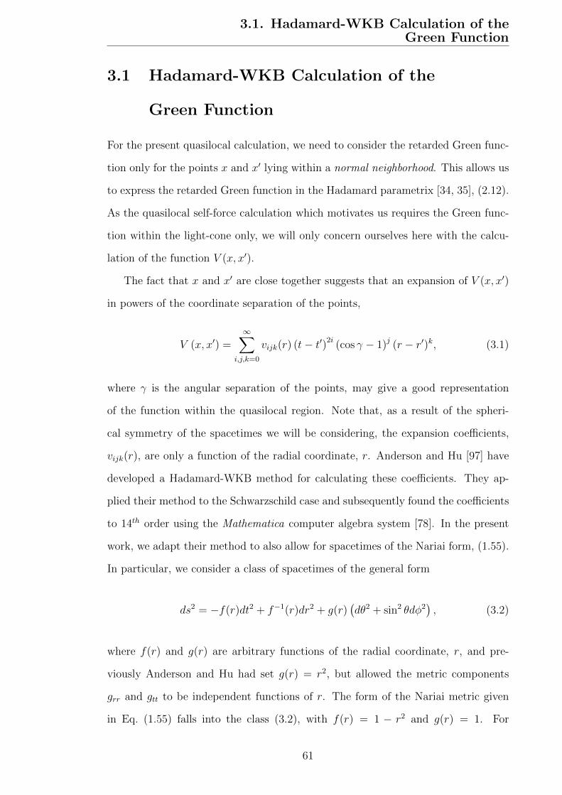
3.1. Hadamard-WKB Calculation of theGreen Function
3.1 Hadamard-WKB Calculation of the
Green Function
For the present quasilocal calculation, we need to consider the retarded Green func-
tion only for the points x and x′ lying within a normal neighborhood. This allows us
to express the retarded Green function in the Hadamard parametrix [34, 35], (2.12).
As the quasilocal self-force calculation which motivates us requires the Green func-
tion within the light-cone only, we will only concern ourselves here with the calcu-
lation of the function V (x, x′).
The fact that x and x′ are close together suggests that an expansion of V (x, x′)
in powers of the coordinate separation of the points,
V (x, x′) =∞∑
i,j,k=0
vijk(r) (t− t′)2i(cos γ − 1)j (r − r′)k, (3.1)
where γ is the angular separation of the points, may give a good representation
of the function within the quasilocal region. Note that, as a result of the spheri-
cal symmetry of the spacetimes we will be considering, the expansion coefficients,
vijk(r), are only a function of the radial coordinate, r. Anderson and Hu [97] have
developed a Hadamard-WKB method for calculating these coefficients. They ap-
plied their method to the Schwarzschild case and subsequently found the coefficients
to 14th order using the Mathematica computer algebra system [78]. In the present
work, we adapt their method to also allow for spacetimes of the Nariai form, (1.55).
In particular, we consider a class of spacetimes of the general form
ds2 = −f(r)dt2 + f−1(r)dr2 + g(r)(dθ2 + sin2 θdφ2
), (3.2)
where f(r) and g(r) are arbitrary functions of the radial coordinate, r, and pre-
viously Anderson and Hu had set g(r) = r2, but allowed the metric components
grr and gtt to be independent functions of r. The form of the Nariai metric given
in Eq. (1.55) falls into the class (3.2), with f(r) = 1 − r2 and g(r) = 1. For
61

3.1. Hadamard-WKB Calculation of theGreen Function
f(r) = 1− 2Mr
and g(r) = r2, this is the Schwarzschild metric of Eq. (1.32).
The method presented in this section differs from that of Ref. [97] in the details
of the WKB approach used, but otherwise remains very similar. Our alternative
WKB approach, based on that of Refs. [98, 99] proves extremely efficient when
implemented in a computer algebra package.
Following the prescription of Ref. [97], the Hadamard parametrix for the real
part of the Euclidean Green function (corresponding to the Euclidean metric arising
from the change of coordinate τ = it) is 1
Re [GE(−iτ, ~x;−iτ ′, ~x′)] =1
2π
(U(x, x′)
σ(x, x′)+ V (x, x′) ln(|σ(x, x′)|) +W (x, x′)
),
(3.3)
where U(x, x′), V (x, x′) and W (x, x′) are real-valued symmetric bi-scalars.
Additionally, for the points x and x′ separated farther apart in the time direction
than in other directions,
σ(x, x′) = −1
2f(r)(t− t′)2 +O
[(x− x′)3
](3.4)
so the logarithmic part of Eq. (3.3) is given by
1
πV (x, x′) ln(τ − τ ′). (3.5)
Therefore, in order to find V (x, x′), it is sufficient to find the coefficient of the
logarithmic part of the Euclidean Green function. We do so by considering the fact
that the Euclidean Green function also has the exact expression for the spacetimes
of the form given in Eq. (3.2):
GE(−iτ, x;−iτ ′, x′) =1
π
∫ ∞
0
dω cos [ω(τ − τ ′)]∞∑
l=0
(2l+1)Pl(cos γ)Cωlpωl(r<)qωl(r>),
(3.6)
where pωl and qωl are solutions (normalised by Cωl) to the homogeneous radial
1Note that this definition of the Green function differs from that of Ref. [97] by a factor of 4πand the definition of V (x, x′) differs by a further factor of 2.
62

3.1. Hadamard-WKB Calculation of theGreen Function
equation comint from the scalar wave equation in the curved background (3.2) (and
where r<, r> are the smaller/larger of r and r′, respectively), along with the fact
that
∫ ∞
λ
dω cos [ω(τ − τ ′)] 1
ω2n+1=
(−1)n+1
(2n)!(τ − τ ′)2n log (τ − τ ′) + · · ·
=−1
(2n)!(t− t′)2n log (t− t′) + · · · , (3.7)
where λ is a low frequency cut-off justified by the fact that we will only need the
log(τ − τ ′) term from the integral. The omitted terms on the right hand side are
smooth and do not contribute to the order log(t− t′) part, so are not of interest to
the present calculation. We can therefore find V (x, x′) as an expansion in powers of
the time separation of the points by expressing the sum
∞∑
l=0
(2l + 1)Pl(cos γ)Cωlpωl(r<)qωl(r>) (3.8)
of Eq. (3.6) as an expansion in inverse powers of ω. This is achieved using a WKB-
like method based on that of Refs. [98, 99]. Given the form (3.6) for the Euclidean
Green function, the radial functions S(r) = pωl(r) and S(r) = qωl(r) must both
satisfy the homogeneous wave equation,
fd2S
dr2+
1
g
d
dr(fg)
dS
dr−[ω2
f+l(l + 1)
g+m2
field + ξR
]S = 0 (3.9)
where mfield is the scalar field mass and ξ is the coupling to the scalar curvature, R.
Next, given the Wronskian W (r) = Cωl(pωlq′ωl − qωlp′ωl), its derivative is
W ′ = Cωl(pωlq′′ωl − qωlp′′ωl) = − 1
fg(fg)′W (3.10)
and the Wronskian condition is therefore
Cωl(pωlq′ωl − qωlp′ωl) = − 1
fg. (3.11)
63

3.1. Hadamard-WKB Calculation of theGreen Function
We now explicitly assume that r > r′ and define the function
B(r, r′) = Cωlpωl(r′)qωl(r). (3.12)
Since the sum of Eq. (3.8) (and hence B(r, r′)) is only needed as an expansion in
powers of (r − r′), we expand B(r, r′) about r′ = r and (using Eq. (3.9) to replace
second order and higher derivatives of B(r, r′) with expressions involving B(r, r′)
and ∂r′B(r, r′)) find that
B(r, r′) = β(r)+α(r)(r′− r)+
[2(η + χ2)
(fg)2
]β(r)− [ln(fg)]′ α(r)
(r′ − r)2
2+ · · ·
(for r > r′) (3.13)
where
β(r) ≡ [B(r, r′)]r′→r− = Cωlpωl(r)qωl(r), (3.14)
α(r) ≡ [∂r′B(r, r′)]r′→r− = Cωlp′ωl(r)qωl(r) (3.15)
and
η(r) ≡ −1
4fg +
(m2
field + ξR)fg2 (3.16)
χ2(r) ≡ ω2g2 + fg
(l +
1
2
)2
. (3.17)
It will therefore suffice to calculate β(r) and α(r). Furthermore, using Eq. (3.11)
we can relate α(r) to the derivative of β(r),
α(r) =β′(r)
2+
1
2f(r)g(r), (3.18)
so it will, in fact, suffice to find β(r) and its derivative, β′(r).
Using Eqs. (3.9) and (3.11), it is immediate to see that β(r) must satisfy the
64

3.1. Hadamard-WKB Calculation of theGreen Function
nonlinear differential equation
fgd
dr
(fgd√β
dr
)−(η + χ2
)√β +
1
4β3/2= 0. (3.19)
The short distance behavior of the Green function is determined by the high-ω
and/or high-l behavior of the integrand of Eq. (3.6), so we seek to express β(r) as
an expansion in inverse powers of χ. To keep track of this expansion we may replace
χ in Eq. (3.19) by χ/ε where ε is a formal expansion parameter which we eventually
set to 1. Then, to balance at leading order we require
(χ/ε)2√β ∼ 1
4β3/2=⇒ β ∼ ε
2χ. (3.20)
We now write
β(r) = εβ0(r) + ε2β1(r) + . . . (3.21)
where β0(r) ≡ 1/(2χ(r)), insert this form for β(r) in Eq. (3.19), and solve formally
order by order in ε to find a recursion relation for the βn(r). On doing so and using
Eq. (3.17) to eliminate (l + 12)2 in favor of ω2 and χ2 we find that we can write
βn(r) =2n∑
m=0
An,m(r)ω2m
χ2n+2m+1(3.22)
so, for example,
β1(r) =A1,0(r)
χ3+A1,1(r)ω2
χ5+A1,2(r)ω4
χ7(3.23)
β2(r) =A2,0(r)
χ5+A2,1(r)ω2
χ7+A2,2(r)ω4
χ9+A2,3(r)ω6
χ11+A2,4(r)ω8
χ13. (3.24)
The recursion relations for βn(r) may then be re-expressed to allow us to recursively
solve for the An,m(r). Such a recursive calculation is ideally suited to implementation
in a computer algebra system (CAS). Even on a computer, this recursive calculation
becomes very long as n becomes large and, in fact, dominates the time required
65

3.1. Hadamard-WKB Calculation of theGreen Function
to calculate the series expansion of V (x, x′) as a whole. For this reason, we have
made available an example implementation in Mathematica, including precalculated
results for several spacetimes of interest [100]. This code calculates analytic results
for An,m(r) on a moderate Linux workstation up to order n ∼ 25, corresponding to
a separation |x−x′|50, in Schwarzschild and Nariai spacetimes in the order of 1 hour
of CPU time.
We also note at this point that knowledge of the An,m(r) (and their r derivative,
which is straightforward to calculate) are all that is required to find the series ex-
pansion of β′(r) and hence α(r). This can be seen by differentiating Eqs. (3.21) and
(3.22) with respect to r to get
β′(r) = εβ′0 + ε2β′1 + . . . , (3.25)
with
β′n(r) =2n∑
m=0
[A′n,m(r)ω2m
χ2n+2m+1− (n+m+
1
2)2χχ′An,m(r)
χ2n+2m+3
]
=2n+1∑
m=0
A′n,m(r)− (n+m+
1
2)An,m(r)
(fg)′
fg(3.26)
−(n+m− 1
2)An,m−1(r)
[(g2)′ − (fg)′
fgg2
]ω2m
χ2n+2m+1(3.27)
where we have used Eq. (3.17) to write
2χχ′ = χ2(fg)′/(fg) + ω2((g2)′ − g2(fg)′/(fg)), (3.28)
and we use the convention An,−1 = An,2m+1 = 0. With the An,m(r) and their
first derivatives calculated, we are faced with the sum over l in Eq. (3.8), where
Eqs. (3.22) and (3.26) yield sums of the form
∞∑
l=0
2(l + 12)Pl(cos γ)
Dn,m(r)ω2m
χ2n+2m+1. (3.29)
66

3.1. Hadamard-WKB Calculation of theGreen Function
with
Dn,m = An,m(r) (3.30)
or
Dn,m = A′n,m(r)− (n+m+1
2)An,m(r)
(fg)′
fg
− (n+m− 1
2)An,m−1(r)
[(g2)′ − (fg)′
fgg2
](3.31)
Since we are considering the points x and x′ to be close together, we can treat
γ as a small quantity and expand the Legendre polynomial in a Taylor series about
γ = 0, or, more conveniently, in powers of (cos γ − 1) about (cos γ − 1) = 0. It is
straightforward to express each term in this series as a polynomial in even powers
of (l + 12):
Pl(cos γ) =2F1 (−l, l + 1; 1; (1− cos γ)/2) (3.32)
=l∑
p=0
((l + 1
2)2 − (1− 1
2)2)· · ·((l + 1
2)2 − (p− 1
2)2)
2p(p!)2(cos γ − 1)p (3.33)
The calculation of the sum in Eq. (3.6) therefore reduces to the calculation of sums
of the form
2Dn,m(r)∞∑
l=0
(l + 12)2p+1ω2m
χ2n+2m+1. (3.34)
For fixed ω and large l the summand behaves as l2(p−n−m), and so only converges if
67

3.1. Hadamard-WKB Calculation of theGreen Function
p < n+m. If p ≥ n+m, we first split the summand as
(l + 12)2p+1ω2m
χ2m+2n+1
=(l + 1
2)2(p−m−n)ω2m
(fg)m+n+1/2
(1 +
ω2g/f(l + 1
2
)2
)−m−n−1/2
(3.35)
=(l + 1
2)2(p−m−n)ω2m
(fg)m+n+1/2
p−m−n∑
k=0
(−1)k(m+ n+ 1/2)kk!
(ω2g/f(l + 1
2
)2
)k
+
+
(
1 +ω2g/f(l + 1
2
)2
)−m−n−1/2
−p−m−n∑
k=0
(−1)k(m+ n+ 1/2)kk!
(ω2g/f(l + 1
2
)2
)k
(3.36)
where (α)k = Γ(α + k)/Γ(α) is the Pochhammer symbol and the sum correspond
to the first (p − n − m) terms in the expansion of (1 + x)−n−m−1/2 about x ≡
(ω2g/f)/(l+ 12)2 = 0. The terms outside the square brackets correspond to positive
powers of ω and so contribute to the light cone singularity, not the tail term V (x, x′)
with which we are concerned in this section. By contrast, the term in square brackets
behaves as (l+ 12)−2 and so converges as l→∞ and will contribute to the tail term.
We denote this term, with its prefactor as
[(l + 1
2)2p+1ω2m
χ2m+2n+1
]
reg
=ω2(p−n)
fp+1/2g2(n+m)−p+1/2xm+n−p×
[(1 + x)−m−n−1/2 −
p−m−n∑
k=0
(−1)k(m+ n+ 1/2)kk!
xk
](3.37)
and adopt the understanding that the sum vanishes if p < m+ n.
To proceed further, we use the Sommerfeld-Watson formula [101],
∞∑
l=0
F (l + 12) =Re
[1
i
∫
γ
dz F (z) tan(πz)
]
=
∫ ∞
0
F (λ) dλ− Re
(i
∫ ∞
0
2
1 + e2πλF (iλ) dλ
)(3.38)
which is valid provided we can rotate the contour of integration for F (z) tan(πz) from
68

3.1. Hadamard-WKB Calculation of theGreen Function
just above the real axis to the positive imaginary axis. Defining z ≡ (f/g)1/2λ/ω =
1/√x, where λ ≡ (l + 1/2), the sum (3.34) can then be written as the contour
integral,
ω2(p−n)+1
fp+1g2(m+n)−p
[∫ ∞
0
dz
[z2p+1
(1 + z2)m+n+1/2
]
reg
+(−1)pRe
(∫ ∞
0
2dz
1 + e2πzω√g/f
z2p+1
(1− z2)m+n+1/2
)]. (3.39)
Note that there is no need to include the regularization terms in the second integral
as their contribution is manifestly imaginary and so will not contribute to the final
answer.
For p < m+ n the first integral in Eq. (3.39) may be performed immediately as
∫ ∞
0
dzz2p+1
(1 + z2)m+n+1/2=
p!
2(m+ n− p− 1/2)p+1
. (3.40)
For p ≥ m + n, we use the regularized integrand arising from Eq. (3.37) and tem-
porarily introduce an ultraviolet cutoff 1/ε2 to get
∫ ∞
ε
dx xm+n−p−3/2
[(1 + x)−m−n−1/2 −
p−m−n∑
k=0
(−1)k(m+ n+ 1/2)kk!
xk
]. (3.41)
Integrating by parts p−m−n+1 times, the regularization subtraction terms ensure
that the boundary term goes to zero in the limit ε→ 0 and we are left with
(−1)p−m−n+1 (m+ n+ 1/2)p−m−n+1
(1/2)p−m−n+1
∫ ∞
ε
dx x−1/2(1 + x)−p−3/2
=(−1)p−m−n+1πp!
Γ(m+ n+ 1/2)Γ(p−m− n+ 3/2), (3.42)
where the last equality reflects that after these integrations by parts are completed,
the remaining integral is finite in the limit ε→ 0.
The second integral in Eq. (3.39) is understood as a contour integral as illustrated
in Fig. 3.1. The integrand is understood to be defined on the complex plane cut
69

3.1. Hadamard-WKB Calculation of theGreen Function
from z = −1 to 1 and additionally possesses singularities at z = −1 and z = 1. To
handle these in a fashion consistent with the Watson-Sommerfeld prescription we
consider the contour in 3 parts: C1 running just below the cut from 0 to 1− ε, C2 a
semicircle of radius ε about z = 1, and C3 running along the real axis from z = 1 + ε
to ∞.
Figure 3.1: The second integral in Eq. (3.39) has a pole at z = 1, so we split it intothree parts: (1) an integral from 0 to 1− ε, (2) an arc of radius ε about z = 1, and(3) an integral from z = 1 + ε to ∞.
The integrand along C3 is manifestly imaginary and so gives zero contribution.
Writing the integrand as
G(z)
(1− z)m+n+1/2(3.43)
where
G(z) =z2p+1
(1 + e2πzω√g/f )(1 + z)m+n+1/2
(3.44)
it is straightforward to see that
Re
∫
C2
G(z)
(1− z)m+n+1/2dz = −
∞∑
k=0
(−1)k
k!G(k)(1)
εk−m−n+1/2
k −m− n+ 12
, (3.45)
70

3.1. Hadamard-WKB Calculation of theGreen Function
while integrating by parts m+ n times
∫
C1
G(z)
(1− z)m+n+1/2dz =
m+n−1∑
k=0
(−1)k
k!G(k)(1)
εk−m−n+1/2 − 1
k −m− n+ 12
+
1−ε∫
0
dz
(1− z)m+n+1/2
[G(z)−
m+n−1∑
k=0
(−1)k
k!G(k)(1)(1− z)k
]. (3.46)
Adding the contributions from these components, it is clear that the ε → 0 diver-
gences cancel and we are left with
−m+n−1∑
k=0
(−1)k
k!
G(k)(1)
k −m− n+ 12
+
1∫
0
dz
(1− z)m+n+1/2
[G(z)−
m+n−1∑
k=0
(−1)k
k!G(k)(1)(1− z)k
], (3.47)
where the subtraction terms in the integrand ensure that the integral here is well-
defined.
While we can take this analysis further [102], for our current purpose we note
that we only need the expansion of Eq. (3.47) in terms of inverse powers of ω as
ω → ∞. From Eq. (3.44), it is immediately apparent that the terms in the sum in
(3.47) are exponentially small and so may be ignored for our purposes here. Indeed
we may simultaneously increase the upper limit on the two sums in Eq. (3.47)
without changing the result. Increasing it by 1 (or more), the integrand increases
from z = 0, peaks and then decreases to 0 at z = 1 with the peak approaching
z = 0 as ω →∞. Standard techniques from statistical mechanics then dictate that
the ω → ∞ asymptotic form of the integral follows from expanding the integrand,
aside from the ‘Planck factor’, about z = 0 and extending the upper limit to ∞.
Again, in doing so the contribution from the summation within the integrand gives
an exponentially small contribution so that the powers of ω are determined simply
71

3.2. Convergence of the Series
by
∞∫
0
dz
(1 + e2πzω√g/f )
Seriesz=0
[z2p+1
(1− z2)m+n+1/2
], (3.48)
where Seriesz=0
[· · · ] denotes the series expansion about z = 0. The coefficients in the
series are known analytically, so to expand in inverse powers of ω we only need to
compute integrals of the form
∫ ∞
0
z2N−1
1 + e2πzω√g/f
dz (3.49)
which have the exact solutions [103]
(1− 21−2N
) fN
gNω2N
|B2N |4N
, (3.50)
where BN is the Nth Bernoulli number. This expression allows us to calculate the
integrals very quickly.
Applying this method for summation over l, Eq. (3.6) takes the form required
by Eq. (3.7) so we now have the logarithmic part of the Euclidean Green func-
tion and therefore V (x, x′) as the required power series in (t − t′), (cos γ − 1) and
(r − r′). Because of the length of the expressions involved, we have made available
online [100] a Mathematica code implementing this algorithm, along with precalcu-
lated results for several spacetimes of interest including Schwarzschild, Nariai and
Reissner-Nordstrom. These expressions are in total agreement with those calculated
using the covariant method of Chapter 4. They also correct a factor of 2 error in
Ref. [97] (this correction is also made in the errata [104, 105] for Ref. [97]).
3.2 Convergence of the Series
We have expressed V (x, x′) as a power series in the separation of the points. This
series will, in general, not be convergent for all point separations – the maximum
72

3.2. Convergence of the Series
point separation for which the series remains convergent will be given by its radius
of convergence. In this section, we explore the radius of convergence of the series in
the Nariai and Schwarzschild spacetimes and use this as an estimate on the region
of validity of our series.
For simplicity, we will consider points separated only in the time direction, so
we will have a power series in (t− t′),
V (x, x′) =∞∑
n=0
vn(r) (t− t′)2n, (3.51)
where vn(r) is a real function of the radial coordinate, r only. We will also consider
cases where the points are separated by a fixed amount in the spatial directions,
or where the separation in other directions can be re-expressed in terms of a time
separation, resulting in a similar power series in (t − t′), but with the coefficients,
vn(r), being different. This will give us sufficient insight without requiring overly
complicated convergence tests.
In the next section, we review some tests that will prove useful. In Secs. 3.2.2
and 3.2.3 we present the results of applying those tests in Nariai and Schwarzschild
spacetimes, respectively.
3.2.1 Tests for Estimating the Radius of Convergence
Convergence Tests
For the power series (3.51), there are two convergence tests which will be useful
for estimating the radius of convergence. The first of these, the ratio test, gives an
estimate of the radius of convergence, ∆tRC ,
∆tRC = limn→∞
√∣∣∣∣vnvn+1
∣∣∣∣. (3.52)
Although strictly speaking, the large n limit must be taken, in practice we can
calculate enough terms in the series to get a good estimate of the limit by simply
73

3.2. Convergence of the Series
looking at the last two terms. The ratio test runs into difficulties, however, when
one of the terms in the series is zero. Unfortunately, this occurs frequently for
many cases of interest. It is possible to avoid this issue somewhat by considering
non-adjacent terms in the series, i.e. by comparing terms of order n and n+m,
∆tRC = limn→∞
∣∣∣∣vnvn+m
∣∣∣∣1
2m
. (3.53)
Using the ratio test in this way gives better estimates of the radius of convergence,
although the results are still somewhat lacking.
To get around this difficulty, we also use a second test, the root test,
∆tRC = lim supn→∞
∣∣∣∣1
vn
∣∣∣∣12n
, (3.54)
which is well suited to power series. This gives us another estimate of the radius
of convergence. Again, in practice the last calculated term in the series will give a
good estimate of the limit.
It may appear that only the (better behaved) root test is necessary for estimating
the radius of convergence of the series. However, extra insight can be gained from
including both tests. This is because for the power series (3.51), the ratio test
typically gives values increasing in n while the root test gives values decreasing in
n, effectively giving lower and upper bounds on the radius of convergence.
Normal Neighborhood
The Hadamard parametrix for the retarded Green function, (2.12), is only guaran-
teed to be valid provided x and x′ are within a normal neighborhood (see footnote
1). This arises from the fact that the Hadamard parametrix involves the Synge
world function, σ(x, x′), which is only defined for the points x and x′ separated by
a unique geodesic. It is plausible that the radius of convergence of our series could
exactly correspond to the normal neighborhood size, tNN. This turns out to not be
the case, although it is still helpful to give consideration to tNN as we might expect
74

3.2. Convergence of the Series
it to place an upper bound on the radius of convergence of the series. This upper
bound can be understood from the fact that the series will have a radius of conver-
gence determined by the nearest singularity of V (x, x′), along with the fact that we
expect V (x, x′) to be singular at the boundary of the normal neighborhood2
The normal neighborhood size will be given by the minimum time separation of
the spacetime points such that they are connected by two non-spacelike geodesics.
For typical cases of interest for self-force calculations there will be a particle fol-
lowing a time-like geodesic, so tNN will be given by the minimum time taken by a
null geodesic intersecting the particle’s worldline twice. In typical black hole space-
times, this geodesic will orbit the black hole once before re-intersecting the particle’s
worldline.
Another case of interest is that of the points x and x′ at constant spatial positions,
separated by a constant angle ∆φ. Initially, (i.e. when t = t′), the points will be
separated only by spacelike geodesics. After sufficient time has passed for a null
geodesic to travel between the points (going through an angle ∆φ), they will be
connected first by a null geodesic and subsequently by a sequence of unique timelike
geodesics. Since the geodesics are unique, tNN will not be given by this first null
geodesic time. Rather, tNN will be given by the time taken by the second null
geodesic (passing through an angle 2π−∆φ). This subtle, but important, distinction
will be clearly evident when we study specific cases in the next sections.
Relative Truncation Error
Knowledge of the radius of convergence alone does not give information about the
accuracy of the series representation of V (x, x′). The series is necessarily truncated
after a finite number of terms, introducing a truncation error. The local fractional
2The expectation that V (x, x′) is singular at the boundary of the normal neighborhood maybe justified as follows: V0(x, x′) is defined through an equation involving ∆1/2(x, x′), which issingular at a caustic. As a result, we would also expect V0(x, x′) to be singular at a caustic(this is supported by our numerical calculations, described in Chapter 4). Since V (x, x′) satisfiesthe homogeneous wave equation with characteristic initial data given by V0(x, x′), we expect thissingularity to propagate along characteristics (null geodesics). Therefore, V (x, x′) will be singularwhere the past light-cone of the caustic intersects the time-like geodesics emanating from x. Thisintersection also corresponds to the boundary of the normal neighborhood.
75

3.2. Convergence of the Series
truncation error can be estimated by the ratio between the highest order term in
the expansion (O (∆τn), say) and the sum of all the terms up to that order,
ε ≡ vn(t− t′)2n
∑ni=0 vi(t− t′)2i
. (3.55)
Reference [79] previously calculated these error estimates, but only considered the
first two terms in the series. Since we now have a vastly larger number of terms
available, it is worthwhile to consider these again to determine the accuracy of the
high order series.
3.2.2 Nariai Spacetime
Normal Neighborhood
Allowing only the time separation of the points to change, we consider two cases of
interest for the Nariai spacetime:
1. The static particle which has a normal neighborhood determined by the mini-
mum coordinate time taken by a null geodesic circling the origin (ρ = 0) before
returning. This is the time taken by a null geodesic, starting at ρ = ρ1 and
returning to ρ′ = ρ1, while passing through an angle ∆φ = 2π.
2. Points at fixed radius, ρ1, separated by an angle, say π/2. In this case, there
is a null geodesic which goes through an angle ∆φ = π/2 when travelling
between the points. However, there will not yet be any other (non-spacelike)
geodesic connecting them, so this will not give tNN. Instead, it is the next null
geodesic, which goes through ∆φ = 3π/2, that gives the normal neighborhood
boundary.
76

3.2. Convergence of the Series
In both cases, the coordinate time taken by the null geodesic to travel between
the points is given by (1.70),
tNN = 2 tanh−1(ρ1)+ln
1− ρ1sech2(∆φ/2) + tanh(∆φ/2)
√1− ρ2
1sech2(∆φ/2)
1 + ρ1sech2(∆φ/2)− tanh(∆φ/2)√
1− ρ21sech2(∆φ/2)
.
(3.56)
Results
For the Nariai spacetime, the ratio test suffers from difficulties arising from zeros of
the terms in the series. This is because the ith term of the series (of order (t− t′)2i)
has 2i roots in ρ. In other words, the higher the order of the terms considered, the
more likely one of the coefficients is to be near a zero, and not give a useful estimate
of the radius of convergence. We have therefore compared non-adjacent terms to
avoid this issue as much as possible, by choosing m = n/2 in Eq. (3.53). This
choice of m only affects the number and location of the points where the test fails.
The envelope (interpolating over the points where the test fails) remains unaffected.
Fortunately, the root test is much less affected by such issues and can be used
without any adjustments.
In Fig. 3.2, we fix the radial position of the points at ρ = ρ′ = 1/2 (left panels)
and ρ = ρ′ = 1/99 (right panels) and plot the results of applying the root test
(blue dots) and ratio test (brown squares) for (1) static particle (top panels) and
(2) points at fixed spatial points separated by an angle γ = π/2 (bottom panels)
as a function of the maximum order, nmax, of the terms of the series considered,
vnmax (t− t′)2nmax . It seems in both cases that the plot is limiting towards a constant
value for the radius of convergence. In case (1), we see that this gives a radius of
convergence that is considerably smaller than the normal neighborhood size (purple
dashed line). For case (2), we again see that the values from the convergence tests
are limiting towards a value for the radius of convergence. However, as discussed in
Sec. 3.2.1, it is not the first null geodesic (lower dashed purple line), but the second
null geodesic (upper dashed purple line) that determines the normal neighborhood
77

3.2. Convergence of the Series
0 5 10 15 20 25 300
2
4
6
8
10
12
nmax
t RC
Ρ=Ρ' =12
Γ=0
à àà
à à à à à à à à à à à à à à à à à à à à à à à à à
0 5 10 15 20 25 300
2
4
6
8
10
nmax
t RC
Ρ=Ρ' =199
Γ=0
0 5 10 15 20 25 300
2
4
6
8
10
12
nmax
t RC
Ρ=Ρ' =12
Γ=Π2
à
à
à
à
à
à
à
àà à à à à à à à à à à à à à à à à
àà
à
0 5 10 15 20 25 300
2
4
6
8
10
12
nmaxt R
C
Ρ=Ρ' =199
Γ=Π2
Figure 3.2: Radius of convergence as a function of the number of terms in the seriesfor the Nariai spacetime with curvature coupling ξ = 1/6. The limit as n→∞ willgive the actual radius of convergence, but it appears that just using the terms up ton = 30 is giving a good estimate of this limit. The radius of convergence is estimatedby the root test (blue dots) and ratio test (brown squares) and is compared againstthe normal neighborhood size (purple dashed line) calculated from considerationson null geodesics (see Sec. 3.2.1 and Sec. 3.2.2). Note that plots for the ratio testwere omitted in cases where it did not give meaningful results.Also, the lower plots both have two lines estimating the normal neighborhood size.The lower line indicates the time for a null geodesic to go directly between the points,passing through an angle π/2. It is the upper line, corresponding to the time takenby a null geodesic circling the potential (and going through an angle 3π/2) whichgives the true value of the normal neighborhood size (see Sec. 3.2.2).
and places an upper bound on the radius of convergence of the series.
In Fig. 3.3 we use the root test (blue dots) and ratio test (brown line)3 to inves-
tigate how the radius of convergence of the series varies as a function of the radial
position of the points, ρ1. Again, we look at both cases (1) (left panel) and (2)
(right panel). As a reference, we compare to the normal neighborhood size (pur-
3Note that the ‘blips’ in the ratio test are an artifact of the zeros of the series coefficients usedand are not to be taken to have any physical meaning. In fact, the ‘blips’ occur at different timeswhen considering the series at different orders, so they should be ignored altogether. The ratiotest plots should therefore only be fully trusted away from the ‘blips’. Near the blips, it is clearthat one could interpolate an approximate value, however we have not done so here as the plot isto be taken only as an indication of the radius of convergence.
78
3.2. Convergence of the Series
0.0 0.2 0.4 0.6 0.8 1.00
2
4
6
8
Ρ
t RC
Γ=0
nmax=30
0.0 0.2 0.4 0.6 0.8 1.00
2
4
6
8
10
Ρ
t RC
Γ=Π2
nmax=30
Figure 3.3: Estimates of the domain of validity (i.e. the radius of convergence) ofthe series expansion of V (x, x′) as a function of radial position in Nariai spacetime.The root test on O [(t− t′)60] series is given as blue dots, the ratio test is given bythe brown line (see footnote 3), and the normal neighborhood estimate from nullgeodesics is given by dashed purple lines. The left plot is for case (1), the staticparticle, and the right plot is for case (2), points separated by an angle of π/2. Inboth cases, the series is clearly divergent before the normal neighborhood boundary.This boundary is sometimes given by the second, rather than the first null geodesicas can be seen in the plot on the right. In particular, this is the case for the pointsseparated by an angle γ = π/2 since they are initially separated by only spacelikegeodesics (see Sec. 3.2.2).
ple dashed line). We find that, regardless of the radial position of the points, the
radius of convergence of the series is well within the normal neighborhood, by an
almost constant amount. As before, in the case (2) of the points separated by an
angle, we find that it is the second, not the first null geodesic that gives the normal
neighborhood size.
With knowledge of the radius of convergence of the series established, it is also
important to estimate the accuracy of the series within that radius. To that end,
we plot in Fig. 3.4 the relative truncation error, (3.55), as a function of the time
separation of the points at a fixed radius, ρ = ρ′ = 1/2. We find that the 60th order
series is extremely accurate to within a short distance of the radius of convergence
of the series.
79

3.2. Convergence of the Series
0 1 2 3 410-93
10-77
10-61
10-45
10-29
10-13
t-t'
Rel
ativ
eT
runc
atio
nE
rror
,ΕΡ=Ρ' =12
Γ=0
nmax=30
1 2 3 410-90
10-75
10-60
10-45
10-30
10-15
1
t-t'
Rel
ativ
eT
runc
atio
nE
rror
,Ε
Ρ=Ρ' =12
Γ=Π2
nmax=30
Figure 3.4: Relative truncation error in Nariai spacetime arising from truncatingthe series expansion for V (x, x′) at order |x − x′|60 (i.e. nmax = 30) for case (1)the static particle (left panel) and case (2) points separated by an angle π/2 (rightpanel). In both cases, the radial points are fixed at ρ = ρ′ = 1/2. The series isextremely accurate until we get close to the radius of convergence (see Fig.3.2).
3.2.3 Schwarzschild Spacetime
Normal Neighborhood
For a fixed spatial point at radius r1 in the Schwarzschild spacetime, we would like
to find the null geodesic that intersects it twice in the shortest time. This geodesic
will orbit the black hole once before returning to r1. Clearly, the coordinate time
tNN for this orbit can only depend on r1. The periapsis radius, rp, will be reached
half way through the orbit. For the radially inward half of this motion, the geodesic
equations can be rearranged to give
π =
∫ π
0
dφ = −∫ rp
r1
dr
r2
√1r2p
(1− 2M
rp
)− 1
r2
(1− 2M
r
) (3.57)
tNN2
=
∫ tNN/2
0
dt = −∫ rp
r1
dr
(1− 2M
r
)√1− r2p
r2
(1− 2M
r
) (1− 2M
rp
)−1(3.58)
For a given point r1, we numerically solve the first of these to find the periapsis
radius, rp, and then solve the second to give the normal neighborhood size, tNN.
80

3.2. Convergence of the Series
à
àà
à à à à à à à à à à à à à à à à à à à à à
0 5 10 15 20 25
0
100
200
300
400
500
600
nmax
t RC
M
r1=100 M
0 5 10 15 20 250
20
40
60
80
100
120
140
nmax
t RC
M
r1=10 M
Figure 3.5: Radius of convergence as a function of the number of terms consideredfor the Schwarzschild spacetime. The root test (blue dots), the ratio test (brownsquares – see footnote 3), and the first null geodesic (purple dashed line) are given.Left panel: Static particle at r1 = 100M . Right panel: Static particle at r1 = 10M .The radius of convergence is given by the limit as the number of terms nmax →∞.It is apparent that the right plot is asymptoting to a value near, but slightly lowerthan the normal neighborhood size. This may also be case for the left plot, althoughhigher order terms would be required for a conclusive result. Note that curves forthe ratio test were omitted in cases where it did not give meaningful results.
Results
The ratio test proves more stable for Schwarzschild spacetime than it was for Nariai
spacetime. The series coefficients still have a large number of roots in r, but most
are within r = 6M and therefore do not have an effect for the physically interesting
radii, r ≥ 6M .
Figure 3.5 shows that the radius of convergence, ∆tRC , given by the root test is
a decreasing function of the order of the term used, while that given by the ratio
test is increasing. This effectively gives an upper and lower bound on the radius of
convergence of the series. There is some ‘noise’ in the ratio test plot at lower radii
(where that test is failing to give meaningful results), but we simply ignore this and
omit the ratio test in this case. For the root test, the terms up to order (t − t′)52
were used, while for the ratio test, adjacent terms in the series up to order (t− t′)52
were compared.
In Fig. 3.6 we apply the root (blue dots) and ratio (brown line – see footnote 3)
tests for the case of a static particle at a range of radii in Schwarzschild spacetime.
Using the root test as an upper bound and the ratio test as a lower bound, it is
81

3.2. Convergence of the Series
0 20 40 60 80 100
0
50
100
150
200
250
300
r1M
t RC
M
nmax=26
Figure 3.6: Radius of convergence as a function of radial position for a static pointin Schwarzschild spacetime. The root test (blue dots), the ratio test (brown line –see footnote 3), and the first null geodesic (purple dashed line) are shown.
à
àà
à à à à à à à à à à à à à à à à à à à à à
0 5 10 15 20 25
0
100
200
300
400
500
600
nmax
t RC
M
r1=100 M
0 5 10 15 20 250
20
40
60
80
100
120
nmax
t RC
M
r1=10 M
Figure 3.7: Radius of convergence as a function of the number of terms consideredfor points separated along a circular geodesic in Schwarzschild spacetime. The roottest (blue dots), the ratio test (brown squares – see footnote 3), and the first nullgeodesic (purple dashed line) are shown. Note that curves for the ratio test wereomitted in cases where it did not give meaningful results.
clear that the radius of convergence is near, but likely slightly lower than the normal
neighborhood size (purple dashed line). In this case, for the root test, the term of
order (t−t′)52 was used, while for the ratio test, terms of order (t−t′)52 and (t−t′)26
were compared.
In Figs. 3.7 and 3.8, we repeat this for the case of the points separated on a
circular timelike geodesic. The results are very similar to the static particle case
and show the same features.
82

3.3. Extending the Domain of Series Using PadeApproximants
0 20 40 60 80 100
0
50
100
150
200
250
300
r1M
t RC
M
nmax=30
Figure 3.8: Radius of convergence as a function of radial position for points separatedalong a circular geodesic in Schwarzschild spacetime. The root test (blue dots), theratio test (brown line – see footnote 3), and the first null geodesic (purple dashedline) are shown.
3.3 Extending the Domain of Series Using Pade
Approximants
In the previous section it was shown that the circle of convergence of the series
expansion of V (x, x′) is smaller than the size of the normal neighborhood. This is
not totally unexpected. We would expect the normal neighborhood size to place
an upper limit on the radius of convergence, but we can not necessarily expect the
radius of convergence to be exactly the normal neighborhood size. However, since
the Hadamard parametrix for the Green function is valid everywhere within the
normal neighborhood, it is reasonable to hope that it would be possible to find
an alternative series representation for V (x, x′) which is valid in the region outside
the circle of convergence of the original series, while remaining within the normal
neighborhood.
The radius of convergence found in the previous section locates the distance (in
the complex plane) to the closest singularity of V (x, x′). However, that singularity
could lie anywhere on the (complex) circle of convergence and will not necessarily be
on the real line. In fact, given that the Green function is clearly not singular at the
(real-valued) radius of convergence, it is clear that the singularity of V (x, x′) does
not lie on the real line (see Appendix C for a general discussion of the convergence
properties of series).
83

3.3. Extending the Domain of Series Using PadeApproximants
There are several techniques which can be employed to extend a series beyond
its radius of convergence. Provided the circle of convergence does not constitute a
natural boundary of the function, the method of analytic continuation can be used
to find another series representation for V (x, x′) valid outside the circle of conver-
gence of the original series [106, 107]. This could then be applied iteratively to find
series representations covering the entire range of interest of V (x, x′). Although this
method of analytic continuation should be capable of extending the series expansion
of V (x, x′), there is an alternative method, the method of Pade approximants which
yields impressive results with little effort.
The method of Pade approximants [108, 109] is frequently used to extend the
series representation of a function beyond the radius of convergence of the series. It
has been employed in the context of general relativity data analysis with considerable
success [95, 96]. It is based on the idea of expressing the original series as a rational
function (i.e. a ratio of two polynomials V (x, x′) = R(x, x′)/S(x, x′)) and is closely
related to the continued fraction representation of a function [108]. This captures
the functional form of the singularities of the function on the circle of convergence
of the original series.
The Pade approximant, PNM (t− t′) is defined as
PNM (t− t′) ≡
∑Nn=0 An(t− t′)n∑Mn=0 Bn(t− t′)n
(3.59)
where B0 = 1 and the other (M + N + 1) terms are found by comparing to the
first (M + N + 1) terms of the original power series. The choice of M and N is
arbitrary provided M+N ≤ nmax where nmax is the highest order term that has been
computed for the original series. There are, however, choices for M and N which
give the best results. In particular, the diagonal, PNN , and sub-diagonal, PN
N+1, Pade
approximants yield optimal results.
84
3.3. Extending the Domain of Series Using PadeApproximants
3.3.1 Nariai spacetime
The Green function in Nariai spacetime is known to be given exactly by a quasinor-
mal mode sum [29, 110] at sufficiently late times ((t− t′) > 2ρ?). We can therefore
use this quasinormal mode calculated Green function sum to determine the effective-
ness of the Pade resummation. Figure 3.9 compares the Green function calculated
from a quasinormal mode sum4 with both the original Taylor series representation
and the Pade resummed series for V (x, x′) for a range of cases. We use the Pade ap-
proximant P 3030 , computed from the 60th order Taylor series. In each case, the Taylor
series representation (blue dashed line) diverges near its radius of convergence, long
before the normal neighborhood boundary is reached. The Pade resummed series
(red line), however, remains valid much further and closely matches the quasinormal
mode Green function (black dots) up to the point where the normal neighborhood
boundary is reached.
As was shown in Refs. [111, 29], the Green function in Nariai spacetime is singular
whenever the points are separated by a null geodesic. Furthermore, in Chapter 6
we have derived the functional form of these singularities and shown that they
follow a four-fold pattern: δ(σ), 1/πσ, −δ(σ), −1/πσ, depending on the number
of caustics the null geodesic has passed through (this was also previously shown
by Ori [112]). Within the normal neighborhood (where the Hadamard parametrix,
(1.3), is valid), the δ(σ) singularities (i.e. at exactly the null geodesic times) will be
given by the term involving U(x, x′). However, at times other than the exact null
geodesic times, the Green function will be given fully by V (x, x′). For this reason,
we expect V (x, x′) to reflect the singularities of the Green function near the normal
neighborhood boundary.
The Pade approximant attempts to model this singularity of the function V (x, x′)
(which occurs at the null geodesic time) by representing it as a rational function,
4 There are some caveats with how the quasinormal Green function was used. The fundamentalmode (n = 0) Green function was used and a singularity time offset applied as described inChapter 6 and Ref. [29]. In the case where two singularities are present, two sets of fundamentalmode Green functions were used, each shifted by an appropriate singularity time offset and matchedat an intermediate point.
85
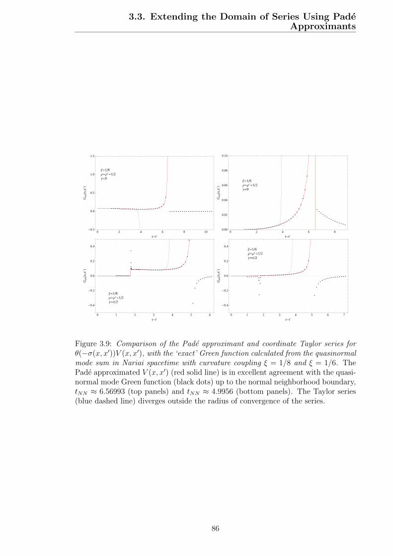
3.3. Extending the Domain of Series Using PadeApproximants
0 2 4 6 8 10-0.5
0.0
0.5
1.0
1.5
t-t'
Gre
tHx,x
'L
Ξ=18Ρ=Ρ' =12Γ=0
0 2 4 6 80.00
0.02
0.04
0.06
0.08
0.10
t-t'
Gre
tHx,x
'L
Ξ=16Ρ=Ρ' =12Γ=0
0 1 2 3 4 5 6
-0.4
-0.2
0.0
0.2
0.4
t-t'
Gre
tHx,x
'L
Ξ=18Ρ=Ρ' =12Γ=Π2
0 1 2 3 4 5 6 7
-0.4
-0.2
0.0
0.2
0.4
t-t'
Gre
tHx,x
'L
Ξ=16Ρ=Ρ' =12Γ=Π2
Figure 3.9: Comparison of the Pade approximant and coordinate Taylor series forθ(−σ(x, x′))V (x, x′), with the ‘exact’ Green function calculated from the quasinormalmode sum in Nariai spacetime with curvature coupling ξ = 1/8 and ξ = 1/6. ThePade approximated V (x, x′) (red solid line) is in excellent agreement with the quasi-normal mode Green function (black dots) up to the normal neighborhood boundary,tNN ≈ 6.56993 (top panels) and tNN ≈ 4.9956 (bottom panels). The Taylor series(blue dashed line) diverges outside the radius of convergence of the series.
86

3.3. Extending the Domain of Series Using PadeApproximants
i.e. a ratio of two power series. By its nature, this will only faithfully reproduce
singularities of integer order. In the Nariai case, however, the asymptotic form of
the singularities is known exactly near the singularity times, tc. In cases where
the points are separated by an angle γ ∈ (0, π) (i.e. away from a caustic), the
singularities are expected to have a 1/(t − t′ − tc) behavior and it is reasonable to
expect the Pade approximant to reproduce the singularity well. When the points are
not separated in the angular direction (i.e. at a caustic), however, the singularities
behave like 1/(t− t′− tc)3/2 and we cannot reasonably expect the Pade approximant
to accurately reflect this singularity without including a large number of terms in
the denominator.
Given knowledge of the functional form of the singularity, however, it is possible
to improve the accuracy of the Pade approximant further. For a singularity of the
form 1/S(t), we first multiply the Taylor series by S(t). The result should then have
either no singularity, or have a singularity which can be reasonably represented by
a power series. The Pade approximant of this new series is then calculated and
the result is divided by S(t) to give an improved Pade approximant. This yields
an approximant which includes the exact form of the singularity and more closely
matches the exact Green function near the singularity. In Fig. 3.10, we illustrate the
improvement with an example case. We consider a static point in Nariai spacetime
and compute the error in the Pade approximant relative to the quasinormal mode
Green function (with overtone number n ≤ 8). The regular Pade approximant (blue
dashed line) is compared against the improved Pade approximant (red solid line).
The relative error remains small closer to the singularity for the improved Pade
approximant case than for the standard Pade approximant. Note that the error for
early times arises from the failure of the quasinormal mode sum to converge and
does not reflect errors in the series approximations.
87

3.3. Extending the Domain of Series Using PadeApproximants
0 1 2 3 4 5 6-0.0001
-0.00005
0.0000
0.00005
0.0001
t-t'
Rel
ativ
eer
ror
Ξ=18Ρ=Ρ' =12Γ=0
Figure 3.10: Relative error in improved vs regular Pade approximant. The relativeerror in the improved Pade approximant (solid red line) remains small closer to thesingularity than the regular Pade approximant (blue dashed line).
0 10 20 30 40
0.0000
0.0002
0.0004
0.0006
0.0008
0.0010
t-t'
Gre
tHx,x
'L
r=r' =10MΓ=0
Figure 3.11: Comparison of the Pade approximant to the Taylor series forSchwarzschild spacetime in the case of a static particle at r = 10M . ThePade approximants P 26
26 (solid red line) and P 2426 (dotted brown line) are likely to
represent V (x, x′) more accurately near the normal neighborhood boundary (att− t′ ≈ 46.2471M) than the regular Taylor series (dashed blue line).
3.3.2 Schwarzschild spacetime
For the Schwarzschild case, there is no quasinormal mode sum with which to com-
pare the Pade approximated series5. However, given the success in the Nariai case,
we remain optimistic that Pade resummation will be successful in the Schwarzschild
spacetime. In an effort to estimate the effectiveness of the Pade approximant, we
compare in Fig. 3.11 the series expression for V (x, x′) with two different Pade re-
summations, P 2426 and P 26
26 . The Pade approximant extends the validity beyond the
radius of convergence of the series, but is less successful at reaching the normal
neighborhood boundary (t− t′ = tNN ≈ 46.2471M) than in the Nariai case.
5A quasinormal mode sum could be computed for the Schwarzschild case, but would be aug-mented by a branch cut integral [29]. This calculation is in progress but has yet to be completed.
88

3.3. Extending the Domain of Series Using PadeApproximants
The failure of the Pade approximant to reach the normal neighborhood boundary
can be understood by the presence of extraneous singularities in the Pade approxi-
mant. The zeros of the denominator, S(t − t′) = 0, give rise to singularities which
occur at times earlier than the null geodesic time. It is possible that this problem
could be reduced to a certain extent using the knowledge of the functional form
of the singularities to compute an improved Pade approximant (as was successful
in the Nariai case). However, to the authors knowledge, the structure of the sin-
gularities in Schwarzschild spacetime is not yet known. While it may be possible
to adapt the work of Chapter 6 to find the asymptotic form of the singularities in
Schwarzschild spacetime, without knowledge of the exact Green function we would
not be able to determine whether an improved Pade approximant would truly give
an improvement. We therefore leave such considerations for later work.
3.3.3 Convergence of the Pade Sequence
The use of Pade approximants has shown remarkable success in improving the accu-
racy and domain of the series representation of V (x, x′). However, this improvement
has not been quantified. There is no general way to determine whether the Pade
approximant is truly approximating the correct function, V (x, x′) or the domain
in which it is valid [109]. In this subsection, we nonetheless attempt to gain some
insight into the validity of the Pade approximants.
The first issue to consider is the presence of extraneous poles in the Pade approx-
imants. In Sec. 3.3.1, the Pade approximant was unable to exactly represent the
1/(t − t′ − tc)3/2 singularity at tc ≈ 6.12 and instead represented it by three (real-
valued) simple poles (at t − t′ ≈ 6.522, 6.854 and 9.488). This leads to the Pade
approximant being a poor representation of the function near the poles. As was
shown in Fig. 3.10, having exact knowledge of the singularity structure allows for
the calculation of an improved Pade approximant without extraneous singularities6.
6The improved Pade approximant has zeros in its denominator at times t− t′ ≈ 2.64, 6.51, 6.59and 8.73. The apparently extraneous singularity within the normal neighborhood (at t− t′ ≈ 2.64)does not cause any difficulty as the numerator also goes to zero at this point.
89

3.3. Extending the Domain of Series Using PadeApproximants
With extraneous poles dealt with, we consider the convergence of the Pade se-
quence of diagonal and sub-diagonal Pade approximants,
P = P 00 , P
01 , P
11 , P
12 , P
22 , P
23 , P
33 , · · · , (3.60)
with PN being the N -th element of the sequence. The convergence of the Pade
approximant sequence is determined by the behavior of the denominators, SN for
large N [108]. Provided S(x, x′)N is not small, the Pade sequence will converge
quickly toward the actual value of V (x, x′). When the first root of the denominator
is at the null geodesic time (i.e. the normal neighborhood boundary), we can,
therefore, be optimistic that the Pade sequence will remain convergent until this root
is reached and that the Pade approximants will accurately represent the function.
To highlight the improvements made by using Pade approximants over regular
Taylor series, we introduce the Taylor sequence (i.e. the sequence of partial sums of
the series), T = T0, T1, T2, · · · , with the Nth element,
TN =
N/2∑
n=0
vn(t− t′)2n. (3.61)
The two sequences PN and TN require approximately the same number of terms in
the original Taylor series, so a direct comparison of their convergence will illustrate
the improved convergence of the Pade approximants.
In Fig. 3.12, we plot the Pade sequence (blue line) and Taylor sequence (purple
dashed line) for the case of static points at ρ = 1/2 in the Nariai spacetime, with
ξ = 1/8. For early times (eg. (t − t′) = 2), it is clear that both Pade and Taylor
sequences converge very quickly. At somewhat later times (eg. (t− t′) = 3.3), both
sequences appear to remain convergent, but the Pade sequence is clearly converging
much faster than the Taylor sequence. Outside the radius of convergence of the
Taylor series (eg. (t − t′) = 5, 6.3), the Pade sequence is slower to converge, but
appears to still do so.
In Fig. 3.13, we again plot the Pade sequence, this time for the case of static
90

3.3. Extending the Domain of Series Using PadeApproximants
0 10 20 30 40 50 60
0.070
0.075
0.080
N
TN
,PN
H t-t' L = 2
0 10 20 30 40 50 600.04
0.05
0.06
0.07
0.08
N
TN
,PN
H t-t' L = 3.3
0 10 20 30 40 50 600.01
0.02
0.03
0.04
0.05
0.06
0.07
0.08
N
PN
H t-t' L = 5
0 10 20 30 40 50 60
-0.5
0.0
0.5
1.0
1.5
N
PN
H t-t' L = 6.3
Figure 3.12: Convergence of the Taylor and Pade sequences for the case of staticpoints at ρ = 1/2 in the Nariai spacetime, with ξ = 1/8. Within the radius ofconvergence of the Taylor series, both Pade (blue solid line) and Taylor (purpledashed line) sequences converge to the exact Green function (black dotted line)as calculated from a quasinormal mode sum with overtone number n ≤ 6. ThePade sequence converges faster, particularly at later times. Outside the radius ofconvergence of the Taylor series (in this case, (t− t′) ≈ 4), only the Pade sequenceis convergent.
91

3.3. Extending the Domain of Series Using PadeApproximants
10 20 30 40 503.4 ´ 10-7
3.6 ´ 10-7
3.8 ´ 10-7
4. ´ 10-7
4.2 ´ 10-7
4.4 ´ 10-7
N
TN
,PN
H t-t' L = 10M
10 20 30 40 50
6. ´ 10-6
8. ´ 10-6
0.00001
0.000012
0.000014
0.000016
N
TN
,PN
H t-t' L = 20M
10 20 30 40 50
0.00005
0.00010
0.00015
N
TN
,PN
H t-t' L = 27M
10 20 30 40 50
-0.0008
-0.0006
-0.0004
-0.0002
0.0000
0.0002
0.0004
N
PN
H t-t' L = 32M
Figure 3.13: Convergence of the Taylor and Pade Sequences for the case of staticpoints at r = 10M in the Schwarzschild spacetime. As in the Nariai case, thePade sequence (blue solid line) converges better and at later times than the Taylorsequence (purple dashed line).
points at r = 10M in the Schwarzschild spacetime. As in the Nariai case, for early
times (eg. (t − t′) = 10M), both Pade and Taylor sequences are converging very
quickly. At slightly later times (eg. (t − t′) = 20M, 27M) the convergence of the
Pade sequence is better than the Taylor sequence. Outside the radius of convergence
of the Taylor series, the Pade sequence is slower to converge, but appears to still do
so. Unfortunately, the convergence of the series is slower in the Schwarzschild case
than in the Nariai case. This is an indication that using more terms may yield a
better result7.
7In the Nariai case (with ξ = 1/8), the Taylor series for V (x, x′) starts at order (t − t′)0 andhas been calculated to order (t − t′)60, while for Schwarzschild it starts at (t − t′)4 and has beencalculated to order (t − t′)52. Since the Nariai series has several extra orders, it is reasonable toexpect it to be a better approximation than the Schwarzschild series.
92

Chapter 4
Transport Equation Approach to
Calculations of Green functions
and DeWitt coefficients
4.1 Introduction
In the previous chapter, we presented methods for obtaining coordinate expansions
for the (tail part of the) retarded Green function in spherically symmetric space-
times. Our ultimate goal in the matched expansion self-force programme is to work
in more general spacetimes, especially Kerr spacetime. As we move away from
specific symmetry conditions, we can no longer rely on methods based on a special
choice of coordinates in the construction of our quasilocal solution and are led instead
to consider other techniques such as transport equations and covariant expansion
methods.
Covariant methods for calculating the Green function of the wave operator and
the corresponding heat kernel, briefly reviewed in Sec. 1.1, are central to a broad
range of problems from radiation reaction to quantum field theory in curved space-
time and quantum gravity. There is an extremely extensive literature on this topic;
here we provide only a very brief overview, referring the reader to the reviews by
93

4.1. Introduction
Vassilevich [113] and Poisson [18] and references therein for a more complete dis-
cussion. These methods have evolved from pioneering work by Hadamard [34] on
the classical theory and DeWitt [13, 37] on the quantum theory. The central ob-
jects in the Hadamard and DeWitt covariant expansions are geometrical bi-tensor
coefficients aAB′
n (x, x′) which are commonly called DeWitt or DeWitt coefficients in
the physics literature. These coefficients are closely related to the short proper-time
asymptotic expansion of the heat kernel of an elliptic operator in a Riemannian
space and so are commonly called heat kernel coefficients in the mathematics liter-
ature. Traditionally most attention has focused on the diagonal value of the heat
kernel KAA(x, x; s), since the coincidence limits aAnA(x, x) play a central role in the
classical theory of spectral invariants [114] and in the quantum theory of the effec-
tive action and trace anomalies [115]. By contrast, for the quasilocal part of the
matched expansion approach to radiation reaction [27, 28], we seek expansions valid
for x and x′ as far apart as geometrical methods permit.
The classical approach to the calculation of these coefficients in the physics lit-
erature (briefly discussed in Sec. 1.1) was to use a recursive approach developed
by DeWitt [37] in the 1960s. Although these recursive methods work well for the
first few terms in the expansion [39, 40], and may be implemented in a tensor
software package [41], the amount of calculation required to compute subsequent
terms quickly becomes prohibitively long, even when implemented as a computer
program. An alternative approach, more common in the mathematics literature,
is to use pseudo-differential operators and invariance theory [114], where a basis of
curvature invariants of the appropriate structure is constructed [116] and then their
coefficients determined by explicit evaluation in simple spacetimes. However, here
too, the size of the basis grows rapidly and there seems little prospect of reach-
ing orders comparable to those we obtained in the highly symmetric configurations
previously studied.
An extremely elegant, non-recursive approach to the calculation of DeWitt coef-
ficients has been given by Avramidi [117, 33], but as his motivation was to study the
94

4.1. Introduction
effective action in quantum gravity he was primarily interested in the coincidence
limit of the DeWitt coefficients, while in the self-force problem, as noted above, we
require point-separated expressions. In addition, Avramidi introduced his method
in the language of quantum mechanics; quite distinct from the language of trans-
port equations, such as the Raychaudhuri equation, more familiar to discussions of
geodesics among relativists. In this chapter we present Avramidi’s approach in the
language of transport equations and show that it is ideal for numerical and symbolic
computation. In so doing we are building on the work of Decanini and Folacci [36]
who wrote many of the equations we present (we indicate below where we deviate
from their approach) and implemented them explicitly by hand. However, calcula-
tions by hand are long and inevitably prone to error, particularly for higher spin
and for higher order terms in the series and are quite impractical for the very high
order expansions we would like for radiation reaction calculations. Instead, we use
the transport equations as the basis for Mathematica code for algebraic calculations
and C code for numerical calculations. Rather than presenting our results in ex-
cessively long equations (our non-canonical expression for a7(x, x) for a scalar field
contains 2 069 538 terms!), we have provided these codes online [118, 119].
In Sec. 4.2, we detail the principles that we consider to encapsulate the key
insights of the Avramidi approach and use these to write down a set of transport
equations for the key bi-tensors of the theory. These provide an adaptation of the
Avramidi approach which is ideally suited to implementation on a computer either
numerically or symbolically.
In Sec. 4.3, we describe a semi-recursive approach to solving for covariant expan-
sion and briefly describe our Mathematica implementation of it and its interface to
the tensor software package xTensor.
In Sec. 4.4, we present a numerical implementation of the transport equation
approach to the calculation of V (x, x′) along a null geodesic.
Given our motivation in studying the radiation reaction problem, we shall phrase
all the discussions of this chapter in 4-dimensional spacetime. The reader is referred
95

4.2. Avramidi Approach to Covariant ExpansionCalculations
to Decanini and Folacci [36] for a discussion of the corresponding situation in space-
times of more general (integer) dimension. We do note however that the DeWitt
coefficients are purely geometric bi-tensors, formally independent of the spacetime
dimension.
4.2 Avramidi Approach to Covariant Expansion
Calculations
The traditional approach to the calculation of covariant expansionss of fundamental
bi-tensors, due to DeWitt [13] and described in Sec. 1.1.3, is to derive a set of
recursion relations for the coefficients of the series. Avramidi [117] has proposed
an alternative, extremely elegant non-recursive method for the calculation of these
series coefficients. Translated into the language of transport equations, this approach
emphasizes two fundamental principles when doing calculations:
1. When expanding about x, always try to take derivatives at x′. The result is
that derivatives only act on the σa’s and not on the coefficients.
2. Where possible, whenever taking a covariant derivative, ∇a′ , contract the
derivative with σa′
Applying these two principles, Avramidi has derived non-recursive1 expressions for
the coefficients of covariant expansions of several bi-tensors. As Avramidi’s deriva-
tions use a rather abstract notation, we will now briefly review his technique in a
more explicit notation. We will also extend the derivation to include several other
bi-tensors and note that equations (4.11), (4.13), (4.15), (4.17), (4.34), (4.35), (4.46)
and (4.49) were previously written down and used by Decanini and Folacci [36].
Throughout this section, we fix the base point x and allow it to be connected to
any other point x′ by a geodesic. In all cases, we expand about the fixed point, x.
1Avramidi retains the recurrance relations for the DeWitt coefficients, ak (and hence theHadamard coefficients, Vr). However, all other relations are non-recursive.
96
4.2. Avramidi Approach to Covariant ExpansionCalculations
Defining the transport operators D and D′ as
D ≡ σα∇α D′ ≡ σα′∇α′ , (4.1)
we can rewrite Eq. (1.23) as
(D − 2)σ = 0 (D′ − 2)σ = 0. (4.2)
Differentiating the second of these equations at x and at x′, we get
(D′ − 1)σa = 0 (D′ − 1)σa′= 0, (4.3)
which, defining
ηab′ ≡ σab′ ξa′
b′ ≡ σa′
b′ (4.4)
can be rewritten as
σa = ηaα′σα′ σa
′= ξa
′
α′σα′ . (4.5)
Finally, we define γa′
b, the inverse of ηab′ ,
γa′
b ≡ (ηba′)−1. (4.6)
and also introduce the definition
λab ≡ σab. (4.7)
We will now derive transport equations for each of these newly introduced quan-
tities along with some others which will be defined as required. Many of these
derivations involve considerable index manipulations and are most easily (and ac-
curately) done using a tensor software package such as xTensor [120].
97

4.2. Avramidi Approach to Covariant ExpansionCalculations
The transport equations of this section may be derived in a recursive manner,
making use of the identities
D′(σa′1...a′na′n+1) = ∇a′n+1
(D′σa′1...a′n)− ξα′a′n+1∇α′σa′1...a′n
+ σα′Rc′
a′1a′n+1α
′σc′...a′n + · · ·+ σα′Rc′
a′na′n+1α
′σa′1...c′ (4.8)
and
D′(σba′1...a′n) = ∇b(D′σa′1...a′n)− ηbα′∇α′σa′1...a′n . (4.9)
and their generalizations, given below. This method is particularly algorithmic
and well suited to implementation on a computer, thus allowing for the automated
derivation of a transport equation for an arbitrary number of derivatives of a bi-
tensor.
4.2.1 Transport equation for ξa′b′
Taking a primed derivative of the second equation in (4.5), we get
ξa′
b′ = ξa′
α′b′σα′ + ξa
′
α′ξα′
b′ . (4.10)
We now commute the last two covariant derivatives in the first term on the right
hand side of this equation and rearrange to get:
D′ξa′
b′ + ξa′
α′ξα′
b′ − ξa′
b′ +Ra′
α′b′β′σα′σβ
′= 0 (4.11)
4.2.2 Transport equation for ηab′
Taking a primed derivative of the first equation in (4.5), we get
ηab′ = ηaα′b′σα′ + ηaα′ξ
α′
b′ (4.12)
98

4.2. Avramidi Approach to Covariant ExpansionCalculations
In this case, since σa is a scalar at x′, we can commute the two primed covari-
ant derivatives in the first term on the right hand side of this equation without
introducing a Riemann term. Rearranging, we get:
D′ηab′ + ηaα′ξα′
b′ − ηab′ = 0 (4.13)
4.2.3 Transport equation for γa′b
Solving Eq. (4.13) for ξa′
b′ and using (4.6), we get
ξa′
b′ = δa′
b′ − γa′
α′
(D′ηα
′
b′
)
= δa′
b′ +(D′γa
′
α′
)ηα′
b′ , (4.14)
Next, substituting Eq. (4.14) into Eq. (4.11) and rearranging, we get a transport
equation for γa′
b′ :
(D′)2γa′
b′ +D′γa′
b′ +Ra′
α′γ′β′γγ′
b′σα′σβ
′= 0. (4.15)
4.2.4 Equation for λab
Differentiating Eq. (1.23) at x and x′, we get
ηab′ = λaαηαb′ +Dηab′ (4.16)
which is easily rearranged to give an equation for λab:
λab = δab − (Dηaα′)γα′
b. (4.17)
99

4.2. Avramidi Approach to Covariant ExpansionCalculations
4.2.5 Transport equation for σa′b′c′
Applying the identity (4.8) to (4.11) and simplifying the resulting expression, we
get
(D′ − 1)σa′
b′c′ + σα′
c′σaα′b′ + σα
′
b′σa′
α′c′ + σa′
α′σα′
b′c′ +Ra′
α′b′β′;c′σα′σβ
′
−Ra′
α′β′b′σβ′σα
′
c′ −Ra′
α′β′c′σβ′σα
′
b′ +Rα′
b′β′c′σβ′σa
′
α′ = 0 (4.18)
4.2.6 Transport equation for σab′c′
Applying the identity (4.9) to (4.11) and simplifying the resulting expression, we
get
(D′ − 1)σab′c′ + σα′
b′σaα′c′ + σα
′
c′σaα′b′ + σaα′σ
α′
b′c′ +Rα′
b′β′c′σaα′σ
β′ = 0 (4.19)
4.2.7 Transport equation for σa′b′c′d′
Applying the identity (4.8) to (4.18) and simplifying the resulting expression, we
get
(D′−1)σa′
b′c′d′+σa′
α′b′c′σα′
d′+σa′
α′b′d′σα′
c′+σa′
α′c′d′σα′
b′+σa′
α′b′σα′
c′d′+σa′
α′c′σα′
b′d′
+ σa′
α′d′σα′
b′c′ + σa′
α′σα′
b′c′d′ +Ra′
α′β′c′Rα′
d′γ′b′σβ′σγ
′+Ra′
α′β′b′Rα′
d′γ′c′σβ′σγ
′
+Ra′
α′β′d′Rα′
c′γ′b′σβ′σγ
′ −Ra′
β′α′d′Rα′
b′γ′c′σβ′σγ
′ −Ra′
β′α′c′Rα′
b′γ′d′σβ′σγ
′
+Ra′
β′b′γ′;c′d′σβ′σγ
′+Rα′
b′β′c′;d′σβ′σa
′
α′ −Ra′
α′β′c′;d′σβ′σα
′
b′ −Ra′
α′β′b′;d′σβ′σα
′
c′
−Ra′
α′β′b′;c′σβ′σα
′
d′ +Rα′
c′β′d′σβ′σa
′
b′α′ +Rα′
b′β′d′σβ′σa
′
c′α′ +Rα′
b′β′c′σβ′σa
′
d′α′
−Ra′
α′β′d′σβ′σα
′
b′c′ −Ra′
α′β′c′σβ′σα
′
b′d′ −Ra′
α′β′b′σβ′σα
′
c′d′ = 0 (4.20)
100

4.2. Avramidi Approach to Covariant ExpansionCalculations
4.2.8 Transport equation for σab′c′d′
Applying the identity (4.9) to (4.18) and simplifying the resulting expression, we
get
(D′ − 1)σab′c′d′ + σaα′b′c′σα′
d′ + σaα′b′d′σα′
c′ + σaα′c′d′σα′
b′ + σaα′b′σα′
c′d′
+ σaα′c′σα′
b′d′ + σaα′d′σα′
b′c′ + σaα′σα′
b′c′d′ +Rα′
b′β′c′;d′σβ′σaα′
+Rα′
b′β′c′σβ′σad′α′ +Rα′
b′β′d′σβ′σac′α′ +Rα′
c′β′d′σβ′σab′α′ = 0 (4.21)
4.2.9 Transport equation for g ba′
The bi-vector of parallel transport is defined by the transport equation
D′g ba′ = g b
a′ ;α′σα′ ≡ 0. (4.22)
4.2.10 Transport equation for gab′;c′
Let
Aabc = g α′
b g β′
c gaα′;β′ (4.23)
Applying D′ and commuting covariant derivatives, we get a transport equation for
Aabc:
D′Aabc + Aabαξβ′
γ′gα
β′ gγ′
c + g α′
a g β′
b g γ′
c Rα′β′γ′δ′σδ′ = 0 (4.24)
4.2.11 Transport equation for gab′;c
Let
Babc = g β′
b gaβ′;c (4.25)
Applying D′ and rearranging, we get a transport equation for Bαβγ:
D′Babc = −Aabαηαβ′g β′
c (4.26)
101

4.2. Avramidi Approach to Covariant ExpansionCalculations
4.2.12 Transport equation for g b′a ;c′d′
Applying D′ to g b′
a ;c′d′ , we get
D′g b′
a ;c′d′ = σα′g b′
a ;c′d′α′ . (4.27)
Commuting covariant derivatives on the right hand side, this becomes
D′g b′
a ;c′d′ = σβ′(g b′
a ;β′c′d′ +Rb′
α′β′d′gα′
a ;c′ +Rb′
α′β′c′gα′
a ;d′
−Rα′
c′β′d′gb′
a ;α′ +Rb′
α′β′c′;d′gα′
a
). (4.28)
Bringing σβ′inside the derivative in the first time on the right hand side, and noting
that g b′
a ;β′σβ′ = 0, this then yields a transport equation for g b′
a ;c′d′ :
D′g b′
a ;c′d′ = −σβ′c′g b′
a ;β′d′ − σβ′
d′gb′
a ;β′c′ − σβ′
c′d′gb′
a ;β′
+Rb′
α′β′d′σβ′g α′
a ;c′ +Rb′
α′β′c′σβ′g α′
a ;d′ −Rα′
c′β′d′σβ′g b′
a ;α′ +Rb′
α′β′c′;d′σβ′g α′
a .
(4.29)
4.2.13 Transport equation for ζ = ln ∆1/2
The Van Vleck determinant, ∆ is a bi-scalar defined by
∆ (x, x′) ≡ det[∆α′
β′
], ∆α′
β′ ≡ −gα′
ασαβ′ = −gα′αηαβ′ (4.30)
By Eq. (4.13), we can write the second equation here as:
∆α′
β′ = −gα′α(D′ηαβ′ + ηαγ′ξ
γ′
β′
)(4.31)
Since D′gα′
α = gα′
α;β′σβ′ = 0, we can rewrite this as
∆α′
β′ = D′∆α′
β′ + ∆α′
γ′ξγ′
β′ (4.32)
102

4.2. Avramidi Approach to Covariant ExpansionCalculations
Introducing the inverse (∆−1)α′
β′ and multiplying it by the above, we get
4 = ξα′
α′ +D′(ln ∆) (4.33)
where we have used the matrix identity δ ln det M = TrM−1δM to convert the trace
to a determinant. This can also be written in terms of ∆1/2:
D′(ln ∆1/2) =1
2
(4− ξα′α′
)(4.34)
4.2.14 Transport equation for the Van Vleck determinant,
∆1/2
By the definition of ζ, the Van Vleck determinant is given by
∆1/2 = eζ , (4.35)
and so satisfies the transport equation
D′∆1/2 =1
2∆1/2
(4− ξα′α′
). (4.36)
4.2.15 Equation for ∆−1/2D(∆1/2)
Defining τ = ∆−1/2D(∆1/2), it is immediately clear that
τ = ∆−1/2D(∆1/2) = Dζ (4.37)
4.2.16 Equation for ∆−1/2D′(∆1/2)
Defining τ ′ = ∆−1/2D′(∆1/2), it is immediately clear that
τ ′ = ∆−1/2D′(∆1/2) = D′ζ (4.38)
103

4.2. Avramidi Approach to Covariant ExpansionCalculations
4.2.17 Equation for ∇a′∆
To derive an equation for ∇a′∆, we note that
∆ ≡ det[−ga′αηαb′
]= − det [ηab′ ] det
[g a′
a
], (4.39)
and make use of Jacobi’s matrix identity
d (det A) = tr (adj (A) dA)
= (det A) tr(A−1dA
)(4.40)
where the operator d indicates a derivative. Applying (4.40) to (4.39), we get an
equation for ∇a′∆:
∇a′∆ = −∆[g αα′ g
α′
α ;a′ + γα′
ασαα′a′
](4.41)
4.2.18 Equation for ′∆
Applying Jacobi’s identity twice, together with d(A−1) = −A−1(dA)A−1, we find
an identity for the second derivative of a matrix:
d2 (det A)
= (det A)[tr(A−1dA
)tr(A−1dA
)− tr
(A−1dAA−1dA
)+ tr
(A−1d2A
) ].
(4.42)
Using this identity in Eq. (4.39), we get an equation for ′∆,
′∆ = ∆[(g αα′ g
α′
α ;µ′ + γα′
ασαα′µ′
)(g αα′ g
α′;µ′
α + γα′
ασα µ′
α′
)
−(g αα′ g
β′
α ;µ′gβ
β′ gα′;µ′
β
)−(γα′
ασαβ′µ′γ
β′
βσβ µ′
α′
)
+(g αα′ g
α′ µ′
α ;µ′
)+(γα′
ασα µ′
α′ µ′
)](4.43)
104

4.2. Avramidi Approach to Covariant ExpansionCalculations
4.2.19 Equation for ′∆1/2
Noting that
′∆1/2 =
(1
2∆−1/2∆;µ′
);µ′
=1
2∆−1/2′∆− 1
4∆−3/2∆;µ′∆;µ′ , (4.44)
it is straightforward to use Eqs. (4.41) and (4.43) to find an equation for ′∆1/2:
′∆1/2 =1
2∆1/2
[1
2
(g αα′ g
α′
α ;µ′ + γα′
ασαα′µ′
)(g αα′ g
α′;µ′
α + γα′
ασα ;µ′
α′
)
−(g αα′ g
β′
α ;µ′gβ
β′ gα′;µ′
β
)−(γα′
ασαβ′µ′γ
β′
βσβ µ′
α′
)
+(g αα′ g
α′ µ′
α ;µ′
)+(γα′
ασα µ′
α′ µ′
)](4.45)
4.2.20 Transport equation for V0
As is given in Eq. (1.8b), V0 satisfies the transport equation
(D′ + 1)V AB′
0 +1
2V AB′
0
(ξµ′
µ′ − 4)
+1
2DB′C′(∆1/2gAC
′) = 0, (4.46)
or equivalently
(D′ + 1)(
∆−1/2V AB′
0
)+
1
2∆−1/2DB′C′(∆1/2gAC
′) = 0. (4.47)
In particular, for a scalar field:
(D′ + 1)V0 +1
2V0
(ξµ′
µ′ − 4)
+1
2(′ −m2 − ξR′)∆1/2 = 0. (4.48)
4.2.21 Transport equations for Vr
As is given in Eq. (1.8a), Vr satisfies the transport equation
(D′ + r + 1)V AB′
r +1
2V AB′
r
(ξµ′
µ′ − 4)
+1
2rDB′C′V AC′
r−1 = 0. (4.49)
105

4.2. Avramidi Approach to Covariant ExpansionCalculations
or equivalently
(D′ + r + 1)(
∆−1/2V AB′
r
)+
1
2r∆−1/2DB′C′V AC′
r−1 = 0. (4.50)
Comparing with Eq. (4.47), it is clear that Eq. (4.50) may be taken to include r = 0
if we replace V AC′r−1 /r by ∆1/2gAC
′.
In particular, for a scalar field:
(D′ + r + 1)Vr +1
2Vr
(ξµ′
µ′ − 4)
+1
2r(′ −m2 − ξR′)Vr−1 = 0. (4.51)
Together with the earlier equations, the transport equation Eq. (4.46) allows us
to immediately solve for V AB′0 along a geodesic. To obtain the higher order Vr we
also need to determine ′V AB′r−1 . At first sight this appears to require integrating
along a family of neighboring geodesics but, in fact, again we can write transport
equations for it. First we note the identity
∇a′(D′TAB
′a′1...a
′n)
= D′(∇a′TAB′
a′1...a′n) + ξα
′a′∇α′T
AB′a′1...a
′n
+ σα′RB′
C′a′α′TAC′
a′1...a′n
− σα′Rc′a′1a′α′T
AC′c′...a′n − · · · − σα
′Rc′
a′na′α′T
AC′a′1...c
′ (4.52)
where RABcd = ∂cAABd−∂cAABd+AACdACBc−AACdACBc. Working with V AB′
r =
∆−1/2V AB′r , on differentiating Eq. (4.50) we obtain a transport equation for the first
derivative of V AB′r
(D′ + r + 1)(V AB′
r ;a′) + ξα′a′V
AB′
r ;α′ + σα′RB′
C′a′α′VAC′
r
+1
2r
(∆−1/2DB′C′
(∆1/2V AC′
r−1
));a′
= 0. (4.53)
As noted above, this equation also includes r = 0 if we replace V AC′r−1 /r in this case
106
4.2. Avramidi Approach to Covariant ExpansionCalculations
by gAC′:
(D′ + 1)(V AB′
0 ;a′) + ξα′a′V
AB′
0 ;α′ + σα′RB′
C′a′α′VAC′
0
+1
2
(∆−1/2DB′C′
(∆1/2gAC
′))
;a′= 0. (4.54)
Repeating the process,
(D′ + r + 1)(V AB′
r ;a′b′) + ξα′b′V
AB′
r ;a′α′ + ξα′a′V
AB′
r ;α′b′ + σα′RB′
C′b′α′VAC′
r ;a′
+ σα′RB′
C′a′α′VAC′
r ;b′ + ξα′a′;b′V
AB′
r ;α′ − σα′Rβ′
a′b′α′VAC′
r ;β′ + ξα′b′RB′
C′a′α′VAC′
r
+ σα′RB′
C′a′α′;b′VAC′
r +1
2r
(∆−1/2DB′C′
(∆1/2V AC′
r−1
));a′b′
= 0, (4.55)
with the V AB′0 ;a′b′ equation given by the same replacement as above.
Clearly this process may be repeated as many times as necessary. At each stage
we require two more derivatives on V AC′r−1 than on V AC′
r but this may be obtained
by a bootstrap process grounded by the V AC′0 equation which involves only the
fundamental objects ∆1/2 and gAC′which we have explored above. While this process
quickly becomes too tedious to follow by hand it is straightforward to programme.
For example, to determine V1 for a scalar field we first need to solve the two
transport equations
(D′ + 1)(V0;a′) + ξc′a′V0;c′ +
1
2
(∆−1/2
(′ −m2 − ξR′
)∆1/2
);a′
= 0, (4.56)
and
(D′ + 1)(V0;a′b′) + ξc′b′V0;a′c′ + ξc
′a′V0;c′b′+
+ ξc′a′;b′V0;c′ − σc
′Rd′
a′b′c′V0;d′ + +1
2
(∆−1/2
(′ −m2 − ξR′
)∆1/2
);a′b′
= 0.
(4.57)
In the next two sections we show how the above system of transport equations
can be solved either as a series expansion or numerically. For sufficiently simple
107

4.3. Semi-recursive Approach to CovariantExpansions
spacetimes, it is also be possible to find closed form solutions which provide a useful
check on our results.
4.3 Semi-recursive Approach to Covariant
Expansions
In this section, we will investigate solutions to the transport equations of Sec. 4.2
in the form of covariant series expansions. The goal is to find covariant series ex-
pressions for the DeWitt coefficients. Several methods have been previously applied
for doing such calculations, both by hand and using computer algebra [121, 122,
123, 124, 125, 126, 127, 128, 129, 130, 131, 132, 133, 134, 135, 136, 137, 138, 139].
However, this effort has been focused primarily on the calculation of the diagonal
coefficients. To the our knowledge, only the work of Decanini and Folacci [36], upon
which our method is based, has been concerned with the off-diagonal coefficients.
Before proceeding further, it is helpful to see how covariant expansions behave
under certain operations. First, applying the operator D′ to the covariant expansion
of any bi-tensor Aa1···ama′1···a′n about the point x, we get
D′Aa1···ama′1···a′n(x, x′) =∞∑
k=0
(−1)n
n!k aa1···ama′1···a′n β1···βk(x)σβ1 · · ·σβkα′σα
′
=∞∑
k=0
(−1)n
n!k aa1···ama′1···a′n β1···βk(x)σβ1 · · ·σβk (4.58)
where the second line is obtained by applying Eq. (4.5) to the first line. In other
words, applying D′ to the k-th term in the series is equivalent to multiplying that
term by k.
Next we consider applying the operator D to the covariant expansion of any
bi-tensor Aa1···ama′1···a′n about the point x. In this case, there will also be a term
108

4.3. Semi-recursive Approach to CovariantExpansions
involving the derivative of the series coefficient, giving
DAa1···ama′1···a′n(x, x′)
=∞∑
k=0
(−1)n
n!
[k aa1···ama′1···a′n β1···βk(x)σβ1 · · ·σβkασα
+ aa1···ama′1···a′n β1···βk;α(x)σβ1 · · ·σβkσα]
=∞∑
k=0
(−1)n
n!
[k aa1···ama′1···a′n β1···βk(x)σβ1 · · ·σβk
+ aa1···ama′1···a′n β1···βk;α(x)σβ1 · · ·σβkσα]. (4.59)
We can also consider multiplication of covariant expansions. For any two ten-
sors, Aab and Bab, with product Ca
α ≡ AαcBcb, say, we can relate their covariant
expansions by
∞∑
n=0
(−1)n
n!Ca
b β1···βnσβ1 · · ·σβn
=
(∞∑
n=0
(−1)n
n!Aaα β1···βnσ
β1 · · ·σβn)(
∞∑
n=0
(−1)n
n!Bα
b β1···βnσβ1 · · ·σβn
)
=∞∑
n=0
(−1)n
n!
n∑
k=0
(n
k
)Aaα β1···βkB
αb βk+1···βnσ
β1 · · ·σβn . (4.60)
Finally, many of the equations derived in the previous section contain terms
involving the Riemann tensor at x′, Ra′
b′c′d′ . As all other quantities are expanded
about x rather than x′, we will also need to rewrite these Riemann terms in terms
of their expansion about x:
Ra′
α′b′β′σα′σβ
′=∞∑
k=0
(−1)k
k!Ra
(α|b|β;γ1···γk)σασβσγ1 · · ·σγk
=∞∑
k=2
(−1)k
(k − 2)!Kab (k), (4.61)
109

4.3. Semi-recursive Approach to CovariantExpansions
where we follow Avramidi [117] in introducing the definition
Kab (n) ≡ Ra(α1|b|α2;α3···αn)σ
α1 · · · σαn
≡ Kab (n)σα1 · · ·σαn . (4.62)
These four considerations will now allow us to rewrite the transport equations
of Sec. 4.2 as recursion relations for the coefficients of the covariant expansions of
the tensors involved.
4.3.1 Recursion relation for coefficients of the covariant
expansion of γa′b
Rewriting Eq. (4.15) in terms of covariant expansions, we get
∞∑
k=0
(−1)k
k!(k2 + k) γa
′
b α1···αk(x)σα1 · · · σαk
+
(∞∑
k=2
(−1)k
(k − 2)!Ka′b (k)
)(∞∑
k=0
(−1)k
k!γa′
b α1···αk(x)σα1 · · ·σαk)
= 0.
(4.63)
From this, the n-th term in the covariant series expansion of γa′
b can be written
recursively in terms of products of lower order terms in the series with K:
γa′
b (0) = −δa′b γa′
ν (1) = 0
γa′
b (n) = −(n− 1
n+ 1
) n−2∑
k=0
(n− 2
k
)ga′
αgββ′Kαβ (n−k)γ
β′
b (k). (4.64)
Many of the following recursion relations will make use of these coefficients.
110

4.3. Semi-recursive Approach to CovariantExpansions
4.3.2 Recursion relation for coefficients of the covariant
expansion of ηab′
Since γa′
b is the inverse of ηab′ , we have
γa′
αηαb′ = δa
′
b′ . (4.65)
Substituting in covariant expansion expressions for γa′
α and ηαb′ , we find that the
n-th term in the covariant series expansion of ηab′ is
ηab′ (0) = −δab′ ηab′ (1) = 0 ηab′ (n) =n∑
k=2
(n
k
)gaα′γ
α′
β (k)ηβb′ (n−k). (4.66)
4.3.3 Recursion relation for coefficients of the covariant
expansion of ξa′b′
Writing Eq. (4.14) in terms of covariant series, it is immediately apparent that the
n-th term in the covariant expansion of ξa′
b′ is
ξa′
b′ (0) = δa′
b′ ξa′
b′ (1) = 0
ξa′
b′ (n) = n ga′
αηαb′ (n) −
n−2∑
k=2
(n
k
)k γa
′
α (n−k)ηαb′ (k). (4.67)
4.3.4 Recursion relation for coefficients of the covariant
expansion of λab
Using Eq. (4.17), we can write an equation for the n-th order coefficient of the
covariant expansion of λab. However, the expression involves the operator D acting
on the covariant series expansion of ηab′ , so we will first need to find an expression
for that. As discussed in the beginning of this section, the derivative in D will
affect both the coefficient and the σa’s. When acting on the σa’s, it has the effect
of multiplying the term by n as was previously the case with D′. When acting on
the coefficient, it will add a derivative to it and increase the order of the term (since
111

4.3. Semi-recursive Approach to CovariantExpansions
we will then be adding a σa). We now appeal to the fact that the terms in the
expansion of ηab′ consists solely of products of Kab (k). This means that applying the
following general rules when D acts on Kab (k), we will get the desired result:
• DKab (k) = kKab (k) +Kab (k+1)
• When encountering compound expressions (i.e. consisting of more than a
single Kab (k)), use the normal rules for differentiation (product rule, distribu-
tivity, etc.)
Taking this into consideration and letting D+ signify the contribution at one higher
order and D0 signify the contribution that keeps the order the same, we can write
the general n-th term in the covariant series expansion of Dηab′ as
(Dηab′)(n) = D+ηab′ (n−1) −D0ηab′ (n) (4.68)
It is then straightforward to write an expression for the n-th term in the covariant
series expansion of λab:
λab (n) =n−2∑
k=0
(n
k
)(n− k)
(D+ηaα′ (n−k−1) −D0ηaα′ (n−k)
)γα′
b (k) (4.69)
4.3.5 Recursion relation for coefficients of the covariant
expansion of Aabc
We can rewrite Eq. (4.24) as
(D′ + 1)(Aabαγαc) +Rabαβσ
αγβc = 0, (4.70)
which when rewritten in terms of covariant series becomes
Aabc (k) = − 1
n+ 1
n∑
k=0
(n
k
)k Rabα (k)γ
αc (n−k) +
n−2∑
k=0
(n
k
)Aabα (k)γ
αc (n−k) (4.71)
112

4.3. Semi-recursive Approach to CovariantExpansions
where we follow Avramidi [117, 33] in defining
Rabc (n) ≡ Rab(α1|c|;α2···αn)σα1 · · ·σαn (4.72)
Alternatively, writing Eq. (4.24) directly in terms of covariant series, we get
Aabc (k) =n
n+ 1Rabc (n) −
1
n+ 1
n−2∑
k=0
(n
k
)Aabα (k)ξ
αc (n−k), (4.73)
which has the benefit of requiring half as much computation as the previous expres-
sion.
4.3.6 Recursion relation for coefficients of the covariant
expansion of Babc
By Eq. (4.26), we can immediately write an equation for the coefficients of the
covariant expansion of Babc:
Babc (n) =1
n
n∑
k=0
(n
k
)Aabα (k)η
αc (n−k) (4.74)
4.3.7 Covariant expansion of ζ
From Eq. (4.34) we immediately obtain expressions for the coefficients of the covari-
ant series of ζ:
ζ(0) = 0 ζ(1) = 0 ζ(n) = − 1
2nξρ′
ρ′ (n) (4.75)
4.3.8 Recursion relation for ∆1/2
Since ζ = ln ∆1/2, we can write
∆1/2D′ζ = D′∆1/2. (4.76)
113

4.3. Semi-recursive Approach to CovariantExpansions
This allows us to write down a recursive equation for the coefficients of the covariant
series expansion of ∆1/2,
∆1/2(n) =
1
n
n∑
k=2
(n
k
)k ζ(k)∆
1/2(n−k). (4.77)
4.3.9 Recursion relation for ∆−1/2
Similarly, the equation
−∆−1/2D′ζ = D′∆−1/2. (4.78)
allows us to write down a recursive equation for the coefficients of the covariant
series expansion of ∆−1/2,
∆−1/2(n) = − 1
n
n∑
k=2
(n
k
)k ζ(k)∆
−1/2(n−k). (4.79)
4.3.10 Covariant expansion of τ
Eq. (4.37) may be immediately written as a covariant series equation,
τ(n) = −nD+ζ(n−1) +D0ζ(n). (4.80)
4.3.11 Covariant expansion of τ ′
Eq. (4.38) may be immediately written as a covariant series equation,
τ ′(n) = nζ(n). (4.81)
4.3.12 Covariant expansion of covariant derivative at x′ of a
bi-scalar
Let T (x, x′) be a general bi-scalar. Writing T as a covariant series,
T =∞∑
n=0
T(n) =∞∑
n=0
Tα1···αn(x)σα1 · · ·σαn , (4.82)
114

4.3. Semi-recursive Approach to CovariantExpansions
and applying a covariant derivative at x′, we get
T;b′ =∞∑
n=0
T(n);b′
=∞∑
n=0
n T(α1···αn)σα1 · · · σαn−1σαnb′
=∞∑
n=0
n T(α1···αn−1ρ)σα1 · · ·σαn−1ηρb′
= −∞∑
n=0
n∑
k=0
(n
k
)(T(k+1))(−1)η(n−k) (4.83)
where we have introduced the notation
(T(n))(−k) ≡ T(α1···α(n−k)a(n−k+1)···αn)σα1 · · · σαn−k (4.84)
4.3.13 Covariant expansion of d’Alembertian at x′ of a
bi-scalar
Let T (x, x′) be a general bi-scalar as in the previous section. Applying (4.83)
twice and taking care to include the term involving gab′ , we can then write the
d’Alembertian, ′T (x, x′) at x′ in terms of covariant series,
(′T )(n) = −n∑
k=0
(n
k
)(T;a(k+1))(−1)η(n−k) −
n∑
k=1
(n
k
)A(k)T;a(n−k). (4.85)
4.3.14 Covariant expansion of ∇a∆1/2
Applying Eq. (4.83) to the case T = ∆1/2, we get
∆1/2;a = −
∞∑
n=0
n∑
k=0
(n
k
)(∆
1/2(k+1)
)(−1)
η(n−k). (4.86)
115

4.3. Semi-recursive Approach to CovariantExpansions
4.3.15 Covariant expansion of ′∆1/2
Applying Eq. (4.85) to the case T = ∆1/2, we get
(′∆1/2)(n) = −n∑
k=0
(n
k
)(∆
1/2;a(k+1)
)(−1)
η(n−k) −n∑
k=1
(n
k
)A(k)∆
1/2;a(n−k), (4.87)
where A(n) is the n-th term in the covariant series of the tensor defined in (4.24).
4.3.16 Covariant expansion of V0
The transport equation for V0, Eq. (4.46), can be written in the alternative form
(D′ + 1)V0 − V0τ′ +
1
2(′ −m2 − ξR)∆1/2 = 0. (4.88)
This equation is then easily written in terms of covariant expansion coefficients,
V0 (n) =1
n+ 1
(n−2∑
k=0
(n
k
)V0(k)τ
′(n−k) −
1
2
((′∆1/2)(n) − (m2 + ξR)∆
1/2(n)
))(4.89)
4.3.17 Covariant expansion of Vr
The transport equation for Vr, Eq. (4.49) can also be written in the alternative form
(D′ + r + 1)Vr − Vrτ ′ +1
2r(′ −m2 − ξR)Vr−1 = 0. (4.90)
Again, this is easily written in terms of covariant expansion coefficients,
Vr (n) =1
r + n+ 1
(n−2∑
k=0
(n
k
)Vr (k)τ
′(n−k) −
1
2r
((Vr−1)(n) − (m2 + ξR)Vr−1 (n)
)).
(4.91)
4.3.18 Results
Tables 4.1 and 4.2 illustrate the performance of our implementation on a desktop
computer (2.4GHz Quad Core Processor with 8GB RAM).
116

4.4. Numerical Solution of Transport Equations
an Time (seconds) Number of terms Memory Used (bytes)
a0 0 0 16a1 0 2 288a2 0 7 2 984a3 0.016 68 36 976a4 0.168 787 522 952a5 3.012 10 183 7 993 792a6 70.196 141 691 128 298 192a7 1016.696 2 069 538 2 123 985 816
Table 4.1: Calculation performance of our semi-recursive implementation of theAvramidi method for computing the coincident (diagonal) DeWitt coefficients, ak.
4.4 Numerical Solution of Transport Equations
In this section, we describe the implementation of the numerical solution of the
transport equations of Sec. 4.2. We use the analytic results for σ, ∆1/2, gab′ and V0
for a scalar field in Nariai spacetime from Ref. [62] and Sec. 1.3.4 as a check on our
numerical code.
For the purposes of numerical calculations, the operator D′ acting on a general
bi-tensor T a′...b′... can be written as
D′T a′...b′... = (s′ − s)(d
dsT a′...b′... + Tα
′...b′...Γ
a′
α′β′uβ′ + · · · − T a′...α′...Γα
′
b′β′uβ′ − · · ·
),
(4.92)
where s is the affine parameter, Γa′
b′c′ are the Christoffel symbols at x′ and ua′
is the
four velocity at x′. Additionally, we make use of the fact that
σa′= (s′ − s)ua′ . (4.93)
which allows us to write Eqs. (4.11), (4.13), (4.18), (4.19), (4.20), (4.21), (4.22),
(4.24), (4.29), (4.34), (4.45) and (4.46) as a system of coupled, tensor ordinary
differential equations. These equations all have the general form:
117

4.4. Numerical Solution of Transport Equations
Order Time (seconds) Number of terms Memory Used (bytes)
0 0 2 5281 0 2 2882 0 8 3 0563 0.004 12 4 8004 0.007 41 18 4005 0.016 72 34 3286 0.024 189 96 9207 0.048 357 193 1208 0.084 810 464 2409 0.132 1 568 938 96010 0.188 3 290 2 067 51211 0.384 6 350 4 164 25612 0.692 12 732 8 689 20813 1.308 24 340 17 230 94414 2.688 47 291 34 697 31215 5.156 89 397 67 881 52816 9.692 169 900 133 241 68817 19.985 317 417 256 127 81618 39.582 593 371 494 810 40819 76.724 1 096 634 937 590 07220 122.943 2 023 297 1 766 643 856
Table 4.2: Calculation performance of the Avramidi method for computing thecovariant series expansion of V0.
d
dsT a′...b′... = (s′)−1Aa
′...b′...+B
a′...b′...+s
′Ca′...b′...−Tα
′...b′...Γ
a′
α′β′uβ′−· · ·+T a′...α′...Γα
′
b′β′uβ′+· · · ,
(4.94)
where we have set s = 0 without loss of generality and where Aa′...b′... = 0 initially
(i.e. at s′ = 0). It is not necessarily true, however, that the derivative of Aα′...b′... is
zero initially. This fact is important when considering initial data for the numerical
scheme.
Solving this system of equations along with the geodesic equations for the space-
time of interest will then yield a numerical value for V0. Moreover, since V = V0
along a null geodesic, the transport equation for V0 will effectively give the full value
of V on the light-cone. We have implemented this numerical integration scheme for
geodesics in Nariai and Schwarzschild spacetimes using the Runge-Kutta-Fehlberg
118

4.4. Numerical Solution of Transport Equations
method in GSL [140]. The source code of our implementation is available online
[119].
4.4.1 Initial Conditions
Numerical integration of the transport equations requires initial conditions for each
of the bi-tensors involved. These initial conditions are readily obtained by consider-
ing the covariant series expansions of V0, ∆1/2, ξa′
b′ , ηab′ and g b′
a and their covariant
derivatives at x′. Initial conditions for all bi-tensors used for calculating V0 are given
in Table 4.3, where we list the transport equation for the bi-tensor, the bi-tensor
itself and its initial value.
Additionally, as is indicated in Eq. (4.94), many of the transport equations will
contain terms involving (s′)−1. These terms must obviously be treated with care in
any numerical implementation. Without loss of generality, we set s = 0. Then, for
the initial time step (s′ = s), we require analytic expressions for
lims′→s
(s′)−1Aα′...b′... (4.95)
which may then be used to numerically compute an accurate initial value for the
derivative. This limit can be computed from the first order term in the covariant
series of Aα′...b′..., which is found most easily by considering the covariant series of its
constituent bi-tensors. For this reason, we list in Table 4.3 the limit as s′ → 0 of all
required bi-tensors multiplied by (s′)−1. In Table 4.4 we list the terms (s′)−1Aα′...b′...
for each transport equation involving (s′)−1, along with their limit as s′ → s.
4.4.2 Results
The accuracy of our numerical code may be verified by comparing with the results of
Ref. [62] and Sec. 1.3.4, which give analytic expressions (for the Nariai spacetime)
for all of the bi-tensors used in this chapter. In Figs. 4.1 and 4.2, we compare
analytic and numerical expressions for ∆1/2 and V0, respectively. We consider the
119

4.4. Numerical Solution of Transport Equations
Equation Bitensor Initial Condition (s′)−1 Initial Condition
(4.11) ξa′
b′ δab 0
(4.13) ηab′ −gab 0
(4.18) σa′
b′c′ 0 −23Ra
(α|b|c)uα
(4.19) σab′c′ 0 12Ra
bαcuα − 1
3Ra
(α|b|c)uα
(4.20) σa′
b′c′d′ −23Ra
(c|b|d)12Ra
(c|b|d;α)uα − 2
3Ra
(α|b|d);cuα
−23Ra
(α|b|c);duα
(4.21) σab′c′d′ −13Ra
(c|b|d) − 12Ra
bcd −12Ra
(c|b|d;α)uα + 2
3Ra
(α|b|d);cuα
(4.22) g ba′ g b
a 0
(4.24) g b′
a ;c′ 0 12Rb
aαcuα
(4.29) g b′
a ;c′d′ −12Rb
acd −23Rb
ac(d;α)uα
(4.34) ∆1/2 1 0
(4.46) V012m2 + 1
2
(ξ − 1
6
)R −1
4
(ξ − 1
6
)R;αu
α
Table 4.3: Initial conditions for tensors used in the numerical calculation of V0.
null geodesic which starts at ρ = 0.5 and moves inwards to ρ = 0.25 before turning
around and going out to ρ = 0.789, where it reaches a caustic (i.e. the edge of the
normal neighborhood). The affine parameter, s, has been scaled so that it is equal
to the angle coordinate, φ. We find that the numerical results faithfully match the
analytic solution up the boundary of the normal neighborhood. For the case of ∆1/2
(Fig. 4.1) the error remains less than one part in 10−6 to within a short distance of
the normal neighborhood boundary. The results for V0(x, x′) are less accurate, but
nonetheless the relative error remains less 1%.
In Figs. 4.3 and 4.4, we present plots calculated from our numerical code which
indicate how ∆1/2 varies over the whole light-cone in Schwarzschild. We find that
it remains close to its initial value of 1 far away from the caustic. As geodesics
120

4.4. Numerical Solution of Transport Equations
0.0 0.5 1.0 1.5 2.0 2.5 3.00
2
4
6
8
10
12
Φ
D1
2
0.0 0.5 1.0 1.5 2.0 2.5 3.0
-0.00001
-5. ´ 10-6
0
5. ´ 10-6
0.00001
Φ
Rel
ativ
eE
rror
Figure 4.1: Comparison of numerical and exact analytic calculations of ∆1/2 as afunction of the angle, φ, along an orbiting null geodesic in Nariai spacetime. Top:The numerical calculation (blue dots) is a close match with the analytic expression(red line). Bottom: With parameters so that the code completes in 1 minute, therelative error is within 0.0001% up to the boundary of the normal neighborhood (atφ = π).
121

4.4. Numerical Solution of Transport Equations
0.0 0.5 1.0 1.5 2.0 2.5 3.0-2.0
-1.5
-1.0
-0.5
0.0
Φ
V0
0.0 0.5 1.0 1.5 2.0 2.5 3.010-7
10-5
0.001
0.1
Φ
Rel
ativ
eE
rror
Figure 4.2: Comparison of numerical and exact analytic calculations of V0 for amassless, minimally coupled scalar field as a function of the angle, φ, along anorbiting null geodesic in Nariai spacetime. Top: The numerical calculation (bluedots) is a close match with the analytic expression (red line). The coincidence valueis V (x, x) = 1
2(ξ − 1
6)R = −1
3, as expected. Bottom: With parameters so that the
code completes in 1 minute, the relative error in the numerical calculation is within1% up to the boundary of the normal neighborhood (at φ = π),
122

4.4. Numerical Solution of Transport Equations
get close to the caustic, ∆1/2 grows and is eventually singular at the caustic. This
is exactly as expected; ∆1/2 is a measure of the strength of focusing of geodesics,
where values greater than 1 correspond to focusing and values less than 1 correspond
to de-focusing. At the caustic, where geodesics are focused to a point, one would
expect ∆1/2 to be singular.
In Figs. 4.5 and 4.6, we present similar plots (again calculated from our numerical
code) which indicate how V (x, x′) varies over the light-cone in Schwarzschild. In this
case there is considerably more structure than was previously the case with ∆1/2.
There is the expected singularity at the caustic. However, travelling along a geodesic,
V (x, x′) also becomes negative for a period before turning positive and eventually
becoming singular at the caustic.
The transport equations may also be applied to calculate Vr(x, x′) along a time-
like geodesic. In Fig. 4.7, we apply our numerical code to the calculation of V0(x, x′)
along the timelike circular orbit at r = 10M in Schwarzschild.
123

4.4. Numerical Solution of Transport Equations
Figure 4.3: ∆1/2 along the light-cone in Schwarzschild Spacetime. The point x atthe vertex of the cone is fixed at r = 10M . ∆1/2 increases along any null geodesicup to the caustic where it is singular.
124

4.4. Numerical Solution of Transport Equations
Figure 4.4: ∆1/2 along the light-cone in Schwarzschild Spacetime. The point x atthe vertex of the cone is fixed at r = 10M . ∆1/2 increases along any null geodesicup to the caustic where it is singular.
125

4.4. Numerical Solution of Transport Equations
Figure 4.5: V (x, x′) for a massless, scalar field along the light-cone in SchwarzschildSpacetime. The point x (the vertex of the cone) is fixed at r = 6M . V (x, x′) is0 initially, then, travelling along a geodesic, it goes negative for a period beforeturning positive and eventually becoming singular at the caustic.
126

4.4. Numerical Solution of Transport Equations
Figure 4.6: V (x, x′) for a massless, scalar field along the light-cone in SchwarzschildSpacetime. The point x (the vertex of the cone) is fixed at r = 6M . V (x, x′) is0 initially, then, travelling along a geodesic, it goes negative for a period beforeturning positive and eventually becoming singular at the caustic.
127

4.4. Numerical Solution of Transport Equations
0.0 0.5 1.0 1.5 2.0 2.5 3.0-0.001
-0.0005
0
0.0005
0.001
0.0015
0.002
-1.0
-0.5
0.0
0.5
1.0
1.5
2.0
Φ
V0
D1
2
0.0 0.5 1.0 1.5 2.0 2.5 3.010-8
10-6
10-4
0.01
1
10-4
0.01
1
100
104
Φ
ÈV0È
D1
2
Figure 4.7: V0(x, x′) (solid blue line) and ∆1/2 (dashed purple line) for a massless,scalar field along the timelike circular orbit at r = 10M in Schwarzschild spacetimeas a function of the angle, φ through which the geodesic has passed. In the logarith-mic plot, the absolute value of V0(x, x′) is plotted, since V0(x, x′) is negative betweenφ ∼ 0.6 and φ ∼ 2.6. The apparent discontinuities in the plot are therefore simplya result of V0(x, x′) passing through 0 at these points.
128

4.4. Numerical Solution of Transport Equations
Equation Terms involving (s′)−1 IC for (s′)−1 terms
(4.11) −(s′)−1(ξa′
α′ξα′
b′ − ξa′
b′
)0
(4.13) −(s′)−1(ηaα′ξ
α′
b′ − ηab′)
0
(4.18) (s′)−1(σa′
b′c′ − ξa′
α′σα′
b′c′ −23Ra
(b|α|c)uα
−ξα′b′σa′
α′c′ − ξα′
c′σa′
α′b′
)
(4.19) (s′)−1(σab′c′ − ηaα′σα
′
b′c′ −12Ra
αbcuα − 1
3Ra
(b|α|c)uα
−ξα′b′σaα′c′ − ξα′
c′σaα′b′
)
(4.20) (s′)−1(σa′
b′c′d′ − σa′
α′b′σα′
c′d′ −32Ra
(b|α|c;d)uα
−σa′α′c′σα′
b′d′ − σa′
α′d′σα′
b′c′
−σa′α′b′c′ξα′
d′ − σa′
α′b′d′ξα′
c′
−σa′α′c′d′ξα′
b′ − σα′
b′c′d′ξa′
α′
)
(4.21) (s′)−1(σab′c′d′ − σaα′b′σα
′
c′d′12Ra
(c|α|d);buα − 5
6Ra
bα(c;d)uα
−σaα′c′σα′
b′d′ − σaα′d′σα′
b′c′ +76Ra
(d|αb|;c)uα
−σaα′b′c′ξα′
d′ − σaα′b′d′ξα′
c′
−σaα′c′d′ξα′
b′ − σα′
b′c′d′ηaα′
)
(4.22) 0 0
(4.24) −(s′)−1g b′
a ;α′ξα′
c′ −12Rb
aαcuα
(4.29) −(s′)−1(g b′
a ;α′d′ξα′
c′ + g b′
a ;α′c′ξα′
d′ −23Rb
aα(c;d)uα
+g b′
a ;α′σα′
c′d′
)
(4.34) −(s′)−1∆1/2(ξa′
a′ − δa′
a′
)0
(4.46) −(s′)−1[ (ξa′
a′ − δa′
a′
)V0 + 2V0
14
(ξ − 1
6
)R;αu
α
+(′ −m2 − ξR)∆1/2]
Table 4.4: Initial conditions (ICs) for transport equations required for the numericalcalculation of V0.
129

Chapter 5
Quasilocal Self-force in Black Hole
Spacetimes
In this chapter, we use the results of Chapters 2, 3 and 4 to evaluate the quasilocal
portion of the scalar self-force for a variety of geodesics and spacetimes.
In Sec. 5.1, we study examples of geodesic motion in both Schwarzschild and
Kerr spacetimes. We find that our results are in agreement with those of [79].
In Sec. 5.2 we consider the case of non-geodesic motion. A strong motivation
for doing so is that it allows us to verify our results against those of Refs. [79]
and [78]. In fact, the comparison allowed a missing factor of 2 in the results of
Ref. [97] to be discovered [104, 105], having a knock on effect on Refs. [79] and [78].
Also, Wiseman [77] has shown that the total self-force in this case of a static scalar
particle in Schwarzschild spacetime is zero. This example of non-geodesic motion
could potentially facilitate a study of the usefulness and accuracy of the matched
expansion approach [27, 79] to the calculation of the self-force.
5.1 Geodesic Motion
Expression (2.30) is a very general result, giving the quasilocal contribution to
the self-force on a scalar charge following an arbitrary time-like geodesic in any
4-dimensional vacuum spacetime. While such a general result is of tremendous ben-
130

5.1. Geodesic Motion
efit in terms of flexibility, it is also interesting to examine some specific cases whose
gravitational analog are of immediate physical interest. We will consider two well-
known black hole spacetimes, Schwarzschild and Kerr, and some astrophysically
probable geodesics paths for EMRI systems.
5.1.1 Schwarzschild Space-time
We begin with the Schwarzschild spacetime as that is the simpler of the two cases.
The line-element of this spacetime is given by Eq. (1.32). From this, we calculate
all necessary components of the Riemann tensor and its covariant derivatives and
hence values for all the va1...ap of Sec. 2.3. While the calculations involved pose no
conceptual difficulty, there is a great deal of scope for numerical slips. Fortunately,
they are well suited to being done using a computer algebra system such as the
GRTensorII [141] package for the Maple [142] computer algebra system.
We consider a particle with a general geodesic 4-velocity, uα, travelling in this
background spacetime. At first glance, it may appear that there are four independent
components of this 4-velocity. However, because of the spherical symmetry of the
problem, we may arbitrarily choose the orientation of the equatorial axis, θ. By
choosing this to line up with the 4-velocity (i.e. θ = π2), we can see immediately
that uθ = 0. Furthermore, the particle is following a time-like geodesic, so the
normalization condition on the 4-velocity uαuα = −1 holds. This allows us to
eliminate one of the three remaining components. In our case, we choose to eliminate
ut, which has the equation:
ut =
√(r
r − 2M
)(1 +
r
r − 2M(ur)2 + r2 (uφ)2
)(5.1)
We are now left with just two independent components of the 4-velocity, uφ and
ur. Substituting in to Eq. (2.30) the values for the known 4-velocity components
uθ and ut along with the Riemann tensor components, we get a general expression
for the scalar self-force in terms of the scalar charge, q, the matching point, ∆τ , the
mass of the Schwarzschild black hole, M , the radial distance of the scalar charge
131

5.1. Geodesic Motion
from the black hole, r and the two independent components of the 4-velocity of
the scalar charge, ur and uφ. We can then use Eqs. (2.15) - (2.17) to obtain the
quasilocal contribution to the equations of motion:
marQL =3q2M2
11200r10
10r2ur[(
r − 2M
r
)(1 + 11
(ruφ)2
+ 13(ruφ)4)
+ (ur)2(
1 + 8(ruφ)2)]
∆τ 4
−[(
r − 2M
r
)((20r − 49M) + 8 (11r − 28M)
(ruφ)2
+ 2 (34r − 89M)(ruφ)4)
+ (ur)2(
(4r − 17M)− 8 (31r − 59M)(ruφ)2 − 30 (14r − 29M)
(ruφ)4)
− 16r (ur)4(
1 + 15(ruφ)2)]
∆τ 5 +O(∆τ 6
)
(5.2a)
maφQL =3q2M2
11200r10uφ
10r2
[(r − 2M
r
)(7 + 20
(ruφ)2 − 13
(ruφ)4)
+ (ur)2(
5 + 8(ruφ)2)]
∆τ 4 + ur
[3 (68r − 141M) + 48 (13r − 27M)
(ruφ)2
+ 30 (14r − 29M)(ruφ)4
+ 48r (ur)2(
3 + 5(ruφ)2)]
∆τ 5 +O(∆τ 6
)
(5.2b)
matQL = − 3q2M2
11200r10
√r
r − 2M
(1 + (ruφ)2 +
r
r − 2M(ur)2
)×
10r2
[(r − 2M
r
)(7(ruφ)2
+ 13(ruφ)4)
+ (ur)2(
1 + 8(ruφ)2)]
∆τ 4
+ ur[(20r − 49M)− 8 (17r − 31M)
(ruφ)2 − 30 (14r − 29M)
(ruφ)4
−16r (ur)2(
1 + 15(ruφ)2)]
∆τ 5 +O(∆τ 6
)
(5.2c)
dm
dτ= − 3q2M2
11200r10
5r2
[(r − 2M
r
)(5 + 28
(ruφ)2
+ 26(ruφ)4)
+ 4 (ur)2(
1 + 4(ruφ)2)]
∆τ 4 − 3ur
[(20r − 41M) + 8 (17r − 35M)
(ruφ)2
+ 10 (14r − 29M)(ruφ)4
+ 16r (ur)2(
1 + 5(ruφ)2)]
∆τ 5 +O(∆τ 6
)
(5.2d)
We would expect that, for motion in the equatorial plane, the θ-component of the
4-acceleration is 0. This is verified by our calculation: we find maθQL is 0 up to the
132

5.1. Geodesic Motion
order considered. We also find that the other three components, marQL, maφQL and
matQL all have their leading order terms at O (∆τ 4) and also have terms at order
O (∆τ 5).
We may also express this result in an alternative way by making use of the
constants of motion [43] (discussed in Sec. 1.2.1):
e =
(r − 2M
r
)ut (5.3a)
l = r2uφ (5.3b)
and the radial four-velocity,
ur = −√e2 − 1− 2Veff(r, e, l) (5.4)
where
Veff(r, e, l) = −Mr
+l2
2r2− Ml2
r3(5.5)
is an effective potential for the motion.
This gives a form for the equations of motion which will prove useful later (as a
check on our result for Kerr spacetime):
mar =3q2M2
11200r17
[−√e2 − 1− 2Veff (20 l2r7 − 40 l2Mr6 + 50 l4r5 − 100 l4Mr4
+10 e2r9 + 80 e2l2r7)∆τ 4 + (−60 l2r6 + 255 l2Mr5 − 270 l2M2r4
−240 l4r4 + 1008 l4Mr3 − 1056 l4M2r2 − 180 l6r2 + 750 l6Mr
−780 l6M2 − 36 e2r8 + 81 e2Mr7 − 264 e2l2r6 + 552 e2l2Mr5
−60 e2l4r4 + 90 e2l4Mr3 + 16 e4r8 + 240 e4l2r6)∆τ 5 +O(∆τ 6
)]
(5.6a)
maφ =3q2M2l
11200r16
[(20 r6 − 40Mr5 + 70 l2r4 − 140 l2Mr3 + 50 l4r2 − 100 l4Mr
+50 e2r6 + 80 e2l2r4)∆τ 4 −√e2 − 1− 2Veff (60 r5 − 135Mr4 + 240 l2r3
−528 l2Mr2 + 180 l4r − 390 l4M + 144 e2r5 + 240 e2l2r3)∆τ 5
133

5.1. Geodesic Motion
+O(∆τ 6
)]
(5.6b)
mat =3q2M2e
11200 (r − 2M) r13
[(−10 r6 + 20Mr5 − 20 l2r4
+40 l2Mr3 + 50 l4r2 − 100 l4Mr + 10 e2r6 + 80 e2l2r4)∆τ 4
−√e2 − 1− 2Veff (−36 r5 + 81Mr4 − 120 l2r3 + 264 l2Mr2
+180 l4r − 390 l4M + 16 e2r5 + 240 e2l2r3)∆τ 5 +O(∆τ 6
)]
(5.6c)
dm
dτ=
3q2M2
11200r14
[(−5 r6 + 10Mr5 − 40 l2r4 + 80 l2Mr3 − 50 l4r2 + 100 l4Mr
−20 e2r6 − 80 e2l2r4)∆τ 4 +√e2 − 1− 2Veff(12 r5 − 27Mr4 + 120 l2r3
−264 l2Mr2 + 180 l4r − 390 l4M + 48 e2r5 + 240 e2l2r3)∆τ 5
+O(∆τ 6
) ](5.6d)
These expressions give us the quasilocal contribution to the equations of motion
for a particle following any geodesic path in a Schwarzschild background. It is now
possible to look at some specific particle paths. In particular, in order to check our
results, we consider three cases for which results using other methods are already
available in the literature [79, 78]1.
1. A particle following a circular geodesic
2. A particle under radial in-fall
3. A particle under radial in-fall from rest
Circular geodesic in Schwarzschild
For a particle following a circular geodesic in Schwarzschild spacetime, we have the
condition ur = 0 along with the previous condition uθ = 0. Furthermore, for a
circular geodesic orbit uφ is uniquely determined by the radius, r, angle, θ and
1Ref. [78] also considers the case of a static particle, but in that case the motion is non-geodesic,so we leave the analysis for Sec. 5.2.
134
5.1. Geodesic Motion
mass, M of the Schwarzschild black hole:
uφ =1
r
√M
r − 3M(5.7)
Substituting (5.7) into (5.1), we also obtain the expression for ut in terms of the
radius, r, and mass, M of the Schwarzschild black hole:
ut =
√r
r − 3M(5.8)
We can now use these values for the 4-velocity in Eqs. (5.2a) - (5.2d). In doing
so, the expressions simplify significantly and we obtain a result for the quasilocal
contribution to the equations of motion for a scalar particle following a circular
geodesic in terms of q, r and M alone:
marQL = −3q2M2 (r − 2M) (20r3 − 81Mr2 + 54rM2 + 53M3)
11200 (r − 3M)2 r11∆τ 5
+O(∆τ 6
)(5.9a)
maφQL =3q2M2 (r − 2M)2 (7r − 8M)
1120 (r − 3M)2 r10
√M
r − 3M∆τ 4 +O
(∆τ 6
)(5.9b)
matQL =3q2M3 (r − 2M) (7r − 8M)
1120 (r − 3M)2 r9
√r
r − 3M∆τ 4 +O
(∆τ 6
)(5.9c)
dm
dτ=
3q2M2 (r − 2M) (13M2 + 2Mr − 5r2)
2240 (r − 3M)2 r9∆τ 4 +O
(∆τ 6
)(5.9d)
Our results exactly match Eqs. (5.25) - (5.32b) containing our corrected version
of the results of Anderson and Wiseman [79].
Radial geodesic in Schwarzschild
A particle following a radial geodesic in Schwarzschild spacetime has the conditions
on the 4-velocity that uφ = 0 in addition to the previous condition uθ = 0. We can
therefore write Eq. (5.1) as:
ut =
√r
r − 2M
(1 +
r
r − 2M(ur)2
)(5.10)
135

5.1. Geodesic Motion
This leaves us with one independent component of the 4-velocity, ur. Substituting for
uφ and ut into (5.2a) - (5.2d), the expression simplifies significantly and we obtain a
result which is only slightly more complicated than for the case of a particle following
a circular geodesic. Our expression for the quasilocal contribution to the equations
of motion is now in terms of the scalar charge, q radius, r, the mass, M and the
radial 4-velocity of the particle, ur:
marQL =3q2M2
11200r11
(r − 2M + r (ur)2) [10r2ur∆τ 4
+(49M − 20r + 16r (ur)2)∆τ 5 +O
(∆τ 6
) ](5.11a)
matQL =−3q2M2ur
11200 (r − 2M) r9
√r − 2M
r+ (ur)2[10r2ur∆τ 4
+(20r − 49M − 16r (ur)2)∆τ 5 +O
(∆τ 6
) ](5.11b)
dm
dτ=−3q2M2
11200r10
[5r(5r − 10M + 4r (ur)2)∆τ 4
+ur(60r − 123M + 48r (ur)2)∆τ 5 +O
(∆τ 6
) ](5.11c)
From angular momentum considerations, we would expect a radially moving
particle in a spherically symmetric background to experience no acceleration in the
θ or φ directions. This is confirmed by our results up to the order considered.
Radial geodesic in Schwarzschild: Starting from rest
In order to calculate the quasilocal contribution to the equations of motion for a
particle under radial infall from rest, we begin with expressions (5.11a) - (5.11c) for
a particle under general radial infall. For the sake of simplicity, we will take τ = 0
to be the proper time at which the particle is released from rest at a point r = r0.
We also assume that at proper time τ = ∆τ , the particle will be at the radial point
r, travelling radially inwards with 4-velocity ur. In this case, expressions (5.11a) -
(5.11c) hold. However, we must now obtain an expression for ur = ur (∆τ) satisfying
the initial condition ur (0) = 0.
We begin with an expression for the radial 4-velocity in radial geodesic motion
136

5.1. Geodesic Motion
starting from rest at r0 [42]:
(ur)2 =
(dr
dτ
)2
= 2M
(1
r− 1
r0
)(5.12)
Assuming that the particle has not travelled too far (i.e. (r − r0)/r0 1), this
equation may be approximately integrated with respect to r from r0 up to r, giving
an approximate expression for r0:
r0 = r +M∆τ 2
2r20
+O(∆τ 3
)= r +
M∆τ 2
2r2+O
(∆τ 3
)(5.13)
Using this in (5.12), we get an approximate expression for ur (we have taken the
negative square root since we are considering infalling particles):
ur = −M∆τ
r2+O
(∆τ 2
)(5.14)
We can then use this expression in (5.11a) - (5.11c) to give the quasilocal contri-
bution to the equations of motion for a particle falling radially inward from rest in
Schwarzschild spacetime:
marQL = − 3q2M2
11200r10
(r − 2M
r
)(20r − 39M) ∆τ 5 +O
(∆τ 6
)(5.15a)
matQL = O(∆τ 6
)(5.15b)
dm
dτ= −3q2M2
448r8
(r − 2M
r
)∆τ 4 +O
(∆τ 6
)(5.15c)
As explained in Section 5.1.4, this result is in agreement with those of Ref. [78].
5.1.2 Kerr Space-time
Next, we look at the much more complicated but astrophysically more interesting
Kerr spacetime. We work with the line-element in Boyer-Lindquist coordinates,
given by Eq. (1.39). Although it is possible to use a computer algebra package to
obtain a totally general solution for the self-force in Kerr spacetime, the length of
137

5.1. Geodesic Motion
the resulting expressions are too unwieldy to be of much benefit in printed form.
For this reason, we will only focus here on equatorial motion, so that θ = π2, keeping
in mind that more general results may be obtained using the same methodology.
From angular momentum considerations [43], it is clear that motion in the
equatorial plane in Kerr spacetime will always remain in the equatorial plane, i.e.
uθ = 0. Additionally, the motion is parametrized by two quantities analogous to the
Schwarzschild case: the conserved energy per unit mass, e and the angular momen-
tum per unit mass along the symmetry axis, l. We can therefore write the three
non-zero components of the 4-velocity in terms of these conserved quantities [43]:
ur =dr
dτ= −
√e2 − 1− 2Veff(r, e, l) (5.16a)
uφ =dφ
dτ=
1
∆
[(r − 2M
r
)l +
2Ma
re
](5.16b)
ut =dt
dτ=
1
∆
[(r2 + a2 +
2Ma2
r
)e− 2Ma
rl
](5.16c)
where
Veff(r, e, l) = −Mr
+l2 − a2 (e2 − 1)
2r2− M (l − ae)2
r3(5.17)
is the effective potential for equatorial motion.
Substituting these values into Eq. (2.30) and computing the relevant components
of the Hadamard coefficients, we arrive at a lengthy but general set of expressions
for the equations of motion for a particle following a geodesic in the equatorial plane
in Kerr spacetime:
mar = − 3q2M2
11200r14
√e2 − 1− 2Veff
[(20 l2r4 − 40 l2Mr3 + 50 l4r2 − 100 l4Mr1
+10 e2r6 + 80 e2l2r4) + a(−120 elr4 + 80 elMr3 − 600 el3r2
+400 el3Mr1 − 160 e3lr4) + a2(150 l2r2 + 500 l4 + 100 e2r4
−40 e2Mr3 + 1500 e2l2r2 − 600 e2l2Mr1 + 80 e4r4) + a3(−300 elr2
−2000 el3 − 1400 e3lr2 + 400 e3lMr1) + a4(150 e2r2 + 3000 e2l2
138

5.1. Geodesic Motion
+450 e4r2 − 100 e4Mr1)− a5(2000 e3l) + a6(500 e4)
]∆τ 4
− 3q2M2
11200r18
[(60 l2r7 − 255 l2Mr6 + 270 l2M2r5 + 240 l4r5 − 1008 l4Mr4
+1056 l4M2r3 + 180 l6r3 − 750 l6Mr2 + 780 l6M2r + 36 e2r9
−81 e2Mr8 + 264 e2l2r7 − 552 e2l2Mr6 + 60 e2l4r5 − 90 e2l4Mr4
−16 e4r9 − 240 e4l2r7)
+ a(− 432 elr7 + 1176 elMr6 − 540 elM2r5
−2760 el3r5 + 7728 el3Mr4 − 4224 el3M2r3 − 2160 el5r3
+6600 el5Mr2 − 4680 el5M2r − 368 e3lr7 + 1104 e3lMr6 + 1680 e3l3r5
+360 e3l3Mr4 + 480 e5lr7)
+ a2(660 l2r5 − 1368 l2Mr4 + 3000 l4r3
−6120 l4Mr2 + 2100 l6r − 4200 l6M + 456 e2r7 − 921 e2Mr6
+270 e2M2r5 + 6720 e2l2r5 − 17136 e2l2Mr4 + 6336 e2l2M2r3
+3120 e2l4r3 − 21750 e2l4Mr2 + 11700 e2l4M2r + 104 e4r7
−552 e4Mr6 − 5400 e4l2r5 − 540 e4l2Mr4 − 240 e6r7)
+a3(− 1800 elr5 + 2736 elMr4 − 13600 el3r3 + 24480 el3Mr2
−8400 el5r + 25200 el5M − 6120 e3lr5 + 15120 e3lMr4
−4224 e3lM2r3 + 5520 e3l3r3 + 36000 e3l3Mr2 − 15600 e3l3M2r
+5520 e5lr5 + 360 e5lMr4)
+ a4(720 l2r3 + 2800 l4r + 1140 e2r5
−1368 e2Mr4 + 22800 e2l2r3 − 36720 e2l2Mr2 + 10500 e2l4r
−63000 e2l4M + 1920 e4r5 − 4704 e4Mr4 + 1056 e4M2r3
−16380 e4l2r3 − 32250 e4l2Mr2 + 11700 e4l2M2r − 1860 e6r5
−90 e6Mr4)
+ a5(− 1440 elr3 − 11200 el3r − 16800 e3lr3
+24480 e3lMr2 + 84000 e3l3M + 13440 e5lr3 + 15000 e5lMr2
−4680 e5lM2r)
+ a6(720 e2r3 + 16800 e2l2r + 4600 e4r3
−6120 e4Mr2 − 10500 e4l2r − 63000 e4l2M − 3720 e6r3
−2850 e6Mr2 + 780 e6M2r)
+ a7(−11200 e3lr + 8400 e5lr
+25200 e5lM) + a8(2800 e4r − 2100 e6r − 4200 e6M)
]∆τ 5
139

5.1. Geodesic Motion
+O(∆τ 6
)(5.18a)
maφ = − 3q2M2
11200(r2 − 2Mr + a2)r16
[(− 20 lr8 + 80 lMr7 − 80 lM2r6 − 70 l3r6
+280 l3Mr5 − 280 l3M2r4 − 50 l5r4 + 200 l5Mr3 − 200 l5M2r2
−50 e2lr8 + 100 e2lMr7 − 80 e2l3r6 + 160 e2l3Mr5)
+ a(60 er8
−160 eMr7 + 80 eM2r6 + 570 el2r6 − 1560 el2Mr5 + 840 el2M2r4
+600 el4r4 − 1700 el4Mr3 + 1000 el4M2r2 + 40 e3r8 − 100 e3Mr7
+160 e3l2r6 − 480 e3l2Mr5)
+ a2(− 170 lr6 + 340 lMr5 − 700 l3r4
+1400 l3Mr3 − 500 l5r2 + 1000 l5Mr − 890 e2lr6 + 2280 e2lMr5
−840 e2lM2r4 − 1500 e2l3r4 + 4800 e2l3Mr3 − 2000 e2l3M2r2
−80 e4lr6 + 480 e4lMr5)
+ a3(210 er6 − 340 eMr5 + 2250 el2r4
−4200 el2Mr3 + 2000 el4r2 − 5000 el4Mr + 390 e3r6 − 1000 e3Mr5
+280 e3M2r4 + 1400 e3l2r4 − 6200 e3l2Mr3 + 2000 e3l2M2r2
−160 e5Mr5)
+ a4(− 150 lr4 − 500 l3r2 − 2400 e2lr4 + 4200 e2lMr3
−3000 e2l3r2 + 10000 e2l3Mr − 450 e4lr4 + 3800 e4lMr3
−1000 e4lM2r2)
+ a5(150 er4 + 1500 el2r2 + 850 e3r4 − 1400 e3Mr3
+2000 e3l2r2 − 10000 e3l2Mr − 900 e5Mr3 + 200 e5M2r2)
+a6(− 1500 e2lr2 − 500 e4lr2 + 5000 e4lMr
)
+a7(500 e3r2 − 1000 e5Mr
)]
∆τ 4
− 3q2M2
11200(r2 − 2Mr + a2)r16
√e2 − 1− 2Veff
[(60 lr7 − 255 lMr6
+270 lM2r5 + 240 l3r5 − 1008 l3Mr4 + 1056 l3M2r3
+180 l5r3 − 750 l5Mr2 + 780 l5M2r + 144 e2lr7 − 288 e2lMr6
+240 e2l3r5 − 480 e2l3Mr4)
+ a(− 192 er7
+528 eMr6 − 270 eM2r5 − 2040 el2r5 + 5688 el2Mr4
−3168 el2M2r3 − 2160 el4r3 + 6240 el4Mr2 − 3900 el4M2r
−128 e3r7 + 288 e3Mr6 − 480 e3l2r5 + 1440 e3l2Mr4)
140

5.1. Geodesic Motion
+a2(660 lr5 − 1368 lMr4 + 3000 l3r3 − 6120 l3Mr2 + 2100 l5r
−4200 l5M + 3360 e2lr5 − 8352 e2lMr4 + 3168 e2lM2r3
+5400 e2l3r3 − 17460 e2l3Mr2 + 7800 e2l3M2r
+240 e4lr5 − 1440 e4lMr4)
+ a3(− 840 er5 + 1368 eMr4
−10080 el2r3 + 18360 el2Mr2 − 8400 el4r + 21000 el4M − 1560 e3r5
+3672 e3Mr4 − 1056 e3M2r3 − 5040 e3l2r3 + 22440 e3l2Mr2
−7800 e3l2M2r + 480 e5Mr4)
+ a4(720 lr3 + 2800 l3r + 11160 e2lr3
−18360 e2lMr2 + 12600 e2l3r − 42000 e2l3M + 1620 e4lr3
−13710 e4lMr2 + 3900 e4lM2r)
+ a5(− 720 er3 − 8400 el2r
−4080 e3r3 + 6120 e3Mr2 − 8400 e3l2r + 42000 e3l2M + 3240 e5Mr2
−780 e5M2r)
+ a6(8400 e2lr + 2100 e4lr − 21000 e4lM
)
+a7(− 2800 e3r + 4200 e5M
)]
∆τ 5 +O(∆τ 6
)(5.18b)
mat = − 3q2M2
11200(r2 − 2Mr + a2)r16
[(10 er10 − 20 eMr9 + 20 el2r8 − 40 el2Mr7
−50 el4r6 + 100 el4Mr5 − 10 e3r10 − 80 e3l2r8)
+a(− 60 lr8 + 160 lMr7 − 80 lM2r6 − 150 l3r6 + 440 l3Mr5
−280 l3M2r4 + 100 l5Mr3 − 200 l5M2r2 + 180 e2lMr7
+600 e2l3r6 − 240 e2l3Mr5 + 160 e4lr8)
+ a2(110 er8
−240 eMr7 + 80 eM2r6 + 620 el2r6 − 2040 el2Mr5 + 840 el2M2r4
−550 el4r4 − 1200 el4Mr3 + 1000 el4M2r2 − 30 e3r8
−140 e3Mr7 − 1580 e3l2r6 + 120 e3l2Mr5 − 80 e5r8)
+a3(− 210 lr6 + 340 lMr5 − 650 l3r4 + 1400 l3Mr3 + 1000 l5Mr
−750 e2lr6 + 2760 e2lMr5 − 840 e2lM2r4 + 2600 e2l3r4
+3800 e2l3Mr3 − 2000 e2l3M2r2 + 1560 e4lr6 + 80 e4lMr5)
+a4(250 er6 − 340 eMr5 + 2100 el2r4 − 4200 el2Mr3 − 500 el4r2
−5000 el4Mr + 280 e3r6 − 1160 e3Mr5 + 280 e3M2r4 − 4500 e3l2r4
141

5.1. Geodesic Motion
−5200 e3l2Mr3 + 2000 e3l2M2r2 − 530 e5r6 − 60 e5Mr5)
+a5(− 150 lr4 − 500 l3r2 − 2250 e2lr4 + 4200 e2lMr3 + 2000 e2l3r2
+10000 e2l3Mr + 3400 e4lr4 + 3300 e4lMr3 − 1000 e4lM2r2)
+a6(150 er4 + 1500 el2r2 + 800 e3r4 − 1400 e3Mr3 − 3000 e3l2r2
−10000 e3l2Mr − 950 e5r4 − 800 e5Mr3 + 200 e5M2r2)
+a7(− 1500 e2lr2 + 2000 e4lr2 + 5000 e4lMr
)+ a8
(500 e3r2
−500 e5r2 − 1000 e5Mr)]
∆τ 4
− 3q2M2
11200(r2 − 2Mr + a2)r16
√e2 − 1− 2Veff
[(− 36 er9 + 81 eMr8
−120 el2r7 + 264 el2Mr6 + 180 el4r5 − 390 el4Mr4 + 16 e3r9
+240 e3l2r7)
+(240 lr7 − 648 lMr6 + 270 lM2r5
+720 l3r5 − 2040 l3Mr4 + 1056 l3M2r3 − 360 l5Mr2 + 780 l5M2r
+240 e2lr7 − 816 e2lMr6 − 2160 e2l3r5 + 1080 e2l3Mr4 − 480 e4lr7)a
+(− 456 er7 + 921 eMr6 − 270 eM2r5 − 3360 el2r5 + 8784 el2Mr4
−3168 el2M2r3 + 2280 el4r3 + 4290 el4Mr2 − 3900 el4M2r − 104 e3r7
+552 e3Mr6 + 5640 e3l2r5 − 900 e3l2Mr4 + 240 e5r7)a2
+(960 lr5 − 1368 lMr4 + 3520 l3r3 − 6120 l3Mr2 − 4200 l5M
+4560 e2lr5 − 11448 e2lMr4 + 3168 e2lM2r3 − 10560 e2l3r3
−13560 e2l3Mr2 + 7800 e2l3M2r − 5520 e4lr5 + 120 e4lMr4)a3
+(− 1140 er5 + 1368 eMr4 − 11640 el2r3 + 18360 el2Mr2 + 2100 el4r
+21000 el4M − 1920 e3r5 + 4704 e3Mr4 − 1056 e3M2r3
+18000 e3l2r3 + 18540 e3l2Mr2 − 7800 e3l2M2r + 1860 e5r5
+90 e5Mr4)a4 +
(720 lr3 + 2800 l3r + 12720 e2lr3
−18360 e2lMr2 − 8400 e2l3r − 42000 e2l3M − 13440 e4lr3
−11760 e4lMr2 + 3900 e4lM2r)a5 +
(− 720 er3 − 8400 el2r
−4600 e3r3 + 6120 e3Mr2 + 12600 e3l2r + 42000 e3l2M + 3720 e5r3
142

5.1. Geodesic Motion
+2850 e5Mr2 − 780 e5M2r)a6 +
(8400 e2lr − 8400 e4lr
−21000 e4lM)a7 +
(− 2800 e3r + 2100 e5r + 4200 e5M
)a8
]∆τ 5
+O(∆τ 6
)(5.18c)
dm
dτ=
3q2M2
11200r15
[(−5 r7 + 10Mr6 − 40 l2r5 + 80 l2Mr4 − 50 l4r3 + 100 l4Mr2
−20 e2r7 − 80 e2l2r5) + a(240 elr5 − 160 elMr4 + 600 el3r3
−400 el3Mr2 + 160 e3lr5) + a2(−20 r5 − 300 l2r3 − 500 l4r
−200 e2r5 + 80 e2Mr4 − 1500 e2l2r3 + 600 e2l2Mr2
−80 e4r5) + a3(600 elr3 + 2000 el3r + 1400 e3lr3 − 400 e3lMr2)
+a4(−300 e2r3 − 3000 e2l2r − 450 e4r3 + 100 e4Mr2)
+a5(2000 e3rl)− a6(500 e4r)
]∆τ 4
+3q2M2
11200r15
√e2 − 1− 2Veff
[(12 r6 − 27Mr5 + 120 l2r4 − 264 l2Mr3
+180 l4r2 − 390 l4Mr + 48 e2r6 + 240 e2l2r4)
+a(− 720 elr4 + 528 elMr3 − 2160 el3r2 + 1560 el3Mr − 480 e3lr4
)
+a2(60 r4 + 1080 l2r2 + 2100 l4 + 600 e2r4 − 264 e2Mr3
+5400 e2l2r2 − 2340 e2l2Mr + 240 e4r4)
+a3(− 2160 elr2 − 8400 el3 − 5040 e3lr2 + 1560 e3lMr
)
+a4(1080 e2r2 + 12600 e2l2 + 1620 e4r2 − 390 e4Mr
)
−a5(8400 e3l
)+ a6
(2100 e4
)]
∆τ 5 +O(∆τ 6
)(5.18d)
On physical grounds, we expect the θ component of the four-acceleration to
be 0. This expectation is verified at all orders considered here. Furtherore, it is
straightforward to see that these results exactly match Eqs. (5.6a) - (5.6d) in the
limit a→ 0.
143

5.1. Geodesic Motion
Release from instantaneous rest
We now consider the motion of a particle which is released from rest relative to an
observer at spatial infinity. This is analogous to the case of radial infall from rest
in Schwarzschild (Section 5.1.1) and we proceed with the calculation in exactly the
same way. Imposing the initial conditions ur(r = r0) = 0 and uφ(r = r0) = 0, Eqs.
(5.16a) and (5.16b) can be solved for the constants of motion:
e =
√r0 − 2M
r0
(5.19a)
l = −2Ma
r0
√r0
r0 − 2M(5.19b)
We then substitute these into Eq. (5.16a) and integrate to get an approximate
expression for r0 in terms of r:
r0 = r +(Mr2
0 −(l2 − a2
(e2 − 1
))r0 + 3M (l − ae)2) ∆τ 2
2r40
(5.20)
This, along with the equations for e and l then allow us to express the 4-velocity
as:
ur = −(r2 − 2rM + a2
r3 (r − 2M)
)M∆τ (5.21a)
uθ = 0 (5.21b)
uφ =1
∆
[−(r − 2M
r
)2Ma
r
√r
r − 2M+
2Ma
r
√r − 2M
r
](5.21c)
ut =1
∆
[(r2 + a2 +
2Ma2
r
)√r − 2M
r+
4M2a2
r2
√r
r − 2M
](5.21d)
We then substitute these values along with the components of the Hadamard
coefficients into Eq. (2.30) and project orthogonal and tangent to the 4-velocity to
144

5.1. Geodesic Motion
get the equations of motion:
mar = − 3q2M2
11200(r2 − 2Mr + a2)3(2M − r)3r23
[
−(39M − 20 r)(2M − r)7r15 − 4a2 (252M3 − 160 rM2
−162 r2M + 95 r3)(2M − r)6r12 − 12a4 (848M5 − 640 rM4
−1404 r2M3 + 960 r3M2 + 291 r4M − 185 r5)(2M − r)5r9
−4a6(12288M7 − 10240 rM6 − 42720 r2M5 + 32640 r3M4
+20844 r4M3 − 14880 r5M2 − 2292 r6M + 1545 r7)(2M − r)4r6
−a8(98304M9 − 81920 rM8 − 811008 r2M7 + 655360 r3M6
+758592 r4M5 − 583680 r5M4 − 187920 r6M3 + 138240 r7M2
+13347 r8M − 9420 r9)(2M − r)3r3 + 12a10 (8M2 − r2)
(15872M7
−12800 rM6 − 30272 r2M5 + 24000 r3M4 + 10704 r4M3 − 8200 r5M2
−921 r6M + 675 r7)(2M − r)2r2 − 10a12 (2M − r)(7296M5
−5760 rM4 − 4704 r2M3 + 3680 r3M2 + 489 r4M − 370 r5)(8M2
−r2)2r + 100a14 (9M − 7 r)(8M2 − r2)4
]∆τ 5 +O
(∆τ 6
)(5.22a)
maφ =3q2M2a
112(−2Mr + r2 + a2)3(2M − r)3/2r37/2
[r8(2M − r)4
+a2r5(16M2 − 7 r2)(2M − r)3
+16 a4r2(4M4 − 6M2r2 + r4)(2M − r)2
−5 a6r(2M − r)(−3 r2 + 8M2)(8M2 − r2)
+5 a8(8M2 − r2)2
]∆τ 4 +O
(∆τ 6
)(5.22b)
mat =3q2M3a2
56(r2 − 2Mr + a2)5(2M − r)5/2r43/2(2Mr3 − r4 + (8M2 − r2)a2)
[− r12(2M − r)7 − a2r9(40M3 − 16 rM2 − 30 r2M + 9 r3)(2M − r)5
−a4r6(256M5 − 64 rM4 − 560 r2M3 + 128 r3M2 + 138 r4M
−31 r5)(2M − r)4 − 2 a6r3(256M7 − 1664M5r2 + 224M4r3
145

5.1. Geodesic Motion
+1100M3r4 − 184M2r5 − 147Mr6 + 27 r7)(2M − r)3
+a8r2(6144M7 − 10752M5r2 + 1024M4r3 + 3680M3r4
−496M2r5 − 324Mr6 + 51 r7)(2M − r)2 − 5 a10 r(2M − r)(−5 r5
+36 r4M + 24 r3M2 − 272 r2M3 + 384M5)(8M2 − r2)
+5a12 (32M3 − 8 r2M + r3)(8M2 − r2)2
]∆τ 4 +O
(∆τ 6
)(5.22c)
dm
dτ= − 3q2M2
448r20(r2 − 2Mr + a2)4(2M − r)2
[r15(r − 2M)7
+16 a2r12(r2 − 2M2)(r − 2M)6
+12 a4r9(7 r4 − 40 r2M2 + 32M4)(r − 2M)5
+8 a6r6(27 r6 − 276M2r4 + 672M4r2 − 256M6)(r − 2M)4
+a8r3(r2 − 8M2)(−512M6 + 3264M4r2 − 2232M2r4
+309 r6)(r − 2M)3 + 12 a10r2(21 r4 − 96 r2M2
+64M4)(r − 2M)2(r2 − 8M2)2 + 10 a12r(r − 2M)(−24M2
+11 r2)(r2 − 8M2)3 + 20 a14(r2 − 8M2)4
]∆τ 4
+O(∆τ 6
)(5.22d)
Again, it is straightforward to see that these results exactly match Eqs. (5.15a) -
(5.15c) in the limit a→ 0.
5.1.3 Coordinate Calculation
In the previous subsections, a covariant expansion approach was used to calculate
the quasilocal contribution to the self-force. An alternative approach to the same
calculation is to work with coordinate, rather than covariant expansions. To do so,
we follow the method prescribed by Anderson and Wiseman [79] and begin with the
same expression we had for the covariant calculation, (2.10).
Next, instead of using a covariant expansion for V (x, x′) as we did previously,
146
5.1. Geodesic Motion
we now use the coordinate expansion calculated in Chapter 3:
V (x, x′) =∞∑
i,j,k=0
vijk (t− t′)2i(cos (γ)− 1)j (r − r′)k (5.23)
We recall that the coordinate γ here is the angle on the 2-sphere between x and x′.
For the spherically symmetric Schwarzschild spacetime, we can set θ = π2
without
loss of generality, so that γ = φ. We next take the partial derivative with respect
to the coordinates r, φ, and t and convert from those coordinates to proper time
τ . Next, we integrate over τ as we did previously in the covariant calculation and
project orthogonal and tangent to the 4-velocity to obtain a final expression for the
quasilocal contribution to the equations of motion. The coordinate transformation
is dependent on the particle’s path so it is in this way that the motion of the particle
affects the self-force and equations of motion. We now work through this calculation
for two of the particle paths investigated previously in the covariant calculation.
Circular Geodesic
For a circular geodesic, the geodesic equations can be integrated to give
r− r′ = 0, θ− θ′ = 0, φ− φ′ = 1
r
√M
r − 3M(τ − τ ′), t− t′ =
√r
r − 3M(τ − τ ′)
(5.24)
We now substitute Eq. (5.23) into (2.10), take the partial derivative, then use the
above to express the coordinate separations in terms of proper time separations.
Finally, we do the easy integration over τ ′ and project orthogonal and parallel to
the 4-velocity to obtain an expression for the quasilocal contribution to the equations
of motion for a particle following a circular geodesic in Schwarzschild spacetime. The
radial component of the quasilocal mass times 4-acceleration is
marQL = marQL [5] ∆τ 5 +marQL [7] ∆τ 7 +O(∆τ 9
)(5.25)
147

5.1. Geodesic Motion
where
marQL [5] = −3q2M2 (r − 2M) (20r3 − 81Mr2 + 54M2r + 53M3)
11200 (r − 3M)2 r11(5.26a)
marQL [7] = − q2M2 (r − 2M)
188160 (r − 3M)3 r14
(560r5 − 6020r4M + 21465r3M2
−26084r2M3 − 5281rM4 + 21510M5)
(5.26b)
The θ component of the quasilocal mass times 4-acceleration is 0 (up to the orders
considered) as would be expected. The φ component of the quasilocal mass times
4-acceleration is:
maφQL = maφQL [4] ∆τ 4 +maφQL [6] ∆τ 6 +O(∆τ 8
)(5.27)
where
maφQL [4] =3q2M2 (r − 2M)2 (7r − 8M)
1120 (r − 3M)2 r10
√M
r − 3M(5.28a)
maφQL [6] =q2M2 (r − 2M)
13440r13 (r − 3M)3
√M
r − 3M× (5.28b)
(126r4 − 1129r3M + 3447M2r2 − 4193M3r + 1623M4
)
The t component of the quasilocal mass times 4-acceleration is:
matQL = matQL [4] ∆τ 4 +matQL [6] ∆τ 6 +O(∆τ 8
)(5.29)
where
matQL [4] =3q2M3 (r − 2M) (7r − 8M)
1120 (r − 3M)2 r9
√r
r − 3M(5.30a)
matQL [6] =q2M3
13440 (r − 3M)3 r12
√r
r − 3M× (5.30b)
(126r4 − 1129r3M + 3447r2M2 − 4193rM3 + 1623M4
)
148
5.1. Geodesic Motion
Finally, the quasilocal contribution to the mass change is:
dm
dτ=dm
dτ[4] ∆τ 4 +
dm
dτ[6] ∆τ 6 +O
(∆τ 8
)(5.31)
where
dm
dτ[4] =
3q2M2 (r − 2M) (13M2 + 2Mr − 5r2)
2240 (r − 3M)2 r9(5.32a)
dm
dτ[6] =
q2M2 (r − 2M)
6720 (r − 3M)3 r12× (5.32b)
(651M4 − 344M3r − 261M2r2 + 189Mr3 − 28 r4
)
Direct comparison between these results for the equations of motion and those
of Ref. [79] for the self-force are not immediately possible. However, it is straightfor-
ward to project the results of Ref. [79] orthogonal to and tangent to the 4-velocity.
In doing so, we find that the results of Ref. [79] agree in their general structure, but
have incorrect numerical coefficients. Furthermore, we note that these results are in
agreement with Eqs. (5.9).
5.1.4 Radial Geodesic: Infall from rest
The case of a particle following a radial geodesic has been investigated by Anderson,
Eftekharzadeh and Hu [78]. They consider a particle held at rest until a time
t = 0. The particle is then allowed to freely fall radially inward. In such a case
they have shown that, provided the particle falls for a sufficiently short amount
of time, it is possible to obtain an expression for the entire self-force, rather than
just the quasilocal part. Unfortunately, direct comparison with our result is not
immediately possible as their results give the full self-force, rather than just the
quasilocal contribution from the radial infall phase. However, as it is straightforward
to calculate the quasilocal contribution using the method they prescribe, we have
done so and found agreement with our results once the corrections to Ref. [97] are
taken into account.
149

5.2. Quasi-local Self-force: Non-Geodesic Motion
As we are only interested in the leading order behavior for comparison to our
own results, we take a slightly more straightforward approach to the calculation.
From the arguments in Section 5.1.1, it is clear that
r−r′ ≈ −M2r2
(τ 2 − τ ′2
), θ−θ′ = 0, φ−φ′ = 0, t−t′ ≈
√r
r − 2M(τ−τ ′) (5.33)
As in the circular geodesic case, we now substitute Eq. (5.23) into (2.10), take the
partial derivative, then use Eq. (5.33) to express the coordinate separations in terms
of proper time separations. Finally, we do the integration and project orthogonal
and parallel to the 4-velocity to obtain an expression for the quasilocal contribution
to the equations of motion for a particle starting at rest at r = r0, τ = 0 and
subsequently falling radially inwards for a proper time ∆τ to a radius r:
marQL = − 3q2M2
11200r10
(r − 2M
r
)(20r − 39M) ∆τ 5 +O
(∆τ 6
)(5.34a)
matQL = O(∆τ 6
)(5.34b)
dm
dτ= −3q2M2
448r8
(r − 2M
r
)∆τ 4 +O
(∆τ 6
)(5.34c)
This is in exact agreement with our covariant results in Eqs. (5.15a) - (5.15c).
5.2 Quasi-local Self-force: Non-Geodesic Motion
In this section, we consider non-geodesic motion in two black hole spacetimes,
Reissner-Nordstrom and Kerr-Newman. These spacetimes were chosen as, while
through their spherical and axial symmetry they retain much of the features of
Schwarzschild and Kerr, their non-vanishing Ricci tensor means that the effects of
non-geodesic motion become apparent at lower order than would otherwise be the
case.
150

5.2. Quasi-local Self-force: Non-Geodesic Motion
5.2.1 Static Particle in Reissner-Nordstrom
spacetime
We now calculate the quasilocal contribution to the scalar self-force on a static
particle in Reissner-Nordstrom spacetime, with line element given by (1.38). Since
this is an example of a particle at rest in a static spacetime, we may use Eqs. (2.50)
and (2.52) in order to calculate the equations of motion. Computing and substituting
in the expressions for the relevant vt...t(x) in Reissner-Nordstrom spacetime, along
with the time component of the 4-velocity,
ut =
(1− 2M
r+Q2
r2
)−1/2
(5.35)
we arrive at our result for the quasilocal contribution to the equations of motion of
a scalar particle held at rest in Reissner-Nordstrom spacetime:
marQL = −q2[Q2(Q2 − 2Mr + r2)
60r11(5Q2 − 8Mr + 3r2)∆τ 3 +
1
6720r15
(1568Q8
−7154MQ6r + 10647M2Q4r2 + 2604Q6r2 − 5265M3Q2r3
−7424MQ4r3 + 198M4r4 + 5147M2Q2r4 + 1236Q4r4 − 171M3r5
−1566MQ2r5 + 36M2r6 + 144Q2r6)∆τ 5 +O(∆τ 7)
](5.36a)
dm
dτ= −q2
[Q2(Q2 − 2Mr + r2)
20r8∆τ 2 +
1
1344r12
(196Q6 − 588MQ4r
+429M2Q2r2 + 204Q4r2 − 18M3r3 − 268MQ2r3 + 9M2r4
+36Q2r4)
+O(∆τ 6)]. (5.36b)
The θ and φ components of the four-acceleration are expected to be 0 as a result of
spherical symmetry. The t component is also expected to be 0 since we have a static
particle in a static spacetime. These expectations are confirmed up to the orders
calculated.
In the limit Q→ 0, this result reduces to the Schwarzschild case, which may be
compared to Ref. [79]. However, Anderson and Wiseman use an incorrect expression
to relate ∆t to (τ − τ ′) and also use the results of Ref. [97] prior to the corrections
151

5.2. Quasi-local Self-force: Non-Geodesic Motion
given in the subsequent errata [104, 105]. Once these two issues are corrected, we
find our results are in exact agreement.
5.2.2 Static Particle in Kerr-Newman spacetime
To illustrate the flexibility of the covariant series approach presented in Chapters 2
and 3, we will now investigate the case of a particle in Kerr-Newman spacetime at
rest relative to an observer at spatial infinity. While it does not appear that the
WKB approach of Ref. [97] could not be extended to such a spacetime, the covariant
approach is easily applied to any spacetime, including Kerr-Newman.
We work with the Kerr-Newman metric in Boyer-Lindquist coordinates given by
the line element of Eq. (1.46). For the case of a particle in such a spacetime at
rest relative to an observer at spatial infinity, the condition on the motion is that
the spatial components of the 4-velocity vanish, i.e. ui = 0. Additionally, the time
component of the 4-velocity may be written as:
ut =
√ρ2
∆− a2 + z2(5.37)
Now, since Kerr-Newman is an example of a stationary spacetime, we may use
Eqs. (2.50) and(2.51) in order to calculate the equations of motion:
dm
dτ= − q2Q2
20∆ρ8(6a4 + Q2 + r[−2M + r]2 − 4Q2 + r[−2M + r]z2 + z4
+ 6a2Q2 − 2Mr + r2 − z2)∆τ 2 − q2
1344∆2ρ14
(28Q107r2 + z2
− 4Q8[343M − 149r]r3 + r[7M + 234r]z2 + 131z4+Q6r4[3565M2
− 3044Mr + 640r2]− 2r2[215M2 − 2654Mr + 1076r2]z2 + [37M2 + 2304Mr
− 1100r2]z4 + 684z6 −Q4[2M − r]r5[2043M2 − 1532Mr + 276r2]
+ r3[−1124M3 + 9971M2r − 7516Mr2 + 1440r3]z2 + r[166M3 + 3119M2r
− 3140Mr2 + 864r3]z4 + [137M2 + 2428Mr − 1008r2]z6 − 156z8
+Q2r6[−2M + r]2[447M2 − 268Mr + 36r2]− 4[2M − r]r4[85M3
152

5.2. Quasi-local Self-force: Non-Geodesic Motion
− 739M2r + 447Mr2 − 63r3]z2 + 4r2[55M4 + 371M3r − 545M2r2
+ 327Mr3 − 72r4]z4 + 4r[109M3 + 516M2r − 427Mr2 + 72r3]z6
+ 3[27M2 − 104Mr + 84r2]z8 − 36z10 − 9M2[2M − r]3r3
+ 9r2[−2M + r]2z2 + 9[2M − r]rz4 + z6ρ4 + 12a6ρ2154Q4
+ 15M2ρ2 + 30Q2[−7Mr + 2ρ2]+ 6a442Q6[13r2 + 9z2]− 8Q4[(224M
− 89r)r3 + 5(28M − 9r)rz2 + 44z4]− 45M2[2Mr − r2 + z2]ρ4
+Q2[M2(1459r4 + 846r2z2 + 59z4)− 20Mr(53r2 − 24z2)ρ2
+ 180(r2 − z2)ρ4]+ 4a27Q8[59r2 + 23z2]−Q6[(2135M − 906r)r3
+ r(623M + 288r)z2 + 690z4] +Q4[r4(3639M2 − 2994Mr + 601r2)
+ r2(670M2 + 1236Mr − 543r2)z2 + (55M2 + 2214Mr − 1083r2)z4 + 61z6]
+ 27M2[r2(−2M + r)2 − 3r(−2M + r)z2 + z4]ρ4 −Q2[4M3r(524r4
+ 61r2z2 + 41z4) +M2(−2446r6 + 1251r4z2 + 1776r2z4 + 95z6)
+ 15Mr(61r4 − 118r2z2 + 3z4)ρ2 − 108(r4 − 3r2z2 + z4)ρ4])
∆τ 4 +O(∆τ 6)
(5.38a)
mat = −q2(Q2 − 2Mr)(a2 − z2)
75600∆5/2ρ17
[11340Q2ρ8∆(2a2 +Q2 − 2Mr + r2 − z2)∆τ 2
+(Q823807r4 + 36895r2z2 + 9632z4 −Q6[119701M − 49004r]r5
+ 8[21670M − 4053r]r3z2 + r[32923M + 60726r]z4 + 44146z6
+ 2025M2r2[−2M + r]2 − 3r[−2M + r]z2 + z4ρ6
+ 3Q42M2[32985r6 + 44155r4z2 + 5033r2z4 + 775z6]− 6Mr[8618r4
− 3695r2z2 − 7549z4]ρ2 + [9749r4 − 20300r2z2 + 2999z4]ρ4
− 3Q2M3[37174r7 + 47910r5z2 + 5970r3z4 + 4450rz6]
−M2[40349r6 − 20415r4z2 − 34905r2z4 − 2725z6]ρ2 + 9Mr[1509r4
− 3090r2z2 + 295z4]ρ4 − 1350[r4 − 3r2z2 + z4]ρ6+ 675a4ρ4124Q4
+ 15M2ρ2 + 30Q2[−5Mr + ρ2]+ 675a2ρ2Q6[145r2
+ 103z2]− 2Q4[(227M − 84r)r3 + (143M − 30r)rz2 + 54z4]− 15M2[2Mr
153

5.2. Quasi-local Self-force: Non-Geodesic Motion
− r2 + z2]ρ4 + 2Q2[M2(7r2 + z2)(25r2 + 11z2)− 2Mr(56r2 − 33z2)ρ2
+ 15(r2 − z2)ρ4])
∆τ 4 +O(∆τ 6)
](5.38b)
mar = −q2(a2 +Q2 + r(−2M + r))
6720∆2ρ18
[112Q2ρ6∆
(30a4r + rQ2 + r[−2M
+ r]5Q2 + r[−8M + 3r]+ 2−2M2r − 11Q2r − 9r3 +M [Q2 + 21r2]z2
+ −4M + 9rz4 + 6a25Q2r + 4r3 − 6rz2 +M [−9r2 + z2])
∆τ 3
+(
56Q10r28r2 + z2+ 14Q8r4[−735M + 298r] + 10[13M − 62r]r2z2
+ [M − 270r]z4+Q6r5[24955M2 − 19786Mr + 3840r2]− 2r3[5285M2
− 23710Mr + 8492r2]z2 + r[763M2 + 11622Mr − 4496r2]z4 + 8[−144M
+ 907r]z6+Q4r6[−26559M3 + 30642M2r − 11462Mr2 + 1380r3]
+ r4[18645M3 − 85118M2r + 56148Mr2 − 9744r3]z2 − r2[3097M3 + 5010M2r
− 4760Mr2 + 1728r3]z+[83M34 + 1886M2r − 25348Mr2 + 9792r3]z6
+ 2[607M + 198r]z8 − 9M2[11M − 4r]r4[−2M + r]2 + 3r2[−4M3
+ 80M2r − 71Mr2 + 16r3]z2 − 9r[4M2 − 19Mr + 8r2]z4 + [−9M + 16r]z6ρ4
+Q24M4r[2682r6 − 2531r4z2 + 780r2z4 − 55z6] +M2r[8315r8
− 45844r6z2 + 4336r4z4 + 20872r2z6 − 1335z8]− 2M3[7865r8 − 25324r6z2
+ 2250r4z4 − 740r2z6 + 109z8]− 6M [309r8 − 2719r6z2 + 2639r4z4 + 41r2z6
− 26z8]ρ2 + 144r[r6 − 12r4z2 + 18r2z4 − 4z6]ρ4
+ 84a6ρ2176Q4r + 15M2rρ2 + 15Q2[M(−15r2 + z2)
+ 4rρ2]+ 2a256Q8r[118r2 + 37z2]− 7Q6[3(1525M − 604r)r4
+ 2r2(299M + 588r)z2 + (−89M + 1692r)z4] + 2Q4[3r5(8491M2
− 6487Mr + 1202r2) + r3(−1918M2 + 16755Mr − 5604r2)z2 + r(−175M2
+ 16965Mr − 7578r2)z4 + 3(−369M + 544r)z6] + 54M2[r3(24M2 − 22Mr
+ 5r2) + r(−4M2 + 45Mr − 20r2)z2 + (−3M + 10r)z4]ρ4
+Q2[4M3(−6812r6 + 1705r4z2 − 514r2z4 + 41z6)
+ 6M2r(4892r6 − 5365r4z2 − 3902r2z4 + 307z6)
154

5.2. Quasi-local Self-force: Non-Geodesic Motion
+ 1080(r9 − 2r7z2 − 5r5z4 + 2rz8)− 15M(671r6 − 1839r4z2
+ 399r2z4 − 3z6)ρ2]+ 6a4168Q6r[26r2 + 17z2]
+ 56Q4[r4(−240M + 89r) + 2r2(−61M + 13r)z2 + (10M − 63r)z4]
− 45M2[(13M − 6r)r2 − (M − 8r)z2]ρ4 +Q2[7M2r(1459r4
+ 550r2z2 − 45z4)− 10M(689r4 − 519r2z2 + 24z4)ρ2
+ 360r(3r2 − 4z2)ρ4])
∆τ 5 +O(∆τ 7)
](5.38c)
maθ =az sin θ
6720∆2ρ18
[112Q2ρ6∆
(30a4 + 5Q4 + r220M2 − 28Mr + 9r2
+ 216M − 9rrz2 + 3z4 + 6a25Q2 − 10Mr + 6r2 − 4z2 − 2Q210Mr
− 7r2 + 8z2)
∆τ 3 +(
56Q1031r2
+ 4z2 − 28Q85[88M − 45r]r3 + 2r[4M + 115r]z2 + 131z4
+Q6r4[32515M2 − 32704Mr + 7912r2]− 2r2[1757M2 − 18928Mr
+ 7508r2]z2 + [259M2 + 16128Mr − 9752r2]z4 + 4104z6
− 2Q4r5[18949M3 − 27967M2r + 13136Mr2 − 1962r3] + r3[−4662M3
+ 36765M2r − 26924Mr2 + 4896r3]z2 + r[581M3 + 10711M2r
− 14632Mr2 + 4536r3]z4 + 3[137M2 + 2428Mr − 904r2]z6 − 390z8
− 18M2[7M − 8r]r3[−2M + r]2 + 18r2[6M2 − 7Mr + 2r2]z2
+ 3[15M − 8r]rz4 + 2z6ρ4 +Q228M4r2[599r4
− 210r2z2 + 55z4] + 8M3r[−3999r6 + 5881r4z2 + 1135r2z4
+ 327z6] +M2[21499r8 − 47896r6z2 − 21452r4z4 + 12060r2z6
+ 405z8]− 120Mr[50r6 − 181r4z2 + 62r2z4 + 13z6]ρ2 + 144[4r6 − 18r4z2
+ 12r2z4 − z6]ρ4+ 84a6ρ2176Q4 + 15M2ρ2 + 60Q2[−4Mr + ρ2]
+ 4a228Q8[127r2 + 46z2]14Q6[(1328M − 603r)r3 + 2r(178M + 33r)z2
−+345z4] + 27M2[2(7M − 5r)(2M − r)r2 + 4(9M − 5r)rz2
+ 5z4]ρ4 −Q2[28M3r(665r4 + 58r2z2 + 41z4) + 3M2(−7755r6 + 2152r4z2
−+4049r2z4 + 190z6)− 540(2r8 − 5r4z4 − 2r2z6 + z8) + 30Mr(303r4
155

5.2. Quasi-local Self-force: Non-Geodesic Motion
− 416r2z2 + 9z4)ρ2] +Q4[7M2(4583r4 + 750r2z2 + 55z4)
+ 42Mr(−671r4 + 130r2z2 + 369z4) + 6(992r4 − 1355r2z2 + 61z4)ρ2]
+ 6a41512Q6[3r2 + 2z2]− 224Q4[(67M − 27r)r3 + 8(5M − 2r)rz2
+ 11z4]− 90M2[7Mr − 4r2 + 3z2]ρ4 +Q2[−1120Mr(8r4 + 5r2z2 − 3z4)
+ 7M2(1755r4 + 950r2z2 + 59z4) + 360(4r2 − 3z2)ρ4])
∆τ 5 +O(∆τ 7)
]
(5.38d)
maφ = − q2a
75600∆3/2ρ17
[11340Q2ρ8∆(2a2 +Q2 − 2Mr + r2 − z2)∆τ 2
+(Q823807r4 + 36895r2z2 + 9632z4 −Q6[119701M − 49004r]r5
+ 8[21670M − 4053r]r3z2 + r[32923M + 60726r]z4 + 44146z6
+ 2025M2r2[−2M + r]2 − 3r[−2M + r]z2 + z4ρ6
+ 3Q42M2[32985r6 + 44155r4z2 + 5033r2z4 + 775z6]
− 6Mr[8618r4 − 3695r2z2 − 7549z4]ρ2 + [9749r4 − 20300r2z2
+ 2999z4]ρ4 − 3Q2M3[37174r7 + 47910r5z2 + 5970r3z4
+ 4450rz6]−M2[40349r6 − 20415r4z2 − 34905r2z4 − 2725z6]ρ2
+ 9Mr[1509r4 − 3090r2z2 + 295z4]ρ4 − 1350[r4 − 3r2z2 + z4]ρ6
+ 675a4ρ4124Q4 + 15M2ρ2 + 30Q2[−5Mr
+ ρ2]+ 675a2ρ2Q6[145r2 + 103z2]− 2Q4[(227M − 84r)r3
+ (143M − 30r)rz2 + 54z4]− 15M2[2Mr − r2 + z2]ρ4 + 2Q2[M2(7r2
+ z2)(25r2 + 11z2)− 2Mr(56r2 − 33z2)ρ2 + 15(r2 − z2)ρ4])
∆τ 4 +O(∆τ 6)
]
(5.38e)
As expected, in the limit a→ 0, these reduce to Eqs. (5.36).
156

5.2. Quasi-local Self-force: Non-Geodesic Motion
5.2.3 Coordinate Calculation
An alternative approach in the special case of a static, spherically symmetric space-
time is to use the Hadamard-WKB approach of Chapter 3 to calculate the coordinate
expansion of the retarded Green function. Upon doing so for Reissner-Nordstrom
spacetime, we find that the coefficients of the expansion of V (x, x′) relevant to the
current static particle calculation are:
v000 = v001 = 0 (5.39a)
and
v100 =− Q2 (Q2 − 2Mr + r2)2t2
20r10(5.39b)
v101 =− Q2 (Q2 − 2Mr + r2) (5Q2 − 8Mr + 3r2)
20r11(5.39c)
v200 =− (Q2 − 2Mr + r2)2
1344r16
[196Q6 + 12r(17r − 49M)Q4 (5.39d)
+ r2(429M2 − 268rM + 36r2
)Q2 + 9M2r3(r − 2M)
]
v201 =− (Q2 − 2Mr + r2)
1344r17
[1568Q8 + 14Q6r(−511M + 186r) (5.39e)
+ 9M2r4(22M2 − 19Mr + 4r2
)+Q4r2
(10647M2 − 7424Mr + 1236r2
)
+Q2r3(−5265M3 + 5147M2r − 1566Mr2 + 144r3
) ]
Additionally, for a particle held at rest in Reissner-Nordstrom, we can immediately
relate the coordinate point separations ∆xα to τ − τ ′,
∆r = 0, ∆θ = 0, ∆φ = 0, ∆t =
(1− 2M
r+Q2
r2
)−1/2
(τ − τ ′) (5.40)
Taking the partial derivative of Eq. (5.23), relating the coordinate separations
to proper time separations using Eqs. (5.40) and performing the integral over τ ′, we
arrive at a result which is in exact agreement with Eqs. (5.36).
157

Chapter 6
The Scalar Self-force in Nariai
Spacetime
In the following sections we demonstrate that accurate self-force calculations via
matched expansions are indeed feasible. We apply the method to compute the self-
force for a scalar charge at fixed position in the Nariai spacetime (introduced in
Sec. 1.3). We introduce a method for calculating the ‘distant past‘ Green function
using an expansion in quasinormal modes. The effect of caustics upon wave prop-
agation is examined. This work is intended to lay a foundation for future studies
of self-force in black hole spacetimes through matched expansions. The prospects
for extending the calculation to the Schwarzschild spacetime appear good, although
the work remains to be conducted.
This chapter is organised as follows. Section 6.1 is concerned with the scalar
Green function on the Nariai spacetime. We begin in Sec. 6.1.1 by expressing the
Green function as a sum over angular modes and integral over frequency. We show
in Sec. 6.1.2 that performing the integral over frequency leaves a sum of residues: a
so-called ‘quasinormal mode sum’, which may be matched onto a ‘quasilocal’ Green
function, described in previous chapters.
In Sec. 6.2 we consider the singular structure of the Green function. In Sec. 6.2.1
we demonstrate that the Green function is singular on the null surface, even beyond
158

6.1. The Scalar Green Function
the boundary of the normal neighborhood and through caustics. We show that the
singular behavior arises from the large-l asymptotics of the quasinormal mode sums.
To investigate further, we employ two closely-related methods for converting sums
into integrals, namely, the Watson transform and Poisson sum (Sec. 6.2.2). The
form of the Green function close to the null cone is studied in detail in Secs. 6.2.4
and 6.2.5, and asymptotic expressions are derived.
In Sec. 6.3 we take a short breath and rewrite the main equations obtained until
then for the Green function.
Section 6.4 describes the calculation of the self-force for the specific case of the
static particle. We show in Sec. 6.4.1 that the massive-field approach of Rosenthal
[91, 85] may be adapted to the Nariai spacetime. This provides an independent check
on the matched expansion calculation which is described in Sec. 6.4.2. Relevant
numerical methods are outlined in Sec. 6.4.3.
In Sec. 6.5 we present a selection of significant numerical results. We start in
Sec. 6.5.1 by examining the properties of the quasinormal mode Green function. In
Sec. 6.5.2 we test the asymptotic expressions describing the singularity structure. In
Sec. 6.5.3 we show that the ‘quasilocal’ and ‘distant past’ Green functions match in
an appropriate regime. In Sec. 6.5.4 we present results for the self-force on a static
particle.
6.1 The Scalar Green Function
6.1.1 Retarded Green function as a Mode Sum
The retarded Green function for a scalar field on the Nariai spacetime is defined by
Eq. (1.2), together with appropriate causality conditions. As mentioned in Sec. 2.2
the retarded Green function may be obtained through a Laplace integral transform
and an angular l-mode sum,
Gret(t, ρ∗; t′, ρ′∗; γ) =
1
2π
∫ +∞+ic
−∞+ic
dω
+∞∑
l=0
glω(ρ∗, ρ′∗)(2l + 1)Pl(cos γ)e−iω(t−t′), (6.1)
159

6.1. The Scalar Green Function
where ρ∗ and t are the ‘tortoise’ and ‘time’ coordinates in the line element (1.55),
c is a positive real constant, t − t′ is the coordinate time difference, and γ is the
spatial angle separating the points. The remaining ingredient in this formulation is
the one-dimensional (radial) Green function glω(ρ∗, ρ′∗) which satisfies
[d2
dρ2∗
+ ω2 − U0
cosh2 ρ∗
]glω(ρ∗, ρ
′∗) = −δ(ρ∗ − ρ′∗) (6.2)
The radial Green function may be constructed from two linearly-independent solu-
tions of the radial equation (1.59). To ensure a retarded Green function we apply
causal boundary conditions: no flux may emerge from the past horizons H−− and
H−+ (see Fig. 1.4). To this end, we will employ a pair of solutions denoted uinlω and
uuplω , in analogy with the Schwarzschild case. These solutions are defined in the next
subsection.
Radial Solutions
The homogeneous radial equation (1.59) may be rewritten as the Legendre differen-
tial equation
d
dρ
((1− ρ2)
dulωdρ
)+
(β(β + 1)− µ2
1− ρ2
)ulω = 0 (6.3)
where
µ = ±iω, β = −1/2 + iλ, (6.4)
λ = ±√
(l + 1/2)2 + d, d = 4ξ − 1/2. (6.5)
We choose µ = iω, λ =√
(l + 1/2)2 + d and note that the choice of signs will not
have a bearing on the result. The value of the constant ξ in the conformally-coupled
case in a D-dimensional spacetime is: (D− 2)/(4(D− 1)). Note that for conformal
coupling in 4-D (ξ = 1/6) the constant is d = 1/6, and for minimal coupling (ξ = 0)
we have d = −1/2. For the special value ξ = 1/8 we have d = 0. The possible
160

6.1. The Scalar Green Function
significance of the value ξ = 1/8, the conformal coupling factor in three dimensions,
was recently noted in a study of the self-force on wormhole spacetimes [93].
The solutions of Eq. (6.3) are associated Legendre functions of complex or-
der, which are defined in terms of hypergeometric functions as follows (Ref. [103]
Eq. (8.771)),
P µβ (ρ) =
1
Γ(1− µ)
(1 + ρ
1− ρ
)µ/22F1
(−β, β + 1; 1− µ;
1− ρ2
). (6.6)
Note that P µ−1/2+iλ(ρ) = P µ
−1/2−iλ(ρ), so clearly any results will be independent of
the choice of sign for λ in (6.5). In the particular case µ = 0, the solutions belong
to the class of conical functions (Eq. (8.840) of Ref. [103]). We define the pair of
linearly-independent solutions to be
u(in)lω (ρ) = Γ(1− µ)P µ
β (−ρ), (6.7)
u(up)lω (ρ) = Γ(1− µ)P µ
β (ρ). (6.8)
These solutions are labelled “in” and “up” because they obey analogous boundary
conditions (see Penrose diagram in Fig. 6.1) to the “ingoing at horizon” and “out-
going at infinity” solutions that are causally appropriate in the Schwarzschild case
[83]. It is straightforward to verify that the “in” and “up” solutions obey
u(in)lω ∼ e−iωρ∗ as ρ∗ → −∞ (6.9)
u(up)lω ∼ e+iωρ∗ as ρ∗ → +∞ (6.10)
To find the asymptotes of u(in)lω near ρ = 1, we may employ the series expansion
2F1(a, b; c; z) =Γ(c)Γ(a+ b− c)
Γ(a)Γ(b)(1− z)c−a−b
[∞∑
k=0
(c− a)k(c− b)k(c+ 1− a− b)k
(1− z)k
k!
]
+Γ(c)Γ(c− a− b)Γ(c− a)Γ(c− b)
[∞∑
k=0
akbk(1 + a+ b− c)k
(1− z)k
k!
](6.11)
where (z)k ≡ Γ(z + k)/Γ(z) is the Pochhammer symbol. In our case a = −β,
161

6.1. The Scalar Green Function
‘in’
H−+
H++
H−−
H+−
‘up’
H−+
H++
H−−
H+−
Figure 6.1: Penrose diagrams for IN and UP radial solutions [143]. The IN solutionsatisfies the boundary condition that no waves should emerge from the black hole(left). The UP solution satisfies boundary conditions such that it gives outgoingwaves at infinity (right).
b = β + 1, c = 1− µ and 1− z = (1− ρ)/2. It is straightforward to show that
u(in)lω (ρ∗) ∼
e−iωρ∗ , ρ∗ → −∞,
A(out)lω eiωρ∗ + A
(in)lω e−iωρ∗ , ρ∗ → +∞,
(6.12)
where
A(in)lω =
Γ(1− iω)Γ(−iω)
Γ(1 + β − iω)Γ(−β − iω), (6.13)
A(out)lω =
Γ(1− iω)Γ(iω)
Γ(1 + β)Γ(−β), (6.14)
with β as defined in (6.4). The “up” solution is found from the “in” solution via
spatial inversion ρ→ −ρ; hence
u(up)lω (ρ∗) ∼
A(out)lω e−iωρ∗ + A
(in)lω eiωρ∗ , ρ∗ → −∞,
eiωρ∗ , ρ∗ → +∞.(6.15)
The Wronskian W of the two linearly-independent solutions uinlω(ρ∗) and uup
lω (ρ∗)
162
6.1. The Scalar Green Function
can be easily obtained:
W = uinlω(ρ∗)
duuplω
dρ∗− uup
lω (ρ∗)duin
lω
dρ∗= 2iωA
(in)lω (6.16)
The one-dimensional Green function glω(ρ∗, ρ′∗) is then given by
glω(ρ∗, ρ′∗) = − 1
W
uinlω(ρ∗)u
uplω (ρ′∗), ρ∗ < ρ′∗,
uuplω (ρ∗)u
inlω(ρ′∗), ρ∗ > ρ′∗,
= 12Γ(1 + β − µ)Γ(−β − µ)P µ
β (−ρ<)P µβ (ρ>), (6.17)
where ρ< ≡ min(ρ, ρ′) and ρ> ≡ max(ρ, ρ′). The four-dimensional retarded Green
function can thus be written as
Gret(x, x′) =
1
4π
+∞∑
l=0
(2l + 1)Pl(cos γ)
∫ +∞+ic
−∞+ic
dωe−iω(t−t′)
× Γ
(1
2+ iλ− iω
)Γ
(1
2− iλ− iω
)P iω−1/2+iλ(−ρ<)P iω
−1/2+iλ(ρ>). (6.18)
Unfortunately, we have not been able to find anywhere in the literature where this
retarded Green function has been obtained in closed form. In this chapter, we
will calculate it and extract interesting information about it (such as its singularity
structure) by using a combination of analytic and numerical techniques.
6.1.2 Distant Past Green Function: The Quasinormal Mode
Sum *
As discussed in Sec. 2.2, the integral over frequency in Eq. (6.1) may be evaluated
by deforming the contour in the complex plane [82, 83]. The deformation is shown
in Fig. 6.2. The left plot (a) shows the Schwarzschild case, and the right plot (b)
shows the Nariai case.
On the Schwarzschild spacetime, it is well-known that a ‘power-law tail’ arises
from the frequency integral along a branch cut along the (negative) imaginary axis
163

6.1. The Scalar Green Function
(Fig. 6.2, part (3)). In the Schwarzschild case, the branch cut is necessary due to
a branch point in glω(r, r′) at ω = 0 [144, 82]. In contrast, for the Nariai case with
ξ > 0, ω = 0 is a regular point of glω(r, r′) (the Wronskian (6.16) is well-defined
and non-zero in the limit ω → 0 and the Legendre functions P µβ (ρ) are regular for
ρ ∈ (−1,+1)). Interestingly, for minimal coupling (ξ = 0), we find that ω = 0 is
a simple pole of glω(r, r′) when l = 0, and yet A(in)l=0,ω=0 6= 0, so this mode does not
obey the QNM boundary conditions (see below); we will not consider the minimal
coupling case here, however. In either case (ξ > 0 and ξ = 0), ω = 0 is not a branch
point and hence power law decay does not arise on the Nariai spacetime.
The simple poles of the Green function (shown as dots in Fig. 6.2) occur in
the lower half of the complex frequency plane. Given that the associated Legendre
functions P µβ (ρ) have no poles for fixed ρ ∈ (−1,+1), and the poles of the Green
function correspond to the zeros of the Wronskian, (6.16). The Wronskian is zero
when the “in” and “up” solutions are linearly-dependent. This occurs at a discrete
set of (complex) Quasinormal Mode (QNM) frequencies ωq. Beyer [110] has shown
that, for the Poschl-Teller potential, the corresponding QNM radial solutions form a
complete basis at sufficiently late times (t > tc, to be defined below). Completeness
means that any wavefunction obeying the correct boundary conditions at ρ∗ →
±∞ can be represented as a sum over quasinormal modes, to arbitrary precision.
Intuitively, we may expect this to mean that, at sufficiently late times, the Green
function itself can be written as a sum over the residues of the poles.
Quasinormal Modes
Quasinormal Modes (QNMs) are solutions to the radial wave equation, Eq. (1.59),
which are left-going (e−iωρ∗) at ρ∗ → −∞ and right-going (e+iωρ∗) as ρ∗ → +∞ .
QNMs occur at discrete complex frequencies ω = ωq for which A(in)lωq
= 0. At QNM
frequencies, the “in” and “up” solutions (uinlωq
and uuplωq
) are linearly-dependent and
the Wronskian ,(6.16), is zero.
The QNMs of the Schwarzschild black hole have been studied in much detail
164

6.1. The Scalar Green Function
(a) Schwarzschild
(1)
(2)
(3)
Re(!)
Im(!)
(2)
(b) Nariai
(1)
Re(!)
Im(!)
Figure 6.2: Contour Integrals. These plots show the deformation of the integral overfrequency in the complex plane to include the poles of the Green function (quasinor-mal modes), for two spacetimes: (a) Schwarzschild [left] (including a branch pointat ω = 0 and the corresponding branch cut) and (b) Nariai [right] (for ξ > 0).
[145, 146, 147, 148]. QNM frequencies are complex, with the real part corresponding
to oscillation frequency, and the (negative) imaginary part corresponding to damping
rate. QNM frequencies ωln are labelled by two integers: l, the angular momentum,
and n = 0, 1, . . .∞, the overtone number. For every multipole l, there are an
infinite number of overtones. In the asymptotic limit l n, the Schwarzschild
QNM frequencies approach [48, 149, 150]
Mω(S)ln ≈
1√27
[±(l + 1/2)− i(n+ 1/2)] . (6.19)
In general, the damping increases with n. The n = 0 (‘fundamental’) modes are the
least-damped.
The quasinormal modes of the Nariai spacetime are found from the condition
A(in)lωln
= 0. Using (6.13), we find
1 + β − iωln = −n or − β − iωln = −n (6.20)
where n is a non-negative integer. These conditions lead to the QNM frequencies
ωln = −λ− i(n+ 1/2), (6.21)
where λ is defined in (6.5). (Note we have chosen the sign of the real part of
165

6.1. The Scalar Green Function
frequency here for consistency with previous studies [48, 49] which use σ = −ω as
the frequency variable.)
The Quasinormal Mode Sum
The quasinormal mode sum is constructed from (2.11) by taking the sum over the
residues of the poles of glω(ρ, ρ′) in the complex-ω plane. Applying Leaver’s analysis
[82] to (2.11), with the radial Green function (6.17), we obtain
GQNMret (t, ρ; t′, ρ′; γ) = 2 Re
+∞∑
n=0
+∞∑
l=0
(2l + 1)Pl(cos γ)Blnuln(ρ)uln(ρ′)e−iωlnT , (6.22)
where
T ≡ t− t′ − ρ∗ − ρ′∗, (6.23)
and the sum is taken over either the third or fourth quadrant of the frequency plane
only. Here, ρ and t are the coordinates in line element (1.55), ρ∗ is defined in (1.57),
ωln are the QNM frequencies and Bln are the excitation factors, defined as
Bln ≡A
(out)lωln
2ωlndA
(in)lω
dω
∣∣∣∣ωln
, (6.24)
and uln(ρ) are the QNM radial functions, defined by
uln(ρ∗) =uinlωln
(ρ∗)
A(out)lωln
eiωlnρ∗. (6.25)
The QNM radial functions are normalised so that uln(ρ) → 1 as ρ → 1 (ρ∗ → ∞).
The excitation factors, defined in (6.24), may be shown to be
Bln =1
2n!
Γ(n+ 1− 2iωln)
[Γ(1− iωln)]2,
=1
2n!
Γ(−n+ 2iλ)
[Γ(−n+ 1/2 + iλ)]2. (6.26)
The steps in the derivation are given in Appendix A.3 of [49].
166

6.1. The Scalar Green Function
The Green function (6.22) now takes the form of a double infinite series, taken
over both angular momentum l and overtone number n. Let us briefly consider the
convergence properties of these sums.
The infinite series over n taken at fixed l is convergent if t − t′ > tc, where
tc ≡ ρ∗ + ρ′∗ (i.e., at ‘late times’ T > 0), and divergent if t − t′ < tc (i.e., at ‘early
times’ T < 0). Note that the QNM frequencies have a negative imaginary part.
The dominant quantity in the series is the exponential exp(−(n + 1/2)T ), which
decays or diverges more powerfully with n than any other factor in the sum [this
can be seen from the exact analytic forms shown below for the excitation factors
and the radial functions and their large-n asymptotic behavior]. More details on
the convergence-with-n in the Schwarzschild case are given in Sec. IIIB of [83], and
their arguments follow through to our case. Beyer [110] has shown in the Nariai
case that, for ‘late times’ T > 0, QNMs form a complete basis. Physically, for the
QNM n-sum to be appropriate, sufficient coordinate time must elapse for a light
ray to propagate inwards from ρ′, reflect off the potential barrier near ρ = 0, and
propagate outwards again to ρ.
The infinite series over l, taken at fixed n, is divergent. For large l, magnitudes of
the factors (l+1/2)Bln, Pl(cos γ) and uln(ρ) asymptote as, respectively, (l+1/2)n+1/2,
(l + 1/2)−1/2 (except at γ = 0, π, where it is equal to +1, (−1)l, respectively; see
Eq. (G.9)) and a bounded term. Therefore, the limit l = +∞ of the summand
in (6.22) is not zero and so the l-series (for fixed n) is divergent. Despite the
series being divergent, we show in Sec. 6.2.3 by applying a Watson transform that
well-defined and meaningful values can be extracted from the series over l. This
procedure (the Watson transform) is not possible globally, as the series also contain
‘physical’ divergences, associated with the null wavefront. We show in Sec. 6.2.1
that the breakdown in validity of the Watson transform is related to a ‘coherent
phase condition’ for terms in the series.
167

6.1. The Scalar Green Function
Green Function near Spatial Infinity, ρ, ρ′ → +1
In the limit that both radial coordinates ρ∗ and ρ′∗ tend to infinity (ρ, ρ′ → +1), the
QNM sum (6.22) may be rewritten
limρ∗,ρ′∗→+∞
GQNMret (T, γ) = 2 Re
∞∑
l=0
(2l + 1)Pl(cos γ)eiλT∞∑
n=0
Blne−(n+1/2)T (6.27)
where λ was defined in (6.5). Using the expression for the excitation factors (6.26),
the sum over n can be evaluated explicitly, as follows,
∞∑
n=0
Blne−(n+1/2)T =z1/2
2
∞∑
n=0
Γ(−n+ 2iλ)
[Γ(−n+ 1/2 + iλ)]2zn
n!
=z1/2
2
Γ(2iλ)
[Γ(1/2 + iλ)]2
∞∑
n=0
(2iλ)−n[(1/2 + iλ)−n]2
zn
n!(6.28)
where z = e−T and (·)k is the Pochhammer symbol. Using the identity (x)−n =
(−1)n/(1−x)n and the duplication formula Γ(z)Γ(z+1/2) = 21−2z√π Γ(2z) we find
∞∑
n=0
Blne−(n+1/2)T =e−T/2
4√π
22iλΓ(iλ)
Γ(1/2 + iλ)2F1(−β,−β;−2β;−e−T ) (6.29)
where 2F1 is the hypergeometric function, and β was defined in (6.4). Hence the
Green function near spatial infinity (ρ, ρ′ → 1) is
GQNMret (T, γ) ∼ e−T/2√
πRe
+∞∑
l=0
(l + 1/2)Γ(iλ)
Γ(1/2 + iλ)Pl(cos γ)eiλ(T+2 ln 2)
× 2F1(−β,−β;−2β;−e−T ), ρ∗, ρ′∗ → +∞. (6.30)
Green Function at Arbitrary ‘Radii’
Unfortunately, it is not straightforward to perform the sum over n explicitly for
general values of ρ and ρ′. Instead we must include the QNM radial functions
uln(ρ∗), defined by (6.7) and (6.25). We note that the Legendre function appearing
in (6.7) can be expressed in terms of a hypergeometric function (see Eq. (6.6)), and
the hypergeometric function can be written as power series about ρ = 1 (Eq. 6.11).
168

6.1. The Scalar Green Function
At quasinormal mode frequencies, the second term in Eq. (6.11) is zero, and hence
the wavefunction is purely outgoing at infinity, as expected. Combining results (6.6),
(6.7), (6.11) and (6.25) we find the normalised wavefunctions to be
uln(ρ) =
(2
1 + ρ
)iωlnSln(ρ), (6.31)
where ρ is the radial coordinate in line element (1.55) and Sln is a finite series with
n terms,
Sln(ρ) =n∑
k=0
1
k!
(−n+ 2iλ)k(−n)k(−n+ 1/2 + iλ)k
(1− ρ
2
)k(6.32)
=2F1
(−n+ 2iλ,−n;−n+
1
2+ iλ;
1− ρ2
), (6.33)
where we have adopted the sign convention ωln = −λ− i(n+ 1/2) of (6.21). Hence
the Green function at arbitrary ‘radii’ may be written as the double sum,
GQNMret (x, x′) = 2 Re
∞∑
l=0
(2l + 1)Pl(cos γ)eiλ[T−ln(2/(1+ρ))−ln(2/(1+ρ′))]
×∞∑
n=0
Bln[
4e−T
(1 + ρ)(1 + ρ′)
]n+1/2
Sln(ρ)Sln(ρ′) (6.34)
Green Function Approximation from Fundamental Modes
Expression (6.34) is complicated and difficult to analyze as it involves a double
infinite sum. It would be useful to have a simple approximate expression, with only
a single sum, which captures the essence of the physics. At late times, we might
expect that the Green function is dominated by the least-damped modes, that is,
the n = 0 fundamental quasinormal modes. If we discard the higher modes n > 0,
we are left with an approximation to the Green function which does indeed seem
to capture the essential features and singularity structure. However, as we show in
section 6.2.4, it does not correctly predict the singularity times.
169

6.1. The Scalar Green Function
The n = 0 approximation to the Green function is
G(n=0)ret (x, x′) =
(e−T
π(1 + ρ)(1 + ρ′)
)1/2
× Re+∞∑
l=0
(2l + 1)Pl(cos γ)Γ(iλ)
Γ(1/2 + iλ)eiλ[T+ln(1+ρ)(1+ρ′)], (6.35)
since Sl0(ρ) ≡ 1. Note that the sum over l is approximately periodic in T (exactly
periodic in the case ξ = 1/8), with period 4π.
6.1.3 Quasilocal Green Function: Hadamard-WKB Expan-
sion
To calculate the Green function within the quasilocal region, we may employ either
the coordinate, covariant or numerical methods described in previous chapters. In
this case, since Nariai is a spherically symmetric spacetime, it proves particularly
straightforward to apply the coordinate method of Chapter 3. We express the re-
tarded Green function in the Hadamard parametrix [34, 35], Eq. (1.3), as usual and
write V (x, x′) as an expansion in powers of the coordinate separation of the points,
as in Eq. (3.1). However, for the non-radial motion considered in the present work,
we will only need the terms of order O [(ρ− ρ′)0] and O [(ρ− ρ′)1]. We note that
the O [(ρ− ρ′)1] terms are easily calculated from the O [(ρ− ρ′)0] terms using the
identity described in Appendix A.2,
vij1(ρ) = −1
2vij0,ρ(ρ). (6.36)
We can therefore use the expansion of V (x, x′) in in powers of (t− t′) and (cos γ−1)
only,
V (x, x′) =+∞∑
i,j=0
vij(ρ) (t− t′)2i(cos γ − 1)j , (6.37)
to give the quasilocal contribution to the retarded Green function as required in the
present context.
170

6.2. Singular Structure of the Green Function
6.2 Singular Structure of the Green Function
In this section we investigate the singular structure of the Green function. We note
that one expects the Green function to be singular when its two argument points
are connected by a null geodesic, on account of the ‘Propagation of Singularities’
theorems of Duistermaat and Hormander [151, 152] and their application to the
Hadamard elementary function (which is, except for a constant factor, the imaginary
part of the Feynman propagator defined below in Eq.(6.74)) for the Klein-Gordon
equation by, e.g., Kay, Radzikowski and Wald [111]: “if such a distributional bi-
solution is singular for sufficiently nearby pairs of points on a given null geodesic,
then it will necessarily remain singular for all pairs of points on that null geodesic.”
We begin in Sec. 6.2.1 by exploring the large-l asymptotics of the quasinormal
mode sum expressions (6.30), (6.34) and (6.35). The large-l asymptotics of the mode
sums are responsible for the singularities in the Green function. We argue that the
Green function is singular whenever a ‘coherent phase’ condition is satisfied. The
coherent phase condition is applied to find the times at which the Green function
is singular. We show that the ‘singularity times’ are exactly those predicted by the
geodesic analysis of Sec. 1.3.3. In Sec. 6.2.2 we introduce two methods for turning
the sum over l into an integral. We show in Sec. 6.2.3 that the Watson transform can
be applied to extract meaningful values from the QNM sums away from singularities.
We show in Sec. 6.2.4 that the Poisson sum formula may be applied to study the
behavior of the Green function near the singularities. We show that there is a
four-fold repeating pattern in the singular structure of the Green function, and use
uniform asymptotics to improve our estimates. In Sec. 6.2.5 we re-derive the same
effects by computing the Van Vleck determinant along orbiting geodesics, to find
the ‘direct’ part of the Green function arising from the Hadamard form. The two
approaches are shown to be consistent.
171

6.2. Singular Structure of the Green Function
6.2.1 Singularities of the Green function: Large-l Asymp-
totics *
We expect the Green function Gret(x, x′) to be ‘singular’ if the spacetime points x
and x′ are connected by a null geodesic. By ‘singular’ we mean that Gret(x, x′) does
not take a finite value, although it may be well-defined in a distributional sense. Here
we show that the Green function is ‘singular’ in this sense if the large-l asymptotics
of the terms in the sum over l satisfy a coherent phase condition.
Near spatial infinity ρ, ρ′ → +1
Insight into the occurrence of singularities in the Green function may be obtained
by examining the large-l asymptotics of the terms in the series (6.30). Let us write
limρ∗,ρ′∗→+∞
GQNMret (x, x′) = Re
∞∑
l=0
Gl(T, γ) (6.38)
The asymptotic behavior of the gamma function ratio is straightforward:
Γ(iλ)/Γ(1/2 + iλ) ∼ λ−1/2e−iπ/4, λ→ +∞. (6.39)
The large-l asymptotics of the hypergeometric function are explored in Appendix
E. We find
2F1(−β,−β;−2β;−e−T )
∼(1 + e−T
)−1/4exp
(iλ
[ln
√1 + e−T + 1√1 + e−T − 1
− 2 ln 2− T
]), λ→ +∞.
(6.40)
172

6.2. Singular Structure of the Green Function
For simplicity, let us consider the special case of spatial coincidence γ = 0 (near
spatial infinity ρ, ρ′ → 1),
Gl(T, γ = 0)
∼ e−T/2√π(1 + e−T )1/4
(l + 1/2)
λ1/2exp
(iλ ln
[√1 + e−T + 1√1 + e−T − 1
]− iπ/4
), λ→∞.
(6.41)
Asymptotically, the magnitude of the terms in this series grows with (l + 1/2)1/2.
Hence the series is divergent. Nevertheless, due to the oscillatory nature of the series,
well-defined values can be extracted (see Sec. 6.2.3), provided that the coherent phase
condition,
liml→+∞
arg (Gl+1/Gl) = 2πN, N ∈ Z, (6.42)
is not satisfied (for a related, but different, coherent phase condition or ‘resonance’
see, for example, [153]). In other words, the Green function is ‘singular’ in our sense
if Eq. (6.42) is satisfied. In this case,
ln
(√1 + e−T + 1√1 + e−T − 1
)= 2πN, N ∈ Z. (6.43)
Rearranging, we see that the Green function (6.30) with γ = 0 is ‘singular’ when
the ‘QNM time’ T is equal to
T (ρ∼1,γ=0) = t− t′ − ρ∗ − ρ′∗ = ln[sinh2(πN)
]. (6.44)
Note that the coherent phase condition (6.42) implies that the Green function is
singular at precisely the null geodesic times (1.71) (with H = 1 and ∆φ = 2πN),
derived in Sec. 6.2.4.
For the more general case where the spacetime points x, x′ are separated by an
angle γ on the sphere, it is straightforward to use the asymptotics of the Legendre
polynomials to show that the Green function (6.30) is singular when the ‘QNM time’
173

6.2. Singular Structure of the Green Function
T is equal to
T (ρ∼1) = t− t′ − ρ∗ − ρ′∗ = ln[sinh2(∆φ/2)
], where ∆φ = 2πN ± γ (6.45)
again in concordance with (1.71).
‘Fundamental mode’ n = 0
In Section 6.1.2 we suggested that a reasonable approximation to the Green function
may be found by neglecting the higher overtones n > 0. The ‘fundamental mode’
series (6.35) also has singularities arising from the coherent phase condition (6.42),
but they occur at slightly different times; we find that these times are
T (n=0) = ∆φ− ln[(1 + ρ)(1 + ρ′)] where ∆φ = 2πN ± γ. (6.46)
Towards spatial infinity, (6.46) simplifies to T (n=0) = ∆φ − 2 ln 2, which should be
compared with the ‘null geodesic time’ given in (1.71) (with H = 1, as it corresponds
to null geodesics). In Sec. 6.2.4 we compare the singularities of the approximation
(6.35) with the singularities of the exact solution (6.30) at spatial infinity. Note
that the singularity times T (n=0) are periodic, with period 2π. Clearly, the periodic
times T (n=0), for any ρ = ρ′ ∈ (−1,+1), are not quite equal to the null geodesic
times. Nevertheless, the latter approaches the former as N → ∞. These last
properties are not surprising: n = 0 corresponds to the least-damped modes, which
are the dominating ones in the QNM Green function at late times. Therefore, one
would expect that the singularity times, at late times, of the n = 0 Green function
correspond to those null geodesics that come in from ρ′, orbit very near the 2-sphere
at ρ = 0 (the unstable photon orbit) a very large number of times (N → ∞) and
then they come back out to ρ. Since it takes a null geodesic a coordinate time of 2π
(recall that all 2-spheres in Nariai have radius a = 1) to orbit around the 2-sphere at
ρ = 0, this time of 2π should be (at least at late times) precisely the time difference
between singularities for the n = 0 QNM Green function.
174

6.2. Singular Structure of the Green Function
To investigate the form of the Green function we now introduce two methods for
converting a sum over l into an integral in the complex l-plane. One method – the
Watson transformation – is used to investigate the Green function away from the
null cone, and the other method – the Poisson sum – is used near the null cone.
6.2.2 Watson Transform and Poisson Sum *
In Sec. 6.1.2, the distant–past Green function was expressed via a sum over l of the
form
I ≡ Re+∞∑
l=0
F(l + 12)Pl(cos γ). (6.47)
Here, F(l+ 12) may be immediately read off from (6.30), (6.34) and (6.35). The so-
called Watson Transform [101] and Poisson Sum Formula [106, 154] (see Eq.(G.6))
provide two closely-related ways of transforming a sum over l into an integral in the
complex l-plane. The two methods provide complementary advantages in under-
standing the sum over l.
A key element of the Watson transform is that, when extending the Legen-
dre polynomial to non-integer l, the function with the appropriate behavior is
Pl(− cos γ). This is obscured by the fact that Pl(− cos γ) = (−1)lPl(cos γ) when
l is an integer. Our first step is then to rewrite the sum (6.47) as
I = Re+∞∑
l=0
ei(2N+1)πlF(l + 12)Pl(− cos γ), (6.48)
where we have also introduced an integer N for later convenience. Using the Watson
transform, we may now express the sum (6.47) as a contour integral
I = Re(−1)N
2i
∫
C1ei2NπνF(ν)Pν−1/2(− cos γ)
dν
cos(πν), (6.49)
where ν = l+ 1/2. The contour C1 starts just below the real axis at∞, encloses the
points ν = 12, 1 + 1
2, 2 + 1
2, . . . which are poles of the integrand and returns to just
above the real axis at ∞. The contour C1 is shown in Fig. 6.3. If the integrand is
175
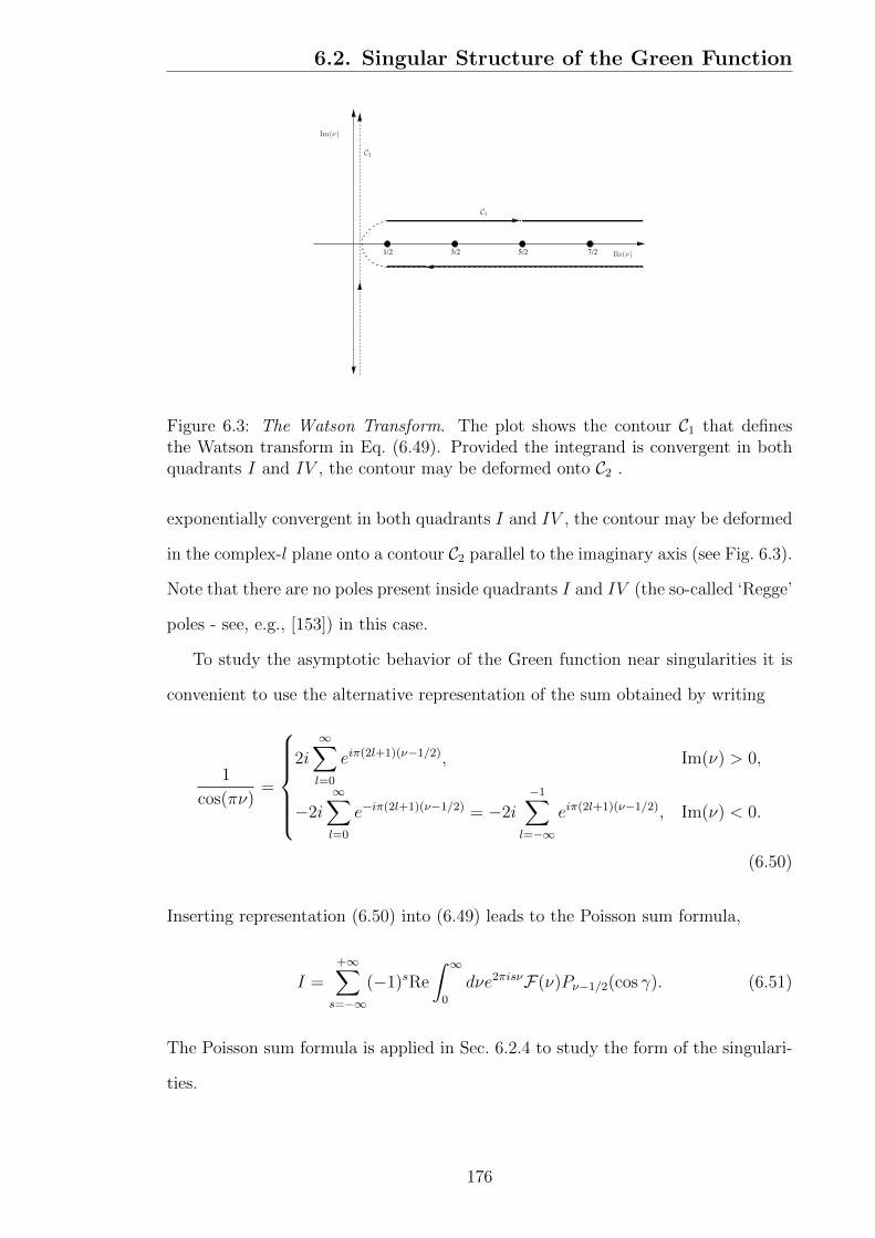
6.2. Singular Structure of the Green Function
3/2 5/2 7/21/2 Re(!)
Im(!)
C1
C2
Figure 6.3: The Watson Transform. The plot shows the contour C1 that definesthe Watson transform in Eq. (6.49). Provided the integrand is convergent in bothquadrants I and IV , the contour may be deformed onto C2 .
exponentially convergent in both quadrants I and IV , the contour may be deformed
in the complex-l plane onto a contour C2 parallel to the imaginary axis (see Fig. 6.3).
Note that there are no poles present inside quadrants I and IV (the so-called ‘Regge’
poles - see, e.g., [153]) in this case.
To study the asymptotic behavior of the Green function near singularities it is
convenient to use the alternative representation of the sum obtained by writing
1
cos(πν)=
2i∞∑
l=0
eiπ(2l+1)(ν−1/2), Im(ν) > 0,
−2i∞∑
l=0
e−iπ(2l+1)(ν−1/2) = −2i−1∑
l=−∞
eiπ(2l+1)(ν−1/2), Im(ν) < 0.
(6.50)
Inserting representation (6.50) into (6.49) leads to the Poisson sum formula,
I =+∞∑
s=−∞
(−1)sRe
∫ ∞
0
dνe2πisνF(ν)Pν−1/2(cos γ). (6.51)
The Poisson sum formula is applied in Sec. 6.2.4 to study the form of the singulari-
ties.
176

6.2. Singular Structure of the Green Function
6.2.3 Watson Transform: Computing the Series *
Let us now show how the Watson transform may be applied to extract well-defined
values from series over l, even if these series are divergent. We will illustrate the
approach by considering the nth-overtone QNM contribution to the Green function,
Eq. (6.34), for which case
F(x, x′; ν) =1
n!
[4e−T
(1 + ρ)(1 + ρ′)
]n+1/2
2νeiλ[T−ln(2/(1+ρ))−ln(2/(1+ρ′))]
× Γ(−n+ 2iλ)
[Γ(−n+ 1/2 + iλ)]22F1
(−n− 2iλ,−n,−n+ 1
2+ iλ; (1− ρ)/2
)
× 2F1
(−n− 2iλ,−n,−n+ 1
2+ iλ; (1− ρ′)/2
),
where λ was defined in (6.5). We will choose the integer N so that this contour may
be deformed into the complex plane (as shown in Fig. 6.3) to a contour on which
the integral converges more rapidly. First, we note that the Legendre function may
be written as the sum of waves propagating clockwise and counterclockwise,
Pν−1/2(cos γ) = Q(+)ν−1/2(cos γ) +Q(−)
ν−1/2(cos γ), (6.52)
where
Q(±)µ (z) =
1
2
[Pµ(z)± 2i
πQµ(z)
](6.53)
and here Qµ(z) is a Legendre function of the second kind. The functions Q(±)ν−1/2
have exponential asymptotics in the limit νγ 1,
Q(±)ν−1/2(cos γ) ∼
(1
2πν sin γ
)1/2
e±iπ/4e∓iνγ. (6.54)
With these asymptotics, and with the large-l asymptotics (6.40) of the hypergeo-
metric functions, one finds that the contour may be rotated to run, for example,
177

6.2. Singular Structure of the Green Function
along a line Re(ν) = c with c a constant between 0 and 12
provided that we choose
N =
[(T + log ((ρ+ 1)(ρ′ + 1)) + γ)/(2π)] for Q(+)
[(T + log ((ρ+ 1)(ρ′ + 1)) + 2π − γ)/(2π)] for Q(−)
(6.55)
where here [x] denotes the greatest integer less than or equal to x.
We performed the integrals numerically along Re(ν) = 14
and found rapid con-
vergence except near the critical times defining the jumps in N given by Eq. (6.55),
when the integrands fall to 0 increasingly slowly. An alternative method for extract-
ing meaningful values from divergent series is described in Sec. 6.4.3.
6.2.4 The Poisson sum formula: Singularities and
Asymptotics *
In this section we study the singularity structure of the Green function by applying
the Poisson sum formula (6.51). The first step is to group the terms together so
that
I =∞∑
N=0
IN where IN ≡ Re
∫ +∞
0
dνF(ν)RN(ν, γ) (6.56)
and
RN =
(−1)N/2[Q(−)ν−1/2(cos γ)eiNπν +Q(+)
ν−1/2(cos γ)e−iNπν], N even,
(−1)(N+1)/2[Q(+)ν−1/2(cos γ)ei(N+1)πν +Q(−)
ν−1/2(cos γ)e−i(N+1)πν], N odd.
(6.57)
and Q(±)ν−1/2 were defined in Eq. (6.53). We can now use the exponential approxima-
tions for Q(±)ν−1/2 given in (6.54) to establish
RN ∼1
(2πν sin γ)1/2
(−1)N/2[e−iπ/4eiν(Nπ+γ) + c.c.
], N even,
(−1)(N+1)/2[eiπ/4eiν((N+1)π−γ) + c.c.
], N odd.
(6.58)
178

6.2. Singular Structure of the Green Function
It should be borne in mind that the exponential approximations (6.54) are valid in
the limit γν 1. Hence the approximations are not suitable in the limit γ → 0
case. Below, we use alternative asymptotics (6.66) to investigate this case.
‘Fundamental mode’ n = 0
Let us apply the method to the ‘fundamental mode’ QNM series (6.35). In this case
we have
F(ν) =
(4e−T
π(1 + ρ)(1 + ρ′)
)1/2ν Γ(iλ)
Γ(1/2 + iλ)eiλχ (6.59)
where T was defined in (6.23), λ was defined in (6.5), and
χ = T + ln[(1 + ρ)(1 + ρ′)]. (6.60)
Taking the asymptotic limit ν →∞ we find
F(ν) ∼(
4ν e−T
iπ(1 + ρ)(1 + ρ′)
)1/2
eiνχ, ν →∞. (6.61)
Now let us combine this with the ‘exponential approximations’ (6.58) for RN ,
F(ν)RN(ν, γ) ∼(
2 e−T
π2 sin γ(1 + ρ)(1 + ρ′)
)1/2
×
(−1)N/2[−ieiν(χ+Nπ+γ) + eiν(χ−Nπ−γ)
], N even,
(−1)(N+1)/2[eiν(χ+(N+1)π−γ) − ieiν(χ−(N+1)π+γ)
], N odd,
(6.62)
for ν →∞. It is clear that the integral in (6.56) will be singular if the phase factor
in either term in (6.62) is zero. In other words, each wave RN gives rise to two
singularities, occurring at particular ‘singularity times’. We are only interested in
the singularities for T > 0; hence we may neglect the former terms in (6.62). Now
let us note that
limε→0+
∫ ∞
0
eiν(ζ+iε)dν = limε→0+
(i
ζ + iε
)= i/ζ + πδ(ζ) (6.63)
179

6.2. Singular Structure of the Green Function
Upon substituting (6.62) into (6.56) and performing the integral, we find
I(n=0)N ∼
(2 e−T
sin γ(1 + ρ)(1 + ρ′)
)1/2
(−1)N/2δ(t− t′ − t(n=0)N ), N even,
(−1)(N+1)/2
π(t− t′ − t(n=0)
N
) , N odd,(6.64)
where I(n=0)N is IN in (6.56) with F(ν) given by (6.59), and
t(n=0)N = ρ∗ + ρ′∗ − ln ((1 + ρ)(1 + ρ′)) +
Nπ + γ, N even,
(N + 1)π − γ, N odd.
(6.65)
These times t(n=0)N are equivalent to the ‘periodic’ times identified in Sec. 6.2.1
(Eq. 6.46) and Sec. 1.3.3 (Eq. 1.72).
Let us consider the implications of Eq. (6.64) carefully. Let us fix the spatial co-
ordinates ρ, ρ′ and γ and consider variations in t−t′ only. Each term IN corresponds
to a particular singularity in the mode sum expression (6.35) for the (n = 0)-Green
function. The Nth singularity occurs at t − t′ = t(n=0)N . For times close to t
(n=0)N ,
we expect the term IN to give the dominant contribution to the (n = 0)-Green
function. Eq. (6.64) suggests that the (n = 0)-Green function has a repeating four-
fold singularity structure. The ‘shape’ of the singularity alternates between a a
delta-distribution (±δ(t− t′− t(n=0)N ), N even) and a singularity with antisymmetric
‘wings’ (±1/(t− t′ − t(n=0)N ), N odd).
The Nth wave may be associated with the Nth orbiting null geodesic shown in
Fig. 2.2. Note that ‘even N’ and ‘odd N’ geodesics pass in opposite senses around
ρ = 0. Now, N has a clear geometrical interpretation: it is the number of caustics
through which the corresponding geodesic has passed. Caustics are points where
neighboring geodesics are focused, and in a spherically-symmetric spacetime caustics
occur whenever a geodesic passes through angles ∆φ = π, 2π, 3π, etc. Equation
(6.64) implies that the singularity structure of the Green function changes each time
the wavefront passes through a caustic [112].
180

6.2. Singular Structure of the Green Function
More accurate approximations to the singularity structure may be found by
using the uniform asymptotics established by Olver [155] (as an improvement on
the ‘exponential asymptotics’ (6.54)),
Q(±)ν−1/2(cos γ) ∼ 1
2
(γ
sin γ
)1/2
H(∓)0 (νγ), (6.66)
where H(±)0 (·) = J0(·)± iY0(·) are Hankel functions of the first (+) and second (−)
kinds. This approximation (6.66) is valid in the large-ν limit for angles in the range
0 ≤ γ < π. With these asymptotics, we replace (6.58) with
RN ∼1
2
(γ
sin γ
)1/2
×
(−1)N/2[H
(+)0 (νγ)eiNπν +H
(−)0 (νγ)e−iNπν
], N even,
(−1)(N+1)/2[H
(−)0 (νγ)ei(N+1)πν +H
(+)0 (νγ)e−i(N+1)πν
], N odd.
(6.67)
In Appendix F we derive the following asymptotics for the ‘fundamental mode’
(n = 0) Green function,
I(n=0)1
∼
2A(γ)√π[(2π − γ)− χ] [(2π + γ)− χ]1/2
E (2γ/[(2π + γ)− χ]) , χ < 2π − γ,
−A(γ)√π
2[χ− (2π − γ)]3/22F1
(3/2, 1/2; 2;
χ− 2π − γχ− 2π + γ
), χ > 2π − γ,
(6.68)
I(n=0)2
∼
−√
2π
γA(γ)δ (χ− (2π + γ)) , χ ≤ 2π + γ,
A(γ)√π
2[χ− (2π − γ)]3/22F1
(3/2, 1/2; 2;
χ− 2π − γχ− 2π + γ
), χ > 2π + γ,
(6.69)
where E is the complete elliptic integral of the second kind, χ was defined in (6.60)
181

6.2. Singular Structure of the Green Function
and
A(γ) =
(γ
sin γ
)1/2(e−T
π(1 + ρ)(1 + ρ′)
)1/2
. (6.70)
The asymptotics (6.68) and (6.69) provide insight into the singularity structure
near the caustic at ∆φ = 2π. Figure 6.4 shows the asymptotics (6.68) and (6.69)
at ρ = ρ′ → +1 for two cases: (i) γ = π/20 (left) and (ii) γ = 0 (right). In the left
plot, the I(n=0)1 integral has a (nearly) antisymmetric form. The I(n=0)
2 integral is
a delta function with a ‘tail’. However, the ‘tail’ is exactly canceled by the I(n=0)1
integral in the regime χ > 2π + γ. The cancellation creates a step discontinuity in
the Green function at χ = 2π + γ. The form of the divergence shown in the right
plot (γ = 0) may be understood by substituting γ = 0 into (6.68) to obtain
I(n=0)1 (γ = 0) ∼
(e−T
(1 + ρ)(1 + ρ′)
)1/2
(2π − χ)−3/2. (6.71)
Near spatial infinity, ρ, ρ′ → +1
It is straightforward to repeat the steps in the above analysis for the closed-form
Green function (6.30), valid for ρ, ρ′ → +1. We reach a result of the same form as
(6.64), but with modified singularity times,
t(ρ∼1)N ∼ ρ∗ + ρ′∗ +
ln(sinh2 ([Nπ + γ]/2)
), N even,
ln(sinh2 ([(N + 1)π − γ]/2)
), N odd,
(6.72)
corresponding to the geodesic times (1.71). For instance, with the exponential
asymptotics (6.58) applied to (6.30) we obtain
I(ρ∼1)N ∼
(e−T
2 sin γ√
1 + e−T
)1/2
(−1)N/2 δ(t− t′ − t(ρ∼1)
N
), N even,
(−1)(N+1)/2
π(t− t′ − t(ρ∼1)
N
) , N odd.(6.73)
182

6.2. Singular Structure of the Green Function
Figure 6.4: Singularities of the ‘fundamental mode’ Green function (6.35) near thecaustic at 2π and ρ = ρ′ → +1. These plots show the I1 (dashed) and I2 (dotted)contributions to the Poisson sum, given explicitly by (6.68) and (6.69). The topplot shows an angular separation γ = π/20 and the bottom plot shows angularcoincidence γ = 0. Note that, for T > 2π + γ − 2 ln 2, the I1 and I2 integrals areequal and opposite and will exactly cancel out (see text).
183
6.2. Singular Structure of the Green Function
In Sec. 6.5 the asymptotic expressions derived here are compared against numerical
results from the mode sums.
We believe that the 4-fold cycle in the singularity structure of the Green function
which we have just unearthed using tricks we picked up from seismology [154] is
characteristic of the S2 topology (different types of cycle arising in different cases).
This cycle may thus also appear in the more astrophysically interesting case of the
Schwarzschild spacetime. Indeed, Ori [112] has suggested that this truly is the case
for Schwarzschild. However, since this cycle does not seem to be widely known in the
field of General Relativity (with the notable exception of Ori’s work), in Appendix
G we apply the large-l asymptotic analysis of this section to the simplest case with
S2 topology: the spacetime of T × S2, where the same cycle blossoms in a clear
manner.
6.2.5 Hadamard Approximation and the Van Vleck
Determinant
In this section, we re-derive the singularity structure found in (6.64) and (6.73)
using a ‘geometrical’ argument based on the Hadamard form of the Green func-
tion. In Sec. 6.1.3 we used the Hadamard parametrix of the Green function to
find the quasilocal contribution to the self-force. Strictly speaking, the Hadamard
parametrix of Eq. (1.3), is only valid when x and x′ are within a normal neighbor-
hood [35] (see footnote 1). Nevertheless, it is plausible (particularly in light of the
previous sections) that the Green function near the singularities may be adequately
described by a Hadamard-like form, but with contributions from all appropriate
orbiting geodesics (rather than just the unique timelike geodesic joining x and x′).
We first introduce the Feynman propagator GF (x, x′) (see, e.g., [13, 115]) which
satisfies the inhomogeneous scalar wave equation (1.2). The Hadamard form, which
in principle is only valid for points x′ within the normal neighborhood of x, for the
184

6.2. Singular Structure of the Green Function
Feynman propagator in 4-D is [13, 156]
GF (x, x′) =i
2π
[U(x, x′)
σ + iε+ V (x, x′) ln(σ + iε) +W (x, x′)
], (6.74)
where U(x, x′), V (x, x′) (already introduced in Sec. 1.1.1) and W (x, x′) are bi-tensors
which are regular at coincidence (x→ x′) and σ(x, x′) is the Synge world function:
half the square of the geodesic distance along a specific geodesic joining x and x′.
Note the Feynman prescription ‘σ → σ + iε’ in (6.74), where ε is an infinitesimally
small positive value, which is necessary so that the Feynman propagator has the
appropriate analytical properties; this implies that Eq. (6.75) below is then satisfied.
The retarded Green function is readily obtained from the Feynman propagator
by
Gret(x, x′) = 2θ−(x, x′) Re (GF (x, x′)) , (6.75)
which yields (1.3) inside the normal neighborhood, since U(x, x′), V (x, x′) and
W (x, x′) are real-valued there. We posit that the ‘direct’ part of the Green function
remains in Hadamard form,
Gdir.ret (x, x′) = lim
ε→0+
1
πRe
[iU(x, x′)
σ + iε
]= Re
[U(x, x′)
(δ(σ) +
i
πσ
)], (6.76)
even outside the normal neighborhood [note that outside the normal neighborhood
we still use the term ‘direct’ part to refer to the contribution from the U(x, x′)
term, even if its support may not be restricted to the null cone anymore]. It is
plausible that the Green function near the Nth singularity (see previous section) is
dominated by the ‘direct’ Green function (6.76) calculated along geodesics near the
Nth orbiting null geodesic. To test this assertion, we will calculate the structure
and magnitude of the singularities and compare with (6.73).
In four dimensional spacetimes, the symmetric bi-tensor U(x, x′) is given by
U(x, x′) = ∆1/2(x, x′), (6.77)
185

6.2. Singular Structure of the Green Function
where ∆(x, x′) is the Van Vleck determinant [157, 158, 159]. In Sec. 1.3, we derived
an analytic expression for the Van Vleck determinant,
∆(x, x′) =
(γ
sin γ
)(η
sinh η
). (6.78)
where γ ∈ [0, π) is the geodesic distance traversed on the two-sphere and η is the
geodesic distance traversed in the two-dimensional de Sitter subspace. Hence the
Van Vleck determinant is singular at the angle γ = π.
This may be seen another way. Using the spherical symmetry, let us assume
without loss of generality that the motion is in the plane θ = π/2, from which it
follows that the equation for σθθ in (4.11) decouples from the remainder; it is
φ′dσθ
′θ′
dφ′+ φ′2 − σθ′θ′(1− σθ
′θ′) = 0 (6.79)
Here, as before, we have rescaled the affine parameter s to be equal to the angle
φ subtended by the geodesic. Note that here we let φ take values greater than
π. It is straightforward to show that the solution of Eq. (6.79) is σθ′θ′ = φ′ cotφ′.
Hence σθ′θ′ is singular at the angles φ = π, 2π, 3π, etc. In other words, the Van
Vleck determinant is singular at the antipodal points, where neighboring geodesics
are focused: the caustics. The Van Vleck determinant may be separated in the
following manner: ∆ = ∆θ∆tρ, where
φ′d ln ∆θ
dφ′= 1− σθ′θ′ , (6.80)
φ′d ln ∆tρ
dφ′= 2− σt′ t′ − σρ
′ρ′ . (6.81)
Eq. (6.80) yields
ln ∆θ = ln
(φ
φ0
)−∫ φ
φ0
dφ′ cotφ′ (6.82)
which can be integrated analytically by following a Landau contour in the complex
φ′-plane around the (simple) poles of the integrand (located at φ′ = kπ, k ∈ Z),
which are the caustic points. Following the Feynman prescription ‘σ → σ + iε’, we
186

6.2. Singular Structure of the Green Function
choose the Landau contour so that the poles lie below the contour. We then obtain
(setting φ0 = 0 without loss of generality)
∆θ =
∣∣∣∣φ
sinφ
∣∣∣∣ e−iNπ. (6.83)
Here, N is the number of caustic points the geodesic has passed through. The phase
factor, obtained by continuing the contour of integration past the singularities at
φ = π, 2π, etc., is crucial. Inserting the phase factor e−iNπ/2 in (6.76) leads to exactly
the four-fold singularity structure predicted by the large-l asymptotics of the mode
sum (6.73). That is:
GdirN ∼
(η
sinh η
)1/2(φ
sinφ
)1/2
(−1)N/2δ(σ), N even,
(−1)(N−1)/2
πσ, N odd.
(6.84)
The accumulation of a phase of ‘−i’ on passing through a caustic, and the al-
ternating singularity structure which results, is well-known to researchers in other
fields involving wave propagation – for example, in acoustics [160], seismology [154],
symplectic geometry [161] and quantum mechanics [162] the integer N is known as
the Maslov index [163, 164].
We would expect to find an analogous effect in, for example, the Schwarzschild
spacetime. The four-fold structure has been noted before by at least one researcher
[112]. Nevertheless, the effect of caustics on wave propagation in four-dimensional
spacetimes does not seem to have received much attention in the gravitational lit-
erature (see [165, 166] for exceptions).
To compare the singularities in the mode-sum expression (6.73) with the singu-
larities in the Hadamard form (6.84), let us consider the ‘odd-n’ singularities of 1/σ
form. We will rearrange (6.73) into analogous form by expanding σ to first-order
in t− t(ρ∼1)N , where t
(ρ∼1)N is the Nth singularity time for orbiting geodesics starting
and finishing at ρ → 1. For the orbiting geodesics described in Sec. 1.3.3 we have
187

6.3. Summary
σ = −12(H2 − 1)φ2. At ρ→ 1, expanding to first order and using (1.71) yields
σ ∼ −(Hφ) tanh(Hφ/2)(t− t(ρ∼1)
N
). (6.85)
The mode-sum expression (6.73) may then be rewritten in analogous form to the
‘N odd’ expression in (6.84),
GQNMret ∼ (−1)(N−1)/2
∣∣∆(QNM)
∣∣1/2
πσ(6.86)
where∣∣∆(QNM)
∣∣1/2 =
(Hη sinh(η/2)
2 cosh3(η/2)
)1/2 ∣∣∣∣φ
sinφ
∣∣∣∣1/2
. (6.87)
Here η = Hφ, where H is the constant of motion introduced in Sec. 1.3.3. We
find very good agreement between (6.78) and (6.87) in the φ & π regime. The
disagreement at small angles is not unexpected as the QNM sum is invalid at early
times (or equivalently, for orbiting geodesics which have passed through small angles
φ).
6.3 Summary
After a series of equations and results, for the benefit of the reader we will now take
a moment to recap and (literally) rewrite the main equations obtained thus far. We
recall that β = −1/2 + iλ, λ =√
(l + 1/2)2 + 4ξ − 1/2, ρ∗ = tanh−1 ρ, that we tend
to use T = t−t′−ρ∗−ρ′∗ as the independent ‘time’ variable, and that the unbounded
orbital angle is given by ∆φ = Nπ + γ for N even and by ∆φ = (N + 1)π − γ for
N odd, where N is the number of caustics the null geodesic has gone through.
The main equations for the ‘retarded’ Green function we have obtained so far
are:
188

6.3. Summary
• QNM ‘retarded’ Green function (valid ∀x, x′ where T > 0), Eq. (6.34):
GQNMret (x, x′) = 2 Re
∞∑
l=0
(2l + 1)Pl(cos γ)eiλ[T−ln(2/(1+ρ))−ln(2/(1+ρ′))]
×∞∑
n=0
Bln[
4e−T
(1 + ρ)(1 + ρ′)
]n+1/2
Sln(ρ)Sln(ρ′). (6.88)
where Bln are the excitation factors (6.26) and Sln(ρ) is the finite series (6.32)
essentially based on the radial functions evaluated at the QNM frequencies.
• QNM ‘retarded’ Green function (after summing over all overtone numbers n)
at ρ∗, ρ′∗ → +∞ (and T > 0), Eq. (6.30):
GQNMret (T, γ) ∼ e−T/2√
πRe
+∞∑
l=0
(l + 1/2)Γ(iλ)
Γ(1/2 + iλ)
× Pl(cos γ)eiλ(T+2 ln 2)2F1(−β,−β;−2β;−e−T ), ρ∗, ρ
′∗ → +∞, (6.89)
with singularities at times given by Eq. (6.45) (also Eq. (1.71) with H = 1
and Eq. (6.72)), T (ρ∼1) = ln[sinh2(∆φ/2)
]. The corresponding singularity
structure is given by Eq. (6.73):
I(ρ∼1)N ∼
(e−T
2 sin γ√
1 + e−T
)1/2
(−1)N/2 δ(t− t′ − t(ρ∼1)
N
), N even,
(−1)(N+1)/2
π(t− t′ − t(ρ∼1)
N
) , N odd,
(6.90)
where I(ρ∼1)N is the contribution IN to the ‘retarded’ Green function associated
with the Nth orbiting null geodesic in the case where the points are located
at spatial infinity.
• Contribution of the ‘fundamental mode’ n = 0 to the QNM ‘retarded’ Green
189
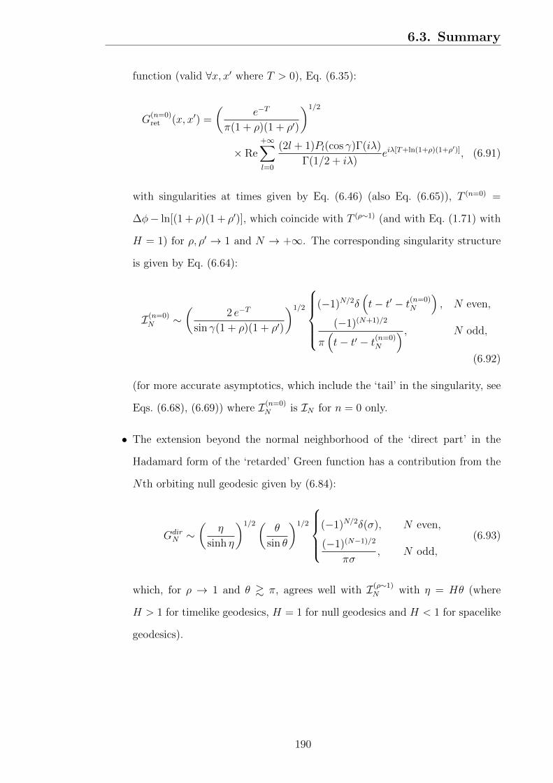
6.3. Summary
function (valid ∀x, x′ where T > 0), Eq. (6.35):
G(n=0)ret (x, x′) =
(e−T
π(1 + ρ)(1 + ρ′)
)1/2
× Re+∞∑
l=0
(2l + 1)Pl(cos γ)Γ(iλ)
Γ(1/2 + iλ)eiλ[T+ln(1+ρ)(1+ρ′)], (6.91)
with singularities at times given by Eq. (6.46) (also Eq. (6.65)), T (n=0) =
∆φ− ln[(1 + ρ)(1 + ρ′)], which coincide with T (ρ∼1) (and with Eq. (1.71) with
H = 1) for ρ, ρ′ → 1 and N → +∞. The corresponding singularity structure
is given by Eq. (6.64):
I(n=0)N ∼
(2 e−T
sin γ(1 + ρ)(1 + ρ′)
)1/2
(−1)N/2δ(t− t′ − t(n=0)
N
), N even,
(−1)(N+1)/2
π(t− t′ − t(n=0)
N
) , N odd,
(6.92)
(for more accurate asymptotics, which include the ‘tail’ in the singularity, see
Eqs. (6.68), (6.69)) where I(n=0)N is IN for n = 0 only.
• The extension beyond the normal neighborhood of the ‘direct part’ in the
Hadamard form of the ‘retarded’ Green function has a contribution from the
Nth orbiting null geodesic given by (6.84):
GdirN ∼
(η
sinh η
)1/2(θ
sin θ
)1/2
(−1)N/2δ(σ), N even,
(−1)(N−1)/2
πσ, N odd,
(6.93)
which, for ρ → 1 and θ & π, agrees well with I(ρ∼1)N with η = Hθ (where
H > 1 for timelike geodesics, H = 1 for null geodesics and H < 1 for spacelike
geodesics).
190

6.4. Self-Force on the Static Particle
6.4 Self-Force on the Static Particle
In this section we turn our attention to a simple case: the self-force acting on a static
scalar particle in the Nariai spacetime. By ‘static’ we mean a particle with constant
spatial coordinates. It is not necessarily at rest, since its worldline may not be a
geodesic, and it may require an external force to keep it static. This is analogous to
the case of a static particle in Schwarzschild. In Sec. 6.4.1 we explore an analytic
method for computing the static self-force in Nariai spacetime. This method, based
on the massive field approach of Rosenthal [91, 85] provides an independent check
on the matched-expansion approach. In Sec. 6.4.2 we describe how the method of
matched expansions may be applied to the static case. To compute the self-force, we
require robust numerical methods for evaluating the quasinormal mode sums such
as (6.88); two such methods are outlined in Sec. 6.4.3. The results of all methods
are validated and compared in Sec. 6.5.
6.4.1 Static Green Function Approach
The conventional approach to calculating the self-force on a static particle due to
Wiseman [77] uses the ‘scalarstatic’ Green function. Following Copson [87], Wise-
man was able to obtain this Green function by summing the Hadamard series. Only
by performing the full sum was he able to verify that his Green function satisfied the
appropriate boundary conditions. Linet [167] has classified all spacetimes in which
the scalarstatic equation is solvable by the Copson ansatz [87] and, unfortunately,
the Nariai metric does not fall into any of the classes given. Therefore, instead we
work with the mode form for the static Green function. This corresponds to the
integrand at ω = 0 of Eq. (6.18) (with integral measure dω2π
),
Gstatic(ρ,Ω; ρ′,Ω′) =∞∑
l=0
(2l + 1)Pl(cos γ)πP−1/2+iλ(−ρ<)P−1/2+iλ(ρ>)
2 cosh(πλ)(6.94)
where, as before, λ =√
(l + 12)2 + d. This equation, having only one infinite series,
is amenable to numerical computation.
191

6.4. Self-Force on the Static Particle
To regularize the self-force we follow the method of Rosenthal [85], who used a
massive field approach to calculate the static self-force in Schwarzschild. Following
his prescription, we calculate the derivative of the scalar field and of a massive
scalar field. In the limit of the field mass going to infinity, we obtain the derivative
of the radiative field which is regular. This method can be carried through to Nariai
spacetime (for details see Appendix D), where it yields the expression
maρ = q2(1− ρ2)32 limρ′→ρ−
[∂ρGstatic(ρ,Ω; ρ′,Ω) +
1
(ρ− ρ′)2− (ξR− 2
3)
2(1− ρ2)
], (6.95)
where R = 4 here. Note that the massive field approach was developed in [85]
for the case ξ = 0, but it can be seen that it equally applies to ξ 6= 0 too. The
limiting process ρ′ → ρ− does not affect the term with 1/(1 − ρ2) in (6.95). We
will therefore omit it from the following calculation and we will trivially subtract it
from the self-force in the calculations we carry out later in Sec. 6.5.4. The singular
(as ρ′ → ρ−) subtraction term may be expressed in a convenient form using the
identity [168, 169],
∫ +∞
0
dλλ tanh(πλ)πP−1/2+iλ(−ρ<)P−1/2+iλ(ρ>)
cosh(πλ)=
1
ρ> − ρ<(6.96)
Subtracting (6.96) from (6.94), we can express the regularized Green function as a
sum of two well-defined and easily calculated sums/integrals
Gstatic(ρ,Ω; ρ′,Ω)− 1
ρ> − ρ<= I(ρ, ρ′) + J (ρ, ρ′) (6.97)
where
I(ρ, ρ′) =
∫ +∞
0
dλ λ (1− tanh(πλ))πP−1/2+iλ(−ρ<)P−1/2+iλ(ρ>)
cosh(πλ)(6.98)
192

6.4. Self-Force on the Static Particle
and
J (ρ, ρ′) =+∞∑
l=0
(l + 12)πP−1/2+iλ(−ρ<)P−1/2+iλ(ρ>)
cosh(πλ)
−∫ +∞
0
dλ λπP−1/2+iλ(−ρ<)P−1/2+iλ(ρ>)
cosh(πλ). (6.99)
The term J (ρ, ρ′) may either be calculated directly as a sum or by using the Watson-
Sommerfeld transform to write
∞∑
l=0
g
(l +
1
2
)= Re
[1
i
∫
γ
dz tan(πz)g(z)
], (6.100)
where γ runs from 0 to ∞ just above the real axis, and for us
g(z) = zπP−1/2+i
√z2+d(−ρ<)P−1/2+i
√z2+d(ρ>)
cosh(π√z2 + d)
. (6.101)
Writing
tan(πz) = i− 2i
1 + e−2πiz, (6.102)
the first term yields
∫ ∞
0
dx g(x) =
∫ ∞√d
dλ λπP−1/2+iλ(−ρ<)P−1/2+iλ(ρ>)
cosh(πλ). (6.103)
The contribution from the second term can be best evaluated by rotating the original
contour to a contour γ′, running from 0 to i∞ just to the right of the imaginary
axis. This is permitted since the Legendre functions are analytic functions of their
parameter and the contribution from the arc at infinity vanishes for our choice of
g(z). From the form of g(z) it is clear that it possesses poles along the contour γ′
but these give a purely imaginary contribution to the integral. We conclude that
J (ρ, ρ′) = −∫ √d
0
tdt tanh(π√d− t2)
πP−1/2+it(−ρ<)P−1/2+it(ρ>)
cosh(πt)+
+ P∫ +∞
0
2πtdt
(1 + e2π√d+t2) cos(πt)
P−1/2−t(−ρ<)P−1/2−t(ρ>) (6.104)
193

6.4. Self-Force on the Static Particle
where P denotes the Principal Value. These integrals and that defining I(ρ, ρ′) and
their derivatives with respect to ρ are very rapidly convergent and easily calculated.
6.4.2 Matched Expansions for Static Particle
In Sec. 2.2, we outlined the method of matched expansions. In this subsection, we
show how to apply the method to a specific case: the computation of the self-force
on a static particle in the Nariai spacetime.
The four velocity of the static particle is simply
uρ = uθ = uφ = 0, ut = (1− ρ2)−1/2 (6.105)
and hence dτ ′ = (1 − ρ2)1/2dt′. We find from Eqs. (2.15), (2.17) and (2.6) that
mat = maθ = maφ = 0 and
maρ = q2
(1
3aρ + lim
ε→0+
∫ τ−ε
−∞gρρ∂ρGret(z(τ), z(τ ′))dτ ′
)(6.106)
dm
dτ= −q2
(1
12(1− 6ξ)R +
(1− ρ2
)−1/2limε→0+
∫ τ−ε
−∞∂tGret(z(τ), z(τ ′))dτ ′
)(6.107)
We note that in the tail integral of the mass loss equation, (6.107), the time derivative
∂t may be replaced with−∂t′ since the retarded Green function is a function of (t−t′).
Hence we obtain a total integral,
(1− ρ2
)−1/2limε→0+
∫ τ−ε
−∞∂tGret(z(τ), z(τ ′))dτ ′ = − lim
ε→0+
∫ t−ε
−∞∂t′Gret(z(τ), z(τ ′))dt′
= − limε→0+
[Gret(x, x′)]t′=t−εt′→−∞ (6.108)
The total integral depends only on the values of the Green function at the present
time and in the infinite past (t′ → ∞). The QNM sum expressions for the Green
function (e.g. Eq. (6.89)) are zero in the infinite past, as the quasinormal modes
decay exponentially. The value of the Green function at coincidence (t′ → t) is
found from the coincidence limit of the function −V (x, x′) in the Hadamard form
194

6.4. Self-Force on the Static Particle
(1.3). It is 112
(1−6ξ)R, which exactly cancels the local contribution in the mass loss
equation (6.107). It is no surprise to find that this cancellation occurs – the local
terms were originally derived from the coincidence limit of the Green function. In
fact, because dΦRdτ
= 0 due to time-translation invariance, we can see directly from
the original equation (2.17) that the mass loss is zero in the static case.
Now let us consider the radial acceleration (6.106). The acceleration keeping the
particle in a static position is constant (aρ = 0). The remaining tail integral may
be split into two parts,
maρ = q2(1− ρ2)3/2
[− lim
ε→0+
∫ t−ε
t−∆t
∂ρV (z(t), z(t′))dt′
+
∫ t−∆t
−∞∂ρGret(z(t), z(t′))dt′
], (6.109)
where ∆t is a free parameter corresponding to ∆τ introduced in (2.8) that determines
the matching time in the matched expansions method. For the first part of (6.109),
we use the quasilocal calculation of V (x, x′) from Sec. 6.1.3. As V (x, x′) is given
as a power series in (ρ − ρ′) and (t − t′), the derivatives and integrals can be done
termwise and are straightforward. The quasilocal integral contribution is therefore
simply
limε→0
∫ t−ε
t−∆t
∂ρV (z(t), z(t′))dt′ =1
2
+∞∑
k=0
1
(2k + 1)∂ρvk0(∆t)2k+1. (6.110)
The second part of (6.109) can be computed using the QNM sum (6.88). To
illustrate the approach, let us rewrite (6.88) as
GQNMret (ρ, t; ρ′, t; γ) = Re
∑
l,n
Gln(ρ′, γ)e−iωln(t−t′−ρ∗−ρ′∗)uln(ρ). (6.111)
Applying the derivative with respect to ρ and taking the integral with respect to t′
195

6.4. Self-Force on the Static Particle
leads to
∫ t−∆t
−∞∂ρGret(z(t), z(t′))dt′
=
(dρ
dρ∗
)−1 ∫ t−∆t
−∞∂t′G
QNMret dt′ + Re
∑
l,n
∫ t−∆t
−∞Glne−iωln(t−t′−ρ∗−ρ′∗)duln
dρdt′
=(1− ρ2
)−1[Gret]
t′=t−∆t +∑
l,n
Glniωln
e−iωln(∆t−ρ∗−ρ′∗)dulndρ
(6.112)
It is straightforward to find the derivative of the radial wavefunction from the defi-
nition (6.31). In Sec. 6.4.3 we outline two methods for numerically computing mode
sums such as (6.112).
The self-force computed via (6.109), (6.110) and (6.112) should be independent of
the choice of the matching time (we verify this in Sec. 6.5.4). This invariance provides
a useful test of the validity of our matched expansions. Additionally, through varying
∆τ we may estimate the numerical error in the self-force result.
6.4.3 Numerical Methods for Computing Mode Sums *
The static-self-force calculation requires the numerical calculation of mode sums
like (6.112). We used two methods for robust numerical calculations: (1) ‘smoothed
sum’, and (2) Watson transform (described previously in Sec. 6.2.3). We see in Sec.
6.5 that the results of the two methods are consistent.
The ‘smoothed sum’ method is straightforward to describe and implement. Let
us suppose that we wish to extract a meaningful numerical value from an infinite
series+∞∑
l=0
al (6.113)
such that liml→∞ al 6= 0, and so the series is divergent. One may expect it to not
be possible for a divergent series to be summed to yield a finite value. However, the
summation of divergent series is on a firm footing, having been extensively studied
with significant rigour (for example, see Hardy [170]). For the case of mode sums
such as (6.112), we employ the ‘φ’ method (Sec. 4.7 and Theorem 25 of Ref. [170])
196

6.5. Results
for summing the divergent series. In this method, the terms, al, of the series are
multiplied by a function φl(x) such that φl(x)→ 1 for each l as x→ 0. In particular,
we choose1
φl(x) = e−l2x2/2 (6.114)
and define lcut ≡ 1x. The ‘φ’ method is regular2 provided the condition
0 ≤ φn+1(x) ≤ φn(x) (6.115)
Thus instead of computing the sum (6.113), we may compute the sum
φ
(1
lcut
)=∞∑
l=0
ale−l2/2l2cut , (6.116)
where limlcut→∞ φ(
1lcut
)= s and s is the finite value we extract from the sum (6.113).
In practise, for our numerical approximation it is sufficient to compute the finite sum
S (l∞) ≡l∞∑
l=0
ale−l2/2l2cut . (6.117)
The choice of l∞ must be large enough to suppress any high-l oscillations in the
result (typically l∞ > 4lcut). We find that (6.116) is a good approximation to
(6.113) provided we are not within δt ∼ 1/lcut of a singularity of the Green function.
Increasing the cutoff lcut therefore improves the resolution of the singularities. The
introduction of such a cutoff is – although of different magnitude – in the same spirit
as the Feynman prescription of Sec. 6.2.5.
6.5 Results
We now present a selection of results from our numerical calculations. In Sec. 6.5.1
the distant past Green function is examined. We plot the Green function as a
1A similar ‘regulator’ function was proposed by Ching, et al. [171].2A method for summing a divergent sum is said to be regular if it sums every convergent series
to its ordinary sum.
197

6.5. Results
function of coordinate time t − t′ for fixed spatial points. A four-fold singularity
structure is observed. In Sec. 6.5.2 we test the asymptotic approximations of the
singular structure, derived in Secs. 6.2.5 and 6.2.4 (Eqs. 6.90 and 6.93). We show
that the ‘fundamental mode’ (n = 0) series (6.91) is a good approximation of the
exact result (6.89), if a ‘time-offset’ correction is applied. In Sec. 6.5.3 the quasilocal
and distant past expansions for the Green function are compared and matched. We
show that the two methods for finding the Green function are in excellent agreement
for a range of matching times ∆τ . In Sec. 6.5.4 we consider the special case of the
static particle. We present the Green function, the tail field and the self-force in
turn. The radial self-force acting on the static particle is computed via the matched
expansion method (described in Secs. 2.2 and 6.4.2), and plotted as a function of
the radial coordinate ρ, and compared with the result derived in Sec. 6.4.1.
6.5.1 The Green Function Near Infinity from Quasinormal
Mode Sums *
Let us begin by looking at the Green function for fixed points near spatial infinity,
ρ = ρ′ → 1 (i.e. ρ∗ = ρ′∗ → +∞). The Green function may be computed numerically
by applying either the Watson transform (Sec. 6.2.3) or the ‘smoothed sum’ method
(Sec. 6.4.3) to the QNM sum (6.89).
Figure 6.5 shows the Green function for fixed spatially-coincident points near
infinity (ρ = ρ′ → 1, γ = 0) and ξ = 1/6. The Green function has been calculated
from series (6.89) using the ‘smoothed sum’ method. It is plotted as a function of
QNM time, T = t− t′− (ρ∗+ρ′∗). We see that singularities occur at the times (1.71)
predicted by the geodesic analysis of Sec. 1.3.3. In this case, TC = ln[sinh2(Nπ)] ≈
4.893, 11.180, 17.463, etc. At times prior to the first singularity at T ≈ 4.893, the
Green function shows a smooth power-law rise. At the singularity itself, there is
a feature resembling a delta-distribution, with a negative sign. Immediately after
the singularity the Green function falls close to zero (although there does appear a
small ‘tail’). This behavior is even more marked in the case ξ = 1/8 (not shown).
198

6.5. Results
-0.4
-0.3
-0.2
-0.1
0
0.1
0.2
0.3
0.4
0 2 4 6 8 10 12 14 16 18
’Dist
ant P
ast’
Gre
en F
unct
ion
T = t - t’ - !* - !*’
" = 0# = 1/6
Figure 6.5: Distant Past Green Function for spatially-coincident points near infinity(ρ = ρ′ → 1, γ = 0). The Green function was calculated from mode sum (6.89)numerically using the smoothed sum method (6.116) with lcut = 200 and curvaturecoupling ξ = 1/6.
A similar pattern is found close to the second singularity at T ≈ 11.180, but here
the Green function takes the opposite sign, and its amplitude is smaller.
Figure 6.6 shows the Green function for points near infinity (ρ = ρ′ → 1) sepa-
rated by an angle of γ = π/2 and ξ = 1/6. The Green function shown here is com-
puted from the ‘fundamental mode’ approximation (6.91), again using the ‘smoothed
sum’ method. In this case, the singularities occur at ‘periodic’ times (1.72), given
by T = ∆φ− 2 ln 2 ≈ 0.1845, 3.326, 6.468, etc., where ∆φ = π/2, 3π/2, 5π/2, . . .. As
discussed, there is a one-to-one correspondence between singularities and orbiting
null geodesics, and the four-fold singularity pattern predicted in Sec. 6.2.4 (6.93)
and Sec. 6.2.5 (6.90) is clearly visible. Every ‘even’ singularity takes the form of a
delta distribution. Numerically, the delta distribution is manifest as a Gaussian-like
spike whose width (height) decreases (increases) as lcut is increased. By contrast
(for γ 6= 0, π), every ‘odd’ singularity diverges as 1/(T − Tc); it has antisymmetric
wings on either side. The singularity amplitude diminishes as T increases.
199

6.5. Results
-0.4
-0.3
-0.2
-0.1
0
0.1
0.2
0.3
0.4
0 2 4 6 8 10 12
Dist
ant P
ast G
reen
Fun
ctio
n
T = t - t’ - !* - !*’
" = 1/6# = $/2
Figure 6.6: Distant Past Green Function near spatial infinity (ρ = ρ′ → 1) for pointsseparated by angle γ = π/2 and ξ = 1/6. The Green function was calculated fromthe ‘fundamental mode’ approximation (6.91) numerically using the smoothed summethod with lcut = 1000. Note the four-fold singularity structure (see text).
6.5.2 Asymptotics and Singular Structure *
The analyses of Sec. 6.2.4 and Sec. 6.2.5 yielded approximations for the singularity
structure of the Green function. In particular, Eq. (6.90) gives an estimate for
the amplitude of the ‘odd’ singularities as ρ, ρ′ → 1. We tested our numerical
computations against these predictions. Figure 6.7 shows the Green function near
the singularity associated with the null geodesic passing through an angle ∆φ =
3π/2. The left plot compares the numerically-determined Green function (6.91)
with the asymptotic prediction (6.90). The right plot shows the same data on a
log-log plot. The asymptotic prediction (6.90) is a straight line with gradient −1,
and it is clear that the numerical data is in excellent agreement.
Improved asymptotic expressions for the singular structure of the fundamental
mode Green function were given in (6.68) and (6.69). These asymptotics are valid
all the way up to γ = 0. Figure 6.8 compares the asymptotic expressions (6.68) and
(6.69)(solid line) with numerical computations (broken lines) from the mode sum
(6.91). It is clear that the asymptotics (6.68) and (6.69) are in excellent agreement
with the numerically-determined Green function. Closest agreement is found near
200

6.5. Results
-15
-10
-5
0
5
10
15
3.24 3.26 3.28 3.3 3.32 3.34 3.36 3.38 3.4
Gre
en’s
Func
tion
(GF)
T = t - t’ - !* - !*’
" = 1/6, ! = 1, # = $/2Tc = 3$/2 - 2ln(2) = 3.3261
-0.5
0
0.5
1
1.5
2
2.5
-4 -3.5 -3 -2.5 -2 -1.5 -1
log 1
0|GF|
log10|T - Tc|
" = 1/6, ! = 1, # = $/2Tc = 3$/2 - 2ln(2) = 3.3261
Mode sum lmax = 2500Approximation
Figure 6.7: Green function near the singularity arising from a null geodesic passingthrough an angle ∆φ = 3π/2 and with ρ = ρ′ → 1. The ‘fundamental mode’(n = 0) Green function (6.91) (with lcut = 2500) is compared with approximations(6.90) and (6.93) from considering high-l asymptotics. The approximations giveGret ∼ −0.04268/(T − Tc) and Gret ∼ −0.04344/(T − Tc), respectively. The leftpanel shows the Green function in the vicinity of the (‘periodic’) singularity atTc = 3π/2 − 2 ln 2 ≈ 3.3261. The right panel shows the same data on a log-logscale, and compares the mode sum (dashed) with the approximation (dotted). Thediscrepancy close to the singularity may be improved by increasing lcut.
the singular times, but the asymptotics provide a remarkably good fit over a range
of t.
In Fig. 6.9, the ‘fundamental mode’ (n = 0) approximation (6.91) is compared
with the exact QNM Green function (6.89) near spatial infinity. Away from singu-
larities, the former is found to be a good approximation to the latter. However, close
to singularities this is not the case. The singularities of the ‘fundamental mode’ ap-
proximation (6.91) occur at slightly different times to the singularities of the exact
solution (6.89), as discussed in Sec. 6.2.1. For the fundamental mode series (6.91),
the singularity times TNreg given in Eq. (6.46) are periodic. For the exact solution
(6.89) near spatial infinity, the singularity times TNexact are precisely the ‘null geodesic
times’ given in Eq. (1.71). Remarkably, if we apply a singularity time offset to the
‘fundamental mode’ approximation (T → T + ∆T where ∆T = TNexact − TNreg) we
find that the ‘fundamental mode’ Green function is an almost perfect match to the
exact Green function. This is clearly shown in the lower plot of Fig. 6.9. Compar-
ing the series (6.91) and (6.89) we see that, in both cases, the magnitude of the
201

6.5. Results
-2
-1.5
-1
-0.5
0
0.5
1
1.5
2
4.2 4.4 4.6 4.8 5 5.2 5.4
Gre
en F
unct
ion
T = t - t’ - !* - !*’
" = # / 20
Poisson SumMode Sum, $ = 1/8Mode Sum, $ = 1/6
-1
-0.5
0
0.5
1
1.5
2
4.2 4.4 4.6 4.8 5 5.2 5.4
Gre
en F
unct
ion
T = t - t’ - !* - !*’
" = 0
Poisson SumMode Sum, # = 1/8Mode Sum, # = 1/6
Figure 6.8: Singularities of the ‘Fundamental Mode’ Green function (6.91) comparedwith asymptotics from the Poisson sum (6.68) and (6.69). The upper plot shows asmall angular separation γ = π/20, and the lower plot shows coincidence γ = 0, forρ, ρ′ → 1.
202

6.5. Results
terms in the series increases as (l + 1/2)1/2 in the large-l limit (see Eqs.(6.41) and
(6.61)). This observation raises the possibility that the n = 0 modes may give the
essential features of the full solution; if true, this would certainly aid the analysis of
the Schwarzschild case, where it is probably not feasible to perform a sum over n
analytically.
6.5.3 Matched Expansions: Quasilocal and Distant Past
Let us now turn our attention to the match between quasilocal and distant past
Green functions. The quasilocal expansion (3.1) is valid within the convergence
radius of the series, t−t′ < tQL, while the QNM n-series is convergent at ‘late’ times,
t − t′ > ρ∗ + ρ′∗. Hence, a matched expansion method will only be practical if the
quasilocal and distant past Green functions overlap in an intermediate regime ρ∗ +
ρ′∗ < t− t′ < tQL. It is expected that the convergence radius of the quasilocal series,
tQL, will lie within the normal neighborhood, tNN , of spacetime point x. The size of
the normal neighborhood is limited by the earliest time at which spacetime points
x and x′ may be connected by more than one non-spacelike geodesic. Typically this
will happen when a null geodesic has orbited once, taking a time tNN > ρ∗ + ρ′∗,
so we can be optimistic that an intermediate regime will exist. To test this idea,
we computed the quasilocal Green function using (3.1), and the distant past Green
function (6.88) (or its approximation (6.91) for n = 0) for a range of situations.
Figure 6.10 shows the n = 0 retarded Green function (6.91) as a function of
coordinate time t − t′ for a static particle at ρ = ρ′ = 0.5. At early times, the
quasilocal Green function is well-defined, but the distant past Green function is not.
Conversely, at late times the quasilocal series is not convergent. At intermediate
times 1.099 < ∆t . 3.45, we find an excellent match. Figure 6.10 also shows that
the results of the two numerical methods for evaluating QNM sums are equiva-
lent. That is, the Green function found from the Watson transform (Sec. 6.2.3, red
line) coincides with the Green function calculated by the method of smoothed sums
(Sec. 6.4.3, black dots).
203

6.5. Results
-40
-30
-20
-10
0
10
20
30
40
3.26 3.28 3.3 3.32 3.34 3.36
Gre
en F
unct
ion
T = t - t’ - !* - !*’
Texact = ln(sinh2(3"/4)) = 3.3080Treg = 3"/2 - 2ln(2) = 3.3261
# = "/2
-40
-30
-20
-10
0
10
20
30
40
3.26 3.28 3.3 3.32 3.34 3.36
Gre
en F
unct
ion
T = t - t’ - !* - !*’
Time Offset Applied$T = Texact - Treg
# = "/2 Fundamental modes (n = 0)Exact (all n)
Figure 6.9: Singularities of ‘Fundamental Mode’ approximation. The top plot showsthe Green function near spatial infinity (ρ = ρ′ → 1, ρ∗ = ρ′∗ →∞ ), for an angularseparation γ = π/2. It compares the exact solution (6.89) [plain solid (red) line] andthe approximation from the fundamental modes [crossed (blue) line], as a functionof time T = t − t′ − ρ∗ − ρ′∗. The singularities occur at two distinct times, markedTexact and Treg respectively. If a time offset is applied to the ‘Fundamental Mode’approximation (see text), then we find the singularities look remarkably similar(lower plot).
204

6.5. Results
0 2 4 6 8-0.1
0.0
0.1
0.2
0.3
0.4
0.5
t-t'
Gre
tHt,t'
L
Matching Quasi-local and Non-local Green Functions HΞ=18L
Quasilocal H60th orderLæ Smoothed Sum Hn=0L
Watson Transform Hn=0L
Figure 6.10: Matching of the Quasilocal and Distant Past Green Functions for ξ =1/8 and for a static particle at ρ = ρ′ = 0.5. Here, the Green functions are plottedas functions of coordinate time, t − t′ (not ‘QNM time’ as in most other plots).The (black) dots and solid (red) line show the results of the ‘smoothed sum’ and‘Watson transform’ methods applied to compute the n = 0 QNM sum (6.91) (seetext). The dashed (blue) line shows the quasilocal series expansion taken to order(t − t′)60. The distant past Green function cannot be computed for early timest − t′ < ρ∗ + ρ′∗ = 2 tanh−1(1/2) = 1.099, whereas the quasilocal series divergesat large t − t′ & 3.46. In the intermediate regime, we find excellent agreement(see also Figs. 6.11 and 6.12). Note that the quasilocal Green function tends to112
(1− 6ξ)R = 112
in the limit t′ → t.
205

6.5. Results
Let us now examine the matching procedure in more detail. Figure 6.11 shows
the match between the distant past and quasilocal Green functions, computed from
(6.88) and (3.1), in the case ρ = ρ′ = 0.5. The double sum in (6.88) has been
calculated by applying the ‘smoothed sum’ method (6.116) to the l-sum and by
summing over n up to the value nmax = 4. In Fig. 6.11, the upper plot shows
the case for conformal coupling ξ = 1/6 and the lower plot shows the case for
ξ = 1/8. Note that Green function tends to the constant value 112
(1 − 6ξ)R in the
limit ∆t→ 0+. In both cases, we find that the fit between ‘quasilocal’ and ‘distant
past’ Green functions is good up to nearly the radius of convergence of the quasilocal
series.
Figure 6.12 quantifies the accuracy of the match between quasilocal and distant
past Green functions. Here, we have used the ‘smoothed sum’ method (Sec. 6.4.3)
to compute the distant past Green function from (6.88). To apply this method, we
must choose appropriate upper limits for l (angular momentum) and n (overtone
number). We have experimented with various cutoffs lcut and nmax. As expected,
better accuracy is obtained by increasing lcut and nmax, although the run time for
the code increases commensurately. With care, a relative accuracy of one part in 104
to 105 is possible. This accuracy is sufficient for confidence in the self-force values
computed via matched expansions, presented in Sec. 6.5.4.
6.5.4 The Self-Force on a Static Particle
In this section, we present a selection of results for a specific case: a ‘static’ particle
at fixed spatial coordinates. Our goal is to compute the self-force as a function of
ρ, to demonstrate the first practical application of the Poisson-Wiseman-Anderson
method of matched expansions [81, 79].
The tail field may be found by integrating the Green function with respect to
τ ′, where dτ ′ = (1 − ρ2)1/2dt′. Integrating a mode sum like (6.91) with respect to
t′ is straightforward; we simply multiply each term in the sum by a factor 1/(iωln).
206

6.5. Results
0
0.005
0.01
0.015
0.02
0 0.5 1 1.5 2 2.5 3 3.5
Gre
en F
unct
ion
t - t’ - !* - !*’
Comparison of QL and DP Green Functions
" = 1/6angle # = 0! = !’ = 0.5
Quasilocal series (60th order)QNM sum (lcut = 100, n <= 4)
0
0.02
0.04
0.06
0.08
0.1
0 0.5 1 1.5 2 2.5
Gre
en F
unct
ion
t - t’ - !* - !*’
Comparison of QL and DP Green Functions
" = 1/8angle # = 0! = !’ = 0.5
Quasilocal series (60th order)QNM sum (lcut = 100, n <= 4)
Figure 6.11: Matching of the Quasilocal and Distant Past Green Functions. Theupper plot shows curvature coupling ξ = 1/6 and the lower plot shows ξ = 1/8,for a static particle at ρ = ρ′ = 0.5. Note the timescale on the horizontal axis,T = t − t′ − ρ∗ − ρ′∗. The distant past Green function [(blue) lines reaching up tothe last value for T ] cannot be computed for T < 0, whereas the quasilocal series[(red) lines not reaching up to the last value for T ] clearly diverges at large T . Inthe intermediate regime, we find excellent agreement.
207

6.5. Results
-8
-7
-6
-5
-4
-3
-2
-1
0
0 0.5 1 1.5 2 2.5 3
mat
chin
g er
ror,
log 1
0 |Q
uasil
ocal
- Q
NM s
um|
T = t - t’ - !* - !*’
Comparison of QL and DP Green Functions: Matching Error
" = 0, # = 1/6
Green Functionlcut = 100, n <= 1lcut = 100, n <= 2lcut = 100, n <= 3lcut = 100, n <= 4lcut = 200, n <= 4lcut = 400, n <= 4
Figure 6.12: Error in Matching the Quasilocal and Distant Past Green Functions.This plot shows the difference between the quasilocal and distant past Green func-tions in the matching regime. The magnitude of the Green function as a functionof time T = t− t′ − ρ∗ − ρ′∗ is shown as a solid red line. The broken lines show the‘matching error’: the difference between the quasilocal and QNM sum Green func-tions, for various lcut in (6.116) (see Sec. 6.4.3) and nmax. Note the logarithmic scaleon the vertical axis. It is clear that the matching error is reduced by increasing nmax
and lcut, and that the best agreement is found close to the radius of convergence ofthe quasilocal series (at T ∼ 1.9). The plot shows that matching accuracy of aboveone part in 104 is achievable.
208

6.5. Results
Hence it is straightforward to compute a partial field defined by
Φpartial(∆t) = q(1− ρ2
)1/2∫ t−∆t
−∞Gret(t− t′, ρ = ρ′, γ = 0)dt′. (6.118)
This may be interpreted as “the field generated by the segment of the static-particle
world line lying between t′ → −∞ and t′ = t−∆t”. In the limit ∆t→ 0, the partial
field Φpartial will coincide with the tail field. An example of this calculation is shown
in Fig. 6.13. Here, q−1Φpartial is plotted as a function of T = ∆t−ρ∗−ρ′∗ for a static
particle near spatial infinity, ρ→ 1. We have used the n = 0 QNM Green function
(6.91) together with the method of smoothed sums (Sec. 6.4.3), with lcut = 200.
The ‘partial field’ Φpartial shares singular points with Gret. Figure 6.13 shows that
a significant amount of the total tail field arises from the segment of the worldline
after the first singularity. The Green function tends to zero in the limit ∆t→ 0 (for
ξ = 1/6). On the other hand, the partial field tends to a constant non-zero value in
this limit. The constant value is the tail field.
An accurate value for the total tail field is found by using the quasilocal Green
function to extend Φpartial to (almost) coincidence, ∆t → 0+. The method is illus-
trated in Fig. 6.14 (upper plot). The dashed line shows the quasilocal contribution
to the tail field, and the dotted line shows the distant past contribution to the tail
field, as a function of matching time. The former is the result of integrating from
the matching point τ −∆τ to (almost) coincidence, and the latter from integrating
from −∞ to the matching point. Here, ∆τ varies linearly with the x-axis scale T
(see caption). The lower plot illustrates the same calculation for the radial self-force.
Here, the dotted line representing the contribution from the distant past is found
from the sum (6.112) using the ‘smoothed sum’ method (6.116) with lcut = 400 for
the l-sum and summing over n up to the value nmax = 4.
Figure 6.15 shows the total tail field generated by a static particle in the Nariai
spacetime. The field is plotted as a function of ρ, for two cases: ξ = 1/6 and ξ = 1/8.
In the former case, the field is negative. In the latter case, the field is positive, and
about two orders of magnitude greater in amplitude. In both cases, the amplitude
209

6.5. Results
-0.15
-0.1
-0.05
0
0.05
0.1
0.15
0 2 4 6 8 10 12 14T = t - t’ - !* - !*’
" = 1/6# = 0, ! = !’ = 0.5
Green FunctionPartial Field
Figure 6.13: ‘Partial Field’ Generated by a Static Particle at ρ = 0.5. The dotted(blue) line shows the n = 0 QNM Green function (6.91). The solid (red) line showsthe partial field q−1Φpartial defined in Eq. (6.118). This may be interpreted as theportion of tail field generated by the segment of the static-particle worldline betweent′ → −∞ and t′ = t −∆t. Here ∆t = T + ρ∗ + ρ′∗, where T is the time coordinateshown on the horizontal axis.
210
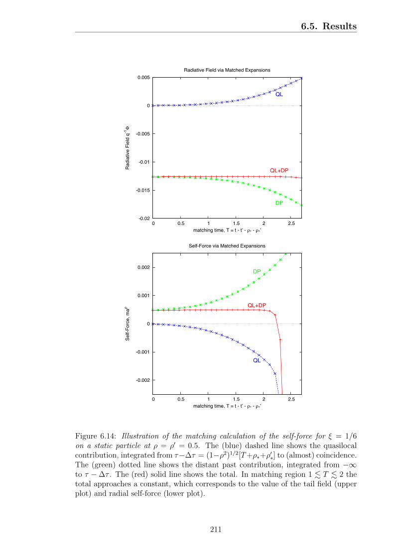
6.5. Results
-0.02
-0.015
-0.01
-0.005
0
0.005
0 0.5 1 1.5 2 2.5
Radi
ative
Fie
ld q
-1!
matching time, T = t - t’ - "* - "*’
Radiative Field via Matched Expansions
QL+DP
QL
DP
-0.002
-0.001
0
0.001
0.002
0 0.5 1 1.5 2 2.5
Self-
Forc
e, m
a!
matching time, T = t - t’ - !* - !*’
Self-Force via Matched Expansions
QL+DP
QL
DP
Figure 6.14: Illustration of the matching calculation of the self-force for ξ = 1/6on a static particle at ρ = ρ′ = 0.5. The (blue) dashed line shows the quasilocalcontribution, integrated from τ−∆τ = (1−ρ2)1/2[T+ρ∗+ρ
′∗] to (almost) coincidence.
The (green) dotted line shows the distant past contribution, integrated from −∞to τ −∆τ . The (red) solid line shows the total. In matching region 1 . T . 2 thetotal approaches a constant, which corresponds to the value of the tail field (upperplot) and radial self-force (lower plot).
211

6.5. Results
-0.014
-0.012
-0.01
-0.008
-0.006
-0.004
-0.002
0
0 0.1 0.2 0.3 0.4 0.5 0.6 0.7 0.8 0.9 1
Radi
ative
Fie
ld, q
-1 !
"
# = 1/6
0
0.05
0.1
0.15
0.2
0.25
0.3
0.35
0 0.1 0.2 0.3 0.4 0.5 0.6 0.7 0.8 0.9 1
Radi
ative
fiel
d, q
-1 !
"
# = 1/8
Figure 6.15: The Tail Field Generated by the Static Particle. The plot shows thetail field for the static particle at ρ = ρ′. For the case ξ = 1/6 (top) the field isnegative whereas for the case ξ = 1/8 it is positive (bottom). Note the differingscales on the vertical axis.
of the field is maximal at ρ = 0 and tends to zero as ρ→ 1 as ΦR ∼ (1− ρ2)1/2.
Figure 6.16 shows the radial self-force maρ acting on a static particle. The results
of the matched expansion results are shown as points, and the results of the ‘massive
field regularization method’ (described in Sec. 6.4.1) are shown as the solid line. The
latter method provides an independent check on the accuracy of the former. We find
agreement to approximately six decimal places between the two approaches. We find
the self-force at ρ = 0 to be zero, as expected from the symmetry of the static region
of the Nariai spacetime. The self-force also tends to zero as ρ → 1. Between these
212

6.5. Results
0.0 0.2 0.4 0.6 0.8 1.00.0000
0.0001
0.0002
0.0003
0.0004
0.0005
Ρ
Rad
ialS
elf-
forc
e,m
aΡ
q2
Radial Self-Force on a Static Particle in Nariai Spacetime
Ξ=16
0.0 0.2 0.4 0.6 0.8 1.00.00
0.01
0.02
0.03
Ρ
Rad
ialS
elf-
forc
e,m
aΡ
q2
Radial Self-Force on a Static Particle in Nariai Spacetime
Ξ=18
Figure 6.16: The Radial Self-Force on the Static Particle. The radial componentof the self-force, q−2maρ, is plotted as a function of the ρ of the static particle.The self-force was calculated by two methods: ‘matched expansion’ [(black) dots]and ‘massive field regularization’ [(blue) curve]. The left plot shows the curvaturecoupling ξ = 1/6 whereas the right plot shows ξ = 1/8. Note the difference in scalesfor the two cases.
limits, the self-force rises to a single peak, the magnitude and location of which
depends on the curvature coupling ξ. We find that the peak of the self-force (in
units such that the scalar charge, q, is 1) is approximately 4.9 × 10⁻⁴ for ξ = 1/6
and approximately 3.8 × 10⁻² for ξ = 1/8. Note that the argument (see Sec.2.2.1)
in [93] that the scalar self-force with ξ = 1/8 should be zero for a static particle in
a spacetime (such as Nariai) possessing a conformally flat 3-D spatial section does
not seem to hold here.
213

Discussion
The self-force acting on a particle is determined by its entire past history. This
is encapsulated in the MiSaTaQuWa equation through an integral of the retarded
Green function along a timelike worldline, therefore requiring knowledge of the Green
function for points separated along that worldline (other methods negate the need
for knowledge of the Green function by computing the regularized field [172, 71, 67]
or metric perturbation [69] directly). In this thesis, we have presented the first
practical demonstration of a self-force calculation using the method of matched
expansions, first proposed over a decade ago by Poisson and Wiseman [81]. The
method relies on an expansion of the Green function in two regions: a quasilocal
region, corresponding to the recent history of the particle, and a distant past region.
In particular, the primary focus of this thesis has been on computing the Green
function within the quasilocal region.
The examples of self force calculations presented in this thesis are for the case of
a scalar field. From an astrophysical perspective, we are more interested in the case
of a gravitational field. The quasilocal contribution to the gravitational self-force has
previously been calculated for vacuum spacetimes up to O(σ3/2) [80]. As is apparent
from Chapter 6, it is necessary to take the calculation to higher order to allow the
matching point ∆τ to lie far enough into the particle’s past to match onto a quasi-
normal mode sum calculated Green function. Fortunately, the covariant method
of Chapter 4 is largely independent of the type of field considered, the only issue
being the specific form of the transport equations, (1.8a) and (1.8b) for V AB′r (x, x′)
and V AB′0 (x, x′), respectively. The gravitational version of this equation contains
214

Discussion
additional factors of gab′ (and its derivatives) over its scalar counterpart. However,
we have already provided transport equations for these additional bi-tensors and
our Mathematica code can calculate their covariant series expansions. It should
therefore be possible to calculate the gravitational Green function with little extra
effort.
In Chapter 2 we introduced the method of matched expansions and derived
expressions for the quasilocal contribution to the scalar self-force. These expressions
are totally general and may be applied to the computation of the quasilocal scalar
self-force for both geodesic and non-geodesic motion in any spacetime, with any
coupling constant and any field mass.
In Chapters 3 and 4 we developed methods for calculating the Green function
within the quasilocal region, where the Hadamard form may be used. The coordinate
approach of Chapter 3 exploits the spherical symmetry of a spacetime to yield an
efficient method for computing the quasilocal Green function. This allowed the
coordinate series expansion of V (x, x′), appearing in the Hadamard parametrix of
the Green function, to be computed to significantly higher order than was done
previously [97, 78]. However, we feel that the method has now been taken to the
limit of its potential. It is necessarily restricted to spherically symmetric spacetimes,
which are inadequate for a full study of the self-force in the context of EMRIs.
In contrast, the covariant method of Chapter 4 is totally general, being valid for
any type of field in any spacetime with arbitrary field mass and arbitrary curvature
coupling. This method has the flexibility required for a complete study of the
quasilocal self-force. Furthermore, it also has applications in other areas such as
quantum field theory in curved spacetime and quantum gravity.
Several of the covariant expansion expressions computed by our code using the
Avramidi method have been previously given in Ref. [36], albeit to considerably
lower order (for example, in Ref. [36] Decanini and Folacci give V (x, x′) to order
(σa)4 compared to order (σa)20 here). Comparison between the two results gives
exact agreement, providing a reassuring confirmation of the accuracy of both our
215

Discussion
expressions and those of Ref. [36] (and confirming the error in Ref. [173] found by
Decanini and Folacci). For expansions not given by Decanini and Folacci, we have
compared our results with those found by Christensen [39, 40]. Again, we have
found that our code is in exact agreement.
The expressions for the DeWitt coefficients as computed by our Mathematica
code are very general. However, they are not necessarily given as a minimal set.
For example, the DeWitt coefficient a3 may be written as a sum of four terms, yet
our code produces a sum of seven equivalent terms. It is quite probable, however,
that a set of transformation rules could be produced to reduce our expression to a
canonical form in terms of some basis. Some progress in that direction has already
been made. Fulling, et al. [116] (and more recently Decanini and Folacci [156])
have establish a linearly independent basis for the Riemann polynomials3, involving
product of Riemann and Ricci tensors. The first steps towards the automation of
the canonicalization process have been taken with the release of the Invar package
[174, 175] for Mathematica, which is so far able to quickly canonicalize the scalar
algebraic invariants with up to 7 Riemann tensors and differential invariants up to
12 metric derivatives. As our code is already written in Mathematica [176] and has
the ability to output into the xTensor [120] notation used by Invar, an extension of
the package to allow for the canonicalization of tensor invariants would allow our
expressions to be immediately canonicalized with no further effort.
There remains one context in which a coordinate expansion of the Green function
is more appropriate: the case of non-geodesic motion. This is not very surprising as
the benefit of using a covariant expansion hinges on having a geodesic along which to
expand. The coordinate expansion, on the other hand, more naturally characterizes
motion which is not along a geodesic. However, as Sec. 5.2.2 demonstrates, even
in this case, beginning with a covariant expansion and computing the coordinate
expansion from it is preferable as it allows the calculation to be done for arbitrary
3The terms in these polynomials are classified [116] by their rank (number of free indices), order(number of derivatives of the metric - 2 per riemann tensor and 1 per explicit covariant derivative)and degree (number of factors). For example RaβγδRb
βγδ is rank 2, order 4 and degree 2, whileR(a|αβγ|RbβγδRαcd|δ|;e) is rank 5, order 7 and degree 3.
216

Discussion
spacetimes, rather than only those with spherical symmetry.
The covariant expansion method yields expressions involving Riemann tensor
polynomials. In order to compute the Green function in a specific spacetime, it is
necessary to explicitly evaluate these polynomials in terms of the spacetime coordi-
nates. In Chapter 5, we gave examples of such an evaluation using the GRTensorII
[141] tensor algebra package. Only the leading two orders in the series were consid-
ered (up to order (σa)5), yet the calculation was already reaching the limit of the
ability of GRTensorII given currently available computational power. Improvements
in computational performance will be of limited benefit; the complexity of the cal-
culation is exponential in the order of the term considered so that even an order
of magnitude increase in performance will make little difference. A better solution
would be to develop improved algorithms. Some hope lies in the fact that we are
most interested in calculating V AB′(x, x
′) for massless fields in 4-dimensional type-
D vacuum spacetimes. This suggests [177] that the Geroch-Held-Penrose (GHP)
adaptation [178] (for a thorough treatment, see Refs. [179, 180]) of the Newman-
Penrose formalism [181] may be of use in producing significantly simplified expres-
sions. There is additional hope that the canonicalization process proposed above
may yield expressions which are significantly simplified and therefore more easily
evaluated for a specific spacetime.
The high order expansions of the quasilocal Green function facilitated an inves-
tigation of the convergence properties of the series, described in detail in Chapter 3.
We found that the series was divergent before the normal neighborhood boundary
was reached. However, this divergence does not correspond to a singularity in the
Green function for real-valued point separation (in general the radius of conver-
gence of a Taylor series extends to the first occurrence in the complex plane of a
singularity of the function being approximated). We have found that, using Pade
resummation, the domain of validity of the series can be extended beyond the circle
of convergence, to within a short distance of the normal neighborhood boundary.
For convenience, the Pade resummation was applied to the coordinate expansion of
217

Discussion
the Green function. We expect it to be equally applicable to the covariant series
method of Chapter 4; both expansions are Taylor series and there is no physical
singularity in the Green function before the edge of the normal neighborhood is
reached. Additionally, our analysis focused on the case of one dimensional series.
This was done for reasons of simplicity and clarity. For multi-dimensional series,
one could re-express each of the coordinates in terms of a single parameter, as was
done in Sec. 3.2 for the case of a circular geodesic in Schwarzschild. Alternatively,
one could employ the generalization of Pade resummation to double (and higher
dimensional) power series, as developed by Chisholm [182, 183].
In Sec. 4.4, we discussed a numerical implementation of the transport equation
approach to the calculation of V0. This implementation is capable of computing V0
along a geodesic in any spacetime, although we have chosen Nariai and Schwarzschild
spacetimes as examples. The choice of Nariai spacetime has the benefit that an
expression for V0 is known exactly [62] (the key analytic results are presented in
Sec. 1.3.4). This makes it possible to compare our numerical results with the analytic
expressions to determine both the validity of the approach and the accuracy of the
numerical calculation. Given parameters allowing the code to run in under a minute,
we found that the numerical implementation is accurate to less than 1% out as far
as the location of the singularity of V0, at the caustic point (i.e. everywhere within
the normal neighborhood).
In integrating the transport equations given in Sec. 4.2 along a specific geodesic,
we are not limited to the normal neighborhood. The only difficulty arises at caustics,
where some bi-tensors such as ∆1/2 and V0 become singular. However, this is not
an insurmountable problem. The singular components may be separated out and
methods of complex analysis employed to integrate through the caustics, beyond
which the bi-tensors once more become regular (but not necessarily real-valued)
[29]. This is highlighted in Fig. 4.7, where our plot of ∆1/2 and V0 extends outside
the normal neighborhood, the boundary of which is at φ ≈ 1.25, where the first null
geodesic re-intersects the orbit. It does not necessarily follow, however, that the
218

Discussion
Green function outside the normal neighborhood is given by this value for V (x, x′).
Instead, one might expect to obtain the Green function by considering the sum of
the contributions obtained by integrating along all geodesics connecting x and x′
(other than at caustics, there will be a discrete number of geodesics).
In Chapter 6, we presented a full application of the method of matched expan-
sions in the Nariai spacetime. Through matching the ‘quasilocal’ and ‘distant past’
expansions, the full retarded Green function may be reconstructed. With full knowl-
edge of the Green function, one may accurately compute the ‘tail’ contribution to
the self-force. In Sec. 6.4.2, we employed the matched expansion method to numeri-
cally compute the self-force acting on a static particle in the Nariai spacetime. The
resulting value for the self-force is in excellent agreement with the result from an
alternative method (Sec. 6.4.1), to approximately one part in 106.
This study of the self-force in Nariai spacetime has provided a number of insights
into the properties of the Green function, which are of relevance to any future
investigation of the Schwarzschild spacetime. Namely,
• The Green function Gret(x, x′) is singular whenever x and x′ are connected
by a null geodesic. The nature of the singularity depends on the number of
caustics that the wave front has passed through. After an even number of
caustics, the singularity is a delta-distribution, with support only on the light
cone. After an odd number of caustics, the Green function diverges as 1/πσ.
A four-fold repeating pattern occurs, i.e. δ(σ), 1/πσ, −δ(σ), −1/πσ, δ, etc.
• The four-fold singular structure can be shown to arise from a Hadamard-like
ansatz (6.76) valid even outside the normal neighborhood, if we allow U(x, x′)
to pick up a phase of −i upon passing through a caustic. The accumulation
of phase may be deduced by analytically continuing the integral for the Van
Vleck determinant through the singularities (due to caustics).
• The effect of caustics on wave propagation has been well-studied in a number
of other fields, such as optics [184], acoustics [160], seismology [154], symplectic
219

Discussion
geometry [161] and quantum mechanics [162]. It may be that mathematical
results developed in other fields may be usefully applied to wave propagation
in gravitational physics.
• The ‘tail’ self-force cannot be calculated from the ‘quasilocal’ contribution
alone. For instance, Fig. 6.13 would appear to show that a significant part of
the tail field is generated by the segment of the world line which lies outside
of the normal neighborhood. Unlike in flat space, the field generated by an
accelerated particle may propagate several times around the black hole before
later re-intersecting the worldline of the particle (see Fig. 2.2). Radiation from
near these orbits will give an important contribution to the self-force which
cannot be neglected.
The calculation of the ‘distant past’ Green function in Nariai spacetime relies on
a ‘quasinormal mode sum’ expansion. The QNM sum is only valid at ‘late times’,
t − t′ ≥ tc, where tc is approximately the time it takes for a geodesic to reflect
from the peak of the potential barrier. One may wonder whether the quasilocal
Green function may be accurately calculated in an overlapping spacetime region at
times later than this light reflection time. In the Nariai case, we have demonstrated
that this is the case. There is a sufficient regime of overlap in t − t′ in which both
the ‘quasilocal’ and ‘QNM sum’ expansions are valid for the method to be applied
successfully. There is also a strong indication that this is the case in Schwarzschild.
From Sec. 3.3.3 we see that the higher order terms of the quasilocal series only have
a significant contribution near the radius of convergence (for the Taylor series) or
normal neighborhood boundary (for the Pade approximant), while the reflection
time (t− t′ = 2r∗ ≈ 12.77M , for the case of a static particle at r = 10M considered
in Sec. 3.3.3) is well within the normal neighborhood. We can therefore be optimistic
that matched expansion self-force calculations will be possible for Schwarzschild.
The question of whether this also follows through for the Kerr spacetime is yet
to be studied, but there is little reason to expect the answer to be different than
in the Schwarzschild and Nariai cases. The full caustic structure of Kerr spacetime
220

Discussion
has recently been studied [185] and shown to have additional features compared to
the Schwarzschild case. However, if the motion is restricted to the equatorial plane,
the caustic structure of Kerr bears a striking resemblance to that of Schwarzschild
(see Fig. 1.2).
221

Discussion
Light cone for the Kerr spacetime. The θ coordinate is suppressed so that onlygeodesics in the equatorial plane are shown. The caustic structure bears a strikingresemblance to that of Schwarzschild (Fig. 1.2).
222

Appendix A
Odd Order Series Coefficients of
Symmetric Bi-scalars
A.1 Covariant Series
In this appendix, we derive an expression for rewriting odd order coefficients of
covariant series expansions of any symmetric bi-scalar in terms of the lower even
order coefficients. This not only allows for the simplification of covariant series
expressions, but allows the order of an even order covariant expansion to be increased
by one order with ease.
Taking, for example, the symmetric bi-scalar V (x, x′) appearing in the Hadamard
form of the Green function, we have the identity,
V (x, x′) = V (x′, x) . (A.1)
Repeatedly taking symmetrized covariant derivatives of both sides of this equation
and taking coincidence limits, we arrive at an expressions for the odd order terms
in terms of all the lower (even) order terms [186]:
Va1a2...an =1
2
n−1∑
k=0
(n
k
)(−1)kV(a1a2...ak;,ak+1...an) for n odd. (A.2)
223

A.2. Odd Order Coordinate Series Coefficients ofSymmetric Bi-scalars
Recursively applying this identity to eliminate all odd order terms, we get expres-
sions for the coefficients of the terms of order σ52 :
vabcde =1
2v;(abcde) −
5
2v(ab;cde) +
5
2v(abcd;e) (A.3a)
vabc = −1
4v;(abc) +
3
2v(ab;c) (A.3b)
va =1
2v;a (A.3c)
In general, this can be written as
Va1a2...an =n−1∑
k=0k even
(n
k
)2(2n−k+1 − 1)
n− k + 1Bn−k+1V(a1a2...ak,ak+1...an) for n odd (A.4)
where the Bn are the Bernoulli numbers [103]. These expressions are equally valid
for any symmetric bi-tensor, so we may use it for both the calculation of higher
order V(n) a1...an as used in (1.4) and higher order Va1...an as used in (2.23).
A.2 Odd Order Coordinate Series Coefficients of
Symmetric Bi-scalars
Similarly to the case of covariant series described in Appendix A.1, we may express
odd order coefficients of coordinate series expansions of any symmetric bi-scalar in
terms of the lower even order coefficients. Again, taking, for example, the symmetric
bi-scalar V (x, x′) appearing in the Hadamard form of the Green function, we have
the identity,
V (x, x′) = V (x′, x) (A.5)
224

A.2. Odd Order Coordinate Series Coefficients ofSymmetric Bi-scalars
We use expression (5.23) for v (x, x′) in the above to give:
∞∑
i,j,k=0
vijk (r) (t− t′)2i(cos (γ)− 1)j (r − r′)k
=∞∑
i,j,k=0
vijk (r′) (t′ − t)2i(cos (γ′)− 1)
j(r′ − r)k (A.6)
Now, in a similar vein to Appendix A.1, if we take a sufficient number of symmetrized
derivatives of both sides and then take the coincidence limit, it is possible to express
odd order coefficients in terms of derivatives of the lower order coefficients.
For the cases of the coordinate series expansion of V (x, x′) relevant to the current
work, the calculation is made even simpler by spherical symmetry. The coefficients
vijk are functions of r only (i.e. they have no dependence on t or γ). Additionally,
since (t − t′)2i and (cos(γ) − 1)j are both even functions, they are invariant under
interchange of primed and unprimed coordinates. This means that we can express
(A.6) in the simpler form:
∞∑
k=0
vijk (r) (r − r′)k =∞∑
k=0
vijk (r′) (r′ − r)k (A.7)
Taking r-derivatives of both sides of this equation and taking the coincidence limit
r′ → r gives the result
vij1 = −1
2vij0,r (A.8)
As a specific example, this can be applied to the results of Ref. [97] to calculate
v301, v211, v121 and v031. This gives:
v301 = − 1
960
M2 (r − 2M)2 (598rM2 − 195Mr2 + 20r3 − 585M3)
r16(A.9a)
v211 =1
896
M2 (r − 2M) (3352rM2 − 1099Mr2 + 112r3 − 3240M3)
r13(A.9b)
v121 = − 9
1120
M2 (228rM2 − 91Mr2 + 12r3 − 189M3)
r10(A.9c)
v031 =1
3360
M2 (−155Mr + 56r2 + 36M2)
r7(A.9d)
225

Appendix B
Vacuum expressions for the
DeWitt Coefficients
The expressions given in Chapter 4 and Ref. [36] are unnecessarily long and unwieldy
for the purposes of the self-force calculations of Chapter 5. There, we are only
interested in massless fields in vacuum spacetimes (mfield = 0, Rαβ = 0, R = 0),
so the majority of the terms vanish and we are left with much more manageable
expressions for the vna1...ap . They are:
v0 = 0 (B.1a)
v0 a = 0 (B.1b)
v0 ab = − 1
720gabI (B.1c)
v0 abc = − 1
480g(abI;c) (B.1d)
v0 abcd = − 2
525Cρ
(a|σ|bCσc|ρ|d) −
2
105Cρστ
(aC|ρστ |b;cd) −1
280Cρ ;τ(a|σ|b Cσ
c|ρ|d);τ
− 1
56Cρστ
(a;bC|ρστ |c;d) −2
1575CρστκCρ(a|τ |bC|σ|c|κ|d)
− 2
525Cρκτ
(aCσ
|ρτ | bC|σ|c|κ|d) −8
1575Cρκτ
(aCσ
|ρ| |τ |bC|σ|c|κ|d)
− 4
1575Cρτκ
(aCσ
|ρτ | bC|σ|c|κ|d) (B.1e)
v1 =1
720I (B.1f)
v1 a =1
1440I;a (B.1g)
226

Appendix B. Vacuum expressions for the DeWittCoefficients
v1 ab = − 1
1400CρστκCρστ(a;b)κ +
1
1575Cρστ
aCρστb +29
25200CρστκCρστκ;(ab)
+1
1680Cρστ
a;κC;κ
ρστb +1
1344Cρστκ
;aCρστκ;b +1
756CρκσλCτ
ρσaCτκλb
− 1
1800CρκσλCρστaC
τκλ b +
19
18900CρσκλCρστaC
τκλ b (B.1h)
v2 = − 1
6720CρστκC
ρστκ − 1
8960Cρστκ;λC
ρστκ;λ
− 1
9072CρκσλCρασβC
α βκ λ −
11
18440CρσκλCρσαβC
αβκλ (B.1i)
where Cabcd is the Weyl tensor and I = CαβγδCαβγδ.
Moreover, we have chosen to work with an expression for V (x, x′) as given in
(2.23), rather than the expression used in Chapter 4, Ref. [36] and Eq. (1.4). The
two sets of coefficients may be related by using
2σ = σασα (B.2)
to rewrite (1.4) in terms of a series expansion in powers of σα. We can then equate,
power by power, the coefficients of powers of σα to the corresponding terms in (2.23)
to give:
v = v0 (B.3a)
va = v0 a (B.3b)
vab = v0 ab + v1gab (B.3c)
vabc = v0 abc + 3v1 (agbc) (B.3d)
vabcd = v0 abcd + 6v1 (abgcd) + 6v2g(abgcd) (B.3e)
vabcde =1
2v;(abcde) −
5
2v(ab;cde) +
5
2v(abcd;e) (B.3f)
Filling in the values for the vna1...ap we see that a large number of terms either cancel
227

Appendix B. Vacuum expressions for the DeWittCoefficients
or combine to give:
v = 0 (B.4a)
va = 0 (B.4b)
vab = 0 (B.4c)
vabc = 0 (B.4d)
vabcd = − 1
280Cρ σ(a b|;α|C
;α|ρ|c|σ|d) −
2
315CρστκCρ(a|τ |bC|σ|c|κ|d)
+1
105Cρ σ(a bC
τκ|ρ|cC|τκσ|d) +
1
840CρστκC λ
ρσ (aC|τκλ|bgcd)
+1
8960Ig(abgcd) −
1
40320CρστκC uv
ρσ Cτκuvg(abgcd) (B.4e)
vabcde =5
2v(abcd;e) (B.4f)
Here, we have used a slight modification of the basis of Riemann tensor polyno-
mials suggested by Fulling, et al. [116] in order to express the result in its simplest
possible canonical form. We have chosen an equivalent basis for Weyl tensor poly-
nomials by ignoring all terms involving Rab and R and replacing Rabcd by Cabcd. We
have also ignored all terms which vanish or are not independent under symmetriza-
tion of the free indices. Next, we have eliminated terms involving two covariant
derivatives of a tensor in favor of terms involving two covariant derivatives of a
scalar and single covariant derivatives of a tensor. We have done this as it is com-
putationally faster and easier to calculate the covariant derivative of a scalar than
of a tensor. Finally, we have used the identity [187]:
∇(r)Cρστ
(a∇(s)C|ρστ |b) =1
4g(ab)∇(r)C
ρστκ∇(s)Cρστκ (B.5)
(where ∇(r) indicates r covariant derivatives) to combine some of the remaining
terms. The motivation for working with V (x, x′) rather than the Vn(x, x′) is imme-
diately apparent from the vast simplification that occurs.
228
Appendix C
Pade Approximants and
Convergence Properties of Series
In this appendix, we will review some of the key features of Pade approximants and
of the convergence properties of series. We give two simple examples, which serve
to highilight these features for those less familiar with these topics.
In Chapter 3, we investigated the convergence properties of the series expansion
of the function V (x, x′) appearing in the Hadamard form of the Green function. We
found that the Taylor series was divergent at a point (the radius of convergence)
where the actual Green function was behaving normally (i.e. not singular). We
asserted that this divergence must be as a result of V (x, x′) being singular some-
where (in the complex plane) on the circle of convergence. We also demonstrated
how the method of Pade approximants may be used to extend the domain of the
series beyond its radius of convergence. Both the divergence of the Taylor series and
the effectiveness of the Pade approximants may at first seem mysterious. V (x, x′)
is a real-valued function with real arguments, so how can complex values possi-
bly have any effect? To aid in the understanding, it is helpful to consider some
simple functions and investigate the convergence properties of their series represen-
tations and Pade approximants. In this Appendix, we will study two cases which
are particularly illuminating. Further details, including examples may be found in
229

Appendix C. Pade Approximants and ConvergenceProperties of Series
æ
æ
-1.5 -1.0 -0.5 0.0 0.5 1.0 1.5-1.5
-1.0
-0.5
0.0
0.5
1.0
1.5
Re@xD
Im@x
D
Figure C.1: Circle of convergence of the Taylor series of f(x) = 1/(1 + x2). Sincef(x) is singular at x = ±i, its Taylor series also diverges everywhere outside itscircle of convergence.
Refs. [106, 107, 108, 109].
Example 1
Consider the real-valued function
f(x) ≡ 1
1 + x2(C.1)
with real argument x. f(x) has the Taylor series expansion
1
1 + x2=∞∑
n=0
(−1)nx2n (C.2)
about x = 0. This series is only convergent provided |x| < 1, yet f(x) is clearly
finite for all real x. So, what is the cause of the failure of the series to diverge for
|x| ≥ 1? The answer is found by allowing x to be complex. We then find that f(x)
is singular at x = ±i. Somewhat surprisingly, it is this singularity that also causes
the Taylor series to diverge for real-valued |x| ≥ 1. In fact, the Taylor series will
diverge at all points outside the circle of convergence (see Fig. C.1).
We next try to improve the convergence of the Taylor of series using Pade ap-
230

Appendix C. Pade Approximants and ConvergenceProperties of Series
-2 -1 0 1 20.0
0.2
0.4
0.6
0.8
1.0
x
gHxL
Figure C.2: Series expansion of 1/(1 + x2). The Taylor series (purple) diverges at|x| = 1, whereas f(x) (blue) is finite for all real x. The Pade approximant is exactlyequal to f(x), so their plots are overlapping.
proximants. We find that, provided the Pade approximant is chosen such that it
can accurately represent the 1/(1 + x2) singularity of f(x), it will successfully ex-
tend the domain of the series representation beyond the radius of convergence. This
requirement amounts to requiring that the series in the denominator be at least of
order x2. In fact, in this case we find that the Pade approximant fully recovers the
original function,
PNM =
1
1 + x2∀ M ≥ 2. (C.3)
This remarkable result is illustrated in Fig. C.2.
Example 2
In the previous case, we found that the Pade approximant was able to exactly re-
produce the original function from its Taylor series. This success stems from the
polynomial nature of the numerator and denominator of f(x). However, Pade resum-
mation may also be extremely effective for functions which may not be represented
as a rational function of two polynomials. To illustrate this point, consider the
real-valued function
g(x) ≡ ln (1 + x)
x, (C.4)
231

Appendix C. Pade Approximants and ConvergenceProperties of Series
0 5 10 15 200.0
0.5
1.0
1.5
2.0
x
gHxL
Figure C.3: Series expansion of g(x) = ln(1 + x)/x. The Taylor series (purple)diverges at |x| = 1, whereas g(x) (blue) is finite for all real x. The diagonal Padeapproximant P 2
2 (brown) dramatically outperforms the off-diagonal Pade approxi-mant P 32
8 (green) despite needing much fewer terms from the Taylor series.
with real argument x ∈ (−1,∞). g(x) has the Taylor series expansion
ln (1 + x)
x=∞∑
n=0
(−1)n
n+ 1xn (C.5)
about x = 0. As before, this series is only convergent provided |x| < 1, yet g(x)
is finite for all real x > −1. This divergence at |x| ≥ 1 may be attributed to the
singularity of g(x) at x = −1.
Since g(x) cannot be written as a rational function, one may not expect Pade
resummation to be so effective. On the contrary, Fig. C.3 shows that Pade resum-
mation may be extremely effetive, particularly when the right choice of N and M is
made. In particular, the diagonal Pade approximant, P 22 yields remarkable results
with only 4 terms in the Taylor series required. Not only does its domain extend far
beyond the radius of convergence of the Taylor series, it also dramatically outper-
forms the off-diagonal Pade approximant, P 328 , while requiring only a tenth as many
terms from the original Taylor series. This highlights the importance of choosing
the correct Pade approximant for the problem. In general, the choice N ∼ M is
best.
232

Appendix D
Massive Scalar Field in Nariai
In Sec. 6.4.1 we used the massive field approach of Rosenthal [91] to compute the
regularized self-force acting on a static particle in Nariai spacetime. In this prescrip-
tion, we must compute the derivative of a massive scalar field in the limit of the
field mass going to infinity. In this appendix, we derive an explicit expression for
the massive scalar field, closely following the method of Ref. [85], which considered
the Schwarzschild case.
We will solve the massive scalar field equation,
(− Λ2 − ξR
)φΛ = −4πρΛ, (D.1)
where Λ is the mass of the field, ξ is the coupling to the scalar curvature, R = 4 is
the Ricci scalar in Nariai and ρΛ represents a static point source. Decomposing into
spherical harmonics and switching to the ‘tortoise’ coordinate defined by
dρ∗dρ
=1
f, (D.2)
where f(ρ) = 1− ρ2, the radial part of the wave equation becomes
φΛlm,ρ∗ρ∗ −
(f(ρ)l(l + 1) + f(ρ)
(Λ2 + ξR
))φΛlm = −4πρΛ
lmf(ρ) (D.3)
233

Appendix D. Massive Scalar Field in Nariai
with
ρΛlm = qδ (ρ− ρ0)
√f (ρ0)Y lm∗ (θ0, φ0) . (D.4)
Assuming two linearly independent solutions χ+ and χ− to the homogeneous equa-
tion, both dependent on l , the solution can be expressed as
φΛlm = −4πq
√f (ρ0)Y lm∗ (θ0, φ0)
χ− (ρ<)χ+ (ρ>)
W [χ−, χ+]ρ0(D.5)
where W [χ−, χ+]ρ0 is the Wronskian evaluated at ρ0. Note, that the factor of f(ρ)
has been absorbed into the fact that the derivatives of the Wronskian are changed
from ρ to ρ∗ derivatives. Now, performing the sum over m, we get
φΛl = −2q
(l +
1
2
)√f (ρ0)
χ− (ρ<)χ+ (ρ>)
W [χ−, χ+]ρ0(D.6)
where there is no Legendre polynomial since we let θ − θ′ = 0. We now need to
take a ρ derivative and sum over l. To do so, we split into a part which is regular
as ρ→ ρ0 and a part which is divergent,
φΛ,ρ =
∞∑
l=0
hl +∞∑
l=0
(φΛl,ρ − hl
). (D.7)
We use a WKB approximation [108] to find the large l behavior of hl(ρ):
χ+ = e−S0/δ+S1−S2δ (D.8a)
χ− = c1eS0/δ+S1+S2δ + c2e
−S0/δ+S1−S2δ. (D.8b)
Note that for the outer solution, we want the field to be 0 at infinity, which fixes
the boundary conditions. Also note that S0 and S2 must have the same sign as a
result of the differential equations they satisfy. The differential equations satisfied by
S0, S1 and S2 are found by substituting eS0/δ+S1+S2δ into (D.3), and independently
setting each power of δ equal to zero, noting that the term involving V (ρ) will be
234

Appendix D. Massive Scalar Field in Nariai
large for large l and so balances the dominant 1/δ2 term. This gives
S ′0(ρ) =1
f(ρ)
√V (ρ) (D.9a)
S ′1(ρ) = − V′(ρ)
4V (ρ)(D.9b)
S ′2(ρ) =1
f(ρ)
(f(ρ)(f(ρ)V ′(ρ)),ρ
8V (ρ)3/2− 5
(f(ρ)V ′(ρ))2
32V (ρ)5/2
), (D.9c)
where the equation for S1 may be solved immediately, giving
S1 = −1
4lnV (ρ). (D.10)
We note that the Sn goes like L1−n and Λ1−n, where L ≡ (l + 1/2). Next, we
substitute our two WKB solutions, (D.8), into (D.6) and differentiate with respect
to ρ to get
φΛl ,ρ =
eS(ρ)(c1 + c2e
−2(S0(ρ0)+S2(ρ0)))LqS ′(ρ)
c1
√f(ρ0) (S ′0(ρ0) + S ′2(ρ0))
, (D.11)
where
S(ρ) ≡ S0(ρ0)− S1(ρ0) + S2(ρ0)− (S0(ρ)− S1(ρ) + S2(ρ)). (D.12)
We can now drop the c2 term since it dies off for large L faster than any negative
power of L (since it is like e−L), and are left with
φΛl ,ρ =
eS(ρ)LqS ′(ρ)√f(ρ0) (S ′0(ρ0) + S ′2(ρ0))
. (D.13)
Expanding S(ρ) in a large L asymptotic series, we find that the order L contribution
(coming from S0) is given by
α ≡ sin−1(ρ)− sin−1(ρ0) ≈ ρ− ρ0√1− ρ2
0
+ρ0(ρ− ρ0)2
2 (1− ρ20)
3/2+O
[(ρ− ρ0)3
]. (D.14)
We now deal with the essential singularity in (D.13) (from the order L term in
235

Appendix D. Massive Scalar Field in Nariai
S(ρ)) by rewriting the derivative of the field as
φΛl, ρ = e−αL
(eS(ρ)+αLLqS ′(ρ)√
f(ρ0) (S ′0(ρ0) + S ′2(ρ0))
)(D.15)
and we can find an asymptotic expansion in L for the term in the brackets. The
order L component is
Al = −q(1− ρ20)1/4
(1− ρ2)3/4(D.16a)
The order 1 component is
Bl =1
48q
[−1 + ρ20
−1 + ρ2
]1/4
24ρ
1− ρ2
+1√
1− ρ2
[6(−1 + 4Λ2 + 4Rξ
)(sin−1(ρ)− sin−1(ρ0))
+12(−10 + ρ)(873649 + 2ρ(−27460 + 779ρ))
(1− ρ20)
7/2
](D.16b)
The order L−1 component is
Cl =q
4608 (1− ρ2)7/4 (1− ρ20)
27/4
576
(−1 + ρ2
0
)6 (ρ2 − ρ2
0
)
+(−1 + ρ2
) [− 12(−10 + ρ)(873649 + 2ρ(−27460 + 779ρ))
− 6(1− ρ2
0
)7/2 (−1 + 4Λ2 + 4Rξ)
(sin−1(ρ)− sin−1(ρ0))]2
+48ρ
1− ρ2
(1− ρ2
)3/2 (1− ρ2
0
)7[− 12(−10 + ρ)(873649 + 2ρ(−27460 + 779ρ))
− 6(1− ρ2
0
)7/2 (−1 + 4Λ2 + 4Rξ)
(sin−1(ρ)− sin−1(ρ0))]
. (D.16c)
Next, we must calculate the sum over L,
∞∑
l=0
hl =∞∑
l=0
e−αL[AlL+Bl + ClL
−1 +O(L−2)]. (D.17)
236

Appendix D. Massive Scalar Field in Nariai
where we can make use of the identities
∞∑
l=0
Le−αL =cosh(α/2)
4 sinh2(α/2)(D.18a)
∞∑
l=0
e−αL =1
2 sinh(α/2)(D.18b)
∞∑
l=0
L−1e−αL = 2 tanh−1(e−α/2
)(D.18c)
In the end, we only need our result as an expansion in inverse powers of (ρ−ρ0), up
to order (ρ− ρ0)0. Combining (D.14), (D.16) and (D.17) and expanding in (ρ− ρ0),
we get
∞∑
l=0
hl = −q√
1− ρ20
(ρ− ρ0)2+q (−2 + 3Λ2 + 3Rξ)
6√
1− ρ20
+O[(ρ− ρ0)1
]. (D.19)
With the divergent part of Eq. (D.7) calculated, we must now calculate the
regular part for large Λ. In this case, we only need the term that is constant in ρ,
so that we have ρ = ρ0. Letting L → λY and using the Riemann integral over Y,
we can then compute the sum over l of this regular part to get
− qρ0Λ
2(1− ρ20). (D.20)
Combining this with Eq. (D.19) we get the expression for the radial derivative of
the scalar field (up to O [(ρ− ρ0)0]):
φΛ,ρ = −q
√1− ρ2
0
(ρ− ρ0)2+
(− qρ0Λ
2(1− ρ20)
+q (−2 + 3Λ2 + 3Rξ)
6√
1− ρ20
)+O
[(ρ− ρ0)1
]. (D.21)
Finally, applying the massive field prescription for calculating the self-force:
fρ = q limΛ→∞
limδ→0
∆φ,ρ +1
2q[Λ2nρ + Λaρ
](D.22)
where
∆φ,ρ ≡ φ,ρ − φΛ,ρ (D.23)
237

Appendix D. Massive Scalar Field in Nariai
we see that the O(Λ) and O(Λ2) terms exactly cancel and we get
fρ = q φ− q√
1− ρ20
(ρ− ρ′)2+
(ξR− 23)
2√
1− ρ2. (D.24)
This is exactly the expression, (6.95), used for computing the static self-force in
Nariai spacetime in Chapter 6.
238

Appendix E
Large-λ Asymptotics of the
Hypergeometric 2F1 function *
To determine the singularity structure of the Green function in Sec. 6.2.1 we required
the large λ asymptotic behavior of 2F1(−β,−β;−2β; z) where β = −12
+ iλ, z =
−e−T . The required asymptotics may be found by applying the WKB method [108]
to the hypergeometric differential equation
z(1− z)d2u
dz2− [2β(1− z) + z]
du
dz− β2u = 0 (E.1)
which has solutions u(z) = 2F1(−β,−β;−2β; z). Inserting the WKB ansatz
u(z) ∼ eλS0(z)+S1(z)+λ−1S2(z)... (E.2)
immediately yields a quadratic equation for S ′0,
z(1− z)(S ′0)2 − 2i(1− z)S ′0 + 1 = 0. (E.3)
239

Appendix E. Large-λ Asymptotics of the Hypergeometric2F1 function *
In our case, z = −e−T , we require the root which is finite at z = 0. We impose
S0(0) = 0 to get
S ′0 =i
z
(1− (1− z)−1/2
)
⇒ S0(z) = ln
((−z)
4
[√1− z + 1
][√
1− z − 1])
= −T − 2 ln 2 + ln
(√1 + e−T + 1√1 + e−T − 1
)(E.4)
At next order, we obtain the equation
2 [i(1− z)− z(1− z)S ′0]S ′1 = z(1− z)S ′′0 + (1− 2z)S ′0 + i. (E.5)
It is straightforward to show that this reduces to
S ′1 = (4(1− z))−1 ⇒ S1 = −1
4ln(1 + e−T
). (E.6)
Inserting (E.6) and (E.4) into (E.2) leads to the quoted result, Eq. (6.40). Of course,
the asymptotic approximation may be further refined by taking the WKB method
to higher orders.
240

Appendix F
Poisson Sum Asymptotics *
In this appendix we derive asymptotic approximations for the singular structure of
the Green function using the Poisson sum formula (6.56). Our starting point is
expression (6.67) for the ‘n=0’ fundamental modes, in which the Legendre poly-
nomials Pl(cos γ) have been replaced by angular waves Q(±)ν−1/2(cos γ) which are, in
turn, approximated by Hankel functions H(∓)0 (νγ) using (6.66).
Let us consider the I1 and I2 integrals arising from substituting (6.67) into
(6.56). These integrals are singular at χ = 2π − γ and χ = 2π + γ, respectively.
First, let us consider I1 (6.56) which can be written
I1 ≈ −A(γ)Re
∫ ∞
0
dν(−iν)1/2ei(χ−2π)νH(+)0 (νγ) (F.1)
with A(γ) as defined in Eq. (6.70) .
For χ > 2π− γ, the integral may be computed by rotating the contour onto the
positive imaginary axis (ν = iz) to obtain
I1 ≈ −2A(γ)
π
∫dzz1/2e−(χ−2π)zK0(γz)
≈ − A(γ)√π
2[χ− (2π − γ)]3/22F1
(3/2, 1/2; 2;
χ− 2π − γχ− 2π + γ
)(F.2)
Here we have applied the identity H(+)0 (ix) = 2K0(x)/(iπ), where K0 is the modified
Bessel function of the second kind, and the integral is found from Eq. 6.621(3) of
241

Appendix F. Poisson Sum Asymptotics *
Ref. [103].
For χ < 2π− γ, the integral may be computed by rotating the contour onto the
negative imaginary axis (ν = −iz). First, we make the replacement
H(+)0 (νγ) = 2J0(νγ)−H(−)
0 (νγ) (F.3)
and note H(−)0 (−ix) = 2K0(x)/(−iπ) to obtain
I1 ≈2A(γ)
πRe
∫dzz1/2e−(2π−χ)z [πI0(γz) + iK0(γz)] (F.4)
Here I0 is a modified Bessel function of the first kind. Since we are taking the real
part, the K0 term is eliminated, and we obtain
I1 ≈2A(γ)√
π(2π − γ − χ)−1 (2π + γ − χ)−1/2E
(2γ
2π + γ − χ
)(F.5)
where E is the elliptic integral of the second kind defined in, for example, Equa-
tion. 8.111(3) of Ref. [103].
The I2 integral may be calculated in a similar manner. For χ < 2π+γ, we rotate
the contour onto the negative imaginary axis,
I2 ≈ −A(γ)Re
∫ ∞
0
dν(−iν)1/2H(−)0 (νγ)ei(χ−2π)ν
≈ 2A(γ)
πRe i
∫ ∞
0
dzz1/2e−(2π−χ)zK0(γz) = 0 (F.6)
For χ > 2π+ γ, we rotate the contour onto the positive imaginary axis after taking
the complex conjugate
I2 ≈ −A(γ)Re
∫ ∞
0
dν(iν)1/2H(+)0 (νγ)ei(χ−2π)ν
≈ 2A(γ)
πRe
∫ ∞
0
dzz1/2e−(χ−π)z (iπI0(γz) +K0(γz)) (F.7)
The imaginary term does not contribute and hence I2 is equal and opposite to I1
242

Appendix F. Poisson Sum Asymptotics *
defined by Eq. (F.2) when χ > 2π + γ.
243

Appendix G
Green function on T × S2 *
To the best of our knowledge, the four-fold singularity structure for the Green func-
tion of Sec. 6.2 has not been shown before in the literature (with the exception
of [112]) within the theory of General Relativity. We therefore wish to illustrate its
derivation and manifestation in the simplest of spacetimes including S2-topology:
ds2 = −dt2 + dΩ22, (G.1)
where the Synge world function is simply given by σ = 12
(−∆t2 + ∆φ2), in the case
of a conformally-coupled (ξ = 1/8) scalar field. Let x = (t, θ, φ) denote any point in
this spacetime. In this appendix, ∆t ≡ t − t′ is the time interval between any two
spacetime points x and x′ (rather than the free parameter determining the matching
time).
We introduce the Wightman function G+(x, x′) (it satisfies the homogeneous
scalar wave equation - see, e.g., [115]), from which the ‘retarded’ Green function
Gret(x, x′) is easily obtained:
G+(x, x′) =+∞∑
l=0
+l∑
m=−l
Φlm(x)Φ∗lm(x′) =1
4π
+∞∑
l=0
e−i(l+1/2)∆tPl(cos γ), (G.2)
Gret(x, x′) = −2θ(∆t) Im (G+(x, x′)) , (G.3)
244

Appendix G. Green function on T × S2 *
where
Φlm(x) = e−i(l+1/2)tYlm(θ, φ)/√
(2l + 1) (G.4)
are the Fourier-decomposed scalar field modes on (G.1) normalized with respect to
the scalar product
(Φlm,Φl′m′) = −i∫
Σ
dV nµ [Φlm(x)∂µΦ∗l′m′(x)− Φ∗l′m′(x)∂µΦlm(x)] = δll′δmm′ ,
(G.5)
where Σ is a Cauchy hypersurface with future-directed unit normal vector nµ and
volume element dV .
We now apply exactly the same tricks as in section 6.2.4 in order to derive the
four-fold singularity structure in the Green function from the large-l asymptotics of
the field modes. We use the Poisson sum formula [106, 154]
+∞∑
l=0
g(l + 1/2) =+∞∑
s=−∞
(−1)s∫ +∞
0
dνg(ν)e2πisν (G.6)
to re-write the mode sum in (G.2) as
4πG+(x, x′) =+∞∑
s=−∞
(−1)s∫ +∞
0
dνe−iν∆tPν−1/2(cos γ)e2πisν =+∞∑
N=1
GN+ , (G.7)
GN+ (x, x′) ≡
∫ +∞
0
dνRN(cos γ)e−iν∆t. (G.8)
The Legendre functions Pµ(cos γ) and Qµ(cos γ), as well as RN(cos γ), are stand-
ing waves. This is in contrast to Q(±)µ (cos γ), which are travelling waves.
We can now use large-order uniform asymptotics (see [155, 188]) for the Legendre
245

Appendix G. Green function on T × S2 *
functions:
Pν−1/2(cos γ) ∼(
γ
sin γ
)1/2
J0(νγ), |ν| → ∞, (G.9)
“valid in a closed uniform interval containing γ = 0”,
Qν−1/2(cos γ) ∼ −π2
(γ
sin γ
)1/2
Y0(νγ), |ν| → ∞, (G.10)
“valid with respect to γ ∈ (0, π/2]”,
Q(±)ν−1/2(cos γ) ∼ 1
2
(γ
sin γ
)1/2
H(∓)0 (νγ), |ν| → ∞, (G.11)
to leading order.
The contribution to the Wightman function from the N = 1 orbit wave is im-
mediately obtained by using the large-order asymptotics of the Legendre function
Pν(cos γ) only, which are “valid in a closed uniform interval containing γ = 0” -
this is what we will mean by a result being valid “near” γ = 0. Similarly, we can
obtain a result valid “near” γ = π by using in (G.2) the symmetry Pl(cos γ) =
(−1)lPl(cos(π − γ)) for l ∈ N. We then obtain for N = 1:
4πGN=1+ (x, x′) ∼
√γ
sin γ
1√γ2 −∆t2
, “near” γ = 0
(G.12)
4πGN=1+ (x, x′) ∼
√π − γ
sin(π − γ)
−i√(π − γ)2 − (∆t− π)2
(G.13)
=
√π − γ
sin(π − γ)
−i√−(∆t− γ) [∆t− (2π − γ)]
, “near” γ = π
(G.14)
where, for convergence, a small imaginary part was given to ∆t and/or γ, in agree-
ment with the Feynman prescription ‘σ → σ + iε’. The result for GN=1+ (x, x′) valid
“near” γ = 0 is singular at ∆t = ±γ, corresponding to σ = 0 before a caustic has
been crossed. It is in accord with the Hadamard form in 3-D [36] and the Van Vleck
determinant (6.83), before a caustic has been crossed (and so without the phase
factor). The result for GN=1+ (x, x′) valid “near” γ = π is singular at ∆t = γ, corre-
246

Appendix G. Green function on T × S2 *
sponding to the case where it has not gone through any caustics, and at ∆t = 2π−γ,
corresponding to the case where it has gone through one caustic; it has thus picked
up a factor “−i”, as expected. Note that these zeros inside the square root in the
denominator are simple zeros along the null geodesic, except at the caustic point
itself, where the two zeros coincide and so it becomes a double zero.
Similarly to N = 1, we can use (G.7) and the asymptotics (G.11) together
with [103]
I±(T, γ) ≡∫ ∞
0
dνe−iν(T−iε)H(±)0 (νγ)
=1√
γ2 − (T − iε)2
[1∓ 2i
πln(iX +
√1−X2
)], T ∈ R, ε > |Imγ|, (G.15)
where X ≡ (T − iε)/γ (again, a small imaginary part needs to be given for conver-
gence, in accordance with the Feynman prescription), in order to obtain for N > 1:
4πGN+ (x, x′) ∼
√Ξ
sin Ξ
(−1)N/2
2
×
[I+(∆t+Nπ,Ξ) + I−(∆t−Nπ,Ξ)] , “near” γ = 0
−i [I+(∆t+ (N − 1)π,Ξ) + I−(∆t− (N + 1)π,Ξ)] , “near” γ = π
(G.16)
for N even, where Ξ = γ “near” γ = 0 and Ξ = π − γ “near” γ = π. For N
odd, merely: (1) swap I± → I∓, and (2) replace N by N − 1 if “near” γ = 0 or
N by N + 1 if “near” γ = π in (G.16). We can re-write: γ2 − (∆t ± Nπ − iε)2 =
− [(∆t− iε)− (∓Nπ − γ)] [(∆t− iε)− (γ ∓Nπ)]. Note, however, that I±(T, γ) is
regular at X = ∓1.
We then have that the singular behavior goes as
4πG+(x, x′) ∼ 1
2
√Ξ
sin Ξ
+I+(∆t, γ), 0 < ∆t < π, γ ∼ 0
−iI+(∆t− π, π − γ), π < ∆t < 2π, γ ∼ π
−I+(∆t− 2π, γ), 2π < ∆t < 3π, γ ∼ 0
+iI+(∆t− 3π, π − γ), 3π < ∆t < 4π, γ ∼ π
(G.17)
247

Appendix G. Green function on T × S2 *
The 4-fold singularity structure arises clearly: a phase of π/2 is picked up every
time the null geodesic joining x and x′ goes through a caustic (γ = 0 or π).
The expression for G+(x, x′) is simplified by noting that, “near” γ = 0: For N
even
4π[GN
+ (x, x′) +GN+1+ (x, x′)
]∼
iN√
γ
sin γ
[1√
γ2 − (∆t−Nπ − iε)2+
1√γ2 − (∆t+Nπ − iε)2
], (G.18)
and for N odd
4π[GN
+ (x, x′) +GN+1+ (x, x′)
]
∼ iN√
π − γsin(π − γ)
[1√
(π − γ)2 − (∆t−Nπ − iε)2
+1√
(π − γ)2 − (∆t+Nπ − iε)2
]. (G.19)
Similarly “near” γ = π. The Poisson sum formula has yielded a sum over geodesic
paths, labelled by the index N , and the large-order asymptotics for the Legendre
functions have yielded the correct singularity structure near the null geodesics, al-
lowing for the correct phase change at each caustic.
248

Bibliography
[1] http://www.ligo.caltech.edu.
[2] http://www.virgo.infn.it.
[3] http://geo600.aei.mpg.de.
[4] http://lisa.nasa.gov.
[5] T. E. Bell, Nature 452, 18 (2008).
[6] M. Vallisneri, Class. Quantum Grav. 26, 094024 (2009), arXiv:0812.0751.
[7] F. Pretorius, Phys. Rev. Lett. 95, 121101 (2005), gr-qc/0507014.
[8] J. A. Gonzalez, U. Sperhake, and B. Bruegman (2008), arXiv:0811.3952.
[9] S. A. Hughes, S. Drasco, E. E. Flanagan, and J. Franklin, Phys. Rev. Lett.
94, 221101 (2005).
[10] J. R. Gair, L. Barack, T. Creighton, C. Cutler, S. L. Larson, E. S. Phinney,
and M. Vallisneri, Classical and Quantum Gravity 21, S1595 (2004).
[11] S. Detweiler and B. F. Whiting, Phys. Rev. D 67, 024025 (2003).
[12] P. A. M. Dirac, Proc. R. Soc. Lond. A 167, 148 (1938).
[13] B. S. DeWitt and R. W. Brehme, Ann. Phys. 9, 220 (1960).
[14] J. M. Hobbs, Ann. Phys. 47, 141 (1968).
[15] T. C. Quinn and R. M. Wald, Phys. Rev. D56, 3381 (1997), gr-qc/9610053.
249

BIBLIOGRAPHY
[16] S. E. Gralla, A. I. Harte, and R. M. Wald, Phys. Rev. D80, 024031 (2009),
0905.2391.
[17] Y. Mino, M. Sasaki, and T. Tanaka, Phys. Rev. D55, 3457 (1997), gr-qc/
9606018.
[18] E. Poisson, Living Rev. Relativity 7, 6 (2004), gr-qc/0306052.
[19] S. E. Gralla and R. M. Wald, Class. Quantum Grav. 25, 205009 (2008), arXiv:
0806.3293.
[20] T. C. Quinn, Phys. Rev. D62, 064029 (2000), gr-qc/0005030.
[21] S. Detweiler, Class. Quantum Grav. 22, S681 (2005), gr-qc/0501004.
[22] C. R. Galley, B. L. Hu, and S.-Y. Lin, Phys. Rev. D 74, 024017 (2006).
[23] A. I. Harte, Class. Quantum Grav. 25, 235020 (2008).
[24] T. Futamase, P. A. Hogan, and Y. Itoh, Phys. Rev. D 78, 104014 (2008).
[25] E. E. Flanagan and T. Hinderer, Phys. Rev. D 78, 064028 (2008).
[26] A. H. Norton, Class. Quantum Grav. 26 (2009).
[27] A. C. Ottewill and B. Wardell, Phys. Rev. D77, 104002 (2008), arXiv:0711.
2469.
[28] A. C. Ottewill and B. Wardell, Phys. Rev. D79, 024031 (2009), arXiv:0810.
1961.
[29] M. Casals, S. R. Dolan, A. C. Ottewill, and B. Wardell, Phys. Rev. D 79,
124043 (2009), arXiv:0903.0395.
[30] M. Casals, S. R. Dolan, A. C. Ottewill, and B. Wardell, Phys. Rev. D 79,
124044 (2009), arXiv:0903.5319.
[31] A. C. Ottewill and B. Wardell, A transport equation approach to calculations
of Green functions and HaMiDeW coefficients, arXiv:0906.0005.
250

BIBLIOGRAPHY
[32] C. W. Misner, K. S. Thorne, and J. A. Wheeler, Gravitation (Freeman, San
Francisco, 1973).
[33] I. G. Avramidi, Heat Kernel and Quantum Gravity (Springer, Berlin, 2000).
[34] J. Hadamard, Lectures on Cauchy’s Problem in Linear Partial Differential
Equations (Dover Publications, New York, 1923).
[35] F. G. Friedlander, The Wave Equation on a Curved Space-time (Cambridge
University Press, Cambridge, England, 1975).
[36] Y. Decanini and A. Folacci, Phys. Rev. D73, 044027 (2006), gr-qc/0511115.
[37] B. S. DeWitt, Dynamical theory of groups and fields (Gordon and Breach,
New York, 1965).
[38] G. Gibbons, Quantum Field Theory in Curved Spacetime (Cambridge Univer-
sity Press, Cambridge, 1979), chap. 13, pp. 639–679.
[39] S. M. Christensen, Phys. Rev. D14, 2490 (1976).
[40] S. M. Christensen, Phys. Rev. D17, 946 (1978).
[41] S. M. Christensen, Computational Challenges in Heat Kernel Calculations
(Texas A & M University, 1995), pp. 47–64, Discourses in Mathematics and
Its Applications.
[42] S. Chandrasekhar, The Mathematical Theory of Black Holes (Oxford Univer-
sity Press, 1992).
[43] J. B. Hartle, Gravity (Addison Wesley, 2003).
[44] V. Perlick, Living Rev. Relativity 7, 9 (2004).
[45] B. Carter, Phys. Rev. 174, 1559 (1968).
[46] C. B. Boyer and R. W. Lindquist, J. Math. Phys. 8, 265 (1967).
251

BIBLIOGRAPHY
[47] G. Poschl and E. Teller, Zeitschr. Phys. 83, 143 (1933).
[48] V. Ferrari and B. Mashhoon, Phys. Rev. D 30, 295 (1984).
[49] E. Berti and V. Cardoso, Phys. Rev. D 74, 104020 (2006).
[50] V. Cardoso and J. P. S. Lemos, Phys. Rev. D 67, 084020 (2003), gr-qc/
0301078.
[51] S. Zerbini and L. Vanzo, Phys. Rev. D 70, 044030 (2004), hep-th/0402103.
[52] H. Nariai, Sci. Rep. Tohoku Univ. 34, 160 (1950).
[53] H. Nariai, Sci. Rep. Tohoku Univ. 35, 62 (1951).
[54] M. Ortaggio, Phys. Rev. D65, 084046 (2002).
[55] S. W. Hawking and G. F. R. Ellis, The Large-Scale Structure of Spacetime
(Cambridge University Press, 1973).
[56] G. Gibbons and S. Hawking, Phys. Rev. D15, 2738 (1977).
[57] P. Ginsparg and M. J. Perry, Nucl. Phys. B 222, 245 (1983).
[58] O. J. C. Dias and J. P. S. Lemos, Phys. Rev. D 68, 104010 (2003).
[59] V. Cardoso, O. J. C. Dias, and J. P. S. Lemos, Phys. Rev. D 70, 024002
(2004), hep-th/0401192.
[60] R. Bousso and S. W. Hawking, Phys. Rev. D 52, 5659 (1995).
[61] R. Bousso and S. W. Hawking, Phys. Rev. D 54, 6312 (1996).
[62] M. Casals, S. R. Dolan, B. Nolan, A. C. Ottewill, and B. Wardell, in prepara-
tion.
[63] B. Allen and T. Jacobson, Commun.Math.Phys. 103, 669 (1986).
[64] L. Barack and A. Ori, Phys. Rev. D 61, 061502 (2000).
252

BIBLIOGRAPHY
[65] L. Barack, Phys. Rev. D 64, 084021 (2001).
[66] L. Barack, Y. Mino, H. Nakano, A. Ori, and M. Sasaki, Phys. Rev. Lett. 88,
091101 (2002).
[67] L. Barack and N. Sago, Phys. Rev. D75, 064021 (2007), gr-qc/0701069.
[68] S. Detweiler, E. Messaritaki, and B. F. Whiting, Phys. Rev. D67, 104016
(2003), gr-qc/0205079.
[69] I. Vega and S. Detweiler, Phys. Rev. D 77, 084008 (2008).
[70] R. Haas, Phys. Rev. D75, 124011 (2007), arXiv:0704.0797.
[71] L. Barack, D. A. Golbourn, and N. Sago, Phys. Rev. D76, 124036 (2007),
arXiv:0709.4588.
[72] L. Barack, A. Ori, and N. Sago, Phys. Rev. D 78, 084021 (2008), arXiv:
0808.2315.
[73] N. Sago, L. Barack, and S. Detweiler, Phys. Rev. D 78, 124024 (2008), arXiv:
0810.2530.
[74] L. Blanchet, L. P. Grishchuk, and G. Schaefer, in Proceedings of the 11th
Marcel Grossman Meeting on General Relativity, edited by H. Kleinert and
R. T. Jantzen (World Scientific, 2009), p. 2475.
[75] T. Damour and A. Nagar, Phys. Rev. D 79, 081503 (2009), arXiv:0902.0136.
[76] S. Detweiler, Phys. Rev. D 77, 124026 (2008), arXiv:0804:3529.
[77] A. G. Wiseman, Phys. Rev. D61, 084014 (2000), gr-qc/0001025.
[78] P. R. Anderson, A. Eftekharzadeh, and B. L. Hu, Phys. Rev. D73, 064023
(2006), gr-qc/0507067.
[79] W. G. Anderson and A. G. Wiseman, Class. Quantum Grav. 22, S783 (2005),
gr-qc/0506136.
253

BIBLIOGRAPHY
[80] W. G. Anderson, E. E. Flanagan, and A. C. Ottewill, Phys. Rev. D71, 024036
(2005), gr-qc/0412009.
[81] E. Poisson and A. G. Wiseman, Suggestion at the 1st capra ranch meeting on
radiation reaction (1998).
[82] E. W. Leaver, Phys. Rev. D 34, 384 (1986).
[83] N. Andersson, Phys. Rev. D 55, 468 (1997).
[84] A. Smith and C. Will, Phys. Rev. D 22, 1276 (1980).
[85] E. Rosenthal, Phys. Rev. D70, 124016 (2004), gr-qc/0410022.
[86] D. Cho, A. Tsokaros, and A. G. Wiseman, Class. Quantum Grav. 24, 1035
(2007).
[87] E. Copson, Proc. R. Soc. London, A 118, 184 (1928).
[88] B. Linet, J. Phys. A: Math. Gen. 9, 1081 (1976).
[89] A. Zel’nikov and V. Frolov, Zh. Eksp. Teor. Fiz. 82, 321 (1982).
[90] A. Zel’nikov and V. Frolov, Sov. Phys.-JETP 55, 191 (1982).
[91] E. Rosenthal, Phys. Rev. D69, 064035 (2004), gr-qc/0309103.
[92] J. Hobbs, Ann. Phys. 47, 166 (1968).
[93] V. Bezerra and N. Khusnutdinov, Phys. Rev. D 79, 064012 (2009), arXiv:
0901.0480.
[94] J. L. Synge, Relativity: The General Theory (North-Holland, Amsterdam,
1960), ISBN 978-0720400663.
[95] T. Damour, B. R. Iyer, and B. S. Sathyaprakash, Phys. Rev. D 57, 885 (1998).
[96] E. K. Porter and B. S. Sathyaprakash, Phys. Rev. D 71, 024017 (2005), gr-qc/
0406038.
254

BIBLIOGRAPHY
[97] P. R. Anderson and B. L. Hu, Phys. Rev. D69, 064039 (2004), gr-qc/0308034.
[98] K. W. Howard, Phys. Rev. D30, 2532 (1984).
[99] E. Winstanley and P. M. Young, Phys. Rev. D77, 024008 (2008), arXiv:
0708.3820.
[100] http://www.barrywardell.net/research/code/hadamard-wkb.
[101] G. Watson, Proc. Roy. Soc. Lond. A 95, 83 (1918).
[102] A. C. Ottewill, E. Winstanley, and P. M. Young (2009), in preparation.
[103] I. Gradshteyn and I. Ryzhik, Table of Integrals, Series, and Products (Aca-
demic Press, New York, 2007).
[104] P. R. Anderson and B. L. Hu, Phys. Rev. D75, 129901(E) (2007), gr-qc/
0308034.
[105] P. R. Anderson and B. L. Hu, Phys. Rev. D77, 089901(E) (2008), gr-qc/
0308034.
[106] P. Morse and H. Feshbach, Methods of Theoretical Physics (McGraw-Hill, New
York, 1953).
[107] E. T. Whittaker and G. Watson, A Course of Modern Analysis (Cambridge
University Press, 1927), 4th ed.
[108] C. M. Bender and S. A. Orszag, Advanced Mathematical Methods for Scientists
and Engineers (Springer, New York, 1999).
[109] W. H. Press, S. A. Teukolsky, W. T. Betterling, and B. P. Flannery, Numerical
Recipes (Cambridge University Press, Cambridge, England, 2007), 3rd ed.
[110] H. R. Beyer, Commun. Math. Phys. 204, 397 (1999).
[111] B. Kay, M. Radzikowski, and R. Wald, Commun. Math. Phys. 183, 533 (1997).
255

BIBLIOGRAPHY
[112] A. Ori (2008), The four-fold structure of the singular part of the Green func-
tion beyond the caustics was found by Ori some time ago. He also conducted
measurements in an analog acoustic system, which seem to verify the theoret-
ical prediction. Private Communication (2008) and report (2009) available at
http://physics.technion.ac.il/~amos/acoustic.pdf.
[113] D. Vassilevich, Phys.Rept. 388, 279 (2003).
[114] P. Gilkey, Invariance Theory, The Heat Equation, and the Atiyah-Singer Index
Theorem (Publish or Perish, Inc., Willmington, Delaware, 1984).
[115] N. Birrell and P. Davies, Quantum Fields in Curved Space (Cambridge Uni-
versity Press, Cambridge, 1984).
[116] S. A. Fulling, R. C. King, B. G. Wybourne, and C. J. Cummins, Class. Quan-
tum Grav. 9, 1151 (1992).
[117] I. G. Avramidi, Ph.D. thesis, Covariant methods for the calculation of the
effective action in quantum field theory and investigation of higher-derivative
quantum gravity. , Moscow State University (1986), hep-th/9510140.
[118] http://www.barrywardell.net/research/code/covariantseries.
[119] http://www.barrywardell.net/research/code/transport.
[120] J. M. Martın-Garcıa, Comp. Phys. Commun. 179, 597 (2008), http://
metric.iem.csic.es/Martin-Garcia/xAct/.
[121] A. A. Bel’kov, A. V. Lanyov, and A. Schaale, Comp. Phys. Commun. 95, 123
(1996).
[122] S. A. Fulling, J. Symb. Comp. 9, 73 (1990).
[123] V. P. Gusynin and V. V. Kornyak, J. Symb. Comp. 17, 283 (1994).
[124] A. A. Bel’kov, D. Ebert, A. V. Lanyov, and A. Schaale, Int.J.Mod.Phys. C4,
775 (1993).
256

BIBLIOGRAPHY
[125] S. A. Fulling, in Proceedings of the Third International Colloquium on Differ-
ential Equations, edited by D. Bainov and V. Covachev (VSP International
Science Publishers, 1993), pp. 63–76.
[126] P. B. Gilkey, Compositio Mathematica 38, 201 (1979).
[127] P. B. Gilkey, Duke Mathematical Journal 47, 511 (1980).
[128] A. E. M. van den Ven, Class. Quantum Grav. 15, 2311 (1998).
[129] D. Anselmi and A. Benini, Journal of High Energy Physics 10 (2007).
[130] J. S. Dowker and K. Kirsten, Class. Quantum Grav. 16, 1917 (1999), hep-th/
9806168.
[131] V. P. Gusynin and V. V. Kornyak, Fundamental and Applied Mathematics 5,
649 (1999), math/9909145.
[132] L. L. Salcedo, Eur. Phys. J. C3 (2001), hep-th/0107133.
[133] L. L. Salcedo, Eur. Phys. J. C37, 511 (2004), hep-th/0409140.
[134] L. L. Salcedo, Phys. Rev. D 76, 44009 (2007), arXiv:0706.1875.
[135] V. Gayral, B. Iochum, and D. V. Vassilevich, Commun. Math. Phys. 273, 415
(2006), hep-th/0607078.
[136] M. J. Booth (1998), hep-th/9803113.
[137] I. G. Avramidi and R. Schimming, Algorithms for the calculation of the heat
kernel coefficients (Teubner-Texte zur Physik, 1996), vol. 30, pp. 150–162,
hep-th/9510206.
[138] A. O. Barvinsky and G. A. Vilkovisky, Phys. Repts. 119, 1 (1985).
[139] D. Fliegner, P. Haberl, M. G. Schmidt, and C. Schubert, Annals of Physics
264, 51 (1998).
257

BIBLIOGRAPHY
[140] M. Galassi et al., GNU Scientific Library Reference Manual, 3rd ed. (2009).
[141] http://www.grtensor.org.
[142] http://www.maplesoft.com.
[143] V. P. Frolov and I. D. Novikov, Black Hole Physics: Basic Concepts and New
Developments (Kluwer Academic Publishers, 1998).
[144] J. B. Hartle and D. C. Wilkins, Commun. Math. Phys. 38, 47 (1974).
[145] E. W. Leaver, Proc. Roy. Soc. Lond. A 402, 285 (1985).
[146] H.-P. Nollert, Class. Quantum Grav. 16, R159 (1999).
[147] K. D. Kokkotas and B. G. Schmidt, Living Rev. Relativity 2, 2 (1999).
[148] V. Cardoso, A. S. Miranda, E. Berti, H. Witek, and V. T. Zanchin, Phys. Rev.
D 79, 064016 (2009), arXiv:0812.1806.
[149] S. Iyer, Phys. Rev. D35, 3632 (1987).
[150] V. Cardoso, R. Konoplya, and J. P. S. Lemos, Phys. Rev. D68, 044024 (2003),
gr-qc/0305037.
[151] J. Duistermaat and L. Hormander, Acta Mathematica 128, 183 (1972).
[152] L. Hormander, The Analysis of Linear Partial Differential Operators IV
(Springer, Berlin, Heidelberg, New York, 1985).
[153] Y. Decanini, A. Folacci, and B. Jensen, Phys. Rev. D 67, 124017 (2003).
[154] K. Aki and P. G. Richards, Quantitative Seismology (University Science Books,
2002).
[155] F. W. J. Olver, Asymptotics and special functions (New York: Academic Press,
1974).
[156] Y. Decanini and A. Folacci, Phys. Rev. D78, 044025 (2008), gr-qc/0512118.
258

BIBLIOGRAPHY
[157] J. H. Van Vleck, Proc. Nat. Acad. Sci. 14, 178 (1928).
[158] C. Morette, Phys. Rev. 81, 848 (1951).
[159] M. Visser, Phys. Rev. D 47, 2395 (1993).
[160] Y. A. Kravtsov, Sov. Phys.-Acoust. 14, 1 (1968).
[161] V. I. Arnold, Singularities of Caustics and Wave Fronts (Kluwer Academic
Publishers, 1990).
[162] M. Berry and K. Mount, Rept. Prog. Phys. 35, 315 (1972).
[163] V. Maslov, Theory of Perturbations and Asymptotic Methods [in Russian]
(Izd-vo Moskov. Gos. Univ., Moscow, 1965), [French transl. (Dunod, Paris,
1972)].
[164] V. Maslov, “The WKB Method in the Multidimensional Case”, Appendix II
to the Book: G.Heading, Introduction to the Phase Integral Method (WKB
Method) (Wiley, New York) [Russian translation] p. 177 (1965).
[165] H. Friedrich and J. M. Stewart, Proc. R. Soc. Lond. A 385, 345 (1983).
[166] J. Ehlers and E. T. Newman, J. Math. Phys. 41, 3344 (2000).
[167] B. Linet, Gen. Rel. Grav. 37, 2145 (2005), gr-qc/0507072.
[168] A. Erdelyi, W. Magnus, F. Oberhettinger, and F. Tricomi, Higher Transcen-
dental Functions Vol I (McGraw-Hill, New York, 1953).
[169] P. Candelas and B. Jensen, Phys. Rev. D 33, 1596 (1986).
[170] G. H. Hardy, Divergent Series (Oxford University Press, London, 1948).
[171] E. S. C. Ching, P. T. Leung, W. M. Suen, and K. Young, Phys. Rev. D 52,
2118 (1995).
[172] L. Barack and D. A. Golbourn, Phys. Rev. D76, 044020 (2007), arXiv:0705.
3620.
259
BIBLIOGRAPHY
[173] N. G. Phillips and B. L. Hu, Phys. Rev. D67, 104002 (2003), gr-qc/0209056.
[174] J. M. Martın-Garcıa, R. Portugal, and L. Manssur, Comp. Phys. Commun.
177, 640 (2007), arxiv:0704.1756.
[175] J. M. Martın-Garcıa, D. Yllanes, and R. Portugal, Comp. Phys. Commun.
179, 586 (2008), arxiv:0802.1274.
[176] Wolfram Research, Inc., Mathematica (Wolfram Research, Inc., Champaign,
Illinois, 2008), Version 7.0 ed.
[177] L. R. Price and B. F. Whiting, Class. Quantum Grav. 22, S589 (2005).
[178] R. Geroch, A. Held, and R. Penrose, J. Math. Phys. 14, 874 (1973).
[179] R. Penrose and W. Rindler, Spinors and Space-time 1. Two Spinor Calculus
and Relativistic Fields (Cambridge Monographs On Mathematical Physics,
Cambridge, UK, 1984).
[180] R. Penrose and W. Rindler, Spinors and Space-time 2. Spinor and Twistor
Methods in Space-time Geometry (Cambridge Monographs On Mathematical
Physics, Cambridge, UK, 1986).
[181] E. T. Newman and R. Penrose, J. Math. Phys. 3, 566 (1962).
[182] J. S. R. Chisholm, Mathematics of Computation 27, 841 (1973).
[183] J. S. R. Chisholm and J. McEwan, Proc. R. Soc. Lond. A 336, 421 (1974).
[184] O. N. Stavroudis, Optics of Rays, Wavefronts and Caustics (Academic Press,
1972).
[185] V. Bozza, Phys. Rev. D78, 063014 (2008), arXiv:0806.4102.
[186] M. R. Brown and A. C. Ottewill, Phys. Rev. D34, 1776 (1986).
[187] P. Gunther, Huygens Principle and Hyperbolic Equations (Academic Press,
London, 1988).
260

BIBLIOGRAPHY
[188] D. Jones, Math. Methods in the Applied Sciences 24, 369 (2001).
261


![[Hans C. Ohanian] Gravitation and spacetime(BookSee.org) (1)](https://img.pdfslide.net/doc/110x75/6362c86b0bc31e3c170556c4/hans-c-ohanian-gravitation-and-spacetimebookseeorg-1.jpg)


