Griffon: Reasoning about Job Anomalies with Unlabeled Data

Griffon: Reasoning about Job Anomalies withUnlabeled Data in Cloud-based Platforms

Liqun ShaoMicrosoft

Yiwen ZhuMicrosoft

Siqi Liu∗University of Pittsburgh, PA, USA

Abhiram EswaranMicrosoft

Kristin LieberMicrosoft

Janhavi MahajanMicrosoft

Minsoo ThigpenMicrosoft

Sudhir DarbhaMicrosoft

Subru KrishnanMicrosoft

Soundar SrinivasanMicrosoft

Carlo CurinoMicrosoft

Konstantinos KaranasosMicrosoft

ABSTRACTMicrosoft’s internal big data analytics platform is comprised ofhundreds of thousands of machines, serving over half a million jobsdaily, from thousands of users. The majority of these jobs are recur-ring and are crucial for the company’s operation. Although admin-istrators spend significant effort tuning system performance, somejobs inevitably experience slowdowns, i.e., their execution timedegrades over previous runs. Currently, the investigation of suchslowdowns is a labor-intensive and error-prone process, which costsMicrosoft significant human and machine resources, and whichnegatively impacts several lines of business.

In this work, we present Griffon, a system we built and havedeployed in our production analytics clusters since last year to au-tomatically discover the root cause of job slowdowns. Most existingsolutions rely on labeled data (i.e., resolved incidents with labeledreasons for job slowdowns), which is in most practical scenariosnon-existent or non-trivial to acquire. Others rely on time-seriesanalysis of individual metrics that do not target specific jobs holisti-cally. In contrast, in Griffon we cast the problem to a correspondingregression one that predicts the runtime of a job, and we showhow the relative contributions of the features used to train ourinterpretable model can be exploited to rank the potential causesof job slowdowns. Evaluated over historical incidents, we showthat Griffon discovers slowdown causes that are consistent withthe ones validated by domain-expert engineers in a fraction of thetime required by them.

∗Work done while the author was at Microsoft.

Permission to make digital or hard copies of all or part of this work for personal orclassroom use is granted without fee provided that copies are not made or distributedfor profit or commercial advantage and that copies bear this notice and the full citationon the first page. Copyrights for components of this work owned by others than ACMmust be honored. Abstracting with credit is permitted. To copy otherwise, or republish,to post on servers or to redistribute to lists, requires prior specific permission and/or afee. Request permissions from [email protected] ’19, November 20–23, 2019, Santa Cruz, CA, USA© 2019 Association for Computing Machinery.ACM ISBN 978-1-4503-6973-2/19/11. . . $15.00https://doi.org/10.1145/3357223.3362716

CCS CONCEPTS• Computing methodologies → Causal reasoning and diag-nostics; Anomaly detection; Classification and regression trees; •Mathematics of computing→ Regression analysis; • Computersystems organization→ Cloud computing.

KEYWORDSJob anomaly, job slowdown, anomaly detection, root cause analysis,unlabeled data, analytics job, big data analytics cluster, reasoningand diagnostics

ACM Reference Format:Liqun Shao, Yiwen Zhu, Siqi Liu, Abhiram Eswaran, Kristin Lieber, Jan-havi Mahajan, Minsoo Thigpen, Sudhir Darbha, Subru Krishnan, SoundarSrinivasan, Carlo Curino, and Konstantinos Karanasos. 2019. Griffon: Rea-soning about Job Anomalies with Unlabeled Data in Cloud-based Plat-forms. In ACM Symposium on Cloud Computing (SoCC ’19), November

20–23, 2019, Santa Cruz, CA, USA. ACM, New York, NY, USA, 12 pages.https://doi.org/10.1145/3357223.3362716

1 INTRODUCTIONMicrosoft operates one of the biggest data lakes worldwide for itsbig data analytics needs [9]. It is comprised of several clusters for atotal of over 250k machines and receives approximately half a mil-lion jobs daily that process exabytes of data on behalf of thousandsof users across the organization. The majority of these jobs arerecurring and several of them are critical services for the company.Hence, administrators and users put significant effort in tuning thesystem and the jobs to optimize their performance. Nevertheless,some jobs inevitably experience slowdowns in their execution time(i.e., they take longer to complete than their previous occurrences)due to either system-induced (e.g., upgrades in the execution envi-ronment, network issues, hotspots in the cluster) or user-inducedreasons (e.g., changes in job scripts, increase in data consumed).

Such job slowdowns can have a catastrophic impact to the com-pany. In fact, runtime predictability is often considered more impor-tant than pure job performance in recurring production jobs [17].First, several jobs are interdependent, that is, the output of a job

https://doi.org/10.1145/3357223.3362716

https://doi.org/10.1145/3357223.3362716

SoCC ’19, November 20–23, 2019, Santa Cruz, CA, USA Liqun Shao, Yiwen Zhu, Siqi Liu, et al.

might be consumed by multiple other jobs [7]. Thus, the slowdownof the first job can have a cascading effect on all other dependentjobs, impacting vital services across the company. Second, somebusiness-critical jobs are associated with deadlines in the form ofservice-level objectives (SLOs). Missing those SLOs can result insubstantial financial penalties on the order of millions of dollars.

Despite the importance of promptly resolving such incidents,the current approach remains largely manual. Job slowdowns aresignaled either through tickets raised by customers or by misseddeadlines (for jobs with SLOs). In either case, a slow, labor-intensiveprocess of error triaging and root-cause analysis must be initiatedas the causes are usually far from the effects. In particular, on-call engineers manually investigate causes of job slowdowns byanalyzing hundreds of logs and system traces through a complexmonitoring dashboard. Despite the existence of detailed metrics,it can sometimes take several hours to resolve an incident. Thisbottleneck costs millions of dollars in engineering time wasted oninvestigation and in job SLO violations, and results in degradeduser experience.

In this work, we present Griffon, the system we built and havedeployed in our production big data analytics infrastructure toautomatically discover the main factors causing a job’s runtimedeviation through the use of machine learning. Griffon greatlyimproves the situation described above. First, it helps users au-tomatically find user-induced causes of their job slowdowns andprevents them from raising tickets that are “false alarms” to systemadministrators. Second, in case of actual infrastructure issues, itdirects administrators towards the most probable causes for a jobslowdown and allows early elimination of factors unrelated to theslowdown. Third, by observing slowdowns in jobs submitted fortesting purposes, administrators can resolve system issues beforethey affect user jobs.

Existing related works have used detection methods such as clas-sification and clustering to perform analysis of anomalies in cloudcomputing [1, 25]. However, to analyze anomalies, these methodsrely on labeled data, e.g., data from existing incidents that associatejobs with their slowdown causes. Such labeled training data in pro-duction cloud systems are extremely hard to obtain and can also beerroneous. A few approaches do consider unlabeled data, but relyeither on time-series analysis or restrict their focus to machine orVM behavior [5, 8, 10, 15, 30, 31, 34]. In contrast, we focus on jobinstances that span several hundreds of machines but only duringthe lifetime of the job. As a result, existing techniques are frequentlynot applicable to identify root causes of job slowdowns.

Unlike existing efforts, Griffon employs an interpretable regres-sion model to predict job runtime, which it leverages to suggestreasons for runtime deviations. In particular, Griffon relies on:(1) telemetry data that we collect at various levels of abstraction inour clusters (i.e., at the job, machine, and cluster level); and (2) thefact that the majority of our analytics jobs are recurring, i.e., simi-lar jobs are executed at regular intervals (e.g., every hour, day, orweek) [9]. Combining these two, Griffon uses recurring jobs ashistorical data to build models for predicting the runtime of futureoccurrences of these jobs, using the collected metrics. Then, basedon the relative contribution of each metric/feature to the runtimeof a job that experienced a slowdown, we emit a list of possiblecauses for the slowdown, ranked by their importance.

Tues Wed Sat Sun MonThurs Fri

Num

ber o

f run

ning

task

s

Day of the week

None

All

UTC-7

Guaranteed container cosmos08-prod-co3cGuaranteed container cosmos15-prod-cyGuaranteed container cosmos09-prod-co3cGuaranteed container cosmos14-Prod-cy2Guaranteed container cosmos11-prod-cy2Guaranteed container cosmos17-prod-co

1/7

4. Jun 6. Jun 8. Jun 10. Jun5. Jun 7. Jun 9. Jun0

100k

200k

300k

400k

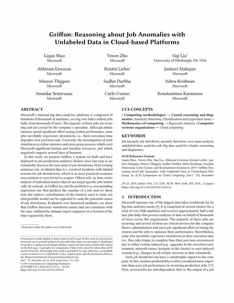
Figure 1: Running tasks in one of Microsoft’s production an-alytics clusters, comprised of tens of thousands ofmachines.

Our contributions in this paper are the following:(1) We present an end-to-end ranking system to identify the

root causes of job slowdowns without human-labeled data.(2) We show how an interpretable regression model can be used

to reason about job slowdowns.(3) We experimentally compare various models in terms of ac-

curacy, scalability in the model size and number of jobs, andgeneralizability to jobs not seen before by the system.

(4) Griffon is deployed in our clusters and is used by our engi-neers. Early indications show that slowdown causes gener-ated by Griffon are closely correlated to causes validated bydomain experts. At the same time, Griffon drops the timeof investigation by orders of magnitude compared to theexisting manual process.

The rest of the paper is organized as follows. Section 2 providesdetails on our production environment and the relevance of theproblem we focus on. Section 3 gives an overview of Griffon. Sec-tion 4 describes our anomaly reasoning algorithm, while Section 5discusses feature engineering and data collection. Section 6 pro-vides details on Griffon’s deployment, and Section 7 presents theresults of our experimental evaluation. Section 8 discusses relatedwork, and Section 9 provides our concluding remarks.

2 BACKGROUND ON OUR ENVIRONMENTIn this section, we provide background on the characteristics ofour analytics clusters to give a sense of the scale of the problem wetarget (Section 2.1). Then, we describe the current state of affairs infinding the reasons for a job’s slowdown (Section 2.2).

2.1 Cluster CharacteristicsAt Microsoft we operate a massive data infrastructure, poweringour internal analytics processing [9]. This infrastructure consists ofseveral clusters, each comprised of tens of thousands of machines—Table 1 highlights some details of our clusters’ scale. To make thesituation even more challenging, our cluster environments are alsoheterogeneous, including several generations of machines.

Tens of thousands of users submit hundreds of thousands of jobsto these clusters daily. Each job is a directed-acyclic graph (DAG) ofoperators (which we term stages), and each stage consists of several

Griffon: Reasoning about Job Anomalies with Unlabeled Data in Cloud-based Platforms SoCC ’19, November 20–23, 2019, Santa Cruz, CA, USA

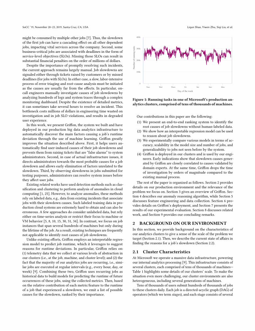
Figure 2: The critical path of execution for two occurrences of the same job. The top one completed in 57mins, while the bottomone took 88 mins to complete. Each line of each occurrence corresponds to a job stage’s start/finish time. Just by looking atthis visualization tool, one might think that the top job is the errant job (due to some long stages), while in fact the bottomone is the one diverging from the normal behavior.

Dimension Description SizeDaily Data I/O Total bytes processed daily >1EBFleet Size Number of servers in the fleet >250kCluster Size Number of servers per cluster >50k

Table 1: Microsoft cluster environments.

tasks [35]. Each task gets executed in a cluster’s machine (and eachmachine runs several tasks in parallel). Figure 1 depicts the numberof running tasks in one of our clusters over the course of a week. Ateach moment in time there are between 200k–300k tasks running.

Given this extreme scale and complexity, job slowdowns are quitecommon. Manually investigating such slowdowns, as we explainin the following section is a painful and time-consuming effort.

2.2 Manual Job Slow-down InvestigationWe now describe how Microsoft engineers used to approach jobslowdowns before Griffon got deployed in our clusters. Figure 2shows two occurrences of the same job. The top one correspondsto its regular execution, taking 57 mins to complete. The bottomone experiences a slow down with a completion time of 88 mins.The figure visualizes how long the various stages of the job taketo execute (although several stages might run in parallel, this toolshows the ones in the critical path, as those determine the job’sexecution time).

To investigate this slowdown, an engineer will typically start bylooking at the visualization tool of Figure 2, trying to detect thestages that seem abnormal. Note, however, that in this example, the“regular” top occurrence is the one that seems to have longer stages.Therefore, this tool is of limited use. Next, the engineer will haveto manually combine several other tools and system files to get

more information about the job and the system during the time thisjob was executed. Given the scale of the system and the amount ofmetrics collected, this process can take a considerable amount oftime to complete. Multiply this by the number of slowdowns andone can easily see the significant opportunity in saving engineeringtime and improving user experience by speeding up this process.Note also that only a few engineers have the knowledge to performthis manual analysis.

3 SYSTEM OVERVIEWGriffon’s goal is to find the causes for job runtime degradationsin our big data analytics clusters. A central requirement we setwhen we started designing Griffon was to not rely on labeled data,i.e., there should be no need for existing slowdown instances as-sociated with their causes. Acquiring labeled data in a complexinfrastructure like ours that has been operating for years is veryhard. Labeling data requires both infrastructure support and en-gineering training. Most importantly, it would require significantengineering time to label years-worth of historical data to get to ameaningful training set.

Each job in our clusters is associated with a set of telemetry datathat we already collect for monitoring and debugging purposes (e.g.,number of tasks, size of input data, load of machines the job wasexecuted on—see Section 5 for details), some of which contributedto the job’s slowdown. Instead of finding a subset of the slowdowncauses (as a system that relies on labeled data would do), Griffonranks the causes (i.e., the features) in the order they affected thedeviation of the job’s runtime from its expected runtime, and thensuggests the top causes to the users. A formal description of theproblem and our approach for solving it is presented in Section 4.

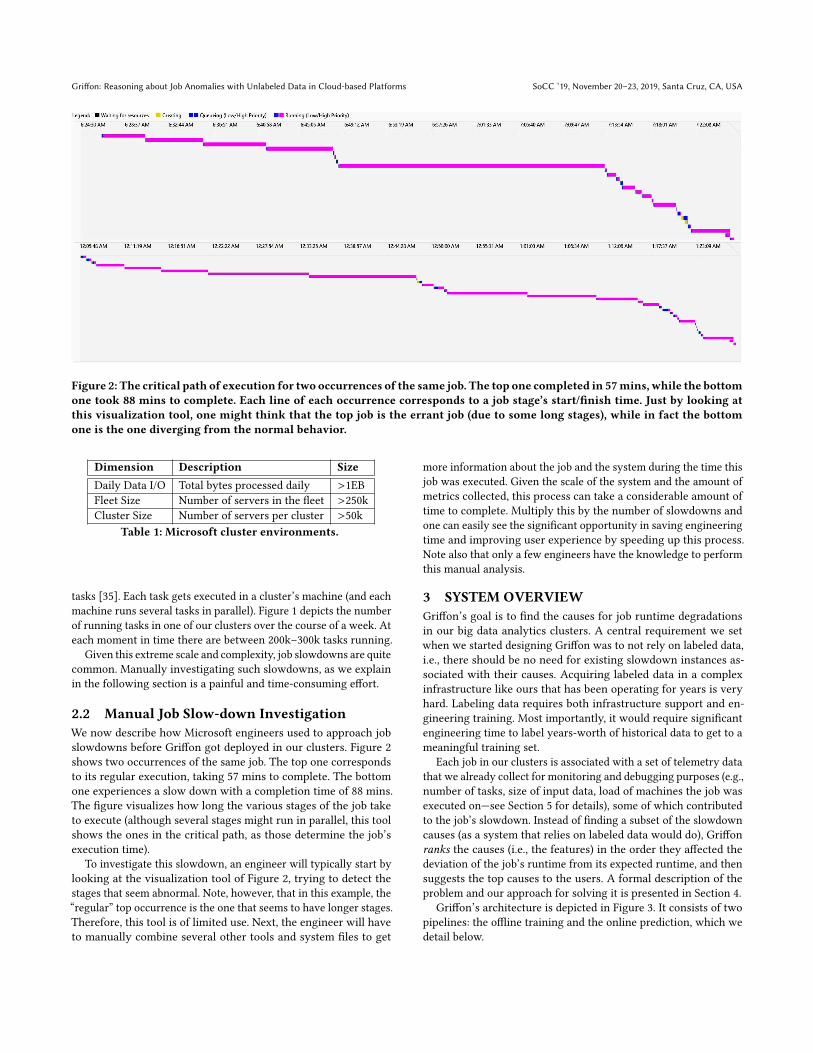
Griffon’s architecture is depicted in Figure 3. It consists of twopipelines: the offline training and the online prediction, which wedetail below.


Data Preparation

Pre-processing

Tracking Server

AnomalyReasoningAlgorithm(Online)

ML Model Training

Artifacts

Metrics & Hyperparameters

Delta Feature Contribution

Predicted Runtime

Causes of Job Slowdown

Confidence Level

Mapping

Deployment

Model Server VM

Online Feature Building

2 3

5 4Predicted Results

Features

Web Application

Features for Job ID

Job ID

Output: Prediction Report

6

Input: Job ID

1

User Scenario

Offline Training Pipeline Online Prediction Pipeline

Best Saved Model

Saved Model

Historic Data

Filtered Data

Features

Feature Selection

Feature Extraction

Pre-processed Data

Figure 3: System architecture.

33%

19%16%

15%

11%6%

DataWrite

CapacityAllocation

MaxTaskExecutionTime

InputSize

OrganizationPriority

IntermediateDataWritten

ConfidenceLevel:High

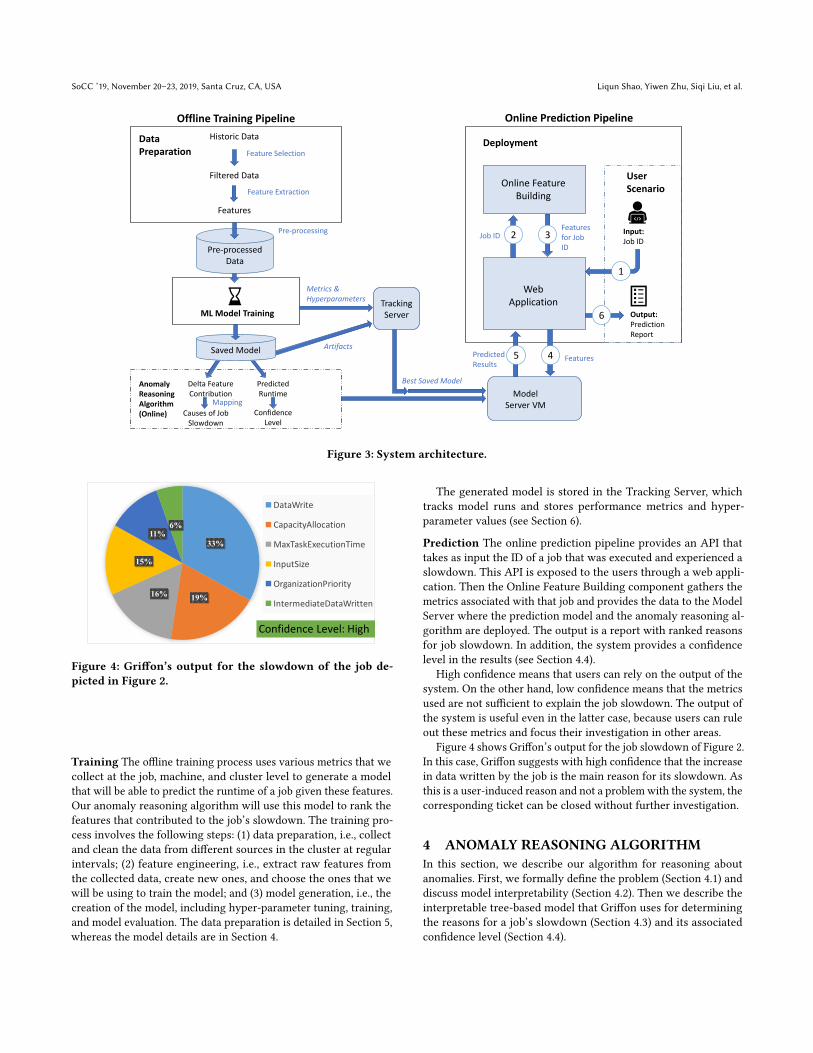
Figure 4: Griffon’s output for the slowdown of the job de-picted in Figure 2.

Training The offline training process uses various metrics that wecollect at the job, machine, and cluster level to generate a modelthat will be able to predict the runtime of a job given these features.Our anomaly reasoning algorithm will use this model to rank thefeatures that contributed to the job’s slowdown. The training pro-cess involves the following steps: (1) data preparation, i.e., collectand clean the data from different sources in the cluster at regularintervals; (2) feature engineering, i.e., extract raw features fromthe collected data, create new ones, and choose the ones that wewill be using to train the model; and (3) model generation, i.e., thecreation of the model, including hyper-parameter tuning, training,and model evaluation. The data preparation is detailed in Section 5,whereas the model details are in Section 4.

The generated model is stored in the Tracking Server, whichtracks model runs and stores performance metrics and hyper-parameter values (see Section 6).

Prediction The online prediction pipeline provides an API thattakes as input the ID of a job that was executed and experienced aslowdown. This API is exposed to the users through a web appli-cation. Then the Online Feature Building component gathers themetrics associated with that job and provides the data to the ModelServer where the prediction model and the anomaly reasoning al-gorithm are deployed. The output is a report with ranked reasonsfor job slowdown. In addition, the system provides a confidencelevel in the results (see Section 4.4).

High confidence means that users can rely on the output of thesystem. On the other hand, low confidence means that the metricsused are not sufficient to explain the job slowdown. The output ofthe system is useful even in the latter case, because users can ruleout these metrics and focus their investigation in other areas.

Figure 4 shows Griffon’s output for the job slowdown of Figure 2.In this case, Griffon suggests with high confidence that the increasein data written by the job is the main reason for its slowdown. Asthis is a user-induced reason and not a problem with the system, thecorresponding ticket can be closed without further investigation.

4 ANOMALY REASONING ALGORITHMIn this section, we describe our algorithm for reasoning aboutanomalies. First, we formally define the problem (Section 4.1) anddiscuss model interpretability (Section 4.2). Then we describe theinterpretable tree-based model that Griffon uses for determiningthe reasons for a job’s slowdown (Section 4.3) and its associatedconfidence level (Section 4.4).


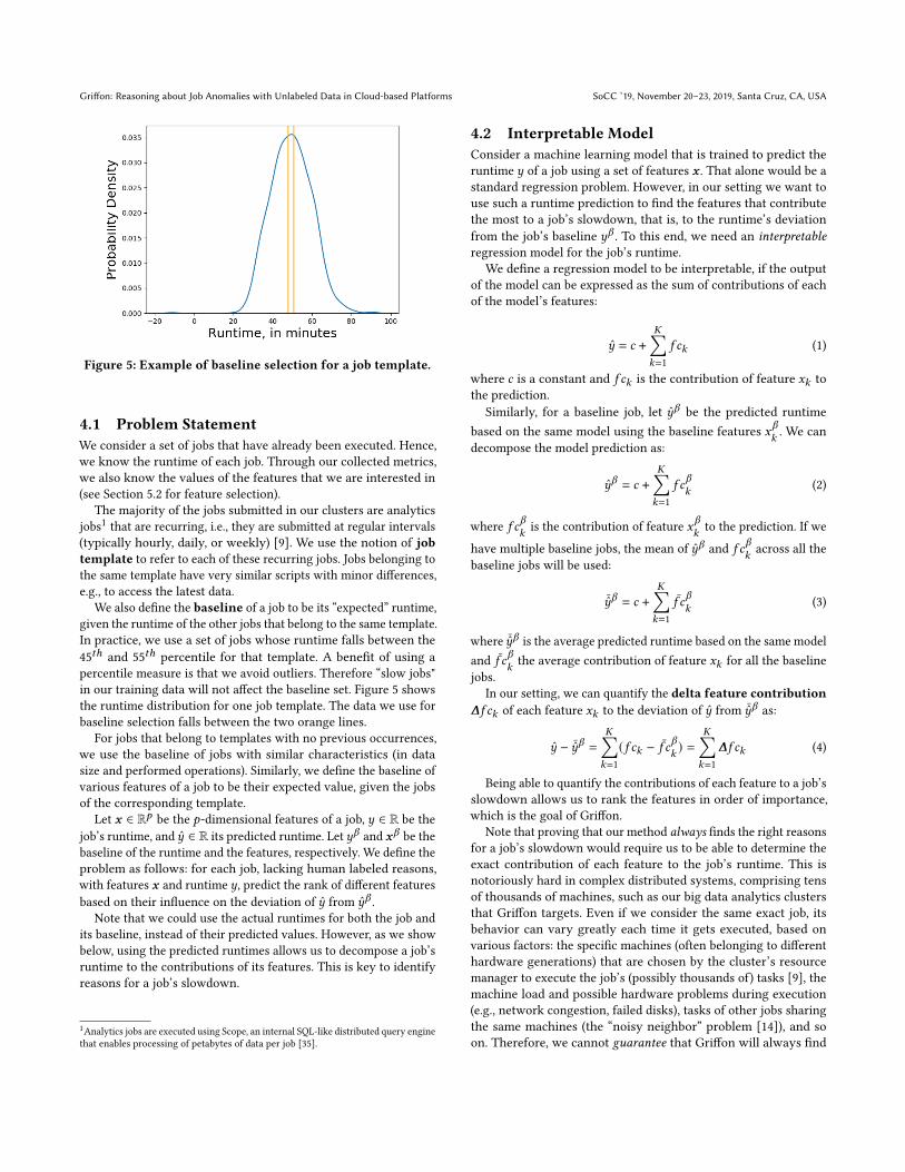
Figure 5: Example of baseline selection for a job template.

4.1 Problem StatementWe consider a set of jobs that have already been executed. Hence,we know the runtime of each job. Through our collected metrics,we also know the values of the features that we are interested in(see Section 5.2 for feature selection).

The majority of the jobs submitted in our clusters are analyticsjobs1 that are recurring, i.e., they are submitted at regular intervals(typically hourly, daily, or weekly) [9]. We use the notion of jobtemplate to refer to each of these recurring jobs. Jobs belonging tothe same template have very similar scripts with minor differences,e.g., to access the latest data.

We also define the baseline of a job to be its “expected” runtime,given the runtime of the other jobs that belong to the same template.In practice, we use a set of jobs whose runtime falls between the45𝑡ℎ and 55𝑡ℎ percentile for that template. A benefit of using apercentile measure is that we avoid outliers. Therefore “slow jobs"in our training data will not affect the baseline set. Figure 5 showsthe runtime distribution for one job template. The data we use forbaseline selection falls between the two orange lines.

For jobs that belong to templates with no previous occurrences,we use the baseline of jobs with similar characteristics (in datasize and performed operations). Similarly, we define the baseline ofvarious features of a job to be their expected value, given the jobsof the corresponding template.

Let 𝒙 ∈ R𝑝 be the 𝑝-dimensional features of a job, 𝑦 ∈ R be thejob’s runtime, and𝑦 ∈ R its predicted runtime. Let𝑦𝛽 and 𝒙𝛽 be thebaseline of the runtime and the features, respectively. We define theproblem as follows: for each job, lacking human labeled reasons,with features 𝒙 and runtime 𝑦, predict the rank of different featuresbased on their influence on the deviation of 𝑦 from 𝑦𝛽 .

Note that we could use the actual runtimes for both the job andits baseline, instead of their predicted values. However, as we showbelow, using the predicted runtimes allows us to decompose a job’sruntime to the contributions of its features. This is key to identifyreasons for a job’s slowdown.

1Analytics jobs are executed using Scope, an internal SQL-like distributed query enginethat enables processing of petabytes of data per job [35].

4.2 Interpretable ModelConsider a machine learning model that is trained to predict theruntime 𝑦 of a job using a set of features 𝒙 . That alone would be astandard regression problem. However, in our setting we want touse such a runtime prediction to find the features that contributethe most to a job’s slowdown, that is, to the runtime’s deviationfrom the job’s baseline 𝑦𝛽 . To this end, we need an interpretableregression model for the job’s runtime.

We define a regression model to be interpretable, if the outputof the model can be expressed as the sum of contributions of eachof the model’s features:

𝑦 = 𝑐 +𝐾∑𝑘=1

𝑓 𝑐𝑘 (1)

where 𝑐 is a constant and 𝑓 𝑐𝑘 is the contribution of feature 𝑥𝑘 tothe prediction.

Similarly, for a baseline job, let 𝑦𝛽 be the predicted runtimebased on the same model using the baseline features 𝑥𝛽

𝑘. We can

decompose the model prediction as:

𝑦𝛽 = 𝑐 +𝐾∑𝑘=1

𝑓 𝑐𝛽

𝑘(2)

where 𝑓 𝑐𝛽𝑘is the contribution of feature 𝑥𝛽

𝑘to the prediction. If we

have multiple baseline jobs, the mean of 𝑦𝛽 and 𝑓 𝑐𝛽𝑘across all the

baseline jobs will be used:

¯̂𝑦𝛽 = 𝑐 +𝐾∑𝑘=1

𝑓 𝑐𝛽

𝑘(3)

where ¯̂𝑦𝛽 is the average predicted runtime based on the same modeland 𝑓 𝑐𝛽

𝑘the average contribution of feature 𝑥𝑘 for all the baseline

jobs.In our setting, we can quantify the delta feature contribution

∆𝑓 𝑐𝑘 of each feature 𝑥𝑘 to the deviation of 𝑦 from ¯̂𝑦𝛽 as:

𝑦 − ¯̂𝑦𝛽 =

𝐾∑𝑘=1

(𝑓 𝑐𝑘 − 𝑓 𝑐𝛽

𝑘) =

𝐾∑𝑘=1

∆𝑓 𝑐𝑘 (4)

Being able to quantify the contributions of each feature to a job’sslowdown allows us to rank the features in order of importance,which is the goal of Griffon.

Note that proving that our method always finds the right reasonsfor a job’s slowdown would require us to be able to determine theexact contribution of each feature to the job’s runtime. This isnotoriously hard in complex distributed systems, comprising tensof thousands of machines, such as our big data analytics clustersthat Griffon targets. Even if we consider the same exact job, itsbehavior can vary greatly each time it gets executed, based onvarious factors: the specific machines (often belonging to differenthardware generations) that are chosen by the cluster’s resourcemanager to execute the job’s (possibly thousands of) tasks [9], themachine load and possible hardware problems during execution(e.g., network congestion, failed disks), tasks of other jobs sharingthe same machines (the “noisy neighbor” problem [14]), and soon. Therefore, we cannot guarantee that Griffon will always find


the right reasons for a slowdown. Nevertheless, our experimentalresults (see Section 7) show that in most practical scenarios, Griffondoes find the same reasons that were identified by expert engineers.In parallel, we quantify the level of trust that a user should have ona prediction by defining the confidence level for a prediction (seeSection 4.4).

Model choice We considered various model categories to predictthe runtime of a job, namely Linear Regression (LR), Random For-est (RF), Gradient Boosted Tree (GBT), and Deep Neural Network(DNN). Our main requirements were that the model be interpretableand that it offers good accuracy.

A linear model can be expressed as 𝑦 = 𝛼 +∑𝐾𝑘=1 𝛽𝑘𝑥𝑘 , where

𝛼, 𝛽𝑘 ∈ R. It is trivial to show that it satisfies the interpretabilitycriterion of Eq. 1. However, as we show in Section 7.2, the accuracyis worse than that of the other models. The DNN has acceptableaccuracy, but its interpretability is hard to establish. The GBT isless accurate than RF. The RF model exhibited the best accuracy inour experiments and therefore, is our model of choice in Griffon. Inthe next section, we describe an appropriate tree interpreter thatreformulates a tree-based model to a linear form, so that we canuse it to rank feature contributions to job slowdowns.

Note that when training our models, we considered both a globaland per-templatemodels. In the former case, we train a single unifiedmodel to predict runtime using jobs of all templates together in thetraining set. In the latter, we train one model per job template uti-lizing training data drawn exclusively from jobs that belong to theparticular template. In Section 7, we compare the two approachesin terms of accuracy, scalability, and generalizability.

4.3 Interpretable Random ForestIn a Random Forest (RF) model, for each tree, in order to make aprediction, we traverse a path from the root of the tree to a leaf. Thispath consists of a series of decisions based on the model’s features.Assuming there are𝑀 nodes on the path, each node separates thefeature space into two, given a feature 𝑥𝑘 and a threshold 𝑡𝑘 : theone child node corresponds to 𝑥𝑘 ≤ 𝑡𝑘 , the other to 𝑥𝑘 > 𝑡𝑘 . Inother words, from the root node where all the samples reside, apartition based on feature 𝑥𝑘 and threshold 𝑡𝑘 thus separates thedata samples to the two children that correspond to smaller featurespaces.

Consider a tree 𝑗 of the model and a node𝑚 ∈ 𝑗 that is parti-tioned from its sibling based on feature 𝑥𝑘 . Let 𝑦𝑚,𝑗 be the meantarget value for all samples that reside on node𝑚. Then the contri-bution of feature 𝑥𝑘 to the final prediction due to this partitioningis calculated as:

Δ𝑚contrib𝑗 (𝑥, 𝑘) = (𝑦𝑚,𝑗 − 𝑦𝑚−1, 𝑗 )𝐼 𝑗 (𝑚,𝑘) (5)

for 2 < 𝑚 ≤ 𝑀 , where node 𝑚−1 is 𝑚’s parent. 𝐼 𝑗 (𝑚,𝑘) equalsto 1 if the partitioning at node𝑚−1 involves feature 𝑥𝑘 for tree 𝑗or 0 otherwise. The number of samples that reside on each nodebecomes smaller and smaller by traversing the path, as the featurespace gets smaller. The contribution of 𝑥𝑘 to the final predictioncan be calculated as the sum of all Δ𝑚contrib𝑗 (𝑥, 𝑘):

contrib𝑗 (𝑥, 𝑘) =𝑀∑𝑚=2

Δ𝑚contrib𝑗 (𝑥, 𝑘) (6)

=

𝑀∑𝑚=2

(𝑦𝑚,𝑗 − 𝑦𝑚−1, 𝑗 )𝐼 𝑗 (𝑚,𝑘) (7)

The prediction of the target value from this tree is 𝑦𝑀,𝑗 and canbe expressed using the sum of all features’ contributions along thepath:

𝑦 𝑗 = 𝑦𝑀,𝑗 = 𝑦1, 𝑗 +𝑀∑𝑚=2

𝑦𝑚,𝑗 − 𝑦𝑚−1, 𝑗 (8)

= 𝑐 𝑗 +𝑀∑𝑚=2

𝐾∑𝑘=1

Δ𝑚contrib𝑗 (𝑥, 𝑘) (9)

where 𝑐 𝑗 is the full sample mean. TreeInterpreter [28] combines theresults of all trees in our Random Forest by taking the sum of thecontribution from each tree. Thus, each prediction is decomposedinto a sum of contributions from the features, as follows:

𝑦 =1𝐽

𝐽∑𝑗=1

𝑐 𝑗 +𝐾∑𝑘=1

( 1𝐽

𝐽∑𝑗=1

contrib𝑗 (𝑥, 𝑘)) (10)

where 𝐽 is the number of trees, 𝑐 𝑗 is the full sample mean for each𝑗𝑡ℎ tree, and 𝐾 is the number of features involved.

Refers to Eq. 10, using 𝑐 =1𝐽

∑𝐽𝑗=1 𝑐 𝑗 for the average runtime

across the whole training set and 𝑓 𝑐𝑘 =1𝐽

∑𝐽𝑗=1 contrib𝑗 (𝑥, 𝑘) for

the contribution of feature 𝑥𝑘 to the predicted runtime, we getto Eq. 1, which shows that our Random Forest model meets theinterpretability criterion. Therefore, it can be used to detect reasonsfor job slowdowns in Griffon.

4.4 Confidence LevelThe confidence level shows how reliable is the prediction made byour model for the contribution of each feature to a job’s slowdown.We consider two factors that affect our model confidence: (1) therelative error in predicting the runtime of the job (by comparingthe model prediction with the actual runtime of the job);2 (2) theconfidence intervals estimated by the random forest [20].

The relative error is defined as following:

error_rate =|predicted_runtime − actual_runtime|

actual_runtime(11)

We use two thresholds, 𝑡1 and 𝑡2, for the relative error, as ex-plained below.

The confidence interval of the random forest method is es-timated based on the prediction of each decision tree, 𝑦 𝑗 ,∀𝑗 ∈{1, 2, 3, · · · , 𝐽 }. We take the 𝑝th and (100 − 𝑝)th percentile of thedistribution of 𝑦 𝑗 . If the final prediction 𝑦 is within this range, we

2We also considered taking into account the prediction errors for the baseline jobs inthe definition of confidence. However, we decided to not include them, as we observedthat the prediction for baseline jobs is very accurate (with a Mean Absolute Ratio Errorof 2.2%). This is due to the fact that a large part of the baseline jobs are included inthe training set of the prediction models. Therefore, it is expected that predictionsespecially for these jobs to be very accurate.


consider the prediction to have low variance, since the predictionsfrom all trees are consistent.We define three confidence levels as follows:

High The prediction 𝑦 is within the range of 𝑝th and (100 −𝑝)th percentile of 𝑦 𝑗 , and the relative error is lower thanthreshold 𝑡1;

Medium The relative error is between 𝑡1 and 𝑡2;Low Other scenarios.

Parameters 𝑝 , 𝑡1 and 𝑡2 are tuned as hyper parameters usingvalidation data. High confidence means our model can reliablypredict the slowdown reasons. Low confidence means the reasonsare likely to fall outside the metrics we used. In the API, the userwill be presented the level of confidence. A low confidence indicatesmore investigation will be needed. However, even in this case, asthe model has examined many metrics, the DRI can focus theirinvestigation in other areas.

5 DATA PREPARATION AND FEATUREENGINEERING

5.1 Data PreparationIn our clusters, we keep hundreds of metrics for monitoring, report-ing, and troubleshooting purposes, which result in petabytes of logsand metrics per day. Moreover, the features we are interested inare scattered both physically (in different files across our hundredsof thousands of machines) and logically (we need to process andcombine different files to generate features). To perform the re-quired data preparation and extract features out of the data, we useScope [35], which provides a SQL-like language and can supportour scale.

Feature extraction occurs both during the offline training phaseand the online prediction (see Figure 3). Given that data freshnessis not an issue for training (we do not need data of the currentday), we use data that becomes available daily in our clusters andincludes years-worth of historical data. For prediction, we need tocollect features only for a single job (or a group of jobs), but latestdata is required, as a user might want to debug their job that justfinished. Thus, we use different data sources that allow us to accessdata within minutes from when they are produced (but that do notallow access to historical data, so cannot be used for training).

5.2 Feature Engineering and SelectionIn collaboration with domain experts, we selected a subset of thefeatures we collect to train our models in Griffon, based on whatcould potentially impact the runtime of a job. As already discussed,a job can experience a slowdown compared to its previous oc-currences, due to either user-induced or system-induced reasons.User-induced reasons can be captured by metrics collected at thejob-level, whereas metrics related to system-induced reasons canbe split to either machine-level or cluster-level, as detailed below.

Job-level These are metrics collected for each job. Griffon cur-rently uses approximately 15 such features, including dataread within and across racks, data written, data skewnessmetrics, job priority, execution DAG features (e.g., numberof stages and tasks), and user information.

Machine-level These are metrics collected at the machinesused during the execution of a job, such as CPU load, al-location delays, I/O reads/writes. Due to the challenges ofcollecting such features and correlating them with each job,in production Griffon currently uses only a few of them, butwe are working on adding more.

Cluster-level These relate to the cluster environment whena job was executed. Examples of the ones we use are jobqueuing times, number of failed and revoked vertices, andexecution environment version.

ChallengesOne of the biggest challenges with feature engineeringis the correlation between features, which often results in highvariance in the model prediction. While certain highly correlatedfeatures (> 0.95) were removed, feature data was preserved to thegreatest extent, because correlated features may indicate differentproblems with a job. For instance, input size and input size pertask have a correlation of 0.9. However, the former might indicatethat the slowness reason was more data, whereas the latter mightindicate data skew. Fortunately, random forest models, as the oneGriffon relies on, are by design robust to correlated features thanksto the way they are constructed. First, each tree of the forest isdeveloped based on a small subset of the overall features. Thisautomatically reduces the likelihood of having correlated featureswithin the same tree. Second, once a set of features is picked for atree, this tree is constructed using a decision tree learner algorithm.This algorithm typically works top-down, by choosing a featureat each step that “best” splits the dataset. Given that correlatedfeatures would split the dataset in a similar way, once a feature ispicked, its correlated features are less likely to be picked.

6 TRACKING AND DEPLOYMENT

Model Tracking Machine learning is an iterative process, andreproducibility and versioning are crucial to productionalize ma-chine learning models. To track model history in Griffon, we useMLflow [24] in our Tracking Server (see Figure 3), which is de-ployed as an Azure Linux VM. For each model, we track loggingparameters, code versions, metrics, and model artifacts.

Model Serving In order to make available to end users a modelthat we trained and stored in the Tracking Server, we use one ofMLflow’s “flavors”3 to build an Azure Machine Learning image outof that model. Then we deploy this image as an Azure ContainerInstance, using the Azure ML Service’s [23] in the Model Server(see Figure 3).

The models that are deployed in the Model Server are madeavailable to end users through a web application, which exposes ascoring API. The web application runs on a flask web server [13].

Model Monitoring It is critical to monitor the model performanceand retrain models if they go stale. To ensure this, we have pro-visioned our pipeline to allow single click retraining. Decouplingdata sources from the training pipeline helps to easily refresh ourdata, retrain, and deploy the model with minimal impact to endusers.

3An MLflow flavor is a convention that deployment tools use to understand the model.


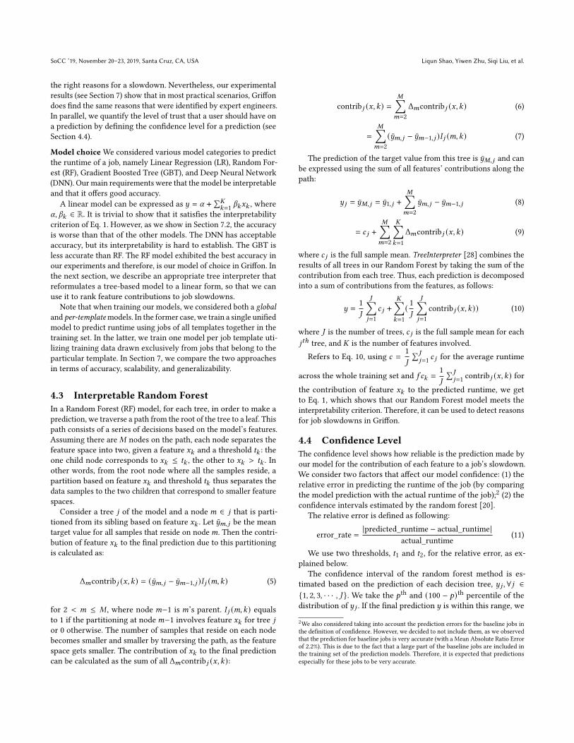
Figure 6: Runtime distribution for the jobs of different tem-plates.

7 EVALUATIONWe now present our experimental evaluation for Griffon. In Sec-tion 7.1 we discuss Griffon’s effectiveness in finding the actualcauses of job slowdowns. In Section 7.2 we compare different ma-chine learning models for training, whereas Section 7.3 studiesthe scalability of different models as the number of job templatesincreases. In Section 7.4 we compare the model performance whentraining our model with an increasing number of jobs per template.In Section 7.5 we show early evidence that Griffon can be applicablein different domains.

We carried out our experiments on Windows using Python 3.7.We used a machine with eight 2.90 GHz processors and 64 GB RAMfor the experiments in Sections 7.1 and 7.2, and a high-memoryVirtual Machine (VM) for the scalability experiments of Section 7.3.

The job and feature data is obtained from the Microsoft pro-duction clusters, as described in Section 5.1. We use historical jobdata with different job templates, as described in Section 5.2, over aperiod of three months.

7.1 Validation ResultsWorking with domain experts at Microsoft, we picked a set ofjob templates that are considered important for our productionclusters (SLO critical), and trained Griffon based on those. Notethat the runtime distribution of the jobs of different templatesvaries significantly, which poses extra challenges for the runtimeprediction based on machine learning models. Figure 6 shows theruntime distributions for five of the templates that we used.

From these templates, we then randomly picked seven jobs thatexperienced slowdowns (five from these templates and two fromdifferent templates), and compared the causes for slowdowns thatwere identified by the experts with those suggested by Griffon. Forthese jobs, Table 2 shows the reasons identified by the experts andGriffon (with their ranking), Griffon’s confidence level, and if thejob belonged to one of the templates used for training the model(in-t). We use 𝑅𝑥 to denote the reason that Griffon predicted fora job’s slowdown with rank 𝑥 . For readability, we show only the

reasons that were common between Griffon and experts and use𝑅𝑥 variables for the rest.

The results in Table 2 show that the reasons generated by Griffonare highly correlated with the reasons manually validated by ourdomain expert engineers. For job 1, the top predicted reason is thesame as the manually validated reason with high confidence. Forjobs 2 and 4, our system predicted the validated reason in the top 5slowdown reasons, which is consistent with the confidence levelmedium. For job 3, our model does not identify the same reasonsas the experts, also consistent with low confidence. Adding morefeatures as planned (e.g., additional machine-level features) willallow us to improve the model’s prediction capability and minimizesuch low-confidence cases. Jobs 6, 7 and 8 show the robustnessof our model: although Griffon was not trained using these jobtemplates, it can still find the correct reasons with high confidenceby using knowledge gathered by other similar job templates. Impor-tantly, we observed no misleading predictions, i.e., there were nocases where Griffon predicted wrong slowdown reasons with highconfidence. This means that even predictions with low confidence,which are usually due to large deviations between the predictedand the actual runtimes of a job, can be useful in ruling out thecurrently used features from the investigation.

7.2 Picking the Right ModelAs discussed in Section 4, we experimented with various categoriesof models for the job runtime prediction, including Linear Regres-sion (LR), Random Forest (RF), Gradient Boosted Trees (GBT) andDeep Neural Networks (DNN) with two hidden layers without hy-per parameter tuning. For each of these categories, we considerboth a global and per-template models.

We use Mean Absolute Ratio Error (MARE) as a metric to eval-uate each model’s accuracy. As the runtime distribution variessignificantly across different job templates, we normalize the es-timation error by the baseline runtime of each job template (seeSection 4.1), calculating the average runtime per job template inthe training data:

MARE =1𝑛

𝑛∑𝑖=1

|𝑦test𝑖 − 𝑦test𝑖

𝑦𝛽

test𝑖

| (12)

where 𝑛 is the number of jobs in the testing data, 𝑦test𝑖 , 𝑦test𝑖 , and𝑦𝛽

test𝑖 are the predicted, actual, and baseline runtime from testingdata, respectively.

Table 3 shows the results of MARE scores for the four modelcategories. Random forest performs best in terms of accuracy, bothfor the global and per-template model. Given its high accuracy andinterpretability (as discussed in Section 4.2), RF is the approach weuse in our production Griffon deployments. Moreover, we observethat the global model tracks closely the performance of the per-template model, while allowing to reason about jobs that we havenot sufficiently encountered previously. In the next section, wedemonstrate that the global model scales much better than the per-template models with an increasing number of templates. Hence,we use the global model in production.


Table 2: Result subset validated by engineers.

Job Griffon’s Predicted List ofRanked Reasons

Engineer ValidatedReason

ConfidenceLevel

in-t

1 [Input Size, 𝑅2, 𝑅3] Input size High Yes2 [𝑅1, 𝑅2, 𝑅3, Revocation, 𝑅5] Revocation Medium Yes3 [𝑅1, 𝑅2, 𝑅3, 𝑅4, 𝑅5, 𝑅6] Framework issue Low Yes4 [𝑅1, 𝑅2, 𝑅3, 𝑅4, High compute hours] High compute hours Medium Yes5 [Time skew, 𝑅2, 𝑅3, 𝑅4] Time skew High Yes6 [High compute hours, 𝑅2, 𝑅3] High compute hours High No7 [𝑅1, Usable machine count, 𝑅3, 𝑅4] Usable machine count High No8 [High compute hours, 𝑅2] High compute hours High No

1 2 4 8 16 32 64 128240Number of Templates

101

102

103

104

105

MS

(MB)

global MSsingle MS

0

1000

2000

3000

4000

5000

6000

TT (s

ec)

global TTsingle TT

(a) MS and TT

1 2 4 8 16 32 64 128240Number of Templates

0.000

0.025

0.050

0.075

0.100

0.125

0.150

MAR

E

global MAREsingle MARE

0.000

0.025

0.050

0.075

0.100

0.125

0.150

SIT

(sec

)

global SITsingle SIT

(b) MARE and SIT

Figure 7: Scalability of global vs. per-template models

Table 3: MARE scores for runtime predictions by LR, RF,GBT, and DNN with global and per-template models (loweris better).

LR RF GBT DNN

Per-TemplateModel

0.186 0.116 0.124 0.146

Global Model 0.235 0.121 0.277 0.353

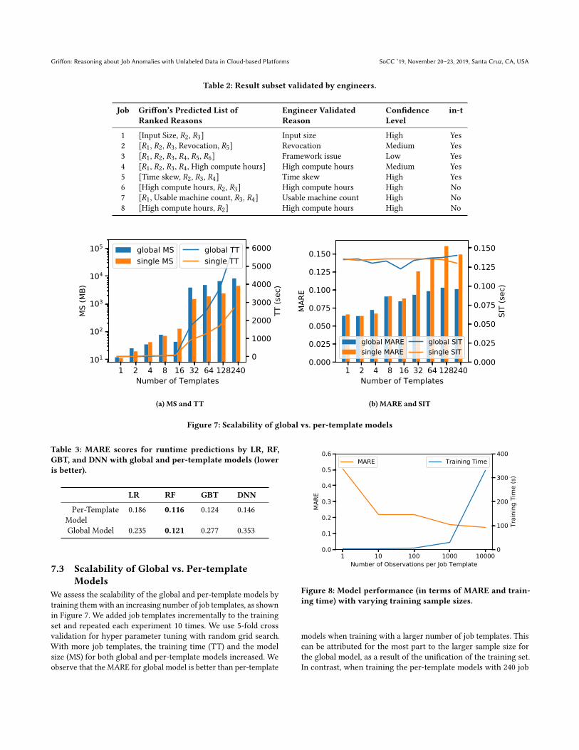
7.3 Scalability of Global vs. Per-templateModels

We assess the scalability of the global and per-template models bytraining themwith an increasing number of job templates, as shownin Figure 7. We added job templates incrementally to the trainingset and repeated each experiment 10 times. We use 5-fold crossvalidation for hyper parameter tuning with random grid search.With more job templates, the training time (TT) and the modelsize (MS) for both global and per-template models increased. Weobserve that the MARE for global model is better than per-template

1 10 100 1000 10000Number of Observations per Job Template

0.0

0.1

0.2

0.3

0.4

0.5

0.6

MAR

E

MARE

0

100

200

300

400

Trai

ning

Tim

e (s

)

Training Time

Figure 8: Model performance (in terms of MARE and train-ing time) with varying training sample sizes.

models when training with a larger number of job templates. Thiscan be attributed for the most part to the larger sample size forthe global model, as a result of the unification of the training set.In contrast, when training the per-template models with 240 job


Table 4: Contribution of each feature to the high gasmileageof American-made Ford Granada compared to other Ameri-can cars.

Feature FordGranada

Mean Baseline Delta FC(in mpg)

Year 81 76 75 2.07Horsepower 88 104 106 1.07Weight 3060 2978 3224 0.7Displacement 200 194 221 0.04Acceleration 17.1 15.5 16.1 -0.19Cylinders 6 5.5 5.8 -1.4

templates, many templates only have a small number of samplesand theMARE is high.We also report the prediction time on a singlejob, i.e. the single inference time (SIT). The SIT didn’t increase withthe model size, which is important to deliver a real-time experienceto Griffon’s users.

Overall, the above experiments demonstrate the scalability ofthe global model for cloud-scale training. At the other extreme, atemplate-specific model suffers from lack of training data and theability to generalize to new (unseen) templates. As part of our futurework, we plan to cluster job templates using unsupervised machinelearning methods and train “semi-global” models that take intoaccount multiple job templates that share similar characteristics tostrike a balance between the two approaches.

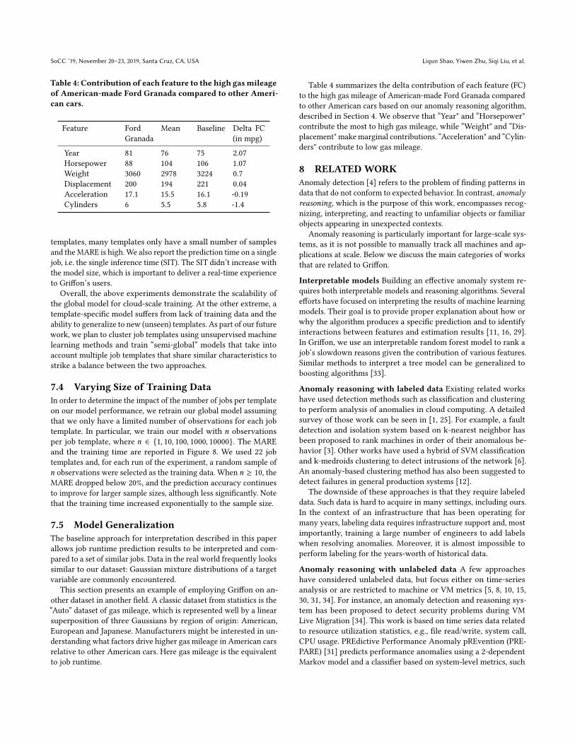
7.4 Varying Size of Training DataIn order to determine the impact of the number of jobs per templateon our model performance, we retrain our global model assumingthat we only have a limited number of observations for each jobtemplate. In particular, we train our model with 𝑛 observationsper job template, where 𝑛 ∈ {1, 10, 100, 1000, 10000}. The MAREand the training time are reported in Figure 8. We used 22 jobtemplates and, for each run of the experiment, a random sample of𝑛 observations were selected as the training data. When 𝑛 ≥ 10, theMARE dropped below 20%, and the prediction accuracy continuesto improve for larger sample sizes, although less significantly. Notethat the training time increased exponentially to the sample size.

7.5 Model GeneralizationThe baseline approach for interpretation described in this paperallows job runtime prediction results to be interpreted and com-pared to a set of similar jobs. Data in the real world frequently lookssimilar to our dataset: Gaussian mixture distributions of a targetvariable are commonly encountered.

This section presents an example of employing Griffon on an-other dataset in another field. A classic dataset from statistics is the“Auto” dataset of gas mileage, which is represented well by a linearsuperposition of three Gaussians by region of origin: American,European and Japanese. Manufacturers might be interested in un-derstanding what factors drive higher gas mileage in American carsrelative to other American cars. Here gas mileage is the equivalentto job runtime.

Table 4 summarizes the delta contribution of each feature (FC)to the high gas mileage of American-made Ford Granada comparedto other American cars based on our anomaly reasoning algorithm,described in Section 4. We observe that “Year" and “Horsepower"contribute the most to high gas mileage, while “Weight" and “Dis-placement" makemarginal contributions. “Acceleration" and “Cylin-ders" contribute to low gas mileage.

8 RELATEDWORKAnomaly detection [4] refers to the problem of finding patterns indata that do not conform to expected behavior. In contrast, anomalyreasoning, which is the purpose of this work, encompasses recog-nizing, interpreting, and reacting to unfamiliar objects or familiarobjects appearing in unexpected contexts.

Anomaly reasoning is particularly important for large-scale sys-tems, as it is not possible to manually track all machines and ap-plications at scale. Below we discuss the main categories of worksthat are related to Griffon.

Interpretable models Building an effective anomaly system re-quires both interpretable models and reasoning algorithms. Severalefforts have focused on interpreting the results of machine learningmodels. Their goal is to provide proper explanation about how orwhy the algorithm produces a specific prediction and to identifyinteractions between features and estimation results [11, 16, 29].In Griffon, we use an interpretable random forest model to rank ajob’s slowdown reasons given the contribution of various features.Similar methods to interpret a tree model can be generalized toboosting algorithms [33].

Anomaly reasoning with labeled data Existing related workshave used detection methods such as classification and clusteringto perform analysis of anomalies in cloud computing. A detailedsurvey of those work can be seen in [1, 25]. For example, a faultdetection and isolation system based on k-nearest neighbor hasbeen proposed to rank machines in order of their anomalous be-havior [3]. Other works have used a hybrid of SVM classificationand k-medroids clustering to detect intrusions of the network [6].An anomaly-based clustering method has also been suggested todetect failures in general production systems [12].

The downside of these approaches is that they require labeleddata. Such data is hard to acquire in many settings, including ours.In the context of an infrastructure that has been operating formany years, labeling data requires infrastructure support and, mostimportantly, training a large number of engineers to add labelswhen resolving anomalies. Moreover, it is almost impossible toperform labeling for the years-worth of historical data.

Anomaly reasoning with unlabeled data A few approacheshave considered unlabeled data, but focus either on time-seriesanalysis or are restricted to machine or VM metrics [5, 8, 10, 15,30, 31, 34]. For instance, an anomaly detection and reasoning sys-tem has been proposed to detect security problems during VMLive Migration [34]. This work is based on time series data relatedto resource utilization statistics, e.g., file read/write, system call,CPU usage. PREdictive Performance Anomaly pREvention (PRE-PARE) [31] predicts performance anomalies using a 2-dependentMarkov model and a classifier based on system-level metrics, such


as CPU, memory, network traffic. Another related work developedan Unsupervised Behavior Learning (UBL) system to capture theanomalies and infer their causes [10]. To circumvent the need forlabeling data, Self Organizing Map (SOM) has been suggested tomodel the system behavior, and deviations are used for the anomalydetection [18].

Similar to Griffon, those methods estimate the contribution ofeach attribute to the anomaly and provides information aboutwhich system-level metrics to look into. However, they requiretime-dependent series of data to capture the anomalies. In contrast,we focus on job instances that span several hundreds of machinesbut only during the lifetime of the job. Thus, our features are nei-ther time series nor machine-centric (although we do employ somesystem-level data to examine the system’s impact on a particularjob’s execution).

Other works in anomaly reasoning aim to pinpoint the faultycomponents of a system by tracing the system’s activities [2, 21, 22,26]. The methods rely more on the estimation of the time series’change point and the propagation pattern or the execution graph.However, those methods require significant domain knowledge andare hard to generalize.

To the best of our knowledge, Griffon is the first anomaly rea-soning system to be deployed at this scale in production to identifythe causes of job slowdowns in analytics clusters. Unlike existingapproaches, it follows a job-centric approach and does not relyneither on labeled data nor on time series analysis.

Weak supervision Acknowledging the difficulty of hand-labelingdata but also the importance of having labeled data, weak super-vision attempts to strike a balance between supervised and unsu-pervised learning. Recent systems, such as Snorkel [27], bypassthe problem of hand-labeling data by instead providing labelingfunctions, which label data programmatically. It would be inter-esting to see how a system like Griffon can use such techniquesto encode knowledge of domain expert engineers as functions tofurther improve its anomaly detection capabilities.

9 CONCLUSION & FUTUREWORKWe presented Griffon, a system that we built and have deployedin production to detect the causes of job slowdowns in Microsoft’sbig data analytics clusters, consisting of hundreds of thousands ofmachines. Griffon does not require labeled data to perform anomalyreasoning. Instead, it uses an interpretable machine learning modelto predict the runtime of a job that has experienced a slowdown.Using this model, we can determine the contribution of each featurein the deviation of the job’s runtime compared to previous normalexecutions of the job (or of jobs with similar characteristics).

Our evaluation results using historical incidents showed thatGriffon discovers the same slowdown reasons that were detected bydomain expert engineers. We also compared various categories ofmodels and showed that a global (i.e., trained over all jobs) randomforest model strikes a good balance between accuracy, training time,model size, and generalization capabilities.

Towards data-driven decisions Griffon is part of our bigger vi-sion towards employing data-driven decisions to optimize various

aspects of our systems. Taking Griffon’s capabilities a step fur-ther, knowing the job slowdown reasons allows us to automaticallytune the system to avoid such slowdowns in the future. This mayinclude both system parameters, such as dynamically setting thenumber of running tasks per machine, and application parameters,such as the degree of parallelism for each stage of a job. Moreover,such parameter autotuning does not have to be constrained to jobslowdowns—we can use it to automatically and dynamically setvarious parameters in our systems to improve their performance.

Furthermore, although Griffon currently targets our internalanalytics clusters, the above techniques can be applied to otherenvironments, such as various public Azure services, including theAzure SQL and HDInsight offerings. Similar data-driven decisionsare increasingly applied in various companies [19, 32].

ACKNOWLEDGMENTSWe would like to thank Microsoft ’s Big Data analytics team, and inparticular Sarvesh Sakalanaga, Vamsi Kuppa, Sankar Nemani, DavidOlix, and Anusha Chavva, for their invaluable help in bringingGriffon to production. We also thank Anupam Upadhyay for manystimulating discussions that helped shape this effort, as well asPanagiotis Garefalakis for his initial work on visualizing clustermetrics. Finally, we thank Mathias Lécuyer, our shepherd, and theanonymous reviewers for their insightful feedback and suggestions.

REFERENCES[1] Shikha Agrawal and Jitendra Agrawal. 2015. Survey on anomaly detection using

data mining techniques. Procedia Computer Science 60 (2015), 708–713.[2] Marcos K Aguilera, Jeffrey C Mogul, Janet L Wiener, Patrick Reynolds, and

Athicha Muthitacharoen. 2003. Performance debugging for distributed systemsof black boxes. In ACM SIGOPS Operating Systems Review, Vol. 37. ACM, 74–89.

[3] Kanishka Bhaduri, Kamalika Das, and Bryan L Matthews. 2011. Detecting abnor-mal machine characteristics in cloud infrastructures. In 2011 IEEE 11th Interna-tional Conference on Data Mining Workshops. IEEE, 137–144.

[4] Varun Chandola, Arindam Banerjee, and Vipin Kumar. 2009. Anomaly detection:A survey. ACM Comput. Surv. 41 (2009), 15:1–15:58.

[5] Ludmila Cherkasova, Kivanc Ozonat, Ningfang Mi, Julie Symons, and EvgeniaSmirni. 2009. Automated anomaly detection and performance modeling of enter-prise applications. ACM Transactions on Computer Systems (TOCS) 27, 3 (2009),6.

[6] Roshan Chitrakar and Chuanhe Huang. 2012. Anomaly based intrusion detectionusing hybrid learning approach of combining k-medoids clustering and naivebayes classification. In 2012 8th International Conference on Wireless Communica-tions, Networking and Mobile Computing. IEEE, 1–5.

[7] Andrew Chung, Carlo Curino, Subru Krishnan, Konstantinos Karanasos, GregGanger, and Panagiotis Garefalakis. 2019. Peering through the dark: an Owl’sview of inter-job dependencies and jobs’ impact in shared clusters. In SIGMOD.

[8] Ira Cohen, Jeffrey S Chase, Moises Goldszmidt, Terence Kelly, and Julie Symons.2004. Correlating Instrumentation Data to System States: A Building Block forAutomated Diagnosis and Control.. In OSDI, Vol. 4. 16–16.

[9] Carlo Curino, Subru Krishnan, Konstantinos Karanasos, Sriram Rao, Giovanni M.Fumarola, Botong Huang, Kishore Chaliparambil, Arun Suresh, Young Chen,Solom Heddaya, Roni Burd, Sarvesh Sakalanaga, Chris Douglas, Bill Ramsey, andRaghu Ramakrishnan. 2019. Hydra: a federated resource manager for data-centerscale analytics. In NSDI.

[10] Daniel Joseph Dean, Hiep Nguyen, and Xiaohui Gu. 2012. Ubl: Unsupervisedbehavior learning for predicting performance anomalies in virtualized cloudsystems. In Proceedings of the 9th international conference on Autonomic computing.ACM, 191–200.

[11] Filip Karlo Došilović, Mario Brčić, and Nikica Hlupić. 2018. Explainable artificialintelligence: A survey. In 2018 41st International convention on information andcommunication technology, electronics and microelectronics (MIPRO). IEEE, 0210–0215.

[12] Songyun Duan, Shivnath Babu, and Kamesh Munagala. 2009. Fa: A system forautomating failure diagnosis. In 2009 IEEE 25th International Conference on DataEngineering. IEEE, 1012–1023.

[13] Flask. 2019. Flask - A Python Microframework.


[14] Panagiotis Garefalakis, Konstantinos Karanasos, Peter R Pietzuch, Arun Suresh,and Sriram Rao. 2018. Medea: scheduling of long running applications in sharedproduction clusters. EuroSys (2018).

[15] Xiaohui Gu and HaixunWang. 2009. Online anomaly prediction for robust clustersystems. In 2009 IEEE 25th International Conference on Data Engineering. IEEE,1000–1011.

[16] David Gunning. 2017. Explainable artificial intelligence (xai). Defense AdvancedResearch Projects Agency (DARPA), nd Web (2017).

[17] Sangeetha Abdu Jyothi, Carlo Curino, Ishai Menache, ShravanMatthur Narayana-murthy, Alexey Tumanov, Jonathan Yaniv, Ruslan Mavlyutov, Iñigo Goiri, SubruKrishnan, Janardhan Kulkarni, and Sriram Rao. 2016. Morpheus: Towards Auto-mated SLOs for Enterprise Clusters. In OSDI.

[18] Teuvo Kohonen. 2012. Self-organizing maps. Vol. 30. Springer Science & BusinessMedia.

[19] linkedinds 2019. An Introduction to AI at LinkedIn. https://engineering.linkedin.com/blog/2018/10/an-introduction-to-ai-at-linkedin.

[20] Nicolai Meinshausen. 2006. Quantile Regression Forests. Journal of MachineLearning Research 7 (2006), 983–999.

[21] Haibo Mi, Huaimin Wang, Gang Yin, Hua Cai, Qi Zhou, and Tingtao Sun. 2012.Performance problems diagnosis in cloud computing systems by mining requesttrace logs. In 2012 IEEE Network Operations and Management Symposium. IEEE,893–899.

[22] Haibo Mi, HuaiminWang, Gang Yin, Hua Cai, Qi Zhou, Tingtao Sun, and YangfanZhou. 2011. Magnifier: Online detection of performance problems in large-scale cloud computing systems. In 2011 IEEE International Conference on ServicesComputing. IEEE, 418–425.

[23] Microsoft. 2019. Azure Machine Learning Service - Build, train, and deploy modelsfrom the cloud to the edge.

[24] MLflow. 2019. MLflow - A platform for machine learning lifecycle.[25] Chirag Modi, Dhiren Patel, Bhavesh Borisaniya, Hiren Patel, Avi Patel, and

Muttukrishnan Rajarajan. 2013. A survey of intrusion detection techniques in

cloud. Journal of network and computer applications 36, 1 (2013), 42–57.[26] Hiep Nguyen, Yongmin Tan, and Xiaohui Gu. 2011. Pal: Propagation-aware

anomaly localization for cloud hosted distributed applications. In ManagingLarge-scale Systems via the Analysis of System Logs and the Application of MachineLearning Techniques. ACM, 1.

[27] Alexander Ratner, Stephen H. Bach, Henry R. Ehrenberg, Jason Alan Fries, SenWu, and Christopher Ré. 2017. Snorkel: Rapid Training Data Creation with WeakSupervision. PVLDB (2017).

[28] Ando Saabas. 2018. TreeInterpreter.[29] Wojciech Samek, Thomas Wiegand, and Klaus-Robert Müller. 2017. Explainable

artificial intelligence: Understanding, visualizing and interpreting deep learningmodels. arXiv preprint arXiv:1708.08296 (2017).

[30] Yongmin Tan, Xiaohui Gu, and Haixun Wang. 2010. Adaptive system anomalyprediction for large-scale hosting infrastructures. In Proceedings of the 29th ACMSIGACT-SIGOPS symposium on Principles of distributed computing. ACM, 173–182.

[31] Yongmin Tan, Hiep Nguyen, Zhiming Shen, Xiaohui Gu, Chitra Venkatramani,and Deepak Rajan. 2012. Prepare: Predictive performance anomaly preventionfor virtualized cloud systems. In 2012 IEEE 32nd International Conference onDistributed Computing Systems. IEEE, 285–294.

[32] uberds 2019. How Uber Organizes Around Machine Learning. https://urlzs.com/J4Rk9.

[33] Soeren HWelling, Hanne HF Refsgaard, Per B Brockhoff, and Line H Clemmensen.2016. Forest floor visualizations of random forests. arXiv preprint arXiv:1605.09196(2016).

[34] Qiannan Zhang, Yafei Wu, Tian Huang, and Yongxin Zhu. 2013. An intelli-gent anomaly detection and reasoning scheme for VM live migration via clouddata mining. In 2013 IEEE 25th International Conference on Tools with ArtificialIntelligence. IEEE, 412–419.

[35] Jingren Zhou, Nicolas Bruno, Ming-Chuan Wu, Per-Åke Larson, Ronnie Chaiken,and Darren Shakib. 2012. SCOPE: parallel databases meet MapReduce. VLDB J.21, 5 (2012), 611–636.

https://engineering.linkedin.com/blog/2018/10/an-introduction-to-ai-at-linkedin

https://engineering.linkedin.com/blog/2018/10/an-introduction-to-ai-at-linkedin

https://urlzs.com/J4Rk9

https://urlzs.com/J4Rk9

Documents

Griffon: Reasoning about Job Anomalies with Unlabeled Data