Gromov hyperbolicity in Cartesian product graphs

Proc. Indian Acad. Sci. (Math. Sci.) Vol. 120, No. 5, November 2010, pp. 593–609.© Indian Academy of Sciences

Gromov hyperbolicity in Cartesian product graphs

JUNIOR MICHEL1, JOSE M RODRIGUEZ1,JOSE M SIGARRETA2 and MARIA VILLETA3

1Departamento de Matematicas, Universidad Carlos III de Madrid,Av. de la Universidad 30, 28911 Leganes, Madrid, Spain2Facultad de Matematicas, Universidad Autonoma de Guerrero, Carlos E. Adame 5,Col. La Garita, Acapulco, Guerrero, Mexico3Departamento de Estadıstica e Investigacion Operativa III, Universidad Complutensede Madrid, Av. Puerta de Hierro s/n., 28040 Madrid, SpainE-mail: [email protected]; [email protected];[email protected]; [email protected]

MS received 3 June 2010; revised 23 July 2010

Abstract. If X is a geodesic metric space and x1, x2, x3 ∈ X, a geodesic triangleT = {x1, x2, x3} is the union of the three geodesics [x1x2], [x2x3] and [x3x1] in X.The space X is δ-hyperbolic (in the Gromov sense) if any side of T is contained in aδ-neighborhood of the union of the two other sides, for every geodesic triangle T inX. If X is hyperbolic, we denote by δ(X) the sharp hyperbolicity constant of X, i.e.δ(X) = inf{δ ≥ 0: X is δ-hyperbolic}. In this paper we characterize the product graphsG1 × G2 which are hyperbolic, in terms of G1 and G2: the product graph G1 × G2 ishyperbolic if and only if G1 is hyperbolic and G2 is bounded or G2 is hyperbolic and G1

is bounded. We also prove some sharp relations between the hyperbolicity constant ofG1 × G2, δ(G1), δ(G2) and the diameters of G1 and G2 (and we find families of graphsfor which the inequalities are attained). Furthermore, we obtain the precise value of thehyperbolicity constant for many product graphs.

Keywords. Infinite graphs; Cartesian product graphs; connectivity; geodesics;Gromov hyperbolicity.

1. Introduction

The study of mathematical properties of Gromov hyperbolic spaces and its applications isa topic of recent and increasing interest in graph theory; see, for instance [2–4, 7–9, 11,12, 18–22, 24, 26, 27, 29, 30].

The theory of Gromov’s spaces was used initially for the study of finitely generatedgroups, where it was demonstrated to have an enormous practical importance. This theorywas applied principally to the study of automatic groups (see [23]), that play an importantrole in sciences of the computation. Another important application of these spaces is securetransmission of information by internet (see [18, 19]). In particular, the hyperbolicity alsoplays an important role in the spread of viruses through the network (see [18, 19]). Thehyperbolicity is also useful in the study of DNA data (see [7]).

In recent years several researchers have been interested in showing that metrics usedin geometric function theory are Gromov hyperbolic. For instance, the Gehring–Osgoodj -metric is Gromov hyperbolic; and the Vuorinen j -metric is not Gromov hyperbolic

593

594 Junior Michel et al

except in the punctured space (see [13]). The study of Gromov hyperbolicity of the quasi-hyperbolic and the Poincare metrics is the subject of [1, 5, 14–17, 24, 25, 27–30]. In parti-cular, in [24, 27, 29, 30] it is proved the equivalence of the hyperbolicity of Riemannianmanifolds and the hyperbolicity of a simple graph; hence, it is useful to know hyperbolicitycriteria for graphs.

In our study on hyperbolic graphs we use the notations of [10]. We now give the basicfacts about Gromov’s spaces. If γ is a continuous curve in a metric space (X, d), we saythat γ is a geodesic if it is an isometry, i.e. d(γ (t), γ (s)) = s − t for every t < s. We saythat X is a geodesic metric space if for every x, y ∈ X there exists a geodesic joiningx and y; we denote by [xy] any such geodesics (since we do not require uniqueness ofgeodesics, this notation is ambiguous, but it is convenient). It is clear that every geodesicmetric space is path-connected. If X is a graph, we use the notation [u, v] for the edge ofa graph joining the vertices u and v.

In order to consider a graph G as a geodesic metric space, we must identify any edge[u, v] ∈ E(G) with the real interval [0, l] (if l := L([u, v])); hence, if we consider [u, v]as a graph with just one edge, then it is isometric to [0, l]. Therefore, any point in theinterior of the edge [u, v] is a point of G. A connected graph G is naturally equipped witha distance or, more precisely, metric defined on its points, induced by taking shortest pathsin G. Then, we see G as a metric graph.

Along the paper we just consider (finite or infinite) graphs with edges of length 1, whichare connected and locally finite (i.e., every vertex has finite degree). These conditionsguarantee that the graph is a geodesic space. We do not allow loops and multiple edges inthe graphs.

If X is a geodesic metric space and J = {J1, J2, . . . , Jn} is a polygon, with sidesJj ⊆ X, we say that J is δ-thin if for every x ∈ Ji we have that d(x, ∪j �=iJj ) ≤ δ.We denote by δ(J ) the sharp thin constant of J , i.e. δ(J ) := inf{δ ≥ 0: J is δ-thin}.If x1, x2, x3 ∈ X, a geodesic triangle T = {x1, x2, x3} is the union of the three geodesics[x1x2], [x2x3] and [x3x1]. The space X is δ-hyperbolic (or satisfies the Rips conditionwith constant δ) if every geodesic triangle in X is δ-thin. We denote by δ(X) the sharphyperbolicity constant of X, i.e. δ(X) := sup{δ(T ): T is a geodesic triangle in X}. We saythat X is hyperbolic if X is δ-hyperbolic for some δ ≥ 0. If X is hyperbolic, then δ(X) =inf{δ ≥ 0: X is δ-hyperbolic}.

A bigon is a geodesic triangle {x1, x2, x3} with x2 = x3. Therefore, every bigon in aδ-hyperbolic geodesic metric space is δ-thin.

Remark 1. There are several definitions of Gromov hyperbolicity (see e.g. [6, 10]). Thesedifferent definitions are equivalent in the sense that if X is δA-hyperbolic with respect tothe definition A, then it is δB -hyperbolic with respect to the definition B, and there existuniversal constants c1, c2 such that c1δA ≤ δB ≤ c2 δA. However, for a fixed δ ≥ 0, the setof δ-hyperbolic graphs with respect to the Definition A, is different, in general, from theset of δ-hyperbolic graphs with respect to the Definition B. We have chosen this definitionsince it has a deep geometric meaning (see e.g. [10]).

The following are interesting examples of hyperbolic spaces. The real line R is0-hyperbolic: in fact, any point of a geodesic triangle in the real line belongs to two sidesof the triangle simultaneously, and therefore we can conclude that R is 0-hyperbolic. TheEuclidean plane R

2 is not hyperbolic: it is clear that equilateral triangles can be drawnwith arbitrarily large diameter, so that R

2 with the Euclidean metric is not hyperbolic.This argument can be generalized in a similar way to higher dimensions: a normed vector

Gromov hyperbolicity in Cartesian product graphs 595

space E is hyperbolic if and only if dim E = 1. Every arbitrary length metric tree is0-hyperbolic: in fact, all points of a geodesic triangle in a tree belong simultaneously to twosides of the triangle. Every bounded metric space X is (diamX)-hyperbolic. Every simplyconnected complete Riemannian manifold with sectional curvature verifying K ≤ −k2,for some positive constant k, is hyperbolic. We refer to [6, 10] for more background andfurther results.

If D is a closed connected subset of X, we always consider in D the inner metric obtainedby the restriction of the metric in X, that is

dD(z, w) := inf{LX(γ ): γ ⊂ D is a continuous curve joining z and w}≥ dX(z, w).

Consequently, LD(γ ) = LX(γ ) for every curve γ ⊂ D.We would like to point out that deciding whether or not a space is hyperbolic is usually

extraordinarily difficult: Notice that, first of all, we have to consider an arbitrary geodesictriangle T , and calculate the minimum distance from an arbitrary point P of T to the unionof the other two sides of the triangle to which P does not belong to. And then we have totake supremum over all the possible choices for P and then over all the possible choicesfor T . Without disregarding the difficulty of solving this minimax problem, notice that, ingeneral, the main obstacle is that we do not know the location of geodesics in the space.Therefore, it is interesting to obtain inequalities relating the hyperbolicity constant andother parameters of graphs.

In §3 of this paper we find several lower and upper bounds for the hyperbolicity constantof G1 × G2, involving δ(G1), δ(G2) and the diameters of G1 and G2; the main results ofthis kind are Theorems 13 and 18. These results allow us to obtain Theorem 21, the mainresult of the paper; it characterizes the product graphs G1 × G2 which are hyperbolic, interms of G1 and G2: the product graph G1×G2 is hyperbolic if and only if G1 is hyperbolicand G2 is bounded or G2 is hyperbolic and G1 is bounded. We also find families of graphsfor which many of the inequalities in §3 are attained. Furthermore, in §4 we obtain theprecise value of the hyperbolicity constant for many product graphs.

2. The distance in product graphs

Before starting the study of the hyperbolicity of product graphs, it will be very useful tostudy first the distance function in product graphs.

DEFINITION 1

Let G1, G2 be two connected locally finite graphs with edges of length 1 without loops normultiple edges. We define G1 × G2 as the graph with vertices V (G1 × G2) = V (G1) ×V (G2) and [(u1, u2), (v1, v2)] ∈ E(G1 × G2) if and only if we have either u1 = v1 ∈V (G1) and [u2, v2] ∈ E(G2) or u2 = v2 ∈ V (G2) and [u1, v1] ∈ E(G1). We considerthat every edge of G1 × G2 has length 1.

Remark 2. A point (u, v) belongs to G1×G2 if and only if we have u ∈ G1 and v ∈ V (G2)

or v ∈ G2 and u ∈ V (G1).

The following result allows to compute the distance between any two points in G1 ×G2.


PROPOSITION 3

For every graph G1, G2 we have

(a) If u1, v1 /∈ V (G1), u1, v1 ∈ [a1, b1] ∈ E(G1), and u2 �= v2, then,

dG1×G2((u1, u2), (v1, v2))

= dG2(u2, v2) + min{dG1(u1, a1) + dG1(v1, a1), dG1(u1, b1) + dG1(v1, b1)}.(b) If u2, v2 /∈ V (G2), u2, v2 ∈ [a2, b2] ∈ E(G2), and u1 �= v1, then,

dG1×G2((u1, u2), (v1, v2))

= dG1(u1, v1) + min{dG2(u2, a2) + dG2(v2, a2), dG2(u2, b2) + dG2(v2, b2)}.(c) Otherwise, we have

dG1×G2((u1, u2), (v1, v2)) = dG1(u1, v1) + dG2(u2, v2).

Proof. We will prove each item separately.

• Let us start with the case (a). Since u1, v1 /∈ V (G1), u1, v1 ∈ [a1, b1] ∈ E(G1), andu2 �= v2. Then u2, v2 ∈ V (G2) and the two shortest possible paths to go from (u1, u2)

to (v1, v2) have lengths dG1(b1, u1) + dG2(u2, v2) + dG1(b1, v1), and dG1(a1, u1) +dG2(u2, v2) + dG1(a1, v1); therefore,

dG1×G2((u1, u2), (v1, v2))

= dG2(u2, v2) + min{dG1(u1, a1) + dG1(v1, a1), dG1(u1, b1) + dG1(v1, b1)}.• By symmetry, we also have (b).• In order to prove (c), let us distinguish the following cases:

(i) u2 = v2 ∈ V (G2),(ii) u1 ∈ V (G1), v2 ∈ V (G2),

(iii) u2, v2 ∈ V (G2), u1, v1 do not belong to the same edge,(i′) u1 = v1 ∈ V (G1),(ii′) u2 ∈ V (G2), v1 ∈ V (G1),(iii′) u1, v1 ∈ V (G1), u2, v2 do not belong to the same edge.

It is clear by Remark 2 that if (u1, u2), (v1, v2) are in case (c), then they are either in(i), (ii), (iii), (i′), (ii′) or (iii′).In (i), we have

dG1×G2((u1, u2), (v1, u2)) = dG1×{u2}((u1, u2), (v1, u2))

= dG1(u1, v1) = dG1(u1, v1) + dG2(u2, u2).

In (ii),

dG1×G2((u1, u2), (v1, v2))

= dG1×G2((u1, u2), (u1, v2)) + dG1×G2((u1, v2), (v1, v2))

= d{u1}×G2((u1, u2), (u1, v2)) + dG1×{v2}((u1, v2), (v1, v2))

= dG1(u1, v1) + dG2(u2, v2).


In order to prove (iii), let u be any vertex of a geodesic in G1 joining u1 with v1. Then

dG1×G2((u1, u2), (v1, v2))

= dG1×G2((u1, u2), (u, u2)) + dG1×G2((u, u2), (u, v2))

+ dG1×G2((u, v2), (v1, v2))

= dG1(u1, u) + dG2(u2, v2) + dG1(u, v1)

= dG1(u1, v1) + dG2(u2, v2).

The cases (i′), (ii′), (iii′) are similar to (i), (ii), (iii) by symmetry.

COROLLARY 4


(a) If u1, v1 /∈ V (G1), u1, v1 ∈ [a1, b1] ∈ E(G1), and u2 �= v2, then

dG1×G2((u1, u2), (v1, v2)) ≤ dG2(u2, v2) + 1.

(b) If u2, v2 /∈ V (G2), u2, v2 ∈ [a2, b2] ∈ E(G2), and u1 �= v1, then

dG1×G2((u1, u2), (v1, v2)) ≤ dG1(u1, v1) + 1.

Proof. It suffices to prove case (a), since case (b) is similar. Note that, by Proposition 3we have

dG1×G2((u1, u2), (v1, v2))

= dG2(u2, v2) + min{dG1(u1, a1) + dG1(v1, a1), dG1(u1, b1) + dG1(v1, b1)}.It suffices to prove that min{dG1(u1, a1) + dG1(v1, a1), dG1(u1, b1) + dG1(v1, b1)} ≤ 1.In fact, we have that dG1(u1, a1) + dG1(v1, a1) + dG1(u1, b1) + dG1(v1, b1) = 2;this implies that dG1(u1, a1) + dG1(v1, a1) ≤ 1 or dG1(u1, b1) + dG1(v1, b1) ≤ 1;therefore, min{dG1(u1, a1) + dG1(v1, a1), dG1(u1, b1) + dG1(v1, b1)} ≤ 1. �

These results allow us to obtain information about the geodesics in G1 × G2.

COROLLARY 5

Let us consider the projection Pj : G1 × G2 −→ Gj for j = 1, 2.

(a) If γ is a geodesic joining x and y in G1 × G2, then for each j = 1, 2 there exists ageodesic γ ∗ in Gj joining Pj (x) and Pj (y), with γ ∗ ⊆ Pj (γ ) and dGj

(p, γ ∗) ≤ 1/2for every p ∈ Pj (γ ).

(b) If γ is a geodesic joining two points of G1 × G2 in the case (c) of Proposition 3, thenPj (γ ) is a geodesic in Gj for j = 1, 2.

Theorem 6. For every graph G1, G2 we have

(i) dG1×G2((u1, u2), (v1, v2)) = dG1(u1, v1)+dG2(u2, v2), for every (u1, u2), (v1, v2) ∈V (G1 × G2),

(ii) dG1(u1, v1)+dG2(u2, v2) ≤ dG1×G2((u1, u2), (v1, v2)) ≤ dG1(u1, v1)+dG2(u2, v2)+1, for every (u1, u2), (v1, v2) ∈ G1 × G2.


Proof. It is clear that (i) is a direct consequence of case (c) in Proposition 3.In order to prove (ii), it suffices to check it for case (a) in Proposition 3 (since case (b)

is similar). This is equivalent to prove that

dG1(u1, v1) ≤ min{dG1(u1, a1) + dG1(v1, a1), dG1(u1, b1) + dG1(v1, b1)}≤ dG1(u1, v1) + 1.

The second inequality is a direct consequence of Corollary 4. The first inequality is aconsequence of the triangle inequality, since

dG1(u1, v1) ≤ dG1(a1, u1) + dG1(a1, v1),

dG1(u1, v1) ≤ dG1(b1, u1) + dG1(b1, v1). �

Although it is simple to check that diamG1×G2V (G1 × G2) = diamG1V (G1) +diamG2V (G2), it is not so simple to compute diamG1×G2(G1 × G2).

Theorem 7. Let G1, G2 be any graph. If diam′GG := sup{dG(u, v), u ∈ G, v ∈ V (G)},

then we have

diamG1×G2(G1 × G2) = max{diamG1V (G1) + diamG2G2, diamG2V (G2)

+ diamG1G1, diam′G1

G1 + diam′G2

G2}.Proof. We can assume that Gj has at least two vertices, since otherwise diamG1×G2(G1 ×G2) = diamGj

Gj , for some j ∈ {1, 2} and the formula holds. Parts (a) and (b) ofProposition 3 give

sup{dG1×G2((u1, u2), (v1, v2)): (u1, u2) and (v1, v2) hold either (a) or (b)}≤ max{1 + diamG1G1, 1 + diamG2G2}.

Since Gj has at least two vertices, diamGjV (Gj ) ≥ 1, j = 1, 2, which implies that

sup{dG1×G2((u1, u2), (v1, v2)): (u1, u2) and (v1, v2) hold either (a) or (b)}≤ max{diamG1V (G1) + diamG2G2, diamG2V (G2) + diamG1G1}.

In case (c), we have

sup{dG1×G2((u1, u2), (v1, v2)): (c) holds}= sup{dG1(u1, v1) + dG2(u2, v2): (c) holds}.

We denote by (i), (ii), (iii), (i′), (ii′), (iii′) the cases in the proof of Proposition 3.If u2 = v2 ∈ V (G2), then

sup{dG1×G2((u1, u2), (v1, u2)): (i) holds}≤ sup{dG1(u1, v1): u1, v1 ∈ G1}≤ diamG1G1 ≤ diamG1G1 + diamG2V (G2).

If u1 ∈ V (G1), v2 ∈ V (G2), then

sup{dG1×G2((u1, u2), (v1, v2)): (ii) holds}= sup{dG1(u1, v1) + dG2(u2, v2): (ii) holds}


≤ sup{dG1(u1, v1): u1 ∈ V (G1)} + sup{dG2(u2, v2): v2 ∈ V (G2)}≤ diam′

G1G1 + diam′

G2G2.

If u2, v2 ∈ V (G2) and u1, v1 do not belong to the same edge, then

sup{dG1×G2((u1, u2), (v1, v2)): (iii) holds}= sup{dG1(u1, v1) + dG2(u2, v2): (iii) holds}≤ sup{dG1(u1, v1): u1, v1 ∈ G1} + sup{dG2(u2, v2): u2, v2 ∈ V (G2)}= diamG1G1 + diamG2V (G2).

The cases (i′), (ii′), (iii′) are treated in the same way. Therefore,

sup{dG1×G2((u1, u2), (v1, v2)): (c) holds}≤ max{diamG1V (G1) + diamG2G2, diamG2V (G2)


G1 + diam′G2

G2}.Combining (a), (b), (c), we deduce that

diamG1×G2(G1 × G2)

≤ max{diamG1V (G1) + diamG2G2, diamG2V (G2)


G1 + diam′G2

G2}.

Let u1, v1 ∈ G1, u2, v2 ∈ G2 be such that dG1(u1, v1) = diam′G1

G1 and dG2(u2, v2) =diam′

G2G2 with u1 ∈ V (G1), v2 ∈ V (G2). Then

dG1×G2((u1, u2), (v1, v2)) = dG1(u1, v1) + dG2(u2, v2)

= diam′G1

G1 + diam′G2

G2.

Now let u1, v1 ∈ V (G1) be such that dG1(u1, v1) = diamG1V (G1), and let us chooseu2, v2 ∈ G2 such that dG2(u2, v2) = diamG2G2 (u2, v2 are not in the interior of the sameedge). Then


= diamG1V (G1) + diamG2G2.

Changing the role of u1, v1 and u2, v2 we also obtain


= diamG1G1 + diamG2V (G2).

Hence

diamG1×G2(G1 × G2) ≥ max{diamG1V (G1) + diamG2G2, diamG2V (G2)


G1 + diam′G2

G2}.This inequality completes the proof. �


We can deduce several results from Theorem 7. The first one says that diamG1G1 +diamG2G2 is a good approximation for the diameter of G1 × G2.

COROLLARY 8


diamG1G1 + diamG2G2 − 1 ≤ diamG1×G2(G1 × G2)

≤ diamG1G1 + diamG2G2.

Proof. We always have

max{diamG1V (G1) + diamG2G2, diamG2V (G2)


G1 + diam′G2

G2}≤ diamG1G1 + diamG2G2.

On the other hand, every graph G with edges of length 1 satisfies

diamGG ≤ diam′GG + 1/2, diamGG ≤ diamGV (G) + 1.

Therefore,

diamG1G1 + diamG2G2 − 1

≤ max{diamG1V (G1) + diamG2G2, diamG2V (G2)


G1 + diam′G2

G2},and Theorem 7 gives the result. �

Furthermore, we can characterize the graphs for which the diameter of G1 ×G2 is equalto diamG1G1 + diamG2G2.

COROLLARY 9

The equality diamG1×G2(G1 × G2) = diamG1G1 + diamG2G2 holds if and only if wehave diamG1G1 = diamG1V (G1), or diamG2G2 = diamG2V (G2), or diamGj

Gj =diam′

GjGj for j = 1, 2.

COROLLARY 10

If T is any tree and G is any graph, then

diamT ×G(T × G) = diamT T + diamGG.

3. Bounds for the hyperbolicity constant

The following result will be useful.

Theorem 11 (Theorem 8 in [26]). In any graph G the inequality δ(G) ≤ 12 diamG holds

and it is sharp.

Corollary 8 and Theorem 11 give the following result.


COROLLARY 12

For every graph G1, G2, we have δ(G1 × G2) ≤ 12 (diamG1G1 + diamG2G2), and the

inequality is sharp.

Theorem 26 provides a family of examples for which the equality in Corollary 12 isattained: Pm × Cn with m − 1 ≤ [n/2].

We have the following upper bound for δ(G1 × G2).


δ(G1 × G2) ≤ min{max{1/2 + diamG2V (G2), δ(G1) + diam′G2

G2},max{1/2 + diamG1V (G1), δ(G2) + diam′

G1G1}},

and the inequality is sharp.

Proof. By symmetry, it suffices to show that δ(G1 × G2) ≤ max{1/2 + diamG2V (G2),

δ(G1) + diam′G2

G2}. We can assume that diamG2V (G2) ≥ 1, since if G2 has a singlevertex, then G1×G2 is isometric to G1 and the inequality is direct. If δ(G1)+diam′

G2G2 =

∞, then the inequality holds. Hence, without loss of generality we can assume that G1 ishyperbolic and G2 is bounded. Let T0 = {γ1, γ2, γ3} be any geodesic triangle in G1 ×G2.

Let P1 be the projection P1: G1 × G2 −→ G1 and γ ′j := P1(γj ). By Corollary 5 there

exist geodesics γ ∗j ⊆ γ ′

j (j = 1, 2, 3) joining the images by P1 of the vertices of T0, suchthat γ ′

j is contained in a 1/2-neighborhood of γ ∗j , for j = 1, 2, 3.

Assume first that γ ′1 = γ ∗

1 , i.e. that γ ′1 is a geodesic in G1. Consider the geodesic triangle

T ∗ = {γ ′1, γ

∗2 , γ ∗

3 }. Since G1 is hyperbolic, then dG1(a, γ ∗2 ∪ γ ∗

3 ) ≤ δ(G1), for everya ∈ γ ′

1. Let now (u, v) ∈ G1×G2 be any point in γ1. Let us consider p ∈ γ ∗2 ∪γ ∗

3 ⊆ γ ′2∪γ ′

3with dG1(u, γ ∗

2 ∪ γ ∗3 ) = dG1(u, p) ≤ δ(G1) and q ∈ G2 with (p, q) ∈ γ2 ∪ γ3.

If u, p belong to the interior of the same edge [a1, b1] ∈ E(G1), then v, q ∈ V (G2).If v = q, then

dG1×G2((u, v), γ2 ∪ γ3) ≤ dG1×G2((u, v), (p, v))

= dG1(u, p) < 1 ≤ diamG2V (G2) + 1/2.

If v �= q, then [a1, b1] × {q} ⊆ γ2 ∪ γ3, since otherwise there exists a point of γ1 in theinterior of the edge [a1, b1] × {q} and hence, γ ′

1 is not a geodesic in G1. Consequently,

dG1×G2((u, v), γ2 ∪ γ3) ≤ dG1×G2((u, v), [a1, b1] × {q})≤ diamG2V (G2) + 1/2.

If v, q belong to the interior of the same edge [a2, b2] ∈ E(G2), then Corollary 4 givesdG1×G2((u, v), (p, q)) ≤ dG1(u, p) + 1 ≤ δ(G1) + diamG2V (G2).

If u, p do not belong to the interior of the same edge in G1 and v, q do not belong tothe interior of the same edge in G2, then Proposition 3 gives

dG1×G2((u, v), (p, q)) = dG1(u, p) + dG2(v, q).

Assume that dG2(v, q) ≤ diam′G2

G2; then dG1×G2((u, v), (p, q)) ≤ δ(G1)+ diam′G2

G2.Assume now that dG2(v, q) > diam′

G2G2; then v, q are not vertices of G2, and q belongs


to the interior of the same edge [a3, b3] ∈ E(G2). If (p, a3) or (p, b3) belongs to γ2 ∪ γ3,without loss of generality we can assume that (p, a3) belongs to γ2 ∪ γ3, and we have

dG1×G2((u, v), γ2 ∪ γ3) ≤ dG1×G2((u, v), (p, a3))

= dG1(u, p) + dG2(v, a3) ≤ δ(G1) + diam′G2

G2.

If (p, a3), (p, b3) /∈ γ2 ∪γ3, then γ2 ∪γ3 ⊂ {p}× [a3, b3] and hence, γ1 ⊂ {p}× [a3, b3].Therefore, we have dG1×G2((u, v), γ2 ∪ γ3) = 0.

Assume now that γ ′1 is not a geodesic in G1. By Proposition 3, γ1 joins two points

(u1, u2) and (v1, v2) with u1, v1 in the interior of some edge [α1, β1] and u2, v2 ∈ V (G2);furthermore, L(γ1) ≤ 1 + dG2(u2, v2) ≤ 1 + diamG2V (G2).

If (u, v) ∈ γ1, then dG1×G2((u, v), γ2 ∪ γ3) ≤ L(γ1)/2 ≤ (1 + diamG2V (G2))/2.Therefore, δ(T0) ≤ max{1/2 + diamG2V (G2), δ(G1) + diam′

G2G2}, for every

geodesic triangle T0 in G1 × G2, and consequently δ(G1 × G2) ≤ max{1/2 +diamG2V (G2), δ(G1) + diam′

G2G2}.

In order to check that the inequality is sharp, it suffices to note that the inequality inTheorem 15 (which is a particular case of this one) is sharp. �

We have the following consequences of Theorem 13.


δ(G1 × G2) ≤ min{max{1/2, δ(G1)}+ diam′

G2G2, max{1/2, δ(G2)} + diamG1G1}

≤ 1/2 + min{δ(G1) + diam′G2

G2, δ(G2) + diam′G1

G1}.The following bound for the hyperbolicity constant will be very useful. It is a conse-

quence of Theorem 13 and the inequality diam′GG ≤ diamGV (G) + 1/2.

Theorem 15. If T is any tree and G is any graph, then

δ(T × G) ≤ diamGV (G) + 1/2

and the inequality is sharp.

Theorem 24 gives that the equality in Theorem 15 is attained for every tree and everygraph with diamT T > diamGV (G).

Theorem 16. For every graph G1, G2 which are not trees we have

δ(G1 × G2) ≤ min{δ(G1) + diam′G2

G2, δ(G2) + diam′G1

G1}.Proof. Theorem 11 in [22] gives that if G is not a tree, then δ(G) ≥ 3/4. This fact andTheorem 13 give the result. �

We say that a subgraph � of G is isometric if d�(x, y) = dG(x, y) for every x, y ∈ �.

The following result will be useful.

Lemma 17 (Lemma 5 in [26]). If � is an isometric subgraph of G, then δ(�) ≤ δ(G).

We also have the following lower bounds for δ(G1 × G2).



(a) δ(G1 × G2) ≥ max{δ(G1), δ(G2)},(b) δ(G1 × G2) ≥ min{diamG1V (G1), diamG2V (G2)},(c) δ(G1 × G2) ≥ min{diamG1V (G1), diamG2V (G2)} + 1/2, if diamG1V (G1) �=

diamG2V (G2),

(d) δ(G1 × G2) ≥ 12 min{δ(G1) + diamG2V (G2), δ(G2) + diamG1V (G1)}.

Furthermore, inequalities in (b) and (c) are sharp, as the first and second item inTheorem 23 show.

Proof. Part (a) is immediate: G1 ×{v} and {u}×G2 are isometric supbgraphs of G1 ×G2for every (u, v) ∈ V (G1 × G2); then Lemma 17 gives that δ(G1 × G2) ≥ δ(G1 × {v}) =δ(G1) and δ(G1 × G2) ≥ δ({u} × G2) = δ(G2). Hence, we obtain δ(G1 × G2) ≥max{δ(G1), δ(G2)}.

In order to prove (b), let D := min{diamG1V (G1), diamG2V (G2)}. If D < ∞, let usconsider a geodesic square K := γ1 ∪ γ2 ∪ γ3 ∪ γ4 in G1 × G2 with sides of lengthD; then T := {γ1, γ2, γ } is a geodesic triangle in G1 × G2, where γ := γ3 ∪ γ4. It isclear that the midpoint p = γ3 ∩ γ4 of γ satisfies dG1×G2(p, γ1 ∪ γ2) = D; thereforeδ(T ) ≥ D, and consequently δ(G1 × G2) ≥ D. If D = ∞, we can repeat the sameargument for any integer N instead of D, and we obtain δ(G1 × G2) ≥ N , for every N :hence, δ(G1 × G2) = ∞ = D.

In order to prove (c), we can assume that D < ∞, since if D = ∞ then part (b) givesthe result. Without loss of generality we can assume that diamG1V (G1) < diamG2V (G2).Let us consider a geodesic rectangle R := σ1 ∪ σ2 ∪ σ3 ∪ σ4 in G1 × G2 with L(σ1) =L(σ3) = diamG1V (G1) and L(σ2) = L(σ4) = diamG2V (G2). Then B := {σ, γ } is ageodesic bigon in G1 × G2, where σ := σ1 ∪ σ2, γ := σ3 ∪ σ4. Let p be the point in σ2with dG1×G2(p, σ1 ∩ σ2) = 1/2; then

dG1×G2(p, γ ) = 1/2 + diamG1V (G1)

= 1/2 + min{diamG1V (G1), diamG2V (G2)}.

Consequently, δ(G1 × G2) ≥ δ(B) ≥ 1/2 + min{diamG1V (G1), diamG2V (G2)}.In order to prove (d), let E := max{δ(G1), δ(G2)}. Then from parts (a) and (b), we have

δ(G1 × G2) ≥ max{D, E} ≥ 1

2(D + E)

= 1

2min{diamG1V (G1) + E, diamG2V (G2) + E},

≥ 1

2min{diamG1V (G1) + δ(G2), δ(G1) + diamG2V (G2)}. �

Note that the items (a) and (d) will play an important qualitative role in the rest of thepaper.

Corollary 12 and Theorem 18 allow us to give lower and upper bounds for δ(G1 × G2)

just in terms of distances in G1 and G2.


COROLLARY 19


min{diamG1V (G1), diamG2V (G2)} ≤ δ(G1 × G2)

≤ 1

2(diamG1G1 + diamG2G2).

Theorems 14 and 18 give that δ(G1×G2) is equivalent, in a precise way, to min{δ(G1)+diamG2, δ(G2) + diamG1}.

COROLLARY 20


1

2min{δ(G1) + diamG2V (G2), δ(G2) + diamG1V (G1)}

≤ δ(G1 × G2) ≤ 1

2+ min{δ(G1) + diam′

G2G2, δ(G2) + diam′

G1G1}.

Corollary 20 allows to obtain the main result on this topic: the characterization of thehyperbolic graphs G1 × G2.

Theorem 21. For every graph G1, G2 we have that G1 × G2 is hyperbolic if and only ifG1 is hyperbolic and G2 is bounded or G2 is hyperbolic and G1 is bounded.

Many parameters γ of graphs satisfy the inequality γ (G1 × G2) ≥ γ (G1) + γ (G2).Therefore, one could think that the inequality δ(G1 × G2) ≥ δ(G1) + δ(G2) holds forevery graph G1, G2. However, this is false, as the following example shows:

Example 22. δ(P × C3) < δ(P ) + δ(C3), where P is the Petersen graph.

Proof. We have that

diamP V (P ) = 2, diam′P P = 5/2, diamP P = 3,

diamC3V (C3) = 1, diam′C3

C3 = diamC3C3 = 3/2.

Theorem 11 in [26] gives that δ(P ) = 3/2 and δ(C3) = 3/4. Theorem 7 givesdiamP×C3(P × C3) = 4 and by Theorem 11, we obtain δ(P × C3) ≤ 2 < 3/2 + 3/4 =δ(P ) + δ(C3). �

4. Computation of the hyperbolicity constant for some product graphs

We obtain in this section the value of the hyperbolicity constant for many product graphs.

Theorem 23. The following graphs have these precise values of δ:

• δ(Pn × Pn) = n − 1, for every n ≥ 2.• δ(Pm × Pn) = min{m, n} − 1/2, for every m, n ≥ 2 with m �= n.• δ(Qn) = n/2, for every n ≥ 2.


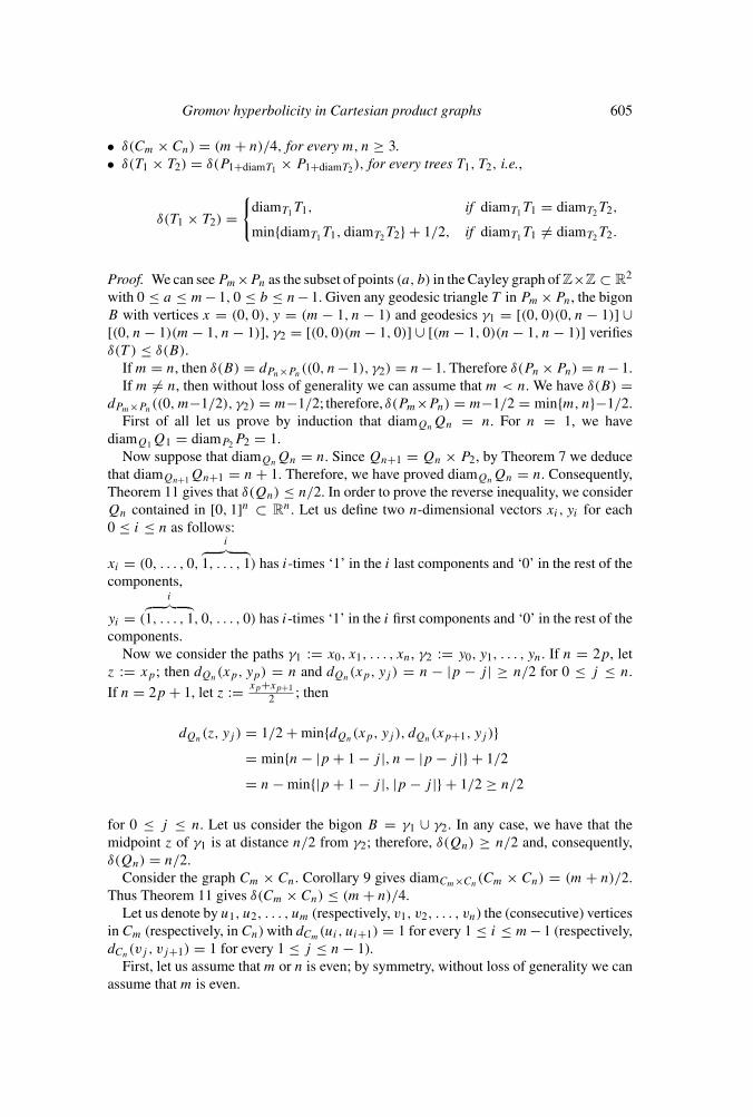
• δ(Cm × Cn) = (m + n)/4, for every m, n ≥ 3.• δ(T1 × T2) = δ(P1+diamT1 × P1+diamT2), for every trees T1, T2, i.e.,

δ(T1 × T2) ={

diamT1T1, if diamT1T1 = diamT2T2,

min{diamT1T1, diamT2T2} + 1/2, if diamT1T1 �= diamT2T2.

Proof. We can see Pm×Pn as the subset of points (a, b) in the Cayley graph of Z×Z ⊂ R2

with 0 ≤ a ≤ m− 1, 0 ≤ b ≤ n− 1. Given any geodesic triangle T in Pm ×Pn, the bigonB with vertices x = (0, 0), y = (m − 1, n − 1) and geodesics γ1 = [(0, 0)(0, n − 1)] ∪[(0, n − 1)(m − 1, n − 1)], γ2 = [(0, 0)(m − 1, 0)] ∪ [(m − 1, 0)(n − 1, n − 1)] verifiesδ(T ) ≤ δ(B).

If m = n, then δ(B) = dPn×Pn((0, n− 1), γ2) = n− 1. Therefore δ(Pn ×Pn) = n− 1.If m �= n, then without loss of generality we can assume that m < n. We have δ(B) =

dPm×Pn((0, m−1/2), γ2) = m−1/2; therefore, δ(Pm×Pn) = m−1/2 = min{m, n}−1/2.First of all let us prove by induction that diamQnQn = n. For n = 1, we have

diamQ1Q1 = diamP2P2 = 1.Now suppose that diamQnQn = n. Since Qn+1 = Qn × P2, by Theorem 7 we deduce

that diamQn+1Qn+1 = n + 1. Therefore, we have proved diamQnQn = n. Consequently,Theorem 11 gives that δ(Qn) ≤ n/2. In order to prove the reverse inequality, we considerQn contained in [0, 1]n ⊂ R

n. Let us define two n-dimensional vectors xi, yi for each0 ≤ i ≤ n as follows:

xi = (0, . . . , 0,

i︷︸︸︷1, . . . , 1) has i-times ‘1’ in the i last components and ‘0’ in the rest of the

components,

yi = (

i︷︸︸︷1, . . . , 1, 0, . . . , 0) has i-times ‘1’ in the i first components and ‘0’ in the rest of the

components.Now we consider the paths γ1 := x0, x1, . . . , xn, γ2 := y0, y1, . . . , yn. If n = 2p, let

z := xp; then dQn(xp, yp) = n and dQn(xp, yj ) = n − |p − j | ≥ n/2 for 0 ≤ j ≤ n.

If n = 2p + 1, let z := xp+xp+12 ; then

dQn(z, yj ) = 1/2 + min{dQn(xp, yj ), dQn(xp+1, yj )}= min{n − |p + 1 − j |, n − |p − j |} + 1/2

= n − min{|p + 1 − j |, |p − j |} + 1/2 ≥ n/2

for 0 ≤ j ≤ n. Let us consider the bigon B = γ1 ∪ γ2. In any case, we have that themidpoint z of γ1 is at distance n/2 from γ2; therefore, δ(Qn) ≥ n/2 and, consequently,δ(Qn) = n/2.

Consider the graph Cm × Cn. Corollary 9 gives diamCm×Cn(Cm × Cn) = (m + n)/2.Thus Theorem 11 gives δ(Cm × Cn) ≤ (m + n)/4.

Let us denote by u1, u2, . . . , um (respectively, v1, v2, . . . , vn) the (consecutive) verticesin Cm (respectively, in Cn) with dCm(ui, ui+1) = 1 for every 1 ≤ i ≤ m− 1 (respectively,dCn(vj , vj+1) = 1 for every 1 ≤ j ≤ n − 1).

First, let us assume that m or n is even; by symmetry, without loss of generality we canassume that m is even.


If n is even, let z = vn/2+1; then we define

γ1 := [u1um/2+1] × {v1} ∪ {um/2+1}× [v1z] (with u2 ∈ [u1um/2+1] and v2 ∈ [v1z])

and

γ2 := [um/2+1u1] × {z} ∪ {u1}× [zv1] (with um ∈ [um/2+1u1] and vn ∈ [zv1]).

If n is odd, let z be the midpoint of [v(n+1)/2, v(n+3)/2]; then

γ1 := [u1um/2+1] × {v1} ∪ {um/2+1}× [v1z] (with u2 ∈ [u1um/2+1] and v2 ∈ [v1z])

and

γ2 := {um/2+1} × [zv(n+3)/2] ∪ [um/2+1u1]

× {v(n+3)/2} ∪ {u1} × [v(n+3)/2v1] (with um ∈ [um/2+1u1]).

We have that B = {γ1, γ2} is a bigon and L(γ1) = L(γ2) = (m + n)/2. If p is themidpoint of γ1, then dCm×Cn(p, γ2) = (m + n)/4; therefore, δ(Cm × Cn) ≥ δ(B) ≥(m + n)/4.

Now, let us assume that m, n are odd. Let w be the midpoint of [u(m+1)/2, u(m+3)/2] andz the midpoint of [v(n+1)/2, v(n+3)/2]; then we define

γ1 := [wu1] × {v1} ∪ {u1} × [v1z] (with u2 ∈ [wu1] and v2 ∈ [v1z])

and

γ2 := {u1} × [zv(n+3)/2] ∪ [u1u(m+3)/2]

× {v(n+3)/2} ∪ {u(m+3)/2} × [v(n+3)/2v1] ∪ [u(m+3)/2w] × {v1}.We have that L(γ1) = L(γ2) = (m + n)/2. If p is the midpoint of γ1, then

dCm×Cn(p, γ2) = (m + n)/4; therefore, δ(Cm × Cn) ≥ δ(B) ≥ (m + n)/4.Then we conclude in any case that δ(Cm × Cn) = (m + n)/4.Now let us consider the graph T1 × T2. We have that there exists an isometric subgraph

�j of Tj with �j isometric to P1+diamTj, for j = 1, 2; then �1×�2 is an isometric subgraph

of T1 ×T2 and Lemma 17 gives δ(P1+diamT1 ×P1+diamT2) ≤ δ(T1 ×T2). In order to provethe reverse inequality let us consider two cases.

If diamT1T1 = diamT2T2, then diamT1×T2(T1 × T2) = 2diamT1T1 by Corollary 9. Now,Theorem 11 and the first item of Theorem 23 give

δ(T1 × T2) ≤ 1

2diamT1×T2(T1 × T2)

= diamT1T1 = δ(P1+diamT1 × P1+diamT2).

If diamT1T1 �= diamT2T2, by symmetry we can assume that diamT1T1 > diamT2T2. ThenTheorem 15 and the second item of Theorem 23 give

δ(T1 × T2) ≤ diamT2T2 + 1/2

= 1 + diamT2T2 − 1/2 = δ(P1+diamT1 × P1+diamT2). �


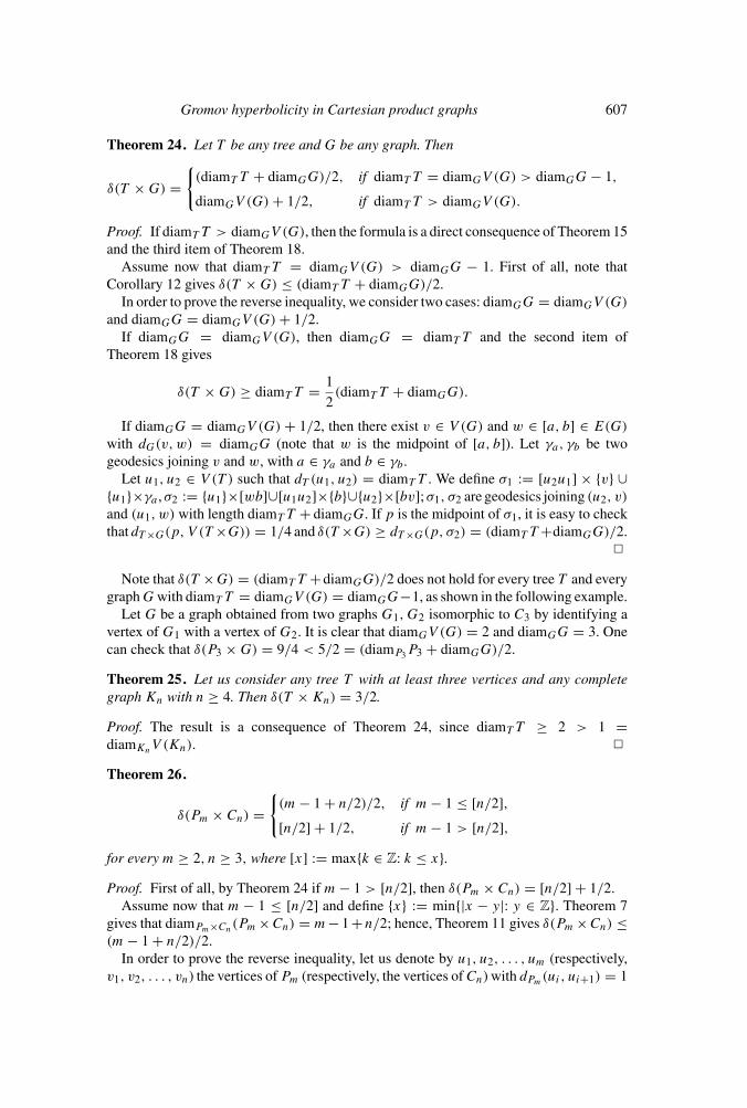
Theorem 24. Let T be any tree and G be any graph. Then

δ(T × G) ={

(diamT T + diamGG)/2, if diamT T = diamGV (G) > diamGG − 1,

diamGV (G) + 1/2, if diamT T > diamGV (G).

Proof. If diamT T > diamGV (G), then the formula is a direct consequence of Theorem 15and the third item of Theorem 18.

Assume now that diamT T = diamGV (G) > diamGG − 1. First of all, note thatCorollary 12 gives δ(T × G) ≤ (diamT T + diamGG)/2.

In order to prove the reverse inequality, we consider two cases: diamGG = diamGV (G)

and diamGG = diamGV (G) + 1/2.If diamGG = diamGV (G), then diamGG = diamT T and the second item of

Theorem 18 gives

δ(T × G) ≥ diamT T = 1

2(diamT T + diamGG).

If diamGG = diamGV (G) + 1/2, then there exist v ∈ V (G) and w ∈ [a, b] ∈ E(G)

with dG(v, w) = diamGG (note that w is the midpoint of [a, b]). Let γa, γb be twogeodesics joining v and w, with a ∈ γa and b ∈ γb.

Let u1, u2 ∈ V (T ) such that dT (u1, u2) = diamT T . We define σ1 := [u2u1] × {v} ∪{u1}×γa , σ2 := {u1}×[wb]∪[u1u2]×{b}∪{u2}×[bv]; σ1, σ2 are geodesics joining (u2, v)

and (u1, w) with length diamT T + diamGG. If p is the midpoint of σ1, it is easy to checkthat dT ×G(p, V (T ×G)) = 1/4 and δ(T ×G) ≥ dT ×G(p, σ2) = (diamT T +diamGG)/2.

�

Note that δ(T ×G) = (diamT T +diamGG)/2 does not hold for every tree T and everygraph G with diamT T = diamGV (G) = diamGG−1, as shown in the following example.

Let G be a graph obtained from two graphs G1, G2 isomorphic to C3 by identifying avertex of G1 with a vertex of G2. It is clear that diamGV (G) = 2 and diamGG = 3. Onecan check that δ(P3 × G) = 9/4 < 5/2 = (diamP3P3 + diamGG)/2.

Theorem 25. Let us consider any tree T with at least three vertices and any completegraph Kn with n ≥ 4. Then δ(T × Kn) = 3/2.

Proof. The result is a consequence of Theorem 24, since diamT T ≥ 2 > 1 =diamKnV (Kn). �

Theorem 26.

δ(Pm × Cn) ={

(m − 1 + n/2)/2, if m − 1 ≤ [n/2],

[n/2] + 1/2, if m − 1 > [n/2],

for every m ≥ 2, n ≥ 3, where [x] := max{k ∈ Z: k ≤ x}.Proof. First of all, by Theorem 24 if m − 1 > [n/2], then δ(Pm × Cn) = [n/2] + 1/2.

Assume now that m − 1 ≤ [n/2] and define {x} := min{|x − y|: y ∈ Z}. Theorem 7gives that diamPm×Cn(Pm ×Cn) = m− 1 +n/2; hence, Theorem 11 gives δ(Pm ×Cn) ≤(m − 1 + n/2)/2.

In order to prove the reverse inequality, let us denote by u1, u2, . . . , um (respectively,v1, v2, . . . , vn) the vertices of Pm (respectively, the vertices of Cn) with dPm(ui, ui+1) = 1


for every 1 ≤ i ≤ m − 1 (respectively, dCn(vj , vj+1) = 1 for every 1 ≤ j ≤ n − 1). Letx := v1 and y be the point in Cn such that dCn(x, y) = n/2. Let us define the geodesicsσ1 := [(um, x)(u1, x)] ∪ [(u1, x)(u1, y)], where [(u1, x)(u1, y)] is the geodesic contain-ing (u1, v2), σ2 := [(u1, y)(um, y)] ∪ [(um, y)(um, x)] if n is even (with (um, vn−1) ∈[(um, y)(um, x)]), and σ2 := [(u1, y)(u1, v(n+3)/2)] ∪ [(u1, v(n+3)/2)(um, v(n+3)/2)] ∪[(um, v(n+3)/2)(um, x)] if n is odd; note that σ1, σ2 are geodesics of length m − 1 + n/2.

Now let us consider the bigon B = {σ1, σ2}. Then the midpoint p of σ1 satisfies

dPm×Cn(p, σ2) = min{(m − 1 + n/2)/2, [n/2] + {(m − 1 + n/2)/2}};therefore,

δ(Pm × Cn) ≥ min{(m − 1 + n/2)/2, [n/2] + {(m − 1 + n/2)/2}}.We will now show that (m − 1 + n/2)/2 ≤ [n/2] + {(m − 1 + n/2)/2}. If n is even, then[n/2] = n/2 and m − 1 ≤ n/2; hence, m − 1 + n/2 ≤ n and

(m − 1 + n/2)/2 ≤ n/2 = [n/2] ≤ [n/2] + {(m − 1 + n/2)/2}.If n is odd, then [n/2] = (n− 1)/2 and (m− 1 +n/2)/2 ∈ (N+ 1/4)∪ (N+ 3/4); hence,{(m − 1 + n/2)/2} = 1/4, m − 1 + n/2 ≤ (n − 1)/2 + n/2 = n − 1 + 1/2 and

(m − 1 + n/2)/2 ≤ (n − 1)/2 + 1/4 = [n/2] + {(m − 1 + n/2)/2}.Therefore, δ(Pm × Cn) ≥ (m − 1 + n/2)/2 and we conclude that δ(Pm × Cn) =(m − 1 + n/2)/2. �

Acknowledgements

This work was partly supported by the Spanish Ministry of Science and Innovation throughprojects MTM2009-07800; MTM2008-02829-E and by the grant ‘Estudio de la hiper-bolicidad de superficies en el sentido de Gromov’ (SEP-CONACYT, Mexico, 2009).

We would like to thank the referee for a careful reading of the manuscript and for hisvaluable comments and suggestions.

References

[1] Balogh Z M and Buckley S M, Geometric characterizations of Gromov hyperbolicity,Invent. Math. 153 (2003) 261–301

[2] Bermudo S, Rodrıguez J M, Sigarreta J M and Vilaire J-M, Mathematical properties ofGromov hyperbolic graphs, to appear in AIP Conference Proceedings (2010)

[3] Bermudo S, Rodrıguez J M, Sigarreta J M and Vilaire J-M, Gromov hyperbolic graphs,preprint

[4] Bermudo S, Rodrıguez J M, Sigarreta J M and Tourıs E, Hyperbolicity and complementof graphs, preprint

[5] Bonk M, Heinonen J and Koskela P, Uniformizing Gromov hyperbolic spaces, Asterisque270 (2001) 99 pp.

[6] Bowditch B H, Notes on Gromov’s hyperobolicity criterion for path-metric spaces.Group theory from a geometrical viewpoint, Trieste, 1990 (eds) E Ghys, A Haefliger andA Verjovsky (River Edge, NJ: World Scientific) (1991) pp. 64–167


[7] Brinkmann G, Koolen J and Moulton V, On the hyperbolicity of chordal graphs, Ann.Comb. 5 (2001) 61–69

[8] Chepoi V, Dragan F F, Estellon B, Habib M and Vaxes Y, Notes on diameters, centers andapproximating trees of δ-hyperbolic geodesic spaces and graphs, Electr. Notes DiscreteMath. 31 (2008) 231–234

[9] Frigerio R and Sisto A, Characterizing hyperbolic spaces and real trees, Geom Dedicata142 (2009) 139–149

[10] Ghys E and de la Harpe P, Sur les Groupes Hyperboliques d’apres Mikhael Gromov,Progress in Mathematics 83 (Boston, MA: Birkhauser Boston Inc.) (1990)

[11] Gromov M, Hyperbolic groups, in ‘Essays in group theory’ (ed) S M Gersten (MSRIPubl., Springer) (1987) vol. 8, pp. 75–263

[12] Gromov M (with appendices by M Katz, P Pansu and S Semmes), Metric structures forRiemannian and non-Riemannnian spaces, Progress in Mathematics (Birkhauser) (1999)vol. 152

[13] Hasto P A, Gromov hyperbolicity of the jG and jG metrics, Proc. Am. Math. Soc. 134(2006) 1137–1142

[14] Hasto P A, Linden H, Portilla A, Rodrıguez J M and Tourıs E, Gromov hyperbolicity ofDenjoy domains with hyperbolic and quasihyperbolic metrics, preprint

[15] Hasto P A, Portilla A, Rodrıguez J M and Tourıs E, Gromov hyperbolic equivalence ofthe hyperbolic and quasihyperbolic metrics in Denjoy domains, to appear in Bull. LondonMath. Soc.

[16] Hasto P A, Portilla A, Rodrıguez J M and Tourıs E, Comparative Gromov hyperbolicityresults for the hyperbolic and quasihyperbolic metrics, to appear in Complex Variablesand Elliptic Equations

[17] Hasto P A, Portilla A, Rodrıguez J M and Tourıs E, Uniformly separated sets and Gromovhyperbolicity of domains with the quasihyperbolic metric, to appear in Medit. J. Math.

[18] Jonckheere E A, Controle du trafic sur les reseaux a geometrie hyperbolique–Uneapproche mathematique a la securite de l’acheminement de l’information, JournalEuropeen de Systemes Automatises 37(2) (2003) 145–159

[19] Jonckheere E A and Lohsoonthorn P, Geometry of network security, American ControlConf. ACC (2004) 111–151

[20] Jonckheere E A, Lohsoonthorn P and Bonahon F, Scaled Gromov hyperbolic graphs,J. Graph Theory 2 (2007) 157–180

[21] Koolen J H and Moulton V, Hyperbolic Bridged Graphs, Europ. J. Combinatorics 23(2002) 683–699

[22] Michel J, Rodrıguez J M, Sigarreta J M and Villeta M, Hyperbolicity and parameters ofgraphs, to appear in Ars Combinatoria

[23] Oshika K, Discrete groups (AMS Bookstore) (2002)[24] Portilla A, Rodrıguez J M and Tourıs E, Gromov hyperbolicity through decomposition

of metric spaces II, J. Geom. Anal. 14 (2004) 123–149[25] Portilla A and Tourıs E, A characterization of Gromov hyperbolicity of surfaces with

variable negative curvature, Publ. Mat. 53 (2009) 83–110[26] Rodrıguez J M, Sigarreta J M, Vilaire J-M and Villeta M, On the hyperbolicity constant

in graphs, preprint[27] Rodrıguez J M and Tourıs E, Gromov hyperbolicity through decomposition of metric

spaces, Acta Math. Hungar. 103 (2004) 53–84[28] Rodrıguez J M and Tourıs E, A new characterization of Gromov hyperbolicity for

Riemann surfaces, Publ. Mat. 50 (2006) 249–278[29] Rodrıguez J M and Tourıs E, Gromov hyperbolicity of Riemann surfaces, Acta Math.

Sinica 23 (2007) 209–228[30] Tourıs E, Graphs and Gromov hyperbolicity of non-constant negatively curved surfaces,

preprint

Documents

Gromov hyperbolicity in Cartesian product graphs