General rights Copyright and moral rights for the publications made accessible in the public portal are retained by the authors and/or other copyright owners and it is a condition of accessing publications that users recognise and abide by the legal requirements associated with these rights.

Users may download and print one copy of any publication from the public portal for the purpose of private study or research.

You may not further distribute the material or use it for any profit-making activity or commercial gain

You may freely distribute the URL identifying the publication in the public portal If you believe that this document breaches copyright please contact us providing details, and we will remove access to the work immediately and investigate your claim.

Downloaded from orbit.dtu.dk on: Feb 12, 2022

Group-Contribution based Property Estimation and Uncertainty analysis forFlammability-related Properties

Frutiger, Jerome; Marcarie, Camille; Abildskov, Jens; Sin, Gürkan

Published in:Journal of Hazardous Materials

Link to article, DOI:10.1016/j.jhazmat.2016.06.018

Publication date:2016

Document VersionPeer reviewed version

Link back to DTU Orbit

Citation (APA):Frutiger, J., Marcarie, C., Abildskov, J., & Sin, G. (2016). Group-Contribution based Property Estimation andUncertainty analysis for Flammability-related Properties. Journal of Hazardous Materials, 318, 783–793.https://doi.org/10.1016/j.jhazmat.2016.06.018

Accepted Manuscript

Title: Group-Contribution based Property Estimation andUncertainty analysis for Flammability-related Properties

Author: Jerome Frutiger Camille Marcarie Jens AbildskovGurkan Sin

PII: S0304-3894(16)30573-8DOI: http://dx.doi.org/doi:10.1016/j.jhazmat.2016.06.018Reference: HAZMAT 17807

To appear in: Journal of Hazardous Materials

Received date: 30-3-2016Revised date: 20-5-2016Accepted date: 8-6-2016

Please cite this article as: Jerome Frutiger, Camille Marcarie, Jens Abildskov,Gurkan Sin, Group-Contribution based Property Estimation and Uncertaintyanalysis for Flammability-related Properties, Journal of Hazardous Materialshttp://dx.doi.org/10.1016/j.jhazmat.2016.06.018

This is a PDF file of an unedited manuscript that has been accepted for publication.As a service to our customers we are providing this early version of the manuscript.The manuscript will undergo copyediting, typesetting, and review of the resulting proofbefore it is published in its final form. Please note that during the production processerrors may be discovered which could affect the content, and all legal disclaimers thatapply to the journal pertain.

1

Group-Contribution based Property Estimation and

Uncertainty analysis for Flammability-related

Properties

Jérôme Frutiger, Camille Marcarie, Jens Abildskov, Gürkan Sin*

The CAPEC-PROCESS Research Center, Department of Chemical and Biochemical

Engineering, Technical University of Denmark (DTU), Building 229, DK-2800 Lyngby,

Denmark

*corresponding author

2

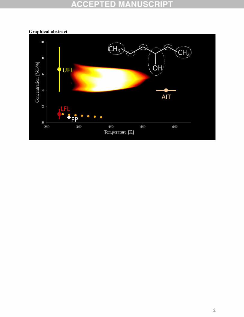
Graphical abstract

3

Group-Contribution based Property Estimation and

Uncertainty analysis for Flammability-related Properties

Jérôme Frutiger, Camille Marcarie, Jens Abildskov, Gürkan Sin*

The CAPEC-PROCESS Research Center, Department of Chemical and Biochemical

Engineering, Technical University of Denmark (DTU), Building 229, DK-2800 Lyngby,

Denmark

*corresponding author

Highlights

1) Novel group contribution model for lower and upper flammability limit

2) Reporting 95%-confidence interval of predicted value for safety-related properties

3) Simple approach to describe temperature-dependent lower flammability limit

4) Robust parameter regression and thorough uncertainty analysis

5) Improved group contribution factors for flash point and auto ignition temperature

4

ABSTRACT

This study presents new group contribution (GC) models for the prediction of Lower and Upper

Flammability Limits (LFL and UFL), Flash Point (FP) and Auto Ignition Temperature (AIT) of

organic chemicals applying the Marrero/Gani (MG) method. Advanced methods for parameter

estimation using robust regression and outlier treatment have been applied to achieve high

accuracy. Furthermore, linear error propagation based on covariance matrix of estimated

parameters was performed. Therefore, every estimated property value of the flammability-related

properties is reported together with its corresponding 95%-confidence interval of the prediction.

Compared to existing models the developed ones have a higher accuracy, are simple to apply and

provide uncertainty information on the calculated prediction. The average relative error and

correlation coefficient are 11.5% and 0.99 for LFL, 15.9% and 0.91 for UFL, 2.0% and 0.99 for

FP as well as 6.4% and 0.76 for AIT. Moreover, the temperature-dependence of LFL property

was studied. A compound specific proportionality constant ( ) between LFL and

temperature is introduced and an MG GC model to estimate is developed. Overall the

ability to predict flammability-related properties including the corresponding uncertainty of the

prediction can provide important information for a qualitative and quantitative safety-related risk

assessment studies.

Keywords: Group contribution, Uncertainty, Flammability limit, Flash point, Auto ignition

temperature

5

1. Introduction

The safety characteristics of hazardous substances provide indispensable information for the risk

assessment of chemical products in industrial and domestic processes. In particular flammability-

related properties such as the lower and upper flammability limit (LFL and UFL), the flash point

(FP) and the auto ignition temperature (AIT) are important to quantify the risk of fire and

explosion. In the early design phase a large amount of alternative products and processes are

generally analysed, compared and ranked. Whenever experimental values are unavailable

property prediction models become a valuable tool [1].

Group contribution (GC) based property models try to estimate a chemical property based on

structurally dependent parameters. GC methods are known to be advantageous compared to ab

initio procedures, quantitative structure property relationship (QSPR) or prediction based on

artificial neural networks (ANN), because they are easy to apply, computationally less

demanding and have a wide application range [2]. Frutiger et al. [3] stressed the need for

thorough parameter estimation and uncertainty analysis for GC models in order to obtain

accurate and reliable property predictions. For safety-related properties the provision of

uncertainty information (i.e. the upper and lower bound of the 95%-confidence interval) is of

particular interest, because the statistical uncertainty should be taken into account, when risk

calculations are being carried out [4]. However, there is still a lack of application of uncertainty

analysis techniques for safety-related property prediction.

The lower flammability limit (LFL) and the upper flammability limit (UFL) are defined as the

lowest and the highest possible concentration of a substance in air at which a flammable mixture

is formed. These concentrations are stated at a specific temperature (298K) and pressure (1 atm).

6

However, LFL and UFL change with increasing temperature [5]. The flash point (FP) is the

lowest temperature where a liquid forms an ignitable vapour-air mixture. The auto ignition

temperature (AIT) is the lowest possible temperature above which a substance will ignite in air

without an external ignition source [6].

The review of Vidal et al. [7] provides an overview of the abundant literature, which is available

on single point calculations of LFL and FP. Rowley et al. [8] compared extensively a large

variety of the developed methods to estimate LFL at a predefined temperature of 298K (single

point prediction). The comparison contains purely correlation-based, GC methods and also

detailed mechanistic models. Among the GC based models for LFL and UFL prediction there are

several methods suggested in the literature. Shimy [9] derived formulas for different classes of

chemicals relating the number of carbon atoms with LFL. Solovev et al. [10] as well as Oehley

[11] used atomic indices to calculate LFL. Shebeko et al. [12] used atom and bond connectivity

indices in order to model LFL and UFL of pure compounds. Kondo et al. [13][14] developed a

GC method to estimate the ratio between LFL and UFL, which they called F-number. All of

these methods are simple and easy to apply, but employ very little structural information on the

molecules and a limited application range. Hence, the average relative error is high considering

different classes of chemicals [8]. Seaton [15] developed a GC method for LFL and UFL of pure

compounds. The application range of the latter method is limited by the relatively small number

of functional groups. The methods of Shebeko and Seaton have been used to predict non-

experimental property values for LFL in the DIPPR 801 database [16]. Albahri [17] developed a

structural GC method to predict LFL and LFL. A QSPR model for LFL has been developed by

Gharagheizi [18]. Pan et al. [19][20] used topological, charge, and geometric descriptors to

describe a QSPR model for LFL and UFL. Recently, Gharagheizi [21] as well as Albahri [22]

7

calculated GC-factors for LFL using artificial neural networks (ANN). Furthermore, Gharagheizi

[23] developed a QSPR model for UFL. In a similar approach using ANN, Lazzús [24] predicted

the LFL and UFL of various organic compounds. Bagheri et al. [25] used a nonlinear machine

learning model to develop a LFL QSPR method. However, the mathematical structure of the

latter methods using ANN or machine learning approaches for LFL and UFL is very complex,

making model building very tedious. High et al. [26] set up a simple GC model with a limited

amount of groups for UFL and included estimations of the upper and lower bound of the

confidence limits. Shu et al. [27] presented a method using the threshold temperature (e.g. the

ignition temperature) to evaluate UFL of a hydrocarbon diluted within an inert gas. The same

authors also presented a model to evaluate the flammable zones of hydrocarbon-air-CO2

mixtures based on flame temperature theory [28]. Rowley et al. [8] provided a GC method that

is based on the relationship between LFL, the respective enthalpies of the substance as well as air

and the adiabatic flame temperature, obtaining high accuracy. Mendiburu et al. [29][30]

developed semi empirical methods for determination of LFL and UFL of C-H compounds, which

took into account the stoichiometry of combustion process and the estimation of the adiabatic

flame temperature. Except to High et al., none of the above mentioned methods includes a

thorough uncertainty analysis. Hence, no information about the respective 95% confidence

interval for a specific prediction of LFL and UFL is provided.

The temperature-dependence of LFL and UFL of organic compounds is generally depicted by

the modified Burgess-Wheeler law [31], that relates LFL, temperature, the heat capacity of the

fuel-air mixture and the heat of combustion . Britton et al. [32][33] suggested correlations

between LFL and the adiabatic flame temperature. Both methods assume that the adiabatic flame

temperature is independent of the initial temperature, which was found to be only true for

8

experimental condition, where LFL was measured in a narrow tube [8][34]. A purely empirical

correlation of LFL on a wide range of temperature has been proposed by Catoire et al. [35]

taking into account the corresponding stoichiometric mixture of fuel and air mixture and the

number of carbon atoms in the molecule. However, the model strongly depends on the data set

itself. Rowley et al. [8] improved the modified Burgess-Wheeler law by taking into account the

temperature-dependence of the adiabatic flame temperature and relating it to the number of

carbon atoms. However, there is only limited amount of structural information of the molecules

(i.e. the carbon number) taken into account.

Hukkerikar et al. [36] developed a GC model using Marrero/Gani (MG) method for FP and AIT

including an uncertainty analysis based on the parameter covariance matrix and performance

criteria to assess the quality of parameter estimation. Frutiger et al. [3] developed a GC model for

the heat of combustion taking into account different parameter regression methods,

optimization algorithms, alternative uncertainty analysis methods and advanced outlier

treatment. The same authors also analyzed parameter identifiability issues as the source of

prediction inaccuracy and uncertainty. Furthermore, they calculated and reported the 95%

confidence interval of GC model predictions (prediction accuracy). This thorough and systematic

methodology led to significant improvement of GC based model development.

In this study, we therefore aim to provide a new set of improved group contribution models using

Marrero/Gani (MG) method [37] to estimate LFL and UFL, FP and AIT at standard conditions

using the systematic model development and analysis method of Frutiger et al. [3]. Furthermore,

we suggest a GC method to include temperature-dependency in lower flammability limit

calculation. The models include a thorough uncertainty analysis (i.e. estimation of the 95%-

confidence interval) of every prediction, in order to provide additional information on the

9

reliability of the estimated property. In that sense it is possible to obtain an overall picture of the

different flammability properties of a chemical based on the same property prediction

methodology.

The paper is organized as follows: (i) the overall methodology for the GC model development

and uncertainty analysis for single point LFL, UFL, FP and AIT is shown; (ii) the LFL model is

extended to include temperature-dependence; (iii) the performances of the novel GC models are

compared with that of existing models; (iv) an application example for 3-Hexanol to calculate

LFL including 95% confidence interval is provided.

10

2. Method

The procedure to develop the GC model for the single point LFL UFL, FP and AIT, to estimate

its parameters and to perform the uncertainty analysis, follows the work of Frutiger et al. [3].

Robust regression method as well as the covariance based uncertainty analysis has been applied

for this study. Frutiger et al. [3] suggested and compared also alternative methods for parameter

estimation and uncertainty analysis, e.g. in order to take into account experimental uncertainties.

GC MG factors for FP and AIT are re-estimated using robust regression and outlier treatment,

aiming an improved parameter fit compared to the previous estimations [36].

2.1. GC model functions

As a GC model structure the Marrero/Gani (MG) [37] method is chosen, which considers

structural contributions on three levels. The MG method is written as

(1)

(2)

A specific functional group (1st order parameters j) is expressed by the factor Cj that occurs Nj

times. Dk is the contribution factor of the polyfunctional (2nd order parameters k) that occurs Mk

times in the molecular structure. Finally structural groups (3rd order parameters l) are taken into

account by the contribution El that has Ol occurrences. The function f(X) needs to be specified for

a certain property X. The factors can be determined for a specific molecule following the rules of

Marrero et al. [37]. The GC parameters can be summarized in vector with T being the

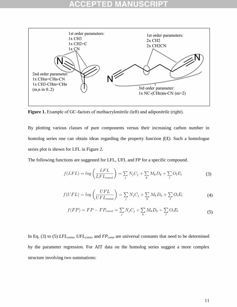
occurrence matrix of the factors (see Eq. (2)). MG groups are shown for methacrylonitrile and

adiponitrile in Figure 1.

11

Figure 1. Example of GC-factors of methacrylonitrile (left) and adiponitrile (right).

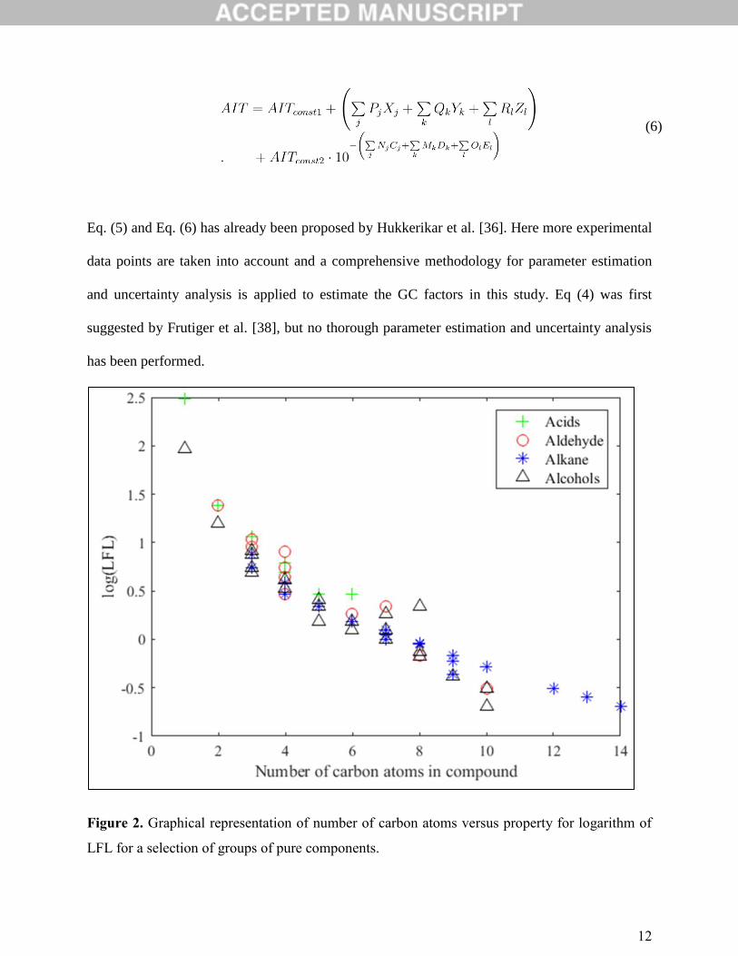
By plotting various classes of pure components versus their increasing carbon number in

homolog series one can obtain ideas regarding the property function f(X). Such a homologue

series plot is shown for LFL in Figure 2.

The following functions are suggested for LFL, UFL and FP for a specific compound.

(3)

(4)

(5)

In Eq. (3) to (5) LFLconst, UFLconst, and FPconst are universal constants that need to be determined

by the parameter regression. For AIT data on the homolog series suggest a more complex

structure involving two summations:

12

(6)

Eq. (5) and Eq. (6) has already been proposed by Hukkerikar et al. [36]. Here more experimental

data points are taken into account and a comprehensive methodology for parameter estimation

and uncertainty analysis is applied to estimate the GC factors in this study. Eq (4) was first

suggested by Frutiger et al. [38], but no thorough parameter estimation and uncertainty analysis

has been performed.

Figure 2. Graphical representation of number of carbon atoms versus property for logarithm of

LFL for a selection of groups of pure components.

13

In order to account for the temperature-dependence of LFL the approach of Rowley et al. [8] is

used as a basis to derive a new MG GC method. The latter authors also provided a detailed

derivation and explanation of the following equations.

The temperature-dependent LFL of Rowley et al. is based on the following energy balance of the

combustion process:

(7)

where is the heat of combustion, is the heat capacity of the compound and air

is the heat capacity of the combustion products and is the adiabatic flame

temperature. Rowley et al. further assumed:

1) to be roughly equal to 2) the adiabatic flame temperature as linearly

decreasing with increasing initial temperature [34].

This leads to the following generalization of the Burgess-Wheeler law [8]:

(8)

where is assumed to be

(9)

is the compound specific linear constant of , is the heat capacity of a specific

compound at the reference temperature and is the heat capacity of air at the reference

temperature .

Comparing experimental flammability data for different temperatures and various compounds,

usually a linear dependence between LFL and the temperature T is reported by [5][34][39].

Based on this premise, we present a simplified model as follows:

14

(10)

where is the proportionality constant between LFL and T for a specific compound i.

could be determined for a certain compound i by analyzing the experimental work of Coward et

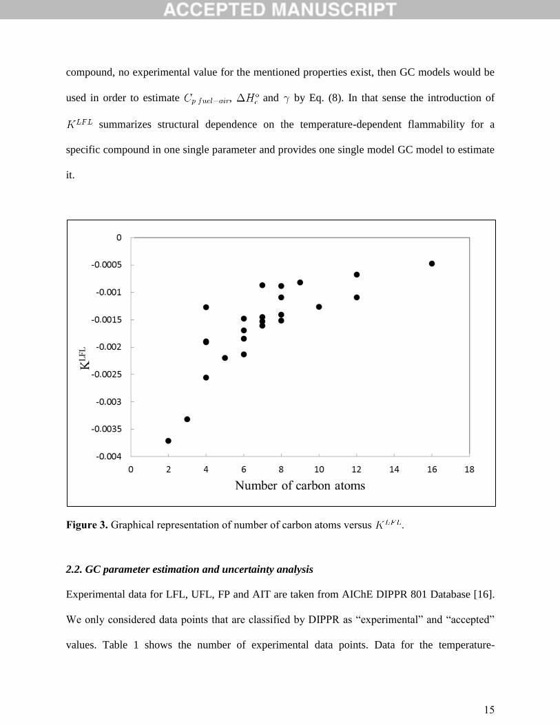
al. [39] and Rowley et al. [34]. Plotting versus the corresponding carbon number of the

compounds implies the possibility of describing this constant by GC models using a reciprocal

model function (see Figure 3). Therefore, we propose the following Marrero/Gani GC model to

estimate for a specific compound:

(11)

with as the universal correlation constant and Cj the first order parameters that occurs Nj

times.

Comparison with the generalized Burgess-Wheeler law in Eq. (8) with Eq. (10), shows that our

proposed proportionality constant can be considered as a lumped parameter of several properties:

(12)

Calculating directly from GC factors reduces the amount of parameters in the model

which makes it easier to apply. Furthermore, it lumps properties that showed to be correlated

with increasing carbon number or structurally-dependent group contribution factors in previous

studies: is linearly depending on the heat capacities and . Joback and

Reid depicted the dependence of the heat capacity on the structurally dependent parameters [40].

is strongly depending on the carbon numbers and a MG GC method has been developed by

Frutiger et al. [3]. Rowley et al. [8] showed dependence of on the carbon numbers. If for a

15

compound, no experimental value for the mentioned properties exist, then GC models would be

used in order to estimate , and by Eq. (8). In that sense the introduction of

summarizes structural dependence on the temperature-dependent flammability for a

specific compound in one single parameter and provides one single model GC model to estimate

it.

Figure 3. Graphical representation of number of carbon atoms versus .

2.2. GC parameter estimation and uncertainty analysis

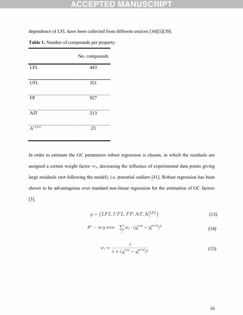
Experimental data for LFL, UFL, FP and AIT are taken from AIChE DIPPR 801 Database [16].

We only considered data points that are classified by DIPPR as “experimental” and “accepted”

values. Table 1 shows the number of experimental data points. Data for the temperature-

16

dependence of LFL have been collected from different sources [34][5][39].

Table 1. Number of compounds per property.

No. compounds

LFL 443

UFL 351

FP 927

AIT 513

23

In order to estimate the GC parameters robust regression is chosen, in which the residuals are

assigned a certain weight factor , decreasing the influence of experimental data points giving

large residuals (not following the model), i.e. potential outliers [41]. Robust regression has been

shown to be advantageous over standard non-linear regression for the estimation of GC factors

[3].

(13)

(14)

(15)

17

is the parameter (1st, 2

nd and 3

rd order group contributions) estimates and is the

prediction of compound i according to Eq. (3) to (6) and its corresponding experimental

value.

Outliers are identified using the empirical cumulative distribution function (CDF) of the

residuals between experimental and predicted values, which has been described for GC models

by Frutiger et al.[38]. The empirical CDF is defined as a step function increasing by 1/n in every

data point. The major advantage of this methodology is that the distribution of the residuals is

estimated from the data themselves, not a priori assuming normal distribution. Outliers are

considered as data points that that lie below the 2.5% or above the 97.5% probability levels.

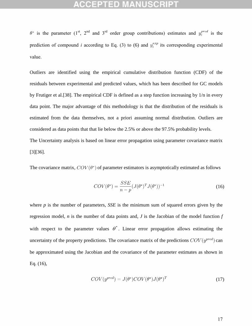
The Uncertainty analysis is based on linear error propagation using parameter covariance matrix

[3][36].

The covariance matrix, of parameter estimators is asymptotically estimated as follows

(16)

where p is the number of parameters, SSE is the minimum sum of squared errors given by the

regression model, n is the number of data points and, J is the Jacobian of the model function f

with respect to the parameter values * . Linear error propagation allows estimating the

uncertainty of the property predictions. The covariance matrix of the predictions can

be approximated using the Jacobian and the covariance of the parameter estimates as shown in

Eq. (16),

(17)

18

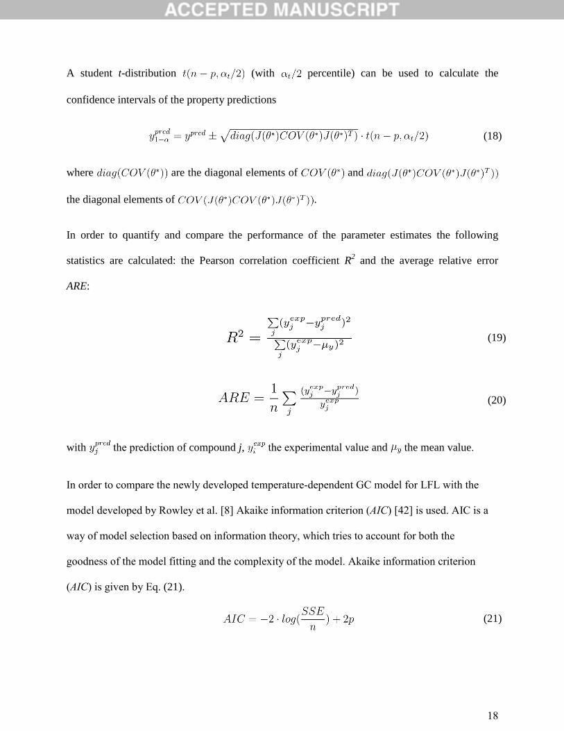
A student t-distribution (with percentile) can be used to calculate the

confidence intervals of the property predictions

(18)

where are the diagonal elements of and

the diagonal elements of .

In order to quantify and compare the performance of the parameter estimates the following

statistics are calculated: the Pearson correlation coefficient R2 and the average relative error

ARE:

(19)

(20)

with the prediction of compound j, the experimental value and the mean value.

In order to compare the newly developed temperature-dependent GC model for LFL with the

model developed by Rowley et al. [8] Akaike information criterion (AIC) [42] is used. AIC is a

way of model selection based on information theory, which tries to account for both the

goodness of the model fitting and the complexity of the model. Akaike information criterion

(AIC) is given by Eq. (21).

(21)

19

SSE is the sum of squared errors, n the number of data points and p the number of parameters

[42].

20

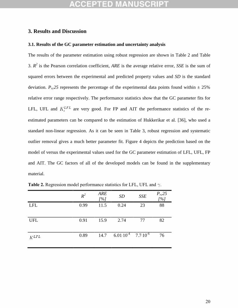
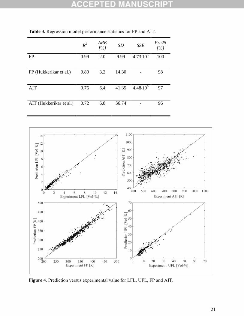
3. Results and Discussion

3.1. Results of the GC parameter estimation and uncertainty analysis

The results of the parameter estimation using robust regression are shown in Table 2 and Table

3. R2 is the Pearson correlation coefficient, ARE is the average relative error, SSE is the sum of

squared errors between the experimental and predicted property values and SD is the standard

deviation. Prc25 represents the percentage of the experimental data points found within ± 25%

relative error range respectively. The performance statistics show that the GC parameter fits for

LFL, UFL and are very good. For FP and AIT the performance statistics of the re-

estimated parameters can be compared to the estimation of Hukkerikar et al. [36], who used a

standard non-linear regression. As it can be seen in Table 3, robust regression and systematic

outlier removal gives a much better parameter fit. Figure 4 depicts the prediction based on the

model of versus the experimental values used for the GC parameter estimation of LFL, UFL, FP

and AIT. The GC factors of all of the developed models can be found in the supplementary

material.

Table 2. Regression model performance statistics for LFL, UFL and .

R

2

ARE

[%] SD SSE

Prc25

[%]

LFL 0.99 11.5 0.24 23 88

UFL 0.91 15.9 2.74 77 82

0.89 14.7 6.01 10-4

7.7 10-6

76

21

Table 3. Regression model performance statistics for FP and AIT.

Figure 4. Prediction versus experimental value for LFL, UFL, FP and AIT.

R

2

ARE

[%] SD SSE

Prc25

[%]

FP 0.99 2.0 9.99 4.73 105 100

FP (Hukkerikar et al.) 0.80 3.2 14.30 - 98

AIT 0.76 6.4 41.35 4.48 106 97

AIT (Hukkerikar et al.) 0.72 6.8 56.74 - 96

22

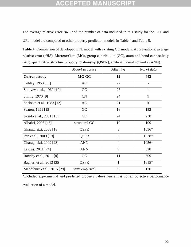
The average relative error ARE and the number of data included in this study for the LFL and

UFL model are compared to other property prediction models in Table 4 and Table 5.

Table 4. Comparison of developed LFL model with existing GC models. Abbreviations: average

relative error (ARE), Marrero/Gani (MG), group contribution (GC), atom and bond connectivity

(AC), quantitative structure property relationship (QSPR), artificial neural networks (ANN).

Model structure ARE [%] No. of data

Current study MG GC 12 443

Oehley, 1953 [11] AC 27 -

Solovev et al., 1960 [10] GC 25 -

Shimy, 1970 [9] CN 24 9

Shebeko et al., 1983 [12] AC 21 70

Seaton, 1991 [15] GC 16 152

Kondo et al., 2001 [13] GC 24 238

Albahri, 2003 [43] structural GC 10 109

Gharagheizi, 2008 [18] QSPR 8 1056*

Pan et al., 2009 [19] QSPR 5 1038*

Gharagheizi, 2009 [23] ANN 4 1056*

Lazzús, 2011 [24] ANN 9 328

Rowley et al., 2011 [8] GC 11 509

Bagheri et al., 2012 [25] QSPR 1 1615*

Mendiburu et al., 2015 [29] semi empirical 9 120

*included experimental and predicted property values hence it is not an objective performance

evaluation of a model.

23

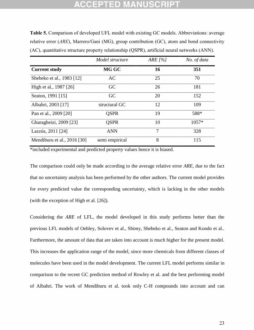
Table 5. Comparison of developed UFL model with existing GC models. Abbreviations: average

relative error (ARE), Marrero/Gani (MG), group contribution (GC), atom and bond connectivity

(AC), quantitative structure property relationship (QSPR), artificial neural networks (ANN).

Model structure ARE [%] No. of data

Current study MG GC 16 351

Shebeko et al., 1983 [12] AC 25 70

High et al., 1987 [26] GC 26 181

Seaton, 1991 [15] GC 20 152

Albahri, 2003 [17] structural GC 12 109

Pan et al., 2009 [20] QSPR 19 588*

Gharagheizi, 2009 [23] QSPR 10 1057*

Lazzús, 2011 [24] ANN 7 328

Mendiburu et al., 2016 [30] semi empirical 8 115

*included experimental and predicted property values hence it is biased.

The comparison could only be made according to the average relative error ARE, due to the fact

that no uncertainty analysis has been performed by the other authors. The current model provides

for every predicted value the corresponding uncertainty, which is lacking in the other models

(with the exception of High et al. [26]).

Considering the ARE of LFL, the model developed in this study performs better than the

previous LFL models of Oehley, Solovev et al., Shimy, Shebeko et al., Seaton and Kondo et al..

Furthermore, the amount of data that are taken into account is much higher for the present model.

This increases the application range of the model, since more chemicals from different classes of

molecules have been used in the model development. The current LFL model performs similar in

comparison to the recent GC prediction method of Rowley et al. and the best performing model

of Albahri. The work of Mendiburu et al. took only C-H compounds into account and can

24

therefore not be compared directly to the model of this study. The ANN methods of Lazzús and

Albahri shows better performance statistics as well. However, these authors took a lower amount

of experimental data points into account for the fitting of their model. Hence, the application

range is narrower. Furthermore, the ANN structure is very complex for even a relatively small

number of fitted data. In that sense its applicability is more difficult and its application range is

smaller. Similar conclusions can be made for UFL, where the developed model is superior to

Shebeko, High et al., Seaton and Pan et al.. Albahri and Lazzús perform slightly better, but they

used a smaller amount of data points, which leads to a smaller application range.

The ANN and QSPR models of Gharagheizi, Pan et al. and Bagheri et al. for LFL and UFL have

a lower ARE and more data points. However, the amount of data consist of all experimental data

and predicted values available in the DIPPR database which is not a scientifically accepted way

to compare model performance statistics. A parameter estimation should solely be based on

experimental data points only [44]. While comparing ANN or QSPR with GC models for

flammability, it is important to state that ANN/QSPR and are fundamentally different to GC

methods in the sense that the aim is to build the best possible model structure (i.e. considering

variables and descriptors). However, the model structure is fixed in GC methods and its goal is to

estimate the parameters in the best possible way given a certain available set of experimental

data. The structure of the MG GC model is much simpler compared to ANN and easier to apply

in practice. Furthermore, whereas the reliability of the GC model predictions have been

statistically demonstrated and verified against application in practice, establishing the reliability

and confidence of parameter estimation in ANN or QSPR remains to be demonstrated.

Furthermore, GC models allow adding new experimental values to the parameter estimation

25

without changing the model structure. In QSPR and ANN model building need to be performed

all over again [3].

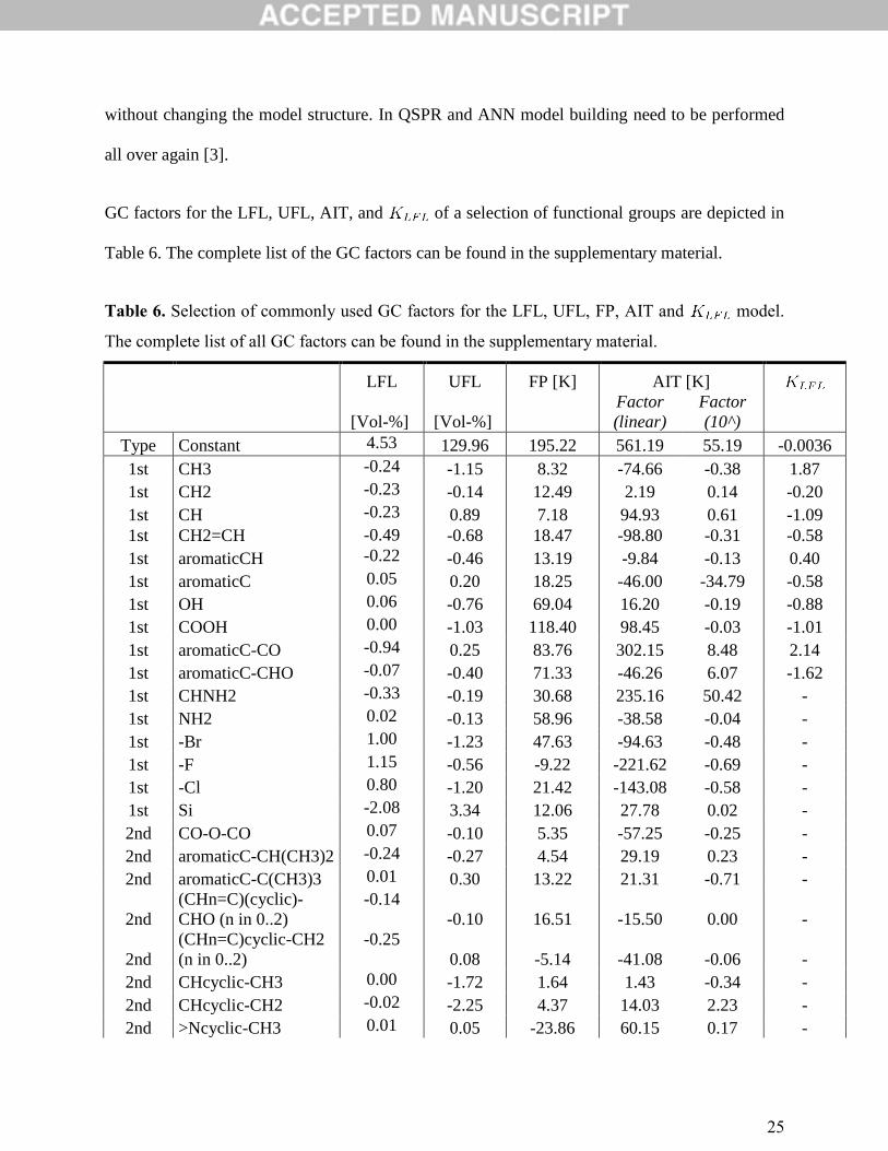
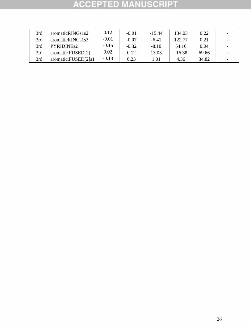
GC factors for the LFL, UFL, AIT, and of a selection of functional groups are depicted in

Table 6. The complete list of the GC factors can be found in the supplementary material.

Table 6. Selection of commonly used GC factors for the LFL, UFL, FP, AIT and model.

The complete list of all GC factors can be found in the supplementary material.

LFL UFL FP [K] AIT [K]

[Vol-%] [Vol-%]

Factor

(linear)

Factor

(10^)

Type Constant 4.53 129.96 195.22 561.19 55.19 -0.0036

1st CH3 -0.24 -1.15 8.32 -74.66 -0.38 1.87

1st CH2 -0.23 -0.14 12.49 2.19 0.14 -0.20

1st CH -0.23 0.89 7.18 94.93 0.61 -1.09

1st CH2=CH -0.49 -0.68 18.47 -98.80 -0.31 -0.58

1st aromaticCH -0.22 -0.46 13.19 -9.84 -0.13 0.40

1st aromaticC 0.05 0.20 18.25 -46.00 -34.79 -0.58

1st OH 0.06 -0.76 69.04 16.20 -0.19 -0.88

1st COOH 0.00 -1.03 118.40 98.45 -0.03 -1.01

1st aromaticC-CO -0.94 0.25 83.76 302.15 8.48 2.14

1st aromaticC-CHO -0.07 -0.40 71.33 -46.26 6.07 -1.62

1st CHNH2 -0.33 -0.19 30.68 235.16 50.42 -

1st NH2 0.02 -0.13 58.96 -38.58 -0.04 -

1st -Br 1.00 -1.23 47.63 -94.63 -0.48 -

1st -F 1.15 -0.56 -9.22 -221.62 -0.69 -

1st -Cl 0.80 -1.20 21.42 -143.08 -0.58 -

1st Si -2.08 3.34 12.06 27.78 0.02 -

2nd CO-O-CO 0.07 -0.10 5.35 -57.25 -0.25 -

2nd aromaticC-CH(CH3)2 -0.24 -0.27 4.54 29.19 0.23 -

2nd aromaticC-C(CH3)3 0.01 0.30 13.22 21.31 -0.71 -

2nd

(CHn=C)(cyclic)-

CHO (n in 0..2)

-0.14

-0.10 16.51 -15.50 0.00 -

2nd

(CHn=C)cyclic-CH2

(n in 0..2)

-0.25

0.08 -5.14 -41.08 -0.06 -

2nd CHcyclic-CH3 0.00 -1.72 1.64 1.43 -0.34 -

2nd CHcyclic-CH2 -0.02 -2.25 4.37 14.03 2.23 -

2nd >Ncyclic-CH3 0.01 0.05 -23.86 60.15 0.17 -

26

3rd aromaticRINGs1s2 0.12 -0.01 -15.44 134.03 0.22 -

3rd aromaticRINGs1s3 -0.01 -0.07 -6.41 122.77 0.21 -

3rd PYRIDINEs2 -0.15 -0.32 -8.10 54.16 0.04 -

3rd aromatic.FUSED[2] 0.02 0.12 13.03 -16.38 69.66 -

3rd aromatic.FUSED[2]s1 -0.13 0.23 1.01 4.36 34.82 -

27

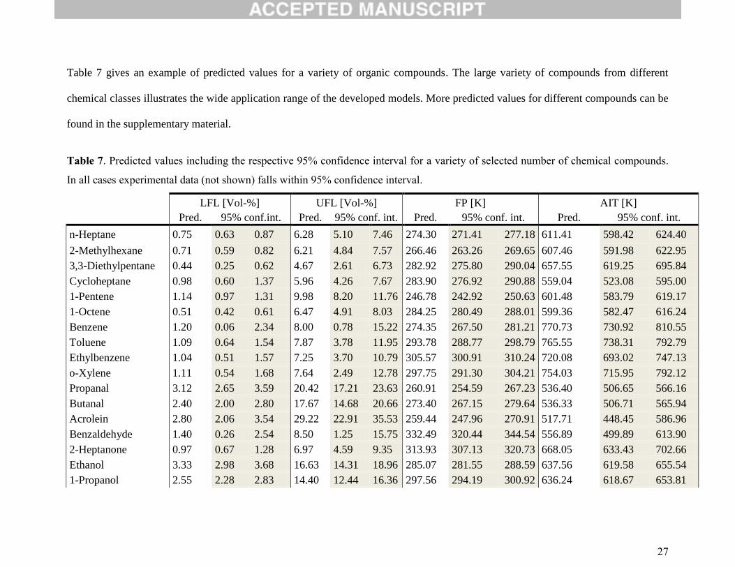
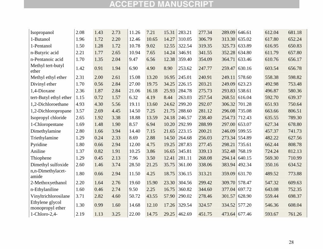
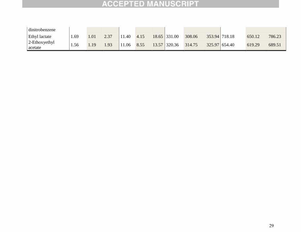
Table 7 gives an example of predicted values for a variety of organic compounds. The large variety of compounds from different

chemical classes illustrates the wide application range of the developed models. More predicted values for different compounds can be

found in the supplementary material.

Table 7. Predicted values including the respective 95% confidence interval for a variety of selected number of chemical compounds.

In all cases experimental data (not shown) falls within 95% confidence interval.

LFL [Vol-%] UFL [Vol-%] FP [K] AIT [K]

Pred. 95% conf.int. Pred. 95% conf. int. Pred. 95% conf. int. Pred. 95% conf. int.

n-Heptane 0.75 0.63 0.87 6.28 5.10 7.46 274.30 271.41 277.18 611.41 598.42 624.40

2-Methylhexane 0.71 0.59 0.82 6.21 4.84 7.57 266.46 263.26 269.65 607.46 591.98 622.95

3,3-Diethylpentane 0.44 0.25 0.62 4.67 2.61 6.73 282.92 275.80 290.04 657.55 619.25 695.84

Cycloheptane 0.98 0.60 1.37 5.96 4.26 7.67 283.90 276.92 290.88 559.04 523.08 595.00

1-Pentene 1.14 0.97 1.31 9.98 8.20 11.76 246.78 242.92 250.63 601.48 583.79 619.17

1-Octene 0.51 0.42 0.61 6.47 4.91 8.03 284.25 280.49 288.01 599.36 582.47 616.24

Benzene 1.20 0.06 2.34 8.00 0.78 15.22 274.35 267.50 281.21 770.73 730.92 810.55

Toluene 1.09 0.64 1.54 7.87 3.78 11.95 293.78 288.77 298.79 765.55 738.31 792.79

Ethylbenzene 1.04 0.51 1.57 7.25 3.70 10.79 305.57 300.91 310.24 720.08 693.02 747.13

o-Xylene 1.11 0.54 1.68 7.64 2.49 12.78 297.75 291.30 304.21 754.03 715.95 792.12

Propanal 3.12 2.65 3.59 20.42 17.21 23.63 260.91 254.59 267.23 536.40 506.65 566.16

Butanal 2.40 2.00 2.80 17.67 14.68 20.66 273.40 267.15 279.64 536.33 506.71 565.94

Acrolein 2.80 2.06 3.54 29.22 22.91 35.53 259.44 247.96 270.91 517.71 448.45 586.96

Benzaldehyde 1.40 0.26 2.54 8.50 1.25 15.75 332.49 320.44 344.54 556.89 499.89 613.90

2-Heptanone 0.97 0.67 1.28 6.97 4.59 9.35 313.93 307.13 320.73 668.05 633.43 702.66

Ethanol 3.33 2.98 3.68 16.63 14.31 18.96 285.07 281.55 288.59 637.56 619.58 655.54

1-Propanol 2.55 2.28 2.83 14.40 12.44 16.36 297.56 294.19 300.92 636.24 618.67 653.81

28

Isopropanol 2.08 1.43 2.73 11.26 7.21 15.31 283.21 277.34 289.09 646.61 612.04 681.18

1-Butanol 1.96 1.72 2.20 12.46 10.65 14.27 310.05 306.79 313.30 635.02 617.80 652.24

1-Pentanol 1.50 1.28 1.72 10.78 9.02 12.55 322.54 319.35 325.73 633.89 616.95 650.83

n-Butyric acid 2.21 1.77 2.65 10.94 7.65 14.24 346.91 341.55 352.28 634.80 611.79 657.80

n-Pentanoic acid 1.70 1.35 2.04 9.47 6.56 12.38 359.40 354.09 364.71 633.46 610.76 656.17

Methyl tert-butyl

ether 1.42 0.91 1.94 6.90 4.90 8.90 253.62 247.77 259.47 630.16 603.54 656.78

Methyl ethyl ether 2.31 2.00 2.61 15.08 13.20 16.95 245.01 240.91 249.11 578.60 558.38 598.82

Divinyl ether 1.70 0.56 2.84 27.00 19.75 34.25 226.15 203.21 249.09 623.23 492.98 753.48

1,4-Dioxane 2.36 1.87 2.84 21.06 16.18 25.93 284.78 275.73 293.83 538.61 496.87 580.36

tert-Butyl ethyl ether 1.15 0.72 1.57 6.32 4.19 8.44 263.03 257.54 268.51 616.04 592.70 639.37

1,2-Dichloroethane 4.93 4.30 5.56 19.11 13.60 24.62 299.20 292.07 306.32 701.28 651.93 750.64

1,2-Dichloropropane 3.57 2.69 4.45 14.50 7.25 21.75 288.60 281.12 296.08 735.08 663.66 806.51

Isopropyl chloride 2.65 1.92 3.38 18.88 13.59 24.18 246.57 238.40 254.73 712.43 635.55 789.30

1-Chloropentane 1.69 1.48 1.90 8.57 6.94 10.20 292.99 288.99 297.00 653.07 627.34 678.80

Dimethylamine 2.80 1.66 3.94 14.40 7.15 21.65 223.15 200.21 246.09 599.55 457.37 741.73

Triethylamine 1.29 0.24 2.33 8.69 2.88 14.50 264.68 256.03 273.34 554.89 482.22 627.56

Pyridine 1.80 0.66 2.94 12.00 4.75 19.25 287.83 277.45 298.21 735.61 662.44 808.78

Aniline 1.37 0.82 1.91 10.25 3.86 16.65 345.81 339.13 352.48 768.19 724.24 812.13

Thiophene 1.29 0.45 2.13 7.96 3.50 12.41 281.11 268.08 294.14 640.15 569.30 710.99

Dimethyl sulfoxide 2.60 1.46 3.74 28.50 21.25 35.75 361.00 338.06 383.94 492.34 350.16 634.52

n,n-Dimethylacet-

amide 1.80 0.66 2.94 11.50 4.25 18.75 336.15 313.21 359.09 631.70 489.52 773.88

2-Methoxyethanol 2.20 1.64 2.76 19.60 15.90 23.30 304.56 299.42 309.70 578.47 547.32 609.63

n-Ethylaniline 1.60 0.46 2.74 9.50 2.25 16.75 360.82 344.60 377.04 697.72 643.08 752.35

Vinyltrichlorosilane 3.71 2.82 4.60 50.72 43.55 57.90 290.02 278.46 301.57 628.90 559.44 698.37

Ethylene glycol

monopropyl ether 1.30 0.99 1.60 14.68 12.10 17.26 329.54 324.57 334.52 577.20 546.36 608.04

1-Chloro-2,4- 2.19 1.13 3.25 22.00 14.75 29.25 462.69 451.75 473.64 677.46 593.67 761.26

29

dinitrobenzene

Ethyl lactate 1.69 1.01 2.37 11.40 4.15 18.65 331.00 308.06 353.94 718.18 650.12 786.23

2-Ethoxyethyl

acetate 1.56 1.19 1.93 11.06 8.55 13.57 320.36 314.75 325.97 654.40 619.29 689.51

30

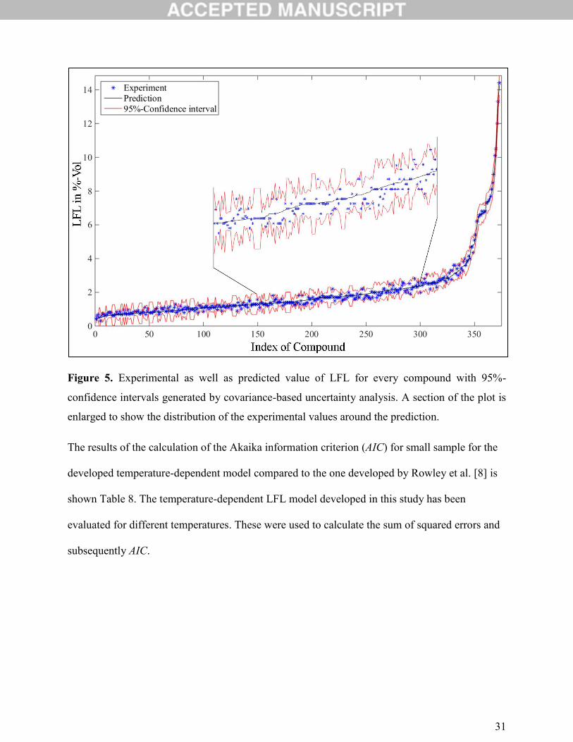
Figure 5 shows the results of the covariance-based uncertainty analysis, exemplified for the case

of LFL. The experimental and the predicted values of LFL with the respective 95%-confidence

interval of the prediction highest value and for every substance are shown. The compounds are

ordered from lowest to highest given an index number respectively. The 95%-confidence interval

is a narrow band that includes the experimental values. The detailed covariance-based

uncertainty analysis is another advantage of the developed GC models. Whereas the majority of

the other authors define the quality of their model only with ARE, we can provide the 95%-

confidence interval for every prediction. This additional information, i.e. the reliability of the

prediction, can be vital in the context of a quantitative safety-related risk analysis. For example it

is possible to use the lower-bound value of the confidence interval in a conservative analysis

approach. In fact, the lower bound of the confidence interval for LFL, is approximately 20% of

the LFL values. The latter is commonly used as a rule of thumb in quantitative risk analysis

(QRA) studies [45].

Although the extension to mixtures lies far beyond the scope of this work, users can calculate the

properties of mixtures from the current pure component model by applying simple mixing rules

(e.g. le Chatelier's mixing rule for flammability limit [46]).

31

Figure 5. Experimental as well as predicted value of LFL for every compound with 95%-

confidence intervals generated by covariance-based uncertainty analysis. A section of the plot is

enlarged to show the distribution of the experimental values around the prediction.

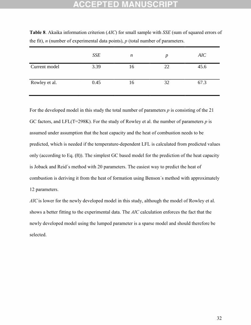
The results of the calculation of the Akaika information criterion (AIC) for small sample for the

developed temperature-dependent model compared to the one developed by Rowley et al. [8] is

shown Table 8. The temperature-dependent LFL model developed in this study has been

evaluated for different temperatures. These were used to calculate the sum of squared errors and

subsequently AIC.

32

Table 8. Akaika information criterion (AIC) for small sample with SSE (sum of squared errors of

the fit), n (number of experimental data points), p (total number of parameters.

SSE n p AIC

Current model 3.39 16 22 45.6

Rowley et al. 0.45 16 32 67.3

For the developed model in this study the total number of parameters p is consisting of the 21

GC factors, and LFL(T=298K). For the study of Rowley et al. the number of parameters p is

assumed under assumption that the heat capacity and the heat of combustion needs to be

predicted, which is needed if the temperature-dependent LFL is calculated from predicted values

only (according to Eq. (8)). The simplest GC based model for the prediction of the heat capacity

is Joback and Reid´s method with 20 parameters. The easiest way to predict the heat of

combustion is deriving it from the heat of formation using Benson´s method with approximately

12 parameters.

AIC is lower for the newly developed model in this study, although the model of Rowley et al.

shows a better fitting to the experimental data. The AIC calculation enforces the fact that the

newly developed model using the lumped parameter is a sparse model and should therefore be

selected.

33

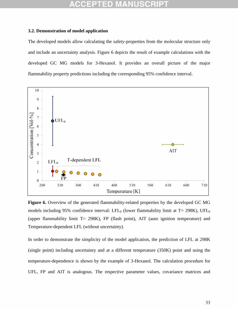
3.2. Demonstration of model application

The developed models allow calculating the safety-properties from the molecular structure only

and include an uncertainty analysis. Figure 6 depicts the result of example calculations with the

developed GC MG models for 3-Hexanol. It provides an overall picture of the major

flammability property predictions including the corresponding 95% confidence interval.

Figure 6. Overview of the generated flammability-related properties by the developed GC MG

models including 95% confidence interval: LFL0 (lower flammability limit at T= 298K), UFL0

(upper flammability limit T= 298K), FP (flash point), AIT (auto ignition temperature) and

Temperature-dependent LFL (without uncertainty).

In order to demonstrate the simplicity of the model application, the prediction of LFL at 298K

(single point) including uncertainty and at a different temperature (350K) point and using the

temperature-dependence is shown by the example of 3-Hexanol. The calculation procedure for

UFL, FP and AIT is analogous. The respective parameter values, covariance matrices and

34

jacobians for the model are given in the supplementary material. Further information (e.g. on the

identification of the GC factor for a new molecule) can also be provided by the authors upon

request.

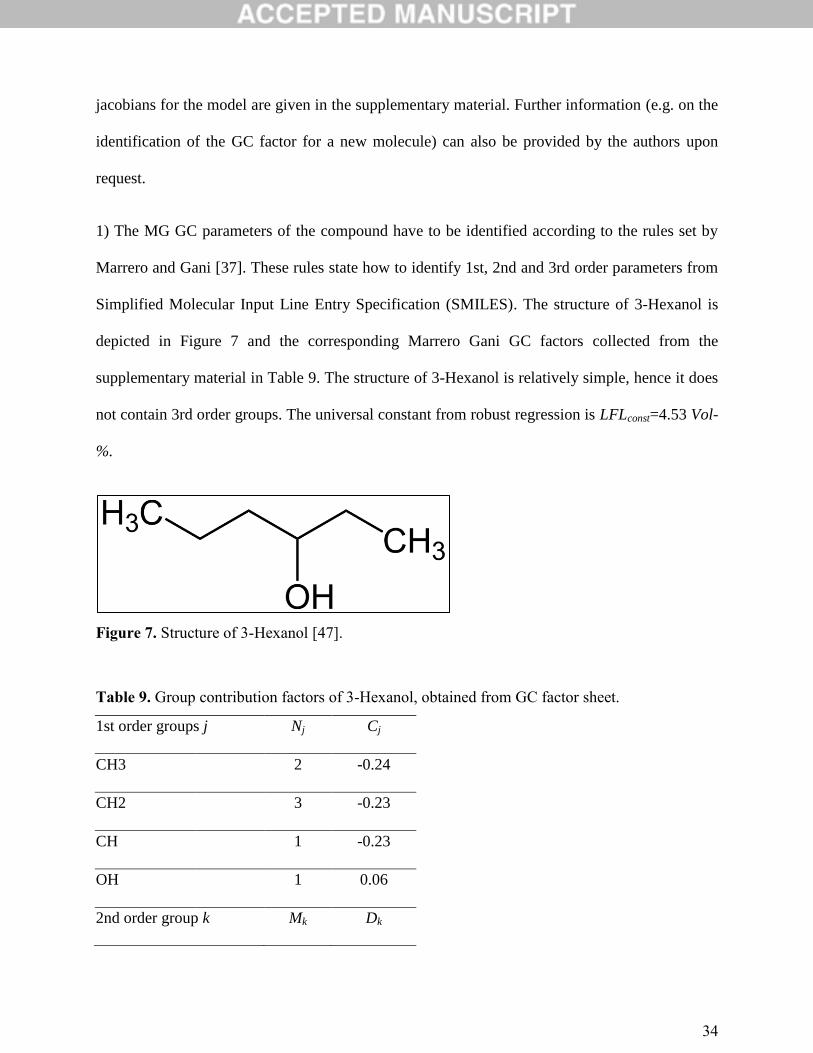
1) The MG GC parameters of the compound have to be identified according to the rules set by

Marrero and Gani [37]. These rules state how to identify 1st, 2nd and 3rd order parameters from

Simplified Molecular Input Line Entry Specification (SMILES). The structure of 3-Hexanol is

depicted in Figure 7 and the corresponding Marrero Gani GC factors collected from the

supplementary material in Table 9. The structure of 3-Hexanol is relatively simple, hence it does

not contain 3rd order groups. The universal constant from robust regression is LFLconst=4.53 Vol-

%.

Figure 7. Structure of 3-Hexanol [47].

Table 9. Group contribution factors of 3-Hexanol, obtained from GC factor sheet.

1st order groups j Nj Cj

CH3

2 -0.24

CH2

3 -0.23

CH

1 -0.23

OH

1 0.06

2nd order group k Mk Dk

35

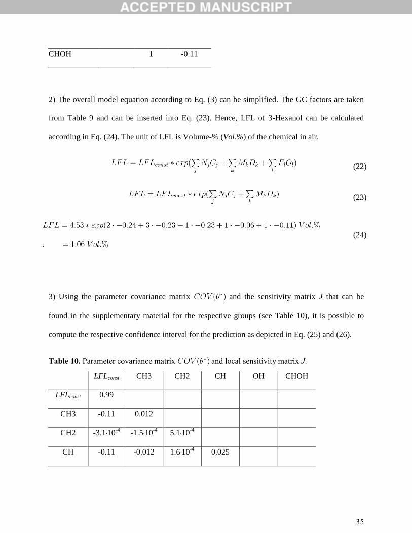
CHOH

1 -0.11

2) The overall model equation according to Eq. (3) can be simplified. The GC factors are taken

from Table 9 and can be inserted into Eq. (23). Hence, LFL of 3-Hexanol can be calculated

according in Eq. (24). The unit of LFL is Volume-% (Vol.%) of the chemical in air.

(22)

(23)

(24)

3) Using the parameter covariance matrix and the sensitivity matrix J that can be

found in the supplementary material for the respective groups (see Table 10), it is possible to

compute the respective confidence interval for the prediction as depicted in Eq. (25) and (26).

Table 10. Parameter covariance matrix and local sensitivity matrix J.

LFLconst CH3 CH2 CH OH CHOH

LFLconst 0.99

CH3 -0.11 0.012

CH2 -3.1 10-4

-1.5 10-4

5.1 10-4

CH -0.11 -0.012 1.6 10-4

0.025

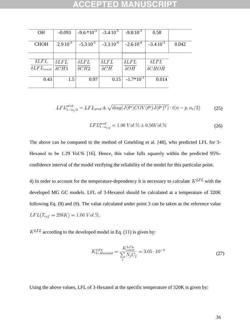
36

OH -0.093 -9.6 *10-3

-3.4 10-5

-9.8 10-3

0.58

CHOH 2.9 10-3

-5.3 10-5

-3.3 10-4

-2.6 10-4

-3.4 10-3

0.042

0.43 1.5 0.97 0.15 -1.7*10-3

0.014

(25)

(26)

The above can be compared to the method of Gmehling et al. [48], who predicted LFL for 3-

Hexanol to be 1.29 Vol.% [16]. Hence, this value falls squarely within the predicted 95%-

confidence interval of the model verifying the reliability of the model for this particular point.

4) In order to account for the temperature-dependency it is necessary to calculate with the

developed MG GC models. LFL of 3-Hexanol should be calculated at a temperature of 320K

following Eq. (8) and (9). The value calculated under point 3 can be taken as the reference value

.

according to the developed model in Eq. (11) is given by:

(27)

Using the above values, LFL of 3-Hexanol at the specific temperature of 320K is given by:

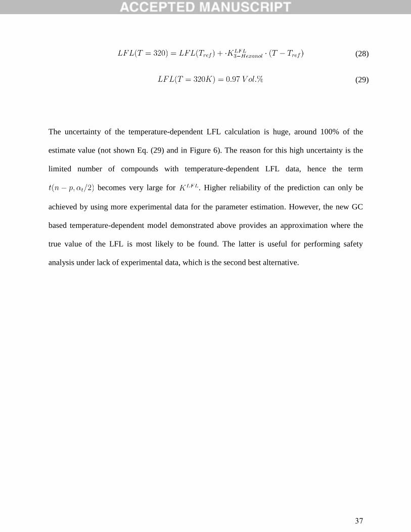
37

(28)

(29)

The uncertainty of the temperature-dependent LFL calculation is huge, around 100% of the

estimate value (not shown Eq. (29) and in Figure 6). The reason for this high uncertainty is the

limited number of compounds with temperature-dependent LFL data, hence the term

becomes very large for . Higher reliability of the prediction can only be

achieved by using more experimental data for the parameter estimation. However, the new GC

based temperature-dependent model demonstrated above provides an approximation where the

true value of the LFL is most likely to be found. The latter is useful for performing safety

analysis under lack of experimental data, which is the second best alternative.

38

4. Conclusion

In this study, a new GC method has been developed for the calculation of LFL and UFL as well

as a new model for estimating temperature dependence of LFL. Furthermore, the parameters for

the previous model of FP and AIT have been improved thanks to expanded data sets and a

comprehensive parameter estimation methodology. The systematic parameter estimation and

uncertainty analysis provides uncertainty information for the single point predictions.

The developed LFL and UFL model has a higher accuracy than existing GC models and

is much simpler to apply than current ANN or QSPR models.

A temperature-dependent LFL model based on a GC model for a lumped parameter has

been developed.

The advanced parameter estimation using (robust regression) and the systematic outlier

treatment using the empirical CDF together with additional experimental data could

improve the existing GC MG model for FP and AIT.

The report of the 95%-confidence interval of the predicted value for the safety-related

properties provided important information on the uncertainty (reliability) of the predicted

values. The latter is crucial in a quantitative risk assessment as it provides a safety factor

for LFL analysis.

The simplicity of the model application has been demonstrated for the 3-Hexanol as a

motivating example.

39

The availability of a class of GC models for predicting flammability related properties of

chemicals is expected to facilitate the quantitative risk assessment as part of process

safety analysis.

40

Supporting information

The Supporting Information is available on the website:

Group contribution factors for and formulas for all developed models are shown in tabular form.

Furthermore, examples of predicted values including 95% confidence interval for a variety of

chemical compounds are given.

The authors developed a software tool where the developed models are implemented. Please

contact the corresponding author for more information.

Author information

Corresponding Author

*Tel.: +45 45252806, E-mail address: gsi@kt.dtu.dk

Author Contributions

The manuscript was written through contributions of all authors. All authors have given approval

to the final version of the manuscript.

Funding Sources

This work was funded by the Innovation Fund Denmark under the Thermcyc project.

41

References

[1] R. Gani, J.P. O’Connell, Properties and CAPE: From present uses to future challenges,

Comput. Chem. Eng. 25 (2001) 3–14.

[2] A.S. Hukkerikar, R.J. Meier, G. Sin, R. Gani, A method to estimate the enthalpy of

formation of organic compounds with chemical accuracy, Fluid Phase Equilib. 348 (2013)

23–32.

[3] J. Frutiger, C. Marcarie, J. Abildskov, G. Sin, A comprehensive methodology for

development, parameter estimation, and uncertainty analysis of group contribution based

property models – an application to heat of combustion, J. Chem. Eng. Data. 61 (2016)

602–613.

[4] M.E. Paté-Cornell, Uncertainties in risk analysis: Six levels of treatment, Reliab. Eng.

Syst. Saf. 54 (1996) 95–111.

[5] M.G. Zabetakis, Flammability characteristics of combustible gases and vapors,

Washington DC, 1965.

[6] D.A. Crowl, J.F. Louvar, Definitions of fires and explosions, in: Chem. Process Saf.,

Prentice Hall International Series in the Physical and Chemical Engineering Sciences,

Boston, 2011: pp. 241–243.

[7] M. Vidal, W.J. Rogers, J.C. Holste, M.S. Mannan, A review of estimation methods for

flash points and flammability limits, Process Saf. Prog. 23 (2004) 47–55.

[8] J.R. Rowley, R.L. Rowley, W. V Wilding, Estimation of the lower flammability limit of

organic compounds as a function of temperature., J. Hazard. Mater. 186 (2011) 551–557.

[9] A.A. Shimy, Calculating flammability characteristics of hydrocarbons and alcohols, Fire

42

Technol. 6 (1970) 135–139.

[10] N.V. Solovev, A.N. Baratov, Lower limit of flammability of hydrocarbon–air mixtures as

a function of the molecular structure of the combustible component, Russ. J. Phys. Chem.

34 (1960) 1661–1670.

[11] E. Oehley, Ableitung empirischer Gleichungen fur die untere Explosionsgrenze und den

Flammpunkt, Chemie Ingenieu Tech. 25 (1953) 399–403.

[12] Y.N. Shebeko, A. V Ivanov, T.M. Dmitrieva, Methods of Calculating the Lower

Concentration Limits of Ignition of Gases and Vapors in Air., Sov. Chem. Ind. 15 (1983)

311–317.

[13] S. Kondo, Y. Urano, K. Tokuhashi, A. Takahashi, K. Tanaka, Prediction of flammability

of gases by using F-number analysis, J. Hazard. Mater. 82 (2001) 113–128.

[14] S. Kondo, A. Takahashi, K. Tokuhashi, Experimental exploration of discrepancies in F-

number correlation of flammability limits, J. Hazard. Mater. 100 (2003) 27–36.

[15] W.H. Seaton, Group contribution method for predicting the lower and the upper

flammable limits of vapors in air, J. Hazard. Mater. 27 (1991) 169–185.

[16] R. L. Rowley, W. V. Wilding, J. L. Oscarson, T. A. Knotts, N. F. Giles, DIPPR® Data

Compilation of Pure Chemical Properties, Design Institute for Physical Properties,

AIChE, New York, NY, (2014).

[17] T. a. Albahri, Flammability characteristics of pure hydrocarbons, Chem. Eng. Sci. 58

(2003) 3629–3641.

[18] F. Gharagheizi, Quantitative Structure - Property Relationship for Prediction of the Lower

Flammability Limit of Pure Compounds, Energy & Fuels. 22 (2008) 3037–3039.

[19] Y. Pan, J. Jiang, R. Wang, H. Cao, Y. Cui, A novel QSPR model for prediction of lower

43

flammability limits of organic compounds based on support vector machine, J. Hazard.

Mater. 168 (2009) 962–969.

[20] Y. Pan, J. Jiang, R. Wang, H. Cao, Y. Cui, Prediction of the upper flammability limits of

organic compounds from molecular structures, Ind. Eng. Chem. Res. 48 (2009) 5064–

5069.

[21] F. Gharagheizi, A new group contribution-based model for estimation of lower

flammability limit of pure compounds., J. Hazard. Mater. 170 (2009) 595–604.

[22] T. a. Albahri, Prediction of the lower flammability limit percent in air of pure compounds

from their molecular structures, Fire Saf. J. 59 (2013) 188–201.

[23] F. Gharagheizi, Prediction of upper flammability limit percent of pure compounds from

their molecular structures., J. Hazard. Mater. 167 (2009) 507–10.

[24] J.A. Lazzús, Neural network/particle swarm method to predict flammability limits in air of

organic compounds, Thermochim. Acta. 512 (2011) 150–156.

[25] M. Bagheri, M. Rajabi, M. Mirbagheri, M. Amin, BPSO-MLR and ANFIS based

modeling of lower flammability limit, J. Loss Prev. Process Ind. 25 (2012) 373–382.

doi:10.1016/j.jlp.2011.10.005.

[26] M.S. High, R.P. Danner, Prediction of upper flammability limit by a group contribution

method, Ind. Eng. Chem. Res. 26 (1987) 1395–1399.

[27] G. Shu, B. Long, H. Tian, H. Wei, X. Liang, Evaluating upper flammability limit of low

hydrocarbon diluted with an inert gas using threshold temperature, Chem. Eng. Sci. 138

(2015) 810–813. doi:10.1016/j.ces.2015.09.013.

[28] G. Shu, B. Long, H. Tian, H. Wei, X. Liang, Flame temperature theory-based model for

evaluation of the flammable zones of hydrocarbon-air-CO2 in mixtures, J. Hazard. Mater.

44

294 (2015) 137–144.

[29] A.Z. Mendiburu, J.A. de Carvalho, C.R. Coronado, Estimation of lower flammability

limits of C-H compounds in air at atmospheric pressure, evaluation of temperature

dependence and diluent effect, J. Hazard. Mater. 285 (2015) 409–418.

[30] A.Z. Mendiburu, J.A. de Carvalho, C.R. Coronado, Estimation of upper flammability

limits of C-H compounds in air at atmospheric pressure, evaluation of temperature

dependence and diluent effect, J. Hazard. Mater. 304 (2016) 512–521.

[31] M.G. Zabetakis, S. Lambiris, G.S. Scott, Flame temperatures of limit mixtures, in: 7th

Symp. Combust., 1959: p. 484.

[32] L.G. Britton, Using heats of oxidation to evaluate flammability hazards, Process Saf. Prog.

21 (2002) 31–54.

[33] L.G. Britton, D.J. Frurip, Further uses of the heat of oxidation in chemical hazard

assessment, Process Saf. Prog. 22 (2003) 1–19.

[34] J.R. Rowley, R.L. Rowley, W.V. Wilding, Experimental determination and re-

examination of the effect of initial temperature on the lower flammability limit of pure

liquids, J. Chem. Eng. Data. 55 (2010) 3063–3067.

[35] L. Catoire, V. Naudet, Estimation of temperature-dependent lower flammability limit of

pure organic compounds in air at atmospheric pressure, Process Saf. Prog. 24 (2005) 130–

137.

[36] A.S. Hukkerikar, B. Sarup, A. Ten Kate, J. Abildskov, G. Sin, R. Gani, Group-

contribution+ (GC+) based estimation of properties of pure components: Improved

property estimation and uncertainty analysis, Fluid Phase Equilib. 321 (2012) 25–43.

[37] J. Marrero, R. Gani, Group-contribution based estimation of pure component properties,

45

Fluid Phase Equilib. 183-184 (2001) 183–208.

[38] J. Frutiger, J. Abildskov, G. Sin, Outlier treatment for improving parameter estimation of

group contribution based models for upper flammability limit, in: K. V. Gernaey, J.K.

Huusom, R. Gani (Eds.), 12th Int. Symp. Process Syst. Eng. 25th Eur. Symp. Comput.

Aided Process Eng., Copenhagen, 2015.

[39] H.F. Coward, G.W. Jones, Limits of flammability of gases and vapors, Washington DC,

1952.

[40] K. Joback, R. Reid, Estimation of pure-component properties from group-contribution,

Chem. Eng. Commun. 57 (1987) 233 – 243.

[41] G. Seber, C. Wild, Nonlinear Regression, John Wiley & Sons, Inc., Hoboken, NJ, USA,

1989.

[42] K.P. Burnham, D.R. Andersen, Multimodel Inference: Understanding AIC and BIC in

Model Selection, Sociol. Methods Res. 33 (2004) 261–304.

[43] T. a. Albahri, Structural Group Contribution Method for Predicting the Octane Number of

Pure Hydrocarbon Liquids, Ind. Eng. Chem. Res. 42 (2003) 657–662.

[44] K.C. Kroenlein, R. Chirico, V. Diky, A. Bazyleva, J. Magee, Thermophysical Property

Reliability Issues in the Context of Automated Consumption, in: 19th Symp. Thermophys.

Prop., Boulder, CO, 2015.

[45] Center for Chemical Process Safety, Guidelines for Vapor Cloud Explosion, Pressure

Vessel Burst, BLEVE and Flash Fire Hazards, 2nd Editio, Wiley, 2011.

[46] D.A. Crowl, J.F. Louvar, Chemical process safety, 2nd ed., Prentice Hall International

Series in the Physical and Chemical Engineering Sciences, New Jersey, 2013.

[47] N. Mills, ChemDraw Ultra 10.0, J. Am. Chem. Soc. 128 (2006) 13649–13650.

46

[48] J. Gmehling, P. Rasmussen, Flash Points of Flammable Liquid Mixtures using UNIFAC,

Ind. Eng. Chem. Fundam. (1982) 186–188.