Growth Alone is not Enough

Ivan Lyubimov

February 11, 2016

Abstract

One of the most intriguing results of the Georgian parliamentary elections of

2012 is that economic success of a growth-enhancing policy might not be con-

verted into political popularity. In the context of a non-overlapping generations

growth model with high-skilled and low-skilled employees, we argue that a po-

tential explanation for this result is that growth policies ignore the importance of

income redistribution. Even though reforms enhance economic growth, most of

their benefits might be transferred to high-skilled individuals. Their low-skilled

counterparts’ gains from economic growth are instead low and therefore this group

remains sensitive to income transfers. If the latter are not provided, the reformist

regime’s likelihood to survive in power declines, even though its policies results in

higher growth rates. We also show that a policy which enhances social mobility,

thus helping low-skilled individuals to transit to the high-skilled group, can be a

long-run substitue for income redistribution, but can not replace the latter in the

short term.

1

.

1 Introduction

жПпа In October 2012, after 8 years of profound institutional reforms which re-

sulted in a substantial reduction in the level of bureaucratic corruption, a higher effec-

tiveness of the national energy sector, the emergence of modern public finance system

and professional and transparent bureaucracy, Georgian president Saakashvili’s United

National Movement lost an election against the Georgian Dream, a political alterna-

tive established by a billionaire Bidzina Ivanishvili. Despite high growth rates, which

reached double-digit levels in particular years and on average a nearly double-digit

level between 2004 and 2007, Saakashvili’s rule was also characterized by low level

of income redistribution and relatively high poverty. Growth was not followed by an

adequate job creation, while the wages of employed individuals were instead increas-

ing substantially. High-educated citizens reaped significant benefits from economic

growth, whereas most of low-educated Georgians stayed poor. Overall, the level of

poverty declined from 28.5% in 2003 to 24.7% in 2009, which was not proportion-

ate to the speed of economic growth within the same period. According to the World

Bank (2011), "Economic growth in Georgia has not been pro-poor... ". Unfavorable

distribution of benefits from economic growth induced poor individuals not to support

Saakashvili and his reforms, but instead to grant their votes to alternative political force,

which they considered as potentially less reformist, but also as more redistributing and

therefore pro-poor.

This recent episode can be considered as a part of a broader context which, since

1980s, has been affecting the mainstream development roadmaps, as, for instance, the

Washington or the Post-Washington Consensuses. Both of them emphasized the im-

portance of growth-enhancing policies, leaving, however, a peripheral role to income

redistribution. The lack of redistribution concerns as an important inadequacy of a de-

velopment plan was also indicated by Joseph Stiglitz (2004) in his critical review of

the Post-Washington Consensus:

"Is a society in which the vast majority of its citizens are becoming worse

off - but in which a few at the top are doing so well that average incomes

are rising - better off than one in which the vast majority are doing better?

While there may be disagreements - and those at the very top may well

stress that average income is the appropriate measure - the possibility that

2

increases in GDP may not benefit most individuals means that we cannot

simply ignore issues of distribution. Some economists argued that distri-

bution concerns could be ignored because they believed in trickle down

economics - somehow everybody would benefit; a rising tide would lift

all boats. But the evidence against trickle down economics is now over-

whelming, at least in the sense that an increase in average incomes is not

sufficient to raise the incomes of the poor for quite prolonged periods.

Some economists argued that distribution concerns could and should be

ignored, because such concerns were outside the province of economics;

economists should focus on efficiency and growth alone. Distribution was

a matter for politics".

We argue that the lack of income redistribution concerns is an important flaw of

modern development practices. As the presence of a large disadvantaged cohort which

is disconnected from fast growing sectors1 is a feature of many developing societies,

economic growth alone might therefore not be very helpful for reducing the level of

poverty. It thus needs to be complemented with a redistribution policy, which, as long

as the poor cohort is separated from rapidly developing economic activities, might play

an important role for mitigating the most severe consequences of poverty.

That economic growth can play a limited role in reducing the level of poverty is

recognized by modern development practices,such as, for instance, Inclusive Growth.

However, instead of implementing direct redistribution, the latter suggests to expand

the disadvantaged cohort’s opportunities to participate in fast-growing economic activ-

ities, as it follows from the World Bank (2009):

"While absolute pro-poor growth can be the result of direct income redis-

tribution schemes, for growth to be inclusive, productivity must be im-

proved and new employment opportunities created. In short, inclusive

growth is about raising the pace of growth and enlarging the size of the

economy, while levelling the playing field for investment and increasing

productive employment opportunities" and "Inclusive Growth focuses on

productive employment rather than income redistribution".

We argue though that as the main effects of such a policy might realize after a long

time, it thus can not substitute income redistribution in the short term. For instance,1As, for instance, individuals who are self-employed in subsistence farming.

3

a reform which increases the accessibility of education in order to enhance social mo-

bility, can achieve its goals years later, as transferring human capital is inherently a

long-term process. Therefore, before the main effects of this reform are realized, the

disadvantaged cohort can remain poor and thus sensitive to income redistribution poli-

cies. If the latter are not implemented, poor individuals might support a political regime

which practices income transfers, even though this regime’s growth-enhancing policies

are, at the same time, potentially less effective. It is therefore essential to incorporate

income redistribution into development policies, as otherwise the latter might become

politically unfeasible.

To introduce this intuition in the form of a model, we consider a non-overlapping

generation developing economy where high-educated and low-educated individuals

combine their human capital with evolving technology to produce output.

We incorporate institutions into the model and show that the pace of technological

evolution and, as a consequence, economic growth are larger under the higher-quality

institutions, and they are instead small in the opposite case of low-quality institutions.

We assume that, as opposed to the large group of low-educated individuals, a rela-

tively small high-educated cohort controls a larger share in output, and therefore its rep-

resentative member derives comparatively high benefits from economic growth. The

less educated individuals’ share in output is instead low, and, as a result, their bene-

fits from economic growth are low as well. As a consequence, a high level of poverty

might sustain even in the presence of high growth rates.

To link these features with political outcomes, we consider two alternative political

regimes.

A clientelistic regime derives benefits if the quality of institutions remains low, and

therefore it has incentives to retain low-quality institutions as long as possible. As low-

quality institutions are broadly recognized as a key impediment to economic growth

(see, for instance, Blume, Rubinfeld and Shapiro 1984, Kaplow 1986, and Epstein

2008), growth rates remain low as long as the clientelistic regime keeps power. How-

ever, as staying in power requires retaining a certain level of popularity, the clientelistic

regime implements a redistribution policy which benefits low-educated individuals and

thus earns their political sympathies.

A reformist regime instead improves the quality of institutions, which increases the

pace of technological evolution, accelerates human capital accumulation, and results

in faster economic growth. We show, however, that the latter might be insufficient for

sustaining political popularity, as growth and human capital accumulation mostly affect

4

the high-educated group, and not the low-educated one. The latter, making up a major-

ity of individuals, remains comparatively more sensitive to income redistribution, than

to economic growth. Therefore, complementing an institutional reform with income

redistribution policy might be a key to winning political competition. We conclude that

the reformist regime might loose political competition against the clientelistic alterna-

tive, if it ignores income redistribution.2 As a result, growth-enhancing policy can be

reversed and the economy might end up in a non-convergence trap.

As an alternative to income redistribution, a part of the low-educated cohort can

transit to the high-educated group if the authority, instead of redistributing incomes,

implements a reform which increases the accessibility of education. As a result of the

latter reform, the level of output becomes larger, as well as the size of the middle class,

and thus the number of individuals who benefit from economic growth increases. We

therefore follow Muller and Shavit, (1998), as we assume that a broader access to high-

quality educational services enhances the attainment of the middle-class occupations,

which results in the emergence of a larger middle class. Our key assumption, how-

ever, suggests that the time which is required for the acquisition of additional human

capital is comparatively long, and, as a consequence, the educational reform might im-

pact only the following generation of low-educated individuals, without affecting the

current one.3 As is argued in Tiongson (2012) "...Education policy reforms have long

term effects on poverty and income distribution...". As a result, inclusive growth can

not substitute income redistribution in the short term, as the current generation of low-

educated individuals can still have low sensitivity to economic growth. Its dependence

on income redistribution, by contrast, remains comparatively high.

The remainder of the paper is organized as follows. Section 2 reviews the litera-

ture and provides the model outline. Section 3 addresses the problem of low-quality

institutions in the context of our benchmark growth model, and shows how does its

presence result in a non-convergence trap. We introduce political competition as an

2Even though it is associated with slow growth, the clientelistic regime, nevertheless, might earn substan-tial political popularity among the low-educated group, as income transfers which it provides might be moreimportant for the low-educated individuals than economic growth.

3At the same time, we assume that much less time is needed to improve the quality of institutions in aparticular economy. Moreover, economic effect of improved institutions might also realize relatively fast.For instance, Georgia needed 3 years to increase its FDI inflow from 500 million USD in 2004 to 2 bln USDin 2007, as a result of its anti-corruption efforts which were implemented within the same years. Anotherillustration is a successful anti-corruption campaign which was implemented in Liberia. The latter madesubstantial progress in reducing the level of corruption, as it had been ranked 137 out of 158 countriesaccording to Transparency International’s Corruption Perception Index in 2005, but ended up at the 87thposition out of 178 economies in 2010 (see Transparency International, 2011). By contrast, economic effectof an educational policy is intrinsically more delayed, as years are required to implement the reform, toeducate individuals, to employ them, etc.

5

opportunity to remove low-quality institutions in Section 4, where we also show how

this opportunity can remain unexploited if an institutional reform is not complemented

with income redistribution. In the extension to our paper, which we present in Section

5, we argue that the effect of investing into human capital, which we consider as a

potential alternative to income redistribution policy, realizes only in the long-run, and

therefore can not reduce the level of income inequality in the short term. Section 6

provides a summary.

2 Literature Review and Model Outline

Our model brings together different strands of the literature. First, our argument is

related to the extensive literature which studies the link between growth and inequality.

For instance, Alesina and Rodrik (1994), Persson and Tabellini (1994) and Alesina

(1994) argue that polarization is an obstacle to economic growth, as it shifts political

focus from economic growth to income redistribution. As a result, a larger political

pressure for redistribution discourages investment and therefore reduces the pace of

economic growth.

Another set of arguments related to income polarization, as the ones of Loury

(1981) or Galor and Zeira (1993), focuses on credit market imperfections as an im-

portant flaw which reduces poor individuals’ investment opportunities and therefore

lowers growth rates. As a result of a low accessibility of credit, poor individuals

might be restricted from undertaking the optimal level of investment. In the pres-

ence of decreasing returns, their underfunded projects, however, are characterized by

higher marginal product, and therefore, as redistribution might compensate the lack

of investment credit, economic growth can become faster. In this context, Galor and

Zeira (1993), for instance, argue that a society with high income inequality has a small

middle class. The poor class is instead large and facing a binding liquidity constraint,

which reduces its opportunities to accumulate human capital, thus resulting in a lower

level of production.

There is also a literature which links income inequality and security of property

rights. In the presence of a widening gap between rich and poor, the latter have motiva-

tion to expropriate assets from the former, and thus, as investing becomes less secure,

incentives to invest decline (see, for instance, Grossman, 1991, 1994, Acemoglu, 1995,

Tornell and Velasco, 1992, Benhabib and Rustichini, 1996).

Finally, Adelman and Morris (1967) and Landes (1998), provide historical evidence

6

for the importance of the middle class, and therefore lower inequality, for economic

development in Europe.

Even though we also link inequality and economic growth, our focus is, however,

different. We argue that, as inequality results in a higher popularity of income re-

distribution, it therefore might enhance political survival of ineffective and populist

regimes, thus negatively affecting the long-term growth. For instance, even though

a rent-seeking regime can cause a substantial slowing down in economic growth, it

might, nevertheless, remain popular if it provides income transfers to the poor. We

therefore emphasize that income redistribution might be a key ingredient for political

success, and thus it should also be implemented by reformist regimes to enhance their

political sustainability.

Our paper is also related to political science literature which addresses the issue

of persistence of clientelistic policies (see, for instance, Kitschelt, 2000). Brusco et

al (2004) and Calvo and Murillo (2004) argue that poor voters in Argentina are more

willing to support Peronists as the latter deliver clientelistic policies. Robinson and

Verdier (2003) show that poor and less productive societies practice clientelism more

often. This literature, however, focuses on popularity of clientelistic regimes among

poor voters, without, by contrast to our argument, linking the latter with economic

growth.

Finally, a vast literature considers education as an important link between indi-

viduals’ social origin and their later social destination. Acemoglu (2002), Aghion et

al (1999) and Katz and Murphy (1992) indicate that education and skills play an im-

portant role in wage differences, therefore implying that a more accessible education

system will result in a lower income inequality and a larger middle class. We refer

to this literature, as we consider a policy which enhances the availability of education

for the poor in order to integrate the latter into fast growing economic activities. This

literature does not, however, link income redistribution with political sustainability and

economic growth.

In our setting a firm which is owned by the representative capitalist combines tech-

nology and human capital to produce output. Following Lucas (1988), Acemoglu

(1994) and Redding (1996), we consider a non-overlapping generations economy where

output is shared between the capitalist and two groups of employees, a low-educated

group and a high-educated one. When young, each employee receives a particular en-

dowment of human capital from the previous generation and becomes a high-educated

individual if the level of human capital endowment is large, or a low-educated indi-

7

vidual in the opposite case of a low intergenerational transfer of human capital. High-

and low-educated individuals then decide how to allocate their human capital endow-

ments between production and acquisition of additional human capital. Their decision

is affected by the capitalist, who invests a part of his revenue from production into the

acquisition of a new technology. The capitalist and employees share the same informa-

tion, and thus the employees can perfectly foresee how much output does the capitalist

plan to invest in a new technology. When the capitalist invests more into technological

evolution, both groups of employees also prefer to acquire more human capital, since

in this case the latter will earn a higher return. Higher educational attainments and

investment into a new technology result, respectively, in a larger human capital stock

and a more advanced technology, which are used to produce output when the capitalist,

high-educated and low-educated employees become old.

We incorporate the quality of institutions into the model, and consider it as an

important determinant of the level of investment into new technologies. When the

quality of institutions is high, the economy develops faster, as the representative capi-

talist invests more into technological evolution, imitating technologies from the leading

economy and thus letting domestic technology move closer to the world technological

frontier. However, as empirical evidence suggest that convergence with more devel-

oped countries did not take place in the case of many developing economies (see, for

instance, Acemoglu, 2008), we also consider the case of low-quality institutions, and

show how the latter reduce the capitalist’s incentives to invest into new technologies.

Since production factors are complements, both groups of employees reduce their in-

vestments into human capital in response to a slower pace of technological advance-

ment.

We then introduce political competition into our model and consider it as an oppor-

tunity to replace low-quality institutions with the high-quality ones. We assume that a

reformist regime pursues a growth-enhancing policy, and, to this end, it improves the

quality of institutions. As the latter results in higher growth rates and therefore makes

the capitalists and the employees better off, the reformist regime should acquire a broad

political support, while its clientelistic opponent, which instead practices rent seeking

and thus maintains low-quality institutions, should become extremely unpopular. As

we show, the latter, however, is not necessarily the case if most of the current genera-

tion’s employees belong to the low-educated group. As in this case less educated indi-

viduals acquire low benefits from economic growth, their support to growth-enhancing

policy remains low as well. On the contrary, a sufficiently generous redistribution

8

policy can increase the low-educated cohort income level more substantially. If the

reformist regime does not transfer incomes to the low-educated employees, while its

clientelistic opponent instead does, the political survival of the former, and therefore

the implementation of institutional reform, becomes less feasible. Thus, to win politi-

cal competition, the reformist regime should combine institutional reform with income

redistribution.

Finally, we consider the working of a particular growth policy4 which helps low-

educated employees transit to the high-educated group. We assume that the reformist

regime, instead of using tax revenues to redistribute incomes, can improve the quality

of education and transfer more human capital to the less educated cohort, therefore

decreasing its size and increasing instead the size of the high-educated group. We

suppose, however, that the former effect realizes in the long run, benefiting the next

generation of low-educated employees, but not the current one. The latter implies that

in the short term the educational policy can’t substitute income redistribution, which

remains an important determinant of the reformist regime’s political survival.

3 The Benchmark Model of Economic Growth

In this section we introduce our baseline growth model, where two representative

groups of employees and the representative capitalist, all belonging to a particular

generation, combine, respectively, human capital and technology in order to produce

output. Moreover, the employees acquire additional human capital, and the capitalist

instead improves upon the technology which he inherited from the previous generation.

After the current generation passes away, the human capital stock and technology are

transferred to the next generation.

Incentives to acquire new technologies and human capital are affected by the qual-

ity of institutions. In the presence of low-quality institutions, the representative capi-

talist invests less into a new technology, while the employees, in turn, accumulate less

human capital. As a result, the economy fails to move closer economically to a more

developed reference country, and stays far behind the latter as long as the quality of

institutions remains low.4As, for instance, Inclusive Growth

9

3.1 Production

Following Redding (1996), we consider two non-overlapping generations economies,5

D and F ,6 where every generation lives for two periods 1 and 2. We focus our analysis

on country D, while country F is instead introduced as a reference economy.

In period 1 a new generation t is born, it produces output Y it,1, i = D,F , invests a

particular share of Y it,1 in the acquisition of new technologies and accumulates human

capital. In the following period, i.e. in period 2, the same generation t produces output

Y it,2 and passes away.

We assume for simplicity that the size of population in D does not change over

time, and it is as large as the size of population in country F . Each generation is made

up of L(ni + 1

)individuals, where L represents the number of capitalists in economy

i = D,F and ni = ni1 + ni2 corresponds to the number of employees working for a

typical capitalist in economy i = D,F . A group of employees of size ni1 working for

the representative capitalist receives a large per capita human capital endowment hi,1t,1,

while in the other group of size ni2 a typical employee inherits instead a low level of

human capital hi,2t,1, which implies that hi,1t,1 > hi,2t,1, i = D,F .

The representative capitalist owns a firm, where technology, which belongs to the

capitalist, is combined with human capital, belonging instead to the employees, in order

to produce the final output yit,1, i = D,F . In both periods j = 1, 2, the representative

firm in each economy produces a particular level of output according to the following

production function:

yit,j =(Ait,j

)1−θ1−θ2 (hi,1t,jn

i1

)θ (hi,2t,jn

i2

)θ2(1)

where i = D,F and j = 1, 2.

Therefore, within periods 1 and 2, the representative firm in economy i = D,F

produces as much output as follows:

yit =2j=1

(Ait,j

)1−θ1−θ2 (hi,1t,jn

i1

)θ1 (hi,2t,jn

i2

)θ2(2)

where yit is the level of output which is produced by the representative firm belonging to

generation t in economy i, Ait,j is the level of technology belonging to the representa-

5We do not use a standard overlapping generations approach, as we need to make sure that investing intwo factors of production takes place synchronically. The latter is possible if the owners of the respectiveproduction factors make up the same generation.

6Where D and F correspond to "Domestic " and "Foreign" respectively.

10

tive capitalist in country i = D,F in period j = 1, 2, hi,1t,j and hi,2t,j reflect, respectively,

the amount of human capital per the representative employee from the more and the

less educated groups in country i = D,F in period j = 1, 2, and ni1 and ni2 represent

the number of employees per firm, belonging to the more and the less educated groups

correspondingly, i = D,F .

We assume that θ1 > θ2, which implies that high-educated employees are more

important for production.

In both periods j = 1, 2 the representative employee belonging to the more edu-

cated group and employed at a typical firm receives a wage rate wi,1t,j , while her coun-

terpart from the less educated group receives instead wi,2t,j , i = D,F . The equilibrium

wage rate wi,1t,j is equal to the marginal productivity of employing ni1 individuals from

the more educated group:

wi,1t,j = θ1(Ait,j

)1−θ1−θ2 (hi,1t,j

)θ1 (hi,2t,jn

i2

)θ2 (ni1)θ1−1 (3)

while the ratewi,2t,j corresponds to the marginal productivity of ni2 employees belonging

to the less educated group:

wi,2t,j = θ2(Ait,j

)1−θ1−θ2 (hi,1t,jn

i1

)θ1 (hi,2t,j

)θ2 (ni2)θ2−1 (4)

In total, the high-educated and the low-educated groups working at a typical firm,

receive the following income in period j = 1, 2:

Iit,j = ni1wi,1t,j + ni2w

i,2t,j (5)

The representative capitalist therefore acquires the remaining part of output:

W it,j = Yt,j − ni1w

i,1t,1 − ni2w

i,2t,1 = (1− θ1 − θ2)Y it,j (6)

In both economies, D and F , a new generation inherits technology and human

capital from the previous generation. Therefore, when a new generation is young, it

uses the following technology to produce output:

Ait,1 = Ait−1,2 (7)

where Ait−1,2 is the level of technology a new generation t inherited from its prede-

11

cessor, generation t − 1. In economy D, each generation can invest in the acquisition

of new technologies, therefore increasing the level of technology it inherited from the

previous generation.

In the benchmark model we assume that the level of technology in country F , i.e.

AF , is a constant.7 We also assume that the initial generation t = 0 in country D owns

a technology which is less developed than the one in economy F , i.e. AH0,1 < AF .

Following Lucas (1988), we also assume that, similar to the level of technology,

the human capital stock Hit−1,2 is transferred from the previous generation t− 1 to the

current one, i.e. to t. We assume that the more educated group of employees receives

a larger per capita share 0 < δ1 < 1 in the total human capital stock Hit−1,2, while per

capita share belonging to the less educated cohort, δ2, is instead smaller. Within each

group the level of human capital endowment is, however, identical for all the members

belonging to a particular cohort, which reflects equal distribution of wealth in each

cohort.8

Similarly to the level of AF , we also assume that the total human capital stock in

country F , i.e. HF , is a constant. Finally, we assume that HD0,1 < HF which implies

that for the initial generation t = 0 the stock of human capital in D is lower than the

one in economy F .

Given our assumption that employees are identically distributed between high-

educated and low-educated cohorts in both D and F , i.e. nD1 = nF1 and nD2 = nF2 ,9

these two conditions, i.e. AD0,1 < AF and HD0,1 < HF , together with production func-

tion yit,1 =(Ait,1

)1−θ1−θ2 (hi,1t,1n

i1

)θ1 (hi,2t,1n

i2

)θ2, imply that for the initial generation

t = 0, in period j = 1, the level of output produced by the representative firm in

country F is larger than the one produced in economy D.

3.2 Investment

At the end of the first period, j = 1, the representative capitalist in D decides whether

to improve uponADt,1, the level of technologyD inherited from the previous generation

t− 1, or to invest in a storage technology.

7However, we relax this assumption in Appendix IV, as considering the level of the leading technologicalfrontier represented by AF as a constant is not realistic. Adding a possibility of evolution of the worldtechnological frontier does not, however, affect our key results.

8A different assumption would result in a more complicated aggregation of our key variables, and thewhole analysis of the model would become more complicated as well, without delivering, at the same time,any interesting and important insights.

9We will relax this assumption later, when we discuss the Inclusive Growth policy.

12

The storage technology is available in both economies, D and F , and pays a return

r = 0 in period j = 2 if the capitalist invests his income in this technology in period

j = 1. We introduce a storage technology to capture a possibility of non-convergence

trap, which emerges when D fails to catch up with country F . The representative firm

in D invests in the storage asset if the payoff from improving upon ADt,1 is negative.

In the latter case, the capitalist in D stops investing into technological progress, and

therefore the economy stays with the same level of technology.

The representative capitalist can improve upon the old technology, i.e upon ADt,1 =

ADt−1,2, in the following way:

ADt,2 = η (xt)AF + (1− η (xt))ADt,1 (8)

Equation (8) reflects a possibility of adoption from the leading technological fron-

tier, which is represented by AF , the level of technology in country F . As a result of

adoption, the level of technology in economy D in period j = 2 , i.e. ADt,2, becomes

larger and contains two parts: first, this is ADt,1, the level of technology the capitalist

inherited from the previous generation t − 1 and which is used to produce output in

period j = 1, and second, this is an additional part, which the capitalist adopts from the

leading frontier AF .10 0 ≤ xt ≤ 1 corresponds to the share of the capitalist’s income

(1− θ1 − θ2) yDt,j in period j = 1, invested into a new technology. η (xt) satisfies the

following properties: 0 ≤ η (xt) ≤ 1, η′ (xt) > 0, η′′ (xt) < 0, η (0) = 0, it also

follows the Inada conditions, i.e. η′(∞) = 0 and η′(0) =∞.

In period j = 1, the capitalist invests a share xt of his income (1− θ1 − θ2) yDt,1into a new technology, and the return is realized in period j = 2. Therefore, the

capitalist receives (1− xt) (1− θ1 − θ2) yDt,1 in period j = 1 and (1− θ1 − θ2) yDt,2 in

the following period, j = 2.

In period j = 1, the more and the less educated employees, working at the rep-

resentative firm in economy D, receive, correspondingly, θ1yDt,1 and θ2yDt,1, and in the

next period, j = 2 these groups’ incomes change to θ1yDt,2 and θ2yDt,2. A member of the

more educated group can invest a fraction ϕ1t of her human capital endowment to aug-

ment her human capital stock, while a typical employee from the less educated group

can instead invest a fraction ϕ2t of her human capital endowment to have more human

capital in period j = 2. For simplicity, we assume that in both groups human capital

10We can rewrite ADt,2, corresponding to the left-hand side of equation (8), as the level of the old tech-nology which is represented by ADt,1 plus a part of the distance between the old technology and the leading

frontier, i.e.: ADt,2 = ADt,1 + η (xt)(AF −ADt,1

)

13

is created according to a one-to-one technology11, and therefore in period j = 2 an

employee from the more educated group receives(1 + ϕ1

t

)h1,Dt,1 in case she invested

ϕth1,Dt,1 in period j = 1, while her counterpart from the less educated group receives(

1 + ϕ2t

)h2,Dt,1 if ϕ2

th2,Dt,1 was invested in period j = 1Ñ

3.3 Institutions

In this subsection, we incorporate institutions into the model. We show how the pres-

ence of low-quality institutions, which is a feature of many developing economies,

reduces country D’s opportunities to catch up with more developed economy F . Fol-

lowing Blume, Rubinfeld and Shapiro (1984), Kaplow (1986), and Epstein (2008), we

argue that the presence of low-quality institutions, which we model as a positive prob-

ability p of expropriation of a firm belonging to the representative capitalist, results in

slower economic growth. In particular, we show that expropriation reduces the pace of

technological evolution and human capital accumulation, therefore leading to a non-

reducible distance between the level of technology in D and the world technological

frontier.

We assume that the ruling regime can either maintain low-quality institutions, which

corresponds to a positive level of probability of expropriation p, or, alternatively, it can

choose high-quality institutions resulting in p = 0. In the presence of low-quality in-

stitutions, the regime can expropriate the firm from the representative capitalist. We

assume that the ruling regime has no skills to run the firm profitably, and, as a conse-

quence, it never expropriates it in period j = 1, as if, instead, the firm is expropriated

in the following period j = 2, the regime will receive at least as much as it can receive

in period j = 1. The latter is a result of a higher level of output in period j = 2, i.e.

a higher yDt,2, as in period j = 2 a payoff from investing into a new technology and

human capital is realized. When the regime expropriates the firm in period j = 2, it

keeps the capitalist’s income (1− θ1 − θ2) yDt,2 and then shuts the firm down. When

the following generation t + 1 arrives, a new capitalist establishes a new firm and the

same story repeats again.

If the quality of institutions is instead high, p equals to zero, and therefore the

representative owner receives (1− θ1 − θ2) yDt,2 in period j = 2.

11A different assumption would cost us algebraic and geometric convenience, including explicit algebraicsolutions and their geometric counterparts, without producing any tangible benefits and additional insights.

14

3.4 Equilibrium

We write down the capitalist’s payoff function, which, according to equation (6), takes

the following form:

WDt = (1− xt)WD

t,1 +WDt,2 =

= (1− xt) (1− θ1 − θ2) yDt,1 + (1− p) (1− θ1 − θ2) yDt,2 (9)

where the level of output produced at the representative firm in period j = 1 is as large

as the following:

yDt,1 =(ADt,1

)1−θ1−θ2 (hD,1t,1 n

D1

(1− ϕ1

t

))θ1 (hD,2t,1 n

D2

(1− ϕ2

t

))θ2while in the next period j = 2 the level of output is equal to:

yDt,2 =(ADt,2

)1−θ1−θ2 (hD,1t,1 n

D1

(1 + ϕ1

t

))θ1 (hD,2t,1 n

D2

(1 + ϕ2

t

))θ2Considering the employees, in the more educated group the representative em-

ployee’s payoff function corresponds to the following expression:

wD,1t,1 + wD,1t,2 −→ maxϕ1

(10)

where wD,1t,1 is a wage rate which an employee belonging to the more educated

group receives in period j = 1:

wD,1t,1 = θ1(ADt,1

)1−θ1−θ2 (hD,1t,1

(1− ϕ1

t

))θ1 (hD,2t,1 n

D2

(1− ϕ2

t

))θ2 (nD1)θ1−1

(11)

while wD,1t,2 is a wage she acquires in the following period, i.e. j = 2:

wD,1t,2 = θ1(ADt,2

)1−θ1−θ2 (hD,1t,1

(1 + ϕ1

t

))θ1 (hD,2t,1 n

D2

(1 + ϕ2

t

))θ2 (nD1)θ1−1

(12)

A typical employee from the less educated group maximizes instead the following

income:

wD,2t,1 + wD,2t,2 −→ maxϕ2

(13)

where wD,2t,1 is a wage rate which an employee from the less educated cohort earns

15

in period j = 1:

wD,2t,1 = θ2(ADt,1

)1−θ1−θ2 (hD,1t,1 n

D1

(1− ϕ1

t

))θ1 (hD,2t,1 n

D2

(1− ϕ2

t

))θ2 (nD2)θ2−1

(14)

and wD,2t,2 is instead her wage in period j = 2

wD,2t,2 = θ2(ADt,2

)1−θ1−θ2 (hD,1t,1 n

D1

(1 + ϕ1

t

))θ1 (hD,2t,1 n

D2

(1 + ϕ2

t

))θ2 (nD2)θ2−1

(15)

In period j = 1, the capitalist makes a decision about the level of investment into

a new technology, while the employees decide instead how much human capital to

acquire.

Maximization of equations (9), (10) and (13) with respect to xt, ϕ1t and ϕ2

t corre-

spondingly, and combining the respective FOCs, results in the following expression:

η′(x∗t ) =1

(1− θ1 − θ2) (1− p)(AF

t,1

ADt,1− 1) (16)

From equation (16) we can conclude that a larger importance of technology for

production, i.e. a higher level of 1 − θ1 − θ2, a larger distance to the leading frontierAF

t,1

ADt,1

, and a lower probability of expropriation p, all result in a higher level of investment

into a new technology.

Employees instead search for the optimal share of human capital ϕt which they

invest in education. Maximizing equations (10) and (13) with respect to ϕ1t and ϕ2

t

correspondingly, produces the following first order condition:

ϕ∗t = ϕ1t = ϕ2

t =ADt,2 −ADt,1ADt,2 +ADt,1

(17)

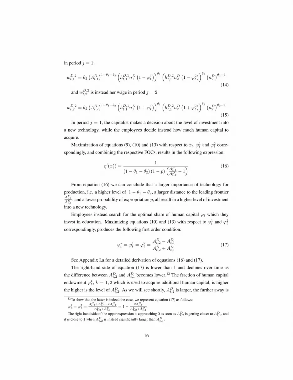
See Appendix I.a for a detailed derivation of equations (16) and (17).

The right-hand side of equation (17) is lower than 1 and declines over time as

the difference between ADt,2 and ADt,1 becomes lower.12 The fraction of human capital

endowment ϕkt , k = 1, 2 which is used to acquire additional human capital, is higher

the higher is the level of ADt,2. As we will see shortly, ADt,2 is larger, the further away is

12To show that the latter is indeed the case, we represent equation (17) as follows:

ϕ1t = ϕ2

t =AD

t,2+ADt,1−2AD

t,1

ADt,2+A

Dt,1

= 1−2AD

t,1

ADt,2+A

Dt,1

The right-hand side of the upper expression is approaching 0 as soon asADt,2 is getting closer toADt,1, andit is close to 1 when ADt,2 is instead significantly larger than ADt,1.

16

the level of technology in D from the leading frontier AF .

We are now ready to formulate our first result.

Proposition 1.

1. The level of technology in economyD converges to the unique steady-state.

The latter corresponds to the leading technology AF when the quality of

institutions is high, i.e. when the probability of expropriation p is equal

to zero. However, the steady-state level of technology is below the world

technological frontier AF if the quality of institutions is instead low, i.e.

when the probability of expropriation p is positive. Moreover, a larger p

results in a higher level of technological backwardness corresponding to a

higher distance to technological frontier AF

ADt,1

.

2. Furthermore, the distance to the leading frontier AF

ADt,1

and the measure of

importance of technology for production 1 − θ1 − θ2, both affect the level

of investments into technology and human capital accumulation positively.

By contrast, the probability of expropriation p reduces the representative

capitalist’s incentives to imitate technologies from Foreign. The latter also

lowers the optimal level of human capital acquisition ϕ∗t .

3. Low-educated and high-educated employees invest the same fraction ϕ∗tof their human capital endowment in the acquisition of additional human

capital.

Proof. To prove the first part of Proposition 1, we lag equation (8) one step back, such

that it corresponds to generation t − 1. We use equation (7) to show that as ADt,1 is a

function of x∗t−1, the more the previous generation, i.e. generation t− 1, invested into

a new technology, i.e. the higher was the level of x∗t−1, the larger becomes the level of

technology which was inherited from generation t−1, i.e. the higher isADt,1. As a result

of a higher level of domestic technology ADt,1 in period j = 1, the distance between

ADt,1 and the leading technological frontier AF reduces. From the expropriation-free,

i.e. p = 0, version of equation (16) corresponding to the following expression

η′(x∗t ) =1

(1− θ1 − θ2)(AF

t,1

ADt,1− 1) (18)

17

it follows that x∗t becomes smaller when the distance to frontier AF

ADt,1

declines. It there-

fore follows that x∗t−1 is larger than x∗t . Nevertheless, as x∗t is positive, the level of

technology in economy D moves closer to the leading frontier technology AF . When

the level of technology in country D, i.e. ADt,1, converges to AF entirely, the denom-

inator of the right-hand side of equation (18) becomes equal to zero, and the whole

right-hand side of this expression therefore becomes equal to infinity. As η′(0) = ∞by assumption, the level of x∗t thus equals to 0, which corresponds to the steady-state

level of investment into a new technology in the absence of expropriation, i.e. when

p = 0. As AF is a constant, the steady-state level of technology in economy D also

remains a constant, as there is nothing to adopt from economy F any longer.13

From equation (17) it follows that the steady-state level of investment into human cap-

ital equals to zero as well.

In the presence of low-quality institutions, probability of expropriation p is instead

positive. If the capitalist invests into a new technology, his payoff function corresponds

to equation (9), which we reproduce below for convenience:

WDt = (1− xt) (1− θ1 − θ2) yDt,1 + (1− p) (1− θ1 − θ2) yDt,2

where in period j = 1 the level of output produced at the representative firm is as

large as the following:

yDt,1 =(ADt,1

)1−θ1−θ2 (hD,1t,1 n

D1

(1− ϕ1

t

))θ1 (hD,2t,1 n

D2

(1− ϕ2

t

))θ2while in the next period j = 2 the level of output is instead equal to:

yDt,2 =(ADt,2

)1−θ1−θ2 (hD,1t,1 n

D1

(1 + ϕ1

t

))θ1 (hD,2t,1 n

D2

(1 + ϕ2

t

))θ2Investing into the storage technology results in the following payoff:

SDt = (1− θ1 − θ2) yDt,1 + (1− θ1 − θ2) (1− p) yDt,1 (19)

where, as, following the capitalist’s decision not to invest into a new technology, high-

educated and low-educated employees do not acquire additional human capital, the

13We complete the proof of uniqueness and global stability of the steady-state in Appendix I.

18

level of yDt,1 is as large as the following:

yDt,1 =(ADt,1

)1−θ1−θ2 (hD,1t,1 n

D1

)θ1 (hD,2t,1 n

D2

)θ2From equations (9) and (19) it follows that the capitalist is indifferent between acquir-

ing a new technology and investing into the storage asset when the following equality

holds:

(1− ϕ(x∗t ))θ1+θ2

[1− x∗t + (1− p) 1 + ϕ(x∗t )

1− ϕ(x∗t )

]= 2− p (20)

In Appendix II we show that the left-hand side of equation (20) equals to 2 − p when

x∗t = 0, it becomes lower than 2 − p when x∗t is located between 0 and p, attains a

minimum level when x∗t = p, and it starts growing when the value of x∗t is larger than

p. Therefore, for a particular set of values of x∗t the left-hand side of equation (20) is

lower than 2 − p, corresponding instead to the right-hand side of equation (20). The

latter implies that the capitalist receives a higher payoff when he invests into the storage

technology.

Equation (20) has two solutions, x̂1t = 0 and x̂2t > 0. The former solution occurs

when the level of technology in economy D converges to the one in country F , i.e.

when AF

ADt,1

equals to 1. However, the presence of expropriation reduces country D’s

opportunities to converge to AF . To see this, consider the second solution of equation

(20), x̂2t > 0. As x̂2t is positive, from equation (8) it follows that the level of tech-

nology in economy D becomes larger. As a result of a higher level of technology in

D, the distance to technological frontier instead becomes lower, which, according to

equation (16), results in a lower share of income the representative capitalist belonging

to generation t + 1 invests into a new technology, i.e. a lower x∗t+1. However, as the

level of x∗t+1 is lower than x̂2t > 0, which is the positive solution of equitation (20)

and a minimal level of xt satisfying equation (20), the left-hand side of equation (20)

becomes lower than its right-hand side. In this case, the representative capitalist prefers

investing into the storage asset instead of investing into a new technology. Therefore,

the actual level of xt+1 equals to 0, and thus the level of technology in economy D

remains constant.

In Appendix III we show that the level of x̂2t > 0, a positive solution to equation

(20), becomes larger when the probability of expropriation p becomes higher. Accord-

ing to equation (16) a higher level of x̂2t corresponds to a larger distance to the leading

technological frontier AF

ADt,1

. Therefore, a large value of p results in a higher level of

19

technological backwardness AF

ADt,1

. Intuitively, in the presence of expropriation, the cap-

italist has incentives to invest into a new technology if the latter results in a sufficiently

high level of return, which, according to equation (16), is the case when the level ofAF

ADt,1

is large.

The proof of the second and the third parts of the proposition follows directly from

equations (16) and (17).

To transit to a graphical representation of these results, we introduce a number of

important definitions which we will also be using throughout the paper.

We start from comparing the capitalist’s payoffs from investing into a new technol-

ogy and the storage asset. The former is at least as large as the latter when the following

inequality holds:

(ADt,1

)1−θ1−θ2 (hD,1t,1 n

D1

)θ1 (hD,2t,1 n

D2

)θ2(1− ϕ(x∗t ))

θ1+θ2

[1− x∗t + (1− p)1 + ϕ(x∗t )

1− ϕ(x∗t )

]≥

≥ (2− p)(ADt,1

)1−θ1−θ2 (hD,1t,1 n

D1

)θ1 (hD,2t,1 n

D2

)θ2(21)

We divide both sides of inequality (21) over(ADt,1

)1−θ1−θ2 (hD,1t,1 n

D1

)θ1 (hD,2t,1 n

D2

)θ2in order to transform it into the following expression:

(1− ϕ(x∗t ))θ1+θ2

[1− x∗t + (1− p)1 + ϕ(x∗t )

1− ϕ(x∗t )

]≥ 2− p (22)

We call the left-hand side of inequality (22) the adoption function, as it reflects the

capitalist’s payoff from investing in the adoption of new technologies. The right-hand

side of inequality (22) instead corresponds to the payoff from investing into the storage

technology.

We also divide the level of output produced in country F by generation t, which

corresponds to the following equation:

Y F = 2L(AF)1−θ1−θ2 (

hF,1nF1)θ1 (

hF,2nF2)θ2 (23)

20

over the output level which is produced in economy D by the same generation t

in period j = 1, i.e. over Y Dt,1 = L(ADt,1

)1−θ1−θ2 (hD,1t,1 n

D1

)θ1 (hD,2t,1 n

D2

)θ2. As we

temporarily assume that nD1 = nF1 and nD2 = nF2 , we receive the following ratio:

Y F

Y Dt,1= 2

(AF

ADt,1

)1−θ1−θ2 (hF,1

hD,1t,1

)θ1 (hF,2

hD,2t,1

)θ2(24)

We call the latter expression the output gap function, as it reflects the gap in income

levels between economies D and F .

As it follows from Proposition 1, when the probability of expropriation p is equal

to 0, the level of domestic technology, i.e. ADt,1, entirely converges to the leading

frontier AF , and, as a result, AF

ADt,1

equals to 1 in the steady-state. If, at the same time,

high-educated and low-educated employees in economyD become as educated as their

foreign counterparts, hF,1

hD,1t,2

and hF,2

hD,2t,2

both equal to 1 as well, and then equation (24)

reduces to Y F

Y Dt,1

= 2, which implies that the output gap between D and F disappears.

We replicate these results in the following figure.

21

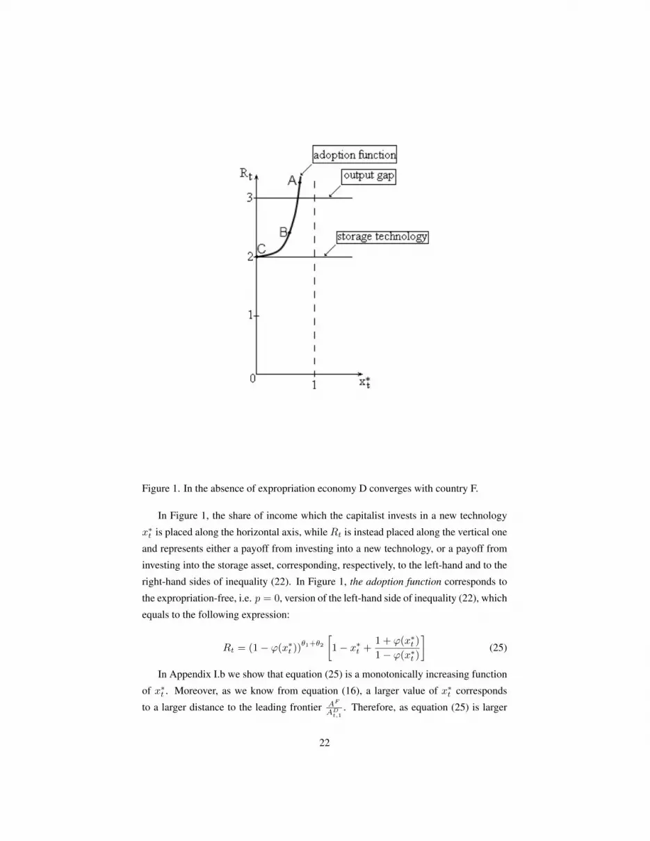
Figure 1. In the absence of expropriation economy D converges with country F.

In Figure 1, the share of income which the capitalist invests in a new technology

x∗t is placed along the horizontal axis, while Rt is instead placed along the vertical one

and represents either a payoff from investing into a new technology, or a payoff from

investing into the storage asset, corresponding, respectively, to the left-hand and to the

right-hand sides of inequality (22). In Figure 1, the adoption function corresponds to

the expropriation-free, i.e. p = 0, version of the left-hand side of inequality (22), which

equals to the following expression:

Rt = (1− ϕ(x∗t ))θ1+θ2

[1− x∗t +

1 + ϕ(x∗t )

1− ϕ(x∗t )

](25)

In Appendix I.b we show that equation (25) is a monotonically increasing function

of x∗t . Moreover, as we know from equation (16), a larger value of x∗t corresponds

to a larger distance to the leading frontier AF

ADt,1

. Therefore, as equation (25) is larger

22

when x∗t is higher, it thus is also larger when the distance to the leading frontier AF

ADt,1

is

higher. As a result, the value of equation (25) declines when the distance to the leading

frontier becomes smaller. Therefore, since a larger value of x∗t corresponds to a higher

level of AF

ADt,1

, a point on the adoption function which is close to the dashed line, as point

A, reflects a lower stage of technological development. On the contrary, a point as B,

which is instead relatively far away from the dashed line, corresponds to a lower share

of income which the capitalist invests into a new technology x∗t and thus to a smaller

distance to the leading frontier AF

ADt,1

. The economy thus becomes more developed as

long as it moves along the adoption function towards the steady-state point C. In point

C the share of income which the capitalist invests into a new technology x∗t equals to

0, reflecting the absence of investment into a new technology. As a result, the left-hand

side of inequality (24) becomes equal to 2, which indicates that the level of output in

country D totally converges with the one in economy F .

The horizontal line which is called "storage technology", reflects the payoff from

investing into the storage asset. As this line intersects the vertical axis in Rt = 2,

corresponding to expropriation-free, i.e. p = 0, version of the right-hand side of in-

equality (22), it follows that the payoff from investing into the storage technology is

lower than the payoff from investing into a new technology as long as x∗t > 0, which is

the case when AF

At,1> 1. The latter follows from equation (25), as its right-hand side,

representing the payoff from investing into a new technology, is larger than 2 as long

as x∗t > 0. Therefore, in the absence of expropriation, the capitalist always chooses

investment into a new technology, leaving instead the opportunity to invest into the

storage asset unexploited.

When economy D reaches the steady-state level of technology, technological gap

between D and F reduces to zero, i.e. AF

ADt,1

= 1, and therefore D does not adopt new

technologies any longer. Nor, according to equation (17), it invests into the acquisition

of additional human capital, as, when x∗t = 0, the level of technology remains constant,

i.e. ADt,1 = ADt.2 = AF , and, as it follows from equation (17), the share of human

capital which is used to acquire additional capital is, thus, ϕ1t = ϕ2

t = ϕ(x∗t ) = 0.

As long asD converges to economyF , the output gap between these two economies

reduces, which results in a downward shift of the output gap function. Form Proposi-

tion 1, equation (24), and the assumption that the high-educated and low-educated em-

ployees in economy D become as educated as their foreign counterparts, i.e. hF,1

hD,1t,2

=

hF,2

hD,2t,2

= 1, it follows that the output gap between countryD and economy F disappears

23

in the steady-state, i.e. Y F

Y Dt,1

= 2 .

We now consider the case when p is instead positive. According to Proposition

1, as a result of a positive probability of expropriation p, the level of technology in

economy D, i.e. ADt,1, fails to catch up with the world technological frontier AF . We

illustrate this result in the following figure:

Figure 2. Non-convergence trap.

The presence of expropriation changes the shape of adoption function. In Appendix

II.a, we show that as long as p > 0, the adoption function has a minimum point at

x∗t = p ≥ 0 instead of x∗t = 0 as in the case of p = 0. As a result, a part of

the adoption function is now located below the horizontal line representing the payoff

from the storage technology, which was not the case in the absence of expropriation.

We call the set of values of x∗t corresponding to this part of the adoption function as

"non-convergence set". This set is represented as a bold section on the horizontal axis.

In point A the capitalist is indifferent between acquiring a new technology or in-

vesting into the storage asset. Therefore, this point corresponds to the share x∗t > 0

satisfying equation (20), which we reproduce below for convenience:

24

(1− ϕ(x∗t ))θ1+θ2

[1− x∗t + (1− p) 1 + ϕ(x∗t )

1− ϕ(x∗t )

]= 2− p

As in the case of x∗t > 0 the level of technology becomes higher, from equation

(16) it follows that the next generation t+ 1 will choose x∗t+1 < x∗t . As x∗t+1 does not

satisfy equation (20), the right-hand side of this expression becomes larger than its left-

hand side. The latter implies that the storage technology will thus pay a higher return

to the capitalist belonging to generation t+ 1, and, as the result, the capitalist does not

have incentives to invest into a new technology. Therefore, the level of technology in

Home ADt,1 remains lower than the world technological frontier AF .

From equation (17) it follows that expropriation also lowers the rate of human capi-

tal accumulation. As expropriation reduces investment into a new technology, employ-

ees, correspondingly, reduce their investments into human capital. The latter implies

that, in addition to a non-reducible technological gap AF

ADt,1

, expropriation also results

in a constant educational gap between economies D and F , reflected in hF,1t

hD,1t,1

> 1 and

hF,2

hD,2t,1

> 1. Therefore, a positive probability of expropriation p also leads to educational

backwardness.

From equation (24) it follows that technological and educational gaps translate into

a non-reducible output gap. Therefore, in the presence of expropriation the output gap

between economies D and F always remains positive, which implies that Y Ft

Y Dt,1> 2.

4 Political Equilibrium

As expropriation results in a lower pace of technological development, slower human

capital accumulation, and, as a consequence, lower rate of economic growth, an insti-

tutional reform which reduces the risk of expropriation, might help the economy transit

to its expropriation-free version. The implementation of this policy, therefore, should

gain substantial popularity, as it makes everyone, apart from the corrupt regime, better

off.

To show why the latter is indeed possible, we combine equations (17), (14) and

(15) to derive the optimal life-time labor incomes belonging to typical individuals from

high-educated and low-educated groups, which, respectively, correspond to the follow-

ing expressions:

wD,1t,1 + wD,1t,2 =

25

= θ1(ADt,1

)1−θ1−θ2 (hD,1t,1

)θ1 (hD,2t,1 n

D2

)θ2 (nD1)θ1−1 2

(1− ϕt)1−θ1−θ2(26)

wD,2t,1 + wD,2t,2 =

= θ2(ADt,1

)1−θ1−θ2 (hD,1t,1 n

D1

)θ1 (hD,2t,1

)θ2 (nD2)θ2−1 2

(1− ϕt)1−θ1−θ2(27)

As, according to equation (17), a higher pace of technological evolution results in

a larger ϕt, from equations (26) and (27) it follows that a faster technological progress

increases the level of life-time income for both groups of employees. Therefore, as

an institutional reform results in faster technological development, it benefits all the

employees, as well as the capitalist. As a consequence, a political regime which elimi-

nates expropriation should earn substantial popularity, and thus the presence of political

competition should help solving the problem of expropriation, as individuals receive

an opportunity to replace a regime which practices expropriation with the one which

instead will eliminate it. We show, however, that low-educated employees might not

support the reformist policy, and therefore regardless the harm the expropriating regime

produces for the economy, it can nevertheless be politically survivable.

In this section, we incorporate political competition into the model and introduce

two political regimes. We assume that under the rule of clientelistic regime the qual-

ity of institutions remains low, which is reflected in a positive level of probability of

expropriation p, while the reformist regime instead chooses high-quality institutions

resulting in p = 0As we show, even though the policy of the reformist regime re-

sults in faster economic growth, the latter might play little role for the representative

low-educated employee.14 On the contrary, income transfers can make the current gen-

eration of low-educated individuals substantially better off. Therefore, if low-educated

employees make up a majority of population and thus play an important political role,

providing income redistribution might become a key to political success.

14This is a consequence of a low labor income of the representative employee belonging to the low-educated cohort. The income level is low as the output share belonging to the less educated group, i.e. θ2, issmall, and, moreover, the number of low-educated employees is instead large, which lowers this group’s percapita labor income even further. As a consequence, even fast economic growth might result in a too smallincrease in per capita income level of the representative employee belonging to the low-educated cohort.

26

4.1 The Reformist Regime

We first consider a policy which is implemented by the reformist regime. We assume

that the latter eliminates expropriation, and therefore the probability of expropriation p

becomes equal to 0. As a result, inequality (22) changes to the following expression:

(1− ϕ(x∗t ))θ1+θ2

[1− x∗t +

1 + ϕ(x∗t )

1− ϕ(x∗t )

]≥ 2 (28)

As we show in Appendix I, when p = 0, the left-hand side of inequality (28)

becomes a monotonic function of x∗t , which is reflected in Figure 1 in the previous

section. From Figure 1 it follows that in the absence of expropriation the adoption

function is placed above the storage technology line as long as x∗t > 0. The latter

implies that the payoff from investing into a new technology is always at least as large

as the one from investing into the storage asset, and therefore the capitalist acquires new

technologies until economy D entirely converges to the world technological frontier.

As x∗t remains positive as long as economy D converges to the leading frontier,

from equation (17) it follows that high-educated and low-educated employees acquire

additional human capital, i.e. ϕt = ϕ1t = ϕ2

t > 0. As investment into new technologies

and human capital remains positive along the whole economy D’s path towards the

leading technological frontier, the output gap function, corresponding to the following

equation

Y F

Y Dt,1= 2

(AF

ADt,1

)1−θ1−θ2 (hF,1

hD,1t,1

)θ1 (hF,2

hD,2t,1

)θ2moves down and for a particular generation t it becomes equal to 2, which implies that

the output level in D entirely converges to the one in economy F .

We therefore conclude that the reformist policy results in faster economic growth

and lets economy D reach substantially larger level of income, benefiting all the em-

ployees.

4.2 The Clientelistic Regime

Even though higher-quality institutions, corresponding to p = 0, result in faster growth,

its benefits might be inequally allocated among the employees. To show this, we again

consider labor incomes which are earned by the more educated and the less educated

groups working at the representative firm. The high-educated group employed at a

27

typical firm receives the following income:

nDt,1

(wD,1t,1 + wD,1t,2

)= θ1y

Dt (29)

while the labor income of low-educated employees is instead as large as the following:

nDt,2

(wD,2t,1 + wD,2t,2

)= θ2y

Dt (30)

The representative capitalist receives the remaining part of income, i.e. (1− θ1 − θ2) yDt .

We notice that, given our assumption about income shares, i.e. θ1 > θ2, form equa-

tions (29) and (30) it follows that per capita income level in the more educated group is

unambiguously larger than the one in the low-educated cohort whenever nDt,1 ≤ nDt,2,

i.e. when the size of the less educated group is at least as large as the size of the more

educated one. The latter result follows directly after we divide equations (29) and (30),

over nDt,1 and nDt,2 respectively, such that they are transformed into per capita labor

incomes:

wD,1t,1 + wD,1t,2 =θ1y

Dt

nDt,1(31)

wD,2t,1 + wD,2t,2 =θ2y

Dt

nDt,2(32)

From equation (32) it follows that a low θ2 and a high nDt,2, both lead to a low level

of per capita income in the less educated group. As a consequence, even fast economic

growth can add too little to the level of per capita income within the low-educated

cohort. Less educated employees can, therefore, be sensitive to redistribution policy,

as the latter might result in a larger increase in the level of per capita income. Thus,

even though the clientelistic regime can not compete with the reformist one regarding

economic growth, it can, however, provide larger income transfers to the low-educated

cohort.

We assume that under the rule of the clientelistic regime, the share of the low-

educated cohort in output is as large as βC,2t ≥ θ2, while under the rule of the reformist

regime it is instead equal to βR,2t ≥ θ2.

28

4.3 Political Competition

We assume that the low-educated cohort forms a majority in economyD, and therefore

the representative employee from this group plays a pivotal role in politics.15 To earn

political sympathies of a typical employee from the low-educated cohort, the clientelis-

tic regime should implement redistribution policy which makes the employee’s income

larger than the one which she would receive under the reformist regime’s rule. The

latter is reflected in the following expression:

wCt,1 + wCt,2 ≥ wRt,1 + wRt,2 (33)

wherewCt,1+wCt,2 is the representative low-educated employee’s labor income under

the clientelistic regime rule, while wRt,1 + wRt,2 corresponds instead to the level of her

labor income in the economy where the reformist regime is in power. We denote the

lowest βC,2t , the low-educated cohort’s share under the rule of clientelistic regime,

satisfying inequality (33) as βC,2t,min,16 and therefore at point βC,2t = βC,2t,min inequality

(33) transforms into the following equation:

βC,2t,min

2

(1− ϕt(p))1−θ1−θ2= βR,2t

2

(1− ϕt)1−θ1−θ2(34)

We notice that βC,2t,min should be less than 1, as if βC,2t,min is instead equal to 1, then

neither the capitalist, nor the employees belonging to the other group receive a positive

income.17

After rearranging, equation (34) turns into the following expression:

βC,2t,min =

(1− ϕt (p)1− ϕt

)1−θ1−θ2βR,2t (35)

We notice that the share of human capital endowment which is invested in the

acquisition of additional human capital, i.e. ϕt, is positively linked with the rate of

economic growth: a larger level of ϕt results in faster growth in economy D. We

15The latter assumption holds for developing economies, where the level of education is comparativelylow, and the level of education of a typical employee is normally low. This assumption also implies that towin political competition the ruling regime needs to be supported by the majority of population. The latter,according to our assumptions, is represented by the low-educated cohort

16We consider the minimum level of redistribution βC,2t,min as the ruling regime receivesp (1− β1 − β2)Yt,2 and therefore it has incentives to minimize the level of β2, as the latter results ina higher level of regime’s income.

17We assume that all the employees and the capitalists receive a strictly positive income.

29

therefore can use ϕt to measure the pace of output growth.

From equation (35) it follows that a large difference between the growth rate under

the reformist regime rule and the one under the rule of clientelistic alternative, reflected

in 1−ϕt(p)1−ϕt

, and a higher share in output βR,2t of a typical employee from the low-

educated group under the rule of the reformist regime, both result in a higher level of

βC,2t,min, the representative employee’s share in output when the clientelistic regime is in

power.

Regarding the difference in growth rates reflected in 1−ϕt(p)1−ϕt

, a positive probability

of expropriation p > 0 under the clientelistic regime rule results in a lower level of

investment in the acquisition of new technologies, a slower speed of human capital

accumulation and, as a consequence, a smaller pace of economic growth compared to

the case when expropriation is instead absent. A higher level of p results in a larger

difference between growth rates under the rule of reformist and clientelistic regimes,

reflected in a larger value of 1−ϕt(p)1−ϕt

. Moreover, when economy D ends up in a non-

convergence trap, then no investment into new technology and human capital takes

place, and, as a result, ϕt (p) = 0, i.e. economy D does not grow at all.

From equation (27) it follows that a higher probability of expropriation p and a low

pace of economic growth reflected in a low level of ϕt (p) also translates into slower

growth of a low-educated employee’s labor income wCt,1 + wCt,2. To compensate for

a slower growth of the representative low-educated employee’s earnings, i.e. wCt,1 +

wCt,2, the clientelistic regime needs to transfer more output to a typical low-educated

employee, which results in a higher level of βC,2t,min.

A higher share in output belonging to the representative employee from the low-

educated group under the reformist regime’s rule, i.e. a higher βRt,2, also induces the

clientelistic regime to redistribute more output towards the employees.

Therefore, if under the reformist regime rule the economy is growing at a high

rate, compared to the rate under the rule of the clientelistic regime, and, moreover,

employees benefit from growth, from equation (35) it follows that βC,2t,min should be

large to let the clientelistic regime win the political competition against the reformist

opponent. As the maximum value of βC,2t,min is strictly lower than 1, the reformist regime

can therefore choose the share βR,2t such that winning political competition becomes

impossible for the clientelistic regime. From equation (35) it follows that for the latter

to be the case, the lowest value of βR,2t should be equal to the following expression:

βR,2t,min =

(1− ϕt

1− ϕt(p)

)1−θ1−θ2(36)

30

as, if equation (36) holds, the level of βC,2t,min is equal to 1, which contradicts our

assumption that the largest βC,2t,min should be instead strictly less than 1.

From equation (36) it follows that a larger difference between growth rates under

the reformist and clientelistic regimes rules results in a lower right-hand side of equa-

tion (36), and therefore the reformist regime needs to redistribute comparatively less

income to win political competition against the clientelistic alternative. The difference

between growth rates is large when the probability of expropriation p is high, as in this

case ϕt(p) is low compared to ϕt.

On the contrary, the difference between growth rates is comparatively low if the

clientelistic regime is less corrupt. Alternatively, this difference declines when D be-

comes more matured economy, as in the latter case, according to equation (17), ϕt is

relatively low, and therefore the difference between ϕt and ϕt(p) is low as well. The

latter result implies that as soon as D becomes more developed, the level of redistri-

bution which is implemented by the reformist regime should increase. We therefore

notice the important difference between policies in the less developed economies and

the more developed ones: in the latter, redistribution plays a comparatively more im-

portant role in political competition than in the former.

If, however, the reformist regime redistributes less than what is implied by equation

(36), as, for instance, βRt,2 = θ2, corresponding to the case of no redistribution, then

political opportunities of the clientelistic regime become larger.

We summarize our findings in the following proposition:

Proposition 2. A high difference between growth rates under the rule of the reformist

and the clientelistic regimes, reflected in a large distance between ϕt and ϕt(p), and

a large share in output belonging to the representative employee under the reformist

regime’s rule βR,2t , all reduce the clientelistic regime’s political opportunities.

Proof. From equation (35) it follows that a larger distance between ϕt, reflecting the

rate of growth under the reformist regime, and ϕt(p), corresponding to growth rate

when, instead, the clientelistic regime is in power, and a higher βR,2t reflecting the

output share of the representative employee from the low-educated group under the

reformist regime, all result in a higher level of βC,2t,min, the output share belonging to a

typical employee when the clientelistic regime is in office. As βC,2t,min should be strictly

lower than 1, there is less chance that βC,2t,min corresponding to equation (35) will meet

the latter requirement, when the difference between ϕt and ϕt(p), as well as the level

of βR,2t , are large.

31

4.4 Discussion

We therefore conclude that redistribution might be important for political survival of

the reformist regime. If the difference between growth rates provided by two regimes

is comparatively low, income redistribution might be a key to political feasibility of

growth enhancing policy.

What are the alternatives to the policy of income redistribution? Is there another

policy which, on one hand, is effective for enhancing political popularity of the re-

formist regime, but can also capitalize resources which are spent as a result of this

policy? As we argue, even though such a policy exists, its benefits, however, are re-

alized in the long run. Within a shorter period of time, income redistribution is still

necessary to facilitate political survival of the reformist regime.

To show the latter, we notice that political survival of the clientelistic regime be-

comes low when the representative employee belongs to the high-educated group. In

this case, equation (35) changes to the following expression:

βC,2t,min =

(1− ϕt (p)1− ϕt

)1−θ1−θ2θ1 (37)

As 1−ϕt(p)1−ϕt

is larger than 1, and θ1 is large compared to θ2, βC,2t,min should also be

sufficiently large. As βC,2t,min is strictly lower than 1 by assumption, there is little chance

that the clientelistic regime will win the political competition.

However, for the high-educated group to make up a majority, the ruling regime

should implement an educational policy, which at a particular cost transfers a larger per

capita share δ1 of the aggregate human capital stock HDt−1,2 to the majority of young

individuals. The latter reform corresponds to the Inclusive Growth policy, which we

briefly mentioned in the introductory part of the paper. The policy aims to increase the

level of productivity in developing societies, in order to enhance the effect of economic

growth: "While absolute pro-poor growth can be the result of direct income redistri-

bution schemes, for growth to be inclusive, productivity must be improved and new

employment opportunities created. In short, inclusive growth is about raising the pace

of growth and enlarging the size of the economy, while levelling the playing field for

investment and increasing productive employment opportunities".18

In the extension to our paper, which we present in the following subsection, we

show that, regardless the benefits this policy brings about to economy D, as, for in-

18The World Bank (2009).

32

stance, "enlarging the size of the economy", "raising the pace of growth" or increasing

the size of the high-educated cohort, it still might be less popular than the conventional

income redistribution policy which can be implemented by the clientelistic regime.

The key assumption which leads to this result is that the implementation of this pol-

icy might take a lot of time, as, for instance, transferring human capital is typically

a long-term process, and therefore the main benefits of it will impact the following,

but not the current generation of the low-educated employees, who instead will mostly

stay unaffected. Inclusive growth thus can not be a substitute for income transfers in

the short run. As a result, the current generation of low-educated individuals remains

sensitive to income transfers, and if the latter are not provided by the reformist regime,

then political chances of the clientelistic alternative become higher.

5 Extension: Inclusive Growth and Redistribution

As we mentioned in the previous subsection, economic growth alone might be insuf-

ficient to deliver sufficiently high benefits to a broad cohort of individuals, as in the

presence of a large disadvantaged group, benefits from the implementation of the in-

stitutional reform will not be equally distributed. A typical employee belonging to the

high-educated cohort will derive substantial benefits from the introduction of the re-

form, which, however, will not be the case for the representative employee from the

low-educated group. This, however, can be changed if the ruling regime transfers more

human capital to employees, therefore increasing the size of the high-educated group.19

At the same time, we assume that this policy affects the next generation of employees,

but not the current one.

To show how does this reform can be implemented, we maximize equations (10)

and (13) with respect to ϕ1t and ϕ2

t again, which, as was shown in Section 3, results in

the following expression:

ϕ2t = ϕ1

t =AHt,2 (xt)−AHt,1AHt,2 (xt) +AHt,1

(38)

We combine equations (38), (10) and (13) to derive labor incomes belonging to the

representative employees from the high-educated and the low-educated groups.

As a result, we receive that the representative individual belonging to the more

19This is, of course, the reformist regime which implements this policy, as the clientelistic one does nothave incentives to introduce such a reform.

33

educated cohort earns the following income:

wD,1t,1 + wD,1t,2 = θ1

(hD,1t,1

)θ1(nD1)1−θ1 (AHt,1)θ1 (hD,2t,1 n

D2

)θ2 2

(1− ϕ1t )

1−θ1−θ2 (39)

The equilibrium level of labor income of her counterpart from the less educated

group is instead as large as:

wD,2t,1 + wD,2t,2 = θ2

(hD,2t,1

)θ2(nD2)1−θ2 (AHt,1)θ1 (hD,1t,1 n

D1

)θ1 2

(1− ϕ1t )

1−θ1−θ2 (40)

The ratio between equation (39) and equation (40) reflects the wage gap between

two groups of employees:wD,1t,1 + wD,1t,2

wD,2t,1 + wD,2t,2

=θ1θ2

nD2nD1

(41)

As was shown in the previous subsection, from equation (41) it follows that a larger

number of employees belonging to the less educated group, reflected in higher nD2 , and

a low importance of this group for production, which is mirrored in a low level of θ2,

both result in a smaller wD,2t,1 +wD,2t,2 , the labor income of a typical individual from the

low-educated group, compared to wD,1t,1 +wD,1t,2 , the labor income of the representative

individual belonging to the high-educated cohort.

As a consequence, the implementation of a policy which eliminates expropriation

and therefore enhances economic growth, might produce a limited effect on the low-

educated group. Even fast economic growth might result in a too small increase in

per capita income level of the representative employee belonging to the less educated

cohort. The positive effect of a reform which reduces the risk of expropriation can,

however, become more substantial for the low-educated group if such a reform is com-

plemented by an educational policy which results in transferring the high per capita

share δ1 of the aggregate human capital stock Ht−1,2 to a larger group of employees.

As a result of the educational policy, the number of low-educated employees declines,

while the size of the high-educated cohort instead increases. Therefore, nD2

nD1

becomes

lower, and thus according to equation (41) the wage gap becomes lower as well. To im-

plement this policy, the reformist regime needs to spend a particular amount of output

which it receives from taxation.

We assume that this reform does not, however, affect the current generation of

34

employees. Instead, it impacts individuals belonging to generation t+ 1.20 As a result

of this reform, a high level of human capital endowment hD,1t+1,1 is transferred to a

broader group of individuals belonging to generation t + 1, and therefore the size of

the high-educated group increases. As a consequence, a reform which eliminates the

risk of expropriation will benefit a larger number of employees, as the more educated

employees’ labor income is higher compared to the one of the low-educated workers.

We show in Appendix VI, that the optimal number of high-educated employees

belonging to generation t + 1, n∗t+1,1 is derived from maximization of the following

expression:

yt+1,1(nD1 ) + yt+1,2(n

D1 ) −→ max

nDt+1,1

(42)

and satisfies the following condition:

θ1θ2

n∗t+1,2

n∗t+1,1

= 1 (43)

As we can notice, from equations (43) and (41) it follows that if the number of em-

ployees belonging to the more educated group is defined optimally, the labor incomes

of two groups of employees become identical:

wD,1t+1,1 + wD,1t+1,2 = wD,2t+1,1 + wD,2t+1,2 (44)

As θ1 > θ2 by assumption, which implies that the high-educated group is more

important for production, from equation (43) it, therefore, follows that in the optimum

the number of low-educated employees n∗t+1,2 should be lower than the size of the

high-educated cohort, i.e. n∗t+1,1. As a result, economic growth will benefit a larger

number of employees, as the low-educated cohort becomes smaller, while the high-

educated, and better paid one becomes instead larger.

We combine identity nD = nDt+1,1 + nDt+1,2 with equation (43) to receive the

following solutions:

n∗t+1,1 = nDθ1

θ1 + θ2(45)

and

n∗t+1,2 = nDθ2

θ1 + θ2(46)

From equations (45) and (46) it follows that a larger importance of the high-educated

20The rest of employees from generation t+1 are provided with the low per capita share δ2 in aggregatedhuman capital stock Ht−1,2, δ2 < δ1.

35

group for production reflected in a higher level of θ1 results in a larger optimal number

of high-educated individuals n∗t+1,1.

We summarize our findings in the following proposition:

Proposition 3. If high-educated employees are more important for production, i.e. if

θ1 > θ2, then the optimal size of the more educated group belonging to generation

t+ 1 will be larger than its low-educated counterpart, i.e. n∗t+1,1 > n∗t+1,2.

Proof. If the high-educated group is more important for production than the low-

educated one, i.e. if θ1 is larger than θ2, then according to equations (45) and (46)

the number of high-educated individuals n∗t+1,1 is larger than n∗t+1,2, reflecting instead

the size of the low-educated group. This establishes the result

As the labor incomes within the high-educated and the low-educated cohorts are the

same when equation (43) holds, i.e. wD,1t+1,1 + wD,1t+1,2 = wD,2t+1,1 + wD,2t+1,2, both groups

of employees equally benefit from economic growth. Moreover, wD,2t+1,1 + wD,2t+1,2 sat-

isfying equation (44) is larger than the level of labor income belonging to the repre-

sentative low-educated employee in the case of non-optimally large size of the less

educated group. This implies that the less educated cohort can derive higher benefits

from economic growth and therefore the institutional reform which was considered in

the previous subsection, not only results in higher rates of economic growth, but also

benefits a larger cohort of employees.21

Our findings are consistent with the resent history of Georgia, where in October21We also notice that if the number of high-educated individuals in economy D is lower than the level

n∗t+1,1 corresponding to equation (45), then the output gap between countries D and F remains positive

even if the level of technology and the human capital stock in economy D catch up with the ones in countryF . To show this, we normalize equation (23) which reflects the level of output produced by generation t+1in economy F in the absence of technological development:

Y Ft+1 = 2LF(AFt+1,1

)1−θ1−θ2 (hF,1t+1,1n

Ft+1,1

)θ1 (hF,2t+1,1n

Ft+1,2

)θ2(47)

over the level of output produced by generation t + 1 in country D in period j = 1 if the level oftechnology in D also remains constant

Y Dt+1 = LH(AHt+1,1

)1−θ1−θ2 (hD,1t+1,1n

Dt+1,1

)θ1 (hD,2t+1,1n

Dt+1,2

)θ2(48)

which, if technology and human capital stocks are the same in F and D, results in the following expres-sion:

Y Ft+1

Y Dt+1

= 2

(nFt+1,1

nDt+1,1

)θ1 (nFt+1,2

nDt+1,2

)θ2(49)

As it follows from equation (49), if the number of high-educated employees nFt+1,1 in economy F ischosen optimally, while in countryD the size of the high-educated cohort nDt+1,1 is lower than it is optimally

required, then, as θ1 > θ2, the output gap remains positive, i.e.Y Ft+1

YDt+1

> 2, even if technology and the level

of human capital in economy D are as large as the ones in country F .

36

2012, after 8 years of reforms, president Saakashvili’s United National Movement lost

an election against the Georgian Dream, a populist alternative established by a billion-

aire Bidzina Ivanishvili. Despite the reforms which resulted in a substantial improve-

ment in the public sector quality, corresponding, in terms of our model, to a lower p,

and higher growth rates reflected in a larger ϕt, Saakashvili’s rule was also charac-

terized by a low level of redistribution and relatively high poverty. Growth was not

followed by an adequate job creation, while, by contrast, wages of employed individ-

uals were increasing substantially. In terms of our model, employed Georgians can be

considered as individuals with a high level of human capital endowment hD,1t,1 , while

poor Georgians correspond instead to those employees who inherited a low human

capital level hD,2t,1 . As poor individuals did not benefit from growth, their incentives to

vote for Saakashvili and his reforms were low. Instead, they granted their votes to a

political force which was characterized by a larger corruption potential,22 but promised

to provide more redistribution.

6 Conclusion

We consider a non-overlapping generations economy where individuals combine hu-

man capital and technology to produce output. Each generation lives for two periods

and is made up of capitalists who own a technology, and two groups of employees,

possessing instead the human capital stock. Each capitalist employs a particular num-

ber of individuals from both groups in order to produce output. Using a possibility

of adoption from exogenously given leading technological frontier, the representative

capitalist improves upon a technology which he inherited from the previous generation.

In our setting, high-educated employees inherit a large human capital endowment,

while their low-educated counterparts, by contrast, receive a low level of human capital

stock from the previous generation. Both groups of employees, a high-educated and a

low-educated one, invest in the acquisition of additional human capital. As human cap-

ital and technology are complementary factors of production, employees accumulate

more human capital if the pace of technological evolution is larger. The latter occurs

when the capitalist invests more in the acquisition of a new technology.

According to our assumption, the high-educated cohort is more important for pro-

duction, and therefore it acquires a larger share in output and thus receives higher ben-

efits when the latter increases. The share of the low-educated group is instead smaller,

22And therefore low growth rates.

37

and, if this cohort is large, the level of per capita income in this group, as well as

benefits from economic growth, are, by contrast, low.

We also introduce low-quality institutions into the benchmark economy and show

how do bad institutions result in a lower level of investment into a new technology,

slower accumulation of human capital stock and a smaller pace of economic growth.

In the presence of low-quality institutions the economy can not converge to the leading

technological frontier and therefore remains a technological laggard.

We then assess under which circumstances a reform which improves the quality of

institutions increases the pace of economic growth, and thus makes all the employees,

as well as the capitalists, better off, might be politically infeasible. To this end, we in-

corporate political competition into the model and consider two political regimes, one

of them benefiting from expropriation and therefore maintaining the quality of institu-

tions at a low level, while the other, by contrast, improves the quality of institutions.

In order to gain political popularity to stay in power, the former regime implements

income redistribution, making transfers to the low-educated cohort. If individuals be-

longing to the latter make up a majority of population, their per capita income level

is low, and so are their benefits from economic growth. As a result, the low-educated

group’s sensitivity to income redistribution remains high and its members thus support

the regime which provides redistribution. We therefore conclude that the alternative,

or the reformist, regime should complement its institutional reform with income redis-

tribution policy to become more popular than its clientelistic opponent. If, instead, the

redistribution policy is neglected by the reformist regime, its popularity might be low,

and therefore the regime, as well as the institutional reform, can become less politically

feasible.

As an alternative to income redistribution, we consider a policy which, instead

of redistributing incomes, transfers more human capital to the employees in order to

enhance social mobility, enlarge the high-educated cohort and therefore broaden the

group of individuals benefiting from economic growth. We assume, however, that the

latter effect realizes in the long run, therefore affecting the next generation of employ-

ees, but not the current one. As a result, this policy might substitute income redistri-

bution in the long run, however, in the short run income transfers remain an impor-

tant component of political competition. We suggest to replace income transfers with

growth enhancing policy gradually, redistributing less to those individuals who tran-

sited to the high-educated cohort and continuing transferring incomes to those ones

who instead remain poor.

38

7 References

1. Acemoglu, D., 1994. "Search in the labour market, incomplete contracts and

growth," CEPR Discussion paper, no 1026;

2. Acemoglu, D., 1995. "Reward Structures and Allocation of Talent," European

Economic Review, 39, pp. 17-34;

3. Acemoglu, D., 2002a. "Technical Change, Inequality and the Labor Market,"

Journal of Economic Literature, 40, 7 - 72;

4. Acemoglu, D., 2008. "Introduction to Modern Economic Growth," Part 1, 3-27,

Princeton University Press;

5. Adelman, I., Morris, C., 1967. "Society, politics, and economic development: a

quantitative approach," Johns Hopkins Press;

6. Aghion, P., Caroli, E., Garcıa-Penalosa, C., 1999. "Inequality and Economic

Growth: The Perspective of the New Growth Theories," Journal of Economic

Literature, 37, 1615 - 1660;

7. Alesina, A., 1994. "Political Models of Macroeconomic Policy and Fiscal Re-

forms," Oxford University Press;

8. Alesina, A., Rodrik, D., 1994. "Distributive politics and economic growth,"

Quarterly Journal of Economics 108, 465-90;

9. Alesina, A., Danninger, S., Rostagno, M., 1999. "Redistribution Through Public

Employment: the Case of Italy." IMF Working Paper no WP/99/177;

10. Benhabib, J., Rustichini, A., 1996. "Social Conflict and Growth," Journal of

Economic Growth, 1, 129-146;

11. Blume, L., Rubinfeld, D., Shapiro P., 1984. "The Taking of Land: When Should

Compensation be Paid?," Quarterly Journal of Economics, 100, 71–92;

12. Brusco, V., Nazareno, M., Stokes, S., 2004."Vote Buying in Argentina," Latin

America Research Review, 39, 66-88;

13. Calvo, E., Murillo, M., 2004. "Who Delivers? Partisan Clients in the Argentine

Electoral Market," American Journal of Political Science, 48, 742-757;

39

14. Epstein, R., 1998. "Supreme Neglect: How to Revive Constitutional Protection

for Private Property," Oxford University Press;

15. Galor, O., Zeira, J., 1993. "Income distribution and macroeconomics," Review

of Economic Studies, 60, 35-52;

16. Grossman, H., 1991. "A General Model of Insurrections," American Economic

Review, 81, 912-921;

17. Grossman, H., 1994. "Production, Appropriation and Land Reform," American

Economic Review, 84, 705-712;

18. Kaplow, L., 1986. "An Economic Analysis of Legal Transitions," Harvard Law

Review, 99, 509–617;

19. Katz, L., Murphy, K., 1992. "Changes in Relative Wages, 1963-1987: Supply

and Demand Factors," Quarterly Journal of Economics, 107, 35 - 78;

20. Kitschelt, H., 2000. "Linkages Between Citizens and Politicians in Democratic

Politics," Comparative Political Studies, 33, 845-879;

21. Landes, D., 1998. "The Wealth and Poverty of Nations," Norton;

22. Loury, G., 1981. "Intergenerational Transfers and the Distribution of Earnings,"

Econometrica, 49, 843-867;

23. Lucas, R., 1988. "On the Mechanics of Development Planning," Journal of Mon-

etary Economics, 22, 3-42;

24. Muller, W., Shavit, Y., 1998. "The Institutional Embeddedness of the Stratifica-

tion Process," Oxford;

25. Persson, T., Tabellini G., 1994. "Is inequality harmful for growth?" American

Economic Review, 84, 600-621;

26. Redding, S., 1996. "The Low-Skill, Low-Quality Trap: Strategic Complemen-

tarities between Human Capital and RD," Economic Journal, 106, 458-70;

27. Robinson, J., Verdier, T., 2003. "The Political Economy of Clientelism," C.E.P.R.

Discussion Papers series, no 3205;

28. Stiglitz, J., 2004. "The Post-Washington Consensus Consensus?" The Initiative

for Policy Dialogue;

40

29. Tornell, A., Velasco, A., 1992. "The Tragedy of the Commons and Economic

Growth: Why does Capital Flow from Poor to Rich Countries?" Journal of Po-

litical Economy, 100, 1208-1231;

30. Transparency International, 2011. "Anti-corruption progress in Georgia, Liberia,

Rwanda", U4 Expert Answer;

31. World Bank, 2009. "What is Inclusive Growth?"

World Bank, 2011. "Georgia Poverty Dynamics, 2003-2010."

41

8 Appendix

Appendix I

Appendix I.a. Derivation of equations (16), (86), (17).

In period j = 1 a typical employee belonging to the more educated group receives the

following wage:

wD,1t,1 = θ1(ADt,1

)1−θ1−θ2 (hD,1t,1

(1− ϕ1

t

))θ1 (hD,1t,2 n

D2

(1− ϕ2

t

))θ2 (nD1)θ1−1

(50)

and in period j = 2 the same employee receives instead the wage rate which is

equal to:

wD,1t,2 = θ1(ADt,2

)1−θ1−θ2 (hD,1t,1

(1 + ϕ1

t

))θ1 (hD,1t,2 n

D2

(1 + ϕ2

t

))θ2 (nD1)θ1−1

(51)

Similarly, in period j = 1 an employee from the more educated cohort receives the

following wage:

wD,2t,1 = θ2(ADt,1

)1−θ1−θ2 (hD,1t,1 n

D1

(1− ϕ1

t

))θ1 (hD,1t,2

(1− ϕ2

t

))θ2 (nD2)θ2−1

(52)

and in period j = 2 the same employee receives the wage rate which is as large as

the following:

wD,2t,2 = θ2(ADt,2

)θ1 (h1n

D1

(1 + ϕ1

t

))θ1 (h2(1 + ϕ2

t

))θ2 (nD2)θ2−1 (53)

An employee from the more educated group solves the following problem:

wD,1t,1 + wD,1t,2 −→ maxϕ1

t

(54)

While her counterpart from the less educated group instead maximizes the follow-

ing payoff function:

wD,2t,1 + wD,2t,2 −→ maxϕ2

t

(55)

42

The capitalist maximizes his payoff, which is equal to the following expression:

(1− xt)[yDt,1 − nD1 w

D,1t,1 − nD2 w

D,2t,1

]+(1− p)

[yDt,2 − nD1 w

D,1t,2 − nD2 w

D,2t,2

]−→ max

xt

(56)

where

yDt,1 =(ADt,1

)1−θ1−θ2 (hD,1t,1 n

D1

(1− ϕ1

t

))θ1 (hD,2t,1 n

D2

(1− ϕ2

t

))θ2and

yDt,2 =(ADt,2

)1−θ1−θ2 (hD,1t,1 n

D1

(1 + ϕ1

t

))θ1 (hD,2t,1 n

D2

(1 + ϕ2

t

))θ2After taking derivatives and rearranging we receive the following first order condi-

tions: (ADt,2 (xt)

ADt,1

)1−θ1−θ2 (1 + ϕ1

t

1− ϕ1t

)θ1=

(1 + ϕ2

t

1− ϕ2t

)1−θ2(57)

or (ADt,2 (xt)

ADt,1

)1−θ1−θ2 (1 + ϕ2

t

1− ϕ2t

)θ2=

(1 + ϕ1

t

1− ϕ1t

)1−θ1(58)

and(ADt,2 (xt)

ADt,1

)1−θ1−θ2 (1 + ϕ1

t

1− ϕ1t

)θ1 (1 + ϕ2t

1− ϕ2t

)θ2=

ADt,2

(1− θ1 − θ2) (1− p)∂(AD

t,2(xt))∂xt

(59)

Dividing equation (57) over equation (58) results in the following expression:

1 + ϕ2t

1− ϕ2t

=1 + ϕ1

t

1− ϕ1t

(60)

which, after rearranging, leads to the following result:

ϕ2t = ϕ1

t (61)

Substituting equation (60) into equation (59) and equation (58) results in the fol-

lowing expression:ADt,2 (xt)

ADt,1=

1 + ϕ2t

1− ϕ2t

=1 + ϕ1

t

1− ϕ1t

(62)

43

or, after rearranging:

ϕ2t = ϕ1

t =ADt,2 (xt)−ADt,1ADt,2 (xt) +ADt,1

(63)

From equations (59) and (60) results in the following expression:

∂ADt,2∂xt

=ADt,1

(1− θ1 − θ2) (1− p)(64)

One can combine equation (64) with equation (8) or with equation (85) from Ap-

pendix IV to derive equation (16) or equation (86) respectively.

Dynamics of x∗t .

We can rewrite equation (16) as follows:

η′(x∗t ) =1

(1− θ1 − θ2) (1− p)(

AFt−1,1(1+g)

ADt−1,1+η(x

∗t−1)(AF

t−1,1−ADt−1,1)

− 1

) (65)

From equation (65) it follows that when the denominator of

AFt−1,1(1 + g)

ADt−1,1 + η(x∗t−1)(AFt−1,1 −ADt−1,1

)increases more than its numerator, the economy approaches the leading technological

frontier, and therefore the gap between the level of local technology and the leading

frontier declines.

AsAF

t,1

ADt,1

positively affects the level of x∗t , this implies that x∗t < x∗t−1.

When, on the contrary, the denominator of

AFt−1,1(1 + g)

ADt−1,1 + η(x∗t−1)(AFt−1,1 −ADt−1,1

)increases less than the numerator, then the distance to technological frontier increases

as well, which results in x∗t > x∗t−1.

Finally, when the numerator of

AFt−1,1(1 + g)

ADt−1,1 + η(x∗t−1)(AFt−1,1 −ADt−1,1

)44

increases as much as does the denominator, x∗t = x∗t−1.

Appendix I.b. Uniqueness and global stability of the steady-state level of x∗t .

First we show uniqueness:

∂(x∗t+1

x∗t

)∂x∗t

=

∂x∗t+1

∂x∗tx∗t − x∗t+1

(x∗t )2 < 0

The latter result holds as from equation (16) we know that ∂x∗t+1

∂x∗t< 0. This implies

that x∗t+1

x∗t

increases when x∗t decreases. As x∗t+1

x∗t

= 1 in the steady-state, and x∗t+1

x∗t

is

everywhere increasing when x∗t is decreasing, the steady-state is unique.

Global stability of the steady-state level of x∗t .

η′(x∗t ) =1

(1− θ1 − θ2) (1− p)(AF

t,1

ADt,1− 1) (66)

Since η′(x∗t ) is monotonically decreasing in x∗t , we can write the following expres-

sion:

x∗t = (η′)−1

1

(1− θ1 − θ2) (1− p)(AF

t,1

ADt,1− 1) (67)

Since η(x∗t ) is concave, which implies that η′′(x∗t ) < 0, the inverse of η′(x∗t ),

which is (η′)−1, is also a decreasing function of its argument. To prove global stability,

we consider x∗t ∈ (x∗, x∗0), where x∗ is a steady-state share in output x∗t , and x∗0 is a

share in output for the initial generation t = 0.

We use equation (67) to show that

x∗t+1 − x∗ = (η′)−1

1

(1− θ1 − θ2) (1− p)(

AFt+1,1

ADt+1,1(x

∗t )− 1)−

− (η′)−1

1

(1− θ1 − θ2) (1− p)(

AFt,1

ADt,1(x

∗)− 1) =

45

= −x∗0x∗

((η′)−1)′> 0 (68)

Since we proved that x∗t+1

x∗t

increases when x∗t instead decreases, we can now derive

the following result:

x∗t+1

x∗t− 1 =

(η′)−1

1

(1−θ1−θ2)(

AFt+1,1

ADt+1,1

(x∗t )−1

)

(η′)−1

1

(1−θ1−θ2)(

AFt,1

ADt,1(x∗

t−1)−1

) − 1 <

x∗

x∗− 1 = 0 (69)

Equation (68) together with equation (69) establish that for all x∗t ∈ (x∗, x∗0) the

following result holds: x∗t+1 ∈ (x∗, x∗t ). Using a similar argument we can show

that for all x∗t ≤ x∗, x∗t+1 ∈ (x∗t , x∗). Therefore, a sequence {x∗t }

∞0 monotonically

converges to x∗ and is globally stable.

Appendix I.c. Adoption function is decreasing in x∗t when p = 0. To show that

(1− ϕ(x∗t ))θ1+θ2

[1− x∗t +

1+ϕ(x∗t )

1−ϕ(x∗t )

]is increasing with respect to x∗t , we first rewrite

it as follows:

(ADt,2 +ADt,1

ADt,1− x∗t

)(2ADt,1

ADt,2 +ADt,1

)θ1+θ2and then differentiate it with respect to

x∗t :

(1

1− θ1 − θ2− 1

)(2ADt,1

ADt,2 +ADt,1

)θ1+θ2−

− (θ1 + θ2)

(2ADt,1

ADt,2 +ADt,1

)θ1+θ2ADt,1

(1− θ1 − θ2)(ADt,2 +ADt,1

) (ADt,2 +ADt,1ADt,1

− x∗t

)=

=

(1

1− θ1 − θ2− 1

)(2ADt,1

ADt,2 +ADt,1

)θ1+θ2x∗t

ADt,1ADt,2 +ADt,1

> 0

which establishes the result

46

Appendix II

We take a derivative of the adoption function Rt with respect to x∗t . First we use

ϕ(x∗t ) =AD

t,2−ADt,1

ADt,2+A

Dt,1

to rewrite the adoption function

Rt = (1− ϕ(x∗t ))θ1+θ2

[1− x∗t + (1− p)1 + ϕ(x∗t )

1− ϕ(x∗t )

](70)

as follows

Rt =

(2ADt,1

ADt,2 +ADt,1

)θ1+θ2 [ADt,2ADt,1

(1− p) + 1− x∗t

](71)

Taking a derivative of equation (71) with respect to x∗t results in the following

expression:

∂Rt∂x∗t

= − (θ1 + θ2)

(2ADt,1

ADt,2 +ADt,1

)θ1+θ2−1 2ADt,1∂AD

t,2

∂x∗t(

ADt,2 +ADt,1)2(ADt,2ADt,1

(1− p) + 1− x∗t

)+

+

(1− p)∂AD

t,2

∂x∗t

ADt,1− 1

( 2ADt,1ADt,2 +ADt,1

)θ1+θ2(72)

From equations (8) and (16) it follows that∂AD

t,2

∂x∗t

=AD

t,1

(1−θ1−θ2)(1−p) . We therefore

can rewrite equation (72) as follows

∂Rt∂x∗t

=

(2ADt,1

ADt,2 +ADt,1

)θ1+θ2

[− θ1 + θ21− θ1 − θ2

ADt,1

(1− p)(ADt,2 +ADt,1

) (AD2,tAD1,t

(1− p) + 1− x∗t

)+

θ1 + θ21− θ1 − θ2

=

=

(2ADt,1

ADt,2 +ADt,1

)θ1+θ2θ1 + θ2

1− θ1 − θ2

47

[−

AD2,t (1− p)(ADt,2 +ADt,1

)(1− p)

−ADt,1 (1− x∗t )

(1− p)(ADt,2 +ADt,1

) + (1− p)(ADt,2 +ADt,1

)(1− p)

(ADt,2 +ADt,1

)] =

=

(2ADt,1

ADt,2 +ADt,1

)θ1+θ2θ1 + θ2

1− θ1 − θ2ADt,1

(1− p)(ADt,2 +ADt,1

) (x∗t − p) (73)

From equation (73) it follows that equation (70) reaches its minimum value when

x∗t = p, it increases whenever x∗t > p and declines whenever the opposite occurs.

We now show that the minimum point of equation (70) declines when p increases.

We substitute x∗t = p into equation (70)

Rt = (1− ϕ(p))θ1+θ2[1− p+ (1− p)1 + ϕ(p)

1− ϕ(p)

]= (1− p) 2

(1− ϕ(p))1−θ1−θ2(74)

and take a derivative of equation (74) with respect to p:

∂Rt∂p

=

−2 (1− ϕ(p))1−θ1−θ2 + 2 (1− θ1 − θ2) (1− ϕ(p))−θ1−θ2 (1− p)∂ϕ(p)∂p

(1− ϕ(p))2(1−θ1−θ2)=

=2

(1− ϕ(p))1−θ1−θ2

[(1− θ1 − θ2) (1− p)∂ϕ(p)∂p

1− ϕ(p)− 1

](75)

We substitute ϕ(x∗t ) =At,2−At,1

At,2+At,1into equation (75) and use equation (16) to re-

ceive the following result:∂Rt∂p

=

2(ADt,2 +ADt,1

)1−θ1−θ2(2ADt,1

)1−θ1−θ2[

ADt,1ADt,2 +ADt,1

− 1

]=

−2(ADt,2 +ADt,1

)1−θ1−θ2(2ADt,1

)1−θ1−θ2 ADt,2ADt,2 +ADt,1

< 0 (76)

Expression (76) implies that a larger p reduces the minimum point of Rt.

48

Appendix III.a

We now show that a larger p results in a larger x∗t corresponding to the intersection

point between equation (70) and 2− p.

At the intersection point, equation (70) equals to 2− p:

Rt = (1− ϕ(x∗t ))θ1+θ2

[1− x∗t + (1− p)1 + ϕ(x∗t )

1− ϕ(x∗t )

]= 2− p (77)

As, according to equation (16), x∗t is a function of p, we can rewrite equation (77)

as follow

(1− ϕ(x∗t (p)))θ1+θ2

[1− x∗t (p) + (1− p)1 + ϕ(x∗t (p))

1− ϕ(x∗t (p))

]− 2 + p = 0 (78)

We use ϕ(α∗t ) =AD

t,2−ADt,1

ADt,2+A

Dt,1

together with the implicit function theorem to derive

the following result:

−(θ1 + θ2)

(2ADt,1

ADt,2(x∗t (p)) +ADt,1

)θ1+θ2−1 2ADt,1∂AD

t,2

∂x∗t(

ADt,2(x∗t (p)) +ADt,1

)2 ∂x∗t∂p[ADt,2(x

∗t (p))

ADt,1(1− p) + 1− x∗t (p)

]+

+

(2ADt,1

ADt,2(x∗t (p)) +ADt,1

)θ1+θ2 ∂x∗t∂p

∂ADt,2

∂x∗t

ADt,1(1− p)−

ADt,2(x∗t (p))

ADt,1− ∂x∗t

∂p

+ 1 = 0

(79)

We can simplify the upper expression in order to receive the following result (most

derivations replicate the ones from Appendix II):

∂x∗t∂p

=

ADt,2(x

∗t (p))

ADt,1

−(AD

t,2(x∗t (p))+A

Dt,1

2ADt,1

)θ1+θ2AD

t,1(x∗t (p)−p)

(1−p)(ADt,2(x

∗t (p))+A

Dt,1)

(θ1+θ2

1−θ1−θ2

) (80)

To define the sign of equation (80) we have to find the sign of x∗t (p) − p andAD

t,2(x∗t (p))

At,1−(AD

t,2(x∗t (p))+A

Dt,1

2ADt,1

)θ1+θ2. Equation (77) holds for a value of x∗t (p) which

is located to the right from the minimum point x∗t (p) = p, i.e. x∗t (p) > p, which

49

implies that x∗t (p)− p > 0. We now rewriteAD

t,2(x∗t (p))

At,1−(AD

t,2(x∗t (p))+At,1

2At,1

)θ1+θ2as

follows:

ADt,2(x

∗t (p))

ADt,1

(AD

t,2(x∗t (p))+A

Dt,1

2ADt,1

)1−θ1−θ2− AD

t,2(x∗t (p))+A

Dt,1

2ADt,1(

ADt,2(x

∗t (p))+A

Dt,1

2ADt,1

)1−θ1−θ2 =

=

ADt,2(x

∗t (p))

ADt,1

[(AD

t,2(x∗t (p))+A

Dt,1

2ADt,1

)1−θ1−θ2− 1

2

]− 1

2(AD

t,2(x∗t (p))+A

Dt,1

2ADt,1

)1−θ1−θ2 (81)

The numerator of equation (81) is positive, since(AD

t,2(x∗t (p))+A

Dt,1

2ADt,1

)1−θ1−θ2> 1,

which implies that(AD

t,2(x∗t (p))+A

Dt,1

2ADt,1

)1−θ1−θ2> 1

2 , and therefore, sinceAD

t,2(x∗t (p))

ADt,1

>

1,AD

t,2(x∗t (p))

ADt,1

[(AD

t,2(x∗t (p))+A

Dt,1

2ADt,1

)1−θ1−θ2− 1

2

]> 1

2 as well.

Thus we conclude that ∂x∗t

∂p > 0.

Appendix IV

In Section 3 we assumed that the level of AFt is constant, and, as imitation of tech-

nologies from country F was the only opportunity for economy D to improve upon its

domestic technology, the steady-state level of technology in country D also remained

constant.

However, as a constant level of the world technological frontier is not a realistic

assumption, in this Appendix we allow for a positive growth rate of the leading tech-

nology level, corresponding to AFt , which is the level of technology in country F . We

therefore introduce a more natural assumption of evolving technological frontier, and

assume that the level of technology in economy F grows at a constant rate g.

As it follows from equation (16), when the leading technology is growing at a

constant rate g, the steady-state level of ADt also increases at the same rate. However,

even in the absence of expropriation, i.e. when p = 0, the level of technology in

country D can not entirely converge to the one in F . To show the latter, we use the

50

following result:

ADt,1(1 + g) = η (x∗)AFt + (1− η (x∗))ADt,1 (82)

where x∗ is a steady-state level of x∗t . Equation (82) implies that the steady-state

level of ADt increases at a rate g. After rearranging, equation (82) results in the follow-

ing expression:

ADt,1 =η (x∗)AFtg + η (x∗)

(83)

As η(x∗)g+η(x∗) is less than 1, from equation (83) it follows that the steady-state level

of ADt,1 always remains below AFt . Therefore, the level of output in economy D can

not entirely converge to the one in country F . From equation (24) it follows that the

output gap always remains positive, as ADt,1, and, as a result, hD,1t,1 and hD,2t,1 as well,

do not catch up, correspondingly, with AFt,1, hF,1t,1 and hF,1t,1 . It follows that Y F

Y Dt,1

=

2(AF

ADt,1

)1−θ1−θ2 (hF,1

hD,1t,1

)θ1 (hF,2

hD,2t,1

)θ2, which is equation (24), is larger than 2. The

latter implies that D does not catch up with economy F .23

Therefore, to converge to the leading frontier AFt , the level of technology in econ-

omy D should always grow at a rate which is higher than g. To allow for convergence,

we thus assume that country D substitutes imitation of technologies with innovation as

soon as the adoption-induced technological growth becomes sufficiently slow.24

If the capitalist in economy D invests into innovations, he spends a share xt of his

income in period j = 1, which results in a higher level of technology λ(xt)ADt,1 in

period j = 2 with probability µ > 0, where λ(xt) ≥ 1, λ′(xt) > 0, λ′′(xt) < 0,

λ(0) = 1, λ′(0) = ∞ and λ′(∞) = 0. With probability 1 − µ investing into a new

technology results instead in no improvement in the level of technology. Therefore, in

period j = 2 the level of technology in economy D equals to the following expression:

ADt,2 = µλ(xt)ADt,1 + (1− µ)ADt,1 (85)

23From the previous subsection we know that economy D converges to country F entirely when Y Ft

YDt,1

is,

on the contrary, equal to 224Country D substitutes imitation with innovation when the following inequality holds:

µ ≥g

λ(x∗t )− 1(84)

Inequality (84) implies that starting from a particular level of x∗t innovation results in a faster technologicalprogress than adoption. AsADt,1 grows faster than doesAFt , the level of technology in economyD convergesto the one in country F . If condition (84) instead does not hold, economy D imitates technologies forever,and therefore economy D never converges to F .

51

We then substitute this result into equations (9), (10) and (13). Maximizing equa-

tions (9), (10) and (13) with respect to xt, ϕ1t and ϕ2

t respectively and rearranging,

results in the following expression:

λ′(x∗t ) =1

(1− θ1 − θ2) (1− p)µ(86)

If the capitalist invests into innovations, the optimal level of xt thus corresponds to

equation (86). Therefore, equation (86) replaces equation (16) if the economy substi-

tutes imitation with innovation. We notice that, as (1− θ1 − θ2), µ and p are constants,

from equation (86) it thus follows that x∗t is a constant as well.

We are ready to formulate our next proposition:

Proposition 4. The rate of technological development in economy D converges to the

unique steady-state when the quality of institutions is high, i.e. when the probability of

expropriation p is equal to zero. In the latter case, the representative capitalist transits

from imitating of technology to innovating. As a result, the steady-state rate of techno-

logical evolution corresponds to the rate of technological innovations.

However, if the quality of institutions is instead low, i.e. when the probability of expro-

priation p is positive, the rate of technological progress in economyD is equal to g, the

rate of evolution of technology in country F . In the latter case, the level of technology

in economy D remains below the world technological frontier AFt .

Proof. We first consider the case when the probability of expropriation p is equal to

zero. If the probability of successful innovation µ is at least as large as gλ(x∗

t )−1, the

representative capitalist substitutes imitation with innovation. In the latter case, the

pace of technological evolution is defined from the expropriation-free version of equa-

tion (86), which corresponds to the following expression:

λ′(x∗t ) =1

(1− θ1 − θ2)µ(87)

From equation (87) it follows that the optimal level of x∗t is a constant, as (1− θ1 − θ2)and µ are both constants, and therefore it corresponds to the steady-state rate of tech-

nological evolution.

We proceed with considering the case of low-quality institutions, when the proba-

bility of expropriation p is positive. We notice that if the capitalist invests into innova-

52

tion, his optimal payoff function corresponds to the following expression:

WC =

(ADt,1

)1−θ1−θ2 (hD,1t,1 n

D1

)θ1 (hD,2t,1 n

D2

)θ2(1− ϕ(x∗))θ1+θ2

[1− x∗ + (1− p)1 + ϕ(x∗)

1− ϕ(x∗)

](88)

where (1− ϕ(x∗))θ1+θ2[1− x∗ + (1− p) 1+ϕ(x

∗)1−ϕ(x∗)

]is a constant, as x∗ is equal

to a constant.

Normalizing equation (88) over(ADt,1

)1−θ1−θ2 (hD,1t,1 n1

)θ1 (hD,2t,1 n2

)θ2results into

the following expression:

Rt = (1− ϕ(x∗))θ1+θ2[1− x∗ + (1− p)1 + ϕ(x∗)

1− ϕ(x∗)

](89)

Equation (89) corresponds to the innovation function, which we also depict in the

following Figure:

Figure 3. Non-convergence trap in the case with innovations.

We remind that according to equation (20), which we again reproduce below for

53

convenience:

(1− ϕ(x∗t ))θ1+θ2

[1− x∗t + (1− p) 1 + ϕ(x∗t )

1− ϕ(x∗t )

]= 2− p

the adoption function, corresponding to the left-hand side of equation (20), decreases

when 0 ≤ x∗t < p, attains its minimum at x∗t = p, and increases when x∗t > p. If the

value of x∗t belongs to the non-convergence set represented as interval[0; x̂2t

], where

x̂2t is a positive solution to equation (20) corresponding to point A in Figure 3, the

respective value of the adoption function is less than 2 − p. As a consequence, the

capitalist prefers not to invest into a new technology, which results in the absence of

convergence with the leading frontier.

In the example which is reflected in Figure 3, two points at which the innovation

function intersects the adoption curve, correspond to x∗1 and x∗2 on the horizontal axis,

both belonging to the bold section of the horizontal axis, reflecting the non-convergence

set. The latter implies that economy D does not transit to the innovation stage.

We notice the important difference between the case of constant leading technology

AF , which we considered in the main part of the paper, and the one of the current

Appendix, where AFt,1 instead grows at a rate g. In the main part of the paper, ending

up in the non-convergence trap resulted in the absence of growth. However, when the

world frontier grows at a positive rate, the trapped economy develops at the same rate

as well. To show the latter result, consider again, as in the the main part of the paper,

point A, where the capitalist is indifferent between acquiring a new technology and

investing into the storage asset. From equation (16) it follows that the next generation

t + 1 will choose x∗t+1 < x∗t . As x∗t+1 does not satisfy equation (20), the right-hand

side of this equation becomes larger than its left-hand side. The latter implies that the

storage technology will thus pay a higher return to the capitalist belonging to generation

t + 1, and, as a result, the capitalist does not have incentives to invest into a new

technology. As a consequence, the level of ADt+1,1 remains constant, while the level

of the world technology AFt instead increases at a rate g. As a result, next generation

t + 2 inherits a technology which is more faraway from the leading frontier, i.e. the

distance to the world frontierAF

t+2,1

ADt+2,1

becomes larger. From equation (16) it follows that

the level of x∗t+2 becomes larger as well. If the distance to the leading frontierAF

t+2,1

ADt+2,1

and therefore the level of x∗t+2, are sufficiently large, the left-hand side of equation

(20) becomes larger than its right-hand side, which implies that investing into a new

technology benefits the capitalist more than investing into the storage technology. As a

54

result of investment into a new technology, the level of ADt+3,1 becomes larger, which

reduces the distance to the leading frontierAF

t+3,1

ADt+3,1

. Because of a smallerAF

t+3,1

ADt+3,1

, the

level of x∗t+3, the optimal share of income the representative capitalist belonging to

generation t + 3 would invests into a new technology becomes lower and therefore

investing into a new technology might again be less beneficial for the capitalist. Thus,

the level of technology in D develops when the distance to the world frontier becomes

sufficiently large, and it, instead, does not evolve when the distance to the leading

technology declines. On average, the level of technology in economy D grows at the

rate g, i.e. as fast as does the leading technology AFt,1. As a result, ADt,1, on average,

remains a constant fraction of the world technological frontier, which implies that the

level of technology in country D does not converge to the frontier technology.

We therefore conclude that the presence of expropriation reduces the rate of eco-

nomic growth, which results in a non-diminishable distance between the level of tech-

nology in economies F and D.

Appendix V

We take a derivative of

Rt = (1− ϕ(x∗t ))θ1+θ2

[1− x∗t + (1− p)1 + ϕ(x∗t )

1− ϕ(x∗t )

]= 2− p (90)

with respect p. We use ϕt =AD

t,2(xt)−ADt,1

ADt,2(xt)+AD

t,1to derive the following result:

−(θ1 + θ2)

(2ADt,1

ADt,2(x∗t (p)) +ADt,1

)θ1+θ2−1 2ADt,1∂AD

t,2

∂x∗t(

ADt,2(x∗t (p)) +ADt,1

)2 ∂x∗t∂p[ADt,2(x

∗t (p))

ADt,1(1− p) + 1− x∗t (p)

]+

+

(2ADt,1

ADt,2(x∗t (p)) +ADt,1

)θ1+θ2 ∂x∗t∂p

∂ADt,2

∂x∗t

ADt,1(1− p)−

ADt,2(x∗t (p))

ADt,1− ∂x∗t

∂p

(91)

The derivative of 2 − p with respect to p equals to −1. We need to compare −1with expression (91), or, alternatively

55

∂x∗t∂p

ADt,1(x∗t (p)− p)

(1− p)(ADt,2(x

∗t (p)) +ADt,1

) ( θ1 + θ21− θ1 − θ2

)−ADt,2(x

∗t (p))

ADt,1(92)

with

(ADt,2(x

∗t (p)) +ADt,12ADt,1

)θ1+θ2(93)

We have already shown thatAD

t,2(x∗t (p))

ADt,1

>

(AD

t,2(x∗t (p))+A

Dt,1

2ADt,1

)θ1+θ2which implies

that −ADt,2(x

∗t (p))

ADt,1

< −(AD

t,2(x∗t (p))+A

Dt,1

2ADt,1

)θ1+θ2. From λ′(x∗t ) =

1(1−θ1−θ2)µ we know

that ∂x∗t

∂p < 0. Therefore, if x∗t (p) − p > 0 expression (92) is smaller than expression

(93).

Appendix VI

The representative employee from the high-educated cohort receives the following in-

come:

w11 + w2

1 = θ1hθ1t,1

n1−θ1t,1

(ADt,1

)1−θ1−θ2 (ht,2n

Dt,2

)θ2 2

(1− ϕt)θ1+θ2(94)

while her counterpart from the low-educated group earns instead as much as:

w1t,2 + w2

t,2 = θ2hθ2t,2(

nDt,2)1−θ2 (ADt,1)1−θ1−θ2 (ht,1nDt,1)θ1 2

(1− ϕt)θ1+θ2(95)

We divide equation (94) over equation (95) to receive the following result:

w1t,1 + w2

t,1

w1t,2 + w2

t,2

=θ1θ2

nDt,2nDt,1

(96)

The reformist regime maximizes the following expression with respect to nt,1

yDt,1 + yDt,2 −→ maxnDt,1

(97)

56

Maximization results in the following first order condition:

θ11

nDt,1− θ2

1

n− nDt,1+ θ1

1

nDt,1

1 + ϕ1t

1− ϕ1t

− θ21

n− nDt,11 + ϕ1

t

1− ϕ1t

= 0 (98)

which simplifies to the following result:

θ1θ2

nDt,2nDt,1

= 1 (99)

As nDt,1 + nDt,2 = n, and the total number of employees in economy D is equal to LnD

we can derive the following results:

nDt,1 = nDθ1

θ1 + θ2(100)

nDt,2 = nDθ2

θ1 + θ2(101)

Finally, we combine equations (99) and (96) to receive the following expression:

w1t,1 + w2

t,1

w1t,2 + w2

t,2

= 1 (102)

57