Embed Size (px)
Citation preview
Universidad Autónoma de Nuevo León Facultad de Ciencias Políticas y
Relaciones Internacionales
GUIA DE ESTUDIO: Antropología Ambiental
Docente Responsable MSc. Paulina Jiménez Quintana
Academia: Desarrollo Sustentable Coordinador: Dra. Ana María Romo
06/02/2020
TEMAS
1. ConceptosbásicoseimplicacionesdelaAntropologíaAmbiental,comunidades
vulnerablesypazambiental.
1.1. Zsögön,J.(2014).AntropologíaAmbiental.EditorialDykinson,S.L.Madrid,
España.
1.2. TEDTalk:SirMartinRees–“CanwestoptheendoftheWorld?”
1.3. UNESCO,diversepublicationsconcerningtoEducationforSustainable
Development.
2. Relaciónentreculturaynaturaleza,paradigmasrelacionadosconlaresolucióndelas
problemáticasambientalesatravésdeltiempo:ecológico,simbólico–cognitivoy
político.
2.1. Duxbury,N.,Gillete,E.(2007).Cultureasakeydimensionofsustainability:
exploringconcepts,themes,andmodels.CreativeCityNetworkofCanada.Centre
ofexpertiseoncultureandcommunities,Canada.
2.2. Santamarina,B.(2008)Antropologíaymedioambiente.Revisióndeunatradición
ynuevasperspectivasdelanálisisenlaproblemáticaecológica.Universidadde
Valencia,España.
2.3. TEDTalk:DaveWade–“Dreamsfromenderagedcultures”
3. Lavisióncontemporáneadelosserviciosambientalesylarelaciónconlacultura.
3.1. Kareiva,P.,Tallis,H.,Ricketts,T.,Daily,G.,Polasky,S.(2011).NaturalCapital:
TheoryandPracticeofMappingEcosystemServices(Chapters1and2).Oxford
UniversityPressInc.NewYork.U.S.A.
WOR
KING P
APER
Nancy Duxbury and Eileen Gillette
February 2007
Culture as a KeyDimension of Sustainability:Exploring Concepts, Themes, and Models
Creative City Network of Canada
NO. 1
Nancy Duxbury is Director of Research of the Creative City Network of Canada and an Adjunct Professor at Simon Fraser
University. Eileen Gillette is a graduate of Simon Fraser University’s School of Communication and Centre for Sustainable
Community Development.
© Centre of Expertise on Culture and Communities
CREATIVE CITY NETWORK OF CANADA – CENTRE OF EXPERTISE ON CULTURE AND COMMUNITIES
WORKING PAPER NO. 1
Culture as a Key Dimension of Sustainability:
Exploring Concepts, Themes, and Models
Nancy Duxbury and Eileen Gillette
FEBRUARY 2007
Abstract: The paper begins with an overview of how sustainability and community development
inform emerging views of sustainable community development. The cultural threads running
through literature on sustainability and community development are highlighted, intertwined with
discussions on social sustainability and community capital, and informed by community cultural
development and eco-arts. Part two outlines ten prevailing themes in the emerging cultural
sustainability literature. Part three presents three models of sustainability that include culture as a
significant component: the four-pillar model of sustainability, the four well-beings of community
sustainability, and the medicine wheel approach to sustainability. A brief chronology of key points
in the co-evolution of thinking about sustainability, development, and culture is presented in
Appendix A.
Résumé : Le mémoire se divise en trois parties et débute par un aperçu des diverses perspectives
émergentes concernant l’incidence de la viabilité et du développement communautaire sur le
développement communautaire viable. Pour illustrer le propos, divers ouvrages portant sur la
viabilité et le développement communautaire sont mis de l’avant, en filigrane d’analyses sur la
viabilité sociale, le capital social et l’épanouissement culturel d’une communauté, ainsi que sur
l’art écologique. La deuxième partie identifie dix thèmes prédominants dans la littérature actuelle
sur la viabilité culturelle. La troisième partie propose trois modèles de viabilité privilégiant la
composante culturelle : le modèle des quatre piliers de la viabilité; les quatre éléments de bien-être
d’une collectivité viable; et la roue médicinale de la viabilité. Une chronologie sommaire de
l’évolution de la nouvelle pensée en matière de viabilité, de développement et de culture est
présentée à l’annexe A.
Sustainable development:
... improving the quality of life whilst living within the carrying capacity
of supporting ecosystems.
—World Conservation Union et al. (1991)
... meets the needs of the present without compromising the ability of
future generations to meet their own needs.
—World Commission on Environment and Development (1987)
Culture as a Key Dimension of Sustainability – Duxbury & Gillette 2
Ultimately, the pursuit of sustainability is a local undertaking not only because each
community is ecologically and culturally unique but also because its citizens have
specific place-based needs and requirements.
—Robert E. Rhoades (2006, p. 1)
Traditionally, sustainability has largely been defined at the global and national level. Only recently has it
begun to be applied to cities and communities (Mitlan & Satterthwaite, 1994). This shift in focus is
reinforced, in part, through the adoption of sustainability frameworks and concerns by the community
development field. Parallel to this “local turn” has been a greater appreciation for culture as a significant
component of sustainability: this idea is thinly distributed but pervasive in the literature. Within the
community development field, cultural considerations often emerge through discussions about social
sustainability or community capital; in both contexts, culture is just now emerging as a topic of inquiry.
The pattern is similar: community sustainability continues to be most commonly seen as a way to
improve a community’s “well-being” in social, economic, and environmental terms, with culture
gradually forming a part of this vision.
This paper consists of three parts. First, it presents a brief overview of how sustainability and community
development inform emerging views of sustainable community development. The cultural threads
running through literature on sustainability and community development are highlighted, intertwined with
discussions on social sustainability and community capital, and informed by community cultural
development and eco-arts. Second, it outlines prevailing themes in the emerging cultural sustainability
literature. Third, it presents three models of sustainability that include culture as a significant component.
A brief chronology of key points in the co-evolution of thinking about sustainability, development, and
culture is presented in Appendix A.
I. Background/Key Informing Contexts
This section provides a brief overview of key contexts and concepts influencing emerging views of
sustainable community development that incorporate culture as a significant component. It is difficult to
organize these evolving concepts as they overlap and inform one another in organic and co-evolutionary
ways. For instance, discussions of sustainability incorporate both social and cultural ideas. Community
development practices include sustainable community development and community cultural development.
Cultural and social capital are incorporated in both sustainability and community development. Eco-arts
practices influence thinking about relationships between culture and the environment. As well, the
different areas are often linked in practice through a number of common values and approaches; these
linkages are also highlighted.
Sustainability
Sustainability is a vision and a process, not an end product.
—Newman & Kenworthy (1999, p. 5)
Sustainability is fundamentally about adapting to a new ethic of living on the planet and creating a more
equitable and just society through the fair distribution of social goods and resources in the world (see, for
example, Darlow, 1996). Sustainable development questions consumption-based lifestyles and decision-
making processes that are based solely upon economic efficiency, but its ethical underpinnings go beyond
obligation to the environment and the economy—it is a holistic and creative process that we must

Culture as a Key Dimension of Sustainability – Duxbury & Gillette 3
constantly strive towards (Newman & Kenworthy, 1999). This is complicated by the fact that sustainable
development is based on society’s always changing worldviews and values (Williams, 2003).
Environmental, social, and economic models of sustainability view culture as an important dimension, yet
there is still a general lack of understanding of what culture relates to and contributes. In Aesthetics of
Sustainability, Hildegard Kurt notes the “lack of cultural considerations in sustainability discourse” in the
sustainable development field (i.e., in the 1992 Rio Declaration and Agenda 21 documents) and observes
that “questions about the cultural and aesthetic dimensions of sustainability have lagged behind the
debates on the topic that originated in the natural and social sciences during the mid 1980s” (2004, p. 6).
To date, culture has traditionally been viewed as a component of the social dimensions of sustainability or
as part of discussions on social capital, and has largely been unexamined. As Matthew Pike (2003)
observes, “while there has been much written in recent years about social capital, there has been
comparatively little said about cultural capital. Yet the art, the food, the music and the values that lie
beneath these are of profound importance in bringing people together” (p. 18; cited in Borrup, 2003, p. 4).
In part, the issue is a lack of recognition of cultural considerations as such. For instance, the intertwined
origin of cultural and social sustainability considerations is well illustrated by the use of the term social
sustainability “to describe the conditions needed for the survival of identifiable ethno-cultural groups, that
is, the optimum population required, combined with the density of that population and processes of
cultural reproduction” (Bourne, 1999, cited in Williams, 2003, p. 14).
Social sustainability / Social capital
Mark Roseland et al. (2005) states that a socially sustainable community “must have the ability to
maintain and build on its own resources and have the resiliency to prevent and/or address problems in the
future” (p. 154). Similarly, Maureen Williams (2003) writes: “Socially sustainable communities have the
capacity to deal with change and to adapt to new situations, attributes that are now becoming increasingly
essential in a globalized world” (p. 18). This capacity requires individuals to have “the freedom to choose
how to improve their quality of life in the context of their own communities and social networks” (p. 14).
According to the British Columbia Round Table on the Environment and Economy, socially sustainable
communities are able to:
• achieve and maintain personal health: physical, mental and physiological;
• feed themselves adequately;
• provide adequate and appropriate shelter for themselves;
• have opportunities for gainful and meaningful employment;
• improve their knowledge and understanding of the world around them;
• find opportunities to express creativity and enjoy recreation in ways that satisfy spiritual and
psychological needs;
• express a sense of identity through heritage, art and culture;
• enjoy a sense of belonging;
• be assured of mutual social support from their community;
• enjoy freedom from discrimination and, for those who are physically challenged, move about a
barrier-free community;
• enjoy freedom from fear, and security of person; and
• participate actively in civic affairs.
(BCRTEE, 1993, cited in Roseland et al., 2005, p. 155)
Culture as a Key Dimension of Sustainability – Duxbury & Gillette 4
Closely related to social sustainability is the concept of social capital, defined as “the relationships,
networks and norms that facilitate collective action” (OECD, 2001) or “the shared knowledge,
understandings, and patterns of interaction that a group of people bring to any productive activity”
(Roseland et al., 2005, p. 9, drawing from Coleman, 1988; Putnam, Leonardi, & Nanetti, 1993). Social
capital includes: “community cohesion, connectedness, reciprocity, tolerance, compassion, patience,
forbearance, fellowship, love, commonly accepted standards of honesty, discipline and ethics, and
commonly shared rules, laws and information” (Roseland et al., 2005, p. 9).
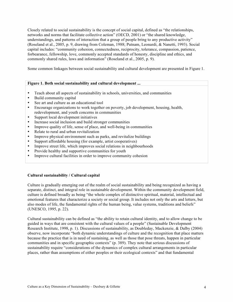
Some common linkages between social sustainability and cultural development are presented in Figure 1.
Figure 1. Both social sustainability and cultural development ...
• Teach about all aspects of sustainability in schools, universities, and communities
• Build community capital
• See art and culture as an educational tool
• Encourage organizations to work together on poverty, job development, housing, health,
redevelopment, and youth concerns in communities
• Support local development initiatives
• Increase social inclusion and build stronger communities
• Improve quality of life, sense of place, and well-being in communities
• Relate to rural and urban revitalization
• Improve physical environment such as parks, and revitalize buildings
• Support affordable housing (for example, artist cooperatives)
• Improve street life, which improves social relations in neighbourhoods
• Provide healthy and supportive communities for youth
• Improve cultural facilities in order to improve community cohesion
Cultural sustainability / Cultural capital
Culture is gradually emerging out of the realm of social sustainability and being recognized as having a
separate, distinct, and integral role in sustainable development. Within the community development field,
culture is defined broadly as being “the whole complex of distinctive spiritual, material, intellectual and
emotional features that characterize a society or social group. It includes not only the arts and letters, but
also modes of life, the fundamental rights of the human being, value systems, traditions and beliefs”
(UNESCO, 1995, p. 22).
Cultural sustainability can be defined as “the ability to retain cultural identity, and to allow change to be
guided in ways that are consistent with the cultural values of a people” (Sustainable Development
Research Institute, 1998, p. 1). Discussions of sustainability, as Doubleday, Mackenzie, & Dalby (2004)
observe, now incorporate “both dynamic understandings of culture and the recognition that place matters
because the practice that is in need of sustaining, as well as those that pose threats, happen in particular
communities and in specific geographic contexts” (p. 389). They note that serious discussions of
sustainability require “considerations of the dynamics of complex cultural arrangements in particular
places, rather than assumptions of either peoples or their ecological contexts” and that fundamental

Culture as a Key Dimension of Sustainability – Duxbury & Gillette 5
debates on sustainability must contrast “environmental and cultural preservation with active practices of
living in culturally constituted places” (pp. 389-390).1
Within the sustainability field, culture is discussed in terms of cultural capital, defined as “traditions and
values, heritage and place, the arts, diversity and social history” (Roseland et al., 2005, p. 12). The stock
of cultural capital, both tangible and intangible, is what we inherit from past generations and what we will
pass onto future generations.
From a philosophical perspective, Pilotti & Rinaldin (2004) discuss how the “sustainability of cultural
resources means an increase over time of a better quality of life [defined] as [a] better knowledge of
ourselves” (p. 1). From a more tangible perspective, in Ecology of Place, Beatley & Manning note that
sustainable communities must foster a sense of place that stimulates and reinforces social attachment:
[C]ommunities must nurture built environment and settlement patterns that are uplifting,
inspirational, and memorable, and that engender a special feeling of attachment and belonging....
A sustainable community respects the history and character of those existing features that nurture
a sense of attachment to, and familiarity with, place. Such “community landmarks” may be
natural—a meadow or an ancient tree, an urban creek—or built—a civic monument, a local diner,
an historic courthouse or clock tower. Finally, in a sustainable place, special effort is made to
create and preserve places, rituals, and events that foster greater attachment to the social fabric of
the community. (1997, p. 32)
From a policy perspective, the Government of Canada, Agenda 21 for Culture, and UNESCO’s Decade
for Education for Sustainable Development (2005-2014) encompass cultural development as related to
social policy and goals such as fostering social inclusion, cultural diversity, rural diversity, rural
revitalization, public housing, health, ecological preservation, and sustainable development.
Community development
Community development aims to strengthen the economy and the social ties within a community through
locally based initiatives. The community development process is often characterized as a “triple bottom
line” of amalgamating environmental, social, and economic well-being into a common audit. The bottom
line is now expanding to include cultural well-being and good governance.
The central goals of community development rely on residents having the ability to express their values,
be self-reliant, satisfy basic human needs, and have greater participation and accountability in their
community. This is accomplished by education, citizen participation, consensus building, and access to
information. Creating a sense of place in the community is central as it empowers residents to become
decision-makers over their own environment, resources, and future.
Community development empowers communities to position local issues within a larger political context.
An important aspect of community development is that it is not handed down from experts or
governments. As Margaret Ledwith (2005) observes, “community development begins at the everyday
lives of local people. This is the initial context of sustainable change” (p. xviii).
1 Related to this is particularly interesting research that links markers of cultural continuity in First Nations
communities with rates of teenage suicide in these communities (Chandler & Lalonde, 1998). The authors conclude:
“Communities that have taken active steps to preserve and rehabilitate their own cultures are shown to be those in
which youth suicide rates are dramatically lower” (p. 191).

Culture as a Key Dimension of Sustainability – Duxbury & Gillette 6
Although community development strategies differ in their focus and approach from community to
community, the underlying goal is to improve the quality of life of residents. According to the Centre for
Sustainable Community Development at Simon Fraser University, approaches to community
development include: identifying community challenges, locating local resources, analyzing local power
structures and human needs, and acting on residents’ concerns in the community.
Common types of community development include:
• Community economic development
• Community capacity building
• Political participatory development
• Sustainable community development (discussed below)
• Community cultural development (discussed below)
Sustainable community development
... sustainability is reflected in the capacity of the community to cope with change and adapt to
new situations.
—Williams (2003, p. 15)
Community sustainability goes beyond environmental practices and economic growth: it is about creating
a more just and equitable community through encouraging social and cultural diversity (Beatley &
Manning, 1997; Roseland et al., 2005). It also requires the community to define sustainability from its
own values and perspective. This involves community participation and a collective decision-making
process that meets the social, cultural, environmental, and economic needs of the community.
Sustainable community development is a process of developing a local and self-reliant economy that does
not damage the world’s ecosystem or the social well-being of communities. Community residents in
sustainable communities “employ strategies and solutions that are integrative and holistic. They seek
ways of combining polices, programs, and design solutions to bring about multiple objectives” (Beatley
& Manning, 1997, p. 33).
Community capital
During the 1990s, as sustainability became a central force in community development, the field
increasingly focused on building the local capacity of an area in order to create more environmentally
friendly and socially equitable places to live. In the course of this work, and informed by Robert Putnam
and others interested in community capital and participation, scholars and policymakers increasingly
embraced the idea that this process depends on increasing a community’s available stock of social capital,
and became more concerned with social capital formation (Bridger & Luloff, 2001).
Today, professionals and academics in the field consider sustainable community development to be an
appreciation of many types of community capital and/or assets within a community, as “all forms of
capital are created by spending time and effort in transformation and transaction activities” (Roseland et
al., 2005, p. 4). For example, the Centre for Sustainable Community Development at Simon Fraser
University considers community capital as including natural, physical, economic, human, social, and
cultural forms of capital. By strengthening each, communities are empowered to build the necessary
foundation for sustainable community development (Roseland et al., 2005; see Figure 2).
Within this context in recent years, community development practitioners in North America believe that
culture must have its own form of capital. They argue that after years of working with Aboriginal
Culture as a Key Dimension of Sustainability – Duxbury & Gillette 7
communities and communities abroad, they now view culture as separate from social capital and argue
that cultural capital needs to be better understood in the sustainable development process (Beatley &
Manning, 1997; Pike, 2003; Putnam, 2000; Roseland et al., 2005).
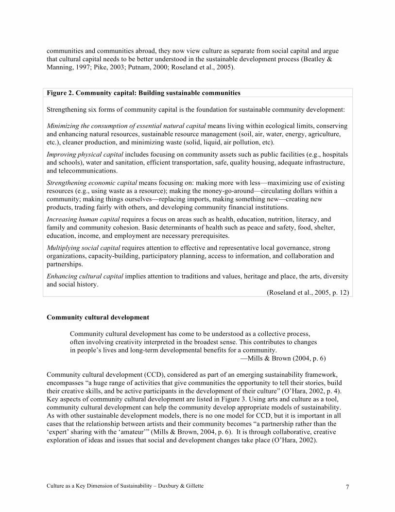
Figure 2. Community capital: Building sustainable communities
Strengthening six forms of community capital is the foundation for sustainable community development:
Minimizing the consumption of essential natural capital means living within ecological limits, conserving
and enhancing natural resources, sustainable resource management (soil, air, water, energy, agriculture,
etc.), cleaner production, and minimizing waste (solid, liquid, air pollution, etc).
Improving physical capital includes focusing on community assets such as public facilities (e.g., hospitals
and schools), water and sanitation, efficient transportation, safe, quality housing, adequate infrastructure,
and telecommunications.
Strengthening economic capital means focusing on: making more with less—maximizing use of existing
resources (e.g., using waste as a resource); making the money-go-around—circulating dollars within a
community; making things ourselves—replacing imports, making something new—creating new
products, trading fairly with others, and developing community financial institutions.
Increasing human capital requires a focus on areas such as health, education, nutrition, literacy, and
family and community cohesion. Basic determinants of health such as peace and safety, food, shelter,
education, income, and employment are necessary prerequisites.
Multiplying social capital requires attention to effective and representative local governance, strong
organizations, capacity-building, participatory planning, access to information, and collaboration and
partnerships.
Enhancing cultural capital implies attention to traditions and values, heritage and place, the arts, diversity
and social history.
(Roseland et al., 2005, p. 12)
Community cultural development
Community cultural development has come to be understood as a collective process,
often involving creativity interpreted in the broadest sense. This contributes to changes
in people’s lives and long-term developmental benefits for a community.
—Mills & Brown (2004, p. 6)
Community cultural development (CCD), considered as part of an emerging sustainability framework,
encompasses “a huge range of activities that give communities the opportunity to tell their stories, build
their creative skills, and be active participants in the development of their culture” (O’Hara, 2002, p. 4).
Key aspects of community cultural development are listed in Figure 3. Using arts and culture as a tool,
community cultural development can help the community develop appropriate models of sustainability.
As with other sustainable development models, there is no one model for CCD, but it is important in all
cases that the relationship between artists and their community becomes “a partnership rather than the
‘expert’ sharing with the ‘amateur’” (Mills & Brown, 2004, p. 6). It is through collaborative, creative
exploration of ideas and issues that social and development changes take place (O’Hara, 2002).

Culture as a Key Dimension of Sustainability – Duxbury & Gillette 8
CCD, largely seen as a grassroots strategy, is slowly being incorporated into current development models.
It engages artists and cultural organizations in development and revitalization processes in cities and
communities. It lends itself to sustainability planning through supporting a community culture,
empowering residents, and strengthening cultural infrastructure and participation in a community. CCD
has also been linked to other sustainable community development initiatives, such as health, affordable
housing, education, youth, poverty, education, policy, and planning. Having a cultural lens in all these
areas is an emerging component of sustainable development.
An important aspect of community cultural development is the concept of shared culture, which entails
having a mutual respect for every culture in a community. Through this collective experience,
communities gain respect for their own and others’ histories, resources, hopes, and dreams.
Figure 3. Key aspects of community cultural development
• Focusing on arts-based solutions, rather than on identifying problems
• Involving policymakers in CCD planning
• Forming and maintaining new social networks with organizations, groups, artists, and government
• Creating and maintaining public spaces that draw people together
• Supporting multiculturalism
• Integrating local customs, crafts, and practices into education
• Using arts and culture as a tool for regeneration and sustainability
• Enhancing residents’ ability to work and communicate with others
• Building community identity and pride
• Supporting positive community norms, such as cultural understanding and free expression
• Improving human capital, skills, and creative abilities in communities
• Increasing opportunities for individuals to become more involved in the arts
• Contributing to the resiliency and sustainability of a community or people
• Reducing delinquency in high-risk youth
• Integrating the community into community art projects
• Fostering trust between community residents
In short, CCD is a community-building tool that promotes a sense of place, empowerment, and public
participation—all key components in the sustainable community development field. CCD and sustainable
community development share common values, principals, key elements, and dynamics, and can help
inform emerging cultural sustainability models. Figure 4 presents a list of common linkages between
community cultural development and sustainable community development.

Culture as a Key Dimension of Sustainability – Duxbury & Gillette 9
Figure 4. Both community cultural development and sustainable community development ...
• View residents as experts in their community
• Foster common experiences that express a sense of place
• Create and support local policies, development, and economic strategies
• Build self-reliant communities
• Increase community participation and dialogue
• Support and build community infrastructure
• Advise, mentor, and build networks and trust in communities
• Build partnerships with community members and with local government, businesses, and
organizations active in the community
• Collaborate with a broad range of partners (for example, housing)
• Encourage residents to take ownership over their own community resources and identity
• Provide experiences for participants to learn technical and interpersonal skills, which are important
for collective organizing
• Create public spaces that draw people together who would otherwise not be engaged in constructive
social activities
• Support activities and events that create a source of pride for residents and increase their sense of
connection with their community
• Foster trust between community residents
• Increase quality of life in communities
• Engage fellow allies in the community decision-making process
• Provide an experience of getting large groups of people together to spur further collective action in
communities
Eco-arts practice
Finally, we must acknowledge influences on thinking about the role of culture in sustainability from the
developing field of eco-arts.
Some artists find inspiration from the environment, while others use art to tackle critical environmental
issues. In recent years, relationships between some artists and environmentalists have grown stronger,
based on their similar values and worldviews toward the preservation and protection of the environment.
For instance, there is an increase of creative projects and educational programs that use arts and culture
activities to:
• Inform people about environmental issues
• Blend creativity with environmental projects and planning in communities
• Promote a living relationship with the land and living in harmony with nature, inspired by a
growing interest in indigenous practices
Eco-art practices can be traced back to the 1960s, “a time when artist were looking to break free of the
traditional white box of the gallery. Land Art, or Earthworks, emerged during this period and it is
important to note that these works frequently objectified the land as a medium or as a site” (Carruthers,
2006, p. 6; see also Fowkes & Fowkes, 2005).
Eco-art projects are often collaborations initiated by artists, environmental groups, local musicians, or
communities and “tend to be connected to a sense of place and spring from local concerns with polluted
waters, social erosion, habitat loss, reclamation of post-industrial sites and the remnants of resource

Culture as a Key Dimension of Sustainability – Duxbury & Gillette 10
extraction” (p. 8). Artists who are engaged in cultural sustainability often see their creative projects as an
environmental practice (Carruthers, 2006). Figure 5 lists some linkages between cultural and
environmental sustainability.
Figure 5. Both cultural sustainability and environmental sustainability ...
• Retain and preserve heritage buildings
• Support ecologically sustainable art products and services
• Promote environment-friendly craft products
• Use under-utilized space for arts activity
• Disseminate information on environmental sustainability through arts activities
• Protect Canadian green space and parks
• Inform community residents about environmental issues and problems facing the globe through art
• Increase the development of eco-art practices
II. Emerging Literature on Cultural Sustainability
A review of the emerging literature on cultural sustainability reveals ten key themes:
1. The culture of sustainability
This relates to the need for a cultural shift in the way that individuals and society address economic,
social, and environmental issues. In this context, the culture of sustainability refers to people changing
their behaviour and consumption patterns, and adapting to a more sustainability-conscious lifestyle.
2. Globalization
Culture needs to be protected from globalization and market forces, as many fear that individual
communities will lose their cultural identity, traditions, and languages to dominant ideals and culture. In
response to these concerns, sustainability discussions focus on education, community development, and
locally based policy that is open to change and consistent with the cultural values of the community. The
creation of opportunities to expand and deepen diversity may act as a balance to this.
3. Heritage conservation
This is a common stream in cultural sustainability research, and primarily focuses on three key areas:
i. Preserving cultural heritage sites, practices, and infrastructure from outside influences
Preserving cultural heritage sites is seen to link the past with the present and the future. Sustainability
discussions on cultural heritage focus on the need to preserve cultural heritage for future generations, and
to recognize the history of a place and the tangible and intangible attributes of its landscapes and
communities (Matthews & Herbert, 2004).
ii. Cultural tourism
Preserving intangible and tangible cultural heritage ensures that tourism and regional economic
development are sustainable over the long term, so that future generations may also benefit from them.
iii. Revitalizing and re-using heritage buildings for cultural facilities
Retaining already existing spaces encourages sustainable development and sense of place in communities.

Culture as a Key Dimension of Sustainability – Duxbury & Gillette 11
4. Sense of place
Sustainability discussions focus on how culture contributes to a sense of place in communities and cities.
For example, the Western Australia State Sustainability Strategy recognizes “the critical importance of a
‘sense of place’, heritage and symbolism for the success of this strategy, with ‘civil society’ being seen as
the repository of the long-term values and visions necessary for a sustainable future” (Mills & Brown,
2004, p. 35). The strategy acknowledges the role of the arts in raising community awareness and interest
in sustainability, and further recognizes the role that the arts and intellectual life can play in resolving
conflict between social, environmental, and economic development by providing “the creative edge
needed to face the new and potentially difficult problems of sustainability, to find the ethics which
underlies every element and every issue in sustainability. Multiculturalism provides the opportunity for
different answers to be found and to build a whole community approach to sustainability” (Western
Australian Government, 2002, p. 165).
5. Indigenous knowledge and traditional practices
Cultural sustainability is linked to the recovery and protection of cultural health, history, and the culture
of indigenous knowledge in society. It is linked to previous traditional practices through celebrating local
and regional histories and passing down cultural values to future generations. Storytelling is often
discussed as a tool to preserve indigenous knowledge and traditional practices; it is seen “to keep memory
alive; to celebrate our history or identity; to derive lessons about how to act effectively; to inspire action;
and, as tools of persuasion in policy debates” (Matthews & Herbert, 2004, p. 383).
6. Community cultural development
Supporting community engagement through arts and culture activities helps to discover new
understanding of the relationship between culture and sustainability.
Community cultural development is a form of sustainable development that promotes a self-reliant
economy and locally based cultural policy. Arts and culture are development tools that contribute to
building networks and trust in the community, and help create a sense of place and occasions for
sociability that draw people together who might not otherwise be engaged in constructive social activities.
CCD encourages grassroots cultural activists, local organizations, and residents to take an active role in
community decision-making, as well as to take ownership over their own community resources and
identity. Culture as a development tool increases the level of civic discourse between artists, cultural
groups, and community residents by providing opportunities and experiences that inspire, provoke, and
facilitate discourse. This creates a collaborative atmosphere in which the arts sector can engage and forge
stronger partnerships with others, including government, business, and the broader community.
7. Arts, education, and youth
The arts are seen as both development and communicative tools in communities and schools, as they
increase the effectiveness of teaching, research, policy, and actions toward cultural sustainability and
development. The arts offer an opportunity to engage in collective, collaborative activities, and enable
youth and the community to become more publicly involved and active in political processes. Universities
and other educational institutions are involved in cultural sustainability through integrating customs,
crafts, and arts and culture activities into the educational arena.
Engaging youth is key to sustainability discussions, as there is concern that youth are disenchanted with
the direction of the world. Involving youth in educational programs on cultural, social, environmental,
and economic forms of sustainability can help provide them with a more optimistic and sustainable
outlook on the future.
Culture as a Key Dimension of Sustainability – Duxbury & Gillette 12
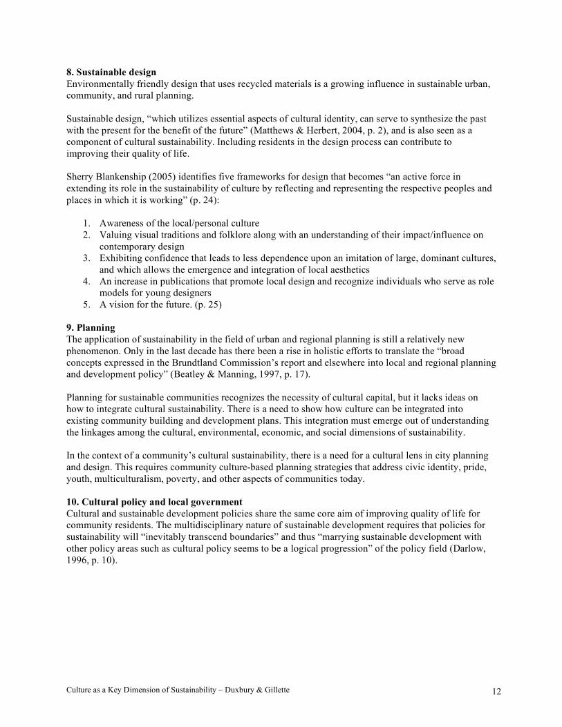
8. Sustainable design
Environmentally friendly design that uses recycled materials is a growing influence in sustainable urban,
community, and rural planning.
Sustainable design, “which utilizes essential aspects of cultural identity, can serve to synthesize the past
with the present for the benefit of the future” (Matthews & Herbert, 2004, p. 2), and is also seen as a
component of cultural sustainability. Including residents in the design process can contribute to
improving their quality of life.
Sherry Blankenship (2005) identifies five frameworks for design that becomes “an active force in
extending its role in the sustainability of culture by reflecting and representing the respective peoples and
places in which it is working” (p. 24):
1. Awareness of the local/personal culture
2. Valuing visual traditions and folklore along with an understanding of their impact/influence on
contemporary design
3. Exhibiting confidence that leads to less dependence upon an imitation of large, dominant cultures,
and which allows the emergence and integration of local aesthetics
4. An increase in publications that promote local design and recognize individuals who serve as role
models for young designers
5. A vision for the future. (p. 25)
9. Planning
The application of sustainability in the field of urban and regional planning is still a relatively new
phenomenon. Only in the last decade has there been a rise in holistic efforts to translate the “broad
concepts expressed in the Brundtland Commission’s report and elsewhere into local and regional planning
and development policy” (Beatley & Manning, 1997, p. 17).
Planning for sustainable communities recognizes the necessity of cultural capital, but it lacks ideas on
how to integrate cultural sustainability. There is a need to show how culture can be integrated into
existing community building and development plans. This integration must emerge out of understanding
the linkages among the cultural, environmental, economic, and social dimensions of sustainability.
In the context of a community’s cultural sustainability, there is a need for a cultural lens in city planning
and design. This requires community culture-based planning strategies that address civic identity, pride,
youth, multiculturalism, poverty, and other aspects of communities today.
10. Cultural policy and local government
Cultural and sustainable development policies share the same core aim of improving quality of life for
community residents. The multidisciplinary nature of sustainable development requires that policies for
sustainability will “inevitably transcend boundaries” and thus “marrying sustainable development with
other policy areas such as cultural policy seems to be a logical progression” of the policy field (Darlow,
1996, p. 10).

Culture as a Key Dimension of Sustainability – Duxbury & Gillette 13
III. Models of Sustainability Incorporating Culture
A review of the literature around sustainable development reveals three models significantly
incorporating a cultural component:
1. Four-pillar model of sustainability (originating with Jon Hawkes, Australia)
2. Four well-beings of community sustainability (from New Zealand’s Ministry for Culture and
Heritage)
3. The medicine wheel approach to sustainability (developed by the Centre for Native Policy
Research in Vancouver, BC)
1. The four-pillar model of sustainability
In 2001, Jon Hawkes, a cultural analyst and one of Australia’s leading commentators on cultural policy,
wrote The Fourth Pillar of Sustainability: Culture’s Essential Role in Public Planning. Since the book’s
publication, there has been a growing interest in cultural sustainability and how it can be applied to
emerging community and city planning models (Hawkes, 2006).
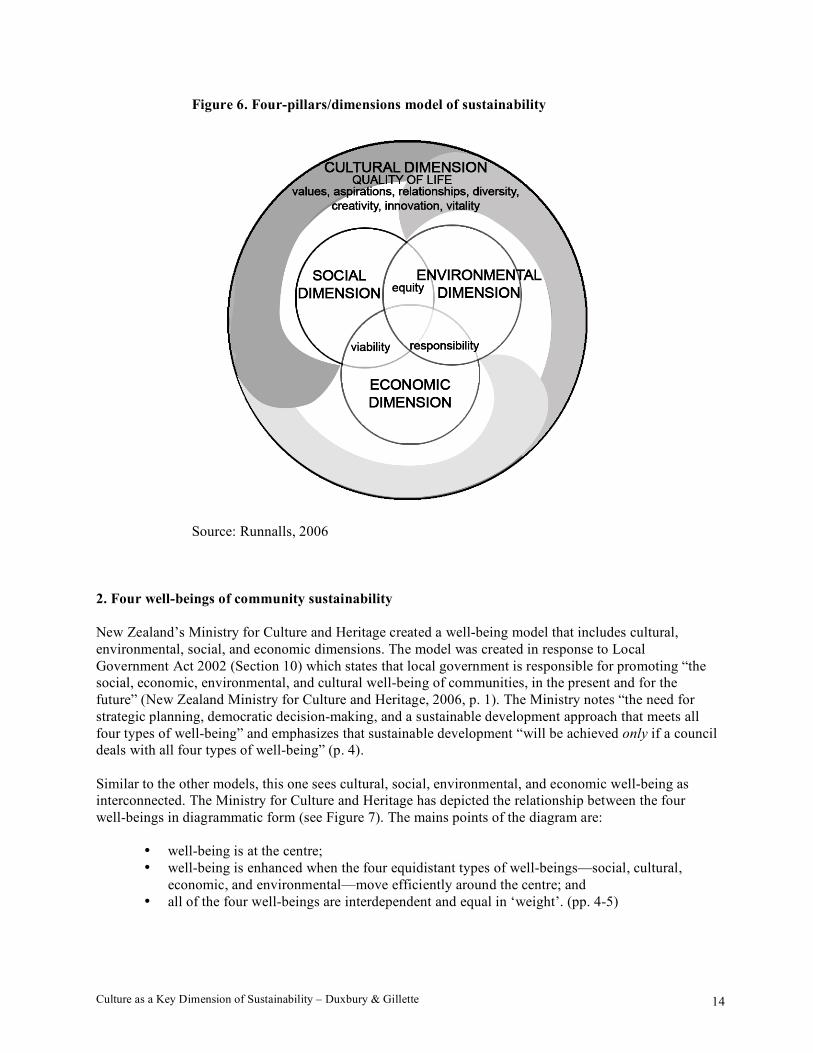
The Fourth Pillar of Sustainability incorporates four interlinked dimensions: environmental
responsibility, economic health, social equity, and cultural vitality. Hawkes addresses the need for a
cultural perspective in public planning and policy by proposing practical measures for integration. In
order for public planning to be more effective, Hawkes argues that government must develop a
framework that evaluates the cultural impacts of environmental, economic, and social decisions and plans
currently being implemented in cities and communities.
The four-pillar model of sustainability recognizes that a community’s vitality and quality of life is closely
related to the vitality and quality of its cultural engagement, expression, dialogue, and celebration. This
model further demonstrates that the contribution of culture to building lively cities and communities
where people want to live, work, and visit plays a major role in supporting social and economic health.
The key to cultural sustainability is fostering partnerships, exchange, and respect between different
streams of government, business, and arts organizations. Culture as the fourth pillar promotes these
partnerships and is quickly gaining currency in policy and planning initiatives in Canada, Australia, New
Zealand, and Europe.
Culture as a Key Dimension of Sustainability – Duxbury & Gillette 14
Figure 6. Four-pillars/dimensions model of sustainability
Source: Runnalls, 2006
2. Four well-beings of community sustainability
New Zealand’s Ministry for Culture and Heritage created a well-being model that includes cultural,
environmental, social, and economic dimensions. The model was created in response to Local
Government Act 2002 (Section 10) which states that local government is responsible for promoting “the
social, economic, environmental, and cultural well-being of communities, in the present and for the
future” (New Zealand Ministry for Culture and Heritage, 2006, p. 1). The Ministry notes “the need for
strategic planning, democratic decision-making, and a sustainable development approach that meets all
four types of well-being” and emphasizes that sustainable development “will be achieved only if a council
deals with all four types of well-being” (p. 4).
Similar to the other models, this one sees cultural, social, environmental, and economic well-being as
interconnected. The Ministry for Culture and Heritage has depicted the relationship between the four
well-beings in diagrammatic form (see Figure 7). The mains points of the diagram are:
• well-being is at the centre;
• well-being is enhanced when the four equidistant types of well-beings—social, cultural,
economic, and environmental—move efficiently around the centre; and
• all of the four well-beings are interdependent and equal in ‘weight’. (pp. 4-5)

Culture as a Key Dimension of Sustainability – Duxbury & Gillette 15
The New Zealand Ministry for Culture and Heritage has defined cultural well-being as:
the vitality that communities and individuals enjoy through:
• participation in recreation, creative and cultural activities; and
• the freedom to retain, interpret and express their arts, history, heritage and traditions. (p. 1)
Figure 7. Four well-beings of community sustainability
Source: New Zealand Ministry for Culture and Heritage, 2006, p. 5
3. The medicine wheel approach to sustainability
Nathan Cardinal and Emilie Adin’s An Urban Aboriginal Life: The 2005 Indicators Report on the Quality
of Life of Aboriginal People in the Greater Vancouver Region uses the medicine wheel as a framework to
determine categories and indicators for exploring and documenting the state of Aboriginal life in and
around Vancouver (see Figure 8).
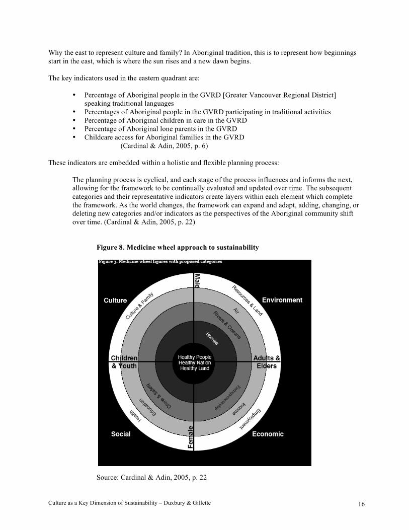
The medicine wheel depicts four traditional directions: north (environmental), south (social), west
(economic), and east (cultural).
The four elements are crosscut by various segments of Aboriginal society which influence, and
are in turn influenced by each of the elements. These four segments represent different groups
and viewpoints in Aboriginal society: male, female, children & youth, adults & elders. Each of
these four segments is critical to forming the context for measuring the overall well-being of the
Aboriginal community.
Surrounding the medicine wheel is a development planning process, designed to guide the
development and maintenance of the framework and its subsequent categories and indicators.
(Cardinal & Adin, 2005, p. 21)
Culture as a Key Dimension of Sustainability – Duxbury & Gillette 16
Why the east to represent culture and family? In Aboriginal tradition, this is to represent how beginnings
start in the east, which is where the sun rises and a new dawn begins.
The key indicators used in the eastern quadrant are:
• Percentage of Aboriginal people in the GVRD [Greater Vancouver Regional District]
speaking traditional languages
• Percentages of Aboriginal people in the GVRD participating in traditional activities
• Percentage of Aboriginal children in care in the GVRD
• Percentage of Aboriginal lone parents in the GVRD
• Childcare access for Aboriginal families in the GVRD
(Cardinal & Adin, 2005, p. 6)
These indicators are embedded within a holistic and flexible planning process:
The planning process is cyclical, and each stage of the process influences and informs the next,
allowing for the framework to be continually evaluated and updated over time. The subsequent
categories and their representative indicators create layers within each element which complete
the framework. As the world changes, the framework can expand and adapt, adding, changing, or
deleting new categories and/or indicators as the perspectives of the Aboriginal community shift
over time. (Cardinal & Adin, 2005, p. 22)
Figure 8. Medicine wheel approach to sustainability
Source: Cardinal & Adin, 2005, p. 22
Culture as a Key Dimension of Sustainability – Duxbury & Gillette 17
Acknowledgements
Thank you to Kaija Pepper for her editorial support.
References
Agenda 21 for culture. (2004). Developed by United Cities and Local Governments—Working Group on
Culture. www.agenda21culture.net
Al-Hindawi, Iman. (2003, November). Panel 2: Culture & development: The place of the arts. Paper
presented at the Second World Summit on the Arts and Culture. Singapore: International Federation of
Arts Councils and Culture Agencies. http://svc354.bne098u.server-
web.com/worldsummit/files/Iman_Al_Hindawi_paper.pdf
Beatley, Timothy & Manning, Kristy. (1997). The ecology of place: Planning for environment, economy,
and community. Washington, DC: Island Press.
Blankenship, Sherry. (2005, Winter). Outside the center: Defining who we are. Design Issues, 21(1), 24-
31. www.mitpressjournals.org/doi/pdf/10.1162/0747936053103084
Borrup, Tom. (2003). Toward asset-based community cultural development: A journey through the
disparate worlds of community building. North Carolina, USA: Community Arts Network.
www.communityarts.net/readingroom/archivefiles/2003/04/toward_assetbas.php
Bourne, L.S. (1999, May). Migration, immigration and social sustainability: The recent Toronto
experience in comparative context. CERIS Working Paper No. 5. Toronto: Joint Centre of Excellence
Research on Immigration and Settlement.
http://ceris.metropolis.net/Virtual%20Library/WKPP%20List/WKPP1999/CWP05_Bourne_final.pdf
Bridger, Jeffery C. & Luloff, A.E. (2001, Fall). Building sustainable community: Is social capital the
answer? Sociological Inquiry, 71(4), 458-472.
Cardinal, Nathan & Adin, Emilie (2005, November). An urban Aboriginal life: The 2005 indicators
report on the quality of life of Aboriginal people in the Greater Vancouver region. Vancouver, BC:
Centre for Native Policy and Research.
www.cnpr.ca/assets/pdfs/An%20Urban%20Aboriginal%20Life%20%20CNPR%20Indicators%20reportp
df.pdf
Carruthers, Beth. (2006, April 27). Mapping the terrain of contemporary EcoART practice and
collaboration. Prepared for “Art in ecology—A think tank on arts and sustainability,” Vancouver, BC.
Commissioned by Canadian Commission for UNESCO.
www.unesco.ca/en/activity/sciences/documents/BethCarruthersArtinEcologyResearchReportEnglish.pdf
Carson, Rachel. (2002). Silent spring (40th anniversary ed.). Boston: Houghton Mifflin.
Centre for Sustainable Community Development website. What is sustainable community development?
Burnaby, BC: Centre for Sustainable Community Development, Simon Fraser University.
www.sfu.ca/cscd/what_is_sust_community.htm
Culture as a Key Dimension of Sustainability – Duxbury & Gillette 18
Chandler, Michael J. & Lalonde, Christopher. (1998, June). Cultural continuity as a hedge against suicide
in Canada’s First Nations. Transcultural Psychiatry, 35, 191-219.
Coleman, J.S. (1988). Social capital in the creation of human capital. American Journal of Sociology, 94
(supplement): S95-S120.
Darlow, Alison. (1996). Cultural policy and urban sustainability: Making a missing link? Planning
Practice and Research, 11(3), 291-301.
Doubleday, Nancy, Mackenzie, Fiona, & Dalby, Simon. (2004, Winter). Reimagining sustainable
cultures: Constitutions, land and art. The Canadian Geographer, 48(40), 389-402.
Hawkes, Jon. (2006, October 25). Creative democracy. Keynote address at Interacció ’06: Community
Cultural Policies, Barcelona Provincial Council, Barcelona.
Hawkes, Jon. (2001). The fourth pillar of sustainability: Culture’s essential role in public planning.
Commissioned by the Cultural Development Network, Victoria. Melbourne: Common Ground
Publishing.
Interacció ’04. Towards an Agenda 21 for culture. (2004, June). Dialogue synthesis: The Agenda 21 for
Culture, Forum Barcelona 2004.
www.barcelona2004.org/eng/banco_del_conocimiento/documentos/ficha.cfm?IdDoc=2909
Kurt, Hildegard. (2004). Aesthetics of sustainability. In Heike Strelow & Vera David (Eds.), Aesthetics of
ecology: Art in environmental design, theory and practice. Basel, Berlin, & Boston: Birkhäuser.
Ledwith, Margaret. (2005). Community development: A critical approach. Bristol, UK: Policy Press.
Matthews, John & Herbert, David. (Eds.). (2004). Unifying geography: Common heritage, shared future?
Oxfordshire, UK: Routledge.
Mills, Deborah & Brown, Paul. (2004). Art and wellbeing. Sydney, Australia: Australia Council for the
Arts.
Mitlan, Diana & Satterthwaite, David. (1994). Cities and sustainable development: Background paper for
Global Forum '94. London: International Institute for Environment and Development.
New Zealand Ministry for Culture and Heritage. (2006). Cultural well-being and local government.
Report 1: Definition and context of cultural well-being. Wellington, NZ: New Zealand Ministry for
Culture and Heritage.
Newman, Peter & Kenworthy, Jeffrey. (1999). Sustainability and cities: Overcoming automobile
dependence. Washington, DC: Island Press.
OECD. (2001). The well-being of nations: The role of human and social capital. Paris: Organization for
Economic Cooperation and Development (OECD).
O’Hara, Scott. (2002). Hand ON! Practices and projects supported by the Community Cultural
Development Board. NSW, Australia: Australia Council for the Arts.
Pike, Matthew. (2003). Can do citizens. London, UK: Social Enterprise Services & Scarman Trust.
Culture as a Key Dimension of Sustainability – Duxbury & Gillette 19
Pilotti, Luciano & Rinaldin, Marina. (2004, November). Culture & arts as knowledge resources towards
sustainability for identity of nations and cognitive richness of human being. Milan, Italy: Department of
Economics University & Departmental Working Papers. www.economia.unimi.it/uploads/wp/wp187.pdf
Putnam, Robert D. (2000). Bowling alone: Collapse and revival of American community. Cambridge,
MA: Simon & Schuster.
Putnam, R., Leonardi, R., & Nanetti, R. (1993). Making democracy work: Civic traditions in modern
Italy. Princeton, NJ: Princeton University Press.
Rhoades, Robert E. (Ed.). (2006). Development with identity: Community, culture and sustainability in
the Andes. Oxfordshire, UK: CABI Publishing.
Roseland, Mark, with Connelly, Sean, Hendrickson, David, Lindberg, Chris, & Lithgow, Michael. (2005).
Towards sustainable communities: Resources for citizens and their governments. (Rev. ed.). Gabriola
Island, BC: New Society Publishers.
Runnalls, Catherine R. (2006, October). Choreographing community sustainability: The importance of
cultural planning to community viability. Unpublished thesis, Masters of Arts in Leadership and Training,
Royal Rhodes University, Victoria, BC.
Schumacher, E.F. (1973). Small is beautiful: Economics as if people mattered. New York: Harper and
Row.
Smith, Stephanie. (2005). Beyond green toward a sustainable art. Chicago & New York: Smart Museum
of Art, University of Chicago, and Independent Curators International.
Sustainable Development Research Institute. (1998, November 16-17). Social capital formation and
institutions for sustainability. Workshop proceedings prepared by Asoka Mendis. Vancouver: Sustainable
Development Research Institute. www.williambowles.info/mimo/refs/soc_cap.html
Fowkes, Maja & Fowkes, Reuben. (2005, June). The principles of sustainability in contemporary art.
Translocal.org. http://translocal.org/writings/principlesofsustainability.htm
UN Department of Economic and Social Affairs. (2006). Agenda 21. Division for sustainable
development. www.un.org/esa/sustdev/documents/agenda21/index.htm
UNESCO. (1995). The cultural dimension of development: Towards a practical approach. Culture and
Development Series. Paris: UNESCO Publishing.
UNESCO: Cultural Sector (July, 2006). “Culture and Development.”
http://portal.unesco.org/culture/en/ev.phpURL_ID=11407&URL_DO=DO_PRINTPAGE&URL_SECTI
ON=201.html
UNESCO—Decade for Education for Sustainable Development.
http://portal.unesco.org/education/en/ev.php-
URL_ID=27234&URL_DO=DO_TOPIC&URL_SECTION=201.html
Culture as a Key Dimension of Sustainability – Duxbury & Gillette 20
Western Australian Government. (2002). Focus on the future: The Western Australian state sustainability
strategy. Perth, Australia: Sustainability Policy Unit.
Williams, Maureen. (2003, January). Sustainable development and social sustainability. Hull, QC:
Strategic Research and Analysis, Department of Canadian Heritage. Reference: SRA-724.
World Commission on Culture and Development. (1995). Our creative diversity. Paris: UNESCO.
World Commission on Environment and Development. (1987). Our common future. Oxford & New
York: Oxford University Press.
World Conservation Union (IUCN), United Nations Environment Program (UNEP), & World Wide Fund
for Nature (WWF). (1991). Caring for the earth: A strategy for sustainable living. Gland, Switzerland:
IUCN, UNEP, WWF.
Appendix A
Sustainability, development, and culture: A brief chronology of key points
1960s – In Canada, community development stems out of the work of cooperatives, credit unions, and
caisses populaires. Also, eco-art practices can be traced back to this decade.
1970s – Prevailing models and notions of development and environmentalism came under sustained
criticism:
• Discussions on environmental globalism were criticized for not addressing the linkages between
environmental degradation and inequalities experienced by the developing world, such as abject
poverty and unfair access to world resources.
• Development models were critiqued by the international community as narrowly defining
development “too exclusively in terms of tangibles, such as dams, factories, houses, food and
water” (UNESCO, 2006). Although these are undeniably vital goods, economic growth alone did
not recognize how “intellectual, emotional, moral and spiritual existence” in communities and
cities creates a “set of capacities that allows groups, communities and nations to define their
futures in an integrated manner” (UNESCO, 2006).
• As international organizations and governments were heavily criticized for their top–down
development approaches (for example, in Rachel Carson’s Silent Spring and E. F. Schumacher’s
Small is Beautiful), community development agencies and practitioners in Canada, the United
States, and elsewhere took on a more active role in development, promoting locally based
initiatives that focused on building self-reliant communities through civic participation and
engagement.
• Cultural factors later began to take a more active role in development policy, seen to be
synonymous with emerging socio-economic and political development models (Al-Hindawi,
2003):
... the definition of culture must broaden to encompass complex, spiritual, material,
intellectual and emotional features that are not only limited to the field of social science,
but encompass ideas relating to modes of life, fundamental human rights, political value
Culture as a Key Dimension of Sustainability – Duxbury & Gillette 21
systems, traditions and beliefs. Moreover, a further proof of the need to expand the
definition of culture to include socio-economic developments is the realization in the
1970s that development policies solely based on economic indicators and models without
taking into account factors such as intellectual, spiritual and cultural existence failed to
live up to their expectations. This paved the way during the 1980s for cultural factors to
occupy an important place in development planning. Therefore, culture has become
synonymous with socio-economic development and political development.
(Al-Hindawi, 2003, p. 2)
1972 – UN Conference on the Human Environment (Stockholm): The “first elements of sustainability”
emerged at this event, where governments, professionals, and practitioners came together to discuss
environmental issues on a global scale (Newman & Kenworthy, 1999, p. 1).
1983 – The UN created the World Commission on Environment and Development.
1987 – The World Commission published Our Common Future, in which former Norwegian Prime
Minister Gro Harlem Brundtland defined sustainable development as a type of “development that meets
the needs of the present without compromising the ability of future generations to meet their own needs”
(World Commission on Environment and Development, 1987, p. 8).
Four broad principles on sustainability, derived from the Brundtland Report, are seen as the essential
approach to global sustainability:
1. The elimination of poverty, especially in the Third World, is necessary not just on human grounds
but as an environmental issue.
2. The First World must reduce its consumption of resources and production of wastes.
3. Global cooperation on environmental issues is no longer a soft option.
4. Change toward sustainability can occur only with community-based approaches that take local
cultures seriously.
(Newman & Kenworthy, 1999, adapted from pp. 2-3, emphasis added)
1990s – The popularity of Robert Putnam and others discussing community capital and participation led
the field of community development to become more concerned with social capital formation.
1992 – The Earth Summit in Rio de Janeiro produced Agenda 21, a “comprehensive plan of action to be
taken globally, nationally and locally by organizations of the United Nations System, Governments, and
Major Groups in every area in which human[s] impact…on the environment” (UN Department of
Economic and Social Affairs, 2006).
1995 – The challenges of culture being addressed within the economic and social dimensions of
sustainable development was discussed in Our Creative Diversity, a report which summarizes the
deliberations of UNESCO’s World Commission on Culture and Development (World Commission on
Culture and Development, 1995; Smith, 2005). The recognition of culture as a development tool led many
practitioners in the cultural development field to document and share their practices and impacts with
others working in communities.
2004 – In response to the lack of cultural considerations in Agenda 21, an Agenda 21 for Culture was
created and approved at the IV Forum of Local Authorities of Porto Alegre in Barcelona. Agenda 21 for
Culture promotes the “adoption of a series of principles, commitments and recommendations to
strengthen the development of culture on an international scale from the local arena, considering it as a
collective right to participation in the life of societies” (Interacció ’04, 2004).

Culture as a Key Dimension of Sustainability – Duxbury & Gillette 22
2005-2014 – UNESCO’s Decade for Education for Sustainable Development promotes cultural
development as a tool for social policy to foster social inclusion, cultural diversity, rural diversity, rural
revitalization, public housing, health, ecological preservation, and sustainable development (see Figure 9).
Figure 9. UNESCO’s Decade for Education for Sustainable Development
• Underlines the importance of cultural aspects for sustainable development
• Recognizes diversity, i.e. the rich tapestry of human experience in the many physical and socio-
cultural contexts of the world
• Encourages respect and tolerance of difference, and sees contact with otherness as enriching,
challenging, and stimulating
• Acknowledges values in open debate and with a commitment to keep the dialogue going
• Models values of respect and dignity, which underpin sustainable development, in personal and
institutional life
• Builds human capacity in all aspects of sustainable development
• Uses local indigenous knowledge of flora and fauna and sustainable agricultural practices, water use,
etc.
• Fosters support of practices and traditions which build sustainability—including aspects such as
preventing excessive rural exodus
• Recognizes and works with culturally specific views of nature, society, and the world rather than
ignoring or destroying them, consciously or inadvertently, in the name of development
• Employs local patterns of communication, including the use and development of local languages, as
vectors of interaction and cultural identity

© 2007 Centre of Expertise on Culture and Communities
Creative City Network of CanadaTransforming communities through culture
The Creative City Network of Canada is a national non-profit organization that operates as a knowledge-sharing, research, public education, and professional development resource in the field of local cultural policy, planning and practice.
Through its work, the Creative City Network helps build the capacity of local cultural planning professionals— and by extension their local governments—to nurture and support cultural development in their communities. By doing so, the Creative City Network aims to improve the operating climate and conditions for artists and arts and cultural organizations across the country, and the quality of life in Canadian communities of all sizes.
The members of the Creative City Network are local governments across Canada.
More information is available at www.creativecity.ca
Centre of Expertise on Culture and CommunitiesLocated at Simon Fraser University’s Vancouver campus, the Centre of Expertise on Culture and Communities is a three-year project of the Creative City Network of Canada in collaboration with Simon Fraser University’s School of Communication. It is supported by Infrastructure Canada, the Department of Canadian Heritage, the City of Ottawa, and the Centre for Policy Research on Science and Technology (CPROST) at SFU. It is advised by a national multidisciplinary team of project collaborators consisting of leading individuals in the cultural, government, and academic fields.
The Centre’s work includes three interlinked components: knowledge generation (research), outreach and networking, and awareness/knowledge exchange. It conducts research and brings together academia and practice in four areas:
1. The state of cultural infrastructure in Canadian cities and communities 2. Culture as the fourth pillar of community sustainability 3. Culture in communities: Cultural systems and local planning 4. The impacts of cultural infrastructure and activity in cities and communities
For more information, visit: www.creativecity.ca/cecc
Production of this paper has been made possible through a financial contribution from Infrastructure Canada. The views expressed herein do not necessarily represent the views of the Government of Canada or those of the Creative City Network of Canada.

Natural Capital

This page intentionally left blank
Natural Capital Theory & Practice of Mapping Ecosystem Services
EDITED BY
Peter Kareiva The Nature Conservancy and Santa Clara University, USA
Heather Tallis Natural Capital Project, Stanford University, USA
Taylor H. Ricketts World Wildlife Fund, USA
Gretchen C. Daily Stanford University, USA
Stephen Polasky University of Minnesota, USA
1

1 Great Clarendon Street, Oxford ox2 6dpOxford University Press is a department of the University of Oxford. It furthers the University’s objective of excellence in research, scholarship, and education by publishing worldwide inOxford New York Auckland Cape Town Dar es Salaam Hong Kong Karachi Kuala Lumpur Madrid Melbourne Mexico City Nairobi New Delhi Shanghai Taipei Toronto With offi ces inArgentina Austria Brazil Chile Czech Republic France Greece Guatemala Hungary Italy Japan Poland Portugal Singapore South Korea Switzerland Thailand Turkey Ukraine Vietnam
Oxford is a registered trade mark of Oxford University Press in the UK and in certain other countries
Published in the United States by Oxford University Press Inc., New York
© Oxford University Press 2011
The moral rights of the authors have been asserted Database right Oxford University Press (maker)
First published 2011
All rights reserved. No part of this publication may be reproduced, stored in a retrieval system, or transmitted, in any form or by any means, without the prior permission in writing of Oxford University Press, or as expressly permitted by law, or under terms agreed with the appropriate reprographics rights organization. Enquiries concerning reproduction outside the scope of the above should be sent to the Rights Department, Oxford University Press, at the address above
You must not circulate this book in any other binding or cover and you must impose the same condition on any acquirer
British Library Cataloguing in Publication Data Data available
Library of Congress Cataloging in Publication Data Library of Congress Control Number: 2010942945
Typeset by SPI Publisher Services, Pondicherry, India Printed in Great Britainon acid-free paper byCPI Antony Rowe, Chippenham, Wiltshire
ISBN 978-0-19-958899-2 (Hbk.)978-0-19-958900-5 (Pbk.)
1 3 5 7 9 10 8 6 4 2
Contents
List of contributors xi Foreword (Hal Mooney) xv How to read this book xvii Acknowledgments xviii
Section I: A vision for ecosystem services in decisions
1: Mainstreaming natural capital into decisions 3 Gretchen C. Daily, Peter M. Kareiva, Stephen Polasky, Taylor H. Ricketts, and Heather Tallis
1.1 Mainstreaming ecosystem services into decisions 3 1.2 What is new today that makes us think we can succeed? 4 1.3 Moving from theory to implementation 5 1.4 Using ecosystem production functions to map and assess natural capital 6 1.5 Roadmap to the book 6 Box 1.1: The everyday meaning of natural capital to the world’s rural poor ( M. Sanjayan ) 7 1.6 Open questions and future directions 9 Box 1.2: Sorting among options for a more sustainable world ( Stephen R. Carpenter ) 10 1.7 A general theory of change 12 References 12
2: Interpreting and estimating the value of ecosystem services 15 Lawrence H. Goulder and Donald Kennedy
2.1 Introduction: why is valuing nature important? 15 2.2 Philosophical issues: values, rights, and decision-making 16 2.3 Measuring ecosystem values 20 2.4 Some case studies 27 Box 2.1: Designing coastal protection based on the valuation of natural coastal ecosystems ( R. K. Turner ) 29 2.5 Conclusions 31 References 33
3: Assessing multiple ecosystem services: an integrated tool for the real world 34 Heather Tallis and Stephen Polasky
3.1 Today’s decision-making: the problem with incomplete balance sheets 34 3.2 The decision-making revolution 34 3.3 The ecological production function approach 35
vi CONTENTS
3.4 InVEST: mapping and valuing ecosystem services with ecological production functions and economic valuation 37 Box 3.1: Unsung ecosystem service heroes: seed dispersal and pest control ( Liba Pejchar ) 39 3.5 Future directions and open questions 47 References 48
Section II: Multi-tiered models for ecosystem services
4: Water supply as an ecosystem service for hydropower and irrigation 53 Guillermo Mendoza, Driss Ennaanay, Marc Conte, Michael Todd Walter, David Freyberg, Stacie Wolny, Lauren Hay, Sue White, Erik Nelson, and Luis Solorzano
4.1 Introduction 53 4.2 Tier 1 water supply model 54 Box 4.1 Can we apply our simple model where groundwater really matters? ( Heather Tallis, Yukuan Wang, and Driss Ennaanay ) 54 4.3 Tier 1 valuation 59 4.4 Limitations of the tier 1 water yield models 62 4.5 Tier 2 water supply model 62 4.6 Tier 2 valuation model 65 4.7 Sensitivity analyses and testing of tier 1 water supply models 65 4.8 Next steps 70 References 71
5: Valuing land cover impact on storm peak mitigation 73 Driss Ennaanay, Marc Conte, Kenneth Brooks, John Nieber, Manu Sharma, Stacie Wolny, and Guillermo Mendoza
5.1 Introduction 73 5.2 Tier 1 biophysical model 74 5.3 Tier 1 valuation 78 Box 5.1: Integrated fl ood risk management: gaining ecosystem services and increasing revenue ( David Harrison ) 80 5.4 Tier 2 supply and use model 84 5.5 Tier 2 valuation 85 5.6 Limitations and next steps 86 References 87
6: Retention of nutrients and sediment by vegetation 89 Marc Conte, Driss Ennaanay, Guillermo Mendoza, Michael Todd Walter, Stacie Wolny, David Freyberg, Erik Nelson, and Luis Solorzano
6.1 Introduction 89 6.2 Tier 1 biophysical models 90 6.3 Tier 1 economic valuation 96 6.4 Tier 2 biophysical models 99 6.5 Tier 2 economic valuation models 102 6.6 Constraints and limitations 104 6.7 Testing tier 1 models 105 Box 6.1: China forestry programs take aim at more than fl oods ( Christine Tam ) 107 6.8 Next steps 108 References 109
CONTENTS vii
7: Terrestrial carbon sequestration and storage 111 Marc Conte, Erik Nelson, Karen Carney, Cinzia Fissore, Nasser Olwero, Andrew J. Plantinga, Bill Stanley, and Taylor Ricketts
7.1 Introduction 111 7.2 Tier 1 supply model 112 Box 7.1: Noel Kempff case study: capturing carbon fi nance ( Bill Stanley and Nicole Virgilio ) 115 7.3 Tier 1 valuation model: an avoided economic damage approach 118 Box 7.2: Valuing the Arc: measuring and monitoring forest carbon for offsetting ( Andrew R. Marshall and P. K. T. Munishi ) 119 7.4 Tier 2 supply model 121 7.5 Tier 2 valuation: an application of the avoided economic damage approach 122 7.6 Limitations and next steps 124 References 126
8: The provisioning value of timber and non-timber forest products 129 Erik Nelson, Claire Montgomery, Marc Conte, and Stephen Polasky
8.1 Introduction 129 Box 8.1: Wildlife conservation, corridor restoration, and community incentives: a paradigm from the Terai Arc landscape ( Eric Wikramanayake, Rajendra Gurung, and Eric Dinerstein ) 130 8.2 The supply, use, and value of forests’ provisioning service in tier 1 132 8.3 The supply, use, and value of forests’ provisioning service in tier 2 141 8.4 Limitations and next steps 146 References 147
9: Provisioning and regulatory ecosystem service values in agriculture 150 Erik Nelson, Stanley Wood, Jawoo Koo , and Stephen Polasky
9.1 Introduction 150 9.2 Defi ning agricultural scenarios 151 9.3 Tier 1 152 9.4 Tier 2 158 9.5 Mapping the impacts of agriculture on important ecological processes 161 9.6 Uncertainty 162 9.7 Limitations and next steps 163 References 164
10: Crop pollination services 168 Eric Lonsdorf, Taylor Ricketts, Claire Kremen, Rachel Winfree, Sarah Greenleaf, and Neal Williams
10.1 Introduction 168 Box 10.1: Assessing the monetary value of global crop pollination services ( Nicola Gallai, Bernard E. Vaissière, Simon G. Potts, and Jean-Michel Salles ) 169 10.2 Tier 1 supply model 173 10.3 Tier 1 farm abundance map 175 10.4 Tier 1 valuation model 175 10.5 Tier 2 supply model 176 10.6 Tier 2 farm abundance map 177 10.7 Tier 2 valuation model 177 10.8 Sensitivity analysis and model validation 178
10.9 Limitations and next steps 182 Box 10.2: Pollination services: beyond agriculture ( Berry Brosi ) 183 References 185
11: Nature-based tourism and recreation 188 W. L. (Vic) Adamowicz, Robin Naidoo, Erik Nelson, Stephen Polasky, and Jing Zhang
11.1 Nature-based tourism and recreation values in context 188 11.2 Tier 1 tourism supply and use model 190 11.3 Tier 2 tourism supply and use model 193 11.4 Tier 1 and 2 use value 197 Box 11.1: How the economics of tourism justifi es forest protection in Amazonian Peru ( Christopher Kirkby, Renzo Giudice, Brett Day, Kerry Turner, Bridaldo Silveira Soares-Filho, Hermann Oliveira-Rodrigues, and Douglas W. Yu ) 198 11.5 State-of-the-art tourism value 201 11.6 Limitations and next steps 202 References 204
12: Cultural services and non-use values 206 Kai M. A. Chan, Joshua Goldstein, Terre Satterfi eld, Neil Hannahs, Kekuewa Kikiloi, Robin Naidoo, Nathan Vadeboncoeur, and Ulalia Woodside
12.1 Introduction 206 Box 12.1: The sacred geography of Kawagebo ( Jianzhong Ma and Christine Tam ) 211 12.2 Methods: integrating cultural services and non-use values into decisions 213 Box 12.2: People of color and love of nature ( Hazel Wong ) 221 12.3 Limitations and next steps 225 References 226
13: Terrestrial biodiversity 229 Erik Nelson, D. Richard Cameron, James Regetz, Stephen Polasky, and Gretchen C. Daily
13.1 Introduction 229 13.2 Tier 1: habitat-quality and rarity model 229 Box 13.1: Integrating biodiversity and agriculture: a success story in South Asia ( Jai Ranganathan and Gretchen C. Daily ) 230 13.3 Tier 2 models of terrestrial biodiversity 233 13.4 Tier 1 and 2 examples with sensitivity analysis 236 13.5 Limitations and next steps 242 References 244
Section III: Extensions, applications, and the next generation of ecosystem service assessments
14: Putting ecosystem service models to work: conservation, management, and trade-offs 249 Stephen Polasky, Giorgio Caldarone, T. Ka’eo Duarte, Joshua Goldstein, Neil Hannahs, Taylor Ricketts, and Heather Tallis
14.1 Introduction 249 14.2 Applying ecosystem service and biodiversity models in management and conservation contexts 250 Box 14.1: Plight of a people ( Neil Hannahs ) 256 14.3 Extending the frontier: challenges facing ecosystem management 260 References 262
viii CONTENTS
15: How much information do managers need? The sensitivity of ecosystem service decisions to model complexity 264 Heather Tallis and Stephen Polasky
15.1 Introduction 264 Box 15.1: How much data do we need to support our models: a case study using biodiversity mapping and conservation planning ( Craig Groves and Edward Game ) 265 15.2 Testing agreement between simple and complex ecosystem service models 268 15.3 Future directions and open questions 276 References 277
16: Poverty and the distribution of ecosystem services 278 Heather Tallis, Stefano Pagiola, Wei Zhang, Sabina Shaikh, Erik Nelson, Charlotte Stanton, and Priya Shyamsundar
16.1 Introduction 278 16.2 Ecosystem services and the poor 279 Box 16.1: Can the natural capital of agroecosystems provide a pathway out of poverty? ( C. Peter Timmer ) 280 Box 16.2: Poverty and ecosystem service mapping at work in Kenya ( Norbert Henninger and Florence Landsberg ) 282 16.3 Mapping poverty and ecosystem services 283 16.4 Case studies 285 16.5 Including institutions: the way forward 293 References 293
17: Ecosystem service assessments for marine conservation 296 Anne D. Guerry, Mark L. Plummer, Mary H. Ruckelshaus, and Chris J. Harvey
17.1 Introduction 296 17.2 Ecosystem services provided by marine environments 297 Box 17.1: Nonlinear wave attenuation and the economic value of mangrove land-use choices ( Edward B. Barbier ) 299 Box 17.2: Valuation of coral reefs in the Caribbean ( Emily Cooper and Lauretta Burke ) 301 17.3 Mapping and modeling the fl ow of marine ecosystem services: a case study
of Puget Sound 303 17.4 Future directions 317 References 318
18: Modeling the impacts of climate change on ecosystem services 323 Joshua J. Lawler, Erik Nelson, Marc Conte, Sarah L. Shafer, Driss Ennaanay, and Guillermo Mendoza
18.1 Introduction 323 18.2 Previous analyses of climate-driven changes in ecosystem services 323 18.3 Using ecosystem-service models to evaluate the impact of climate change on natural and human systems 324 Box 18.1: An estimate of the effects of climate change on global agricultural ecosystem services ( David Lobell ) 325 18.4 Climate impacts on ecosystem-services in the Willamette Basin of Oregon 326 18.5 Discussion and conclusions 335 References 337
CONTENTS ix
19: Incorporating ecosystem services in decisions 339 Emily McKenzie, Frances Irwin, Janet Ranganathan, Craig Hanson, Carolyn Kousky, Karen Bennett, Susan Ruffo, Marc Conte, James Salzman, and Jouni Paavola
19.1 Introduction 339 19.2 Putting ecosystem services on the agenda 340 Box 19.1: An assessment of ecosystem services helps a paper and packaging business respond to emerging risks ( Craig Hanson ) 343 19.3 Instruments for sustaining and enhancing ecosystem services 344 19.4 Choosing the right instrument 348 19.5 Building stronger organization 349 Box 19.2: Cultural evolution as an enabling condition for the use of ecosystem services in decisions ( Paul R. Ehrlich, Lee D. Ross, and Gretchen C. Daily ) 350 19.6 Future directions 352 References 352
Index 357
x CONTENTS
xi
W. L. (Vic) Adamowicz — Department of Rural Economy, University of Alberta, Edmonton, Alberta, Canada T6G 2H1
Edward B. Barbier — Department of Economics and Finance, University of Wyoming, Laramie, WY 82071-3985, USA
Karen Bennett — World Resources Institute, 10 G Street NE, Suite 800, Washington, DC 20002, USA
Kenneth Brooks — Department of Forest Resources, University of Minnesota, 1530 Cleveland Avenue North, Saint Paul, MN 55108-6112, USA
Berry Brosi— Department of Environmental Studies, Emory University, 400 Dowman Dr., Ste. E510, Atlanta, GA 30322, USA
Lauretta Burke — World Resources Institute, 10 G Street NE, Suite 800, Washington, DC 20002, USA
Giorgio Caldarone — Land Assets Division, Kamehameha Schools, 567 South King Street, Suite 200, Honolulu, HI 96813, USA
D. Richard Cameron — The Nature Conservancy—California, 201 Mission Street, 4th Floor, San Francisco, CA 94105, USA
Karen Carney — Stratus Consulting, Inc., 1920 L Street NW, Suite 420, Washington, DC, 20036, USA
Stephen R. Carpenter — Center for Limnology, University of Wisconsin, 680 North Park Street, Madison WI 53706, USA
Kai M. A. Chan — Institute for Resources, Environment, and Sustainability, University of British Columbia, Vancouver, BC, Canada
Marc Conte — Department of Biology and Natural Capital Project, Woods Institute for the Environment, 371 Serra Mall, Stanford University, Stanford, CA 94305-5020, USA
Emily Cooper — World Resources Institute, 10G Street NE, Suite 800, Washington, DC 20002, USA
Gretchen C. Daily — Department of Biology and Natural Capital Project, Woods Institute for the Environment, Stanford University, 371 Serra Mall, Stanford, CA 94305-5020, USA
Brett Day — Centre for Social and Economic Research on the Global Environment (CSERGE), School of Environmental Sciences, University of East Anglia, Norwich, NR4 7TJ, UK
Eric Dinerstein — Conservation Science Program, World Wildlife Fund-US, 1240, 24th Street NW, Washington, DC 20037, USA
T. Ka’eo Duarte — Land Assets Division, Kamehameha Schools, 567 South King Street, Suite 200, Honolulu, HI 96813, USA
Paul R. Ehrlich — Department of Biology, 371 Serra Mall, Stanford University, Stanford, CA 94305-5020, USA
Driss Ennaanay — Department of Biology and Natural Capital Project, Woods Institute for the Environment, 371 Serra Mall, Stanford University, Stanford, CA 94305-5020, USA
Cinzia Fissore — Department of Soil, Water, and Climate, University of Minnesota, 439 Borlaug Hall, Saint Paul, MN 55108, USA
David Freyberg — Department of Civil and Environmental Engineering, 473 Via Ortega, Stanford University, Stanford, CA 94305, USA
Nicola Gallai — INRA, UMR406 Abeilles & Environnement, 84914 Avignon Cedex 9, France and INRA, UMR LAMETA, 2 place Viala, 34060 Montpellier Cedex 1, France
Edward Game — The Nature Conservancy, PO Box 5681, West End, QLD 4101, Australia
Renzo Giudice — Centre for Ecology, Evolution and Conservation (CEEC), School of Biological Sciences, University of East Anglia, Norwich, NR4 7TJ, UK
Contributors
Joshua Goldstein — Department of Human Dimen-sions of Natural Resources, Colorado State University, Fort Collins, CO 80523, USA
Lawrence H. Goulder— Environmental and Resou-rce Economics, Stanford University, Stanford, CA 94305, USA
Sarah Greenleaf — Department of Biological Sciences, California State University, 6000 J Street, Sacramento, CA 95819, USA
Craig Groves — The Nature Conservancy, 520 E. Babcock Street, Bozeman, MT 59715, USA
Anne D. Guerry — Department of Biology and Natural Capital Project, Woods Institute for the Environment, 371 Serra Mall, Stanford University, Stanford, CA 94305-5020, USA AND Conservation Biology Division, NOAA Northwest Fisheries Science Center, 2725 Montlake Boulevard E, Seattle, WA 98112, USA
Rajendra Gurung — World Wildlife Fund Nepal Program, Baluwatar, Nepal
Neil Hannahs — Kamehameha Schools, 567 South King Street, Suite 200, Honolulu, HI 96813, USA
Craig Hanson — World Resources Institute, 10 G Street NE, Suite 800, Washington, DC 20002, USA
David Harrison — The Nature Conservancy, USA Chris J. Harvey — Conservation Biology Division,
NOAA Northwest Fisheries Science Center, 2725 Montlake Blvd E, Seattle, WA 98112, USA
Lauren Hay — USGS Denver Federal Center, Lakewood, CO, USA
Norbert Henninger — World Resources Institute, 10 G Street NE Suite 800, Washington DC 20002, USA
Frances Irwin — World Resources Institute, 10 G Street NE, Suite 800, Washington, DC 20002, USA
Peter Kareiva — The Nature Conservancy, USA Donald Kennedy — Environmental Sciences,
Stanford University, Stanford, CA 94305, USA Kekuewa Kikiloi — Land Assets Division,
Kamehameha Schools, Honolulu, HI, USA Christopher Kirkby — State Key Laboratory of
Genetic Resources and Evolution; Ecology, Conservation and Environment Center (ECEC), Kunming Institute of Zoology, Chinese Academy of Science, Kunming, Yunnan, 650223, China, AND
Centre for Ecology, Evolution and Conservation (CEEC), School of Biological Sciences, University of East Anglia, Norwich, NR4 7TJ, UK, AND Centre for Social and Economic Research on the Global Environment (CSERGE), School of Environmental Sciences, University of East Anglia, Norwich, NR4 7TJ, UK
Jawoo Koo — International Food Policy Research Institute, 2033 K Street NW, Washington, DC 20006, USA
Carolyn Kousky —Resources for the Future, 1616 P Street NW, Washington, DC 20036, USA
Claire Kremen — Department of Environmental Science, Policy and Management, University of California, 217 Wellman Hall, Berkeley, CA 94720-3114, USA
Florence Landsberg— World Resources Institute, 10 G Street NE Suite 800, Washington, DC 20002, USA
Joshua J. Lawler — School of Forest Resources, University of Washington, Box 352100, Seattle, WA 98195, USA
David Lobell — Environmental Earth System Science, Stanford University, 473 Via Ortega, Stanford CA 94305, USA
Eric Lonsdorf — Urban Wildlife Institute, Lincoln Park Zoo, 2001 North Clark Street, Chicago, IL 60614, USA
Jianzhong Ma — The Nature Conservancy, China Program, Yunnan Provincial Meteorological Building, 8th Floor, 77 Xi Chang Road, Kunming, Yunnan Province, People’s Republic of China 650034
Andrew R. Marshall — Research Fellow, Environ-ment Department, University of York, Heslington, York YO10 5DD, UK
Emily McKenzie — World Wildlife Fund and The Natural Capital Project, 1250 24th Street NW, Washington, DC 20009, USA
Guillermo Mendoza — National Research Council—Research Associateships Program Fellow, 500 5th Street NW, Washington, DC 20001 USA
Harold Mooney — Department of Biology, Stanford University, 371 Serra Mall, Stanford, CA 94305-5020, USA
Claire Montgomery — Department of Forest Resources, Oregon State University, 205 Peavy Hall, Corvallis, OR 97331, USA
xii CONTRIBUTORS
P.K.T. Munishi — Department of Forest Biology, Faculty of Forestry and Nature Conservation, Sokoine University of Agriculture (SUA), PO Box 3010, Morogoro, Tanzania
Robin Naidoo — Conservation Science Program, World Wildlife Fund-US, 1250 24th Street NW, Washington, DC 20009, USA
Erik Nelson — Department of Economics, Bowdoin College, 9700 College Station, Brunswick, Maine 04011–8497, USA
John Nieber — Department of Bioproducts and Biosystems Engineering, University of Minnesota, 1390 Eckles Avenue, St Paul, MN 55108-3005, USA
Hermann Oliveira-Rodrigues — CSR, Universidade Federal de Minas Gerais, Belo Horizonte, 31270-901, MG, Brazil
Nasser Olwero — Conservation Science Program, World Wildlife Fund-US, 1250 24th Street NW, Washington, DC 20037-1193, USA
Jouni Paavola — School of Earth and Environment, University of Leeds, Leeds, LS2 9JT, UK
Stefano Pagiola — Economics Unit, Socially Sustainable Development Department, Latin America and Caribbean, World Bank
Liba Pejchar — Warner College of Natural Resources, Colorado State University, Fort Collins, CO 80534-1401, USA
Andrew J. Plantinga — Department of Agricultural and Resource Economics, Oregon State University, 213 Ballard Extension Hall, Corvallis, OR 97331-4501, USA
Mark L. Plummer — Conservation Biology Division, NOAA Northwest Fisheries Science Center, 2725 Montlake Blvd E, Seattle, WA 98112, USA
Stephen Polasky — Department of Applied Economics, Department of Ecology, Evolution and Behavior, University of Minnesota, 1994 Buford Avenue, St. Paul, MN 55108, USA
Simon G. Potts — Centre for Agri-Environmental Research, University of Reading, RG6 6AR, UK
Jai Ranganathan — National Center for Ecological Analysis and Synthesis, 735 State Street, Suite 300, Santa Barbara, CA 93101, USA
Janet Ranganathan — World Resources Institute, 10 G Street NE, Suite 800, Washington, DC 20002, USA
James Regetz — National Center for Ecological Analysis and Synthesis (NCEAS), University of California, 735 State Street, Suite 300, Santa Barbara, CA 93101, USA
Taylor H. Ricketts — World Wildlife Fund-US, 1250 24th Street NW, Washington, DC 20090, USA
Lee D. Ross — Department of Psychology, Bldg 420-Rm 380, Stanford University, Stanford, CA 94305-2130, USA
Mary H. Ruckelshaus — Natural Capital Project, Woods Institute for the Environment, Stanford University, 371 Serra Mall, Stanford, CA 94305–5020, USA
Susan Ruffo — The Nature Conservancy, 4245 North Fairfax Drive, Suite 100, Arlington, VA 22203, USA
Jean-Michel Salles — CNRS, UMR LAMETA, 2 place Viala, 34060 Montpellier Cedex 1, France
James Salzman — Law School and Nicholas School of the Environment and Earth Sciences, Duke University, P.O. Box 90360, Durham, NC 27708, USA
M. Sanjayan — The Nature Conservancy, 1011 Poplar Street, Missoula, MT 59802, USA
Terre Satterfi eld — Institute for Resources, Environ-ment, and Sustainability, University of British Columbia, Vancouver, BC, Canada
Sarah L. Shafer — U.S. Geological Survey, 3200 SW Jefferson Way, Corvallis, OR 97331, USA
Sabina Shaikh — Public Policy Studies and Program on Global Environment, University of Chicago and RCF Economic Consulting, USA
Manu Sharma — Natural Capital Project, Woods Institute for the Environment, 371 Serra Mall, Stanford University, Stanford, CA 94305-5020, USA
Priya Shyamsundar — South Asian Network for Development and Environmental Economics
Britaldo Silveira Soares-Filho — State Key Labora-tory of Genetic Resources and Evolution; Ecology, Conservation and Environment Center (ECEC), Kunming Institute of Zoology, Chinese Academy of Science, Kunming, Yunnan, 650223, China
Luis Solorzano — Gordon and Betty Moore Foundation, 1661 Page Mill Road, Palo Alto, CA 94304, USA
Bill Stanley — Climate Change Team, The Nature Conservancy, 4245 North Fairfax Drive, Arlington, VA 22203, USA
CONTRIBUTORS xiii
Charlotte Stanton — Emmett Interdisciplinary Program in Environment and Resources, 397 Panama Mall, Stanford University, Stanford, CA 94305, USA
Heather Tallis — Natural Capital Project, Woods Institute for the Environment, 371 Serra Mall, Stanford University, Stanford, CA 94305, USA
Christine Tam — Natural Capital Project, Woods Institute for the Environment, 371 Serra Mall, Stanford University, Stanford, CA 94305, USA
C. Peter Timmer — Harvard Professor of Development Studies, emeritus, P.O. Box 1402, Kenwood, CA 95452, USA
R. Kerry Turner — Centre for Social and Economic Research on the Global Environment (CSERGE), School of Environmental Sciences, University of East Anglia, Norwich, NR4 7TJ, UK
Bernard E. Vaissière — INRA, UMR406 Abeilles & Environnement, 84914 Avignon Cedex 9, France
Nathan Vadeboncoeur — Institute for Resources, Environment, and Sustainability, University of British Columbia, Vancouver, BC, Canada
Nicole Virgilio — Climate Change Team, The Nature Conservancy, 4245 North Fairfax Drive, Arlington, VA 22203, USA
Michael Todd Walter — Department of Biological and Environmental Engineering, Riley Robb Hall, Cornell University, Ithaca, NY 14853-5701, USA
Yukuan Wang — Institute of Mountain Hazards, Chinese Academy of Sciences, No.9, Block 4, Renminnan Road, Chengdu, China
Sue White — School of Applied Sciences, Building 53, Cranfi eld University, Cranfi eld, Bedfordshire, UK
Eric Wikramanayake — Conservation Science Program, World Wildlife Fund-US, 1240 24th Street NW, Washington, DC 20037, USA
Neal Williams — Department of Biology, Bryn Mawr University, Park Science Building, 101 N. Merion Avenue, Bryn Mawr, PA 19010, USA
Rachel Winfree — Department of Entomology, State University New Brunswick, 119 Blake Hall 93 Lipman Drive, Rutgers, NJ 08901, USA
Stacie Wolny — Department of Biology and Natural Capital Project, Woods Institute for the Environment, 371 Serra Mall, Stanford University, Stanford, CA 94305, USA
Stanley Wood— International Food Policy Research Institute, 2033 K Street NW, Washington, DC 20006, USA
Ulalia Woodside — Land Assets Division, Kamehameha Schools, Honolulu, HI, USA
Hazel Wong — The Nature Conservancy, USA Douglas W. Yu — State Key Laboratory of Genetic
Resources and Evolution; Ecology, Conservation and Environment Center (ECEC), Kunming Institute of Zoology, Chinese Academy of Science, Kunming, Yunnan, 650223, China, AND Centre for Ecology, Evolution and Conservation (CEEC), School of Biological Sciences, University of East Anglia, Norwich, NR4 7TJ, UK
Jing Zhang — Department of Bioresource Policy, Business and Economics, University of Saskatchewan, Saskatoon, Saskatchewan, Canada, S7N 5A8
Wei Zhang — International Food Policy Research Institute
xiv CONTRIBUTORS
xv
Getting there
In 1997 two books were published that focused on the signifi cance of biological diversity for the welfare of humankind. One was Yvonne Baskin’s delightful book on The Work of Nature: How the Diversity of Life Sustains Us ( Baskin 1997 ) and the second, the highly infl uential volume edited by Gretchen Daily on Nature’s Services: Societal Dependence on Natural Ecosystems ( Daily 1997 ). These volumes provided a compelling rationale for conserving biological diver-sity as not only a social responsibility of society but also as a necessity for human prosperity and sur-vival. The crucial interface between biological diver-sity and ecosystem services to human well-being had fi nally been made explicit in these seminal publica-tions. These books marked a turning point in ecologi-cal science and conservation.
The idea that ecosystem services provide an imperative for conservation became the launching pad for the monumental Millennium Ecosystem Assessment (MA). Using the ecosystem service par-adigm, the MA took a global view of the status and trends of ecosystems and the services they provide, plausible scenarios of the capacity of ecosystems to deliver services in the future, and the response options available to society that would lead to the continuance of the delivery of the vital services that underpin human endeavors.
The MA was developed under the auspices of the UN, and guided by wide representation including those from intergovernmental conventions, NGO’s, and industry. Over 1300 scientists were involved in the production of a number of products that received wide distribution. The social process that led to its development, as well as the resultant publications, sparked the interest of a wide audience including
the policy-making community, one of the targeted audiences. Throughout the world ecosystem serv-ice concepts are now being incorporated into devel-opment and strategic planning. The concept that ecosystem services benefi t society has resonated with an extraordinary breadth of constituencies, including the development community that has tra-ditionally viewed environmental priorities as an impediment to development.
So, the case has been made, but the means to practical utilization of the concepts and fi ndings of the MA are not suffi ciently developed for easy implementation. It was noted in the MA summary that, “the scientifi c and assessment tools and mod-els available to undertake a cross-scale integrated assessments and to project future changes in eco-system changes in ecosystem services are only now being developed” ( MA 2005 ). The tools needed to carry out assessments at local levels, in the frame-work of the MA, have been aided greatly by the recent publication of A Manual for Assessment Practitioners ( Ash et al . 2010 ).
Now, this volume represents a major leap forward in providing tools to utilize ecosystem service con-cepts in decision-making. It has been produced by a team with an unusual history. In 2006, three veter-ans of the MA formed a unique partnership to take the next step toward bringing ecosystem services science into practice. Gretchen Daily (Stanford University), Peter Kareiva (The Nature Conser-vancy), and Taylor Ricketts (World Wildlife Fund) founded the Natural Capital Project, dedicated to producing quantitative tools for spatially explicit valuation of ecosystem services, and applying them in major resource decisions worldwide. The project has blended the muscle of a research university with the practical perspectives and global networks of the
Foreword
xvi FOREWORD
two largest conservation organizations. From the outset, Stephen Polasky (University of Minnesota) and Heather Tallis (Stanford University) have co-led the modeling efforts, and Minnesota has recently joined as a fourth formal partner.
This team has produced a series of models for an array of key ecosystem services that can be used in concert to provide scenarios of the land-use deci-sions on the subsequent delivery of a bundle of services. These models were designed for use by a wide range of practitioners and have the capacity to utilize input data of differing levels of resolution. The Natural Capital Project has not only developed these models, but has been applying them in many regions in the world.
There is no doubt that the application of the mate-rial in this volume will provide a major step forward
in the search for practical approaches that will become mainstream and will further the goal of society of conserving the biological diversity that produces the ecosystem services vital for our future well-being.
Hal Mooney
Ash, N., Blanco, H. et al ., Eds. (2010). Ecosystems and Human Well-Being. A Manual for Assessment Practioners. Island Press, Washington, DC.
Baskin, Y. (1997). The Work of Nature. How the Diversity of Life Sustains Us. Island Press, Washington, DC.
Daily, G.D., Ed. (1997). Nature’s Services. Societal Dependence on Natural Ecosystems. Island Press, Washington, DC.
MA (2005). Millennium Ecosystem Assessment. Eco-systems and Human Well-being. Synthesis. Island Press, Washington, DC.
xvii
This book is an outgrowth of the Natural Capital Project, which seeks to ensure that nature’s value is accounted for in all of our business, policy, and development decisions. In this sense, the book depicts the “state of science” relevant to the Natural Capital Project. Together, the chapters lay the scien-tifi c foundation for our project, and are linked by that common goal. More importantly, however, each chapter represents a general contribution to modeling ecosystem services and connecting them to resource management. Each is written to “stand alone” as much as possible. The book therefore need not be read front to back—read the chapters of inter-est to you.
In order to cover a wide array of topics concern-ing nature’s benefi ts and how those benefi ts might shape public and private decisions, we have had to ask authors to leave out a lot of important detail. To fi nd more details on the models one can go to http://naturalcapitalproject.org/InVEST.html, and to fi nd publications in technical journals about vari-ous applications of these models go to the Natural
Capital website: http://naturalcapitalproject.org/publications.html.
We recognize that thousands of scientists and pol-icy makers around the world are striving to incorpo-rate nature’s value into their work. There are hundreds of stories that reveal personal and institu-tional discoveries surrounding nature’s benefi ts. In order to capture some of this exciting diversity of experience regarding the value of nature, we include essays throughout the book—set off in boxes—that tell some story apart from the technical details of the main text. These boxes can be read on their own. They are not intended to be part of the main course—they are appetizers.
Finally, we encourage all readers to join the com-munity of scientists and policy makers working to create a world molded by better-informed decisions that factor in the services nature provides for human well-being. We invite you all to go to the Natural Capital Project website and join a community of users for the models described in this book.
The Editors
How to read this book
xviii
This book was possible only because of the generous support of several foundations and donors. We are grateful for the support of the National Science Foundation, the John D. and Catherine T. MacArthur Foundation, the David and Lucille Packard Foundation, the Gordon and Betty Moore Foundation, the Google Inc. Charitable Giving Fund of Tides Foundation, the Leverhulme Trust, the Resources Legacy Fund Foundation, the Winslow Foundation, and the National Center for Ecological Analysis and Synthesis. Several indi-viduals have also donated their time, advice, and fi nancial support. In particular, we could not even have begun this project without start-up funding from Vicki and Roger Sant, and Peter and Helen Bing.
Advice is cheap, but good advice is hard to come by. We are lucky to have received advice from some of the leading thinkers in conservation and science, including Paul Ehrlich, Steve McCormick,
Walt Reid, Hal Mooney, Jane Lubchenco, Mary Ruckelshaus, Buzz Thompson, Jeff Koseff, Jim Salzman, Chuck Katz, Kerry Turner, Joshua Galdstein, Neil Hannahs, Dennis White, Joshua Lawler, Jimmy Kagan, Stacie Wolny, Sue White, Andrew Balmford, Neil Burgess, Mattieu Rouget, Kai Chan, Rebecca Shaw, Nasser Olwero, Jim Regetz, Yukuan Wang, Hua Zheng, Zhiyun Ouyang, Li Shuzhuo, Mark Plummer, Robin Naidoo, George Jambiya, Silvia Benitez, Eric Lonsdorf, Dick Cameron, and many others. We are also deeply grateful to the practitioners at WWF and TNC who continue to fi eld test our ideas and give critical, real-world feedback to our efforts. Finally, our employers have given us the freedom to occasion-ally ignore our day jobs and get this book done and for their tolerance and patience we are grate-ful to Stanford University, WWF, The Nature Conservancy, and the University of Minnesota.
The Editors
Acknowledgments
SECTION I
A vision for ecosystem services in decisions

This page intentionally left blank
3
CHAPTER 1
Mainstreaming natural capital into decisions Gretchen C. Daily, Peter M. Kareiva, Stephen Polasky, Taylor H. Ricketts, and Heather Tallis
1.1 Mainstreaming ecosystem services into decisions
The past several decades have produced tremen-dous change in how people think about the envi-ronment and human development. The focus of environmental issues in the 1960s and 1970s was on air and water pollution with an immediate impact on the local surroundings. Actions to reduce pollu-tion occurred primarily in relatively wealthy coun-tries able to afford it.
Now the focus has expanded to encompass the benefi ts from (and losses to) living natural capital: Earth’s lands and waters and their biodiversity. Food and fi ber production, provision of clean water, maintenance of a livable climate, security from fl oods, the basis for many pharmaceuticals, and appreciation of the wonders and beauty of the natu-ral world are a few of the many dimensions of human well-being that hinge on living natural capi-tal ( Daily 1997 ).
The importance of maintaining natural capital for the ecosystem service benefi ts that fl ow from it is increasingly seen as vital in both poor and rich countries alike. Indeed, declining natural capital poses a direct threat to rural poor since they depend closely on the environment for their livelihood ( Dasgupta 2010 ). After spending decades struggling to fence off nature from people, conservation is emerging on the global stage with a new vision that emphasizes the importance of connecting nature and people (Kareiva and Marvier 2007).
One of the largest efforts to date, the Millennium Ecosystem Assessment, illustrated the many ways in which natural systems are vital assets critical for
human well-being (MA 2005). The Millennium Ecosystem Assessment took a giant step forward in developing a widely shared vision, a conceptual framework, and a synthesis of existing knowledge. It spawned a suite of further efforts, including an Intergovernmental Science-Policy Platform for Biodiversity and Ecosystem Services ( Mooney and Mace 2009 ; Larigauderie and Mooney 2010 ). By almost any measure—scientifi c papers published, media mentions, Google search trends—awareness of natural capital and efforts to sustain it have sky-rocketed since the Millennium Assessment.
The Millennium Ecosystem Assessment’s vision is starting to take hold. China, for instance, has invested over 700 billion yuan (approximately $100 billion) in ecosystem service payments over 1998–2010 ( Zhang et al. 2000 ; Liu et al. 2008 ). In addition, China has established a new system of “ecosystem function conservation areas,” spanning 25% of the nation’s land area where the most vital elements of living natural capital will be protected for securing and harmonizing human and natural well-being.
It is not just giant modernizing nations that are bringing a new view to nature. The value of natural capital is being included in decisions taken by com-munity leaders, traditional cultures, and global cor-porations. For example, payments for watershed service projects make up a signifi cant portion of existing ecosystem services schemes (many others relate to carbon) ( Goldman et al. 2010 ). These schemes typically involve water users paying upstream land managers for the delivery of clean, consistent water supplies ( Brauman et al. 2007 ; Porras et al. 2007 ; Wunder et al. 2008 ), and have in some places become more extensive and sophisticated in design (e.g., Nel
4 MAINSTREAMING NATURAL CAPITAL INTO DECIS IONS
et al. 2009 ). In Hawai`i, policies and payments for a wide array of services is being promoted through local watershed agreements, the state’s House Concurrent Resolution on Ecosystem Services (passed in 2006), the state’s Climate Bill (passed in 2007), and leadership of the state’s largest private landowner, Kamehameha Schools ( Chapter 14 ). Companies including Coca-Cola, LaFarge, and Mondi are evaluating the role of ecosystem services within their supply chains and working to invest in them ( Varga 2009 , WRI 2010, McKenzie et al. , Chapter 19 this volume).
Including the value of ecosystem services in the decisions of governments, corporations, tradi-tional cultures, and individuals does not replace or undermine the intrinsic value of nature, nor the moral imperative to conserve it (e.g., Leopold 1949 ; Norton 1987 ; Ehrenfeld 1988 ; Rolston 2000 ). Instead, valuing ecosystem services and natural capital complements these moral concerns, broad-ening our understanding of the roles nature plays in our lives and the reasons for conserving it. If we can add how nature contributes to human well-being to the arguments for conservation, why wouldn’t we?
While the recent transformation in the way peo-ple think about nature and human development has been productive, the urgent challenge now is in moving from ideas to action on a broad scale ( Carpenter et al. 2006 , 2009 ). Mainstreaming ecosys-tem services into everyday decisions requires a sys-tematic method for characterizing their value—and the change in value resulting from alternative polices or human activities. Unlike the well-estab-lished accounting tools we apply to measure the value of traditional economic goods and services, we have no ready set of accounting tools to measure the value of ecosystem services (MA 2005; NRC 2005; Mäler et al. 2008 ). Absent these, ecosystem services are invariably undervalued or not valued at all—by governments, businesses, and the public ( Daily et al. 2000 ; Balmford et al. 2002; NRC 2005; Dasgupta 2010 ). The result is continued losses in natural capital and biodiversity. Often, it is only after their loss that we recognize the importance of ecosystem services, such as in the wake of Hurricane Katrina or cyclones in India (Stokstad 2005; Das and Vincent 2009 ).
But who and what will catalyze the next giant step forward? Part of the answer lies with improv-ing science. The natural and social science commu-nities need to attack a set of diffi cult and compelling issues: How can such complex processes as the role of forests in fl ood control or crop pollination be quantifi ed accurately? How can such diverse values as are embodied in cultural services be character-ized meaningfully? How can we make credible pro-jections of natural capital under scenarios of change, such as in population, climate, or resource manage-ment? And how can we build the capacity in civil society and institutions—and in deep aspects of human beliefs and behavior—to take account of ecosystem services and natural capital?
This book tackles these science issues, while acknowledging the many other social and political elements to the problem. It is intended to supply one of the catalysts required for a new approach that harmonizes conservation and development.
1.2 What is new today that makes us think we can succeed?
An appreciation of ecosystems as valuable capital assets traces back to Plato and doubtless much ear-lier ( Mooney and Ehrlich 1997 ), and the current research agenda on ecosystem services continues long-standing lines of work. For example, renewa-ble resources have been an active area of study in economics since at least the 1950s, when Gordon ( 1954 ), Scott ( 1955 ), and Schaefer ( 1957 ) character-ized harvesting a biological stock and the problems of open-access fi sheries. In the 1960s and 1970s, economists set out to measure “the value of services that natural areas provide” ( Krutilla and Fisher 1975 , p. 12) that included the value of renewable resources ( Krutilla 1967 ; Clark 1990 ), non-renewa-ble resources ( Dasgupta and Heal 1979 ), and envi-ronmental amenities ( Freeman 1993 ). More recent advances in a broad range of areas, such as in ecol-ogy and global change, economics, policy and insti-tutions, and especially their integration, have broadened this work to include a wider set of eco-system services and an examination of the set of human actions needed to maintain the fl ow the services (e.g., Dasgupta 2001 ; MA 2005; NRC 2005; Ruhl et al. 2007 ).
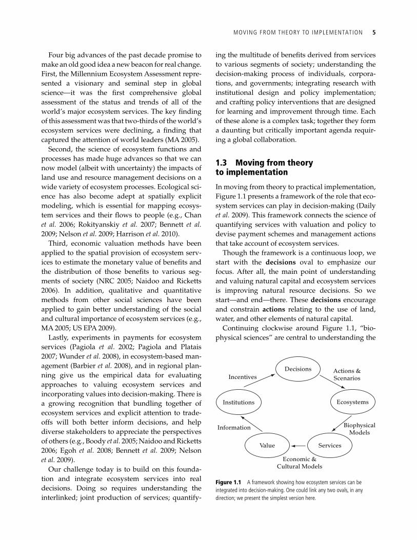
MOVING FROM THEORY TO IMPLEMENTATION 5
Four big advances of the past decade promise to make an old good idea a new beacon for real change. First, the Millennium Ecosystem Assessment repre-sented a visionary and seminal step in global science—it was the fi rst comprehensive global assessment of the status and trends of all of the world’s major ecosystem services. The key fi nding of this assessment was that two-thirds of the world’s ecosystem services were declining, a fi nding that captured the attention of world leaders (MA 2005).
Second, the science of ecosystem functions and processes has made huge advances so that we can now model (albeit with uncertainty) the impacts of land use and resource management decisions on a wide variety of ecosystem processes. Ecological sci-ence has also become adept at spatially explicit modeling, which is essential for mapping ecosys-tem services and their fl ows to people (e.g., Chan et al. 2006 ; Rokityanskiy et al. 2007 ; Bennett et al. 2009 ; Nelson et al. 2009 ; Harrison et al. 2010 ).
Third, economic valuation methods have been applied to the spatial provision of ecosystem serv-ices to estimate the monetary value of benefi ts and the distribution of those benefi ts to various seg-ments of society (NRC 2005; Naidoo and Ricketts 2006 ). In addition, qualitative and quantitative methods from other social sciences have been applied to gain better understanding of the social and cultural importance of ecosystem services (e.g., MA 2005; US EPA 2009).
Lastly, experiments in payments for ecosystem services ( Pagiola et al . 2002 ; Pagiola and Platais 2007 ; Wunder et al. 2008 ), in ecosystem-based man-agement ( Barbier et al. 2008 ), and in regional plan-ning give us the empirical data for evaluating approaches to valuing ecosystem services and incorporating values into decision-making. There is a growing recognition that bundling together of ecosystem services and explicit attention to trade-offs will both better inform decisions, and help diverse stakeholders to appreciate the perspectives of others (e.g., Boody et al. 2005 ; Naidoo and Ricketts 2006 ; Egoh et al. 2008 ; Bennett et al. 2009 ; Nelson et al. 2009 ).
Our challenge today is to build on this founda-tion and integrate ecosystem services into real decisions. Doing so requires understanding the interlinked; joint production of services; quantify-
ing the multitude of benefi ts derived from services to various segments of society; understanding the decision-making process of individuals, corpora-tions, and governments; integrating research with institutional design and policy implementation; and crafting policy interventions that are designed for learning and improvement through time. Each of these alone is a complex task; together they form a daunting but critically important agenda requir-ing a global collaboration.
1.3 Moving from theory to implementation
In moving from theory to practical implementation, Figure 1.1 presents a framework of the role that eco-system services can play in decision-making ( Daily et al. 2009 ). This framework connects the science of quantifying services with valuation and policy to devise payment schemes and management actions that take account of ecosystem services.
Though the framework is a continuous loop, we start with the decisions oval to emphasize our focus. After all, the main point of understanding and valuing natural capital and ecosystem services is improving natural resource decisions. So we start—and end—there. These decisions encourage and constrain actions relating to the use of land, water, and other elements of natural capital.
Continuing clockwise around Figure 1.1 , “bio-physical sciences” are central to understanding the
Decisions
Ecosystems
ServicesValue
Institutions
Economic &Cultural Models
Actions &Scenarios
BiophysicalModels
Information
Incentives
Figure 1.1 A framework showing how ecosystem services can be integrated into decision-making. One could link any two ovals, in any direction; we present the simplest version here.
6 MAINSTREAMING NATURAL CAPITAL INTO DECIS IONS
link between decisions and ecosystems , and along with economics and social science, the links between ecosystems and services . We study the former link with classic ecology and conservation biology to, for example, estimate impacts of land-use change on biodiversity (e.g., Daily et al. 2001 ; Steffan-Dewenter et al. 2007 ). And we pursue the latter link with “ecological production functions” that relate, say, forest condition and management practices to the supply of carbon storage, pollination, and other ecosystem services (e.g., Ricketts et al. 2004 ).
Social sciences are also central to understanding the value of services to people (“economic and cul-tural models”). Economic valuation techniques are commonly used for this link, to place monetary value on natural capital. Value is often not fully cap-tured in monetary terms, though, so it is important to characterize value in multiple dimensions, including, for example, health, livelihood support, cultural signifi cance (e.g., Dasgupta 2001 ). This will help ensure that valuation and broader decision-making approaches are inclusive of the range of benefi ts and people concerned ( Heal 2000a , 2000b ).
Finally, valuing ecosystem services provides use-ful information that can help shape institutions (e.g., agricultural markets, subsidies, land-use poli-cies, conservation NGOs) to guide resource man-agement and policy. Having the right institutions can create incentives so that the decisions of indi-viduals, communities, corporations, and govern-ments promote widely shared values. The links between the value , institutions , and decisions ovals are much more the art and politics of social change than science, though scientists can inform these debates if they target specifi c decisions and are attuned to the social and political contexts.
This idealized framework is helpful in clarifying the many frontiers of research and implementation en route to operationalizing ecosystem services into decisions (see also Carpenter et al. 2009 ). This includes continued biophysical research on the impacts of human actions on ecosystems, all the way to studies on the way landowners respond to conservation incentives. Chapters in this book touch on all ovals and all arrows within the framework, but the core chapters focus on moving from ecosys-tems to services, and from services to value, using production functions and valuation techniques.
1.4 Using ecosystem production functions to map and assess natural capital
There are several methods for mapping and assign-ing value to ecosystem services, each with its own advantages and limitations. The initial valuation work in the fi eld of ecosystem services primarily used what is called the benefi t transfer approach (e.g., Costanza et al. 1997 ). This approach typically uses empirical estimates of the value of goods pro-duced from some habitat type and transfers those benefi ts to similar habitats elsewhere, including anywhere in the world ( Costanza et al. 1997 ). Local knowledge can be used to adjust the benefi ts because one knows, for instance, that the west coast marshes of North America are less productive than the east coast marshes and so forth. The general idea, however, is to use lookup tables of benefi ts per unit area of habitat type, and thereby quantify over-all natural capital.
An alternative method favored in this book is called a “production function approach.” Instead of relying on lookup tables, we build models that pre-dict local ecosystem service supply based on land cover, land use, ecosystem attributes, human demand, etc. These functions are analogous to those long used in agriculture, which relate amounts of water, fertilizer, and labor to resulting crop yield. In our view, production functions have key advan-tages over benefi ts transfer, and we delve into these further in Chapter 3 .
1.5 Roadmap to the book
Our book begins with three chapters that introduce the core approach and hypotheses of our work on natural capital. Chapter 2 examines the philosophi-cal bases for ecosystem service value and explores ways of measuring such value, distinguishing alter-native approaches and highlighting some ethical issues underlying the choices among them. It also explores the strengths and weaknesses of these measurement approaches, and indicates which approaches are best suited to the different types of value conferred by ecosystem services. Chapter 3 then introduces the modeling approach we have developed, which strives to integrate many differ-
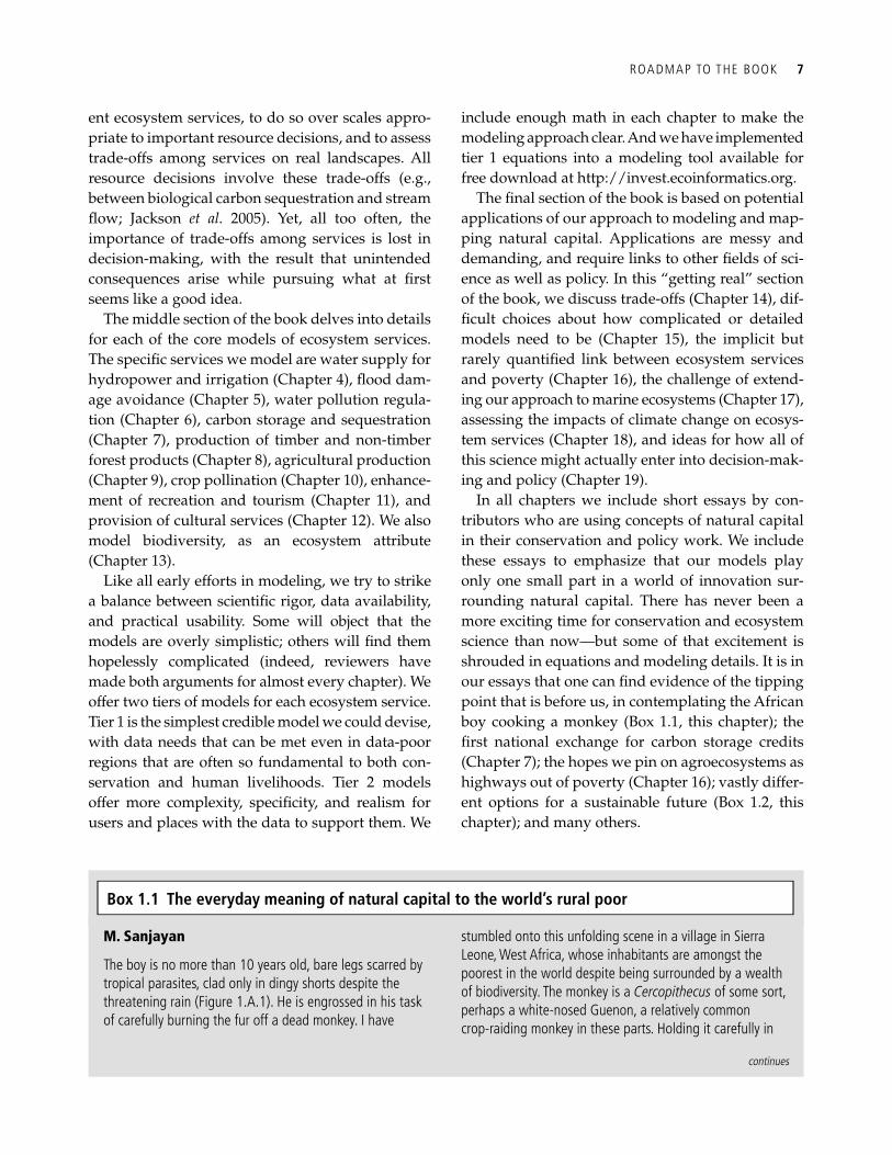
ROADMAP TO THE BOOK 7
M. Sanjayan
The boy is no more than 10 years old, bare legs scarred by tropical parasites, clad only in dingy shorts despite the threatening rain ( Figure 1.A.1 ). He is engrossed in his task of carefully burning the fur off a dead monkey. I have
stumbled onto this unfolding scene in a village in Sierra Leone, West Africa, whose inhabitants are amongst the poorest in the world despite being surrounded by a wealth of biodiversity. The monkey is a Cercopithecus of some sort, perhaps a white-nosed Guenon, a relatively common crop-raiding monkey in these parts. Holding it carefully in
ent ecosystem services, to do so over scales appro-priate to important resource decisions, and to assess trade-offs among services on real landscapes. All resource decisions involve these trade-offs (e.g., between biological carbon sequestration and stream fl ow; Jackson et al. 2005 ). Yet, all too often, the importance of trade-offs among services is lost in decision-making, with the result that unintended consequences arise while pursuing what at fi rst seems like a good idea.
The middle section of the book delves into details for each of the core models of ecosystem services. The specifi c services we model are water supply for hydropower and irrigation ( Chapter 4 ), fl ood dam-age avoidance ( Chapter 5 ), water pollution regula-tion ( Chapter 6 ), carbon storage and sequestration ( Chapter 7 ), production of timber and non-timber forest products ( Chapter 8 ), agricultural production ( Chapter 9 ), crop pollination ( Chapter 10 ), enhance-ment of recreation and tourism ( Chapter 11 ), and provision of cultural services ( Chapter 12 ). We also model biodiversity, as an ecosystem attribute ( Chapter 13 ).
Like all early efforts in modeling, we try to strike a balance between scientifi c rigor, data availability, and practical usability. Some will object that the models are overly simplistic; others will fi nd them hopelessly complicated (indeed, reviewers have made both arguments for almost every chapter). We offer two tiers of models for each ecosystem service. Tier 1 is the simplest credible model we could devise, with data needs that can be met even in data-poor regions that are often so fundamental to both con-servation and human livelihoods. Tier 2 models offer more complexity, specifi city, and realism for users and places with the data to support them. We
include enough math in each chapter to make the modeling approach clear. And we have implemented tier 1 equations into a modeling tool available for free download at http://invest.ecoinformatics.org.
The fi nal section of the book is based on potential applications of our approach to modeling and map-ping natural capital. Applications are messy and demanding, and require links to other fi elds of sci-ence as well as policy. In this “getting real” section of the book, we discuss trade-offs ( Chapter 14 ), dif-fi cult choices about how complicated or detailed models need to be ( Chapter 15 ), the implicit but rarely quantifi ed link between ecosystem services and poverty ( Chapter 16 ), the challenge of extend-ing our approach to marine ecosystems ( Chapter 17 ), assessing the impacts of climate change on ecosys-tem services ( Chapter 18 ), and ideas for how all of this science might actually enter into decision-mak-ing and policy ( Chapter 19 ).
In all chapters we include short essays by con-tributors who are using concepts of natural capital in their conservation and policy work. We include these essays to emphasize that our models play only one small part in a world of innovation sur-rounding natural capital. There has never been a more exciting time for conservation and ecosystem science than now—but some of that excitement is shrouded in equations and modeling details. It is in our essays that one can fi nd evidence of the tipping point that is before us, in contemplating the African boy cooking a monkey ( Box 1.1 , this chapter); the fi rst national exchange for carbon storage credits ( Chapter 7 ); the hopes we pin on agroecosystems as highways out of poverty ( Chapter 16 ); vastly differ-ent options for a sustainable future ( Box 1.2 , this chapter); and many others.
Box 1.1 The everyday meaning of natural capital to the world’s rural poor
continues

8 MAINSTREAMING NATURAL CAPITAL INTO DECIS IONS
both hands, the boy slowly turns it as the pelt singes and curls into soft gray ash. It is clearly a delicate task, with the fl ames struggling to catch the rain-soaked pieces of stick fed into the weak fi re. Occasionally the boy pauses and, with a piece of tin sheet metal, furiously fans the smoky mess. An acrid odor hangs in the heavy air.
The monkey will soon be food. It will be dismembered, every bit from nose to tail, thrown into a pot with some okra, peppers, or other meager vegetables, and a few drops of palm oil—a stew ultimately yielding, based on the small crush of spectators, what I estimate to be about two tablespoons of meat protein for each person. A small monkey in a big pot. Fascinated by the boy’s handiwork, I pull out my camera and snap a photo—and immediately feel a little shabby about it. The boy just giggles.
Spend any amount of time quietly observing the daily rituals of rural village life in any tropical country and you cannot but be impressed by the magnitude and diversity of services people derive from their immediate surroundings; nature if you will. However, these services provided by nature are nearly always taken for granted. Local communities are usually myopic in their understanding of similar communities, encircling what are to them virtually endless resources, and governments who can see the big picture are reluctant to acknowledge it lest they expose their shortcomings. Plus, changes are usually slow and accumulate over a long period of time, thus hiding cumulative impacts in the imperfect memories of the elders.
As I see it, six basic services provide most of the daily needs of extremely poor rural people. Fresh water is the most obvious and its procurement is taxing, particularly to women, who bear most of the load. While there are taps sprouting in many rural villages in Africa, few connect to sustainable water sources. Fuel wood, collected from forests, plantations, or local groves, is indispensible for the heating and cooking needs of 40% of rural homes. Gathering it is the second most taxing chore (after water) that impacts daily life. Fisheries provide protein to 20% of the world’s population. On the Ganges River in India, for example, ten million people in 2000 villages depend on fi shing to both meet their daily needs and provide jobs. Fertility of soils, and its natural renewal through processes of nutrient cycling, is essential to places untouched by the Green Revolution and does not involve the consequences of industrial fertilization in terms of energy use and nutrient overload. Forest products, like meat for protein from forest animals, fruit, honey, medicinal plants, and fi ber, have a myriad of vital uses. Fodder, in terms of grass and browse for livestock, is important in rural communities because it is one of the few ways through which the poor can access the global economy. Livestock is the common bank for rural populations. These “6 Fs” of nature (six free services) are part of the staple packet of goods and services that virtually every rural community depends upon and that governments conveniently ignore, and non-profi ts underestimate the importance of. Lose them and people will suffer.
Box 1.1 continued
Figure 1.A.1 Young boy preparing to eat a monkey, rural Sierra Leone. Photo by M. Sanjayan.
OPEN QUEST IONS AND FUTURE DIRECTIONS 9
1.6 Open questions and future directions
This book and the modeling approaches we intro-duce are only a beginning. We anticipate the research community adding other ecosystem services over time, as well as continually improving the models and data for those presented in this book. These additions and improvements will come from con-fronting these and other models with a variety of real-world data and challenges. Here we mention two of the many key arenas in which further under-standing is crucial.
First, major advances in methods and tools are needed to incorporate dynamic effects, as well as shocks and uncertainty. Dynamic changes (e.g., in climate and in the nitrogen cycle) and changes aris-ing through economic development and evolving human preferences over time are important to include. The possibility of feedbacks within ecosys-tems, and between ecosystem services and human behavior, are important areas for further develop-ment. Feedback effects can give rise to thresholds and rapid changes in systems that can fundamen-tally alter system states ( Scheffer et al. 2001 ). The ability to incorporate shocks and the possibility of surprises is another area where further develop-ment is needed. Fires, droughts, and disease all can
have major infl uences on ecosystems and affect the services produced. Changes in economic conditions or fads in human behavior can similarly cause major changes in systems (e.g., fi nancial crises). The occur-rence of each of these and other potential distur-bances is diffi cult to predict but virtually certain to come about. Understanding their likely impacts on ecological and social systems will help us prepare for them.
A second major area for further development is in relating ecosystem condition to human health. The relationships between biophysical attributes of eco-systems and human communities are complex ( Myers and Patz 2009 ). Destruction of ecosystems can at times improve aspects of community health. For example, draining swamps can reduce habitat for the mosquito vector that transmits the parasite that causes malaria. On the other hand, ecosystems provide many services that sustain human health, for which substitutes are not available at the required scale, such as purifi cation and regulation of drinking water fl ow; regulation of air quality; nutrition (especially of protein and micronutrients); psychological benefi ts; and, in complex ways, regu-lation of vector-borne disease (Levy et al. in press). To date, there is little rigorous research establishing the links between ecosystem conditions and human health.
Later, when I look through my day’s pictures on my camera, it is not the dead monkey that draws my attention. It’s the sheet of tin metal, the one the boy used to fan the fl ames that I focus on. It’s a piece of a signboard—one of millions that line roads all over Africa, from charities, governments, and religious organizations. On this one, framed against a white background, are the blue letters—WFP—suspended over the image of a bundle of grain. The World Food Programme. Here is this kid, fanning the fl ames with a sign board for a humanitarian organiza-tion, to burn the fur off a dead monkey from the forest, which is what he is actually going to eat. For the poor, nature often provides when governments and institutions don’t suffi ce, and that is a powerful lesson.
As we begin to better map, quantify, and assign monetary value on nature’s services, from carbon to water,
to more diffi cult-to-assess services like fodder, we need to ensure that we are adequately capturing the roughly one-sixth of the world’s population who live on the very margins of national or global economies but whose needs for such services are not just dire, but virtually irreplaceable. The value of water to a woman in West Africa trying to prepare a meal is far higher (though not in strictly monetary terms) than that to a woman fi lling up her swimming pool in California. Valuation of ecosystem services must properly recognize, and incorporate, this vast social net that nature provides to the poor.
I think about returning to the village and bartering for the sign; hanging in my offi ce, it would be a powerful reminder of this insight. But I have nothing useful to trade. Nothing sustainable. For now, the boy needs it more than I do.

10 MAINSTREAMING NATURAL CAPITAL INTO DECIS IONS
Stephen R. Carpenter
“What gives you the most hope for the environment over the next 50 years?” When we asked that question of 59 global leaders in 2003, we expected great variability in the answers. To our surprise, the answers fell rather cleanly into three clusters. Some respondents were not worried and simply had faith in economic growth, being convinced that a sustainable environment would follow automatically from economic development. Two clusters stood out, however, because they envisioned futures that were less automatic, and that would need some guidance if we were to achieve a hopeful outcome. The fi rst of these “we need change” clusters thought that innovation and investments in environmentally friendly technology was the key. The second “we need change” group felt that governance should be restructured to motivate local innovation and learning, and thereby create sustainable landscapes from the bottom up.
These two clusters of ideas became the Technogarden and Adapting Mosaic scenarios of the Millennium Ecosystem Assessment (MA 2005). We evaluated the condition of 24 global ecosystem services from 2000 to
2050 under these and other scenarios. Technogarden and Adapting Mosaic were the most successful scenarios for maintaining ecosystem services. However, these two scenarios represent very different policies that lead to different bundles of global ecosystem services by 2050.
In Technogarden , society addresses global environmental problems such as climate heating, materials cycles, and nutrient mobilization through innovations in energy production, buildings, transportation, and agriculture ( Figure 1.B.1 ). Improvements in agriculture and urban design make it possible to feed and house humanity without extensive new conversion of wild lands. Market mechanisms and sophisticated economic instruments are deployed to manage ecosystem services. International cooperation on incentives for better technology lays the foundation for improved cooperation on other problems of the global commons, such as pelagic marine fi sheries, disease containment, and conservation of antibiotics. Expanded access to education leads to smaller family sizes and thereby slows the pace of population growth. Even though many ecosystem services are in sustainable condition by 2050, there are some downsides. Some aesthetic, cultural, and spiritual aspects of ecosystems are
Box 1.2 Sorting among options for a more sustainable world
Figure 1.B.1 Depiction of the Technogarden scenario of the Millennium Ecosystem Assessment. From Ecosystems and Human Well-Being: Scenarios , by the Millennium Ecosystem Assessment. Copyright © 2005 Millennium Ecosystem Assessment. Reproduced by permission of Island Press, Washington, D.C.
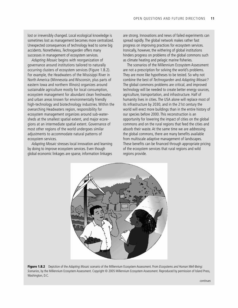
OPEN QUEST IONS AND FUTURE DIRECTIONS 11
lost or irreversibly changed. Local ecological knowledge is sometimes lost as management becomes more centralized. Unexpected consequences of technology lead to some big accidents. Nonetheless, Technogarden offers many successes in management of ecosystem services .
Adapting Mosaic begins with reorganization of governance around institutions tailored to naturally occurring clusters of ecosystem services ( Figure 1.B.2 ). For example, the Headwaters of the Missisippi River in North America (Minnesota and Wisconsin, plus parts of eastern Iowa and northern Illinois) organizes around sustainable agriculture mostly for local consumption, ecosystem management for abundant clean freshwater, and urban areas known for environmentally friendly high-technology and biotechnology industries. Within the overarching Headwaters region, responsibility for ecosystem management organizes around sub-water-sheds at the smallest spatial extent, and major ecore-gions at an intermediate spatial extent. Governance of most other regions of the world undergoes similar adjustments to accommodate natural patterns of ecosystem services.
Adapting Mosaic stresses local innovation and learning by doing to improve ecosystem services. Even though global economic linkages are sparse, information linkages
are strong. Innovations and news of failed experiments can spread rapidly. The global network makes rather fast progress on improving practices for ecosystem services. Ironically, however, the withering of global institutions hinders progress on problems of the global commons such as climate heating and pelagic marine fi sheries.
The scenarios of the Millennium Ecosystem Assessment are not a prescription for solving the world’s problems. They are more like hypotheses to be tested. So why not combine the best of Technogarden and Adapting Mosaic ? The global commons problems are critical, and improved technology will be needed to create better energy sources, agriculture, transportation, and infrastructure. Half of humanity lives in cities. The USA alone will replace most of its infrastructure by 2030, and in the 21st century the world will erect more buildings than in the entire history of our species before 2000. This reconstruction is an opportunity for lowering the impact of cities on the global commons and on the rural regions that feed the cities and absorb their waste. At the same time we are addressing the global commons, there are many benefi ts available from multiscale adaptive management of landscapes. These benefi ts can be fi nanced through appropriate pricing of the ecosystem services that rural regions and wild regions provide.
Figure 1.B.2 Depiction of the Adapting Mosaic scenario of the Millennium Ecosystem Assessment. From Ecosystems and Human Well-Being: Scenarios , by the Millennium Ecosystem Assessment. Copyright © 2005 Millennium Ecosystem Assessment. Reproduced by permission of Island Press, Washington, D.C.
continues
12 MAINSTREAMING NATURAL CAPITAL INTO DECIS IONS
1.7 A general theory of change
Mainstreaming natural capital into decisions is a long-term proposition, requiring co-evolving advances in knowledge, social institutions, and cul-ture. Certainly a single book is not suffi cient for achieving this. We propose instead that our book contributes to an overall theory of change ( Bradach et al. 2008 ) involving three key, broad elements.
First, businesses, governments, and individuals must fi nd it easy to inculcate ecosystem services and natural capital into their decisions, and the methods for doing so must be transparent, credible, and predictable. In many cases, sectors of society are open to the idea of ecosystem services and natu-ral capital, but simply do not know how to take the idea and use it in a concrete way.
Second, there need to be examples of projects or enterprises that—as a result of properly valuing ecosystem services and natural capital—end up with improved decisions, institutions, and human well-being. These examples both test our science against real-world problems and produce compel-ling stories of how an ecosystem services approach made a difference.
Lastly, political and thought leaders must appre-ciate these examples of success and spread the word. This is where the lessons of a set of examples can be mainstreamed into the myriad decisions—by businesses, governments, farmers, and banks—that are made every year and that impact our natural world. This is where the impact of scattered projects can be magnifi ed into worldwide change.
None of these steps are complicated, and our the-ory of change does not require a brilliant and novel strategy. In fact, we are convinced that all three ingredients are within striking distance. The envi-ronmental movement has a much bigger and more diverse and powerful community behind it now than ever before ( Daily and Matson 2008 ). Science is
beginning to provide tools and methods that will reduce the transaction costs. And there are enough policy experiments underway that compelling examples of natural capital stewardship enhancing human well-being should be forthcoming.
Our book targets the fi rst element of our theory: to make quantifying and valuing natural capital straightforward and routine. Science is not every-thing, but both modeling and empirical science pro-vide the foundation for action. The models we rely on are not a fait accompli —they are the fi rst step in an iterative process between basic science and application to real-world problems. That is why we highlight case studies in which valuation of natural capital is being used to infl uence land and water management. Science by itself cannot change the world, but science plus the vision and action of leaders can—and that is what we seek.
References
Balmford, A., Bruner, A., Cooper, P., et al. (2002). Economic reasons for conserving wild nature. Science , 297 , 950–3.
Barbier, E., Koch, E., Silliman, B., et al. (2008). Coastal eco-system-based management with non-linear ecological functions and values. Science , 319 , 321–3.
Bennett, E., Peterson, G., and Gordon, L. (2009). Understanding relationships among multiple ecosys-tem services. Ecology Letters , 12 , 1394–1404.
Boody, G., Vondracek, B., Andow, D., et al. (2005). Multifunctional agriculture in the United States. BioScience , 55 , 27–38.
Bradach, J., Tierney, T., and Stone, N. (2008). Delivering on the promise of nonprofi ts. Harvard Business Review , Dec. , 88–97.
Brauman, K., Daily, G. C., Duarte, T. K., and Mooney, H. A. (2007). The nature and value of ecosystem services: An overview highlighting hydrologic services. Annual Review in Environment and Resources , 32 , 67–98.
Carpenter, S., DeFries, R., Dietz T., et al. (2006). Millennium Ecosystem Assessment: research needs. Science , 314 , 257–8.
Even though the Millennium Ecosystem Assessment did not compute an optimal path to 2050, it is likely that the best mix of options is some combination of Technogarden and Adapting Mosaic . The challenge is to understand which
combinations of ecosystem services are biophysically possible, the trade-offs among different bundles of ecosystem services possible from a given region, and the institutional frameworks that enable ongoing fl ows of ecosystem services.
Box 1.2 continued
A GENERAL THEORY OF CHANGE 13
Carpenter, S., Mooney, H., Agard, J., et al. (2009). Science for managing ecosystem services: Beyond the Millennium Ecosystem Assessment. Proceedings of the National Academy of Sciences, USA , 106 , 1305–12.
Chan, K. M. A., Shaw, M. R., Cameron, D. R., et al. (2006). Conservation planning for ecosystem services. PLoS Biol , 4 , e379.
Clark, C. (1990). Mathematical Bioeconomics: The Optimal Management of Renewable Resources , 2nd edn. Wiley, New York.
Costanza, R., d’Arge, R., de Groot, R., et al. (1997). The value of the world’s ecosystem services and natural capital. Nature , 387 , 253–60.
Daily, G. C., Ed. (1997). Nature’s Services: Societal Dependence on Natural Ecosystems , Island Press, Washington, DC.
Daily, G. C., Söderqvist, T., Aniyar, S., et al. (2000). The value of nature and the nature of value. Science , 289 , 395–6.
Daily, G. C., Ehrlich, P. R., and Sánchez-Azofeifa, G. (2001). Countryside biogeography: Use of human-dominated habitats by the avifauna of southern Costa Rica. Ecological Applications , 11 , 1–13.
Daily, G. C., and Matson, P. (2008). Ecosystem services: From theory to implementation. Special Feature. Proceedings of the National Academy of Sciences, USA , 105 , 9455–6.
Daily, G. C., Polasky, S., Goldstein, J., et al. (2009). Ecosystem services in decision-making: time to deliver. Frontiers in Ecology and the Environment , 7 , 21–8.
Das, S., and Vincent, J. (2009). Mangroves protected vil-lages and reduced death toll during Indian super cyclone. Proceedings of the National Academy of Sciences, USA , 106 , 7357–60.
Dasgupta, P., and Heal, G. (1979). Economic Theory and Exhaustible Resources . Cambridge University Press, Cambridge.
Dasgupta, P. (2001). Human Well-Being and the Natural Environment , Oxford University Press, Oxford.
Dasgupta, P. (2010). Nature’s role in sustaining economic development. Philosophical Transactions of the Royal Society B , 365 , 5–11.
Egoh, B., Reyers, B., Rouget, M., et al. (2008). Mapping eco-system services for planning and management. Agriculture Ecosystems and Environment , 127 , 135–40.
Ehrenfeld, D. (1988). Why put a value on biodiversity? In Biodiversity , E. O. Wilson, Ed., National Academy Press, Washington, DC.
Freeman, A. M., III (1993). The Measurement of Environmental and Resource Values: Theory and Methods . Resources for the Future, Washington, DC.
Goldman, R., Benítez, S., Calvache, A., and Rámos, A. (2010). Water funds: protecting watersheds for nature and people. The Nature Conservancy, Arlington.
Gordon, H. (1954). The economic theory of a common-property resource: the fi shery. Journal of Political Economy , 62 , 124–42.
Harrison, J., Bouwman, A., Mayorga, E., and Seitzinger, S. (2010). Magnitudes and sources of dissolved inorganic phosphorus inputs to surface fresh waters and the coastal zone: A new global model. Global Biogeochemical Cycles , 24 , 271–9.
Heal, G. (2000a). Nature and the Marketplace: Capturing the Value of Ecosystem Services. Island Press, Washington, DC.
Heal, G. (2000b). Valuing ecosystem services. Ecosystems , 3 , 24–30.
Jackson, R. B., Jobággy, E., Avissar, R., et al. (2005) Trading water for carbon with biological carbon sequestration. Science , 310 , 1944–7.
Kareiva, P., and Marvier, M. (2007). Conservation for the people. Scientifi c American , 297 , 50–7.
Krutilla, J. (1967). Conservation reconsidered. American Economic Review , 47 , 777–86.
Krutilla, J., and Fisher, A. (1975). The Economics of Natural Environments: Studies in the Valuation of Commodity and Amenity Resources . Johns Hopkins University Press, Baltimore.
Larigauderie, A., and Mooney, H. (2010). The Inter-governmental Science-Policy Platform on Biodiversity and Ecosystem Services: moving a step closer to an IPCC-like mechanism for biodiversity. Current Opinion in Environmental Sustainability , 2 , 9–14.
Leopold, A. (1949). A Sand County Almanac . Oxford University Press, Oxford.
Levy, K., Daily, G. C., and Myers, S. (in press). Ecosystem services and human health: A conceptual framework.
Liu, J., Li, S., Ouyang, Z., Tam, C. and Chen, X. (2008). Ecological and socioeconomic effects of China’s policies for ecosystem services. Proceedings of the National Academy of Sciences, USA , 105 , 9489–94.
MA (Millennium Ecosystem Assessment). (2005). Eco-systems and Human Well-being: The Assessment Series (Four Volumes and Summary). Island Press, Washington, DC.
Mäler K.-G., Aniyar, S., and Jansson, A. (2008). Accounting for ecosystem services as a way to understand the requirements for sustainable development. Proceedings of the National Academy of Sciences USA , 105 , 9501–06.
Mooney, H., and Ehrlich, P. (1997). Ecosystem services: A fragmentary history. In G. Daily, Ed., Nature’s Services . Island Press, Washington, DC.
Mooney, H. and Mace, G. (2009). Biodiversity policy chal-lenges. Science, 325 , 1474.
Myers, S. and Patz, J. (2009). Emerging threats to human health from global environmental change. Annual Review of Environment and Resources , 34 , 223–52.
14 MAINSTREAMING NATURAL CAPITAL INTO DECIS IONS
Naidoo, R. and Ricketts, T. H. (2006). Mapping the eco-nomic costs and benefi ts of conservation. PLoS Biology , 4 , e360.
Nel, D., Marais, C., and Blignaut, J. (2009). Water neutral-ity: A fi rst quantitative framework for investing in water in South Africa. Conservation Letters , 2 , 11–18.
Nelson, E., Mendoza, G., Regetz, J., et al. (2009). Modeling multiple ecosystem services, biodiversity conservation, commodity production, and tradeoffs at landscape scales. Frontiers in Ecology and the Environment , 7 , 4–11.
Norton, B. (1987). Why Preserve Natural Variety? Princeton University Press, Princeton.
NRC (National Research Council) (2005). Valuing Ecosystem Services: Toward Better Environmental Decision-Making . National Academies Press, Washington, DC.
Pagiola, S., Bishop, J., and Landell-Mills, N. (2002). Selling Forest Environmental Services . Earthscan, London.
Pagiola, S. and Platais, G. (2007). Payments for Environmental Services: From Theory to Practice . World Bank, Washington, DC.
Porras, I., Grieg-Gran, M., and Neves, N. (2007). All That Glitters: A Review of Payments for Watershed Services in Developing Countries . International Institute of Environment and Development, London.
Ricketts, T. H., Daily, G. C., Ehrlich, P. R., and Michener, C. (2004). Economic value of tropical forest to coffee pro-duction. Proceedings of the National Academy of Sciences, USA , 34 , 12579–82.
Rokityanskiy, D., Benítez, P., Kraxner, F., et al. (2007). Geographically explicit global modeling of land-use change, carbon sequestration, and biomass supply. Technological Forecasting and Social Change , 74 , 1057–82.
Rolston, H., III (2000). The land ethic at the turn of the mil-lennium. Biodiversity and Conservation , 9 , 1045–58.
Ruhl, J., Kraft, S., and Lant, C. (2007). The Law and Policy of Ecosystem Services . Island Press, Washington, DC.
Schaefer, M. B. (1957). Some considerations of population dynamics and economics in relation to the manage-ment of marine fi shes. Journal of the Fisheries Research Board of Canada , 14 , 669–81.
Scheffer, M., Carpenter, S. R., Foley, J. et al. (2001). Catastrophic shifts in ecosystems. Nature , 413 , 591–6.
Scott, A. (1955). The fi shery: the objectives of sole owner-ship. Journal of Political Economy , 63 , 116–24.
Steffan-Dewenter, I., Kessler, M., Barkmann, J., et al. (2007). Tradeoffs between income, biodiversity, and ecosystem functioning during tropical rainforest conversion and agroforestry intensifi cation. Proceedings of the National Academy of Sciences USA , 104 , 4973–8.
Stokstad, E. (2005). Louisiana’s wetlands still struggle for survival. Science , 310 , 1264–6.
US EPA (United States Environmental Protection Agency) Science Advisory Board. (2009). Valuing the Protection of Ecological Systems and Services . EPA-SAB-09-012. US EPA, Washington, DC.
Varga, A. (2009). Payments for Ecosystem Service: An Analysis of Cross Cutting Issues in Ten Case Studies. Columbia University, New York.
WRI (World Resources Institute). (2010). Lafarge Presque Island Quarry: Corporate Ecosystem Services Review. World Resources Institute, Washington, DC.
Wunder, S., Engel, S., and Pagiola, S. (2008). Taking stock: a comparative analysis of payments for environmental service programs in developed and developing countries. Ecological Economics , 65 , 834–52.
Zhang, P., Shao, G., Zhao, G., et al. (2000). China’s forest policy for the 21st century. Science , 288 , 2135–6.
15
CHAPTER 2
Interpreting and estimating the value of ecosystem services Lawrence H. Goulder and Donald Kennedy
2.1 Introduction: why is valuing nature important?
Many of the critical ecosystem services generated by natural capital (such as pollination services, fl ood control, water fi ltration, and provision of hab-itat for biodiversity) are externalities—they are not given a price in markets. As a result, unfettered markets often lead to the compromising or collapse of ecosystems, much to the detriment of human welfare. Oftentimes society would benefi t from greater protection of ecosystems and their services than results from unregulated markets.
Public policy has a crucial role to play in regulat-ing or infl uencing markets so as to prevent them from producing unfortunate societal outcomes. Yet decisions about such public policies are often con-tentious. Agricultural interests will vie for greater ability to purchase wetlands and convert them through drainage to agricultural land. Urban devel-opers will push to convert open space to new hous-ing tracts.
Perhaps the most important basis for supporting a policy that would protect otherwise threatened ecosystem services is evidence that society gains more value from such protections than it gives up. Providing such evidence requires an understanding of the biophysical processes involved, that is, the various services offered by the ecosystem in ques-tion. It also requires an assessment of the benefi ts to well-being—or values to society—of these ecosys-tem services.
This chapter clarifi es how such an assessment of ecosystem services can be made. It has two main components. One is to examine the philosophical basis of ecosystem service value. In considering this
basis, we contrast competing approaches to value and bring out some ethical issues underlying the choice among different approaches.
The other component is to lay out various meth-ods for measuring the values of ecosystem services, and to consider the strengths and limitations of these approaches. Quantitative assessments of eco-system service value have become much more widespread in recent years. The expanding litera-ture now includes estimates of the value of such ecosystem services as pollination, pest control, and water purifi cation. These assessments are begin-ning to play a signifi cant role in the formulation of land-use policies.
Setting out the values of ecosystem services to society provides a basis for making public policy decisions. However, it is not the only basis. As we discuss briefl y below, it may make sense to con-sider as well whether a policy decision is consist-ent with preserving the intrinsic rights of the various organisms or ecosystems that might be affected by the decision. If intrinsic rights are involved, it is reasonable to restrict the set of seri-ous alternatives to those that are consistent with these rights.
The chapter is organized as follows. Section 2.2 examines alternative philosophical foundations for valuing living things and ecosystems. It also con-siders how attention to intrinsic rights might sup-plement or even offer an alternative to a consideration of values. This philosophical discus-sion lays the groundwork for Section 2.3 ’s examina-tion of empirical valuation methods. In Section 2.4 we indicate some valuation problems that arise in a few specifi c real-world cases. Our fi nal section draws conclusions.
16 INTERPRET ING AND EST IMATING THE VALUE OF ECOSYSTEM SERVICES
2.2 Philosophical issues: values, rights, and decision-making
2.2.1 Competing philosophical approaches to value
2.2.1.1 The anthropocentric approach From what do nature’s values derive? When we claim that a given living thing or species or habitat is worth such-and-such, what is the basis of that claim?
Among US policy analysts, the prevailing approach to value is anthropocentric. This approach claims that natural things (indeed, all things) have value to the extent that they confer satisfactions to humans. It stipulates that value is based on the ability to give utility (or well-being) to humans. Economists tend to support this viewpoint which, as we discuss below, is inherent in benefi t–cost analysis.
At fi rst blush, this anthropocentric approach might seem inconsistent with safeguarding the planet or protecting non-human forms of life. But the approach does not necessarily imply a ruthless exploitation of nature. On the contrary, it can be consistent with the fervent protection of non-human things, both individually and as collectivities. After all, we may feel that the protection of nature or par-ticular non-human forms of life is important to our satisfaction or well-being, and thus we may place a high value on these forms. The anthropocentric approach does not rule out our making substantial sacrifi ces to protect and maintain other living things. However, it asserts that we should assign value (and therefore help other forms of life) only insofar as we humans gain satisfaction or well-being from doing so. The notion of satisfaction here should be interpreted broadly, to encompass not only mun-dane enjoyments (as with consuming plants or ani-mals for food) but also more lofty pursuits (such as marveling at the beauty of an eagle).
Anthropocentric value can be categorized accord-ing to the way the satisfaction is generated. Use value refers to satisfaction that involves (directly or indirectly) a physical encountering with the object in question. There are direct use values (for exam-ple, the satisfaction from catching or eating trout) as well as indirect use values (for example, the value that can be attached to plankton because it provides
nutrients for other living things that in turn feed humans). The anthropocentric approach does not restrict value to forms of nature that are consumed: there are both consumptive and non-consumptive use values. Examples of the former are the values that might be attached to ducks insofar as they provide food. Examples of the latter are the values ducks provide in the form of pleasure to bird-watchers.
Satisfactions also include non-use values: values that involve no actual direct or indirect physical involvement with the natural thing in question. The most important value of this type may be existence value (or passive use value)—the satisfaction one enjoys from the pure contemplation of the existence of some entity. For example, a New Jersey resident who has never seen the Grand Canyon and who never intends to visit it can derive satisfaction sim-ply from knowing it exists. As another example, many people experienced a loss of satisfaction or well-being simply from learning of the ecological damage resulting from the Bluewater Horizon oil spill in the Gulf of Mexico in 2010. This was a loss of existence value.
The array of services provided by ecosystems spans all of these categories of values. The pest con-trol and fl ood control services they offer have direct use value to nearby agricultural producers. Their provision of habitat for migratory birds confers an indirect use value for people who enjoy watching them (non-consumptive) or hunting them (con-sumptive). Ecosystems also yield an existence value: wetlands, for example, provide such value to peo-ple who simply appreciate the fact that wetlands or their services exist.
The fundamental assertion of the anthropocentric approach is that the value of a given species or form of nature to an individual is entirely based on its ability to yield satisfaction to that person (directly or indirectly). Benefi t–cost analysis invokes the anthropocentric approach, while introducing a fur-ther assumption—that the value to society of the natural thing is the sum of the values it confers to persons.
Benefi t–cost analysis offers a rather convenient way of measuring the overall social values of alter-native policies. Thus it provides a basis for making diffi cult policy decisions. It seeks to ascertain in monetary terms the gain or loss of satisfaction to
PHILOSOPHICAL ISSUES: VALUES, R IGHTS, AND DECIS ION-MAKING 17
different groups of humans under each of various policy alternatives. Under each alternative, it adds up the gains and subtracts the losses, and then compares the net gains across policy options. Importantly, benefi t–cost analysis often does not differentiate between one person’s valuation of a given species and another’s—that is, each person’s valuation receives the same weight as another’s. Many times, no attempt is made to correct for dif-ferences in awareness, education, or “enlighten-ment” among individuals. The preferences of people who have no concern for future generations, or who have no sense of the ecological implications of their actions, are often counted equally with those of people who are more altruistic or who recognize more fully the fragility of ecosystems.
Such benefi t–cost analyses are non-discriminat-ing, perhaps to a fault. Consider the fact that pref-erences change. They may change for a given person over his or her lifetime, or from generation to generation. To impute values for future genera-tions (such as the value that future generations might place on certain ecosystem functions), bene-fi t–cost analysis must impute preferences to these generations. Clearly, this can only involve guess-work. Usually benefi t–cost analyses assume that future generations’ preferences are similar to those of the current generation. Costanza et al. (1995) indicate that preferences seem to evolve toward an increasing concern for sustainability. They consider the notion that this natural evolution of preferences ought to be accounted for in social decisions—that more evolved, developed preferences deserve greater weight in analyses of policy options. However, some benefi t–cost analyses do in fact give special attention to the assessments offered by experts.
Many ecologists are uneasy with the tendency of benefi t–cost assessments to give considerable weight to valuations made by relatively unin-formed individuals. There is a basic appeal to the idea that the preferences of some individuals—particularly those who are better informed or have more relevant expertise—should count more. But it is very diffi cult to arrive at an objective standard for “relevant expertise.” Philosophers offer vary-ing viewpoints as to what’s appropriate here (NRC 2004).
2.2.1.2 A biocentric approach The biocentric approach offers another basis for value. It asserts that value consists in the ability to provide well-being or utility to humans and to other species. Under the anthropocentric approach, the well-being of other species counts only indirectly: such well-being is important only to the extent that it contributes to human well-being. In contrast, the biocentric approach gives weight directly to the well-being of other species. Thus, it allows for the possibility that another species will have value even if it does not confer satisfaction directly or indirectly to humans. This independent value is sometimes referred to as intrinsic value.
Defenders of the anthropocentric approach point out that since human beings are the domi-nant species on the planet; they are obliged to defi ne ethical principles in terms of human wants and needs. However, biocentrists can counter by pointing out the following implication of anthro-pocentric logic. Suppose that representatives of another species should arrive from outer space, a species clearly superior to human beings in intelligence, perceptiveness, and technological know-how. To the extent that defenders of anthro-pocentrism have invoked the “dominant species” argument, consistency would require humans to allocate some decision-making authority to this other species, no matter whether humans like their decisions or not. Human well-being would count only insofar as it served the well-being of the superior species. This may seem troubling to many of us! What if the dominant species felt it was best to exterminate humans? This reductio ad absurdum argument has been invoked to support a biocentric approach that gives weight directly to a range of species.
While the biocentric approach may have some appeal, it is diffi cult to implement. As discussed below, “willingness to pay” offers a measure of the change in well-being to humans generated by a given policy change to protect nature or environ-mental quality. No comparable measure is currently available for assessing changes in satisfaction to other species or communities of them. Also, it is dif-fi cult to draw a clear line between biocentric value and certain anthropocentric values. When individu-als call for a biocentric approach, they may actually
18 INTERPRET ING AND EST IMATING THE VALUE OF ECOSYSTEM SERVICES
be expressing the anthropocentric satisfaction they would gain if that approach were followed. For example, when someone calls for the preservation of a given habitat on the grounds that the species residing there has intrinsic value, that individual may really be revealing the (anthropocentric) exist-ence value that the species provides. It thus becomes diffi cult to distinguish biocentric intrinsic value from existence value, which suggests that the bio-centric approach may be superfl uous.
2.2.2 Intrinsic rights: a further consideration
Under the value-based approaches just discussed, social decisions are to be made based on a com-parison of values. If Policy A generates greater value than Policy B, then Policy A should be given preference over Policy B. Consider in particular the anthropocentric approach to value. If a given a species or other element of nature does not convey satisfaction to human beings directly or indirectly, then according to this approach it should be given no value. It must produce no use value, either directly or indirectly. Thus, it must be something we do not enjoy eating (there is no consumptive use value) and something we do not enjoy observ-ing (there is no non-consumptive use value). In addition, the organism must not serve any positive ecosystem function (there must be no indirect use value). Also it must be the case that we are certain that humans’ tastes and ecosystem function will not change to give rise to a future use value. To complete the picture, the organism must also have zero existence value—humans must not enjoy con-templating this thing. Is there any real-world organism that fi ts this picture? Perhaps some lowly species of cockroach comes close. Whether it exactly fi ts the picture is not important. The key point is that such a creature would be given virtu-ally no value in a benefi t–cost analysis. This means that if we are considering a development project that threatens its existence, this threat does not cause us to refrain from undertaking the project. As long as there are some benefi ts from the project and no other, “signifi cant” form of life is put at risk, we would not prevent the loss of this particu-lar species. If destroying the habitat and putting the area involved to an alternative use (e.g., resi-
dential housing) had any value at all, then accord-ing to the anthropocentric approach this is the best option for society.
Based on examples of this sort, some philoso-phers argue that the fate of other species becomes too precarious when it must depend on a link to human values or satisfactions. (See, for example, Skidmore 2001.) An intrinsic rights approach pro-vides an entirely different basis for decision- making. When intrinsic rights are involved, then the appro-priate social decision must respect those rights. Attention to intrinsic rights can in some cases com-plement the weighing of values. In such cases, pol-icy makers would fi rst restrict the set of options to be considered to those that respect intrinsic rights. Within this restricted set, policy makers would then choose the option that yielded the highest value.
In other cases, an attention to intrinsic rights is fully dispositive. This applies, for example, when any change to a given habitat would violate the claimed intrinsic rights of the species that currently reside there. In such circumstances, a defender of intrinsic rights could argue that the value-based approach is inappropriate: any comparison of ben-efi ts (values gained) and costs (values sacrifi ced) is not justifi ed. Many analysts argue that species and natural communities have intrinsic rights to exist and prosper. They claim that, consequently, society should uphold these rights irrespective of the val-ues gained (benefi ts) or sacrifi ced (costs) in the process.
Arguments for intrinsic rights are not entirely independent of references to well-being or satisfac-tions of other species. For example, in Animal Liberation , ethicist Peter Singer argues that non-human animals have the basic right to be spared of suffering deliberately caused by humans (Singer 1975). This argument is grounded in the notion that, like humans, other animals are sentient creatures, capable of experiencing pleasure and pain, and that there is something fundamentally wrong about causing pain to any creature. However, even though the call for intrinsic rights may be based on a con-cern for well-being, it proposes a very different basis for decision-making: the appropriate social decision must respect intrinsic rights. A policy that satisfi es a benefi t–cost test should be rejected if it violates intrinsic rights.
PHILOSOPHICAL ISSUES: VALUES, R IGHTS, AND DECIS ION-MAKING 19
2.2.3 Public policy’s inconsistent approach to decision-making
When should a value-based approach be employed, and when should attention to intrinsic rights sup-ply the primary basis for decision-making? And which of the two approaches do societies in fact adopt? United States environmental policy adopts both the anthropocentric value approach (via bene-fi t–cost analysis) and an intrinsic rights approach, and often acts inconsistently. Oftentimes the man-date for a particular environmental law will embrace the intrinsic rights approach, but actual implemen-tation yields to a value-based approach.
A key example is the US Endangered Species Act, passed in 1973 after a previous Act was brought up to date and linked to the Convention on International Trade in Endangered Species. In addition to defi n-ing the status of “endangered” and “threatened,” it made eligible for protection all plants and inverte-brates, and prohibited the “taking” of all endan-gered animals. “Taking” included destruction of essential habitat. Federal agencies were required to use their authority to conserve listed species and were prohibited from undertaking actions that would jeopardize listed species or modify their crit-ical habitats.
There is an assumption here that certain species under threat have an intrinsic right to exist. However, when it comes to actual implementation of the Endangered Species Act, the Congress only allocated funds suffi cient for protecting a small fraction of species that may qualify for the designa-tion of threatened or endangered. Based on threat criteria and the availability of appropriated funds, the Interior Department decided that some species are more worthy of protection than others. In effect, it adopted an anthropogenic, value-based approach, with the priorities refl ecting the range of values that people place on different species. Charismatic meg-afauna like the wolf or the peregrine falcon get more protection than the white-footed mouse. The anthro-pocentric, value-based approach involved in imple-mentation contradicts the intrinsic rights basis of the mandate declared by Congress.
One might be tempted to fault Congress for fail-ing to allocate enough funds to protect all species. However, the allocation refl ects the preferences of
the broader public: to protect every species would require far more funds than the public generally wishes to devote to this purpose. People want spe-cies protection, but they also want funds for other things (e.g., education, defense, and their own consumption).
The case of the Endangered Species Act is not unusual. The US Clean Air offers another example. The mandate is broad: setting air quality standards tight enough to assure an “adequate margin of safety” to all individuals. There is no reference to a comparison of benefi ts and costs. Yet in the actual establishment of the standards, the EPA paid close attention to costs, and the ultimate standards imposed were not tight enough to prevent serious health problems or premature mortality to the most pollution-sensitive individuals.
In many instances there is a fundamental incon-sistency between the stated objectives of environ-mental laws and the way the laws are implemented. Lawmakers and the public may experience rewards from establishing broad mandates that declare intrinsic rights. At the same time, they are free to implement the laws much more restrictively; so that people need not sacrifi ce as many other things as they would had they enforced intrinsic rights fully.
We do not suggest that society must choose between the universal application of an intrinsic rights approach and the across-the-board adoption of a value-based approach. In certain circumstances, it may be best to invoke intrinsic rights. In the Clean Water Act, Congress essentially found that the pop-ulation of the United States had an intrinsic right to clean water. In other circumstances the appeals to intrinsic rates are fairly rare; for example, there are few claims that farmers enjoying the pollination services provided to agriculture by bees inhabiting nearby natural habitats have an intrinsic right to such services. Are these pollination services some-what less “fundamental” than the various services offered by clean water? Does this explain the rela-tive infrequency of claims that woodland-based pollination services are an intrinsic right?
Even if one adopts a value-based approach rather than an intrinsic rights approach in making policy decisions, this does not necessarily preclude invoking additional evaluation criteria in the decision process. Benefi t–cost analysis considers
20 INTERPRET ING AND EST IMATING THE VALUE OF ECOSYSTEM SERVICES
the aggregate values gained (benefi ts) and values sacrifi ced (costs) of a given policy option. It usually does not focus on how the benefi ts and costs are dis-tributed across members of society (rich vs. poor, current generations vs. future generations, etc.; see Chapter 16 for further discussion). The distribution of policy impacts is important and deserves atten-tion as well. Other evaluative criteria (minimization of risk and political feasibility) can also be impor-tant. Thus, the results of a benefi t–cost study may not be suffi cient to settle the question of which policy is best.
2.3 Measuring ecosystem values
Although attention to values need not be the sole criterion for decision-making, we believe it is suffi -ciently important to justify a focus on how to meas-ure various values. Here we describe central methods for measuring anthropocentric value. Considerable progress has been made over the years in developing such methods. However, the science is far from perfect. Controversies persist.
Ecosystem services are especially diffi cult to measure for the same reason that ecosystems are threatened. Many of the services provided by eco-systems are positive externalities. The fl ood control benefi ts, water fi ltration services, and species-sus-taining services offered by ecosystems are usually external to the parties involved in the market deci-sion as to whether and at what price a given habitat will be sold. As a result, the habitats that support complex ecosystems tend to be sold too cheaply in the absence of public intervention, since important social benefi ts are not captured in the price. Public attention to the values of these (largely external) benefi ts is important for providing support for rea-sonable public policies to protect important habi-tats. This makes it all the more important to determine the values of these services.
2.3.1 Willingness to pay
As indicated, under the anthropocentric approach the value of a given living thing is the amount of human satisfaction that thing provides. How could such satisfaction be measured? Nearly every empir-ical approach assumes that the value of a given
natural amenity is revealed by the amount that peo-ple would be willing to pay or sacrifi ce in order to enjoy it. Willingness to pay is thus the measure of satisfaction.
It is important to be clear as to what is meant by “willingness to pay.” It is not always an actual, expressed willingness; it is not restricted to what we observe from people’s actual payments in mar-ket transactions. Rather, it represents a kind of psychological equivalence. Suppose a project would improve water quality an individual enjoys. That individual’s willingness to pay is the income sacrifi ce that just brings the individual back to his or her original utility level after the improvement in water quality. More formally, the willingness to pay W for a given improvement to environmental quality Q is the value W that leads to the following equality:
U(Q + DQ, Y – W) = U(Q, Y), (2.1)
where U stands for the individual’s utility and Y is the individual’s income. Willingness to pay expresses the maximum payment an individual would make that just compensates for (or undoes) the utility gain from the environmental improve-ment. It is the size of the payment that, if made, would keep the person’s utility from changing. It is not necessarily what people say they are willing to pay. In some cases, markets indicate individuals’ true willingness to pay as defi ned above: for exam-ple, the market price of a tomato might indicate what consumers are willing to pay at the margin for this product. But in other circumstances research-ers need to rely on other, more indirect methods to fathom it.
2.3.2 Methods for measuring the values of ecosystem services
Above, we have distinguished various types of eco-system service values. The ecosystem services themselves can be placed in various categories as well. As in the Millennium Ecosystem Assessment (2003), we will distinguish provisioning, regulating, and other services offered by ecosystems. Below, we consider the types of values associated with each of these major categories of service. Different types of
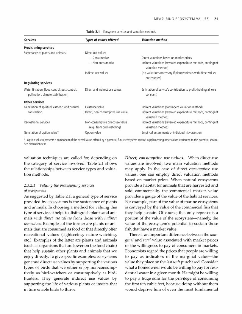
MEASURING ECOSYSTEM VALUES 21
valuation techniques are called for, depending on the category of service involved. Table 2.1 shows the relationships between service types and valua-tion methods.
2.3.2.1 Valuing the provisioning services of ecosystems As suggested by Table 2.1 , a general type of service provided by ecosystems is the sustenance of plants and animals. In choosing a method for valuing this type of service, it helps to distinguish plants and ani-mals with direct use values from those with indirect use values. Examples of the former are plants or ani-mals that are consumed as food or that directly offer recreational values (sightseeing, nature-watching, etc.). Examples of the latter are plants and animals (such as organisms that are lower on the food chain) that help sustain other plants and animals that we enjoy directly. To give specifi c examples: ecosystems generate direct use values by supporting the various types of birds that we either enjoy non-consump-tively as bird-watchers or consumptively as bird-hunters. They generate indirect use values by supporting the life of various plants or insects that in turn enable birds to thrive.
Direct, consumptive use values. When direct use values are involved, two main valuation methods may apply. In the case of direct consumptive use values, one can employ direct valuation methods based on market prices. When natural ecosystems provide a habitat for animals that are harvested and sold commercially, the commercial market value provides a gauge of the value of the habitat services. For example, part of the value of marine ecosystems is conveyed by the value of the commercial fi sh that they help sustain. Of course, this only represents a portion of the value of the ecosystem—namely, the value of the ecosystem’s potential to sustain those fi sh that have a market value.
There is an important difference between the mar-ginal and total value associated with market prices or the willingness to pay of consumers in markets. Economists regard the prices that people are willing to pay as indicators of the marginal value—the value they place on the last unit purchased. Consider what a homeowner would be willing to pay for resi-dential water in a given month. He might be willing to pay a huge sum for the privilege of consuming the fi rst ten cubic feet, because doing without them would deprive him of even the most fundamental
Table 2.1 Ecosystem services and valuation methods
Services Types of values offered Valuation method
Provisioning services Sustenance of plants and animals Direct use values
—Consumptive Direct valuations based on market prices —Non-consumptive Indirect valuations (revealed expenditure methods, contingent
valuation method) Indirect use values (No valuations necessary if plants/animals with direct values
are counted) Regulating services
Water fi ltration, fl ood control, pest control, pollination, climate stabilization
Direct and indirect use values Estimation of service’s contribution to profi t (holding all else constant)
Other services Generation of spiritual, esthetic, and cultural
satisfaction Existence value Indirect valuations (contingent valuation method) Direct, non-consumptive use value Indirect valuations (revealed expenditure methods, contingent
valuation method) Recreational services Non-consumptive direct use value
(e.g., from bird-watching) Indirect valuations (revealed expenditure methods, contingent
valuation method)
Generation of option value * Option value Empirical assessments of individual risk-aversion
* Option value represents a component of the overall value offered by a potential future ecosystem service, supplementing other values attributed to this potential service. See discussion text.
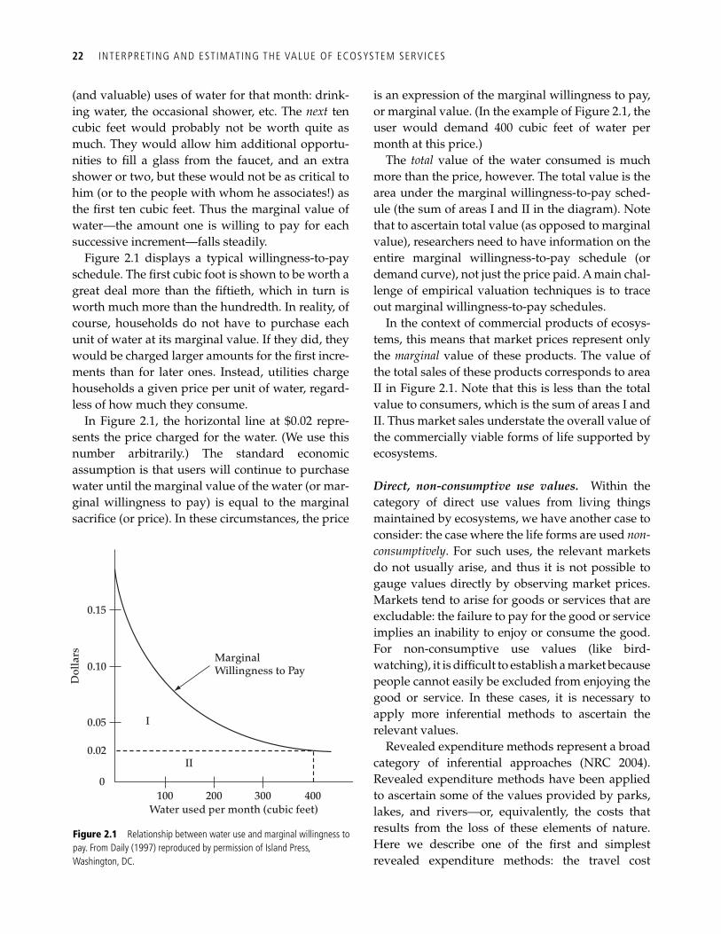
22 INTERPRET ING AND EST IMATING THE VALUE OF ECOSYSTEM SERVICES
(and valuable) uses of water for that month: drink-ing water, the occasional shower, etc. The next ten cubic feet would probably not be worth quite as much. They would allow him additional opportu-nities to fi ll a glass from the faucet, and an extra shower or two, but these would not be as critical to him (or to the people with whom he associates!) as the fi rst ten cubic feet. Thus the marginal value of water—the amount one is willing to pay for each successive increment—falls steadily.
Figure 2.1 displays a typical willingness-to-pay schedule. The fi rst cubic foot is shown to be worth a great deal more than the fi ftieth, which in turn is worth much more than the hundredth. In reality, of course, households do not have to purchase each unit of water at its marginal value. If they did, they would be charged larger amounts for the fi rst incre-ments than for later ones. Instead, utilities charge households a given price per unit of water, regard-less of how much they consume.
In Figure 2.1 , the horizontal line at $0.02 repre-sents the price charged for the water. (We use this number arbitrarily.) The standard economic assumption is that users will continue to purchase water until the marginal value of the water (or mar-ginal willingness to pay) is equal to the marginal sacrifi ce (or price). In these circumstances, the price
is an expression of the marginal willingness to pay, or marginal value. (In the example of Figure 2.1 , the user would demand 400 cubic feet of water per month at this price.)
The total value of the water consumed is much more than the price, however. The total value is the area under the marginal willingness-to-pay sched-ule (the sum of areas I and II in the diagram). Note that to ascertain total value (as opposed to marginal value), researchers need to have information on the entire marginal willingness-to-pay schedule (or demand curve), not just the price paid. A main chal-lenge of empirical valuation techniques is to trace out marginal willingness-to-pay schedules.
In the context of commercial products of ecosys-tems, this means that market prices represent only the marginal value of these products. The value of the total sales of these products corresponds to area II in Figure 2.1 . Note that this is less than the total value to consumers, which is the sum of areas I and II. Thus market sales understate the overall value of the commercially viable forms of life supported by ecosystems.
Direct, non-consumptive use values. Within the category of direct use values from living things maintained by ecosystems, we have another case to consider: the case where the life forms are used non-consumptively . For such uses, the relevant markets do not usually arise, and thus it is not possible to gauge values directly by observing market prices. Markets tend to arise for goods or services that are excludable: the failure to pay for the good or service implies an inability to enjoy or consume the good. For non-consumptive use values (like bird-watching), it is diffi cult to establish a market because people cannot easily be excluded from enjoying the good or service. In these cases, it is necessary to apply more inferential methods to ascertain the relevant values.
Revealed expenditure methods represent a broad category of inferential approaches (NRC 2004). Revealed expenditure methods have been applied to ascertain some of the values provided by parks, lakes, and rivers—or, equivalently, the costs that results from the loss of these elements of nature. Here we describe one of the fi rst and simplest revealed expenditure methods: the travel cost
I
II
1000
0.02
0.05
0.10
0.15
Dol
lars
200 300 400
MarginalWillingness to Pay
Water used per month (cubic feet)
Figure 2.1 Relationship between water use and marginal willingness to pay. From Daily ( 1997 ) reproduced by permission of Island Press, Washington, DC.
MEASURING ECOSYSTEM VALUES 23
method (Freeman 1993). In recent years several more general and sophisticated approaches have tended to supplant the travel cost method, but the basic logic of the newer approaches is the same as that of the travel cost method.
Non-consumptive uses are not directly bought or sold in markets; prices are not usually charged for their use. In those instances when use prices are charged (through entry fees, etc.), the prices are unlikely to be good indicators of (marginal) value. That is because the users of these resources actually “pay” more than the entry fees to use them. For example, the cost of a family visit to Yosemite National Park is much greater than the daily use fee. The travel cost method recognizes that by add-ing to the entry fee (if any) the transportation cost and time cost expended to visit a particular site, one can ascertain the overall travel cost. This method regards the overall travel cost as a measure of the marginal willingness to pay by a visitor to the park; this is considered to be the same as the marginal value of the park to the visitor. The underlying assumption is that people will continue to visit the park until the value of the last unit (that is, the mar-ginal value) is just equal to the travel cost.
It is also possible to employ survey methods, such as the contingent valuation method, to deter-mine how much value people place on the non-consumptive uses. In contingent valuation assessments of value, interviewees are asked what they would be willing to pay in order to prevent some real or hypothetical amenity. For an exposi-tion of this approach, see Mitchell and Carson (1989). Many economists distrust results from sur-vey approaches, claiming that individuals’ asserted preferences in the hypothetical circumstances posed by surveys bear no systematic relationship to their true preferences. Defenders of survey meth-ods counter that, in many cases, surveys are the only method available. This “only game in town” argument may have force when existence values are involved, as discussed below.
Indirect use values. Ecosystems contain many living organisms that support other, often “higher” forms of life that provide direct or indirect value to humans. It could be assumed that the value of ecosystem services should include the values of the
services provided by these life forms. In fact, there is no need to include the values of these services in an accounting of the overall value of an ecosystem! These values are already captured in the values attached to the life forms that humans enjoy. Consider the value of certain plants whose fruits are eaten by birds and other “higher” life forms; assume humans obtain no direct use value from these plants. If we abide by the anthropocentric approach to value, then there is no value to these plants over and above the value that we attach to the higher life forms to which they contribute. To add their indirect use values to the direct use values would be double counting. The accounting here is perfectly analogous to the economic valuation of net economic output, which disregards the value of intermediate inputs, that is, inputs used up in the process of producing fi nal goods such as consumer goods and capital goods.
2.3.2.2 Valuing the regulating services of ecosystems Table 2.1 lists four examples of production inputs from ecosystems: water fi ltration, fl ood control, pol-lination, and climate stabilization. These services are inputs to the sustained production of agricul-tural products in the sense that it would be diffi cult to maintain agricultural production without rela-tively pure water, fl ood control, pest control, or a stable climate.
An appropriate measure of the value of produc-tive inputs is the additional economic income or profi t that they provide, holding everything else constant. Thus, for example, the value of pest con-trol services provided by ecosystems is their contri-bution to profi ts. To assess these values, agronomists and other researchers develop models in which the profi tability of various agricultural products is assessed in the presence and absence of ecosystem-provided pest control, a key production input. The difference is the value of the pest control services. Similarly, one can gauge the value of fl ood control services by comparing profi tability in the presence and absence of such services. A favorable climate can be considered a productive input. Numerous studies have aimed to assess the damage from cli-mate change to agriculture by comparing yields and agricultural profi ts under current climate with those that would apply after predicted future
24 INTERPRET ING AND EST IMATING THE VALUE OF ECOSYSTEM SERVICES
climate change (e.g. Mendelsohn et al. 1994 ; Schlenker et al. 2005). The damage from a changed climate is equivalent to the monetized benefi t or value from avoiding this change.
Pollination services are another example of an important production input. In the Central Valley of northern California, various specialty crops, includ-ing melons, nuts, and tree fruits, depend upon the pollination services supplied by wild bees whose population is maintained by breeding sites in nearby “natural” areas such as undeveloped forest-land. The value of these pollination services is the additional profi t generated by the populations of wild bees.
These pollination services have declined over time as larger and larger proportions of the region have been developed for agricultural purposes. One can only assume that at some point in the develop-mental history of this unusually productive agricul-ture, wild insect populations alone were suffi cient to guarantee some base level of pollination services and thus guarantee yields adequate to keep the farmers in business. Since that is clearly no longer the case, farmers now have to substitute a costly alternative—pollination services from the bees sup-plied by commercial beekeepers. This is now an economically signifi cant activity in these regions. In this example, the avoided cost is the difference in cost between the case where farmers enjoyed free pollination services from wild bees and the case where they must pay for the services of bees hus-banded by commercial beekeepers.
It is sometimes suggested that one can place a value on production inputs by examining what costs or expenditures agricultural producers man-age to avoid by having these inputs and thus not having to substitute other inputs for them. For example, where ecosystems provide effective pest control, farmers can avoid having to pay for alter-native pest control methods such as the use of syn-thetic pesticides. In fact, avoided cost is not a theoretically valid indicator of value. To see this, consider the following (extreme) situation. Suppose it were infi nitely costly for farmers to fi nd an alter-native to wetlands in providing fl ood control. If avoided cost indicated value, then the value of the wetlands’ fl ood control services would be consid-
ered infi nite. In fact, although the loss of fl ood con-trol services would cause a signifi cant loss of profi t to farmers, the loss would not be infi nite.
Although avoided cost is not a measure of value, it is still important information. It indicates the net advantage of having access to the productive input provided by ecosystems, as opposed to having to achieve the same input through an alternative. It provides a rationale for preserving the ecosystem service. For example, when the New York City Water District struggled with how to preserve water quality in the Catskills, it determined that it was far less costly to do so by restoring the ecosystems sur-rounding the city’s upstate reservoirs rather than by constructing a new water treatment plant. The very high avoided cost motivated the decision to pursue ecosystem-generated water quality control (Daily and Ellison 2002).
2.3.2.3 Valuing ecosystem services offering non-use values Other important services include the generation of spiritual, esthetic, and cultural satisfaction, the pro-vision of recreational services, and the generation of option value. Recreational services provide a non-consumptive direct use value. For example, a National Park offers opportunities for hiking, swim-ming, and bird-watching. Park visitors engaging in these activities physically encounter the ecosystems involved (implying a use value), but (hopefully) do not use up the hiking trails, lakes, or birds in the process of enjoying them. The non-consumptive use values from these activities can be estimated using the methods described for such values under Section 2.1 above.
Ecosystems also provide services with values other than use values—values that do not derive from a physical encounter with the item of nature in question. The values provided here are non-use values. There are two main types of non-use value.
Existence value. This is the value that derives from the sheer contemplation of the existence of ecosystems. While much of our enjoyment of biodiversity involves use value—that is, it derives from a physical encountering with various plants
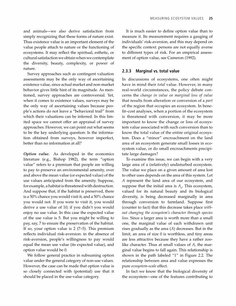
MEASURING ECOSYSTEM VALUES 25
and animals—we also derive satisfaction from simply recognizing that these forms of nature exist. Thus existence value is an important element of the value people attach to nature or the functioning of ecosystems. It may refl ect the spiritual, esthetic, or cultural satisfaction we obtain when we contemplate the diversity, beauty, complexity, or power of nature.
Survey approaches such as contingent valuation assessments may be the only way of ascertaining existence value, since actual market and non- market behavior gives little hint of its magnitude. As men-tioned, survey approaches are controversial. Yet, when it comes to existence values, surveys may be the only way of ascertaining values because peo-ple’s actions do not leave a “behavioral trail” from which their valuations can be inferred. In this lim-ited space we cannot offer an appraisal of survey approaches. However, we can point out what seems to be the key underlying question: Is the informa-tion obtained from surveys, however imperfect, better than no information at all?
Option value. As developed in the economics literature (e.g., Bishop 1982), the term “option value” refers to a premium that people are willing to pay to preserve an environmental amenity, over and above the mean value (or expected value) of the use values anticipated from the amenity. Suppose, for example, a habitat is threatened with destruction. And suppose that, if the habitat is preserved, there is a 50% chance you would visit it, and a 50% chance you would not. If you were to visit it, you would derive a use value of 10; if you didn’t you would enjoy no use value. In this case the expected value of the use value is 5. But you might be willing to pay, say, 7 to ensure the preservation of the habitat. If so, your option value is 2 (7–5). This premium refl ects individual risk-aversion: in the absence of risk-aversion, people’s willingness to pay would equal the mean use value (its expected value), and option value would be 0.
We follow general practice in subsuming option value under the general category of non-use values. However, the case can be made that option value is so closely connected with (potential) use that it should be placed in the use-value category.
It is much easier to defi ne option value than to measure it. Its measurement requires a gauging of individuals’ risk-aversion, and this may depend on the specifi c context: persons are not equally averse to different types of risk. For an empirical assess-ment of option value, see Cameron (1992).
2.3.3 Marginal vs. total value
In discussions of ecosystems, one often might have in mind their total value. However, in many real-world circumstances, the policy debate con-cerns the change in value or marginal loss of value that results from alteration or conversion of a part of the region that occupies an ecosystem. In bene-fi t–cost analyses, when a portion of the ecosystem is threatened with conversion, it may be more important to know the change or loss of ecosys-tem value associated with such conversion than to know the total value of the entire original ecosys-tem. Does a “minor” encroachment on the land area of an ecosystem generate small losses in eco-system value, or do small encroachments precipi-tate large damages?
To examine this issue, we can begin with a very large area of a (relatively) undisturbed ecosystem. The value we place on a given amount of area lost to other uses depends on the area of this system. Let A represent the land area of our ecosystem, and suppose that the initial area is A 0 . This ecosystem, valued for its natural beauty and its biological diversity, is being decreased marginally in area through conversion to farmland. Suppose fi rst (counter to fact) that this decrease takes place with-out changing the ecosystem’s character through species loss. Since a larger area is worth more than a small one, the marginal value of each withdrawn unit rises gradually as the area ( A ) decreases. But in the limit, an area of size 0 is worthless, and tiny areas are less attractive because they have a rather zoo-like character. Thus at small values of A , the mar-ginal value begins to fall again. This relationship is shown in the path labeled “1” in Figure 2.2 . The relationship between area and value expresses the pure ecosystem-scale effect.
In fact we know that the biological diversity of the ecosystem—one of the features contributing to
26 INTERPRET ING AND EST IMATING THE VALUE OF ECOSYSTEM SERVICES
its value to nature lovers—is not area-independent. The relationship, established mainly in studies on islands and (to a more limited extent) on tropical forests, is a non-linear one. The precise form varies, but in a variety of studies the number of species lost is slight until a quarter to a half of the area is lost, and rises precipitously after about three-quarters of the area is lost. The effect on marginal value is to exaggerate the loss of ecosystem value as A is reduced. The impact of the loss in numbers of spe-cies as A is reduced may be termed the diversity effect. This effect is taken into account in the path labeled “2” in Figure 2.2 . As indicated by the differ-ences between paths 1 and 2, this intensifi es the marginal loss of value from a given reduction in A .
A third effect needs to be considered. The species in ecosystem A are not considered to be of equal value to humans. People seem to care more about eagles and panthers than about mosses and bacte-ria. We also know that species are related to one another in a complex, co-evolved web of dependen-cies: prey and predator, plant and pollinator. Trophic relationships are also vitally important. Often, higher order species on the food chain have the most exacting environmental requirements, and are thus valuable indicators of the health of the entire ecosystem; they or others may also be critical “key-stone” species because they are located at the center of a network of interdependencies. Thus, as a
practical matter, species values become proxies for ecosystem values: the Endangered Species Act in the United States is an embodiment of this principle in policy. Of course we regularly justify large expen-ditures to save some species (e.g., the Black Rhinoceros) but not others (there is no Save the Furbish Lousewort Society).
On what basis do we assign value to species? The following are some axes along which different peo-ple make selections.
Taxonomic proximity . We like animals that are like us. Primates attract human attention not only because there may be utility in the relationship (“animal models” for human disease) but because we respond to their quasi-human qualities. Rarity . All other things being equal, we have more interest in rare things than in common ones. This is not simply a matter of vulnerability, although it is true that rare organisms are more vulnerable to extinction than abundant ones. Rarity itself can be the attraction; in some sense animals and plants in nature are “collectibles,” if only in the sense of fi nd-ing and listing them, and collections of the rare are more desired than collections of the commonplace. Indeed, “collection” in the form of listing is a motive with powerful economic consequences. Many bird-watchers will undertake extreme expenditures to visit ecosystems harboring rare species for the pur-pose of expanding their “life-lists.” Genetic uniqueness . If a species represents a unique evolutionary line—is, for example, the only extant member of its genus or family—then it may be enti-tled to higher value than it would otherwise. Scientists especially would favor the use of this criterion. Importance to ecosystem function . Certain species (often called “keystone” species) create conditions that permit the maintenance of the entire ecosys-tem. The dominant trees in a forest, or birds that dig nest-holes in trees that are used by other species, or insects vital to the pollination of a dominant plant, would be examples.
How can these preferences be related to the mar-ginal value calculation? Biological diversity is reduced as A shrinks, but species do not fall out randomly; certain kinds tend to drop out relatively early, others only when A becomes quite small. For
Tota
l Val
ue
Area (A)
(2)
(1)
(3)
A0
Figure 2.2 Relationship between loss of habitat area and loss of ecosystem value viewed through three different dimensions: ecosystem scale effect (1), diversity effect (2), and species effects (3). A o denotes the initial area of the ecosystem and the curves show how value declines as that initial area is reduced. In all cases there is some threshold area that is too small to support any value.
SOME CASE STUDIES 27
conservation biologists and others, this means that wise policies cannot be made unless some value is attached to the different kinds. If, for example, the ones we view as most valuable did well in relatively small areas, we might argue for a patchwork of little parks, whereas if the opposite were true we would insist on large refuges.
Obviously the number of possible criteria is large enough to prohibit development of a precise rela-tionship among area, species loss, and value. However, larger organisms with broad ranges that are especially area-sensitive would be likely to be rarer, on average closer taxonomically to humans, favored for “charm,” and important to ecosystem function. Thus it is reasonable to assume a species-composition effect : that as A is reduced, the species lost early in the reduction are more valuable than those lost later. When this effect is taken into account, the marginal loss from a reduction in species area is even greater than indicated by path 2. Path 3 incor-porates this effect (and the others). Indeed, our anal-ysis applies specifi cally to the simple case in which A is reduced by shrinkage from the outside edges. In many situations, the reduction occurs by fragmenta-tion—a patch here, a patch there, leading to a check-erboard of “natural” and “modifi ed” areas. The new habitats provided by “edge effects” can raise local biodiversity (at least transiently). In the longer run the area/diversity rule will apply over the entire region, but the value of species lost may differ. In recent studies of plant diversity in grassland patches, the fi rst species lost are the most effective, narrow-niche competitors: fragmentation gives an advan-tage to those species adept at dispersal and at rapid colonization ( Tilman 1997 ).
Clearly some of these relationships are uncertain, and the exercise could be applied to real natural areas only after substantial research. However, it points up the importance of thinking about value in marginal rather than aggregate terms, and suggests a discipline that could be applied in the framing of general conservation policy.
2.4 Some case studies
2.4.1 Wetlands in the United States
Wetlands provide important ecosystem services, including fl ood control, water purifi cation, and pro-
vision of habitat for numerous species. The values of these and many other services are very diffi cult to quantify. Perhaps even more important to the measurement challenge is the complexity of the net-work that links wetlands to groundwater and thence to streams and lakes and other “navigable waters.”
In theory, society could decide on the desired level of protection of wetlands and their ecosystem serv-ices by calculating the values of the numerous eco-system services, determining the extent of wetlands that maximizes the net benefi ts from these services minus the opportunity cost to society, and then implementing laws that protect just this amount of wetland. In fact, wetland protection has largely ignored valuation. In the United States, the law does not invoke an explicit comparison of benefi ts or costs as a basis for the protection offered; this may partly refl ect the measurement diffi culties just men-tioned. Indeed, US law does not even acknowledge cost as a consideration in determining the extent to which wetlands or their services are to be protected. Rather, these broad ecosystem services are treated like a public “right,” something to be safeguarded irrespective of the cost of protection.
That right is protected by two public agencies under several laws. The Clean Water Act, adminis-tered through the Environmental Protection Agency, has several sections devoted to wetlands protection, and these refer to the general set of the “navigable waters” referred to above. The Food Quality Protection Act has a provision colloquially known as the “swampbuster” clause that prohibits the drainage or alteration of wetlands for farming pur-poses. That provision is administered by the US Army Corps of Engineers. These two agencies are required to issue permits when a landowner under-takes measures that would contribute fi ll or pollut-ants to wetlands that lay within the drainage system of the owner’s property. In an important wetlands case called Borden Ranch, the Supreme Court ruled that a California farmer could not be issued a per-mit for a technique of plowing called “deep rip-ping,” on the grounds that it violated provisions of the Clean Water Act. In short, the Court found that the connection of the groundwater under the farm-er’s plow to the navigable waters could not be dis-turbed or interrupted.
28 INTERPRET ING AND EST IMATING THE VALUE OF ECOSYSTEM SERVICES
In a much later case, the Supreme Court again split about a proposal to fi ll some wetlands near Lake St. Claire in Michigan. This particular wetland was some distance from the lake, which clearly fi t any ordinary defi nition of a “navigable water.” Once again, the issue rested on the question on whether a wetland that is distant from clearly navigable sur-face waters is nevertheless entitled to protection. The responsibility, again shared by the Environmental Protection Agency and the Army Corps of Engineers, was complicated once again by the ambiguity of the Clean Water Act’s language. A four-four split on the Court was eventually decided by Justice Kennedy, who wrote in his opinion that the Clean Water Act intended to apply its provisions to the nation’s waters generally, not restricted to surface waters. However, he also argued that the case should be ultimately decided scientifi cally by the federal agen-cies responsible for applying the protection.
This case exemplifi es the diffi culty of interpreting Congressional intention. It also highlights the diffi -culties of measuring ecosystem values in a network of rivers, lakes, wetlands, and groundwater that is diffuse, interconnected, and complex. In the face of such diffi culties, policy-makers might prefer simply to establish a broad right to protection, rather than aim to compare values gained and values sacrifi ced under alternative levels of protection.
2.4.2 Vegetation and coastal protection
About one-third of the world’s population lives in coastal areas or small islands, and they are at risk from buffeting and damage from storms and extreme weather events, like the hurricanes that regularly visit Caribbean and Gulf of Mexico coast-lines and the recent tsunamis that swept across Indonesia and coastlines in the south Pacifi c and Indian Oceans. In coastal areas, societies often must make diffi cult choices between economic develop-ment activities and risk-reducing conservation measures. Decision-makers practicing ecosystem-based management are required to address both of these competing needs in a way that balances the welfare of residents. In order to do this, they must be able to measure the values associated with the ecosystem services provided by conservation meas-ures (see Box 2.1 ).
This problem has been analyzed by Barbier and a team of fi fteen authors (Barbier et al. 2008; Box 17.1 in this book) from various international institutions. Their analysis examined the trade-offs between conservation of coastal mangroves in Thailand and the conversion of mangrove lands to shrimp aquac-ulture. The authors of the study started with the reasonable assumption that the buffering capacity of the mangroves would depend on their area. On measuring the ocean wave attenuation at various distances inland from the shore, they showed that the storm buffering service provided by the man-groves was in fact nonlinear owing to the shape of the declining wave attenuation.
Using the estimated nonlinear relationship, Barbier et al. (2008) found that the policy that pro-vides the greatest overall benefi t to the local popu-lation is one that prohibits shrimp aquaculture in much, but not all, of the area in question, and thus reserves some area for shrimp farming ponds. Some economic benefi ts to aquaculture investors were retained. (In contrast, the assumption of a linear relationship between area conserved and buffering capacity would have suggested that pro-hibition of all shrimp farming was optimal.) This signifi cant effort at ecosystem service valuation provided the basis for a solution favoring both stakeholders—both conservation groups and inves-tors in aquaculture.
2.4.3 The Galapagos Islands
A third example, international in character, is pro-vided by the Galapagos Islands. This archipelago, located 600 miles west of the Ecuador coast, consists of thirteen large islands and a number of smaller ones. All are of recent volcanic origin (100 000 to a 1 000 000 years old), and they contain a unique assemblage of plants and animals. They were vis-ited by Charles Darwin during the voyage of the Beagle , and now are an important site for contempo-rary studies of evolutionary biology.
Managed as a National Park by Ecuador since the 1950s, the islands have also become a favorite destination for tourists, who explore the islands from boats and debark on the islands to follow carefully marked trails in the company of trained naturalist-guides. With the growth in popularity of

SOME CASE STUDIES 29
R. K. Turner
Depending on the precise defi nition used, coastal zones occupy around 20% of the earth’s surface but host more than 45% of the global population and 75% of the world’s megacities (> 10 million inhabitants). The zone’s underpinning coastal ecosystems—coral reefs, mangroves, salt marshes and other wetlands, sea grasses and seaweed beds, beaches and sand dunes, estuaries and lagoons, forests and grasslands—necessary to sustain human occupation, are highly diverse, productive, and biocomplex. These ecosystems provide a range of services, such as, nutrient and sediment storage, water fl ow regulation and quality control, and storm and erosion buffering, summarized in Table 2.A.1 ( Crossland et al . 2005 ). Coastal zones are impacted by dynamic environmental changes that occur both ways across the land–ocean boundary. The natural and anthropogenic drivers of change (including climate change) cause impacts ranging from erosion, siltation, eutrophication, and over-fi shing to expansion of the built environment, and inundation due to sea level rise. All coastal zone natural capital assets have suffered signifi cant losses over the past three decades (e.g., 50% of marshes lost or degraded, 35% of mangroves, and 30% of reefs) (MA 2005). The consequences for services and economic value of this loss at the margin are considerable but have yet to be properly recognized and more precisely quantifi ed and evaluated ( Daily 1997 ; Turner et al. 2003; Barbier et al. 2008).
The ecosystem services (storm buffering) valuation example illustrated below is drawn from the European coastal zone context and in particular the east coast of England, which is one of UK’s most “at-risk” areas from climate change and other impacts. The European coastal zone is around 600 000 km 2 (within 10 km of shorelines) and home to 80 million people and 280 major cities. The annual value of coastal tourism alone is 75 billion EUR ( The Changing Faces of Europe’s Coastal Areas (2006): http://reports.eea.europa.eu/eea_report_2006_6/en). In response to the multitude of pressures bearing down on coastal areas, coastal protection and sea defense policy in the UK and Europe is being reappraised and reoriented toward a more fl exible and adaptive strategy anchored to an ecosystem services approach and decision support system (Turner and Daily 2008; Turner et al. 2008).
The Millennium Ecosystem Assessment (MA 2005) states that “ecosystem services are the benefi ts people obtain from ecosystems” and subdivides them into supporting,
regulating, provisioning, and cultural services. Building on this platform, it can be argued that when the focus is on national accounting (Boyd and Banzhaf 2007), or landscape management (Wallace 2007), or in our example valuation of service benefi ts (Fisher et al. 2008), further elaboration is required for actual choice-making involving human welfare. A key step is the separation of ecosystem processes and functions into intermediate and fi nal services, with the latter yielding welfare benefi ts (see Table 2.A.1 ).
The generation of services and the enjoyment of benefi ts is spatially conditioned and therefore a key step in any evaluation process must be the setting of the ecosystems in their appropriate contexts. The valuation process must also be restricted to marginal gains/losses and should avoid double counting and should note possible threshold effects and any nonlinearity between change in ecosystem services and habitat variables such as size of area. Failure to account for these limitations will lead to under-/overestimated economic values and unnecessarily polarized cost–benefi t decision choices (Turner 2007; Barbier et al. 2008).
Traditional sea defense and coastal protection strategies in Europe have sought to provide rigid engineered “hold-the-line” protection for people, property, and other assets against the vagaries of dynamic coastal environments. Given the growing awareness of the consequences of climate change a policy switch is taking place toward a “coping strategy” based on a mixed approach with engineered protection focused on high commercial value areas, and the rest of the coastline left to adapt to change more naturally. Measures such as “managed realignment,” which involves the deliberate breaching of engineered defenses to allow coastal migration and the creation of extended intertidal marshes and mudbanks, at the expense of agricultural land, are now being tested. Testing sites have been carefully chosen to minimize impacts on existing people, property, and environmental assets that enjoy engineered protection from the sea. The question is do they represent cost-effective strategies for society?
Managed realignment schemes yield benefi ts in terms of ecosystem services. They generate carbon storage benefi ts (via saltmarsh creation) that can be valued in terms of the damage costs avoided per tonne of CO 2 . The sites also serve to improve fi sheries’ productivity via nursery areas and this gain can be valued via market prices for commercial species. There are also general recreation and amenity benefi ts related to walking, bird-watching, and other recreational activities, as well as biodiversity
Box 2.1 Designing coastal protection based on the valuation of natural coastal ecosystems
continues

30 INTERPRET ING AND EST IMATING THE VALUE OF ECOSYSTEM SERVICES
Table 2.A.1 Coastal zone services * and benefi ts
Intermediate services Final services Benefi ts Econ valuation methods
e.g:• Geodynamics: sediment and
nutrient cycling and transport • Primary production • Water cycling • Climate mitigation
e.g:• Creation of beaches,
dunes, estuaries • Sediment, nutrients,
contaminants retention/storage
• Biomass export • Maintenance of fi sh
nurseries and refuges • Regulation of water fl ow
and quality • Carbon sequestration • Recreation and amenity • Cultural heritage
e.g:• Flood/storm buffering • Shoreline stabilization/erosion control • Fish production • Biodiversity maintenance • Carbon storage • Amenity and recreation activities • Cultural/heritage conservation
e.g:• Market prices/damage cost avoided • Production function market prices • Survey-based contingent valuation/
choice experimentation • Damage cost avoided • Travel cost, hedonic pricing, survey
based CV or CE • Survey based CV or CE
*. European coastal areas including estuaries and saltmarshes.
Box 2.1 continued
maintenance and existence value benefi ts. An indication of the composite value of some of these amenity and related benefi ts can be estimated by transferring benefi ts data from the published literature if the spatial and other contextual variables are similar, or, more properly, by conducting site-specifi c contingent valuation/choice experiment studies to estimate willingness-to-pay values. Finally, the maintenance costs of the existing engineered defenses will be saved as realignment schemes are implemented. On the costs side, secondary defenses may be required further inland and there are opportunity costs associated with any agricultural land that is sacrifi ced as the old defenses are breached.
Cost–benefi t analysis of managed realignment schemes took the following approach.
The “status quo” existing protection system is appraised as follows:
sq sq sqt m, t
0
1[( )],
(1 )== −
+∑T
t
t
PVr
I C (2.A.1)
where PV sqt is the present value of total costs of current
defenses (£million), r is the discount rate, l sq is the length of defenses and C sq
m,t is the maintenance costs (£km –1 yr –1 ).
The costs and benefi ts of managed realignment is given as follows:
=
⎡ ⎤+= ⎢ ⎥− −+ ⎢ ⎥⎣ ⎦
∑ l C CPV
a L a Br
mr mr mrTk, t m, tmr
t agrmr mrtt 0 t agr, t h e, t
( )1( ) ( )(1 )
(2.A.2)
where mrtPV is the present value of managed realignment
schemes (£million), l mr is the length of managed realignment (km), Cmr
k,t is the capital cost of realignment, Cmr
m,t is the maintenance costs, amrt is the agricultural land
lost, Lagragr, t is the forgone agricultural land value, amr
h is the area of intertidal habitat created, and B e,t is the ecosystem value benefi ts (£ha –1 ).
Finally, the overall CBA result is found as:
NPV PV PV( )= −mr sq mrt t t (2.A.3)
where NPV mrt is the net present value of managed
realignment compared to hold-the-line for a given stretch of coastline at time t (£million).
The analysis was carried out with data from a number of different estuaries, and indicates that appropriately sited schemes do represent gains in economic effi ciency if declining discount rates are applied over a 100-year time horizon (see Turner et al. 2007 and Luisetti et al. 2008 for further details).
CONCLUSIONS 31
“ecotourism,” the Galapagos now attract over 150 000 visitors each year.
There is a resident population on several of the larger islands, with a few service industries and a subsistence economy that depends on agriculture and fi shing. These have been augmented by other direct uses that compete with the “natural” state of the larger islands, whereas recent reports suggest that the less occupied islands are doing better than they did 25 years ago. A signifi cant fi shery for sea cucumbers, a delicacy prized in Asian and French cuisine, developed in the 1990s and still exists, although the catch is declining. Illegal long-line shark fi shing continues to create a problem. Not only do these activities threaten the intertidal fauna, they pose signifi cant risks to the terrestrial ecosys-tem through the introduction of “exotic” species and destructive camping on some islands. Fortunately, the Park’s protection system is much more effective now than in the past, and efforts to eradicate goats, cats, and other invasive species are continuing, most effectively on the four smaller, less-inhabited islands.
Arrayed against these direct, consumptive use values are two other values. The fi rst is the direct, non-consumptive use value from ecotourism, which brings signifi cant revenue. A sample calcula-tion of this value would be that the average visitor (a week on a boat is a typical excursion) spends well more than $10 000. If the visitor is from the USA, additional revenue will accrue to the Ecuadorian economy through accommodations on the mainland, the fl ight to the islands, and (if a national carrier is used) the fl ight to Quito or Guayaquil. A total per-visit value of $15 000 would be a reasonable fi gure for the “overseas” visitor: if half were Ecuadorian nationals and half from else-where, the value of the industry would approach one billion annually.
Local residents, however, would make quite a different calculation. The shops and restaurants at Puerto Ayora collect some money, and the support of the Darwin Station by tourists fl ows into the local economy. Some boat operators are islanders, and some services for all vessels are locally provided. However, the vast majority of the revenue fl ows to tour operators, many of them non-Ecuadorian, and to other off-island entities.
Thus it is not surprising that a sometimes violent controversy has arisen over the protection of the islands. When the government closed the sea cucumber fi shery in 1994 because the catch limit was being vastly exceeded, fi shermen and some other local residents seized the Darwin Station and took scientists hostage. In a political controversy over a bill that would have given the islanders more local autonomy (and relaxed many of the ecological protections) there was another takeover. The tense historical contest between extraction and conserva-tion in the Galapagos is, at least with respect to this particular indirect use value, the result of distribu-tional effects. The economic potential of ecotourism is almost certainly greater than that of the resource-extraction uses. Yet the residents retain most of the rents from the second, and little from the fi rst.
A second use value stems from the (uncertain) future benefi ts that would emanate from the scien-tifi c research underway on the Galapagos. The large number of endemic species found there, and the recentness of their evolutionary divergence from mainland relatives, make the islands a living labo-ratory for studies of species formation. Important recent work (see Grant 1986) depends on the integ-rity of the ecosystems of certain islands. Calculating its value, of course, would be extremely diffi cult.
Finally, there are two important non-use values. First, as in the case of the wetland example, people who have never been to the Galapagos and never expect to may experience a loss of existence value that they would willingly pay to avoid. The unique quality of the islands and the considerable publicity they have received as a mecca for naturalists gives this consideration a weight it might lack in less spe-cial areas. In addition, in the presence of uncertainty, people might be willing to pay a premium (over and above the expected future use value) to ensure the preservation of the unique fl ora and fauna of the islands. This is the option value.
2.5 Conclusions
Society must often make diffi cult choices about how and how much to protect natural capital and the ecosystem services such capital generates. Perhaps the most important basis for supporting a policy that would protect otherwise threatened ecosystem
32 INTERPRET ING AND EST IMATING THE VALUE OF ECOSYSTEM SERVICES
services is evidence that society gains more value from such protections than it gives up. This requires an assessment of the values that human beings place on such services—values that often are not expressed in markets.
In this chapter we have aimed to clarify the philo-sophical underpinnings of these values. The most prevalent and perhaps most workable philosophi-cal basis is anthropocentric—value consists in the ability to provide satisfaction or well-being to humans. Although anthropocentric, this approach is consistent with society’s making great sacrifi ces in order to protect valued species and ecosystem services.
We have also indicated the various types of value generated by ecosystem services, and laid out prin-cipal empirical methods for measuring these val-ues. None of the empirical approaches is perfect; the uncertainties in measurement can be vast. However, even with the imperfections the methods generally are good enough to provide a basis for public policies to protect ecosystem services. The InVEST models described throughout this book represent the frontier in valuing ecosystem services. These models exemplify the substantial progress of the past decade in researchers’ abilities to depict the gains and losses associated with the protection of a wide range of ecosystems and their services.
Many of the benefi ts from ecosystem services are not captured by unregulated markets. An individu-al’s private gain from protecting ecosystem services falls short of the value of such protection to society. Hence private markets tend to fail to provide suffi -cient protection, and there is an important role for public policy to protect these services.
Two types of public policy could stem from the information offered by the InVEST models and other empirical studies. One is the introduction of quantitative restrictions that restrict the way natu-ral capital gets used or converted and thereby pro-tect the services such capital generates. Limits on wetland conversion, for example, help protect the various ecosystem services (fl ood control, water purifi cation, and habitat provision) that wetlands offer. Another approach is the introduction of prices for ecosystem services—prices that the market would not generate on its own. For example, a tax on wetland conversion would serve to reduce the
rate of such conversion. According to economic theory, the tax rate should be set equal to the mar-ginal value of the ecosystem services provided by the natural capital or ecosystem in question. This tax rate would lead to a lowered frequency of con-version that maximizes the net gain to society from intact wetlands—the benefi t to agriculture minus the lost ecosystem service value. In many cases, the tax would prevent any conversion from taking place. These are instances in which the marginal value of the existing ecosystem services exceeds the marginal value generated by any conversion or alternative use of the natural capital.
Although our discussion acknowledges a key role for benefi t–cost analysis in the valuation of eco-system services, we would emphasize that such analysis is usually not suffi cient for deciding policy. Benefi t–cost analyses yield useful information on aggregate net benefi ts under alternative policy sce-narios, but usually ignore issues of fairness or dis-tribution. These analyses need to be accompanied by an assessment of the distribution of the gains and losses, both across the current generation and between current and future generations. If a pro-posed policy clearly would lead to serious inequi-ties, it is reasonable to reject the policy, even if it passes a benefi t–cost test.
The topics of valuation and policy choice raise a number of imponderables. In arriving at the social value of a given option, should every person’s will-ingness to pay count equally, or should some mem-bers be given more weight than others? Are the preferences of sophisticated ecologists worth more than those of city-dwellers who evidence neither knowledge of nor interest in “nature”? How much weight should we give to the preferences or well-being of future generations, as compared to that of current inhabitants of the planet? How can we gauge the preferences of future generations in attempts to ascertain the gains or losses they might experience under different policies?
The fact that these questions have no easy answers need not make us pessimistic about the prospects for sensible public policy. We can go a long way toward improving policy-making by calling atten-tion to the underlying philosophical questions, by developing empirical methods that generate better information about the gains and losses at stake
CONCLUSIONS 33
under alternative public policies, and by develop-ing channels for communicating this information to the general public.
References
Barbier, E., Koch, E., Silliman, B., et al. (2008). Coastal eco-system-based management with nonlinear ecological functions and values. Science , 319 , 321–3.
Bishop, R. C. (1982). Option value: an exposition and extension. Land Economics , 58 , 1–15.
Boyd, J., and Banzhaf, S. (2007). What are ecosystem serv-ices? Ecological Economics , 63 , 616–26.
Cameron, T. (1992). Nonuser resource values. American Journal of Agricultural Economics , 74 , 1133–7.
Costanza, R., Norton, B., and Bishop. R. C. (1995) The evo-lution of preferences: Why sovereign preferences may not lead to sustainable policies and what to do about it . SCASSS workshop on Economics. Ethics and the Environment, Sweden.
Crossland, C. J., Kremer, H. H., Lindeboom, H. J., et al. , Eds. (2005). Coastal fl uxes in the anthropocene , IGBP Series. Springer, Berlin.
Daily, G. C., Ed. (1997). Nature’s services: Societal depend-ence on natural ecosystems. Island Press, Washington, DC.
Daily, G. C., and Ellison, K. (2002). The New Economy of Nature. Island Press, Washington, DC.
Fisher, B., Turner, K., Zylstra, M., et al. (2008). Ecosystem services and economic theory: integration for policy-relevant research, Ecological Applications , 18 , 2050–67.
Freeman, A. M. (1993). The Measurement of Environmental and Resources Values: Theory and Methods . Resources for the Future, Washington, DC.
Grant, P. (1986). Ecology and Evolution of Darwin’s Finches . Princeton University Press, Princeton.
Luisetti, T., Turner, R. K., and Bateman, I. J. (2008) An ecosystems’ services approach to assess managed realign-ment coastal policy in england , CSERGE Working Paper, ECM 2008–04,CSERGE, University of East Anglia, Norwich.
Mendelsohn, R., Nordhaus, W., and Shaw, D. (1994) The impact of global warming on agriculture: a Ricardian analysis. American Economic Review , 84 , 753–71.
Millennium Ecosystem Assessment (MA) (2003). Concepts of ecosystem value and valuation approaches. In Ecosystems and Human Well-being, A Framework for Assessment; A Report of the Conceptual Framework Working Group of the Millennium Ecosystem Assessment . Island Press, Washington, DC.
Mitchell, R. C., and Carson, R. T. (1989). Using Surveys to Value Public Goods: The Contingent Valuation Method . Resources for the Future, Washington, DC.
National Research Council (NRC) (2004). Valuing Ecosystem Services: Toward Better Environmental Decision-Making . National Academies Press, Washington, DC.
Schlenker, W., Hanemann, W. M., and Fisher, A. (2005). Will US agriculture really benefi t from global warming? American Economic Review , 95 , 395–406.
Singer, P. (1975). Animal Liberation . Random House, New York.
Skidmore, J. (2001). Duties to animals: The failure of Kant’s Moral Theory. Journal of Value Inquiry , 35 , 541–59.
Tilman, D. (1997). Biodiversity and ecosystem functioning. In G. C. Daily, Ed., Nature’s Services: Societal Dependence on Natural Ecosystems . Island Press, Washington, DC.
Turner, R. K. (2007). Limits to CBA in UK and European environmental policy: Retrospects and future prospects. Environmental and Resource Economics , 37 , 253–69.
Turner, R. K., Burgess, D., Hadley, D., et al . (2007). A cost-benefi t appraisal of coastal managed realignment policy. Global Environmental Change , 17 , 397–407.
Turner, R. K., and Daily, G. C. (2008). The ecosystem serv-ices framework and natural capital conservation. Environmental and Resource Economics , 39 , 25–35.
Turner, R. K., Georgiou, S., and Fisher B. (2008). Valuing ecosystem services: The case of multifunctional wetlands . Earthscan, London.
Wallace, K. J. (2007). Classifi cation of ecosystem services: Problems and solutions. Biological Conservation , 139 , 235–46.
Watson, R. A. (1983) A critique of anti-anthropocentric bio-centrism. Environmental Ethics , 5 , 245–56.
34
CHAPTER 3
Assessing multiple ecosystem services: an integrated tool for the real world Heather Tallis and Stephen Polasky
3.1 Today’s decision-making: the problem with incomplete balance sheets
Conservation and natural resource management have been dominated by approaches that focus on a single sector and a single objective. These approaches often fail to include a wider set of consequences of decision-making. For example, maximizing profi t from industrial production often leads to negative impacts on air quality and human health. Maximizing agricultural production often leads to poor water quality and in some cases losses of productivity in downstream fi sheries. Maximizing biodiversity con-servation can come at the cost of local jobs, food pro-duction, and other important benefi ts.
Many of these consequences are the result of management decisions that overlook the broad suite of ecosystem conditions and processes that sustain and enrich human life. Ecosystem services, defi ned as the contribution of ecosystem conditions and processes to human well-being, include the production of goods (such as agricultural crops, seafood, timber, and natural pharmaceuticals), processes that control variability and support life (climate regulation, fl ood mitigation, pollination, and the provision of soil fertility and clean water), enrich cultural life (recreational opportunities, and satisfaction of aesthetic and spiritual needs), and preserve options ( Ehrlich and Ehrlich 1981 ; Daily 1997 ; MA 2005).
In most cases and for most services, there is little incentive for business managers and local landown-ers to account for the provision of ecosystem serv-ices in their decision-making. Landowners receive fi nancial rewards for producing crops or for devel-
oping their land as real estate. They typically do not receive fi nancial rewards for providing public goods from ecosystems, such as pollution fi ltration or fl ood mitigation. For example, in tropical coastal ecosys-tems, mangroves are routinely cleared for shrimp aquaculture. People clearing the mangroves receive high market prices for the shrimp they produce but they do not bear the full costs associated with the loss of habitat for coastal fi sheries, storm surge pro-tection ( Das and Vincent 2009 ), pollution fi ltration, or the loss of other ecosystem services provided by mangrove ecosystems. A more complete accounting shows that maintaining mangroves generally pro-vides greater benefi ts for society than shrimp aquac-ulture provides ( Sathirathai and Barbier 2001 ; Barbier 2007 ). A single-sector approach, which ignores the multitude of connections among compo-nents of natural and social systems, generally fails to provide as high a value to society as would manage-ment that accounted for the full range of social benefi ts.
3.2 The decision-making revolution
In this chapter, we outline the major challenges in taking an integrated approach to decision-making, and present a new spatially explicit modeling tool that takes critical steps toward addressing these challenges. The inclusion of ecosystem services in decision-making provides a framework that ena-bles managers to broaden their perspectives by con-sidering the multiple, interlinked consequences of their decisions. Our approach builds from the Millennium Ecosystem Assessment (MA), which contributed substantially to our understanding of
THE ECOLOGICAL PRODUCTION FUNCTION APPROACH 35
how to take such an approach at a global scale (MA 2005). Within a year of its completion, fi ndings from the MA were incorporated into the Convention on Biological Diversity, the RAMSAR Convention on Wetlands, and the Convention to Combat Desertifi cation ( Boerner 2007 ). Despite the overall success of the MA at the global scale, we are still left with the grand challenge of bringing useful models and information to bear at local, regional, and national scales where most decisions are made. Although ecosystem service assessment has been attempted at sub-global scales ( Imperial 1999 ) there are no systematic tools that can be applied in a gen-eral, consistent way across sites at the spatial scales and time frames relevant to major decisions affect-ing ecosystems.
One of the most challenging aspects of creating such tools is integrating robust ecological models and understanding in “ecological production func-tions” that defi ne how the spatial extent, structure, and functioning of ecosystems determine the pro-duction of ecosystem services. This challenge is par-ticularly acute with ecosystem functions and services that operate across ecosystem boundaries (such as nutrient transport from land to sea) and across spatial scales ( Engel et al. 2008 ).
A second major challenge of including ecosystem services in specifi c decisions is generating estimates of the value of ecosystem services in economic and other terms. This task requires linking ecological models and understanding with social and eco-nomic methods to reveal the values people hold for different ecosystem services (NRC 2005). This task is especially hard for the many ecosystem services that generate global public benefi ts, such as climate regulation or existence value of species, for which there are no market prices or other readily available signals of value. Over the past 40 years or so, econ-omists have developed a number of methods and tools for “non-market valuation” that can be applied to estimate the value of ecosystem services ( Freeman 2003 , NRC 2005). Whether for market or non-market values, appropriately linking social and economic valuation with ecological produc-tion functions is necessary to ensure that values refl ect underlying ecological conditions. We describe these challenges further below and offer plausible solutions.
3.3 The ecological production function approach
An ecological production function specifi es the out-put of ecosystem services provided (“produced”) by an ecosystem given its condition and processes. These functions vary spatially due to site- and eco-system-specifi c relationships. Once an ecological production function is specifi ed, researchers can quantify the impact of landscape change on the level of ecosystem service outputs. In the twentieth century, human alteration of ecosystems on a large scale, such as the conversion of native ecosystems to monoculture agriculture, led to an increase in some provisioning services (e.g., food production) at the expense of many regulating, supporting, and cultural services ( Vitousek et al. 1997 ; MA 2005).
Most applications of an ecological production function modeling approach have been done at small scales or for a small set of services. There are a growing number of such studies (e.g., Ellis and Fisher 1987 ; Barbier and Strand 1998 ; Wilson and Carpenter 1999 ; Barbier 2000 ; Kaiser and Roumasset 2002 ; Ricketts et al. 2004 ) and useful overviews and summaries have been compiled ( Pagiola et al. 2004 ; NRC 2005; Barbier 2007 ). One of the most challeng-ing tenets of production functions is to integrate modeling across multiple services. The essential next step toward informing decision-making is a systematic approach that combines the rigor of the small-scale studies with the breadth of broad-scale assessments. Recent work has taken strides in this vein (e.g., Boody et al. 2005 ; Jackson et al. 2005 ; Antle and Stoorvogel 2006 ; Naidoo and Ricketts 2006 ; Nelson et al. 2008 , 2009 ).
There are some cases where an understanding of ecological production functions alone is suffi cient. Many government agencies make decisions about what activities will be allowed based on whether or not they meet an environmental standard. For example, an agency may assess how activities will likely affect the ability of an ecosystem to meet water quality standards. Their decision is not based on how much it would cost to treat that water for consumption or the value of access to clean drink-ing water, but rather on the expected change in con-taminant levels or the likelihood of crossing a contamination threshold. In these cases, simply
36 ASSESS ING MULTIPLE ECOSYSTEM SERVICES
knowing how ecosystem services will change in biophysical terms is informative and useful.
Other decisions are tied to fi nancial costs and benefi ts, and many decision-makers are conditioned to analyzing policy alternatives in terms of the net benefi ts measured in monetary terms. One concern about keeping measurement of ecosystem services in biophysical units is that services not measured in monetary terms may not be given full weight in decision-making or may be ignored altogether ( Daily 1997 ). In these cases it can be very useful to combine ecological production functions with eco-nomic valuation methods to estimate and report the monetary value of ecosystem services.
Some ecological production function approaches have been combined with appropriate market prices and non-market valuation methods to estimate eco-nomic value, and illustrate the change in the mone-tary value of services with changing environmental conditions (e.g., Swallow 1994 ; Naidoo and Ricketts 2006 ; Barbier 2007 ). Ecological production functions can be used to determine how the provision of vari-ous market goods and services change as ecosystem conditions or processes change. The value of the changes in output of marketed goods and services can be evaluated using market prices for marginal changes or by using changes in consumer and pro-ducer surplus for non-marginal changes ( Just et al. 2004 ; Barbier 2007 ). Non-market valuation meth-ods, including revealed preference and stated pref-erence methods, can be used for ecosystem services that are not traded in markets ( Freeman 2003 ; NRC 2005). At present, however, we lack comprehensive studies that tie together economic valuation meth-ods with ecological production functions to esti-mate the monetary value of ecosystem services both for a broad range of ecosystem services and at a broad geographic scale (NRC 2005, but see Naidoo and Ricketts 2006 ).
Detailed non-market valuation studies appro-priate to a particular service in a particular place tend to be time- and-resource intensive, limiting the applicability to broad-scale assessments. Benefi t transfer provides a less time-intensive approach than production functions for generat-ing broad-scale monetary estimates of ecosystem services. Benefi t transfer studies of the value of ecosystem services have garnered signifi cant inter-
national attention especially following Costanza et al. ( 1997 ), which estimated the monetary value of ecosystem services for the entire planet. The most common application of the benefi t transfer approach uses estimates of the value of services per unit area from a single or small number of locations and applies this value to other locations with the same ecosystem type (e.g., Costanza et al. 1997 ; Konarska et al. 2002 ; Troy and Wilson 2006 ; Turner et al. 2007 ). This approach relies on existing estimates and does not require any additional analysis, which is a distinct advantage if decisions are imminent and primary data collection is not feasible ( Wilson and Hoehn 2006 ).
The assumption of constant per hectare values that makes the benefi t transfer approach so tractable, however, has signifi cant disadvantages that limit its social, economic, and ecological realism. In some cases, the benefi ts transfer approach provides an esti-mate of total economic value rather than estimates of value for individual services (e.g., Konarska et al . 2002 ). When limited to estimates of total economic value, we cannot analyze how the provision and value of each individual service will change under new conditions. If a wetland is converted to agricul-tural land, how does this subsequently affect the pro-vision of clean drinking water, fl oods downstream, climate regulation, or soil fertility? Without service-specifi c information, it is impossible to design effec-tive policies or payment programs that ensure the continued provision of ecosystem services.
Further, assuming that every hectare of a given habitat type is of equal value ignores well-demon-strated differences between sites in terms of scar-city, spatial confi guration, size, quality of habitat, number of nearby people, or their social practices and preferences, all of which may be crucial in determining the value of ecosystem services. These simplifi cations mean that area-based benefi t esti-mates that rely on transferring values from a study site (where original valuation took place) to a pol-icy site cannot consider important spatial aspects of land use, habitat distribution and geometry, or economic insights on the importance of proximity and value. For these reasons, we do not believe that application of benefi ts transfer based on value per hectare by habitat type is a good direction to pursue.
INVEST: MAPPING AND VALUING ECOSYSTEM SERVICES 37
A more promising approach to benefi t transfer is to use a value function approach, which estimates value as a function of ecological and socio-economic conditions, rather than a unit value approach that depends only on habitat type. Value functions can be estimated from data at a single site or from a meta-analysis of a number of sites ( Rosenberger and Phipps 2007 ). Although the fi eld of benefi t trans-fer is moving toward value function approaches that include socio-demographic characteristics, environmental attitudes, and biophysical contexts at study and policy sites ( Wilson and Hoehn 2006 ; Rosenberger and Stanley 2006 ; Eshet et al. 2007 ), examples of sound applications are still hard to fi nd ( Plummer 2009 ).
The creation of general tools capable of integrat-ing ecological production functions with valuation for multiple services would allow a major advance toward integrated decision-making in diverse con-texts across scales. At present, the lack of such tools makes ecosystem approaches to most resource deci-sions expensive, time-consuming, unwieldy, and diffi cult to replicate. In the next section, we describe the development of a new general tool aimed at fi ll-ing this gap.
3.4 InVEST: mapping and valuing ecosystem services with ecological production functions and economic valuation
The Natural Capital Project (http:// www.naturalcapitalproject.org ) has developed a new tool designed to facilitate integrated decision-making, bringing together credible, useful models based on ecological production functions and economic valu-ation methods. The intention is to incorporate bio-physical and economic information about ecosystem services into conservation and natural resource decisions at an appropriate scale. The tool is called InVEST, for Integrated Valuation of Ecosystem Services and Tradeoffs. We have built in several key features that make this a fl exible yet scientifi cally grounded tool. InVEST is a set of computer-based models that:
• Focuses on ecosystem services themselves, rather than on the underlying biophysical processes alone;
• Is spatially explicit; • Provides output in both biophysical and mone-tary terms; • Is scenario driven; • Clearly reveals relationships among multiple services; and • Has a modular, tiered approach to deal fl exibly with data availability and the state of system knowledge.
Several of these features are discussed in greater detail below.
3.4.1 A multiple ecosystem service approach
Managers are often forced to make trade-offs among sectors and goals. A fundamental socio-economic truth is that a manager cannot simultaneously max-imize returns for all sectors of society at once. As the old saying goes, we cannot have our cake and eat it too. Despite the ubiquity of trade-offs, managers frequently lack a set of tools to inform them about the trade-offs they face. Often, mental assessments of the existence and magnitude of trade-offs are wrong and lead to decisions that result in poor out-comes. Although management actions that strike a balance among goals may be plausible, these actions are often hard to identify in a highly charged politi-cal environment. Arguments commonly based on qualitative assumptions are diffi cult to balance in a systematic and clearly understood way. A formal modeling framework that can reveal the likely rela-tionship among services can help dispel incorrect assumptions and identify management options that provide a high level of a range of ecosystem serv-ices. There is growing evidence that decision-mak-ers are ready for this kind of approach, if only they had tools to help them move forward (see examples in Section 3.4.4 ).
Trade-offs among sectors, or among ecosystem services exist because services are not perfectly cor-related. Using data from the Willamette Basin in Oregon, Nelson et al. ( 2008 ) found that targeting policies to provide carbon sequestration, by limit-ing enrollment to landowners who would grow for-ests on their land, was effective at increasing carbon storage but not effective for species conservation. Alternatively, targeting policies to meet species
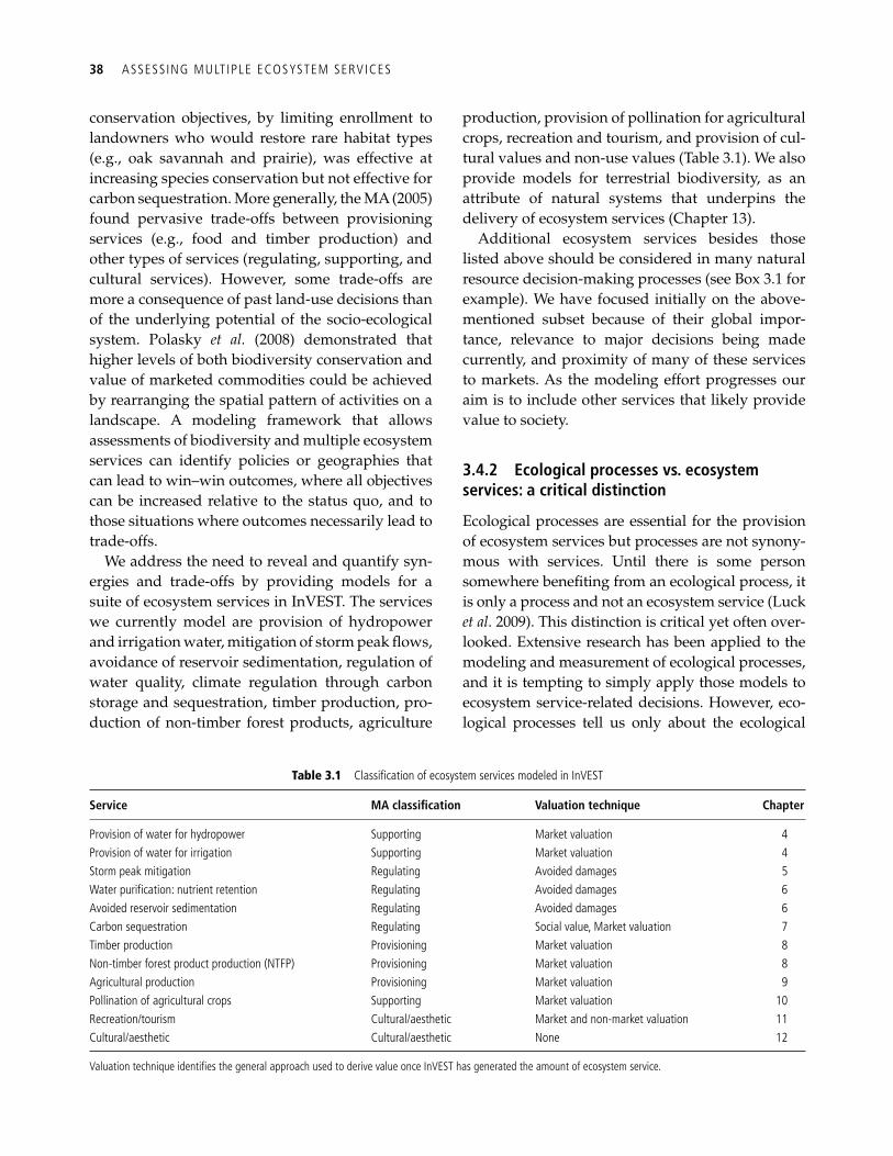
38 ASSESS ING MULTIPLE ECOSYSTEM SERVICES
Table 3.1 Classifi cation of ecosystem services modeled in InVEST
Service MA classifi cation Valuation technique Chapter
Provision of water for hydropower Supporting Market valuation 4 Provision of water for irrigation Supporting Market valuation 4 Storm peak mitigation Regulating Avoided damages 5 Water purifi cation: nutrient retention Regulating Avoided damages 6 Avoided reservoir sedimentation Regulating Avoided damages 6 Carbon sequestration Regulating Social value, Market valuation 7 Timber production Provisioning Market valuation 8 Non-timber forest product production (NTFP) Provisioning Market valuation 8 Agricultural production Provisioning Market valuation 9 Pollination of agricultural crops Supporting Market valuation 10 Recreation/tourism Cultural/aesthetic Market and non-market valuation 11 Cultural/aesthetic Cultural/aesthetic None 12
Valuation technique identifi es the general approach used to derive value once InVEST has generated the amount of ecosystem service.
conservation objectives, by limiting enrollment to landowners who would restore rare habitat types (e.g., oak savannah and prairie), was effective at increasing species conservation but not effective for carbon sequestration. More generally, the MA (2005) found pervasive trade-offs between provisioning services (e.g., food and timber production) and other types of services (regulating, supporting, and cultural services). However, some trade-offs are more a consequence of past land-use decisions than of the underlying potential of the socio-ecological system. Polasky et al. ( 2008 ) demonstrated that higher levels of both biodiversity conservation and value of marketed commodities could be achieved by rearranging the spatial pattern of activities on a landscape. A modeling framework that allows assessments of biodiversity and multiple ecosystem services can identify policies or geographies that can lead to win–win outcomes, where all objectives can be increased relative to the status quo, and to those situations where outcomes necessarily lead to trade-offs.
We address the need to reveal and quantify syn-ergies and trade-offs by providing models for a suite of ecosystem services in InVEST. The services we currently model are provision of hydropower and irrigation water, mitigation of storm peak fl ows, avoidance of reservoir sedimentation, regulation of water quality, climate regulation through carbon storage and sequestration, timber production, pro-duction of non-timber forest products, agriculture
production, provision of pollination for agricultural crops, recreation and tourism, and provision of cul-tural values and non-use values ( Table 3.1 ). We also provide models for terrestrial biodiversity, as an attribute of natural systems that underpins the delivery of ecosystem services ( Chapter 13 ).
Additional ecosystem services besides those listed above should be considered in many natural resource decision-making processes (see Box 3.1 for example). We have focused initially on the above-mentioned subset because of their global impor-tance, relevance to major decisions being made currently, and proximity of many of these services to markets. As the modeling effort progresses our aim is to include other services that likely provide value to society.
3.4.2 Ecological processes vs. ecosystem services: a critical distinction
Ecological processes are essential for the provision of ecosystem services but processes are not synony-mous with services. Until there is some person somewhere benefi ting from an ecological process, it is only a process and not an ecosystem service ( Luck et al . 2009 ). This distinction is critical yet often over-looked. Extensive research has been applied to the modeling and measurement of ecological processes, and it is tempting to simply apply those models to ecosystem service-related decisions. However, eco-logical processes tell us only about the ecological
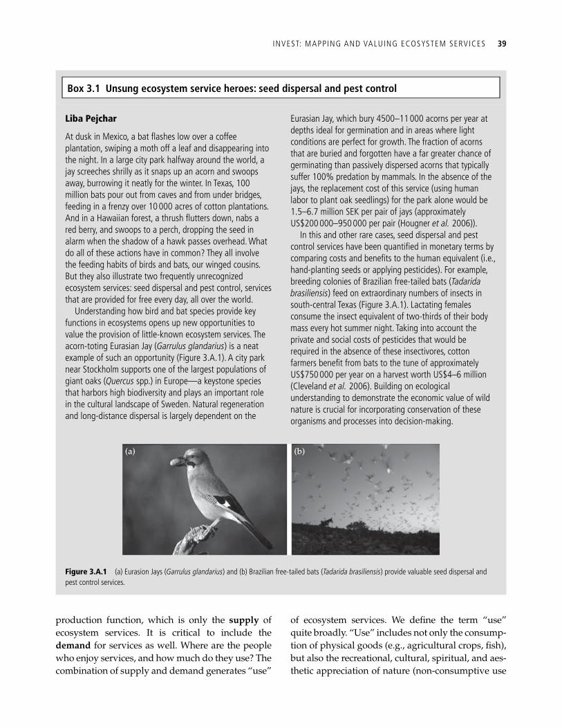
INVEST: MAPPING AND VALUING ECOSYSTEM SERVICES 39
Liba Pejchar
At dusk in Mexico, a bat fl ashes low over a coffee plantation, swiping a moth off a leaf and disappearing into the night. In a large city park halfway around the world, a jay screeches shrilly as it snaps up an acorn and swoops away, burrowing it neatly for the winter. In Texas, 100 million bats pour out from caves and from under bridges, feeding in a frenzy over 10 000 acres of cotton plantations. And in a Hawaiian forest, a thrush fl utters down, nabs a red berry, and swoops to a perch, dropping the seed in alarm when the shadow of a hawk passes overhead. What do all of these actions have in common? They all involve the feeding habits of birds and bats, our winged cousins. But they also illustrate two frequently unrecognized ecosystem services: seed dispersal and pest control, services that are provided for free every day, all over the world.
Understanding how bird and bat species provide key functions in ecosystems opens up new opportunities to value the provision of little-known ecosystem services. The acorn-toting Eurasian Jay ( Garrulus glandarius ) is a neat example of such an opportunity ( Figure 3.A.1 ). A city park near Stockholm supports one of the largest populations of giant oaks ( Quercus spp.) in Europe—a keystone species that harbors high biodiversity and plays an important role in the cultural landscape of Sweden. Natural regeneration and long-distance dispersal is largely dependent on the
Eurasian Jay, which bury 4500–11 000 acorns per year at depths ideal for germination and in areas where light conditions are perfect for growth. The fraction of acorns that are buried and forgotten have a far greater chance of germinating than passively dispersed acorns that typically suffer 100% predation by mammals. In the absence of the jays, the replacement cost of this service (using human labor to plant oak seedlings) for the park alone would be 1.5–6.7 million SEK per pair of jays (approximately US$200 000–950 000 per pair ( Hougner et al. 2006 )).
In this and other rare cases, seed dispersal and pest control services have been quantifi ed in monetary terms by comparing costs and benefi ts to the human equivalent (i.e., hand-planting seeds or applying pesticides). For example, breeding colonies of Brazilian free-tailed bats ( Tadarida brasiliensis ) feed on extraordinary numbers of insects in south-central Texas ( Figure 3.A.1 ). Lactating females consume the insect equivalent of two-thirds of their body mass every hot summer night. Taking into account the private and social costs of pesticides that would be required in the absence of these insectivores, cotton farmers benefi t from bats to the tune of approximately US$750 000 per year on a harvest worth US$4–6 million ( Cleveland et al. 2006 ). Building on ecological understanding to demonstrate the economic value of wild nature is crucial for incorporating conservation of these organisms and processes into decision-making .
production function, which is only the supply of ecosystem services. It is critical to include the demand for services as well. Where are the people who enjoy services, and how much do they use? The combination of supply and demand generates “use”
of ecosystem services. We defi ne the term “use” quite broadly. “Use” includes not only the consump-tion of physical goods (e.g., agricultural crops, fi sh), but also the recreational, cultural, spiritual, and aes-thetic appreciation of nature (non-consumptive use
Box 3.1 Unsung ecosystem service heroes: seed dispersal and pest control
Figure 3.A.1 (a) Eurasion Jays ( Garrulus glandarius ) and (b) Brazilian free-tailed bats ( Tadarida brasiliensis ) provide valuable seed dispersal and pest control services.
(a) (b)
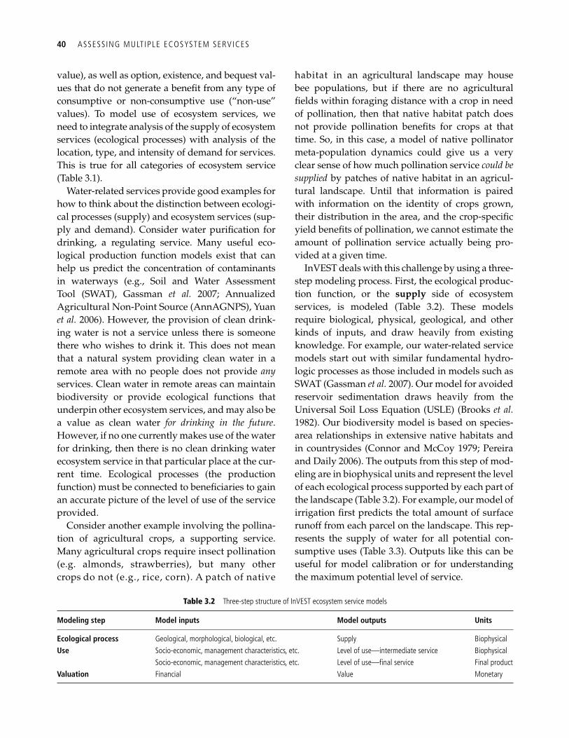
40 ASSESS ING MULTIPLE ECOSYSTEM SERVICES
value), as well as option, existence, and bequest val-ues that do not generate a benefi t from any type of consumptive or non-consumptive use (“non-use” values). To model use of ecosystem services, we need to integrate analysis of the supply of ecosystem services (ecological processes) with analysis of the location, type, and intensity of demand for services. This is true for all categories of ecosystem service ( Table 3.1 ).
Water-related services provide good examples for how to think about the distinction between ecologi-cal processes (supply) and ecosystem services (sup-ply and demand). Consider water purifi cation for drinking, a regulating service. Many useful eco-logical production function models exist that can help us predict the concentration of contaminants in waterways (e.g., Soil and Water Assessment Tool (SWAT), Gassman et al. 2007 ; Annualized Agricultural Non-Point Source (AnnAGNPS), Yuan et al. 2006 ). However, the provision of clean drink-ing water is not a service unless there is someone there who wishes to drink it. This does not mean that a natural system providing clean water in a remote area with no people does not provide any services. Clean water in remote areas can maintain biodiversity or provide ecological functions that underpin other ecosystem services, and may also be a value as clean water for drinking in the future . However, if no one currently makes use of the water for drinking, then there is no clean drinking water ecosystem service in that particular place at the cur-rent time. Ecological processes (the production function) must be connected to benefi ciaries to gain an accurate picture of the level of use of the service provided.
Consider another example involving the pollina-tion of agricultural crops, a supporting service. Many agricultural crops require insect pollination (e.g. almonds, strawberries), but many other crops do not (e.g., rice, corn). A patch of native
habitat in an agricultural landscape may house bee populations, but if there are no agricultural fi elds within foraging distance with a crop in need of pollination, then that native habitat patch does not provide pollination benefi ts for crops at that time. So, in this case, a model of native pollinator meta-population dynamics could give us a very clear sense of how much pollination service could be supplied by patches of native habitat in an agricul-tural landscape. Until that information is paired with information on the identity of crops grown, their distribution in the area, and the crop-specifi c yield benefi ts of pollination, we cannot estimate the amount of pollination service actually being pro-vided at a given time.
InVEST deals with this challenge by using a three-step modeling process. First, the ecological produc-tion function, or the supply side of ecosystem services, is modeled ( Table 3.2 ). These models require biological, physical, geological, and other kinds of inputs, and draw heavily from existing knowledge. For example, our water-related service models start out with similar fundamental hydro-logic processes as those included in models such as SWAT ( Gassman et al. 2007 ). Our model for avoided reservoir sedimentation draws heavily from the Universal Soil Loss Equation (USLE) ( Brooks et al. 1982 ). Our biodiversity model is based on species-area relationships in extensive native habitats and in countrysides ( Connor and McCoy 1979 ; Pereira and Daily 2006 ). The outputs from this step of mod-eling are in biophysical units and represent the level of each ecological process supported by each part of the landscape ( Table 3.2 ). For example, our model of irrigation fi rst predicts the total amount of surface runoff from each parcel on the landscape. This rep-resents the supply of water for all potential con-sumptive uses ( Table 3.3 ). Outputs like this can be useful for model calibration or for understanding the maximum potential level of service.
Table 3.2 Three-step structure of InVEST ecosystem service models
Modeling step Model inputs Model outputs Units
Ecological process Geological, morphological, biological, etc. Supply Biophysical Use Socio-economic, management characteristics, etc. Level of use—intermediate service Biophysical Socio-economic, management characteristics, etc. Level of use—fi nal service Final product Valuation Financial Value Monetary
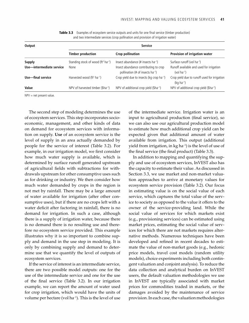
INVEST: MAPPING AND VALUING ECOSYSTEM SERVICES 41
The second step of modeling determines the use of ecosystem services. This step incorporates socio-economic, management, and other kinds of data on demand for ecosystem services with informa-tion on supply. Use of an ecosystem service is the level of supply in an area actually demanded by people for the service of interest ( Table 3.2 ). For example, in our irrigation model, we fi rst consider how much water supply is available, which is determined by surface runoff generated upstream of agricultural fi elds with subtractions for with-drawals upstream for other consumptive uses such as for drinking or industry. We then consider how much water demanded by crops in the region is not met by rainfall. There may be a large amount of water available for irrigation (after other con-sumptive uses), but if there are no crops left with a water defi cit after factoring in rainfall, there is no demand for irrigation. In such a case, although there is a supply of irrigation water, because there is no demand there is no resulting use and there-fore no ecosystem service provided. This example illustrates why it is so important to combine sup-ply and demand in the use step in modeling. It is only by combining supply and demand to deter-mine use that we quantify the level of outputs of ecosystem services.
If the service of interest is an intermediate service, there are two possible model outputs: one for the use of the intermediate service and one for the use of the fi nal service ( Table 3.2 ). In our irrigation example, we can report the amount of water used for crop irrigation, which would have the units of volume per hectare (vol ha –1 ). This is the level of use
of the intermediate service. Irrigation water is an input to agricultural production (fi nal service), so we can also use our agricultural production model to estimate how much additional crop yield can be expected given that additional amount of water available from irrigation. This output (additional yield from irrigation, in kg ha –1 ) is the level of use of the fi nal service (the fi nal product) ( Table 3.3 ).
In addition to mapping and quantifying the sup-ply and use of ecosystem services, InVEST also has the capacity to estimate their value. As discussed in Section 3.3 , we use market and non-market valua-tion approaches to arrive at monetary values for ecosystem service provision ( Table 3.2 ). Our focus in estimating value is on the social value of each service, which captures the total value of the serv-ice to society as opposed to the value it offers to the owner of the service-providing land. While the social value of services for which markets exist (e.g., provisioning services) can be estimated using market prices, estimating the social value of serv-ices for which there are not markets requires alter-native methods. Numerous techniques have been developed and refi ned in recent decades to esti-mate the value of non-market goods (e.g., hedonic price models, travel cost models (random utility models), choice experiments including both contin-gent valuation and conjoint analysis). To reduce the data collection and analytical burden on InVEST users, the default valuation methodologies we use in InVEST are typically associated with market prices for commodities traded in markets, or the damages avoided by the maintenance of service provision. In each case, the valuation methodologies
Table 3.3 Examples of ecosystem service outputs and units for one fi nal service (timber production) and two intermediate services (crop pollination and provision of irrigation water)
Output Service
Timber production Crop pollination Provision of irrigation water
Supply Standing stock of wood (ft 3 ha –1 ) Insect abundance (# insects ha –1 ) Surface runoff (vol ha –1 ) Use—intermediate service None Insect abundance contributing to crop
pollination (# of insects ha –1 ) Runoff available and used for irrigation
(vol ha –1 ) Use—fi nal service Harvested wood (ft 3 ha –1 ) Crop yield due to insects (kg crop ha –1 ) Crop yield due to runoff used for irrigation
(kg ha –1 ) Value NPV of harvested timber ($ha –1 ) NPV of additional crop yield ($ha –1 ) NPV of additional crop yield ($ha –1 )
NPV = net present value.
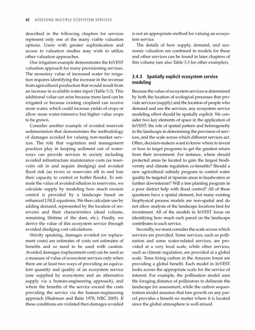
42 ASSESS ING MULTIPLE ECOSYSTEM SERVICES
described in the following chapters for services represent only one of the many viable valuation options. Users with greater sophistication and access to valuation studies may wish to utilize other valuation approaches.
Our irrigation example demonstrates the InVEST valuation approach for many provisioning services. The monetary value of increased water for irriga-tion requires identifying the increase in the revenue from agricultural production that would result from an increase in available water input ( Table 3.3 ). This additional value can arise because more land can be irrigated or because existing cropland can receive more water, which could increase yields of crops or allow more water-intensive but higher value crops to be grown.
Consider another example of avoided reservoir sedimentation that demonstrates the methodology of damages avoided for valuing non-market serv-ices. The role that vegetation and management practices play in keeping sediment out of water-ways can provide services to society including avoided infrastructure maintenance costs (as reser-voirs silt in and require dredging) and avoided fl ood risk (as rivers or reservoirs silt in and lose their capacity to control or buffer fl oods). To esti-mate the value of avoided siltation in reservoirs, we calculate supply by modeling how much erosion control is provided by a landscape based on enhanced USLE equations. We then calculate use by adding demand, represented by the location of res-ervoirs and their characteristics (dead volume, remaining lifetime of the dam, etc.). Finally, we derive the value of this ecosystem service through avoided dredging cost calculations.
Strictly speaking, damages avoided (or replace-ment costs) are estimates of costs not estimates of benefi ts and so need to be used with caution. Avoided damages (replacement cost) can be used as a measure of value of ecosystem services only when there are at least two ways of providing an equiva-lent quantity and quality of an ecosystem service (one supplied by ecosystems and an alternative supply via a human-engineering approach), and where the benefi ts of the service exceed the costs providing the service via the human-engineering approach ( Shabman and Batie 1978 ; NRC 2005). If these conditions are violated then damages avoided
is not an appropriate method for valuing an ecosys-tem service.
The details of how supply, demand, and eco-nomic valuation are combined in models for these and other services can be found in later chapters of this volume (see also Table 3.3 for other examples).
3.4.3 Spatially explicit ecosystem service modeling
Because the value of ecosystem services is determined by both the location of ecological processes that pro-vide services (supply) and the location of people who demand and use the services, any ecosystem service modeling effort should be spatially explicit. We con-sider two key elements of space in the application of InVEST: the role of spatial pattern and heterogeneity in the landscape in determining the provision of serv-ices, and the scale across which different services act. Often, decision-makers want to know where to invest or how to target programs to get the greatest return from their investment. For instance, where should protected areas be located to gain the largest biodi-versity and climate regulation co-benefi ts? Should a new agricultural subsidy program to control water quality be targeted at riparian areas in headwaters or further downstream? Will a tree planting program in a poor district help with fl ood control? All of these questions have a spatial element, but many existing biophysical process models are non-spatial and do not allow analysis of the landscape locations best for investment. All of the models in InVEST focus on identifying how much each parcel on the landscape contributes to each service.
Secondly, we must consider the scale across which services are provided. Some services, such as polli-nation and some water-related services, are pro-vided at a very local scale, while other services, such as climate regulation, are provided at a global scale. Trees fi xing carbon in the Amazon forest are providing a global benefi t. Each model in InVEST looks across the appropriate scale for the service of interest. For example, the pollination model uses the foraging distance of pollinators to delineate the landscape for assessment, while the carbon seques-tration model assumes that tree growth on any par-cel provides a benefi t no matter where it is located since the global atmosphere is well-mixed.
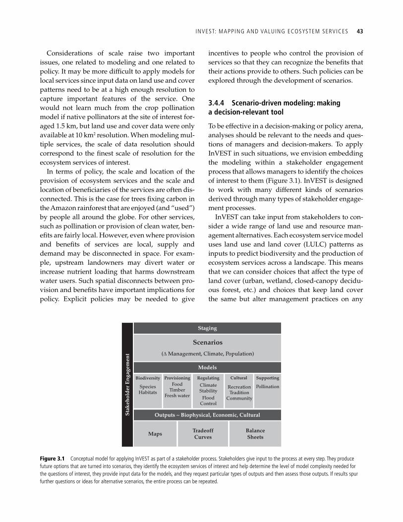
INVEST: MAPPING AND VALUING ECOSYSTEM SERVICES 43
Considerations of scale raise two important issues, one related to modeling and one related to policy. It may be more diffi cult to apply models for local services since input data on land use and cover patterns need to be at a high enough resolution to capture important features of the service. One would not learn much from the crop pollination model if native pollinators at the site of interest for-aged 1.5 km, but land use and cover data were only available at 10 km 2 resolution. When modeling mul-tiple services, the scale of data resolution should correspond to the fi nest scale of resolution for the ecosystem services of interest.
In terms of policy, the scale and location of the provision of ecosystem services and the scale and location of benefi ciaries of the services are often dis-connected. This is the case for trees fi xing carbon in the Amazon rainforest that are enjoyed (and “used”) by people all around the globe. For other services, such as pollination or provision of clean water, ben-efi ts are fairly local. However, even where provision and benefi ts of services are local, supply and demand may be disconnected in space. For exam-ple, upstream landowners may divert water or increase nutrient loading that harms downstream water users. Such spatial disconnects between pro-vision and benefi ts have important implications for policy. Explicit policies may be needed to give
incentives to people who control the provision of services so that they can recognize the benefi ts that their actions provide to others. Such policies can be explored through the development of scenarios.
3.4.4 Scenario-driven modeling: making a decision-relevant tool
To be effective in a decision-making or policy arena, analyses should be relevant to the needs and ques-tions of managers and decision-makers. To apply InVEST in such situations, we envision embedding the modeling within a stakeholder engagement process that allows managers to identify the choices of interest to them ( Figure 3.1 ). InVEST is designed to work with many different kinds of scenarios derived through many types of stakeholder engage-ment processes.
InVEST can take input from stakeholders to con-sider a wide range of land use and resource man-agement alternatives. Each ecosystem service model uses land use and land cover (LULC) patterns as inputs to predict biodiversity and the production of ecosystem services across a landscape. This means that we can consider choices that affect the type of land cover (urban, wetland, closed-canopy decidu-ous forest, etc.) and choices that keep land cover the same but alter management practices on any
Scenarios
(D Management, Climate, Population)
Biodiversity
SpeciesHabitats
FoodTimber
Fresh water
Maps TradeoffCurves
Outputs ~ Biophysical, Economic, Cultural
Models
Stak
ehol
der
Enga
gem
ent
Staging
BalanceSheets
ClimateStability
RecreationTradition
Community
Pollination
FloodControl
Provisioning Regulating Cultural Supporting
Figure 3.1 Conceptual model for applying InVEST as part of a stakeholder process. Stakeholders give input to the process at every step. They produce future options that are turned into scenarios, they identify the ecosystem services of interest and help determine the level of model complexity needed for the questions of interest, they provide input data for the models, and they request particular types of outputs and then assess those outputs. If results spur further questions or ideas for alternative scenarios, the entire process can be repeated.
44 ASSESS ING MULTIPLE ECOSYSTEM SERVICES
particular part of the landscape (change in release pattern from an existing dam, change in crop type planted in existing agricultural areas, change in fer-tilizer type or amount used, change in rotation time in existing plantation forests, etc.). Most natural resource management decisions will have effects on land use and cover patterns, either directly or indi-rectly, so sensitivity of InVEST models to LULC pat-terns translates into broad sensitivity to management choices.
For InVEST to assess the choices that managers or other stakeholders want to consider, we need to translate those choices into likely future land use and cover patterns. There are many different meth-ods for turning choices into LULC patterns. When decision-makers hold full control over the area of interest, their own planning processes usually include the development of scenarios that can be assessed by InVEST for likely ecosystem service provision. When the area of interest is a more com-plex landscape with multiple ownership and multi-ple drivers of change, more complex scenario generation options are available. One can develop predictions of how landowners will react given the various market forces, institutions, and incentives that they face at regional (e.g., Nelson et al. 2008 ; Sohl and Sayler 2008 ), national (e.g., Veldkamp and Fresco 1996 ), or global scales (e.g., Alcamo et al. 1994 ). For example, we can use models of land-owner decision-making to predict how landowners would react to changes in crop prices or to govern-ment policies to generate scenarios of land use and land cover that can be input into InVEST models. In more demonstrative applications, users may want to explore what is possible on a particular landscape given the fundamental ecosystem service relation-ships in place. In these cases, landscape optimiza-tion modeling can be used to fi nd solutions that maximize the provision of a combination of serv-ices. We have used this approach to maximize a measure of species conservation for a given value of commodity production (and vice versa) using early versions of InVEST models ( Polasky et al. 2008 ).
We have emphasized management decisions as drivers of landscape change, but there are obviously other factors at work. Climate change and human population growth will strongly infl uence LULC pat-terns and climate conditions in the future. Scenarios
can be built to include these drivers of change in addi-tion to management practices. Many efforts have now down-scaled global climate models and used regional predictions to drive vegetation patterns, giving us maps of likely future land cover and climate. Similarly, a variety of research groups are in the process of turn-ing numeric projections of population change into spatially explicit human population density estimates or urban/rural area extents (e.g., Salvatore et al. 2005 ). When models or maps of these drivers are available, they can be combined with any approaches that project management impacts, giving scenarios that represent all three major drivers of future change. We demonstrate one such application of InVEST with cli-mate scenarios in Chapter 18 . In the next section we explore the specifi cs of several real-world decisions being addressed through scenario analysis with InVEST.
3.4.5 Examples of scenario development and InVEST application
In many cases, managers want to know the likely outcomes of a proposed program, policy, or man-agement action before they decide how to proceed ( Ghazoul 2007 ). Maps of ecosystem service provi-sion can be used for planning, priority setting, determining compensation or offset levels, design-ing policies or monitoring programs, or identifying which members of society are controlling the provi-sion of ecosystem services and which members are receiving benefi ts. Here, we consider several man-agement questions and explore how InVEST can help answer them. These are all real cases where InVEST and its precursors are being applied.
The Chinese national government has a pro-gram to set up conservation areas to protect the natural capital that supports human well-being. Where should these areas be located?
This is an optimization question, like those com-monly asked in the conservation arena. To answer this question, we need to know which areas of the landscape provide the highest level of services at the least cost. We can fi rst use production function and economic valuation models to estimate ecosys-tem service levels and values. We can then feed
INVEST: MAPPING AND VALUING ECOSYSTEM SERVICES 45
these maps into optimization algorithms that deter-mine which parts of the landscape, if protected or managed in a certain way, meet goals the policy maker sets for ecosystem service provision at the lowest cost (e.g., number of hectares, purchase value of the land, opportunity cost of foregone activities). For those familiar with conservation planning, this could be done by running MARXAN, or a similar program, with ecosystem service tar-gets. While InVEST does not include an optimiza-tion routine, outputs of InVEST easily can be used in standard optimization packages to answer ques-tions of this sort.
The Nature Conservancy has completed an analysis of priority sites for conservation action in the Willamette Basin, Oregon (USA). They want to work fi rst in the places that also give the highest possible benefi t for human well-being. Where should they work?
This is also a priority setting question, but one that places biodiversity conservation above ecosystem service provision. In this case, we do not have to apply production function models to the whole landscape but can instead focus analyses on the pri-ority sites for biodiversity conservation. The options for confi gurations of priority areas become scenar-ios and InVEST can be used to estimate the levels and values of services that society will receive from conservation of each site. Planners can then choose where to act.
Colombia’s Ministry of the Environment is responsible for permitting and licensing all major production sectors in the country. They are considering requiring offsets and mitiga-tion for biodiversity and ecosystem service damages caused by development in sectors such as mining, agriculture, oil and gas, and infrastructure. If the expanded approach becomes law, how much mitigation should be required for a given development plan or set of permits, and where should the mitigation be done to adequately offset the damages?
InVEST has great potential for application in the mit-igation and offsetting arena because it explicitly con-siders the connection between ecosystem processes
and people. In many mitigation cases, offsets may be designed with the intention of providing services, but the actual connection to people is not considered explicitly. In Florida for example, a wetland mitiga-tion bank was created on a nearshore island to com-pensate for development in a coastal watershed. People in this area get drinking water from groundwa-ter wells. The wetland bank was meant to replace bio-diversity and water fi ltration services for clean drinking water lost through development, but the island hous-ing the bank was located over a different aquifer with no inhabitants. There was technically no net loss of wetland area or function, but the drinking water- related services provided to people were lost entirely.
InVEST models can be used to identify where on a landscape services are produced and used. Colombia’s Ministry has generated scenarios that represent proposed mines and other development projects and InVEST in being used to identify how much service will be gained or lost, and where. InVEST is also being used to identify other areas in the same landscape that provide similar levels of service to the same people, thus allowing targeted offsetting that will come closer to ensuring no net loss of ecosystem services.
A state agency in Oregon (USA) could design a subsidy that would motivate conservation of natural habitat on private lands. The objective would be to achieve biodiversity protection and climate regulation (through carbon sequestration) with this single program. How should they target payments to get the best returns for both goals on a fi xed budget? How much more return could they get if they increased the budget?
In data-rich environments like Oregon, scenarios can be developed by computer-based land transi-tion models. This was the approach taken by Nelson et al. ( 2008 ). Scenarios were created to represent fi ve possible subsidy programs, each designed to target a different set of landowners: (i) all landowners, (ii) owners of land in riparian zones, (iii) owners who could restore certain rare types of habitat, (iv) owners who could restore forests with large poten-tial to sequester carbon, and (v) owners with parcels with high species conservation value. Researchers
46 ASSESS ING MULTIPLE ECOSYSTEM SERVICES
projected land use change trajectories based on his-toric land change data in the region and altered the land change patterns based on an econometric model that determined which landowners would likely participate in each subsidy program. InVEST and its precursor models were used to project changes in biodiversity and service provision under each policy scenario, clearly revealing returns asso-ciated with each policy design and showed the trade-off in biodiversity conservation and ecosys-tem service provision under alternative policies.
Kamehameha Schools, the largest private landowner in Hawai’i, seeks to manage their lands to balance economic, environmental, educational, cultural, and community values. They are considering several possible manage-ment plans for providing these values on an iconic 26 000-ha parcel of land, the North Shore of O`ahu. Which plan will yield the best results?
In some cases, like this one, the key stakeholder has control over the whole area of analysis. In this case, hand-drawing scenarios is an alternative to compu-ter simulation of scenarios since there is little in the land use and cover patterns that is left to outside social drivers or chance. We worked with Kamehameha Schools to mark up a map of the par-cel, identifying which parts of the landscape would be under different uses in the alternate plans. We then rendered these ideas with GIS software, creat-ing landscape scenarios that were assessed with InVEST. Managers will use the multiple service out-puts of InVEST to identify how well each possible scenario measures up against their multiple objec-tives. These results will help inform the type of management plan implemented.
The Pacifi c Northwest Ecosystem Research Consortium, a group of representatives from government agencies, non-government organizations, and production sectors, is cur-rently trying to align the policy trajectory of the Willamette Basin (Oregon, USA) with the desires of its inhabitants. Which future will provide the greatest benefi ts to society, both in terms of current market commodities and in
terms of ecosystem services not presently val-ued? Do some alternatives offer more equita-ble distribution of benefi ts to residents?
Most natural resource management decisions have major impacts on the balance of society, infl uencing who receives higher income streams, who has access to markets, who must follow restrictive regulations, or even who has the right of access or ownership. In this case, the policies implemented in the Basin will determine the balance of revenues among agricul-ture, timber, and real estate sectors, and which areas will be developed or conserved. To better under-stand the kinds of policies people living in the Basin would like to see implemented, the Consortium led a multi-stakeholder process to create three plausible scenarios for the future that fell within the bounds of society’s comfort level. The three scenarios were assessed with InVEST to reveal the trade-offs and synergies among commodities and ecosystem serv-ices that can be expected under each possible future ( Nelson et al. 2009 ).
Going one step further, we can combine produc-tion function models such as InVEST with socio-economic data to understand how each possible future will affect social equity. Such analyses can help identify options that may lead to inequities before social groups or sectors are marginalized. Preliminary analyses of this type are discussed in Chapter 16 .
3.4.6 Tiered modeling: fl exibility for a data-limited world
There is always a trade-off in modeling between making a model more complex and detailed and keeping it simple. Simple models require fewer data, are often less prone to parameter estimation errors and subsequent error propagation, and can be easier to explain and understand. Complex mod-els require more information, but they often inspire greater confi dence because they more faithfully depict the details and underlying intricacies of proc-esses. Different applications and different users will have specifi c needs for either complicated or simple models of ecosystem services and valuation. For this reason, we have developed a tiered system of models in InVEST ( Figure 3.2 ) .
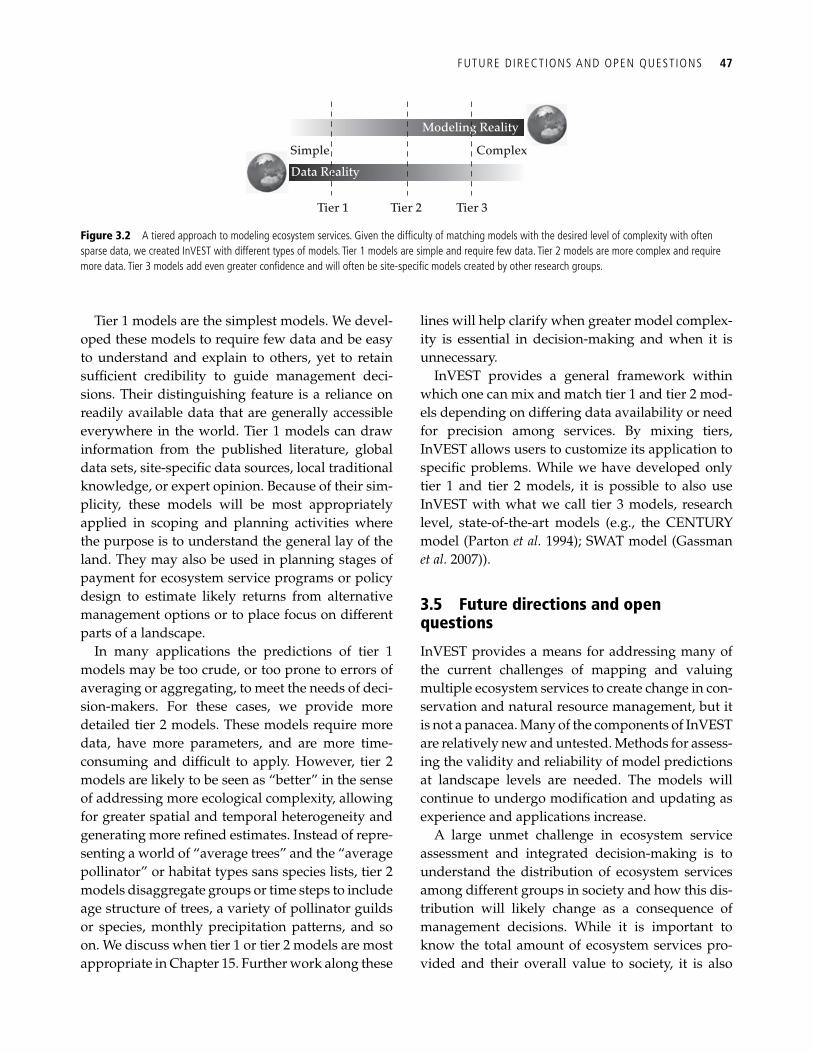
FUTURE DIRECTIONS AND OPEN QUEST IONS 47
Tier 1 models are the simplest models. We devel-oped these models to require few data and be easy to understand and explain to others, yet to retain suffi cient credibility to guide management deci-sions. Their distinguishing feature is a reliance on readily available data that are generally accessible everywhere in the world. Tier 1 models can draw information from the published literature, global data sets, site-specifi c data sources, local traditional knowledge, or expert opinion. Because of their sim-plicity, these models will be most appropriately applied in scoping and planning activities where the purpose is to understand the general lay of the land. They may also be used in planning stages of payment for ecosystem service programs or policy design to estimate likely returns from alternative management options or to place focus on different parts of a landscape.
In many applications the predictions of tier 1 models may be too crude, or too prone to errors of averaging or aggregating, to meet the needs of deci-sion-makers. For these cases, we provide more detailed tier 2 models. These models require more data, have more parameters, and are more time-consuming and diffi cult to apply. However, tier 2 models are likely to be seen as “better” in the sense of addressing more ecological complexity, allowing for greater spatial and temporal heterogeneity and generating more refi ned estimates. Instead of repre-senting a world of “average trees” and the “average pollinator” or habitat types sans species lists, tier 2 models disaggregate groups or time steps to include age structure of trees, a variety of pollinator guilds or species, monthly precipitation patterns, and so on. We discuss when tier 1 or tier 2 models are most appropriate in Chapter 15 . Further work along these
lines will help clarify when greater model complex-ity is essential in decision-making and when it is unnecessary.
InVEST provides a general framework within which one can mix and match tier 1 and tier 2 mod-els depending on differing data availability or need for precision among services. By mixing tiers, InVEST allows users to customize its application to specifi c problems. While we have developed only tier 1 and tier 2 models, it is possible to also use InVEST with what we call tier 3 models, research level, state-of-the-art models (e.g., the CENTURY model ( Parton et al. 1994 ); SWAT model ( Gassman et al. 2007 )).
3.5 Future directions and open questions
InVEST provides a means for addressing many of the current challenges of mapping and valuing multiple ecosystem services to create change in con-servation and natural resource management, but it is not a panacea. Many of the components of InVEST are relatively new and untested. Methods for assess-ing the validity and reliability of model predictions at landscape levels are needed. The models will continue to undergo modifi cation and updating as experience and applications increase.
A large unmet challenge in ecosystem service assessment and integrated decision-making is to understand the distribution of ecosystem services among different groups in society and how this dis-tribution will likely change as a consequence of management decisions. While it is important to know the total amount of ecosystem services pro-vided and their overall value to society, it is also
Simple Complex
Data Reality
Modeling Reality
Tier 1 Tier 2 Tier 3
Figure 3.2 A tiered approach to modeling ecosystem services. Given the diffi culty of matching models with the desired level of complexity with often sparse data, we created InVEST with different types of models. Tier 1 models are simple and require few data. Tier 2 models are more complex and require more data. Tier 3 models add even greater confi dence and will often be site-specifi c models created by other research groups.
48 ASSESS ING MULTIPLE ECOSYSTEM SERVICES
important to know who benefi ts from the provision of services and their social and economic status. Without information about the distribution of ben-efi ts from ecosystem services, management deci-sions can lead to serious unintended consequences for equity and well-being. This concern is especially strong for management actions that negatively affect underprivileged segments of society ( Pagiola et al . 2005 ). In developing countries, for example, establishing a new national park or conservation area has in some cases resulted in removing and separating people and their work ( Kareiva and Marvier 2007 ), leading to a decline in their liveli-hood or well-being.
Whether a particular social group wins, loses, or remains unaffected by a decision is determined by several factors. Of utmost importance is access. Underprivileged members of society will not benefi t or lose from changes in ecosystem services if they cannot access those services. Access has two critical components in this context: physical overlap in space and legal rights (and their enforcement). InVEST can show clearly where services will be provided on a landscape and how their provision is likely to change in space. This ability can give insights into the spatial overlap part of access. Rapid advances are being made in the mapping of social indicators of poverty (CIESIN 2006; World Resources Institute 2007 ), and we can draw from these approaches to ask where ecosystem services and the poor overlap on the land-scape. We provide some examples of this kind of exercise in Chapter 16 . However, we currently do not have a standardized way for bringing information about institutions and their level of enforcement into a mapping and valuation context. Developing ways to represent and predict the interactions among eco-system services, people, and institutions will be criti-cal to the assessment of the distributional effects of management decisions.
A related challenge lies in altering fi nancial and institutional infrastructure to give incentives that maintain and enhance the provision of ecosystem services. Often there is a spatial or temporal mis-match between those who control the provision of ecosystem services and those who benefi t from the services. Without the ability to connect the demand for services with the supply from those who control it, there will be insuffi cient incentive for suppliers
to protect and maintain ecosystems. Addressing this mismatch and providing proper incentives for provision of ecosystem services will require changes in policies of local and national governments and in international agreements. Some progress on these fronts can be seen, as with the recent emergence of carbon markets, international policy discussions on Reduced Emissions from Deforestation in Developing Countries (REDD), and expansion of programs of Payments for Ecosystem Services (PES). Successfully linking the science of mapping and valuing ecosystem services with proper institu-tions and policies will likely remain a major chal-lenge for decades to come.
Finally, there is the need to expand InVEST to include models for other key terrestrial (see Box 3.1 ), freshwater, and marine ecosystem services. Useful groundwork is being laid for comprehensive mod-eling of marine ecosystem services ( Chapter 17 ) and the Natural Capital Project is now developing InVEST models for fi sheries production, shoreline protection, marine tourism and recreation, and marine biodiversity.
A user’s guide for InVEST can be found at http://invest.ecoinformatics.org and there is a growing community that seeks to develop and apply multi-objective ecosystem service models to decision-making. Whether one uses InVEST or any of several other ecosystem service modeling approaches (e.g., Artifi cial Intelligence for Ecosystem Services (ARIES; ARIES 2008 ), EcoMetrix ( Primozich 2008 ), Multiscale Integrated Models of Ecosystem Services (MIMES; unpublished)), the greatest challenge is not in developing the models, but in linking the models pragmatically to everyday land- and resource-use decisions.
References
ARIES. (2008). ARIES white paper . University of Vermont, Burlington.
Alcamo, J., Kreileman, G. J. J., Krol, M., et al . (1994). Modeling the global society-biosphere-climate system, 1. Model description and testing. Water Air and Soil Pollution , 76 , 1–35.
Antle, J. M., and Stoorvogel, J. J. (2006). Incorporating sys-tems dynamics and spatial heterogeneity in integrated assessment of agricultural production systems. Environment and Development Economics , 11, 39–58.
FUTURE DIRECTIONS AND OPEN QUEST IONS 49
Barbier, E. B., and Strand, I. (1998). Valuing mangrove-fi shery linkages: A case study of Campeche, Mexico. Environmental and Resource Economics , 12, 151–66.
Barbier, E. B. (2000). Valuing the environment as input: Applications to mangrove-fi shery linkages. Ecological Economics , 35, 47–61.
Barbier, E. B. (2007). Valuing ecosystem services as pro-ductive inputs. Economic Policy , 22, 177–229.
Boerner, B. (2007). Ecosystem services, agriculture, and rural poverty in the Eastern Brazilian Amazon: Interrelationships and policy prescriptions. Amsterdam, The Netherlands.
Boody, G., Vondracek, B., Andow, D. A., et al. (2005). Multifunctional agriculture in the United States. Bioscience , 55, 27–38.
Brooks, K. N., Gregersen, H. M., Berglund, E. R., et al. (1982). Economic evaluation of watershed projects—an overview methodology and application. Water Resources Bulletin , 18, 245.
Center for International Earth Science Information Network (CIESIN). (2006). Where the poor are: An atlas of poverty. The Earth Institute at Columbia University, New York.
Cleveland, C. J., Betke, M., Federico, P. et al. (2006). Economic value of the pest control service provided by the Brazilian free-tailed bats in south-central Texas. Frontiers in Ecology and Evolution , 4, 238–43.
Connor, E. F., and McCoy, E. D. (1979). The statistics and biology of the species–area relationship. American Naturalist , 113, 791–833.
Costanza, R., d’Arge, R., de Groot, R., et al. (1997). The value of the world’s ecosystem services and natural capital. Nature , 387, 253–60.
Daily, G. C. (1997). Nature’s Services. Island Press, Washington, DC.
Das, S., and Vincent, J. R. (2009). Mangroves protected vil-lages and reduced death toll during Indian super cyclone. Proceedings of the National Academy of Sciences of the United States of America . Early Edition , 1–4.
Ehrlich, P. R., and Ehrlich, A. H. (1981). Extinction: The Causes and Consequences of the Disappearance of Species . Random House, New York.
Ellis, G. M., and Fisher, A. C. (1987). Valuing the einvron-ment as an input. Journal of Environmental Management , 25, 149–56.
Engel, S., Pagiola, S., and Wunder, S. (2008). Designing payments for environmental services in theory and practice: An overview of the issues. Ecological Economics , 65, 663–74.
Eshet, T., Baron, M. G., and Shechter, M. (2007). Exploring benefi t transfer: disamenities of waste transfer stations. Environmental and Resource Economics , 37 , 521–47.
Freeman, A. M. I. (2003). The Measurement of Environmental and Resource Values: Theory and Methods . Resources for the Future, Washington, DC.
Gassman, P. W., Reyes, M. R., Green, C. H., et al. (2007). The soil and water assessment tool: historical develop-ment, applications and future research directions. Transactions of the American Society of Agricultural and Biological Engineers , 50, 1211–50.
Ghazoul, J. (2007). Recognising the complexities of ecosys-tem management and the ecosystem service concept. Gaia , 16 , 215–21.
Hougner, C., Colding, J., and Soderqvist, T. (2006). Economic valuation of a seed dispersal service in the Stockholm National Urban Park, Sweden. Ecological Economics , 59, 364–74.
Imperial, M. T. (1999). Institutional analysis and ecosys-tem-based management: The institutional analysis and development framework. Environmental Management , 24, 449–65.
Jackson, R. B., Jobbagy, E. G., Avissar, R., et al. (2005). Trading water for carbon with biological sequestration. Science , 310, 1944–7.
Just, R. E., Hueth, D. L., and Schmitz, A. (2004). The Welfare Economics of Public Policy: A Practical Approach to Project and Policy Evaluation . Edward Elgar, Cheltenham, UK and Northampton, MA.
Kaiser, B., and Roumasset, J. (2002). Valuing indirect eco-system services: the case of tropical watersheds. Environment and Development Economics , 7, 701–14.
Kareiva, P., and Marvier, M. (2007). Conversation for the people—Pitting nature and biodiversity against people makes little sense. Many conservationists now argue that human health and well-being should be central to conservation efforts. Scientifi c American, 297, 50–7.
Konarska, K. M., Sutton, P. C., and Castellon, M. (2002). Evaluationg scale dependence of ecosystem service val-uation: a comparison of NOAA-AVHRR and Landsat TM datasets. Ecological Economics, 41, 491–507.
Luck, G. W., Harrington, R., Harrison, P. A. et al. (2009). Quantifying the contribution of organisms to the provi-sion of ecosystem services. BioScience , 59 , 223–35.
Millennium Ecosystem Assessment (MA). (2005). Ecosystems and Human Well-being: Synthesis. Island Press, Washington, DC.
Naidoo, R., and Ricketts, T. H. (2006). Mapping the eco-nomic costs and benefi ts of conservation. PLoS Biology , 4, 2153–64.
National Research Council (NRC). (2005). Valuing ecosys-tem services: Toward better environmental decision-making. National Academies Press, Washington, DC.
Nelson, E., Polasky, S., Lewis, D. J., et al. (2008). Effi ciency of incentives to jointly increase carbon sequestration
50 ASSESS ING MULTIPLE ECOSYSTEM SERVICES
and species conservation on a landscape. Proceedings of the National Academy of Sciences of the United States of America , 105, 9471–6.
Nelson, E. N., Mendoza, G. M., Regetz, J., et al. (2009). Modeling multiple ecosystem services, biodiversity conservation, commodity production and tradeoffs at landscape scales. Frontiers in Ecology and the Environment , 7 , 4–11.
Pagiola, S., von Ritter, K., and Bishop, J. (2004). How Much is an Ecosystem Worth? Assessing the Economic Value of Conservation. The World Bank, Washington, DC.
Pagiola, S., Arcenas, A., and Platais, G. (2005). Can pay-ments for environmental services help reduce poverty? An exploration of the issues and the evidence to date from Latin America. World Development , 33, 237–53.
Parton, W. J., Schimel, D. S., Ojima, D. S., et al . (1994). Quantitative modeling of soil forming processes. In R. B. Bryant and R. W. Arnold et al ., Eds. Special Publication , pp. 147–67. Soil Science Society of America, Madison, WI.
Pereira, H. M., and Daily, G. C. (2006). Modeling biodiver-sity dynamics in countryside landscapes. Ecology , 87, 1877–85.
Plummer, M. (2009). Assessing benefi t transfer for the valuation of ecosystem services. Frontiers in Ecology and the Environment , 7 , 38–45.
Polasky, S., Nelson, E., Camm, J., et al. (2008). Where to put things? Spatial land management to sustain biodiver-sity and economic returns. Biological Conservation , 141, 1505–24.
Primozich, D. (2008). Developing the Willamette ecosystem marketplace. Willamette Partnerhsip, Salem.
Ricketts, H. T., Daily, G. C., Ehrlich, P. R., et al . (2004). Economic value of tropical forest to coffee production. Proceedings of the National Academy of Sciences of the United States of America , 101, 12579–82.
Rosenberger, R. S., and Stanley, T. D. (2006). Measurement, generalization, and publication: Sources of error in ben-efi t transfers and their management. Ecological Economics , 60 , 372–8.
Rosenberger, R. S. and Phipps, T. T. (2007). Correspondence and convergence in benefi t transfer accuracy: A meta-analytic review of the literature. In: S. Navrud, and R. Ready, Eds., Environmental Values Transfer: Issues and Methods . Springer, Dordrecht.
Salvatore, M., Pozzi, F., Ataman, E., et al . (2005). Mapping global urban and rural population distributions. Food and Agriculture Organization, Rome.
Sathirathai, S. and Barbier, E. B. (2001). Valuing mangrove conservation in southern Thailand. Contemporary Economic Policy , 19, 109–22.
Shabman, L. A., and Batie, S. S. (1978). Economic value of natural coastal wetlands: a critique. Coastal Zone Management Journal , 4 , 231–47.
Sohl, T. and Sayler, K. (2008). Using the FORE-SCE model to project land-cover change in the southeastern United States. Ecological Modelling , 219 , 49–65.
Swallow, S. K. (1994). Renewable and nonrenewable resource theory applied to coastal agriculture, forest, wetland and fi shery linkages. Marine Resource Economics , 9, 291–310.
Troy, A. and Wilson, M. A. (2006). Mapping ecosystem services: Practical challenges and opportunities in link-ing GIS and value transfer. Ecological Economics , 60, 435–49.
Turner, W. R., Brandon, K., Brooks, T. M., et al . (2007). Global conservation of biodiveristy and ecosystem serv-ices. Bioscience , 57, 868–73.
Veldkamp, A., and Fresco, L. O. (1996). CLUE-CR: An integrated multi-scale model to simulate land use change scenarios in Costa Rica. Ecological Modeling , 91, 231–48.
Vitousek, P. M., Aber, J. D., Howarth, R. W., et al. (1997). Human alteration of the global nitrogen cycle: Sources and consequences. Ecological Applications , 7, 737–50.
Wilson, M. A. and Carpenter, S. R. (1999). Economic valu-ation of freshwater ecosystem services in the United States: 1971–1997. Ecological Applications , 9, 772–83.
Wilson, M. A. and Hoehn, J. P. (2006). Valuing environ-mental goods and services using benefi t transfer: The state-of-the-art and science. Ecological Economics , 60 , 335–42.
World Resources Institute. (2007). Nature’s Benefi ts in Kenya: An atlas of ecosystem services and human well-being. World Resources Institute, Washington, DC.
Yuan, Y., Bingner, R. L., and Boydstun, J. (2006). Development of TMDL watershed implementation plan using Annualized AGNPS. Land Use and Water Resources Research , 6 , 2.1–2.8.
SECTION II
Multi-tiered models for ecosystem services

This page intentionally left blank
53
CHAPTER 4
Water supply as an ecosystem service for hydropower and irrigation Guillermo Mendoza, Driss Ennaanay, Marc Conte, Michael Todd Walter, David Freyberg, Stacie Wolny, Lauren Hay, Sue White, Erik Nelson, and Luis Solorzano
4.1 Introduction
Water is necessary for all life. Precipitation through stream runoff and groundwater that is tapped via wells provide the world’s supply of water for drink-ing, irrigation, and hydropower generation. The spatial and temporal availability of this water is strongly infl uenced by watershed geomorphology, vegetation, and land and water management prac-tices. As such, natural capital (in this case, vegeta-tion and soil) can support the provision of water services by regulating the amount and timing of water availability. In this chapter, we presents mod-els that link land use and land cover (LULC) and several other key attributes to the quantity of sur-face water available for irrigation and for hydro-power production.
We focus on irrigation and hydropower because of their global economic signifi cance. The vast majority of water used worldwide is used for irriga-tion, accounting for up to 85% of fresh water use in developing nations (IWMI 2001). The benefi t of access to irrigation is the associated increase in crop yield: irrigated agriculture provides 40% of the glo-bal food production (FAO, 2003). Water supply for hydropower is also an economically signifi cant service, and one likely to become even more impor-tant because of its presumed low carbon emissions. For example, hydropower supplies 9% of the US electricity and 49% of all renewable energy used in the USA (Edwards 2003). Some countries depend almost exclusively on hydropower, such as Tanzania where hydropower accounts for more than 60% of total generated capacity (Lyimo 2005).
Although there is a lot still to be learned about the connections between land management, vegetation cover, and water yield (e.g., Chomitz and Kumari 1998 ; Bruijnzeel 2001; Bosch and Hewlett 1982 ; Oyebande 1998), there is a demand for science-based decision-making regarding policies, pay-ments, or activities that can alter water use. Decision-makers need a credible and convenient methodology that explicitly links land use to water delivery (Tallis et al . 2008). Several complex models are available for simulating water yield—most notably Hydrological Simulation Program—Fortran (HSPF; Donigian et al. 1984) and Soil and Water Assessment Tool (SWAT; Arnold et al. 1998 ). SWAT and HSPF are quasi-process-based hydrology mod-els that are data- and time-intensive; they are diffi -cult to apply in data-poor regions of the world, or in situations lacking technically sophisticated support staff to calibrate the models. For this reason there is a need for simpler models that can be more easily applied, especially in a context of examining many ecosystem services at once, where trade-offs and relative comparisons may be suffi cient.
We present two models that explicitly connect land use and land cover to the regulation of surface water fl ows. We describe methods for converting modeled fl ows into the level and value of two eco-system services: the regulation of water fl ow for hydropower production and the regulation of water fl ow for agricultural crop irrigation. We provide two sets of models called tier 1 and tier 2 models. The tier 1 models are the simplest and require the fewest data. They provide annual average outputs
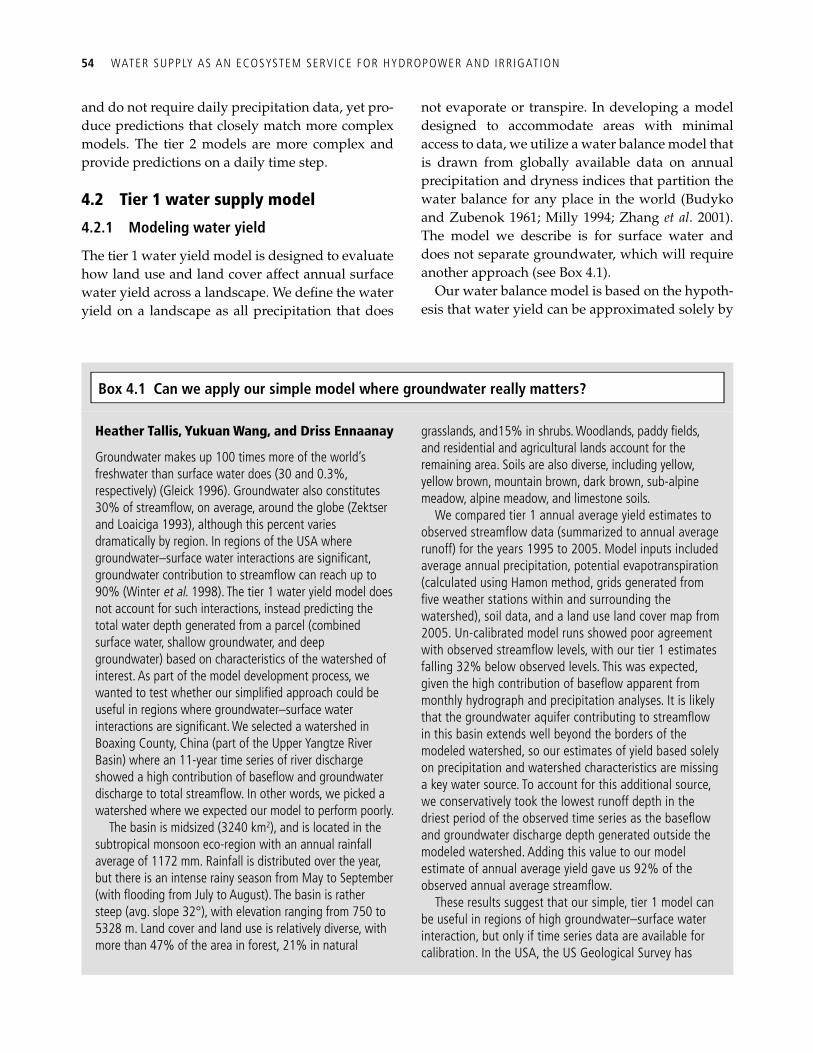
54 WATER SUPPLY AS AN ECOSYSTEM SERVICE FOR HYDROPOWER AND IRRIGATION
and do not require daily precipitation data, yet pro-duce predictions that closely match more complex models. The tier 2 models are more complex and provide predictions on a daily time step.
4.2 Tier 1 water supply model
4.2.1 Modeling water yield
The tier 1 water yield model is designed to evaluate how land use and land cover affect annual surface water yield across a landscape. We defi ne the water yield on a landscape as all precipitation that does
not evaporate or transpire. In developing a model designed to accommodate areas with minimal access to data, we utilize a water balance model that is drawn from globally available data on annual precipitation and dryness indices that partition the water balance for any place in the world (Budyko and Zubenok 1961; Milly 1994; Zhang et al . 2001). The model we describe is for surface water and does not separate groundwater, which will require another approach (see Box 4.1 ).
Our water balance model is based on the hypoth-esis that water yield can be approximated solely by
Heather Tallis, Yukuan Wang, and Driss Ennaanay
Groundwater makes up 100 times more of the world’s freshwater than surface water does (30 and 0.3%, respectively) ( Gleick 1996 ). Groundwater also constitutes 30% of streamfl ow, on average, around the globe ( Zektser and Loaiciga 1993 ), although this percent varies dramatically by region. In regions of the USA where groundwater–surface water interactions are signifi cant, groundwater contribution to streamfl ow can reach up to 90% ( Winter et al . 1998 ). The tier 1 water yield model does not account for such interactions, instead predicting the total water depth generated from a parcel (combined surface water, shallow groundwater, and deep groundwater) based on characteristics of the watershed of interest. As part of the model development process, we wanted to test whether our simplifi ed approach could be useful in regions where groundwater–surface water interactions are signifi cant. We selected a watershed in Boaxing County, China (part of the Upper Yangtze River Basin) where an 11-year time series of river discharge showed a high contribution of basefl ow and groundwater discharge to total streamfl ow. In other words, we picked a watershed where we expected our model to perform poorly.
The basin is midsized (3240 km 2 ), and is located in the subtropical monsoon eco-region with an annual rainfall average of 1172 mm. Rainfall is distributed over the year, but there is an intense rainy season from May to September (with fl ooding from July to August). The basin is rather steep (avg. slope 32°), with elevation ranging from 750 to 5328 m. Land cover and land use is relatively diverse, with more than 47% of the area in forest, 21% in natural
grasslands, and15% in shrubs. Woodlands, paddy fi elds, and residential and agricultural lands account for the remaining area. Soils are also diverse, including yellow, yellow brown, mountain brown, dark brown, sub-alpine meadow, alpine meadow, and limestone soils.
We compared tier 1 annual average yield estimates to observed streamfl ow data (summarized to annual average runoff) for the years 1995 to 2005. Model inputs included average annual precipitation, potential evapotranspiration (calculated using Hamon method, grids generated from fi ve weather stations within and surrounding the watershed), soil data, and a land use land cover map from 2005. Un-calibrated model runs showed poor agreement with observed streamfl ow levels, with our tier 1 estimates falling 32% below observed levels. This was expected, given the high contribution of basefl ow apparent from monthly hydrograph and precipitation analyses. It is likely that the groundwater aquifer contributing to streamfl ow in this basin extends well beyond the borders of the modeled watershed, so our estimates of yield based solely on precipitation and watershed characteristics are missing a key water source. To account for this additional source, we conservatively took the lowest runoff depth in the driest period of the observed time series as the basefl ow and groundwater discharge depth generated outside the modeled watershed. Adding this value to our model estimate of annual average yield gave us 92% of the observed annual average streamfl ow.
These results suggest that our simple, tier 1 model can be useful in regions of high groundwater–surface water interaction, but only if time series data are available for calibration. In the USA, the US Geological Survey has
Box 4.1 Can we apply our simple model where groundwater really matters?
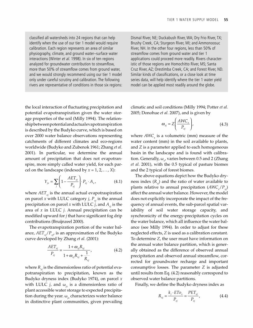
T IER 1 WATER SUPPLY MODEL 55
the local interaction of fl uctuating precipitation and potential evapotranspiration given the water stor-age properties of the soil (Milly 1994). The relation-ship between potential and actual evapotranspiration is described by the Budyko curve, which is based on over 2000 water balance observations representing catchments of different climates and eco-regions worldwide (Budyko and Zubenok 1961; Zhang et al . 2001). In particular, we determine the annual amount of precipitation that does not evapotran-spire, more simply called water yield, for each par-cel on the landscape (indexed by x = 1, 2, . . . , X ):
⎛ ⎞
= − ⋅ ⋅⎜ ⎟⎝ ⎠
∑ 1 ,xjjx xj x
j xj
AETY P A
P (4.1)
where AET xj is the annual actual evapotraspiration on parcel x with LULC category j , P xj is the annual precipitation on parcel x with LULC j , and A xj is the area of x in LULC j . Annual precipitation can be modifi ed upward for j that have signifi cant fog drip contributions ( Bruijnzeel 2000 ).
The evapotranspiration portion of the water bal-ance, AET xj / P xj , is an approximation of the Budyko curve developed by Zhang et al . (2001):
w
w
+=
+ +
1,11
xj xj xj
xjxj xj
xj
AET R
P RR
(4.2)
where R xj is the dimensionless ratio of potential eva-potranspiration to precipitation, known as the Budyko dryness index (Budyko 1974), on parcel x with LULC j , and ω jx is a dimensionless ratio of plant accessible water storage to expected precipita-tion during the year. ω jx characterizes water balance in distinctive plant communities, given prevailing
climatic and soil conditions (Milly 1994; Potter et al. 2005; Donohue et al . 2007), and is given by
w⎛ ⎞
= ⎜ ⎟⎝ ⎠
,xxj
xj
AWCZ
P (4.3)
where AWC x is a volumetric (mm) measure of the water content (mm) in the soil available to plants, and Z is a parameter applied to each homogeneous basin in the landscape and is found with calibra-tion. Generally, ω x , varies between 0.5 and 2 (Zhang et al . 2001), with the 0.5 typical of pasture biomes and the 2 typical of forest biomes.
The above equations depict how the Budyko dry-ness index ( R xj ) and the ratio of water available to plants relative to annual precipitation ( AWC x / P xj ) affect the annual water balance. However, the model does not explicitly incorporate the impact of the fre-quency of annual events, the sub-parcel spatial var-iability of soil water storage capacity, and synchronicity of the energy-precipitation cycles on the water balance, which all infl uence the water bal-ance (see Milly 1994). In order to adjust for these neglected effects, Z is used as a calibration constant. To determine Z , the user must have information on the annual water balance partition, which is gener-ally obtained as the difference of observed annual precipitation and observed annual streamfl ow, cor-rected for groundwater recharge and important consumptive losses. The parameter Z is adjusted until results from Eq. (4.2) reasonably correspond to observed water balance partitions.
Finally, we defi ne the Budyko dryness index as
⋅
= = ,j x xjxj
xj xj
k ETo PETR
P P (4.4)
classifi ed all watersheds into 24 regions that can help identify when the use of our tier 1 model would require calibration. Each region represents an area of similar physiography, climate, and ground water–surface water interactions ( Winter et al. 1998 ). In six of ten regions analyzed for groundwater contribution to streamfl ow, more than 50% of streamfl ow comes from ground water, and we would strongly recommend using our tier 1 model only under careful scrutiny and calibration. The following rivers are representative of conditions in those six regions:
Dismal River, NE; Duckabush River, WA; Dry Frio River, TX; Brushy Creek, CA; Sturgeon River, MI; and Ammonoosuc River, NH. In the other four regions, less than 50% of streamfl ow comes from ground water and tier 1 applications could proceed more readily. Rivers character-istic of those regions are Homochitto River, MS; Santa Cruz River, AZ; Orestimba Creek, CA; and Forest River, ND. Similar kinds of classifi cations, or a close look at time series data, will help identify where the tier 1 water yield model can be applied most readily around the globe.
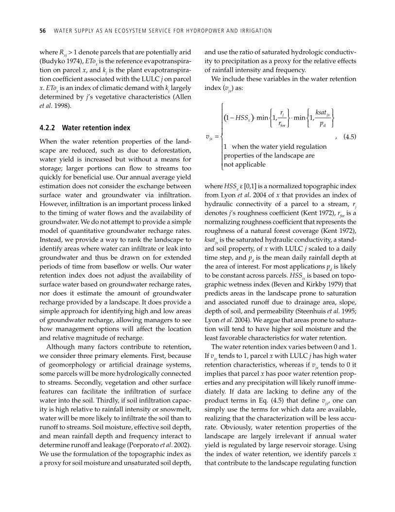
56 WATER SUPPLY AS AN ECOSYSTEM SERVICE FOR HYDROPOWER AND IRRIGATION
where R xj > 1 denote parcels that are potentially arid (Budyko 1974), ETo x is the reference evapotranspira-tion on parcel x , and k j is the plant evapotranspira-tion coeffi cient associated with the LULC j on parcel x . ETo x is an index of climatic demand with k j largely determined by j ’s vegetative characteristics ( Allen et al . 1998 ).
4.2.2 Water retention index
When the water retention properties of the land-scape are reduced, such as due to deforestation, water yield is increased but without a means for storage; larger portions can fl ow to streams too quickly for benefi cial use. Our annual average yield estimation does not consider the exchange between surface water and groundwater via infi ltration. However, infi ltration is an important process linked to the timing of water fl ows and the availability of groundwater. We do not attempt to provide a simple model of quantitative groundwater recharge rates. Instead, we provide a way to rank the landscape to identify areas where water can infi ltrate or leak into groundwater and thus be drawn on for extended periods of time from basefl ow or wells. Our water retention index does not adjust the availability of surface water based on groundwater recharge rates, nor does it estimate the amount of groundwater recharge provided by a landscape. It does provide a simple approach for identifying high and low areas of groundwater recharge, allowing managers to see how management options will affect the location and relative magnitude of recharge.
Although many factors contribute to retention, we consider three primary elements. First, because of geomorphology or artifi cial drainage systems, some parcels will be more hydrologically connected to streams. Secondly, vegetation and other surface features can facilitate the infi ltration of surface water into the soil. Thirdly, if soil infi ltration capac-ity is high relative to rainfall intensity or snowmelt, water will be more likely to infi ltrate the soil than to runoff to streams. Soil moisture, effective soil depth, and mean rainfall depth and frequency interact to determine runoff and leakage (Porporato et al . 2002). We use the formulation of the topographic index as a proxy for soil moisture and unsaturated soil depth,
and use the ratio of saturated hydrologic conductiv-ity to precipitation as a proxy for the relative effects of rainfall intensity and frequency.
We include these variables in the water retention index ( vjx ) as:
( )⎧
⎧ ⎫⎧ ⎫⎪ − ⋅ ⋅⎨ ⎬ ⎨ ⎬⎪ ⎩ ⎭ ⎩ ⎭⎪⎪= ⎨⎪⎪⎪⎪⎩
for d
1 min 1, min 1,
,1 when the water yield regulation properties of the landscape are not applicable
j jxx
jx
r ksatHSS
r p
v
(4.5)
where HSS x ε [0,1] is a normalized topographic index from Lyon et al . 2004 of x that provides an index of hydraulic connectivity of a parcel to a stream, r j denotes j ’s roughness coeffi cient (Kent 1972), r for is a normalizing roughness coeffi cient that represents the roughness of a natural forest coverage (Kent 1972), ksat jx is the saturated hydraulic conductivity, a stand-ard soil property, of x with LULC j scaled to a daily time step, and p d is the mean daily rainfall depth at the area of interest. For most applications p d is likely to be constant across parcels. HSS ix is based on topo-graphic wetness index ( Beven and Kirkby 1979 ) that predicts areas in the landscape prone to saturation and associated runoff due to drainage area, slope, depth of soil, and permeability ( Steenhuis et al. 1995 ; Lyon et al. 2004). We argue that areas prone to satura-tion will tend to have higher soil moisture and the least favorable characteristics for water retention.
The water retention index varies between 0 and 1. If vjx tends to 1, parcel x with LULC j has high water retention characteristics, whereas if vjx tends to 0 it implies that parcel x has poor water retention prop-erties and any precipitation will likely runoff imme-diately. If data are lacking to defi ne any of the product terms in Eq. (4.5) that defi ne vjx , one can simply use the terms for which data are available, realizing that the characterization will be less accu-rate. Obviously, water retention properties of the landscape are largely irrelevant if annual water yield is regulated by large reservoir storage. Using the index of water retention, we identify parcels x that contribute to the landscape regulating function
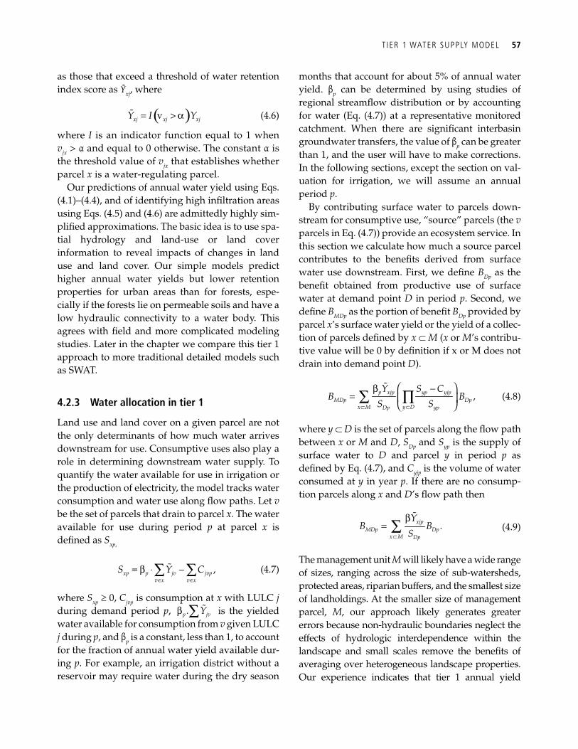
T IER 1 WATER SUPPLY MODEL 57
as those that exceed a threshold of water retention index score as Ỹ xj , where
( )= >! vxj xj xjY I Yα (4.6)
where I is an indicator function equal to 1 when vjx > α and equal to 0 otherwise. The constant α is the threshold value of vjx that establishes whether parcel x is a water-regulating parcel.
Our predictions of annual water yield using Eqs. (4.1)–(4.4), and of identifying high infi ltration areas using Eqs. (4.5) and (4.6) are admittedly highly sim-plifi ed approximations. The basic idea is to use spa-tial hydrology and land-use or land cover information to reveal impacts of changes in land use and land cover. Our simple models predict higher annual water yields but lower retention properties for urban areas than for forests, espe-cially if the forests lie on permeable soils and have a low hydraulic connectivity to a water body. This agrees with fi eld and more complicated modeling studies. Later in the chapter we compare this tier 1 approach to more traditional detailed models such as SWAT.
4.2.3 Water allocation in tier 1
Land use and land cover on a given parcel are not the only determinants of how much water arrives downstream for use. Consumptive uses also play a role in determining downstream water supply. To quantify the water available for use in irrigation or the production of electricity, the model tracks water consumption and water use along fl ow paths. Let v be the set of parcels that drain to parcel x . The water available for use during period p at parcel x is defi ned as S xp,
∈ ∈
= ⋅ −∑ ∑! ,xp p jv jvpv x v x
S Y Cβ (4.7)
where S xp ³ 0, C jvp is consumption at x with LULC j during demand period p , .p jvY∑ !β is the yielded water available for consumption from v given LULC j during p , and β p is a constant, less than 1, to account for the fraction of annual water yield available dur-ing p . For example, an irrigation district without a reservoir may require water during the dry season
months that account for about 5% of annual water yield. β p can be determined by using studies of regional streamfl ow distribution or by accounting for water (Eq. (4.7)) at a representative monitored catchment. When there are signifi cant interbasin groundwater transfers, the value of β p can be greater than 1, and the user will have to make corrections. In the following sections, except the section on val-uation for irrigation, we will assume an annual period p .
By contributing surface water to parcels down-stream for consumptive use, “source” parcels (the v parcels in Eq. (4.7)) provide an ecosystem service. In this section we calculate how much a source parcel contributes to the benefi ts derived from surface water use downstream. First, we defi ne B Dp as the benefi t obtained from productive use of surface water at demand point D in period p . Second, we defi ne B MDp as the portion of benefi t B Dp provided by parcel x ’s surface water yield or the yield of a collec-tion of parcels defi ned by x Ì M ( x or M ’s contribu-tive value will be 0 by defi nition if x or M does not drain into demand point D ).
⊂⊂
⎛ ⎞−= ⎜ ⎟
⎝ ⎠∑ ∏
!,p xjp yp yjp
MDp Dpy Dx M Dp yp
Y S CB B
S Sβ
(4.8)
where y Ì D is the set of parcels along the fl ow path between x or M and D , S Dp and S yp is the supply of surface water to D and parcel y in period p as defi ned by Eq. (4.7), and C yjp is the volume of water consumed at y in year p . If there are no consump-tion parcels along x and D ’s fl ow path then
.xjpMDp Dp
x M Dp
YB B
S⊂= ∑
!β (4.9)
The management unit M will likely have a wide range of sizes, ranging across the size of sub-watersheds, protected areas, riparian buffers, and the smallest size of landholdings. At the smaller size of management parcel, M , our approach likely generates greater errors because non-hydraulic boundaries neglect the effects of hydrologic interdependence within the landscape and small scales remove the benefi ts of averaging over heterogeneous landscape properties. Our experience indicates that tier 1 annual yield
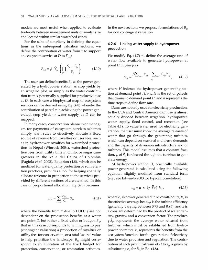
58 WATER SUPPLY AS AN ECOSYSTEM SERVICE FOR HYDROPOWER AND IRRIGATION
models are most useful when applied to evaluate trade-offs between management units of similar size and located within similar watershed zones.
For the sake of simplicity in defi ning the equa-tions in the subsequent valuation sections, we defi ne the contribution of water from x to support an ecosystem service at D as F jxD :
y jyjxD jx
y D y
S CF Y
Sb
∈
⎛ ⎞−= ⋅ ⋅ ⎜ ⎟
⎝ ⎠∏! . (4.10)
The user can defi ne benefi ts B D as the power gen-erated by a hydropower station, as crop yields by an irrigated plot, or simply as the water contribu-tion from x potentially supplied for productive use at D . In each case a biophysical map of ecosystem services can be derived using Eq. (4.8) whereby the contribution of parcel x in achieving the power gen-erated, crop yield, or water supply at D can be mapped.
In many cases, conservation planners or manag-ers for payments of ecosystem services schemes simply want rules to effectively allocate a fi xed source of revenue from royalties or user fees, such as in hydropower royalties for watershed protec-tion in Nepal (Winrock 2004), watershed protec-tion fees from utility bills in Quito, or sugar cane growers in the Valle del Cauca of Colombia ( Pagiola et al. 2002 ). Equation (4.8), which can be modifi ed for water quality protection or soil reten-tion practices, provides a tool for helping spatially allocate revenue in proportion to the services pro-vided by different sections of a watershed. In this case of proportional allocation, Eq. (4.8) becomes
jxDM B
x M D
FB B
S⊂= ⋅∑ , (4.11)
where the benefi ts from x due to LULC j are not dependent on the production benefi ts at a water use point D , but rather a fi xed value or budget, B B , that in this case corresponds to willingness to pay (contingent valuation) a proportion of royalties or utility fees for conservation, or a total “score” value to help prioritize the landscape. B M might corre-spond to an allocation of the fi xed budget for protection, conservation, or restoration activities.
In the next sections we propose formulations of B D for non contingent valuation.
4.2.4 Linking water supply to hydropower production
We modify Eq. (4.7) to defi ne the average rate of water fl ow available to generate hydropower at point H in year p as
b
⊂ ⊂−
= ∑ ∑! !vjp vjp vjpv H v H
Hp
Y C YS
n , (4.12)
where H indexes the hydropower generating sta-tion at demand point H , v Ì H is the set of parcels that drains to demand point H , and n represents the time steps to defi ne fl ow rate.
Dams are not only used for electricity production. In the USA and Central America dam use is almost equally divided between irrigation, hydropower, water supply, fl ood control, and recreation (see Table 4.1 ). To value water used for electricity gen-eration, the user must know the average releases of water that go through the generating turbines, which can depend on seasonal multi-use demands and the capacity of diversion infrastructure and of turbines. This model assumes that a constant frac-tion, γ , of S H is released through the turbines to gen-erate energy.
At hydropower station H , practically available power generated is calculated using the following equation, slightly modifi ed from standard form (e.g., see Edwards 2003 for typical formulation):
e m g= ⋅ ⋅ ⋅ ⋅( ) ,HH HS hk (4.13)
where ε H is power generated in kilowatt-hours, h H is the effective average head, μ is the turbine effi ciency (generally varying between 0.75 and 0.95), and κ is a constant determined by the product of water den-sity, gravity, and a conversion factor. The product, γ· S H , represents the average water released from turbines, which must be established from hydro-power operators. ε H represents the benefi ts from the ecosystem functions for the generation of electricity due to water provision and regulation. The contri-bution of each pixel upstream of H to ε H is given by substituting ε H for B D in Eq. (4.8).
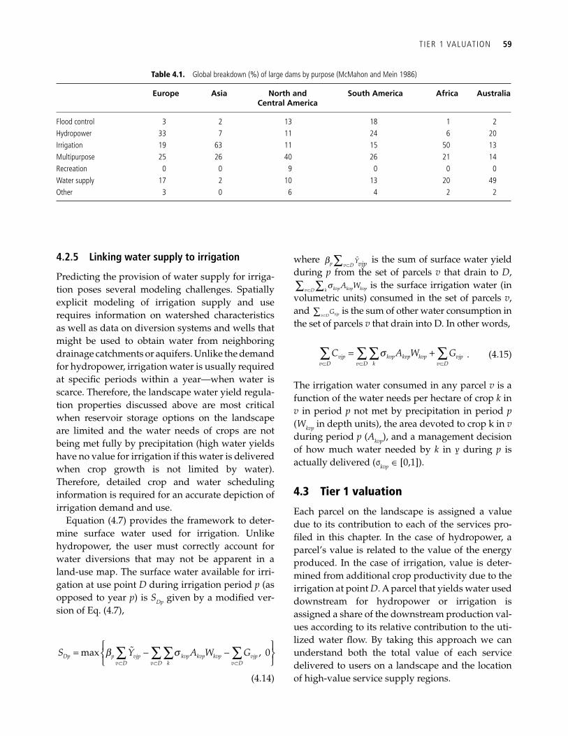
T IER 1 VALUATION 59
4.2.5 Linking water supply to irrigation
Predicting the provision of water supply for irriga-tion poses several modeling challenges. Spatially explicit modeling of irrigation supply and use requires information on watershed characteristics as well as data on diversion systems and wells that might be used to obtain water from neighboring drainage catchments or aquifers. Unlike the demand for hydropower, irrigation water is usually required at specifi c periods within a year—when water is scarce. Therefore, the landscape water yield regula-tion properties discussed above are most critical when reservoir storage options on the landscape are limited and the water needs of crops are not being met fully by precipitation (high water yields have no value for irrigation if this water is delivered when crop growth is not limited by water). Therefore, detailed crop and water scheduling information is required for an accurate depiction of irrigation demand and use.
Equation (4.7) provides the framework to deter-mine surface water used for irrigation. Unlike hydropower, the user must correctly account for water diversions that may not be apparent in a land-use map. The surface water available for irri-gation at use point D during irrigation period p (as opposed to year p ) is S Dp given by a modifi ed ver-sion of Eq. (4.7),
b
⊂ ⊂ ⊂
⎧ ⎫= − −⎨ ⎬⎩ ⎭
∑ ∑ ∑ ∑!max , 0Dp p vjp kvp kvp kvp vjpv D v D k v D
S Y A W Gs
(4.14)
where b⊂∑ !
p v DYvjp is the sum of surface water yield
during p from the set of parcels v that drain to D , s
⊂∑ ∑ kvp kvp kvpv D kA W is the surface irrigation water (in
volumetric units) consumed in the set of parcels v , and
⊂∑ vjpv DG is the sum of other water consumption in
the set of parcels v that drain into D. In other words,
vjp kvp kvp kvp vjpv D v D k v D
C A W Gs⊂ ⊂ ⊂
= +∑ ∑ ∑ ∑ . (4.15)
The irrigation water consumed in any parcel v is a function of the water needs per hectare of crop k in v in period p not met by precipitation in period p ( W kvp in depth units), the area devoted to crop k in v during period p ( A k v p ), and a management decision of how much water needed by k in v during p is actually delivered (σ kvp Î [0,1]).
4.3 Tier 1 valuation
Each parcel on the landscape is assigned a value due to its contribution to each of the services pro-fi led in this chapter. In the case of hydropower, a parcel’s value is related to the value of the energy produced. In the case of irrigation, value is deter-mined from additional crop productivity due to the irrigation at point D . A parcel that yields water used downstream for hydropower or irrigation is assigned a share of the downstream production val-ues according to its relative contribution to the uti-lized water fl ow. By taking this approach we can understand both the total value of each service delivered to users on a landscape and the location of high-value service supply regions.
Table 4.1. Global breakdown (%) of large dams by purpose (McMahon and Mein 1986)
Europe Asia North and Central America
South America Africa Australia
Flood control 3 2 13 18 1 2 Hydropower 33 7 11 24 6 20 Irrigation 19 63 11 15 50 13 Multipurpose 25 26 40 26 21 14 Recreation 0 0 9 0 0 0 Water supply 17 2 10 13 20 49 Other 3 0 6 4 2 2
60 WATER SUPPLY AS AN ECOSYSTEM SERVICE FOR HYDROPOWER AND IRRIGATION
4.3.1 The value of water fl ow for hydropower
Albery ( 1968 ) estimates the maximum willingness to pay for water by comparing the cost of electricity production from hydropower with that of the cheapest alternative source of electricity. The differ-ence between these two costs can be interpreted as the economic rent to the water resource. In order to estimate this value, the user must have information about the cost of hydropower production as well as the next cheapest alternative cost of power genera-tion. While this approach is theoretically accurate, it is also data intensive, requiring that users have information about the costs of hydropower and other sources of energy production. For this reason, we choose to value water in hydropower genera-tion based on the price of hydropower alone. While this approach will not fully capture the social value of hydropower production (such as reduced green-house gas emissions compared to coal-fi red power plants), it will provide a lower bound estimate of this value.
Under this framework, the net present value of hydropower production is given by
( )
1
0
( )1
Te H H
H tt
p cNPVH
re−
=
−=+∑ (4.16)
where p e is the market price of electricity (per unit of energy) provided by hydropower plant at dam d , ε H represents the annual energy generated by hydro-power station H , c H represents the average annual cost of operating hydropower station H and should include the external environmental damages of dam construction, T indicates the number of years we expect present landscape conditions to persist or the expected remaining lifetime of the station at H (set T to the smallest value if the two time values differ), and r is the market discount rate.
We rely on a parcel’s relative contribution of water used for hydropower to distribute the above value to the parcels upon which the electricity- generating water is generated. Let F xHj represent the amount of water that originates on parcel x in LULC j that is available for use for hydropower produc-tion at demand point H (see Eqs. (4.8) and (4.10)). Then, the contribution of water values for hydro-
power, NPVHC xH derived from management unit, M , is obtained as
xHjHM H
x M H
FNPVHC NPVH
S⊂= ∑ , (4.17)
where S H represents the total water used in electric-ity generation at point H .
Application example. Let us consider the value of water available for electricity generation in fi ve hydropower plants of the Willamette river basin ( Figure 4.1 ; see Plate 1). Given specifi c power generation ratings, and a LULC pattern from 1990, Eq. (4.1) simulates annual water yield at a 30 × 30 m parcel resolution. In this example, the estimate of the net present value of water for hydropower is based on a price of electricity of $0.01 per kilowatt, with a discount rate of 5% for a 100-year productive lifespan. Our model assigns the highest landscape values to the Detroit and Green Peter hydropower plant catchments because they have high power ratings with respect to their drainage areas (Figure 4.1a). The landscape draining into Lookout Point has lower per-parcel values despite its high energy rating because the contributing area is large. To examine how LULC change might impact the quantity and value of water available for hydropower production, we developed a scenario in which all the forested area below 1000 m in elevation was converted into pasture. Using our tier 1 surface water yield model, the increase in water yield of our deforested landscape enhanced annual runoff by up to 105 mm per parcel (Figure 4.1b). Since we were only evaluating total annual yield in this example, our tier 1 approach assigned greater landscape gains for hydropower provision to the deforested parcels (Figure 4.1c). Notice, that while deforestation is likely to negatively impact biodiversity and carbon emissions, in this situation it enhances potential hydropower production thru increased water yield. If deforestation also enhances sediment discharge into the reservoir, the net impact on hydropower generation might be reduced (see Chapter 6 ). This example is a good illustration of the trade-offs inherent in most land-use decisions, but glossed over when considering one service at a time.
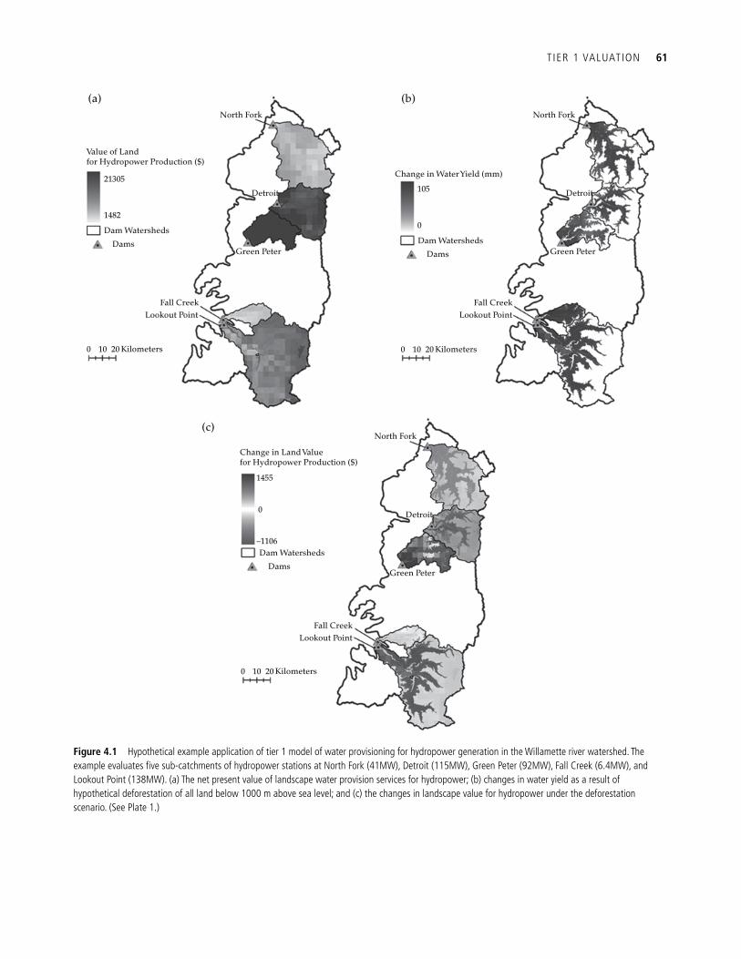
T IER 1 VALUATION 61
Value of Landfor Hydropower Production ($)
21305
1482
Dam Watersheds
Dams
0 10 20 Kilometers 0 10 20 Kilometers
0 10 20 Kilometers
Fall CreekLookout Point
Change in Land Valuefor Hydropower Production ($)
Green Peter Green Peter
Detroit Detroit
Green Peter
Detroit
North Fork North Fork
North Fork
Change in Water Yield (mm)
105
0
0
–1106
1455
Dams
Fall CreekLookout Point
Fall CreekLookout Point
Dam Watersheds
Dams
Dam Watersheds
(b)
(c)
(a)
Figure 4.1 Hypothetical example application of tier 1 model of water provisioning for hydropower generation in the Willamette river watershed. The example evaluates fi ve sub-catchments of hydropower stations at North Fork (41MW), Detroit (115MW), Green Peter (92MW), Fall Creek (6.4MW), and Lookout Point (138MW). (a) The net present value of landscape water provision services for hydropower; (b) changes in water yield as a result of hypothetical deforestation of all land below 1000 m above sea level; and (c) the changes in landscape value for hydropower under the deforestation scenario. (See Plate 1.)
62 WATER SUPPLY AS AN ECOSYSTEM SERVICE FOR HYDROPOWER AND IRRIGATION
4.3.2 The value of water fl ow used for irrigation at the crop fi eld
The monetary value of the amount of water used at D for irrigation purposes is given by B D . The water available for irrigation, S Dp , at D is given by Eq. (4.14). Let Irr Dp indicate the annual amount of surface water required for consumption by annual crop irrigation demand at D that is required dur-ing crop cycle with period, p , in an average year ( Irr Dp ≤ S Dp ). In this case B D is equal to the net value of agriculture production in D with Irr Dp . See Chapter 9 for details on determining B D at irri-gated points D . The contribution of each manage-ment parcel in the landscape to B D is approximated using Eq. (4.8).
4.4 Limitations of the tier 1 water yield models
As a general rule, the tier 1 water yield models are most physically realistic at watershed scales, spe-cifi cally, for areas that are hydrologically coherent. A hydrologically coherent area maintains the integrity of surface and subsurface water fl ow paths or drainage to a point of discharge, such as up to rivers, streams, creeks, or springs. When a watershed is subdivided without accounting for the potential fl ows between them, our tier 1 mod-eling approach presented can estimate relative contributions of different parts of the landscape to water fl ow, retention, and consumption but will likely misrepresent the integrated watershed response. Second, we do not explicitly model groundwater, especially in terms of pumping from shallow aquifers for irrigation. A third major short-coming of tier 1 water yield models is its annual timeframe. Many critical hydrological events or demands for water use occur on the timescale of days, and representing hydrology as an annual output can lead to large errors of interpretation. One way around this is to build seasonal models, so that as a compromise between annual and daily, one breaks the year up into different seasons, within which seasonal averages provide approxi-mations that can get much closer to the degree of realism one seeks. Tier 2 addresses this shortcom-ing in that it is a daily time step model.
4.5 Tier 2 water supply model
Our tier 2 water models simulate hydrologic variabil-ity, incorporate the temporal nature of management, and model additional hydrologic processes that infl u-ence the ecosystem services discussed in this chapter. In addition, tier 2 provides the tools for characterizing water resources infrastructure. Irrigation water is diverted and often stored to support or permit agri-cultural production when water is lacking at crop fi elds. Similarly, infrastructure for hydropower plants diverts, stores, or enhances energy production.
The soil matrix, vegetation roots, and shallow aquifers of a watershed provide a regulatory func-tion by enhancing opportunities for basefl ow or groundwater recharge. In effect, this provides a storage value to the watershed landscape. Tier 2 provides the means to simulate daily hydrology and climate variability, water resources infrastruc-ture, and all the rules of operation, management, and rights. This additional functionality provides greater accuracy in absolute and temporal terms. However, the tier 2 approach requires far more effort in compiling necessary data, and calibrating the models, and may not be feasible unless one has formal hydrological and modeling training and rel-atively long time windows for analysis.
The hydrology in the tier 2 models is driven by a modular system that allows users to replace or add different hydrology modules based on site-specifi c conditions, existing data, and hydrologic under-standing. In addition, the modular approach allows one to adjust model complexity as needed to explain site-specifi c phenomena (Farmer et al. 2003). Our tier 2 approach uses the Precipitation Runoff Modeling System (PRMS) developed by the US Geological Survey (Leavesley et al. 1983) to estimate water supply. Supply then becomes an input to a water resources systems model that incorporates demand, or use. Outputs of this model are then linked back to the watershed, such that the service provisioning is a function of hydrology, infrastruc-ture, and management.
4.5.1 Tier 2 modeling of physical hydrology
Our tier 2 hydrology model evaluates the impacts of various combinations of precipitation, climate,
T IER 2 WATER SUPPLY MODEL 63
and LULC on streamfl ow, sediment yields, and general basin hydrology. In PRMS the spatial mod-eling units are defi ned as Hydrologic Response Units (HRUs), which represent watershed parcels of homogenous geomorphology, vegetation, man-agement, and hydraulic connectivity. We simulate the hydrologic regime on a daily time step and per storm event using historical records or probabi-listic hydrology based on stochastic methods. By incorporating inter- and intra-annual variability, we can effectively examine the nonlinear response of hydrology to climate or management practices (i.e., dry years often lead to disproportionate scarcity). Within each HRU modeling parcel, the model keeps track of critical hydrological variables such as infi l-tration, soil moisture, and canopy interception of water—all of which will impact water supply. In the tier 2 equations that follow, parcels or landscape units, x , are HRUs.
4.5.2 Modeling of water resource systems: water accounting
Once water supply is estimated with the PRMS model, the tier 2 approach accounts for water resource systems and their impacts on fl ows. In par-ticular, we recommend using the Water Evaluation and Planning System (WEAP), which is a readily available tool that links hydrology to water resources systems (Siebert and Purkey 2007). In tier 2, the water from parcel x available for use, S d , at demand point d is described in its most generic form for any time, t , as
( ) ( ) ( ) ( )
( ) ( ),, ,
,,
d u u u STO ux d u d u d
u usto u
sto d u d u
S t Q t D t R t
Irr tV t
WRR
s s
ss
∈ ∈ ∈
∈ ∈
= − +
− −
∑ ∑ ∑
∑ ∑ (4.18)
where ( )∈∑ x dQ t represents streamfl ow (including
both storm runoff and shallow groundwater dis-charge components) from parcels x in the watershed available for use at d during time step t . ( )
x d
Q t∈
∑ results from interaction of each hydrology module, such as canopy interception, infi ltration and percolation, transpiration and evaporation, groundwater proc-esses, and vegetation growth. Each of the biophysi-cal processes represented by the modules can be represented at a level of complexity commensurate
with the data available and the user’s understand-ing and needs. D u ( t ,σ u ) represents water withdraw-als during t to satisfy demand u , which, like x , are part of the watershed landscape benefi tting d . Different demands for water u will have different priorities, or management policies, σ u , that can be function of t and Q(t) . R u,STO ( t ,σ u ) are fl ow releases from reservoirs STO , or return fl ows from demands u during t . Return fl ows vary depending on the type and effi ciency of water use and transport. They usu-ally represent the difference between water diverted to satisfy a demand and the amount of water actu-ally consumed, which is often 80 to 90% of demand for municipal and industrial uses (Loucks and Van Beek 2005). V sto ( t ) is the water stored during t in a lake or reservoir, or unavailable water being routed through the stream channel network. Irr u ( t ,σ u ) is that irrigation water required at u , and WRR u is the water requirement ratio, a fraction to account for transmis-sion losses or other irrigation requirements for excess demand of irrigation water. See Chapter 9 for information on Irr ud ( t ,σ u ).
The temporal dimension of Eq. (4.18) denoted by t introduces seasonality and interannual variability, such as dry and wet seasons or wet and dry years, which are often key to meeting demand for ecosys-tem services. In addition, in tier 2, the last four terms of Eq. (4.18) incorporate human effects on water availability, such as storage infrastructure, diver-sions, management strategies, and water rights policies. As might be evident, the greater is the alteration of fl ow regimes by human infl uence dur-ing t ; the lower is the relative importance of land-scape hydrology. The temporal and engineering system management dimensions of tier 2 provide the tools for broader examination of ecosystem services and trade-off options. The following sec-tions describe how we link the ecosystem provision of water, S d ( t ), to hydropower production and how we perform the valuation of the landscape. See Chapter 9 for the approach used in valuing the landscape for irrigation.
4.5.3 Linking water supply to hydropower production
Our tier 2 biophysical model allows us to calcu-late the daily water yield and use on a parcel. This
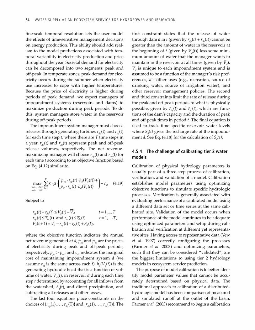
64 WATER SUPPLY AS AN ECOSYSTEM SERVICE FOR HYDROPOWER AND IRRIGATION
fi ne-scale temporal resolution lets the user model the effects of time-sensitive management decisions on energy production. This ability should add real-ism to the model predictions associated with tem-poral variability in electricity production and price throughout the year. Societal demand for electricity can be decomposed into two segments: peak and off-peak. In temperate zones, peak demand for elec-tricity occurs during the summer when electricity use increases to cope with higher temperatures. Because the price of electricity is higher during periods of peak demand, we expect managers of impoundment systems (reservoirs and dams) to maximize production during peak periods. To do this, system managers store water in the reservoir during off-peak periods.
The impoundment system manager must choose releases through generating turbines r dp (t) and r do (t) for each time step t , where there are T time steps in a year. r dp (t) and r do (t) represent peak and off-peak release volumes, respectively. The net revenue-maximizing manager will choose r dp (t) and r do (t) for each time t according to an objective function based on Eq. (4.12) similar to
1
1
,...,1,...,
( ) ( ( ))max
( ) ( ( ))dp dpT
do doT
Tp dp d d
dtr r o do d dtr r
p r t h V tc
p r t h V te
ek m
=
⋅ ⋅ +⎛ ⎞⋅ ⋅ −⎜ ⎟⋅ ⋅⎝ ⎠∑ (4.19)
Subject to
( ) ( ) ( ) 1,...,ddp do dr t r t V t V t T+ ≤ − = ≤ ≤ =( ) ( ) and ( ) ( ) 1,..., ,dp dp do dor t r t r t r t t T + = − − +( 1) ( ) ( ) ( ),d d dp do dV t V r t r t S t
where the objective function indicates the annual net revenue generated at d , p pε and p oε are the prices of electricity during peak and off-peak periods, respectively, p pε > p oε , and c dt indicates the marginal cost of maintaining impoundment system d (we assume c dt is the same across each t ). h d ( V d ( t )) is the generating hydraulic head that is a function of vol-ume of water, V d ( t ), in reservoir d during each time step t determined by accounting for all infl ows from the watershed, S d (t), and direct precipitation, and subtracting all releases and other losses.
The last four equations place constraints on the choices of r dp (1), . . . , r dp (T) and r do (1), . . . , r do (T). The
fi rst constraint states that the release of water through dam d in t (given by r dp ( t) + r do ( t )) cannot be greater than the amount of water in the reservoir at the beginning of t (given by V d (t)) less some mini-mum amount of water that the manager wants to maintain in the reservoir at all times (given by V– d ). V– d is unique to each impoundment system and is assumed to be a function of the manager’s risk pref-erences, d ’s other uses (e.g., recreation, source of drinking water, source of irrigation water), and other reservoir management policies. The second and third constraints limit the rate of release during the peak and off-peak periods to what is physically possible, given by r dp ( t ) and r do ( t ), which are func-tions of the dam’s capacity and the duration of peak and off-peak times in period t . The fi nal equation is used to track time-specifi c reservoir water levels where S d (t) gives the recharge rate of the impound-ment d . See Eq. (4.18) for the calculation of S d (t) .
4.5.4 The challenge of calibrating tier 2 water models
Calibration of physical hydrology parameters is usually part of a three-step process of calibration, verifi cation, and validation of a model. Calibration establishes model parameters using optimizing objective functions to simulate specifi c hydrologic processes. Verifi cation is generally associated with evaluating performance of a calibrated model using a different data set or time series at the same cali-brated site. Validation of the model occurs when performance of the model continues to be adequate using optimized parameters and setup during cali-bration and verifi cation at different yet representa-tive sites. Having access to representative data (Yew et al . 1997) correctly confi guring the processes (Farmer et al . 2003) and optimizing parameters, such that they can be considered “validated”, are the biggest limitations to using tier 2 hydrology models in ecosystem service prediction.
The purpose of model calibration is to better iden-tify model parameter values that cannot be accu-rately determined based on physical data. The traditional approach to calibration of a distributed-hydrologic model has been comparison of measured and simulated runoff at the outlet of the basin. Farmer et al . (2003) recommend to begin a calibration
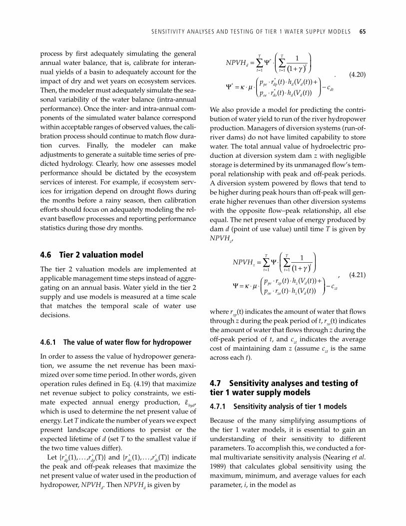
SENSIT IV ITY ANALYSES AND TEST ING OF T IER 1 WATER SUPPLY MODELS 65
process by fi rst adequately simulating the general annual water balance, that is, calibrate for interan-nual yields of a basin to adequately account for the impact of dry and wet years on ecosystem services. Then, the modeler must adequately simulate the sea-sonal variability of the water balance (intra-annual performance). Once the inter- and intra-annual com-ponents of the simulated water balance correspond within acceptable ranges of observed values, the cali-bration process should continue to match fl ow dura-tion curves. Finally, the modeler can make adjustments to generate a suitable time series of pre-dicted hydrology. Clearly, how one assesses model performance should be dictated by the ecosystem services of interest. For example, if ecosystem serv-ices for irrigation depend on drought fl ows during the months before a rainy season, then calibration efforts should focus on adequately modeling the rel-evant basefl ow processes and reporting performance statistics during those dry months.
4.6 Tier 2 valuation model
The tier 2 valuation models are implemented at applicable management time steps instead of aggre-gating on an annual basis. Water yield in the tier 2 supply and use models is measured at a time scale that matches the temporal scale of water use decisions.
4.6.1 The value of water fl ow for hydropower
In order to assess the value of hydropower genera-tion, we assume the net revenue has been maxi-mized over some time period. In other words, given operation rules defi ned in Eq. (4.19) that maximize net revenue subject to policy constraints, we esti-mate expected annual energy production, ε hyd , which is used to determine the net present value of energy. Let T indicate the number of years we expect present landscape conditions to persist or the expected lifetime of d (set T to the smallest value if the two time values differ).
Let r d p * ( 1 ) , . . . , r d p
* ( T ) and r d o * ( 1 ) , . . . , r d o
* ( T ) indicate the peak and off-peak releases that maximize the net present value of water used in the production of hydropower, NPVH d . Then NPVH d is given by
( )g
k m
= =
⎛ ⎞= Ψ ⋅⎜ ⎟+⎝ ⎠
⎛ ⎞⋅ ⋅ +Ψ = ⋅ ⋅ −⎜ ⎟⋅ ⋅⎝ ⎠
∑ ∑*
1 1
**
*
11
( ) ( ( ))
( ) ( ( ))
T T
d tt t
pe dp d ddt
oe do d d
NPVH
p r t h V tc
p r t h V t
. (4.20)
We also provide a model for predicting the contri-bution of water yield to run of the river hydropower production. Managers of diversion systems (run-of-river dams) do not have limited capability to store water. The total annual value of hydroelectric pro-duction at diversion system dam z with negligible storage is determined by its unmanaged fl ow’s tem-poral relationship with peak and off-peak periods. A diversion system powered by fl ows that tend to be higher during peak hours than off-peak will gen-erate higher revenues than other diversion systems with the opposite fl ow–peak relationship, all else equal. The net present value of energy produced by dam d (point of use value) until time T is given by NPVH z ,
( )g
k m
= =
⎛ ⎞= Ψ⋅⎜ ⎟+⎝ ⎠
⋅ ⋅ +⎛ ⎞Ψ = ⋅ ⋅ −⎜ ⎟⋅ ⋅⎝ ⎠
∑ ∑1 1
11
( ) ( ( ))( ) ( ( ))
T T
z tt t
pe zp z dzt
oe zo z d
NPVH
p r t h V tc
p r t h V t
, (4.21)
where r zp (t) indicates the amount of water that fl ows through z during the peak period of t , r zo (t) indicates the amount of water that fl ows through z during the off-peak period of t , and c zt indicates the average cost of maintaining dam z (assume c zt is the same across each t ).
4.7 Sensitivity analyses and testing of tier 1 water supply models
4.7.1 Sensitivity analysis of tier 1 models
Because of the many simplifying assumptions of the tier 1 water models, it is essential to gain an understanding of their sensitivity to different parameters. To accomplish this, we conducted a for-mal multivariate sensitivity analysis (Nearing et al . 1989) that calculates global sensitivity using the maximum, minimum, and average values for each parameter, i , in the model as
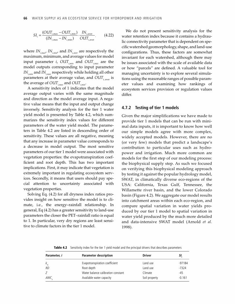
66 WATER SUPPLY AS AN ECOSYSTEM SERVICE FOR HYDROPOWER AND IRRIGATION
−
= ⋅−
,max ,min ,aver
,max ,min ,aver
( ),
( )i i i
ii i i
OUT OUT INSI
IN IN OUT (4.22)
where IN i , max, IN i , min , and IN i , aver are respectively the maximum, minimum, and average values for model input parameter i , OUT i , min and OUT i , max are the model outputs corresponding to input parameter IN i , min and IN i , max respectively while holding all other parameters at their average value, and OUT i , aver is the average of OUT i , max and OUT i , min .
A sensitivity index of 1 indicates that the model average output varies with the same magnitude and direction as the model average input. A nega-tive value means that the input and output change inversely. Sensitivity analysis for the tier 1 water yield model is presented by Table 4.2 , which sum-marizes the sensitivity index values for different parameters of the water yield model. The parame-ters in Table 4.2 are listed in descending order of sensitivity. These values are all negative, meaning that any increase in parameter value corresponds to a decrease in model output. The most sensitive parameters of our tier 1 model were associated with vegetation properties: the evapotranspiration coef-fi cient and root depth. This has two important implications. First, it may indicate that vegetation is extremely important in regulating ecosystem serv-ices. Secondly, it means that users should pay spe-cial attention to uncertainty associated with vegetation properties.
Solving Eq. (4.2) for all dryness index ratios pro-vides insight on how sensitive the model is to cli-mate, i.e., the energy–rainfall relationship. In general, Eq (4.2) has a greater sensitivity to land-use parameters the closer the PET–rainfall ratio is equal to 1. In particular, very dry regions are least sensi-tive to climate factors in the tier 1 model.
We do not present sensitivity analysis for the water retention index because it contains a hydrau-lic connectivity parameter that is dependent on spe-cifi c watershed geomorphology, shape, and land-use confi gurations. Thus, these factors are somewhat invariant for each watershed, although there may be issues associated with the scale of available data or how “parcels” are defi ned. A valuable tool for managing uncertainty is to explore several simula-tions using the reasonable ranges of possible param-eter values and examining how rankings of ecosystem services provision or regulation values differ.
4.7.2 Testing of tier 1 models
Given the major simplifi cations we have made to provide tier 1 models that can be run with mini-mal data inputs, it is important to know how well our simple models agree with more complex, widely accepted models. However, there are no (or very few) models that predict a landscape’s contribution to particular uses such as hydro-power and irrigation. Much more common are models for the fi rst step of our modeling process: the biophysical supply step. As such we focused on verifying this biophysical modeling approach by testing it against the popular hydrology model, SWAT, in climatically diverse eco-regions of the USA: California, Texas Gulf, Tennessee, the Willamette river basin, and the lower Colorado basin ( Figure 4.2 ). We aggregate our model results into catchment areas within each eco-region, and compare spatial variation in water yields pro-duced by our tier 1 model to spatial variation in water yield produced by the much more detailed and data-intensive SWAT model ( Arnold et al. 1998 ) .
Table 4.2 Sensitivity index for the tier 1 yield model and the principal drivers that describes parameters
Parameter, i Parameter description Driver SI i
k xj Evapotranspiration coeffi cient Land use -97184 RD Root depth Land use -7324 Z Water balance calibration constant Climate -45 AWC x Available water capacity Soil property -0.161
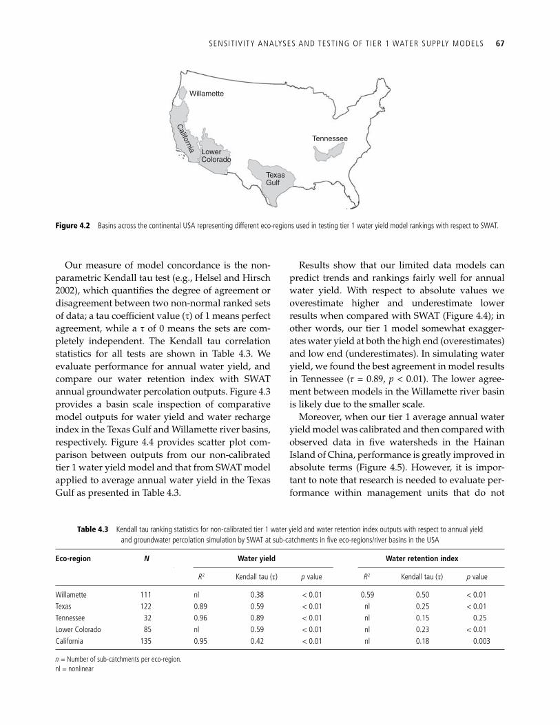
SENSIT IV ITY ANALYSES AND TEST ING OF T IER 1 WATER SUPPLY MODELS 67
Our measure of model concordance is the non-parametric Kendall tau test (e.g., Helsel and Hirsch 2002), which quantifi es the degree of agreement or disagreement between two non-normal ranked sets of data; a tau coeffi cient value (τ) of 1 means perfect agreement, while a τ of 0 means the sets are com-pletely independent. The Kendall tau correlation statistics for all tests are shown in Table 4.3 . We evaluate performance for annual water yield, and compare our water retention index with SWAT annual groundwater percolation outputs. Figure 4.3 provides a basin scale inspection of comparative model outputs for water yield and water recharge index in the Texas Gulf and Willamette river basins, respectively. Figure 4.4 provides scatter plot com-parison between outputs from our non-calibrated tier 1 water yield model and that from SWAT model applied to average annual water yield in the Texas Gulf as presented in Table 4.3 .
Results show that our limited data models can predict trends and rankings fairly well for annual water yield. With respect to absolute values we overestimate higher and underestimate lower results when compared with SWAT ( Figure 4.4 ); in other words, our tier 1 model somewhat exagger-ates water yield at both the high end (overestimates) and low end (underestimates). In simulating water yield, we found the best agreement in model results in Tennessee ( τ = 0.89, p < 0.01). The lower agree-ment between models in the Willamette river basin is likely due to the smaller scale.
Moreover, when our tier 1 average annual water yield model was calibrated and then compared with observed data in fi ve watersheds in the Hainan Island of China, performance is greatly improved in absolute terms ( Figure 4.5 ). However, it is impor-tant to note that research is needed to evaluate per-formance within management units that do not
Willamette
LowerColorado
TexasGulf
Tennessee
California
Figure 4.2 Basins across the continental USA representing different eco-regions used in testing tier 1 water yield model rankings with respect to SWAT.
Table 4.3 Kendall tau ranking statistics for non-calibrated tier 1 water yield and water retention index outputs with respect to annual yield and groundwater percolation simulation by SWAT at sub-catchments in fi ve eco-regions/river basins in the USA
Eco-region N Water yield Water retention index
R 2 Kendall tau (τ) p value R 2 Kendall tau (τ) p value
Willamette 111 nl 0.38 < 0.01 0.59 0.50 < 0.01 Texas 122 0.89 0.59 < 0.01 nl 0.25 < 0.01 Tennessee 32 0.96 0.89 < 0.01 nl 0.15 0.25 Lower Colorado 85 nl 0.59 < 0.01 nl 0.23 < 0.01 California 135 0.95 0.42 < 0.01 nl 0.18 0.003
n = Number of sub-catchments per eco-region. nl = nonlinear
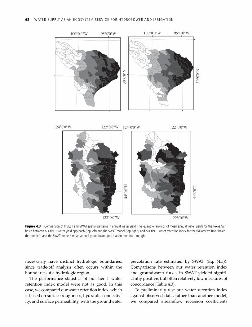
68 WATER SUPPLY AS AN ECOSYSTEM SERVICE FOR HYDROPOWER AND IRRIGATION
necessarily have distinct hydrologic boundaries, since trade-off analysis often occurs within the boundaries of a hydrologic region.
The performance statistics of our tier 1 water retention index model were not as good. In this case, we compared our water retention index, which is based on surface roughness, hydraulic connectiv-ity, and surface permeability, with the groundwater
percolation rate estimated by SWAT (Eq. (4.5)). Comparisons between our water retention index and groundwater fl uxes in SWAT yielded signifi -cantly positive, but often relatively low measures of concordance ( Table 4.3 ).
To preliminarily test our water retention index against observed data, rather than another model, we compared streamfl ow recession coeffi cients
Figure 4.3 Comparison of InVEST and SWAT spatial patterns in annual water yield. Five quantile rankings of mean annual water yields for the Texas Gulf basin between our tier 1 water yield approach (top left) and the SWAT model (top right), and our tier 1 water retention index for the Willamette River basin (bottom left) and the SWAT model’s mean annual groundwater percolation rate (bottom right).
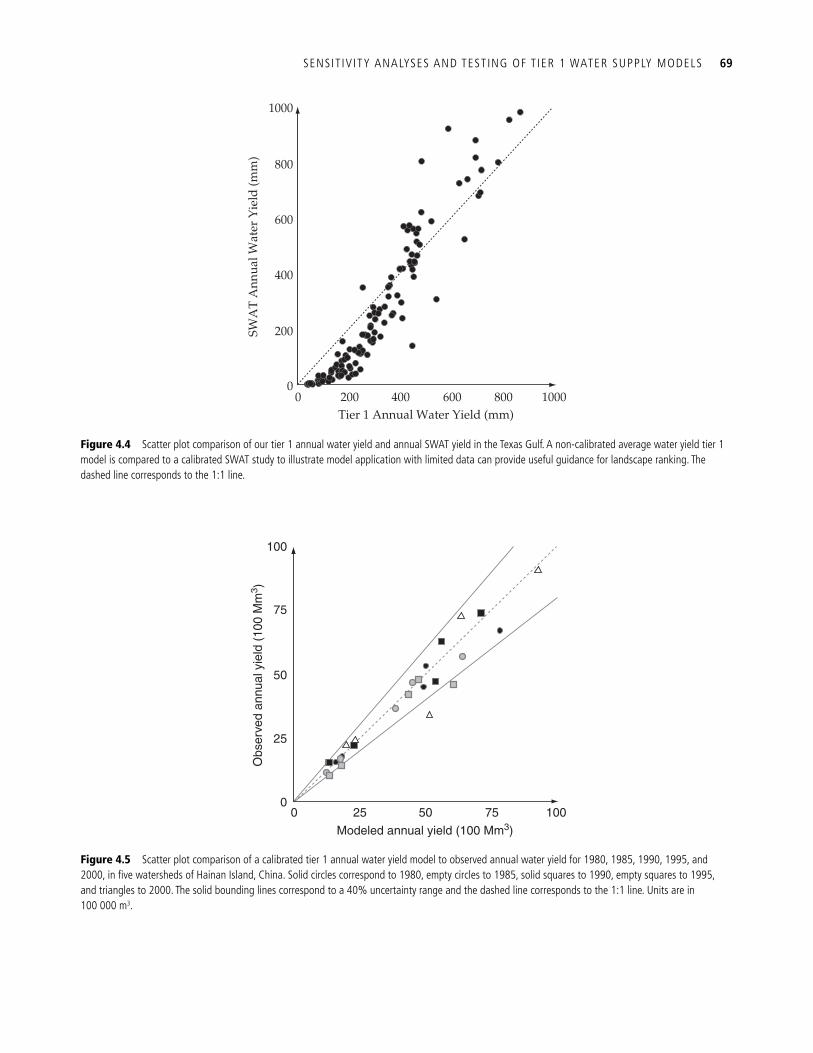
SENSIT IV ITY ANALYSES AND TEST ING OF T IER 1 WATER SUPPLY MODELS 69
00
200
400
SWA
T A
nnua
l Wat
er Y
ield
(mm
)
600
800
1000
200Tier 1 Annual Water Yield (mm)
400 600 800 1000
Figure 4.4 Scatter plot comparison of our tier 1 annual water yield and annual SWAT yield in the Texas Gulf. A non-calibrated average water yield tier 1 model is compared to a calibrated SWAT study to illustrate model application with limited data can provide useful guidance for landscape ranking. The dashed line corresponds to the 1:1 line.
100
75
50
25
00 25 50 75
Modeled annual yield (100 Mm3)
Obs
erve
d an
nual
yie
ld (
100
Mm
3 )
100
Figure 4.5 Scatter plot comparison of a calibrated tier 1 annual water yield model to observed annual water yield for 1980, 1985, 1990, 1995, and 2000, in fi ve watersheds of Hainan Island, China. Solid circles correspond to 1980, empty circles to 1985, solid squares to 1990, empty squares to 1995, and triangles to 2000. The solid bounding lines correspond to a 40% uncertainty range and the dashed line corresponds to the 1:1 line. Units are in 100 000 m 3 .
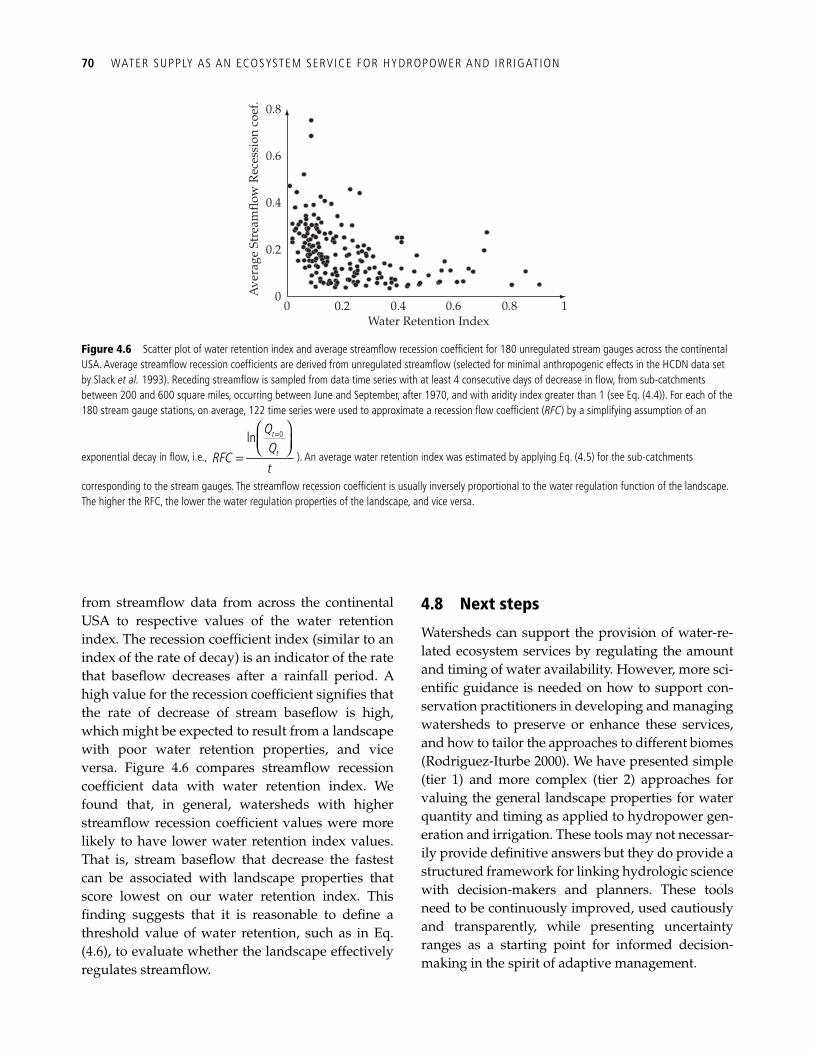
70 WATER SUPPLY AS AN ECOSYSTEM SERVICE FOR HYDROPOWER AND IRRIGATION
from streamfl ow data from across the continental USA to respective values of the water retention index. The recession coeffi cient index (similar to an index of the rate of decay) is an indicator of the rate that basefl ow decreases after a rainfall period. A high value for the recession coeffi cient signifi es that the rate of decrease of stream basefl ow is high, which might be expected to result from a landscape with poor water retention properties, and vice versa. Figure 4.6 compares streamfl ow recession coeffi cient data with water retention index. We found that, in general, watersheds with higher streamfl ow recession coeffi cient values were more likely to have lower water retention index values. That is, stream basefl ow that decrease the fastest can be associated with landscape properties that score lowest on our water retention index. This fi nding suggests that it is reasonable to defi ne a threshold value of water retention, such as in Eq. (4.6), to evaluate whether the landscape effectively regulates streamfl ow.
4.8 Next steps
Watersheds can support the provision of water-re-lated ecosystem services by regulating the amount and timing of water availability. However, more sci-entifi c guidance is needed on how to support con-servation practitioners in developing and managing watersheds to preserve or enhance these services, and how to tailor the approaches to different biomes (Rodriguez-Iturbe 2000). We have presented simple (tier 1) and more complex (tier 2) approaches for valuing the general landscape properties for water quantity and timing as applied to hydropower gen-eration and irrigation. These tools may not necessar-ily provide defi nitive answers but they do provide a structured framework for linking hydrologic science with decision-makers and planners. These tools need to be continuously improved, used cautiously and transparently, while presenting uncertainty ranges as a starting point for informed decision-making in the spirit of adaptive management.
00
0.2
0.2
0.4
0.6
0.8
0.4 0.6Water Retention Index
Ave
rage
Str
eam
flow
Rec
essi
on c
oef.
0.8 1
Figure 4.6 Scatter plot of water retention index and average streamfl ow recession coeffi cient for 180 unregulated stream gauges across the continental USA. Average streamfl ow recession coeffi cients are derived from unregulated streamfl ow (selected for minimal anthropogenic effects in the HCDN data set by Slack et al. 1993). Receding streamfl ow is sampled from data time series with at least 4 consecutive days of decrease in fl ow, from sub-catchments between 200 and 600 square miles, occurring between June and September, after 1970, and with aridity index greater than 1 (see Eq. (4.4)). For each of the 180 stream gauge stations, on average, 122 time series were used to approximate a recession fl ow coeffi cient ( RFC ) by a simplifying assumption of an
exponential decay in fl ow, i.e.,
0ln =⎛ ⎞⎜ ⎟⎝ ⎠=
t
t
RFCt
). An average water retention index was estimated by applying Eq. (4.5) for the sub-catchments
corresponding to the stream gauges. The streamfl ow recession coeffi cient is usually inversely proportional to the water regulation function of the landscape. The higher the RFC, the lower the water regulation properties of the landscape, and vice versa.
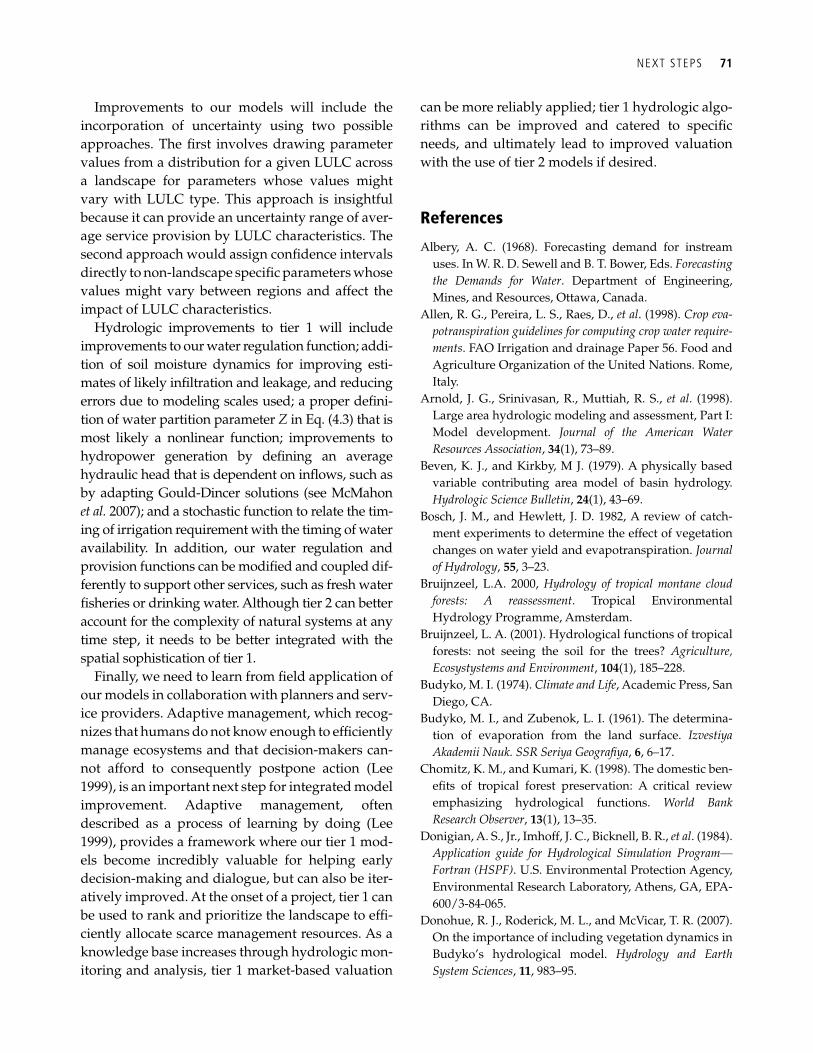
NEXT STEPS 71
Improvements to our models will include the incorporation of uncertainty using two possible approaches. The fi rst involves drawing parameter values from a distribution for a given LULC across a landscape for parameters whose values might vary with LULC type. This approach is insightful because it can provide an uncertainty range of aver-age service provision by LULC characteristics. The second approach would assign confi dence intervals directly to non-landscape specifi c parameters whose values might vary between regions and affect the impact of LULC characteristics.
Hydrologic improvements to tier 1 will include improvements to our water regulation function; addi-tion of soil moisture dynamics for improving esti-mates of likely infi ltration and leakage, and reducing errors due to modeling scales used; a proper defi ni-tion of water partition parameter Z in Eq. (4.3) that is most likely a nonlinear function; improvements to hydropower generation by defi ning an average hydraulic head that is dependent on infl ows, such as by adapting Gould-Dincer solutions (see McMahon et al. 2007); and a stochastic function to relate the tim-ing of irrigation requirement with the timing of water availability. In addition, our water regulation and provision functions can be modifi ed and coupled dif-ferently to support other services, such as fresh water fi sheries or drinking water. Although tier 2 can better account for the complexity of natural systems at any time step, it needs to be better integrated with the spatial sophistication of tier 1.
Finally, we need to learn from fi eld application of our models in collaboration with planners and serv-ice providers. Adaptive management, which recog-nizes that humans do not know enough to effi ciently manage ecosystems and that decision-makers can-not afford to consequently postpone action (Lee 1999), is an important next step for integrated model improvement. Adaptive management, often described as a process of learning by doing (Lee 1999), provides a framework where our tier 1 mod-els become incredibly valuable for helping early decision-making and dialogue, but can also be iter-atively improved. At the onset of a project, tier 1 can be used to rank and prioritize the landscape to effi -ciently allocate scarce management resources. As a knowledge base increases through hydrologic mon-itoring and analysis, tier 1 market-based valuation
can be more reliably applied; tier 1 hydrologic algo-rithms can be improved and catered to specifi c needs, and ultimately lead to improved valuation with the use of tier 2 models if desired.
References
Albery, A. C. (1968). Forecasting demand for instream uses. In W. R. D. Sewell and B. T. Bower, Eds. Forecasting the Demands for Water . Department of Engineering, Mines, and Resources, Ottawa, Canada.
Allen, R. G., Pereira, L. S., Raes, D., et al . (1998). Crop eva-potranspiration guidelines for computing crop water require-ments . FAO Irrigation and drainage Paper 56. Food and Agriculture Organization of the United Nations. Rome, Italy.
Arnold, J. G., Srinivasan, R., Muttiah, R. S., et al . (1998). Large area hydrologic modeling and assessment, Part I: Model development. Journal of the American Water Resources Association , 34 (1), 73–89.
Beven, K. J., and Kirkby, M J. (1979). A physically based variable contributing area model of basin hydrology. Hydrologic Science Bulletin , 24 (1), 43–69.
Bosch, J. M., and Hewlett, J. D. 1982, A review of catch-ment experiments to determine the effect of vegetation changes on water yield and evapotranspiration. Journal of Hydrology , 55 , 3–23.
Bruijnzeel, L.A. 2000, Hydrology of tropical montane cloud forests: A reassessment . Tropical Environmental Hydrology Programme, Amsterdam.
Bruijnzeel, L. A. (2001). Hydrological functions of tropical forests: not seeing the soil for the trees? Agriculture, Ecosystystems and Environment , 104 (1), 185–228.
Budyko, M. I. (1974). Climate and Life , Academic Press, San Diego, CA.
Budyko, M. I., and Zubenok, L. I. (1961). The determina-tion of evaporation from the land surface. Izvestiya Akademii Nauk. SSR Seriya Geografi ya , 6 , 6–17.
Chomitz, K. M., and Kumari, K. (1998). The domestic ben-efi ts of tropical forest preservation: A critical review emphasizing hydrological functions. World Bank Research Observer , 13 (1), 13–35.
Donigian, A. S., Jr., Imhoff, J. C., Bicknell, B. R., et al . (1984). Application guide for Hydrological Simulation Program—Fortran (HSPF) . U.S. Environmental Protection Agency, Environmental Research Laboratory, Athens, GA, EPA-600/3-84-065.
Donohue, R. J., Roderick, M. L., and McVicar, T. R. (2007). On the importance of including vegetation dynamics in Budyko’s hydrological model. Hydrology and Earth System Sciences , 11 , 983–95.
72 WATER SUPPLY AS AN ECOSYSTEM SERVICE FOR HYDROPOWER AND IRRIGATION
Edwards, B. K. (2003). The economics of hydroelectric power . Edward Elgar, Northampton, MA.
Farmer, D., Sivalapan, M., and Jothityangkoon, C. (2003). Climate, soil, and vegetation controls upon the variabil-ity of water balance in temperate and semi-arid land-scapes: Downward approach to water balance analysis. Water Resources Research , 39 (2), 1–21.
FAO. (2003). The state of food insecurity in the world , Food and Agriculture Organization of the United Nations, Rome.
Gleick, P. H. (1996). Water resources. In S. H. Schneider, Ed., Encyclopedia of Climate and Weather . Oxford University Press, New York.
Helsel, D. R., and Hirsch, R. M. (2002). Statistical methods in water resources . US Geological Survey, Washington, DC.
IWMI (2001). Water for rural development: draft background paper on water for rural development prepared for the World Bank . International Water Management Institute, Colombo, Sri Lanka.
Kent, K. (1972). Section 4: Hydrology. In National Engineering Handbook. United States Department of Agriculture, Washington, DC.
Leavesley, G. H., Lichty, R. W., Troutman, B. M., et al . (1983). Precipitation-runoff modeling system: user’s manual . US Geological Survey, Washington, DC.
Lee, K. N. (1999). Appraising adaptive management. Conservation Ecology , 3 (2), article 3.
Loucks, D. P., and Van Beek, E. (2005). Water resources sys-tems planning and management: an introduction to methods, models and applications . Studies and reports in hydrol-ogy. UNESCO, Paris.
Lyimo, B. M. (2005). Energy and sustainable development in Tanzania , Helio International, Paris.
Lyon, S. W., Gerard-Marcant, P., Walter, M. T., et al . (2004). Using a topographic index to distribute variable source area runoff predicted with the SCS–Curve Number equation. Hydrology Proceedings. 18 (15), 2757–71.
McMahon, T. A., and Mein, R. G. (1986). River and reservoir yield . Water Resources Publications, Littleton, CO.
McMahon, T. A., Pegram, G. G. S., Vogel, R. M., et al . (2007). Review of Gould-Dincer reservoir storage-yield-relia-bility estimates. Advances in Water Resources , 30 , 1873–82.
Milly, P. C. D. (1994). Climate, soil water storage, and the average annual water balance. Water Resources Research , 3 (7), 2143–56.
Nearing, M. A., Ascough, L. D., and Chaves, H. M. L. (1989). WEPP model sensitivity analysis. In L. J. Lane and M. A. Nearing, Eds., USDA-Water Erosion Prediction Project: Hillside profi le model documentation, NSERL Report No. 2 . USDA-ARS-NSERL, West Lafayette, IN.
Oyebande, L. (1998). Effects of tropical forest on water yield. In E. R. C. Reynolds and F. Thompson, Eds., Forests, climate, and hydrology: regional impacts , pp. 16–50. United Nations University; Kefford Press, Singapore.
Pagiola, S., Bishop, J. and Landell-Mills, N. (2002). Selling forest environmental services: Market-based mecha-nisms for conservation and development. Earthscan, London.
Porporato, A., D’Odorico, P., Laio, F., et al . (2002). Ecohydrology of water-controlled ecosystems. Advances in Water Resources , 25 , 1335–48.
Potter, N. J., Zhang, L., Milly, P. C. D., et al . (2005). Effects of rainfall seasonality and soil moisture capacity on mean annual water balance for Australian catchments. Water Resources Research , 41 (6).
Rodriguez-Iturbe, I. (2000). Ecohydrology: A hydrologic perspective of climate-soil-vegetation dynamics. Water Resources Research , 36 (1), 3–9.
Siebert, J., and Purkey, D. (2007). WEAP: water evaluation and planning system—users guide . Stockholm Environment Institute, Sommerville, MA.
Slack, J. R., Lumb, A. M., and Landwehr, J. M. (1993). Hydro-Climatic Data Network (HCDN): Streamfl ow data set, 1874–1988 . US Geological Survey Water-Resources Investigation Report 93-4076 (CD).
Steenhuis, T. S., Winchell, M., Rossing, J., et al . (1995). SCS runoff equation revisited for variable-source runoff areas. Journal of Irrigation and Drainage Engineering , 121 (3), 234–8.
Tallis, H., Kareiva, P., Marvier, M., et al . (2008). An ecosys-tem services framework to support both practical con-servation and economic development. Proceedings of the National Academy of Sciences , 105 (28), 9457–64.
Winrock International (2004). Financial incentives to com-munities for stewardship of environmental resources . Feasibility study: LAG-A-00-99-00037-00. USAID, Washington, DC.
Winter, T. C., Harvey, J. W., Frankey, O. L., et al . (1998). Ground water and surface water a single resource. US Geological Survey Curcular 1139 . US Government Printing Offi ce, Denver, CO.
Yew, D. T., Dlamini, E. M., and Biftu, G. F. (1997). Effects of model complexity and structure, data quality, and objec-tive functions on hydrologic modeling. Journal of Hydrology , 192 , 81–103.
Zektser, I. S., and Loaiciga, H. A. (1993). Groundwater fl uxes in the global hydrologic cycle: past, present and future. Journal of Hydrology , 144 , 405–27.
Zhang, L., Dawes, W. R., and Walker, G. R. (2001). Response of mean annual evapotranspiration to vegetation changes at catchment scale. Water Resources Research , 37 , 701–8.
73
CHAPTER 5
Valuing land cover impact on storm peak mitigation Driss Ennaanay, Marc Conte, Kenneth Brooks, John Nieber, Manu Sharma, Stacie Wolny, and Guillermo Mendoza
5.1 Introduction
Images of floods displacing or even killing peo-ple provide a constant reminder of the power of nature and human vulnerability to natural disas-ters. Although storms and storm events are highly unpredictable, it is possible to use hydro-logical models to predict the magnitude of a par-ticular flood, given information on the local geology, soil properties, vegetation, and manage-ment practices. We have developed approaches for quantifying the link between changes in land use and land cover (LULC), and flood risk. In flood management, risk has three ingredients: the hydrological response to a storm, the possi-ble failure of flood protection infrastructure (such as a levee breaking), and the value of what might be destroyed by a flood. We focus on the hydrology and economic value of what may be destroyed, leaving structural integrity to be addressed by civil engineers. Given a well-de-fined storm, we estimate the severity of flooding in terms of water volumes and flow rates, and corresponding damages from the storm.
In general, the combination of meteorological (e.g., rainfall intensity, extent and duration of the event) and geophysical (e.g., basin size, basin geomorphology, soil characteristics, and land use) characteristics are the main factors influenc-ing major flooding following large rainfall events ( Hamilton and King 1983 ; Kattelmann 1987 ; Bruijnzeel 1990 , 2004 ). In some situations, natu-ral landscapes and vegetation can offer storm peak mitigation. For example, forests and deep
permeable soils often reduce runoff as the result of enhanced soil infiltration and soil water stor-age capacity. Conversion of forests and wetlands to agricultural or developed land covers will tend to increase the volume of runoff and the flooding associated with storm events for medium and small return period events ( Ennaanay 2006 ). However, forests have limited ability to mitigate flooding associated with large return period storm events because enhanced soil infiltration only captures a small fraction of total precipitation depth for such storms ( FAO and CIFOR 2005 ). We develop models in this chapter that can help decision-makers take advantage of nature-based mitigation of floods and storm damage from medium and small return period events to avoid unnecessary flood risk due to poor land management.
This chapter presents two different types of mod-els for quantifying the impact of LULC on storm outcomes. The data-sparse tier 1 model quantifi es the reduction in storm peak volume due to LULC relative to bare soil on a parcel-by-parcel basis and values this reduction based on each parcel’s relative contribution to mitigation. In the present formula-tion the tier 1 model is not set up to predict the extent of downstream fl ooded area associated with a storm peak. The more robust, data-intensive tier 2 model provides probabilistic output for fl ood mag-nitudes as affected by incremental changes in the landscape mosaic and quantifi es the incremental changes in risks associated with a specifi c fl ood vol-ume, where risk is associated with a cost. In tier 2, the extent of fl ooded area is determined using the
74 VALUING LAND COVER IMPACT ON STORM PEAK MIT IGATION
Hydrologic Engineering Centers River Analysis System software (HEC-RAS) and streamfl ow time series from the Precipitation Runoff Modeling System (PRMS) model.
5.1.1 Storm peak mitigation modeling theory
For small to medium storms vegetation may retain water as it falls and fl ows through the land-scape (through canopy interception, enhanced infi ltration, soil water storage) and thus reduce peak fl ow. In a modeling study using the Hydrologic Simulation Program Fortran (HSPF) in the Cottonwood River watershed within the Minnesota River Basin, Ennaanay ( 2006 ) showed that conversion of different percent acreage (60, 75, and 86% of watershed area) of annual crop-ping systems (soy and corn) to perennial vegeta-tion over a 50-year simulation period showed a decrease in annual instantaneous peak fl ows for small event storms, but not for larger event storms. Similarly, studies from small paired experimental basins showed that clear-cutting and road building increased only some peak storm discharges ( Wright et al. 1990 ). Indeed, in the Pacifi c Northwest, increases in the peaks were greater for small early wet season storms but there was no signifi cant increase in peak fl ows for the largest storms ( Rothacher 1970 ).
Wetlands in both up- and downstream areas, and floodplains have a significant role in miti-gating floods and storm peaks. Both land-use types have storage capacities higher than many other LULC types. Ennaanay ( 2006 ) showed that conversion of 27% of the annual cropping sys-tems to wetlands could significantly reduce peak flows for small and moderate storm events. Wetlands not only reduce the peak flows but also significantly delay time to peak flows, and alter the inflow–discharge relationship and rough-ness. Floodplains have impacts similar to those of wetlands on flood mitigation and storm peak attenuation.
The spatial resolution of our models differs between tier 1 and tier 2. In tier 1, the analysis takes place at the parcel level, where parcel size is defi ned by the spatial resolution of the input data. In tier 2, the analysis is based on hydrologic response units
(HRUs), which are homogeneous with regard to LULC, soil, and slope. It should be noted that while the LULC category is a key determinant of an area’s ability to intercept rainfall, the equations presented below will not include direct references to LULC categories, as they are captured by the parcel and HRU indices. It should also be noted that while the analyses in tiers 1 and 2 occur at the parcel and HRU level, respectively, the model results can be reported at other scales more relevant to manage-ment decisions such as individually owned parcels or counties.
The key parameters linking LULC to storm peak mitigation are canopy interception, soil infi ltra-tion, LULC type, soil water storage, and land-use positioning on the landscape. Peak fl ows will increase as soil infi ltration, interception by canopy, or soil water storage is reduced. However, if the magnitude of storm depth becomes large, the impact that soil and plants have on storm fl ow peaks is small relative to water inputs ( Bruijnzeel 1990 ; Brooks et al. 2003 ; Ennaanay 2006 ) and thus of reduced value in terms of fl ood risk reduction. The impacts of land use on fl ooding also depend on the size of the area being examined. In particu-lar, land-use impacts on fl ooding are most evident in watersheds less than 1000 km 2 ( Kiersch 2001 ) because the sheer length of stream channels and extent of fl oodplains in larger basins provide storm peak mitigation, swamping the signal of land use. For example, forest harvesting has produced detectable changes in peak discharges in basins up to 600 km 2 in size. Increases are a result of changes in fl ow routing (due to roads) rather than to mere changes in water storage due to vegetation removal in small basins.
5.2. Tier 1 biophysical model
5.2.1 Modeling storm mitigation properties
The tier 1 model for storm peak mitigation focuses on a storm event of a specifi c size defi ned by the user. Our approach estimates the impact of land use on fl ood mitigation at the parcel level by determin-ing the amount of on-parcel storm runoff retained by each parcel following a rainfall event. We use GIS capabilities to generate a synthetic hydrograph
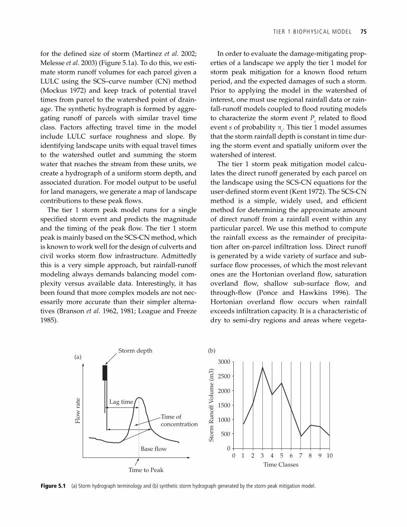
T IER 1 B IOPHYSICAL MODEL 75
for the defi ned size of storm ( Martinez et al. 2002 ; Melesse et al. 2003 ) ( Figure 5.1 a). To do this, we esti-mate storm runoff volumes for each parcel given a LULC using the SCS–curve number (CN) method (Mockus 1972) and keep track of potential travel times from parcel to the watershed point of drain-age. The synthetic hydrograph is formed by aggre-gating runoff of parcels with similar travel time class. Factors affecting travel time in the model include LULC surface roughness and slope. By identifying landscape units with equal travel times to the watershed outlet and summing the storm water that reaches the stream from these units, we create a hydrograph of a uniform storm depth, and associated duration. For model output to be useful for land managers, we generate a map of landscape contributions to these peak fl ows.
The tier 1 storm peak model runs for a single specifi ed storm event and predicts the magnitude and the timing of the peak fl ow. The tier 1 storm peak is mainly based on the SCS-CN method, which is known to work well for the design of culverts and civil works storm fl ow infrastructure. Admittedly this is a very simple approach, but rainfall-runoff modeling always demands balancing model com-plexity versus available data. Interestingly, it has been found that more complex models are not nec-essarily more accurate than their simpler alterna-tives ( Branson et al. 1962 , 1981 ; Loague and Freeze 1985 ).
In order to evaluate the damage-mitigating prop-erties of a landscape we apply the tier 1 model for storm peak mitigation for a known fl ood return period, and the expected damages of such a storm. Prior to applying the model in the watershed of interest, one must use regional rainfall data or rain-fall-runoff models coupled to fl ood routing models to characterize the storm event P s related to fl ood event s of probability π s . This tier 1 model assumes that the storm rainfall depth is constant in time dur-ing the storm event and spatially uniform over the watershed of interest.
The tier 1 storm peak mitigation model calcu-lates the direct runoff generated by each parcel on the landscape using the SCS-CN equations for the user-defi ned storm event ( Kent 1972 ). The SCS-CN method is a simple, widely used, and effi cient method for determining the approximate amount of direct runoff from a rainfall event within any particular parcel. We use this method to compute the rainfall excess as the remainder of precipita-tion after on-parcel infi ltration loss. Direct runoff is generated by a wide variety of surface and sub-surface fl ow processes, of which the most relevant ones are the Hortonian overland fl ow, saturation overland fl ow, shallow sub-surface fl ow, and through-fl ow ( Ponce and Hawkins 1996 ). The Hortonian overland fl ow occurs when rainfall exceeds infi ltration capacity. It is a characteristic of dry to semi-dry regions and areas where vegeta-
Figure 5.1 (a) Storm hydrograph terminology and (b) synthetic storm hydrograph generated by the storm peak mitigation model.
Time ofconcentration
Lag time
Storm depth(a)
Base flow
Time to Peak
Flow
rat
e
00
500
Stor
m R
unof
f Vol
ume
(m3)
1000
1500
2000
2500
3000
(b)
1 2 3 4 5Time Classes
6 7 8 9 10
76 VALUING LAND COVER IMPACT ON STORM PEAK MIT IGATION
tion is sparse and the soil surface is highly dis-turbed. The saturation overland fl ow occurs after the soil profi le has become saturated because of either high antecedent soil moisture or high rain-fall depth that fi lls in the soil profi le; this mecha-nism is referred to as the Dunne mechanism. Shallow sub-surface fl ow describes the process that takes place when water fl ows downslope in the shallow soil profi le quickly and contributes to storm fl ow. Kirkby and Chorley ( 1967 ) show that the shallow sub-surface fl ow can be similar to the through-fl ow that occurs in heavily vegetated landscapes with thick soil covers and less perme-able soil profi les atop impermeable bedrock ( Kirkby and Chorley 1967 ). In our approach we use the curve number to quantify runoff under the assumption that the storm event occurs uniformly throughout the watershed and that Hortonian run-off is the dominant process that generates the storm peak. Nonetheless, the CN method can be used in landscapes dominated by saturation over-land fl ow as demonstrated by Boughton ( 1987 ), Steenhuis et al. ( 1995 ), and Lyon et al. ( 2004 ), but would require some adjustments in how we develop the synthetic hydrograph. Although ini-tially designed for watershed catchment runoff estimates, a distributed CN method has been applied effectively to large parcels (from 900 m 2 up to several hectares) defi ned as HRUs in the Soil and Water Assessment Tool (SWAT) model ( Arnold et al. 1998 , and see Hawkins et al. 2009 ). There is no published guidance on an acceptable lower limit to parcel size for application of the CN approach.
The parcel size in our model is defi ned by the user and can be as small as is commensurate with input data. A common input data resolution is 900 m 2 , corresponding with the resolution of widely available digital elevation models. Our approach of applying the CN model on a parcel-by-parcel basis that is then aggregated (distributed approach) rather than on a watershed catchment (lumped approach) is not standard. We argue that runoff dif-ferences between distributed and lumped approaches are minimized in evaluations of mid- to larger sized storm events since the curve number becomes more linear at greater volumes. In addi-tion, since differences are smallest in homogeneous landscapes, such as natural landscapes, the user
should be most wary of heterogeneous landscapes, such as heavily urbanizing encroachments into forests.
The SCS-CN equation determines storm direct runoff depth at parcel x for a fl ood event s that occurs with probability π s generated by rainfall depth P s as
( )2
25400254
0 if 0.2
0.2 if 0.2
0.8
xjxj
sxj s xj
s xjsxj s xj
s xj
SCN
Q P S
P SQ P S
P S
= −′′
= ≤⎧⎪⎪ −⎨
= >⎪ +⎪⎩
, (5.1)
where xjCN′′ is the medium soil moisture condition curve number adjusted for slope, 0.2 S x is the initial abstraction, which accounts for the amount of pre-cipitation occurring before runoff, or the rainfall interception by vegetation. The value has been set to 0.2 S x through developmental history and docu-mentation; however, Hawkins ( 1979 ) showed that using 0.2 S x did not result in good runoff prediction unless S x was dependent on rainfall amounts. Q sx is the direct runoff or quick-fl ow that is potentially generated by P s at x .
The SCS-CN method uses the CN values that were developed and assumed to be appropriate for slopes of 5%. Our model uses the CN adjustment recommended by Williams ( 1995 ) to slopes differ-ent than 5%,
−−⎛ ⎞= − ⋅ +′′ ⎜ ⎟⎝ ⎠
13.86100* (1 2 ) ,
3xxxj
xj xj
CNCN e CNθ (5.2)
where CN xj is the CN value associated with LULC j in x applied for soil conditions of medium wet-ness type II (USDA 1986) with a 5% slope. However, the user can specify one of three wet-ness conditions (dry, medium, or wet): in temper-ate conditions, generally forested lands are drier than annual crops after long dry periods, and q x is the parcel’s slope.
Once direct runoff is calculated, we estimate travel time of that water to the point of interest. When defi ning the drainage area to evaluate the storm-mitigating properties of the landscape, it is important to exclude parcels that drain into inter-
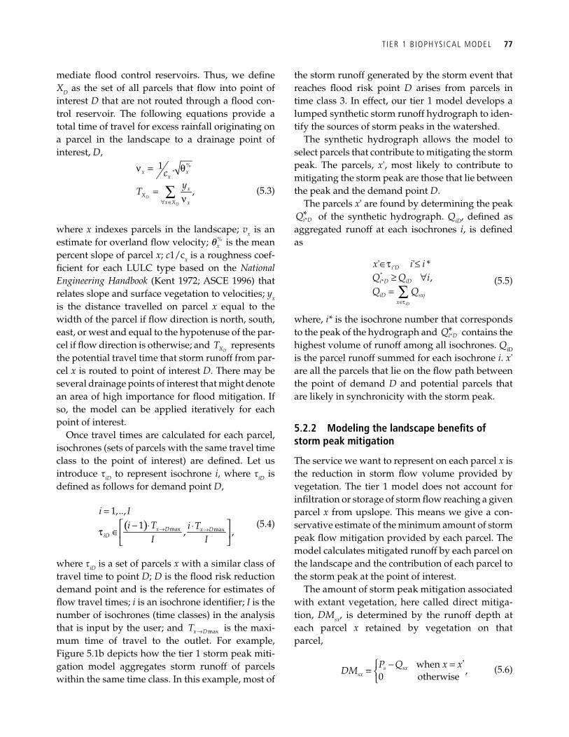
T IER 1 B IOPHYSICAL MODEL 77
mediate fl ood control reservoirs. Thus, we defi ne X D as the set of all parcels that fl ow into point of interest D that are not routed through a fl ood con-trol reservoir. The following equations provide a total time of travel for excess rainfall originating on a parcel in the landscape to a drainage point of interest, D ,
ν θ
ν∀ ∈
=
= ∑
%1 .
,D
D
x xx
xX
x X x
cy
T (5.3)
where x indexes parcels in the landscape; v x is an estimate for overland fl ow velocity; q %
x is the mean percent slope of parcel x ; c 1/cx is a roughness coef-fi cient for each LULC type based on the National Engineering Handbook ( Kent 1972 ; ASCE 1996) that relates slope and surface vegetation to velocities; y x is the distance travelled on parcel x equal to the width of the parcel if fl ow direction is north, south, east, or west and equal to the hypotenuse of the par-cel if fl ow direction is otherwise; and
DXT represents the potential travel time that storm runoff from par-cel x is routed to point of interest D . There may be several drainage points of interest that might denote an area of high importance for fl ood mitigation. If so, the model can be applied iteratively for each point of interest.
Once travel times are calculated for each parcel, isochrones (sets of parcels with the same travel time class to the point of interest) are defi ned. Let us introduce τ iD to represent isochrone i, where τ iD is defi ned as follows for demand point D ,
( ) → →
=⎡ ⎤− ⋅ ⋅∈⎢ ⎥⎣ ⎦
max max
1,..,1
, ,x D x DiD
i Ii T i T
I Iτ
(5.4)
where τ iD is a set of parcels x with a similar class of travel time to point D ; D is the fl ood risk reduction demand point and is the reference for estimates of fl ow travel times; i is an isochrone identifi er; I is the number of isochrones (time classes) in the analysis that is input by the user; and maxx DT → is the maxi-mum time of travel to the outlet. For example, Figure 5.1b depicts how the tier 1 storm peak miti-gation model aggregates storm runoff of parcels within the same time class. In this example, most of
the storm runoff generated by the storm event that reaches fl ood risk point D arises from parcels in time class 3. In effect, our tier 1 model develops a lumped synthetic storm runoff hydrograph to iden-tify the sources of storm peaks in the watershed.
The synthetic hydrograph allows the model to select parcels that contribute to mitigating the storm peak. The parcels, x' , most likely to contribute to mitigating the storm peak are those that lie between the peak and the demand point D .
The parcels x' are found by determining the peak *
*i DQ of the synthetic hydrograph. Q iD , defi ned as
aggregated runoff at each isochrones i , is defi ned as
′
∈
∈ ≤≥ ∀
= ∑**
' ' * ,
iD
i D
i D iD
iD sxjx
x i iQ Q iQ Q
τ
τ
(5.5)
where, i* is the isochrone number that corresponds to the peak of the hydrograph and *
*i DQ contains the
highest volume of runoff among all isochrones. Q iD is the parcel runoff summed for each isochrone i . x ' are all the parcels that lie on the fl ow path between the point of demand D and potential parcels that are likely in synchronicity with the storm peak.
5.2.2 Modeling the landscape benefi ts of storm peak mitigation
The service we want to represent on each parcel x is the reduction in storm fl ow volume provided by vegetation. The tier 1 model does not account for infi ltration or storage of storm fl ow reaching a given parcel x from upslope. This means we give a con-servative estimate of the minimum amount of storm peak fl ow mitigation provided by each parcel. The model calculates mitigated runoff by each parcel on the landscape and the contribution of each parcel to the storm peak at the point of interest.
The amount of storm peak mitigation associated with extant vegetation, here called direct mitiga-tion, DM sx , is determined by the runoff depth at each parcel x retained by vegetation on that parcel,
− =⎧= ⎨⎩
when ,0 otherwise
's sxsx
P Q x xDM (5.6)
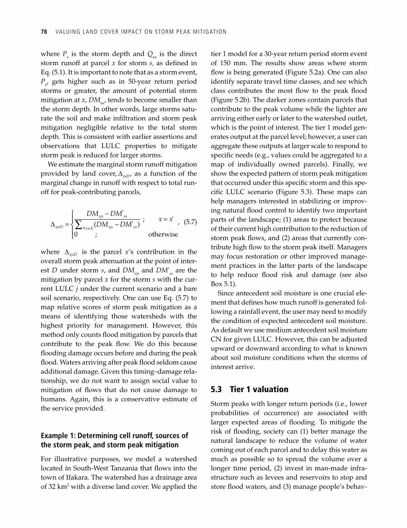
78 VALUING LAND COVER IMPACT ON STORM PEAK MIT IGATION
where P s is the storm depth and Q sx is the direct storm runoff at parcel x for storm s, as defi ned in Eq. (5.1). It is important to note that as a storm event, P s , gets higher such as in 50-year return period storms or greater, the amount of potential storm mitigation at x , DM sx , tends to become smaller than the storm depth. In other words, large storms satu-rate the soil and make infi ltration and storm peak mitigation negligible relative to the total storm depth. This is consistent with earlier assertions and observations that LULC properties to mitigate storm peak is reduced for larger storms.
We estimate the marginal storm runoff mitigation provided by land cover, xsD∆ , as a function of the marginal change in runoff with respect to total run-off for peak-contributing parcels,
'
' ; '( )
0 ; o t h e r w i s e
xjs xs
xjsD xjs xsx X
DM DMx x
DM DM∀ ∈
−⎧=⎪∆ = −⎨
⎪⎩∑ , (5.7)
where xjsD∆ is the parcel x ’s contribution in the overall storm peak attenuation at the point of inter-est D under storm s , and DM xjs and DM' xs are the mitigation by parcel x for the storm s with the cur-rent LULC j under the current scenario and a bare soil scenario, respectively. One can use Eq. (5.7) to map relative scores of storm peak mitigation as a means of identifying those watersheds with the highest priority for management. However, this method only counts fl ood mitigation by parcels that contribute to the peak fl ow. We do this because fl ooding damage occurs before and during the peak fl ood. Waters arriving after peak fl ood seldom cause additional damage. Given this timing–damage rela-tionship, we do not want to assign social value to mitigation of fl ows that do not cause damage to humans. Again, this is a conservative estimate of the service provided.
Example 1: Determining cell runoff, sources of the storm peak, and storm peak mitigation
For illustrative purposes, we model a watershed located in South-West Tanzania that fl ows into the town of Ifakara. The watershed has a drainage area of 32 km 2 with a diverse land cover. We applied the
tier 1 model for a 30-year return period storm event of 150 mm. The results show areas where storm fl ow is being generated ( Figure 5.2a ). One can also identify separate travel time classes, and see which class contributes the most fl ow to the peak fl ood (Figure 5.2b). The darker zones contain parcels that contribute to the peak volume while the lighter are arriving either early or later to the watershed outlet, which is the point of interest. The tier 1 model gen-erates output at the parcel level; however, a user can aggregate these outputs at larger scale to respond to specifi c needs (e.g., values could be aggregated to a map of individually owned parcels). Finally, we show the expected pattern of storm peak mitigation that occurred under this specifi c storm and this spe-cifi c LULC scenario ( Figure 5.3 ). These maps can help managers interested in stabilizing or improv-ing natural fl ood control to identify two important parts of the landscape; (1) areas to protect because of their current high contribution to the reduction of storm peak fl ows, and (2) areas that currently con-tribute high fl ow to the storm peak itself. Managers may focus restoration or other improved manage-ment practices in the latter parts of the landscape to help reduce fl ood risk and damage (see also Box 5.1 ).
Since antecedent soil moisture is one crucial ele-ment that defi nes how much runoff is generated fol-lowing a rainfall event, the user may need to modify the condition of expected antecedent soil moisture. As default we use medium antecedent soil moisture CN for given LULC. However, this can be adjusted upward or downward according to what is known about soil moisture conditions when the storms of interest arrive.
5.3 Tier 1 valuation
Storm peaks with longer return periods (i.e., lower probabilities of occurrence) are associated with larger expected areas of fl ooding. To mitigate the risk of fl ooding, society can (1) better manage the natural landscape to reduce the volume of water coming out of each parcel and to delay this water as much as possible so to spread the volume over a longer time period, (2) invest in man-made infra-structure such as levees and reservoirs to stop and store fl ood waters, and (3) manage people’s behav-
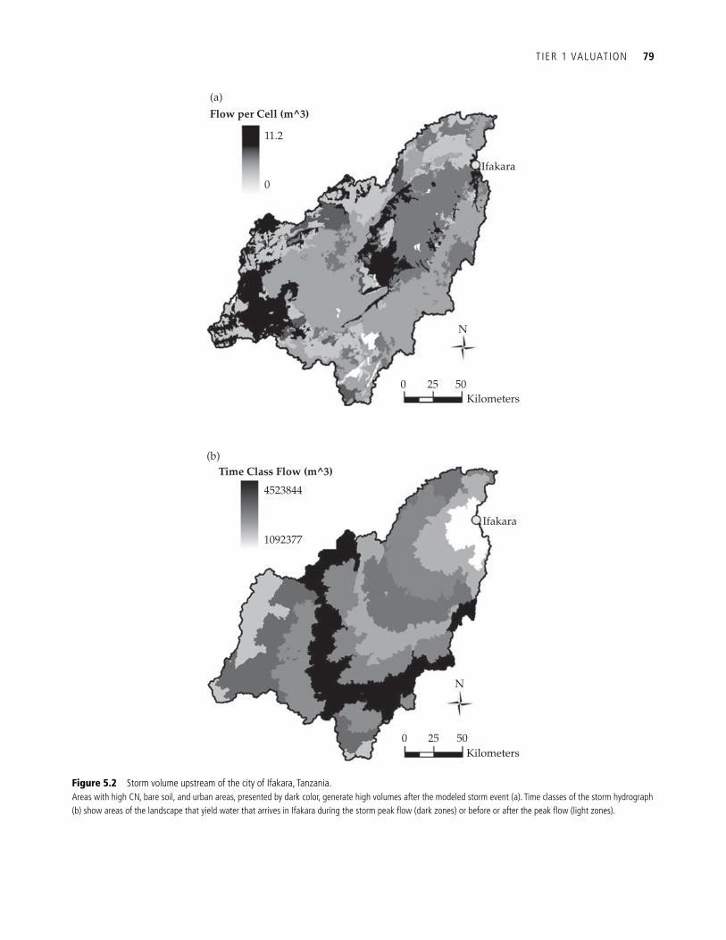
T IER 1 VALUATION 79
Figure 5.2 Storm volume upstream of the city of Ifakara, Tanzania. Areas with high CN, bare soil, and urban areas, presented by dark color, generate high volumes after the modeled storm event (a). Time classes of the storm hydrograph (b) show areas of the landscape that yield water that arrives in Ifakara during the storm peak fl ow (dark zones) or before or after the peak fl ow (light zones).
Flow per Cell (m^3)(a)
11.2
Ifakara
0 25 50Kilometers
N
0
Time Class Flow (m^3)
4523844
(b)
1092377
Ifakara
0 25 50Kilometers
N
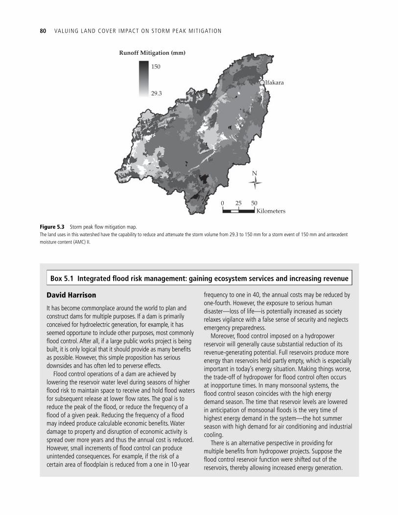
80 VALUING LAND COVER IMPACT ON STORM PEAK MIT IGATION
Runoff Mitigation (mm)
150
29.3
Ifakara
0 25 50Kilometers
N
Figure 5.3 Storm peak fl ow mitigation map. The land uses in this watershed have the capability to reduce and attenuate the storm volume from 29.3 to 150 mm for a storm event of 150 mm and antecedent moisture content (AMC) II.
David Harrison
It has become commonplace around the world to plan and construct dams for multiple purposes. If a dam is primarily conceived for hydroelectric generation, for example, it has seemed opportune to include other purposes, most commonly fl ood control. After all, if a large public works project is being built, it is only logical that it should provide as many benefi ts as possible. However, this simple proposition has serious downsides and has often led to perverse effects.
Flood control operations of a dam are achieved by lowering the reservoir water level during seasons of higher fl ood risk to maintain space to receive and hold fl ood waters for subsequent release at lower fl ow rates. The goal is to reduce the peak of the fl ood, or reduce the frequency of a fl ood of a given peak. Reducing the frequency of a fl ood may indeed produce calculable economic benefi ts. Water damage to property and disruption of economic activity is spread over more years and thus the annual cost is reduced. However, small increments of fl ood control can produce unintended consequences. For example, if the risk of a certain area of fl oodplain is reduced from a one in 10-year
frequency to one in 40, the annual costs may be reduced by one-fourth. However, the exposure to serious human disaster—loss of life—is potentially increased as society relaxes vigilance with a false sense of security and neglects emergency preparedness.
Moreover, fl ood control imposed on a hydropower reservoir will generally cause substantial reduction of its revenue-generating potential. Full reservoirs produce more energy than reservoirs held partly empty, which is especially important in today’s energy situation. Making things worse, the trade-off of hydropower for fl ood control often occurs at inopportune times. In many monsoonal systems, the fl ood control season coincides with the high energy demand season. The time that reservoir levels are lowered in anticipation of monsoonal fl oods is the very time of highest energy demand in the system—the hot summer season with high demand for air conditioning and industrial cooling.
There is an alternative perspective in providing for multiple benefi ts from hydropower projects. Suppose the fl ood control reservoir function were shifted out of the reservoirs, thereby allowing increased energy generation.
Box 5.1 Integrated fl ood risk management: gaining ecosystem services and increasing revenue
T IER 1 VALUATION 81
ior in fl ood prone areas—i.e., fl ood plain manage-ment, through Federal Flood insurance in the USA—limiting development in fl ood prone areas is often the most feasible and economically viable option. None of these approaches is foolproof, and both have to be designed in reference to the particu-lar severity of storm events. When severe storms occur, fl ooding is likely to ensue, particularly if the mitigation efforts are focused on less extreme events.
5.3.1 Calculating fl ood damage as a function of storm peak and LULC pattern
Our models are not designed to predict the fl ooded area. This means that if one wants to calculate dam-ages they need to obtain fl ood area maps. In the USA, fl ood footprint maps can be obtained from Federal Emergency Management Agency (FEMA) or fl ood insurance companies. In the developing world local knowledge ( Tran et al. 2009 ) can help piece together scant information. It may often be necessary to develop fl ood prints directly using river channel hydraulic software such as HEC-RAS (USACE, 2002; ESRI-HEC 2004) applied to each storm of interest. Once fl oodmaps have been obtained, using economic valuation techniques, we attach a damage value to each of the mapped fl ood events. To isolate the value of storm peak mitigation provided by LULC, we must compare the damages associated with events on bare soil with events on extant vegetation.
5.3.2 Determining D ks
Flooding can affect crops, infrastructure, and the production of valuable ecosystem services. Under certain conditions, the magnitude of fl ood events is impacted by the pattern of land use in a watershed. The value of storm peak mitigation increases with the ability of a LULC scheme to reduce the peak fl ow after a signifi cant rainfall event in the watershed.
In this model, we determine each parcel’s contri-bution to a fl ooding event at the watershed’s base. Next, we identify each parcel’s contribution to the economic damages in the fl ood area. Finally, we determine the potential savings or additional losses in total fl ood damage when a parcel changes LULC.
Let V xt indicate the total economic value of parcel x in year t . If possible, V xt should include all market values and monetized ecosystem service values. The total present value of damage due to a fl ood in area k with storm peak s is given by
( )
11 ,
(1 )1
Txh xh xT
ks h t Tx ks h t
V CD
rrα +
− +∈ =
= +++∑ ∑ (5.8)
where x Î ks indicates the parcels in k that are fl ooded given storm peak s . T indicates the number of years for which the value of parcel x cannot be fully real-ized due to storm peak s . α xt is an approximation of x 's portion of the value damaged by the fl ood in each year (i.e., if a fl ood covers land upon which a
This is feasible if fl ood risk management were to be accomplished by management in the fl ood plain itself. Increased hydropower revenues deriving from fuller reservoirs could be directed to a specifi c fund to provide revenues for this management.
The management of fl ood risks in the fl ood plain can be accomplished through the following measures:
1. Develop and maintain a comprehensive and effective emergency preparedness plan—early warning, orderly evacuation, equipped refuge locations, and orderly system for reoccupation and recuperation of property. 2. Restore fl ood plain ecosystems that provide not only ecological values but also fl ood attenuation values.
3. Use funds for regular assessment of the condition of fl ood plain infrastructure—inspection and maintenance of those levees and detention facilities—to reduce risk of infrastructure failure. 4. Develop new fi nancial instruments for fl ood risk coverage. Reinvent fl ood insurance applications to be based on incremental hydropower revenues. Recognize that inevitably water will occupy the land at some times, but that productive uses of the land will otherwise continue.
The fundamental idea is that integrated planning for fl ood risk management, hydropower production, and ecosystem protection has much to offer over simply imposing multiple purposes on planned infrastructure.
82 VALUING LAND COVER IMPACT ON STORM PEAK MIT IGATION
20-story skyscraper is built, the entire value of that building may not be lost as a result of the storm event, although the ability of workers to go to their offi ce might be). C represents the costs that must be incurred in order to return parcel x to its productive capacity (e.g., construction costs to rebuild struc-tures). r represents the annual discount rate. While the linear damage function (area-discharge) might seem arbitrary, Dutta et al. ( 2003 ) specify depth–damage curves for urban damage estimation that are linear until 3 m of depth above the fl oor level, the depth at which the damage function plateaus at 60% of total structure value.
As noted in Merz et al. ( 2004 ), the majority of fl ood damage estimation methodologies are based on direct tangible damage caused to structures in the fl ood zone. However, the cost of inundating land may be greater than the structural damage caused by the storm event. The true costs imposed by the fl ooding are the stream of profi t and serv-ice values foregone during the period of inunda-tion and drainage as well as any expenses that must be incurred to return the parcel to produc-tive use.
Information on the stream of expected profi t and service values at the parcel level may be dif-fi cult to gather. In many cases, especially if the fl ood event in question affects urban or rural-res-idential areas, the value of real estate can proxy for the discounted stream of all future profi ts emanating from a parcel ( Polasky et al. 2008 ). Note that such an approximation is only reason-able in areas with fully functioning land markets. Because the value of real estate in functioning markets refl ects the infi nite profi t stream associ-ated with optimal use of a parcel, but a parcel will only be impaired for a period of time ( t to T ), V xt could be set equal to
( )
,1
Txt
h th t
RVr −
= +∑ (5.9)
where RV xt is the annual rental value of real estate in parcel x in year t .
The value of storm peak mitigation is captured by the difference in expected damages due to the pres-ence of vegetation in the landscape. In the tier 1
model, the area of the landscape inundated by storm s is not impacted by the LULC pattern. As a result, we are unable to identify how the presence of native vegetation mitigates the damages caused by fl ooding. We provide an estimate of the true value of this impact as
(1 )fsks ks
bs
B Dωω
= − , (5.10)
where ω fs represents the volume of post-peak water delivered to the damage point during storm s when the landscape is covered by the current LULC pat-tern and ω bs represents the volume of post-peak water delivered to the damage point when the land-scape is covered by bare soil.
The model then aggregates sources of runoff from parcels into isochrones. Finally, we distribute B ks across the parcels that are in isochrones that precede the peak. These groups include all parcels that con-tribute water to the storm fl ow that impacts area k . B ks is distributed among these parcels according to each parcel’s relative contribution of water volume. Let B xks represent parcel x 's share of B ks , where
1
ksXks xksx
B B=
= ∑ , x indexes the parcels contributing to the storm volume, and X ks is the set of all such par-cels. Then B xks can be defi ned as
*xks ks xjsDB B= ∆ , (5.11)
where D xks = 0 if x lies within a time class that pre-cedes the storm peak, or the storm return period is greater than 100 years, assuming that at 100 years, LULC has no signifi cant impact on reducing storm peak.
5.3.4 Accounting for the distribution of storm peak return periods
Whether or not a particular return period storm will occur on a landscape in any given year (i.e., the probability that a particular storm peak will occur on the landscape in any given year) is uncertain. The return period indicates on average whether a fl ood of a particular size will occur at least once during that time period.
Accurate valuation of storm peak mitigation requires calculation of the expected damages
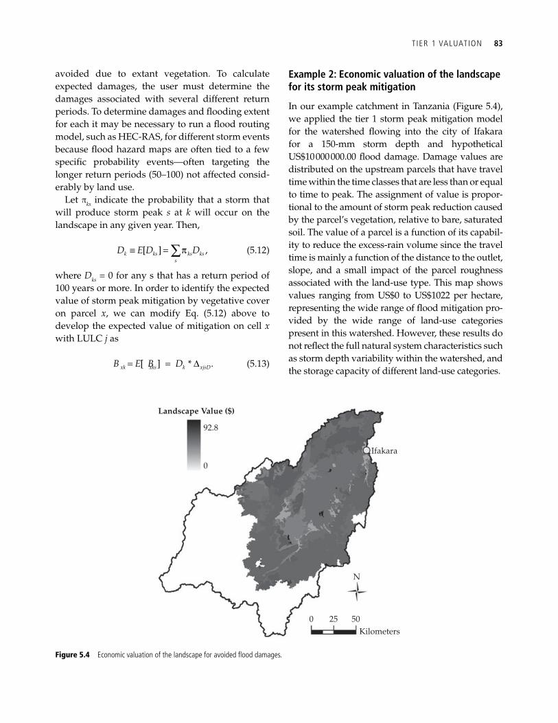
T IER 1 VALUATION 83
avoided due to extant vegetation. To calculate expected damages, the user must determine the damages associated with several different return periods. To determine damages and fl ooding extent for each it may be necessary to run a fl ood routing model, such as HEC-RAS, for different storm events because fl ood hazard maps are often tied to a few specifi c probability events—often targeting the longer return periods (50–100) not affected consid-erably by land use.
Let π ks indicate the probability that a storm that will produce storm peak s at k will occur on the landscape in any given year. Then,
[ ] ,k ks ks kss
D E D Dπ≡ = ∑ (5.12)
where D ks = 0 for any s that has a return period of 100 years or more. In order to identify the expected value of storm peak mitigation by vegetative cover on parcel x , we can modify Eq. (5.12) above to develop the expected value of mitigation on cell x with LULC j as
[ ] *xk xks k xjsDB E B D= = ∆ . (5.13)
Example 2: Economic valuation of the landscape for its storm peak mitigation
In our example catchment in Tanzania ( Figure 5.4 ), we applied the tier 1 storm peak mitigation model for the watershed fl owing into the city of Ifakara for a 150-mm storm depth and hypothetical US$10 000 000.00 fl ood damage. Damage values are distributed on the upstream parcels that have travel time within the time classes that are less than or equal to time to peak. The assignment of value is propor-tional to the amount of storm peak reduction caused by the parcel’s vegetation, relative to bare, saturated soil. The value of a parcel is a function of its capabil-ity to reduce the excess-rain volume since the travel time is mainly a function of the distance to the outlet, slope, and a small impact of the parcel roughness associated with the land-use type. This map shows values ranging from US$0 to US$1022 per hectare, representing the wide range of fl ood mitigation pro-vided by the wide range of land-use categories present in this watershed. However, these results do not refl ect the full natural system characteristics such as storm depth variability within the watershed, and the storage capacity of different land-use categories.
Landscape Value ($)
Ifakara
92.8
0
0 25 50Kilometers
N
Figure 5.4 Economic valuation of the landscape for avoided fl ood damages.
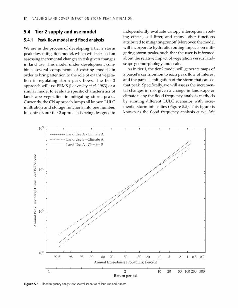
84 VALUING LAND COVER IMPACT ON STORM PEAK MIT IGATION
5.4 Tier 2 supply and use model
5.4.1 Peak fl ow model and fl ood analysis
We are in the process of developing a tier 2 storm peak fl ow mitigation model, which will be based on assessing incremental changes in risk given changes in land use. This model under development com-bines several components of existing models in order to bring attention to the role of extant vegeta-tion in regulating storm peak fl ows. The tier 2 approach will use PRMS ( Leavesley et al. 1983 ) or a similar model to evaluate specifi c characteristics of landscape vegetation in mitigating storm peaks. Currently, the CN approach lumps all known LULC infi ltration and storage functions into one number. In contrast, our tier 2 approach is being designed to
independently evaluate canopy interception, root-ing effects, soil litter, and many other functions attributed to mitigating runoff. Moreover, the model will incorporate hydraulic routing impacts on miti-gating storm peaks, such that the user is informed about the relative impact of vegetation versus land-scape geomorphology and scale.
As in tier 1, the tier 2 model will generate maps of a parcel’s contribution to each peak fl ow of interest and the parcel’s mitigation of the storm that caused that peak. Specifi cally, we will assess the incremen-tal changes in risk given a change in landscape or climate using the fl ood frequency analysis methods by running different LULC scenarios with incre-mental storm intensities ( Figure 5.5 ). This fi gure is known as the fl ood frequency analysis curve. We
1
99.5102
103
104
105
98 95 90 80 70Annual Exceedance Probability, Percent
Ann
ual P
eak
Dis
char
ge C
ubic
Fee
t Per
Sec
ond
50 30 20 10 5 2 1 0.5 0.2
2Return period
10 20 50 100 200 500
Land Use A - Climate ALand Use B - Climate ALand Use A - Climate B
Figure 5.5 Flood frequency analysis for several scenarios of land use and climate.
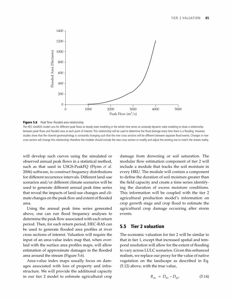
T IER 2 VALUATION 85
will develop such curves using the simulated or observed annual peak fl ows in a statistical method, such as that used in USGS-PeakFQ ( Flynn et al. 2006 ) software, to construct frequency distributions for different recurrence intervals. Different land-use scenarios and/or different climate scenarios will be used to generate different annual peak time series that reveal the impacts of land-use changes and cli-mate changes on the peak fl ow and extent of fl ooded area.
Using the annual peak time series generated above, one can run fl ood frequency analyses to determine the peak fl ow associated with each return period. Then, for each return period, HEC-RAS can be used to generate fl ooded area profi les at river cross sections of interest. Valuation will require the input of an area-value index map that, when over-laid with the surface area profi les maps, will allow estimation of approximate damages in the fl ooded area around the stream ( Figure 5.6 ).
Area-value index maps usually focus on dam-ages associated with loss of property and infra-structure. We will provide the additional capacity in our tier 2 model to estimate agricultural crop
damage from drowning or soil saturation. The modular fl ow estimation component of tier 2 will include a module that tracks the soil moisture in every HRU. The module will contain a component to defi ne the duration of soil moisture greater than the fi eld capacity and create a time series identify-ing the duration of excess moisture conditions. This information will be coupled with the tier 2 agricultural production model’s information on crop growth stage and crop fl ood to estimate the agricultural crop damage occurring after storm events.
5.5 Tier 2 valuation
The economic valuation for tier 2 will be similar to that in tier 1, except that increased spatial and tem-poral resolution will allow for the extent of fl ooding to vary across LULC scenarios. Given this enhanced realism, we replace our proxy for the value of native vegetation on the landscape as described in Eq. (5.12) above, with the true value,
xks kbs kfsB D D= − , (5.14)
1400
1200
1000
800
600
400
Floo
ded
Are
a (H
ecta
res)
200
00 1000 2000
Peak Flow (m3/s)3000 4000 5000
Figure 5.6 Peak fl ow–fl ooded area relationship.The HEC-GeoRAS model runs for different peak fl ows at steady state modeling or the whole time series at unsteady-dynamic state modeling to draw a relationship between peak fl ows and fl ooded area at each point of interest. This relationship will be used to determine the fl ood damage every time there is a fl ooding. However, studies show that the channel geomorphology is constantly changing such that the river cross sections will be different between separate fl ood events. Changes in river cross section will change this relationship; therefore the modeler should include the new cross section or modify and adjust the existing one to match the stream reality.
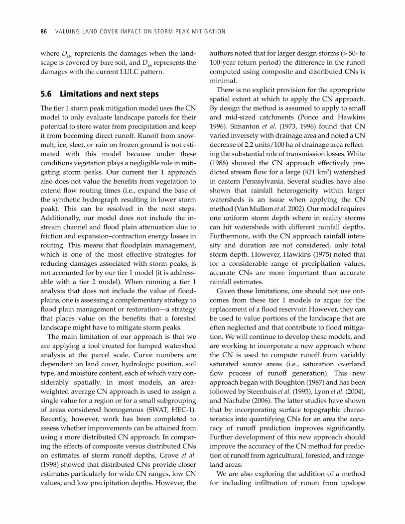
86 VALUING LAND COVER IMPACT ON STORM PEAK MIT IGATION
where D kbs represents the damages when the land-scape is covered by bare soil, and D kfs represents the damages with the current LULC pattern.
5.6 Limitations and next steps
The tier 1 storm peak mitigation model uses the CN model to only evaluate landscape parcels for their potential to store water from precipitation and keep it from becoming direct runoff. Runoff from snow-melt, ice, sleet, or rain on frozen ground is not esti-mated with this model because under these conditions vegetation plays a negligible role in miti-gating storm peaks. Our current tier 1 approach also does not value the benefi ts from vegetation to extend fl ow routing times (i.e., expand the base of the synthetic hydrograph resulting in lower storm peak). This can be resolved in the next steps. Additionally, our model does not include the in-stream channel and fl ood plain attenuation due to friction and expansion–contraction energy losses in routing. This means that fl oodplain management, which is one of the most effective strategies for reducing damages associated with storm peaks, is not accounted for by our tier 1 model (it is address-able with a tier 2 model). When running a tier 1 analysis that does not include the value of fl ood-plains, one is assessing a complementary strategy to fl ood plain management or restoration—a strategy that places value on the benefi ts that a forested landscape might have to mitigate storm peaks.
The main limitation of our approach is that we are applying a tool created for lumped watershed analysis at the parcel scale. Curve numbers are dependent on land cover, hydrologic position, soil type, and moisture content, each of which vary con-siderably spatially. In most models, an area-weighted average CN approach is used to assign a single value for a region or for a small subgrouping of areas considered homogenous (SWAT, HEC-1). Recently, however, work has been completed to assess whether improvements can be attained from using a more distributed CN approach. In compar-ing the effects of composite versus distributed CNs on estimates of storm runoff depths, Grove et al. ( 1998 ) showed that distributed CNs provide closer estimates particularly for wide CN ranges, low CN values, and low precipitation depths. However, the
authors noted that for larger design storms (> 50- to 100-year return period) the difference in the runoff computed using composite and distributed CNs is minimal.
There is no explicit provision for the appropriate spatial extent at which to apply the CN approach. By design the method is assumed to apply to small and mid-sized catchments ( Ponce and Hawkins 1996 ). Simanton et al. ( 1973 , 1996 ) found that CN varied inversely with drainage area and noted a CN decrease of 2.2 units/100 ha of drainage area refl ect-ing the substantial role of transmission losses. White ( 1986 ) showed the CN approach effectively pre-dicted stream fl ow for a large (421 km 2 ) watershed in eastern Pennsylvania. Several studies have also shown that rainfall heterogeneity within larger watersheds is an issue when applying the CN method ( Van Mullem et al. 2002 ). Our model requires one uniform storm depth where in reality storms can hit watersheds with different rainfall depths. Furthermore, with the CN approach rainfall inten-sity and duration are not considered, only total storm depth. However, Hawkins ( 1975 ) noted that for a considerable range of precipitation values, accurate CNs are more important than accurate rainfall estimates.
Given these limitations, one should not use out-comes from these tier 1 models to argue for the replacement of a fl ood reservoir. However, they can be used to value portions of the landscape that are often neglected and that contribute to fl ood mitiga-tion. We will continue to develop these models, and are working to incorporate a new approach where the CN is used to compute runoff from variably saturated source areas (i.e., saturation overland fl ow process of runoff generation). This new approach began with Boughton ( 1987 ) and has been followed by Steenhuis et al. ( 1995 ), Lyon et al. ( 2004 ), and Nachabe ( 2006 ). The latter studies have shown that by incorporating surface topographic charac-teristics into quantifying CNs for an area the accu-racy of runoff prediction improves signifi cantly. Further development of this new approach should improve the accuracy of the CN method for predic-tion of runoff from agricultural, forested, and range-land areas.
We are also exploring the addition of a method for including infi ltration of runon from upslope
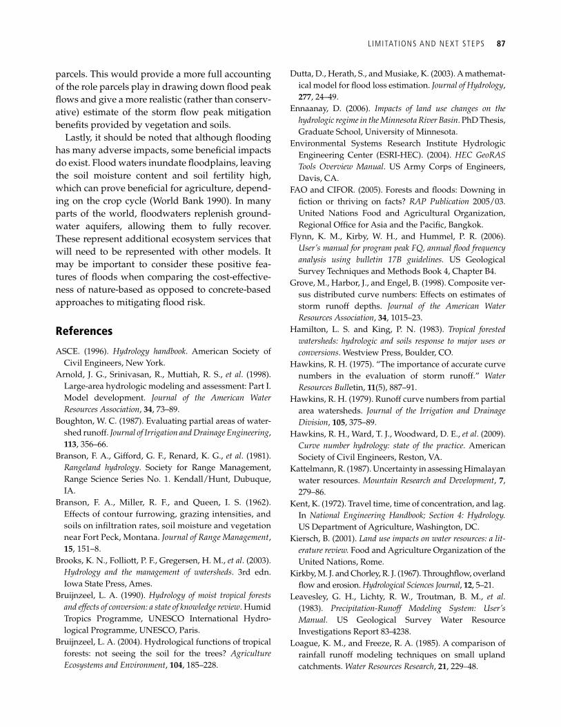
L IMITATIONS AND NEXT STEPS 87
parcels. This would provide a more full accounting of the role parcels play in drawing down fl ood peak fl ows and give a more realistic (rather than conserv-ative) estimate of the storm fl ow peak mitigation benefi ts provided by vegetation and soils.
Lastly, it should be noted that although fl ooding has many adverse impacts, some benefi cial impacts do exist. Flood waters inundate fl oodplains, leaving the soil moisture content and soil fertility high, which can prove benefi cial for agriculture, depend-ing on the crop cycle ( World Bank 1990 ). In many parts of the world, fl oodwaters replenish ground-water aquifers, allowing them to fully recover. These represent additional ecosystem services that will need to be represented with other models. It may be important to consider these positive fea-tures of fl oods when comparing the cost-effective-ness of nature-based as opposed to concrete-based approaches to mitigating fl ood risk.
References
ASCE. (1996). Hydrology handbook . American Society of Civil Engineers, New York.
Arnold, J. G., Srinivasan, R., Muttiah, R. S., et al . (1998). Large-area hydrologic modeling and assessment: Part I. Model development. Journal of the American Water Resources Association , 34 , 73–89.
Boughton, W. C. (1987). Evaluating partial areas of water-shed runoff. Journal of Irrigation and Drainage Engineering , 113 , 356–66.
Branson, F. A., Gifford, G. F., Renard, K. G., et al . (1981). Rangeland hydrology . Society for Range Management, Range Science Series No. 1. Kendall/Hunt, Dubuque, IA.
Branson, F. A., Miller, R. F., and Queen, I. S. (1962). Effects of contour furrowing, grazing intensities, and soils on infi ltration rates, soil moisture and vegetation near Fort Peck, Montana. Journal of Range Management , 15 , 151–8.
Brooks, K. N., Folliott, P. F., Gregersen, H. M., et al . (2003). Hydrology and the management of watersheds . 3rd edn. Iowa State Press, Ames.
Bruijnzeel, L. A. (1990). Hydrology of moist tropical forests and effects of conversion: a state of knowledge review . Humid Tropics Programme, UNESCO International Hydro-logical Programme, UNESCO, Paris.
Bruijnzeel, L. A. (2004). Hydrological functions of tropical forests: not seeing the soil for the trees? Agriculture Ecosystems and Environment , 104 , 185–228.
Dutta, D., Herath, S., and Musiake, K. (2003). A mathemat-ical model for fl ood loss estimation. Journal of Hydrology , 277 , 24–49.
Ennaanay, D. (2006). Impacts of land use changes on the hydrologic regime in the Minnesota River Basin . PhD Thesis, Graduate School, University of Minnesota.
Environmental Systems Research Institute Hydrologic Engineering Center (ESRI-HEC). (2004). HEC GeoRAS Tools Overview Manual . US Army Corps of Engineers, Davis, CA.
FAO and CIFOR. (2005). Forests and fl oods: Downing in fi ction or thriving on facts? RAP Publication 2005/03. United Nations Food and Agricultural Organization, Regional Offi ce for Asia and the Pacifi c, Bangkok.
Flynn, K. M., Kirby, W. H., and Hummel, P. R. (2006). User’s manual for program peak FQ, annual fl ood frequency analysis using bulletin 17B guidelines. US Geological Survey Techniques and Methods Book 4, Chapter B4.
Grove, M., Harbor, J., and Engel, B. (1998). Composite ver-sus distributed curve numbers: Effects on estimates of storm runoff depths. Journal of the American Water Resources Association , 34 , 1015–23.
Hamilton, L. S. and King, P. N. (1983). Tropical forested watersheds: hydrologic and soils response to major uses or conversions . Westview Press, Boulder, CO.
Hawkins, R. H. (1975). “The importance of accurate curve numbers in the evaluation of storm runoff.” Water Resources Bull etin, 11 (5), 887–91.
Hawkins, R. H. (1979). Runoff curve numbers from partial area watersheds. Journal of the Irrigation and Drainage Division , 105 , 375–89.
Hawkins, R. H., Ward, T. J., Woodward, D. E., et al . (2009). Curve number hydrology: state of the practice . American Society of Civil Engineers, Reston, VA.
Kattelmann, R. (1987). Uncertainty in assessing Himalayan water resources. Mountain Research and Development , 7 , 279–86.
Kent, K. (1972). Travel time, time of concentration, and lag. In National Engineering Handbook; Section 4: Hydrology. US Department of Agriculture, Washington, DC.
Kiersch, B. (2001). Land use impacts on water resources: a lit-erature review. Food and Agriculture Organization of the United Nations, Rome.
Kirkby, M. J. and Chorley, R. J. (1967). Throughfl ow, overland fl ow and erosion. Hydrological Sciences Journal , 12 , 5–21.
Leavesley, G. H., Lichty, R. W., Troutman, B. M., et al . (1983). Precipitation-Runoff Modeling System: User’s Manual. US Geological Survey Water Resource Investigations Report 83-4238.
Loague, K. M., and Freeze, R. A. (1985). A comparison of rainfall runoff modeling techniques on small upland catchments. Water Resources Research , 21 , 229–48.
88 VALUING LAND COVER IMPACT ON STORM PEAK MIT IGATION
Lyon, S. W., Walter, M. T., Garard-Marchant, P., et al . (2004). Using a topographic index to distribute variable source area runoff predicted with the SCS–curve number equa-tion, Hydrological Processes , 18 , 2757–71.
Martinez, V., Garcia, A. I., and Ayuga, F. (2002). Distributed routing techniques developed on GIS for generating synthetic hydrographs. Transactions of the American Society of Agricultural Engineers , 45 , 1825–34.
Melesse, A. M., Graham, W. D., and Jordan, J. D. (2003). Spatially distributed watershed mapping and modeling: GIS based storm runoff response and hydrograph anal-ysis. Part 2. Journal of Spatial Hydrology , 3 , 2–28.
Merz, B., Kreibich, H., Thieken, A., et al . (2004). Estimation uncertainty of direct monetary fl ood damage to build-ings. Natural Hazards and Earth System Sciences , 4 , 153–63.
Mockus, V. (1972). Estimation of direct runoff from storm rainfall. In National Engineering Handbook; Section 4: Hydrology . US Department of Agriculture, Washington, DC.
Nachabe, M. H. (2006). Equivalence between topmodel and the NRCS curve number method in predicting vari-able runoff source areas. Journal of the American Water Resources Association , 42 (1), 225–35.
Polasky, S., Nelson, E., Camm, J., et al . (2008). Where to put things? Spatial land management to sustain biodiver-sity and economic returns. Biological Conservation , 141 , 1505–24.
Ponce, V. M., and Hawkins, R. H. (1996). Runoff curve number: Has it reached maturity? Journal of Hydrologic Engineering , 1 , 11–18.
Rothacher, J. (1970). Increases in water yield following clear-cut logging in the Pacifi c Northwest. Water Resources Research , 6 , 653–8.
Simanton, J. R., Renard, K. G., and Sutter, N. G. (1973). Procedures for identifying parameters affecting storm runoff volumes in a semiarid environment. USDA-ARS Agricultural Reviews and Manuals ARM-W-1. USDA-ARS, Washington, DC.
Simanton, J. R., Hawkins, R. H., Mohseni-Saravi, M., et al . (1996). Runoff curve number variation with drainage area, Walnut Gulch, Arizona. Transactions of the American Society of Agricultural Engineers , 39 , 1391–4.
Steenhuis, T. S., Winchell, M., Rossing, J., et al . (1995). SCS runoff equation revisited for variable-source runoff areas. Journal of Irrigation and Drainage Engineering , 121 , 234–8.
Tran, P., Shaw, R., Chantry, G., and Norton, J. (2009). GIS and local knowledge in disaster management: a case study of fl ood risk mapping in Viet Nam. Disasters , 33 (1), 152–69.
United States Army Corps of Engineers (USACE). (2002). HEC-RAS River Analysis System . US Army Corps of Engineers, Davis, CA. Available at http://furat.eng.uci.edu/wsmodeling/Software/USACE_HEC/HEC-RAS/V4Beta/docs/HEC-RAS_Reference_Manual.pdf
United States Department of Agriculture (USDA). (1986). Urban Hydrology for Small Watersheds. Soil Conser-vation Service, Engineering Division, Technical Release 55 (TR-55).
Van Mullem, J. A., Woodward, D. E., Hawkins, R. H., et al . (2002). Runoff Curve Number Method: Beyond the Handbook . US Geological Survey Advisory Committee on Water Information—Second Federal Interagency Hydrologic Modeling Conference. July 28—August 1, Las Vegas, NV.
White, D. (1986). Synoptic-Scale Assessment of Surface Runoff: An Analysis of the Soil Conservation Service Runoff Curve Number. Proceedings of the Annual Pittsburgh Conference , 17 , 159–63.
Williams, J. R. (1995). The EPIC model. In V. P. Singh, Ed., Computer Models of Watershed Hydrology , pp. 909–1000.Water Resources Publications, Highlands Ranch, CO.
World Bank. (1990). Flood Control in Bangladesh: A Plan for Action . World Bank, Washington, DC.
Wright, K.A., Sendek, K.H., Rice, R.M., and Thomas, R.B. (1990). Logging effects on streamfl ow: Storm runoff at Casper Creek in Northwestern California. Water Resources Research, 26 , 1657–67.
89
CHAPTER 6
Retention of nutrients and sediment by vegetation Marc Conte, Driss Ennaanay, Guillermo Mendoza, Michael Todd Walter, Stacie Wolny, David Freyberg, Erik Nelson, and Luis Solorzano
6.1 Introduction
As water fl ows across the land, its physical and bio-chemical characteristics are shaped by human activ-ities and the vegetative cover on the landscape. Of particular importance to society is the transport of nutrients and sediment from upstream locations to downstream water bodies. For example, the trans-port of nitrogen from upstream agricultural lands is partially responsible for the extreme eutrophication of coastal waters that has led to the dead zone in the Gulf of Mexico. From the perspective of sediment pollution, more than 0.5% of global reservoir stor-age is lost annually due to sedimentation (White 2001) at possible costs of US$13 billion per year (Palmieri et al. 2003). The degree to which surface fl ows remove and deliver nutrients and sediment from their sources to downstream locations is highly dependent on the pattern of land use and land cover (LULC) on the landscape. By retaining portions of the nutrients and sediment released and trans-ported by surface fl ows, vegetation can help to miti-gate damages downstream.
The quantities of nutrients and sediment retained by vegetation are largely functions of slope, vegeta-tion type, volume of water fl owing across the land, and the vegetation’s location in the watershed. Lands with intact natural vegetation will tend to be net retainers of both nutrients and sediment, whereas lands used intensively for agricultural production will tend to be sources of both nutrients and sedi-ment. The likelihood of retaining nutrients and sedi-ments increases as proximity to source areas increases.
Also, vegetated areas with low slopes tend to pro-vide higher levels of nutrient and sediment retention than steeply-sloped areas. Pulling these ideas together, we present two methods of landscape anal-ysis regarding sediment and nutrient retention. The simple, tier 1 models are based on average annual precipitation levels as well as data related to land-scape topography and nutrient loading. The outputs from these models include annual average maps of nutrient export and retention, sediment export and retention, and the value of different parcels of land based on their nutrient and sediment retention.
Because the rate of water fl owing across the land-scape infl uences nutrient and sediment retention, and can vary enormously from day to day, annual water volumes may not capture the differential retention properties of assorted parcels of land. In particular, analysis conducted at a fi ne temporal resolution (e.g., daily) will be able to provide more accurate estimates of nutrient and sediment reten-tion. The tier 2 models capture these temporal dynamics by using the Agriculture Non-Point Source (AnnGNPS) model to estimate nutrient export and retention and the Precipitation Runoff Modeling System (PRMS) to predict the amount of sediment eroded and delivered to focal water bod-ies. Both models can provide daily estimates. While models in tier 2 provide more realistic estimates of nutrient and sediment retention in the landscape, they require data that are costly to collect and a detailed understanding of local hydrology.
The models here focus solely on the nutrients and sediment that move with surface water fl ows across
90 RETENTION OF NUTRIENTS AND SEDIMENT BY VEGETATION
the landscape from non-point sources. There are several other damaging non-point source particu-lates that move with surface water, including heavy metals and pesticides; our modeling approach could be adapted for these other pollutants as long as the reactions of these pollutants with soil and the ambient environment could be described.
6.1.1 Modeling fl ows relevant to nutrient and sediment retention
The tier 1 and tier 2 models that we develop rely on the principle of saturation excess runoff to generate nutrient and sediment runoff estimates. These mod-els use a runoff index obtained from a topographic index that contains a permeability function. By com-bining the concept of hydraulic connectivity with pixel-specifi c runoff indices, these models allow us to estimate the amount of nutrient and sediment retention on individual pixels based on their loca-tion in the watershed and their position along the fl ow path to the downstream body of water .
6.1.2 Implementing theory to model ecosystem-service provision
Many processes drive the impairment of water bod-ies by nutrient and sediment loading. The magni-tude and timing of precipitation events, irrigation scheduling, stream and soil cycling, soil characteris-tics, and landscape geomorphology and topography are some of the variables that affect the impact of nutrient pollutant loading and sediment transport to a water body. Detailed information about all of the above processes may not be available in all regions struggling to cope with the effects of nutri-ent and sediment deposition in water bodies. Our tier 1 model of nutrient retention uses as key inputs a water yield index (as a proxy for contributing area, precipitation, soil type, and slope), LULC, export coeffi cients, and downslope retention. Our tier 1 model of sediment retention uses as key inputs LULC, downslope retention, slope, rainfall erosivity, and soil erodibility. The processes chosen as inputs for our models tend to be associated with more eas-ily-accessible data, making them more practical.
The economic valuation for nutrient retention is based on the cost of water treatment, which is meant
to represent the lower bound of the social value of nutrient retention. For sediment retention, the social value is approximated using the dredging costs that are avoided by having sediment-retaining vegetation on the landscape, which should be interpreted as a lower bound of the value of this ecosystem service.
In areas with more-detailed information, plan-ners can apply our tier 2 models that extend the hydrologic principles of tier 1 to include the tempo-ral dynamics of hydrology and nutrient and sediment loading on the landscape. The setup of tier 2 models requires additional data and expertise for calibration, verifi cation, and validation. Our tier 2 approach to nutrient retention has the capability of distinguishing between infi ltration and satura-tion excess runoff transportation pathways. It simu-lates the timing of nutrient application activities with respect to the generation of runoff.
The tier 2 framework for sediment retention uses methods from PRMS to simulate erosion and sedi-ment processes. PRMS simulates sediment detach-ment using a revised form of the universal soil loss evaporation (USLE) method (Leavesley et al. 1983). The detachment rate of sediment in PRMS is depend-ent on rainfall intensity, geomorphology, and runoff volumes (Hjelmfelt et al. 1975), and the movement of sediment in the stream channel is coupled with the energy in simulated fl ows. PRMS accounts for both sheetwash and streambank erosion, by incorporat-ing stream scouring and deposition processes, which improves the model’s ability to assign value to sedi-ment retention on vegetated parcels.
6.2 Tier 1 biophysical models
The models presented in this chapter use LULC cat-egory as a principle driver of the processes being modeled, including water yield, pollutant loading, and sediment retention. The unit of analysis in these models is the parcel, whose size is based on the spa-tial resolution of the available data in the study area. The model assumes that each parcel is homogene-ous with respect to LULC, meaning that there is a single LULC category associated with each parcel. For this reason, the parcel index captures the impact of LULC on each of the processes being modeled, and we do not include LULC indices in the chapter equations unless this assumption is relaxed.
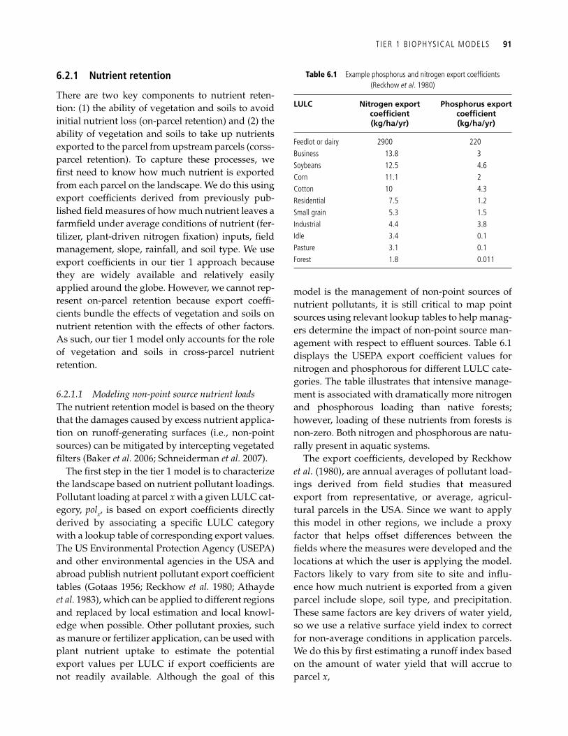
T IER 1 B IOPHYSICAL MODELS 91
6.2.1 Nutrient retention
There are two key components to nutrient reten-tion: (1) the ability of vegetation and soils to avoid initial nutrient loss (on-parcel retention) and (2) the ability of vegetation and soils to take up nutrients exported to the parcel from upstream parcels (corss-parcel retention). To capture these processes, we fi rst need to know how much nutrient is exported from each parcel on the landscape. We do this using export coeffi cients derived from previously pub-lished fi eld measures of how much nutrient leaves a farmfi eld under average conditions of nutrient (fer-tilizer, plant-driven nitrogen fi xation) inputs, fi eld management, slope, rainfall, and soil type. We use export coeffi cients in our tier 1 approach because they are widely available and relatively easily applied around the globe. However, we cannot rep-resent on-parcel retention because export coeffi -cients bundle the effects of vegetation and soils on nutrient retention with the effects of other factors. As such, our tier 1 model only accounts for the role of vegetation and soils in cross-parcel nutrient retention.
6.2.1.1 Modeling non-point source nutrient loads The nutrient retention model is based on the theory that the damages caused by excess nutrient applica-tion on runoff-generating surfaces (i.e., non-point sources) can be mitigated by intercepting vegetated fi lters (Baker et al. 2006; Schneiderman et al. 2007).
The fi rst step in the tier 1 model is to characterize the landscape based on nutrient pollutant loadings. Pollutant loading at parcel x with a given LULC cat-egory, pol x , is based on export coeffi cients directly derived by associating a specifi c LULC category with a lookup table of corresponding export values. The US Environmental Protection Agency (USEPA) and other environmental agencies in the USA and abroad publish nutrient pollutant export coeffi cient tables (Gotaas 1956; Reckhow et al. 1980; Athayde et al. 1983), which can be applied to different regions and replaced by local estimation and local knowl-edge when possible. Other pollutant proxies, such as manure or fertilizer application, can be used with plant nutrient uptake to estimate the potential export values per LULC if export coeffi cients are not readily available. Although the goal of this
model is the management of non-point sources of nutrient pollutants, it is still critical to map point sources using relevant lookup tables to help manag-ers determine the impact of non-point source man-agement with respect to effl uent sources. Table 6.1 displays the USEPA export coeffi cient values for nitrogen and phosphorous for different LULC cate-gories. The table illustrates that intensive manage-ment is associated with dramatically more nitrogen and phosphorous loading than native forests; however, loading of these nutrients from forests is non-zero. Both nitrogen and phosphorous are natu-rally present in aquatic systems.
The export coeffi cients, developed by Reckhow et al. (1980), are annual averages of pollutant load-ings derived from fi eld studies that measured export from representative, or average, agricul-tural parcels in the USA. Since we want to apply this model in other regions, we include a proxy factor that helps offset differences between the fi elds where the measures were developed and the locations at which the user is applying the model. Factors likely to vary from site to site and infl u-ence how much nutrient is exported from a given parcel include slope, soil type, and precipitation. These same factors are key drivers of water yield, so we use a relative surface yield index to correct for non-average conditions in application parcels. We do this by fi rst estimating a runoff index based on the amount of water yield that will accrue to parcel x ,
Table 6.1 Example phosphorus and nitrogen export coeffi cients (Reckhow et al . 1980)
LULC Nitrogen export coeffi cient (kg/ha/yr)
Phosphorus export coeffi cient (kg/ha/yr)
Feedlot or dairy 2900 220 Business 13.8 3 Soybeans 12.5 4.6 Corn 11.1 2 Cotton 10 4.3 Residential 7.5 1.2 Small grain 5.3 1.5 Industrial 4.4 3.8 Idle 3.4 0.1 Pasture 3.1 0.1 Forest 1.8 0.011
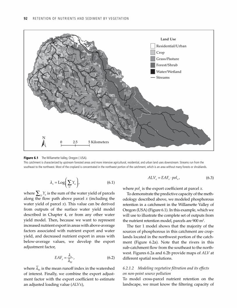
92 RETENTION OF NUTRIENTS AND SEDIMENT BY VEGETATION
l ⎛ ⎞= ⎜ ⎟⎝ ⎠∑Log ,x uU
Y (6.1)
where ∑ uUY is the sum of the water yield of parcels
along the fl ow path above parcel x (including the water yield of parcel x ). This value can be derived from outputs of the surface water yield model described in Chapter 4 , or from any other water yield model. Then, because we want to represent increased nutrient export in areas with above- average factors associated with nutrient export and water yield, and decreased nutrient export in areas with below-average values, we develop the export adjustment factor,
ll
= ,xx
W
EAF (6.2)
where lW is the mean runoff index in the watershed of interest. Finally, we combine the export adjust-ment factor with the export coeffi cient to estimate an adjusted loading value ( ALVx ),
= ⋅ ,x x xALV EAF pol (6.3)
where pol x is the export coeffi cient at parcel x. To demonstrate the predictive capacity of the meth-
odology described above, we modeled phosphorous retention in a catchment in the Willamette Valley of Oregon (USA) ( Figure 6.1 ). In this example, which we will use to illustrate the complete set of outputs from the nutrient retention model, parcels are 900 m 2 .
The tier 1 model shows that the majority of the sources of phosphorous in this catchment are crop-lands located in the northwest portion of the catch-ment (Figure 6.2a). Note that the rivers in this sub-catchment fl ow from the southeast to the north-west. Figures 6.2a and 6.2b provide maps of ALV at different spatial resolutions.
6.2.1.2 Modeling vegetative fi ltration and its effects on non-point source pollution To model cross-parcel nutrient retention on the landscape, we must know the fi ltering capacity of
N0 2.5 5 Kilometers
Residential/Urban
Land Use
Crop
Grass/Pasture
Forest/Shrub
Water/Wetland
Streams
Figure 6.1 The Willamette Valley, Oregon ( USA).This catchment is characterized by upstream forested areas and more intensive agricultural, residential, and urban land uses downstream. Streams run from the southeast to the northwest. Most of the cropland is concentrated in the northwest portion of the catchment, which is an area without many forests or shrublands.
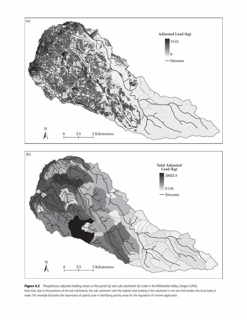
Figure 6.2 Phosphorous adjusted loading values at the parcel (a) and sub-catchment (b) scale in the Willamette Valley, Oregon (USA).Note that, due to the positions of the sub-catchments, the sub-catchment with the highest total loading in the catchment is not one that borders the focal body of water. This example illustrates the importance of spatial scale in identifying priority areas for the regulation of nutrient application.
13.61
(a)
0N
2.5 5 Kilometers
Adjusted Load (kg)
0
Streams
(b)
20023.5
0.136
Streams
Total AdjustedLoad (kg)
0N
2.5 5 Kilometers
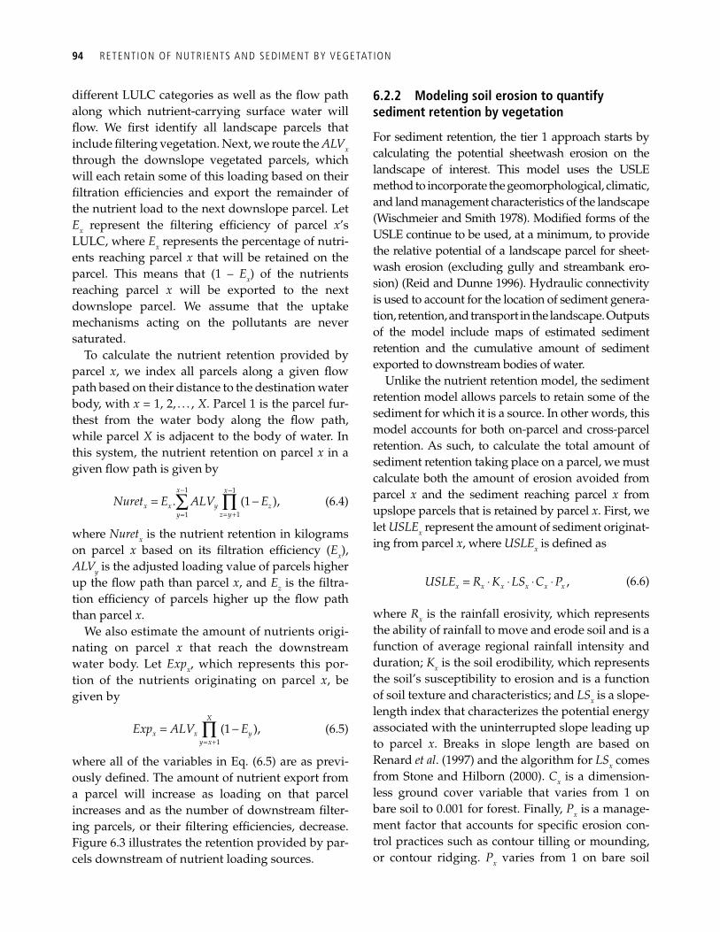
94 RETENTION OF NUTRIENTS AND SEDIMENT BY VEGETATION
different LULC categories as well as the fl ow path along which nutrient-carrying surface water will fl ow. We fi rst identify all landscape parcels that include fi ltering vegetation. Next, we route the ALV x through the downslope vegetated parcels, which will each retain some of this loading based on their fi ltration effi ciencies and export the remainder of the nutrient load to the next downslope parcel. Let E x represent the fi ltering effi ciency of parcel x ’s LULC, where E x represents the percentage of nutri-ents reaching parcel x that will be retained on the parcel. This means that (1 – E x ) of the nutrients reaching parcel x will be exported to the next downslope parcel. We assume that the uptake mechanisms acting on the pollutants are never saturated.
To calculate the nutrient retention provided by parcel x , we index all parcels along a given fl ow path based on their distance to the destination water body, with x = 1, 2, . . . , X . Parcel 1 is the parcel fur-thest from the water body along the fl ow path, while parcel X is adjacent to the body of water. In this system, the nutrient retention on parcel x in a given fl ow path is given by
− −
= +== −∑ ∏
1 1
11
. (1 ),x x
x x y zz yy
Nuret E ALV E (6.4)
where Nuret x is the nutrient retention in kilograms on parcel x based on its fi ltration effi ciency ( E x ), ALV y is the adjusted loading value of parcels higher up the fl ow path than parcel x , and E z is the fi ltra-tion effi ciency of parcels higher up the fl ow path than parcel x .
We also estimate the amount of nutrients origi-nating on parcel x that reach the downstream water body. Let Exp x , which represents this por-tion of the nutrients originating on parcel x , be given by
= +
= −∏1
(1 ),X
x x yy x
Exp ALV E (6.5)
where all of the variables in Eq. (6.5) are as previ-ously defi ned. The amount of nutrient export from a parcel will increase as loading on that parcel increases and as the number of downstream fi lter-ing parcels, or their fi ltering effi ciencies, decrease. Figure 6.3 illustrates the retention provided by par-cels downstream of nutrient loading sources.
6.2.2 Modeling soil erosion to quantify sediment retention by vegetation
For sediment retention, the tier 1 approach starts by calculating the potential sheetwash erosion on the landscape of interest. This model uses the USLE method to incorporate the geomorphological, climatic, and land management characteristics of the landscape (Wischmeier and Smith 1978). Modifi ed forms of the USLE continue to be used, at a minimum, to provide the relative potential of a landscape parcel for sheet-wash erosion (excluding gully and streambank ero-sion) ( Reid and Dunne 1996 ). Hydraulic connectivity is used to account for the location of sediment genera-tion, retention, and transport in the landscape. Outputs of the model include maps of estimated sediment retention and the cumulative amount of sediment exported to downstream bodies of water.
Unlike the nutrient retention model, the sediment retention model allows parcels to retain some of the sediment for which it is a source. In other words, this model accounts for both on-parcel and cross-parcel retention. As such, to calculate the total amount of sediment retention taking place on a parcel, we must calculate both the amount of erosion avoided from parcel x and the sediment reaching parcel x from upslope parcels that is retained by parcel x . First, we let USLE x represent the amount of sediment originat-ing from parcel x , where USLE x is defi ned as
= ⋅ ⋅ ⋅ ⋅ ,x x x x x xUSLE R K LS C P (6.6)
where R x is the rainfall erosivity, which represents the ability of rainfall to move and erode soil and is a function of average regional rainfall intensity and duration; K x is the soil erodibility, which represents the soil’s susceptibility to erosion and is a function of soil texture and characteristics; and LS x is a slope-length index that characterizes the potential energy associated with the uninterrupted slope leading up to parcel x . Breaks in slope length are based on Renard et al . (1997) and the algorithm for LS x comes from Stone and Hilborn (2000). C x is a dimension-less ground cover variable that varies from 1 on bare soil to 0.001 for forest. Finally, P x is a manage-ment factor that accounts for specifi c erosion con-trol practices such as contour tilling or mounding, or contour ridging. P x varies from 1 on bare soil
T IER 1 B IOPHYSICAL MODELS 95
with no erosion control to about 0.1 with tiered ridging on a gentle slope (Roose 1996).
The tier 1 model of sediment retention determines the potential sediment release on each parcel on the landscape of interest. These soil particles are detached and move through the watershed with runoff along fl ow paths. As in the nutrient retention model, we index all parcels along a given fl ow path based on their distance to the destination water body, with x= 1, 2, . . . , X . Parcel 1 is the parcel fur-thest from the water body along the fl ow path, while parcel X is adjacent to the body of water. The model routes the sediment originating on parcel x , USLE x , along the fl ow path, with vegetated parcels retaining some of this sediment based on their sediment retention effi ciency and exporting the remaining loading to the next parcel in the fl ow path. SEDR x , the retention by parcel x 's LULC of
sediment originating on parcels higher up the fl ow path, is given by
− −
= +== −∑ ∏
1 1
11
(1 ),x x
x x y zz yy
SEDR SE USLE SE (6.7)
where SE x is the sediment retention effi ciency of parcel x, USLE y is the sediment generated on upstream parcel y , and SE z is the sediment retention effi ciency of upstream parcel z .
The potential amount of sheetwash sediment trapped by landscape vegetation or best manage-ment practices in soil conservation upstream of reservoir D , SEDRET xD , can be estimated by the dif-ference between the geomorphological characteris-tics of x that might promote soil loss, and the retention properties of the parcel’s LULC that help contain sediment released by on-site erosion ( C x and P x ) and upstream transport ( SEDR x ):
0N
235.99
Nutrient Retention (kg)
0Streams
2.5 5 Kilometers
Figure 6.3 Average phosphorous retention values in the Willamette Valley, Oregon (USA).This map underscores the point that our model formulations make it such that native vegetation must be downstream of loading sources to provide nutrient retention of value to society. As the large area of contiguous forest in the eastern part of the catchment lies upstream of anthropogenic phosphorous sources, it does not provide much, if any, cross-parcel nutrient retention in the eastern part (light zones). However, in buffer areas, forested lands around streams provide much retention. Loadings in the western part of the watershed are retained and removed by forested lands abutting streams (dark zones close to streams).
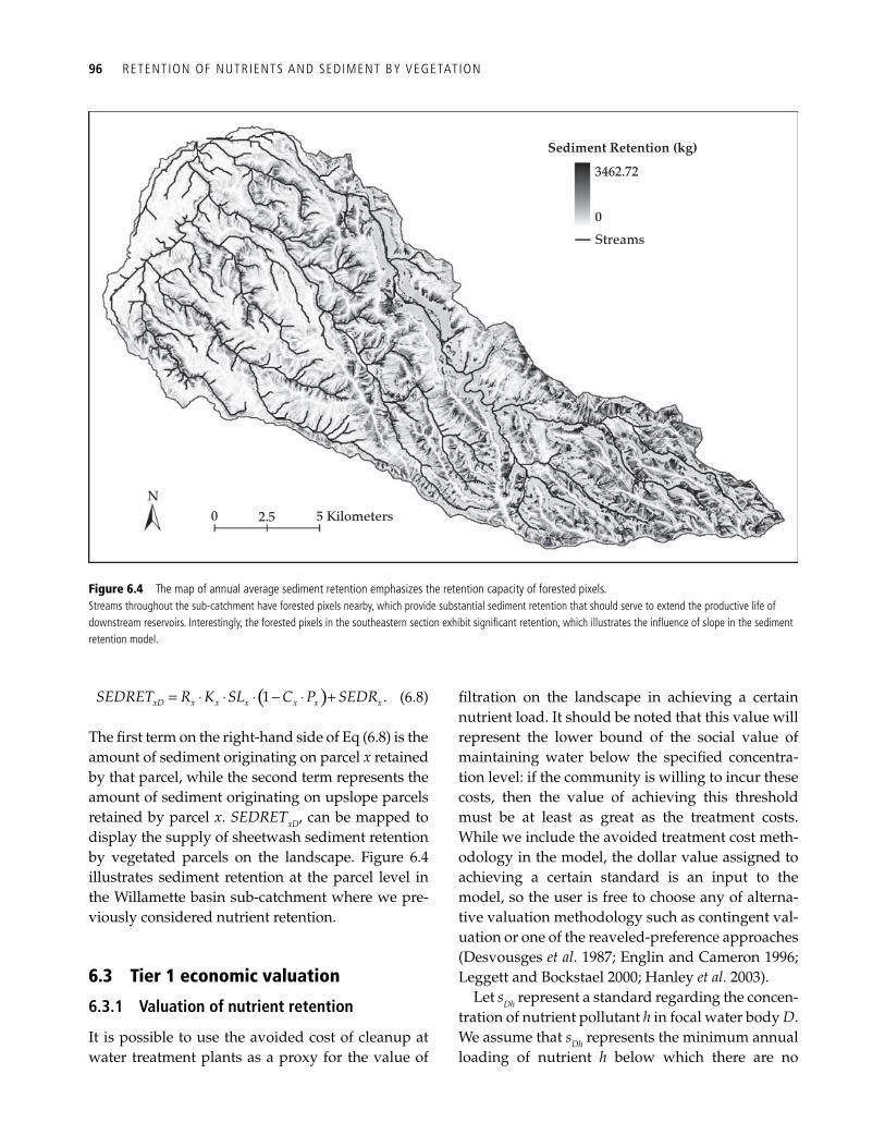
96 RETENTION OF NUTRIENTS AND SEDIMENT BY VEGETATION
( )= ⋅ ⋅ ⋅ − ⋅ +1 .xD x x x x x xSEDRET R K SL C P SEDR (6.8)
The fi rst term on the right-hand side of Eq (6.8) is the amount of sediment originating on parcel x retained by that parcel, while the second term represents the amount of sediment originating on upslope parcels retained by parcel x . SEDRET xD , can be mapped to display the supply of sheetwash sediment retention by vegetated parcels on the landscape. Figure 6.4 illustrates sediment retention at the parcel level in the Willamette basin sub-catchment where we pre-viously considered nutrient retention.
6.3 Tier 1 economic valuation
6.3.1 Valuation of nutrient retention
It is possible to use the avoided cost of cleanup at water treatment plants as a proxy for the value of
fi ltration on the landscape in achieving a certain nutrient load. It should be noted that this value will represent the lower bound of the social value of maintaining water below the specifi ed concentra-tion level: if the community is willing to incur these costs, then the value of achieving this threshold must be at least as great as the treatment costs. While we include the avoided treatment cost meth-odology in the model, the dollar value assigned to achieving a certain standard is an input to the model, so the user is free to choose any of alterna-tive valuation methodology such as contingent val-uation or one of the reaveled-preference approaches (Desvousges et al. 1987; Englin and Cameron 1996; Leggett and Bockstael 2000; Hanley et al. 2003).
Let s Dh represent a standard regarding the concen-tration of nutrient pollutant h in focal water body D . We assume that s Dh represents the minimum annual loading of nutrient h below which there are no
0N
3462.72
Sediment Retention (kg)
0
Streams
2.5 5 Kilometers
Figure 6.4 The map of annual average sediment retention emphasizes the retention capacity of forested pixels.Streams throughout the sub-catchment have forested pixels nearby, which provide substantial sediment retention that should serve to extend the productive life of downstream reservoirs. Interestingly, the forested pixels in the southeastern section exhibit signifi cant retention, which illustrates the infl uence of slope in the sediment retention model.
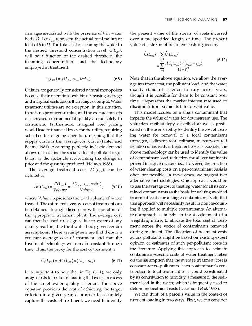
T IER 1 ECONOMIC VALUATION 97
damages associated with the presence of h in water body D . Let L Dh represent the actual total pollutant load of h in D . The total cost of cleaning the water to the desired threshold concentration level, C(L Dh ) , will be a function of the desired threshold, the incoming concentration, and the technology employed in treatment:
=( ) ( , , ).Dh Dh Dh DC L f L s tech (6.9)
Utilities are generally considered natural monopolies because their operations exhibit decreasing average and marginal costs across their range of output. Water treatment utilities are no exception. In this situation, there is no producer surplus, and the welfare impacts of increased environmental quality accrue solely to consumers. Furthermore, marginal cost pricing would lead to fi nancial losses for the utility, requiring subsidies for ongoing operation, meaning that the supply curve is the average cost curve ( Foster and Beattie 1981 ). Assuming perfectly inelastic demand allows us to defi ne the social value of pollutant regu-lation as the rectangle representing the change in price and the quantity produced (Holmes 1988).
The average treatment cost, AC ( L Dh ), can be defi ned as
= = " "( , , tech )( )( ) ,Dh DDh
Dhf L sC L
AC LVolume Volume
(6.10)
where Volume represents the total volume of water treated. The estimated average cost of treatment can be obtained through discussion with operators of the appropriate treatment plant. The average cost can then be used to assign value to water of any quality reaching the focal water body given certain assumptions. These assumptions are that there is a constant average cost of treatment and that the treatment technology will remain constant through time. Thus, the proxy for the cost of treatment is
= × −" " "ˆ ( ) ( ) ( ).t D Dh D DC L AC L L s (6.11)
It is important to note that in Eq. (6.11), we only assign costs to pollutant loading that exists in excess of the target water quality criterion. The above equation provides the cost of achieving the target criterion in a given year, t . In order to accurately capture the costs of treatment, we need to identify
the present value of the stream of costs incurred over a pre-specifi ed length of time. The present value of a stream of treatment costs is given by
1
1
ˆ ˆ( ) ( )
( ) ( ).(1 )
T
D t DtT
t Dh D Dt
t
C L C L
AC L L sr
=
=
=
× −=+
∑
∑
" "
" "
(6.12)
Note that in the above equation, we allow the aver-age treatment cost, the pollutant load, and the water quality standard criterion to vary across years, though it is possible for them to be constant over time. r represents the market interest rate used to discount future payments into present value.
This model focuses on a single contaminant that impacts the value of water for downstream use. The valuation methodology described above is predi-cated on the user’s ability to identify the cost of treat-ing water for removal of a focal contaminant (nitrogen, sediment, fecal coliform, mercury, etc.). If isolation of individual treatment costs is possible, the above methodology can be used to identify the value of contaminant load reduction for all contaminants present in a given watershed. However, the isolation of water cleanup costs on a per-contaminant basis is often not possible. In these cases, we suggest two alternative methodologies. One approach would be to use the average cost of treating water for all its con-tained contaminants as the basis for valuing avoided treatment costs for a single contaminant. Note that this approach will necessarily result in double-count-ing if applied to multiple contaminants. An alterna-tive approach is to rely on the development of a weighting matrix to allocate the total cost of treat-ment across the vector of contaminants removed during treatment. The allocation of treatment costs across pollutants might be based on existing expert opinion or estimates of such per-pollutant costs in the literature. Applying this approach to estimate contaminant-specifi c costs of water treatment relies on the assumption that the average treatment cost is constant across pollutants. Each contaminant’s con-tribution to total treatment costs could be estimated by its contribution to turbidity, a measure of the sedi-ment load in the water, which is frequently used to determine treatment costs (Dearmont et al. 1998).
We can think of a parcel’s value in the context of nutrient loading in two ways. First, we can consider
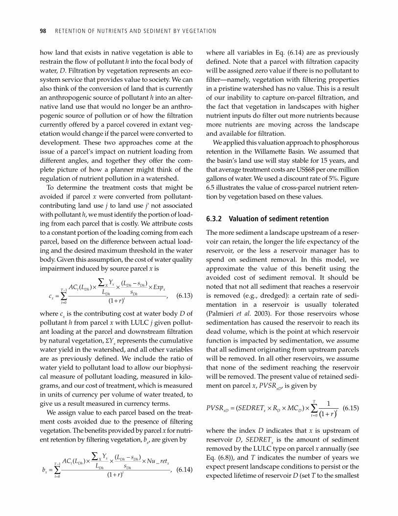
98 RETENTION OF NUTRIENTS AND SEDIMENT BY VEGETATION
how land that exists in native vegetation is able to restrain the fl ow of pollutant h into the focal body of water, D . Filtration by vegetation represents an eco-system service that provides value to society. We can also think of the conversion of land that is currently an anthropogenic source of pollutant h into an alter-native land use that would no longer be an anthro-pogenic source of pollution or of how the fi ltration currently offered by a parcel covered in extant veg-etation would change if the parcel were converted to development. These two approaches come at the issue of a parcel’s impact on nutrient loading from different angles, and together they offer the com-plete picture of how a planner might think of the regulation of nutrient pollution in a watershed.
To determine the treatment costs that might be avoided if parcel x were converted from pollutant-contributing land use j to land use j' not associated with pollutant h , we must identify the portion of load-ing from each parcel that is costly. We attribute costs to a constant portion of the loading coming from each parcel, based on the difference between actual load-ing and the desired maximum threshold in the water body. Given this assumption, the cost of water quality impairment induced by source parcel x is
−
=
−× × ×=
+
∑∑
1
0
( )( ),
(1 )
x Dh DhXt Dh xT
Dh Dhx t
t
Y L sAC L Exp
L sc
r (6.13)
where c x is the contributing cost at water body D of pollutant h from parcel x with LULC j given pollut-ant loading at the parcel and downstream fi ltration by natural vegetation, Σ Y x represents the cumulative water yield in the watershed, and all other variables are as previously defi ned. We include the ratio of water yield to pollutant load to allow our biophysi-cal measure of pollutant loading, measured in kilo-grams, and our cost of treatment, which is measured in units of currency per volume of water treated, to give us a result measured in currency terms.
We assign value to each parcel based on the treat-ment costs avoided due to the presence of fi ltering vegetation. The benefi ts provided by parcel x for nutri-ent retention by fi ltering vegetation, b x , are given by
−
=
−× × ×=
+
∑∑
1
0
( )( ) _,
(1 )
x Dh DhXt Dh xT
Dh Dhx t
t
Y L sAC L Nu ret
L sb
r (6.14)
where all variables in Eq. (6.14) are as previously defi ned. Note that a parcel with fi ltration capacity will be assigned zero value if there is no pollutant to fi lter—namely, vegetation with fi ltering properties in a pristine watershed has no value. This is a result of our inability to capture on-parcel fi ltration, and the fact that vegetation in landscapes with higher nutrient inputs do fi lter out more nutrients because more nutrients are moving across the landscape and available for fi ltration.
We applied this valuation approach to phosphorous retention in the Willamette Basin. We assumed that the basin’s land use will stay stable for 15 years, and that average treatment costs are US$68 per one million gallons of water. We used a discount rate of 5%. Figure 6.5 illustrates the value of cross-parcel nutrient reten-tion by vegetation based on these values.
6.3.2 Valuation of sediment retention
The more sediment a landscape upstream of a reser-voir can retain, the longer the life expectancy of the reservoir, or the less a reservoir manager has to spend on sediment removal. In this model, we approximate the value of this benefi t using the avoided cost of sediment removal. It should be noted that not all sediment that reaches a reservoir is removed (e.g., dredged): a certain rate of sedi-mentation in a reservoir is usually tolerated (Palmieri et al. 2003). For those reservoirs whose sedimentation has caused the reservoir to reach its dead volume, which is the point at which reservoir function is impacted by sedimentation, we assume that all sediment originating from upstream parcels will be removed. In all other reservoirs, we assume that none of the sediment reaching the reservoir will be removed. The present value of retained sedi-ment on parcel x , PVSR xD , is given by
( )=
= × × ×+∑
0
1( ) ,
1
T
xD x D D tt
PVSR SEDRET R MCr
(6.15)
where the index D indicates that x is upstream of reservoir D , SEDRET x is the amount of sediment removed by the LULC type on parcel x annually (see Eq. (6.8)), and T indicates the number of years we expect present landscape conditions to persist or the expected lifetime of reservoir D (set T to the smallest
T IER 2 B IOPHYSICAL MODELS 99
value if the two time values differ). R D , the retention factor of reservoir D , describes the fraction of deliv-ered sediment that is retained in reservoir. MC D is the marginal cost of sediment removal from reser-voir D and is based on the appropriate regional tech-nologies available, and the size and purpose of the reservoir. For simplifying purposes, we assume a constant marginal cost of sediment removal.
Sediment removal technologies have widely dif-ferent costs and include fl ushing, sluicing density current venting, dredging, dry excavation, and hydrosuction (Palmieri et al. 2003). Note that the specifi cation of Eq. (6.15) treats sediment retention and the marginal cost of removal as constant across time and assumes a constant marginal cost of removal.
We applied this approach to a sub-catchment of the Willamette River, Oregon (USA) ( Figure 6.6 ). We
assumed that sediment dredging costs US$1.37 ton –1 (based on costs for removing river sediment in 1983; Moore and McCarl 1987). We assumed a productive lifetime for the reservoir of 100 years and a discount rate of 5%.
6.4 Tier 2 biophysical models
The tier 1 models are created with the goal of pro-viding a credible depiction of nutrient and sediment retention on the landscape, while imposing mini-mal data requirements on model users. Achieving this goal required the development of novel hydro-logical models. The tier 2 models aim to provide more realistic depictions of these processes, which is partially achieved by relying on existing hydro-logic models that provide fi ner scale temporal resolution.
0N
59, 467
0Streams
Value of NutrientRetention ($)
2.5 5 Kilometers
Figure 6.5 Avoided water treatment costs in the Willamette Valley, Oregon (USA).The most valuable pixels providing nutrient retention in this catchment are those located closest to the sources of pollution rather than those that have the highest fi ltration capacity (a). When results were aggregated to the sub-catchment level (b), the maximum value is assigned to those that do not include the pixels with the highest value, again emphasizing the importance of spatial scale regarding management decisions.
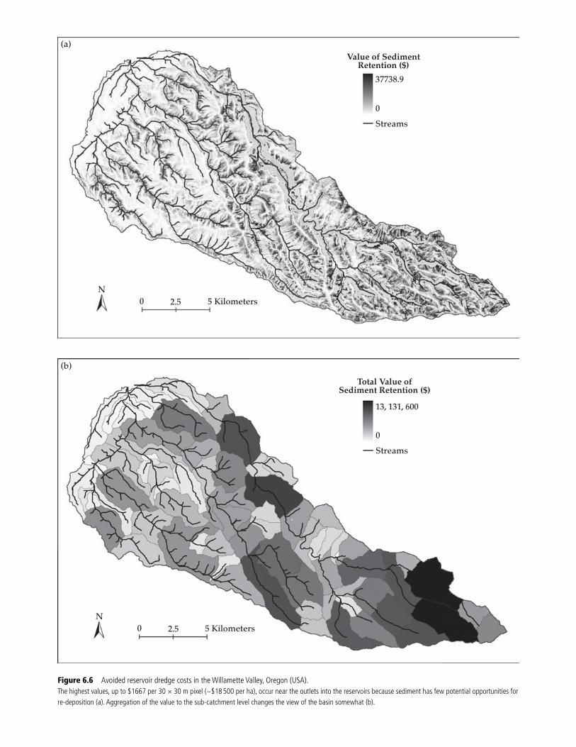
Figure 6.6 Avoided reservoir dredge costs in the Willamette Valley, Oregon (USA).The highest values, up to $1667 per 30 × 30 m pixel (~$18 500 per ha), occur near the outlets into the reservoirs because sediment has few potential opportunities for re-deposition (a). Aggregation of the value to the sub-catchment level changes the view of the basin somewhat (b).
0N
(a)
37738.9
0
Streams
Value of SedimentRetention ($)
2.5 5 Kilometers
0N
(b)
13, 131, 600
0
Streams
Total Value ofSediment Retention ($)
2.5 5 Kilometers
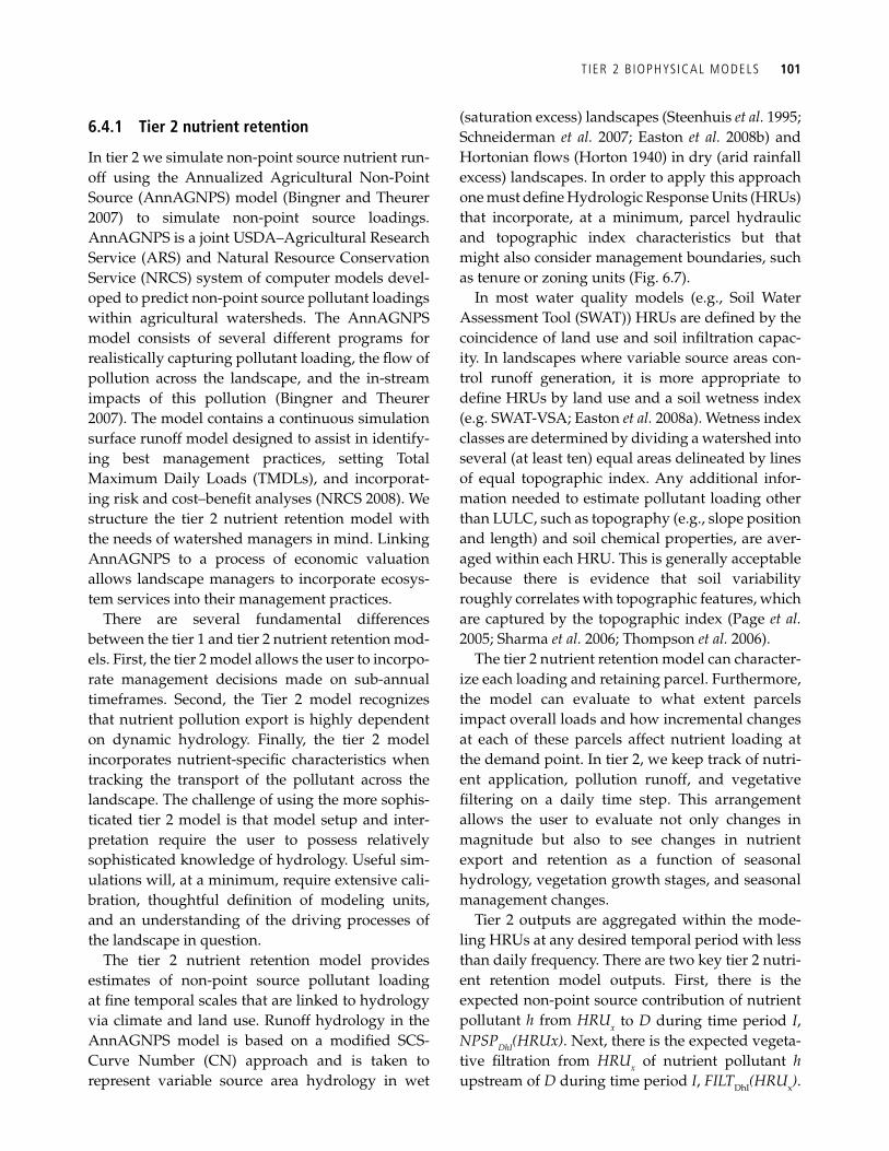
T IER 2 B IOPHYSICAL MODELS 101
6.4.1 Tier 2 nutrient retention
In tier 2 we simulate non-point source nutrient run-off using the Annualized Agricultural Non-Point Source (AnnAGNPS) model (Bingner and Theurer 2007) to simulate non-point source loadings. AnnAGNPS is a joint USDA–Agricultural Research Service (ARS) and Natural Resource Conservation Service (NRCS) system of computer models devel-oped to predict non-point source pollutant loadings within agricultural watersheds. The AnnAGNPS model consists of several different programs for realistically capturing pollutant loading, the fl ow of pollution across the landscape, and the in-stream impacts of this pollution (Bingner and Theurer 2007). The model contains a continuous simulation surface runoff model designed to assist in identify-ing best management practices, setting Total Maximum Daily Loads (TMDLs), and incorporat-ing risk and cost–benefi t analyses (NRCS 2008). We structure the tier 2 nutrient retention model with the needs of watershed managers in mind. Linking AnnAGNPS to a process of economic valuation allows landscape managers to incorporate ecosys-tem services into their management practices.
There are several fundamental differences between the tier 1 and tier 2 nutrient retention mod-els. First, the tier 2 model allows the user to incorpo-rate management decisions made on sub-annual timeframes. Second, the Tier 2 model recognizes that nutrient pollution export is highly dependent on dynamic hydrology. Finally, the tier 2 model incorporates nutrient-specifi c characteristics when tracking the transport of the pollutant across the landscape. The challenge of using the more sophis-ticated tier 2 model is that model setup and inter-pretation require the user to possess relatively sophisticated knowledge of hydrology. Useful sim-ulations will, at a minimum, require extensive cali-bration, thoughtful defi nition of modeling units, and an understanding of the driving processes of the landscape in question.
The tier 2 nutrient retention model provides estimates of non-point source pollutant loading at fi ne temporal scales that are linked to hydrology via climate and land use. Runoff hydrology in the AnnAGNPS model is based on a modifi ed SCS-Curve Number (CN) approach and is taken to represent variable source area hydrology in wet
(saturation excess) landscapes (Steenhuis et al. 1995; Schneiderman et al. 2007; Easton et al. 2008b) and Hortonian fl ows (Horton 1940) in dry (arid rainfall excess) landscapes. In order to apply this approach one must defi ne Hydrologic Response Units (HRUs) that incorporate, at a minimum, parcel hydraulic and topographic index characteristics but that might also consider management boundaries, such as tenure or zoning units (Fig. 6.7).
In most water quality models (e.g., Soil Water Assessment Tool (SWAT)) HRUs are defi ned by the coincidence of land use and soil infi ltration capac-ity. In landscapes where variable source areas con-trol runoff generation, it is more appropriate to defi ne HRUs by land use and a soil wetness index (e.g. SWAT-VSA; Easton et al. 2008a). Wetness index classes are determined by dividing a watershed into several (at least ten) equal areas delineated by lines of equal topographic index. Any additional infor-mation needed to estimate pollutant loading other than LULC, such as topography (e.g., slope position and length) and soil chemical properties, are aver-aged within each HRU. This is generally acceptable because there is evidence that soil variability roughly correlates with topographic features, which are captured by the topographic index (Page et al. 2005; Sharma et al. 2006; Thompson et al. 2006).
The tier 2 nutrient retention model can character-ize each loading and retaining parcel. Furthermore, the model can evaluate to what extent parcels impact overall loads and how incremental changes at each of these parcels affect nutrient loading at the demand point. In tier 2, we keep track of nutri-ent application, pollution runoff, and vegetative fi ltering on a daily time step. This arrangement allows the user to evaluate not only changes in magnitude but also to see changes in nutrient export and retention as a function of seasonal hydrology, vegetation growth stages, and seasonal management changes.
Tier 2 outputs are aggregated within the mode-ling HRUs at any desired temporal period with less than daily frequency. There are two key tier 2 nutri-ent retention model outputs. First, there is the expected non-point source contribution of nutrient pollutant h from HRU x to D during time period I , NPSP DhI (HRUx) . Next, there is the expected vegeta-tive fi ltration from HRU x of nutrient pollutant h upstream of D during time period I , FILT DhI (HRU x ) .
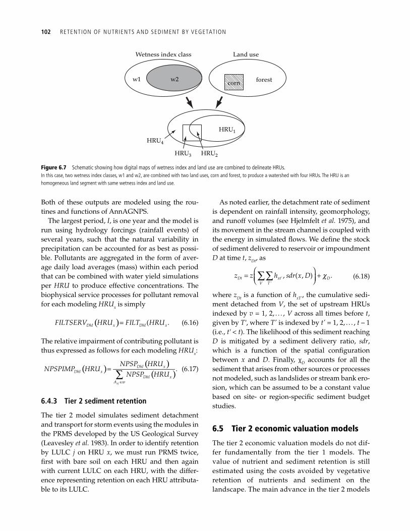
102 RETENTION OF NUTRIENTS AND SEDIMENT BY VEGETATION
Both of these outputs are modeled using the rou-tines and functions of AnnAGNPS.
The largest period, I , is one year and the model is run using hydrology forcings (rainfall events) of several years, such that the natural variability in precipitation can be accounted for as best as possi-ble. Pollutants are aggregated in the form of aver-age daily load averages (mass) within each period that can be combined with water yield simulations per HRU to produce effective concentrations. The biophysical service processes for pollutant removal for each modeling HRU x is simply
( )= ( .DhI x DhI xFILTSERV HRU FILT HRU (6.16)
The relative impairment of contributing pollutant is thus expressed as follows for each modeling HRU x :
( ) ( )( )
∈
= ∑ .
xj
DhI xDhI x
DhI xA w
NPSP HRUNPSPIMP HRU
NPSP HRU (6.17)
6.4.3 Tier 2 sediment retention
The tier 2 model simulates sediment detachment and transport for storm events using the modules in the PRMS developed by the US Geological Survey (Leavesley et al. 1983). In order to identify retention by LULC j on HRU x , we must run PRMS twice, fi rst with bare soil on each HRU and then again with current LULC on each HRU, with the differ-ence representing retention on each HRU attributa-ble to its LULC.
As noted earlier, the detachment rate of sediment is dependent on rainfall intensity, geomorphology, and runoff volumes (see Hjelmfelt et al. 1975), and its movement in the stream channel is coupled with the energy in simulated fl ows. We defi ne the stock of sediment delivered to reservoir or impoundment D at time t , z Dt , as
c⎛ ⎞= +⎜ ⎟⎝ ⎠∑∑ ''
, ( , ) .Dt xt DV T
z z h sdr x D (6.18)
where z Dt is a function of h xT´ , the cumulative sedi-ment detached from V , the set of upstream HRUs indexed by v = 1, 2, . . . , V across all times before t , given by T' , where T’ is indexed by t’ = 1, 2, . . . , t – 1 (i.e., t' < t ). The likelihood of this sediment reaching D is mitigated by a sediment delivery ratio, sdr , which is a function of the spatial confi guration between x and D . Finally, χ D accounts for all the sediment that arises from other sources or processes not modeled, such as landslides or stream bank ero-sion, which can be assumed to be a constant value based on site- or region-specifi c sediment budget studies.
6.5 Tier 2 economic valuation models
The tier 2 economic valuation models do not dif-fer fundamentally from the tier 1 models. The value of nutrient and sediment retention is still estimated using the costs avoided by vegetative retention of nutrients and sediment on the landscape. The main advance in the tier 2 models
Wetness index class Land use
w1 w2 corn
HRU1
HRU2HRU3
HRU4
forest
Figure 6.7 Schematic showing how digital maps of wetness index and land use are combined to delineate HRUs.In this case, two wetness index classes, w1 and w2, are combined with two land uses, corn and forest, to produce a watershed with four HRUs. The HRU is an homogeneous land segment with same wetness index and land use.
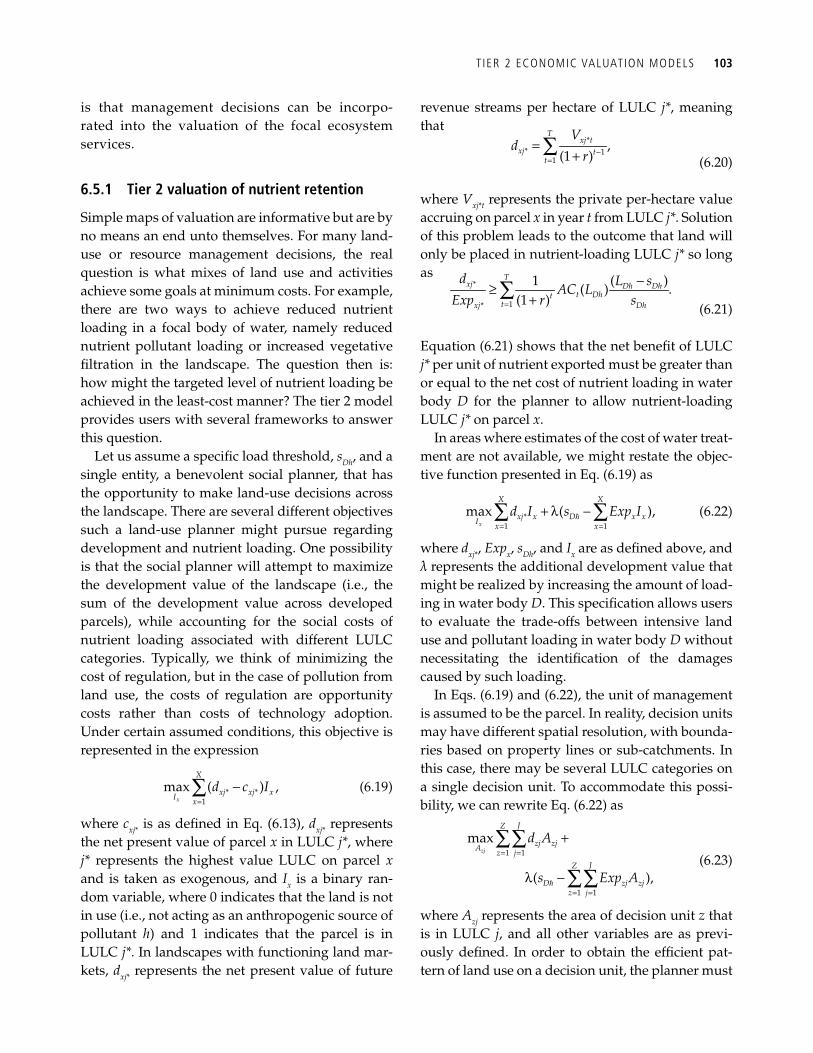
T IER 2 ECONOMIC VALUATION MODELS 103
is that management decisions can be incorpo-rated into the valuation of the focal ecosystem services.
6.5.1 Tier 2 valuation of nutrient retention
Simple maps of valuation are informative but are by no means an end unto themselves. For many land-use or resource management decisions, the real question is what mixes of land use and activities achieve some goals at minimum costs. For example, there are two ways to achieve reduced nutrient loading in a focal body of water, namely reduced nutrient pollutant loading or increased vegetative fi ltration in the landscape. The question then is: how might the targeted level of nutrient loading be achieved in the least-cost manner? The tier 2 model provides users with several frameworks to answer this question.
Let us assume a specifi c load threshold, s Dh , and a single entity, a benevolent social planner, that has the opportunity to make land-use decisions across the landscape. There are several different objectives such a land-use planner might pursue regarding development and nutrient loading. One possibility is that the social planner will attempt to maximize the development value of the landscape (i.e., the sum of the development value across developed parcels), while accounting for the social costs of nutrient loading associated with different LULC categories. Typically, we think of minimizing the cost of regulation, but in the case of pollution from land use, the costs of regulation are opportunity costs rather than costs of technology adoption. Under certain assumed conditions, this objective is represented in the expression
* *1
max ( ) ,x
X
xj xj xI x
d c I=
−∑ (6.19)
where c xj* is as defi ned in Eq. (6.13), d xj* represents the net present value of parcel x in LULC j* , where j* represents the highest value LULC on parcel x and is taken as exogenous, and I x is a binary ran-dom variable, where 0 indicates that the land is not in use (i.e., not acting as an anthropogenic source of pollutant h ) and 1 indicates that the parcel is in LULC j* . In landscapes with functioning land mar-kets, d xj* represents the net present value of future
revenue streams per hectare of LULC j* , meaning that
** 1
1
,(1 )
Txj t
xj tt
Vd
r −=
=+∑
(6.20)
where V xj*t represents the private per-hectare value accruing on parcel x in year t from LULC j* . Solution of this problem leads to the outcome that land will only be placed in nutrient-loading LULC j* so long as
*
1*
1 ( )( ) .(1 )
Txj Dh Dh
t Dhttxj Dh
d L sAC L
Exp r s=
−≥+∑
(6.21)
Equation (6.21) shows that the net benefi t of LULC j* per unit of nutrient exported must be greater than or equal to the net cost of nutrient loading in water body D for the planner to allow nutrient-loading LULC j* on parcel x .
In areas where estimates of the cost of water treat-ment are not available, we might restate the objec-tive function presented in Eq. (6.19) as
*1 1
max ( ),x
X X
xj x D x xI x x
d I s Exp Iλ= =
+ −∑ ∑" (6.22)
where d xj* , Exp x , s Dh , and I x are as defi ned above, and λ represents the additional development value that might be realized by increasing the amount of load-ing in water body D . This specifi cation allows users to evaluate the trade-offs between intensive land use and pollutant loading in water body D without necessitating the identifi cation of the damages caused by such loading.
In Eqs. (6.19) and (6.22), the unit of management is assumed to be the parcel. In reality, decision units may have different spatial resolution, with bounda-ries based on property lines or sub-catchments. In this case, there may be several LULC categories on a single decision unit. To accommodate this possi-bility, we can rewrite Eq. (6.22) as
1 1
1 1
max
( ),
zj
JZ
zj zjA z jJZ
D zj zjz j
d A
s Exp Aλ
= =
= =
+
−
∑∑
∑∑"
(6.23)
where A zj represents the area of decision unit z that is in LULC j , and all other variables are as previ-ously defi ned. In order to obtain the effi cient pat-tern of land use on a decision unit, the planner must
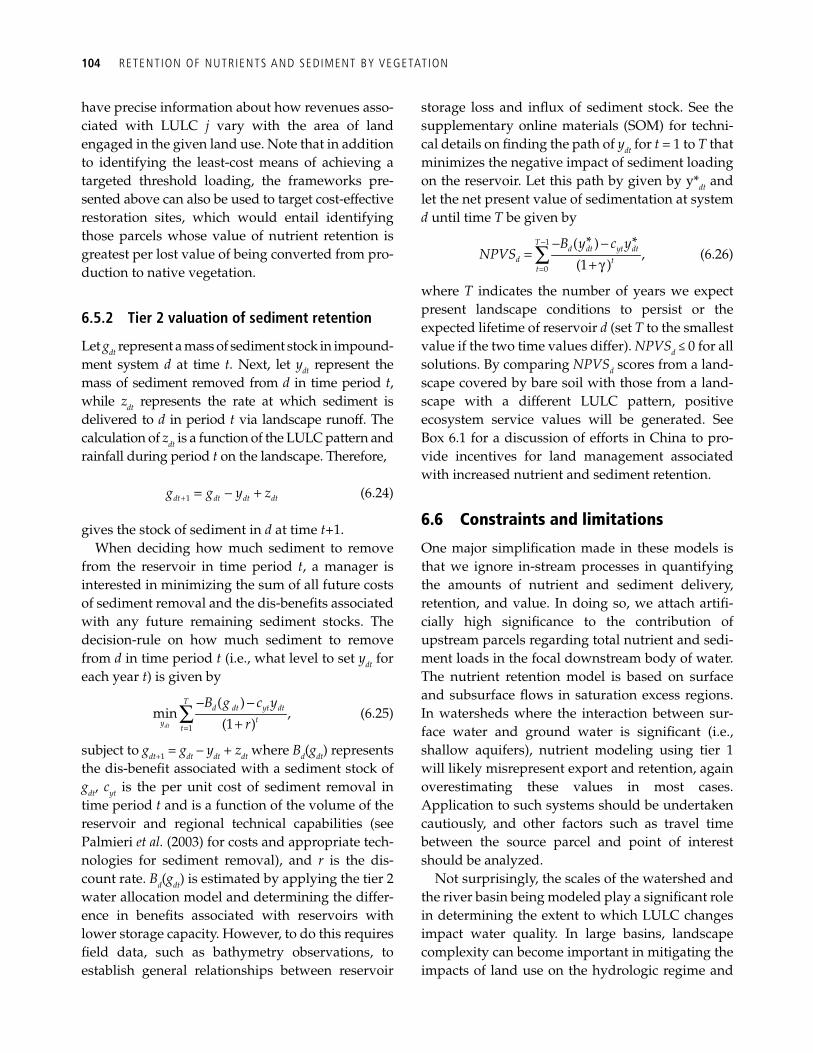
104 RETENTION OF NUTRIENTS AND SEDIMENT BY VEGETATION
have precise information about how revenues asso-ciated with LULC j vary with the area of land engaged in the given land use. Note that in addition to identifying the least-cost means of achieving a targeted threshold loading, the frameworks pre-sented above can also be used to target cost- effective restoration sites, which would entail identifying those parcels whose value of nutrient retention is greatest per lost value of being converted from pro-duction to native vegetation.
6.5.2 Tier 2 valuation of sediment retention
Let g dt represent a mass of sediment stock in impound-ment system d at time t . Next, let y dt represent the mass of sediment removed from d in time period t , while z dt represents the rate at which sediment is delivered to d in period t via landscape runoff. The calculation of z dt is a function of the LULC pattern and rainfall during period t on the landscape. Therefore,
+ = − +1dt dt dt dtg g y z (6.24)
gives the stock of sediment in d at time t +1. When deciding how much sediment to remove
from the reservoir in time period t , a manager is interested in minimizing the sum of all future costs of sediment removal and the dis-benefi ts associated with any future remaining sediment stocks. The decision-rule on how much sediment to remove from d in time period t (i.e., what level to set y dt for each year t ) is given by
1
( )min ,
(1 )dt
Td dt yt dt
tyt
B g c yr=
− −+∑ (6.25)
subject to g dt +1 = g dt – y dt + z dt where B d ( g dt ) represents the dis-benefi t associated with a sediment stock of g dt , c yt is the per unit cost of sediment removal in time period t and is a function of the volume of the reservoir and regional technical capabilities (see Palmieri et al. (2003) for costs and appropriate tech-nologies for sediment removal), and r is the dis-count rate. B d ( g dt ) is estimated by applying the tier 2 water allocation model and determining the differ-ence in benefi ts associated with reservoirs with lower storage capacity. However, to do this requires fi eld data, such as bathymetry observations, to establish general relationships between reservoir
storage loss and infl ux of sediment stock. See the supplementary online materials (SOM) for techni-cal details on fi nding the path of y dt for t = 1 to T that minimizes the negative impact of sediment loading on the reservoir. Let this path by given by y* dt and let the net present value of sedimentation at system d until time T be given by
1
0
* *( ),
(1 )
Td dt yt dt
d tt
B y c yNPVS
γ
−
=
− −=
+∑ (6.26)
where T indicates the number of years we expect present landscape conditions to persist or the expected lifetime of reservoir d (set T to the smallest value if the two time values differ). NPVS d ≤ 0 for all solutions. By comparing NPVS d scores from a land-scape covered by bare soil with those from a land-scape with a different LULC pattern, positive ecosystem service values will be generated. See Box 6.1 for a discussion of efforts in China to pro-vide incentives for land management associated with increased nutrient and sediment retention.
6.6 Constraints and limitations
One major simplifi cation made in these models is that we ignore in-stream processes in quantifying the amounts of nutrient and sediment delivery, retention, and value. In doing so, we attach artifi -cially high signifi cance to the contribution of upstream parcels regarding total nutrient and sedi-ment loads in the focal downstream body of water. The nutrient retention model is based on surface and subsurface fl ows in saturation excess regions. In watersheds where the interaction between sur-face water and ground water is signifi cant (i.e., shallow aquifers), nutrient modeling using tier 1 will likely misrepresent export and retention, again overestimating these values in most cases. Application to such systems should be undertaken cautiously, and other factors such as travel time between the source parcel and point of interest should be analyzed.
Not surprisingly, the scales of the watershed and the river basin being modeled play a signifi cant role in determining the extent to which LULC changes impact water quality. In large basins, landscape complexity can become important in mitigating the impacts of land use on the hydrologic regime and
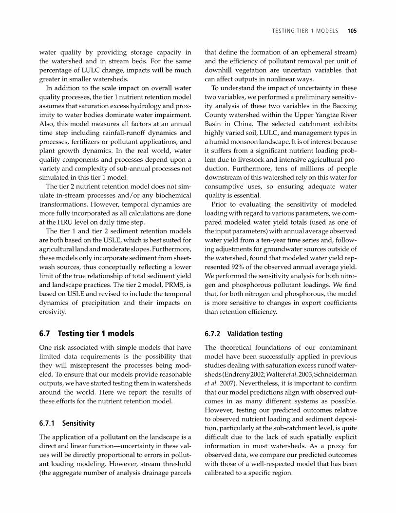
TEST ING T IER 1 MODELS 105
water quality by providing storage capacity in the watershed and in stream beds. For the same percentage of LULC change, impacts will be much greater in smaller watersheds.
In addition to the scale impact on overall water quality processes, the tier 1 nutrient retention model assumes that saturation excess hydrology and prox-imity to water bodies dominate water impairment. Also, this model measures all factors at an annual time step including rainfall-runoff dynamics and processes, fertilizers or pollutant applications, and plant growth dynamics. In the real world, water quality components and processes depend upon a variety and complexity of sub-annual processes not simulated in this tier 1 model.
The tier 2 nutrient retention model does not sim-ulate in-stream processes and/or any biochemical transformations. However, temporal dynamics are more fully incorporated as all calculations are done at the HRU level on daily time step.
The tier 1 and tier 2 sediment retention models are both based on the USLE, which is best suited for agricultural land and moderate slopes. Furthermore, these models only incorporate sediment from sheet-wash sources, thus conceptually refl ecting a lower limit of the true relationship of total sediment yield and landscape practices. The tier 2 model, PRMS, is based on USLE and revised to include the temporal dynamics of precipitation and their impacts on erosivity.
6.7 Testing tier 1 models
One risk associated with simple models that have limited data requirements is the possibility that they will misrepresent the processes being mod-eled. To ensure that our models provide reasonable outputs, we have started testing them in watersheds around the world. Here we report the results of these efforts for the nutrient retention model.
6.7.1 Sensitivity
The application of a pollutant on the landscape is a direct and linear function—uncertainty in these val-ues will be directly proportional to errors in pollut-ant loading modeling. However, stream threshold (the aggregate number of analysis drainage parcels
that defi ne the formation of an ephemeral stream) and the effi ciency of pollutant removal per unit of downhill vegetation are uncertain variables that can affect outputs in nonlinear ways.
To understand the impact of uncertainty in these two variables, we performed a preliminary sensitiv-ity analysis of these two variables in the Baoxing County watershed within the Upper Yangtze River Basin in China. The selected catchment exhibits highly varied soil, LULC, and management types in a humid monsoon landscape. It is of interest because it suffers from a signifi cant nutrient loading prob-lem due to livestock and intensive agricultural pro-duction. Furthermore, tens of millions of people downstream of this watershed rely on this water for consumptive uses, so ensuring adequate water quality is essential.
Prior to evaluating the sensitivity of modeled loading with regard to various parameters, we com-pared modeled water yield totals (used as one of the input parameters) with annual average observed water yield from a ten-year time series and, follow-ing adjustments for groundwater sources outside of the watershed, found that modeled water yield rep-resented 92% of the observed annual average yield. We performed the sensitivity analysis for both nitro-gen and phosphorous pollutant loadings. We fi nd that, for both nitrogen and phosphorous, the model is more sensitive to changes in export coeffi cients than retention effi ciency.
6.7.2 Validation testing
The theoretical foundations of our contaminant model have been successfully applied in previous studies dealing with saturation excess runoff water-sheds (Endreny 2002; Walter et al. 2003; Schneiderman et al. 2007). Nevertheless, it is important to confi rm that our model predictions align with observed out-comes in as many different systems as possible. However, testing our predicted outcomes relative to observed nutrient loading and sediment deposi-tion, particularly at the sub-catchment level, is quite diffi cult due to the lack of such spatially explicit information in most watersheds. As a proxy for observed data, we compare our predicted outcomes with those of a well-respected model that has been calibrated to a specifi c region.
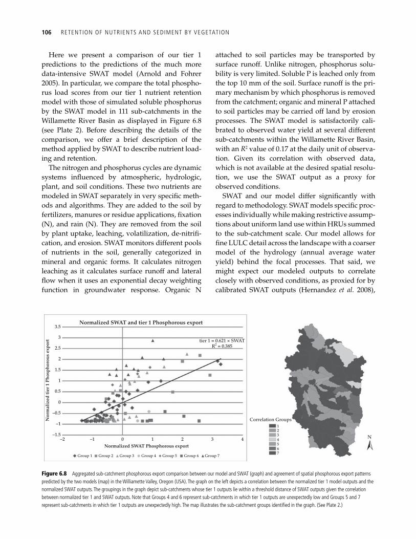
106 RETENTION OF NUTRIENTS AND SEDIMENT BY VEGETATION
Here we present a comparison of our tier 1 predictions to the predictions of the much more data-intensive SWAT model (Arnold and Fohrer 2005). In particular, we compare the total phospho-rus load scores from our tier 1 nutrient retention model with those of simulated soluble phosphorus by the SWAT model in 111 sub-catchments in the Willamette River Basin as displayed in Figure 6.8 (see Plate 2). Before describing the details of the comparison, we offer a brief description of the method applied by SWAT to describe nutrient load-ing and retention.
The nitrogen and phosphorus cycles are dynamic systems infl uenced by atmospheric, hydrologic, plant, and soil conditions. These two nutrients are modeled in SWAT separately in very specifi c meth-ods and algorithms. They are added to the soil by fertilizers, manures or residue applications, fi xation (N), and rain (N). They are removed from the soil by plant uptake, leaching, volatilization, de-nitrifi -cation, and erosion. SWAT monitors different pools of nutrients in the soil, generally categorized in mineral and organic forms. It calculates nitrogen leaching as it calculates surface runoff and lateral fl ow when it uses an exponential decay weighting function in groundwater response. Organic N
attached to soil particles may be transported by surface runoff. Unlike nitrogen, phosphorus solu-bility is very limited. Soluble P is leached only from the top 10 mm of the soil. Surface runoff is the pri-mary mechanism by which phosphorus is removed from the catchment; organic and mineral P attached to soil particles may be carried off land by erosion processes. The SWAT model is satisfactorily cali-brated to observed water yield at several different sub-catchments within the Willamette River Basin, with an R 2 value of 0.17 at the daily unit of observa-tion. Given its correlation with observed data, which is not available at the desired spatial resolu-tion, we use the SWAT output as a proxy for observed conditions.
SWAT and our model differ signifi cantly with regard to methodology. SWAT models specifi c proc-esses individually while making restrictive assump-tions about uniform land use within HRUs summed to the sub-catchment scale. Our model allows for fi ne LULC detail across the landscape with a coarser model of the hydrology (annual average water yield) behind the focal processes. That said, we might expect our modeled outputs to correlate closely with observed conditions, as proxied for by calibrated SWAT outputs ( Hernandez et al. 2008 ),
Normalized SWAT and tier 1 Phosphorous export3.5
3tier 1 = 0.621 × SWAT
R2 = 0.3852.5
2
1.5
1
0.5
0
–0.5
–1
–1.5–2 –1
Group 1 Group 2 Group 3 Group 4 Group 5 Group 6 Group 7
0Normalized SWAT Phosphorous export
Nor
mal
ized
tier
1 P
hosp
horo
us e
xpor
t
1 2 3 4
Correlation Groups
N
1234567
Figure 6.8 Aggregated sub-catchment phosphorous export comparison between our model and SWAT (graph) and agreement of spatial phosphorous export patterns predicted by the two models (map) in the Williamette Valley, Oregon (USA). The graph on the left depicts a correlation between the normalized tier 1 model outputs and the normalized SWAT outputs. The groupings in the graph depict sub-catchments whose tier 1 outputs lie within a threshold distance of SWAT outputs given the correlation between normalized tier 1 and SWAT outputs. Note that Groups 4 and 6 represent sub-catchments in which tier 1 outputs are unexpectedly low and Groups 5 and 7 represent sub-catchments in which tier 1 outputs are unexpectedly high. The map illustrates the sub-catchment groups identifi ed in the graph. (See Plate 2.)

TEST ING T IER 1 MODELS 107
Christine Tam
In the wake of the devastating Yangtze River fl oods of 1998 and unprecedented extent of the drying of the Yellow River in 1997, the Government of China (GOC) initiated a number of forestry programs aimed at water and soil conservation to mitigate these impacts in the future. Since these initial forestry programs began, provincial- and national-level government investment has continued and even expanded to protect watershed services more widely. Often with little quantifi cation of actual service delivery, these programs experienced relatively rapid approval and initiation and generally sustain widespread support and compliance, in part because of a strong belief in the overall benefi ts of forests and in part for their ability to address a variety of associated objectives.
For the past two decades, China has experienced a consistent level of fl ood damage despite heavy investment in structural solutions to fl ood control. These damages culminated in 1998 with the Yangtze fl oods. A follow-up UNEP study (1999) attributed the effects of upper watershed deforestation and overgrazing in reducing water storage capacity as a key factor that aggravated the impacts of prolonged and substantial rainfall. Not only were the degraded soils less able to retain water, but eroded soils washed downstream fi lling river channels, lakes, and reservoirs, reducing their ability to mitigate fl ood waters (Zong and Chen 2000).
A direct response to this disaster was consideration and development of a more comprehensive system of fl ood management that addressed both structural and non-structural components. Among the non-structural components that included fl ood forecasting, resettlement from high fl ood risk areas, and fl ood detention basin compensation, the Chinese government also enthusiastically initiated the Natural Forest Protection Program (NFPP) and Sloping Lands Conversion Program (SLCP) to address upper watershed impacts. These programs, fi rst piloted then approved for the period 2000 to 2010, banned logging of natural forests on 30 million ha and supported reforestation of 15 million ha of sloping cropland, respectively, along the upper Yangtze and upper and middle Yellow rivers. The original investment of the SLCP reached nearly US$40 billion through annual grain and cash payments to farmers for retiring and reforesting cropland, while the GOC has allocated over $11 billion for the NFPP over the same timeframe, numbering these
among the world’s largest payments for ecological services schemes (Liu et al . 2008).
These two forestry programs were initiated with substantial funding from the central government for soil and water retention benefi ts but rapidly gained further political favor for addressing an additional broader suite of government priorities and objectives. Besides reducing soil erosion, the SLCP also aims to alleviate poverty, especially in remote, mountainous areas with low productivity lands, reducing urban–rural development imbalances. In addition, the SLCP promotes local economic development (Xu and Cao 2002), facilitates shifts from farming to more sustainable production structures (SFA 2003), and bolstered a then-troubled State Grain Bureau (Bennett 2008). Subscription to the program was highly successful given the relatively high rates of payments such that local and regional implementation almost always met or exceeded targets.
The NFPP additionally supported restructuring of rural economies, retraining and relocating over 700 000 former forestry workers (ADB 2006). Economies once solely dependent on timber production were now more reliant on multiple industries, including forest management, plantation farming, and tourism (Liu et al . 2008). Compliance with the NFPP has been relatively successful, with little illegal commercial logging. Villagers, even for subsistence use, must apply to their local forestry bureaus for fuelwood or domestic construction timber allocations. State-run logging companies were eliminated virtually overnight, and new economies, such as that of Jiuzhaigou in Sichuan or Zhongdian, renamed “Shangri-La,” in Yunnan have successfully embraced tourism as their alternative income source.
The success of these two programs in compliance and participation coupled with belief in their ecological benefi ts has led the GOC to expand its forestry programs to conserve further watershed services. More recently, the Forest Ecological Benefi t Compensation Fund (FEBCF) was approved. First conceived of in the late 1980s, the FEBCF achieved legal backing in April 1998, initiated pilot work in 2001, and was expanded across China in 2004, providing payments of 5 rmb (7 rmb = US$) per mu to maintain natural forest land (Sun and Chen 2000). Land demarcated as “state ecological forests” based on a suite of mostly ecological criteria are subject to use restrictions and associated payment, spanning both state- and collective-owned forests. Provincial governments are encouraged to
Box 6.1 China forestry programs take aim at more than fl oods
continues
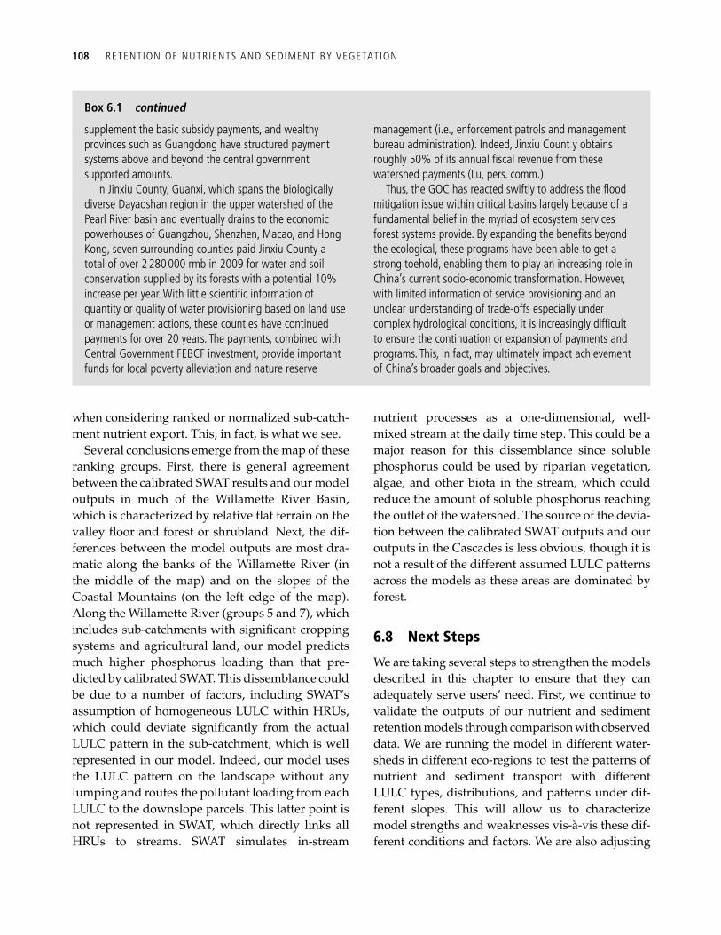
108 RETENTION OF NUTRIENTS AND SEDIMENT BY VEGETATION
when considering ranked or normalized sub-catch-ment nutrient export. This, in fact, is what we see.
Several conclusions emerge from the map of these ranking groups. First, there is general agreement between the calibrated SWAT results and our model outputs in much of the Willamette River Basin, which is characterized by relative fl at terrain on the valley fl oor and forest or shrubland. Next, the dif-ferences between the model outputs are most dra-matic along the banks of the Willamette River (in the middle of the map) and on the slopes of the Coastal Mountains (on the left edge of the map). Along the Willamette River (groups 5 and 7), which includes sub-catchments with signifi cant cropping systems and agricultural land, our model predicts much higher phosphorus loading than that pre-dicted by calibrated SWAT. This dissemblance could be due to a number of factors, including SWAT’s assumption of homogeneous LULC within HRUs, which could deviate signifi cantly from the actual LULC pattern in the sub-catchment, which is well represented in our model. Indeed, our model uses the LULC pattern on the landscape without any lumping and routes the pollutant loading from each LULC to the downslope parcels. This latter point is not represented in SWAT, which directly links all HRUs to streams. SWAT simulates in-stream
nutrient processes as a one-dimensional, well-mixed stream at the daily time step. This could be a major reason for this dissemblance since soluble phosphorus could be used by riparian vegetation, algae, and other biota in the stream, which could reduce the amount of soluble phosphorus reaching the outlet of the watershed. The source of the devia-tion between the calibrated SWAT outputs and our outputs in the Cascades is less obvious, though it is not a result of the different assumed LULC patterns across the models as these areas are dominated by forest.
6.8 Next Steps
We are taking several steps to strengthen the models described in this chapter to ensure that they can adequately serve users’ need. First, we continue to validate the outputs of our nutrient and sediment retention models through comparison with observed data. We are running the model in different water-sheds in different eco-regions to test the patterns of nutrient and sediment transport with different LULC types, distributions, and patterns under dif-ferent slopes. This will allow us to characterize model strengths and weaknesses vis-à-vis these dif-ferent conditions and factors. We are also adjusting
supplement the basic subsidy payments, and wealthy provinces such as Guangdong have structured payment systems above and beyond the central government supported amounts.
In Jinxiu County, Guanxi, which spans the biologically diverse Dayaoshan region in the upper watershed of the Pearl River basin and eventually drains to the economic powerhouses of Guangzhou, Shenzhen, Macao, and Hong Kong, seven surrounding counties paid Jinxiu County a total of over 2 280 000 rmb in 2009 for water and soil conservation supplied by its forests with a potential 10% increase per year. With little scientifi c information of quantity or quality of water provisioning based on land use or management actions, these counties have continued payments for over 20 years. The payments, combined with Central Government FEBCF investment, provide important funds for local poverty alleviation and nature reserve
management (i.e., enforcement patrols and management bureau administration). Indeed, Jinxiu Count y obtains roughly 50% of its annual fi scal revenue from these watershed payments (Lu, pers. comm.).
Thus, the GOC has reacted swiftly to address the fl ood mitigation issue within critical basins largely because of a fundamental belief in the myriad of ecosystem services forest systems provide. By expanding the benefi ts beyond the ecological, these programs have been able to get a strong toehold, enabling them to play an increasing role in China’s current socio-economic transformation. However, with limited information of service provisioning and an unclear understanding of trade-offs especially under complex hydrological conditions, it is increasingly diffi cult to ensure the continuation or expansion of payments and programs. This, in fact, may ultimately impact achievement of China’s broader goals and objectives.
Box 6.1 continued
NEXT STEPS 109
the model to allow for the inclusion of biological pathogens (e.g., fecal coliform). To achieve this goal, we have included the option of adding the pathogen source map, pathogen concentration (intensity) and vegetation fi ltration effi ciency for this pathogen to the nutrient pollutant model.
Finally, the models described above are functions of several parameters whose values are drawn from a distribution in reality although they have been described as deterministic throughout the chapter. We are currently taking steps to incorporate uncer-tainty into our models, which will allow the users to understand the impacts of this uncertainty on model outputs. For a limited set of input parameters, we will allow the user to explore the impacts of param-eter uncertainty on model outputs in one of two ways. The fi rst methodology involves treating each parcel in the landscape as a realization of an under-lying distribution. The second involves providing a confi dence interval as well as a point estimate for use in supply estimation.
References
Agnew, L. J., Lyon, S., Gérard-Marchant, P., et al . (2006). Identifying hydrologically sensitive areas: bridging the gap between science and application. Journal of Environmental Management , 78 (1), 63–76.
Arnold, J. G., and Fohrer, N. (2005). SWAT2000: Current capabilities and research opportunities in applied watershed modeling. Hydrological Processes , 19 (3), 563–72.
Asia Development Bank (ADB). May 2006. Poverty Revolution in Key Forestry Conservation Programs. Final Draft Report.
Athayde, D. N., Shelley, P. E., Driscol, E. D., et al . (1983). Results of the nationwide urban runoff program: Final report . US Environmental Protection Agency, Water Plannning Division, Washington, DC.
Baker, M., Weller, D., and Jordan, T. (2006). Improved methods for quantifying potential nutrient interception by riparian buffers. Landscape Ecology , 21 (8), 1327–45.
Bennett, Michael. (2008). China’s sloping land conversion program: institutional innovation or business as usual. Ecological Economics 65: 699–711.
Bingner, R. L., and Theurer, F. D. (2007). Research: AGNPS. US Department of Agriculture–Agricultural Research Service . [Online]. Available: http://www.ars.usda.gov/Research/docs.htm?docid=5199 Accessed 10 October 2008.
Dearmont, D., McCarl, B. A., and Tolman, D. A. (1998). Costs of water treatment due to diminished water qual-ity: A case study in Texas. Water Resources Research , 34 (4), 849–54.
Desvousges, W. H., Smith, V. K., and Fischer, A. (1987). Option price estimates for water quality improvements: A contingent valuation study for the Monongahela River. Journal of Environmental Economics and Management , 14 (3), 248–67.
Easton, Z. M., Fuka, D. R., Walter, M. T., et al . (2008a). Re-conceptualizing the Soil and Water Assessment Tool (SWAT) model to predict saturation excess runoff from variable source areas. Journal of Hydrology , 348 (3–4), 279–91.
Easton, Z. M., Walter, M. T., and Steenhuis, T. S. (2008b). Combined monitoring and modeling indicate the most effective agricultural best management practices. Journal of Environmental Quality , 37 , 1798–1809.
Endreny, T. A. (2002). Forest buffer strips: Mapping the water quality benefi ts. Journal of Forestry , (January/February), 35–40.
Englin, J., and Cameron, T. A. (1996). Augmenting travel cost models with contingent behavior data. Environmental and Resource Economics , 7 (2), 133–47.
Foster, H. S. J., and Beattie, B. R. (1981). On the specifi ca-tion of price in studies of consumer demand under block price scheduling. Land Economics , 57 (2), 624–9.
Gotaas, H. B. (1956). Composting: Sanitary disposal and rec-lamation of organic wastes , Colombia Ubiversity Press, New York.
Hanley, N., Bell, D., and Alvarez-Farizo, B. (2003). Valuing the benefi ts of coastal water quality improvements using contingent and real behavior. Environmental and Resource Economics , 24 (3), 273–85.
Hernandez, M., Kepnerb, W. G., Goodrich, D. G., et al . (2008). The use of scenario analysis to assess water ecosystem services in response to future land use change in the Willamette River Basin, Oregon. IOS Press, Amsterdam, The Netherlands.
Hjelmfelt, A. T., Piest, R. P., and Saxon, K. E. (1975). Mathematical modeling of erosion on upland areas. In Congress of the 16th International Association for Hydraulic Research , pp. 40.
Holmes, T. (1988). Soil erosion and water treatment. Land Economics , 64 (3), 356–66.
Horton, R. E. (1940). An approach toward a physical inter-pretation of infi ltration-capacity. Soil Science Society of America Proceedings , 5 , 399–417.
Leavesley, G. H., Lichty, R. W., Troutman, B. M., et al . (1983). Precipitation-runoff modeling system: user’s manual . US Geological Survey, Washington, DC.
110 RETENTION OF NUTRIENTS AND SEDIMENT BY VEGETATION
Leggett, C. G., and Bockstael, N. E. (2000). Evidence of the effects of water quality on residential land price. Journal of Environmental Economics and Management , 39 (2), 121–44.
Liu, Jianguo, Shuxin Li, Zhiyun Ouyang, Christine Tam, and Xiaodong Chen. (2008). Ecological and Socio-economic effects of China’s policies for ecosystem serv-ices. Proceedings of the National Academy of Sciences. 105 (28): 9477–9482.
Moore, W. B., and McCarl, B. A. (1987). Off-site costs of soil erosion: a case study in the Willamette valley. Western Journal of Agricultural Economics , 12 (1), 42–9.
Page, T., Haygarth, P. M., Beven, K. J., et al . (2005). Spatial variability of soil phosphorus in relation to the topo-graphic index and critical source areas: Sampling for assessing risk to water quality. Journal of Environmental Quality , 34 , 2263–77.
Palmieri, A., Shah, F., Annandale, G., et al . (2003). Reservoir conservation , vol. 1: The RESCON approach . World Bank, Washington, DC.
Reckhow, K. H., Beaulac, M. N., and Simpson, J. T. (1980). Modeling phosphorus loading and lake response under uncer-tainty: a manual and compilation of export coeffi cients . US Environmental Protection Agency, Washington, DC.
Reid, L. M., and Dunne, T. (1996). Rapid evaluation of sedi ment budgets . Catena Verlag GMBH, Reiskirchen, Germany.
Renard, K. G., Foster, G. R., Weesies, G. A., et al . (1997). Predicting soil erosion by water: a guide to conservation planning with the revised universal soil loss equation (RUSLE). USDA Agriculture Handbook 703. USDA, Washington, DC.
Roose, E. (1996). Land husbandry—components and strategy , 70 FAO Soils Bulletin. Food and Agriculture Organization of the UN, Rome, Italy.
Schneiderman, E. M., Steenhuis, T. S., Thongs, D. J., et al . (2007). Incorporating variable source area hydrology into a curve-number-based watershed model. Hydrological Processes , 21 , 3420–30.
Sharma, S. K., Mohanty, B. P., and Zhu, J. T. (2006). Including topography and vegetation attributes for developing pedotransfer functions. Soil Science Society of America Journal , 70 , 1430–40.
State Forestry Administration (SFA). (2003). Sloping Land Conversion Program Plan (2001–2010). (In Chinese.)
Steenhuis, T. S., Winchell, M., Rossing, J., et al . (1995). SCS runoff equation revisited for variable-source runoff areas. Journal of Irrigation and Drainage Engineering , 121 (3), 234–8.
Stone, R. P., and Hilborn, D. (2000). Universal soil loss equa-tion (USLE): Factsheet. Government of Ontario, Ministry of Agriculture, Food and Rural Affairs . [Online]. Available at: http://www.omafra.gov.on.ca/english/engineer/facts/00-001.htm#tab3a Accessed May 2008.
Thompson, J. A., Pena-Yewtukhiw, E. M. and Grove, J. H. (2006). Soil-landscape modeling across a physiographic region: topographic patterns and model transportabil-ity. Geoderma , 133 , 57–70. UNEP Assessment of 1998 Yangtze Floods. 1999.
White, W. R. (2001). Evacuation of sediments from reservoirs . Thomas Telford, London.
Wischmeier, W. H., and Smith, D. (1978). Predicting rainfall erosion losses: a guide to conservation planning . USDA-ARS Agriculture Handbook, Washington, DC.
Xu, J. and Cao Y. (2002). On sustainability a of converting farmland to forests/grasslands. International Economics Review 22: 56–60 (in Chinese), Zong, Yongqiang and Xiqing Chen. 2000. The 1998 Flood on the Yangtze, China. Natural Hazards 22: 165–184.
111
CHAPTER 7
Terrestrial carbon sequestration and storage Marc Conte, Erik Nelson, Karen Carney, Cinzia Fissore, Nasser Olwero, Andrew J. Plantinga, Bill Stanley, and Taylor Ricketts
7.1 Introduction
Ecosystems help regulate Earth’s climate by adding and removing greenhouse gases (GHGs) such as carbon dioxide (CO 2 ) from the atmosphere (IPCC 2006). Terrestrial ecosystems currently store four times more carbon than is found in the atmosphere (3 060 versus 760 gigatons (Gt); see Lal 2004 ). Changes in land use and land cover (LULC) due to timber harvesting, land-clearing for agriculture, and fi re can release substantial amounts of terrestri-ally stored carbon. For example, tropical deforesta-tion was responsible for 15–25% of the globe’s total GHG emissions in the 1990s (including fossil-fuel use and other land-use change; see Gibbs et al. ( 2007 ) and the Technical Summary in IPCC (2007a)). In Africa, deforestation accounted for nearly 70% of the continent’s total GHG emissions at the end of the twentieth century ( Gibbs et al. 2007 ).
We can mitigate the expected economic damages due to climate change by slowing down GHG accu-mulation in the atmosphere ( Stern 2007 ). This fact has intensifi ed global interest in enlarging or at least maintaining the size of the terrestrial carbon pool (e.g., IPCC 2007a, Lehmann 2007 ). A variety of land management techniques can be used to achieve this end, including lengthening harvest rotation time in plantation forests (e.g., Sohngen and Brown 2008 ), planting trees to restore forests (reforestation; e.g., Canadell and Raupach 2008 ), planting trees in aban-doned croplands (afforestation; e.g., Nilsson and Schopfhauser 1995 ), improving soil management (e.g., Schuman et al. 2002 , Lal 2004 ), reducing forest fi re and forest disease risk (e.g., Brown et al. 2002 ), reducing deforestation and forest degradation
(REDD; Ebeling and Yasue 2008 ), and replacing annual crops with perennials ( Fargione et al . 2008 ).
Concerns about climate change have led to both regulated and voluntary emissions reduction. Regu-lated markets such as the European Union Emissions Trading System (EU ETS; Victor et al. 2005 ) and the Regional Greenhouse Gas Initiative ( Burtraw et al . 2006 ), and voluntary offset markets like the Chicago Climate Exchange provide a forum in which land-owners can generate carbon credits, through incre-ased carbon sequestration on their lands, that can be bought by entities looking to offset their own emissions (Marechal and Hecq 2006). Further, the Kyoto Protocol allows signatory nations to claim GHG emission reductions by funding afforestation and reforestation projects in developing nations (e.g., Pfaff et al. 2000 ). Finally, discussion at the 2007 United Nations Framework Convention on Climate Change Conference focused on developing fi nan-cial incentives to reward developing nations for reducing emissions by avoiding deforestation and forest degradation (e.g., Mollicone et al. 2007 ; Ebeling and Yasue 2008 ).
Given the growing interest in carbon markets and offset programs, decision-makers need a way to simply and quickly understand how much carbon is held in landscapes today, and how storage and sequestration will change under different manage-ment options. Such information will help managers fi nd and create opportunities for additional carbon sequestration and associated payments in their landscapes. We present two tiers of relatively sim-ple models that address these needs by using mini-mal data to estimate carbon sequestration and storage on a landscape.
112 TERRESTRIAL CARBON SEQUESTRATION AND STORAGE
Unlike other ecosystem services, there is no dif-ference between the supply and use of carbon sequestration and storage (see Chapter 3 for defi ni-tions of “supply” and “use” used throughout the book); every unit of sequestered GHG emission will allow us to avoid some economic damage that would have occured otherwise (although current and proposed sequestration and storage markets only pay for a portion of the avoided damage; see below). Further, because GHGs uniformly mix in the atmosphere the whole world benefi ts from a unit of sequestration regardless of where it occurs. After presenting our ecosystem service supply model, we present an approach for estimating the economic value of this supply. We also discuss how we might approximate carbon offsets and avoided emission credits with our model.
Gathering the data needed to estimate total car-bon sequestration and storage on a landscape, including species-specifi c growth rates, associated carbon storage, and species compositions, can be a time-intensive effort. The IPCC has developed an approach that assigns carbon stocks to different LULC categories based on a meta-analysis of fi eld storage studies (IPCC 2006). The models presented in this chapter are grounded in this approach. In our simplest storage and sequestration model, tier 1, we associate carbon storage with different LULC categories and each LULC category is assumed to be in storage equilibrium at any point in time ( Section 7.2.1 ). In tier 1, the amount of carbon sequestered in a parcel is the difference in steady-state storage at two points in time ( Section 7.2.2 ). In this simple model, carbon sequestration is not regis-tered in a parcel unless the parcel’s LULC changes or it is subject to harvest of wood.
7.2 Tier 1 supply model
7.2.1 Carbon stored on a landscape
We disaggregate terrestrial carbon storage into fi ve pools: (1) aboveground biomass, (2) belowground biomass, (3) soil, (4) other organic matter, and (5) harvested wood products (HWPs). Aboveground biomass is composed of all living plant material above the soil (e.g., grass, herbaceous material, bark, tree trunks, branches, leaves, and other
woody understory). Belowground biomass is the root system of the aboveground biomass. Sequestration and storage accounting in the soil pool is generally concerned with soil organic car-bon (SOC) in mineral soils; in certain land cover types, however, SOC in organic soils (e.g., wet-lands, peatlands, rice paddies) is the dominant soil carbon ( Post and Kwon 2000 ). The other organic matter pool includes plant litter and dead wood. The HWPs pool includes all carbon stored in prod-ucts made with wood removed from the landscape (e.g., furniture, paper, charcoal; Harmon et al. 1990 ; Smith et al. 2006 ).
Let C aj , C bj , C sj , and C oj indicate the metric tons of carbon stored per hectare (Mg of C ha –1 ), in the aboveground, belowground, soil, and other organic matter pools of LULC j respectively, where j = 1, 2, . . . , J indexes all LULC found on the landscape. LULC types can simply indicate land use and or cover (e.g., conifer forest, cropland) or include other landscape details that affect pool-storage val-ues such as time since disturbance (e.g., conifer for-est 120 years or more since a clear-cut, cropland that is plowed annually), extent of disturbance (e.g., heavily disturbed conifer forest due to illegal timber harvest), soil properties (cropland on clay soil; e.g., Torn et al. 1997 ), and climatic conditions (conifer forest below 1000 m, where elevation bands proxy for precipitation gradients; see McGuire et al. 2001 ; Raich et al. 2006 ). Adding specialized LULC classes such as these can help add more reality to the estimates of this steady-state model. For exam-ple, using age-specifi c forest classes with fi ne enough temporal resolution can help represent additional carbon sequestration as forests mature and change LULC classes.
The carbon stored in a parcel’s HWPs pool, C p , is the sum of the carbon in the woody material removed from the parcel in the past (even if the removed material eventually leaves the parcel) less the decay over time in the products that were made from this woody material (which releases carbon in the form of CO 2 ) and the carbon-equivalent emis-sions from manufacturing and transporting the fi nal products. Let
( )1
0
, ,xW
px hqx hqx qx qxq
C C f q−
== −∑ q q s (7.1)
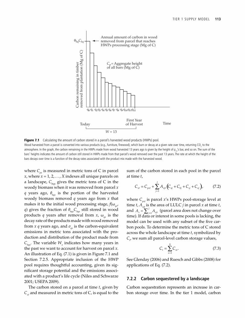
T IER 1 SUPPLY MODEL 113
where C px is measured in metric tons of C in parcel x , where x = 1, 2, . . . , X indexes all unique parcels on a landscape, C hqx gives the metric tons of C in the woody biomass when it was removed from parcel x q years ago, θ hqx is the portion of the harvested woody biomass removed q years ago from x that makes it to the initial wood processing stage, f (ω qx , q ) gives the fraction of θ hqx C hqx still stored in wood products q years after removal from x , ω qx is the decay rate of the products made with wood removed from x q years ago, and σ qx is the carbon-equivalent emissions in metric tons associated with the pro-duction and distribution of the product made from C hqx . The variable W x indicates how many years in the past we want to account for harvest on parcel x . An illustration of Eq. (7.1) is given in Figure 7.1 and Section 7.2.5 . Appropriate inclusion of the HWP pool requires thoughtful accounting, given its sig-nifi cant storage potential and the emissions associ-ated with a product’s life cycle (Niles and Schwarze 2001 ; USEPA 2009).
The carbon stored on a parcel at time t , given by C xt and measured in metric tons of C, is equal to the
sum of the carbon stored in each pool in the parcel at time t ,
( )1
,J
xt pxt xjt aj bj sj ojj
C C A C C C C=
= + + + +∑ (7.2)
where C pxt is parcel x ’s HWPs pool-storage level at time t , A xjt is the area of LULC j in parcel x at time t , and
== ∑ 1
J
x xjtjA A (parcel area does not change over
time). If data or interest in some pools is lacking, the model can be used with any subset of the fi ve car-bon pools. To determine the metric tons of C stored across the whole landscape at time t , symbolized by C t , we sum all parcel-level carbon storage values,
1
.X
t xtx
C C=
= ∑ (7.3)
See Glenday ( 2006 ) and Ruesch and Gibbs ( 2008 ) for applications of Eq. (7.2).
7.2.2 Carbon sequestered by a landscape
Carbon sequestration represents an increase in car-bon storage over time. In the tier 1 model, carbon
Annual amount of carbon in woodremoved from parcel that reachesHWPs processing stage (Mg of C)
Cp = Aggregate heightof all bars (Mg of C)
TodayFirst Yearof Harvest Time
W = 13
Car
bon
rem
aini
ng in
tim
ber
rem
oved
from
pla
ntat
ion
(Mg
of C
)
qhqChq
q0 q1 q2q3 q4 q5 q6 q7 q8 q9q10q11q12
Figure 7.1 Calculating the amount of carbon stored in a parcel’s harvested wood products (HWPs) pool. Wood harvested from a parcel is converted into various products (e.g., furniture, fi rewood), which burn or decay at a given rate over time, returning CO 2 to the atmosphere. In the graph, the carbon remaining in the HWPs made from wood harvested 13 years ago is given by the height of q 12 ’s bar, and so on. The sum of the bars’ heights indicates the amount of carbon still stored in HWPs made from that parcel’s wood removed over the past 13 years. The rate at which the height of the bars decays over time is a function of the decay rates associated with the product mix made with the harvested wood.
114 TERRESTRIAL CARBON SEQUESTRATION AND STORAGE
sequestration or loss in a parcel is registered when the parcel’s LULC mix changes, its management or production of HWPs changes, or its HWPs pool is not in equilibrium. Otherwise, for the sake of mode-ling simplicity, in tier 1 we assume storage in a parcel is in equilibrium or steady state and will not change over time despite any evidence to the contrary.
To determine the amount of carbon sequestered in a parcel from year t to year T ( t < T ), given by ∆ C xtT , we use Eq. (7.2) to calculate the amount of car-bon stored in a parcel in year t , C xt , and in year T , C xT , which accounts for any changes in the parcel’s LULC or HWP management or production between t and T , and then subtract C xt from C xT ,
,xtT xT xtC C C∆ = − (7.4)
where
1
X
tT xtTx
C C=
∆ = ∆∑ (7.5)
gives the change in carbon storage from t to T over the entire landscape.
In this case, C xt is the point of reference or base-line for determining whether net sequestration has occurred from t to T . If ∆ C xtT or ∆ C tT is positive, then sequestration has occurred from t to T in the parcel or landscape, respectively. If they are nega-tive, carbon has been lost between t and T . See Cairns et al. ( 2000 ) and Glenday ( 2006 ) for applica-tions of Eq. (7.4).
7.2.3 Additional sequestration in offset markets
Markets and programs that give carbon credits to landowners in exchange for enhancing terrestrial carbon sequestration on their lands currently only recognize additional sequestration in market-eligi-ble pools (see Box 7.1 for an illustration). Additional sequestration is the amount of sequestration above and beyond the sequestration that would have occurred in the absence of a carbon offset market or program (i.e., baseline sequestration). Additional sequestration in a parcel’s eligible pools from t to T ,
OffxtTC∆ , can be approximated in our model by calcu-
lating a parcel’s sequestration from time t to T under its baseline LULC mix as of time T ,
,Off BxtTC∆ , and sub-
tracting this from the parcel’s sequestration from time t to T under an alternative, offset program- infl uenced LULC mix as of time T ,
,Off AxtTC∆ :
, ,max 0, .Off Off A Off BxtT xtT xtTC C C∆ = ∆ − ∆ (7.6)
Such new, program-infl uenced scenarios are not generated by our models, but rather can be assessed by our models to reveal the additional carbon ben-efi ts associated with the offset program.
Two other carbon market issues are permanence and leakage, and both are topics of intense policy debate (e.g., Brown 2002 ; Vohringer et al. 2006 ; Murray et al. 2007 ) ( Box 7.1 ). Permanence is a con-cern because trees and other biomass eventually decay; fi res and illegal logging can occur regardless of management efforts; soil can be disturbed, releas-ing trapped carbon back into the atmosphere; and offset providers may decide to convert their forest to another use even with an existing offset contract. Therefore, when a landowner is compensated for additional sequestration, we might say that they are renting a temporary benefi t to society. How much society should pay for this temporary benefi t and at what point temporary sequestration becomes permanent sequestration in a climatic sense is con-tested (e.g., Chomitz 2002 ; Marechal and Hecq 2006). Leakage is an additional concern with offset, rather than regulatory, programs because when a land-owner decides to manage her land for additional sequestration instead of clearing it for agriculture or urban development the economic pressure to clear the land for other uses will not disappear. Instead it may be “leaked” or displaced to other parts of the landscape or globe where subsequent clearing will release stored carbon, decreasing the amount of additional sequestration. Leakage is accounted for in this model if it occurs within the study landscape and between the years t and T , so broadening both spatial and temporal scales can reduce the issue.
7.2.4 Preventing emissions from deforestation and degradation
REDD is a policy mechanism, currently under debate, that rewards efforts to reduce deforestation, forest degradation, and their associated carbon emissions in developing countries (e.g., Ebeling and
T IER 1 SUPPLY MODEL 115
Bill Stanley and Nicole Virgilio
Policies that constrain carbon dioxide (CO 2 ) emissions, and include provisions for trading carbon sequestered in forests and other ecosystems, are anticipated to be the largest driver of payments for carbon capture and storage and are a major topic of discussion in the development of national and international climate change policies and legislative language. If successful, these programs could generate billions of dollars of annual funding for forest carbon projects.
The Noel Kempff Mercado Climate Action Project (NKCAP) in Bolivia, borne of a partnership between The Nature Conservancy and Fundación Amigos de la Naturaleza with funding from industry and contributions by the Bolivian Government, is one example of such a project, designed to simultaneously address climate change, conserve biodiversity, and bring sustainable development benefi ts to local communities by avoiding logging and agricultural land conversion. The 1.5 million-acre project, which began in 1997 and expanded the Noel Kempff Mercado National Park, is the largest effort of its kind. It is expected to prevent the release of up to 5.8 million tons of CO 2 into the atmosphere over 30 years. As with any carbon sequestration project, there were a number of issues that had to be addressed to ensure high-quality carbon offsets.
Key factor 1: additionality Nearly all voluntary frameworks, as well as the few compliance programs in place or proposed, require that project-based emissions reductions and removals must be beyond “business as usual” to be credited (e.g., Alig and Butler 2004 , UNFCCC 1995, UNCCCS 1997, and several US Senate bills including the Forest Resources for the Environment and the Economy Act (S. 1547), the International Carbon Sequestration Incentive Act (S 2540), and the Lieberman–Warner Climate Security Act (S.3036)). The guidelines suggest that a scenario of what would have happened without the project must be developed for comparison against project management. The difference in carbon storage and other greenhouse gas emissions (GHGs) between the two represents the GHG impacts that are truly additional rather than simply the result of incidental or non-project factors such as recent market or
environmental changes (IPCC 2000). In the case of NKCAP, the project provided carbon fi nancing to stop logging in the park and deforestation around communities. Without this funding, these activities would have continued, leading to the loss of forest cover and release of carbon dioxide.
Key factor 2: baseline The business-as-usual, or “without-project” scenario, is also called the baseline , and its development should be among the fi rst steps to assessing the carbon benefi ts of a project. Baselines are essentially predictions, or future projections based empirically upon historical information or a performance benchmark, of what may have happened had the project not been put into place. The success of any forest carbon emissions reduction project will depend on the estimated carbon storage in the baseline or benchmark, subtracted from the performance of the project itself. Most recently, in the context of programs being considered within the context of the United Nations Framework Convention on Climate Change for activities to reduce emissions from deforestation and degradation (REDD), several national-scale baseline emission scenarios have been proposed. These proposals vary widely, and the baseline approach established as policy will have a signifi cant impact on the emissions reductions that could be claimed. To determine the total emission reductions that were additional to business-as-usual activities at Noel Kempff, baseline rates of deforestation were developed by GIS analysis of a time series of satellite photos from 1986, 1992, and 1996–7 and then were applied in a spatially explicit land-use change model to project future deforestation. The rates and models are to be reassessed periodically. Also, a national-scale economic model of Bolivian timber markets was created to develop baseline rates of logging and fi eld work was undertaken to determine the amount of emissions associated with the logging.
Key factor 3: leakage Leakage has been defi ned as “the unanticipated decrease or increase in GHG benefi ts outside of the project’s accounting boundary . . . as a result of project activities” ( Chapter 5 of IPCC 2000). A straightforward example of leakage from conservation is where a farmer who is seeking to clear a plot of uninhabited forest for conversion
Box 7.1 Noel Kempff case study: capturing carbon fi nance
continues
116 TERRESTRIAL CARBON SEQUESTRATION AND STORAGE
Yasue 2008 ). In this case, if deforestation and degra-dation that would have occurred under a business-as-usual LULC trajectory is prevented, then ecosystems retain additional carbon, thereby avoid-ing climate change-related economic damages that were originally expected.
Here we illustrate how we can use our models to approximate the carbon credits that could be gener-ated under REDD or similar programs to compen-sate avoided forest loss and degradation. This illustration relies on several assumptions. First, we assume that forest type j' ’s carbon stock in parcel x is in steady state at time t . Next, we assume that if forest type j' is cleared from x in order to establish LULC j , the carbon storage at time T is lower than it was at time t (i.e., C xt > C xT ). Let the change in stor-age on x be given by ∆ C xtT , where ∆ C xtT = 0 if forest type j' remains on the parcel as of time T and ∆ C xtT < 0 if the forest is cleared. (We assume that there are only two possible future states for parcel x at time T :
it can remain as is or be converted to a LULC with lower carbon storage.) Let Loss
xtTC∆ indicate the case where ∆ C xtT < 0.
The expected loss in a parcel’s carbon stock due to conversion from LULC j' to some other LULC by time T is the product of the difference in carbon stock ∆ C xtT and the overall probability that the forest in parcel x will be converted at some point between t and T , π xtT , under the business-as-usual baseline. Let there be i = 1, 2, . . . , I events that can cause forest type j' in parcel x to be converted by T . If we assume that the probability of each event occurring, given by π xtT , i , under the baseline is independent and addi-tive, then
,1
min 1, .I
xtT xtT ii=
⎧ ⎫= ⎨ ⎬⎩ ⎭
∑π π (7.7)
The expected amount of aboveground biomass car-bon storage in parcel x at time T under the baseline is given by
to agricultural fi elds is told that the land has been made part of a carbon project and is now protected. Leakage occurs if the farmer moves to the next available land and clears that forest instead. The project would simply displace the farmer’s activity and emissions, and not result in any real reductions of atmospheric CO 2 . The risk of leakage can be minimized through thoughtful project design, taking local conditions into consideration and addressing the underlying drivers of deforestation ( Schwarze et al. 2002 ). For example, NKCAP attempted to limit leakage just outside the project area by working with the bordering community to develop a sustainable management plan, with which they applied for legal land title through the Bolivian government. This reduced the risk of uncontrolled forest conversion ( Aukland et al . 2002 ). Market leakage that was not avoided was estimated using an economic model ( Sohngen and Brown 2004 ) and deducted from the claimed carbon savings.
Key factor 4: permanence One of the fi rst issues that critics of forest carbon crediting will cite is the possibility for the reversal of the carbon sequestration. Project success is dependent upon keeping the forest healthy and standing. Illegal logging, invasive
pests, fi re, and political turnover all have the potential to release carbon sequestered in the forest (IPCC 2000). Thus, permanence must be taken into consideration during the project planning stage, targeting areas where land is likely to remain intact indefi nitely and using approaches like permanent conservation easements and sustainable forestry, which will reduce likelihood that the carbon storage will be lost, or that those losses will be sustained, over time. Carbon offset policies generally establish liability for losses. To ensure against these losses one tool is to set aside “buffer” credits that can be drawn upon should the stored carbon be unexpectedly lost. To ensure the permanence of NKCAP, the national park was expanded to include the project area and a permanent endowment was established to fund protection activities into the future.
Conclusion Obviously, there are many factors that must be considered in the successful employment of forest carbon emissions reductions programs. Additionality, baseline, leakage, and permanence are challenges, but pilot projects such as NKCAP have shown that it is possible to address and overcome them.
Box 7.1 continued
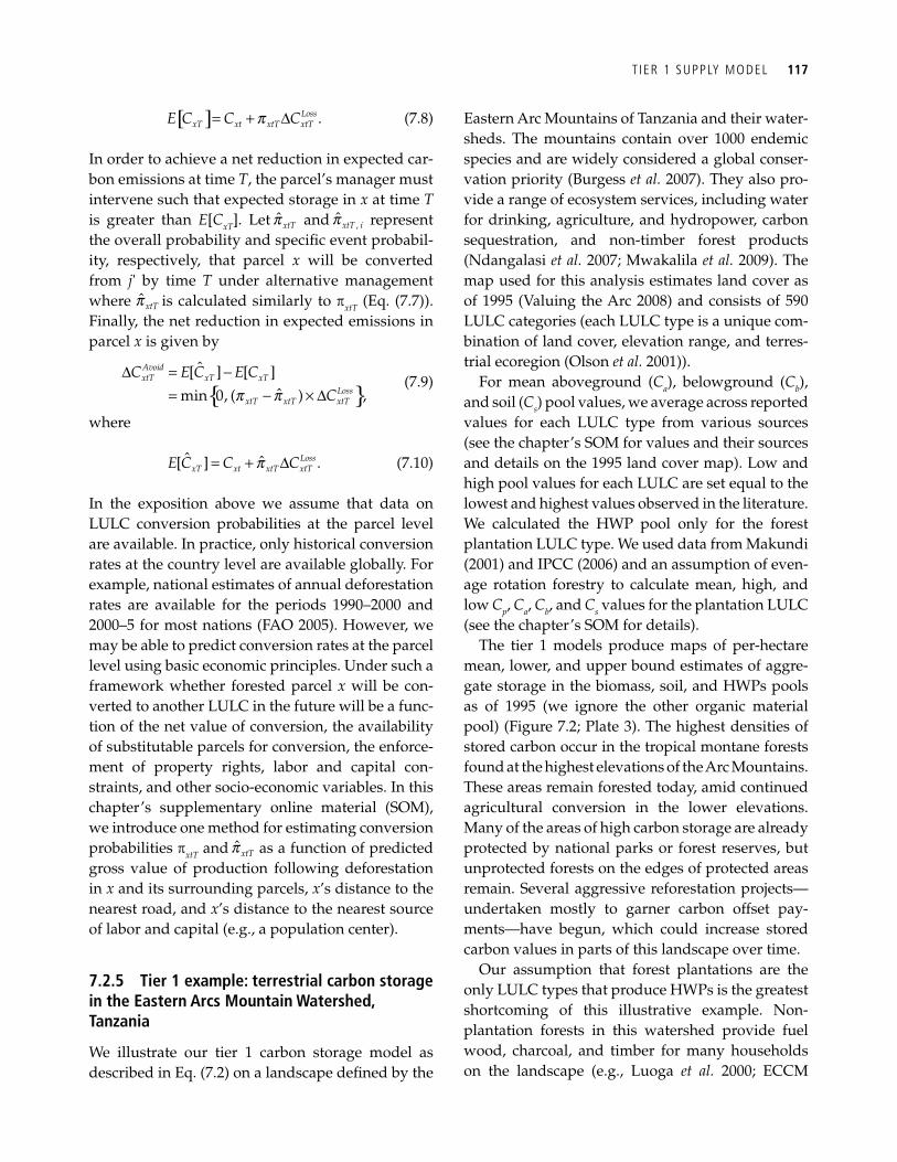
T IER 1 SUPPLY MODEL 117
[ ] .LossxT xt xtT xtTE C C Cp= + ∆ (7.8)
In order to achieve a net reduction in expected car-bon emissions at time T , the parcel’s manager must intervene such that expected storage in x at time T is greater than E [ C xT ]. Let ˆ xtTp and ,ˆ xtT ip represent the overall probability and specifi c event probabil-ity, respectively, that parcel x will be converted from j' by time T under alternative management where ˆ xtTp is calculated similarly to π xtT (Eq. (7.7)). Finally, the net reduction in expected emissions in parcel x is given by
ˆ[ ] [ ]
ˆmin 0, ( ) ,
AvoidxtT xT xT
LossxtT xtT xtT
C E C E CCp p
∆ = −= − × ∆
(7.9)
where
ˆ ˆ[ ] .LossxT xt xtT xtTE C C Cp= + ∆ (7.10)
In the exposition above we assume that data on LULC conversion probabilities at the parcel level are available. In practice, only historical conversion rates at the country level are available globally. For example, national estimates of annual deforestation rates are available for the periods 1990–2000 and 2000–5 for most nations ( FAO 2005 ). However, we may be able to predict conversion rates at the parcel level using basic economic principles. Under such a framework whether forested parcel x will be con-verted to another LULC in the future will be a func-tion of the net value of conversion, the availability of substitutable parcels for conversion, the enforce-ment of property rights, labor and capital con-straints, and other socio-economic variables. In this chapter’s supplementary online material (SOM), we introduce one method for estimating conversion probabilities π xtT and ˆ xtTp as a function of predicted gross value of production following deforestation in x and its surrounding parcels, x ’s distance to the nearest road, and x ’s distance to the nearest source of labor and capital (e.g., a population center).
7.2.5 Tier 1 example: terrestrial carbon storage in the Eastern Arcs Mountain Watershed, Tanzania
We illustrate our tier 1 carbon storage model as described in Eq. (7.2) on a landscape defi ned by the
Eastern Arc Mountains of Tanzania and their water-sheds. The mountains contain over 1000 endemic species and are widely considered a global conser-vation priority ( Burgess et al. 2007 ). They also pro-vide a range of ecosystem services, including water for drinking, agriculture, and hydropower, carbon sequestration, and non-timber forest products ( Ndangalasi et al. 2007 ; Mwakalila et al. 2009 ). The map used for this analysis estimates land cover as of 1995 ( Valuing the Arc 2008 ) and consists of 590 LULC categories (each LULC type is a unique com-bination of land cover, elevation range, and terres-trial ecoregion ( Olson et al. 2001 )).
For mean aboveground ( C a ), belowground ( C b ), and soil ( C s ) pool values, we average across reported values for each LULC type from various sources (see the chapter’s SOM for values and their sources and details on the 1995 land cover map). Low and high pool values for each LULC are set equal to the lowest and highest values observed in the literature. We calculated the HWP pool only for the forest plantation LULC type. We used data from Makundi ( 2001 ) and IPCC (2006) and an assumption of even-age rotation forestry to calculate mean, high, and low C p , C a , C b , and C s values for the plantation LULC (see the chapter’s SOM for details).
The tier 1 models produce maps of per-hectare mean, lower, and upper bound estimates of aggre-gate storage in the biomass, soil, and HWPs pools as of 1995 (we ignore the other organic material pool) ( Figure 7.2 ; Plate 3). The highest densities of stored carbon occur in the tropical montane forests found at the highest elevations of the Arc Mountains. These areas remain forested today, amid continued agricultural conversion in the lower elevations. Many of the areas of high carbon storage are already protected by national parks or forest reserves, but unprotected forests on the edges of protected areas remain. Several aggressive reforestation projects—undertaken mostly to garner carbon offset pay-ments—have begun, which could increase stored carbon values in parts of this landscape over time.
Our assumption that forest plantations are the only LULC types that produce HWPs is the greatest shortcoming of this illustrative example. Non-plantation forests in this watershed provide fuel wood, charcoal, and timber for many households on the landscape (e.g., Luoga et al. 2000; ECCM
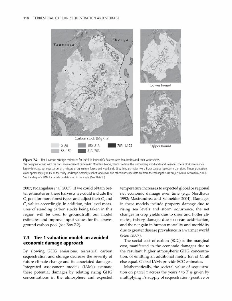
118 TERRESTRIAL CARBON SEQUESTRATION AND STORAGE
2007; Ndangalasi et al. 2007 ). If we could obtain bet-ter estimates on these harvests we could include the C p pool for more forest types and adjust their C a and C b values accordingly. In addition, plot level meas-ures of standing carbon stocks being taken in this region will be used to groundtruth our model estimates and improve input values for the above-ground carbon pool (see Box 7.2 ).
7.3 Tier 1 valuation model: an avoided economic damage approach
By slowing GHG emissions, terrestrial carbon sequestration and storage decrease the severity of future climate change and its associated damages. Integrated assessment models (IAMs) estimate these potential damages by relating rising GHG concentrations in the atmosphere and expected
temperature increases to expected global or regional net economic damage over time (e.g., Nordhaus 1992 ; Mastrandrea and Schneider 2004 ). Damages in these models include property damage due to rising sea levels and storm occurrence, the net changes in crop yields due to drier and hotter cli-mates, fi shery damage due to ocean acidifi cation, and the net gain in human mortality and morbidity due to greater disease prevalence in a warmer world ( Stern 2007 ).
The social cost of carbon (SCC) is the marginal cost, manifested in the economic damages due to the resultant higher atmospheric GHG concentra-tion, of emitting an additional metric ton of C, all else equal. Global IAMs provide SCC estimates.
Mathematically, the societal value of sequestra-tion on parcel x across the years t to T is given by multiplying x ’s supply of sequestration (positive or
T a n z a n i aK e n y a
Dar Es Salaam Lower bound
Upper bound783–1,122150–313313–783
0–88
Carbon stock (Mg/ha)
88–150
Figure 7.2 Tier 1 carbon storage estimates for 1995 in Tanzania’s Eastern Arcs Mountains and their watersheds. The polygons formed with the dark lines represent Eastern Arc Mountain blocks, which rise from the surrounding woodlands and savannas. These blocks were once largely forested, but now consist of a mixture of agriculture, forest, and woodlands. Gray lines are major rivers. Black squares represent major cities. Timber plantations cover approximately 0.3% of the study landscape. Spatially explicit land cover and other landscape data are from the Valuing the Arc project (2008; Mwakalila 2009). See the chapter’s SOM for details on data used in the maps. (See Plate 3.)

T IER 1 VALUATION MODEL: AN AVOIDED ECONOMIC DAMAGE APPROACH 119
Andrew R. Marshall and P. K. T. Munishi
Carbon offsetting programs and associated policy tools (REDD, MAC, CERs, etc.) require accurate quantifi cation of terrestrial carbon stocks. While there are continuing efforts to determine vegetation structure remotely, permanent sample plots (PSPs) of woody vegetation continue to give the most reliable estimates ( Brown 2002 ; Gibbs et al . 2007 ). These estimates can both calibrate remotely sensed measures and provide inputs to models like those described in this book. The many environmental and human impacts on carbon storage levels in forests must be considered when interpreting PSP data. Outputs of PSPs can also be combined with data on other ecosystem services produced by the forest to determine the overall economic value of a forest ecosystem.
The Valuing the Arc project, funded by the Leverhulme Trust, is doing just that in the Eastern Arc Mountains of Tanzania, one of the world’s most important areas for species richness and endemism ( http://www.valuingthearc.org ). The combined importance of carbon and biodiversity production in a forest is likely to be far more appealing to policy-makers than biodiversity alone.
Plot location and size There are many considerations for planning the location of PSPs and the methods to use for estimating its carbon content. First, PSP locations need to be representative of the area. This will require prior knowledge of the variation in environmental and human infl uences. In montane habitats such as those found in the Eastern Arc Mountains, elevation is the primary predictor of vegetation composition and tree allometry, particularly the height to diameter ratio (Marshall et al. in prep.). For this reason a stratifi ed random design for locating plots is advisable. The size and number of plots should provide a balance between time and resources to sample the maximum range of environmental conditions. One-hectare plots have been adopted by many international projects, but may be impractical for short-term projects or for sampling broad environmental gradients.
The majority of aboveground carbon in forest habitats is contained within the large trees and lianas (as much as 95% in some tropical forests; Chave et al . 2003 ). A huge amount of measurement and taxonomic identifi cation time can be saved in limiting surveys to these stems.
Tree volume The most important measurement for estimating tree volume is the diameter at breast height (dbh, typically 1.3 m) (e.g., Kuebler 2003 ). Where environmental conditions are thought to cause the dbh-to-height ratio to deviate from observed norms, it is also important to measure tree height. This can be time-consuming and it is advisable to simply measure a representative sample (e.g., 10 from each size class; 10–20, 20–30, 30–40, 40–50, and > 50 cm dbh). The dbh-to-height relationship in the sample can then be determined from regression analysis and extrapolated to the remaining stems in each PSP.
The above measures are used to estimate the volume of a tree bole, but other components of the tree are more complicated. Calculating the volume of branches and roots requires destruction of the trees, so that they can then be placed in water to observe the volume displaced. Estimating the volume of foliage and dead wood requires litterfall traps, but litterfall is highly variable among species, elevations, and seasons. Because of these complications, most studies either focus on the bole carbon alone or apply a simple expansion factor to adjust the fi nal carbon estimate (see below).
Calculating tree biomass and carbon content The next step is to calculate the biomass of a tree, given its estimated volume. Many equations have been employed for this purpose, and these vary according to habitat and location, due to variations in environmental conditions and tree allometry ( Chave et al. 2005 ). All approaches, however, involve multiplying tree volume by its wood density (g cm –3 ). The standard measure of wood density is wood specifi c gravity (WSG), which is the oven-dry mass divided by green volume. WSG is typically determined by taking a core from a live tree, or a section of a freshly dead tree. WSG for many species is unknown. Studies therefore often use estimates from the most closely related species, genus, or family.
Around 50% of the biomass in woody vegetation is composed of carbon; therefore, the fi nal amount of elemental carbon is calculated by simply multiplying biomass by 0.5. If this calculation is limited to the tree bole, IPCC recommends expansion factors of 0.24, 0.25, and 0.05 for the carbon in branches, roots, and foliage, respectively (IPCC 2003). These have mostly been derived
Box 7.2 Valuing the Arc: measuring and monitoring forest carbon for offsetting
continues
120 TERRESTRIAL CARBON SEQUESTRATION AND STORAGE
negative) over that time period by the SCC, dis-counting all annual values to year t values, and then summing across all discounted values:
1
, , 1 1 ,(1 )
Tx z z z
xtT z tz t
C SCCVAD
r
−+ +
−=
∆=
+∑ (7.11)
where VAD xtT (value of avoided damage) is the present value of all economic damage avoided (or additional damage caused if negative) due to car-bon sequestration on x (emitted from x ) from time t to T . In Eq. (7.11) ∆ C x , z , z +1 measures the metric tons of C sequestered (emitted) on x between year z and z + 1 (if we only have estimated ∆ C xtT or sequestration for several time steps in between t and T , we can approximate annual sequestration with linear interpolation), SCC z+ 1 is the SCC in year z + 1, and r is the real (infl ation-adjusted) discount rate. The landscape-level analog of VAD xtT is given by
1
.X
tT xtTx
VAD V=
= ∑ (7.12)
In Eqs. (7.11) and (7.12) we assume every unit of sequestration after time z , even if it is just tempo-rary, is valuable to society because it reduces the stock of carbon in the atmosphere, thereby (margin-ally) mitigating or delaying climate change and related damages associated with the continuation of C xz levels into the future (i.e., C xz is the storage baseline in year z ). However, if we only want to value the supply of additional sequestration or avoided emissions then ∆ C x , z , z +1 in Eq. (7.11) could be replaced by an annualized Off
xC∆ (see Eq. (7.6)) or Avoid
xC∆ (see Eq. (7.9)). Finally, by indexing the SCC with z in Eq. (7.11), we allow it to change over time. There is some expectation that the SCC will grow over time as the marginal impact of avoided emis-sions becomes even more valuable in a world deal-
from studies carried out in association with commercial logging, as felled trees can be physically measured.
There are many sources of error from the various stages of calculation. In terms of allometry some studies have incorporated measurements from the bole to buttress edge (e.g., Glenday 2006 ). Lianas and stranglers also pose problems due to their unpredictable shape. Estimates of wood density are also highly dependent on the availability of data, and the reliability of using estimates from closely related species is debated. Furthermore the impact of human disturbance on forest ecosystems is particularly hard to quantify. Despite the many sources of error, published estimates for intact tropical forests are usually relatively consistent between studies (typically 100–250 t ha –1 ) and precision within 10% of the mean is usually possible ( Brown 2002 ). Remote methods including optical, radar, or laser sensors are becoming more widely used, but do not have the accuracy and consistency of inventories using vegetation plots (e.g., Gibbs et al. 2007 ).
Implementation of offset programs Accurate calculation of carbon emissions is paramount to determining national terrestrial carbon budgets, including
sinks by woody biomass, sinks by soil, and releases by human activity. Accurate calculation is also important for the development of a market that pays landowners for reduced emissions from deforestation and degradation (REDD). Interest in REDD markets is driven by the fact that 20% of global CO 2 emissions come from forest destruction and degradation, and that much of this is occurring in developing countries that have limited funds and capacity to address it. A key question is whether the developing world is already, or can be assisted to become, ready for REDD. In some countries this answer is likely to be no due to inadequate policy and environmental law enforcement. More positively, Tanzania may be among the developing countries with highest potential for carbon trading and entering the REDD market in coming years. Tanzania is politically stable, with an advanced forest policy and legislation, has huge forest resources, and has for many years been attractive for international development funding. It also has one of the world’s most extensive protected area networks, with nearly 40% of land area covered by National Parks and various other forms of reserved land ( Chape et al. 2008 ). These combined factors have led the Norwegian government to approve a US$100 million grant for the implementation of REDD in Tanzania. There is also considerable interest from other nations, the United Nations, and the World Bank.
Box 7.2 continued
T IER 2 SUPPLY MODEL 121
ing with a rapidly changing climate (e.g., the IPCC assumes that the SCC will grow at a rate of 2.4% per annum; see Chapter 20 of IPCC 2007b).
It is not clear whether the real (infl ation-adjusted) discount rate in the denominator of Eq. (7.11), r , should match the discount rate embedded in our chosen SCC (see below). The denominator of Eq. (7.11) discounts all future costs and benefi ts from ∆ C x , z , z +1 over z Î [ t , T ] to t ’s value of money, allowing for the aggregation of costs and benefi ts incurred over time. The real discount rate used in Eq. (7.11) measures our preference for more immediate con-sumption over investment and our expectations regarding economic growth. For short time spans, and when comparing VAD tT to other benefi ts and costs real-ized in the near term, we may want to use a real dis-count rate closer to an observed market discount rate.
There remains much uncertainty and debate over the appropriate value of the SCC (e.g., Nordhaus 2007 ; Stern 2007 ; Weitzman 2007 ). Any SCC esti-mate is a function of the assumptions in its source IAM, including the trajectory of global GHG emis-sions over time and the impact that climate change will have on the social welfare of people around the world today and in the future. As a result, estimates of SCC vary widely. By using an average or median SCC estimate, however, we can avoid assuming some of the more idiosyncratic predictions of global emission, economic, and demographic trends. Tol ( 2009 ) surveyed the peer-reviewed SCC literature and found representative current estimates that range from $46 to $91 Mg –1 of C but with a large variance (values are given in 1995 dollars).
Another cause of divergence in SCC estimates is disagreement over the appropriate discount rate to use when determining the SCC in an IAM. The dis-count rate, which combines expectations about future economic growth and our preferences for present consumption over future consumption, equates future climate change-related damages to more immediate damages. A lower discount rate will lead to higher estimates of the SCC, as future events, including the risk of catastrophic change, are more heavily weighted with lower interest rates (Chapter 20 of IPCC 2007b). Some economists argue that the discount rates used in climate change anal-ysis should be lower than what is typically used for cost–benefi t analyses (e.g., a discount rate of 1.4%
per annum in Stern ( 2007 ) and 2–4% in Weitzman ( 2007 ) versus a “typical” cost–benefi t analysis rate of 7%) whether due to intergenerational equity con-cerns ( Stern 2007 ) or concerns over the highly unlikely but particularly disastrous scenarios of catastrophic change ( Weitzman 2007 ). Other econo-mists argue that in order to avoid a potentially mas-sive misallocation of monetary resources, climate change mitigation activities should be judged with the discount rate we use to judge all other policies (i.e., 5 to 10% per annum; e.g., Nordhaus 2007 ).
Further, the SCC is a marginal cost—that is, it meas-ures the economic damage avoided for very small changes in carbon emissions relative to total global stock. While signifi cant amounts of carbon are at stake at landscape scales, most applications of this model will only involve small changes in carbon stocks rela-tive to any emission baseline. For our purposes, then, SCC is a legitimate and useful estimate of social cost.
Finally, the SCC will invariably differ from the market price for carbon offsets as the market-clear-ing price of an offset (the price that sellers and buy-ers agree on) has no functional relationship to the social value of carbon sequestration. In regulated markets, buyers and sellers will settle on a price that is a function of the offset provider’s cost of par-ticipating in the offset program and the buyer’s willingness to pay for an offset (a function of GHG abatement costs in the industrial, electrical, and transportation sectors and emission caps). In volun-tary markets, several other factors may impact price, as the motivation of offset buyers is not solely to achieve least-cost emission reduction (see Conte and Kotchen ( 2009 ) for further discussion of deter-minants of voluntary offset prices).
7.4 Tier 2 supply model
In the tier 1 supply model, sequestration between time t and T only registers in parcel x if x ’s LULC mix changes between t and T , x ’s wood harvest rates or harvest management changes between t and T , or x ’s HWP carbon pool is not in a steady state at time t . However, terrestrial carbon storage levels, especially on recently disturbed land, tend to change continuously due to vegetation growth and decay and organic matter accumulation in the soil. In the tier 2 terrestrial carbon supply model we
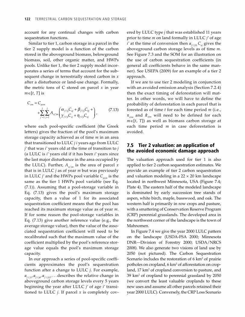
122 TERRESTRIAL CARBON SEQUESTRATION AND STORAGE
account for any continual changes with carbon sequestration functions.
Similar to tier 1, carbon storage in a parcel in the tier 2 supply model is a function of the carbon stored in the aboveground biomass, belowground biomass, soil, other organic matter, and HWPs pools. Unlike tier 1, the tier 2 supply model incor-porates a series of terms that account for the sub-sequent change in terrestrially stored carbon in x after a disturbance or land-use change. Formally, the metric tons of C stored on parcel x in year m Î [ t , T ] is
' 1 1
,
xm pxm
J Jj i ji aj j i ji bj
xj jmj i ji sj j i ji ojj j
C CC C
AC C
′ ′ ′ ′′
′ ′ ′ ′= =
=+ +⎛ ⎞
+ ⎜ ⎟+⎝ ⎠∑∑a bg h
(7.13)
where each pool-specifi c coeffi cient (the Greek letters) gives the fraction of the pool’s maximum storage capacity achieved as of time m in an area that transitioned to LULC j i years ago from LULC j ' that was i ' years old at the time of transition to j (a LULC is i' years old if it has been i' years since the last major disturbance in the area occupied by the LULC). Further, A xj´jm is the area of parcel x that is in LULC j as of year m but was previously in LULC j' and the HWPs pool variable C pxm is the same as the tier 1 HWPs pool variable (see Eq. (7.1)). Assuming that a pool-storage variable in Eq. (7.13) gives the pool’s maximum storage capacity, then a value of 1 for its associated sequestration coeffi cient means that the pool has reached its maximum storage value as of year m . If for some reason the pool-storage variables in Eq. (7.13) give another reference value (e.g., the average storage value), then the value of the asso-ciated sequestration coeffi cient will need to be recalibrated such that the maximum value of the coeffi cient multiplied by the pool’s reference stor-age value equals the pool’s maximum storage capacity.
In our approach a series of pool-specifi c coeffi -cients approximates the pool’s sequestration function after a change to LULC j . For example, α j i j 1 , α j i j 6 , α j i j 11 , . . . describes the relative change in aboveground carbon storage levels every 5 years beginning the year after LULC j' of age i' transi-tioned to LULC j . If parcel x is completely cov-
ered by LULC type j that was established 11 years prior to time m on land formally in LULC j' of age i' at the time of conversion then α j i j 11 C a j gives the aboveground carbon storage levels as of time m . See Figure 7.3 and the SOM for an illustration on the use of carbon sequestration coeffi cients (in general all coeffi cients behave in the same man-ner). See USEPA (2009) for an example of a tier 2 approach.
If we are to use tier 2 modeling in conjunction with an avoided emission analysis ( Section 7.2.4 ) then the exact timing of deforestation will mat-ter. In other words, we will have to define the probability of deforestation in each parcel that is forested as of time t for each time period m (i.e., π xtm and xtmp will need to be defined for each m Î [ t , T ]) as well as biomass carbon storage at each time period m in case deforestation is avoided.
7.5 Tier 2 valuation: an application of the avoided economic damage approach
The valuation approach used for tier 1 is also applied to tier 2 carbon sequestration estimates. We provide an example of tier 2 carbon sequestration and valuation modeling in a 22 × 20 km landscape located in northwest Minnesota, USA ( Figure 7.4 ; Plate 4). The eastern half of the modeled landscape is dominated by early succession tree stands of aspen, white birch, maple, basswood, and oak. The western half is primarily in row crops and pasture, with a smattering of Conservation Reserve Program (CRP) perennial grasslands. The developed area in the northwest corner of the landscape is the town of Mahnomen.
In Figure 7.4 we give the year 2000 LULC pattern on the landscape (USDA-FSA 2000; Minnesota DNR—Division of Forestry 2000; USDA/NRCS 2008). We also generate two visions of land use by 2050 (not pictured). The Carbon Sequestration Scenario includes the restoration of 6 km 2 of prairie potholes on cropland, 6 km 2 of afforestation on crop-land, 17 km 2 of cropland conversion to pasture, and 39 km 2 of cropland to perennial grassland by 2050 (we convert the least valuable croplands to these new uses and assume all other parcels retained their year 2000 LULC). Conversely, the CRP Loss Scenario
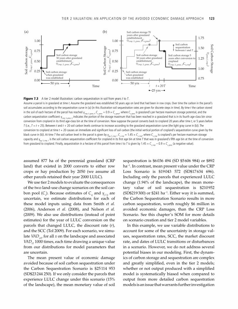
T IER 2 VALUATION: AN APPL ICATION OF THE AVOIDED ECONOMIC DAMAGE APPROACH 123
assumed 877 ha of the perennial grassland (CRP land) that existed in 2000 converts to either row crops or hay production by 2050 (we assume all other parcels retained their year 2000 LULC).
We use tier 2 models to evaluate the consequences of the two land-use change scenarios on the soil car-bon pool ( C s ). Because estimates of C sj and γ j i j i are uncertain, we estimate distributions for each of these model inputs using data from Smith et al. ( 2006 ), Anderson et al. ( 2008 ), and Nelson et al. ( 2009 ). We also use distributions (instead of point estimates) for the year of LULC conversion on the parcels that changed LULC, the discount rate ( r ), and the SCC ( Tol 2009 ). For each scenario, we simu-late VAD xtT for all x on the landscape and associated VAD tT 1000 times, each time drawing a unique value from our distributions for model parameters that are uncertain.
The mean present value of economic damage avoided because of soil carbon sequestration under the Carbon Sequestration Scenario is $25 114 953 (SD$23 244 250). If we only consider the parcels that experience LULC change under this scenario (15% of the landscape), the mean monetary value of soil
sequestration is $6 036 494 (SD $5 606 984) or $892 ha −1 . In contrast, mean present value under the CRP Loss Scenario is $19 043 572 (SD$17 634 696). Including only the parcels that experienced LULC change (1.94% of the landscape), the mean mone-tary value of soil sequestration is $210 952 (SD$219 300) or $241 ha −1 . Either way it is summed, the Carbon Sequestration Scenario results in more carbon sequestration, worth roughly $6 million in avoided economic damages, than the CRP Loss Scenario. See this chapter’s SOM for more details on scenario creation and tier 2 model variables.
In this example, we use variable distributions to account for some of the uncertainty in storage val-ues, sequestration rates, SCC, the market discount rate, and dates of LULC transitions or disturbances in a scenario. However, we do not address several potential biases in our modeling. First, the dynam-ics of carbon storage and sequestration are complex and greatly simplifi ed, even in the tier 2 models; whether or not output produced with a simplifi ed model is systematically biased when compared to output from more detailed carbon sequestration models is an issue that warrants further investigation
(a)
Soil carbon storage50 years after grasslandestablishment
Soil carbon storagewhen grasslandwas established
Soil
carb
on s
tora
ge
50 yrsTime
0.00
0.25
0.50
0.75
1.00
t
(gcrop, 3, grass, 4Cs,grass)
(gcr
op,i’
, gra
ss,i
Cs,
gras
s)(b)
1.75
1.50
1.25
Soil Carbon Storage1.00
0.75
Soil carbon storage50 years after grasslandestablishment
Soil carbon storage 70years after grasslandestablishment
Soil carbon storagewhen grasslandwas established
Soil
Car
bon
Stor
age
50 yrsTime
0.00
0.25
0.50
0.75
1.00
t t + 20T25 yrs
(gcrop, 3, grass, 4Cs,grass)
Soil carbon storage 5years after conversion tocropland
Soil carbonsequestrationbetween t and T
(gcrop, 5, grass, 1Cs,crop)
(ggrass,i’,crop,i )
(gcr
op,i’
, gra
ss,i
Cs,
gras
s)
(gcrop, 3, grass, 5Cs,grass)
Figure 7.3 A tier 2 model illustration: carbon sequestration in soil from years t to T . Assume a parcel is in grassland at time t . Assume the grassland was established 50 years ago on land that had been in row crops. Over time the carbon in the parcel’s soil accumulates according to the sequestration curve in (a) (in this illustration soil sequestration rates are given for discrete steps in time). By time t the carbon stored in the soil of each hectare of the parcel has reached γ crop, 3, grass, 4 C s, grass = 0.9 × C s, grass , where C s, grass is grassland’s per hectare maximum storage potential, and the carbon sequestration coeffi cient γ crop, 3, grass, 4 indicates the portion of the storage maximum that has been reached in a grassland that is in its fourth age-class bin since conversion from cropland in its third age-class bin at the time of conversion. Now suppose the parcel converts back to cropland 20 years after time t , or 5 years before T (i.e., T = t + 25). Between t and t + 20 soil carbon levels continue to increase according to the grassland sequestration curve (the light gray curve in (b)). The conversion to cropland at time t + 20 causes an immediate and signifi cant loss of soil carbon (the initial vertical portion of cropland’s sequestration curve given by the black curve in (b)). At time T the soil carbon level in the parcel is given by γ pg, 5, crop, 1 C s, crop = 1.45 × C s, crop , where C s, crop is cropland’s per hectare maximum storage capacity and γ pg, 5, crop, 1 is the soil carbon sequestration coeffi cient for cropland in its fi rst age bin at time T that was in grassland’s fi fth age bin at the time of conversion from grassland to cropland. Finally, sequestration in a hectare of this parcel from time t to T is given by 1.45 × C s, crop – 0.9 × C s, grass (a negative value).
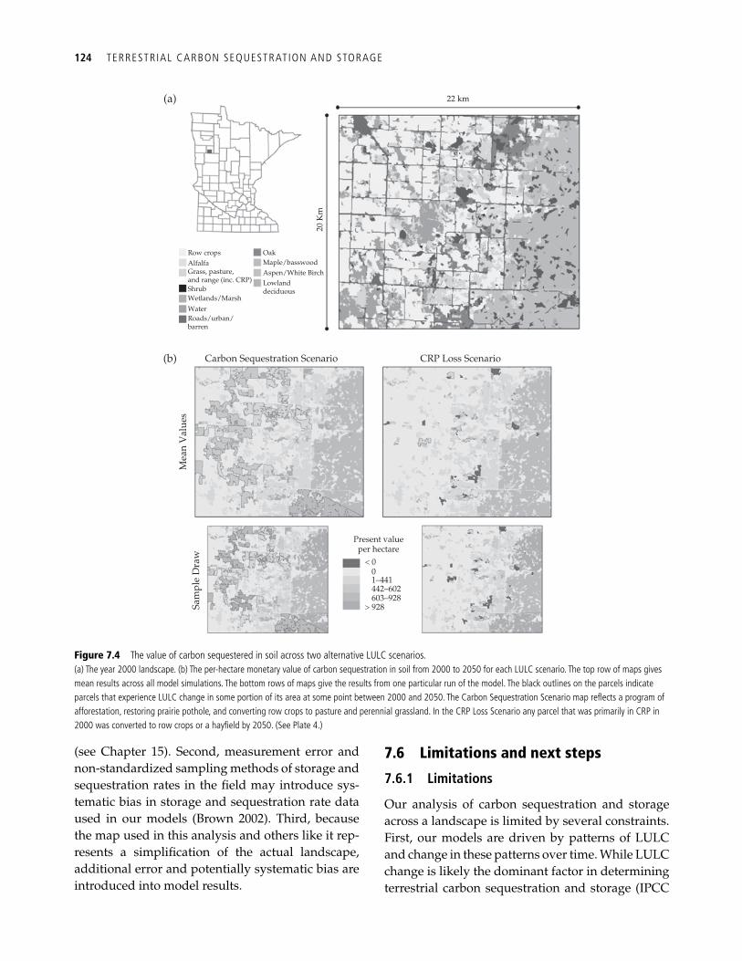
124 TERRESTRIAL CARBON SEQUESTRATION AND STORAGE
(see Chapter 15 ). Second, measurement error and non-standardized sampling methods of storage and sequestration rates in the fi eld may introduce sys-tematic bias in storage and sequestration rate data used in our models ( Brown 2002 ). Third, because the map used in this analysis and others like it rep-resents a simplifi cation of the actual landscape, additional error and potentially systematic bias are introduced into model results.
7.6 Limitations and next steps
7.6.1 Limitations
Our analysis of carbon sequestration and storage across a landscape is limited by several constraints. First, our models are driven by patterns of LULC and change in these patterns over time. While LULC change is likely the dominant factor in determining terrestrial carbon sequestration and storage (IPCC
(a)
(b)
Row crops
20 K
m
OakMaple/basswoodAspen/White BirchLowlanddeciduous
AlfalfaGrass, pasture,and range (inc. CRP)ShrubWetlands/MarshWaterRoads/urban/barren
Carbon Sequestration Scenario CRP Loss Scenario
22 km
Present valueper hectare< 0
> 928
01–441442–602603–928
Mea
n V
alue
sSa
mpl
e D
raw
Figure 7.4 The value of carbon sequestered in soil across two alternative LULC scenarios. (a) The year 2000 landscape. (b) The per-hectare monetary value of carbon sequestration in soil from 2000 to 2050 for each LULC scenario. The top row of maps gives mean results across all model simulations. The bottom rows of maps give the results from one particular run of the model. The black outlines on the parcels indicate parcels that experience LULC change in some portion of its area at some point between 2000 and 2050. The Carbon Sequestration Scenario map refl ects a program of afforestation, restoring prairie pothole, and converting row crops to pasture and perennial grassland. In the CRP Loss Scenario any parcel that was primarily in CRP in 2000 was converted to row crops or a hayfi eld by 2050. (See Plate 4.)
L IMITATIONS AND NEXT STEPS 125
2006), the nature and rate of disturbance events are also important (e.g., see IPCC 2006; Bond-Lamberty et al. 2007 ; Kurz et al. 2008 ). Prairie and forest fi res, forest disease outbreak, and exotic species invasion can have signifi cant impacts on storage and seques-tration, but may not be refl ected in typical LULC maps. Our models do not explicitly consider such events, but using more nuanced LULC classifi ca-tions may begin to capture them (e.g., diseased conifer forest, disease-free conifer forest).
Second, our models largely ignore local varia-tions in climate, which also have a signifi cant impact on carbon storage and sequestration rates (e.g., McGuire et al. 2001 ). Rainfall and temperature patterns determine such ecosystem processes as net primary productivity (NPP) and soil erosion, the primary inputs in terrestrial carbon storage capacity and sequestration rates. The best strategy for minimizing this limitation is to use “local” car-bon sequestration and storage data when possible and to limit the extent of the modeled landscape in order to minimize over-extrapolation of carbon estimates. Another way to deal with this limitation is to stratify LULC categories by landscape features that may refl ect microclimate. This requires, how-ever, observations of model parameters for each of the climate-related strata created within each broad LULC type. Further, as a climate changes, vegeta-tion patterns may shift on the landscape. To account for this we can modify LULC types on future scenario maps according to climate–vegetation models. See Chapter 17 for such an exercise.
Finally, land-use management practices that do not have a large impact on carbon storage in plant biomass and soils can still be signifi cant sources of other GHG emissions. For example, crop residue burning (e.g., IPCC 2006), livestock use (e.g., IPCC 2006), and various soil management practices on farms (e.g., Bouwman et al. 2002 ) can signifi cantly increase the rate of methane and nitrous oxide emis-sions, two powerful GHGs (see Chapter 9 ). In addi-tion, all of the GHGs emitted by fossil fuel-burning machinery used to support farms and other LULC are not reported except for the production and delivery of HWPs (see Eq. (7.1)).
In part to understand the consequences of our simple model and its corresponding constraints, we have begun to validate its results against more
sophisticated models. For scenarios of LULC change in California that consider climate change ( Shaw et al . 2009 ), we are comparing our results to those derived from a more detailed, process-based model of carbon storage used in Shaw et al . ( 2009 ). We will compare our simple results in Tanzania (see Section 7.2.5 ) to more detailed models developed by the Valuing the Arc Programme ( Mwakalila et al . 2009 ). These comparisons will allow us to estimate the accuracy of our simple approach and the limitations and biases it presents.
7.6.2 Next steps
The models presented in this chapter can be used for many purposes. We can layer maps of sequestra-tion and storage and their value with other ecosys-tem service maps to identify areas of ecosystem service synergies and trade-offs on the landscape (see Chapter 14 ). We can also compare sequestra-tion supplies and values to those of other ecosystem service across a landscape to determine the oppor-tunity costs of increasing carbon sequestration in both biophysical and economic terms (e.g., Jackson et al. 2005 ; Nelson et al. 2008 ).
Further, we can estimate the additional carbon sequestration on a landscape by comparing a baseline scenario of LULC with an alternative projection that refl ects efforts to sequester carbon or reduce emis-sions (see the SOM for further details). By overlaying these maps with an opportunity cost map we can begin to predict market prices for offsets and avoided emissions credits ( Kindermann et al. 2008 ), and to construct additional sequestration supply curves for different policies (e.g., Lubowski et al. 2006 ). Please see the SOM for descriptions of our efforts to validate the biophysical and deforestation risk models.
Finally, these models can serve as the foundation for a tier 3 approach to carbon storage and seques-tration modeling. A tier 3 sequestration and storage model would not only consider how land use and conversion decisions effects storage, but it would also simulate the affect of climate and landscape-level disturbance stochasticity on biomass growth and carbon formation in and release from soils. Models such as CENTURY ( Parton et al. 1992 ) and the vegetation model LPJ ( Sitch et al. 2003 ) are exam-ples of tier 3 models.
126 TERRESTRIAL CARBON SEQUESTRATION AND STORAGE
References
Alig, R. J., and Butler, B. J. (2004). Projecting large-scale area changes in land use and land cover for terrestrial carbon analyses. Environmental Management, 33 , 443–56.
Anderson, J., Beduhn, R., Current, D., et al . (2008). The potential for terrestrial carbon sequestration in Minnesota: a report to the Department of Natural Resources from the Minnesota Terrestrial Carbon Sequestration Initiative . University of Minnesota, St. Paul.
Aukland, L., Sohngen, B., Hall, M., et al . (2002). 2001 Analysis of leakage, baselines, and carbon benefi ts for the Noel Kempff Climate Action Project . Winrock International, Arlington, VA.
Bond-Lamberty, B., Peckham, S. D., Ahl, D. E., et al . (2007). Fire as the dominant driver of central Canadian boreal forest carbon balance. Nature, 450 , 89–92.
Bouwman, A. F., Boumans, L. J. M. and Batjes, N. H. (2002). Modeling global annual N 2 O and NO emissions from fertilized fi elds, Global Biogeochemical Cycles, 16 , 1080.
Brown, S. (2002). Measuring, monitoring, and verifi cation of carbon benefi ts for forest-based projects. Philosophical Transactions of the Royal Society of London, Series A-Mathematical Physical and Engineering Sciences, 360, 1669–83.
Brown, S., Swingland, I. R., Hanbury-Tenison, R., et al . (2002). Changes in the use and management of forests for abating carbon emissions: issues and challenges under the Kyoto Protocol. Philosophical Transactions of the Royal Society of London Series A-Mathematical Physical and Engineering Sciences, 360 , 1593–605.
Burgess, N. D., Butynski, T. M., Cordeiro, N. J., et al . (2007). The biological importance of the Eastern Arc Mountains of Tanzania and Kenya. Biological Conservation, 134 , 209–31.
Burtraw, D., Kahn, D., and Palmer, K. (2006). CO2 allow-ance allocation in the regional greenhouse gas initiative and the effect on electricity investors. Electricity Journal, 19 , 79–90.
Cairns, M. A., Haggerty, P. K., Alvarez, R., et al . (2000). Tropical Mexico’s recent land-use change: A region’s contribution to the global carbon cycle. Ecological Applications, 10 , 1426–41.
Canadell, J. G., and Raupach, M. R. (2008). Managing for-ests for climate change mitigation. Science, 320 (5882), 1456–7.
Chape, S., Spalding, M., and Jenkins, M., Eds. (2008). The worlds protected areas: status, values and prospects in the 21st century . University of California Press, Berkeley.
Chave, J., Andalo, C., Brown, S., et al . (2005). Tree allome-try and improved estimation of carbon stocks and bal-ance in tropical forests. Oecologia, 145 , no. 1, 87–99.
Chave, J., Condit, R., Lao, S., et al . (2003). Spatial and tem-poral variation of biomass in a tropical forest: results from a large census plot in Panama. Journal of Ecology, 91 , 240–52.
Chomitz, K. M. (2002). Baseline, leakage and measure-ment issues: how do forestry and energy projects com-pare? Climate Policy, 2 , 35–49.
Conte, M. N., and Kotchen, M. J. (2009). Explaining the price of voluntary carbon offsets. NBER Working Paper 15294.
Ebeling, J., and Yasue, M. (2008). Generating carbon fi nance through avoided deforestation and its potential to create climatic, conservation and human develop-ment benefi ts. Philosophical Transactions of the Royal Society B: Biological Sciences, 363 , 1917–24.
Edinburgh Centre for Carbon Management (ECCM). (2007). Establishing Mechanisms for Payments for Carbon Environmental Services in the Eastern Arc Mountains, Tanzania .
FAO. 2005. State of the World’s Forests 2005 . FAO, Rome. Also available at http://www.fao.org/docrep/011/i0350e/i0350e00.HTM .
Fargione, J., Hill, J., Tilman, D., et al . (2008). Land clearing and the biofuel carbon debt. Science , 319 , 1235–8.
Gibbs, H. K., Brown, S., Niles, J. O., et al . (2007). Monitoring and estimating tropical forest carbon stocks: making REDD a reality. Environmental Research Letters, 2, 045023.
Glenday, J. (2006). Carbon storage and emissions offset potential in an East African tropical rainforest. Forest Ecology and Management , 235 , 72–83.
Harmon, M. E., Ferrell, W. K., and Franklin, J. F. (1990). Effects on carbon storage of conversion of old-growth forests to young forests. Science, 247 , 699–702.
Intergovernmental Panel on Climate Change (IPCC). (2000). IPCC special report on land use land-use change, and forestry . Cambridge University Press, Cambridge, UK.
Intergovernmental Panel on Climate Change (IPCC). (2003). Good practice guidance for land use, land-use change and forestry . Institute for Global Environmental Strategies (IGES), Hayama, Kanagawa, Japan.
Intergovernmental Panel on Climate Change (IPCC). (2006). 2006 IPCC guidelines for national greenhouse gas inventories. Institute for Global Environmental Strategies, Hayama, Kanagawa, Japan.
Intergovernmental Panel on Climate Change (IPCC). (2007a). Climate change 2007: mitigation of climate change: Contribution of Working Group III to the Fourth Assessment Report of the Intergovernmental Panel on Climate Change, Cambridge University Press, New York.
Intergovernmental Panel on Climate Change (IPCC). (2007b). Climate change 2007: impacts, adaptation and vul-nerability: contribution of Working Group II to the Fourth
L IMITATIONS AND NEXT STEPS 127
Assessment Report of the Intergovernmental Panel on Climate Change, Cambridge University Press, New York.
Jackson, R. B., Jobbagy, E. G., Avissar, R., et al . (2005). Trading water for carbon with biological sequestration. Science, 310 , 1944–7.
Kindermann, G., Obersteiner, M., Sohngen, B., et al . (2008). Global cost estimates of reducing carbon emissions through avoided deforestation. Proceedings of the National Academy of Sciences, 105 , 10302–7.
Kuebler, C. (2003). Standardized vegetation monitoring proto-col . Centre for Applied Biodiversity Science, Conser-vation International, Washington, DC.
Kurz, W. A., Dymond, C. C., Stinson, G., et al . (2008). Mountain pine beetle and forest carbon feedback to cli-mate change. Nature, 452 , 987–90 .
Lal, R. (2004). Soil carbon sequestration impacts on global climate change and food security. Science, 304 , 1623–7.
Lehmann, J. (2007). A handful of carbon. Nature, 447 , 143–4.
Lubowski, R. N., Plantinga, A. J., and Stavins, R. N. (2006). Land-use change and carbon sinks: econometric estima-tion of the carbon sequestration supply function. Journal of Environmental Economics and Management, 51 , 135–52.
Luoga, E. J., Witkowski, E. T., F., and Balkwill, K. (2000). Economics of charcoal production in miombo wood-lands of eastern Tanzania: some hidden costs associated with commercialization of the resources. Ecological Economics 35 , 243–57.
McGuire, A. D., Sitch, S., Clein, J. S., et al . (2001). Carbon balance of the terrestrial biosphere in the twentieth cen-tury: Analyses of CO2, climate and land use effects with four process-based ecosystem models. Global Biogeo-chemical Cycles, 15 , 183–206.
Makundi, W. R. (2001). Carbon mitigation potential and costs in the forest sector in Tanzania. Mitigation and Adaptation Strategies for Global Change, 6 , 335–53.
Maréchal, K., and Hecq, W. (2006). Temporary credits: A solution to the potential non-permanence of carbon sequestration in forests? Ecological Economics, 58 , 699–716.
Marshall, A. R., Lewis, S., Lovett, J. C., Burgess, N., et al . (In preparation). Variation in carbon storage and tree allometry with elevation in the eastern arc.
Mastrandrea, M. D., and Schneider, S. H. (2004). Probabilistic integrated assessment of dangerous climate change. Science, 304 , 571–5.
Minnesota Department of Natural Resources (DNR)—Division of Forestry (2000). GAP Land Cover Map of Minnesota . Minnesota Department of Natural Resources, St. Paul, MN.
Mollicone, D., Achard, F., Federici, S., et al . (2007). An incentive mechanism for reducing emissions from con-
version of intact and non-intact forests. Climatic Change, 83 , 477–93.
Murray, B. C., Sohngen, B., and Ross, M. (2007). Economic consequences of consideration of permanence, leakage and additionality for soil carbon sequestration projects. Climatic Change, 80 (1), 127–43.
Mwakalila, S., Burgess, N. D., Ricketts, T., et al . (2009). Valuing the Arc: linking science with stakeholders to sustain natural capital. Arc Journal, 23, 25–30.
Nelson, E., Mendoza, G., Regetz, J., et al . (2009). Modeling multiple ecosystem services, biodiversity conserva-tion, commodity production, and tradeoffs at land-scape scales. Frontiers in Ecology and the Environment, 7 , 4–11.
Nelson, E., Polasky, S., Lewis, D. J., et al . (2008). Effi ciency of incentives to jointly increase carbon sequestration and species conservation on a landscape. Proceedings of the National Academy of Sciences, 105 , 9471–6.
Ndangalasi, H. J., Bitariho, R. and Dovie, D. B. K. (2007). Harvesting of non-timber forest products and implica-tions for conservation in two montane forests of East Africa. Biological Conservation, 134 , 242–50.
Niles, J. O., and Schwarze, R. (2001). The value of careful carbon accounting in wood products. Climatic Change , 49 , 371–6.
Nilsson, S. and Schopfhauser, W. (1995). The carbon-se-questration potential of a global afforestation program. Climatic Change, 30 , 267–93.
Nordhaus, W. D. (1992). An optimal transition path for controlling greenhouse gases. Science, 258 , 1315–19.
Nordhaus, W. D. (2007). Critical assumptions in the Stern review on climate change. Science, 317 , 201–2.
Olson, D. M., Dinerstein, E., Wikramanayake, E. D., et al . (2001). Terrestrial ecoregions of the worlds: A new map of life on Earth. Bioscience, 51 , 933–8.
Parton, W. J., McKeown, B., Kirchner, V., et al . (1992). CENTURY users manual . NREL, Colorado State University, Fort Collins, Colorado.
Pfaff, A. S. P., Kerr, S., Hughes, R. F., et al . (2000). The Kyoto protocol and payments for tropical forest: An interdisci-plinary method for estimating carbon-offset supply and increasing the feasibility of a carbon market under the CDM. Ecological Economics, 35 , 203–21.
Post, W. M., and Kwon, K. C. (2000). Soil carbon sequestra-tion and land-use change: processes and potential. Global Change Biology, 6 , 317–27.
Raich, J. W., Russell, A. E., Kitayama, K., et al . (2006). Temperature infl uences carbon accumulation in moist tropical forests. Ecology, 87 , 76–87.
Ruesch, A. S., and Gibbs, H. K. (2008). New IPCC tier-1 global biomass carbon map for the year 2000. Available online from the Carbon Dioxide Information Analysis
128 TERRESTRIAL CARBON SEQUESTRATION AND STORAGE
Center ( http://cdiac.ornl.gov ), Oak Ridge National Laboratory, Oak Ridge, Tennessee.
Schuman, G. E., Janzen, H. H., and Herrick, J. E. (2002). Soil carbon dynamics and potential carbon sequestration by rangelands. Environmental Pollution, 116 , 391–6.
Schwarze, R., Niles, J. O., and Olander, J. (2002). Understanding and managing leakage in forest-based green-house gas mitigation projects . Institute for Environmental Economics at the Technische Univer sität Berlin, Berlin.
Shaw, R., Pendleton, L., Cameron, R., et al . (2009). The impact of climate change on California’s ecosystem services . California Climate Change Center. Draft Paper.
Sitch, S., Smith, B., Prentice, I. C., et al . (2003). Evaluation of ecosystem dynamics, plant geography and terrestrial carbon cycling in the LPJ dynamic global vegetation model. Global Change Biology, 9 , 161–85.
Smith, J. E., Heath, L. S., Skog, K. E., and et al . (2006). Methods for calculating forest ecosystem and harvested car-bon with standard estimates for forest types of the United States . General Technical Report NE-343, US Department of Agriculture, Forest Service, Northeastern Research Station, Newtown Square, PA.
Sohngen, B., and Brown, S. (2004). Measuring leakage from carbon projects in open economies: a stop timber harvesting project in Bolivia as a case study. Canadian Journal of Forest Research-Revue Canadienne De Recherche Forestiere, 34 , 829–39.
Sohngen, B., and Brown, S. (2008). Extending timber rota-tions: carbon and cost implications. Climate Policy, 8 , 435–51.
Stern, N. (2007). The economics of climate change: the Stern review . Cambridge University Press, Cambridge, UK.
Tol, Richard S. J. (2009). The economic effects of climate change. Journal of Economic Perspectives, 23, 29–51.
Torn, M. S., Trumbore, S. E., Chadwick, O. A., Vitousek, et al . (1997). Mineral control of soil organic carbon stor-age and turnover. Nature, 389 , 170–3.
United Nations Climate Change Convention Secretariat (UNCCCS). (1997). UNFCCC AIJ Methodological Issues . UNCCCS, Bonn, Germany.
United Nations Framework Convention on Climate Change (UNFCCC). (1995). Decision 5/CP.1 from Report of the Conference of the Parties on its fi rst session, held at Berlin from 28 March to 7 April 1995. Addendum. Part two: Action taken by the Conference of the Parties at its fi rst session . UNFCCC, Berlin, Germany.
United States Department of Agriculture-Natural Resource Conservation Service (USDA/NRCS). (2008). USDA-NASS Cropland Data Layer . 2006 . USDA/NRCS, Washington, DC.
United States Department of Agriculture-Farm Service Agency (USDA-FSA). (2000). Conservation reserve pro-gram map of Minnesota. 1997 . USDA-FSA, Washington, DC.
United States Environmental Protection Agency (USEPA). (2009). Inventory of US greenhouse gas emissions and sinks: 1990–2007 . USEPA, Washington, DC.
Valuing the Arc (2008). Land use and land cover map of the Eastern Arc Mountains and surrounding watersheds . Valuing the Arc, Cambridge, UK.
Victor, D. G., House, J. C., and Joy, S. (2005). A Madisonian approach to climate policy. Science, 309 , 1820–1.
Vohringer, F., Kuosmanen, T., and Dellink, R. (2006). How to attribute market leakage to CDM projects. Climate Policy, 5 , 503–16.
Weitzman, M. L. (2007). A review of the Stern review on the economics of climate change. Journal of Economic Literature, 45 , 703–24.
129
CHAPTER 8
The provisioning value of timber and non-timber forest products Erik Nelson, Claire Montgomery, Marc Conte, and Stephen Polasky
8.1 Introduction
Forests play an iconic role in environmental conser-vation campaigns and are habitat to much of the world’s known terrestrial biodiversity ( Repetto and Gillis 1988 ). Forests also provide and regulate many important ecosystem services (e.g., Williams 2003 ; Ricketts 2004 ; Ticktin 2004 ; Maass et al. 2005 ), includ-ing carbon sequestration (e.g., Scholes 1996 ; Sohngen and Brown 2006 ), potable water supply (e.g., Núñez et al. 2006 ), and a stock of plants and animals that can be used to meet human needs for food, materials, and medicine (e.g., Milner-Gulland and Clayton 2002 ; Belcher et al. 2005 ; Damania et al. 2005 ; Ndangalasi et al. 2007 ). In fact, the legal and illegal harvest of timber and non-timber forest products (NTFPs) supports and supplements the livelihoods of millions of families around the world (e.g., Justice et al. 2001 ; Pattanayak and Sills 2001 ; Vedeld et al. 2004 ; Box 8.1 ). The ability of relatively intact forests to provide habitat and valuable ecosystem services year in and year out is the main argument given for forest conservation (e.g., Peters et al. 1989 ; Boot and Gullison 1995 ; Bawa and Seidler 1998 ; Arnold and Pérez 2001 ; Silvertown 2004 ; Sinha and Brault 2005 ).
In this chapter we present approaches for modeling the quantity and value of timber and NTFP harvest from forested parcels across a landscape (the role that forests play in the regulation and provision of other ecosystem services is covered in other chapters of this book). Timber and NTFP harvest levels and patterns are largely determined by forest ecology and property rights structure. Open-access forests are those in which anyone can harvest forest stocks. At the other extreme, a forest may be regulated with exclusive harvest
rights, where only a limited number of individuals or entities have the legal right to harvest ( Feder and Feeny 1991 ). An individual or entity with an exclu-sive right to harvest forest stocks has an incentive to maximize the net present value of economic returns to harvest over time, whereas open-access harvest tends to be characterized by a race to exploit the resource. Therefore, forests with well-enforced property rights will tend to have lower harvest rates and greater biological stocks at any point in time than open-access forests (e.g., Luoga et al . 2005 ; Birdyshaw and Ellis 2007 ; for a discussion on excep-tions to this general rule see Larson and Bromley 1990 ).
As with other models presented in this book we present two tiers of analysis. Tier 1 involves approaches that are analytically simpler and require less data than the approaches in tier 2. In tier 1 mod-els, we assume that the rate of harvest equals the harvested stock’s natural regeneration rates, leav-ing the biological stock unchanged or in steady state over a harvest period. Steady-state harvest implies that the forest is being sustainably managed and future harvests of stocks can continue indefi nitely. However, in many forested landscapes around the world stock levels are declining (e.g., FAO 2006). To accommodate the reality of forest degradation, we develop a tier 2 dynamic approach that allows for an estimation of harvest volume and value when harvest rates do not necessarily equal stock growth rates and forest stocks can degrade (or improve) over time.
The focus of this chapter is on forest and forest stocks but our approach can be used to model other land-cover types that provide extractive resources
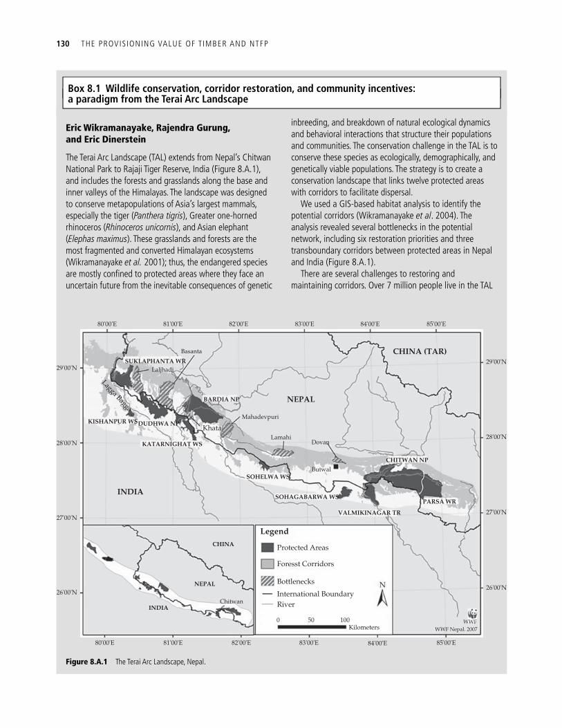
130 THE PROVIS IONING VALUE OF T IMBER AND NTFP
Eric Wikramanayake, Rajendra Gurung, and Eric Dinerstein
The Terai Arc Landscape (TAL) extends from Nepal’s Chitwan National Park to Rajaji Tiger Reserve, India ( Figure 8.A.1 ), and includes the forests and grasslands along the base and inner valleys of the Himalayas. The landscape was designed to conserve metapopulations of Asia’s largest mammals, especially the tiger ( Panthera tigris ), Greater one-horned rhinoceros ( Rhinoceros unicornis ), and Asian elephant ( Elephas maximus ). These grasslands and forests are the most fragmented and converted Himalayan ecosystems ( Wikramanayake et al. 2001 ); thus, the endangered species are mostly confi ned to protected areas where they face an uncertain future from the inevitable consequences of genetic
inbreeding, and breakdown of natural ecological dynamics and behavioral interactions that structure their populations and communities. The conservation challenge in the TAL is to conserve these species as ecologically, demographically, and genetically viable populations. The strategy is to create a conservation landscape that links twelve protected areas with corridors to facilitate dispersal.
We used a GIS-based habitat analysis to identify the potential corridors ( Wikramanayake et al . 2004 ). The analysis revealed several bottlenecks in the potential network, including six restoration priorities and three transboundary corridors between protected areas in Nepal and India ( Figure 8.A.1 ).
There are several challenges to restoring and maintaining corridors. Over 7 million people live in the TAL
Box 8.1 Wildlife conservation, corridor restoration, and community incentives:a paradigm from the Terai Arc Landscape
Figure 8.A.1 The Terai Arc Landscape, Nepal.
SUKLAPHANTA WR
NEPAL
CHINA (TAR)
KISHANPUR WSDUDHWA NP
KATARNIGHAT WS
SOHELWA WS
CHINA
Legend
NEPAL
INDIA
SOHAGABARWA WS
VALMIKINAGAR TR
PARSA WR
CHITWAN NP
BARDIA NP
INDIA
Basanta
80'00'E 81'00'E 82'00'E 83'00'E 84'00'E 85'00'E
80'00'E 81'00'E 82'00'E 83'00'E 84'00'E 85'00'E
29'00'N
28'00'N
27'00'N
26'00'N
29'00'N
28'00'N
27'00'N
26'00'N
Laljhadi
Lagga Bagga
Mahadevpuri
KhataLamahi
Dovan
Chitwan
Protected Areas
Foresst Corridors
Bottlenecks
International BoundaryN
River
0 50 100Kilometers
WWFWWF Nepal. 2007
Butwal

INTRODUCTION 131
and tend over 4.5 million head of livestock (MFSC 2004). Immigration to the Terai still continues, and contributes signifi cantly to the 2.86% population growth rate (WWF 2006). Most immigrants encroach into state forests, clear land, and begin to cultivate. After a couple of years, some sell the land and move on to encroach and occupy another forest patch, creating a chronic process of forest degradation.
Most of the livestock are “scrub” cattle which are allowed to free-range in state forests. As a result, these forests are overgrazed. Controlling cattle grazing in state forest land is diffi cult because the forest department is under-resourced.
To restore bottlenecks the TAL program identifi ed and facilitated the conversion of strategic corridor areas to community forests, a forest management strategy that has worked well to restore forests in Nepal ( Nagendra et al. 2005 ). Under community forestry, degraded state forests are assigned to local forest user groups to manage, based on plans approved by the Forest Department ( Nagendra 2002 ). Because user groups receive management and usufruct rights they have a vested interest in sustainably managing the forests.
Even within the context of community forestry, however, user groups still require fuelwood and other forest resources. Therefore, alternatives to reduce this demand were necessary. The fuelwood demand was eased by providing subsidies to the communities for biogas plants, which use cattle dung to produce methane for cooking and lighting. Better cattle breeds promote stall-feeding, instead of free-grazing, with the added incentive of making it easier to collect cattle dung for biogas plants.
Five years after bottleneck restoration began the “big three” species—tigers, rhinoceros, and elephants—have begun to use the corridors. Tigers are present in four corridors, rhinoceros in two, and the frequency of elephant movement has increased in fi ve. In some corridors elephants have returned after a lapse of 50 years, according to local residents.
Since 2002, the TAL program has facilitated the conversion of over 193 km 2 to community forests in strategic areas of six bottlenecks to 196 forest users groups. These forests are being used by over 24 500 households. The biogas plants and fuel-effi cient cooking stoves provided from 2001 to 2006 have saved an estimated 21 000 metric tons of fuelwood annually, representing an equivalent of over 1.6 km 2 of clear-cut forests. Biogas as an alternative energy also represents an
opportunity for carbon trading in the voluntary market. As of 2005, the biogas program qualifi ed as a Gold Standard CDM-VER project.
The transboundary Khata corridor represents an interesting case. It links Bardia National Park with Katerniaghat Tiger Reserve, and tigers harbored in both parks now use the corridor. Bardia also supports an important rhinoceros population. Several rhinos now use the corridor, and fi ve rhinoceros from Bardia have begun to reside in Katerniaghat. Elephants have also begun to use the corridor. Thus Khata is now a functional wildlife corridor.
In Khata, the TAL program has promoted community-based enterprises that use forest products. For instance, Bel fruits ( Aegel marmelos ) are used to produce juice under a community-based project. During the fi scal year 2005–6 over 25 metric tons of fruit were harvested and sold to the cooperative. Over 17 400 bottles of Bel juice were produced and marketed, which earned a net profi t of about US$6000, a considerable sum for rural communities.
The TAL program has also promoted mentha ( Mentha piperita ) farming, and provided a distillery to extract oil. Mentha was originally promoted as a “live fence” to prevent crop damage by elephants. But the fi nancial benefi ts from mentha oil proved to be so lucrative that more farmers adopted it as a primary cash crop and the output exceeded the carrying capacity of the distillation plant, and three additional distillation plants had to be built to accommodate the demand. In fi scal year 2008, the income from 80 ha of mentha production was US$59 000. The TAL program also established a community-based rattan furniture-making enterprise that earns the user groups over US$3000 annually. The rattan is sustainably harvested from the community forests.
Over 160 men and women from the user groups are also involved in community-led anti-poaching operations in Khata. This group patrols the corridor to safeguard the forests and wildlife from illegal activities such as encroachment, logging and collection of forest products, and poaching. Even though several rhinos have been poached from within the core of Bardia National Park, no poaching incidents have occurred in the corridor, under the vigilance of the community anti-poaching units.
The experiences from the TAL show that restoration and conservation of wildlife habitat in a larger landscape is possible through local stewardship, as long as the local communities benefi t fi nancially from their natural resources management.
132 THE PROVIS IONING VALUE OF T IMBER AND NTFP
under a range of property right structures. For example, open-access grasslands can provide food and fuel for local households as well as a food and water source for their livestock (e.g., Swallow and Bromley 1995 ; Thwaites et al . 1998 ; Adger and Luttrell 2000 ).
8.2 The supply, use, and value of forests’ provisioning service in tier 1
In our ecosystem service taxonomy only the por-tion of a forest’s stock that is harvested represents the forest’s provisioning service. We place a value on the use of a forest’s provisioning services when we convert the forest’s harvest volume into a mon-etary value. Accurately quantifying timber and NTFP harvest levels and values requires socio-eco-nomic and ecological data. Because data availabil-ity and quality will vary, we provide several alternative approaches in tier 1 to quantify harvest volume and value. We fi rst introduce a method that uses current or historical harvest volume or harvest effort, harvest costs, and stock price data to meas-ure a current or baseline period’s volume and value of harvest in a forest parcel ( Section 8.2.1 ). We then provide a method for estimating steady-state har-vest volume and value in a forest parcel when data on harvest volume or effort are not available ( Section 8.2.2 ).
8.2.1 Calculating harvest value when harvest volume or harvest effort is observable
In some cases, such as with commercial timber harvests in developed countries, relatively good data exist on harvest volumes, harvest costs, and product prices. This data can come from one of several sources, including fi eld monitoring of harvests, surveys of harvesters, government sta-tistics, or, if the stocks are sold in the market, market data. We denote harvest volume of some product from a forest over a time period (typi-cally a year) with H . If we cannot fi nd data on H but instead can fi nd data on harvesting “effort” (measured in hours) in the forest over the time period, denoted by E , and the harvest volume col-lected per hour by a typical harvester, given by V ,
we can generate an estimate of H from E and V ; H = E × V .
The cost of harvesting a stock is comprised of two components, the wages paid to labor and the capital costs associated with harvesting equipment. Let the total cost of harvesting the stock in the for-est parcel over a harvest period be given by C . In rare cases, information on costs will be directly available. More commonly, cost estimates can be generated by multiplying harvest effort by the sum of hourly average wage rate of labor, W , and the amortized cost of capital equipment used per unit of harvest effort, Y (in this cost calculation we ignore the opportunity costs associated with har-vesters traveling to and back from forest parcels and any costs associated with transporting har-vested stocks to processing centers).
The price or value of the product made from the harvested stock, denoted by p , is the fi nal data element needed to compute harvest value. If the harvested product is traded in a market then market prices can be used. Otherwise, if the product is generally con-sumed directly by the harvester and not traded in a market, then other methods, such as non-market valu-ation methods, will need to be used to estimate p .
The net value of a product’s harvest from the for-est parcel over the given time period is equal to the revenue from that harvest minus the costs incurred in the process,
( ) ( )( ),NV p H C E p V W Y= × − = × × − − (8.1)
where harvest volume can be observed, H , or calcu-lated with E × V , and costs can be observed, C , or calculated with E × ( W + Y ).
In Eq. (8.1) increasing harvest effort in a time period increases both revenue and costs in a linear fashion (each additional unit of E generates p × V in revenue but costs W + Y ). However, large jumps in effort may lead to nonlinear changes in net returns. This may occur because a large pulse in effort over the course of a harvest period could drastically reduce the stock’s level, making the stock harder to fi nd as the time period progresses. Such a dynamic will reduce the harvest rate V as the harvester has to use more time to search for the increasingly scarcer stock. If V does fall as effort increases, then net value will fall as well because per unit effort costs remain
THE SUPPLY, USE, AND VALUE OF FORESTS’ PROVIS IONING SERVICE IN T IER 1 133
the same no matter the effort level. Therefore, cau-tion should be exercised in using the same V value across very different effort levels.
We can map all harvest volumes and values on the landscape by expanding the net value equation over all harvested biological stocks and forest par-cels on the landscape,
( )( )= × − = × − − ,xz z xz xz xz x xzNV p H C E p V W Y (8.2)
where x = 1, 2, . . . , X indicates distinct forest parcels on the landscape and z = 1, 2, . . . , Z indexes biological stocks available in the landscape’s forest parcels. The sum of H xz and NV xz over all z represents the use and net value of forest parcel x ’s provisioning service over the given time period, respectively, and the sum of H xz and NV xz over all z and x represents the use and net value of the landscape’s forest provisioning service over the given time period, respectively.
If we do not observe harvest volumes or harvest effort then we cannot calculate the current or baseline period’s net value of harvest with Eq. (8.1) and we need to apply alternative methods described below.
8.2.2 Calculating steady-state harvest volume and value
Let G ( S ) indicate the growth of a biological stock over a time period in a forest parcel where S indi-cates the level of the stock. For many stocks growth slows down as stock increases due to resource limitations (density-dependent growth rates; see Boot and Gullison 1995 ). In steady-state harvest-ing, the per period harvest of a stock from a forest parcel is equal to its biological growth rate in the parcel,
( ) ( ),H E V S G S= × = (8.3)
where we now explicitly indicate that a stock’s har-vest rate, V , is a function of its biological stock level. If we can observe the level of the biological stock from a forest inventory and can specify the stock’s growth function G ( S ) then we can use Eqs. (8.3) and (8.1) to estimate a period’s steady-state harvest and its net value (assuming we have cost and price data). We can map all steady-state biological stocks, harvest volumes, and values on the landscape if we
can specify the biological stock levels and their growth functions in every forest parcel.
However, even if we lack observations of biological stock, we can still estimate harvest volumes and values under steady-state conditions if we can specify V ( S ) and G ( S ) and ascribe certain behavior to harvesters. In the next sub-sections we describe several methods for fi nding harvest volumes and values without stock data. The method we use to fi nd harvest volumes and values will depend on the presence and protection of harvest rights and our assumptions about harvest behavior. We begin with a situation of open-access har-vesting, followed by exclusive harvest rights, and con-clude by discussing a case of intermediate access.
8.2.2.1 Open-access steady-state harvest volume and value In many parts of the world, especially in develop-ing countries, households harvest stocks from for-ests to supplement their incomes (e.g., Monela et al . 1993 ). Household harvesting is most active in forest parcels where harvest rights are not established or not enforced, so-called “open-access” parcels ( Feder and Feeny 1991 ; Hyde 2003 ). When using such open- access forests, households typically do not consider the value of leaving biological stock in situ to mature and harvest at a later date because other harvesters are likely to harvest it in the meantime. As long as household labor is not in short supply on the landscape, we can expect households to con-tinue to enter the forest and harvest resources until the last entrant cannot make an economic profi t from further harvesting (where foregone wages in the market and any harvesting equipment costs represents household harvesting costs; see Gordon 1954 ; Conrad and Clark 1987 ; Clark 1990 ; Lopez-Feldman and Wilen 2008 ).
This means that if all households earn the same return from a unit of harvest effort, then in open- access equilibrium no household will make an eco-nomic profi t from harvesting (i.e., the revenues from harvesting equal the wages a household foregoes to harvest plus any equipment costs). However, when households are differentiated, either because they have different harvesting skills, different travel dis-tances to harvest sites, or have different transport access to harvest sites (e.g., bicycle versus truck), then some households may earn positive net returns
134 THE PROVIS IONING VALUE OF T IMBER AND NTFP
in open-access equilibrium. With differentiation, there will be a critical distance or skill level at which a household choosing to harvest will just break even (the value of harvest will just equal the household’s opportunity cost of harvesting plus any equipment costs). In open-access equilibrium, those households closer to the forest or with higher skill level will har-vest while other households will not.
Here we illustrate the case of open access where households are identical in all ways except for their proximity to the forest. Suppose that a standard har-vesting trip to a forest parcel for a certain stock involves e hours of harvesting in the forest as well as the travel time to and from the forest. Let d h be the hours spent traveling to and from the forest for household h . We can either model the actual locations of all households, or if spatially explicit census data is coarser, we can divide the landscape into regions and treat all house-holds in a region as having the same distance.
The household most distant from the forest that engages in harvest, labeled household n , will earn zero economic profi t from a harvesting trip,
( ) ( )( ).npH pV S e W Y e d= = + + (8.4)
We can use Eq. (8.4) to solve for the distance (meas-ured in hours) that household n travels to harvest,
[ ( ) ( )]
.( )
n pV S W Y ed
W Y− +=
+ (8.5)
If we order households from closest to furthest from the forest, then all households with a travel time less than or equal to d n , given by h = 1, 2, . . . , n , will enter the forest to harvest. Household harvest over some time period is
( ) ,oH V S nFe= × (8.6)
where H o indicates aggregate household harvest of the stock from the forest parcel over the time period, F is the average number of trips that the household takes during the time period, and E o = nFe is the household’s aggregate harvest effort in the forest over the given time period (the superscript “ o ” sig-nifi es household behavior versus exclusive harvest-right holder behavior). Hereinafter the lower case “ e ” indicates sub-time period harvest effort and E indicates the effort over the entire time period of
interest (e.g., e indicates daily effort decisions and E is the annual sum of all daily decisions).
On each harvest trip, a household will earn ( W + Y )( d n – d h ) (see the supplementary online material (SOM) for a proof). This represents the difference in travel time to the forest parcel between household h and household n multi-plied by the value of an hour to a household. Because household n earns zero net returns, the value added to household h from harvest is sim-ply given by the value of time that h does not have to spend traveling. All household net returns from harvesting over the time period is given by,
1
( )( ).n
n h
h
NV F W Y d d=
= + −∑ (8.7)
Implementing this model requires specifi cation of travel time to the harvest site as a function of dis-tance, location of households relative to the site, average productivity of harvest in the site, V ( S ), wage and equipment costs per unit of time, W + Y , average amount of effort per trip for households that harvest from the site, e , and average number of harvest trips in a time period, F . We can map all open-access steady-state harvest volumes and val-ues on the landscape by expanding the harvest vol-ume Eq. (8.6) and the net value Eq. (8.7) over all relevant biological stocks and open-access forest parcels on the landscape.
8.2.2.2 Exclusive harvest-right steady-state harvest volume and value At the other extreme from open access, harvests in a forest can be completely limited to those with a property right to harvest. Exclusive harvest rights can be granted to private companies, com-munities, or governments ( Feder and Feeny 1991 ; Engel and Lopez 2008 ; Guariguata et al. 2008 ). In most cases exclusive harvest rights pertain to tim-ber harvest.
If there are no restrictions on forest structure then we assume the holder of a timber concession will create a monoculture forest where a targeted vol-ume of wood can be harvested at regular periods (rotational forestry; see Tahvonen and Salo 1999 ; Dauber et al. 2005 ). Further, we would expect rota-tional forest operators to structure their holdings
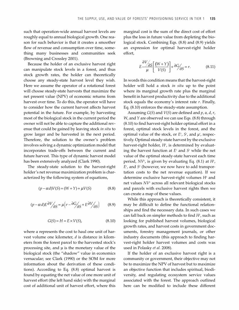
THE SUPPLY, USE, AND VALUE OF FORESTS’ PROVIS IONING SERVICE IN T IER 1 135
such that operation-wide annual harvest levels are roughly equal to annual biological growth. One rea-son for such behavior is that it creates a smoother fl ow of revenue and consumption over time, some-thing many businesses and communities seek ( Browning and Crossley 2001 ).
Because the holder of an exclusive harvest right can manipulate stock levels in a forest, and thus stock growth rates, the holder can theoretically choose any steady-state harvest level they wish. Here we assume the operator of a rotational forest will choose steady-state harvests that maximize the net present value (NPV) of economic returns from harvest over time. To do this, the operator will have to consider how the current harvest affects harvest potential in the future. For example, by harvesting most of the biological stock in the current period the owner will not be able to capture the additional rev-enue that could be gained by leaving stock in situ to grow larger and be harvested in the next period. Therefore, the solution to the owner’s problem involves solving a dynamic optimization model that incorporates trade-offs between the current and future harvest. This type of dynamic harvest model has been extensively analyzed (Clark 1990 ).
The steady-state solution to the harvest-right holder’s net revenue maximization problem is char-acterized by the following system of equations,
( ) ( ) ( ) ( )p d V S W Y V Sa m− = + + (8.8)
( ) V G Vp d E r ES S Sa m ⎛ ⎞⎜ ⎟⎝ ⎠
∂ ∂ ∂− = − +∂ ∂ ∂ (8.9)
( ) ( ),G S H E V S= = × (8.10)
where α represents the cost to haul one unit of har-vest volume one kilometer, d is distance in kilom-eters from the forest parcel to the harvested stock’s processing site, and μ is the monetary value of the biological stock (the “shadow” value in economics vernacular; see Clark ( 1990 ) or the SOM for more information about the derivation of these condi-tions). According to Eq. (8.8) optimal harvest is found by equating the net value of one more unit of harvest effort (the left hand side) with the marginal cost of additional unit of harvest effort, where this
marginal cost is the sum of the direct cost of effort plus the loss in future value from depleting the bio-logical stock. Combining Eqs. (8.8) and (8.9) yields an expression for optimal harvest-right holder effort,
( ) .( )
V W YS GE rSV Sm
∂ +⎡ ⎤∂ ∂+ =⎢ ⎥ ∂⎣ ⎦ (8.11)
In words this condition means that the harvest-right holder will hold a stock in situ up to the point where its marginal growth rate plus the marginal benefi t in harvest productivity due to the additional stock equals the economy’s interest rate r . Finally, Eq. (8.10) enforces the steady-state assumption.
Assuming G ( S ) and V ( S ) are defi ned and p , α , d , r , W , and Y are observed we can use Eqs. (8.8) through (8.10) to fi nd harvest-right holder optimal effort in a forest, optimal stock levels in the forest, and the optimal value of the stock, or E c , S c , and µ c , respec-tively. Optimal steady-state harvest by the exclusive harvest-right holder, H c , is determined by evaluat-ing the harvest function at E c and S c while the net value of the optimal steady-state harvest each time period, NV c , is given by evaluating Eq. (8.1) at H c , E c , and S c (however, we now have to add transpor-tation costs to the net revenue equation). If we determine exclusive harvest-right volumes H c and net values NV c across all relevant biological stocks and parcels with exclusive harvest rights then we can create a map of these values.
While this approach is theoretically consistent, it may be diffi cult to defi ne the functional relation-ships and fi nd the necessary data. In such cases we can fall back on simpler methods to fi nd H c , such as looking for published harvest volumes, biological growth rates, and harvest costs in government doc-uments, forestry management journals, or other industry documents (this approach to fi nding har-vest-right holder harvest volumes and costs was used in Polasky et al. 2008 ).
If the holder of an exclusive harvest right is a community or government, their objective may not be to maximize the NPV of harvest but to maximize an objective function that includes spiritual, biodi-versity, and regulating ecosystem service values associated with the forest. The approach outlined here can be modifi ed to include these different
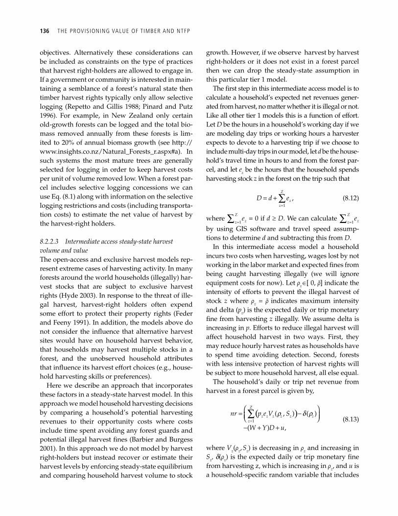
136 THE PROVIS IONING VALUE OF T IMBER AND NTFP
objectives. Alternatively these considerations can be included as constraints on the type of practices that harvest right-holders are allowed to engage in. If a government or community is interested in main-taining a semblance of a forest’s natural state then timber harvest rights typically only allow selective logging ( Repetto and Gillis 1988 ; Pinard and Putz 1996 ). For example, in New Zealand only certain old-growth forests can be logged and the total bio-mass removed annually from these forests is lim-ited to 20% of annual biomass growth (see http://www.insights.co.nz/Natural_Forests_r.aspx#a). In such systems the most mature trees are generally selected for logging in order to keep harvest costs per unit of volume removed low. When a forest par-cel includes selective logging concessions we can use Eq. (8.1) along with information on the selective logging restrictions and costs (including transporta-tion costs) to estimate the net value of harvest by the harvest-right holders.
8.2.2.3 Intermediate access steady-state harvest volume and value The open-access and exclusive harvest models rep-resent extreme cases of harvesting activity. In many forests around the world households (illegally) har-vest stocks that are subject to exclusive harvest rights ( Hyde 2003 ). In response to the threat of ille-gal harvest, harvest-right holders often expend some effort to protect their property rights ( Feder and Feeny 1991 ). In addition, the models above do not consider the infl uence that alternative harvest sites would have on household harvest behavior, that households may harvest multiple stocks in a forest, and the unobserved household attributes that infl uence its harvest effort choices (e.g., house-hold harvesting skills or preferences).
Here we describe an approach that incorporates these factors in a steady-state harvest model. In this approach we model household harvesting decisions by comparing a household’s potential harvesting revenues to their opportunity costs where costs include time spent avoiding any forest guards and potential illegal harvest fi nes ( Barbier and Burgess 2001 ). In this approach we do not model by harvest right-holders but instead recover or estimate their harvest levels by enforcing steady-state equilibrium and comparing household harvest volume to stock
growth. However, if we observe harvest by harvest right-holders or it does not exist in a forest parcel then we can drop the steady-state assumption in this particular tier 1 model.
The fi rst step in this intermediate access model is to calculate a household’s expected net revenues gener-ated from harvest, no matter whether it is illegal or not. Like all other tier 1 models this is a function of effort. Let D be the hours in a household’s working day if we are modeling day trips or working hours a harvester expects to devote to a harvesting trip if we choose to include multi-day trips in our model, let d be the house-hold’s travel time in hours to and from the forest par-cel, and let e z be the hours that the household spends harvesting stock z in the forest on the trip such that
1
,Z
zz
D d e=
= + ∑ (8.12)
where 1
Z
zze
=∑ = 0 if d ³ D . We can calculate 1
Z
zze
=∑ by using GIS software and travel speed assump-tions to determine d and subtracting this from D .
In this intermediate access model a household incurs two costs when harvesting, wages lost by not working in the labor market and expected fi nes from being caught harvesting illegally (we will ignore equipment costs for now). Let ρ z Î [ 0 , ρ ] indicate the intensity of efforts to prevent the illegal harvest of stock z where ρ z = ρ indicates maximum intensity and delta (pz) is the expected daily or trip monetary fi ne from harvesting z illegally. We assume delta is increasing in p . Efforts to reduce illegal harvest will affect household harvest in two ways. First, they may reduce hourly harvest rates as households have to spend time avoiding detection. Second, forests with less intensive protection of harvest rights will be subject to more household harvest, all else equal.
The household’s daily or trip net revenue from harvest in a forest parcel is given by,
( )
1
( , ) ( )
( ) ,
Z
z z z z z zz
nr p e V S
W Y D u
r d r=
⎛ ⎞= −⎜ ⎟⎝ ⎠− + +
∑ (8.13)
where V z (ρ z , S z ) is decreasing in ρ z and increasing in S z , d(ρ z ) is the expected daily or trip monetary fi ne from harvesting z, which is increasing in ρ z , and u is a household-specifi c random variable that includes
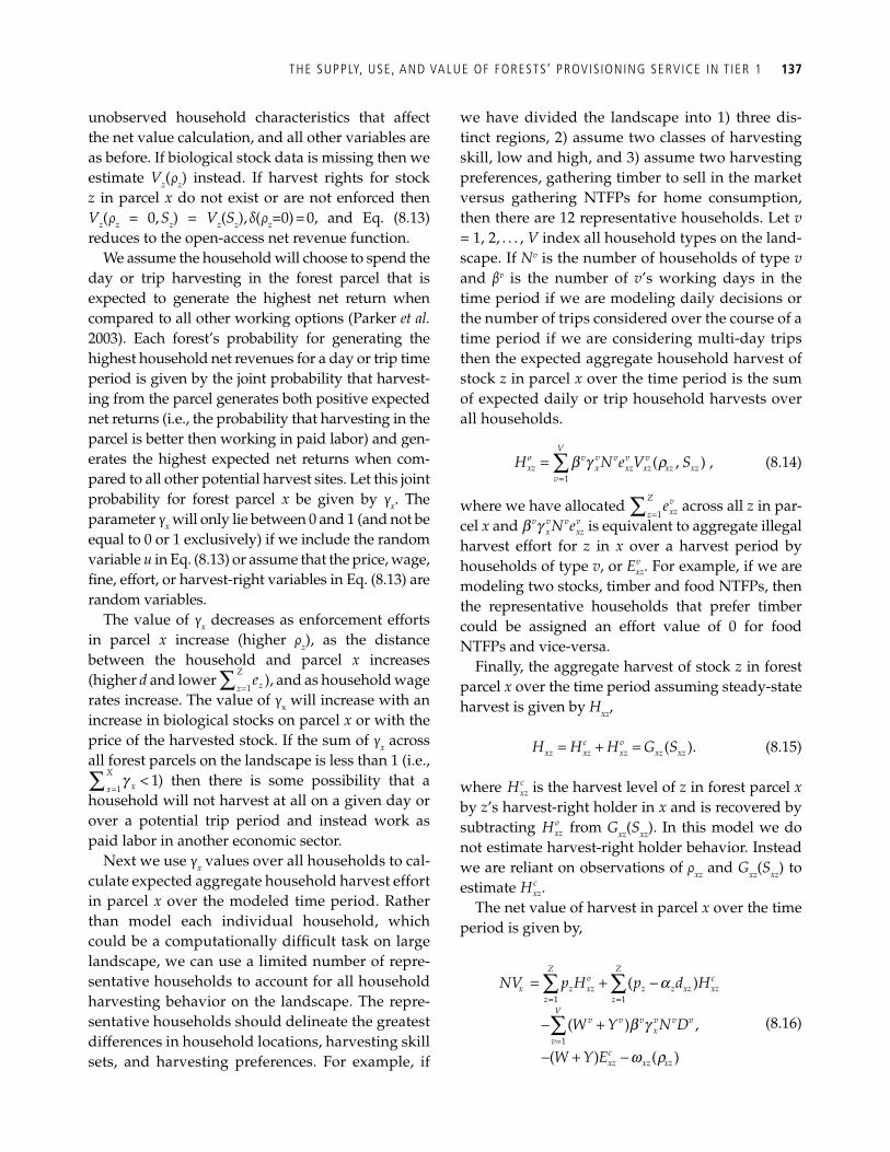
THE SUPPLY, USE, AND VALUE OF FORESTS’ PROVIS IONING SERVICE IN T IER 1 137
unobserved household characteristics that affect the net value calculation, and all other variables are as before. If biological stock data is missing then we estimate V z (ρ z ) instead. If harvest rights for stock z in parcel x do not exist or are not enforced then V z (ρ z = 0, S z ) = V z ( S z ), δ(ρ z =0) = 0, and Eq. (8.13) reduces to the open-access net revenue function.
We assume the household will choose to spend the day or trip harvesting in the forest parcel that is expected to generate the highest net return when compared to all other working options ( Parker et al. 2003 ). Each forest’s probability for generating the highest household net revenues for a day or trip time period is given by the joint probability that harvest-ing from the parcel generates both positive expected net returns (i.e., the probability that harvesting in the parcel is better then working in paid labor) and gen-erates the highest expected net returns when com-pared to all other potential harvest sites. Let this joint probability for forest parcel x be given by γ x . The parameter γ x will only lie between 0 and 1 (and not be equal to 0 or 1 exclusively) if we include the random variable u in Eq. (8.13) or assume that the price, wage, fi ne, effort, or harvest-right variables in Eq. (8.13) are random variables.
The value of γ x decreases as enforcement efforts in parcel x increase (higher ρ z ), as the distance between the household and parcel x increases (higher d and lower
1
Z
zze
=∑ ), and as household wage rates increase. The value of γ x will increase with an increase in biological stocks on parcel x or with the price of the harvested stock. If the sum of γ x across all forest parcels on the landscape is less than 1 (i.e.,
11
X
xxg
=<∑ ) then there is some possibility that a
household will not harvest at all on a given day or over a potential trip period and instead work as paid labor in another economic sector.
Next we use γ x values over all households to cal-culate expected aggregate household harvest effort in parcel x over the modeled time period. Rather than model each individual household, which could be a computationally diffi cult task on large landscape, we can use a limited number of repre-sentative households to account for all household harvesting behavior on the landscape. The repre-sentative households should delineate the greatest differences in household locations, harvesting skill sets, and harvesting preferences. For example, if
we have divided the landscape into 1) three dis-tinct regions, 2) assume two classes of harvesting skill, low and high, and 3) assume two harvesting preferences, gathering timber to sell in the market versus gathering NTFPs for home consumption, then there are 12 representative households. Let v = 1, 2, . . . , V index all household types on the land-scape. If N v is the number of households of type v and β v is the number of v ’s working days in the time period if we are modeling daily decisions or the number of trips considered over the course of a time period if we are considering multi-day trips then the expected aggregate household harvest of stock z in parcel x over the time period is the sum of expected daily or trip household harvests over all households.
1
( , ) ,V
o v v v v vxz x xz xz xz xz
v
H N e V S=
= ∑b g r (8.14)
where we have allocated 1
Z vxzz
e=∑ across all z in par-
cel x and v v v vx xzN eb g is equivalent to aggregate illegal
harvest effort for z in x over a harvest period by households of type v , or v
xzE . For example, if we are modeling two stocks, timber and food NTFPs, then the representative households that prefer timber could be assigned an effort value of 0 for food NTFPs and vice-versa.
Finally, the aggregate harvest of stock z in forest parcel x over the time period assuming steady-state harvest is given by H xz ,
( ).c oxz xz xz xz xzH H H G S= + = (8.15)
where cxzH is the harvest level of z in forest parcel x
by z ’s harvest-right holder in x and is recovered by subtracting o
xzH from G xz ( S xz ). In this model we do not estimate harvest-right holder behavior. Instead we are reliant on observations of ρ xz and G xz ( S xz ) to estimate c
xzH . The net value of harvest in parcel x over the time
period is given by,
= =
=
= + −
− +
− + −
∑ ∑
∑1 1
1
( )
( ) ,
( ) ( )
Z Zo c
x z xz z z xz xzz z
Vv v v v v v
xv
cxz xz xz
NV p H p d H
W Y N D
W Y E
a
b g
w r
(8.16)
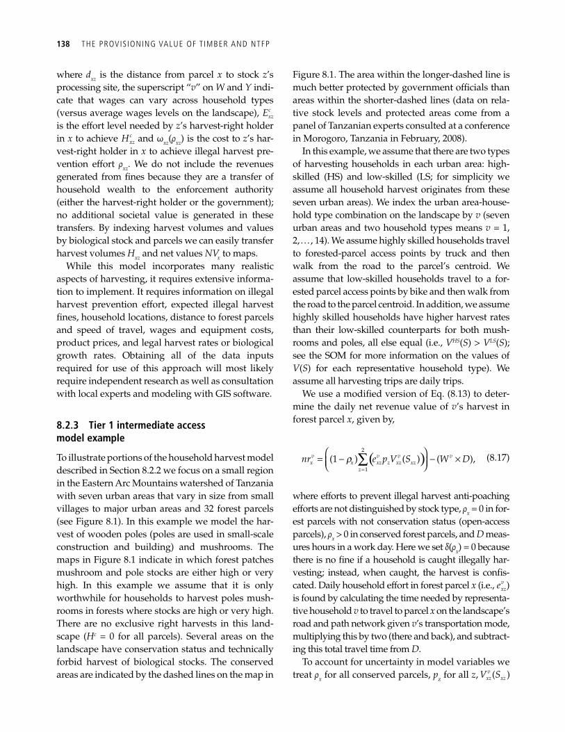
138 THE PROVIS IONING VALUE OF T IMBER AND NTFP
where d xz is the distance from parcel x to stock z ’s processing site, the superscript “ v ” on W and Y indi-cate that wages can vary across household types (versus average wages levels on the landscape), c
xzE is the effort level needed by z ’s harvest-right holder in x to achieve c
xzH and ω xz (ρ xz ) is the cost to z ’s har-vest-right holder in x to achieve illegal harvest pre-vention effort ρ xz . We do not include the revenues generated from fi nes because they are a transfer of household wealth to the enforcement authority (either the harvest-right holder or the government); no additional societal value is generated in these transfers. By indexing harvest volumes and values by biological stock and parcels we can easily transfer harvest volumes H xz and net values NV x to maps.
While this model incorporates many realistic aspects of harvesting, it requires extensive informa-tion to implement. It requires information on illegal harvest prevention effort, expected illegal harvest fi nes, household locations, distance to forest parcels and speed of travel, wages and equipment costs, product prices, and legal harvest rates or biological growth rates. Obtaining all of the data inputs required for use of this approach will most likely require independent research as well as consultation with local experts and modeling with GIS software.
8.2.3 Tier 1 intermediate access model example
To illustrate portions of the household harvest model described in Section 8.2.2 we focus on a small region in the Eastern Arc Mountains watershed of Tanzania with seven urban areas that vary in size from small villages to major urban areas and 32 forest parcels (see Figure 8.1 ). In this example we model the har-vest of wooden poles (poles are used in small-scale construction and building) and mushrooms. The maps in Figure 8.1 indicate in which forest patches mushroom and pole stocks are either high or very high. In this example we assume that it is only worthwhile for households to harvest poles mush-rooms in forests where stocks are high or very high. There are no exclusive right harvests in this land-scape ( H c = 0 for all parcels). Several areas on the landscape have conservation status and technically forbid harvest of biological stocks. The conserved areas are indicated by the dashed lines on the map in
Figure 8.1 . The area within the longer-dashed line is much better protected by government offi cials than areas within the shorter-dashed lines (data on rela-tive stock levels and protected areas come from a panel of Tanzanian experts consulted at a conference in Morogoro, Tanzania in February, 2008).
In this example, we assume that there are two types of harvesting households in each urban area: high-skilled (HS) and low-skilled (LS; for simplicity we assume all household harvest originates from these seven urban areas). We index the urban area-house-hold type combination on the landscape by v (seven urban areas and two household types means v = 1, 2, . . . , 14). We assume highly skilled households travel to forested-parcel access points by truck and then walk from the road to the parcel’s centroid. We assume that low-skilled households travel to a for-ested parcel access points by bike and then walk from the road to the parcel centroid. In addition, we assume highly skilled households have higher harvest rates than their low-skilled counterparts for both mush-rooms and poles, all else equal (i.e., V HS ( S ) > V LS ( S ); see the SOM for more information on the values of V ( S ) for each representative household type). We assume all harvesting trips are daily trips.
We use a modifi ed version of Eq. (8.13) to deter-mine the daily net revenue value of v ’s harvest in forest parcel x , given by,
( )2
1
(1 ) ( ) ( ),v v v vx x xz z xz xz
z
nr e p V S W D=
⎛ ⎞= − − ×⎜ ⎟⎝ ⎠∑r (8.17)
where efforts to prevent illegal harvest anti-poaching efforts are not distinguished by stock type, ρ x = 0 in for-est parcels with not conservation status (open-access parcels), ρ x > 0 in conserved forest parcels, and D meas-ures hours in a work day. Here we set δ(ρ x ) = 0 because there is no fi ne if a household is caught illegally har-vesting; instead, when caught, the harvest is confi s-cated. Daily household effort in forest parcel x (i.e., v
xze ) is found by calculating the time needed by representa-tive household v to travel to parcel x on the landscape’s road and path network given v ’s transportation mode, multiplying this by two (there and back), and subtract-ing this total travel time from D .
To account for uncertainty in model variables we treat ρ x for all conserved parcels, p z for all z , ( )v
xz xzV S
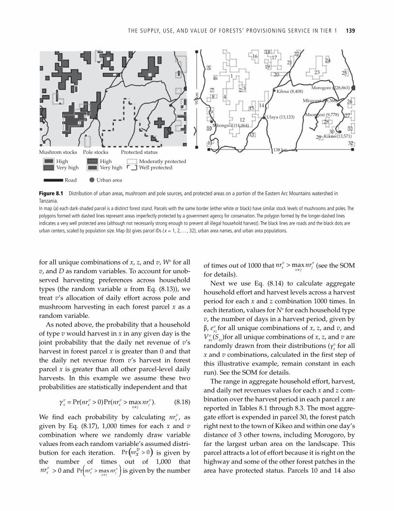
THE SUPPLY, USE, AND VALUE OF FORESTS’ PROVIS IONING SERVICE IN T IER 1 139
for all unique combinations of x , z , and v , W v for all v , and D as random variables. To account for unob-served harvesting preferences across household types (the random variable u from Eq. (8.13)), we treat v ’s allocation of daily effort across pole and mushroom harvesting in each forest parcel x as a random variable.
As noted above, the probability that a household of type v would harvest in x in any given day is the joint probability that the daily net revenue of v ’s harvest in forest parcel x is greater than 0 and that the daily net revenue from v ’s harvest in forest parcel x is greater than all other parcel-level daily harvests. In this example we assume these two probabilities are statistically independent and that
Pr( 0)Pr( max ).v v v vx x x jx j
nr nr nrg≠
= > > (8.18)
We fi nd each probability by calculating vxnr , as
given by Eq. (8.17), 1,000 times for each x and v combination where we randomly draw variable values from each random variable’s assumed distri-bution for each iteration. ( )Pr 0vnrx > is given by the number of times out of 1,000 that v
xnr > 0 and Pr maxv vx jx j
nr nr≠
⎛ ⎞>⎝ ⎠ is given by the number
of times out of 1000 that maxv vx jx j
nr nr≠
> (see the SOM for details).
Next we use Eq. (8.14) to calculate aggregate household effort and harvest levels across a harvest period for each x and z combination 1000 times. In each iteration, values for N v for each household type v , the number of days in a harvest period, given by β, e x z
v for all unique combinations of x , z , and v , and V x z
v ( S x z ) for all unique combinations of x , z , and v are randomly drawn from their distributions ( γ x
v for all x and v combinations, calculated in the fi rst step of this illustrative example, remain constant in each run). See the SOM for details.
The range in aggregate household effort, harvest, and daily net revenues values for each x and z com-bination over the harvest period in each parcel x are reported in Tables 8.1 through 8.3 . The most aggre-gate effort is expended in parcel 30, the forest patch right next to the town of Kikeo and within one day’s distance of 3 other towns, including Morogoro, by far the largest urban area on the landscape. This parcel attracts a lot of effort because it is right on the highway and some of the other forest patches in the area have protected status. Parcels 10 and 14 also
Mushrom stocks
HighVery high
HighVery high
Moderatly protected
91 k
m
Well protected
Road Urban area
Pole stocks Protected status
Mbongwa (14,064)
5
1618
17
1920
21
22
23
24
25
26
27
31
3229
30
28
6
78
9
10
11
12
13
15 14
2 3
1
4
Ulaya (13,123)
138 km
Kilosa (8,408)Morogoro (228,863)
Mkuyuni (19,366)
Msongozi (9,778)
Kikeo (13,571)
Figure 8.1 Distribution of urban areas, mushroom and pole sources, and protected areas on a portion of the Eastern Arc Mountains watershed in Tanzania. In map (a) each dark-shaded parcel is a distinct forest stand. Parcels with the same border (either white or black) have similar stock levels of mushrooms and poles. The polygons formed with dashed lines represent areas imperfectly protected by a government agency for conservation. The polygon formed by the longer-dashed lines indicates a very well protected area (although not necessarily strong enough to prevent all illegal household harvest). The black lines are roads and the black dots are urban centers, scaled by population size. Map (b) gives parcel IDs ( x = 1, 2, . . . , 32), urban area names, and urban area populations.
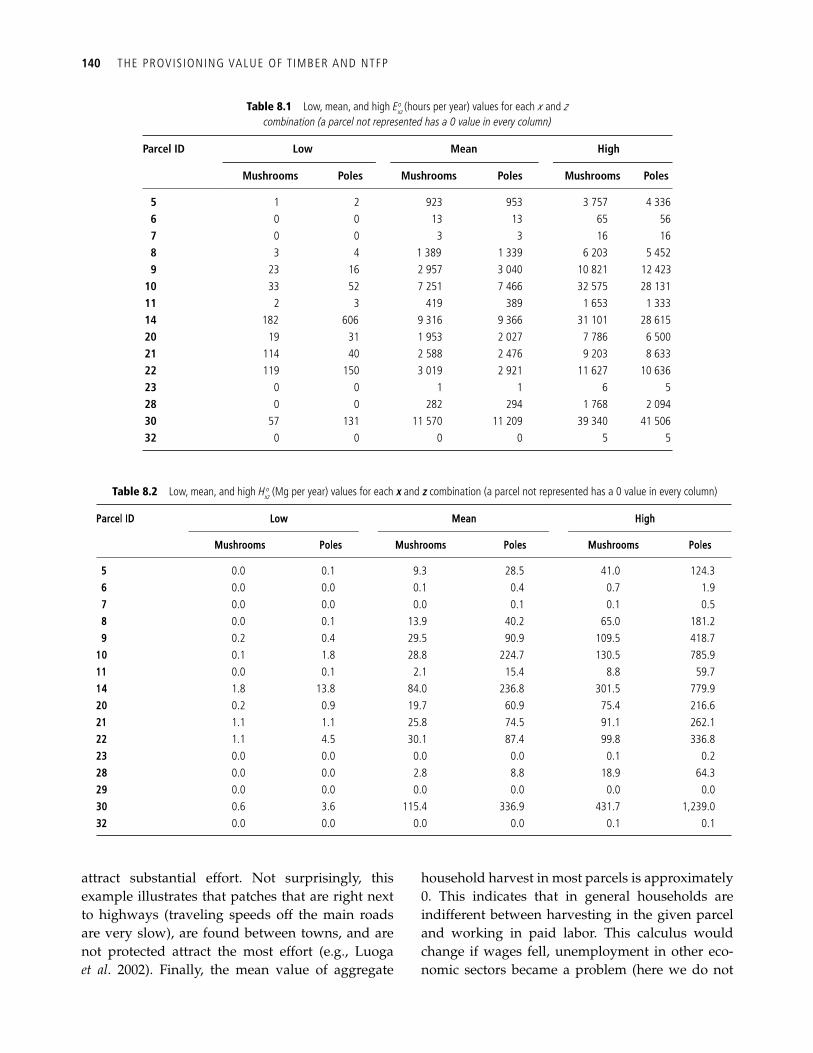
140 THE PROVIS IONING VALUE OF T IMBER AND NTFP
attract substantial effort. Not surprisingly, this example illustrates that patches that are right next to highways (traveling speeds off the main roads are very slow), are found between towns, and are not protected attract the most effort (e.g., Luoga et al . 2002 ). Finally, the mean value of aggregate
household harvest in most parcels is approximately 0. This indicates that in general households are indifferent between harvesting in the given parcel and working in paid labor. This calculus would change if wages fell, unemployment in other eco-nomic sectors became a problem (here we do not
Table 8.1 Low, mean, and high E xz o (hours per year) values for each x and z
combination (a parcel not represented has a 0 value in every column)
Parcel ID Low Mean High
Mushrooms Poles Mushrooms Poles Mushrooms Poles
5 1 2 923 953 3 757 4 336 6 0 0 13 13 65 56 7 0 0 3 3 16 16 8 3 4 1 389 1 339 6 203 5 452 9 23 16 2 957 3 040 10 821 12 423
10 33 52 7 251 7 466 32 575 28 131 11 2 3 419 389 1 653 1 333 14 182 606 9 316 9 366 31 101 28 615 20 19 31 1 953 2 027 7 786 6 500 21 114 40 2 588 2 476 9 203 8 633 22 119 150 3 019 2 921 11 627 10 636 23 0 0 1 1 6 5 28 0 0 282 294 1 768 2 094 30 57 131 11 570 11 209 39 340 41 506 32 0 0 0 0 5 5
Table 8.2 Low, mean, and high H xz o (Mg per year) values for each x and z combination (a parcel not represented has a 0 value in every column)
Parcel ID Low Mean High
Mushrooms Poles Mushrooms Poles Mushrooms Poles
5 0.0 0.1 9.3 28.5 41.0 124.3 6 0.0 0.0 0.1 0.4 0.7 1.9 7 0.0 0.0 0.0 0.1 0.1 0.5 8 0.0 0.1 13.9 40.2 65.0 181.2 9 0.2 0.4 29.5 90.9 109.5 418.7
10 0.1 1.8 28.8 224.7 130.5 785.9 11 0.0 0.1 2.1 15.4 8.8 59.7 14 1.8 13.8 84.0 236.8 301.5 779.9 20 0.2 0.9 19.7 60.9 75.4 216.6 21 1.1 1.1 25.8 74.5 91.1 262.1 22 1.1 4.5 30.1 87.4 99.8 336.8 23 0.0 0.0 0.0 0.0 0.1 0.2 28 0.0 0.0 2.8 8.8 18.9 64.3 29 0.0 0.0 0.0 0.0 0.0 0.0 30 0.6 3.6 115.4 336.9 431.7 1,239.0 32 0.0 0.0 0.0 0.0 0.1 0.1
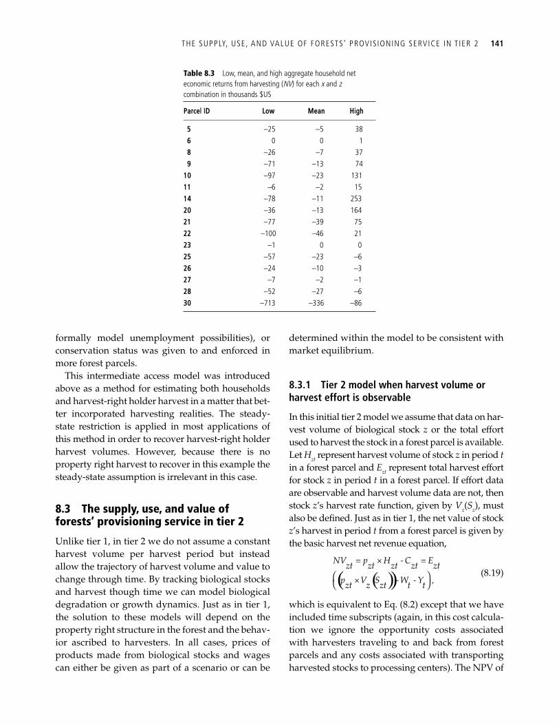
THE SUPPLY, USE, AND VALUE OF FORESTS’ PROVIS IONING SERVICE IN T IER 2 141
formally model unemployment possibilities), or conservation status was given to and enforced in more forest parcels.
This intermediate access model was introduced above as a method for estimating both households and harvest-right holder harvest in a matter that bet-ter incorporated harvesting realities. The steady-state restriction is applied in most applications of this method in order to recover harvest-right holder harvest volumes. However, because there is no property right harvest to recover in this example the steady-state assumption is irrelevant in this case.
8.3 The supply, use, and value of forests’ provisioning service in tier 2
Unlike tier 1, in tier 2 we do not assume a constant harvest volume per harvest period but instead allow the trajectory of harvest volume and value to change through time. By tracking biological stocks and harvest though time we can model biological degradation or growth dynamics. Just as in tier 1, the solution to these models will depend on the property right structure in the forest and the behav-ior ascribed to harvesters. In all cases, prices of products made from biological stocks and wages can either be given as part of a scenario or can be
determined within the model to be consistent with market equilibrium.
8.3.1 Tier 2 model when harvest volume or harvest effort is observable
In this initial tier 2 model we assume that data on har-vest volume of biological stock z or the total effort used to harvest the stock in a forest parcel is available. Let H zt represent harvest volume of stock z in period t in a forest parcel and E zt represent total harvest effort for stock z in period t in a forest parcel. If effort data are observable and harvest volume data are not, then stock z ’s harvest rate function, given by V z ( S z ), must also be defi ned. Just as in tier 1, the net value of stock z ’s harvest in period t from a forest parcel is given by the basic harvest net revenue equation,
( )( )⎛ ⎞⎝ ⎠
NV = p × H - C = Ezt zt zt zt zt
p ×V S - W - Y ,zt z zt t t (8.19)
which is equivalent to Eq. (8.2) except that we have included time subscripts (again, in this cost calcula-tion we ignore the opportunity costs associated with harvesters traveling to and back from forest parcels and any costs associated with transporting harvested stocks to processing centers). The NPV of
Table 8.3 Low, mean, and high aggregate household net economic returns from harvesting ( NV ) for each x and z combination in thousands $US
Parcel ID Low Mean High
5 –25 –5 38 6 0 0 1 8 –26 –7 37 9 –71 –13 74
10 –97 –23 131 11 –6 –2 15 14 –78 –11 253 20 –36 –13 164 21 –77 –39 75 22 –100 –46 21 23 –1 0 0 25 –57 –23 –6 26 –24 –10 –3 27 –7 –2 –1 28 –52 –27 –6 30 –713 –336 –86
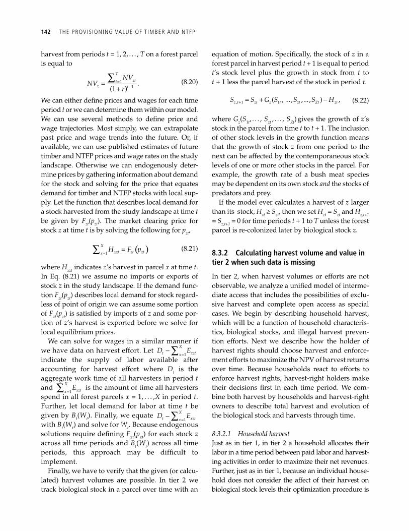
142 THE PROVIS IONING VALUE OF T IMBER AND NTFP
harvest from periods t = 1, 2, . . . , T on a forest parcel is equal to
=−=
+∑ 1
1 .(1 )
T
zttz t
NVNV
r (8.20)
We can either defi ne prices and wages for each time period t or we can determine them within our model. We can use several methods to defi ne price and wage trajectories. Most simply, we can extrapolate past price and wage trends into the future. Or, if available, we can use published estimates of future timber and NTFP prices and wage rates on the study landscape. Otherwise we can endogenously deter-mine prices by gathering information about demand for the stock and solving for the price that equates demand for timber and NTFP stocks with local sup-ply. Let the function that describes local demand for a stock harvested from the study landscape at time t be given by F zt ( p zt ). The market clearing price for stock z at time t is by solving the following for p zt ,
( )==∑ 1
X
xzt zt ztxH F p (8.21)
where H xzt indicates z ’s harvest in parcel x at time t . In Eq. (8.21) we assume no imports or exports of stock z in the study landscape. If the demand func-tion F zt ( p zt ) describes local demand for stock regard-less of point of origin we can assume some portion of F zt ( p zt ) is satisfi ed by imports of z and some por-tion of z ’s harvest is exported before we solve for local equilibrium prices.
We can solve for wages in a similar manner if we have data on harvest effort. Let
1
X
t xztxD E
=− ∑
indicate the supply of labor available after accounting for harvest effort where D t is the aggregate work time of all harvesters in period t and
1
X
xztxE
=∑ is the amount of time all harvesters spend in all forest parcels x = 1, . . . , X in period t . Further, let local demand for labor at time t be given by B t ( W t ). Finally, we equate
1
Xt xztx
D E=
− ∑ with B t ( W t ) and solve for W t . Because endogenous solutions require defi ning F zt ( p zt ) for each stock z across all time periods and B t ( W t ) across all time periods, this approach may be diffi cult to implement.
Finally, we have to verify that the given (or calcu-lated) harvest volumes are possible. In tier 2 we track biological stock in a parcel over time with an
equation of motion. Specifi cally, the stock of z in a forest parcel in harvest period t + 1 is equal to period t ’s stock level plus the growth in stock from t to t + 1 less the parcel harvest of the stock in period t .
z t zt z t zt Zt ztS S G S S S H, 1 1( , ..., ,..., ) ,+ = + − (8.22)
where G z ( S 1 t , . . . , S z t , . . . , S Z t ) gives the growth of z ’s stock in the parcel from time t to t + 1. The inclusion of other stock levels in the growth function means that the growth of stock z from one period to the next can be affected by the contemporaneous stock levels of one or more other stocks in the parcel. For example, the growth rate of a bush meat species may be dependent on its own stock and the stocks of predators and prey.
If the model ever calculates a harvest of z larger than its stock, H zt ³ S zt , then we set Hzt = Szt and H z,t+1 = S z,t+1 = 0 for time periods t + 1 to T unless the forest parcel is re-colonized later by biological stock z .
8.3.2 Calculating harvest volume and value in tier 2 when such data is missing
In tier 2, when harvest volumes or efforts are not observable, we analyze a unifi ed model of interme-diate access that includes the possibilities of exclu-sive harvest and complete open access as special cases. We begin by describing household harvest, which will be a function of household characteris-tics, biological stocks, and illegal harvest preven-tion efforts. Next we describe how the holder of harvest rights should choose harvest and enforce-ment efforts to maximize the NPV of harvest returns over time. Because households react to efforts to enforce harvest rights, harvest-right holders make their decisions fi rst in each time period. We com-bine both harvest by households and harvest-right owners to describe total harvest and evolution of the biological stock and harvests through time.
8.3.2.1 Household harvest Just as in tier 1, in tier 2 a household allocates their labor in a time period between paid labor and harvest-ing activities in order to maximize their net revenues. Further, just as in tier 1, because an individual house-hold does not consider the affect of their harvest on biological stock levels their optimization procedure is
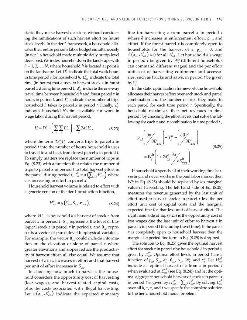
THE SUPPLY, USE, AND VALUE OF FORESTS’ PROVIS IONING SERVICE IN T IER 2 143
static; they make harvest decisions without consider-ing the ramifi cations of such harvest effort on future stock levels. In the tier 2 framework, a household allo-cates their entire period’s labor budget simultaneously (in tier 1 a household made multiple daily or trip-level decisions). We index households on the landscape with h = 1, 2, . . . , N , where household h is located at point h on the landscape. Let h
tD indicate the total work hours in time period t for household h , h
xztE indicate the total time (in hours) that h uses to harvest stock z in forest parcel x during time period t , h
xtd indicate the one-way travel time between household h and forest parcel x in hours in period t , and h
xtI indicate the number of trips household h takes to parcel x in period t . Finally, h
tL indicates household h ’s time available for work in wage labor during the harvest period.
⎛ ⎞= − −⎜ ⎟⎝ ⎠∑∑ ∑2 ,h h h h h
t t xzt xt xtx z x
L D E d I (8.23)
where the term 2 h hxt xtd I converts trips to parcel x in
period t into the number of hours household h uses to travel to and back from forest parcel x in period t . To simply matters we replace the number of trips in Eq. (8.23) with a function that relates the number of trips to parcel x in period t to total harvest effort in the parcel during period t , ( )σ
== ∑ 1
Zh hxt xztz
I E , where σ is increasing in effort in parcel x .
Household harvest volume is related to effort with a generic version of the tier 1 production function,
( )h hxzt xzt xzt xztH y E S, ,= σ , (8.24)
where hxztH is household h ’s harvest of stock z from
parcel x in period t , S xzt represents the level of bio-logical stock z in parcel x in period t , and q xzt repre-sents a vector of parcel-level biophysical variables. For example, the vector q xzt could include informa-tion on the elevation or slope of parcel x where greater elevations and slopes reduce the productiv-ity of harvest effort, all else equal. We assume that harvest of z in x increases in effort and that harvest per unit of effort increases in S xzt .
In choosing how much to harvest, the house-hold considers the opportunity cost of harvesting (lost wages), and harvest-related capital costs, plus the costs associated with illegal harvesting. Let ( ), h
xzt xztEδ ρ indicate the expected monetary
fi ne for harvesting z from parcel x in period t where δ increases in enforcement effort, ρ xzt , and effort. If the forest parcel x is completely open to households for the harvest of z , ρ xzt = 0, and ( ), h
xzt xztEδ ρ = 0 for all hxztE . Let household h ’s wage
in period t be given by W t h (different households
can command different wages) and the per effort unit cost of harvesting equipment and accesso-ries, such as trucks and saws, in period t be given by Y t
h . In the static optimization framework the household
allocates their harvest effort over each stock and parcel combination and the number of trips they make to each parcel for each time period t . Specifi cally, the household maximizes their net revenues in time period t by choosing the effort levels that solve the fol-lowing for each z and x combination in time period t ,
y hp Yh hzt tE Exzt xzt
d⎛ ⎞ ⎛ ⎞∂ ∂⎜ ⎟ ⎜ ⎟− −⎜ ⎟ ⎜ ⎟∂ ∂⎝ ⎠ ⎝ ⎠
h hW d ht xt Exzt1 2
⎛ ⎞∂⎜ ⎟= +⎜ ⎟∂⎝ ⎠
σ
(8.25)
If household h spends all of their working time har-vesting and never works in the paid labor market then W t
h in Eq. (8.25) should be replaced by h ’s marginal value of harvesting. The left hand side of Eq. (8.25) measures the revenue generated by the last unit of effort used to harvest stock z in parcel x less the per effort unit cost of capital costs and the marginal expected fi ne for that less unit of harvest effort. The right hand side of Eq. (8.25) is the opportunity cost of lost wages due the last unit of effort to harvest z in parcel x in period t (including travel time). If the parcel x is completely open to household harvest then the marginal expected fi ne term in Eq. (8.25) is dropped.
The solution to Eq. (8.25) gives the optimal harvest effort for stock z in parcel x by household h in period t , given by *h
xztE . Optimal effort levels in period t are a function of p zt , S xzt , d xt
h , q xzt , ρ xzt , W t h , and Y t
h . Let *hxztH
indicate h ’s optimal harvest of z from x in period t when evaluated at *h
xztE f (see Eq. (8.24)) and let the opti-mal aggregate household harvest of stock z in parcel x in period t is given by **o h
xzt xzthH H= ∑ . By solving *h
xztE over all h , x , z , and t we specify the complete solution to the tier 2 household model problem.
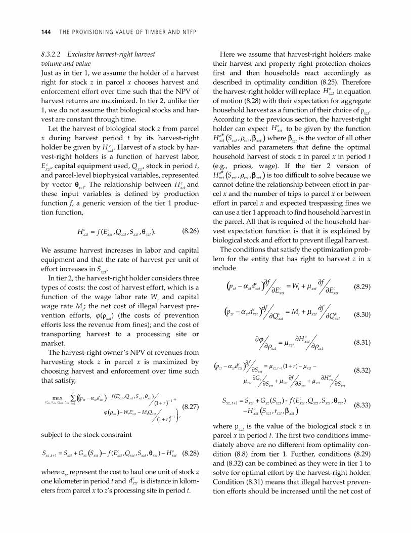
144 THE PROVIS IONING VALUE OF T IMBER AND NTFP
8.3.2.2 Exclusive harvest-right harvest volume and value Just as in tier 1, we assume the holder of a harvest right for stock z in parcel x chooses harvest and enforcement effort over time such that the NPV of harvest returns are maximized. In tier 2, unlike tier 1, we do not assume that biological stocks and har-vest are constant through time.
Let the harvest of biological stock z from parcel x during harvest period t by its harvest-right holder be given by H xzt c . Harvest of a stock by har-vest-right holders is a function of harvest labor, E xzt c , capital equipment used, Q xzt , stock in period t , and parcel-level biophysical variables, represented by vector q xzt . The relationship between H xzt c and these input variables is defi ned by production function f , a generic version of the tier 1 produc-tion function,
= θ( , , , ).c cxzt xzt xzt xzt xztH f E Q S (8.26)
We assume harvest increases in labor and capital equipment and that the rate of harvest per unit of effort increases in S xzt .
In tier 2, the harvest-right holder considers three types of costs: the cost of harvest effort, which is a function of the wage labor rate W t and capital wage rate M t ; the net cost of illegal harvest pre-vention efforts, φ(ρ xzt ) (the costs of prevention efforts less the revenue from fi nes); and the cost of transporting harvest to a processing site or market.
The harvest-right owner’s NPV of revenues from harvesting stock z in parcel x is maximized by choosing harvest and enforcement over time such that satisfy,
( )(
=−∑
, , , 1
maxcxzt xzt xzt xzt
Tc
zt zt xztE S Q t
p dρ
α( )
q− +
+ 1( , , , )
1
cxzt xzt xzt xzt
tf E Q S
r
( )( )
j−
⎞− −⎟+ ⎠1 ,
1
cxzt t xzt t xzt
tW E M Q
rr
(8.27)
subject to the stock constraint
( )+ = + − −, 1 ( , , , )c oxz t xzt xz xzt xzt xzt xzt xzt xztS S G S f E Q S Hq (8.28)
where α zt represent the cost to haul one unit of stock z one kilometer in period t and c
xztd is distance in kilom-eters from parcel x to z ’s processing site in period t .
Here we assume that harvest-right holders make their harvest and property right protection choices fi rst and then households react accordingly as described in optimality condition (8.25). Therefore the harvest-right holder will replace o
xztH in equation of motion (8.28) with their expectation for aggregate household harvest as a function of their choice of ρ xzt . According to the previous section, the harvest-right holder can expect o
xztH to be given by the function ( )* , ,o
xzt xzt xzt xztH S r b where b xzt is the vector of all other variables and parameters that defi ne the optimal household harvest of stock z in parcel x in period t (e.g., prices, wage). If the tier 2 version of ( )* , ,o
xzt xzt xzt xztH S r b is too diffi cult to solve because we cannot defi ne the relationship between effort in par-cel x and the number of trips to parcel x or between effort in parcel x and expected trespassing fi nes we can use a tier 1 approach to fi nd household harvest in the parcel. All that is required of the household har-vest expectation function is that it is explained by biological stock and effort to prevent illegal harvest.
The conditions that satisfy the optimization prob-lem for the entity that has right to harvest z in x include
( )cc czt zt xzt t xztxzt xzt
f fp d WE Ea m∂ ∂− = +∂ ∂ (8.29)
( )cc czt zt xzt t xztxzt xzt
f fp d MQ Qa m∂ ∂− = +∂ ∂ (8.30)
oxzt
xztxzt zxt
Hj mr r∂∂ =∂ ∂ (8.31)
( ) , 1(1 )czt zt xzt xz t xzt
xzto
z xztxzt xzt xzt
xzt xzt xzt
fp d rSfG H
S S S
a m m
m m m
−∂− = + − −∂
∂∂ ∂+ +∂ ∂ ∂
(8.32)
( )
( ) ( )cxz, t+1 xzt xz xzt xzt xzt xzt xzt
oxzt xzt xzt xzt
S = S +G S - f E ,Q ,S ,H S ,r ,−
qb
(8.33)
where μ xzt is the value of the biological stock z in parcel x in period t . The fi rst two conditions imme-diately above are no different from optimality con-dition (8.8) from tier 1. Further, conditions (8.29) and (8.32) can be combined as they were in tier 1 to solve for optimal effort by the harvest-right holder. Condition (8.31) means that illegal harvest preven-tion efforts should be increased until the net cost of
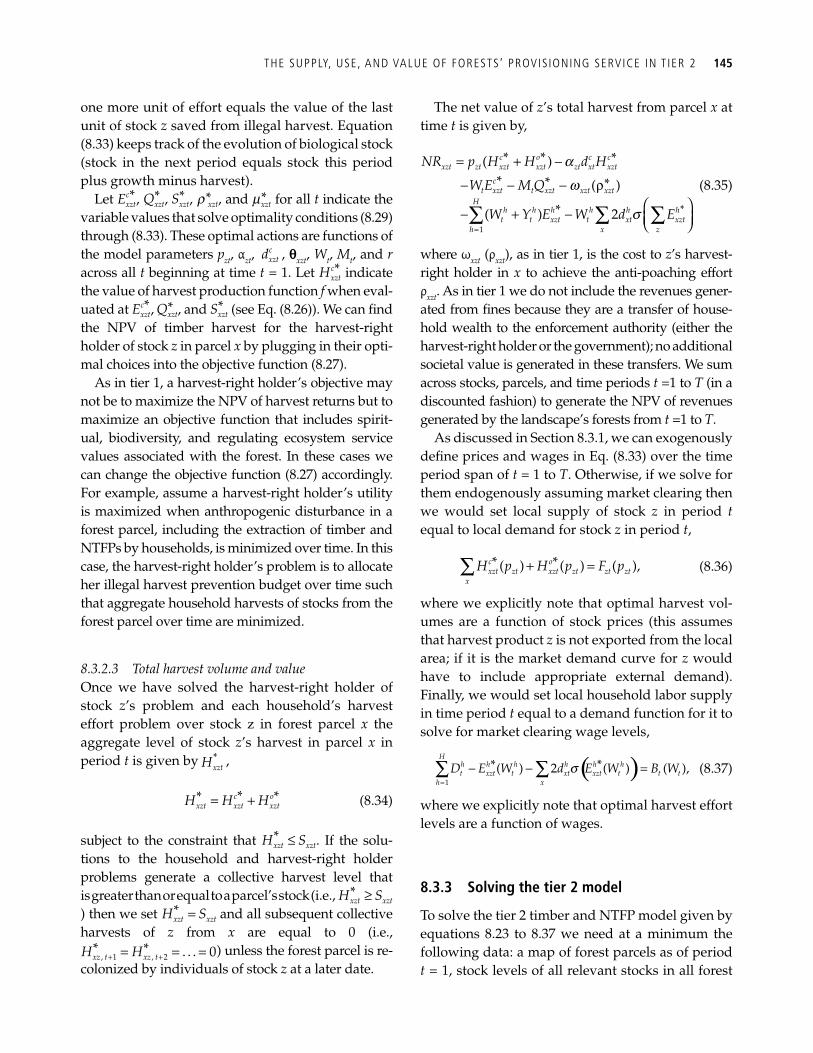
THE SUPPLY, USE, AND VALUE OF FORESTS’ PROVIS IONING SERVICE IN T IER 2 145
one more unit of effort equals the value of the last unit of stock z saved from illegal harvest. Equation (8.33) keeps track of the evolution of biological stock (stock in the next period equals stock this period plus growth minus harvest).
Let *cxztE , *
xztQ , *xztS , *xztr , and *
xztm for all t indicate the variable values that solve optimality conditions (8.29) through (8.33). These optimal actions are functions of the model parameters p zt , α zt ,
cxztd , q xzt , W t , M t , and r
across all t beginning at time t = 1. Let *cxztH indicate
the value of harvest production function f when eval-uated at *c
xztE , *xztQ , and *
xztS (see Eq. (8.26)). We can fi nd the NPV of timber harvest for the harvest-right holder of stock z in parcel x by plugging in their opti-mal choices into the objective function (8.27).
As in tier 1, a harvest-right holder’s objective may not be to maximize the NPV of harvest returns but to maximize an objective function that includes spirit-ual, biodiversity, and regulating ecosystem service values associated with the forest. In these cases we can change the objective function (8.27) accordingly. For example, assume a harvest-right holder’s utility is maximized when anthropogenic disturbance in a forest parcel, including the extraction of timber and NTFPs by households, is minimized over time. In this case, the harvest-right holder’s problem is to allocate her illegal harvest prevention budget over time such that aggregate household harvests of stocks from the forest parcel over time are minimized.
8.3.2.3 Total harvest volume and value Once we have solved the harvest-right holder of stock z ’s problem and each household’s harvest effort problem over stock z in forest parcel x the aggregate level of stock z ’s harvest in parcel x in period t is given by *
xztH ,
* ** c oxzt xzt xztH H H= + (8.34)
subject to the constraint that *xzt xztH S≤ . If the solu-
tions to the household and harvest-right holder problems generate a collective harvest level that is greater than or equal to a parcel’s stock (i.e., *
xzt xztH S≥ ) then we set *
xzt xztH S= and all subsequent collective harvests of z from x are equal to 0 (i.e., , 1 , 2
* * . . . 0xz t xz tH H+ += = = ) unless the forest parcel is re-colonized by individuals of stock z at a later date.
The net value of z ’s total harvest from parcel x at time t is given by,
a
w
s=
= + −
− − −⎛ ⎞− + − ⎜ ⎟⎝ ⎠∑ ∑ ∑
1
*
* * *( )* * *( )
*( ) 2
c o c cxzt zt xzt xzt zt xt xzt
ct xzt t xzt xzt xzt
Hh h h h h h
t t xzt t xt xzth x z
NR p H H d H
W E M Q
W Y E W d E
ρ (8.35)
where ω xzt (ρ xzt ), as in tier 1, is the cost to z ’s harvest-right holder in x to achieve the anti-poaching effort ρ xzt . As in tier 1 we do not include the revenues gener-ated from fi nes because they are a transfer of house-hold wealth to the enforcement authority (either the harvest-right holder or the government); no additional societal value is generated in these transfers. We sum across stocks, parcels, and time periods t =1 to T (in a discounted fashion) to generate the NPV of revenues generated by the landscape’s forests from t =1 to T .
As discussed in Section 8.3.1 , we can exogenously defi ne prices and wages in Eq. (8.33) over the time period span of t = 1 to T . Otherwise, if we solve for them endogenously assuming market clearing then we would set local supply of stock z in period t equal to local demand for stock z in period t ,
* *( ) ( ) ( ),c oxzt zt xzt zt zt zt
x
H p H p F p+ =∑ (8.36)
where we explicitly note that optimal harvest vol-umes are a function of stock prices (this assumes that harvest product z is not exported from the local area; if it is the market demand curve for z would have to include appropriate external demand). Finally, we would set local household labor supply in time period t equal to a demand function for it to solve for market clearing wage levels,
( )=
− − =∑ ∑H
h h h h h ht xzt t xt xzt t t t
h x
D E W d E W B W1
**( ) 2 ( ) ( ),s (8.37)
where we explicitly note that optimal harvest effort levels are a function of wages.
8.3.3 Solving the tier 2 model
To solve the tier 2 timber and NTFP model given by equations 8.23 to 8.37 we need at a minimum the following data: a map of forest parcels as of period t = 1, stock levels of all relevant stocks in all forest
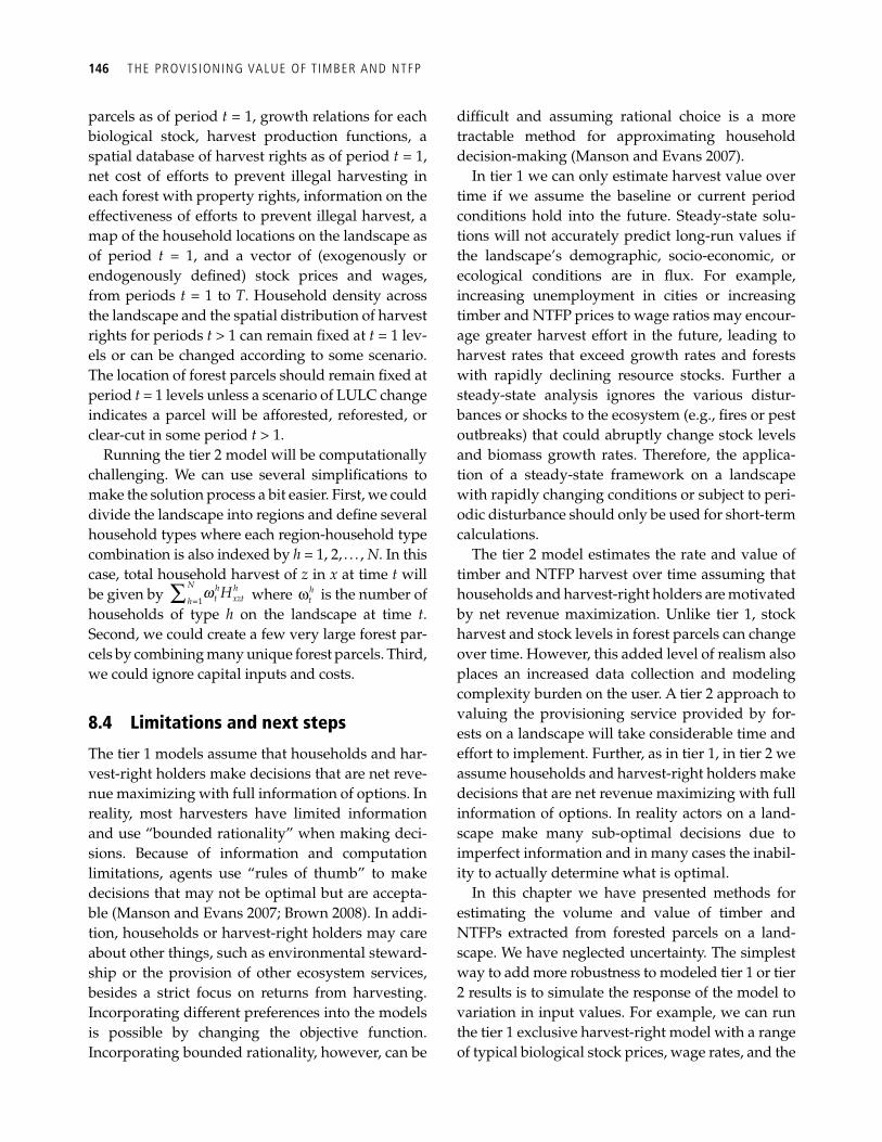
146 THE PROVIS IONING VALUE OF T IMBER AND NTFP
parcels as of period t = 1, growth relations for each biological stock, harvest production functions, a spatial database of harvest rights as of period t = 1, net cost of efforts to prevent illegal harvesting in each forest with property rights, information on the effectiveness of efforts to prevent illegal harvest, a map of the household locations on the landscape as of period t = 1, and a vector of (exogenously or endogenously defi ned) stock prices and wages, from periods t = 1 to T . Household density across the landscape and the spatial distribution of harvest rights for periods t > 1 can remain fi xed at t = 1 lev-els or can be changed according to some scenario. The location of forest parcels should remain fi xed at period t = 1 levels unless a scenario of LULC change indicates a parcel will be afforested, reforested, or clear-cut in some period t > 1.
Running the tier 2 model will be computationally challenging. We can use several simplifi cations to make the solution process a bit easier. First, we could divide the landscape into regions and defi ne several household types where each region-household type combination is also indexed by h = 1, 2, . . . , N . In this case, total household harvest of z in x at time t will be given by 1
N h ht xzthHw
=∑ where htω is the number of
households of type h on the landscape at time t . Second, we could create a few very large forest par-cels by combining many unique forest parcels. Third, we could ignore capital inputs and costs.
8.4 Limitations and next steps
The tier 1 models assume that households and har-vest-right holders make decisions that are net reve-nue maximizing with full information of options. In reality, most harvesters have limited information and use “bounded rationality” when making deci-sions. Because of information and computation limitations, agents use “rules of thumb” to make decisions that may not be optimal but are accepta-ble ( Manson and Evans 2007 ; Brown 2008 ). In addi-tion, households or harvest-right holders may care about other things, such as environmental steward-ship or the provision of other ecosystem services, besides a strict focus on returns from harvesting. Incorporating different preferences into the models is possible by changing the objective function. Incorporating bounded rationality, however, can be
diffi cult and assuming rational choice is a more tractable method for approximating household decision-making ( Manson and Evans 2007 ).
In tier 1 we can only estimate harvest value over time if we assume the baseline or current period conditions hold into the future. Steady-state solu-tions will not accurately predict long-run values if the landscape’s demographic, socio-economic, or ecological conditions are in fl ux. For example, increasing unemployment in cities or increasing timber and NTFP prices to wage ratios may encour-age greater harvest effort in the future, leading to harvest rates that exceed growth rates and forests with rapidly declining resource stocks. Further a steady-state analysis ignores the various distur-bances or shocks to the ecosystem (e.g., fi res or pest outbreaks) that could abruptly change stock levels and biomass growth rates. Therefore, the applica-tion of a steady-state framework on a landscape with rapidly changing conditions or subject to peri-odic disturbance should only be used for short-term calculations.
The tier 2 model estimates the rate and value of timber and NTFP harvest over time assuming that households and harvest-right holders are motivated by net revenue maximization. Unlike tier 1, stock harvest and stock levels in forest parcels can change over time. However, this added level of realism also places an increased data collection and modeling complexity burden on the user. A tier 2 approach to valuing the provisioning service provided by for-ests on a landscape will take considerable time and effort to implement. Further, as in tier 1, in tier 2 we assume households and harvest-right holders make decisions that are net revenue maximizing with full information of options. In reality actors on a land-scape make many sub-optimal decisions due to imperfect information and in many cases the inabil-ity to actually determine what is optimal.
In this chapter we have presented methods for estimating the volume and value of timber and NTFPs extracted from forested parcels on a land-scape. We have neglected uncertainty. The simplest way to add more robustness to modeled tier 1 or tier 2 results is to simulate the response of the model to variation in input values. For example, we can run the tier 1 exclusive harvest-right model with a range of typical biological stock prices, wage rates, and the
L IMITATIONS AND NEXT STEPS 147
interest rates to approximate the range in potential steady-state exclusive harvest volumes and values (see Section 8.2.4). We can also explore how sensitive tier 1 and 2 modeled results are to changes in func-tional relationships, such as harvest rates, growth rates, and expected fi nes for illegal harvesting. For example, climate change could change stock growth rates in forests over time ( Aber et al. 2001 ). We could explore the ramifi cations of such changes on harvest volumes and values ( Irland et al. 2001 ) by varying G ( S ) for all relevant stocks in a manner that is con-sistent with climate change estimates.
We can also add structural uncertainty and risk to the model. For example, we could assume a house-hold harvester will not always fi nd wage employ-ment while not harvesting. In this case we could make the prospect of fi nding wage work probabilis-tic. And we could add the risk of forest disturbances, such as fi re or disease ( Dale et al. 2001 ), into stocks’ equations of motion ( Sohngen and Sedjo 1996 ). It would be useful then to map out how the inclusion of risk parameters in the model causes it to deviate from deterministic solutions.
In addition to examining uncertainty, it is impor-tant to consider the negative impacts that stock har-vests can have on other ecosystem processes and services (e.g., Luoga et al. 2000 ). If we can modify LULC defi nitions according to the harvest volumes and stocks calculated in the models above then the ramifi cations of predicted harvests can be incorpo-rated into almost every other ecosystem service model described in this book. For example, if the water quality function is a function of forest type (degraded versus intact) then harvest volumes and stocks as calculated in the models above will affect water quality model output. Alternatively, we can modify other ecosystem service model outputs ex post with results from this model. For example, suppose we have data on the carbon storage potential of a rela-tively intact forest type. If modeled harvest volumes in a parcel with this forest type are high then the par-cel’s predicted carbon storage in the aboveground and belowground biomass pools could be scaled downward to refl ect modeled stock loss in the forest.
Finally, a major source of global land-use change is the clearing of forests to open land for agricul-tural or residential use ( Repetto and Gillis 1988 ). Here we value harvests in forests that begin and, for
the most part, remain in forest from time t = 1 to T (if it is completely drained of all of its stocks by time T then it is no longer a forest); these are not models of land-use change. To model such changes we rely on LULC change scenarios that are created with land-use change models. These models can provide output that would be useful to such LULC change models. Specifi cally, estimates of the NPV of forest harvest from forests across a landscape along with estimates of the NPV of returns from alternative uses of forested areas could be used by LULC change models to determine which forest parcels would most likely remain forested.
References
Aber, J., Neilson, R. P., McNulty, S., et al . (2001). Forest processes and global environmental change: Predicting the effects of individual and multiple stressors. Bioscience, 51 , 735–51.
Adger, W. N., and Luttrell, C. (2000). Property rights and the utilisation of wetlands. Ecological Economics, 35 , 75–89.
Arnold, J. E. M., and Pérez, M. R. (2001). Can non-timber forest products match tropical forest conservation and development objectives? Ecological Economics, 39 , 437–47.
Barbier, E. B., and Burgess, J. C. (2001). The economics of tropical deforestation. Journal of Economic Surveys, 15 , 413–33.
Bawa, K. S., and Seidler, R. (1998). Natural forest manage-ment and conservation of biodiversity in tropical for-ests. Conservation Biology, 12 , 46–55.
Belcher, B., Ruíz-Pérez, M., and Achdiawan, R. (2005). Global patterns and trends in the use and management of commercial NTFPs: Implications for livelihoods and conservation. World Development, 33 , 1435–52.
Birdyshaw, E., and Ellis, C. (2007). Privatizing an open-access resource and environmental degradation. Ecological Economics, 61 , 469–77.
Boot, R. G. A., and Gullison, R. E. (1995). Approaches to developing sustainable extraction systems for tropical forest products. Ecological Applications, 5 , 896–903.
Brown, D. R. (2008). A spatiotemporal model of shifting cultivation and forest cover dynamics. Environment and Development Economics, 13 , 643–71.
Browning, M., and Crossley, T. F. (2001). The life-cycle model of consumption and saving. Journal of Environmental Perspectives, 15 , 3–22.
Clark, C. W. (1990). Mathematical bioeconomics: the optimal management of renewable resources . Wiley, New York.
148 THE PROVIS IONING VALUE OF T IMBER AND NTFP
Conrad, J. M., and Clark, C. W. (1987). Natural resource eco-nomics: notes and problems . Cambridge University Press, Cambridge.
Dale, V. H., Joycel, L. A., McNulty, S., et al . (2001). Climate change and forest disturbances. Bioscience, 51 , 723–34.
Damania, R., Milner-Gulland, E. J., and Crookes, D. J. (2005). A bioeconomic analysis of bushmeat hunting. Proceedings of the Royal Society B-Biological Sciences, 272 , 259–66.
Dauber, E., Fredericksen, T.S. and Peña, M. (2005). Sustainability of timber harvesting in Bolivian tropical forests, Forest Ecology and Management, 214 , 294–304.
Engel, S., and Lopez, R. (2008). Exploiting common resources with capital-intensive technologies: The role of external forces. Environment and Development Economics, 13 , 565–89.
FAO. (2006). Global forest resources assessment 2005: progress toward sustainable forest management . United Nations Food and Agricultural Organization, Rome.
Feder, G., and Feeny, D. (1991). Land tenure and property rights: Theory and implications for development policy. World Bank Economic Review, 5 , 135–53.
Gordon, H. S. (1954). The economic theory of a common-property resource: The fi shery. Journal of Political Economy, 62 , 124.
Guariguata, M. R., Cronkleton, P., Shanley, P., et al . (2008). The compatibility of timber and non-timber forest prod-uct extraction and management. Forest Ecology and Management, 256 , 1477–81.
Hyde, W. F. (2003). Economic considerations on instru-ments and institutions. In Y. Dube and F. Schmithusen, Eds., Cross-sectoral policy impacts between forestry and other sectors , FAO Forestry Paper 142. Rome.
Irland, L.C., Adams, D., Alig, R., et al. (2001). Assessing socioeconomic impacts of climate change on US forests, wood-product markets, and forest recreation. Bioscience, 51 , 753–64.
Justice, C., Wilkie, D., Zhang, Q., et al . (2001). Central African forests, carbon and climate change. Climate Research, 17 , 229–46.
Larson, B., and Bromley, D. (1990). Property rights, exter-nalities, and resource degradation: Locating the tragedy. Journal of Development Economics, 33 , 235–62.
Lopez-Feldman, A., and Wilen, J. E. (2008). Poverty and spatial dimensions of non-timber forest extraction. Environment and Development Economics, 13 , 621–42.
Luoga, E. J., Witkowski, E. T. F., and Balkwill, K. (2000). Economics of charcoal production in miombo wood-lands of eastern Tanzania: Some hidden costs associated with commercialization of the resources. Ecological Economics, 35 , 243–57.
Luoga, E. J., Witkowski, E. T. F. and Balkwill, K. (2002). Harvested and standing wood stocks in protected and
communal miombo woodlands of eastern Tanzania. Forest Ecology and Management, 164 , 15–30.
Luoga, E. J., Witkowski, E. T. F., and Balkwill, K. (2005). Land cover and use changes in relation to the institu-tional framework and tenure of land and resources in Eastern Tanzania miombo woodlands. Environment, Development and Sustainability, 7 , 71–93.
Maass, J., Balvanera, P., Castillo, A., et al . (2005). Ecosystem services of tropical dry forests: Insights from long-term ecological and social research on the Pacifi c Coast of Mexico. Ecology and Society, 10 , 17.
Manson, S. M., and Evans, T. (2007). Agent-based mode-ling of deforestation in southern Yucatan, Mexico, and reforestation in the Midwest United States. Proceedings of the National Academy of Sciences of the United States of America, 104 , 20678–83.
Milner-Gulland, E. J., and Clayton, L. (2002). The trade in babirusas and wild pigs in North Sulawesi, Indonesia. Ecological Economics, 42 , 165–83.
Monela, G. C., O’Kting’ati, A., and Kiwele, P. M. (1993). Socio-economic aspects of charcoal consumption and environmental consequences along the Dar-es-Salaam–Morogoro highway, Tanzania. Forest Ecology and Management, 58 , 249–58.
Nagendra, H. (2002). Tenure and forest conditions: Community forestry in the Nepal Terai. Environmental Conservation, 29 , 530–9.
Nagendra, H., Karmacharya, M., and Karna, B. (2005). Evaluating forest management in Nepal: Views across space and time. Ecology and Society , 10 , 24.
Ndangalasi, H. J., Bitariho, R., and Dovie, D. B. K. (2007). Harvesting of non-timber forest products and implica-tions for conservation in two montane forests of East Africa. Biological Conservation, 134 , 242–50.
Núñez, D., Nahuelhual, L., and Oyarzún, C. (2006). Forests and water: The value of native temperate forests in sup-plying water for human consumption. Ecological Economics, 58 , 606–16.
Parker, D. C., Manson, S. M., Janssen, M. A., et al . (2003). Multi-agent systems for the simulation of land-use and land-cover change: A review. Annals of the Association of American Geographers, 93 , 314–37.
Pattanayak, S. K., and Sills, E. O. (2001). Do tropical forests provide natural insurance? The microeconomics of non-timber forest product collection in the Brazilian Amazon. Land Economics, 77 , 595–612.
Peters, C. M., Gentry, A. H., and Mendelsohn, R. O. (1989). Valuation of an Amazonian rainforest. Nature, 339 , 655–6.
Pinard, M. A. and Putz, F. E. (1996). Retaining forest bio-mass by reducing logging damage. Biotropica, 28 , 278–95.
L IMITATIONS AND NEXT STEPS 149
Polasky, S., Nelson, E., Camm, J., et al . (2008). Where to put things? Spatial land management to sustain biodiver-sity and economic returns. Biological Conservation, 141 , 1505–24.
Repetto, R. C. and Gillis, M., Eds. (1988). Public policies and the misuse of forest resources . Cambridge University Press, New York.
Ricketts, T. H. (2004). Tropical forest fragments enhance pollinator activity in nearby coffee crops. Conservation Biology, 18 , 1262–71.
Scholes, R. J. (1996). Miombo woodlands and carbon seques-tration. In B.M. Campbell, Ed., The Miombo in transition: woodlands and welfare in Africa . Centre for International Forestry Research (CIFOR), Bogor, Indonesia.
Silvertown, J. (2004). Sustainability in a nutshell. Trends in Ecology and Evolution, 19 , 276–8.
Sinha, A., and Brault, S. (2005). Assessing sustainability of nontimber forest product extractions: How fi re affects sustainability. Biodiversity and Conservation, 14 , 3537–63.
Sohngen, B. L., and Sedjo, R. (1996). A comparison of timber models for use in public policy analysis . Resources for the Future, Washington, DC.
Sohngen, B., and Brown, S. (2006). The infl uence of con-version of forest types on carbon sequestration and other ecosystem services in the South Central United States. Ecological Economics, 57 , 698–708.
Swallow, B. M., and Bromley, D. W. (1995). Institutions, governance and incentives in common property regimes
for African rangelands. Environmental and Resource Economics, 6 , 99–118.
Tahvonen, O., and Salo, S. (1999). Optimal forest rotation with in situ preferences. Journal of Environmental Economics and Management , 37 , 106–28.
Thwaites, R., De Lacy, T., Li, Y. H., et al . (1998). Property rights, social change, and grassland degradation in Xilingol Biosphere Reserve, Inner Mongolia, China. Society and Natural Resources, 11 , 319–38.
Ticktin, T. (2004). The ecological implications of harvest-ing non-timber forest products. Journal of Applied Ecology, 41 , 11–21.
Vedeld, P., Angelsen, A., Bojö, J., et al . (2004). Forest envi-ronmental incomes and the rural poor. Forest Policy and Economics, 9 , 869–79.
Wikramanayake, E., Dinerstein, E., Loucks, C., et al . (2001). Terrestrial ecoregions of the Indo-Pacifi c: a conservation assessment . Island Press, Washington, DC.
Wikramanayake, E., McKnight, M., Dinerstein, E., et al . (2004). Designing a conservation landscape for tigers in human-dominated environments. Conservation Biology , 18 , 839–44.
Williams, M. (2003). Deforesting the earth: from prehis-tory to global crisis . University of Chicago Press, Chicago.
World Wildlife Fund. (2006). Demographic analysis: Terai Arc Landscape—Nepal . World Wildlife Fund, Nepal Program, Kathmandu, Nepal.
150
CHAPTER 9
Provisioning and regulatory ecosystem service values in agriculture Erik Nelson, Stanley Wood, Jawoo Koo, and Stephen Polasky
9.1 Introduction
Ecological processes combine with human labor and inputs such as fertilizer and irrigation to produce agricultural goods used for food, fodder, fi ber, and fuel. The ecosystem processes that infl uence agricul-tural production include soil retention, pest control, nutrient recycling in the soil, water capture, and ani-mal pollination (e.g., Wood et al. 2005 ; Swinton et al. 2007 ). By contributing to agricultural productivity, these processes become ecosystem services. The value of these services can be proxied by their con-tributions to the monetary value of commercial agri-cultural production or the utility value of subsistence agricultural production. Because of the agricultural sector’s importance in regional economic develop-ment, especially in developing countries ( Byerlee et al. 2009 ), estimating the potential agricultural out-put on as yet unconverted natural habitat may also be of interest because it represents production value foregone.
There is a range of approaches for estimating the value of agricultural production and the contribu-tion that particular ecosystem services make to it. These approaches are largely differentiated by their geographical scale, the degree to which they incor-porate behavioral responses by farmers to changes in biophysical and market variables, and the extent to which they track the impacts of agricultural pro-duction on ecological processes.
Landscape-scale, regional, or global agricultural models typically assess expected or potential crop
yield as a function of climate, soil type, input use intensity, and, sometimes, basin-wide water resource availability (e.g., Fischer et al. 2002 ; Bruinsma 2003 ; Rosegrant et al. 2005 ; Nelson et al. 2009 ). These broader-scale models do not provide an explicit framework for examining changes in farmer behavior and profi ts due to policy, price, or environmental changes. Nor, in general, do they assess the ecological consequences of agricultural production (e.g., Naidoo and Ricketts 2006 ; Cassman and Wood 2005 ).
Conversely, in farm-level models, farmers are usually represented as making crop and production method choices that are expected to maximize their economic profi ts. In farm-level models, the value of a change in an ecosystem service input is equal to the change in profi t it induces. For example, the value of an increased supply of irrigation water on a farm can be estimated by the change in farm prof-its due to the additional water volume. Farm-scale models can be applied to understand how farmers might respond to taxes or subsidies (e.g., Just and Antle 1990 ; Wu et al. 2004 ; Wossink and Swinton 2007 ) and—if the models relate agriculture produc-tion to environmental impact—how they might respond to payments for ecosystem services (e.g., Holden 2005 ; Antle and Valdivia 2006 ; Antle et al. 2007 ). Further, farm-level models can be used in conjunction with commodity demand models to assess the impact of agricultural policies and changes in ecosystem service inputs on commodity supply and food prices (e.g., Gillig et al. 2004 ;
DEFINING AGRICULTURAL SCENARIOS 151
Zilberman et al. 2008 ). When appropriate, farm models can assume alternative optimization strate-gies among farmers, such as risk minimizing behav-ior by subsistence households in developing countries. In many cases subsistence farmers adopt production systems that minimize food insecurity risk rather than those that maximize expected prof-its (e.g., Dercon 1996 ; Kinsey et al. 1998 ; Kandlikar and Risbey 2000 ; Luckert et al. 2000 ).
In this chapter we propose an approach to assess and map the expected value of agricultural produc-tion and the value added by ecosystem services at the landscape scale. As in other chapters, we present the approach in two tiers that differ by information needs, data availability, model sophistication, out-put scope, and treatment of time. In tier 1, we use broad-scale crop production, yield, and cost maps along with crop prices to assess the value of agricul-tural production across coarser time steps. When possible, we also assess the contributions of sup-porting and regulating services to output value. The tier 1 approach can be implemented with exist-ing maps of agricultural production or productivity (e.g. crop yield) or those we create. In tier 1, our ability to model farmer response to market or envi-ronmental change is limited.
In tier 2, we model agricultural production from a more detailed perspective and consider the deci-sions that farmers make over fi ner time steps. Unlike tier 1, optimum spatial patterns of agricul-tural production across the landscape and changes in agricultural output and input prices can be deter-mined within the tier 2 model. We also discuss methods for evaluating landscape-scale ecological consequences of agricultural land use, including the emissions of greenhouse gases (GHGs) as well as water and nutrient uptake.
9.2 Defi ning agricultural scenarios
Our starting point is to generate alternative sce-narios of land use/land cover (LULC) pertinent to agricultural productivity. For each LULC scenario we need to specify the crops grown and the method of production on each agricultural parcel in the landscape, as well as crop prices and crop-production costs. As with all other ecosystem service models in this book, the landscape is
divided into parcels, indexed by x = 1, 2, . . . , X , where a parcel can be any geographic unit, includ-ing a polygon, grid cell, or hexagon. Let the har-vested area (in hectares) of crop c ( c = 1, 2, . . . , C ) grown under production system k ( k = 1, 2, . . . , K ) in parcel x over some time period (e.g., a growing season, the whole year) be given by A ckx . In this formulation a crop can represent a single crop (e.g., maize), a crop mix (e.g., an intercrop of maize and beans), a crop rotation (e.g., maize-soybeans), or a livestock type (e.g., cattle). Let p c be the per-unit output price of crop c . Let s ckx be the ha –1 costs incurred by the farmers in parcel x when produc-ing and delivering crop c to market under produc-tion system k .
In subsistence agriculture crops may be pro-duced and consumed within a household and not sold in a market, in which case we may not observe a market price. In these cases we will need to use other proxies for value. For example, subsistence agriculture prices could be based on measures of the caloric, protein, or micronutrient value of crops. Costs in subsistence agriculture could be expressed in terms of total wages foregone from working in another economic sector. From an ecosystem serv-ice perspective, it is also possible to express the “price” of farm outputs in terms of appropriated ecosystem services (e.g., water consumed or nutri-ent extracted; see Section 9.5 ) rather than in mone-tary terms.
Production systems can be differentiated on the basis of production outputs, technologies and prac-tices utilized, and use of inputs (e.g., fl ood irriga-tion, drip irrigation, rainfed commercial, or slash-and-burn subsistence using, say, inorganic fertilizer and genetically modifi ed seeds). Production system defi nitions can be general or quite specifi c. Examples of general production sys-tems come from the Global Agro-Ecological Zone (GAEZ) datasets where a combination of a technol-ogy/input use category (low, medium, and high; see Fisher et al. 2002) and a binary variable that indi-cates whether a system is irrigated or rainfed defi nes a production system. Alternatively, a production system can be defi ned with an exact specifi cation of the fertilizer, pesticide, irrigation water, and other inputs applied over the course of a growing season and a precise defi nition of production methods and
152 PROVIS IONING AND REGULATORY ECOSYSTEM SERVICE VALUES IN AGRICULTURE
technology used. In tier 2 the timing of input use is also part of a production system defi nition.
If the agricultural production map being evalu-ated is from the current or a past year then current or past commodity prices and production costs can be used. If we are using a published agricultural production forecast we can use the forecast's accompanying prices (e.g., the USDA Long-term Projections, the OECD-FAO Agricultural Outlooks); otherwise we will have to use some other method to determine prices. In tier 2 we can exogenously defi ne all scenario components, as in tier 1, or with additional data and analytical effort we can deter-mine crop-production system choices endogenously by assuming profi t maximizing or other farmer behavior under a given set of prices. We can extend the scenario creation process even further in tier 2 by determining all prices endogenously under the assumption of market equilibrium.
9.3 Tier 1
9.3.1 The supply and use of agricultural production
First we need to gather information on the potential or expected yield for crop c grown with production system k on parcel x , denoted as Y c k x . In our ecosys-tem service taxonomy, Y c k x represents the measure of the land’s ability to supply the ecosystem service of agricultural production at point x . For agricul-tural production, ecosystem service supply and use (as defi ned in Chapter 3 ) are the same. Expected yield is a function of a set of biophysical character-istics such as soil quality, weather, and animal pol-linator abundance, and a set of managed inputs such as fertilizer and irrigation water, as well as the production system itself. Formally, Y ckx can be repre-sented as,
ckxY = ( ),c x kg q j . (9.1)
where g c is crop c ’s yield function and is explained by q x , the vector of biophysical characteristics or ecological processes in parcel x , and j k , the vector of managed input levels used in production system k .
Ideally we will be able to fi nd completely speci-fi ed functions g c ( q x , j k ) for all potential values of
q x, j k . This would allow us to estimate the change in yield with respect to any change in biophysical characteristics or managed inputs, including many ecosystem services. However, if such yield func-tions cannot be found we suggest two methods for deriving information about yield across the land-scape: fi rst, using existing yield “lookup” tables or maps and, second, estimating a yield function with observed data.
Prepared maps of Y c k x can be found for major crops for many areas in the world. For example, the USDA-NRCS (2001) has published observed yields of various crops in each US county as a function of soil capability class (a parameter in q ) under typical management practices. These county-level lookup tables of yield as a function of soil class have been used in conjunction with the behavioral assump-tion of profi t maximization to predict land-use deci-sions across the USA in response to a hypothetical carbon sequestration payment policy ( Lubowski et al. 2006 ) and to measure the opportunity costs of biodiversity conservation in the Willamette Basin, Oregon, U.S ( Polasky et al. 2008 ). Similarly, Vera-Diaz (2008) has calculated expected soybean yields (and net economic returns) across a gridded map of Brazil. For the GAEZ project ( Fischer et al. 2002 ), global maps of Y c k x were generated with yield mod-els explained by general production management categories, ecological characteristics and processes, and climate. Naidoo and Iwamura ( 2007 ) used expected yield maps from GAEZ to plot the expected opportunity costs of conservation in forest ecosys-tems and across the globe.
While these ready-made yield maps may be suffi -cient for the purposes of some applications, they will not allow us to answer several questions of interest. For one, static maps of yield are not sensitive to changes in ecological processes or climate. Second, these yield maps may ignore the impacts of atypical conditions on yields, such as droughts, fl oods, major pest and pathogen infestations, and future climate change. Third, some existing yield maps are com-posed of large spatial units, masking the heterogene-ity in local farming systems and ecological characteristics and processes (e.g., a parcel in a GAEZ map covers approximately 10 000 hectares).
As an alternative, we can use statistical techniques to estimate a relationship between expected yields
T IER 1 153
and input management, ecological processes, and environmental conditions. This estimation process requires contemporaneous data on crop yield, Y c , agricultural input use, j , and biophysical data, q , from enough sites on a landscape that statistically robust yield functions can be estimated with regres-sion techniques (see Pender 2005 for a review of regression techniques used to build crop yield func-tions). It is also useful to have data from a number of growing seasons so variations in climate and atypi-cal events such as drought or pest outbreaks can be refl ected in estimated yield functions.
The advantage of the statistical approach is that it allows us to build yield functions that are explained by input and biophysical data we can collect. If these inputs include ecological processes then we can predict changes in agriculture output due to a change in such inputs. For example, if we build yield functions that are explained by crop access to water during the growing season then we could estimate the impact of a crop-production system only receiving half of its prescribed irrigation water needs. Drawbacks associated with the statistical technique include the need for a large data set and the necessary time and expertise to assemble and analyze the data. In addition, the confi dence in pre-dicted yields decreases when estimated yield func-tions are applied with explanatory variable levels that differ signifi cantly from those used to estimate the yield function (e.g., predicting yield on a land-scape signifi cantly affected by future climate change with functions estimated with data from historic climate patterns).
9.3.2 The value of agriculture’s provisioning services
Maps of crop-production areas, expected yields, and expected costs can be combined with crop price databases to produce a map of expected net agricul-tural production value. In standard parlance used in this book (see Chapter 3 ), crop production in a parcel represents the supply and use of agriculture’s provisioning service in that parcel, while the net value of this production represents the use value ( Bockstael et al. 2000 ).
Expected net production value in parcel x for a growing season, AV x , is found by multiplying the
harvested area of each crop-production system in the parcel over the course of the growing season by its expected ha –1 revenue less its ha –1 production and transportation costs,
1 1
ˆ( ).K C
x ckx c ckx ckxk c
AV A p Y s= =
= −∑∑ (9.2)
If there is a price premium for crops grown under certain conditions (e.g., organic apples versus con-ventionally grown apples) then such price effects can be included in Eq. (9.2) by stratifying crop price by production system, p ck . Prices and costs should not include production subsidies or cost share pay-ments from a government even if they are payments for ecosystem services. We are interested in assess-ing the net social value of agricultural production in this model; taxes and subsidy payments are trans-fers of wealth from one group in society to another, and not a creation of value (the societal losses cre-ated by taxation ineffi ciencies are beyond the scope of this chapter). The benefi ts of subsidized environ-mentally friendly production choices, for example, cleaner water, less soil carbon emissions, are accounted for when we model these specifi c services.
Easily accessible and reliable estimates of pro-duction costs for most crop-production systems grown around the world do not exist ( Naidoo and Iwamura 2007 ). USDA-ERS (2009) estimates typi-cal ha –1 production costs for most major commodi-ties grown under best management practices in the USA. Cost estimates can also be generated using published budget sheets that itemize the cost of most or all inputs used in a production process (e.g., Polasky et al. 2008 ). The cost of trans-porting produce to a market can be calculated with road network data and information on per-unit transportation costs. However, in many cases cost data will need to be gathered from local experts. If the cost term is dropped from Eq. (9.2), then AV x will measure the gross agricultural production value in parcel x rather than agriculture’s provi-sioning value. Only if production costs are fairly uniform over every combination of c , k and x on the landscape will gross agricultural production value give a reliable picture of the spatial variation in the net value of agriculture across the landscape.
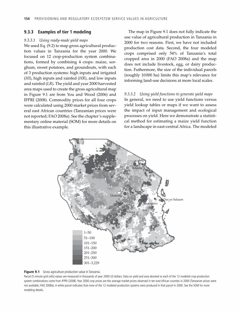
154 PROVIS IONING AND REGULATORY ECOSYSTEM SERVICE VALUES IN AGRICULTURE
9.3.3 Examples of tier 1 modeling
9.3.3.1 Using ready-made yield maps W e used Eq. (9.2) to map gross agricultural produc-tion values in Tanzania for the year 2000. We focused on 12 crop-production system combina-tions, formed by combining 4 crops: maize, sor-ghum, sweet potatoes, and groundnuts, with each of 3 production systems: high inputs and irrigated ( HI ), high inputs and rainfed ( HR ), and low inputs and rainfed ( LR ). The yield and year 2000 harvested area maps used to create the gross agricultural map in Figure 9.1 are from You and Wood ( 2006 ) and IFPRI (2008). Commodity prices for all four crops were calculated using 2000 market prices from sev-eral east African countries (Tanzanian prices were not reported; FAO 2008a). See the chapter’s supple-mentary online material (SOM) for more details on this illustrative example.
The map in Figure 9.1 does not fully indicate the use value of agricultural production in Tanzania in 2000 for two reasons. First, we have not included production cost data. Second, the four modeled crops comprised only 54% of Tanzania’s total cropped area in 2000 (FAO 2008a) and the map does not include livestock, egg, or dairy produc-tion. Futhermore, the size of the individual parcels (roughly 10 000 ha) limits this map’s relevance for informing land-use decisions at more local scales.
9.3.3.2 Using yield functions to generate yield maps In general, we need to use yield functions versus yield lookup tables or maps if we want to assess the impact of input management and ecological processes on yield. Here we demonstrate a statisti-cal method for estimating a maize yield function for a landscape in east-central Africa. The modeled
Arusha
Dodoma
Iringa
Dar es SalaamMorogoro
1–5051–100101–150151–200201–250251–300301–3,229
Figure 9.1 Gross agriculture production value in Tanzania.Parcel (5 minute grid cells) values are measured in thousands of year 2000 US dollars. Data on yield and area devoted to each of the 12 modeled crop-production system combinations come from IFPRI (2008). Year 2000 crop prices are the average market prices observed in ten east African counties in 2000 (Tanzanian prices were not available; FAO 2008a). A white parcel indicates that none of the 12 modeled production systems were produced in that parcel in 2000. See the SOM for more modeling details.
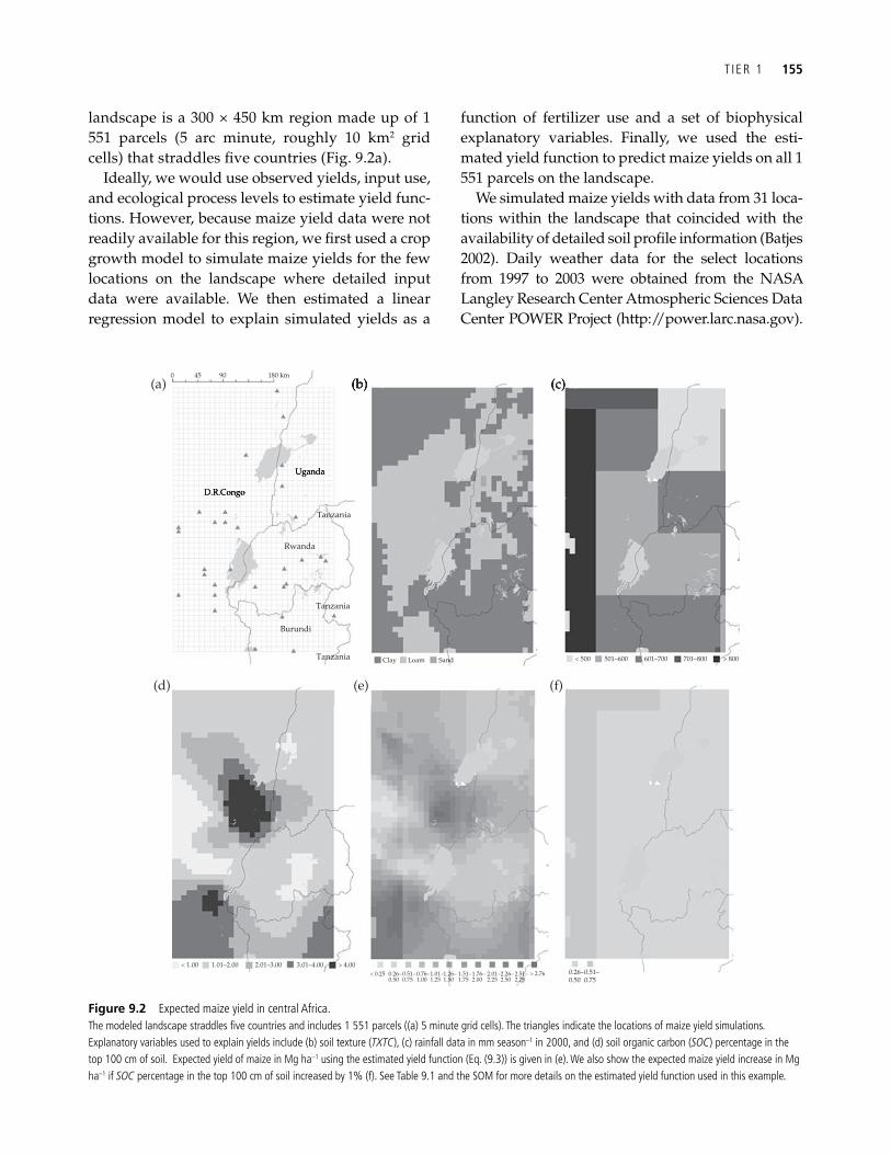
T IER 1 155
landscape is a 300 × 450 km region made up of 1 551 parcels (5 arc minute, roughly 10 km 2 grid cells) that straddles fi ve countries ( Fig. 9.2a ).
Ideally, we would use observed yields, input use, and ecological process levels to estimate yield func-tions. However, because maize yield data were not readily available for this region, we fi rst used a crop growth model to simulate maize yields for the few locations on the landscape where detailed input data were available. We then estimated a linear regression model to explain simulated yields as a
function of fertilizer use and a set of biophysical explanatory variables. Finally, we used the esti-mated yield function to predict maize yields on all 1 551 parcels on the landscape.
We simulated maize yields with data from 31 loca-tions within the landscape that coincided with the availability of detailed soil profi le information ( Batjes 2002 ). Daily weather data for the select locations from 1997 to 2003 were obtained from the NASA Langley Research Center Atmospheric Sciences Data Center POWER Project (http://power.larc.nasa.gov).
(a) (b) (c)
D.R.Congo
Uganda
0 45 90 180 km
Tanzania
Rwanda
Tanzania
Burundi
Tanzania Clay < 500
< 1.00< 0.25 0.26–
0.500.51–0.75
0.76–1.00
1.01–1.25
1.26–1.50
1.51–1.75
1.76–2.00
2.01–2.25
2.26–2.50
0.26–0.50
0.51–0.75
2.51–2.75
1.01–2.00 2.01–3.00 3.01–4.00 > 4.00> 2.76
> 800501–600 601–700 701–800Loam Sand
(d) (e) (f)
Figure 9.2 Expected maize yield in central Africa.The modeled landscape straddles fi ve countries and includes 1 551 parcels ((a) 5 minute grid cells). The triangles indicate the locations of maize yield simulations. Explanatory variables used to explain yields include (b) soil texture ( TXTC ), (c) rainfall data in mm season –1 in 2000, and (d) soil organic carbon ( SOC ) percentage in the top 100 cm of soil. Expected yield of maize in Mg ha –1 using the estimated yield function (Eq. (9.3)) is given in (e). We also show the expected maize yield increase in Mg ha –1 if SOC percentage in the top 100 cm of soil increased by 1% (f). See Table 9.1 and the SOM for more details on the estimated yield function used in this example.
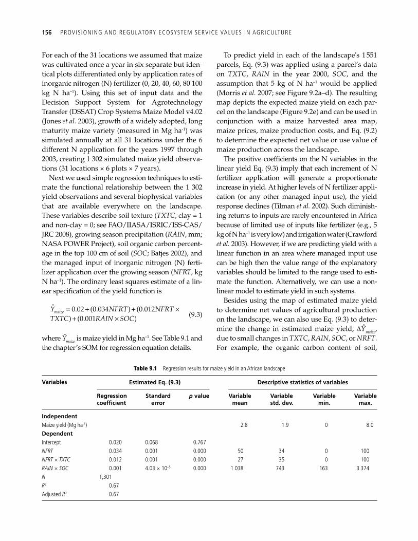
156 PROVIS IONING AND REGULATORY ECOSYSTEM SERVICE VALUES IN AGRICULTURE
For each of the 31 locations we assumed that maize was cultivated once a year in six separate but iden-tical plots differentiated only by application rates of inorganic nitrogen (N) fertilizer (0, 20, 40, 60, 80 100 kg N ha –1 ). Using this set of input data and the Decision Support System for Agrotechnology Transfer (DSSAT) Crop Systems Maize Model v4.02 ( Jones et al. 2003 ), growth of a widely adopted, long maturity maize variety (measured in Mg ha-1) was simulated annually at all 31 locations under the 6 different N application for the years 1997 through 2003, creating 1 302 simulated maize yield observa-tions (31 locations × 6 plots × 7 years).
Next we used simple regression techniques to esti-mate the functional relationship between the 1 302 yield observations and several biophysical variables that are available everywhere on the landscape. These variables describe soil texture ( TXTC , clay = 1 and non-clay = 0; see FAO/IIASA/ISRIC/ISS-CAS/JRC 2008), growing season precipitation ( RAIN , mm; NASA POWER Project), soil organic carbon percent-age in the top 100 cm of soil ( SOC ; Batjes 2002 ), and the managed input of inorganic nitrogen (N) ferti-lizer application over the growing season ( NFRT , kg N ha –1 ). The ordinary least squares estimate of a lin-ear specifi cation of the yield function is
ˆ 0.02 (0.034 ) (0.012
) (0.001 )maizeY NFRT NFRT
TXTC RAIN SOC= + + ×
+ × (9.3)
where Y m a i z e is maize yield in Mg ha –1 . See Table 9.1 and the chapter’s SOM for regression equation details.
To predict yield in each of the landscape's 1 551 parcels, Eq. (9.3) was applied using a parcel’s data on TXTC , RAIN in the year 2000, SOC , and the assumption that 5 kg of N ha –1 would be applied ( Morris et al. 2007 ; see Figure 9.2a –d). The resulting map depicts the expected maize yield on each par-cel on the landscape ( Figure 9.2e ) and can be used in conjunction with a maize harvested area map, maize prices, maize production costs, and Eq. (9.2) to determine the expected net value or use value of maize production across the landscape.
The positive coeffi cients on the N variables in the linear yield Eq. (9.3) imply that each increment of N fertilizer application will generate a proportionate increase in yield. At higher levels of N fertilizer appli-cation (or any other managed input use), the yield response declines ( Tilman et al. 2002 ). Such diminish-ing returns to inputs are rarely encountered in Africa because of limited use of inputs like fertilizer (e.g., 5 kg of N ha –1 is very low) and irrigation water ( Crawford et al. 2003 ). However, if we are predicting yield with a linear function in an area where managed input use can be high then the value range of the explanatory variables should be limited to the range used to esti-mate the function. Alternatively, we can use a non-linear model to estimate yield in such systems.
Besides using the map of estimated maize yield to determine net values of agricultural production on the landscape, we can also use Eq. (9.3) to deter-mine the change in estimated maize yield, D Y m a i z e , due to small changes in TXTC , RAIN , SOC , or NRFT . For example, the organic carbon content of soil,
Table 9.1 Regression results for maize yield in an African landscape
Variables Estimated Eq. (9.3) Descriptive statistics of variables
Regression coeffi cient
Standard error
p value Variable mean
Variable std. dev.
Variable min.
Variable max.
Independent Maize yield (Mg ha-1) 2.8 1.9 0 8.0 Dependent Intercept 0.020 0.068 0.767 NFRT 0.034 0.001 0.000 50 34 0 100 NFRT × TXTC 0.012 0.001 0.000 27 35 0 100 RAIN × SOC 0.001 4.03 × 10 –5 0.000 1 038 743 163 3 374 N 1,301 R 2 0.67 Adjusted R 2 0.67
T IER 1 157
SOC , refl ects an ecological process that infl uences yield and is controlled to some degree by LULC and land management choices on the landscape. Therefore, if the land could be managed such that SOC increased by 1 percentage point in a parcel then the expected change in maize yield in the par-cel would be equal to 0.001 × Rain (i.e., ∂ Y m a i z e ! ∂ S O C ; see Figure 9.2f ) In the next section we discuss in more depth a method for fi nding the service value provided by changes in ecological processes and conditions mediated by land-use and management choices.
9.3.4 Measuring the value of regulatory and supporting ecosystem service inputs to agriculture
A change in the supply of one or more ecological processes that is an input into agricultural pro-duction (i.e., an ecosystem service) can change the expected value of crop production. For example, the net value generated by pollinator-dependent crop can decline if the number of animal pollina-tors in the parcel declines. We can measure the value of the change in the regulating or supporting ecosystem service by comparing the expected net agricultural value before and after the change in the service. Let q i x
0 and q j x 0 be the initial level of eco-
system services i and j in parcel x and let q i x 1 and q j x
1 be the levels after the change. Using the tier 1 yield function, we can defi ne the pre- and post-change expected yields as Y c k x
0 = g c ( j k , q i x 0 , q j x
0 , q ~ x ) and Y c k x 1 = g c ( j k , q i x
1 , q j x 1 , q ~ x ) , respectively, where q ~ x defi nes
all ecological process inputs other than i and j . If appropriate, Y c k x 0 and Y c k x 1 can include even more changes in ecological processes and/or changes in managed inputs, such as water use for irrigation, defi ned with j i x
0 , j i x 1 , and j ~ x .
The change in the net value of agricultural output due to the change in the supply of ecosystem serv-ices i and j is given by ∆ AV x ,
K C
x ckx c ckx ckx ckx c ckx ckxk c
AV A p Y s A p Y s1 1 1 1 0 0 0 0
1 1
ˆ ˆ( ) ( ) .= =
⎡ ⎤∆ = − − −⎣ ⎦∑∑ (9.4)
where ∆ AV x can also be interpreted as the value of the joint change in ecosystem services i and j as expressed through agricultural production ( Shiferaw
et al. 2005 ; Swinton 2005 ). In this analysis we allow for the possibility that changes in ecosystem service inputs can lead to changes in other input use, crop-production system combination choices ( A c k x 1 ), pro-duction costs ( s c k x 1 ), and crop prices ( p c
1 ). For example, in response to honeybee declines, farmers of animal-pollinated crops are experimenting with ways to attract native pollinators to their fi elds ( Kremen et al. 2008 ). Such experimentation will change input costs and may change cropping practices. In tier 1 we do not include a formal method for determining changes in A ckx , p c , or s ckx in response to changes in ecological processes (we do in tier 2).
As presented here, we gain the greatest fl exibility in measuring the incremental value of regulatory or supporting services when we use yield functions that are continuous in their levels of provision. However, in some cases we can still approximate the impact of a change in the provision of a service on production values with expected yield maps, as we illustrate next.
9.3.4.1 An example of supporting service valuation: the case of surface water supply in Tanzania Surface water that fl ows across a landscape can con-tribute to agricultural production if it is used for irrigation. We used the map and datasets discussed in Section 9.3.3 and a version of Eq. (9.4) to estimate the decline in gross agricultural production value from a small reduction in surface water availability. Specifi cally, we estimated the percentage decline in year 2000 aggregate gross production values across Tanzania if 5% of the area of high input irrigated ( HI ) maize and sorghum found in each parcel could no longer be irrigated due to reduced surface water fl ow (see Figure 9.3 ). In this analysis we ignored irrigation via groundwater (such practice is rare in Tanzania, FAO 2008b) and we ignored sweet potato and groundnut systems because they are not typi-cally irrigated.
The maize and sorghum yield maps do not explic-itly include surface water supply for irrigation as an explanatory variable. Instead, we assumed that farmers of the hectares formerly in HI maize or sor-ghum production, in reaction to the loss in irriga-tion water, grew the same crops but under rainfed conditions with less intensive input use ( LR pro-duction). In many cases farmers without access to
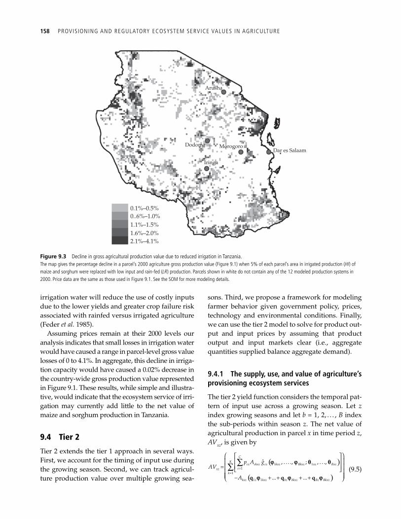
158 PROVIS IONING AND REGULATORY ECOSYSTEM SERVICE VALUES IN AGRICULTURE
irrigation water will reduce the use of costly inputs due to the lower yields and greater crop failure risk associated with rainfed versus irrigated agriculture (Feder et al. 1985).
Assuming prices remain at their 2000 levels our analysis indicates that small losses in irrigation water would have caused a range in parcel-level gross value losses of 0 to 4.1%. In aggregate, this decline in irriga-tion capacity would have caused a 0.02% decrease in the country-wide gross production value represented in Figure 9.1. These results, while simple and illustra-tive, would indicate that the ecosystem service of irri-gation may currently add little to the net value of maize and sorghum production in Tanzania.
9.4 Tier 2
Tier 2 extends the tier 1 approach in several ways. First, we account for the timing of input use during the growing season. Second, we can track agricul-ture production value over multiple growing sea-
sons. Third, we propose a framework for modeling farmer behavior given government policy, prices, technology and environmental conditions. Finally, we can use the tier 2 model to solve for product out-put and input prices by assuming that product output and input markets clear (i.e., aggregate quantities supplied balance aggregate demand).
9.4.1 The supply, use, and value of agriculture’s provisioning ecosystem services
The tier 2 yield function considers the temporal pat-tern of input use across a growing season. Let z index growing seasons and let b = 1, 2, . . . , B index the sub-periods within season z . The net value of agricultural production in parcel x in time period z , AV xz , is given by
( )
( )=
=
⎛ ⎞⎡ ⎤⎢ ⎥⎜ ⎟⎢ ⎥= ⎜ ⎟⎣ ⎦⎜ ⎟⎜ ⎟− + + + +⎝ ⎠
∑∑C
Kcz ckxz cz kxz Bkxz xz Bxz
cxzk
kxz z kxz bz bkxz Bz Bkxz
p A gAV
A
1 11
1
1 1
ˆ , . . . ., ; , . . .,
... ...
j j q q
j j jq q q (9.5)
Arusha
Dodoma
Iringa
Dar es SalaamMorogoro
0.1%–0.5%0..6%–1.0%1.1%–1.5%1.6%–2.0%2.1%–4.1%
Figure 9.3 Decline in gross agricultural production value due to reduced irrigation in Tanzania.The map gives the percentage decline in a parcel’s 2000 agriculture gross production value ( Figure 9.1 ) when 5% of each parcel’s area in irrigated production ( HI ) of maize and sorghum were replaced with low input and rain-fed ( LR ) production. Parcels shown in white do not contain any of the 12 modeled production systems in 2000. Price data are the same as those used in Figure 9.1 . See the SOM for more modeling details.
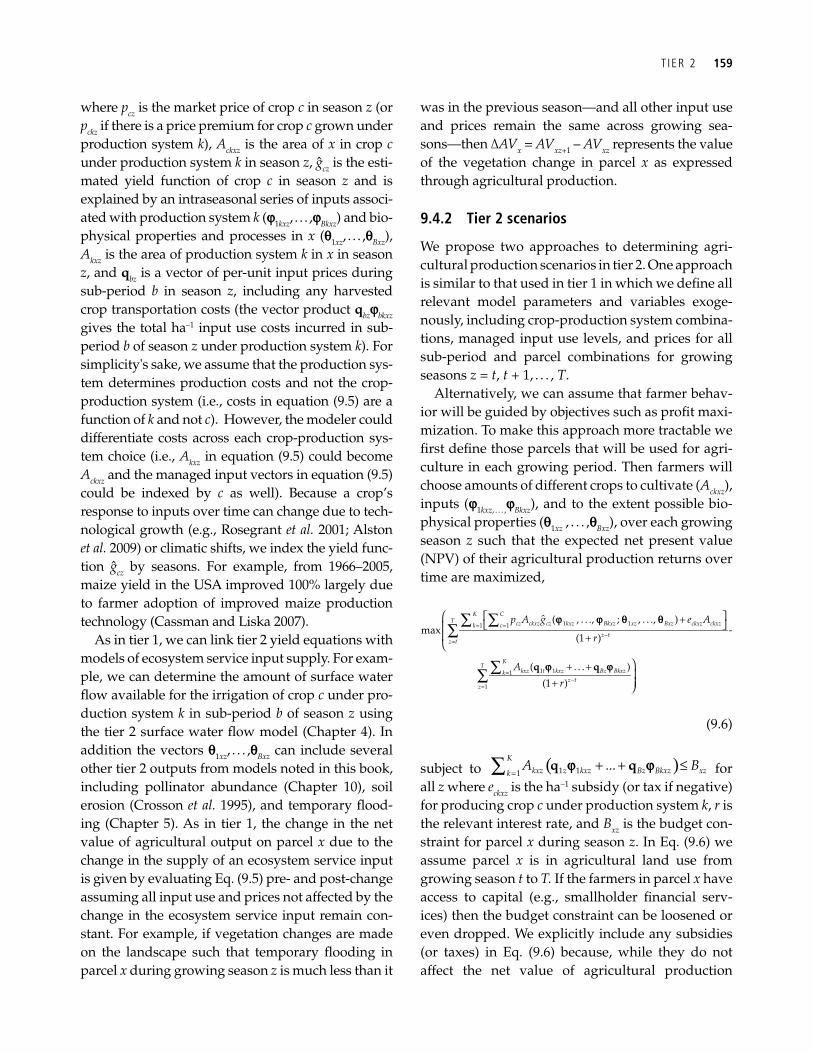
T IER 2 159
where p cz is the market price of crop c in season z (or p ckz if there is a price premium for crop c grown under production system k ), A ckxz is the area of x in crop c under production system k in season z , g c z is the esti-mated yield function of crop c in season z and is explained by an intraseasonal series of inputs associ-ated with production system k ( j 1 k x z , . . . , j B k x z ) and bio-physical properties and processes in x ( q 1 x z , . . . , q B x z ), A kxz is the area of production system k in x in season z , and q bz is a vector of per-unit input prices during sub-period b in season z , including any harvested crop transportation costs (the vector product q b z j b k x z gives the total ha –1 input use costs incurred in sub-period b of season z under production system k ). For simplicity's sake, we assume that the production sys-tem determines production costs and not the crop-production system (i.e., costs in equation (9.5) are a function of k and not c ). However, the modeler could differentiate costs across each crop-production sys-tem choice (i.e., A kxz in equation (9.5) could become A ckxz and the managed input vectors in equation (9.5) could be indexed by c as well). Because a crop’s response to inputs over time can change due to tech-nological growth (e.g., Rosegrant et al. 2001 ; Alston et al. 2009 ) or climatic shifts, we index the yield func-tion g c z by seasons. For example, from 1966–2005, maize yield in the USA improved 100% largely due to farmer adoption of improved maize production technology ( Cassman and Liska 2007 ).
As in tier 1, we can link tier 2 yield equations with models of ecosystem service input supply. For exam-ple, we can determine the amount of surface water fl ow available for the irrigation of crop c under pro-duction system k in sub-period b of season z using the tier 2 surface water fl ow model ( Chapter 4 ). In addition the vectors q 1 xz , . . . , q Bxz can include several other tier 2 outputs from models noted in this book, including pollinator abundance ( Chapter 10 ), soil erosion ( Crosson et al. 1995 ), and temporary fl ood-ing ( Chapter 5 ). As in tier 1, the change in the net value of agricultural output on parcel x due to the change in the supply of an ecosystem service input is given by evaluating Eq. (9.5) pre- and post-change assuming all input use and prices not affected by the change in the ecosystem service input remain con-stant. For example, if vegetation changes are made on the landscape such that temporary fl ooding in parcel x during growing season z is much less than it
was in the previous season—and all other input use and prices remain the same across growing sea-sons—then ∆ AV x = AV xz +1 – AV xz represents the value of the vegetation change in parcel x as expressed through agricultural production.
9.4.2 Tier 2 scenarios
We propose two approaches to determining agri-cultural production scenarios in tier 2. One approach is similar to that used in tier 1 in which we defi ne all relevant model parameters and variables exoge-nously, including crop-production system combina-tions, managed input use levels, and prices for all sub-period and parcel combinations for growing seasons z = t , t + 1, . . . , T .
Alternatively, we can assume that farmer behav-ior will be guided by objectives such as profi t maxi-mization. To make this approach more tractable we fi rst defi ne those parcels that will be used for agri-culture in each growing period. Then farmers will choose amounts of different crops to cultivate ( A ckxz ), inputs ( j 1kxz, . . . , j Bkxz ), and to the extent possible bio-physical properties ( q 1 xz , . . . , q Bxz ), over each growing season z such that the expected net present value (NPV) of their agricultural production returns over time are maximized,
= =
−=
=−
=
⎛ ⎡ ⎤+⎣ ⎦⎜ −⎜ +⎝
⎞+ +⎟⎟+ ⎠
∑ ∑∑
∑∑
K CT cz ckxz cz kxz Bkxz xz Bxz ckxz ckxzk c
z tz t
KT
kxz t kxz Bz Bkxzkz t
z
p A g e A
r
A
r
1 11 1
1 11
1
ˆ ( , . . ., ; , . . ., )max
(1 )
( . . . )(1 )
j j q q
j jq q
(9.6)
subject to ( )1 11...
K
kxz z kxz Bz Bkxz xzkA B
=+ + ≤∑ q qj j for
all z where e ckxz is the ha –1 subsidy (or tax if negative) for producing crop c under production system k , r is the relevant interest rate, and B xz is the budget con-straint for parcel x during season z . In Eq. (9.6) we assume parcel x is in agricultural land use from growing season t to T. If the farmers in parcel x have access to capital (e.g., smallholder fi nancial serv-ices) then the budget constraint can be loosened or even dropped. We explicitly include any subsidies (or taxes) in Eq. (9.6) because, while they do not affect the net value of agricultural production
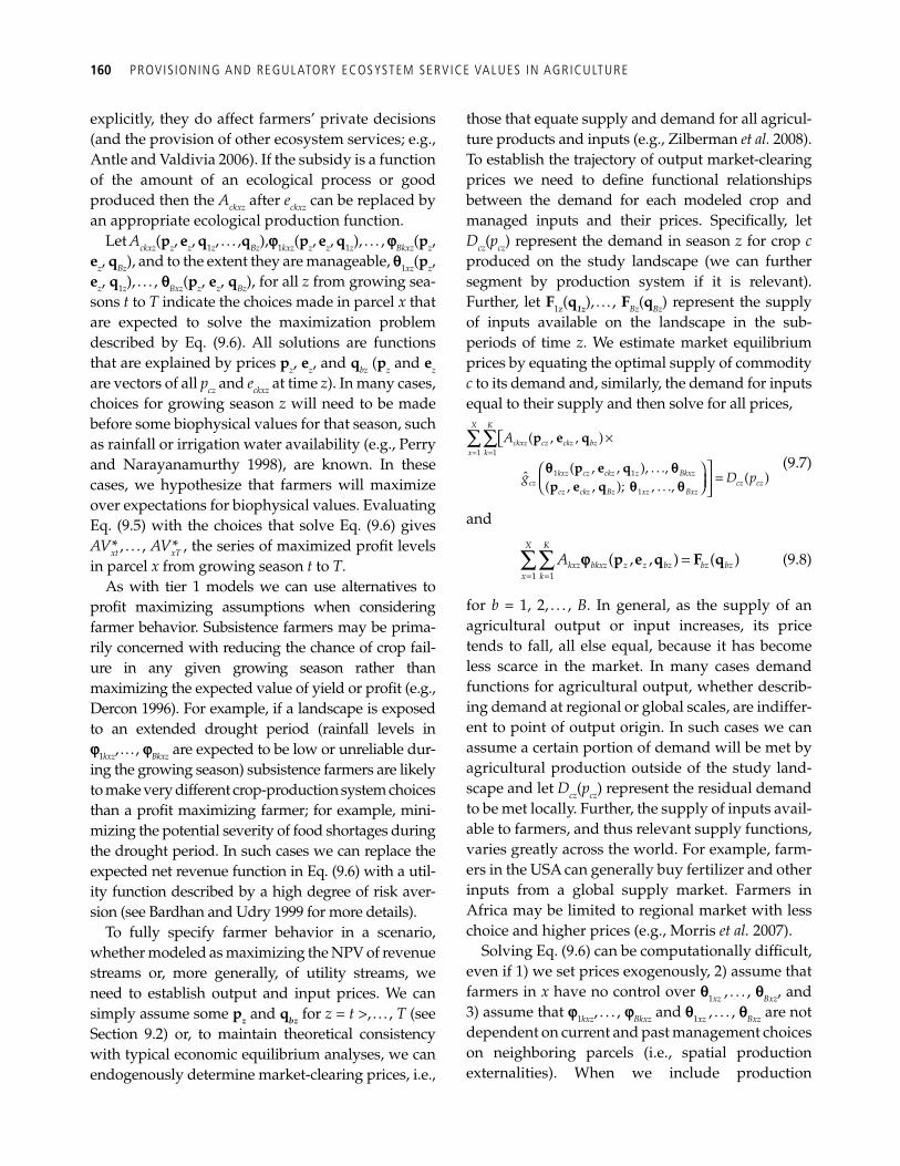
160 PROVIS IONING AND REGULATORY ECOSYSTEM SERVICE VALUES IN AGRICULTURE
explicitly, they do affect farmers’ private decisions (and the provision of other ecosystem services; e.g., Antle and Valdivia 2006 ). If the subsidy is a function of the amount of an ecological process or good produced then the A ckxz after e ckxz can be replaced by an appropriate ecological production function.
Let A c k x z ( p z , e z , q 1 z , . . . , q B z ) , j 1 k x z ( p z , e z , q 1 z ) , . . . , j B k x z ( p z , e z , q B z ) , and to the extent they are manageable, q 1 x z ( p z , e z , q 1 z ) , . . . , q B x z ( p z , e z , q B z ) , for all z from growing sea-sons t to T indicate the choices made in parcel x that are expected to solve the maximization problem described by Eq. (9.6). All solutions are functions that are explained by prices p z , e z , and q bz ( p z and e z are vectors of all p cz and e ckxz at time z ). In many cases, choices for growing season z will need to be made before some biophysical values for that season, such as rainfall or irrigation water availability (e.g., Perry and Narayanamurthy 1998 ), are known. In these cases, we hypothesize that farmers will maximize over expectations for biophysical values. Evaluating Eq. (9.5) with the choices that solve Eq. (9.6) gives A V x t * , . . . , A V x T * , the series of maximized profi t levels in parcel x from growing season t to T .
As with tier 1 models we can use alternatives to profi t maximizing assumptions when considering farmer behavior. Subsistence farmers may be prima-rily concerned with reducing the chance of crop fail-ure in any given growing season rather than maximizing the expected value of yield or profi t (e.g., Dercon 1996 ). For example, if a landscape is exposed to an extended drought period (rainfall levels in j 1 k x z , . . . , j B k x z are expected to be low or unreliable dur-ing the growing season) subsistence farmers are likely to make very different crop-production system choices than a profi t maximizing farmer; for example, mini-mizing the potential severity of food shortages during the drought period. In such cases we can replace the expected net revenue function in Eq. (9.6) with a util-ity function described by a high degree of risk aver-sion (see Bardhan and Udry 1999 for more details).
To fully specify farmer behavior in a scenario, whether modeled as maximizing the NPV of revenue streams or, more generally, of utility streams, we need to establish output and input prices. We can simply assume some p z and q bz for z = t >, . . . , T (see Section 9.2 ) or, to maintain theoretical consistency with typical economic equilibrium analyses, we can endogenously determine market-clearing prices, i.e.,
those that equate supply and demand for all agricul-ture products and inputs (e.g., Zilberman et al. 2008 ). To establish the trajectory of output market-clearing prices we need to defi ne functional relationships between the demand for each modeled crop and managed inputs and their prices. Specifi cally, let D cz ( p cz ) represent the demand in season z for crop c produced on the study landscape (we can further segment by production system if it is relevant). Further, let F 1 z ( q 1z ), . . . , F Bz ( q Bz ) represent the supply of inputs available on the landscape in the sub- periods of time z . We estimate market equilibrium prices by equating the optimal supply of commodity c to its demand and, similarly, the demand for inputs equal to their supply and then solve for all prices,
= =×⎡⎣
⎤⎛ ⎞ =⎥⎜ ⎟⎝ ⎠ ⎦
∑∑X K
ckxz cz ckz bzx k
kxz cz ckz z Bkxzcz cz cz
cz ckz Bz xz Bxz
A
g D p
1 1
1 1
1
( , , )
( , , ), . . .,ˆ ( )( , , ); , . . .,
p e q
p e qp e q
q qq q
(9.7)
and
= =
=∑∑1 1
( , , ) ( )X K
kxz bkxz z z bz bz bzx k
A p e q F qj (9.8)
for b = 1, 2, . . . , B . In general, as the supply of an agricultural output or input increases, its price tends to fall, all else equal, because it has become less scarce in the market. In many cases demand functions for agricultural output, whether describ-ing demand at regional or global scales, are indiffer-ent to point of output origin. In such cases we can assume a certain portion of demand will be met by agricultural production outside of the study land-scape and let D cz ( p cz ) represent the residual demand to be met locally. Further, the supply of inputs avail-able to farmers, and thus relevant supply functions, varies greatly across the world. For example, farm-ers in the USA can generally buy fertilizer and other inputs from a global supply market. Farmers in Africa may be limited to regional market with less choice and higher prices (e.g., Morris et al. 2007 ).
Solving Eq. (9.6) can be computationally diffi cult, even if 1) we set prices exogenously, 2) assume that farmers in x have no control over q 1 xz , . . . , q Bxz , and 3) assume that j 1 kxz , . . . , j Bkxz and q 1 xz , . . . , q Bxz are not dependent on current and past management choices on neighboring parcels (i.e., spatial production externalities). When we include production
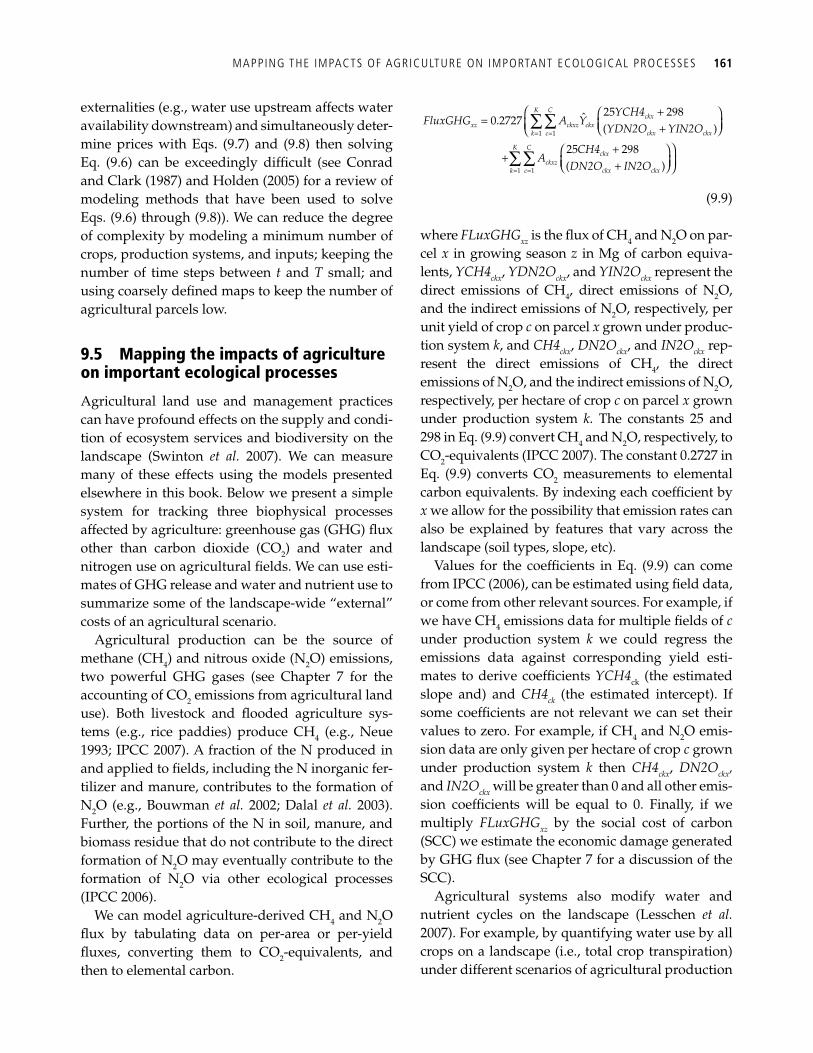
MAPPING THE IMPACTS OF AGRICULTURE ON IMPORTANT ECOLOGICAL PROCESSES 161
externalities (e.g., water use upstream affects water availability downstream) and simultaneously deter-mine prices with Eqs. (9.7) and (9.8) then solving Eq. (9.6) can be exceedingly diffi cult (see Conrad and Clark ( 1987 ) and Holden ( 2005 ) for a review of modeling methods that have been used to solve Eqs. (9.6) through (9.8)). We can reduce the degree of complexity by modeling a minimum number of crops, production systems, and inputs; keeping the number of time steps between t and T small; and using coarsely defi ned maps to keep the number of agricultural parcels low.
9.5 Mapping the impacts of agriculture on important ecological processes
Agricultural land use and management practices can have profound effects on the supply and condi-tion of ecosystem services and biodiversity on the landscape ( Swinton et al. 2007 ). We can measure many of these effects using the models presented elsewhere in this book. Below we present a simple system for tracking three biophysical processes affected by agriculture: greenhouse gas (GHG) fl ux other than carbon dioxide (CO 2 ) and water and nitrogen use on agricultural fi elds. We can use esti-mates of GHG release and water and nutrient use to summarize some of the landscape-wide “external” costs of an agricultural scenario.
Agricultural production can be the source of methane (CH 4 ) and nitrous oxide (N 2 O) emissions, two powerful GHG gases (see Chapter 7 for the accounting of CO 2 emissions from agricultural land use). Both livestock and fl ooded agriculture sys-tems (e.g., rice paddies) produce CH 4 (e.g., Neue 1993 ; IPCC 2007). A fraction of the N produced in and applied to fi elds, including the N inorganic fer-tilizer and manure, contributes to the formation of N 2 O (e.g., Bouwman et al. 2002 ; Dalal et al. 2003 ). Further, the portions of the N in soil, manure, and biomass residue that do not contribute to the direct formation of N 2 O may eventually contribute to the formation of N 2 O via other ecological processes (IPCC 2006).
We can model agriculture-derived CH 4 and N 2 O fl ux by tabulating data on per-area or per-yield fl uxes, converting them to CO 2 -equivalents, and then to elemental carbon.
K Cckx
xz ckxz ckxckx ckxk c
K Cckx
ckxzckx ckxk c
YCH4FluxGHG A Y
YDN2O YIN2O
CH4A
DN2O IN2O
1 1
1 1
25 298ˆ0.2727( )
25 298( )
= =
= =
+⎛ ⎛ ⎞= ⎜ ⎜ ⎟+⎝ ⎠⎝+ ⎞⎛ ⎞+ ⎟⎜ ⎟+⎝ ⎠ ⎠
∑∑
∑∑
(9.9)
where FLuxGHG xz is the fl ux of CH 4 and N 2 O on par-cel x in growing season z in Mg of carbon equiva-lents, YCH4 ckx , YDN2O ckx , and YIN2O ckx represent the direct emissions of CH 4 , direct emissions of N 2 O, and the indirect emissions of N2O, respectively, per unit yield of crop c on parcel x grown under produc-tion system k , and CH4 ckx , DN2O ckx , and IN2O ckx rep-resent the direct emissions of CH 4 , the direct emissions of N 2 O, and the indirect emissions of N 2 O, respectively, per hectare of crop c on parcel x grown under production system k . The constants 25 and 298 in Eq. (9.9) convert CH 4 and N 2 O, respectively, to CO 2 -equivalents (IPCC 2007). The constant 0.2727 in Eq. (9.9) converts CO 2 measurements to elemental carbon equivalents. By indexing each coeffi cient by x we allow for the possibility that emission rates can also be explained by features that vary across the landscape (soil types, slope, etc).
Values for the coeffi cients in Eq. (9.9) can come from IPCC (2006), can be estimated using fi eld data, or come from other relevant sources. For example, if we have CH 4 emissions data for multiple fi elds of c under production system k we could regress the emissions data against corresponding yield esti-mates to derive coeffi cients YCH4 ck (the estimated slope and) and CH4 ck (the estimated intercept). If some coeffi cients are not relevant we can set their values to zero. For example, if CH 4 and N 2 O emis-sion data are only given per hectare of crop c grown under production system k then CH4 ckx , DN2O ckx , and IN2O ckx will be greater than 0 and all other emis-sion coeffi cients will be equal to 0. Finally, if we multiply FLuxGHG xz by the social cost of carbon (SCC) we estimate the economic damage generated by GHG fl ux (see Chapter 7 for a discussion of the SCC).
Agricultural systems also modify water and nutrient cycles on the landscape ( Lesschen et al. 2007 ). For example, by quantifying water use by all crops on a landscape (i.e., total crop transpiration) under different scenarios of agricultural production
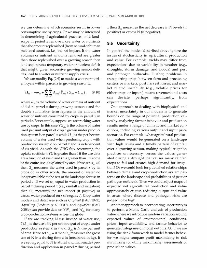
162 PROVIS IONING AND REGULATORY ECOSYSTEM SERVICE VALUES IN AGRICULTURE
we can determine which scenarios result in lower consumptive use by crops. Or we may be interested in determining if agricultural practices on a land-scape in period z remove more water or nutrients than the amount replenished (from natural or human mediated sources), i.e., the net impact. If the water volumes or nutrient amounts removed are greater than those replenished over a growing season then landscapes run a temporary water or nutrient defi cit that might, given successive growing season defi -cits, lead to a water or nutrient supply crisis.
We can modify Eq. (9.9) to model a water or nutri-ent cycle within parcel x in growing season z ,
K C
xz xz ckxz ckxz ckx ckxk c
A Y YU U1 1
ˆ( ) ,w= =
Ω = − + +∑∑ (9.10)
where ω xz is the volume of water or mass of nutrient added to parcel x during growing season z and the double summation term represents the amount of water or nutrient consumed by crops in parcel x in period z . For example, suppose we are tracking water use by crops. In this case YU ckx is the volume of water used per unit output of crop c grown under produc-tion system k on parcel x while U ckx is the per hectare volume of water used when producing crop c with production system k on parcel x and is independent of c ’s yield. As with the GHG fl ux accounting, the uptake coeffi cient YU is greater than 0 if the use data are a function of yield and U is greater than 0 if some or the entire use is explained by area. If we set ω xz = 0 then Ω xz measures the water used in parcel x by its crops or, in other words, the amount of water no longer available to the rest of the landscape for use in period z . If we set ω xt equal to water production in parcel x during period z (i.e., rainfall and irrigation) then Ω xz measures the net import (if positive) or excess water produced on x (if negative). Crop water models and databases such as CropWat (FAO 1992), AquaCrop ( Steduto et al. 2009 ), and AquaStat (FAO 2008b) can provide data on YW ckx and W ckx for many crop-production systems across the globe.
If we are tracking N use instead of water use, YU ckx is the use of N per unit output of crop c under production system k in x and U ckx is N use per unit of area. If we set ω xz = 0 then Ω xz measures the gross use of N in x during time z in (measured in kg). If we set ω xt equal to N (natural and man-made) pro-duction and application in parcel x during period
z then Ω xz measures the net decrease in N levels (if positive) or excess N (if negative).
9.6 Uncertainty
In general the models described above ignore the issues of stochasticity in agricultural production and value. For example, yields may differ from expectations due to variability in weather (e.g., droughts, storm damage, and fl oods) and pest and pathogen outbreaks. Further, problems in transporting crops between farm and processing centers or markets, post harvest losses, and mar-ket related instability (e.g., volatile prices for either crops or inputs) means revenues and costs can deviate, perhaps signifi cantly, from expectations.
One approach to dealing with biophysical and market uncertainty in our models is to generate bounds on the range of potential production val-ues by analyzing farmer behavior and production results under a range of climatic and market con-ditions, including various output and input price scenarios. For example, what agricultural produc-tion values would be generated on a landscape with high levels and a timely pattern of rainfall over a growing season, making typical irrigation practices unnecessary, versus the values gener-ated during a drought that causes many rainfed crops to fail and creates high demand for irriga-tion? Or we could look for published relationships between climate and crop-production system pat-terns on the landscape and probabilities of pest or pathogen outbreak. Then we could adjust maps of expected net agricultural production and value appropriately ex post , reducing output and value in areas where disease and pathogen risks are judged to be high.
Another approach to incorporating uncertainty is to perform a Monte Carlo analysis of production value where we introduce random variation around expected values of environmental conditions, prices, input availability, and farmer behavior to generate histograms of model outputs. Or, if we are using the tier 2 framework to model farmer behav-ior we might compare profi t maximizing to risk minimizing (or utility maximizing) assessments of production values.
L IMITATIONS AND NEXT STEPS 163
9.7 Limitations and next steps
9.7.1 Limitations
In this chapter we propose two tiers of agricul-tural modeling, aiming for a range of conceptually sound and tractable approaches to estimating and mapping values of agricultural production and the ecosystem services that support agricultural production. However, the app roaches outlined do have several limitations that are important to acknowledge. First, we did not explicitly model livestock operations. We propose modeling live-stock production systems as if they are a crop with expected yield (e.g., kg of meat ha –1 , animal units supported ha –1 yr –1 ) and input use defi ned by a production system k . However, the physical size of intensive and confi ned livestock production enterprises may be too small to be represented on the LULC maps that form the basis of the agricul-tural production models described in this chapter. In such cases we may need to add point data to the LULC maps to account for these systems, or account for them outside the mapping framework. A better understanding of the links between live-stock production and water and air pollution, eco-system processes, and biodiversity conservation is becoming more important as meat demand increases throughout the world ( Delgado et al . 1999 ; Steinfeld et al. 2006 ).
Second, many agricultural landscapes include a diversity of crops and systems of input use. Most applications of the approaches described here focus on major crops, both due to data limitations and time constraints. This restriction may under-estimate production and ecosystem service value and distort the spatial distribution of that value—especially if the modeled systems are likely to be allocated across the landscape differently than non-modeled systems. Further, by ignoring minor crops we might miss important niche products on the landscape and overlook important crop alter-natives that could improve environmental condi-tions on the land while maintaining the value of agricultural output.
Climate change is likely to have a large impact on agricultural yield functions, crop-production system patterns, crops prices, production costs and man-
agement decisions in the future (e.g., Mendelsohn et al. 1994 ; Schlenker et al. 2005 ; Luedeling et al. 2009 ; Mendelsohn and Dinar 2009 ). If we have yield func-tions that include climate variables then we may be able to predict some of the changes in the agricul-tural sector from climate change (see Chapter 18 ). In addition, we can model some of the expected effects of climate change on agriculture production via changes in ecosystem services that are inputs to agricultural production (see Chapters 4 and 10 ). However, major climate change might cause unan-ticipated changes in crop and animal growth pat-terns that cannot be predicted with statistical models based on current or historic relationships between yields and agricultural inputs (crop simulation mod-els would appear better able to model yields in response to climate change; e.g., Parry et al. 1999 ). Further, predicting commodity supply and demand in a climate change-affected world will also be very diffi cult, making the endogenous price determina-tion method discussed in the tier 2 approach partic-ularly challenging to implement for future scenarios under climate change.
9.7.2 Next steps
The output from the agriculture models described here can be used for several types of analyses. We can use expected net production value maps to determine the opportunity costs of setting aside agriculture land for conservation, or conversely, the value added to society from bringing land into agricultural production. We can use maps of agri-cultural production values, the value added to agri-culture production by regulating and supporting ecosystem services, and agriculture-related GHG fl ux maps along with maps of other ecosystem serv-ice use to create a series of service trade-off analyses (see Chapter 14 ).
Other models presented in this book are able to use outputs from the agriculture models described here. For example, when we assign fertilizer and pesticide use to each crop-production system and then map these systems we have also mapped ferti-lizer and pesticide use. The water pollution regula-tion model (see Chapter 6 ) can use these data to estimate agriculture’s impact on water quality across the landscape. Surface water withdrawals for
164 PROVIS IONING AND REGULATORY ECOSYSTEM SERVICE VALUES IN AGRICULTURE
irrigation will affect water use in other sectors of the economy (see Chapter 4 ). We could also use the out-puts from this model to make predictions about the number of rural households in developing coun-tries that are involved in timber and non-timber for-est product harvesting. In general, the lower the predicted net values from agriculture the more that rural households will look to supplement their incomes with products generated by nearby forests (see Chapter 8 ).
Moving beyond tier 2 to gain even more mode-ling realism implies the use of more elaborate yield, biophysical, and economic simulation mod-els. For example, we can better model crop yields by using one of more specialized crop growth sim-ulation models such as DSSAT, APSIM, or EPIC (e.g., Bryant et al. 1992 ). These models, as partly demonstrated in Section 9.3.3 where we used DSSAT to generate “observed” maize yields, are data intensive and usually require detailed data-sets and specialized training to use. Complex mod-els that track nutrient cycles in soils (e.g., CENTURY, RothC-26.3, or SCUAF), water balance and quality, and other environmental impacts of farming (e.g., WATBAL, PERFECT, or SWAT; see Wani et al. 2005 for a review of all of these and other simulation models) are also available. However, these models often require signifi cant calibration effort and data not readily available in developing countries. Finally, far more elaborate agricultural production models that embed micro-economic principles within macroeconomic and general equilibrium analytical components are available to evaluate trajectories of land-use deci-sions and ecosystem service provision over time (e.g., Eickhout et al. 2006 ; Bouwman et al. 2006 ; Nelson et al. 2009 ). Once again, however, these models are complex and are often only accessible to the research groups that developed and main-tain the models.
References
Alston, J. M., Beddow, J. M., and Pardey, P. G. (2009). Agricultural research, productivity, and food prices in the long run. Science, 325 , 1209–10.
Antle, J. M., and Valdivia, R. (2006). Modelling the supply of ecosystem services from agriculture: a minimum-data
approach. Australian Journal of Agricultural and Resource Economics, 50 , 1–15.
Antle, J. M., Capalbo, S., Paustian, K., et al . (2007). Estimating the economic potential for agricultural soil carbon sequestration in the Central United States using an aggregate econometric-process simulation model. Climatic Change, 80 , 145–71.
Bardhan, P. K., and Udry, C. (1999). Development Microeconomics, Oxford University Press, New York.
Batjes, N. H. (2002). A homogenized soil profi le data set for global and regional environmental research (WISE, version 1.1) . International Soil Reference and Information Centre, Wageningen.
Bockstael, N. E., Freeman, A. M., Kopp, R. J., et al . (2000). On measuring economic values for nature. Journal of Environmental Science and Technology, 34 , 1384–9.
Bouwman, A. F., Boumans, L. J. M., and Batjes, N. H. (2002). Modeling global annual N 2 O and NO emissions from fertilized fi elds. Global Biogeochemical Cycles, 16 , 1080.
Bouwman, A. F., Van Der Hoek, K. W., and Van Drecht, G. (2006). Modelling livestock-crop-land use interactions in global agricultural production systems. In A. F. Bouwman, T. Kram, and K. K. Goldewijk, Eds., Integrated modelling of global environmental change: An overview of IMAGE 2.4 . Netherlands Environmental Assessment Agency (MNP), Bilthoven.
Bruinsma, J. (2003). World agriculture: towards 2015/2030 . In: J. Bruinsma, ed., An FAO perspective . Earthscan, London.
Bryant, K. J., Benson, V. W., Kiniry, J. R., et al . (1992). Simulating corn yield response to irrigation timings: Validation of the EPIC model. Journal of Production Agriculture, 5, 237–42.
Byerlee, D., de Janvry, A., and Sadoulet, E. (2009). Agriculture for development: Toward a new paradigm. Annual Review of Resource Economics, 1 , 15–31.
Cassman, K. G., and Liska, A. J. (2007). Food and fuel for all: realistic or foolish? Biofuels, Bioproducts and Biorefi ning, 1 , 23.
Conrad, J. M., and Clark, C. W. (1987). Natural resource eco-nomics: Notes and problems. Cambridge University Press, New York.
Crawford, E., Kelly, V., Jayne, T. S., et al . (2003). Input use and market development in Sub-Saharan Africa: an overview. Food Policy, 28 , 277–92.
Crosson, P., Pimentel, D., Harvey, C., et al . (1995). Soil ero-sion estimates and costs. Science, 269 , 461–5.
Dalal, R. C., Wang, W., Robertson, G. P., et al . (2003). Nitrous oxide emission from Australian agricultural lands and mitigation options: a review. Australian Journal of Soil Research, 41 , 165–95.
L IMITATIONS AND NEXT STEPS 165
Delgado, C., Rosegrant, M., Steinfeld, H., et al . (1999). Livestock to 2020. The Next Food Revolution . International Food Policy Research Institute (IFPRI), Washington, DC.
Dercon, S. (1996). Risk, crop choice, and savings: Evidence from Tanzania. Economic Development and Cultural Change, 44 , 485–513.
Eickhout, B., van Meijl, H., and Tabeau, A. (2006). Modelling agricultural trade and food production under different trade policies. In A. F. Bouwman, T. Kram, and K. K. Goldewijk, eds., Integrated modeling of global environmental change: An overview of IMAGE 2.4 . Netherlands Environmental Assessment Agency (MNP), Bilthoven.
Feder, G. Just, R. E., and Zilberman, D. (1985). Adoption of agricultural innovations in developing countries: A sur-vey. Economic Development and Cultural Change, 33 , 255–98.
Fischer, G., van Velthuizen, H., Medow, S. and Nachtergaele, F. (2002). Global agro-ecological assessment for agriculture in the 21st century , Food and Agricultural Organization/International Institute for Applied Systems Analysis (FAO/IIASA), Laxenburg.
Food and Agriculture Organization of the United Nations (FAO) (1992). CROPWAT, a computer program for irriga-tion planning and management by M. Smith , FAO Irrigation and Drainage Paper 26, Food and Agriculture Organization of the United Nations (FAO), Rome.
Food and Agriculture Organization of the United Nations (FAO). (2008a). [Online]. Available: http://faostat.fao.org/default.aspx .
Food and Agriculture Organization of the United Nations (FAO). (2008b). Aquastat , [Online]. Available: http://www.fao.org/nr/water/aquastat/main/index.stm .
Food and Agriculture Organization of the United Nations/International Institute for Applied Systems Analysis/International Soil Reference and Information Centre/Institute of Soil Science—Chinese Academy of Sciences/Joint Research Centre of the European Commission (FAO/IIASA/ISRIC/ISS-CAS/JRC). (2008). Harmonized world soil database (version 1.1) , Food and Agriculture Organization of the United Nations (FAO) and International Institute for Applied Systems Analysis (IIASA), Rome.
Gillig, D., McCarl, B. A., and Sands, R. D. (2004). Integrating agricultural and forestry GHG mitigation response into general economy frameworks: Developing a family of response functions. Mitigation and Adaptation Strategies for Global Change, 9 , 241–59.
Holden, S. T. (2005). Bioeconomic modelling for natural resource management impact assessment. In B. Shiferaw, H. A. Freeman, and S. M. Swinton, Eds., Natural Resource Management in Agriculture: Methods for Assessing
Economic and Environmental Impacts . CABI Publishing, Cambridge.
Intergovernmental Panel on Climate Change (IPCC). (2007). Climate change 2007: the physical science basis. Contribution of Working Group I to the Fourth Assessment Report of the Intergovernmental Panel on Climate Change. Cambridge University Press, New York.
Intergovernmental Panel on Climate Change (IPCC). (2006). 2006 IPCC Guidelines for National Greenhouse Gas Inventories. In H. S. Eggleston, L. Buendia, K. Miwa, et al. , Eds., Prepared by the National Greenhouse Gas Inventories Programme . Institute for Global Environmental Strategies, Hayama, Kanagawa.
International Food Policy Research Institute, The (IFPRI). (2008). Spatial allocation model (SPAM) . International Food Policy Research Institute (IFPRI), Washington, DC. Accessed at http://www.mapspam.info
Jones, J. W., Hoogenboom, G., Porter, C. H., et al . (2003). The DSSAT cropping system model. European Journal of Agronomy, 18 , 235–65.
Just, R. E., and Antle, J. M. (1990). Interactions between agricultural and environmental policies: A concep-tual framework. American Economic Review , 80 , 197–202.
Kandlikar, M., and Risbey, J. (2000). Agricultural impacts of climate change: If adaptation is the answer, what is the question? Climatic Change, 45 , 529–39.
Kinsey, B., Burger, K., and Gunning, J. W. (1998). Coping with drought in Zimbabwe: Survey evidence on responses of rural households to risk. World Development, 26 , 89–110.
Kremen, C., Daily, G. C., Klein, A., et al . (2008). Inadequate assessment of the ecosystem service rationale for con-servation: Reply to Ghazoul. Conservation Biology, 22 , 795–8.
Lesschen, J., Stoorvogel, J., Smaling, E., et al . (2007). A spa-tially explicit methodology to quantify soil nutrient balances and their uncertainties at the national level. Nutrient Cycling in Agroecosystems, 78 , 111–31.
Lubowski, R. N., Plantinga, A. J., and Stavins, R. N. (2006). Land-use change and carbon sinks: Econometric esti-mation of the carbon sequestration supply function. Journal of Environmental Economics and Management, 51, 135–52.
Luckert, M. K., Wilson, J., Adamowicz, V., et al . (2000). Household resource allocations in response to risks and returns in a communal area of western Zimbabwe. Ecological Economics, 33 , 383–94.
Luedeling, E., Zhang, M., and Girvetz, E. H. (2009). Climatic changes lead to declining winter chill for fruit and nut trees in California during 1950–2099. PLoS ONE, 4 , e6166.
166 PROVIS IONING AND REGULATORY ECOSYSTEM SERVICE VALUES IN AGRICULTURE
Mendelsohn, R., Nordhaus, W. D., and Shaw, D. (1994). The impact of global warming on agriculture: A Ricardian analysis. American Economic Review, 84 , 753–71.
Mendelsohn, R., and Dinar, A. (2009). Land use and cli-mate change interactions. Annual Review of Resource Economics, 1 , 309–32.
Cassman, K. G., Wood S. (2005). Cultivated Systems. In Millennium Ecosystem Assessment: Global Ecosystem Assessment Report on Conditions and Trends. Island Press, Washington, DC.
Morris, M., Kelly, V., Kopicki, R., et al . (2007). Fertilizer use in African agriculture: lessons learned and good practice guidelines . World Bank, Washington, DC .
Naidoo, R., and Iwamura, T. (2007). Global-scale mapping of economic benefi ts from agricultural lands: Implications for conservation priorities. Biological Conservation, 140 , 40–9.
Naidoo, R., and Ricketts, T. H. (2006). Mapping the eco-nomic costs and benefi ts of conservation. PLoS Biology, 4, 2153–64.
Nelson, G. C., Rosegrant, M. W., Koo, J., et al . (2009). Climate change. impact on agriculture and costs of adapta-tion . International Food Policy Research Institute (IFPRI), Washington, DC.
Neue, H. (1993). Methane emission from rice fi elds. Bioscience, 43 , 466–74.
Parry, M., Rosenzweig, C., Iglesias, A., et al . (1999). Climate change and world food security: a new assessment. Global Environmental Change, 9 , S51–S67.
Pender, J. (2005). Econometric methods for measuring natural resource management impacts: Theoretical issues and illustrations from Uganda. In: B. Shiferaw, H. A. Freeman, and S.M. Swinton, Eds., Natural resource management in agriculture: methods for assessing economic and environmental impacts . CABI Publishing, Cambridge.
Perry, C. J., and Narayanamurthy, S. G. (1998). Farmer response to rationed and uncertain irrigation supplies . International Water Management Institue, Colombo.
Polasky, S., Nelson, E., Camm, J., et al . (2008). Where to put things? Spatial land management to sustain biodiver-sity and economic returns. Biological Conservation, 141 , 1505–24.
Rosegrant, M. W., Paisner, M. S., Meijer, S., and Witcover, J. (2001). Global food projections to 2020: emerging trends and alternative futures . International Food Policy Research Institute, Washington, DC.
Rosegrant, M. W., Ringler, C., Msangi, S., et al . (2005). International Model for Policy Analysis of Agricultural Commodities and Trade (IMPACT-WATER): Model Des-cription . International Food Policy Research Institute, Washington, DC.
Schlenker, W., Hanemann, W. M., and Fisher, A. C. (2005). Will US agriculture really benefi t from global warming? Accounting for irrigation in the hedonic approach. American Economic Review, 95 , 395–406.
Shiferaw, H., Freeman, H. A., and Navrud, S. (2005). Valuation methods and approaches for assessing natural resource management impacts. In B. Shiferaw, H. A. Freeman, and S. M. Swinton, Eds., Natural resource management in agriculture: methods for assessing economic and environmental impacts . CABI Publishing, Cambridge.
Steduto, P., Hsiao, T. C., Raes, D., et al . (2009). AquaCrop—the FAO crop model to simulate yield response to water: I. Concepts and underlying principles. Agronomy Journal, 101 , 426–37.
Steinfeld, H., Gerber, P., Wassenaar, T., et al . (2006). Livestock’s long shadow — environmental issues and options . Food and Agriculture Organization of the United Nations (FAO), Rome.
Swinton, S. M. (2005). Assessing economic impacts of nat-ural resource management using economic surplus. In B. Shiferaw, H. A. Freeman, and S. M. Swinton, Eds., Natural resource management in agriculture: methods for assessing economic and environmental impacts . CABI Publishing, Cambridge.
Swinton, S. M., Lupi, F., Robertson, G. P., et al . (2007). Ecosystem services and agriculture: Cultivating agricultural ecosystems for diverse benefi ts. Ecological Economics, 64 , 245–52.
Tilman, D., Cassman, K. G., Matson, P. A., et al . (2002). Agricultural sustainability and intensive production practices. Nature, 418 , 671–7.
United States Department of Agriculture-Economic Research Service (USDA-ERS). (2009). Commodity Costs and Returns . Accessed at http://www.ers.usda.gov/Data/CostsAndReturns/ .
United States Department of Agriculture-Natural Resources Conservation Service (USDA-NRCS). (2001). National SSURGO (Soil Survey Geographic) Database .
Vera-Diaz, M. D. C., Kaufmann, R. K., Nepstad, D. C., et al . (2008). An interdisciplinary model of soybean yield in the Amazon Basin: The climatic, edaphic, and economic determinants. Ecological Economics , 65, 420–31.
Wani, S. P., Singh, P., Dwivedi, R. S., et al . (2005). Biophysical indicators of agro-ecosystem services and methods for monitoring the impacts of NRM technologies at differ-ent scales. In B. Shiferaw, H. A. Freeman, and S. M. Swinton, eds., Natural resource management in agriculture: methods for assessing economic and environmental impacts . CABI Publishing, Cambridge.
Wood, S., Ehui, S., Alder, J., et al . (2005). Food. In Ecosystems and human well-being , vol. 1: Current state and trends:

L IMITATIONS AND NEXT STEPS 167
Millennium Ecosystem Assessment . Island Press, Washington, DC.
Wossink, A., and Swinton, S. M. (2007). Jointness in pro-duction and farmers’ willingness to supply non-mar-keted ecosystem services. Ecological Economics, 64 , 297–304.
Wu, J. J., Adams, R. M., Kling, C. L., et al . (2004). From microlevel decisions to landscape changes: An assess-
ment of agricultural conservation policies. American Journal of Agricultural Economics, 86 , 26–41.
You, L., and Wood, S. (2006). An entropy approach to spatial disaggregation of agricultural production. Agricultural Systems, 90 , 329–47.
Zilberman, D., Lipper, L., and McCarthy, N. (2008). When could payments for environmental services benefi t the poor? Environment and Development Economics, 13 , 255–78.
168
CHAPTER 10
Crop pollination services Eric Lonsdorf, Taylor Ricketts, Claire Kremen, Rachel Winfree, Sarah Greenleaf, and Neal Williams
10.1 Introduction
10.1.1 Importance to agriculture and policy
Crop pollination by bees and other animals is an ecosystem service of enormous economic value (Losey andVaughan 2006; Allsopp et al . 2008). Pollination can increase the yield, quality, and sta-bility of crops as diverse as almond, cacao, canola, coffee, sunfl ower, tomato and watermelon. Indeed, Klein et al . (in press) found that 75% of globally important crops benefi t from animal pollination. The value of this service, while diffi cult to quantify properly, has been estimated several times over the past decade (Southwick and Southwick 1992; Costanza et al. 1997; Losey and Vaughan 2006; Allsopp et al . 2008) with a recent estimate of 195 bil-lion Euros (~$200 billion) worldwide ( Box 10.1 ).
While much research and policy attention has focused on managed bees (especially the honey bee, Apis mellifera ), wild bees and other insect species also contribute importantly to crop pollination. Our models focus on wild bees, because the pollination they deliver represents an ecosystem service from natural systems. In fact, for some crops (e.g., blue-berry), wild bees are more effi cient and effective pollinators than honey bees (Cane 1997). Diverse bee communities potentially provide more stable polli-nation services over time, compared to single (man-aged) species (Greenleaf and Kremen 2006; Hoehn et al. . 2008). Finally, if alarming regional declines in honeybee populations continue (National Research Council of the National Academies 2006; Stokstad 2007; Klein et al ., in press), wild pollinators may become increasingly important to farmers.
Maintaining pollinator habitats in agricultural land-scapes, therefore, can help ensure food production, quality, and security. While other pollinators (e.g., bats and moths) also pollinate crops, bees are the most important crop pollinators (Free 1993) and are thus the focus of our models.
The pollination models aim to quantify and map scores for relative pollinator abundance across an entire landscape, including farms requiring pollina-tion. The models use these results to indicate areas supplying pollinators that increase crop yields. Alternatively, intermediate results can be integrated into our agricultural model (see Chapter 9 ) to esti-mate the economic value of pollination services as an input to crop yields in a more sophisticated man-ner. Either way, these models can inform agricultural and land management policies in several ways. First, land-use planners could predict consequences of different policies on pollination services and income to farmers (Priess et al. 2007). Second, farmers could use these tools to locate crops in places where their pollination needs are most likely to be met. Third, conservation organizations that guide land manage-ment and restoration could use the tool to optimize conservation investments for both biodiversity and crop productivity. Finally, governments or others proposing payment schemes for ecosystem services could incorporate the results into plans for who should pay whom, and how much.
10.1.2 Scientifi c foundations and context
Our pollination models are founded on an increas-ing number of studies that have investigated the impacts of landscape structure and habitat-quality
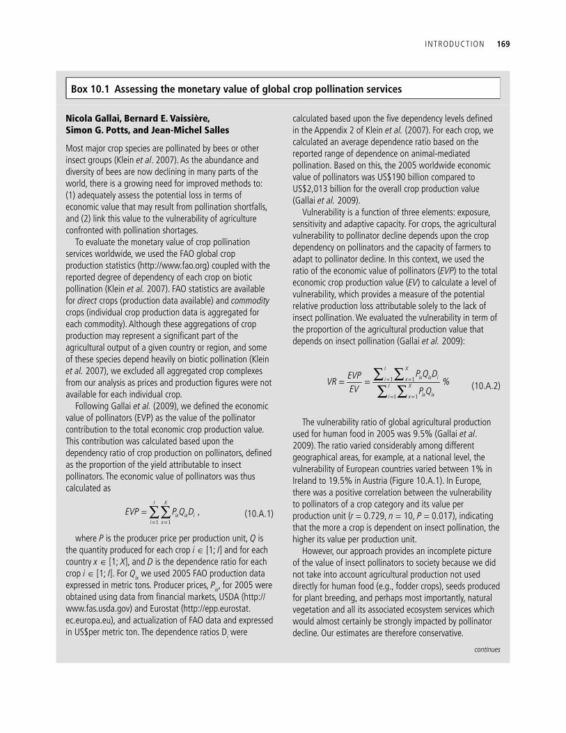
INTRODUCTION 169
Nicola Gallai, Bernard E. Vaissière,Simon G. Potts, and Jean-Michel Salles
Most major crop species are pollinated by bees or other insect groups (Klein et al . 2007). As the abundance and diversity of bees are now declining in many parts of the world, there is a growing need for improved methods to: (1) adequately assess the potential loss in terms of economic value that may result from pollination shortfalls, and (2) link this value to the vulnerability of agriculture confronted with pollination shortages.
To evaluate the monetary value of crop pollination services worldwide, we used the FAO global crop production statistics (http://www.fao.org) coupled with the reported degree of dependency of each crop on biotic pollination (Klein et al. 2007). FAO statistics are available for direct crops (production data available) and commodity crops (individual crop production data is aggregated for each commodity). Although these aggregations of crop production may represent a signifi cant part of the agricultural output of a given country or region, and some of these species depend heavily on biotic pollination (Klein et al. 2007), we excluded all aggregated crop complexes from our analysis as prices and production fi gures were not available for each individual crop.
Following Gallai et al. (2009), we defi ned the economic value of pollinators (EVP) as the value of the pollinator contribution to the total economic crop production value. This contribution was calculated based upon the dependency ratio of crop production on pollinators, defi ned as the proportion of the yield attributable to insect pollinators. The economic value of pollinators was thus calculated as
I X
ix ix ii x
EVP = P Q D ,= =∑∑
1 1 (10.A.1)
where P is the producer price per production unit, Q is the quantity produced for each crop i Î [1; I ] and for each country x Î [1; X ], and D is the dependence ratio for each crop i Î [1; I ]. For Q ix we used 2005 FAO production data expressed in metric tons. Producer prices, P ix , for 2005 were obtained using data from fi nancial markets, USDA (http://www.fas.usda.gov) and Eurostat (http://epp.eurostat.ec.europa.eu), and actualization of FAO data and expressed in US$per metric ton. The dependence ratios D i were
calculated based upon the fi ve dependency levels defi ned in the Appendix 2 of Klein et al. (2007). For each crop, we calculated an average dependence ratio based on the reported range of dependence on animal-mediated pollination. Based on this, the 2005 worldwide economic value of pollinators was US$190 billion compared to US$2,013 billion for the overall crop production value (Gallai et al. 2009).
Vulnerability is a function of three elements: exposure, sensitivity and adaptive capacity. For crops, the agricultural vulnerability to pollinator decline depends upon the crop dependency on pollinators and the capacity of farmers to adapt to pollinator decline. In this context, we used the ratio of the economic value of pollinators ( EVP ) to the total economic crop production value ( EV ) to calculate a level of vulnerability, which provides a measure of the potential relative production loss attributable solely to the lack of insect pollination. We evaluated the vulnerability in term of the proportion of the agricultural production value that depends on insect pollination (Gallai et al. 2009):
1
I X
ix ix ii xI X
ix ixi x
P Q DEVPVR %
EV P Q= =
= =
= = ∑ ∑∑ ∑
1 1
1
(10.A.2)
The vulnerability ratio of global agricultural production used for human food in 2005 was 9.5% (Gallai et al . 2009). The ratio varied considerably among different geographical areas, for example, at a national level, the vulnerability of European countries varied between 1% in Ireland to 19.5% in Austria (Figure 10.A.1). In Europe, there was a positive correlation between the vulnerability to pollinators of a crop category and its value per production unit ( r = 0.729, n = 10, P = 0.017), indicating that the more a crop is dependent on insect pollination, the higher its value per production unit.
However, our approach provides an incomplete picture of the value of insect pollinators to society because we did not take into account agricultural production not used directly for human food (e.g., fodder crops), seeds produced for plant breeding, and perhaps most importantly, natural vegetation and all its associated ecosystem services which would almost certainly be strongly impacted by pollinator decline. Our estimates are therefore conservative.
Box 10.1 Assessing the monetary value of global crop pollination services
continues
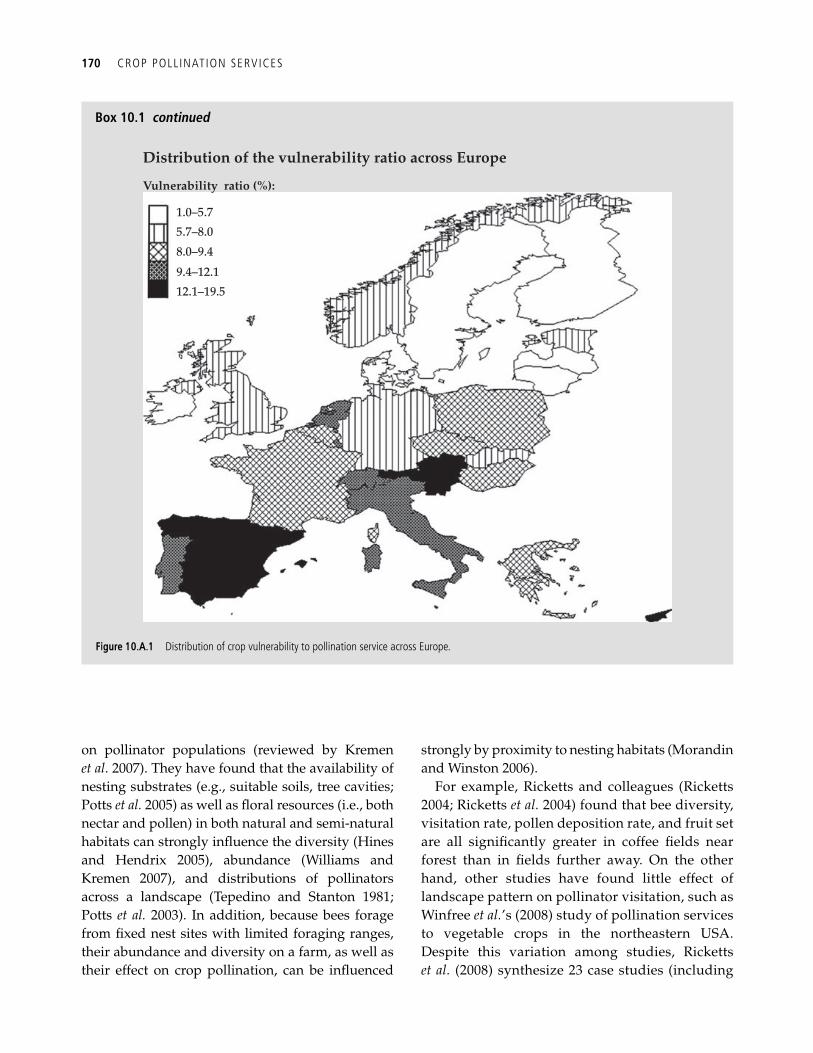
170 CROP POLL INATION SERVICES
on pollinator populations (reviewed by Kremen et al . 2007). They have found that the availability of nesting substrates (e.g., suitable soils, tree cavities; Potts et al. 2005) as well as fl oral resources (i.e., both nectar and pollen) in both natural and semi-natural habitats can strongly infl uence the diversity (Hines and Hendrix 2005), abundance (Williams and Kremen 2007), and distributions of pollinators across a landscape (Tepedino and Stanton 1981; Potts et al. 2003). In addition, because bees forage from fi xed nest sites with limited foraging ranges, their abundance and diversity on a farm, as well as their effect on crop pollination, can be infl uenced
strongly by proximity to nesting habitats (Morandin and Winston 2006).
For example, Ricketts and colleagues (Ricketts 2004; Ricketts et al. 2004) found that bee diversity, visitation rate, pollen deposition rate, and fruit set are all signifi cantly greater in coffee fi elds near forest than in fi elds further away. On the other hand, other studies have found little effect of landscape pattern on pollinator visitation, such as Winfree et al. ’s (2008) study of pollination services to vegetable crops in the northeastern USA. Despite this variation among studies, Ricketts et al. (2008) synthesize 23 case studies (including
Figure 10.A.1 Distribution of crop vulnerability to pollination service across Europe.
Box 10.1 continued
1.0–5.7
5.7–8.0
8.0–9.4
9.4–12.1
12.1–19.5
Vulnerability ratio (%):
Distribution of the vulnerability ratio across Europe
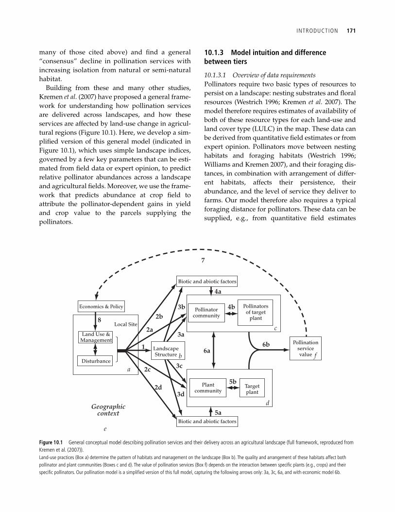
INTRODUCTION 171
many of those cited above) and fi nd a general “consensus” decline in pollination services with increasing isolation from natural or semi-natural habitat.
Building from these and many other studies, Kremen et al. (2007) have proposed a general frame-work for understanding how pollination services are delivered across landscapes, and how these services are affected by land-use change in agricul-tural regions ( Figure 10.1 ). Here, we develop a sim-plifi ed version of this general model (indicated in Figure 10.1 ), which uses simple landscape indices, governed by a few key parameters that can be esti-mated from fi eld data or expert opinion, to predict relative pollinator abundances across a landscape and agricultural fi elds. Moreover, we use the frame-work that predicts abundance at crop fi eld to attribute the pollinator-dependent gains in yield and crop value to the parcels supplying the pollinators.
10.1.3 Model intuition and difference between tiers
10.1.3.1 Overview of data requirements Pollinators require two basic types of resources to persist on a landscape: nesting substrates and fl oral resources (Westrich 1996; Kremen et al. 2007). The model therefore requires estimates of availability of both of these resource types for each land-use and land cover type (LULC) in the map. These data can be derived from quantitative fi eld estimates or from expert opinion. Pollinators move between nesting habitats and foraging habitats (Westrich 1996; Williams and Kremen 2007), and their foraging dis-tances, in combination with arrangement of differ-ent habitats, affects their persistence, their abundance, and the level of service they deliver to farms. Our model therefore also requires a typical foraging distance for pollinators. These data can be supplied, e.g., from quantitative fi eld estimates
7
4a
4b
6b
5b
c
b
a
e
f
d
3b2b
2a3a
6a
3c
3d2d
2c
1
5a
Biotic and abiotic factors
Local Site
Land Use &Management
Disturbance
8
Geographiccontext
Pollinatorcommunity
Pollinatorsof target
plant
Pollinationservicevalue
Targetplant
Plantcommunity
LandscapeStructure
Economics & Policy
Biotic and abiotic factors
Figure 10.1 General conceptual model describing pollination services and their delivery across an agricultural landscape (full framework, reproduced from Kremen et al. (2007)). Land-use practices (Box a) determine the pattern of habitats and management on the landscape (Box b). The quality and arrangement of these habitats affect both pollinator and plant communities (Boxes c and d). The value of pollination services (Box f) depends on the interaction between specifi c plants (e.g., crops) and their specifi c pollinators. Our pollination model is a simplifi ed version of this full model, capturing the following arrows only: 3a, 3c, 6a, and with economic model 6b.
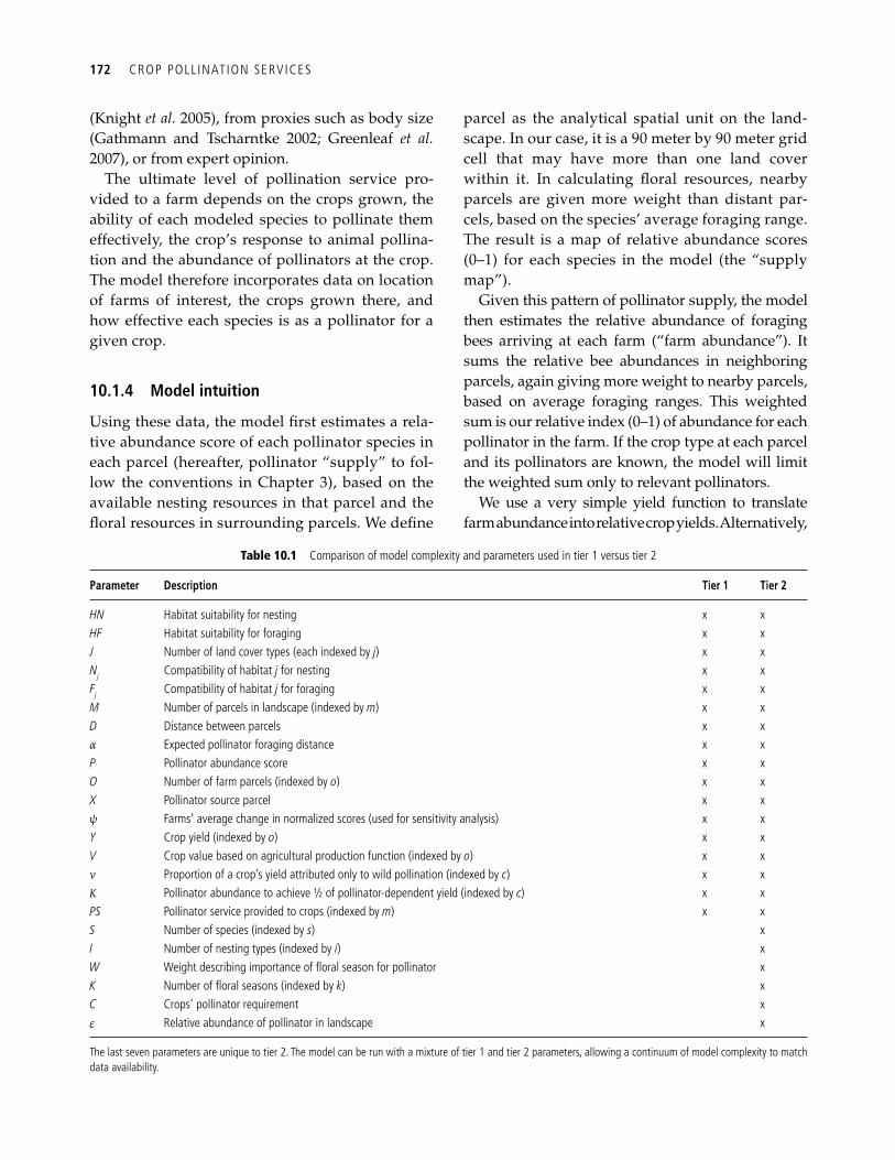
172 CROP POLL INATION SERVICES
(Knight et al. 2005), from proxies such as body size (Gathmann and Tscharntke 2002; Greenleaf et al. 2007), or from expert opinion.
The ultimate level of pollination service pro-vided to a farm depends on the crops grown, the ability of each modeled species to pollinate them effectively, the crop’s response to animal pollina-tion and the abundance of pollinators at the crop. The model therefore incorporates data on location of farms of interest, the crops grown there, and how effective each species is as a pollinator for a given crop.
10.1.4 Model intuition
Using these data, the model fi rst estimates a rela-tive abundance score of each pollinator species in each parcel (hereafter, pollinator “supply” to fol-low the conventions in Chapter 3 ), based on the available nesting resources in that parcel and the fl oral resources in surrounding parcels. We defi ne
parcel as the analytical spatial unit on the land-scape. In our case, it is a 90 meter by 90 meter grid cell that may have more than one land cover within it. In calculating fl oral resources, nearby parcels are given more weight than distant par-cels, based on the species’ average foraging range. The result is a map of relative abundance scores (0–1) for each species in the model (the “supply map”).
Given this pattern of pollinator supply, the model then estimates the relative abundance of foraging bees arriving at each farm (“farm abundance”). It sums the relative bee abundances in neighboring parcels, again giving more weight to nearby parcels, based on average foraging ranges. This weighted sum is our relative index (0–1) of abundance for each pollinator in the farm. If the crop type at each parcel and its pollinators are known, the model will limit the weighted sum only to relevant pollinators.
We use a very simple yield function to translate farm abundance into relative crop yields. Alternatively,
Table 10.1 Comparison of model complexity and parameters used in tier 1 versus tier 2
Parameter Description Tier 1 Tier 2
HN Habitat suitability for nesting x x HF Habitat suitability for foraging x x J Number of land cover types (each indexed by j ) x x N j Compatibility of habitat j for nesting x x F j Compatibility of habitat j for foraging x x M Number of parcels in landscape (indexed by m ) x x D Distance between parcels x x α Expected pollinator foraging distance x x P Pollinator abundance score x x O Number of farm parcels (indexed by o ) x x X Pollinator source parcel x x ψ Farms’ average change in normalized scores (used for sensitivity analysis) x x Y Crop yield (indexed by o ) x x V Crop value based on agricultural production function (indexed by o ) x x ν Proportion of a crop’s yield attributed only to wild pollination (indexed by c ) x x Κ Pollinator abundance to achieve ½ of pollinator-dependent yield (indexed by c ) x x PS Pollinator service provided to crops (indexed by m ) x x S Number of species (indexed by s ) x I Number of nesting types (indexed by i ) x W Weight describing importance of fl oral season for pollinator x K Number of fl oral seasons (indexed by k ) x C Crops’ pollinator requirement x ε Relative abundance of pollinator in landscape x
The last seven parameters are unique to tier 2. The model can be run with a mixture of tier 1 and tier 2 parameters, allowing a continuum of model complexity to match data availability.
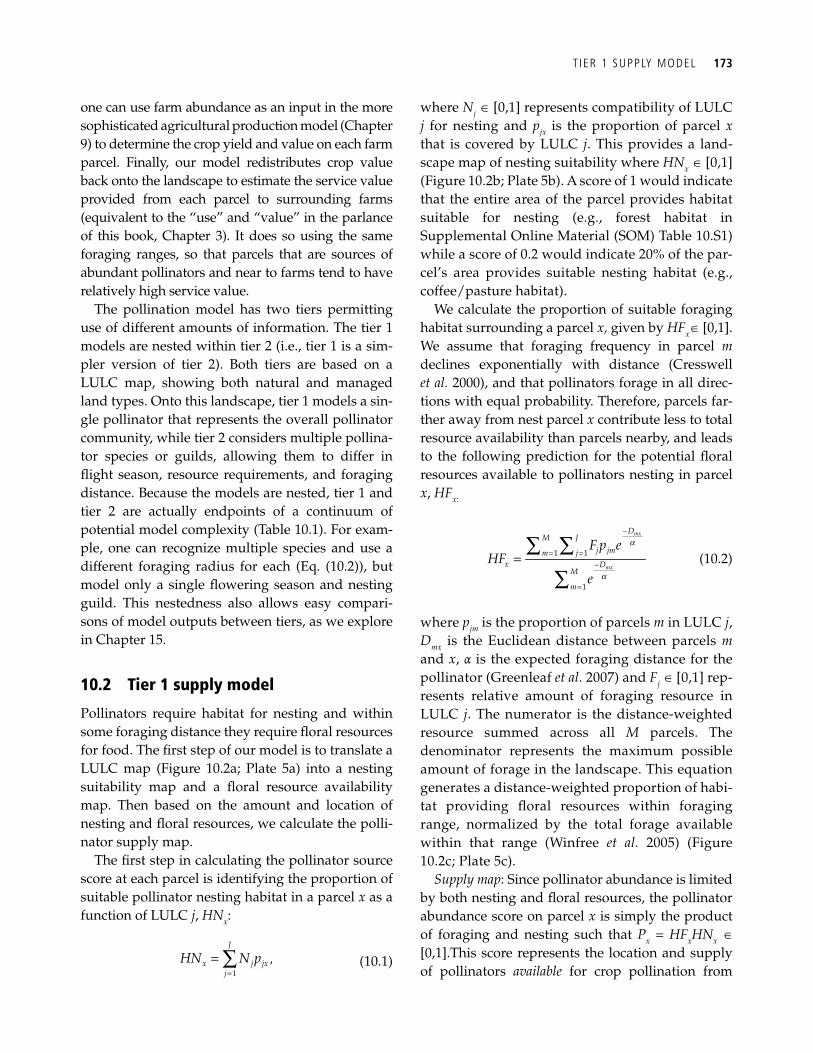
T IER 1 SUPPLY MODEL 173
one can use farm abundance as an input in the more sophisticated agricultural production model ( Chapter 9 ) to determine the crop yield and value on each farm parcel. Finally, our model redistributes crop value back onto the landscape to estimate the service value provided from each parcel to surrounding farms (equivalent to the “use” and “value” in the parlance of this book, Chapter 3 ). It does so using the same foraging ranges, so that parcels that are sources of abundant pollinators and near to farms tend to have relatively high service value.
The pollination model has two tiers permitting use of different amounts of information. The tier 1 models are nested within tier 2 (i.e., tier 1 is a sim-pler version of tier 2). Both tiers are based on a LULC map, showing both natural and managed land types. Onto this landscape, tier 1 models a sin-gle pollinator that represents the overall pollinator community, while tier 2 considers multiple pollina-tor species or guilds, allowing them to differ in fl ight season, resource requirements, and foraging distance. Because the models are nested, tier 1 and tier 2 are actually endpoints of a continuum of potential model complexity ( Table 10.1 ). For exam-ple, one can recognize multiple species and use a different foraging radius for each (Eq. (10.2)), but model only a single fl owering season and nesting guild. This nestedness also allows easy compari-sons of model outputs between tiers, as we explore in Chapter 15 .
10.2 Tier 1 supply model
Pollinators require habitat for nesting and within some foraging distance they require fl oral resources for food. The fi rst step of our model is to translate a LULC map ( Figure 10.2a ; Plate 5a) into a nesting suitability map and a fl oral resource availability map. Then based on the amount and location of nesting and fl oral resources, we calculate the polli-nator supply map.
The fi rst step in calculating the pollinator source score at each parcel is identifying the proportion of suitable pollinator nesting habitat in a parcel x as a function of LULC j , HN x :
=
= ∑1
,J
x j jxj
HN N p (10.1)
where N j Î [0,1] represents compatibility of LULC j for nesting and p jx is the proportion of parcel x that is covered by LULC j . This provides a land-scape map of nesting suitability where HN x Î [0,1] ( Figure 10.2b ; Plate 5b). A score of 1 would indicate that the entire area of the parcel provides habitat suitable for nesting (e.g., forest habitat in Supplemental Online Material (SOM) Table 10.S1 ) while a score of 0.2 would indicate 20% of the par-cel’s area provides suitable nesting habitat (e.g., coffee/pasture habitat).
We calculate the proportion of suitable foraging habitat surrounding a parcel x, given by HF x Î [0,1]. We assume that foraging frequency in parcel m declines exponentially with distance (Cresswell et al. 2000), and that pollinators forage in all direc-tions with equal probability. Therefore, parcels far-ther away from nest parcel x contribute less to total resource availability than parcels nearby, and leads to the following prediction for the potential fl oral resources available to pollinators nesting in parcel x , HF x :
a
a
−
= =−
=
=∑ ∑
∑1 1
1
mx
mx
DM J
j jmm jx D
M
m
F p eHF
e
(10.2)
where p jm is the proportion of parcels m in LULC j , D mx is the Euclidean distance between parcels m and x , α is the expected foraging distance for the pollinator (Greenleaf et al. 2007) and F j Î [0,1] rep-resents relative amount of foraging resource in LULC j . The numerator is the distance-weighted resource summed across all M parcels. The denominator represents the maximum possible amount of forage in the landscape. This equation generates a distance-weighted proportion of habi-tat providing fl oral resources within foraging range, normalized by the total forage available within that range (Winfree et al. 2005) ( Figure 10.2c ; Plate 5c).
Supply map : Since pollinator abundance is limited by both nesting and fl oral resources, the pollinator abundance score on parcel x is simply the product of foraging and nesting such that P x = HF x HN x Î [0,1].This score represents the location and supply of pollinators available for crop pollination from
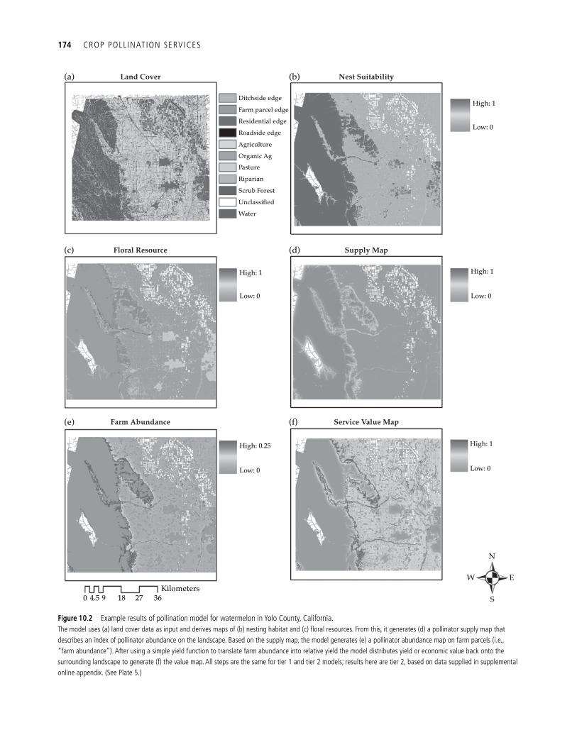
174 CROP POLL INATION SERVICES
Ditchside edge
Farm parcel edge
Residential edge
Roadside edge
Agriculture
Organic Ag
Pasture
Riparian
Scrub Forest
Unclassified
Water
Land Cover
High: 1
Low: 0
Nest Suitability
High: 1
Low: 0
Floral Resource(c)
(e)
(a)
(d)
(f)
(b)
High: 1
Low: 0
Supply Map
High: 0.25
Kilometers0 4.5 9 18 27 36
N
S
EW
Low: 0
Farm Abundance
High: 1
Low: 0
Service Value Map
Figure 10.2 Example results of pollination model for watermelon in Yolo County, California. The model uses (a) land cover data as input and derives maps of (b) nesting habitat and (c) fl oral resources. From this, it generates (d) a pollinator supply map that describes an index of pollinator abundance on the landscape. Based on the supply map, the model generates (e) a pollinator abundance map on farm parcels (i.e., “farm abundance”). After using a simple yield function to translate farm abundance into relative yield the model distributes yield or economic value back onto the surrounding landscape to generate (f) the value map. All steps are the same for tier 1 and tier 2 models; results here are tier 2, based on data supplied in supplemental online appendix. (See Plate 5.)
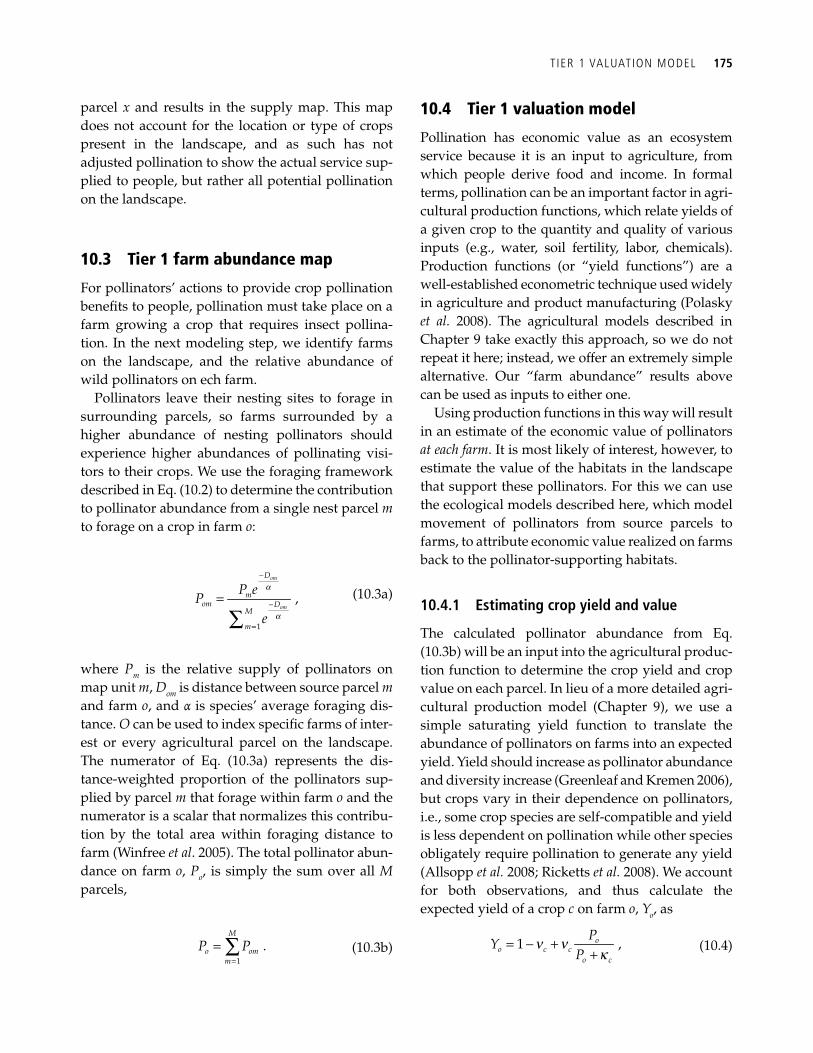
T IER 1 VALUATION MODEL 175
parcel x and results in the supply map. This map does not account for the location or type of crops present in the landscape, and as such has not adjusted pollination to show the actual service sup-plied to people, but rather all potential pollination on the landscape.
10.3 Tier 1 farm abundance map
For pollinators’ actions to provide crop pollination benefi ts to people, pollination must take place on a farm growing a crop that requires insect pollina-tion. In the next modeling step, we identify farms on the landscape, and the relative abundance of wild pollinators on ech farm.
Pollinators leave their nesting sites to forage in surrounding parcels, so farms surrounded by a higher abundance of nesting pollinators should experience higher abundances of pollinating visi-tors to their crops. We use the foraging framework described in Eq. (10.2) to determine the contribution to pollinator abundance from a single nest parcel m to forage on a crop in farm o :
a
a
−
−
=
=∑ 1
,
om
om
D
mom D
M
m
P eP
e
(10.3a)
where P m is the relative supply of pollinators on map unit m , D om is distance between source parcel m and farm o , and α is species’ average foraging dis-tance. O can be used to index specifi c farms of inter-est or every agricultural parcel on the landscape. The numerator of Eq. (10.3a) represents the dis-tance-weighted proportion of the pollinators sup-plied by parcel m that forage within farm o and the numerator is a scalar that normalizes this contribu-tion by the total area within foraging distance to farm (Winfree et al . 2005). The total pollinator abun-dance on farm o , P o , is simply the sum over all M parcels,
=
= ∑1
.M
o omm
P P (10.3b)
10.4 Tier 1 valuation model
Pollination has economic value as an ecosystem service because it is an input to agriculture, from which people derive food and income. In formal terms, pollination can be an important factor in agri-cultural production functions, which relate yields of a given crop to the quantity and quality of various inputs (e.g., water, soil fertility, labor, chemicals). Production functions (or “yield functions”) are a well-established econometric technique used widely in agriculture and product manufacturing (Polasky et al. 2008). The agricultural models described in Chapter 9 take exactly this approach, so we do not repeat it here; instead, we offer an extremely simple alternative. Our “farm abundance” results above can be used as inputs to either one.
Using production functions in this way will result in an estimate of the economic value of pollinators at each farm . It is most likely of interest, however, to estimate the value of the habitats in the landscape that support these pollinators. For this we can use the ecological models described here, which model movement of pollinators from source parcels to farms, to attribute economic value realized on farms back to the pollinator-supporting habitats.
10.4.1 Estimating crop yield and value
The calculated pollinator abundance from Eq. (10.3b) will be an input into the agricultural produc-tion function to determine the crop yield and crop value on each parcel. In lieu of a more detailed agri-cultural production model ( Chapter 9 ), we use a simple saturating yield function to translate the abundance of pollinators on farms into an expected yield. Yield should increase as pollinator abundance and diversity increase (Greenleaf and Kremen 2006), but crops vary in their dependence on pollinators, i.e., some crop species are self-compatible and yield is less dependent on pollination while other species obligately require pollination to generate any yield (Allsopp et al. 2008; Ricketts et al. 2008). We account for both observations, and thus calculate the expected yield of a crop c on farm o , Y o , as
n nk
= − ++
1 ,oo c c
o c
PY
P (10.4)
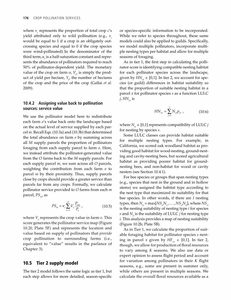
176 CROP POLL INATION SERVICES
where ν c represents the proportion of total crop c ’s yield attributed only to wild pollination (e.g., ν c would be equal to 1 if a crop is an obligately out-crossing species and equal to 0 if the crop species were wind-pollinated). . In the denominator of the third term, κ c is a half-saturation constant and repre-sents the abundance of pollinators required to reach 50% of pollinator-dependent yield. The monetary value of the crop on farm o, V o , is simply the prod-uct of yield per hectare, Y o , the number of hectares of the crop and the price of the crop (Gallai et al. 2009).
10.4.2 Assigning value back to pollination sources: service value
We use the pollinator model here to redistribute each farm o ’s value back onto the landscape based on the actual level of service supplied by each par-cel m . Recall Eqs. (10.3a) and (10.3b) that determined the total abundance on farm o by summing across all M supply parcels the proportion of pollinators foraging from each supply parcel to farm o . Here, we instead attribute the pollinator-generated value from the O farms back to the M supply parcels. For each supply parcel m , we sum across all O parcels, weighting the contribution from each farm o to parcel m by their proximity. Thus, supply parcels close by crops should provide a greater service than parcels far from any crops. Formally, we calculate pollinator service provided to O farms from each m parcel, PS m , as
n=
= ∑1
,O
omm c o
o o
PPS V
P (10.5)
where V o represents the crop value in farm o . This score generates the pollinator service map ( Figure 10.2f ; Plate 5F) and represents the location and value based on supply of pollinators that provide crop pollination to surrounding farms (i.e., equivalent to “value” results in the parlance of Chapter 3 ).
10.5 Tier 2 supply model
The tier 2 model follows the same logic as tier 1, but each step allows for more detailed, season-specifi c
or species-specifi c information to be incorporated. While we refer to species throughout, these same models could also be applied to guilds. Specifi cally, we model multiple pollinators, incorporate multi-ple nesting types per habitat and allow for multiple seasons of foraging.
As in tier 1, the fi rst step in calculating the polli-nator score is identifying compatible nesting habitat for each pollinator species across the landscape, given by HN sx Î [0,1]. In tier 2, we account for spe-cies (or guild) differences in habitat suitability so that the proportion of suitable nesting habitat in a parcel x for pollinator species s as a function LULC j , HN sx is
=
= ∑1
,J
sx js jxj
HN N p (10.6)
where N js Î [0,1] represents compatibility of LULC j for nesting by species s .
Some LULC classes can provide habitat suitable for multiple nesting types. For example, in California, we scored oak woodland habitat as pro-viding good habitat for wood-nesting, ground-nest-ing and cavity-nesting bees, but scored agricultural habitat as providing poorer habitat for ground-nesting bees, and non-habitat for wood or cavity nesters (see Section 10.4.1 ).
For bee species or groups that span nesting types (e.g., species that nest in the ground and in hollow stems) we assigned the habitat type according to the nest type that maximized its suitability for that bee species. In other words, if there are I nesting types, then N js = max[ NS si N ji , . . . , NS sI N jI ], where NS si is the nesting suitability of nesting type i for species s and N ji is the suitability of LULC j for nesting type i . This analysis provides a map of nesting suitability ( Figure 10.2b ; Plate 5B).
As in Tier 1, we calculate the proportion of suit-able foraging habitat for pollinator species s nest-ing in parcel x given by HF sx Î [0,1]. In tier 2, though, we allow for production of fl oral resources to vary among K seasons. We also use data or expert opinion to assess fl ight period and account for variation among pollinators in their K fl ight seasons, e.g., some are present in summer only, while others are present in multiple seasons. We calculate the overall fl oral resources available as a
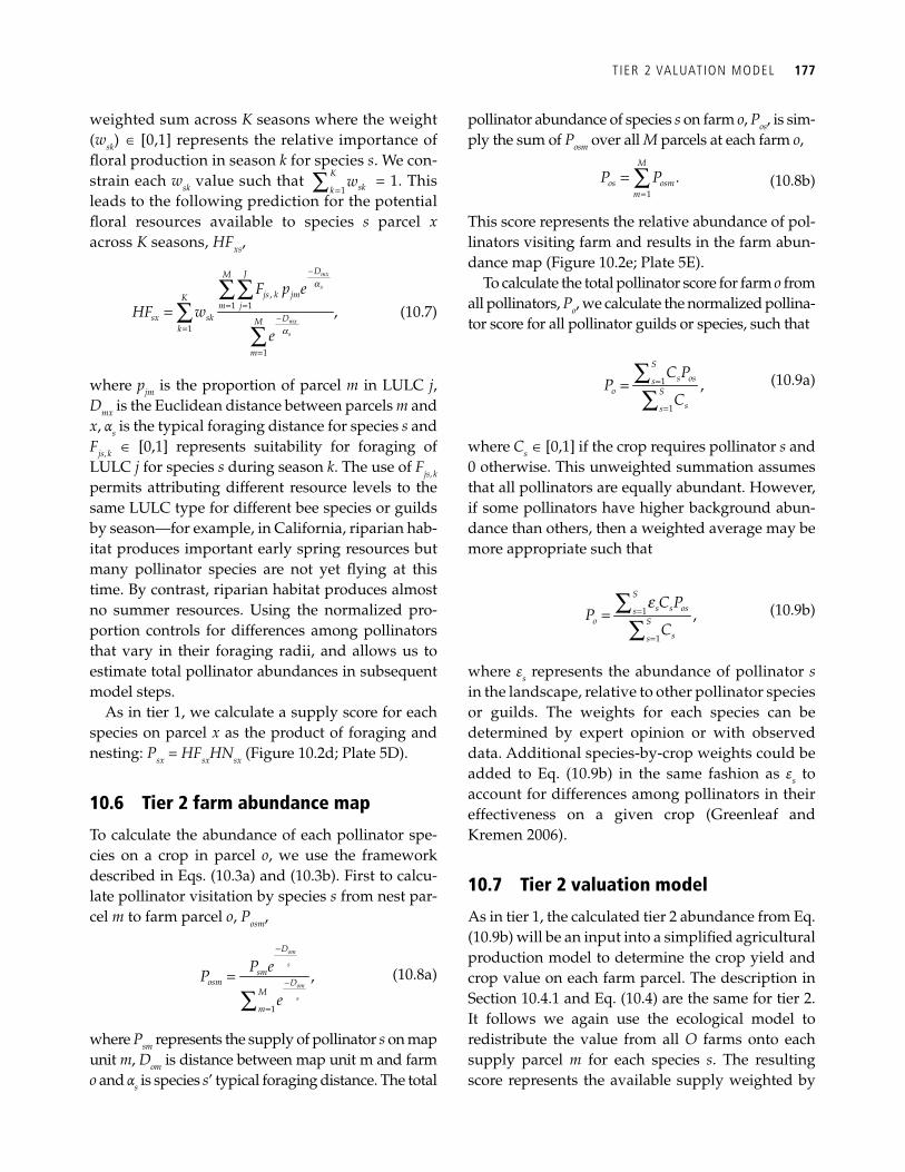
T IER 2 VALUATION MODEL 177
weighted sum across K seasons where the weight ( w sk ) Î [0,1] represents the relative importance of fl oral production in season k for species s . We con-strain each w sk value such that
=∑ 1
K
skkw = 1. This
leads to the following prediction for the potential fl oral resources available to species s parcel x across K seasons, HF xs ,
mx
s
mx
s
DJM
js k jmKm j
sx sk DMk
m
F p eHF w
e
,1 1
1
1
,
a
a
−
= =−
=
=
=∑∑
∑∑
(10.7)
where p jm is the proportion of parcel m in LULC j , D mx is the Euclidean distance between parcels m and x , α s is the typical foraging distance for species s and F js, k Î [0,1] represents suitability for foraging of LULC j for species s during season k . The use of F js, k permits attributing different resource levels to the same LULC type for different bee species or guilds by season—for example, in California, riparian hab-itat produces important early spring resources but many pollinator species are not yet fl ying at this time. By contrast, riparian habitat produces almost no summer resources. Using the normalized pro-portion controls for differences among pollinators that vary in their foraging radii, and allows us to estimate total pollinator abundances in subsequent model steps.
As in tier 1, we calculate a supply score for each species on parcel x as the product of foraging and nesting: P sx = HF sx HN sx ( Figure 10.2d ; Plate 5D).
10.6 Tier 2 farm abundance map
To calculate the abundance of each pollinator spe-cies on a crop in parcel o , we use the framework described in Eqs. (10.3a) and (10.3b). First to calcu-late pollinator visitation by species s from nest par-cel m to farm parcel o , P osm ,
om
s
om
s
D
smosm D
M
m
P eP
e1
,
−
−
=
=
∑
(10.8a)
where P sm represents the supply of pollinator s on map unit m , D om is distance between map unit m and farm o and α s is species s ’ typical foraging distance. The total
pollinator abundance of species s on farm o , P os , is sim-ply the sum of P osm over all M parcels at each farm o ,
=
= ∑1
.M
os osmm
P P (10.8b)
This score represents the relative abundance of pol-linators visiting farm and results in the farm abun-dance map ( Figure 10.2e ; Plate 5E).
To calculate the total pollinator score for farm o from all pollinators, P o , we calculate the normalized pollina-tor score for all pollinator guilds or species, such that
S
s osso S
ss
C PP
C1
1
,=
=
= ∑∑
(10.9a)
where C s Î [0,1] if the crop requires pollinator s and 0 otherwise. This unweighted summation assumes that all pollinators are equally abundant. However, if some pollinators have higher background abun-dance than others, then a weighted average may be more appropriate such that
S
s s osso S
ss
C PP
C1
1
,e
=
=
= ∑∑
(10.9b)
where ε s represents the abundance of pollinator s in the landscape, relative to other pollinator species or guilds. The weights for each species can be determined by expert opinion or with observed data. Additional species-by-crop weights could be added to Eq. (10.9b) in the same fashion as ε s to account for differences among pollinators in their effectiveness on a given crop (Greenleaf and Kremen 2006).
10.7 Tier 2 valuation model
As in tier 1, the calculated tier 2 abundance from Eq. (10.9b) will be an input into a simplifi ed agricultural production model to determine the crop yield and crop value on each farm parcel. The description in Section 10.4.1 and Eq. (10.4) are the same for tier 2. It follows we again use the ecological model to redistribute the value from all O farms onto each supply parcel m for each species s . The resulting score represents the available supply weighted by
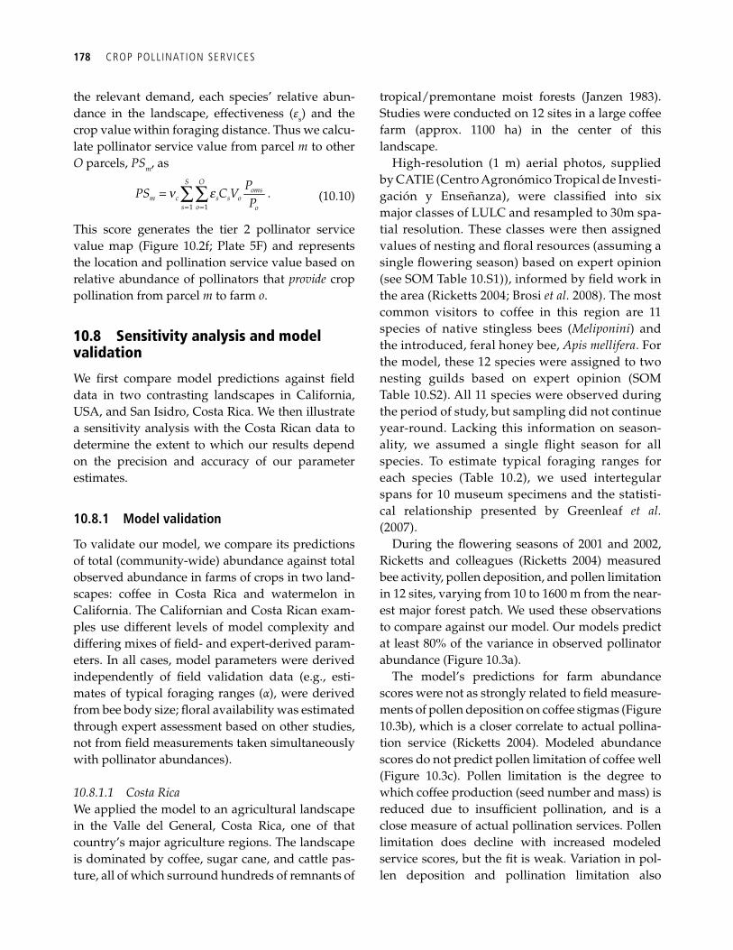
178 CROP POLL INATION SERVICES
the relevant demand, each species’ relative abun-dance in the landscape, effectiveness ( ε s ) and the crop value within foraging distance. Thus we calcu-late pollinator service value from parcel m to other O parcels, PS m , as
n e= =
= ∑∑1 1
.S O
omsm c s s o
s o o
PPS C V
P (10.10)
This score generates the tier 2 pollinator service value map ( Figure 10.2f ; Plate 5F) and represents the location and pollination service value based on relative abundance of pollinators that provide crop pollination from parcel m to farm o .
10.8 Sensitivity analysis and model validation
We fi rst compare model predictions against fi eld data in two contrasting landscapes in California, USA, and San Isidro, Costa Rica. We then illustrate a sensitivity analysis with the Costa Rican data to determine the extent to which our results depend on the precision and accuracy of our parameter estimates.
10.8.1 Model validation
To validate our model, we compare its predictions of total (community-wide) abundance against total observed abundance in farms of crops in two land-scapes: coffee in Costa Rica and watermelon in California. The Californian and Costa Rican exam-ples use different levels of model complexity and differing mixes of fi eld- and expert-derived param-eters. In all cases, model parameters were derived independently of fi eld validation data (e.g., esti-mates of typical foraging ranges ( α ), were derived from bee body size; fl oral availability was estimated through expert assessment based on other studies, not from fi eld measurements taken simultaneously with pollinator abundances).
10.8.1.1 Costa Rica We applied the model to an agricultural landscape in the Valle del General, Costa Rica, one of that country’s major agriculture regions. The landscape is dominated by coffee, sugar cane, and cattle pas-ture, all of which surround hundreds of remnants of
tropical/premontane moist forests (Janzen 1983). Studies were conducted on 12 sites in a large coffee farm (approx. 1100 ha) in the center of this landscape.
High-resolution (1 m) aerial photos, supplied by CATIE (Centro Agronómico Tropical de Investi-gación y Enseñanza), were classifi ed into six major classes of LULC and resampled to 30m spa-tial resolution. These classes were then assigned values of nesting and fl oral resources (assuming a single fl owering season) based on expert opinion (see SOM Table 10.S1 )), informed by fi eld work in the area (Ricketts 2004; Brosi et al. 2008). The most common visitors to coffee in this region are 11 species of native stingless bees ( Meliponini ) and the introduced, feral honey bee, Apis mellifera . For the model, these 12 species were assigned to two nesting guilds based on expert opinion (SOM Table 10.S2 ). All 11 species were observed during the period of study, but sampling did not continue year-round. Lacking this information on season-ality, we assumed a single fl ight season for all species. To estimate typical foraging ranges for each species ( Table 10.2 ), we used intertegular spans for 10 museum specimens and the statisti-cal relationship presented by Greenleaf et al. (2007).
During the fl owering seasons of 2001 and 2002, Ricketts and colleagues (Ricketts 2004) measured bee activity, pollen deposition, and pollen limitation in 12 sites, varying from 10 to 1600 m from the near-est major forest patch. We used these observations to compare against our model. Our models predict at least 80% of the variance in observed pollinator abundance ( Figure 10.3a ).
The model’s predictions for farm abundance scores were not as strongly related to fi eld measure-ments of pollen deposition on coffee stigmas ( Figure 10.3b ), which is a closer correlate to actual pollina-tion service (Ricketts 2004). Modeled abundance scores do not predict pollen limitation of coffee well ( Figure 10.3c ). Pollen limitation is the degree to which coffee production (seed number and mass) is reduced due to insuffi cient pollination, and is a close measure of actual pollination services. Pollen limitation does decline with increased modeled service scores, but the fi t is weak. Variation in pol-len deposition and pollination limitation also
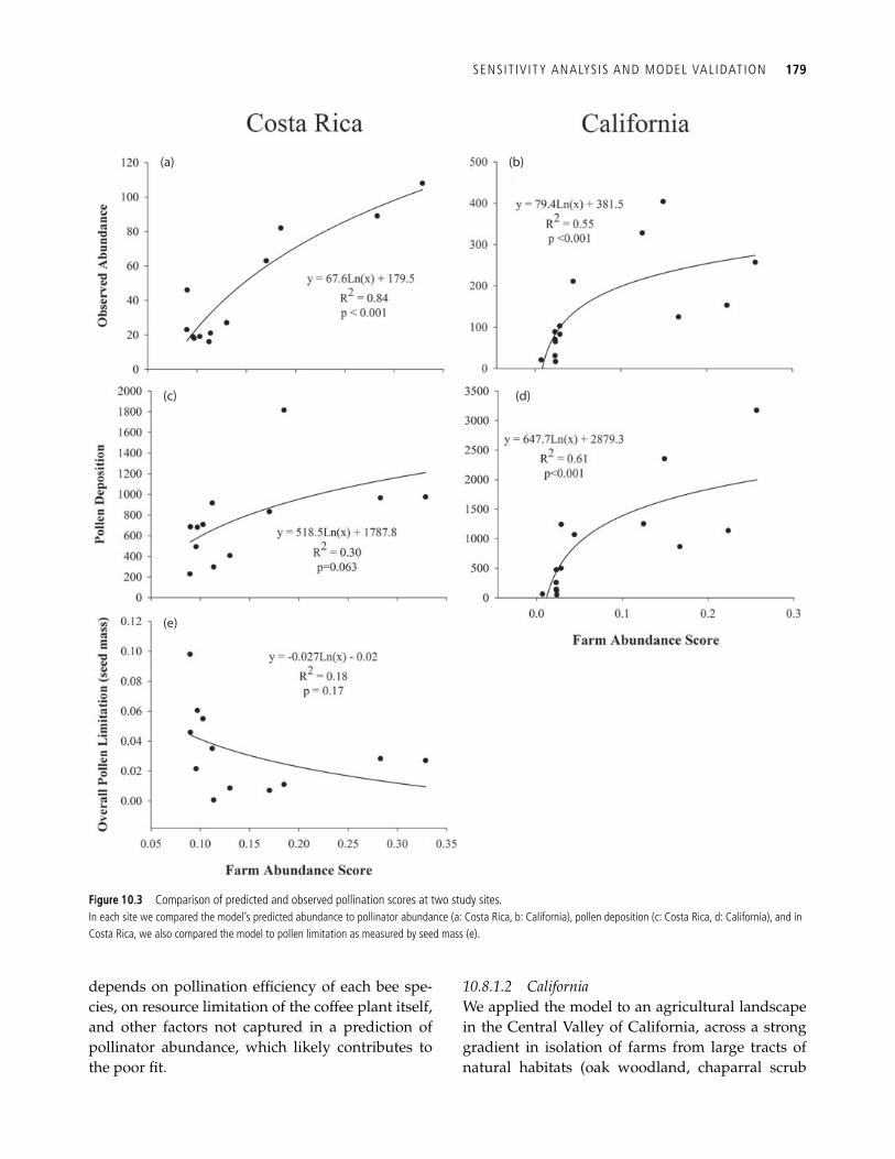
SENSIT IV ITY ANALYSIS AND MODEL VAL IDATION 179
depends on pollination effi ciency of each bee spe-cies, on resource limitation of the coffee plant itself, and other factors not captured in a prediction of pollinator abundance, which likely contributes to the poor fi t.
10.8.1.2 California We applied the model to an agricultural landscape in the Central Valley of California, across a strong gradient in isolation of farms from large tracts of natural habitats (oak woodland, chaparral scrub
(a) (b)
(c) (d)
(e)
Figure 10.3 Comparison of predicted and observed pollination scores at two study sites. In each site we compared the model’s predicted abundance to pollinator abundance (a: Costa Rica, b: California), pollen deposition (c: Costa Rica, d: California), and in Costa Rica, we also compared the model to pollen limitation as measured by seed mass (e).
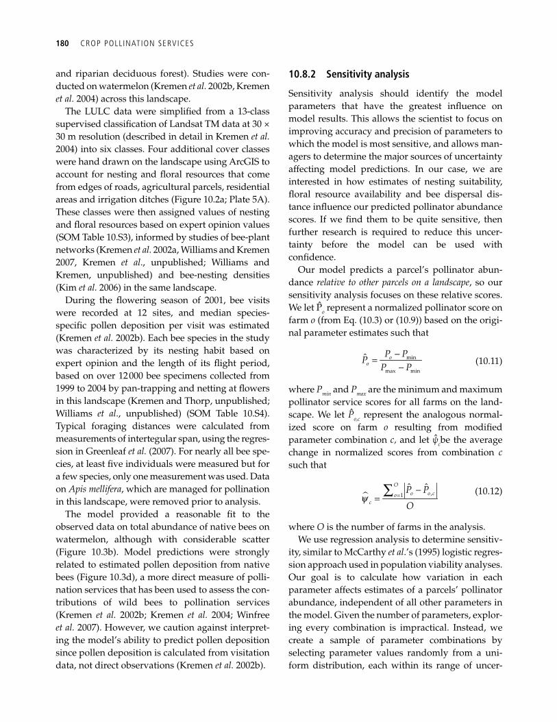
180 CROP POLL INATION SERVICES
and riparian deciduous forest). Studies were con-ducted on watermelon (Kremen et al. 2002b, Kremen et al. 2004) across this landscape.
The LULC data were simplifi ed from a 13-class supervised classifi cation of Landsat TM data at 30 × 30 m resolution (described in detail in Kremen et al. 2004) into six classes. Four additional cover classes were hand drawn on the landscape using ArcGIS to account for nesting and fl oral resources that come from edges of roads, agricultural parcels, residential areas and irrigation ditches ( Figure 10.2a ; Plate 5A). These classes were then assigned values of nesting and fl oral resources based on expert opinion values (SOM Table 10.S3 ), informed by studies of bee-plant networks (Kremen et al. 2002a, Williams and Kremen 2007, Kremen et al ., unpublished; Williams and Kremen, unpublished) and bee- nesting densities (Kim et al. 2006) in the same landscape.
During the fl owering season of 2001, bee visits were recorded at 12 sites, and median species- specifi c pollen deposition per visit was estimated (Kremen et al. 2002b). Each bee species in the study was characterized by its nesting habit based on expert opinion and the length of its fl ight period, based on over 12 000 bee specimens collected from 1999 to 2004 by pan-trapping and netting at fl owers in this landscape (Kremen and Thorp, unpublished; Williams et al ., unpublished) (SOM Table 10.S4 ). Typical foraging distances were calculated from measurements of intertegular span, using the regres-sion in Greenleaf et al. (2007). For nearly all bee spe-cies, at least fi ve individuals were measured but for a few species, only one measurement was used. Data on Apis mellifera , which are managed for pollination in this landscape, were removed prior to analysis.
The model provided a reasonable fi t to the observed data on total abundance of native bees on watermelon, although with considerable scatter ( Figure 10.3b ). Model predictions were strongly related to estimated pollen deposition from native bees ( Figure 10.3d ), a more direct measure of polli-nation services that has been used to assess the con-tributions of wild bees to pollination services (Kremen et al. 2002b; Kremen et al. 2004; Winfree et al. 2007). However, we caution against interpret-ing the model’s ability to predict pollen deposition since pollen deposition is calculated from visitation data, not direct observations (Kremen et al. 2002b).
10.8.2 Sensitivity analysis
Sensitivity analysis should identify the model parameters that have the greatest infl uence on model results. This allows the scientist to focus on improving accuracy and precision of parameters to which the model is most sensitive, and allows man-agers to determine the major sources of uncertainty affecting model predictions. In our case, we are interested in how estimates of nesting suitability, fl oral resource availability and bee dispersal dis-tance infl uence our predicted pollinator abundance scores. If we fi nd them to be quite sensitive, then further research is required to reduce this uncer-tainty before the model can be used with confi dence.
Our model predicts a parcel’s pollinator abun-dance relative to other parcels on a landscape , so our sensitivity analysis focuses on these relative scores. We let P o represent a normalized pollinator score on farm o (from Eq. (10.3) or (10.9)) based on the origi-nal parameter estimates such that
min
max min
ˆ oo
P PP
P P−=− (10.11)
where P min and P max are the minimum and maximum pollinator service scores for all farms on the land-scape. We let P o , c represent the analogous normal-ized score on farm o resulting from modifi ed parameter combination c, and let ψ c be the average change in normalized scores from combination c such that
#y =−
=∑ ,1
ˆ ˆO
o o coc
P P
O (10.12)
where O is the number of farms in the analysis. We use regression analysis to determine sensitiv-
ity, similar to McCarthy et al .’s (1995) logistic regres-sion approach used in population viability analyses. Our goal is to calculate how variation in each parameter affects estimates of a parcels’ pollinator abundance, independent of all other parameters in the model. Given the number of parameters, explor-ing every combination is impractical. Instead, we create a sample of parameter combinations by selecting parameter values randomly from a uni-form distribution, each within its range of uncer-
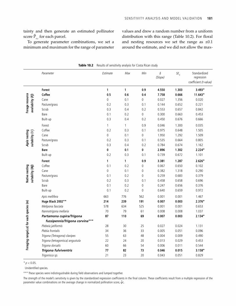
SENSIT IV ITY ANALYSIS AND MODEL VAL IDATION 181
tainty and then generate an estimated pollinator score P o , c for each parcel.
To generate parameter combinations, we set a minimum and maximum for the range of parameter
values and drew a random number from a uniform distribution with this range ( Table 10.2 ). For fl oral and nesting resources we set the range as ±0.1 around the estimate, and we did not allow the max-
Table 10.2 Results of sensitivity analysis for Costa Rican study
Parameter Estimate Max Min δ (Slope)
SE δ Standardized regression
coeffi cient (t -value)
Fora
ge re
sour
ce
avai
labi
lity
( F j )
Forest 1 1 0.9 4.550 1.303 3.493* Coffee 0.5 0.6 0.4 7.758 0.666 11.643* Cane 0 0.1 0 0.027 1.356 0.020 Pasture/grass 0.2 0.3 0.1 0.144 0.652 0.221 Scrub 0.3 0.4 0.2 0.553 0.657 0.842 Bare 0.1 0.2 0 0.300 0.663 0.453 Built-up 0.3 0.4 0.2 0.450 0.676 0.666
Api
s ne
stin
g su
itabi
lity
( N j )
Forest 1 1 0.9 0.046 1.300 0.035 Coffee 0.2 0.3 0.1 0.975 0.648 1.505 Cane 0 0.1 0 1.950 1.292 1.509 Pasture/grass 0.2 0.3 0.1 0.535 0.664 0.805 Scrub 0.3 0.4 0.2 0.784 0.674 1.162 Bare 0 0.1 0 2.896 1.302 2.224* Built-up 0.2 0.3 0.1 0.739 0.672 1.101
Nativ
e ne
stin
g su
itabi
lity
( N j )
Forest 1 1 0.9 3.381 1.287 2.626* Coffee 0.1 0.2 0 0.067 0.650 0.102 Cane 0 0.1 0 0.382 1.318 0.290 Pasture/grass 0.1 0.2 0 0.259 0.683 0.379 Scrub 0.2 0.3 0.1 0.458 0.658 0.696 Bare 0.1 0.2 0 0.247 0.656 0.376 Built-up 0.1 0.2 0 0.640 0.659 0.972
Fora
ging
rang
e( α s
) for
eac
h sp
ecie
s (m
)
Apis mellifera 663 776 562 0.001 0.001 1.467 Huge Black 2002** 214 239 191 0.007 0.003 2.376* Melipona fasciata 578 634 525 0.001 0.001 0.653 Nannotrigona mellaria 70 79 61 0.008 0.008 1.037 Partamona cupira/Trigona
fussipennis/Trigona corvina *** 87 110 69 0.007 0.003 2.134*
Plebeia jatiformis 28 30 25 0.027 0.024 1.131 Plebia frontalis 34 36 33 0.005 0.051 0.096 Trigona (Tetragona) clavipes 55 63 48 0.004 0.009 0.490 Trigona (tetragonisca) angustula 22 24 20 0.013 0.029 0.453 Trigona dorsalis 60 66 54 0.006 0.011 0.544 Trigona fulviventris 77 82 73 0.046 0.015 3.158* Trigonisca sp. 21 23 20 0.043 0.051 0.829
* p < 0.05.
Unidentifi ed species.
*** These species were indistinguishable during fi eld observations and lumped together.
The strength of the model’s sensitivity is given by the standardized regression coeffi cients in the fi nal column. These coeffi cients result from a multiple regression of the parameter value combinations on the average change in normalized pollination score, ψ c .
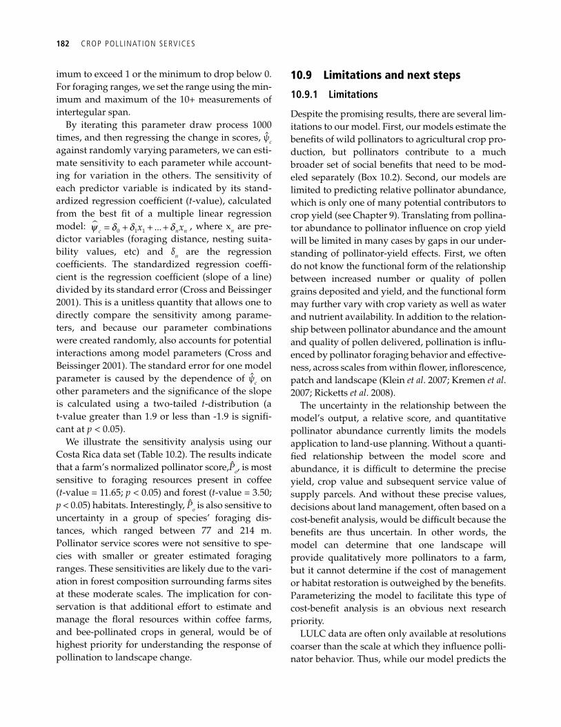
182 CROP POLL INATION SERVICES
imum to exceed 1 or the minimum to drop below 0. For foraging ranges, we set the range using the min-imum and maximum of the 10+ measurements of intertegular span.
By iterating this parameter draw process 1000 times, and then regressing the change in scores, ψ c against randomly varying parameters, we can esti-mate sensitivity to each parameter while account-ing for variation in the others. The sensitivity of each predictor variable is indicated by its stand-ardized regression coeffi cient ( t -value), calculated from the best fi t of a multiple linear regression model: # 0 1 1 ... n nc x xy d d d= + + + , where x n are pre-dictor variables (foraging distance, nesting suita-bility values, etc) and δ n are the regression coeffi cients. The standardized regression coeffi -cient is the regression coeffi cient (slope of a line) divided by its standard error (Cross and Beissinger 2001). This is a unitless quantity that allows one to directly compare the sensitivity among parame-ters, and because our parameter combinations were created randomly, also accounts for potential interactions among model parameters (Cross and Beissinger 2001). The standard error for one model parameter is caused by the dependence of ψ c on other parameters and the signifi cance of the slope is calculated using a two-tailed t -distribution (a t-value greater than 1.9 or less than -1.9 is signifi -cant at p < 0.05).
We illustrate the sensitivity analysis using our Costa Rica data set ( Table 10.2 ). The results indicate that a farm’s normalized pollinator score, P o , is most sensitive to foraging resources present in coffee ( t -value = 11.65; p < 0.05) and forest ( t -value = 3.50; p < 0.05) habitats. Interestingly, P o is also sensitive to uncertainty in a group of species’ foraging dis-tances, which ranged between 77 and 214 m. Pollinator service scores were not sensitive to spe-cies with smaller or greater estimated foraging ranges. These sensitivities are likely due to the vari-ation in forest composition surrounding farms sites at these moderate scales. The implication for con-servation is that additional effort to estimate and manage the fl oral resources within coffee farms, and bee-pollinated crops in general, would be of highest priority for understanding the response of pollination to landscape change.
10.9 Limitations and next steps
10.9.1 Limitations
Despite the promising results, there are several lim-itations to our model. First, our models estimate the benefi ts of wild pollinators to agricultural crop pro-duction, but pollinators contribute to a much broader set of social benefi ts that need to be mod-eled separately ( Box 10.2 ). Second, our models are limited to predicting relative pollinator abundance, which is only one of many potential contributors to crop yield (see Chapter 9 ). Translating from pollina-tor abundance to pollinator infl uence on crop yield will be limited in many cases by gaps in our under-standing of pollinator-yield effects. First, we often do not know the functional form of the relationship between increased number or quality of pollen grains deposited and yield, and the functional form may further vary with crop variety as well as water and nutrient availability. In addition to the relation-ship between pollinator abundance and the amount and quality of pollen delivered, pollination is infl u-enced by pollinator foraging behavior and effective-ness, across scales from within fl ower, infl orescence, patch and landscape (Klein et al . 2007; Kremen et al . 2007; Ricketts et al . 2008).
The uncertainty in the relationship between the model’s output, a relative score, and quantitative pollinator abundance currently limits the models application to land-use planning. Without a quanti-fi ed relationship between the model score and abundance, it is diffi cult to determine the precise yield, crop value and subsequent service value of supply parcels. And without these precise values, decisions about land management, often based on a cost-benefi t analysis, would be diffi cult because the benefi ts are thus uncertain. In other words, the model can determine that one landscape will provide qualitatively more pollinators to a farm, but it cannot determine if the cost of management or habitat restoration is outweighed by the benefi ts. Parameterizing the model to facilitate this type of cost-benefi t analysis is an obvious next research priority.
LULC data are often only available at resolutions coarser than the scale at which they infl uence polli-nator behavior. Thus, while our model predicts the
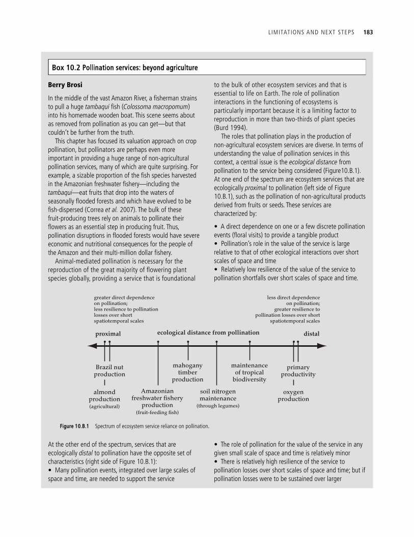
L IMITATIONS AND NEXT STEPS 183
At the other end of the spectrum, services that are ecologically distal to pollination have the opposite set of characteristics (right side of Figure 10.B.1): • Many pollination events, integrated over large scales of space and time, are needed to support the service
• The role of pollination for the value of the service in any given small scale of space and time is relatively minor • There is relatively high resilience of the service to pollination losses over short scales of space and time; but if pollination losses were to be sustained over larger
Berry Brosi
In the middle of the vast Amazon River, a fi sherman strains to pull a huge tambaqui fi sh ( Colossoma macropomum ) into his homemade wooden boat. This scene seems about as removed from pollination as you can get—but that couldn’t be further from the truth.
This chapter has focused its valuation approach on crop pollination, but pollinators are perhaps even more important in providing a huge range of non-agricultural pollination services, many of which are quite surprising. For example, a sizable proportion of the fi sh species harvested in the Amazonian freshwater fi shery—including the tambaqui —eat fruits that drop into the waters of seasonally fl ooded forests and which have evolved to be fi sh-dispersed (Correa et al. 2007). The bulk of these fruit-producing trees rely on animals to pollinate their fl owers as an essential step in producing fruit. Thus, pollination disruptions in fl ooded forests would have severe economic and nutritional consequences for the people of the Amazon and their multi-million dollar fi shery.
Animal-mediated pollination is necessary for the reproduction of the great majority of fl owering plant species globally, providing a service that is foundational
to the bulk of other ecosystem services and that is essential to life on Earth. The role of pollination interactions in the functioning of ecosystems is particularly important because it is a limiting factor to reproduction in more than two-thirds of plant species (Burd 1994).
The roles that pollination plays in the production of non-agricultural ecosystem services are diverse. In terms of understanding the value of pollination services in this context, a central issue is the ecological distance from pollination to the service being considered (Figure10.B.1). At one end of the spectrum are ecosystem services that are ecologically proximal to pollination (left side of Figure 10.B.1), such as the pollination of non-agricultural products derived from fruits or seeds. These services are characterized by:
• A direct dependence on one or a few discrete pollination events (fl oral visits) to provide a tangible product • Pollination’s role in the value of the service is large relative to that of other ecological interactions over short scales of space and time • Relatively low resilience of the value of the service to pollination shortfalls over short scales of space and time.
Box 10.2 Pollination services: beyond agriculture
Figure 10.B.1 Spectrum of ecosystem service reliance on pollination.
greater direct dependenceon pollination;less resilience to pollinationlosses over shortspatiotemporal scales
less direct dependenceon pollination;
greater resilience topollination losses over short
spatiotemporal scales
almondproduction(agricultural)
Brazil nutproduction
proximal distalecological distance from pollination
Amazonianfreshwater fishery
production(fruit-feeding fish)
soil nitrogenmaintenance
(through legumes)
mahoganytimber
production
maintenanceof tropical
biodiversity
primaryproductivity
oxygenproduction
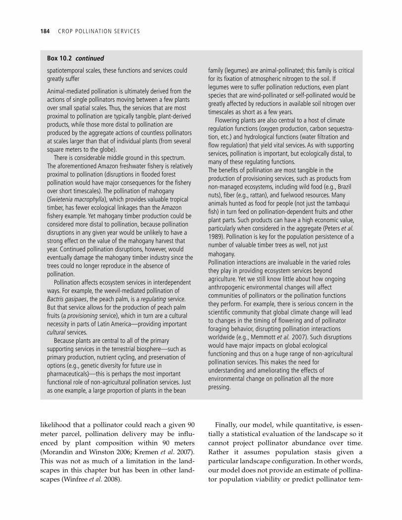
184 CROP POLL INATION SERVICES
spatiotemporal scales, these functions and services could greatly suffer
Animal-mediated pollination is ultimately derived from the actions of single pollinators moving between a few plants over small spatial scales. Thus, the services that are most proximal to pollination are typically tangible, plant-derived products, while those more distal to pollination are produced by the aggregate actions of countless pollinators at scales larger than that of individual plants (from several square meters to the globe).
There is considerable middle ground in this spectrum. The aforementioned Amazon freshwater fi shery is relatively proximal to pollination (disruptions in fl ooded forest pollination would have major consequences for the fi shery over short timescales). The pollination of mahogany ( Swietenia macrophylla ), which provides valuable tropical timber, has fewer ecological linkages than the Amazon fi shery example. Yet mahogany timber production could be considered more distal to pollination, because pollination disruptions in any given year would be unlikely to have a strong effect on the value of the mahogany harvest that year. Continued pollination disruptions, however, would eventually damage the mahogany timber industry since the trees could no longer reproduce in the absence of pollination.
Pollination affects ecosystem services in interdependent ways. For example, the weevil-mediated pollination of Bactris gasipaes , the peach palm, is a regulating service. But that service allows for the production of peach palm fruits (a provisioning service), which in turn are a cultural necessity in parts of Latin America—providing important cultural services.
Because plants are central to all of the primary supporting services in the terrestrial biosphere—such as primary production, nutrient cycling, and preservation of options (e.g., genetic diversity for future use in pharmaceuticals)—this is perhaps the most important functional role of non-agricultural pollination services. Just as one example, a large proportion of plants in the bean
family (legumes) are animal-pollinated; this family is critical for its fi xation of atmospheric nitrogen to the soil. If legumes were to suffer pollination reductions, even plant species that are wind-pollinated or self-pollinated would be greatly affected by reductions in available soil nitrogen over timescales as short as a few years.
Flowering plants are also central to a host of climate regulation functions (oxygen production, carbon sequestra-tion, etc.) and hydrological functions (water fi ltration and fl ow regulation) that yield vital services. As with supporting services, pollination is important, but ecologically distal, to many of these regulating functions. The benefi ts of pollination are most tangible in the production of provisioning services, such as products from non-managed ecosystems, including wild food (e.g., Brazil nuts), fi ber (e.g., rattan), and fuelwood resources. Many animals hunted as food for people (not just the tambaqui fi sh) in turn feed on pollination-dependent fruits and other plant parts. Such products can have a high economic value, particularly when considered in the aggregate (Peters et al. 1989). Pollination is key for the population persistence of a number of valuable timber trees as well, not just mahogany. Pollination interactions are invaluable in the varied roles they play in providing ecosystem services beyond agriculture. Yet we still know little about how ongoing anthropogenic environmental changes will affect communities of pollinators or the pollination functions they perform. For example, there is serious concern in the scientifi c community that global climate change will lead to changes in the timing of fl owering and of pollinator foraging behavior, disrupting pollination interactions worldwide (e.g., Memmott et al. 2007). Such disruptions would have major impacts on global ecological functioning and thus on a huge range of non-agricultural pollination services. This makes the need for understanding and ameliorating the effects of environmental change on pollination all the more pressing.
Box 10.2 continued
likelihood that a pollinator could reach a given 90 meter parcel, pollination delivery may be infl u-enced by plant composition within 90 meters (Morandin and Winston 2006; Kremen et al . 2007). This was not as much of a limitation in the land-scapes in this chapter but has been in other land-scapes (Winfree et al. 2008).
Finally, our model, while quantitative, is essen-tially a statistical evaluation of the landscape so it cannot project pollinator abundance over time. Rather it assumes population stasis given a particular landscape confi guration. In other words, our model does not provide an estimate of pollina-tor population viability or predict pollinator tem-
L IMITATIONS AND NEXT STEPS 185
poral dynamics or interaction of time and space through meta-population dynamics. As such, it does not incorporate stochastic events, which may infl uence long-term population dynamics and yield.
10.9.2 Next steps
While new ecological data are needed to gain a better understanding of the relationship between crop pollination and yield, we can use this current model framework to advance our understanding in a number of ways. First, we can apply this model to a much larger set of crop studies con-ducted at the landscape scale (viz, studies in Ricketts et al. 2008). Second, using statistical tech-niques, we can relate the landscape-level outputs of the model (pollinator supply) to the observed measure of pollination services in each study (e.g., pollen deposition, pollen limitation) to attempt to develop a direct relationship between landscape and yield effects via pollinator abundances. Third, by manipulating modeled landscapes (e.g., by increasing fl oral or nesting resources in different spatial confi gurations), we can estimate the effects on pollinator abundances and pollination services across a range of changes in resources, and look for generalities across landscapes in the density and arrangement of resources needed to provide adequate pollinators and pollination services. This would inform efforts to preserve existing habitats within degraded landscape and also guide planning of habitat restoration. Similar to our sensitivity analysis of model parameters, we also envision analyses exploring the sensitivity of modeled pollination services to resource patchi-ness at different grain sizes or to different land-scape confi gurations.
Acknowledgments
This work was facilitated by McDonnell Foundation 21st Century and University of California Chancellor’s Partnership awards to C.K., and by two National Center for Ecological Analysis and Synthesis working groups ( Restoring an ecosystem service to degraded landscapes: native bees and crop pol-
lination ; PI’s C.K. and N.M.W. Conservation priorities: Can we have our biodiversity and ecosystem services too? PI’s P. Kareiva, T. Ricketts, G. Daily) supported by NSF grant DEB-00–72909, the University of California at Santa Barbara, and the State of California. Kirsten Almberg helped with fi gures and Jaime Florez provided measurements of inter-tegular spans for Costa Rican bees. Berry Brosi pro-vided expert assessment of nesting and fl oral resources for the Costa Rica validation. Peter Kareiva, Erik Nelson, Berry Brosi, and Kai Chan all provided input in early development of the model. Saul Cunningham and Alexandra Klein provided valuable comments and corrections that improved the chapter.
References
Allsopp, M. H., de Lange, W. J., and Veldtman, R. (2008). Valuing insect pollination services with cost of replace-ment. PLoS One 3, e3128.
Brosi, B. J., Daily, G. C., Shih, T. M., et al . (2008). The effects of forest fragmentation on bee communities in tropical countryside. Journal of Applied Ecology 45 , 773–83.
Burd, M. (1994). Bateman’s principle and plant reproduc-tion—the role of pollen limitation in fruit and seed set. Botanical Review 60 , 83–139.
Cane, J. H. (1997). Lifetime monetary value of individual pollinators: the bee Habropoda laboriosa at rabbiteye blue-berry ( Vaccinium ashei Reade). Acta Horticulturae 446 , 67–70.
Correa, S. B., Winemiller, K. O., Lopez-Fernandez, H., et al . (2007). Evolutionary perspectives on seed consumption and dispersal by fi shes. Bioscience 57 , 748–56.
Costanza, R., dArge, R., deGroot, R., et al . (1997). The value of the world’s ecosystem services and natural capital. Nature 387 , 253–60.
Cresswell, J. E., Osborne, J. L., and Goulson, D. (2000). An economic model of the limits to foraging range in cen-tral place foragers with numerical solutions for bumble-bees. Ecological Entomology 25 , 249–55.
Cross, P. C., and Beissinger, S. R. (2001). Using logistic regression to analyze the sensitivity of PVA models: A comparison of methods based on African wild dog models. Conservation Biology 15 , 1335–46.
Free, J. B. (1993). Insect pollination of crops . Academic Press, San Diego.
Gallai, N., Salles, J. M., Settele, J., et al . 2009. Economic valu-ation of the vulnerability of world agriculture confronted with pollinator decline. Ecological Economics 68 , 810–21.

186 CROP POLL INATION SERVICES
Gathmann, A., and Tscharntke, T. (2002). Foraging ranges of solitary bees. Journal of Animal Ecology 71 , 757–64.
Greenleaf, S., Williams, N., Winfree, R., et al . (2007). Bee foraging ranges and their relationships to body size. Oecologia 153 , 589–96.
Greenleaf, S. S., and Kremen, C. (2006). Wild bee species increase tomato production and respond differently to surrounding land use in Northern California. Biological Conservation 133 , 81–7.
Hines, H. M., and Hendrix, S. D. (2005). Bumble bee ( Hymenoptera apidae ) diversity and abundance in tall-grass prairie patches: Effects of local and landscape fl o-ral resources. Environmental Entomology 34 , 1477–84.
Hoehn, P., Tscharntke, T., Tylianakis, J. M., and Steffan-Dewenter, I. 2008. Functional group diversity of bee pol-linators increases crop yield. Proceedings of the Royal Society B: Biological Sciences 275 , 2283–91.
Janzen, D. H., Ed. (1983). Costa Rican natural history . University of Chicago Press, Chicago.
Kim, J., Williams, N., and Kremen, C. 2006. Effects of culti-vation and proximity to natural habitat on ground- nesting native bees in California sunfl ower fi elds. Journal of the Kansas Entomological Society 79 , 309–20.
Klein, A. M., Mueller, C. M., Hoehn, P., et al . (in press). Understanding the role of species richness for pollina-tion services. In: D. Bunker, A. Hector, M. Loreau, et al ., Eds., The consequences of changing biodiversity—solutions and scenarios . Oxford University Press, Oxford.
Klein, A. M., Vaissière, B. E., Cane, J. H., et al . (2007). Importance of pollinators in changing landscapes for world crops. Proceedings of the Royal Society 274 , 303–13.
Knight, M. E., Martin, A. P., Bishop, S., et al . (2005). An interspecifi c comparison of foraging range and nest density of four bumblebee ( Bombus ) species. Molecular Ecology 14 , 1811–20.
Kremen, C., Bugg, R. L., Nicola, N., et al . (2002a). Native bees, native plants and crop pollination in California. Fremontia 30 , 41–9.
Kremen, C., Williams, N. M., and Thorp, R. W. (2002b). Crop pollination from native bees at risk from agricul-tural intensifi cation. Proceedings of the National Academy of Sciences 99 , 16812–16.
Kremen, C., Williams, N. M., Bugg, R. L., et al . (2004). The area requirements of an ecosystem service: crop pollina-tion by native bee communities in California. Ecology Letters 7 , 1109–19.
Kremen, C., Williams, N. M., Aizen, M. A., et al . (2007). Pollination and other ecosystem services produced by mobile organisms: a conceptual framework for the effects of land-use change. Ecology Letters 10 , 299–314.
Losey, J. E., and Vaughan, M. (2006). The economic value of ecological services provided by insects. Bioscience 56 , 311–23.
McCarthy, M. A., Burgman, M. A., and Ferson, S. (1995). Sensitivity analysis for models of population viability. Biological Conservation 73 , 93–100.
Memmott, J., Craze, P. G., Waser, N. M., et al . (2007). Global warming and the disruption of plant-pollinator interac-tions. Ecology Letters 10 , 710–717.
Morandin, L. A., and Winston, M. L. (2006). Pollinators provide economic incentive to preserve natural land in agroecosystems. Agriculture, Ecosystems & Environment 116 , 289–92.
National Research Council of the National Academies. 2006. Status of pollinators in North America . National Academy Press, Washington, DC.
Peters, C. M., Gentry, A. H., and Mendelsohn, R. O. (1989). Valuation of an Amazonian rainforest. Nature 339 , 655–6.
Polasky, S., Nelson, E., Camm, J., et al . (2008). Where to put things? Spatial land management to sustain biodiver-sity and economic returns. Biological Conservation 141 , 1505–24.
Potts, S. G., Vulliamy, B., Dafni, A., et al . (2003). Linking bees and fl owers: how do fl oral communities structure pollinator communities? Ecology 84 , 2628–42.
Potts, S. G., Vulliamy, B., Roberts, S., et al . (2005). Role of nesting resources in organising diverse bee communi-ties in a Mediterranean landscape. Ecological Entemology 30 , 78–85.
Priess, J. A., Mimler, M., Klein, A. M., et al . (2007). Linking deforestation scenarios to pollination services and eco-nomic returns in coffee agroforestry systems. Ecological Applications 17 , 407–17.
Ricketts, T. H. (2004). Tropical forest fragments enhance pollinator activity in nearby coffee crops. Conservation Biology 18 , 1262–71.
Ricketts, T. H., Daily, G. C., Ehrlich, P. R., et al . (2004). Economic value of tropical forest to coffee production. Proceedings of the National Academy of Sciences of the USA 101 , 12579–82.
Ricketts, T. H., Regetz, J., Steffan-Dewenter, I., et al . (2008). Landscape effects on crop pollination services: are there general patterns? Ecology Letters 11 , 499–515.
Southwick, E. E., and Southwick, L. (1992). Estimating the economic value of honey-bees (hymenoptera, apidae) as agricultural pollinators in the United States. Journal of Ecological Entomology 85 , 621–33.
Stokstad, E. (2007). The case of the empty hives. Science 316 , 970–2.
Tepedino, V. J., and Stanton, N. L. (1981). Diversity and competition in bee-plant communities on short-grass prairie. Oikos 36 , 35–44.
Westrich, P. (1996). Habitat requirements of central European bees and the problems of partial habitats. In: A. Matheson, S. L. Buchmann, C. O’Toole, et al. , Eds., The conservation of bees . Academic Press, London, pp. 1–16.

L IMITATIONS AND NEXT STEPS 187
Williams, N., and Kremen, C. (2007). Floral resource distri-bution among habitats determines productivity of a solitary bee, Osmia lignaria , in a mosaic agricultural landscape. Ecological Applications 17 , 910–21.
Winfree, R., Dushoff, J., Crone, E., et al . (2005). Testing sim-ple indices of habitat proximity. American Naturalist 165 , 707–17.
Winfree, R., Williams, N. M., Dushoff, J., et al . (2007). Native bees provide insurance against ongoing honey bee losses. Ecology Letters 10 , 1105–13.
Winfree, R., Williams, N. M., Gaines, H., et al . (2008). Wild bee pollinators provide the majority of crop visitation across land-use gradients in New Jersey and Pennsylvania, USA. Journal of Applied Ecology 45 , 793–802.
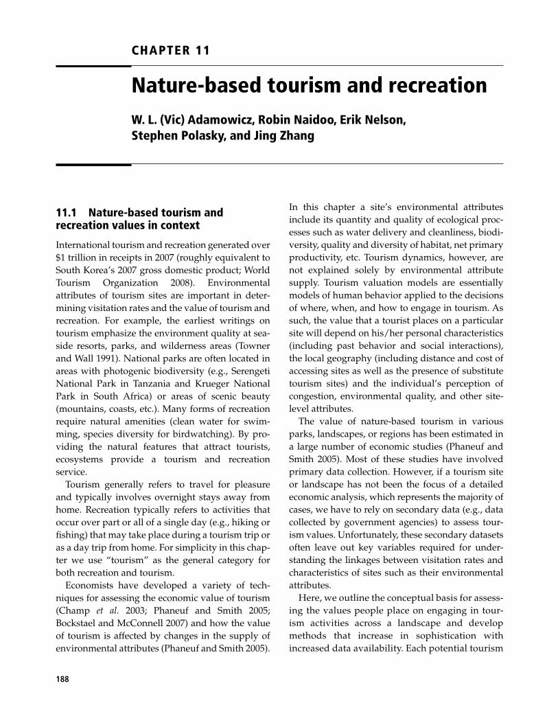
188
CHAPTER 11
Nature-based tourism and recreation W. L. (Vic) Adamowicz, Robin Naidoo, Erik Nelson, Stephen Polasky, and Jing Zhang
11.1 Nature-based tourism and recreation values in context
International tourism and recreation generated over $1 trillion in receipts in 2007 (roughly equivalent to South Korea’s 2007 gross domestic product; World Tourism Organization 2008 ). Environmental attributes of tourism sites are important in deter-mining visitation rates and the value of tourism and recreation. For example, the earliest writings on tourism emphasize the environment quality at sea-side resorts, parks, and wilderness areas ( Towner and Wall 1991 ). National parks are often located in areas with photogenic biodiversity (e.g., Serengeti National Park in Tanzania and Krueger National Park in South Africa) or areas of scenic beauty (mountains, coasts, etc.). Many forms of recreation require natural amenities (clean water for swim-ming, species diversity for birdwatching). By pro-viding the natural features that attract tourists, ecosystems provide a tourism and recreation service.
Tourism generally refers to travel for pleasure and typically involves overnight stays away from home. Recreation typically refers to activities that occur over part or all of a single day (e.g., hiking or fi shing) that may take place during a tourism trip or as a day trip from home. For simplicity in this chap-ter we use “tourism” as the general category for both recreation and tourism.
Economists have developed a variety of tech-niques for assessing the economic value of tourism ( Champ et al. 2003 ; Phaneuf and Smith 2005 ; Bockstael and McConnell 2007 ) and how the value of tourism is affected by changes in the supply of environmental attributes ( Phaneuf and Smith 2005 ).
In this chapter a site’s environmental attributes include its quantity and quality of ecological proc-esses such as water delivery and cleanliness, biodi-versity, quality and diversity of habitat, net primary productivity, etc. Tourism dynamics, however, are not explained solely by environmental attribute supply. Tourism valuation models are essentially models of human behavior applied to the decisions of where, when, and how to engage in tourism. As such, the value that a tourist places on a particular site will depend on his/her personal characteristics (including past behavior and social interactions), the local geography (including distance and cost of accessing sites as well as the presence of substitute tourism sites) and the individual’s perception of congestion, environmental quality, and other site-level attributes.
The value of nature-based tourism in various parks, landscapes, or regions has been estimated in a large number of economic studies ( Phaneuf and Smith 2005 ). Most of these studies have involved primary data collection. However, if a tourism site or landscape has not been the focus of a detailed economic analysis, which represents the majority of cases, we have to rely on secondary data (e.g., data collected by government agencies) to assess tour-ism values. Unfortunately, these secondary datasets often leave out key variables required for under-standing the linkages between visitation rates and characteristics of sites such as their environmental attributes.
Here, we outline the conceptual basis for assess-ing the values people place on engaging in tour-ism activities across a landscape and develop methods that increase in sophistication with increased data availability. Each potential tourism
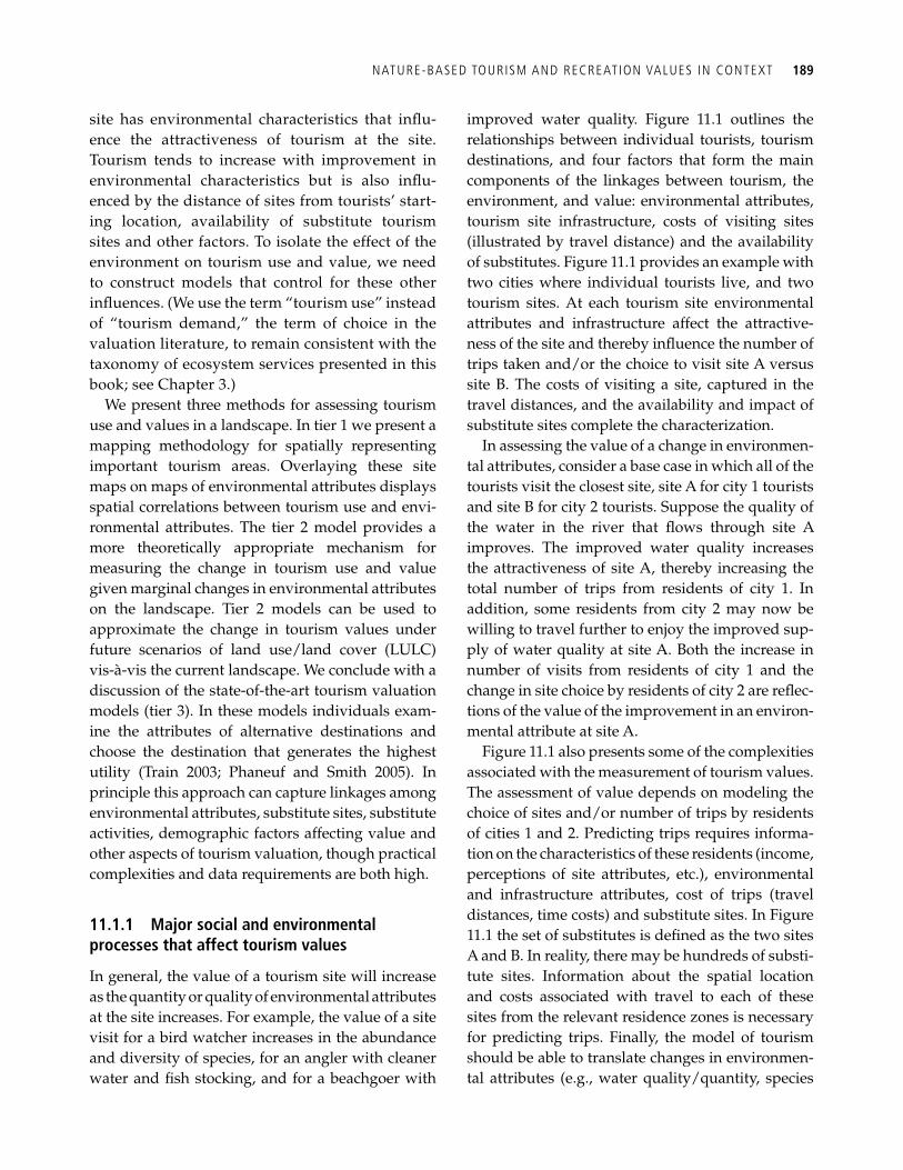
NATURE-BASED TOURISM AND RECREATION VALUES IN CONTEXT 189
site has environmental characteristics that infl u-ence the attractiveness of tourism at the site. Tourism tends to increase with improvement in environmental characteristics but is also infl u-enced by the distance of sites from tourists’ start-ing location, availability of substitute tourism sites and other factors. To isolate the effect of the environment on tourism use and value, we need to construct models that control for these other infl uences. (We use the term “tourism use” instead of “tourism demand,” the term of choice in the valuation literature, to remain consistent with the taxonomy of ecosystem services presented in this book; see Chapter 3 .)
We present three methods for assessing tourism use and values in a landscape. In tier 1 we present a mapping methodology for spatially representing important tourism areas. Overlaying these site maps on maps of environmental attributes displays spatial correlations between tourism use and envi-ronmental attributes. The tier 2 model provides a more theoretically appropriate mechanism for measuring the change in tourism use and value given marginal changes in environmental attributes on the landscape. Tier 2 models can be used to approximate the change in tourism values under future scenarios of land use/land cover (LULC) vis-à-vis the current landscape. We conclude with a discussion of the state-of-the-art tourism valuation models (tier 3). In these models individuals exam-ine the attributes of alternative destinations and choose the destination that generates the highest utility ( Train 2003 ; Phaneuf and Smith 2005 ). In principle this approach can capture linkages among environmental attributes, substitute sites, substitute activities, demographic factors affecting value and other aspects of tourism valuation, though practical complexities and data requirements are both high.
11.1.1 Major social and environmental processes that affect tourism values
In general, the value of a tourism site will increase as the quantity or quality of environmental attributes at the site increases. For example, the value of a site visit for a bird watcher increases in the abundance and diversity of species, for an angler with cleaner water and fi sh stocking, and for a beachgoer with
improved water quality. Figure 11.1 outlines the relationships between individual tourists, tourism destinations, and four factors that form the main components of the linkages between tourism, the environment, and value: environmental attributes, tourism site infrastructure, costs of visiting sites (illustrated by travel distance) and the availability of substitutes. Figure 11.1 provides an example with two cities where individual tourists live, and two tourism sites. At each tourism site environmental attributes and infrastructure affect the attractive-ness of the site and thereby infl uence the number of trips taken and/or the choice to visit site A versus site B. The costs of visiting a site, captured in the travel distances, and the availability and impact of substitute sites complete the characterization.
In assessing the value of a change in environmen-tal attributes, consider a base case in which all of the tourists visit the closest site, site A for city 1 tourists and site B for city 2 tourists. Suppose the quality of the water in the river that fl ows through site A improves. The improved water quality increases the attractiveness of site A, thereby increasing the total number of trips from residents of city 1. In addition, some residents from city 2 may now be willing to travel further to enjoy the improved sup-ply of water quality at site A. Both the increase in number of visits from residents of city 1 and the change in site choice by residents of city 2 are refl ec-tions of the value of the improvement in an environ-mental attribute at site A.
Figure 11.1 also presents some of the complexities associated with the measurement of tourism values. The assessment of value depends on modeling the choice of sites and/or number of trips by residents of cities 1 and 2. Predicting trips requires informa-tion on the characteristics of these residents (income, perceptions of site attributes, etc.), environmental and infrastructure attributes, cost of trips (travel distances, time costs) and substitute sites. In Figure 11.1 the set of substitutes is defi ned as the two sites A and B. In reality, there may be hundreds of substi-tute sites. Information about the spatial location and costs associated with travel to each of these sites from the relevant residence zones is necessary for predicting trips. Finally, the model of tourism should be able to translate changes in environmen-tal attributes (e.g., water quality/quantity, species
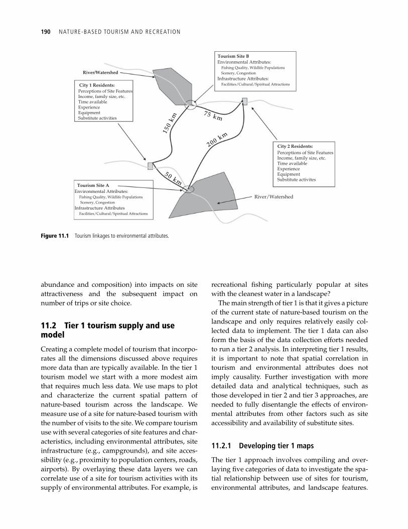
190 NATURE-BASED TOURISM AND RECREATION
abundance and composition) into impacts on site attractiveness and the subsequent impact on number of trips or site choice.
11.2 Tier 1 tourism supply and use model
Creating a complete model of tourism that incorpo-rates all the dimensions discussed above requires more data than are typically available. In the tier 1 tourism model we start with a more modest aim that requires much less data. We use maps to plot and characterize the current spatial pattern of nature-based tourism across the landscape. We measure use of a site for nature-based tourism with the number of visits to the site. We compare tourism use with several categories of site features and char-acteristics, including environmental attributes, site infrastructure (e.g., campgrounds), and site acces-sibility (e.g., proximity to population centers, roads, airports). By overlaying these data layers we can correlate use of a site for tourism activities with its supply of environmental attributes. For example, is
recreational fi shing particularly popular at sites with the cleanest water in a landscape?
The main strength of tier 1 is that it gives a picture of the current state of nature-based tourism on the landscape and only requires relatively easily col-lected data to implement. The tier 1 data can also form the basis of the data collection efforts needed to run a tier 2 analysis. In interpreting tier 1 results, it is important to note that spatial correlation in tourism and environmental attributes does not imply causality. Further investigation with more detailed data and analytical techniques, such as those developed in tier 2 and tier 3 approaches, are needed to fully disentangle the effects of environ-mental attributes from other factors such as site accessibility and availability of substitute sites.
11.2.1 Developing tier 1 maps
The tier 1 approach involves compiling and over-laying fi ve categories of data to investigate the spa-tial relationship between use of sites for tourism, environmental attributes, and landscape features.
150
km
200 km
75 km
50 km
River/Watershed
Perceptions of Site FeaturesIncome, family size, etc.Time availableExperienceEquipmentSubstitute activities
City 1 Residents:
Tourism Site B
City 2 Residents:
Tourism Site AEnvironmental Attributes:
Fishing Quality, Wildlife Populations Scenery, Congestion
Environmental Attributes:Fishing Quality, Wildlife Populations
Scenery, CongestionInfrastructure Attributes:
Facilities/Cultural/Spiritual Attractions
Perceptions of Site FeaturesIncome, family size, etc.Time availableExperienceEquipmentSubstitute activites
Infrastructure AttributesFacilities/Cultural/Spiritual Attractions
River/Watershed
Figure 11.1 Tourism linkages to environmental attributes.

T IER 1 TOURISM SUPPLY AND USE MODEL 191
The fi rst data layer includes the sites that provide tourism opportunities. Tourism sites can include national, provincial, state, county, or privately held parks and recreation areas. In some cases, tourism activities are not restricted to easily defi ned places on the landscape. Some tourism activities take place across a broad region or landscape. For example, duck hunting occurs on private and public land throughout the Prairie Pothole Region of the Midwest USA. To account for this type of activity we may subdivide the landscape into zones to iden-tify the portions of the landscape where diffuse tourism activity is more and less popular.
The second data layer maps visitation data. Visitation data can be measured a number of ways: site visits per unit time (where one person can reg-ister multiple visits over the course of the time period), number of visitors to the site per unit time, visitor days per unit time (the sum of all visitors’ length of stay in days), number of visitors purchas-ing entrance permits per unit time, etc. Stratifying visit data by visitor place of origin, reason for visit, and time allows more detailed and comprehensive analysis. For example, stratifying visitors by inter-national and domestic origin can show differences in visitation rates by cost (on average, international visitors pay much more to tour than domestic tour-ists). We discuss a way of placing a monetary value on the annual number of visits in Section 11.4 below.
The third data layer maps information on envi-ronmental attributes and other landscape features at sites. For example, does the site include a lake that would be a draw for swimming or fi shing, major changes in elevation good for hiking or dramatic views, habitat for charismatic species that are a draw for wildlife viewing? High water quality, suffi cient water fl ow, and abundant game fi sh are vital for certain stretches of rivers if they are to provide tourism value via recreational fi shing.
The fourth data layer maps information on impor-tant infrastructure at each site. Infrastructure impor-tant for determining tourism site visits includes roads, hiking trails, lodges, camping sites, and inter-pretative facilities.
The fi fth data layer maps major transportation infrastructure and urban areas. With these data we
can calculate distance and travel time from urban areas to each tourism site.
11.2.2 Example application of tier 1: Willamette Basin, Oregon, USA
We applied the tier 1 approach to tourism in the state parks of the Willamette Basin, Oregon, USA. The Willamette River and the Basin’s major high-ways and cities are located in the Basin’s valley fl oor ( Figure 11.2A ). Most state parks lie near cities and are on the main stem of the Willamette River or one of its tributaries; a few parks are in the Cascades mountain range on the eastern side of the Basin ( Figure 11.2A ).
Figures 11.2b through 11.2d present maps of environmental attributes and other features in the Basin (ODFW 2005; OGEO 2008; PNW-ERC 2008).
The state parks in the Basin with the most day visitors (not deconstructed by activity) are located in the Cascade Mountains and offer outstanding scenic attractions or recreation opportunities ( Figure 11.3a ). Silver Falls State Park, which con-tains many large waterfalls, had the most visits in 2004 even though its aggregate distance to the Basin’s cities was more than most other state parks.
Detroit Lake State Park, higher up in the Cascades than Silver Falls and of greater distance from cities, was the most popular destination in the Basin for overnight camping (an activity that is generally more costly than a day visit, given the time require-ments and the price of camping permits; see Figure 11.3b ). Many sites in the northeast corner of the Basin (and just outside the Basin along the Columbia River) were popular tourism destinations both because they are close to the largest urban center in the Basin (Portland) and feature the spec-tacular scenery around Mount Hood and the Columbia River Gorge.
The greater use of nature-based tourism in the northeast corner of the Basin is also refl ected in hunting data. The Santiam hunting region (the region that includes Mount Hood National Forest, Silver Falls State Park, Detroit Lake State Park, and part of the Columbia River Gorge) is the most pop-ular region for big game hunting, with 127 446 hunter days in 2004 (see Figure 11.4a ).
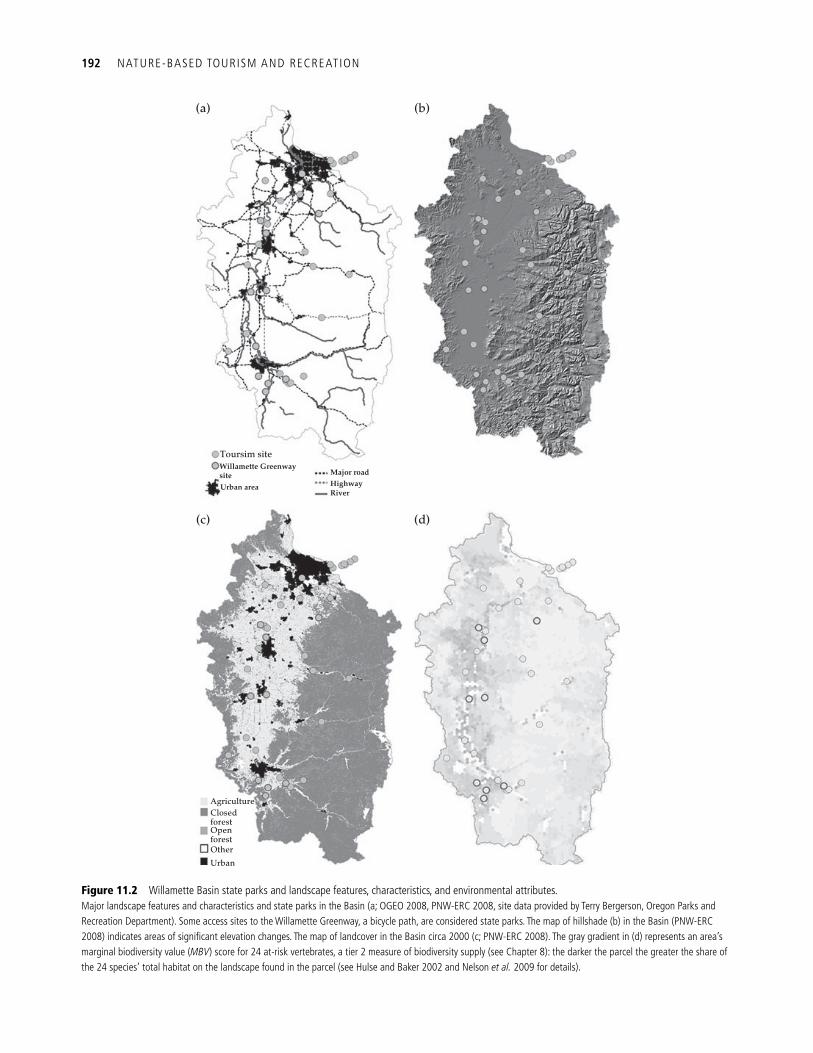
192 NATURE-BASED TOURISM AND RECREATION
Toursim site
(a) (b)
(c) (d)
Willamette GreenwaysiteUrban area
AgricultureClosedforestOpenforestOther
Urban
Major roadHighwayRiver
Figure 11.2 Willamette Basin state parks and landscape features, characteristics, and environmental attributes. Major landscape features and characteristics and state parks in the Basin (a; OGEO 2008, PNW-ERC 2008, site data provided by Terry Bergerson, Oregon Parks and Recreation Department). Some access sites to the Willamette Greenway, a bicycle path, are considered state parks. The map of hillshade (b) in the Basin (PNW-ERC 2008) indicates areas of signifi cant elevation changes. The map of landcover in the Basin circa 2000 (c; PNW-ERC 2008). The gray gradient in (d) represents an area’s marginal biodiversity value ( MBV ) score for 24 at-risk vertebrates, a tier 2 measure of biodiversity supply (see Chapter 8 ): the darker the parcel the greater the share of the 24 species’ total habitat on the landscape found in the parcel (see Hulse and Baker 2002 and Nelson et al. 2009 for details).
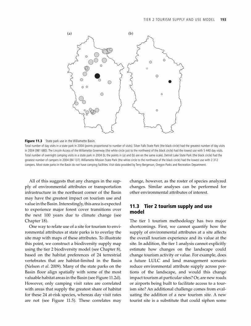
T IER 2 TOURISM SUPPLY AND USE MODEL 193
All of this suggests that any changes in the sup-ply of environmental attributes or transportation infrastructure in the northeast corner of the Basin may have the greatest impact on tourism use and value in the Basin. Interestingly, this area is expected to experience major forest cover transitions over the next 100 years due to climate change (see Chapter 18 ).
One way to relate use of a site for tourism to envi-ronmental attributes at state parks is to overlay the site map with maps of these attributes. To illustrate this point, we construct a biodiversity supply map using the tier 2 biodiversity model (see Chapter 8 ), based on the habitat preferences of 24 terrestrial vertebrates that are habitat-limited in the Basin ( Nelson et al. 2009 ). Many of the state parks on the Basin fl oor align spatially with some of the most valuable habitat areas in the Basin (see Figure 11.2d ). However, only camping visit rates are correlated with areas that supply the greatest share of habitat for these 24 at-risk species, whereas day visit rates are not (see Figure 11.5 ). These correlates may
change, however, as the roster of species analyzed changes. Similar analyses can be performed for other environmental attributes of interest.
11.3 Tier 2 tourism supply and use model
The tier 1 tourism methodology has two major shortcomings. First, we cannot quantify how the supply of environmental attributes at a site affects the overall tourism experience and its value at the site. In addition, the tier 1 analysis cannot explicitly estimate how changes on the landscape could change tourism activity or value. For example, does a future LULC and land management scenario reduce environmental attribute supply across por-tions of the landscape, and would this change impact tourism at particular sites? Or, are new roads or airports being built to facilitate access to a tour-ism site? An additional challenge comes from eval-uating the addition of a new tourism site. A new tourist site is a substitute that could siphon some
(a) (b)
Figure 11.3 State park use in the Willamette Basin.Total number of day visits in a state park in 2004 (points proportional to number of visits). Silver Falls State Park (the black circle) had the greatest number of day visits in 2004 (981 680). The Lincoln Access of the Willamette Greenway (the white circle just to the northwest of the black circle) had the lowest use with 5 440 day visits. Total number of overnight camping visits in a state park in 2004 (b; the points in (a) and (b) are on the same scale). Detroit Lake State Park (the black circle) had the greatest number of campers in 2004 (84 137). Willamette Mission State Park (the white circle to the northwest of the black circle) had the lowest use with 2 312 campers. Most state parks in the Basin do not have camping facilities. Visit data provided by Terry Bergerson, Oregon Parks and Recreation Department.
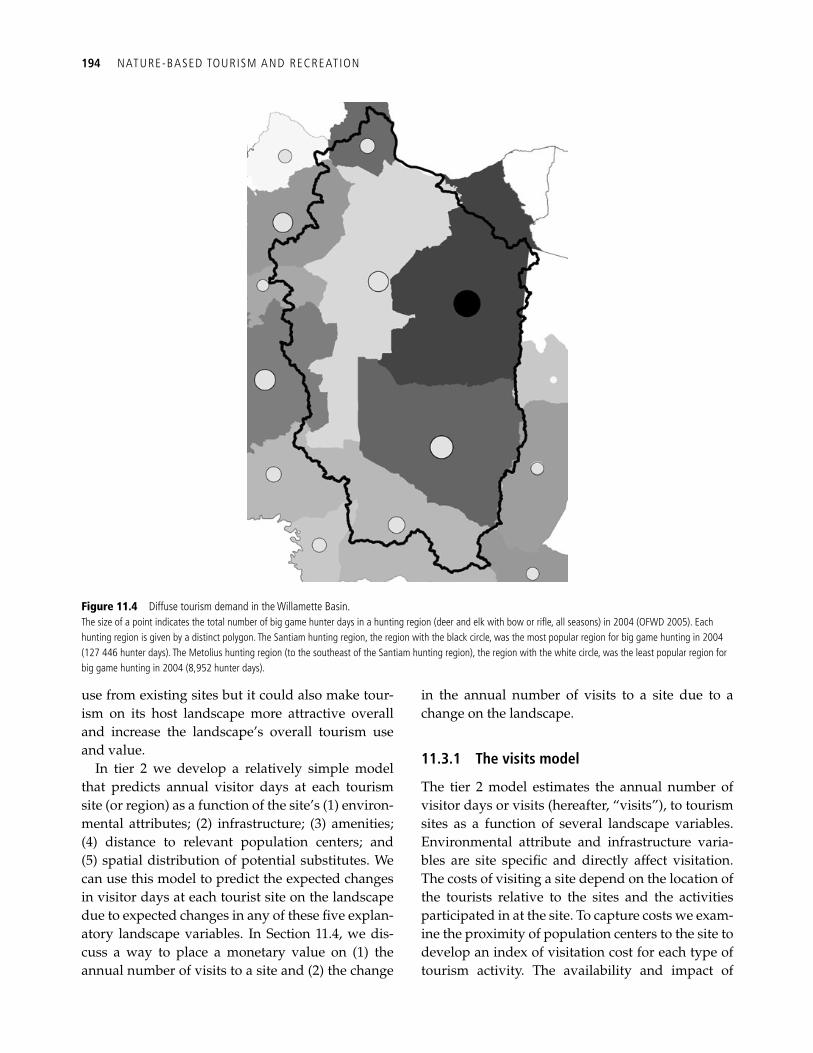
194 NATURE-BASED TOURISM AND RECREATION
use from existing sites but it could also make tour-ism on its host landscape more attractive overall and increase the landscape’s overall tourism use and value.
In tier 2 we develop a relatively simple model that predicts annual visitor days at each tourism site (or region) as a function of the site’s (1) environ-mental attributes; (2) infrastructure; (3) amenities; (4) distance to relevant population centers; and (5) spatial distribution of potential substitutes. We can use this model to predict the expected changes in visitor days at each tourist site on the landscape due to expected changes in any of these fi ve explan-atory landscape variables. In Section 11.4 , we dis-cuss a way to place a monetary value on (1) the annual number of visits to a site and (2) the change
in the annual number of visits to a site due to a change on the landscape.
11.3.1 The visits model
The tier 2 model estimates the annual number of visitor days or visits (hereafter, “visits”), to tourism sites as a function of several landscape variables. Environmental attribute and infrastructure varia-bles are site specifi c and directly affect visitation. The costs of visiting a site depend on the location of the tourists relative to the sites and the activities participated in at the site. To capture costs we exam-ine the proximity of population centers to the site to develop an index of visitation cost for each type of tourism activity. The availability and impact of
Figure 11.4 Diffuse tourism demand in the Willamette Basin.The size of a point indicates the total number of big game hunter days in a hunting region (deer and elk with bow or rifl e, all seasons) in 2004 (OFWD 2005). Each hunting region is given by a distinct polygon. The Santiam hunting region, the region with the black circle, was the most popular region for big game hunting in 2004 (127 446 hunter days). The Metolius hunting region (to the southeast of the Santiam hunting region), the region with the white circle, was the least popular region for big game hunting in 2004 (8,952 hunter days).
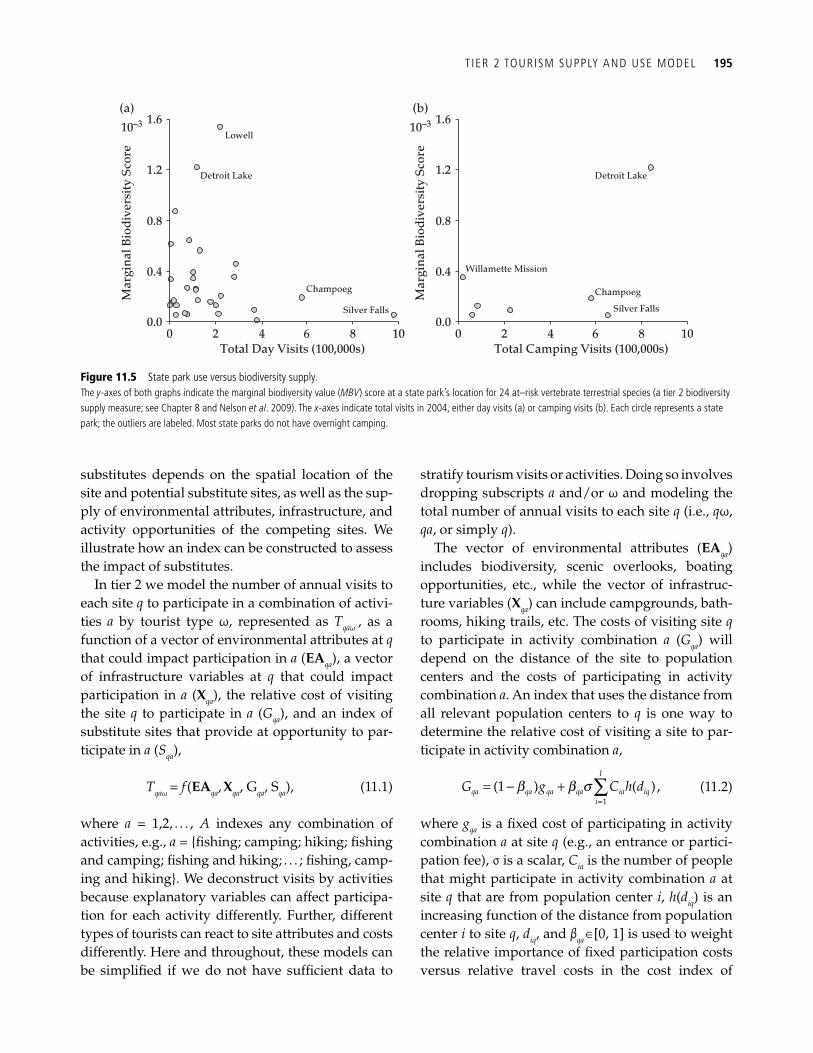
T IER 2 TOURISM SUPPLY AND USE MODEL 195
substitutes depends on the spatial location of the site and potential substitute sites, as well as the sup-ply of environmental attributes, infrastructure, and activity opportunities of the competing sites. We illustrate how an index can be constructed to assess the impact of substitutes.
In tier 2 we model the number of annual visits to each site q to participate in a combination of activi-ties a by tourist type ω, represented as T qaω , as a function of a vector of environmental attributes at q that could impact participation in a ( EA qa ), a vector of infrastructure variables at q that could impact participation in a ( X qa ), the relative cost of visiting the site q to participate in a ( G qa ), and an index of substitute sites that provide at opportunity to par-ticipate in a ( S qa ),
T q a ω = f ( E A q a , X q a , G q a , S q a ) , (11.1)
where a = 1,2, . . . , A indexes any combination of activities, e.g., a = fi shing; camping; hiking; fi shing and camping; fi shing and hiking; . . . ; fi shing, camp-ing and hiking. We deconstruct visits by activities because explanatory variables can affect participa-tion for each activity differently. Further, different types of tourists can react to site attributes and costs differently. Here and throughout, these models can be simplifi ed if we do not have suffi cient data to
stratify tourism visits or activities. Doing so involves dropping subscripts a and/or ω and modeling the total number of annual visits to each site q (i.e., q ω, qa , or simply q ).
The vector of environmental attributes ( EA qa ) includes biodiversity, scenic overlooks, boating opportunities, etc., while the vector of infrastruc-ture variables ( X qa ) can include campgrounds, bath-rooms, hiking trails, etc. The costs of visiting site q to participate in activity combination a ( G qa ) will depend on the distance of the site to population centers and the costs of participating in activity combination a . An index that uses the distance from all relevant population centers to q is one way to determine the relative cost of visiting a site to par-ticipate in activity combination a ,
I
qa qa qa qa ia iqi
G g C h d1
(1 ) ( ),b b s=
= − + ∑ (11.2)
where g qa is a fi xed cost of participating in activity combination a at site q (e.g., an entrance or partici-pation fee), σ is a scalar, C ia is the number of people that might participate in activity combination a at site q that are from population center i , h ( d iq ) is an increasing function of the distance from population center i to site q , d iq , and β qa Î [0, 1] is used to weight the relative importance of fi xed participation costs versus relative travel costs in the cost index of
(a)1.6
Lowell
Detroit Lake
Champoeg
Silver Falls
10–3
1.2
0.8
Mar
gina
l Bio
dive
rsity
Sco
re
0.4
0.00 2 4 6
Total Day Visits (100,000s)8 10
(b)1.6
Willamette Mission
Detroit Lake
Champoeg
Silver Falls
10–3
1.2
0.8
Mar
gina
l Bio
dive
rsity
Sco
re
0.4
0.00 2 4 6
Total Camping Visits (100,000s)8 10
Figure 11.5 State park use versus biodiversity supply.The y -axes of both graphs indicate the marginal biodiversity value ( MBV ) score at a state park’s location for 24 at–risk vertebrate terrestrial species (a tier 2 biodiversity supply measure; see Chapter 8 and Nelson et al . 2009 ). The x -axes indicate total visits in 2004, either day visits (a) or camping visits (b). Each circle represents a state park; the outliers are labeled. Most state parks do not have overnight camping.
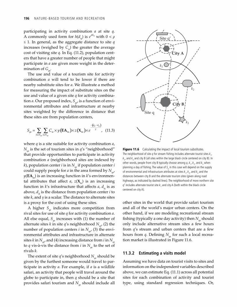
196 NATURE-BASED TOURISM AND RECREATION
participating in activity combination a at site q . A commonly used form for h ( d iq ) is iqder with 0 < ρ ≤ 1. In general, as the aggregate distance to site q increases (weighed by C ia ) the greater the average cost of visiting site q . In Eq. (11.2), population cent-ers that have a greater number of people that might participate in a are given more weight in the deter-mination of G qa .
The use and value of a tourism site for activity combination a will tend to be lower if there are nearby substitute sites for a . We illustrate a method for measuring the impact of substitute sites on the use and value of a given site q for activity combina-tion a . Our proposed index, S qa , is a function of envi-ronmental attributes and infrastructure at nearby sites weighted by the difference in distance that these sites are from population centers,
( ) ( )( )
,ik iq
qa qa
d d
qa ia ka kak N i N
S C y z e g− −
∈ ∈= × × ×∑ ∑ EA X (11.3)
where q is a site suitable for activity combination a , N qa is the set of tourism sites in q ’s “neighborhood” that provide opportunities to participate in activity combination a (neighborhood sites are indexed by k ), population center i is in N qa if population center i could supply people for a in the area formed by N qa , y ( EA ka ) is an increasing function in k ’s environmen-tal attributes that affect a , z ( X ka ) is an increasing function in k ’s infrastructure that affects a , d iq is as above, d ik is the distance from population center i to site k , and γ is a scalar. The distance to alternate sites is a proxy for the cost of using these sites.
A higher S qa indicates more competition from rival sites for use of site q for activity combination a . All else equal, S qa increases with (1) the number of alternate sites k in site q ’s neighborhood N qa , (2) the number of population centers i in N qa , (3) the envi-ronmental attributes and infrastructure in alternate sites k in N qa , and (4) increasing distance from i in N qa to q vis-à-vis the distance from i in N qa to the set of rivals k .
The extent of site q ’s neighborhood N qa should be given by the furthest someone would travel to par-ticipate in activity a . For example, if a is a wildlife safari, an activity that people will travel around the globe to participate in, then q should be a site that provides safari tourism and N qa should include all
other sites in the world that provide safari tourism and all of the world’s major urban centers. On the other hand, if we are modeling recreational stream fi shing (typically a one day activity) then N qa should only include alternative stream sites a few hours from q ’s stream and urban centers that are a few hours from q . Defi ning N qa for such a local recrea-tion market is illustrated in Figure 11.6 .
11.3.2 Estimating a visits model
Assuming we have data on tourist visits to sites and information on the independent variables described above, we can estimate Eq. (11.1) across all potential sites for each combination of activity and tourist type, using standard regression techniques. Or,
Site q’
Site q
k1
k2
k3
City A
City B
Figure 11.6 Calculating the impact of local tourism substitutes.The neighborhood of site q for stream fi shing includes alternate tourist sites k 1 , k 2 , and k 3 and city B (all sites within the large black circle centered on city B). In other words, people from city B typically choose among q , k 1 , k 2 , and k 3 when planning a day of fi shing. The value of S q in this case will depend on the supply of environmental and infrastructure attributes at sites k 1 , k 2 , and k 3 and the distances between city B and the alternate tourism sites (given along road highways, as indicated by dashed lines). The neighborhood of more northern site q includes alternate tourist site k 1 and city A (both within the black circle centered on city A).
T IER 1 AND 2 USE VALUE 197
given that all activities in a site will be affected by similar unobserved factors (e.g., the macroeconomic conditions in the demonstration site’s country, the macroeconomic conditions in the countries that supply the tourists, country stability), it may be most appropriate to pool all activity and tourist type models. A promising technique for this approach is the seemingly unrelated regression framework (see Greene ( 2003 ) for details). In Section 11.4.1 we fi t Eq. (11.1) to data for the Willamette Valley in Oregon, USA.
11.4 Tier 1 and 2 use value
A monetary value of tourism at each site can be gen-erated by multiplying the number of observed (tier 1) or estimated (tier 2) visits by an average value per visit (or visitor day). The value of a tourist visit to a site equals the benefi t generated by this visit over and above the costs of this visit. This measure of value is known as consumer surplus ( Loomis 2005 ). In general, consumer surplus can vary by site, type of tourist, and tourist activity. By aggregating the consumer surplus generated by each visit to a site over the course of a year we calculate a site’s annual value (effectively the value lost if access to the site is removed). In addition, using the tier 2 methodol-ogy, an estimate of the monetary effect of a change in environmental attributes can be developed by comparing the predicted value (trips multiplied by value per trip) at the site under the baseline condi-tions against the predicted value at the site after a change in environmental attribute.
Let the annual value of tourism at site q be given by AVT q where
A
q qa qaa
AVT V T1 1
,w ww
Ω
= == ∑∑ (11.4)
where T qaω is trips as above, V qaω is the average con-sumer surplus generated by a visit to site q to par-ticipate in activity combination a by tourist type ω (drop all a and/or ω subscripts if we do not have data by activity combination or type).
We can measure the change in AVT q due to a change in environmental attributes at q by using the regression-estimated Eq. (11.1) to predict changes in visitation with a change in environmental attributes, and assuming that consumer surplus per trip
remains constant. If the landscape has changed such that environmental attributes in q have changed, represented by ∆ EA q , then the expected change in predicted T qaω is given by
ˆ ( , , , ),qa a q q qa qaT f G Sw w∆ = ∆ ∆EA X (11.5)
where f aω indicates the regression-estimated Eq. (11.1) for combination a , ω, and ∆ S qa indicates any change in the substitute index due to the change in ∆ EA q (a change on the landscape that changes EA at q could also change EA at some other q ). ∆ EA q can include just one change (e.g., the change in water quality at q ) or multiple changes (e.g., the change in water delivery and quality at q ). We can also meas-ure ˆ
qaT w∆ due to changes in X q and G qa . The expected change in monetary value at site q
due to the change in ˆqaT w∆ is,
A
q qa qa qa qa qaa
AVT V T T V T1 1
ˆ ˆ[ ( )] [ ],w w w w ww
Ω
= =∆ = ∆ + −∑∑ (11.6)
where ˆqaV w represents the new value per trip after the change in environmental attributes on the landscape.
The landscape-level annual value of tourism and annual change in the value of tourism due to changes in environmental quality is given by sum-ming AVT q and ∆ AVT q , respectively, across all q on the landscape.
Finally, we can replace V qa ω in the equations above with other values of interest, for example, expendi-tures in the region by tourists participating in activ-ity combination a at site q , to generate other tourism-related economic information (e.g., the eco-nomic impacts on local businesses). See this chap-ter’s text box ( Box 11.1 ) for a discussion on tourism revenues generated by visits to Tambopata, Peru.
If we do not have consumer surplus estimates for the site we are studying, we may be able to use a consumer surplus estimate from a valuation study of a similar region as a proxy (for example, using an estimate of recreation values per day generated by a study in a nearby state). As noted in Chapter 3 there are limitations to benefi ts transfer approaches, thus primary studies are preferable. In this case we only transfer the value per unit of recreation activity (days, trips). For behavioral response (visits) to changes on the landscape, we use a locally calibrated
198 NATURE-BASED TOURISM AND RECREATION
Christopher Kirkby, Renzo Giudice, Brett Day, Kerry Turner, Britaldo Silveira Soares-Filho, Hermann Oliveira-Rodrigues, and Douglas W. Yu
The province of Madre de Dios in south-east Peru, an Amazonian frontier region bordering Bolivia and Brazil, is renowned amongst scientists for its biologically and culturally rich landscape. One area of this region in particular, known as Tambopata, is now also firmly entrenched in the minds of international travellers as the quintessential Amazon rainforest destination, attracting 39 565 ecotourists in 2005. Tambopata’s growing popularity is largely the result of (i) ease of access, only a 30-minute flight from Cusco (the gateway city to Machu Picchu) to Puerto Maldonado (the gateway town to Tambopata) followed by a few hours of river travel in motorised canoe; (ii) the proximity to two large protected areas, the Tambopata National Reserve (TNR, 274 690 ha) and the Bahuaja-Sonene National Park (BSNP, 1 091 416 ha); (iii) a healthy natural ecosystem showcasing primates, giant otters, macaws, and other charismatic fauna; (iv) intact oxbow lakes and clay-licks that concentrate fauna in predictable ways; (v) a choice of 37 ecotourist establishments (lodges), from 100-bed operations to small research stations and village guesthouses; and (vi) spending on international marketing by the larger lodges. In 2005, ecotourists spent a total of US$11.6 million to visit Tambopata, of which US$5.9 million were lodge revenues, US$5.2 million were airline revenues for airfares between Cusco and Puerto Maldonado, and US$0.5 million were TNR entrance fees and airport taxes. US$3.8 million (32.5%) of these revenues were in turn spent locally, in that the first-order transaction took place in Tambopata. This local spending could be further divided into low (12.2%, e.g., local staff, produce) and high leakage (20.3%, e.g., gasoline, boat motors) to the national economy. The TNR entrance fees exceeded the local park management budget, allowing US$172 530 to be transferred to the national budget. In 2005, the lodges earned a combined, after-tax profit of US$844 472. Additional (but only partly quantified) profits were distributed to some of the lodge owners in the form of above-market wages, possibly as much as doubling the above profit
figure. High levels of profitability, and the expectation of future profits, have created the incentive and the means for lodge owners to protect their businesses by protecting forest cover. Many lodges have taken advantage of government legislation, passed in 2002, that lets private businesses lease public forest outside of protected areas as concessions, for renewable 40-year terms. By 2005, lodges had taken control of 32 477 ha, with 90% of this area acquired by the four most profitable operators, together managing 8 lodges. Another 16 159 ha have been provisionally awarded as of early 2008, totalling 48 636 ha ( Figure 11.A.1 ). Eight other lodges own and manage <100 ha each. In 2005, the pre-tax profit value of lodge-controlled lands corresponding to 12 fully operational lodges (for which economic and land-use data were available) was US$38.9 ha −1 [US$1 238 002/31 807 ha]. This figure exceeds the 2005 pre-tax profit value of titled lands, covering 10 2511 ha, that were managed by 200 generalist rural households for agriculture, fruit production, animal husbandry (cattle ranching, chickens, and pigs), and timber extraction, which was calculated at US$27.1 ha −1 [US$277 472/10 2511 ha]. However, when it comes to those households that specialize in a given land use (> 50% of household revenues), unsustainable cattle ranchers (with stocking rates >3.5 animals ha −1 , N = 4), who owned 262 ha, extracted a pre-tax profit value of US$39.0 ha −1 , whilst sustainable cattle ranchers (stocking <3.5 animals ha −1 , N = 15), who owned 1 154 ha, extracted US$35.8 ha −1 . We note, though, that cattle ranchers are generally located within 2 km of a road, for ease of transport, which limits the land area where this activity would compete with tourism. For households specialized in timber extraction or annual agriculture (i.e., rice, maize, manioc, and bananas), the pre-tax profit value of land is US$35.7 ha −1 and US$21.3 ha −1 , respectively. We expect that specialist producers, especially unsustainably stocked ranchers, will suffer reduced profits in the future as productivity drops, which should lower the present value of their profit stream below that expected for tourism. Our comparisons are also conservative in that we do not include the above-market-rate wages paid to lodge owners. One stated motive for lodges acquiring forest concessions is to exclude competitors from primary
Box 11.1 How the economics of tourism justifi es forest protection in Amazonian Peru
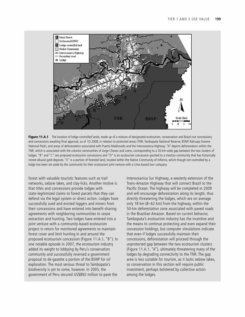
T IER 1 AND 2 USE VALUE 199
forest with valuable touristic features such as trail networks, oxbow lakes, and clay-licks. Another motive is that titles and concessions provide lodges with state-legitimized claims to forest parcels that they can defend via the legal system or direct action. Lodges have successfully sued and evicted loggers and miners from their concessions and have entered into benefit-sharing agreements with neighboring communities to cease extraction and hunting. Two lodges have entered into a joint venture with a community-based ecotourism project in return for monitored agreements to maintain forest cover and limit hunting in and around the proposed ecotourism concession ( Figure 11.A.1 , “B”). In one notable episode in 2007, the ecotourism industry added its weight to lobbying by Peru’s conservation community and successfully reversed a government proposal to de-gazette a portion of the BSNP for oil exploration. The most serious threat to Tambopata’s biodiversity is yet to come, however. In 2005, the government of Peru secured US$892 million to pave the
Interoceanica Sur Highway, a westerly extension of the Trans-Amazon Highway that will connect Brazil to the Pacific Ocean. The highway will be completed in 2009 and will encourage deforestation along its length, thus directly threatening the lodges, which are on average only 18 km (8–62 km) from the highway, within the 50-km deforestation zone associated with paved roads in the Brazilian Amazon. Based on current behavior, Tambopata’s ecotourism industry has the incentive and the means to continue protecting and even expand their concession holdings, but computer simulations indicate that even if lodges successfully maintain their concessions, deforestation will proceed through the unprotected gap between the two ecotourism clusters ( Figure 11.A.1 , “A”), ultimately threatening many of the lodges by degrading connectivity to the TNR. The gap area is less suitable for tourism, as it lacks oxbow lakes, so conservation in this section will require public investment, perhaps bolstered by collective action among the lodges.
Figure 11.A.1 The location of lodge-controlled lands, made up of a mixture of designated ecotourism, conservation and Brazil-nut concessions, and concessions awaiting fi nal approval, as of 1Q 2008, in relation to protected areas (TNR, Tambopata National Reserve; BSNP, Bahuaja-Sonene National Park), and areas of deforestation associated with Puerto Maldonado and the Interoceanica Highway. “A” depicts deforestation within the TNR, which is associated with the colonist communities of Jorge Chavez and Loero, corresponding to a 20-km wide gap between the two clusters of lodges. “B” and “C” are proposed ecotourism concessions and “D” is an ecotourism concession granted to a mestizo community that has historically mined alluvial gold deposits. “E” is a portion of forested land, located within the Native Community of Infi erno, which though not controlled by a lodge has been set aside by the community for their ecotourism joint venture with a Lima-based tour company.
200 NATURE-BASED TOURISM AND RECREATION
production function (Eq. (11.1)). Loomis ( 2005 ) pro-vides estimates of consumer surplus for US nature-based recreation and tourism, and Shrestha and Loomis ( 2001 ) provide estimates in other parts of the world. A roster of tourism consumer surplus databases is provided at http://recvaluation. forestry.oregonstate.edu/brief_history.html. Defenders of Wildlife and Colorado State University have constructed a “Toolkit” for benefi t transfer that includes databases, meta-analyses and visitor use models: http://dare.colostate.edu/tools/bene-fi ttransfer.aspx. Finally, a database of values from around the world, called the Environmental Valuation Reference Inventory, can be found at http://www.EVRI.ca. The reader should be aware, however, and as we emphasize in Chapter 3 , the evidence on the extent to which environmental ben-efi t measures are transferable is mixed at best ( Navrud and Ready 2007 ).
11.4.1 Example of tier 2 using data from the Willamette Basin
In this example we illustrate the estimation of a tier 2 visitation model and the value of a change in envi-ronmental attributes in state parks in the Willamette Basin. This model is very similar to the approach that Hill and Courtney ( 2006 ) use to estimate the effect of changes in landscape variables on visits to public and private forests in Great Britain.
First, we use Eq. (11.1) and data from 41 Willamette Basin state parks to assess the role of environmental attributes, infrastructure, and park location, on visitation rates. The model used in this example is a simplifi ed form of Eq. (11.1) for two reasons: (1) visitation data are not stratifi ed by activity combination a or tourist type, and (2) we did not model a substitution effect ( S ). We explain the number of visits to state park q in 2004, T q , with seven factors. For the EA vector, we include presence/absence for four environmental attributes: (1) fi shing possibilities, (2) wildlife viewing possibilities, (3) canyon features, and (4) boating facilities. We assume that a park with can-yon features has dramatic views and good hiking opportunities. For the X vector, we include two infrastructure variables: the area of the park (assuming that larger sites have more access
points and may support more visits before becom-ing congested), and the presence/absence of his-toric sites. For G , we approximate the overall cost of accessing each site with a variable that meas-ures the population living within 20 miles of the park (i.e., C ia in Eq. (11.2) is replaced by C q , the population living within 20 miles of q , σ = 1, 1iqde− = for all i , q , and β a = 1 for all q ).
We estimate the visitation model with ordinary least squares regression ( Table 11.1 ). Fishing and wildlife opportunities are highly related (i.e., parks tend to have both or neither), so we estimate the model twice, once with each of these variables included. We found that canyon features increase park visitation. Somewhat surprisingly, fi shing and wildlife viewing opportunities do not explain visitation in a statistically signifi cant manner. Parks that are less costly for more people to access (as indicated by population around the park) are used more. Based on these results one might assume that important environmental attributes do not contribute to tourism use. What is more likely is that there is relatively little variation in these variables over the sites, particularly when they are measured using coarse indicators like presence/absence. This lack of variation in eco-system-based variables is a common challenge in econometric studies of this type (e.g., Adamowicz et al. 1994 ). Improved information on levels of environmental attributes will help alleviate these problems.
Though this illustrative model is fairly simple, it reveals a great deal about the marginal value of environmental attributes at state parks in the Basin. For example, if a site that currently supports boating experienced a change in water delivery and/or quality to the degree that boating could no longer be supported, then, all else equal, the aver-age site is predicted to lose between 65 000 (model 1) and 97 000 (model 2) visitors a year (the average ∆ T across all sites given the loss of boating). Given that the average visitation rate at the parks is about 200 000 visitors per year, this is a substantial loss. If we could obtain a measure of the consumer sur-plus in the Basin before and after a potential loss of boating in a state park, given by V q and V q , respec-tively, we could derive coarse estimates of lost value using Eq. (11.6).
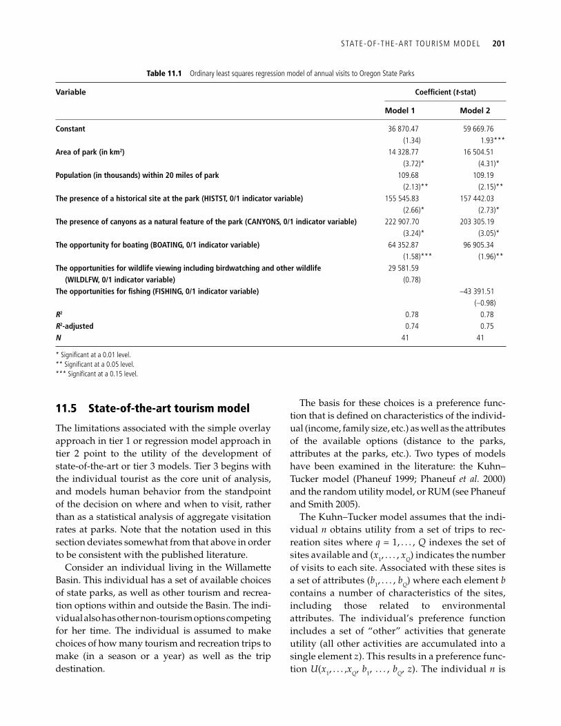
STATE-OF-THE-ART TOURISM MODEL 201
11.5 State-of-the-art tourism model
The limitations associated with the simple overlay approach in tier 1 or regression model approach in tier 2 point to the utility of the development of state-of-the-art or tier 3 models. Tier 3 begins with the individual tourist as the core unit of analysis, and models human behavior from the standpoint of the decision on where and when to visit, rather than as a statistical analysis of aggregate visitation rates at parks. Note that the notation used in this section deviates somewhat from that above in order to be consistent with the published literature.
Consider an individual living in the Willamette Basin. This individual has a set of available choices of state parks, as well as other tourism and recrea-tion options within and outside the Basin. The indi-vidual also has other non-tourism options competing for her time. The individual is assumed to make choices of how many tourism and recreation trips to make (in a season or a year) as well as the trip destination.
The basis for these choices is a preference func-tion that is defi ned on characteristics of the individ-ual (income, family size, etc.) as well as the attributes of the available options (distance to the parks, attributes at the parks, etc.). Two types of models have been examined in the literature: the Kuhn–Tucker model ( Phaneuf 1999 ; Phaneuf et al. 2000 ) and the random utility model, or RUM (see Phaneuf and Smith 2005 ).
The Kuhn–Tucker model assumes that the indi-vidual n obtains utility from a set of trips to rec-reation sites where q = 1, . . . , Q indexes the set of sites available and ( x 1 , . . . , x Q ) indicates the number of visits to each site. Associated with these sites is a set of attributes ( b 1 , . . . , b Q ) where each element b contains a number of characteristics of the sites, including those related to environmental attributes. The individual’s preference function includes a set of “other” activities that generate utility (all other activities are accumulated into a single element z ). This results in a preference func-tion U ( x 1 , . . . , x Q , b 1 , . . . , b Q , z ). The individual n is
Table 11.1 Ordinary least squares regression model of annual visits to Oregon State Parks
Variable Coeffi cient ( t -stat)
Model 1 Model 2
Constant 36 870.47 59 669.76 (1.34) 1.93 ***
Area of park (in km 2 ) 14 328.77 16 504.51 (3.72) * (4.31) *
Population (in thousands) within 20 miles of park 109.68 109.19 (2.13) ** (2.15) **
The presence of a historical site at the park (HISTST, 0/1 indicator variable) 155 545.83 157 442.03 (2.66) * (2.73) *
The presence of canyons as a natural feature of the park (CANYONS, 0/1 indicator variable) 222 907.70 203 305.19 (3.24) * (3.05) *
The opportunity for boating (BOATING, 0/1 indicator variable) 64 352.87 96 905.34 (1.58) *** (1.96) **
The opportunities for wildlife viewing including birdwatching and other wildlife (WILDLFW, 0/1 indicator variable)
29 581.59 (0.78)
The opportunities for fi shing (FISHING, 0/1 indicator variable) –43 391.51 (–0.98)
R 2 0.78 0.78 R 2 -adjusted 0.74 0.75 N 41 41
* Signifi cant at a 0.01 level. ** Signifi cant at a 0.05 level. *** Signifi cant at a 0.15 level.
202 NATURE-BASED TOURISM AND RECREATION
assumed to maximize utility ( U n ) subject to income ( m ) over the period and the prices of accessing the recreation alternatives ( p 1 , . . . , p Q ; usually travel cost plus the opportunity cost of time plus site access costs) as well as the price of the “good” z (which is normalized to unity). The individual maximizes utility by choosing the number of trips to each site q , given by x 1 , . . . x Q where some or all x can be 0:
1
1 1, . . ., ,max ( , . . ., , , . . ., , )
QQ Qx x z
U x x b b z (11.7)
Subject to p x + z = m . The model provides estimates of the relationship
between travel costs, attributes, income (and other demographic characteristics) and the frequency of visits to each of the defi ned alternatives. Typically, *
qx , the number of visits to q that solves problem (11.7), will decrease as the environmental attributes at q decreases, all else equal.
The random utility model ( Phaneuf and Smith 2005 ) examines the individual’s choice on a particu-lar occasion (a single trip). Rather than assessing the number of trips, the utility or satisfaction associated with visiting an alternative is described as a func-tion of the travel costs and site environmental and infrastructure attributes (and potentially individual specifi c characteristics such as income, demograph-ics, etc.). The utility (or preference) function for the choice to visit to site q (from individual n ’s view-point) takes the form:
( , ).nq q qV V m p b= − (11.8)
A common approach is to model the probability of individual n visiting a particular alternative q (or 0 ≤ π nq ≤ 1) as
1, . . .
,nq
nk
V
nq Vk Q
ee
p=
= ∑ (11.9)
where the V nq function would have to be estimated using observed data in a regression analysis ( Train 2003 ).
Equation (11.9) expresses the probability that an individual visits a particular alternative (on a par-ticular choice occasion—e.g., a day, a week) as a function of the attributes and prices. If the supply of
a desirable environmental attribute at site q declines then the probability of choosing site q for tourism declines. According to Eq. (11.9), as quality declines at one site, visitation will increase at other sites. This addresses one of the major limitations of the tier 2 model: the diffi culty with satisfactorily modeling substitutability when explaining tourism visits (the index S qa ). Further, because this model incorporates the preferences of the individuals in the conditional indirect utility function ( V ) it can also be used to calculate the economic value of the change directly. In this case the value of the decline at site q is given by the amount of money it would take to make per-son n as well off as they were before the change at q ; this can be calculated using the utility expression in (11.8) over the entire set of sites available. The rela-tively simple model can be combined with ecologi-cal models that describe the linkages between attributes to create an integrated ecological— economic model. An example of such a model is Naidoo and Adamowicz ( 2005 ) in which a behavio-ral model of tourism site choice is integrated with an ecological model of landscape change and bird diversity.
There have been many signifi cant advances in the modeling framework outlined above. Some of the most signifi cant include: (1) accounting for unob-served attribute effects in the model ( Murdock 2006 ); (2) incorporation of congestion into the model as an example of interdependence between tourists ( Timmins and Murdock 2007 ); (3) the incorporation of time (habits, variety seeking) into the framework (e.g., Swait et al. 2004 ); (4) inclusion of preference heterogeneity among tourists (Scarpa et al. , forth-coming; Boxall and Adamowicz 2002 ; Train 1998 , 2003 ); and (5) the development of models that account for different alternatives in the choice set or set of sites that a tourist considers ( Haab and Hicks 1997 ; von Haefen 2008) as well as a host of other advances in the modeling of choice data.
11.6 Limitations and next steps
We have outlined three approaches (tiers 1, 2, and 3) for assessing the value of nature-based tourism and recreation on the landscape and the changes in value that could be expected with a change in envi-ronmental attributes on the landscape.
L IMITATIONS AND NEXT STEPS 203
Tier 1 provides an assessment of observed visi-tation rates to sites. If information on the value of a unit of visitation is available from other studies (benefi ts transfer) then these visitation rates can be used to approximate measures of economic value. The tier 1 methodology does not specify a relationship between changes in environmental attributes and changes in tourism value nor does it disentangle effects on visitation rates from envi-ronmental attributes, infrastructure, distance to population centers, and availability of substitute sites.
Tier 2 approximates visitation behavior by devel-oping a statistical relationship between visitation and attributes at the sites. This approach can pro-vide additional insight into the changes that may be expected in visitation rates and values if envi-ronmental attributes change on the landscape. Tier 2 approaches, however, suffer from several limitations.
First, the required data are usually highly corre-lated, and attributes often do not vary strongly among sites. Sites with good fi shing quality also tend to have boating, picnicking, and other facili-ties. And sites often share many features, preclud-ing the opportunity to identify the impact that these features have on visitation rates. Identifying the impact of the change in environmental attributes in such cases will be diffi cult. Increasing the number of parks or expanding the spatial extent of the range of parks may help, but these actions will also increase the complexity of the research task.
Second, there are few linkages to information about the tourists. Only the potential tourism popu-lation is included in the model. Factors such as spe-cifi c travel and time costs of visiting (instead of an index), incomes, experience levels of the tourists, the substitution between tourism and other uses of time, and other demographic features are not included.
Third, tier 2 models will generally rely on benefi ts transfer procedures to provide estimates of eco-nomic value rather than estimating the values from the population of interest. Evidence on the applica-bility of values from one site to others is decidedly mixed, but may be the only option ( Navrud and Ready 2007 ).
Finally, the models described here are static and do not refl ect trends in preferences, demographics or other factors that might infl uence visitation rates. For example, Pergams and Zaradic ( 2006 , 2008 ) argue that there have been widespread declines in nature-based recreation visits. Meanwhile Balmford et al. (2009) fi nd that visits to protected areas in most parts of the world are in fact increasing. These are clearly areas for further research.
Tier 3 generates value estimates based on the behavior of the individuals. It is a fully integrated model of tourism and the environment. However, it is also very demanding in terms of data require-ments and familiarity with sophisticated modeling techniques. As the model is individual based it requires information on the individual’s residential location (for the determination of travel and time costs), the set of sites the individual considers when planning trips, as well as information on the attributes of the sites. There are several “scale” issues including assessment of the relevant geo-graphical scale (how large is the area that is relevant for the demand for recreation tourism at a particu-lar site) and the relevant time scale (is an annual time scale appropriate for decision making or are the trips more seasonal or perhaps a one- every-5-years type of trip; is there a broad trend of declining participation in recreation and preferences for nature?). Only a few regions will have the data available for such analysis.
Ideally the data for tier 3 models would be col-lected from general population surveys. Data col-lection of this type could provide excellent sampling properties and would provide information on the total number of visits taken by a population as well as the sites selected. However, such data are rarely collected. An alternative is to sample at the recrea-tion sites and collect information on the partici-pants. This is known as choice-based sampling ( Ben-Akiva and Lerman 1985 ) and is commonplace in the transportation demand literature. This approach may provide the most practical solution for the development of tier 3 models.
An additional area that has not been investigated to any great extent is the feedback between visita-tion rates, congestion and environmental quality. There has been some assessment of the role of con-gestion in nature-based tourism, and examination
204 NATURE-BASED TOURISM AND RECREATION
of the impact of tourism on environmental quality, but little examination of the three elements jointly. These issues as well as the continuing evolution of niche markets for tourism and emerging trends form the basis for a rich research agenda.
Acknowledgments
Thanks to Isla Fishburn, University of Sheffi eld, for collecting much of the Willamette data used in this chapter.
References
Adamowicz, W. L., Louviere, J., and Williams, M. (1994). Combining stated and revealed preference methods for valuing environmental amenities. Journal of Environmental Economics and Management , 26 , 271–92.
Balmford, A., Beresford, J., Green, J., et al . (2009). A global perspective on trends in nature-based tourism. PloS Biology , 7 (6), e1000144. doi:10.1371/journal.pbio.1000144.
Ben-Akiva, M., and Lerman, S. R. (1985). Discrete choice analysis: theory and application to predict travel demand . MIT Press, Cambridge.
Bockstael, N. E., and McConnell, K. E. (2007). Environmental and resource valuation with revealed preferences: a theoretical guide to empirical models . Springer, Dordrecht, The Netherlands.
Boxall, P. C., and Adamowicz, W. L. (2002). Understanding heterogeneous preferences in random utility models: a latent class approach. Environmental and Resource Economics, 23 , 421–46.
Champ, P. A., Boyle, K. J., and Brown, T. C. (2003). A primer on nonmarket valuation . Kluwer, Dordrecht, The Netherlands.
Greene, W. H. (2003). Econometric analysis, 5th edn. Prentice-Hall, Upper Saddle River, NJ.
Haab, T. C., and Hicks, R. L. (1997). Accounting for choice set endogeneity in random utility models of recreation demand. Journal of Environmental Economics and Management, 34 , 127–47.
Hill, G. W., and Courtney, P. R. (2006). Demand analysis projections for recreational visits to countryside wood-lands in Great Britain. Forestry, 79 , 185–200.
Hulse D., Gregory, S., and Baker, J., Eds. (2002). Willamette River Basin planning atlas: trajectories of environmental and ecological change . Oregon State University Press, Corvallis.
Loomis, J. (2005). Updated outdoor recreation use values on national forests and other public lands. General
Technical Report PNW-GTR-658. US Department of Agriculture, Forest Service, Pacifi c Northwest Research Station, Portland, OR.
Murdock, J. (2006). Handling unobserved site characteris-tics in random utility models of recreation demand. Journal of Environmental Economics and Management, 51 , 1–25.
Naidoo, R., and Adamowicz, W. L. (2005). Economic ben-efi ts of biodiversity exceed costs of conservation at an African rainforest reserve. Proceedings of the National Academy of Sciences of the USA, 102 , 16712–16.
Navrud, S., and Ready, R. (2007). Environmental value transfer: issues and methods . Springer, Dordrecht, The Netherlands.
Nelson, E., Mendoza, G., Regetz, J., et al . (2009). Modeling multiple ecosystem services, biodiversity conservation, commodity production, and tradeoffs at landscape scales. Frontiers in Ecology and the Environment, 7 , 4–11.
Oregon Fish and Wildlife Department (OFWD). (2005). 2005 Big Game Statistics.
Oregon Geospatial Enterprise Offi ce (OGEO). (2008). Oregon geospatial data clearinghouse. Accessed at http://www.oregon.gov/DAS/EISPD/GEO/alphalist.shtml in 2008 .
Pacifi c Northwest Ecological Research Consortium (PNW-ERC). (2008). The datasets. Accessed at http://www.fsl.orst.edu/pnwerc/wrb/access.html .
Pergams, O. R. W., and Zaradic, P. A. (2006). Is love of nature in the US becoming love of electronic media? 16-year downtrend in national park visits explained by watching movies, playing video games, internet use, and oil prices. Journal of Environmental Management, 80 , 387–93.
Pergams, O. R. W., and Zaradic, P. A. (2008). Evidence for a fundamental and pervasive shift away from nature-based recreation. Proceedings of the National Academy of Sciences of the USA, 105 , 2295–300.
Phaneuf, D. (1999). A dual approach to modeling corner solutions in recreation demand. Journal of Environmental Economics and Management , 37 , 85–105.
Phaneuf, D., Kling, C., and Herriges, J. (2000). Estimation and welfare calculations in a generalized corner solu-tion model with an application to recreation demand. Review of Economics and Statistics, 82 , 83–92.
Phaneuf, D., and Smith, V. K. (2005). Recreation demand models. Handbook of Environmental Economics, 2 , 671–751.
Scarpa, R., Thiene, M., and Train, K. (forthcoming). Utility in willingness to pay space: a tool to address the con-founding random scale effects in destination choice to the Alps. American Journal of Agricultural Economics , Appendices.

L IMITATIONS AND NEXT STEPS 205
Shrestha, R. K., and Loomis, J. B. (2001). Testing a meta-analysis model for benefi t transfer in interna-tional outdoor recreation. Ecological Economics, 39 , 67–83.
Swait, J., Adamowicz, W., and Van Bueren, M. (2004). Choice and temporal welfare impacts: Incorporating history into discrete choice models. Journal of Environmental Economics and Management, 47 , 94–116.
Timmins, C., and Murdock, J. (2007). A revealed prefer-ence approach to the measurement of congestion in travel cost models. Journal of Environmental Economics and Management, 53 , 230–49.
Towner, J., and Wall, G. (1991). History and tourism. Annals of Tourism Research, 18 , 71–84.
Train, K. (1998). Recreation demand models with taste variation. Land Economics, 74 , 230–9.
Train, K. (2003). Discrete choice methods with simulation . Cambridge University Press, Cambridge.
Von Haefen, R. H. (2008). Latent consideration sets and continuous demand systems. Environmental and Resource Economics , 41 , 363–79.
World Tourism Organization. (2008). UNWTO World Tourism Barometer , 6 (2, June). Accessed at http://www.unwto.org/facts/eng/barometer.htm .
206
CHAPTER 12
Cultural services and non-use values Kai M. A. Chan, Joshua Goldstein, Terre Satterfi eld, Neil Hannahs, Kekuewa Kikiloi, Robin Naidoo, Nathan Vadeboncoeur, and Ulalia Woodside
12.1 Introduction
12.1.1 Defi ning cultural ecosystem services and non-use values
In the ongoing effort to better defi ne ecosystem services (MA 2005; Boyd and Banzhaf 2007 ; Costanza 2008 ; Fisher and Turner 2008 ; Wallace 2008 ) and their valuation, few classes of value have been more diffi cult to identify and measure than those con-nected with the cultural and non-use dimensions of ecosystems. Whereas other ecosystem services make life possible in biophysical terms, cultural ecosystem services and non-use values inspire deep attachment in human communities. Accordingly, they need to be integrated into conservation and broader policy if societies are to sustain meaningful links between people and nature, and indeed many say if societies are to sustain themselves at all.
Cultural services and their connected values have come to represent nonmaterial benefi ts derived by those who use, might use, or share an attachment to a [natural] area. Costanza et al. ( 1997 ) defi ned cultural values-cum-service as “aesthetic, artistic, educational, spiritual and/or scientifi c values of ecosystems” (p. 254). The Millennium Ecosystem Assessment ( 2005 , p. 894) expanded this defi nition to include the “nonmaterial benefi ts peo-ple obtain from ecosystems through spiritual enrichment, cognitive development, refl ection, rec-reation, and aesthetic experience, including, e.g., knowledge systems, social relations, and aesthetic values.” Others focus more fully on the educational benefi ts of cultural services. Chiesura and de Groot ( 2003 ), for example, delineate key socio-cultural
dimensions of natural capital as scientifi c, cultural, historical, religious, and artistic educational bene-fi ts or fl ows.
More recently, the “cultural” class of value has come to encompass the concerns of indigenous peoples who might have a political and moral right to a natural area, such as a Treaty-based right to traditional territory. Hence, a number of studies in the values literature have begun to defi ne such intangible things as place value ( Basso 1996 ; Norton and Hannon 1997 ; Brown et al. 2002 ), spir-itual value ( Milton 2002 ), heritage value ( Throsby 2001 ), and social-relational value ( Lin 2001 ; Sable and Kling 2001 ).
Here we defi ne cultural services inclusively as ecosystems’ contribution to the nonmaterial benefi ts (e.g., capabilities and experiences) that arise from human-ecosystem relationships . For example, cul-tural services include the contribution of ecosys-tems to recreational experiences, to sense of place, and to the knowledge that a valued nonhuman species exists or will exist for future generations (knowledge that has existence value or bequest value, respectively). For clarity, and to align this chapter with other chapters in this book, we adopt the economics convention of differentiating values into use and non-use values. Use value refers to the direct (consumptive and non-consumptive) and indirect uses of ecosystem goods and services, while non-use encompasses all values separate from use ( Goulder and Kennedy 1997 ). Our treat-ment of cultural ecosystem services includes both use and non-use values. Indeed, for all cultures, maintenance of cultural values requires the active use of biological resources and nonmaterial
INTRODUCTION 207
interaction with important sites, among other direct and indirect uses.
Non-use values can be categorized into compo-nent values, which often include existence value, bequest value, and option value. Krutilla ( 1967 ), an economist, fi rst introduced the concept of “exist-ence value” to capture the provision of “satisfac-tion from mere knowledge that part of wilderness North America [ sic ] remains” regardless of any intention the valuing agent has of ever visiting such destinations. More broadly, existence value can be designated geographically as well as in ref-erence to specifi c biophysical units such as a par-ticular species or ecosystem. While existence value is specifi c to an individual’s satisfaction, bequest value relates to knowing that an environmental amenity will be available for future generations. Option value represents “the premium that people are willing to pay to preserve an environmental amenity, over and above the mean value (or expected value) of the use values anticipated from the amenity” ( Goulder and Kennedy 1997 ; Chapter 2 ). While option value has a stronger con-nection to use values, non-use values is the broad category capturing non-users’ preferences for the continued existence of ecosystem goods and serv-ices ( Cicchetti and Wilde 1992 ).
The property of intangibility is central to cul-tural ecosystem services and non-use values and often renders them diffi cult to classify and meas-ure. Classifi cation and measurement of these val-ues and services are nonetheless necessary as the risks associated with their loss are central to pub-lic thinking and discontent with land manage-ment decisions ( Satterfi eld and Roberts 2008 ). An analogous “intangibility” case in point for many First Nations communities in Canada is enshrined in the concept “cultural keystone species” ( Garibaldi and Turner 2004 ). The term refers to species, for example, salmon in the Pacifi c Northwest, which, if diminished, result in not just material loss of a provisioning service (the salmon), but a much larger suite of linked cul-tural losses or impacts including enduring prac-tices. These may include food sharing and the social cohesion and alliances engendered by such exchanges; the transmission of traditional knowl-edge; and the maintenance of key cultural institu-
tions such as naming and gifting ceremonies and feasts wherein keystone foods are central (see also Turner et al. 2008 ).
The non-market nature of many cultural serv-ices and non-use values creates another impor-tant characteristic. Whereas many other services are the production of things or conditions that have value in relation to some market (supporting services do not produce marketed commodities, but they may be essential steps in the production of such commodities, such as the pollination of agricultural crops), cultural services and non-use values generally involve the production of experi-ences that are valued without entering markets. In such cases, the production and valuation are inti-mately linked, both occurring in part in the valu-er’s mind. These services are therefore co-produced by ecosystems and people in a deeper sense than other services. For example, if we consider the contribution to aesthetic experi-ences, there is no metric of production that does not involve the valuer. In other words, potential supply and realized supply cannot be differenti-ated as they can be for market services. There is no objective way to claim that a site provides a great aesthetic service except by appealing to people’s behaviors and stated preferences regard-ing the object, which must generally be assessed for each site in turn.
While many assume that what matters gets measured ( Meadows 2001 ), this is not so with cul-tural services. Their consideration is long overdue. In the following sections, we lay a conceptual back-ground from which we identify components of cultural and non-use values and then link these values to ecosystem services.
12.1.2 From values to valuation: methodological conundrums
To the extent that the defi nition of cultural values has been controversial, the same may be said for methodological efforts to value them. While eco-nomics continues to provide important conceptual and methodological approaches for ecosystem serv-ice valuation (e.g., Champ 2003; National Research Council (US) 2005), there is another dialogue raising concerns that the common approach of expressing
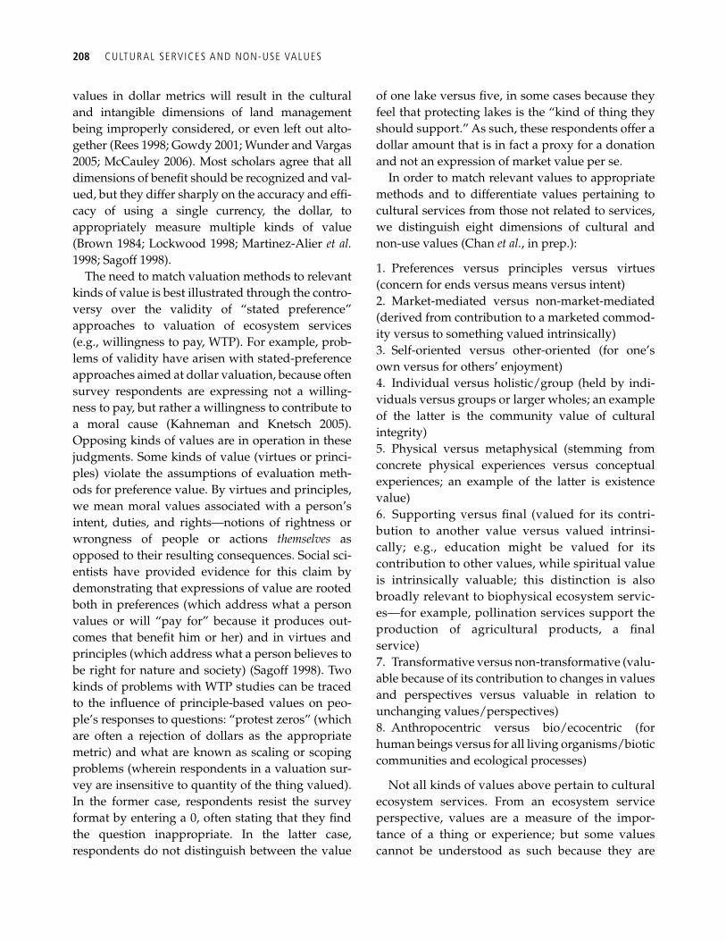
208 CULTURAL SERVICES AND NON-USE VALUES
values in dollar metrics will result in the cultural and intangible dimensions of land management being improperly considered, or even left out alto-gether ( Rees 1998 ; Gowdy 2001 ; Wunder and Vargas 2005 ; McCauley 2006 ). Most scholars agree that all dimensions of benefi t should be recognized and val-ued, but they differ sharply on the accuracy and effi -cacy of using a single currency, the dollar, to appropriately measure multiple kinds of value ( Brown 1984 ; Lockwood 1998 ; Martinez-Alier et al. 1998 ; Sagoff 1998 ).
The need to match valuation methods to relevant kinds of value is best illustrated through the contro-versy over the validity of “stated preference” approaches to valuation of ecosystem services (e.g., willingness to pay, WTP). For example, prob-lems of validity have arisen with stated-preference approaches aimed at dollar valuation, because often survey respondents are expressing not a willing-ness to pay, but rather a willingness to contribute to a moral cause ( Kahneman and Knetsch 2005 ). Opposing kinds of values are in operation in these judgments. Some kinds of value (virtues or princi-ples) violate the assumptions of evaluation meth-ods for preference value. By virtues and principles, we mean moral values associated with a person’s intent, duties, and rights—notions of rightness or wrongness of people or actions themselves as opposed to their resulting consequences. Social sci-entists have provided evidence for this claim by demonstrating that expressions of value are rooted both in preferences (which address what a person values or will “pay for” because it produces out-comes that benefi t him or her) and in virtues and principles (which address what a person believes to be right for nature and society) ( Sagoff 1998 ). Two kinds of problems with WTP studies can be traced to the infl uence of principle-based values on peo-ple’s responses to questions: “protest zeros” (which are often a rejection of dollars as the appropriate metric) and what are known as scaling or scoping problems (wherein respondents in a valuation sur-vey are insensitive to quantity of the thing valued). In the former case, respondents resist the survey format by entering a 0, often stating that they fi nd the question inappropriate. In the latter case, respondents do not distinguish between the value
of one lake versus fi ve, in some cases because they feel that protecting lakes is the “kind of thing they should support.” As such, these respondents offer a dollar amount that is in fact a proxy for a donation and not an expression of market value per se.
In order to match relevant values to appropriate methods and to differentiate values pertaining to cultural services from those not related to services, we distinguish eight dimensions of cultural and non-use values (Chan et al. , in prep.):
1. Preferences versus principles versus virtues (concern for ends versus means versus intent) 2. Market-mediated versus non-market-mediated (derived from contribution to a marketed commod-ity versus to something valued intrinsically) 3. Self-oriented versus other-oriented (for one’s own versus for others’ enjoyment) 4. Individual versus holistic/group (held by indi-viduals versus groups or larger wholes; an example of the latter is the community value of cultural integrity) 5. Physical versus metaphysical (stemming from concrete physical experiences versus conceptual experiences; an example of the latter is existence value) 6. Supporting versus fi nal (valued for its contri-bution to another value versus valued intrinsi-cally; e.g., education might be valued for its contribution to other values, while spiritual value is intrinsically valuable; this distinction is also broadly relevant to biophysical ecosystem servic-es—for example, pollination services support the production of agricultural products, a fi nal service) 7. Transformative versus non-transformative (valu-able because of its contribution to changes in values and perspectives versus valuable in relation to unchanging values/perspectives) 8. Anthropocentric versus bio/ecocentric (for human beings versus for all living organisms/biotic communities and ecological processes)
Not all kinds of values above pertain to cultural ecosystem services. From an ecosystem service perspective, values are a measure of the impor-tance of a thing or experience; but some values cannot be understood as such because they are
INTRODUCTION 209
underlying ideals (virtues and principles, which overlap closely with held values— Brown 1984 ). Others are not considered to be products of ecosys-tem services because the services framework is focused on people (so bio- and ecocentric values are excluded). Whereas the eight dimensions of kinds of values are crucial for determining appro-priate kinds of valuation, it is also worth distin-guishing categories of values associated with cultural ecosystem services and non-use dimen-sions of ecosystems. These ten proposed general categories of values are a way of organizing the nature of reason that a thing or experience is valued (e.g., because it provides knowledge, or social cap-ital). Some of the values are neither strictly non-use nor really “cultural” values (e.g., activity value); they are included here because they are crucial components of services in these categories (e.g., recreation, subsistence).
12.1.3 Distinguishing values from services
We distinguish values from services (the produc-tion of things of value) for two principal reasons ( Table 12.2 ). First, values do not exist as entities for probing or characterizing as separate from objects and activities; rather, they are merely one way in which we organize our ideas about moral-ity and preference. Accordingly, they generally require some concrete thing or activity to enable their elicitation (as in valuation): any attempt to ask people how much they value a landscape/seascape for its contribution to knowledge is likely to be far too abstract to get useful and meaningful answers. In our typology, we propose that serv-ices be the contribution to those concrete activities that ground values and provide a forum for their expression (or non-activities like contemplation, in the case of metaphysical services). So why not simply stop at services—why do we need to iden-tify values at all? This brings us to our second reason.
Second, individual cultural ecosystem services simultaneously produce multiple intertwined val-ues, so any attempt to valuate or characterize serv-ices must account for these interdependencies (see Section 12.2.1 ). With many cultural services, a
one-to-one mapping from services to values is challenging, and sometimes inappropriate. Certain ecosystem services, such as the provision of water, can be distinguished in such a way that each service produces one value: e.g., one might distinguish the provision of water for irrigation from the provision of water for household use, calling each a separate ecosystem service with a separate use. With many cultural ecosystem services, a one-to-one mapping is awkward because component values of activi-ties/objects generally cannot be properly separated in people’s minds. For example, the physical-suste-nance value of salmon to First Nations cultures of British Columbia cannot be effectively decoupled from the social and cultural values of the harvest and the ceremonies that depend upon this cultural keystone species ( Garibaldi and Turner 2004 ). Perhaps more importantly, disentangling co-occur-ring values can be deeply offensive to people and antithetical to their cultures.
Another example of the diffi culty of separating values can be drawn from the cultural world of Hawaiians. Kalo (taro), is referenced in the ancient cosmogonic history of the Hawaiian Islands not only as a prominent staple crop, but also as emerg-ing from the body of Haloa-naka-lau-kapalili (Haloa-of-the-quivering-leaf), the fi rst-born son of Wakea and Ho‘ohokukalani. Stillborn, his body was returned to the earth and grew into the fi rst kalo plant in Hawai’i. Their second-born son, named Haloa in honor of his older sibling, became the progenitor from whom all kanaka maoli (indigenous Hawaiians) descend. These are not just cosmological narratives, but are equally refl ec-tive of what, for lack of appropriate terms in English, refl ect Hawaiians’ genealogical or kin-like connections to both the human and nonhu-man world. Such meanings—inscribed in and inextricably linked to physical places or goods of importance (in this case, kalo)—are crucial prod-ucts of metaphysical ecosystem services. These may be as important to Hawaiian people today as they were to ancestors who planted the fi rst fi elds of kalo over a hundred generations ago. They also represent an important sense of responsibility to all of one’s ancestors: cosmological (Haloa), human, and nonhuman (e.g., kalo), and thus a
210 CULTURAL SERVICES AND NON-USE VALUES
need to care for this heritage plant as one would care for family. Reducing this complex, spiritual kinship to an economic currency is tantamount to pricing one’s great-grandparent. Not only is the measure diffi cult to derive, the effort to derive it could be construed as deeply offensive.
Table 12.1 illustrates that an individual service can provide multiple benefi ts. While we agree that it would be simplest to map one service to one ben-efi t, we do not see this being possible with cultural services. Spiritual, inspiration, and place values are not products of single kinds of experiences; rather these benefi ts are products of all manner of experi-ences associated with ecosystems (including meta-physical contemplation). Rather than expecting that we can partition separate “spiritual” and “inspira-tion” categories of ecosystem service ( de Groot et al. 2005 ) and value each category separately, we must recognize that the production of these benefi ts is a deeply complex function of many activities and components. For any service, each kind of benefi t denoted by an “x” may contribute to the values that people assign to the service’s pertinent activities and components (e.g., a person may enjoy hiking and berry-picking partly—and inseparably—be-
cause of the spiritual experience and the inspiration of photography). Valuation exercises must account for these multiple benefi ts.
An example may help illustrate the point. In a Hawaiian forest, trees are regarded as manifesta-tions or the embodiment of deities, such that they simultaneously provide use values and spiritual values. One source for this spiritual belief arises from a perceptive grasp of the role the forest plays in sustaining hydrologic ecosystem services. Hawaiians say, “ Hahai no ka ua i ka ulula`au.” Rains always follow the forest. Knowing this and honor-ing the deities’ embodiments, Hawaiians hewed only the trees that were needed and ensured that a suffi cient stand was left in place to perform a key function in the hydrological cycle. Sacred sites in Tibet also seem to be revered and protected in part because of their contribution to ecosystem services such as fl ood mitigation ( Box 12.1 ).
We distinguish between categories of benefi ts and services based on the potential for one site to substitute for another in production of the benefi t/service ( Table 12.1 ). There is a difference between the variation across sites and the possibility for sub-stitution: for example, the provision of employment
Table 12.1 Categories of cultural ecosystem services and associated benefi ts, and the site substitutability of each—with one possible mapping of ecosystem services to benefi ts
Benefi ts
Service Contribution to . . . (experiences)
Plac
e/he
rita
ge
Act
ivit
y
Spir
itua
l
Insp
irat
ion
Kno
wle
dge
Exis
tenc
e,
Bequ
est
Opt
ion
Soci
al c
apit
al
and
cohe
sion
Aes
thet
ic
Empl
oym
ent
Iden
tity
Site
Su
bsti
tuta
bilit
y
Subsistence x x x x x x x x x varies Recreation x x x x x x x x x depends Education & research x x x x x x x x x x depends Artistic x x x x x x x varies ‘Ceremonial’ x x x x x x x varies Site substitutability low high varies depends high low high varies
Site substitutability is low if the service or value is linked directly to particular places, and high if not; it depends on whether there are clearly identifi able and under-standable qualitative differences in instances within a category (e.g., existence value may be site-substitutable for valued species, but not for sacred sites); or it varies if the logic of the variation is more complex (e.g., the provision of subsistence opportunities is not site-specifi c for activity values, but it may be for place values). The contributions to employment and subsistence experiences are directly linked to provisioning services but the experiential portions are included here as a benefi t that has not been (and likely would not be) captured effectively by strict market valuation. For example, the value of employment transcends its contribution to aggregate economic values: consider the intangible value of employment that allows a person to care for and sustain a relationship to a place or resources of cultural or spiritual signifi cance.

INTRODUCTION 211
Box 12.1 The sacred geography of Kawagebo
Jianzhong Ma and Christine Tam
Kawagebo Mountain, rising 6740 m along the eastern Tibetan Plateau, lies at the heart of a region dominated by sacred geography at the headwaters of three of the great rivers of Asia—the Yangtze, the Mekong, and the Salween. Sacred natural sites abound across this 1600 km 2 area, from springs to lakes, rocks to caves, trees to whole forests. Inhabited for over 2000 years, the region gained stature primarily in the thirteenth century when the living Buddhas Karma Pakshi and Karma Rinpo Dorje paid formal respect to Kawagebo, leaving behind offerings of scriptures that elevated the mountain to one of the most sacred in all the Tibetan world ( Ma 2005 ). More recently, the surrounding mountains and valleys, dotted with small Tibetan villages, were included in the area declared a World Heritage site in 2002 as the Three Parallel Rivers. This strength of culture based on sacred geography, in fact, lays the foundation and framework for protection of the extraordinarily rich biodiversity, critical life-support functions, stunning landscapes, and cultural traditions that attracted UNESCO here in the fi rst place.
Tibetan sacred geography is an embodiment of the integration of cultural sites and natural ecosystems, beliefs arising from a mixture of Tibetan Buddhism and the local Bon folk religion that attributed all natural things with spirit. In the Kawagebo region, sacred geography is expressed in four main forms: sacred mountains, “rigua,” other sacred natural sites, and pilgrimage routes. Sacred mountains, or “rida” in Tibetan, are the main form of sacred geography, numbering over 70 in the region, and are venerated by local clans, specifi c communities, the broader region, and in some cases by all of Tibetan culture. The sacred mountain of Kawagebo is actually comprised of fi ve major Gods that are the fi ve highest peaks: Miancimu (Goddess, 6 054 m), Jiewarena (Crests of Five Buddhas, 5 470 m), Buqiongsongjiewuxie (Prince), Mabingzalawangdui (Fight God for Subduing the Devil, 6 400 m), and Kawagebo itself (Major God, 6 740 m) (Xiroa 2001). Reverence for these mountains includes restricting use of resources on their slopes.
“Rigua” are traditional zones established to seal off mountain areas especially for sustainable resource utilization, strictly controlling normal production activities. Use restrictions range from prohibitions on tree felling and hunting, to limitations on herding and non-timber product (NTP) collection. These zones often coincide with protection
of ecosystem service provisioning for communities, such as prevention of mountain slope erosion or protection of water resources. Indeed the ties between the belief system and the provisioning of ecosystem services are strong. Ubiquitous local stories cite the importance of sacred sites in securing human well-being. Adong village is one such example. The fl oodwaters of Zhili-Rongqu of Adenggong inundated a large stretch of farmland and its households on the lower reaches of the mountain during the 1990s, while the main channel near Adong experienced three fl oods in the 1980s. The community organized all its resources for fl ood prevention, but was unsuccessful. It was only when the sacred mountain was established and sealed from direct human activity that the fl oods stopped. In another example, the people in and around Waha Village, who traditionally harvested the forest around their headwater springs, suffered from a decrease in water supply. In the end, it was after inviting the Living Buddha Da-De to establish a sealed sacred mountain area encompassing the springs that the water supply returned to normal (KCA 2004). Biologically, sacred sites have also been found to encompass greater biodiversity than similar habitats at similar elevations that are not sacred ( Anderson et al . 2005 ), suggesting the special protection powers that fears of divine punishment can offer.
Other sacred natural sites may include temple forests, lakes, waterfalls, and forests or grasslands near sacred marks, and number over 300 in the Kawagebo region. Lastly, two pilgrimage routes circle Kawagebo, and host thousands of devotees each year from across the Tibetan region to pray for good fortune as they circumambulate the sacred mountain God.
Culturally, Tibetans draw three main functions from these types of sites. They solidify their religious core, structure moral thinking and behavior, and strengthen group identity ( Ma 2005 ). Veneration of sacred mountains originated from the awe and mystery surrounding the ever-changing natural environment of Tibetans who “live at the roof of the world,” spawning a psychology of fear and respect for nature. These early mountain gods were elevated under Buddhism to symbols of Buddhist doctrine. At the same time, sacred natural sites play a moral role by shaping fi xed sets of rules to be obeyed related to the landscape and its resources, thereby stabilizing community action and thought. Hillside zones or mountain tops have designated rules of use, and those who violate the rules will be punished by divinities. Lastly, these sites strengthen
continues
212 CULTURAL SERVICES AND NON-USE VALUES
opportunities might be high (temporarily) for for-estry in one woodlot due to the old-growth forests that occur there; but there is high potential for sub-stitution in theory because—for the purposes of employment—the site could be replaced by other sites. In the case of place value, in contrast, particu-lar places are of value, so site substitutability is low. In some cases, site substitutability depends on the kind of opportunity provided: e.g., it depends on whether recreation is place-based because of some site-specifi c (e.g., historical) signifi cance (low sub-stitutability), or mainly because of a site’s aesthetic beauty (high substitutability). Variation in site sub-stitutability is less easily pinned down in cases such as the provision of artistic or ceremonial opportuni-ties, which are often complex functions of site-spe-cifi c and other attributes.
While researchers might benefi t from an under-standing of the categories of ecosystem services at play, and the attendant categories and kinds of val-ues, we do not recommend belaboring the applica-tion of any typology. Several points follow and explain this position. First, these typologies are intended for researchers and analysts, not for con-stituents and stakeholders. Those who are inter-viewed do not need to know how their values are being interpreted and organized in terms that have meaning principally in relation to the academic lit-erature; what matters is that we as researchers can organize them in ways that will help us characterize the various ways that human values may be affected
by ecosystem change. Second, the principal purpose of identifying the categories and kinds of values at stake is to determine appropriate kinds of valuation and decision-making methods, and appropriate ways to apply and combine these ( Figure 12.1 ). Some of these methods cover only a subset of the kinds of values (e.g., market valuation and eco-nomic non-market valuation), while others address many or all kinds of values (e.g., structured deci-sion-making).
12.1.4 Environmental and social processes that affect service production
The production of cultural ecosystem services is affected by many of the environmental processes that affect other ecosystem services and biodiver-sity. Accordingly, principal environmental threats to service production are land-use change (includ-ing habitat loss and fragmentation), pollution, cli-mate change, overharvesting, invasive species, and disease.
Because cultural ecosystem services are co-pro-duced by ecosystems and people, they are deeply affected by social processes—at both the production and valuation stages. For example, if social proc-esses have led people away from nature-based rec-reation ( Pergams and Zaradic 2006 ; Louv 2008 ), then these processes also affect the ecosystem con-tribution to recreational experiences and the corre-sponding value.
community cultural identity through common religion, values, beliefs, and living habits. Community activities and rituals surround these sites, resulting ultimately even in institutionalization of commonly held boundaries, such as the delineation between national and community land in China, or the international borders between China-India or China-Nepal ( Ma 2005 ).
Most recently, vineyard conversion, infrastructure construction, tourism expansion, and other associated development have been intensifying in this area. With the declaration of the UNESCO World Heritage site, plans have become even more ambitious to transform this remote mountainous landscape into a thriving
modern economy. The key to successful development, however, most likely lies in the sacred geography of the region, for it is this cultural and religious belief system that sets out a protected area network much stronger in many ways than the formal nature reserve networks established by government entities. The framework for sustainable utilization through zoned restrictions and strict protection directed by sacred geography also helps to ensure the continued provisioning of ecosystem services to the millions of people living downstream of this area, not only in China, but in the neighboring countries of Myanmar, Thailand, Vietnam, Laos, and Cambodia.
Box 12.1 continued
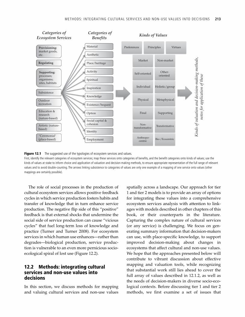
METHODS: INTEGRATING CULTURAL SERVICES AND NON-USE VALUES INTO DECIS IONS 213
The role of social processes in the production of cultural ecosystem services allows positive feedback cycles in which service production fosters habits and transfer of knowledge that in turn enhance service production. The negative fl ip side of this “positive” feedback is that external shocks that undermine the social side of service production can cause “vicious cycles” that fuel long-term loss of knowledge and practice ( Turner and Turner 2008 ). For ecosystem services in which human use enhances—rather than degrades—biological production, service produc-tion is vulnerable to an even more pernicious socio-ecological spiral of lost use ( Figure 12.2 ).
12.2 Methods: integrating cultural services and non-use values into decisions
In this section, we discuss methods for mapping and valuing cultural services and non-use values
spatially across a landscape. Our approach for tier 1 and tier 2 models is to provide an array of options for integrating these values into a comprehensive ecosystem services analysis with attention to link-ages with models described in other chapters of this book, or their counterparts in the literature. Capturing the complex nature of cultural services (or any service) is challenging. We focus on gen-erating summary information that decision-makers can use, with place-specifi c knowledge, to support improved decision-making about changes in ecosystems that affect cultural and non-use values. We hope that the approaches presented below will contribute to vibrant discussion about effective mapping and valuation tools, while recognizing that substantial work still lies ahead to cover the full array of values described in 12.1.2 , as well as the needs of decision-makers in diverse socio-eco-logical contexts. Before discussing tier 1 and tier 2 methods, we fi rst examine a set of issues that
Subsistence
Outdoorrecreation
Education &research(nature-based)
Artistic (nature-based)
‘Ceremonial’(place-based)
Place/heritage
Activity
Spiritual
Inspiration
Knowledge
Existence/bequest
Option
Social capital &cohesion
Identity
Preferences Principles Virtues
Market Non-market
Self-oriented Other-oriented
Individual Holistic/group
Physical Metaphysical
Final Supporting
Non-transformative
Transformative
Anthropo-centric
Bio-/Ecocentric
Supporting:processes;organisms;sites, habitats
Regulating
Provisioning:market goods,etc.
Material
Aesthetic
Employment
Categories of Ecosystem Services
Categories ofBenefits
Kinds of Values
Kin
ds o
f val
uatio
n an
d de
cisi
on-m
akin
g m
etho
ds,
note
s for
app
licat
ion
of th
ese
Figure 12.1 The suggested use of the typologies of ecosystem services and values. First, identify the relevant categories of ecosystem services; map these services onto categories of benefi ts, and the benefi t categories onto kinds of values; use the kinds of values at stake to inform choice and application of valuation and decision-making methods, to ensure appropriate representation of the full range of relevant values and to avoid double-counting. The arrows linking subsistence to categories of values are only one example of a mapping of one service onto values (other mappings are certainly possible).
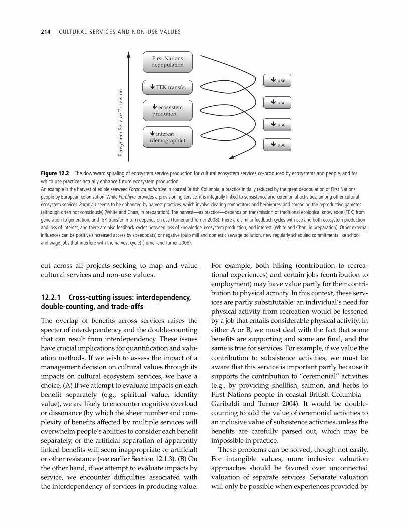
214 CULTURAL SERVICES AND NON-USE VALUES
cut across all projects seeking to map and value cultural services and non-use values.
12.2.1 Cross-cutting issues: interdependency, double-counting, and trade-offs
The overlap of benefi ts across services raises the specter of interdependency and the double- counting that can result from interdependency. These issues have crucial implications for quantifi cation and valu-ation methods. If we wish to assess the impact of a management decision on cultural values through its impacts on cultural ecosystem services, we have a choice. (A) If we attempt to evaluate impacts on each benefi t separately (e.g., spiritual value, identity value), we are likely to encounter cognitive overload or dissonance (by which the sheer number and com-plexity of benefi ts affected by multiple services will overwhelm people’s abilities to consider each benefi t separately, or the artifi cial separation of apparently linked benefi ts will seem inappropriate or artifi cial) or other resistance (see earlier Section 12.1.3 ). (B) On the other hand, if we attempt to evaluate impacts by service, we encounter diffi culties associated with the interdependency of services in producing value.
For example, both hiking (contribution to recrea-tional experiences) and certain jobs (contribution to employment) may have value partly for their contri-bution to physical activity. In this context, these serv-ices are partly substitutable: an individual’s need for physical activity from recreation would be lessened by a job that entails considerable physical activity. In either A or B, we must deal with the fact that some benefi ts are supporting and some are fi nal, and the same is true for services. For example, if we value the contribution to subsistence activities, we must be aware that this service is important partly because it supports the contribution to “ceremonial” activities (e.g., by providing shellfi sh, salmon, and herbs to First Nations people in coastal British Columbia— Garibaldi and Turner 2004 ). It would be double-counting to add the value of ceremonial activities to an inclusive value of subsistence activities, unless the benefi ts are carefully parsed out, which may be impossible in practice.
These problems can be solved, though not easily. For intangible values, more inclusive valuation approaches should be favored over unconnected valuation of separate services. Separate valuation will only be possible when experiences provided by
First Nationsdepopulation
Í TEK transferÍ use
Í use
Í use
Í use
Ecos
yste
m S
ervi
ce P
rovi
sion
Í ecosystemprodution
Í interest(demographic)
Figure 12.2 The downward spiraling of ecosystem service production for cultural ecosystem services co-produced by ecosystems and people, and for which use practices actually enhance future ecosystem production. An example is the harvest of edible seaweed Porphyra abbottiae in coastal British Columbia, a practice initially reduced by the great depopulation of First Nations people by European colonization. While Porphyra provides a provisioning service, it is integrally linked to subsistence and ceremonial activities, among other cultural ecosystem services. Porphyra seems to be enhanced by harvest practices, which involve clearing competitors and herbivores, and spreading the reproductive gametes (although often not consciously) (White and Chan, in preparation). The harvest—as practice—depends on transmission of traditional ecological knowledge (TEK) from generation to generation, and TEK transfer in turn depends on use ( Turner and Turner 2008 ). There are similar feedback cycles with use and both ecosystem production and loss of interest, and there are also feedback cycles between loss of knowledge, ecosystem production, and interest (White and Chan, in preparation). Other external infl uences can be positive (increased access by speedboats) or negative (pulp mill and domestic sewage pollution, new regularly scheduled commitments like school and wage jobs that interfere with the harvest cycle) ( Turner and Turner 2008 ).
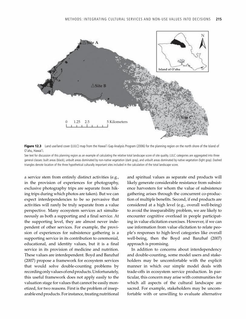
METHODS: INTEGRATING CULTURAL SERVICES AND NON-USE VALUES INTO DECIS IONS 215
a service stem from entirely distinct activities (e.g., in the provision of experiences for photography, exclusive photography trips are separate from hik-ing trips during which photos are taken). But we can expect interdependencies to be so pervasive that activities will rarely be truly separate from a value perspective. Many ecosystem services act simulta-neously as both a supporting and a fi nal service. At the supporting level, they are almost never inde-pendent of other services. For example, the provi-sion of experiences for subsistence gathering is a supporting service in its contribution to ceremonial, educational, and identity values, but it is a fi nal service in its provision of medicine and nutrition. These values are interdependent. Boyd and Banzhaf ( 2007 ) propose a framework for ecosystem services that would solve double-counting problems by recording only values of end products. Unfortunately, this useful framework does not apply easily to the valuation stage for values that cannot be easily mon-etized, for two reasons. First is the problem of insep-arable end products. For instance, treating nutritional
and spiritual values as separate end products will likely generate considerable resistance from subsist-ence harvesters for whom the value of subsistence gathering arises through the concurrent co-produc-tion of multiple benefi ts. Second, if end products are considered at a high level (e.g., overall well-being) to avoid the inseparability problem, we are likely to encounter cognitive overload in people participat-ing in value elicitation exercises. However, if we can use information from value elicitation to relate peo-ple’s responses to high-level categories like overall well-being, then the Boyd and Banzhaf ( 2007 ) approach is promising.
In addition to concerns about interdependency and double-counting, some model users and stake-holders may be uncomfortable with the explicit manner in which our simple model deals with trade-offs in ecosystem service production. In par-ticular, this concern may arise with communities for which all aspects of the cultural landscape are sacred. For example, stakeholders may be uncom-fortable with or unwilling to evaluate alternative
0 1.25 2.5 5 Kilometers
Site B
Site C
Site A
N
Island of O’ahu
Figure 12.3 Land use/land cover (LULC) map from the Hawai’i Gap Analysis Program (2006) for the planning region on the north shore of the Island of O’ahu, Hawai’i.See text for discussion of this planning region as an example of calculating the relative total landscape score of site quality. LULC categories are aggregated into three general classes: built areas (black), unbuilt areas dominated by non-native vegetation (dark gray), and unbuilt areas dominated by native vegetation (light gray). Dashed triangles denote location of the three hypothetical culturally important sites included in the calculation of the total landscape score.
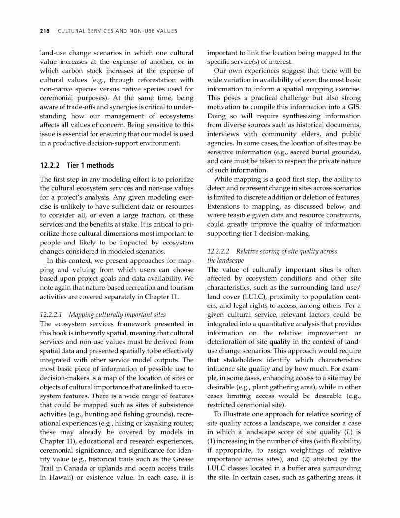
216 CULTURAL SERVICES AND NON-USE VALUES
land-use change scenarios in which one cultural value increases at the expense of another, or in which carbon stock increases at the expense of cultural values (e.g., through reforestation with non-native species versus native species used for ceremonial purposes). At the same time, being aware of trade-offs and synergies is critical to under-standing how our management of ecosystems affects all values of concern. Being sensitive to this issue is essential for ensuring that our model is used in a productive decision-support environment.
12.2.2 Tier 1 methods
The fi rst step in any modeling effort is to prioritize the cultural ecosystem services and non-use values for a project’s analysis. Any given modeling exer-cise is unlikely to have suffi cient data or resources to consider all, or even a large fraction, of these services and the benefi ts at stake. It is critical to pri-oritize those cultural dimensions most important to people and likely to be impacted by ecosystem changes considered in modeled scenarios.
In this context, we present approaches for map-ping and valuing from which users can choose based upon project goals and data availability. We note again that nature-based recreation and tourism activities are covered separately in Chapter 11 .
12.2.2.1 Mapping culturally important sites The ecosystem services framework presented in this book is inherently spatial, meaning that cultural services and non-use values must be derived from spatial data and presented spatially to be effectively integrated with other service model outputs. The most basic piece of information of possible use to decision-makers is a map of the location of sites or objects of cultural importance that are linked to eco-system features. There is a wide range of features that could be mapped such as sites of subsistence activities (e.g., hunting and fi shing grounds), recre-ational experiences (e.g., hiking or kayaking routes; these may already be covered by models in Chapter 11 ), educational and research experiences, ceremonial signifi cance, and signifi cance for iden-tity value (e.g., historical trails such as the Grease Trail in Canada or uplands and ocean access trails in Hawaii) or existence value. In each case, it is
important to link the location being mapped to the specifi c service(s) of interest.
Our own experiences suggest that there will be wide variation in availability of even the most basic information to inform a spatial mapping exercise. This poses a practical challenge but also strong motivation to compile this information into a GIS. Doing so will require synthesizing information from diverse sources such as historical documents, interviews with community elders, and public agencies. In some cases, the location of sites may be sensitive information (e.g., sacred burial grounds), and care must be taken to respect the private nature of such information.
While mapping is a good fi rst step, the ability to detect and represent change in sites across scenarios is limited to discrete addition or deletion of features. Extensions to mapping, as discussed below, and where feasible given data and resource constraints, could greatly improve the quality of information supporting tier 1 decision-making.
12.2.2.2 Relative scoring of site quality across the landscape The value of culturally important sites is often affected by ecosystem conditions and other site characteristics, such as the surrounding land use/land cover (LULC), proximity to population cent-ers, and legal rights to access, among others. For a given cultural service, relevant factors could be integrated into a quantitative analysis that provides information on the relative improvement or deterioration of site quality in the context of land-use change scenarios. This approach would require that stakeholders identify which characteristics infl uence site quality and by how much. For exam-ple, in some cases, enhancing access to a site may be desirable (e.g., plant gathering area), while in other cases limiting access would be desirable (e.g., restricted ceremonial site).
To illustrate one approach for relative scoring of site quality across a landscape, we consider a case in which a landscape score of site quality ( L ) is (1) increasing in the number of sites (with fl exibility, if appropriate, to assign weightings of relative importance across sites), and (2) affected by the LULC classes located in a buffer area surrounding the site. In certain cases, such as gathering areas, it
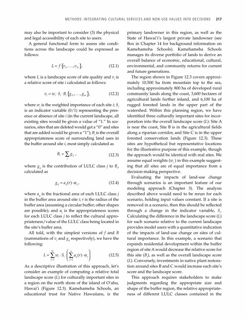
METHODS: INTEGRATING CULTURAL SERVICES AND NON-USE VALUES INTO DECIS IONS 217
may also be important to consider (3) the physical and legal accessibility of each site to users.
A general functional form to assess site condi-tions across the landscape could be expressed as follows:
NL f v v1 , . . ., ,= (12.1)
where L is a landscape score of site quality and v i is a relative score of site i calculated as follows:
i i i i i inv w S B g g1 , . . ., ,= ⋅ ⋅ (12.2)
where w i is the weighted importance of each site i ; S i is an indicator variable (0/1) representing the pres-ence or absence of site i (in the current landscape, all existing sites would be given a value of “1.” In sce-narios, sites that are deleted would get a “0” and sites that are added would be given a “1”); B i is the overall appropriateness score of surrounding land uses in the buffer around site i , most simply calculated as
= ∑ ,i ijj
B g (12.3)
where g ij is the contribution of LULC class j to B i , calculated as
( ) ,ij ij jg a r a= ⋅ (12.4)
where a ij is the fractional area of each LULC class j in the buffer area around site i ; r is the radius of the buffer area (assuming a circular buffer; other shapes are possible); and α j is the appropriateness scores for each LULC class j to refl ect the cultural appro-priateness/value of the LULC class being located in the site’s buffer area.
All told, with the simplest versions of f and B (summations of v i and g ij respectively), we have the following:
a= =
⎛ ⎞= ⋅ ⋅ ⋅⎜ ⎟⎝ ⎠
∑ ∑1 1
( )N n
i i ij ji j
L w S a r (12.5)
As a descriptive illustration of this approach, let’s consider an example of computing a relative total landscape score ( L ) for culturally important sites in a region on the north shore of the island of O’ahu, Hawai’i ( Figure 12.3 ). Kamehameha Schools, an educational trust for Native Hawaiians, is the
primary landowner in this region, as well as the State of Hawai’i’s largest private landowner (see Box in Chapter 14 for background information on Kamehameha Schools). Kamehameha Schools manages its diverse portfolio of lands to derive an overall balance of economic, educational, cultural, environmental, and community returns for current and future generations.
The region shown in Figure 12.3 covers approxi-mately 10,500 ha from mountain top to the sea, including approximately 800 ha of developed rural community lands along the coast, 3,600 hectares of agricultural lands further inland, and 6,100 ha of rugged forested lands in the upper part of the watershed. Within this planning region, we have identifi ed three culturally important sites for incor-poration into the overall landscape score ( L ): Site A is near the coast, Site B is in the agricultural fi elds along a riparian corridor, and Site C is in the upper forested conservation lands ( Figure 12.3 ). These sites are hypothetical but representative locations for the illustrative purpose of this example, though the approach would be identical with real sites. We assume equal weights ( w i ) in this example suggest-ing that all sites are of equal importance from a decision-making perspective.
Evaluating the impacts of land-use change through scenarios is an important feature of our modeling approach ( Chapter 3 ). The analysis described above would need to be rerun for each scenario, holding input values constant. If a site is removed in a scenario, then this should be refl ected through a change in the indicator variable, S i . Calculating the difference in the landscape score ( L ) for each scenario relative to the current landscape provides model users with a quantitative indication of the impacts of land-use change on sites of cul-tural importance. In this example, a scenario that expands residential development within the buffer region of site A would decrease the relative score for this site ( B i ), as well as the overall landscape score ( L ). Conversely, investments in native plant restora-tion around sites B and C would increase each site’s score and the landscape score.
This approach requires stakeholders to make judgments regarding the appropriate size and shape of the buffer region, the relative appropriate-ness of different LULC classes contained in the
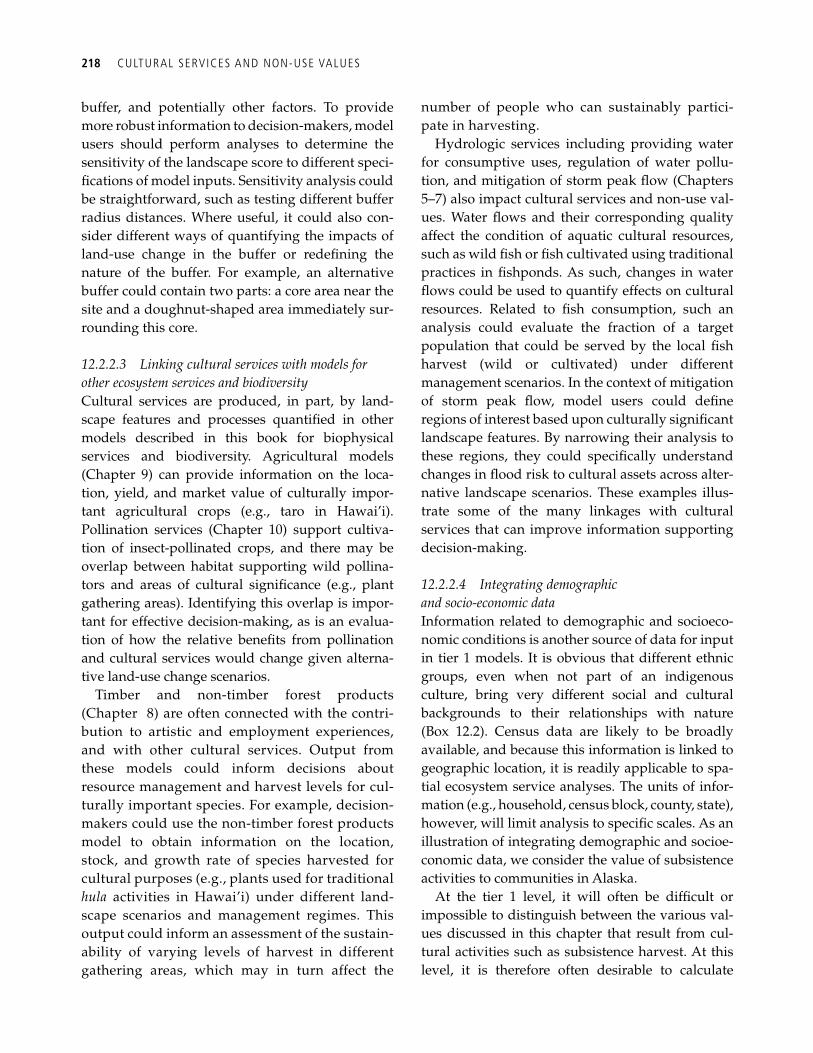
218 CULTURAL SERVICES AND NON-USE VALUES
buffer, and potentially other factors. To provide more robust information to decision-makers, model users should perform analyses to determine the sensitivity of the landscape score to different speci-fi cations of model inputs. Sensitivity analysis could be straightforward, such as testing different buffer radius distances. Where useful, it could also con-sider different ways of quantifying the impacts of land-use change in the buffer or redefi ning the nature of the buffer. For example, an alternative buffer could contain two parts: a core area near the site and a doughnut-shaped area immediately sur-rounding this core.
12.2.2.3 Linking cultural services with models for other ecosystem services and biodiversity Cultural services are produced, in part, by land-scape features and processes quantifi ed in other models described in this book for biophysical services and biodiversity. Agricultural models ( Chapter 9 ) can provide information on the loca-tion, yield, and market value of culturally impor-tant agri cultural crops (e.g., taro in Hawai’i). Pollination services ( Chapter 10 ) support cultiva-tion of insect-pollinated crops, and there may be overlap between habitat supporting wild pollina-tors and areas of cultural signifi cance (e.g., plant gathering areas). Identifying this overlap is impor-tant for effective decision-making, as is an evalua-tion of how the relative benefi ts from pollination and cultural services would change given alterna-tive land-use change scenarios.
Timber and non-timber forest products ( Chapter 8 ) are often connected with the contri-bution to artistic and employment experiences, and with other cultural services. Output from these models could inform decisions about resource management and harvest levels for cul-turally important species. For example, decision-makers could use the non-timber forest products model to obtain information on the location, stock, and growth rate of species harvested for cultural purposes (e.g., plants used for traditional hula activities in Hawai’i) under different land-scape scenarios and management regimes. This output could inform an assessment of the sustain-ability of varying levels of harvest in different gathering areas, which may in turn affect the
number of people who can sustainably partici-pate in harvesting.
Hydrologic services including providing water for consumptive uses, regulation of water pollu-tion, and mitigation of storm peak fl ow ( Chapters 5 – 7 ) also impact cultural services and non-use val-ues. Water fl ows and their corresponding quality affect the condition of aquatic cultural resources, such as wild fi sh or fi sh cultivated using traditional practices in fi shponds. As such, changes in water fl ows could be used to quantify effects on cultural resources. Related to fi sh consumption, such an analysis could evaluate the fraction of a target population that could be served by the local fi sh harvest (wild or cultivated) under different management scenarios. In the context of mitigation of storm peak fl ow, model users could defi ne regions of interest based upon culturally signifi cant landscape features. By narrowing their analysis to these regions, they could specifi cally understand changes in fl ood risk to cultural assets across alter-native landscape scenarios. These examples illus-trate some of the many linkages with cultural services that can improve information supporting decision-making.
12.2.2.4 Integrating demographic and socio-economic data Information related to demographic and socioeco-nomic conditions is another source of data for input in tier 1 models. It is obvious that different ethnic groups, even when not part of an indigenous culture, bring very different social and cultural backgrounds to their relationships with nature ( Box 12.2 ). Census data are likely to be broadly available, and because this information is linked to geographic location, it is readily applicable to spa-tial ecosystem service analyses. The units of infor-mation (e.g., household, census block, county, state), however, will limit analysis to specifi c scales. As an illustration of integrating demographic and socioe-conomic data, we consider the value of subsistence activities to communities in Alaska.
At the tier 1 level, it will often be diffi cult or impossible to distinguish between the various val-ues discussed in this chapter that result from cul-tural activities such as subsistence harvest. At this level, it is therefore often desirable to calculate
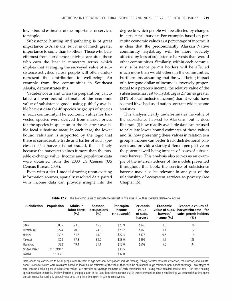
METHODS: INTEGRATING CULTURAL SERVICES AND NON-USE VALUES INTO DECIS IONS 219
lower bound estimates of the importance of services to people.
Subsistence hunting and gathering is of great importance to Alaskans, but it is of much greater importance to some than to others. Those who ben-efi t most from subsistence activities are often those who earn the least in monetary terms, which implies that averaging the surveyed value of sub-sistence activities across people will often under-represent the contribution to well-being. An example from fi ve communities in Southeast Alaska, demonstrates this.
Vadeboncoeur and Chan (in preparation) calcu-lated a lower bound estimate of the economic value of subsistence goods using publicly availa-ble harvest data for 48 species or groups of species in each community. The economic values for har-vested species were derived from market prices for the species in question or the cheapest availa-ble local substitute meat. In each case, the lower bound valuation is supported by the logic that there is considerable trade and barter of such spe-cies, so if a harvest is not traded, this is likely because the harvester values it more than the pos-sible exchange value. Income and population data were obtained from the 2000 US Census ( US Census Bureau 2003 ).
Even with a tier 1 model drawing upon existing information sources, spatially resolved data paired with income data can provide insight into the
degree to which people will be affected by changes in subsistence harvest. For example, based on per-capita economic values as a percentage of income, it is clear that the predominantly Alaskan Native community Hydaburg will be more severely affected by loss of subsistence harvests than would other communities. Similarly, within each commu-nity, subsistence permit holders will be affected much more than would others in the communities. Furthermore, assuming that the well-being impact of a foregone dollar of income is inversely propor-tional to a person’s income, the relative value of the subsistence harvest to Hydaburg is 2.7 times greater (34% of local inclusive income) than it would have seemed if we had used nation- or state-wide income statistics.
This analysis clearly underestimates the value of the subsistence harvest to Alaskans, but it does illustrate (i) how readily available data can be used to calculate lower bound estimates of these values and (ii) how presenting these values in relation to a group’s income can better track distributional con-cerns and provide a starkly different perspective on the potential well-being impacts of losses of subsist-ence harvest. This analysis also serves as an exam-ple of the interrelatedness of the models presented throughout this book; the service of subsistence harvest may also be relevant in analyses of the relationship of ecosystem services to poverty (see Chapter 15 ).
Table 12.2 The economic value of subsistence harvest in fi ve sites in Southeast Alaska relative to income
Jurisdiction Population Adults in labor force
(%)
Seasonal occupations
(%)
Per-capita income
(thousands)
Per-captia value
of subs. harvest
Economic value of subs.
harvest/income (%)
Economic values of harvest/income—for subs. permit holders
(%)
Sitka 8835 73.6 15.9 $23.9 $246 1.0 10 Petersburg 3224 70.8 24.6 $26.2 $368 1.4 7 Haines 2392 61.6 18.9 $22.3 $176 0.8 9 Yakutat 808 77.8 33.2 $23.0 $392 1.7 33 Hydaburg 382 49.1 21.1 $12.0 $602 5.0 34 United states 301 139 947 $30.5 Alaska 670 153 $32.0
Here, adults are considered to be all people over 16 years of age. Seasonal occupations include farming, fi shing, forestry, resource extraction, construction, and mainte-nance. Economic values were calculated based on lower bound estimates of the values that could be obtained through reciprocal non-market exchange. Percentages of total income (including these subsistence values) are provided for average members of each community and—using more detailed harvest data—for those holding special subsistence permits. The low fraction of the population in the labor force demonstrates that in these communities time is not limiting; we assumed that time spent on subsistence harvesting is generally not detracting from time spent in gainful employment.
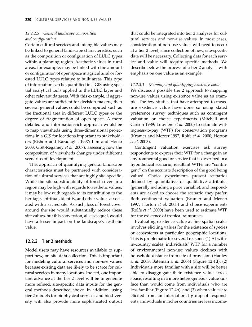
220 CULTURAL SERVICES AND NON-USE VALUES
12.2.2.5 General landscape composition and confi guration Certain cultural services and intangible values may be linked to general landscape characteristics, such as the composition or confi guration of LULC types within a planning region. Aesthetic values in rural areas, for example, may be linked with the amount or confi guration of open space in agricultural or for-ested LULC types relative to built areas. This type of information can be quantifi ed in a GIS using spa-tial analytical tools applied to the LULC layer and other relevant datasets. With this example, if aggre-gate values are suffi cient for decision-makers, then several general values could be computed such as the fractional area in different LULC types or the degree of fragmentation of open space. A more detailed and information-rich approach would be to map viewsheds using three-dimensional projec-tions in a GIS for locations important to stakehold-ers ( Bishop and Karadaglis 1997 ; Lim and Honjo 2003 ; Grêt-Regamey et al. 2007 ), assessing how the composition of viewsheds changes under different scenarios of development.
This approach of quantifying general landscape characteristics must be partnered with considera-tion of cultural services that are highly site-specifi c. While the site substitutability of forest cover in a region may be high with regards to aesthetic values, it may be low with regards to its contribution to the heritage, spiritual, identity, and other values associ-ated with a sacred site. As such, loss of forest cover around the site would substantially reduce these site values, but this conversion, all else equal, would have a lesser impact on the landscape’s aesthetic value.
12.2.3 Tier 2 methods
Model users may have resources available to sup-port new, on-site data collection. This is important for modeling cultural services and non-use values because existing data are likely to be scarce for cul-tural services in many locations. Indeed, one impor-tant advance at the tier 2 level will be to generate more refi ned, site-specifi c data inputs for the gen-eral methods described above. In addition, using tier 2 models for biophysical services and biodiver-sity will also provide more sophisticated output
that could be integrated into tier 2 analyses for cul-tural services and non-use values. In most cases, consideration of non-use values will need to occur at a tier 2 level, since collection of new, site-specifi c data will be necessary. Collecting data for each serv-ice and value will require specifi c methods. We describe below the process of a tier 2 analysis with emphasis on one value as an example.
12.2.3.1 Mapping and quantifying existence value We discuss a possible tier 2 approach to mapping non-use values using existence value as an exam-ple. The few studies that have attempted to meas-ure existence value have done so using stated preference survey techniques such as contingent valuation or choice experiments ( Mitchell and Carson 1989 ; Louviere et al. 2000 ) to estimate will-ingness-to-pay (WTP) for conservation programs ( Kramer and Mercer 1997 ; Rolfe et al. 2000 ; Horton et al. 2003 ).
Contingent valuation exercises ask survey respondents to express their WTP for a change in an environmental good or service that is described in a hypothetical scenario; resultant WTPs are “contin-gent” on the accurate description of the good being valued. Choice experiments present scenarios defi ned by quantitative or qualitative attributes (generally including a price variable), and respond-ents are asked to choose the scenario they prefer. Both contingent valuation ( Kramer and Mercer 1997 ; Horton et al. 2003 ) and choice experiments ( Rolfe et al. 2000 ) have been used to estimate WTP for the existence of tropical rainforests.
Evaluating existence value at fi ne spatial scales involves eliciting values for the existence of species or ecosystems at particular geographic locations. This is problematic for several reasons: (1) At with-in-country scales, individuals’ WTP for a number of environmental non-use values declines with household distance from site of provision ( Hanley et al. 2003 ; Bateman et al. 2006 ) (Figure 12.4d); (2) Individuals more familiar with a site will be better able to disaggregate their existence value across space, resulting in a more heterogeneous value sur-face than would come from individuals who are less familiar (Figure 12.4b); and (3) when values are elicited from an international group of respond-ents, individuals in richer countries are less income-

METHODS: INTEGRATING CULTURAL SERVICES AND NON-USE VALUES INTO DECIS IONS 221
Box 12.2 People of color and love of nature
Hazel Wong
For the fi rst 10 years of my life, the outdoors was my playground. Growing up in the Seychelles, without television, my sisters and I spent our vacation days and Saturdays immersed in creative play outdoors. Sundays were reserved for either a beach outing or a family lunch feast followed by seven people piling into a car to tour the island, making pit stops along the way for my parents to say hello to their friends and our extended family. I have memories of my paternal grandmother watching fourteen grand children at once. The house, a modest four-bedroom home, was by no means big enough to accommodate that many rambunctious children. Looking back, grand-mere had help, the outdoors. The only reasons to set foot inside the house were to eat lunch and use the bathroom.
On September 14, 1980, I woke up in the desert of Las Vegas, Nevada after my family left the Seychelles following a coup d’état and ensuing unrest. At ten years old, I remember feeling a tremendous loss for the beautiful island I left behind. Slowly, the desert became my new playground. Back then, there was plenty of desert in Las Vegas, the no-end-in-sight development boom that started in the late eighties had not taken place. Our introduction to television, even in a limited and supervised capacity, replaced playing outdoors, especially during the winter months, a new and not so welcome season for those born on an island with a year round average temperature of 80°F.
Life in the States was very different from the Seychelles; my parents had to adjust to a new culture, a lack of family support and raising fi ve girls in an unfamiliar setting. Their number one priority at all times was our education, and they worked and saved to ensure we had a head start in life. This left little time and resources to explore the natural world in America. Yet, my father had a voracious appetite for nature books and television programs—fueling my knowledge, curiosity, and sense of amazement.
Years later, I am now a self identifi ed conservationist and one of the 10% of people of color working in the conservation fi eld. I also served on the board of the Nevada Conservation League for fi ve years, serving as chair for over a year. My childhood exposure to the natural world, embedded in my psyche a love and passion for the environment, instilling in me a value system that fi rmly believes in the rights of nature.
Like many individuals, I am multifaceted and my appreciation of nature competes with other activities and passions. For example, I have driven to mountains, seeking nature’s solitude and the comfort of the vast open space to gain clarity and strength for major decisions in my life. Yet, I have been camping only once in all my years, and I am not an avid hiker—I would rather do a two-hour martini lunch with friends than hike on most days. (I hope this confession is not grounds for revoking my conservationist card.) However, that does not negate my devotion and passion to protect the natural world.
Working in the conservation fi eld for six years, I quickly learned that the Anglo Saxon culture defi nes the meaning of the word conservationist and narrowly interprets what constitutes the correct way of valuing and recreating in the natural world. I have concluded that the problem is not that people of color do not value and care about conservation issues. They are under represented in the conservation movement because of conservation’s history of class, privilege, and a homogenous culture that has rendered a myopic view, perhaps a benign neglect and at worst actual resistance to conservation becoming a more inclusive movement.
Conservation’s past is a history of white male privilege, conserving nature for the pleasure and enjoyment of the well-to-do class. In fact, conservation history books are fi lled with stories of how John Muir worked to save the redwoods and later founded the Sierra Club, or how Theodore Roosevelt established our national park system. While there is much to be proud of in the early conservation movement, there is also some disturbing history which rarely gets documented. When our national parks were founded, Native Americans were removed from their homes and displaced as contaminators of pristine nature. Cities were held with disdain as the dark polluted homes of industry, as well as society’s undesirable poor minorities. John Muir, long heralded as the father of the conservation movement, was also known for his disparaging remarks about Native Americans and African Americans. Native Americans were “dirty,” “savage,” and needed the wilderness to cure “the grossness of their lives.” African Americans “made a great deal of noise and did little work.” While today’s conservationists do not hold these views of Native Americans and African Americans, the legacy is that
continues
222 CULTURAL SERVICES AND NON-USE VALUES
conservation organizations’ appeal beyond the Anglo Saxon culture has been limited.
If you look at the surface statistics, reasonable people may draw the conclusion that people of color do not value conservation. Indeed, 90% of people working in conservation are white. To many, this could be interpreted to mean that people of color have no interest in this fi eld. Furthermore, over 90% of members and donors to conservation organizations are white, again, leading many to conclude that people of color do not support conservation because they do not fi nancially contribute. Lastly, people of color do not value nature because they do not recreate in nature as much, or in the same manner as the dominant culture.
The paradox, and what most conservationists are unaware of, is that people of color consistently vote overwhelmingly in favor of conservation measures placed on the ballot and often times they are taxing themselves to support public funding for conservation. Furthermore, qualitative and quantitative analysis through focus groups and public opinion research surveys show that communities of color value the natural world just as much (and in some cases more) than whites and that they support policies to address global climate change. Protecting land, air and water is a core value of communities of color. The challenge is to get these communities actively engaged in fi nancing and advocating for conservation.
Today’s conservation organizations’ marketing and outreach efforts continue to target the dominant group in American society, a group of donors getting older and narrower in terms of overall population numbers. In the next three decades, communities of color will comprise 50% of the US population and the lack of cultivation of diverse groups means potential new donors and members are being neglected while nonprofi ts compete with each other for limited private resources. Furthermore, a lack of diversity in the work force continues to send a message of disconnect with communities of color, and ultimately leads to conservation losses as the talents of diverse people are not being harnessed. Unfortunately, the insular mode of hiring makes it that “who you know” is still the prevalent hiring practice. When you start with a 90% homogenous culture—that “who you know” way of hiring contributes to a lack of meaningful outreach for diverse candidates.
The rapid and profound demographic changes means we, the conservation community, are already behind in our outreach efforts to ensure a more diverse constituency base is working to protect our natural resources. Therefore, reaching out to communities to color should be a priority
strategy just as ecosystem services is a strategy to connect and drive home a key message with a key audience that nature has an economic value. Those of us who work in the conservation arena value nature for its intrinsic worth, and that is not the case for the vast majority of Americans including many of our decision-makers. The existence of ecosystem services as a fi eld substantiates that fact. Ecosystem services is a strategy to get people to connect with nature who do not value nature for nature’s sake but may value it for its economic benefi ts. The purist in me abhors the idea that the natural world must have a dollar value in order for us to protect it. However, given the lay of land, where economics reigns supreme, ecosystem services is pragmatic, strategic and will resonate with key infl uencers in the political arena. More importantly it will help us achieve our conservation goals.
Along that same line, conservationists must take a pro-active and strategic approach to ensure protecting our natural world is an investment that everyone is on board with politically, culturally and economically. It starts with researching and developing strategic messages and outreach plans to target communities of color and bring them into the membership and donor base. Although all humans depend on the benefi ts of a healthy ecosystem, delivering that message with an emphasis on biodiversity and wilderness protection to communities of color simply will not work.
Van Jones, an advocate for environmental and social justice, points out that the standard gloom and doom messages about species extinction, polar bears and melting glaciers do not resonate with a wide swath of the population. As an alternative message, he is touting ecosystem services as it relates to green jobs and the new green economy. Yet, he is not calling it ecosystem services—a term that only has resonance and meaning to a small number of insiders.
In conclusion, ecosystem services can play a pivotal role in the outreach to communities of color. For conservation to be relevant in the twenty-fi rst century, we must frame our message beyond biodiversity protection to include nature’s benefi ts to people such as green jobs, children’s health, economic solutions, spirituality, quality of life issues such as clean air and clean water, and protecting places for families to gather. We need conservation messages to be more relevant to all demographics, and more directly connected to people’s everyday lives. We also need to ensure that all people “see” themselves and those like them working in conservation. When we do that, we will fi nd the common ground to build a movement that truly includes everyone. And the good news is, we do not have to change our mission.
Box 12.2 continued
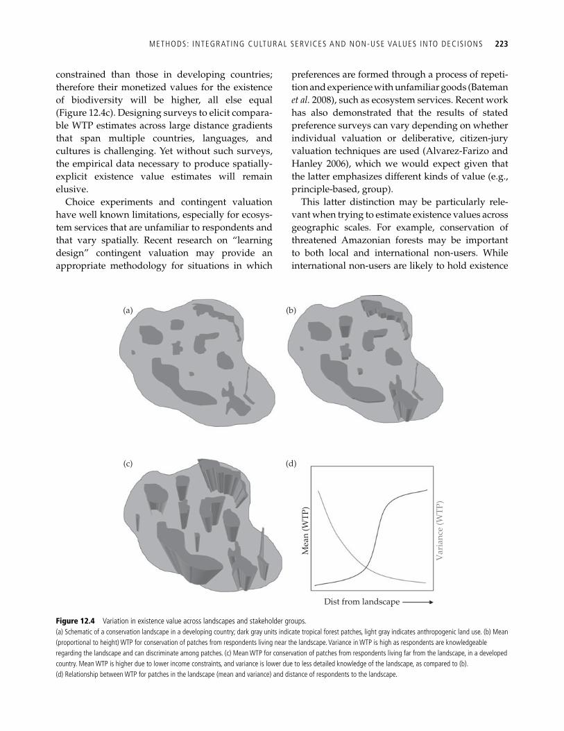
METHODS: INTEGRATING CULTURAL SERVICES AND NON-USE VALUES INTO DECIS IONS 223
constrained than those in developing countries; therefore their monetized values for the existence of biodiversity will be higher, all else equal (Figure 12.4c). Designing surveys to elicit compara-ble WTP estimates across large distance gradients that span multiple countries, languages, and cultures is challenging. Yet without such surveys, the empirical data necessary to produce spatially-explicit existence value estimates will remain elusive.
Choice experiments and contingent valuation have well known limitations, especially for ecosys-tem services that are unfamiliar to respondents and that vary spatially. Recent research on “learning design” contingent valuation may provide an appropriate methodology for situations in which
preferences are formed through a process of repeti-tion and experience with unfamiliar goods ( Bateman et al. 2008 ), such as ecosystem services. Recent work has also demonstrated that the results of stated preference surveys can vary depending on whether individual valuation or deliberative, citizen-jury valuation techniques are used ( Alvarez-Farizo and Hanley 2006 ), which we would expect given that the latter emphasizes different kinds of value (e.g., principle-based, group).
This latter distinction may be particularly rele-vant when trying to estimate existence values across geographic scales. For example, conservation of threatened Amazonian forests may be important to both local and international non-users. While international non-users are likely to hold existence
(a) (b)
(c) (d)
Mea
n (W
TP)
Var
ianc
e (W
TP)
Dist from landscape
Figure 12.4 Variation in existence value across landscapes and stakeholder groups. (a) Schematic of a conservation landscape in a developing country; dark gray units indicate tropical forest patches, light gray indicates anthropogenic land use. (b) Mean (proportional to height) WTP for conservation of patches from respondents living near the landscape. Variance in WTP is high as respondents are knowledgeable regarding the landscape and can discriminate among patches. (c) Mean WTP for conservation of patches from respondents living far from the landscape, in a developed country. Mean WTP is higher due to lower income constraints, and variance is lower due to less detailed knowledge of the landscape, as compared to (b). (d) Relationship between WTP for patches in the landscape (mean and variance) and distance of respondents to the landscape.
224 CULTURAL SERVICES AND NON-USE VALUES
values independent of other members of their com-munity, locals may see forests as a community asset. As such, a deliberative group valuation approach may be the most appropriate to use when multiple perspectives like these exist, rather than an individ-ual survey ( Spash 2007 ).
Bearing in mind all of these issues and constraints, a program to evaluate the existence value of a par-ticular biophysical feature across a landscape (e.g., tropical forests, endangered species) might follow the following steps:
1. Identify the group or groups of people whose existence values one wishes to elicit. 2. Consider the service being valued and use a vari-ety of methods (focus groups, literature reviews, expert knowledge, etc.) to identify the features of the good that people care about. 3. Using similar methods, identify appropriate units of the service on the landscape. These units are liable to be larger/coarser for individuals who have little knowledge of the area. 4. Characterize each of the landscape units with regard to the important features identified in step 2. 5. Using maps and detailed descriptions, construct a survey that will elicit people’s WTP for the exist-ence of the feature across the landscape. We do not dwell here on the multitude of issues associated with constructing a stated preference survey; good references are Mitchell and Carson ( 1989 ) and Louviere et al. ( 2000 ). 6. Summarize WTP values for each particular unit of the service being valued across the land-scape; inference can then be made about WTP across the population that the sampled group represents. 7. Modeling approaches ( Mitchell and Carson 1989 ; Louviere et al. 2000 ) can be used to explain variation in WTP across both individuals and sites; this may be useful for predictive purposes in other contexts.
12.2.3.2 Mapping and quantifying other values Many of the problems addressed in assigning meas-ures to existence value apply, equally, to the larger class of cultural ecosystem services and values articulated here. While WTP methods continue to be employed, so too are expressed preference
surveys drawn from the social sciences. Especially important, are techniques drawn from sociology ( Dunlap et al. 2000 ), human ecology ( Dietz et al. 2005 ), psychology ( Gregory et al. 1993 ), anthro-pology ( Kempton et al. 1995 ; Satterfi eld 2001 ), multi-attribute utility theory ( Russell et al. 2001 ), and legal methods designed for the valuation of loss ( Rutherford et al. 1998 ).
Ultimately newer practices must address above-mentioned problems of human judgment (e.g., the instability in WTP judgments based on framing effects), and yet also achieve a balance between the benefi ts of group deliberation (collective and demo-cratic conversations about what matters); the recog-nition and accommodation of political factors (justice, equity, land tenure, Treaty rights, etc.); and the kinds of quantitative and qualitative analyses necessary to arrive at robust and defensible valuations. Good practice with regard to analysis ensures that the val-uations assigned refl ect the full range of values perti-nent to the case and are thereafter expressed as ordinal or cardinal scales amenable to trade-offs. It also requires that the constituents and/or the rights of different stakeholders are well defi ned thereby signaling important political concerns.
For these reasons, many valuation methods are moving away from the aggregation of willingness-to-pay judgments and toward deliberative proc-esses whereby such values are arrived at collectively. Often know as “deliberative monetary valuation” (DMV), the intent is to arrive at a “social willingness to pay.” In so doing, new classifi cations of value and concomitant valuation practices have arisen ( Spash 2007 , 2008 ). These include values and valuation based on exchange value, charitable contributions, and prices negotiated in reference to equity or linked social values. Others have moved toward the valuation of loss (for services since extinguished or degraded) by combining conjoint analyses (simple paired comparisons) and damage schedules (see, for example, Chuenpagdee et al. 2001 ). Also promis-ing is the application of multi-attribute utility theory to non-market goods including the use of swing weighting ( McDaniels and Trousdale 2005 ). Finally, practices derived from structured decision-making are particularly likely to be useful to the more intangible dimensions of cultural services ( Gregory et al. 1993 ; Gregory 1999 ). This is due to
L IMITATIONS AND NEXT STEPS 225
the practice of constructive scaling, which assumes that a locally defi ned valuation metric (achieved through deliberation) is optimal when natural or proxy scales do not exist ( Keeney and Gregory 2005 ) and when there are many different sub- components of a singularly important value. Com-pelling examples of this method can be found in work with First Nation/Native American commu-nities in Canada ( Gregory et al. 2008 ) and in environmental decision-making more broadly ( O’Neill and Spash 2000 ).
12.3 Limitations and next steps
We have provided a framework for understanding, categorizing, mapping, and valuing cultural ecosys-tem services and non-use values. This contribution supports the notion that it is possible to quantify many of these services and their corresponding val-ues through spatial landscape analysis that facili-tates integration with output from other biophysical and economic service models. Such integration is essential for ensuring that cultural services and non-use values are considered on equal footing with other services and biodiversity in land management and policy decisions. At the same time, although we have presented a typology and categorization of val-ues and services, the methods discussed above do not cover all of these values and services ( Table 12.2 ). Expanding the set of mapping and valuation tools represents an important frontier for research and conservation practice; but as we have discussed, there are several obstacles to comprehensive valua-tion including interdependency between values and services and associated double-counting.
Modeling efforts explore ways to assign value to the cultural and non-use dimensions of ecosystems. For many stakeholders, an equally important consideration will be people’s preferences regard-ing the processes by which decisions are made. This may be particularly true in the context of cultural services given the personal and community ties that they evoke. People’s preferences or principles stem from their underlying or held values ( Brown 1984 ), such as fairness, responsibility, autonomy, and sovereignty. For our proposed models to be effec-tive tools guiding land-use decisions, the biophysical, economic, and non-economic values
produced must be integrated into broader decision-making processes considered legitimate by its par-ticipants and stakeholders.
Citizen juries and multi-criteria decision-making (MCDM) processes implicitly or explicitly include such process-oriented values, so they are possible alternatives ( Chee 2004 ) or addenda to valuation of ecosystem services. Both approaches involve gath-ering groups of citizens intended to represent the spectrum of stakeholders affected by an issue, to carefully consider a body of evidence and collec-tively make decisions. They differ in that citizen juries involve competing teams of experts present-ing alternative viewpoints ( Shrader-Frechette 1985 ; Coote and Lenaghan 1997 ), and MCDM involves explicit structuring of the multiple dimensions rel-evant to the decision ( Saaty 1996 ; Munda 2004 ). Both approaches could be undertaken based on (1) solely biophysical attributes, (2) biophysical attributes and a subset of valuation metrics (e.g., from market values), or (3) biophysical attributes and a full set of valuation results.
There are pros and cons to these various possibili-ties. On one hand, defensible valuation of the full set of ecosystem services at stake is likely to be time-consuming and diffi cult (e.g., to avoid double-counting and account for interdependencies). Not only is value elicitation time-consuming in its own right, but in order to have accurate results, these valuation exercises should be performed using real-istic scenarios of outcomes from decision options—ideally, therefore, valuation will follow biophysical analysis and not run in parallel. Furthermore, explicit measurement of some intangible or sacred values will always trigger discomfort, whereas this discomfort may be lessened considerably if the decision is made without prices or similar metrics (as in citizen juries and MCDM).
On the other hand, citizen juries and MCDM are also time-consuming and diffi cult, and they, too must follow biophysical analysis. Furthermore, they require that participants integrate in their minds the multitude of diverse values that will be affected by management scenarios, often indi-rectly—a considerable cognitive challenge. Finally, they involve giving a certain authority to the small subset of stakeholders invited to the decision- making table, authority likely to be questioned by
226 CULTURAL SERVICES AND NON-USE VALUES
parties unhappy with the resulting decision, per-haps even if considerable time is invested in choos-ing and vetting stakeholders involved.
The most thorough option (3), which can capture the full set of values and consider them in appropri-ate context through democratic, deliberative proc-esses, is likely the most time-consuming and expensive. Fair, inclusive, and enlightened environ-mental decision-making is the Holy Grail. We hope this chapter has provided insights and approaches that move us partway toward this goal.
References
Alvarez-Farizo, B., and Hanley, N. (2006). Improving the process of valuing non-market benefi ts: Combining citi-zens’ juries with choice modelling. Land Economics , 82 , 465–78.
Anderson, D., Salick, J., Moseley, R., et al . (2005). Conserving the Sacred Medicine Mountains: a vegeta-tion analysis of Tibetan sacred sites in Northwest Yunnan. Biodiversity and Conservation, 14 , 3065–91.
Basso, K. H. (1996). Wisdom sits in places: landscape and lan-guage among the Western Apache . University of New Mexico Press, Albuquerque.
Bateman, I. J., Burgess, D., Hutchinson, W. G., et al . (2008). Learning design contingent valuation (LDCV): NOAA guidelines, preference learning and coherent arbitrari-ness. Journal of Environmental Economics and Management, 55 , 127–41.
Bateman, I. J., Day, B. H., Georgiou, S., et al . (2006). The aggregation of environmental benefi t values: Welfare measures, distance decay and total WTP. Ecological Economics , 60 , 450–60.
Bishop, I. D., and Karadaglis, C. (1997). Linking modelling and visualisation for natural resources management. Environment and Planning B: Planning and Design , 24 , 345–58.
Boyd, J., and Banzhaf, S. (2007). What are ecosystem services? The need for standardized environmental accounting units. Ecological Economics, 63 , 616–26.
Brown, G. G., Reed, P., and Harris, C. C. (2002). Testing a place-based theory for environmental evaluation: an Alaska case study. Applied Geography , 22 , 49–76.
Brown, T. C. (1984). The concept of value in resource allo-cation. Land Economics, 60 , 231–46.
Champ, P. A., Boyle, K. J., and Brown, T. C., Ed. (2003). A primer on nonmarket valuation: the economics of non- market goods and resources. Kluwer Academic, Dordrecht, The Netherlands.
Chee, Y. E. (2004). An ecological perspective on the valua-tion of ecosystem services. Biological Conservation , 120 , 549–65.
Chiesura, A., and de Groot, R. (2003). Critical natural capital: a socio-culural perspective. Ecological Economics, 44 , 219–31.
Chuenpagdee, R., Knetsch, J. L., and Brown, T. C. (2001). Coastal management using public judgments, impor-tance scales, and predetermined schedule. Coastal Management , 29 , 253–70.
Cicchetti, C. J., and Wilde, L. L. (1992). Uniqueness, irre-versibility, and the theory of nonuse values. American Journal of Agricultural Economics, 74 , 1121–5.
Coote, A., and Lenaghan, J. (1997). Citizens’ juries: theory into practice. Institute for Public Policy Research, London.
Costanza, R. (2008). Ecosystem services: Multiple classifi -cation systems are needed. Biological Conservation, 141 , 350–2.
Costanza, R., d’Arge, R., de Groot, R., et al . (1997). The value of the world’s ecosystem services and natural capital. Nature , 387 , 253–60.
de Groot, R., Ramakrishnan, P. S., v. d. Berg, A., et al . (2005). Cultural and amenity services. in Millennium Ecosystem Assessment, Ed., Ecosystems and human well-being: current status and trends. Island Press, Washington, DC, pp. 455–76.
Dietz, T., Fitzgerald, A., and Shwom, R. (2005). Environmental values. Annual Review of Environment and Resources , 30 , 335–72.
Dunlap, R. E., Van Liere, K. D., Mertig, A. G., et al . (2000). Measuring endorsement of the new ecological paradigm: A revised NEP scale. Journal of Social Issues 56 , 425–42.
Fisher, B., and Turner, R. K. (2008). Ecosystem services: classifi cation for valuation. Biological Conservation , 141 , 1167–9.
Garibaldi, A., and Turner, N. (2004). Cultural keystone species: Implications for ecological conservation and restoration. Ecology and Society , 9 (3), article 1.
Goulder, L. H., and Kennedy, D. (1997). Valuing ecosystem services: philosophical bases and empirical methods. In G. C. Daily, Ed., Nature’s services: societal dependence on natural ecosystems . Island Press, Washington, DC, pp. 23–47.
Gowdy, J. M. (2001). The monetary valuation of biodiver-sity: Promises, pitfalls, and rays of hope. In V. C. Hollowell, Ed., Managing human-dominated ecosystems: proceedings of the symposium at the Missouri Botanical Garden , St. Louis, Missouri, 26–29 March 1998, pp. 141–9. Missouri Botanical Garden Press, St. Louis.
Gregory, R. (1999). Identifying environmental values. In V. H. Dale and M. R. English, Eds., Tools to aid environ-
L IMITATIONS AND NEXT STEPS 227
mental decision making. Springer-Verlag, New York, pp. 32–58.
Gregory, R., Lichtenstein, S. and Slovic, P. (1993). Valuing environmental resources: A constructive approach. Journal of Risk and Uncertainty , 7 , 177–97.
Gregory, R., Failing, L., and Harstone, M. (2008). Meaningful resource consultations with fi rst peoples: notes from British Columbia. Environment , 50 , 34–45.
Grêt-Regamey, A., Bishop, I. D., and Bebi, P. (2007). Predicting the scenic beauty value of mapped landscape changes in a mountainous region through the use of GIS. Environment and Planning B: Planning and Design , 34 , 50–67.
Hanley, N., Schlapfer, F., and Spurgeon, J. (2003). Agg-regating the benefi ts of environmental improvements: distance-decay functions for use and non-use values. Journal of Environmental Management, 68 , 297–304.
Horton, B., Colarullo, G., Bateman, I. J., et al . (2003). Evaluating non-user willingness to pay for a large-scale conservation programme in Amazonia: a UK/Italian contingent valuation study. Environmental Conservation, 30 , 139–46.
Kahneman, D. and Knetsch, J. L. (2005). Valuing public goods: The purchase of moral satisfaction. In L. Kalof and T. Satterfi eld, Eds., The Earthscan Reader in environ-mental values. Earthscan, Sterling, pp. 229–43.
Kawagebo Culture Association (KCA). (2004). Report on Sacred Sites in the Kawagebo Area. Submitted to The Nature Conservancy China Program.
Keeney, R. L., and Gregory, R. S. (2005). Selecting attributes to measure the achievement of objectives. Operations Research, 53 , 1–11.
Kempton, W., Boster, J. S., and Hartley, J. A. (1995). Environmental values in American culture . MIT Press, Cambridge, MA.
Kramer, R. A., and Mercer, D. E. (1997). Valuing a global environmental good: US residents’ willingness to pay to protect tropical rain forests. Land Economics , 73 , 196–210.
Krutilla, J. V. (1967). Conservation reconsidered. American Economic Review , 57 , 777–86.
Lim, E.-M., and Honjo, T. (2003). Three-dimensional visu-alization forest of landscapes by VRML. Landscape and Urban Planning , 63 , 175–86.
Lin, N. (2001). Social capital: a theory of social structure and action . Cambridge University Press, Cambridge.
Lockwood, M. (1998). Integrated value assessment using paired comparisons. Ecological Economics, 25 , 73–87.
Louv, R. (2008). Last child in the woods: saving our children from nature-defi cit disorder . Updated and expanded edition . Algonquin Books, Chapel Hill.
Louviere, J. J., Hensher, D. A., and Swait, J. D. (2000). Stated choice methods: analysis and applications. Cambridge University Press, Cambridge.
Ma, J. (2005). Sacred natural sites and conservation in the Meili area. In J. Ma and J. Chen, Eds., Tibetan Culture and Biodiversity Conservation. Yunnan Nationality Press, China, pp. 33–40.
McCauley, D. J. (2006). Selling out on nature. Nature, 443 , 27–8.
McDaniels, T. L., and Trousdale, W. (2005). Resource com-pensation and negotiation support in an aboriginal con-text: Using community-based multi-attribute analysis to evaluate non-market losses. Ecological Economics , 55 , 173–86.
Martinez-Alier, J., Munda, G., and O’Neill, J. (1998). Weak comparability of values as a foundation for ecological economics. Ecological Economics , 26 , 277–86.
Meadows, D. H. (2001). Dancing with systems. Whole Earth (Winter).
Millennium Ecosystem Assessment. (2005). Ecosystems and human well-being: synthesis . Island Press, Washington, DC.
Milton, K. (2002). Loving nature: towards an ecology of emo-tion . Routledge, London.
Mitchell, R. C., and Carson, R. T. (1989). Using surveys to value public goods: the contingent valuation method , 3rd edn. Resources for the Future, Washington, DC.
Munda, G. (2004). Social multi-criteria evaluation: Methodological foundations and operational conse-quences. European Journal of Operational Research , 158 , 662–77.
National Research Council (US). Committee on Assessing and Valuing the Services of Aquatic and Related Terrestrial Ecosystems. (2005). Valuing ecosystem services: toward better environmental decision-making . National Research Council, Washington, DC.
Norton, B. G., and Hannon, B. (1997). Environmental values: A place-based theory. Environmental Ethics , 19 , 227–45.
O’Neill, J., and Spash, C. L. (2000). Conceptions of value in environmental decision-making. Environmental Values , 9 , 521–35.
Pergams, O. R. W., and Zaradic, P. A. (2006). Is love of nature in the US becoming love of electronic media? 16-year downtrend in national park visits explained by watching movies, playing video games, internet use, and oil prices. Journal of Environmental Management , 80 , 387–93.
Rees, W. E. (1998). How should a parasite value its host? Ecological Economics, 25 , 49–52.
Rolfe, J., Bennett, J. and Louviere, J. (2000). Choice model-ling and its potential application to tropical rainforest preservation. Ecological Economics , 35 , 289–302.
Russell, C., Dale, V., Lee, J. S., et al . (2001). Experimenting with multi-attribute utility survey methods in a multi-
228 CULTURAL SERVICES AND NON-USE VALUES
dimensional valuation problem. Ecological Economics , 36 . 87–108.
Rutherford, M. B., Knetsch, J. L., and Brown, T. C. (1998). Assessing environmental losses: judgments of impor-tance and damage schedules. Harvard Environmental Law Review, 22 , 51–101.
Saaty, T. L. (1996). Multicriteria decision making: the analytic hierarchy process: planning, priority setting, resource alloca-tion , 2nd edn. RWS Publications, Pittsburgh.
Sable, K., and Kling, R. (2001). The double public good: A conceptual framework for “shared experience” values associated with heritage conservation. Journal of Cultural Economics, 25 , 77–89.
Sagoff, M. (1998). Aggregation and deliberation in valuing environmental public goods: A look beyond contingent pricing. Ecological Economics , 24 , 213–30.
Satterfi eld, T. (2001). In search of value literacy: sugges-tions for the elicitation of environmental values. Environmental Values , 10 , 331–59.
Satterfi eld, T., and Roberts, M. (2008). Incommensurate risks and the regulator’s dilemma: considering culture in the governance of genetically modifi ed organisms. New Genetics and Society , 27 , 201–16.
Shrader-Frechette, K. S. (1985). Science policy, ethics, and economic methodology of social science: some problems of
technology assessment and environmental impact analysis. Springer, Dordrecht, The Netherlands.
Spash, C. L. (2007). Deliberative monetary valuation (DMV): Issues in combining economic and political processes to value environmental change. Ecological Economics , 63 , 690–9.
Spash, C. L. (2008). Deliberative monetary valuation and the evidence for a new value theory. Land Economics , 84 , 469–88.
Throsby, D. (2001). Economics and culture. Cambridge University Press, Cambridge.
Turner, N. J., Gregory, R., Brooks, C., et al . (2008). From invisibility to transparency: identifying the implica-tions. Ecology and Society , 13 (2), 7.
Turner, N. J., and Turner, K. L. (2008). “Where our women used to get the food”: cumulative effects and loss of eth-nobotanical knowledge and practice; case study from coastal British Columbia. Botany-Botanique , 86 , 103–15.
US Census Bureau. (2003). U.S. Census 2000 . Wallace, K. J. (2008). Ecosystem services: Multiple clas-
sifi cations or confusion? Biological Conservation , 141 , 353–4.
Wunder, S., and Vargas, M. T. (2005). Beyond “markets”: Why terminology matters. Ecosystem Marketplace. The Katoomba Group.
229
CHAPTER 13
Terrestrial biodiversity Erik Nelson, D. Richard Cameron, James Regetz, Stephen Polasky, and Gretchen C. Daily
13.1 Introduction
Biodiversity is the variety of life at all levels of organization, from genetically distinct populations to species, habitats, ecosystems, and biomes ( Leopold 1949 ; Wilson 1992 ). While biodiversity infl uences the provision of all ecosystem services, and is the basis for many (Sekercioglu et al . 2004; Díaz et al . 2005), it also inspires conservation for its own sake (e.g., Ehrlich and Ehrlich 1982 , Chapter 2 ). To protect what remains of declining biodiversity ( Hughes et al . 1997 ; Dirzo and Raven 2003 ; Worm et al . 2006 ) conservationists seek to identify habitat conserva-tion networks that maximize habitat or species per-sistence. The design of these networks typically uses species distribution maps (e.g., Ceballos et al . 2005 ) and an understanding of the factors that affect spe-cies presence and persistence on the landscape (e.g., Sekercioglu et al . 2007). More recently, the design of conservation networks have considered the fi nan-cial and opportunity cost of network conservation and implementation ( Ando et al . 1998 ; Wilson et al . 2007 ; Polasky et al . 2008 ). Systematic conservation planning (SCP) ( Margules and Pressey 2000 ) mar-ries many of these network design principles and conservation organizations implement SCP princi-ples in their work ( Groves et al. 2002 ).
We present three relatively simple biodiversity models that spring from this conservation planning literature. The models are straightforward to imple-ment and are designed for analysis at landscape scales. Our simplest model, tier 1, combines basic informa-tion about land cover and threats to biodiversity to produce habitat-quality and habitat rarity maps. In tier 1 we assume that protection of a variety of high-quality habitats will confer protection to their compo-nent species and populations ( Groves et al . 2002 ).
Because the tier 1 biodiversity model uses data that are available virtually everywhere in the world and empirical data on the status of rare, endemic, and other species of conservation concern are unavailable for many places, a habitat analysis, instead of a species-based approach is commonly implemented as the fi rst phase of a conservation assessment.
In tier 2 we assume data on potential distribu-tions or ranges of species and on habitat suitability (as gauged by breeding and foraging activity) are available to us. We present two tier 2 models that rely on this species-specifi c data. The fi rst model combines these data to calculate the relative contri-bution of a parcel’s habitat to the overall quantity of suitable habitat across a landscape or region. This approach is similar to deductive species distribu-tion modeling ( Stoms et al . 1992 ), the rarity-weighted richness methodology ( Williams et al . 1996 ), and the Biological Intactness Index (BII) system ( Scholes and Biggs 2005 ). The second tier 2 model aggregates information on species distributions and habitat suitability into a single landscape score. This score is derived using species–area relationships to trans-late habitat area into a measure of landscape-wide biodiversity status, based on work by Sala et al . ( 2005 ) and Pereira and Daily ( 2006 ). In addition, we can incorporate tier 1 output into tier 2 modeling in order to weight suitable habitat area by quality. Such quality weighting of habitat is common in algorithms that are used to select networks of areas for conservation (e.g., Schill and Raber 2008 ).
13.2 Tier 1: habitat-quality and rarity model
Habitat-quality depends on its proximity to human land uses and the intensity of these land uses.
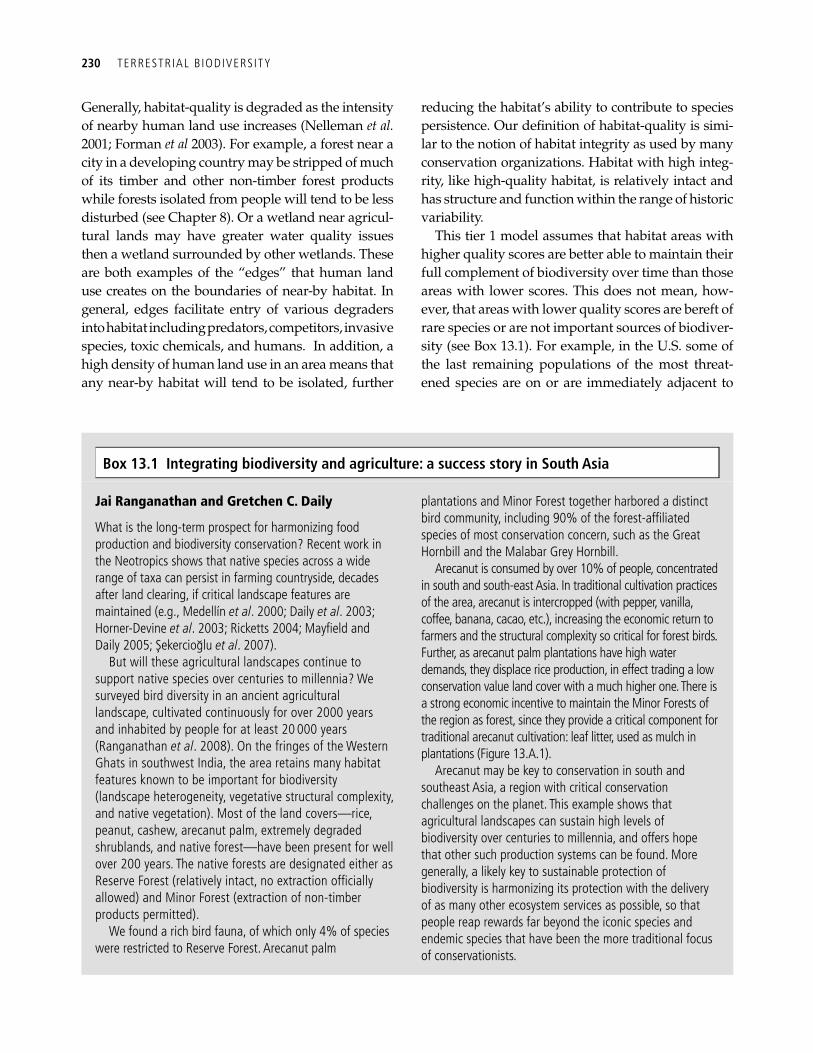
230 TERRESTRIAL B IODIVERSITY
Generally, habitat-quality is degraded as the intensity of nearby human land use increases ( Nelleman et al. 2001 ; Forman et al 2003 ). For example, a forest near a city in a developing country may be stripped of much of its timber and other non-timber forest products while forests isolated from people will tend to be less disturbed (see Chapter 8 ). Or a wetland near agricul-tural lands may have greater water quality issues then a wetland surrounded by other wetlands. These are both examples of the “edges” that human land use creates on the boundaries of near-by habitat. In general, edges facilitate entry of various degraders into habitat including predators, competitors, invasive species, toxic chemicals, and humans. In addition, a high density of human land use in an area means that any near-by habitat will tend to be isolated, further
reducing the habitat’s ability to contribute to species persistence. Our defi nition of habitat-quality is simi-lar to the notion of habitat integrity as used by many conservation organizations. Habitat with high integ-rity, like high-quality habitat, is relatively intact and has structure and function within the range of historic variability.
This tier 1 model assumes that habitat areas with higher quality scores are better able to maintain their full complement of biodiversity over time than those areas with lower scores. This does not mean, how-ever, that areas with lower quality scores are bereft of rare species or are not important sources of biodiver-sity (see Box 13.1 ). For example, in the U.S. some of the last remaining populations of the most threat-ened species are on or are immediately adjacent to
Jai Ranganathan and Gretchen C. Daily
What is the long-term prospect for harmonizing food production and biodiversity conservation? Recent work in the Neotropics shows that native species across a wide range of taxa can persist in farming countryside, decades after land clearing, if critical landscape features are maintained (e.g., Medellín et al . 2000; Daily et al . 2003 ; Horner-Devine et al . 2003 ; Ricketts 2004 ; Mayfi eld and Daily 2005 ; Sekercioglu et al . 2007 ).
But will these agricultural landscapes continue to support native species over centuries to millennia? We surveyed bird diversity in an ancient agricultural landscape, cultivated continuously for over 2000 years and inhabited by people for at least 20 000 years ( Ranganathan et al . 2008 ). On the fringes of the Western Ghats in southwest India, the area retains many habitat features known to be important for biodiversity (landscape heterogeneity, vegetative structural complexity, and native vegetation). Most of the land covers—rice, peanut, cashew, arecanut palm, extremely degraded shrublands, and native forest—have been present for well over 200 years. The native forests are designated either as Reserve Forest (relatively intact, no extraction offi cially allowed) and Minor Forest (extraction of non-timber products permitted).
We found a rich bird fauna, of which only 4% of species were restricted to Reserve Forest. Arecanut palm
plantations and Minor Forest together harbored a distinct bird community, including 90% of the forest-affi liated species of most conservation concern, such as the Great Hornbill and the Malabar Grey Hornbill.
Arecanut is consumed by over 10% of people, concentrated in south and south-east Asia. In traditional cultivation practices of the area, arecanut is intercropped (with pepper, vanilla, coffee, banana, cacao, etc.), increasing the economic return to farmers and the structural complexity so critical for forest birds. Further, as arecanut palm plantations have high water demands, they displace rice production, in effect trading a low conservation value land cover with a much higher one. There is a strong economic incentive to maintain the Minor Forests of the region as forest, since they provide a critical component for traditional arecanut cultivation: leaf litter, used as mulch in plantations ( Figure 13.A.1 ).
Arecanut may be key to conservation in south and southeast Asia, a region with critical conservation challenges on the planet. This example shows that agricultural landscapes can sustain high levels of biodiversity over centuries to millennia, and offers hope that other such production systems can be found. More generally, a likely key to sustainable protection of biodiversity is harmonizing its protection with the delivery of as many other ecosystem services as possible, so that people reap rewards far beyond the iconic species and endemic species that have been the more traditional focus of conservationists.
Box 13.1 Integrating biodiversity and agriculture: a success story in South Asia
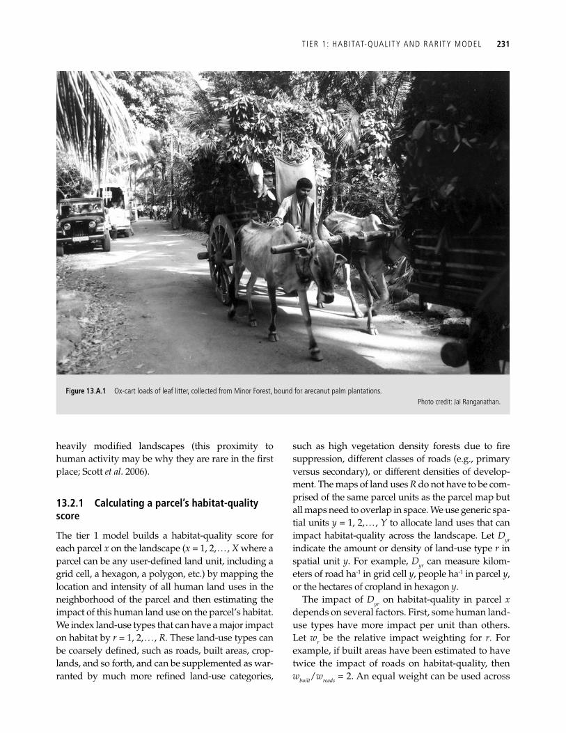
T IER 1 : HABITAT-QUALITY AND RARITY MODEL 231
heavily modifi ed landscapes (this proximity to human activity may be why they are rare in the fi rst place; Scott et al . 2006 ).
13.2.1 Calculating a parcel’s habitat-quality score
The tier 1 model builds a habitat-quality score for each parcel x on the landscape ( x = 1, 2, . . . , X where a parcel can be any user-defi ned land unit, including a grid cell, a hexagon, a polygon, etc.) by mapping the location and intensity of all human land uses in the neighborhood of the parcel and then estimating the impact of this human land use on the parcel’s habitat. We index land-use types that can have a major impact on habitat by r = 1, 2, . . . , R . These land-use types can be coarsely defi ned, such as roads, built areas, crop-lands, and so forth, and can be supplemented as war-ranted by much more refi ned land-use categories,
such as high vegetation density forests due to fi re suppression, different classes of roads (e.g., primary versus secondary), or different densities of develop-ment. The maps of land uses R do not have to be com-prised of the same parcel units as the parcel map but all maps need to overlap in space. We use generic spa-tial units y = 1, 2, . . . , Y to allocate land uses that can impact habitat-quality across the landscape. Let D yr indicate the amount or density of land-use type r in spatial unit y . For example, D yr can measure kilom-eters of road ha -1 in grid cell y , people ha -1 in parcel y , or the hectares of cropland in hexagon y .
The impact of D yr on habitat-quality in parcel x depends on several factors. First, some human land-use types have more impact per unit than others. Let w r be the relative impact weighting for r . For example, if built areas have been estimated to have twice the impact of roads on habitat-quality, then w built / w roads = 2. An equal weight can be used across
Figure 13.A.1 Ox-cart loads of leaf litter, collected from Minor Forest, bound for arecanut palm plantations. Photo credit: Jai Ranganathan.
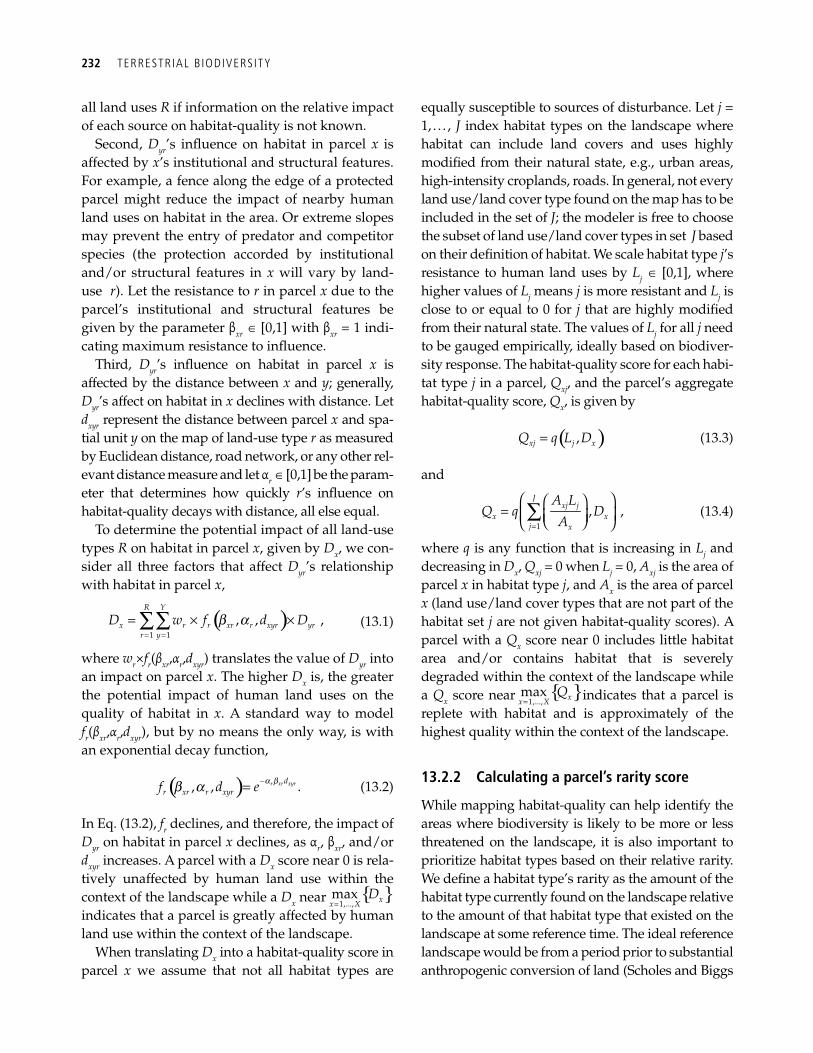
232 TERRESTRIAL B IODIVERSITY
all land uses R if information on the relative impact of each source on habitat-quality is not known.
Second, D yr ’s infl uence on habitat in parcel x is affected by x ’s institutional and structural features. For example, a fence along the edge of a protected parcel might reduce the impact of nearby human land uses on habitat in the area. Or extreme slopes may prevent the entry of predator and competitor species (the protection accorded by institutional and/or structural features in x will vary by land-use r ). Let the resistance to r in parcel x due to the parcel’s institutional and structural features be given by the parameter β xr Î [0,1] with β xr = 1 indi-cating maximum resistance to infl uence.
Third, D yr ’s infl uence on habitat in parcel x is affected by the distance between x and y ; generally, D yr ’s affect on habitat in x declines with distance. Let d xyr represent the distance between parcel x and spa-tial unit y on the map of land-use type r as measured by Euclidean distance, road network, or any other rel-evant distance measure and let α r Î [0,1] be the param-eter that determines how quickly r ’s infl uence on habitat-quality decays with distance, all else equal.
To determine the potential impact of all land-use types R on habitat in parcel x , given by D x , we con-sider all three factors that affect D yr ’s relationship with habitat in parcel x ,
( )b a= =
= × ×∑∑1 1
, , ,R Y
x r r xr r xyr yrr y
D w f d D (13.1)
where w r × f r ( β x r , α r , d x y r ) translates the value of D yr into an impact on parcel x . The higher D x is, the greater the potential impact of human land uses on the quality of habitat in x . A standard way to model f r ( β x r , α r , d x y r ) , but by no means the only way, is with an exponential decay function,
( ) r xr xyrdr xr r xyrf d e, , a bb a −= . (13.2)
In Eq. (13.2), f r declines, and therefore, the impact of D yr on habitat in parcel x declines, as α r , β xr , and/or d xyr increases. A parcel with a D x score near 0 is rela-tively unaffected by human land use within the context of the landscape while a D x near
1,...,max xx X
D=
indicates that a parcel is greatly affected by human land use within the context of the landscape.
When translating D x into a habitat-quality score in parcel x we assume that not all habitat types are
equally susceptible to sources of disturbance. Let j = 1, . . . , J index habitat types on the landscape where habitat can include land covers and uses highly modifi ed from their natural state, e.g., urban areas, high-intensity croplands, roads. In general, not every land use/land cover type found on the map has to be included in the set of J; the modeler is free to choose the subset of land use/land cover types in set J based on their defi nition of habitat. We scale habitat type j ’s resistance to human land uses by L j Î [0,1], where higher values of L j means j is more resistant and Lj is close to or equal to 0 for j that are highly modifi ed from their natural state. The values of L j for all j need to be gauged empirically, ideally based on biodiver-sity response. The habitat- quality score for each habi-tat type j in a parcel, Q xj , and the parcel’s aggregate habitat-quality score, Q x , is given by
( ),xj j xQ q L D= (13.3)
and
J
xj jx x
j x
A LQ q D
A1
, ,=
⎛ ⎞⎛ ⎞= ⎜ ⎟⎜ ⎟⎝ ⎠⎝ ⎠
∑ (13.4)
where q is any function that is increasing in L j and decreasing in D x , Qxj = 0 when Lj = 0, A xj is the area of parcel x in habitat type j , and A x is the area of parcel x (land use/land cover types that are not part of the habitat set j are not given habitat-quality scores). A parcel with a Q x score near 0 includes little habitat area and/or contains habitat that is severely degraded within the context of the landscape while a Q x score near
1,...,max xx X
Q= indicates that a parcel is
replete with habitat and is approximately of the highest quality within the context of the landscape.
13.2.2 Calculating a parcel’s rarity score
While mapping habitat-quality can help identify the areas where biodiversity is likely to be more or less threatened on the landscape, it is also important to prioritize habitat types based on their relative rarity. We defi ne a habitat type’s rarity as the amount of the habitat type currently found on the landscape relative to the amount of that habitat type that existed on the landscape at some reference time. The ideal reference landscape would be from a period prior to substantial anthropogenic conversion of land ( Scholes and Biggs
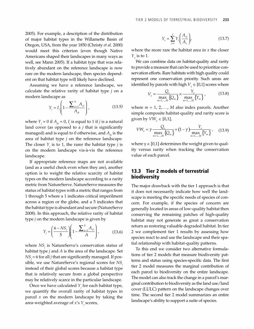
T IER 2 MODELS OF TERRESTRIAL B IODIVERSITY 233
2005 ). For example, a description of the distribution of major habitat types in the Willamette Basin of Oregon, USA, from the year 1850 ( Christy et al . 2000 ) would meet this criterion (even though Native Americans shaped their landscapes in many ways as well, see Mann 2005 ). If a habitat type that was rela-tively abundant on the reference landscape is now rare on the modern landscape, then species depend-ent on that habitat type will likely have declined.
Assuming we have a reference landscape, we calculate the relative rarity of habitat type j on a modern landscape as
=
⎛ ⎞= ⎜ − ⎟
⎜ ⎟⎝ ⎠
∑ 11 ,X
xjxj j
jb
AY I
A (13.5)
where Y j = 0 if A jb = 0, I j is equal to 1 if j is a natural land cover (as opposed to a j that is signifi cantly managed) and is equal to 0 otherwise, and A jb is the area of habitat type j on the reference landscape. The closer Y j is to 1, the rarer the habitat type j is on the modern landscape vis-à-vis the reference landscape.
If appropriate reference maps are not available (and as a useful check even when they are), another option is to weight the relative scarcity of habitat types on the modern landscape according to a rarity metric from NatureServe. NatureServe measures the status of habitat types with a metric that ranges from 1 through 5 where a 1 indicates critical imperilment across a region or the globe, and a 5 indicates that the habitat type is abundant and secure ( NatureServe 2008 ). In this approach, the relative rarity of habitat type j on the modern landscape is given by
=⎛ ⎞−⎛ ⎞
= ⎜ − ⎟⎜ ⎟ ⎜ ⎟⎝ ⎠ ⎝ ⎠
∑ 16
1 ,5
X
xjj xj
ANSY
A (13.6)
where NS j is NatureServe’s conservation status of habitat type j and A is the area of the landscape. Set NS j = 6 for all j that are signifi cantly managed. If pos-sible, we use NatureServe’s regional scores for NS j instead of their global scores because a habitat type that is relatively secure from a global perspective may be relatively scarce in the particular landscape.
Once we have calculated Y j for each habitat type, we quantify the overall rarity of habitat types in parcel x on the modern landscape by taking the area-weighted average of x ’s Y j scores,
J
xjx j
j x
AY Y
A1
,=
⎛ ⎞= ⎜ ⎟⎝ ⎠∑ (13.7)
where the more rare the habitat area in x the closer Y x is to 1.
We can combine data on habitat-quality and rarity to provide a measure that can be used to prioritize con-servation efforts. Rare habitats with high quality could represent one conservation priority. Such areas are identifi ed by parcels with high V x Î [0,1] scores where
= =
= ×1,..., 1,...,
,max max
x xx
m mm M m M
Q YV
Q Y (13.8)
where m = 1, 2, . . . , M also index parcels. Another simple composite habitat-quality and rarity score is given by VW x Î [0,1],
( ) g g= =
= + −1,..., 1,...,
1 ,max max
x xx
m mm M m M
Q YVW
Q Y (13.9)
where γ Î [0,1] determines the weight given to qual-ity versus rarity when tracking the conservation value of each parcel.
13.3 Tier 2 models of terrestrial biodiversity
The major drawback with the tier 1 approach is that it does not necessarily indicate how well the land-scape is meeting the specifi c needs of species of con-cern. For example, if the species of concern are generally located in areas of low-quality habitat then conserving the remaining patches of high-quality habitat may not generate as great a conservation return as restoring valuable degraded habitat. In tier 2 we complement tier 1 results by assessing how species react to and use the landscape and their spa-tial relationship with habitat-quality patterns.
To this end we consider two alternative formula-tions of tier 2 models that measure biodiversity pat-terns and status using species-specifi c data. The fi rst tier 2 model measures the marginal contribution of each parcel to biodiversity on the entire landscape. The model can also track the change in a parcel’s mar-ginal contribution to biodiversity as the land use/land cover (LULC) pattern on the landscape changes over time. The second tier 2 model summarizes an entire landscape’s ability to support a suite of species.
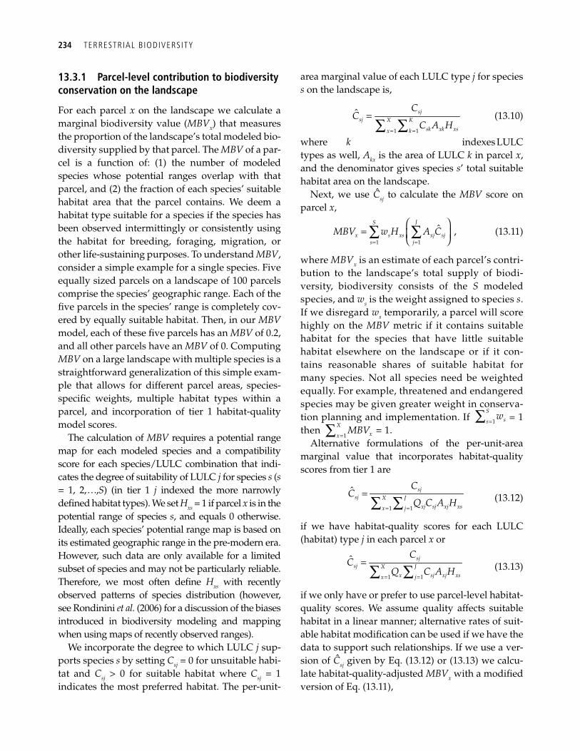
234 TERRESTRIAL B IODIVERSITY
13.3.1 Parcel-level contribution to biodiversity conservation on the landscape
For each parcel x on the landscape we calculate a marginal biodiversity value ( MBV x ) that measures the proportion of the landscape’s total modeled bio-diversity supplied by that parcel. The MBV of a par-cel is a function of: (1) the number of modeled species whose potential ranges overlap with that parcel, and (2) the fraction of each species’ suitable habitat area that the parcel contains. We deem a habitat type suitable for a species if the species has been observed intermittingly or consistently using the habitat for breeding, foraging, migration, or other life-sustaining purposes. To understand MBV , consider a simple example for a single species. Five equally sized parcels on a landscape of 100 parcels comprise the species’ geographic range. Each of the fi ve parcels in the species’ range is completely cov-ered by equally suitable habitat. Then, in our MBV model, each of these fi ve parcels has an MBV of 0.2, and all other parcels have an MBV of 0. Computing MBV on a large landscape with multiple species is a straightforward generalization of this simple exam-ple that allows for different parcel areas, species-specifi c weights, multiple habitat types within a parcel, and incorporation of tier 1 habitat-quality model scores.
The calculation of MBV requires a potential range map for each modeled species and a compatibility score for each species/LULC combination that indi-cates the degree of suitability of LULC j for species s ( s = 1, 2, . . ., S ) (in tier 1 j indexed the more narrowly defi ned habitat types). We set H xs = 1 if parcel x is in the potential range of species s , and equals 0 otherwise. Ideally, each species’ potential range map is based on its estimated geographic range in the pre-modern era. However, such data are only available for a limited subset of species and may not be particularly reliable. Therefore, we most often defi ne H xs with recently observed patterns of species distribution (however, see Rondinini et al. ( 2006 ) for a discussion of the biases introduced in biodiversity modeling and mapping when using maps of recently observed ranges).
We incorporate the degree to which LULC j sup-ports species s by setting C sj = 0 for unsuitable habi-tat and C sj > 0 for suitable habitat where C sj = 1 indicates the most preferred habitat. The per-unit-
area marginal value of each LULC type j for species s on the landscape is,
= =
=∑ ∑1 1
ˆ sjsj X K
sk xk xsx k
CC
C A H (13.10)
where k indexes LULC types as well, A kx is the area of LULC k in parcel x , and the denominator gives species s ’ total suitable habitat area on the landscape.
Next, we use C s j to calculate the MBV score on parcel x ,
JS
x s xs xj sjs j
MBV w H A C1 1
ˆ ,= =
⎛ ⎞= ⎜ ⎟⎝ ⎠
∑ ∑ (13.11)
where MBV x is an estimate of each parcel’s contri-bution to the landscape’s total supply of biodi-versity, biodiversity consists of the S modeled species, and w s is the weight assigned to species s . If we disregard w s temporarily, a parcel will score highly on the MBV metric if it contains suitable habitat for the species that have little suitable habitat elsewhere on the landscape or if it con-tains reasonable shares of suitable habitat for many species. Not all species need be weighted equally. For example, threatened and endangered species may be given greater weight in conserva-tion planning and implementation. If 1
Sss
w=∑ = 1
then 1
Xxx
MBV=∑ = 1.
Alternative formulations of the per-unit-area marginal value that incorporates habitat-quality scores from tier 1 are
1 1
ˆ sjsj X J
xj sj xj xsx j
CC
Q C A H= =
=∑ ∑ (13.12)
if we have habitat-quality scores for each LULC (habitat) type j in each parcel x or
1 1
ˆ sjsj X J
x sj xj xsx j
CC
Q C A H= =
=∑ ∑ (13.13)
if we only have or prefer to use parcel-level habitat-quality scores. We assume quality affects suitable habitat in a linear manner; alternative rates of suit-able habitat modifi cation can be used if we have the data to support such relationships. If we use a ver-sion of C s j given by Eq. (13.12) or (13.13) we calcu-late habitat-quality-adjusted MBV x with a modifi ed version of Eq. (13.11),
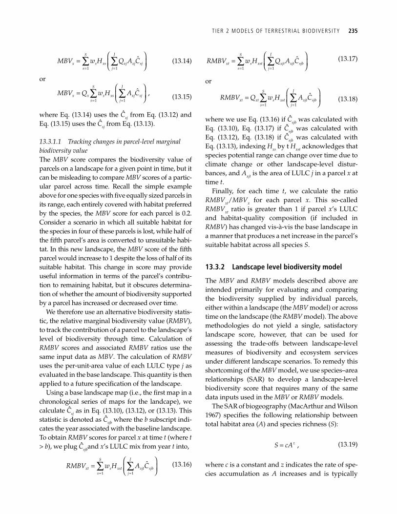
T IER 2 MODELS OF TERRESTRIAL B IODIVERSITY 235
= =
⎛ ⎞= ⎜ ⎟⎝ ⎠
∑ ∑1 1
ˆJS
x s xs xj xj sjs j
MBV w H Q A C (13.14)
or
= =
⎛ ⎞= ⎜ ⎟⎝ ⎠
∑ ∑1 1
ˆ ,JS
x x s xs xj sjs j
MBV Q w H A C (13.15)
where Eq. (13.14) uses the C s j from Eq. (13.12) and Eq. (13.15) uses the C s j from Eq. (13.13).
13.3.1.1 Tracking changes in parcel-level marginal biodiversity value The MBV score compares the biodiversity value of parcels on a landscape for a given point in time, but it can be misleading to compare MBV scores of a partic-ular parcel across time. Recall the simple example above for one species with fi ve equally sized parcels in its range, each entirely covered with habitat preferred by the species, the MBV score for each parcel is 0.2. Consider a scenario in which all suitable habitat for the species in four of these parcels is lost, while half of the fi fth parcel’s area is converted to unsuitable habi-tat. In this new landscape, the MBV score of the fi fth parcel would increase to 1 despite the loss of half of its suitable habitat. This change in score may provide useful information in terms of the parcel’s contribu-tion to remaining habitat, but it obscures determina-tion of whether the amount of biodiversity supported by a parcel has increased or decreased over time.
We therefore use an alternative biodiversity statis-tic, the relative marginal biodiversity value ( RMBV ), to track the contribution of a parcel to the landscape’s level of biodiversity through time. Calculation of RMBV scores and associated RMBV ratios use the same input data as MBV . The calculation of RMBV uses the per-unit-area value of each LULC type j as evaluated in the base landscape. This quantity is then applied to a future specifi cation of the landscape.
Using a base landscape map (i.e., the fi rst map in a chronological series of maps for the landcape), we calculate C s j as in Eq. (13.10), (13.12), or (13.13). This statistic is denoted as C s j b where the b subscript indi-cates the year associated with the baseline landscape. To obtain RMBV scores for parcel x at time t (where t > b ), we plug C s j b and x ’s LULC mix from year t into,
= =
⎛ ⎞= ⎜ ⎟⎝ ⎠
∑ ∑1 1
ˆJS
xt s xst xjt sjbs j
RMBV w H A C (13.16)
= =
⎛ ⎞= ⎜ ⎟⎝ ⎠
∑ ∑1 1
ˆJS
xt s xst xjt xjt sjbs j
RMBV w H Q A C (13.17)
or
= =
⎛ ⎞= ⎜ ⎟⎝ ⎠
∑ ∑1 1
ˆJS
xt xt s xst xjt sjbs j
RMBV Q w H A C (13.18)
where we use Eq. (13.16) if C s j b was calculated with Eq. (13.10), Eq. (13.17) if C s j b was calculated with Eq. (13.12), Eq. (13.18) if C s j b was calculated with Eq. (13.13), indexing Hxs by t H xst acknowledges that species potential range can change over time due to climate change or other landscape-level distur-bances, and A xjt is the area of LULC j in a parcel x at time t .
Finally, for each time t , we calculate the ratio RMBV xt / MBV x for each parcel x . This so-called RMBV xt ratio is greater than 1 if parcel x ’s LULC and habitat-quality composition (if included in RMBV ) has changed vis-à-vis the base landscape in a manner that produces a net increase in the parcel’s suitable habitat across all species S .
13.3.2 Landscape level biodiversity model
The MBV and RMBV models described above are intended primarily for evaluating and comparing the biodiversity supplied by individual parcels, either within a landscape (the MBV model) or across time on the landscape (the RMBV model). The above methodologies do not yield a single, satisfactory landscape score, however, that can be used for assessing the trade-offs between landscape-level measures of biodiversity and ecosystem services under different landscape scenarios. To remedy this shortcoming of the MBV model, we use species–area relationships (SAR) to develop a landscape-level biodiversity score that requires many of the same data inputs used in the MBV or RMBV models.
The SAR of biogeography ( MacArthur and Wilson 1967 ) specifi es the following relationship between total habitat area ( A ) and species richness ( S ):
= ,zS cA (13.19)
where c is a constant and z indicates the rate of spe-cies accumulation as A increases and is typically
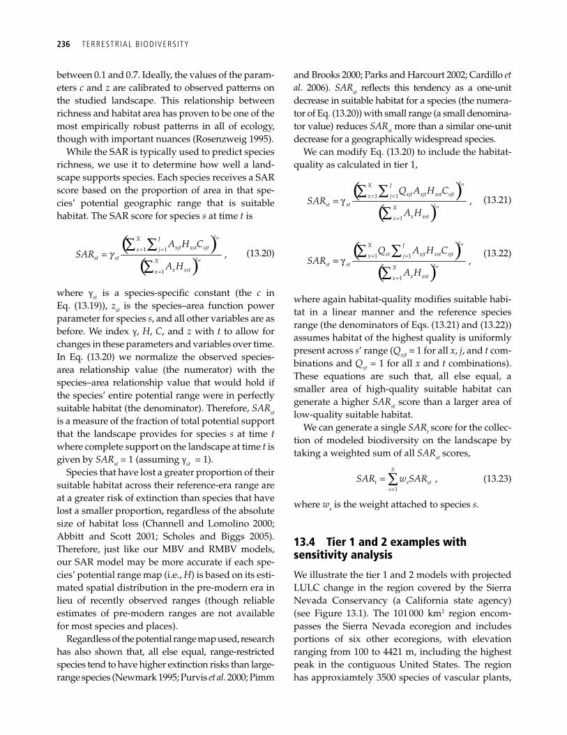
236 TERRESTRIAL B IODIVERSITY
between 0.1 and 0.7. Ideally, the values of the param-eters c and z are calibrated to observed patterns on the studied landscape. This relationship between richness and habitat area has proven to be one of the most empirically robust patterns in all of ecology, though with important nuances ( Rosenzweig 1995 ).
While the SAR is typically used to predict species richness, we use it to determine how well a land-scape supports species. Each species receives a SAR score based on the proportion of area in that spe-cies’ potential geographic range that is suitable habitat. The SAR score for species s at time t is
( )
( )g = =
=
=∑ ∑
∑1 1
1
,
st
st
zX J
xjt xst sjtx jst st zX
x xstx
A H CSAR
A H (13.20)
where γ st is a species-specifi c constant (the c in Eq. (13.19)), z st is the species–area function power parameter for species s , and all other variables are as before. We index γ, H , C , and z with t to allow for changes in these parameters and variables over time. In Eq. (13.20) we normalize the observed species-area relationship value (the numerator) with the species–area relationship value that would hold if the species’ entire potential range were in perfectly suitable habitat (the denominator). Therefore, SAR st is a measure of the fraction of total potential support that the landscape provides for species s at time t where complete support on the landscape at time t is given by SAR st = 1 (assuming γ st = 1).
Species that have lost a greater proportion of their suitable habitat across their reference-era range are at a greater risk of extinction than species that have lost a smaller proportion, regardless of the absolute size of habitat loss ( Channell and Lomolino 2000 ; Abbitt and Scott 2001 ; Scholes and Biggs 2005 ). Therefore, just like our MBV and RMBV models, our SAR model may be more accurate if each spe-cies’ potential range map (i.e., H ) is based on its esti-mated spatial distribution in the pre-modern era in lieu of recently observed ranges (though reliable estimates of pre-modern ranges are not available for most species and places).
Regardless of the potential range map used, research has also shown that, all else equal, range-restricted species tend to have higher extinction risks than large-range species ( Newmark 1995 ; Purvis et al . 2000 ; Pimm
and Brooks 2000 ; Parks and Harcourt 2002 ; Cardillo et al . 2006 ). SAR st refl ects this tendency as a one-unit decrease in suitable habitat for a species (the numera-tor of Eq. (13.20)) with small range (a small denomina-tor value) reduces SAR st more than a similar one-unit decrease for a geographically widespread species.
We can modify Eq. (13.20) to include the habitat-quality as calculated in tier 1,
( )( )
= =
=
=∑ ∑
∑1 1
1
,
st
st
zX J
xjt xjt xst sjtx jst st zX
x xstx
Q A H CSAR
A Hγ
(13.21)
( )( )
= =
=
=∑ ∑
∑1 1
1
,
st
st
zX J
xt xjt xst sjtx jst st zX
x xstx
Q A H CSAR
A Hγ
(13.22)
where again habitat-quality modifi es suitable habi-tat in a linear manner and the reference species range (the denominators of Eqs. (13.21) and (13.22)) assumes habitat of the highest quality is uniformly present across s ’ range ( Q xjt = 1 for all x , j , and t com-binations and Q xt = 1 for all x and t combinations). These equations are such that, all else equal, a smaller area of high-quality suitable habitat can generate a higher SAR st score than a larger area of low-quality suitable habitat.
We can generate a single SAR t score for the collec-tion of modeled biodiversity on the landscape by taking a weighted sum of all SAR st scores,
=
= ∑1
,S
t s sts
SAR w SAR (13.23)
where w s is the weight attached to species s .
13.4 Tier 1 and 2 examples with sensitivity analysis
We illustrate the tier 1 and 2 models with projected LULC change in the region covered by the Sierra Nevada Conservancy (a California state agency) (see Figure 13.1 ). The 101 000 km 2 region encom-passes the Sierra Nevada ecoregion and includes portions of six other ecoregions, with elevation ranging from 100 to 4421 m, including the highest peak in the contiguous United States. The region has approxiamtely 3500 species of vascular plants,
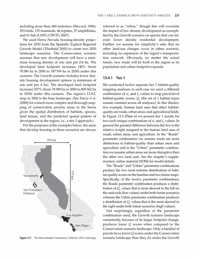
T IER 1 AND 2 EXAMPLES WITH SENSIT IV ITY ANALYSIS 237
including more than 400 endemics ( Shevock 1996 ); 293 birds, 135 mammals, 46 reptiles, 37 amphibians, and 61 fi sh (CDFG-CIWTG 2007).
We used Sierra Nevada housing-density projec-tions for 2030 from the Spatially Explicit Regional Growth Model ( Theobald 2005 ) to create two 2030 landscape scenarios. The Conservation scenario assumes that new development will have a mini-mum housing density of one unit per 0.6 ha. The developed land footprint increases 140% (from 78 389 ha in 2000 to 187 769 ha in 2030) under this scenario. The Growth scenario includes lower den-sity housing development options (a minimum of one unit per 4 ha). The developed land footprint increases 927% (from 78 389 ha in 2000 to 805 362 ha in 2030) under this scenario. The region’s LULC map in 2000 is the base landscape. (See Davis et al . ( 2006 ) for a much more complex and thorough map-ping of conservation priority areas in the Sierra given the spatial distribution of habitats, species, land tenure, and the predicted spatial pattern of development in the region, i.e., a tier 3 approach.)
For the purposes of the examples below, the areas that develop housing in these scenarios are always
referred to as “urban,” though this will overstate the impact of low density development as exempli-fi ed by the Growth scenario on species that can tol-erate lower density residential development. Further, we assume for simplicity’s sake that no other land-use changes occur in either scenario, including no expansion of the region’s transporta-tion network. Obviously, no matter the actual future, new roads will be built in the region as its population and urban footprint expands.
13.4.1 Tier 1
We conducted twelve separate tier 1 habitat-quality mapping analyses; in each case we used a different combination of w r and L j values to map parcel-level habitat-quality scores, Q x (the set of 1 habitat types remain constant across all analyses). In this illustra-tive example, human land uses that affect habitat-quality are roads, urban areas, and agricultural fi elds. In Figure 13.2 (Plate 6) we present tier 1 results for two such unique combinations of w r and L j values. In general the greatest difference between the two is the relative weight assigned to the human land uses of roads, urban areas, and agriculture. In the “Roads” parameter combination we assume roads are more deleterious to habitat-quality than urban areas and agriculture and in the “Urban” parameter combina-tion we assume urban areas are more disruptive then the other two land uses. See the chapter’s supple-mentary online material (SOM) for model details.
The “Roads” and “Urban” parameter combinations produce the two most extreme distributions of habi-tat-quality scores on the baseline and two future maps. Specifi cally, of the twelve parameter combinations, the Roads parameter combination produces a distri-bution of Q x values that is most skewed to the left on the unit scale (low values) under both future scenarios whereas the Urban parameter combination produces a distribution of Q x values that is the most skewed to the right under both future scenarios (high values).
Not surprisingly, regardless of the parameter combination used, the Growth scenario landscape consistently, because of its larger footprint change, produces lower Q scores when compared to the Conservation scenario landscape. Only a handful of parcels have lower Q scores under the Conservation scenario landscape than they do under the Growth
350 km
775 kmSacramento
San Francisco/Oakland
Los Angeles
San Diego
Figure 13.1 The Sierra Nevadas Conservancy, California, USA in dark gray.
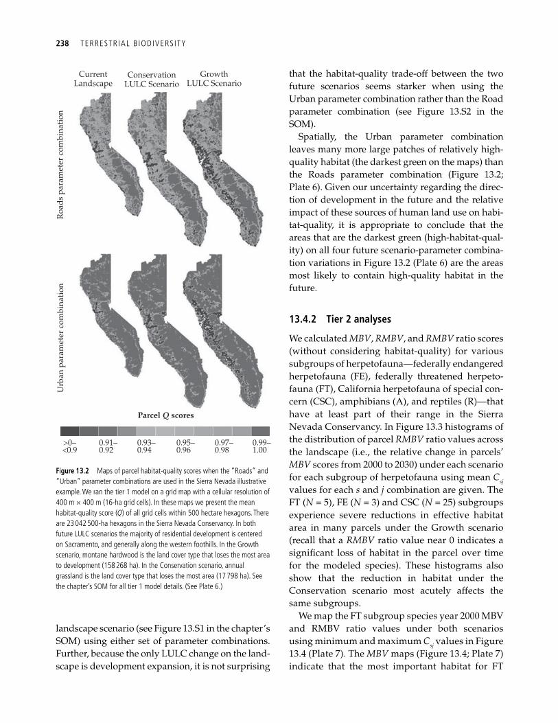
238 TERRESTRIAL B IODIVERSITY
landscape scenario (see Figure 13.S1 in the chapter’s SOM) using either set of parameter combinations. Further, because the only LULC change on the land-scape is development expansion, it is not surprising
that the habitat-quality trade-off between the two future scenarios seems starker when using the Urban parameter combination rather than the Road parameter combination (see Figure 13.S2 in the SOM).
Spatially, the Urban parameter combination leaves many more large patches of relatively high-quality habitat (the darkest green on the maps) than the Roads parameter combination ( Figure 13.2 ; Plate 6). Given our uncertainty regarding the direc-tion of development in the future and the relative impact of these sources of human land use on habi-tat-quality, it is appropriate to conclude that the areas that are the darkest green (high-habitat-qual-ity) on all four future scenario-parameter combina-tion variations in Figure 13.2 (Plate 6) are the areas most likely to contain high-quality habitat in the future.
13.4.2 Tier 2 analyses
We calculated MBV , RMBV , and RMBV ratio scores (without considering habitat-quality) for various subgroups of herpetofauna—federally endangered herpetofauna (FE), federally threatened herpeto-fauna (FT), California herpetofauna of special con-cern (CSC), amphibians (A), and reptiles (R)—that have at least part of their range in the Sierra Nevada Conservancy. In Figure 13.3 histograms of the distribution of parcel RMBV ratio values across the landscape (i.e., the relative change in parcels’ MBV scores from 2000 to 2030) under each scenario for each subgroup of herpetofauna using mean C sj values for each s and j combination are given. The FT ( N = 5), FE ( N = 3) and CSC ( N = 25) subgroups experience severe reductions in effective habitat area in many parcels under the Growth scenario (recall that a RMBV ratio value near 0 indicates a signifi cant loss of habitat in the parcel over time for the modeled species). These histograms also show that the reduction in habitat under the Conservation scenario most acutely affects the same subgroups.
We map the FT subgroup species year 2000 MBV and RMBV ratio values under both scenarios using minimum and maximum C sj values in Figure 13.4 (Plate 7). The MBV maps ( Figure 13.4 ; Plate 7) indicate that the most important habitat for FT
CurrentLandscape
>0–<0.9
0.91–0.92
0.93–0.94
0.95–0.96
0.97–0.98
0.99–1.00
Parcel Q scores
Roa
ds p
aram
eter
com
bina
tion
Urb
an p
aram
eter
com
bina
tion
ConservationLULC Scenario
GrowthLULC Scenario
Figure 13.2 Maps of parcel habitat-quality scores when the “Roads” and “Urban” parameter combinations are used in the Sierra Nevada illustrative example. We ran the tier 1 model on a grid map with a cellular resolution of 400 m × 400 m (16-ha grid cells). In these maps we present the mean habitat-quality score ( Q ) of all grid cells within 500 hectare hexagons. There are 23 042 500-ha hexagons in the Sierra Nevada Conservancy. In both future LULC scenarios the majority of residential development is centered on Sacramento, and generally along the western foothills. In the Growth scenario, montane hardwood is the land cover type that loses the most area to development (158 268 ha). In the Conservation scenario, annual grassland is the land cover type that loses the most area (17 798 ha). See the chapter’s SOM for all tier 1 model details. (See Plate 6.)
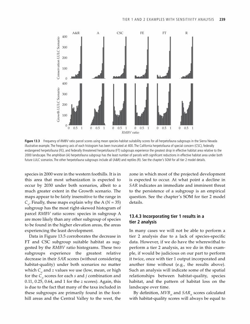
T IER 1 AND 2 EXAMPLES WITH SENSIT IV ITY ANALYSIS 239
species in 2000 were in the western foothills. It is in this area that most urbanization is expected to occur by 2030 under both scenarios, albeit to a much greater extent in the Growth scenario. The maps appear to be fairly insensitive to the range in C sj . Finally, these maps explain why the A ( N = 35) subgroup has the most right-skewed histogram of parcel RMBV ratio scores: species in subgroup A are more likely than any other subgroup of species to be found in the higher elevation areas, the areas experiencing the least development.
Data in Figure 13.5 corroborates the decrease in FT and CSC subgroup suitable habitat as sug-gested by the RMBV ratio histograms. These two subgroups experience the greatest relative decrease in their SAR scores (without considering habitat-quality) under both scenarios no matter which C sj and z values we use (low, mean, or high for the C sj scores for each s and j combination and 0.11, 0.25, 0.64, and 1 for the z scores). Again, this is due to the fact that many of the taxa included in these subgroups are primarily found in the foot-hill areas and the Central Valley to the west, the
zone in which most of the projected development is expected to occur. At what point a decline in SAR indicates an immediate and imminent threat to the persistence of a subgroup is an empirical question. See the chapter’s SOM for tier 2 model details.
13.4.3 Incorporating tier 1 results in a tier 2 analysis
In many cases we will not be able to perform a tier 2 analysis due to a lack of species-specifi c data. However, if we do have the wherewithal to perform a tier 2 analysis, as we do in this exam-ple, if would be judicious on our part to perform it twice, once with tier 1 output incorporated and another time without (e.g., the results above). Such an analysis will indicate some of the spatial relationships between habitat-quality, species habitat, and the pattern of habitat loss on the landscape over time.
By defi nition, MVB xt and SAR st scores calculated with habitat-quality scores will always be equal to
A&R400
300
200
100
0Con
serv
atio
n LU
LC S
cena
rio
400
300
200
100
00 0.5 1 0 0.5 1 0 0.5 1 0
RMBV ratio0.5 1 0 0.5 1 0 0.5 1
Gro
wth
LU
LC S
cena
rio
A CSC FE FT R
Figure 13.3 Frequency of RMBV ratio parcel scores using mean species-habitat suitability scores for all herpetofauna subgroups in the Sierra Nevada illustrative example. The frequency axis of each histogram has been truncated at 400. The California herpetofauna of special concern (CSC), federally endangered herpetofauna (FE), and federally threatened herpetofauna (FT) subgroups experience the greatest drop in effective habitat area relative to the 2000 landscape. The amphibian (A) herpetofauna subgroup has the least number of parcels with signifi cant reductions in effective habitat area under both future LULC scenarios. The other herpetofauna subgroups include all (A&R) and reptiles (R). See the chapter’s SOM for all tier 2 model details.
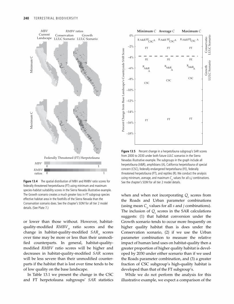
240 TERRESTRIAL B IODIVERSITY
or lower than those without. However, habitat-quality-modifi ed RMBV xt ratio scores and the change in habitat-quality-modifi ed SAR st scores over time may be more or less than their unmodi-fi ed counterparts. In general, habitat-quality- modifi ed RMBV ratio scores will be higher and decreases in habitat-quality-modifi ed SAR scores will be less severe than their unmodifi ed counter-parts if the habitat that is lost over time tends to be of low quality on the base landscape.
In Table 13.1 we present the change in the CSC and FT herpetofauna subgroups’ SAR statistics
when and when not incorporating Q x scores from the Roads and Urban parameter combinations (using mean C sj values for all s and j combinations). The inclusion of Q x scores in the SAR calculations suggests: (1) that habitat conversion under the Growth scenario tends to occur more frequently on higher quality habitat than is does under the Conservation scenario, (2) if we use the Urban parameter combination to measure the relative impact of human land uses on habitat-quality then a greater proportion of higher quality habitat is devel-oped by 2030 under either scenario than if we used the Roads parameter combination, and (3) a greater fraction of CSC subgroup’s high-quality habitat is developed than that of the FT subgroup’s.
While we do not perform the analysis for this illustrative example, we expect a comparison of the
MBVCurrent
Landscape
RMBV ratios
RMBVratios
MBV
ConservationLULC Scenario
Federally Threatened (FT) Herpetofauna
0
0
1
1
Min
imum
CM
axim
um C
GrowthLULC Scenario
Figure 13.4 The spatial distribution of MBV and RMBV ratio scores for federally threatened herpetofauna (FT) using minimum and maximum species-habitat suitability scores in the Sierra Nevada illustrative example. The Growth scenario creates a much greater loss in FT subgroup species effective habitat area in the foothills of the Sierra Nevada than the Conservation scenario does. See the chapter’s SOM for all tier 2 model details. (See Plate 7.)
R0%
–2%
–4%
–6%
–8%
–10%
–12%
–14%
–16%
–18%
RFE FE
FTFT
FE FE FE
CSCCSC
CSC
Perc
ent C
hang
e fr
om B
ase
Land
scap
e¢s
Cou
ntry
side
SA
R S
core
Con
serv
atio
LULC
Sce
nari
oG
row
thLU
LC S
cena
rio
FT
FTFT FT
CSCA CSCA CSC A A&R
R
AA&R
RA
A&RR
AA&R
A&R R FEA&R
Minimum C Maximum CAverage C
Figure 13.5 Percent change in a herpetofauna subgroup’s SAR scores from 2000 to 2030 under both future LULC scenarios in the Sierra Nevadas illustrative example. The subgroups in the graph include all herpetofauna (A&R), amphibians (A), California herpetofauna of special concern (CSC), federally endangered herpetofauna (FE), federally threatened herpetofauna (FT), and reptiles (R). We conduct the analysis using minimum, average, and maximum C sj values for all s , j combinations. See the chapter’s SOM for all tier 2 model details.

Table 13.1 Percent change in SAR statistic from
2000 to 2030 where z = 1
2030 LULC scenario Conservation
Growth
Q scores from tier 1 are not
included (%)
Q scores from the tier 1
“Roads” parameter
combination are included
(%)
Q scores from the tier 1
“Urban” parameter
combination are included
(%)
Q scores from tier 1 are not
included (%)
Q scores from the tier 1
“Roads” parameter
combination are included
(%)
Q scores from the tier 1
“Urban” parameter
combination are included
(%)
Herpetofauna subgroup
California herpetofauna of special concern (CSC)
−1.11 −0.88
−1.11 −8.26
−9.95 −10.14
Federally threatened herpetofauna (FT)
−2.35 −1.76
−2.15 −15.58
−17.91 −18.16
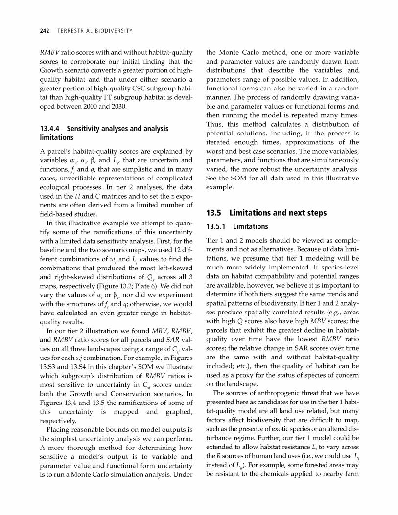
242 TERRESTRIAL B IODIVERSITY
RMBV ratio scores with and without habitat-quality scores to corroborate our initial fi nding that the Growth scenario converts a greater portion of high-quality habitat and that under either scenario a greater portion of high-quality CSC subgroup habi-tat than high-quality FT subgroup habitat is devel-oped between 2000 and 2030.
13.4.4 Sensitivity analyses and analysis limitations
A parcel’s habitat-quality scores are explained by variables w r , α r , β, and L j , that are uncertain and functions, f r and q , that are simplistic and in many cases, unverifi able representations of complicated ecological processes. In tier 2 analyses, the data used in the H and C matrices and to set the z expo-nents are often derived from a limited number of fi eld-based studies.
In this illustrative example we attempt to quan-tify some of the ramifi cations of this uncertainty with a limited data sensitivity analysis. First, for the baseline and the two scenario maps, we used 12 dif-ferent combinations of w r and L j values to fi nd the combinations that produced the most left-skewed and right-skewed distributions of Q x across all 3 maps, respectively ( Figure 13.2 ; Plate 6). We did not vary the values of α r or β xr nor did we experiment with the structures of f r and q ; otherwise, we would have calculated an even greater range in habitat-quality results.
In our tier 2 illustration we found MBV , RMBV , and RMBV ratio scores for all parcels and SAR val-ues on all three landscapes using a range of C sj val-ues for each s , j combination. For example, in Figures 13.S3 and 13.S4 in this chapter’s SOM we illustrate which subgroup’s distribution of RMBV ratios is most sensitive to uncertainty in C sj scores under both the Growth and Conservation scenarios. In Figures 13.4 and 13.5 the ramifi cations of some of this uncertainty is mapped and graphed, respectively.
Placing reasonable bounds on model outputs is the simplest uncertainty analysis we can perform. A more thorough method for determining how sensitive a model’s output is to variable and parameter value and functional form uncertainty is to run a Monte Carlo simulation analysis. Under
the Monte Carlo method, one or more variable and parameter values are randomly drawn from distributions that describe the variables and parameters range of possible values. In addition, functional forms can also be varied in a random manner. The process of randomly drawing varia-ble and parameter values or functional forms and then running the model is repeated many times. Thus, this method calculates a distribution of potential solutions, including, if the process is iterated enough times, approximations of the worst and best case scenarios. The more variables, parameters, and functions that are simultaneously varied, the more robust the uncertainty analysis. See the SOM for all data used in this illustrative example.
13.5 Limitations and next steps
13.5.1 Limitations
Tier 1 and 2 models should be viewed as comple-ments and not as alternatives. Because of data limi-tations, we presume that tier 1 modeling will be much more widely implemented. If species-level data on habitat compatibility and potential ranges are available, however, we believe it is important to determine if both tiers suggest the same trends and spatial patterns of biodiversity. If tier 1 and 2 analy-ses produce spatially correlated results (e.g., areas with high Q scores also have high MBV scores; the parcels that exhibit the greatest decline in habitat-quality over time have the lowest RMBV ratio scores; the relative change in SAR scores over time are the same with and without habitat-quality included; etc.), then the quality of habitat can be used as a proxy for the status of species of concern on the landscape.
The sources of anthropogenic threat that we have presented here as candidates for use in the tier 1 habi-tat-quality model are all land use related, but many factors affect biodiversity that are diffi cult to map, such as the presence of exotic species or an altered dis-turbance regime. Further, our tier 1 model could be extended to allow habitat resistance Lj to vary across the R sources of human land uses (i.e., we could use Lj instead of Ljr ). For example, some forested areas may be resistant to the chemicals applied to nearby farm
L IMITATIONS AND NEXT STEPS 243
fi elds but particularly affected by a nearby road’s pro-vision of easy access to gatherers of timber and non-timber forest products. In addition, the source of human land use and its ecological impact may be thousands of miles apart. This is most strikingly dem-onstrated by the pronounced effect of fertilizer use on farm fi elds of the upper Midwest US on water quality in the Gulf of Mexico. Such broad-scale impacts will not be characterized by our tier 1 model.
Integrating landscape structure and connectivity analyses in the tier 2 model would allow for more explicit population viability modeling (for examples of such modeling see Hanski and Ovaskainen 2000 ; Vos et al . 2001 , Schumaker et al . 2004 ). Other than the spatial relationship between potential range space and habitat type, the tier 2 biodiversity models pre-sented here do not consider how the spatial confi gu-ration of suitable habitat on a landscape may affect species. Further, the models do not consider the size of habitat patches or the ability of animals to move from patch to patch (see Polasky et al . 2005 ; Winfree et al . 2005 ; Nelson et al . 2008 ; Polasky et al . 2008 for examples of species conservation models that do consider species movement among patches). In addition, issues of minimum viable population size, population stochasticity, competition and other spe-cies interactions, are not addressed in our models.
By treating a landscape as an island surrounded by terra incognito we may under- or overestimate species status in the broader region. For example, a species with a small amount of suitable habitat in its potential range on the studied landscape will have a low SAR st score. However, if the spe-cies has effective habitat in a signifi cant portion of its potential range outside of the landscape in question then a low SAR score may not be indica-tive of the species’ overall status. On the other hand, a species can have a high SAR score in the studied landscape yet only have a small portion of its regional or global potential range space in suit-able habitat.
13.5.2 Next steps
All of the models presented in this chapter can be extended in fruitful ways. For example, the set of habitat types J and Lj values in a tier 1 analysis can be defi ned according to the habitat needs and suit-
abilities of some specifi c objective of biodiversity conservation; for example, a species guild that shares habitat or ecological roles. We would then be calculating guild-specifi c Q xj and Q x scores. For example, if mapping the habitat-quality of interior forest-dependent species, we would construct the set of habitat types J and Lj values according to their needs, suitabilities, and reaction to different sources of disturbance. Then a species MBV , RMBV , and RMBV ratio scores for these interior forest-depend-ent species, as well as the countryside SAR score for the entire landscape, could be modifi ed by Q xj or Q x scores that are more descriptive of the habitat limi-tations facing this particular guild.
Both tiers of the biodiversity model can be easily integrated with systematic conservation planning processes, such as ecoregional assessments or biodi-versity visions. The habitat-quality model in tier 1 could be used to ensure that the portfolio of selected sites includes those features with the highest quality. In addition, ecosystem service planning processes can use these models to calculate the biodiversity “costs” or trade-offs, if any exist at all, associated with LULC changes designed to enhance or conserve eco-system service provision where landscape-level bio-diversity costs are given by changes in SAR values and spatial biodiversity costs by RMBV ratio maps (e.g., Chan et al . 2006 ; Nelson et al . 2008 ). In compar-ing spatial patterns of biodiversity and ecosystem services we may identify areas where conservation investments can benefi t species and increase the sup-ply and value of ecosystem services ( Balvanera et al . 2001 ; Naidoo and Ricketts 2006 ; Turner et al . 2007 ).
Finally, the output from either tier could be used as input into a site-selection algorithm, such as Marxan, to design alternative conservation area networks ( Ball and Possingham 2000 ). For example, a conser-vation objective could be to fi nd LULC changes that increase as many RMBV ratio parcel scores, or alter-natively minimize the number of RMBV ratio parcel scores below 1, subject to some conservation budget constraint (see Nelson et al . 2008 for details on a opti-mization model that maximized the gain in SAR across a suite of species for a given conservation budget). Then, once a network of conservation areas is selected to meet targets, the habitat-quality model could be used to conduct a threats assessment on pro-posed or existing protected areas.
244 TERRESTRIAL B IODIVERSITY
References
Abbitt, R., and Scott, J. (2001). Examining differences between recovered and declining endangered species. Conservation Biology , 15 , 1274–84.
Ando, A., Camm, J., Polasky, S., et al . (1998). Species distri-butions, land values, and effi cient conservation. Science , 279 , 2126–8.
Ball, I., and Possingham, H. (2000). MARXAN (v1.8.2): Marine reserve design using spatially explicit annealing .
Balvanera, P., Daily, G., Ehrlich, P. et al . (2001). Conserving biodiversity and ecosystem services. Science, 291 , 2047.
California Department of Fish and Game. California Interagency Wildlife Task Group (CDFG-CIWTG). (2007). CWHR personal computer program .
Cardillo, M., Mace, G., Gittleman, J. et al . (2006). Latent extinction risk and the future battlegrounds of mammal conservation. Proceedings of the National Academy of Sciences, 103 , 4157–61.
Ceballos, G., Ehrlich, P., Soberon, J., et al . (2005). Global mammal conservation: What must we manage? Science, 309 , 603–7.
Chan, K., Shaw, M., Cameron, D., et al . (2006). Conservation planning for ecosystem services. Plos Biology, 4 , 2138–52.
Channell, R. and Lomolino, M. (2000). Dynamic biogeog-raphy and conservation of endangered species. Nature, 403 , 84–6.
Christy, J., Alverson, E., Dougherty, M., et al . (2000). Presettlement vegetation for the Willamette Valley, Oregon, version 4.0, compiled from records of the General Land Offi ce Surveyors ( c .1850) .
Daily, G., Ceballos, G., Pacheco, J., et al . (2003). Countryside biogeography of neotropical mammals. Conservation Biology, 17 , 1814–26.
Davis, F., Costello, C., and Stoms, D. (2006). Effi cient con-servation in a utility-maximization framework. Ecology and Society, 11, 33.
Diaz, S., Tilman, D., and Fargione, J. (2005). Biodiversity regulation of ecosystem services. In: R. Hassan, R. Scholes, and N. Ash, Eds., Ecosystems and human well-being: current state and trends. Island Press, Washington, DC, pp. 297–329.
Dirzo, R., and Raven, P. (2003). Global state of biodiversity and loss. Annual Review of Environment and Natural Resources , 28 , 137–67.
Ehrlich, P. R., and Ehrlich, A. H. (1982). Extinction . Ballantine, New York.
Forman, R., Sperling, D., Bissonette, J., et al . (2003). Road Ecology . Island Press, Washington, DC.
Groves, C. R., Jensen, D. B., Valutis, L. L., et al . (2002). Planning for biodiversity conservation. Bioscience , 52 , 499–512.
Hanski, I., and Ovaskainen, O. (2000). The metapopula-tion capacity of a fragmented landscape. Nature , 404 , 755–8.
Horner-Devine, M. C., Daily, G. C., Ehrlich, P. R., et al . (2003). Countryside biogeography of tropical butter-fl ies. Conservation Biology, 17 , 168–77.
Hughes, J. B., Daily, G. C., and Ehrlich, P. R. (1997). Population diversity: Its extent and extinction. Science , 278 , 689–92.
Leopold, A. (1949). Sand county almanac, and sketches here and there . Oxford University Press, New York.
MacArthur, R. H., and Wilson, E. O. (1967). The theory of island biogeography . Princeton University Press, Princeton, NJ.
Mann, C. C. (2005). 1491: new revelations of the Americas before Columbus. Vintage Books, New York.
Margules C. R., and Pressey, R. L. (2000). Systematic con-servation planning. Nature , 405 , 243–53.
Mayfi eld, M. M., and Daily, G. C. (2005). Countryside bio-geography of neotropical herbaceous and shrubby plants. Ecological Applications , 15 , 423–39.
Medellin, R. A., Equihua, M. and Amin, M. A. (2000). Bat diversity and abundance as indicators of disturbance in neotropical rainforests. Conservation Biology , 14 , 1666–75.
Naidoo, R., and Ricketts, T. H. (2006). Mapping eco-nomic costs and benefi ts of conservation. PLoS Biology, 4 , e360.
NatureServe. (2008). NatureServe Explorer: Ecological Communities and Sytems. Accessed at http://www.natureserve.org
Nelleman, C., Kullered, L., Vistnes, I., et al . (2001). GLOBIO. Global methodology for mapping human impacts on the biosphere. United Nations Environment Program (UNEP); Report UNEP/DEWA/TR.01–3.
Nelson, E., Polasky, S., Lewis, D., et al . (2008). Effi ciency of incentives to jointly increase carbon sequestration and species conservation on a landscape. Proceedings of the National Academy of Sciences . 105 , 9471–6.
Newmark, W. (1995). Extinction of mammal populations in western American national parks. Conservation Biology , 9 , 512–26.
Parks, S., and Harcourt, A. (2002). Reserve size, local human density, and mammalian extinctions in U.S. pro-tected areas. Conservation Biology , 16 , 800–8.
Pereira, H., and Daily, G. (2006). Modeling biodiversity dynamics in countryside landscapes. Ecology, 87 , 1877–85.
Pimm, S., and Brooks, T. (2000). The sixth extinction: How large, where, and when? In: T. Raven and P. H. Williams, Eds., Nature and human society , pp. 46–62. National Academy Press, Washington, DC.
L IMITATIONS AND NEXT STEPS 245
Polasky, S., Nelson, E., Lonsdorf, E., et al . (2005). Conserving species in a working landscape: land use with biological and economic objectives. Ecological Applications , 15 , 1387–1401.
Polasky, S., Nelson, E., Camm, J. et al . (2008). Where to put things? Spatial land management to sustain biodiver-sity and economic returns. Biological Conservation , 141 , 1505–24.
Purvis, A., Gittleman, J., Cowlishaw, G., et al . (2000). Predicting extinction risk in declining species. Proceedings of the Royal Society of London, Series B: Biological Sciences . 267 , 1947–52.
Ranganathan, J., Daniels, R., Chandran, S., et al . (2008). Sustaining biodiversity in ancient tropical countryside. Proceedings of the National Academy of Sciences , 105 , 17852–4.
Ricketts, T. (2004). Tropical forest fragments enhance pol-linator activity in nearby coffee crops. Conservation Biology , 18 , 1262–71.
Rondinini, C., Wilson, K., Boitani, L., et al . (2006). Tradeoffs of different types of species occurrence data for use in systematic conservation planning. Ecology Letters , 9 , 1136–45.
Rosenzweig, M. (1995). Species diversity in space and time. Cambridge University Press, Cambridge.
Sala, O., Vuuren, D. v., Pereira, H., et al . (2005). Biodiversity across scenarios. In: S. Carpenter, P. Pingali, E. Bennett, and M. Zurek, Eds., Ecosystems and human well-being , vol. 2: Scenarios , pp. 375–408. Island Press, Washington, DC.
Schill, S. and Raber, G. (2008). Protected Area Tools (PAT) for ArcGIS 9.2 (version 2.0) software.
Scholes, R. and Biggs, R. (2005). A biodiversity intactness index. Nature, 434 , 45–9.
Schumaker, N., Ernst, T., White, D., et al . (2004). Projecting wildlife responses to alternative future landscapes in Oregon’s Willamette Basin. Ecological Applications , 14 , 381–400.
Scott, J. M., Goble, D., and Davis, F. (2006). The Endangered Species Act at thirty: conserving biodiversity in
human-dominated landscapes , vols 1 and 2. Island Press, Washington, DC.
Sekercioglu, Ç., Daily, G., and Ehrlich, P. (2004). Ecosystem consequences of bird declines. Proceedings of the National Academy of Sciences, 101 , 18042–7.
Sekercioglu, Ç., Loarie, S., Brenes, F., et al . (2007). Persistence of forest birds in the Costa Rican agricul-tural countryside. Conservation Biology , 21 , 482–94.
Shevock, J. (1996). Status of rare and endemic plants. In: D. C. Erman, Ed., Sierra Nevada ecosystem project: fi nal report to Congress , vol. II, pp. 691–707. University of California—Davis, Centers for Water Centers for Water and Wildland Resources, Davis.
Stoms, D., Davis, F., and Cogan, C. (1992). Sensitivity of wild-life habitat models to uncertainties in GIS data. Photogrammetric Engineering and Remote Sensing , 58 , 843–50.
Theobald, D. (2005). Landscape patterns of exurban growth in the USA from 1980 to 2020. Ecology and Society , 10 , 32.
Turner, W., Brandon, K., Brooks, T., et al . (2007). Global conservation of biodiversity and ecosystem services. BioScience, 57 , 868–73.
Vos, C., Verboom, J., Opdam, P., et al . (2001). Toward eco-logically scaled landscape indices. American Naturalist , 157 , 24–41.
Williams, P. H., Gibbons, D., Margules, C., et al . (1996). A comparison of richness hotspots, rarity hotspots, and complementary areas for conserving diversity of British birds. Conservation Biology , 10 , 155–74.
Wilson, E. O. (1992). The diversity of life . Harvard University Press, Cambridge, MA.
Wilson, K., Underwood, E., Morrison, S., et al . (2007). Conserving biodiversity effi ciently: What to do, where, and when. PLoS Biology , 5 , e223.
Winfree, R., Dushoff, J., Crone, E., et al . (2005). Testing sim-ple indices of habitat proximity. American Naturalist , 165 , 707–17.
Worm B., Barbier, E., Beaumont, N. et al . (2006). Impacts of biodiversity loss on ocean ecosystem services. Science , 314 , 787–90.

This page intentionally left blank
SECTION III
Extensions, applications, and the next generation of ecosystem service assessments

This page intentionally left blank
249
CHAPTER 14
Putting ecosystem service models to work: conservation, management, and trade-offs Stephen Polasky, Giorgio Caldarone, T. Ka’eo Duarte, Joshua Goldstein, Neil Hannahs, Taylor Ricketts, and Heather Tallis
14.1 Introduction
Changing land use or land management affects the provision and value of a range of ecosystem services as well as biodiversity. The large number of poten-tially competing objectives can complicate decisions about landscape management. In rare cases the best choice among management alternatives will be obvi-ous because one alternative delivers higher levels of all ecosystem services and biodiversity compared to other alternatives (“win–win” solutions). In most cases, however, comparing among management alter-native requires evaluating trade-offs among various ecosystem services and biodiversity conservation.
The models described in this book generate pre-dictions about the provision of multiple ecosystem services and biodiversity for any given pattern of land use and management across a landscape. In this chapter we illustrate how one might use these pre-dictions collectively to analyze alternative conserva-tion and management strategies. By comparing maps of ecosystem services and biodiversity, managers can locate areas that, if managed correctly, can provide high levels of both. By comparing outcomes across different management alternatives, conservationists and managers can gain insight into which alterna-tives may be most desirable. Further, the analyses can be used to suggest and investigate new strategies that may improve results for key ecosystem services or biodiversity conservation objectives.
Trade-offs and potential win–win solutions are illustrated in Figure 14.1 , which shows a simple styl-
ized example for two ecosystem services, carbon sequestration and water quality, under four manage-ment alternatives (A, B, C, and D). For simplicity of the illustration, suppose that the cost of implement-ing each management is the same and that managers care only about water quality (measured on the verti-cal axis) and carbon sequestration (measured on the horizontal axis). Alternatives B and C are preferred to alternative A because both carbon sequestration and water quality scores are higher under these alter-natives. Choosing among B, C, or D (or between A and D), however, involves a trade-off with each alter-native providing more of one service and less of the other. Which of these alternatives (B, C, or D) will be preferred depends on the relative value of the two ecosystem services. If carbon sequestration is highly valued relative to water quality, then alternative D will be preferred to the other alternatives. As water quality increases suffi ciently in value relative to car-bon sequestration, alternative B or C will be the most preferred. Alternative A, however, will never be the most preferred option regardless of the value judg-ment about how to weight the value of carbon sequestration relative to water quality because it is dominated by other alternatives (B and C).
Here we describe four different approaches to analyzing conservation and management alterna-tives that illustrate potential application of models of the type described in this book. We start with an example that builds from conservation planning in which the planner chooses sites to include in a reserve network. We expand upon the traditional
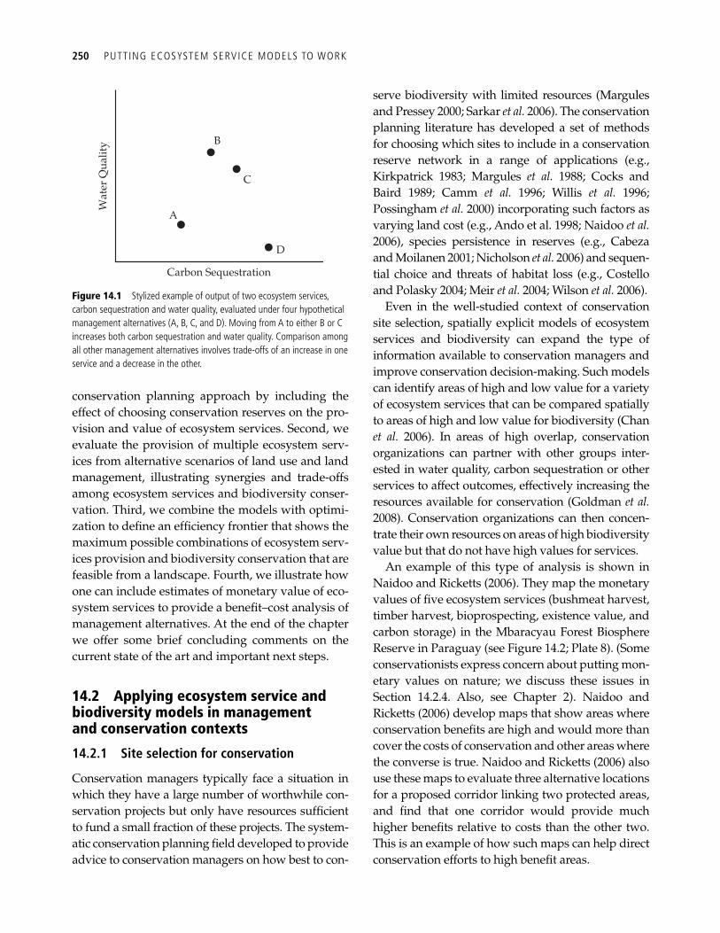
250 PUTTING ECOSYSTEM SERVICE MODELS TO WORK
conservation planning approach by including the effect of choosing conservation reserves on the pro-vision and value of ecosystem services. Second, we evaluate the provision of multiple ecosystem serv-ices from alternative scenarios of land use and land management, illustrating synergies and trade-offs among ecosystem services and biodiversity conser-vation. Third, we combine the models with optimi-zation to defi ne an effi ciency frontier that shows the maximum possible combinations of ecosystem serv-ices provision and biodiversity conservation that are feasible from a landscape. Fourth, we illustrate how one can include estimates of monetary value of eco-system services to provide a benefi t–cost analysis of management alternatives. At the end of the chapter we offer some brief concluding comments on the current state of the art and important next steps.
14.2 Applying ecosystem service and biodiversity models in management and conservation contexts
14.2.1 Site selection for conservation
Conservation managers typically face a situation in which they have a large number of worthwhile con-servation projects but only have resources suffi cient to fund a small fraction of these projects. The system-atic conservation planning fi eld developed to provide advice to conservation managers on how best to con-
serve biodiversity with limited resources ( Margules and Pressey 2000 ; Sarkar et al. 2006 ). The conservation planning literature has developed a set of methods for choosing which sites to include in a conservation reserve network in a range of applications (e.g., Kirkpatrick 1983 ; Margules et al. 1988 ; Cocks and Baird 1989 ; Camm et al. 1996 ; Willis et al. 1996 ; Possingham et al. 2000 ) incorporating such factors as varying land cost (e.g., Ando et al. 1998 ; Naidoo et al. 2006 ), species persistence in reserves (e.g., Cabeza and Moilanen 2001 ; Nicholson et al. 2006 ) and sequen-tial choice and threats of habitat loss (e.g., Costello and Polasky 2004 ; Meir et al. 2004 ; Wilson et al. 2006 ).
Even in the well-studied context of conservation site selection, spatially explicit models of ecosystem services and biodiversity can expand the type of information available to conservation managers and improve conservation decision-making. Such models can identify areas of high and low value for a variety of ecosystem services that can be compared spatially to areas of high and low value for biodiversity ( Chan et al. 2006 ). In areas of high overlap, conservation organizations can partner with other groups inter-ested in water quality, carbon sequestration or other services to affect outcomes, effectively increasing the resources available for conservation ( Goldman et al. 2008 ). Conservation organizations can then concen-trate their own resources on areas of high biodiversity value but that do not have high values for services.
An example of this type of analysis is shown in Naidoo and Ricketts ( 2006 ). They map the monetary values of fi ve ecosystem services (bushmeat harvest, timber harvest, bioprospecting, existence value, and carbon storage) in the Mbaracyau Forest Biosphere Reserve in Paraguay (see Figure 14.2 ; Plate 8). (Some conservationists express concern about putting mon-etary values on nature; we discuss these issues in Section 14.2.4 . Also, see Chapter 2 ). Naidoo and Ricketts ( 2006 ) develop maps that show areas where conservation benefi ts are high and would more than cover the costs of conservation and other areas where the converse is true. Naidoo and Ricketts ( 2006 ) also use these maps to evaluate three alternative locations for a proposed corridor linking two protected areas, and fi nd that one corridor would provide much higher benefi ts relative to costs than the other two. This is an example of how such maps can help direct conservation efforts to high benefi t areas.
B
C
A
D
Carbon Sequestration
Wat
er Q
ualit
y
Figure 14.1 Stylized example of output of two ecosystem services, carbon sequestration and water quality, evaluated under four hypothetical management alternatives (A, B, C, and D). Moving from A to either B or C increases both carbon sequestration and water quality. Comparison among all other management alternatives involves trade-offs of an increase in one service and a decrease in the other.
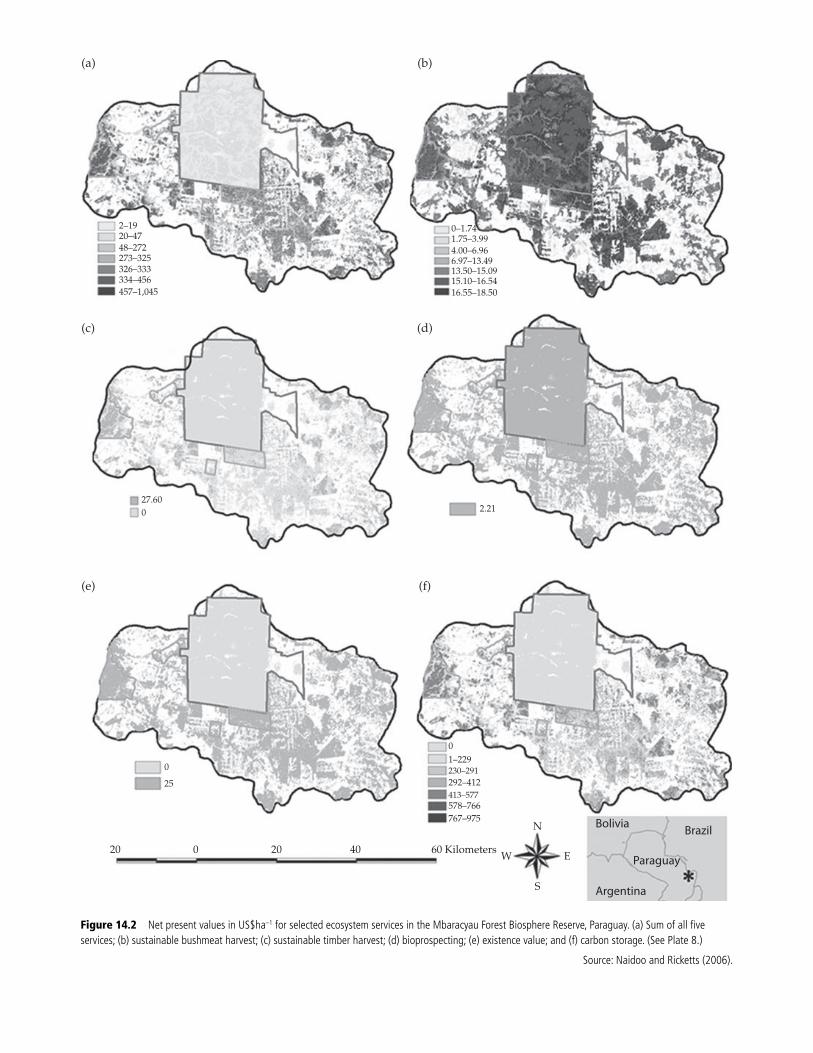
2–1920–4748–272273–325326–333334–456457–1,045
27.60
(e) (f)
(c) (d)
(a) (b)
2.21
01–229230–291292–412413–577578–766767–975
60 Kilometers4020020
25
0
W E
S
N Bolivia
Argentina
Brazil
Paraguay
0
0–1.741.75–3.994.00–6.966.97–13.4913.50–15.0915.10–16.5416.55–18.50
Figure 14.2 Net present values in US$ha –1 for selected ecosystem services in the Mbaracyau Forest Biosphere Reserve, Paraguay. (a) Sum of all fi ve services; (b) sustainable bushmeat harvest; (c) sustainable timber harvest; (d) bioprospecting; (e) existence value; and (f) carbon storage. (See Plate 8.)
Source: Naidoo and Ricketts ( 2006 ).
252 PUTTING ECOSYSTEM SERVICE MODELS TO WORK
In some cases, particularly in cases involving the protection of municipal drinking water supply (e.g., Bogota, New York City, Quito), the value of ecosys-tem services is high enough to choose management decisions that also support conservation ( Chichilnisky and Heal 1998 ; NRC 2000; Echevarrıa 2002 ). In such cases, payments for ecosystem serv-ices can be more than suffi cient and there is little or no need for a conservation organization to spend their scarce resources to accomplish conservation objectives. In other cases, promoting the provision of ecosystem services may align with conservation, but the services themselves may not be valuable enough to tip the balance toward biodiversity-friendly management. In this case, conservation organizations can usefully partner with other groups interested in the provision of ecosystem services. Finally, there will be other cases where management for ecosystem services does not align with conservation objectives. In these cases, conser-vation organizations will be on their own, just as they would be with no consideration of ecosystem services.
Spatially explicit information on ecosystem serv-ices can also be integrated with conservation plan-ning exercises in other ways. For example, if ecosystem services are valued in monetary terms, the cost of including a particular site could be reduced by the increase in value of ecosystem serv-ices provided if the site is chosen as a reserve. Doing so would shift conservation priorities toward sites that generate valuable ecosystem services in a fash-ion similar to priority given to inexpensive sites. It is also possible to require that targets could be spec-ifi ed for certain ecosystem services and only reserve networks that met these targets would be consid-ered as potential solutions in the conservation plan-ning exercise.
Using spatially explicit models that incorporate both ecosystem services and biodiversity is power-ful because conservation decisions are often inher-ently spatial: Where to protect? How much area is needed? Where to allow development? In this way, adding maps of ecosystem services broadens an existing approach to conservation planning that is used and understood by many conservation practi-tioners ( Groves 2003 ). Using spatially explicit mod-els of ecosystem services expands the set of
outcomes considered in planning beyond biodiver-sity conservation targets. Doing so can show areas on the landscape that are of high priority for conser-vation targets and various ecosystem services.
The main disadvantage of using spatially explicit models in this manner is that results do not neces-sarily indicate how the landscape should be man-aged. Management to promote a particular ecosystem service might differ from management to promote another service or biodiversity conser-vation. For example, carbon sequestration may be maximized by planting trees but this may decrease surface water runoff and reduce availability for downstream users ( Jackson et al . 2005 ). In classic conservation site selection the management choice is simple—either protect a site or don’t—and a pro-tected site is assumed to benefi t all species. With the inclusion of ecosystem services, however, the choice of management options is of greater interest and complexity. When different management options at the same spatial location are best for different objec-tives just highlighting high priority areas on the landscape is not enough. What is needed in this case is an analysis that shows outcomes for ecosys-tem services and biodiversity under different types of management.
14.2.2 Analysis of management alternatives
The spatially explicit models defi ned in earlier chap-ters are designed to evaluate multiple ecosystem services and biodiversity objectives under alternative conservation or management plans. In this section we highlight the use of these models to analyze the effect of alternative land-use plans on the provision of eco-system services and biodiversity conservation. The fi rst case study involves evaluating alternative future scenarios for land use in the Willamette Basin in Oregon. The second case study involves evaluating alternative land uses for a watershed owned by Kamehameha Schools on O`ahu, Hawai`i.
14.2.2.1 Alternative future scenarios in the Willamette Basin, Oregon Nelson et al. ( 2009 ) applied several of the spatially explicit models described in previous chapters, or their precursors. These models were used to predict changes in ecosystem services and conservation of
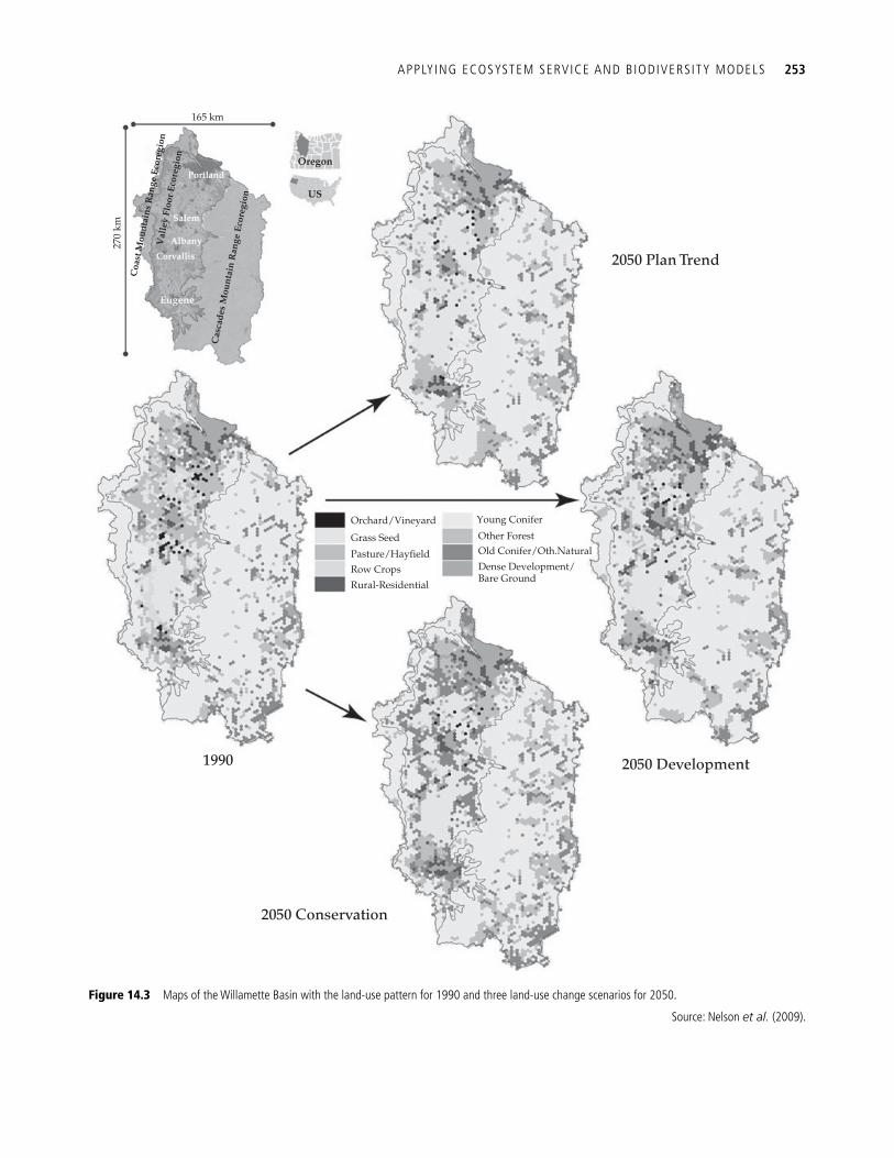
APPLYING ECOSYSTEM SERVICE AND BIODIVERSITY MODELS 253
Orchard/Vineyard
Grass Seed
Pasture/HayfieldRow CropsRural-Residential
Young Conifer
Other ForestOld Conifer/Oth.NaturalDense Development/ Bare Ground
Oregon
US
2050 Plan Trend
2050 Development1990
2050 Conservation
Portland
Salem
Albany
Corvallis
Eugene
Coa
st M
ount
ains
Ran
ge E
core
gion
Val
ley
Floo
r Ec
oreg
ion
Cas
cade
s M
ount
ain
Ran
ge E
core
gion
270
km165 km
Figure 14.3 Maps of the Willamette Basin with the land-use pattern for 1990 and three land-use change scenarios for 2050.
Source: Nelson et al. ( 2009 ).
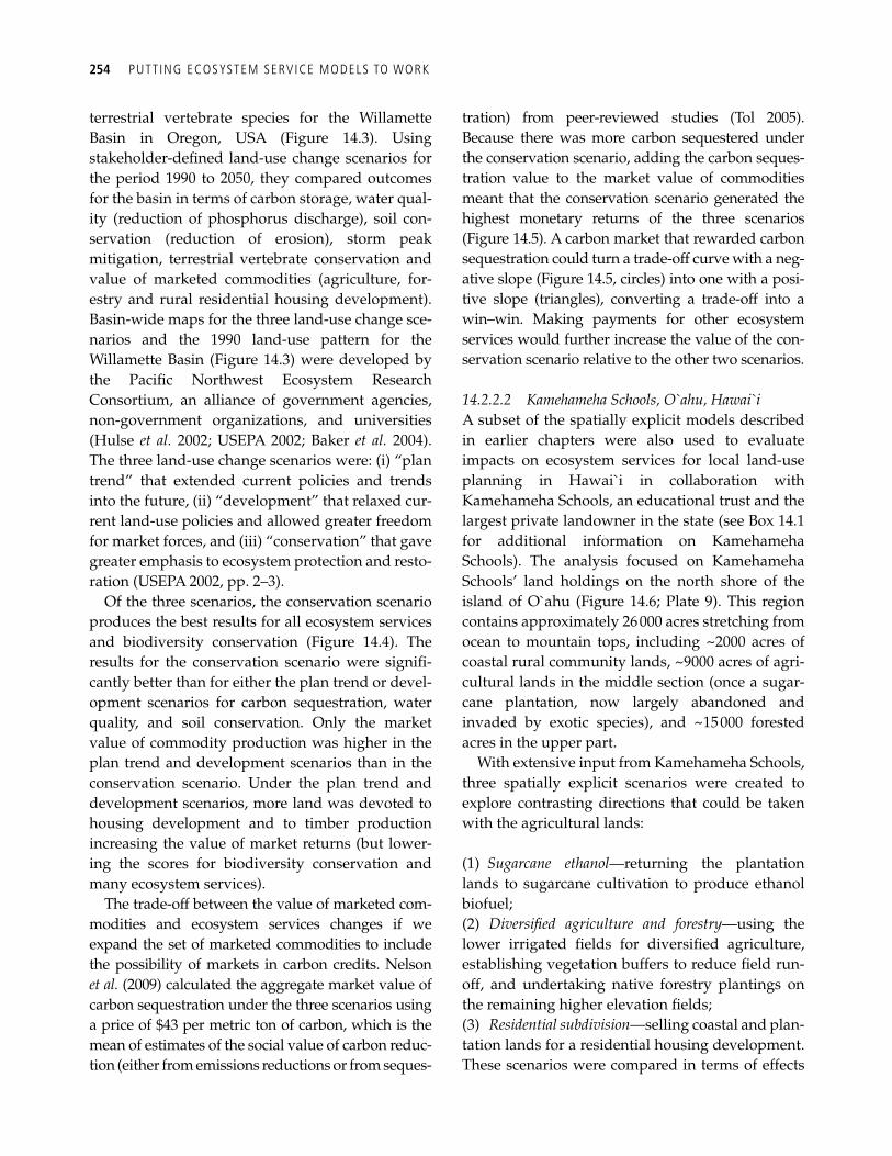
254 PUTTING ECOSYSTEM SERVICE MODELS TO WORK
terrestrial vertebrate species for the Willamette Basin in Oregon, USA ( Figure 14.3 ). Using stakeholder-defi ned land-use change scenarios for the period 1990 to 2050, they compared outcomes for the basin in terms of carbon storage, water qual-ity (reduction of phosphorus discharge), soil con-servation (reduction of erosion), storm peak mitigation, terrestrial vertebrate conservation and value of marketed commodities (agriculture, for-estry and rural residential housing development). Basin-wide maps for the three land-use change sce-narios and the 1990 land-use pattern for the Willamette Basin ( Figure 14.3 ) were developed by the Pacifi c Northwest Ecosystem Research Consortium, an alliance of government agencies, non-government organizations, and universities ( Hulse et al. 2002 ; USEPA 2002; Baker et al. 2004 ). The three land-use change scenarios were: (i) “plan trend” that extended current policies and trends into the future, (ii) “development” that relaxed cur-rent land-use policies and allowed greater freedom for market forces, and (iii) “conservation” that gave greater emphasis to ecosystem protection and resto-ration (USEPA 2002, pp. 2–3).
Of the three scenarios, the conservation scenario produces the best results for all ecosystem services and biodiversity conservation ( Figure 14.4 ). The results for the conservation scenario were signifi -cantly better than for either the plan trend or devel-opment scenarios for carbon sequestration, water quality, and soil conservation. Only the market value of commodity production was higher in the plan trend and development scenarios than in the conservation scenario. Under the plan trend and development scenarios, more land was devoted to housing development and to timber production increasing the value of market returns (but lower-ing the scores for biodiversity conservation and many ecosystem services).
The trade-off between the value of marketed com-modities and ecosystem services changes if we expand the set of marketed commodities to include the possibility of markets in carbon credits. Nelson et al. ( 2009 ) calculated the aggregate market value of carbon sequestration under the three scenarios using a price of $43 per metric ton of carbon, which is the mean of estimates of the social value of carbon reduc-tion (either from emissions reductions or from seques-
tration) from peer-reviewed studies ( Tol 2005 ). Because there was more carbon sequestered under the conservation scenario, adding the carbon seques-tration value to the market value of commodities meant that the conservation scenario generated the highest monetary returns of the three scenarios ( Figure 14.5 ). A carbon market that rewarded carbon sequestration could turn a trade-off curve with a neg-ative slope ( Figure 14.5 , circles) into one with a posi-tive slope (triangles), converting a trade-off into a win–win. Making payments for other ecosystem services would further increase the value of the con-servation scenario relative to the other two scenarios.
14.2.2.2 Kamehameha Schools, O ahu, Hawai`i A subset of the spatially explicit models described in earlier chapters were also used to evaluate impacts on ecosystem services for local land-use planning in Hawai`i in collaboration with Kamehameha Schools, an educational trust and the largest private landowner in the state (see Box 14.1 for additional information on Kamehameha Schools). The analysis focused on Kamehameha Schools’ land holdings on the north shore of the island of O`ahu ( Figure 14.6 ; Plate 9). This region contains approximately 26 000 acres stretching from ocean to mountain tops, including ~2000 acres of coastal rural community lands, ~9000 acres of agri-cultural lands in the middle section (once a sugar-cane plantation, now largely abandoned and invaded by exotic species), and ~15 000 forested acres in the upper part.
With extensive input from Kamehameha Schools, three spatially explicit scenarios were created to explore contrasting directions that could be taken with the agricultural lands:
(1) Sugarcane ethanol —returning the plantation lands to sugarcane cultivation to produce ethanol biofuel; (2) Diversifi ed agriculture and forestry —using the lower irrigated fi elds for diversifi ed agriculture, establishing vegetation buffers to reduce fi eld run-off, and undertaking native forestry plantings on the remaining higher elevation fi elds; (3) Residential subdivision —selling coastal and plan-tation lands for a residential housing development. These scenarios were compared in terms of effects
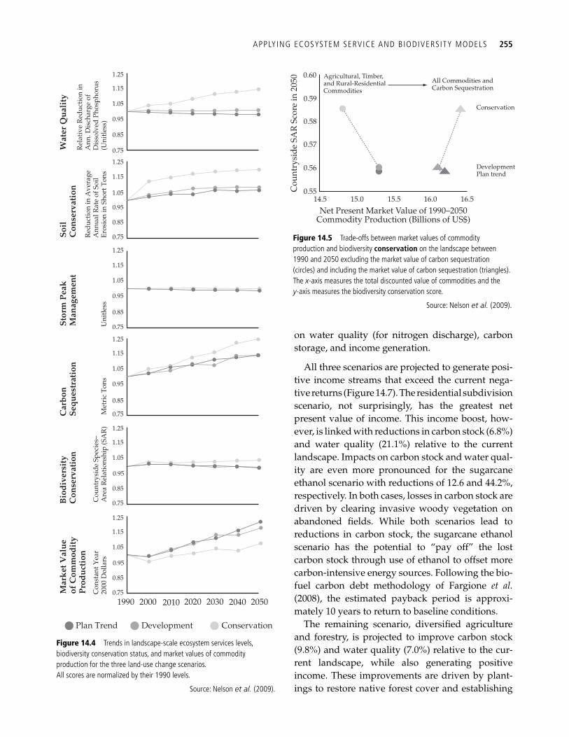
on water quality (for nitrogen discharge), carbon storage, and income generation.
All three scenarios are projected to generate posi-tive income streams that exceed the current nega-tive returns ( Figure 14.7 ). The residential subdivision scenario, not surprisingly, has the greatest net present value of income. This income boost, how-ever, is linked with reductions in carbon stock (6.8%) and water quality (21.1%) relative to the current landscape. Impacts on carbon stock and water qual-ity are even more pronounced for the sugarcane ethanol scenario with reductions of 12.6 and 44.2%, respectively. In both cases, losses in carbon stock are driven by clearing invasive woody vegetation on abandoned fi elds. While both scenarios lead to reductions in carbon stock, the sugarcane ethanol scenario has the potential to “pay off” the lost carbon stock through use of ethanol to offset more carbon-intensive energy sources. Following the bio-fuel carbon debt methodology of Fargione et al. ( 2008 ), the estimated payback period is approxi-mately 10 years to return to baseline conditions.
The remaining scenario, diversifi ed agriculture and forestry, is projected to improve carbon stock (9.8%) and water quality (7.0%) relative to the cur-rent landscape, while also generating positive income. These improvements are driven by plant-ings to restore native forest cover and establishing
1.25
1.15
1.05
0.95
0.85
Rel
ativ
e R
educ
tion
inA
nn. D
isch
arge
of
Dis
solv
ed P
hosp
horu
s(U
nitle
ss)
Wat
er Q
uali
ty
0.75
1.25
1.15
1.05
0.95
0.85
Red
uctio
n in
Ave
rage
Ann
ual R
ate
of S
oil
Eros
ion
in S
hort
Ton
s
Soil
Con
serv
atio
n
0.75
1.25
1.15
1.05
0.95
0.85
Uni
tless
Met
ric
Tons
Cou
ntry
side
Spe
cies
–A
rea
Rel
atio
nshi
p (S
AR
)C
onst
ant Y
ear
2000
Dol
lars
Stor
m P
eak
Man
agem
ent
Car
bon
Sequ
estr
atio
nB
iodi
vers
ity
Con
serv
atio
nM
arke
t Val
ueof
Com
mod
ity
Prod
ucti
on
0.75
1.25
1.15
1.05
0.95
0.85
0.75
1.25
1.15
1.05
0.95
0.85
0.75
1.25
1.15
1.05
0.95
0.85
0.751990
Plan Trend Development Conservation
2000 2010 2020 2030 2040 2050
Figure 14.4 Trends in landscape-scale ecosystem services levels, biodiversity conservation status, and market values of commodity production for the three land-use change scenarios. All scores are normalized by their 1990 levels.
Source: Nelson et al. ( 2009 ).
APPLYING ECOSYSTEM SERVICE AND BIODIVERSITY MODELS 255
0.60
0.59
0.58
0.57
0.5514.5 15.0
DevelopmentPlan trend
Conservation
All Commodities andCarbon Sequestration
Agricultural, Timber,and Rural-ResidentialCommodities
15.5Net Present Market Value of 1990–2050
Commodity Production (Billions of US$)
Cou
ntry
side
SA
R S
core
in 2
050
16.0 16.5
0.56
Figure 14.5 Trade-offs between market values of commodity production and biodiversity conservation on the landscape between 1990 and 2050 excluding the market value of carbon sequestration (circles) and including the market value of carbon sequestration (triangles). The x -axis measures the total discounted value of commodities and the y -axis measures the biodiversity conservation score.
Source: Nelson et al. ( 2009 ).
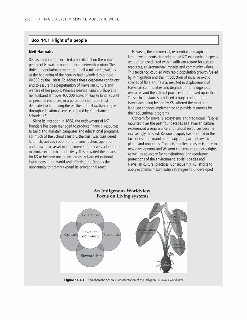
256 PUTTING ECOSYSTEM SERVICE MODELS TO WORK
Box 14.1 Plight of a people
Neil Hannahs
Disease and change exacted a horrifi c toll on the native people of Hawaii throughout the nineteenth century. The thriving population of more than half a million Hawaiians at the beginning of the century had dwindled to a mere 40 000 by the 1880s. To address these desperate conditions and to assure the perpetuation of Hawaiian culture and welfare of her people, Princess Bernice Pauahi Bishop and her husband left over 400 000 acres of Hawaii land, as well as personal resources, in a perpetual charitable trust dedicated to improving the wellbeing of Hawaiian people through educational services offered by Kamehameha Schools (KS).
Since its inception in 1884, the endowment of KS’ founders has been managed to produce fi nancial resources to build and maintain campuses and educational programs. For much of the School’s history, the trust was considered land rich, but cash poor. To fund construction, operation and growth, an asset management strategy was adopted to maximize economic productivity. This provided the means for KS to become one of the largest private educational institutions in the world and afforded the Schools the opportunity to greatly expand its educational reach.
However, the commercial, residential, and agricultural land developments that brightened KS’ economic prospects were often conducted with insuffi cient regard for cultural resources, environmental impacts and community values. This tendency, coupled with rapid population growth fueled by in-migration and the introduction of invasive exotic species of fl ora and fauna, resulted in displacement of Hawaiian communities and degradation of indigenous resources and the cultural practices that thrived upon them. These circumstances produced a tragic conundrum: Hawaiians being helped by KS suffered the most from land-use changes implemented to provide resources for their educational programs.
Concern for Hawaii’s ecosystems and traditional lifestyles mounted over the past four decades as Hawaiian culture experienced a renaissance and natural resources became increasingly stressed. Resource supply has declined in the face of rising demand and ravaging impacts of invasive plants and ungulates. Confl icts manifested as resistance to new development and Western concepts of property rights, as well as advocacy for constitutional and regulatory protections of the environment, at-risk species and Hawaiian cultural practices. Consequently, KS’ efforts to apply economic maximization strategies to undeveloped
Education
An Indigenous Worldview:Focus on Living systems
HawaiianCommunityCulture Economics
Ho‘oulu KaiauluCommunity
Ho‘ona’auaoEducation
EaCulture
WaiwaiEconomics
MalamaAina
Environment
MauliWellBeing
Stewardship
¯
¯¯
Figure 14.A.1 Kamehameha Schools’ representation of the indigenous Hawai’i worldview.
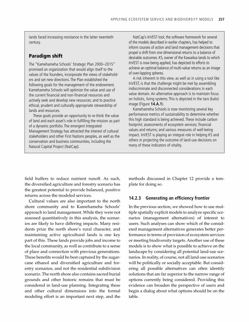
fi eld buffers to reduce nutrient runoff. As such, the diversifi ed agriculture and forestry scenario has the greatest potential to provide balanced, positive returns across the modeled services.
Cultural values are also important to the north shore community and to Kamehameha Schools’ approach to land management. While they were not assessed quantitatively in this analysis, the scenar-ios are likely to have differing impacts. Many resi-dents prize the north shore’s rural character, and maintaining active agricultural lands is one key part of this. These lands provide jobs and income to the local community, as well as contribute to a sense of place and connection with previous generations. These benefi ts would be best captured by the sugar-cane ethanol and diversifi ed agriculture and for-estry scenarios, and not the residential subdivision scenario. The north shore also contains sacred burial grounds and other historic remains that must be considered in land-use planning. Integrating these and other cultural dimensions into the formal modeling effort is an important next step, and the
methods discussed in Chapter 12 provide a tem-plate for doing so.
14.2.3 Generating an effi ciency frontier
In the previous section, we showed how to use mul-tiple spatially explicit models to analyze specifi c sce-narios (management alternatives) of interest to users. Such analyses can show which of the consid-ered management alternatives generates better per-formance in terms of provision of ecosystem services or meeting biodiversity targets. Another use of these models is to show what is possible to achieve on the landscape by considering all potential land-use sce-narios. In reality, of course, not all land-use scenarios will be politically or socially acceptable. But consid-ering all possible alternatives can often identify solutions that are far superior to the narrow range of options currently being considered. Providing this evidence can broaden the perspective of users and begin a dialog about what options should be on the table.
APPLYING ECOSYSTEM SERVICE AND BIODIVERSITY MODELS 257
lands faced increasing resistance in the latter twentieth century.
Paradigm shift The “Kamehameha Schools’ Strategic Plan 2000–2015” promised an organization that would align itself to the values of the founders, incorporate the views of stakehold-ers and set new directions. The Plan established the following goals for the management of the endowment. Kamehameha Schools will optimize the value and use of the current fi nancial and non-fi nancial resources and actively seek and develop new resources; and to practice ethical, prudent and culturally appropriate stewardship of lands and resources.
These goals provide an opportunity to re-think the value of land and each asset’s role in fulfi lling the mission as part of a dynamic portfolio. The emergent Integrated Management Strategy has attracted the interest of cultural stakeholders and other First Nations peoples, as well as the conservation and business communities, including the Natural Capital Project (NatCap).
NatCap’s InVEST tool, the software framework for several of the models described in earlier chapters, has helped to inform courses of action and land management decisions that propel a shift from one dimensional returns to a balance of desirable outcomes. KS, owner of the Kawailoa lands to which InVEST is now being applied, has depicted its efforts to achieve an optimal balance of multi-value returns as an image of over-lapping spheres.
A risk inherent in this view, as well as in using a tool like InVEST, is that the challenge might be met by assembling indiscriminate and disconnected considerations in each value domain. An alternative approach is to maintain focus on holistic, living systems. This is depicted in the taro (kalo) image (Figure 14.A.1 ).
Kamehameha Schools is now monitoring several key performance metrics of sustainability to determine whether this high standard is being achieved. These include carbon footprint; assessments of ecosystem services; fi nancial values and returns; and various measures of well-being impact. InVEST is playing an integral role in helping KS and others in projecting the outcome of land-use decisions on many of these indicators of vitality.
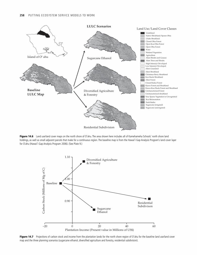
258 PUTTING ECOSYSTEM SERVICE MODELS TO WORK
Undefined
Land Use/Land Cover Classes
Native Shrubland/Sparse Ohia
Uluhe ShrublandClosed Ohia ForestOpen Koa-Ohia ForestOpen Ohia ForestWater
Wetland VegetationAgriculture
Alien Trees and Shrubs
High Intensiyt DevelopedLow Intensiyt DevelopedAlien Grassland
Alien Shrubland
Alien Forest
Closed Kukui ForestKiawe Forest and ShrublandKiawe-Koa Haole Forest and ShrublandUncharacterized ForestUncharacterized shrubland
Very Sparse Vegetation to UnvegetatedKoa ReforestationField BufferSugarcane (irrigated)Sugarcane (unirrigated)
Christmas Berry ShrublandKoa Haole Shrubland
Alien Shrubs and GrassesSugarcane EthanolIsland of O¢ ahu
Diversified Agriculture& Forestry
Residential Subdivision
BaselineLULC Map
LULC Scenarios
Figure 14.6 Land use/land cover maps on the north shore of O’ahu. The area shown here includes all of Kamehameha Schools’ north shore land holdings, as well as small adjacent parcels that make for a continuous region. The baseline map is from the Hawai’i Gap Analysis Program’s land cover layer for O`ahu ( Hawai’i Gap Analysis Program 2006 ). (See Plate 9.)
1.10
1.00
Diversified Agriculture& Forestry
0.90
–20
Baseline
Car
bon
Stoc
k (M
illio
ns o
f Mg
of C
)
SugarcaneEthanol
ResidentialSubdivison
0 20Plantation Income (Present value in Millions of US$)
40 60
Figure 14.7 Projections of carbon stock and income from the plantation lands for the north shore region of O’ahu for the baseline land use/land cover map and the three planning scenarios (sugarcane ethanol, diversifi ed agriculture and forestry, residential subdivision).
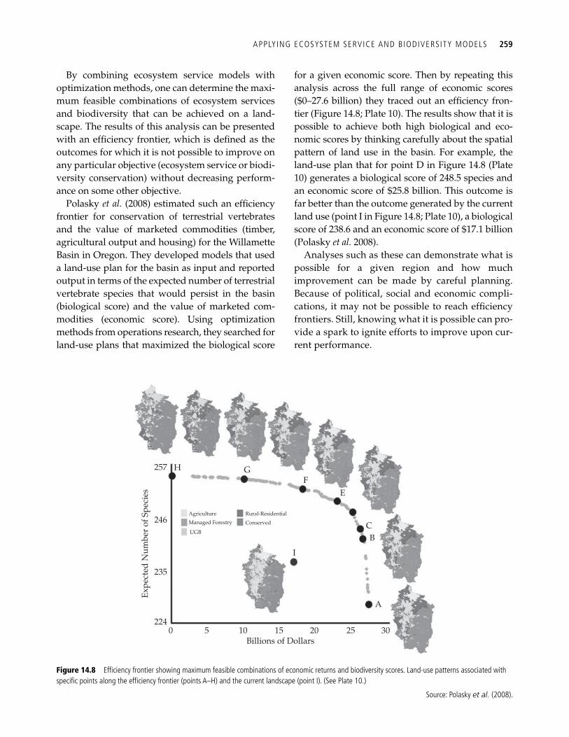
By combining ecosystem service models with optimization methods, one can determine the maxi-mum feasible combinations of ecosystem services and biodiversity that can be achieved on a land-scape. The results of this analysis can be presented with an effi ciency frontier, which is defi ned as the outcomes for which it is not possible to improve on any particular objective (ecosystem service or biodi-versity conservation) without decreasing perform-ance on some other objective.
Polasky et al. ( 2008 ) estimated such an effi ciency frontier for conservation of terrestrial vertebrates and the value of marketed commodities (timber, agricultural output and housing) for the Willamette Basin in Oregon. They developed models that used a land-use plan for the basin as input and reported output in terms of the expected number of terrestrial vertebrate species that would persist in the basin (biological score) and the value of marketed com-modities (economic score). Using optimization methods from operations research, they searched for land-use plans that maximized the biological score
for a given economic score. Then by repeating this analysis across the full range of economic scores ($0–27.6 billion) they traced out an effi ciency fron-tier ( Figure 14.8 ; Plate 10). The results show that it is possible to achieve both high biological and eco-nomic scores by thinking carefully about the spatial pattern of land use in the basin. For example, the land-use plan that for point D in Figure 14.8 (Plate 10) generates a biological score of 248.5 species and an economic score of $25.8 billion. This outcome is far better than the outcome generated by the current land use (point I in Figure 14.8 ; Plate 10), a biological score of 238.6 and an economic score of $17.1 billion ( Polasky et al. 2008 ).
Analyses such as these can demonstrate what is possible for a given region and how much improvement can be made by careful planning. Because of political, social and economic compli-cations, it may not be possible to reach effi ciency frontiers. Still, knowing what it is possible can pro-vide a spark to ignite efforts to improve upon cur-rent performance.
APPLYING ECOSYSTEM SERVICE AND BIODIVERSITY MODELS 259
257 H
Agriculture
Managed Forestry
UGB
Rural-Residential
Conserved
GF
E
CB
A
I
246
235
2240 5 10 15
Billions of Dollars
Expe
cted
Num
ber
of S
peci
es
20 25 30
Figure 14.8 Effi ciency frontier showing maximum feasible combinations of economic returns and biodiversity scores. Land-use patterns associated with specifi c points along the effi ciency frontier (points A–H) and the current landscape (point I). (See Plate 10.)
Source: Polasky et al. ( 2008 ).
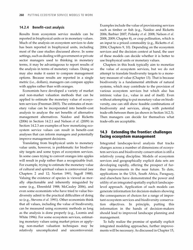
260 PUTTING ECOSYSTEM SERVICE MODELS TO WORK
14.2.4 Benefi t–cost analysis
Results from ecosystem service models can be reported in biophysical units or in monetary values. Much of the analysis on ecosystem services to date has been reported in biophysical units, including most of the case studies discussed above. In some settings, such as dealing with government or private sector managers used to thinking in monetary terms, it may be advantageous to report results of the analysis in terms of monetary values. Doing so may also make it easier to compare management options. Because results are reported in a single metric (i.e., dollars), managers can compare apples with apples rather than with oranges.
Economists have developed a variety of market and non-market valuation methods that can be applied to estimate the monetary value of ecosys-tem services ( Freeman 2003 ). The estimates of mon-etary value can be incorporated into benefi t–cost analysis to analyze the net benefi ts of alternative management alternatives. Naidoo and Ricketts ( 2006 ) in Section 14.2.1 and Nelson et al. ( 2009 ) in Section 14.2.3 are examples of how monetizing eco-system service values can result in benefi t–cost analyses that can inform managers and potentially improve management decisions.
Translating from biophysical units to monetary value units, however, is problematic for biodiver-sity targets and some types of ecosystem services. In some cases trying to convert oranges into apples will result in pulp rather than a recognizable fruit. For example, trying to estimate the monetary value of cultural and spiritual values is controversial (see Chapters 2 and 12 ; Norton 1991 ; Sagoff 1988 ). Valuing the existence of species is viewed as mor-ally objectionable and inherently misguided by some (e.g., Ehrenfeld 1988 ; McCauley 2006 ), and even some economists who have tried to value bio-diversity admit to the practical diffi culties of doing so (e.g., Stevens et al. 1991 ). Other economists think that all values, including the value of biodiversity, can be measured using economic methods as long as the analysis is done properly (e.g., Loomis and White 1996 ). For some ecosystem services, estimat-ing monetary values using market prices or apply-ing non-market valuation techniques may be relatively uncomplicated and uncontroversial.
Examples include the value of provisioning services such as timber or fi sh (e.g., Naidoo and Ricketts 2006 ; Barbier 2007 ; Polasky et al. 2008 ; Nelson et al. 2008 , 2009 ; Chapter 8 ), or crop pollination, which is an input to a priced commodity (e.g., Ricketts et al. 2004 ; Chapters 9 , 10 ). Depending on the ecosystem services and the decision context at hand, the user of these models can decide whether it is better to use biophysical units or monetary values.
Chapters in this book typically aim to monetize the value of ecosystem services, but we do not attempt to translate biodiversity targets to a mone-tary measure of value ( Chapter 13 ). That is because biodiversity is a fundamental attribute of natural systems, which may contribute to the provision of various ecosystem services but which also has intrinsic value (i.e., value in and of itself). Even without attempting to put monetary value on biodi-versity, one can still show feasible combinations of biodiversity and services, along with potential trade-offs between them (as shown in Section 14.2.3 ). Then managers can decide for themselves what trade-offs are acceptable.
14.3 Extending the frontier: challenges facing ecosystem management
Integrated landscape-level analysis that tracks changes across a number of dimensions of ecosys-tem services and biodiversity conservation is still a relatively young discipline. Models of ecosystem services and geographically explicit data sets are developing rapidly, offering the prospect of fur-ther improvements in the near future. To date, applications in the USA, South Africa, Paraguay, and elsewhere have demonstrated the power and utility of an integrated spatially explicit landscape-level approach. Application of such models can generate information for decision-makers showing the consequences of choices for a range of impor-tant ecosystem services and biodiversity conserva-tion objectives. In principle, putting this information in the hands of decision-makers should lead to improved landscape planning and management.
To fully realize the promise of spatially explicit integrated modeling approaches, further improve-ments will be necessary. As discussed in Chapter 15 ,
EXTENDING THE FRONTIER: CHALLENGES FACING ECOSYSTEM MANAGEMENT 261
more work on improving and validating the com-ponent models of particular services is needed. Our understanding of the links between management actions and provision of ecosystem services is lim-ited for many services. Additional empirical research on provision of services in a wide variety of circumstances will improve understanding and accuracy of models. Additional understanding of ecosystem functions and conditions that link together provision of multiple services, such as con-nections between land cover, water availability, nutrient cycling and local climate, will also improve the overall modeling effort. Perhaps the greatest need on the biophysical modeling side, however, is improved understanding and inclusion of system dynamics and feedback effects. Coupled human and natural systems may exhibit threshold effects and non-linear responses in which provision of eco-system services might change suddenly as condi-tions in the system evolve.
Even with knowledge of biophysical systems, understanding the provision of ecosystem services also requires detailed understanding of what is of value to people. For example, the provision of clean drinking water in areas without people will not provide an ecosystem service of value while the same provision in a watershed providing water to a major city will have great value. Understanding the value of ecosystem services requires integration of natural and social science. Such integrated work, partly in response to the focus on ecosystem serv-ices, has begun to expand rapidly in recent years but is still limited relative to what is needed to seamlessly integrate the supply of services (prima-rily the province of natural science) with the demand for services (primarily the province of social science). Integrated understanding of ecosystem services has progressed to the point where we can highlight important areas on a landscape for eco-system services. In many cases, however, we cannot yet provide the level of certainty, either in terms of biophysical or economic modeling, to underpin payments for ecosystem services or other policy approaches that require numerical estimates of value (see Chapters 15 and 19 for further discussion).
An important aspect of integrated spatially explicit models is the ability to show not only the
total value of ecosystem services to society but also the distribution of benefi ts to various groups in society. Such distributional analysis is important for understanding the effects of conservation and man-agement decisions on the poor (see Chapter 16 ). Distributional analysis of the people who benefi t and bear the costs of alternative conservation and management is also important for the design of policy approaches to ensure that those who make decisions affecting ecosystems have incentives to provide ecosystem services of value to society (see Chapter 19 ).
It is important to recognize that estimates of value, spatial priorities, trade-off analyses, and most other results reviewed in this chapter depend strongly on the choice of ecosystem services to include. Ecosystem management affects a large range of ecosystem services, not all of which may be feasible to model given limited time, resources, data or scientifi c understanding. In many cases, water quantity and quality, carbon sequestration, and the market value of commodities will be of great impor-tance. Biodiversity conservation will be of primary importance in many conservation applications. However, other services may also be important in particular applications (e.g., non-timber forest prod-ucts, pollination services, effects on poverty, number of jobs). Early and continuous engagement with people potentially impacted by ecosystem manage-ment is the best approach to ensuring that the most important ecosystem services and other policy dimensions (e.g., number of jobs) are included in the analysis.
Finally, the analysis of integrated spatially explicit models is but one step in a much larger and longer process needed to implement real change on the ground. As Knight et al. ( 2006 ) and Cowling et al. ( 2008 ) emphasize, there are plenty of analyses and reams of plans but far less action, and that “our understanding of these techniques currently far exceeds our ability to apply them effectively to pragmatic conservation problems” ( Knight et al. 2006 , p. 408). Spatially explicit integrated models can provide useful information but unless they are embedded in a larger policy process that involves those who use land and resources the information will not be utilized to improve ecosystem manage-ment or conservation outcomes.
262 PUTTING ECOSYSTEM SERVICE MODELS TO WORK
References
Ando, A., Camm, J. D., Polasky, S., et al . (1998). Species distributions, land values and effi cient conservation. Science , 279 , 2126–8.
Baker, J. P., Hulse, D. W., Gregory, S. V., et al . (2004). Alternative futures for the Willamette River Basin, Oregon. Ecological Applications , 14 , 313–24.
Barbier, E. B. (2007). Valuing ecosystem services as pro-ductive inputs. Economic Policy , 22 , 177–229.
Cabeza, M., and Moilanen, A. (2001). Design of reserve networks and the persistence of biodiversity. Trends in Ecology and Evolution , 16 , 242–8.
Camm, J., Polasky, S., Solow, A., et al . (1996). A note on optimization algorithms for reserve site selection. Biological Conservation , 78 , 353–5.
Chan K. M. A., Shaw, M. R., Cameron, D. R., et al . (2006). Conservation planning for ecosystem services. PLoS Biology , 4 , 2138–52.
Chichilnisky, G., and Heal, G. (1998). Economic returns from the biosphere. Nature , 391 , 629–30.
Cocks, K. D., and Baird, I. A. (1989). Using mathematical programming to address the multiple reserve selection problem: an example from the Eyre Peninsula, South Australia. Biological Conservation , 78 , 113–30.
Costello, C., and Polasky, S. (2004). Dynamic reserve site selection. Resource and Energy Economics , 26 , 157–74.
Cowling, R. M., Egoh, B., Knight, A. T., et al . (2008). An operational model for mainstreaming ecosystem serv-ices for implementation. Proceedings of the National Academy of Sciences , 105, 9483–8.
Echevarrıa, M. (2002). Financing watershed conservation: The FONAG water fund in Quito, Ecuador. In: S. Pagiola, J. Bishop, and N. Landell-Mills, Eds., Selling for-est environmental services: market-based mechanisms for conservation and development , pp. 91–102. Earthscan, London.
Ehrenfeld, D. (1988). Why put a value on biodiversity? In: E. O. Wilson, Ed., Biodiversity , pp. 212–16. National Academy Press, Washington, DC.
Fargione, J., Hill, J., Tilman, D., et al . (2008). Land clearing and the biofuel carbon debt. Science , 319 , 1235–8.
Freeman, A. M. III. (2003). The measurement of environmen-tal and resource values . Resources for the Future, Washington, DC.
Goldman, R. L., Tallis, H., Kareiva, P., et al . (2008). Field evidence that ecosystem service projects support biodi-versity and diversify options. Proceedings of the National Academy of Sciences of the USA 105 (27), 9445–8.
Groves, C. R. (2003). Drafting a conservation blueprint: a practitioner’s guide to planning for biodiversity . Island Press, Washington, DC.
Hawai’i Gap Analysis Program. (2006). Land cover . US Geological Survey, Honolulu.
Hulse, D., Gregory, S., and Baker, J., Eds. (2002). Willamette River Basin Planning Atlas: trajectories of environmental and ecological change . Oregon State University Press, Corvallis.
Jackson, R. B., Jobbagy, E. G., Avissar, R., et al . (2005). Trading water for carbon with biological carbon seques-tration. Science , 310 , 1944–7.
Kirkpatrick, J. B. (1983). An iterative method for establish-ing priorities for the selection of natural reserves: an example from Tasmania. Biological Conservation , 25 , 127–34.
Knight, A. T., Cowling, R. M., and Campbell, B. M. (2006). An operational model for implementing conservation action. Conservation Biology , 20 , 408–19.
Loomis, J. B., and White, D. S. (1996). Economic benefi ts of rare and endangered species: summary and meta-anal-ysis. Ecological Economics , 18 , 197–206.
McCauley, D. (2006). Selling out on nature. Nature , 443 , 26–7.
Margules, C. R., Nicholls, A. O., and Pressey, R. L. (1988). Selecting networks of reserves to maximize biological diversity. Biological Conservation , 43 , 63–76.
Margules, C. R. and Pressey, R. L. (2000). Systematic con-servation planning. Nature , 405 , 242–53.
Meir, E., Andelman, S., and Possingham, H. P. (2004). Does conservation planning matter in a dynamic and uncer-tain world? Ecology Letters , 7 , 615–22.
Naidoo, R., Balmford, A., Ferraro, P. J., et al . (2006). Integrating economic costs into conservation planning. Trends in Ecology and Evolution , 21 , 681–7.
Naidoo, R., and Ricketts, T.H. (2006). Mapping the eco-nomic costs and benefi ts of Conservation. PLoS Biol , 4 , 2153–64.
National Research Council (NRC). (2000). Watershed man-agement for potable water supply: assessing the New York City strategy . National Academies Press, Washington, DC.
Nelson, E., Polasky, S., Lewis, D. J., et al . (2008). Effi ciency of incentives to jointly increase carbon sequestration and species conservation on a landscape. Proceedings of the National Academy of Sciences , 105 , 9471–6.
Nelson, E., Mendoza, G., Regetz, J., et al . (2009). Modeling multiple ecosystem services, biodiversity conservation, commodity production, and tradeoffs at landscape scales. Frontiers in Ecology and the Environment , 7 , 4–11.
Nicholson, E., Westphal, M. I., Frank, K., et al . (2006). A new method for conservation planning for the persist-ence of multiple species. Ecology Letters , 9 , 1049–60.
Norton, B. G. (1991). Toward unity among environmentalists . Oxford University Press, New York.
EXTENDING THE FRONTIER: CHALLENGES FACING ECOSYSTEM MANAGEMENT 263
Polasky, S., Nelson, E., Camm, J., et al . (2008). Where to put things? Spatial land management to sustain biodiver-sity and economic returns. Biological Conservation , 141 , 1505–24.
Possingham, H. P., Ball, I. R., and Andelman, S. (2000). Mathematical methods for identifying representative reserve networks. In: S. Ferson and M. Burgman, Eds., Quantitative methods for conservation biology , pp. 291–305. Springer-Verlag, New York.
Ricketts, T. H., Daily, G. C., Ehrlich, P. R., et al . (2004). Economic value of tropical forest to coffee production. Proceedings of the National Academy of Sciences , 101 , 12579–82.
Sagoff, M. (1988). The economy of the earth . Cambridge University Press, New York.
Sarkar, S., Pressey, R. L., Faith, D. P., et al . (2006). Biodiversity conservation planning tools: present status and challenges for the future. Annual Review of Environment and Resources , 31 ,123–59.
Stevens, T. H., Echeverria, J., Glass, R. J., et al . (1991). Measuring the existence value of wildlife: what do CVM estimates really show? Land Economics 67 , 390–400.
Tol, R. S. J. (2005). The marginal damage costs of carbon dioxide emissions: an assessment of the uncertainties. Energy Policy , 33 , 2064–74.
US Environmental Protection Agency (USEPA). (2002) Willamette Basin alternative futures analysis : environmen-tal assessment approach that facilitates consensus building . EPA 600/R-02/045(a). US Environmental Protection Agency, Offi ce of Research and Development, Washington, DC.
Willis C. K., Lombard, A. T., Cowling, R. M., et al . (1996). Reserve systems for the limestone endemic fl ora of the Cape lowlands: iterative vs linear programming tech-niques. Biological Conservation , 77 , 53–62.
Wilson, K. A., McBride, M. R., Bode, M., et al . (2006). Prioritizing global conservation efforts. Nature , 440 , 337–40.
264
CHAPTER 15
How much information do managers need? The sensitivity of ecosystem service decisions to model complexity Heather Tallis and Stephen Polasky
15.1 Introduction
Natural systems and human systems are inherently complex. When they are examined as coupled sys-tems, which is necessary for the valuation of ecosys-tem services, the complexity can be daunting. Because it is usually impractical to apply experi-ments to human systems, models represent the pri-mary tool for studying coupled human-natural systems. We use models in two ways: (1) to simplify the complexity and extract the key dynamics, and (2) to run simulations or experiments that can only be done on a computer, but that are necessary for anticipating the consequences of different policies and different economic activities.
Although models can never fully represent the intricacies of the real world, they can yield insights into how systems work. Or, as modeler George Box famously put it, “All models are wrong but some are useful.” Modelers of ecosystem services face the same challenge all modelers face: deciding how much complexity and detail to include. The major question is how to create models that are suffi ciently complex to represent system dynamics, yet simple enough to be understood and appropriately param-eterized with often limited data (see Van Nes and Scheffer 2005 for a discussion of the issue). This bal-ancing act is a long standing dilemma in fi elds as diverse as hydrology (e.g., Gan et al. 1997 ) and pop-ulation biology (e.g., Pascual et al. 1997 , Stephens et al. 2002 ).
There is no formulaic recipe for determining the degree of complexity and detail needed. In practice, researchers have found that different levels of com-
plexity are needed for different types of questions. For example, in water resource management, sim-ple models have proven suitable for predicting run-off in relatively dry watersheds ( Gan et al. 1997 ). Similarly, in fi sheries and wildlife management, set-ting optimal fi shing effort levels in systems with relatively little variability ( Ludwig and Walters 1985 ) and identifying area requirements for sustain-ing individual species (such as the marmot ( Marmota marmot ; Stephens et al. 2002 )) are exercises well addressed with simple models. However, more complex models may be required for other manage-ment decisions, such as accurately predicting the consequences of harvesting when species interact or predicting the effect of climate change on species persistence ( Stephens et al. 2002 ).
Understanding when simpler models can be used is critical to managers since they often function with short deadlines and limited information ( Box 15.1 ). Simple models typically have reduced data require-ments, are easier to set up and run and are more transparent and easier to explain than more com-plex models. If simple models give the same answers as more complicated models, they would obviously be the preferred option. Elsewhere (e.g., Chapter 4 ) we compare models to actual fi eld data. Here we focus on comparing models to models, asking to what extent simpler models are able to do the same things and give similar answers to more data- hungry, complex models. To supplement our gen-eral discussion we focus in particular on the correspondence between simple and complex mod-els in providing information about carbon seques-tration and crop pollination.

INTRODUCTION 265
Box 15.1 How much data do we need to support our models: a case study using biodiversity mapping and conservation planning
Craig Groves and Edward Game
Governments and non-governmental organizations worldwide commonly develop regional-scale conservation plans that identify areas important for biodiversity conservation. The amount of data—both biodiversity data and other important related information—is highly variable around the world. A few areas have been well surveyed for elements of biodiversity but most areas have limited data sets. As a result, planners are often confronted with the challenging issue of deciding how many data are needed and whether or not to spend resources gathering additional information.
There are at least two reasons why additional invest-ments in biodiversity data may not deliver a commensurate increase in the quality of the planning effort. First, the selection of priority areas for conservation is usually driven by many factors in addition to biodiversity information. For example, active use of lands and waters for production that forecloses the opportunity for conservation, degraded habitats or ecosystem processes of available lands and waters, or prohibitively high costs of conservation due to escalating land prices can be overriding factors that restrict options without much need for complete biodiversity data.
The second and more obvious reason why additional data may not be worth the investment is related to the time and money needed to acquire the additional information as well as conservation opportunities that may be lost while this information is being gathered. Several studies, mostly from South Africa, have evaluated the infl uence of amounts of data on conservation planning results. Perhaps the best example is a recent paper by Grantham and colleagues ( 2008 ) who took advantage of an extensive and nearly complete data set on the distribution of Protea species in South Africa’s Fynbos biome. They asked the question of whether additional investments in surveys, mapping, and modeling would lead to better planning decisions given the costs of undertaking these surveys and the fact that ongoing land clearing would continue to lead to some losses while the surveys were carried out. Their results clearly showed that while investing in minimal survey data can improve a plan substantially, especially if there is little biodiversity data available to begin with, there are rapidly diminishing returns in additional data ( Figure 15.A.1 ).
Other studies using different data have reached a similar conclusion. For example, in a widely cited study, Gaston and Rodrigues ( 2003 ) used data on bird distribution and abundances from a South African bird atlas to evaluate different levels of data (abundance data, presence/absence data, low sampling effort, no data) on the design of reserve networks. Their results showed that even low sampling efforts can be reasonably effective at representing bird species in a network of reserves, suggesting that reserve designs based on methods of complementarity can be effective in regions of the world with limited biological data.
The one disadvantage of fewer data that stands out is a less effi cient design of conservation areas, meaning that fewer options are identifi ed that can achieve conservation and that it often takes a greater amount of area to achieve the same conservation result. For example, a study by Grand et al. ( 2007 ) using the same data set as Grantham and colleagues reached this very conclusion. As a result, there is a trade-off that planners must balance between a reduction in effi ciency of the planning effort and the costs of getting better information.
Can results from these sorts of studies be generalized more broadly? That is diffi cult to know with confi dence. The distribution and quantity of available data, assumptions about land-use change, the timing and amount of new conservation areas established, the costs of implementa-tion, and a host of other factors all affect the outcomes of conservation plans ( Grantham et al. 2008 ). At the very least, these efforts suggest that the amount of biodiversity data used in conservation plans may not be the limiting factor that we once thought it was.
A related but equally important question is whether relatively simple plans with limited data can have conservation impact. Evidence, again from South Africa, clearly suggests that simple, straightforward plans can indeed have conservation impact. Reyers et al. ( 2005 ) prepared a biodiversity profi le and priority assessment of South Africa’s grasslands, a large biome in eastern South Africa. Like most grasslands worldwide, South Africa’s are under-represented in protected areas, highly threatened, and easily converted to farmland. Their assessment, which aimed to integrate knowledge about this large area and use it to direct investment in mainstreaming conservation efforts in the grassland, was completed in just two months without collecting additional data (B. Reyers, personal
continues
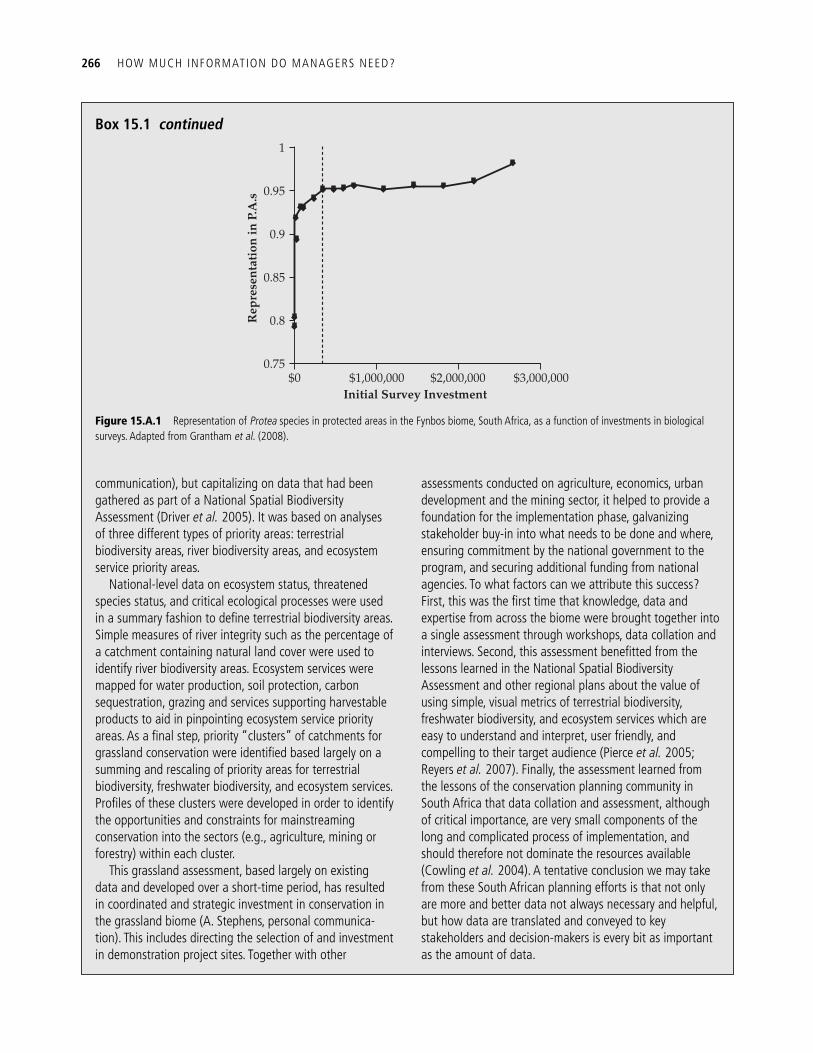
266 HOW MUCH INFORMATION DO MANAGERS NEED?
$00.75
0.8
0.85
0.9
0.95
1
$1,000,000 $2,000,000Initial Survey Investment
Rep
rese
ntat
ion
in P
.A.s
$3,000,000
Figure 15.A.1 Representation of Protea species in protected areas in the Fynbos biome, South Africa, as a function of investments in biological surveys. Adapted from Grantham et al. ( 2008 ).
communication), but capitalizing on data that had been gathered as part of a National Spatial Biodiversity Assessment ( Driver et al. 2005 ). It was based on analyses of three different types of priority areas: terrestrial biodiversity areas, river biodiversity areas, and ecosystem service priority areas.
National-level data on ecosystem status, threatened species status, and critical ecological processes were used in a summary fashion to defi ne terrestrial biodiversity areas. Simple measures of river integrity such as the percentage of a catchment containing natural land cover were used to identify river biodiversity areas. Ecosystem services were mapped for water production, soil protection, carbon sequestration, grazing and services supporting harvestable products to aid in pinpointing ecosystem service priority areas. As a fi nal step, priority “clusters” of catchments for grassland conservation were identifi ed based largely on a summing and rescaling of priority areas for terrestrial biodiversity, freshwater biodiversity, and ecosystem services. Profi les of these clusters were developed in order to identify the opportunities and constraints for mainstreaming conservation into the sectors (e.g., agriculture, mining or forestry) within each cluster.
This grassland assessment, based largely on existing data and developed over a short-time period, has resulted in coordinated and strategic investment in conservation in the grassland biome (A. Stephens, personal communica-tion). This includes directing the selection of and investment in demonstration project sites. Together with other
assessments conducted on agriculture, economics, urban development and the mining sector, it helped to provide a foundation for the implementation phase, galvanizing stakeholder buy-in into what needs to be done and where, ensuring commitment by the national government to the program, and securing additional funding from national agencies. To what factors can we attribute this success? First, this was the fi rst time that knowledge, data and expertise from across the biome were brought together into a single assessment through workshops, data collation and interviews. Second, this assessment benefi tted from the lessons learned in the National Spatial Biodiversity Assessment and other regional plans about the value of using simple, visual metrics of terrestrial biodiversity, freshwater biodiversity, and ecosystem services which are easy to understand and interpret, user friendly, and compelling to their target audience ( Pierce et al. 2005 ; Reyers et al. 2007 ). Finally, the assessment learned from the lessons of the conservation planning community in South Africa that data collation and assessment, although of critical importance, are very small components of the long and complicated process of implementation, and should therefore not dominate the resources available ( Cowling et al. 2004 ). A tentative conclusion we may take from these South African planning efforts is that not only are more and better data not always necessary and helpful, but how data are translated and conveyed to key stakeholders and decision-makers is every bit as important as the amount of data.
Box 15.1 continued
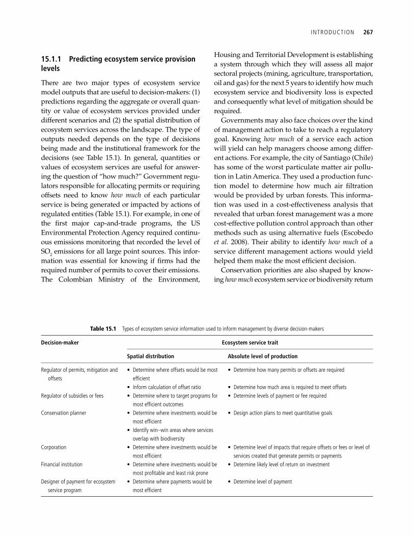
INTRODUCTION 267
15.1.1 Predicting ecosystem service provision levels
There are two major types of ecosystem service model outputs that are useful to decision-makers: (1) predictions regarding the aggregate or overall quan-tity or value of ecosystem services provided under different scenarios and (2) the spatial distribution of ecosystem services across the landscape. The type of outputs needed depends on the type of decisions being made and the institutional framework for the decisions (see Table 15.1 ). In general, quantities or values of ecosystem services are useful for answer-ing the question of “how much?” Government regu-lators responsible for allocating permits or requiring offsets need to know how much of each particular service is being generated or impacted by actions of regulated entities ( Table 15.1 ). For example, in one of the fi rst major cap-and-trade programs, the US Environmental Protection Agency required continu-ous emissions monitoring that recorded the level of SO 2 emissions for all large point sources. This infor-mation was essential for knowing if fi rms had the required number of permits to cover their emissions. The Colombian Ministry of the Environment,
Housing and Territorial Development is establishing a system through which they will assess all major sectoral projects (mining, agriculture, transportation, oil and gas) for the next 5 years to identify how much ecosystem service and biodiversity loss is expected and consequently what level of mitigation should be required.
Governments may also face choices over the kind of management action to take to reach a regulatory goal. Knowing how much of a service each action will yield can help managers choose among differ-ent actions. For example, the city of Santiago (Chile) has some of the worst particulate matter air pollu-tion in Latin America. They used a production func-tion model to determine how much air fi ltration would be provided by urban forests. This informa-tion was used in a cost-effectiveness analysis that revealed that urban forest management was a more cost-effective pollution control approach than other methods such as using alternative fuels ( Escobedo et al. 2008 ). Their ability to identify how much of a service different management actions would yield helped them make the most effi cient decision.
Conservation priorities are also shaped by know-ing how much ecosystem service or biodiversity return
Table 15.1 Types of ecosystem service information used to inform management by diverse decision-makers
Decision-maker Ecosystem service trait
Spatial distribution Absolute level of production
Regulator of permits, mitigation and offsets
• Determine where offsets would be most effi cient
• Determine how many permits or offsets are required
• Inform calculation of offset ratio • Determine how much area is required to meet offsets Regulator of subsidies or fees • Determine where to target programs for
most effi cient outcomes • Determine levels of payment or fee required
Conservation planner • Determine where investments would be most effi cient
• Design action plans to meet quantitative goals
• Identify win–win areas where services overlap with biodiversity
Corporation • Determine where investments would be most effi cient
• Determine level of impacts that require offsets or fees or level of services created that generate permits or payments
Financial institution • Determine where investments would be most profi table and least risk prone
• Determine likely level of return on investment
Designer of payment for ecosystem service program
• Determine where payments would be most effi cient
• Determine level of payment
268 HOW MUCH INFORMATION DO MANAGERS NEED?
they can be expect from different geographic patterns of protection or restoration ( Box 15.1 ). The Nature Conservancy is looking at this question in the Willamette Basin in Oregon, by asking how much ecosystem service return they are likely to get if they are successful in protecting their entire portfolio of conservation priority sites. Corporations trying to meet either internally set goals or government regula-tions need to know how much offsetting their pro-posed activities will cost for budgeting and strategic planning. BC Hydro, the third largest electric utility in Canada, has set an internal goal to become “envi-ronment neutral” in the next 20 years, meaning that they intend to reduce environmental impacts as much as possible and then offset unavoidable damages. To achieve this goal, they need to know how much impact their activities will have on biodiversity and ecosystem services so that they can reduce these effects or mitigate them elsewhere.
In general, when the amount of an ecosystem service is of primary interest, then questions of appropriate model complexity should focus on comparing levels of ecosystem services.
15.1.2 Predicting ecosystem service patterns in space
Ecosystem services are not delivered or valued uni-formly across landscapes. Certain locations harbor more biodiversity, or provide more carbon storage or other ecosystem services than other locations. Delivery of some services, such as fl ood control or provision of clean drinking water, is more valuable if it takes place near large cities. In general, the effectiveness of any management action aimed at delivering an ecosystem service will be determined by the location of management activity. This means that mapped predictions of the relative value of dif-ferent locations in terms of ecosystem service provi-sion can be very useful when implementing investments, incentives or regulations. For exam-ple, in the United States, the spatial orientation of damaged areas and corresponding mitigation areas is used to determine the required mitigation ratio (specifi ed as how many acres of restored or pro-tected habitat are required for each acre damaged). For example, under the Clean Water Act, selecting a mitigation site outside the impacted watershed
doubles the required mitigation ratio (e.g., from 2 acres restored/protected: 1 acre damaged to 4:1) (ACOE 2004). An obvious goal for conservation is effi ciency which translates into identifying where conservation activities should be distributed across a landscape to get the greatest possible biodiversity and ecosystem service returns ( Box 15.1 ). Similarly, regulators developing new subsidy or fee programs can achieve effi ciency by considering where in space to target payments or levy charges (e.g., Nelson et al. 2008 ).
15.2 Testing agreement between simple and complex ecosystem service models
In statistical theory it is relatively straightforward to compare the performance of models when the models are nested in terms of complexity, the easi-est form of which is a multiple linear regression with a succession of possible additional predictors. However, deciding between simple versus complex models is more diffi cult when the alternatives are not nested and use different data sets ( Pascual et al. 1997 ), as is the case with most of our tier 1 (simple) and tier 2 (complex) models. Here we focus on assessing how well the simple tier 1 models agree with more complex tier 2 models, and if models disagree, how using predictions from one particular model are likely to infl uence management decisions.
15.2.1 Carbon stock and carbon sequestration
The tier 1 and tier 2 models for estimating carbon stocks both predict the amount of carbon stored in a land use and land cover type on the landscape in Mg carbon ha -1 (see Chapter 7 for details). Both tier 1 and tier 2 models can also predict the amount or value of carbon sequestered over time (Mg carbon ha -1 yr -1 or $US (or other currency) ha -1 yr -1 ). The two models differ in their treatment of carbon storage as vegetation grows and decays, and in their treatment of carbon changes with land use and cover transi-tions. The simpler tier 1 model assumes that all par-cels within a specifi ed land use and cover type hold the same amount of carbon, regardless of the age of vegetation. The tier 1 model also assumes that car-bon sequestration rates in a given land cover class
TEST ING AGREEMENT BETWEEN S IMPLE AND COMPLEX ECOSYSTEM SERVICE MODELS 269
are not related to previous land-use practices or cover types, or to the time since transition. Tier 1 is thus most appropriate for analysis of average or equilibrium “steady-state” values of carbon stor-age. The tier 2 model uses a coeffi cient to adjust the amount of carbon stored in a land cover type for its age, relative to the maximum possible storage of carbon in that land cover class. The tier 2 model also accounts for the previous land use and cover type and the amount of time that has passed since the transition to the current type occurred.
15.2.1.1 Predicting carbon storage and sequestration levels Predicting the total amount of carbon stored or sequestered by a parcel can be important in the design of payment for ecosystem service programs or in the process landowners or corporations go through to determine whether they should partici-pate in voluntary carbon markets. Carbon storage or sequestration levels may also be useful when companies or organizations are trying to assess the value of their current land assets. For instance, The Nature Conservancy or Exxon-Mobil may want to know how much carbon sequestration benefi t is being provided by lands currently under their management.
We used the application of both tier 1 and tier 2 models in the Willamette Basin, Oregon (USA) to ask whether these differences in model complexity lead to important differences in the prediction of absolute levels of carbon storage and sequestration on the landscape for conditions in 1990 and three future land-use scenarios. All maps used to represent land use and land cover future scenarios were developed by a multi-stakeholder alliance ( Hulse et al . 2002 ; US EPA 2002; Baker et al. 2004 ) that scripted three different management pathways: (1) conservation, where greater emphasis is placed on ecosystem protection and restoration, (2) develop-ment, where market forces are given greater free rein across all components of the landscape, and (3) planned trend, where current policies are imple-mented as written and recent trends continue.
In all cases, there was close agreement between the simple and complex models ( Figures 15.1 a, b, c). As predictions progressed farther into the future, the tier 2 model predicted higher carbon storage
values than the tier 1 model, which was expected since the tier 2 model accounts for changes in car-bon storage with age while the tier 1 model does not. As forests mature or carbon builds up in soils over decades, estimates of their carbon stocks stay static in the tier 1 model, while they move closer to the maximum possible storage capacity of each land cover type in the tier 2 model. Managers interested in using our models to track carbon sequestration where land use and cover types have changed in the recent past, or may change in the future, should use the tier 2 model if possible. In the Willamette application, conservation planners or landowners using the tier 1 model to report the contribution of their holdings can be confi dent that they are likely presenting conservative estimates.
15.2.1.2 Predicting carbon sequestration patterns in space Information describing the spatial confi guration of carbon storage or sequestration is useful when inves-tors, governments, corporations or conservation groups are trying to identify the best places for action, or the best course of action. Policy makers designing new subsidy or fee programs, or conservation groups choosing new sites for action, may want to know where carbon will be sequestered or lost as a result of a proposed management program. We asked how well the tier 1 and tier 2 models agree on these kinds of spatial questions by taking the difference between the carbon storage maps produced by the two mod-els for the Willamette Basin (USA) ( Figure 15.2 ). We found differences in the prediction of carbon storage for initial conditions in the 1990 landscape. These dif-ferences, however, show no clear pattern and seem to be fairly randomly distributed across the landscape. By 2050, the age class and landscape transition con-siderations included in the tier 2 model lead to much higher estimates of carbon storage in forested areas than those given by the tier 1 model (especially for the conservation scenario in 2050; Figure 15.2 ). Tier 2 shows lower estimates for carbon storage in con-verted areas.
The type and age of land use and land cover classes included in the scenario being examined affected how much the models disagreed. This can be seen most clearly by comparing the estimates of carbon sequestration (or change in carbon storage) over time
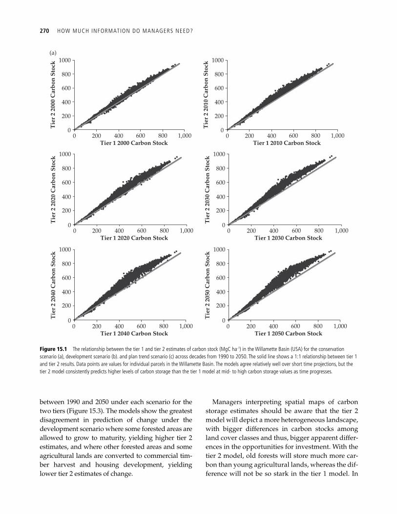
270 HOW MUCH INFORMATION DO MANAGERS NEED?
between 1990 and 2050 under each scenario for the two tiers ( Figure 15.3 ). The models show the greatest disagreement in prediction of change under the development scenario where some forested areas are allowed to grow to maturity, yielding higher tier 2 estimates, and where other forested areas and some agricultural lands are converted to commercial tim-ber harvest and housing development, yielding lower tier 2 estimates of change.
Managers interpreting spatial maps of carbon storage estimates should be aware that the tier 2 model will depict a more heterogeneous landscape, with bigger differences in carbon stocks among land cover classes and thus, bigger apparent differ-ences in the opportunities for investment. With the tier 2 model, old forests will store much more car-bon than young agricultural lands, whereas the dif-ference will not be so stark in the tier 1 model. In
1000(a)
800
600
400
200
00 200 400
Tier 1 2000 Carbon Stock
Tie
r 2
2000
Car
bon
Stoc
k
600 800 1,000
1000
800
600
400
200
00 200 400
Tier 1 2020 Carbon Stock
Tie
r 2
2020
Car
bon
Stoc
k
600 800 1,000
1000
800
600
400
200
00 200 400
Tier 1 2040 Carbon Stock
Tie
r 2
2040
Car
bon
Stoc
k
600 800 1,000
1000
800
600
400
200
00 200 400
Tier 1 2050 Carbon Stock
Tie
r 2
2050
Car
bon
Stoc
k
600 800 1,000
1000
800
600
400
200
00 200 400
Tier 1 2030 Carbon Stock
Tie
r 2
2030
Car
bon
Stoc
k
600 800 1,000
1000
800
600
400
200
00 200 400
Tier 1 2010 Carbon Stock
Tie
r 2
2010
Car
bon
Stoc
k
600 800 1,000
Figure 15.1 The relationship between the tier 1 and tier 2 estimates of carbon stock (MgC ha-1) in the Willamette Basin (USA) for the conservation scenario (a), development scenario (b). and plan trend scenario (c) across decades from 1990 to 2050. The solid line shows a 1:1 relationship between tier 1 and tier 2 results. Data points are values for individual parcels in the Willamette Basin. The models agree relatively well over short time projections, but the tier 2 model consistently predicts higher levels of carbon storage than the tier 1 model at mid- to high carbon storage values as time progresses.
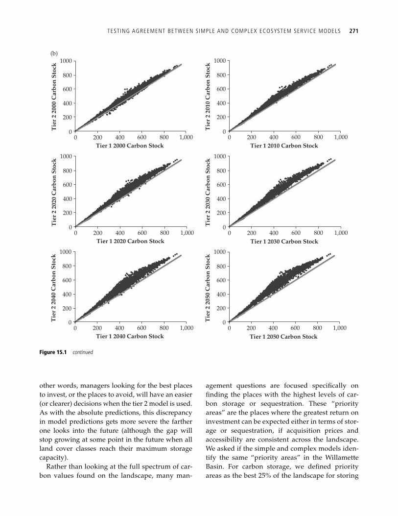
TEST ING AGREEMENT BETWEEN S IMPLE AND COMPLEX ECOSYSTEM SERVICE MODELS 271
1000(b)
800
600
400
200
00 200 400
Tier 1 2000 Carbon Stock
Tie
r 2
2000
Car
bon
Stoc
k
600 800 1,000
1000
800
600
400
200
00 200 400
Tier 1 2010 Carbon Stock
Tie
r 2
2010
Car
bon
Stoc
k
600 800 1,000
1000
800
600
400
200
00 200 400
Tier 1 2030 Carbon Stock
Tie
r 2
2030
Car
bon
Stoc
k
600 800 1,000
1000
800
600
400
200
00 200 400
Tier 1 2020 Carbon Stock
Tie
r 2
2020
Car
bon
Stoc
k
600 800 1,000
1000
800
600
400
200
00 200 400
Tier 1 2040 Carbon Stock
Tie
r 2
2040
Car
bon
Stoc
k
600 800 1,000
1000
800
600
400
200
00 200 400
Tier 1 2050 Carbon Stock
Tie
r 2
2050
Car
bon
Stoc
k
600 800 1,000
Figure 15.1 continued
other words, managers looking for the best places to invest, or the places to avoid, will have an easier (or clearer) decisions when the tier 2 model is used. As with the absolute predictions, this discrepancy in model predictions gets more severe the farther one looks into the future (although the gap will stop growing at some point in the future when all land cover classes reach their maximum storage capacity).
Rather than looking at the full spectrum of car-bon values found on the landscape, many man-
agement questions are focused specifi cally on fi nding the places with the highest levels of car-bon storage or sequestration. These “priority areas” are the places where the greatest return on investment can be expected either in terms of stor-age or sequestration, if acquisition prices and accessibility are consistent across the landscape. We asked if the simple and complex models iden-tify the same “priority areas” in the Willamette Basin. For carbon storage, we defi ned priority areas as the best 25% of the landscape for storing
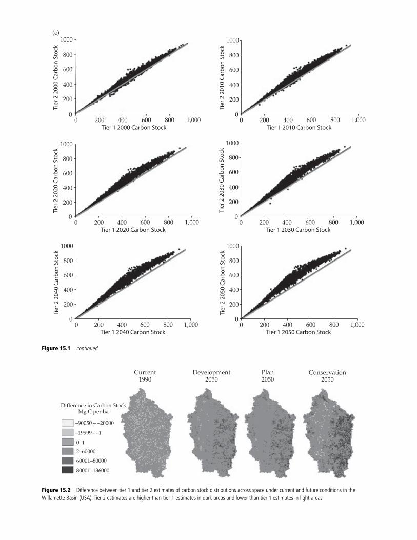
1000(c)
800
600
400
200
00 200 400
Tier 1 2000 Carbon Stock
Tier
2 2
000
Carb
on S
tock
600 800 1,000
1000
800
600
400
200
00 200 400
Tier 1 2010 Carbon Stock
Tier
2 2
010
Carb
on S
tock
600 800 1,000
1000
800
600
400
200
00 200 400
Tier 1 2030 Carbon StockTi
er 2
203
0 Ca
rbon
Sto
ck600 800 1,000
1000
800
600
400
200
00 200 400
Tier 1 2020 Carbon Stock
Tier
2 2
020
Carb
on S
tock
600 800 1,000
1000
800
600
400
200
00 200 400
Tier 1 2040 Carbon Stock
Tier
2 2
040
Carb
on S
tock
600 800 1,000
1000
800
600
400
200
00 200 400
Tier 1 2050 Carbon Stock
Tier
2 2
050
Carb
on S
tock
600 800 1,000
Figure 15.1 continued
Current1990
Difference in Carbon StockMg C per ha
–90050 – –20000
–19999– –1
0–1
2–60000
60001–80000
80001–136000
Development2050
Plan2050
Conservation2050
Figure 15.2 Difference between tier 1 and tier 2 estimates of carbon stock distributions across space under current and future conditions in the Willamette Basin (USA). Tier 2 estimates are higher than tier 1 estimates in dark areas and lower than tier 1 estimates in light areas.
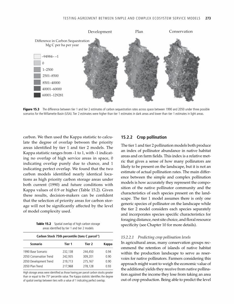
TEST ING AGREEMENT BETWEEN S IMPLE AND COMPLEX ECOSYSTEM SERVICE MODELS 273
Development
Difference in Carbon SequestrationMg C per ha per year
–94984– –1
0
1–2500
2501–8500
8501–40000
40001–60000
60001–129281
Plan Conservation
Figure 15.3 The difference between tier 1 and tier 2 estimates of carbon sequestration rates across space between 1990 and 2050 under three possible scenarios for the Willamette Basin (USA). Tier 2 estimates were higher than tier 1 estimates in dark areas and lower than tier 1 estimates in light areas.
carbon. We then used the Kappa statistic to calcu-late the degree of overlap between the priority areas identifi ed by tier 1 and tier 2 models. The Kappa statistic ranges from -1 to 1, with -1 indicat-ing no overlap of high service areas in space, 0 indicating overlap purely due to chance, and 1 indicating perfect overlap. We found that the two carbon models identifi ed nearly identical loca-tions as high priority carbon storage areas under both current (1990) and future conditions with Kappa values of 0.9 or higher ( Table 15.2 ). Given these results, decision-makers can be confi dent that the selection of priority areas for carbon stor-age will not be signifi cantly affected by the level of model complexity used.
15.2.2 Crop pollination
The tier 1 and tier 2 pollination models both produce an index of pollinator abundance in native habitat areas and on farm fi elds. This index is a relative met-ric that gives a sense of how many pollinators are likely to be present on the landscape, but it is not an estimate of actual pollination rates. The main differ-ence between the simple and complex pollination models is how accurately they represent the compo-sition of the native pollinator community and the characteristics of each species present on the land-scape. The tier 1 model assumes there is only one generic species of pollinator on the landscape while the tier 2 model considers each species separately and incorporates species specifi c characteristics for foraging distance, nest site choice, and fl oral resource specifi city (see Chapter 10 for more details).
15.2.2.1 Predicting crop pollination levels In agricultural areas, many conservation groups rec-ommend the retention of islands of native habitat within the production landscape to serve as reser-voirs for native pollinators. Farmers considering this approach might want to weigh the economic value of the additional yields they receive from native pollina-tion against the income they lose from taking an area out of crop production. Being able to predict the level
Table 15.2 Spatial overlap of high carbon storage areas identifi ed by tier 1 and tier 2 models
Carbon Stock 75 th percentile (tons C parcel -1 )
Scenario Tier 1 Tier 2 Kappa
1990 Base Scenario 232,138 244,450 0.94 2050 Conservation Trend 242,935 309,201 0.90 2050 Development Trend 219,713 275,167 0.90 2050 Plan Trend 217,968 278,128 0.93
High storage areas were identifi ed as those having per parcel carbon stocks greater than or equal to the 75 th percentile value. The Kappa statistic identifi es the degree of spatial overlap between tiers with a value of 1 indicating perfect overlap.
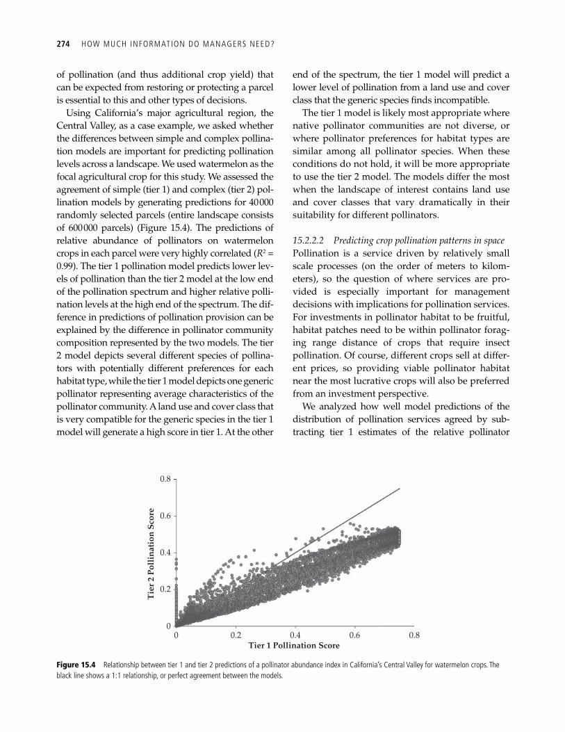
274 HOW MUCH INFORMATION DO MANAGERS NEED?
of pollination (and thus additional crop yield) that can be expected from restoring or protecting a parcel is essential to this and other types of decisions.
Using California’s major agricultural region, the Central Valley, as a case example, we asked whether the differences between simple and complex pollina-tion models are important for predicting pollination levels across a landscape. We used watermelon as the focal agricultural crop for this study. We assessed the agreement of simple (tier 1) and complex (tier 2) pol-lination models by generating predictions for 40 000 randomly selected parcels (entire landscape consists of 600 000 parcels) ( Figure 15.4 ). The predictions of relative abundance of pollinators on watermelon crops in each parcel were very highly correlated ( R 2 = 0.99). The tier 1 pollination model predicts lower lev-els of pollination than the tier 2 model at the low end of the pollination spectrum and higher relative polli-nation levels at the high end of the spectrum. The dif-ference in predictions of pollination provision can be explained by the difference in pollinator community composition represented by the two models. The tier 2 model depicts several different species of pollina-tors with potentially different preferences for each habitat type, while the tier 1 model depicts one generic pollinator representing average characteristics of the pollinator community. A land use and cover class that is very compatible for the generic species in the tier 1 model will generate a high score in tier 1. At the other
end of the spectrum, the tier 1 model will predict a lower level of pollination from a land use and cover class that the generic species fi nds incompatible.
The tier 1 model is likely most appropriate where native pollinator communities are not diverse, or where pollinator preferences for habitat types are similar among all pollinator species. When these conditions do not hold, it will be more appropriate to use the tier 2 model. The models differ the most when the landscape of interest contains land use and cover classes that vary dramatically in their suitability for different pollinators.
15.2.2.2 Predicting crop pollination patterns in space Pollination is a service driven by relatively small scale processes (on the order of meters to kilom-eters), so the question of where services are pro-vided is especially important for management decisions with implications for pollination services. For investments in pollinator habitat to be fruitful, habitat patches need to be within pollinator forag-ing range distance of crops that require insect pollination. Of course, different crops sell at differ-ent prices, so providing viable pollinator habitat near the most lucrative crops will also be preferred from an investment perspective.
We analyzed how well model predictions of the distribution of pollination services agreed by sub-tracting tier 1 estimates of the relative pollinator
0.8
0.6
0.4
0.2
00 0.2 0.4
Tier 1 Pollination Score
Tie
r 2
Poll
inat
ion
Scor
e
0.6 0.8
Figure 15.4 Relationship between tier 1 and tier 2 predictions of a pollinator abundance index in California’s Central Valley for watermelon crops. The black line shows a 1:1 relationship, or perfect agreement between the models.
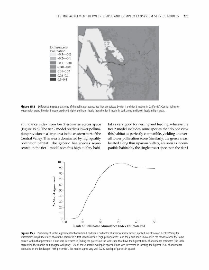
TEST ING AGREEMENT BETWEEN S IMPLE AND COMPLEX ECOSYSTEM SERVICE MODELS 275
abundance index from tier 2 estimates across space ( Figure 15.5 ). The tier 2 model predicts lower pollina-tion provision in a large area in the western part of the Central Valley. This area is dominated by high quality pollinator habitat. The generic bee species repre-sented in the tier 1 model sees this high quality habi-
tat as very good for nesting and feeding, whereas the tier 2 model includes some species that do not view this habitat as perfectly compatible, yielding an over-all lower pollination score. Similarly, the green areas, located along thin riparian buffers, are seen as incom-patible habitat by the single insect species in the tier 1
Difference inPollination
–0.3– –0.2–0.2– –0.1–0.1– –0.01–0.01–0.010.01–0.030.03–0.10.1–0.4
Figure 15.5 Difference in spatial patterns of the pollinator abundance index predicted by tier 1 and tier 2 models in California’s Central Valley for watermelon crops. The tier 2 model predicted higher pollinator levels than the tier 1 model in dark areas and lower levels in light areas.
1000
10
20
30
40
50
60
70
80
90
100
90 80Rank of Pollinator Abundance Index Estimate (%)
% M
odel
Agr
eem
ent
70 60 50
Figure 15.6 Summary of spatial agreement between tier 1 and tier 2 pollinator abundance index models applied in California’s Central Valley for watermelon crops. The x axis shows the percentile cutoff used to defi ne “high priority areas” and the y axis shows how often the models chose the same parcels within that percentile. If one was interested in fi nding the parcels on the landscape that have the highest 10% of abundance estimates (the 90th percentile), the models do not agree well (only 15% of those parcels overlap in space). If one was interested in locating the highest 25% of abundance estimates on the landscape (75th percentile), the models agree very well (92% overlap of parcels in space).
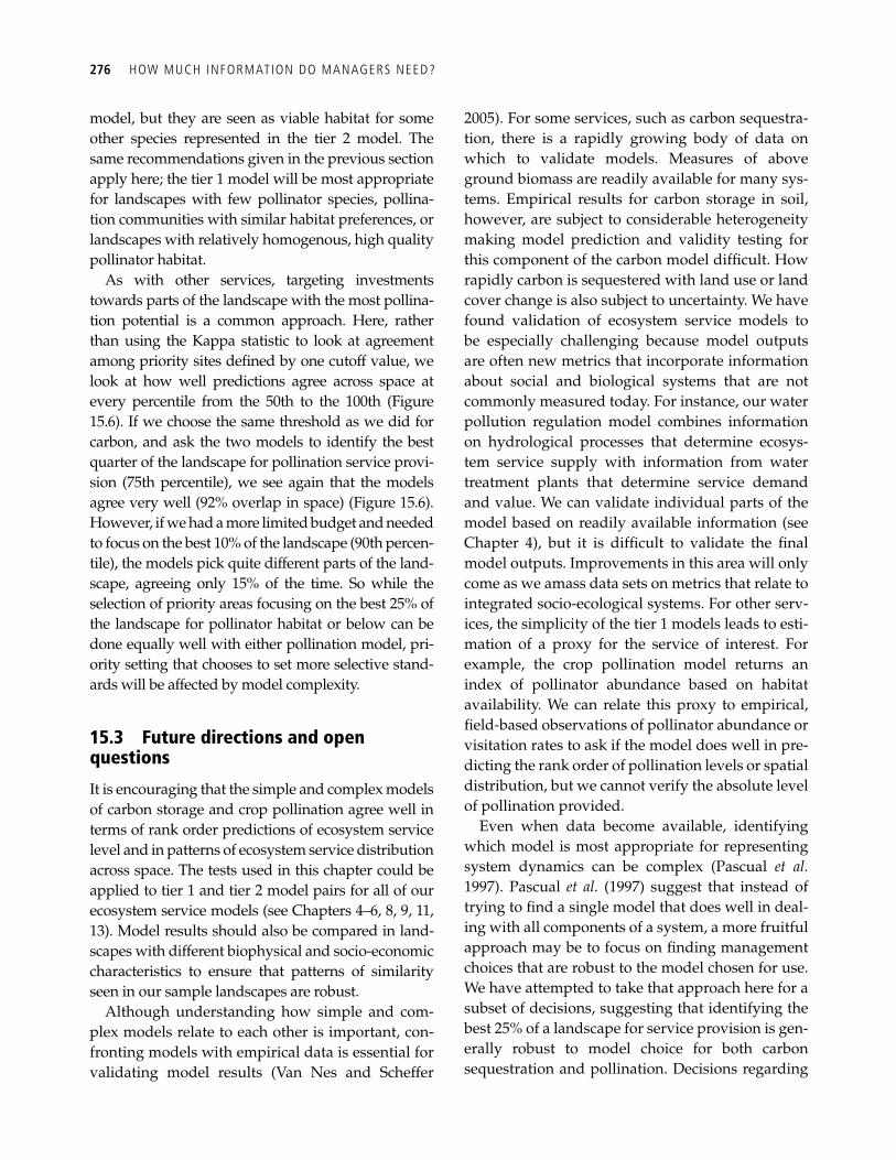
276 HOW MUCH INFORMATION DO MANAGERS NEED?
model, but they are seen as viable habitat for some other species represented in the tier 2 model. The same recommendations given in the previous section apply here; the tier 1 model will be most appropriate for landscapes with few pollinator species, pollina-tion communities with similar habitat preferences, or landscapes with relatively homogenous, high quality pollinator habitat.
As with other services, targeting investments towards parts of the landscape with the most pollina-tion potential is a common approach. Here, rather than using the Kappa statistic to look at agreement among priority sites defi ned by one cutoff value, we look at how well predictions agree across space at every percentile from the 50th to the 100th ( Figure 15.6 ). If we choose the same threshold as we did for carbon, and ask the two models to identify the best quarter of the landscape for pollination service provi-sion (75th percentile), we see again that the models agree very well (92% overlap in space) ( Figure 15.6 ). However, if we had a more limited budget and needed to focus on the best 10% of the landscape (90th percen-tile), the models pick quite different parts of the land-scape, agreeing only 15% of the time. So while the selection of priority areas focusing on the best 25% of the landscape for pollinator habitat or below can be done equally well with either pollination model, pri-ority setting that chooses to set more selective stand-ards will be affected by model complexity.
15.3 Future directions and open questions
It is encouraging that the simple and complex models of carbon storage and crop pollination agree well in terms of rank order predictions of ecosystem service level and in patterns of ecosystem service distribution across space. The tests used in this chapter could be applied to tier 1 and tier 2 model pairs for all of our ecosystem service models (see Chapters 4 – 6 , 8 , 9 , 11 , 13 ). Model results should also be compared in land-scapes with different biophysical and socio-economic characteristics to ensure that patterns of similarity seen in our sample landscapes are robust.
Although understanding how simple and com-plex models relate to each other is important, con-fronting models with empirical data is essential for validating model results ( Van Nes and Scheffer
2005 ). For some services, such as carbon sequestra-tion, there is a rapidly growing body of data on which to validate models. Measures of above ground biomass are readily available for many sys-tems. Empirical results for carbon storage in soil, however, are subject to considerable heterogeneity making model prediction and validity testing for this component of the carbon model diffi cult. How rapidly carbon is sequestered with land use or land cover change is also subject to uncertainty. We have found validation of ecosystem service models to be especially challenging because model outputs are often new metrics that incorporate information about social and biological systems that are not commonly measured today. For instance, our water pollution regulation model combines information on hydrological processes that determine ecosys-tem service supply with information from water treatment plants that determine service demand and value. We can validate individual parts of the model based on readily available information (see Chapter 4 ), but it is diffi cult to validate the fi nal model outputs. Improvements in this area will only come as we amass data sets on metrics that relate to integrated socio-ecological systems. For other serv-ices, the simplicity of the tier 1 models leads to esti-mation of a proxy for the service of interest. For example, the crop pollination model returns an index of pollinator abundance based on habitat availability. We can relate this proxy to empirical, fi eld-based observations of pollinator abundance or visitation rates to ask if the model does well in pre-dicting the rank order of pollination levels or spatial distribution, but we cannot verify the absolute level of pollination provided.
Even when data become available, identifying which model is most appropriate for representing system dynamics can be complex ( Pascual et al. 1997 ). Pascual et al. ( 1997 ) suggest that instead of trying to fi nd a single model that does well in deal-ing with all components of a system, a more fruitful approach may be to focus on fi nding management choices that are robust to the model chosen for use. We have attempted to take that approach here for a subset of decisions, suggesting that identifying the best 25% of a landscape for service provision is gen-erally robust to model choice for both carbon sequestration and pollination. Decisions regarding
FUTURE DIRECTIONS AND OPEN QUEST IONS 277
the placement of investments by conservation groups, fi nancial institutions or others in the private sector, along with decisions about where to direct mitigation and offsetting or payments for services could all be made with tier 1 or tier 2 models with equal confi dence. This approach can easily be applied to the many other models discussed in this book.
The biggest challenge in terms of model selection and testing entails questions of “how much” as opposed to “where are the best places.” There need to be national ecosystem monitoring programs that report spatially explicit data on water quality, carbon sequestration and other vital ecosystem outputs if we are to understand which models to use and how much confi dence to have in model results.
References
Army Corps of Engineers (ACOE). (2004). Chicago District 2004 mitigation requirements . Chicago District of the U.S. Army Corps of Engineers, Chicago.
Baker, J. P., Hulse, D. W., Gregory, S. V., et al . (2004). Alternative futures for the Willamette River Basin, Oregon. Ecological Applications , 14 , 313–24.
Cowling, R. M., Knight, A. T., Faith, D. P., et al . (2004). Nature conservation requires more than a passion for species. Conservation Biology , 18 , 1674–7.
Driver, A., Maxe, K., Rouget, M., et al . (2005). National spa-tial biodiversity assessment 2004: Priorities for biodiversity conservation in South Africa . South African National Biodiversity Institute, Pretoria.
Escobedo, F. J., Wagner, J. E., Nowak, D. J., et al . (2008). Analyzing the cost effectiveness of Santiago, Chile’s policy of using urban forests to improve air quality. Journal of Environmental Management , 86 , 148–57.
Gan, T. Y., Dlamini, E. M., and Biftu, G. F. (1997). Effects of model complexity and structure, data quality, and objec-tive functionson hydrologic modeling. Journal of Hydrology , 192 , 81–103.
Gaston, K. J., and Rodrigues, A. S. I. (2003). Reserve selec-tion in regions with poor biological data. Conservation Biology, 17 , 188–95.
Grand, J., Cummings, M. P., Rebelo, T. G., et al . (2007). Biased data reduce effi ciency and effectiveness of con-servation reserve networks. Ecology Letters , 10 , 364–74.
Grantham, H. S., Moilanen, A., Wilson, K. A., et al . (2008). Diminishing return on investment for biodiverstiy data in conservation planning. Conservation Letters , 1 , 190–8.
Hulse, D., Gregory, S., and Baker, J. (2002). Willamette River Basin planning atlas: trajectories of environmental and ecological change. Oregon State University Press, Corvallis.
Ludwig, D., and Walters, C. J. (1985). Are age-structured models appropriate for catch-effort data? Canadian Journal of Fisheries and Aquatic Sciences , 42 , 1066.
Nelson, E., Polasky, S., Lewis, D. J. et al . (2008). Effi ciency of incentives to jointly increase carbon sequestration and species conservation on a landscape. Proceedings of the National Academy of Sciences of the USA , 105 , 9471–6.
Pascual, M. A., Kareiva, P., and Hilborn, R. (1997). The Infl uence of Model Structure on Conclusions about the Viability and Harvesting of Serengeti Wildebeest. Conservation Biology , 11 , 966–76.
Pierce, S. M., Cowling, R. M., Knight, A. T., et al . (2005). Systematic conservation assessment products for lan-duse planning: interpretation for implementation. Biological Conservation , 125 , 441–8.
Reyers, B., Nel, J., Egoh, B., et al . (2005). A conservation assessment of South Africa’s grassland biome: Integrating terrestrial, river, ecosystem services and fi ne scale priorities. SCIR, Cape Town.
Reyers, B., Rouget, M., Jonas, Z., et al . (2007). Developing products for conservation decision-making: Lessons from a spatial biodiversity assessment for South Africa. Diversity and Distributions , 13 , 608–19.
Stephens, P. A., Frey-Roos, F., Arnold, W., et al . (2002). Model complexity and population predictions, The alpine marmot as a case study. Journal of Animal Ecology , 71 , 343–61.
United States Environmental Protection Agency (US EPA) (2002). Willamette Basin alternative futures analysis. Environmental assessment approach that facilitates consen-sus building. US EPA Offi ce of Research and Development, Washington, DC.
Van Nes, E. H., and Scheffer, M. (2005). A strategy to improve the contribution of complex simulation models to ecological theory. Ecological Modelling , 185 , 153–64.
278
CHAPTER 16
Poverty and the distribution of ecosystem services Heather Tallis, Stefano Pagiola, Wei Zhang, Sabina Shaikh, Erik Nelson, Charlotte Stanton, and Priya Shyamsundar
16.1 Introduction
The planet’s stocks of natural assets continue to diminish while widespread poverty persists throughout the developing world (Chen and Ravallion 2008). Recognizing the link between humans and nature has never been more salient for policy-makers and researchers concerned with con-servation and poverty alleviation (Sanderson and Redford 2003; Millennium Ecosystem Assessment 2005 ). Information detailing the specifi c links between the poor and the environment is building (e.g. Albla-Betrand 1993; Scherr et al. 2003; Delang 2006) and efforts are underway to determine how international agreements concerned with poverty alleviation can, and should, incorporate conserva-tion as a means to their ends. For example, Roe and Elliott (2004) note that United Nations (UN) Millennium Development Goals (MDGs), adopted by the General Assembly of the UN, have direct ties to environmental condition and stability. Of the eight goals, only one is explicitly environmental, but the success of fi ve others will rely on healthy ecosystems (Roe and Elliott 2004).
Incorporation of these advances in local and regional decision-making has proven challenging. Creating policies that account for interactions and trade-offs among environmental, economic and social values is diffi cult today because many of the connections between humans and the environment are not formally recognized by political and eco-nomic systems. Instead, decisions made today based on costs and benefi ts to society leave out many of the public goods and services provided to the poor by the environment, such as the provision
of clean water, food from bushmeat and native plants, medicinal plants, and protection from “nat-ural disasters,” such as storms and fl oods ( Millennium Ecosystem Assessment 2005 ). For example, conventional household economic sur-veys fail to include directly the contributions of natural assets to rural household welfare (Cavendish 2000), making it diffi cult to assess how they will be affected by public or private programs that change the status of these resources. Similarly, ecosystem services that make up a country’s aggregated natu-ral capital are largely absent in national accounting. Progress in economic valuation of ecosystem serv-ices is needed to support the development of a standardized methodology for the inclusion of eco-system values into Standard National Accounts (Mäler et al. 2008) and other policy decisions. The fundamental problem with incorporating ecosys-tem services into the balance sheets used in deci-sion-making is the lack of tools that easily track the status of or changes in these services, and their dis-tributional effects on human well-being.
In this chapter, we examine how the emerging fi eld of modeling and mapping ecosystem services can address this gap. We begin by discussing the need for a detailed understanding of the linkages between poverty and ecosystem services, and pro-vide a brief review of the literature on these links ( Section 16.2 ). We then examine the opportunities for and diffi culties with an integrated approach to mapping poverty with ecosystem services ( Section 16.3 ). Finally, we demonstrate how several of the mapping and valuation models described in earlier chapters ( Chapter 8 ) and developed elsewhere can be applied in this context using case studies of
ECOSYSTEM SERVICES AND THE POOR 279
the Amazon Basin and Guatemala’s highlands ( Section 16.4 ).
16.2 Ecosystem services and the poor
16.2.1 Dependence of the poor on ecosystem services
Earth’s ecosystems provide myriad goods and serv-ices that are essential to the well-being of all people, but natural capital contributes disproportionately to the welfare of the poor (see Section 16.3.2 for a discussion of “poor”), in some cases signifi cantly, because often the poor have limited capacity to pur-chase goods and services from elsewhere ( Table 16.1 ) ( World Bank 2008 ). For instance, Vedeld et al. (2004) found that about 22% of rural household income can be attributed to the harvest of goods from for-ests, contributing almost twice as much to the incomes of the poor as to the non-poor ( Table 16.1 ). This fi nding cannot be generalized to all rural households, but it is relevant to those living on the fringes of forests, those that are largely depend-ent on natural resources for subsistence, or those who are engaged in agricultural activities that rely heavily on natural capital and ecosystem processes ( Box 16.1 ).
In addition to providing income, natural resources can serve as safety nets for the poor during times of stress ( Justice et al. 2001; World Bank 2008 ). The poor have been shown to respond to known agri-cultural risks and sudden agricultural shocks by increasing their dependence on natural resources
(Pattanayak and Sills 2001), and the insurance pro-vided by natural resources can make it feasible for households to recoup after natural disasters (McSweeney 2005). Large changes in access to or availability of these services are likely to have sig-nifi cant effects on the poor (Ferraro 2002; World Bank 2008 ), making it essential that policy-makers recognize the possible costs that choices related to resource sectors impose on the poor through changes in services ( World Bank 2008 ).
16.2.2 The poor as agents or victims of environmental degradation
Depending on the context, the poor may be agents of degradation, its victims, or both. When the poor are agents of environmental degradation, they can cause declines in ecosystem service provision for themselves and for others. For example, the use of forests for fuel wood and other non-timber forest products by the poor has been the main cause of forest degradation in India (Baland et al. 2006) and Tanzania (Luoga et al. 2000; Ndangalasi et al. 2007). Similarly, degradation in Peru’s Pacaya-Samiria National Reserve was largely the result of the sub-sistence use of resources by households living around the reserve (Takasaki et al. 2004). Degradation can affect the functions of local ecosystems, increase ecological fragility, and increase the vulnerability of the poor to natural shocks (Shyamsundar 2001).
Despite its apparent irrationality, one of the rea-sons that households degrade ecosystem services
Table 16.1 Environmental income as percentage of total income in resource-poor and resource-rich areas
Study Resource-rich areas Resource-poor/low access areas
Average
Poor Rich Poor Rich Poor Rich
Jodha (1986) 9–26 1–4 Cavendish (2000) 44 30 Vedeld et al. (2004) a 32 17 Narain et al. (2005) 41 23 18 18 Chettri-Khattri (forthcoming) b 20 14 2 1
a Data reported are from multiple earlier studies. b Nontimber forest product (NTFP) income only. In most cases, “poor” refers to poorest 20% and “rich” to the richest 20% of households. Adapted with permission from World Bank ( 2008 ).
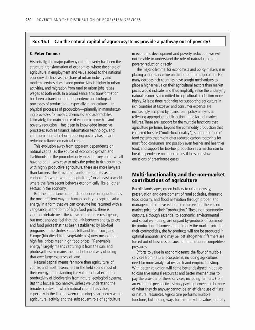
280 POVERTY AND THE DISTRIBUTION OF ECOSYSTEM SERVICES
Box 16.1 Can the natural capital of agroecosystems provide a pathway out of poverty?
C. Peter Timmer
Historically, the major pathway out of poverty has been the structural transformation of economies, where the share of agriculture in employment and value added to the national economy declines as the share of urban industry and modern services rises. Labor productivity is higher in urban activities, and migration from rural to urban jobs raises wages at both ends. In a broad sense, this transformation has been a transition from dependence on biological processes of production— especially in agriculture—to physical processes of production—primarily in manufactur-ing processes for metals, chemicals, and automobiles. Ultimately, the main source of economic growth—and poverty reduction—has been in knowledge-intensive processes such as fi nance, information technology, and communications. In short, reducing poverty has meant reducing reliance on natural capital.
This evolution away from apparent dependence on natural capital as the source of economic growth and livelihoods for the poor obviously missed a key point: we all have to eat. It was easy to miss the point: in rich countries with highly productive agriculture, there are more lawyers than farmers. The structural transformation has as its endpoint “a world without agriculture,” or at least a world where the farm sector behaves economically like all other sectors in the economy.
But the importance of our dependence on agriculture as the most effi cient way for human society to capture solar energy in a form that we can consume has returned with a vengeance, in the form of high food prices. There is vigorous debate over the causes of the price resurgence, but most analysts feel that the link between energy prices and food prices that has been established by bio-fuel programs in the Unites States (ethanol from corn) and Europe (bio-diesel from vegetable oils) now means that high fuel prices mean high food prices. “Renewable energy” largely means capturing it from the sun, and photosynthesis remains the most effi cient way of doing that over large expanses of land.
Natural capital means far more than agriculture, of course, and most researchers in the fi eld spend most of their energy understanding the value to local economic productivity of biodiversity from natural ecological systems. But this focus is too narrow. Unless we understand the broader context in which natural capital has value, especially in the link between capturing solar energy as an agricultural activity and the subsequent role of agriculture
in economic development and poverty reduction, we will not be able to understand the role of natural capital in poverty reduction directly.
The major dilemma, for economists and policy-makers, is in placing a monetary value on the output from agriculture. For many decades rich countries have sought mechanisms to place a higher value on their agricultural sectors than market prices would indicate, and thus, implicitly, value the underlying natural resources committed to agricultural production more highly. At least three rationales for supporting agriculture in rich countries at taxpayer and consumer expense are increasingly accepted by mainstream policy analysts as refl ecting appropriate public action in the face of market failures. These are: support for the multiple functions that agriculture performs, beyond the commodity production that is offered for sale (“multi-functionality”); support for “local” food systems that might offer reduced carbon footprints for most food consumers and possibly even fresher and healthier food; and support for bio-fuel production as a mechanism to break dependence on imported fossil fuels and slow emissions of greenhouse gases.
Multi-functionality and the non-market contributions of agriculture Bucolic landscapes, green buffers to urban density, preservation and development of rural societies, domestic food security, and fl ood alleviation through proper land management all have economic value even if there is no market price for their “production.” These non-commodity outputs, although essential to economic, environmental and social well-being, are unpaid by-products of commod-ity production. If farmers are paid only the market price for their commodities, the by-products will not be produced in optimal amounts, and may be lost altogether if farmers are forced out of business because of international competitive pressures.
Efforts to value in economic terms the fl ow of multiple services from natural ecosystems, including agriculture, need far more analytical research and empirical testing. With better valuation will come better designed initiatives to conserve natural resources and better mechanisms to pay the provider of these services, including farmers. From an economic perspective, simply paying farmers to do more of what they do anyway cannot be an effi cient use of fi scal or natural resources. Agriculture performs multiple functions, but fi nding ways for the market to value, and pay
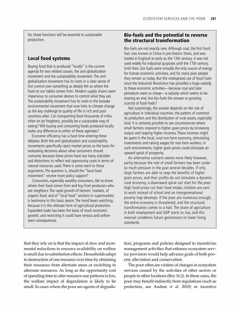
ECOSYSTEM SERVICES AND THE POOR 281
that they rely on is that the impact of slow and incre-mental reductions in resource availability on welfare is small due to substitution effects. Households adapt to destruction of one resource over time by obtaining their resources from alternate areas or switching to alternate resources. As long as the opportunity cost of spending time to alter resource-use patterns is low, the welfare impact of degradation is likely to be small. In cases where the poor are agents of degrada-
tion, programs and policies designed to incentivize management activities that enhance ecosystem serv-ice provision would help advance goals of both pov-erty alleviation and conservation.
The poor often are victims of changes in ecosystem services caused by the activities of other sectors or people in other locations ( Box 16.2 ). In these cases, the poor may benefi t indirectly from regulations (such as protection, see Andam et al. 2010) or incentive
for, these functions will be essential to sustainable production.
Local food systems Buying food that is produced “locally” is the current agenda for two related causes: the anti-globalization movement and the sustainability movement. The anti-globalization movement has its roots in a clear sense of lost control over something as deeply felt as where the food on our tables comes from. Modern supply chains seem impervious to consumer desires to control what they eat. The sustainability movement has its roots in the broader environmental movement that now links to climate change as the key challenge to quality of life in rich and poor countries alike. Can transporting food thousands of miles, often on jet freighters, possibly be a sustainable way of eating? Will buying and consuming foods produced locally make any difference to either of these agendas?
Economic effi ciency has a hard time entering these debates. Both the anti-globalization and sustainability movements specifi cally reject market prices as the basis for evaluating decisions about what consumers should consume, because these prices have too many subsidies and distortions to refl ect real opportunity costs in terms of natural resources used. There is some merit to these arguments. The question is, should the “local food movement” receive more policy support?
Consumers, especially wealthy consumers, like to know where their food comes from and buy from producers who are neighbors. The rapid growth of farmers’ markets, of organic food, and of “local food” sections in supermarkets is testimony to this basic desire. The trend bears watching, because it is the ultimate form of agricultural protection. Expanded trade has been the basis of much economic growth, and restricting it could have serious and unfore-seen consequences.
Bio-fuels and the potential to reverse the structural transformation Bio-fuels are not exactly new. Although coal, the fi rst fossil fuel, was known in China in pre-historic times, and was traded in England as early as the 13th century, it was not used widely for industrial purposes until the 17th century. Until then, bio-fuels were virtually the only source of energy for human economic activities, and for many poor people they remain so today. But the widespread use of fossil fuels since the Industrial Revolution has provided a huge subsidy to these economic activities—because coal and later petroleum were so cheap—a subsidy which seems to be nearing an end. Are bio-fuels the answer to growing scarcity of fossil fuels?
Not surprisingly, the answer depends on the role of agriculture in individual countries, the pattern of commod-ity production and the distribution of rural assets, especially land. It is certainly possible to see circumstances where small farmers respond to higher grain prices by increasing output and reaping higher incomes. These incomes might be spent in the local, rural non-farm economy, stimulating investments and raising wages for non-farm workers. In such environments, higher grain prices could stimulate an upward spiral of prosperity.
An alternative scenario seems more likely however, partly because the role of small farmers has been under so much pressure in the past several decades. If only large farmers are able to reap the benefits of higher grain prices, and their profits do not stimulate a dynamic rural economy, a downward spiral can start for the poor. High food prices cut their food intake, children are sent to work instead of school and an intergenerational poverty trap develops. If the poor are numerous enough, the entire economy is threatened, and the structural transformation comes to a halt. The share of agriculture in both employment and GDP starts to rise, and this reversal condemns future generations to lower living standards.
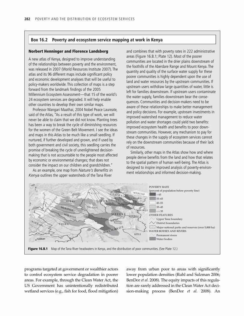
282 POVERTY AND THE DISTRIBUTION OF ECOSYSTEM SERVICES
programs targeted at government or wealthier actors to control ecosystem service degradation in poorer areas. For example, through the Clean Water Act, the US Government has unintentionally redistributed wetland services (e.g., fi sh for food, fl ood mitigation)
away from urban poor to areas with signifi cantly lower population densities (Ruhl and Salzman 2006; BenDor et al . 2008). The equity impacts of this regula-tion are rarely addressed in the Clean Water Act deci-sion-making process (BenDor et al. 2008). An
Box 16.2 Poverty and ecosystem service mapping at work in Kenya
Norbert Henninger and Florence Landsberg
A new atlas of Kenya, designed to improve understanding of the relationships between poverty and the environment, was released in 2007 ( World Resources Institute 2007 ). The atlas and its 96 different maps include signifi cant policy and economic development analyses that will be useful to policy-makers worldwide. This collection of maps is a step forward from the landmark fi ndings of the 2005 Millennium Ecosystem Assessment—that 15 of the world’s 24 ecosystem services are degraded. It will help enable other countries to develop their own similar maps.
Professor Wangari Maathai, 2004 Nobel Peace Laureate, said of the Atlas, “As a result of this type of work, we will never be able to claim that we did not know. Planting trees has been a way to break the cycle of diminishing resources for the women of the Green Belt Movement. I see the ideas and maps in this Atlas to be much like a small seedling. If nurtured, if further developed and grown, and if used by both government and civil society, this seedling carries the promise of breaking the cycle of unenlightened decision-making that is not accountable to the people most affected by economic or environmental changes; that does not consider the impact on our children and grandchildren.”
As an example, one map from Nature’s Benefi ts in Kenya outlines the upper watersheds of the Tana River
and combines that with poverty rates in 222 administrative areas (Figure 16.B.1; Plate 12). Most of the poorer communities are located in the drier plains downstream of the foothills of the Aberdare Range and Mount Kenya. The quantity and quality of the surface water supply for these poorer communities is highly dependent upon the use of land and water resources by the upstream communities. If upstream users withdraw large quantities of water, little is left for families downstream. If upstream users contaminate the water supply, families downstream bear the conse-quences. Communities and decision-makers need to be aware of these relationships to make better management and policy decisions. For example, upstream investments in improved watershed management to reduce water pollution and water shortages could yield two benefi ts: improved ecosystem health and benefi ts to poor down-stream communities. However, any mechanism to pay for these changes in the supply of ecosystem services cannot rely on the downstream communities because of their lack of resources.
Similarly, other maps in the Atlas show how and where people derive benefi ts from the land and how that relates to the spatial pattern of human well-being. The Atlas is designed to inspire improved analysis of poverty-environ-ment relationships and informed decision-making.
N
ABERDARE RANGE
K I A M A B U
NAIROBI
T H I K A
M A C H A K O S
KITUI
M B E E R E
E M B UN Y E R I
MURANGA
MARAGUA
M E R UC E NT R A L
M W I N G I
M E R U S O U T H
T H A R A K A
M E R U N.P.
MasingoReservoir
Tana River
KIRINYAGA
MT. K E N Y A
POVERTY RATE
OTHER FEATURES
(percent of population below poverty line)> 65
< = 35
55–65
Upper Tana boundaryDistrict boundaries
Major national parks and reserves (over 5,000 ha)
Permanent riversWater bodies
WATER BODIES AND RIVERS
45–5535–45
Figure 16.B.1 Map of the Tana River headwaters in Kenya, and the distribution of poor communities. (See Plate 12.)
MAPPING POVERTY AND ECOSYSTEM SERVICES 283
alternative regulatory approach could intentionally direct wetland mitigation activities towards areas with poor populations, thereby improving the poor’s access to wetlands’ many services.
16.3 Mapping poverty and ecosystem services
The relationship between the poor and natural resources is mediated by factors at various scales, such as labor and credit markets, property rights and other institutions, and information about best practices (Bluffstone 1995; Duraiappah 1998; Wunder 2001; Adhikari 2005). In some cases, a lack of markets contributes to degradation of natural systems; in other cases growth in markets can lead to ecosystem declines. Weak governance institu-tions, ill-defi ned property rights or lax enforcement, high discount rates, and population growth will all likely continue to contribute to degradation of local natural capital.
Given the complexities of connections between the poor and the environment, it is not easy to map pov-erty and ecosystem services together in a way that is robust and practically useful. Ideally, poverty and ecosystem service mapping would be done such that (1) the resolution of both poverty and ecosystem service information is suffi cient to represent patterns in each accurately, (2) the poverty indicators chosen are directly tied to the component of human well-being of interest and well matched with the ecosys-tem service(s) of concern, and (3) the institutions that control the provision of services are represented. Here, we discuss what can be done today as fi rst steps toward this ideal and what challenges remain.
16.3.1 Data resolution
Robust poverty analyses require uniform and high-quality data that are often unavailable, especially in developing countries. In most cases, indicators such as poverty rates are only available for relatively large administrative units. These data are often of little use for detailed analysis because administra-tive boundaries seldom match those of the ecosys-tems of interest, and because neither ecosystem services nor the poor are likely to be distributed uniformly within these boundaries.
More detailed poverty maps are typically created by using comprehensive data from small-sample household budget surveys to obtain a predictive relationship for poverty rates that is then applied to data from a national census at the highest available level of disaggregation (Poggi et al. 1998; Elbers et al. 2002). This approach has been used to generate poverty maps for several countries (Hentschel et al. 2000; Minot 2000; Müller et al. 2006; Bedi et al. 2007; Nelson and Chomitz 2007). However, even this fi ner scale analysis still produces maps based on administrative divisions (census tracts) and not ecosystem boundaries. Nelson and Chomitz (2007) dealt with this limitation by converting a poverty map of Guatemala to a watershed map. Even with poverty maps aligned to ecosystem boundaries, the assumption of uniform distribution within an eco-system can seriously distort analysis. Within a watershed, for example, it may matter whether the poor are concentrated in the steeper upper slopes or the fl atter riparian zones ( Box 16.2 ).
16.3.2 Poverty indicators
In addition to challenges with mapping poverty at an appropriate resolution for analysis, we also face the challenge of defi ning poverty in different set-tings. Poverty historically has been defi ned in strictly economic terms, with income as the com-mon indicator. Some analysts now argue that con-sumption is a better measure of poverty, as it is more closely related to well-being and refl ects capacity to meet basic needs through income and access to credit. It also avoids the problem of income fl ows being erratic at certain times of the year, espe-cially in poor agrarian economies where fl uctua-tions can cause reporting errors.
All money-based indicators have the limitation that they cannot refl ect individuals’ feelings of well-being and access to basic services. In recent years, a broader understanding has developed in which poverty encompasses not only deprivation of mate-rially-based well-being, but also a broader depriva-tion of opportunities ( World Bank 2001 ; UNEP 2004 ). The Millennium Ecosystem Assessment (MA) rec-ognized fi ve linked components of poverty: the nec-essary material for a good life, health, good social relations, security, and freedom of choice ( Millennium
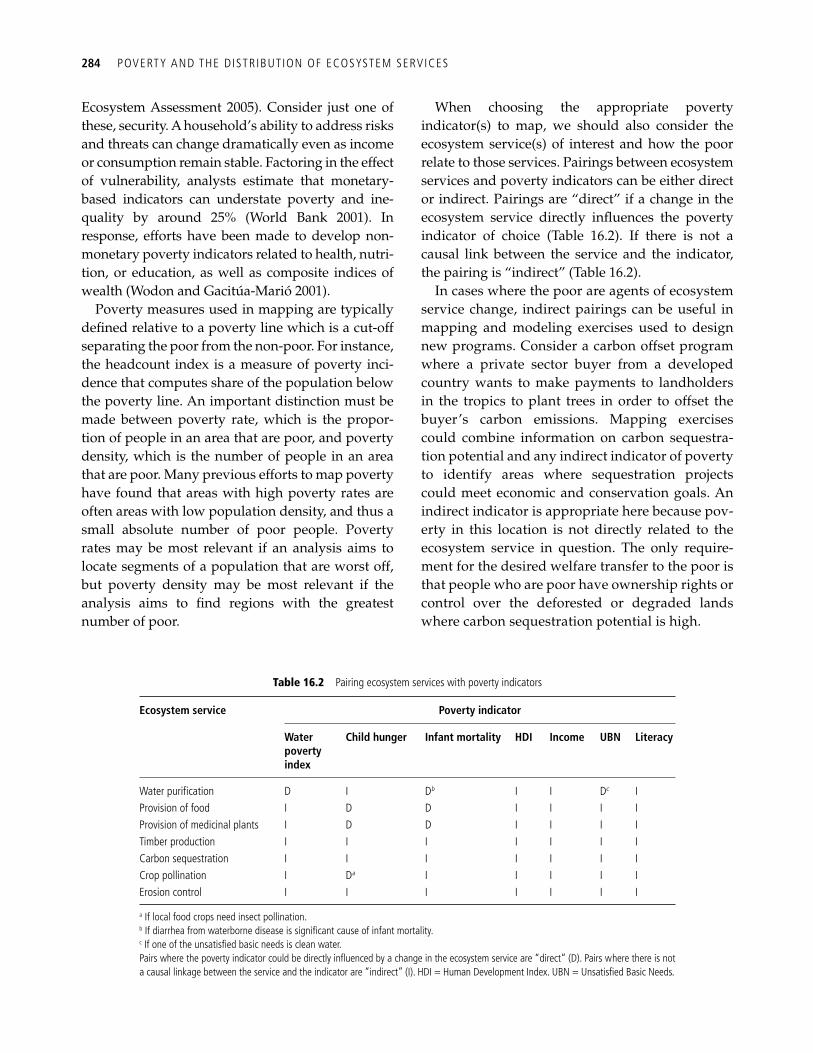
284 POVERTY AND THE DISTRIBUTION OF ECOSYSTEM SERVICES
Ecosystem Assessment 2005 ). Consider just one of these, security. A household’s ability to address risks and threats can change dramatically even as income or consumption remain stable. Factoring in the effect of vulnerability, analysts estimate that monetary-based indicators can understate poverty and ine-quality by around 25% ( World Bank 2001 ). In response, efforts have been made to develop non-monetary poverty indicators related to health, nutri-tion, or education, as well as composite indices of wealth (Wodon and Gacitúa-Marió 2001).
Poverty measures used in mapping are typically defi ned relative to a poverty line which is a cut-off separating the poor from the non-poor. For instance, the headcount index is a measure of poverty inci-dence that computes share of the population below the poverty line. An important distinction must be made between poverty rate, which is the propor-tion of people in an area that are poor, and poverty density, which is the number of people in an area that are poor. Many previous efforts to map poverty have found that areas with high poverty rates are often areas with low population density, and thus a small absolute number of poor people. Poverty rates may be most relevant if an analysis aims to locate segments of a population that are worst off, but poverty density may be most relevant if the analysis aims to fi nd regions with the greatest number of poor.
When choosing the appropriate poverty indicator(s) to map, we should also consider the ecosystem service(s) of interest and how the poor relate to those services. Pairings between ecosystem services and poverty indicators can be either direct or indirect. Pairings are “direct” if a change in the ecosystem service directly infl uences the poverty indicator of choice ( Table 16.2 ). If there is not a causal link between the service and the indicator, the pairing is “indirect” ( Table 16.2 ).
In cases where the poor are agents of ecosystem service change, indirect pairings can be useful in mapping and modeling exercises used to design new programs. Consider a carbon offset program where a private sector buyer from a developed country wants to make payments to landholders in the tropics to plant trees in order to offset the buyer’s carbon emissions. Mapping exercises could combine information on carbon sequestra-tion potential and any indirect indicator of poverty to identify areas where sequestration projects could meet economic and conservation goals. An indirect indicator is appropriate here because pov-erty in this location is not directly related to the ecosystem service in question. The only require-ment for the desired welfare transfer to the poor is that people who are poor have ownership rights or control over the deforested or degraded lands where carbon sequestration potential is high.
Table 16.2 Pairing ecosystem services with poverty indicators
Ecosystem service Poverty indicator
Water poverty index
Child hunger Infant mortality HDI Income UBN Literacy
Water purifi cation D I D b I I D c I Provision of food I D D I I I I Provision of medicinal plants I D D I I I I Timber production I I I I I I I Carbon sequestration I I I I I I I Crop pollination I D a I I I I I Erosion control I I I I I I I
a If local food crops need insect pollination. b If diarrhea from waterborne disease is signifi cant cause of infant mortality. c If one of the unsatisfi ed basic needs is clean water. Pairs where the poverty indicator could be directly infl uenced by a change in the ecosystem service are “direct” (D). Pairs where there is not a causal linkage between the service and the indicator are “indirect” (I). HDI = Human Development Index. UBN = Unsatisfi ed Basic Needs.
CASE STUDIES 285
When the poor are victims of environmental degra-dation, or benefi ciaries of services, improvements in well-being occur through improvements in service delivery, not through payments or incentives to the poor. In these cases, directly pairing ecosystem service provision with poverty indicators tied to the service(s) of interest is appropriate. For example, consider a change in the wetland mitigation example given above where the government requires developers to target offsets to benefi t the poor. The most appropriate poverty indicators to use are those associated with wetland benefi ts: hunger where wetlands provide fi sh for consumption, access to clean drinking water where wetlands provide water purifi cation, or fl ood vulner-ability where wetlands provide storm surge protec-tion. Using an income-based indicator, such as the percent of the population below the poverty line, to recommend the allocation of improved wetland serv-ices would be inappropriate if household income is not sensitive to changes in wetland services.
16.4 Case studies
The following two case studies represent some of the analyses we can do today. They highlight the types of decisions that can be informed by currently available data and methods, while identifying remaining challenges.
16.4.1 Deforestation in the Amazon Basin
The Amazon Basin is one of the world’s most threat-ened and most diverse ecosystems, in terms of both biological and cultural diversity (~380 ethnic groups; Porro et al. 2008). Many of the people who reside here, poor and non-poor alike, rely directly on ecosystem services for their subsistence and liveli-hoods (e.g., Clement 1993; Barham et al. 1999; Pattanayak and Sills 2001). Alarming rates of forest loss in the basin (Malhi et al. 2008) cause great con-cern for biodiversity loss, but we still have little sense of what this loss means for society beyond species extinction and climate change (e.g., Laurance 1998; Ferraz et al . 2003). In this case study, we address current and future provision of non-timber forest products (NTFP) and implications for the poor.
First, we used a mapping and valuation model (see Nelson et al. 2009) to predict current levels of
non-timber forest product harvest in the Amazon (Porro et al. 2008; see fi nal model in Chapter 8; results presented here are output from an earlier version of the NTFP model ). The model estimates the relative level of current NTFP harvest as a func-tion of the association between harvested species and habitat types, current NTFP stock (assuming that more pristine forests were harvested less in the past and have a higher stock of products for harvest today), travel time from population centers (³ 1000 people) along roads and waterways, and ease of product harvest and current legal protection from harvest (assuming enforcement) (Porro et al. 2008; Peralvo et al. 2008). Forest regions with greater stocks of an NTFP, that were easier to reach, and were currently open to all households were assumed to be harvested the most; the region with the high-est likely harvest has an index score of 1.0 for that NTFP. We focused on the provision of wood, fruits and nuts, and medicinal plants sold in the market and wood, fi ber, hunted bushmeat, fruits and nuts, and medicinal plants used for subsistence ( Figure 16.1 ).
Next, we used both direct and indirect pairings of these NTFP harvest projections with poverty indicators to determine if current NTFP harvest is aligned spatially with areas of poverty. We also investigated the impact of projected road expansion and deforestation over the next 20 years on the provision of NTFPs (deforestation scenario from the Instituto de Pesquisa Ambiental da Amazonia, road development scenario from the Initiative for Integration of Regional Infrastructure in the South (Porro et al. 2008)). These analyses are the fi rst step in understanding whether the poor are at a greater risk of losing their livelihood and well-being as a result of new roads and deforestation.
We represented current poverty with percentage of underweight (UW) children ( Figure 16.2a ; Plate 11a) and the percentage of the population with unsatisfi ed basic needs (UBN) ( Figure 16.2c ; Plate 11c). The resolution of UW children data var-ied by country and was generally very coarse (cen-sus blocks range in area from 13 202 km 2 to 3 778 690 km 2 ). Basic needs refer to any human need where lack of satisfaction is considered to be an indicator of deprivation or poor living conditions (Abaleron 1995). Basic needs, and the appropriate
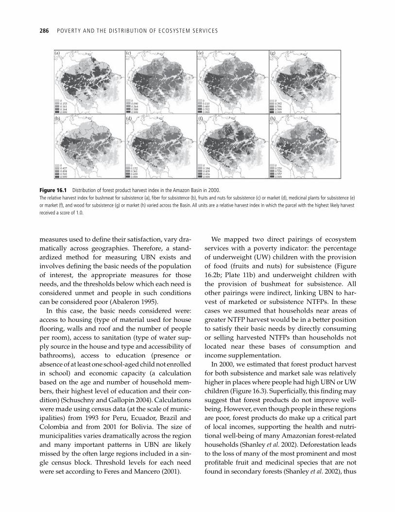
286 POVERTY AND THE DISTRIBUTION OF ECOSYSTEM SERVICES
measures used to defi ne their satisfaction, vary dra-matically across geographies. Therefore, a stand-ardized method for measuring UBN exists and involves defi ning the basic needs of the population of interest, the appropriate measures for those needs, and the thresholds below which each need is considered unmet and people in such conditions can be considered poor (Abaleron 1995).
In this case, the basic needs considered were: access to housing (type of material used for house fl ooring, walls and roof and the number of people per room), access to sanitation (type of water sup-ply source in the house and type and accessibility of bathrooms), access to education (presence or absence of at least one school-aged child not enrolled in school) and economic capacity (a calculation based on the age and number of household mem-bers, their highest level of education and their con-dition) (Schuschny and Gallopin 2004). Calculations were made using census data (at the scale of munic-ipalities) from 1993 for Peru, Ecuador, Brazil and Colombia and from 2001 for Bolivia. The size of municipalities varies dramatically across the region and many important patterns in UBN are likely missed by the often large regions included in a sin-gle census block. Threshold levels for each need were set according to Feres and Mancero (2001).
We mapped two direct pairings of ecosystem services with a poverty indicator: the percentage of underweight (UW) children with the provision of food (fruits and nuts) for subsistence ( Figure 16.2b ; Plate 11b) and underweight children with the provision of bushmeat for subsistence. All other pairings were indirect, linking UBN to har-vest of marketed or subsistence NTFPs. In these cases we assumed that households near areas of greater NTFP harvest would be in a better position to satisfy their basic needs by directly consuming or selling harvested NTFPs than households not located near these bases of consumption and income supplementation.
In 2000, we estimated that forest product harvest for both subsistence and market sale was relatively higher in places where people had high UBN or UW children ( Figure 16.3 ). Superfi cially, this fi nding may suggest that forest products do not improve well-being. However, even though people in these regions are poor, forest products do make up a critical part of local incomes, supporting the health and nutri-tional well-being of many Amazonian forest-related households (Shanley et al. 2002). Deforestation leads to the loss of many of the most prominent and most profi table fruit and medicinal species that are not found in secondary forests (Shanley et al. 2002), thus
0
(a) (c) (e) (g)
(b) (d) (f) (h)
0.1530.1610.1640.999
00.0900.3640.5880.999
00.1100.4000.7020.999
00.4270.4940.5020.999
00.1520.3610.4390.999
00.1840.4090.4160.999
00.2200.5260.5570.999
00.3920.5960.5990.999
Figure 16.1 Distribution of forest product harvest index in the Amazon Basin in 2000. The relative harvest index for bushmeat for subsistence (a), fi ber for subsistence (b), fruits and nuts for subsistence (c) or market (d), medicinal plants for subsistence (e) or market (f), and wood for subsistence (g) or market (h) varied across the Basin. All units are a relative harvest index in which the parcel with the highest likely harvest received a score of 1.0.
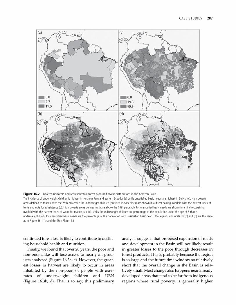
CASE STUDIES 287
continued forest loss is likely to contribute to declin-ing household health and nutrition.
Finally, we found that over 20 years, the poor and non-poor alike will lose access to nearly all prod-ucts analyzed ( Figure 16.3a , c). However, the great-est losses in harvest are likely to occur in areas inhabited by the non-poor, or people with lower rates of underweight children and UBN ( Figure 16.3b , d). That is to say, this preliminary
analysis suggests that proposed expansion of roads and development in the Basin will not likely result in greater losses to the poor through decreases in forest products. This is probably because the region is so large and the future time window so relatively short that the overall change in the Basin is rela-tively small. Most change also happens near already developed areas that tend to be far from indigenous regions where rural poverty is generally higher
(a)
0.87.717.5
0.019.395.3
(c)
(b) (d)
Figure 16.2 Poverty indicators and representative forest product harvest distributions in the Amazon Basin. The incidence of underweight children is highest in northern Peru and eastern Ecuador (a) while unsatisfi ed basic needs are highest in Bolivia (c). High poverty areas defi ned as those above the 75th percentile for underweight children (outlined in dark black) are shown in a direct pairing, overlaid with the harvest index of fruits and nuts for subsistence (b). High poverty areas defi ned as those above the 75th percentile for unsatisfi ed basic needs are shown in an indirect pairing, overlaid with the harvest index of wood for market sale (d). Units for underweight children are percentage of the population under the age of 5 that is underweight. Units for unsatisfi ed basic needs are the percentage of the population with unsatisfi ed basic needs. The legends and units for (b) and (d) are the same as in Figure 16.1 (c) and (h). (See Plate 11.)
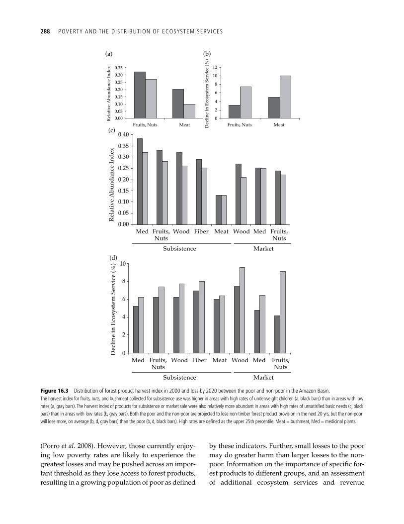
288 POVERTY AND THE DISTRIBUTION OF ECOSYSTEM SERVICES
(Porro et al. 2008). However, those currently enjoy-ing low poverty rates are likely to experience the greatest losses and may be pushed across an impor-tant threshold as they lose access to forest products, resulting in a growing population of poor as defi ned
by these indicators. Further, small losses to the poor may do greater harm than larger losses to the non-poor. Information on the importance of specifi c for-est products to different groups, and an assessment of additional ecosystem services and revenue
(a)
(c)
(d)
0.350.30
0.250.20
0.15
0.100.05
Rel
ativ
e A
bund
ance
Inde
xR
elat
ive
Abu
ndan
ce In
dex
0.00
0.40
Fruits, Nuts Meat
(b)
12
10
8
6
4
2
0
Dec
line
in E
cosy
stem
Ser
vice
(%)
Dec
line
in E
cosy
stem
Ser
vice
(%)
Fruits, Nuts Meat
0.35
0.30
0.25
0.20
0.15
0.10
0.05
0.00
10
8
6
4
2
0Med Fruits,
NutsWood Fiber Meat Wood Med Fruits,
Nuts
Med Fruits,Nuts
Wood Fiber Meat Wood Med Fruits,Nuts
MarketSubsistence
MarketSubsistence
Figure 16.3 Distribution of forest product harvest index in 2000 and loss by 2020 between the poor and non-poor in the Amazon Basin. The harvest index for fruits, nuts, and bushmeat collected for subsistence use was higher in areas with high rates of underweight children (a, black bars) than in areas with low rates (a, gray bars). The harvest index of products for subsistence or market sale were also relatively more abundant in areas with high rates of unsatisfi ed basic needs (c, black bars) than in areas with low rates (b, gray bars). Both the poor and the non-poor are projected to lose non-timber forest product provision in the next 20 yrs, but the non-poor will lose more, on average (b, d, gray bars) than the poor (b, d, black bars). High rates are defi ned as the upper 25th percentile. Meat = bushmeat, Med = medicinal plants.
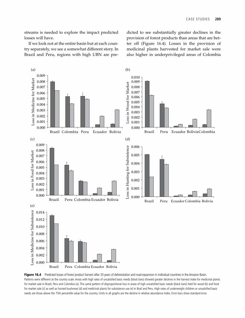
CASE STUDIES 289
streams is needed to explore the impact predicted losses will have.
If we look not at the entire basin but at each coun-try separately, we see a somewhat different story. In Brazil and Peru, regions with high UBN are pre-
dicted to see substantially greater declines in the provision of forest products than areas that are bet-ter off ( Figure 16.4 ). Losses in the provision of medicinal plants harvested for market sale were also higher in underprivileged areas of Colombia
0.000
0.001
Brazil Colombia Peru Ecuador Bolivia
0.002
Loss
in M
edic
ine
for
Mar
ket
0.0030.0040.0050.006
0.0070.008
0.009
(a) (b)
(c)
(e)
(d)
0.0000.001
Brazil ColombiaPeru Ecuador Bolivia
0.002
Loss
in F
ood
for
Mar
ket
0.0030.0040.0050.006
0.0070.0080.009
0.000Brazil ColombiaPeru Ecuador Bolivia
0.002
Loss
in M
edic
ine
for
Subs
iste
nce
0.004
0.006
0.008
0.010
0.012
0.014
0.000
0.001
Brazil ColombiaPeru Ecuador Bolivia
0.002
Loss
in H
untin
g fo
r Su
bsis
tenc
e
0.003
0.004
0.005
0.006
0.000
0.002
Brazil ColombiaPeru Ecuador Bolivia
0.001
0.003
Loss
in W
ood
for
Mar
ket
0.0040.0050.0060.0070.0080.0090.010
Figure 16.4 Predicted losses of forest product harvest after 20 years of deforestation and road expansion in individual countries in the Amazon Basin. Patterns were different at the country scale. Areas with high rates of unsatisfi ed basic needs (black bars) showed greater declines in the harvest index for medicinal plants for market sale in Brazil, Peru and Colombia (a). This same pattern of disproportional loss in areas of high unsatisfi ed basic needs (black bars) held for wood (b) and food for market sale (c) as well as hunted bushmeat (d) and medicinal plants for subsistence use (e) in Brail and Peru. High rates of underweight children or unsatisfi ed basic needs are those above the 75th percentile value for the country. Units in all graphs are the decline in relative abundance index. Error bars show standard error.
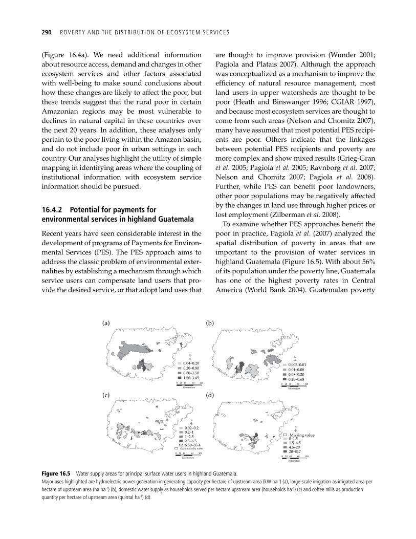
290 POVERTY AND THE DISTRIBUTION OF ECOSYSTEM SERVICES
( Figure 16.4a ). We need additional information about resource access, demand and changes in other ecosystem services and other factors associated with well-being to make sound conclusions about how these changes are likely to affect the poor, but these trends suggest that the rural poor in certain Amazonian regions may be most vulnerable to declines in natural capital in these countries over the next 20 years. In addition, these analyses only pertain to the poor living within the Amazon basin, and do not include poor in urban settings in each country. Our analyses highlight the utility of simple mapping in identifying areas where the coupling of institutional information with ecosystem service information should be pursued.
16.4.2 Potential for payments for environmental services in highland Guatemala
Recent years have seen considerable interest in the development of programs of Payments for Environ-mental Services (PES). The PES approach aims to address the classic problem of environmental exter-nalities by establishing a mechanism through which service users can compensate land users that pro-vide the desired service, or that adopt land uses that
are thought to improve provision (Wunder 2001; Pagiola and Platais 2007). Although the approach was conceptualized as a mechanism to improve the effi ciency of natural resource management, most land users in upper watersheds are thought to be poor (Heath and Binswanger 1996; CGIAR 1997 ), and because most ecosystem services are thought to come from such areas (Nelson and Chomitz 2007), many have assumed that most potential PES recipi-ents are poor. Others indicate that the linkages between potential PES recipients and poverty are more complex and show mixed results (Grieg-Gran et al. 2005; Pagiola et al. 2005; Ravnborg et al. 2007; Nelson and Chomitz 2007; Pagiola et al. 2008). Further, while PES can benefi t poor landowners, other poor populations may be negatively affected by the changes in land use through higher prices or lost employment (Zilberman et al. 2008).
To examine whether PES approaches benefi t the poor in practice, Pagiola et al . (2007) analyzed the spatial distribution of poverty in areas that are important to the provision of water services in highland Guatemala ( Figure 16.5 ). With about 56% of its population under the poverty line, Guatemala has one of the highest poverty rates in Central America ( World Bank 2004 ). Guatemalan poverty
(a) (b)
(c)
0.04–0.20
N
0 20 40 60
Kilometers
120
0.20–0.800.80–1.501.50–3.45
(d)
0.02–0.2
N
0 20 40 60
Kilometers
Guatemala city metro
100
0.2–11–2.52.5–6.56.50–55.4
0–1.5
N
0 20 40 60
Kilometers
100
1.5–4.54.5–2020–817
Missing value
0.005–0.01
N
0 20 40 60
Kilometers
120
0.01–0.080.08–0.200.20–0.68
Figure 16.5 Water supply areas for principal surface water users in highland Guatemala. Major uses highlighted are hydroelectric power generation in generating capacity per hectare of upstream area (kW ha -1 ) (a), large-scale irrigation as irrigated area per hectare of upstream area (ha ha -1 ) (b), domestic water supply as households served per hectare upstream area (households ha -1 ) (c) and coffee mills as production quantity per hectare of upstream area (quintal ha -1 ) (d).
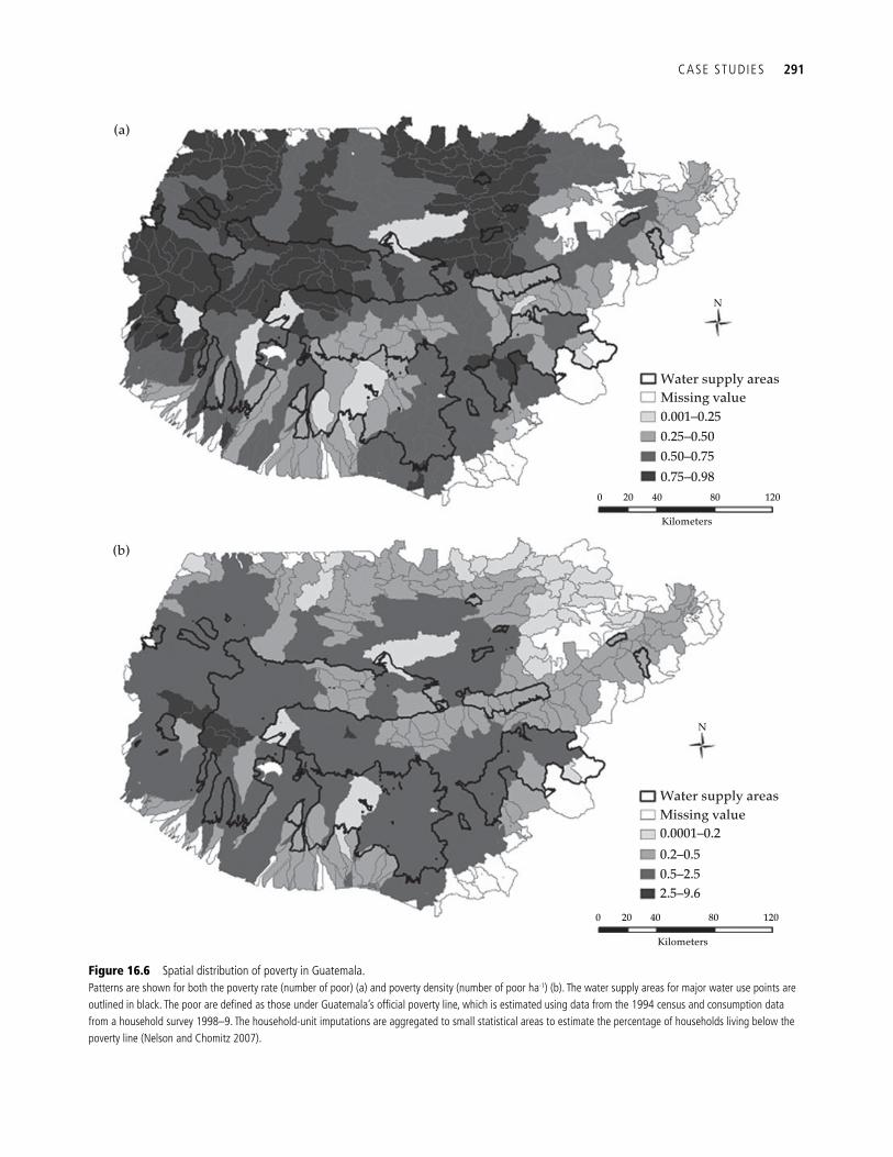
CASE STUDIES 291
(a)
(b)
Water supply areasMissing value0.001–0.250.25–0.500.50–0.750.75–0.98
0 20 40 80
Kilometers
120
N
Water supply areasMissing value0.0001–0.20.2–0.50.5–2.52.5–9.6
0 20 40 80
Kilometers
120
N
Figure 16.6 Spatial distribution of poverty in Guatemala. Patterns are shown for both the poverty rate (number of poor) (a) and poverty density (number of poor ha -1 ) (b). The water supply areas for major water use points are outlined in black. The poor are defi ned as those under Guatemala’s offi cial poverty line, which is estimated using data from the 1994 census and consumption data from a household survey 1998–9. The household-unit imputations are aggregated to small statistical areas to estimate the percentage of households living below the poverty line (Nelson and Chomitz 2007).
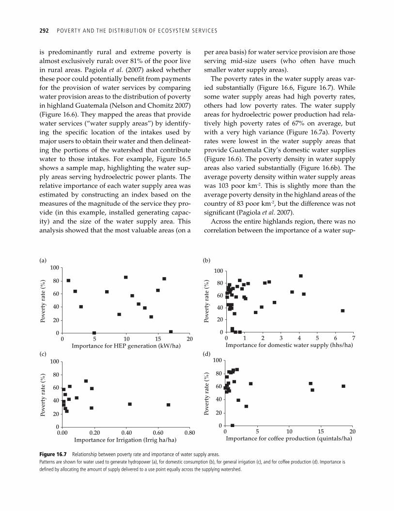
292 POVERTY AND THE DISTRIBUTION OF ECOSYSTEM SERVICES
is predominantly rural and extreme poverty is almost exclusively rural : over 81% of the poor live in rural areas. Pagiola et al. (2007) asked whether these poor could potentially benefi t from payments for the provision of water services by comparing water provision areas to the distribution of poverty in highland Guatemala (Nelson and Chomitz 2007) ( Figure 16.6 ). They mapped the areas that provide water services (“water supply areas”) by identify-ing the specifi c location of the intakes used by major users to obtain their water and then delineat-ing the portions of the watershed that contribute water to those intakes. For example, Figure 16.5 shows a sample map, highlighting the water sup-ply areas serving hydroelectric power plants. The relative importance of each water supply area was estimated by constructing an index based on the measures of the magnitude of the service they pro-vide (in this example, installed generating capac-ity) and the size of the water supply area. This analysis showed that the most valuable areas (on a
per area basis) for water service provision are those serving mid-size users (who often have much smaller water supply areas).
The poverty rates in the water supply areas var-ied substantially ( Figure 16.6 , Figure 16.7 ). While some water supply areas had high poverty rates, others had low poverty rates. The water supply areas for hydroelectric power production had rela-tively high poverty rates of 67% on average, but with a very high variance ( Figure 16.7a ). Poverty rates were lowest in the water supply areas that provide Guatemala City’s domestic water supplies ( Figure 16.6 ). The poverty density in water supply areas also varied substantially ( Figure 16.6b ). The average poverty density within water supply areas was 103 poor km -2 . This is slightly more than the average poverty density in the highland areas of the country of 83 poor km -2 , but the difference was not signifi cant (Pagiola et al. 2007).
Across the entire highlands region, there was no correlation between the importance of a water sup-
100(a)
80
60
40
20Pove
rty
rate
(%)
00 5 10
Importance for HEP generation (kW/ha)15 20
100
80
60
40
20
(c)
Pove
rty
rate
(%)
00.00 0.20 0.40
Importance for Irrigation (Irrig ha/ha)0.60 0.80
100
80
60
40
20
(d)
Pove
rty
rate
(%)
00 5 10Importance for coffee production (quintals/ha)
15 20
100
(b)
80
60
40
20Pove
rty
rate
(%)
00 2Importance for domestic water supply (hhs/ha)
6 73 4 51
Figure 16.7 Relationship between poverty rate and importance of water supply areas. Patterns are shown for water used to generate hydropower (a), for domestic consumption (b), for general irrigation (c), and for coffee production (d). Importance is defi ned by allocating the amount of supply delivered to a use point equally across the supplying watershed.
INCLUDING INST ITUTIONS: THE WAY FORWARD 293
ply area and the poverty rate of people living within it ( Figure 16.7 ). However, there were at least some areas with high water service provision and a high incidence of poverty. This suggests that payments targeted to these areas would have the potential to meet the joint goals of ecosystem service provision and poverty alleviation. However, these analyses do not include information about the nature of insti-tutions in the region governing control of the water supply or the relationship between the poor and water-regulating land-use activities. The poor in important water supply watersheds may have no control over land-use practices that alter the provi-sion of water-related services, and as such, pay-ments made to the poor may not result in ecosystem service returns. If the poor control water resources and PES mechanisms were developed in all the water supply areas, 1.76 million people, or 73% of the poor in highland Guatemala could potentially be reached. This fi gure engenders enough promise that taking the next step to identify water resource institutions in highland Guatemala would be well worth the investment.
16.5 Including institutions: the way forward
As the case studies demonstrate, overlaying maps of poverty indicators and ecosystem services can be an informative fi rst step in understanding the com-plex relationships between the poor and the envi-ronment, but it is not suffi cient. Current poverty mapping seldom makes explicit connections between the poor and the resources they rely on. For example, poverty maps rarely distinguish between land owners and the landless, simply because the necessary information is not available. Land users that are renters have less ability to dic-tate how resources are managed. Similarly, even if land users have title to their land, their tenure may be insecure or not supported by local institutions. Again, this will inhibit their ability to change practices and alter the level of ecosystem services provided by the landscape. Information about insti-tutions such as property rights, ownership, or man-agement responsibility, and their stability must be incorporated into poverty mapping exercises to maximize their utility for understanding who
currently provides and benefi ts from ecosystem services, and who will gain or lose from future man-agement changes.
References
Abaleron, C. A. (1995). Marginal urban space and unsatis-fi ed basic needs: the case of San Carlos de Bariloche, Argentina. Environment and Urbanization, 7, 97–116.
Adhikari, B. (2005). Poverty, property rights and collective action: understanding the distributive aspects of com-mon property resource management. Environment and Development Economics, 10, 7–31.
Albla-Betrand, J. M. (1993). The political economy of large natural disasters. Clarendon Press, Oxford.
Andam, K. S., Ferraro, P. J., Sims, K. R. E., et al . (2010). Protected areas reduced poverty in Costa Rica and Thailand. Proceedings of the National Academy of Sciences of the USA , 107, 9996–10001.
Baland, J., Bardhan, P., Das, S., et al . (2006). Managing the environmental consequences of growth: Forest degradation in the Indian mid-Himalayas . National Council of Applied Economic Research, India, New Delhi.
Barham, B. L., Coomes, O. T. and Takasaki, Y. (1999). Rainforest livelihoods: income generation, household wealth and forest use. Unasylva, 50, 34–42.
Bedi, T., Coudouel, A. and Simler, K. (2007). More than a pretty picture: using poverty maps to design better policies and interventions . World Bank, Washington, DC.
BenDor, T., Brozovic, N., and Pallathucheril, V. G. (2008). The social impacts of wetland mitigation policies in the United States. Journal of Planning Literature , 22 , 341–57.
Bluffstone, R. (1995). The effects of labor markets on defor-estation in developing countries under open access: an example from rural Nepal. Journal of Environmental Economics and Management, 29, 42–63.
Cavendish, W. (2000). Empirical regularities in the poverty-environment relationship of rural households: Evidence from Zimbabwe. World Development, 28, 1979–2003.
CGIAR. (1997). Report of the study on CBIAR research priori-ties for marginal lands . Consultative Group on International Agricultural Research, Technical Advisory Committee Secretariat, Food and Agriculture Organization of the United Nations, Rome.
Chen, S., and Ravallion, M. (2008). The developing world is poorer than we thought, but no less successful in the fi ght against poverty . World Bank, Washington, DC.
Clement, C. (1993). Native Amazonian fruits and nuts: Composition, production and potential use for sustainable development. UNESCO, New York.
294 POVERTY AND THE DISTRIBUTION OF ECOSYSTEM SERVICES
Delang, C. O. (2006). The role of wild food plants in pov-er4ty alleviation and biodiversity conservation in tropi-cal countries. Progress in Development Studies, 6, 275–86.
Duraiappah, A. K. (1998). Poverty environment degrada-tion: A review and analyses of the nexus. World Development, 26, 2169–79.
Elbers, C., Lanjouw, J. O., and Lanjouw, P. F. (2002). Micro-level estimation of welfare . World Bank, Washington, DC.
Feres, J. C. and Mancero, X. (2001). El metodo de las necesi-dades basicas insatisfechas (NBI) y sus aplicaciones en America Latina. Division de Estadistica y Proyecciones Economicas, CEPAL-ECLAC, Bogota.
Ferraro, P. J. (2002). The local costs of establishing protected areas in low-income nations: Ranomafana National Park, Madagascar. Ecological Economics, 43 , 261–75.
Ferraz, G., Russel, G. J., Stouffer, P. C., et al . (2003). Rates of species loss from Amazonian forest fragments. Proceedings of the National Academy of Sciences of the USA, 100, 14069–73.
Grieg-Gran, M., Porras, I., and Wunder, S. (2005). How can market mechanisms for forest environmental services help the poor? Preliminary lessons from Latin America. World Development, 33, 1511–27.
Heath, J., and Binswanger, H. (1996). Natural resource degradation effects of poverty and population growth are largely policy-induced: the case of Colombia. Environment and Development Economics, 1, 65–84.
Hentschel, J., Lanjouw, J. O., Lanjouw, P. F., et al . (2000). Combining census and survey data to trace the spatial dimensions of poverty: A case study of Ecuador. World Bank Economic Review, 14, 147–65.
Jodha, N. S. (1986). Common property resources and the rural poor in dry regions of India. Economic and Political Weekly , 21 , 1169-81.
Justice, C., Wilkie, D., Zhang, Q., et al . (2001). Central African forests, carbon and climate change. Climate Research, 17, 229–46.
Laurance, W. F. (1998). A crisis in the making: responses of Amazonian forests to land use and climate change. Trends in Ecology and Evolution , 13 , 411–15.
Luoga, E. M., Witkowski, E. T. F., and Balkwill, K. (2000). Economics of charcoal production in miombo wood-lands of eastern Tanzania: some hidden costs associated with commercialization of the resources. Ecological Economics, 35 , 243–57.
McSweeney, K. (2005). Natural insurance, forest access and compounded misfortune: forest resources in small-holder coping strategies before and after Hurricane Mitch, north eastern Honduras. World Development, 33, 1453–71.
Mäler, K., Aniyar, S., and Jansson, A. (2008). Accounting for ecosystem services as a way to understand the require-
ments for sustainable development. Proceedings of the National Academy of Sciences of the USA, 105, 9501–6.
Malhi, Y., Roberts, J. T., Betts, R. A., et al . (2008). Climate change, deforestation, and the fate of the Amazon. Science, 319, 169–72.
Millennium Ecosystem Assessment. (2005). Ecosystems and human well-being: synthesis . Island Press, Washington, DC.
Minot, N. (2000). Generating disaggregated poverty maps: an application in Vietnam. World Development, 28, 319–31.
Müller, D., Epprecht, M., and Sunderlin, W. D. (2006). Where are the poor and where are the trees? Targeting of pov-erty reduction and forest conservation in Vietnam . CIFOR, Bogor.
Narain, U., Gupta, S., and Van ‘t Veld, K. (2005). Poverty and the environment: exploring the relationship between household incomes, private assets, and natural assets. Poverty Reduction and Environmental Management (PREM) Working Paper 05/09. Institute for Environmental Studies, Vrije University, Amsterdam.
Ndangalasi, H. J., Bitariho, R., and Dovie, D. B. K. (2007). Harvesting of non-timber forest products and implica-tions for conservation in two montate forests of East Africa. Biological Conservation, 134 , 242–50.
Nelson, A., and Chomitz, K. (2007). The forest-hydrology-poverty nexus in Central America: An heuristic analysis. Environment, Development and Sustainability, 9, 369–85.
Nelson, E. N., Mendoza, G. M., Regetz, J. et al. (2009). Modeling multiple ecosystem services, biodiversity conservation, commodity production and tradeoffs at landscape scales. Frontiers in Ecology and the Environment , 7 , 4–11.
Pagiola, S., Arcenas, A. and Platais, G. (2005). Can pay-ments for environmental services help reduce poverty? An exploration of the issues and the evidence to date from Latin America. World Development, 33, 237–53.
Pagiola, S., and Platais, G. (2007). Payments for environmen-tal services: from theory to Practice. World Bank, Washington, DC.
Pagiola, S., Zhang, W. and Colom, A. (2007). Assessing the potential for payments for watershed services to reduce poverty in highland Guatemala . World Bank, Washington, DC.
Pagiola, S., Rios, A. R., and Arcenas, A. (2008). Can the poor participate in payments for environmental serv-ices? Lessons from the Silvopastoral Project in Nicaragua. Environment and Development Economics, 13, 299–325.
Pattanayak, S. K., and Sills, E. O. (2001). Do tropical forests provide natural insurance? The microeconomics of non-timber forest product collection in the Brazilian Amazon. Land Economics, 77, 595–612.
INCLUDING INST ITUTIONS: THE WAY FORWARD 295
Peralvo, M., Benitez, S., Nelson, E., et al . (2008). Mapping spatial patterns of supply and demand of ecosystem services in the Amazon Basin. The Nature Conservancy, Quito.
Poggi, J., Lanjouw, J. O., Hentschel, J., et al . (1998). Combining census and survey data to study spatial dimen-sions of poverty . World Bank, Washington, DC.
Porro, R., Borner, J., Jarvis, A., et al. (2008). Challenges to managing ecosystems sustainably for poverty alleviation: securing well-being in the Andes/Amazon. Amazon Initiative Consortium, Belem.
Ravnborg, H. M., Damsgaard, M. G., and Raben, K. (2007). Payment for ecosystem services-issues and pro-poor opportu-nities for development assistance . Danish Institute for International Studies, Copenhangen.
Roe, D., and Elliott, J. (2004). Poverty reduction and biodiver-sity conservation: rebuilding the bridges. Oryx, 38, 137–9.
Ruhl, J. B., and Salzman, J. (2006). The effects of wetland mitigation banking on people. National Wetlands Newsletter, 28, 9–14.
Sanderson, S. E., and Redford, K. H. (2003). Contested relationships between biodiversity conservation and poverty alleviation. Oryx, 37, 389–90.
Scherr, S. J., White, A., and Kaimowitz, D. (2003). A new agenda for forest conservation and poverty reduction . Forest Trends, Washington, DC.
Schuschny, A. R., and Gallopin, G. C. (2004). La distribu-cion espacial de la pobreza en relacion a los sistemas ambien-tales en America Latina . Division de Desarrollo Sostenible y Asentamientos Humanos, United Nations, Santiago.
Shanley, P., Luz, L., and Swingland, I. R. (2002). The faint promise of a distant market: a survey of Belem’s trade in non-timber forest products. Biodiversity and Conservation, 11, 615–36.
Shyamsundar, P. (2001). Poverty-environment indicators . World Bank, Washington, DC.
Takasaki, Y., Barham, B. L., and Coomes, O. T. (2004). Risk coping strategies in tropical forests: Flood, illnesses and resource extraction. Environment and Development Economics, 9, 203–24.
UNEP. (2004). Human well-being, poverty and ecosystem services: exploring the links. Premier Printing, Winnipeg.
Vedeld, P., Angelsen, A., Bojö, J., et al . (2004). Forest envi-ronmental incomes and the rural poor. Forest Policy and Economics , 9 , 869–79.
Wodon, Q., and Gacitúa-Marió, E. (2001). Measurement and meaning: combiing quantative and qualitative methods for the analysis of poverty and social exclusion in Latin America . World Bank, Washington, DC.
World Bank. (2001). World Development Report 2000/2001: attacking poverty. Oxford University Press, Oxford.
World Bank. (2004). Poverty in Guatemala . World Bank, Washington, DC.
World Bank. (2008). P overty and the environment: under-standing linkages at the household level. World Bank, Washington, DC.
World Resources Institute. (2007). Nature’s benefi ts in Kenya: an atlas of ecosystems and human well-being. World Resources Institute, Nairobi.
Wunder, S. (2001). Poverty alleviation and tropical forests: What scope for synergies? World Development, 29, 1817–33.
Zilberman, D., Lipper, L., and McCarthy, N. (2008). When could payments for environmental services benefi t the poor? Environment and Development Economics , 13 , 255–78.
296
CHAPTER 17
Ecosystem service assessments for marine conservation Anne D. Guerry, Mark L. Plummer, Mary H. Ruckelshaus, and Chris J. Harvey
17.1 Introduction
Humans always have benefi ted from marine eco-systems—either obviously in the form of food resources, or more subtly in the form of cultural and recreational opportunities. For example, 80–85 mil-lion tons of fi sh were landed in marine capture fi sh-eries worldwide in 2006, and fi sh account for approximately 15% of the annual animal protein consumption by humans ( FAO Fisheries Department 2009 ). A growing recognition of the degradation of global marine ecosystems has led to numerous calls for a shift toward more holistic, ecosystem-based management of marine systems ( Pew Oceans Commission 2003 ; US Commission on Ocean Policy 2004 ; Council on Environmental Quality 2009 ). Ecosystem-based management is a coordinated effort to manage the diverse human impacts that affect an ecosystem to ensure the sustainability of the ecosystem services it provides (Rosenberg and Mcleod 2005). Two key aspects of ecosystem-based management are relevant here. First, ecosystem-based management fundamentally recognizes the inseparability of human and ecological systems. Human well-being is derived from ecosystems through ecosystem services and, in turn, human behavior affects natural systems. Second, ecosys-tem-based management is inherently multifaceted, encompassing suites of services, rather than the tra-ditional approach of sector-by-sector management. Importantly, the framework of ecosystem services can provide performance metrics for different management strategies that attempt to balance multiple objectives by allowing for the explicit
examination of trade-offs in ecosystem services provided under alternative management scenarios (National Research Council 2004).
Using an ecosystem services framework also has the potential to draw a larger and more diverse population of people to marine and other conserva-tion efforts, beyond those who value the environ-ment purely for its direct uses. For example, many residents are drawn to the Puget Sound region, USA because of the sound’s physical beauty and con-comitant aesthetic benefi ts to their well-being. Indeed, existence values have been found to be among the “most important” benefi ts provided by the Puget Sound system ( Iceland et al. 2008 ). If such cultural values can be included in tallies of the con-sequences of ecosystem protection, conservation efforts are likely to engage a greater fraction of the population. Helping people to see the many ways their well-being is affected by marine and coastal environments is key to the success of conservation.
In principle, marine ecosystem services are not fundamentally different from their terrestrial coun-terparts. In practice, however, the valuation and mapping of ecosystem services in marine environ-ments is not as well developed as it is for terrestrial ecosystems. As described in Chapters 4 – 13 , there have been some early successes applying ecosystem service mapping and modeling tools in diverse ter-restrial and freshwater settings. These approaches and models all start with basic land cover and land-use data layers. The same approach can work for marine environments—marine systems have patchy habitats that provide fl ows of ecosystem services, and management actions can alter those habitats
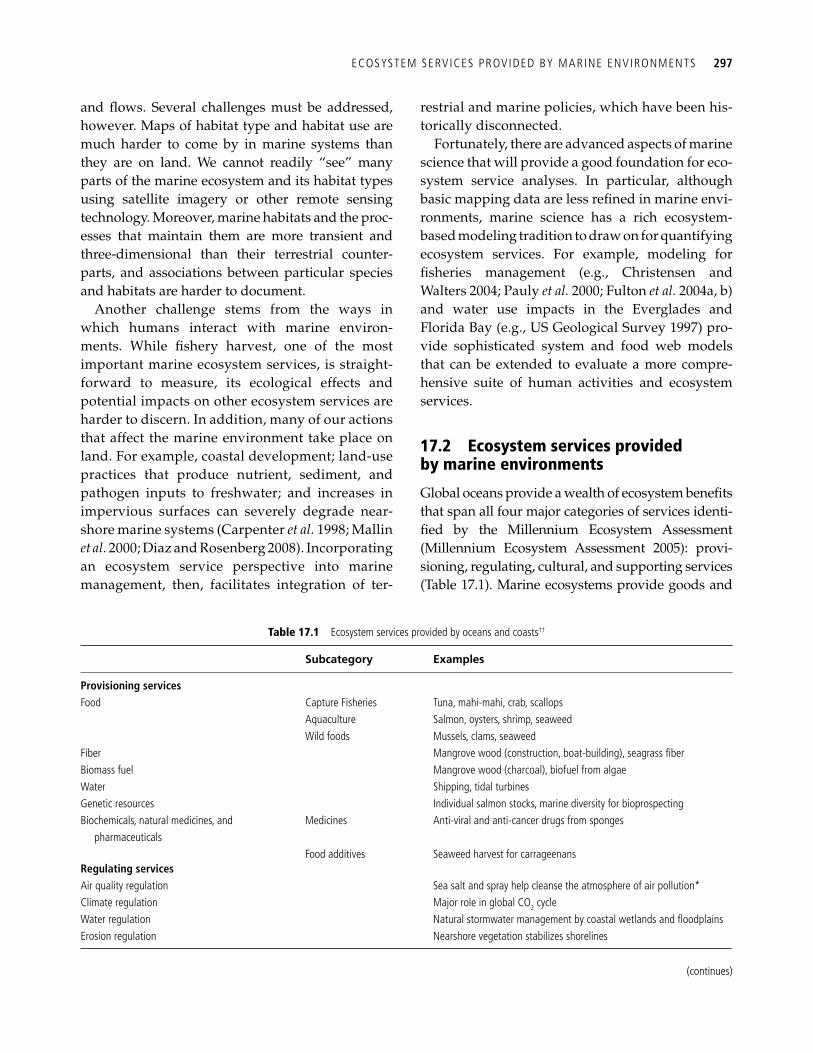
ECOSYSTEM SERVICES PROVIDED BY MARINE ENVIRONMENTS 297
and fl ows. Several challenges must be addressed, however. Maps of habitat type and habitat use are much harder to come by in marine systems than they are on land. We cannot readily “see” many parts of the marine ecosystem and its habitat types using satellite imagery or other remote sensing technology. Moreover, marine habitats and the proc-esses that maintain them are more transient and three-dimensional than their terrestrial counter-parts, and associations between particular species and habitats are harder to document.
Another challenge stems from the ways in which humans interact with marine environ-ments. While fi shery harvest, one of the most important marine ecosystem services, is straight-forward to measure, its ecological effects and potential impacts on other ecosystem services are harder to discern. In addition, many of our actions that affect the marine environment take place on land. For example, coastal development; land-use practices that produce nutrient, sediment, and pathogen inputs to freshwater; and increases in impervious surfaces can severely degrade near-shore marine systems ( Carpenter et al. 1998 ; Mallin et al. 2000 ; Diaz and Rosenberg 2008 ). Incorporating an ecosystem service perspective into marine management, then, facilitates integration of ter-
restrial and marine policies, which have been his-torically disconnected.
Fortunately, there are advanced aspects of marine science that will provide a good foundation for eco-system service analyses. In particular, although basic mapping data are less refi ned in marine envi-ronments, marine science has a rich ecosystem-based modeling tradition to draw on for quantifying ecosystem services. For example, modeling for fi sheries management (e.g., Christensen and Walters 2004 ; Pauly et al. 2000 ; Fulton et al. 2004a , b ) and water use impacts in the Everglades and Florida Bay (e.g., US Geological Survey 1997 ) pro-vide sophisticated system and food web models that can be extended to evaluate a more compre-hensive suite of human activities and ecosystem services.
17.2 Ecosystem services provided by marine environments
Global oceans provide a wealth of ecosystem benefi ts that span all four major categories of services identi-fi ed by the Millennium Ecosystem Assessment ( Millennium Ecosystem Assessment 2005 ): provi-sioning, regulating, cultural, and supporting services ( Table 17.1 ). Marine ecosystems provide goods and
Table 17.1 Ecosystem services provided by oceans and coasts ††
Subcategory Examples
Provisioning services Food Capture Fisheries Tuna, mahi-mahi, crab, scallops Aquaculture Salmon, oysters, shrimp, seaweed Wild foods Mussels, clams, seaweed Fiber Mangrove wood (construction, boat-building), seagrass fi ber Biomass fuel Mangrove wood (charcoal), biofuel from algae Water Shipping, tidal turbines Genetic resources Individual salmon stocks, marine diversity for bioprospecting Biochemicals, natural medicines, and
pharmaceuticals Medicines Anti-viral and anti-cancer drugs from sponges
Food additives Seaweed harvest for carrageenans Regulating services Air quality regulation Sea salt and spray help cleanse the atmosphere of air pollution * Climate regulation Major role in global CO 2 cycle Water regulation Natural stormwater management by coastal wetlands and fl oodplains Erosion regulation Nearshore vegetation stabilizes shorelines
(continues)
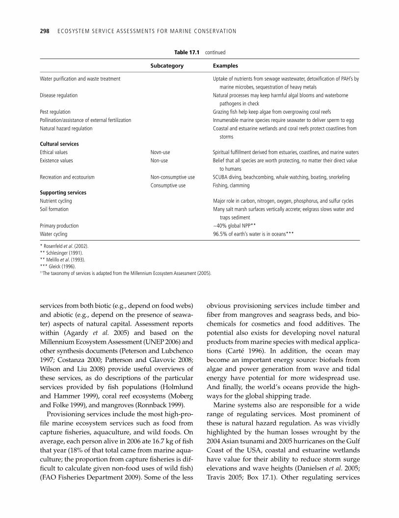
298 ECOSYSTEM SERVICE ASSESSMENTS FOR MARINE CONSERVATION
services from both biotic (e.g., depend on food webs) and abiotic (e.g., depend on the presence of seawa-ter) aspects of natural capital. Assessment reports within ( Agardy et al. 2005 ) and based on the Millennium Ecosystem Assessment (UNEP 2006) and other synthesis documents ( Peterson and Lubchenco 1997 ; Costanza 2000 ; Patterson and Glavovic 2008; Wilson and Liu 2008 ) provide useful overviews of these services, as do descriptions of the particular services provided by fi sh populations ( Holmlund and Hammer 1999 ), coral reef ecosystems ( Moberg and Folke 1999 ), and mangroves ( Ronnback 1999 ).
Provisioning services include the most high-pro-fi le marine ecosystem services such as food from capture fi sheries, aquaculture, and wild foods. On average, each person alive in 2006 ate 16.7 kg of fi sh that year (18% of that total came from marine aqua-culture; the proportion from capture fi sheries is dif-fi cult to calculate given non-food uses of wild fi sh) ( FAO Fisheries Department 2009 ). Some of the less
obvious provisioning services include timber and fi ber from mangroves and seagrass beds, and bio-chemicals for cosmetics and food additives. The potential also exists for developing novel natural products from marine species with medical applica-tions (Carté 1996). In addition, the ocean may become an important energy source: biofuels from algae and power generation from wave and tidal energy have potential for more widespread use. And fi nally, the world’s oceans provide the high-ways for the global shipping trade.
Marine systems also are responsible for a wide range of regulating services. Most prominent of these is natural hazard regulation. As was vividly highlighted by the human losses wrought by the 2004 Asian tsunami and 2005 hurricanes on the Gulf Coast of the USA, coastal and estuarine wetlands have value for their ability to reduce storm surge elevations and wave heights ( Danielsen et al. 2005 ; Travis 2005 ; Box 17.1 ). Other regulating services
Subcategory Examples
Water purifi cation and waste treatment Uptake of nutrients from sewage wastewater, detoxifi cation of PAH’s by marine microbes, sequestration of heavy metals
Disease regulation Natural processes may keep harmful algal blooms and waterborne pathogens in check
Pest regulation Grazing fi sh help keep algae from overgrowing coral reefs Pollination/assistance of external fertilization Innumerable marine species require seawater to deliver sperm to egg Natural hazard regulation Coastal and estuarine wetlands and coral reefs protect coastlines from
storms Cultural services Ethical values Novn-use Spiritual fulfi llment derived from estuaries, coastlines, and marine waters Existence values Non-use Belief that all species are worth protecting, no matter their direct value
to humans Recreation and ecotourism Non-consumptive use SCUBA diving, beachcombing, whale watching, boating, snorkeling Consumptive use Fishing, clamming Supporting services Nutrient cycling Major role in carbon, nitrogen, oxygen, phosphorus, and sulfur cycles Soil formation Many salt marsh surfaces vertically accrete; eelgrass slows water and
traps sediment Primary production ~40% global NPP ** Water cycling 96.5% of earth’s water is in oceans ***
* Rosenfeld et al . ( 2002 ). ** Schlesinger ( 1991 ). ** Melillo et al . ( 1993 ). *** Gleick ( 1996 ). ††The taxonomy of services is adapted from the Millennium Ecosystem Assessment ( 2005 ).
Table 17.1 continued
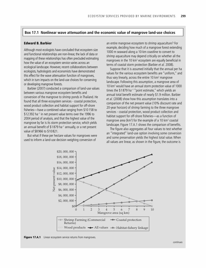
ECOSYSTEM SERVICES PROVIDED BY MARINE ENVIRONMENTS 299
Edward B. Barbier
Although most ecologists have concluded that ecosystem size and functional relationships are non-linear, the lack of data or mapping of these relationships has often precluded estimating how the value of an ecosystem service varies across an ecological landscape. However, recent collaborations between ecologists, hydrologists and economists have demonstrated this effect for the wave attenuation function of mangroves, which in turn impacts on the land-use choices for conserving or developing mangrove forests.
Barbier ( 2007 ) conducted a comparison of land-use values between various mangrove ecosystem benefi ts and conversion of the mangrove to shrimp ponds in Thailand. He found that all three ecosystem services - coastal protection, wood product collection and habitat support for off-shore fi sheries—have a combined value ranging from $10 158 to $12 392 ha –1 in net present value terms over the 1996 to 2004 period of analysis, and that the highest value of the mangrove by far is its storm protection service, which yields an annual benefi t of $1 879 ha –1 annually, or a net present value of $8 966 to $10 821.
But what if these per hectare values for mangroves were used to inform a land-use decision weighing conversion of
an entire mangrove ecosystem to shrimp aquaculture? For example, deciding how much of a mangrove forest extending 1000 m seaward along a 10-km coastline to convert to shrimp aquaculture may depend critically on whether all the mangroves in the 10 km 2 ecosystem are equally benefi cial in terms of coastal storm protection ( Barbier et al. 2008 ).
Suppose that it is assumed initially that the annual per ha values for the various ecosystem benefi ts are “uniform,” and thus vary linearly, across the entire 10 km 2 mangrove landscape. Following this assumption, a mangrove area of 10 km 2 would have an annual storm protection value of 1000 times the $1 879 ha –1 “point estimate,” which yields an annual total benefi t estimate of nearly $1.9 million. Barbier et al. ( 2008 ) show how this assumption translates into a comparison of the net present value (10% discount rate and 20-year horizon) of shrimp farming to the three mangrove services - coastal protection, wood product collection and habitat support for off-shore fi sheries—as a function of mangrove area (km 2 ) for the example of a 10 km 2 coastal landscape. Figure 17.A.1 shows the comparison of benefi ts.
The fi gure also aggregates all four values to test whether an “integrated” land-use option involving some conversion and some preservation yields the highest total value. When all values are linear, as shown in the fi gure, the outcome is
Box 17.1 Nonlinear wave attenuation and the economic value of mangrove land-use choices
continues
0$0
$2, 000, 000
$4, 000, 000
$6, 000, 000
$8, 000, 000
$10, 000, 000
$12, 000, 000
$14, 000, 000
$16, 000, 000
$18, 000, 000
$20, 000, 000
1 2 3 4 5Mangrove area (sq km)
Net
pre
sent
val
ue
6 7 8 9 10
Shrimp Farming (CommercialReturns)
Coastal protection
Wood products Habitat-fishery linkageAll values
Figure 17.A.1 Linear ecosystem service returns from mangroves.
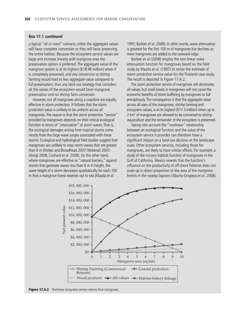
300 ECOSYSTEM SERVICE ASSESSMENTS FOR MARINE CONSERVATION
a typical “all or none” scenario; either the aggregate values will favor complete conversion or they will favor preserving the entire habitat. Because the ecosystem service values are large and increase linearly with mangrove area the preservation option is preferred. The aggregate value of the mangrove system is at its highest ($18.98 million) when it is completely preserved, and any conversion to shrimp farming would lead to less aggregate value compared to full preservation, thus any land-use strategy that considers all the values of the ecosystem would favor mangrove preservation and no shrimp farm conversion
However, not all mangroves along a coastline are equally effective in storm protection. It follows that the storm protection value is unlikely to be uniform across all mangroves. The reason is that the storm protection “service” provided by mangroves depends on their critical ecological function in terms of “attenuation” of storm waves. That is, the ecological damages arising from tropical storms come mostly from the large wave surges associated with these storms. Ecological and hydrological fi eld studies suggest that mangroves are unlikely to stop storm waves that are greater than 6 m ( Forbes and Broadhead 2007 ; Wolanski 2007 ; Alongi 2008; Cochard et al. 2008 ). On the other hand, where mangroves are effective as “natural barriers,” against storms that generate waves less than 6 m in height, the wave height of a storm decreases quadratically for each 100 m that a mangrove forest extends out to sea ( Mazda et al.
1997 ; Barbier et al. 2008 ). In other words, wave attenuation is greatest for the fi rst 100 m of mangroves but declines as more mangroves are added to the seaward edge.
Barbier et al ( 2008 ) employ the non-linear wave attenuation function for mangroves based on the fi eld study by Mazda et al. ( 1997 ) to revise the estimate of storm protection service value for the Thailand case study. The result is depicted in Figure 17.A.2 .
The storm protection service of mangroves still dominates all values, but small losses in mangroves will not cause the economic benefi ts of storm buffering by mangroves to fall precipitously. The consequence is that the aggregate value across all uses of the mangroves, shrimp farming and ecosystem values, is at its highest ($17.5 million) when up to 2 km 2 of mangroves are allowed to be converted to shrimp aquaculture and the remainder of the ecosystem is preserved.
Taking into account the “nonlinear” relationship between an ecological function and the value of the ecosystem service it provides can therefore have a signifi cant impact on a land-use decision at the landscape scale. Other ecosystem services, including those for mangroves, are likely to have similar effects. For example, a study of the nursery habitat function of mangroves in the Gulf of California, Mexico reveals that the function’s infl uence on the productivity of off-shore fi sheries does not scale-up in direct proportion to the area of the mangrove forests in the nearby lagoons ( Aburto-Oropeza et al. 2008 ).
Figure 17.A.2 Nonlinear ecosystem service returns from mangroves.
$0
$2, 000, 000
$4, 000, 000
$6, 000, 000
$8, 000, 000
$10, 000, 000
$12, 000, 000
$14, 000, 000
$16, 000, 000
$18, 000, 000
Net
pre
sent
val
ue
0 1 2 3 4 5Mangrove area (sq km)
6 7 8 9 10
Shrimp Farming (CommercialReturns)
Coastal protection
Wood products Habitat-fishery linkageAll values
Box 17.1 continued
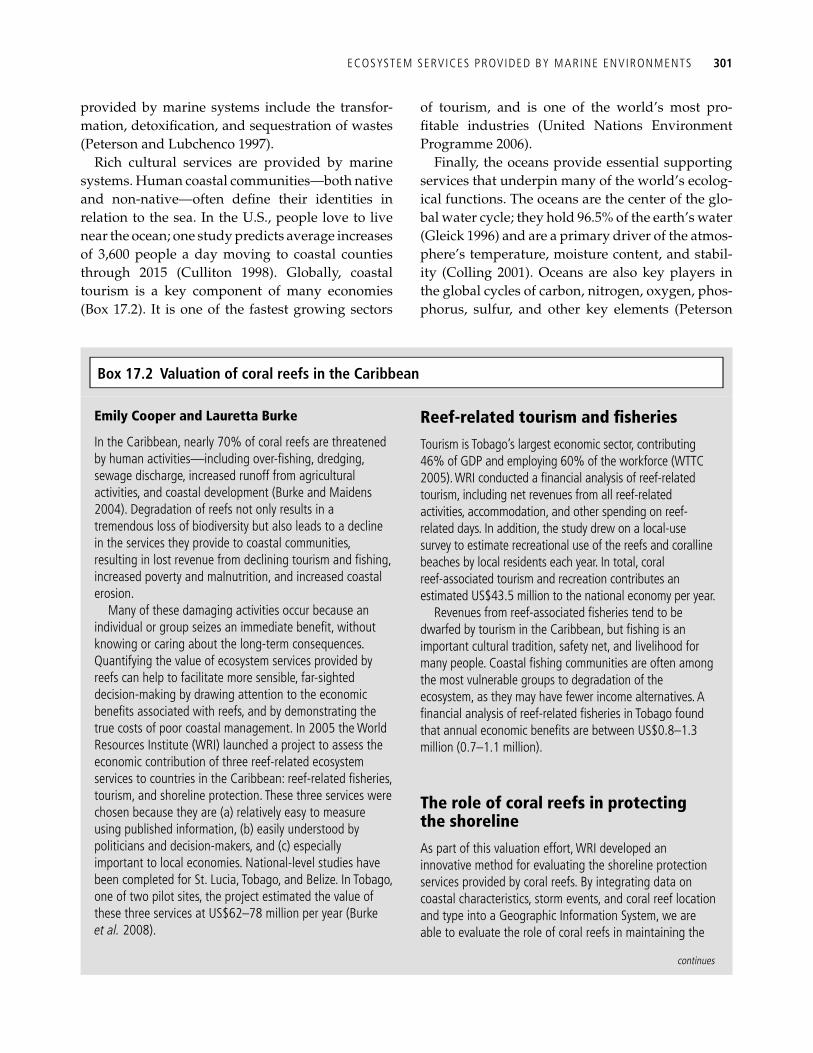
ECOSYSTEM SERVICES PROVIDED BY MARINE ENVIRONMENTS 301
provided by marine systems include the transfor-mation, detoxifi cation, and sequestration of wastes ( Peterson and Lubchenco 1997 ).
Rich cultural services are provided by marine systems. Human coastal communities—both native and non-native—often defi ne their identities in relation to the sea. In the U.S., people love to live near the ocean; one study predicts average increases of 3,600 people a day moving to coastal counties through 2015 ( Culliton 1998 ). Globally, coastal tourism is a key component of many economies ( Box 17.2 ). It is one of the fastest growing sectors
of tourism, and is one of the world’s most pro-fi table industries ( United Nations Environment Programme 2006 ).
Finally, the oceans provide essential supporting services that underpin many of the world’s ecolog-ical functions. The oceans are the center of the glo-bal water cycle; they hold 96.5% of the earth’s water ( Gleick 1996 ) and are a primary driver of the atmos-phere’s temperature, moisture content, and stabil-ity ( Colling 2001 ). Oceans are also key players in the global cycles of carbon, nitrogen, oxygen, phos-phorus, sulfur, and other key elements ( Peterson
Box 17.2 Valuation of coral reefs in the Caribbean
Emily Cooper and Lauretta Burke
In the Caribbean, nearly 70% of coral reefs are threatened by human activities—including over-fi shing, dredging, sewage discharge, increased runoff from agricultural activities, and coastal development ( Burke and Maidens 2004 ). Degradation of reefs not only results in a tremendous loss of biodiversity but also leads to a decline in the services they provide to coastal communities, resulting in lost revenue from declining tourism and fi shing, increased poverty and malnutrition, and increased coastal erosion.
Many of these damaging activities occur because an individual or group seizes an immediate benefi t, without knowing or caring about the long-term consequences. Quantifying the value of ecosystem services provided by reefs can help to facilitate more sensible, far-sighted decision-making by drawing attention to the economic benefi ts associated with reefs, and by demonstrating the true costs of poor coastal management. In 2005 the World Resources Institute (WRI) launched a project to assess the economic contribution of three reef-related ecosystem services to countries in the Caribbean: reef-related fi sheries, tourism, and shoreline protection. These three services were chosen because they are (a) relatively easy to measure using published information, (b) easily understood by politicians and decision-makers, and (c) especially important to local economies. National-level studies have been completed for St. Lucia, Tobago, and Belize. In Tobago, one of two pilot sites, the project estimated the value of these three services at US$62–78 million per year ( Burke et al. 2008 ).
Reef-related tourism and fi sheries Tourism is Tobago’s largest economic sector, contributing 46% of GDP and employing 60% of the workforce (WTTC 2005). WRI conducted a fi nancial analysis of reef-related tourism, including net revenues from all reef-related activities, accommodation, and other spending on reef-related days. In addition, the study drew on a local-use survey to estimate recreational use of the reefs and coralline beaches by local residents each year. In total, coral reef-associated tourism and recreation contributes an estimated US$43.5 million to the national economy per year.
Revenues from reef-associated fi sheries tend to be dwarfed by tourism in the Caribbean, but fi shing is an important cultural tradition, safety net, and livelihood for many people. Coastal fi shing communities are often among the most vulnerable groups to degradation of the ecosystem, as they may have fewer income alternatives. A fi nancial analysis of reef-related fi sheries in Tobago found that annual economic benefi ts are between US$0.8–1.3 million (0.7–1.1 million).
The role of coral reefs in protecting the shoreline As part of this valuation effort, WRI developed an innovative method for evaluating the shoreline protection services provided by coral reefs. By integrating data on coastal characteristics, storm events, and coral reef location and type into a Geographic Information System, we are able to evaluate the role of coral reefs in maintaining the
continues
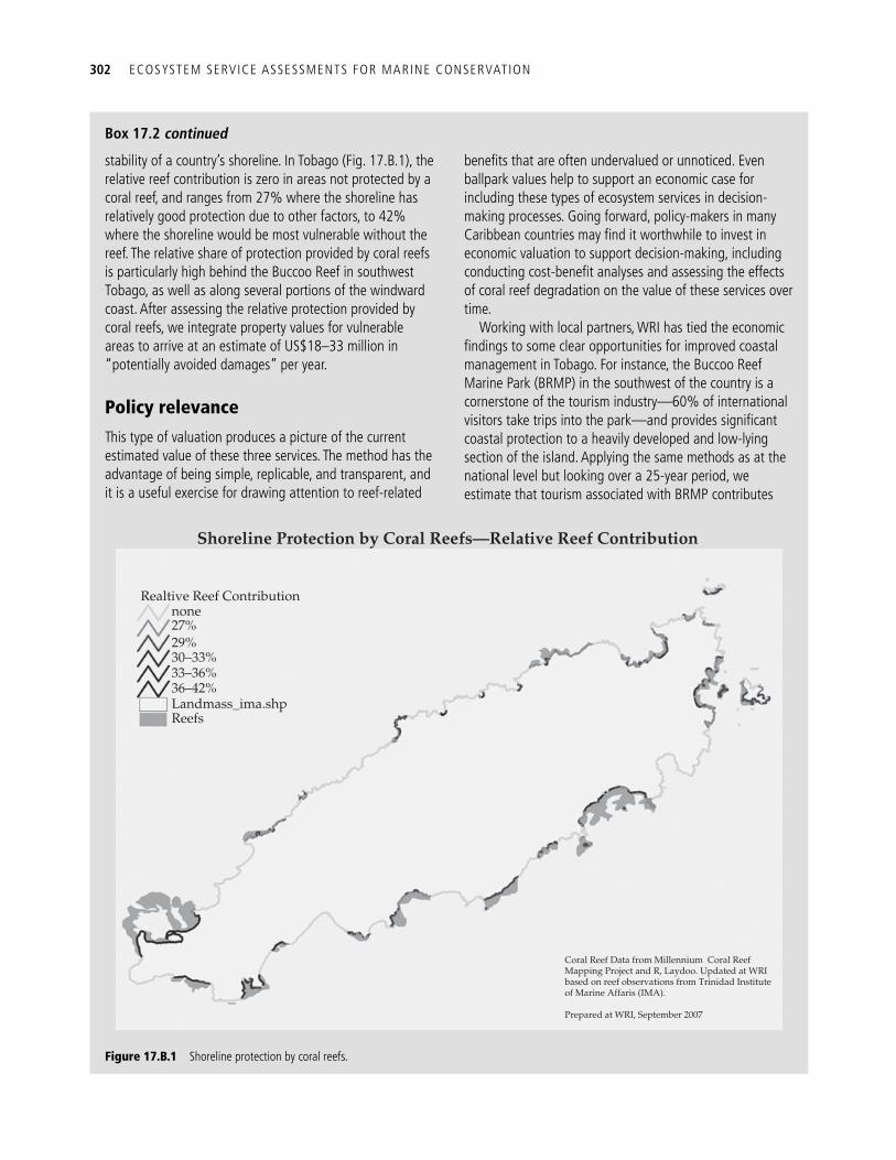
302 ECOSYSTEM SERVICE ASSESSMENTS FOR MARINE CONSERVATION
stability of a country’s shoreline. In Tobago (Fig. 17.B.1), the relative reef contribution is zero in areas not protected by a coral reef, and ranges from 27% where the shoreline has relatively good protection due to other factors, to 42% where the shoreline would be most vulnerable without the reef. The relative share of protection provided by coral reefs is particularly high behind the Buccoo Reef in southwest Tobago, as well as along several portions of the windward coast. After assessing the relative protection provided by coral reefs, we integrate property values for vulnerable areas to arrive at an estimate of US$18–33 million in “potentially avoided damages” per year.
Policy relevance This type of valuation produces a picture of the current estimated value of these three services. The method has the advantage of being simple, replicable, and transparent, and it is a useful exercise for drawing attention to reef-related
benefi ts that are often undervalued or unnoticed. Even ballpark values help to support an economic case for including these types of ecosystem services in decision-making processes. Going forward, policy-makers in many Caribbean countries may fi nd it worthwhile to invest in economic valuation to support decision-making, including conducting cost-benefi t analyses and assessing the effects of coral reef degradation on the value of these services over time.
Working with local partners, WRI has tied the economic fi ndings to some clear opportunities for improved coastal management in Tobago. For instance, the Buccoo Reef Marine Park (BRMP) in the southwest of the country is a cornerstone of the tourism industry—60% of international visitors take trips into the park—and provides signifi cant coastal protection to a heavily developed and low-lying section of the island. Applying the same methods as at the national level but looking over a 25-year period, we estimate that tourism associated with BRMP contributes
Box 17.2 continued
Figure 17.B.1 Shoreline protection by coral reefs .
Realtive Reef Contributionnone27%29%30–33%33–36%36–42%Landmass_ima.shpReefs
Coral Reef Data from Millennium Coral ReefMapping Project and R, Laydoo. Updated at WRIbased on reef observations from Trinidad Instituteof Marine Affaris (IMA).
Prepared at WRI, September 2007
Shoreline Protection by Coral Reefs—Relative Reef Contribution
MAPPING AND MODELING THE FLOW OF MARINE ECOSYSTEM SERVICES: A CASE STUDY OF PUGET SOUND 303
and Lubchenco 1997 ) and are responsible for approximately 40% of global net primary produc-tivity ( Schlesinger 1991 ; Melillo et al. 1993 ). The oceans are home to vast reservoirs of genetic and ecological diversity, arguably the most fundamen-tal of supporting services as it is directly linked to the rate of evolution and therefore the ability to adapt to a changing climate (Pergams and Kareiva, in press).
The valuation of marine ecosystem services lags behind efforts aimed at terrestrial systems, although coastal wetlands ( Batie and Wilson 1978 ; Lynne et al. 1981 ; Farber 1988 ; Bell 1989 ), coral reefs ( Spurgeon 1992 ; Moberg and Folke 1999 ; Cesar 2000 ; Brander et al. 2007 ), and mangroves ( Bennett and Reynolds 1993 ; Gilbert and Janssen 1998 ; Ronnback 1999 ; Ruitenbeek 1994 ; Barbier 2000 ; Sathirathai and Barbier 2001 ; Barbier 2003 , 2007 ; Barbier et al. 2008 ) are notable exceptions. Marine and coastal ecosystem services have been included in a few comprehensive valuation exer-cises. Costanza et al. ( 1997 ) used a (mostly) bene-fi ts-transfer approach, applying estimates of ecosystem service values for specifi c terrestrial and marine habitats to extrapolate the global value of ecosystem services. Without careful matching of sites to ensure that the benefi ts can and should be transferred, however, this approach can be mis-leading ( Plummer 2009 ). One of the most interest-ing discussions of ecosystem service valuation in the marine environment entails four case studies that demonstrate how valuing a suite of ecosystem services has the potential to inform decision-mak-ing in the Swedish coastal zone ( Soderqvist et al . 2005 ). One of these case studies explores the costs (increased water treatment and reduced fertilizer
use) and benefi ts (recreational and other cultural benefi ts) of improved water quality in the Stockholm Archipelago. Recent examinations of shoreline stabilization and trade-offs with aquac-ulture are illustrative of a general growing interest in services from coastal environments ( Box 17.1 , Barbier et al. 2008 ).
17.3 Mapping and modeling the fl ow of marine ecosystem services: a case study of Puget Sound
Ecosystem services are a useful currency for cost-benefi t analyses or assessments of the trade-offs among alternative strategies for achieving multi-ple objectives in marine systems. This is especially true when those ecosystem objectives explicitly include human well-being in addition to tradi-tional conservation goals, which is the situation in Washington’s Puget Sound region. In this section, we present a small step forward in applying the concept of quantifying dynamic fl ows of ecosys-tem services to the management of Puget Sound. The Puget Sound ecosystem in Washington State is home to 3.8 million people encompassed in a 42 000-km 2 basin, including temperate-latitude lands and rivers from the crests of the Cascade and Olympic mountains through a deep, fjord-type estuary to the Pacifi c Ocean. The region’s marine environment produces basic provisioning services such as commercial and tribal subsistence fi sheries for salmon ( Oncorhynchus spp.) and other species, as well as clam, oyster, crab, and other shellfi sh harvests. It provides regulating services as global as the carbon cycle, and as local as waste treatment through the breakdown of PAHs (polycyclic
between US$128 and 156 million in net present value over 25 years. The reef offers protection valued at between US$140 and 250 million over the same period (using a 3% discount rate). The park is meant to be a no-take zone, so fi shing is not assessed.
There is little enforcement of park regulations, and the reefs suffer from over-fishing as well as sediment and nutrient runoff. Steps to preserve the reefs could include (from lowest cost to highest): increasing
enforcement, re-routing a sewer drain out of the lagoon, improving watershed management and installing sediment traps, or building a sewage treatment plant for the area. A cost-effectiveness assessment of these interventions was outside the scope of this study, but would be fairly straightforward. Local conservation groups hope the valuation findings will draw attention to a threatened and valuable resource, and point to the need for change.
304 ECOSYSTEM SERVICE ASSESSMENTS FOR MARINE CONSERVATION
aromatic hydrocarbons) and PCBs (polychlorin-ated biphenyls) by eelgrass ( Huesemann et al. 2009 ). It offers numerous cultural services through bird and whale watching, recreational fi shing, water recreation, educational opportunities, and simply the human value placed on the existence of the region’s biodiversity. Puget Sound also pro-vides a rich cultural heritage for native Indian tribes. And underlying all of these are basic sup-porting services such as primary production and the provision of habitat for the Pacifi c Northwest icons salmon and orcas ( Orcinus orca ).
Using Puget Sound as a case study is motivated by the region’s move toward an ecosystem-level management approach. In 2007, the Washington State Legislature mandated formation of a new State agency guided by a public-private council—the Puget Sound Partnership (Partnership)—whose charge is to recover the ecosystem by 2020. The Partnership’s governance structure and man-date for ecosystem recovery presents an opportu-nity to apply principles from ecological theory and the science of ecosystem services to help pri-oritize management actions for Puget Sound. The Partnership recognizes that ecosystem recovery will require changes in the way local, state, Federal and tribal governments act and—just as importantly—changes in choices human residents make about how they commute to work, where they buy their food, homes, and so forth ( Puget Sound Partnership 2006 ). To meet these chal-lenges, the Partnership has adopted a system-wide approach to restoring the ecosystem, and they have explicitly defi ned their multiple objec-tives in terms of what ecosystem services people in the region care the most about ( Puget Sound Partnership 2008 ).
Identifying these public values is an essential step toward making an ecosystem services frame-work of practical use. In Puget Sound, a diverse group of stakeholders including those from fi sher-ies and aquaculture, tourism, ports and shipping, cities, counties, tribal governments, environmental interests, agriculture, forestry, homebuilding, and business sectors were interviewed to identify those services they believe to be “most important.” The interviewers fi rst educated the participants about the concept of ecosystem services and offered them
a list of 24 services translated from the Millennium Ecosystem Assessment into locally relevant termi-nology. Across 12 different sectors, there was broad agreement that water quantity and water regula-tion, recreation and ecotourism, and ethical and existence values were of the utmost importance; capture fi sheries, aquaculture, water purifi cation and waste treatment also ranked highly ( Iceland et al. 2008 ). Trade-offs are likely to occur among services even in this short list of valued ecosystem benefi ts. Representing outcomes of management choices in terms of multiple benefi ts, in currencies related to human well being, has promise for engaging a broader spectrum of the public in chart-ing a path forward.
An early focus of the Partnership’s effort is near-shore habitats. This builds on the work of a number of previous planning efforts in Puget Sound, which identifi ed specifi c actions aimed at either protecting existing nearshore habitats or restoring degraded areas to provide improved function for species, habitat maintenance, or human access (Shared Strategy 2007; Puget Sound Nearshore Ecosystem Restoration Project 2008 ; Alliance for Puget Sound Shorelines 2008 ). These nearshore recovery schemes in Puget Sound have broadly similar objectives in their common desire to increase the amount of func-tioning nearshore habitat.
In the remainder of this chapter, we focus on the suite of ecosystem services that nearshore habitats produce and support in Puget Sound, and how those services could change in response to a set of possible management actions. To illustrate this approach, we quantify the outcomes of nearshore protection or restoration for three distinct kinds of services that fl ow from an important foundation species—eelgrass ( Zostera marina ): (1) carbon sequestration for climate regulation (a regulating service with global reach), (2) marine commercial harvest (a provisioning service), and (3) non-con-sumptive values (recreation and existence values) associated with species that belong to the Puget Sound food web. We examine how changes in eco-system services are created by changes in eelgrass itself (carbon sequestration) and how changes in eelgrass produce changes in services provided through higher levels of the food web (harvest, rec-reation, and existence values).
MAPPING AND MODELING THE FLOW OF MARINE ECOSYSTEM SERVICES: A CASE STUDY OF PUGET SOUND 305
17.3.1 Eelgrass
Eelgrass ( Zostera marina ) is a widely distributed, clonal seagrass that forms large, often monospecifi c stands in shallow temperate estuaries worldwide. Much of the vegetative biomass of eelgrass is below the surface of sediments and the above-ground biomass tends to be highly seasonal. Ecosystem services attributed to seagrass beds include the sequestration of carbon, the provision of habitat for fi sh and invertebrates, and the control of erosion through sediment stabilization ( Williams and Heck 2001 ). Threats to eelgrass in Puget Sound are similar to those facing this habitat type elsewhere, including mechanical damage (such as through dredging and anchoring), eutrophication, some aquaculture prac-tices, siltation, coastal construction, invasions by non-native species, alterations to coastal food webs, and climate change ( Williams and Heck 2001 ; Duarte 2002 ; Bando 2006 ). Eelgrass beds currently occur along approximately 37% of the coast of Puget Sound, where they provide habitat for mobile organ-isms such as crabs and small fi shes and feeding hab-itat for larger consumers such as seabirds, salmon, and marine mammals ( National Marine Fisheries Service 2007 ). They also provide spawning and rear-ing habitat for Pacifi c herring ( Clupea pallasi ), a key species in the regional food web ( Penttila 2007 ; National Marine Fisheries Service 2007 ).
To evaluate policy scenarios for the nearshore, we ask how management actions are likely to affect eel-grass, and then how multiple ecosystem services provided by eelgrass are likely to change as a result. We estimate ecosystem services using simple approaches for the sake of illustration, and do not include ecological nuances such as spatial or tem-poral variation in their production and delivery. Also, it is important to note that since we are exam-ining changes in fl ows of services that are likely to result from changes in a foundation species, we focus on bottom-up effects; future scenario work will include the examination of top-down effects such as changes in harvest of key fi sh species.
We know from previous work that the total area of eelgrass in Puget Sound has declined from historical levels ( Thom and Hallum 1990 ). Although the rea-sons for this decline are not well understood ( Thom and Albright 1990 ; Thom and Hallum 1990 ), we
assume for the sake of illustration that the Partnership can identify and implement policies capable of pro-tecting eelgrass and halting this decline. In addition, we examine other policies aimed at restoring eelgrass in areas where it used to occur. To assess the potential for restoration, we built a spatially explicit habitat suitability model for eelgrass in Puget Sound, with the aim of identifying locations in which eelgrass has the potential to grow but where its current status is unknown ( Figure 17.1 ; Plate 13, Davies et al. , in prep-aration). Our model suggests that an additional 36 877 ha of Puget Sound’s benthic area has the potential to be occupied by eelgrass. If even half of this were to be occupied in the future due to restora-tion projects, it would represent nearly a doubling of the current area of eelgrass and would yield area similar to that estimated to be present historically (41 239 ha compared to 47 328 ha summarized from Thom and Hallum 1990).
17.3.2 How do changes in eelgrass habitats affect carbon storage and sequestration?
Estimates of carbon storage and sequestration in marine systems are rare. For example, a marine ana-log does not exist that is similar to the look-up tables for carbon storage and sequestration values for various land use/land cover categories available in terrestrial systems (Intergovernmental Panel on Climate Change 2006). Our approach to estimating the ecosystem service value of eelgrass carbon seques-tration is similar to that of Chapter 7 (this book) and is summarized in Table 17.2a . We fi rst estimate the amount of carbon stored in eelgrass biomass and soils. We then estimate the rate of carbon sequestra-tion for eelgrass in Puget Sound, noting that carbon also fl ows through eelgrass to be consumed by her-bivores, decomposed within the system, and exported from the system. These two estimates yield ecosys-tem service values for the scenarios examined. In the end, our approach illustrates how changes in eelgrass habitats result in changes in the amounts and values of carbon storage and sequestration.
17.3.2.1 Carbon storage Our estimates of carbon storage in Puget Sound eel-grass beds and sediments range from 1–6.3 TgC ( Table 17.2a ). The amount of C in the sediment pool
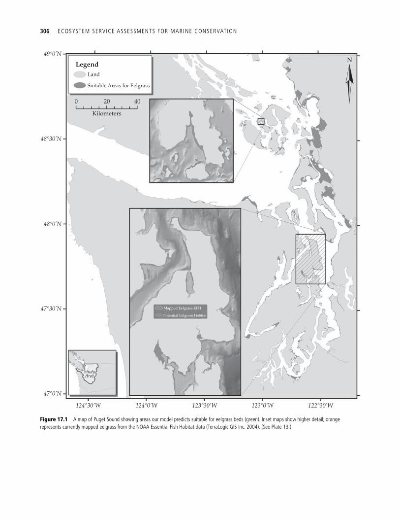
306 ECOSYSTEM SERVICE ASSESSMENTS FOR MARINE CONSERVATION
Land
Legend
49°0’N
48°30’N
48°0’N
47°30’N
StudyArea
47°0’N
124°30’W 124°0’W 123°30’W 123°0’W 122°30’W
Suitable Areas for Eelgrass
0 20 40
N
Kilometers
Mapped Eelgrass-EFH
Potential Eelgrass Habitat
Figure 17.1 A map of Puget Sound showing areas our model predicts suitable for eelgrass beds (green). Inset maps show higher detail; orange represents currently mapped eelgrass from the NOAA Essential Fish Habitat data (TerraLogic GIS Inc. 2004). (See Plate 13.)
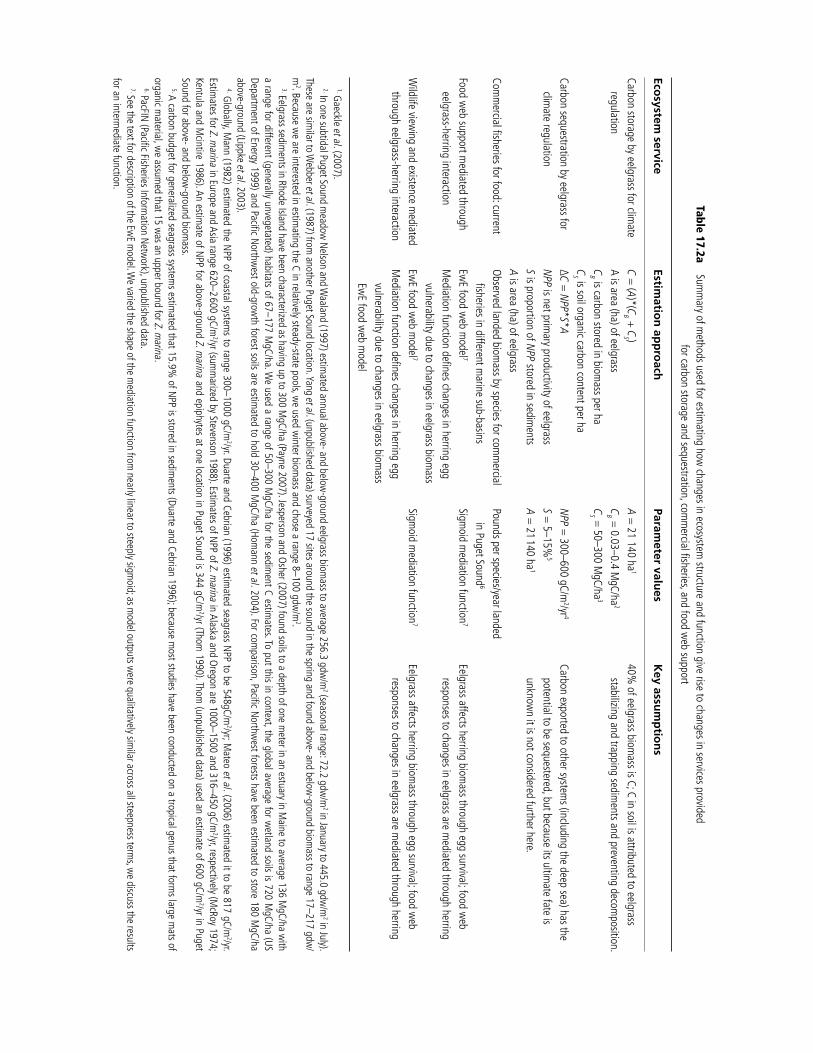
Table 17.2a Sum
mary of m
ethods used for estimating how
changes in ecosystem structure and function give rise to changes in services provided
for carbon storage and sequestration, comm
ercial fi sheries, and food web support
Ecosystem service
Estimation approach
Parameter values
Key assum
ptions
Carbon storage by eelgrass for climate
regulation C = ( A )*( C B + C S )
A = 21 140 ha 1 40%
of eelgrass biomass is C; C in soil is attributed to eelgrass
stabilizing and trapping sediments and preventing decom
position. A is area (ha) of eelgrass
C B = 0.03–0.4 MgC/ha 2
C B is carbon stored in biomass per ha
C S = 50–300 MgC/ha 3
C S is soil organic carbon content per ha
Carbon sequestration by eelgrass for clim
ate regulation ∆ C = NPP * S * A
NPP = 300–600 gC/m 2 /yr 4
Carbon exported to other systems (including the deep sea) has the
potential to be sequestered, but because its ultimate fate is
unknown it is not considered further here.
NPP is net primary productivity of eelgrass
S = 5–15% 5
S is proportion of NPP stored in sediments
A = 21 140 ha 1 A is area (ha) of eelgrass
Comm
ercial fi sheries for food: current Observed landed biom
ass by species for comm
ercial fi sheries in different m
arine sub-basins Pounds per species/year landed
in Puget Sound 6
Food web support m
ediated through eelgrass-herring interaction
EwE food w
eb model 7
Sigmoid m
ediation function 7 Eelgrass affects herring biom
ass through egg survival; food web
responses to changes in eelgrass are mediated through herring
Mediation function defi nes changes in herring egg vulnerability due to changes in eelgrass biom
ass W
ildlife viewing and existence m
ediated through eelgrass-herring interaction
EwE food w
eb model 7
Sigmoid m
ediation function 7 Eelgrass affects herring biom
ass through egg survival; food web
responses to changes in eelgrass are mediated through herring
Mediation function defi nes changes in herring egg vulnerability due to changes in eelgrass biom
ass Ew
E food web m
odel
1. Gaeckle et al . ( 2007 ). 2. In one subtidal Puget Sound m
eadow Nelson and W
aaland ( 1997 ) estimated annual above- and below
-ground eelgrass biomass to average 256.3 gdw
/m 2 (seasonal range: 72.2 gdw
/m 2 in January to 445.0 gdw
/m 2 in July).
These are similar to W
ebber et al . ( 1987 ) from another Puget Sound location. Yang et al . (unpublished data) surveyed 17 sites around the sound in the spring and found above- and below
-ground biomass to range 17–217 gdw
/m
2 . Because we are interested in estim
ating the C in relatively steady-state pools, we used w
inter biomass and chose a range 8–100 gdw
/m 2 .
3. Eelgrass sediments in Rhode Island have been characterized as having up to 300 M
gC/ha ( Payne 2007 ). Jesperson and Osher ( 2007 ) found soils to a depth of one meter in an estuary in M
aine to average 136 MgC/ha w
ith a range for different (generally unvegetated) habitats of 67–177 M
gC/ha. We used a range of 50–300 M
gC/ha for the sediment C estim
ates. To put this in context, the global average for wetland soils is 720 M
gC/ha ( US Departm
ent of Energy 1999 ) and Pacifi c Northwest old-grow
th forest soils are estimated to hold 30–400 M
gC/ha ( Homann et al . 2004 ). For com
parison, Pacifi c Northwest forests have been estim
ated to store 180 MgC/ha
above-ground ( Lippke et al . 2003 ). 4. Globally, M
ann ( 1982 ) estimated the NPP of coastal system
s to range 300–1000 gC/m 2 /yr. Duarte and Cebrian ( 1996 ) estim
ated seagrass NPP to be 548gC/m 2 /yr; M
ateo et al . ( 2006 ) estimated it to be 817 gC/m
2 /yr. Estim
ates for Z. marina in Europe and Asia range 620–2 600 gC/m
2 /yr (summ
arized by Stevenson 1988 ). Estimates of NPP of Z. m
arina in Alaska and Oregon are 1000–1500 and 316–450 gC/m 2 /yr, respectively ( M
cRoy 1974 ; Kentula and M
cintire 1986 ). An estimate of NPP for above-ground Z. m
arina and epiphytes at one location in Puget Sound is 344 gC/m 2 /yr ( Thom
1990 ). Thom (unpublished data) used an estim
ate of 600 gC/m 2 /yr in Puget
Sound for above- and below-ground biom
ass. 5. A carbon budget for generalized seagrass system
s estimated that 15.9%
of NPP is stored in sediments ( Duarte and Cebrian 1996 ); because m
ost studies have been conducted on a tropical genus that forms large m
ats of organic m
aterial, we assum
ed that 15 was an upper bound for Z. m
arina . 6. PacFIN (Pacifi c Fisheries Inform
ation Network), unpublished data.
7. See the text for description of the EwE m
odel. We varied the shape of the m
ediation function from nearly linear to steeply sigm
oid; as model outputs w
ere qualitatively similar across all steepness term
s, we discuss the results
for an intermediate function.
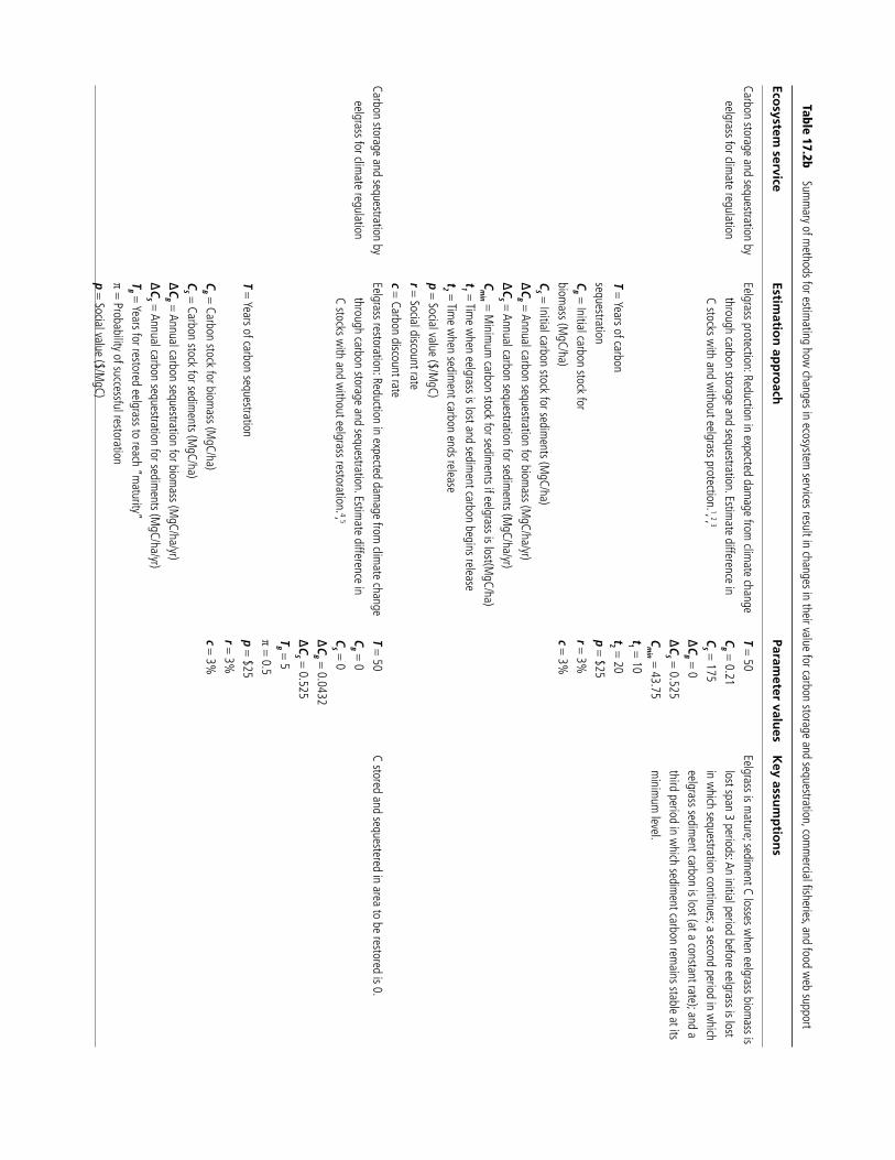
Table 17.2b Sum
mary of m
ethods for estimating how
changes in ecosystem services result in changes in their value for carbon storage and sequestration, com
mercial fi sheries, and food w
eb support
Ecosystem service
Estimation approach
Parameter values
Key assum
ptions
Carbon storage and sequestration by eelgrass for clim
ate regulation Eelgrass protection: Reduction in expected dam
age from clim
ate change through carbon storage and sequestration. Estim
ate difference in C stocks w
ith and without eelgrass protection. 1 , 2 , 3
T = 50 Eelgrass is m
ature; sediment C losses w
hen eelgrass biomass is
lost span 3 periods: An initial period before eelgrass is lost in w
hich sequestration continues; a second period in which
eelgrass sediment carbon is lost (at a constant rate); and a
third period in which sedim
ent carbon remains stable at its
minim
um level.
C B = 0.21 C S = 175 ∆ C B = 0 ∆ C S = 0.525 C m
in = 43.75 t 1 = 10
T = Years of carbon t 2 = 20
sequestration p = $25
C B = Initial carbon stock for r = 3%
biom
ass (MgC/ha)
c = 3%
C S = Initial carbon stock for sediments (M
gC/ha) ∆ C B = Annual carbon sequestration for biom
ass (MgC/ha/yr)
∆ C S = Annual carbon sequestration for sediments (M
gC/ha/yr) C m
in = Minim
um carbon stock for sedim
ents if eelgrass is lost(MgC/ha)
t 1 = Time w
hen eelgrass is lost and sediment carbon begins release
t 2 = Time w
hen sediment carbon ends release
p = Social value ($/MgC)
r = Social discount rate c = Carbon discount rate
Carbon storage and sequestration by eelgrass for clim
ate regulation Eelgrass restoration: Reduction in expected dam
age from clim
ate change through carbon storage and sequestration. Estim
ate difference in C stocks w
ith and without eelgrass restoration. 4 , 5
T = 50 C stored and sequestered in area to be restored is 0.
C B = 0 C S = 0 ∆ C B = 0.0432 ∆ C S = 0.525 T B = 5 π = 0.5
T = Years of carbon sequestration p = $25 r = 3%
C B = Carbon stock for biom
ass (MgC/ha)
c = 3%
C S = Carbon stock for sediments (M
gC/ha) ∆ C B = Annual carbon sequestration for biom
ass (MgC/ha/yr)
∆ C S = Annual carbon sequestration for sediments (M
gC/ha/yr) T B = Years for restored eelgrass to reach “m
aturity” π = Probability of successful restoration p = Social value ($/M
gC)
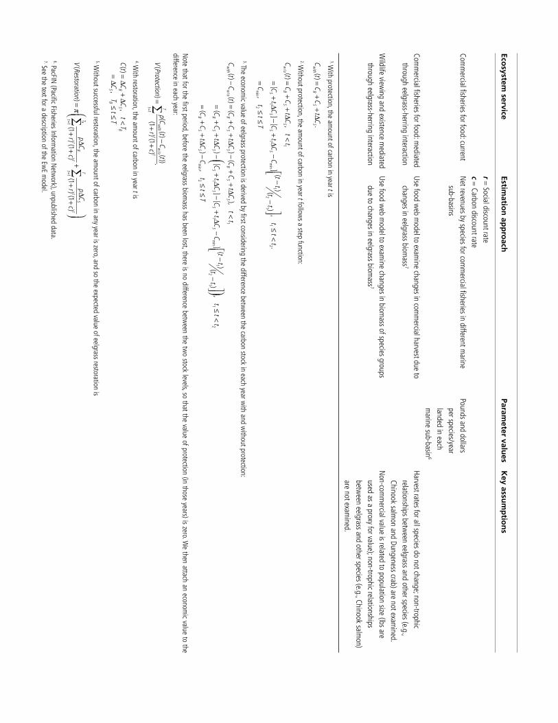
Ecosystem service
Estimation approach
Parameter values
Key assum
ptions
r = Social discount rate c = Carbon discount rate
Comm
ercial fi sheries for food: current Net revenues by species for com
mercial fi sheries in different m
arine sub-basins
Pounds and dollars per species/year landed in each m
arine sub-basin 6
Comm
ercial fi sheries for food: mediated
through eelgrass-herring interaction Use food w
eb model to exam
ine changes in comm
ercial harvest due to changes in eelgrass biom
ass 7 Harvest rates for all species do not change; non-trophic
relationships between eelgrass and other species (e.g.,
Chinook salmon and Dungeness crab) are not exam
ined. W
ildlife viewing and existence m
ediated through eelgrass-herring interaction
Use food web m
odel to examine changes in biom
ass of species groups due to changes in eelgrass biom
ass 7 Non-com
mercial value is related to population size (lbs are
used as a proxy for value); non-trophic relationships betw
een eelgrass and other species (e.g., Chinook salmon)
are not examined.
1. With protection, the am
ount of carbon in year t is
with
BS
SC
tC
Ct
C()
.=
++
∆
2. Without protection, the am
ount of carbon in year t follows a step function:
wo
BS
S
SS
SS
Ct
CC
tC
tt
tt
Ct
CC
tC
Ct
tt
tt
Ct
tT
/1
11
1m
in1
22
1
min
2
(),
()
[]
[]
,.
()
,
=+
+∆
<−
⎡⎤
=+
∆−
+∆
−≤
<−
⎢⎥
⎣⎦
=≤
≤
3. The economic value of eelgrass protection is derived by fi rst considering the difference betw
een the carbon stock in each year with and w
ithout protection:
with
wo
BS
SB
SS
BS
SS
SS
S
BS
S
Ct
Ct
CC
tC
CC
tC
tt
tt
CC
tC
Ct
CC
tC
Ct
tt
tt
CC
tC
Ct
tT
/1
11
1m
in1
22
1
min
2
()()
()
(),
()
()
[]
[]
,(
)(
),
−=
++
∆−
++
∆<
−⎛
⎞⎡
⎤=
++
∆−
+∆
−+
∆−
≤<
⎜⎟
−⎢
⎥⎝
⎠⎣
⎦=
++
∆−
≤≤
Note that for the fi rst period, before the eelgrass biomass has been lost, there is no difference betw
een the two stock levels, so that the value of protection (in those years) is zero. W
e then attach an economic value to the
difference in each year:
Tw
ithw
ot
tt
pC
tC
tV
Protectionr
c /
1
(()
())(
).
(1)(1
)=
−=
++
∑
4. With restoration, the am
ount of carbon in year t is
BS
B
SB
Ct
CC
tT
CT
tT
(),
,=
∆+
∆<
=∆
≤≤
5. Without successful restoration, the am
ount of carbon in any year is zero, and so the expected value of eelgrass restoration is
B TT
BS
tt
tt
tt
pC
pC
VRestoration
rc
rc
11
()
(1)(1
)(1
)(1)
p=
=
⎛⎞
∆∆
=+
⎜⎟
++
++
⎝⎠
∑∑
6. PacFIN (Pacifi c Fisheries Information Netw
ork), unpublished data. 7. See the text for a description of the Ew
E model.
310 ECOSYSTEM SERVICE ASSESSMENTS FOR MARINE CONSERVATION
dwarfs that in the biomass pool (such that the bio-mass pool is truly negligible). In comparison, total US forest carbon stocks are estimated to be in the range of 40 000–50 000 TgC. Pacifi c Northwest (western OR and WA) forests are estimated to con-tain approximately 351 TgC ( US Environmental Protection Agency 2007 ).
17.3.2.2 Carbon sequestration Seagrasses stabilize sediments, slow water motion, and cause the deposition of organic matter from the water column ( Gacia and Duarte 1999 ; Gacia et al. 1999 ). Below the sediment surface, anoxia and light-limitation inhibit microbial processing and photo-degradation ( Jesperson and Osher 2007 ), allowing for the build-up of C. Soil carbon generally has long residence times—particularly when submerged—and is therefore considered “sequestered carbon” ( Wang and Hseih 2002 ). Despite ideal conditions for production and preservation of organic matter, the C-sequestration capacity of the soils of coastal eco-systems has been under-studied ( Chmura et al. 2003 ; Thom et al. 2003 ; Jesperson and Osher 2007 ).
Our initial estimate of a sequestration rate in Puget Sound is 3 171–19 026 Mg C/yr, or 11 627–69 762 Mg CO 2 /yr ( Table 17.2a ). This represents 0.02–0.1% of the emissions of Washington State, 0.06–0.36% of the emissions of King County (Seattle’s home), and up to 72% of the annual emissions of all transit busses in King County ( King County 2007 ). For comparison, the carbon contained in all US forests offset approximately 10% of total US CO 2 emissions in 2005 ( Woodbury et al. 2007 ).
If a restoration policy is being pursued, particular habitat types would be changing to eelgrass from a previous habitat type, and the original state would have had its own C-storage/sequestration values. Similarly, if eelgrass habitat is being lost, it is being replaced with another habitat type, and a similar comparison could be made. This makes marginal changes impossible to calculate without going through the same exercise for all habitat types. Among possible habitat types, however, we expect eelgrass to have the greatest capacity for carbon storage and sequestration, compared to other non-vegetated intertidal and shallow subtidal habitats such as rocky reefs, cobble, mud-, or sand-fl ats.
17.3.2.3 Valuing ecosystem service value changes for carbon The ecosystem service value of carbon storage and sequestration is based on the reduction in the expected damage from climate change. Increasing levels of carbon dioxide and other greenhouse gases are linked to harmful changes in temperature and other aspects of climate. Controlling carbon dioxide by sequestering carbon therefore mitigates those harmful effects, which counts as an economic ben-efi t. This value is enjoyed by society at large, and so it is referred to as the social value of carbon storage and sequestration.
For eelgrass, this ecosystem service value can be generated either by protecting current eelgrass or investing in eelgrass restoration, as described above. Protection provides value if existing eelgrass areas are threatened and the projected amount without protection decreases over time; restoration provides value when eelgrass would otherwise decline or remain stable in the future. In either case, the eco-nomic value is based on the difference in carbon stocks over time for two scenarios, one with the appropriate action (protection or restoration) and one without that action. Thus, it is important to understand what form of carbon sequestration and storage (if any) would either replace eelgrass (for the case of protection) or be replaced by eelgrass (in the case of restoration). Calculating this economic value is relatively straightforward ( Chapter 7 ), but settling on the values for some of the parameters is fraught with controversy ( Nordhaus 2007 ; Weitzman 2007 ). For the purposes of this chapter, we pick values merely to illustrate how the calculation and resulting value depends on the scenarios described above ( Table 17.2b ).
Based on the methods outlined in Table 17.2b , the social value of eelgrass protection is much higher than that of restoration: $1 496 to 4 585 versus $104 ha –1 . The range in values for protection refl ect different assumptions about the loss of carbon from sediments, with the high value representing an assumed total loss of stored carbon when eelgrass is left unprotected and the low value resulting from a ten-year lag before carbon is released, a ten-year carbon release period, and a 25% minimum carbon stock that remains in the sediments without eel-grass. The large disparity is due in large part to the
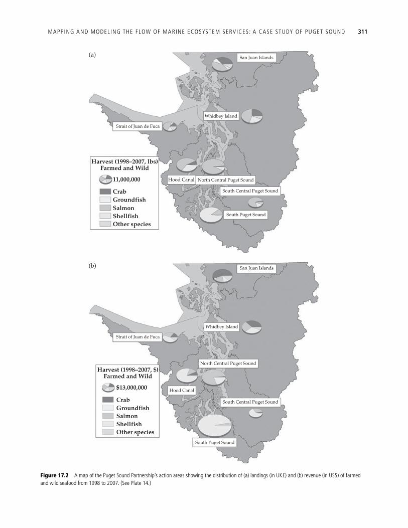
MAPPING AND MODELING THE FLOW OF MARINE ECOSYSTEM SERVICES: A CASE STUDY OF PUGET SOUND 311
Figure 17.2 A map of the Puget Sound Partnership’s action areas showing the distribution of (a) landings (in UK£) and (b) revenue (in US$) of farmed and wild seafood from 1998 to 2007. (See Plate 14.)
San Juan Islands
Whidbey Island
Strait of Juan de Fuca
(a)
Harvest (1998–2007, lbs)Farmed and Wild
11,000,000
CrabGroundfishSalmonShellfishOther species
Hood Canal North Central Puget Sound
South Central Puget Sound
South Puget Sound
San Juan Islands
Whidbey Island
Strait of Juan de Fuca
Harvest (1998–2007, $)Farmed and Wild
$13,000,000
CrabGroundfishSalmonShellfishOther species
Hood Canal
North Central Puget Sound
South Central Puget Sound
South Puget Sound
(b)
312 ECOSYSTEM SERVICE ASSESSMENTS FOR MARINE CONSERVATION
assumed loss of stored carbon when eelgrass is left unprotected. If leaving eelgrass unprotected does not produce a signifi cant loss of stored carbon in the sediments, the value of protection and its advantage over restoration is diminished accordingly.
17.3.3 Marine harvest and non-consumptive values
Puget Sound’s living marine resources, though depleted relative to historic times, remain a bounti-ful source of provisioning and other ecosystem services. Commercial fi sheries harvest over 35 spe-cies of fi nfi sh and shellfi sh, and generate more than $50 million in annual revenue (Pacifi c States Marine Fisheries Commission, Pacifi c Coast Fisheries Information Network (PacFIN), unpublished data). Recreational harvest concentrates on Pacifi c salmon and steelhead ( Oncorhynchus mykiss ) but also includes shellfi sh such as Dungeness crab ( Cancer magister ) and butter clams ( Saxidomus giganteus ) (Washington State Department of Fish and Wildlife (WDFW), unpublished data). Puget Sound Indian tribes enjoy a rich tradition of ceremonial harvest. Aquaculture uses the ecological functioning of Puget Sound to produce more than $30 million in annual revenue for shellfi sh and almost $20 million for Atlantic salmon ( Salmo salar ) (WDFW, unpub-lished data). Non-consumptive activities, such as recreational whale and bird watching, also provide an important fl ow of services, while just the exist-ence of some species produces value for Puget Sound residents and visitors.
In order to provide a perspective with which to gauge the effects of changes in the ecosystem, we tallied the commercial harvest coming from Puget Sound in biological (lbs.) and monetary ($) units (PacFIN; Figures 17.2a , b; Plate 14). This snapshot of the seafood provisioning service allows us to exam-ine where particular types of harvest are highest. For example, shellfi sh, which are particularly lucra-tive, are predominately produced in southern Puget Sound.
The mobility of fi sh and their use of multiple hab-itat types necessitates a food web-based modeling approach rather than a habitat-based one. To under-stand how changes in nearshore environments and
eelgrass are likely to affect changes in the food web-based ecosystem service fl ows, we focus on the link between eelgrass, a foundation species, and one other species with wide-ranging food web interac-tions, Pacifi c herring.
17.3.3.1 How might changes in eelgrass habitats affect marine harvest and non-consumptive values? In order to begin to understand how changes in nearshore environments are likely to affect changes in the fl ows of harvest and other services, we exam-ined the habitat associations of the top 25 species harvested in the sound (including: geoducks ( Panopea abrupta ), salmon, Dungeness crab, and oysters), and categorized their dependence on near-shore habitats. Only 5 of these species (spiny dog-fi sh, ( Squalus acanthias ), and 4 salmon—steelhead; sockeye ( Oncorhynchus nerka ), coho ( Oncorhynchus kisutch ), and pink ( Oncorhynchus gorbuscha )) did not rely on nearshore habitats for at least one part of their life cycle. Thus, harvest levels of most species in the top 25 are likely to be sensitive to changes in nearshore habitats, but further modeling is neces-sary to understand how.
Pacifi c herring are a key food web species that interacts with eelgrass—they aggregate in the near-shore prior to reproducing then spawn in shallow water, usually on submerged vegetation (eelgrass or algae). Submerged vegetation provides spawn-ing substrate, food resources, cover, and nursery habitat ( Thayer and Phillips 1977 ; Dean et al. 2000 ; Penttila 2007 ). Survivorship of eggs is higher with lower spawn density ( Galkina 1971 ; Taylor 1971 ). To survive, planktonic larvae must have suffi cient supplies of microplankton; blooms of which are believed to be earlier, more dense and more consist-ent in sheltered bays ( Penttila 2007 ). The survival of larval herring (determined particularly by food availability and predation) is thought to have a sig-nifi cant impact on the future abundance of the year-class ( Alderdice and Hourston 1985 ). Juveniles spend several months inshore before moving into deeper waters ( Penttila 2007 ). Herring are impor-tant prey to seabirds, crabs, salmon, marine mam-mals, and numerous other groups ( Haegele 1993a , b ; Penttila 2007 ). Given the strong connection between herring and nearshore habitat, we focus here on the consequences of how changes in
MAPPING AND MODELING THE FLOW OF MARINE ECOSYSTEM SERVICES: A CASE STUDY OF PUGET SOUND 313
nearshore habitat give rise to changes in herring, and how such effects can propagate through the food web.
17.3.3.2 Puget Sound food web model Biomass dynamics of eelgrass and herring take place in the context of a broader community of interacting species, and resulting feedbacks within the food web are diffi cult to anticipate without the benefi t of models. We used the Ecopath with Ecosim (EwE; Christensen and Walters 2004 ) software to construct a food web model for the central basin of Puget Sound ( Figure 17.3a ; Plate 15; Harvey et al. 2010). EwE models trophically and reproductively link biomass pools using a mass-balance modeling approach that satisfi es two master equations describing production (as a function of catch, pre-dation, migration, and biomass) and consumption (as a function of production, respiration, and unas-similated food). An initial mass-balanced snapshot of the ecosystem can then be used to explore dynamic simulations by expressing biomass fl ux rates among pools through time. The model of Puget Sound’s Central Basin (Harvey et al. 2010) has functional groups ranging from primary producers to marine mammals and seabirds, as well as sev-eral fi sheries. The model results we present below are preliminary outcomes that illustrate the com-plex and often unforeseen nature of community responses to perturbations ( Christensen and Walters 2004 ).
Manipulating eelgrass production in EwE has negligible effects on the food web through con-sumption—a result that refl ects our current under-standing of eelgrass as a relatively unimportant direct food source ( Mumford 2007 ). In contrast, non-trophic effects of eelgrass—such as habitat pro-visioning—are known to be very important ( Thayer and Phillips 1977 ; Orth et al. 1984 ; Hosack et al. 2006 ; Mumford 2007 ). Such effects have important posi-tive effects on other species and can be refl ected in EwE through density-dependent mediation func-tions ( Ainsworth et al. 2008 ). Mediation functions quantitatively link the vulnerability of a group (in this case, herring eggs) to the biomass of a mediat-ing group (in this case, eelgrass): in other words, the less eelgrass is present, the more vulnerable herring eggs are to their predators. This is but one of numer-
ous mechanisms by which changes in eelgrass could lead to changes in herring populations. Here we present only indirect effects that act through her-ring ( Figure 17.3b ; Plate 15) and focus on species and/or groups whose relationship with eelgrass is either trophic (i.e., they consume it) or is mediated through direct or indirect trophic interactions with herring.
We simulated a 50% decrease, a 50% increase, and a doubling of eelgrass biomass, and linked this to herring egg vulnerability. Depending on eelgrass biomass, herring eggs became either more or less vulnerable to predation by several groups (ducks and brants, gulls, ratfi sh, Dungeness crabs, small nearshore fi shes, and small crustacean omnivores). Increases in eelgrass biomass yielded increases in herring and in turn increases in harbor seals ( Phoca vitulina , whose primary prey is herring), ducks and brants (consumers of eelgrass), and greenlings (con-sumers of small crustaceans who feed on herring eggs). Increases in eelgrass yielded decreases in gulls and terns, skates, gadoids, lingcod ( Ophiodon elongatus ), and numerous fl atfi sh. Most of these decreases result from competition with increased herring populations. Skates, however, likely decline with increases in eelgrass and herring because their primary predators are harbor seals, a species that increases with eelgrass and herring. Results for decreases in eelgrass biomass generally mirrored those of increases.
17.3.3.3 Valuing commercial harvest and non-consumptive services from food web changes The species in the Puget Sound food web model pro-vide consumptive services that include commercial harvest, and non-consumptive services such as whale and bird watching and existence value (because of data limitations on recreational fi shing values, we do not consider recreational harvest in this section). Of the functional groups in the Puget Sound food web model, 15 are harvested commer-cially ( Table 17.3 ). By weight, the most important fi sheries are salmon (sockeye; chum, Oncorhynchus keta ; coho; and Chinook, Oncorhynchus tshawytscha , both wild and hatchery stocks), geoduck, Pacifi c herring, and Dungeness crab, in that order. By value, the same fi sheries dominate but the geoduck’s high price per pound makes it the most economically
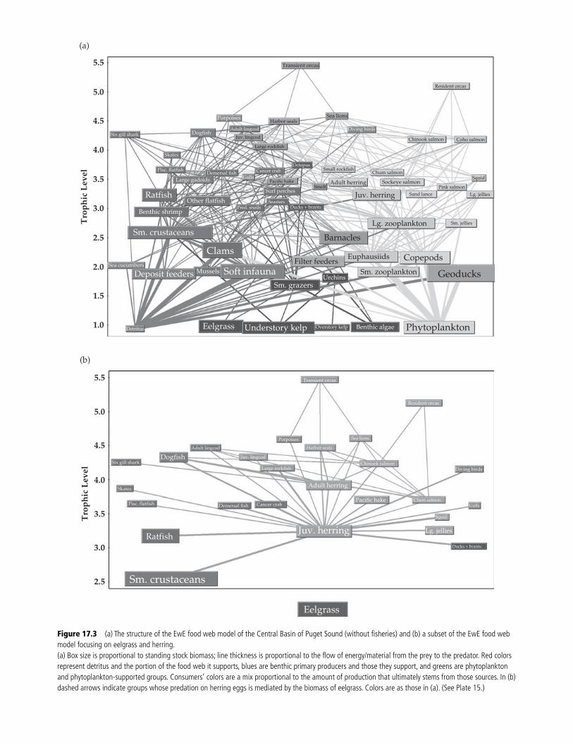
Figure 17.3 (a) The structure of the EwE food web model of the Central Basin of Puget Sound (without fi sheries) and (b) a subset of the EwE food web model focusing on eelgrass and herring. (a) Box size is proportional to standing stock biomass; line thickness is proportional to the fl ow of energy/material from the prey to the predator. Red colors represent detritus and the portion of the food web it supports, blues are benthic primary producers and those they support, and greens are phytoplankton and phytoplankton-supported groups. Consumers’ colors are a mix proportional to the amount of production that ultimately stems from those sources. In (b) dashed arrows indicate groups whose predation on herring eggs is mediated by the biomass of eelgrass. Colors are as those in (a). (See Plate 15.)
Six gill shark
Skates
Pisc. flatfish
Large gadoids
Dogfish
Porpoises
Transient orcas
Sea lions
Diving birds
Resident orcas
Coho salmonChinook salmon
Squid
Lg. jelliesPink salmon
Sm. jellies
Sand lance
Chum salmonSmall rockfish
SmeltAdult herring
Juv. herring
Lg. zooplankton
Sockeye salmon
Harbor seals
Juv. lingcod
Large rockfish
OctopusCancer crab
GullsPacific hake
SeastarsPred. snails Ducks + brants
Surf perches
Adult lingcod
Other flatfish
Clams
Soft infauna
Understory kelpEelgrass
Filter feeders Euphausiids
Sm. zooplankton Geoducks
Phytoplankton
Copepods
Barnacles
Sm. grazersUrchins
Benthic algaeOverstory kelp
Ratfish
Sm. crustaceans
Deposit feeders
Benthic shrimp
Sea cucumbers
Detritus
Mussels
Demersal fish
5.5
5.0
4.5
4.0
3.5
3.0
Tro
phic
Lev
el
2.5
2.0
1.5
1.0
(a)
Adult lingcod
Juv. lingcod
Large rockfish
Harbor seals
Porpoises Sea lions
Resident orcas
Transient orcas
Chinook salmon
Pacific hake Chum salmon
Squid
Gulls
Diving birds
Ducks + brants
Lg. jellies
Adult herring
Six gill shark
Skates
Pisc. flatfish Demersal fish Cancer crab
Ratfish
Dogfish
Sm. crustaceans
Juv. herring
Eelgrass
5.5
5.0
4.5
4.0
Tro
phic
Lev
el
3.5
3.0
2.5
(b)
MAPPING AND MODELING THE FLOW OF MARINE ECOSYSTEM SERVICES: A CASE STUDY OF PUGET SOUND 315
valuable commercial species ($5.4 million, average annual revenue, 2005–7; PacFIN data). This value is split about evenly between the northern and south-ern parts of the Central Basin. Salmon and herring harvest, valued annually at $3.8 million and $159.3 thousand respectively, however, occur predomi-nantly in the southern part of the Central Basin. Fifteen functional groups in the food web, including orcas, seals, ducks, sea stars, and the three groups of wild salmon, arguably have non-consumptive eco-nomic values based on outdoor recreation or simply for their existence ( Table 17.3 ).
How are these values affected by the changes in nearshore conditions we have modeled? In biologi-cal terms, the food web model results show that the abundance of some species increases while it decreases for others. An ecosystem service value framework provides us with a way of evaluating these trade-offs. Ideally, expressing values in a com-mon metric (dollars) enables one to make a grand aggregation of all the changes, producing a bottom
line in terms of how nearshore conditions deter-mine Puget Sound ecosystem service values. Two primary roadblocks prevent such an aggregation at this point: (1) we lack complete data on these val-ues—commercial species are relatively easy to value, non-consumptive value species are not; and (2) we have not modeled the non-trophic relation-ships between eelgrass and a number of important species (e.g., Chinook salmon, chum salmon, and Dungeness crab).
To address these two issues, we assume that the non-consumptive value of a species is related to population numbers, using pounds as a proxy metric for these values; and we limit our discus-sion below to species whose primary interaction with eelgrass is through direct consumption of eelgrass or is mediated through their interactions with herring ( Table 17.3 ). Among these species is Pacifi c hake (or whiting), Merluccius productus , which is currently considered a “species of con-cern” by NOAA Fisheries. This status indicates some concern about the viability of the species but insuffi cient information is available to make a for-mal ruling ( National Marine Fisheries Service 2004 ). We consider this species separately, then, because further decreases in its status might trig-ger additional legal protections. Other species that currently have legal protection under the ESA (i.e., Chinook and summer chum salmon, steel-head, orca) are not examined here because they neither consume eelgrass nor primarily interact with eelgrass indirectly through their interactions with herring.
For the limited set of commercial species identi-fi ed in this way, the herring fi shery is the most important (in pounds harvested and revenue). Assuming the harvest rates for all species do not change, total herring harvest responds positively to changes in eelgrass, approximately doubling as eel-grass ranges from 50 to 200% of its baseline level. In contrast, spiny dogfi sh harvest increases by about 24% over that range, and surf smelt harvest decreases by about 23%; however, harvest yields for both of these species are considerably less than that of herring. Over the modeled range of eelgrass changes and using the average prices for each fi sh-ery (2005–7; PacFIN), the total harvest revenue for this limited set of commercial species would
Table 17.3 Groups with signifi cant commercial and non-consumptive values in the Puget Sound food web
Commercial harvest value Non-consumptive value (group)
Geoducks Transient orcas (cetacean)* Sockeye and chum salmon
(wild & hatchery) Resident orcas (cetacean)*
Chinook and coho salmon (wild & hatchery)
Porpoises (cetacean)*
Dungeness crab Gray whales (cetacean)* Clams (various spp.) Harbor seals (pinniped)* Pacifi c herring* Sea lions (pinniped)* Shrimp (various spp.) Gulls (bird)* Sea cucumbers Piscivorous diving birds (bird)* Dogfi sh* Murrelets (bird)* Burrowing shrimp Ducks and brants (bird)* Wild pink salmon Seastars (invertebrate) Surf smelt* Wild Chinook and coho salmon Sea urchins Wild pink salmon salmon Wild sockeye and chum salmon Pacifi c hake (species of concern) *
* Species whose primary interaction with eelgrass is mediated through their inter-actions with herring (or who directly consume eelgrass). The commercial list includes all species groups with more than $1000 annual harvest in 2003–7. The non-consumptive group is subjectively chosen to repre-sent species humans care about. The “group” for species of non-consumptive values indicates assignments to taxonomic groups for analysis of responses to eelgrass and herring perturbations in the EwE model.

316 ECOSYSTEM SERVICE ASSESSMENTS FOR MARINE CONSERVATION
increase by 82% or $942 000 as eelgrass increases to 200% of its baseline.
For non-consumptive value species, the aggre-gate weight of this group is negatively related to increases in eelgrass biomass, decreasing by 15% across the range of eelgrass levels. Expressing their total value as a simple summation of pounds, how-ever, implicitly assumes that these species have an equal per-lb economic value. Although data are not available to provide any guidance to differentiate these values, dividing the group into subgroups defi ned by taxonomy and legal status reveals poten-tially important differences ( Figure 17.4 ). Pinnipeds have a strong positive relation with eelgrass bio-mass, birds and cetaceans have a very weak posi-tive relation, and Pacifi c hake exhibits a negative relation.
These results are heavily qualifi ed, of course, by the absence in our modeling to date of ecological relations between eelgrass and species other than herring. It is not yet possible to assess the overall direction of the change in values captured in the Puget Sound food web in response to changes in
nearshore habitat conditions. Our point here, how-ever, is not so much to “accurately” depict the ecol-ogy of central Puget Sound, as to illustrate some important issues for using ecosystem service val-ues. Commercial fi sheries harvests are one of the most straightforward and easily measured ecosys-tem service values, and so producing a credible “bottom line” for this ecosystem service is possible as long as there are credible food web models. The modeling also allows us to understand that trade-offs among individual fi sheries are still possible, and so improvements in ecological conditions may not be universally supported. The same can be seen in the trade-offs among non-consumptive value species.
17.3.4 Suites of ecosystem services in space
Overlaying carbon storage and sequestration serv-ices, and marine harvest and non-consumptive val-ues is another way to consider spatial variation in ecosystem services. Herring spawn in twenty to twenty-one locations around Puget Sound and
0.60
0.70
0.80
0.90
1.00
1.10
1.20
1.30
1.40
Eelgrass Index
Rel
ativ
e B
iom
ass
Bird Invertebrate Cetacean Pinniped Pacific hake (ESA Species of Concern)
0.0 0.5 1.0 1.5 2.0
Figure 17.4 EwE model results for taxonomic groupings of non-consumptive value species (see Table 17.3 for group membership). The eelgrass index is eelgrass biomass/initial eelgrass biomass so values to the right of 1 represent increases in eelgrass biomass from the original baseline and values to the left represent decreases.
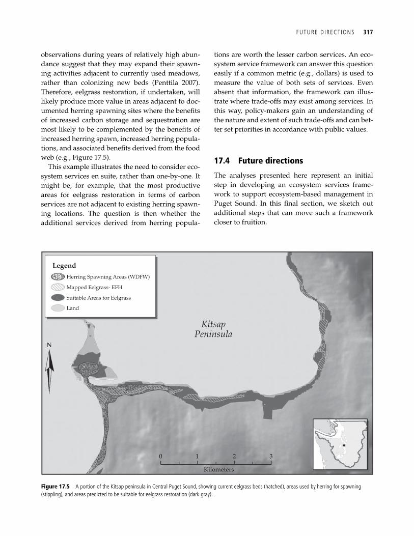
FUTURE DIRECTIONS 317
observations during years of relatively high abun-dance suggest that they may expand their spawn-ing activities adjacent to currently used meadows, rather than colonizing new beds ( Penttila 2007 ). Therefore, eelgrass restoration, if undertaken, will likely produce more value in areas adjacent to doc-umented herring spawning sites where the benefi ts of increased carbon storage and sequestration are most likely to be complemented by the benefi ts of increased herring spawn, increased herring popula-tions, and associated benefi ts derived from the food web (e.g., Figure 17.5 ).
This example illustrates the need to consider eco-system services en suite, rather than one-by-one. It might be, for example, that the most productive areas for eelgrass restoration in terms of carbon services are not adjacent to existing herring spawn-ing locations. The question is then whether the additional services derived from herring popula-
tions are worth the lesser carbon services. An eco-system service framework can answer this question easily if a common metric (e.g., dollars) is used to measure the value of both sets of services. Even absent that information, the framework can illus-trate where trade-offs may exist among services. In this way, policy-makers gain an understanding of the nature and extent of such trade-offs and can bet-ter set priorities in accordance with public values.
17.4 Future directions
The analyses presented here represent an initial step in developing an ecosystem services frame-work to support ecosystem-based management in Puget Sound. In this fi nal section, we sketch out additional steps that can move such a framework closer to fruition.
Herring Spawning Areas (WDFW)
Mapped Eelgrass- EFH
Suitable Areas for Eelgrass
0 1
Kilometers
2 3
Land
NNN
Legend
KitsapPeninsula
Figure 17.5 A portion of the Kitsap peninsula in Central Puget Sound, showing current eelgrass beds (hatched), areas used by herring for spawning (stippling), and areas predicted to be suitable for eelgrass restoration (dark gray ).
318 ECOSYSTEM SERVICE ASSESSMENTS FOR MARINE CONSERVATION
A more complete evaluation of protection or res-toration strategies will incorporate spatial variation in carbon storage and sequestration or food web functions and assess specifi c locations in terms of their current or potential production of these bene-fi ts. This information can provide useful guidance for recovery of the Puget Sound nearshore by pro-viding a map with sites categorized according to their likely ecosystem service benefi ts under protec-tion (for currently intact sites) or restoration (for sites that are currently degraded but with high intrinsic potential) strategies.
Such an evaluation also needs to expand the modeling of marine ecosystem services beyond the current set covered. Incorporating more links between nearshore habitat conditions and the marine food web will allow us to investigate other potential trade-offs among the provisioning serv-ices of commercial fi sheries for salmon and other fi nfi sh, clam, oyster, crab, and other shellfi sh har-vests, as well as the numerous cultural services that include bird and whale watching and recreational fi shing. Waste treatment through the breakdown of PAHs (polycyclic aromatic hydrocarbons) and PCBs (polychlorinated biphenyls) by eelgrass should be added to the list of marine ecosystem services included in the analysis.
It also is possible in Puget Sound to extend the ecosystem services approach to include upland activities and their associated ecosystem services—basin-wide maps exist of current provisioning of water yields, water retention for fl oods, water puri-fi cation potential, carbon storage, and commercial values of working landscapes in watersheds ( Aukema et al. 2009 ; Rogers and Cooke 2009 ). The Partnership is interested in understanding how those watershed-based ecosystem benefi ts affect nearshore services provided to inform how and where to encourage different land-use practices around the region.
Clearly, developing a framework for assessing marine ecosystem services useful to policy-makers is an ambitious undertaking. Marine systems lack the commonly available spatial data that inform assess-ments of terrestrial services. As a result, building an assessment toolkit for marine environments may always be reliant on a richer set of local data and models developed for a particular location. We are
using lessons learned from working in the Puget Sound region to develop models for multiple marine ecosystem services. The Marine Initiative of the Natural Capital Project is developing a marine InVEST tool that, like its terrestrial counterpart, will be an ecosystem services scenario assessment tool for application in ecosystem-based management proc-esses with diverse stakeholders and across multiple scales. Building on the success of InVEST on land, we will connect existing models through the land-sea interface to new and existing marine models.
Ultimately, quantifying, mapping, and valuing marine ecosystem services has the potential to fun-damentally change the ways in which decisions about marine and coastal environments are made. Making explicit the connections between human activities in one sector and their effects on a broad range of other sectors forces decision-makers and the human communities they represent to think about whole ecosystems and to manage them accordingly. By making clear the life-sustaining services oceans and coasts provide, appropriately valuing marine natural capital can help human communities make better choices about how we use these treasured environments.
References
Aburto-Oropeza, O., Ezcurra, E., Danemann, G., et al . (2008). Mangroves in the Gulf of California increase fi shery yields. Proceedings of the National Academy of Sciences, 105 , 10456–9.
Agardy, T., Alder, J., Dayton, P., et al . (2005). Coastal sys-tems: assessment report , Chapter 19. Millennium Ecosystem Assessment.
Ainsworth, C., Varkey, D., and Pitcher, T. (2008). Ecosystem simulations supporting ecosystem-based fi sheries man-agement in the Coral Triangle, Indonesia. Ecological Modeling, 214 , 361–74.
Alderdice, D. F., and Hourston, A. S. (1985). Factors infl u-encing development and survival of Pacifi c Herring ( Clupea harengus pallasi ) eggs and larvae to beginning of exogenous feeding. Canadian Journal of Fisheries and Aquatic Sciences, 42 , 56–68.
Alliance for Puget Sound Shorelines. (2008). http://www.shorelinealliance.org/ .
Alongi, D. M. (2008). Mangrove forests: Resilience, protec-tion from tsunamis, and responses to global climate change. Estuarine, Coastal and Shelf Science, 76 , 1–13.
FUTURE DIRECTIONS 319
Aukema, J., Vigerstol, K., and Foster, J. (2009). Application of InVEST models in Puget Sound , March 20, 2009. Unpublished report available from authors upon request.
Bando, K. J. (2006). The roles of competition and distur-bance in a marine invasion. Biological Invasions, 8 , 755–63.
Barbier, E. B. (2000). Valuing the environment as input: Applications to mangrove-fi shery linkages. Ecological Economics, 35 , 47–61.
Barbier, E. B. (2003). Habitat-fi shery linkages and man-grove loss in Thailand. Contemporary Economic Policy , 21 , 59–77.
Barbier, E. B. (2007). Valuing ecosystem services as pro-ductive inputs. Economic Policy , 22 , 177–229.
Barbier, E. B., Koch, E. W., Silliman, B. R., et al . (2008). Coastal Ecosystem-Based Management with Nonlinear Ecological Functions and Values. Science, 319 , 321–3.
Batie, S., and Wilson, J. (1978). Economic values attributa-ble to Virginia’s coastal wetlands as inputs in oyster production. Southern Journal of Agricultural Economics, 10 , 111–18.
Bell, F. (1989). Application of wetland valuation theory to Florida fi sheries . Florida Sea Grant Program, Florida State University, Tallahassee.
Bennett, E. L., and Reynolds, C. J. (1993). The value of a mangrove area in Sarawak. Biodiversity and Conservation, 2 , 359–75.
Brander, L. M., Van Beukering, P., and Cesar, H. S. J. (2007). The recreational value of coral reefs: a meta-analysis. Ecological Economics , 63 , 209–18.
Burke, L., and Maidens, J. (2004). Reefs at risk in the Carribean. World Resources Institute, Washington, DC. Available online at: http://pdf.wri.org/reefs_carib-bean_front.pdf
Burke, L., Greenhalgh, S., Prager, D., et al . (2008). Coastal capital—economic valuation of coral reefs in Tobago and St. Lucia. World Resources Institute, Washington, DC. Online at: http://www.wri.org/project/coral-reefs .
Carpenter, S., Caraco, N., Correll, D., et al . (1998). Nonpoint pollution of surface waters with phosphorus and nitro-gen. Ecological Applications, 8 , 559–68.
Carte, B. K. (1996). Biomedical potential of marine natural products. Bioscience , 46 , 271–86.
Cesar, H. S. J., Ed. (2000). Collected essays on the economics of coral reefs . CORDIO, Kalmar Univeristy, Sweden.
Chmura, G., Anisfeld, S., Cahoon, D., et al . (2003). Global carbon sequestration in tidal, saline wetlands soils. Global Biogeochemical Cycles , 17 , 1111.
Christensen, V., and Walters, C. (2004). Ecopath with Ecosim: methods, capabilities and limitations. Ecological Modeling , 172 , 109–39.
Cochard, S. L., Ranamukhaarachchi, G. P., Shivakotib, O. V., et al . (2008). The 2004 tsunami in Aceh and Southern Thailand: A review on coastal ecosystems, wave hazards and vulnerability. Perspectives in Plant Ecology, Evolution and Systematics, 10 , 3–40.
Colling, A. (2001). Ocean circulation. Butterworth Heineman/Open University, Milton Keynes.
Costanza, R. (2000). The ecological, economic and social importance of the oceans. In: C. R. C. Sheppard, Ed., Seas at the millenium: an environmental evaluation , vol. 3: global issues and processes. Pergamon Press, New York.
Costanza, R., dArge, R., deGroot, R., et al . (1997). The value of the world’s ecosystem services and natural capital. Nature , 387 , 253–60.
Council on Environmental Quality. (2009). Interim Report of the Interagency Ocean Policy Task Force. September 10, 2009. available at: http://www.white-house.gov/administration/eop/ceq/initiatives/oceans/interimrep .
Culliton, T. (1998). Population: distribution, density, and growth . National Oceanic and Atmospheric Admini-stration, Silver Spring, MD.
Danielsen, F., Sorensen, M., Olwig, M., et al . (2005). The Asian tsunami: a protective role for coastal vegetation. Science , 370 , 643.
Davies, J., Guerry, A., Ruckelshaus, M. (In preparation). Mapping the potential distrubution of shallow-subti-dal eelgrass in the greater Puget Sound region of Washington state.
Dean, T., Haldorson, L., Laur, D., et al . (2000). The distribu-tion of nearshore fi shes in kelp and eelgrass communi-ties in Prince William Sound, Alaska: Associations with vegetation and physical habitat characteristics. Environmental Biology of Fishes , 57 , 271–87.
Diaz, R., and Rosenberg, R. (2008). Spreading dead zones and consequences for marine ecosystems. Science , 321 , 926–9.
Duarte, C. M. (2002). The future of seagrass meadows. Environmental Conservation, 29 , 192–206.
Duarte, C., and Cebrian, J. (1996). The fate of marine auto-trophic production. Limnology and Oceanography, 41 , 1758–66.
FAO Fisheries Department. (2009). The state of world fi sher-ies and aquaculture—2008 (SOFIA). FAO, Rome.
Farber, S. (1988). The value of coastal wetlands for recrea-tion—an application of travel cost and contingent valua-tion methodologies. Journal of Environmental Management, 26 , 299–312.
Forbes, K., and Broadhead, J. (2007). The role of coastal forests in the mitigation of tsunami impacts . RAP Publication 2007/1, Food and Agricultural Organization of the United Nations, Regional Offi ce for Asia and the Pacifi c, Bangkok.
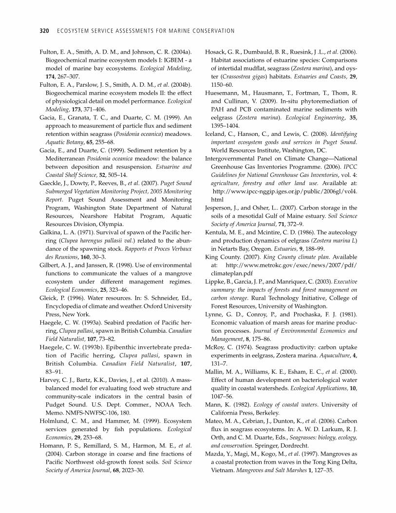
320 ECOSYSTEM SERVICE ASSESSMENTS FOR MARINE CONSERVATION
Fulton, E. A., Smith, A. D. M., and Johnson, C. R. (2004a). Biogeochemical marine ecosystem models I: IGBEM - a model of marine bay ecosystems. Ecological Modeling , 174 , 267–307.
Fulton, E. A., Parslow, J. S., Smith, A. D. M., et al . (2004b). Biogeochemical marine ecosystem models II: the effect of physiological detail on model performance. Ecological Modeling, 173 , 371–406.
Gacia, E., Granata, T. C., and Duarte, C. M. (1999). An approach to measurement of particle fl ux and sediment retention within seagrass ( Posidonia oceanica ) meadows. Aquatic Botany , 65 , 255–68.
Gacia, E., and Duarte, C. (1999). Sediment retention by a Mediterranean Posidonia oceanica meadow: the balance between deposition and resuspension. Estuarine and Coastal Shelf Science, 52 , 505–14.
Gaeckle, J., Dowty, P., Reeves, B., et al . (2007). Puget Sound Submerged Vegetation Monitoring Project, 2005 Monitoring Report . Puget Sound Assessment and Monitoring Program, Washington State Department of Natural Resources, Nearshore Habitat Program, Aquatic Resources Division, Olympia.
Galkina, L. A. (1971). Survival of spawn of the Pacifi c her-ring ( Clupea harengus pallasii val. ) related to the abun-dance of the spawning stock. Rapports et Proces Verbaux des Reunions , 160 , 30–3.
Gilbert, A. J., and Janssen, R. (1998). Use of environmental functions to communicate the values of a mangrove ecosystem under different management regimes. Ecological Economics , 25 , 323–46.
Gleick, P. (1996). Water resources. In: S. Schneider, Ed., Encyclopedia of climate and weather. Oxford University Press, New York.
Haegele, C. W. (1993a). Seabird predation of Pacifi c her-ring, Clupea pallasi , spawn in British Columbia. Canadian Field Naturalist, 107 , 73–82.
Haegele, C. W. (1993b). Epibenthic invertebrate preda-tion of Pacific herring, Clupea pallasi , spawn in British Columbia. Canadian Field Naturalist , 107 , 83–91.
Harvey, C. J., Bartz, K.K., Davies, J., et al. (2010). A mass-balanced model for evaluating food web structure and community-scale indicators in the central basin of Pudget Sound. U.S. Dept. Commer., NOAA Tech. Memo. NMFS-NWFSC-106, 180.
Holmlund, C. M., and Hammer, M. (1999). Ecosystem services generated by fi sh populations. Ecological Economics , 29 , 253–68.
Homann, P. S., Remillard, S. M., Harmon, M. E., et al . (2004). Carbon storage in coarse and fi ne fractions of Pacifi c Northwest old-growth forest soils. Soil Science Society of America Journal , 68 , 2023–30.
Hosack, G. R., Dumbauld, B. R., Ruesink, J .L., et al . (2006). Habitat associations of estuarine species: Comparisons of intertidal mudfl at, seagrass ( Zostera marina ), and oys-ter ( Crassostrea gigas ) habitats. Estuaries and Coasts, 29 , 1150–60.
Huesemann, M., Hausmann, T., Fortman, T., Thom, R. and Cullinan, V. (2009). In-situ phytoremediation of PAH and PCB contaminated marine sediments with eelgrass ( Zostera marina ). Ecological Engineering , 35 , 1395–1404.
Iceland, C., Hanson, C., and Lewis, C. (2008). Identifying important ecosystem goods and services in Puget Sound . World Resources Institute, Washington, DC.
Intergovernmental Panel on Climate Change—National Greenhouse Gas Inventories Programme. (2006). IPCC Guidelines for National Greenhouse Gas Inventories , vol. 4: agriculture, forestry and other land use. Available at: http://www.ipcc-nggip.iges.or.jp/public/2006gl/vol4.html
Jesperson, J., and Osher, L.. (2007). Carbon storage in the soils of a mesotidal Gulf of Maine estuary. Soil Science Society of America Journal, 71 , 372–9.
Kentula, M. E., and Mcintire, C. D. (1986). The autecology and production dynamics of eelgrass (Zostera marina L ) in Netarts Bay, Oregon. Estuaries, 9 , 188–99.
King County. (2007). King County climate plan. Available at: http://www.metrokc.gov/exec/news/2007/pdf/climateplan.pdf
Lippke, B., Garcia, J. P., and Manriquez, C. (2003). Executive summary: the impacts of forests and forest management on carbon storage . Rural Technology Initiative, College of Forest Resources, University of Washington.
Lynne, G. D., Conroy, P., and Prochaska, F. J. (1981). Economic valuation of marsh areas for marine produc-tion processes. Journal of Environmental Economics and Management , 8 , 175–86.
McRoy, C. (1974). Seagrass productivity: carbon uptake experiments in eelgrass, Zostera marina. Aquaculture , 4 , 131–7.
Mallin, M. A., Williams, K. E., Esham, E. C., et al . (2000). Effect of human development on bacteriological water quality in coastal watersheds. Ecological Applications, 10 , 1047–56.
Mann, K. (1982). Ecology of coastal waters . University of California Press, Berkeley.
Mateo, M. A., Cebrian, J., Dunton, K., et al . (2006). Carbon fl ux in seagrass ecosystems. In: A. W. D. Larkum, R. J. Orth, and C. M. Duarte, Eds., Seagrasses: biology, ecology, and conservation. Springer, Dordrecht.
Mazda, Y., Magi, M., Kogo, M., et al . (1997). Mangroves as a coastal protection from waves in the Tong King Delta, Vietnam. Mangroves and Salt Marshes 1 , 127–35.
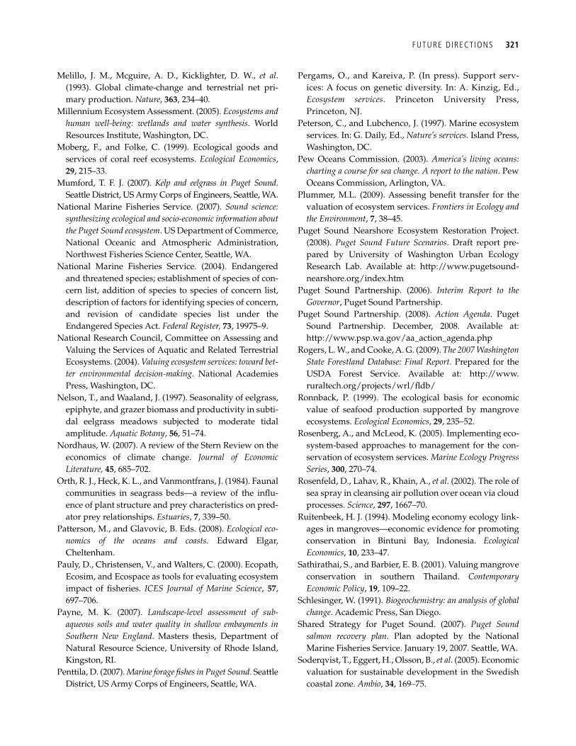
FUTURE DIRECTIONS 321
Melillo, J. M., Mcguire, A. D., Kicklighter, D. W., et al . (1993). Global climate-change and terrestrial net pri-mary production. Nature , 363 , 234–40.
Millennium Ecosystem Assessment. (2005). Ecosystems and human well-being: wetlands and water synthesis . World Resources Institute, Washington, DC.
Moberg, F., and Folke, C. (1999). Ecological goods and services of coral reef ecosystems. Ecological Economics , 29 , 215–33.
Mumford, T. F. J. (2007). Kelp and eelgrass in Puget Sound . Seattle District, US Army Corps of Engineers, Seattle, WA.
National Marine Fisheries Service. (2007). Sound science: synthesizing ecological and socio-economic information about the Puget Sound ecosystem . US Department of Commerce, National Oceanic and Atmospheric Administration, Northwest Fisheries Science Center, Seattle, WA.
National Marine Fisheries Service. (2004). Endangered and threatened species; establishment of species of con-cern list, addition of species to species of concern list, description of factors for identifying species of concern, and revision of candidate species list under the Endangered Species Act. Federal Register, 73 , 19975–9.
National Research Council, Committee on Assessing and Valuing the Services of Aquatic and Related Terrestrial Ecosystems. (2004). Valuing ecosystem services: toward bet-ter environmental decision-making . National Academies Press, Washington, DC.
Nelson, T., and Waaland, J. (1997). Seasonality of eelgrass, epiphyte, and grazer biomass and productivity in subti-dal eelgrass meadows subjected to moderate tidal amplitude. Aquatic Botany , 56 , 51–74.
Nordhaus, W. (2007). A review of the Stern Review on the economics of climate change. Journal of Economic Literature, 45 , 685–702.
Orth, R. J., Heck, K. L., and Vanmontfrans, J. (1984). Faunal communities in seagrass beds—a review of the infl u-ence of plant structure and prey characteristics on pred-ator prey relationships. Estuaries , 7 , 339–50.
Patterson, M., and Glavovic, B. Eds. (2008). Ecological eco-nomics of the oceans and coasts. Edward Elgar, Cheltenham.
Pauly, D., Christensen, V., and Walters, C. (2000). Ecopath, Ecosim, and Ecospace as tools for evaluating ecosystem impact of fi sheries. ICES Journal of Marine Science , 57 , 697–706.
Payne, M. K. (2007). Landscape-level assessment of sub- aqueous soils and water quality in shallow embayments in Southern New England . Masters thesis, Department of Natural Resource Science, University of Rhode Island, Kingston, RI.
Penttila, D. (2007). Marine forage fi shes in Puget Sound . Seattle District, US Army Corps of Engineers, Seattle, WA.
Pergams, O., and Kareiva, P. (In press). Support serv-ices: A focus on genetic diversity. In: A. Kinzig, Ed., Ecosys tem services . Princeton University Press, Princeton, NJ.
Peterson, C., and Lubchenco, J. (1997). Marine ecosystem services. In: G. Daily, Ed., Nature’s services . Island Press, Washington, DC.
Pew Oceans Commission. (2003). America’s living oceans: charting a course for sea change. A report to the nation . Pew Oceans Commission, Arlington, VA.
Plummer, M.L. (2009). Assessing benefi t transfer for the valuation of ecosystem services. Frontiers in Ecology and the Environment , 7 , 38–45.
Puget Sound Nearshore Ecosystem Restoration Project. (2008). Puget Sound Future Scenarios . Draft report pre-pared by University of Washington Urban Ecology Research Lab. Available at: http://www.pugetsound-nearshore.org/index.htm
Puget Sound Partnership. (2006). Interim Report to the Governor , Puget Sound Partnership.
Puget Sound Partnership. (2008). Action Agenda . Puget Sound Partnership. December, 2008. Available at: http://www.psp.wa.gov/aa_action_agenda.php
Rogers, L. W., and Cooke, A. G. (2009). The 2007 Washington State Forestland Database: Final Report. Prepared for the USDA Forest Service. Available at: http://www.ruraltech.org/projects/wrl/fl db/
Ronnback, P. (1999). The ecological basis for economic value of seafood production supported by mangrove ecosystems. Ecological Economics , 29 , 235–52.
Rosenberg, A., and McLeod, K. (2005). Implementing eco-system-based approaches to management for the con-servation of ecosystem services. Marine Ecology Progress Series , 300 , 270–74.
Rosenfeld, D., Lahav, R., Khain, A., et al . (2002). The role of sea spray in cleansing air pollution over ocean via cloud processes. Science , 297 , 1667–70.
Ruitenbeek, H. J. (1994). Modeling economy ecology link-ages in mangroves—economic evidence for promoting conservation in Bintuni Bay, Indonesia. Ecological Economics , 10 , 233–47.
Sathirathai, S., and Barbier, E. B. (2001). Valuing mangrove conservation in southern Thailand. Contemporary Economic Policy , 19 , 109–22.
Schlesinger, W. (1991). Biogeochemistry: an analysis of global change . Academic Press, San Diego.
Shared Strategy for Puget Sound. (2007). Puget Sound salmon recovery plan . Plan adopted by the National Marine Fisheries Service. January 19, 2007. Seattle, WA.
Soderqvist, T., Eggert, H., Olsson, B., et al . (2005). Economic valuation for sustainable development in the Swedish coastal zone. Ambio , 34 , 169–75.
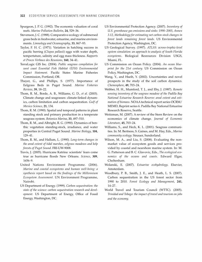
322 ECOSYSTEM SERVICE ASSESSMENTS FOR MARINE CONSERVATION
Spurgeon, J. P. G. (1992). The economic valuation of coral reefs. Marine Pollution Bulletin , 24 , 529–36.
Stevenson, J. C. (1988). Comparative ecology of submersed grass beds in freshwater, estuarine, and marine environ-ments. Limnology and Oceanography , 33 , 867–93.
Taylor, F. H. C. (1971). Variation in hatching success in pacifi c herring ( Clupea pallasii ) eggs with water depth, tempertature, salinity and egg mass thickness. Rapports et Proces Verbaux des Reunions , 160 , 34–41.
TerraLogic GIS Inc. (2004). Public seagrass compilation for west coast Essential Fish Habitat (EFH) Environmental Impact Statement . Pacifi c States Marine Fisheries Commission, Portland, OR.
Thayer, G., and Phillips, S. (1977). Importance of Eelgrass Beds in Puget Sound. Marine Fisheries Review , 39 , 18–22.
Thom, R. M., Borde, A. B., Williams, G. D., et al . (2003). Climate change and seagrasses: climate-linked dynam-ics, carbon limitation and carbon sequestration. Gulf of Mexico Science , 21 , 134.
Thom, R. M. (1990). Spatial and temporal patterns in plant standing stock and primary production in a temperate seagrass system. Botanica Marina , 33 , 497–510.
Thom, R. M., and Albright, R. G. (1990). Dynamics of ben-thic vegetation standing-stock, irradiance, and water properties in Central Puget Sound. Marine Biology , 104 , 129–41.
Thom, R. M., and Hallum, L. (1990). Long-term changes in the areal extent of tidal marshes, eelgrass meadows and kelp forests of Puget Sound . FRI-UW-9008.
Travis, J. (2005). Hurricane Katrina: scientists’ fears come true as hurricane fl oods New Orleans. Science , 309 , 1656–9.
United Nations Environment Programme. (2006). Marine and coastal ecosystems and human well-being: a synthesis report based on the fi ndings of the Millennium Ecosystem Assessment. UN Environment Programme, Nairobi.
US Department of Energy. (1999). Carbon sequestration: the state of the science: carbon sequestration research and devel-opment . US Department of Energy, Offi ce of Fossil Energy, Washington, DC.
US Environmental Protection Agency. (2007). Inventory of U.S. greenhouse gas emissions and sinks: 1990–2005, Annex 3.12, Methodology for estimating net carbon stock changes in forest lands remaining forest lands . US Environmental Protection Agency, Washington, DC.
US Geological Survey. (1997). ATLSS: across-trophic-level system simulation: an approach to analysis of South Florida ecosystems . Biological Resrources Division USGS, Miami, FL.
US Commission on Ocean Policy. (2004). An ocean blue-print for the 21st century. US Commission on Ocean Policy, Washington, DC.
Wang, Y., and Hseih, Y. (2002). Uncertainties and novel prospects in the study of the soil carbon dynamics. Chemosphere , 49 , 703–24.
Webber, H. H., Mumford, T. J., and Eby, J. (1987). Remote sensing inventory of the seagrass meadow of the Padilla Bay National Estuarine Research Reserve: areal extent and esti-mation of biomass . NOAA technical report series OCRM/MEMD, Reprint series 6. Padilla Bay National Estuarine Research Reserve, Seattle.
Weitzman, M. (2007). A review of the Stern Review on the economics of climate change. Journal of Economic Literature , 45 , 703–24.
Williams, S., and Heck, K. L. (2001). Seagrass communi-ties. In: M. Bertness, S. Gaines, and M. Hay, Eds., Marine community ecology. Sinauer, Sunderland.
Wilson, M. A., and Liu, S. (2008). Evaluating the non-market value of ecosystem goods and services pro-vided by coastal and nearshore marine system. In: M. G. Patterson and B. C. Glavovic, Eds., The ecological eco-nomics of the oceans and coasts . Edward Elgar, Cheltenham.
Wolanski, E. (2007). Estuarine ecohydrology . Elsevier, Amsterdam.
Woodbury, P. B., Smith, J. E., and Heath, L. S. (2007). Carbon sequestration in the US forest sector from 1990 to 2010. Forest Ecology and Management , 241 , 14–27.
World Travel and Tourism Council (WTTC). (2005). Trinidad and Tobago: the impact of travel and tourism on jobs and the economy.
323
CHAPTER 18
Modeling the impacts of climate change on ecosystem services Joshua J. Lawler, Erik Nelson, Marc Conte, Sarah L. Shafer, Driss Ennaanay, and Guillermo Mendoza
18.1 Introduction
The Earth’s climate has already changed signifi -cantly in response to increased greenhouse-gas con-centrations from human activities, and future climatic changes are projected to be even more dra-matic, with global average temperatures expected to rise between 1.1 and 6.4˚C by 2100, depending on future emissions from human activities ( Alley et al. 2007 ). With the rise in temperature will also come changes in precipitation patterns, with some areas becoming drier, and others wetter. Climate change of this magnitude is certain to have major impacts on basic ecosystem processes such as primary pro-duction, hydrological cycles, and nutrient cycles ( Cramer et al. 2001 ; Stewart et al. 2005 ; Betts et al. 2007 ). In this chapter, we discuss how models that link land cover and land use to ecosystem services can also be used to assess the impact of climate change on ecosystem services. Many studies have addressed how specifi c ecosystem services, particu-larly water availability and agricultural production or food security, are expected to respond to climate change. Here, we go one step beyond and demon-strate how climate impacts can be integrated by examining several ecosystem services within the same framework.
18.2 Previous analyses of climate-driven changes in ecosystem services
Much of the world’s population relies on surface water for drinking and irrigation. Given the clear links between climate and hydrology, projected changes in climate will likely have signifi cant effects
on water availability. Climate change is projected to increase surface-water availability at far northern latitudes, across much of Asia, and parts of eastern Africa and southeastern South America ( Milly et al. 2005 ). In contrast, water availability is projected to decrease in the Middle East, mid-latitude western North America, southern Africa, and southern Europe ( Milly et al. 2005 ). However, not all studies agree on the geographic distribution of potential future hydrologic changes, particularly when human population growth is taken into account ( Vörösmarty et al. 2000 ; Arnell 2004 ). Furthermore, the effects of changes in temperature and precipita-tion on water availability are not necessarily simple. For example, across Africa, decreases in precipita-tion are projected to have very different effects on runoff in areas with different annual rainfall regimes ( de Wit and Stankiewicz 2006 ). A 10% decrease in precipitation was projected to result in a 20% decrease in runoff in Ouagadougou, Burkina Faso, whereas the same decrease in precipitation was projected to produce a 77% decrease in runoff in Okavango, Botswana ( de Wit and Stankiewicz 2006 ).
Changes in water availability as well as changes in temperature and atmospheric CO 2 concentra-tions will affect water demand, agricultural produc-tion, and, in some cases, food security ( Alcamo and Henrichs 2002 ; Arnell 2004 ; Battisti and Naylor 2009 ). For example, there are clear linkages between recent changes in temperature and crop production (Box 18.1)—increases in temperature have been linked to overall decreases in corn and soybean yields in the USA ( Lobell and Asner 2003 ). As one would expect, however, the direction of this trend
324 MODELING THE IMPACTS OF CL IMATE CHANGE ON ECOSYSTEM SERVICES
differs by geographic region—US corn and soybean yields in cooler areas have responded positively to warming whereas yields in warmer areas have responded negatively. Globally, crop yields have been projected to increase with a doubling of atmos-pheric CO 2 concentrations ( Rosenzweig and Parry 1994 ). Again, however, some regions will likely experience gains in crop yields while others will experience signifi cant losses.
Individual wild species will also respond to cli-mate change, resulting in changes in the ecosystem services they provide. The most frequently docu-mented effects of climate change on wild species include shifts in distributions and shifts in phenol-ogy ( Walther et al. 2002 ; Parmesan and Yohe 2003 ; Root et al. 2003 ; Parmesan 2006 ). Most directly, the abundance or location of species that are themselves directly harvested for food may be altered by cli-mate change. For example, increases in temperature will likely reduce the overall range of many cool- and coldwater fi sh, including salmonids. Further-more, reductions in snowpack have the potential to alter fl ow regimes potentially affecting spawning habitat and egg survival of salmonids. Battin et al. ( 2007 ) explored the potential combined effects of climate change and stream restoration on Chinook salmon in a watershed in western Washington in the western United States. Projected changes in the modeled salmon population for 2050 ranged from a decrease of 40% to an increase of 19% depending on the climate-change scenario that was used as well as the extent of habitat restoration that was assumed to take place. It is likely that studies of other eco-nomically important wild species will also reveal changes in their productivity as a result of climate change.
18.3 Using ecosystem-service models to evaluate the impact of climate change on natural and human systems
Water supply is dependent on climate, geology, topography, land cover and land management ( Chapter 4 , this volume). By combining land-use and land-cover data with climate projections it is possible to examine likely changes in intercon-nected ecosystem services (see Chapters 5 through 13 ). The simplest models (tier 1) for water-related
services are based on average annual inputs of cli-matic conditions and provide annual average out-puts of service provision. Therefore, in regions where climate change is expected to affect annual precipitation and temperature patterns, the tier 1 water-related service models provide informative but temporally-coarse projections. However, in many cases, climate change is expected to shift sea-sonal precipitation patterns, but leave annual total precipitation relatively unchanged. For these cases, tier 1 models will be inappropriate and the ramifi -cations of climate change on water services can only be estimated with water-related service models that make projections based on monthly or daily inputs (tier 2 models).
In most cases, the agricultural production models described in Chapter 9 can also be directly applied to climate simulations. If the tier 1 agriculture pro-duction model employs yield functions that include average temperature or total water budget during the growing season as an input, then the effect of changes in these variables on agriculture produc-tion are easily simulated. The tier 2 agriculture pro-duction model discussed in Chapter 9 uses climate inputs at a daily or monthly resolution. In most cases, tier 2 models will more accurately capture changes in agricultural production because growth in most agricultural plants is a process that operates on the scale of hours to months, not seasons to years.
Climate will also indirectly alter ecosystem serv-ices by altering vegetation type, land cover, and even land management ( Bachelet et al. 2001 ; Ramankutty et al. 2002 ). Climate is also known to infl uence the abundance and distribution of plants and animals and in turn biodiversity. Several differ-ent approaches can be taken to modeling climate-driven shifts in land cover, land management, and individual species. For example, dynamic global vegetation models can be used to project changes in the distribution of plant functional types which can be translated into maps of potential vegetation change (e.g., Sitch et al. 2003 ). Other approaches take both climate-driven changes in potential vege-tation and climate-change infl uenced land-use decisions into account (e.g., Bouwman et al. 2006 ). There are likewise different approaches to mode-ling climate-driven changes in individual species
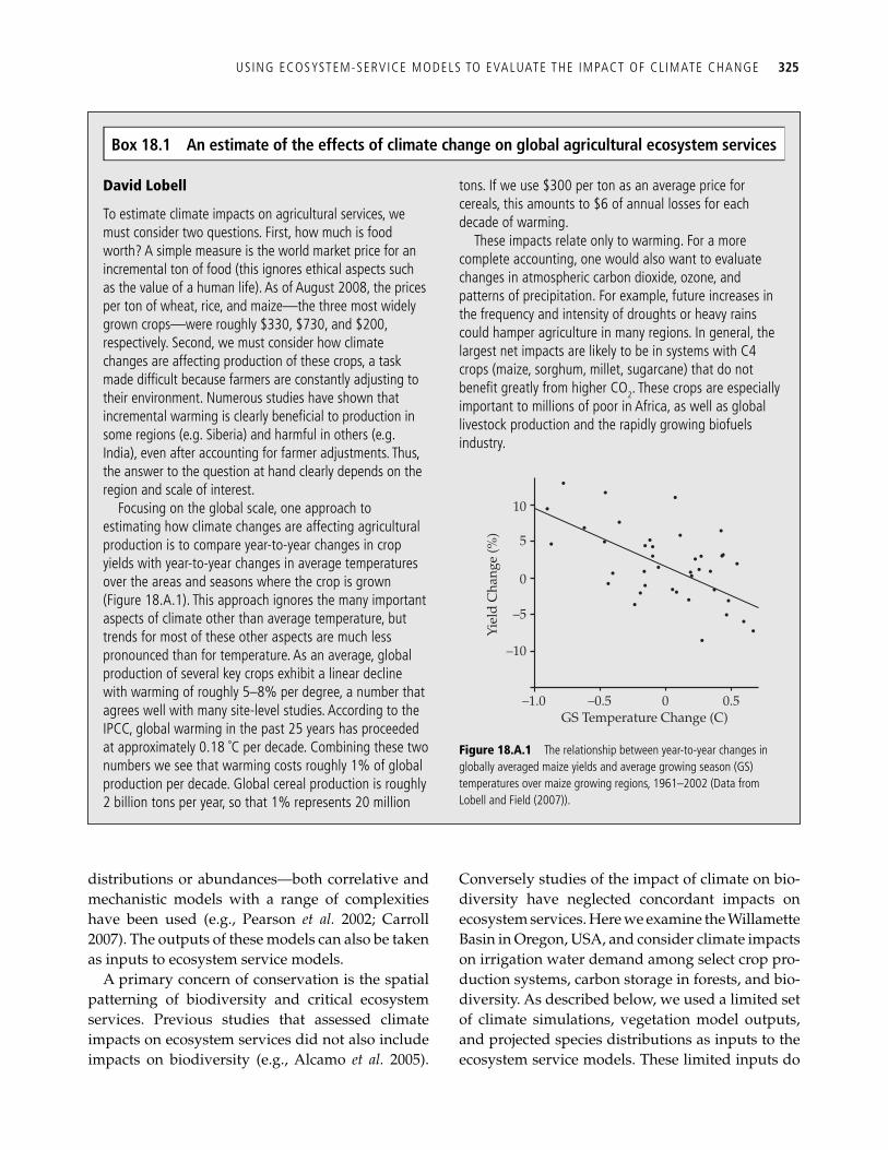
distributions or abundances—both correlative and mechanistic models with a range of complexities have been used (e.g., Pearson et al. 2002 ; Carroll 2007 ). The outputs of these models can also be taken as inputs to ecosystem service models.
A primary concern of conservation is the spatial patterning of biodiversity and critical ecosystem services. Previous studies that assessed climate impacts on ecosystem services did not also include impacts on biodiversity (e.g., Alcamo et al. 2005 ).
Conversely studies of the impact of climate on bio-diversity have neglected concordant impacts on ecosystem services. Here we examine the Willamette Basin in Oregon, USA, and consider climate impacts on irrigation water demand among select crop pro-duction systems, carbon storage in forests, and bio-diversity. As described below, we used a limited set of climate simulations, vegetation model outputs, and projected species distributions as inputs to the ecosystem service models. These limited inputs do
USING ECOSYSTEM-SERVICE MODELS TO EVALUATE THE IMPACT OF CL IMATE CHANGE 325
David Lobell
To estimate climate impacts on agricultural services, we must consider two questions. First, how much is food worth? A simple measure is the world market price for an incremental ton of food (this ignores ethical aspects such as the value of a human life). As of August 2008, the prices per ton of wheat, rice, and maize—the three most widely grown crops—were roughly $330, $730, and $200, respectively. Second, we must consider how climate changes are affecting production of these crops, a task made diffi cult because farmers are constantly adjusting to their environment. Numerous studies have shown that incremental warming is clearly benefi cial to production in some regions (e.g. Siberia) and harmful in others (e.g. India), even after accounting for farmer adjustments. Thus, the answer to the question at hand clearly depends on the region and scale of interest.
Focusing on the global scale, one approach to estimating how climate changes are affecting agricultural production is to compare year-to-year changes in crop yields with year-to-year changes in average temperatures over the areas and seasons where the crop is grown ( Figure 18.A.1 ). This approach ignores the many important aspects of climate other than average temperature, but trends for most of these other aspects are much less pronounced than for temperature. As an average, global production of several key crops exhibit a linear decline with warming of roughly 5–8% per degree, a number that agrees well with many site-level studies. According to the IPCC, global warming in the past 25 years has proceeded at approximately 0.18 ˚C per decade. Combining these two numbers we see that warming costs roughly 1% of global production per decade. Global cereal production is roughly 2 billion tons per year, so that 1% represents 20 million
tons. If we use $300 per ton as an average price for cereals, this amounts to $6 of annual losses for each decade of warming.
These impacts relate only to warming. For a more complete accounting, one would also want to evaluate changes in atmospheric carbon dioxide, ozone, and patterns of precipitation. For example, future increases in the frequency and intensity of droughts or heavy rains could hamper agriculture in many regions. In general, the largest net impacts are likely to be in systems with C4 crops (maize, sorghum, millet, sugarcane) that do not benefi t greatly from higher CO 2 . These crops are especially important to millions of poor in Africa, as well as global livestock production and the rapidly growing biofuels industry.
10
5
0
–5
–10
Yiel
d C
hang
e (%
)
–1.0 –0.5 0GS Temperature Change (C)
0.5
Figure 18.A.1 The relationship between year-to-year changes in globally averaged maize yields and average growing season (GS) temperatures over maize growing regions, 1961–2002 (Data from Lobell and Field ( 2007 )).
Box 18.1 An estimate of the effects of climate change on global agricultural ecosystem services
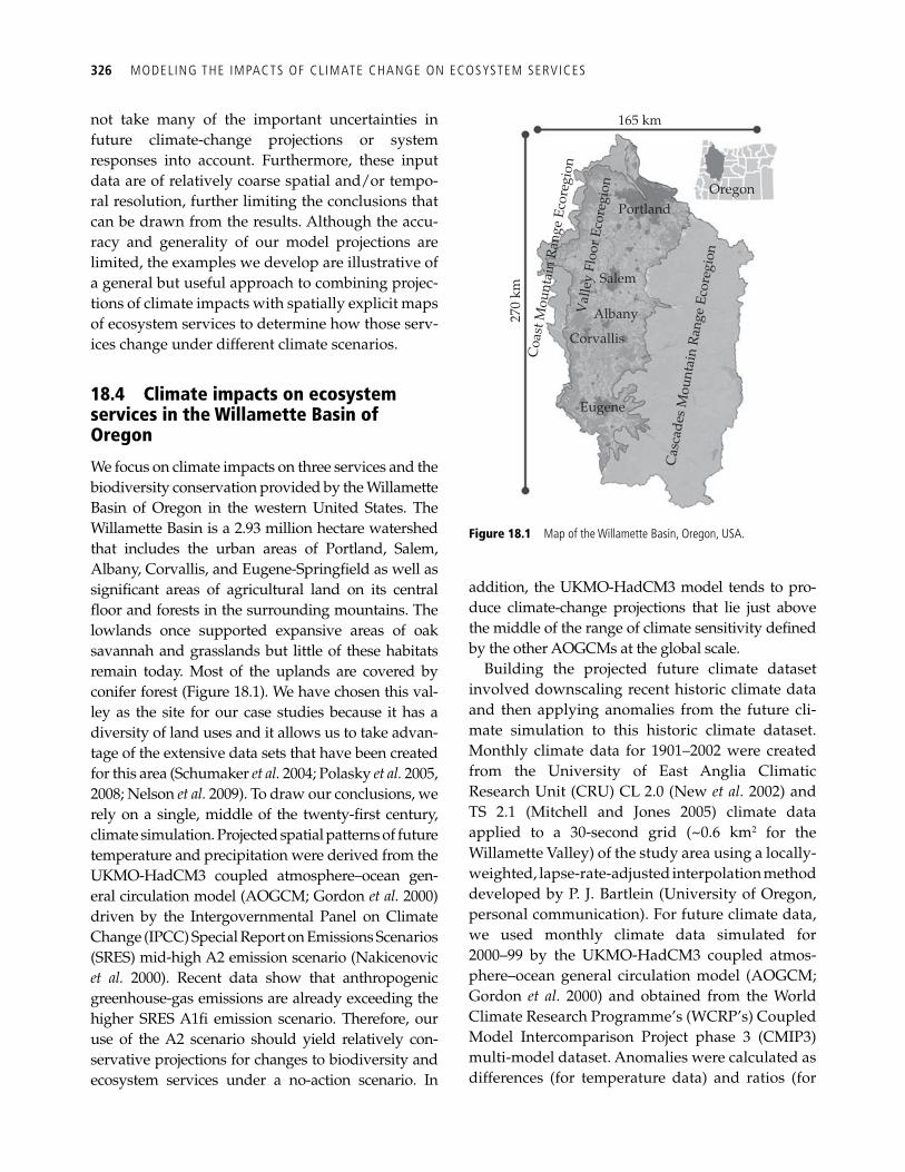
326 MODELING THE IMPACTS OF CL IMATE CHANGE ON ECOSYSTEM SERVICES
not take many of the important uncertainties in future climate-change projections or system responses into account. Furthermore, these input data are of relatively coarse spatial and/or tempo-ral resolution, further limiting the conclusions that can be drawn from the results. Although the accu-racy and generality of our model projections are limited, the examples we develop are illustrative of a general but useful approach to combining projec-tions of climate impacts with spatially explicit maps of ecosystem services to determine how those serv-ices change under different climate scenarios.
18.4 Climate impacts on ecosystem services in the Willamette Basin of Oregon
We focus on climate impacts on three services and the biodiversity conservation provided by the Willamette Basin of Oregon in the western United States. The Willamette Basin is a 2.93 million hectare watershed that includes the urban areas of Portland, Salem, Albany, Corvallis, and Eugene-Springfi eld as well as signifi cant areas of agricultural land on its central fl oor and forests in the surrounding mountains. The lowlands once supported expansive areas of oak savannah and grasslands but little of these habitats remain today. Most of the uplands are covered by conifer forest ( Figure 18.1 ). We have chosen this val-ley as the site for our case studies because it has a diversity of land uses and it allows us to take advan-tage of the extensive data sets that have been created for this area ( Schumaker et al. 2004 ; Polasky et al. 2005 , 2008 ; Nelson et al. 2009 ). To draw our conclusions, we rely on a single, middle of the twenty-fi rst century, climate simulation. Projected spatial patterns of future temperature and precipitation were derived from the UKMO-HadCM3 coupled atmosphere–ocean gen-eral circulation model (AOGCM; Gordon et al. 2000) driven by the Intergovernmental Panel on Climate Change (IPCC) Special Report on Emissions Scenarios (SRES) mid-high A2 emission scenario ( Nakicenovic et al. 2000 ). Recent data show that anthropogenic greenhouse-gas emissions are already exceeding the higher SRES A1fi emission scenario. Therefore, our use of the A2 scenario should yield relatively con-servative projections for changes to biodiversity and ecosystem services under a no-action scenario. In
addition, the UKMO-HadCM3 model tends to pro-duce climate-change projections that lie just above the middle of the range of climate sensitivity defi ned by the other AOGCMs at the global scale.
Building the projected future climate dataset involved downscaling recent historic climate data and then applying anomalies from the future cli-mate simulation to this historic climate dataset. Monthly climate data for 1901–2002 were created from the University of East Anglia Climatic Research Unit (CRU) CL 2.0 ( New et al. 2002 ) and TS 2.1 ( Mitchell and Jones 2005 ) climate data applied to a 30-second grid (~0.6 km 2 for the Willamette Valley) of the study area using a locally-weighted, lapse-rate-adjusted interpolation method developed by P. J. Bartlein (University of Oregon, personal communication). For future climate data, we used monthly climate data simulated for 2000–99 by the UKMO-HadCM3 coupled atmos-phere–ocean general circulation model (AOGCM; Gordon et al. 2000) and obtained from the World Climate Research Programme’s (WCRP’s) Coupled Model Intercomparison Project phase 3 (CMIP3) multi-model dataset. Anomalies were calculated as differences (for temperature data) and ratios (for
165 km
OregonPortland
Salem
Val
ley
Floo
r Eco
regi
on
Coa
st M
ount
ain
Ran
ge E
core
gion
Cas
cade
s M
ount
ain
Ran
ge E
core
gion
Albany
Corvallis
Eugene
270
km Figure 18.1 Map of the Willamette Basin, Oregon, USA.
CLIMATE IMPACTS ON ECOSYSTEM SERVICES IN THE WILLAMETTE BASIN OF OREGON 327
precipitation and percent cloud cover data) between each 2000–99 simulated monthly value and 1961–90 30-year mean monthly values calculated from the UKMO-HadCM3 simulated monthly data for the twentieth century. The anomalies were bi-linearly interpolated to the 30-second grid of the study area and applied to CRU-derived 1961–90 30-year mean data to create the future climate data used in this study.
Importantly, we were not simply interested in cli-mate impacts, but climate impacts assuming differ-ent scenarios of land use and land cover. Projections of human land use were taken from Hulse et al. ( 2002 ) and represent alternative maps of agriculture, forest, and residential and industrial development assuming three different development scenarios. The three scenarios include a “development” trajec-tory that portrays an increase in development pres-sure, a “plan trend” trajectory that continues development at current rates and in current pat-terns, and a “conservation” trajectory that limits development in ways that promote the conservation of natural systems in the Basin. All three land-use scenarios assume that human population in the Basin will increase from 2.0 million in 1990 to 3.9 million people in 2050.
18.4.1 Water availability for agriculture in the Willamette Basin
At the heart of the Willamette Basin is a fertile river valley that produces a wide variety of agricultural goods, ranging from staple grains to wine grapes. Although the region receives signifi cant amounts of precipitation, summers are dry and some of the crops grown in the valley must be irrigated to meet production goals. Here, we explore the potential impacts of future climate change on the provision of freshwater relative to the demand for irrigation water for berries and wine grapes, two of the val-ley’s most valuable crops. We determine, all else being equal, how much irrigation water would be necessary to achieve current crop yields under a hypothesized future climate.
To estimate climate-driven changes in irrigation demand, we compared the volume of water needed for agricultural production under current condi-tions to the volume required under projected future
climatic conditions. For the future time period, we averaged the projected monthly precipitation totals and monthly average temperatures from 2041 to 2070 and used these 30-year monthly means to rep-resent the average climatic conditions for the mid-dle of the century. In this example, we used observed climate in 2000 to represent current (baseline) cli-mate. Ideally, we would have used an averaged 30-year period (as we did with the future projec-tions) to represent baseline conditions. However, our choice of a baseline period was limited by the availability of specifi c crop-yield information in the Basin.
In addition to climate projections, forecasting future irrigation demand requires an estimate of where vineyards and berry fi elds would be located by the middle of the 21st century. We use the pro-jected “plan trend” land-use scenario to identify counties that will likely be involved in agricultural production in 2050 ( Hulse et al. 2002 ). The allocation of vineyards and berry fi elds in a county in 2050 was based on current allocations of these crop types in the county. Of all the counties in the Basin, only Columbia County does not currently produce any of our focal agricultural products; therefore, we excluded it from our irrigation analyses.
By assuming the proportion of crop lands within a county dedicated to berry or grape production in 2050 would be the same as the proportion in 2000, we have likely overestimated the area dedicated to these crops in some regions and underestimated it in others. It is likely that some farmers will take various measures to adapt to changes in climate. Farmers will inevitably cease the cultivation of crops that demand too much irrigation or that fail to thrive under new climatic conditions. In some cases, new crops will be planted and, in more extreme cir-cumstances, agriculture will be abandoned entirely. Although it would be more realistic to try to capture the effects of potential adaptation strategies in our analyses, doing so would introduce additional uncertainties. Early contributions of economic stud-ies that addressed climate-change impacts on agri-cultural production attempted to allow for the mitigating impacts of adaptation ( Mendelsohn et al. 1994 ). More recent efforts, however, have aban-doned the focus on adaptation to avoid the poten-tial biases associated with the functional form
328 MODELING THE IMPACTS OF CL IMATE CHANGE ON ECOSYSTEM SERVICES
assumptions necessary to allow for adaptation ( Deschenes and Greenstone, 2007 ; Schlenker et al. 2005 ). In the interest of simplicity, in our case stud-ies, we did not model the potential effects of adap-tation strategies.
We estimated crop-specifi c water requirements based on local climatic conditions. These require-ments are outputs of CropWat, a tool developed by the Land and Water Development Division of FAO to aid in the design and management of irrigation schemes ( FAO 1992 ). The inputs to this tool include climate data, crop coeffi cients (e.g., root depth and depletion fraction) and growth stages, and soil data for calculating plant water use. The growth-stage specifi c crop coeffi cients for the different agricul-tural products were taken from AgriMet, a satellite-based network of automated agricultural weather stations operated and maintained by the US Bureau of Reclamation. Although the AgriMet data pro-vided the crop coeffi cients as a percentage of growth, the length of the growing season in CropWat is measured in days. The necessary crop coeffi cient values were interpolated assuming linear plant growth. The soil data for the counties in the region were derived from the SSURGO Soil Data Viewer ( USDA 2008 ). Using the climate, land-use, and soils data, we ran CropWat for the fi ve crops we focused on, raspberries, blackberries, strawberries, blueber-ries, and wine grapes.
We translated the crop-specifi c water require-ments from CropWat into the total volume of irriga-tion water required within each county for year 2000 production of each of the fi ve focus crops by multi-plying each crop’s water depth by the total area within each county in 2000 dedicated to the growth of that specifi c crop (crop area data are from the Oregon Agricultural Information Network (OAIN)).
We used the tier 1 water-availability model described in Chapter 4 to project average annual water depth across the landscape for current and predicted mid-century climatic conditions. The tier 1 water model requires temperature, precipita-tion, and land-cover inputs. Again, land cover was assumed to change based on the 2050 plan-trend scenario. Unlike the two other case studies below, our water-availability projections do not include the effects of potential climate-driven shifts in vegetation.
Most of the Basin, including the areas dedicated to wine grape and berry production, is projected to experience decreases in water yield ( Figure 18.2 ; Plate 16). The largest decreases are along the crest of the Cascade Range, but decreases are also forecast for much of the basin fl oor. The largest increases are projected for the foothills of the Cascade Range and the northwestern corner of the basin. The decreases in water yields, in conjunction with increasing tem-peratures, led to increased irrigation demands in berry and grape fi elds across all counties expected to grow these products in 2050 ( Table 18.1; recall that the spatial pattern of cropland in 2050 is based on 2050 projections but the fraction of these lands in the fi ve focus crops is based on observed 2000 patterns ). All counties were projected to require at least a 50% increase in irrigation water to maintain current berry and grape yields, with some counties expected to see as much as an 85% increase in irrigation needs.
These analyses make it clear that increased irriga-tion demand for berries and grapes is one of the potential impacts of climate change for the Willamette Basin. Of course, our analyses were done at relatively coarse temporal and spatial scales, whereas climatic extremes at fi ne temporal scales, such as frosts or water shortages, will signifi cantly impact agricultural yields. Changes in the nature or frequency of climatic extremes, which are also asso-ciated with climate change ( Alley et al. 2007 ) and specifi c weather events could signifi cantly alter irri-gation demands. Mismatches between precipitation events and water demand at a fi ner temporal reso-lution may increase irrigation demand above the levels projected by our models. Finally, as discussed above, some farmers will likely change cultivation practices and/or crops in response to changes in cli-mate, thus, altering irrigation requirements.
18.4.2 Carbon storage in the Basin’s upland forests
The uplands of the Willamette Basin are blanketed in forests, mostly conifer. The forests have contributed to the region’s timber economy for over a century and include remnants of old-growth forests that pro-vide important habitat for a variety of species. Here, we project the potential impacts of climate change on carbon storage in the Basin’s upland forests. We used
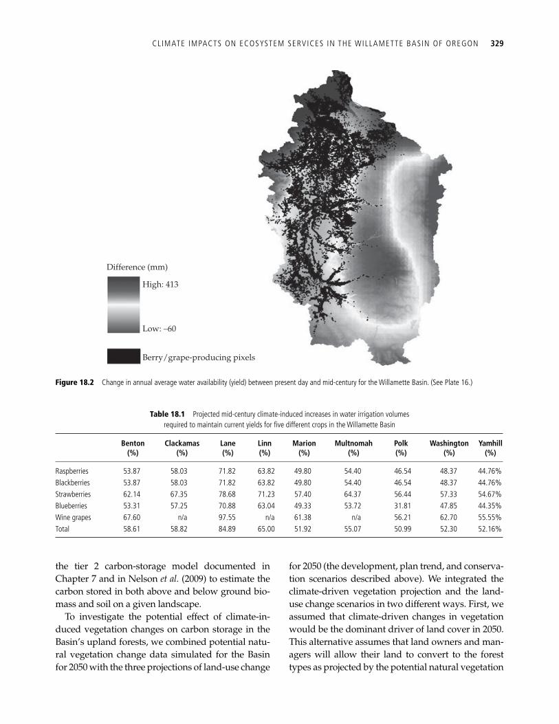
CLIMATE IMPACTS ON ECOSYSTEM SERVICES IN THE WILLAMETTE BASIN OF OREGON 329
Table 18.1 Projected mid-century climate-induced increases in water irrigation volumes required to maintain current yields for fi ve different crops in the Willamette Basin
Benton (%)
Clackamas (%)
Lane (%)
Linn (%)
Marion (%)
Multnomah (%)
Polk (%)
Washington(%)
Yamhill(%)
Raspberries 53.87 58.03 71.82 63.82 49.80 54.40 46.54 48.37 44.76% Blackberries 53.87 58.03 71.82 63.82 49.80 54.40 46.54 48.37 44.76% Strawberries 62.14 67.35 78.68 71.23 57.40 64.37 56.44 57.33 54.67% Blueberries 53.31 57.25 70.88 63.04 49.33 53.72 31.81 47.85 44.35% Wine grapes 67.60 n/a 97.55 n/a 61.38 n/a 56.21 62.70 55.55% Total 58.61 58.82 84.89 65.00 51.92 55.07 50.99 52.30 52.16%
Difference (mm)
High: 413
Low: –60
Berry/grape-producing pixels
Figure 18.2 Change in annual average water availability (yield) between present day and mid-century for the Willamette Basin. (See Plate 16.)
the tier 2 carbon-storage model documented in Chapter 7 and in Nelson et al. ( 2009 ) to estimate the carbon stored in both above and below ground bio-mass and soil on a given landscape.
To investigate the potential effect of climate-in-duced vegetation changes on carbon storage in the Basin’s upland forests, we combined potential natu-ral vegetation change data simulated for the Basin for 2050 with the three projections of land-use change
for 2050 (the development, plan trend, and conserva-tion scenarios described above). We integrated the climate-driven vegetation projection and the land-use change scenarios in two different ways. First, we assumed that climate-driven changes in vegetation would be the dominant driver of land cover in 2050. This alternative assumes that land owners and man-agers will allow their land to convert to the forest types as projected by the potential natural vegetation
330 MODELING THE IMPACTS OF CL IMATE CHANGE ON ECOSYSTEM SERVICES
change maps. This approach leads to more closed mixed and hardwood forests in the Basin’s uplands. We refer to this as the “unmitigated management” scenario. For the second approach, we assumed that forest management actions would be the dominant driver of forest land cover. In this scenario, timber companies, individual land owners, and natural resource management agencies would manage for-ests in such a way that the closed conifer forests that provide much of the economically valuable timber in the Basin’s uplands today would be maintained regardless of changes in climate. In this scenario, for-est management activities are allowed to mitigate the potential effects of climate change on closed canopy conifer forest, however, climate change is still assumed to be the driving factor for changes in all other land-cover types. We refer to this second sce-nario as the “mitigated management” scenario (see the chapter’s online appendix for details on how these mitigated scenario maps were created).
The unmitigated and mitigated management scenarios represent two extreme cases—the actual contribution of land management to mitigating cli-mate-driven land-cover change will likely lie some-where between these two extremes. Table 18.2 summarizes the projected vegetation transitions for the six climate-affected mid-century land-cover sce-
narios (three land-use scenarios and two methods for combining land-use and climate-driven vegeta-tion projections) relative to the mid-century land-use scenario maps that assume no climate-driven change in vegetation.
Before running the carbon-storage model, each of the six climate-change-affected and three baseline 2050 land-use maps, projected at a 30-m grid resolu-tion, were summarized on a grid composed of 500-ha hexagons. We did this to reduce the number of spatial units that had to be run through the car-bon-storage model. These hexagons merely served as spatial units over which the land-cover data were summarized. For example, a 500-ha hexagon could have 200 ha in 0- to 20-year closed conifer forest, 100 ha in 21- and 40-year closed conifer forest, and 300 ha in mixed conifer forest.
In general, climate change is projected to have a negative effect on carbon storage for the Willamette Basin ( Table 18.3 ; see chapter’s online appendix for calculation details). This trend is consistent across all six land-cover and management scenarios when compared to their relevant 2050 baseline maps ( Figure 18.3 ). The 2050 landscapes that consider projected climate-driven changes in vegetation are estimated to store less carbon because the vegeta-tion simulations project a shift from carbon rich,
Table 18.2 Modeled changes in mid-century vegetation cover in the Willamette Basin (in hectares) as a result of hypothesized climatic changes relative to projected mid-century land-cover maps that do not consider climate change
2050 LULC Scenario
Plan trend Development Conservation
Unmitigated Mitigated Unmitigated Mitigated Unmitigated Mitigated
Gain in closed mixed forest 147 420 97 458 147 394 96 029 147 314 124 293 Gain in closed hardwood forest 34 027 25 155 34 068 23 674 34 191 27 776 Loss in closed mixed forest 20 596 14 611 20 569 14 583 20 706 14 717 Loss in closed hardwood forest 1 783 1 783 1 777 1 777 1 784 1 784 Loss in closed conifer forest 159 067 106 218 159 116 103 343 159 014 135 569 Loss in semi-closed hardwood forest 0.18 0.18 0 0 0 0
The projected climate-driven vegetation maps were superimposed on three different potential mid-century land-use scenarios that do not consider climate change (the plan trend, development, and conservation scenarios). The projected vegetation maps were merged with each mid-century land-use scenario map twice. In the fi rst merge, known as the unmitigated management approach, the vegetation map always determined land cover when there was a disagreement between the land-use scenario and vegetation maps. In the second merge, the mitigated management approach, closed conifer forest 0–60 years of age was managed for timber and continued to be closed conifer forest despite any projected climate-driven transitions to other forest types. Likewise, 50% of all closed mixed forest was assumed to remain in mixed forest despite any projected climate change due to management actions. Thus, the mitigated mid-century land-cover maps assume that land managers will be able to maintain a desired forest type despite climate change—an assumption that may not be valid in many cases. The unmitigated approach makes no such assumption. All changes are relative to the relevant baseline mid-century land-use scenario map.
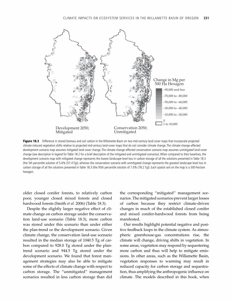
CLIMATE IMPACTS ON ECOSYSTEM SERVICES IN THE WILLAMETTE BASIN OF OREGON 331
older closed conifer forests, to relatively carbon poor, younger closed mixed forests and closed hardwood forests ( Smith et al. 2006 ) ( Table 18.3 ).
Despite the slightly larger negative effect of cli-mate change on carbon storage under the conserva-tion land-use scenario ( Table 18.3 ), more carbon was stored under this scenario than under either the plan-trend or the development scenario. Given climate change, the conservation land-use scenario resulted in the median storage of 1040.5 Tg of car-bon compared to 928.0 Tg stored under the plan-trend scenario and 944.5 Tg stored under the development scenario. We found that forest man-agement strategies may also be able to mitigate some of the effects of climate change with respect to carbon storage. The “unmitigated” management scenarios resulted in less carbon storage than did
the corresponding “mitigated” management sce-narios. The mitigated scenarios prevent larger losses of carbon because they restrict climate-driven changes in much of the established closed conifer and mixed conifer-hardwood forests from being manifested.
Our results highlight potential negative and posi-tive feedback loops in the climate system. As atmos-pheric greenhouse-gas concentrations rise, the climate will change, driving shifts in vegetation. In some areas, vegetation may respond by sequestering more carbon and thus will help to mitigate emis-sions. In other areas, such as the Willamette Basin, vegetation responses to warming may result in reduced capacity for carbon storage and sequestra-tion, thus amplifying the anthropogenic infl uence on climate. The models described in this book, when
Change in Mg per500 Ha Hexagon
Conservation 2050;Unmitigated
Development 2050;Mitigated
–90,000 and less
–70,000 to –80,000
–50,000 to –60,000
–30,000 to –40,000
–10,000 to –20,000
01 to 10,000
Figure 18.3 Difference in stored biomass and soil carbon in the Willamette Basin on two mid-century land-cover maps that incorporate projected climate-induced vegetation shifts relative to projected mid-century land-cover maps that do not consider climate change. The climate-change-affected development scenario map assumes mitigated land-cover change. The climate-change-affected conservation scenario map assumes unmitigated land-cover change (see description in legend for Table 18.2 for a brief description of the mitigated and unmitigated scenarios). When compared to their baselines, the development scenario map with mitigated change represents the lowest landscape-level loss in carbon storage of all the solutions presented in Table 18.3 (the 5th percentile solution of 5.6% (57.4 Tg)), whereas the conservation scenario with unmitigated change represents the greatest landscape-level loss in carbon storage of all the solutions presented in Table 18.3 (the 95th percentile solution of 7.0% (78.2 Tg)). Each spatial unit on the map is a 500-hectare hexagon.
332 MODELING THE IMPACTS OF CL IMATE CHANGE ON ECOSYSTEM SERVICES
Table 18.3 Percentage loss (and absolute loss in Tg) in biomass and soil carbon storage in the Willamette Basin due to hypothesized climatic changes relative to projected mid-century land-cover maps that do not consider climate change
Management approach 2050 LULC scenario
Plan trend Development Conservation
Median Median Median [5th–95th Percentile] [5th–95th Percentile] [5th–95th Percentile]
Unmitigated 6.7% (66.2) 6.6% (66.6) 7.0% (77.8) [6.6 (65.7)–6.7% (66.4)]
[6.5 (66.3)–6.6% (67.0)]
[6.9 (77.5)–7.0% (78.2)]
Mitigated 6.0% (59.9) 5.7% (57.5) 6.7% (75.6) [6.0 (59.6)–6.1% (60.3)]
[5.6 (57.4)–5.7% (58.0)]
[6.7 (75.0)–6.8% (75.8)]
See the legend for Table 18.2 for a brief description of the various mid-century land-use scenario maps considered in this table. There is variability in results because we randomly simulated forest-age structure (this information is not provided by the mid-century land-cover maps) before calculating carbon-storage values. We repeated this process 1000 times. See the chapter’s online appendix for simulation details. All losses are relative to the relevant baseline mid-century land-use use scenario map.
linked with ecosystem or vegetation models, provide a useful tool for investigating where these tradeoffs may occur and where management may be useful if increased carbon storage and sequestration is a goal.
18.4.3 Terrestrial vertebrate diversity in the Basin
The Willamette Basin hosts a rich biota that inhabits diverse environments including oak savannah, mixed hardwood and conifer forests, remnant ripar-ian gallery forests, and young and mature temper-ate conifer rainforest. Here, we explore some of the potential effects of climate change on terrestrial ver-tebrate diversity in the Willamette Basin. Specifi cally, we investigate the effects of hypothesized clim-driven shifts in species distributions and vegetation change (i.e., habitat availability) on two measures of biodiversity status described in detail in Chapter 13 , marginal biodiversity value (MBV) and countryside species area relationship (SAR). In short, MBV is a parcel-level measure of biodiversity based on both the number of species with geographic range in a parcel and the proportion of the parcel that likely serves as habitat for each of the species. SAR is a landscape-level estimate of biodiversity value based on multi-habitat species area relationships ( Pereira and Daily 2006 ). The measure is referred to as a “countryside” metric because it was designed to
assess biodiversity value in diverse, human-domi-nated landscapes.
To model climate-driven changes in species dis-tributions in the Willamette Basin, we used pro-jected range shifts developed for a hemispheric assessment of species’ geographic responses to cli-mate change ( Lawler et al. 2009 ). These range shifts are based on the same climate-change simulation used in the agriculture production and carbon-stor-age case studies above. Although the previous two case studies used the climate and vegetation projec-tions at their native resolutions, (e.g., the 30-second grid), species range-shift projections were gener-ated at a 50-km resolution. These projections were made for the average simulated climatic conditions for a period 2041–70. Our analyses use a set of bird, mammal, and amphibian species for which we have data on current and projected future geographic ranges as well as general habitat associations. This set includes 187 species (136 bird, 47 mammal, and 4 amphibian species). The modeled range shifts resulted in a potential loss of 8 of these species from the Basin by the middle of the century. At the same time, the climate model projects potential range expansions that could result in 17 new species mov-ing into the Basin by the middle of the century, including 3 mammals and 14 birds (see Table 18.4 for a complete list of species with potential ranges that were projected to move in or out of the Basin).
CLIMATE IMPACTS ON ECOSYSTEM SERVICES IN THE WILLAMETTE BASIN OF OREGON 333
As in the carbon-storage case study described above, we imposed projected climate-driven changes in vegetation (i.e., habitat availability) on the three 2050 land-use projections ( Hulse et al. 2002 ) assuming two different land management responses (the unmitigated management and mitigated management schemes described in the carbon-storage example), thereby generating six 2050 maps affected to some degree or another by climate change. We also considered the three 2050 land-use projections that assume no climate-change effects (the baseline 2050 land covers). We also use a year 2000 land-cover map of the Basin for additional comparison purposes (this year 2000 map does not assume any climate-driven change in habitat avail-ability). Finally, as we did in the carbon-storage case
study, land cover on all maps was summarized by 500-ha hexagon. Finally, unlike the carbon-storage case, we included the whole Basin in the biodiver-sity analysis, not just its upland forest areas.
Using these various scenarios, we generated sev-eral alternative landscapes across which we evalu-ated vertebrate diversity. First, we combined the 2000 land-cover map with the maps of current spe-cies distributions. This provided a map of current vertebrate biodiversity. Second, we combined each of the nine 2050 land-cover maps, including the three baseline maps, with maps of projected species distributions. This provided projections of how cli-mate change and land-use change would likely affect vertebrate diversity values when both range shifts and climate-driven changes in habitat are taken into account and when range shifts alone are taken into account. Finally, we combined each of the nine 2050 land-cover maps, including the three baseline maps, with maps of current species distri-butions (i.e., the 2050 land cover assuming no climate-driven shifts in species ranges). This last combination provided an estimate of how both land-use and climate-driven changes in habitat would affect vertebrate diversity when range shifts were not taken into account.
For all projected vertebrate diversity maps, MBV values were calculated for each 500-ha hexagon and the SAR score was calculated for the entire land-scape. As mentioned earlier, MBV measures the pro-portion of the modeled biodiversity supported by a hexagon (or, conversely, the proportion of the land-scape’s total biodiversity that would be lost if the hexagon were suddenly unable to support any spe-cies; see this chapter’s online appendix for species-habitat compatibility scores for all modeled species).
One of the limitations of the MBV index is that it cannot be used to indicate the overall status of ter-restrial biodiversity on the landscape (the summa-tion of MBV values across all hexagons always equals one and does not allow for direct compari-son of collective biodiversity status across scenar-ios). Instead, an MBV map indicates the relative provision of biodiversity across a landscape at some point in time. In contrast, the SAR scores allow for comparison across different landscapes, including the same landscape at different points in time. The SAR score for a species indicates the proportion of
Table 18.4 Species with geographic ranges projected to shift out of or into the Willamette Basin by mid-century
Emigrants Immigrants
Gulo gulo (wolverine) Myodes gapperi (Southern red-backed vole)
Anas acuta (Northern Pintail) Onychomys leucogaster (Northern grasshopper mouse)
Histrionicus histrionicus (Harlequin Duck)
Ovis canadensis (Bighorn sheep)
Bucephala islandica (Barrow’s Goldeneye)
Aeronautes saxatalis (White-throated swift)
Picoides dorsalis (Three-toed woodpecker)
Amphispiza bilineata (Black-throated sparrow)
Vireo olivaceus (Red-Eyed Vireo)
Carpodacus cassinii (Cassin’s Finch)
Ammodramus savannarum (Grasshopper Sparrow)
Tringa semipalmata (Willet)
Xanthocephalus xanthocephalus (Yellow-Headed Blackbird)
Coccyzus americanus (Yellow-billed Cuckoo)
Falco columbarius (Merlin) Phalaenoptilus nuttallii (Common
Poorwill) Polioptila caerulea (Blue-gray
Gnatcatcher) Recurvirostra americana (American
Avocet) Sphyrapicus nuchalis (Red-naped
Sapsucker) Tyrannus tyrannus (Eastern Kingbird) Anas crecca (Green-winged Teal) Aythya collaris (Ring-necked Duck) Melanerpes lewis (Lewis’ Woodpecker)
334 MODELING THE IMPACTS OF CL IMATE CHANGE ON ECOSYSTEM SERVICES
its range space that contains compatible habitat raised to a power that is between 0 and 1 (the z score). A low z score is indicative of a species that only needs to fi nd compatible habitat in a small por-tion of its range space to be relatively secure; increases beyond this threshold improve the condi-tion for that species, but not dramatically. In con-trast, the status of a species with a high z score is more affected by any changes in habitat in its range space. The landscape’s SAR is the (weighted) aver-age score for all species on the landscape. We calcu-lated landscape SAR values in this case study assuming equal species weights and that each spe-cies had the same z score. Because we do not have information on the species’ z scores, we calculated each landscape’s SAR score four times, exploring a range of different z scores.
In general, simulated climate-driven changes in species ranges and habitat availability resulted in notable changes in the spatial distribution of hexa-gon MBVs from 2000 to 2050 under both the devel-opment and conservation land-use scenarios ( Figure 18.4 ; we do not include the 2050 plan-trend maps in Figure 18.4 because these maps tend to lie between the extremes provided by the conservation and development scenarios). Climate impacts on MBV values appeared to be greatest along the crest of the Cascade Range and across portions of the basin fl oor. The distribution of MBVs on the maps that included climate-change effects, range shifts only, or both climate-driven range and habitat avail-ability changes under “unmitigated” management (the last two 2050 maps for both scenarios in Figure 18.4 ), are signifi cantly different than the dis-tributions on the 2050 baseline maps (the fi rst 2050 map for both scenarios in Figure 18.4 ) in several respects. First, climate change is projected to result in higher MBV values at higher elevations in the Cascade Range (the darker areas on the far right side of the maps) and some northern portions of the Coast Range. Second, climate change is projected to result in lower MBV values in the northern foothills of the Cascade Range and across portions of the Basin fl oor. These changes are a result of projected shifts in species distributions to higher elevations. In general, climate-driven changes in species ranges had a greater effect on the change in the spatial dis-tribution of MBV values than did climate-driven changes in habitat—the differences in the leftmost
and middle of the three 2050 maps are more sub-stantial than the differences between the middle and rightmost maps.
Climate change had a negative effect on overall biodiversity value as assessed by the SAR score ( Table 18.5 ). Under the climate-change scenario, SAR scores decreased from the year 2000 to 2050 by 5.18 to 7.68% depending on the land-use scenario, the z score, and whether climate-driven range shifts only or climate-driven range shifts and climate-driven vegetation changes were considered. In con-trast, in the absence of climate change, SAR scores decreased between 0.23 and 1.19% under the devel-opment scenario and increased between 0.12 and 0.48% under the conservation scenario. The pattern of land-cover change under the conservation sce-nario mitigated some of the deleterious effects of climate-driven changes in species ranges on SAR scores. However, this mitigating effect was rela-tively small. For example, with a z score of 0.64, climate-driven changes in species ranges resulted in a decrease in the SAR score of 6.18% under the con-servation scenario, which was only slightly lower than the 7.25% decrease under the development scenario. When both climate-driven range shifts and climate-driven changes in vegetation were con-sidered, the conservation scenario did little to miti-gate the effects of climate change, particularly at higher z scores. Although these results indicate that general conservation strategies—such as those embodied in our conservation scenario—may be able to mitigate some of the potential effects of cli-mate change on biodiversity, they ultimately sug-gest that conservation planning will need to directly address climate change with specifi c adaptation strategies for offsetting climate-driven habitat changes and range shifts.
Caution is needed when interpreting our analy-ses. First, it is not clear what a 5–8% decrease in landscape-level SAR scores means to the actual con-servation status of the modeled species. Do these apparently modest decreases in SAR scores suggest that a species or two might go locally extinct? If so, the loss of even a single species from a region may have cascading ecological effects—a nuance not captured in our analyses. Second, although the veg-etation models capture some of the basic changes in habitat availability, they likely fail to adequately describe changes in the habitats of many species
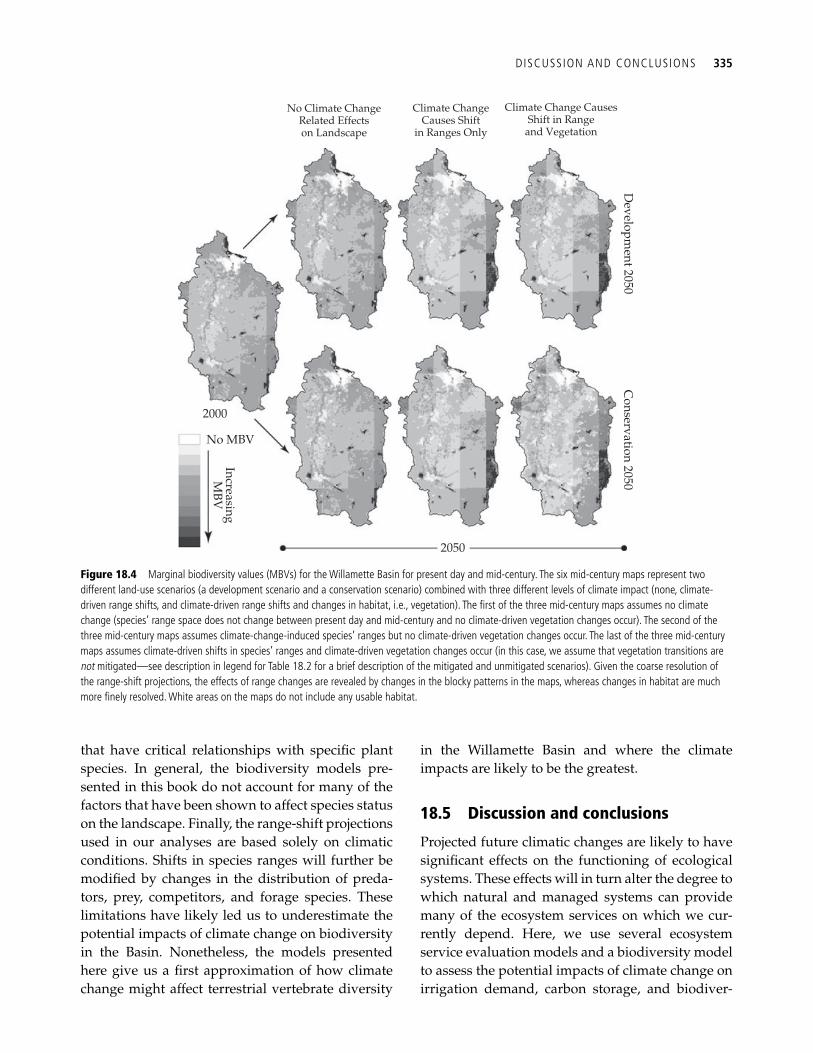
DISCUSSION AND CONCLUSIONS 335
No Climate ChangeRelated Effectson Landscape
2000
No MBV
2050
Climate ChangeCauses Shift
in Ranges Only
Climate Change CausesShift in Range
and Vegetation
Developm
ent 2050C
onservation 2050
IncreasingM
BV
Figure 18.4 Marginal biodiversity values (MBVs) for the Willamette Basin for present day and mid-century. The six mid-century maps represent two different land-use scenarios (a development scenario and a conservation scenario) combined with three different levels of climate impact (none, climate-driven range shifts, and climate-driven range shifts and changes in habitat, i.e., vegetation). The fi rst of the three mid-century maps assumes no climate change (species’ range space does not change between present day and mid-century and no climate-driven vegetation changes occur). The second of the three mid-century maps assumes climate-change-induced species’ ranges but no climate-driven vegetation changes occur. The last of the three mid-century maps assumes climate-driven shifts in species’ ranges and climate-driven vegetation changes occur (in this case, we assume that vegetation transitions are not mitigated—see description in legend for Table 18.2 for a brief description of the mitigated and unmitigated scenarios). Given the coarse resolution of the range-shift projections, the effects of range changes are revealed by changes in the blocky patterns in the maps, whereas changes in habitat are much more fi nely resolved. White areas on the maps do not include any usable habitat.
that have critical relationships with specifi c plant species. In general, the biodiversity models pre-sented in this book do not account for many of the factors that have been shown to affect species status on the landscape. Finally, the range-shift projections used in our analyses are based solely on climatic conditions. Shifts in species ranges will further be modifi ed by changes in the distribution of preda-tors, prey, competitors, and forage species. These limitations have likely led us to underestimate the potential impacts of climate change on biodiversity in the Basin. Nonetheless, the models presented here give us a fi rst approximation of how climate change might affect terrestrial vertebrate diversity
in the Willamette Basin and where the climate impacts are likely to be the greatest.
18.5 Discussion and conclusions
Projected future climatic changes are likely to have signifi cant effects on the functioning of ecological systems. These effects will in turn alter the degree to which natural and managed systems can provide many of the ecosystem services on which we cur-rently depend. Here, we use several ecosystem service evaluation models and a biodiversity model to assess the potential impacts of climate change on irrigation demand, carbon storage, and biodiver-
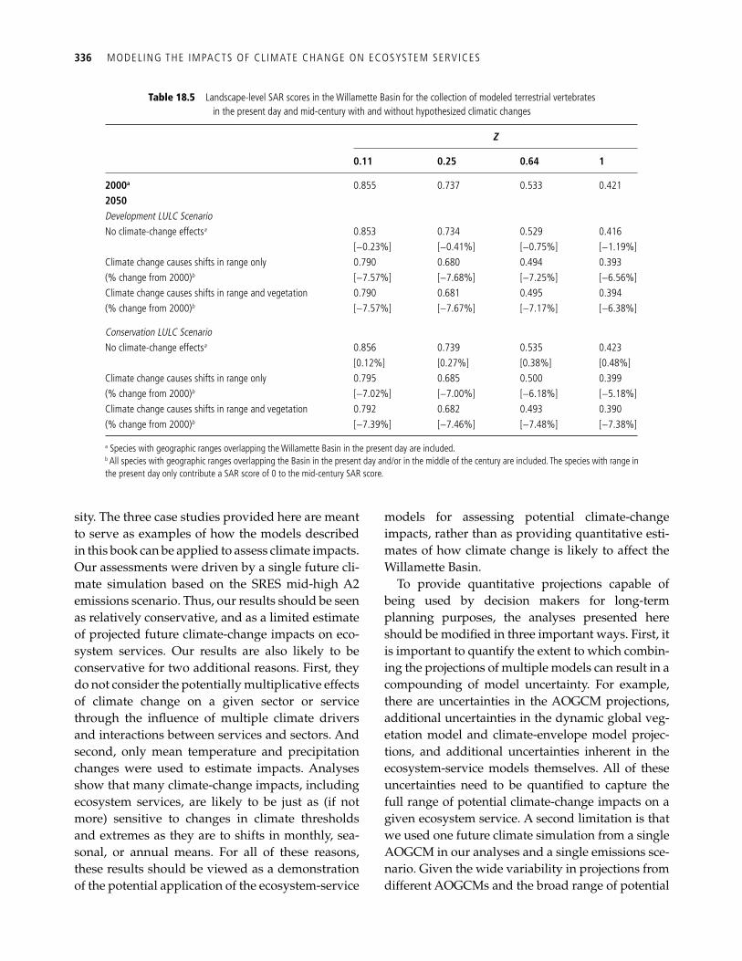
336 MODELING THE IMPACTS OF CL IMATE CHANGE ON ECOSYSTEM SERVICES
sity. The three case studies provided here are meant to serve as examples of how the models described in this book can be applied to assess climate impacts. Our assessments were driven by a single future cli-mate simulation based on the SRES mid-high A2 emissions scenario. Thus, our results should be seen as relatively conservative, and as a limited estimate of projected future climate-change impacts on eco-system services. Our results are also likely to be conservative for two additional reasons. First, they do not consider the potentially multiplicative effects of climate change on a given sector or service through the infl uence of multiple climate drivers and interactions between services and sectors. And second, only mean temperature and precipitation changes were used to estimate impacts. Analyses show that many climate-change impacts, including ecosystem services, are likely to be just as (if not more) sensitive to changes in climate thresholds and extremes as they are to shifts in monthly, sea-sonal, or annual means. For all of these reasons, these results should be viewed as a demonstration of the potential application of the ecosystem-service
models for assessing potential climate-change impacts, rather than as providing quantitative esti-mates of how climate change is likely to affect the Willamette Basin.
To provide quantitative projections capable of being used by decision makers for long-term planning purposes, the analyses presented here should be modifi ed in three important ways. First, it is important to quantify the extent to which combin-ing the projections of multiple models can result in a compounding of model uncertainty. For example, there are uncertainties in the AOGCM projections, additional uncertainties in the dynamic global veg-etation model and climate-envelope model projec-tions, and additional uncertainties inherent in the ecosystem-service models themselves. All of these uncertainties need to be quantifi ed to capture the full range of potential climate-change impacts on a given ecosystem service. A second limitation is that we used one future climate simulation from a single AOGCM in our analyses and a single emissions sce-nario. Given the wide variability in projections from different AOGCMs and the broad range of potential
Table 18.5 Landscape-level SAR scores in the Willamette Basin for the collection of modeled terrestrial vertebrates in the present day and mid-century with and without hypothesized climatic changes
Z
0.11 0.25 0.64 1
2000 a 0.855 0.737 0.533 0.421 2050 Development LULC Scenario No climate-change effects a 0.853 0.734 0.529 0.416
[−0.23%] [−0.41%] [−0.75%] [−1.19%] Climate change causes shifts in range only 0.790 0.680 0.494 0.393 (% change from 2000) b [−7.57%] [−7.68%] [−7.25%] [−6.56%] Climate change causes shifts in range and vegetation 0.790 0.681 0.495 0.394 (% change from 2000) b [−7.57%] [−7.67%] [−7.17%] [−6.38%]
Conservation LULC Scenario No climate-change effects a 0.856 0.739 0.535 0.423
[0.12%] [0.27%] [0.38%] [0.48%] Climate change causes shifts in range only 0.795 0.685 0.500 0.399 (% change from 2000) b [−7.02%] [−7.00%] [−6.18%] [−5.18%] Climate change causes shifts in range and vegetation 0.792 0.682 0.493 0.390 (% change from 2000) b [−7.39%] [−7.46%] [−7.48%] [−7.38%]
a Species with geographic ranges overlapping the Willamette Basin in the present day are included. b All species with geographic ranges overlapping the Basin in the present day and/or in the middle of the century are included. The species with range in the present day only contribute a SAR score of 0 to the mid-century SAR score.
DISCUSSION AND CONCLUSIONS 337
future emissions, it will be necessary to investigate the effects of alternative climate-change projections to begin to understand the range of possible climate impacts on ecosystem services. And lastly, capturing the potential impacts of climate change will require evaluating the effects of realistic adaptation strate-gies. Our analysis of irrigation demand did not take into account that farmers will likely shift crops or modify irrigation methods in response to climate change. Nor did we account for the multitude of ways in which forest managers might respond to climate-driven changes in tree-species composition.
Despite these limitations, the case studies investi-gated here demonstrate the importance of making even preliminary estimates of potential climate impacts on ecosystem services. For example, one can use the projected climate-induced change in each ecosystem service as a metric of “impact.” The land-use scenario that yields the lowest impact score is the land-use scenario that provides the greatest potential for adaptation to climate change. In our assessments, this was generally the conservation scenario. Although, it is important to note that care must be taken in assessing the results of such sce-nario comparisons. For example, although we found a greater climate-driven loss in carbon storage under the conservation scenario, this differential resulted from the fact that the conservation scenario gener-ated more carbon storage to begin with and thus there was more to lose by the middle of the century. More generally, given that climate change is expected to have profound effects on both human and natural systems, it will be critical to consider estimates of potential climate impacts when forecasting ecosys-tem services. As evidenced by the results of our sim-ple case studies, climate change will alter many of the ecosystem services we rely on today. Both miti-gating and adapting to climate impacts will require an understanding of how ecosystems and ecosystem services will respond to climate change. Models designed to assess ecosystem services will likely prove indispensable in our struggle to address cli-mate change in the coming decades.
Acknowledgments
We thank Michelle Marvier, Katherine Hayhoe, Nathan Schumaker, and David Turner for useful
comments and suggestions. We are also grateful to Peter Kareiva for his insightful editing and to Evan Girvetz for useful discussions. S. Shafer was sup-ported by the US Geological Survey’s Earth Surface Dynamics Program.
References
Alcamo, J., and Henrichs, T. (2002). Critical regions: A model-based estimation of world water resources sensi-tive to global changes. Aquatic Sciences—Research across Boundaries, 64 , 352–62.
Alcamo, J., Vuuren, D. v., Ringler, C., et al . (2005). Changes in nature’s balance sheet: model-based estimates of future worldwide ecosystem services. Ecology and Society , 10 , Art. 19.
Alley, R., Berntsen, T., Bindoff, N. L., et al . (2007). Climate change 2007: the physical science basis, summary for policy-makers . Working Group I contribution to the Intergovernmental Panel on Climate Change, Fourth Assessment Report, Geneva.
Arnell, N. W. (2004). Climate change and global water resources: SRES emissions and socio-economic scenar-ios. Global Environmental Change , 14 , 31–52.
Bachelet, D., Neilson, R. P., Lenihan, J. M., et al . (2001). Climate change effects on vegetation distribution and carbon budget in the United States. Ecosystems , 4 , 164–85.
Battin, J., Wiley, M. W., Ruckelshaus, M. H., et al . (2007). Projected impacts of climate change on salmon habitat restoration. Proceedings of the National Academy of Sciences of the USA , 104 , 6720–5.
Battisti, D. S., and Naylor, R. L. (2009). Historical warnings of future food insecurity with unprecedented seasonal heat. Science, 323 , 240–4.
Betts, R. A., Boucher, O., Collins, M., et al . (2007). Projected increase in continental runoff due to plant responses to increasing carbon dioxide. Nature , 448 , 1037.
Bouwman, A. F., Kram, T., and Goldewijk, K. K. (2006). Integrated modelling of global environmental change. An overview of IMAGE 2.4 . Netherlands Environmental Assessment Agency (MPN), Bilthoven.
Carroll, C. (2007). Interacting effects of climate change, land-scape conversion, and harvest on carnivore populations at the range margin: marten and lynx in the Northern Appalachians. Conservation Biology, 21 , 1092–104.
Cramer, W., Bondeau, A., Woodward, F. I., et al . (2001). Global response of terrestrial ecosystem structure and function to CO 2 and climate change: results from six dynamic global vegetation models. Global Change Biology , 7 , 357–73.
338 MODELING THE IMPACTS OF CL IMATE CHANGE ON ECOSYSTEM SERVICES
Deschenes, O., and Greenstone, M. (2007). The economic impacts of climate change: evidence from agricultural output and random fl uctuations in weather. American Economic Review , 97 , 354–85.
de Wit, M., and Stankiewicz, J. (2006). Changes in surface water supply across Africa with predicted climate change. Science , 311 , 1917–21.
FAO. (1992). CROPWAT, a computer program for irrigation planning and management by M. Smith . FAO Irrigation and Drainage Paper 26, Rome.
Gordon, C., Cooper, C., Senior, C. A., et al . (2000). The sim-ulation of SST, sea ice extents and ocean heat transports in a version of the Hadley Centre coupled model with-out fl ux adjustments. Climate Dynamics , 16 , 147–68.
Hulse, D., Gregory, S., and Baker, J. (2002). Willamette River Basin planning atlas: trajectories of environmental and eco-logical change . Oregon State University, Corvallis.
Lawler, J. J., Shafer, S. L., White, D., et al . (2009). Projected climate-induced faunal change in the western hemi-sphere. Ecology , 90 , 588–97.
Lobell, D. B., and Asner, G. P. (2003). Climate and manage-ment contributions to recent trends in U.S. agricultural yields. Science , 299 , 1032.
Lobell, D. B., and Field, C. B. (2007). Global scale climate–crop yield relationships and the impacts of recent warm-ing. Environmental Research Letters, 2 , 014002.
Mendelsohn, R., Nordhaus, W. D., and Shaw, D. (1994). The impact of global warming on agriculture: A Ricardian analysis. American Economic Review, 84 , 753–71.
Milly, P. C. D., Dunne, K. A., and Vecchia, A. V. (2005). Global pattern of trends in streamfl ow and water avail-ability in a changing climate. Nature , 438 , 347–50.
Mitchell, T. D., and Jones, P. D. (2005). An improved method of constructing a database of monthly climate observations and associated high-resolution grids. International Journal of Climatology , 25 , 693–712.
Nakicenovic, N., Alcamo, J., Davis, G., et al . (2000). Special report on emissions scenarios: a special report of Working Group III of the Intergovernmental Panel on Climate Change. Cambridge University Press, Cambridge.
Nelson, E., Mendoza, G., Regetz, J., et al . (2009). Modeling multiple ecosystem services, biodiversity conservation, commodity production, and tradeoffs at landscape scales. F rontiers in Ecology and the Environment, 7 , 4–11.
New, M., Lister, D., Hulme, M., et al . (2002). A high-resolu-tion data set of surface climate over global land areas. Climate Research , 21 , 1–25.
Parmesan, C., and Yohe, G. (2003). A globally coherent fi n-gerprint of climate change impacts across natural sys-tems. Nature , 421 , 37–42.
Parmesan, C. (2006). Ecological and evolutionary responses to recent climate change. Annual Review of Ecology and Systematics , 37 , 637–69.
Pearson, R. G., Dawson, T. P., Berry, P. M., et al . (2002). SPECIES: A Spatial Evaluation of Climate Impact on the Envelope of Species. Ecological Modelling, 154 , 289–300.
Pereira, H. M., and Daily, G. C. (2006). Modeling biodiver-sity dynamics in countryside landscapes. Ecology , 87 , 1877–85.
Polasky, S., Nelson, E., Lonsdorf, E., et al . (2005). Conserving species in a working landscape: land use with biological and economic objectives. Ecological Applications , 15 , 1387–401.
Polasky, S., Nelson, E., Camm, J., et al . (2008). Where to put things? Spatial land management to sustain biodiver-sity and economic returns. Biological Conservation , 141 , 1505–24.
Ramankutty, N., Foley, J. A., Norman, J., et al . (2002). The global distribution of cultivable lands: current patterns and sensitivity to possible climate change. Global Ecology and Biogeography , 11 , 377–92.
Root, T. L., Price, J. T., Hall, K. R., et al . (2003). Fingerprints of global warming on wild animals and plants. Nature , 421 , 57–60.
Rosenzweig, C., and Parry, M. L. (1994). Potential impact of climate change on world food supply. Nature , 367 , 133–8.
Schlenker, W., Hanemann, W. M., and Fisher, A. C. (2005). Will U.S. agriculture really benefi t from global warm-ing? Accounting for irrigation in the hedonic approach. American Economic Review, 95 , 395–406.
Schumaker, N. H., Ernst, T., White, D., et al . (2004). Projecting wildlife responses to alternative future land-scapes in Oregon’s Willamette Basin. Ecological Applications , 14 , 381–400.
Sitch, S., Smith, B., Prentice, I. C., et al . (2003). Evaluation of ecosystem dynamics, plant geography and terrestrial carbon cycling in the LPJ dynamic global vegetation model. Global Change Biology , 9 , 161–85.
Smith, J. E., Heath, L. S., and Skog, K. E. (2006). Methods for calculating forest ecosystem and harvested carbon with stand-ard estimates for forest types of the United States. Gen Tech Rep NE-343 . US Department of Agriculture, Forest Service, Northeastern Research Station, Newtown Square.
Stewart, I. T., Cayan, D. R., and Dettinger, M. D. (2005). Changes toward earlier streamfl ow timing across west-ern North America. Journal of Climate , 18 , 1136–55.
USDA. (2008). Soil Survey Geographic (SSURGO) Database for Willamette Valley, Oregon.
Vörösmarty, C. J., Green, P., Salisbury, J., et al . (2000). Global water resources: vulnerability from climate change and population growth. Science , 289 , 284–8.
Walther, G.-R., Post, E., Convey, P., et al . (2002). Ecological responses to recent climate change. Nature , 416 , 389–95.
339
CHAPTER 19
Incorporating ecosystem services in decisions Emily McKenzie, Frances Irwin, Janet Ranganathan, Craig Hanson, Carolyn Kousky, Karen Bennett, Susan Ruffo, Marc Conte, James Salzman, and Jouni Paavola
19.1 Introduction
The world now faces unprecedented and intercon-nected challenges – reducing poverty, addressing cli-mate change, and halting widespread environmental degradation. Scientifi c information on the links between humans and nature can help solve these problems ( Lubchenco 1998 ; Bingham et al . 1995 ; Pielke 2007; MA 2005a ). However, to seize this oppor-tunity, scientifi c knowledge must be translated into action (NRC 2004; Daily et al . 2009 ; Cash et al . 2003 ). Advances in scientifi c modeling such as those described in this book are necessary but not suffi -cient. Here we provide an explicit examination of the channels through which the science of mapping and valuing ecosystem services can improve decisions.
Opportunities to use information on ecosystem services occur in all sectors of the economy and at all levels of decision-making: a mayor aims to increase fl ood protection for a city’s citizens; a busi-ness requires a reliable supply of water for its man-ufacturing process; an international development agency attempts to reduce poverty by increasing small farm production. Although not always termed “ecosystem services,” in each example, considera-tion of the benefi ts we gain from the environment is essential for making wise decisions. Information on ecosystem services can tell us how and which serv-ices are relevant to our goals, whether important services are at risk, where services are provided, who is affected, and the trade-offs of different choices; all key pieces of information for the design and implementation of a broad set of policy mechanisms.
19.1.1 Role of ecosystem service information in decisions
Scientifi c models move us from abstract, conceptual arguments about the importance of ecosystem serv-ices to specifi c quantifi cation of the level, value and spatial distribution of ecosystem service benefi ts. This is of great relevance to the real world because such information can be applied to a range of poli-cies and decisions, as in the examples from Oregon and Hawaii in Chapter 14 (see also Turner et al . 2000 ; Naidoo and Ricketts 2006 ; Nelson et al . 2009 ). A modeling framework that captures impacts on multiple ecosystem services over alternative sce-narios enables stakeholders to weigh tradeoffs can serve as a basis for negotiation ( Ghazoul 2007 ). Without such information, decision-makers tend to use intuitive or heuristic approaches that ignore ecosystem service values and distributional issues ( Kiker et al . 2005 ). As noted by Ascher and Healy ( 1990 ), “information shapes many aspects of how resource issues are viewed and addressed: the focus of attention, the way problems come to be defi ned, and the ways that success or failure . . . is attributed to a project or policy.”
There are several characteristics of ecosystem service models that are relevant to common policy contexts ( Table 19.1 ). For example, the development of stakeholder-driven scenarios can ensure that eco-system service valuations are aligned with the prob-lems of interest to decision-makers, revealing sources of confl ict and building consensus ( Henrichs et al . 2008 ). This does not happen automatically, however, and typically requires active, iterative and
340 INCORPORATING ECOSYSTEM SERVICES IN DECIS IONS
inclusive communication between scientifi c experts and stakeholders ( Lubchenco 1998 ).
19.2 Putting ecosystem services on the agenda
People continue to degrade our environment in part because we simply do not appreciate the links
between ecosystems and human well-being ( Leopold 1949 ; Daly 1968 ; Wilson 1998 ; MA 2005c). When government ministries initiate programs or companies launch new ventures, they rarely con-sider how ecosystem services will affect their suc-cess, or the costs of replacing degraded services ( Ranganathan et al . 2008 ).
Table 19.1 Characteristics of ecosystem service models with relevance for decision-making
Model characteristics Relevance to decisions
Integrated framework, including multiple ecosystem services • Provides consistent standard for evaluating projects and policies • Encourages consideration of all ecosystem services including those that have not been
emphasized in past policies • Enables analysis of trade-offs between different ecosystem services, stakeholders, and
geographic areas • Informs and encourages coordinated, multi-sectoral, ecosystem-based management
Packaged as a “tool” • Translates complex scientifi c results into policy relevant outputs, e.g., trade-off curves, effi ciency frontiers (see Chapters 3 and 14 )
• Facilitates capacity building in ecosystem service modeling and valuation • Increases uptake due to lower costs and reduced diffi culty of doing ecosystem service
studies Different levels of model complexity • Tailors modeling to the level of certainty suffi cient for different policy contexts (see
Chapter 15 ) Produces information on biophysical changes • Enables use of biophysical ecosystem service units when they suffi ce for specifi c decision
contexts • Can feed into decision-support tools such as multi-criteria analysis
Produces information on economic values • Emphasizes connections between environmental sustainability and economic development • Provides common monetary metric, facilitating comparison of policy alternatives • Can feed into cost–benefi t analysis
Scalable • Enables selection of spatial scale most relevant to decision context and level of governance
Scenario based • Provides structured way to consider implications of possible futures and policy alternatives • Tailors analysis to priority policy questions • Explores uncertain aspects of the future • Challenges assumptions about how systems operate
Stakeholder driven • Encourages uptake and use of results • Enables local knowledge and policy priorities to shape the analysis
Spatially explicit • Visual appeal for communication and advocacy • Determines where to target investments, policies, and payments • Determines locations where ecosystem services and biodiversity overlap • High-resolution maps enable policy responses to be targeted and context specifi c
Produces information on opportunity costs • Determines the lower bound for payments for ecosystem services, and other incentive schemes
Possible to disaggregate to individual services • Enables users to focus on individual services targeted by specifi c policies, such as payments for water yield
Enables analysis of distribution of ecosystem service costs and benefi ts
• Helps identify who bears benefi ts and costs of different policies, thereby identifying possible locations for payments for ecosystem services
• Helps clarify how environmental policies affect social goals and priorities, such as poverty reduction
PUTTING ECOSYSTEM SERVICES ON THE AGENDA 341
19.2.1 Building better development policies
The Millennium Development Goals (MDGs) pro-vide an example where the importance of ecosystem services to achieve poverty alleviation was not ini-tially (but is now increasingly) recognized. In 2001, leaders adopted eight goals aimed at cutting global poverty by 50% by 2015. Although the MDGs origi-nally included an environmental sustainability goal, it was narrowly defi ned, without consideration of the role of ecosystem services in achieving other goals ( WRI 2005 ). Goals to increase incomes and reduce hunger did not account for how water, fertile soil and pollinators support agriculture. When coun-tries made plans to achieve the MDGs, the links between development and nature were not addressed. Later analysis on the ecosystem service benefi ts of conservation found that signifi cant envi-ronmental investment is required to achieve poverty reduction ( Pearce 2005 ). Focusing targets on ecosys-tem services is now increasingly recognized as criti-cal to achieve all eight MDGs ( WRI 2005 ).
Some countries now explicitly consider ecosys-tem services in national poverty reduction strate-gies. Tanzania’s 2005 National Strategy for Growth and Reduction of Poverty exemplifi es this shift. It includes 15 environmental targets to protect and enhance ecosystem services ( Assey et al . 2007 ). Distributional and social information is particularly important for policy formulation in developing countries such as Tanzania; investments that increase the supply of services and improve the welfare of certain groups of people may reduce services that support the livelihoods and well-being of others living in poverty (see Chapter 16 ). In Kenya, these types of trade-offs were explored by overlaying poverty maps—showing where poor people live and aspects of their well-being—with maps of ecosystems and their services. This identi-fi ed where poverty indicators overlap with service supply and demand areas ( Snel 2004 ; WRI 2007 ). For example, in the upper Tana region around Mt. Kenya, a large number of poor communities rely directly and exclusively on ecosystems to pro-vide and fi lter drinking water. This type of informa-tion can be used to make sure that polices that impact ecosystems do not exacerbate the poverty of vulnerable communities.
Information on ecosystem services and their val-ues can also infl uence decisions over major devel-opment projects. Ecosystem services that lack market prices are often not considered in project evaluations, enabling other interests to determine decisions ( Balmford et al . 2002 ). Economic valuation of non-marketed ecosystem services makes their values clear in monetary terms, enabling compari-son of all costs and benefi ts of proposed projects. This can help create political consensus around decisions that sustain ecosystem services. For exam-ple, in Borneo a rapid assessment of the economic value of ecosystem services provided by standing forests infl uenced conservation policy decisions over proposed oil palm plantations. The study assessed the ecosystem service benefi ts of carbon storage, the avoidance of health costs from forest fi res, and the benefi ts of forest-agriculture mosaics. The information appears to have played a role in the policy decision, with the government represent-ative declaring the oil palm development would not go forward because Borneo “is a resource of life for Kalimantan” ( Naidoo et al . 2009 ).
It is possible to integrate ecosystem services into existing decision-support and environmental assessment tools ( Le Quesne and McNally 2004 ). If mandated and enforced, these tools can ensure sys-tematic, transparent evaluation of ecosystem service impacts. Examples include strategic environmental assessments (SEA) and regulatory impact assess-ments for evaluating policies and legislation, typi-cally at the level of an economic sector or region, and cost–benefi t analyses (CBA) and environmental impact assessments for individual projects. Although historically restricted to human health impacts of pollution, many CBAs and SEAs now consider a wider range of ecosystem services (DAC Network on Environment and Development Co-operation (ENVIRONET) 2008). For example, a recent SEA for a district planning process in Rwanda linked ecosystem service degradation to food, water, and fuel scarcity ( UNDP 2007 ).
19.2.2 Building better business strategies
Businesses can use information on ecosystem serv-ices to shape their investments and strategies. Just as governments can fi nd that ecosystem services are
342 INCORPORATING ECOSYSTEM SERVICES IN DECIS IONS
linked to the wellbeing of citizens, businesses can discover that ecosystem services contribute to prof-its. Although businesses can adversely impact eco-systems through consumption of natural resources, pollution, and land conversion, businesses also depend on ecosystems. Agribusiness, for example, depends on pollination, and control of pests and erosion (see Chapter 10 ). Approximately 75% of the world’s 100 top agricultural crops rely on natural pollinators ( Klein et al . 2007 ). Property developers benefi t from the coastal protection provided by coral reefs, coastal forests and coastal wetlands ( Turner et al . 1998 ; Cesar 2000 ). The tourism indus-try benefi ts from these ecosystems’ aesthetic beauty ( De Groot 1994 ).
Because of these impacts and dependencies, the degradation of ecosystem services presents signifi -cant risk to—and opportunities for—corporate performance (see Table 19.2 and Box 19.1 ). For example, industries relying on steady supplies of clean freshwater face operational risks when upstream deforestation increases sedimentation of rivers, disrupting business operations and increas-ing costs (see Chapter 6 ). Companies may face per-mit restrictions or damage brand image if they
pollute ecosystems with value to communities, leading to lawsuits and fi nes, and challenging their license to operate. Conversely, businesses that sus-tainably manage land or water resources may increase effi ciency, differentiate their brand, reduce costs, and even generate new sources of revenue through markets for ecosystem services. Although these emerging markets face challenges in prac-tice, they offer rewards to early business entrants (e.g., markets for carbon offsets or certifi ed tim-ber—see Section 19.3 ).
Most companies, however, fail to connect ecosys-tems with their business bottom line ( Hanson et al . 2008 ). Many are not aware of the extent to which they impact or depend on ecosystem services, nor the ramifi cations of those impacts. Likewise, busi-ness tools such as environmental management sys-tems and environmental impact assessments are often not attuned to the risks and opportunities arising from use and degradation of ecosystem services. Rather, they are suited to “traditional” issues of pollution and natural resource consump-tion. As a result, companies may be unprepared for ecosystem service risks or miss new sources of rev-enue associated with ecosystem change.
Table 19.2 Business risks and opportunities arising from dependencies and impacts on ecosystem services
Type Risk Opportunity
Operational • Increased scarcity or cost of inputs • Increased effi ciency • Reduced output or productivity • Low impact industrial processes • Disruption to business operations
Regulatory and legal • Extraction moratoria • Formal license to expand operations • Lower quotas • New products to meet new regulations • Fines • Opportunity to shape government policy • User fees • Permit or license suspension • Permit denial • Lawsuits
Reputational • Damage to brand or image • Improved or differentiated brand • Challenge to social “license to operate”
Market and product • Changes in customer preferences • New products or services (public sector, private sector) • Markets for certifi ed products
• Markets for ecosystem services • New revenue streams from company-owned or managed ecosystems
Financing • Higher cost of capital • Increased investment by progressive lenders and socially responsible investment funds • More rigorous lending requirements

PUTTING ECOSYSTEM SERVICES ON THE AGENDA 343
Craig Hanson
One approach for businesses to identify connections between ecosystem services and their bottom line is to conduct a Corporate Ecosystem Services Review (ESR) ( Hanson et al . 2008 ). The ESR is a structured methodology that helps managers proactively develop strategies to manage business risks and opportunities arising from their company’s dependence and impact on ecosystems. Conducting an ESR involves identifying priority ecosystem services for a company (a facility, product or supply chain), analyzing trends in these services, and identifying business risks and opportunities. With this information, the company can develop response strategies.
Mondi is a leading international paper and packaging business. As of 2006, the company was Europe’s largest producer of offi ce paper, with operations in 35 countries. Much of the company’s pulp comes from its plantations in South Africa. Mondi conducted an ESR to understand what business risks—and opportunities—might arise as changes in ecosystem services affect its plantations.
During its ESR, Mondi assessed the dependence and impact of these plantations on 24 different ecosystem services. The analysis identifi ed six services as having the most impact on Mondi’s corporate performance:
• Freshwater. Pine and eucalypt plantations signifi cantly depend upon and affect the quantity of freshwater in their watersheds. • Water regulation. Plantations rely on and impact the surrounding ecosystems that regulate the timing of water fl ows. • Biomass fuel. As a byproduct, plantations generate biomass that can be used for energy by the company’s mills and local villages. • Global climate regulation. Plantations can sequester carbon dioxide thereby mitigating climate change (albeit dependent on the stage of the carbon cycle—see Chapter 7 ). • Recreation and ecotourism. One of the plantations is located next to the isiMangaliso Wetland Park—a World Heritage Site—and contains wetlands and grasslands that could potentially provide new opportunities for recreation and ecotourism. • Livestock. The plantations preclude surrounding villagers from using the land for large-scale livestock
grazing. Selective controlled grazing is, however, widely practiced.
A trends analysis of these six ecosystem services uncovered a number of emerging risks and opportunities facing Mondi. Freshwater in the three plantation watersheds is becoming increasingly scarce due to the proliferation of invasive alien plant species, increasing demand for water from nearby farmers, and climate change. This scarcity threatens to increase the cost of water, reduce the availability of wood fi ber, and expose the company to reputational and regulatory risk. Meanwhile, new opportunities are arising as ecotourism grows in the region and new markets emerge for biomass fuel. Through the ESR process, Mondi identifi ed several strategies for managing these risks and opportunities:
• Improve water-use effi ciency. To improve water effi ciency, the company is now clearing invasive species more aggressively. It will also better match tree species to site conditions and more frequently burn grasslands. These strategies complement the company’s past efforts to remove plantations from wetlands, thereby restoring natural hydrological systems. • Use invasive species as biomass fuel. Mondi can tap into the growing market for biomass fuel by using the invasive species cleared from its plantations as feedstock for power and heat generation. Potential users of the feedstock are Mondi’s own paper mills and a new biomass pellet manufacturer located close to one plantation. • Promote coppiced small-scale tree farms (woodlots) for biomass fuel. Using the company’s forestry expertise, Mondi can help local landowners and villages establish woodlots on degraded land for growing biomass fuel on coppiced rotations. Mondi could provide seedlings and offer extension services. Mondi could also purchase the wood to use in its mills or sell to nearby wood pellet manufacturers. These woodlots would provide additional income for villagers and thereby strengthen Mondi’s reputation and stakeholder relationships. • Engage policy-makers to improve freshwater policies. Mondi can support policies that encourage water-use effi ciency in South Africa and, leveraging its expertise in water management, provide input into policy design.
Box 19.1 An assessment of ecosystem services helps a paper and packaging business respond to emerging risks
344 INCORPORATING ECOSYSTEM SERVICES IN DECIS IONS
Information on the value of ecosystem services can play a role in raising business awareness of the links between ecosystems and profi ts. Spatially explicit information on where ecosystem services are supplied can help businesses determine where to invest in ecosystem protection and restoration or where to avoid activity that degrades ecosystems.
19.2.3 Building public awareness
Because people often fail to connect their wellbeing to ecosystem conditions ( Irwin and Ranganathan 2007 ), there is a need to build public awareness about this linkage before we can expect the public to hold decision-makers accountable ( Pielke 2007 ). Education and awareness programs may be espe-cially effective if they are directed at landowners or managers who lack information. For instance, if a farmer does not realize that an increase in habitat for native pollinators will raise yields, simply pro-viding the type of information provided by the models outlined in Chapter 10 may induce land-owners to set aside habitat. An example comes from a US Federal “Conservation Buffers” program, where training and advice is given to farmers on designing buffer zones to fi lter pollution along streams and wind barriers to reduce soil erosion (NRCS 2008). Some consider technical training to be more successful at altering land-use practices than direct payments ( Daily and Ellison 2002 ; Salzman 2005 ).
When “externalities” exist—impacts that affect people other than the decision-maker—information alone will not suffi ce. For example, a farmer may learn that applying fertilizer causes water quality problems downstream but continue to do so because it leads to higher crop yields and the resulting water quality problem affects others. In these cases, edu-cation and awareness programs need to target the broader public to create demand for reform.
19.3 Instruments for sustaining and enhancing ecosystem services
When ecosystem service management becomes an institutional priority, several policy instruments can be used to infl uence the way people interact with the environment (MA 2005d). Some ecosystem
services are private goods (e.g., agricultural pro-duction and timber), and as such, are easily traded in markets that regulate their provision. Other important services (e.g., pollination, climate regula-tion, and cultural values) are “public goods,” which means private individuals cannot reap profi ts from providing them. Governments can develop regula-tions or incentives to alter the provision of these services. Here, we discuss a range of policy instru-ments for affecting the provision of both public and private goods.
19.3.1 Regulation
Government regulations have only recently begun to consider the full range of services provided by ecosystems, investing in them to meet human needs effi ciently and effectively ( Ruhl et al . 2007 ). Several kinds of regulations have recently been altered to include ecosystem services: licensing and permit-ting, zoning and land-use planning, and environ-mental standards.
Currently, most governments grant licenses and permits for extractive activities (e.g. mining, oil and gas) and infrastructure development (e.g. roads, developments) based on projected impacts to biodi-versity and a subset of environmental conditions linked to human health. However, standard assess-ments usually fail to account for the full set of social impacts associated with proposed activities. Governments are slowly moving toward permitting and licensing procedures that more fully account for environmental and social damages. Models such as those discussed in this book can be informative for these new, expanded impact assessments. For example, the Colombian Ministry of Environment, Housing and Territorial Development is expanding the impacts considered in its licensing process for activities related to oil and gas, mining, and infra-structure to avoid, minimize, mitigate and compen-sate for biodiversity and ecosystem service damages. The Ministry plans to use information on where services are supplied and realized to identify risks from industrial activities, and to shape permit con-ditions and offset compensation programs.
Regulations of common pool resources, such as protected areas in marine, coastal and inland water ecosystems, are widespread. However, they
INSTRUMENTS FOR SUSTAINING AND ENHANCING ECOSYSTEM SERVICES 345
are usually designed to maintain a single ecosys-tem service, such as fi sheries or freshwater. Regulatory limits can be designed to supply a broader range of services such as water purifi ca-tion, waste treatment and recreation. For example, in the United Kingdom, the Department of Environment, Food and Rural Affairs (DEFRA) estimated the economic value of a range of ecosys-tem services affected by marine protected areas to inform the design of new regulations—Marine Conservation Zones—that are part of a national Marine Bill ( McVittie and Moran 2008 ; Moran et al. 2007 ). The impact assessment supporting the Marine Bill legislation demonstrated that the ben-efi ts of Marine Conservation Zones outweigh the costs to industry. If the Marine Bill is passed, information on the value and location of ecosys-tem services and biodiversity is intended to inform selection of protected areas that provide multiple benefi ts matching policy priorities. A similar shift is happening in the United States, where a new ocean policy will likely require an ecosystem-based approach to marine zoning that explicitly considers a wide range of ecosystem services ( Lubchenco and Sutley 2010 ).
Governments can also use information on the provision or value of ecosystem services to ban or set standards for activities that degrade the envi-ronment beyond a socially defi ned limit. In the Republic of the Marshall Islands, information on the value of coastal ecosystem services—protection from erosion, along with tourism, recreation and fi sheries benefi ts—was used to advocate banning reef blasting and near-shore dredging (McKenzie et al . 2006). In addition, liability rules can hold those degrading ecosystem services responsible for the damage they cause, and enforce compensation for negligent actions, such as pollution ( Thompson 2008b ). In these cases, information on the economic value of degraded services can lead to more accu-rate estimates of environmental damages, and help build consensus about compensation among con-fl icting stakeholders ( Van Beukering et al . 2007 ). For example, after the Exxon Valdez oil spill in Alaska in 1989, a study estimated the lower bound eco-nomic value of damages at $2.8 billion, based on the stated willingness to pay to prevent another similar spill ( Carson et al . 1992 ).
19.3.2 Market-based approaches
To support regulation, governments may construct market-based instruments that create incentives for people to account for ecosystem services. The crea-tion of property rights, typically enforced and regu-lated by governments, is common to many of these approaches, facilitating trade in activities that increase or maintain services. In theory, market-based approaches are cost effective as services can be provided at the lowest possible cost ( Montgomery 1972 ). This is particularly the case when producers have fl exibility—they can provide a service in dif-fering ways and at differing costs ( Revesz and Stavins 2004 ). In practice, effi ciency advantages can be outweighed by the costs of operating these—often complex—mechanisms. Here we discuss sev-eral forms of market-based approaches that have been used to infl uence ecosystem service provision and detail how quantitative analyses can improve or facilitate the development of these policy instruments.
19.3.2.1 Cap and trade programs Under “cap and trade” programs, the government sets a limit on an environmental externality, such as pollution. Permits to emit are issued to fi rms, who can then trade them. Cap and trade programs have reduced emissions at lower costs than regulations, a notable example being the market for SO 2 permits in the United States. Carbon markets are now emerging as a mechanism to achieve greenhouse gas emissions reductions. In this context, the scope of cap and trade programs may expand to encom-pass ecosystem services. For example, payments for Reduced Emissions from Deforestation and Forest Degradation (REDD) allow benefi ciaries of the cli-mate regulation service provided by forests to com-pensate those who conserve them ( UNFCCC 2008 ). In this case, maps of carbon storage and projected estimates of future carbon change can be used to identify areas where carbon investments in natural or restored systems would be most profi table.
19.3.2.2 Voluntary markets In addition to regulated markets, voluntary markets are emerging, such as the Chicago Climate Exchange for carbon. Given that most ecosystem services are
346 INCORPORATING ECOSYSTEM SERVICES IN DECIS IONS
public goods or plagued by externalities, voluntary markets are only one part of the solution. In volun-tary carbon markets, individuals or companies buy certifi ed reductions in carbon emissions for moral reasons or to improve their reputation. As men-tioned above, certifi cation schemes exist to meet demand for “charismatic” carbon activities that deliver additional benefi ts (CCBA 2008b). For exam-ple, the Climate, Community and Biodiversity Alliance recently awarded the Juma Reserve project in Brazil a Gold rating, verifying additional benefi ts through income generation and the promotion of local business and biodiversity (CCBA 2008a). Integrated models of multiple ecosystem services can estimate how activities to reduce greenhouse gas emissions will change a larger suite of ecosys-tem services. Such estimates might be used to grant certifi cation to projects whose projected impacts benefi t multiple services. Follow up monitoring will be essential in determining whether these projected benefi ts are realized, but modeling can help mini-mize negative impacts of early carbon investments.
The Voluntary Carbon Standard (VCS—a widely accepted certifi cation scheme for carbon offsets) is adding the need for a different kind of analysis. Under VCS, projects must demonstrate that their emissions reductions are additional to what would have happened anyway. To pass, a project must be neither legally mandated nor common practice, and face unique barriers to implementation that carbon fi nance could help overcome (VCS 2008). Modeling the consequences of different scenarios can help estimate additional ecosystem service benefi ts, by comparing a “baseline” scenario (what is assumed to happen without the project), with a “project” sce-nario. The difference in service delivery helps iden-tify the truly additional quantity, or that eligible for compensation. When framed by baseline scenarios, the models described in the rest of this book can make this type of calculation, estimating both addi-tional carbon sequestration benefi ts (see Chapter 7 ) and the additional benefi ts of other services.
19.3.2.3 Payments for ecosystem services (PES) Payments for ecosystem services (PES) represent an increasingly popular method for creating incentives to sustain services. PES involve contracts in which one party agrees to compensate another party in
exchange for a guarantee that a specifi ed amount of an ecosystem service, or a particular land use or practice believed to provide that service, will be delivered ( Wunder 2005 ). A famous example of a PES program involves payments by Nestle (the owner of the Vittel mineral water company) to farmers in north eastern France to safeguard the water supply. Upstream farmers had replaced natu-ral grasslands—which fi ltered and cleaned the water—with corn and cattle, resulting in nitrate contamination of the aquifer. After calculating the higher costs of water purifi cation plants, Nestle decided to use a PES approach. The company signed long-term contracts with farmers to manage their animal waste, graze cattle sustainably, and reforest water fi ltration areas ( Perrot-Maitre 2006 ).
The majority of PES schemes are government-funded. For example, in the well-known Catskills example, the city of New York decided to protect the Delaware and Catskills watersheds, which pro-vide 90% of its drinking water ( Heal 2000 , NRC 2004) . Regulations were important for driving the scheme; the US Safe Drinking Water Act required that water must be fi ltered unless watersheds are suffi ciently protected. The costs of a new fi ltration plant vastly outweighed the costs of restoring and protecting the watersheds ( Postel and Thompson 2005 ). To protect the watersheds, a set of policy measures were introduced alongside standard pay-ments, including land purchase and easements. Within the fi rst fi ve years of the policy initiative, the city purchased approximately 14 000 ha of land and another 1000 ha of conservation easements, thereby doubling the buffer zones around important reser-voirs. The scheme had to be carefully negotiated with diverse landowners; in this case there were 477 property owners ( Postel and Thompson 2005 ). Those providing water quality services beyond the regulated minimum are rewarded with a payment package, including additional income, but also in-kind benefi ts, such as farm management consulta-tions ( Appleton 2002 ).
Beyond the New York City watershed case, most existing water-related PES programs have been established without information on where invest-ments will provide the greatest ecosystem service returns, and payments are made based on implementation of activities, not on actual changes
INSTRUMENTS FOR SUSTAINING AND ENHANCING ECOSYSTEM SERVICES 347
in ecosystem service levels. This approach can lead to ineffi cient programs that fail to produce desired ecosystem service returns because the marginal changes in ecosystem services associated with a given management change are not constant ( Jack et al. 2008 ). For example, a kilometer of fencing installed along a riverbank where cattle graze will usually reduce erosion much more than a kilometer of fencing installed around croplands in the upper reaches of the same watershed. Although policy creation in such contexts is diffi cult, it can be dra-matically simplifi ed with the use of models that reveal how management changes in different regions affect desired ecosystem services. More complex, but effi cient payment designs (e.g. differ-ential taxes, trading zones) can be established with such information. In addition, models such as those described in this book can help locate areas for new PES schemes by identifying where there are sources of service supply and benefi ciaries who may be willing to pay for service delivery. This is particu-larly powerful when combined with information on land tenure, to determine who can infl uence service delivery and should receive payments. For further discussion on additional conditions under which PES can be most effective, see Jack et al . ( 2008 ).
19.3.2.4 Government fi scal incentives Governments can create further fi nancial incentives to supply ecosystem services using subsidies, sub-sidy reform and taxes. Subsidies differ from PES schemes in that payments are not conditional on service delivery, or some proxy for it. Subsidies that account for the full economic value of ecosystem services can help to maintain or increase their pro-vision. Many existing subsidies, however, actually encourage activities that degrade services, by focus-ing on a narrowly defi ned outcome and ignoring ecosystem service losses ( Myers 2001 ). Signifi cant cases exist from agricultural subsidies. Farmers in Europe and the United States have long received payments linked to crop productivity ( OECD 1999 ). Such payments promote land conversion, leading to erosion of topsoil, and increasing use of fertiliz-ers and pesticides that affect water quality. Recent reforms have attempted to replace agricultural sub-sidies with payment programs (often called “agri-environment” schemes), which reward farm-
ers for managing the land sustainably and provid-ing ecosystem services, such as regulating nutrient runoff and soil erosion, and maintaining the spirit-ual and symbolic values of agricultural landscapes ( Baylis et al . 2008 , Ilbery and Bowler 1998 ).
Although growing in scale, agri-environment programs nevertheless remain a small proportion of agricultural expenditure ( OECD 2003 ). Reducing agricultural subsidies has proved particularly diffi -cult in Europe and the United States due to per-ceived impacts on farmers’ livelihoods and lifestyles ( Myers 2001 ). As subsidies are often maintained by rent-seeking by special interest groups who lose out from subsidy reform, reform policies are more pop-ular if done gradually and combined with public awareness campaigns (Pearce and Finck von Finckenstein 1999). Such campaigns can draw on valuation studies that quantify the effects of subsi-dies on ecosystem services to build political sup-port, and create transparency and accountability about who wins and who loses from policy change.
19.3.2.5 Offsets Offset schemes attempt to ensure that degradation of ecosystem services in one location is compen-sated through activities elsewhere. For example, wetland mitigation banking is a consolidated offset scheme in the United States to encourage compli-ance with the Clean Water Act. This regulation requests that developers avoid dredging wetlands connected to other water bodies and offset any una-voidable damages through creation of wetlands elsewhere. Landowners that restore, establish, enhance, and (in exceptional circumstances) pre-serve wetlands gain permits that can be sold to developers fi lling wetlands. However, mitigation banking has been controversial because of the scheme’s potential to redistribute wetland ecosys-tem services between human populations and the mixed quality of offsets relative to the wetlands destroyed ( Ruhl et al . 2007 ). Offsets work best when there is a well-defi ned, scalable unit that can be exchanged, whether it is an acre of wetland or a pound of CO 2 , and when exchanges are fungi-ble—an acre of wetland in one location produces the same services as an acre elsewhere ( Salzman and Ruhl 2000 ). Since an acre of wetland seldom provides the same service in different watershed

348 INCORPORATING ECOSYSTEM SERVICES IN DECIS IONS
contexts, standard, reproducible, and relatively easy ways of measuring ecosystem services are essential for establishing trades that actually avoid the loss of ecosystem services. Combining biophysi-cal models with information on benefi ciaries can determine how offsets affect the distribution of services among stakeholder groups, allowing agen-cies to preempt equity issues associated with devel-opments and their offsets.
19.4 Choosing the right instrument
Decision-makers need to select the policy mecha-nism most appropriate to their local context if they are to succeed in delivering ecosystem services. How to choose? Some approaches are appropriate
to certain institutions—governments are the only entity with authority to levy taxes, for example—and some will be constrained by the nature of the service (its “production function”). Others require strong systems of governance and institutions that may not exist in developing countries, such as clear property rights and competitive markets ( Pearce 2005 ). To choose the best approach, information is required on a range of issues, many of which are summarized in Table 19.3 . For further details within the conservation context, see McKenney et al. ( 2008 ) who describe a set of enabling conditions affecting the success of ecosystem service projects.
A summary of the main conditions affecting suc-cessful use of each policy mechanism is given in Table 19.4 .
Table 19.3 Information needed to select a policy instrument to provide ecosystem services
The service • How do interventions alter the level of service being produced? • Can these changes be measured? • What (if any) other policies and interventions are compatible with providing the service? • Is a particular spatial pattern of land uses required? • Can the service be broken down into discrete, fungible units? • At what scale is the service produced? • Are other services co-produced with the desired one? • Is there uncertainty regarding the link between actions and service delivery? • Are there unpredictable shocks that could alter service levels?
Producers • If other land uses are compatible with service provision, are behaviors that increase or decrease service levels observable and enforceable?
• Are there any relevant information asymmetries between producers, the decision-maker, and benefi ciaries? Benefi ciaries • Who benefi ts from the ecosystem service? Where are they located?
• Will this change over time? • Can others be prevented from benefi ting from the service (in the language of economics, is the service a public good)?
Costs and funding • Who is bearing the costs? Where are they located? • What are the costs of various approaches for providing the service? (This should include direct costs, indirect costs such as
reductions in the supply of other ecosystem services, and transaction costs.) • How much are people willing to pay? How much funding is available (and over what time frame) and where is it coming
from? Goals • What are the goals of the policy? Goals could be improving livelihoods, biodiversity conservation, or simply
cost-effectiveness. Institutional context • What institutions are needed for an approach and are they present (for example, contracts enforced by a court of law)?
• Are there clear property rights? • What other laws are in existence that might affect implementation of the approach? Do these confl ict with or enhance
any of the approaches to providing the service? Views of stakeholders • Who wins and who loses with each approach?
• Which stakeholder groups could prevent implementation? • Whose support is needed and what are their views?
Performance over time • How will each approach respond to changing conditions over time, such as price changes, changes in technology, changes in funding levels, or changes in drivers of service degradation?
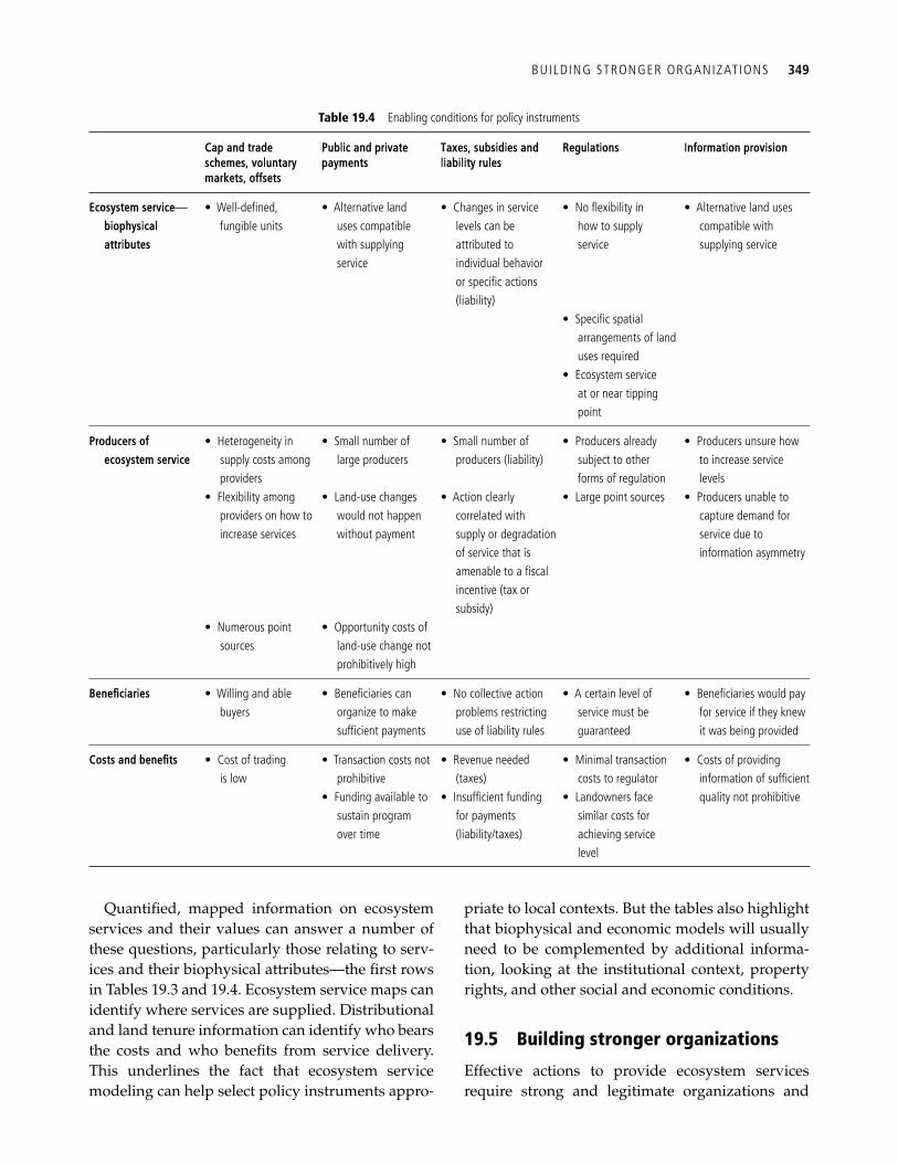
BUILDING STRONGER ORGANIZATIONS 349
Quantifi ed, mapped information on ecosystem services and their values can answer a number of these questions, particularly those relating to serv-ices and their biophysical attributes—the fi rst rows in Tables 19.3 and 19.4 . Ecosystem service maps can identify where services are supplied. Distributional and land tenure information can identify who bears the costs and who benefi ts from service delivery. This underlines the fact that ecosystem service modeling can help select policy instruments appro-
priate to local contexts. But the tables also highlight that biophysical and economic models will usually need to be complemented by additional informa-tion, looking at the institutional context, property rights, and other social and economic conditions.
19.5 Building stronger organizations
Effective actions to provide ecosystem services require strong and legitimate organizations and
Table 19.4 Enabling conditions for policy instruments
Cap and trade schemes, voluntary markets, offsets
Public and private payments
Taxes, subsidies and liability rules
Regulations Information provision
Ecosystem service—biophysical attributes
• Well-defi ned, fungible units
• Alternative land uses compatible with supplying service
• Changes in service levels can be attributed to individual behavior or specifi c actions (liability)
• No fl exibility in how to supply service
• Alternative land uses compatible with supplying service
• Specifi c spatial arrangements of land uses required
• Ecosystem service at or near tipping point
Producers of ecosystem service
• Heterogeneity in supply costs among providers
• Small number of large producers
• Small number of producers (liability)
• Producers already subject to other forms of regulation
• Producers unsure how to increase service levels
• Flexibility among providers on how to increase services
• Land-use changes would not happen without payment
• Action clearly correlated with supply or degradation of service that is amenable to a fi scal incentive (tax or subsidy)
• Large point sources • Producers unable to capture demand for service due to information asymmetry
• Numerous point sources
• Opportunity costs of land-use change not prohibitively high
Benefi ciaries • Willing and able buyers
• Benefi ciaries can organize to make suffi cient payments
• No collective action problems restricting use of liability rules
• A certain level of service must be guaranteed
• Benefi ciaries would pay for service if they knew it was being provided
Costs and benefi ts • Cost of trading is low
• Transaction costs not prohibitive
• Revenue needed (taxes)
• Minimal transaction costs to regulator
• Costs of providing information of suffi cient quality not prohibitive • Funding available to
sustain program over time
• Insuffi cient funding for payments (liability/taxes)
• Landowners face similar costs for achieving service level
350 INCORPORATING ECOSYSTEM SERVICES IN DECIS IONS
processes for making decisions ( Pearce and Seccombe-Hett 2000 ). The Millennium Ecosystem Sub-global Assessments found that “effective” responses to ecosystem degradation tended to involve collaboration across governance levels. Organizations must be equipped to implement coordinated, cross-sectoral policies that consider multiple services and trade-offs. There are three key prerequisites that need to be met for organizations to become effective implementers of ecosystem service policy.
First, ecosystem services must move from the periphery to the center of environmental and natu-ral resource management organizations’ agendas. Currently, natural resource ministries typically focus on provisioning services, such as fi sh, timber and water, and neglect regulating services. Fortuantely, there are indications that governments are giving regulating services—and ecosystem serv-ices in general—a more central role. For example, the US Forest Service has recently reformulated its mission to focus on conserving ecosystem services. In the United Kingdom, DEFRA has adopted an action plan to take a more holistic approach to poli-cy-making to maintain ecosystem services and ensure their values are refl ected in decisions (DEFRA 2007).
Second, organizations must establish mecha-nisms to distribute benefi ts and costs of ecosystem service change equitably, both at the local level and between local, regional and global levels (see Chapter 16 ). Ecosystem degradation is a signifi cant factor—sometimes the principal one—exacerbating poverty (MA 2005b) because the rural poor depend on ecosystems for their livelihoods ( Paavola 2008 ). Yet local communities have often been left out of environmental management decisions, typically dominated by national or international interests. One positive example of a step in the right direc-tion entails Namibia, which in 1996, adopted the Nature Conservation Act giving rural communities rights to form conservancies in communal lands to build tourism and wildlife industries. By 2007, 50 conservancies benefi ted over 230 000 rural people and covered 14% of the country’s area. Improved management has increased wildlife populations and reduced overgrazing ( WRI 2008 ). In this case, decentralizing authority to representative local institutions and establishing clear property rights strengthened environmental management. Equity is not only about the distribution of costs and ben-efi ts: participation is also important ( Paavola 2007 ). If boundaries of participation are set locally, a for-est assessment might focus on timber and non-tim-
Paul R. Ehrlich, Lee D. Ross, and Gretchen C. Daily
The idea of “ecosystem services” originated through cultural evolution, and this idea holds the secret to their continuation. Most human evolution does not involve changes in our DNA, but rather alterations in the gigantic library of non-genetic information—the culture—of Homo sapiens . Culture comprises such evolving entities as languages, beliefs, scientifi c theories, and systems of justice and oppression, in addition to the information embodied in books, songs, computer disks, and artifacts ranging from potsherds to jumbo jets. The decisions we make and the policies we devise to manage our ecosystem services are shaped by our culture. Improving those decisions and policies thus depends on cultural evolution.
The idea of ecosystem services entered the modern mainstream of cultural evolution about three decades ago,
as it became clear that the norm of “putting aside a nature reserve to save a charismatic species” was failing to stem the loss of biodiversity. The “ecosystem service norm” now spreading makes plain the dependence of human wellbeing on investment in natural capital (e.g., Daily and Matson 2008 ; Goldman et al . 2008 ; Kareiva and Marvier 2007 ; MA, 2003). Policy efforts to reward investments in natural capital must tap into, and reinforce, this emerging norm.
Numerous failed civilizations attest to the diffi culty of directing cultural evolution toward environmentally sustainable practices ( Diamond 2005 ; Tainter 1988 ). On Easter Island, early inhabitants surely knew that chopping down the entire palm forest would not be a good thing. They depended heavily on porpoise meat, hunted from palm wood canoes. Nonetheless, they cut down every last
Box 19.2 Cultural evolution as an enabling condition for the use of ecosystem services in decisions
BUILDING STRONGER ORGANIZATIONS 351
ber forest products. If set more broadly, water regulation and fi ltration, and climate regulation may receive greater emphasis ( Reid et al . 2006 ). If local voices are excluded, important ecosystem services may continue to be degraded. This empha-sizes the need for participatory stakeholder
processes for framing ecosystem service modeling assessments.
Third, there is a need to coordinate across sectors, levels and timeframes. Organizations, such as a national forestry agency or a city council, follow political boundaries and jurisdictions, rather than
tree. They then wiped out coastal food resources, resorted in desperation to eating rats, and fi nally turned on each other. Possession of “scientifi c” understanding—the importance and declining availability of palms would have been evident to all—did not prevent disaster. Other islands followed equally grim paths. But on others, truly sustainable economies emerged. What accounted for the difference? It appears that size matters. Tikopia, a model of success, is only about 1.7 mi 2 . Kirch ( 1997 ) proposes that where everyone knew everyone else, ecological limits to human activities were more likely to be accepted, and major “policy changes” (like giving up pork) and new institutions (regulating fertility) adopted. Conversely, the Easter-scale (64 m 2 ) islands were prone to dividing into “them” and “us” in a race to the bottom.
Two island lessons are particularly relevant to today. First, like the islanders, we know enough scientifi cally to recognize trouble and start moving in the right direction. Second, human beings evolved as a small-group animal. Our future prospects depend on whether, in a population of 6 billion-plus, we can design and implement cooperative solutions.
Social psychology is central to understanding cultural evolution, and has important, often counter intuitive lessons for fostering change. Consider a popular policy option: payments for ecosystem service (PES). Three key issues arise: what should people pay for; how much can and should they pay; and what time frame for payment is best?
On the question of what people should pay for, social psychologists stress that overselling, as a way of achieving greater public “buy-in” for the measures being advocated, should be avoided as it may be both counterproductive in the long run and unnecessary. School lunch programs in the United States, for example, were promoted as a means to achieve a range of social goals (kids with full bellies, it was claimed, could learn better, leave school with better job prospects, and be less likely to turn to crime). American taxpayers did not see these effects, and resistance to the program increased. The irony is that Americans would probably have supported lunch programs for disadvantaged students on
the basis of decency norms that no child should go hungry in school.
The ecosystem service outcomes that are promised, whenever feasible, should reinforce existing norms and show results in a satisfying time frame. In cases where we know a lot scientifi cally, as with carbon sequestration, we might do well to promise outcomes that are specifi c, attainable within a generation (or two), and congruent with shared values (for example preserving forests). Where we know less or have less local/regional control, as with provision of water quantity, it may prove detrimental to make specifi c promises. Our scientifi c understanding is sure to evolve greatly; policy instruments, and the institutions that shape them, need to evolve with this.
On the question of how much to pay, relying on fi nancial incentives or disincentives can be tricky. Payments for ecosystem services may actually reduce their supply if they remove cultural norm violation as a factor infl uencing behavior. Yet carefully tuned payments are important for establishing new norms, especially where suppliers and benefi ciaries of services are widely separated.
On the question of how long payments should be made, evidence from social psychology argues for shorter-term (one generation, say) payments to achieve greater support. Once a program is adopted and becomes the status quo, people are unlikely to violate group norms by not “doing their share.” They are unlikely to exert political pressure to “opt out” (even if they had not initially favored “opting in”).
Underlying these tactical questions are deeper ones. What combination of services should be targeted in policy, given that there are trade-offs among services? Who decides? The answers may emerge quite differently in different places. Yet, our culture is evolving rapidly in the way people think about the environment, and we have a window of opportunity to foster this change productively around the world. This will require cooperative efforts to develop and deploy innovative policy approaches worldwide. A Millennium Assessment of Human Behavior may be the best shot at achieving the “small group” communication necessary to do this ( Ehrlich and Kennedy 2005 ). With luck, it might keep us from eating each other.
352 INCORPORATING ECOSYSTEM SERVICES IN DECIS IONS
the ecosystem service boundaries. Yet effective management requires partnerships and networks across ecosystem boundaries. “Bridging organiza-tions” can lower the costs of collaboration and con-fl ict resolution ( Folke 2005 ). An increasingly popular approach, co-management, involves government agencies working with local stakeholders and organizations. A national agency’s authority to adopt regulations, provide scientifi c data, and obtain funding and political support complements local organizations’ on the ground understanding of the natural resource and management capability ( Irwin and Ranganathan 2007 ; WRI 2005 ). For exam-ple, locally managed marine areas in Fiji and else-where in the Pacifi c use traditional practices to set aside portions of fi shing grounds as restricted areas, allowing fi sheries to recover. Local communities lead in designating restricted areas, monitoring, and enforcement. The national government used its regulatory authority to introduce a 12-mile limit on fi shing by foreign trawlers ( WRI 2008 ).
19.6 Future directions
Our scientifi c understanding of ecosystem services is growing increasingly sophisticated—both in the natural and social sciences. However, to improve outcomes on the ground, information must be sali-ent to the world’s problems, and channeled into behavior change. We have seen that information on ecosystem services is already making a difference. Governments, businesses and the public increas-ingly realize the signifi cance of ecosystem services for achieving their ends. A variety of policy instru-ments and business practices are being imple-mented more effectively to maintain important services. And organizations are evolving to manage ecosystem services effectively and equitably, using approaches such as adaptive co-management. Models with the characteristics described in this book can be powerful forces for change. They can alter perceptions about the importance of the envi-ronment for people. They can also answer many of the questions needed to select, design and imple-ment different policy instruments.
While progress is evident, it is diffi cult to change the way people perceive and value ecosystems; one may have to fi ght fi erce political battles, build new
laws, and wrestle with powerful vested interests. As a fi rst step, there is much to learn from the exist-ing understanding of best practice. Objective evalu-ations are required in two areas: fi rst, to evaluate how ecosystem service interventions perform over time and in different contexts, and thereby learn how to be most effective ( Berkes et al . 2003 ; Ostrom 2005 ; Carpenter et al . 2009 ); second, to assess con-tinually the information, and level of certainty of that information, required for different interven-tions, so that scientifi c models and tools can be refi ned in light of user needs.
Our constant challenge is to ensure that science and practice are effectively integrated, by working across disciplines and political boundaries, and sharing ideas and experiences. Ecosystem service science needs to be grounded in sound theory but, to be most effective, it must always keep the fi nal application—the “practice”—fi rmly in mind.
References
Appleton, A. F. (2002). How New York City used an eco-system services strategy carried out through an urban-rural partnership to preserve the pristine quality of its drinking water and save billions of dollars. A paper for Forest Trends. Tokyo.
Ascher, W. and Healy, R. (1990). The policy process and complexity in natural resource policy-making. Natural resource policy-making in developing countries: Environment, economic growth, and income distribution. Duke University Press, Durham.
Assey, P., Bass, S., Cheche, B., et al . (2007). Environment at the heart of Tanzania’s development: lessons from Tanzania’s National Strategy for Growth and Reduction of Poverty—MKUKUTA National Resource Issues Series 6 . International Institute for Environment and Development, London.
Balmford, A., Bruner, A., Cooper, P., et al . (2002). Economic reasons for conserving wild nature. Science, 297, 950–3.
Baylis, K., Peplow, S., Rausser, G., et al . (2008). Agri-environmental policies in the EU and United States: A comparison. Ecological Economics, 65, 753–64.
Berkes, F., Colding, J., and Folke, C. (2003). Navigating social-ecological systems: Building resilience for complexity and change. Cambridge University Press, Cambridge.
Bingham, G., Bishop, R., Brody, M., et al . (1995). Issues in ecosystem valuation: Improving information for deci-sion making. Ecological Economics, 14, 73–90.
FUTURE DIRECTIONS 353
Carpenter, S. R., Mooney, H. A., Agard, J., et al . (2009). Science for managing ecosystem services: Beyond the Millennium Ecosystem Assessment. Proceedings of National Academy of Sciences, 106, 1305–12.
Carson, R. T., Mitchell, R. C., Hanemann, W. M., et al . (1992). A contingent valuation study of lost passive use values resulting from the Exxon Valdez oil spill. Attorney General of the State of Alaska.
Climate Community and Biodiversity Alliance (CCBA). (2008a). The Juma Sustainable Development Reserve Project: reducing greenhouse gas emissions from deforestation in the States of Amazonas, Brazil. CCB—Validation Report. TUV SUD Industrie Service GmbH.
Climate Community and Biodiversity Alliance (CCBA). (2008b). Climate, Community and Biodiversity Project Design Standards , second edi. CCBA, Arlington VA.
Cesar, H. S. J. (2000). Collected essays on the economics of coral reefs , CORDIO, Kalmar University, Sweden.
DAC Network on Environment and Development Co-operation (ENVIRONET). (2008). Strategic environ-mental assessment and ecosystem services. OECD.
Daily, G. C., and Ellison, K. (2002). The new economy of nature: The quest to make conservation profi table. Island Press, Washington, DC.
Daily, G. C., and Matson, P. A. (2008). Ecosystem services: from theory to implementation. Proceedings of National Academy of Sciences, 105, 2455–6.
Daily, G. C., Polasky, S., Goldstein, J., et al . (2009). Ecosystem services in decision-making: Time to deliver. Frontiers in Ecology and the Environment, 7, 21–8.
Daly, H. E. (1968). On economics as a life science. Journal of Political Economy, 76, 392–406.
De Groot, R. (1994). Environmental functions and the eco-nomic value of natural systems. In: A. M. Jansson, M. Hammer, C. Folke, and R. Costanza, Eds., Investing in natural capital: the ecological economics approach to sus-tainability . Island Press, Washington, DC.
DEFRA. (2007). Securing a healthy natural environment: An Action Plan for embedding an ecosystems approach. Department for Environment Food and Rural Affairs, London.
Diamond, J. (2005). Collapse: how societies choose to fail or succeed . Viking, New York
Ehrlich, P. R., and Kennedy, D. (2005). Millennium assess-ment of human behavior. Science, 309 , 562–3.
Folke, C. (2005). Adaptive governance of social-ecological systems. Annual Review of Environment and Resources, 30, 441–73.
Ghazoul, J. (2007). Recognising the complexities of ecosys-tem management and the ecosystem service concept. GAIA—Ecological Perspectives for Science and Society, 16, 215–21.
Goldman, R. L., Tallis, H., Kareiva, P., et al . (2008). Field evidence that ecosystem service projects support biodi-versity and diversify options. Proceedings of National Academy of Sciences, 105, 9445–8.
Hanson, C., Ranganathan, J., Iceland, C., et al . (2008). The Corporate Ecosystem Services Review: guidelines for identi-fying business risks and opportunties arising from ecosystem change . World Resources Institute, Washington, DC.
Heal, G. (2000). Nature and the market-place: capturing the value of ecosystem services , Island Press, Washington, DC.
Henrichs, T., Zurek, M., Eickhout, B., et al. (2008). Scenario development and analysis for forward-looking ecosys-tem assessments. Ecosystems and human well-being: A manual for assessment practitioners. Draft for external review.
Ilbery, B. and Bowler, I. (1998). From agricultural produc-tivism to post-productivism. In: B. Ilbery, Ed., The geog-raphy of rural change. Prentice Hall, London.
Irwin, F., and Ranganathan, J. (2007). Restoring nature’s capital , World Resources Institute, Washington, DC.
Jack, B., Kousky, C. and Sims, K. E. (2008). Designing pay-ments for ecosystem services: Lessons from previous experience with incentive-based mechanisms. Proceedings of National Academy of Sciences, 105, 9465–70.
Kareiva, P., and Marvier, M. (2007). Conservation for the people. Scientifi c American , 297 , 50–7.
Kiker, G. A., Bridges, T. S., Varghese, A., et al . (2005). Application of multicriteria decision analysis in envi-ronmental decision making. Integrated Environmental Assessment and Management, 1, 95–108.
Kirch, P. V. (1997). Microcosmic histories: Island perspec-tives on “global” change. American Anthropologist, 99 , 3–42.
Klein, A.-M., Vaissiere, B. E., Cane, J. H., et al . (2007). Importance of pollinators in changing landscapes for world crops. Proceedings of the Royal Society Biological Sciences, 274, 303–13.
Le Quesne, T. and McNally, R. (2004). The green buck— using economic tools to deliver conservation goals: a WWF fi eld guide , WWF-UK.
Leopold, A. (1949). A Sand County Almanac, and sketches here and there . Oxford University Press, Oxford.
Lubchenco, J., and Sutley, N. (2010). Proposed ocean pol-icy for ocean, coast and great lakes stewardship. Science , 3 28, 1485–6.
Lubchenco, J. (1998). Entering the century of the envi-ronment: A new social contract for science. Science, 279, 491–7.
Millennium Ecosystem Assessment (MA). (2003). Ecosystems and human well-being: a framework for assess-ment . Island Press, Washington, DC.
354 INCORPORATING ECOSYSTEM SERVICES IN DECIS IONS
Millennium Ecosystem Assessment (MA). (2005b). Ecosystems and human well-being: synthesis. Island Press, Washington, DC.
Millennium Ecosystem Assessment (MA). (2005c). Living beyond our means: natural assets and human well-being: Statement from the Board . World Resources Institute, Washington, DC.
Millennium Ecosystem Assessment (MA). (2005d). Ecosystems and human well-being: policy responses . Island Press, Washington DC.
McKenney, B., Morris, B. and McKenzie, E. (2008). Framework for assessing the viability of an ecosystem service approach to conservation: the top 10 screening criteria. Nature Conservancy, Natural Capital Project, and WWF-US.
McVittie, A., and Moran, D. (2008). Determining monetary values for use and non-use goods and services: Marine biodiversity—primary valuation. Department for Environment, Food and Rural Affairs, London.
Montgomery, D. W. (1972). Markets in licenses and effi -cient pollution control programs. Journal of Economic Theory, 5, 395–418.
Moran, D., Hussain, S., and Fofana, A. (2007). Marine Bill marine nature conservation proposals: Valuing the ben-efi ts. Department for Environment, Food and Rural Affairs, London.
Myers, N. (2001). Perverse subsidies: How tax dollars can undercut the environment and the economy . Island Press, Washington, DC.
Naidoo, R., Malcolm, T., and Tomasek, A. (2009). Economic benefi ts of standing forests in highland areas of Borneo: quantifi cation and policy impacts. Conservation Letters, 2 , 35–44.
Naidoo, R., and Ricketts, T. H. (2006). Mapping the eco-nomic costs and benefi ts of conservation. PLoS Biology, 4, 2153–64.
Nelson, E., Mensoza, G. M., Regetz, J., et al . (2009). Modeling multiple ecosystem services, biodiversity conservation, commodity production and tradeoffs at landscape scales. Frontiers in Ecology and the Environment, 7, 4–11.
NRC. (2004). Valuing ecosystem services: toward better envi-ronmental decision-making. National Academies Press, Washington, DC.
NRCS. (2008) Buffer strips: common sense conservation. United States Department of Agriculture, Natural Resources Conservation Science.
OECD (1999). Agricultural policies in OECD countries: Monitoring and evaluation . Organisation for Economic Co-operation and Development, Paris.
OECD (2003). The greening of the WTO Green Box . Organisation for Economic Co-operation and Development, Paris.
Ostrom, E. (2005). Understanding institutional diversity. Princeton University Press, Princeton.
Paavola, J. (2007). Institutions and environmental govern-ance: a reconceptualisation. Ecological Economics, 63, 93–103.
Paavola, J. (2008). Livelihoods, vulnerability and adapta-tion to climate change: lessons from Morogoro, Tanzania. Environmental Science & Policy, 11 , 642–54.
Pearce, D. W. (2005). Investing in environmental wealth for poverty reduction: environment for the MDGs . United Nations Development Programme, United Nations Environment Programme, International Institute for Environment and Development, IUCN, World Resources Institute, New York.
Pearce, D. W., and Finck Von Finckenstein, D. (1999). Advancing subsidy reform: towards a viable policy package. Finance for sustainable development: Testing new policy approaches. United Nations Division for Sustainable Development.
Pearce, D. W., and Seccombe-Hett, T. (2000). Economic valuation and environmental decision-making in Europe. Environmental Science & Technology, 34, 1419–25.
Perrot-Maitre, D. (2006). The Vittel payments for ecosys-tem services: A perfect “PES” case?, International Institute for Environment and Development.
Pielke, R. A., Jr. (2007). The honest broker: making sense of science in policy and politics . Cambridge University Press, Cambridge.
Postel, S. L., and Thompson, B. (2005). Watershed protec-tion: capturing the benefi ts of nature’s water supply services. Natural Resources Forum, 29, 104–5.
Ranganathan, J., Raudsepp-Hearne, C., Lucas, N., et al. (2008). Ecosystem services: a guide for decision makers . World Resources Institute, Washington, DC.
Reid, W., Berkes, F., Wilbanks, T. J., et al . (2006). Bridging scales and knowledge systems: Concepts and applications in ecosystem assessment . World Resources Institute, Washington, DC.
Revesz, R. L., and Stavins, R. (2004). Environmental law and policy. In: A. M. Polinsky and S. Shavell, Eds., The handbook of law and economics. Elsevier Science, Amsterdam.
Ruhl, J. B., Kraft, S. E., and Lant, S. L. (2007). The law and policy of ecosystem services . Island Press, Washington, DC.
Salzman, J. (2005). Creating markets for ecosystem serv-ices: Notes from the fi eld. NYU Law Review, 80, 870–961.
Salzman, J., and Ruhl, J. B. (2000). Currencies and the com-modifi cation of environmental law. Stanford Law Review, 53, 607–94.
FUTURE DIRECTIONS 355
Snel, M. (2004). Poverty-conservation mapping applica-tions. IUCN World Conservation Congress. Cooperazione Italiana, IUCN, UNEP and GRID Arendal.
Tainter, J. (1988). The collapse of complex societies . Cambridge University Press, Cambridge.
Thompson, D. (2008b) Union Pacifi c to pay $102 million for forest fi re. Associated Press.
Turner, R. K., Lorenzoni, I., Beaumont, N., et al . (1998). Coastal management for sustainable development: ana-lysing environmental and socio-economic changes on the UK coast. The Geographical Journal, 164, 269(1).
Turner, R. K., Van den Bergh, J. C. J. M., Soderqvist, T., et al . (2000). Ecological-economic analysis of wetlands: Scientifi c integration for management and policy. Ecological Economics, 35, 7–23.
UNDP (2007). Pilot integrated ecosystem assessment of Bugesera. United Nations Environment Programme, Repubulika y’u Rwanda and United Nations Environment Programme.
UNFCCC (2008). United Nations Climate Change Conference in Bali.
Van Beukering, P., Brander, L., Thompson, E., et al . (2007). Valuing the environment in small islands: An environmental
economics toolkit . Joint Nature Conservation Committee, Peterborough, UK.
Voluntary Carbon Standard (VCS). (2008). Voluntary Carbon Standard 2007.1: Specifi cation for the project-level quantifi cation, monitoring and reporting as well as validation and verifi cation of greenhouse gas emission reductions or removals.
Wilson, E. O. (1998). Consilience: the unity of knowledge. Kopf, New York.
WRI (2005). The wealth of the poor—Managing ecosystems to fi ght poverty . World Resources Institute, Washington, DC.
WRI (2007). Nature’s benefi ts in Kenya: An atlas of ecosystems and human well-being . World Resources Institute, Washington, DC; Department of Resource Surveys and Remote Sensing, Ministry of Environment and Natural Resources, Kenya; Central Bureau of Statistics, Ministry of Planning and National Development, Kenya; International Livestock Research Institute; Nairobi.
WRI (2008). Roots of resilience—growing the wealth of the poor. World Resources Institute, Washington, DC.
Wunder, S. (2005). Payments for environmental services: Some nuts and bolts. Occasional Paper 42. Center for International Forestry Research, Jakarta.

This page intentionally left blank
357
Index
accounting for ES, incentives 363 accounting tools 4 Adapting Mosaic scenario, MA 10–12 adaptive management of
landscapes 11 , 71 African Americans 221–2 agricultural ES
estimate of effects of climate change 325
monetary value 280 native animal pollinators 157 , 183 non-market contributions 280 nutrient uptake 151 , 161–2 provisioning services 153–5
value 159 supply and use of
production 152–3 Tier 1 modeling 154–8 , 324 Tier 2 modeling 158–62 , 324
limitations and next steps 163–4 value of regulatory and supporting
ES inputs 157–9 yield functions 154–5 , 324
agriculture 150–67 and biodiversity, South Asia 230 Hawai’i 254–5 high food prices 280 LULC scenarios 151–2 mapping impact on ecological
processes 161–2 temperature change, and crop
production 323 water use, total crop
transpiration 161–2 water-related services 327–8
AgriMet 328 Alaska, subsistence activities 218–20 Amazon Basin case study ,
deforestation 285–90 Amazonian Peru
cattle ranchers 198 forest protection economics and
tourism 196–9 lodge revenues 198
lodge-controlled lands, map 199 Trans-Amazon Highway 199
anthropocentric value 16–17 , 20–7 benefi t–cost analysis 16–17
aquaculture, mangrove lands 28 , 34 Asia, South, agriculture and
biodiversity 230 atmosphere–ocean general circulation
model (AOGCM) 326–7 attributes, environmental, nature-based
tourism 189–92 , 200 , 203 avoided costs 24 , 96 , 98–100
dredging costs 42 , 90 , 98–100 sediment retention modeling 40 ,
42 , 90 , 98–100 water treatment costs 99
bats, and pest control 39–40 bees see pollination services behavior change 352 benefi ciaries of ES 43
and poverty 278–93 poverty alleviation
agroecosystems as pathway 280–1
and human development 7–8 , 341 trade-offs 341
benefi t transfer studies estimate of total economic value vs
value of individual services 36 nature-based tourism 200 , 203 value of ES 36
benefi t–cost analysis 16–17 , 30 , 341 see also cost–benefi t analyses
(CBA) bio-fuels 281
and high food prices 280 biocentric value, willingness to
pay 17–18 biodiversity
and agriculture, South Asia 230 bees 168 Endangered Species Act (US),
inconsistency of approach 19
marginal biodiversity value (MBV) 233 , 235
range shifts 332–5 species–area relationships
(SAR) 236–7 , 241 terrestrial 229–46 see also marine conservation ;
terrestrial biodiversity biodiversity model
landscape level 235 linking with models for cultural
services 218 biogas trading, Nepal 131 Biological Intactness Index (BII)
system 229 bioprospecting 250 black people, and conservation
organizations 221–2 boating 200 Bolivia, Noel Kempff Project
(NKCAP) 115 Borden Ranch case, wetlands in USA 27 Borneo, oil palm development 341 Budyko model, dryness index 54–5 bushmeat harvest 7–8 , 250–1 , 254 business strategies,
improvement 341–2
calibration Tier 2 model 64–5 , 90 verifi cation, validation (models) 90 water balance calibration
constant 66 California, Central Valley, pollination
services 273–6 camping, visit rates 193 , 195 cap and trade programs 345 carbon offsets 114 , 347
tree biomass estimation 119–20 carbon sequestration/storage 111–25 ,
261 , 268–73 aggregate market value 254 changes in ES value 308 maximization 252
358 INDEX
carbon sequestration/storage (cont.) offset markets 114–15
REDD 114–16 , 119 , 345 predicting levels 269 predicting patterns in space 269–72 Puget Sound 310–12 soil model 123 Tier 1 supply model 112–21 Tier 1 valuation model 118–21 Tier 2 supply model 121–4 Tier 2 valuation model 122 see also timber
carbon stock 268–73 carbon storage
harvested wood products (HWPs) 113
marine habitats 305–10 per hectare 112 predicting levels 269
carbon storage pools 112 Caribbean, coral reef valuation 301–3 census data, correlations 218 China
ecosystem function conservation areas 3
ecosystem service payments (1998–2010) 3
fl ood damage and forestry programs 107–8
Forest Ecological Benefi t Compensation Fund (FEBCF) 107
Natural Forest Protection Program (NFPP) 107
Sloping Lands Conversion Program (SLCP) 107
CITES, and US Endangered Species Act 19
Clean Water Act (US) 27 Borden Ranch case 27 intrinsic rights 19 , 27 redistribution of wetland services 282
climate change adaptation strategies 327–8 and crop production 323
climate simulation (mid-21C), Willamette Basin (Oregon) 326–37
climate-driven changes in ES, modeling 323–38
previous analyses 323–4 climate-envelope models 336 co-management 352 coastal protection
benefi t–cost analysis 30 coastal zone services and
benefi ts 30
coral reef valuation 301–3 design based on valuation of
coastal ecosystems 28–30 economic value of degraded
services 345 mangrove lands, effect of shrimp
aquaculture 28 , 34 storm surge alleviation 298
Colombia, government regulation of ES 344–5
community forestry, degraded state forests 131
confl ict resolution 352 congestion, nature-based tourism 203 conservation areas, location 44 conservation, forests, compensation
for conservation 345 conservation, marine 296–318 conservation organizations, and
people of color 221–2 conservation planning (SCP) 229 , 254 conservation site selection
opportunity costs, Global Agro-Ecological Zone (GAEZ) datasets 152
spatially explicit models 250 , 252 consumer surplus, nature-based
tourism 197 , 200 consumptive/non-consumptive uses
of ES 16 , 22–4 contingent valuation 21 , 23 , 30 , 41 coral reef valuation 301–3 corridor restoration
benefi ts relative to costs 250 , 256 Nepal 130–1
cost–benefi t analyses (CBA) 16 , 30 , 260 , 341
anthropocentric value 16–17 , 20–7
corridor restoration 250 ecosystem service models 260
crop pollination services 15 , 24 , 40 , 168–87 , 273–6
crop production, and climate change 323
CropWat 328 cultural evolution, and ES 350 cultural keystone species 207 cultural services 206–26
defi ned 206 distinguishing values from
services 209–12 environmental/social processes,
and service production 212–13 interdependency, double-counting,
and trade-offs 214–15 limitations and next steps 222–3
linking with models for other ES and biodiversity 218
methods eight dimensions 208 for ES valuation 207–9 integrating cultural services and
non-use values 213–15 non-use values 25 , 207–26 Tier 1 methods 216–20 Tier 2 methods 220–2
dams, fl ood risk management 80–1 decision-making using ES 3–6 , 339–55
better business strategies 341 better development policies 341 building public awareness 344 business risks and
opportunities 342 (table) characteristics of relevant ES
models 340 (table) ecological production function
approach 35–7 framework 5 impacts of climate change 323–38 incomplete balance sheets intrinsic rights 18 , 19 , 27 methods and tools for non-market
valuation 35 multi-criteria decision-making
(MCDM) 225 , 340 policy mechanisms 339 , 345 , 348 role of ES information 339–40
deforestation Amazon Basin case study 285–90
loss of livelihood and well being 285–90
non-timber forest production (NTFP) 279 , 285–90
degraded state forests 131 GHG emissions 111
degraded services 131 liability rules 345 , 349
deliberative monetary valuation (DMV) 224
demand for ES 39–40 development
policies, decision-making using ES 341
pressure, climate simulation (mid-21C) 326
discount rates 30 , 60 , 82 , 98 , 104 , 121 , 123
distribution of ES, and poverty 278–93 dredging costs, avoided 42 , 90 , 98–100 dryness index, Budyko model 54–5 dynamic global vegetation
models 324 , 336
INDEX 359
Easter Island, degradation 350–1 ecological processes (supply), vs
ecosystem services (supply and demand) 38–40
ecological production function changes in output of marketed
goods and services 36–7 modeling approach 35–7
economic growth and sustainable environment 10 see also development
economic valuation methods 5 nutrient retention 90
ecosystem production functions, map/assess natural capital 6
ecosystem services (ES) changes in value, carbon storage/
sequestration, commercial fi sheries, and food web support 308
free services (6 Fs) 8 models see modeling of ES multiple ecosystem services 34–50 norms 350 predicting ES patterns in space 268 valuation methods 21 (table) see also value of ES
Ecosystem Services Review (ESR) 343 ecotourism see nature-based tourism education and awareness
programs 244 eelgrass
carbon storage 305–10 Puget Sound (Washington State)
case study 305–18 effi ciency frontier 257–60
Willamette Basin (Oregon) 257 , 259 Endangered Species Act (US) 19 ethics, intrinsic rights 18 , 19 , 27 evapotranspiration coeffi cient 66 existence value (passive use
value) 16 , 24–5 , 31 , 250 evaluation 224 mapping and quantifying 220–1 ,
223–4 Exxon Valdez oil spill, economic
value of degraded services 345
Federal Emergency Management Agency (FEMA) 81
feedback 9 fi sh/fi shing
correlation with wildlife viewing 200
and seed-dispersal services 182
fi sheries, changes in ES value 308 fl ood control 23 fl ood risk
calculating fl ood damage 81 integrated fl ood risk
management 80–1 LULC Tier 1 and Tier 2
modeling 73–88 see also water-related services
food, local food systems 281 Food Quality Protection Act,
swampbuster clause 27 food web support, changes in ES
value 308 forests 129–50
compensation for conservation 345 degraded state forests 131 provisioning service
supply and value 141–2 Tier 1 132 Tier 2 141–6 see also deforestation ; timber
production framing effects, willingness-to-pay
(WTP) 224 free services (6 Fs) 8 fuels, bio-fuels 280–1 fuelwood, and provision of subsidies
for biogas 131 future directions of ES practice 9
Galapagos Islands contest between extraction and
conservation 31 ecotourism 28–31
general theory of change 12 GHG emissions
deforestation 111 see also climate change
GHG fl ux 161 Global Agro-Ecological Zone (GAEZ)
datasets 151–3 opportunity costs of
conservation 152 global vegetation models 324 , 336 governance, incentives for people to
account for ES 363 government
fi scal incentives to supply ES 347 and property rights, enforcement/
regulation 345 Guatemala
payments for ES (PES) 290–3 water services case study 290–3
habitat, loss of habitat area, and loss of ecosystem value 26
habitat-quality and habitat rarity maps 229
harvest-right holders exclusive harvest volume and
value 144–6 limitations and next steps 146–7 protection of property rights 136 supply, use and value of
provisioning service 141–2 harvested wood products (HWPs)
carbon storage 113 steady-state harvest volume and
value 133 volumes, costs and product
prices 132–8 Hawai’i, policies and payments for ES 4 Hawai’i, Kamehameha Schools 254–5
contrasting directions with agricultural lands 254–5
cultural values 257 educational services 256 land use/land cover maps 258 residential housing
development 254–5 scenarios 254–6 , 258 social value of carbon
reduction 254 spatially explicit scenarios 254–5 Strategic Plan 2000–2015 257 sugarcane ethanol scheme 254–5 timber production 254–5 win-win solutions 249 , 254
herring, Puget Sound (Washington State) case study 316–17
history, study of renewable resources 4
Hortonian fl ows/runoff 75–6 , 101 household harvest volume 143 human development
human well-being 279–83 poverty 7–8 , 278–95 , 341
hunting 16 , 191 , 194 , 217 subsistence 219 , 289
hydro energy demand, monsoonal fl oods 80
Hydrologic Engineering Centers River Analysis System (HEC–RAS) 74
Hydrologic Response Units (HRUs) 63 , 74 , 101
Hydrological Simulation Program–Fortran (HSPF) 53 , 74
hydropower 53 , 60–2
impact assessments 341 impacts of climate change on ES,
modeling 323–38
360 INDEX
incentives, for people to account for ES 363
information and ES decisions 264–77 future directions and open
questions 276–7 used to inform management by
diverse decision-makers 267 information from ES, impact on
decision-making 323–38 infrastructure variables, visitation
model 194–6 insects, control by bats 39 institutions, new 351 intangibility, cultural keystone
species 207 intrinsic rights 18 , 19 , 27
vs value of ES 18 InVEST models 32 , 37–47
applying as part of a stakeholder process 43 (table)
classifi cation of ES modeled 38 (table)
future directions and open questions 47–9
land management decisions 257 land use and land cover (LULC)
patterns 43–4 marine 318 multiple ES 37–47 Natural Capital Project 318 nutrient retention 96 as part of stakeholder process 43 scenario-driven modeling 43–4
applications 44–6 three-step structure 40 (table) tiered system 46–7 valuation 59 vs SWAT, spatial patterns in water
yield 68 water supply 53–72
irrigation 41–2 , 53 CropWat 328 demand, climate-driven
changes 327–8 surface water supply value,
example 157–8 see also water-related services
island lessons 350–1 isochrones 77
jay, seed dispersal 39
Kendall tau ranking statistics 67 (table)
Kenya, poverty ES mapping 282 trade-offs 341
keystone species 26 , 207 Kuhn–Tucker model 201–2
land management, unmitigated/mitigated scenarios 330
land use and land cover (LULC) patterns 43–4
agriculture 151–2 cultural services 220 fl ood risk
Tier 1 modeling 74–84 Tier 1 valuation 78 Tier 2 modeling 84–6 Tier 2 valuation 84
land-use change 216–18 alternative land-use plans 252–3
landscape level biodiversity model 235
least squares regression model, annual visits to Oregon State Parks 201
liability rules 345 , 349 degraded services 345 , 349
local food systems 281 lodge revenues, Amazonian Peru 198 loss of habitat area, and loss of
ecosystem value 26 LULC see land use and land cover
(LULC) patterns
mahogany timber production, and pollination services 183
mainstreaming natural capital into decisions 3–14
management adaptive management of
landscapes 11 , 71 land, unmitigated and mitigated
management scenarios 330 mangrove lands
nonlinear wave attenuation 299–300 shrimp aquaculture 28–9 , 34
marginal biodiversity value (MBV) 233 , 235
relative RMBV 235 marginal value, vs total value 25 marine conservation 296–318
Caribbean, coral reef valuation 301–3
mangrove land-use choices, nonlinear wave attenuation 299–300
oceans and coasts, ES provided 297–8
Puget Sound case study 303–18 Marine Conservation Zones 345 market prices, marginal and total
values 21
market-based instruments 345–8 cap and trade programs 345 governmentfi scal incentives 347 payments for ecosystem services
(PES) 346 selection of policy mechanism 348 voluntary markets 345–6
Marshall Islands, value of coastal ecosystem services 345
measurement of ES anthropocentric value 16–17 , 20–7 ecological production function
approach 36 valuation methods 21 (table) willingness to pay 17 , 20 , 220–1
mentha oil, Nepal 131 Millennium Development Goals
(MDGs) 278 , 341 Millennium Ecosystem Assessment
(MA) xv 3–5 , 20 , 29 , 34–5 , 206 , 278 , 304 ,
350–1 ES provided by oceans and
coasts 297–8 fi ve linked components of
poverty 282–4 Technogarden and Adapting Mosaic
scenarios 10–12 mitigation banking, wetlands
scheme 347 mitigation and offsetting, InVEST 45 modeling of ES 5 , 249–62
agricultural ES 154–64 , 324 analysis of location, type, and
intensity of demand for services 58
atmosphere–ocean general circulation model (AOGCM) 326–7
benefi t–cost analysis 260 biodiversity model 218 , 235
landscape level 235 linking with models for cultural
services 218 calibration, verifi cation, validation
(models) 64–5 , 90 carbon sequestration 123 climate-driven changes 323–38 climate-envelope 336 complexity, sensitivity of ES
decisions 264–77 conservation site selection 250 , 252 cost–benefi t analyses (CBA) 260 cultural services, linking with
biodiversity 218 decision-making, characteristics of
relevant ES models 340 (table)
INDEX 361
dryness index, Budyko model 54–5 dynamic global vegetation
models 324 , 336 ecological production
function 35–7 ecosystem service models 249–62 fl ood risk 73–88 global vegetation models 324 , 336 impacts of climate change on
ES 323–38 Kuhn–Tucker model 201–2 management 260 methods/tools, future directions 9 nature-based tourism 190–202 nutrient retention models 90–104 parks
infrastructure variables 194–6 least squares regression model 201 visitation model 194–203
pollination services 174–7 , 275 Precipitation Runoff Modeling
System (PRMS) 62–3 , 84 , 89–90 , 102 , 105
Puget Sound (Washington State) case study
food web model 313–16 mapping and modeling fl ows of
ES 303–17 prediction sites, eelgrass 306
random utility model 202 scenario-driven modeling 43–4 ,
340 , 346 , 364 sediment retention modeling 42 ,
90 , 98–100 soil erosion modeling 94–6 spatially explicit models 42–3 , 250 ,
252 storm peak mitigation 73–88 Tanzania, Eastern Arcs Mountain
Watershed 136–43 terrestrial biodiversity 229–36 testing agreement, simple vs
complex ES models 268–73 UKMO-HadCM3 coupled
model 326 vegetation, dynamic global
vegetation models 324 , 336 water treatment 110–13 water use modeling 53–92 Willamette Basin (Oregon),
nutrient and sediment retention 89–106
see also InVEST models ; land use and land cover (LULC) patterns ; scenario-driven modeling ; sediment retention modeling ; headings above
Mondi, Ecosystem Services Review (ESR) 343
monetary value of ES agricultural ES 280 deliberative monetary valuation
(DMV) 224 market/non-market valuation
methods 260 monsoonal fl oods, hydro energy
demand 80 Monte Carlo simulation analysis 162 ,
242 Muir, John 221 multi-criteria decision-making
(MCDM) 225 multiple ecosystem services 34–50
ecological production function approach 35–7
InVEST tool 37–47 methods and tools for non-market
valuation 35
Native Americans 221–2 natural capital
mapping/assessing 6 value to rural poor 7–8
Natural Capital Project (NatCap) 37 , 257
see also InVEST models nature-based tourism 30 , 188–205
attributes spatial correlations 189 , 200 , 203 tourism linkages 189–90 , 200 , 203
benefi t transfer 200 , 203 choice-based sampling 203 consumer surplus 197 , 200 environmental attributes 189–90 ,
200 , 203 for F3 state-of-the-art (Tier 3)
model 201–2 forest protection in Amazonian
Peru 197–8 Kuhn–Tucker model 201–2 limitations and next steps 202–3 linkages to environmental
attributes 190 random utility model 202 social and environmental
processes 188–90 social interactions 188 substitute sites and activities 189–94 Tier 1 tourism supply and use
model 190–3 , 197–8 Tier 2 tourism supply and use
model 193–7 Tier 3 (state-of-the-art)
model 201–2
time costs of visiting 189 , 203 travel costs 196 , 202 visitation data 191 , 194–203
NatureServe 230 negotiation 339 , 346 Nepal
corridor restoration 130–1 Terai Arc Landscape (TAL) 130
Nestle, payments for ecosystem services (PES) 346
New York City watershed case 346 New Zealand, logging restriction 136 Noel Kempff Mercado Climate
Action Project (NKCAP), Bolivia 115
non-timber forest products (NTFPs) 129–50
Amazon Basin case study 279 , 285–90 non-use values 25 , 206–26 norms
ecosystem service norm 350 social norms 351
nutrient export 102 , 103–5 nutrient retention
constraints and limitations 104–8 economic valuation 90 Tier 1 model 90–9 Tier 2 model 99–104
Oahu see Hawai’i, Kamehameha Schools
oak, seed dispersal 39 oceans and coasts, providing
ES 297–8 offset schemes 347 oil palm development, Borneo 341 opportunity costs of
conservation 152–3 option value 25 , 31 Oregon see Willamette Basin (Oregon) organizations
building 349–52 and confl ict resolution 352
Paraguay, Mbaracyau Forest Biosphere Reserve 250–5
particulate matter air pollution 267 payments for ecosystem services
(PES) 5 , 48 , 346 , 351 Guatemala 290–3 payments by Nestle 346
people of color, and conservation organizations 221–2
Peru cattle ranchers 198 forest protection economics and
tourism 196–9
362 INDEX
Peru (cont.) lodge revenues 198 lodge-controlled lands, map 199 Madre de Dios 198 Tambopata National Reserve
(TNR) 198–9 pest control 39–40 philosophical foundations, value of
ES 16–20 planning processes 341 , 344 poaching, anti-poaching units 131 policy evaluations 340 , 341 policy mechanisms 339 , 345 , 348
trajectory, alignment 46 pollination services 15 , 24 , 40 ,
168–87 , 273–6 animal-mediated 157 , 182–3 bees
diversity 168 foraging 40 , 171–82
beyond agriculture 182 California 177–8 Central Valley, California 273–6 Costa Rica 178 crop vulnerability across
Europe 170 , 183 economic value of pollinators
169–70 , 342 mahogany timber production 183 monetary value of global
services 169–70 predicting crop pollination
levels 273 predicting crop pollination patterns
in space 274 relative crop yields 172 , 175 , 177 , 182 and seed dispersal, fi sh/
fi shing 182 sensitivity analysis 177 , 181 Tier 1 modeling 174–6 , 275 Tier 1 valuation 175 Tier 1 vs Tier 2 172 , 274
spatial agreement 275 Tier 2 modeling 176–7 , 275 Tier 2 valuation 177
pollutants particulate matter air pollution 267 regulation, social value 96–7 water treatment 91 , 101 , 103 , 105 , 108
poverty alleviation agroecosystems as pathway 280–1 and human development 7–8 , 341 solar energy 280
poverty and distribution of ES 278–95 agents/victims of environmental
degradation 279–83 data resolution 283
dependence on ES 279–83 including institutions 293 Kenya, ES mapping and
poverty 282 mapping poverty and ES 283–5 potential for payments for ES, in
highland Guatemala case study 290–3
UBN (unsatisfi ed basic needs) 285–9
poverty indicators 283–5 environmental income, % of total
income in resource-poor/resource-rich areas 279
pairing with ES 284 Precipitation Runoff Modeling
System (PRMS) 62–3 , 84 , 89–90 , 102 , 105
principle-based values 208 , 213 production functions see ecological
production function project and policy evaluations 340 , 341 property rights, enforced/regulated
by governments 345 provisioning services 21–3 , 129–50 ,
153–5 , 159 agriculture 153–5 , 159 direct vs indirect use values 21–3 forests 141–2 harvest-right holders 141–2
Puget Sound Partnership, action areas (map) 311
Puget Sound (Washington State) case study 303–18
carbon sequestration 310–12 carbon storage habitats 305–10 changes in habitats 305–12 eelgrass 305–18
model prediction sites (map) 306 food web model 313–16 future directions 317–18 mapping and modeling fl ows of
ES 303–17 changes in ES structure and
function 307–9 marine harvest and
non-consumptive values 312–16
spatial variation, herring spawn locations 316–17
random utility model 202 range shifts, biodiversity 332–5 ranking, Kendall tau ranking
statistics 67 (table) rattan, Nepal 131 recreation
defi ned 188 see also nature-based tourism
recreational services 24 Reduced Emissions from
Deforestation and Forest Degradation (REDD) 71 , 114–15
carbon investments in natural or restored systems 345
regulation of ES direct vs indirect use values 23–4 government policies 344–5
reservoir sedimentation, avoided 40 revealed expenditure methods 22–3 river channel hydraulic software,
HEC–RAS 81 roadmap 6–7 runoff, direct 75–6 , 86
Curve Number 75–6 , 86–7 , 101
Safe Drinking Water Act 346 saturation overland fl ow 56 , 75–6 , 85–6 scenario-driven modeling 43 , 340 ,
346 , 364 2030 landscape scenarios, Sierra
Nevada Conservancy 237 2050 land-use change 253 Adapting Mosaic , MA 10–12 agriculture (LULC) 151–2 alternative (Willamette Basin) 252 applications 44 climate simulation (mid-21C) 326 conservation 254 Hawai’i, Kamehameha
Schools 254–6 , 258 InVEST models 43–6 land management, unmitigated/
mitigated management 330 land-use change 216–18 , 253 stakeholder-driven 254 , 339 Technogarden , MA 10–12
SCS–curve number (CN) approach 75–6 , 86–7 , 101
sediment export 58 , 94 sediment retention modeling 58 ,
89–106 avoided dredging costs 42 , 90 ,
98–100 avoided water treatment costs 99 export coeffi cients 91–2 sheetwash erosion 90 , 94 , 96 , 105 social value 90 , 96–7 Tier 1 biophysical models 90–6
testing 105–8 Tier 1 economic valuation 96–9 Tier 2 biophysical models 99–102 Tier 2 economic valuation 102–4
INDEX 363
seed dispersal 39–40 sensitivity analyses 65–6 , 236–42
and analysis limitations 242 pollination services 181
sensitivity of ES decisions, to model complexity 264–77
shrimp aquaculture, mangrove lands 28–9 , 34
Sierra Nevada Conservancy (California) 236–45
2030 landscape scenarios 237 site selection for conservation 250–2 Sloping Lands Conversion Program
(SLCP), China 107 social norms 351 social processes
cultural services 212–13 nature-based tourism 188–90
social value carbon reduction 254 ecosystem services 90 , 96–7 sediment retention modeling 90 , 96–7
soil erosion modeling 94–6 Universal Soil Loss Equation
(USLE) 40 , 90 Soil and Water Assessment Tool
(SWAT) 40 , 53 , 60 , 66–70 , 76 , 86 , 101 , 106 , 108 , 164
soil water storage 73 , 90–2 solar energy, poverty alleviation 280 spatial correlations
census data 218 environmental attributes and
tourism 189 , 200 , 203 spatially explicit models,
conservation site selection 250 , 252
species value 26 keystone species 26 , 207
species–area relationships (SAR) 236–7 , 241
stakeholder-driven scenarios 254 , 339 state-of-the-art tourism model 201–2 storm depth 74–5 , 78 , 83–4 , 86 storm peak
direct runoff 75–6 , 86 return periods 73 , 75 , 78 , 82–6
storm peak mitigation 73–88 economic valuation of the
landscape 83 limitations and next steps 86 LULC, Tier 1 and Tier 2
modeling 73–88 SCS–curve number (CN)
approach 75–6 , 86–7 , 101 Tier 1 and Tier 2 modeling 73–88 Tier 2 supply and use model 84–6
Willamette Basin (Oregon) 218 , 254 , 255
strategic environmental assessments (SEA) 341
streamfl ow recession, and water retention 70
subsidy programs 347 InVEST 45–6
subsistence activities Alaska 218–20 hunting 219 , 289
‘swampbuster clause’ 27 SWAT 40 , 53 , 60 , 66–70 , 76 , 86 , 101 ,
106 , 108 , 164 systematic conservation planning
(SCP) 229
Tanzania poverty reduction strategies 341 surface water supply value,
example 157–8 Tanzania, Eastern Arcs Mountain
Watershed 117–18 peak fl ow mitigation map 80 storm volume upstream of city of
Ifakara, Tanzania 79 Tier 1 intermediate access model
example 136–41 Tier 2 model (harvest volume/
effort observable) 141–3 Technogarden , MA scenario 10–12 temperature change, and crop
production 323 terrestrial biodiversity 229–46
limitations and next steps 242–3
Tier 1 and 2 examples with sensitivity analysis 236–42
Tier 1 habitat-quality and rarity model 229–33
Tier 2 models 233–6 theory of change 12 theory to implementation 5–6 Tikopia 351 timber production 129–50
harvest volumes, costs, and product prices 132–8
intermediate services 41 (table) provisioning supply, use and
value 129–50 Tier 1 132–41 Tier 2 141–6
steady-state harvest volume and value 133
sustainable 251 see also harvested wood products
(HWPs)
time costs, visiting nature-based tourism 189 , 203
tourism see nature-based tourism trade-offs
converting to a win–win 254 possibility of markets in carbon
credits 254–5 travel costs 22 , 23 , 30
nature-based tourism 196 , 202 Yosemite 23
tree biomass and carbon content 119 tree volume, estimation 119
UKMO-HadCM3 coupled model AOGCM 326
Universal Soil Loss Equation (USLE) 40 , 90
use of ES defi ned 39–40 use values 206 , 210
validation of ES models 64 , 177–8 , 206
Tier 2 model 90 value of ES 15–33 , 206
aesthetic, artistic, educational, spiritual and/or scientifi c values 206
anthropocentric value 16–17 , 20–7 area-based benefi t estimates 36 benefi t transfer studies 36 biocentric value 17–18 carbon sequestration 254 , 308 case studies 27–31
Galapagos Islands 28–31 vegetation and coastal
protection 28–30 wetlands in USA 27–8
coastal protection 345 consumptive/non-consumptive
uses of ES 16 , 22–4 cultural services 209–12 direct, non-consumptive use
values 22–3 direct vs indirect use values 23–4 economic value of pollinators
169–70 , 342 existence/passive use value 16 ,
24–5 , 31 , 220–1 , 223–4 , 250 fi sheries 308 food web support 308 forests 141–2
harvested wood products (HWPs) 133
timber production 129–50 harvest-right holders 144–6 and loss of habitat area 26
364 INDEX
value of ES (cont.) marginal biodiversity value
(MBV) 233 , 235 marginal vs total value 25–6 marine (oceans and coasts)
297–8 methodological approaches for ES
valuation 207–10 monetary value of ES 224 , 260 , 280 non-use values 24–5 , 206–26 option value 25 , 31 philosophical foundations 16–20 pollination services 169–70 , 342 pollutant regulation 96–7 principle-based values 208 , 213 provisioning services 21–3 , 129–50 ,
153–5 , 159 regulating services 23–4 revealed expenditure
methods 22–3 social values 90 , 96–7 , 254 species value 26 , 207 travel cost method of estimating 23 use values 206 , 210 virtue-based values 208 , 213 vs intrinsic rights 18 , 19 , 27 water-related services 58 , 61 , 106
cultural values 218 and cultural values 218 surface water supply
value 157–8 wetlands in USA 27–8
see also monetary value of ES value of species
assigning 26 keystone species 26 , 207
vegetation and coastal protection 28–30 dynamic global vegetation
models 324 , 336 and land cover valuation, storm
peak mitigation 73–88 retention of nutrients and
sediment 89–109 ] verifi cation, Tier 2 model 90 vertebrate diversity, range
shifts 332–5 virtue-based values 208 , 213 visitation model 194–203
camping visit rates 193 , 195 and congestion 200 , 203 infrastructure variables 194–6 ordinary least squares regression
model 201 Voluntary Carbon Standard
(VCS) 346 voluntary markets 345–6
Water Evaluation and Planning System (WEAP) 63
water partition 71 water retention, and streamfl ow
recession 70 water runoff, direct 75–6 , 86
Curve Number 75–6 , 86–7 , 101 water saturation overland fl ow 56 ,
75–6 , 85–6 water treatment
avoided costs 99 modeling fl ows relevant to
nutrient and sediment retention 110–13
pollutant loading 91 , 101 , 103 , 105 , 108
water use modeling 53–92 hydropower 53 , 60–2 irrigation 41–2 , 53 and marginal willingness to
pay 22 Tier 1 water supply model 54–9
hydrologic improvements 71 limitations 62 sensitivity analyses and
testing 65–6 valuation 59–62
Tier 2 water supply model 62–70 valuation 65
water-related services 40 availability for agriculture 327–8 Clean Water Act 19 , 27 , 282
intrinsic rights 19 , 27 climate-driven changes in
ES 323–4 and cultural values 218 effects of changes in temperature
and precipitation on water availability 323
US Safe Drinking Water Act 346 water balance calibration
constant 66 water fl ows 218 water retention, and streamfl ow
recession 70 water supply as ES 53–92 , 106 water yield 65–9
calculation 63 Tier 1 model 54–9 vs run of river hydropower
production 65 see also fl ood risk ; irrigation
wetlands in USA Borden Ranch case 27 mitigation banking 347 swampbuster clause 27 value of ES 27–8
wildlife viewing, correlation with fi shing 200
Willamette Basin (Oregon) alternative future
scenarios 252–3 avoided dredging costs 42 , 90 ,
98–100 avoided water treatment costs
99 berry and grape production
327 biodiversity
conservation, opportunity costs 152–3
range shifts 332–5 vertebrates 332–7
boating 200 camping visit rates 193 , 195 carbon sequestration and
stock 268–73 carbon storage in upland
forests 328–32 climate impacts on ES 326
adaptation strategies 327–8 climate simulation (mid-21C)
326–37 carbon storage 328–32 scenarios: development
pressure; plan trend; conservation 326
terrestrial vertebrate diversity 332–7
day visit rates 195 effi ciency frontier 257 , 259 environmental attributes (EA) 185 ,
189–90 , 192 fi shing, correlation with wildlife
viewing 200 irrigation demand 327 land management 330
unmitigated and mitigated management scenarios 330
modeling fl ows relevant to nutrient and sediment retention 89–106
nature-based tourism 191–5 , 200–1
policies to provide carbon sequestration 37 , 45
policy trajectory 46 scenarios
alternative 252 climate simulation (mid-21C)
326 conservation 254 land-use change for 2050
253

INDEX 365
state parks and landscape features, characteristics, and attributes 192
storm peak mitigation 218 , 254 , 255
Tier 1 and 2 use value 197 Tier 2 visitation model 194 ,
200–2
water availability for agriculture 327–8
water treatment, pollutant loading 91 , 101 , 103 , 105 , 108
willingness-to-pay (WTP) 17 , 20 conservation programs 220–1 framing effects 224
marginal and total values 21 , 22 World Climate Research Programme
(WCRP), CMIP3 326–7
yield functions 154–5 agricultural ES 154–5 , 324
Yosemite, travel cost method of valuation 23

This page intentionally left blank
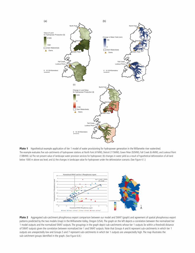
Plate 1 Hypothetical example application of tier 1 model of water provisioning for hydropower generation in the Willamette river watershed.The example evaluates fi ve sub-catchments of hydropower stations at North Fork (41MW), Detroit (115MW), Green Peter (92MW), Fall Creek (6.4MW), and Lookout Point (138MW). (a) The net present value of landscape water provision services for hydropower; (b) changes in water yield as a result of hypothetical deforestation of all land below 1000 m above sea level; and (c) the changes in landscape value for hydropower under the deforestation scenario. (See Figure 4.1.)
Value of Landfor Hydropower Production ($)
21305
1482
Dam Watersheds
Dams
0 10 20 Kilometers 0 10 20 Kilometers
0 10 20 Kilometers
Fall CreekLookout Point
Change in Land Valuefor Hydropower Production ($)
Green Peter Green Peter
Detroit Detroit
Green Peter
Detroit
North Fork North Fork
North Fork
Change in Water Yield (mm)
105
0
0
–1106
1455
Dams
Fall CreekLookout Point
Fall CreekLookout Point
Dam Watersheds
Dams
Dam Watersheds
(b)
(c)
(a)
Plate 2 Aggregated sub-catchment phosphorous export comparison between our model and SWAT (graph) and agreement of spatial phosphorous export patterns predicted by the two models (map) in the Williamette Valley, Oregon (USA). The graph on the left depicts a correlation between the normalized tier 1 model outputs and the normalized SWAT outputs. The groupings in the graph depict sub-catchments whose tier 1 outputs lie within a threshold distance of SWAT outputs given the correlation between normalized tier 1 and SWAT outputs. Note that Groups 4 and 6 represent sub-catchments in which tier 1 outputs are unexpectedly low and Groups 5 and 7 represent sub-catchments in which tier 1 outputs are unexpectedly high. The map illustrates the sub-catchment groups identifi ed in the graph. (See Figure 6.8.)
Normalized SWAT and tier 1 Phosphorous export3.5
3tier 1 = 0.621 × SWAT
R2 = 0.3852.5
2
1.5
1
0.5
0
–0.5
–1
–1.5–2 –1
Group 1 Group 2 Group 3 Group 4 Group 5 Group 6 Group 7
0Normalized SWAT Phosphorous export
Nor
mal
ized
tier
1 P
hosp
horo
us e
xpor
t
1 2 3 4
Correlation Groups
N
1234567
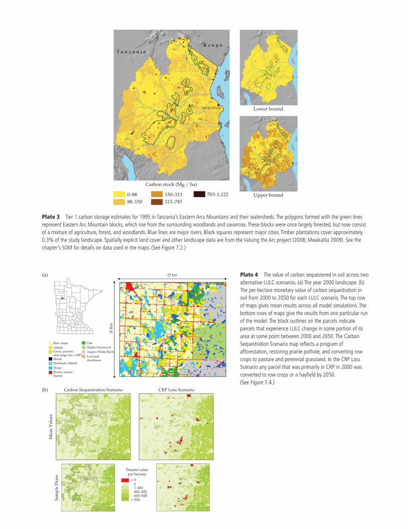
T a n z a n i aK e n y a
Dar Es Salaam Lower bound
Upper bound783–1,122150–313313–783
0–88
Carbon stock (Mg / ha)
88–150
Plate 3 Tier 1 carbon storage estimates for 1995 in Tanzania’s Eastern Arcs Mountains and their watersheds. The polygons formed with the green lines represent Eastern Arc Mountain blocks, which rise from the surrounding woodlands and savannas. These blocks were once largely forested, but now consist of a mixture of agriculture, forest, and woodlands. Blue lines are major rivers. Black squares represent major cities. Timber plantations cover approximately 0.3% of the study landscape. Spatially explicit land cover and other landscape data are from the Valuing the Arc project (2008; Mwakalila 2009). See the chapter’s SOM for details on data used in the maps. (See Figure 7.2.)
(a)
(b)
Row crops
20 K
m
OakMaple/basswoodAspen/White BirchLowlanddeciduous
AlfalfaGrass, pasture,and range (inc. CRP)ShrubWetlands/MarshWaterRoads/urban/barren
Carbon Sequestration Scenario CRP Loss Scenario
22 km
Present valueper hectare< 0
> 928
01–441442–602603–928
Mea
n V
alue
sSa
mpl
e D
raw
Plate 4 The value of carbon sequestered in soil across two alternative LULC scenarios. (a) The year 2000 landscape. (b) The per-hectare monetary value of carbon sequestration in soil from 2000 to 2050 for each LULC scenario. The top row of maps gives mean results across all model simulations. The bottom rows of maps give the results from one particular run of the model. The black outlines on the parcels indicate parcels that experience LULC change in some portion of its area at some point between 2000 and 2050. The Carbon Sequestration Scenario map refl ects a program of afforestation, restoring prairie pothole, and converting row crops to pasture and perennial grassland. In the CRP Loss Scenario any parcel that was primarily in CRP in 2000 was converted to row crops or a hayfi eld by 2050. (See Figure 7.4.)
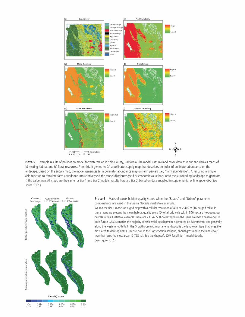
Ditchside edge
Farm parcel edge
Residential edge
Roadside edge
Agriculture
Organic Ag
Pasture
Riparian
Scrub Forest
Unclassified
Water
Land Cover
High: 1
Low: 0
Nest Suitability
High: 1
Low: 0
Floral Resource(c)
(e)
(a)
(d)
(f)
(b)
High: 1
Low: 0
Supply Map
High: 0.25
Kilometers0 4.5 9 18 27 36
N
S
EW
Low: 0
Farm Abundance
High: 1
Low: 0
Service Value Map
Plate 5 Example results of pollination model for watermelon in Yolo County, California. The model uses (a) land cover data as input and derives maps of (b) nesting habitat and (c) fl oral resources. From this, it generates (d) a pollinator supply map that describes an index of pollinator abundance on the landscape. Based on the supply map, the model generates (e) a pollinator abundance map on farm parcels (i.e., “farm abundance”). After using a simple yield function to translate farm abundance into relative yield the model distributes yield or economic value back onto the surrounding landscape to generate (f) the value map. All steps are the same for tier 1 and tier 2 models; results here are tier 2, based on data supplied in supplemental online appendix. (See Figure 10.2.)
CurrentLandscape
>0–<0.9
0.91–0.92
0.93–0.94
0.95–0.96
0.97–0.98
0.99–1.00
Parcel Q scores
Roa
ds p
aram
eter
com
bina
tion
Urb
an p
aram
eter
com
bina
tion
ConservationLULC Scenario
GrowthLULC Scenario
Plate 6 Maps of parcel habitat quality scores when the “Roads” and “Urban” parameter combinations are used in the Sierra Nevada illustrative example.We ran the tier 1 model on a grid map with a cellular resolution of 400 m × 400 m (16-ha grid cells). In these maps we present the mean habitat quality score ( Q ) of all grid cells within 500 hectare hexagons, our parcels in this illustrative example. There are 23 042 500-ha hexagons in the Sierra Nevada Conservancy. In both future LULC scenarios the majority of residential development is centered on Sacramento, and generally along the western foothills. In the Growth scenario, montane hardwood is the land cover type that loses the most area to development (158 268 ha). In the Conservation scenario, annual grassland is the land cover type that loses the most area (17 798 ha). See the chapter’s SOM for all tier 1 model details. (See Figure 13.2.)
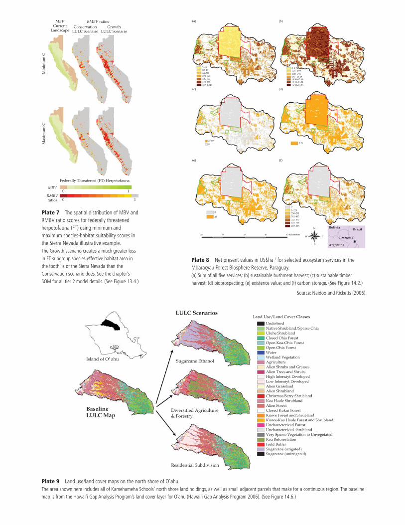
MBVCurrent
Landscape
RMBV ratios
RMBVratios
MBV
ConservationLULC Scenario
Federally Threatened (FT) Herpetofauna
0
0
1
1
Min
imum
CM
axim
um C
GrowthLULC Scenario
Plate 7 The spatial distribution of MBV and RMBV ratio scores for federally threatened herpetofauna (FT) using minimum and maximum species-habitat suitability scores in the Sierra Nevada illustrative example.The Growth scenario creates a much greater loss in FT subgroup species effective habitat area in the foothills of the Sierra Nevada than the Conservation scenario does. See the chapter’s SOM for all tier 2 model details. (See Figure 13.4.)
2–1920–4748–272273–325326–333334–456457–1,045
27.60
(e) (f)
(c) (d)
(a) (b)
2.21
01–229230–291292–412413–577578–766767–975
60 Kilometers4020020
25
0
W E
S
N Bolivia Brazil
Paraguay
Argentina
0
0–1.741.75–3.994.00–6.966.97–13.4913.50–15.0915.10–16.5416.55–18.50
Plate 8 Net present values in US$ha -1 for selected ecosystem services in the Mbaracyau Forest Biosphere Reserve, Paraguay.(a) Sum of all fi ve services; (b) sustainable bushmeat harvest; (c) sustainable timber harvest; (d) bioprospecting; (e) existence value; and (f) carbon storage. (See Figure 14.2.)
Source: Naidoo and Ricketts (2006).
Undefined
Land Use/Land Cover Classes
Native Shrubland/Sparse OhiaUluhe ShrublandClosed Ohia ForestOpen Koa-Ohia ForestOpen Ohia ForestWaterWetland VegetationAgriculture
Alien Trees and ShrubsHigh Intensiyt DevelopedLow Intensiyt DevelopedAlien GrasslandAlien Shrubland
Alien ForestClosed Kukui ForestKiawe Forest and ShrublandKiawe-Koa Haole Forest and ShrublandUncharacterized ForestUncharacterized shrublandVery Sparse Vegetation to UnvegetatedKoa ReforestationField BufferSugarcane (irrigated)Sugarcane (unirrigated)
Christmas Berry ShrublandKoa Haole Shrubland
Alien Shrubs and GrassesSugarcane EthanolIsland of O¢ ahu
Diversified Agriculture& Forestry
Residential Subdivision
BaselineLULC Map
LULC Scenarios
Plate 9 Land use/land cover maps on the north shore of O’ahu.The area shown here includes all of Kamehameha Schools’ north shore land holdings, as well as small adjacent parcels that make for a continuous region. The baseline map is from the Hawai’i Gap Analysis Program’s land cover layer for O`ahu (Hawai’i Gap Analysis Program 2006). (See Figure 14.6.)
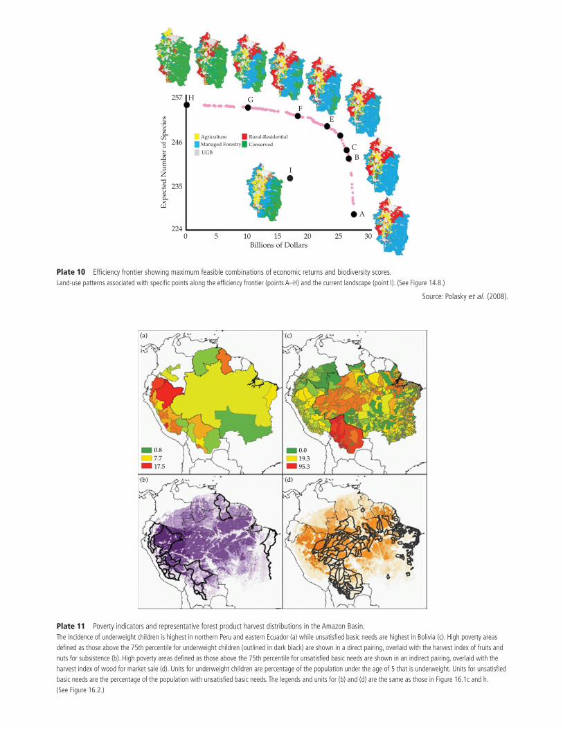
257 H
AgricultureManaged Forestry
UGB
Rural-ResidentialConserved
GF
E
CB
A
I
246
235
2240 5 10 15
Billions of Dollars
Expe
cted
Num
ber
of S
peci
es
20 25 30
Plate 10 Effi ciency frontier showing maximum feasible combinations of economic returns and biodiversity scores.Land-use patterns associated with specifi c points along the effi ciency frontier (points A–H) and the current landscape (point I). (See Figure 14.8.)
Source: Polasky et al. (2008).
(a)
0.87.717.5
0.019.395.3
(c)
(b) (d)
Plate 11 Poverty indicators and representative forest product harvest distributions in the Amazon Basin.The incidence of underweight children is highest in northern Peru and eastern Ecuador (a) while unsatisfi ed basic needs are highest in Bolivia (c). High poverty areas defi ned as those above the 75th percentile for underweight children (outlined in dark black) are shown in a direct pairing, overlaid with the harvest index of fruits and nuts for subsistence (b). High poverty areas defi ned as those above the 75th percentile for unsatisfi ed basic needs are shown in an indirect pairing, overlaid with the harvest index of wood for market sale (d). Units for underweight children are percentage of the population under the age of 5 that is underweight. Units for unsatisfi ed basic needs are the percentage of the population with unsatisfi ed basic needs. The legends and units for (b) and (d) are the same as those in Figure 16.1c and h. (See Figure 16.2.)
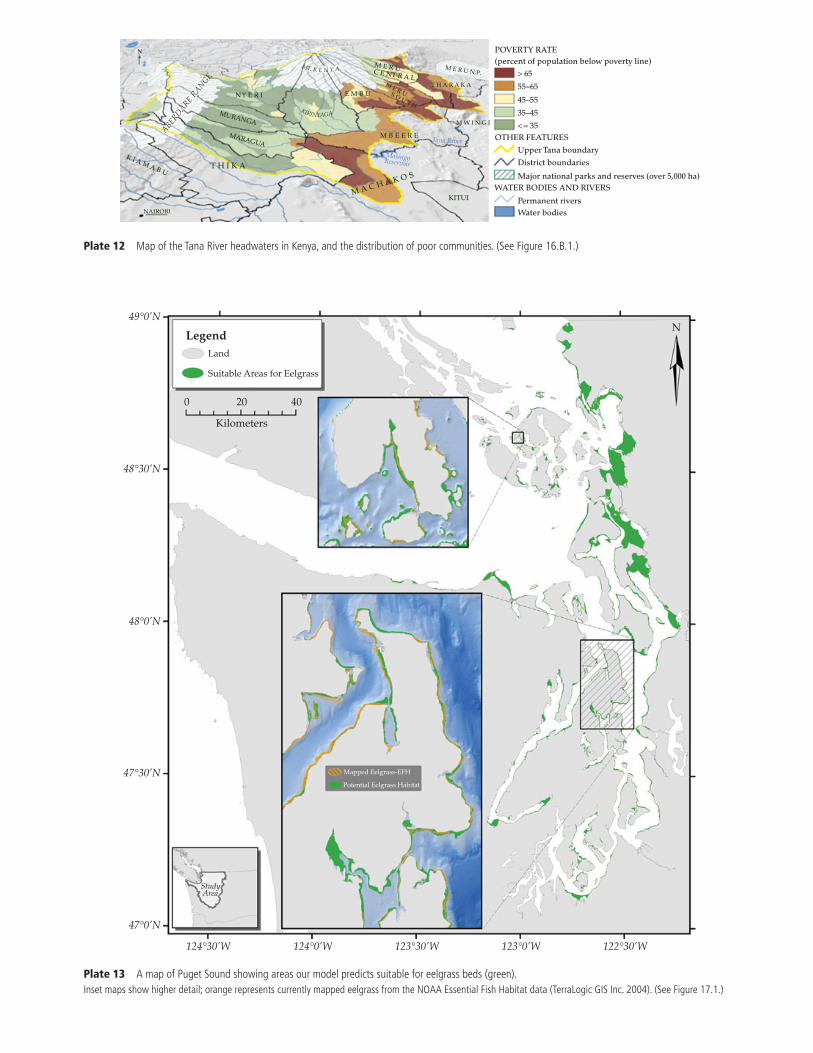
N
ABERDARE RANGE
K I A M A B U
NAIROBI
T H I K A
M A C H A K O S
KITUI
M B E E R E
E M B UN Y E R I
MURANGA
MARAGUA
M E R UC E NT R A L
M W I N G I
M E R U S O U T H
T H A R A K A
M E R U N.P.
MasingoReservoir
Tana River
KIRINYAGA
MT. K E N Y A
POVERTY RATE
OTHER FEATURES
(percent of population below poverty line)> 65
< = 35
55–65
Upper Tana boundaryDistrict boundaries
Major national parks and reserves (over 5,000 ha)
Permanent riversWater bodies
WATER BODIES AND RIVERS
45–55
35–45
Plate 12 Map of the Tana River headwaters in Kenya, and the distribution of poor communities. (See Figure 16.B.1.)
Land
Legend
49°0’N
48°30’N
48°0’N
47°30’N
StudyArea
47°0’N
124°30’W 124°0’W 123°30’W 123°0’W 122°30’W
Suitable Areas for Eelgrass
0 20 40
N
Kilometers
Mapped Eelgrass-EFH
Potential Eelgrass Habitat
Plate 13 A map of Puget Sound showing areas our model predicts suitable for eelgrass beds (green).Inset maps show higher detail; orange represents currently mapped eelgrass from the NOAA Essential Fish Habitat data (TerraLogic GIS Inc. 2004). (See Figure 17.1.)
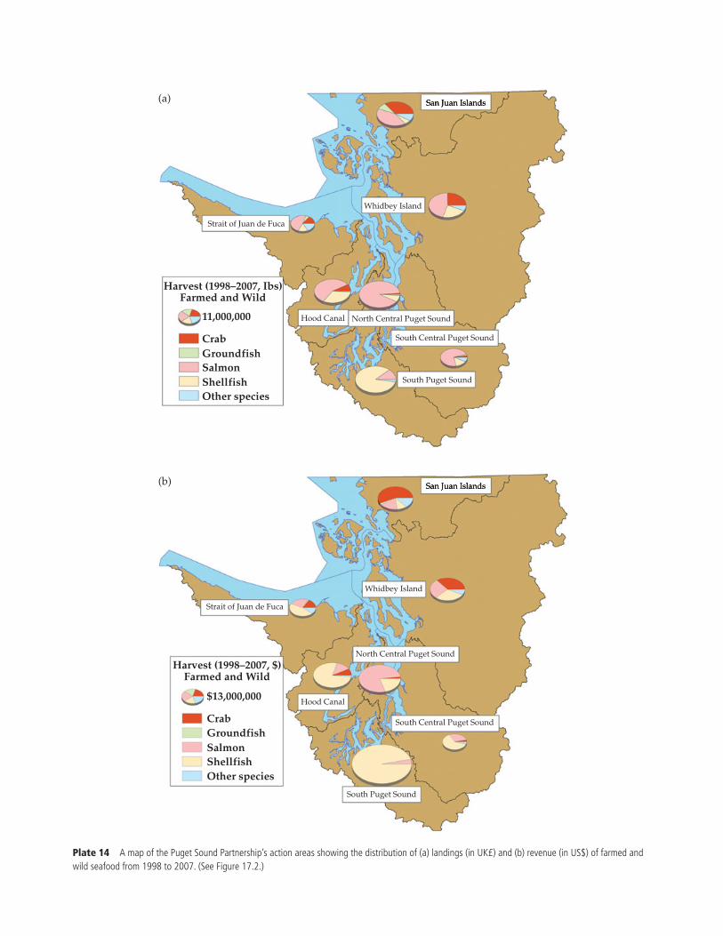
Whidbey Island
Strait of Juan de Fuca
(a)
Harvest (1998–2007, Ibs)Farmed and Wild
11,000,000
CrabGroundfishSalmonShellfishOther species
Hood Canal North Central Puget Sound
South Central Puget Sound
South Puget Sound
Whidbey Island
Strait of Juan de Fuca
Harvest (1998–2007, $)Farmed and Wild
$13,000,000
CrabGroundfishSalmonShellfishOther species
Hood Canal
North Central Puget Sound
South Central Puget Sound
South Puget Sound
(b)
Plate 14 A map of the Puget Sound Partnership’s action areas showing the distribution of (a) landings (in UK£) and (b) revenue (in US$) of farmed and wild seafood from 1998 to 2007. (See Figure 17.2.)
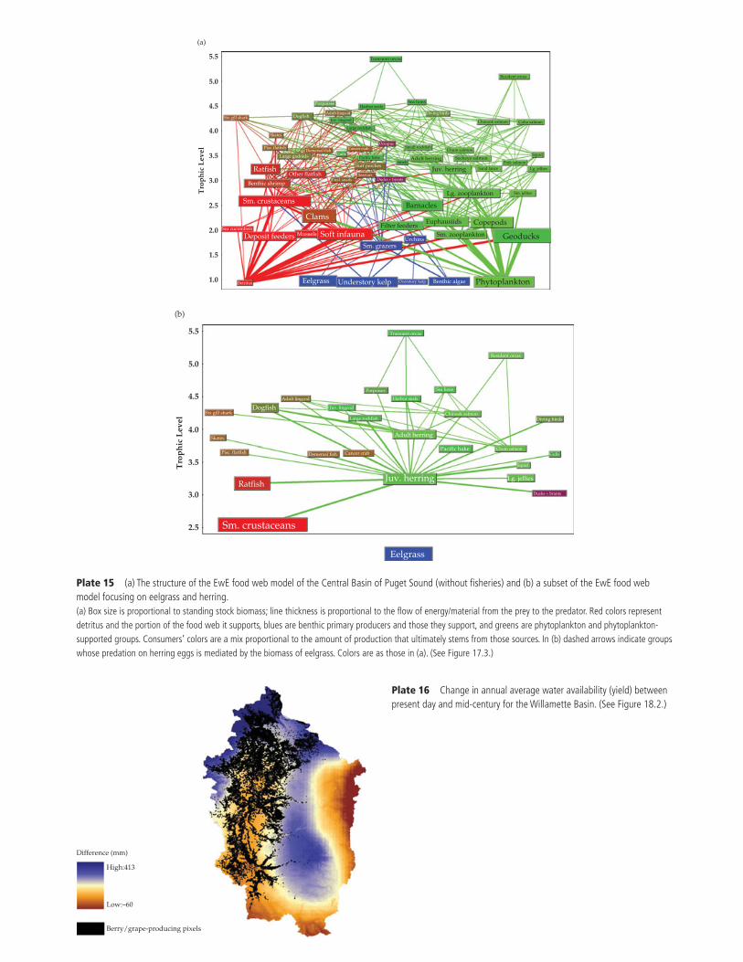
Six gill shark
Skates
Pisc. flatfish
Large gadoids
Dogfish
Porpoises
Transient orcas
Sea lions
Diving birds
Resident orcas
Coho salmonChinook salmon
Squid
Lg. jelliesPink salmon
Sm. jellies
Sand lance
Chum salmonSmall rockfish
SmeltAdult herring
Juv. herring
Lg. zooplankton
Sockeye salmon
Harbor seals
Juv. lingcod
Large rockfish
OctopusCancer crab
GullsPacific hake
SeastarsPred. snails Ducks + brants
Surf perches
Adult lingcod
Other flatfish
Clams
Soft infauna
Understory kelpEelgrass
Filter feeders Euphausiids
Sm. zooplankton Geoducks
Phytoplankton
Copepods
Barnacles
Sm. grazersUrchins
Benthic algaeOverstory kelp
Ratfish
Sm. crustaceans
Deposit feeders
Benthic shrimp
Sea cucumbers
Detritus
Mussels
Demersal fish
5.5
5.0
4.5
4.0
3.5
3.0
Tro
phic
Lev
el2.5
2.0
1.5
1.0
(a)
Adult lingcod
Juv. lingcod
Large rockfish
Harbor seals
Porpoises Sea lions
Resident orcas
Transient orcas
Chinook salmon
Pacific hake Chum salmon
Squid
Gulls
Diving birds
Ducks + brants
Lg. jellies
Adult herring
Six gill shark
Skates
Pisc. flatfish Demersal fish Cancer crab
Ratfish
Dogfish
Sm. crustaceans
Juv. herring
Eelgrass
5.5
5.0
4.5
4.0
Tro
phic
Lev
el
3.5
3.0
2.5
(b)
Plate 15 (a) The structure of the EwE food web model of the Central Basin of Puget Sound (without fi sheries) and (b) a subset of the EwE food web model focusing on eelgrass and herring.(a) Box size is proportional to standing stock biomass; line thickness is proportional to the fl ow of energy/material from the prey to the predator. Red colors represent detritus and the portion of the food web it supports, blues are benthic primary producers and those they support, and greens are phytoplankton and phytoplankton-supported groups. Consumers’ colors are a mix proportional to the amount of production that ultimately stems from those sources. In (b) dashed arrows indicate groups whose predation on herring eggs is mediated by the biomass of eelgrass. Colors are as those in (a). (See Figure 17.3.)
Difference (mm)
High:413
Low:–60
Berry/grape-producing pixels
Plate 16 Change in annual average water availability (yield) between present day and mid-century for the Willamette Basin. (See Figure 18.2.)
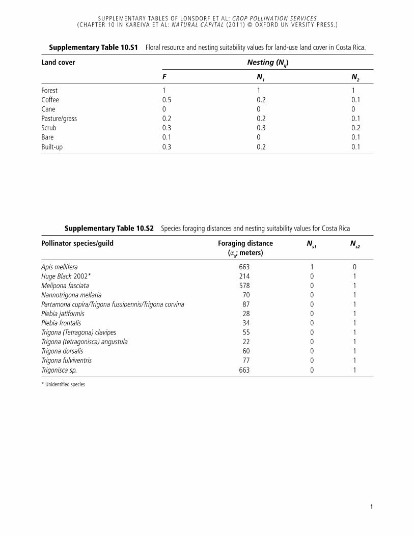
1
SUPPLEMENTARY TABLES OF LONSDORF ET AL : CROP POLL INATION SERVICES (CHAPTER 10 IN KAREIVA ET AL : NATURAL CAPITAL (2011) © OXFORD UNIVERSITY PRESS. )
Supplementary Table 10.S2 Species foraging distances and nesting suitability values for Costa Rica
Pollinator species/guild Foraging distance (α s ; meters)
N s1 N s2
Apis mellifera 663 1 0 Huge Black 2002* 214 0 1 Melipona fasciata 578 0 1 Nannotrigona mellaria 70 0 1 Partamona cupira/Trigona fussipennis/Trigona corvina 87 0 1 Plebia jatiformis 28 0 1 Plebia frontalis 34 0 1 Trigona (Tetragona) clavipes 55 0 1 Trigona (tetragonisca) angustula 22 0 1 Trigona dorsalis 60 0 1 Trigona fulviventris 77 0 1 Trigonisca sp. 663 0 1
* Unidentifi ed species
Supplementary Table 10.S1 Floral resource and nesting suitability values for land-use land cover in Costa Rica.
Land cover Nesting (N ij )
F N 1 N 2
Forest 1 1 1 Coffee 0.5 0.2 0.1 Cane 0 0 0 Pasture/grass 0.2 0.2 0.1 Scrub 0.3 0.3 0.2 Bare 0.1 0 0.1 Built-up 0.3 0.2 0.1
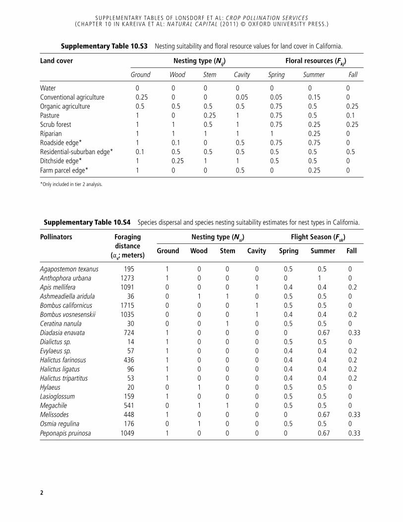
2
SUPPLEMENTARY TABLES OF LONSDORF ET AL : CROP POLL INATION SERVICES (CHAPTER 10 IN KAREIVA ET AL : NATURAL CAPITAL (2011) © OXFORD UNIVERSITY PRESS. )
Supplementary Table 10.S4 Species dispersal and species nesting suitability estimates for nest types in California.
Pollinators Foraging distance
(α s ; meters)
Nesting type ( N si ) Flight Season ( F sk )
Ground Wood Stem Cavity Spring Summer Fall
Agapostemon texanus 195 1 0 0 0 0.5 0.5 0 Anthophora urbana 1273 1 0 0 0 0 1 0 Apis mellifera 1091 0 0 0 1 0.4 0.4 0.2 Ashmeadiella aridula 36 0 1 1 0 0.5 0.5 0 Bombus californicus 1715 0 0 0 1 0.5 0.5 0 Bombus vosnesenskii 1035 0 0 0 1 0.4 0.4 0.2 Ceratina nanula 30 0 0 1 0 0.5 0.5 0 Diadasia enavata 724 1 0 0 0 0 0.67 0.33 Dialictus sp. 14 1 0 0 0 0.5 0.5 0 Evylaeus sp. 57 1 0 0 0 0.4 0.4 0.2 Halictus farinosus 436 1 0 0 0 0.4 0.4 0.2 Halictus ligatus 96 1 0 0 0 0.4 0.4 0.2 Halictus tripartitus 53 1 0 0 0 0.4 0.4 0.2 Hylaeus 20 0 1 0 0 0.5 0.5 0 Lasioglossum 159 1 0 0 0 0.5 0.5 0 Megachile 541 0 1 1 0 0.5 0.5 0 Melissodes 448 1 0 0 0 0 0.67 0.33 Osmia regulina 176 0 1 0 0 0.5 0.5 0 Peponapis pruinosa 1049 1 0 0 0 0 0.67 0.33
Supplementary Table 10.S3 Nesting suitability and fl oral resource values for land cover in California.
Land cover Nesting type ( N ij ) Floral resources ( F kj )
Ground Wood Stem Cavity Spring Summer Fall
Water 0 0 0 0 0 0 0 Conventional agriculture 0.25 0 0 0.05 0.05 0.15 0 Organic agriculture 0.5 0.5 0.5 0.5 0.75 0.5 0.25 Pasture 1 0 0.25 1 0.75 0.5 0.1 Scrub forest 1 1 0.5 1 0.75 0.25 0.25 Riparian 1 1 1 1 1 0.25 0 Roadside edge* 1 0.1 0 0.5 0.75 0.75 0 Residential-suburban edge* 0.1 0.5 0.5 0.5 0.5 0.5 0.5 Ditchside edge* 1 0.25 1 1 0.5 0.5 0 Farm parcel edge* 1 0 0 0.5 0 0.25 0
*Only included in tier 2 analysis.

AIBR. Revista de Antropología IberoamericanaISSN: [email protected]ón de Antropólogos Iberoamericanosen RedOrganismo Internacional
Santamarina Campos, BeatrizAntropología y medio ambiente. revisión de una tradición y nuevas perspectivas de análisis en la
problemática ecológicaAIBR. Revista de Antropología Iberoamericana, vol. 3, núm. 2, mayo-agosto, 2008, pp. 144-184
Asociación de Antropólogos Iberoamericanos en RedMadrid, Organismo Internacional
Disponible en: http://www.redalyc.org/articulo.oa?id=62330203
Cómo citar el artículo
Número completo
Más información del artículo
Página de la revista en redalyc.org
Sistema de Información CientíficaRed de Revistas Científicas de América Latina, el Caribe, España y Portugal
Proyecto académico sin fines de lucro, desarrollado bajo la iniciativa de acceso abierto
Antropología y Medio Ambiente
AIBR. Revista de Antropología Iberoamericana. www.aibr.org Volumen 3, Número 2. Mayo-Agosto 2008. Pp. 144-184 Madrid: Antropólogos Iberoamericanos en Red. ISSN: 1695-9752
144
ANTROPOLOGÍA Y MEDIO AMBIENTE.
REVISIÓN DE UNA TRADICIÓN Y NUEVAS
PERSPECTIVAS DE ANÁLISIS EN LA
PROBLEMÁTICA ECOLÓGICA
Beatriz Santamarina Campos
Universidad de Valencia
Recibido: 26 de febrero de 2008
Aceptado: 8 de abril de 2008
Resumen Durante los últimos años la producción etnográfica sobre el conflicto medio ambiental ha generado un volumen considerable de aportaciones. En este artículo se contextualiza, en la tradición antropológica, las distintas perspectivas (la ecológica, la simbólica cognitiva y la política) que se han ocupado del entorno, de la construcción de la naturaleza y del papel otorgado a la naturaleza en la distribución de relaciones de poder. Todo para situar a las perspectivas de la ecología simbólica y ecología política como los enfoques, desde nuestro punto de vista, más pertinentes para abordar el conflicto medio ambiental. En un mundo donde se imponen visiones hegemónicas y discursos ecológicos globalizados, basados en una racionalidad político-económica que se pretende única, se hace necesario un análisis crítico para descifrar las claves de nuestra práctica cultural y para poner en práctica todo el conocimiento local aprendido, que permita sacar a la luz otros discursos practicables posibles desde lógicas marginales.
Palabras claves Ecología cultural, Ecología simbólica, ecología política, antropología medio ambiental
ANTHROPOLOGY AND THE ENVIRONMENT. REVISION OF A TRADITION AND NEW ANALYTICAL PERSPECTIVES FOR THE ECOLOGICAL PROBLEM
Abstract In recent years, ethnographic work on environmental conflict has generated a considerable amount of activity. This article contextualizes the different perspectives (ecological, symbolic-cognitive and political) that have dealt with the environment, the construction of nature, and the role given to nature in the distribution of power relations. The authors consider the perspectives of symbolic ecology and political ecology to be the approaches that are most relevant for addressing environmental conflict. In a world of imposed hegemonic visions and globalized ecological discourses based on a political-economic rationality that claims to be unique, a critical analysis is needed to decipher the code of our practice of culture and to put into practice all of the acquired local knowledge, which will allow us to draw out other possible, viable discourses from marginal logics.
Beatriz Santamarina
AIBR. Revista de Antropología Iberoamericana. www.aibr.org
Volumen 3, Número 2. Mayo-Agosto 2008. Pp. 144-184 Madrid: Antropólogos Iberoamericanos en Red. ISSN: 1695-9752
145
Key words Cultural Ecology, Political Ecology, Symbolic Ecology, Environmental Anthropology
1. Introducción
esde la antropología, hacer una aproximación reflexiva al medio ambiente en
nuestra práctica cultural supone invitar a la consideración de un tema que ha
ocupado un importante volumen en la producción etnográfica. El medio
ambiente se presenta como una recapacitación entre dos polos tensionales tan
clásicos en la antropología como en nuestra sociedad: naturaleza-cultura. Nos es
imposible pensar el medio ambiente sin una referencia explícita a la Naturaleza, y con
ella se abre una reflexión sobre lo nuestro. Ahora bien, el fenómeno medioambiental y
la necesidad de abordarlo desde una visión concreta, exige una primera mirada sobre
cómo la antropología ha contribuido no sólo a la comprensión de nuestras relaciones
con la naturaleza, sino también a configurar el mundo de lo natural. Dicha reflexión
debe hacerse en dos sentidos. En primer lugar, podemos observar cómo la naturaleza
ha sido un eje de vital importancia en el desarrollo de la disciplina antropológica,
apareciendo como un polo fundamental en su constitución y distribución de sentidos.
Así, una aportación indiscutible de la antropología1 es haber definido la cultura frente a
la naturaleza; de hecho “la relación entre cultura y naturaleza (o entre población y
entorno, si prefiere utilizarse el vocabulario ecológico-técnico) ha ocupado una parte
sustancial del análisis antropológico” (Comas d’Argemir, 1998:124). En este sentido,
hasta la segunda mitad del siglo XX, la delimitación de la cultura era “negativa porque
hablar de cultura equivalía a hacer algún tipo de referencia, implícita o explícitamente,
a lo que se estimaba su contrapartida, la naturaleza” (Luque Baena, 1990:93).
Después de este largo periodo, asistimos a un reconocimiento de la complejidad y del
dinamismo para explicar ambos conceptos, pero las fronteras y las relaciones entre
ambos vendrán marcadas, de igual modo, por la delimitación de esferas. Hay que
esperar hasta mediados de los 80, con la aparición y el desarrollo de la ecología
simbólica, la ecología política y la antropología de la ciencia, para asistir a la
superación de esta dicotomía clásica. Sin duda, la reflexión sobre el medio ambiente,
1 Una característica que no es propia de la disciplina porque, como veremos más adelante, la constitución moderna de la ciencia occidental se basa en la distinción ontológica entre mundo natural y mundo social (Latour, 1993).
D
Antropología y Medio Ambiente
AIBR. Revista de Antropología Iberoamericana. www.aibr.org Volumen 3, Número 2. Mayo-Agosto 2008. Pp. 144-184 Madrid: Antropólogos Iberoamericanos en Red. ISSN: 1695-9752
146
en un contexto marcado por la globalización y la reestructuración del capitalismo y
caracterizado por la destrucción/degradación del entorno, ha contribuido a una
redefinición del problema.
Y, en segundo lugar, este papel central ha posibilitado una atención especial a
la construcción social del mundo de lo ‘natural’. Así, nos interesa atender a las
contribuciones que desde la disciplina antropológica ayudan a descubrir la
complejidad y las múltiples dimensiones del complejo cultural ‘naturaleza’. Las
diferentes tradiciones en antropología han abordado la ‘naturaleza’ de distinta manera:
como proceso evolutivo en continuo, como esfera delimitada y contrapuesta, como
sistema de flujos..., y en este artículo pretendemos acercarnos a ellas. No obstante, el
objetivo no es hacer una síntesis exhaustiva sobre el papel otorgado por los
antropólogos a la naturaleza, sino más bien poner al descubierto la importancia y la
centralidad que dicha categoría ha ocupado y la pertinencia hoy en día de reflexionar
sobre este legado.
En definitiva, en este texto, atenderemos, a las diferentes perspectivas
antropológicas que se han ocupado, de forma especial, del mundo de lo natural. Así,
diferenciaremos tres grandes perspectivas: la ecológica, la simbólica cognitiva y la
política. En la perspectiva ecológica revisaremos la elaboración antropológica del
entorno, lo que se ha venido llamando ecología cultural. En cuanto a la perspectiva
simbólico-cognitiva veremos la manera en que se ha utilizado como construcción
cultural, observando las distintas interpretaciones y manifestaciones a las que ha
dado lugar la noción de naturaleza. Y, por último, en la perspectiva política,
analizaremos el papel otorgado a la naturaleza en la distribución de relaciones de
poder significativas. Todo para situar a las perspectivas de la ecología simbólica y
ecología política como los enfoques, desde nuestro punto de vista, más pertinentes
para abordar el conflicto medio ambiental, sin renunciar con ello a las aportaciones
que se han venido haciendo desde la disciplina y que han permitido un debate
constante sobre el entorno.
2. Las perspectivas de la(s) naturaleza(s) en antropología
El papel que se asignó a la naturaleza como eje fundamental en el discurso
antropológico proporcionó a la disciplina tanto herramientas analíticas para la
Beatriz Santamarina
AIBR. Revista de Antropología Iberoamericana. www.aibr.org
Volumen 3, Número 2. Mayo-Agosto 2008. Pp. 144-184 Madrid: Antropólogos Iberoamericanos en Red. ISSN: 1695-9752
147
investigación como un marcador de identidad. La naturaleza cobró un lugar
destacado epistemológicamente, ya que garantizaba tanto la posibilidad de establecer
un primer proceso constitutivo de atribución de orden y sentido, como un primer
marco de comprensión de los fenómenos que se pretendían estudiar. Así, la
naturaleza actuaba como un polo tensional para construir un universo de significación y
como una fuente primordial para la constitución sistemática de una cosmovisión del
mundo. De ahí que, durante largo tiempo, se tendiera a definir la cultura por
oposición a la naturaleza.
En algunos planteamientos, dicho eje se torna fundamental, como es el caso
del funcionalismo psicobiológico de Malinowski (1944), donde podemos encontrar
una versión de este tipo de interpretaciones. Sin embargo, Malinowski no fue el
primero ni el único que tomó el modelo dualista como motor de su teoría. Antes que él
los evolucionistas la habían consagrado para su esquema interpretativo de la evolución
de la historia. Después, debates como el idealista-materialista, que coparon buena
parte de las décadas de los 60 y 70 del siglo XX, escondían tras ellos la polémica entre
naturaleza y cultura. De facto, la confrontación naturaleza/cultura es posible rastrearla
hasta bien entrado el último cuarto del siglo XX. Podemos decir que tanto en la
ecología cultural, como en las propuestas materialistas e incluso en algunas marxistas,
se encuentra un esquema reduccionista sustentado en la dicotomía naturaleza-cultura.
Del mismo modo, en la antropología estructuralista o simbólica, hallamos un esbozo
similar basado en el binomio naturaleza-cultura pero, en este caso, como propuesta
analítica para interpretar diferentes procesos sociales. Así, detrás de la aparente
diferencia, entre el enfoque estructuralista y simbólico subyace una misma concepción
basada en la polaridad (Descola y Pálsson, 1996). Las consecuencias que dicha
representación ha traído consigo se pueden resumir fundamentalmente en dos: en
primer lugar, el modelo dualista ha obstaculizado una visión ecológica de las relaciones
entre los seres humanos y el medio ambiente (Hornborg, 1996; Descola, 1996;
Hornborg y Pálsson, 2000) y, en segundo lugar, ha imposibilitado interpretar el
conocimiento ecológico y tecnológico de otras culturas por estar las mismas
supeditadas a las pautas de comprensión del modelo occidental (Hviding, 1996; Ellen,
1996).
Distintas aproximaciones han puesto en entredicho el modelo dualista,
aduciendo que las diferenciaciones establecidas por el pensamiento científico
Antropología y Medio Ambiente
AIBR. Revista de Antropología Iberoamericana. www.aibr.org Volumen 3, Número 2. Mayo-Agosto 2008. Pp. 144-184 Madrid: Antropólogos Iberoamericanos en Red. ISSN: 1695-9752
148
occidental no son ni exportables a otros modelos culturales ni, necesariamente, se
encuentran en ellos (Hornborg, y Pálsson, 2000). Desde la etnografía, Descola (1993,
1998, 2003), como veremos más adelante, ha puesto en evidencia cómo la dicotomía
naturaleza-cultura pierde el sentido en algunas prácticas culturales. Siguiendo a esta
crítica, numerosos autores han mostrado, en diferentes contextos etnográficos, cómo
en distintos saberes locales no hay posibilidad de aplicar el dualismo cultura-
naturaleza, entrando en las cosmologías toda suerte de interrelaciones entre humanos,
objetos, espíritus y animales (Arhem, 1996; Rival, 1996). Ello hasta el punto de que
han puesto en duda que en algunas culturas exista realmente una categoría específica
que haga referencia a lo que nosotros denominamos naturaleza (Howell, 1996). Pero la
dicotomía naturaleza-cultura no sólo ha sido desacertada para el estudio de realidades
no occidentales. Esta polaridad tampoco da cuenta de las relaciones existentes entre
naturaleza y cultura en nuestra propia sociedad. Latour (1993) ha puesto en evidencia
cómo en la práctica de la ciencia moderna nunca se ha superado el modelo dualista.
Pese a que la constitución moderna se basa en la división entre el mundo natural y el
mundo social (separación resultado de un proceso epistemológico de ‘purificación’ que
crea dos zonas ontológicas diferenciadas), en realidad, al existir otro conjunto de
prácticas que (por un proceso de ‘traducción’) permiten la multiplicación de los híbridos
de la naturaleza y la cultura, la ciencia moderna nunca ha podido llegar a cumplir la
máxima del modelo dualista; de tal forma que, nunca hemos sido modernos.
Por otro lado, la inconsistencia del modelo dualista también ha salido a la luz
cuando se ha prestado una mayor atención a los procesos de elaboración científica,
considerándolos como generadores de culturas locales y que están sujetos a
tradiciones, a contextos productivos específicos y a relaciones de poder. Por poner un
ejemplo, Nothnagel (1996) ha estudiado cómo la ciencia ‘reproduce’ la naturaleza, es
decir, no sólo estudia los fenómenos dados ‘naturalmente’ sino que es capaz de
reproducir artificialmente sus propios fenómenos. Asimismo, es evidente que la
aparición de múltiples híbridos como la oveja Dolly, los bebés probetas, los alimentos
transgénicos, etc., fuerzan a repensar los frágiles límites establecidos entre naturaleza
y cultura (Santamarina, 2007). Autores como Haraway (1995, 1999) hablan de la
reinvención posmoderna de la naturaleza, donde la iconografía del cyborg (un híbrido
entre máquina y organismo) encapsularía ejemplarmente la disolución de límites : “el
cyborg aparece mitificado precisamente donde la frontera entre lo animal y lo humano
Beatriz Santamarina
AIBR. Revista de Antropología Iberoamericana. www.aibr.org
Volumen 3, Número 2. Mayo-Agosto 2008. Pp. 144-184 Madrid: Antropólogos Iberoamericanos en Red. ISSN: 1695-9752
149
es transgredida” (Haraway, 1995:257). Y Papagaroufali (1996) considera que las
prácticas biotecnológicas, como los xenotrasplantes y la transgénesis, cuestionan y
jerarquizan las fronteras establecidas entre lo humano y lo animal.
Junto a lo señalado, el nuevo contexto de degradación medioambiental ha
puesto sobre la mesa el debate sobre nuestras relaciones con el medio y con lo que
consideramos el mundo de lo natural (Eder, 1996), unas relaciones fundamentadas en
una visión del mundo dualista y jerárquica, que ha desencadenado una destrucción sin
límites. Al reducirse la naturaleza simplemente a “la materia prima de la cultura,
apropiada, reservada, esclavizada, exaltada o hecha flexible para su utilización por
parte de la cultura en la lógica del colonialismo capitalista” (Haraway, 1995:341),
hemos asistido a una dominación, ligada a la lógica de la producción y del capital,
que permite la reducción sistemática de espacios (naturales, colectivos y
discursivos) con total impunidad. La crisis medioambiental pone sobre la mesa la
irresponsabilidad de nuestros cimientos y supone el quiebro del mito moderno de una
dominación absoluta de la naturaleza (Santamarina, 2006a).
Con todo, antes de la deconstrucción del modelo dualista, se han producido
en antropología numerosas contribuciones que suponen un importante legado para
esta tradición de pensamiento. Tres perspectivas (ecológica, simbólica y política)
agrupan las distintas aportaciones que se han ocupado especialmente del mundo de
lo natural; de ellas nos ocupamos a continuación, viendo sus limitaciones y las
propuestas que permiten superarlas.
2.1 La perspectiva ecológica
Al comenzar cualquier monografía clásica de antropología, lo primero que nos
encontramos es un capítulo de introducción dedicado al hábitat y al entorno de la
cultura observada. El medio donde se ha desarrollado la investigación y donde se
desenvuelve la sociedad estudiada sirve como un primer marco de referencia, es el
contexto que da sentido al texto. Sin embargo, eso no significa que los antropólogos
hayan considerado siempre el entorno como un factor explicativo de los fenómenos
culturales2. La perspectiva ecológica no llega a la disciplina hasta los años cuarenta,
va a ser entonces cuando se importen los primeros conceptos de la doctrina
Antropología y Medio Ambiente
AIBR. Revista de Antropología Iberoamericana. www.aibr.org Volumen 3, Número 2. Mayo-Agosto 2008. Pp. 144-184 Madrid: Antropólogos Iberoamericanos en Red. ISSN: 1695-9752
150
darwiniana (Valdés y Valdés, 1996). Las tensiones generadas entre la biología y la
antropología hicieron posible el desarrollo de la ecología cultural. Este enfoque centró
su atención en los procesos adaptativos de la cultura, entendiendo que las culturas se
adaptan al medio, y que en ese proceso podemos ver cómo una cultura se constituye.
El debate de los ecólogos culturales parece moverse en una discusión centrada sobre
el determinismo cultural y el determinismo ambiental3. Comenzaremos con Kroeber,
como un claro exponente de la concepción de la autonomía cultural en un espacio
determinado; su obra perfila de manera ejemplar la tensión entre la biología y la
antropología. Seguiremos con White, como continuador de la tradición boasiana y
antecedente inmediato de la adopción de la perspectiva ecológica. El punto de
inflexión viene dado por Steward, al que se le atribuye la paternidad de la ecología
cultural. En él observaremos el primer intento de conjugar los factores biológicos con
los culturales; por ello, se considera a este autor como una bisagra entre dos modos
fundamentales de entender las relaciones entre naturaleza y cultura. Aunque, como
veremos, sus continuadores, materialistas e idealistas, vuelven a situar en dos polos la
naturaleza y la cultura respectivamente. Para terminar, nos aproximaremos a los
enfoques principales a los que ha dado lugar el desarrollo de la ecología cultural: el
sistémico y el individualista. Nos detendremos sólo en el sistémico, a través de la
obra de Rappaport, para analizar las dificultades que arrastra la perspectiva ecológica
y para tomar a este autor como puente hacia las nuevas ecologías (Biersack, 1999a).
Kroeber (1917) en su clásico artículo ‘Lo superorgánico’ delimita y contrapone
cultura y naturaleza, siguiendo el camino iniciado por Boas, intentando tanto combatir
las formulaciones de biólogos evolucionistas, como delimitar la cultura como un
campo específico de investigación. Para él, la cultura es ‘superorgánica’, está por
encima de lo orgánico, de lo natural. La frontera entre lo natural y lo cultural es trazada
de forma clara y contrapuesta. La naturaleza, lo orgánico, pasa a ocupar un papel
2 Más bien, dicha descripción se ha utilizado como una doble estrategia: permitía ubicar y dar realidad a una sociedad concreta. Eso legitimaba al antropólogo al reconocerse su conocimiento del terreno. 3 Seguiremos para este bosquejo las periodizaciones de Orlove (1980) y Valdés y Valdés (1996). Orlove (1980) diferencia tres estadios en el desarrollo de la antropología ecológica: un primero caracterizado, por el trabajo de Steward y White; un segundo ocupado por las teorías neofuncionalistas y neoevolucionistas; y un tercero, donde se desarrollan las enfoques procesuales. Valdés y Valdés (1996) señalan tres etapas: una marcada por la discusión de los argumentos posibilistas y la aparición de la ecología cultural, otra caracterizada por el afán de fundar una disciplina más general, y que da lugar al enfoque sistémico y a la perspectiva individualista; y, por último, la etapa actual, en la que se produce una síntesis de los enfoques anteriores (homeostático y procesual). Por otro lado, hay que señalar que Milton (2001a) utiliza otro esquema para hablar del desarrollo de la perspectiva ecológica, aunque hemos preferido utilizar estos porque se ajustan más, desde nuestro punto de vista, a una visión global de las distintas etapas de la perspectiva de la ecología cultural.
Beatriz Santamarina
AIBR. Revista de Antropología Iberoamericana. www.aibr.org
Volumen 3, Número 2. Mayo-Agosto 2008. Pp. 144-184 Madrid: Antropólogos Iberoamericanos en Red. ISSN: 1695-9752
151
pasivo (el entorno tiene sólo un sentido delimitador, un papel negativo); es la cultura,
lo supraorgánico, quien cobra el protagonismo (lo social es lo que determina lo social).
En 1952, después de las fuertes críticas suscitadas por el valor otorgado a lo
superorgánico, ofrece una definición de cultura más elaborada; sin embargo, los
postulados no difieren de sus planteamientos anteriores. El esquema se repite: existe
una ‘natural’ naturaleza de la cultura. Esta es quizás la frase que mejor resume el
planteamiento de Kroeber.
Los planteamientos de Kroeber fueron muy atacados en su época, pero, como
ha señalado Harris, “el más decidido apoyo a lo superorgánico de Kroeber llegó de un
ángulo totalmente inesperado. En ‘The expansion of the scope of science’, Leslie
White defiende a Kroeber como uno de los pocos antropólogos que se han esforzado
por formular la filosofía de una ciencia de la cultura” (1987:287). La concepción de
White parte de unas premisas muy parecidas a las de Kroeber, pero radicalizando aún
más el determinismo cultural. Para él, la cultura sólo se explica a través de la cultura
([1959]1975b) puesto que la cultura tiene un desarrollo propio una vez se ha
desprendido de su origen en la evolución biológica. La delimitación entre la naturaleza
y la cultura queda establecida de forma precisa por la capacidad simbólica de los
seres humanos4. En su teoría cobra especial importancia la relación entre la energía,
la eficacia tecnológica y la evolución. Su modelo contempla tres subsistemas: el
tecnológico, el social y el ideológico. De ellos, el tecnológico es el principal y explica la
evolución de la cultura. Su esquema es sencillo: la evolución depende de la capacidad
para aprovechar la energía que hay en el entorno, y esto se consigue a través del
sistema tecnológico5. Dicha fórmula “contradice el postulado inicial de White. ¿Cómo
argumentar que la cultura sólo se explica por la cultura si hay al menos un elemento
exógeno que la determina?” (Luque Baena, 1990:98). Al definir la cultura le concede
una autonomía propia pero, al explicar el desarrollo de la humanidad en términos
tecnológicos-energéticos, da entrada al medio como un factor explicativo en la
evolución cultural. Para White, la clave está en controlar los recursos naturales. La
diferencia radica en que no es lo mismo apropiarse de ellos que aprovecharlos y
transformarlos. El factor tecnológico se convierte en fundamental para explicar el
4 La cultura es “la clase de las cosas y acontecimientos que dependen de simbolizar, en cuanto son consideradas en un contexto extrasomático” (White, [1959]1975:139). 5 “La cultura se desarrolla según aumenta la cantidad de energía aprovechada per cápita al año, o según aumenta la eficacia de los medios instrumentales que ponen la energía en funcionamiento” ([1949]1993b:325).
Antropología y Medio Ambiente
AIBR. Revista de Antropología Iberoamericana. www.aibr.org Volumen 3, Número 2. Mayo-Agosto 2008. Pp. 144-184 Madrid: Antropólogos Iberoamericanos en Red. ISSN: 1695-9752
152
progreso, ya que la energía utilizada depende del mismo. El sistema tecnológico
condiciona a los otros subsistemas, los convierte en subsidiarios; de ahí la critica a su
determinismo tecnológico-mecánico. En definitiva, la evolución está condicionada por
la facultad de extraer energía y por los diferentes grados de desarrollo tecnológico6. La
metáfora orgánica le permite ver la cultura como un proceso evolutivo.
Si bien White introduce la perspectiva ecológica, al reconocer la influencia del
entorno en la cultura, será Steward quien definitivamente integrará en su perspectiva
las interrelaciones entre cultura y naturaleza, aunque seguirá anclado en el modelo
dualista. Su aportación más notable reside en su conceptualización de la adaptación
cultural y de las relaciones entre entorno y cultura, que permite el desarrollo del nuevo
enfoque de la ecología cultural. Para Steward, el problema de la adaptación al entorno
(ecología) del ser humano radica en que se introduce el ‘factor superorgánico de la
cultura’. De ahí que “el problema de explicar el comportamiento cultural del hombre es
de un orden diferente al de explicar su evolución biológica. Los modelos culturales ( )
no pueden analizarse del mismo modo que las características orgánicas”
([1955]1993:335). Crítica el papel minúsculo otorgado al entorno por parte de los
antropólogos que, al dedicarse a la historia y la cultura, han obviado el medio,
reservándole un ‘papel secundario y pasivo’. Según él, el concepto normativo de
cultura ha dejado de lado las adaptaciones ambientales, al considerarse que todo está
determinado por la cultura. Pero, la cultura no sólo se explica por la cultura, sino
también por el entorno. Así, se deshacía de la concepción circular de la cultura
ofreciendo un nuevo paradigma, “la ecología cultural difiere de la ecología humana y
social en la búsqueda por explicar el origen de modelos y características culturales
que caracterizan áreas diferentes más que por derivar principios aplicables a cualquier
situación cultural y ambiental. Difiere de las concepciones relativista neoevolutiva de la
historia cultural en que introduce el entorno local como factor extracultural en la
infructuosa suposición de que la cultura viene de la cultura” ([1955]1993:338)7.
White lo expresa en la siguiente fórmula E x T = C, donde E es la energía per cápita, T la eficiencia para aprovecharla y C el grado de desarrollo cultural. 6 “Los sistemas culturales, igual que los del nivel biológico, tienen capacidad para crecer. Es decir, el poder de captar energía es también la capacidad de aprovecharla cada vez más. Así, los sistemas culturales, igual que los organismos biológicos, se desarrollan, multiplican y expanden” ([1949] 1993: 366). 7 Para Steward, los aspectos de la cultura son interdependientes, pero varía el grado y el tipo. El concepto de ‘núcleo cultural’ permite ver cómo existen elementos que están más vinculados a la subsistencia y a la economía (también en el núcleo se encuentran las pautas sociales, políticas y religiosas), aunque existen otros elementos secundarios que dependen de factores histórico-culturales, y que pueden dar una imagen distinta entre dos culturas que tienen un mismo núcleo. Así, “la ecología cultural presta especial atención a aquellas características con las
Beatriz Santamarina
AIBR. Revista de Antropología Iberoamericana. www.aibr.org
Volumen 3, Número 2. Mayo-Agosto 2008. Pp. 144-184 Madrid: Antropólogos Iberoamericanos en Red. ISSN: 1695-9752
153
Como han señalado Valdés y Valdés, “Steward admitía la actuación conjunta
de una doble causalidad, la bioecológica y la cultural, pero fue incapaz de precisar
los respectivos ámbitos de aplicación” (1996:98). De todas formas, fue el precursor
de la problemática ambiental en la antropología, sentando tanto las bases para un
posterior análisis del interaccionismo como estimulando el debate entre sus
seguidores, divididos en dos posiciones extremas: el materialismo y el idealismo. La
discusión entre ambas posturas, entre razón práctica y cultura, queda personificada
en sus dos máximos exponentes, Harris y Sahlins respectivamente. Detrás de este
debate aparece, una vez más, la dicotomización naturaleza/cultura o, si se prefiere,
la reducción de una sobre la otra. Para el materialismo vulgar, la cultura se explica
en términos de naturaleza. Para el idealismo, la cultura es autónoma,
autodeterminante y explicable en sus propios términos.
El materialismo de Harris parte de considerar “que la vida social humana es
una reacción frente a los problemas prácticos de la vida terrenal” (1982:11), y que,
por tanto, el énfasis debe ponerse en la relación entre producción, reproducción y
ecología. Los condiciones tecnoecológicas y tecnoeconómicas ocupan un lugar
privilegiado en su formulación, ya que serán los factores responsables de la
organización social y la ideología. Este determinismo infraestructural viene
justificado porque los seres humanos no podemos cambiar las leyes de la
naturaleza, estamos sujetas a ellas. La tecnología permite alterar las tasas
productivas y reproductivas pero, aún así, queda sujeta a las leyes biológicas y
ecológicas, y a la capacidad de cada hábitat de ser modificado. Los
constreñimientos infraestructurales son los que determinan los componentes
estructurales y superestructurales8. Ejemplo de su argumentación lo encontramos en
su interpretación de los tabúes alimentarios (1989, 1997). Harris ([1985]1997)
cuestiona los postulados de Lévi-Strauss, planteándose si los alimentos son buenos
para pensar o para comer. Su respuesta es clara: “las gentes hacen lo que hacen
por buenas y suficientes razones prácticas y la comida no es a este respecto una
excepción” ([1985]1997:13). Así, las cosas, “la comida debe nutrir el estómago
colectivo antes de poder alimentar la mente colectiva” ([1985]1997:14). Para él, los
que el análisis empírico muestra estar más estrechamente relacionado en la utilización del entorno de modos culturalmente prescritos” ([1955]1993:339). 8 “A la naturaleza le da lo mismo que Dios sea un padre amantísimo o un sanguinario caníbal. Pero no le es indiferente que el período de barbecho de un campo cultivado por el método de roza dure un año o diez”(1982:73).
Antropología y Medio Ambiente
AIBR. Revista de Antropología Iberoamericana. www.aibr.org Volumen 3, Número 2. Mayo-Agosto 2008. Pp. 144-184 Madrid: Antropólogos Iberoamericanos en Red. ISSN: 1695-9752
154
alimentos ‘buenos para comer’ son, sin duda, aquellos que tienen una relación
coste/beneficio más óptimo en comparación con los que son ‘malos para comer’. En
esta relación coste/beneficio, nos dirá Harris, las culturas no sólo tienen en cuenta el
valor nutritivo sino también el coste/beneficio9 de la producción y sus efectos sobre
el medio. Las cocinas serán más carnívoras o más herbívoras dependiendo de las
poblaciones, los hábitats y los recursos tecnológicos, de tal forma que todos los
rasgos culturales tienen un sentido ecológico. El determinismo ambiental de su
explicación es evidente al otorgar al ambiente un papel sobresaliente en el desarrollo
de las culturas y al considerar los rasgos culturales como expresiones de la
racionalidad adaptativa. En suma, el materialismo cultural enarbolado por Harris,
reduce la cultura a la naturaleza, la ideología a la práctica, lo ideal a lo material, y
todo desde un determinismo infraestructural que desvaloriza el orden cultural y que
reduce sus explicaciones a la adaptación al medio por parte de los sistemas. Las
críticas a esta perspectiva han sido numerosas, aunque el ataque más directo le
viene formulado por Sahlins y Godelier10.
Nada más contrario al materialismo cultural que la posición adoptada por
Sahlins, la cual queda bien recogida en Cultura y Razón práctica ([1976]1997). En su
comienzo advierte: “este libro contribuye a una crítica antropológica de la idea de que
las culturas humanas se formulan a partir de la actividad práctica y, subyacente a ella,
del interés utilitario” (Sahlins, [1976]1997:9). Frente a la razón práctica, Sahlins
propone la razón simbólica o cognitiva; frente al postulado de que los humanos nos
movemos en un mundo material adopta la consideración de que somos los únicos
seres que tenemos esquemas significativos. De ahí que parta de la premisa de que la
cultura debe explicarse en términos de ella misma. Para él, las culturas son órdenes
significativos sistemáticos y no pueden ser simplemente aleatorias invenciones de la
mente. La cultura no puede ser vista como una variable dependiente de la lógica
práctica, ni debe ser entendida a partir de las fuerzas materiales; más bien al
contrario, los efectos materiales dependen de la interpretación cultural. Su postura
frente a la naturaleza es justo la inversa a la de Harris, puesto que para él se produce
9 Estos costes/beneficios se traducirían en las economías de mercado en ‘bueno para comer, bueno para vender’. 10 Las principales críticas de Godelier al materialismo vulgar se centran en subrayar el reduccionismo que establece Harris de las relaciones entre economía y sociedad, en su definición histórica como una serie de hechos con cierta frecuencia estadística y en su concepción del término adaptación. Volveremos a Godelier más adelante.
Beatriz Santamarina
AIBR. Revista de Antropología Iberoamericana. www.aibr.org
Volumen 3, Número 2. Mayo-Agosto 2008. Pp. 144-184 Madrid: Antropólogos Iberoamericanos en Red. ISSN: 1695-9752
155
una culturización de la naturaleza (‘naturaleza culturizada’). La naturaleza es sólo
materia prima en espera de que los seres humanos le den una forma significativa y un
contenido. El orden cultural es el encargado de definir la naturaleza, en este sentido,
las leyes de la naturaleza son indeterminadas. Esta concepción idealista reduce la
naturaleza a la cultura, de la misma forma que el materialismo reducía la cultura a la
naturaleza, e imposibilita pensar las relaciones naturaleza/cultura de otra forma que no
sea la confrontación y el menoscabo de una por la otra. Sahlins, en su empeño de
subrayar la dimensión ideológica, cae en la misma trampa que Harris.
Sin embargo, siguiendo con el desarrollo de la ecología cultural, vemos cómo
en los años setenta dicha perspectiva se apartó de los presupuestos de Steward y
puso mayor énfasis en los conceptos de adaptación y ecosistema. A ese nuevo
enfoque se le ha denominando sistémico, por el acento puesto en la interrelación de
factores dentro de un sistema que se considera autorregulado y funcional, y por el
estudio de los factores que inciden en la conservación del equilibrio de un sistema. En
Rappaport podemos apreciar el giro hacia esta nueva visión. El planteamiento inicial
es justo el inverso del visto hasta ahora: se trata de establecer qué es lo que no es
humano en vez de observar lo que es exclusivamente humano11. Así, al situar a los
seres humanos como animales, se pueden adoptar las perspectivas ecológicas y
biológicas en las generalizaciones antropológicas. El punto de partida es que “los
hombres son animales, y como todos los animales están indisolublemente ligados a
medios ambientes compuestos de otros organismos y sustancias inorgánicas de los
cuales deben obtener materia y energía para sustentarse y a los cuales deben
adaptarse para no perecer” (1975:269). Rappaport reconoce que en los seres
humanos nos encontramos con adaptaciones culturales al medio, pero en el proceso
de adaptación entran en juego las mismas reglas que podemos encontrar en la
adaptación biológica. Esto abre las puertas para la adopción de una perspectiva
ecológica. La complejidad está en las relaciones que se establecen entre naturaleza y
seres humanos porque “aunque el hombre actúa en la naturaleza de acuerdo con sus
conceptos y deseos, es sobre la naturaleza donde actúa, a la vez que ésta actúa
sobre el hombre” (1975:271). El problema radica en las discrepancias que existen
entre el ‘modelo percibido’ y el ‘modelo operativo’ en la comprensión de la naturaleza.
11 “Aunque la antropología ecológica comparte con el resto de la antropología cultural el objetivo de esclarecer la cultura humana, difiere en una gran parte de aquella en que intenta explicar la cultura en términos de la parte que juega en los aspectos de la existencia humana que son comunes a los seres vivientes” (Rappaport, 1975:268).
Antropología y Medio Ambiente
AIBR. Revista de Antropología Iberoamericana. www.aibr.org Volumen 3, Número 2. Mayo-Agosto 2008. Pp. 144-184 Madrid: Antropólogos Iberoamericanos en Red. ISSN: 1695-9752
156
El trabajo de los antropólogos ecólogos será integrar ambas perspectivas para
‘evaluar la capacidad adaptativa’. Para Rappaport todo puede ser explicado como un
proceso adaptativo.
El neofuncionalismo de Rappaport se hace evidente en su explicación. Toda la
argumentación responde a un mecanismo discursivo circular: la adaptación cultural al
medio contribuye a mantener el equilibrio en el ecosistema porque es adaptativa. Al
partir de una inversión (de la especificidad humana se pasa al énfasis de su condición
de animal), legitima su posición de adoptar el lenguaje de la ecología para explicar la
cultura; los seres humanos como seres animales no escapan al natural proceso
adaptativo de cualquier especie. El medio condiciona todas las relaciones de los seres
humanos. La tensión entre ecología y cultura se resuelve a favor del primero. La
cultura es un factor independiente que funciona como instrumento de adaptación a la
naturaleza. Si bien reconoce la influencia entre ambas, parece que, en última
instancia, el medio impone restricciones. El enfoque sistémico reduce las
interrelaciones a constricciones en aras de un sistema equilibrado y autorregulado12.
En resumidas cuentas, podemos decir que la perspectiva ecológica tradicional
arrastra serias dificultades teóricas. Desde diversas ópticas encontramos críticas a los
planteamientos de la ecología cultural. El uso de la terminología de la ciencia
ecológica aplicada al estudio de la cultura genera más de un problema, empezando
por el polémico proceso de adaptación. El concepto implica que existen una serie de
rasgos que son adaptativos y otros inadaptativos; la dificultad está en establecer qué
condiciones son las que nos permiten atribuir las mencionadas características. Como
señala Godelier, “hay que concebir la adaptación y la inadaptación como dos aspectos
de una misma realidad dinámica, movida por sus propias contradicciones” (1989:59).
Además, el enfoque ha dejado de lado aspectos tan importantes como el conflicto o
como la construcción social de las relaciones con el medio. La tensión entre ecología
12 Tal enfoque será sustituido a finales de los setenta por la ecología evolutiva, una perspectiva individualista, que bebe tanto de la teoría evolucionista y genética como de los modelos matemáticos. Las unidades de análisis ya no serán las poblaciones sino los individuos, y el interés se centra en ver cómo un organismo individual es capaz de desarrollar estrategias para resolver la adaptación al entorno. En los ochenta este enfoque conducirá a un análisis procesual de las sociedades cazadoras-recolectoras (Optimal Foraging Theory). El presupuesto de esta teoría es que la conducta depredadora ha sido proyectada por selección natural como adaptación a las situaciones cambiantes, y que las respuestas procuran el mayor beneficio posible. Es decir, se trata de observar a qué problemas se enfrenta un depredador para ver qué estrategias pone en marcha el individuo para asegurarse la supervivencia y la reproducción. Según Valdés y Valdés, “las últimas investigaciones ecológicas en antropología apuntan a una síntesis de estos dos enfoques, el sistémico y el individualista [...] La tendencia es abandonar la concepción monolítica tanto del entorno como del organismo que se adapta a él y considerar la variabilidad tanto ambiental como individual” (1996:101).
Beatriz Santamarina
AIBR. Revista de Antropología Iberoamericana. www.aibr.org
Volumen 3, Número 2. Mayo-Agosto 2008. Pp. 144-184 Madrid: Antropólogos Iberoamericanos en Red. ISSN: 1695-9752
157
y cultura sólo se resuelve en el plano simbólico a través de la denominación de este
enfoque como ‘ecología cultural’. Detrás se evidencian las dificultades de
conceptulizar la naturaleza y la cultura. Tras el determinismo ambiental, cuyo debate
se centraba en el modo en que la naturaleza actuaba sobre la cultura, y el enfoque
sistémico basado en el ecosistema, cuya premisa consideraba a la naturaleza y la
cultura como independientes pero en un sistema de influencia mutua, subyace un
mismo esquema dualista que permitía a los antropólogos tener un primer marco de
referencia para su interpretación (Milton, 2001b:17). Pese a que el planteamiento
iniciado por Steward intentaba establecer las interrelaciones entre ambas, la
naturaleza y la cultura se siguen viendo como realidades diferenciadas. El esquema
pasa de la mera confrontación a la búsqueda de influencias mutuas, pero ese
reconocimiento no escapa de la visión de dos entidades autónomas relacionadas
externamente.
A finales de los 80 y a lo largo de los 90, se aprecia un cambio profundo de
esta perspectiva. Biersack (1999a) expone que las nuevas ecologías han dejado de
lado los viejos debates (materialismo/idealismo) y dicotomías del pasado
(naturaleza/cultura). Al mismo tiempo, los flujos transnacionales y la articulación local-
global han contribuido a un cambio que ha dado lugar a nuevas perspectivas. La obra
de Rappaport representa -para Biersack- el puente entre el pasado, marcado por el
materialismo reduccionista, y el presente, caracterizado por una ecología neo-
materialista. En este sentido, lo considera como el precursor de las emergentes
ecologías actuales y como el antecedente inmediato para entender la nueva dirección
de la antropología ecológica. Para él, las nuevas ecologías beben de muy distintas
fuentes y, aunque se enmarcan en el contexto de las viejas ecologías, se distancian
de ellas al incorporar diferentes tradiciones analíticas (economía política, antropología
simbólica y antropología histórica). Pese a la dificultad de establecer sus genealogías,
el autor reconoce el legado rappaportiano en las mismas, de ahí que se convierta en
puente. Según Biersack, las críticas suscitadas tras la publicación de Cerdos para los
antepasados, en el contexto de la controversia entre materialistas e idealistas, fueron
contestadas por Rappaport mediante dos textos claves: Ecology, Meaning and
Religion (1979) y en el epílogo de la nueva edición de Cerdos para los antepasados
(1984). En ellos, el autor se distancia del funcionalismo y del reduccionismo
materialista de su obra, desarrollando una hipótesis sobre la complejidad de la
Antropología y Medio Ambiente
AIBR. Revista de Antropología Iberoamericana. www.aibr.org Volumen 3, Número 2. Mayo-Agosto 2008. Pp. 144-184 Madrid: Antropólogos Iberoamericanos en Red. ISSN: 1695-9752
158
condición humana. Rappaport redefine, en estos escritos13, su ecología, ya no habla
en términos de la utilidad adaptativa de la cultura, sino que la considera como un
aparato heurístico que permite poner al descubierto los aspectos disfuncionales de las
relaciones ser humano-naturaleza, insistiendo en la complejidad de la condición
humana, que es al mismo tiempo significante y natural. Para Biersack, “Rappaport
había llegado a la conclusión de que la vida es intersticial, a caballo entre la
Naturaleza y la Cultura. Ser humano exige vivir la relación entre la Naturaleza y la
Cultura y habitar un mundo basado en esa relación” (1999a:7). Dicha reorientación, no
determinista y no reduccionista, sienta las bases para el desarrollo de nuevas
ecologías, al distanciarse de la disyuntiva entre idealismo y materialismo y al
introducirse en el terreno de la ecología política.
La deconstrucción del modelo dualista y los cambios actuales han forzado a
repensar las proposiciones reduccionistas del pasado. En el contexto de la
globalización, la nueva antropología ecológica, o medio ambiental, debe diferenciarse
de la de antaño no sólo por las nuevas unidades analíticas y los métodos utilizados,
sino por su conciencia política frente a la vieja antropología ecológica (Kottak, 1999).
Para Kottak, los antropólogos son testigos de las amenazas externas que sufren las
personas estudiadas y no pueden, ni deben, quedarse indiferentes. De ahí que
aparezcan nuevas orientaciones, como la ecología política, más comprometidos con la
realidad que viven.
En definitiva, podemos decir que la antropología adoptó pronto el modelo
ecológico, dando al entorno un papel protagonista, aunque dicha incorporación no
estuvo exenta de serias dificultades teóricas y metodológicas. El nuevo giro de la
ecología cultural hacia nuevas ecologías (simbólica, histórica, y política) pone en
evidencia la necesidad de romper las dicotomías de antaño y la urgencia de explorar
nuevos campos de análisis más acordes con la transformación del mundo de hoy.
2.2 Perspectiva simbólica-cognitiva
Como venimos apuntando, en la disciplina ha habido un esfuerzo por situar
diferencialmente su producción respecto a otras disciplinas y otros objetos. Las
13 En su último libro, Ritual y Religión (1999), podemos ver claramente el cambio en los planteamientos de Rappaport.
Beatriz Santamarina
AIBR. Revista de Antropología Iberoamericana. www.aibr.org
Volumen 3, Número 2. Mayo-Agosto 2008. Pp. 144-184 Madrid: Antropólogos Iberoamericanos en Red. ISSN: 1695-9752
159
características intrínsecas de lo ‘humano’ han permitido extraer las condiciones
necesarias para la constitución de una forma de vida distinta a la de otros seres. El
énfasis se ha puesto en la diferencia, dando paso a una reflexión sobre la alteridad
(quiénes, cómo, qué somos y quiénes, cómo, qué son los otros). En dicha elaboración
encontramos un dispositivo clásico en la construcción de identidades: nos asimilamos
a la naturaleza (otro) y la establecemos como parte integrante de lo nuestro; y la
expulsamos de lo nuestro, marcando límites que nos diferencien de un todo. La
expresión de la búsqueda de la naturaleza humana resume esta doble estrategia y, en
este sentido, lo simbólico ha jugado un papel destacado como marca de diferencia.
Cassirer, desde la antropología filosófica, se plantea qué es lo que realmente
nos distingue del resto de organismos; para él la respuesta está en el modo, tanto
cuantitativo como cualitativo, de adaptarse al medio. Los seres humanos
experimentan con respecto a los animales una realidad no sólo más amplia sino
también distinta14. Los seres humanos retardan su respuesta al medio porque el
individuo “ya no vive solamente en un puro universo físico sino en un universo
simbólico” (1965:47). Esta es la diferencia fundamental entre los dos mundos, el
natural y el cultural. Gracias al simbolismo Cassirer puede establecer una frontera
nítida entre dos formas de vida. La posibilidad de establecer la ‘clave de la naturaleza
del hombre’ la realiza a través de la diferencia. La alteridad se construye frente a los
‘otros seres’ al ofrecernos el referente necesario para pensarnos. En Cassirer
podemos ver cómo dentro del modelo dualista la naturaleza ha sido utilizada como
delimitadora y sustentadora de un orden diferente que permite hablar desde un lugar
distinto del mundo natural, situándonos en un plano opuesto al resto de los ‘otros’ por
nuestras propias características constitutivas. El situar lo animal frente a lo cultural
(somos seres simbólicos) proporcionaría un primer esquema analítico. Pero las
aportaciones más relevantes en el campo simbólico-cognitivo han venido de la
consideración de la naturaleza como modelo de orden y clasificación, y como
esquema analítico para la comprensión de múltiples procesos sociales. En este
sentido, destaca el estructuralismo de Lévi-Strauss. En su teoría, el par
naturaleza/cultura juega un papel fundamental como principio metodológico (Lévi-
Strauss, [1962]1988:358), aunque su consideración de la naturaleza y cultura va
14 “Existe una diferencia innegable entre las reacciones orgánicas y las respuestas humanas. En el caso primero, una respuesta directa e inmediata sigue al estímulo externo, en el segundo la respuesta es demorada, es interrumpida y retardada en un proceso lento y complicado de pensamiento” (1965:47)
Antropología y Medio Ambiente
AIBR. Revista de Antropología Iberoamericana. www.aibr.org Volumen 3, Número 2. Mayo-Agosto 2008. Pp. 144-184 Madrid: Antropólogos Iberoamericanos en Red. ISSN: 1695-9752
160
modificándose a través del tiempo. Dicho eje atraviesa toda su argumentación en dos
sentidos: en primer lugar, el paso de la naturaleza a la cultura instaura la norma y el
orden; en segundo lugar, aparece como base para comprender los procesos mentales
y los principios organizativos de categorización y diferenciación social a partir de los
objetos naturales.
En Las estructuras elementales de parentesco ([1949]1981) podemos ver cómo
el puente entre naturaleza y cultura constituye el cimiento, no sólo de su teoría del
parentesco, sino también de toda su concepción antropológica. Para Lévi-Strauss, el
átomo de parentesco es la alianza, o en negativo, la prohibición del incesto y la función
de esta prohibición consiste en impulsar el intercambio recíproco de las mujeres. El
incesto se elevará a la expresión de un principio universal de reciprocidad y, aunque
éste no sea un principio explicativo, sí lo será orientativo. Además, el principio de
reciprocidad es remitido finalmente a la estructura mental subyacente. Lévi-Strauss
parte de formular una cuestión clave en su interpretación, “¿Dónde termina la
naturaleza? ¿Dónde comienza la cultura?” ([1949]1981:36). Él mismo dice que es
imposible saber dónde se produce el pasaje de una a otra. Sólo sabemos que, cuando
aparece la regla, estamos hablando de cultura y que, cuando tomamos como criterio
lo universal, hemos atravesado la frontera de la naturaleza. Así, pasa a demostrar que
la prohibición del incesto cumple los dos criterios que definen tanto a la cultura como a
la naturaleza: la regla y la universalidad. La regla del incesto es social pero, al mismo
tiempo, es presocial por la universalidad y por el tipo de relaciones que impone su
norma. La prohibición se encuentra en el umbral de la cultura, en la cultura y es la
cultura misma. No tiene un origen cultural o natural, constituye “el pasaje de la
naturaleza a la cultura (...) el vínculo de unión entre una y otra” ([1949]1981:59).
Supone el nacimiento de un nuevo orden al superarse ‘la naturaleza a sí misma’. De
modo que el incesto representa “el pasaje del hecho natural de la consanguinidad al
hecho cultural de la alianza” ([1949]1981:66)15. En este sentido, el incesto instaura la
regla (domestica el azar) al establecer un orden que inaugura la organización. La
prohibición del incesto es el estigma del principio de organización. Supone un sistema
de prestaciones y contraprestaciones que conecta a los miembros entre sí. La regla
15 La misma naturaleza actuaría bajo el doble principio de dar y recibir, que se traduce en la oposición de matrimonio y filiación. La alianza está más libre puesto que la naturaleza no le fija su contenido; inversamente, la filiación se halla determinada por la naturaleza. La alianza se presenta como el único fenómeno universal sobre el que la naturaleza no ha acabado de decirlo todo, la impone pero sin determinarla. El papel desempeñado por la cultura es el de sustituir el desorden por la organización.
Beatriz Santamarina
AIBR. Revista de Antropología Iberoamericana. www.aibr.org
Volumen 3, Número 2. Mayo-Agosto 2008. Pp. 144-184 Madrid: Antropólogos Iberoamericanos en Red. ISSN: 1695-9752
161
permite afirmar lo social sobre lo natural, lo colectivo sobre lo individual, lo organizado
sobre lo caótico. La exogamia es la expresión social ampliada del incesto. Ambas,
exogamia e incesto, son en lo formal idénticas para Lévi-Strauss. El contenido
negativo que se esconde tras ellas, se transforma en motor insustituible de
intercambio. De manera que la exogamia representa el arquetipo de la reciprocidad,
mientras que el incesto se transforma en la donación por excelencia y en carácter total
de todo sistema de parentesco ([1949]1981). El vínculo de la alianza asegura la
primacía de lo social sobre lo biológico, lo cultural sobre lo natural16. El incesto se
convierte en el principio de la cultura y en el final de la naturaleza. Una metáfora del
eslabón perdido que le permite situar a la cultura sobre la naturaleza, una concepción
del tránsito de una a otra que es, a la vez, evolutiva y brusca. La cultura se sitúa en el
orden, la regla es su identificación por excelencia. La naturaleza se ubica en el
desorden, la universalidad es su característica. Y el incesto bebe de ambas, abriendo
paso a la alianza, a la familia; en definitiva, a la sociedad. Vemos, pues, cómo el eje
naturaleza/cultura se convierte en el principio que dota de sentido a su argumentación,
aunque la brusquedad de dicha demostración hipotética (el paso de una a otra) no
resulta muy convincente.
Pero, como ya hemos apuntado, en la obra levistraussiana la relación entre
cultura y naturaleza es también clave en otro sentido. Si en el parentesco veíamos el
tránsito entre naturaleza y cultura, ahora veremos cómo el pensamiento se convierte
en ‘mediador’ entre ambas esferas. Para Lévi-Strauss, la naturaleza ofrece a los
seres humanos un esquema de intelección que éstos ciertamente aprovechan, “el
mundo vegetal y el mundo animal no son utilizados solamente porque se encuentren
ahí, sino porque proponen al hombre un método de pensamiento (...) la vinculación
real entre los dos órdenes es indirecta, porque pasa por la mente” ([1962]1997:26)17.
La evolución de un conocimiento sistemático no puede deberse de forma exclusiva a
su uso práctico (satisfacer las necesidades), sino que su desarrollo se corresponde
16 Lenguaje e incesto jugarán para el autor el mismo papel universal ([1949]1981:571), mientras que lenguaje y exogamia cumplen la misma función de comunicación entre los hombres. 17 Según Malinowski o Radcliffe-Brown, todo animal totémico podía ser explicado por el principio de ‘bueno para comer’; sin embargo, para Lévi-Strauss dicha teoría no deja de ser una imagen simplista del tótem que, en cierta medida, se corresponde con las visiones tradicionales acerca de los pueblos salvajes o primitivos. En dicho sentido aclarará “nunca y en ninguna parte, el ‘salvaje’ ha sido, sin la menor duda, ese ser salido apenas de la condición de animal, entregado todavía al imperio de sus necesidades y de sus instintos, que demasiado a menudo nos hemos complacido en imaginar y, mucho menos, esa conciencia dominada por la afectividad y ahogada en la confusión y la participación” ([1962]1988:69).
Antropología y Medio Ambiente
AIBR. Revista de Antropología Iberoamericana. www.aibr.org Volumen 3, Número 2. Mayo-Agosto 2008. Pp. 144-184 Madrid: Antropólogos Iberoamericanos en Red. ISSN: 1695-9752
162
más bien a exigencias intelectuales18. El sistema totémico se revela como una
reflexión particular que permite el ordenamiento y la clasificación de la realidad. El
mundo natural ofrece al mundo social una nomenclatura privilegiada para denotar y
no sólo se utiliza porque existe sino porque sirve como método de pensamiento. El
totemismo permite establecer principios de categorización y diferenciación social,
por lo que resulta absurdo considerarlo un mero recurso primitivo. Además, el hecho
de establecer un orden está en la base de todo pensamiento; por tanto, el
pensamiento salvaje no hace otra cosa que hacer suya la exigencia de orden. La
gran virtud del totemismo es adoptar códigos que permiten la transformación de
mensajes de diferentes niveles. Una de las funciones principales del operador
totémico será la “mediación entre naturaleza y cultura” ([1962]1988:136). La
naturaleza se convierte en objeto de pensamiento y ofrece un modelo de
diferenciación para la cultura: “el totemismo establece una equivalencia lógica entre
una sociedad de especies naturales y un universo de grupos sociales (...) la división
natural y la división social son homólogas; y la elección de la división en un orden
implica la adopción de la división correspondiente en el otro, al menos como forma
privilegiada” ([1962]1988:155). Así, se establece una homología entre dos sistemas
de diferencias, uno en la naturaleza y otro en la cultura. Los seres humanos se valen
de mediadores para superar la oposición naturaleza/cultura y poder pensar en
términos de totalidad organizada. Las taxonomías y clasificaciones que operan en
los sistemas indígenas resultan al final ser, en el plano de lo formal, idénticas a las
utilizadas por el biólogo. Lévi-Strauss se esfuerza en demostrar la semejanzas que
existen entre el pensamiento salvaje y el científico19, reconociendo que “el sistema
entero del conocimiento humano cobra, así, un carácter cerrado” ([1962]1988:390).
Pero el estructuralismo lévistraussiano no ha sido el único en reparar que el
mundo natural ofrece un modelo de pensamiento para el mundo social, a partir de la
confrontación naturaleza-cultura. En este sentido, el libro que mejor recoge esta
tradición quizás sea el de Douglas, Símbolos Naturales. Como la autora reconoce “el
título de este volumen encierra a primera vista una contradicción. La Naturaleza se
18“Se comprende que las especies naturales no sean elegidas por ‘buenas para comer’ sino por ‘buenas para pensar’” ([1962]1997:131).Como ya vimos dicha permisa será contestada por el materialismo cultural (Harris, [1985]1997). 19 La diferencia entre tipos de conocimiento (salvaje/científico) se diluye, según Lévi-Strauss, porque ambos constituyen “los dos niveles estratégicos en que la naturaleza se deja atacar por el conocimiento científico: uno de ellos aproximativamente ajustado a la percepción y la imaginación y el otro desplazado” (Lévi-Strauss, [1962]1988:33).
Beatriz Santamarina
AIBR. Revista de Antropología Iberoamericana. www.aibr.org
Volumen 3, Número 2. Mayo-Agosto 2008. Pp. 144-184 Madrid: Antropólogos Iberoamericanos en Red. ISSN: 1695-9752
163
conoce por medio de símbolos (...), artificios y convencionalismos, y, por ello,
contrarios a lo natural” ([1970]1988:13). La naturaleza se interpreta por medio de
símbolos fundados en la experiencia y los símbolos son una elaboración del
pensamiento. No tiene sentido, pues, hablar de un sistema ‘natural’ de símbolos
naturales. En primer lugar, porque todo sistema de símbolos se desarrolla en un
contexto particular, se rige dentro de un esquema general más amplio y con unas
normas particulares; en segundo lugar, porque las propias características de una
cultura los hacen diferentes; y tercero, porque la propia estructura social condiciona
aún más la diversificación. Su argumentación acaba siendo paradójica: parte de una
culturización de la naturaleza y su demostración se convierte en una naturalización de
la cultura. El problema reside en que, a veces, aplica una definición antropológica al
término naturaleza y otras se rige por el lenguaje común. Al final, resulta que la cultura
construye sistemas simbólicos a partir de la experiencia de la naturaleza, y que la
naturaleza ofrece un ‘sistema natural’ de símbolos, “la búsqueda de símbolos
naturales se transforma así, en la búsqueda de sistemas naturales de simbolización”
([1970]1988:14).
Douglas inicia su propuesta distanciándose de Lévi-Strauss, aunque el modelo
aplicado no deja de ser muy diferente en el plano de lo formal. Sigue un
estructuralismo de corte durkheimiano, al considerar que no es la mente, con las
oposiciones binarias, la que determina la aprehensión, sino la propia estructura social
quien prescribe la forma en que conocemos. Según ella, el cuerpo social determina la
experiencia del cuerpo físico, en la medida que la imagen que tenemos de éste se
corresponde con una determinada experiencia social. Las categorías a través de las
cuales percibimos el cuerpo se corresponden con las categorías sociales20. Lo
importante es señalar que “el cuerpo físico puede tener un significado universal sólo
en cuanto sistema que responde al sistema social” ([1970]1988:107). No existen
símbolos naturales que no respondan a la experiencia de una estructura social. De
hecho, los símbolos naturales permiten manifestar la relación que se establece entre
el individuo y la sociedad, simbolizan la correspondencia de las partes con el todo.
Así, Douglas invita a una reflexión sobre las categorías culturales a través de las
cuales los sistemas simbólicos persiguen la construcción de un orden. Los símbolos
20 Existe “una tendencia natural a expresar determinado tipo de situaciones por medio de un estilo corporal adecuado a ellas. Esa tendencia puede calificarse de natural en tanto que es inconsciente y se obedece a ella en todas las culturas” (Douglas, [1970]1988:93).
Antropología y Medio Ambiente
AIBR. Revista de Antropología Iberoamericana. www.aibr.org Volumen 3, Número 2. Mayo-Agosto 2008. Pp. 144-184 Madrid: Antropólogos Iberoamericanos en Red. ISSN: 1695-9752
164
expresan la cosmología de una sociedad, establecen las directrices, y con ellas, las
normas y el control social. Las categorías sociales se expresan por símbolos
‘naturales construidos’ pero, a su vez, parece como si existiera, en su explicación, un
‘natural’ sistema de ‘símbolos naturales’ que facilitaría la correspondencia de
categorías. Es preciso retener que Douglas, al igual que Turner, como veremos a
continuación, considera que se produce una culturización de la naturaleza.
En Turner ([1967]1980) podemos ver otro ejemplo de la utilización de la
dicotomía naturaleza-cultura como marco analítico para la interpretación. En cada
ritual, nos dice, podemos encontrar una teleología propia con unos fines
determinados, siendo los símbolos los vehículos a través de los cuáles se pueden
alcanzar esos fines. Los símbolos son representaciones sociales, hechos sociales.
Así, ve las celebraciones rituales “como fases específicas de los procesos sociales por
los que los grupos llegaban a ajustarse a sus cambios internos y adaptarse a su
medio ambiente” ([1967]1980:22). Para Turner, lo importante es establecer de partida
cuáles son las características propias de los símbolos rituales. Estos presentan tres
rasgos fundamentales: la propiedad de condensación; la capacidad de unificar
significados dispares; y la polarización de sentido. Este último está referido a los dos
polos de sentido: uno ideológico y uno sensorial. En el primero, los significados se
refieren a elementos de los órdenes moral y social, se encuentra en él una distribución
de las normas y valores de la sociedad, los principios de organización social; en el
segundo polo, los significados están referidos a fenómenos naturales o fisiológicos,
existe una correlación entre el contenido y la forma externa del símbolo. Los símbolos
son multirreferenciales, “su cualidad esencial consiste en su yuxtaposición de lo
groseramente físico con lo estructuralmente normativo, de lo orgánico con lo social”
(Turner, [1967]1980:33). Dicha culturización de la naturaleza, expresada a través de
los símbolos, es lo que para Turner hace posible la aceptación del sistema social. Los
símbolos rituales son medios para conducir la realidad social y natural ([1968]1990). El
ritual, a través de sus símbolos, pone de relieve elementos de su cultura y, a su vez,
los relaciona con regularidades naturales y fisiológicas. Es una ‘representación
económica’ de aspectos fundamentales, “en la medida en que representa la
destilación o la condensación de muchas costumbres seculares y de muchas
regularidades naturales” (Turner, [1967]1980:55). Los símbolos son capaces de
aglutinar, por un lado, referentes de carácter natural y, por otro, los principios que
Beatriz Santamarina
AIBR. Revista de Antropología Iberoamericana. www.aibr.org
Volumen 3, Número 2. Mayo-Agosto 2008. Pp. 144-184 Madrid: Antropólogos Iberoamericanos en Red. ISSN: 1695-9752
165
rigen la sociedad. Dicha particularidad hace que un mismo símbolo represente
conjuntamente lo moral y lo material, lo obligatorio y lo deseable21. La cultura socializa
a la naturaleza, en la medida en que la experiencia fisiológica de los humanos sirve
como fuente de configuraciones primarias que le permiten una primera taxonomía
para interpretar la realidad. Los símbolos son capaces de encapsular lo groseramente
físico con lo normativo estructural.
En definitiva, el modelo dualista es evidente detrás de las explicaciones de
Douglas y Turner; además, sería injusto no reconocer la notable influencia que estos
autores recibieron del legado levistraussiano. De hecho gracias al trabajo de Lévi-
Strauss, se estimularon los estudios simbólicos sobre los objetos y animales naturales
como modelos de organización social. Y fue precisamente un alumno suyo, Descola,
quien introdujo una nueva perspectiva, al conjugar la antropología simbólica con la
antropología ecológica, dando como resultado el desarrollo de la ecología simbólica22.
Pero, quizás, el legado más importante de la obra de Descola ha sido cuestionar las
argumentaciones clásicas de la antropología ecológica, lo que ha permitido una nueva
reconsideración de la dicotomía entre naturaleza y cultura23. En sus trabajos este
autor reconoce la influencia que ha recibido tanto del estructuralismo lévistraussiano
como de la antropología marxista de Godelier, señalando que ambos le han enseñado
que, para comprender las lógicas sociales, es necesario estudiar los modos materiales
e intelectuales de la socialización de la naturaleza. Para él, la ecología24 debe ser
entendida como un hecho social total, es decir, como una síntesis de elementos
técnicos, económicos y religiosos. Por tanto, para comprender la socialización de la
21 Turner pone, como ejemplo, la clasificación de los colores en el ritual ndembu, un sistema clasificatorio basado en una tríada de colores. En el contexto ritual, los colores son símbolos que representan la experiencia humana de lo orgánico, los productos del cuerpo humano, y esa experiencia física vinculada a los colores es, a su vez, expresión de las experiencias de las relaciones sociales. Además, los colores no sólo manifiestan las experiencias corporales, sino que suponen un esquema de clasificación fundamental de la realidad. 22 Biersack (1999a) reconoce que Descola fue el primero en utilizar el neologismo ‘ecología simbólica’, aunque apunta que existieron numerosos antecedentes al mismo. Entre ellos destaca, como fundamental, el legado de Rappaport por su distinción entre modelos cognitivos y modelos operativos y por la importancia que otorga a la construcción de la naturaleza. No obstante, ve en la mitología de Lévi-Strauss, en la antropología simbólica de los 60 y 70, en la etnosemántica de los 50 y 60, y en el estudio de Mauss y Durkheim sobre la clasificación primitiva, los primeros pasos hacia la misma. Además, considera que el trabajo de MacCormak y Strathern (1980) fue el primero en explicitar que la naturaleza era una construcción socialmente variable. Por otra parte, señala que la ecología simbólica también ha sido influenciada por diferentes disciplinas que van desde la geografía cultural o la historia del arte, hasta la ecocrítica en literatura y los estudios de historia sobre la construcción histórica de la naturaleza. 23 Anteriormente, Strathern (1980) ya había insistido en la necesidad de no interpretar bajo nuestros esquemas de naturaleza, cultura y sociedad a otras culturas, puesto que ‘naturaleza y cultura’ son productos culturales, no realidades dadas. 24 Descola la define como “el estudio de las relaciones entre una comunidad de organismos vivos y su medio” (1986:15)
Antropología y Medio Ambiente
AIBR. Revista de Antropología Iberoamericana. www.aibr.org Volumen 3, Número 2. Mayo-Agosto 2008. Pp. 144-184 Madrid: Antropólogos Iberoamericanos en Red. ISSN: 1695-9752
166
naturaleza hay que combinar de forma indisoluble los aspectos materiales y los
simbólicos, es imposible separar las determinaciones técnicas de las mentales.
Su punto de partida es rechazar las dos concepciones dominantes sobre las
relaciones de los seres humanos con el medio, ya que una se caracteriza por el
énfasis puesto en las producciones mentales, y la otra por la reducción de la práctica a
la función adaptativa, ignorando todo significado. En contraste, Descola considera
que, para acceder a las relaciones ser humano-naturaleza, es necesario observar las
interacciones simbólicas entre las técnicas de socialización de la naturaleza y los
sistemas simbólicos que las organizan. Así, muestra cómo la práctica social de la
naturaleza se articula a la vez sobre la idea que la sociedad tiene de sí misma, sobre
la idea que se hace de su medio ambiente natural y sobre la idea que se forma de su
intervención sobre este medio ambiente. De su aportación, interesa resaltar, sobre
todo, la ruptura de la dicotomía naturaleza/cultura. A través de su etnografía,
demuestra la existencia de otros modelos culturales de aprehensión de la naturaleza
alejados del nuestro. Al analizar el orden antropocéntrico de los achuar pone en
evidencia que, en su construcción de la naturaleza, no existe división entre naturaleza
y cultura; los animales, las plantas y los humanos pertenecen a la misma comunidad y
están sujetos a las mismas reglas. La idea de la naturaleza como una realidad
independiente es totalmente extraña en dicha comunidad; para ellos existe una
continuidad entre los seres humanos y los seres de la naturaleza, entre el mundo
cultural de la sociedad humana y el mundo natural de la sociedad animal. No existe
una separación entre lo natural, lo humano y lo sobrenatural y esta continuidad es
patente en símbolos, rituales y prácticas. Las relaciones sociales engloban a un todo.
Como reconoce el propio Descola, ésta es una de las lecciones más importantes que
ha recibido: “La naturaleza no existe en todas partes ni es eterna; o más exactamente,
que esta separación radical establecida hace mucho tiempo por Occidente entre el
mundo de la naturaleza y el mundo de los hombres no tiene mucha importancia para
otros pueblos que confieren a las plantas y los animales los atributos de la vida social,
los consideran como sujetos antes que como objetos y no sabrían, por tanto,
expulsarlos a una esfera autónoma” (Descola, 1993:440). Y esta lección es, sin duda,
una contribución fundamental para acabar con una dicotomía tan fuertemente
instalada en nuestra práctica social y en la disciplina antropológica. La posibilidad de
reconocer otros modelos locales de naturaleza ha supuesto iniciar un nuevo
Beatriz Santamarina
AIBR. Revista de Antropología Iberoamericana. www.aibr.org
Volumen 3, Número 2. Mayo-Agosto 2008. Pp. 144-184 Madrid: Antropólogos Iberoamericanos en Red. ISSN: 1695-9752
167
movimiento contra el reduccionismo etnocéntrico y contra los prejuicios presentes en
las concepciones sobre las relaciones medio ambiente/ser humano.
Pero, Descola (1999) va más lejos, al concluir que la manera en que una
sociedad conceptualiza sus relaciones con un medio dado es independiente de las
características locales del ecosistema y de las técnicas de uso de los recursos25.
Esta idea la justifica con dos ejemplos etnográficos, mostrando que sociedades con
una organización social comparable, un ecosistema similar y unas técnicas
idénticas, perciben sus relaciones con el medio ambiente de forma muy diferente; y,
a la inversa, observando cómo sociedades que tienen ecosistemas completamente
diferentes, con técnicas disímiles, perciben el medio de manera similar. Estos casos
le llevan a preguntarse ‘¿de qué dependen entonces los valores?’ ‘¿cuál es la
naturaleza de los esquemas?’. Para él, los ‘esquemas prácticos de la práctica’
estructuran la forma en que se construyen las representaciones del medio y la
manera en que se interactúa con él, de forma que existe una correspondencia
estrecha ‘entre los modos de objetivación y el tratamiento de los humanos’ y ‘los
modos de objetivación y el tratamiento de los no humanos’. Los esquemas no son
para Descola estructuras universales del pensamiento humano, sino más bien
modelos mentales que orientan las relaciones con el medio y que varían en el
tiempo y en el espacio. Horizontes éticos que cada cultura escoge privilegiando unas
relaciones sobre otras.
El postestructuralismo de Descola ha contribuido de forma directa al
replanteamiento del modelo dualista y ha influido en numerosos autores al situar el
simbolismo y la ecología dentro de una perspectiva dinámica26. En esta línea,
distintas aportaciones han puesto de manifiesto cómo existen otras formas de
concebir las relaciones naturaleza-cultura. Howell (1996) ha señalado que el
esquema dualista occidental debe considerarse, no tanto un principio universalista,
como un ejemplo etnográfico, entre otros, de cómo los seres humanos construyen su
identidad y su medio ambiente. En su trabajo sobre los chewongs muestra cómo
dicho grupo mantiene una cosmovisión del mundo muy alejada de nuestro modelo:
25 “Una experiencia etnográfica en Amazonia me ha convencido finalmente de la idea que las ligaduras técnicas y ecológicas no son informaciones que existen fuera del pensamiento, y que las lecciones económicas de una sociedad son mayormente debidas a la manera en que sus miembros se representan la relación con los componentes orgánicos e inorgánicos de su entorno” (Descola, 1999:118). 26 Como él mismo apunta, “comprender los mecanismos que hacen posible, en los diferentes contextos históricos, la actualización de estos esquemas de la práctica me parece que constituyen la tarea prioritaria de
Antropología y Medio Ambiente
AIBR. Revista de Antropología Iberoamericana. www.aibr.org Volumen 3, Número 2. Mayo-Agosto 2008. Pp. 144-184 Madrid: Antropólogos Iberoamericanos en Red. ISSN: 1695-9752
168
no existe ni una separación entre los seres humanos y los animales, ni entre el
cuerpo y la mente, ni entre el mundo natural y el cultural. No tienen una categoría
que haga referencia a lo que nosotros entendemos por naturaleza, las distinciones
entre seres, objetos y plantas las establecen en función de si son personajes o no.
Una frontera que, en cualquier caso, nos dice el autor, es fluida. Rival (1996), por su
parte, en su estudio sobre los huaorani, pone en evidencia cómo en su cosmología
no hay separación entre el mundo animal y humano, ambos se relacionan
activamente. Y, por poner otro ejemplo, Arhem (1996) señala que entre los makunas
no se da una división jerárquica entre la naturaleza y la cultura, sino un orden
integrado donde los seres (humanos, espíritus, animales y plantas) están
interconectados en una continuidad entre naturaleza y cultura.
En este sentido, la ecología simbólica ha permitido que lo simbólico y lo
material dejen de ser vistos como dicotómicos, reconociendo que interactúan y que
dicha interacción es la que tiene efectos en la realidad. Así, es posible descubrir que
las relaciones humano/naturaleza son dialécticas, siendo el medio ambiente tanto un
producto de esas relaciones como de sus sedimentaciones. Frente a las nociones
clásicas de nicho y medio ambiente (caracterizadas por lo físico, estático, ahistórico,
no relacional...), aparecen nuevas apuestas para definir el entorno. Tal es, por
ejemplo, el caso de Biersack (1999b) que nos propone la noción de ‘lugar’ para una
antropología de la naturaleza focalizada en la interacción de lo simbólico y la
realidad física27. El lugar entendido como una construcción discursiva y material, es
decir, como un producto de la imaginación humana y de la historia, pero también una
realidad material producida por las relaciones sociales28.
Para concluir, podemos decir que la dimensión simbólica de la naturaleza cobra
hoy un nuevo protagonismo, al poner en evidencia que existen muchos modos de
edificar las relaciones ser humano/naturaleza y al sacar a la luz las prácticas, las
instituciones y los discursos que condicionan nuestra percepción del medio. La
percepción dualista se sustenta, desde la época clásica, en la filosofía moral de
una ciencia social renovada que no hace más distinciones entre los objetos de la antropología, de la historia y de la sociología” (1999:128). 27 Define el lugar como un término flexible que analice las articulaciones local/global y la dialéctica entre lo simbólico/lo material. 28 Biersack (1999b) realiza un estudio sobre la minería de oro en Papúa Nueva Guinea siguiendo los modelos cognitivos de Rappaport. En el mismo señala que, para poder interpretar la cosmología y mitología actual de los paielas, es necesario entender que se trata de modelos cognitivos híbridos resultado del conjunto de las relaciones entre lo simbólico y lo material.
Beatriz Santamarina
AIBR. Revista de Antropología Iberoamericana. www.aibr.org
Volumen 3, Número 2. Mayo-Agosto 2008. Pp. 144-184 Madrid: Antropólogos Iberoamericanos en Red. ISSN: 1695-9752
169
occidente y trae consigo una jerarquización que legitima distintos campos de
dominación. El desarrollo de la ecología simbólica abre las puertas de una crítica más
rigurosa sobre nuestro sistema de representación del mundo. Esta desmantelación
sistemática de categorías interpretativas que han condicionado los discursos
etnográficos, es un primer paso hacia una antropología crítica.
2.3 Perspectiva política
La dimensión política de la naturaleza ha sido obviada durante largo tiempo en
la disciplina antropológica. La dicotomía naturaleza-cultura y el reduccionismo implícito
que conllevaba no fue superado hasta mediados de los ochenta. Además, en este
periodo, el aumento de los problemas y desastres ecológicos provocó una respuesta
por parte de diferentes perspectivas teóricas. El postmodernismo, el feminismo o el
marxismo, se hicieron participes de la discusión sobre la crisis ecológica impulsando el
desarrollo de la ecología política. En la práctica antropológica, la ecología política es
un nuevo enfoque que introduce en sus análisis las relaciones entre economía,
ecología y poder, alejándose de las viejas ecologías al considerar las relaciones
locales/globales y al partir del presupuesto de que el mundo de hoy se caracteriza por
flujos constantes que no permiten seguir viendo a las culturas como islas. En este
sentido, ha sabido incorporar a sus trabajos diferentes aproximaciones y disciplinas,
como la crítica posmoderna a las concepciones clásicas de la cultura y del trabajo de
campo (Clifford y Marcus, 1991), que han supuesto un movimiento de renovación; las
aportaciones de Foucault (1991, 1994, 1997) a la investigación sobre las
interrelaciones entre poder/saber/discurso, su concepción de la gubernamentalidad y
su contribución al estudio de las técnicas y aparatos disciplinarios, que han puesto de
manifiesto la necesidad de prestar una mayor atención a los mecanismos de poder;
las nuevas propuestas marxistas en el análisis de lo ecológico, como la capitalización
de la producción y de la representación. (O’Connor; 1992, O’Connor, 1994), que ha
contribuido a desarrollar la necesidad de profundizar sobre lo ecológico en los
conflictos sociales; o las críticas surgidas del feminismo, como las elaboradas por
Holland-Cunz (1996), Mies y Vandana (1997,1998) o, desde una posición contraria a
éstas últimas las de Salleh (1994 y 1995) y Molyneux y Steinberg (1994). De dichas
elaboraciones se ha sabido beneficiar la perspectiva antropológica de la ecología
Antropología y Medio Ambiente
AIBR. Revista de Antropología Iberoamericana. www.aibr.org Volumen 3, Número 2. Mayo-Agosto 2008. Pp. 144-184 Madrid: Antropólogos Iberoamericanos en Red. ISSN: 1695-9752
170
política, que se distancia de la ecología simbólica al conceder mayor importancia a la
politización de las representaciones y al papel jugado por los discursos con sus
efectos políticos y materiales. Buen ejemplo de ello es la ecología política
postestructural de Escobar (1995b), quien considera el discurso, no como un reflejo de
la realidad, sino como la constitución de la realidad misma. Para él, la comprensión
cultural dominante, la narrativa, define los tipos de comportamiento deseables y
razonables y la forma de los modelos de uso de los recursos.
Según Comas D’Argemir (1998) es difícil determinar los precedentes en el
desarrollo de la ecología política en la antropología si bien los autores más citados
son: Wolf, que aplica por primera vez el término de ecología política29, y Polanyi y
Geertz, que realizan sus trabajos bajo esta perspectiva30. Siguiendo a Comas, en la
obra de Polanyi La gran transformación (1944) encontramos un análisis que se
aproxima mucho a la ecología política actual. En él, el autor se plantea cómo el
mercado capitalista convierte a la naturaleza en mercancía, y cómo en una sociedad
dominada por la lógica del mercado se subordina lo social a la obtención del máximo
beneficio. Por su parte, Geertz (1963), plantea que para comprender la involución
agrícola, el proceso que produce una intensificación del trabajo para conseguir
rendimientos, es necesario atender a los factores políticos, la colonización y la
independencia.
Pero, sin duda, en la obra de Wolf (1982), podemos ver sintetizadas las
aportaciones a la ecología política. Entre ellas nos parece fundamental resaltar dos.
En primer lugar, el énfasis puesto en las conexiones entre lo local y lo global, con el
objeto de sacar a la luz que “la gente que dice que la historia le pertenece como la
gente a quien se le ha negado la historia afloran como participantes en la misma
trayectoria histórica” (Wolf, 1982:39). Así, insiste en que es necesario considerar al
mundo como un todo de relaciones. En este sentido, Wolf considera que la
hegemonía ideológica reduce los nombres (naciones, culturas, etc.) a cosas para la
dominación31. Desde esta consideración, deconstruye el concepto de historia
eurocéntrico, viendo cómo la historia ha sido edificada como un modelo de
29 Siguiendo a Comas (1998), Wolf utiliza el concepto de ecología política, por primera vez, en 1972, en una ponencia en la que se relaciona los sistemas de propiedad y transmisión con las formas de aprovechamiento de los recursos, analizando los factores económicos y políticos globales que inciden en los sistemas locales. 30 Ahora bien, apunta que si tomamos como antecedentes los autores que han relacionado ecología y política habría que incluir a muchos más, como F. Barth y J. Friedman. 31 De tal manera que “los nombres se volvieron cosas y a las cosas señaladas con una x se les podía considerar como blancos de guerra” (1982:20).
Beatriz Santamarina
AIBR. Revista de Antropología Iberoamericana. www.aibr.org
Volumen 3, Número 2. Mayo-Agosto 2008. Pp. 144-184 Madrid: Antropólogos Iberoamericanos en Red. ISSN: 1695-9752
171
culminación moral; su invitación pasa por contemplar la historia como un conjunto de
‘relaciones entre conjuntos de relaciones’. Y, en segundo lugar, la importancia
analítica que concede al concepto de modo de producción, ya que permite “revelar las
relaciones clave por medio de las cuales el trabajo social deja huella en la naturaleza”
(Wolf, 1982:466) y “poner de relieve los modos cambiantes en que un modo, el
capitalista, interactuó con otros modos para lograr su dominio actual” (Wolf, 1982:101).
En su análisis de los procesos históricos del desarrollo mercantil y capitalista, estudia
paralelamente las consecuencias sobre diferentes prácticas locales. Además, tiene en
cuenta que dichos efectos no se producen sobre sujetos pasivos (gente sin historia),
sino que suponen la participación de muchos pueblos que contribuyeron de forma
activa a las transformaciones sufridas, siendo en cada caso una síntesis ecléctica de
sus propios rasgos con las nuevas demandas del mercado. Desde esta perspectiva
considera que los diferentes pueblos “no son ‘antecesores contemporáneos’, ni
pueblos sin historia” (Wolf, 1982:465), sino agentes activos con una historia propia que
debe ser entendida en un contexto global. Wolf ofrece, en definitiva, una historia (con
la no-historia), para comprender los efectos de la explotación y de la dominación. Y en
esa historia ocupan un lugar destacado los recursos y la manera en que concebimos
nuestras relaciones con la naturaleza. De hecho, se separa, de forma tajante, del
postulado estructuralista, al considerar que es por medio del trabajo social como se
transforma la naturaleza32. Cada modo de producción formará una ‘ecología de
representaciones colectivas’ y es en ellas donde es posible observar los procesos de
selección y la práctica del poder33.
Ahora bien, Wolf no ha sido el único en centrar su atención en los modos de
producción, desde diferentes ángulos se ha tomado dicho concepto como eje
interpretativo. El argumento defendido es que, para superar el modelo dualista, es
necesario atender a las relaciones establecidas entre lo cultural y lo tecnoecológico
que quedan sintetizados, precisamente, en los modos de producción. En la producción
es posible observar la complejidad de las respuestas culturales, más allá de
considerarlas un mero proceso adaptativo, sacando a la luz los intereses, conflictos y
32 Frente a quien “sostiene que la Mente sigue un curso independiente y propio, yo sostengo que la construcción de ideología no surge de la confrontación del pensar del Hombre Desnudo sobre la Naturaleza Desnuda; creo que más bien ocurre dentro del ámbito determinado de un modo de producción cuyo fin es hacer que la naturaleza se preste al uso humano” (Godelier,1982:469). 33 En “Cognizing ‘Cognized Models’ ” (1999), Wolf realiza una reflexión sobre las contribuciones de Rappaport; en él podemos ver su insistencia en la necesidad de estudiar el poder estructural desde la perspectiva de la ecología política y la historia ecológica.
Antropología y Medio Ambiente
AIBR. Revista de Antropología Iberoamericana. www.aibr.org Volumen 3, Número 2. Mayo-Agosto 2008. Pp. 144-184 Madrid: Antropólogos Iberoamericanos en Red. ISSN: 1695-9752
172
estrategias en juego. En Godelier encontramos una versión de este tipo de
argumento, siendo su propuesta de la ‘racionalidad económica’ una contribución
fundamental a la ecología política. Para Godelier, cada sistema económico-social
determina un modo particular de explotación de los recursos. No existe una
racionalidad económica única34, “cada sistema económico determina un modo
específico de explotación de los recursos naturales y de empleo de la fuerza del
trabajo humana, y en consecuencia determina las normas específicas del ‘buen’ y
‘mal’ uso de tales recursos y de tal fuerza, es decir, una forma específica y original de
racionalidad económica intencional” (Godelier, 1989:63). Y la racionalidad intencional
es “un sistema de reglas sociales, conscientemente elaboradas y aplicadas para
conseguir del mejor modo un conjunto de objetivos” (Godelier, 1989:63). Por tanto, la
racionalidad es la adaptación específica de cada cultura; y por adaptación entenderá
la lógica material y social de explotación de los recursos y las condiciones de
reproducción35. En el desarrollo de cada sistema social encontramos contradicciones
(en el nivel de funcionamiento de la sociedad y en los niveles de organización de la
sociedad) porque no hay un sistema totalmente integrado. Cuando se da una
contradicción entre las relaciones sociales y sus condiciones de producción y
reproducción (contradicciones no intencionales), los seres humanos tienen que
hacerse cargo de ellas y actuar (intencionales). En la evolución de las sociedades
vemos actuar ambas lógicas, intencional y no intencional, cuyo producto es la
historia36. Pero la suerte de los humanos, y su principal condición, depende de su
facultad de hacerse cargo de la parte no intencional de su existencia. Sin embargo,
esta especificidad humana no implica que podamos someter de forma total a la
naturaleza ni dominar todas sus leyes. Para Godelier, si aceptamos esto, estamos
reconociendo a la naturaleza cierta independencia y autonomía o, lo que es lo mismo,
estamos reconociendo que no todo es una construcción cultural. En definitiva, los
procesos de adaptación de las culturas (contradictorios e inestables) siempre implican
la construcción de un sistema de representación de la naturaleza y las relaciones que
se mantienen con ella dependen de ese sistema de interpretación. Para comprender
34 Para Godelier es necesario tener presente que lo racional no es una búsqueda de optimización, sino más bien una respuesta de conducta intencional que permite la adaptación. 35 El concepto de modo de producción difiere de Wolf a Godelier; de hecho, en este último, es un término más impreciso. 36“La intención y la acción de los hombres echa siempre sus raíces y encuentra los límites de sus efectos en las propiedades y las necesidades no intencionales de las relaciones sociales y de las condiciones de existencia. La historia, pues, no explica nada, puesto que ella misma precisa ser explicada” (Godelier, 1989:94).
Beatriz Santamarina
AIBR. Revista de Antropología Iberoamericana. www.aibr.org
Volumen 3, Número 2. Mayo-Agosto 2008. Pp. 144-184 Madrid: Antropólogos Iberoamericanos en Red. ISSN: 1695-9752
173
el desarrollo de una sociedad hay que tener en cuenta dos tipos de materialidades:
una que procede de los seres humanos y otra que procede de la naturaleza. Las
primeras han sido puestas en funcionamiento para actuar sobre las de las segundas.
Pero no siempre la acción humana tiene todo el control sobre la naturaleza. Los
efectos no intencionales nos recuerdan la imposibilidad de someterla por completo, ya
que ésta guarda un grado de independencia con respecto a nosotros.
Si la racionalidad económica de Godelier, entre otras, ha sido una contribución
fundamental, también es cierto que “la ecología política no tiene un corpus
homogéneo, por lo que podemos encontrar reflejados en ella distintos enfoques
teóricos” (Comas D’Argemir, 1998:144). El eclecticismo teórico, la
multidisciplinariedad, la heterogeneidad de su metodología son, sin duda, sus rasgos
más sobresalientes (Vaccaro y Beltran, 2007). Así, la ecología política tiene en común
con la economía política ciertos intereses, pero tiene tantas similitudes como
diferencias respecto a ella. Ambas comparten preocupaciones como las relaciones de
poder que determinan los usos del medio ambiente, la historia del capitalismo y su
crítica, y la desigualdad que ha generado el capitalismo a escala global. Pero la
ecología política se diferencia de la economía política al subrayar los impactos del
medio ambiente, las relaciones de poder que se establecen, no sólo entre clases, sino
entre los seres humanos y la naturaleza (la dominación de la naturaleza) y al
incorporar no sólo las complejas relaciones entre local-global, nacional-global,
nacional-regional, sino también las asimetrías de poder de género, etnia, raza, etc, es
decir, sobre cualquier ecoviolencia (Biersack, 1999a).
De este modo, la nueva perspectiva de la ecología política está generando
múltiples investigaciones, enfatizando el papel de las prácticas y los discursos, que
plantea nuevas interpretaciones sobre intereses clásicos de la antropología (como el
ritual), sobre temas tradicionales de las investigaciones sociales (como los
movimientos sociales) y sobre el conflicto medioambiental (como la construcción
política de la naturaleza en el discursos, las prácticas y las instituciones). El trabajo de
Gezon sobre los Antankarana37 (1999) es un ejemplo de cómo se puede analizar un
conflicto ecológico y un ritual desde la perspectiva de la ecología política38. Desde una
visión postestructuralista, se analiza cómo el simbolismo ritual es desplegado
37 Los Antankarana viven en el norte de Madagascar, en una región rica en recursos de importancia nacional e internacional.
Antropología y Medio Ambiente
AIBR. Revista de Antropología Iberoamericana. www.aibr.org Volumen 3, Número 2. Mayo-Agosto 2008. Pp. 144-184 Madrid: Antropólogos Iberoamericanos en Red. ISSN: 1695-9752
174
discursivamente para conseguir la jurisdicción sobre los recursos, puestos en peligro
por las incursiones exteriores. Así, se examinan las relaciones entre los distintos
niveles políticos y las interacciones entre significado y relaciones materiales39. Para
Gezon, los Antankarana realizan rituales para reclamar los recursos marinos en una
tentativa de defenderse de los competidores nacionales e internacionales. Además,
dichas respuestas deben entenderse en un contexto espacial y temporal más amplio;
el estudio etnográfico del presente necesita atender a la historia de las relaciones
interétnicas de la región (entre los Antankarana, los franceses y los Merina). El ritual,
para Gezon, no es un instrumento regulador y una herramienta adaptativa, sino más
bien un elemento discursivo que representa una política de oposición40. El fisehana es
una herramienta política que debe entenderse en el doble contexto de la historia
colonial y poscolonial de la lucha interétnica, y de la participación regional en el
mercado global. La memoria histórica y la representación ritual proporcionan un marco
ideológico para la negociación del control y uso del medioambiente. Gezon concluye
que las relaciones ser humano/medio ambiente se forman, histórica y
discursivamente, en y a través de la política y los instrumentos simbólicos.
Los estudios de Brosius (1997, 1999a, 1999b) son también un ejemplo, desde
la ecología política, del análisis de las relaciones de poder y las tensiones entre lo
local y lo global. Para el autor, el aumento y la rápida proliferación de los movimientos
medioambientales representa una nueva forma política y un cambio fundamental en la
distribución del poder41. Desde su punto de vista, el estudio de los movimientos
sociales se ha centrado en las imágenes, en la contestación y en la transnacionalidad,
olvidando lo que él considera crucial desde una posición foucaultiana: el hecho de que
los movimientos ambientales están creando un desarrollo progresivo de vigilancia y
gobierno del medio ambiente, a través de una ‘institucionalización de la tierra’42. Pese
38 El estudio se centra en la industria de la pesca y en el papel que juega la posesión de los espíritus y la innovación ritual como instrumento de lucha para reclamar los recursos territoriales 39 El contexto del análisis es el incremento, desde la década de los 70, de la pesca del camarón en Madasgascar, lo que provocó la reacción de los Antankarana. Su líder político, reclamó la jurisdicción sobre las aguas de la costa. 40 En este sentido, se separa de las nociones funcionalistas rappaportianas criticando sus conceptos de homeostasis y equilibrio dinámico, y entendiendo que las perturbaciones son inherentes a los sistemas. 41 Dicho proceso habría despertado el interés por ellos por dos motivos. En primer lugar, porque los movimientos están presentes en el contexto de investigación de los antropólogos. Y, en segundo lugar, por los nuevos intereses de la antropología (Brosius, 1999a:37). Ahora bien, indica que muy pocos antropólogos han prestado atención al campo de la institucionalización. 42 Brosius sigue los trabajos de Escobar (1995b) sobre la ‘institucionalización’, en los que crítica el desarrollo de instituciones internacionales y sus manifestaciones locales. A través de un análisis de la construcción del tercer mundo, pone de manifiesto cómo se han creado aparatos eficaces para edificar conocimientos, desplegándose un régimen de gobierno sobre el mismo.
Beatriz Santamarina
AIBR. Revista de Antropología Iberoamericana. www.aibr.org
Volumen 3, Número 2. Mayo-Agosto 2008. Pp. 144-184 Madrid: Antropólogos Iberoamericanos en Red. ISSN: 1695-9752
175
a que la institucionalización puede ser vista, en algunos aspectos, como positiva (el
propósito es la conservación medio ambiental), es necesario atender al proceso por el
cual estas instituciones inscriben y naturalizan ciertos discursos, ya que al tiempo que
proponen alternativas para la preservación medio ambiental, excluyen otras
posibilidades, privilegian a ciertos actores y marginalizan a otros. Podemos ver esto en
el proceso de desplazamiento de las iniciativas y voces indígenas por las voces
nacionales e internacionales en la campaña internacional contra la destrucción de la
selva y los derechos indígenas en el estado de Sarawak (al este de Malasia), en los
años 90 (Brosius, 1999a). En su análisis muestra cómo los actores indígenas son
desplazados por ‘instituciones para la vigilancia y gobierno medioambiental local,
nacional y global’ (el gobierno malayo y las ONG medio ambientales del Norte43 y
malayas). Los acontecimientos hicieron que el domino moral y político se deslizara
hacia el dominio de la gubernamentalidad y la burocratización, a través de privilegios y
exclusiones, ya que las instituciones capacitan o limitan, concretan los espacios de
discurso y de praxis, definen o redefinen los espacios de acción, privilegian algunas
formas de acción y limitan otras. Esta dinámica representa el desplazamiento político
en el dominio del medio ambiente y debe ser leída como un proceso de
gubernamentabilidad en el sentido foucaultiano44. Brosius concluye que las
instituciones medio ambientales, lejos de ser liberadoras, son formas de intervención.
En este sentido, Benabou (2007) en su trabajo sobre el ecoturismo en la Reserva de
Nanda Devi, habla también del carácter paradójico de las ONG medioambientales al
constituirse en portadoras de reivindicaciones locales pero también en figuras
autoritarias. Asimismo algunos autores, como Lauer (2005) en su análisis sobre los
ye’kwana del Alto Orinoco, reconocen la visión idealista y reduccionista de las ONG
sobre los pueblos indígenas (visión naturalizada, podríamos añadir, que ha
impregnado no sólo a las ONG)45. Y otros como Arach (2002), en su investigación
sobre el movimiento originado por la represa de Yacyretá en Paraguay, apuntan que
43 “A la hora de hablar de ‘medioambientalistas del Norte’, imito el uso actual en el que se emplea el término ‘Norte’ para referirse a los países industrializados de Europa, Estados Unidos, Japón y Australia (frente al término ‘Sur’ que se refiere al ‘Tercer Mundo’)” (Brosius, 1999a:51). 44 “Utilizo el término ‘gubernamentalidad’ en el sentido Foucaultiano de ‘racionalidad gubernamental’ (Gordon, 1991). Cuando hablaba de ‘gubernamentalidad’, Foucault se refería, no sólo al dominio civil/político del gobierno en su acepción habitual, sino que aludía a un dominio más amplio de discursos y prácticas que crean y administran a los sujetos mediante la presencia de una serie de aparatos creadores de conocimientos” (Brosius, 1999a:51). 45 Nos encontraríamos con el mito señalado por Milton (1996) de la ‘sabiduría ambiental primitiva’ o, como dice Descola (1998), con la ‘figura filosófica del buen salvaje’ que convierte, bajo la mirada del mundo industrializado, a los indígenas “en sagaces sociedades de botánicos y farmacólogos” (1998:221).
Antropología y Medio Ambiente
AIBR. Revista de Antropología Iberoamericana. www.aibr.org Volumen 3, Número 2. Mayo-Agosto 2008. Pp. 144-184 Madrid: Antropólogos Iberoamericanos en Red. ISSN: 1695-9752
176
los intereses y perspectivas entre las ONG y las comunidades locales divergen,
aunque la acción puede converger.
En esta dirección, Kottak (1999) ha señalado que las etnoecologías locales, es
decir, las percepciones sociales del medio ambiente, se encuentran hoy en día
desafiadas, transformadas y reemplazadas por las propias transformaciones del
mundo actual. Las migraciones, la difusión de los mass-media, las tecnologías, la
industria, etc., han provocado la importación de valores y prácticas que entran a
menudo en conflicto con las representaciones indígenas. Los sistemas tradicionales
(sus valores, sus ideas, sus lugares) son atacados por todas partes. Pero los impactos
de las fuerzas externas no son uniformes, puesto que cada comunidad tiene su propia
historia y tradición; de ahí que la extensión del desarrollismo y medio ambientalismo
se vea influenciada siempre por las etnoecologías nacionales, regionales y locales, y
por sus poderes de adaptación y resistencia. Desde esta perspectiva, considera que la
existencia de discursos homogeneizadores, como el discurso del desarrollo
sostenible, está imponiendo una moral ecológica global al reemplazar las prácticas
locales por normalizaciones externas. Así, Brosius (1999b) habla del aparato
transnacional del desarrollo sostenible.
Pero la perspectiva de la ecología política no ha sido solamente aplicada en los
contextos postcoloniales. Pese a que su impulso en la disciplina, sobre todo, en la
década de los noventa, se centró en estos contextos por las propias condiciones de
producción (la sustitución de las teorías desarrollistas, la degradación ecológica y el
impulso de los estudios sobre el conflicto medioambiental, el aumento de las
desigualdades sociales, la correspondencia entre la crisis ecológica y el
empobrecimiento, las relaciones desiguales entre lo local y lo global, etcétera), durante
la última década vemos la pertinencia de incorporar dicha mirada en los países
industrializados. Escobar (1995a, 1996, 2000) ha puesto de manifiesto precisamente
cómo el desarrollo sostenible se fundamenta en los logros de la modernidad occidental,
asumiéndolos acríticamente. En dicho enunciado, la construcción histórica del
complejo económico no se pone en duda, ni tampoco su concreción ni su realidad, de
tal forma que la ‘economización de la naturaleza’ se presenta como dada (recursos,
valores, productos, mercados...). Así, denuncia que el juego establecido entre
economía y ecología oculta la creencia de que el sistema sólo necesita pequeños
ajustes en el mercado para lograr un desarrollo ecológico, cuando en realidad lo que se
Beatriz Santamarina
AIBR. Revista de Antropología Iberoamericana. www.aibr.org
Volumen 3, Número 2. Mayo-Agosto 2008. Pp. 144-184 Madrid: Antropólogos Iberoamericanos en Red. ISSN: 1695-9752
177
necesita es una reestructuración integral del sistema (Santamarina, 2004). Su crítica
más contundente va dirigida hacia la consideración de la naturaleza como mercancía y
su propuesta pasa por la articulación de resistencias para construir nuevas estrategias
productivas y para edificar una nueva representación de la Naturaleza. Para Escobar la
raíz de los problemas ambientales está precisamente en la forma de organización
social (1995a).
La propia crítica de Escobar al desarrollo sostenible y su consideración de que
es necesario que ‘antropologicemos’ nuestra práctica cultural distanciándonos de la
misma para comprender las estructuras históricas, ha sido continuada por numerosos
antropólogos. Por ejemplo, Vaccaro (2005) ha trabajado sobre el proceso de
gubernamentalidad del paisaje en el Pirineo español. La expropiación y apropiación del
territorio por parte del estado moderno evidencia las relaciones entre el paisaje y la
intervención política sobre el territorio y los recursos a lo largo del tiempo. En el mismo
camino, se insertan los trabajos compilatorios de Fernández y Florido del Corral (2005),
de Frigolé y Roigé (2006), de Vaccaro y Beltran (2007) o de Selmi y Hirtzel (2007) que
introducen la perspectiva de la ecología política en el análisis del paisaje y los parques
naturales estudiando la relación entre los cambios ecológicos, los procesos políticos y
los económicos. Mi propio trabajo sobre la institucionalización y normalización de lo
ecológico (Santamarina, 2006a) o sobre el análisis de las prácticas y narraciones en la
conformación de los espacios naturales y de los discursos hegemónicos (Santamarina,
2005; 2006b) se sitúan en esta línea.
En definitiva, la perspectiva de la ecología política se nos presenta hoy como
un campo de análisis fructífero, que permite destapar los mecanismos implícitos de las
relaciones de poder. El desarrollo de la ecología política supone un nuevo esfuerzo en
la comprensión de los vínculos ideológicos que subyacen a cualquier representación
ecológica. La incorporación en los análisis de las relaciones entre lo local y lo global;
el énfasis en mostrar que las prácticas y los discursos, como productos históricos y
culturales, condicionan nuestras relaciones con el entorno; el hecho de sacar a la luz
que hay distintas lógicas materiales y sociales que determinan nuestra relación con el
medio y que existen otras formas posibles de configurar los vínculos
naturaleza/cultura, son aportaciones que nos invitan a una nueva consideración sobre
lo ecológico más allá de los determinismos tradicionales de nuestra disciplina.
Antropología y Medio Ambiente
AIBR. Revista de Antropología Iberoamericana. www.aibr.org Volumen 3, Número 2. Mayo-Agosto 2008. Pp. 144-184 Madrid: Antropólogos Iberoamericanos en Red. ISSN: 1695-9752
178
4. Recapitulación: hacia una nueva antropología comprometida
La antropología, igual que ha ocurrido con el desarrollo de otras ciencias, ha
sido presa de sus propias representaciones conduciendo, en muchos casos, a una
reafirmación de los modelos culturales occidentales como hegemónicos de los
sistemas cognitivos. De hecho, es sorprendente que, hasta hace relativamente poco,
la disciplina no haya logrado deconstruir las categorías de naturaleza y cultura,
sobre todo si se tiene en cuenta que dichos conceptos son centrales en una serie de
oposiciones clave del pensamiento occidental que los antropólogos han conseguido
desmantelar con cierta solvencia, tales como mente-cuerpo, sujeto-objeto, etc.
(Descola y Pálsson, 1996). Ahora bien, después de haber puesto en tela de juicio
dicha dicotomía, la disciplina ha abierto un nuevo campo de análisis especialmente
interesante en el contexto actual de una degradación medioambiental sin
precedentes y sin límites. Desde nuestra consideración, las perspectivas de la
ecología simbólica y de la ecología política, son las que mejor permiten entablar un
diálogo sobre cómo nuestros procesos culturales han construido una imagen muy
particular del mundo natural y sobre cómo se está elaborando la compleja categoría
de medio ambiente. Desde nuestro punto de vista, el medio ambiente se nos
presenta como una categoría política producida desde instancias tecno-científicas,
que desplaza el mundo de lo natural en favor de un único mundo cultural, al reducir
la naturaleza a una mera mercancía (materia, producto, recurso). Y, al hacerlo,
parece haber obviado las múltiples dimensiones, así como los límites que en sí
misma contiene.
En este sentido, se hace ineludible comprender los mecanismos de poder que
subyacen a nuestra práctica cultural y recordar que la naturaleza y la cultura son
realidades construidas por procesos culturales a través de prácticas, discursos e
instituciones. La estrategia de reducción para el control y la destrucción de la(s)
naturaleza(s) y de la(s) cultura(s) se ha basado en una edificación objetiva de estas
realidades como objetos transaccionales y como sujetos de apropiación lícita. La
legitimación sobre el(los) otro(s) ha pasado por estrategias de subordinación que
incluían su confinamiento como paso necesario para su colonización. Tras la
práctica de naturalizar a las culturas y a los diversos otros (mujeres, razas, clases...)
y tras la práctica de culturizar a la naturaleza (convertida, de igual modo, en otro)
Beatriz Santamarina
AIBR. Revista de Antropología Iberoamericana. www.aibr.org
Volumen 3, Número 2. Mayo-Agosto 2008. Pp. 144-184 Madrid: Antropólogos Iberoamericanos en Red. ISSN: 1695-9752
179
encontramos un aparato análogo que permite imponer una visión normal y
normalizada de nuestras relaciones con el mundo a partir de la comparación, la
diferencia, la exclusión y la jerarquización. Estos dispositivos tradicionales han
domesticado y, en muchos casos, destruido (en lo real y en lo simbólico) a todos
estos Otros bajo distintos discursos disfrazados de paternalismo autoritario46. Todo
esto se ha llevado a cabo desde relaciones de poder asimétricas, que se sustentan
en aras del desarrollo, la evolución, el bienestar, la protección... y que siguen
fabricando nuevos modelos de interpretación, las cuales, lejos de romper con las
viejas fórmulas opresivas, las reafirman (globalización) (Petras y Veltmeyer, 2002).
El resultado de dicho proceso ha sido la constitución de una cultura (bajo la capa de
lo occidental), caracterizada por su cualidad de ser global, universal y homogénea,
que acosa a los conocimientos locales y reduce a la naturaleza a su dominio. En
suma, lo que tratamos de poner de manifiesto es que, en la construcción de la
naturaleza ha jugado un papel destacado nuestra manera de concebir la cultura y los
otros. Y que dicha concepción responde a una misma lógica de reducción y
normalización que han sufrido de forma paralela la cultura, los otros y la naturaleza.
Al margen de otro tipo de consideraciones (de la destrucción de modos de vida, de
la desposesión de masas ingentes, del asesinato, del ecocidio,...), el gran éxito del
progreso es un mundo cultural que impone a destajo sus productos, sus
objetividades y sus autenticidades.
En definitiva, podemos decir que, en un sistema donde se nos imponen
visiones hegemónicas y discursos ecológicos globalizados, basados en una
racionalidad político-económica que se pretende única, se hace necesario un
análisis crítico para descifrar las claves de nuestra práctica cultural y para poner en
práctica todo el conocimiento local aprendido, que permita sacar a la luz otros
discursos practicables posibles desde lógicas marginales. Tal y como ha puesto de
manifiesto Escobar, “si es cierto que siempre hay formas de posdesarrollo, no
capitalismo y ‘otras naturalezas’ en construcción, entonces, hay esperanza de que
se puedan llegar a constituir nuevas bases para la existencia y rearticulaciones
significativas de la subjetividad y de la alteridad en sus dimensiones económica,
46 Las culturas a través de las distintas formas de colonialismo y de dependencia (bajo manifestaciones ideológicas, políticas, económicas, religiosas, científicas...), la naturaleza a través del capitalismo y de la explotación de los recursos (bajo manifestaciones ideológicas, políticas, económicas, religiosas, científicas...), y las mujeres, por poner un ejemplo más, a través del patriarcado y del androcentrismo (bajo manifestaciones ideológicas, políticas, económicas, religiosas, científicas...).
Antropología y Medio Ambiente
AIBR. Revista de Antropología Iberoamericana. www.aibr.org Volumen 3, Número 2. Mayo-Agosto 2008. Pp. 144-184 Madrid: Antropólogos Iberoamericanos en Red. ISSN: 1695-9752
180
cultural y ecológica” (2000:209). Así el reto de la nueva antropología ecológica o
medio ambiental pasa porque la práctica antropológica “pueda usarse como un
instrumento para la reflexión crítica y como una herramienta para la liberación
humana” (Scheper-Hughes, 1997:39). Y como nos sugiere Ingold, “el último objetivo
de la investigación medio ambiental en antropología social” debería desestabilizar la
jerarquía de poder y control, siendo sus recursos “no tanto técnicos y metodológicos
como políticos y epistemológicos” (Ingold, 2000: 222). Denunciar los desequilibrios y
desigualdades de nuestro mundo y recuperar otras maneras posibles de construir
nuevos escenarios para el presente presupone un esfuerzo y compromiso colectivo
por redefinir nuestro mundo.
Bibliografía Arach, Omar (2002). Ambientalismo, desarrollo y transnacionalidad: las proestas sociales en torno a
la represa de Yacyretá. Cuadernos para el Debate, 16:5-46.
Arhem, Kaj (1996). The cosmic food web: human-nature relatedness in the Northwest Amazon. En
Nature and Society. Anthropological perspectives. Philippe Descola. y Gísli Pálsson, eds.
Londres: Routledge.
Benabou, Sarah (2007). Les dimensions socio-culturelles de la mise en écotourisme. Le cas de la
réserve de biosphère Nanda Devi. Cahiers d’antropologie sociale, 3:109-123.
Biersack, Aletta (1999a). From the ‘New Ecology’ to the New Ecologies. American Anthropologist,
101(1): 2-18.
Biersack, Aletta (1999b). The Mount Kare Python and His Gold: Totemism and Ecology in the Papua
New Guinea Highlands. American Anthropologist, 101(1):68-87.
Brosius Peter (1997). Endangered Forests, Endangered People. Environmentalist Representations of
Indigenous Knowledge. Human Ecology, 25: 47-69
Brosius, Peter (1999a). Green Dots, Pink Hearts: Displacing Politics from the Malaysian Rain Forest.
American Anthropologist 101(1): 36-57.
Brosius, Peter (1999b). Anthropological engagements with enviromentalism. Current Anthropology,
40(5):277-309.
Cassirer, Ernst (1965). Antropología filosófica: introducción a una filosofía de la cultura. México: FCE.
Comas d’Argemir, Dolors (1998). Antropología económica. Barcelona: Ariel.
Clifford, James y Marcus, George (1991). Retóricas de la Antropología. Madrid: Júcar.
Descola, Philippe (1986). La Nature Domestiqué. Symbolisme et praxis dans l’écologie des Achuar.
Paris: Maison des sciences de l’homme.
Descola, Philippe (1993). Les lances du crépuscule. Relations Jivaros, Haute-Amazonie. Paris: Plon.
Beatriz Santamarina
AIBR. Revista de Antropología Iberoamericana. www.aibr.org
Volumen 3, Número 2. Mayo-Agosto 2008. Pp. 144-184 Madrid: Antropólogos Iberoamericanos en Red. ISSN: 1695-9752
181
Descola, Philippe (1996): “Constructing natures: symbolic ecology and social practice”. En Nature and
Society. Anthropological perspectives. Philippe Descola. y Gísli Pálsson, eds. Londres:
Routledge.
Descola, Philippe (1998). Las comologías de los indios de la Amazonía. Zainak, 17:219-227.
Descola, Philippe (1999). Écologiques. En La production du social. Philippe Descola, Jacques Hamel,
y Pierre Lemonnier, eds. Paris: Fayard.
Descola, Philippe (2003). Antropología de la naturaleza. Lima: Instituto Francés de Estudios Andinos.
Lluvia Editores.
Descola, Philippe y Pálsson, Gísli (ed.)(1996). Nature and Society. Anthropological perspectives.
Londres: Routledge.
Douglas, Mary (1973). Sobre la naturaleza de las cosas (la evidencia). Madrid: Anagrama.
Douglas, Mary (1988). Símbolos naturales. Madrid: Alianza Universidad.
Ellen, Roy (1996). The cognitive geometry of nature: a contextual approach. En Nature and Society.
Anthropological perspectives. Philippe Descola. y Gísli Pálsson, eds. Londres: Routledge.
Escobar, Arturo (1995a) El desarrollo sostenible: Diálogo de discursos. Ecología Política, 9:7-27.
Escobar, A., (1995b): The Making and Unmaking of the third world. Princeton University Press.
Estados Unidos.
Escobar, Arturo (1996). Constructing Nature. Elements for a postructural political ecology. En
Liberation ecologies. Peet, R., y Watts, M., ed. Londres: Routledge.
Escobar, Arturo (2000). El lugar de la naturaleza y la naturaleza del lugar. En Antropología del
desarrollo. Andreu Viola, comp.Barcelona: Paidós.
Fernández, Pascual y Florido del Corral, David (2005).¿Protegiendo los recursos? Áreas protegidas,
poblaciones locales y sostenibilidad. Sevilla: Fundación Monte.
Foucault, Michel [1966](1997). Las palabras y las cosas. Madrid: SXXI.
Foucault, Michel [1975](1994). Vigilar y Castigar. Madrid: SXXI.
Foucault, Michel [1978](1991). La gubernamentalidad. En Espacios de poder. Castel, Robert y otros.
Madrid:Piqueta.
Frigolé, Joan y Roigé, Xavier (2006). Globalización y localidad: perspectiva etnográfica. Barcelona:
Publicacions i Edicions UB.
Gezon, Lisa (1999). Of Shrimps and Spirit Possession: Toward a Political Ecology of Resource
Management in Northern Madagascar”. American Anthropologist, 101(1):58-67.
Godelier, Maurice (1989). Lo ideal y lo material. Madrid: Taurus.
Goledier, Maurice (1998). El enigma del don. Barcelona: Paidós.
Haraway, Donna (1995). Ciencia, cyborgs y mujeres. La reinvención de la naturaleza. Madrid:
Cátedra.
Haraway, Donna (1999). Las promesas de los monstruos: una política regeneradora para los otros
inapropiados/bles. Política y Sociedad, 30:121-164.
Harris, Marvin (1982). El materialismo cultural. Madrid: Alianza.
Harris, Marvin [1968](1987). El desarrollo de la teoría antropológica. Una historia de las teorías de la
cultura. Madrid: SXXI.
Antropología y Medio Ambiente
AIBR. Revista de Antropología Iberoamericana. www.aibr.org Volumen 3, Número 2. Mayo-Agosto 2008. Pp. 144-184 Madrid: Antropólogos Iberoamericanos en Red. ISSN: 1695-9752
182
Harris, Marvin [1974](1989). Vacas, cerdos, guerras y brujas. Madrid: Alianza.
Harris, Marvin [1985](1997). Bueno para comer. Madrid: Alianza.
Holland-Cunz, Barbara (1996): Ecofeminismos. Valencia: Cátedra
Hornborg, Alf (1996). Ecology as semiotics: outlines of a contextualist paradigm for human ecology”.
En Nature and Society. Anthropological perspectives. Philippe Descola. y Gísli Pálsson, eds.
Londres: Routledge.
Hornborg, Alf y Pálsson, Gísli (2000). Negotiating Nature: Culture, Power, and Environmental
Argument. Lund: Lund University Press.
Howell, Signe (1996). Nature in culture or culture in nature? Chewong ideas of ‘humans’ and the other
species. En Nature and Society. Anthropological perspectives. Philippe Descola. y Gísli
Pálsson, eds. Londres: Routledge.
Hviding, Edvard (1996). Nature, culture, magic, science: on meta-languages for comparison in cultural
ecology. En Nature and Society. Anthropological perspectives. Philippe Descola. y Gísli
Pálsson, eds. Londres: Routledge.
Ingold, Tim (2000). Concluding Commentary. En Negotiating Nature: Culture, Power, and
Environmental Argument, Alf Hornborg y Gísli Pálsson (eds). Lund: Lund University Press.
Kottak, Conrad (1999). The New Ecological Anthropology. American Anthropologist ,101(1):23-35.
Kroeber, Alfred [1917](1975). Lo superorgánico. En El concepto de cultura: textos fundamentales.
Joel Kahn. Barcelona: Anagrama.
Kroeber, Alfred [1952](1993). Los determinantes de la cultura. En Antropología. Lecturas. Paul
Bohannan y Mark Glazer, eds. México: McGraw-Hill.
Latour, Bruno (1993). Nunca hemos sido modernos. Ensayo de antropología simétrica. Madrid:
Debate.
Latour, Bruno (2001). La esperanza de Pandora. Ensayos sobre la realidad de los estudios de la
ciencia. Barcelona: Gedisa.
Lauer, Matthew (2005). Lideres políticos indígenas en Amazonia: política y auto-representación.
AIBR. Revista de Antropología Iberoamericana, 41:1-20.
Lévi-Strauss, Claude [1949](1981). Las estructuras elementales de parentesco. Barcelona: Paidós.
Lévi-Strauss, Claude [1962](1988). El pensamiento salvaje. México: F.C.E.
Lévi-Strauss, Claude [1962](1997). El totemismo en la actualidad. Madrid: F.C.E.
Lévi-Strauss, Claude [1978](1987). Mito y significado. Madrid: Alianza.
Luque Baena, Enrique (1990). Del conocimiento antropológico. Madrid: CIS.
MacCormack, Carol y Strathern, Marilyn (1980). Nature, Culture and Gener. Nueva York: Cambridge
University.
Malinowski, Bronislaw [1944](1984). Una teoría científica de la cultura. Madrid: Sarpe.
Mies, María y Shiva, Vandana (1997). Ecofeminismo. Teoría, crítica y perspectivas. Barcelona: Icaria.
Mies, María y Shiva, Vandana (1998). La praxis del ecofeminismo. Biotecnología, consumo,
reproducción. Barcelona: Icaria.
Milton, Kay (1996). Environmentalism and Cultural Theory. Londres: Routdge.
Beatriz Santamarina
AIBR. Revista de Antropología Iberoamericana. www.aibr.org
Volumen 3, Número 2. Mayo-Agosto 2008. Pp. 144-184 Madrid: Antropólogos Iberoamericanos en Red. ISSN: 1695-9752
183
Milton, Kay (2001a). Ecologías: antropología, cultura y entorno. Revista Internacional de Ciencias
Sociales, 154:86-115.
Milton, Kay (2001b). Loving Nature. Towards an ecology of emotion. Londres: Routdge.
Molyneux, Maxina y Steinberg, Lynn (1994): El ecofeminismo de Shiva y Mies: ¿Regreso al futuro?.
Ecología Política, 8:13-25.
Nothnagel, Detlev (1996). The reproduction of nature in contemporary high-energy physics. En Nature
and Society. Anthropological perspectives. Philippe Descola. y Gísli Pálsson, eds. Londres:
Routledge.
O’Connor, James (1992). Las dos contradicciones del capitalismo. Ecología Política 3:111.
O’Connor, Martin (1994). El mercadeo de la naturaleza. Sobre los infortunios de la naturaleza
capitalista. Ecología Política, 7: 15-35
Orlove, Benjamin (1980). Ecological Anthropology. Annual Reviews Anthropology, 9:235-273.
Papagaroufali, Eleni (1996). Xenotransplantation and transgenesis: im-moral stories abaot human-
animal relations in the West. En Nature and Society. Anthropological perspectives. Philippe
Descola. y Gísli Pálsson, eds. Londres: Routledge.
Petras, James y Veltmeyer, Henry (2002). El imperialismo en el siglo XXI. La globalización
desenmascarada. Madrid: Popular.
Rappaport, Roy (1975). Naturaleza, cultura y antropología ecológica. En Hombre, cultura y sociedad.
Shapiro, ed. México: FCE.
Rappaport, Roy (1987). Cerdos para los antepasados. El ritual en la ecología de un pueblo de Nueva
Guinea. Madrid: SXXI.
Rappaport, Roy (1999). Ritual y religión en la formación de la humanidad. Madrid: Cambridge.
Rival, Laura (1996). Blowpipes and spears: the social significance of Huaorani technological choices.
En Nature and Society. Anthropological perspectives. Philippe Descola. y Gísli Pálsson, eds.
Londres: Routledge.
Sahlins, Marshall [1976](1997) Cultura y Razón Práctica. Barcelona: Gedisa.
Salleh, Ariel (1994). Naturaleza, mujer, trabajo, capital: la más profunda contradicción. Ecología
Política, 7: 35-47.
Salleh, Ariel (1995) Ecosocialismo-ecofeminismo. Ecología Política, 8:89-93.
Santamarina, Beatriz (2004). Desarrollo sostenible. Una suerte de comodín. Arxius de Ciencias
Sociales, 11: 201-215.
Santamarina, Beatriz. (2005). La patrimonialización de la naturaleza: figuras y discursos. En
¿Protegiendo los recursos? Áreas protegidas, poblaciones locales y sostenibilidad. Pascual
Fernández y David Florido del Corral, eds. Sevilla: Fundación Monte.
Santamarina, Beatriz (2006a). Ecología y poder. El discurso medioambiental como mercancía.
Madrid: Libros de la Catarata.
Santamarina, Beatriz (2006b) Del desarrollo sostenible a la sostenibilidad del desarrollo. Un análisis
sobre las estrategias políticas del desarrollo sostenible. En Territorializaiçao, Meio Ambiente e
Desenvolvimiento no Brasil e na Espanha. José María Valcuente del Rio, J. y Lais Cardia.
Río: Editorial Universidade Federal do Acre.
Antropología y Medio Ambiente
AIBR. Revista de Antropología Iberoamericana. www.aibr.org Volumen 3, Número 2. Mayo-Agosto 2008. Pp. 144-184 Madrid: Antropólogos Iberoamericanos en Red. ISSN: 1695-9752
184
Santamarina, Beatriz (2007). Mezcla y disolución: Priones y clones. Revista Inserticios de Sociología,
1(1): 139-146.
Schepper-Hughes, Nancy (1997). La muerte sin llanto. Violencia y vida cotidiana en Brasil. Barcelona:
Ariel.
Selmi, Adel y Hirtzel, Vincent (2007). Gouverner la nature. Cahiers d’antropologie sociale. Paris:
Herne.
Steward, Julian [1955](1993). El concepto y el método de la ecología cultural. En Antropología.
Lecturas. Paul Bohannan y Mark Glazer, eds. México: McGraw-Hill.
Turner, Victor [1967](1980). La selva de los símbolos. Madrid: SXXI.
Turner, Victor [1968](1990). El proceso ritual. Estructura y antiestructura. Madrid: Taurus.
Vaccaro, Ismael (2005). Property Mosaic and State-making: Governmentality, Expropriation and
Conservation in the Pyrenees. Journal of Ecological Anthropology, 9: 4-19.
Vaccaro, Ismael y Beltran, Orial (2007). Ecología política de los Pirineos. Estado, Historia y Paisaje.
Barcelona: Garsineu Edicions. Valdés, María y Valdés, Ramón (1996). Ecología y cultura. En Ensayos de antropología cultural. Joan
Prat y Angel Martínez (ed). Barcelona: Ariel.
White, Leslie [1949](1993a). El símbolo: el origen y la base del comportamiento. En Antropología.
Lecturas. Paul Bohannan y Mark Glazer, eds. México: McGraw-Hill.
White, Leslie [1949](1993b). La energía y la evolución de la cultura. En Antropología. Lecturas. Paul
Bohannan y Mark Glazer, eds. México: McGraw-Hill.
White, Leslie [1959](1975). El concepto de cultura En El concepto de cultura: textos fundamentales.
Joel Kahn. Barcelona: Anagrama.
Wolf, Eric (1982): Europa y la gente sin historia. México: FCE.
Wolf, Eric (1999). Cognizing ‘Cognized Models. American Anthropologist, 101(1): 19-22.


