Embed Size (px)
Citation preview
ICARUS 129, 254–267 (1997)ARTICLE NO. IS975759
Habitable Planets with High Obliquities1
Darren M. Williams
Department of Astronomy and Astrophysics, Pennsylvania State University, 525 Davey Laboratory, University Park, Pennsylvania 16802E-mail: [email protected]
and
James F. Kasting
Department of Geosciences, Pennsylvania State University, 211 Deike Building, University Park, Pennsylvania 16802
Received September 19, 1996; revised April 21, 1997
Butler and Marcy 1996, Gatewood 1996, Butler et al. 1996,Cochran et al. 1996) have generated widespread anticipa-Earth’s obliquity would vary chaotically from 08 to 858 were
it not for the presence of the Moon (J. Laskar, F. Joutel, and tion of detecting an Earth-like planet around a nearbyP. Robutel, 1993, Nature 361, 615–617). The Moon itself is solar-type star. As of this writing, all of the companionsthought to be an accident of accretion, formed by a glancing found around Sun-like main-sequence stars are at least 1.5blow from a Mars-sized planetesimal. Hence, planets with simi- times the mass of Saturn, and none of these objects orbitlar moons and stable obliquities may be extremely rare. This entirely within a circumstellar habitable zone, or HZ (Wil-has lead Laskar and colleagues to suggest that the number of
liams et al. 1997). We follow Kasting et al. (1993, henceforthEarth-like planets with high obliquities and temperate, life-KWR) in defining the HZ as the region around a star insupporting climates may be small.which an Earth-like planet (of comparable mass and havingTo test this proposition, we have used an energy-balancean atmosphere containing N2 , H2O, and CO2) is climati-climate model to simulate Earth’s climate at obliquities up tocally suited for surface-dwelling, water-dependent life.908. We show that Earth’s climate would become regionally
severe in such circumstances, with large seasonal cycles and KWR conservatively estimated the Sun’s HZ to be p0.4accompanying temperature extremes on middle- and high-lati- AU wide, comparable in width to the average spacing oftude continents which might be damaging to many forms of terrestrial planets in the Solar System. The 4.5-byr continu-life. The response of other, hypothetical, Earth-like planets to ously habitable zone (CHZ) is about half this width, basedlarge obliquity fluctuations depends on their land–sea distribu- on the same conservative assumptions. If planets in othertion and on their position within the habitable zone (HZ) around
systems are spaced similarly to those in our own Solartheir star. Planets with several modest-sized continents or equa-System, the chances of finding one within another star’storial supercontinents are more climatically stable than thoseHZ are pretty good, perhaps approaching 100% for starswith polar supercontinents. Planets farther out in the HZ areof 1M( (Wetherill 1996).less affected by high obliquities because their atmospheres
Laskar and Robutel (1993) complicated the discussionshould accumulate CO2 in response to the carbonate–silicatecycle. Dense, CO2-rich atmospheres transport heat very effec- of planetary habitability with their discovery that the obliq-tively and therefore limit the magnitude of both seasonal cycles uities of the terrestrial planets (including a hypotheticaland latitudinal temperature gradients. We conclude that a moon-less Earth) in the Solar System undergo large-ampli-significant fraction of extrasolar Earth-like planets may still tude, chaotic fluctuations on time scales of p10 myr. Thebe habitable, even if they are subject to large obliquity reasons for obliquity variations are well understood. Afluctuations. 1997 Academic Press
gravitational couple exerted by the Sun (and the Moon inthe case of Earth) on a planet’s equatorial bulge causesprecession of the spin axis about the orbit normal, as well1. INTRODUCTIONas nutation, which changes the obliquity. Gravitational in-teractions with other planets cause orbit normals them-The recent discoveries of extrasolar planets (e.g., Wolsz-
czan 1994, Mayor and Queloz 1995, Marcy and Butler 1996, selves to nutate and precess about the normal to the SolarSystem’s invariable plane (the plane defined by the com-bined angular momenta of all the planets). When the pre-1 Based on a poster paper presented at the 27th Lunar and Planetary
Science Conference. cessions of the spin axis and orbit axis come into resonance,
2540019-1035/97 $25.00Copyright 1997 by Academic PressAll rights of reproduction in any form reserved.
HABITABLE PLANETS WITH HIGH OBLIQUITIES 255
large and unpredictable excursions in obliquity occur. Res- on high-latitude continents. Here, we show that an Earth-like planet can have its seasonal cycles damped and equa-onances between spin axis precession and the rate of pre-
cession of perihelion in a planet’s orbit can also be im- tor-to-pole temperature gradient reduced, provided it pos-sesses a dense CO2 atmosphere built up in response to theportant. Both types of interactions are termed secular
resonances because they involve motions that are averaged carbonate–silicate cycle. Such an atmosphere is expectedto exist on planets located toward the outer edge of theover many planetary orbits.
This behavior has been well studied in the case of Mars HZ. Weathering on tectonically active planets enforces abalanced exchange of CO2 between the atmosphere and(e.g., Ward 1973, 1979, 1991) whose spin axis fluctuates
between 158 and 358 with dominant periods of 0.12 and the carbonate rock reservoir within the crust. Less thanp0.001% of Earth’s 60-bar subsurface CO2 inventory re-1.2 myr. Mars’ obliquity possibly reaches 458 or 508 if a
spin–orbit resonance is encountered (Ward 1991, Touma sides in the atmosphere; however, Earth-like planets withinthe outer HZ (1.1–1.4 AU) might lose more than 2% ofand Wisdom 1993). Laskar and Robutel (1993) predict
chaotic obliquity fluctuations for Mars in spin–orbit reso- their crustal carbonate in forming CO2-rich atmospheres,provided they demonstrate similar amounts of volcanicnance in the range 08 to 608. A companion paper (Laskar
et al. 1993) showed that Earth’s obliquity would vary even activity. Many of these planets could have relatively stableclimates even if they were subject to large obliquity varia-more radically (08 to 858) were it not for the stabilizing
presence of the Moon. Nearly two-thirds of Earth’s couple tions. By demonstrating this explicitly, we show that obliq-uity variations are not an insurmountable obstacle to find-on its oblate figure is contributed by the Moon, with the
remainder contributed by the Sun. Consequently, Earth ing life around other stars.precesses faster than any of the other terrestrial planets,and so avoids the numerous secular resonances that exist 2. MODEL DESCRIPTIONat lower frequencies.
Ward (1974) was perhaps first to mention that Earth’s A. Energy-Balance Methodsobliquity would vary much more than it does today if the
The model employed for this study is a zonally averagedMoon were not present. Although the variation found byenergy-balance climate model (EBCM), of the kind de-Ward for a moon-less Earth was relatively small (6108),scribed in detail by North and Coakley (1979) and Northhe recognized that larger hypothetical variations wouldet al. (1981) (see also Caldeira and Kasting 1992).profoundly affect climate. For example, if Earth’s obliquity
The operating principle of EBCMs is straightforward:ever exceeded 548, the planet would receive more annual-planets in thermal equilibrium must on average radiate asaverage insolution at the poles than at the equator. Sea-much long-wave energy to space as they receive at UV,sonal cycles at high latitudes would also become very pro-visible, and near-IR wavelengths from stars. Radiative en-nounced when a planet’s obliquity is high. The discoveryergy fluxes entering or leaving a particular region are bal-that Earth might possibly reach an obliquity as high as 858anced by dynamic fluxes of heat transported into or awayled Laskar et al. (1993) to suggest (albeit implicitly) thatfrom the region by winds. Our model divides Earth intoaccompanying changes to climate might render Earth unin-18 latitudinal zones, each 108 wide. We express radiativehabitable. The number of habitable planets around otherand dynamic energy balance for each zone bystars may, therefore, be proportional to the fraction of
planets with sizable moons. Earth’s moon is currentlythought to have been formed as a result of a glancing C
T(x, t)t
2
xD(1 2 x2)
T(x, t)x
1 I 5 S(1 2 A), (1)collision with a Mars-sized object during the latter stagesof accretion (Hartmann et al. 1986). Such moon-formingcollisions may be relatively improbable events; Earth is where x is the sine of latitude and T is the zonally averaged
surface temperature. The terms in the energy-balancethe only terrestrial planet with a large moon. If most Earth-sized planets lack large moons, and if the climatic excur- equation represent, from right to left, the absorbed fraction
of incident solar flux, S, where A is the top-of-atmospheresions caused by the obliquity variations are too severe, thechances of finding life elsewhere in the galaxy may be albedo; outgoing infrared flux to space, I; latitudinal heat
transport (modeled as diffusion); and the rate of seasonalsignificantly reduced.We have used a one-dimensional (1-D) energy-balance heating and cooling. The thermal inertia is determined by
the effective heat capacity, C, of the surface ocean andclimate model to investigate the effects of large obliquityfluctuations on climate and to formulate a reply to Laskar atmosphere. The diffusion coefficient, D, is a measure of
the transport efficiency, which is assumed to depend onand colleagues’ suggestion. Early versions of the model(Williams et al. 1996) gave surprisingly pessimistic results: atmospheric pressure (see Section 2C).
We used a 1-D radiative–convective model (Kasting andmonstrous seasonal cycles for planets with high obliquitiesyielded opposing solstice temperatures of 220 and 430 K Ackerman 1986, Kasting 1988, 1991) to parameterize top-
256 WILLIAMS AND KASTING
of-atmosphere albedo as a function of surface temperature, ate heat capacities to the atmosphere over sea-ice and overthe ice caps, to best reproduce Earth’s seasonal cycles.CO2 partial pressure, solar zenith angle, and surface al-
bedo. For these calculations, the atmosphere was assumedB. The Carbonate–Silicate Cycleto consist of 1.0 bar N2 and variable amounts of CO2 and
H2O. The stratosphere was assumed to be isothermal, fol- A key aspect of our attempt to simulate climate onlowing Kasting (1991), and the troposphere was assumed planets with orbital characteristics and obliquities far re-to be fully saturated with water vapor. Using a more realis- moved from Earth’s was to include the carbonate–silicatetic (for present Earth) distribution of relative humidity cycle, which controls the concentration of atmospheric CO2would have complicated the model without changing any and, thus, the magnitude of the greenhouse effect. In thisof our basic conclusions. cycle, CO2 released from volcanos is consumed by weather-
Top-of-atmosphere albedo depends implicitly on tem- ing of silicate minerals and precipitation of carbonate sedi-perature through its effect on the concentration of tropo- ments on the sea floor. The rates of these processes onspheric water vapor, which reduces albedo by absorbing Earth must balance on time scales in excess of a half-incoming solar energy in the near IR. We chose to exclude million years (see Holland 1978, Berner et al. 1983). TheO2 from the calculations because we wanted to give equal negative feedback that keeps the cycle in balance involvesconsideration to planets without photosynthetic life from the dependence of silicate weathering rate on temperaturewhich Earth’s present oxygen level is derived. Again, the (Walker et al. 1981). If surface temperatures become toomodel results are only weakly sensitive to this assumption. low, silicate weathering slows down, and volcanic CO2 ac-CO2 affects the albedo primarily through its contribution cumulates in the atmosphere until the surface warms up.to Rayleigh scattering, which is important for the dense Conversely, if the surface temperature is too high, silicateatmospheres encountered here. weathering speeds up, CO2 is removed from the atmo-
All of the planets that we considered have Earth-like sphere, the greenhouse effect diminishes, and the surface(30 : 70) land–sea ratios, and their geography is similar to cools down.Earth’s unless otherwise indicated. Each latitudinal zone Weathering was parameterized in the model as a func-was partitioned between three surfaces: land, ocean, and tion of zonal temperature and the available weatheringsea-ice. The zone fraction covered by ocean was assigned surface, which is the zonal land fraction with T . 273 K.a surface albedo that depends on solar zenith angle through We adopted the weathering dependence on temperaturethe Fresnel reflectance formulas for water (see Appendix). suggested by Berner et al. (1983),Other surfaces were assigned albedos consistent with ob-servations (Kondrat’ev 1969) and by making assumptions
W(T) 5 [1 1 0.087(T 2 T0)(2)about snow cover. To keep the model simple, we have not
attempted to simulate snowfall or the growth and decay 1 1.86 3 1023(T 2 T0)2]W0 ,of ice sheets. Rather, we simply assumed that snow ispresent on land surfaces at temperatures below 273 K, that where T is the zonally averaged surface temperature, T0its albedo diminishes with increasing temperature (Kon- is taken to be the planet average temperature (288 K) ofdrat’ev 1969), that ice begins to form in the ocean below present Earth, and W0 is the present rate of CO2 consump-273 K, and that the ocean fraction covered by ice also tion by silicate weathering, 3.3 3 1014 g year21 (Hollanddepends inversely on surface temperatures. 1978). Averaged over all latitude belts and over the sea-
The radiative effects of H2O clouds on climate are to sonal cycle, the mean weathering rate, W, must equal theraise the albedo and reduce the outgoing IR flux. We estimated global CO2 production by volcanos, which isapproximated Earth to be 50% overcast at any given mo- assumed to be equal to W0 . This balance may be written asment, and we assumed that this fraction remains constantover a wide range of obliquities and orbital distances. Im-proving on this assumption would require a climate modelmuch more sophisticated than the one we have developed,and even then one might not get the answer right. Our
W 5
Cw Et
0dt On belts
n51An[1 1 0.087(Tn 2 T0)
1 1.86 3 1023(Tn 2 T0)2]
Et
0dt
, (3)parameterization of short-wave cloud albedo was chosen toreproduce Earth’s known latitudinal distribution of albedo(see Appendix).
Thermal inertia over the continents is determined by where An is the fractional zonal area available for weather-ing, t 5 1 year, and Cw 5 2.88 is a constant which wethe heat capacity and IR opacity of the atmosphere. Oce-
anic areas contribute additional inertia from that heat ca- adjusted to balance global weathering and outgassing forpresent Earth. The additional constant is required becausepacity of the wind-mixed oceanic layer. We used a wind-
mixed oceanic layer depth of 50 m and assigned intermedi- our time- and spatially varying weathering rate does not
HABITABLE PLANETS WITH HIGH OBLIQUITIES 257
equal the weathering rate calculated at a fixed global-mean eters. Venus’ atmosphere is p100 times more massive thanEarth’s and exhibits an extensive Hadley circulation thatsurface temperature.
In our parameterization, the globally and annually aver- heats the poles to within a few degrees of the equatorialtemperature (Schubert 1983). A measure of the efficiencyaged silicate weathering rate is always assumed to be equal
to the volcanic outgassing rate of CO2 on the present Earth. and poleward extent of the Hadley circulation is theRossby number, R, expressed by Farrell (1990) asThis implies that a planet that receives less sunlight than
does Earth must have a higher atmospheric CO2 concentra-tion. Thus, planets farther out in the HZ tend to accumu- R 5 gHdh/V2r2, (4)late dense, CO2-rich atmospheres. [The terrestrial planetsdo not follow this pattern, but that is because Venus is where g is gravitational acceleration, r is planet radius, Hinside the inner edge of the HZ (Kasting 1988), and Mars is pressure scale height, V is planet rotation rate, and dhis too small to recycle CO2 effectively (Pollack et al. 1987).] is latitudinal temperature gradient.Atmospheric CO2 levels can also change in our model if The Rossby number for Earth is p0.2, which corres-the planetary obliquity is varied or if the surface geography ponds to a Hadley cutoff latitude of p308 (Farrell 1990).is changed, because both of these factors affect the weath- The Rossby parameter for Venus is p104 times that ofering rates calculated by Eq. (3). Earth, allowing its Hadley circulation to reach the pole.
Note that our model assumes that atmospheric CO2 lev- An examination of the Rossby number form, however,els respond instantly to changes in planetary obliquity. This reveals no explicit atmospheric pressure dependence, indi-is a reasonable assumption for a planet with Earth’s CO2 cating that the strength of Hadley transport on Venusconcentration, because the time scale for the carbonate– derives not so much from its dense atmosphere as it doessilicate cycle to equilibrate (p0.5 myr) is shorter than the from its slow rotation (2f/V 5 243 days). Hadley circula-10-myr time scale for large, chaotic obliquity fluctuations tion is truncated at midlatitudes on rapidly rotating planets(Laskar and Robutel 1993); however, atmospheric CO2 (e.g., Earth) by large Coriolis forces that deflect air masseswould not have time to equilibrate over the 41,000-year azimuthally and disrupt the symmetry of the north–period of Earth’s current obliquity variation or over the south flow.shorter (120,000-year) of the two dominant periods over Neither Venus nor Earth rotates at its primordial rota-which Mars’ obliquity varies. So, the obliquities assumed tion rate, as they have been affected by tidal interactionsin our climate simulations may be thought of as the average with the Sun and Moon, respectively (Laskar and Robutelover one of these short-term cycles. 1993); however, the 24-hr rotation rate of Mars suggests
that terrestrial planets born and evolving in relative tidalisolation will have rotation periods of many hours ratherC. Dynamic Heat Transportthan many days. For want of a better choice, the planets we
Transport of heat by advection is critical to the zonal consider here are assumed to have 24-hr rotation periods,energy balance of planets with high obliquities because which implies that the extent of their Hadley circulationstheir atmospheres develop large temperature gradients should be similar to Earth’s.which should drive the winds. Traditional treatment of Changes to scale height, H 5 RT/mg, will also affectdynamic heat transport in EBCMs has been to average Hadley heat transport. Temperatures do not vary much inthe velocity field over a scale height and around the planet the model atmospheres considered here, but the meanand to model the heat flow as diffusion using the transport molecular weight, m, increases as the atmospheres becometerm of Eq. (1). The diffusion coefficient, D, is commonly more CO2-rich. All else being equal, larger mean molecularadjusted until models comfortably reproduce Earth’s pres- weights for atmospheres of planets in the outer HZ (assum-ent latitudinal temperature gradient (see North et al. 1981). ing N2 is the other dominant gas) will cause the extent ofSome investigators (Lindzen and Farrell 1977) have at- their Hadley circulations to be slightly smaller.tempted a more realistic representation of transport by The above discussion implies that dynamic heat trans-parameterizing D as a function of latitude, allowing for the port on rapidly rotating, Earth-like planets will be accom-differences in transport efficiency between the symmetric plished most effectively by baroclinic eddies. The dynami-Hadley regime below 308 latitude to a baroclinic eddy cal heat flux, Qd , caused by eddy circulation is expressed bytransport regime at midlatitudes. Here we have employed Gierasch and Toon (1973) as the following proportionality:a methodology similar to that of Hoffert et al. (1981), whoparameterized transport efficiency as a function of dynamic
Qd Y Ey
0rcpvT dz. (5)
factors which may vary greatly from one atmosphere to an-other.
The case of Venus suggests that atmospheric pressure The velocity, v , and temperature, T, of the flow are aver-aged over longitude and time, r is the density, cp is theand planetary rotation rate are important transport param-
258 WILLIAMS AND KASTING
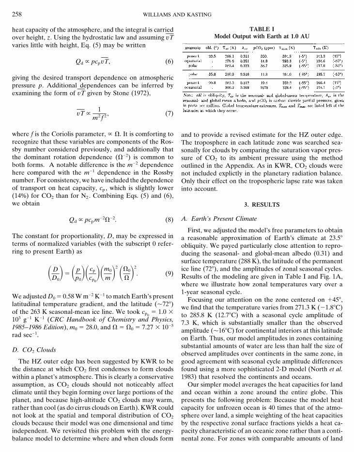
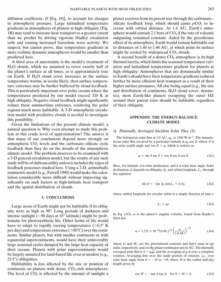
TABLE Iheat capacity of the atmosphere, and the integral is carriedModel Output with Earth at 1.0 AUover height, z. Using the hydrostatic law and assuming vT
varies little with height, Eq. (5) may be written
Qd Y pcpvT, (6)
giving the desired transport dependence on atmosphericpressure p. Additional dependences can be inferred byexamining the form of vT given by Stone (1972),
vT Y1
m2 f 2 , (7)
where f is the Coriolis parameter, Y V. It is comforting to and to provide a revised estimate for the HZ outer edge.recognize that these variables are components of the Ros- The troposphere in each latitude zone was searched sea-sby number considered previously, and additionally that sonally for clouds by comparing the saturation vapor pres-the dominant rotation dependence (V22) is common to sure of CO2 to its ambient pressure using the methodboth forms. A notable difference is the m22 dependence outlined in the Appendix. As in KWR, CO2 clouds werehere compared with the m21 dependence in the Rossby not included explictly in the planetary radiation balance.number. For consistency, we have included the dependence Only their effect on the tropospheric lapse rate was takenof transport on heat capacity, cp , which is slightly lower into account.(14%) for CO2 than for N2 . Combining Eqs. (5) and (6),we obtain 3. RESULTS
A. Earth’s Present ClimateQd Y pcp m22V22. (8)
First, we adjusted the model’s free parameters to obtainThe constant for proportionality, D, may be expressed in a reasonable approximation of Earth’s climate at 23.58terms of normalized variables (with the subscript 0 refer- obliquity. We payed particularly close attention to repro-ring to present Earth) as ducing the seasonal- and global-mean albedo (0.31) and
surface temperature (288 K), the latitude of the permanentice line (728), and the amplitudes of zonal seasonal cycles.SD
D0D5 S p
p0DScp
cp0
DSm0
mD2 SV0
VD2
. (9) Results of the modeling are given in Table I and Fig. 1A,where we illustrate how zonal temperatures vary over a1-year seasonal cycle.
We adjusted D0 5 0.58 W m22 K21 to match Earth’s present Focusing our attention on the zone centered on 1458,latitudinal temperature gradient, and the latitude (p728) we find that the temperature varies from 271.3 K (21.88C)of the 263 K seasonal-mean ice line. We took cp0
5 1.0 3 to 285.8 K (12.78C) with a seasonal cycle amplitude of103 g21 K21 (CRC Handbook of Chemistry and Physics, 7.3 K, which is substantially smaller than the observed1985–1986 Edition), m0 5 28.0, and V 5 V0 5 7.27 3 1025
amplitude (p168C) for continental interiors at this latituderad sec21. on Earth. Thus, our model amplitudes in zones containing
substantial amounts of water are less than half the size ofD. CO2 Clouds
observed amplitudes over continents in the same zone, ingood agreement with seasonal cycle amplitude differencesThe HZ outer edge has been suggested by KWR to be
the distance at which CO2 first condenses to form clouds found using a more sophisticated 2-D model (North et al.1983) that resolved the continents and oceans.within a planet’s atmosphere. This is clearly a conservative
assumption, as CO2 clouds should not noticeably affect Our simpler model averages the heat capacities for landand ocean within a zone around the entire globe. Thisclimate until they begin forming over large portions of the
planet, and because high-altitude CO2 clouds may warm, presents the following problem: Because the model heatcapacity for unfrozen ocean is 40 times that of the atmo-rather than cool (as do cirrus clouds on Earth). KWR could
not look at the spatial and temporal distribution of CO2 sphere over land, a simple weighting of the heat capacitiesby the respective zonal surface fractions yields a heat ca-clouds because their model was one dimensional and time
independent. We revisited this problem with the energy- pacity characteristic of an oceanic zone rather than a conti-nental zone. For zones with comparable amounts of landbalance model to determine where and when clouds form
HABITABLE PLANETS WITH HIGH OBLIQUITIES 259
paratively little time near the zenith at low latitudes. Also,each pole would be heated for 6 months, as they are at23.58 obliquity, but with the Sun spending more than 40days within 208 of polar zenith. Because the opposite periodof cooling would be equivalent to the length of darknessexperienced by the pole at any obliquity, the net changeto polar climate would be a warming, which would causethe ice to melt.
In these circumstances, Earth’s oceanic (northern) andcontinental (southern) poles would demonstrate markedlydifferent seasonal cycle amplitudes because of their differ-ent thermal inertias. Despite the relatively high thermalinertia of the northern pole, the intensity and duration ofsunlight experienced there at high obliquity doubles theamplitude of its temperature cycle (Fig. 1), bringing sum-mer temperatures over the Arctic Ocean above 320 K. Theseasonal variation in temperature over the southern poleis even more dramatic, with summer temperatures reaching353 K, slightly lower than the survivable high-temperaturelimit (383 K) for thermophilic bacteria (Segerer et al. 1993),but higher than the maximum temperatures at which moreadvanced life forms survive today (p330 K). The seasonalminimum temperatures still dip below the freezing pointof water.
Large seasonal temperature variations might also pres-ent a problem for life at lower latitudes. At 1458, forexample, model temperatures are found to vary between268 and 304 K. Over the continents at this latitude, theseasonal temperature variation could be twice this large,which would allow summertime temperatures to exceed322 K and wintertime temperatures to fall below 250K. Even more remarkable is that this variation, whichexceeds the present range of temperatures observed on
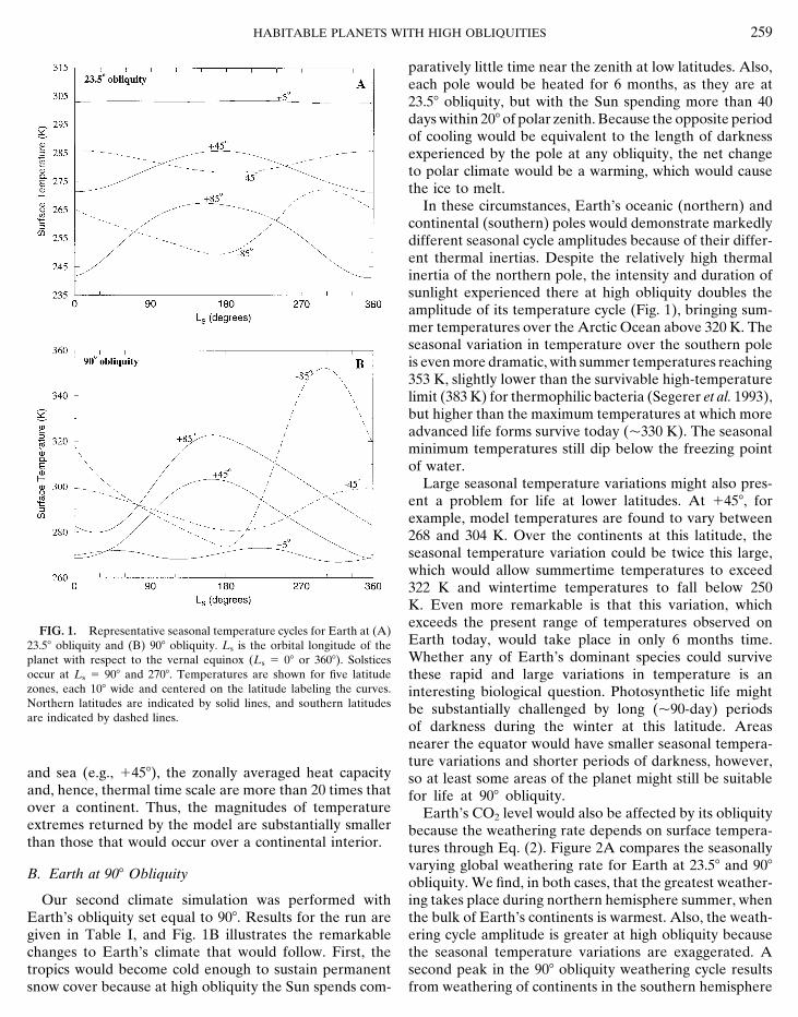
FIG. 1. Representative seasonal temperature cycles for Earth at (A)Earth today, would take place in only 6 months time.23.58 obliquity and (B) 908 obliquity. Ls is the orbital longitude of theWhether any of Earth’s dominant species could surviveplanet with respect to the vernal equinox (Ls 5 08 or 3608). Solstices
occur at Ls 5 908 and 2708. Temperatures are shown for five latitude these rapid and large variations in temperature is anzones, each 108 wide and centered on the latitude labeling the curves. interesting biological question. Photosynthetic life mightNorthern latitudes are indicated by solid lines, and southern latitudes be substantially challenged by long (p90-day) periodsare indicated by dashed lines.
of darkness during the winter at this latitude. Areasnearer the equator would have smaller seasonal tempera-ture variations and shorter periods of darkness, however,
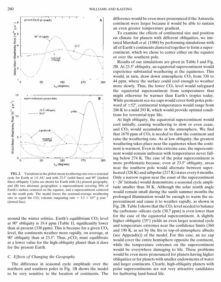
and sea (e.g., 1458), the zonally averaged heat capacity so at least some areas of the planet might still be suitableand, hence, thermal time scale are more than 20 times that for life at 908 obliquity.over a continent. Thus, the magnitudes of temperature Earth’s CO2 level would also be affected by its obliquityextremes returned by the model are substantially smaller because the weathering rate depends on surface tempera-than those that would occur over a continental interior. tures through Eq. (2). Figure 2A compares the seasonally
varying global weathering rate for Earth at 23.58 and 908B. Earth at 908 Obliquity
obliquity. We find, in both cases, that the greatest weather-ing takes place during northern hemisphere summer, whenOur second climate simulation was performed with
Earth’s obliquity set equal to 908. Results for the run are the bulk of Earth’s continents is warmest. Also, the weath-ering cycle amplitude is greater at high obliquity becausegiven in Table I, and Fig. 1B illustrates the remarkable
changes to Earth’s climate that would follow. First, the the seasonal temperature variations are exaggerated. Asecond peak in the 908 obliquity weathering cycle resultstropics would become cold enough to sustain permanent
snow cover because at high obliquity the Sun spends com- from weathering of continents in the southern hemisphere
260 WILLIAMS AND KASTING
difference would be even more pronounced if the Antarcticcontinent were larger because it would be able to sustainan even greater temperature gradient.
To examine the effects of continental size and positionon climate for planets with different obliquities, we imi-tated Marshall et al. (1988) by performing simulations withall of Earth’s continents clustered together to form a super-continent, which we chose to center either on the equatoror over the southern pole.
Results of our simulations are given in Table I and Fig.2B. At 23.58 obliquity, an equatorial supercontinent wouldexperience substantial weathering at the equinoxes. Thiswould, in turn, draw down atmospheric CO2 from 330 to44 ppm, where the surface could cool enough to weathermore slowly. Thus, the lower CO2 level would safeguardthe equatorial supercontinent from temperatures thatmight otherwise be warmer than Earth’s tropics today.While permanent sea-ice caps would cover both poles pole-ward of 6528, continental temperatures would range from286 K to a mild 293 K, which would provide optimal condi-tions for terrestrial-type life.
At high obliquity, the equatorial supercontinent wouldcool initially, causing weathering to slow or even cease,and CO2 would accumulate in the atmosphere. We findthat 1670 ppm of CO2 is needed to thaw the continent andraise the weathering rate. As at low obliquity, the greatestweathering takes place near the equinoxes when the conti-nent is warmest. Even in this extreme case, the superconti-nent would remain unfrozen with temperatures never fall-ing below 274 K. The case of the polar supercontinent ismore problematic because, even at 23.58 obliquity, areasnear the southern pole would alternate between super-heated (326 K) and subpolar (217 K) states every 6 months.FIG. 2. Variations in the global-mean weathering rate over a seasonalOnly a narrow region near the coast of the supercontinentcycle for Earth at 1.0 AU and with 23.58 (solid lines) and 908 (dashed
lines) obliquity. Cycles are shown for Earth with (A) present geography, (2268 latitude) would demonstrate a seasonal cycle ampli-and (B) two alternate geographies: a supercontinent covering 30% of tude smaller than 30 K. Although the solar zenith angleEarth’s surface centered on the equator, and a supercontinent centered would remain small during the sunlit summer months theon the south pole. The model forces the seasonal-average weathering
prolonged illumination would be enough to warm the su-rate to equal the CO2 volcanic outgassing rate 5 3.3 3 1014 g year21
percontinent and cause it to weather rapidly, as shown in(dotted line).Fig. 2B. Table I shows that the CO2 level needed to balancethe carbonate–silicate cycle (38.7 ppm) is even lower thanfor the case of the equatorial supercontinent. A slightly
around the winter solstice. Earth’s equilibrium CO2 level higher obliquity (358) yields an even larger seasonal cycleat 908 obliquity is 19.4 ppm (Table I), significantly lower and temperature extremes near the confidence limits (360than at present (330 ppm). This is because for a given CO2 and 190 K, as set by the fits to top-of-atmosphere albedolevel, the continents weather more rapidly, on average, at (see Appendix)) of the model. For this case, an ice cap908 obliquity than at 23.58. Thus, pCO2 must equilibrate would cover the entire hemisphere opposite the continent,at a lower value for the high-obliquity planet than it does while the temperature extremes on the supercontinentfor the present Earth. would be everywhere damaging to life. These problems
would be even more pronounced for planets having higherC. Effects of Changing the Geography
obliquities or for planets with smaller endowments of waterand larger continents. Clearly, high-obliquity planets withThe difference in seasonal cycle amplitude over the
northern and southern poles in Fig. 1B shows the model polar supercontinents are not very attractive candidatesfor harboring land-based life.to be very sensitive to the location of continents. The
HABITABLE PLANETS WITH HIGH OBLIQUITIES 261
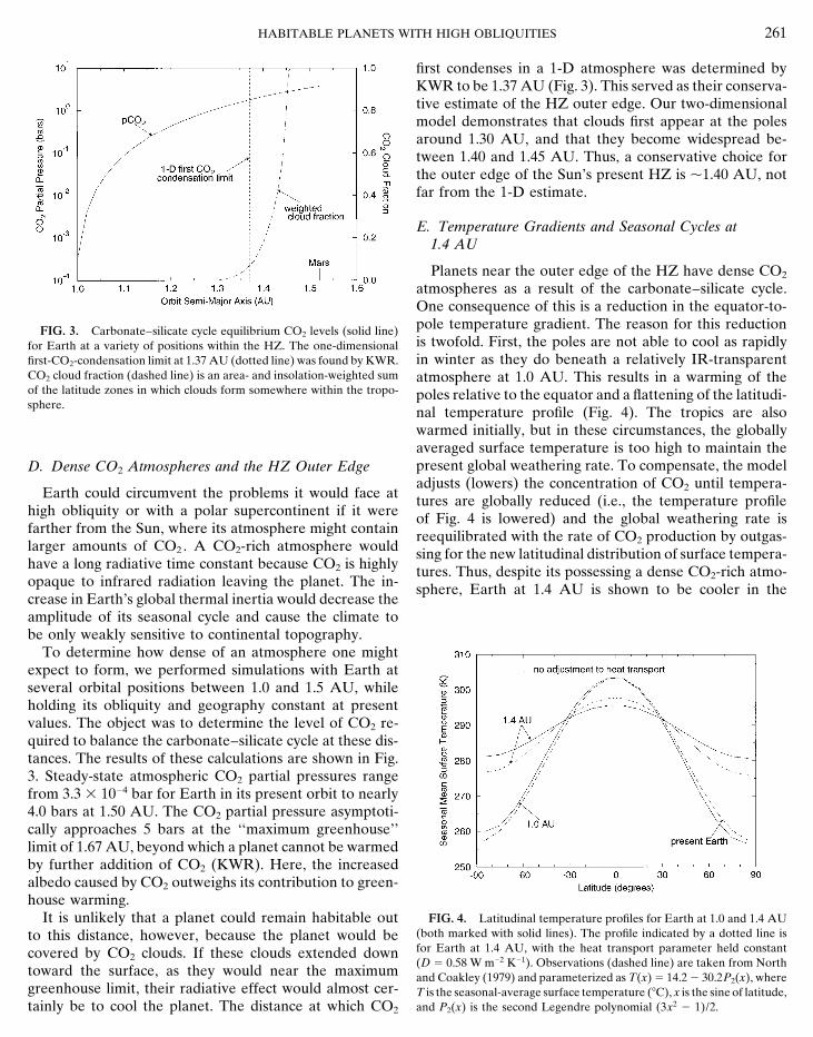
first condenses in a 1-D atmosphere was determined byKWR to be 1.37 AU (Fig. 3). This served as their conserva-tive estimate of the HZ outer edge. Our two-dimensionalmodel demonstrates that clouds first appear at the polesaround 1.30 AU, and that they become widespread be-tween 1.40 and 1.45 AU. Thus, a conservative choice forthe outer edge of the Sun’s present HZ is p1.40 AU, notfar from the 1-D estimate.
E. Temperature Gradients and Seasonal Cycles at1.4 AU
Planets near the outer edge of the HZ have dense CO2
atmospheres as a result of the carbonate–silicate cycle.One consequence of this is a reduction in the equator-to-pole temperature gradient. The reason for this reductionFIG. 3. Carbonate–silicate cycle equilibrium CO2 levels (solid line)is twofold. First, the poles are not able to cool as rapidlyfor Earth at a variety of positions within the HZ. The one-dimensionalin winter as they do beneath a relatively IR-transparentfirst-CO2-condensation limit at 1.37 AU (dotted line) was found by KWR.
CO2 cloud fraction (dashed line) is an area- and insolation-weighted sum atmosphere at 1.0 AU. This results in a warming of theof the latitude zones in which clouds form somewhere within the tropo- poles relative to the equator and a flattening of the latitudi-sphere. nal temperature profile (Fig. 4). The tropics are also
warmed initially, but in these circumstances, the globallyaveraged surface temperature is too high to maintain thepresent global weathering rate. To compensate, the modelD. Dense CO2 Atmospheres and the HZ Outer Edgeadjusts (lowers) the concentration of CO2 until tempera-
Earth could circumvent the problems it would face at tures are globally reduced (i.e., the temperature profilehigh obliquity or with a polar supercontinent if it were of Fig. 4 is lowered) and the global weathering rate isfarther from the Sun, where its atmosphere might contain reequilibrated with the rate of CO2 production by outgas-larger amounts of CO2 . A CO2-rich atmosphere would sing for the new latitudinal distribution of surface tempera-have a long radiative time constant because CO2 is highly tures. Thus, despite its possessing a dense CO2-rich atmo-opaque to infrared radiation leaving the planet. The in- sphere, Earth at 1.4 AU is shown to be cooler in thecrease in Earth’s global thermal inertia would decrease theamplitude of its seasonal cycle and cause the climate tobe only weakly sensitive to continental topography.
To determine how dense of an atmosphere one mightexpect to form, we performed simulations with Earth atseveral orbital positions between 1.0 and 1.5 AU, whileholding its obliquity and geography constant at presentvalues. The object was to determine the level of CO2 re-quired to balance the carbonate–silicate cycle at these dis-tances. The results of these calculations are shown in Fig.3. Steady-state atmospheric CO2 partial pressures rangefrom 3.3 3 1024 bar for Earth in its present orbit to nearly4.0 bars at 1.50 AU. The CO2 partial pressure asymptoti-cally approaches 5 bars at the ‘‘maximum greenhouse’’limit of 1.67 AU, beyond which a planet cannot be warmedby further addition of CO2 (KWR). Here, the increasedalbedo caused by CO2 outweighs its contribution to green-house warming.
FIG. 4. Latitudinal temperature profiles for Earth at 1.0 and 1.4 AUIt is unlikely that a planet could remain habitable out(both marked with solid lines). The profile indicated by a dotted line isto this distance, however, because the planet would befor Earth at 1.4 AU, with the heat transport parameter held constantcovered by CO2 clouds. If these clouds extended down(D 5 0.58 W m22 K21). Observations (dashed line) are taken from North
toward the surface, as they would near the maximum and Coakley (1979) and parameterized as T(x) 5 14.2 2 30.2P2(x), wheregreenhouse limit, their radiative effect would almost cer- T is the seasonal-average surface temperature (8C), x is the sine of latitude,
and P2(x) is the second Legendre polynomial (3x2 2 1)/2.tainly be to cool the planet. The distance at which CO2
262 WILLIAMS AND KASTING
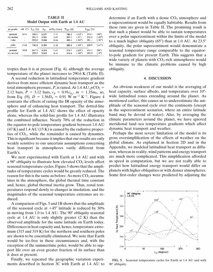
TABLE II determine if an Earth with a dense CO2 atmosphere andModel Output with Earth at 1.4 AU a supercontinent would be equally habitable. Results from
these runs are given in Table II. The promising result isthat such a planet would be able to sustain temperaturesover a polar supercontinent within the limits of the modelto a much higher obliquity (658) than at 1.0 AU. At 23.58obliquity, the polar supercontinent would demonstrate aseasonal temperature range comparable to the equator-to-pole gradient for present Earth. This suggests that awide variety of planets with CO2-rich atmospheres wouldbe immune to the climatic problems caused by highobliquity.tropics than it is at present (Fig. 4), although the average
temperature of the planet increases to 290.6 K (Table II).A second reduction in latitudinal temperature gradient 4. DISCUSSION
derives from more efficient dynamic heat transport as theAn obvious weakness of our model is the averaging oftotal atmospheric pressure, P, is raised. At 1.4 AU, pCO2 5
heat capacity, surface albedo, and temperature over 108-2.12 bars, P 5 3.12 bars, cp 5 0.91cp0, m 5 1.35m0 , so,
wide latitudinal zones extending around the planet. Asfrom Eq. (9), D 5 1.56D0 5 0.91 W m22 K21. Figure 4mentioned earlier, this causes us to underestimate the am-contrasts the effects of raising the IR opacity of the atmo-plitude of the seasonal cycle over the continents (exceptsphere and of enhancing heat transport. The dotted-linein the supercontinent scenarios, where an entire latitudeprofile for Earth at 1.4 AU shows the effect of opacityband may be devoid of water). Also, by averaging thealone, whereas the solid-line profile for 1.4 AU illustratesclimate parameters around the planet, we have ignoredthe combined influence. Nearly 70% of the reduction inmeridional land–sea temperature gradients which affectthe equator-to-pole temperature gradient between 1.0 AUdynamic heat transport and weather.(47 K) and 1.4 AU (15 K) is caused by the radiative proper-
Perhaps the most severe limitation of the model is itsties of CO2 , while the remainder is caused by dynamics.gross oversimplification of the effects of weather on theThis is significant because it implies that our results are onlyglobal climate. As explained in Section 2D and in theweakly sensitive to our uncertain assumptions concerningAppendix, we modeled latitudinal heat transport as diffu-heat transport in atmospheres vastly different fromsion, whereas in reality, wind patterns and energy transportEarth’s.are much more complicated. This simplification affordedWe next experimented with Earth at 1.4 AU and withus speed in computation, but we are not really able toa 908 obliquity to illustrate how elevated CO2 levels affectpredict how latitudinal energy transport would differ onseasonal temperature cycles. Figure 5 shows that the ampli-planets with higher obliquities or with denser atmospheres.tudes of temperature cycles would be greatly reduced. TheSome first-order changes were predicted by adjusting thereason for this is the same as before: As more CO2 accumu-
lates in the atmosphere, the global thermal time constantand, hence, global thermal inertia grow. Thus, zonal tem-peratures respond slowly to changes in insolation, and themagnitudes of the seasonal temperature extremes are re-duced.
A comparison of Figs. 5 and 1B shows that the amplitudeof the seasonal cycle at 1458 latitude is reduced by 30%in moving from 1.0 to 1.4 AU. The 908 obliquity seasonalcycle at 1.4 AU is only slightly greater (2 K) than theobserved amplitude for the same latitude on Earth today.Differences in heat capacity and, hence, temperature extre-mum (315 and 319 K) for the northern and southern polesare shown to be essentially eliminated. We note that Earthwould be ice-free in these circumstances and, with theexception of the summertime poles, would be able to sup-port life over an even greater fraction of its surface thanit does at present.
Finally, we repeated the geographic variation experi- FIG. 5. Seasonal temperature cycles for Earth at 1.4 AU and with908 obliquity.ments described in Section 3C with Earth at 1.4 AU to
HABITABLE PLANETS WITH HIGH OBLIQUITIES 263
diffusion coefficient, D [Eq. (9)], to account for changes planet receives from its parent star through the carbonate–silicate feedback loop, which should cause pCO2 to in-to atmospheric pressure. Large latitudinal temperature
gradients in atmospheres of planets at high obliquity (Fig. crease with orbital distance. At 1.4 AU, Earth’s atmo-sphere would contain 2.1 bars of CO2 if the rate of volcanic1B) may tend to increase heat transport to a greater extent
than we predict by driving vigorous Hadley circulation outgassing remained constant. Aided by the greenhouseeffect of its atmosphere, Earth would remain habitable outcells and causing increased baroclinic wave activity. We
suspect, but cannot prove, that temperature gradients in to distances of 1.40 to 1.46 AU, at which point its surfacemight be cooled by widespread CO2 clouds.more realistic dynamic atmospheres would be smaller than
predicted here. A second benefit of a dense CO2 atmosphere is its highthermal inertia, which limits the seasonal temperature vari-A third area of uncertainty is the model’s treatment of
H2O clouds, which we assumed to cover exactly half of ation and latitudinal temperature gradient for planets athigh obliquity. Atmospheres that are dynamically similarthe planet’s surface at all times, as is approximately true
on Earth. If H2O cloud cover increases as the surface to Earth’s should have their temperature gradients reducedfurther by more efficient heat transport as a result of theirtemperature warms, as seems likely, then surface tempera-
ture extremes may be further buffered by cloud feedback. higher surface pressures. All else being equal (e.g., the sizeand distribution of continents, H2O cloud cover, dynam-This is particularly important over polar oceans where the
temperatures predicted by our model exceed 320 K at ics), most Earth-like planets occupying the outer HZaround their parent stars should be habitable regardlesshigh obliquity. Negative cloud feedback might significantly
reduce these summertime extremes, rendering the polar of their obliquity.regions much more habitable. A 3-D atmospheric circula-tion model with predictive clouds is needed to investigate
APPENDIX: THE ENERGY-BALANCEthis possibility.CLIMATE MODELGiven the limitations of the present climate model, a
natural question is: Why even attempt to study this prob- A. Diurnally Averaged Incident Solar Flux (S)lem at this crude level of approximation? The answer is
The bolometric solar flux at 1.0 AU, q0 , is 1360 W m22. The instanta-that many of our conclusions depend more strongly onneous solar flux received by a particular latitude is q0 cos Z, where Z isatmospheric CO2 levels and the carbonate–silicate cycle the solar zenith angle and cos Z 5 e, which is written as
feedback than they do on the details of the atmosphericclimate model. The problem deserves to be examined with
e 5 sin u sin d 1 cos u cos d cos h. (A1)a 3-D general circulation model, but the results of any suchstudy will be of dubious utility unless it includes the types of
Here, u is latitude, d is solar declination, and h is solar hour angle. Solarfeedback processes studied here. Using a 2-D, azimuthally declination, d, depends on obliquity, d0 , and orbital longitude, Ls , throughsymmetric model (e.g., Farrell 1990) would make the calcu- the equationlation considerably more difficult without improving sig-nificantly on such factors as high-latitude heat transport sin d 5 2sin d0 cos(Ls 1 f/2), (A2)and the spatial distribution of clouds.
where orbital longitude for circular orbits is a simple function of time t:5. CONCLUSIONS
Ls 5 gt. (A3)Large areas of Earth might not be habitable if its obliq-
uity were as high as 908. Long periods of darkness andIn Eq. (A3), g is the planet’s angular velocity, found from Kepler’sintense sunlight (p90 days at 458 latitude) might be prob-third law,
lematic for photosynthetic life. Other forms of life wouldhave to adapt to rapidly varying temperatures (.0.58 Kper day) and temperature extremes (.808C) over the conti- g 5 1.721 3 10220(GM()1/2 S a
1.0 AUD23/2
, (A4)nents. Similar planets, but with smaller continents or withequatorial supercontinents, would have their unfavorably
where G and M( are the gravitational constant and Sun’s mass in cgslarge seasonal cycles damped by the large heat capacity ofunits, respectively, and a is the planet semimajor axis in AU. The diurnallytheir oceans. Planets with polar supercontinents wouldaveraged solar flux is S 5 q0e, and the averaging of e is over a complete
be largely unsuited for land-based life even at modest (e.g., rotation. Averaging first over the sunlit portion of rotation, i.e., over23.58) obliquities. solar hour angle from h 5 2H to 1H, where H is the radian half-day
length given byHabitability is less affected by the size or position ofcontinents on planets with dense, CO2-rich atmospheres.The level of CO2 is affected by the amount of sunlight a cos H 5 2tan u tan d, for 0 , H , f, (A5)
264 WILLIAMS AND KASTING
we obtain A 5 1.1082 1 1.5172as 2 5.7993 3 1023T 1 1.9705 3 1022p
2 1.8670 3 1021e 2 3.1355 3 1022asp 2 1.0214
e 5EH
2Hdh(sin u sin d 1 cos u cos d cos h)
EH
2Hdh
(A6)3 1022ep 1 2.0986 3 1021ase 2 3.7098 3 1023asT
2 1.1335 3 1024eT 1 5.3714 3 1025pT 1 7.5887
5 Ssin u sin d 1 cos u cos dsin H
H D. 3 1022as2 1 9.2690 3 1026T 2 2 4.1327 3 1024p2
1 6.3298 3 1022e2. (A10)Now, the averaging of e over the entire diurnal cycle is completed byscaling Eq. (A6) by the factor H/f, because H 5 f if the Sun remains
The rms errors for the fits are 7.58 and 4.66 W m22, respectively, whenabove the horizon for a complete rotation. The diurnally averaged solarscaled by the planetary-average incident solar flux (q0/4). The fits wereflux, S, may then be written asobtained assuming an isothermal stratosphere (as in Kasting 1991) anda troposphere that is fully saturated with H2O vapor.
S 5 q0SHfD e
(A7)
One should note that there is a discrepancy between Eqs. (A9) and(A10) above and their analog equation, Eq. 5, of Caldeira and Kasting(1992). An analysis of these formulas reveals that TOA albedo increases
5q0
f(H sin u sin d 1 cos u cos d sin H),
with Z in Eqs. (A9) and (A10) above, as it should, but decreases withZ in the older Eq. 5. The inconsistency originated with differences in the
which may be expressed for any planet having an orbital semimajor axis way the radiative–convective model, which was used to make both setsa as of fits, was used to calculate stratospheric temperature, Tstrat . Caldeira
and Kasting calculated Tstrat using Eq. 1 of Kasting (1991),S 5
q0
f S1.0 AUa D2
(A8)Tstrat 5
121/4 F S
4s(1 2 A)G1/4
, (A11)(H sin u sin d 1 cos u cos d sin H).
B. Top-of-Atmosphere Albedo (A)where S is incident solar flux, and s is the Stefan–Boltzmann constant.
The fraction of short-wave solar energy returned to space as a conse- This equation, however, is appropriate only for global-average conditionsquence of atmospheric or surface scattering is the top-of-atmosphere (i.e., for Z 5 608) and, thus, was applied incorrectly in calculating Tstrat(TOA) albedo. TOA albedo depends both on the distance photons travel and TOA albedo for latitudes having solar zenith angles different fromthrough the atmosphere, which is set by the solar zenith angle, and on this value. We circumvented this problem by parameterizing Tstrat as thethe surface albedo. Levels of CO2 and H2O affect TOA albedo by their following function of Z:respective contributions to Rayleigh scattering and absorption. CO2 raisesthe albedo significantly because its cross section for Rayleigh scatteringis more than 2.5 times that of nitrogen. H2O is an efficient Rayleigh Tstrat(Z) 5 Tstrat(608) F Fs(Z)
Fs(608)G1/4
. (A12)scatterer, but it is also a good absorber in the near IR. Hence, for thelow temperatures and small H2O mixing ratios encountered by our model,
Here, in the notation of Kasting (1991), Fs is the absorbed fraction ofthe dominant effect of H2O is to decrease albedo by raising atmosphericincident solar flux, which was calculated for a variety of zenith anglesabsorption. The water vapor contribution to Rayleigh scattering does notbetween 08 and 908 using the radiative–convective model, and Tstrat(608)begin to dominate its contribution to absorption until surface tempera-was obtained using Eq. (A11) as before.tures exceed p360 K, and the stratospheric H2O mixing ratio becomes
large (Kasting 1988).Following Caldeira and Kasting (1992), we parameterized TOA albedo C. Surface Albedo (as)
as a second-order polynomial of four variables: pCO2 (here referred toZonal area was partitioned between ocean and continents for the threeas p), e, surface temperature, T, and surface albedo, as . We obtained
geographic cases given in Table III. Zonal land–sea fractions for presentbest fits to the results of more than 24,000 runs of the radiative–convectiveEarth were taken from Sellers (1965). Surface albedo depends on temper-climate model used by Kasting and Ackerman (1986) and Kasting (1988,ature through its effect on the extent and reflectance properties of snow1991). We divided model output in half at a temperature T 5 280 K toand ice cover. We assigned albedos to land and oceanic surfaces for threeyield smaller rms errors than was possible with one fit over the entiredifferent temperature regimes.temperature range (190 K , T , 360 K). The fits we obtained may be
For T . 273 K, land was assigned an albedo of 0.20, which is characteris-applied confidently for 1025 bar , p , 10 bars, 0 , as , 1, andtic of many terrestrial surfaces (Kondrat’ev 1969). The albedo of unfrozen0 , e , 1.ocean depends on solar zenith angle through the Fresnel reflectanceFor 190 K , T , 280 K,formulas for water and can range from 0 to 100%. The fraction of incident
A 5 26.8910 3 1021 1 1.0460as 1 7.8054 3 1023T 2 2.8373 short-wave energy reflected from a smooth oceanic surface (n 5 1.33),for 08 , Z , 908, was read from a table prepared by Kondrat’ev (1969,3 1023p 2 2.8899 3 1021 e 2 3.7412 3 1022as pp. 439).
2 6.3499 3 1023ep 1 2.0122 3 1021ase 2 1.8508 For 263 K , T , 273 K, land was allowed an unstable snow coverhaving an albedo of 0.45, and sea-ice with as 5 0.55 was permitted to
3 1023asT 1 1.3649 3 1024eT 1 9.8581 3 1025pTform in the oceans. We used data from Table 1 of Thompson and Barron(1981) to parameterize the ocean fraction covered by sea ice, fi , as a1 7.3239 3 1022as
2 2 1.6555 3 1025T 2 1 6.5817function of surface temperature,
3 1024p2 1 8.1218 3 1022e2, (A9)
and for 280 K , T , 370 K, fi 5 1 2 e(T2273 K)/10. (A13)
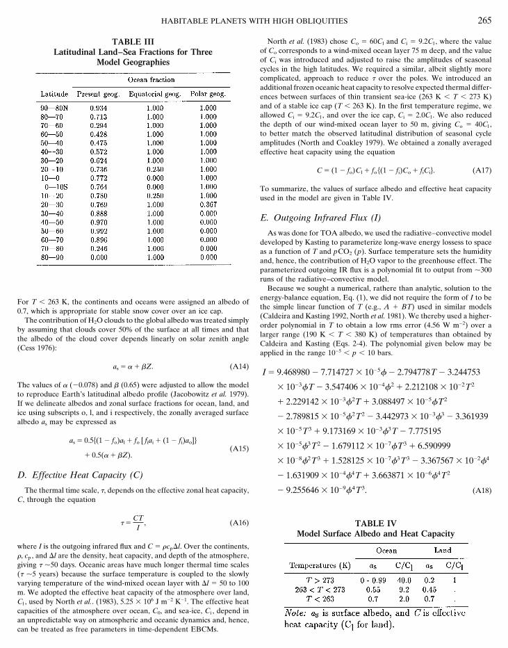
HABITABLE PLANETS WITH HIGH OBLIQUITIES 265
North et al. (1983) chose Co 5 60Cl and Ci 5 9.2Cl , where the valueTABLE IIIof Co corresponds to a wind-mixed ocean layer 75 m deep, and the valueLatitudinal Land–Sea Fractions for Threeof Ci was introduced and adjusted to raise the amplitudes of seasonalModel Geographiescycles in the high latitudes. We required a similar, albeit slightly morecomplicated, approach to reduce t over the poles. We introduced anadditional frozen oceanic heat capacity to resolve expected thermal differ-ences between surfaces of thin transient sea-ice (263 K , T , 273 K)and of a stable ice cap (T , 263 K). In the first temperature regime, weallowed Ci 5 9.2Cl , and over the ice cap, Ci 5 2.0Cl . We also reducedthe depth of our wind-mixed ocean layer to 50 m, giving Co 5 40Cl ,to better match the observed latitudinal distribution of seasonal cycleamplitudes (North and Coakley 1979). We obtained a zonally averagedeffective heat capacity using the equation
C 5 (1 2 fo)Cl 1 fo h(1 2 fi)Co 1 fiCij. (A17)
To summarize, the values of surface albedo and effective heat capacityused in the model are given in Table IV.
E. Outgoing Infrared Flux (I)
As was done for TOA albedo, we used the radiative–convective modeldeveloped by Kasting to parameterize long-wave energy lossess to spaceas a function of T and pCO2 (p). Surface temperature sets the humidityand, hence, the contribution of H2O vapor to the greenhouse effect. Theparameterized outgoing IR flux is a polynomial fit to output from p300runs of the radiative–convective model.
Because we sought a numerical, rathere than analytic, solution to theenergy-balance equation, Eq. (1), we did not require the form of I to be
For T , 263 K, the continents and oceans were assigned an albedo ofthe simple linear function of T (e.g., A 1 BT) used in similar models
0.7, which is appropriate for stable snow cover over an ice cap.(Caldeira and Kasting 1992, North et al. 1981). We thereby used a higher-
The contribution of H2O clouds to the global albedo was treated simplyorder polynomial in T to obtain a low rms error (4.56 W m22) over a
by assuming that clouds cover 50% of the surface at all times and thatlarger range (190 K , T , 380 K) of temperatures than obtained by
the albedo of the cloud cover depends linearly on solar zenith angleCaldeira and Kasting (Eqs. 2-4). The polynomial given below may be
(Cess 1976):applied in the range 1025 , p , 10 bars.
as 5 a 1 bZ. (A14)I 5 9.468980 2 7.714727 3 1025f 2 2.794778T 2 3.244753
The values of a (20.078) and b (0.65) were adjusted to allow the model 3 1023fT 2 3.547406 3 1024f2 1 2.212108 3 1022T2
to reproduce Earth’s latitudinal albedo profile (Jacobowitz et al. 1979).1 2.229142 3 1023f2T 1 3.088497 3 1025fT2
If we delineate albedos and zonal surface fractions for ocean, land, andice using subscripts o, l, and i respectively, the zonally averaged surface 2 2.789815 3 1025f2T2 2 3.442973 3 1023f3 2 3.361939albedo as may be expressed as
3 1025T3 1 9.173169 3 1023f3T 2 7.775195as 5 0.5h(1 2 fo)al 1 fo [ fiai 1 (1 2 fi)ao]j
(A15) 3 1025f3T2 2 1.679112 3 1027fT3 1 6.5909991 0.5(a 1 bZ).
3 1028f2T3 1 1.528125 3 1027f3T3 2 3.367567 3 1022f4
D. Effective Heat Capacity (C) 2 1.631909 3 1024f4T 1 3.663871 3 1026f4T2
The thermal time scale, t, depends on the effective zonal heat capacity, 2 9.255646 3 1029f4T3. (A18)C, through the equation
t 5CT
I, (A16) TABLE IV
Model Surface Albedo and Heat Capacitywhere I is the outgoing infrared flux and C 5 rcpDl. Over the continents,r, cp , and Dl are the density, heat capacity, and depth of the atmosphere,giving t p50 days. Oceanic areas have much longer thermal time scales(t p5 years) because the surface temperature is coupled to the slowlyvarying temperature of the wind-mixed ocean layer with Dl 5 50 to 100m. We adopted the effective heat capacity of the atmosphere over land,Cl , used by North et al.. (1983), 5.25 3 106 J m22 K21. The effective heatcapacities of the atmosphere over ocean, C0, and sea-ice, Ci , depend inan unpredictable way on atmospheric and oceanic dynamics and, hence,can be treated as free parameters in time-dependent EBCMs.
266 WILLIAMS AND KASTING
Here, f 5 loge(p/3.3 3 1024). As with the albedo fit, the troposphere The TOA albedo, outgoing IR flux, and weathering rate, which all dependon surface temperature, followed from Eqs. (A9)/(A10), (A18), and (3),was assumed to be fully saturated with H2O and the stratosphere was
isothermal. Reduction in the outgoing IR flux by H2O-cloud absorption respectively. The dynamic heat transport term of Eq. (1) was spatiallydifferenced to second order in x, and operated on the global latitudinalwas taken into account by subtracting 14.06 W m22 from Eq. (A18). The
value of the cloud correction was determined by requiring the model to temperature profile. The pressure-dependent transport coefficient D wascalculated using Eq. (9). Once the climate parameters for each zone wereobtain Earth’s observed globablly averaged surface temperature (288 K)
for the observed globally averaged TOA albedo (0.31). computed, the first term of Eq. (1) was temporally differenced accordingto our assumptions made concerning effective heat capacity, and thesurface temperatures were updated.F. CO2 Clouds
Every five orbits, we compared the seasonal-global mean weatheringThe troposphere for each zone was searched for the presence of CO2 rate to the rate of CO2 production by volcanos, and if the ratio of weather-
clouds using the following assumptions and procedures. The depth of the ing to outgassing was less than unity, we increased pCO2 . Conversely,troposphere was determined by our assumptions regarding stratospheric we decreased pCO2 for ratios greater than unity. The size of the adjust-temperature. We parameterized Tstrat as a function of pCO2 and T, in ment was proportional to the size of the rate imbalance. We staggeredthe same way we performed the fit to I to obtain Eq. (A18). We obtained the adjustments to pCO2 by five orbital periods to allow the slowly varying
temperature of the oceans time to respond. We iterated on this procedureuntil the weathering rate converged to within 1023 of the outgassing rate.Tstrat 5 2188.1 2 1.955f 1 3.810f2 1 2.328T 1 3.733
The rate of convergence was affected predominantly by semimajor3 1024fT 2 2.856 3 1022f2T 2 3.329 3 1023T 2
axis, which set the orbital period, by the step size Dt, and by the initialchoice for pCO2 . For a 5 1.0 AU, Dt 5 8.64 3 104 sec, and p0 5 3301 2.214 3 1025fT 2 1 4.605 3 1025f2T 2, (A19)ppm, the model calculations required 38 sec of CPU time on a CRAYsupercomputer. By contrast, convergence took 59 sec for the same timewhere f is the same as before. The fit was performed with Z 5 608 usingstep, but with a 5 1.4 AU, and p0 5 2.0 bars.Eq. (A11), which means that we slightly overestimated Tstrat , and hence
tropospheric depth, at the poles while underestimating their values atthe equator. This suggests that clouds in reality are less likely to form ACKNOWLEDGMENTSat the poles and more likely to form at the equator than the modelindicates. The effect of this error on our results, however, is expected to
DMW was supported by a NASA Graduate Student Research Fellow-be small because a counterbalancing error is introduced in approximating
ship awarded in 1995, and JFK was supported by the NASA Exobiol-tropospheric lapse rate, as will be discussed below.
ogy Program.Once Tstrat was found, the troposphere was divided into 20 layers of
equal thickness. The model stepped from the surface to the tropopauseby assuming a constant lapse rate c 5 6.5 K km21 and the barometric REFERENCESlaw for CO2:
Berner, R. A., A. C. Lasaga, and R. M. Garrels 1983. The carbonate–silicate geochemical cycle and its effect on atmospheric carbon dioxide
p(h) 5 p(0) ST(h)T(0)Dmg/kc
. (A20)over the past 100 million years. Am. J. Sci. 283, 641–683.
Butler, R. P., and G. W. Marcy 1996. A planet orbiting 47 Ursae Majoris.Here, g is the gravitational constant, k is the Boltzmann constant, h is Astrophys. J. 464, L153–L156.physical height, and, here, m is the mean molecular weight of the atmo- Butler, R. P., G. W. Marcy, E. Williams, H. Hauser, and P. Shirts 1996.sphere. Our assumed lapse rate for this calculation is slightly smaller Three new ‘‘51 Peg-type’’ planets. Astrophys. J., submitted.than over the poles (p10 K km21) and slightly larger than over the tropics
Caldeira, K., and J. F. Kasting 1992. Susceptibility of early Earth to(3–4 K km21) in reality, and so, here, we underestimated polar cloud
irreversible glaciation caused by carbon dioxide clouds. Nature 359,cover while overestimating clouds in the tropics. Thus, we err in the226–228.opposite sense of our previous error introduced in approximating Tstrat ,
Cess, R. D. 1976. Climatic change: An appraisal of atmospheric feedbackwhich should mitigate the effects of both approximations for this calcula-mechanisms employing zonal climatology. J. Atmos. Sci. 33, 1831–1843.tion. Clouds form at a height at which p . psat , the saturation vapor
pressure, which we calculated using Eqs. A5 and A6 of Kasting (1991). Cochran, W. D., A. P. Hatzes, R. P. Butler, and G. W. Marcy 1996.Finally, we determined the fraction of the globe that is covered with CO2 The discovery of a planetary companion to 16 Cygni B. Astrophys.clouds by summing over the latitudes in which clouds form and weighting J., submitted.them by zonal area and insolation. Farrell, B. F. 1990. Equable climate dynamics. J. Atmos. Sci. 47, 2986–
2995.G. Solving the Model Gatewood, G. 1996. Lalande 21185. Bull. Am. Astron. Soc. 28, 885.
Gierasch, P. J., and O. B. Toon 1973. Atmospheric pressure variationWe obtained latitudinal temperature profiles by finding numerical solu-and the climate of Mars. J. Atmos. Sci. 30, 1502–1508.tions to the zonal energy-balance equation, Eq. (1), with the constraint
that the profiles also be solutions to the CO2 weathering-balance equation, Hartmann, W. K., R. J. Phillips, and G. J. Taylor 1986. Origin of theEq. (3). We integrated both equations simultaneously using the following Moon. Lunar and Planetary Inst., Houston.method. We began with an isothermal planet (e.g., T 5 288 K) at the Hoffert, M. I., A. J. Callegari, C. T. Hsiech, and W. Ziegler 1981. Liquidvernal equinox (Ls 5 0), and stepped the planet in its orbit by incre-
water on Mars: An energy balance climate model for CO2/H2O atmo-menting the time (104 , Dt , 8.64 3 104 sec) and orbit longitude using
spheres. Icarus 47, 112–129.Eq. (A3).
Holland, H. D. 1978. The Chemistry of the Atmosphere and Oceans.For each Dt, we performed a spatial integration over all latitude zones.Wiley, New York.Orbital longitude set the solar declination according to Eq. (A2) and,
hence, the diurnally averaged insolation for each zone using Eq. (A8). Jacobowitz, H., W. L. Smith, H. B. Howell, F. W. Nagle, and J. R. Hickery
HABITABLE PLANETS WITH HIGH OBLIQUITIES 267
1979. The first 18 months of planetary radiation budget measurements Schubert, G. 1983. General circulation and the dynamical state of thefrom Nimbus 6 ERB experiment. J. Atmos. Sci. 36, 501–507. Venus atmosphere. In Venus (D. M. Hunten, L. Colin, T. M.
Donahue, and V. I. Moroz, Eds.), pp. 681–765. Univ. of ArizonaKasting, J. F. 1988. Runaway and moist greenhouse atmospheres and thePress, Tucson.evolution of Earth and Venus. Icarus 74, 472–494.
Segerer, A. H., S. Burggraf, G. Fiala, G. Huber, R. Huber, and K. O.Kasting, J. F. 1991. CO2 condensation and the climate of early Mars.Stetter 1993. Life in hot springs and hydrothermal vents. Origins LifeIcarus 94, 1–13.23, 77–90.Kasting, J. F., and T. P. Ackerman 1986. Climatic consequences of very
Sellers, W. D. 1965. Physical Climatology. Univ. of Chicago Press,high carbon dioxide levels in the Earth’s early atmosphere. ScienceLondon.234, 1383–1385.
Stone, P. H. 1972. A simplified radiative–dynamical model for the staticKasting, J. F., D. P. Whitmire, and R. T. Reynolds 1993. Habitable zonesaround main sequence stars. Icarus 101, 108–128. stability of rotating atmospheres. J. Atmos. Sci. 29, 405–417.
Kondrat’ev, K. Y. A. 1969. Albedo of the underlying surface and clouds. Thompson, S. L., and E. J. Barron 1981. Comparison of Cretaceous andIn Radiation in the Atmosphere (K. Y. A. Kondrat’ev, Ed.), pp. 411–452. present Earth albedos: Implications for the causes of paleoclimates. J.Academic Press, New York. Geol. 89, 143–167.
Laskar, J., and P. Robutel 1993. The chaotic obliquity of the planets. Touma, J., and J. Wisdom 1993. The chaotic obliquity of Mars. ScienceNature 361, 608–614. 259, 1294–1297.
Laskar, J., F. Joutel, and P. Robutel 1993. Stabilization of the Earth’s Walker, J. C. G., P. B. Hays, and J. F. Kasting 1981. A negative feedbackobliquity by the Moon. Nature 361, 615–617. mechanism for the long-term stabilization of Earth’s surface tempera-
Lindzen, R. S., and B. Farrell 1977. Some realistic modifications of simple ture. J. Geophys. Res. 86, 9776–9782.climate models. J. Atmos. Sci. 34, 1487–1501. Ward, W. R. 1973. Large scale variations in the obliquity of Mars. Science
Marcy, G. W., and R. P. Butler 1996. A planetary companion to 70 181, 260–262.Virginis. Astrophys. J. 464, L147–L151. Ward, W. R. 1974. Climatic variations on Mars: I. Astronomical theory
Marshall, H. G., J. C. G. Walker, and W. R. Kuhn 1988. Long-term of insolation. J. Geophys. Res. 79, 3375–3386.climate change and the geochemical cycle of carbon. J. Geophys. Res.
Ward, W. R. 1979. Present obliquity oscillations of Mars: Fourth-order93, 791–801.
accuracy in orbital e and i J. Geophys. Res. 84, 237–241.Mayor, M., and D. Queloz 1995. A Jupiter-mass companion to a solar-
Ward, W. R. 1991. Resonant obliquity of Mars? Icarus 94, 160–164.type star. Nature 378, 355–359.Wetherill, G. W. 1996. The formation and habitability of extra-solarNorth, G. R., and J. A. Coakley 1979. Differences between seasonal and
planets Icarus 119, 219–238.mean annual energy balance model calculations of climate and climateWilliams, D. M., J. F. Kasting, and K. Caldeira 1996. Chaotic obliquitysensitivity. J. Atmos. Sci. 36, 1189–1203.
variations and planetary habitability. In Circumstellar HabitableNorth, G. R., R. F. Cahalan, and J. A. Coakley 1981. Energy balanceZones—Proceedings of the First International Conference (L. Doyle,climate models. Rev. Geophys. Space Phys. 19, 91–121.Ed.), pp. 43–62. Travis House, Menlo Park, CA.North, G. R., J. G. Mengel, and D. A. Short 1983. Simple energy balance
Williams, D. M., J. F. Kasting, and R. A. Wade 1997. Habitable moonsmodel resolving the seasons and the continents: Application to thearound extrasolar giant planets. Nature 385, 234–236.astronomical theory of the ice ages. J. Geophys. Res. 88, 6576–6586.
Wolszczan, A. 1994. Confirmation of Earth-mass planets orbiting thePollack, J. B., J. F. Kasting, S. M. Richardson, and K. Poliakoff 1987.The case for a wet, warm climate on early Mars. Icarus 71, 203–224. millisecond pulsar PSR B1257 1 12. Science 264, 538–542.


