Hausdorff dimension for horseshoes inR3

Ergod. Th. & Dynam. Sys.(1999),19, 1343–1363Printed in the United Kingdom c© 1999 Cambridge University Press

Hausdorff dimension for horseshoes inR3

KAROLY SIMON† and BORIS SOLOMYAK‡

† Institute of Mathematics, University of Miscolc, Miscolc-Egyetemvaros,H-315, Hungary

(e-mail: [email protected])‡ Department of Mathematics, Box 354350, University of Washington,

Seattle, WA 98195, USA(e-mail: [email protected])

(Received30July1997and accepted in revised form26March1998)

Abstract. Using pressure formulas we compute the Hausdorff dimension of thebasic set of ‘almost every’C1+α horseshoe map inR3 of the form F(x, y, z) =(γ (x, z), τ (y, z), ψ(z)), where|ψ ′| > 1 and 0< |γ ′x |, |τ ′y | < 1

2 on the basic set. Similar

results are obtained for attractors of nonlinear ‘baker’s maps’ inR3.

1. Introduction1.1. Results. McCluskey and Manning [22] have computed the Hausdorff dimensionof the basic set of aC1 Axiom A surface diffeomorphism using pressure formulas. Sincetheir work, it has been an open problem to compute the dimension of an Axiom A basicset inRn for n > 2. In this paper we give a partial solution to this problem; namely, wecompute the Hausdorff dimension of ‘almost every’ horseshoe map inR3 from the classdefined below. The results of McMullen [23] on self-affine sets show that we cannot expecta similar result for all horseshoe maps inR3. Our methods extend ton > 3 but we onlyconsider the casen = 3 for the sake of simplicity.

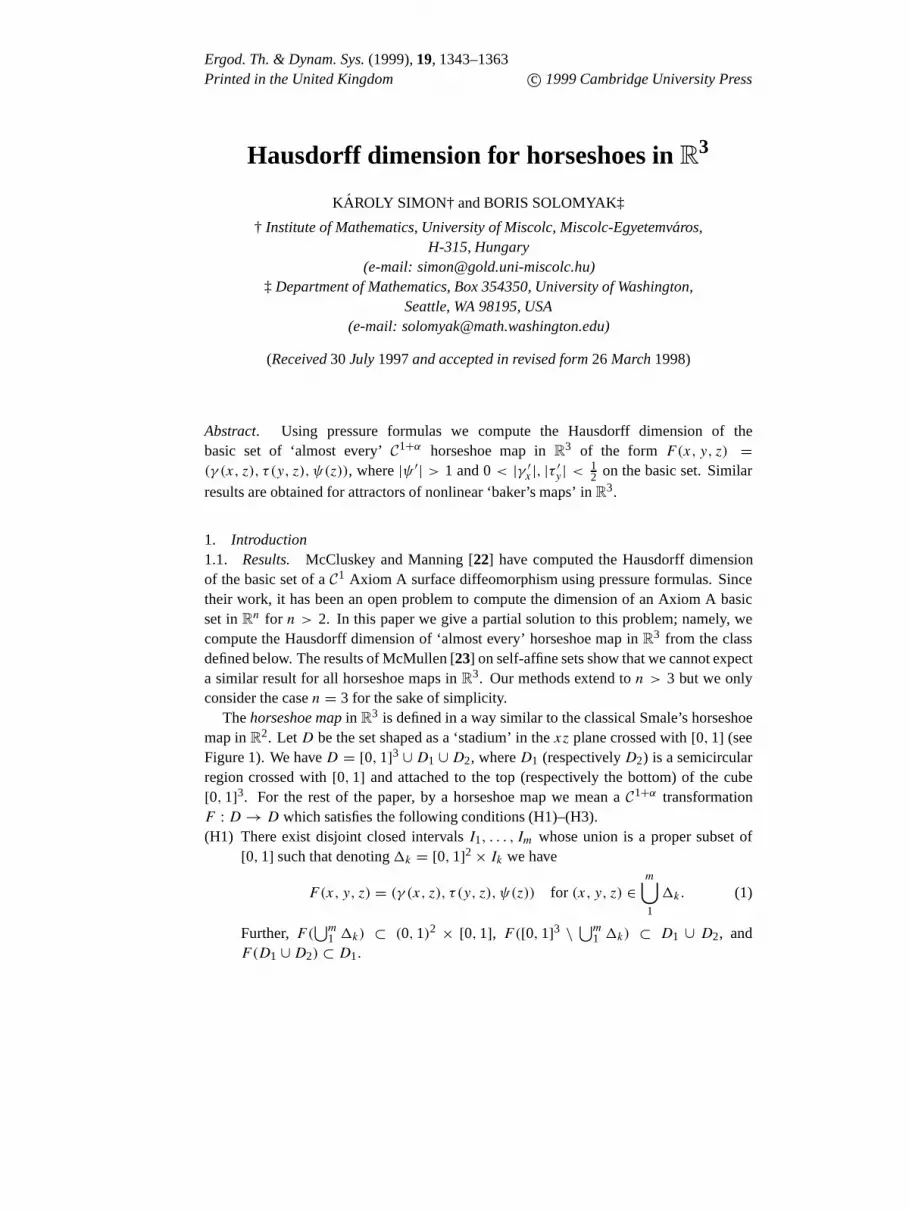
Thehorseshoe mapin R3 is defined in a way similar to the classical Smale’s horseshoemap inR2. LetD be the set shaped as a ‘stadium’ in thexz plane crossed with[0,1] (seeFigure 1). We haveD = [0,1]3 ∪D1 ∪D2, whereD1 (respectivelyD2) is a semicircularregion crossed with[0,1] and attached to the top (respectively the bottom) of the cube[0,1]3. For the rest of the paper, by a horseshoe map we mean aC1+α transformationF : D→ D which satisfies the following conditions (H1)–(H3).(H1) There exist disjoint closed intervalsI1, . . . , Im whose union is a proper subset of

[0,1] such that denoting1k = [0,1]2× Ik we have

F(x, y, z) = (γ (x, z), τ (y, z), ψ(z)) for (x, y, z) ∈m⋃1

1k. (1)

Further,F(⋃m

1 1k) ⊂ (0,1)2 × [0,1], F([0,1]3 \ ⋃m1 1k) ⊂ D1 ∪ D2, and

F(D1 ∪D2) ⊂ D1.

1344 K. Simon and B. Solomyak

FIGURE 1. Horseshoe map.

(H2) λ1 < |γ ′x |, |τ ′y | < λ2, where 0< λ1 < λ2 <12 are fixed for the rest of the paper.

(H3) |ψ ′| > 1 onIk andψ(Ik) = [0,1] for eachk = 1, . . . ,m.We do not assume thatF is one-to-one. The basic set3 = 3(F) = ⋂

n∈ZFn([0,1]3)is called a horseshoe. Note that the precise form ofF outside

⋃m1 1k does not affect this

basic set. The two contracting directions are thex andy axes, and the expanding directionis thez axis. Thet-perturbation ofF , denoted byF t , is a horseshoe map satisfying

F t(x, y, z) = (γ (x, z)+ t1k , τ (y, z)+ t2k , ψ(z)) for (x, y, z) ∈ 1k, k ≤ m,where t = ((t11, t

21), . . . , (t

1m, t

2m)) ∈ R2m. We say thatt ∈ R2m is F -admissibleif

F t(⋃m

1 1k) ⊂ (0,1)2 × [0,1]. ThenF t can be extended to aC1+α map onD satisfying(H1)–(H3). Clearly, the set ofF -admissiblet is a non-empty open set.

We are going to compute the Hausdorff dimension for almost all horseshoes in thefollowing sense: a statementS holds for almost all horseshoe mapsmeans that for everyF , the statementS is true forF t for Lebesgue-a.e.F -admissiblet ∈ R2m.

The Hausdorff dimension is computed using four pressure (Bowen) equations. Theformulas below apply ifF is invertible; in the non-invertible case we have to pass to thesymbolic space, see §2 for details. We writePT (φ) for the pressure of a functionφ withrespect to the transformationT .

The rates of contraction in the two stable directions are given by the following functionsdefined on3:

f1 = log |γ ′x | and f2 = log |τ ′y |.Denote bys1, s2, r1, r2 the (unique) solutions of the following four pressure equations:

PF−1(s1f1) = 0, PF−1(s2f2) = 0,

PF−1(f1 + r1f2) = 0, PF−1(r2f1 + f2) = 0.

Hausdorff dimension for horseshoes inR3 1345

Further, let

s = max{s1, s2}, r = max{r1, r2}.By the monotonicity of pressure, ifs = s1 > 1 thenf1 < s1f1, so PF−1(f1) > 0.Therefore, ifPF−1(f1 + r1f2) = 0 thenr1 > 0, hence

s > 1H⇒ r > 0. (2)

Finally, letδu be such that

PF (−δu log |ψ ′|) = 0. (3)

We denote by dimH (3) and dimB(3), respectively, the Hausdorff and the box(Minkowski) dimension of3. The reader is referred to Falconer [11] for the definitionsand basic facts of dimension theory.

THEOREM 1. For almost every horseshoe mapF with the basic set3:

(i) if s ≤ 1 thendimH(3) = dimB(3) = δu + s;(ii) if s > 1 thendimH (3) = dimB(3) = δu + 1+min{r,1}.

A similar statement is proved for some ‘baker’s maps’. LetIk be closed intervals withdisjoint interiors such that

⋃m1 Ik = [0,1]. A piecewiseC1+α mapF : [0,1]3 → [0,1]3

is called anonlinear skinny baker’s transformationif it satisfies (1), (H2) and (H3). Herewe do not assume thatF is one-to-one either. The term ‘skinny’ is used by Chinet al[7] to emphasize that the contraction rates are less than1

2. We consider the attractor3 = ⋂∞

n=1Fn([0,1]3). As in the horseshoe case, we definet-perturbations andF -

admissiblet which gives meaning to the words ‘almost every baker’s map’. We thenproceed to definer and s via four pressure equations. The Lebesgue measure inRk isdenoted byLk.

THEOREM 2. For almost every nonlinear skinny baker’s transformation:

(i) if s ≤ 1 thendimH(3) = dimB(3) = 1+ s;(ii) if s > 1 thendimH (3) = dimB(3) = 2+min{r,1};(iii) if r > 1 thenL3(3) > 0.

Remarks.1. The ‘skinny’ condition|γ ′x |, |τ ′y | < 12 in Theorems 1 and 2 is essential;

the statements may fail if one of the contraction rates is bigger than12. The appropriate

example is given in the next subsection. We should note, however, that all known examplesare linear and have a rather special number-theoretic nature. It is believed that for a‘generic’ horseshoe the dimension formulas hold assuming just|γ ′x|, |τ ′y | < 1. This isone of the major unsettled problems in the field.

2. Perhaps one can replace the four pressure equations used in Theorems 1 and 2 by onlyone (but more complicated) equation, using the non-additive thermodynamic formalismintroduced by Barreira [1].

3. In Theorems 1 and 2, the caser > 1 is only possible whenF is non-invertible. Thiscan be deduced, for example, from Corollary 3.2(i) below.


1.2. Discussion. Here we consider ‘projections’ and some special cases of our resultsrestricting ourselves to horseshoe maps; baker’s maps require obvious modifications. Thenwe mention some related results in the literature. Finally, a few comments on the proof ofTheorem 1 are given.

1.2.1. LetF be a horseshoe map (1) satisfying (H1)–(H3). The projectionPz3 of the basicset onto thez-axis is the easiest to understand. It follows from the definition ofF and3that

Pz3 = Rep(ψ) :={ζ ∈ [0,1] : ψl(ζ ) ∈

m⋃1

Ik, ∀l ≥ 0

}. (4)

In other words,Pz3 is the repeller forψ or, equivalently, the attractor of the iteratedfunction system{ψ−1

k }mk=1, whereψ−1k : [0,1] → Ik are the branches ofψ−1. Such

sets are sometimes called ‘cookie-cutter sets’; see Bedford [2] and Falconer [14, Ch. 4].Recall thatψ ∈ C1+α. Let g(z) = − log |ψ ′(z)| for z ∈ Rep(ψ). Further, denoteJi1...in = ψ−1

i1◦ · · · ◦ ψ−1

in([0,1]). The next theorem is well known and has a long history

starting with Bowen [5] and Ruelle [28]; part (v) is due to Falconer [11]. In fact, it holdsfor C1-maps, see Barreira [1] and Gatzouras and Peres [16].

THEOREM 3. (Classical)If t = dimH (Rep(ψ)) then:(i) Pψ(tg) = 0;(ii) t = sup(hν/−

∫g dν), where the supremum is taken over all invariant measuresν,

andhν is the entropy;(iii) t = limn→∞ dn, wheredn satisfies the equation

∑i1...in|Ji1...in |dn = 1;

(iv) 0 < Ht (Rep(ψ)) <∞, whereHt is the Hausdorff measure;(v) dimB(Rep(ψ)) = t .1.2.2. Now consider the special case whenγ (x, z) = γk(x) and τ (y, z) = τk(y) for(x, y, z) ∈ 1k. Then3 = 3′ ×Pz3, where3′ is the projection of3 onto thexy plane, sowe may refer to3 as a ‘product’ horseshoe. Observe that3′ is the attractor of the iteratedfunction system{(γk(x), τk(y))}m1 on the square[0,1]2. It is a nonlinear ‘self-affine set’,in the terminology of Bedford and Urbański [3]. The dimension of such sets is difficult tocompute, even when they are linear, that is, whenγk(x) = γkx+ ak andτk(y) = τky+ bk.McMullen [23] has shown that the Hausdorff dimension may be strictly smaller than thebox dimension. However, Falconer [10] proved that foralmost all linear self-affine sets,that is, for almost all translations(ak, bk)m1 , the Hausdorff and box dimensions coincide,provided the contraction rates are sufficiently small. ‘Sufficiently small’ was less than1

3 inFalconer [10] and relaxed to less than12 in Solomyak [31]. If one of the contraction rates isgreater than12, even the ‘almost-all’-type results may fail. Indeed, letm = 2 andγi = γ ,τi = τ for i = 1,2. As observed by Edgar [8], it follows from Przytycki and Urbański[27] that if γ ∈ (1

2,1) satisfies 1=∑p

i=1 γi andτ ∈ (0, 1

2), then the Hausdorff dimensionof the self-affine set is strictly smaller than the box dimension,for almost all translations.This is the example we referred to in Remark 1 at the end of §1.1.

1.2.3. Now we go back to the horseshoe mapF(x, y, z) = (γ (x, z), τ (y, z), ψ(z)) andconsider the projection onto thexz plane. Of course, the projection onto theyz plane can


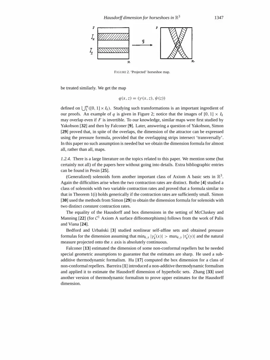
FIGURE 2. ‘Projected’ horseshoe map.

be treated similarly. We get the map

q(x, z) = (γ (x, z), ψ(z))defined on

⋃m1 ([0,1]×Ik). Studying such transformations is an important ingredient of

our proofs. An example ofq is given in Figure 2; notice that the images of[0,1] × Ikmay overlap even ifF is invertible. To our knowledge, similar maps were first studied byYakobson [32] and then by Falconer [9]. Later, answering a question of Yakobson, Simon[29] proved that, in spite of the overlaps, the dimension of the attractor can be expressedusing the pressure formula, provided that the overlapping strips intersect ‘transversally’.In this paper no such assumption is needed but we obtain the dimension formula for almostall, rather than all, maps.

1.2.4. There is a large literature on the topics related to this paper. We mention some (butcertainly not all) of the papers here without going into details. Extra bibliographic entriescan be found in Pesin [25].

(Generalized) solenoids form another important class of Axiom A basic sets inR3.Again the difficulties arise when the two contraction rates are distinct. Bothe [4] studied aclass of solenoids with two variable contraction rates and proved that a formula similar tothat in Theorem 1(i) holds generically if the contraction rates are sufficiently small. Simon[30] used the methods from Simon [29] to obtain the dimension formula for solenoids withtwo distinctconstantcontraction rates.

The equality of the Hausdorff and box dimensions in the setting of McCluskey andManning [22] (for C1 Axiom A surface diffeomorphisms) follows from the work of Palisand Viana [24].

Bedford and Urbański [3] studied nonlinear self-affine sets and obtained pressureformulas for the dimension assuming that mink,x |γ ′k(x)| > maxk,y |τ ′k(y)| and the naturalmeasure projected onto thex axis is absolutely continuous.

Falconer [13] estimated the dimension of some non-conformal repellers but he neededspecial geometric assumptions to guarantee that the estimates are sharp. He used a sub-additive thermodynamic formalism. Hu [17] computed the box dimension for a class ofnon-conformal repellers. Barreira [1] introduced a non-additive thermodynamic formalismand applied it to estimate the Hausdorff dimension of hyperbolic sets. Zhang [33] usedanother version of thermodynamic formalism to prove upper estimates for the Hausdorffdimension.


Chinet al [7] studied the correlation dimension (with respect to the natural measure) foralmost alllinear skinny baker’s maps (and withγ andτ independent ofz). Hunt [19] isinvestigating dimension characteristics of the natural measure on the attractor for nonlinearmaps similar to those considered in Theorem 2.

In the survey of Gatzouras and Peres [15] the variational principle for dimension onrepellers is discussed; their paper also contains a large bibliography on linear self-affinesets which we do not duplicate. Some self-affine sets inR2 and the corresponding ‘product’horseshoes inR3, with one of the contraction rates greater than1

2, were considered byPollicott and Weiss [26].

1.2.5. Now let us make some comments about the proof of Theorem 1. The upperestimates are proved for the upper box dimension; they are rather standard and hold for all(not just almost all) horseshoes under consideration. We use potential theoretic methodsto get lower estimates of the Hausdorff dimension. ‘Almost-all’ type results follow fromFubini’s theorem, so we have no way to check concrete cases. This method goes backto Kaufman [20]. Our proof relies on the scheme of Falconer [10] in several places. Weuse the tools of thermodynamic formalism, especially Gibbs (equilibrium) measures. Itfollows from (H1)–(H3) that the stable manifolds are horizontal planes and the unstablemanifolds are smooth curves which can be parameterized byz. Thez-slices of the basicset can be represented as attractors of iterated function systems but with a different familyof contractions applied at each step. This is taken into account by the two-sided symboliccoding. There are two cases in Theorem 1, corresponding to parts (i) and (ii). They arereferred to as the case of ‘small contractions’ and ‘large contractions’ respectively. In thecase of small contractions the dimension of almost every3 turns out to be the maximumof dimensions of its projections onto thexz andyz planes.

2. PreliminariesFirst we give definitions ofr ands valid in the general (possibly non-invertible) case. Thenwe consider ‘projections’ of our horseshoe maps and develop tools to study them.

Fix a horseshoe mapF . Let6 = {1, . . . ,m}Z. We denote the natural projection fromthe symbolic space6 to the basic set3 by5F :

5F (i) = 5F (. . . , i−n, . . . , i0, . . . , in, . . . )

=∞⋂n=0

[1(i0, . . . , i−n)

⋂Fn(1(in, . . . , i1))

],

where1(j0, . . . , jk) := [0,1]2 × {ζ ∈ [0,1] : ψl(ζ ) ∈ Ijl , l = 0, . . . , k}. Then5F ◦ σ−1 = F ◦ 5F , whereσ is the left shift on6. We write5F = (51

F ,52F ,5

3F ).

Consider the functions

φ1(i) := log |γ ′x(51F (σ i),53

F (σ i))| and φ2(i) := log |τ ′y(52F (σ i),53

F (σ i))|. (5)

Thens1, s2, r1, r2 are defined as the unique solutions of the equations

P(s1φ1) = 0, P (s2φ2) = 0, P (φ1 + r1φ2) = 0, P (r2φ1+ φ2) = 0, (6)


whereP is the pressure with respect toσ . If F is invertible, the projection5F is one-to-one and this definition coincides with the one given in §1.1; see, for example, Bowen [5].

Recall (4) that Rep(ψ) ⊂ [0,1] is the repeller ofψ, that is, the set on which all forwarditerates ofψ are defined. Since3 =⋂n∈ZFn([0,1]3) is a subset of[0,1]2×Rep(ψ) weare only interested inF on this set. Observe that allt-perturbationsF t have the samezcomponentψ; we fixψ for the rest of the paper. Notice that

53(i) := 53F (i) = lim

n→∞ψ−1i0◦ · · · ◦ ψ−1

i−n (0)

depends only onψ, so53 will be the same for all maps under consideration. Forz ∈ [0,1]let 6z = {i ∈ 6 : 53(i) = z}. Clearly,6z 6= ∅ if and only if z ∈ Rep(ψ). Let6+ := {1, . . . ,m}N . It is easy to see that the projectionP+ : 6 → 6+ restricted to6z isa bijection, so we can identify6z with 6+. This identification will be meant whenever wewrite6z ∼ 6+.

For every horseshoe mapF(x, y, z) = (γ (x, z), τ (y, z), ψ(z)) there are two associated‘projected’ maps:

q(x, z) = (γ (x, z), ψ(z)) and r(y, z) = (τ (y, z), ψ(z)).It is convenient to consider these maps on their own, in such a way thatF is not usedexplicitly. We shall work withq andγ in thexz plane; obvious modifications are neededfor theyz plane. Clearly,q : [0,1]×Rep(ψ)→ [0,1]×Rep(ψ). An example of the mapq is given in Figure 2, see §1. Fori ∈ 6 let

Gi(x) := γ (x,ψ−1i1(53(i))).

ThenGi : [0,1] → [0,1] andλ1 < |G′i(x)| < λ2 for eachx ∈ [0,1]. The collection of allG = {Gi}i∈6 obtained in this way (so ultimately arising from some horseshoe map) willbe denoted0. The correspondingt-perturbations are

Gti (x) = γ (x,ψ−1

i1(53(i)))+ ti1. (7)

We say thatt is G-admissible ifGt ∈ 0. Since53(i) is uniquely determined by(. . . , i−2, i−1, i0), it follows from the definition ofGi that

ik = jk for −∞ < k ≤ 1⇒ Gi(x) ≡ Gj (x). (8)

Denote

Gi,n(x) := Gi ◦Gσ i ◦ · · · ◦Gσn−1i(x). (9)

It follows from (8) that

ik = jk for −∞ < k ≤ n⇒ Gi,n(x) ≡ Gj ,n(x). (10)

We shall need cylinder sets[i1 . . . in] = {j ∈ 6 : jk = ik,1 ≤ k ≤ n}. Forz ∈ Rep(ψ) let Iz,i1,...,in := Gi,n([0,1]), wherei ∈ [i1 . . . in] is such thatz = 53(i).ThenIz,i1,...,in ⊂ Iz,i1,...,in−1. ForG ∈ 0 define

5G(i) :=∞⋂n=1

Iz,i1,...,in = limn→∞Gi,n(0), wherez = 53(i). (11)


It follows from the definitions of5F andGi,n that5G ≡ 51F . Set3G(z) = 5G(6z).

Then3G(z) is just the projection of the slice3(z) onto thex axis. It follows from (9) that{Gi,n} is a cocycle:

Gi,n+m(x) = Gi,n(Gσni,m(x)),

therefore,

5G(i) = Gi,n(5G(σni)). (12)

By the definition ofIz,i1,...,in and the mean value theorem, for anyn ≥ 1 andi ∈ 6z, thereexistsu ∈ [0,1] such that

G′i,n(u) = |Iz,i1,...,in |. (13)

For eachG ∈ 0 define

ϕG(i) := log |G′i(5G(σ i))|. (14)

It is immediate from the definitions thatϕG ≡ φ1 (see (5)). Sinceγ ∈ C1+α, the functionϕG is Holder continuous. One easily computes

log |G′i,n(x)| =n−1∑k=0

ϕG(σk i), (15)

wherex = 5G(σni).Recall that for each continuous functionf : 6 → R the topological pressure off (with

respect toσ ) is defined by

P(f ) := limn→∞

1

nlog

∑i1...in

exp

[sup

i∈[i1...in]

n−1∑k=0

f (σ k i)];

see Bowen [5].

3. Beginning of the proofWe continue to work with the class0 introduced in the previous section. The Lipschitzconstant forG = {Gi}i∈6 ∈ 0 is defined by

L(G) := supx,y∈[0,1],i∈6

|G′i(x)−G′i(y)||x − y|α .

The distance between two elementsT ,G of 0 is

%(G,T ) := supi∈6‖Gi − Ti‖,

where

‖h‖ := ‖h‖sup+ ‖h′‖sup+ supx,y∈[0,1]

|h′(x)− h′(y)||x − y|α .

Next we prove some distortion inequalities and collect their immediate consequences.There are many similar estimates in the literature, but since they are of crucial importancefor us, complete proofs are given.


LEMMA 3.1. There exists a constantC1 > 0 such that for allG,T ∈ 0, n ∈ N and foranyi ∈ 6, u, v ∈ [0,1],(i)

C−L(G)1 <

|G′i,n(u)||G′i,n(v)|

< CL(G)1 .

(ii) For anyG ∈ 0 there exists a constantC2 = C2(α,L(G), λ1, λ2) such that for allT ∈ 0 satisfying%(G,T ) ≤ 1 and for anyi ∈ 6, n ∈ N,

exp[−n · C2 · %(G,T )α] <|T ′i,n(0)||G′i,n(0)|

< exp[n · C2 · %(G,T )α].

Proof. (i) It is clearly enough to check one inequality. We have

log|G′i,n(u)||G′i,n(v)|

=n−1∑k=0

log

∣∣∣∣∣G′σk i(Gσk+1i,(n−1−k)(u))

G′σk i(Gσk+1i,(n−1−k)(v))

∣∣∣∣∣≤n−1∑k=0

∣∣∣∣∣G′σk i(Gσk+1i,(n−1−k)(u))−G′σk i(Gσk+1i,(n−1−k)(v))

G′σk i(Gσk+1i,(n−1−k)(u))

∣∣∣∣∣≤ L(G)

λ1

n−1∑k=0

|Gσk+1i,(n−1−k)(u)−Gσk+1i,(n−1−k)(v)|α

≤ L(G)λ1

n−1∑k=0

λ(n−k)α2 · |v − u|α < L(G) · 1

λ1(1− λ2α),

and the desired statement follows. In the second displayed line above we used thatlog |x/y| ≤ |(x − y)/y|, and in the last but one inequality we used that by the mean valuetheorem, ∣∣Gj ,m(u)−Gj ,m(v)

∣∣ ≤ λ2 · |Gσ j ,m−1(u)−Gσ j ,m−1(v)|.(ii) Observe that

|Tj ,m(u)−Gj ,m(u)| ≤ |Tj (Tσ j ,m−1(u))−Gj (Tσ j ,m−1(u))|+ |Gj (Tσ j ,m−1(u))−Gj (Gσ j ,m−1(u))|≤ %(T ,G)+ λ2|Tσ j ,m−1(u)−Gσ j ,m−1(u)|< %(T ,G) 1

1− λ2.

Thus,

|T ′σk i(Tσk+1i,(n−1−k)(0))−G′σk i(Gσk+1i,(n−1−k)(0))|

< |T ′σk i(Tσk+1i,(n−1−k)(0))−G′σk i(Tσk+1i,(n−1−k)(0))|+ |G′

σk i(Tσk+1i,(n−1−k)(0))−G′σk i(Gσk+1i,(n−1−k)(0))|< %(T ,G)+ L(G)|Tσk+1i,(n−1−k)(0)−Gσk+1i,(n−1−k)(0)|α≤ %(T ,G)+ L(G)%(T ,G)α(1− λ2)

−α

≤ [1+ L(G)(1− λ2)−α] · %(T ,G)α,


using that%(T ,G) ≤ 1 in the last step.Since log|x/y| ≤ |(x − y)/y| we obtain fork ≥ 0 that

log

∣∣∣∣∣ T′σk i(Tσk+1i,(n−1−k)(0))

G′σk i(Gσk+1i,(n−1−k)(0))

∣∣∣∣∣ ≤ [1+ L(G)(1− λ2)−α] · %(T ,G)α

λ1

whence

1

nlog

∣∣∣∣∣ T′i,n(0)

G′i,n(0)

∣∣∣∣∣ = 1

n

n−1∑k=0

log

∣∣∣∣∣ T′σk i(Tσk+1i,(n−1−k)(0))

G′σk i(Gσk+1i,(n−1−k)(0))

∣∣∣∣∣≤ [1+ L(G)(1− λ2)

−α] · %(T ,G)αλ1

.

This implies the desired inequality and completes the proof of the lemma. 2

COROLLARY 3.2. For anyG = {Gi} andT = {Ti} in 0 the following hold:(i)

P(aϕG + bϕT ) = limn→∞

1

nlog

∑i1...in

|G′i,n(0)|a · |T ′i,n(0)|b;

(ii)

exp(−n · C2 · ‖t‖α) <|(Gt

i,n)′(0)|

|G′i,n(0)|< exp(n · C2 · ‖t‖α),

where‖t‖ = maxi |ti | andC2 is the constant from Lemma 3.1(ii).(iii) For 0< ε < min{1, s(G)} anda > 0 define

δ :=(−1

2ε logλ2

aC2

)1/α

.

Then for arbitraryi, n,

|(Gti,n)′(0)|−a ≤ |G′i,n(0)|−a−ε/2 for all t ∈ Bδ(0).

(iv) For all z such that6z 6= ∅ and anyi, j ∈ 6z such thatn = max{l ∈ Z : ik =jk for all k ≤ l},

|5G(i)−5G(j )| ≥ C−L(G)1 |G′i,n(0)| · |5G(σni)−5G(σnj )|.

Proof. (i) It follows from (15) thatf = aϕG + bϕT satisfies

exp

[sup

i∈[i1...in]

n−1∑k=0

f (σ k i)]= sup

i∈[i1...in]|G′i,n(51(σni))|a · |T ′i,n(51(σni))|b.

Then Lemma 3.1(i) implies the result.(ii) follows from Lemma 3.1(ii), lettingT = Gt and using the fact that%(Gt ,G) = ‖t‖.(iii) is an easy calculation using part (ii) of this corollary and the fact that|G′i,n| ≤ λn2.(iv) follows from (10), (12) and Lemma 3.1(i). 2


Recall that forG ∈ 0 a vectort ∈ Rm isG-admissible ifGt ∈ 0. The set ofG-admissiblet is open and non-empty. The next lemma establishes, in some sense, ‘transversality in theparameter space’. It is an adaptation of Lemma 3.1 in Falconer [10], with a modificationsimilar to Proposition 3.1 in Solomyak [31].

LEMMA 3.3. LetG ∈ 0 and letB ⊂ Rm be a convex set ofG-admissible vectors. Fix anarbitrary z with6z 6= ∅. Then there exists a constantC3 such that

∀ i, j ∈ 6z with i1 6= j1, Lm{t ∈ B : |5Gt (i)−5Gt (j )| ≤ ρ} ≤ C3ρ for ρ > 0. (16)

Proof. We have by (7) and (11), for alli ∈ 6z,5Gt (i) = lim

n→∞Gti,n(0) = ti1 +Gi(ti2 +Gσ i(ti3 +Gσ2i(ti4 + · · · ))).

Thus, for allk ≤ m,

∂5Gt (i)∂tk

= δi1,k +G′i(5Gt (σ i))[δi2,k +G′σ i(5Gt (σ 2i))(δi3,k + · · · )], (17)

whereδi,k is the Kronecker symbol. We need to analyse

f (t) := 5Gt (i)−5Gt (j ),

wherei1 6= j1 andi, j ∈ 6z (consequently,ik = jk for all k ≤ 0).To simplify notation, assume thati1 = 1 andj1 = 2. Then we have from (17) that

∂f (t)∂t1− ∂f (t)

∂t2

= 2+G′i(5Gt (σ i))[(δi2,1− δi2,2)+G′σ i(5Gt (σ 2i))((δi3,1− δi3,2)+ · · · )]−G′j (5Gt (σ j ))[(δj2,1− δj2,2)+G′σ j (5Gt (σ 2j ))((δj3,1− δj3,2)+ · · · )].

Since|G′i(x)| ≤ λ2 < 1/2 we have fori ∈ 6 that

∂f (t)∂t1− ∂f (t)

∂t2≥ 2− 2λ2(1+ λ2(1+ λ2(1+ · · · )))

= 2− 2∑n≥1

λn2 =2(1− 2λ2)

1− λ2> 0, (18)

Consider the transformationT : B → Rm defined by

T (t) = y = (y1, . . . ym),

wherey1 = f (t), y2 = t1+ t2, yk = tk for k 6= 1,2.

It is easy to see from (18) and the convexity ofB thatT is one-to-one onB. The JacobiandeterminantJ T satisfies

|J T (t)| =∣∣∣∣∂f (t)∂t1

− ∂f (t)∂t2

∣∣∣∣ ≥ 2(1− 2λ2)

1− λ2> 0.


LetAρ := {t ∈ B : |5Gt (i)−5Gt (j )| ≤ ρ}.

We have

Lm(Aρ) ≤ maxy∈Rm|J T (y)|−1Lm(TAρ)

≤ 1− λ2

2(1− 2λ2)· Lm{y ∈ T B : |y1| ≤ ρ}

≤ 1− λ2

2(1− 2λ2)· 2m+1ρ.

The last inequality holds sincet is G-admissible hence|yk| = |tk| ≤ 1 for k 6= 1,2 and|y2| ≤ |t1| + |t2| ≤ 2. The estimate (16) is proved. 2

COROLLARY 3.4. LetG ∈ 0. Fix arbitrary z with6z 6= ∅. Then for any0< a < 1 thereexists a constantC4 = C4(G, a) (independent ofz) such that for alli, j ∈ 6z with i1 6= j1,∫

t∈Bdt

|5Gt (i)−5Gt (j )|a ≤ C4,

whereB is a convex set ofG-admissiblet.

Proof. It is immediate, writing the integral in terms of the distribution function and using(16). 2

The following lemma will be used in the proof of Theorem 1(ii). For technical reasons,in this lemma we usev instead oft.

LEMMA 3.5. LetG ∈ 0. There exists a constantC5 > 0 such that for eachθ > 0 one canchooseδ > 0 so that

Lm{v ∈ Bδ(0) ⊂ Rm : |5Gv(i)−5Gv(j )| ≤ ρ} ≤ C5 ·min

{ρ

|G′i,n(0)|1+θ,1

}holds ifik = jk for all −∞ < k ≤ n.

Proof. It follows from (10) thatGvi,n ≡ Gv

j ,n. Using (12) we obtain that

|5Gv(i)−5Gv(j )| = |Gvi,n(5Gv(σni))−Gv

i,n(5Gv(σnj ))|= |(Gv

i,n)′(x)| · |5Gv(i′)−5Gv(j ′)|,

for i′ = σni, j ′ = σnj andx ∈ (0,1). Next, by Lemma 3.1(i),

|(Gvi,n)′(x)| ≥ C−L(G)1 · |(Gv

i,n)′(0)| ≥ C−L(G)1 · |G′i,n(0)|1+θ

for eachv ∈ Bδ(0), whereδ is chosen as in Corollary 3.2(iii) fora = 1 and12ε = θ , and

so that allt ∈ Bδ(0) areG-admissible. Thus,

Lm{v ∈ Bδ(0) : |5Gv(i)−5Gv(j )| ≤ ρ}

≤ Lm{

v ∈ Bδ(0) : |5Gv(i′)−5Gv(j ′)| ≤ CL(G)1 ρ

|G′i,n(0)|1+θ}

≤ min

{CL(G)1 · C3ρ

|G′i,n(0)|1+θ,Lm(Bδ(0))

}.

Here we applied Lemma 3.3. 2


4. The case of ‘small contractions’Here, after some preparation, we prove lemmas that will be used in the proof ofTheorem 1(i).

ConsiderG ∈ 0 and the corresponding functionϕG on 6 (see §2 for definitions).Define the function9G(a) := P(aϕG) for a > 0. It follows from Corollary 3.2(i) andthe inequalitiesλn1 ≤ |G′i,n| ≤ λn2 that

logλ1 ≤ 9G(a + u)−9G(a)u

≤ logλ2 (19)

for all positivea andu. Since9G(0) = logm > 0, this implies that the function9G hasa unique zero, which we denotes(G). One can show thats(G) = limn→∞ dn(z) where∑i1,...,in

|Iz,i1,...,in |dn(z) = 1, for all z such that6z 6= ∅. We omit the calculation since it israther standard and we do not need it for the proof.

In this section we letν = νG be the Gibbs measure fors(G)ϕG on6 (recall that thisfunction is Holder continuous, so the Gibbs measure exists). SinceP(sϕG) = 0, by thedefinition of a Gibbs measure,

ν([i1 . . . in]) ∈ [C−16 , C6] · exp

[s ·

n−1∑k=0

ϕG(σk i)], (20)

whereC6 > 0 depends only onG. By Lemma 3.1(i), (13) and (15),

C−L(G)1 ≤

exp[∑n−1

k=0 ϕG(σk i)]

|Iz,i1,...,in |≤ CL(G)1 .

Thus, there is a constantC7 = C7(G) > 0, such that for eachu, v ∈ [0,1] andi1 . . . in,

|Iu,i1...in ||Iv,i1...in |

∈ [C−17 , C7], |Iu,i1...in |

|G′i,n(0)|∈ [C−1

7 , C7] andν([i1 . . . in])|Iu,i1...in |s

∈ [C−17 , C7].

(21)

LEMMA 4.1. Suppose thatG ∈ 0. Then(i) dimB(3

G(z)) ≤ s(G) for all z such that6z 6= ∅;(ii) the functions(G) is continuous on0.

Proof. (i) We say thatIz,i1,...,in is anε-interval if |Iz,i1,...,in | ≤ ε but |Iz,i1,...,in−1| > ε.All ε-intervals (for fixedz) form a cover of3G(z). It follows from (20) and (21) that thenumber ofε-intervals is of the orderε−s , up to a multiplicative constant; see, for example,Proposition 2.1 in Hueter and Lalley [18] for details. By the definition of the upper boxdimension, the desired inequality follows.

(ii) Recall that9G(a) = P(aϕG). We have forT ∈ 0,

|9G(s(T ))| = |P(s(T )ϕG)| = |P(s(T )ϕG)− P(s(T )ϕT )|

= limn→∞

1

n

∣∣∣∣∣log

∑i1...in|G′i,n(0)|s(T )∑

i1...in|T ′i,n(0)|s(T )

∣∣∣∣∣< C2 · s(T ) · %(G,T )α


by Lemma 3.1(ii). Therefore, by (19),

|s(T )− s(G)| ≤ |9G(s(T ))−9G(s(G))||logλ2|= |9G(s(T ))||logλ2| ≤

C2 · s(T ) · %(G,T )α|logλ2|

which implies that the functions is continuous atT . 2

The next lemma contains the major part of the proof of Theorem 1(i).

LEMMA 4.2. LetG ∈ 0 be such thats(G) ≤ 1. Further, letz be arbitrary with6z 6= ∅.Then for everyε > 0 there existsδ > 0 such that

dimH(3Gt(z)) > s(G)− ε

for Lebesgue-a.e.t ∈ Bδ(0).Proof. Let s = s(G). Recall thatν is the Gibbs measure for the functionsϕG . Considerthe projected measure on6+. It induces a measureµ on6z since6z ∼ 6+. Then (20)and (21) imply

µ([i1, . . . , in]) ∈ (C−18 , C8) · |G′i,n(0)|s, (22)

where the constantC8 depends onG. Denote the product measureµ × µ by µ2. By thepotential-theoretic characterization of the Hausdorff dimension (see Falconer [12, p. 64]),it is enough to show that

R(t) =∫ ∫

6z×6zdµ2(i, j )

|5Gt (i)−5Gt (j )|s−ε <∞

for a.e.t ∈ Bδ(0) ⊂ Rm for someδ > 0. Indeed, this means that the(s − ε)-energy of the‘push-down’ measureµ ◦ (5Gt

)−1 on3Gt(z) is finite. Following the scheme of Kaufman

[20], we shall prove that∫t∈Bδ(0)

R(t) dt <∞ whereδ =(−1

2ε logλ2

(s − ε)C2

)1/α

andC2 comes from Lemma 3.1(ii) and Corollary 3.2(ii).Let i, j ∈ 6z. Below we writei∧j = τ for a finite wordτ = (τ1, . . . , τn) if ik = jk = τk

for all 1 ≤ k ≤ n andin+1 6= jn+1. We have by Fubini’s theorem that∫t∈Bδ(0)

R(t) dt =∑n≥0

∑τ=(i1...in)

∫ ∫i∧j=τ

(∫t∈Bδ(0)

dt

|5Gt (i)−5Gt (j )|s−ε)dµ2(i, j )

< constant·∑n≥0

∑τ=(i1...in)

∫ ∫i∧j=τ

[|G′i,n(0)|−(s−ε/2)

×∫

t∈Bδ(0)dt

|5Gt (σni)−5Gt (σnj )|s−ε]dµ2(i, j )


∑τ=(i1...in)

∫ ∫i∧j=τ

|G′i,n(0)|−(s−ε/2) dµ2(i, j )



λnε/22

∑τ=(i1...in)

∫ ∫i∧j=τ

1

µ([τ ]) · dµ2(i, j )

= constant·∑n≥0

λnε/22 <∞,

where the first inequality follows from Corollary 3.2(iii) and (iv). The second one is justCorollary 3.4 and the third inequality comes from (22). This concludes the proof of thelemma. 2

COROLLARY 4.3. LetG ∈ 0. Fix anyz such that6z 6= ∅. Then

dimH (3Gt(z)) = s(Gt) for a.e.G-admissiblet such thats(Gt) ≤ 1.

Proof. The upper estimate for dimension follows from Lemma 4.1(i) since dimH ≤ dimB ;it holds for allG-admissiblet.

Suppose that the statement of the corollary is false. Then for someε > 0 there existsa density pointt0 of thoset for which dimH(3G

t(z)) < s(Gt) − ε ≤ 1− ε. Sinces(Gt)

is continuous by Lemma 4.1(ii) and thet-perturbation ofGt0 coincides with the(t0 + t)-perturbation ofG, this contradicts Lemma 4.2. 2

5. The case of ‘large contractions’In the previous section we considered the cases ≤ 1. Here we assume thats > 1 preparingfor the proof of Theorem 1(ii). As we saw in (2) this implies thatr > 0. Therefore, withoutloss of generality we may assume throughout this section thatr = r1 > 0 (see (6) for thedefinition ofr1).

We introduce some notation used throughout §5. Fix an arbitrary horseshoe mapF(x, y, z) = (γ (x, z), τ (y, z), ψ(z)) satisfying (H1)–(H3) andz such that6z 6= ∅. Put62z := 6z×6z. LetG,T be the elements of0 defined by the first two component functions

of F , that is

Gi(x) := γ (x,ψ−1i1(53(i))) and Ti(y) := τ (y,ψ−1

i1(53(i))). (23)

The functions associated with them, as in (14), will be denotedϕG and ϕT . In thissection we letν be the Gibbs measure of the functionϕG + rϕT . The measureµ is theinduced measure on6z, that is, we first consider the projected measure on6+ and thenthe measure on6z using the identification6z ∼ 6+. (Warning: µ andν in this sectionare different fromµ andν in the previous section.) By the definition of Gibbs measure andLemma 3.1(i) there existsC9 > 0 such that

µ([i1, . . . , in]) ∈ (C−19 , C9) · |G′i,n(0)| · |T ′i,n(0)|r . (24)

In this sectiont1, t2 are always vectors fromRm, and whenever we writet it isalways a vector fromRm × Rm with t = (t1, t2). We use thel∞ norm onR2m. Put5t(i) := (5Gt1 (i),5T t2 (i)) for i ∈ 6. We write3t for the basic set ofF t . Further,3t(z)

denotes thez-horizontal section of3t , so that3t(z) = 5t (6z). Fort ∈ R2m we denote byGt andT t thet-perturbations ofG andT and writeϕt

G, ϕtT for the corresponding functions

on6. Let r1(t) be the solution of the equationP(ϕG + r1(t)ϕT ) = 0.


LEMMA 5.1. The functiont 7→ r1(t) is continuous.

Proof. As in Lemma 4.1(ii), we prove a more general statement. The calculations aresimilar to those of Lemma 4.1(ii), so we shall be brief.

Let G,T ∈ 0. Denote byr1(G,T ) the unique solution of the equation

P(ϕG + r1(G,T )ϕT ) = 0.

We shall prove that(G,T ) 7→ r1(G,T ) is continuous in the metric induced by%(G,H).Let G,T ,H,U ∈ 0. Using Corollary 3.2(i), it is easy to see that

|P(ϕG + r1(H,U)ϕT )| = |P(ϕG + r1(G,T )ϕT )− P(ϕG + r1(H,U)ϕT )|≥ |logλ2||r1(G,T )− r1(H,U)|.

On the other hand, again using Corollary 3.2(i) and Lemma 3.1(ii), we obtain

|P(ϕG + r1(H,U)ϕT )| = |P(ϕG + r1(H,U)ϕT )− P(ϕH + r1(H,U)ϕU )|< C2r1(H,U)[%(G,H)α + r1(H,U)%(T ,U)α].

Combining the inequalities yields the desired continuity. 2

Below we denoteB2δ (0) := Bδ(0)× Bδ(0).

LEMMA 5.2. Fix θ > 0 and letδ > 0 be as in Lemma 3.5. Further, fixi, j ∈ 6z suchthat i ∧ j = (i1, . . . , in). LetK := |G′i,n(0)|1+θ andL := |T ′i,n(0)|1+θ . Then for each1< a < 2 there is a positive constantC′1 = C′1(a) (independent ofi, j , n) such that

I :=∫

t∈B2δ (0)

dt‖5t(i)−5t(j )‖a ≤ C

′1 min

{1

K · La−1 ,1

L ·Ka−1

}.

Proof. Without loss of generality, we may assumeK ≥ L. Using Lemma 3.5 twice (forv = t1 andv = t2 and the familiesG, T respectively), one can see that

I = a∫ ∞ρ=0L2m{t ∈ B2

δ (0) : ‖5t(i)−5t(j )‖ ≤ ρ}ρ−1−a dρ

≤ C25 · a ·

∫ ∞ρ=0

min{ ρK,1}·min

{ ρL,1}· ρ−1−a dρ

≤ C25 · a ·

[ ∫ L

0

ρ2

KLρ−1−a dρ +

∫ ∞L

ρ

Kρ−1−a dρ

]= C′1(a) ·

1

KLa−1≤ C′1(a) ·

1

LKa−1. 2

Now we are ready for the main lemma in the proof of Theorem 1(ii).

LEMMA 5.3.(i) Suppose that0< r ≤ 1. Then for everyε > 0 there existsδ > 0 such that

dimH(3t(z)) ≥ 1+ r − ε for a.e.t ∈ B2

δ (0).

(ii) If r > 1 thenL2(3

t(z)) > 0 for a.e.t ∈ B2δ (0).


Proof. (i) Fix ε such that 1≥ r = r1 > ε > 0 and then chooseθ satisfying

0< θ <ε logλ2

2 logλ1. (25)

Determineδ from θ as in Lemma 3.5. The desired estimate follows from the potential-theoretic characterization of the Hausdorff dimension if we show that

I :=∫

t∈B2δ (0)

∫ ∫62z

dµ2(i, j )‖5t(i)−5t(j )‖1+r1−ε dt <∞.

Using Fubini’s theorem we obtain

I =∑n≥0

∑τ=(i1...in)

∫ ∫i∧j=τ

(∫t∈B2

δ (0)

dt‖5t(i)−5t(j )‖1+r1−ε

)dµ2(i, j )


∑τ=(i1...in)

∫ ∫i∧j=τ

dµ2(i, j )|G′i,n(0)|1+θ · |T ′i,n(0)|(1+θ)(r1−ε)

,

by Lemma 5.2 witha = 1+ r1 − ε ∈ (1,2). It follows from (24) that

µ2({(i, j ) ∈ 62z : i ∧ j = (i1, . . . , in)}) ≤ C9|G′i,n(0)| · |T ′i,n(0)|r1 · µ([i1, . . . , in]).

Thus,

I ≤ constant·∑n≥0

∑(i1...in)

|G′i,n(0)| · |T ′i,n(0)|r1 · µ([i1, . . . , in])|G′i,n(0)|1+θ · |T ′i,n(0)|(r1−ε)(1+θ)

. (26)

Sinceθ < ε/2 andr ≤ 1 we haver1− (1+ θ)(r1− ε) = ε+ εθ − θr1 ≥ ε/2. Therefore,

|G′i,n(0)| · |T ′i,n(0)|r1|G′i,n(0)|1+θ · |T ′i,n(0)|(r1−ε)(1+θ)

≤ λ−nθ1 λnε/22 < λn3

for someλ3 < 1, sinceλε/22 < λθ1 by (25). Now (26) implies

I ≤ constant∑n≥0

λn3

∑(i1...in)

µ([i1, . . . , in]) = constant∑n≥0

λn3 <∞

and the proof of part (i) is complete.(ii) The proof of this part follows the scheme of Mattila [21, p. 130]. As above, we

assume thatr = r1 sor1 > 1. Letµt := µ ◦ (5t)−1 be the push-down measure supportedon3t(z) and set

D(µt,u) := lim infρ→0

µt(Bρ(u))L2(Bρ(u)))

,

whereu ∈ R2 andBρ(u) is the ball inR2 in the l∞-metric. To prove thatL2(3t(z)) > 0

for a.e.t ∈ B2δ (0) it is enough to show thatµt is absolutely continuous with respect toL2

for a.e.t ∈ B2δ (0). However, to see this it is enough to prove the following statement (see

Mattila [21, p. 36]):

I :=∫

t∈B2δ (0)

∫3t (z)

D(µt,u) dµt dt <∞.


We fix θ so that

0< θ < (r1− 1)logλ2

logλ1+ logλ2

and chooseδ for thisθ as in Lemma 3.5. Then we apply Fatou’s lemma and make a changeof variable to get

I ≤ lim infρ→0

1

4ρ2

∫ ∫62z

L2m{t ∈ B2δ (0) : ‖5t(i)−5t(j )‖ ≤ ρ} dµ2(i, j ). (27)

For anyi, j ∈ 62z with i ∧ j = (i1, . . . , in), applying Lemma 3.5 twice we obtain

L2m{t ∈ B2δ (0) : ‖5t(i)−5t(j )‖ ≤ ρ} ≤ C2

5ρ2

|G′i,n(0)|1+θ |T ′i,n(0)|1+θ.

This and (27) yield

I ≤ constant·∑n≥0

∑(i1...in)

µ([i1, . . . in])|G′i,n(0)|1+θ |T ′i,n(0)|1+θ

µ([i1, . . . in])

≤ constant·∑n≥0

∑(i1...in)

|G′i,n(0)||T ′i,n(0)|r1µ([i1, . . . in])|G′i,n(0)|1+θ |T ′i,n(0)|1+θ

≤ constant·∑n≥0

λ−nθ1 λ(r1−1−θ)n2

∑(i1...in)

µ([i1, . . . in]) <∞,

sinceλ(r1−1−θ)2 < λθ1 by the choice ofθ . This completes the proof of part (ii). 2

COROLLARY 5.4. Letz ∈ [0,1] be such that6z 6= ∅ and letQ be the set ofF -admissiblet. Then:(i) dimH (3

Gt(z)) ≥ 1+min{r(t),1} for a.e.t ∈ Q such thatr(t) > 0;

(ii) L2(3t(z)) > 0 for a.e.t ∈ Q such thatr(t) > 1.

Proof. (i) follows from Lemma 5.3(i) and Lemma 5.1 (the continuity ofr(t)) similar to theproof of Corollary 4.3.

(ii) Suppose that the statement is false. Then there is an admissible pointt0 suchthat r(t0) > 1 but in any ball aroundt0 there is a set oft having positiveL2-measurefor which L2

(3t(z)

) = 0. Considering3t0 instead of3 leads to a contradiction withLemma 5.3(ii). 2

6. Conclusion of the proofIn the following lemma we collect estimates above for the upper box dimension. They arerather standard and hold for all, not just almost all, horseshoes.

LEMMA 6.1. Let3 be a horseshoe andz ∈ [0,1] is such that6z 6= 0. Then:(i) dimB(3(z)) ≤ s = max{s1, s2};(ii) dimB(3(z)) ≤ 1+ r = 1+max{r1, r2} provideds > 1 (and hencer > 0);

(iii) dimB(3) ≤ δu +{s

1+ r if s > 1.Hereri , si are defined in (6) andδu is from (3).


Proof. (i) Let I1z,i1,...,in

:= Gi,n([0,1]) and I2z,i1,...,in

:= Ti,n([0,1]), wherez = 53(i).Then ⋃

i1,...,in

(I1z,i1,...,in

× I2z,i1,...,in

) ⊃ 3(z).

We say thatI jz,i1,...,in is anε-interval if |I jz,i1,...,in−1| ≤ ε but |I jz,i1,...,in−1

| > ε (herej can be

1 or 2). The number ofε-intervalsI j is not greater than constant·ε−sj , similar to the proofof Lemma 4.1(i). It follows that3(z) can be covered by constant· (ε−s1 + ε−s2) squaresof sideε which implies the desired estimate.

(ii) Let A1 be the set of finite sequencesu = (i1, . . . , in) (for any n) such thatI1z,i1,...,in

is anε-interval and|I2z,i1,...,in

| ≥ |I1z,i1,...,in

|. LetA2 be the set of finite sequences

u = (i1, . . . , in) (for anyn) such thatI2z,i1,...,in

is anε-interval and|I1z,i1,...,in

| ≥ |I2z,i1,...,in

|.It is easy to see that anyi ∈ 6z belongs to a cylinder set[u], with u ∈ A1 ∪ A2. Thus,3(z) is covered by ⋃

u∈A1

(I1z,u × I2

z,u) ∪⋃u∈A2

(I1z,u × I2

z,u).

The rectanglesI1z,u × I2

z,u for u ∈ A1 ∪ A2 have the shorter side of length betweenλ1ε

andε. If u ∈ A1 the rectangle is stretched in they direction, and ifu ∈ A2 the rectangle isstretched in thex direction. LetN(ε) be the minimal number of squares of sideε neededto cover3(z). Then

N(ε) ≤∑u∈A1

( |I2z,u||I1z,u|+ 1

)+∑u∈A2

( |I1z,u||I2z,u|+ 1

)

≤ 2

λ1ε

[ ∑u∈A1

|I2z,u| +

∑u∈A2

|I1z,u|]. (28)

Letµ be the measure on6z as in §5. Then

µ([u]) ≥ C′2|I1z,u| · |I2

z,u|r1

for someC′2 > 0 by (21). Therefore,

1 ≥∑u∈A2

µ([u]) ≥ C′2∑u∈A2

|I1z,u| · |I2

z,u|r1 ≥ C′2(ελ1)r1∑u∈A2

|I1z,u|,

hence∑u∈A2|I1z,u| ≤ constant· λ−r11 ε−r1. Similarly, using the Gibbs measure for

r2ϕG+ϕT we obtain that∑u∈A1|I2z,u| ≤ constant·λ−r21 ε−r2. Combining these inequalities

with (28) yieldsN(ε) ≤ constant· ε−(1+r),

wherer = max{r1, r2}. SincedimB(3(z)) = lim supε→0 logN(ε)/ log 1/ε, the statementis proved.

(iii) A straightforward calculation based on (1), (H2) and (H3) shows that the unstablemanifolds for our horseshoe map are smooth curves which form angles bounded away fromzero with horizontal planes (the stable manifolds). Then the statement routinely followsfrom parts (i) and (ii) and Theorem 3. 2


Now we are ready to prove our theorems which follow by Fubini’s Theorem fromLemma 6.1, Corollary 4.3, and Corollary 5.4.

Proof of Theorem 1.The upper estimates are obtained in Lemma 6.1 so we only have toshow the lower estimates. Fix a horseshoe mapF and letQ be the set ofF -admissiblet. ThenQ is a non-empty bounded open set. Forz fixed, we defineG andT as in (23).Further, we writes(t) := max{s(Gt1), s(T t2)} for t = (t1, t2) ∈ R2m. Then Corollary 4.3implies that dimH (3t(z)) ≥ s(t) for a.e.t such thats(t) ≤ 1 since3G

t1 (z) is the projectionof 3(z) onto thex axis and3G

t2 (z) is the projection of3(z) onto they axis. Thus, wehave, together with Corollary 5.4(i), that for everyz ∈ Rep(ψ), for Lebesgue almost everyt ∈ Q,

dimH(3t(z)) ≥

{s(t) if s(t) ≤ 1

1+ r(t) if s(t) > 1.(29)

Recall (Theorem 3) that 0< Hδu(Rep(ψ)) < ∞. DefineA := Q × Rep(ψ). Then(L2m ×Hδu)(A) > 0. We call a pair(t, z) ∈ A ‘good’ if (29) holds. By Fubini’s theorem,for L2m-almost everyt ∈ Q, forHδu -a.e.z ∈ Rep(ψ), the pair(t, z) is ‘good.’ Then bythe ‘generalized slicing theorem’ (see Corollary 7.12 in Falconer [12]) we get the desiredlower bound. The proof of Theorem 1 is complete. 2

Proof of Theorem 2.The proof is the same as for Theorem 1, except that hereδu = 1. Part(iii) follows from Fubini’s theorem and Corollary 5.4(ii). 2

Acknowledgements.We are grateful to the referee for the careful reading of themanuscript and many helpful comments. KS was supported by OTKA Foundation grantF019099. BS was supported by NSF Grant 9500744.

REFERENCES

[1] L. M. Barreira. A non-additive thermodynamic formalism and applications to dimension theory ofhyperbolic dynamical systems.Ergod. Th. & Dynam. Sys.16 (1996), 871–927.

[2] T. Bedford. Applications of dynamical systems theory to fractals—a study of cookie-cutter Cantor sets.Fractal Geometry and Analysis. Eds J. Belair and S. Dubuc. Kluwer, Dordrecht, 1991, pp. 1–44.

[3] T. Bedford and M. Urbański. The box and Hausdorff dimension of self-affine sets.Ergod. Th. & Dynam.Sys.10 (1990), 627–644.

[4] H. G. Bothe. The Hausdorff dimension of certain solenoids.Ergod. Th. & Dynam. Sys.15 (1995), 449–474.

[5] R. Bowen.Equilibrium States and the Ergodic Theory of Anosov Diffeomorphisms (Lecture Notes inMathematics, 470). Springer, New York, 1975.

[6] R. Bowen. Hausdorff dimension of quasi-circles.Publ. Math. I.H.E.S.50 (1979), 11–26.[7] W. Chin, B. Hunt and J. A. Yorke. Correlation dimension for iterated function systems.Trans. Amer.

Math. Soc.349(1997), 1783–1796.[8] G. A. Edgar. Fractal dimension of self-similar sets: some examples.Suppl. Rend. Circ. Mat. Palermo,

Ser. II28 (1992), 341–358.[9] K. Falconer. The Hausdorff dimension of some fractals and attractors of overlapping construction.J. Stat.

Phys.47(1/2) (1987).


[10] K. Falconer. The Hausdorff dimension of self-affine fractals.Math. Proc. Camb. Phil. Soc.103 (1988),339–350.

[11] K. Falconer. Dimensions and measures of quasi self-similar sets.Proc. Amer. Math. Soc.106 (1989),543–554.

[12] K. Falconer.Fractal Geometry: Mathematical Foundations and Applications. Wiley, Chichester, 1990.[13] K. Falconer. Bounded distortion and dimension for non-conformal repellers.Math. Proc. Camb. Phil.

Soc.115(1994), 315–334.[14] K. Falconer.Techniques in Fractal Geometry. Wiley, Chichester, 1997.[15] D. Gatzouras and Y. Peres. The variational principle for Hausdorff dimension.Ergodic Theory ofZd-

Actions (LMS Lecture Notes Series, 228).Cambridge University Press, 1996, pp. 259–272.[16] D. Gatzouras and Y. Peres. Invariant measures of full dimension for some expanding maps.Ergod. Th. &

Dynam. Sys.17 (1997), 147–167.[17] H. Hu. Box dimension and topological pressure for some expanding maps.Comm. Math. Phys.191(2)

(1998), 397–407.[18] I. Hueter and S. P. Lalley. Falconer’s formula for the Hausdorff dimension of a self-affine set inR

2.Ergod. Th. & Dynam. Sys.15 (1995), 77–97.

[19] B. Hunt. Pointwise dimension of attractors of iterated function systems with overlap.Preprint, 1999.[20] R. Kaufman. On Hausdorff dimension of projections.Mathematika15 (1968), 153–155.[21] P. Mattila.Geometry of Sets and Measures in Euclidean Spaces. Cambridge University Press, 1995.[22] H. McCluskey and A. K. Manning. Hausdorff dimension for horseshoes.Ergod. Th. & Dynam. Sys.3

(1983), 251–260.[23] K. McMullen. The Hausdorff dimension of general Sierpinski gasket.Nagoya Math. J.96 (1984), 1–9.[24] J. Palis and M. Viana. On the continuity of Hausdorff dimension and limit capacity of horseshoe.

Dynamical Systems, Valparaiso 1986 (Lecture Notes in Mathematics, 1331). Springer, 1988, pp. 150–160.

[25] Ya. Pesin.Dimension Theory in Dynamical Systems. The University of Chicago Press, 1997.[26] M. Pollicott and H. Weiss. The dimensions of some self affine limit sets in the plane.J. Stat. Phys.77

(1994), 841–866.[27] F. Przytycki and M. Urbański. On Hausdorff dimension of some fractal sets.Studia Mathematica93

(1989), 155–186.[28] D. Ruelle. Repellers for real analytic maps.Ergod. Th. & Dynam. Sys.2 (1982), 99–107.[29] K. Simon. Hausdorff dimension for non-invertible maps.Ergod. Th. & Dynam. Sys.13 (1993), 199–212.[30] K. Simon. The Hausdorff dimension of the general Smale–Williams solenoid.Proc. Amer. Math. Soc.

125:4(1997), 1221–1228.[31] B. Solomyak. Measure and dimension for some fractal families.Math. Proc. Cambridge Phil. Soc.124(3)

(1998), 531–546.[32] M. V. Yakobson. Invariant measures for some one dimensional attractors.Ergod. Th. & Dynam. Sys.2

(1982), 317–337.[33] Y. Zhang. Dynamical upper bounds for Hausdorff dimension of invariant sets.Ergod. Th. & Dynam. Sys.

17 (1997), 739–756.

Documents

Hausdorff dimension for horseshoes inR3