Embed Size (px)
Citation preview
HEARING THE WEIGHTS OF WEIGHTED PROJECTIVE
PLANES
MIGUEL ABREU, EMILY B. DRYDEN, PEDRO FREITAS, AND LEONOR GODINHO
Abstract. Which properties of an orbifold can we “hear,” i.e., which topo-logical and geometric properties of an orbifold are determined by its Laplacespectrum? We consider this question for a class of four-dimensional Kahlerorbifolds: weighted projective planes M := CP 2(N1, N2, N3) with three iso-lated singularities. We show that the spectra of the Laplacian acting on 0-and 1-forms on M determine the weights N1, N2, and N3. The proof involvesanalysis of the heat invariants using several techniques, including localizationin equivariant cohomology. We show that we can replace knowledge of thespectrum on 1-forms by knowledge of the Euler characteristic and obtain thesame result. Finally, after determining the values of N1, N2, and N3, we canhear whether M is endowed with an extremal Kahler metric.
1. Introduction
An orbifold consists of a Hausdorff topological space together with an atlas ofcoordinate charts satisfying certain equivariance conditions (cf. §2.1). We willbe interested in compact Kahler orbifolds; in particular, we focus on weightedprojective planes, asking what the Laplace spectrum of such a space can tell usabout its properties.
For manifolds, the asymptotic expansion of the heat kernel can be used to con-nect the geometry of the manifold to its spectrum. The so-called heat invariantsappearing in the asymptotic expansion tell us the dimension, volume, and variousquantities involving the curvature of the manifold. We are interested in the Kahlersetting; using the heat invariants, results have been obtained on spectral determi-nation of complex projective spaces [5], Einstein manifolds [24, 30], and generalKahler manifolds [29, 30]. These results are all for smooth manifolds, while we willbe interested in the effects of the presence of singularities.
Orbifolds began appearing sporadically in the spectral theory literature in theearly 1990’s, and have been receiving more dedicated attention in the last five years.It is known that the volume and dimension of an orbifold are spectrally determined[15]. The nature of the singularities allowed to appear in an isospectral set hasbeen studied; in general, there can be at most finitely many isotropy types (upto isomorphism) in a set of isospectral Riemannian orbifolds that share a uniformlower bound on Ricci curvature [28]. On the other hand, N. Shams, E. Stanhopeand D. Webb [27] constructed arbitrarily large (but always finite) isospectral sets
2000 Mathematics Subject Classification. Primary 58J50 Secondary 53D20, 55N91.Key words and phrases. Laplace spectrum, heat invariants, weighted projective planes.M. Abreu and L. Godinho were partially supported by Fundacao para a Ciencia e a Tecnolo-
gia (FCT) by the program POCTI 2010/FEDER and by grant POCTI/MAT/57888/2004, andL. Godinho was also partially supported by the Fundacao Calouste Gulbenkian; P. Freitas waspartially supported by FCT through grant POCTI/0208/2003.
1
2 MIGUEL ABREU, EMILY B. DRYDEN, PEDRO FREITAS, AND LEONOR GODINHO
which satisfy this curvature condition, where each element in a given set has pointsof distinct isotropy. One interesting question is whether the spectrum determinesthe orders of the singular points for large classes of orbifolds; we show that this isthe case for weighted projective planes. In particular, we prove (see §6)
Theorem 1. Let M := CP 2(N1, N2, N3) be a four-dimensional weighted projectivespace with isolated singularities, equipped with a Kahler metric. Then the spectraof the Laplacian acting on 0- and 1-forms on M determine the weights N1, N2, N3.
Note that we need to consider the spectrum of the Laplacian acting on both 0-and 1-forms. We conjecture that the spectrum of the Laplacian acting on 0-formsdetermines the weights, and have verified this with extensive computer testing.However, we cannot prove Theorem 1 using only this information at this point (cf.Section 6.2)
The proof of Theorem 1 involves introducing new techniques into the analysisof the heat invariants. In particular, we use localization in equivariant cohomologyto obtain expressions for topological invariants of CP 2(N1, N2, N3) in terms of N1,N2, and N3. We also use a decomposition of the Riemannian curvature tensorinside the space of Kahlerian curvature tensors to exploit the complex structureon our weighted projective spaces. We show that we can replace knowledge of thespectrum on 1-forms by knowledge of the Euler characteristic and obtain the sameresult. Finally, after determining the values of N1, N2, and N3, we can hear whetherthe metric on CP 2(N1, N2, N3) is an extremal Kahler metric in the sense of Calabi[10].
The same methods can be used with higher-dimensional weighted projectivespaces to obtain conditions on the weights (cf. Remark 2 in §6). However, theseconditions do not uniquely determine the weights. To obtain additional informationwe would need to impose restrictions on the metric and to use higher-order termsof the asymptotic expansion of the heat trace.
The paper is organized as follows. We begin with the necessary backgroundon orbifolds and orbi-bundles, then introduce the localization formula for orbifoldsand give the setup necessary to apply it in our case. The decomposition of theRiemannian curvature in terms of Kahlerian curvature tensors is presented. Lo-calization is then used to compute various integrals whose values we will need inthe proof of Theorem 1. In §4, we use a certain polytope associated to a givensymplectic toric orbifold to give a description of extremal metrics on weighted pro-jective planes, and to calculate the integral of the square of the scalar curvature ona weighted projective plane. In §5, we recall the asymptotic expansion of the heattrace of an orbifold as given in [14], and we calculate the first few heat invariantsfor CP 2(N1, N2, N3). Finally, we bring all of these tools together to prove Theorem1 and related results in §6.
2. Preliminaries
2.1. Orbifolds and Orbi-bundles. An orbifold M is a singular manifold whosesingularities are locally isomorphic to quotient singularities of the form Rn/Γ, whereΓ is a finite subgroup of GL(n, R). An orbifold chart on M is a triple (U, Γ, V )consisting of an open subset U of M , a finite group Γ ⊂ GL(n, R), an open subset Vof Rn and a homeomorphism U = V/Γ. An orbifold structure on the paracompactHausdorff space |M | is then a collection of orbifold charts (Ui, Γi, Vi) covering
HEARING THE WEIGHTS OF WEIGHTED PROJECTIVE PLANES 3
|M |, subject to appropriate compatibility conditions. In particular, these conditionsensure that on each connected component of M , the generic stabilizers of the Γi-actions are isomorphic. For each singularity p ∈ M , there is a finite subgroup Γp ofGL(n, R), unique up to conjugation, such that open neighborhoods of p in M arehomeomorphic to neighborhoods of the origin in Rn/Γp. We call Γp the orbifoldstructure group of p.
Example 1. Let N = (N1, . . . , Nm+1) be a vector of positive integers which arepairwise relatively prime. The weighted projective space
CPm(N) := CPm(N1, . . . , Nm+1) := (Cm+1)∗/ ∼ ,
where
((z1, . . . , zm+1) ∼ (λN1z1, . . . , λNm+1zm+1), λ ∈ C∗) ,
is a compact orbifold. It has m + 1 isolated singularities at the points [1 : 0 : · · · :0], . . . , [0 : · · · : 0 : 1], with orbifold structure groups ZN1
, . . . , ZNm+1. Note that
CPm(1) is the usual smooth projective space CPm.
The definitions of vector fields, differential forms, metrics, group actions, etc.naturally extend to orbifolds. For instance, a symplectic orbifold is an orbifoldequipped with a closed non-degenerate 2-form ω.
Given any orbifold M , fiber orbi-bundles (or orbifold bundles) π : E−→M aredefined by Γ-equivariant fiber bundles Z−→EV −→V in orbifold charts (U, Γ, V ),together with suitable compatibility conditions. Each fiber π−1(p) is not, in general,diffeomorphic to Z, but to some quotient of Z by the action of the orbifold structuregroup Γp.
Line orbi-bundles π : L−→Σ over a 2-dimensional orbifold Σ (also called an orbi-surface) of genus g with k cone singularities with orders N1, . . . , Nk, correspond toSeifert fibrations (3-dimensional manifolds together with an S1 action with finitestabilizers [26, 25, 16]) when we take the corresponding circle bundles. Hence, toeach line orbi-bundle we can associate a collection of integers (b, m1, · · · , mk), calledthe Seifert invariant of L over Σ, as well as its Chern number or degree defined
by the formula deg(L) := b +∑k
i=1mi
Ni. Let us briefly recall how to obtain this
invariant (see for example [22] and [16] for a detailed construction). If x1, . . . , xk arethe orbifold singularities of Σ and N1, . . . , Nk are the orders of the correspondingorbifold structure groups, then a neighborhood of xi in L is of the form (D2 ×C)/ZNi
, where D2 is a 2-disk and where ZNiacts on D2 × C by
ξNi· (z, w) = (ξNi
z, ξmi
Niw),
for some integer 0 ≤ mi < Ni, and ξNia primitive Ni-th root of unity. Given
Σ and its orbifold singularities x1, . . . , xk, we define special line orbi-bundles Hxi
as follows. Let Σxibe the orbi-surface obtained from Σ by deleting a small open
neighborhood Ui around xi, where Ui is isomorphic to D2/ZNi. Take the trivial
bundle over Σxi, and over Ui take the line orbi-bundle (D2 × C)/ZNi
, for a ZNi-
action given by
ξNi· (z, w) = (ξNi
z, ξNiw)
with gluing map α : ∂Σxi× C−→(∂D2 × C)/ZNi
,
α(eiθ, w) = (e−iθ, e−iθw).
4 MIGUEL ABREU, EMILY B. DRYDEN, PEDRO FREITAS, AND LEONOR GODINHO
That is,
Hxi:=(
Σ+xi
× C)
⋃
α
(D2− × C)/ZNi,
where Σ+xi
is positively oriented and D2−
is negatively oriented. The bundle L ⊗H−m1
x1⊗ · · · ⊗H−mk
xk, called the de-singularization of L, is a trivial line orbi-bundle
over each neighborhood of the xi’s and is naturally isomorphic to a smooth linebundle |L| over the (smooth) surface |Σ|. Taking the first Chern number b of |L|,the collection of integers (b, m1, . . . , mk) is then the Seifert invariant of L over Σ.
This invariant of an orbifold line bundle classifies it. Indeed, denoting by Pict(Σ)the Picard group of topological isomorphism classes of line orbi-bundles over Σ (withgroup operation the tensor product), the map
Pict(Σ) −→ Q ⊕k⊕
i=1
ZNi
L 7→ (deg(L), m1, . . . , mk),
is an injection with image the set of tuples (c, m1, . . . , mk) with c =∑k
i=1 mi/Ni
(mod Z) (cf. [16]). In particular, if the Ni’s are pairwise relatively prime, thenPict(Σ) ∼= Z is generated by a line orbi-bundle L0 with deg(L0) = 1
N1···Nk.
An important class of examples of line orbi-bundles are those over weightedprojective spaces Σ = CP 1(p, q). Just as any line bundle over a sphere is isomorphicto some line bundle O(r) with first Chern number r ∈ Z, defined by (S3 × C)/∼,where (z1, z2, w) ∼ (λz1, λz2, λ
rw) for λ ∈ S1, any line orbi-bundle with isolatedsingularities over an orbifold “sphere” CP 1(p, q) with p and q relatively prime isisomorphic to some Op,q(r) = Lr
0, defined by (S3 × C)/∼, where now (z1, z2, w) ∼(λpz1, λ
qz2, λrw) for λ ∈ S1. Note that deg(Op,q(r)) = r
pq and that, if r > 0,
Op,q(r) is isomorphic to the normal orbi-bundle of CP 1(p, q) inside the weightedprojective space CP 2(p, q, r).
2.2. Group actions and equivariant cohomology. Let (M, ω) be a symplecticorbifold, and G a compact, connected Lie group acting smoothly on M . Since G isconnected, the components of the fixed point set MG are suborbifolds of M . More-over, if G is abelian, the normal orbi-bundle νF of each fixed point component F iseven dimensional, and admits an invariant Hermitian structure. If M is oriented,any choice of such a Hermitian structure defines an orientation in F . The defini-tion of equivariant differential forms, AG(M) (that is, polynomial G-equivariantmappings α from the Lie algebra g of G to the space of differential forms in M)extends naturally to orbifolds equipped with a group action, as does the equivariantdifferential dG : AG(M)−→AG(M) defined as
dG(α)(ξ) = dα(ξ) − 2π i ι(ξM )α(ξ),
where ξM is the fundamental vector field corresponding to ξ.Let us assume now that G = T is abelian, that M is compact, connected and
oriented and consider the integration mapping∫
: AT (M)−→AT (M) and the em-beddings ιF : F−→M of the connected components of the fixed point set. TheAtiyah-Bott and Berline-Vergne localization formula ([4, 6]), generalized to orb-ifolds by Meinrenken [21], states that
HEARING THE WEIGHTS OF WEIGHTED PROJECTIVE PLANES 5
Proposition 2.1. (Localization formula for orbifolds) Suppose G = T is abelian,and let α ∈ AT (M) be dT -closed. Then
1
dM
∫
M
α =∑
F
1
dF
∫
F
ι∗F α
e(νF ),
where the sum is over the connected components of the fixed point set, where, fora connected orbifold X, dX is the order of the orbifold structure group of a genericpoint of X, and where e(νF ) is the equivariant Euler class of νF , the normal orbi-bundle to F .
The right hand side of this equation is very simple if M admits an invariantalmost complex structure. In this case, the computation of the equivariant Chernclasses of νF is given by the corresponding equivariant Chern series cT (νF ) :=∑
i ti cTi (νF ). Moreover (using the splitting principle if necessary) we can assume,
without loss of generality, that νF splits into a direct sum of invariant line orbi-bundles Li with first Chern classes c1(Li) where T acts with rational orbi-weights1
λi, and we have:
(2.1) cTt (νF ) =
∏
i
(1 + t (c1(Li) + λi)) .
As an example, the equivariant Euler class e(νF ) is
(2.2) e(νF ) =∏
i
(c1(Li) + λi)
and the first equivariant Chern class cT1 (νF ) is
(2.3) cT1 (νF ) =
∑
i
(c1(Li) + λi) .
2.3. Circle actions. Let M be a 4-dimensional symplectic orbifold with isolatedcone singularities equipped with a Hamiltonian S1-action, and let F be a fixedpoint. A neighborhood of F is modeled by some quotient C2/ZN for a ZN actiongiven by
ξN · (z, w) = (ξNz, ξmN w),
with 1 ≤ m < N and (m, N) = 1 (we are assuming that the orbifold singularitiesare isolated). The circle action on this neighborhood will be given by
eix · (z, w) = (eik1N
x z, eik2N
x w),
for some integers k1 and k2 (see [19] for details). If F is an isolated fixed point thenthe greatest common divisor (k1, k2) is equal to 1 or N (we are assuming the actionto be effective), and k2 = mk1 (mod N) (in order to have a well-defined action).The numbers k1
N x and k2
N x are the orbi-weights of the action at F and, in these
coordinates, the moment map is given by φ(z, w) = φ(F ) + 12 (k1
N |z|2 + k2
N |w|2). IfF is not an isolated fixed point, then the orbi-weight tangent to the fixed surfacecontaining F is equal to zero while the normal one is equal to ±x (again for theaction to be effective).
1Given an orbifold chart (U, Γ, V ) around a point in F it is not always true that the G-action
on U lifts to V but some finite covering G−→G does. The weights for this action of G on νF arecalled the orbi-weights of G.
6 MIGUEL ABREU, EMILY B. DRYDEN, PEDRO FREITAS, AND LEONOR GODINHO
Example 2. Consider Example 1 with n = 2, i.e., let M be the weighted projectivespace CP 2(N1, N2, N3) where the positive integers Ni are pairwise relatively prime,now equipped with the S1-action given by
eix · [z0 : z1 : z2] = [z0 : z1 : eixz2].
This action is Hamiltonian with respect to the standard symplectic form ω. More-over, it fixes the point F3 := [0 : 0 : 1] as well as the orbi-surface Σ := CP 1(N1, N2).A coordinate system centered at F3 is given by
(z, w) ∈ C2 7−→ [z : w : 1] ∈ M,
with (z, w) ∼ (ξN1
N3z, ξN2
N3w), where ξN3
is a primitive N3-th root of unity. The
action of S1 on this coordinate system is given by
e ix · [z : w : 1] = [z : w : eix] = [e−i
N1N3
x
z : e−i
N2N3
x
w : 1],
implying that the weights of the isotropy representation of S1 on TF3M are −N1
N3x
and −N2
N3x. On the other hand, the orbi-weights at every point in Σ are (x, 0). Note
that the degree of the normal orbi-bundle of Σ inside M is bΣ = N3
N1 N2.
2.4. Riemann curvature tensor. We now review the well-known decompositionof the Riemann curvature tensor of a Riemannian metric. A detailed expositionfor the manifold case can be found for instance in [8, 17, 2]. Since we are inter-ested in weighted projective spaces, which admit a Kahler metric, our goal is toconnect this standard decomposition of the Riemannian curvature to its Kahleriandecomposition.
In what follows, we extract the necessary background from [2]. The curvature Ron a Riemannian orbifold (M, g) is defined, as usual, by
RX,Y Z = ∇[X,Y ]Z − [∇X ,∇Y ] Z
for all vector fields X, Y, Z, where ∇ is the Levi-Civita connection. It is a 2-formwith values in the adjoint orbi-bundle AM (the bundle of skew-symmetric endo-morphisms of the tangent orbi-bundle) and satisfies the Bianchi identity2. Usingthe metric g we can identify AM with Ω2M and so R can be viewed as a sectionof Ω2M ⊗ Ω2M . Moreover, it follows from the Bianchi identity that R belongs tothe symmetric part S2Ω2M of Ω2M ⊗ Ω2M as well as to the kernel of the map
β : S2Ω2M−→Ω4M
determined by the wedge product. The kernel of β, RM , is called the orbi-bundleof abstract curvature tensors.
In addition, we have the Ricci contraction, a linear map
c : RM−→SM,
where SM denotes the orbi-bundle of symmetric bilinear forms on M , which sendsR to the Ricci form Ric.3 Hence, we obtain an orthogonal decomposition
RM = c∗(SM) ⊕ WM,
where WM , called the orbi-bundle of abstract Weyl tensors, is the kernel of c inRM . Consequently, R can be written as R = c∗(h) + W , where W is called the
2RX,Y Z + RY,ZX + RZ,XY = 0.3RicX,Y = tr(Z 7→ RX,ZY ).
HEARING THE WEIGHTS OF WEIGHTED PROJECTIVE PLANES 7
Weyl tensor and h is such that c c∗(h) = Ric. Since, for n ≥ 3 the map c issurjective, c∗ is injective and h is given by
h =τ
2n(n − 1)g +
Ric0
n − 2,
where τ is the scalar curvature (the trace of Ric with respect to g), and where Ric0
denotes the traceless part of Ric (i.e. Ric = τng + Ric0). Hence, the curvature R,
viewed as a symmetric endomorphism of Ω2M using g, decomposes as
(2.4) R =τ
n(n − 1)Id|
Ω2M+
1
n − 2Ric0, · + W,
where Ric0, · acts on α ∈ Ω2M as the anti-commutator, Ric0, α := Ric0 α +α Ric0. We will use the standard notation
U :=τ
n(n − 1)Id|
Ω2M
Z :=1
n − 2Ric0, ·
for the first two terms of this orthogonal decomposition (note that in this notation|R|2 = |U |2 + |Z|2 + |W |2).
Since we are interested in Kahler orbifolds, we can consider an orthogonal com-plex structure J parallel with respect to the Levi-Civita connection and obtain aKahler form ω as ω(X, Y ) = g(JX, Y ). We can also define the Ricci form andits primitive part ρ0 (that is, such that (ρ0, ω) = 0) in the same way4. Note thatthis isomorphism S 7→ S(J ·, ·) =: S J from the J-invariant part of S2Ω2M toΩ1,1M is not an isometry. In fact, |S|2 = 2|S J |2 (for example |g|2 = n = 2mwhile |ω|2 = m). Since the Riemannian curvature R has values in Ω1,1M , theJ-invariant part of Ω2M , it can be viewed as a section of the suborbi-bundle ofabstract Kahlerian curvature tensors, KM , defined as the intersection of RM withΩ1,1M ⊗Ω1,1M . However, in general, none of the components of the decomposition(2.4) is in KM , and we have a new decomposition of R inside KM
R =τ
2m(m + 1)(Id|
ΩJ,++ ω ⊗ω) +
1
m + 2(Ric0, ·|
ΩJ,++ ρ0 ⊗ω + ω ⊗ ρ0) + WK,
where |ΩJ,+ is the orthogonal projection of Ω2M onto its J-invariant part and WK
is the so-called Bochner tensor.Alternatively, we have (cf. [8], p. 77)
(2.5) R =τ
2m2ω ⊗ ω +
1
mρ0 ⊗ ω +
1
mω ⊗ ρ0 + B,
where B decomposes as
B =τ
2m(m + 1)Id|
Ω1,1M+ B0.
Both decompositions (2.4) and (2.5) are related by
|B0|2 = −3(m − 1)
m + 1|U |2 − m − 2
m|Z|2 + |W |2
|ρ0|2 = (m − 1)|Z|2
τ2 = 4m(2m− 1)|U |2.
4ρ(X, Y ) = Ric(JX, Y ) and ρ0(X, Y ) = Ric0(JX, Y )
8 MIGUEL ABREU, EMILY B. DRYDEN, PEDRO FREITAS, AND LEONOR GODINHO
In the particular case where m = 2, (2.5) becomes
(2.6) R =τ
8ω ⊗ ω +
1
2ρ0 ⊗ ω +
1
2ω ⊗ ρ0 + B,
with
|B0|2 = |W |2 − |U |2(2.7)
|ρ0|2 = |Z|2(2.8)
τ2 = 24|U |2.(2.9)
3. Topological integrals on weighted projective planes
In this section we use localization in equivariant cohomology to obtain expres-sions for several integrals, topological invariants of the weighted projective spaceCP 2(N1, N2, N3), in terms of the Ni’s. These will be used in the proof of Theorem 1in §6.
Let us consider M := CP 2(N1, N2, N3) and take the Hamiltonian S1-action fromExample 2. Then Proposition 2.1 becomes
(3.1)
∫
M
α =N3 ι∗F3
α
N1 N2 x2
+
∫
Σ
ι∗Σα
bΣ u + x
,
where: F3 = [0 : 0 : 1] is the isolated fixed point (at which the S1-moment map φtakes its maximum value); Σ = CP 1(N1, N2) is the orbi-surface on which φ takesits minimum value; and bΣ is the degree of νΣ, the normal orbi-bundle of Σ, i.e.,bΣ u = c1(νΣ) for a generator u ∈ H2(Σ) (cf. §2). Here we used the fact that the
orbi-weight over a fiber of νΣ is equal to x, implying that cS1
1 (νΣ) = bΣ u + x.Applying (3.1) to α = 1 yields
0 =N3
N1 N2 x2
+
∫
Σ
1
bΣ u + x
=N3
N1 N2 x2
+1
x
∫
Σ
∞∑
j=0
(−1)j
(
bΣu
x
)j
,
and we conclude, as expected, that bΣ = N3
N1 N2.
Using (3.1) with the equivariant symplectic form ω♯ := ω − φ x (cf. [4]) gives
0 =
∫
M
ω♯ =N3 ι∗F3
ω♯
N1 N2 x2
+
∫
Σ
ι∗Σω♯
bΣ u + x
= − N3
N1 N2xymax +
∫
Σ
ω − ymin x
bΣ u + x
where ymax and ymin denote the values φ(F3) and φ(Σ), i.e., the maximum andminimum values of φ. Hence,
0 = − N3
N1 N2xymax +
∫
Σ
(ω
x
− ymin)∞∑
j=0
(−1)j
(
bΣ u
x
)j
and we have
(3.2) area(Σ) = bΣ(ymax − ymin) =N3
N1 N2(ymax − ymin).
Moreover, using (3.1) with α = (ω♯)2 yields
HEARING THE WEIGHTS OF WEIGHTED PROJECTIVE PLANES 9
∫
M
(ω♯)2 =N3(ι
∗F ω♯)2
N1 N2 x2
+
∫
Σ
(ι∗Σω♯)2
bΣ u + x
=N3
N1 N2y2max +
∫
Σ
(ω − ymin x)2
bΣ u + x
=N3
N1 N2y2max +
1
x
∫
Σ
(−2ymin ω x + y2min x
2)
∞∑
j=0
(−1)j
(
bΣ u
x
)j
=N3
N1 N2y2max − 2ymin area(Σ) − y2
min bΣ
=N3
N1 N2(y2
max − 2 ymin (ymax − ymin) − y2min)
=N3
N1 N2(ymax − ymin)
2.
On the other hand, since∫
M
(ω♯)2 =
∫
M
(ω − φx)2 =
∫
M
ω2 = 2 vol(M),
we conclude that
(3.3) 2 vol(M) =N3
N1N2(ymax − ymin)
2.
If instead we use (3.1) with α = cS1
1 (TM) ∧ ω♯, we obtain (cf. §2.3)∫
M
cS1
1 ∧ ω♯ =N1 + N2
N1 N2ymax +
∫
Σ
(c1(TΣ) + bΣ u + x)(ω − φx)
bΣ u + x
=N1 + N2
N1 N2ymax +
∫
Σ
(( 1N1
+ 1N2
)u + bΣ u + x)(ω − yminx)
bΣ u + x
.
Here we used the fact that
ι∗ΣcS1
1 (TM) = cS1
1 (TΣ) + bΣ u + x
and that, for a general orbi-surface Σ with cone singularities,
cS1
1 (TΣ) = c1(TΣ) = χ(Σ)u = (2 − 2g +
k∑
i=1
(1
αi− 1))u,
where the αi’s are the orders of orbifold structure groups of the singularities of Σ, gis the genus of the underlying topological surface |Σ| and χ(Σ) is the orbifold Eulercharacteristic of Σ (cf. [16]). Then we have
∫
M
cS1
1 ∧ ω♯ =N1 + N2
N1 N2ymax +
∫
Σ
ω − N1 + N2
N1N2
∫
Σ
ymin x u
bΣu + x
=
=N1 + N2
N1 N2ymax + area(Σ) − ymin
N1 + N2
N1 N2
∫
Σ
∞∑
j=0
(−1)j
(
bΣ
x
)j
uj+1
=N1 + N2
N1 N2(ymax − ymin) + area(Σ) =
N1 + N2 + N3
N1N2(ymax − ymin).
On the other hand, since cS1
1 (TM) = c1(TM) + fx where c1 is the ordinary firstChern class and f is a global function on M (cf. [4]), we have, for dimensional
10 MIGUEL ABREU, EMILY B. DRYDEN, PEDRO FREITAS, AND LEONOR GODINHO
reasons,∫
M
cS1
1 ∧ ω♯ =
∫
M
c1 ∧ ω,
and, using (3.3), we obtain
(3.4)
∫
M
c1 ∧ ω =N1 + N2 + N3
N1N2(ymax − ymin) =
N1 + N2 + N3√N1N2N3
√
2 vol(M).
Applying again (3.1) now to α = (cS1
1 )2(TM) yields
∫
M
(cS1
1 )2 =(N1 + N2)
2
N1 N2 N3+
∫
Σ
(c1(TΣ) + bΣ u + x)2
bΣ u + x
=(N1 + N2)
2
N1 N2 N3+
∫
Σ
(( 1N1
+ 1N2
)u + bΣ u + x)2
bΣ u + x
=(N1 + N2)
2
N1 N2 N3+ 2
(
1
N1+
1
N2
)
+
∫
Σ
bΣ u + x
=(N1 + N2 + N3)
2
N1 N2 N3.
Moreover, since we also have∫
M (cS1
1 )2 =∫
M c21, we conclude that
(3.5)
∫
M
c21 =
(N1 + N2 + N3)2
N1 N2 N3.
Finally, using (3.1) with α = cS1
2 (TM), we get∫
M
cS1
2 =1
N3+
∫
Σ
c1(TΣ) · (bΣ u + x)
bΣ u + x
=1
N3+
∫
Σ
( 1N1
+ 1N2
)u · (bΣ u + x)
bΣ u + x
=1
N3+
1
N1+
1
N2.
Here we used the fact that
ι∗ΣcS1
2 (TM) = ι∗Σe(TM) = e(TΣ) · e(νΣ) = cS1
1 (TΣ) · (bΣ u + x).
Since, on the other hand,∫
M cS1
2 =∫
M c2, we obtain
(3.6)
∫
M
c2 =1
N1+
1
N2+
1
N3.
4. Scalar curvature of extremal metrics on weighted projectiveplanes
In this section we follow [1] to give a convenient description of the scalar curvatureof extremal Kahler metrics on weighted projective planes, using toric geometry.We compute in particular the square of its L2-norm on CP 2(N1, N2, N3), which isdetermined by the weights N1, N2, N3.
HEARING THE WEIGHTS OF WEIGHTED PROJECTIVE PLANES 11
4.1. Weighted and labeled projective spaces. The weighted projective spaceCPm(N) described in Example 1 is in fact a compact complex orbifold. Considerthe finite group ΓN defined by
ΓN =(
ZN1× · · · × ZNm+1
)
/ZN ,
where
Nr =
m+1∏
k=1,k 6=r
Nk , N =
m+1∏
k=1
Nk
and
ZN → ZN1× · · · × ZNm+1
ζ 7→(
ζN1 , . . . , ζNm+1)
(Zq ≡ Z/qZ is identified with the group of q-th roots of unity in C). ΓN acts onCPm(N) via
[η] · [z] = [η1z1 : . . . : ηm+1zm+1] , for all [η] ∈ ΓN , [z] ∈ CPm(N) ,
and we define the labeled projective space CPm[N] as the quotient
CPm[N] := CPm(N)/ΓN ,
and denote its points by [[z1 : . . . : zm+1]] ∈ CPm[N].By definition, the induced orbifold structure on CPm[N] is such that the quotient
map
πN : CPm(N)−→CPm[N]
is an orbifold covering map. This means that any orbifold geometric structure onCPm[N] (e.g., symplectic, complex, Kahler, etc) lifts through πN to a ΓN-invariantorbifold geometric structure on CPm(N).
The action of ΓN is free on
CPm
(N) := [z1 : . . . : zm+1] ∈ CPm(N) : zk 6= 0 for all k .
In particular, πN has degree |ΓN| = (N)m−1 and
CPm
[N] := [[z1 : . . . : zm+1]] ∈ CPm[N] : zk 6= 0 for all kis an open dense smooth subset of CPm[N]. On the other hand, one can check(see [1]) that the orbifold structure group of any point in
CPm[N]r := [[z1 : . . . : zm+1]] ∈ CPm[N] : zr = 0 and zk 6= 0 for all k 6= ris isomorphic to ZNr
.
Both CPm(N) and CPm[N] are examples of compact Kahler toric orbifolds, i.e.,Kahler orbifolds of real dimension n = 2m equipped with an effective holomorphicand Hamiltonian action of the standard real m-torus Tm = Rm/2πZm. In fact, thestandard Kahler structure and Tm+1-action on Cm+1 induce a suitable Kahler struc-ture and Tm-action on these quotients (see [1]). For the labeled projective spaceCPm[N] the moment map of the Hamiltonian Tm-action, φ : CPm[N]−→(Rm)∗,has image the simplex Pm
λ ⊂ (Rm)∗ defined by
Pmλ =
m+1⋂
r=1
x ∈ (Rm)∗ : ℓr(x) := 〈x, µr〉 − λ ≥ 0 ,
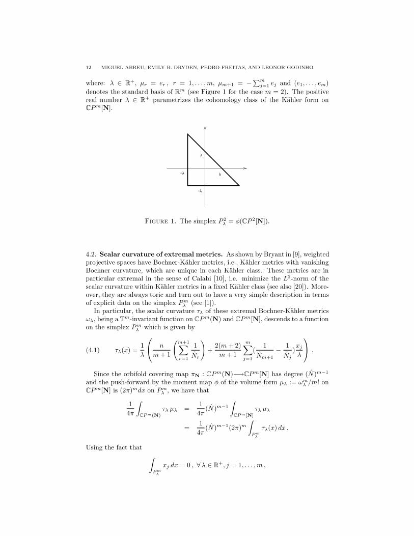
12 MIGUEL ABREU, EMILY B. DRYDEN, PEDRO FREITAS, AND LEONOR GODINHO
where: λ ∈ R+, µr = er , r = 1, . . . , m, µm+1 = −∑mj=1 ej and (e1, . . . , em)
denotes the standard basis of Rm (see Figure 1 for the case m = 2). The positivereal number λ ∈ R+ parametrizes the cohomology class of the Kahler form onCPm[N].
−λ
−λ λ
λ
Figure 1. The simplex P 2λ = φ(CP 2[N]).
4.2. Scalar curvature of extremal metrics. As shown by Bryant in [9], weightedprojective spaces have Bochner-Kahler metrics, i.e., Kahler metrics with vanishingBochner curvature, which are unique in each Kahler class. These metrics are inparticular extremal in the sense of Calabi [10], i.e. minimize the L2-norm of thescalar curvature within Kahler metrics in a fixed Kahler class (see also [20]). More-over, they are always toric and turn out to have a very simple description in termsof explicit data on the simplex Pm
λ (see [1]).In particular, the scalar curvature τλ of these extremal Bochner-Kahler metrics
ωλ, being a Tm-invariant function on CPm(N) and CPm[N], descends to a functionon the simplex Pm
λ which is given by
(4.1) τλ(x) =1
λ
n
m + 1
(
m+1∑
r=1
1
Nr
)
+2(m + 2)
m + 1
m∑
j=1
(1
Nm+1
− 1
Nj
)xj
λ
.
Since the orbifold covering map πN : CPm(N)−→CPm[N] has degree (N)m−1
and the push-forward by the moment map φ of the volume form µλ := ωmλ /m! on
CPm[N] is (2π)mdx on Pmλ , we have that
1
4π
∫
CP m(N)
τλ µλ =1
4π(N)m−1
∫
CP m[N]
τλ µλ
=1
4π(N)m−1(2π)m
∫
P mλ
τλ(x) dx .
Using the fact that
∫
P mλ
xj dx = 0 , ∀λ ∈ R+, j = 1, . . . , m ,
HEARING THE WEIGHTS OF WEIGHTED PROJECTIVE PLANES 13
we then have
1
4π
∫
CP m(N)
τλ µλ = (2π)m−1(N)m−1 m
λ(m + 1)
(
m+1∑
r=1
1
Nr
)
vol(Pmλ )
= (2π)m−1(N)m−2 m
m + 1
(
m+1∑
r=1
Nr
)
vol(Pmλ )
λ
= (2π)m−1(N)m−2 m
m + 1
(
m+1∑
r=1
Nr
)
λm−1vol(Pm1 )
=vol(Pm
1 )1m
N1m
m
m + 1
(
m+1∑
r=1
Nr
)
(
(2πλ)mNm−1vol(Pm1 ))
m−1
m
=vol(Pm
1 )1m
N1m
m
m + 1
(
m+1∑
r=1
Nr
)
(volλ(CPm(N)))m−1
m .
When m = 2 we have that vol(P 21 ) = 9/2 and so
∫
CP 2(N)
c1 ∧ ωλ =1
4π
∫
CP 2(N)
τλ µλ =N1 + N2 + N3√
N1N2N3
√
2volλ(CP 2(N)) ,
which agrees with (3.4) as expected. Note that our normalization of the scalarcurvature is the usual one in Riemannian geometry, which is twice the one oftenused in Kahler geometry.
When m = 2 the integral of the square of the scalar curvature is scale invariant,and so
∫
CP 2(N)
(τλ)2 µλ =
∫
CP 2(N)
(τ1)2 µ1 .
The scalar curvature can be written in this case as
τ1(x) =4
3N1N2N3((N1 + N2 + N3) + 2N3(x1 + x2) − 2N1x1 − 2N2x2) .
Using the fact that∫
P 21
(xi)2 dx =
9
4and
∫
P 21
xixj dx = −9
8, i 6= j ,
one gets∫
CP 2(N)
(τλ)2 µλ = (N1N2N3)(2π)2∫
P 21
(τ1(x))2 dx
= 96π2 N21 + N2
2 + N23
N1N2N3.
5. Heat Invariants
To study the relationship between the geometry and the Laplace spectrum oforbifolds with isolated singularities, we will consider the asymptotic expansion ofthe heat trace K(x, x, t) as t → 0+. The so-called heat invariants appearing in thisexpansion involve geometric quantities such as the dimension, the volume, and thecurvature. For good orbifolds (i.e., those arising as global quotients of manifolds),Donnelly [11] proved the existence of the heat kernel and constructed the asymptoticexpansion for the heat trace. This work was extended to general orbifolds in [14],
14 MIGUEL ABREU, EMILY B. DRYDEN, PEDRO FREITAS, AND LEONOR GODINHO
where the expressions obtained also clarify the contributions of the various pieces ofthe singular set. While [11] and [14] treat the heat trace asymptotics for functions,we will also require the asymptotics for 1-forms. We begin with the function case,extracting the necessary background from [14, §4] and simplifying the expressionswhen possible to reflect the fact that we are only interested in isolated singularities.
Definition. [11] Let h be an isometry of a Riemannian manifold X and let Ω(h)denote the set of (isolated) fixed points of h. For x ∈ Ω(h), define Ah(x) := h∗ :Tx(X)−→Tx(X); note that Ah(x) is non-singular. Set
Bh(x) = (I − Ah(x))−1.
Proposition 5.1. [11] Let (X, g) be a closed Riemannian manifold, let K(t, x, y)be the heat kernel of X, and let h be a nontrivial isometry of X with isolated fixedpoints. Then
∫
XK(t, x, h(x))µg(x) has an asymptotic expansion as t → 0+ of the
form∑
x∈Ω(h)
∞∑
k=0
tk bk(h).
For x ∈ Ω(h), bk(h) depends only on the germs of h and of the Riemannian metricof X at x.
Donnelly gives explicit formulae for b0 and b1 [11, Thm. 5.1] as follows. Allindices run from 1 to n, where n is the dimension of the Riemannian manifoldX . At each point x ∈ Ω(h), choose an orthonormal basis e1, . . . , en of Tx(X).The sign convention on the curvature tensor R of X is chosen so that Rabab is thesectional curvature of the 2-plane spanned by ea and eb. Set
τ =
n∑
a,b=1
Rabab
and
Ricab =
n∑
c=1
Racbc.
Thus τ is the scalar curvature and Ric the Ricci tensor of X . Then
(5.1) b0(h) = |det(Bh(x))|and, summing over repeated indices,
(5.2)
b1(h) = |det(Bh(x))|(
1
6τ +
1
6Rickk +
1
3RiksjBkiBjs
+1
3RiktjBktBji − RkajaBksBjs
)
.
We want to see what the analogous expressions are for orbifolds which are notnecessarily global quotients. We again restrict to the case of orbifolds which haveonly isolated singularities and present the appropriately simplified expressions. LetM be such an orbifold, and choose a singularity x ∈ M . Let (U, V, Γ) be an orbifoldchart for a neighborhood of x, and let γ ∈ Γ. Define
bk(γ) = bk(σ(γ)),
HEARING THE WEIGHTS OF WEIGHTED PROJECTIVE PLANES 15
where σ is an isomorphism from Γ to the isotropy group of a point in the preimageof x under the homeomorphism given by the orbifold chart. That is, we use thecharts to calculate the value of bk locally. Set
Iγ :=
∞∑
k=0
tk bk(γ),
and
Ix :=∑
γ∈Γ
Iγ .
Also set
I0 := (4πt)−dim(M)/2∞∑
k=0
ak(M)tk
where the ak(M) (which we will usually write simply as ak) are the familiar heatinvariants. In particular, a0 = vol(M), a1 = 1
6
∫
Mτ(x)µg , etc. Note that if M
is finitely covered by a Riemannian manifold X , say M = G\X , then ak(M) =1|G|ak(X).
We can now give an expression for the asymptotic expansion of the heat traceof an orbifold M with isolated singularities (see [14] for more details).
Theorem 5.1. [14] Let M be a Riemannian orbifold and let λ1 ≤ λ2 ≤ . . . be thespectrum of the associated Laplacian acting on smooth functions on M . The heattrace
∑∞j=1 e−λjt of M is asymptotic as t → 0+ to
(5.3) I0 +∑
x∈Ω
Ix
|Γ|
where Ω is the set of isolated singularities of M . This asymptotic expansion is ofthe form
(5.4) (4πt)−dim(M)/2∞∑
j=0
cjtj
2 .
Using this expression, we calculate the first few terms in the asymptotic ex-pansion of the heat trace of a 4-dimensional Riemannian orbifold M with isolatedsingularities. Let x ∈ M be a cone point of order N . For any chart (U, V, Γ) aboutx, let γ generate Γ; for j = 1, . . . , N − 1 we have (cf. §2.3)
Aγj = γj∗ =
cos(2jπN ) − sin(2jπ
N ) 0 0
sin(2jπN ) cos(2jπ
N ) 0 0
0 0 cos(2mjπN ) − sin(2mjπ
N )
0 0 sin(2mjπN ) cos(2mjπ
N )
,
for some integer 1 ≤ m < N with (m, N) = 1. Thus
b0(γj) = |det((I − Aγj )−1)| =
1
16 sin2( jπN ) sin2(mjπ
N ).
Hence
Ix =
N−1∑
j=1
1
16 sin2( jπN ) sin2(mjπ
N )+ O(t).
16 MIGUEL ABREU, EMILY B. DRYDEN, PEDRO FREITAS, AND LEONOR GODINHO
Now consider our weighted projective space M := CP 2(N1, N2, N3). Note that
I0 = (4πt)−2∞∑
k=0
ak(M)tk
=1
16π2(a0t
−2 + a1t−1 + a2 + a3t + · · · ).
By Theorem 5.1, we see that the heat trace of M is asymptotic as t → 0+ to
1
16π2(a0t
−2 + a1t−1 + a2) + T + O(t),
where
T =1
N1
N1−1∑
j=1
1
16 sin2(N2jπN1
) sin2(N3jπN1
)+
1
N2
N2−1∑
j=1
1
16 sin2(N1jπN2
) sin2(N3jπN2
)
+1
N3
N3−1∑
j=1
1
16 sin2(N1jπN3
) sin2(N2jπN3
)
and we have replaced the factor m by the appropriate ratios of the Ni’s (see Example2). Hence the coefficient of the term of degree -2 is a0
16π2 , the coefficient of the termof degree -1 is a1
16π2 , and that of the term of degree 0 is a2
16π2 + T . This means thatthe spectrum determines
a0 = vol(M)
a1 =1
6
∫
M
τ(x)µg
and1
360 ∗ 16π2
∫
M
(2||R||2 − 2|Ric|2 + 5τ2)µg + T.
Remark 1. Here, the norm ||.|| is obtained by contracting the tensor with itself,while the norm |.| used in [8] and in §2.4 is the usual norm for antisymmetricproducts of symmetric tensors. Therefore, ||T ∧S|| = 2|T ∧S| for any pair of rank-2symmetric tensors and ||T || = |T |. In particular, ||R|| = 2|R|, while ||Ric|| = |Ric|.
To complete our study of the heat trace asymptotics, we briefly discuss the caseof forms. As Donnelly notes in [12], the results therein “generalize easily to theLaplacian with coefficients in a bundle.” Indeed, by examining [11, 13], we seethat the appropriate coefficient k(p) on the singular part of the heat expansion forforms is
(
np
)
, where n is the dimension of the orbifold M and p is the level of form.
On the smooth part of the expansion, Theorem 3.7.1 of [18] gives a coefficient ofk(p) =
(
np
)
on a0, a coefficient of k0(p) =(
np
)
− 6(
n−2p−1
)
on a1, and coefficients on
the curvature terms appearing in a2 of k1(p) = 2(
np
)
− 30(
n−2p−1
)
+ 180(
n−4p−2
)
, k2(p) =
−2(
np
)
+180(
n−2p−1
)
−720(
n−4p−2
)
, k3(p) = 5(
np
)
−60(
n−2p−1
)
+180(
n−4p−2
)
on ||R||2, |Ric|2, and
τ2, respectively (i.e., a2 = 1360 (4π)−n/2
∫
Mk1(p)||R||2 +k2(p)|Ric|2 +k3(p)τ2µg).
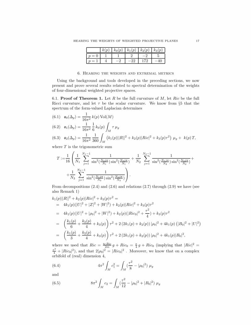
For n = 4, the following table gives the values for these coefficients for p = 0 andp = 1; we will use these values in computations in §6.
HEARING THE WEIGHTS OF WEIGHTED PROJECTIVE PLANES 17
k(p) k0(p) k1(p) k2(p) k3(p)
p = 0 1 1 2 −2 5p = 1 4 −2 −22 172 −40
6. Hearing the weights and extremal metrics
Using the background and tools developed in the preceding sections, we nowpresent and prove several results related to spectral determination of the weightsof four-dimensional weighted projective spaces.
6.1. Proof of Theorem 1. Let R be the full curvature of M , let Ric be the fullRicci curvature, and let τ be the scalar curvature. We know from §5 that thespectrum of the form-valued Laplacian determines
a0(∆p) =1
16π2k(p)Vol(M)(6.1)
a1(∆p) =1
16π2
1
6k0(p)
∫
M
τ µg(6.2)
a2(∆p) =1
16π2
1
360
∫
M
(
k1(p)||R||2 + k2(p)|Ric|2 + k3(p)τ2)
µg + k(p)T,(6.3)
where T is the trigonometric sum
T :=1
16
1
N1
N1−1∑
j=1
1
sin2(N2jπN1
) sin2(N3jπN1
)+
1
N2
N2−1∑
j=1
1
sin2(N1jπN2
) sin2(N3jπN2
)+
+1
N3
N3−1∑
j=1
1
sin2(N1jπN3
) sin2(N2jπN3
)
.
From decompositions (2.4) and (2.6) and relations (2.7) through (2.9) we have (seealso Remark 1)
k1(p)||R||2 + k2(p)|Ric|2 + k3(p)τ2 =
= 4k1(p)(|U |2 + |Z|2 + |W |2) + k2(p)|Ric|2 + k3(p)τ2
= 4k1(p)(|U |2 + |ρ0|2 + |W |2) + k2(p)(|Ric0|2 +τ2
4) + k3(p)τ2
=
(
k1(p)
6+
k2(p)
4+ k3(p)
)
τ2 + 2 (2k1(p) + k2(p)) |ρ0|2 + 4k1(p)(
|B0|2 + |U |2)
=
(
k1(p)
3+
k2(p)
4+ k3(p)
)
τ2 + 2 (2k1(p) + k2(p)) |ρ0|2 + 4k1(p)|B0|2,
where we used that Ric = tr Ric2m g + Ric0 = τ
4 g + Ric0 (implying that |Ric|2 =τ2
4 + |Ric0|2), and that 2|ρ0|2 = |Ric0|2 . Moreover, we know that on a complexorbifold of (real) dimension 4,
(6.4) 4π2
∫
M
c21 =
∫
M
(τ2
8− |ρ0|2) µg
and
(6.5) 8π2
∫
M
c2 =
∫
M
(τ2
12− |ρ0|2 + |B0|2) µg
18 MIGUEL ABREU, EMILY B. DRYDEN, PEDRO FREITAS, AND LEONOR GODINHO
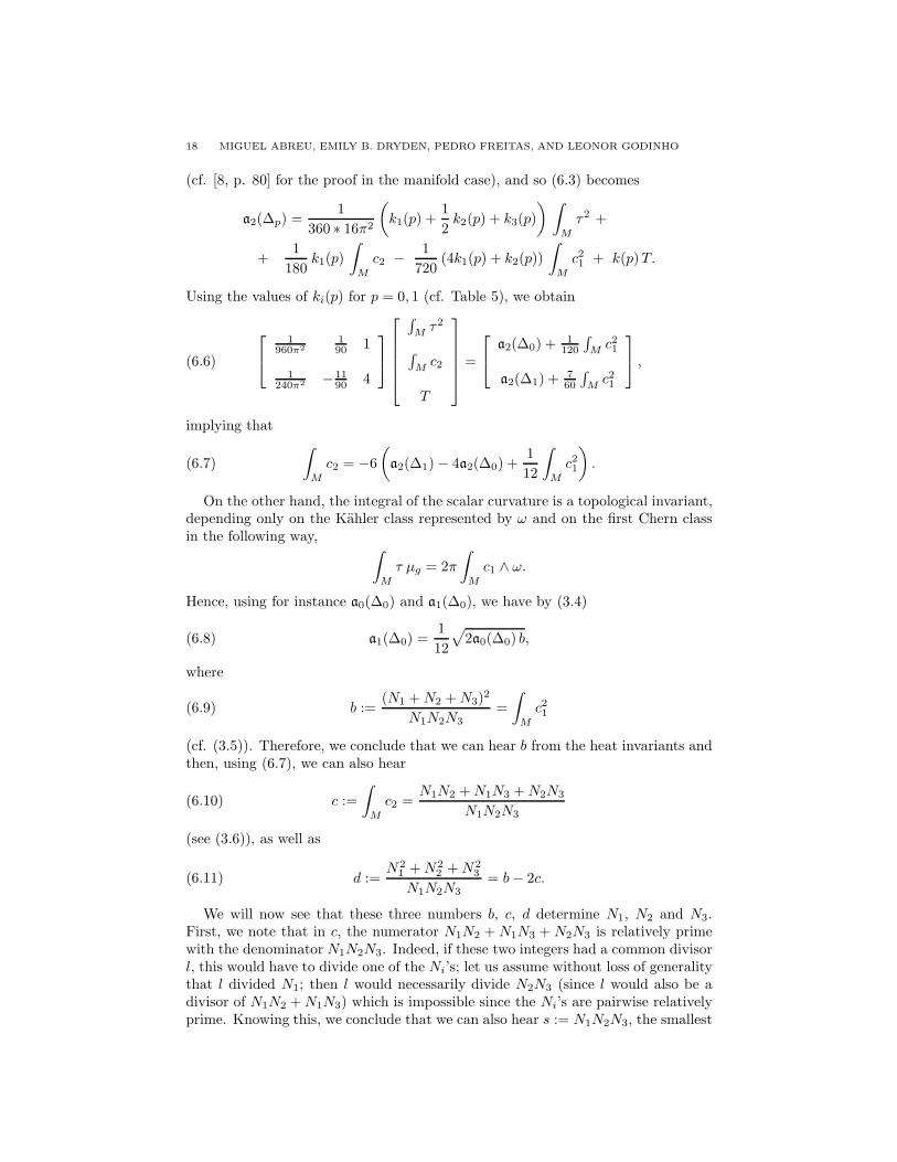
(cf. [8, p. 80] for the proof in the manifold case), and so (6.3) becomes
a2(∆p) =1
360 ∗ 16π2
(
k1(p) +1
2k2(p) + k3(p)
) ∫
M
τ2 +
+1
180k1(p)
∫
M
c2 − 1
720(4k1(p) + k2(p))
∫
M
c21 + k(p)T.
Using the values of ki(p) for p = 0, 1 (cf. Table 5), we obtain
(6.6)
1960π2
190 1
1240π2 − 11
90 4
∫
Mτ2
∫
Mc2
T
=
a2(∆0) + 1120
∫
M c21
a2(∆1) + 760
∫
Mc21
,
implying that
(6.7)
∫
M
c2 = −6
(
a2(∆1) − 4a2(∆0) +1
12
∫
M
c21
)
.
On the other hand, the integral of the scalar curvature is a topological invariant,depending only on the Kahler class represented by ω and on the first Chern classin the following way,
∫
M
τ µg = 2π
∫
M
c1 ∧ ω.
Hence, using for instance a0(∆0) and a1(∆0), we have by (3.4)
(6.8) a1(∆0) =1
12
√
2a0(∆0) b,
where
(6.9) b :=(N1 + N2 + N3)
2
N1N2N3=
∫
M
c21
(cf. (3.5)). Therefore, we conclude that we can hear b from the heat invariants andthen, using (6.7), we can also hear
(6.10) c :=
∫
M
c2 =N1N2 + N1N3 + N2N3
N1N2N3
(see (3.6)), as well as
(6.11) d :=N2
1 + N22 + N2
3
N1N2N3= b − 2c.
We will now see that these three numbers b, c, d determine N1, N2 and N3.First, we note that in c, the numerator N1N2 + N1N3 + N2N3 is relatively primewith the denominator N1N2N3. Indeed, if these two integers had a common divisorl, this would have to divide one of the Ni’s; let us assume without loss of generalitythat l divided N1; then l would necessarily divide N2N3 (since l would also be adivisor of N1N2 + N1N3) which is impossible since the Ni’s are pairwise relativelyprime. Knowing this, we conclude that we can also hear s := N1N2N3, the smallest
HEARING THE WEIGHTS OF WEIGHTED PROJECTIVE PLANES 19
integer that multiplied by c produces an integer, and then, multiplying b, c and dby this number, we hear the integers:
p = N1 + N2 + N3
q = N21 + N2
2 + N23
r = N1N2 + N1N3 + N2N3.
Consider the monic polynomial with roots N1, N2, N3:
(6.12) (y − N1)(y − N2)(y − N3) = y3 − py2 + ry − s.
Since we can hear all the coefficients of this polynomial, we conclude that we canhear the roots, namely N1, N2, N3, up to permutation. Note that (6.12) has aunique triple root if and only if M is a smooth manifold, thus finishing the proofof Theorem 1.
Remark 2. Using the methods of §3 with higher-dimensional weighted projectivespaces M = CPm(N) we can obtain the values of the topological integrals
∫
M
c2 ∧ ωm−2 = (m!Vol(M))m−2
m
∑m+1i,j=1 NiNj
(N1 · · ·Nm+1)2m
,
∫
M
c21 ∧ ωm−2 = (m!Vol(M))
m−2m
(N1 + · · · + Nm+1)2
(N1 · · ·Nm+1)2m
.
Moreover, using ai(∆p) for i, p = 0, 1, 2, the curvature decompositions of §2.4and the expressions
4π2
(m − 2)!
∫
M
c21 ∧ ωm−2 =
∫
M
(
m − 1
4mτ2 − |ρ0|2
)
µg
8π2
(m − 2)!
∫
M
c2 ∧ ωm−2 =
∫
M
(
m − 1
4(m + 1)τ2 − 2(m − 1)
m|ρ0|2 + |B0|2
)
µg
found for instance in [8], we conclude that we can hear∫
M
τ2,
∫
M
c2 ∧ ωm−2 and
∫
M
c21 ∧ ωm−2,
implying that we can hear∑m+1
i,j=1 NiNj
(N1 · · ·Nm+1)2m
and(N1 + · · · + Nm+1)
m
N1 · · ·Nm+1.
To obtain more information on the weights from the Laplace spectra, one couldimpose restrictions on the metric and use higher-order terms of the asymptoticexpansion of the heat trace.
6.2. Hearing weights from the function spectrum. As mentioned in §1, we areunable to extract the weights using only the information provided by the first fewheat invariants for the 0-form spectrum. The recourse to 1-forms was necessitatedby the lack of a closed formula for the value of the trigonometric sum T in termsof the Ni’s. Note that, since
1
sin2 α sin2 β= (1 + cot2 α)(1 + cot2 β) = 1 + cot2 α + cot2 β + cot2 α cot2 β
20 MIGUEL ABREU, EMILY B. DRYDEN, PEDRO FREITAS, AND LEONOR GODINHO
andN−1∑
j=1
cot2(
jπ
N
)
=1
3(N − 1)(N − 3)
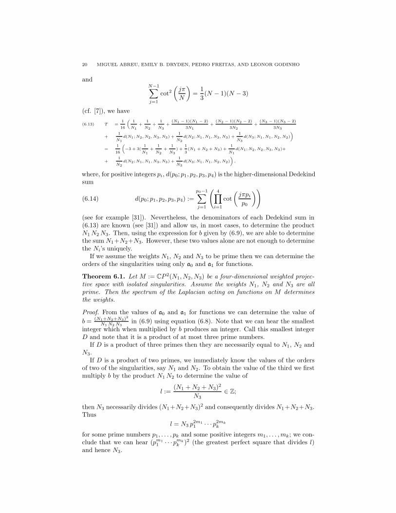
(cf. [7]), we have
T =1
16
„
1
N1
+1
N2
+1
N3
+(N1 − 1)(N1 − 2)
3N1
+(N2 − 1)(N2 − 2)
3N2
+(N3 − 1)(N3 − 2)
3N3
(6.13)
+1
N1
d(N1; N2, N2, N3, N3) +1
N2
d(N2; N1, N1, N3, N3) +1
N3
d(N3; N1, N1, N2, N2)
«
=1
16
„
−3 + 3(1
N1
+1
N2
+1
N3
) +1
3(N1 + N2 + N3) +
1
N1
d(N1; N2, N2, N3, N3)+
+1
N2
d(N2; N1, N1, N3, N3) +1
N3
d(N3; N1, N1, N2, N2)
«
,
where, for positive integers pi, d(p0; p1, p2, p3, p4) is the higher-dimensional Dedekindsum
(6.14) d(p0; p1, p2, p3, p4) :=
p0−1∑
j=1
(
4∏
i=1
cot
(
jπpi
p0
)
)
(see for example [31]). Nevertheless, the denominators of each Dedekind sum in(6.13) are known (see [31]) and allow us, in most cases, to determine the productN1 N2 N3. Then, using the expression for b given by (6.9), we are able to determinethe sum N1+N2+N3. However, these two values alone are not enough to determinethe Ni’s uniquely.
If we assume the weights N1, N2 and N3 to be prime then we can determine theorders of the singularities using only a0 and a1 for functions.
Theorem 6.1. Let M := CP 2(N1, N2, N3) be a four-dimensional weighted projec-tive space with isolated singularities. Assume the weights N1, N2 and N3 are allprime. Then the spectrum of the Laplacian acting on functions on M determinesthe weights.
Proof. From the values of a0 and a1 for functions we can determine the value of
b = (N1+N2+N3)2
N1 N2 N3in (6.9) using equation (6.8). Note that we can hear the smallest
integer which when multiplied by b produces an integer. Call this smallest integerD and note that it is a product of at most three prime numbers.
If D is a product of three primes then they are necessarily equal to N1, N2 andN3.
If D is a product of two primes, we immediately know the values of the ordersof two of the singularities, say N1 and N2. To obtain the value of the third we firstmultiply b by the product N1 N2 to determine the value of
l :=(N1 + N2 + N3)
2
N3∈ Z;
then N3 necessarily divides (N1+N2+N3)2 and consequently divides N1+N2+N3.
Thus
l = N3 p2m1
1 · · · p2mk
k
for some prime numbers p1, . . . , pk and some positive integers m1, . . . , mk; we con-clude that we can hear (pm1
1 · · · pmk
k )2 (the greatest perfect square that divides l)and hence N3.
HEARING THE WEIGHTS OF WEIGHTED PROJECTIVE PLANES 21
Similarly, if D is a product of just one prime, say N1, then we know the valueof the order of one singularity. To retrieve the values of the other two we multiplyb by N1 to obtain
l :=(N1 + N2 + N3)
2
N2 N3∈ Z.
Since (N2, N3) = 1 and l = N2 N3 (pm1
1 · · · pmk
k )2 for some prime numbers p1, . . . , pk
and some positive integers m1, . . . , mk, we can hear the value of the product N2 N3
and consequently of N2 and N3.Finally, if D = 1 (i.e., if b is an integer) then (N1 + N2 + N3)
2 is the product ofN1 N2 N3 by a perfect square and we can again determine N1N2N3 and from thatN1, N2 and N3.
If we remove the restriction that N1, N2 and N3 be prime, we can still determinethe orders of the singularities from a0 and a1 for functions if we fix the Eulercharacteristic of the orbifold. Indeed, if we are given χ(M) := 1
N1+ 1
N2+ 1
N3,
we know the value of c in (6.10) and so, following the argument in the proof ofTheorem 1, we are able to determine s = N1 N2 N3. Assuming we know a0 and a1
we can again determine the value of b in (6.9), using equation (6.8). Then, knowing
b and c allows us to determine d :=N2
1+N22+N2
3
N1N2N3= b − 2c and so we again have the
integers p, q, r and s from the proof of Theorem 1 which allow us to determine N1,N2 and N3. In summary, we have the following theorem.
Theorem 6.2. Let M := CP 2(N1, N2, N3) be a four-dimensional weighted projec-tive space with isolated singularities. If we fix the Euler characteristic of M (i.e.,fix the topological class), then the spectrum of the Laplacian acting on functions onM determines the weights N1, N2, N3.
6.3. Hearing extremal metrics. After determining the values of N1, N2 and N3
we can also hear if a certain metric is extremal (cf. §4.2) from the value of a2.
Theorem 6.3. Let M := CP 2(N1, N2, N3) be a four-dimensional weighted projec-tive space with isolated singularities. Suppose that the values of N1, N2, and N3
are known. Then the value of a2 for the Laplacian acting on functions determineswhether M is endowed with the extremal metric.
Proof. As shown in the proof of Theorem 1 (cf. (6.6)),
(6.15) a2(∆0) =1
960π2
∫
M
τ2 +1
90
∫
M
c2 −1
120
∫
M
c21 + T.
We have explicit expressions for∫
M c2,∫
M c21, and T in terms of N1, N2, and N3
(see (6.9), (6.10)), so using (6.15) we see that we can hear∫
Mτ2 from the value of
a2. If the metric is extremal, we have seen in §4.2 that
(6.16)
∫
M
τ2 = 96π2 N21 + N2
2 + N23
N1N2N3.
Hence, by checking the value we hear for∫
M τ2 against that given by (6.16), wecan see whether M is endowed with the extremal metric. Note that we are usingthe fact that the extremal metric is an absolute minimum for the L2-norm of thescalar curvature among Kahler metrics in a fixed Kahler class.

22 MIGUEL ABREU, EMILY B. DRYDEN, PEDRO FREITAS, AND LEONOR GODINHO
Acknowledgment. The second author thanks the Centro de Analise Matematica,Geometria e Sistemas Dinamicos, Instituto Superior Tecnico, in Lisbon, Portugal,for its support during her work on this project.
References
[1] M. Abreu, Kahler metrics on toric orbifolds, J. Differential Geom. 58 (2001), 151–187.[2] V. Apostolov, D. Calderbank and P. Gauduchon, Hamiltonian 2-forms in Kahler geometry,
I, J. Differential Geom. 73 (2006), 359-412.
[3] M. Atiyah, Convexity and commuting Hamiltonians, Bull. London Math. Soc. 14 (1982),1-15.
[4] M. Atiyah and R. Bott, The moment map and equivariant cohomology, Topology 23 (1984),1-28.
[5] Marcel Berger, Paul Gauduchon, and Edmond Mazet, Le spectre d’une variete riemannienne,Lecture Notes in Mathematics, vol. 194, Springer-Verlag (1971).
[6] N. Berline and M. Vergne, Classes caracteristiques equivariantes. Formule de localisation en
cohomologie equivariante, C. R. Acad. Sci. Paris Ser. I Math. 295 (1982), 539-541.[7] B. Berndt and B. Yeap, Explicit evaluations and reciprocity theorems for finite trigonometric
sums, Adv. in Appl. Math. 29 (2002), 358–385.[8] A. Besse, Einstein manifolds, Ergebnisse der Mathematik und ihrer Grenzgebiete, 10
Springer-Verlag, Berlin-New York, 1987.[9] R. Bryant, Bochner-Kahler metrics, J. Amer. Math. Soc. 14 (2001), 623–715.
[10] E. Calabi, Extremal Kahler metrics, in “Seminar on Differential Geometry” (ed. S.T.Yau),Annals of Math. Studies 102, 259–290, Princeton Univ. Press, 1982.
[11] H. Donnelly, Spectrum and the Fixed Point Sets of Isometries I, Math. Ann. 224 (1976),161-170.
[12] H. Donnelly, Asymptotic expansions for the compact quotients of properly discontinuous
group actions, Illinois J. of Math. 23 (1979), 485-496.[13] H. Donnelly and V.K. Patodi, Spectrum and the fixed point sets of isometries. II, Topology,
16 (1977), 1-11.[14] E. Dryden, C. Gordon, S. Greenwald, Asymptotic Expansion of the Heat Kernel for Orbifolds,
preprint, 2007.[15] Carla Farsi, Orbifold Spectral Theory, Rocky Mountain J. Math., 31 (2001), 215-235.[16] M. Furuta and B. Steer, Seifert fibered homology 3-spheres and the Yang-Mills equations on
Riemann surfaces with marked points, Adv. Math. 96 (1992), 38-102.[17] P. Gauduchon, The Bochner tensor of a weakly Bochner-flat Kahler manifold, An. Univ.
Timisoara Ser. Mat.-Inform. 39 (2001), 189-237.[18] P. Gilkey, Asymptotic formulae in spectral geometry, Studies in Advanced Mathematics, CRC
Press, Boca Raton, FL, 2004.[19] L. Godinho, Classification of symplectic circle actions on 4-orbifolds, in preparation.[20] A. Hwang, On the Calabi energy of extremal Kahler metrics, Internat. J. Math. 6 (1995),
825-830.[21] E. Meinrenken, Symplectic surgery and the Spinc-Dirac operator, Adv. Math. 134 (1998),
240-277.[22] T. Mrowka, P. Ozsvath and B. Yu Seiberg-Witten Monopoles on Seifert Fibered Spaces,
Comm. Anal. Geom. 5 (1997), 685-791.[23] S. Roan, Picard groups of hypersurfaces in toric varieties, Publ. Res. Inst. Math. Sci. 32
(1996), 797-834.[24] T. Sakai, On eigen-values of Laplacian and curvature of Riemannian manifold, Tohoku
Math. J. 23 (1971), 589-603.[25] P. Scott, The geometries of 3-manifolds, Bull. London Math. Soc. 15 (1983), 401-487.[26] H. Seifert, Topologie dreidimensionaler gefaserter Raume, Acta. Math. 60 (1932), 147-283.[27] Naveed Shams, Elizabeth Stanhope, and David L. Webb, One Cannot Hear Orbifold Isotropy
Type, Arch. Math., 87 (2006), 375-384.
[28] Elizabeth A. Stanhope, Spectral Bounds on Orbifold Isotropy, Annals of Global Analysis andGeometry 27 (2005), 355-375.
[29] S. Tanno, Eigenvalues of the Laplacian of Riemannian manifolds, Tohoku Math. J. 25 (1973),391-403.
HEARING THE WEIGHTS OF WEIGHTED PROJECTIVE PLANES 23
[30] S. Tanno, An inequality for 4-dimensional Kahlerian manifolds, Proc. Japan Acad. 49 (1973),257-261.
[31] D. Zagier, Higher dimensional Dedekind sums, Math. Ann. 202 (1973), 149–172.
Centro de Analise Matematica, Geometria e Sistemas Dinamicos, Departamento deMatematica, Instituto Superior Tecnico, Av. Rovisco Pais, 1049-001 Lisboa, Portugal
E-mail address: [email protected]
Department of Mathematics, Bucknell University, Lewisburg, PA 17837, USAE-mail address: [email protected]
Departamento de Matematica, Faculdade de Motricidade Humana (TU Lisbon) andMathematical Physics Group of the University of Lisbon, Complexo Interdisciplinar,Av. Prof. Gama Pinto 2, P-1649-003 Lisboa, Portugal
E-mail address: [email protected]
Centro de Analise Matematica, Geometria e Sistemas Dinamicos, Departamento deMatematica, Instituto Superior Tecnico, Av. Rovisco Pais, 1049-001 Lisboa, Portugal
E-mail address: [email protected]


