Embed Size (px)
Citation preview
Title 0
Heartland Port Project Comprehensive market study 2020
May 2020
Heartland Port Project—Comprehensive market study 2020 i
Contents
Executive summary ............................................................................................................................1
1. Introduction ...................................................................................................................................7
1.1 Objective ............................................................................................................................................. 8
1.2 Structure of the report ........................................................................................................................ 8
1.3 The Heartland Port—project location and study area ........................................................................ 9
2. Freight transportation system in Central Missouri ......................................................................... 10
2.1 Missouri’s freight network ................................................................................................................ 10
2.2 Highways ........................................................................................................................................... 10
2.2 Railroads............................................................................................................................................ 13
2.3 Waterways and public and private ports, marine terminals, and docks .......................................... 13
2.3.1 Marine Highways ....................................................................................................................... 13
2.3.2 Public Port Authorities ............................................................................................................... 15
2.3.3 Private river terminals and docks .............................................................................................. 17
2.3.4 Regional highway connectivity and planned improvements ..................................................... 20
3. Market analysis ............................................................................................................................ 21
3.1 Industry analysis ................................................................................................................................ 21
3.1.1 Market survey—key findings ..................................................................................................... 21
3.1.2 Industries with higher potential to generate traffic for the port .............................................. 25
3.2 State level market trends .................................................................................................................. 25
3.2.1 Non-containerized cargoes ........................................................................................................ 25
3.2.2 Containerized cargoes ................................................................................................................ 27
3.3 Location of freight generators/attractors ......................................................................................... 27
3.3.1 On-farm and commercial grain storage sites ............................................................................. 28
3.3.2 Grain/soybean processors ......................................................................................................... 32
3.3.3 Local livestock and poultry production sites.............................................................................. 33
3.3.4 Ethanol/biodiesel plants ............................................................................................................ 40
3.3.5 Mining sites: metals/nonmetals ................................................................................................ 41
3.3.6 Forestry and lumber ................................................................................................................... 42
3.4 Commodity port flow analysis .......................................................................................................... 44
3.4.1 Soybeans .................................................................................................................................... 45
3.4.2 Corn ............................................................................................................................................ 50
3.4.3 Grain Sorghum ........................................................................................................................... 55
3.4.4 Wheat ......................................................................................................................................... 58
Heartland Port Project—Comprehensive market study 2020 ii
3.5 Market 30-year forecast of non-containerized cargoes ................................................................... 59
3.5.1 Potential non-containerized volumes from the Heartland Port Project study area .................. 59
4. Heartland Port: route economics and key target markets .............................................................. 62
4.1 General Assumptions ........................................................................................................................ 62
4.2 Non-containerized cargoes ............................................................................................................... 64
4.2.1 Incumbent routes ....................................................................................................................... 64
4.2.2 Route costs via incumbent routes (non-containerized)............................................................. 66
4.2.3 Route costs via the Heartland Port Project ................................................................................ 69
4.2.4 Route cost savings offered by the heartland port Project for non-containerized cargo ........... 70
4.2.5 Available non-container volume from the 24-county area ....................................................... 71
4.2.6 Potential market share captured by the Heartland Port ........................................................... 72
4.3 Containerized cargoes ....................................................................................................................... 74
4.3.1 Incumbent routes ....................................................................................................................... 74
4.3.2 Route costs via incumbent routes (containerized) .................................................................... 76
4.3.3 Route costs via the Heartland Port Project ................................................................................ 76
4.3.4 Route cost savings offered by the Heartland Port Project for containerized cargo .................. 77
4.3.5 Containerized cargo market shares and available volume for the 24-county area ................... 79
4.3.6 Potentially divertible intact intermodal imports to the 24-county study area.......................... 82
4.4 Base case volume forecast summary ................................................................................................ 90
5. Conceptual structure of the Heartland Port concession and operational model .............................. 92
5.1 Potential structure of the Heartland Port concession ...................................................................... 92
5.2 Conceptual organizational structure ................................................................................................ 93
5.2.1 Professional staff ........................................................................................................................ 94
5.2.2 Laborers ..................................................................................................................................... 95
5.2.3 Outsourced functions................................................................................................................. 96
5.3 Conceptual operational layout and project site ............................................................................... 96
5.3.1 Berth, facility, and equipment ................................................................................................... 96
5.3.2 Development opportunity A: South Site only ............................................................................ 99
6. Financial analysis ....................................................................................................................... 103
6.1 Description of the financial model .................................................................................................. 103
6.2 Base Case volumes .......................................................................................................................... 105
6.3 Combination of business segments analyzed ................................................................................. 106
6.3.1 Indicative capex ....................................................................................................................... 106
6.3.2 Indicative opex ......................................................................................................................... 109
Heartland Port Project—Comprehensive market study 2020 iii
6.3.3 Handling rates .......................................................................................................................... 111
6.4 Financial analysis ............................................................................................................................. 112
6.4.1 Summary outputs from the financial model ............................................................................ 113
6.5 Key takeaways ................................................................................................................................. 123
7. Environmental regulatory requirements ..................................................................................... 125
7.1 National Environmental Policy Act (NEPA) ..................................................................................... 125
7.1.1 EIS overview ............................................................................................................................. 126
7.1.2 Typical requirements for each stage of the EIS process .......................................................... 126
7.2 The Council on Environmental Quality (CEQ) ................................................................................. 128
7.3 Clean Water Act of 1972 (CWA) ...................................................................................................... 128
7.3.1 The U.S. Army Corps of Engineers (USACE) ............................................................................. 128
7.3.2 Federal Safe Drinking Water Act, Missouri Safe Drinking Water Act ...................................... 130
7.4 Clean Air Act of 1963....................................................................................................................... 130
7.4.1 Air construction permits / new source review permits ........................................................... 131
7.5 Section 106 Tribal Land and Consultation ...................................................................................... 131
7.5.1 The Archeological Historic Preservation Act of 1970 ............................................................... 132
7.5.2 National Historic Preservation Act of 1966 .............................................................................. 132
7.6 Section 7 Fish and Wildlife Service Endangered Species Act .......................................................... 133
7.6.1 Endangered Species Act of 1973 .............................................................................................. 135
7.6.2 Migratory Bird Treaty Act (MBTA) ........................................................................................... 135
7.6.3 Fish and Wildlife Coordination Act .......................................................................................... 137
7.7 Wetlands ......................................................................................................................................... 137
7.7.1 Floodplain management .......................................................................................................... 139
7.8 Missouri Department of Natural Resources (DNR) ......................................................................... 139
7.8.1 Comprehensive Environmental Response, Compensation and Liability Act (CERCLA) ........... 139
7.8.2 Resource Conservation and Recovery Act (RCRA) ................................................................... 140
7.8.3 Missouri Hazardous Waste Management Law ........................................................................ 140
7.8.4 Toxic Substance and Control Act (TSCA) .................................................................................. 140
7.8.5 Missouri Soil Conservation Section 278 ................................................................................... 140
7.8.6 Missouri Solid Waste Management Law.................................................................................. 140
7.9 Missouri Conservation Department ................................................................................................ 140
7.10 Noise impact ................................................................................................................................. 141
7.11 Executive Order 12898: Environmental Justice in Minority and Low-Income Populations ......... 141
7.12 Other laws and regulations ........................................................................................................... 142
Heartland Port Project—Comprehensive market study 2020 iv
Appendix A: Inventory of private river terminals and docks ............................................................ 143
Appendix B: Market survey supporting material ............................................................................. 150
Appendix C: Freight generators/attractors: mines by type ............................................................... 156
Appendix D: Conceptual organizational structure of a mature concessionaire operating the port ..... 160
Appendix E: Standard format for environmental statements ........................................................... 161
Heartland Port Project—Comprehensive market study 2020 v
Figures
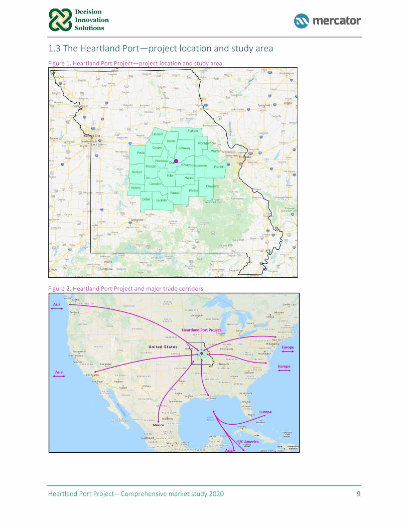
Figure 1. Heartland Port Project—project location and study area .............................................................. 9
Figure 2. Heartland Port Project and major trade corridors .......................................................................... 9
Figure 3. Missouri's Freight Network System .............................................................................................. 11
Figure 4. Highway network serving the movement of freight in Missouri................................................... 12
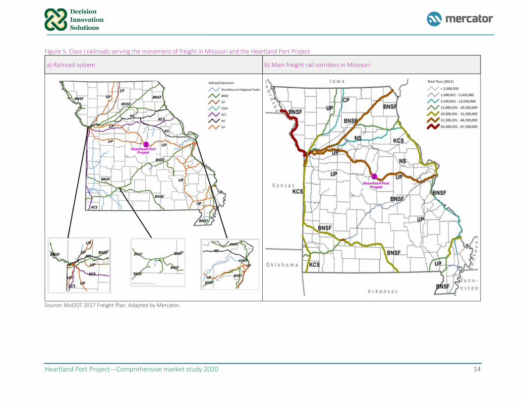
Figure 5. Class I railroads serving the movement of freight in Missouri and the Heartland Port Project .... 14
Figure 6. Private river terminals and docks competitive with the Heartland Port Project by cargo type .... 18
Figure 7. Waterways and public and private ports, terminals, and docks ................................................... 19
Figure 8. 2020-24 CAMPO Transportation Improvement Program ............................................................. 20
Figure 9. Missouri’s total non-containerized import and export volumes, including coal (metric tons) ..... 26
Figure 10. Missouri’s total non-containerized import and export volumes, excluding coal (metric tons) .. 26
Figure 11. State level containerized volumes for Missouri (metric tons) .................................................... 27
Figure 12. On farm grain storage capacity (static), 2012 (000s bushels) ..................................................... 28
Figure 13. Estimated total on-farm storage capacity, 2017-18 marketing year (000s bushels) .................. 29
Figure 14. Estimated total off-farm storage capacity, 2017-18 marketing year (000s bushels) .................. 30
Figure 15. Grain elevators with available transportation mode .................................................................. 31
Figure 16. Estimated soybean processing by county, 2018 (000s bushels) ................................................. 32
Figure 17. Total corn feed demand per county, 2017-18 marketing year (000s bushels) ........................... 33
Figure 18. Net farm corn balance, 2017-18 marketing year (000s bushels) ................................................ 34
Figure 19. Corn deficit county demand points ............................................................................................ 35
Figure 20. Claimed corn supply map ........................................................................................................... 36
Figure 21. Estimated corn export after domestic use allocations ............................................................... 37
Figure 22. Estimated feed mill corn inflow, 2017-18 marketing year (000s bushels) .................................. 38
Figure 23. Feed mill locations, 2019 ............................................................................................................ 39
Figure 24. Ethanol production plants and estimated processing volumes, 2019 (000s bushels) ................ 40
Figure 25. Active mine sites in the state, 2019 ............................................................................................ 41
Figure 26. Total 2017 Corn and Soybean exports, 2017-18 marketing year (000s bushels) ....................... 44
Figure 27. Soybean production, 2017-18 marketing year (000s bushels) ................................................... 45
Figure 28. Estimated net soybean balance by county, 2017-18 marketing year (000s bushels) ................. 46
Figure 29. Total estimated soybeans allocated to exports, 2017-18 marketing year (000s bushels) .......... 47
Figure 30. Soybean production, 2017-18 marketing year (bushels) ............................................................ 48
Figure 31. Soybean exports, 2017-18 marketing year (bushels) ................................................................. 49
Figure 32. Corn available for outflows, 2017-18 marketing year (000s bushels) ........................................ 50
Figure 33. Estimated corn exports, 2017-18 marketing year (000s bushels) .............................................. 51
Figure 34. Corn production, draw area, 2017-18 marketing year (bushels) ................................................ 52
Figure 35. Corn net county inflows, 2017-18 marketing year (bushels) ...................................................... 53
Figure 36. Corn exports, 2017-18 marketing year (bushels) ....................................................................... 54
Figure 37. Grain sorghum production, 2017-18 marketing year (bushels).................................................. 55
Figure 38. Grain sorghum feed, 2017-18 marketing year (bushels) ............................................................ 56
Figure 39. Grain sorghum net county balance, 2017-18 marketing year (bushels) ..................................... 57
Figure 40. Wheat Production, 2017-18 marketing year (bushels) ............................................................... 58
Figure 41. Non-containerized volumes in the 24-county study area—total (million metric tons) .............. 59
Figure 42. Forecast of non-containerized exports for the 24-county study area by commodity (metric tons)
.................................................................................................................................................................... 60
Heartland Port Project—Comprehensive market study 2020 vi
Figure 43. Forecast of non-containerized imports for the 24-county study area by commodity (metric tons)
.................................................................................................................................................................... 61
Figure 44. Heartland Port Project target markets—trade areas by distance to/from the Project .............. 63
Figure 45. Unit capacity by mode of transport, in metric tons .................................................................... 66
Figure 46. Incumbent routes—main rail corridors for non-containerized exports from Missouri .............. 67
Figure 47. Route costs per metric ton (MT) via incumbent routes for non-containerized cargo to Asia, 2020
.................................................................................................................................................................... 68
Figure 48. Route costs per metric ton (MT) via the Heartland Port route for non-containerized cargo to Asia,
2020 ............................................................................................................................................................ 69
Figure 49. Imputed market shares by gateway (at the national level) for the top-5 non-containerized
commodities ................................................................................................................................................ 72
Figure 50. Incumbent intermodal rail routes for containers imported into the Heartland study area ....... 75
Figure 51. Unit capacity by assumed mode of transport, in metric tons and 40 ft containers .................... 76
Figure 52. Route costs via incumbent routes for containerized cargo imports, 2020 ................................. 76
Figure 53. Route costs for imports via the Heartland Port Project—barge and ocean transport cost
assumptions ................................................................................................................................................ 77
Figure 54. Trade Area 1 (0-50 mi)—route cost comparison: incumbent vs new Heartland Port route
(US$/40 ft cont.) .......................................................................................................................................... 78
Figure 55. Map of intact intermodal volumes (in TEUs) cleared at inland US Customs ports in 2019 ........ 81
Figure 56. Shares of US non-energy goods imports by major trade block, 1996-2018 ............................... 85
Figure 57. Scatterplot of GDP to non-energy goods imports, 1996-2018 ................................................... 87
Figure 58. Scatterplots of Real GDP to total port throughput and imports on import-headhaul tradelanes to
total port throughput, 1996-2018 ............................................................................................................... 88
Figure 59. Potential structure of the Heartland Port concession and flow of funds ................................... 93
Figure 60. Conceptual organizational structure of the Heartland Port ....................................................... 94
Figure 61. Typical elements involved in marine river terminal operations .................................................. 98
Figure 62. Development Opportunity A: South Site Only .......................................................................... 100
Figure 63. Modifications the original conceptual site (South Site) adopted by Mercator ......................... 102
Figure 64. Structure of the Heartland Port Project financial model .......................................................... 104
Figure 65. Base Case volume forecast and ramp-up period for non-containerized cargo ........................ 105
Figure 66. Base Case volume forecast and ramp-up for containerized cargo ........................................... 105
Figure 67. Indirect/overhead costs ............................................................................................................ 110
Figure 68. Selling, General Management, and Admin salaries (SG&A) ...................................................... 111
Figure 69. Summary outputs from the financial model: 1–Container and breakbulk (cont+BB) ............... 114
Figure 70. Summary outputs from the financial model: 2–Agribulk .......................................................... 115
Figure 71. Summary outputs from the financial model: 3–Drybulk .......................................................... 116
Figure 72. Summary outputs from the financial model: 4–Liquid bulk ..................................................... 117
Figure 73. Summary outputs from the financial model: 5–Cont+BB+Agribulk .......................................... 118
Figure 74. Summary outputs from the financial model: 6–Cont+BB+Drybulk ........................................... 119
Figure 75. Summary outputs from the financial model: 7–Cont+BB+Liquid bulk ...................................... 120
Figure 76. Summary outputs from the financial model: 8–Cont+BB+Agribulk+Drybulk............................ 121
Figure 77. Summary outputs from the financial model: 8–Cont+BB+Agribulk+Drybulk+Liquid bulk
(conceptual layout fully constructed) ........................................................................................................ 122
Figure 78. EIS process ................................................................................................................................ 126
Figure 79. Regulations under the USACE jurisdiction typically applied to marine river terminals ............. 128
Heartland Port Project—Comprehensive market study 2020 vii
Figure 80. Section 7 Consultation technical assistance process ................................................................ 134
Figure 81. Area definition of the Heartland Project used for this purpose in the IPaC system ................. 134
Figure 82. Inventory of wetlands, riparian, and deepwater habitats in and near the Heartland Port Project
.................................................................................................................................................................. 138
Heartland Port Project—Comprehensive market study 2020 viii
Tables
Table 1. Designated Marine Highways in Missouri ...................................................................................... 13
Table 2. Responses by business type ........................................................................................................... 22
Table 3. Distribution of product/commodity categories ............................................................................. 23
Table 4. Estimates on annual number of shipments or receipts ................................................................. 23
Table 5. Respondents willing to consider barge transportation .................................................................. 24
Table 6. Cost savings threshold by business type ........................................................................................ 24
Table 7. Expectations on shipping and/or receiving volumes ...................................................................... 25
Table 8. Response summary and high potential categories ........................................................................ 25
Table 9. Part names contained in the APHIS database ................................................................................ 42
Table 10. Units of measure.......................................................................................................................... 42
Table 11. Estimated annual exports of forestry and lumber (Missouri and 24-county study area) ............ 43
Table 12. Non-containerized volumes for the 24-county study area (000s metric tons) ............................ 60
Table 13. Route costs via incumbent routes for non-containerized cargo, 2020 ($/metric ton) ................ 69
Table 14. Route cost savings offered by the Heartland Port Project for non-containerized cargo (US$/metric
ton) .............................................................................................................................................................. 70
Table 15. Route cost savings offered by the Heartland Port Project at $6.00/metric ton ........................... 70
Table 16. Imputed market shares by tradelane (at the national level) for the top-5 non-containerized
commodities ................................................................................................................................................ 72
Table 17. Imports and exports of non-containerized cargo by commodity for the 24-counties (000s metric
tons) ............................................................................................................................................................ 73
Table 18. Base Case volume forecast by cargo type from the 24-counties (000, metric tons) ................... 73
Table 19. CAGR of non-containerized cargoes from the 24-counties by cargo type ................................... 74
Table 20. Asia—route cost comparison: incumbent vs. new Heartland Port route (US$/, Box, 40 ft cont.) 77
Table 21. Europe—route cost comparison: incumbent vs. new Heartland Port route (US$/Box, 40 ft cont.)
.................................................................................................................................................................... 78
Table 22. Population and container imports, 2019 ..................................................................................... 82
Table 23. Estimate of initial import volumes for the proposed Heartland Port*......................................... 84
Table 24. Estimate of third-year volumes for the proposed Heartland Port ............................................... 84
Table 25. US non-energy goods imports (nominal USD-millions), 2018-2019 ............................................. 86
Table 26. Base Case 30-year Jefferson City volume forecast....................................................................... 88
Table 27 Exports of containerized cargo by 2-digit NAICS Code and the Top 16 containerized cargos by 2-
digit NAICS code and IMPLAN Code (000s metric tons) .............................................................................. 89
Table 28. Base Case volume forecast by cargo type from the 24-counties (000, metric tons) ................... 90
Table 29. CAGR of non-containerized cargoes from the 24-counties by cargo type ................................... 91
Table 30. Potential market of containerized cargo from the 24-counties (TEUs and Lifts) ......................... 91
Table 31. Startup capex (Yr 0) per business segment or combination of segments modeled (million, $) . 108
Table 32. Gang composition of specialized labor assumed for containers and breakbulk operations (variable
cost) ........................................................................................................................................................... 109
Table 33. Gang composition of specialized labor assumed for bulk operations (variable cost) ................ 109
Table 34. Handling rates used in the financial model ............................................................................... 112
Table 35. Financial modeling results: Base Case volumes (million, $) ....................................................... 113
Table 36. EIS Process ................................................................................................................................. 127
Heartland Port Project—Comprehensive market study 2020 ix
Table 37. Presence of listed, proposed, or candidate endangered species in the Heartland Port Project Area
.................................................................................................................................................................. 135
Table 38. Presence of listed, proposed, or candidate migratory birds in the Heartland Port Project Area
.................................................................................................................................................................. 136
Heartland Port Project—Comprehensive market study 2020 1
Executive summary
The Heartland Port Authority of Central Missouri was created on 2018 in a proactive effort to promote
economic development and marine transportation infrastructure in central Missouri. As part of these
efforts, the Heartland Port Project involves the development of a greenfield public port in the Jefferson City
area, located at the intersection of Callaway and Cole counties. Greenfield projects involve an inherent level
of uncertainty that require the identification and mitigation of potential risks. To assist the Heartland Port
Authority better understand the financial viability of this project, this report presents the findings of a
comprehensive market study and a preliminary assessment of the financial feasibility of the Project.
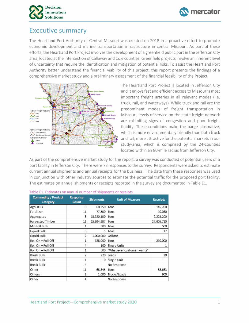
The Heartland Port Project is located in Jefferson City
and it enjoys fast and efficient access to Missouri’s most
important freight arteries in all relevant modes (i.e.
truck, rail, and waterways). While truck and rail are the
predominant modes of freight transportation in
Missouri, levels of service on the state freight network
are exhibiting signs of congestion and poor freight
fluidity. These conditions make the barge alternative,
which is more environmentally friendly than both truck
and rail, more attractive for the potential markets in our
study-area, which is comprised by the 24-counties
located within an 80-mile radius from Jefferson City.
As part of the comprehensive market study for the report, a survey was conducted of potential users of a
port facility in Jefferson City. There were 73 responses to the survey. Respondents were asked to estimate
current annual shipments and annual receipts for the business. The data from these responses was used
in conjunction with other industry sources to estimate the potential traffic for the proposed port facility.
The estimates on annual shipments or receipts reported in the survey are documented in Table E1.
Table E1. Estimates on annual number of shipments or receipts
Heartland Port Project—Comprehensive market study 2020 2
In response to the question on what level of cost saving would be necessary for a respondent to consider
barge transportation, 41% of those answering the question indicated a transportation cost savings of 10%
or less. A cost saving of 20% or less would encourage 67% of those responding to consider barge
transportation. The reported cost savings threshold necessary for a respondent to consider barge
transportation is analyzed in Table 6 of the report.
Our market analysis revealed that there is potential for movement of non-containerized cargo from the 24-
counties via the Heartland Port based on the route cost savings offered by the Heartland Port barge route
to potential port users. Five categories of non-containerized import commodities (Nonmetallic gravels,
stones and minerals; Chemicals and industrial gases; Iron, steel and ferroalloy products; Pesticides,
fertilizers and related agrichem; and nonferrous smelted and refined metals) and five categories of non-
containerized export commodities (soybeans; grains; DDGs; soybean meal; and ethanol) represent the
overall market for which the Heartland Port Project is most likely to attract cargo.
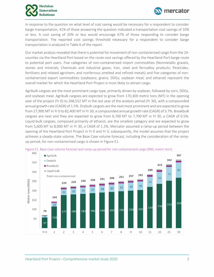
Agribulk cargoes are the most prominent cargo type, primarily driven by soybean, followed by corn, DDGs,
and soybean meal. Agribulk cargoes are expected to grow from 170,300 metric tons (MT) in the opening
year of the project (Yr 0) to 268,552 MT in the last year of the analysis period (Yr 30), with a compounded
annual growth rate (CAGR) of 1.5%. Drybulk cargoes are the next most prominent and are expected to grow
from 27,900 MT in Yr 0 to 82,400 MT in Yr 30, a compounded annual growth rate (CAGR) of 3.7%. Breakbulk
cargoes are next and they are expected to grow from 6,700 MT to 7,700 MT in Yr 30, a CAGR of 0.5%.
Liquid-bulk cargoes, composed primarily of ethanol, are the smallest category and are expected to grow
from 5,600 MT to 8,000 MT in Yr 30, a CAGR of 1.2%. Mercator assumed a ramp-up period between the
opening of the Heartland Port Project in Yr 0 and Yr 3; subsequently, the model assumes that the project
achieves a steady-state volume. The Base Case volume forecast, including the consideration of the ramp-
up period, for non-containerized cargo is shown in Figure E1.
Figure E1. Base Case volume forecast and ramp-up period for non-containerized cargo (000, metric tons)
Heartland Port Project—Comprehensive market study 2020 3
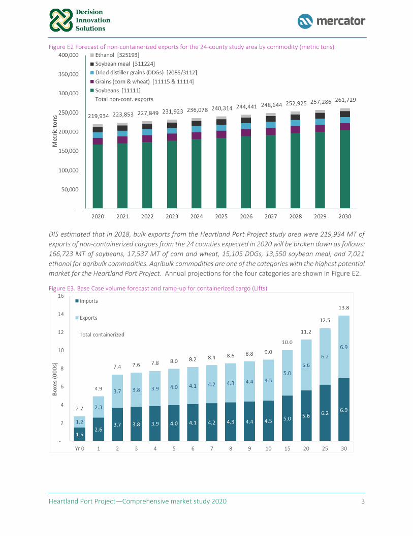
Figure E2 Forecast of non-containerized exports for the 24-county study area by commodity (metric tons)
DIS estimated that in 2018, bulk exports from the Heartland Port Project study area were 219,934 MT of
exports of non-containerized cargoes from the 24 counties expected in 2020 will be broken down as follows:
166,723 MT of soybeans, 17,537 MT of corn and wheat, 15,105 DDGs, 13,550 soybean meal, and 7,021
ethanol for agribulk commodities. Agribulk commodities are one of the categories with the highest potential
market for the Heartland Port Project. Annual projections for the four categories are shown in Figure E2.
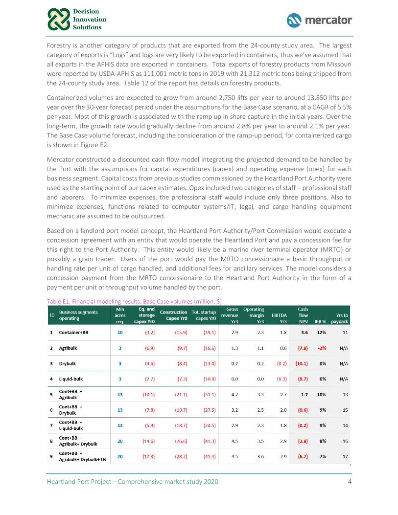
Figure E3. Base Case volume forecast and ramp-up for containerized cargo (Lifts)
Heartland Port Project—Comprehensive market study 2020 4
Forestry is another category of products that are exported from the 24-county study area. The largest
category of exports is “Logs” and logs are very likely to be exported in containers, thus we’ve assumed that
all exports in the APHIS data are exported in containers. Total exports of forestry products from Missouri
were reported by USDA-APHIS as 111,001 metric tons in 2019 with 21,312 metric tons being shipped from
the 24-county study area. Table 12 of the report has details on forestry products.
Containerized volumes are expected to grow from around 2,750 lifts per year to around 13,850 lifts per
year over the 30-year forecast period under the assumptions for the Base Case scenario, at a CAGR of 5.5%
per year. Most of this growth is associated with the ramp up in share capture in the initial years. Over the
long-term, the growth rate would gradually decline from around 2.8% per year to around 2.1% per year.
The Base Case volume forecast, including the consideration of the ramp-up period, for containerized cargo
is shown in Figure E2.
Mercator constructed a discounted cash flow model integrating the projected demand to be handled by
the Port with the assumptions for capital expenditures (capex) and operating expense (opex) for each
business segment. Capital costs from previous studies commissioned by the Heartland Port Authority were
used as the starting point of our capex estimates. Opex included two categories of staff—professional staff
and laborers. To minimize expenses, the professional staff would include only three positions. Also to
minimize expenses, functions related to computer systems/IT, legal, and cargo handling equipment
mechanic are assumed to be outsourced.
Based on a landlord port model concept, the Heartland Port Authority/Port Commission would execute a
concession agreement with an entity that would operate the Heartland Port and pay a concession fee for
this right to the Port Authority. This entity would likely be a marine river terminal operator (MRTO) or
possibly a grain trader. Users of the port would pay the MRTO concessionaire a basic throughput or
handling rate per unit of cargo handled, and additional fees for ancillary services. The model considers a
concession payment from the MRTO concessionaire to the Heartland Port Authority in the form of a
payment per unit of throughput volume handled by the port.
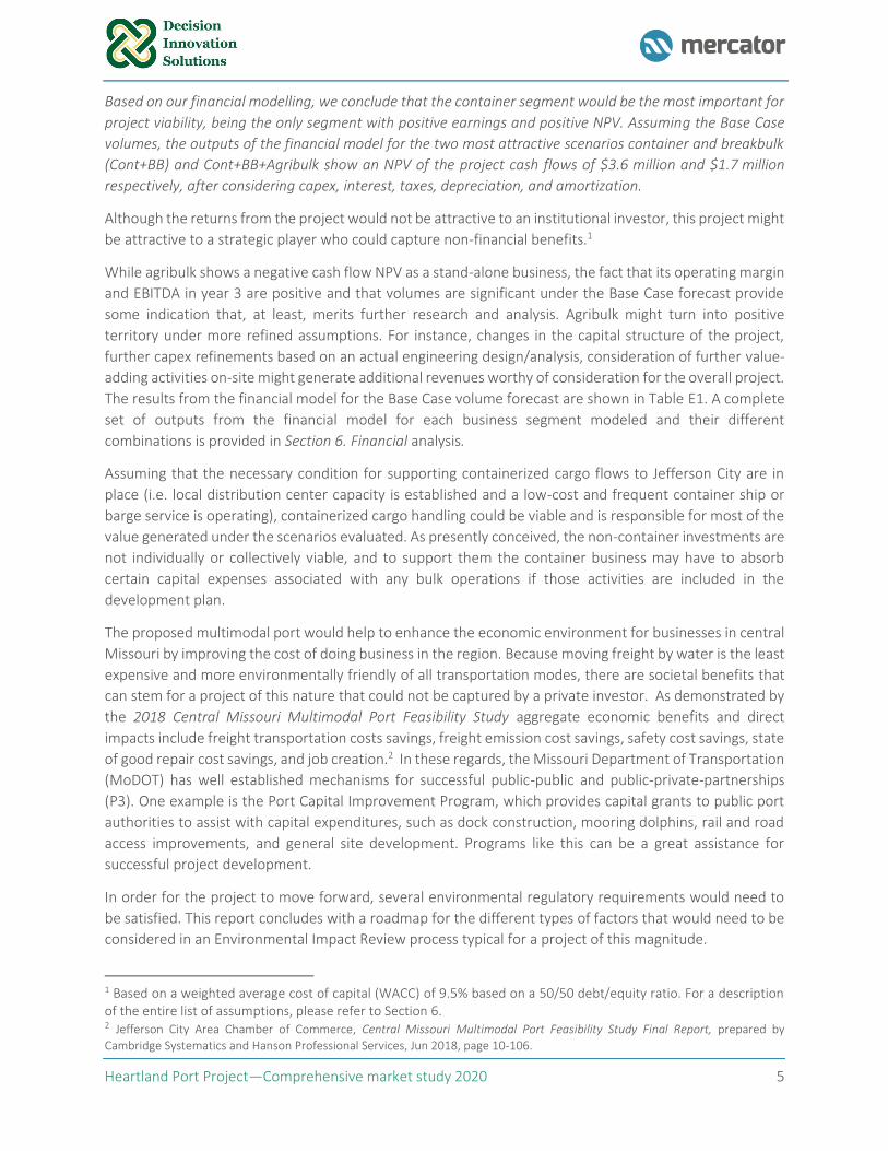
Table E1. Financial modeling results: Base Case volumes (million, $)
Heartland Port Project—Comprehensive market study 2020 5
Based on our financial modelling, we conclude that the container segment would be the most important for
project viability, being the only segment with positive earnings and positive NPV. Assuming the Base Case
volumes, the outputs of the financial model for the two most attractive scenarios container and breakbulk
(Cont+BB) and Cont+BB+Agribulk show an NPV of the project cash flows of $3.6 million and $1.7 million
respectively, after considering capex, interest, taxes, depreciation, and amortization.
Although the returns from the project would not be attractive to an institutional investor, this project might
be attractive to a strategic player who could capture non-financial benefits.1
While agribulk shows a negative cash flow NPV as a stand-alone business, the fact that its operating margin
and EBITDA in year 3 are positive and that volumes are significant under the Base Case forecast provide
some indication that, at least, merits further research and analysis. Agribulk might turn into positive
territory under more refined assumptions. For instance, changes in the capital structure of the project,
further capex refinements based on an actual engineering design/analysis, consideration of further value-
adding activities on-site might generate additional revenues worthy of consideration for the overall project.
The results from the financial model for the Base Case volume forecast are shown in Table E1. A complete
set of outputs from the financial model for each business segment modeled and their different
combinations is provided in Section 6. Financial analysis.
Assuming that the necessary condition for supporting containerized cargo flows to Jefferson City are in
place (i.e. local distribution center capacity is established and a low-cost and frequent container ship or
barge service is operating), containerized cargo handling could be viable and is responsible for most of the
value generated under the scenarios evaluated. As presently conceived, the non-container investments are
not individually or collectively viable, and to support them the container business may have to absorb
certain capital expenses associated with any bulk operations if those activities are included in the
development plan.
The proposed multimodal port would help to enhance the economic environment for businesses in central
Missouri by improving the cost of doing business in the region. Because moving freight by water is the least
expensive and more environmentally friendly of all transportation modes, there are societal benefits that
can stem for a project of this nature that could not be captured by a private investor. As demonstrated by
the 2018 Central Missouri Multimodal Port Feasibility Study aggregate economic benefits and direct
impacts include freight transportation costs savings, freight emission cost savings, safety cost savings, state
of good repair cost savings, and job creation.2 In these regards, the Missouri Department of Transportation
(MoDOT) has well established mechanisms for successful public-public and public-private-partnerships
(P3). One example is the Port Capital Improvement Program, which provides capital grants to public port
authorities to assist with capital expenditures, such as dock construction, mooring dolphins, rail and road
access improvements, and general site development. Programs like this can be a great assistance for
successful project development.
In order for the project to move forward, several environmental regulatory requirements would need to
be satisfied. This report concludes with a roadmap for the different types of factors that would need to be
considered in an Environmental Impact Review process typical for a project of this magnitude.
1 Based on a weighted average cost of capital (WACC) of 9.5% based on a 50/50 debt/equity ratio. For a description of the entire list of assumptions, please refer to Section 6. 2 Jefferson City Area Chamber of Commerce, Central Missouri Multimodal Port Feasibility Study Final Report, prepared by
Cambridge Systematics and Hanson Professional Services, Jun 2018, page 10-106.
Heartland Port Project—Comprehensive market study 2020 6
Overall, the Heartland Port Authority continued work with state and regional economic development
agencies to develop a targeted plan to attract businesses to the port, while at the same time funding
assistance is procured will be crucial for the successful development of this project. Once funding assistance
is secured, the attractiveness of this project for a private investor can be expected to increase substantially,
and the odds for the structuring and implementation of a successful P3 for this project will consequently
increase as well.
Heartland Port Project—Comprehensive market study 2020 7
1. Introduction
Like many other Midwestern states reliant upon infrastructure to move agricultural commodities,
manufactured goods, and raw materials to markets, Missouri’s transportation system needs to be
expanded and, in some cases, upgraded and modernized. The interstate highway system is more than fifty
years old, many of the locks and dams on key river systems date back over seventy years, and the rail
network was originally built in the late 1800s. Agricultural commodities are often transported via multiple
modes and in many cases over a long distance. The same can be said for raw materials (i.e. agribulk and
mineral-bulk commodities) and manufactured goods of many types.
The Mississippi-Missouri River System ranks among the top-5 largest river systems in the world and is the
most important inland waterway in North America, historically serving as the backbone of inland
commercial navigation in the U.S. The immense volume of commerce that takes place along the
Mississippi-Missouri River System has fostered the economic growth of countless cities and communities.
Today, a wide range of industrial products and commodities travel up and down the river system. Upstream
commodity flows are led by sand and gravel, fertilizers, salts, and cement, among others. Downstream
cargo flows are led by grains, which account for most of the volumes for the overall system. The system
represents the main artery for agricultural shipments by barge from the Midwest to New Orleans for export
to destinations worldwide.
Missouri has 1,050 miles of navigable river, including 500 miles on the Mississippi River and 550 miles on
the Missouri River, which are home to 15 public port authorities and more than 200 private river terminals.
Because moving freight by water is the least expensive and more environmentally friendly of all
transportation modes, businesses and industries in Missouri enjoy an unparalleled logistical advantage over
competitors located in areas with no waterways. According to the latest data available from the U.S. Army
Corps of Engineers (USACE), more than 4.5 million metric tons (MT) of freight were shipped through
Missouri ports in 2017, an increase of 80% since 2011.3 Nonetheless, the Missouri River remains under-
utilized, offering great potential to relieve the strain on highways and a competitive, more environmentally
friendly alternative to rail.4
In a proactive effort to promote economic development and marine transportation infrastructure in the
central Missouri region, the Heartland Port Authority of Central Missouri was created in 2018.5 As part of
its mission, the Heartland Port Authority commissioned a study for the Central Missouri Multimodal Port
Project in 2018, which evaluated the market feasibility of logistics-based development opportunities,
developed a conceptual site plan, conducted a benefit-cost analysis (BCA), and quantified the economic
and fiscal impacts arising from the project.6 The Heartland Port Project involves the development of a
public port in the Jefferson City area, located at the intersection of Callaway and Cole counties. The project
considers two sites for the construction of the port facilities: (i) on the north side of the river at the
preexisting OCCI Inc. temporary port, and (ii) on the south side of the river located east of the U.S. National
Guard Facility.
3 US Army Corps of Engineers, Waterborne Commerce National Totals and Selected Inland Waterways for Multiple Years, CY 2017 https://usace.contentdm.oclc.org/utils/getfile/collection/p16021coll2/id/3002.
4 MoDOT, Mo Freight Plan—Missouri Ports and Waterways Network, 2017.
5 Jefferson City Area Chamber of Commerce, MoDOT Port Authority Application—Heartland Port Authority Aug 2018.
6 Jefferson City Area Chamber of Commerce, Central Missouri Multimodal Port Feasibility Study Final Report, prepared by Cambridge Systematics and Hanson Professional Services, Jun 2018.
Heartland Port Project—Comprehensive market study 2020 8
Most, if not all, greenfield projects involve an inherent level of uncertainty that require the identification
and mitigation of potential risks for the project (e.g. unknown cargo capture prospects or volume
commitments for the project, uncertainty in micro- and macro-econometric variables, uncertainty in the
development competitive market environment). Hence, to better understand the viability of this project, it
is critical for the Heartland Port Authority and other project stakeholders to have an analytical framework
that enables them to quantify the potential demand that could realistically be attracted by the Project and
their relationship with its potential financial viability, and better assess the risks of the project.
1.1 Objective
To assist the Heartland Port Authority, the scope of work (SoW) involved several tasks broken down in two
phases:
▪ Phase 1: Comprehensive market study. The objective of this phase was to identify all companies in
a 24-county area that could potentially utilize the Heartland Port for outbound and inbound
shipments, and identify commodity markets and understand how commodities, manufactured
goods, and raw materials flow from producers to markets.
▪ Phase 2: Preliminary assessment of the financial feasibility of the Project. The objective of this
phase was to develop a detailed business model for the port that includes a preliminary analysis of
the potential financial viability of the project based on the commodities with higher potential.
1.2 Structure of the report
This report presents the results of phases 1 and 2 and is structured in seven sections in addition to this
introduction and a set of appendices. These sections are:
▪ Section 1. Proposed Port Development Sites describes the conceptual site plans for the
development opportunities related to this project.
▪ Section 2. Freight Transportation System in Central Missouri provides an overview of the highways,
railroads, and waterways utilized for the movement of freight.
▪ Section 3. Market Analysis presents an overview of the main industries contributing to the
movement of cargo in Missouri and their locations and analyzes the commodities with greater
potential for the port in the short- and long-terms.
▪ Section 4. Heartland Port: route economics and key target markets presents an analysis of the main
target markets for the project and compares key incumbent routes against new, alternates using
the Heartland Port, which substitutes barge for rail on the inland component.
▪ Section 5. Potential Conceptual Structure of the Heartland Port Concession and Operational Model
describes the structure of the concession, a proposed organizational structure for the marine river
terminal concessionaire based on the most promising business segments and describes the overall
project.
▪ Section 6. Potential Levels of Cost Recovery presents the financial analysis of the preliminary
financial viability of the project and a set of potential levels of cost recovery scenarios.
▪ Section 7. Environmental Regulatory Requirements identifies on a preliminary basis the
environmental and regulatory requirements for the project to move forward.
Heartland Port Project—Comprehensive market study 2020 9
1.3 The Heartland Port—project location and study area
Figure 1. Heartland Port Project—project location and study area
Figure 2. Heartland Port Project and major trade corridors
Heartland Port Project—Comprehensive market study 2020 10
2. Freight transportation system in Central Missouri
As with most port projects, the commercial success of the Heartland Port Project will intrinsically be linked
to its ability to generate value for its customers—shippers and beneficial cargo owners (BCOs) moving
target commodities and products—by providing an efficient, reliable, and cost-effective transportation
alternative to their incumbent routes. To maximize the extent of its hinterland reach and successfully
attract volumes, the Heartland Port must demonstrate to its potential customers that substituting barge
transportation on the Missouri-Mississippi River in the their international import and export supply chains
will be superior to rail transport in terms of lower inland transport costs, while not dramatically increasing
or compromising transit-time and reliability. A new route via the Heartland Port and the gateway Port of
New Orleans needs to be a cost-effective to be considered as a potential alternative to incumbent routes.
In order to explore the degree of efficiency of the Heartland Port Project as a transportation alternative,
this section provides an overview of the freight network serving the movement of freight in the state and
assesses the connectivity and accessibility of the Heartland Port Project to the rest of the state’s freight
system. Next, it outlines the main highways and the Class I railroads serving the movement of freight in the
state. This section then presents a comprehensive analysis of public and private ports, marine terminals,
and docks catering to freight along Missouri’s waterways. Lastly, it furnishes a more detailed analysis of the
freight network in the 24 counties that comprise the study area.
2.1 Missouri’s freight network
The Missouri Department of Transportation (MoDOT) defined the freight network for the first time in
2017.7 This network is comprised of highways, rail facilities, ports, airports, pipelines, and intermodal
facilities. As a result, a proposed improvement project must be located on or adjacent to the defined freight
network to be considered in the freight prioritization process for state funding. The Heartland Port Project
is located at the epicenter of the state’s freight network, enjoying access to highways, railroads, and ports,
as illustrated in Figure 3.
2.2 Highways
Truck is the predominant mode of freight transportation in Missouri, closely followed by rail. Missouri’s
highway system comprises 33,700 centerline miles of roadway; however, only 20% are classified as heavily
traveled “major highways”. Major highways include 18 interstate highways, including nine major routes,
and nine auxiliary routes, and they carry about 80% of the overall system’s traffic and a significant portion
of the truck traffic. I-70 and I-44 are the backbone of east-west trade for freight movements destined to
or generated in the central part of the state; these two highways carry the highest volume truck traffic in
the state. I-70 provides connectivity between Kansas City and St. Louis. I-44 connects St. Louis with
Oklahoma. I-49 and I-29 connect the Kansas City metro region and the western part of the state in the
north and south directions. US-61 and I-55 connect the St. Louis region and the eastern part of the state
also in the north and south directions.
7 Missouri Department of Transportation (MoDOT), 2017 Freight Plan.
Heartland Port Project—Comprehensive market study 2020 11
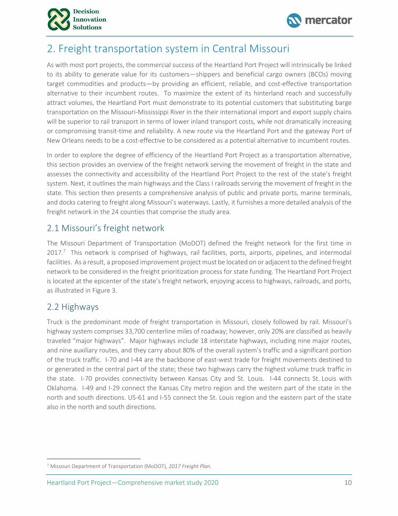
Figure 3. Missouri's Freight Network System
Source: MoDOT 2017 Freight Plan. Adapted by Mercator.
Located 30 miles south from the I-70 corridor in the state’s capital, Jefferson City, the Heartland Port Project
has excellent connectivity to/from major markets and cargo entry/exit points in all directions: it is about
1,000 miles from the East Coast, 1,900 miles from the West Coast, and 900 miles from the Gulf of Mexico.
Inbound and outbound trucks can reach the I-70 corridor in less than one hour when traveling east via the
State Highway 54 or 50 towards St. Louis or in a westerly direction towards Kansas via State Highway 63 or
50. State Highway 63 also provides rapid access to I-44 to the south.
MoDOT’s 2017 Freight Plan reports that about 18% of the total truck traffic is inbound (i.e. coming into the
state) primarily from Wyoming, Illinois, Kansas, Iowa, Arkansas, and Texas; 15% is outbound (i.e. departing
from the state) to Illinois, Texas, Kansas, California, Arkansas, and Iowa; 21% is intrastate (moving between
points within Missouri); and about 46% are trucks just passing through the state. A portion of these flows
are international imports and exports. Furthermore, the Plan reports that the breakdown of the top five
categories of commodities transported by truck are non-metallic materials (21%), secondary traffic (17%),
farm products (16%), food or kindred products (12%), and chemicals or allied products (8%).
Missouri’s highway system, which includes the state’s freight network, and the main freight corridors for
truck traffic are illustrated in Figure 4.
Heartland Port Project—Comprehensive market study 2020 12
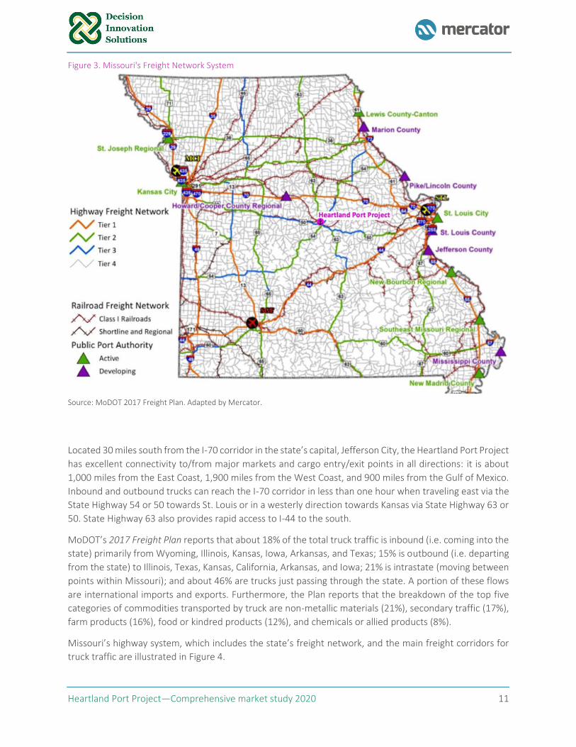
Figure 4. Highway network serving the movement of freight in Missouri
a) Highway system b) Main freight corridors for trucks in Missouri
Source: MoDOT 2017 Freight Plan. Adapted by Mercator.
Heartland Port Project—Comprehensive market study 2020 13
2.2 Railroads
Rail is the second predominant mode of freight transportation in Missouri, closely after truck. Missouri has
a significant freight rail infrastructure with six Class I freight railroads currently operating on 4,218 miles of
main track rail lines and 2,500 miles of yard tracks. Five short-line railroads own and operate a combined
426 miles of track. The UP rail line provides connectivity with two Class I tracks between Kansas City and
the Heartland Port Project, which merge into a single line east of the project towards St. Louis. In Kansas
City, the UP line interchanges with the BNSF, CP, NS, and KCS. In St. Louis, interchanges are available with
the BNSF, NS, and KCS.
Most of the major rail lines in the state are already operating at or near capacity, this includes the UP line
that runs through the Heartland Port Project and connects Kansas City with St. Louis. MoDOT’s 2017 Freight
Plan reports that about 20% of the total rail traffic is inbound (i.e. coming into Missouri), 5% is outbound
(i.e. departing the state), 1% is intrastate, and about 75% is through rail traffic passing through Missouri.
The plan reports that the breakdown of the top five commodity categories transported by rail are coal
(49%), food or kindred products (9%), chemicals or allied products (8%), miscellaneous mixed shipments
(8%), and farm products (8%).
In addition to delays and congestion on the rail lines due to operations being at near capacity, another
concern is at-grade rail crossings, which can represent potential roadway safety and delay issues.
Ownership of the Class I main rail lines and the major rail corridors serving the movement of freight in
Missouri are illustrated in Figure 5.
2.3 Waterways and public and private ports, marine terminals, and docks
Missouri is traversed by 550 miles of the Missouri River and 500 miles of the Mississippi River from north
to south. The Missouri converges into the Mississippi at St. Louis and provides uninterrupted flow
southbound into New Orleans’ ports in the Gulf of Mexico. There are more than 200 public and private
river ports and marine terminals in the state. This section presents a comprehensive analysis of Missouri’s
marine highways, public port authorities, and private ports, river terminals, and docks to better understand
the competitive environment in which the Heartland Port can be expected to operate.
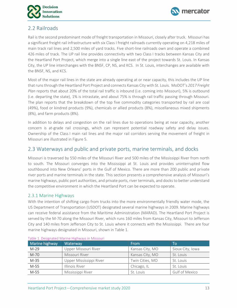
2.3.1 Marine Highways With the intention of shifting cargo from trucks into the more environmentally friendly water mode, the
US Department of Transportation (USDOT) designated several marine highways in 2009. Marine highways
can receive federal assistance from the Maritime Administration (MARAD). The Heartland Port Project is
served by the M-70 along the Missouri River, which runs 160 miles from Kansas City, Missouri to Jefferson
City and 140 miles from Jefferson City to St. Louis where it connects with the Mississippi. There are four
marine highways designated in Missouri, shown in Table 1.
Table 1. Designated Marine Highways in Missouri
Marine highway Waterway From To
M-29 Upper Missouri River Kansas City, MO Sioux City, Iowa
M-70 Missouri River Kansas City, MO St. Louis
M-35 Upper Mississippi River Twin Cities, MO St. Louis
M-55 Illinois River Chicago, IL St. Louis
M-55 Mississippi River St. Louis Gulf of Mexico
Heartland Port Project—Comprehensive market study 2020 14
Figure 5. Class I railroads serving the movement of freight in Missouri and the Heartland Port Project
a) Railroad system b) Main freight rail corridors in Missouri
Source: MoDOT 2017 Freight Plan. Adapted by Mercator.
Heartland Port Project—Comprehensive market study 2020 15
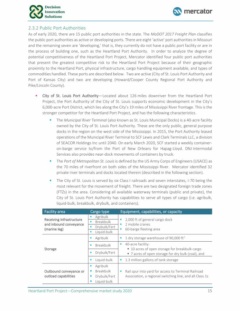
2.3.2 Public Port Authorities As of early 2020, there are 15 public port authorities in the state. The MoDOT 2017 Freight Plan classifies
the public port authorities as active or developing ports. There are eight ‘active’ port authorities in Missouri
and the remaining seven are ‘developing,’ that is, they currently do not have a public port facility or are in
the process of building one, such as the Heartland Port Authority. In order to analyze the degree of
potential competitiveness of the Heartland Port Project, Mercator identified four public port authorities
that present the greatest competitive risk to the Heartland Port Project because of their geographic
proximity to the Heartland Port, physical infrastructure, cargo handling equipment available, and types of
commodities handled. These ports are described below. Two are active (City of St. Louis Port Authority and
Port of Kansas City) and two are developing (Howard/Cooper County Regional Port Authority and
Pike/Lincoln County).
▪ City of St. Louis Port Authority—Located about 126 miles downriver from the Heartland Port
Project, the Port Authority of the City of St. Louis supports economic development in the City’s
6,000-acre Port District, which lies along the City’s 19 miles of Mississippi River frontage. This is the
stronger competitor for the Heartland Port Project, and has the following characteristics.
▪ The Municipal River Terminal (also known as St. Louis Municipal Docks) is a 40-acre facility
owned by the City of St. Louis Port Authority. These are the only public, general purpose
docks in the region on the west side of the Mississippi. In 2015, the Port Authority leased
operations of the Municipal River Terminal to SCF Lewis and Clark Terminals LLC, a division
of SEACOR Holdings Inc until 2040. On early March 2020, SCF started a weekly container-
on-barge service to/from the Port of New Orleans for Hapag-Lloyd. DNJ Intermodal
Services also provides near-dock movements of containers by truck.
▪ The Port of Metropolitan St. Louis is defined by the US Army Corps of Engineers (USACE) as
the 70 miles of riverfront on both sides of the Mississippi River. Mercator identified 32
private river terminals and docks located therein (described in the following section).
▪ The City of St. Louis is served by six Class I railroads and seven interstates, I-70 being the
most relevant for the movement of freight. There are two designated foreign trade zones
(FTZs) in the area. Considering all available waterway terminals (public and private), the
City of St. Louis Port Authority has capabilities to serve all types of cargo (i.e. agribulk,
liquid-bulk, breakbulk, drybulk, and containers).
Facility area Cargo type Equipment, capabilities, or capacity
Receiving Infrastructure and inbound conveyance (marine leg)
▪ Agribulk ▪ 2,000 ft of general cargo dock ▪ 2 mobile cranes ▪ 60-barge fleeting area
▪ Breakbulk
▪ Drybulk/Fert
▪ Liquid-bulk
Storage
▪ Agribulk ▪ 1 dry storage warehouse of 90,000 ft2
▪ Breakbulk ▪ 40-acre facility: ▪ 10 acres of open storage for breakbulk cargo ▪ 7 acres of open storage for dry bulk (coal), and ▪ Drybulk/Fert
▪ Liquid-bulk ▪ 1.3 million gallons of tank storage
Outbound conveyance or outload capabilities
▪ Agribulk
▪ Rail spur into yard for access to Terminal Railroad Association, a regional switching line, and all Class 1s
▪ Breakbulk ▪ Drybulk/Fert ▪ Liquid-bulk
Heartland Port Project—Comprehensive market study 2020 16
▪ Howard/Cooper County Regional Port Authority—Located in Boonville County about 50 miles
upriver from the Heartland Port Project, and situated on less than 1/3 of an acre, it is the only
public facility between Kansas City and St. Louis. The local media reports that the last outbound
barge left port in November 2016.8 MoDOT is providing funding to construct a new dock 100 yards
east of the current port on 18 acres that the port secured; some parts of the existing port will
continue being used.9 This port has the following characteristics.
Facility area Cargo type Equipment, capabilities, or capacity
Receiving Infrastructure and inbound conveyance (marine leg)
▪ Agribulk ▪ General cargo dock with liquid cargo capabilities ▪ A 50-ton crane, and ▪ A 25-ton crane (all located on a floating dock)
▪ Liquid-bulk
▪ Breakbulk
▪ Drybulk/Fert
Storage
▪ Agribulk ▪ 250,000 bushels of grain (about 6,800 MT)
▪ Liquid-bulk ▪ 4 million gallons of liquid chemicals
▪ Breakbulk ▪ 2 dry storage buildings and a 15,000-ton outside storage pad available. ▪ Drybulk/Fert
Outbound conveyance or outload capabilities
▪ Agribulk ▪ Loaders, dump trucks, conveyors and repair equipment available
▪ Within one mile of the Missouri Pacific Railroad, which connects to the main UP branch
▪ Liquid-bulk
▪ Breakbulk
▪ Drybulk/Fert
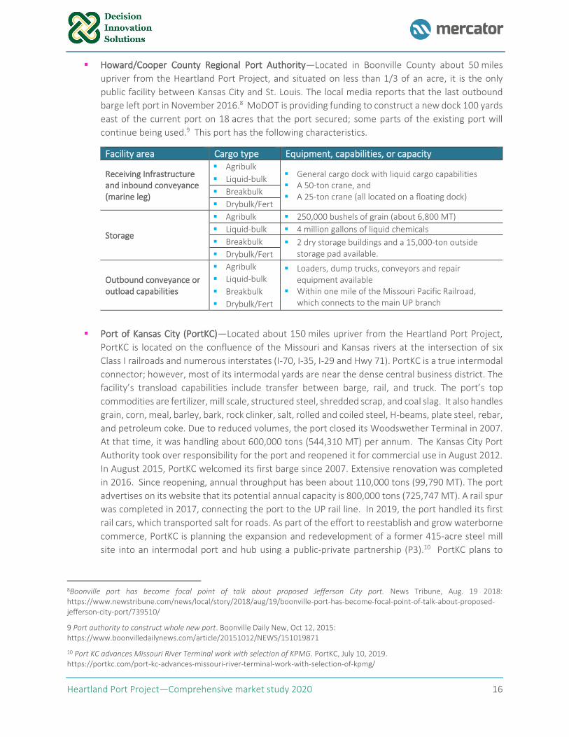
▪ Port of Kansas City (PortKC)—Located about 150 miles upriver from the Heartland Port Project,
PortKC is located on the confluence of the Missouri and Kansas rivers at the intersection of six
Class I railroads and numerous interstates (I-70, I-35, I-29 and Hwy 71). PortKC is a true intermodal
connector; however, most of its intermodal yards are near the dense central business district. The
facility’s transload capabilities include transfer between barge, rail, and truck. The port’s top
commodities are fertilizer, mill scale, structured steel, shredded scrap, and coal slag. It also handles
grain, corn, meal, barley, bark, rock clinker, salt, rolled and coiled steel, H-beams, plate steel, rebar,
and petroleum coke. Due to reduced volumes, the port closed its Woodswether Terminal in 2007.
At that time, it was handling about 600,000 tons (544,310 MT) per annum. The Kansas City Port
Authority took over responsibility for the port and reopened it for commercial use in August 2012.
In August 2015, PortKC welcomed its first barge since 2007. Extensive renovation was completed
in 2016. Since reopening, annual throughput has been about 110,000 tons (99,790 MT). The port
advertises on its website that its potential annual capacity is 800,000 tons (725,747 MT). A rail spur
was completed in 2017, connecting the port to the UP rail line. In 2019, the port handled its first
rail cars, which transported salt for roads. As part of the effort to reestablish and grow waterborne
commerce, PortKC is planning the expansion and redevelopment of a former 415-acre steel mill
site into an intermodal port and hub using a public-private partnership (P3).10 PortKC plans to
8Boonville port has become focal point of talk about proposed Jefferson City port. News Tribune, Aug. 19 2018: https://www.newstribune.com/news/local/story/2018/aug/19/boonville-port-has-become-focal-point-of-talk-about-proposed-jefferson-city-port/739510/
9 Port authority to construct whole new port. Boonville Daily New, Oct 12, 2015: https://www.boonvilledailynews.com/article/20151012/NEWS/151019871
10 Port KC advances Missouri River Terminal work with selection of KPMG. PortKC, July 10, 2019. https://portkc.com/port-kc-advances-missouri-river-terminal-work-with-selection-of-kpmg/
Heartland Port Project—Comprehensive market study 2020 17
eventually develop the site for intermodal, light manufacturing and freight distribution. Key
attributes are listed next.
Facility area Cargo type Equipment, capabilities, or capacity
Receiving Infrastructure and inbound conveyance (marine leg)
▪ Agribulk ▪ 3 load cells and docking structures for 14 barges (on 900-feet of shoreline)
▪ 3 cranes (25-ton) ▪ 8 front-end loaders ▪ Portable conveyor systems
▪ Breakbulk
▪ Drybulk/Fert
Storage
▪ Agribulk ▪ 60,000 tons of covered storage ▪ Open storage space
▪ Breakbulk ▪ Open storage space
▪ Drybulk/Fert ▪ Open storage space ▪ 145 acres of vacant land available for expansion
Outbound conveyance or outload capabilities
▪ Agribulk ▪ Loaders, dump trucks, conveyors ▪ On-site truck scale ▪ Connects to the main UP branch on-dock
▪ Breakbulk
▪ Drybulk/Fert
▪ Pike/Lincoln County—Located on the Mississippi River about 90 miles upriver from St. Louis, Pike
and Lincoln counties were awarded Port Authority Designation in February 2011 from the MoDOT
Waterways Division. The Pike Lincoln County Port Authority recently purchased 24.5 acres of land
outside of Louisiana, Missouri for terminal development. Consequently, this is considered a
developing port. Several businesses in the region already utilize barge service via the Mississippi.
Both Pike and Lincoln counties have access to several major highways in all directions: US highways
61, 54, and State Highway 79; I-70 is the nearest interstate. For rail, KCS runs through both Kansas
City and St. Louis, where there are multiple interchanges. BNSF runs north to south with access in
both Pike and Lincoln counties.
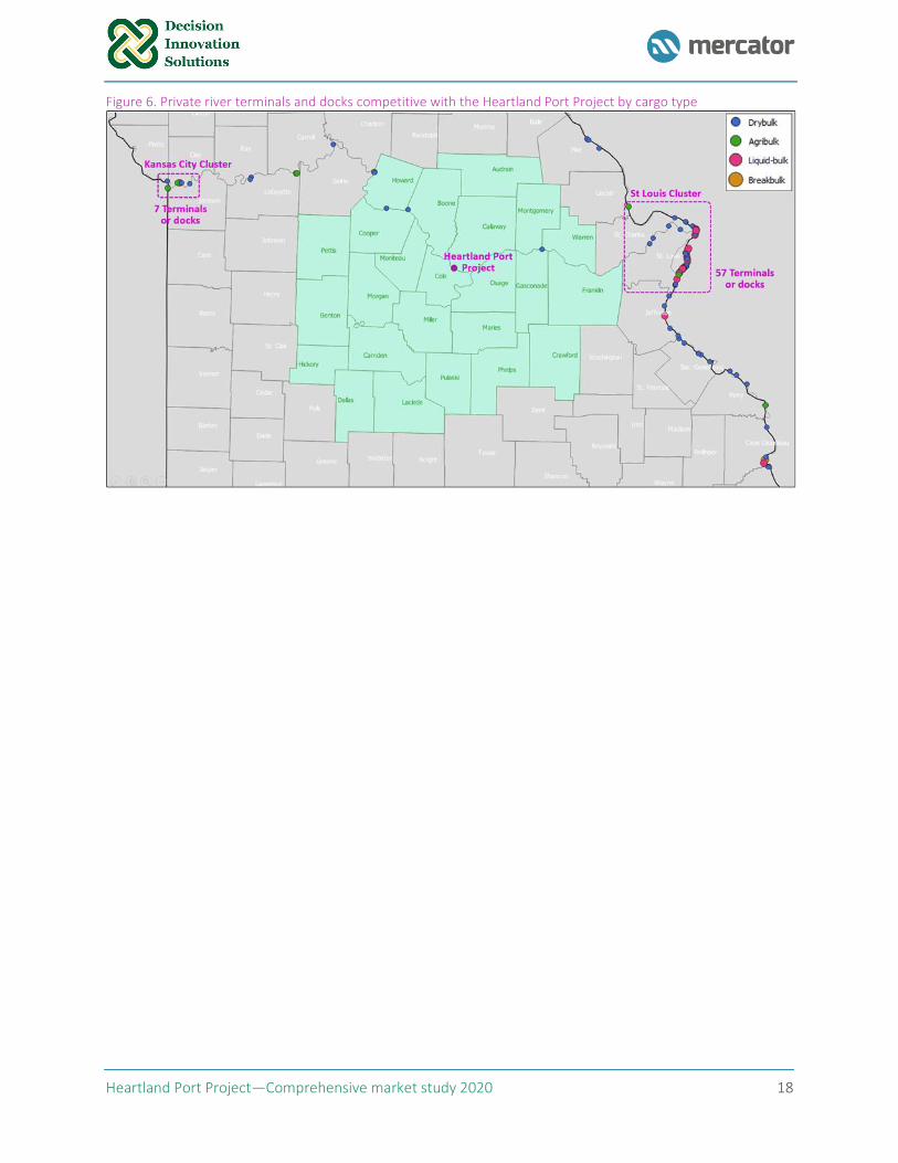
2.3.3 Private river terminals and docks Mercator identified more than 200 waterway facilities (nodes) from the USACE database. This database
was processed in multiple iterations to remove non-cargo facilities, such as dredging zones and abandoned
or non-functional terminals/docks. A visual inspection was performed utilizing aerial imagery from Google
Maps. The resulting database accounts for 84 private ports, river terminals, and docks that Mercator
assumed to be operational. Based on their physical characteristics, as observed in the aerial imagery
inspections, their company name, and reported commodities handled, Mercator classified these facilities
into four major commodity groups: (i) agribulk, (ii) drybulk/fertilizer, (iii) liquid-bulk, and (iv) breakbulk.
Only the SCF facility in St. Louis reported movements of containers on barge.
Similar to the public port authorities, Mercator identified 104 facilities that, due to their geographic
proximity to the project, facilities and equipment available, and major commodities handled, offer the
greatest potential to compete with the Heartland Port Project. These active and developing private facilities
are included in Figure 6, followed by comprehensive maps of the public port authorities and the private
river terminals and docks in Figure 7.
Heartland Port Project—Comprehensive market study 2020 18
Figure 6. Private river terminals and docks competitive with the Heartland Port Project by cargo type
Heartland Port Project—Comprehensive market study 2020 19
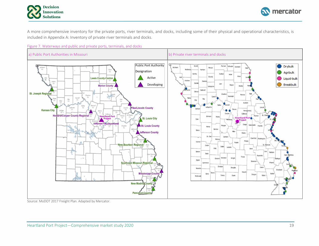
A more comprehensive inventory for the private ports, river terminals, and docks, including some of their physical and operational characteristics, is
included in Appendix A: Inventory of private river terminals and docks.
Figure 7. Waterways and public and private ports, terminals, and docks
a) Public Port Authorities in Missouri b) Private river terminals and docks
Source: MoDOT 2017 Freight Plan. Adapted by Mercator.
Heartland Port Project—Comprehensive market study 2020 20
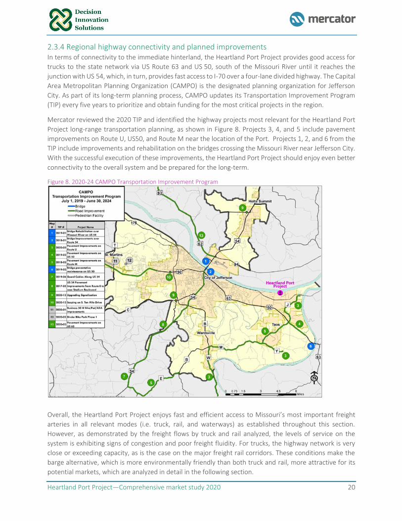
2.3.4 Regional highway connectivity and planned improvements In terms of connectivity to the immediate hinterland, the Heartland Port Project provides good access for
trucks to the state network via US Route 63 and US 50, south of the Missouri River until it reaches the
junction with US 54, which, in turn, provides fast access to I-70 over a four-lane divided highway. The Capital
Area Metropolitan Planning Organization (CAMPO) is the designated planning organization for Jefferson
City. As part of its long-term planning process, CAMPO updates its Transportation Improvement Program
(TIP) every five years to prioritize and obtain funding for the most critical projects in the region.
Mercator reviewed the 2020 TIP and identified the highway projects most relevant for the Heartland Port
Project long-range transportation planning, as shown in Figure 8. Projects 3, 4, and 5 include pavement
improvements on Route U, US50, and Route M near the location of the Port. Projects 1, 2, and 6 from the
TIP include improvements and rehabilitation on the bridges crossing the Missouri River near Jefferson City.
With the successful execution of these improvements, the Heartland Port Project should enjoy even better
connectivity to the overall system and be prepared for the long-term.
Figure 8. 2020-24 CAMPO Transportation Improvement Program
Overall, the Heartland Port Project enjoys fast and efficient access to Missouri’s most important freight
arteries in all relevant modes (i.e. truck, rail, and waterways) as established throughout this section.
However, as demonstrated by the freight flows by truck and rail analyzed, the levels of service on the
system is exhibiting signs of congestion and poor freight fluidity. For trucks, the highway network is very
close or exceeding capacity, as is the case on the major freight rail corridors. These conditions make the
barge alternative, which is more environmentally friendly than both truck and rail, more attractive for its
potential markets, which are analyzed in detail in the following section.

Heartland Port Project—Comprehensive market study 2020 21
3. Market analysis
This section presents the outputs of the comprehensive market study corresponding to Phase 1. The
objective of this phase is to identify all companies that could potentially utilize the Heartland Port for
outbound and inbound shipments of commodities, final products, and raw materials. Phase 1 aims to
identify commodity markets and understand how commodities, manufactured goods, and raw materials
flow from producers to markets. With geographic and industrial scope determined, this section summarizes
the main findings from a survey circulated among the potential users of the Port, aiming to identify the
industries with the higher potential to generate traffic for the Port. This section then presents an analysis
of the locations of the main freight generators/attractors in the state, focusing on those commodities with
a high potential to be attracted by the Port. Subsequently, a port flow analysis is described that identifies
potential volumes in the primary hinterland to be served by the Heartland Port Project. Lastly, we present
our 30-year forecast for the overall market (before analyzing any potential capture rates by the port, which
are analyzed in Section 6).
3.1 Industry analysis
Movement of processed grain and oilseeds is largely determined by location of ethanol/biodiesel plants,
local livestock and poultry production, and size, location and nature of export markets. With geographic
and industrial scope determined, a series of questions will be answered through a survey of potential users
of the Port. These questions, once answered (or as they’re answered in a few instances), will inform Phase
2 of the project. A significant portion of the data for this phase was gathered through direct contacts
(primary research) with producers, manufacturers and consumers of incoming commodities. Depending on
the number of identified businesses, a sample of the group was contacted for input on these questions.
3.1.1 Market survey—key findings The primary research component of the market study (i.e. a set of questions) was organized into three
logical groups. The first group included any data collected about the content of inbound and outbound
shipments in the 24-county study area. The second group included the current status of inbound and
outbound shipments to and from businesses in the study area. The third examined the potential changes
to the current status resulting from adding a new port to the infrastructure of the study area. A copy of
the survey instrument utilized with the questions included within each group are included in Appendix B:
Market survey supporting material.
Survey methodology
A list of businesses within the study area that met at least one of the NAICS Code11 criteria was created
from an internal list maintained by DIS, a business information database maintained by Info USA, and a
membership list provided by the Missouri Forest Products Association. The Info USA list was filtered by
business size to eliminate smaller businesses. The final list contained 2,107 business addresses.
A random selection process was used to identify survey recipients. The selection process included criteria
to make sure all relevant NAICS code groups were represented. An online survey was created and
invitations to participate were sent to 243 businesses. A second invitation and phone calls were initiated.
Survey responses were received from 73 respondents, which represent a 31.7% response rate.
11 The North American Industry Classification System (NAICS) is the standard used by Federal statistical agencies in classifying establishments for the purpose of collecting, analyzing, and publishing statistical data related to the U.S. business economy.
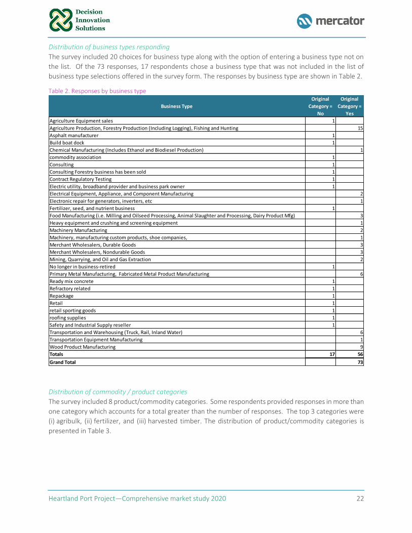
Heartland Port Project—Comprehensive market study 2020 22
Distribution of business types responding
The survey included 20 choices for business type along with the option of entering a business type not on
the list. Of the 73 responses, 17 respondents chose a business type that was not included in the list of
business type selections offered in the survey form. The responses by business type are shown in Table 2.
Table 2. Responses by business type
Distribution of commodity / product categories
The survey included 8 product/commodity categories. Some respondents provided responses in more than
one category which accounts for a total greater than the number of responses. The top 3 categories were
(i) agribulk, (ii) fertilizer, and (iii) harvested timber. The distribution of product/commodity categories is
presented in Table 3.
Business Type
Original
Category =
No
Original
Category =
Yes
Agriculture Equipment sales 1
Agriculture Production, Forestry Production (Including Logging), Fishing and Hunting 15
Asphalt manufacturer 1
Build boat dock 1
Chemical Manufacturing (Includes Ethanol and Biodiesel Production) 1
commodity association 1
Consulting 1
Consulting Forestry business has been sold 1
Contract Regulatory Testing 1
Electric utility, broadband provider and business park owner 1
Electrical Equipment, Appliance, and Component Manufacturing 2
Electronic repair for generators, inverters, etc 1
Fertilizer, seed, and nutrient business 1
Food Manufacturing (i.e. Milling and Oilseed Processing, Animal Slaughter and Processing, Dairy Product Mfg) 3
Heavy equipment and crushing and screening equipment 1
Machinery Manufacturing 2
Machinery, manufacturing custom products, shoe companies, 1
Merchant Wholesalers, Durable Goods 3
Merchant Wholesalers, Nondurable Goods 3
Mining, Quarrying, and Oil and Gas Extraction 2
No longer in business-retired 1
Primary Metal Manufacturing , Fabricated Metal Product Manufacturing 6
Ready mix concrete 1
Refractory related 1
Repackage 1
Retail 1
retail sporting goods 1
roofing supplies 1
Safety and Industrial Supply reseller 1
Transportation and Warehousing (Truck, Rail, Inland Water) 6
Transportation Equipment Manufacturing 1
Wood Product Manufacturing 9
Totals 17 56
Grand Total 73
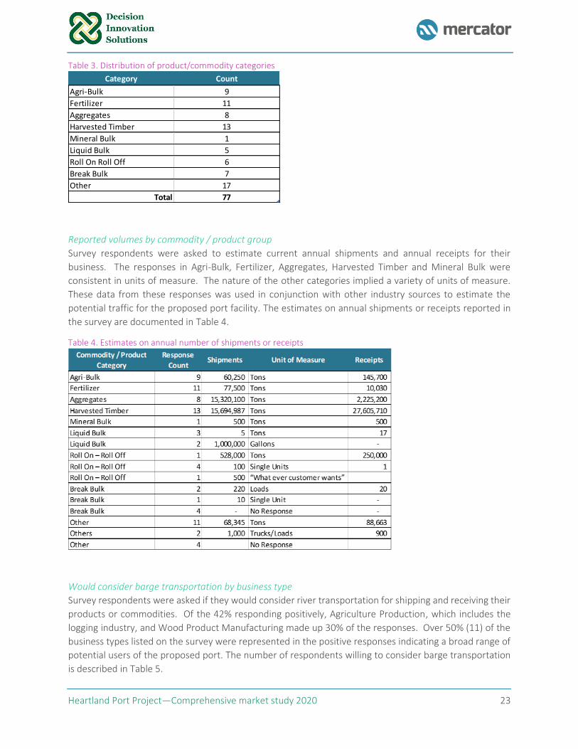
Heartland Port Project—Comprehensive market study 2020 23
Table 3. Distribution of product/commodity categories
Reported volumes by commodity / product group
Survey respondents were asked to estimate current annual shipments and annual receipts for their
business. The responses in Agri-Bulk, Fertilizer, Aggregates, Harvested Timber and Mineral Bulk were
consistent in units of measure. The nature of the other categories implied a variety of units of measure.
These data from these responses was used in conjunction with other industry sources to estimate the
potential traffic for the proposed port facility. The estimates on annual shipments or receipts reported in
the survey are documented in Table 4.
Table 4. Estimates on annual number of shipments or receipts
Would consider barge transportation by business type
Survey respondents were asked if they would consider river transportation for shipping and receiving their
products or commodities. Of the 42% responding positively, Agriculture Production, which includes the
logging industry, and Wood Product Manufacturing made up 30% of the responses. Over 50% (11) of the
business types listed on the survey were represented in the positive responses indicating a broad range of
potential users of the proposed port. The number of respondents willing to consider barge transportation
is described in Table 5.
Category Count
Agri-Bulk 9
Fertilizer 11
Aggregates 8
Harvested Timber 13
Mineral Bulk 1
Liquid Bulk 5
Roll On Roll Off 6
Break Bulk 7
Other 17
Total 77
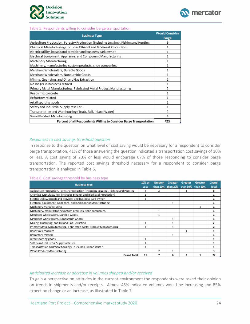
Heartland Port Project—Comprehensive market study 2020 24
Table 5. Respondents willing to consider barge transportation
Responses to cost savings threshold question
In response to the question on what level of cost saving would be necessary for a respondent to consider
barge transportation, 41% of those answering the question indicated a transportation cost savings of 10%
or less. A cost saving of 20% or less would encourage 67% of those responding to consider barge
transportation. The reported cost savings threshold necessary for a respondent to consider barge
transportation is analyzed in Table 6.
Table 6. Cost savings threshold by business type
Anticipated increase or decrease in volumes shipped and/or received
To gain a perspective on attitudes in the current environment the respondents were asked their opinion
on trends in shipments and/or receipts. Almost 45% indicated volumes would be increasing and 85%
expect no change or an increase, as illustrated in Table 7.
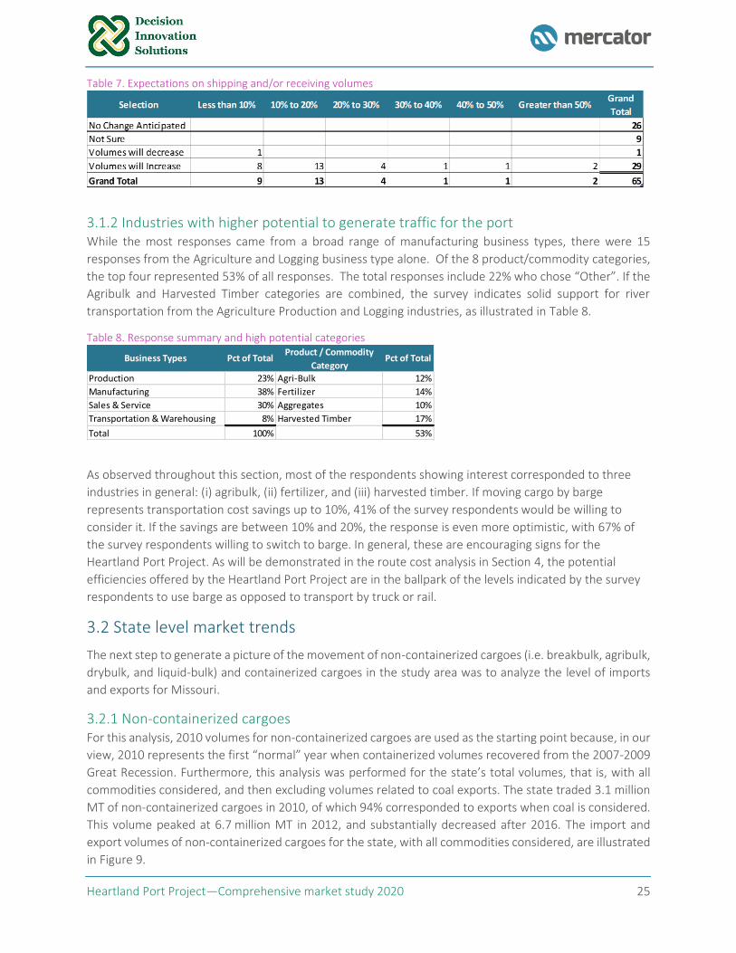
Heartland Port Project—Comprehensive market study 2020 25
Table 7. Expectations on shipping and/or receiving volumes
3.1.2 Industries with higher potential to generate traffic for the port While the most responses came from a broad range of manufacturing business types, there were 15
responses from the Agriculture and Logging business type alone. Of the 8 product/commodity categories,
the top four represented 53% of all responses. The total responses include 22% who chose “Other”. If the
Agribulk and Harvested Timber categories are combined, the survey indicates solid support for river
transportation from the Agriculture Production and Logging industries, as illustrated in Table 8.
Table 8. Response summary and high potential categories
As observed throughout this section, most of the respondents showing interest corresponded to three
industries in general: (i) agribulk, (ii) fertilizer, and (iii) harvested timber. If moving cargo by barge
represents transportation cost savings up to 10%, 41% of the survey respondents would be willing to
consider it. If the savings are between 10% and 20%, the response is even more optimistic, with 67% of
the survey respondents willing to switch to barge. In general, these are encouraging signs for the
Heartland Port Project. As will be demonstrated in the route cost analysis in Section 4, the potential
efficiencies offered by the Heartland Port Project are in the ballpark of the levels indicated by the survey
respondents to use barge as opposed to transport by truck or rail.
3.2 State level market trends
The next step to generate a picture of the movement of non-containerized cargoes (i.e. breakbulk, agribulk,
drybulk, and liquid-bulk) and containerized cargoes in the study area was to analyze the level of imports
and exports for Missouri.
3.2.1 Non-containerized cargoes For this analysis, 2010 volumes for non-containerized cargoes are used as the starting point because, in our
view, 2010 represents the first “normal” year when containerized volumes recovered from the 2007-2009
Great Recession. Furthermore, this analysis was performed for the state’s total volumes, that is, with all
commodities considered, and then excluding volumes related to coal exports. The state traded 3.1 million
MT of non-containerized cargoes in 2010, of which 94% corresponded to exports when coal is considered.
This volume peaked at 6.7 million MT in 2012, and substantially decreased after 2016. The import and
export volumes of non-containerized cargoes for the state, with all commodities considered, are illustrated
in Figure 9.
Business Types Pct of TotalProduct / Commodity
CategoryPct of Total
Production 23% Agri-Bulk 12%
Manufacturing 38% Fertilizer 14%
Sales & Service 30% Aggregates 10%
Transportation & Warehousing 8% Harvested Timber 17%
Total 100% 53%
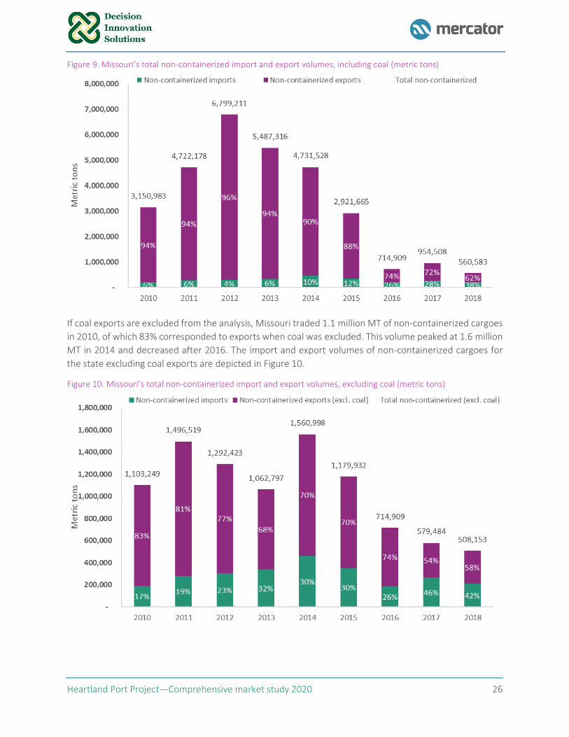
Heartland Port Project—Comprehensive market study 2020 26
Figure 9. Missouri’s total non-containerized import and export volumes, including coal (metric tons)
If coal exports are excluded from the analysis, Missouri traded 1.1 million MT of non-containerized cargoes
in 2010, of which 83% corresponded to exports when coal was excluded. This volume peaked at 1.6 million
MT in 2014 and decreased after 2016. The import and export volumes of non-containerized cargoes for
the state excluding coal exports are depicted in Figure 10.
Figure 10. Missouri’s total non-containerized import and export volumes, excluding coal (metric tons)
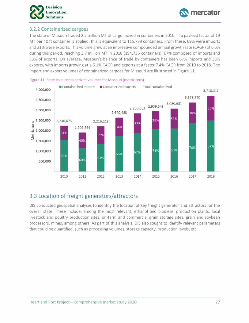
Heartland Port Project—Comprehensive market study 2020 27
3.2.2 Containerized cargoes The state of Missouri traded 2.2 million MT of cargo moved in containers in 2010. If a payload factor of 19
MT per 40 ft container is applied, this is equivalent to 115,789 containers. From these, 69% were imports
and 31% were exports. This volume grew at an impressive compounded annual growth rate (CAGR) of 6.5%
during this period, reaching 3.7 million MT in 2018 (194,736 containers), 67% composed of imports and
33% of exports. On average, Missouri’s balance of trade by containers has been 67% imports and 33%
exports, with imports growing at a 6.1% CAGR and exports at a faster 7.4% CAGR from 2010 to 2018. The
import and export volumes of containerized cargoes for Missouri are illustrated in Figure 11.
Figure 11. State level containerized volumes for Missouri (metric tons)
3.3 Location of freight generators/attractors
DIS conducted geospatial analyses to identify the location of key freight generator and attractors for the
overall state. These include, among the most relevant, ethanol and biodiesel production plants, local
livestock and poultry production sites, on-farm and commercial grain storage sites, grain and soybean
processors, mines, among others. As part of this analysis, DIS also sought to identify relevant parameters
that could be quantified, such as processing volumes, storage capacity, production levels, etc.
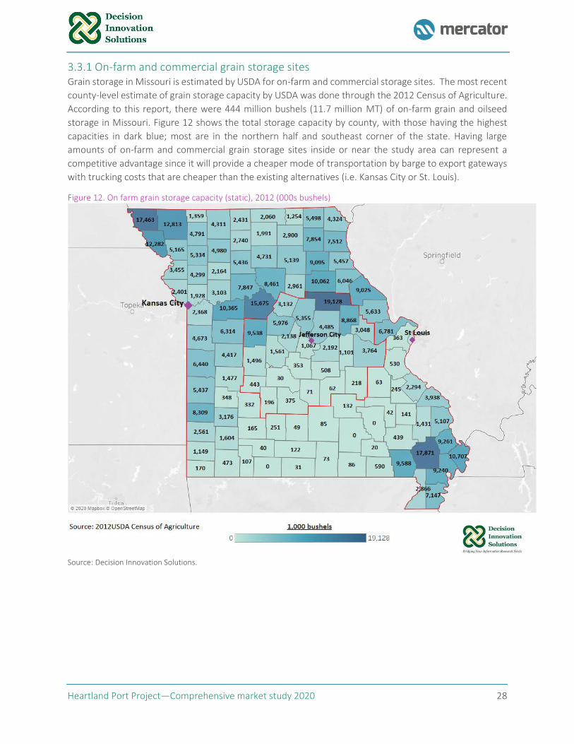
Heartland Port Project—Comprehensive market study 2020 28
3.3.1 On-farm and commercial grain storage sites Grain storage in Missouri is estimated by USDA for on-farm and commercial storage sites. The most recent
county-level estimate of grain storage capacity by USDA was done through the 2012 Census of Agriculture.
According to this report, there were 444 million bushels (11.7 million MT) of on-farm grain and oilseed
storage in Missouri. Figure 12 shows the total storage capacity by county, with those having the highest
capacities in dark blue; most are in the northern half and southeast corner of the state. Having large
amounts of on-farm and commercial grain storage sites inside or near the study area can represent a
competitive advantage since it will provide a cheaper mode of transportation by barge to export gateways
with trucking costs that are cheaper than the existing alternatives (i.e. Kansas City or St. Louis).
Figure 12. On farm grain storage capacity (static), 2012 (000s bushels)
Source: Decision Innovation Solutions.
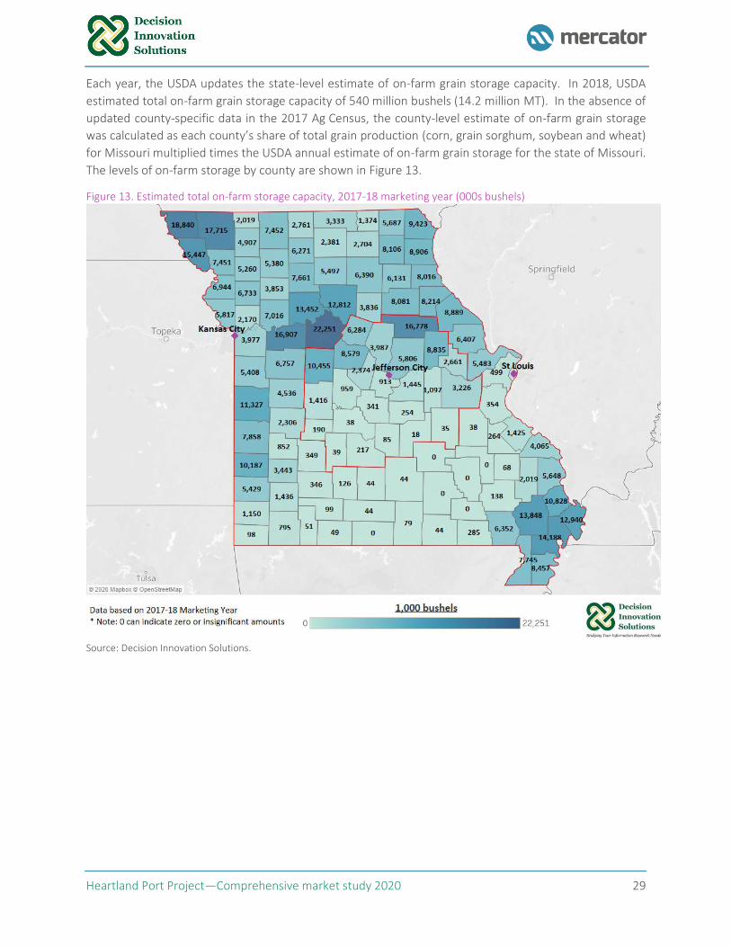
Heartland Port Project—Comprehensive market study 2020 29
Each year, the USDA updates the state-level estimate of on-farm grain storage capacity. In 2018, USDA
estimated total on-farm grain storage capacity of 540 million bushels (14.2 million MT). In the absence of
updated county-specific data in the 2017 Ag Census, the county-level estimate of on-farm grain storage
was calculated as each county’s share of total grain production (corn, grain sorghum, soybean and wheat)
for Missouri multiplied times the USDA annual estimate of on-farm grain storage for the state of Missouri.
The levels of on-farm storage by county are shown in Figure 13.
Figure 13. Estimated total on-farm storage capacity, 2017-18 marketing year (000s bushels)
Source: Decision Innovation Solutions.
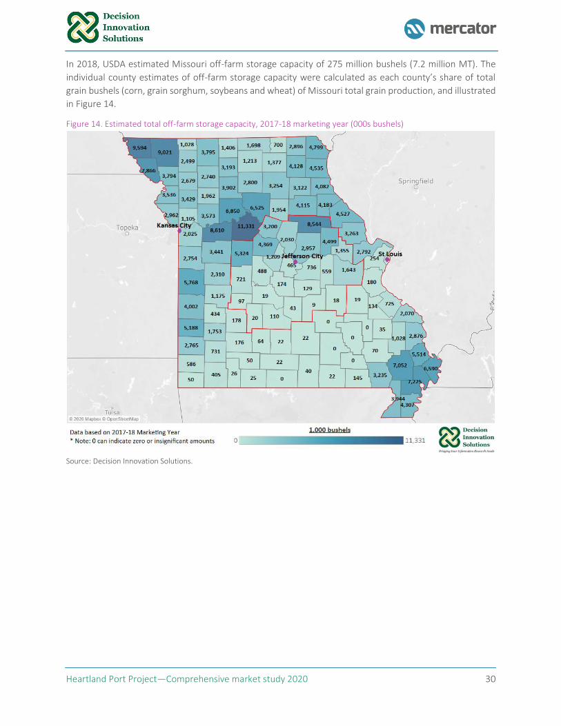
Heartland Port Project—Comprehensive market study 2020 30
In 2018, USDA estimated Missouri off-farm storage capacity of 275 million bushels (7.2 million MT). The
individual county estimates of off-farm storage capacity were calculated as each county’s share of total
grain bushels (corn, grain sorghum, soybeans and wheat) of Missouri total grain production, and illustrated
in Figure 14.
Figure 14. Estimated total off-farm storage capacity, 2017-18 marketing year (000s bushels)
Source: Decision Innovation Solutions.
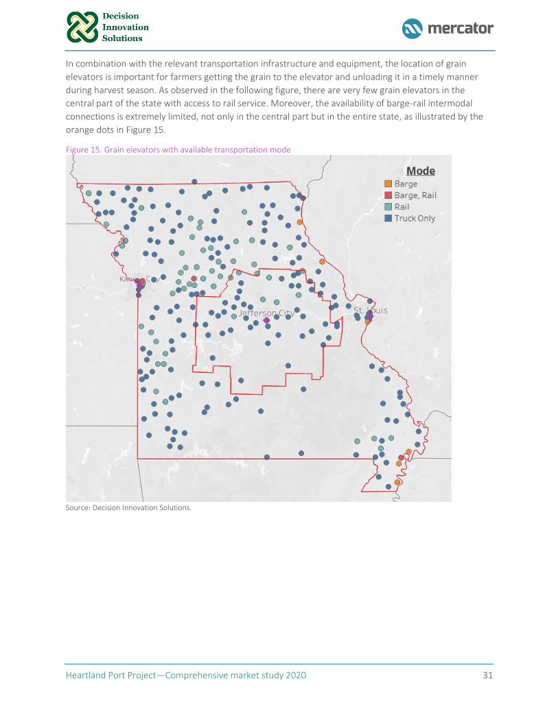
Heartland Port Project—Comprehensive market study 2020 31
In combination with the relevant transportation infrastructure and equipment, the location of grain
elevators is important for farmers getting the grain to the elevator and unloading it in a timely manner
during harvest season. As observed in the following figure, there are very few grain elevators in the
central part of the state with access to rail service. Moreover, the availability of barge-rail intermodal
connections is extremely limited, not only in the central part but in the entire state, as illustrated by the
orange dots in Figure 15.
Figure 15. Grain elevators with available transportation mode
Source: Decision Innovation Solutions.
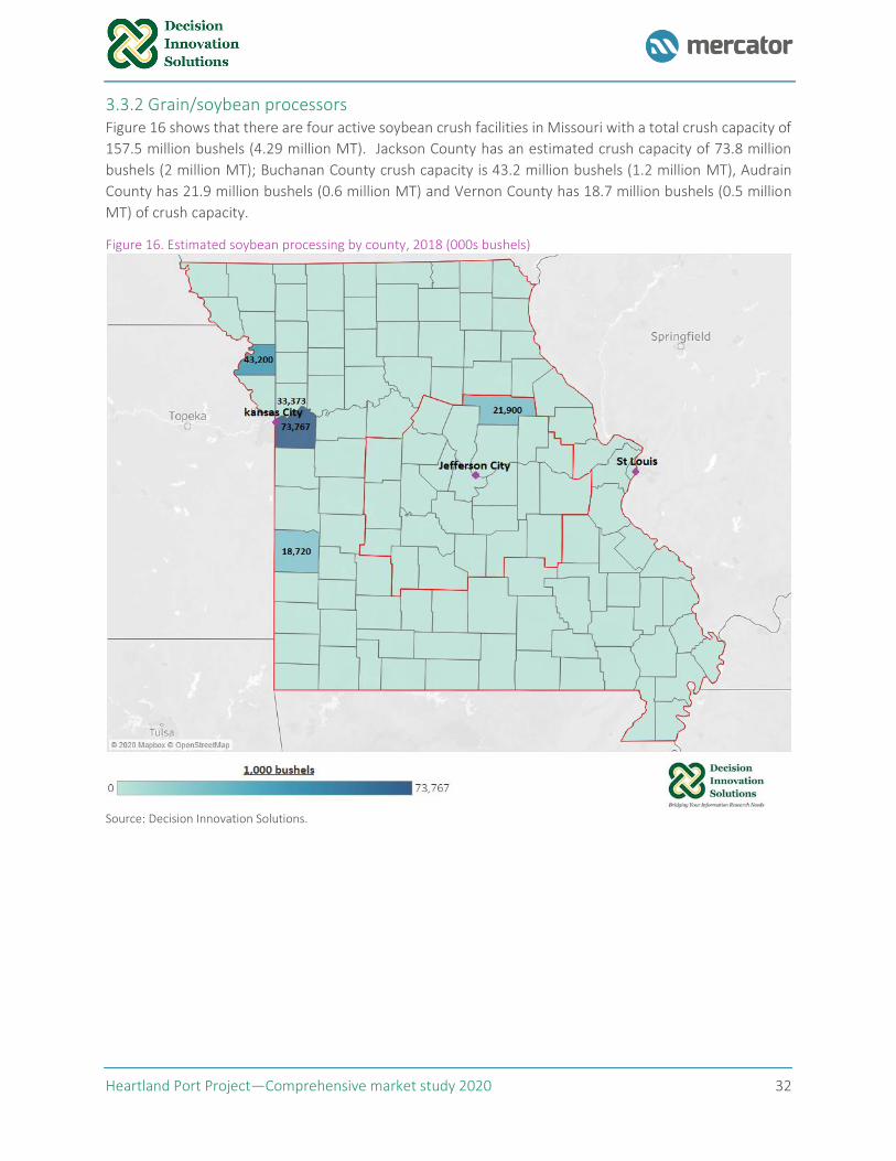
Heartland Port Project—Comprehensive market study 2020 32
3.3.2 Grain/soybean processors Figure 16 shows that there are four active soybean crush facilities in Missouri with a total crush capacity of
157.5 million bushels (4.29 million MT). Jackson County has an estimated crush capacity of 73.8 million
bushels (2 million MT); Buchanan County crush capacity is 43.2 million bushels (1.2 million MT), Audrain
County has 21.9 million bushels (0.6 million MT) and Vernon County has 18.7 million bushels (0.5 million
MT) of crush capacity.
Figure 16. Estimated soybean processing by county, 2018 (000s bushels)
Source: Decision Innovation Solutions.
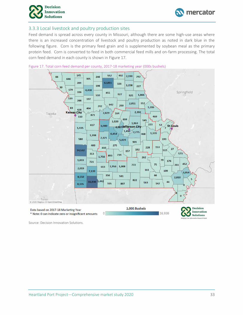
Heartland Port Project—Comprehensive market study 2020 33
3.3.3 Local livestock and poultry production sites Feed demand is spread across every county in Missouri, although there are some high-use areas where
there is an increased concentration of livestock and poultry production as noted in dark blue in the
following figure. Corn is the primary feed grain and is supplemented by soybean meal as the primary
protein feed. Corn is converted to feed in both commercial feed mills and on-farm processing. The total
corn feed demand in each county is shown in Figure 17.
Figure 17. Total corn feed demand per county, 2017-18 marketing year (000s bushels)
Source: Decision Innovation Solutions.
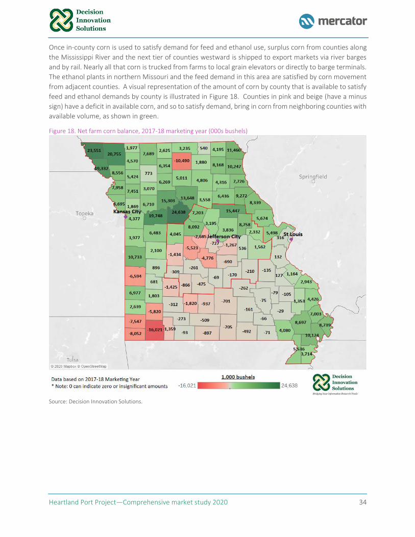
Heartland Port Project—Comprehensive market study 2020 34
Once in-county corn is used to satisfy demand for feed and ethanol use, surplus corn from counties along
the Mississippi River and the next tier of counties westward is shipped to export markets via river barges
and by rail. Nearly all that corn is trucked from farms to local grain elevators or directly to barge terminals.
The ethanol plants in northern Missouri and the feed demand in this area are satisfied by corn movement
from adjacent counties. A visual representation of the amount of corn by county that is available to satisfy
feed and ethanol demands by county is illustrated in Figure 18. Counties in pink and beige (have a minus
sign) have a deficit in available corn, and so to satisfy demand, bring in corn from neighboring counties with
available volume, as shown in green.
Figure 18. Net farm corn balance, 2017-18 marketing year (000s bushels)
Source: Decision Innovation Solutions.
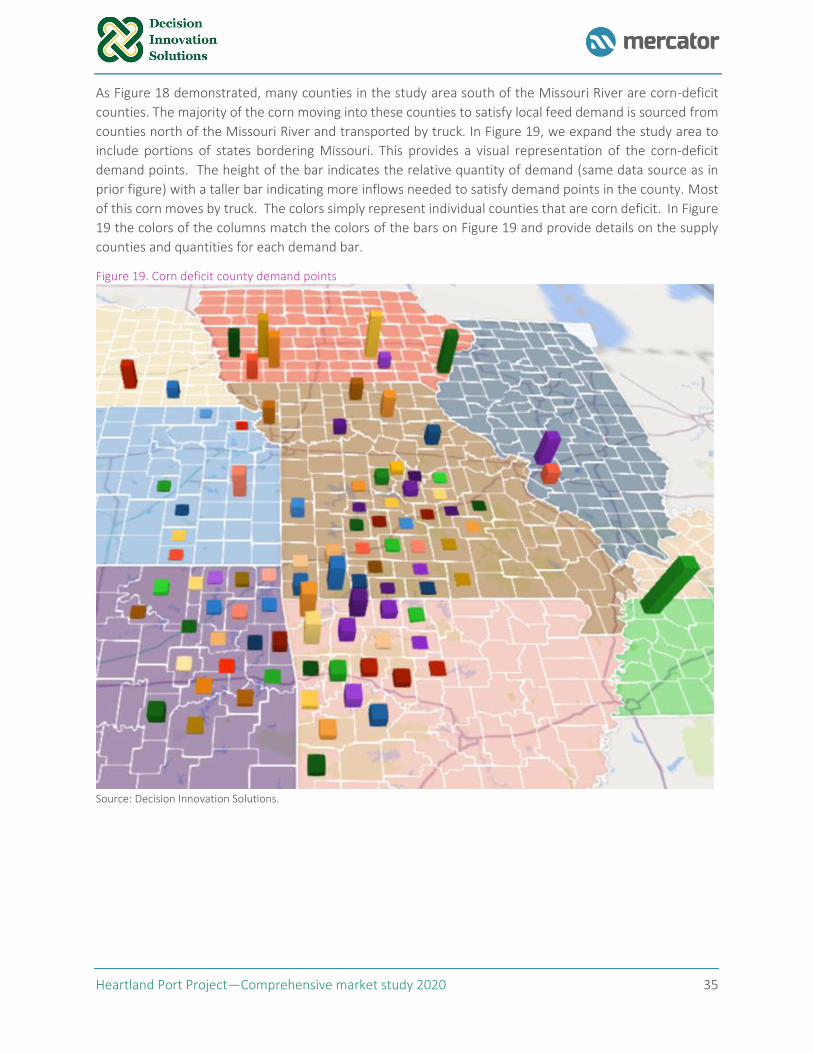
Heartland Port Project—Comprehensive market study 2020 35
As Figure 18 demonstrated, many counties in the study area south of the Missouri River are corn-deficit
counties. The majority of the corn moving into these counties to satisfy local feed demand is sourced from
counties north of the Missouri River and transported by truck. In Figure 19, we expand the study area to
include portions of states bordering Missouri. This provides a visual representation of the corn-deficit
demand points. The height of the bar indicates the relative quantity of demand (same data source as in
prior figure) with a taller bar indicating more inflows needed to satisfy demand points in the county. Most
of this corn moves by truck. The colors simply represent individual counties that are corn deficit. In Figure
19 the colors of the columns match the colors of the bars on Figure 19 and provide details on the supply
counties and quantities for each demand bar.
Figure 19. Corn deficit county demand points
Source: Decision Innovation Solutions.
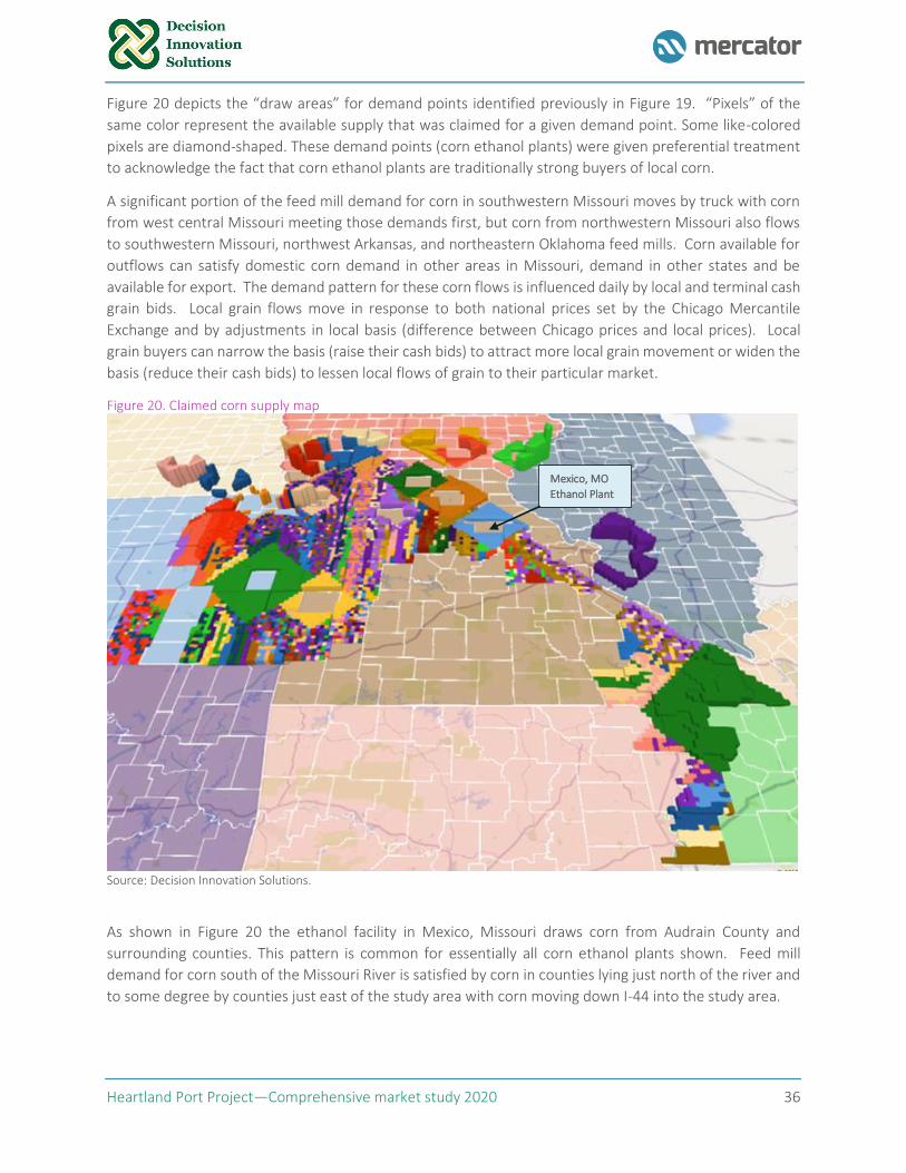
Heartland Port Project—Comprehensive market study 2020 36
Figure 20 depicts the “draw areas” for demand points identified previously in Figure 19. “Pixels” of the
same color represent the available supply that was claimed for a given demand point. Some like-colored
pixels are diamond-shaped. These demand points (corn ethanol plants) were given preferential treatment
to acknowledge the fact that corn ethanol plants are traditionally strong buyers of local corn.
A significant portion of the feed mill demand for corn in southwestern Missouri moves by truck with corn
from west central Missouri meeting those demands first, but corn from northwestern Missouri also flows
to southwestern Missouri, northwest Arkansas, and northeastern Oklahoma feed mills. Corn available for
outflows can satisfy domestic corn demand in other areas in Missouri, demand in other states and be
available for export. The demand pattern for these corn flows is influenced daily by local and terminal cash
grain bids. Local grain flows move in response to both national prices set by the Chicago Mercantile
Exchange and by adjustments in local basis (difference between Chicago prices and local prices). Local
grain buyers can narrow the basis (raise their cash bids) to attract more local grain movement or widen the
basis (reduce their cash bids) to lessen local flows of grain to their particular market.
Figure 20. Claimed corn supply map
Source: Decision Innovation Solutions.
As shown in Figure 20 the ethanol facility in Mexico, Missouri draws corn from Audrain County and
surrounding counties. This pattern is common for essentially all corn ethanol plants shown. Feed mill
demand for corn south of the Missouri River is satisfied by corn in counties lying just north of the river and
to some degree by counties just east of the study area with corn moving down I-44 into the study area.
Mexico, MO
Ethanol Plant
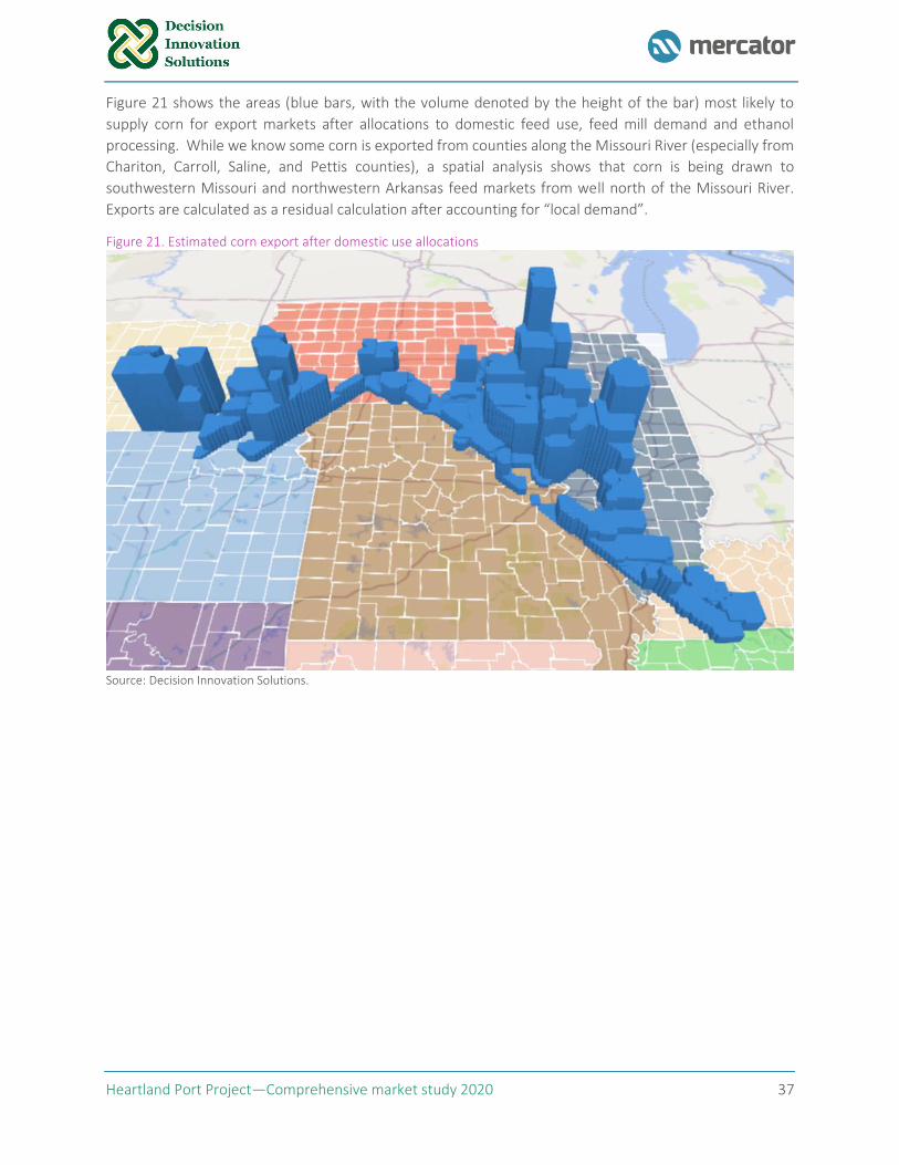
Heartland Port Project—Comprehensive market study 2020 37
Figure 21 shows the areas (blue bars, with the volume denoted by the height of the bar) most likely to
supply corn for export markets after allocations to domestic feed use, feed mill demand and ethanol
processing. While we know some corn is exported from counties along the Missouri River (especially from
Chariton, Carroll, Saline, and Pettis counties), a spatial analysis shows that corn is being drawn to
southwestern Missouri and northwestern Arkansas feed markets from well north of the Missouri River.
Exports are calculated as a residual calculation after accounting for “local demand”.
Figure 21. Estimated corn export after domestic use allocations
Source: Decision Innovation Solutions.
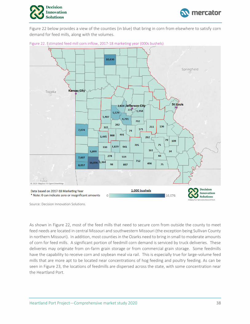
Heartland Port Project—Comprehensive market study 2020 38
Figure 22 below provides a view of the counties (in blue) that bring in corn from elsewhere to satisfy corn
demand for feed mills, along with the volumes.
Figure 22. Estimated feed mill corn inflow, 2017-18 marketing year (000s bushels)
Source: Decision Innovation Solutions.
As shown in Figure 22, most of the feed mills that need to secure corn from outside the county to meet
feed needs are located in central Missouri and southwestern Missouri (the exception being Sullivan County
in northern Missouri). In addition, most counties in the Ozarks need to bring in small to moderate amounts
of corn for feed mills. A significant portion of feedmill corn demand is serviced by truck deliveries. These
deliveries may originate from on-farm grain storage or from commercial grain storage. Some feedmills
have the capability to receive corn and soybean meal via rail. This is especially true for large-volume feed
mills that are more apt to be located near concentrations of hog feeding and poultry feeding. As can be
seen in Figure 23, the locations of feedmills are dispersed across the state, with some concentration near
the Heartland Port.
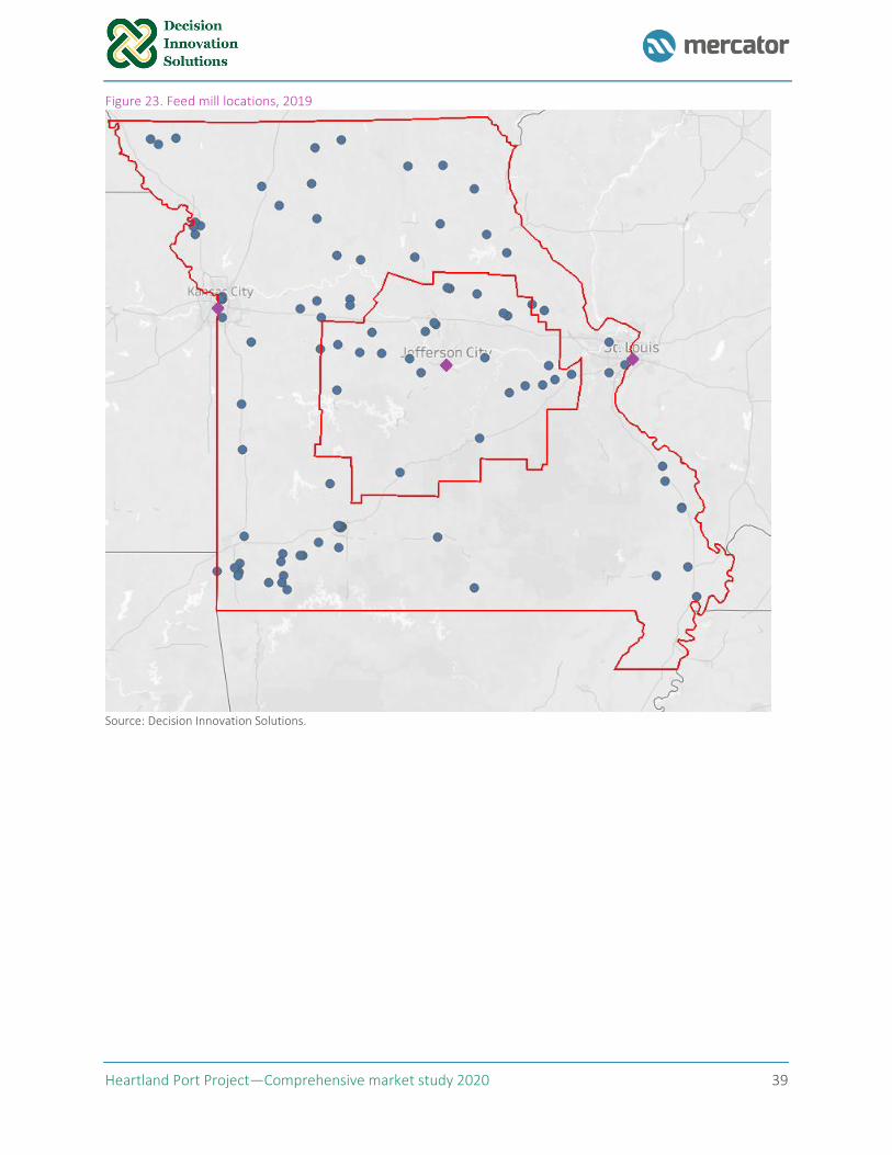
Heartland Port Project—Comprehensive market study 2020 39
Figure 23. Feed mill locations, 2019
Source: Decision Innovation Solutions.
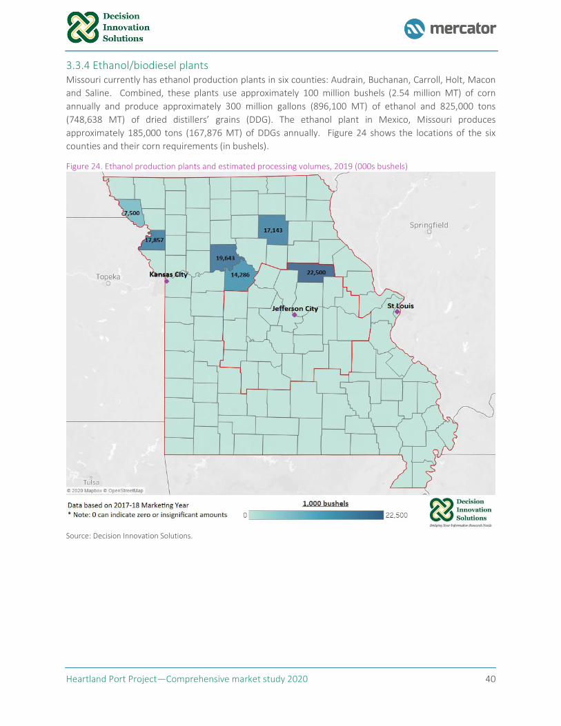
Heartland Port Project—Comprehensive market study 2020 40
3.3.4 Ethanol/biodiesel plants Missouri currently has ethanol production plants in six counties: Audrain, Buchanan, Carroll, Holt, Macon
and Saline. Combined, these plants use approximately 100 million bushels (2.54 million MT) of corn
annually and produce approximately 300 million gallons (896,100 MT) of ethanol and 825,000 tons
(748,638 MT) of dried distillers’ grains (DDG). The ethanol plant in Mexico, Missouri produces
approximately 185,000 tons (167,876 MT) of DDGs annually. Figure 24 shows the locations of the six
counties and their corn requirements (in bushels).
Figure 24. Ethanol production plants and estimated processing volumes, 2019 (000s bushels)
Source: Decision Innovation Solutions.
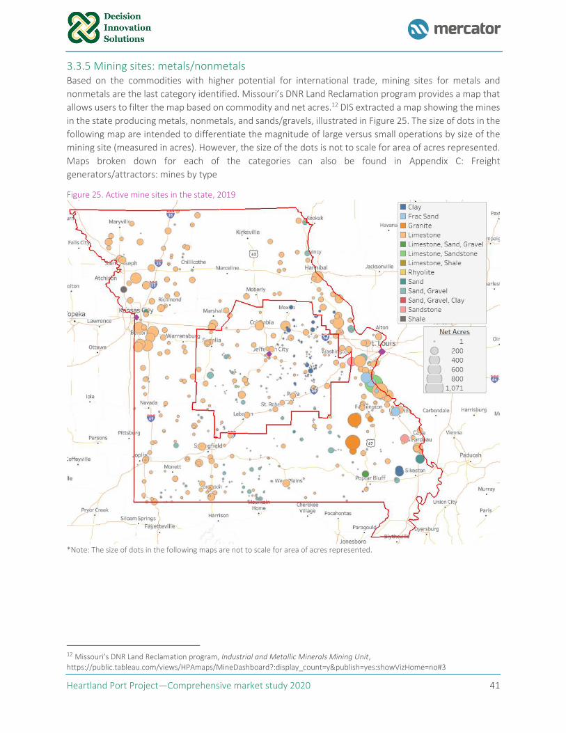
Heartland Port Project—Comprehensive market study 2020 41
3.3.5 Mining sites: metals/nonmetals Based on the commodities with higher potential for international trade, mining sites for metals and
nonmetals are the last category identified. Missouri’s DNR Land Reclamation program provides a map that
allows users to filter the map based on commodity and net acres.12 DIS extracted a map showing the mines
in the state producing metals, nonmetals, and sands/gravels, illustrated in Figure 25. The size of dots in the
following map are intended to differentiate the magnitude of large versus small operations by size of the
mining site (measured in acres). However, the size of the dots is not to scale for area of acres represented.
Maps broken down for each of the categories can also be found in Appendix C: Freight
generators/attractors: mines by type
Figure 25. Active mine sites in the state, 2019
*Note: The size of dots in the following maps are not to scale for area of acres represented.
12 Missouri’s DNR Land Reclamation program, Industrial and Metallic Minerals Mining Unit,
https://public.tableau.com/views/HPAmaps/MineDashboard?:display_count=y&publish=yes:showVizHome=no#3
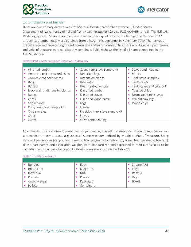
Heartland Port Project—Comprehensive market study 2020 42
3.3.6 Forestry and lumber There are two primary data sources for Missouri forestry and timber exports: (i) United States
Department of Agriculture/Animal and Plant Health Inspection Service (USDA/APHIS), and (ii) The IMPLAN
Modeling System. Missouri-sourced forest and lumber export data for the time period October 2017
through September 2019 were obtained from USDA/APHIS personnel in November 2019. The format of
the data received required significant conversion and summarization to ensure wood species, part names
and units of measure were consistently combined. Table 9 shows the list of all names contained in the
APHIS database.
Table 9. Part names contained in the APHIS database
▪ Air dried lumber ▪ American oak untoasted chips ▪ Aromatic red cedar cants ▪ Bark ▪ Barrels ▪ Black walnut dimension blanks ▪ Bungs ▪ Cants ▪ Cedar cants ▪ Chip/tank stave sample kit ▪ Chip samples ▪ Chips ▪ Cubes
▪ Cuvee tank stave sample kit ▪ Debarked logs ▪ Dimension blanks ▪ Headings ▪ Heat treated lumber ▪ Kiln dried lumber ▪ Kiln dried staves ▪ Kiln dried wood barrel ▪ Logs ▪ Lumber ▪ Precision tank stave sample kit ▪ Staves ▪ Staves and heading
▪ Staves and heading ▪ Stocks ▪ Tank stave samples ▪ Tank staves ▪ Tank staves and crosscut ▪ Toasted chips ▪ Untoasted tank staves ▪ Walnut saw logs ▪ Wood chips
After the APHIS data were summarized by part name, the unit of measure for each part names was
summarized. In some cases, a given part name was summarized by multiple units of measure. Using
standard conversions (i.e. pounds to metric ton, kilograms to metric ton, board feet per metric ton, etc),
all the part names and associated weights were standardized and expressed in metric tons so as to be
consistent with the overall analysis. Units of measure are included in Table 10.
Table 10. Units of measure
▪ Bundles ▪ Board Feet ▪ Individual ▪ Pounds ▪ Cubic Meters ▪ Pallets
▪ Each ▪ Kilograms ▪ MBF ▪ Pieces ▪ Packages ▪ Containers
▪ Square feet ▪ Logs ▪ Barrels ▪ Bags ▪ Boxes
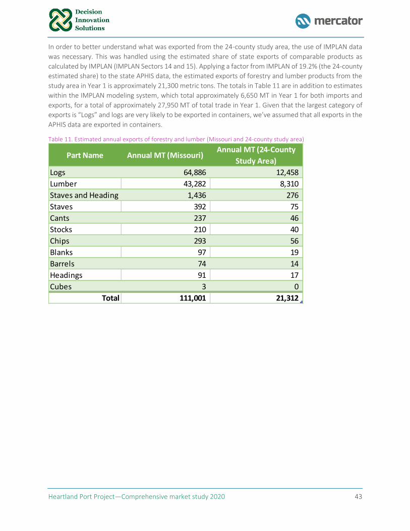
Heartland Port Project—Comprehensive market study 2020 43
In order to better understand what was exported from the 24-county study area, the use of IMPLAN data
was necessary. This was handled using the estimated share of state exports of comparable products as
calculated by IMPLAN (IMPLAN Sectors 14 and 15). Applying a factor from IMPLAN of 19.2% (the 24-county
estimated share) to the state APHIS data, the estimated exports of forestry and lumber products from the
study area in Year 1 is approximately 21,300 metric tons. The totals in Table 11 are in addition to estimates
within the IMPLAN modeling system, which total approximately 6,650 MT in Year 1 for both imports and
exports, for a total of approximately 27,950 MT of total trade in Year 1. Given that the largest category of
exports is “Logs” and logs are very likely to be exported in containers, we’ve assumed that all exports in the
APHIS data are exported in containers.
Table 11. Estimated annual exports of forestry and lumber (Missouri and 24-county study area)
Part Name Annual MT (Missouri)Annual MT (24-County
Study Area)
Logs 64,886 12,458
Lumber 43,282 8,310
Staves and Heading 1,436 276
Staves 392 75
Cants 237 46
Stocks 210 40
Chips 293 56
Blanks 97 19
Barrels 74 14
Headings 91 17
Cubes 3 0
Total 111,001 21,312
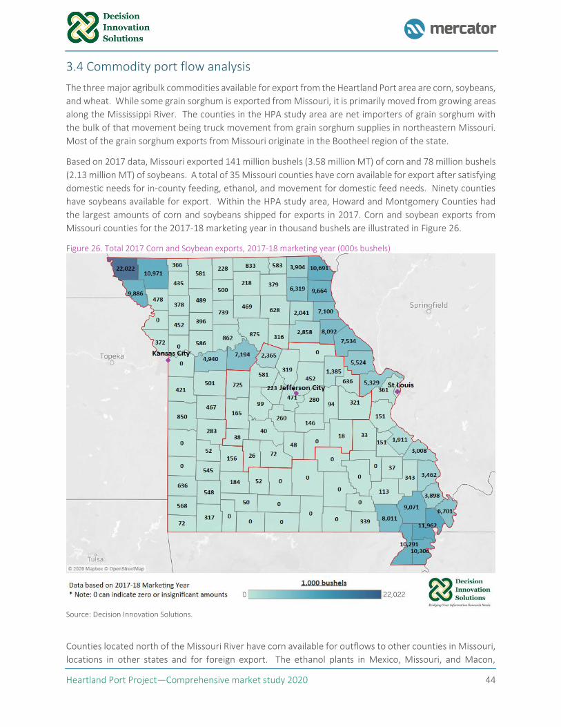
Heartland Port Project—Comprehensive market study 2020 44
3.4 Commodity port flow analysis
The three major agribulk commodities available for export from the Heartland Port area are corn, soybeans,
and wheat. While some grain sorghum is exported from Missouri, it is primarily moved from growing areas
along the Mississippi River. The counties in the HPA study area are net importers of grain sorghum with
the bulk of that movement being truck movement from grain sorghum supplies in northeastern Missouri.
Most of the grain sorghum exports from Missouri originate in the Bootheel region of the state.
Based on 2017 data, Missouri exported 141 million bushels (3.58 million MT) of corn and 78 million bushels
(2.13 million MT) of soybeans. A total of 35 Missouri counties have corn available for export after satisfying
domestic needs for in-county feeding, ethanol, and movement for domestic feed needs. Ninety counties
have soybeans available for export. Within the HPA study area, Howard and Montgomery Counties had
the largest amounts of corn and soybeans shipped for exports in 2017. Corn and soybean exports from
Missouri counties for the 2017-18 marketing year in thousand bushels are illustrated in Figure 26.
Figure 26. Total 2017 Corn and Soybean exports, 2017-18 marketing year (000s bushels)
Source: Decision Innovation Solutions.
Counties located north of the Missouri River have corn available for outflows to other counties in Missouri,
locations in other states and for foreign export. The ethanol plants in Mexico, Missouri, and Macon,
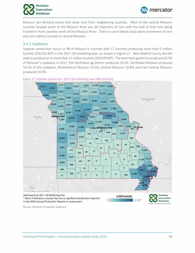
Heartland Port Project—Comprehensive market study 2020 45
Missouri are demand points that draw corn from neighboring counties. Most of the central Missouri
counties located south of the Missouri River are net importers of corn with the bulk of that corn being
trucked in from counties north of the Missouri River. There is some lateral (east-west) movement of corn
into corn-deficit counties in central Missouri.
3.4.1 Soybeans Soybean production occurs in 99 of Missouri’s counties with 17 counties producing more than 5 million
bushels (150,015 MT) in the 2017-18 marketing year, as shown in Figure 27. New Madrid County led the
state in production at more than 11 million bushels (330,033 MT). The boot heel ag district produced 20.5%
of Missouri’s soybeans in 2017; the Northwest ag district produced 19.2%. Northeast Missouri produced
14.5% of the soybeans, Northcentral Missouri 13.5%, Central Missouri 10.8% and East Central Missouri
produced 10.5%.
Figure 27. Soybean production, 2017-18 marketing year (000s bushels)
Source: Decision Innovation Solutions.
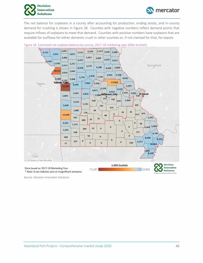
Heartland Port Project—Comprehensive market study 2020 46
The net balance for soybeans in a county after accounting for production, ending stocks, and in-county
demand for crushing is shown in Figure 28. Counties with negative numbers reflect demand points that
require inflows of soybeans to meet that demand. Counties with positive numbers have soybeans that are
available for outflows for either domestic crush in other counties or, if not claimed for that, for export.
Figure 28. Estimated net soybean balance by county, 2017-18 marketing year (000s bushels)
Source: Decision Innovation Solutions.
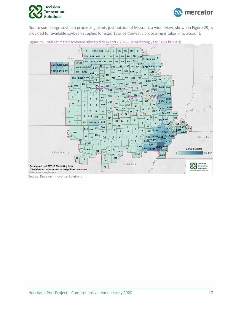
Heartland Port Project—Comprehensive market study 2020 47
Due to some large soybean processing plants just outside of Missouri, a wider view, shown in Figure 29, is
provided for available soybean supplies for exports once domestic processing is taken into account.
Figure 29. Total estimated soybeans allocated to exports, 2017-18 marketing year (000s bushels)
Source: Decision Innovation Solutions.
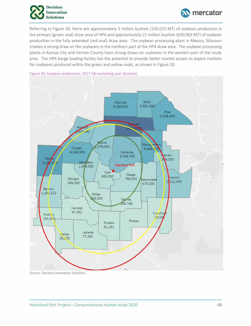
Heartland Port Project—Comprehensive market study 2020 48
Referring to Figure 30, there are approximately 5 million bushels (150,015 MT) of soybean production in
the primary (green oval) draw area of HPA and approximately 21 million bushels (630,063 MT) of soybean
production in the fully extended (red oval) draw area. The soybean processing plant in Mexico, Missouri
creates a strong draw on the soybeans in the northern part of the HPA draw area. The soybean processing
plants in Kansas City and Vernon County have strong draws on soybeans in the western part of the study
area. The HPA barge loading facility has the potential to provide better market access to export markets
for soybeans produced within the green and yellow ovals, as shown in Figure 30.
Figure 30. Soybean production, 2017-18 marketing year (bushels)
Source: Decision Innovation Solutions.
Heartland Port
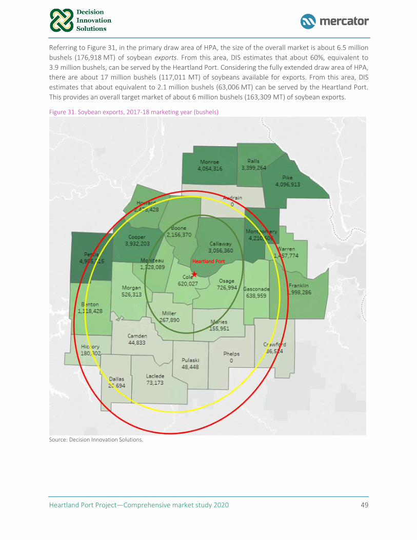
Heartland Port Project—Comprehensive market study 2020 49
Referring to Figure 31, in the primary draw area of HPA, the size of the overall market is about 6.5 million
bushels (176,918 MT) of soybean exports. From this area, DIS estimates that about 60%, equivalent to
3.9 million bushels, can be served by the Heartland Port. Considering the fully extended draw area of HPA,
there are about 17 million bushels (117,011 MT) of soybeans available for exports. From this area, DIS
estimates that about equivalent to 2.1 million bushels (63,006 MT) can be served by the Heartland Port.
This provides an overall target market of about 6 million bushels (163,309 MT) of soybean exports.
Figure 31. Soybean exports, 2017-18 marketing year (bushels)
Source: Decision Innovation Solutions.
Heartland Port
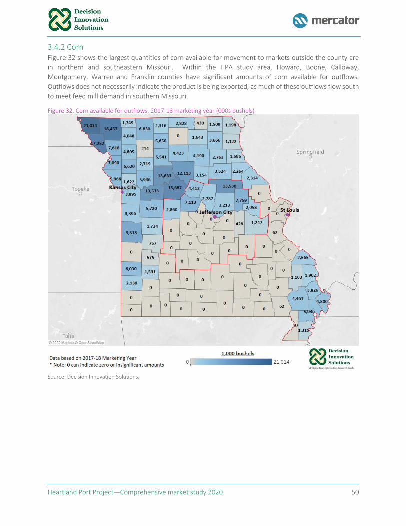
Heartland Port Project—Comprehensive market study 2020 50
3.4.2 Corn Figure 32 shows the largest quantities of corn available for movement to markets outside the county are
in northern and southeastern Missouri. Within the HPA study area, Howard, Boone, Calloway,
Montgomery, Warren and Franklin counties have significant amounts of corn available for outflows.
Outflows does not necessarily indicate the product is being exported, as much of these outflows flow south
to meet feed mill demand in southern Missouri.
Figure 32. Corn available for outflows, 2017-18 marketing year (000s bushels)
Source: Decision Innovation Solutions.
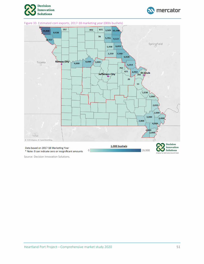
Heartland Port Project—Comprehensive market study 2020 51
Figure 33. Estimated corn exports, 2017-18 marketing year (000s bushels)
Source: Decision Innovation Solutions.
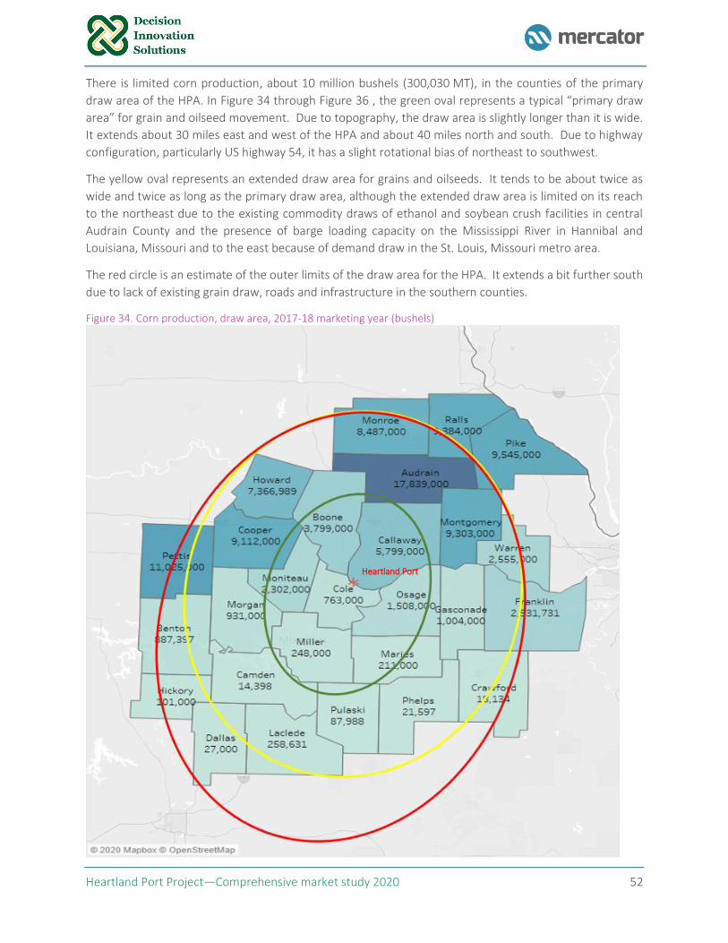
Heartland Port Project—Comprehensive market study 2020 52
There is limited corn production, about 10 million bushels (300,030 MT), in the counties of the primary
draw area of the HPA. In Figure 34 through Figure 36 , the green oval represents a typical “primary draw
area” for grain and oilseed movement. Due to topography, the draw area is slightly longer than it is wide.
It extends about 30 miles east and west of the HPA and about 40 miles north and south. Due to highway
configuration, particularly US highway 54, it has a slight rotational bias of northeast to southwest.
The yellow oval represents an extended draw area for grains and oilseeds. It tends to be about twice as
wide and twice as long as the primary draw area, although the extended draw area is limited on its reach
to the northeast due to the existing commodity draws of ethanol and soybean crush facilities in central
Audrain County and the presence of barge loading capacity on the Mississippi River in Hannibal and
Louisiana, Missouri and to the east because of demand draw in the St. Louis, Missouri metro area.
The red circle is an estimate of the outer limits of the draw area for the HPA. It extends a bit further south
due to lack of existing grain draw, roads and infrastructure in the southern counties.
Figure 34. Corn production, draw area, 2017-18 marketing year (bushels)
Heartland Port
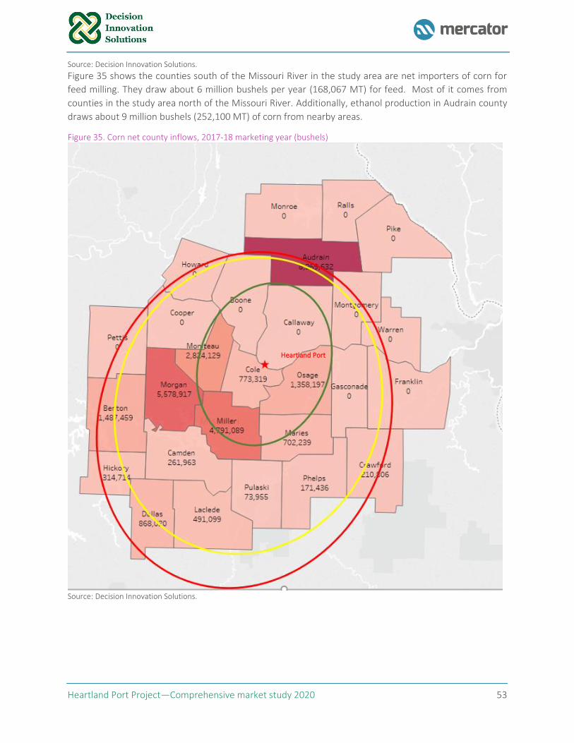
Heartland Port Project—Comprehensive market study 2020 53
Source: Decision Innovation Solutions.
Figure 35 shows the counties south of the Missouri River in the study area are net importers of corn for
feed milling. They draw about 6 million bushels per year (168,067 MT) for feed. Most of it comes from
counties in the study area north of the Missouri River. Additionally, ethanol production in Audrain county
draws about 9 million bushels (252,100 MT) of corn from nearby areas.
Figure 35. Corn net county inflows, 2017-18 marketing year (bushels)
Source: Decision Innovation Solutions.
Heartland Port
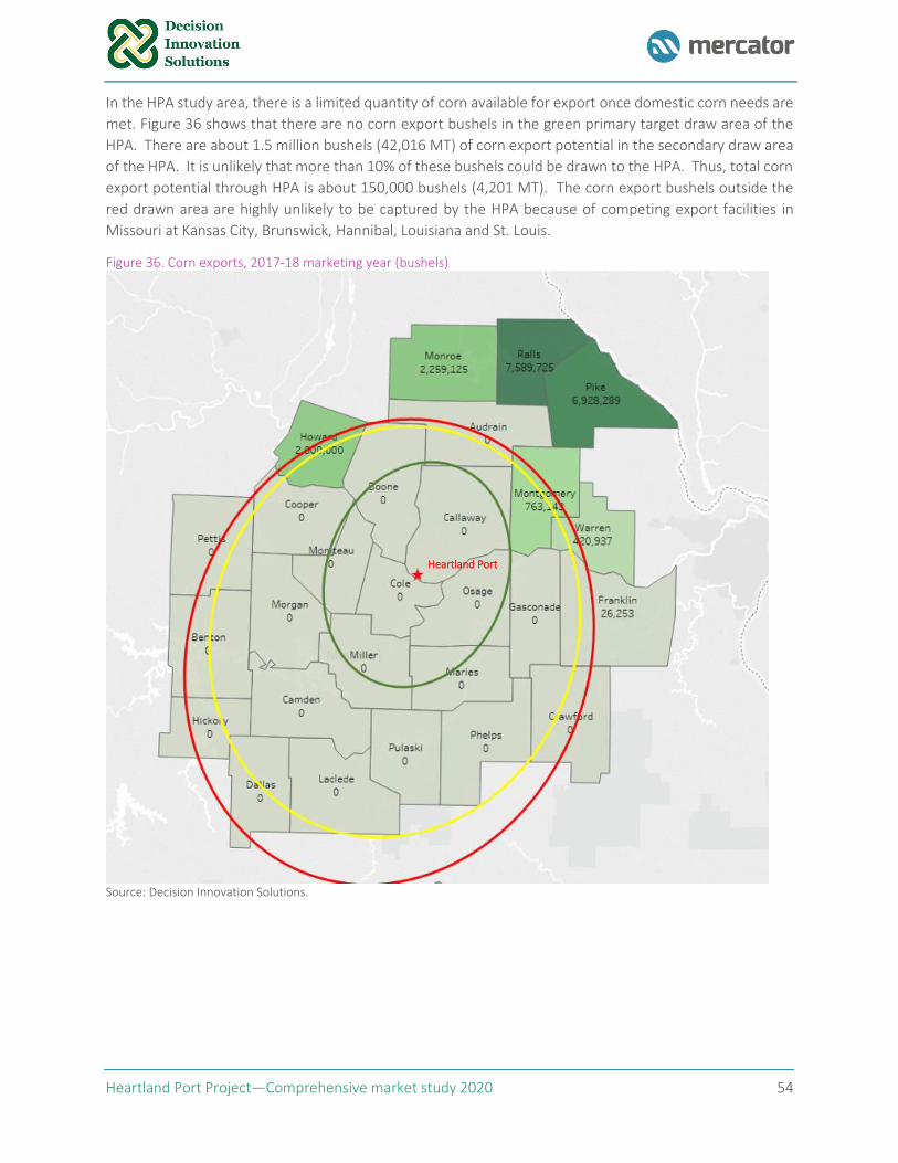
Heartland Port Project—Comprehensive market study 2020 54
In the HPA study area, there is a limited quantity of corn available for export once domestic corn needs are
met. Figure 36 shows that there are no corn export bushels in the green primary target draw area of the
HPA. There are about 1.5 million bushels (42,016 MT) of corn export potential in the secondary draw area
of the HPA. It is unlikely that more than 10% of these bushels could be drawn to the HPA. Thus, total corn
export potential through HPA is about 150,000 bushels (4,201 MT). The corn export bushels outside the
red drawn area are highly unlikely to be captured by the HPA because of competing export facilities in
Missouri at Kansas City, Brunswick, Hannibal, Louisiana and St. Louis.
Figure 36. Corn exports, 2017-18 marketing year (bushels)
Source: Decision Innovation Solutions.
Heartland Port
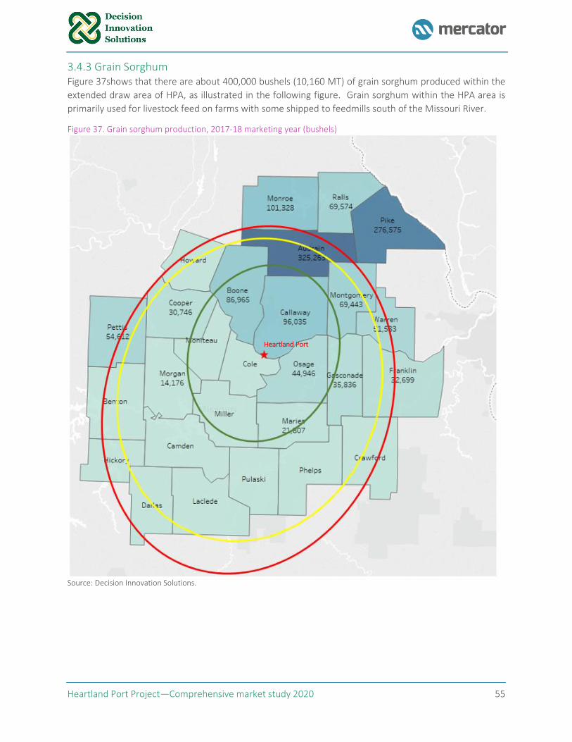
Heartland Port Project—Comprehensive market study 2020 55
3.4.3 Grain Sorghum Figure 37shows that there are about 400,000 bushels (10,160 MT) of grain sorghum produced within the
extended draw area of HPA, as illustrated in the following figure. Grain sorghum within the HPA area is
primarily used for livestock feed on farms with some shipped to feedmills south of the Missouri River.
Figure 37. Grain sorghum production, 2017-18 marketing year (bushels)
Source: Decision Innovation Solutions.
Heartland Port
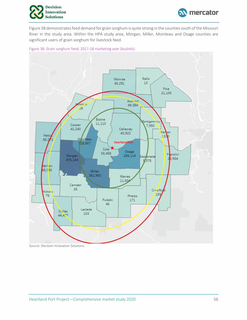
Heartland Port Project—Comprehensive market study 2020 56
Figure 38 demonstrates feed demand for grain sorghum is quite strong in the counties south of the Missouri
River in the study area. Within the HPA study area, Morgan, Miller, Moniteau and Osage counties are
significant users of grain sorghum for livestock feed.
Figure 38. Grain sorghum feed, 2017-18 marketing year (bushels)
Source: Decision Innovation Solutions.
Heartland Port
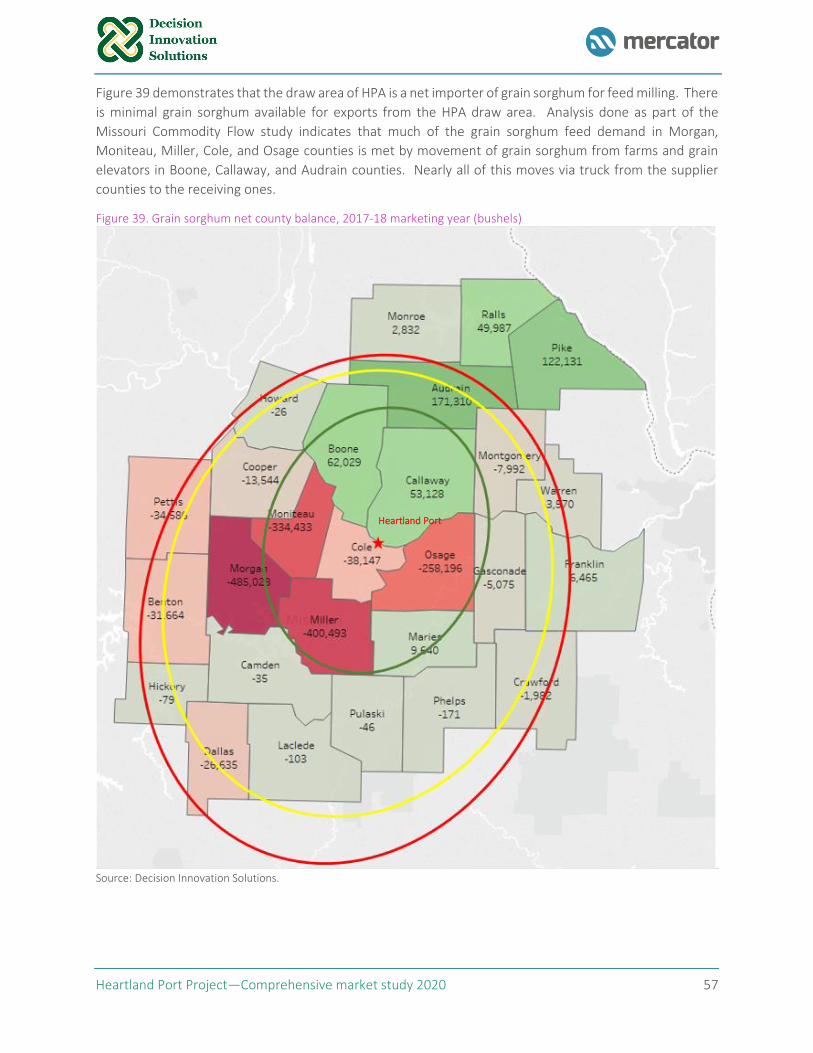
Heartland Port Project—Comprehensive market study 2020 57
Figure 39 demonstrates that the draw area of HPA is a net importer of grain sorghum for feed milling. There
is minimal grain sorghum available for exports from the HPA draw area. Analysis done as part of the
Missouri Commodity Flow study indicates that much of the grain sorghum feed demand in Morgan,
Moniteau, Miller, Cole, and Osage counties is met by movement of grain sorghum from farms and grain
elevators in Boone, Callaway, and Audrain counties. Nearly all of this moves via truck from the supplier
counties to the receiving ones.
Figure 39. Grain sorghum net county balance, 2017-18 marketing year (bushels)
Source: Decision Innovation Solutions.
Heartland Port
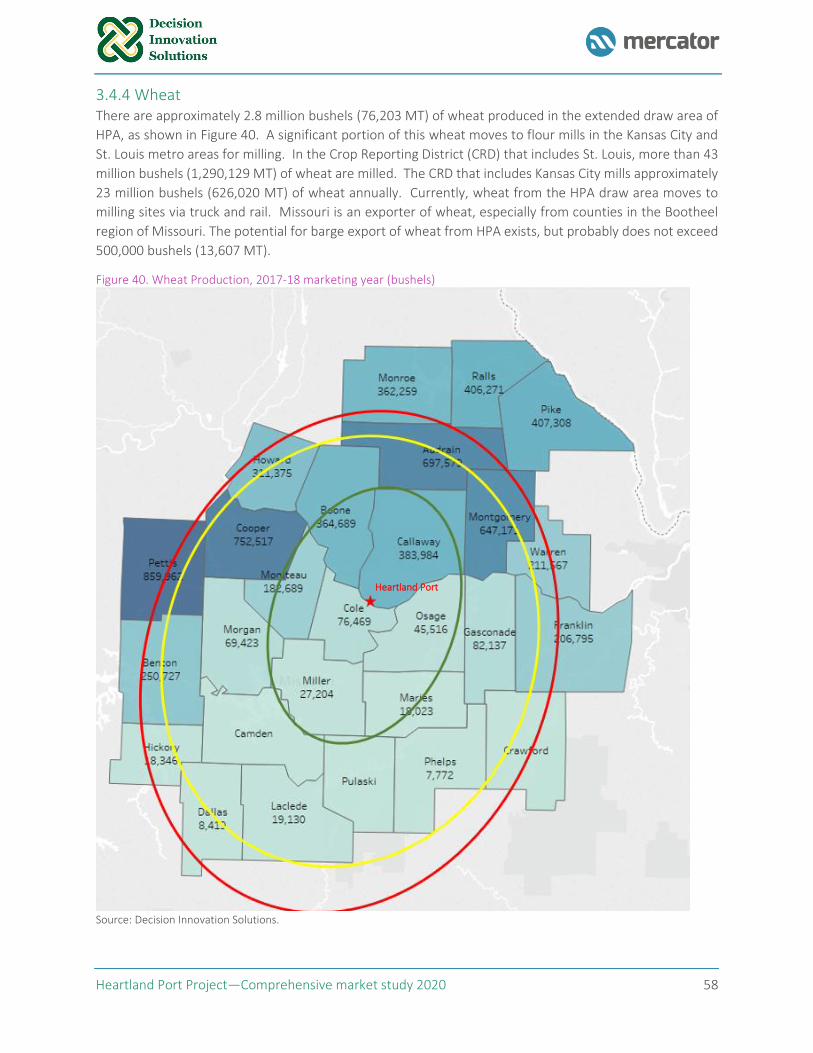
Heartland Port Project—Comprehensive market study 2020 58
3.4.4 Wheat There are approximately 2.8 million bushels (76,203 MT) of wheat produced in the extended draw area of
HPA, as shown in Figure 40. A significant portion of this wheat moves to flour mills in the Kansas City and
St. Louis metro areas for milling. In the Crop Reporting District (CRD) that includes St. Louis, more than 43
million bushels (1,290,129 MT) of wheat are milled. The CRD that includes Kansas City mills approximately
23 million bushels (626,020 MT) of wheat annually. Currently, wheat from the HPA draw area moves to
milling sites via truck and rail. Missouri is an exporter of wheat, especially from counties in the Bootheel
region of Missouri. The potential for barge export of wheat from HPA exists, but probably does not exceed
500,000 bushels (13,607 MT).
Figure 40. Wheat Production, 2017-18 marketing year (bushels)
Source: Decision Innovation Solutions.
Heartland Port
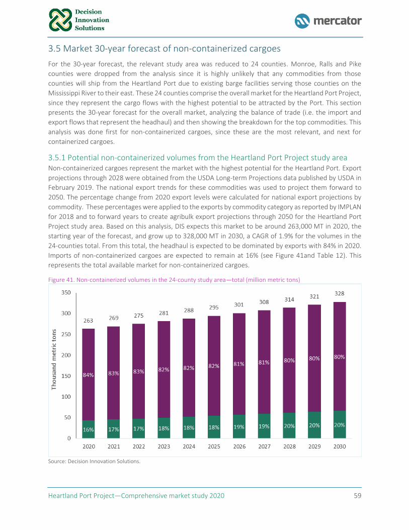
Heartland Port Project—Comprehensive market study 2020 59
3.5 Market 30-year forecast of non-containerized cargoes
For the 30-year forecast, the relevant study area was reduced to 24 counties. Monroe, Ralls and Pike
counties were dropped from the analysis since it is highly unlikely that any commodities from those
counties will ship from the Heartland Port due to existing barge facilities serving those counties on the
Mississippi River to their east. These 24 counties comprise the overall market for the Heartland Port Project,
since they represent the cargo flows with the highest potential to be attracted by the Port. This section
presents the 30-year forecast for the overall market, analyzing the balance of trade (i.e. the import and
export flows that represent the headhaul) and then showing the breakdown for the top commodities. This
analysis was done first for non-containerized cargoes, since these are the most relevant, and next for
containerized cargoes.
3.5.1 Potential non-containerized volumes from the Heartland Port Project study area Non-containerized cargoes represent the market with the highest potential for the Heartland Port. Export
projections through 2028 were obtained from the USDA Long-term Projections data published by USDA in
February 2019. The national export trends for these commodities was used to project them forward to
2050. The percentage change from 2020 export levels were calculated for national export projections by
commodity. These percentages were applied to the exports by commodity category as reported by IMPLAN
for 2018 and to forward years to create agribulk export projections through 2050 for the Heartland Port
Project study area. Based on this analysis, DIS expects this market to be around 263,000 MT in 2020, the
starting year of the forecast, and grow up to 328,000 MT in 2030, a CAGR of 1.9% for the volumes in the
24-counties total. From this total, the headhaul is expected to be dominated by exports with 84% in 2020.
Imports of non-containerized cargoes are expected to remain at 16% (see Figure 41and Table 12). This
represents the total available market for non-containerized cargoes.
Figure 41. Non-containerized volumes in the 24-county study area—total (million metric tons)
Source: Decision Innovation Solutions.
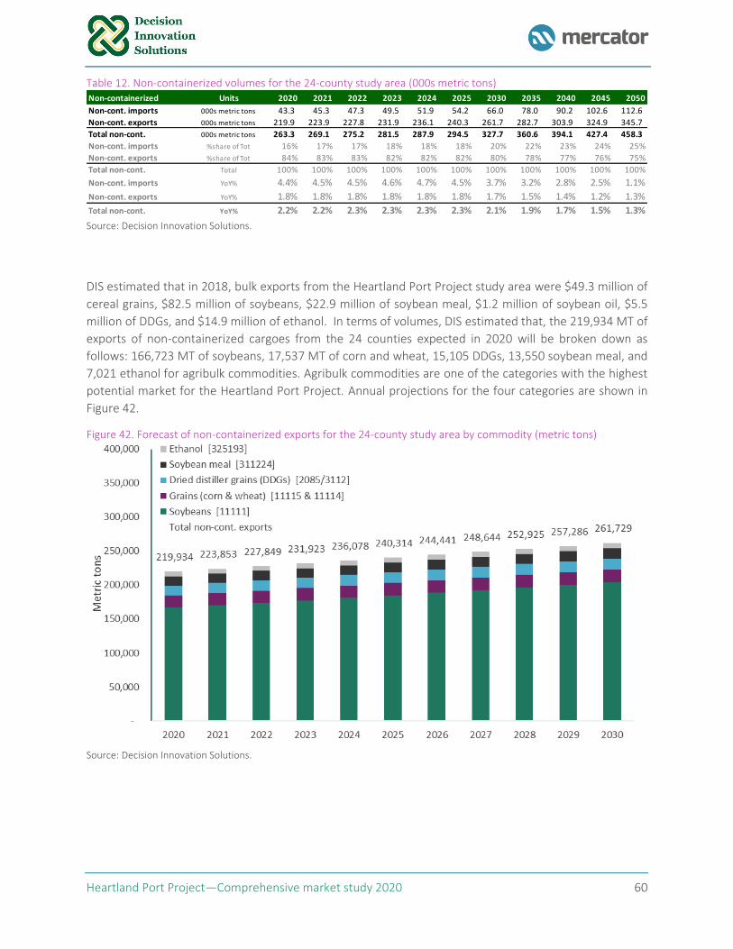
Heartland Port Project—Comprehensive market study 2020 60
Table 12. Non-containerized volumes for the 24-county study area (000s metric tons)
Source: Decision Innovation Solutions.
DIS estimated that in 2018, bulk exports from the Heartland Port Project study area were $49.3 million of
cereal grains, $82.5 million of soybeans, $22.9 million of soybean meal, $1.2 million of soybean oil, $5.5
million of DDGs, and $14.9 million of ethanol. In terms of volumes, DIS estimated that, the 219,934 MT of
exports of non-containerized cargoes from the 24 counties expected in 2020 will be broken down as
follows: 166,723 MT of soybeans, 17,537 MT of corn and wheat, 15,105 DDGs, 13,550 soybean meal, and
7,021 ethanol for agribulk commodities. Agribulk commodities are one of the categories with the highest
potential market for the Heartland Port Project. Annual projections for the four categories are shown in
Figure 42.
Figure 42. Forecast of non-containerized exports for the 24-county study area by commodity (metric tons)
Source: Decision Innovation Solutions.
Non-containerized Units 2020 2021 2022 2023 2024 2025 2030 2035 2040 2045 2050
Non-cont. imports 000s metric tons 43.3 45.3 47.3 49.5 51.9 54.2 66.0 78.0 90.2 102.6 112.6
Non-cont. exports 000s metric tons 219.9 223.9 227.8 231.9 236.1 240.3 261.7 282.7 303.9 324.9 345.7
Total non-cont. 000s metric tons 263.3 269.1 275.2 281.5 287.9 294.5 327.7 360.6 394.1 427.4 458.3
Non-cont. imports %share of Tot 16% 17% 17% 18% 18% 18% 20% 22% 23% 24% 25%
Non-cont. exports %share of Tot 84% 83% 83% 82% 82% 82% 80% 78% 77% 76% 75%
Total non-cont. Total 100% 100% 100% 100% 100% 100% 100% 100% 100% 100% 100%
Non-cont. imports YoY% 4.4% 4.5% 4.5% 4.6% 4.7% 4.5% 3.7% 3.2% 2.8% 2.5% 1.1%
Non-cont. exports YoY% 1.8% 1.8% 1.8% 1.8% 1.8% 1.8% 1.7% 1.5% 1.4% 1.2% 1.3%
Total non-cont. YoY% 2.2% 2.2% 2.3% 2.3% 2.3% 2.3% 2.1% 1.9% 1.7% 1.5% 1.3%
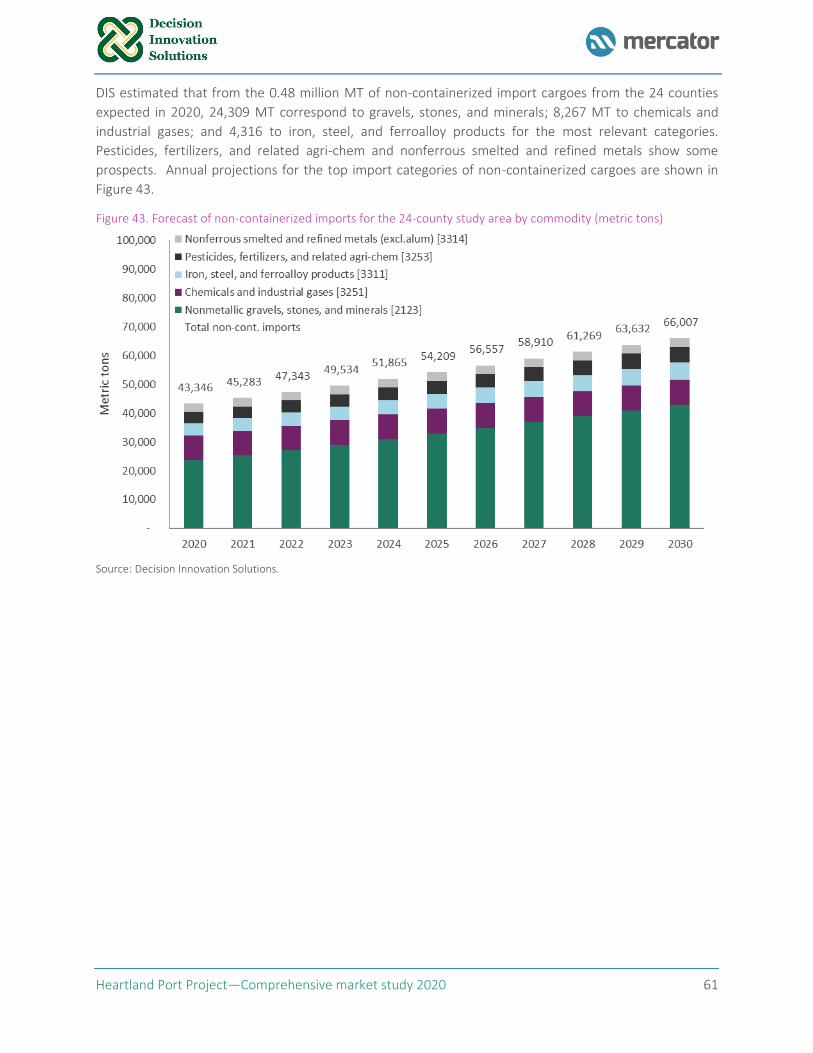
Heartland Port Project—Comprehensive market study 2020 61
DIS estimated that from the 0.48 million MT of non-containerized import cargoes from the 24 counties
expected in 2020, 24,309 MT correspond to gravels, stones, and minerals; 8,267 MT to chemicals and
industrial gases; and 4,316 to iron, steel, and ferroalloy products for the most relevant categories.
Pesticides, fertilizers, and related agri-chem and nonferrous smelted and refined metals show some
prospects. Annual projections for the top import categories of non-containerized cargoes are shown in
Figure 43.
Figure 43. Forecast of non-containerized imports for the 24-county study area by commodity (metric tons)
Source: Decision Innovation Solutions.
Heartland Port Project—Comprehensive market study 2020 62
4. Heartland Port: route economics and key target markets
Section 4 presents an analysis of the main target markets for the Heartland Port Project and compares the
costs for key incumbent routes against new, alternate routes using the Heartland Port, which substitutes
barge for rail on the inland component. These analyses are done for non-containerized cargoes first,
followed by containerized ones. To identify potential markets, we enumerate the incumbent routes,
analyze their route economics, and identify potential route cost savings that could drive cargo to the
Heartland Port Project. We identify the commodities with the highest volumes moving in and out of the
24-county area, and based on the logistical cost advantages of the project quantify the potential cargo
capture for the Heartland Port Project for each of the main non-containerized cargo and containerized
cargoes.
4.1 General Assumptions
Numerous studies have been performed that compared the fuel efficiencies of barge, railroad, and truck
and most conclude that movement of freight by barge is the most fuel-efficient transport mode and the
lowest cost option for shipments moving over medium to long distances.13 Consequently, a fundamental
premise underpinning the Heartland Port Project is that the cost savings from transporting goods via barge
will be large enough to entice beneficial cargo owners (BCO) to use this mode as opposed to transport by
truck or rail, particularly in light of increasing capacity constraints along inland transportation corridors,
such as I-70, and concerns regarding rising greenhouse gas emissions related to trucks.
Mercator analyzed route costs for the key non-containerized and containerized cargoes being exported
from and imported into the Heartland Port’s market region by first segmenting the region into two target
trade areas—counties within a 50 mi radius of Heartland Port (Target Area 1), and counties within an 80 mi
radius of Heartland Port, but excluding those within the 50 mi radius (Target Area 2), as depicted in
Figure 44. The counties included in each of the trade areas are listed in the next bullets:
▪ Target Area 1—includes 14 counties in the first trade area, represented by the interior circle:
Audrain, Boone, Callaway, Camden, Cole, Cooper, Gasconade, Howard, Marries, Miller, Moniteau,
Montgomery, Morgan, and Osage.
▪ Target Area 2—includes 10 in the second, symbolized by the exterior ring: Benton, Crawford,
Dallas, Franklin, Hickory, Laclede, Pettis, Phelps, Pulaski, and Warren.
13 Environmental Advantages of Inland Barge Transportation, U.S. Department of Transportation, Maritime Administration. Final Report, August 1994 http://www.uppermon.org/visions/DOT_environ_barge.htm
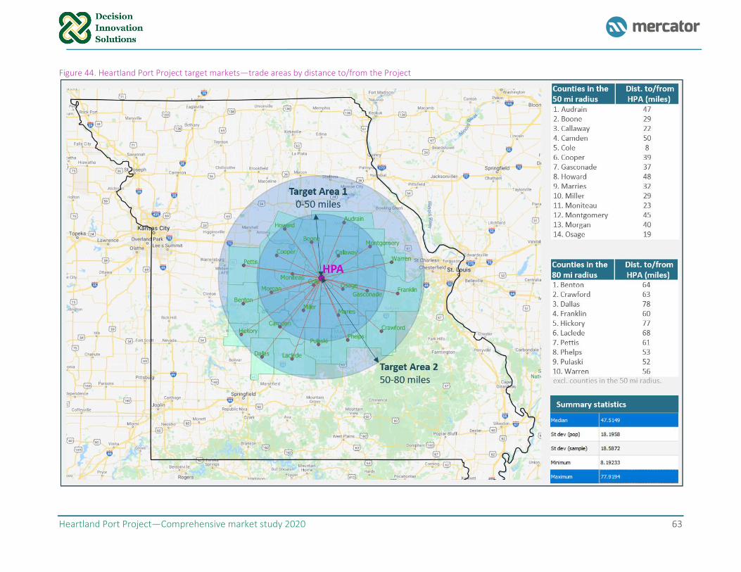
Heartland Port Project—Comprehensive market study 2020 63
Figure 44. Heartland Port Project target markets—trade areas by distance to/from the Project
Heartland Port Project—Comprehensive market study 2020 64
4.2 Non-containerized cargoes
4.2.1 Incumbent routes Based on the organization of trade shares and the mix of commodities and industrial activities with the
highest potential to be attracted by the Heartland Port Project, Mercator identified these five main
incumbent corridors for the movement of non-containerized exports from Missouri. Each route is listed
with the inland point first and then the gateway port or destination (as in the case of Mexico City): (i) St.
Louis-Port of New Orleans, (ii) Kansas City-Port of Portland, (iii) Kansas City-San Pedro Bay (SPB) which
includes the ports of Los Angeles and Long Beach, (iv) St. Louis-Port of Norfolk, and (v) Kansas City-Mexico
City. All five have rail as the inland transport component and two have barge. These incumbent routes are
explained in detail in the following bullets and displayed in Figure 46.
▪ St. Louis-New Orleans. This is the main corridor handling non-containerized exports via the Gulf
Coast. Presently, there are two alternatives to move cargo from St. Louis to New Orleans, by rail
and barge, each described in detail next.
▪ By rail: It is 890 mi long and is served by UP, KCS, and CN in the north-south direction (along
with interchange with BNSF and CSXT in the east-west direction). Presently, the nearest
loading point for exports moving through the Port of New Orleans gateway is St. Louis
(167 mi by truck from the Heartland Port Project study area), although it is also possible to
load the cargo in Kansas City.
▪ By barge: River transportation is available through the Port of St. Louis14 along the
Mississippi River. This route is composed of a 167 mi trip by truck from Jefferson City to St.
Louis and a 1,190 mi movement by barge along marine highway M-55 from St. Louis to
New Orleans, the export gateway. The Port of St. Louis presently handles all cargo-types.
▪ Kansas City-Portland—This is the primary route for non-containerized exports transiting through
the Pacific Northwest (PNW), which includes the ports of Portland, Seattle, and Tacoma, and such
exports are mainly destined to Asia. It is 1,880 mi long and is served by UP and BNSF. Presently, the
nearest loading point to Jefferson City for exports via the PNW is Kansas City (190 mi by truck from
the site of the port).
▪ Kansas City-SPB—This is the corridor for non-containerized exports moving via other ports on the
West Coast (primarily Los Angeles or Long Beach), which is logical since the bulk of this cargo is
destined to Asia. It is 1,740 mi long and is served by UP and BNSF. Presently, the nearest loading
point for exports is Kansas City (190 mi by truck from Jefferson City).
▪ St. Louis-Norfolk—This corridor handles non-containerized exports via Norfolk, VA in the East
Coast. It is 1,510 mi long and is served by the Norfolk Southern (NS) with interchange with CSXT.
Presently, the nearest loading point for exports is St. Louis (167 mi by truck from the Heartland
Port project).
14 The Port of Metropolitan St. Louis (PMSL), as defined by the USACE, is 70 miles long and includes both sides of the Mississippi River. It is the third-largest inland water port by tonnage in the U.S. and the northernmost ice- and lock-free port on the Mississippi River. The City of St. Louis Port District, which is within the PMSL, covers 19 miles of riverfront and 6,000 acres of developable land, including the Municipal River Terminal (MRT). The Port is the second-largest inland port by trip-ton miles, and the third-largest by tonnage in the U.S., with more than 100 docks for barges, 16 public terminals on the river inside the port facility, and about 55 docks/terminals considering those outside the port limits in the towns of Madison, St Clair, and St Charles. The Port of St. Louis presently handles all non-containerized cargo-types and container on-barge by SCF. These terminals are identified in Appendix A.
Heartland Port Project—Comprehensive market study 2020 65
▪ Kansas City-Mexico City—It is 1,680 mi long and is served primarily by UP on the U.S. side of the
border. The Kansas City Southern Mexico (KCSM) corridor that extends from Mexico City (Ciudad
de Mexico, or CDMX) connecting with UP in Laredo, Texas was considered the most logical route
choice between the study area and Central Mexico. Hence, this corridor was selected from the
three main rail corridors connecting with Central Mexico.15 There is also a water route from
Jefferson City to Mexico City, which incorporates truck and barge to New Orleans, a transgulf vessel
to Veracruz and truck to Mexico City.
15 There are three main rail corridors connecting Central Mexico with the Texas border:
(i) The Ferromex corridor that extends from Queretaro, Aguascalientes, Torreon, Chihuahua, and Cd. Juarez connecting with both UP and BNSF in El Paso.
(ii) The KCSM corridor that extends from Mexico City, San Luis Potosi, Saltillo, and Piedras Negras (interchanging with Ferromex) connecting with UP in Eagle Pass.
(iii) The KCSM corridor extends from Mexico City to San Luis Potosi, Saltillo, and Nuevo Laredo connecting with UP in Laredo.
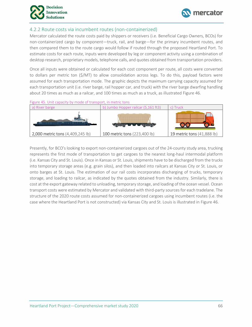
Heartland Port Project—Comprehensive market study 2020 66
4.2.2 Route costs via incumbent routes (non-containerized) Mercator calculated the route costs paid by shippers or receivers (i.e. Beneficial Cargo Owners, BCOs) for
non-containerized cargo by component—truck, rail, and barge—for the primary incumbent routes, and
then compared them to the route cargo would follow if routed through the proposed Heartland Port. To
estimate costs for each route, inputs were developed by leg or component activity using a combination of
desktop research, proprietary models, telephone calls, and quotes obtained from transportation providers.
Once all inputs were obtained or calculated for each cost component per route, all costs were converted
to dollars per metric ton ($/MT) to allow consolidation across legs. To do this, payload factors were
assumed for each transportation mode. The graphic depicts the maximum carrying capacity assumed for
each transportation unit (i.e. river barge, rail hopper car, and truck) with the river barge dwarfing handling
about 20 times as much as a railcar, and 100 times as much as a truck, as illustrated Figure 46.
Figure 45. Unit capacity by mode of transport, in metric tons
a) River barge b) Jumbo Hopper railcar (5,161 ft3) c) Truck
2,000 metric tons (4,409,245 lb) 100 metric tons (223,400 lb) 19 metric tons (41,888 lb)
Presently, for BCO’s looking to export non-containerized cargoes out of the 24-county study area, trucking
represents the first mode of transportation to get cargoes to the nearest long-haul intermodal platform
(i.e. Kansas City and St. Louis). Once in Kansas or St. Louis, shipments have to be discharged from the trucks
into temporary storage areas (e.g. grain silos), and then loaded into railcars at Kansas City or St. Louis, or
onto barges at St. Louis. The estimation of our rail costs incorporates discharging of trucks, temporary
storage, and loading to railcar, as indicated by the quotes obtained from the industry. Similarly, there is
cost at the export gateway related to unloading, temporary storage, and loading of the ocean vessel. Ocean
transport costs were estimated by Mercator and validated with third-party sources for each tradelane. The
structure of the 2020 route costs assumed for non-containerized cargoes using incumbent routes (i.e. the
case where the Heartland Port is not constructed) via Kansas City and St. Louis is illustrated in Figure 46.
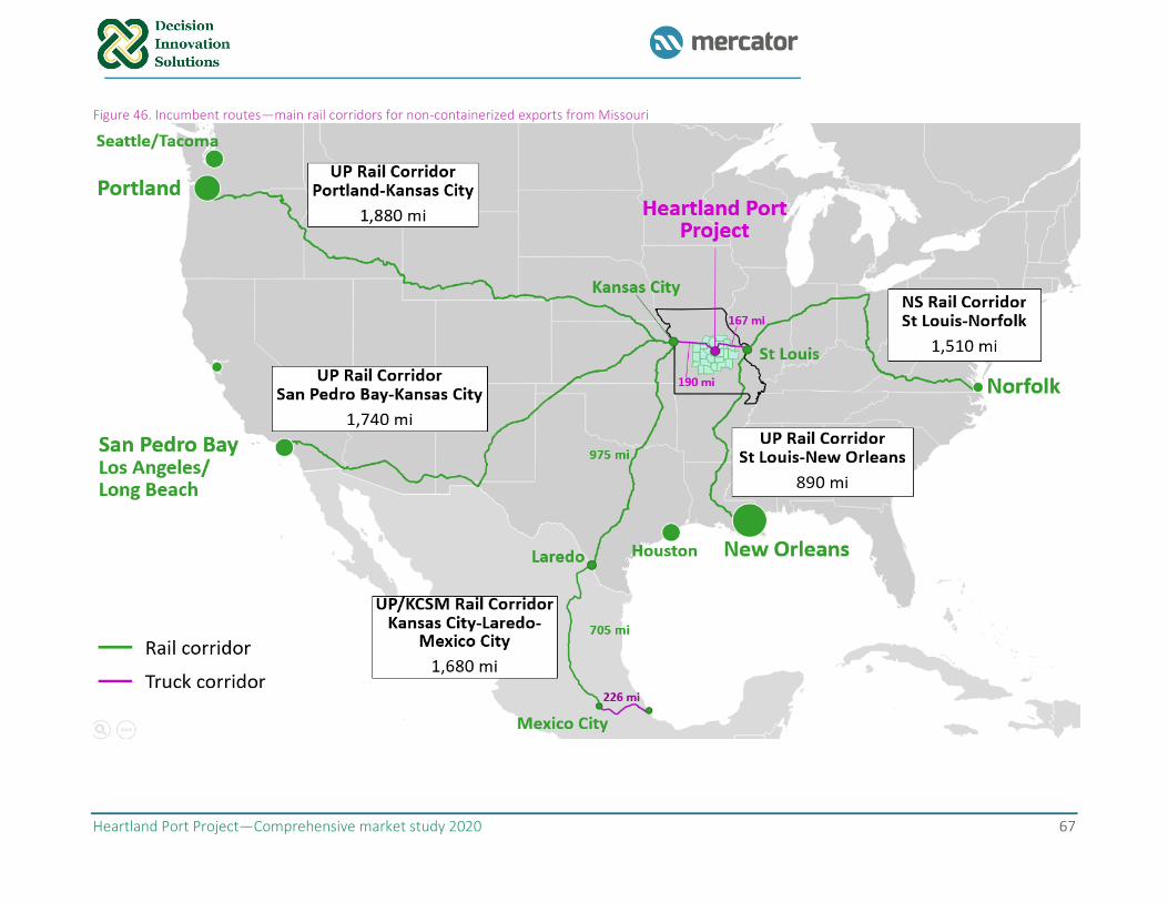
Heartland Port Project—Comprehensive market study 2020 67
Figure 46. Incumbent routes—main rail corridors for non-containerized exports from Missouri
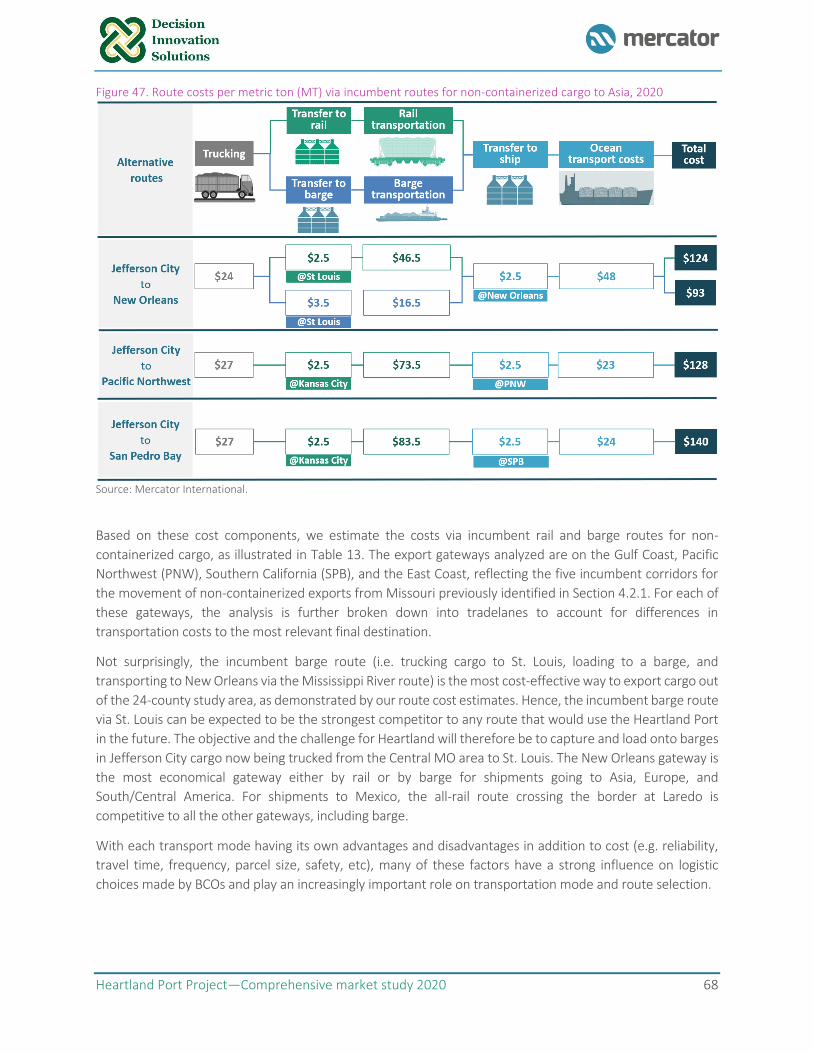
Heartland Port Project—Comprehensive market study 2020 68
Figure 47. Route costs per metric ton (MT) via incumbent routes for non-containerized cargo to Asia, 2020
Source: Mercator International.
Based on these cost components, we estimate the costs via incumbent rail and barge routes for non-
containerized cargo, as illustrated in Table 13. The export gateways analyzed are on the Gulf Coast, Pacific
Northwest (PNW), Southern California (SPB), and the East Coast, reflecting the five incumbent corridors for
the movement of non-containerized exports from Missouri previously identified in Section 4.2.1. For each of
these gateways, the analysis is further broken down into tradelanes to account for differences in
transportation costs to the most relevant final destination.
Not surprisingly, the incumbent barge route (i.e. trucking cargo to St. Louis, loading to a barge, and
transporting to New Orleans via the Mississippi River route) is the most cost-effective way to export cargo out
of the 24-county study area, as demonstrated by our route cost estimates. Hence, the incumbent barge route
via St. Louis can be expected to be the strongest competitor to any route that would use the Heartland Port
in the future. The objective and the challenge for Heartland will therefore be to capture and load onto barges
in Jefferson City cargo now being trucked from the Central MO area to St. Louis. The New Orleans gateway is
the most economical gateway either by rail or by barge for shipments going to Asia, Europe, and
South/Central America. For shipments to Mexico, the all-rail route crossing the border at Laredo is
competitive to all the other gateways, including barge.
With each transport mode having its own advantages and disadvantages in addition to cost (e.g. reliability,
travel time, frequency, parcel size, safety, etc), many of these factors have a strong influence on logistic
choices made by BCOs and play an increasingly important role on transportation mode and route selection.
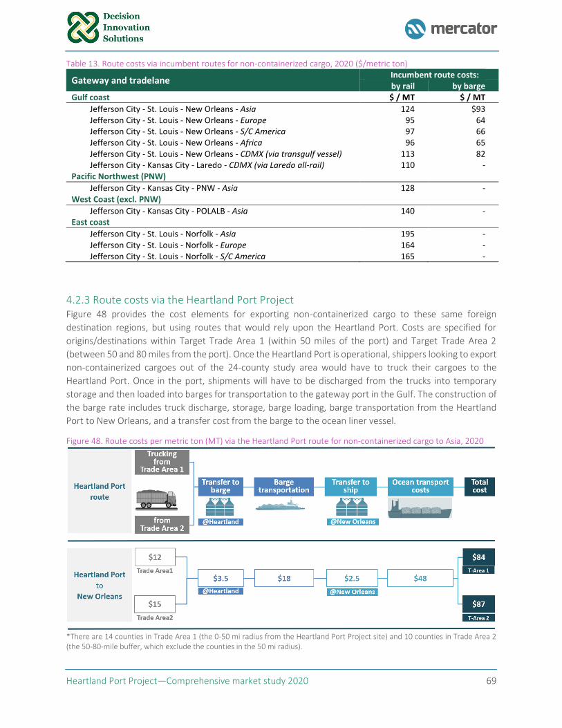
Heartland Port Project—Comprehensive market study 2020 69
Table 13. Route costs via incumbent routes for non-containerized cargo, 2020 ($/metric ton)
Gateway and tradelane Incumbent route costs: by rail by barge
Gulf coast $ / MT $ / MT
Jefferson City - St. Louis - New Orleans - Asia 124 $93 Jefferson City - St. Louis - New Orleans - Europe 95 64 Jefferson City - St. Louis - New Orleans - S/C America 97 66 Jefferson City - St. Louis - New Orleans - Africa 96 65 Jefferson City - St. Louis - New Orleans - CDMX (via transgulf vessel) 113 82 Jefferson City - Kansas City - Laredo - CDMX (via Laredo all-rail) 110 -
Pacific Northwest (PNW)
Jefferson City - Kansas City - PNW - Asia 128 - West Coast (excl. PNW)
Jefferson City - Kansas City - POLALB - Asia 140 - East coast
Jefferson City - St. Louis - Norfolk - Asia 195 - Jefferson City - St. Louis - Norfolk - Europe 164 - Jefferson City - St. Louis - Norfolk - S/C America 165 -
4.2.3 Route costs via the Heartland Port Project Figure 48 provides the cost elements for exporting non-containerized cargo to these same foreign
destination regions, but using routes that would rely upon the Heartland Port. Costs are specified for
origins/destinations within Target Trade Area 1 (within 50 miles of the port) and Target Trade Area 2
(between 50 and 80 miles from the port). Once the Heartland Port is operational, shippers looking to export
non-containerized cargoes out of the 24-county study area would have to truck their cargoes to the
Heartland Port. Once in the port, shipments will have to be discharged from the trucks into temporary
storage and then loaded into barges for transportation to the gateway port in the Gulf. The construction of
the barge rate includes truck discharge, storage, barge loading, barge transportation from the Heartland
Port to New Orleans, and a transfer cost from the barge to the ocean liner vessel.
Figure 48. Route costs per metric ton (MT) via the Heartland Port route for non-containerized cargo to Asia, 2020
*There are 14 counties in Trade Area 1 (the 0-50 mi radius from the Heartland Port Project site) and 10 counties in Trade Area 2 (the 50-80-mile buffer, which exclude the counties in the 50 mi radius).
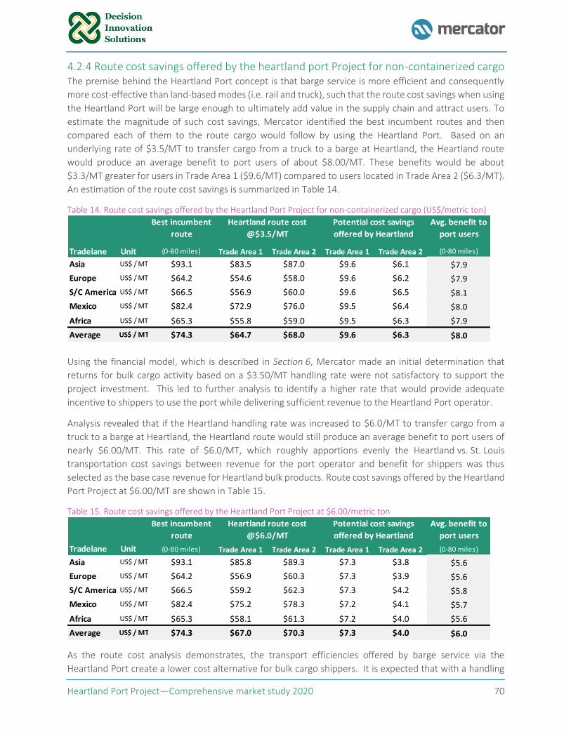
Heartland Port Project—Comprehensive market study 2020 70
4.2.4 Route cost savings offered by the heartland port Project for non-containerized cargo The premise behind the Heartland Port concept is that barge service is more efficient and consequently
more cost-effective than land-based modes (i.e. rail and truck), such that the route cost savings when using
the Heartland Port will be large enough to ultimately add value in the supply chain and attract users. To
estimate the magnitude of such cost savings, Mercator identified the best incumbent routes and then
compared each of them to the route cargo would follow by using the Heartland Port. Based on an
underlying rate of $3.5/MT to transfer cargo from a truck to a barge at Heartland, the Heartland route
would produce an average benefit to port users of about $8.00/MT. These benefits would be about
$3.3/MT greater for users in Trade Area 1 ($9.6/MT) compared to users located in Trade Area 2 ($6.3/MT).
An estimation of the route cost savings is summarized in Table 14.
Table 14. Route cost savings offered by the Heartland Port Project for non-containerized cargo (US$/metric ton)
Using the financial model, which is described in Section 6, Mercator made an initial determination that
returns for bulk cargo activity based on a $3.50/MT handling rate were not satisfactory to support the
project investment. This led to further analysis to identify a higher rate that would provide adequate
incentive to shippers to use the port while delivering sufficient revenue to the Heartland Port operator.
Analysis revealed that if the Heartland handling rate was increased to $6.0/MT to transfer cargo from a
truck to a barge at Heartland, the Heartland route would still produce an average benefit to port users of
nearly $6.00/MT. This rate of $6.0/MT, which roughly apportions evenly the Heartland vs. St. Louis
transportation cost savings between revenue for the port operator and benefit for shippers was thus
selected as the base case revenue for Heartland bulk products. Route cost savings offered by the Heartland
Port Project at $6.00/MT are shown in Table 15.
Table 15. Route cost savings offered by the Heartland Port Project at $6.00/metric ton
As the route cost analysis demonstrates, the transport efficiencies offered by barge service via the
Heartland Port create a lower cost alternative for bulk cargo shippers. It is expected that with a handling
Best incumbent
route
Avg. benefit to
port users
Tradelane Unit (0-80 miles) Trade Area 1 Trade Area 2 Trade Area 1 Trade Area 2 (0-80 miles)
Asia US$ / MT $93.1 $83.5 $87.0 $9.6 $6.1 $7.9
Europe US$ / MT $64.2 $54.6 $58.0 $9.6 $6.2 $7.9
S/C America US$ / MT $66.5 $56.9 $60.0 $9.6 $6.5 $8.1
Mexico US$ / MT $82.4 $72.9 $76.0 $9.5 $6.4 $8.0
Africa US$ / MT $65.3 $55.8 $59.0 $9.5 $6.3 $7.9
Average US$ / MT $74.3 $64.7 $68.0 $9.6 $6.3 $8.0
Heartland route cost
@$3.5/MT
Potential cost savings
offered by Heartland
Best incumbent
route
Avg. benefit to
port users
Tradelane Unit (0-80 miles) Trade Area 1 Trade Area 2 Trade Area 1 Trade Area 2 (0-80 miles)
Asia US$ / MT $93.1 $85.8 $89.3 $7.3 $3.8 $5.6
Europe US$ / MT $64.2 $56.9 $60.3 $7.3 $3.9 $5.6
S/C America US$ / MT $66.5 $59.2 $62.3 $7.3 $4.2 $5.8
Mexico US$ / MT $82.4 $75.2 $78.3 $7.2 $4.1 $5.7
Africa US$ / MT $65.3 $58.1 $61.3 $7.2 $4.0 $5.6
Average US$ / MT $74.3 $67.0 $70.3 $7.3 $4.0 $6.0
Heartland route cost
@$6.0/MT
Potential cost savings
offered by Heartland
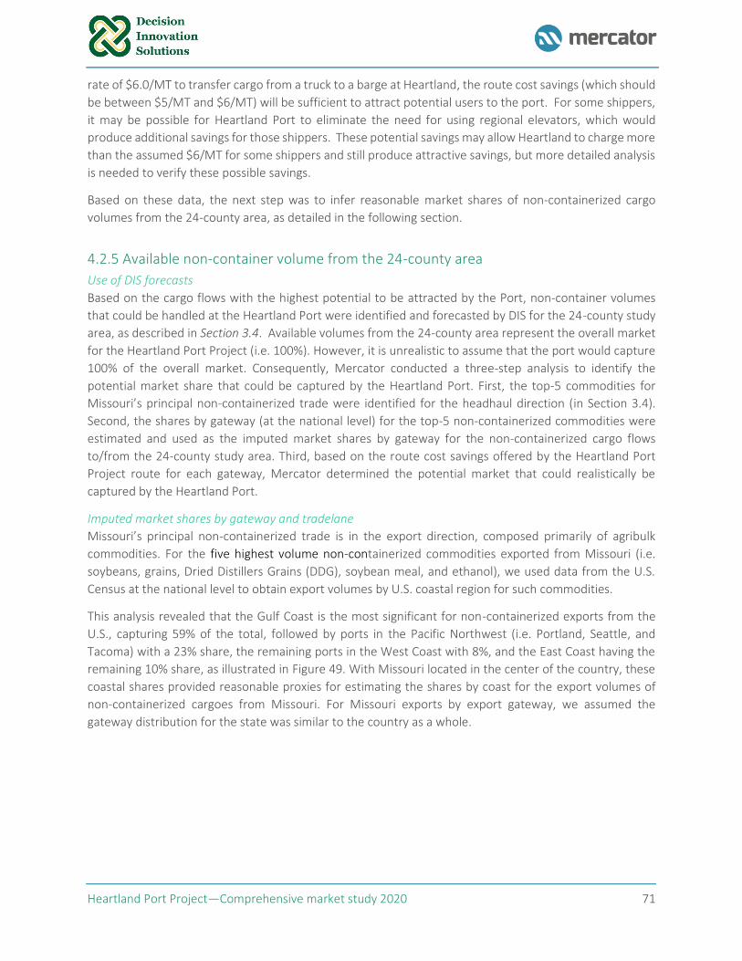
Heartland Port Project—Comprehensive market study 2020 71
rate of $6.0/MT to transfer cargo from a truck to a barge at Heartland, the route cost savings (which should
be between $5/MT and $6/MT) will be sufficient to attract potential users to the port. For some shippers,
it may be possible for Heartland Port to eliminate the need for using regional elevators, which would
produce additional savings for those shippers. These potential savings may allow Heartland to charge more
than the assumed $6/MT for some shippers and still produce attractive savings, but more detailed analysis
is needed to verify these possible savings.
Based on these data, the next step was to infer reasonable market shares of non-containerized cargo
volumes from the 24-county area, as detailed in the following section.
4.2.5 Available non-container volume from the 24-county area
Use of DIS forecasts
Based on the cargo flows with the highest potential to be attracted by the Port, non-container volumes
that could be handled at the Heartland Port were identified and forecasted by DIS for the 24-county study
area, as described in Section 3.4. Available volumes from the 24-county area represent the overall market
for the Heartland Port Project (i.e. 100%). However, it is unrealistic to assume that the port would capture
100% of the overall market. Consequently, Mercator conducted a three-step analysis to identify the
potential market share that could be captured by the Heartland Port. First, the top-5 commodities for
Missouri’s principal non-containerized trade were identified for the headhaul direction (in Section 3.4).
Second, the shares by gateway (at the national level) for the top-5 non-containerized commodities were
estimated and used as the imputed market shares by gateway for the non-containerized cargo flows
to/from the 24-county study area. Third, based on the route cost savings offered by the Heartland Port
Project route for each gateway, Mercator determined the potential market that could realistically be
captured by the Heartland Port.
Imputed market shares by gateway and tradelane
Missouri’s principal non-containerized trade is in the export direction, composed primarily of agribulk
commodities. For the five highest volume non-containerized commodities exported from Missouri (i.e.
soybeans, grains, Dried Distillers Grains (DDG), soybean meal, and ethanol), we used data from the U.S.
Census at the national level to obtain export volumes by U.S. coastal region for such commodities.
This analysis revealed that the Gulf Coast is the most significant for non-containerized exports from the
U.S., capturing 59% of the total, followed by ports in the Pacific Northwest (i.e. Portland, Seattle, and
Tacoma) with a 23% share, the remaining ports in the West Coast with 8%, and the East Coast having the
remaining 10% share, as illustrated in Figure 49. With Missouri located in the center of the country, these
coastal shares provided reasonable proxies for estimating the shares by coast for the export volumes of
non-containerized cargoes from Missouri. For Missouri exports by export gateway, we assumed the
gateway distribution for the state was similar to the country as a whole.
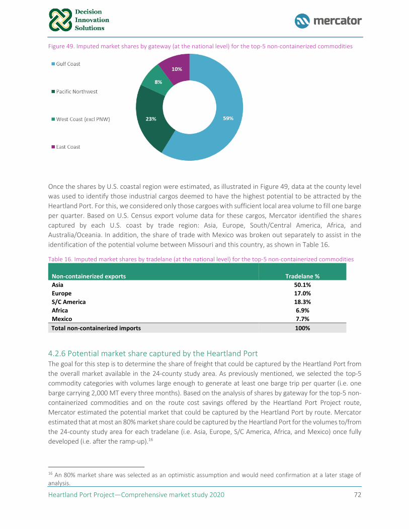
Heartland Port Project—Comprehensive market study 2020 72
Figure 49. Imputed market shares by gateway (at the national level) for the top-5 non-containerized commodities
Once the shares by U.S. coastal region were estimated, as illustrated in Figure 49, data at the county level
was used to identify those industrial cargos deemed to have the highest potential to be attracted by the
Heartland Port. For this, we considered only those cargoes with sufficient local area volume to fill one barge
per quarter. Based on U.S. Census export volume data for these cargos, Mercator identified the shares
captured by each U.S. coast by trade region: Asia, Europe, South/Central America, Africa, and
Australia/Oceania. In addition, the share of trade with Mexico was broken out separately to assist in the
identification of the potential volume between Missouri and this country, as shown in Table 16.
Table 16. Imputed market shares by tradelane (at the national level) for the top-5 non-containerized commodities
Non-containerized exports Tradelane %
Asia 50.1%
Europe 17.0%
S/C America 18.3%
Africa 6.9%
Mexico 7.7%
Total non-containerized imports 100%
4.2.6 Potential market share captured by the Heartland Port The goal for this step is to determine the share of freight that could be captured by the Heartland Port from
the overall market available in the 24-county study area. As previously mentioned, we selected the top-5
commodity categories with volumes large enough to generate at least one barge trip per quarter (i.e. one
barge carrying 2,000 MT every three months). Based on the analysis of shares by gateway for the top-5 non-
containerized commodities and on the route cost savings offered by the Heartland Port Project route,
Mercator estimated the potential market that could be captured by the Heartland Port by route. Mercator
estimated that at most an 80% market share could be captured by the Heartland Port for the volumes to/from
the 24-county study area for each tradelane (i.e. Asia, Europe, S/C America, Africa, and Mexico) once fully
developed (i.e. after the ramp-up).16
16 An 80% market share was selected as an optimistic assumption and would need confirmation at a later stage of analysis.
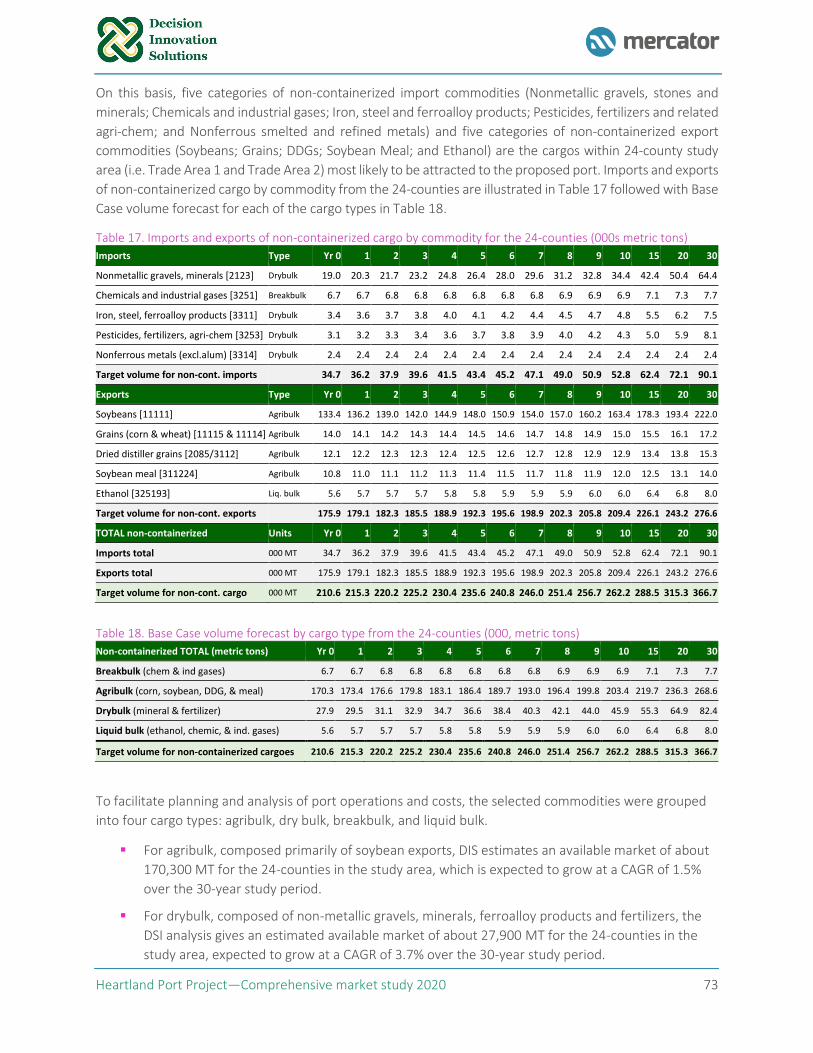
Heartland Port Project—Comprehensive market study 2020 73
On this basis, five categories of non-containerized import commodities (Nonmetallic gravels, stones and
minerals; Chemicals and industrial gases; Iron, steel and ferroalloy products; Pesticides, fertilizers and related
agri-chem; and Nonferrous smelted and refined metals) and five categories of non-containerized export
commodities (Soybeans; Grains; DDGs; Soybean Meal; and Ethanol) are the cargos within 24-county study
area (i.e. Trade Area 1 and Trade Area 2) most likely to be attracted to the proposed port. Imports and exports
of non-containerized cargo by commodity from the 24-counties are illustrated in Table 17 followed with Base
Case volume forecast for each of the cargo types in Table 18.
Table 17. Imports and exports of non-containerized cargo by commodity for the 24-counties (000s metric tons)
Imports Type Yr 0 1 2 3 4 5 6 7 8 9 10 15 20 30
Nonmetallic gravels, minerals [2123] Drybulk 19.0 20.3 21.7 23.2 24.8 26.4 28.0 29.6 31.2 32.8 34.4 42.4 50.4 64.4
Chemicals and industrial gases [3251] Breakbulk 6.7 6.7 6.8 6.8 6.8 6.8 6.8 6.8 6.9 6.9 6.9 7.1 7.3 7.7
Iron, steel, ferroalloy products [3311] Drybulk 3.4 3.6 3.7 3.8 4.0 4.1 4.2 4.4 4.5 4.7 4.8 5.5 6.2 7.5
Pesticides, fertilizers, agri-chem [3253] Drybulk 3.1 3.2 3.3 3.4 3.6 3.7 3.8 3.9 4.0 4.2 4.3 5.0 5.9 8.1
Nonferrous metals (excl.alum) [3314] Drybulk 2.4 2.4 2.4 2.4 2.4 2.4 2.4 2.4 2.4 2.4 2.4 2.4 2.4 2.4
Target volume for non-cont. imports 34.7 36.2 37.9 39.6 41.5 43.4 45.2 47.1 49.0 50.9 52.8 62.4 72.1 90.1
Exports Type Yr 0 1 2 3 4 5 6 7 8 9 10 15 20 30
Soybeans [11111] Agribulk 133.4 136.2 139.0 142.0 144.9 148.0 150.9 154.0 157.0 160.2 163.4 178.3 193.4 222.0
Grains (corn & wheat) [11115 & 11114] Agribulk 14.0 14.1 14.2 14.3 14.4 14.5 14.6 14.7 14.8 14.9 15.0 15.5 16.1 17.2
Dried distiller grains [2085/3112] Agribulk 12.1 12.2 12.3 12.3 12.4 12.5 12.6 12.7 12.8 12.9 12.9 13.4 13.8 15.3
Soybean meal [311224] Agribulk 10.8 11.0 11.1 11.2 11.3 11.4 11.5 11.7 11.8 11.9 12.0 12.5 13.1 14.0
Ethanol [325193] Liq. bulk 5.6 5.7 5.7 5.7 5.8 5.8 5.9 5.9 5.9 6.0 6.0 6.4 6.8 8.0
Target volume for non-cont. exports 175.9 179.1 182.3 185.5 188.9 192.3 195.6 198.9 202.3 205.8 209.4 226.1 243.2 276.6
TOTAL non-containerized Units Yr 0 1 2 3 4 5 6 7 8 9 10 15 20 30
Imports total 000 MT 34.7 36.2 37.9 39.6 41.5 43.4 45.2 47.1 49.0 50.9 52.8 62.4 72.1 90.1
Exports total 000 MT 175.9 179.1 182.3 185.5 188.9 192.3 195.6 198.9 202.3 205.8 209.4 226.1 243.2 276.6
Target volume for non-cont. cargo 000 MT 210.6 215.3 220.2 225.2 230.4 235.6 240.8 246.0 251.4 256.7 262.2 288.5 315.3 366.7
Table 18. Base Case volume forecast by cargo type from the 24-counties (000, metric tons)
Non-containerized TOTAL (metric tons) Yr 0 1 2 3 4 5 6 7 8 9 10 15 20 30
Breakbulk (chem & ind gases) 6.7 6.7 6.8 6.8 6.8 6.8 6.8 6.8 6.9 6.9 6.9 7.1 7.3 7.7
Agribulk (corn, soybean, DDG, & meal) 170.3 173.4 176.6 179.8 183.1 186.4 189.7 193.0 196.4 199.8 203.4 219.7 236.3 268.6
Drybulk (mineral & fertilizer) 27.9 29.5 31.1 32.9 34.7 36.6 38.4 40.3 42.1 44.0 45.9 55.3 64.9 82.4
Liquid bulk (ethanol, chemic, & ind. gases) 5.6 5.7 5.7 5.7 5.8 5.8 5.9 5.9 5.9 6.0 6.0 6.4 6.8 8.0
Target volume for non-containerized cargoes 210.6 215.3 220.2 225.2 230.4 235.6 240.8 246.0 251.4 256.7 262.2 288.5 315.3 366.7
To facilitate planning and analysis of port operations and costs, the selected commodities were grouped
into four cargo types: agribulk, dry bulk, breakbulk, and liquid bulk.
▪ For agribulk, composed primarily of soybean exports, DIS estimates an available market of about
170,300 MT for the 24-counties in the study area, which is expected to grow at a CAGR of 1.5%
over the 30-year study period.
▪ For drybulk, composed of non-metallic gravels, minerals, ferroalloy products and fertilizers, the
DSI analysis gives an estimated available market of about 27,900 MT for the 24-counties in the
study area, expected to grow at a CAGR of 3.7% over the 30-year study period.
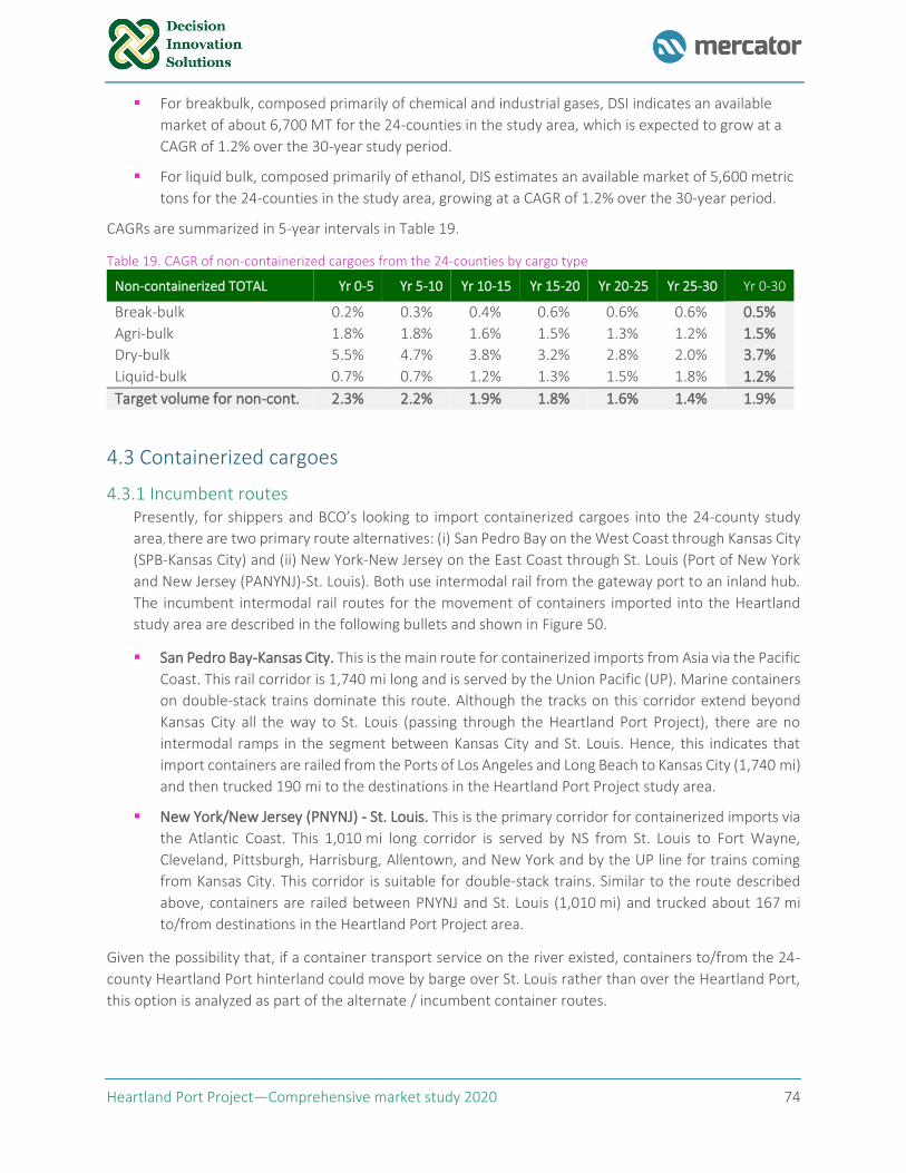
Heartland Port Project—Comprehensive market study 2020 74
▪ For breakbulk, composed primarily of chemical and industrial gases, DSI indicates an available
market of about 6,700 MT for the 24-counties in the study area, which is expected to grow at a
CAGR of 1.2% over the 30-year study period.
▪ For liquid bulk, composed primarily of ethanol, DIS estimates an available market of 5,600 metric
tons for the 24-counties in the study area, growing at a CAGR of 1.2% over the 30-year period.
CAGRs are summarized in 5-year intervals in Table 19.
Table 19. CAGR of non-containerized cargoes from the 24-counties by cargo type
Non-containerized TOTAL Yr 0-5 Yr 5-10 Yr 10-15 Yr 15-20 Yr 20-25 Yr 25-30 Yr 0-30
Break-bulk 0.2% 0.3% 0.4% 0.6% 0.6% 0.6% 0.5%
Agri-bulk 1.8% 1.8% 1.6% 1.5% 1.3% 1.2% 1.5%
Dry-bulk 5.5% 4.7% 3.8% 3.2% 2.8% 2.0% 3.7%
Liquid-bulk 0.7% 0.7% 1.2% 1.3% 1.5% 1.8% 1.2%
Target volume for non-cont. 2.3% 2.2% 1.9% 1.8% 1.6% 1.4% 1.9%
4.3 Containerized cargoes
4.3.1 Incumbent routes Presently, for shippers and BCO’s looking to import containerized cargoes into the 24-county study
area, there are two primary route alternatives: (i) San Pedro Bay on the West Coast through Kansas City
(SPB-Kansas City) and (ii) New York-New Jersey on the East Coast through St. Louis (Port of New York
and New Jersey (PANYNJ)-St. Louis). Both use intermodal rail from the gateway port to an inland hub.
The incumbent intermodal rail routes for the movement of containers imported into the Heartland
study area are described in the following bullets and shown in Figure 50.
▪ San Pedro Bay-Kansas City. This is the main route for containerized imports from Asia via the Pacific
Coast. This rail corridor is 1,740 mi long and is served by the Union Pacific (UP). Marine containers
on double-stack trains dominate this route. Although the tracks on this corridor extend beyond
Kansas City all the way to St. Louis (passing through the Heartland Port Project), there are no
intermodal ramps in the segment between Kansas City and St. Louis. Hence, this indicates that
import containers are railed from the Ports of Los Angeles and Long Beach to Kansas City (1,740 mi)
and then trucked 190 mi to the destinations in the Heartland Port Project study area.
▪ New York/New Jersey (PNYNJ) - St. Louis. This is the primary corridor for containerized imports via
the Atlantic Coast. This 1,010 mi long corridor is served by NS from St. Louis to Fort Wayne,
Cleveland, Pittsburgh, Harrisburg, Allentown, and New York and by the UP line for trains coming
from Kansas City. This corridor is suitable for double-stack trains. Similar to the route described
above, containers are railed between PNYNJ and St. Louis (1,010 mi) and trucked about 167 mi
to/from destinations in the Heartland Port Project area.
Given the possibility that, if a container transport service on the river existed, containers to/from the 24-
county Heartland Port hinterland could move by barge over St. Louis rather than over the Heartland Port,
this option is analyzed as part of the alternate / incumbent container routes.
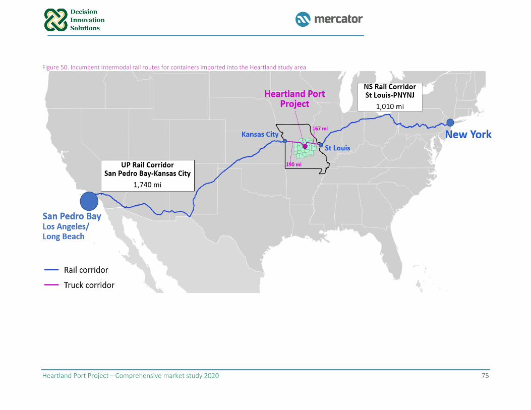
Heartland Port Project—Comprehensive market study 2020 75
Figure 50. Incumbent intermodal rail routes for containers imported into the Heartland study area
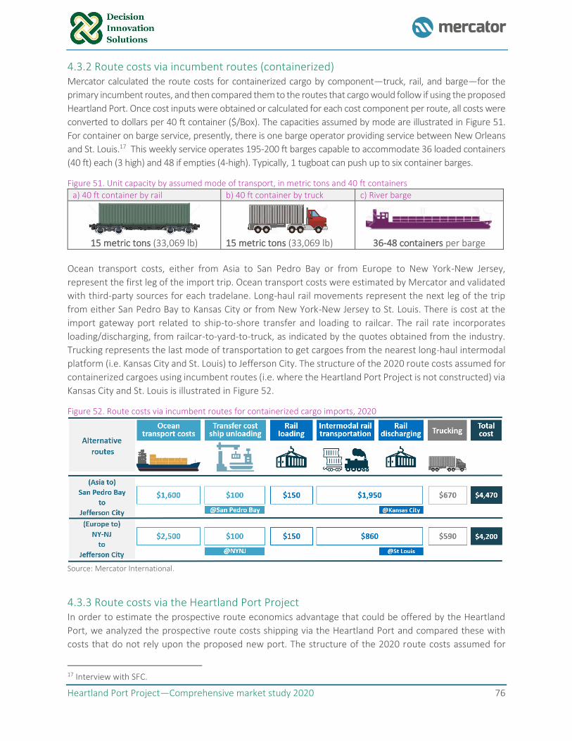
Heartland Port Project—Comprehensive market study 2020 76
4.3.2 Route costs via incumbent routes (containerized) Mercator calculated the route costs for containerized cargo by component—truck, rail, and barge—for the
primary incumbent routes, and then compared them to the routes that cargo would follow if using the proposed
Heartland Port. Once cost inputs were obtained or calculated for each cost component per route, all costs were
converted to dollars per 40 ft container ($/Box). The capacities assumed by mode are illustrated in Figure 51.
For container on barge service, presently, there is one barge operator providing service between New Orleans
and St. Louis.17 This weekly service operates 195-200 ft barges capable to accommodate 36 loaded containers
(40 ft) each (3 high) and 48 if empties (4-high). Typically, 1 tugboat can push up to six container barges.
Figure 51. Unit capacity by assumed mode of transport, in metric tons and 40 ft containers
a) 40 ft container by rail b) 40 ft container by truck c) River barge
15 metric tons (33,069 lb) 15 metric tons (33,069 lb) 36-48 containers per barge
Ocean transport costs, either from Asia to San Pedro Bay or from Europe to New York-New Jersey,
represent the first leg of the import trip. Ocean transport costs were estimated by Mercator and validated
with third-party sources for each tradelane. Long-haul rail movements represent the next leg of the trip
from either San Pedro Bay to Kansas City or from New York-New Jersey to St. Louis. There is cost at the
import gateway port related to ship-to-shore transfer and loading to railcar. The rail rate incorporates
loading/discharging, from railcar-to-yard-to-truck, as indicated by the quotes obtained from the industry.
Trucking represents the last mode of transportation to get cargoes from the nearest long-haul intermodal
platform (i.e. Kansas City and St. Louis) to Jefferson City. The structure of the 2020 route costs assumed for
containerized cargoes using incumbent routes (i.e. where the Heartland Port Project is not constructed) via
Kansas City and St. Louis is illustrated in Figure 52.
Figure 52. Route costs via incumbent routes for containerized cargo imports, 2020
Source: Mercator International.
4.3.3 Route costs via the Heartland Port Project In order to estimate the prospective route economics advantage that could be offered by the Heartland
Port, we analyzed the prospective route costs shipping via the Heartland Port and compared these with
costs that do not rely upon the proposed new port. The structure of the 2020 route costs assumed for
17 Interview with SFC.
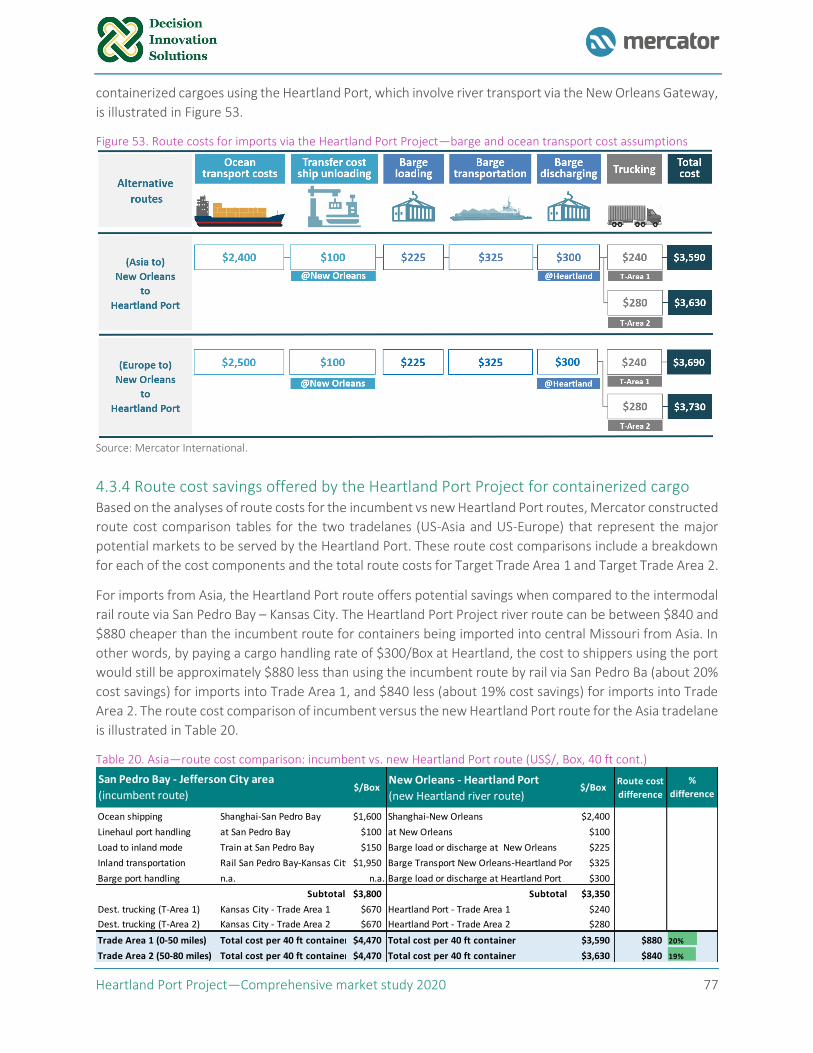
Heartland Port Project—Comprehensive market study 2020 77
containerized cargoes using the Heartland Port, which involve river transport via the New Orleans Gateway,
is illustrated in Figure 53.
Figure 53. Route costs for imports via the Heartland Port Project—barge and ocean transport cost assumptions
Source: Mercator International.
4.3.4 Route cost savings offered by the Heartland Port Project for containerized cargo Based on the analyses of route costs for the incumbent vs new Heartland Port routes, Mercator constructed
route cost comparison tables for the two tradelanes (US-Asia and US-Europe) that represent the major
potential markets to be served by the Heartland Port. These route cost comparisons include a breakdown
for each of the cost components and the total route costs for Target Trade Area 1 and Target Trade Area 2.
For imports from Asia, the Heartland Port route offers potential savings when compared to the intermodal
rail route via San Pedro Bay – Kansas City. The Heartland Port Project river route can be between $840 and
$880 cheaper than the incumbent route for containers being imported into central Missouri from Asia. In
other words, by paying a cargo handling rate of $300/Box at Heartland, the cost to shippers using the port
would still be approximately $880 less than using the incumbent route by rail via San Pedro Ba (about 20%
cost savings) for imports into Trade Area 1, and $840 less (about 19% cost savings) for imports into Trade
Area 2. The route cost comparison of incumbent versus the new Heartland Port route for the Asia tradelane
is illustrated in Table 20.
Table 20. Asia—route cost comparison: incumbent vs. new Heartland Port route (US$/, Box, 40 ft cont.)
$/BoxNew Orleans - Heartland Port
(new Heartland river route)$/Box
Route cost
difference
Ocean shipping Shanghai-San Pedro Bay $1,600 Shanghai-New Orleans $2,400
Linehaul port handling at San Pedro Bay $100 at New Orleans $100
Load to inland mode Train at San Pedro Bay $150 Barge load or discharge at New Orleans $225
Inland transportation Rail San Pedro Bay-Kansas City $1,950 Barge Transport New Orleans-Heartland Port $325
Barge port handling n.a. n.a. Barge load or discharge at Heartland Port $300
Subtotal $3,800 Subtotal $3,350
Dest. trucking (T-Area 1) Kansas City - Trade Area 1 $670 Heartland Port - Trade Area 1 $240
Dest. trucking (T-Area 2) Kansas City - Trade Area 2 $670 Heartland Port - Trade Area 2 $280
Trade Area 1 (0-50 miles) Total cost per 40 ft container $4,470 Total cost per 40 ft container $3,590 $880 20%
Trade Area 2 (50-80 miles) Total cost per 40 ft container $4,470 Total cost per 40 ft container $3,630 $840 19%
%
difference
San Pedro Bay - Jefferson City area
(incumbent route)
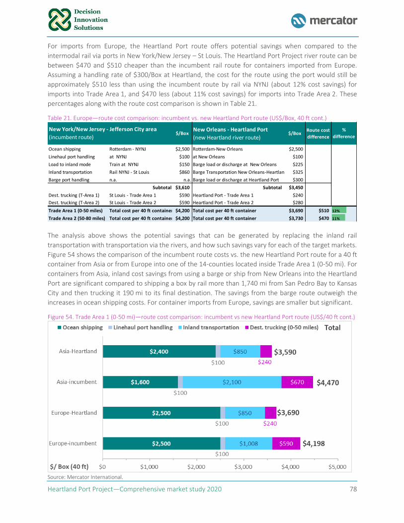
Heartland Port Project—Comprehensive market study 2020 78
For imports from Europe, the Heartland Port route offers potential savings when compared to the
intermodal rail via ports in New York/New Jersey – St Louis. The Heartland Port Project river route can be
between $470 and $510 cheaper than the incumbent rail route for containers imported from Europe.
Assuming a handling rate of $300/Box at Heartland, the cost for the route using the port would still be
approximately $510 less than using the incumbent route by rail via NYNJ (about 12% cost savings) for
imports into Trade Area 1, and $470 less (about 11% cost savings) for imports into Trade Area 2. These
percentages along with the route cost comparison is shown in Table 21.
Table 21. Europe—route cost comparison: incumbent vs. new Heartland Port route (US$/Box, 40 ft cont.)
The analysis above shows the potential savings that can be generated by replacing the inland rail
transportation with transportation via the rivers, and how such savings vary for each of the target markets.
Figure 54 shows the comparison of the incumbent route costs vs. the new Heartland Port route for a 40 ft
container from Asia or from Europe into one of the 14-counties located inside Trade Area 1 (0-50 mi). For
containers from Asia, inland cost savings from using a barge or ship from New Orleans into the Heartland
Port are significant compared to shipping a box by rail more than 1,740 mi from San Pedro Bay to Kansas
City and then trucking it 190 mi to its final destination. The savings from the barge route outweigh the
increases in ocean shipping costs. For container imports from Europe, savings are smaller but significant.
Figure 54. Trade Area 1 (0-50 mi)—route cost comparison: incumbent vs new Heartland Port route (US$/40 ft cont.)
Source: Mercator International.
$/BoxNew Orleans - Heartland Port
(new Heartland river route)$/Box
Route cost
difference
Ocean shipping Rotterdam - NYNJ $2,500 Rotterdam-New Orleans $2,500
Linehaul port handling at NYNJ $100 at New Orleans $100
Load to inland mode Train at NYNJ $150 Barge load or discharge at New Orleans $225
Inland transportation Rail NYNJ - St Louis $860 Barge Transportation New Orleans-Heartland Port$325
Barge port handling n.a. n.a. Barge load or discharge at Heartland Port $300
Subtotal $3,610 Subtotal $3,450
Dest. trucking (T-Area 1) St Louis - Trade Area 1 $590 Heartland Port - Trade Area 1 $240
Dest. trucking (T-Area 2) St Louis - Trade Area 2 $590 Heartland Port - Trade Area 2 $280
Trade Area 1 (0-50 miles) Total cost per 40 ft container $4,200 Total cost per 40 ft container $3,690 $510 12%
Trade Area 2 (50-80 miles) Total cost per 40 ft container $4,200 Total cost per 40 ft container $3,730 $470 11%
%
difference
New York/New Jersey - Jefferson City area
(incumbent route)
Heartland Port Project—Comprehensive market study 2020 79
For containers arriving by water into New Orleans, Mercator estimates the rate could be around $300 per
box for the barge transportation upriver to St. Louis, (excluding loading/unloading). Additionally, a trucking
cost from St. Louis to its final destination would be about $590 must be paid, giving a cost of $890 (plus
handling on and off the barge) for shipments from NOL. For the case where the barge operator continues
all the way to the Heartland Port, Mercator estimates the barge cost would be about 10% - 20% (assume
$50) more than the service to St. Louis due to the extra distance. The extra barge cost, however, is offset
by a reduction in trucking (about $280 from Heartland as compared to about $590 from St. Louis. Using the
Heartland Port, service from NOL would cost about ($350 + $280=) $630, which is about $260 less than
discharging the barge in St. Louis.
Another way to frame the possible savings that could be generated by the Heartland Project is to compare
the economics of a barge service operating directly to Jefferson City with a barge service to St. Louis. The
trucking leg from St. Louis to points near Jefferson City would be about $590/Box, as compared to a cost
from the Heartland Port of between $240/Box for Trade Area 1 and $280/Box for Trade Area 2. Assuming
there is adequate traffic volume to support the service, the cost of extending the barge service to the
Heartland Port (138 river miles beyond St. Louis) should add about 10% - 20% to the New Orleans’ barge
cost, or about $50/box. Because the reduction in trucking costs exceeds the incremental barge cost, barging
to Jefferson City lowers the transportation cost. Some or all of this could accrue to the port operator in
Jefferson City, which could charge a barge discharging rate that is higher than what is charged in St. Louis,
supporting the conclusion that a $300 barge rate ought to be possible.
As this route cost analysis demonstrates, the Heartland Port could provide a competitive alternative to St.
Louis as a gateway for containers on barge to/from New Orleans, particularly for those destined to or
originating within the 24-county study area and in particular to/from Trade Area 1.18
4.3.5 Containerized cargo market shares and available volume for the 24-county area From a container perspective, the majority of volumes that might be attracted to the port would be
associated with the 24-county Jefferson City port hinterland, which has a population of under 1 million
people (approximately 15% of the state of Missouri’s population of over 6 million). This would be a small
container terminal when compared to the rail ramps in Kansas City and St. Louis, and the volumes
forecasted under the base case scenario reflect three critical assumptions. First, it is assumed that a
container line can successfully roll out a weekly service connecting New Orleans to Kansas City via the
Mississippi and Missouri rivers and attract sufficient volumes to make the barge option viable. Second, it
assumes that this new weekly service would choose to call Jefferson City assuming appropriate facilities
are constructed. Third, and related, there is an assumption that a distribution center is constructed with in
a short distance of the port.
Market overview
Most non-energy imports to the US are shipped by ocean in standardized 40 ft or 20 ft containers, and the
standard unit of measure for unitized cargos (i.e. cargos shipped in ocean containers) is the TEU, which
stands for ‘twenty-foot equivalent unit’. Most unitized shipments utilize 40-foot containers, but 20-foot
containers are required in some circumstances. The most common reason for utilizing a 20-foot container
18 SCF, the only container on barge operator in St. Louis, is currently operating a service on a weekly basis between St. Louis and New Orleans for Hapag-Lloyd. SCF estimated it would require at least about 210 boxes/week (11,200 boxes/year) to establish a dedicated service between the Heartland Port and New Orleans.
Heartland Port Project—Comprehensive market study 2020 80
instead of a 40-foot container is that the contents are so dense that fully loading a 40-foot container is not
possible.
Prior to being cleared at by US Customs at one of 328 US Customs ports of entry, containers are considered
to be, and labeled as, ‘intact’. Approximately 80% of containers clear customs at the seaport at which they
are discharged, and the great majority of the remainder are cleared at customs ports associated with major
inland intermodal rail hubs. A majority share of containerized goods imports destined for inland markets
are cleared at the major coastal ports of entry, and only a portion is shipped in intact containers via
intermodal rail.
There are two major US Customs ports of entry in Missouri that are associated with the major rail hubs in
Kansas City and St. Louis with which the proposed Jefferson City port would compete for intact container
volumes.19 The St. Louis facility is located on Missouri’s border with Illinois, and the Kansas City facility is
located on Missouri’s border with Kansas. As such, these two facilities serve a hinterland that extends
beyond Missouri’s border and into Illinois and Kansas.
There is little competition for intact intermodal moves from the only other US Customs port in Kansas
(located in Wichita), and for this reason, all the intact intermodal containers carrying goods destined for
Kansas are assumed to clear customs at the Kansas City location. Similarly, the St. Louis customs clearance
port handles intact intermodal containers that carry goods destined for both Missouri and a portion of
Illinois. The largest inland customs port is associated with the Chicago rail hub, consequently, only a
relatively small portion of goods destined for Illinois is handled at the St. Louis facility.
We estimate that total population of the Kansas City and St. Louis (KC/SL) customs ports hinterland is just
over 10.5 million people, which is roughly 2.9% of the North American population. Population can be used
as a proxy for import20 demand, and without any adjustments made for relative differences in real GDP per
capita, or adjustments for relative differences in the cost of living (two measures which counteract each
other in terms of their impact on import demand), we estimate that the total volume of container imports
destined for the KC/SL hinterland in 2019 was approximately 775,000 TEUs, which is 2.9% of the
26.9 million TEUs of imports to North America that same year21.
Approximately 40% of the 775,000 TEUs of container imports carrying goods destined for consumption in
the KC/SL hinterland are loaded directly onto railcars and moved intact to inland ports. These shipments
are referred to herein as ‘intact intermodal’ volumes/containers. The remainder (i.e. the group that is not
considered to be intact intermodal) clears customs at or near the seaport of entry, and the imports are
processed at distribution centers (or cross-dock warehouses, etc.) and loaded into truck trailers, which, in
turn are either trucked or loaded onto trains.
19 We are interested in “intact” international shipping containers arriving in Central Missouri with the cargo as originally loaded at the foreign point of origin, as distinguished from containerized cargo that may arrive after be deconsolidated and re-loaded into domestic trucks. 20The number of containers loaded with imports to North America greatly outnumber the number of loaded export containers, thus making imports the headhaul. Because inbound and outbound container flows must balance, empty containers must be repositioned, and they therefore account for a significant portion of the backhaul (outbound containers). Because headhaul and backhaul equipment flows must balance, the headhaul flows will drive total volumes, and headhaul flows drive the market. As such, the analysis and forecast presented herein focus on import volumes. Carriers (rail, ocean, and even truck) offer steep discounts to those that want to ship volumes on a backhaul because supply will always be higher than demand, and for this reason we sometimes see commodities that would otherwise more efficiently be transported in bulk (rather than being ‘unitized’, which is to say shipped in containers). In Missouri, a large volume of roundwood exports are shipped in containers for this reason.
21 TEU = 20 ft container equivalent units.
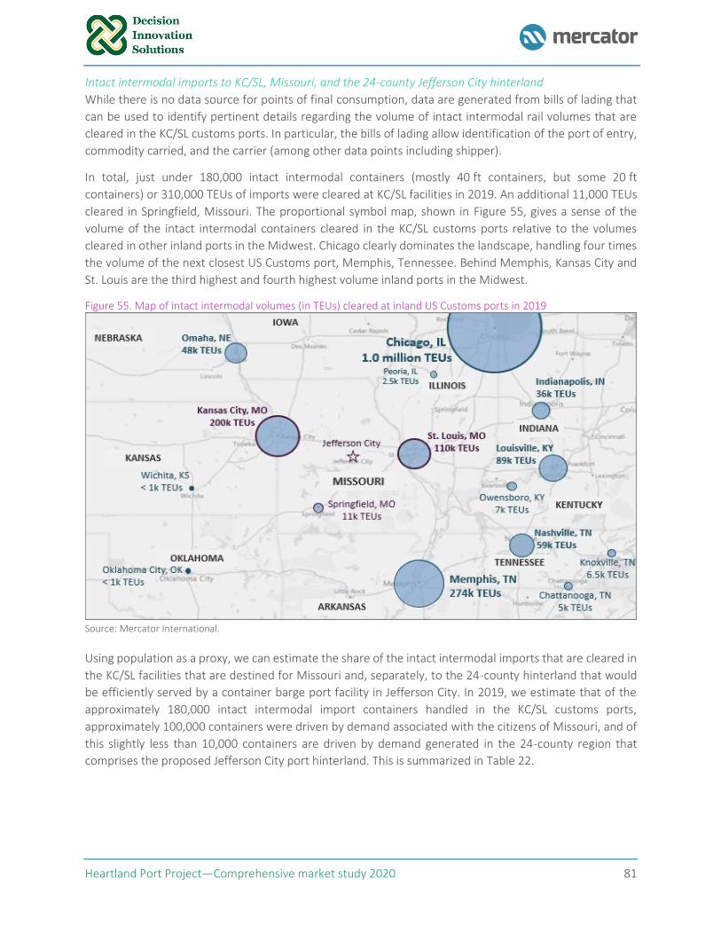
Heartland Port Project—Comprehensive market study 2020 81
Intact intermodal imports to KC/SL, Missouri, and the 24-county Jefferson City hinterland
While there is no data source for points of final consumption, data are generated from bills of lading that
can be used to identify pertinent details regarding the volume of intact intermodal rail volumes that are
cleared in the KC/SL customs ports. In particular, the bills of lading allow identification of the port of entry,
commodity carried, and the carrier (among other data points including shipper).
In total, just under 180,000 intact intermodal containers (mostly 40 ft containers, but some 20 ft
containers) or 310,000 TEUs of imports were cleared at KC/SL facilities in 2019. An additional 11,000 TEUs
cleared in Springfield, Missouri. The proportional symbol map, shown in Figure 55, gives a sense of the
volume of the intact intermodal containers cleared in the KC/SL customs ports relative to the volumes
cleared in other inland ports in the Midwest. Chicago clearly dominates the landscape, handling four times
the volume of the next closest US Customs port, Memphis, Tennessee. Behind Memphis, Kansas City and
St. Louis are the third highest and fourth highest volume inland ports in the Midwest.
Figure 55. Map of intact intermodal volumes (in TEUs) cleared at inland US Customs ports in 2019
Source: Mercator International.
Using population as a proxy, we can estimate the share of the intact intermodal imports that are cleared in
the KC/SL facilities that are destined for Missouri and, separately, to the 24-county hinterland that would
be efficiently served by a container barge port facility in Jefferson City. In 2019, we estimate that of the
approximately 180,000 intact intermodal import containers handled in the KC/SL customs ports,
approximately 100,000 containers were driven by demand associated with the citizens of Missouri, and of
this slightly less than 10,000 containers are driven by demand generated in the 24-county region that
comprises the proposed Jefferson City port hinterland. This is summarized in Table 22.
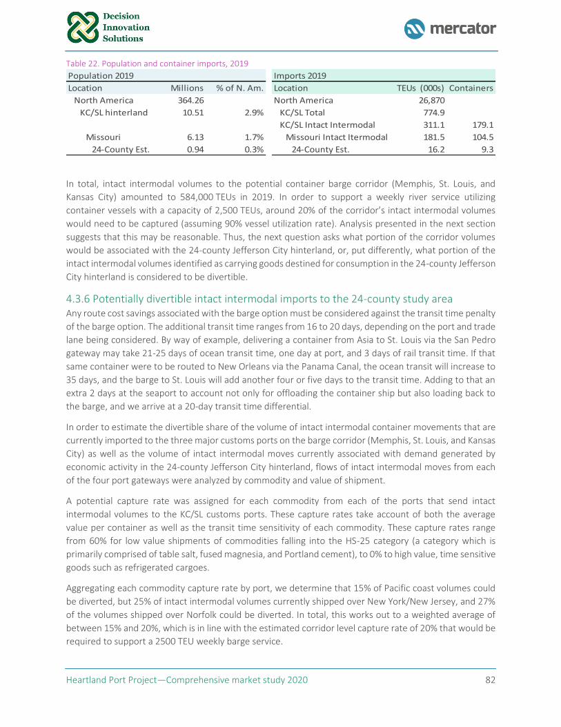
Heartland Port Project—Comprehensive market study 2020 82
Table 22. Population and container imports, 2019
In total, intact intermodal volumes to the potential container barge corridor (Memphis, St. Louis, and
Kansas City) amounted to 584,000 TEUs in 2019. In order to support a weekly river service utilizing
container vessels with a capacity of 2,500 TEUs, around 20% of the corridor’s intact intermodal volumes
would need to be captured (assuming 90% vessel utilization rate). Analysis presented in the next section
suggests that this may be reasonable. Thus, the next question asks what portion of the corridor volumes
would be associated with the 24-county Jefferson City hinterland, or, put differently, what portion of the
intact intermodal volumes identified as carrying goods destined for consumption in the 24-county Jefferson
City hinterland is considered to be divertible.
4.3.6 Potentially divertible intact intermodal imports to the 24-county study area Any route cost savings associated with the barge option must be considered against the transit time penalty
of the barge option. The additional transit time ranges from 16 to 20 days, depending on the port and trade
lane being considered. By way of example, delivering a container from Asia to St. Louis via the San Pedro
gateway may take 21-25 days of ocean transit time, one day at port, and 3 days of rail transit time. If that
same container were to be routed to New Orleans via the Panama Canal, the ocean transit will increase to
35 days, and the barge to St. Louis will add another four or five days to the transit time. Adding to that an
extra 2 days at the seaport to account not only for offloading the container ship but also loading back to
the barge, and we arrive at a 20-day transit time differential.
In order to estimate the divertible share of the volume of intact intermodal container movements that are
currently imported to the three major customs ports on the barge corridor (Memphis, St. Louis, and Kansas
City) as well as the volume of intact intermodal moves currently associated with demand generated by
economic activity in the 24-county Jefferson City hinterland, flows of intact intermodal moves from each
of the four port gateways were analyzed by commodity and value of shipment.
A potential capture rate was assigned for each commodity from each of the ports that send intact
intermodal volumes to the KC/SL customs ports. These capture rates take account of both the average
value per container as well as the transit time sensitivity of each commodity. These capture rates range
from 60% for low value shipments of commodities falling into the HS-25 category (a category which is
primarily comprised of table salt, fused magnesia, and Portland cement), to 0% to high value, time sensitive
goods such as refrigerated cargoes.
Aggregating each commodity capture rate by port, we determine that 15% of Pacific coast volumes could
be diverted, but 25% of intact intermodal volumes currently shipped over New York/New Jersey, and 27%
of the volumes shipped over Norfolk could be diverted. In total, this works out to a weighted average of
between 15% and 20%, which is in line with the estimated corridor level capture rate of 20% that would be
required to support a 2500 TEU weekly barge service.
Population 2019 Imports 2019
Location Millions % of N. Am. Location TEUs (000s) Containers
North America 364.26 North America 26,870
KC/SL hinterland 10.51 2.9% KC/SL Total 774.9
KC/SL Intact Intermodal 311.1 179.1
Missouri 6.13 1.7% Missouri Intact Itermodal 181.5 104.5
24-County Est. 0.94 0.3% 24-County Est. 16.2 9.3
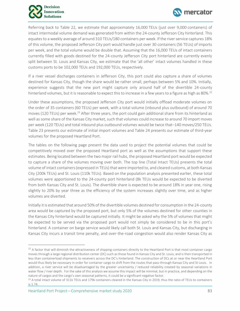
Heartland Port Project—Comprehensive market study 2020 83
Referring back to Table 22, we estimate that approximately 16,000 TEUs (just over 9,000 containers) of
intact intermodal volume demand was generated from within the 24-county Jefferson City hinterland. This
equates to a weekly average of around 310 TEUs/180 containers per week. If the river service captures 18%
of this volume, the proposed Jefferson City port would handle just over 30 containers (56 TEUs) of imports
per week, and the total volume would be double that. Assuming that the 16,000 TEUs of intact containers
currently filled with goods destined for the 24-county Jefferson City port hinterland are currently evenly
split between St. Louis and Kansas City, we estimate that the ‘all other’ intact volumes handled in these
customs ports to be 102,000 TEUs and 192,000 TEUs, respectively.
If a river vessel discharges containers in Jefferson City, this port could also capture a share of volumes
destined for Kansas City, though the share would be rather small, perhaps between 5% and 10%. Initially,
experience suggests that the new port might capture only around half of the divertible 24-county
hinterland volumes, but it is reasonable to expect this to increase in a few years to a figure as high as 80%.22
Under these assumptions, the proposed Jefferson City port would initially offload moderate volumes on
the order of 35 containers (60 TEUs) per week, with a total volume (inbound plus outbound) of around 70
moves (120 TEUs) per week.23 After three years, the port could gain additional share from its hinterland as
well as some share of the Kansas City market, such that volumes could increase to around 70 import moves
per week (120 TEUs) and total inbound plus outbound volumes would be twice that–140 moves/250 TEUs.
Table 23 presents our estimate of initial import volumes and Table 24 presents our estimate of third-year
volumes for the proposed Heartland Port.
The tables on the following page present the data used to project the potential volumes that could be
competitively moved over the proposed Heartland port as well as the assumptions that support these
estimates. Being located between the two major rail hubs, the proposed Heartland port would be expected
to capture a share of the volumes moving over both. The top line (Total Intact TEUs) presents the total
volume of intact containers (expressed in TEUs) that were imported to, and cleared customs, at both Kansas
City (200k TEUs) and St. Louis (110k TEUs). Based on the population analysis presented earlier, these total
volumes were apportioned to the 24-county port hinterland (8k TEUs would be expected to be diverted
from both Kansas City and St. Louis). The divertible share is expected to be around 18% in year one, rising
slightly to 20% by year three as the efficiency of the system increases slightly over time, and as higher
volumes are diverted.
Initially it is estimated that around 50% of the divertible volumes destined for consumption in the 24-county
area would be captured by the proposed port, but only 5% of the volumes destined for other counties in
the Kansas City hinterland would be captured initially. It might be asked why the 5% of volumes that might
be expected to be served via the proposed port would not simply be considered to be in this port’s
hinterland. A container on barge service would likely call both St. Louis and Kansas City, but discharging in
Kansas City incurs a transit time penalty, and over-the-road congestion would also render Kansas City as
22 A factor that will diminish the attractiveness of shipping containers directly to the Heartland Port is that most container cargo moves through a large regional distribution center (DC) such as those found in Kansas City and St. Louis, and is then transported in less than containerload shipments to receivers across the DC’s hinterland. The construction of DCs at or near the Heartland Port would thus likely be necessary in order for container cargo to shift from the routes that pass-through Kansas City and St Louis. In addition, a river service will be disadvantaged by the greater uncertainty / reduced reliability created by seasonal variations in water flow / river depth. For the sake of this analysis we assume this impact will be minimal, but in practice, and depending on the nature of cargos and the cargo’s own seasonal patterns, it could be a significant negative factor. 23 A total intact volume of 311k TEUs and 179k containers cleared in the Kansas City in 2019, thus the ratio of TEUs to containers is 1.74.
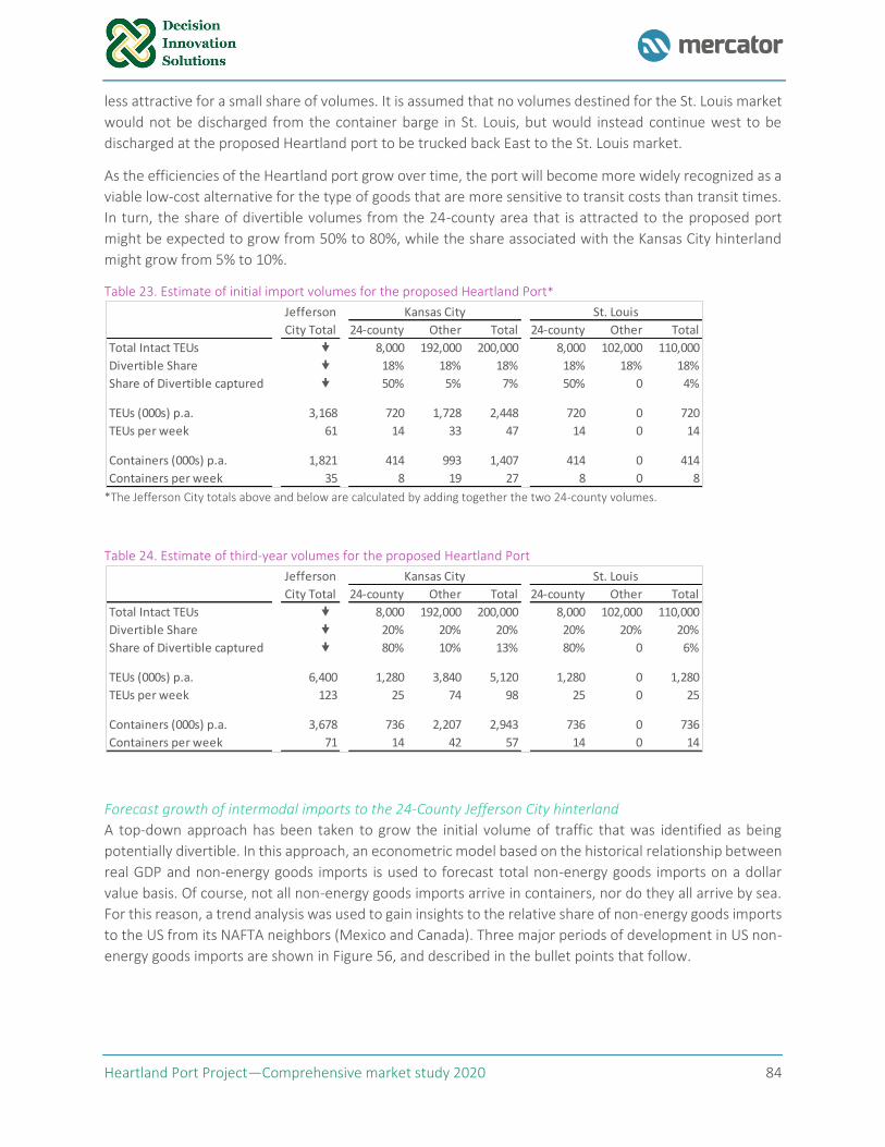
Heartland Port Project—Comprehensive market study 2020 84
less attractive for a small share of volumes. It is assumed that no volumes destined for the St. Louis market
would not be discharged from the container barge in St. Louis, but would instead continue west to be
discharged at the proposed Heartland port to be trucked back East to the St. Louis market.
As the efficiencies of the Heartland port grow over time, the port will become more widely recognized as a
viable low-cost alternative for the type of goods that are more sensitive to transit costs than transit times.
In turn, the share of divertible volumes from the 24-county area that is attracted to the proposed port
might be expected to grow from 50% to 80%, while the share associated with the Kansas City hinterland
might grow from 5% to 10%.
Table 23. Estimate of initial import volumes for the proposed Heartland Port*
*The Jefferson City totals above and below are calculated by adding together the two 24-county volumes.
Table 24. Estimate of third-year volumes for the proposed Heartland Port
Forecast growth of intermodal imports to the 24-County Jefferson City hinterland
A top-down approach has been taken to grow the initial volume of traffic that was identified as being
potentially divertible. In this approach, an econometric model based on the historical relationship between
real GDP and non-energy goods imports is used to forecast total non-energy goods imports on a dollar
value basis. Of course, not all non-energy goods imports arrive in containers, nor do they all arrive by sea.
For this reason, a trend analysis was used to gain insights to the relative share of non-energy goods imports
to the US from its NAFTA neighbors (Mexico and Canada). Three major periods of development in US non-
energy goods imports are shown in Figure 56, and described in the bullet points that follow.
Jefferson Kansas City St. Louis
City Total 24-county Other Total 24-county Other Total
Total Intact TEUs 8,000 192,000 200,000 8,000 102,000 110,000
Divertible Share 18% 18% 18% 18% 18% 18%
Share of Divertible captured 50% 5% 7% 50% 0 4%
TEUs (000s) p.a. 3,168 720 1,728 2,448 720 0 720
TEUs per week 61 14 33 47 14 0 14
Containers (000s) p.a. 1,821 414 993 1,407 414 0 414
Containers per week 35 8 19 27 8 0 8
Jefferson Kansas City St. Louis
City Total 24-county Other Total 24-county Other Total
Total Intact TEUs 8,000 192,000 200,000 8,000 102,000 110,000
Divertible Share 20% 20% 20% 20% 20% 20%
Share of Divertible captured 80% 10% 13% 80% 0 6%
TEUs (000s) p.a. 6,400 1,280 3,840 5,120 1,280 0 1,280
TEUs per week 123 25 74 98 25 0 25
Containers (000s) p.a. 3,678 736 2,207 2,943 736 0 736
Containers per week 71 14 42 57 14 0 14
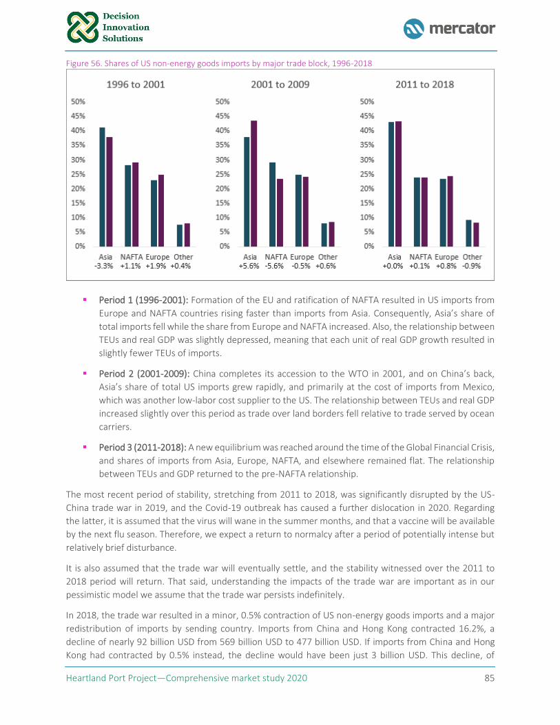
Heartland Port Project—Comprehensive market study 2020 85
Figure 56. Shares of US non-energy goods imports by major trade block, 1996-2018
▪ Period 1 (1996-2001): Formation of the EU and ratification of NAFTA resulted in US imports from
Europe and NAFTA countries rising faster than imports from Asia. Consequently, Asia’s share of
total imports fell while the share from Europe and NAFTA increased. Also, the relationship between
TEUs and real GDP was slightly depressed, meaning that each unit of real GDP growth resulted in
slightly fewer TEUs of imports.
▪ Period 2 (2001-2009): China completes its accession to the WTO in 2001, and on China’s back,
Asia’s share of total US imports grew rapidly, and primarily at the cost of imports from Mexico,
which was another low-labor cost supplier to the US. The relationship between TEUs and real GDP
increased slightly over this period as trade over land borders fell relative to trade served by ocean
carriers.
▪ Period 3 (2011-2018): A new equilibrium was reached around the time of the Global Financial Crisis,
and shares of imports from Asia, Europe, NAFTA, and elsewhere remained flat. The relationship
between TEUs and GDP returned to the pre-NAFTA relationship.
The most recent period of stability, stretching from 2011 to 2018, was significantly disrupted by the US-
China trade war in 2019, and the Covid-19 outbreak has caused a further dislocation in 2020. Regarding
the latter, it is assumed that the virus will wane in the summer months, and that a vaccine will be available
by the next flu season. Therefore, we expect a return to normalcy after a period of potentially intense but
relatively brief disturbance.
It is also assumed that the trade war will eventually settle, and the stability witnessed over the 2011 to
2018 period will return. That said, understanding the impacts of the trade war are important as in our
pessimistic model we assume that the trade war persists indefinitely.
In 2018, the trade war resulted in a minor, 0.5% contraction of US non-energy goods imports and a major
redistribution of imports by sending country. Imports from China and Hong Kong contracted 16.2%, a
decline of nearly 92 billion USD from 569 billion USD to 477 billion USD. If imports from China and Hong
Kong had contracted by 0.5% instead, the decline would have been just 3 billion USD. This decline, of
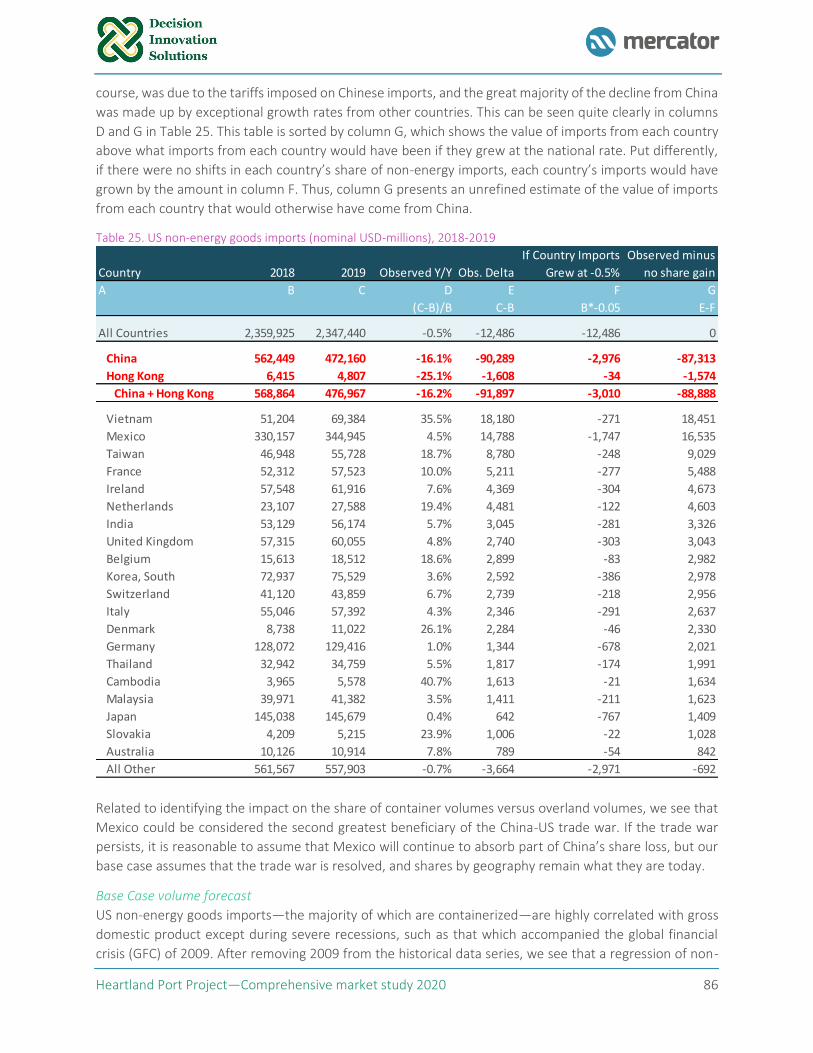
Heartland Port Project—Comprehensive market study 2020 86
course, was due to the tariffs imposed on Chinese imports, and the great majority of the decline from China
was made up by exceptional growth rates from other countries. This can be seen quite clearly in columns
D and G in Table 25. This table is sorted by column G, which shows the value of imports from each country
above what imports from each country would have been if they grew at the national rate. Put differently,
if there were no shifts in each country’s share of non-energy imports, each country’s imports would have
grown by the amount in column F. Thus, column G presents an unrefined estimate of the value of imports
from each country that would otherwise have come from China.
Table 25. US non-energy goods imports (nominal USD-millions), 2018-2019
Related to identifying the impact on the share of container volumes versus overland volumes, we see that
Mexico could be considered the second greatest beneficiary of the China-US trade war. If the trade war
persists, it is reasonable to assume that Mexico will continue to absorb part of China’s share loss, but our
base case assumes that the trade war is resolved, and shares by geography remain what they are today.
Base Case volume forecast
US non-energy goods imports—the majority of which are containerized—are highly correlated with gross
domestic product except during severe recessions, such as that which accompanied the global financial
crisis (GFC) of 2009. After removing 2009 from the historical data series, we see that a regression of non-
If Country Imports Observed minus
Country 2018 2019 Observed Y/Y Obs. Delta Grew at -0.5% no share gain
A B C D E F G
(C-B)/B C-B B*-0.05 E-F
All Countries 2,359,925 2,347,440 -0.5% -12,486 -12,486 0
China 562,449 472,160 -16.1% -90,289 -2,976 -87,313
Hong Kong 6,415 4,807 -25.1% -1,608 -34 -1,574
China + Hong Kong 568,864 476,967 -16.2% -91,897 -3,010 -88,888
Vietnam 51,204 69,384 35.5% 18,180 -271 18,451
Mexico 330,157 344,945 4.5% 14,788 -1,747 16,535
Taiwan 46,948 55,728 18.7% 8,780 -248 9,029
France 52,312 57,523 10.0% 5,211 -277 5,488
Ireland 57,548 61,916 7.6% 4,369 -304 4,673
Netherlands 23,107 27,588 19.4% 4,481 -122 4,603
India 53,129 56,174 5.7% 3,045 -281 3,326
United Kingdom 57,315 60,055 4.8% 2,740 -303 3,043
Belgium 15,613 18,512 18.6% 2,899 -83 2,982
Korea, South 72,937 75,529 3.6% 2,592 -386 2,978
Switzerland 41,120 43,859 6.7% 2,739 -218 2,956
Italy 55,046 57,392 4.3% 2,346 -291 2,637
Denmark 8,738 11,022 26.1% 2,284 -46 2,330
Germany 128,072 129,416 1.0% 1,344 -678 2,021
Thailand 32,942 34,759 5.5% 1,817 -174 1,991
Cambodia 3,965 5,578 40.7% 1,613 -21 1,634
Malaysia 39,971 41,382 3.5% 1,411 -211 1,623
Japan 145,038 145,679 0.4% 642 -767 1,409
Slovakia 4,209 5,215 23.9% 1,006 -22 1,028
Australia 10,126 10,914 7.8% 789 -54 842
All Other 561,567 557,903 -0.7% -3,664 -2,971 -692
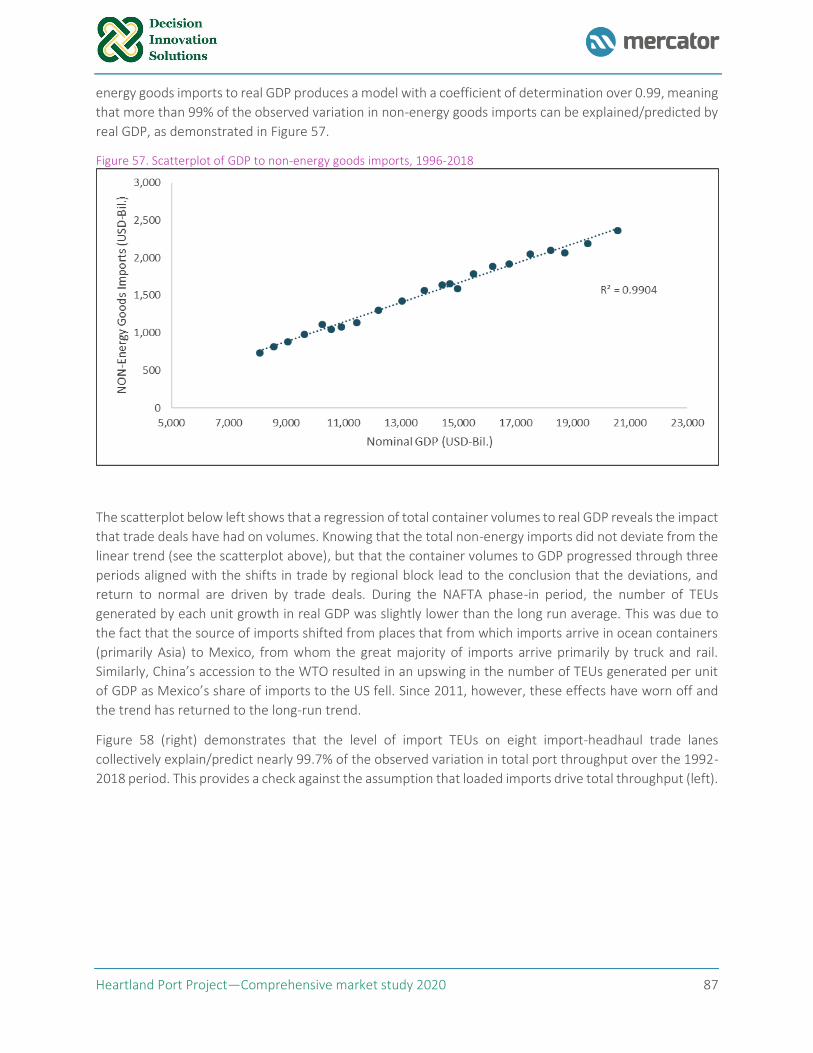
Heartland Port Project—Comprehensive market study 2020 87
energy goods imports to real GDP produces a model with a coefficient of determination over 0.99, meaning
that more than 99% of the observed variation in non-energy goods imports can be explained/predicted by
real GDP, as demonstrated in Figure 57.
Figure 57. Scatterplot of GDP to non-energy goods imports, 1996-2018
The scatterplot below left shows that a regression of total container volumes to real GDP reveals the impact
that trade deals have had on volumes. Knowing that the total non-energy imports did not deviate from the
linear trend (see the scatterplot above), but that the container volumes to GDP progressed through three
periods aligned with the shifts in trade by regional block lead to the conclusion that the deviations, and
return to normal are driven by trade deals. During the NAFTA phase-in period, the number of TEUs
generated by each unit growth in real GDP was slightly lower than the long run average. This was due to
the fact that the source of imports shifted from places that from which imports arrive in ocean containers
(primarily Asia) to Mexico, from whom the great majority of imports arrive primarily by truck and rail.
Similarly, China’s accession to the WTO resulted in an upswing in the number of TEUs generated per unit
of GDP as Mexico’s share of imports to the US fell. Since 2011, however, these effects have worn off and
the trend has returned to the long-run trend.
Figure 58 (right) demonstrates that the level of import TEUs on eight import-headhaul trade lanes
collectively explain/predict nearly 99.7% of the observed variation in total port throughput over the 1992-
2018 period. This provides a check against the assumption that loaded imports drive total throughput (left).
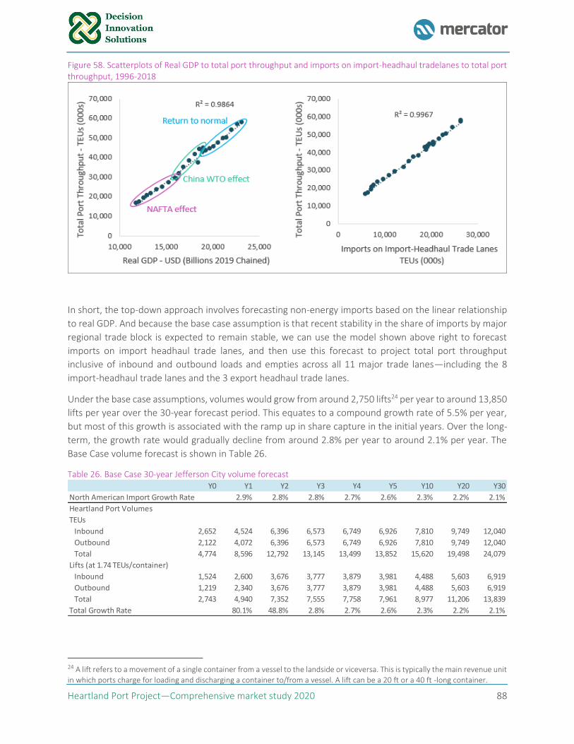
Heartland Port Project—Comprehensive market study 2020 88
Figure 58. Scatterplots of Real GDP to total port throughput and imports on import-headhaul tradelanes to total port throughput, 1996-2018
In short, the top-down approach involves forecasting non-energy imports based on the linear relationship
to real GDP. And because the base case assumption is that recent stability in the share of imports by major
regional trade block is expected to remain stable, we can use the model shown above right to forecast
imports on import headhaul trade lanes, and then use this forecast to project total port throughput
inclusive of inbound and outbound loads and empties across all 11 major trade lanes—including the 8
import-headhaul trade lanes and the 3 export headhaul trade lanes.
Under the base case assumptions, volumes would grow from around 2,750 lifts24 per year to around 13,850
lifts per year over the 30-year forecast period. This equates to a compound growth rate of 5.5% per year,
but most of this growth is associated with the ramp up in share capture in the initial years. Over the long-
term, the growth rate would gradually decline from around 2.8% per year to around 2.1% per year. The
Base Case volume forecast is shown in Table 26.
Table 26. Base Case 30-year Jefferson City volume forecast
24 A lift refers to a movement of a single container from a vessel to the landside or viceversa. This is typically the main revenue unit
in which ports charge for loading and discharging a container to/from a vessel. A lift can be a 20 ft or a 40 ft -long container.
Y0 Y1 Y2 Y3 Y4 Y5 Y10 Y20 Y30
North American Import Growth Rate 2.9% 2.8% 2.8% 2.7% 2.6% 2.3% 2.2% 2.1%
Heartland Port Volumes
TEUs
Inbound 2,652 4,524 6,396 6,573 6,749 6,926 7,810 9,749 12,040
Outbound 2,122 4,072 6,396 6,573 6,749 6,926 7,810 9,749 12,040
Total 4,774 8,596 12,792 13,145 13,499 13,852 15,620 19,498 24,079
Lifts (at 1.74 TEUs/container)
Inbound 1,524 2,600 3,676 3,777 3,879 3,981 4,488 5,603 6,919
Outbound 1,219 2,340 3,676 3,777 3,879 3,981 4,488 5,603 6,919
Total 2,743 4,940 7,352 7,555 7,758 7,961 8,977 11,206 13,839
Total Growth Rate 80.1% 48.8% 2.8% 2.7% 2.6% 2.3% 2.2% 2.1%
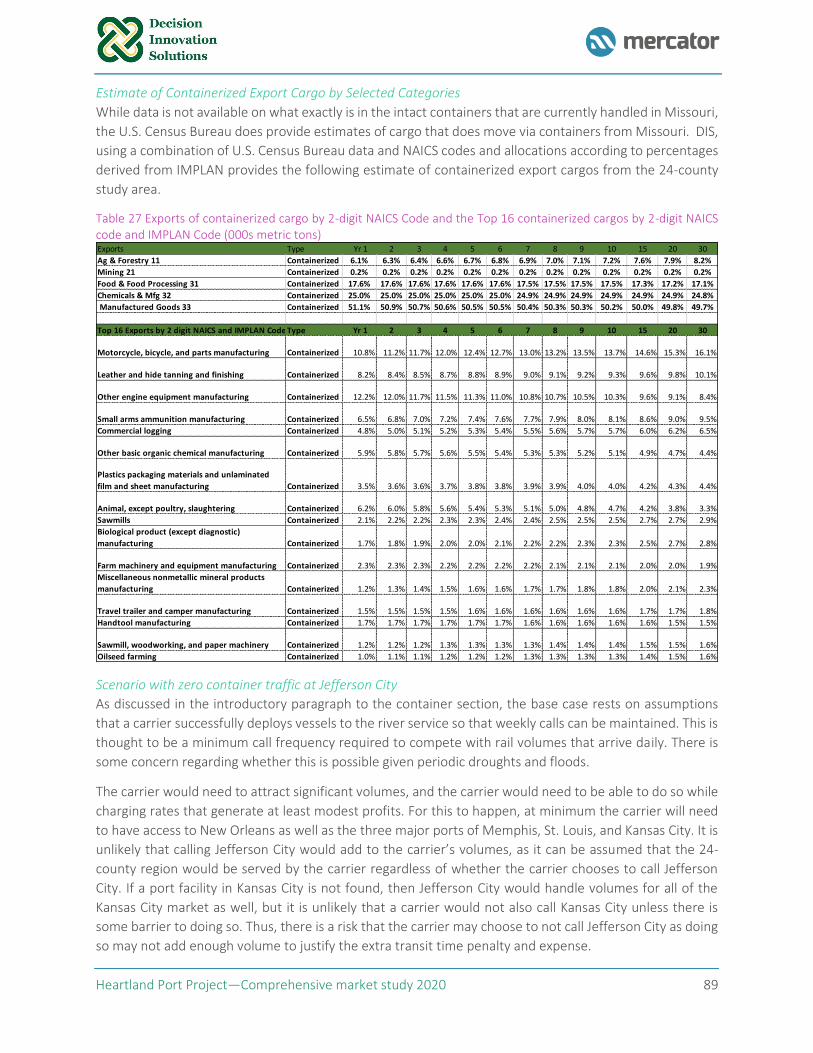
Heartland Port Project—Comprehensive market study 2020 89
Estimate of Containerized Export Cargo by Selected Categories
While data is not available on what exactly is in the intact containers that are currently handled in Missouri,
the U.S. Census Bureau does provide estimates of cargo that does move via containers from Missouri. DIS,
using a combination of U.S. Census Bureau data and NAICS codes and allocations according to percentages
derived from IMPLAN provides the following estimate of containerized export cargos from the 24-county
study area.
Table 27 Exports of containerized cargo by 2-digit NAICS Code and the Top 16 containerized cargos by 2-digit NAICS code and IMPLAN Code (000s metric tons)
Scenario with zero container traffic at Jefferson City
As discussed in the introductory paragraph to the container section, the base case rests on assumptions
that a carrier successfully deploys vessels to the river service so that weekly calls can be maintained. This is
thought to be a minimum call frequency required to compete with rail volumes that arrive daily. There is
some concern regarding whether this is possible given periodic droughts and floods.
The carrier would need to attract significant volumes, and the carrier would need to be able to do so while
charging rates that generate at least modest profits. For this to happen, at minimum the carrier will need
to have access to New Orleans as well as the three major ports of Memphis, St. Louis, and Kansas City. It is
unlikely that calling Jefferson City would add to the carrier’s volumes, as it can be assumed that the 24-
county region would be served by the carrier regardless of whether the carrier chooses to call Jefferson
City. If a port facility in Kansas City is not found, then Jefferson City would handle volumes for all of the
Kansas City market as well, but it is unlikely that a carrier would not also call Kansas City unless there is
some barrier to doing so. Thus, there is a risk that the carrier may choose to not call Jefferson City as doing
so may not add enough volume to justify the extra transit time penalty and expense.
Exports Type Yr 1 2 3 4 5 6 7 8 9 10 15 20 30
Ag & Forestry 11 Containerized 6.1% 6.3% 6.4% 6.6% 6.7% 6.8% 6.9% 7.0% 7.1% 7.2% 7.6% 7.9% 8.2%
Mining 21 Containerized 0.2% 0.2% 0.2% 0.2% 0.2% 0.2% 0.2% 0.2% 0.2% 0.2% 0.2% 0.2% 0.2%
Food & Food Processing 31 Containerized 17.6% 17.6% 17.6% 17.6% 17.6% 17.6% 17.5% 17.5% 17.5% 17.5% 17.3% 17.2% 17.1%
Chemicals & Mfg 32 Containerized 25.0% 25.0% 25.0% 25.0% 25.0% 25.0% 24.9% 24.9% 24.9% 24.9% 24.9% 24.9% 24.8%
Manufactured Goods 33 Containerized 51.1% 50.9% 50.7% 50.6% 50.5% 50.5% 50.4% 50.3% 50.3% 50.2% 50.0% 49.8% 49.7%
Top 16 Exports by 2 digit NAICS and IMPLAN Code Type Yr 1 2 3 4 5 6 7 8 9 10 15 20 30
Motorcycle, bicycle, and parts manufacturing Containerized 10.8% 11.2% 11.7% 12.0% 12.4% 12.7% 13.0% 13.2% 13.5% 13.7% 14.6% 15.3% 16.1%
Leather and hide tanning and finishing Containerized 8.2% 8.4% 8.5% 8.7% 8.8% 8.9% 9.0% 9.1% 9.2% 9.3% 9.6% 9.8% 10.1%
Other engine equipment manufacturing Containerized 12.2% 12.0% 11.7% 11.5% 11.3% 11.0% 10.8% 10.7% 10.5% 10.3% 9.6% 9.1% 8.4%
Small arms ammunition manufacturing Containerized 6.5% 6.8% 7.0% 7.2% 7.4% 7.6% 7.7% 7.9% 8.0% 8.1% 8.6% 9.0% 9.5%
Commercial logging Containerized 4.8% 5.0% 5.1% 5.2% 5.3% 5.4% 5.5% 5.6% 5.7% 5.7% 6.0% 6.2% 6.5%
Other basic organic chemical manufacturing Containerized 5.9% 5.8% 5.7% 5.6% 5.5% 5.4% 5.3% 5.3% 5.2% 5.1% 4.9% 4.7% 4.4%
Plastics packaging materials and unlaminated
film and sheet manufacturing Containerized 3.5% 3.6% 3.6% 3.7% 3.8% 3.8% 3.9% 3.9% 4.0% 4.0% 4.2% 4.3% 4.4%
Animal, except poultry, slaughtering Containerized 6.2% 6.0% 5.8% 5.6% 5.4% 5.3% 5.1% 5.0% 4.8% 4.7% 4.2% 3.8% 3.3%
Sawmills Containerized 2.1% 2.2% 2.2% 2.3% 2.3% 2.4% 2.4% 2.5% 2.5% 2.5% 2.7% 2.7% 2.9%
Biological product (except diagnostic)
manufacturing Containerized 1.7% 1.8% 1.9% 2.0% 2.0% 2.1% 2.2% 2.2% 2.3% 2.3% 2.5% 2.7% 2.8%
Farm machinery and equipment manufacturing Containerized 2.3% 2.3% 2.3% 2.2% 2.2% 2.2% 2.2% 2.1% 2.1% 2.1% 2.0% 2.0% 1.9%
Miscellaneous nonmetallic mineral products
manufacturing Containerized 1.2% 1.3% 1.4% 1.5% 1.6% 1.6% 1.7% 1.7% 1.8% 1.8% 2.0% 2.1% 2.3%
Travel trailer and camper manufacturing Containerized 1.5% 1.5% 1.5% 1.5% 1.6% 1.6% 1.6% 1.6% 1.6% 1.6% 1.7% 1.7% 1.8%
Handtool manufacturing Containerized 1.7% 1.7% 1.7% 1.7% 1.7% 1.7% 1.6% 1.6% 1.6% 1.6% 1.6% 1.5% 1.5%
Sawmill, woodworking, and paper machinery Containerized 1.2% 1.2% 1.2% 1.3% 1.3% 1.3% 1.3% 1.4% 1.4% 1.4% 1.5% 1.5% 1.6%
Oilseed farming Containerized 1.0% 1.1% 1.1% 1.2% 1.2% 1.2% 1.3% 1.3% 1.3% 1.3% 1.4% 1.5% 1.6%
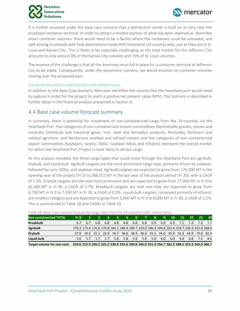
Heartland Port Project—Comprehensive market study 2020 90
It is further assumed under the base case scenario that a distribution center is built on or very near the
proposed container terminal. In order to attract a modest portion of what has been deemed as ‘divertible
intact container volumes’ there would need to be a facility where the containers could be unloaded, and
split among truckloads with final destinations inside HPA hinterland (24-county) area, just as they are in St.
Louis and Kansas City. This is likely to be especially challenging as the total market for the Jefferson City
amounts to only around 8% of the Kansas City volumes and 15% of St. Louis volumes.
The essence of the challenge is that all the dominoes must fall in place for a container terminal at Jefferson
City to be viable. Consequently, under the pessimistic scenario, we would envision no container volumes
moving over the proposed port.
Scenarios required to reach positive net present value
In addition to the Base Case Scenario, Mercator identified the volume that the Heartland port would need
to capture in order for the project to reach a positive net present value (NPV). This Scenario is described in
further detail in the financial analysis presented in Section 6.
4.4 Base case volume forecast summary
In summary, there is potential for movement of non-containerized cargo from the 24-counties via the
Heartland Port. Five categories of non-containerized import commodities (Nonmetallic gravels, stones and
minerals; Chemicals and industrial gases; Iron, steel and ferroalloy products; Pesticides, fertilizers and
related agrichem; and Nonferrous smelted and refined metals) and five categories of non-containerized
export commodities (Soybeans; Grains; DDGs; Soybean Meal; and Ethanol) represent the overall market
for which the Heartland Port Project is most likely to attract cargo.
As this analysis revealed, the three cargo types that could move through the Heartland Port are agribulk,
drybulk, and liquid bulk. Agribulk cargoes are the most prominent cargo type, primarily driven by soybean,
followed by corn, DDGs, and soybean meal. Agribulk cargoes are expected to grow from 170,300 MT in the
opening year of the project (Yr 0) to 268,552 MT in the last year of the analysis period (Yr 30), with a CAGR
of 1.5%. Drybulk cargoes are the next most prominent and are expected to grow from 27,900 MT in Yr 0 to
82,400 MT in Yr 30, a CAGR of 3.7%. Breakbulk cargoes are next and they are expected to grow from
6,700 MT in Yr 0 to 7,700 MT in Yr 30, a CAGR of 0.5%. Liquid-bulk cargoes, composed primarily of ethanol,
are smallest category and are expected to grow from 5,600 MT in Yr 0 to 8,000 MT in Yr 30, a CAGR of 1.2%.
This is summarized in Table 28 and CAGRs in Table 29
Table 28. Base Case volume forecast by cargo type from the 24-counties (000, metric tons)
Non-containerized TOTAL Yr 0 1 2 3 4 5 6 7 8 9 10 15 20 25 30
Breakbulk 6.7 6.7 6.8 6.8 6.8 6.8 6.8 6.8 6.9 6.9 6.9 7.1 7.3 7.5 7.7
Agribulk 170.3 173.4 176.6 179.8 183.1 186.4 189.7 193.0 196.4 199.8 203.4 219.7 236.3 252.6 268.6
Drybulk 27.9 29.5 31.1 32.9 34.7 36.6 38.4 40.3 42.1 44.0 45.9 55.3 64.9 74.6 82.4
Liquid bulk 5.6 5.7 5.7 5.7 5.8 5.8 5.9 5.9 5.9 6.0 6.0 6.4 6.8 7.3 8.0
Target volume for non-cont. 210.6 215.3 220.2 225.2 230.4 235.6 240.8 246.0 251.4 256.7 262.2 288.5 315.3 342.0 366.7
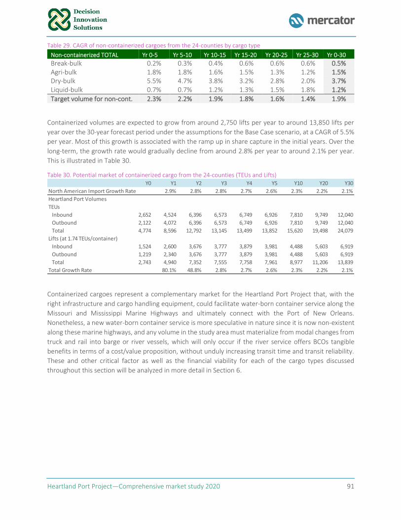
Heartland Port Project—Comprehensive market study 2020 91
Table 29. CAGR of non-containerized cargoes from the 24-counties by cargo type
Non-containerized TOTAL Yr 0-5 Yr 5-10 Yr 10-15 Yr 15-20 Yr 20-25 Yr 25-30 Yr 0-30
Break-bulk 0.2% 0.3% 0.4% 0.6% 0.6% 0.6% 0.5% Agri-bulk 1.8% 1.8% 1.6% 1.5% 1.3% 1.2% 1.5% Dry-bulk 5.5% 4.7% 3.8% 3.2% 2.8% 2.0% 3.7% Liquid-bulk 0.7% 0.7% 1.2% 1.3% 1.5% 1.8% 1.2%
Target volume for non-cont. 2.3% 2.2% 1.9% 1.8% 1.6% 1.4% 1.9%
Containerized volumes are expected to grow from around 2,750 lifts per year to around 13,850 lifts per
year over the 30-year forecast period under the assumptions for the Base Case scenario, at a CAGR of 5.5%
per year. Most of this growth is associated with the ramp up in share capture in the initial years. Over the
long-term, the growth rate would gradually decline from around 2.8% per year to around 2.1% per year.
This is illustrated in Table 30.
Table 30. Potential market of containerized cargo from the 24-counties (TEUs and Lifts)
Containerized cargoes represent a complementary market for the Heartland Port Project that, with the
right infrastructure and cargo handling equipment, could facilitate water-born container service along the
Missouri and Mississippi Marine Highways and ultimately connect with the Port of New Orleans.
Nonetheless, a new water-born container service is more speculative in nature since it is now non-existent
along these marine highways, and any volume in the study area must materialize from modal changes from
truck and rail into barge or river vessels, which will only occur if the river service offers BCOs tangible
benefits in terms of a cost/value proposition, without unduly increasing transit time and transit reliability.
These and other critical factor as well as the financial viability for each of the cargo types discussed
throughout this section will be analyzed in more detail in Section 6.
Y0 Y1 Y2 Y3 Y4 Y5 Y10 Y20 Y30
North American Import Growth Rate 2.9% 2.8% 2.8% 2.7% 2.6% 2.3% 2.2% 2.1%
Heartland Port Volumes
TEUs
Inbound 2,652 4,524 6,396 6,573 6,749 6,926 7,810 9,749 12,040
Outbound 2,122 4,072 6,396 6,573 6,749 6,926 7,810 9,749 12,040
Total 4,774 8,596 12,792 13,145 13,499 13,852 15,620 19,498 24,079
Lifts (at 1.74 TEUs/container)
Inbound 1,524 2,600 3,676 3,777 3,879 3,981 4,488 5,603 6,919
Outbound 1,219 2,340 3,676 3,777 3,879 3,981 4,488 5,603 6,919
Total 2,743 4,940 7,352 7,555 7,758 7,961 8,977 11,206 13,839
Total Growth Rate 80.1% 48.8% 2.8% 2.7% 2.6% 2.3% 2.2% 2.1%
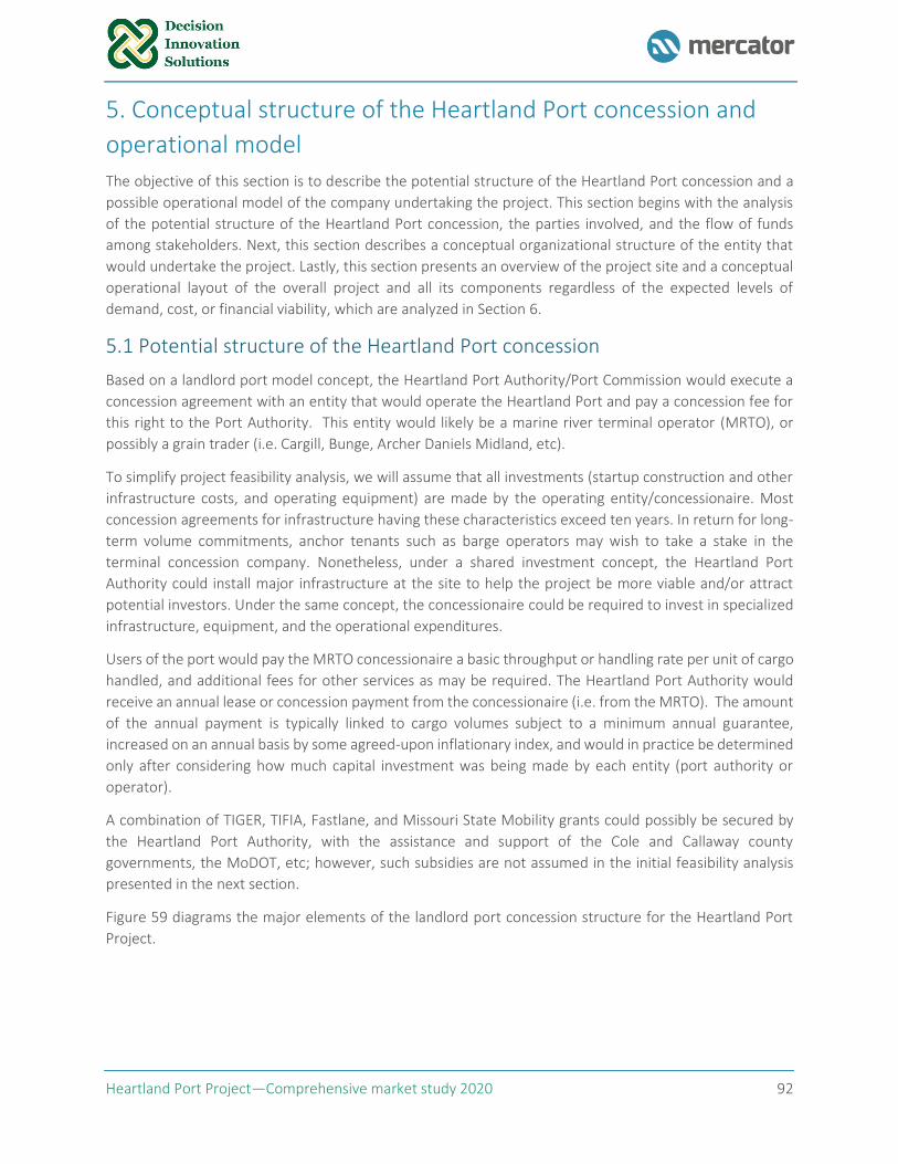
Heartland Port Project—Comprehensive market study 2020 92
5. Conceptual structure of the Heartland Port concession and
operational model
The objective of this section is to describe the potential structure of the Heartland Port concession and a
possible operational model of the company undertaking the project. This section begins with the analysis
of the potential structure of the Heartland Port concession, the parties involved, and the flow of funds
among stakeholders. Next, this section describes a conceptual organizational structure of the entity that
would undertake the project. Lastly, this section presents an overview of the project site and a conceptual
operational layout of the overall project and all its components regardless of the expected levels of
demand, cost, or financial viability, which are analyzed in Section 6.
5.1 Potential structure of the Heartland Port concession
Based on a landlord port model concept, the Heartland Port Authority/Port Commission would execute a
concession agreement with an entity that would operate the Heartland Port and pay a concession fee for
this right to the Port Authority. This entity would likely be a marine river terminal operator (MRTO), or
possibly a grain trader (i.e. Cargill, Bunge, Archer Daniels Midland, etc).
To simplify project feasibility analysis, we will assume that all investments (startup construction and other
infrastructure costs, and operating equipment) are made by the operating entity/concessionaire. Most
concession agreements for infrastructure having these characteristics exceed ten years. In return for long-
term volume commitments, anchor tenants such as barge operators may wish to take a stake in the
terminal concession company. Nonetheless, under a shared investment concept, the Heartland Port
Authority could install major infrastructure at the site to help the project be more viable and/or attract
potential investors. Under the same concept, the concessionaire could be required to invest in specialized
infrastructure, equipment, and the operational expenditures.
Users of the port would pay the MRTO concessionaire a basic throughput or handling rate per unit of cargo
handled, and additional fees for other services as may be required. The Heartland Port Authority would
receive an annual lease or concession payment from the concessionaire (i.e. from the MRTO). The amount
of the annual payment is typically linked to cargo volumes subject to a minimum annual guarantee,
increased on an annual basis by some agreed-upon inflationary index, and would in practice be determined
only after considering how much capital investment was being made by each entity (port authority or
operator).
A combination of TIGER, TIFIA, Fastlane, and Missouri State Mobility grants could possibly be secured by
the Heartland Port Authority, with the assistance and support of the Cole and Callaway county
governments, the MoDOT, etc; however, such subsidies are not assumed in the initial feasibility analysis
presented in the next section.
Figure 59 diagrams the major elements of the landlord port concession structure for the Heartland Port
Project.
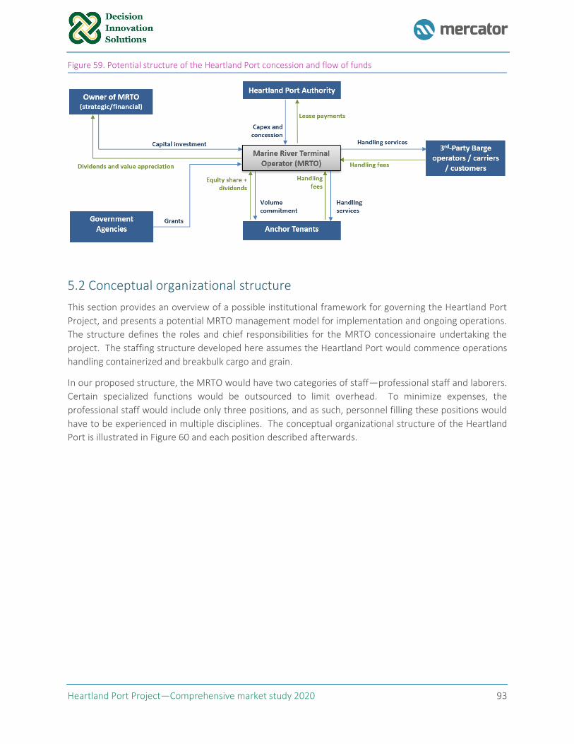
Heartland Port Project—Comprehensive market study 2020 93
Figure 59. Potential structure of the Heartland Port concession and flow of funds
5.2 Conceptual organizational structure
This section provides an overview of a possible institutional framework for governing the Heartland Port
Project, and presents a potential MRTO management model for implementation and ongoing operations.
The structure defines the roles and chief responsibilities for the MRTO concessionaire undertaking the
project. The staffing structure developed here assumes the Heartland Port would commence operations
handling containerized and breakbulk cargo and grain.
In our proposed structure, the MRTO would have two categories of staff—professional staff and laborers.
Certain specialized functions would be outsourced to limit overhead. To minimize expenses, the
professional staff would include only three positions, and as such, personnel filling these positions would
have to be experienced in multiple disciplines. The conceptual organizational structure of the Heartland
Port is illustrated in Figure 60 and each position described afterwards.
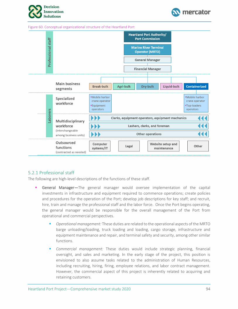
Heartland Port Project—Comprehensive market study 2020 94
Figure 60. Conceptual organizational structure of the Heartland Port
5.2.1 Professional staff The following are high-level descriptions of the functions of these staff.
▪ General Manager—The general manager would oversee implementation of the capital
investments in infrastructure and equipment required to commence operations; create policies
and procedures for the operation of the Port; develop job descriptions for key staff; and recruit,
hire, train and manage the professional staff and the labor force. Once the Port begins operating,
the general manager would be responsible for the overall management of the Port from
operational and commercial perspectives.
▪ Operational management: These duties are related to the operational aspects of the MRTO
barge unloading/loading, truck loading and loading, cargo storage, infrastructure and
equipment maintenance and repair, and terminal safety and security, among other similar
functions.
▪ Commercial management: These duties would include strategic planning, financial
oversight, and sales and marketing. In the early stage of the project, this position is
envisioned to also assume tasks related to the administration of Human Resources,
including recruiting, hiring, firing, employee relations, and labor contract management.
However, the commercial aspect of this project is inherently related to acquiring and
retaining customers.
Heartland Port Project—Comprehensive market study 2020 95
▪ Financial Manager—In the initial stage, the financial manager’s primary responsibilities would
include the management of accounts payables and accounts receivables, banking and bank
reconciliation, financial reporting, creation of the annual budget, volume and revenue forecasting,
capital expense (capex) and operating expense (opex) planning, oversight of the financial data entry
done by the office manager, and management of insurance policies, among others.
▪ Office Manager—The most important responsibilities would include providing administrative
support to management. Tasks related to this position typically include data entry, bookkeeping
support, and office management.
As the Port’s volume and revenue increases in the future, more staff may be hired, as needed. Both
operational and commercial management functions that are secondary in nature and that were originally
performed by the general manager because the operation was a greenfield in the early stage, would
naturally evolve to be delegated and become independent positions according to the responsibilities
required. A hypothetical, conceptual organizational structure of a mature MRTO concessionaire operating
the port is included in Appendix D: Conceptual organizational structure of a mature concessionaire
operating the port for reference.
5.2.2 Laborers The financial model assumes there will be two categories of laborers – those that are specialized, and those
who perform multiple functions. The labor force could be unionized or non-union. The two labor
categories are explained below.
Specialized
▪ Mobile harbor crane (MHC) operator would operate the mobile harbor crane that lifts cargo on
and off vessels. It is expected that the MHC operator would be focused primarily on the container
business segment and occasionally assist with movements of breakbulk cargo.
▪ Top-loader operator would operate the top-loaders that lift containers from the ground, once they
are unloaded from the MHC, and stack them in piles inside the yard (for inbound movements), or
from the pile in the yard and bring them near the dock to be loaded into the barge by the MHC.
Multidisciplinary
▪ Foreman/clerk: This role is responsible for overseeing the activities of the other laborers and for
performing cargo tallies against import/export documentation to ensure the cargo
received/shipped is accurately reflected on the documentation.
▪ Dock / Yard / Barge labor: Assist with all aspects of cargo handling and securing, line handling, etc.
▪ Grain system operator: The position would be responsible for manning the grain conveyor scale,
mixing station and storage silo area.
▪ General equipment operator: The position should be proficient at operating other cargo handling
equipment such as forklifts.
▪ Cargo handling equipment mechanic: This person would repair and perform regular maintenance
on the various cargo handling equipment and systems at the terminal. Note that equipment
maintenance and repair could be outsourced to contractors if the equipment operators are not
skilled in such tasks.
Heartland Port Project—Comprehensive market study 2020 96
The direct labor workforce would be comprised of flexible staff that work only when cargo vessels or barges
are actively being loaded or unloaded, and regularly scheduled staff who handle the receiving and delivery
of cargo and containers on all days that the terminal is open for business.
5.2.3 Outsourced functions Based on the scale of the operation, especially in the early stage of the project, it is expected that the
following and similar functions be outsourced or contracted as needed: computer systems/IT, legal, and
cargo handling equipment mechanic, among others. Each is described in the following bullets.
▪ Computer systems / IT: This person will initially install computer hardware and software at the Port.
The person will develop and manage the computer network; develop and manage network access
security programs to ensure vulnerability is minimized including administering emergency
response plans; put web threat protection, anti-virus, firewall controls, and content filtering in
place; and other duties to make sure the computer hardware and network operates effectively.
▪ Legal: The legal firm would provide legal advice and service on an as needed basis on issues related
to the terminal property and operations. The firm will develop a boilerplate services contract
between the MRTO and its customers and vendors. The firm would represent the MRTO in dispute
arbitration between the MRTO and its customers or vendors.
▪ Facility and equipment maintenance: Repair and maintenance of facilities and equipment as
required.
5.3 Conceptual operational layout and project site
Cargo operations at multipurpose marine river terminals involve a number of steps that also affect the
overall port’s ability to attract and efficiently handle cargo. Terminal design and operational performance
significantly influence the processes, time, and effort involved at each step of the operation (e.g. barge
arrivals/departures, loading/unloading, and landside transportation). This section presents the general
elements that comprise a typical multipurpose marine river terminal and a high-level overview of a typical
operation such as the one expected in the Heartland Port. The elements considered in this section are not
intended to be prescriptive or exhaustive. Rather, they provide an overview of how a multipurpose marine
river terminal could operate.
5.3.1 Berth, facility, and equipment Terminal design has a significant effect on the operational capability and performance. The terminal
operator will have to identify the operating layout that makes the most sense for the Heartland Port and
analyze the design trade-offs. The key elements of a marine river terminal design that will influence
operations include:
▪ Waterside access. This involves the waterway along the Missouri River (M-70) and the barge
fleeting and anchorage sties proposed nearby the Heartland Port.25 The navigation channels in the
Mississippi and Missouri Rivers are maintained by the USACE. Water levels in the Missouri are
subject to the USACE water release program for the river. During drought periods water for
agricultural uses has priority over navigational uses. Subject to availability of water, the USACE is
required to allow enough water flow support from the dams and reservoirs in the upper basin to
25 Jefferson City Area Chamber of Commerce, Central Missouri Multimodal Port Feasibility Study Final Report, prepared by Cambridge Systematics and Hanson Professional Services, Jun 2018.
Heartland Port Project—Comprehensive market study 2020 97
support navigation only during the April – November period. Without dredged waterways, shallow
points can be a limiting factor on the size of barges and small river ships that can access the port.
As identified in Appendix A: Inventory of private river terminals and docks, most terminals reporting
data have water depth between 12 ft and 10 ft. The design for HPA should provide water depth
that is at least comparable to the other ports along the river and the maintained channel depth. It
is reasonable to expect a minimum draft of 10 ft for the Heartland Port to be operational. The
heights of bridges (air drafts) and locks can also constrain access to the port.
▪ Berth length. The berth is the place to stop and secure a barge at a port for loading, unloading, or
simply parking. The Heartland Port is expected to have a berth length of 200 ft with enough water
depth alongside.
▪ Cargo laydown area. This is the main yard where inbound or outbound containerized and breakbulk
cargoes are handled. For the Heartland Port operation, it is envisioned that the main yard will be
designed for containers primarily, and to accommodate breakbulk operations only as a secondary
business segment on the areas of the yard not occupied by containers.
▪ Cargo handling equipment. For containers, the Heartland Port is expected to operate with a mobile
harbor crane (MHC) for the movements between the barge and the yard. The same MHC crane is
expected to handle occasional movements of breakbulk and project cargoes. Top-loaders, tractors
and bombcarts are expected to handle the movement between the MHC and cargo laydown and
storage areas. For bulk cargoes, the Port is expected to operate with a combination of fixed
equipment, including conveyors, dump-pits, and pipelines in the case of liquid-bulks.
▪ Bulk storage area. Bulk terminals require space to store, weigh, and mix cargo when it is transferred
from trucks to storage and then into barges. Agribulk storage at the Heartland Port is expected to
take place in steel grain silos. Drybulk storage can be done in open-pits or steel silos. Liquid-bulk
operations require special tank farms equipped with the appropriate pipeline infrastructure.
▪ Intermodal connections. Since the Port’s natural market is considered to be the 24-county area, it
is expected that cargo will arrive and depart by truck. As analyzed in section 2.3.4, the Heartland
Port enjoys substantial highway connections for trucks moving to and from the main yard. Although
no railroads service is deemed necessary to serve the 24-county area, the conceptual plan
preserves the possibility for a future connection to the rail network. The liquid-bulk storage is also
expected to serve truck-barge movements only; however, the tanks can be connected by pipeline
to nearby main pipelines, manufacturing and processing facilities, tank farms, or other storage and
distribution facilities.
A conceptual layout showing the typical elements involved in marine river terminal operations is described
in Figure 61.
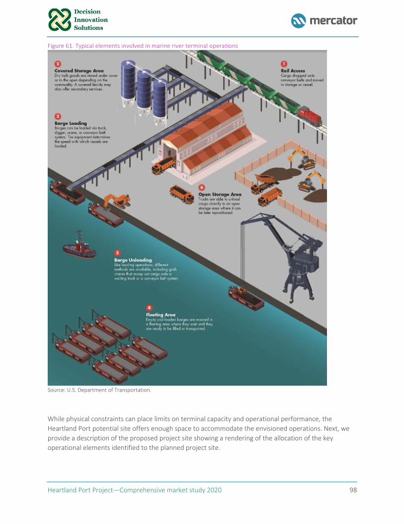
Heartland Port Project—Comprehensive market study 2020 98
Figure 61. Typical elements involved in marine river terminal operations
Source: U.S. Department of Transportation.
While physical constraints can place limits on terminal capacity and operational performance, the
Heartland Port potential site offers enough space to accommodate the envisioned operations. Next, we
provide a description of the proposed project site showing a rendering of the allocation of the key
operational elements identified to the planned project site.
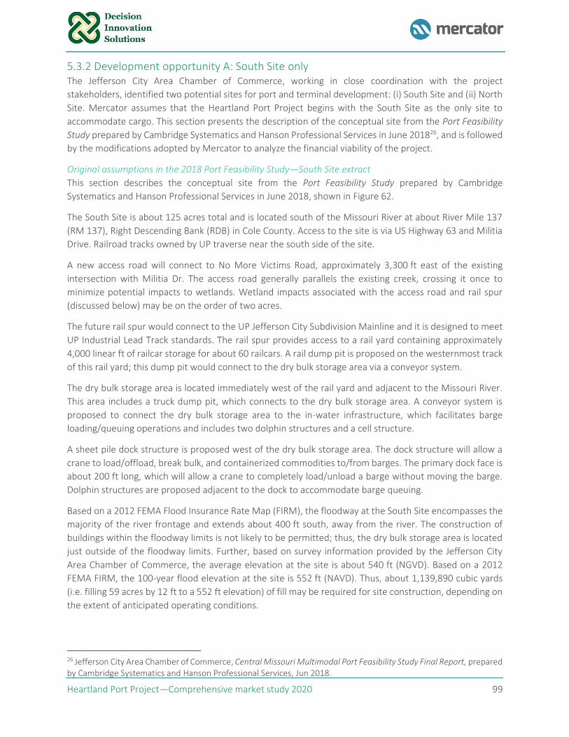
Heartland Port Project—Comprehensive market study 2020 99
5.3.2 Development opportunity A: South Site only The Jefferson City Area Chamber of Commerce, working in close coordination with the project
stakeholders, identified two potential sites for port and terminal development: (i) South Site and (ii) North
Site. Mercator assumes that the Heartland Port Project begins with the South Site as the only site to
accommodate cargo. This section presents the description of the conceptual site from the Port Feasibility
Study prepared by Cambridge Systematics and Hanson Professional Services in June 201826, and is followed
by the modifications adopted by Mercator to analyze the financial viability of the project.
Original assumptions in the 2018 Port Feasibility Study—South Site extract
This section describes the conceptual site from the Port Feasibility Study prepared by Cambridge
Systematics and Hanson Professional Services in June 2018, shown in Figure 62.
The South Site is about 125 acres total and is located south of the Missouri River at about River Mile 137
(RM 137), Right Descending Bank (RDB) in Cole County. Access to the site is via US Highway 63 and Militia
Drive. Railroad tracks owned by UP traverse near the south side of the site.
A new access road will connect to No More Victims Road, approximately 3,300 ft east of the existing
intersection with Militia Dr. The access road generally parallels the existing creek, crossing it once to
minimize potential impacts to wetlands. Wetland impacts associated with the access road and rail spur
(discussed below) may be on the order of two acres.
The future rail spur would connect to the UP Jefferson City Subdivision Mainline and it is designed to meet
UP Industrial Lead Track standards. The rail spur provides access to a rail yard containing approximately
4,000 linear ft of railcar storage for about 60 railcars. A rail dump pit is proposed on the westernmost track
of this rail yard; this dump pit would connect to the dry bulk storage area via a conveyor system.
The dry bulk storage area is located immediately west of the rail yard and adjacent to the Missouri River.
This area includes a truck dump pit, which connects to the dry bulk storage area. A conveyor system is
proposed to connect the dry bulk storage area to the in-water infrastructure, which facilitates barge
loading/queuing operations and includes two dolphin structures and a cell structure.
A sheet pile dock structure is proposed west of the dry bulk storage area. The dock structure will allow a
crane to load/offload, break bulk, and containerized commodities to/from barges. The primary dock face is
about 200 ft long, which will allow a crane to completely load/unload a barge without moving the barge.
Dolphin structures are proposed adjacent to the dock to accommodate barge queuing.
Based on a 2012 FEMA Flood Insurance Rate Map (FIRM), the floodway at the South Site encompasses the
majority of the river frontage and extends about 400 ft south, away from the river. The construction of
buildings within the floodway limits is not likely to be permitted; thus, the dry bulk storage area is located
just outside of the floodway limits. Further, based on survey information provided by the Jefferson City
Area Chamber of Commerce, the average elevation at the site is about 540 ft (NGVD). Based on a 2012
FEMA FIRM, the 100-year flood elevation at the site is 552 ft (NAVD). Thus, about 1,139,890 cubic yards
(i.e. filling 59 acres by 12 ft to a 552 ft elevation) of fill may be required for site construction, depending on
the extent of anticipated operating conditions.
26 Jefferson City Area Chamber of Commerce, Central Missouri Multimodal Port Feasibility Study Final Report, prepared by Cambridge Systematics and Hanson Professional Services, Jun 2018.
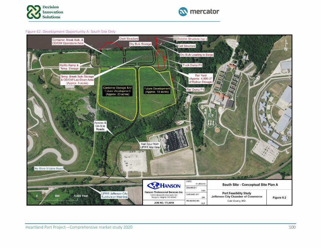
Heartland Port Project—Comprehensive market study 2020 100
Figure 62. Development Opportunity A: South Site Only
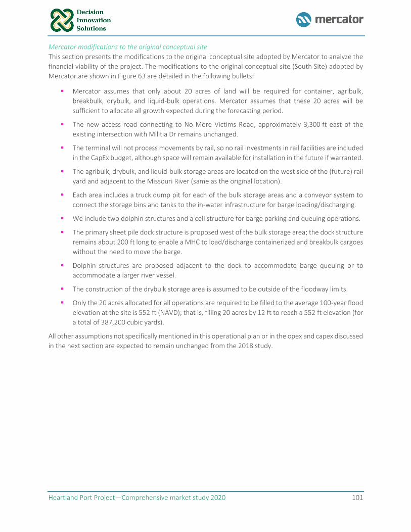
Heartland Port Project—Comprehensive market study 2020 101
Mercator modifications to the original conceptual site
This section presents the modifications to the original conceptual site adopted by Mercator to analyze the
financial viability of the project. The modifications to the original conceptual site (South Site) adopted by
Mercator are shown in Figure 63 are detailed in the following bullets:
▪ Mercator assumes that only about 20 acres of land will be required for container, agribulk,
breakbulk, drybulk, and liquid-bulk operations. Mercator assumes that these 20 acres will be
sufficient to allocate all growth expected during the forecasting period.
▪ The new access road connecting to No More Victims Road, approximately 3,300 ft east of the
existing intersection with Militia Dr remains unchanged.
▪ The terminal will not process movements by rail, so no rail investments in rail facilities are included
in the CapEx budget, although space will remain available for installation in the future if warranted.
▪ The agribulk, drybulk, and liquid-bulk storage areas are located on the west side of the (future) rail
yard and adjacent to the Missouri River (same as the original location).
▪ Each area includes a truck dump pit for each of the bulk storage areas and a conveyor system to
connect the storage bins and tanks to the in-water infrastructure for barge loading/discharging.
▪ We include two dolphin structures and a cell structure for barge parking and queuing operations.
▪ The primary sheet pile dock structure is proposed west of the bulk storage area; the dock structure
remains about 200 ft long to enable a MHC to load/discharge containerized and breakbulk cargoes
without the need to move the barge.
▪ Dolphin structures are proposed adjacent to the dock to accommodate barge queuing or to
accommodate a larger river vessel.
▪ The construction of the drybulk storage area is assumed to be outside of the floodway limits.
▪ Only the 20 acres allocated for all operations are required to be filled to the average 100-year flood
elevation at the site is 552 ft (NAVD); that is, filling 20 acres by 12 ft to reach a 552 ft elevation (for
a total of 387,200 cubic yards).
All other assumptions not specifically mentioned in this operational plan or in the opex and capex discussed
in the next section are expected to remain unchanged from the 2018 study.
Heartland Port Project—Comprehensive market study 2020 102
Figure 63. Modifications the original conceptual site (South Site) adopted by Mercator
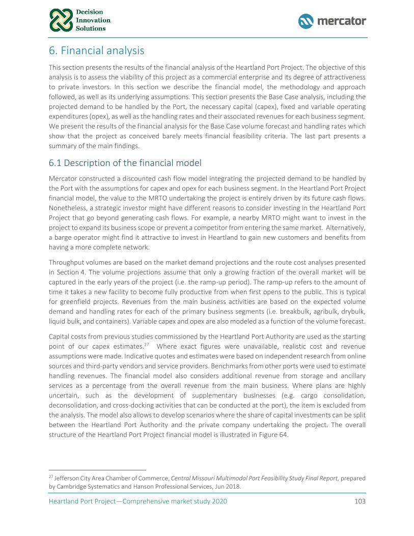
Heartland Port Project—Comprehensive market study 2020 103
6. Financial analysis
This section presents the results of the financial analysis of the Heartland Port Project. The objective of this
analysis is to assess the viability of this project as a commercial enterprise and its degree of attractiveness
to private investors. In this section we describe the financial model, the methodology and approach
followed, as well as its underlying assumptions. This section presents the Base Case analysis, including the
projected demand to be handled by the Port, the necessary capital (capex), fixed and variable operating
expenditures (opex), as well as the handling rates and their associated revenues for each business segment.
We present the results of the financial analysis for the Base Case volume forecast and handling rates which
show that the project as conceived barely meets financial feasibility criteria. The last part presents a
summary of the main findings.
6.1 Description of the financial model
Mercator constructed a discounted cash flow model integrating the projected demand to be handled by
the Port with the assumptions for capex and opex for each business segment. In the Heartland Port Project
financial model, the value to the MRTO undertaking the project is entirely driven by its future cash flows.
Nonetheless, a strategic investor might have different reasons to consider investing in the Heartland Port
Project that go beyond generating cash flows. For example, a nearby MRTO might want to invest in the
project to expand its business scope or prevent a competitor from entering the same market. Alternatively,
a barge operator might find it attractive to invest in Heartland to gain new customers and benefits from
having a more complete network.
Throughput volumes are based on the market demand projections and the route cost analyses presented
in Section 4. The volume projections assume that only a growing fraction of the overall market will be
captured in the early years of the project (i.e. the ramp-up period). The ramp-up refers to the amount of
time it takes a new facility to become fully productive from when first opens to the public. This is typical
for greenfield projects. Revenues from the main business activities are based on the expected volume
demand and handling rates for each of the primary business segments (i.e. breakbulk, agribulk, drybulk,
liquid bulk, and containers). Variable capex and opex are also modeled as a function of the volume forecast.
Capital costs from previous studies commissioned by the Heartland Port Authority are used as the starting
point of our capex estimates.27 Where exact figures were unavailable, realistic cost and revenue
assumptions were made. Indicative quotes and estimates were based on independent research from online
sources and third-party vendors and service providers. Benchmarks from other ports were used to estimate
handling revenues. The financial model also considers additional revenue from storage and ancillary
services as a percentage from the overall revenue from the main business. Where plans are highly
uncertain, such as the development of supplementary businesses (e.g. cargo consolidation,
deconsolidation, and cross-docking activities that can be conducted at the port), the item is excluded from
the analysis. The model also allows to develop scenarios where the share of capital investments can be split
between the Heartland Port Authority and the private company undertaking the project. The overall
structure of the Heartland Port Project financial model is illustrated in Figure 64.
27 Jefferson City Area Chamber of Commerce, Central Missouri Multimodal Port Feasibility Study Final Report, prepared by Cambridge Systematics and Hanson Professional Services, Jun 2018.
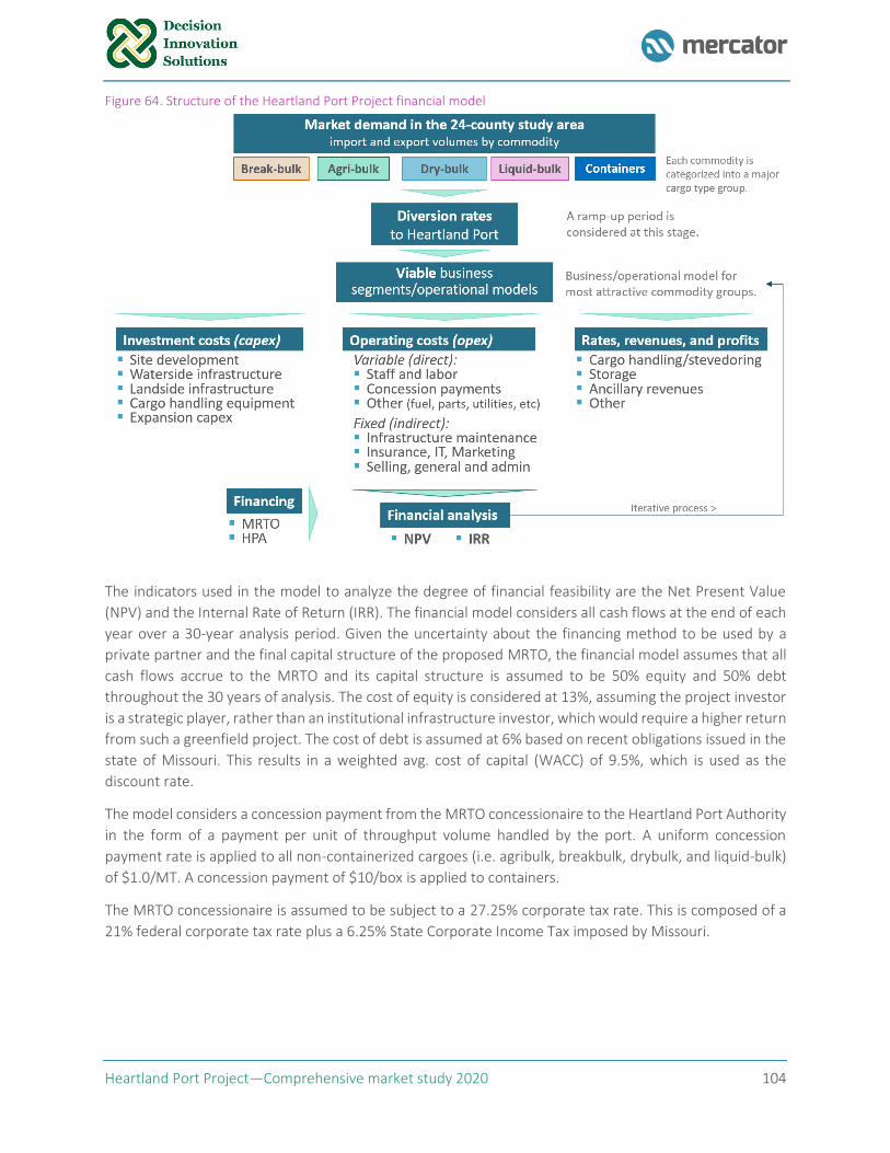
Heartland Port Project—Comprehensive market study 2020 104
Figure 64. Structure of the Heartland Port Project financial model
The indicators used in the model to analyze the degree of financial feasibility are the Net Present Value
(NPV) and the Internal Rate of Return (IRR). The financial model considers all cash flows at the end of each
year over a 30-year analysis period. Given the uncertainty about the financing method to be used by a
private partner and the final capital structure of the proposed MRTO, the financial model assumes that all
cash flows accrue to the MRTO and its capital structure is assumed to be 50% equity and 50% debt
throughout the 30 years of analysis. The cost of equity is considered at 13%, assuming the project investor
is a strategic player, rather than an institutional infrastructure investor, which would require a higher return
from such a greenfield project. The cost of debt is assumed at 6% based on recent obligations issued in the
state of Missouri. This results in a weighted avg. cost of capital (WACC) of 9.5%, which is used as the
discount rate.
The model considers a concession payment from the MRTO concessionaire to the Heartland Port Authority
in the form of a payment per unit of throughput volume handled by the port. A uniform concession
payment rate is applied to all non-containerized cargoes (i.e. agribulk, breakbulk, drybulk, and liquid-bulk)
of $1.0/MT. A concession payment of $10/box is applied to containers.
The MRTO concessionaire is assumed to be subject to a 27.25% corporate tax rate. This is composed of a
21% federal corporate tax rate plus a 6.25% State Corporate Income Tax imposed by Missouri.
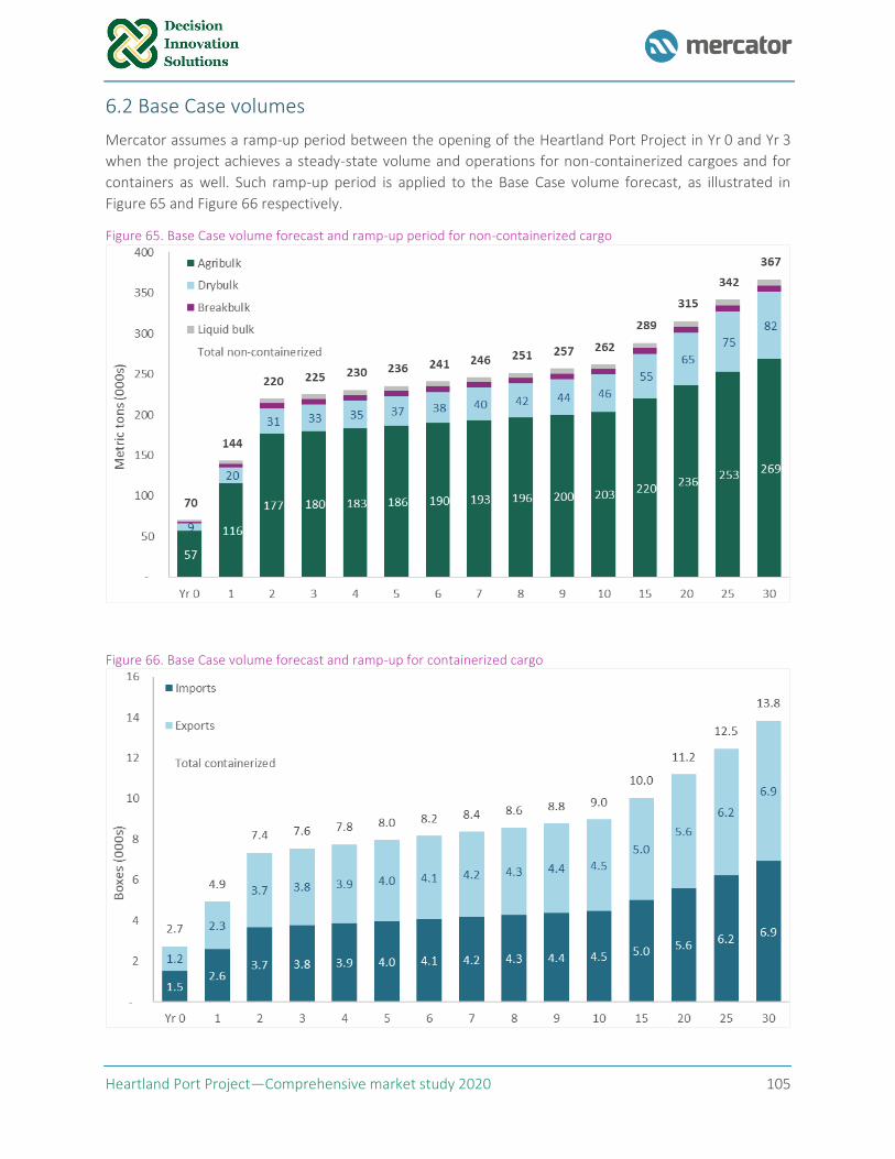
Heartland Port Project—Comprehensive market study 2020 105
6.2 Base Case volumes
Mercator assumes a ramp-up period between the opening of the Heartland Port Project in Yr 0 and Yr 3
when the project achieves a steady-state volume and operations for non-containerized cargoes and for
containers as well. Such ramp-up period is applied to the Base Case volume forecast, as illustrated in
Figure 65 and Figure 66 respectively.
Figure 65. Base Case volume forecast and ramp-up period for non-containerized cargo
Figure 66. Base Case volume forecast and ramp-up for containerized cargo
Heartland Port Project—Comprehensive market study 2020 106
6.3 Combination of business segments analyzed
Mercator analyzed the start-up costs, capital investments, and operational expenditures required to
operate each business segment individually as well as operating one or more combinations of such
segments for a total of nine combinations.
6.3.1 Indicative capex Mercator developed scenario-based capex calculations utilizing the capital costs from studies previously
commissioned by the Heartland Port Authority as the starting point and modified them accordingly to
analyze different combination of business segments.28 Indicative quotes and estimates were obtained from
independent research from online sources and third-party vendors and service providers. Capex related to
handling equipment and storage associated with each business segment account for future expansions
needed to accommodate the expected volumes for each business segment or combination of business
segments modeled. Capex related to construction and civil works consider only the minimum necessary for
a particular business segment to operate.
Capex are organized in the following categories, which form the basis of the combination of business
segments analyzed.
1. Container and breakbulk (cont+BB)—Total start-up capex are $19.1 million:
Since these two business segments share most of the equipment and some operational area, this
combination assumes that no extra capex is required to start the breakbulk operations once the
investment for the container yard is made; hence, the container and breakbulk categories are
grouped and analyzed as a single business segment.
▪ Handling equipment and storage. These two business segments include $3.2 million for
container handling equipment (CHE), which account for one mobile harbor crane (MHC) with
a productivity of 15 moves/hr, and 2 top-loaders and 3 bomb-carts with tractors per crane.
▪ Construction and civil works. These two business segments include $15.9 million, which
consider $3.4 million for waterside works, cells and dolphins, and fill/embankment of 10 acres
for the main yard. For these two business segments to operate, a sheet pile dock structure is
proposed on the west side of the terminal to allow for the crane operation. The proposed
primary dock face is 200 ft long, which will allow a crane to completely load/unload a barge
without moving the barge. Dolphin structures are proposed adjacent to the dock to
accommodate barge queuing. $4.5 million is considered for the construction of the dock and
200 ft sheet pile. Mobilization, engineering, and contingency for these two business segments
only is estimated at $5.7 million.
2. Agribulk—Total start-up capex are $16.6 million:
▪ Handling equipment and storage. This business segments considers $6.9 million for agribulk
storage (for 6,000 metric tons), a truck dump pit, scales/testing equipment, and 900 ft of
conveyor system & foundations.
28 Jefferson City Area Chamber of Commerce, Central Missouri Multimodal Port Feasibility Study Final Report, prepared by Cambridge Systematics and Hanson Professional Services, Jun 2018.
Heartland Port Project—Comprehensive market study 2020 107
▪ Construction and civil works. This business segment includes $1.5 million for waterside cells
and dolphins and fill/embankment only for the 3 acres required to build the bulk area. The bulk
area considers 3 acres for about five silos or tanks. Modeling this business segment alone
assumes no dock for the main yard is required and conveyors connect directly to the cells.
Mobilization, engineering, and contingency is estimated at $6.0 million.
3. Drybulk—Total start-up capex are $13.0 million:
▪ Handling equipment and storage. This business segment considers $4.6 million for drybulk
storage (2,000 metric tons in 1 steel bin), a truck dump pit, scales/related equipment, and
1,000 ft of conveyor system & foundations.29
▪ Construction and civil works. Include $1.5 million for waterside cells and dolphins and
fill/embankment only for the 3 acres required to build the bulk area. Modeling this business
segment alone assumes no dock. Mobilization, engineering, and contingency is $4.7 million.
4. Liquid bulk—Total start-up capex are $10.0 million:
▪ Handling equipment and storage. This business segments considers $2.7 million for liquid bulk
storage (1,000 metric tons in 1 steel tank) and 1,100 ft of pipelines and related systems.
▪ Construction and civil works. Include $1.5 million for waterside cells and dolphins and
fill/embankment only for the 3 acres required to build the bulk area. Modeling this business
segment alone assumes no dock. Mobilization, engineering, and contingency is $3.6 million.
5. Roads and utilities—The model assumes that the same roads and utilities are required for the
terminal independent of the business segments modeled. The cost assumed is $2.2 million. No
cargo flow that utilizes rail has been identified, so rail infrastructure is not built in any of the
scenarios to save capex.
6. Mobilization, engineering, and contingency—Assumes a project cost for mobilization (6%),
engineering/permitting/surveying (14%), and contingency (30%) of the startup capex for the
business segments modeled only.
These assumptions are made with a view to develop an operation as envisioned in the conceptual layout.
Nevertheless, testing these different combinations of business segments allow us to generate an
understanding about the magnitude of the investments required for each business segment, the expected
volumes, potential levels of revenue and earnings, and the business value for each segment. This method
allows us to forecast the cash flows attributable to the subject asset and associated cargo sector being
served. It also helps to determine the optimal levels of investment for each business segment based on
their degree of profitability.
A summary for the startup capex per business segment modeled and their different combinations is shown
in Table 31.
29 Since the expected cargo flows for drybulk are imports, a less expensive operation might be conducted utilizing a crane with clam shell unloaders, a hopper, dump trucks, a dumping pit, a conveyor, and a storage silo bin. This configuration would only work with a dock in place.
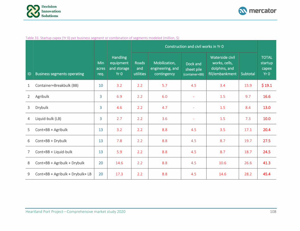
Heartland Port Project—Comprehensive market study 2020 108
Table 31. Startup capex (Yr 0) per business segment or combination of segments modeled (million, $)
ID Business segments operating
Min
acres
req.
Handling
equipment
and storage
Yr 0
Construction and civil works in Yr 0
TOTAL
startup
capex
Yr 0
Roads
and
utilities
Mobilization,
engineering, and
contingency
Dock and
sheet pile (container+BB)
Waterside civil
works, cells,
dolphins, and
fill/embankment Subtotal
1 Container+Breakbulk (BB) 10 3.2 2.2 5.7 4.5 3.4 15.9 $ 19.1
2 Agribulk 3 6.9 2.2 6.0 - 1.5 9.7 16.6
3 Drybulk 3 4.6 2.2 4.7 - 1.5 8.4 13.0
4 Liquid-bulk (LB) 3 2.7 2.2 3.6 - 1.5 7.3 10.0
5 Cont+BB + Agribulk 13 3.2 2.2 8.8 4.5 3.5 17.1 20.4
6 Cont+BB + Drybulk 13 7.8 2.2 8.8 4.5 8.7 19.7 27.5
7 Cont+BB + Liquid-bulk 13 5.9 2.2 8.8 4.5 8.7 18.7 24.5
8 Cont+BB + Agribulk + Drybulk 20 14.6 2.2 8.8 4.5 10.6 26.6 41.3
9 Cont+BB + Agribulk + Drybulk+ LB 20 17.3 2.2 8.8 4.5 14.6 28.2 45.4
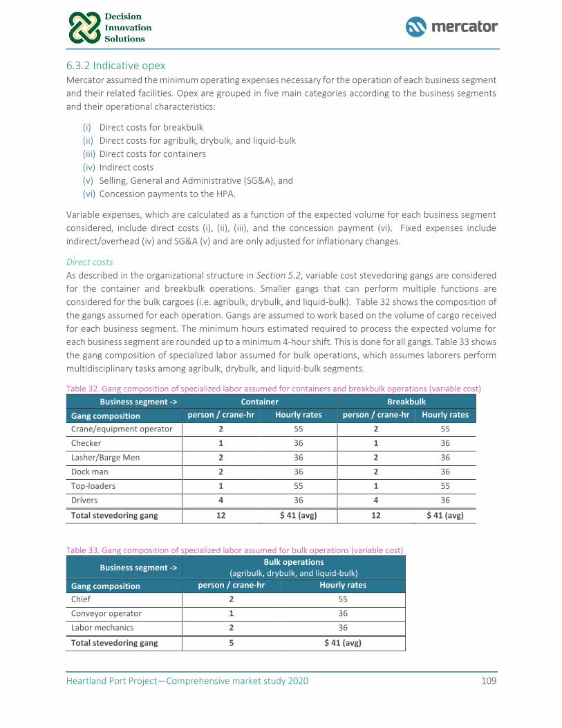
Heartland Port Project—Comprehensive market study 2020 109
6.3.2 Indicative opex Mercator assumed the minimum operating expenses necessary for the operation of each business segment
and their related facilities. Opex are grouped in five main categories according to the business segments
and their operational characteristics:
(i) Direct costs for breakbulk
(ii) Direct costs for agribulk, drybulk, and liquid-bulk
(iii) Direct costs for containers
(iv) Indirect costs
(v) Selling, General and Administrative (SG&A), and
(vi) Concession payments to the HPA.
Variable expenses, which are calculated as a function of the expected volume for each business segment
considered, include direct costs (i), (ii), (iii), and the concession payment (vi). Fixed expenses include
indirect/overhead (iv) and SG&A (v) and are only adjusted for inflationary changes.
Direct costs
As described in the organizational structure in Section 5.2, variable cost stevedoring gangs are considered
for the container and breakbulk operations. Smaller gangs that can perform multiple functions are
considered for the bulk cargoes (i.e. agribulk, drybulk, and liquid-bulk). Table 32 shows the composition of
the gangs assumed for each operation. Gangs are assumed to work based on the volume of cargo received
for each business segment. The minimum hours estimated required to process the expected volume for
each business segment are rounded up to a minimum 4-hour shift. This is done for all gangs. Table 33 shows
the gang composition of specialized labor assumed for bulk operations, which assumes laborers perform
multidisciplinary tasks among agribulk, drybulk, and liquid-bulk segments.
Table 32. Gang composition of specialized labor assumed for containers and breakbulk operations (variable cost)
Business segment -> Container Breakbulk
Gang composition person / crane-hr Hourly rates person / crane-hr Hourly rates
Crane/equipment operator 2 55 2 55
Checker 1 36 1 36
Lasher/Barge Men 2 36 2 36
Dock man 2 36 2 36
Top-loaders 1 55 1 55
Drivers 4 36 4 36
Total stevedoring gang 12 $ 41 (avg) 12 $ 41 (avg)
Table 33. Gang composition of specialized labor assumed for bulk operations (variable cost)
Business segment -> Bulk operations
(agribulk, drybulk, and liquid-bulk)
Gang composition person / crane-hr Hourly rates
Chief 2 55
Conveyor operator 1 36
Labor mechanics 2 36
Total stevedoring gang 5 $ 41 (avg)
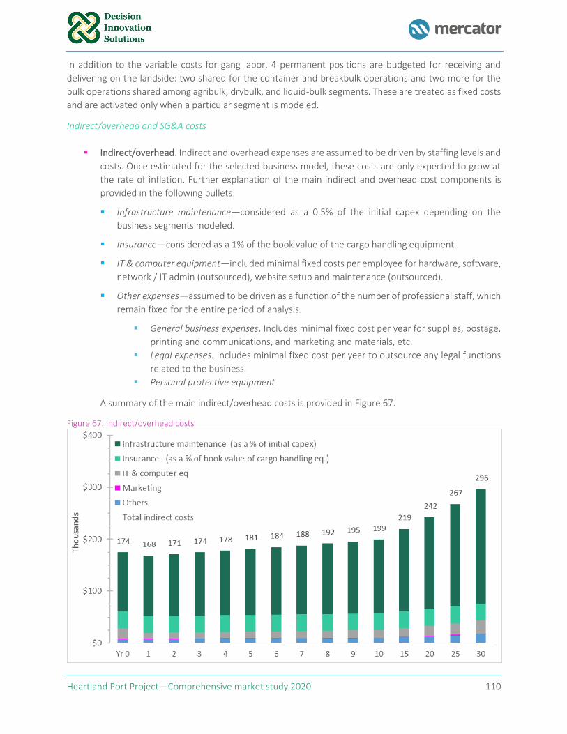
Heartland Port Project—Comprehensive market study 2020 110
In addition to the variable costs for gang labor, 4 permanent positions are budgeted for receiving and
delivering on the landside: two shared for the container and breakbulk operations and two more for the
bulk operations shared among agribulk, drybulk, and liquid-bulk segments. These are treated as fixed costs
and are activated only when a particular segment is modeled.
Indirect/overhead and SG&A costs
▪ Indirect/overhead. Indirect and overhead expenses are assumed to be driven by staffing levels and
costs. Once estimated for the selected business model, these costs are only expected to grow at
the rate of inflation. Further explanation of the main indirect and overhead cost components is
provided in the following bullets:
▪ Infrastructure maintenance—considered as a 0.5% of the initial capex depending on the
business segments modeled.
▪ Insurance—considered as a 1% of the book value of the cargo handling equipment.
▪ IT & computer equipment—included minimal fixed costs per employee for hardware, software,
network / IT admin (outsourced), website setup and maintenance (outsourced).
▪ Other expenses—assumed to be driven as a function of the number of professional staff, which
remain fixed for the entire period of analysis.
▪ General business expenses. Includes minimal fixed cost per year for supplies, postage,
printing and communications, and marketing and materials, etc.
▪ Legal expenses. Includes minimal fixed cost per year to outsource any legal functions
related to the business.
▪ Personal protective equipment
A summary of the main indirect/overhead costs is provided in Figure 67.
Figure 67. Indirect/overhead costs
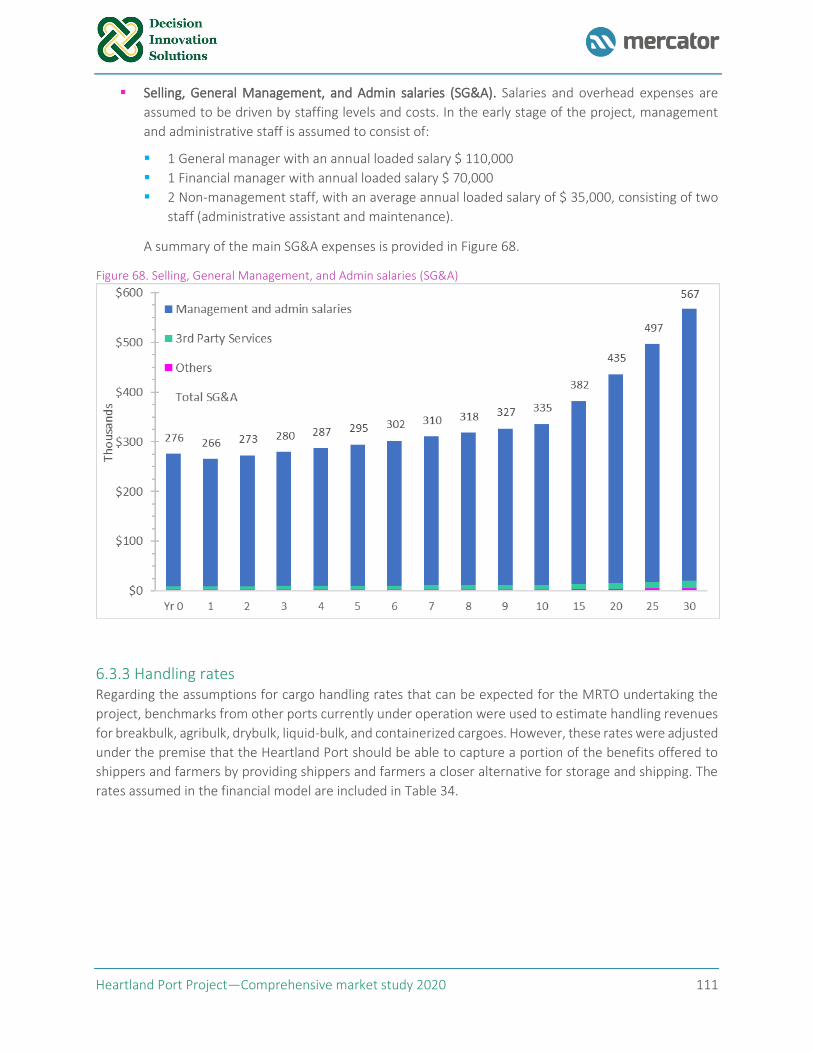
Heartland Port Project—Comprehensive market study 2020 111
▪ Selling, General Management, and Admin salaries (SG&A). Salaries and overhead expenses are
assumed to be driven by staffing levels and costs. In the early stage of the project, management
and administrative staff is assumed to consist of:
▪ 1 General manager with an annual loaded salary $ 110,000
▪ 1 Financial manager with annual loaded salary $ 70,000
▪ 2 Non-management staff, with an average annual loaded salary of $ 35,000, consisting of two
staff (administrative assistant and maintenance).
A summary of the main SG&A expenses is provided in Figure 68.
Figure 68. Selling, General Management, and Admin salaries (SG&A)
6.3.3 Handling rates Regarding the assumptions for cargo handling rates that can be expected for the MRTO undertaking the
project, benchmarks from other ports currently under operation were used to estimate handling revenues
for breakbulk, agribulk, drybulk, liquid-bulk, and containerized cargoes. However, these rates were adjusted
under the premise that the Heartland Port should be able to capture a portion of the benefits offered to
shippers and farmers by providing shippers and farmers a closer alternative for storage and shipping. The
rates assumed in the financial model are included in Table 34.
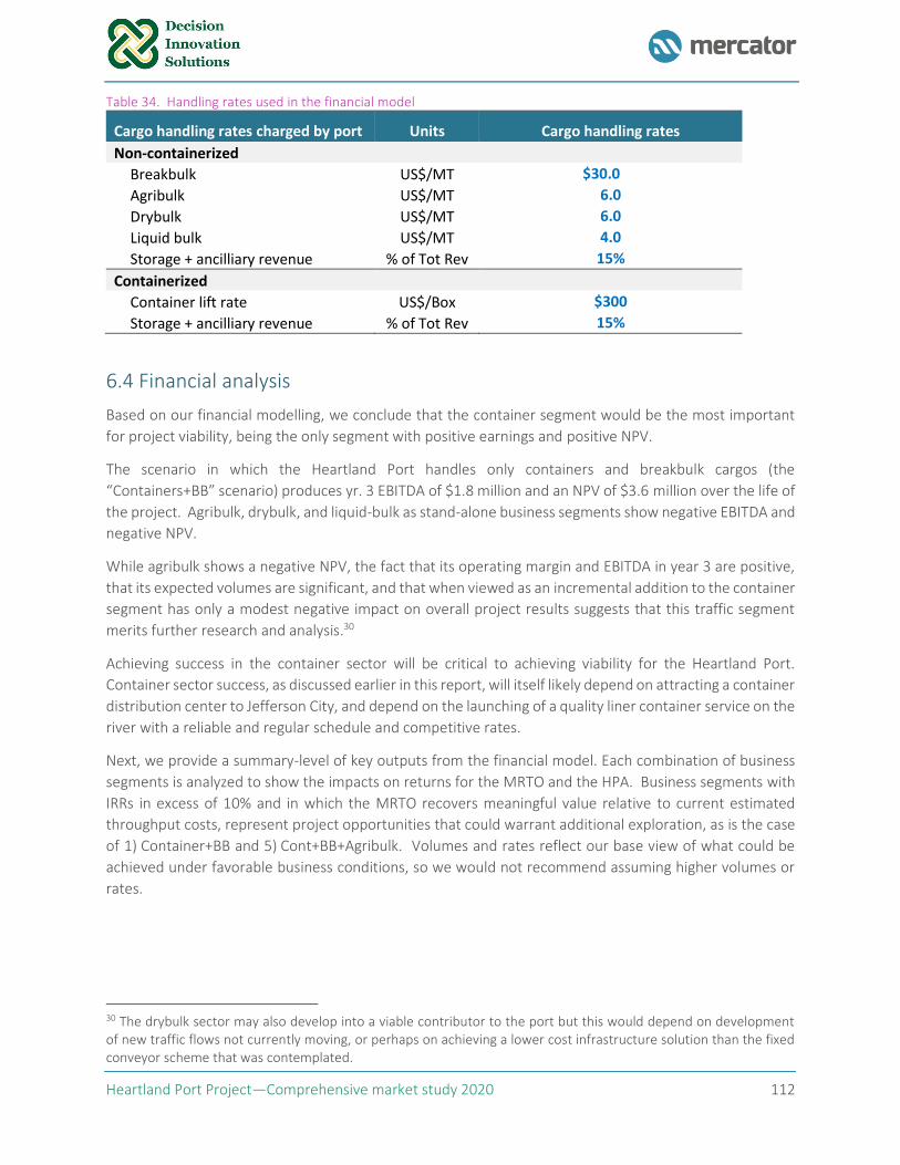
Heartland Port Project—Comprehensive market study 2020 112
Table 34. Handling rates used in the financial model
Cargo handling rates charged by port Units Cargo handling rates
Non-containerized Breakbulk US$/MT $30.0
Agribulk US$/MT 6.0
Drybulk US$/MT 6.0
Liquid bulk US$/MT 4.0
Storage + ancilliary revenue % of Tot Rev 15%
Containerized
Container lift rate US$/Box $300
Storage + ancilliary revenue % of Tot Rev 15%
6.4 Financial analysis
Based on our financial modelling, we conclude that the container segment would be the most important
for project viability, being the only segment with positive earnings and positive NPV.
The scenario in which the Heartland Port handles only containers and breakbulk cargos (the
“Containers+BB” scenario) produces yr. 3 EBITDA of $1.8 million and an NPV of $3.6 million over the life of
the project. Agribulk, drybulk, and liquid-bulk as stand-alone business segments show negative EBITDA and
negative NPV.
While agribulk shows a negative NPV, the fact that its operating margin and EBITDA in year 3 are positive,
that its expected volumes are significant, and that when viewed as an incremental addition to the container
segment has only a modest negative impact on overall project results suggests that this traffic segment
merits further research and analysis.30
Achieving success in the container sector will be critical to achieving viability for the Heartland Port.
Container sector success, as discussed earlier in this report, will itself likely depend on attracting a container
distribution center to Jefferson City, and depend on the launching of a quality liner container service on the
river with a reliable and regular schedule and competitive rates.
Next, we provide a summary-level of key outputs from the financial model. Each combination of business
segments is analyzed to show the impacts on returns for the MRTO and the HPA. Business segments with
IRRs in excess of 10% and in which the MRTO recovers meaningful value relative to current estimated
throughput costs, represent project opportunities that could warrant additional exploration, as is the case
of 1) Container+BB and 5) Cont+BB+Agribulk. Volumes and rates reflect our base view of what could be
achieved under favorable business conditions, so we would not recommend assuming higher volumes or
rates.
30 The drybulk sector may also develop into a viable contributor to the port but this would depend on development of new traffic flows not currently moving, or perhaps on achieving a lower cost infrastructure solution than the fixed conveyor scheme that was contemplated.
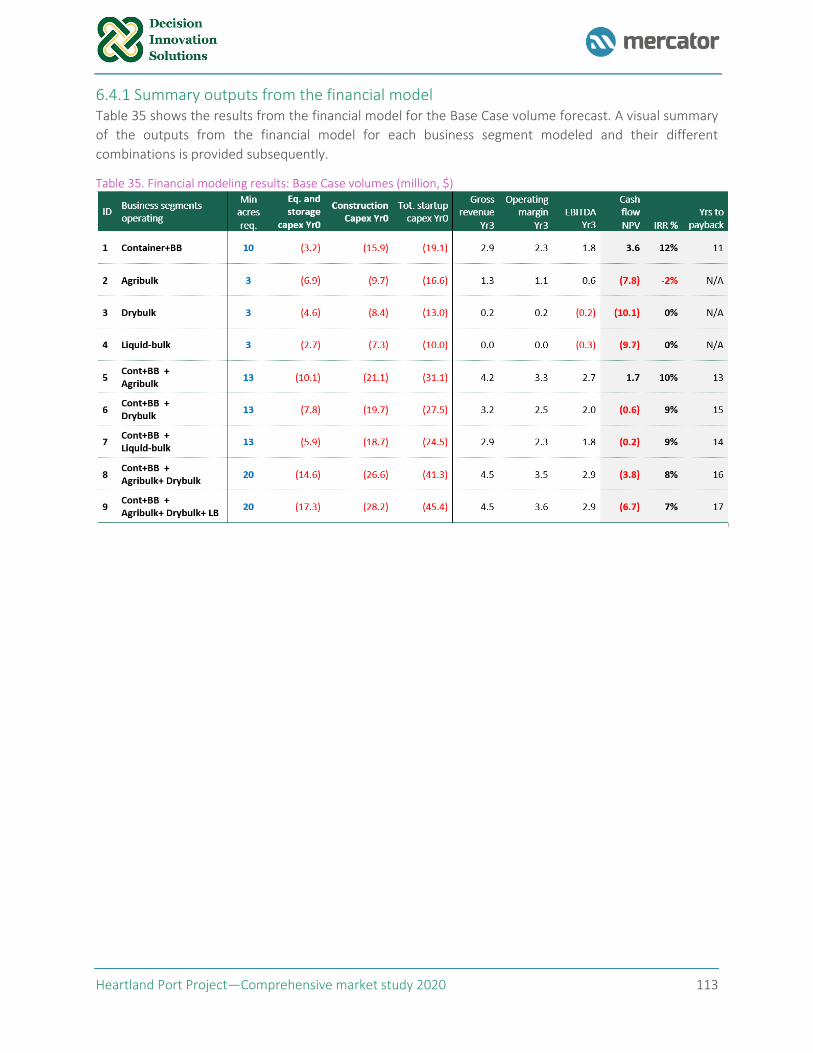
Heartland Port Project—Comprehensive market study 2020 113
6.4.1 Summary outputs from the financial model Table 35 shows the results from the financial model for the Base Case volume forecast. A visual summary
of the outputs from the financial model for each business segment modeled and their different
combinations is provided subsequently.
Table 35. Financial modeling results: Base Case volumes (million, $)
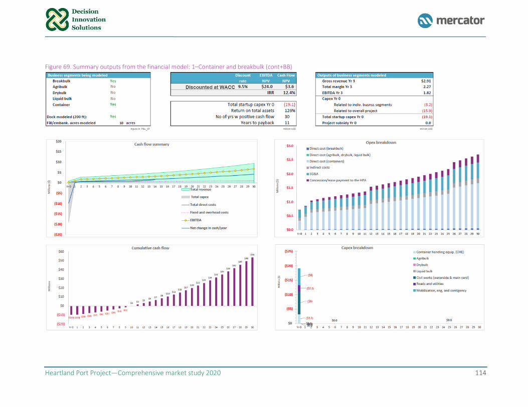
Heartland Port Project—Comprehensive market study 2020 114
Figure 69. Summary outputs from the financial model: 1–Container and breakbulk (cont+BB)
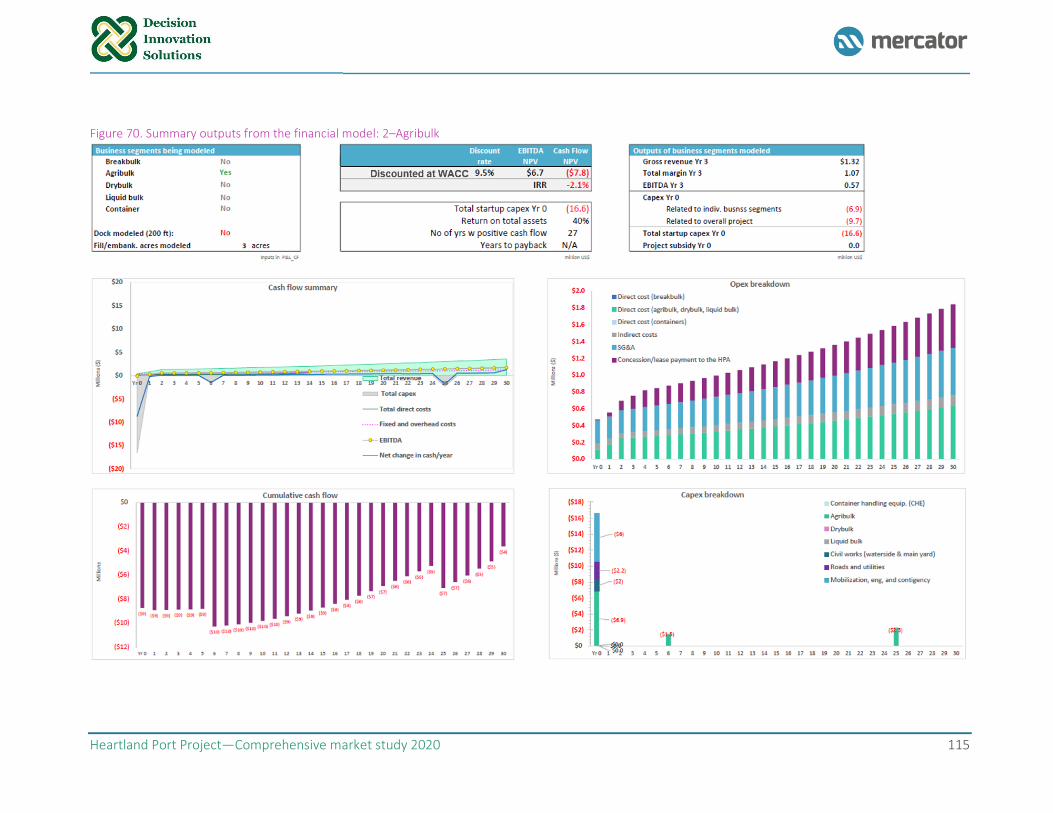
Heartland Port Project—Comprehensive market study 2020 115
Figure 70. Summary outputs from the financial model: 2–Agribulk
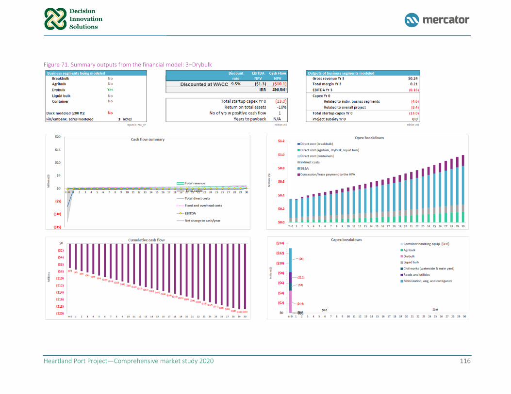
Heartland Port Project—Comprehensive market study 2020 116
Figure 71. Summary outputs from the financial model: 3–Drybulk
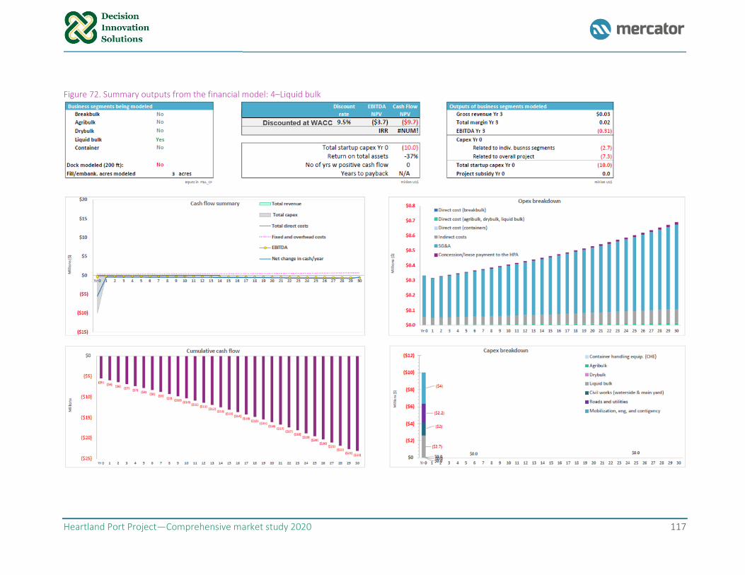
Heartland Port Project—Comprehensive market study 2020 117
Figure 72. Summary outputs from the financial model: 4–Liquid bulk
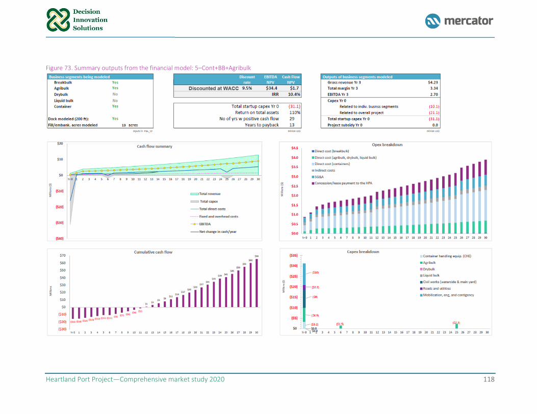
Heartland Port Project—Comprehensive market study 2020 118
Figure 73. Summary outputs from the financial model: 5–Cont+BB+Agribulk
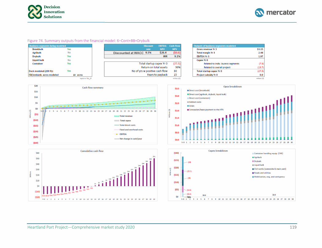
Heartland Port Project—Comprehensive market study 2020 119
Figure 74. Summary outputs from the financial model: 6–Cont+BB+Drybulk
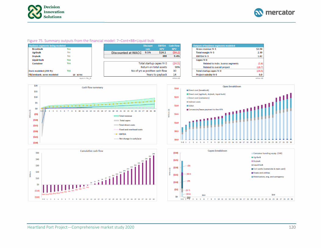
Heartland Port Project—Comprehensive market study 2020 120
Figure 75. Summary outputs from the financial model: 7–Cont+BB+Liquid bulk
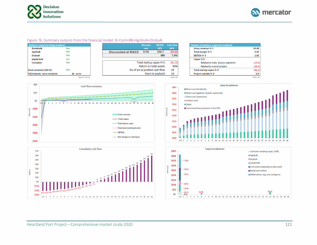
Heartland Port Project—Comprehensive market study 2020 121
Figure 76. Summary outputs from the financial model: 8–Cont+BB+Agribulk+Drybulk
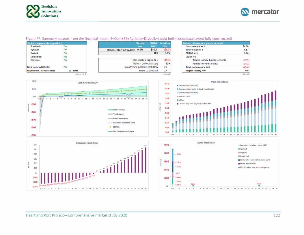
Heartland Port Project—Comprehensive market study 2020 122
Figure 77. Summary outputs from the financial model: 8–Cont+BB+Agribulk+Drybulk+Liquid bulk (conceptual layout fully constructed)
Heartland Port Project—Comprehensive market study 2020 123
6.5 Key takeaways
Assuming that the necessary condition for supporting containerized cargo flows to Jefferson City are in
place (i.e. local distribution center capacity is established and a low-cost and frequent container ship or
barge service is operating), containerized cargo handling could be viable and is responsible for most of the
value generated under the scenarios evaluated. As presently conceived, the non-container investments are
not individually or collectively viable, and to support them the container business may have to absorb
certain capital expenses (and potentially some operational expenses) associated with any bulk operations
if those activities are included in the development plan. Liquid bulk operations seem to be detrimental to
the overall project under the current volume assumptions.
Assuming the Base Case volumes, the outputs of the financial model for the two most attractive scenarios
Cont+BB and Cont+BB+Agribulk show an NPV of the project cash flows of $3.6 million and $1.7 million
respectively, after considering capex, interest, taxes, depreciation, and amortization for these two business
segments. Although the returns from the project would not be attractive to an institutional investor, (IRR
of 10% based on a 50/50 debt/equity ratio) this project might be attractive to a strategic player who could
capture non-financial benefits
While agribulk shows a negative cash flow NPV as a stand-alone business, the fact that its operating margin
and EBITDA in year 3 are positive and that volumes are significant under the Base Case forecast, provide
some indication that, at least, merits further research and analysis. Agribulk might turn into positive
territory under more refined assumptions. For instance, changes in the capital structure of the project,
further capex refinements based on an actual engineering design/analysis, consideration of further value-
adding activities on-site might generate additional revenues worthy of consideration for the overall project.
Because moving freight by water is the least expensive and more environmentally friendly of all
transportation modes, there are societal benefits that can stem for a project of this nature that could not
be captured by a private investor. As demonstrated by the 2018 Central Missouri Multimodal Port Feasibility
Study aggregate economic benefits and direct impacts include freight transportation costs savings, freight
emission cost savings, safety cost savings, state of good repair cost savings, and job creation that exceed
$200 million in the Boone, Callaway, Cole, and Osage Counties.31
The MoDOT has established various mechanisms for successful public/public and public/private
partnerships. These expand financing options for transportation projects that serve a public purpose,
including: highway and rail projects and water transportation facilities. The benefits to a project assisted by
these partnerships may include: inflation cost savings, early economic and public benefits, financing
tailored to the project's needs, and a reduced cost of project financing. One example is the Port Capital
Improvement Program, which provides capital grants to public port authorities to assist with capital
expenditures, such as dock construction, mooring dolphins, access improvements (e.g. rail connectors,
road access improvements), utility extensions, and general site development. Other resources include
federal grants, transportation development districts, cost-sharing programs, among others.32
With a rail connection and the ability to load railcar, the port would have the ability to function as a
collection point for the region even during periods of low water traffic or when the river levels are too low
31 Jefferson City Area Chamber of Commerce, Central Missouri Multimodal Port Feasibility Study Final Report, prepared by
Cambridge Systematics and Hanson Professional Services, Jun 2018, page 10-106.
32 https://www.modot.org/partnership-development
Heartland Port Project—Comprehensive market study 2020 124
for barge traffic. This would provide greater versatility to the marketplace. A rail connection would also
introduce the option of alternative gateway ports beyond US Gulf ports, such as US West Coast ports, which
could be important if severe weather or other conditions constrain the ability to move export freight
through US Gulf Ports. If the Heartland Port becomes successful at attracting imports of containerized
goods, the development of an intermodal rail yard and related infrastructure would allow the facility to
operate as a dry port for exports when the river levels are too low and is not feasible to operate barges.
The proposed multimodal port would help to enhance the economic environment for traded and non-
traded sector businesses in central Missouri by improving the cost of doing business in the region. In those
regards, the Jefferson City Area Chamber of Commerce and the Heartland Port Authority could work with
state and regional economic development agencies to develop a targeted plan to attract businesses to the
port, while at the same time funding assistance is procured. Once funding assistance is secured, the
attractiveness of this project for a private investor can be expected to increase substantially.
Heartland Port Project—Comprehensive market study 2020 125
7. Environmental regulatory requirements
The Heartland Port project is expected to help alleviate traffic congestion on the roadway and railways, and
the potential to reduce truck and rail related emissions and improve highway and rail safety.33 This section
presents a preliminary identification of the environmental regulatory requirements that would need to be
satisfied in order for the project to move forward. The objective of this section is to provide a roadmap for
the different types of factors that would need to be considered in an Environmental Impact Review process
typical for a project of this magnitude. Such roadmap considers the expected roles of and rules in
relationship to the Heartland Port Project of the following environmental agencies and regulations:
National Environmental Policy Act (NEPA), Council on Environmental Quality (CEQ), U.S. Army Corps of
Engineers (USACE), tribal land/consultation, United States Fish and Wildlife Services (USFWS) Endangered
Species Act, field office of MO Conservation department in Jefferson City, Missouri, and the Missouri
Department of Natural Resources (DNR), each is presented in more detail in the following sections.
7.1 National Environmental Policy Act (NEPA)
The National Environmental Policy Act (NEPA) is the nation's basic environmental law that applies to all
actions taken or approved by federal agencies. A Declaration of National Environmental Policy requires the
federal government to use all practical means to create and maintain conditions under which man and
nature can exist in productive harmony. The key goals of NEPA are to assist Federal agency officials with
making well-informed decisions and to ensure both public and other agency’s involvement in decision-
making. NEPA requires that before federal agencies take a major action, they must evaluate environmental
impacts prior to decision making on any major Federal action, such as the review of a permit application.
These agencies must disclose the environmental impacts of their proposed action and evaluate alternatives
that would have fewer environmental costs.
Major Federal actions involved in marine river terminals, such as the Heartland Port Project, typically
involve the USACE Section 10/404/408. The NEPA process consists of an evaluation of the environmental
effects of a federal undertaking including its alternatives. There are three levels of analysis depending on
whether or not an undertaking could significantly affect the environment:
▪ Categorical exclusion determination
▪ Preparation of an environmental assessment/finding of no significant impact (EA/FONSI), and
▪ Preparation of an environmental impact statement (EIS).
Categorical exclusion is used if the proposed action does not “individually or cumulatively have a significant
effect on the human environment” (40CRF 1508.4). If an Environmental Assessment is needed, the two
outcomes are either a finding of no significant impact, which will allow the project to continue, or an
Environmental Impact Statement (EIS) will be required.
An EIS is the mechanism used to comply with the NEPA in the construction of marine river terminals like
the Heartland Port Project. An EIS must be prepared pursuant to the NEPA of 1969 (42 U.S.C. 4321 et seq.)
and the Council on Environmental Quality (CEQ) NEPA Regulations (40 CFR Parts 1500-1508). The typical
requirements of an EIS are described next.
33 Jefferson City Area Chamber of Commerce, Central Missouri Multimodal Port Feasibility Study Final Report, prepared by
Cambridge Systematics and Hanson Professional Services, Jun 2018, page 10-106.
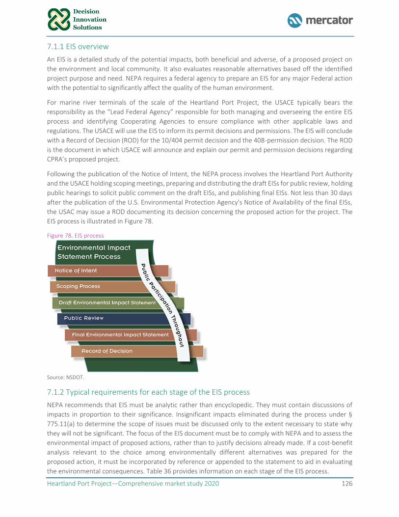
Heartland Port Project—Comprehensive market study 2020 126
7.1.1 EIS overview
An EIS is a detailed study of the potential impacts, both beneficial and adverse, of a proposed project on
the environment and local community. It also evaluates reasonable alternatives based off the identified
project purpose and need. NEPA requires a federal agency to prepare an EIS for any major Federal action
with the potential to significantly affect the quality of the human environment.
For marine river terminals of the scale of the Heartland Port Project, the USACE typically bears the
responsibility as the “Lead Federal Agency” responsible for both managing and overseeing the entire EIS
process and identifying Cooperating Agencies to ensure compliance with other applicable laws and
regulations. The USACE will use the EIS to inform its permit decisions and permissions. The EIS will conclude
with a Record of Decision (ROD) for the 10/404 permit decision and the 408-permission decision. The ROD
is the document in which USACE will announce and explain our permit and permission decisions regarding
CPRA’s proposed project.
Following the publication of the Notice of Intent, the NEPA process involves the Heartland Port Authority
and the USACE holding scoping meetings, preparing and distributing the draft EISs for public review, holding
public hearings to solicit public comment on the draft EISs, and publishing final EISs. Not less than 30 days
after the publication of the U.S. Environmental Protection Agency's Notice of Availability of the final EISs,
the USAC may issue a ROD documenting its decision concerning the proposed action for the project. The
EIS process is illustrated in Figure 78.
Figure 78. EIS process
Source: NSDOT.
7.1.2 Typical requirements for each stage of the EIS process
NEPA recommends that EIS must be analytic rather than encyclopedic. They must contain discussions of
impacts in proportion to their significance. Insignificant impacts eliminated during the process under §
775.11(a) to determine the scope of issues must be discussed only to the extent necessary to state why
they will not be significant. The focus of the EIS document must be to comply with NEPA and to assess the
environmental impact of proposed actions, rather than to justify decisions already made. If a cost-benefit
analysis relevant to the choice among environmentally different alternatives was prepared for the
proposed action, it must be incorporated by reference or appended to the statement to aid in evaluating
the environmental consequences. Table 36 provides information on each stage of the EIS process.
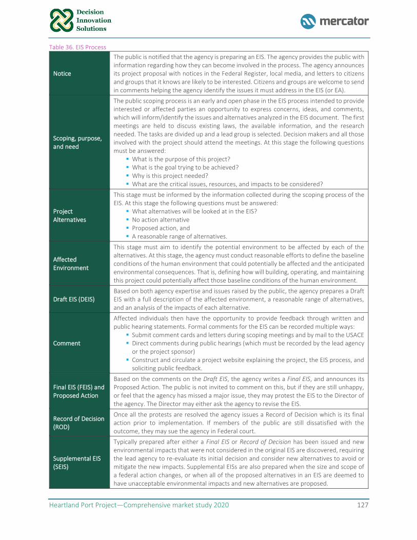
Heartland Port Project—Comprehensive market study 2020 127
Table 36. EIS Process
Notice
The public is notified that the agency is preparing an EIS. The agency provides the public with information regarding how they can become involved in the process. The agency announces its project proposal with notices in the Federal Register, local media, and letters to citizens and groups that it knows are likely to be interested. Citizens and groups are welcome to send in comments helping the agency identify the issues it must address in the EIS (or EA).
Scoping, purpose, and need
The public scoping process is an early and open phase in the EIS process intended to provide interested or affected parties an opportunity to express concerns, ideas, and comments, which will inform/identify the issues and alternatives analyzed in the EIS document. The first meetings are held to discuss existing laws, the available information, and the research needed. The tasks are divided up and a lead group is selected. Decision makers and all those involved with the project should attend the meetings. At this stage the following questions must be answered:
▪ What is the purpose of this project? ▪ What is the goal trying to be achieved? ▪ Why is this project needed? ▪ What are the critical issues, resources, and impacts to be considered?
Project Alternatives
This stage must be informed by the information collected during the scoping process of the EIS. At this stage the following questions must be answered:
▪ What alternatives will be looked at in the EIS? ▪ No action alternative ▪ Proposed action, and ▪ A reasonable range of alternatives.
Affected Environment
This stage must aim to identify the potential environment to be affected by each of the alternatives. At this stage, the agency must conduct reasonable efforts to define the baseline conditions of the human environment that could potentially be affected and the anticipated environmental consequences. That is, defining how will building, operating, and maintaining this project could potentially affect those baseline conditions of the human environment.
Draft EIS (DEIS) Based on both agency expertise and issues raised by the public, the agency prepares a Draft EIS with a full description of the affected environment, a reasonable range of alternatives, and an analysis of the impacts of each alternative.
Comment
Affected individuals then have the opportunity to provide feedback through written and public hearing statements. Formal comments for the EIS can be recorded multiple ways:
▪ Submit comment cards and letters during scoping meetings and by mail to the USACE ▪ Direct comments during public hearings (which must be recorded by the lead agency
or the project sponsor) ▪ Construct and circulate a project website explaining the project, the EIS process, and
soliciting public feedback.
Final EIS (FEIS) and Proposed Action
Based on the comments on the Draft EIS, the agency writes a Final EIS, and announces its Proposed Action. The public is not invited to comment on this, but if they are still unhappy, or feel that the agency has missed a major issue, they may protest the EIS to the Director of the agency. The Director may either ask the agency to revise the EIS.
Record of Decision (ROD)
Once all the protests are resolved the agency issues a Record of Decision which is its final action prior to implementation. If members of the public are still dissatisfied with the outcome, they may sue the agency in Federal court.
Supplemental EIS (SEIS)
Typically prepared after either a Final EIS or Record of Decision has been issued and new environmental impacts that were not considered in the original EIS are discovered, requiring the lead agency to re-evaluate its initial decision and consider new alternatives to avoid or mitigate the new impacts. Supplemental EISs are also prepared when the size and scope of a federal action changes, or when all of the proposed alternatives in an EIS are deemed to have unacceptable environmental impacts and new alternatives are proposed.
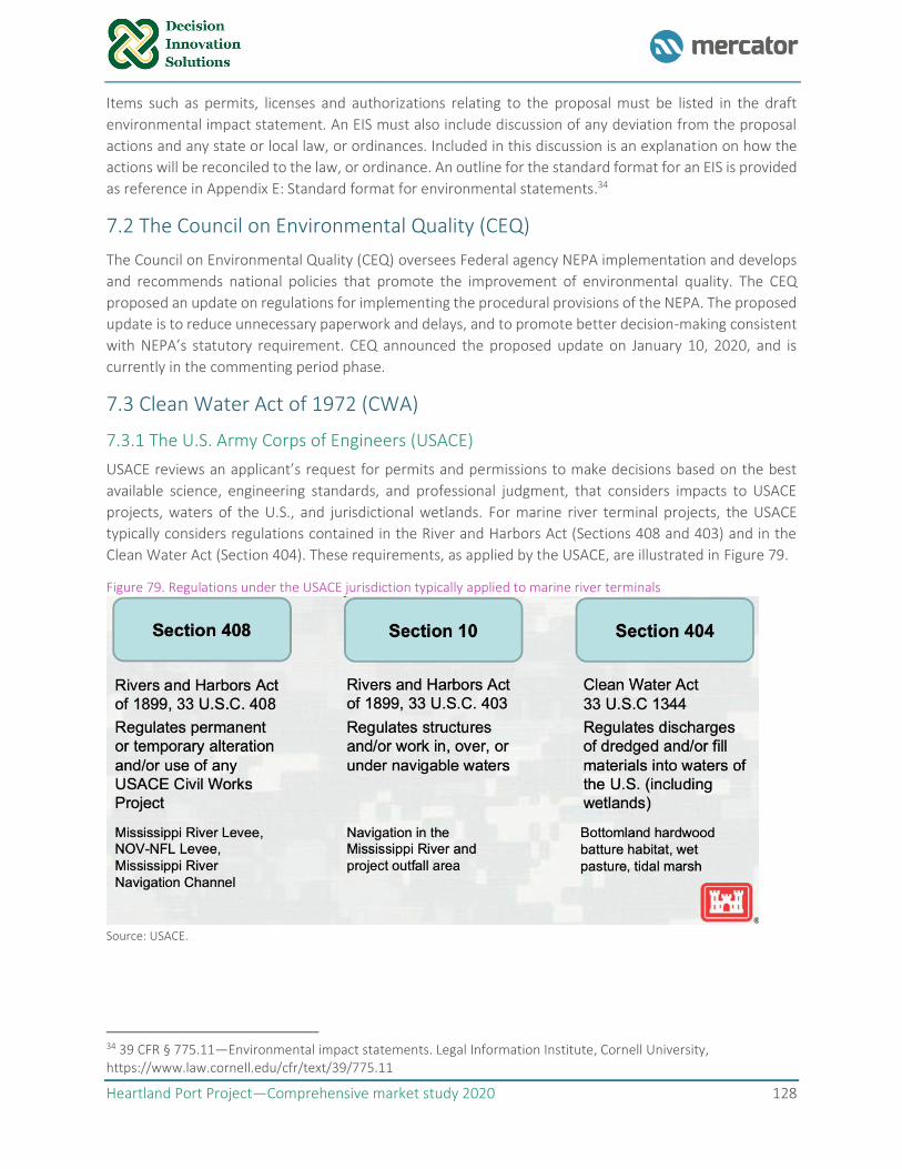
Heartland Port Project—Comprehensive market study 2020 128
Items such as permits, licenses and authorizations relating to the proposal must be listed in the draft
environmental impact statement. An EIS must also include discussion of any deviation from the proposal
actions and any state or local law, or ordinances. Included in this discussion is an explanation on how the
actions will be reconciled to the law, or ordinance. An outline for the standard format for an EIS is provided
as reference in Appendix E: Standard format for environmental statements.34
7.2 The Council on Environmental Quality (CEQ)
The Council on Environmental Quality (CEQ) oversees Federal agency NEPA implementation and develops
and recommends national policies that promote the improvement of environmental quality. The CEQ
proposed an update on regulations for implementing the procedural provisions of the NEPA. The proposed
update is to reduce unnecessary paperwork and delays, and to promote better decision-making consistent
with NEPA’s statutory requirement. CEQ announced the proposed update on January 10, 2020, and is
currently in the commenting period phase.
7.3 Clean Water Act of 1972 (CWA)
7.3.1 The U.S. Army Corps of Engineers (USACE)
USACE reviews an applicant’s request for permits and permissions to make decisions based on the best
available science, engineering standards, and professional judgment, that considers impacts to USACE
projects, waters of the U.S., and jurisdictional wetlands. For marine river terminal projects, the USACE
typically considers regulations contained in the River and Harbors Act (Sections 408 and 403) and in the
Clean Water Act (Section 404). These requirements, as applied by the USACE, are illustrated in Figure 79.
Figure 79. Regulations under the USACE jurisdiction typically applied to marine river terminals
Source: USACE.
34 39 CFR § 775.11—Environmental impact statements. Legal Information Institute, Cornell University, https://www.law.cornell.edu/cfr/text/39/775.11
Heartland Port Project—Comprehensive market study 2020 129
▪ Section 408—A Section 408 permit is required for alterations that builds upon, alters, improves,
moves, occupies, or otherwise affects the usefulness, or structural or ecological integrity of USACE
projects. A decision on the Section 408 must come before a Section 10/404 is issued. In addition,
other environmental compliances must be issued prior to the approval of a Section 408.
Documentation that is needed includes: technical analysis, hydrologic system performance,
geotechnical, NEPA Compliance, real estate requirements, and the requester’s review plan. NEPA
compliance, ESA compliance, and the NHPA compliance should all be provided to the USACE.
▪ Section 10—A Section 10 of the Rivers and Harbors Act of 1899 is required for the construction of
any structure in or over any navigable water of the United States. This includes dredging or disposal
of dredged materials, excavation, filling, or channelization of the water, and any construction in
the water, such as docks, piers, pilings, etc. In addition, compliance with other federal regulations
will also need to be completed in order for the issuance of the Section 10 approval.
Section 10 Navigable Waters of the United States within the Kansas City District, Corps of Engineers
Regulatory Boundary. USACE Kansas City District identified the following nine navigable waters:
▪ Blue River – From river mile 0.0 (mouth at Missouri River) upstream to mile 4.38 (within the
city limits of Kansas City, Missouri);
▪ Gasconade River – From river mile 0.0 to mile 107.0 (confluence with the Missouri River
upstream to the vicinity of Arlington, in Phelps County, Missouri);
▪ Grand River – From river mile 0.0 to mile 3.0 (confluence with the Missouri River upstream to
the vicinity of Brunswick, in Chariton County, Missouri);
▪ Kansas River – From river mile 0.0 to mile 170.4 (confluence with the Missouri River upstream
to its confluence with the Republican and Smoky Hill Rivers in the vicinity of Junction City, in
Geary County, Kansas);
▪ Lamine River – From river mile 0.0 to mile 14.0 (confluence with the Missouri River upstream
to the vicinity of Roberts Bluff Bridge in Cooper County, Missouri);
▪ Missouri River – From river mile 49.8 to mile 552.7 (St. Charles County upstream to the
Missouri/Iowa state line in Atchison County, Missouri);
▪ Osage River – From river mile 0.0 to mile 81.7 (confluence with the Missouri River upstream to
Bagnell Dam in Miller County, Missouri); and
▪ Lake of the Ozarks – From lake mile 0.0 to mile 89.3 (Bagnell Dam to the vicinity of Warsaw, in
Benton County, Missouri).
▪ Section 404—A Section 404 permit is from the Clean Water Act to regulate the discharge of
dredged or fill materials into any waters of the United States (including wetlands). No discharge of
dredged or fill material may be permitted if either a practical alternative exists, or the water would
be significantly degraded. For the permit application, it should be shown how impacts are being
minimized, and if needed, it is possible to provide compensation if there are unavoidable impacts.
▪ Section 401—If the project may involve placing materials in a lake, river, stream, dry streambed or
wetland, and is within jurisdictional waters, it will be considered a regulated activity and may
require a Section 401 Water Quality Permit.
Heartland Port Project—Comprehensive market study 2020 130
Best Management Practices should be established to reduce stormwater pollution. Prior to construction
activities, the contractor would be required to obtain an NDPDES permit and develop a Stormwater
Pollution Prevention Plan (SWPPP). The SWPPP would outline phasing for erosion and sediment controls,
stabilization measures, pollution-prevention measures, and prohibited discharges. The SWPPP would also
include BMPs to minimize erosion, sedimentation, and stormwater runoff (e.g. fiber rolls, straw waddles,
erosion mats, silt fencing, turbidity barriers, mulching, filter fabric fencing, sediment traps and ponds,
surface water interceptor swales, ditches). In addition, waste material would be disposed of in accordance
with state and federal laws. The SWPPP should include dust control measures during construction.
The responsible party or the operator is required to submit a Notice of Intent (NOI) to the Environmental
Protection Agency (EPA) before start of construction project and submit the Notice of Termination (NOT)
to EPA when construction project is complete.
A jurisdictional determination is a decision by the USACE Kansas City Division as to whether areas on
property are regulated under federal statutes. A federally-regulated wetland, lake, pond or stream is called
a "waters of the U.S. USACE performs wetland delineations for potential applicants for permits under
Section 404 of the CWA; however, this can take months and it is highly recommended that the potential
applicant uses qualified consultants to conduct wetland delineations, especially for project of this
magnitude.
However, the EPA released a final rule recently to replace the 2015 Waters of the United States (WOTUS)
regulation, which provided additional federal pollution protections to large and small bodies of water in
accordance with the Clean Water Act (CWA). The rule is the second piece in a two-step process to repeal
and replace WOTUS, pursuant to Executive Order 13778 issued in 2017. The revised definition includes four
categories: territorial seas and traditional navigable waters (TNWs); tributaries; lakes, ponds, and
impoundments of jurisdictional waters; and adjacent wetlands. It also outlines which waters are not subject
to federal control, such as bodies that contain water from rainfall, groundwater, many ditches, prior
converted cropland, farm and stock watering ponds; and water treatment systems. The rule will take
approximately 60 days following publication in the Federal Register.
7.3.2 Federal Safe Drinking Water Act, Missouri Safe Drinking Water Act
A permit is required if the proposed action plans to dispense water to the public, including submission of
predesign studies and plans and specifications, system operation and reliability of the system. Missouri’s
Safe Drinking Water Commission 60 regulates such permit.
7.4 Clean Air Act of 1963
Under the Missouri Air Conservation Law and in accordance with the Clean Air Act (CAA), Missouri
establishes the criteria pollutants have human health-based or welfare-based standards that set the
maximum concentrations that are allowed in the ambient air (i.e. the air that the general public is exposed
to). The federal standards for the criteria pollutants are known as the National Ambient Air Quality
Standards (NAAQS). These criteria pollutants include particulate matter less than 10 microns in diameter
(PM10), particulate matter less than 2.5 microns in diameter (PM2.5), sulfur dioxide (SO2), carbon
monoxide (CO), ozone, nitrogen dioxide (NOx) and lead. Missouri has two additional pollutants which have
ambient air quality standards in addition to the NAAQS. These include hydrogen sulfide and sulfuric acid.
Heartland Port Project—Comprehensive market study 2020 131
▪ A list of all Ambient Air Quality Standards can be found at 10 CSR 10-6.010. List of regulated air
pollutants, please refer to the Code of State Regulations, specifically 10 CSR 10-6.020(3) at the
following website:
▪ http://www.sos.mo.gov/adrules/csr/current/10csr/10csr.asp.
▪ EPA approves States Implementation Plan. The link provides the current status of Missouri
Designated Areas:
▪ https://www3.epa.gov/airquality/urbanair/sipstatus/reports/mo_areabypoll.html
▪ Air Quality Standards, Definitions, Sampling and Reference Methods and Air Pollution Control
Regulations for the Entire State of Missouri can be found here:
▪ https://www.sos.mo.gov/cmsimages/adrules/csr/current/10csr/10c10-6a.pdf
Carbon and non-carbon emissions cost savings resulting from the Heartland Port Project
The Heartland Port project is expected to help alleviate traffic congestion on the roadway and railways, and the potential to reduce truck and rail related emissions. This category of project benefits, freight emissions cost savings, captures the net savings in carbon emission damage costs resulting from truck and rail ton-miles saved (or avoided) due to truck/rail to barge freight diversion. Total net savings in carbon emission costs resulting from the port development project over the 2020-2045 timeframe, account for $46 million. Total net savings in non-carbon emission costs resulting from the port development project over the 2020-2045 timeframe account for $14.6 million (in 2016 dollars), as documented by the 2018 Central Missouri Multimodal Port Feasibility Study.35
7.4.1 Air construction permits / new source review permits Department of Natural Resources Air Pollution Control Program issues air construction permits.
Construction permits are required for new air pollution source. Certain activities have been determined by
the state to be a source of insignificant emissions and are exempt from permitting requirements per 10
CSR 10-6.061. Construction permits allow an installation to construct and operate an air emission source.
There are various types of Air Permits: Air Pollution Control Program issues several types of construction
permits: Major, Minor and De Minimis permits, portable relocation permits, temporary permits, and
permits-by-rule. The Department of Natural Resources provides guidance on Air Quality:
▪ https://dnr.mo.gov/env/apcp/permits/constpmtguide.htm
7.5 Section 106 Tribal Land and Consultation
Agencies are required to consult on a “government-to-government” basis with federally-recognized Indian
tribes and nations on projects receiving federal funds or requiring federal permits.
The lead agency or the project sponsor must consult with federally-recognized Indian tribes with ancestral,
historic, and ceded land connections to Missouri. Consultation with tribes is intended to facilitate avoiding
or minimizing project impacts to cultural resources that a tribe considers of historical or religious
significance. A tribe must determine if the proposed project is located at or near known culturally significant
35 Jefferson City Area Chamber of Commerce, Central Missouri Multimodal Port Feasibility Study Final Report, prepared by
Cambridge Systematics and Hanson Professional Services, Jun 2018, pp. 9-77 - 9-79.
Heartland Port Project—Comprehensive market study 2020 132
sites or localities. Placing this step early in the planning process allows the greatest opportunity to work to
avoid or minimize adverse effects to these culturally sensitive/significant areas.
7.5.1 The Archeological Historic Preservation Act of 1970 The American Indian Religious Freedom Act of 1978 requires consultation with Native American groups
concerning proposed actions on sacred sites on federal land or affecting access to sacred sites. It establishes
federal policy to protect and preserve for American Indians, Eskimos, Aleuts, and Native Hawaiians the right
to free exercise of their religion in the form of site access, use and possession of sacred objects, as well as
the freedom to worship through ceremonial and traditional rites.
The Act requires federal agencies to consider the impacts of their actions on religious sites and objects
important to American Indians, regardless of eligibility for listing on the NRHP.
The Native American Graves Protection and Repatriation Act of 1990 is triggered by the possession of
human remains or cultural items by a federally-funded repository or by the discovery of human remains or
cultural items on federal or Tribal lands and provides for the inventory, protection, and return of cultural
items to affiliated Native American groups. Permits are required for intentional excavation and removal of
Native American cultural items from federal or Tribal lands.
7.5.2 National Historic Preservation Act of 1966
Section 106 of the National Historic Preservation Act (16 U.S.C. § 470), as amended, requires that federally-
funded projects be evaluated for the effects on historic and cultural properties included in, or eligible for
listing on, the NRHP.
The MoDOT has communicated with a large number of Indian tribes and nations with ties to Missouri to
identify areas of tribal interest and concern. To date, 26 federally-recognized Tribes have requested
consultation about transportation projects in some portion of Missouri. MoDOT keeps confidential
information regarding archaeological sites, traditional cultural properties, and sacred sites. MoDOT’s Tribal
Consultation Map indicates the following 10 federally-recognized Tribes in Cole County:
▪ Iowa Tribe of Kansas and Nebraska
▪ Iowa Tribe of Oklahoma
▪ Kaw Indian Nation of Oklahoma
▪ Miami Tribe of Oklahoma
▪ Osage Nation
▪ Ponca Tribe of Nebraska
▪ Ponca Tribe of Oklahoma
▪ Sac and Fox Tribe of the Missouri in Kansas and Nebraska
▪ Sac and Fox Tribe of the Mississippi in Iowa
▪ Sac and Fox Nation of Oklahoma
For the Heartland Port Project, the consultation process must seek, discuss, and consider the views of other
participants, and, where feasible, seek agreement with them on matters arising in the Section 106 process.
Typical Consulting Parties include:
▪ Federal Agency (USACE, FHWA, Forest Service, National Park Service, etc.)
▪ State Historic Preservation Office (SHPO)
▪ Tribes—see tribal consultation page
Heartland Port Project—Comprehensive market study 2020 133
▪ Local governments with jurisdiction over historic properties
▪ Project applicants (MoDOT and local governments)
▪ Missouri Department of Natural Resources (MoDNR)
▪ Those with a demonstrated interest in the undertaking—legal or economic interest in the project
or those with an interest in project effects on historic properties.
The Lead Agency and the project sponsor will need to work in close coordination with the MoDOT Historic
Preservation Section to get the process started.36 MoDOT will work with the State Historic Preservation
Officer (SHPO) to identify consulting parties and invite them to participate in consultation. Participants must
be conferred an official “consulting party” status. Consulting parties help the USACE and MoDOT make
decisions. Because they often live in the community, consulting parties can help identify properties that
are eligible for listing on the National Register of Historic Places. Consulting parties also help identify project
effects on historic properties. An adverse effect occurs when a project alters the characteristics of a
property that make it eligible for inclusion in the National Register in such a way that it diminishes the
integrity of the historic property. If a project will have an adverse effect, consulting parties help to identify
ways to minimize or mitigate the effect. A Section 106 Project Form must be completed in order to initiate
the process. SHPO Section 106 Survey Memo Form, MO 780-1718 must be completed by a professional
archaeologists or architectural historians reporting survey results. According to 36 CFR Part 800, Federal
agencies are responsible for initiating Section 106 review. The Missouri State Historic Preservation Officer
(SHPO) within the Department of Natural Resources, coordinates the state’s historic preservation program
and consults with agencies during Section 106 review. The process will include a cultural resource
survey/inventory, consultation with SHPO and Tribes.
7.6 Section 7 Fish and Wildlife Service Endangered Species Act
Section 7 of the Endangered Species Act of 1973 (ESA) requires all Federal agencies to use their authorities to
conserve endangered and threatened species in consultation with U.S. Fish and Wildlife Service (USFWS). This
‘proactive conservation mandate’ for Federal agencies is articulated in section 7(a)(1) of the law. Section
7(a)(2) contains a complementary consultation mandate for Federal agencies, which we discuss below. Under
the Section 7 implementing regulations (50 CFR Part 402), Federal agencies must review their actions to
determine whether they may affect endangered or threatened species or critical habitat. To accomplish this,
Federal agencies must determine whether any listed species may be present in the action area and whether
that area overlaps with critical habitat. If one or more listed species may be present in the action area – or if
critical habitat overlaps with the action area – agencies must evaluate the potential effects of their action.
Agencies must confer with the USFWS per Section 7(a)(4) of the ESA if any action is likely to jeopardize a
species proposed for listing or to destroy or adversely modify proposed critical habitat. To determine whether
either of these are likely, agencies may follow the same approach that we recommend for listed species and
designated critical habitat – that is, evaluate the likely effects of their actions on any proposed species that
may be present in the action area and on any proposed critical habitat that overlaps with the action area.
Step-by-step instructions for Section 7 Consultation technical assistance are provided in Figure 80.
36 To get the process started the HPA must contact MoDOT Historic Preservation Manager. For contact information and a more comprehensive overview of the entire process please see https://www.modot.org/consultation-under-section-106.
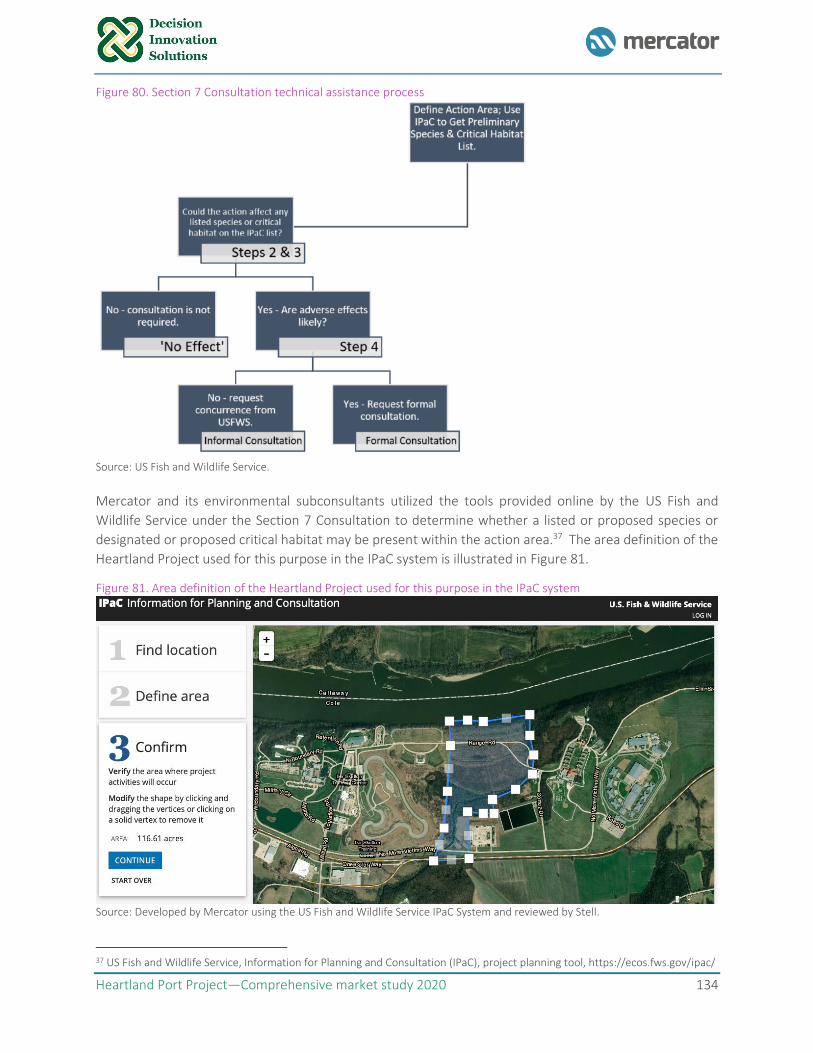
Heartland Port Project—Comprehensive market study 2020 134
Figure 80. Section 7 Consultation technical assistance process
Source: US Fish and Wildlife Service.
Mercator and its environmental subconsultants utilized the tools provided online by the US Fish and
Wildlife Service under the Section 7 Consultation to determine whether a listed or proposed species or
designated or proposed critical habitat may be present within the action area.37 The area definition of the
Heartland Project used for this purpose in the IPaC system is illustrated in Figure 81.
Figure 81. Area definition of the Heartland Project used for this purpose in the IPaC system
Source: Developed by Mercator using the US Fish and Wildlife Service IPaC System and reviewed by Stell.
37 US Fish and Wildlife Service, Information for Planning and Consultation (IPaC), project planning tool, https://ecos.fws.gov/ipac/
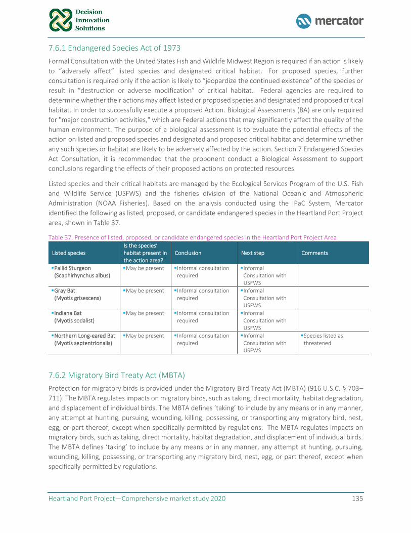
Heartland Port Project—Comprehensive market study 2020 135
7.6.1 Endangered Species Act of 1973
Formal Consultation with the United States Fish and Wildlife Midwest Region is required if an action is likely
to “adversely affect” listed species and designated critical habitat. For proposed species, further
consultation is required only if the action is likely to “jeopardize the continued existence” of the species or
result in “destruction or adverse modification” of critical habitat. Federal agencies are required to
determine whether their actions may affect listed or proposed species and designated and proposed critical
habitat. In order to successfully execute a proposed Action. Biological Assessments (BA) are only required
for "major construction activities," which are Federal actions that may significantly affect the quality of the
human environment. The purpose of a biological assessment is to evaluate the potential effects of the
action on listed and proposed species and designated and proposed critical habitat and determine whether
any such species or habitat are likely to be adversely affected by the action. Section 7 Endangered Species
Act Consultation, it is recommended that the proponent conduct a Biological Assessment to support
conclusions regarding the effects of their proposed actions on protected resources.
Listed species and their critical habitats are managed by the Ecological Services Program of the U.S. Fish
and Wildlife Service (USFWS) and the fisheries division of the National Oceanic and Atmospheric
Administration (NOAA Fisheries). Based on the analysis conducted using the IPaC System, Mercator
identified the following as listed, proposed, or candidate endangered species in the Heartland Port Project
area, shown in Table 37.
Table 37. Presence of listed, proposed, or candidate endangered species in the Heartland Port Project Area
Listed species Is the species’ habitat present in the action area?
Conclusion Next step Comments
▪ Pallid Sturgeon (Scaphirhynchus albus)
▪ May be present ▪ Informal consultation required
▪ Informal Consultation with USFWS
▪ Gray Bat (Myotis grisescens)
▪ May be present ▪ Informal consultation required
▪ Informal Consultation with USFWS
▪ Indiana Bat (Myotis sodalist)
▪ May be present ▪ Informal consultation required
▪ Informal Consultation with USFWS
▪ Northern Long-eared Bat (Myotis septentrionalis)
▪ May be present ▪ Informal consultation required
▪ Informal Consultation with USFWS
▪ Species listed as threatened
7.6.2 Migratory Bird Treaty Act (MBTA)
Protection for migratory birds is provided under the Migratory Bird Treaty Act (MBTA) (916 U.S.C. § 703–
711). The MBTA regulates impacts on migratory birds, such as taking, direct mortality, habitat degradation,
and displacement of individual birds. The MBTA defines ‘taking’ to include by any means or in any manner,
any attempt at hunting, pursuing, wounding, killing, possessing, or transporting any migratory bird, nest,
egg, or part thereof, except when specifically permitted by regulations. The MBTA regulates impacts on
migratory birds, such as taking, direct mortality, habitat degradation, and displacement of individual birds.
The MBTA defines ‘taking’ to include by any means or in any manner, any attempt at hunting, pursuing,
wounding, killing, possessing, or transporting any migratory bird, nest, egg, or part thereof, except when
specifically permitted by regulations.
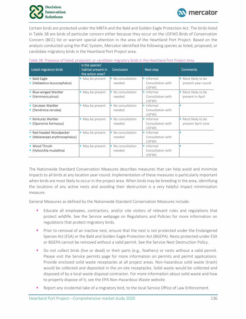
Heartland Port Project—Comprehensive market study 2020 136
Certain birds are protected under the MBTA and the Bald and Golden Eagle Protection Act. The birds listed
in Table 38 are birds of particular concern either because they occur on the USFWS Birds of Conservation
Concern (BCC) list or warrant special attention in the area of the Heartland Port Project. Based on the
analysis conducted using the IPaC System, Mercator identified the following species as listed, proposed, or
candidate migratory birds in the Heartland Port Project area.
Table 38. Presence of listed, proposed, or candidate migratory birds in the Heartland Port Project Area
Listed migratory birds Is the species’ habitat present in the action area?
Conclusion Next step Comments
▪ Bald Eagle ▪ (Haliaeetus leucocephalus)
▪ May be present ▪ No consultation needed.
▪ Informal Consultation with USFWS
▪ Most likely to be present year-round
▪ Blue-winged Warbler ▪ (Vermivora pinus)
▪ May be present ▪ No consultation needed.
▪ Informal Consultation with USFWS
▪ Most likely to be present in April
▪ Cerulean Warbler ▪ (Dendroica cerulea)
▪ May be present ▪ No consultation needed.
▪ Informal Consultation with USFWS
▪
▪ Kentucky Warbler ▪ (Oporornis formosus)
▪ May be present ▪ No consultation needed.
▪ Informal Consultation with USFWS
▪ Most likely to be present April-June
▪ Red-headed Woodpecker ▪ (Melanerpes erythrocephalus)
▪ May be present ▪ No consultation needed.
▪ Informal Consultation with USFWS
▪
▪ Wood Thrush ▪ (Hylocichla mustelina)
▪ May be present ▪ No consultation needed.
▪ Informal Consultation with USFWS
▪
The Nationwide Standard Conservation Measures describes measures that can help avoid and minimize
impacts to all birds at any location year-round. Implementation of these measures is particularly important
when birds are most likely to occur in the project area. When birds may be breeding in the area, identifying
the locations of any active nests and avoiding their destruction is a very helpful impact minimization
measure.
General Measures as defined by the Nationwide Standard Conservation Measures include:
▪ Educate all employees, contractors, and/or site visitors of relevant rules and regulations that
protect wildlife. See the Service webpage on Regulations and Policies for more information on
regulations that protect migratory birds.
▪ Prior to removal of an inactive nest, ensure that the nest is not protected under the Endangered
Species Act (ESA) or the Bald and Golden Eagle Protection Act (BGEPA). Nests protected under ESA
or BGEPA cannot be removed without a valid permit. See the Service Nest Destruction Policy.
▪ Do not collect birds (live or dead) or their parts (e.g., feathers) or nests without a valid permit.
Please visit the Service permits page for more information on permits and permit applications.
Provide enclosed solid waste receptacles at all project areas. Non-hazardous solid waste (trash)
would be collected and deposited in the on-site receptacles. Solid waste would be collected and
disposed of by a local waste disposal contractor. For more information about solid waste and how
to properly dispose of it, see the EPA Non-Hazardous Waste website.
▪ Report any incidental take of a migratory bird, to the local Service Office of Law Enforcement.
Heartland Port Project—Comprehensive market study 2020 137
▪ Consult and follow applicable Service industry guidance.
▪ Habitat Measures as defined by the Nationwide Standard Conservation Measures include:
▪ Minimize project creep by clearly delineating and maintaining project boundaries (including staging
areas).
▪ Consult all local, State, and Federal regulations for the development of an appropriate buffer
distance between development site and any wetland or waterway.
▪ Maximize use of disturbed land for all project activities (i.e., siting, lay-down areas, and
construction).
▪ Implement standard soil erosion and dust control measures. For example: (i) Establish vegetation
cover to stabilize soil, (ii) Use erosion blankets to prevent soil loss, and (iii) Water bare soil to
prevent wind erosion and dust issues.
Additional measures and/or permits may be advisable depending on the type of activity and the type of
infrastructure or bird species present on the project site. A complete list of the Nationwide Conservation
Measures can be found here.38
7.6.3 Fish and Wildlife Coordination Act
Fish and Wildlife Coordination Act gives the National Oceanic and Atmospheric Administration (NOAA) an
important advisory role to review and comment on proposed federally permitted activities that could affect
living marine resources. As amended in 1964, the act requires that all federal agencies consult with NOAA
Fisheries, U.S. Fish and Wildlife Service, and state wildlife agencies when proposed actions might result in
modification of a natural stream or body of water. Federal agencies must consider how these projects
would affect fish and wildlife and provide for improvement of these resources. Essential Fish Habitat
mapper can be found here: https://www.fisheries.noaa.gov/resource/map/essential-fish-habitat-mapper
The act allows NOAA Fisheries to provide comments to the U.S. Army Corps of Engineers during review of projects under section 404 of the Clean Water Act (concerning the discharge of dredged materials into navigable waters) and section 10 of the Rivers and Harbors Act of 1899 (obstructions in navigable waterways). NOAA Fisheries comments provided under the Fish and Wildlife Coordination Act are intended to reduce environmental impacts to migratory, estuarine, and marine fisheries and their habitats.
7.7 Wetlands
Lastly, in order to meet USACE’s Dredge and Fill Wetlands Permit Requirements, a wetland delineation is recommended. USACE Wetlands Delineations Manual contains information to identify wetlands. All delineations must be conducted in accordance with the 1987 Corps of Engineers Wetlands Delineation Manual, or appropriate Regional Supplement, and submitted to the District for review and verification.
Based on the outcomes from the IPaC System, Mercator utilized the U.S. Fish and Wildlife Service’s Wetlands Mapper tool to generate current information on the status, extent, characteristics and functions of wetlands, riparian, and deepwater habitats. This information is intended to promote the understanding and conservation of wetland resources and to aid in resource management, research and decision making. The Wetlands Mapper shows wetland type and extent using a biological definition of wetlands. There is no attempt to define the limits of proprietary jurisdiction of any Federal, State, or local government, or to
38 US Fish and Wildlife Service, Nationwide Standard Conservation Measures, https://www.fws.gov/migratorybirds/pdf/management/nationwidestandardconservationmeasures.pdf
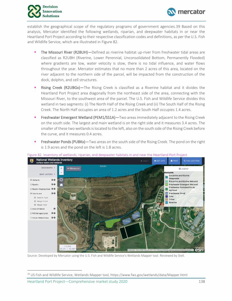
Heartland Port Project—Comprehensive market study 2020 138
establish the geographical scope of the regulatory programs of government agencies.39 Based on this analysis, Mercator identified the following wetlands, riparian, and deepwater habitats in or near the Heartland Port Project according to their respective classification codes and definitions, as per the U.S. Fish and Wildlife Service, which are illustrated in Figure 82.
▪ The Missouri River (R2BUH)—Defined as riverine habitat up-river from freshwater tidal areas are
classified as R2UBH (Riverine, Lower Perennial, Unconsolidated Bottom, Permanently Flooded)
where gradients are low, water velocity is slow, there is no tidal influence, and water flows
throughout the year. Mercator estimates that no more than 2 acres of this area, located on the
river adjacent to the northern side of the parcel, will be impacted from the construction of the
dock, dolphin, and cell structures.
▪ Rising Creek (R2UBGx)—The Rising Creek is classified as a Riverine habitat and it divides the
Heartland Port Project area diagonally from the northeast side of the area, connecting with the
Missouri River, to the southwest area of the parcel. The U.S. Fish and Wildlife Service divides this
wetland in two segments: (i) The North Half of the Rising Creek and (ii) The South Half of the Rising
Creek. The North Half occupies an area of 1.2 acres and the South Half occupies 1.4 acres.
▪ Freshwater Emergent Wetland (PEM1/SS1A)—Two areas immediately adjacent to the Rising Creek
on the south side. The largest and main wetland is on the right side and it measures 3.4 acres. The
smaller of these two wetlands is located to the left, also on the south side of the Rising Creek before
the curve, and it measures 0.4 acres.
▪ Freshwater Ponds (PUBKx)—Two areas on the south side of the Rising Creek. The pond on the right
is 1.9 acres and the pond on the left is 1.8 acres.
Figure 82. Inventory of wetlands, riparian, and deepwater habitats in and near the Heartland Port Project
Source: Developed by Mercator using the U.S. Fish and Wildlife Service’s Wetlands Mapper tool. Reviewed by Stell.
39 US Fish and Wildlife Service, Wetlands Mapper tool, https://www.fws.gov/wetlands/data/Mapper.html
Heartland Port Project—Comprehensive market study 2020 139
7.7.1 Floodplain management
Executive Order 11988 adopts a higher flood standard for future federal investments in and affecting
floodplains. This includes projects where federal funds are used to build new structures and facilities or to
rebuild those that have been damaged. The guidelines address an eight-step process that agencies should
carry out as part of their decision-making on projects that have potential impacts to or within the floodplain.
There are eight steps in the decision-making process required in Section 2(a) of the Order.
7.8 Missouri Department of Natural Resources (DNR)
The Missouri Department of Natural Resources helps to develop mineral, oil and gas resources in an
environmentally safe manner, while promoting the environmentally sound operations of businesses,
communities, agriculture, and industries in the state. The department and its Water Resources Center has
statutory authority for water quantity issues such as statewide water use and availability, water resources
monitoring and planning, drought assessment, flood and hydrology studies and wetland studies. The
Surface Water Section provides technical support by performing water supply analyses, in-stream flow
assessments and floodplain studies. The surface water section also administers the collection and analysis
of statewide water use data in accordance with the Major Water User Law. Depending on the final
configuration of the Heartland Port Project, compliance with additional regulations established by the DNR
might be required. A complete list is included here.40
The Missouri DNR issues permits for wetland or dredge and fill, and land disturbance activities. These
permits are required for any construction, placement, disposal or fill material, or earth movement within a
wetland or body of water. Any land disturbance activities of greater than an acre will require a permit.
Within the permit it is also required to have a stormwater pollution prevention plan implemented to reduce
pollution to the waters. Additionally, the DNR also issues 401 permits. The Clean Water Act section 401
certification can be needed in tandem with a section 404, at the USACE discretion. The Missouri DNR has
authority to issue 401 certification, and would evaluate the application, if needed.
7.8.1 Comprehensive Environmental Response, Compensation and Liability Act (CERCLA)
Hazardous substance, pursuant to the Comprehensive Environmental Response, Compensation, and
Liability Act (CERCLA) (42 U.S.C. § 9601(14)), is defined as: “(A) any substance designated pursuant to
section 1321(b)(2)(A) of Title 33; (B) any element, compound, mixture, solution, or substance designated
pursuant to section 9602 of this title; (C) any hazardous waste having the characteristics identified under
or listed pursuant to section 3001 of the Resource Conservation and Recovery Act (RCRA) of 1976, as
amended, (42 U.S.C. § 6921); (D) any toxic pollutant listed under section 1317(a) of Title 33; (E) any
hazardous air pollutant listed under Section 112 of the CAA (42 U.S.C. § 7412); and (F) any imminently
hazardous chemical substance or mixture with respect to which the Administrator of the USEPA has taken
action pursuant to section 2606 of Title 15. The term does not include petroleum, including crude oil or any
fraction thereof, which is not otherwise specifically listed or designated as a hazardous substance, and the
term does not include natural gas, natural gas liquids, liquefied natural gas, or synthetic gas usable for fuel
(or mixtures of natural gas and such synthetic gas).”
40 Missouri Department of Natural Resources (DNR), Forms, Applications, Permits, Manuals and Other Documents https://dnr.mo.gov/forms/
Heartland Port Project—Comprehensive market study 2020 140
7.8.2 Resource Conservation and Recovery Act (RCRA)
Resource Conservation and Recovery Act (RCRA) defines a hazardous waste in 42 U.S.C. § 6903, as “a solid
waste, or combination of solid wastes, which because of its quantity, concentration, or physical, chemical,
or infectious characteristics may: (A) cause, or significantly contribute to an increase in mortality or an
increase in serious irreversible, or incapacitating reversible, illness; or (B) pose a substantial present or
potential hazard to human health or the environment when improperly treated, stored, transported, or
disposed of, or otherwise managed.”
7.8.3 Missouri Hazardous Waste Management Law
Facilities and properties that (1) have documented releases of hazardous substances or wastes to the
environment or (2) manage hazardous substances or wastes in substantial quantities and have the potential
to release hazardous substances or wastes to the environment are required to report these activities to
federal and state regulatory agencies. The Missouri Department of Natural Resources Hazardous Waste
and Enforcement Unit and USEPA maintain databases to track and monitor these facilities and properties.
The Hazardous Waste and Enforcement Unit handles hazardous waste permits and ensures compliance
with hazardous waste laws and regulations: Revised Statutes of Missouri (Chapter 260.350-260.575), Code
of Federal Regulations (40 CFR 260 – 279) and Code of State Regulations (10 CSR 25).
7.8.4 Toxic Substance and Control Act (TSCA)
The law requires all commercial Polychlorinated Biphenyl (PCB) facilities in Missouri obtain a hazardous
waste permit from the Missouri Department of Natural Resources. The department's Hazardous Waste
Program inspects these facilities to make sure they are following TSCA requirements. The department must
also keep an updated list of all commercial PCB facilities in the state.
7.8.5 Missouri Soil Conservation Section 278
Refer to Soil and Water Districts Commission - Division 70
7.8.6 Missouri Solid Waste Management Law
Section 260.200 through 260.345 only handled by Missouri Solid Waste Division 80.
7.9 Missouri Conservation Department
The Missouri Department of Conservation can be a resource for new projects. The Missouri Conservation
Department works with communities across the state to decrease the negative impacts of urbanization or
construction projects on fish, forests, and wildlife or to benefit from the wiser use of natural resources.
Communities turn to MDC every year for technical assistance. On their publication Conservation Planning
Tools for Missouri Communities—A Reference Manual, the department outlines tools and strategies aimed
to promote conservation practices that are applicable to the growth and management of all Missouri
communities.41
This document recommends the development of a natural resource inventory (NRI). The NRI is a report
that contains maps and descriptions of existing natural resources within the area of interest such as a the
Heartland Port Project area. Most, if not all, of the guidelines recommended by this document will be
satisfied by the EIS. Nonetheless, equipped with the results of an NRI and an assessment of the physical
41 Missouri Conservation Department, Conservation Planning Tools for Missouri Communities—A Reference Manual, https://mdc.mo.gov/sites/default/files/downloads/Conservation%20Planning.pdf.
Heartland Port Project—Comprehensive market study 2020 141
condition of local natural resources, this document recommends that planners and community leaders can
work with the public to craft a vision and set goals related to conservation.
Guiding principles that may be discussed during this process include:
▪ Ecosystem management—An approach to natural resource management that focuses on
sustaining ecosystems to meet both ecological and human needs in the future. Ecosystem
management is adaptive to changing needs and new information. It promotes a shared vision of a
desired future by integrating social, environmental and economic perspectives to manage
geographically defined natural ecological systems. An ecosystem is a dynamic complex of plant,
animal and microorganism communities and their nonliving environment interacting as a
functional unit.
▪ Ecosystem, capital value—The present value of the stream of ecosystem services that an
ecosystem will generate under a particular management or institutional regime.
▪ Ecosystem, direct use value—The benefits derived from the services provided by an ecosystem
that are used directly by an economic agent. These include consumptive uses (e.g. harvesting
goods) and non-consumptive uses (e.g. enjoyment of scenic beauty). Agents are often physically
present in an ecosystem to receive direct use value.
▪ Ecosystem, indirect use value—The benefits derived from the goods and services provided by an
ecosystem that are used indirectly by an ecosystem.
Lastly, the Missouri Department of Conservation provides grants and funding opportunities related to
promotes sustainable development practices and the establishment of natural resource conservation
practices in urban and developing areas. For some of these opportunities, eligible property includes lands
in public ownership or open to the public. Private property is only eligible when another partner(s) is
providing at least a 1:1 cash match or when the private property extends or connects projects on public
land by providing stormwater conveyance, habitat connectivity, or other public benefits. This might be a
resource for the Heartland Port Project. A list of is provided here.42
7.10 Noise impact
Federal Highway Administration (FHWA) has given MoDOT on flexibility of implementing Noise Standard at
23 CFR Part 772. MoDOT program to implement FHWA Noise Standard include traffic noise prediction
requirements, noise analyses, noise abatement criteria and requirements for informing local officials. It
would be beneficial to determine the need for a noise study early in project scoping.
7.11 Executive Order 12898: Environmental Justice in Minority and Low-
Income Populations
In order to meet Executive Order 12898, the EIS must identify and address the disproportionately high and
adverse human health or environmental effects of their actions on minority and low-income populations,
to the greatest extent practicable and permitted by law. The order also directs each agency to develop a
strategy for implementing environmental justice. The order is also intended to promote nondiscrimination
42 Missouri Department of Conservation, Funding Opportunities, https://mdc.mo.gov/property/community-conservation/community-conservation-funding-opportunities
Heartland Port Project—Comprehensive market study 2020 142
in federal programs that affect human health and the environment, as well as provide minority and low-
income communities access to public information and public participation.
7.12 Other laws and regulations
The initial boundaries of the Heartland Port Authority include Counties of Callaway and Cole County, including Jefferson City. Further discussion required to ensure that project meets local laws and ordinances. All project activities must adhere to OSHA Regulations (Standard 1926, 29 CFR).
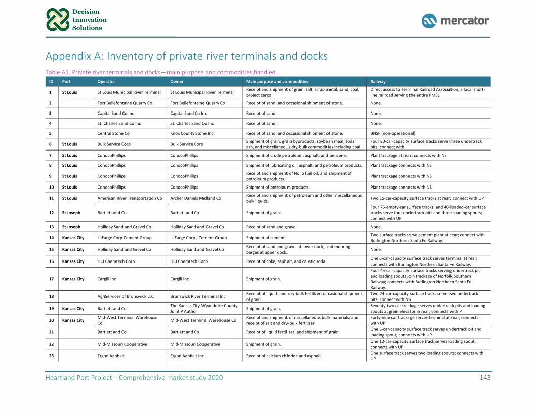
Heartland Port Project—Comprehensive market study 2020 143
Appendix A: Inventory of private river terminals and docks Table A1. Private river terminals and docks—main purpose and commodities handled
ID Port Operator Owner Main purpose and commodities Railway
1 St Louis St Louis Municipal River Terminal St Louis Municipal River Terminal Receipt and shipment of grain, salt, scrap metal, sand, coal, project cargo
Direct access to Terminal Railroad Association, a local short-line railroad serving the entire PMSL
2 Fort Bellefontaine Quarry Co Fort Bellefontaine Quarry Co Receipt of sand; and occasional shipment of stone. None.
3 Capital Sand Co Inc Capital Sand Co Inc Receipt of sand. None.
4 St. Charles Sand Co Inc St. Charles Sand Co Inc Receipt of sand. None.
5 Central Stone Co Knox County Stone Inc Receipt of sand; and occasional shipment of stone. BNSF (non-operational)
6 St Louis Bulk Service Corp Bulk Service Corp Shipment of grain, grain byproducts, soybean meal, soda ash, and miscellaneous dry-bulk commodities including coal.
Four 80-car-capacity surface tracks serve three undertrack pits; connect with
7 St Louis ConocoPhillips ConocoPhillips Shipment of crude petroleum, asphalt, and benzene. Plant trackage at rear; connects with NS
8 St Louis ConocoPhillips ConocoPhillips Shipment of lubricating oil, asphalt, and petroleum products. Plant trackage connects with NS
9 St Louis ConocoPhillips ConocoPhillips Receipt and shipment of No. 6 fuel oil; and shipment of petroleum products.
Plant trackage connects with NS
10 St Louis ConocoPhillips ConocoPhillips Shipment of petroleum products. Plant trackage connects with NS
11 St Louis American River Transportation Co Archer Daniels Midland Co Receipt and shipment of petroleum and other miscellaneous bulk liquids.
Two 15-car-capacity surface tracks at rear; connect with UP
12 St Joseph Bartlett and Co Bartlett and Co Shipment of grain. Four 75-empty-car surface tracks; and 40-loaded-car surface tracks serve four undertrack pits and three loading spouts; connect with UP
13 St Joseph Holliday Sand and Gravel Co Holliday Sand and Gravel Co Receipt of sand and gravel. None.
14 Kansas City LaFarge Corp Cement Group LaFarge Corp., Cement Group Shipment of cement. Two surface tracks serve cement plant at rear; connect with Burlington Northern Santa Fe Railway.
15 Kansas City Holliday Sand and Gravel Co Holliday Sand and Gravel Co Receipt of sand and gravel at lower dock; and mooring barges at upper dock.
None.
16 Kansas City HCI Chemtech Corp HCI Chemtech Corp Receipt of coke, asphalt, and caustic soda. One 6-car-capacity surface track serves terminal at rear; connects with Burlington Northern Santa Fe Railway.
17 Kansas City Cargill Inc Cargill Inc Shipment of grain.
Four 45-car-capacity surface tracks serving undertrack pit and loading spouts join trackage of Norfolk Southern Railway; connects with Burlington Northern Santa Fe Railway.
18 AgriServices of Brunswick LLC Brunswick River Terminal Inc Receipt of liquid- and dry-bulk fertilizer; occasional shipment of grain
Two 24-car-capacity surface tracks serve two undertrack pits; connect with NS
19 Kansas City Bartlett and Co The Kansas City-Wyandotte County Joint P Author
Shipment of grain. Seventy-two car trackage serves undertrack pits and loading spouts at grain elevator in rear; connects with P
20 Kansas City Mid-West Terminal Warehouse Co
Mid-West Terminal Warehouse Co Receipt and shipment of miscellaneous bulk materials; and receipt of salt and dry-bulk fertilizer.
Forty-nine car trackage serves terminal at rear; connects with UP
21 Bartlett and Co Bartlett and Co Receipt of liquid fertilizer; and shipment of grain. One 5-car-capacity surface track serves undertrack pit and loading spout; connects with UP
22 Mid-Missouri Cooperative Mid-Missouri Cooperative Shipment of grain. One 12-car-capacity surface track serves loading spout; connects with UP
23 Ergon Aaphalt Ergon Aaphalt Inc Receipt of calcium chloride and asphalt. One surface track serves two loading spouts; connects with UP
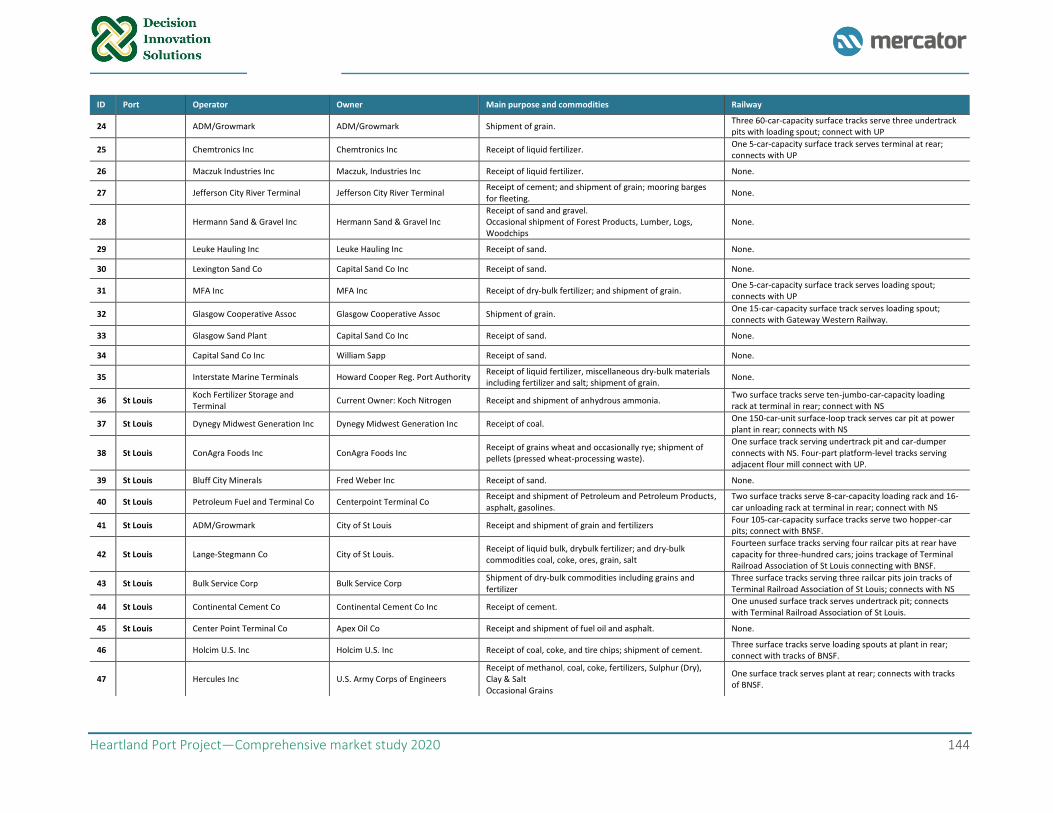
Heartland Port Project—Comprehensive market study 2020 144
ID Port Operator Owner Main purpose and commodities Railway
24 ADM/Growmark ADM/Growmark Shipment of grain. Three 60-car-capacity surface tracks serve three undertrack pits with loading spout; connect with UP
25 Chemtronics Inc Chemtronics Inc Receipt of liquid fertilizer. One 5-car-capacity surface track serves terminal at rear; connects with UP
26 Maczuk Industries Inc Maczuk, Industries Inc Receipt of liquid fertilizer. None.
27 Jefferson City River Terminal Jefferson City River Terminal Receipt of cement; and shipment of grain; mooring barges for fleeting.
None.
28 Hermann Sand & Gravel Inc Hermann Sand & Gravel Inc Receipt of sand and gravel. Occasional shipment of Forest Products, Lumber, Logs, Woodchips
None.
29 Leuke Hauling Inc Leuke Hauling Inc Receipt of sand. None.
30 Lexington Sand Co Capital Sand Co Inc Receipt of sand. None.
31 MFA Inc MFA Inc Receipt of dry-bulk fertilizer; and shipment of grain. One 5-car-capacity surface track serves loading spout; connects with UP
32 Glasgow Cooperative Assoc Glasgow Cooperative Assoc Shipment of grain. One 15-car-capacity surface track serves loading spout; connects with Gateway Western Railway.
33 Glasgow Sand Plant Capital Sand Co Inc Receipt of sand. None.
34 Capital Sand Co Inc William Sapp Receipt of sand. None.
35 Interstate Marine Terminals Howard Cooper Reg. Port Authority Receipt of liquid fertilizer, miscellaneous dry-bulk materials including fertilizer and salt; shipment of grain.
None.
36 St Louis Koch Fertilizer Storage and Terminal
Current Owner: Koch Nitrogen Receipt and shipment of anhydrous ammonia. Two surface tracks serve ten-jumbo-car-capacity loading rack at terminal in rear; connect with NS
37 St Louis Dynegy Midwest Generation Inc Dynegy Midwest Generation Inc Receipt of coal. One 150-car-unit surface-loop track serves car pit at power plant in rear; connects with NS
38 St Louis ConAgra Foods Inc ConAgra Foods Inc Receipt of grains wheat and occasionally rye; shipment of pellets (pressed wheat-processing waste).
One surface track serving undertrack pit and car-dumper connects with NS. Four-part platform-level tracks serving adjacent flour mill connect with UP.
39 St Louis Bluff City Minerals Fred Weber Inc Receipt of sand. None.
40 St Louis Petroleum Fuel and Terminal Co Centerpoint Terminal Co Receipt and shipment of Petroleum and Petroleum Products, asphalt, gasolines.
Two surface tracks serve 8-car-capacity loading rack and 16-car unloading rack at terminal in rear; connect with NS
41 St Louis ADM/Growmark City of St Louis Receipt and shipment of grain and fertilizers Four 105-car-capacity surface tracks serve two hopper-car pits; connect with BNSF.
42 St Louis Lange-Stegmann Co City of St Louis. Receipt of liquid bulk, drybulk fertilizer; and dry-bulk commodities coal, coke, ores, grain, salt
Fourteen surface tracks serving four railcar pits at rear have capacity for three-hundred cars; joins trackage of Terminal Railroad Association of St Louis connecting with BNSF.
43 St Louis Bulk Service Corp Bulk Service Corp Shipment of dry-bulk commodities including grains and fertilizer
Three surface tracks serving three railcar pits join tracks of Terminal Railroad Association of St Louis; connects with NS
44 St Louis Continental Cement Co Continental Cement Co Inc Receipt of cement. One unused surface track serves undertrack pit; connects with Terminal Railroad Association of St Louis.
45 St Louis Center Point Terminal Co Apex Oil Co Receipt and shipment of fuel oil and asphalt. None.
46 Holcim U.S. Inc Holcim U.S. Inc Receipt of coal, coke, and tire chips; shipment of cement. Three surface tracks serve loading spouts at plant in rear; connect with tracks of BNSF.
47 Hercules Inc U.S. Army Corps of Engineers Receipt of methanol, coal, coke, fertilizers, Sulphur (Dry), Clay & Salt Occasional Grains
One surface track serves plant at rear; connects with tracks of BNSF.
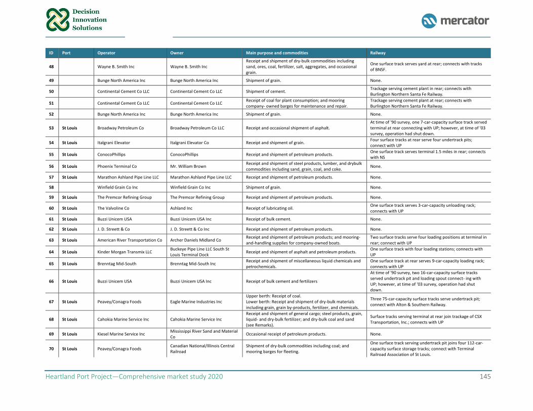
Heartland Port Project—Comprehensive market study 2020 145
ID Port Operator Owner Main purpose and commodities Railway
48 Wayne B. Smith Inc Wayne B. Smith Inc Receipt and shipment of dry-bulk commodities including sand, ores, coal, fertilizer, salt, aggregates, and occasional grain.
One surface track serves yard at rear; connects with tracks of BNSF.
49 Bunge North America Inc Bunge North America Inc Shipment of grain. None.
50 Continental Cement Co LLC Continental Cement Co LLC Shipment of cement. Trackage serving cement plant in rear; connects with Burlington Northern Santa Fe Railway.
51 Continental Cement Co LLC Continental Cement Co LLC Receipt of coal for plant consumption; and mooring company- owned barges for maintenance and repair.
Trackage serving cement plant at rear; connects with Burlington Northern Santa Fe Railway.
52 Bunge North America Inc Bunge North America Inc Shipment of grain. None.
53 St Louis Broadway Petroleum Co Broadway Petroleum Co LLC Receipt and occasional shipment of asphalt. At time of '90 survey, one 7-car-capacity surface track served terminal at rear connecting with UP; however, at time of '03 survey, operation had shut down.
54 St Louis Italgrani Elevator Italgrani Elevator Co Receipt and shipment of grain. Four surface tracks at rear serve four undertrack pits; connect with UP
55 St Louis ConocoPhillips ConocoPhillips Receipt and shipment of petroleum products. One surface track serves terminal 1.5 miles in rear; connects with NS
56 St Louis Phoenix Terminal Co Mr. William Brown Receipt and shipment of steel products, lumber, and drybulk commodities including sand, grain, coal, and coke.
None.
57 St Louis Marathon Ashland Pipe Line LLC Marathon Ashland Pipe Line LLC Receipt and shipment of petroleum products. None.
58 Winfield Grain Co Inc Winfield Grain Co Inc Shipment of grain. None.
59 St Louis The Premcor Refining Group The Premcor Refining Group Receipt and shipment of petroleum products. None.
60 St Louis The Valvoline Co Ashland Inc Receipt of lubricating oil. One surface track serves 3-car-capacity unloading rack; connects with UP
61 St Louis Buzzi Unicem USA Buzzi Unicem USA Inc Receipt of bulk cement. None.
62 St Louis J. D. Streett & Co J. D. Streett & Co Inc Receipt and shipment of petroleum products. None.
63 St Louis American River Transportation Co Archer Daniels Midland Co Receipt and shipment of petroleum products; and mooring- and-handling supplies for company-owned boats.
Two surface tracks serve four loading positions at terminal in rear; connect with UP
64 St Louis Kinder Morgan Transmix LLC Buckeye Pipe Line LLC South St Louis Terminal Dock
Receipt and shipment of asphalt and petroleum products. One surface track with four loading stations; connects with UP
65 St Louis Brenntag Mid-South Brenntag Mid-South Inc Receipt and shipment of miscellaneous liquid chemicals and petrochemicals.
One surface track at rear serves 9-car-capacity loading rack; connects with UP
66 St Louis Buzzi Unicem USA Buzzi Unicem USA Inc Receipt of bulk cement and fertilizers
At time of '90 survey, two 16-car-capacity surface tracks served undertrack pit and loading spout connect- ing with UP; however, at time of '03 survey, operation had shut down.
67 St Louis Peavey/Conagra Foods Eagle Marine Industries Inc Upper berth: Receipt of coal. Lower berth: Receipt and shipment of dry-bulk materials including grain, grain by-products, fertilizer, and chemicals.
Three 75-car-capacity surface tracks serve undertrack pit; connect with Alton & Southern Railway.
68 St Louis Cahokia Marine Service Inc Cahokia Marine Service Inc Receipt and shipment of general cargo; steel products, grain, liquid- and dry-bulk fertilizer; and dry-bulk coal and sand (see Remarks).
Surface tracks serving terminal at rear join trackage of CSX Transportation, Inc.; connects with UP
69 St Louis Kiesel Marine Service Inc Mississippi River Sand and Material Co
Occasional receipt of petroleum products. None.
70 St Louis Peavey/Conagra Foods Canadian National/Illinois Central Railroad
Shipment of dry-bulk commodities including coal; and mooring barges for fleeting.
One surface track serving undertrack pit joins four 112-car-capacity surface storage tracks; connect with Terminal Railroad Association of St Louis.
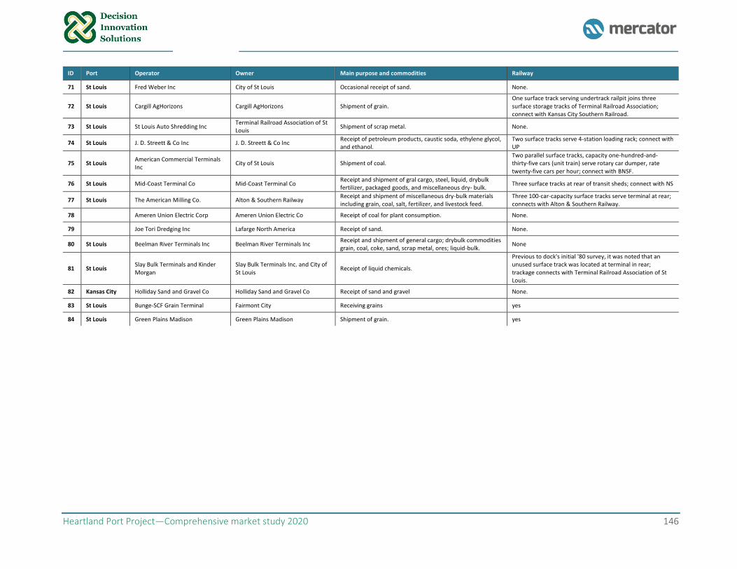
Heartland Port Project—Comprehensive market study 2020 146
ID Port Operator Owner Main purpose and commodities Railway
71 St Louis Fred Weber Inc City of St Louis Occasional receipt of sand. None.
72 St Louis Cargill AgHorizons Cargill AgHorizons Shipment of grain. One surface track serving undertrack railpit joins three surface storage tracks of Terminal Railroad Association; connect with Kansas City Southern Railroad.
73 St Louis St Louis Auto Shredding Inc Terminal Railroad Association of St Louis
Shipment of scrap metal. None.
74 St Louis J. D. Streett & Co Inc J. D. Streett & Co Inc Receipt of petroleum products, caustic soda, ethylene glycol, and ethanol.
Two surface tracks serve 4-station loading rack; connect with UP
75 St Louis American Commercial Terminals Inc
City of St Louis Shipment of coal. Two parallel surface tracks, capacity one-hundred-and- thirty-five cars (unit train) serve rotary car dumper, rate twenty-five cars per hour; connect with BNSF.
76 St Louis Mid-Coast Terminal Co Mid-Coast Terminal Co Receipt and shipment of gral cargo, steel, liquid, drybulk fertilizer, packaged goods, and miscellaneous dry- bulk.
Three surface tracks at rear of transit sheds; connect with NS
77 St Louis The American Milling Co. Alton & Southern Railway Receipt and shipment of miscellaneous dry-bulk materials including grain, coal, salt, fertilizer, and livestock feed.
Three 100-car-capacity surface tracks serve terminal at rear; connects with Alton & Southern Railway.
78 Ameren Union Electric Corp Ameren Union Electric Co Receipt of coal for plant consumption. None.
79 Joe Tori Dredging Inc Lafarge North America Receipt of sand. None.
80 St Louis Beelman River Terminals Inc Beelman River Terminals Inc Receipt and shipment of general cargo; drybulk commodities grain, coal, coke, sand, scrap metal, ores; liquid-bulk.
None
81 St Louis Slay Bulk Terminals and Kinder Morgan
Slay Bulk Terminals Inc. and City of St Louis
Receipt of liquid chemicals.
Previous to dock's initial '80 survey, it was noted that an unused surface track was located at terminal in rear; trackage connects with Terminal Railroad Association of St Louis.
82 Kansas City Holliday Sand and Gravel Co Holliday Sand and Gravel Co Receipt of sand and gravel None.
83 St Louis Bunge-SCF Grain Terminal Fairmont City Receiving grains yes
84 St Louis Green Plains Madison Green Plains Madison Shipment of grain. yes
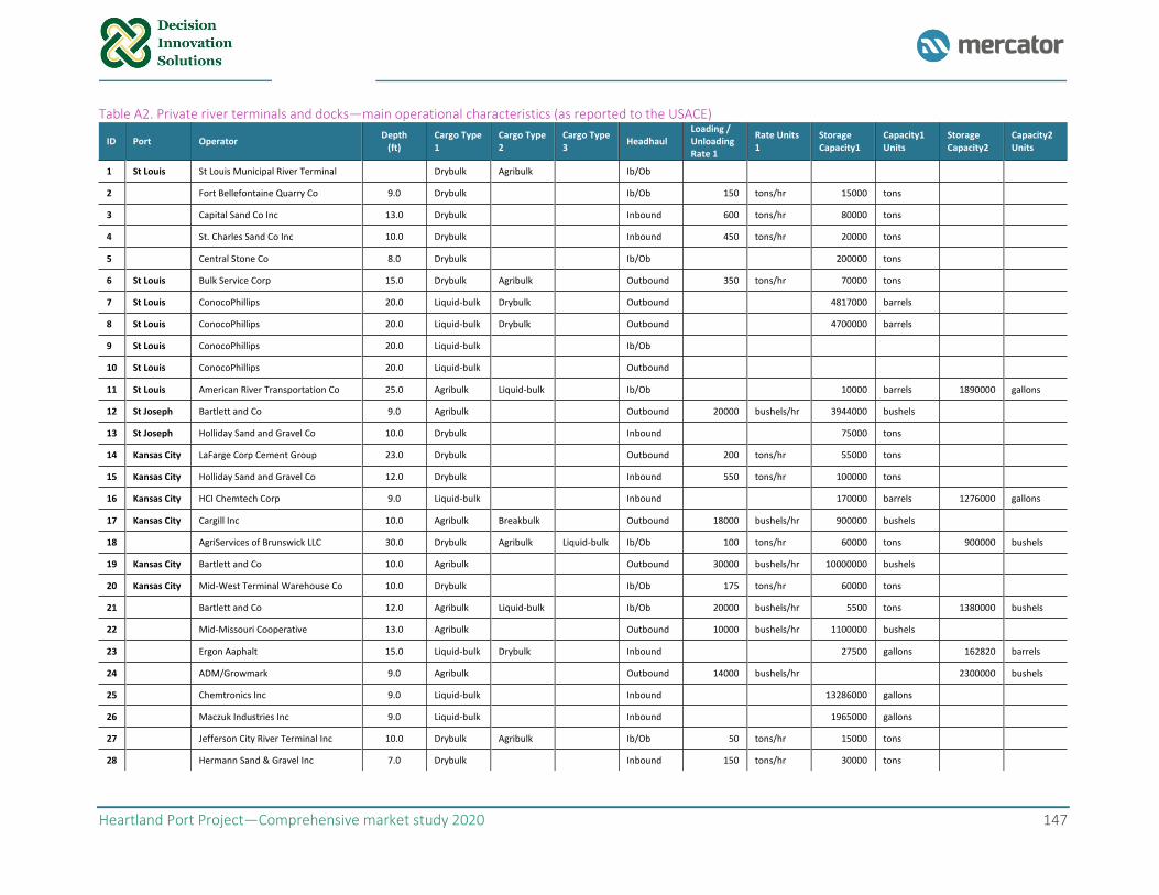
Heartland Port Project—Comprehensive market study 2020 147
Table A2. Private river terminals and docks—main operational characteristics (as reported to the USACE)
ID Port Operator Depth
(ft) Cargo Type 1
Cargo Type 2
Cargo Type 3
Headhaul Loading / Unloading Rate 1
Rate Units 1
Storage Capacity1
Capacity1 Units
Storage Capacity2
Capacity2 Units
1 St Louis St Louis Municipal River Terminal Drybulk Agribulk Ib/Ob
2 Fort Bellefontaine Quarry Co 9.0 Drybulk Ib/Ob 150 tons/hr 15000 tons
3 Capital Sand Co Inc 13.0 Drybulk Inbound 600 tons/hr 80000 tons
4 St. Charles Sand Co Inc 10.0 Drybulk Inbound 450 tons/hr 20000 tons
5 Central Stone Co 8.0 Drybulk Ib/Ob 200000 tons
6 St Louis Bulk Service Corp 15.0 Drybulk Agribulk Outbound 350 tons/hr 70000 tons
7 St Louis ConocoPhillips 20.0 Liquid-bulk Drybulk Outbound 4817000 barrels
8 St Louis ConocoPhillips 20.0 Liquid-bulk Drybulk Outbound 4700000 barrels
9 St Louis ConocoPhillips 20.0 Liquid-bulk Ib/Ob
10 St Louis ConocoPhillips 20.0 Liquid-bulk Outbound
11 St Louis American River Transportation Co 25.0 Agribulk Liquid-bulk Ib/Ob 10000 barrels 1890000 gallons
12 St Joseph Bartlett and Co 9.0 Agribulk Outbound 20000 bushels/hr 3944000 bushels
13 St Joseph Holliday Sand and Gravel Co 10.0 Drybulk Inbound 75000 tons
14 Kansas City LaFarge Corp Cement Group 23.0 Drybulk Outbound 200 tons/hr 55000 tons
15 Kansas City Holliday Sand and Gravel Co 12.0 Drybulk Inbound 550 tons/hr 100000 tons
16 Kansas City HCI Chemtech Corp 9.0 Liquid-bulk Inbound 170000 barrels 1276000 gallons
17 Kansas City Cargill Inc 10.0 Agribulk Breakbulk Outbound 18000 bushels/hr 900000 bushels
18 AgriServices of Brunswick LLC 30.0 Drybulk Agribulk Liquid-bulk Ib/Ob 100 tons/hr 60000 tons 900000 bushels
19 Kansas City Bartlett and Co 10.0 Agribulk Outbound 30000 bushels/hr 10000000 bushels
20 Kansas City Mid-West Terminal Warehouse Co 10.0 Drybulk Ib/Ob 175 tons/hr 60000 tons
21 Bartlett and Co 12.0 Agribulk Liquid-bulk Ib/Ob 20000 bushels/hr 5500 tons 1380000 bushels
22 Mid-Missouri Cooperative 13.0 Agribulk Outbound 10000 bushels/hr 1100000 bushels
23 Ergon Aaphalt 15.0 Liquid-bulk Drybulk Inbound 27500 gallons 162820 barrels
24 ADM/Growmark 9.0 Agribulk Outbound 14000 bushels/hr 2300000 bushels
25 Chemtronics Inc 9.0 Liquid-bulk Inbound 13286000 gallons
26 Maczuk Industries Inc 9.0 Liquid-bulk Inbound 1965000 gallons
27 Jefferson City River Terminal Inc 10.0 Drybulk Agribulk Ib/Ob 50 tons/hr 15000 tons
28 Hermann Sand & Gravel Inc 7.0 Drybulk Inbound 150 tons/hr 30000 tons
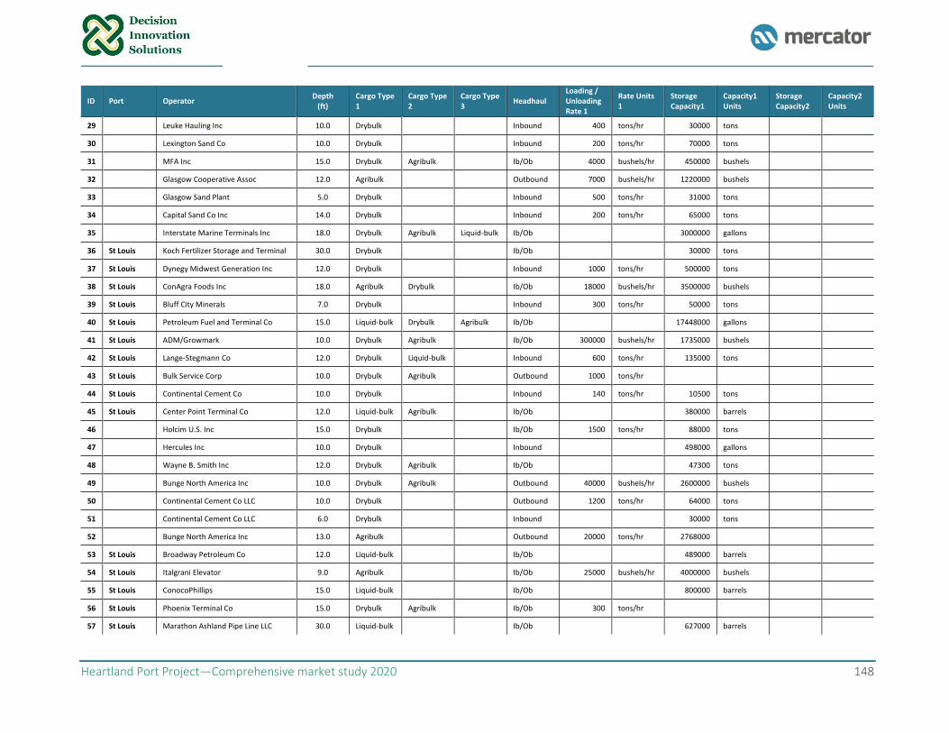
Heartland Port Project—Comprehensive market study 2020 148
ID Port Operator Depth
(ft) Cargo Type 1
Cargo Type 2
Cargo Type 3
Headhaul Loading / Unloading Rate 1
Rate Units 1
Storage Capacity1
Capacity1 Units
Storage Capacity2
Capacity2 Units
29 Leuke Hauling Inc 10.0 Drybulk Inbound 400 tons/hr 30000 tons
30 Lexington Sand Co 10.0 Drybulk Inbound 200 tons/hr 70000 tons
31 MFA Inc 15.0 Drybulk Agribulk Ib/Ob 4000 bushels/hr 450000 bushels
32 Glasgow Cooperative Assoc 12.0 Agribulk Outbound 7000 bushels/hr 1220000 bushels
33 Glasgow Sand Plant 5.0 Drybulk Inbound 500 tons/hr 31000 tons
34 Capital Sand Co Inc 14.0 Drybulk Inbound 200 tons/hr 65000 tons
35 Interstate Marine Terminals Inc 18.0 Drybulk Agribulk Liquid-bulk Ib/Ob 3000000 gallons
36 St Louis Koch Fertilizer Storage and Terminal 30.0 Drybulk Ib/Ob 30000 tons
37 St Louis Dynegy Midwest Generation Inc 12.0 Drybulk Inbound 1000 tons/hr 500000 tons
38 St Louis ConAgra Foods Inc 18.0 Agribulk Drybulk Ib/Ob 18000 bushels/hr 3500000 bushels
39 St Louis Bluff City Minerals 7.0 Drybulk Inbound 300 tons/hr 50000 tons
40 St Louis Petroleum Fuel and Terminal Co 15.0 Liquid-bulk Drybulk Agribulk Ib/Ob 17448000 gallons
41 St Louis ADM/Growmark 10.0 Drybulk Agribulk Ib/Ob 300000 bushels/hr 1735000 bushels
42 St Louis Lange-Stegmann Co 12.0 Drybulk Liquid-bulk Inbound 600 tons/hr 135000 tons
43 St Louis Bulk Service Corp 10.0 Drybulk Agribulk Outbound 1000 tons/hr
44 St Louis Continental Cement Co 10.0 Drybulk Inbound 140 tons/hr 10500 tons
45 St Louis Center Point Terminal Co 12.0 Liquid-bulk Agribulk Ib/Ob 380000 barrels
46 Holcim U.S. Inc 15.0 Drybulk Ib/Ob 1500 tons/hr 88000 tons
47 Hercules Inc 10.0 Drybulk Inbound 498000 gallons
48 Wayne B. Smith Inc 12.0 Drybulk Agribulk Ib/Ob 47300 tons
49 Bunge North America Inc 10.0 Drybulk Agribulk Outbound 40000 bushels/hr 2600000 bushels
50 Continental Cement Co LLC 10.0 Drybulk Outbound 1200 tons/hr 64000 tons
51 Continental Cement Co LLC 6.0 Drybulk Inbound 30000 tons
52 Bunge North America Inc 13.0 Agribulk Outbound 20000 tons/hr 2768000
53 St Louis Broadway Petroleum Co 12.0 Liquid-bulk Ib/Ob 489000 barrels
54 St Louis Italgrani Elevator 9.0 Agribulk Ib/Ob 25000 bushels/hr 4000000 bushels
55 St Louis ConocoPhillips 15.0 Liquid-bulk Ib/Ob 800000 barrels
56 St Louis Phoenix Terminal Co 15.0 Drybulk Agribulk Ib/Ob 300 tons/hr
57 St Louis Marathon Ashland Pipe Line LLC 30.0 Liquid-bulk Ib/Ob 627000 barrels
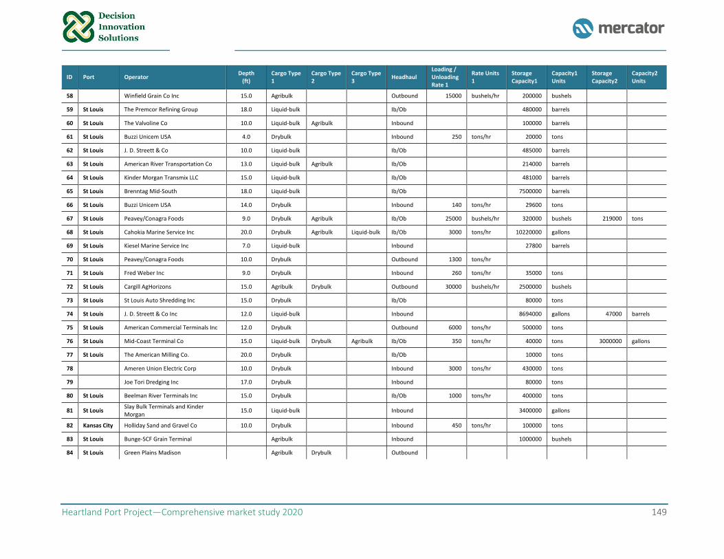
Heartland Port Project—Comprehensive market study 2020 149
ID Port Operator Depth
(ft) Cargo Type 1
Cargo Type 2
Cargo Type 3
Headhaul Loading / Unloading Rate 1
Rate Units 1
Storage Capacity1
Capacity1 Units
Storage Capacity2
Capacity2 Units
58 Winfield Grain Co Inc 15.0 Agribulk Outbound 15000 bushels/hr 200000 bushels
59 St Louis The Premcor Refining Group 18.0 Liquid-bulk Ib/Ob 480000 barrels
60 St Louis The Valvoline Co 10.0 Liquid-bulk Agribulk Inbound 100000 barrels
61 St Louis Buzzi Unicem USA 4.0 Drybulk Inbound 250 tons/hr 20000 tons
62 St Louis J. D. Streett & Co 10.0 Liquid-bulk Ib/Ob 485000 barrels
63 St Louis American River Transportation Co 13.0 Liquid-bulk Agribulk Ib/Ob 214000 barrels
64 St Louis Kinder Morgan Transmix LLC 15.0 Liquid-bulk Ib/Ob 481000 barrels
65 St Louis Brenntag Mid-South 18.0 Liquid-bulk Ib/Ob 7500000 barrels
66 St Louis Buzzi Unicem USA 14.0 Drybulk Inbound 140 tons/hr 29600 tons
67 St Louis Peavey/Conagra Foods 9.0 Drybulk Agribulk Ib/Ob 25000 bushels/hr 320000 bushels 219000 tons
68 St Louis Cahokia Marine Service Inc 20.0 Drybulk Agribulk Liquid-bulk Ib/Ob 3000 tons/hr 10220000 gallons
69 St Louis Kiesel Marine Service Inc 7.0 Liquid-bulk Inbound 27800 barrels
70 St Louis Peavey/Conagra Foods 10.0 Drybulk Outbound 1300 tons/hr
71 St Louis Fred Weber Inc 9.0 Drybulk Inbound 260 tons/hr 35000 tons
72 St Louis Cargill AgHorizons 15.0 Agribulk Drybulk Outbound 30000 bushels/hr 2500000 bushels
73 St Louis St Louis Auto Shredding Inc 15.0 Drybulk Ib/Ob 80000 tons
74 St Louis J. D. Streett & Co Inc 12.0 Liquid-bulk Inbound 8694000 gallons 47000 barrels
75 St Louis American Commercial Terminals Inc 12.0 Drybulk Outbound 6000 tons/hr 500000 tons
76 St Louis Mid-Coast Terminal Co 15.0 Liquid-bulk Drybulk Agribulk Ib/Ob 350 tons/hr 40000 tons 3000000 gallons
77 St Louis The American Milling Co. 20.0 Drybulk Ib/Ob 10000 tons
78 Ameren Union Electric Corp 10.0 Drybulk Inbound 3000 tons/hr 430000 tons
79 Joe Tori Dredging Inc 17.0 Drybulk Inbound 80000 tons
80 St Louis Beelman River Terminals Inc 15.0 Drybulk Ib/Ob 1000 tons/hr 400000 tons
81 St Louis Slay Bulk Terminals and Kinder Morgan
15.0 Liquid-bulk Inbound 3400000 gallons
82 Kansas City Holliday Sand and Gravel Co 10.0 Drybulk Inbound 450 tons/hr 100000 tons
83 St Louis Bunge-SCF Grain Terminal Agribulk Inbound 1000000 bushels
84 St Louis Green Plains Madison Agribulk Drybulk Outbound
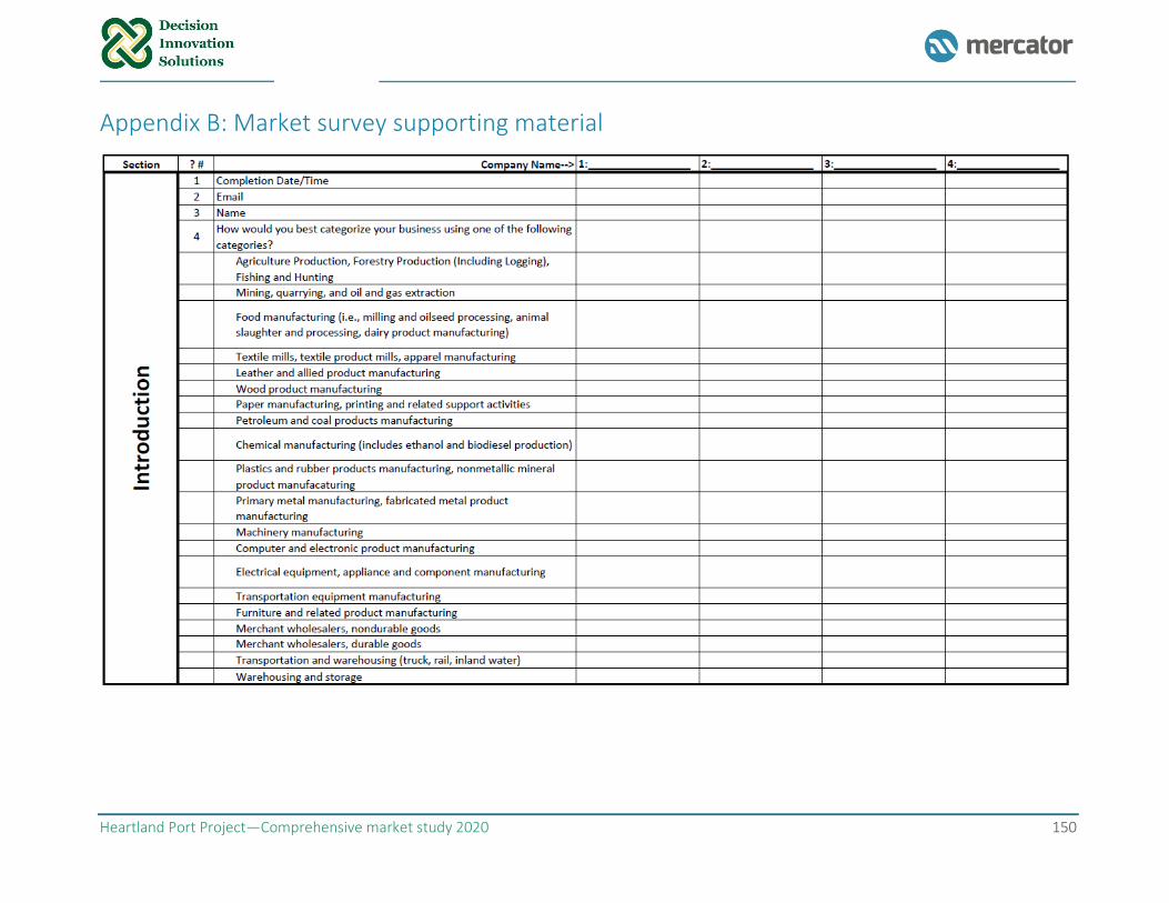
Heartland Port Project—Comprehensive market study 2020 150
Appendix B: Market survey supporting material
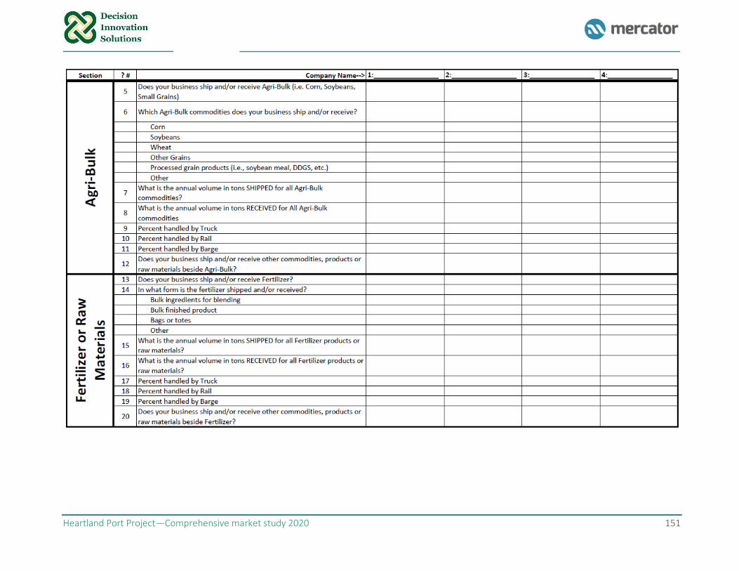
Heartland Port Project—Comprehensive market study 2020 151
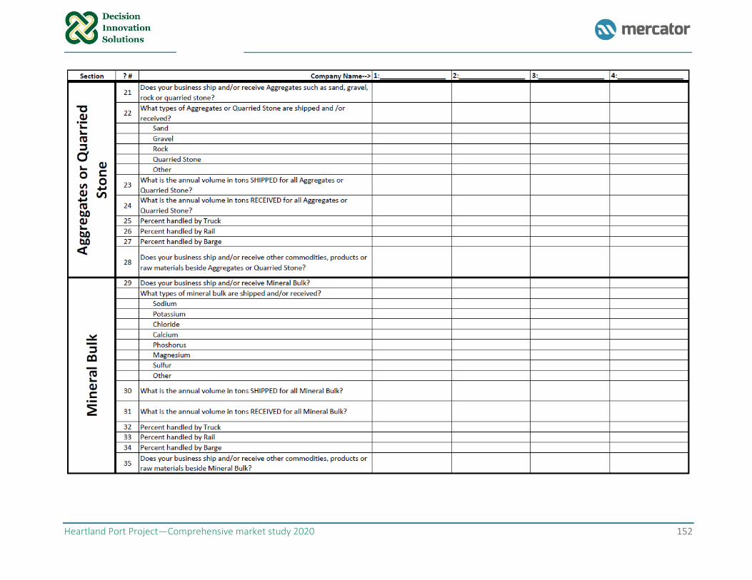
Heartland Port Project—Comprehensive market study 2020 152
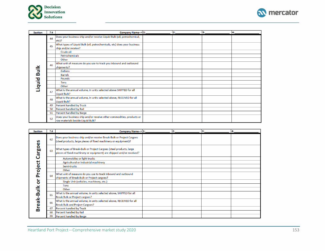
Heartland Port Project—Comprehensive market study 2020 153
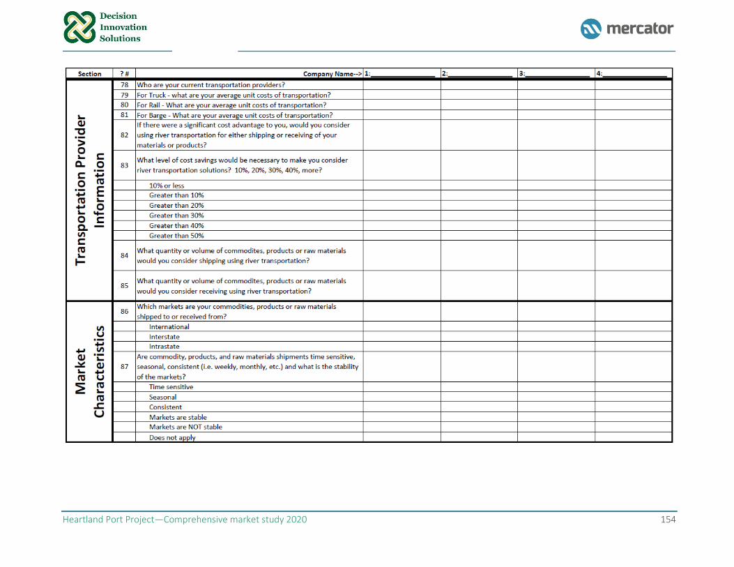
Heartland Port Project—Comprehensive market study 2020 154
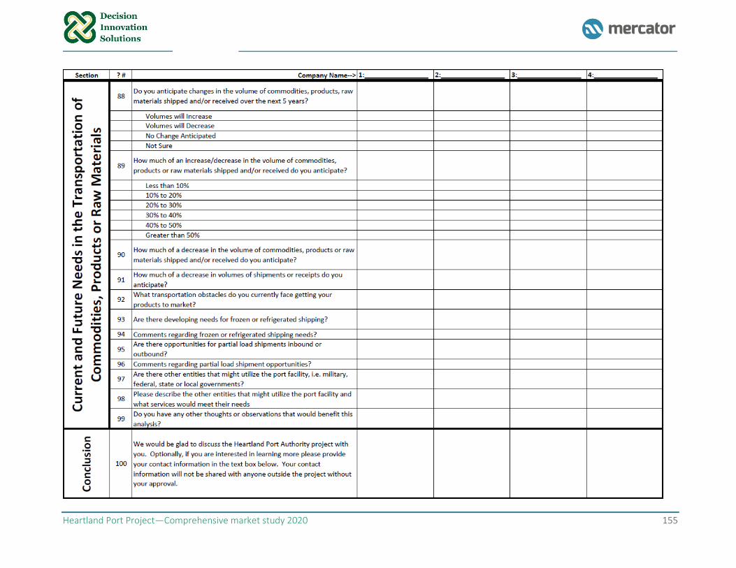
Heartland Port Project—Comprehensive market study 2020 155
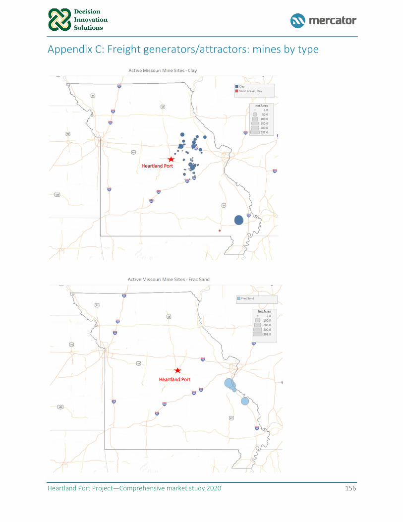
Heartland Port Project—Comprehensive market study 2020 156
Appendix C: Freight generators/attractors: mines by type
Heartland Port
Heartland Port
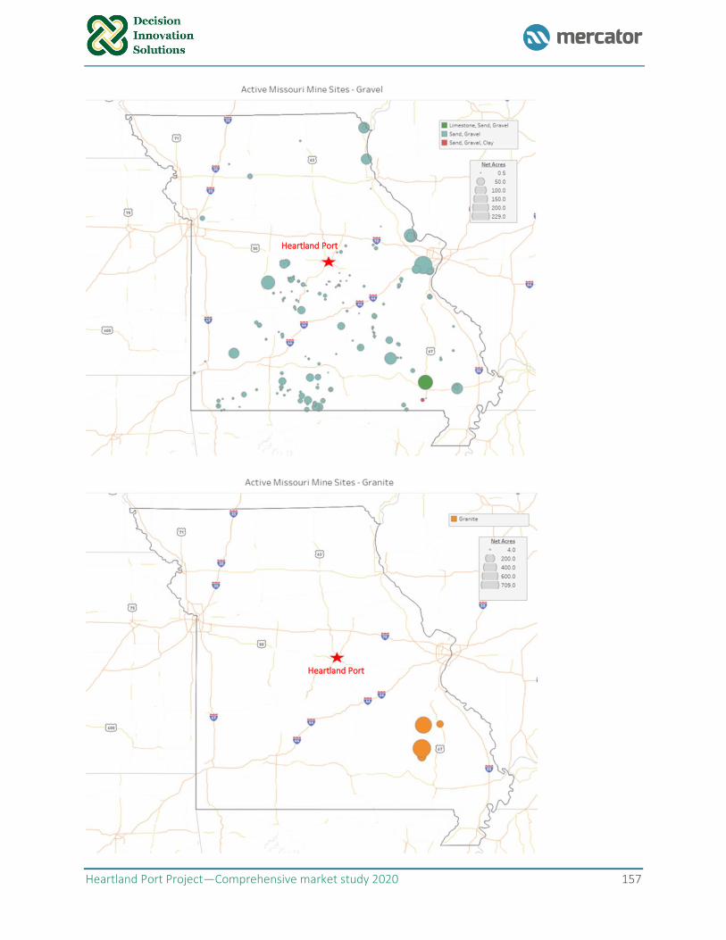
Heartland Port Project—Comprehensive market study 2020 157
Heartland Port
Heartland Port
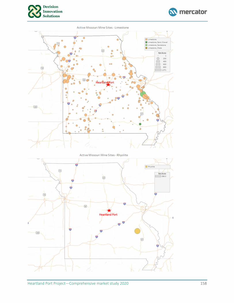
Heartland Port Project—Comprehensive market study 2020 158
Heartland Port
Heartland Port
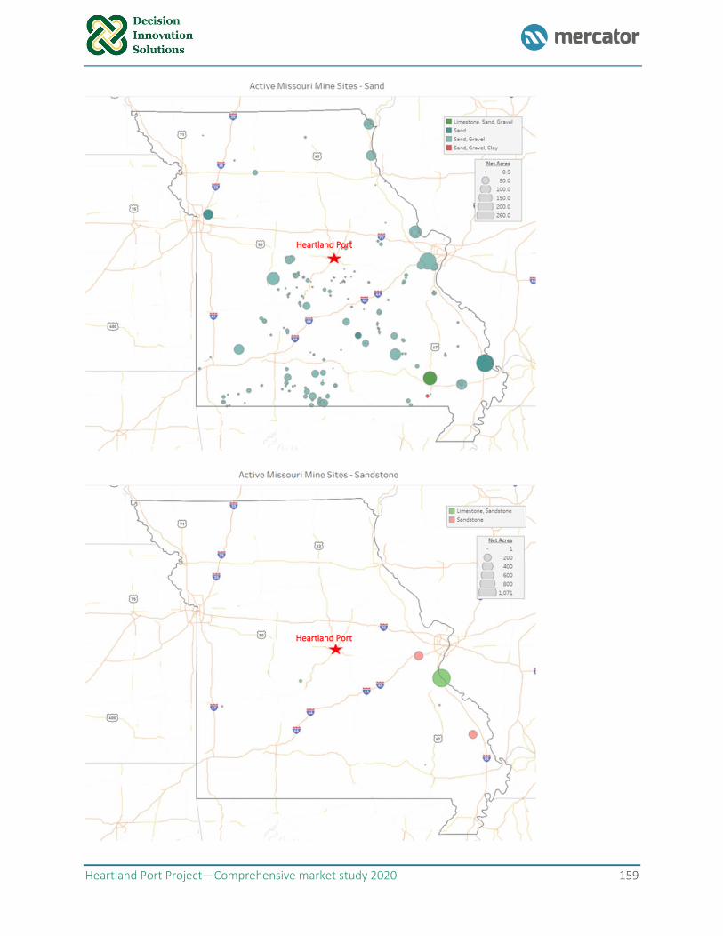
Heartland Port Project—Comprehensive market study 2020 159
Heartland Port
Heartland Port
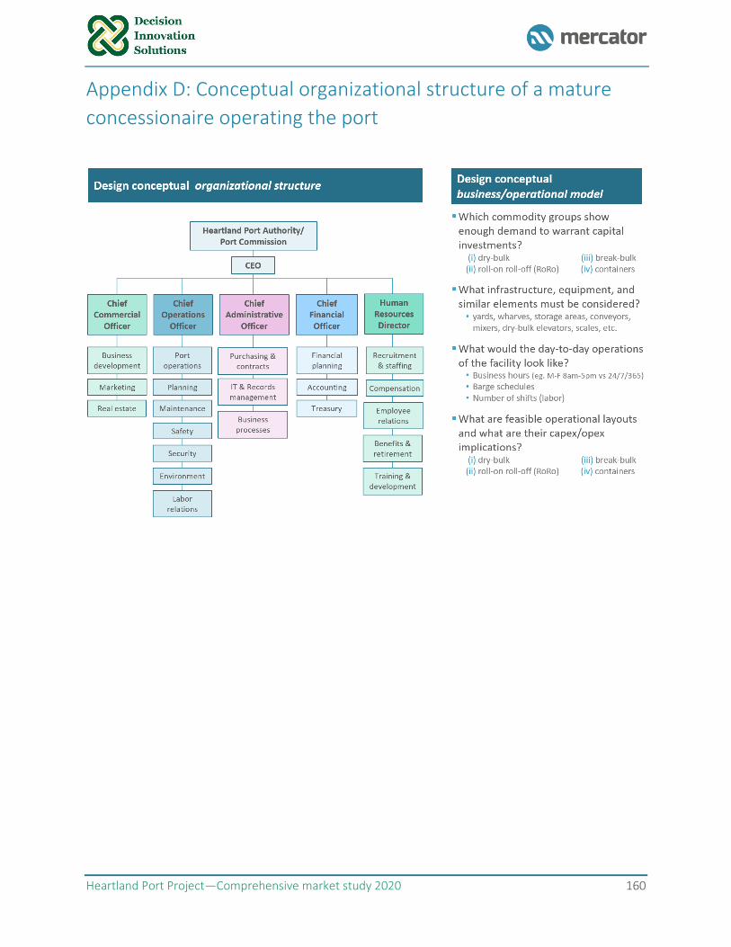
Heartland Port Project—Comprehensive market study 2020 160
Appendix D: Conceptual organizational structure of a mature
concessionaire operating the port
Heartland Port Project—Comprehensive market study 2020 161
Appendix E: Standard format for environmental statements
(c) Format. The standard format for environmental statements is:
(1) Cover Sheet. The cover sheet, not to exceed one page, must include:
(i) A list of the responsible agencies including the lead agency and any cooperating agencies.
(ii) The title of the proposed action that is the subject of the statement (and if appropriate, the titles of
related cooperating agency actions), together with any city, state, and county where the action is to take
place.
(iii) The name, address, and telephone number of a person at the agency who can supply further
information.
(iv) A designation of the document as a draft or final statement or a draft or final supplement.
(v) A one-paragraph abstract of the statement.
(vi) The date by which comments must be received.
(2) Summary. The section should compare and summarize the findings of the analyses of the affected
environment, the environmental impacts, the environmental consequences, the alternatives, and the
mitigation measures. The summary should sharply define the issues and provide a clear basis for choosing
alternatives.
(3) Table of Contents.
(4) Proposed action. This section should clearly outline the need for the EIS and the purpose and
description of the proposed action. The entire action should be discussed, including connected and similar
actions. A clear discussion of the action will assist in consideration of the alternatives.
(5) Alternatives and mitigation. This portion of the environmental impact statement is vitally important.
Based on the analysis in the Affected Environment and Environmental Consequences section (see §
775.11(c)(6)), the environmental impacts and the alternatives are presented in comparative form, thus
sharply defining the issues and providing a clear basis for choosing alternatives. Those preparing the
statement must:
(i) Explore and evaluate all reasonable alternatives, including the “no action” alternative, and briefly
discuss the reasons for eliminating any alternatives.
(ii) Devote substantial treatment to each alternative considered in detail, including the proposed action,
so that reviewers may evaluate their comparative merits.
(iii) Identify the preferred alternative or alternatives in the draft and final statements.
(iv) Describe appropriate mitigation measures not considered to be an integral part of the proposed action
or alternatives. See § 775.9(a)(7).
(6) Affected Environment and Environmental Consequences. For each reasonable alternative, each
affected element of the environment must be described, followed immediately by an analysis of the
impacts (environmental consequences). The analysis must include, among others, the following:
(i) Any adverse environmental effects which cannot be avoided should the action be implemented.
Heartland Port Project—Comprehensive market study 2020 162
(ii) The relationship between short-term uses of the environment and the maintenance and enhancement
of long-term productivity,
(iii) Any irreversible or irretrievable commitments of resources should the action be implemented, and
(iv) Energy requirements and conservation; and natural, or depletable, resource requirements and
conservation.
(7) List of Mitigation Measures.
(8) List of Preparers. List the names, together with the qualifications (expertise, professional disciplines),
of persons who were primarily responsible for preparing the environmental impact statement or
significant background papers.
(9) List of Agencies, Organizations and Persons to Whom Copies of the Statement Are Sent.
(10) Index.
(11) Appendices. Include comments on draft statement in final statement.
(d) Distribution.
(1) Any completed draft environmental impact statement which is made the subject of a public hearing,
must be made available to the public as provided in § 775.12, of this chapter at least 15 days in advance
of the hearing.
(2) Draft and final environmental impact statements must be filed with the Environmental Protection
Agency. Five copies are filed with EPA's headquarters addressed to the Office of Federal Activities (A-
104), Environmental Protection Agency, 401 M Street SW., Washington, DC 20460; five copies are also
filed with the responsible EPA region. Statements may not be filed with the EPA earlier than they are
transmitted to commenting agencies and made available to the public.
(3) Copies of draft and final environmental impact statements must be furnished to:
(i) Any Federal agency which has jurisdiction by law or special expertise with respect to any environmental
impact involved.
(ii) Any appropriate Federal, state, or local agency authorized to develop and enforce environmental
standards.
(iii) The appropriate review officials identified in the Postal Service regulations and procedures governing
intergovernmental review of Postal Service facility project actions, the State Historic Preservation Officer,
and, when National Register or eligible properties may be affected, the Advisory Council on Historic
Preservation.
(iv) Any person, organization or agency requesting them.
(4) Copies of final environmental impact statements must be furnished to any person who, or organization
or agency which, submitted substantive comments on the draft.
(e) Responses to comments.
(1) A final statement responds to comments on a draft statement in one or more of the following ways:
(i) Modification of alternatives, including the proposed action.
(ii) Development and evaluation of alternatives not previously given serious consideration.
Heartland Port Project—Comprehensive market study 2020 163
(iii) Supplementation, improvement, or modification of analyses.
(iv) Correction of facts.
(v) Explanation of why a comment does not warrant a direct response, citing supporting sources,
authorities, or reasons. Relevant circumstances which may trigger reappraisal or further response must
be indicated.
(2) Substantive comments received on a draft statement must be attached to the final statement.
(3) If all of the changes are minor and are confined to responses described in paragraphs (e)(1) (iv) and (v)
of this section, errata sheets may be written, and only the comments and errata sheets need be
recirculated. In such a case, the draft statement with the comments, errata sheets, and a new cover, must
be filed as the final statement.
(f) Supplements.
(1) A supplement to a draft or final environmental impact statement must be issued if:
(i) Substantial changes are made in the proposed action that are relevant to environmental concerns; or
(ii) Significant new circumstances or information bearing on environmental impacts of the proposed
action arise or are discovered.
(2) The decision on a proposed action involving an environmental impact statement, must be delayed
until any necessary supplement has been circulated and has gone through the commenting period. A
supplement is prepared, circulated, and filed in the same manner (except for determining scope) as draft
and final statements, unless alternative procedures are approved by CEQ.
(g) Contracting. A contractor employed to prepare an environmental impact statement must certify that
it has no financial or other interest in the outcome of the project.
(h) Proposals for Legislation. Legislative environmental impact statements must be prepared and
transmitted as follows:
(1) A legislative environmental impact statement is considered part of the formal transmittal of a
legislative proposal to the Congress. It may be transmitted to the Congress up to 30 days after the
proposal. The statement must be available in time for Congressional hearings and deliberations.
(2) Preparation and processing of a legislative statement must conform to the requirements for impact
statements, except as follows:
(i) It is not necessary to determine the scope of issues.
(ii) A draft is considered to be a final statement. Both draft and final statements are needed only when:
(A) A Congressional committee with jurisdiction over the proposal has a rule requiring both.
(B) Both are specifically required by statute for proposals of the type being submitted.
(3) Comments received on a legislative statement, and the Postal Service's responses, must be forwarded
to the Congress.