8

Heuristics and meta-heuristics for lot sizingand scheduling in the soft drinks industry: a

comparison study

D. Ferreira1, P.M. Franca2, A. Kimms3, R. Morabito1, S. Rangel4, andC.F.M. Toledo5

1 Departamento de Engenharia de Producao, Universidade Federal de Sao Carlos,C.P. 676, 13565-905, Sao Carlos, SP, Brazil degafernandes@hotmail.com;morabito@power.ufscar.br

2 Departamento de Matematica, Estatıstica e Computacao, Universidade EstadualPaulista, C.P. 1234, 19060-400, Presidente Prudente, SP, Brazilpaulo.morelato@gmail.com

3 Dept. of Technology and Operations Management, University of Duisburg-Essen,47048, Duisburg, Germany alf.kimms@uni-duisburg-essen.de

4 Departamento de Ciencia da Computacao e Estatıstica, Universidade EstadualPaulista, Rua Cristovao Colombo, 2265, 15054-000, S. J. do Rio Preto, SP,Brazil socorro@ibilce.unesp.br

5 Departamento de Ciencia da Computacao, Universidade Federal de Lavras, C.P.3037, 37200-000, Lavras, MG, Brazil claudio@dcc.ufla.br

Summary. This chapter studies a two-level production planning problem where,on each level, a lot sizing and scheduling problem with parallel machines, capac-ity constraints and sequence-dependent setup costs and times must be solved. Theproblem can be found in soft drink companies where the production process involvestwo interdependent levels with decisions concerning raw material storage and softdrink bottling. Models and solution approaches proposed so far are surveyed andconceptually compared. Two different approaches have been selected to perform aseries of computational comparisons: an evolutionary technique comprising a geneticalgorithm and its memetic version, and a decomposition and relaxation approach.

Key words: Two-level Production Planning, Lot Sizing, Scheduling, SoftDrinks Industry, Genetic Algorithm, Memetic Algorithm.

8.1 Introduction

The motivation behind writing this contribution is to offer the academicand practitioner industrial engineering community dealing with planning and

170 Ferreira et al.

scheduling tasks in the soft drinks industry a text with the most recent con-tributions to the field and also a comparative study with some selected ap-proaches. A major concern that inspired the chapter was to review moderntechniques especially designed for building production schedules applied toreal world settings. The technical literature devoted to planning and schedul-ing is vast and there are plenty of sophisticated methods. However, the speci-ficities of the soft drinks industry require dedicated models and specific solu-tion methodologies that justify a text like this one. Thus, the objective of thischapter is first to discuss the planning features of a soft drinks plant and thento assess the main suitable mathematical models , as well as to explore andevaluate the quality and computing time of some selected solution methods.

8.1.1 Soft Drinks Plant

The consumption of soft drinks has grown considerably worldwide. In Brazil,where part of the present research has been carried out, there are more than800 plants supplying a 13-billion liter annual consumer market, which is thethird in the world. This figure represents an amount which is twice as largeas ten years ago. The diversity of products offered to consumers, the scaleof plants and the complexity of modern filling lines require the adoption ofoptimization-based programs to produce efficient production plans. Indeed, aplenty of specialized commercial packages have been launched over the lastyears as an effort to overcome the difficulties human schedulers have faced.However, in most cases the complexity of the planning task imposes hard man-ual adjustments for the production schedules produced by those packages. Thebiggest contribution of the approaches studied in this chapter is to proposeintegrated optimization-based models able to encompass both the two inter-dependent production levels , namely the tank level and the bottling level.Due to its inherent complexity, the needed synchronization between these twolevels is disregarded by commercial packages thus often leading to ineffectiveproduction schedules.

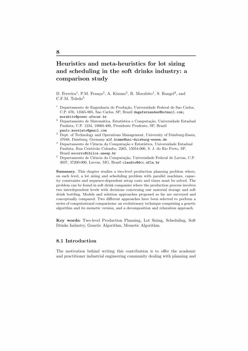
The production process found in medium to large plants consists of anupper level with capacitated mixing tanks used to prepare and store liquidswhich are pumped to the lower level constituted by bottling or canning linesdisposed in parallel (Fig. 8.1). At the tank level , decisions concerning theamount and the time the raw materials have to be stored in every availabletank must be made. Analogously, at the production line level the lot size ofeach demanded item and its corresponding schedule in each line must also bedetermined. However, a line is able to meet the weekly demand only if thenecessary amount of raw material can be stored in a connected tank. Indeed,a solution which integrates these two lot sizing and scheduling problems hasto be determined. Moreover, once the necessary amount of raw material isstored, it can not stay for a long time waiting to be pumped to lines. Thereis a synchronization problem here because the production in lines and thestorage in tanks must be compatible with each other throughout the time

8 Meta-heuristics for lot sizing and scheduling in the soft drinks industry 171

horizon. Hence, a lot sizing and scheduling problem has to be solved at eachone of these two-levels taking into account that the corresponding decisionsmust be synchronized.

xxxxxxxxxxxxxxxxxxxxxxxxxxxxxxxxxxxxxxxxxxxxxxxxxxxxxxxxxxxxxxxxxxxxxxxxxxx

xxxxxxxxxxxxxxxxxxxxxxxxxxxxxxxxxxxxxxxxxxxxxxxxxxxxxxxxxxxxxxxxxxxxxx

xxxxxxxxxxxxxxxxxxxxxxxxxxxxxxxxxxxxxxxxxxxxxxxxxxxxxxxxxxxxxxxxxxxxxxxxxxx

xxxxxxxxxxxxxxxxxxxxxxxxxxxxxxxxxxxxxxxxxxxxxxxxxxxxxxxxxxxxxxxxxxxxxxxxxxx

xxxxxxxxxxxxxxxxxxxxxxxxxxxxxxxxxxxxxxxxxxxxxxxxxxxxxxxxxxxxxxxxxxxxxx

xxxxxxxxxxxxxxx

Tanks

Products

Productionlines

Fig. 8.1: The two-level production process

Possibly the two-level synchronization is the most challenging aspect ofthis problem. Due to this fact, this problem is called the Synchronized andIntegrated Two-level Lot sizing and Scheduling Problem (SITLSP) ( [1]).

The raw materials are the flavors of the liquids which are bottled in theproduction lines. For technical reasons, a tank is only filled up when emptyand two different raw materials cannot be stored at the same time in the sametank. A sequence-dependent changeover time (setup) of up to several hoursoccurs to clean and fill up a tank, even if the same soft drink is replaced.A sequence-dependent setup time means that the time required to prepareand fill a tank for the next liquid depends on the liquid previously stored.Indeed, the setup time when a diet drink follows a plain flavor drink is muchlonger when the sequence is inverted. Nothing can be pumped to a productionline from the tank during the setup time. One tank can be connected toseveral production lines which will share the same raw material. Moreover,the production lines can be connected to any tank. However, it can receiveraw material from only one tank at a time. The final product (item) is definedby the flavor of the soft drink and the type of container (glass bottles, plasticbottles or cans) of different sizes. In large plants it is common to find situationswhere various products can share a common production line and various linescan produce the same product in parallel. The production schedule also hasto take into consideration the impact of product changeovers on the effectivecapacity of the production lines. As in the mixing tanks, these changeovertimes (setups) are also sequence-dependent and occur whenever a line hastwo different products switched.

172 Ferreira et al.

The weekly demands have to be met within a time horizon of a certainnumber of weeks. Since the forecasts of customer orders are error-prone, thereis little interest in seeking solutions in large horizons. Instead, it is morerealistic to work in a rolling-horizon basis with a 3 or 4-week time horizon.The excessive number of final products leads to inventory costs. There arealso inventory costs for the storage of raw materials in tanks in various timeperiods. The sequence-dependent setup costs for products and raw materialsare proportional to the sequence-dependent setup times in lines and tanks,respectively.

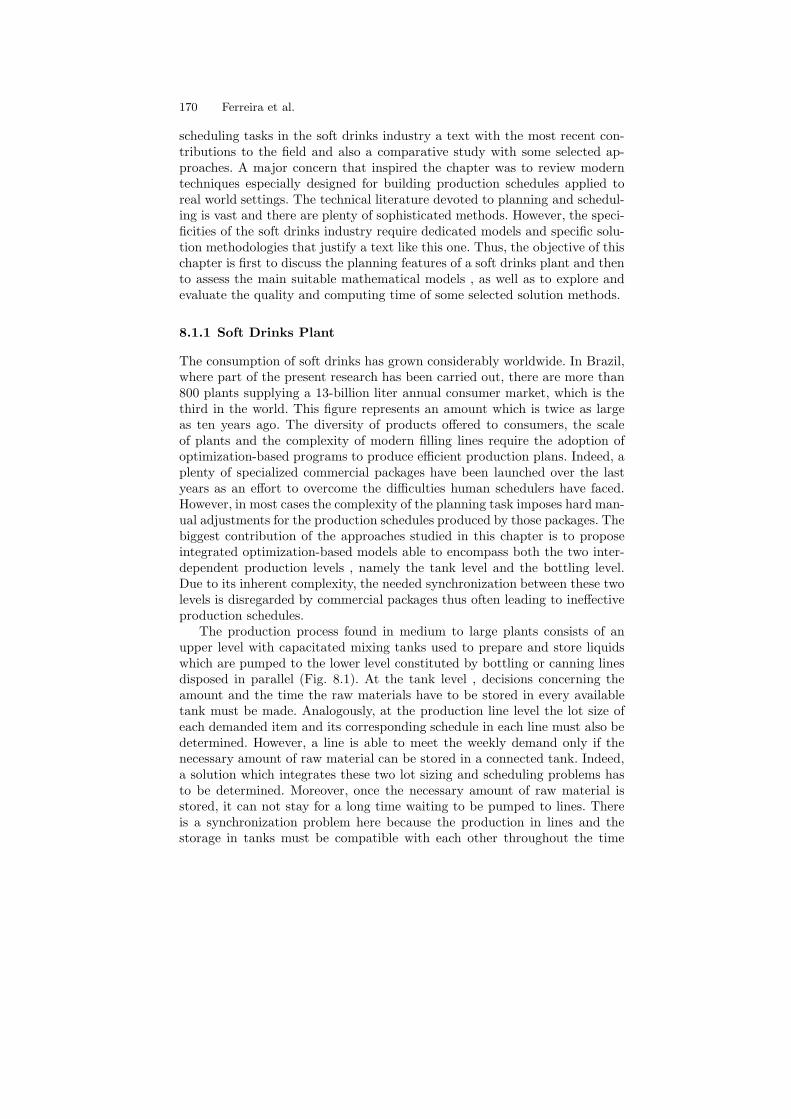
As synchronization is a key feature to be taken into consideration, a deeperexplanation in this respect is now in order. As said before, the lines must waituntil the liquids are ready to be pumped to them. On the other hand, theliquids stored in tanks can not be sent to the lines unless they are ready toinitiate the bottling process. Figure 8.2 illustrates the commitment betweenthe two levels.

P1 P2 P3 P3 P4 P5

xxxxxxxxxxxxxxxxxxxxxxxxxxxxxxxxxxxxxxxxxxxxxxxxxx

xxxxxxxxxxxxxxxxxxxxxxxxxxxxxxxxxxxxxxxxxxxxxxxxxxxxxxxxxxxxxxxxxxxxxxxxxxxxxxxxxxxxxxxxxxxxxxxxxxxxxxxxxxxxxxxxxxxxxxxxxxxxxxxxxxxxxxxxxxxxxxxxxxxxxxxxxxxxxxxxxxxxxxxxxx

xxxxxxxxxxxxxxxxxxxxxxxxxxxxxxxxxxxxxxxxxxxxxxxxxxxxxxxxxxxxxxxxxxxxxxxxxxxxxxxx

xxxxxxxxxxxxxxxxxxxxxxxxxxxxxxxxxxxxxxxxxxxxxxxxxxxxxxxxxxxxxxxxxxxxxxxxxxxxxxxxxxxxxxxxxxxxxxxxxxxxxxxxxxxxxx

xxxxxxxxxxxxxxxxxxxxxxxxxxxxxxxxxxxxxxxxxxxxxxxxxxxxxxx

xxxxxxxxxxxxxxxxxxxxxxxxxxxxxxxxxxxxxxxxxxxxxxxxxxxxxxxxxxxxxxxxxxxxxxxxxxxxxxxxxxxxxxxxxxxxxxxxxxxxxxxxxxxxxxxxxxxxxxxxxxxxxxxxxxxxxxxxxxxxxxxxxxxxxxxxxxxxxxxxxxxxxxxxxx

xxxxxxxxxxxxxxxxxxxxxxxxxxxxxxxxxxxxxxxxxxxxxxxxxxxxxxxxxxxxxxxxxxxxxxxxxxxxxxxx

xxxxxxxxxxxxxxxxxxxxxxxxxxxxxxxxxxxxxxxxxxxxxxxxxxxxxxxxxxxxxxxxxxxxxxxxxxxxxxxxxxxxxxxxxxxxxxxxxxxxxxxxxxxxxx

Micro - 1

rmA

Tank

Line

Micro - 2 Micro - 3 Micro - 4 Micro -5 Micro - 6

rmB rmC rmC rmD rmD

Fig. 8.2: Batches sequenced but not synchronized

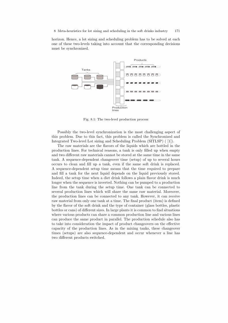
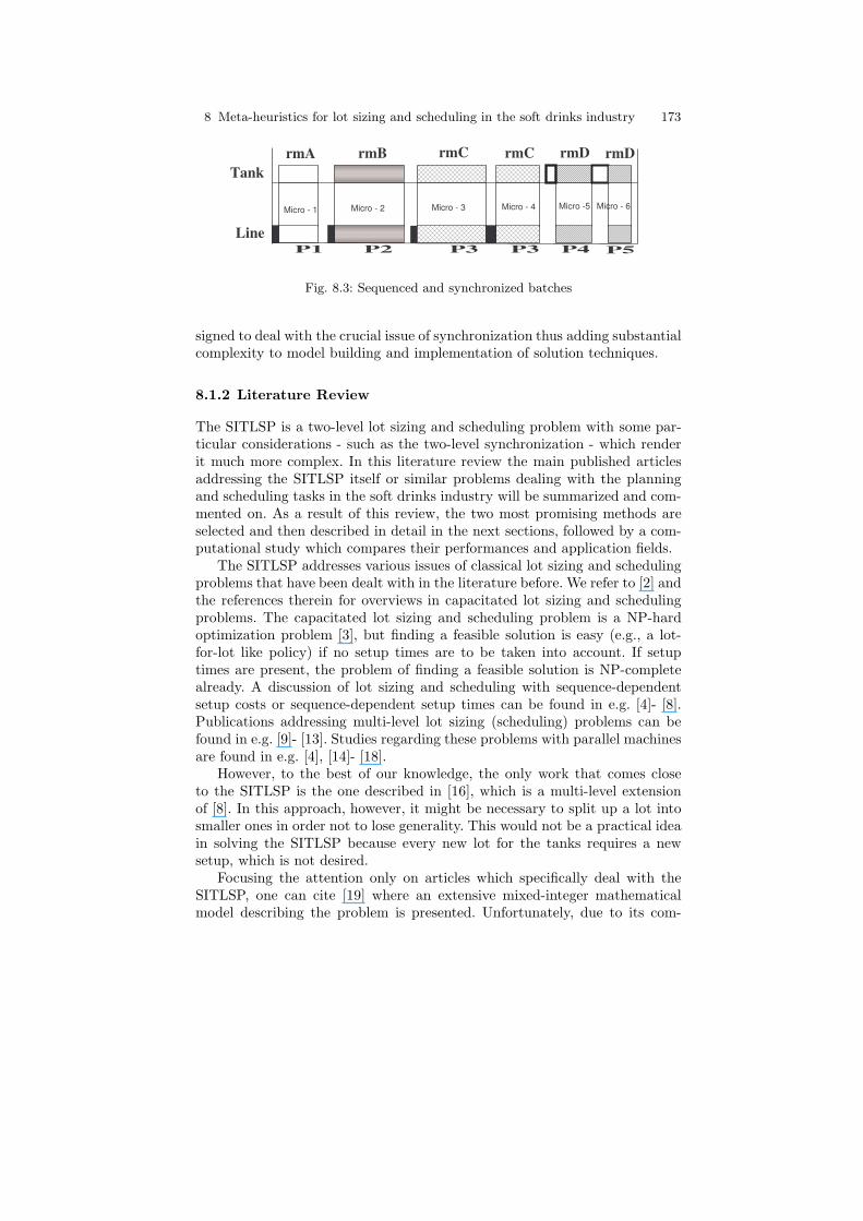
Observe that batches of liquids and items are properly sequenced in thetank and in the line, respectively, but they are not synchronized. The gapsbetween two batches of liquids (rmA, rmB, rmC, rmD) and items (P1, P2,P3, P4, P5) represent given changeover times. The planning horizon is dividedinto 6 micro-periods. Notice that item P3 is produced in both micro-periods3 and 4; it uses the same liquid rmC but needs tank replenishment. Alsoobserve that the same liquid rmD is used in distinct products P4 and P5because they make use of, say, different bottle sizes. Due to the discrepanciesbetween tank and line setup times, the product batches have to be delayed byinserting idle times (black rectangles) in the production line in micro-periods1-4 while the liquid batches must be delayed as well by inserting idle times(empty rectangles) in micro-periods 5 and 6, as shown in Fig. 8.3.

Given that the matter of synchronization has to be treated by postponingbatches, it causes impact on the capacities of tanks and production lines andmay result in infeasible schedules. Therefore, these actions must be consid-ered together with lot sizing and scheduling decisions. Thinking in terms ofmathematical models , they must incorporate decision variables especially de-

8 Meta-heuristics for lot sizing and scheduling in the soft drinks industry 173

Micro - 1

rmA

Tank

Micro - 2 Micro - 3 Micro - 4 Micro -5 Micro - 6

rmB rmC rmC rmD rmD

xxxxxxxxxxxxxxxxxxxxxxxxxxxxxxxxxxxxxxxxxxxxxxxxxxxxxxx

xxxxxxxxxxxxxxxxxxxxxxxxxxxxxxxxxxxxxxxxxxxxxxxxxxxxxxxxxxxxxxxxxxxxxxxxxxxxxxxxxxxxxxxxxxxxxxxxxxxxxxxxxxxxxxxxxxxxxxxxxxxxxxxxxxxxxxxxxxxxxxxxxxxxxxxxxxxxxxxxxx

xxxxxxxxxxxxxxxxxxxxxxxxxxxxxxxxxxxxxxxxxxxxxxxxxxxxxxxxxxxxxxxxxxxxxxxxxxxxxxxx

xxxxxxxxxxxxxxxxxxxxxxxxxxxxxxxxxxxxxxxxxxxxxxxxxxxxxxxxxxxxxxxxxxxxxxxxxxxxxxxxxxxxxxxxxxxxxxxxxxx

P5 P3 P3 P4 P1 P2

xxxxxxxxxxxxxxxxxxxxxxxxxxxxxxxxxxxxxxxxxxxxxxxxxxxxxxx

xxxxxxxxxxxxxxxxxxxxxxxxxxxxxxxxxxxxxxxxxxxxxxxxxxxxxxxxxxxxxxxxxxxxxxxxxxxxxxxxxxxxxxxxxxxxxxxxxxxxxxxxxxxxxxxxxxxxxxxxxxxxxxxxxxxxxxxxxxxxxxxxxxxxxxxxxxxxxxxxxx

xxxxxxxxxxxxxxxxxxxxxxxxxxxxxxxxxxxxxxxxxxxxxxxxxxxxxxxxxxxxxxxxxxxxxxxxxxxxxxxx

xxxxxxxxxxxxxxxxxxxxxxxxxxxxxxxxxxxxxxxxxxxxxxxxxxxxxxxxxxxxxxxxxxxxxxxxxxxxxxxxxxxxxxxx

Line

Fig. 8.3: Sequenced and synchronized batches

signed to deal with the crucial issue of synchronization thus adding substantialcomplexity to model building and implementation of solution techniques.

8.1.2 Literature Review

The SITLSP is a two-level lot sizing and scheduling problem with some par-ticular considerations - such as the two-level synchronization - which renderit much more complex. In this literature review the main published articlesaddressing the SITLSP itself or similar problems dealing with the planningand scheduling tasks in the soft drinks industry will be summarized and com-mented on. As a result of this review, the two most promising methods areselected and then described in detail in the next sections, followed by a com-putational study which compares their performances and application fields.

The SITLSP addresses various issues of classical lot sizing and schedulingproblems that have been dealt with in the literature before. We refer to [2] andthe references therein for overviews in capacitated lot sizing and schedulingproblems. The capacitated lot sizing and scheduling problem is a NP-hardoptimization problem [3], but finding a feasible solution is easy (e.g., a lot-for-lot like policy) if no setup times are to be taken into account. If setuptimes are present, the problem of finding a feasible solution is NP-completealready. A discussion of lot sizing and scheduling with sequence-dependentsetup costs or sequence-dependent setup times can be found in e.g. [4]- [8].Publications addressing multi-level lot sizing (scheduling) problems can befound in e.g. [9]- [13]. Studies regarding these problems with parallel machinesare found in e.g. [4], [14]- [18].

However, to the best of our knowledge, the only work that comes closeto the SITLSP is the one described in [16], which is a multi-level extensionof [8]. In this approach, however, it might be necessary to split up a lot intosmaller ones in order not to lose generality. This would not be a practical ideain solving the SITLSP because every new lot for the tanks requires a newsetup, which is not desired.

Focusing the attention only on articles which specifically deal with theSITLSP, one can cite [19] where an extensive mixed-integer mathematicalmodel describing the problem is presented. Unfortunately, due to its com-

174 Ferreira et al.

plexity and size, the model had to be omitted in this chapter. Instead, a briefexplanation regarding its formulation is given next. The underlying idea tocreate a model for the SITLSP combines issues from the General Lot sizingand Scheduling Problem (GLSP) and the Continuous Setup Lot Sizing Prob-lem (CSLP). A comparison of the CSLP and GLSP and more details aboutthese problems can be found in [2], [20]- [22].

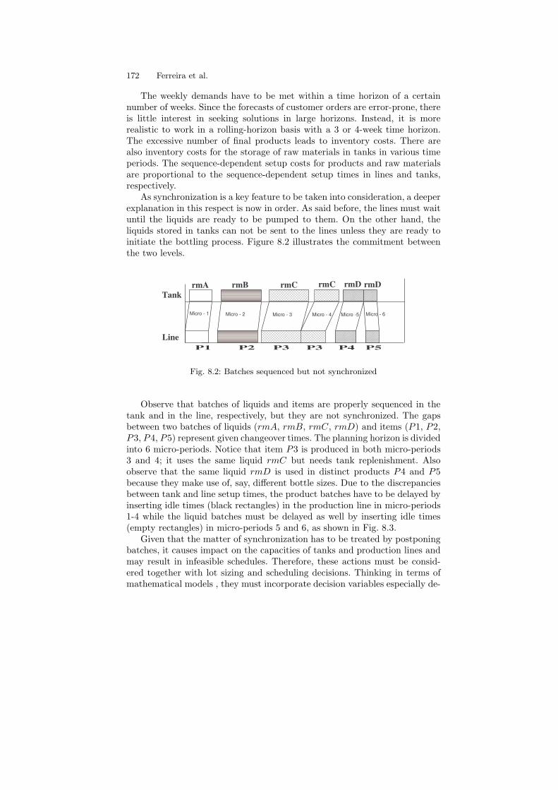
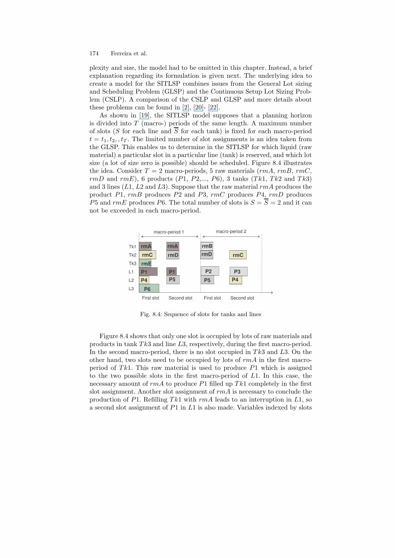
As shown in [19], the SITLSP model supposes that a planning horizonis divided into T (macro-) periods of the same length. A maximum numberof slots (S for each line and S for each tank) is fixed for each macro-periodt = t1, t2, , tT . The limited number of slot assignments is an idea taken fromthe GLSP. This enables us to determine in the SITLSP for which liquid (rawmaterial) a particular slot in a particular line (tank) is reserved, and which lotsize (a lot of size zero is possible) should be scheduled. Figure 8.4 illustratesthe idea. Consider T = 2 macro-periods, 5 raw materials (rmA, rmB, rmC,rmD and rmE), 6 products (P1, P2,..., P6), 3 tanks (Tk1, Tk2 and Tk3)and 3 lines (L1, L2 and L3). Suppose that the raw material rmA produces theproduct P1, rmB produces P2 and P3, rmC produces P4, rmD producesP5 and rmE produces P6. The total number of slots is S = S = 2 and it cannot be exceeded in each macro-period.

xxxxxxxxxxxxxxxxxxxxxxxxxxxxxxxxxxxxxxxxxxxxxxxxxxxxxxxxxxxxxxxxxxxxxx

Tk1

xxxxxxxxxxxxxxxxxxxxxxxxxxxxxxxxxxxxxxxxxxxxxxxxxxxxxxxxxxxxxxxxxxxxxxxxxxxxxxxxxxxxxxxxxxxxxxxxxxxxxxxxxxxxxxxx

Tk2

xxxxxxxxxxxxxxxxxxxxxxxxxxxxxxxxxxxxxxxxxxxxxxxxxxxxxxxxxxxxxxxxxxxxxx

Tk3

L1xxxxxxxxxxxxxxxxxxxxxxxxxxxxxxxxxxxxxxxxxxxxxxxxxxxxxxxxxxxxxxxxxxxxxxxxxxxxxxxxxxxxxxxxxxxxxxxxxxxxxxxxxxxxxxxx

L2

L3xxxxxxxxxxxxxxxxxxxxxxxxxxxxxxxxxxxxxxxxxxxxxxxxxxxxxxxxxxxxxxxxxxxxxxxx xxxxxxxxxxxxxxx

xxxxxxxxxxxxxxxxxxxxxxxxxxxxxxxxxxxxxxxxxxxxxxxxxxxxxxxxxxxxxxxxxxxxxxxxxxxxxxxxxxxxxxxxxx

xxxxxxxxxxxxxxxxxxxxxxxxxxxxxxxxxxxxxxxxxxxxxxxxxxxxxxxxxxxxxxxxxxxxxxxxxxxxxxxxxxxxxxxxxxxxxxxxxxxxxxxxxxxxxxxxxxxxxxxxxxxxxxxxxxxxxxxxxxxxxxxxxxxxxxxxxxxxxxxxxxxxxxxxxxxxxxxxxxxxxxxxxxxxxxxxxxxxxxxxxxxxxxxxxxxxxxxxxxxxxxxxxxxxxxxxxxxxxxxxxxxxxxxxxxxxxxxxxxxxxxxxxxxxxxxxxxxxxxxx

xxxxxxxxxxxxxxxxxxxxxxxxxxxxxxxxxxxxxxxxxxxxxxxxxxxxxxxxxxxxxxxxxxxxxxxxxxxxxxxxxxxxxxxxxxxxxxxxxxxxxxxxxxxxxxxxxxxxxxxxxxxxxxxxxxxxxxxxxxxxxxxxxxxxxxxxxxxxxxxxxxxxxxxxxxxxxxxxxxxxxxxxxxxxxxxxxxxxxxxxxxxxxxxxxxxxxxxxxxxxxxxxxxxxxxxxxxxxxxxxxxxxxxxxxxxxxxxxxxxx

xxxxxxxxxxxxxxxxxxxxxxxxxxxxxxxxxxxxxxxxxxxxxxxxxxxxxxxxxxxxxxxxxxxxxxxxxxxxxxxxxxxxxxxxxxxxxxxxxxxxxxxxxxxxxxxxxxxxxxxxxxxxxxxxxxxxxxxxxxxxxxxxxxxxxxxxxxxxxxxxxxxxxxxxxxxxxxxxxxxxxxxxxxxxxxxxxxxxxxxxxxxxxxxxxxxxxxxxxxxxxxxxxxxxxxxxxxxxxxxxxxxxxxxxxxxxxxxxxxxxxxxxxxxxxxxxxxxxxxxx

xxxxxxxxxxxxxxxxxxxxxxxxxxxxxxxxxxxxxxxxxxxxxxxxxxxxxxxxxxxxxxxxxxxxxxxxxxxxxxxxxxxxxxxxxxxxxxxxxxxxxxxxxxxxxxxxxxxxxxxxxxxxxxxxxxxxxxxxxxxxxxxxxxxxxxxxxxxxxxxxxxxxxxxxxxxxxxxxxxxxxxxxxxxxxxxxxxxxxxxxxxxxxxxxxxxxxxxxxxxxxxxxxxxxxxxxxxxxxxxxxxxxxxxxxxxxxxxxxxxx

xxxxxxxxxxxxxxxxxxxxxxxxxxxxxxxxxxxxxxxxxxxxxxxxxxxxxxxxxxxxxxxxxxxxxxxxxxxxxxxxxxxxxxxxxxxxxxxxxxxxxxxxxxxxxxxx

xxxxxxxxxxxxxxxxxxxxxxxxxxxxxxxxxxxxxxxxxxxxxxxxxxxxxxxxxxxxxxxxxxxxxxxxxxxxxxxxxxxxxxxx

xxxxxxxxxxxxxxxxxxxxxxxxxxxxxxxxxxxxxxxxxxxxxxxxxxxxxxxxxxxxxxxxxxxxxxxxxxxxxxxxxxxxxxxxxxxxxxxxxxxxxxxxxxxxxxxx

macro-period 1 macro-period 2

First slot Second slot First slot Second slot

rmC

rmA rmA rmB

rmCrmD rmD

P4 P4

P1 P1

P5 P5

P6

rmE

P2 P3

Fig. 8.4: Sequence of slots for tanks and lines

Figure 8.4 shows that only one slot is occupied by lots of raw materials andproducts in tank Tk3 and line L3, respectively, during the first macro-period.In the second macro-period, there is no slot occupied in Tk3 and L3. On theother hand, two slots need to be occupied by lots of rmA in the first macro-period of Tk1. This raw material is used to produce P1 which is assignedto the two possible slots in the first macro-period of L1. In this case, thenecessary amount of rmA to produce P1 filled up Tk1 completely in the firstslot assignment. Another slot assignment of rmA is necessary to conclude theproduction of P1. Refilling Tk1 with rmA leads to an interruption in L1, soa second slot assignment of P1 in L1 is also made. Variables indexed by slots

8 Meta-heuristics for lot sizing and scheduling in the soft drinks industry 175

in the SITLSP mathematical model made it possible to write constraints thatintegrate the line and tank occupation ( [1], [19]).

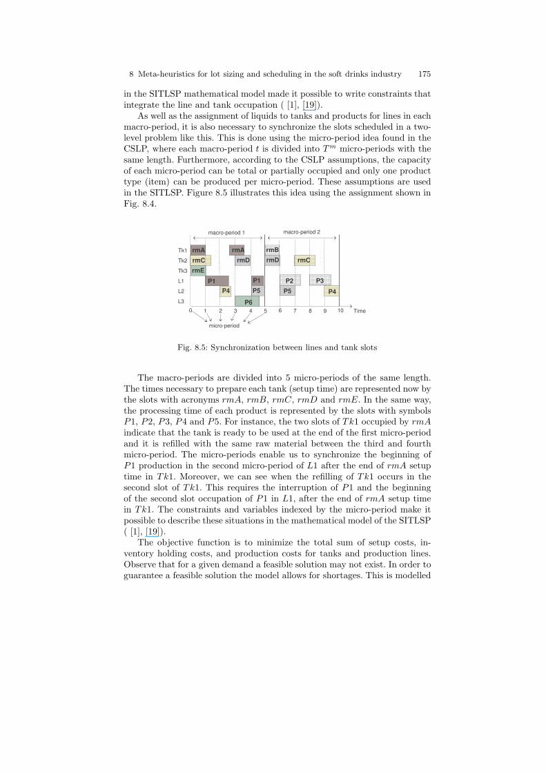
As well as the assignment of liquids to tanks and products for lines in eachmacro-period, it is also necessary to synchronize the slots scheduled in a two-level problem like this. This is done using the micro-period idea found in theCSLP, where each macro-period t is divided into Tm micro-periods with thesame length. Furthermore, according to the CSLP assumptions, the capacityof each micro-period can be total or partially occupied and only one producttype (item) can be produced per micro-period. These assumptions are usedin the SITLSP. Figure 8.5 illustrates this idea using the assignment shown inFig. 8.4.

xxxxxxxxxxxxxxxxxxxxxxxxxxxxxxxxxxxxxxxxxxxxxxxxxxxxxxxxxxxxxxxxxxxxxxxx

Tk1

xxxxxxxxxxxxxxxxxxxxxxxxxxxxxxxxxxxxxxxxxxxxxxxxxxxxxxxxxxxxxxxxxxxxxxxxxxxxxxxxxxxxxxxxxxx

Tk2

xxxxxxxxxxxxxxxxxxxxxxxxxxxxxxxxxxxxxxxxxxxxxxxxxxxxxxxxxxxxxxxxxxxxxx

Tk3

L1xxxxxxxxxxxxxxxxxxxxxxxxxxxxxxxxxxxxxxxxxxxxxxxxxxxxxxxxxxxxxxxxxxxxxxxxxxxxxxxxxxxxxxxxxxxxxxxxxxxxxxxx

L2

L3

0 101 2 3 4 5 6 7 8 9 Time

xxxxxxxxxxxxxxxxxxxxxxxxxxxxxxxxxxxxxxxxxxxxxxxxxxxxxxxxxxxxxxxx xxxxxxxxxxxxxx

xxxxxxxxxxxxxxxxxxxxxxxxxxxxxxxxxxxxxxxxxxxxxxxxxxxxxxxxxxxxxxxxxxxxxxxxxxxxxxxxxxxxxxxxxxxxxxxxxx

xxxxxxxxxxxxxxxxxxxxxxxxxxxxxxxxxxxxxxxxxxxxxxxxxxxxxxxxxxxxxxxxxxxxxxxxxxxxxxxxxxxxxxxxxxxxxxxxxxxxxxxxxxxxxxxxxxxxxxxxxxxxxxxxxxxxxxxxxxxxxxxxxxxxxxxxxxxxxxxxxxxxxxxxxxxxxxxxxxxxxxxxxxxxxxxxxxxxxxxxxxxxxxxxxxxxxxxxxxxxxxxxxxxxxxxxxxxxxxxxxxxxxxx

xxxxxxxxxxxxxxxxxxxxxxxxxxxxxxxxxxxxxxxxxxxxxxxxxxxxxxxxxxxxxxxxxxxxxxxxxxxxxxxxxxxxxxxxxxxxxxxxxxxxxxxxxxxxxxxxxxxxxxxxxxxxxxxxxxxxxxxxxxxxxxxxxxxxxxxxxxxxxxxxxxxxxxxxxxxxxxxxxxxxxxxxxxxxxxxxxxxxxxxxxxxxxxxxxxxxxxxxxxxxxxxxxxxxxxxxxx

xxxxxxxxxxxxxxxxxxxxxxxxxxxxxxxxxxxxxxxxxxxxxxxxxxxxxxxxxxxxxxxxxxxxxxxxxxxxxxxxxxxxxxxxxxxxxxxxxxxxxxxxxxxxxxxxxxxxxxxxxxxxxxxxxxxxxxxxxxxxxxxxxxxxxxxxxxxxxxxxxxxxxxxxxxxxxxxxxxxxxxxxxxxxxxxxxxxxxxxxxxxxxxxxxxxxxxxxxxxxxxxxxxxxxxxxxxxxxxxxxxxxxxx

xxxxxxxxxxxxxxxxxxxxxxxxxxxxxxxxxxxxxxxxxxxxxxxxxxxxxxxxxxxxxxxxxxxxxxxxxxxxxxxxxxxxxxxxxxxxxxxxxxxxxxxxxxxxxxxxxxxxxxxxxxxxxxxxxxxxxxxxxxxxxxxxxxxxxxxxxxxxxxxxxxxxxxxxxxxxxxxxxxxxxxxxxxxxxxxxxxxxxxxxxxxxxxxxxxxxxxxxxxxxxxxxxxxxxxxxxxxxxxxxxxxxxxxxxxxxxxxxxxxxxxxxxx

xxxxxxxxxxxxxxxxxxxxxxxxxxxxxxxxxxxxxxxxxxxxxxxxxxxxxxxxxxxxxxxxxxxxxxxxxxxxxxxxxxxxxxxxxxx

xxxxxxxxxxxxxxxxxxxxxxxxxxxxxxxxxxxxxxxxxxxxxxxxxxxxxxxxxxxxxxxxxxxxxx

xxxxxxxxxxxxxxxxxxxxxxxxxxxxxxxxxxxxxxxxxxxxxxxxxxxxxxxxxxxxxxxxxxxxxxxxxxxxxxxxxxxxxxxxxxxxxxxxxxxxxxxxx

macro-period 1 macro-period 2

micro-period

rmA rmA rmB

rmC rmCrmD rmD

rmE

P1 P1 P2 P3

P4 P4P5 P5

P6

Fig. 8.5: Synchronization between lines and tank slots

The macro-periods are divided into 5 micro-periods of the same length.The times necessary to prepare each tank (setup time) are represented now bythe slots with acronyms rmA, rmB, rmC, rmD and rmE. In the same way,the processing time of each product is represented by the slots with symbolsP1, P2, P3, P4 and P5. For instance, the two slots of Tk1 occupied by rmAindicate that the tank is ready to be used at the end of the first micro-periodand it is refilled with the same raw material between the third and fourthmicro-period. The micro-periods enable us to synchronize the beginning ofP1 production in the second micro-period of L1 after the end of rmA setuptime in Tk1. Moreover, we can see when the refilling of Tk1 occurs in thesecond slot of Tk1. This requires the interruption of P1 and the beginningof the second slot occupation of P1 in L1, after the end of rmA setup timein Tk1. The constraints and variables indexed by the micro-period make itpossible to describe these situations in the mathematical model of the SITLSP( [1], [19]).

The objective function is to minimize the total sum of setup costs, in-ventory holding costs, and production costs for tanks and production lines.Observe that for a given demand a feasible solution may not exist. In order toguarantee a feasible solution the model allows for shortages. This is modelled

176 Ferreira et al.

by allowing every item a certain quantity of units to be “produced” in the firstperiod without using capacity. Naturally, a very high penalty M is attachedto such shortages so that, whenever there is a feasible solution that fulfills alldemands, one would prefer this one.

In short, one can say that the main contribution of the approach used tomodel the SITLSP is to integrate and synchronize two lot sizing and schedul-ing problems. This is done using variables and constraints indexed by slotsand micro-periods. The variables and constraints indexed by slots help to in-tegrate a feasible sequence of occupation in the two levels, while variables andconstraints indexed by micro-periods help to determine a feasible synchro-nization in the two levels within the time horizon. The entire set of variablesand constraints is able to mathematically describe most of the decisions andconstraints present in the industrial problem studied here.

The SITLSP model is coded and solved using the GAMS/CPLEX packagethat uses a branch-and-cut solution approach to find an optimal solution. Forsmall instances the method is fast and reliable but as problem size grows,the number of distinct integer solutions increases exponentially, causing thesearch to take too long even for finding the first integer feasible solution. Thecomputational results in a series of instances with T = 1, 2 , 3 and 4 macro-periods and Tm = 5 micro-periods revealed that for T > 2 the method failedin finding optimal solutions within 1 hour of execution time.

A second paper [23] dealing with the SITLSP introduces an evolutionaryapproach capable of overcoming the limitations faced by the previous method[19] which is not useful to solve real world instances. Being an approximateapproach, optimal solutions are not guaranteed but performance comparisonscarried out in the paper using a set of small instances with known optimalsolutions have shown good behavior in reasonable computing time.

Evolutionary algorithms (EAs) belong to a class of computational meth-ods called bio-inspired systems that simulate biological processes such ascrossover, mutation and natural selection. The simulation of these processesfollows the method when searching for a solution (individual) of a specificproblem. The method begins by analyzing a set of problem solutions (pop-ulation) and determines new solutions applying genetic operators (selection,crossover and mutation) to the previous set of solutions. Some solutions (newor old ones) are selected and form the new set of solutions for the next itera-tion. This procedure is repeated until some stop criterion is satisfied. The firstwork concerning EA was presented by [24] and details on their implementa-tion can be found in [25] and [26]. A memetic algorithm (MA) is a hybridpopulation-based approach [27] which combines the recognized strength ofpopulation methods such as genetic algorithms (GA) with the intensificationcapability of a local search. In a MA, all agents or individuals evolve solutionsuntil they are local minima of a certain neighborhood, i.e. after steps of re-combination and mutation, a local search is applied to the resulting solutions.

The GA presented in [23] proposes a multi-population approach that canbe understood as a variant of island models. The method was developed using

8 Meta-heuristics for lot sizing and scheduling in the soft drinks industry 177

the NP-Opt that is an object-oriented framework written in JAVA code [28].This framework has optimization procedures based on evolutionary computa-tion techniques to address NP-hard problems.

The computational experiments carried out with the GA approach on a setof large instances with up to 12 macro-periods, 10 micro-periods and 15 finalproducts show that the method is able to solve real-world instances. Conse-quently it was one of the approaches selected to take part in the comparisonsusing real data.

Recently another interesting method capable of handling the SITLSP andalso applied to the planning and scheduling of soft drinks has been proposed.Unlike the approach presented in [1] where a highly general (and complex)model is introduced and solved by a commercial MIP package, the MIP modelformulated in [29] is more restricted and amenable to be solved by approxi-mate approaches. Amongst other differences that will be pointed out in detailin Section 8.3, the mathematical formulation is less general than the one pre-sented in [1] as it forces the quantity of tanks to be the same as for the lines.On the other hand it opens up the possibility that a tank can be filled withall liquids needed by its line.

Alternatively from [1], which uses a MIP package for finding optimal so-lutions, the solution approach adopted in [29] relies on different heuristicmethods to obtain approximate production schedules. The details of theseheuristics will be explained fully in the next section.

In [30] a mathematical programming model to deal with the planning of acanning line at a drinks manufacturer is introduced. Compared to the modelspresented in [1] and [29], this one is much more restricted because it disregardsany sequencing considerations when designing production plans. Instead, itfocuses only on planning issues, i.e., lot sizing problems. The MIP modelobjective function minimizes inventories and backorder penalties. The modelallows for different setup times depending on whether the changeover betweencanned products involves a change of liquid or not. However, the model doesnot consider sequence-dependent setup times. Solution strategies consist ofa “lazy” default - simply let an industrial strength branch-and-bound MIPsolver try to find a good solution within a pre-specified amount of time - tomore sophisticated heuristic approaches. One of these that is worth mention-ing is a local search-based metaheuristic which the author called diminishing-neighborhood search (DNS). In this approach one starts the method with thelargest possible neighborhood to avoid bad local optima, and then narrowthe neighborhood in a continuously diminishing way as the search proceedstowards a good solution, even if it is still a non-global optimum. The methodswere tested in real data instances with up to 41 distinct products to be filledfrom 14 different liquids in a planning horizon made up of 13 consecutiveweeks (periods). The final conclusion is that the methods present a classicaltrade off between quality and CPU time with the best results being obtainedby DNS at the expense of 2 hours of computing time. In spite of the inter-esting solution methods and results reported in [30], the approach will not be

178 Ferreira et al.

included in the comparisons mainly due to the more restrictive character ofthe production system for which it was developed.

Closing this introduction, one can conclude that the methods for dealingwith the SITLSP embedded in a soft drinks production planning scenario,and most importantly with potential to be applied in real world situationsin a broad sense, are the EA approaches as the one proposed in [23] and theheuristic model-based method presented in [29]. Therefore, a computationalcomparison involving these two approaches are conducted in a series of prac-tical instances obtained from a large soft drinks manufacturer . One of thepurposes of the comparison is to suggest practical guidance on which methodbest suits the different possible situations found in the industry. The othersections are organized as follows. In Section 8.2 an MA approach based onthe GA developed in [23] is proposed while the methods introduced in [29] arepresented in Section 8.3. Section 8.4 shows the instances used in the compu-tational comparisons and discussions on the test results. Finally, Section 8.5concludes the chapter and discusses some topics for further research.

8.2 Evolutionary Approaches

In this section a memetic version of the GA presented in [23] is proposed tosolve the SITLSP . The term “Memetic Algorithms” [27] [31] (MAs) was intro-duced in the late 80s as a class of meta-heuristics that have the hybridization ofdifferent algorithmic approaches as a crucial aspect in their conceptions. Themajority of the MA applications are population-based approaches in which aset of cooperating and competing agents are engaged in periods of individualimprovement of the solutions while they sporadically interact. The adjective’memetic’ comes from the term ’meme’, coined by Dawkins [32] as an analogyto the term ’gene’ in the context of cultural evolution. It stands for the unitof information which reproduces itself as people exchange ideas. MAs are alsoreferred in the technical literature as ’hybrid genetic algorithms’ and usuallythey take a less sophisticated conception as a combination of GAs with a localsearch procedure applied to some of the individuals in the population.

8.2.1 The MA structure

EAs are global search procedures inspired by biological evolution processes[24] [25]. Amongst the EAs, the GAs are the most popular. A GA differs fromlocal search or constructive heuristics because it has an initial set of solutions(individuals) which have been randomly established. Also called chromosomes,these individuals are solution representations for the problem to be solved. Ateach GA generation, the individual’s fitness is measured and genetic operatorsare executed in the population. These operators are based on genetic behaviorsuch as crossover, mutation and selection. The individuals with better fitness

8 Meta-heuristics for lot sizing and scheduling in the soft drinks industry 179

values remain in the population from one generation to another. MAs and GAshave been applied to solve complex and real-world problems (see [33]- [35]).

The evolutionary methods presented in this section are conceived as amulti-population approach with a hierarchical ternary tree structure. Themulti-population approach was chosen because populations that evolve sep-arately usually have different characteristics according to the genetic driftidea [36]. This can lead to a more effective exploration in the solution spaceof the problem. A better performance of hierarchically structured popula-tions over non-structured population schemes in EAs has been attested inprevious experiments concerning different problems (e.g. machine scheduling,asymmetric travelling salesman, capacitor placement). Computational resultssolving these optimization problems were reported by [18], [28] and [37] using amulti-population GA with a hierarchical ternary tree structure. Furthermore,the authors in [38] reported that the results obtained with the total tardinesssingle machine scheduling problem using GA with hierarchically structuredpopulations are better than the ones with non-structured populations. Thesefindings have been confirmed by the multi-population MA developed to solvethe SITLSP. Moreover, the adoption of the multi-population approach hasenhanced the convergence features of the GA, postponing premature conver-gence and improving its whole effectiveness [23].

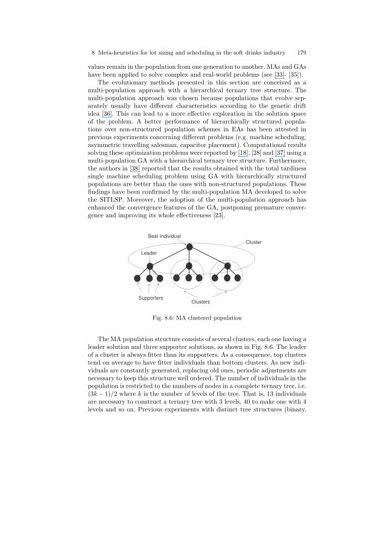
Best Individual

Clusters

Leader

Supporters

Cluster

Fig. 8.6: MA clustered population

The MA population structure consists of several clusters, each one having aleader solution and three supporter solutions, as shown in Fig. 8.6. The leaderof a cluster is always fitter than its supporters. As a consequence, top clusterstend on average to have fitter individuals than bottom clusters. As new indi-viduals are constantly generated, replacing old ones, periodic adjustments arenecessary to keep this structure well ordered. The number of individuals in thepopulation is restricted to the numbers of nodes in a complete ternary tree, i.e.(3k− 1)/2 where k is the number of levels of the tree. That is, 13 individualsare necessary to construct a ternary tree with 3 levels, 40 to make one with 4levels and so on. Previous experiments with distinct tree structures (binary,

180 Ferreira et al.

ternary, etc.) and a variable number of levels (two, three, etc.) attested thatthe best results were obtained by a 3-level ternary tree [6]. Observe that thepopulation is constituted by four distinct clusters, three in the bottom leveland one in the upper level, with four leaders, respectively. The upper levelleader (best individual) is always the fitter individual in the population.

The MA procedure applied to the structured population is summarized inAlgorithm 1. The initial population Pop() is generated and submitted to ageneration loop. Operators recombinePop() and mutatePop() produce a newindividual (or more than one) which is improved by a local search algorithm inoptmizePop(). In structurePop() the population is re-structured to maintainthe hierarchy between agents.

initializePop();repeat

recombinePop();mutatePop();optimizePop();structurePop();

until Termination condition ;Algorithm 1: The MA procedure

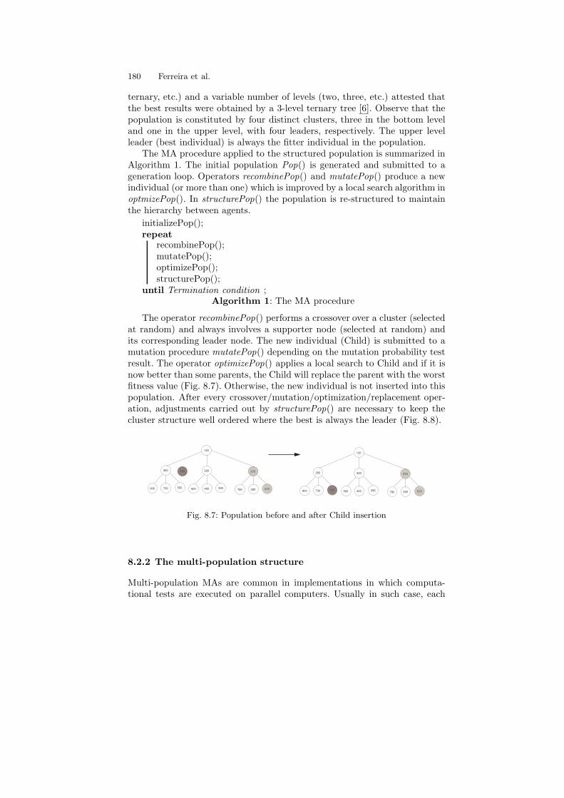
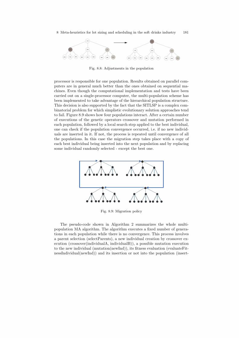
The operator recombinePop() performs a crossover over a cluster (selectedat random) and always involves a supporter node (selected at random) andits corresponding leader node. The new individual (Child) is submitted to amutation procedure mutatePop() depending on the mutation probability testresult. The operator optimizePop() applies a local search to Child and if it isnow better than some parents, the Child will replace the parent with the worstfitness value (Fig. 8.7). Otherwise, the new individual is not inserted into thispopulation. After every crossover/mutation/optimization/replacement oper-ation, adjustments carried out by structurePop() are necessary to keep thecluster structure well ordered where the best is always the leader (Fig. 8.8).

300

395900 400

375

570780 390

350

550800 730

120

110300

395900 400

375

570780 390

350

800 730

120

110

Fig. 8.7: Population before and after Child insertion

8.2.2 The multi-population structure

Multi-population MAs are common in implementations in which computa-tional tests are executed on parallel computers. Usually in such case, each

8 Meta-heuristics for lot sizing and scheduling in the soft drinks industry 181

300

395900 400

375

570780 390350800 730

120

110300

395900 400

375

570780 390350800 730

120

110

Fig. 8.8: Adjustments in the population

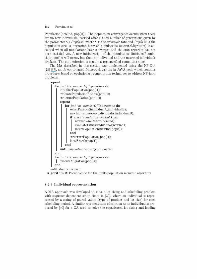
processor is responsible for one population. Results obtained on parallel com-puters are in general much better than the ones obtained on sequential ma-chines. Even though the computational implementation and tests have beencarried out on a single-processor computer, the multi-population scheme hasbeen implemented to take advantage of the hierarchical population structure.This decision is also supported by the fact that the SITLSP is a complex com-binatorial problem for which simplistic evolutionary solution approaches tendto fail. Figure 8.9 shows how four populations interact. After a certain numberof executions of the genetic operators crossover and mutation performed ineach population, followed by a local search step applied to the best individual,one can check if the population convergence occurred, i.e. if no new individ-uals are inserted in it. If not, the process is repeated until convergence of allthe populations. In this case the migration step takes place with a copy ofeach best individual being inserted into the next population and by replacingsome individual randomly selected - except the best one.

Fig. 8.9: Migration policy

The pseudo-code shown in Algorithm 2 summarizes the whole multi-population MA algorithm. The algorithm executes a fixed number of genera-tions in each population while there is no convergence. This process involvesa parent selection (selectParents), a new individual creation by crossover ex-ecution (crossover(individualA, individualB)), a possible mutation executionto the new individual (mutation(newInd)), its fitness evaluation (evaluateFit-nessIndividual(newInd)) and its insertion or not into the population (insert-

182 Ferreira et al.

Population(newInd, pop(i))). The population convergence occurs when thereare no new individuals inserted after a fixed number of generations given bythe parameter γ ∗ PopSize, where γ is the crossover rate and PopSize is thepopulation size. A migration between populations (executeMigration) is ex-ecuted when all populations have converged and the stop criterion has notbeen satisfied yet. A new initialization of the populations (initializePopula-tion(pop(i))) will occur, but the best individual and the migrated individualsare kept. The stop criterion is usually a pre-specified computing time.

The MA described in this section was implemented using the NP-Opt[28] [37], an object-oriented framework written in JAVA code which containsprocedures based on evolutionary computation techniques to address NP-hardproblems.

repeatfor i=1 to numberOfPopulations do

initializePopulation(pop(i));evaluatePopulationFitness(pop(i));structurePopulation(pop(i));repeat

for j=1 to numberOfGenerations doselectParents(individualA,individualB);newInd=crossover(individualA,individualB);if execute mutation newInd then

newInd=mutation(newInd);evaluateFitnessIndividual(newInd);insertPopulation(newInd,pop(i));

endstructurePopulation(pop(i));localSearch(pop(i));

end

until populationConvergence pop(i) ;

endfor i=1 to numberOfPopulations do

executeMigration(pop(i));end

until stop criterion ;Algorithm 2: Pseudo-code for the multi-population memetic algorithm

8.2.3 Individual representation

A MA approach was developed to solve a lot sizing and scheduling problemwith sequence-dependent setup times in [39], where an individual is repre-sented by a string of paired values (type of product and lot size) for eachscheduling period. A similar representation of solution as an individual is pro-posed by [40] for a GA used to solve the capacitated lot sizing and loading

8 Meta-heuristics for lot sizing and scheduling in the soft drinks industry 183

problem with setup times, parallel facilities and overtime. In this approach,the individual is also a string of paired values, where the first value is thelot size and the second is the facility. A GA with more elaborated solutionrepresentation is proposed by [41], where a binary matrix PxT (P productsand T periods) represents an individual for the multi-level lot sizing problem.Each binary entry yi,t = 1, if a setup for product i occurs in t; otherwiseyi,t = 0. All the GA publications mentioned have specific genetic operators.Their crossover, mutation and selection procedures were designed to deal withthose individual representations for lot size and scheduling problems.

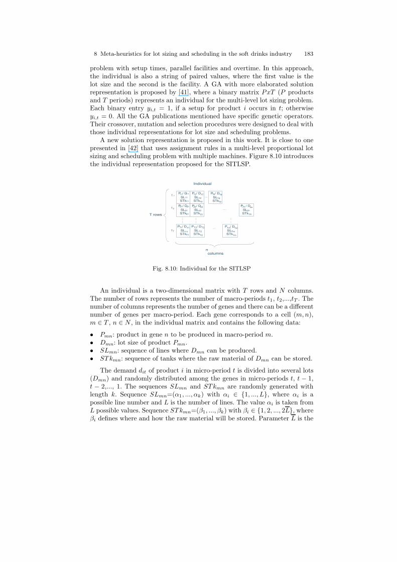
A new solution representation is proposed in this work. It is close to onepresented in [42] that uses assignment rules in a multi-level proportional lotsizing and scheduling problem with multiple machines. Figure 8.10 introducesthe individual representation proposed for the SITLSP.

Individual

P / D

SL

STk

- - -

- - -

---

11 11

11

11

P / D

SLSTk

21 21

21

21

P / D

SLSTk

::

P / D

SLSTk

12 12

12

12

P / D

SLSTk

22 22

22

22

P / D

SL

STk

::

P / D

SLSTk

1p 1p

1p

1p

P / D

SLSTk 2n

P / D

SLSTk

::

t

t 2

1

t T

Tm

T1 T1

T1

T1

T2 T2

T2

T2

Tm Tm

Tm

columnsn

rowsT

2n 2n

2n

Fig. 8.10: Individual for the SITLSP

An individual is a two-dimensional matrix with T rows and N columns.The number of rows represents the number of macro-periods t1, t2,...,tT . Thenumber of columns represents the number of genes and there can be a differentnumber of genes per macro-period. Each gene corresponds to a cell (m,n),m ∈ T , n ∈ N , in the individual matrix and contains the following data:

• Pmn: product in gene n to be produced in macro-period m.• Dmn: lot size of product Pmn.• SLmn: sequence of lines where Dmn can be produced.• STkmn: sequence of tanks where the raw material of Dmn can be stored.

The demand dit of product i in micro-period t is divided into several lots(Dmn) and randomly distributed among the genes in micro-periods t, t − 1,t − 2,..., 1. The sequences SLmn and STkmn are randomly generated withlength k. Sequence SLmn=(α1, ..., αk) with αi ∈ {1, ..., L}, where αi is apossible line number and L is the number of lines. The value αi is taken fromL possible values. Sequence STkmn=(β1, ..., βk) with βi ∈ {1, 2, ..., 2L}, whereβi defines where and how the raw material will be stored. Parameter L is the

184 Ferreira et al.

number of tanks. The βi is taken from 2L possible values, but the real tanknumber j is obtained from βi using:

j =

{βi, 1 ≤ βi ≤ L;βi − L, L < βi ≤ 2L.

(8.1)

If 1 ≤ βi ≤ L, the tank j = i will be occupied after the raw materialpreviously stored has been used. This forces the method to find solutionswhere there is a partial use of the tank capacity. If L < βi ≤ 2L, the tankj = βi − L will be immediately occupied. This forces the method to findsolutions where the tank capacity is completely used. These conditions havesome exceptions. If tank j, selected by one of the previous criterions, storesa raw material different from the raw material of the product Pmn, it will benecessarily occupied after the raw material which was previously stored hasbeen used. The same will happen if tank j is completely full. On the otherhand, if tank j is empty, it will be immediately occupied. If j is not empty, butthe raw material stored is the same as Pmn and the minimum tank capacity hasnot been satisfied, this tank will be also occupied immediately. The individualsin each initial population are generated following the pseudo-code illustratedin Algorithm 3. There are T macro-periods, J products, L lines and L tanks.The variable Dem receives the total demand dPi,t of product Pi in the macro-period t. This demand is randomly divided and distributed among the genes.At this point, the sequences of lines (SLmn) and tanks (STkmn) are alsorandomly generated.

8 Meta-heuristics for lot sizing and scheduling in the soft drinks industry 185

for t = t1, t2, ..., tT dorepeat

Select a product Pi ∈ {P1, P2, ..., PJ} randomly with dPi,t > 0;Set Dem=dPi,t;while Dem > 0 do

Select the matrix row m ∈ {t1, t2, ..., t} of the individualrandomly;Determine n as the first gene available in line m of theindividual;Determine Dm,n 6= 0 with Dm,n ∈ [0, Dem] randomlygenerated;Insert Dm,n and Pi in the gene position (m,n) of theindividual;Generate SLm,n = (α1, ..., αk) with ai ∈ {1, ..., L} randomlyselected;Generate STkm,n = (β1, ..., βk) with βi ∈ {1, ..., 2L}randomly selected;Set Dem = Dem−Dm,n;

end

until All demands have been distributed among the genes ;

endAlgorithm 3: Individual initialization algorithm

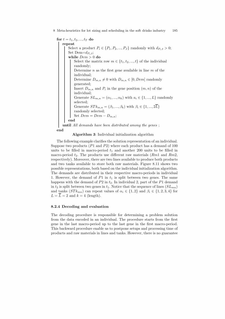
The following example clarifies the solution representation of an individual.Suppose two products (P1 and P2) where each product has a demand of 100units to be filled in macro-period t1 and another 200 units to be filled inmacro-period t2. The products use different raw materials (Rm1 and Rm2,respectively). Moreover, there are two lines available to produce both productsand two tanks available to store both raw materials. Figure 8.11 shows twopossible representations, both based on the individual initialization algorithm.The demands are distributed in their respective macro-periods in individual1. However, the demand of P1 in t1 is split between two genes. The samehappens with the demand of P2 in t2. In individual 2, part of the P1 demandin t2 is split between two genes in t1. Notice that the sequence of lines (SLmn)and tanks (STkmn) can repeat values of αi ∈ {1, 2} and βi ∈ {1, 2, 3, 4} forL = L = 2 and k = 4 (length).

8.2.4 Decoding and evaluation

The decoding procedure is responsible for determining a problem solutionfrom the data encoded in an individual. The procedure starts from the firstgene in the last macro-period up to the last gene in the first macro-period.This backward procedure enable us to postpone setups and processing time ofproducts and raw materials in lines and tanks. However, there is no guarantee

186 Ferreira et al.

P1

t 1 /50 P1

/100 P2 /50

P2

t 2 /100 P2 /100

Individual 1

2 1 2 2 3 3 2 4

1 1 2 14 3 1 2

2 1 1 13 1 2 3

2 2 1 2 3 1 4 4

2 1 1 2 1 2 4 2

P1 /200

1 1 2 2 4 2 3 4

P1

t 1 /50 P1 /100 P

2/100

P2

t 2 /200P1/100

Individual 2

1 1 2 2 1 3 2 4

1 1 2 14 3 1 2

1 1 1 14 1 2 3

2 2 1 2 3 1 4 4

2 1 1 2 1 2 4 2

1P /50

1 1 1 14 1 2 3

Fig. 8.11: Two possible individuals

that all demands will be produced at the end and a penalty in the fitness istaken into account for that.

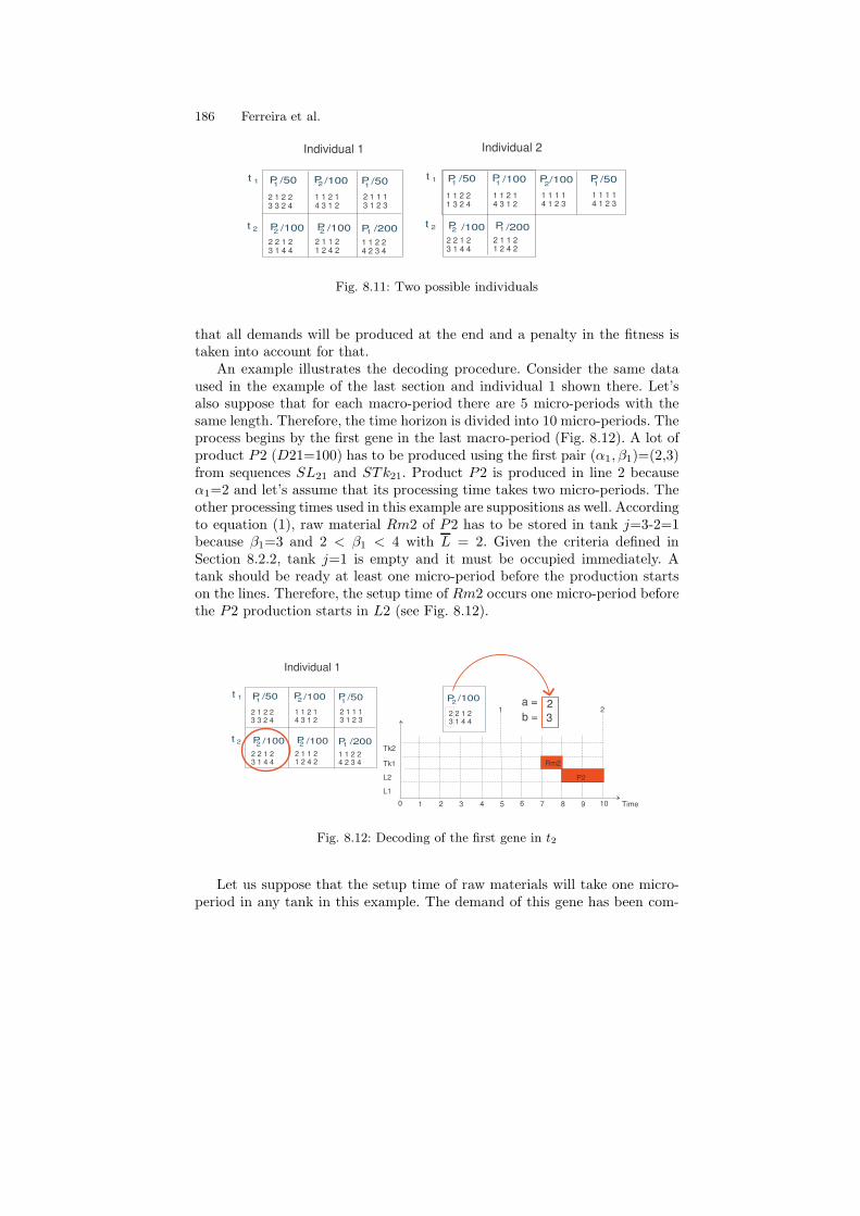
An example illustrates the decoding procedure. Consider the same dataused in the example of the last section and individual 1 shown there. Let’salso suppose that for each macro-period there are 5 micro-periods with thesame length. Therefore, the time horizon is divided into 10 micro-periods. Theprocess begins by the first gene in the last macro-period (Fig. 8.12). A lot ofproduct P2 (D21=100) has to be produced using the first pair (α1, β1)=(2,3)from sequences SL21 and STk21. Product P2 is produced in line 2 becauseα1=2 and let’s assume that its processing time takes two micro-periods. Theother processing times used in this example are suppositions as well. Accordingto equation (1), raw material Rm2 of P2 has to be stored in tank j=3-2=1because β1=3 and 2 < β1 < 4 with L = 2. Given the criteria defined inSection 8.2.2, tank j=1 is empty and it must be occupied immediately. Atank should be ready at least one micro-period before the production startson the lines. Therefore, the setup time of Rm2 occurs one micro-period beforethe P2 production starts in L2 (see Fig. 8.12).

Tk2

Tk1

L2

L1

0 101 2 3 4 5 6 7 8 9 Time

1

P2/100

2

3

P2

2a =

b =

Rm2

2 2 1 2 3 1 4 4

P1

t 1 /50 P1

/100 P2 /50

P2

t 2 /100 P2 /100

Individual 1

2 1 2 2 3 3 2 4

1 1 2 14 3 1 2

2 1 1 13 1 2 3

2 2 1 2 3 1 4 4

2 1 1 2 1 2 4 2

P1 /200

1 1 2 2 4 2 3 4

Fig. 8.12: Decoding of the first gene in t2

Let us suppose that the setup time of raw materials will take one micro-period in any tank in this example. The demand of this gene has been com-

8 Meta-heuristics for lot sizing and scheduling in the soft drinks industry 187

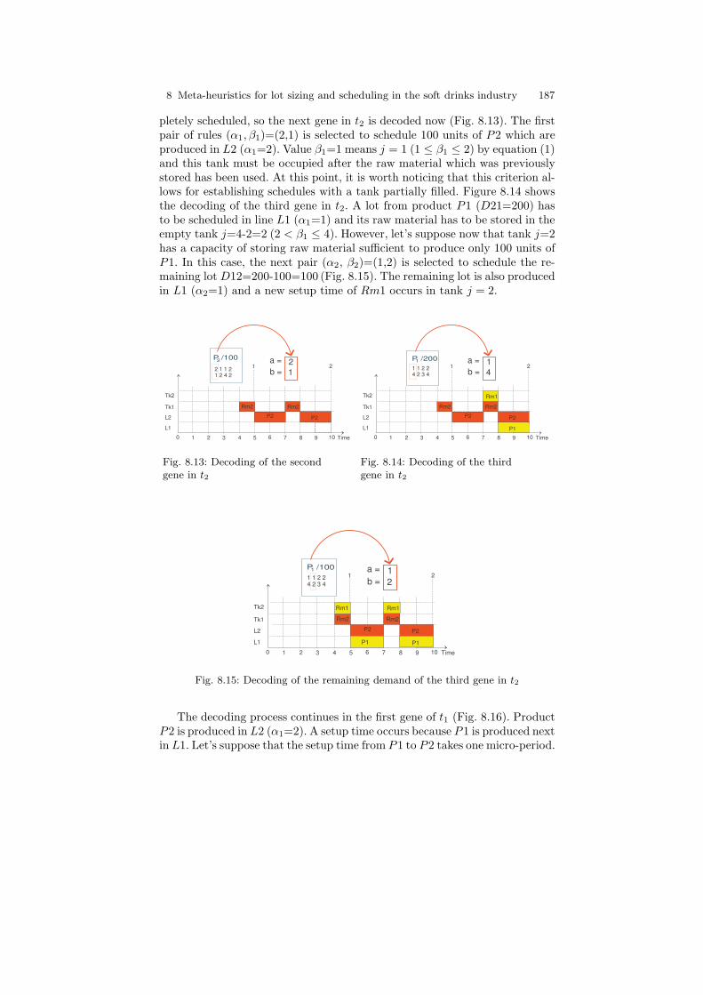
pletely scheduled, so the next gene in t2 is decoded now (Fig. 8.13). The firstpair of rules (α1, β1)=(2,1) is selected to schedule 100 units of P2 which areproduced in L2 (α1=2). Value β1=1 means j = 1 (1 ≤ β1 ≤ 2) by equation (1)and this tank must be occupied after the raw material which was previouslystored has been used. At this point, it is worth noticing that this criterion al-lows for establishing schedules with a tank partially filled. Figure 8.14 showsthe decoding of the third gene in t2. A lot from product P1 (D21=200) hasto be scheduled in line L1 (α1=1) and its raw material has to be stored in theempty tank j=4-2=2 (2 < β1 ≤ 4). However, let’s suppose now that tank j=2has a capacity of storing raw material sufficient to produce only 100 units ofP1. In this case, the next pair (α2, β2)=(1,2) is selected to schedule the re-maining lot D12=200-100=100 (Fig. 8.15). The remaining lot is also producedin L1 (α2=1) and a new setup time of Rm1 occurs in tank j = 2.

Tk2

Tk1

L2

L1

0 101 2 3 4 5 6 7 8 9 Time

1

P2/100

2

1

P2

2a =

b =

Rm2

2 1 1 2 1 2 4 2

P2

Rm2

Fig. 8.13: Decoding of the secondgene in t2

Tk2

Tk1

L2

L1

0 101 2 3 4 5 6 7 8 9 Time

11

4

P2

2a =

b =

Rm2

P2

Rm2

P1 /200

1 1 2 2 4 2 3 4

P1

Rm1

Fig. 8.14: Decoding of the thirdgene in t2

Tk2

Tk1

L2

L1

0 101 2 3 4 5 6 7 8 9 Time

11

2

P2

2a =

b =

Rm2

P2

Rm2

P1 /100

1 1 2 2 4 2 3 4

P1

Rm1

P1

Rm1

Fig. 8.15: Decoding of the remaining demand of the third gene in t2

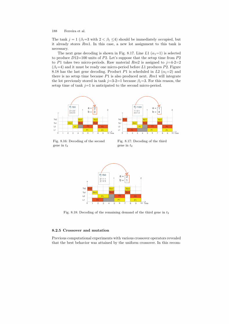
The decoding process continues in the first gene of t1 (Fig. 8.16). ProductP2 is produced in L2 (α1=2). A setup time occurs because P1 is produced nextin L1. Let’s suppose that the setup time from P1 to P2 takes one micro-period.

188 Ferreira et al.

The tank j = 1 (β1=3 with 2 < β1 ≤4) should be immediately occupied, butit already stores Rm1. In this case, a new lot assignment to this tank isnecessary.

The next gene decoding is shown in Fig. 8.17. Line L1 (α1=1) is selectedto produce D12=100 units of P2. Let’s suppose that the setup time from P2to P1 takes two micro-periods. Raw material Rm2 is assigned to j=4-2=2(β1=4) and it must be ready one micro-period before L1 produces P2. Figure8.18 has the last gene decoding. Product P1 is scheduled in L2 (α1=2) andthere is no setup time because P1 is also produced next. Rm1 will integratethe lot previously stored in tank j=3-2=1 because β1=3. For this reason, thesetup time of tank j=1 is anticipated to the second micro-period.

Tk2

Tk1

L2

L1

0 101 2 3 4 5 6 7 8 9 Time

12

3

P2

2a =

b =

Rm2

P2

Rm2

P1

Rm1

P1

Rm1

Rm1

P1

P /501

2 1 2 23 3 2 4

xxxxxxxxxxxxxxxxxxxxxxxxxxxxxxxxxxxxxxxxxxxxxxxxxxxxxxxxxxxxxxxxxxxxxxxxxxxxxxxxxxxxxxxxxxxxxxxxxxxxxxxxxxxxxxxxxxxxxxxxxxxxxxxxxxxxxxxxxxxxxxxxxxxxxxxxxxxxxxxxxxxxxxxxxxxxxxxxxxxxxxxxxxxxxxxxxxxxxxxxxxxxxxxxxxxxxxxxxxxxxxxxxxxxxxxxxxxxxxxxxxxxxxxxxxxxxxxxxxxxxxxxxx

Fig. 8.16: Decoding of the secondgene in t2

Tk2

Tk1

L2

L1

0 101 2 3 4 5 6 7 8 9 Time

11

4

P2

2a =

b =

Rm2

P2

Rm2

P1

Rm1

P1

Rm1

Rm1

P1

P /1002

1 1 2 14 3 1 2

Rm2

P2xxxxxxxxxxxxxxxxxxxxxxxxxxxxxxxxxxxxxxxxxxxxxxxxxxxxxxxxxxxxxxxxxxxxxxxxxxxxxxxxxxxxxxxxxxxxxxxxxxxxxxxxxxxxxxxxxxxxxxxxxxxxxxxxxxxxxxxxxxxxxxxxxxxxxxxxxxxxxxxxxxxxxxxxxxxxxxxxxxxxxxxxxxxxxxxxxxxxxxxxxxxxxxxxxxxxxxxxxxxxxxxxxxxxxxxxxxxxxxxxxxxxxxxxxxxxxxxxxxxxxxxxxxxxxxxxxxxxxxxxxxxxxxxxxxxxxxxxxxxxxxxxxxxxxxxxxxxxxxxxxxxxxxxxxxxxxxxxxxxxxxxxxxxxxxxxxxxxxxxxxxxxxxxxxxxxxxxxxxxxxxxxxxxxxxxxxxxxxxxxxxxxxxxxxxxxxxxxxxxxxxxxxxxxxxxxxxxxxxxxxxxxxxxxxxxxxxxxxxxxxxxxxxxxxxxxxxxxxxxxxxxxxxxxxxxxxxxxxxxxxxxxxxxxxxxxxxxxxxxxxxxxxxxxxxxxxxxxxxxxxxxxxxxxxxxxxxxxxxxxxxxxx

xxxxxxxxxxxxxxxxxxxxxxxxxxxxxxxxxxxxxxxxxxxxxxxxxxxxxxxxxxxxxxxxxxxxxxxxxxxxxxxxxxxxxxxxxxxxxxxxxxxxxxxxxxxxxxxxxxxxxxxxxxxxxxxxxxxxxxxxxxxxxxxxxxxxxxxxxxxxxxxxxxxxxxxxxxxxxxxxxxxxxxxxxxxxxxxxxxxxxxxxxxxxxxxxxxxxxxxxxxxxxxxxxxxxxxxxxxxxxxxxxxxxxxx

Fig. 8.17: Decoding of the thirdgene in t2

Tk2

Tk1

L2

L1

0 101 2 3 4 5 6 7 8 9 Time

12

1

P2

2a =

b =

Rm2

P2

Rm2

P1

Rm1

P1

Rm1

Rm1

P1

Rm2

P2xxxxxxxxxxxxxxxxxxxxxxxxxxxxxxxxxxxxxxxxxxxxxxxxxxxxxxxxxxxxxxxxxxxxxxxxxxxxxxxxxxxxxxxxxxxxxxxxxxxxxxxxxxxxxxxxxxxxxxxxxxxxxxxxxxxxxxxxxxxxxxxxxxxxxxxxxxxxxxxxxxxxxxxxxxxxxxxxxxxxxxxxxxxxxxxxxxxxxxxxxxxxxxxxxxxxxxxxxxxxxxxxxxxxxxxxxxxxxxxxxxxxxxxxxxxxxxxxxxxxxxxxxxxxxxxxxxxxxxxxxxxxxxxxxxxxxxxxxxxxxxxxxxxxxxxxxxxxxxxxxxxxxxxxxxxxxxxxxxxxxxxxxxxxxxxxxxxxxxxxxxxxxxxxxxxxxxxxxxxxxxxxxxxxxxxxxxxxxxxxxxxxxxxxxxxxxxxxxxxxxxxxxxxxxxxxxxxxxxxxxxxxxxxxxxxxxxxxxxxxxxxxxxxxxxxxxxxxxxxxxxxxxxxxxxxxxxxxxxxx

xxxxxxxxxxxxxxxxxxxxxxxxxxxxxxxxxxxxxxxxxxxxxxxxxxxxxxxxxxxxxxxxxxxxxxxxxxxxxxxxxxxxxxxxxxxxxxxxxxxxxxxxxxxxxxxxxxxxxxxxxxxxxxxxxxxxxxxxxxxxxxxxxxxxxxxxxxxxxxxxxxxxxxxxxxxxxxxxxxxxxxxxxxxxxxxxxxxxxxxxxxxxxxxxxxxxxxxxxxxxxxxxxxxx

1P /50

2 1 1 13 1 2 3

Fig. 8.18: Decoding of the remaining demand of the third gene in t2

8.2.5 Crossover and mutation

Previous computational experiments with various crossover operators revealedthat the best behavior was attained by the uniform crossover. In this recom-

8 Meta-heuristics for lot sizing and scheduling in the soft drinks industry 189

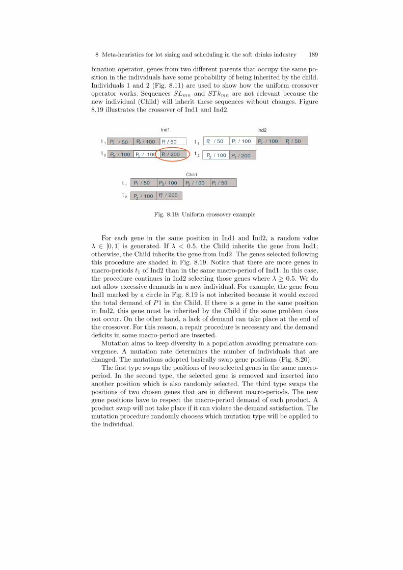
bination operator, genes from two different parents that occupy the same po-sition in the individuals have some probability of being inherited by the child.Individuals 1 and 2 (Fig. 8.11) are used to show how the uniform crossoveroperator works. Sequences SLmn and STkmn are not relevant because thenew individual (Child) will inherit these sequences without changes. Figure8.19 illustrates the crossover of Ind1 and Ind2.

P1 / 50 P2 / 100 P2 / 100 P1 / 50

P2

/ 100

P1 2 P2 | 1 P2 2 P1

P / 100

P / 50 P1 / 100 P2 / 100 P1 / 50

2

P / 100 P /

P2 P2

P / 501 / 50

/ 100

1

/ 100

2

Ind1 Ind2

Child

t 1

t2

t 1

t2

t 1

t2

/ 200P1

/ 200P1

P /1 / 200

1

Fig. 8.19: Uniform crossover example

For each gene in the same position in Ind1 and Ind2, a random valueλ ∈ [0, 1] is generated. If λ < 0.5, the Child inherits the gene from Ind1;otherwise, the Child inherits the gene from Ind2. The genes selected followingthis procedure are shaded in Fig. 8.19. Notice that there are more genes inmacro-periods t1 of Ind2 than in the same macro-period of Ind1. In this case,the procedure continues in Ind2 selecting those genes where λ ≥ 0.5. We donot allow excessive demands in a new individual. For example, the gene fromInd1 marked by a circle in Fig. 8.19 is not inherited because it would exceedthe total demand of P1 in the Child. If there is a gene in the same positionin Ind2, this gene must be inherited by the Child if the same problem doesnot occur. On the other hand, a lack of demand can take place at the end ofthe crossover. For this reason, a repair procedure is necessary and the demanddeficits in some macro-period are inserted.

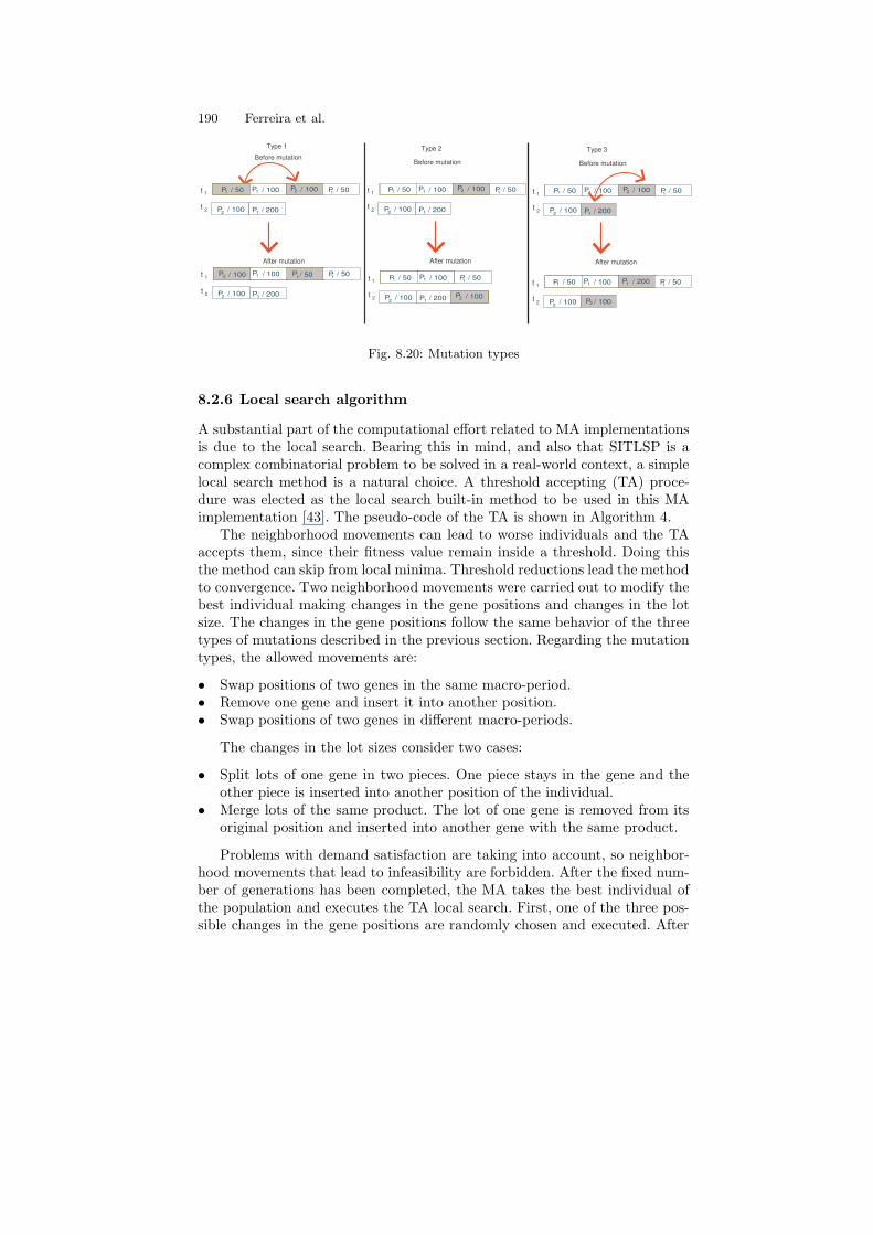
Mutation aims to keep diversity in a population avoiding premature con-vergence. A mutation rate determines the number of individuals that arechanged. The mutations adopted basically swap gene positions (Fig. 8.20).

The first type swaps the positions of two selected genes in the same macro-period. In the second type, the selected gene is removed and inserted intoanother position which is also randomly selected. The third type swaps thepositions of two chosen genes that are in different macro-periods. The newgene positions have to respect the macro-period demand of each product. Aproduct swap will not take place if it can violate the demand satisfaction. Themutation procedure randomly chooses which mutation type will be applied tothe individual.

190 Ferreira et al.

After mutation

Before mutation

Type 1

1 2 P2 | 1 P2 2 P1

P / 100

P / 100P2 / 100 P1 / 50

2

t 1

t2 / 200P1

1P1/ 50

1 2 P2 | 1 P2 2 P1

P / 100

P / 100 P2 / 100 P1 / 50

2

t 1

t2 / 200P1

1P1 / 50

After mutation

Before mutation

Type 2

1 2 P2 | 1 P2 2 P1

P / 100

P / 100 P2 / 100 P1 / 50

2

t 1

t2 / 200P1

1P1 / 50

1 2 P2 | 1 P1

P / 100

P / 100 P1 / 50

2

t 1

t2 / 200P1

1P1 / 50

P2 2P2 / 100

After mutation

Before mutation

Type 3

1 2 P2 | 1 P2 2 P1

P / 100

P / 100 P2 / 100 P1 / 50

2

t 1

t2 / 200P1

1P1 / 50

1 2 P2 | 1 P2 2 P1

P / 100

P / 100 / 200 P1 / 50

2

t 1

t2 / 100

P1 1P1 / 50

P2

Fig. 8.20: Mutation types

8.2.6 Local search algorithm

A substantial part of the computational effort related to MA implementationsis due to the local search. Bearing this in mind, and also that SITLSP is acomplex combinatorial problem to be solved in a real-world context, a simplelocal search method is a natural choice. A threshold accepting (TA) proce-dure was elected as the local search built-in method to be used in this MAimplementation [43]. The pseudo-code of the TA is shown in Algorithm 4.

The neighborhood movements can lead to worse individuals and the TAaccepts them, since their fitness value remain inside a threshold. Doing thisthe method can skip from local minima. Threshold reductions lead the methodto convergence. Two neighborhood movements were carried out to modify thebest individual making changes in the gene positions and changes in the lotsize. The changes in the gene positions follow the same behavior of the threetypes of mutations described in the previous section. Regarding the mutationtypes, the allowed movements are:

• Swap positions of two genes in the same macro-period.• Remove one gene and insert it into another position.• Swap positions of two genes in different macro-periods.

The changes in the lot sizes consider two cases:

• Split lots of one gene in two pieces. One piece stays in the gene and theother piece is inserted into another position of the individual.

• Merge lots of the same product. The lot of one gene is removed from itsoriginal position and inserted into another gene with the same product.

Problems with demand satisfaction are taking into account, so neighbor-hood movements that lead to infeasibility are forbidden. After the fixed num-ber of generations has been completed, the MA takes the best individual ofthe population and executes the TA local search. First, one of the three pos-sible changes in the gene positions are randomly chosen and executed. After

8 Meta-heuristics for lot sizing and scheduling in the soft drinks industry 191

a maximum number of iterations, the TA stops and restarts executing nowchanges in the lot sizes. Moreover, the two possible changes in the lot sizesare randomly chosen and executed over randomly selected genes. In the end,if a better individual is obtained, it is inserted as the new best individual ofthis population.

individual=bestIndividual;repeat

newIndividual = moveExecution(individual);∆f=fitness(Individual)-fitness(newIndividual);if ∆f > −Th∗fitness(individual) then

individual = newIndividual;else

reduce(Th);end

until maxNumberOfIteration ;Algorithm 4: Local search procedure

The MA as conceived here transforms itself into a GA simply by the delet-ing the local search procedure. Although our experience with previous researchhas demonstrated that in most cases the MA versions outperform their GAversions, a comparison within a fixed amount of time will be carried out inSection 8.4. The underlying issue under consideration is whether the timespent by the local search executions in the MA is favorably used to reachbetter solutions or if it could be used better by the GA version which willspend this time executing a higher number of generations.

8.3 The Decomposition and Relaxation Approach

In this section the mathematical model to represent the SITLSP and thesolution approaches proposed in [29] are described. The model considers thesynchrony between the production levels and integrates the lot sizing andscheduling decisions as well as the model in [19]. However, as pointed out inSection 8.1.2, it differs from the latter in many aspects. A simplification ofthe problem is considered supposing that each filling line, thereafter calledmachine, has a dedicated tank. Each tank can be filled, in turn, with all theliquids needed by the associated machine. The planning horizon is dividedinto T macro-periods. It is a big bucket model and to obtain the order atwhich the items will be produced each macro-period is divided into a numberof micro-periods. The total number of micro-periods is defined by the user,but should be set as the maximum number of setups in each macro-period.The micro-period size is flexible and is defined by the model since it dependson the item’s lot size. The total number of micro-periods in both levels is thesame and only one item (liquid flavor) can be produced in each micro-period.

192 Ferreira et al.

8.3.1 Model development

To describe the Two-Level Multi-Machine Lot Scheduling Model (P2LMM)given in [29] [44], let the following parameters define the problem size:

J = number of soft-drinks (items);M = number of machines (and tanks);F =number of liquid flavors;T = number of macro-periods;N = total number of micro-periods (i.e. total number of setups);

and let (i, j,m, k, l, t, s) be the index set defined as:

i, j ∈ {1..J}; t ∈ {1..T }; k, l ∈ {1..F}; s ∈ {1..N};m ∈ {1..M}.

Consider also, that the following sets and data are known:Sets:

St = set of micro-periods in each macro-period t ;Pt = first micro-period of period t ;ρj = set of machines that can produce item j ;δm = set of items that can be produced on machine m;θm = set of liquid flavors that can be produced on tank m;ωml = set of items that can be produced on machine m and need flavor l.

The data and variables described below with superscript I relate to LevelI (tank) and with superscript II relate to Level II (bottling):Data:

djt = demand for item j in macro-period t;hj = non-negative inventory cost for item j;gj =non-negative backorder cost for item j;sI

kl =changeover cost from liquid flavor k to l;

sIIij = changeover cost from item i to j;

bIkl = changeover time from liquid flavor k to l;

bIIij = changeover time from item i to j;

aIImj = production time for one lot of item j;

KIm =total capacity of tank m, in liters of liquid;

KIImt = total time capacity in machine m in period t;

rjl = quantity of liquid flavor l necessary for the production of one lot ofitem j;

qIls = minimum quantity to produce liquid flavor l in micro-period s;I+j0 = Initial inventory for item j.

Variables:

8 Meta-heuristics for lot sizing and scheduling in the soft drinks industry 193

I+jt = inventory for item j at the end of macro-period t ;

I−jt = backorder for item j at the end of macro-period t ;

xIImjs = production quantity in machine m of item j in micro-period s ;

yImls =

{1, if the tank m is setup for syryp l in micro-period s;0, otherwise

yIImjs =

{1, if the machine m is setup for item j in micro-period s0, otherwise

zImkls =

{1, if there is changeover in tank m from syrup k to l in s;0, otherwise

zIImijs =

{1, if there is changeover in machine m from item i to j in s;0, otherwise

To include the synchrony between the two production levels in the P2LMMmodel another set of variables is necessary. As discussed in Section 8.1, amachine must wait until the liquid is ready in the tank. The set of continuousvariables, vII

ms ≥ 0, computes this waiting time for each machine m, in eachmicro-period s. The waiting time is equal to the difference between the tankchangeover time and the machine changeover time. That is:

vIIms ≥

∑

k∈δm

∑

l∈θm

bIklzImkls −

∑

i∈δm

∑

j∈δm

bIIij z

IImijs m = 1...M, s = 1...N

If the machine changeover time from item i to j is greater than the tankchangeover time from liquid flavor k to l, the waiting variable is zero andonly the machine changeover time is considered in the associated capacityconstraint. Otherwise, the total waiting time of the macro-period is takeninto account.

The P2LMM model is then:

Min Z =

J∑

j=1

T∑

t=1

(hj I+jt + gj I

−jt) +

M∑

m=1

N∑

s=1

∑

k∈θm

∑

l∈θm

sIkl z

Imkls

+

M∑

m=1

N∑

s=1

∑

i∈δm

∑

j∈δm

sIIij z

IImijs (8.2)

Subject To

Level I (Tank)

∑j∈ωml

rljxIImjs ≤ K

ImyI

mls, m = 1, ...,M, l ∈ θm, s = 1, ..., N ; (8.3)

194 Ferreira et al.

∑j∈ωml

rljxIImjs ≥ q

Ilsy

Imls, m = 1, ...,M, l ∈ θm, s = 1, ..., N ; (8.4)

∑l∈θm

yIml(s−1) ≥

∑l∈θm

yImls, m = 1, ...,M, t = 1, ..., T, s ∈ St − {Pt};(8.5)

zImkls ≥ y

Imk(s−1)+y

Imls−1, m = 1, ...,M, k, l ∈ θm, s = 2, ..., N ; (8.6)

zImkls ≥

∑j∈ωml

yIImj(s−1)+y

Imls−1, m = 1, ...,M, k, l ∈ θm,

t = 2, ..., (T − 1), s = Pt;(8.7)

∑k∈θm

∑l∈θm

zImkls ≤ 1, m = 1, ...M, s = 1, ..., N ; (8.8)

∑k∈θm

zImkl1 ≥ y

Iml1, m = 1, ...,M, l ∈ θm ; (8.9)

Level II (bottling)

I+j(t−1) + I−

jt+

∑m∈ρj

∑s∈St

xIImjs

= I+jt

+ I−j(t−1)

+ djt, j = 1, ..., J,

t = 1, ..., T(8.10)

∑j∈δm

∑s∈St

aIIj x

IImjs +

∑i∈δm

∑j∈δm

∑s∈St

bIIij z

IImijs +

∑s∈St

vIIms ≤ K

IImt,

m = 1, ...,M, t = 1, ..., T(8.11)

vII

ms ≥∑

k∈θm

∑l∈θm

bIklzImkls −

∑i∈δm

∑j∈δm

bIIij z

IImijs,

m = 1, ...,M, s = 1, ..., N(8.12)

xIImjs ≤

KIImt

aIImj

yIImjs, m = 1, ...,M,

j ∈ δm, t = 1..T, s ∈ St;(8.13)

8 Meta-heuristics for lot sizing and scheduling in the soft drinks industry 195

∑j∈δm

yIImjs = 1, m = 1, ...,M, s = 1, ..., N (8.14)

zIImijs ≥ y

IImi(s−1)+y

IImjs−1 m = 1, ...,M, i, j ∈ δm,

s = 2, ..., N(8.15)

∑i∈δm

∑j∈δm

zIImijs ≤ 1, m = 1, ...,M, s = 1, ..., N ; (8.16)

∑i∈δm

zIImij1 ≥ y

IImj1, m = 1, ...,M, j ∈ δm ; (8.17)

I+jt, I

−jt ≥ 0, j = 1, ..., J, t = 1, ..., T,

zImkls, vms, x

IImjs, z

IImijs ≥ 0, yI

mls, yIImjs ∈ {0, 1}

m = 1, ...,M, i, j ∈ δm, k, l ∈ θm, s = 1, ..., N.

(8.18)

The objective function 8.2 is to minimize the total sum of inventory costs,backorder costs, machine and tank changeover costs. In Level I, the demandfor liquid flavor l is computed in terms of the production variables. That is,the demand for liquid l in each tank m in each micro-period s is given by and∑

j∈ωmlrljx

IImjs. The constraints (8.3), similar to constraints (8.13) in Level II,

together with constraints (8.4) guarantees that if tank m is setup for syrup l inmicro-period s (yI

mls = 1) there will be production of liquid flavor l (betweenthe minimum quantity necessary for liquid homogeny and the tank maximumcapacity). The constraints (8.5) force the idle micro-periods to happen at theend of the associated macro-period. Constraints (8.6), similar to constraints(8.15) in Level II, control the liquid flavor changeover. Note that the tanksetup does not hold from one macro period to another if the setup variable inthe last micro-period is zero. Therefore, constraints (8.7) are needed to countthe changeover between macro-periods. Note also that the setup variables inlevel II indicate which liquid flavor was prepared in the last non-idle micro-period of each macro-period. Constraints (8.8), similar to constraints (8.16) inLevel II, count the first changeover of each tank. Constraints (8.9), similar toconstraints (8.17) in Level II, guarantee that there is at most one changeoverin each tank m in each micro-period s.

In Level II, constraints (8.10) represent the flow conservation constraintsfor each item in each macro-period. Since the production variable is definedfor each micro-period, to obtain the total production of item j in a givenmacro-period t it is necessary to sum the associated production variables overall machines where it can be produced (m ∈ δj) and micro-periods (s ∈St) of macro-period t. Constraints (8.11) represent the machine capacity in

196 Ferreira et al.

each macro-period. Note here the inclusion of the waiting variable, vIIms, to

ensure that the lot schedule will be feasible. The waiting time in machine min each micro-period s is computed by constraints (8.12) as explained above.Constraints (8.13) guarantee that there is a production of item only if theassociated setup variable is set to one, and constraints (8.14) and (8.15) countthe changeover in each machine m in each micro-period s. Constraints (8.14)refer to a single mode production in each micro-period s. Note that productionmay not occur although the machine is always ready to produce an item.

Finally, constraints (8.18) define the non-negativity and integrality restric-tions. Note that the changeover variables zI

mkls and zIImijs are continuous. Con-

straints (8.5), (8.6), (8.14), (8.15), and the optimization sense (minimization)ensure that these variables will take only 0 or 1 values.

As happened to the model presented in [19], the solution of practical in-stances of model P2LMM using the exact methods included in standard soft-ware such as CPLEX [45] was not satisfactory. This indicated the need todevelop specific solution strategies.

8.3.2 Relax and fix strategies

The relax and fix heuristic [46] has been largely used as a method to obtaingood primal bounds (feasible solutions) for hard mixed-integer programs ei-ther on its own or in hybrid algorithms e.g. [47]- [50]. In this approach, firstthe integer variable set is partitioned into P disjunctive sets Qi, i = 1, ..., P .At iteration n, the variables of Qn are defined as integers while all others arerelaxed. The resulting problem is then solved. If it is infeasible, the procedurefinishes since it is not possible to find a feasible solution with the variablesin Qi, i = 1, ..., n− 1 fixed at their actual values. Otherwise the variables ofQn are fixed at their current values and the process is repeated for all theP sets. Besides the variable set partition, criteria to fix the variables in setQn must also be defined before applying the procedure. The main featureof this heuristic is the solution of submodels that are smaller, and possiblyeasier, than the original one. The partition of variables and the criteria usedto fix the variables have a strong connection with the degree of the submodeldifficulty.

In the usual relax and fix strategy the variables are grouped by periods(macro-periods) and only the integer variables are fixed at each iteration. In[47] these criteria were used in the solution of a multi machine multi items lotsizing model. The heuristics iterations number is thus the number of periods.In [48] this heuristic is applied to a class of project scheduling problems andexplores various strategies to partition the set of binary variables. The relaxand fix heuristic has also been used in combination with meta-heuristics suchas Tabu Search. In [49] a hybrid tabu search procedure in which the relaxand fix heuristic is used either to initialize a solution or to complete partialsolutions is presented. The hybrid approach is applied to solve a big bucket lotsizing problem with setup and backlog costs. At each iteration of the relax and

8 Meta-heuristics for lot sizing and scheduling in the soft drinks industry 197

fix heuristic only the variables of a given period that concern a single productis fixed. The strategy is called relax-and-fix-one-product. The main advantageof this strategy is to solve smaller submodels since some mono-period, mono-machine multi-items lot sizing problems are hard to solve. In [1] a relax andfix heuristic to solve the SITLSP model formulated in [19] is proposed. Thecriterion used is to first fix the binary variables in Level I, then the ones inLevel II, in a backward fashion. That is from the last period to the first. Otherrelax and fix strategies also fix continuous variables. In [50] the relax and fixheuristic is classified as a particular case of a progressive interval heuristics.They also mention that fixing continuous variables reduce the flexibility ofthe heuristic and propose various strategies varying the number of continuousvariables fixed.

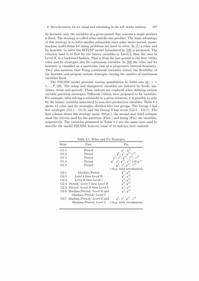
The P2LMM model presents various possibilities to build sets Qi, i =1, ..., P [29]. The setup and changeover variables are indexed by levels, ma-chines, items and periods. These indexes are explored when defining variousvariable partition strategies. Different criteria were proposed to fix variables.For example, after solving a submodel in a given iteration, it is possible to onlyfix the binary variables associated to non-zero production variables. Table 8.1shows 12 relax and fix strategies, divided into two groups. The Group 1 hasfive strategies (G1.1 - G1.5) and the Group 2 has seven (G2.1 - G2.7). Thefirst column shows the strategy name (Strat.), the second and third columnsshow the criteria used for the partition (Part.) and fixing (Fix) the variables,respectively. The variables presented in Table 8.1 are the same ones used todescribe the model P2LMM, however some of its indexes were omitted.

Table 8.1: Relax and Fix Strategies

Strat. Part. Fix

G1.1 Period yI , yII

G1.2 Period yI , zI , yII ,zII

G1.3 Period yI , zI , yII , zII , xII

G1.4 Period yI , zI , yII , zII i.th.p.*G1.5 Period yI , zI , yII , zII

i.th.p. with reevaluationG2.1 Machine/Period yI , yII

G2.2 Level I then Level II yI , yII

G2.3 Level II then Level I yI , yII

G2.4 Period/ Level I then Level II yI , yII

G2.5 Period/ Level II then Level I yI , yII

G2.6 Machine/Period/ Level II and yI , yII

Machine/Period/ Level I

G2.7 Machine/Period/ Level II and yI , zI , yII , zII

Machine/Period/ Level I i.th.p. with reevaluation

198 Ferreira et al.

The first five strategies (G1.1 - G1.5) use the usual criteria of partitioningthe variables according to periods. They differ from each other by the criteriaused to fix the variables in a given iteration. These criteria are based on theidea that the submodels should have a dimension that favors the decisionprocess. The objective was to evaluate the influence of the variables in thesubmodels solution.

The Group 2 strategies explore the multi-machine, two level structure ofthe model to partition the set of variables. The objective was to evaluate theinfluence of each machine (level) in the solution of the submodels. Note thatthe criterion used to fix the variables in this group is the same one used in thestrategy G1.1, except for the strategy G2.7. In this criterion, when the variableyII is fixed to one, it only assures that the machine will be prepared, it doesnot say if the item will be produced or not. The variable yI besides definingthat the tank will be prepared, also states that there will be production ofan item, between the tank capacities (constraints (2) and (3) in the P2LMMmodel). In the strategy G2.7, besides the binary variables, the continuousvariables (zI , zII) are also considered to be fixed when there is production(xII > 0). In this strategy the idle micro-periods in previous iterations whichdid not have any variables fixed are also reevaluated for further variable fixing.

At each iteration of the relax and fix heuristic an instance of a mixedinteger optimization submodel has to be solved. In general, they are solved byexact methods included in standard software (e.g. the branch and cut methodin CPLEX). Although the submodels in each iteration are smaller than theoriginal model, they are still difficult. If the optimal solution of the submodelsolved at each iteration is not achieved in a pre-defined amount of time, thebranch and cut execution is halted and the best solution is used to fix thevariables.

8.3.3 The relaxation approach

In some industries the liquid preparation in Level I does not represent a bottle-neck for the production process. That is, the tank capacities are large enoughto ensure that whenever a machine needs a liquid of a given flavor it willbe ready to be released. Therefore, there is no need to control either thechangeover in the tanks or the synchrony between the two production levels, only the minimum tank capacity constraints to ensure the liquid homogenyis necessary in Level I. This situation was explored as a solution approachto model P2LMM. The Relaxation Approach (RA) is based on the idea thatonce the production decision is taken in Level II, the decision for Level I iseasily taken.

In [29] a one level model to the production planning of a small soft drinkmanufacturer that has only one machine and several tanks is presented. Toextend their model to the multi-machines case, only constraints (8.3), (8.4),(8.10), (8.12)-(8.18) has to be considered, dropping the changeover variablesin Level I, zI

mkls, and adding the constraint:

8 Meta-heuristics for lot sizing and scheduling in the soft drinks industry 199

∑j∈δm

∑s∈St

aIIj x

IImjs +

∑i∈δm

∑j∈δm

∑s∈St

bIIij z

IImijs ≤ K

IImt,

m = 1, ...,M, t = 1, ..., T(8.19)

The objective function is:

Min

J∑

j=1

T∑

t=1

(hj I+jt + gj I

−jt) +

M∑

m=1

N∑

s=1

∑

i∈δm

∑

j∈δm

sIIij z

IImijs (8.20)

These sets of constraints and the objective function 8.20 define a one levelmulti-machines lot scheduling (P1LMM) model. It can be used in the firstphase of the RA algorithm (described below) to define the lot sizing andscheduling of items in Level II. An adjustment of the solution of this modelmight be necessary to take into account the synchrony between the two lev-els. This can be obtained by model P2LMM with the setup variables fixedaccording to the solution of model P1LMM. That is, if item j is producedthen the tank and the machine must be setup. This procedure is outlined inAlgorithm 5, where σj is the liquid flavor necessary to produce item j.

Step 1 Solve the P1LMM model;Step 2 if P1LMM is feasible then

for m=1 to M; j ∈ δm,s = 1, ..., N doif xII

mjs > 0 thenFix the setup variables of P2LMM model according to;for j ∈ δm, l ∈ σj do

yIImjs = 1 and yI

mls = 1

end

end

end

endStep 3 Solve the P2LMM model obtained in Step 2.

Algorithm 5: The RA Algorithm

The relax and fix strategies presented in Section 8.3.2 can also be usedto solve the models in Steps 1 and 3 of Algorithm RA. Note however that inmodel P1LMM in Level I only the capacities constraints are considered andthere are no changeover variables associated to this level. Therefore the relaxand fix strategies described in Table 8.1 have to be modified accordingly. If themodels in Algorithm RA are solved by standard software and their optimalsolution are not achieved in a pre-defined amount of time, the branch and cutexecution is also halted and the best solution is considered. Other solutionapproaches for SITLSP are presented and tested in [44] and [51].

200 Ferreira et al.

8.4 Computational Tests

In this section we present and analyze the computational results of the evo-lutionary algorithms (MA and GA) described in Section 8.2, and the decom-position and relaxation approaches described in Section 8.3, when applied tosolve industrial instances of SITLSP. Among all approaches reported in Sec-tion 8.3, we present the results of only P2LMM G2.7 (relax-and fix strategyG2.7 applied to model P2LMM) and RA G2.1 (relax-and-fix strategy G2.1applied to the model P1LMM of Algorithm RA), since they were the onesthat produced the best solutions for this set of instances tested. Other com-putational tests with randomly generated examples of small-to-moderate andmoderate-to-large sizes and other industrial instances were performed withthe MA and the GA approaches presented in Section 8.2. The P2EMM G2.7,RA G2.1 and the other approaches of Section 8.3 are as well tested in otherexamples. Their results are reported in [23] and [29], respectively.

8.4.1 Generation of instances

The solution methods presented in Sections 8.2 and 8.3 can be easily adaptedto represent the particularities of different soft drinks companies. To follow, wedescribe next the necessary adjustments to represent the situation encounteredat a Brazilian soft drink manufacturer , Plant A, as well as the data used togenerate the instances used in the computational tests described in Section8.4.2.

Plant A produces many types of soft drinks (items) characterized by theliquid flavor and bottle type. It has various tanks and filling lines (machines)with different capacities. Some tanks (machines) are dedicated to produceonly a given subset of flavors (items), whereas others can produce any one.There is a single liquid flavor (l = 4) whose demand is by far superior to theothers. While most of the liquid flavors have demands around 20,000 unitsper period, flavor 4 has demand around 150,000 units. It also has a high setuptime and cost. Therefore, in Plant A there is a tank which is fully dedicatedto continuously produce flavor 4. That is, whenever a machine is ready toproduce an item that uses this flavor, the tank is also ready to release it.

To represent this situation in model P2LMM of Section 8.3, the changeovertime in Level I from any flavor k to flavor 4 and from flavor 4 to any other isset to zero (bIk4 = bI4k = 0). Similar adjustments are made in the evolutionaryalgorithms of Section 8.2. Although there is no need to setup the tanks forflavor 4, there is still a need to setup the machines when items that need thisflavor are produced. However, the tank setup variable, yI

m4s cannot be setto zero, since when this is done, constraints (8.3) together with (8.4) imposethat the production of any item that uses this flavor is zero (if yI

m4s = 0 thenxII

mjs = 0, for j ∈ ωm4). Therefore the tank capacity (constraints (8.3) and(8.4)) for l = 4 is dropped.

8 Meta-heuristics for lot sizing and scheduling in the soft drinks industry 201

When defining the lot size and schedule, Plant A also considers that theinventory in a given period must be enough to cover the demand in the nextperiod. To have a fair comparison between the model and the company solu-tions, a new set of constraints should be included in the model:

I+jt = dj(t+1) j = 1, . . . , J ; t = 2, . . . , T + 1 (8.21)

Two minor modifications were made in the MA and GA to ensure that theirsolutions are comparable to the solutions of P2LMM G2.7 and RA G2.1, aswell as the solutions used by Plant A. The first change refers to the assumptionthat each filling line has a dedicated tank, that is, there is only one tankallocated to only one line. Therefore, the criterion of the MA/GA for selectinga tank, instead of determined by (Section 8.2):

j =

{βi, 1 ≤ βi ≤ L;βi − L, L < βi ≤ 2L.

(8.22)

It was re-defined as: j = βi, where βi = αi. In addition, the fitness func-tion of the MA/GA was modified to include only the product inventory, prod-uct changeover and demand shortage costs. As the company primarily favorsproduction schedules with no demand shortages, the shortage unit cost wasconsidered as a sufficiently large penalization so as to avoid shortages in thesolutions. In cases whereby the MA and GA were unable to find a schedulewithout shortages, their solution was simply considered infeasible. The samewas considered with the solutions of approaches P2LMM G2.7 and RA G2.1.We refer to these modified versions of MA and GA as MA1 and GA1, respec-tively.

The second change in the MA/GA is the consideration of penalization costsover the liquid flavor inventories maintained in the tanks from one period toanother. In other words, besides the costs taken into account in the fitnessfunction of the MA1 and GA1, we also considered penalization costs to avoidholding liquid flavor inventories between consecutive periods. This is becausethe company prefers production schedules that do not hold liquid inventoriesfrom one period to other, because they are perishable. Recall from Section 8.3that approaches P2LMM G2.7 and RA G2.1 do not hold liquid inventories.We refer to these modified versions of the MA and GA as MA2 and GA2,respectively.

Several visits to Plant A were made in order to understand its productionprocesses and to collect the data necessary to simulate their SITLSP. Dataassociated to demands, changeover times in both levels, tank and machinecapacities, etc., were obtained during these visits. The details of the collecteddata are presented in [29] and [51]. The data was used to generate 15 instancesof the SITLSP.

The first instance (P1) was generated based on data related to two ma-chines that can produce items in common. The first one (machine 1) can

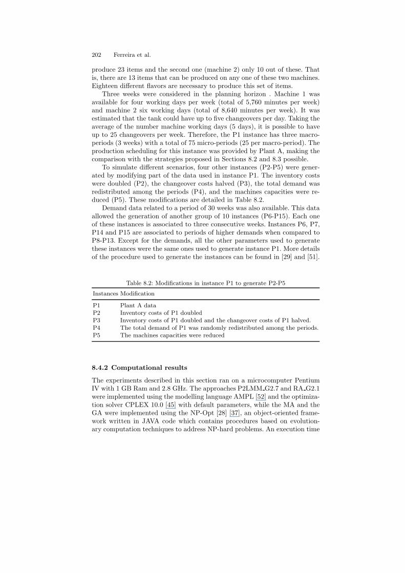
202 Ferreira et al.

produce 23 items and the second one (machine 2) only 10 out of these. Thatis, there are 13 items that can be produced on any one of these two machines.Eighteen different flavors are necessary to produce this set of items.

Three weeks were considered in the planning horizon . Machine 1 wasavailable for four working days per week (total of 5,760 minutes per week)and machine 2 six working days (total of 8,640 minutes per week). It wasestimated that the tank could have up to five changeovers per day. Taking theaverage of the number machine working days (5 days), it is possible to haveup to 25 changeovers per week. Therefore, the P1 instance has three macro-periods (3 weeks) with a total of 75 micro-periods (25 per macro-period). Theproduction scheduling for this instance was provided by Plant A, making thecomparison with the strategies proposed in Sections 8.2 and 8.3 possible.

To simulate different scenarios, four other instances (P2-P5) were gener-ated by modifying part of the data used in instance P1. The inventory costswere doubled (P2), the changeover costs halved (P3), the total demand wasredistributed among the periods (P4), and the machines capacities were re-duced (P5). These modifications are detailed in Table 8.2.

Demand data related to a period of 30 weeks was also available. This dataallowed the generation of another group of 10 instances (P6-P15). Each oneof these instances is associated to three consecutive weeks. Instances P6, P7,P14 and P15 are associated to periods of higher demands when compared toP8-P13. Except for the demands, all the other parameters used to generatethese instances were the same ones used to generate instance P1. More detailsof the procedure used to generate the instances can be found in [29] and [51].

Table 8.2: Modifications in instance P1 to generate P2-P5

Instances Modification

P1 Plant A dataP2 Inventory costs of P1 doubledP3 Inventory costs of P1 doubled and the changeover costs of P1 halved.P4 The total demand of P1 was randomly redistributed among the periods.P5 The machines capacities were reduced

8.4.2 Computational results

The experiments described in this section ran on a microcomputer PentiumIV with 1 GB Ram and 2.8 GHz. The approaches P2LMM G2.7 and RA G2.1were implemented using the modelling language AMPL [52] and the optimiza-tion solver CPLEX 10.0 [45] with default parameters, while the MA and theGA were implemented using the NP-Opt [28] [37], an object-oriented frame-work written in JAVA code which contains procedures based on evolution-ary computation techniques to address NP-hard problems. An execution time

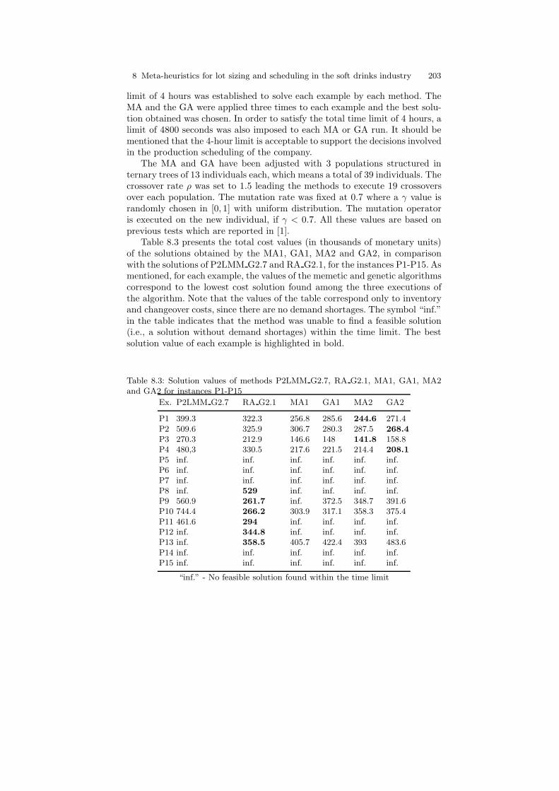
8 Meta-heuristics for lot sizing and scheduling in the soft drinks industry 203

limit of 4 hours was established to solve each example by each method. TheMA and the GA were applied three times to each example and the best solu-tion obtained was chosen. In order to satisfy the total time limit of 4 hours, alimit of 4800 seconds was also imposed to each MA or GA run. It should bementioned that the 4-hour limit is acceptable to support the decisions involvedin the production scheduling of the company.

The MA and GA have been adjusted with 3 populations structured internary trees of 13 individuals each, which means a total of 39 individuals. Thecrossover rate ρ was set to 1.5 leading the methods to execute 19 crossoversover each population. The mutation rate was fixed at 0.7 where a γ value israndomly chosen in [0, 1] with uniform distribution. The mutation operatoris executed on the new individual, if γ < 0.7. All these values are based onprevious tests which are reported in [1].

Table 8.3 presents the total cost values (in thousands of monetary units)of the solutions obtained by the MA1, GA1, MA2 and GA2, in comparisonwith the solutions of P2LMM G2.7 and RA G2.1, for the instances P1-P15. Asmentioned, for each example, the values of the memetic and genetic algorithmscorrespond to the lowest cost solution found among the three executions ofthe algorithm. Note that the values of the table correspond only to inventoryand changeover costs, since there are no demand shortages. The symbol “inf.”in the table indicates that the method was unable to find a feasible solution(i.e., a solution without demand shortages) within the time limit. The bestsolution value of each example is highlighted in bold.

Table 8.3: Solution values of methods P2LMM G2.7, RA G2.1, MA1, GA1, MA2and GA2 for instances P1-P15

Ex. P2LMM G2.7 RA G2.1 MA1 GA1 MA2 GA2

P1 399.3 322.3 256.8 285.6 244.6 271.4P2 509.6 325.9 306.7 280.3 287.5 268.4P3 270.3 212.9 146.6 148 141.8 158.8P4 480,3 330.5 217.6 221.5 214.4 208.1P5 inf. inf. inf. inf. inf. inf.P6 inf. inf. inf. inf. inf. inf.P7 inf. inf. inf. inf. inf. inf.P8 inf. 529 inf. inf. inf. inf.P9 560.9 261.7 inf. 372.5 348.7 391.6P10 744.4 266.2 303.9 317.1 358.3 375.4P11 461.6 294 inf. inf. inf. inf.P12 inf. 344.8 inf. inf. inf. inf.P13 inf. 358.5 405.7 422.4 393 483.6P14 inf. inf. inf. inf. inf. inf.P15 inf. inf. inf. inf. inf. inf.

“inf.” - No feasible solution found within the time limit

204 Ferreira et al.

As discussed in Section 8.4.1, instance P1 is the only one of the problem setfor which we are aware of the corresponding production schedule used by PlantA. This company solution meets all product demands with no delays, yieldinga total cost of 422.7 in thousands of monetary units. Comparing this solutionto the ones presented in Table 8.3, we notice that all methods P2LMM G.7,RA G2.1, MA1, GA1, MA2 and GA2 were able to find better solutions thanthe company, with relative cost reductions of 5.5%, 23.8%, 39.2%, 32.4%,42.1% and 35.8%, respectively. This indicates that these approaches have apotential to generate competitive solutions - note that the cost reductionscan be significant. Moreover, it can be observed that the memetic versionsoutperformed the genetic ones.

In instances P1 and P2-P4 (which are based on instance P1), the solu-tions obtained by MA1, GA1, MA2 and GA2 are better than the ones ob-tained by P2LMM G.7 and RA G2.1 (Table 8.3). For these instances, theP2LMM model involved in approach P2LMM G.7 has 86,359 variables (4,575binary variables) and 86,140 constraints, while the P1LMM model in approachRA G2.1 has 54,559 variables (4,575 binary variables) and 49,544 constraints.Some performance variations between the MA1 and MA2 (and between theGA1 and GA2) are due to the randomly generated initial populations of thealgorithms. In particular, we do not know if instance P5 is feasible (from thepoint of view of demand shortages), since none of the methods found a solu-tion without shortages. This instance was generated using the same data asP1, except for the reduction in the machine capacities (Table 8.2).

The remaining instances P6-P15 refer to collected data of the product de-mands for different months, provided by Plant A. Since we do not have theproduction schedules used by the company for these examples, we are notaware if they are feasible from the point of view of the demand shortages.In these examples, approach RA G2.1 produced better solutions than MA1,GA1, MA2 and GA2. Moreover, for all instances P1-P15, the RA G2.1 solu-tions dominate the ones of P2LMM G.7 (Table 8.3). As well as for instanceP5, we do not know if instances P6, P7, P14 and P15 are feasible, since noneof the methods found a solution without shortages. The minimum capacitynecessary to produce all the items in these instances is higher than in theothers. However, it is worth mentioning that by using realistic backlogging orlost sales unit costs (instead of large penalties) in these methods, they can beemployed to generate effective schedules balancing the trade-offs between theinventory, changeover and shortage costs.

Table 8.4 resumes the relative deviations of the solution values of MA1,GA1, MA2 and GA2 regarding approach RA G2.1. These deviations werecalculated using the expression:Dev(%) = 100(z−z)/z, where z is the solutionvalue of MA1 (or GA1, MA2, GA2) and z is the value found by approachRA G2.1. Note that the deviations of the evolutionary algorithms with respectto RA G2.1 are relatively large, varying from -37.0% to 49.6%. The superiorityof the memetic approach over its genetic version is also corroborated by theseresults.

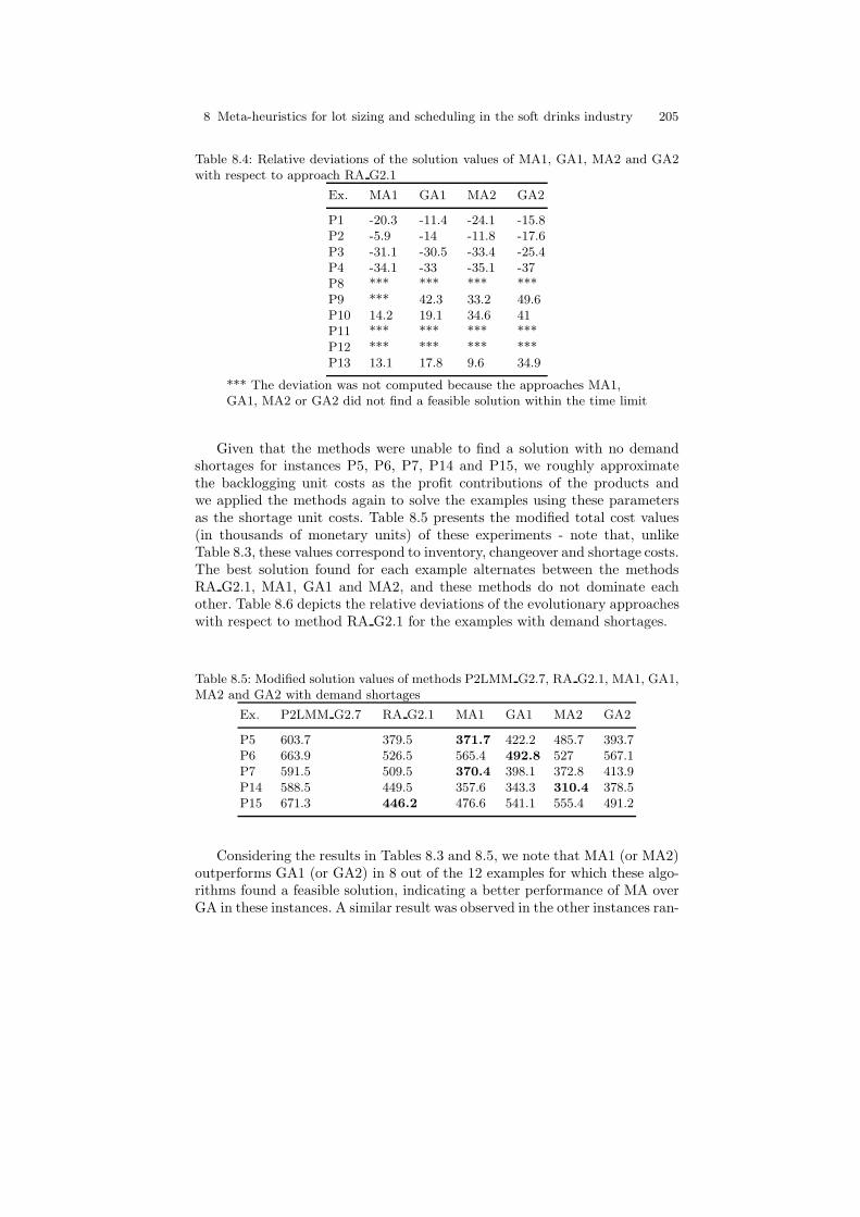
8 Meta-heuristics for lot sizing and scheduling in the soft drinks industry 205

Table 8.4: Relative deviations of the solution values of MA1, GA1, MA2 and GA2with respect to approach RA G2.1

Ex. MA1 GA1 MA2 GA2

P1 -20.3 -11.4 -24.1 -15.8P2 -5.9 -14 -11.8 -17.6P3 -31.1 -30.5 -33.4 -25.4P4 -34.1 -33 -35.1 -37P8 *** *** *** ***P9 *** 42.3 33.2 49.6P10 14.2 19.1 34.6 41P11 *** *** *** ***P12 *** *** *** ***P13 13.1 17.8 9.6 34.9

*** The deviation was not computed because the approaches MA1,GA1, MA2 or GA2 did not find a feasible solution within the time limit

Given that the methods were unable to find a solution with no demandshortages for instances P5, P6, P7, P14 and P15, we roughly approximatethe backlogging unit costs as the profit contributions of the products andwe applied the methods again to solve the examples using these parametersas the shortage unit costs. Table 8.5 presents the modified total cost values(in thousands of monetary units) of these experiments - note that, unlikeTable 8.3, these values correspond to inventory, changeover and shortage costs.The best solution found for each example alternates between the methodsRA G2.1, MA1, GA1 and MA2, and these methods do not dominate eachother. Table 8.6 depicts the relative deviations of the evolutionary approacheswith respect to method RA G2.1 for the examples with demand shortages.

Table 8.5: Modified solution values of methods P2LMM G2.7, RA G2.1, MA1, GA1,MA2 and GA2 with demand shortages

Ex. P2LMM G2.7 RA G2.1 MA1 GA1 MA2 GA2

P5 603.7 379.5 371.7 422.2 485.7 393.7P6 663.9 526.5 565.4 492.8 527 567.1P7 591.5 509.5 370.4 398.1 372.8 413.9P14 588.5 449.5 357.6 343.3 310.4 378.5P15 671.3 446.2 476.6 541.1 555.4 491.2

Considering the results in Tables 8.3 and 8.5, we note that MA1 (or MA2)outperforms GA1 (or GA2) in 8 out of the 12 examples for which these algo-rithms found a feasible solution, indicating a better performance of MA overGA in these instances. A similar result was observed in the other instances ran-

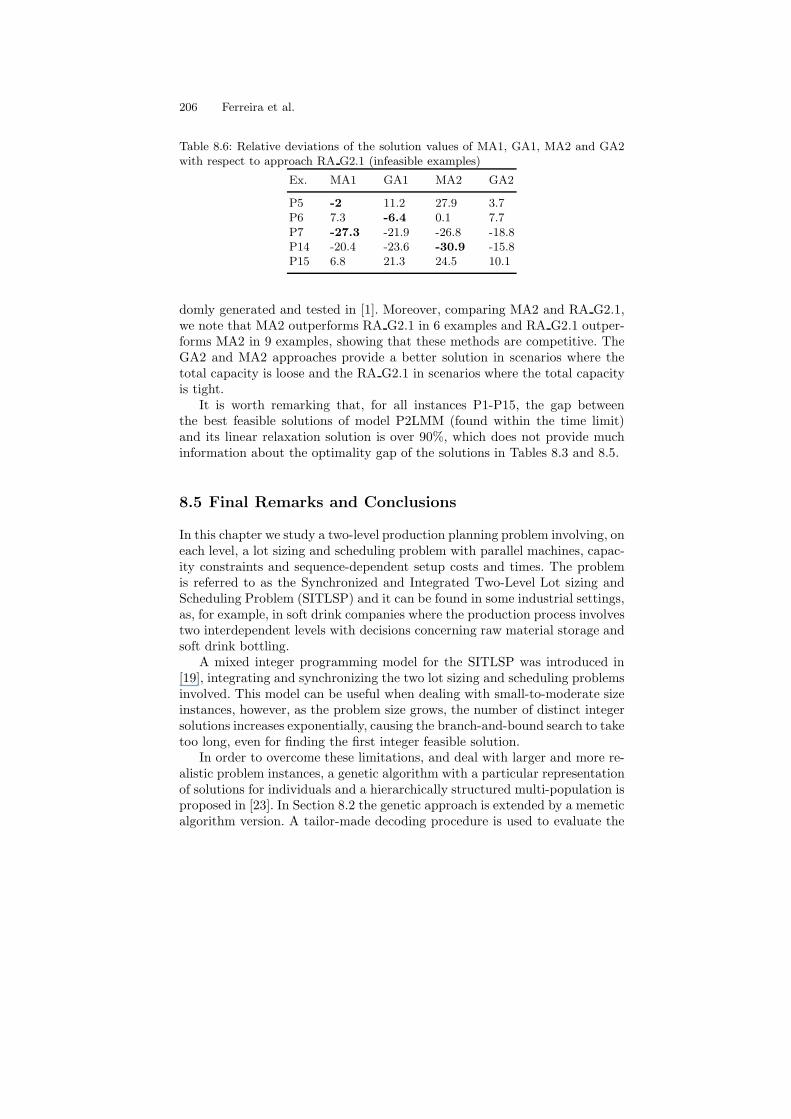
206 Ferreira et al.

Table 8.6: Relative deviations of the solution values of MA1, GA1, MA2 and GA2with respect to approach RA G2.1 (infeasible examples)

Ex. MA1 GA1 MA2 GA2

P5 -2 11.2 27.9 3.7P6 7.3 -6.4 0.1 7.7P7 -27.3 -21.9 -26.8 -18.8P14 -20.4 -23.6 -30.9 -15.8P15 6.8 21.3 24.5 10.1

domly generated and tested in [1]. Moreover, comparing MA2 and RA G2.1,we note that MA2 outperforms RA G2.1 in 6 examples and RA G2.1 outper-forms MA2 in 9 examples, showing that these methods are competitive. TheGA2 and MA2 approaches provide a better solution in scenarios where thetotal capacity is loose and the RA G2.1 in scenarios where the total capacityis tight.

It is worth remarking that, for all instances P1-P15, the gap betweenthe best feasible solutions of model P2LMM (found within the time limit)and its linear relaxation solution is over 90%, which does not provide muchinformation about the optimality gap of the solutions in Tables 8.3 and 8.5.

8.5 Final Remarks and Conclusions

In this chapter we study a two-level production planning problem involving, oneach level, a lot sizing and scheduling problem with parallel machines, capac-ity constraints and sequence-dependent setup costs and times. The problemis referred to as the Synchronized and Integrated Two-Level Lot sizing andScheduling Problem (SITLSP) and it can be found in some industrial settings,as, for example, in soft drink companies where the production process involvestwo interdependent levels with decisions concerning raw material storage andsoft drink bottling.

A mixed integer programming model for the SITLSP was introduced in[19], integrating and synchronizing the two lot sizing and scheduling problemsinvolved. This model can be useful when dealing with small-to-moderate sizeinstances, however, as the problem size grows, the number of distinct integersolutions increases exponentially, causing the branch-and-bound search to taketoo long, even for finding the first integer feasible solution.

In order to overcome these limitations, and deal with larger and more re-alistic problem instances, a genetic algorithm with a particular representationof solutions for individuals and a hierarchically structured multi-population isproposed in [23]. In Section 8.2 the genetic approach is extended by a memeticalgorithm version. A tailor-made decoding procedure is used to evaluate the

8 Meta-heuristics for lot sizing and scheduling in the soft drinks industry 207

solution encoded in the gene of each individual. Moreover, a tailor-made re-combination over population clusters takes place and migrations among differ-ent populations are allowed. The memetic approach is capable of generatingcompetitive solutions if compared with the ones utilized in practice, as shownin Section 8.4.

As an alternative for these metaheuristic approaches, another solutionmethod capable of dealing with realistic problem instances of the SITLSPis presented (Section 8.3). Unlike the highly general and complex MIP modelin [19], a simplified MIP formulation, in the sense that it forces the number oftanks to be the same as the filling lines so that each line has a dedicated tank,is described. The solution approach of the simplified model relies on differentrelax-and-fix heuristics and model decomposition strategies.

The performances of the memetic algorithm-MA (as well as its geneticversion- GA) and the decomposition/relaxation approaches (P2LMM G2.7and RA G2.1) are evaluated solving a set of instances based on actual dataprovided by a Brazilian soft drink company. All approaches are capable ofproducing competitive solutions when compared to the production scheduleused by the company, requiring affordable computational runtime. In somecases the cost savings of the solutions are substantial (Section 8.4). Comparingthe relative performances of the approaches when solving this problem set, it isobserved that the MA outperforms the GA and that the MA and the RA G2.1do not dominate each other. In particular, the MA provides a better solutionin scenarios where the total capacity is loose and the RA G2.1 in scenarioswhere the total capacity is tight.

Topics for future research include new experiments with the methods stud-ied in this chapter involving real instances to be obtained from other softdrinks plants. The evolutionary approaches can be improved by introducingnew genetic operators, especially other crossovers not tested yet and othermore powerful local search-based algorithms such as Simulated Annealing orTabu Search. The introduction of valid inequalities is a research topic to beattempted to improve the decomposition/relaxation approaches .

As point out in the Introduction, the main purpose of this chapter wasbring to the attention of the academic community and also to the industrialengineering practitioners the state-of-the art of computer-aided tools used togenerate effective production schedules in the soft drink industry . Focusingthe SITLSP, a hard combinatorial optimization problem, we believe that themost important conclusions that can be extracted from the studied methods aswell as from the computational assessment performed in this chapter are two-fold: first, mathematical modelling provides deeper insight into a very complexindustrial planning problem, and, second, tailor-made optimization methodscan yield less costly and more effective production schedules in reasonablecomputing times when compared with the ones provided by general purposecommercial packages commonly used by the industry.

208 Ferreira et al.

Acknowledgements

We are indebted to Flavio Veronese and Aldo Fernandes Junior from Com-panhia de Bebidas Ipiranga, Brazil for his kind collaboration. This researchwas partially supported by grants from FAPESP and CNPq.

References

1. Toledo C. F. M. (2005) The integrated two-stage lot sizing and schedulingproblem, Doctoral Thesis (in Portuguese), State University of Campinas, Brazil

2. Drexl A., Kimms A. (1997) Lot sizing and scheduling - survey and extensions,European Journal of Operational Research 99: 221-235.

3. Bitran G. R., Yanasse H.H. (1982) Computational complexity of the capacitedlot size problem, Management Science 28(10): 1174-1186.

4. Clark A. R., Clark S. J. (2000) Rolling-horizon lot sizing when set-up timesare sequence-dependent, International Journal of Production Research 38(10):2287-2307.

5. Fleischmann B. (1994) The discrete lot sizing and scheduling problem withsequence-dependent setup costs, European Journal of Operational Research,75: 395-404.

6. Gupta D., Magnusson T. (2005) The capacitated lot sizing and scheduling prob-lem with sequence-dependent setup costs and setup times, Computers & Op-erations Research 32: 727-747.

7. Haase K., Kimms A. (2000) Lot sizing and scheduling with sequence dependentsetup costs and times and efficient rescheduling opportunities, InternationalJournal of Production Economics 66: 159-169.

8. Meyr H. (2000) Simultaneous lot sizing and scheduling by combining localsearch with dual reoptimization, European Journal of Operational Research120:311-326.

9. Berreta R. E., Franca P. M., Armentano V. (2005) Metaheuristic approachesfor the multilevel resource-constrained lot sizing problem with setup and leadtimes, Asia-Pacific Journal of Operational Research 22(2): 261-286.

10. Franca P. M., Armentano V., Berretta R. E., Clark, A. R. (1997) A heuristicmethod for lot sizing in multi-stage systems, Computers & Operations Research24 (9): 861-874.

11. Kimms A. (1997) Demand shuffle - A method for multi-level proportional lotsizing and scheduling, Naval Research Logistics 44: 319-340.

12. Kimms A. (1997) Multi-level lot sizing and scheduling - Methods for capaci-tated, dynamic, and deterministic models, Physica, Heidelberg.

13. Ozdamar L., Barbarosoglu G. (2000) An integrated lagragean relaxation-simulated annealing approach to the multi-level multi-item capacitated lot siz-ing problem, International Journal of Production Economics 68: 319-331.

14. Kang S., Malik K., Thomas L. J. (1999) Lot sizing and scheduling on parallelmachines with sequence-dependent setup costs, Management Science 45: 273-289.

15. Kuhn H., Quadt, D. (2002) Lot sizing and scheduling in semiconductor assembly- A hierarchical planning approach. In: Mackulak G. T., Fowler J. W., SchomigA. (eds), Proceedings of the International Conference on Modeling and Analysisof Semiconductor Manufacturing, Tempe, USA: 211-216.

8 Meta-heuristics for lot sizing and scheduling in the soft drinks industry 209

16. Meyr H. (2002) Simultaneous lot sizing and scheduling on parallel machines,European Journal of Operational Research 139: 277-292.

17. Quadt D., Kuhn H. (2003) Production planning in semiconductor assembly,Working Paper, Catholic University of Eichstatt-Ingolstadt.

18. Stadtler H. (2003) Multilevel lot sizing with setup times and multiple con-strained resources: internally rolling schedules with lot sizing windows 51(3):487-502.

19. Toledo C.F.M., Kimms A., Franca P.M, Morabito R.(2006) A mathematicalmodel for the synchronized and integrated two-level lot sizing and schedulingproblem, Journal of Operational Research Society: under review.

20. Bitran G. R., Matsuo H. (1986) Approximation formulations for the singleproduct capacitated lot size problem, Operations Research 34: 63-74.

21. Fleischmann B., Meyr, H. (1997) The general lot sizing and scheduling problem,OR Spektrum 19: 11-21.

22. Drexl A., Haase K. (1997) Proportional lotsizing and scheduling, InternationalJournal of Production Economics 40: 73-87.

23. Toledo C. F. M., Franca P. M., Morabito R., Kimms A. (2007) A multi-population genetic algorithm to solve the synchronized and integrated two-level lot sizing and scheduling problem, International Journal of ProductionResearch: in press.

24. Holland J. H. (1975) Adaptation in natural and artificial systems, The Univer-sity of Michigan Press.

25. Goldberg D. E. (1989) Genetic algorithms in search, optimization, and machinelearning, Addison Wesley.

26. Michalewicz Z. (1996) Genetic Algorithms + data structure = evolution pro-grams, Springer-Verlag.

27. Moscato P. (1989) On evolution, search, optimization, genetic algorithms, andmartial arts: towards memetic algorithms, Technical Report, Caltech Concur-rent Computation Program, C3P Report 826.

28. Mendes A. S. (2003) The framework NP-Opt and its applications to optimiza-tion problems, Doctoral Thesis (in Portuguese), State University of Campinas- Brazil.

29. Ferreira D., Rangel S., Morabito R. (2007) Solution approaches for the softdrink integrated lot sizing and scheduling problem, submitted to EuropeanJournal of Operational Research.

30. Clark A. R. (2003) Hybrid heuristics for planning lot setups and sizes, Com-puters & Industrial Engineering 45: 545-562.

31. Moscato P. (1989) On genetic crossover operators for relative order preserva-tion. C3P Report 778, California Institute of Technology, Pasadena, CA 91125.

32. Dawkins R. (1976) The selfish gene. Oxford University Press Oxford.33. Gen M., Cheng R. (1997) Genetic algorithms & engineering design. John Wiley

& Sons New York NY.34. Goldberg D.E. (2002) The design of innovation: lessons from and for competent

genetic algorithms. Addison-Wesley Reading, MA.35. Hart W. E., Krasnogor N., Smith J.E. (Eds.) (2005) Recent advances in

memetic algorithms series: studies in fuzziness and soft computing 166.36. Weiner J. (1995) The beak of the finch. Vintage Books New York.37. Mendes A. S., Franca P. M., Moscato P. (2001) NP-Opt: an optimization frame-

work for NP problems. Proceedings of POM2001: 82-89 Guaruja, Brazil.

210 Ferreira et al.

38. Franca P. M., Mendes A. S., Moscato P. (2001) A memetic algorithm for thetotal tardiness single machine scheduling problem. European Journal of Oper-ational Research 1(132): 224-242.

39. Sikora R. (1996) A genetic algorithm for integrating lot sizing and sequencing inscheduling a capacitated flow line. Computers & Industrial Engineering 30(4):969-981.

40. Ozdamar L., Birbil S. I. (1998) Hybrid heuristic for the capacitated lot sizingand loading problem with setup times and overtime decisions. European Journalof Operational Research 110: 525-547.

41. Dellaert N., Jeunet J., Jonard N. (2000) A genetic algorithm to solve the generalmulti-level lot sizing problem with time-varying costs. International Journal ofProduction Economics 68: 241-257.

42. Kimms A. (1999) A genetic algorithm for multi-level, multi-machine lot sizingand scheduling. Computers & Operations Research 26: 829-848.

43. Dueck G., Scheuer T. (1990) Threshold accepting: A general purpose optimiza-tion algorithm appearing superior to simulated annealing. Journal of Compu-tational Physics 90: 161-175.

44. Ferreira D., Morabito R., Rangel S. (2007) A MIP model and relax and fixheuristics for production planning and scheduling in a small soft drink plant(in Portuguese), submitted to Pesquisa Operacional.

45. ILOG (2001) Using the CPLEX Callable Library, Copyright, ILOG.46. Wolsey L. A. (1998) Integer Programming, John Wiley & Sons.47. Dillemberger C., Escudero L. F., Wu Zhang A. W. (1994) On practical resource

allocation for production planning and scheduling with period overlapping se-tups, European Journal of Operational Research 75: 275-286.

48. Escudero L. F., Salmeron J. (2005) On a fix-and-relax framework for a class ofproject scheduling problems, Annals of Operations Research 140: 163-188.

49. Pedroso J. P., Kubo M. (2005) Hybrid tabu search for lot sizing problems, in Hy-brid Metaheuristics, Lecture Notes in Computer Science 3636: 66-77, Springer,Berlin.

50. Federgruen A., Meissner J., Tzur M. (2004) Progressive interval heuristics formulti-item capacitated lot sizing problems, Operations Research, 55 (3): 490-502.

51. Ferreira D. (2006) Approaches to the integrated problem of the lot sizing andscheduling of the soft drink production, Doctoral Thesis (in Portuguese), Fed-eral University of Sao Carlos, Brazil.

52. Fourer R., Gay M. D., Kernighan B. W. (1993) AMPL - A modeling languagefor mathematical programming, The Scientific Press, Danvers, Massachusetts.