Embed Size (px)
Citation preview
MNRAS 493, 5089–5106 (2020) doi:10.1093/mnras/staa597Advance Access publication 2020 March 3
H I asymmetries in LVHIS, VIVA, and HALOGAS galaxies
T. N. Reynolds ,1,2,3‹ T. Westmeier ,1,3 L. Staveley-Smith ,1,3 G. Chauhan 1,3 andC. D. P. Lagos 1,3
1International Centre for Radio Astronomy Research (ICRAR), The University of Western Australia, 35 Stirling Hwy, Crawley, WA 6009, Australia2CSIRO Astronomy and Space Science, Australia Telescope National Facility, PO Box 76, Epping, NSW 1710, Australia3ARC Centre of Excellence for All Sky Astrophysics in 3 Dimensions (ASTRO 3D)
Accepted 2020 February 25. Received 2020 February 18; in original form 2019 November 14
ABSTRACTWe present an analysis of morphological, kinematic, and spectral asymmetries in observationsof atomic neutral hydrogen (H I) gas from the Local Volume H I Survey (LVHIS), the VLAImaging of Virgo in Atomic Gas (VIVA) survey, and the Hydrogen Accretion in Local GalaxiesSurvey. With the aim of investigating the impact of the local environment density and stellarmass on the measured H I asymmetries in future large H I surveys, we provide recommendationsfor the most meaningful measures of asymmetry for use in future analysis. After controllingfor stellar mass, we find signs of statistically significant trends of increasing asymmetries withlocal density. The most significant trend we measure is for the normalized flipped spectrumresidual (Aspec), with mean LVHIS and VIVA values of 0.204 ± 0.011 and 0.615 ± 0.068at average weighted 10th nearest-neighbour galaxy number densities of log (ρ10/Mpc−3) =−1.64 and 0.88, respectively. Looking ahead to the Widefield ASKAP L-band Legacy All-sky Blind survey on the Australian Square Kilometre Array Pathfinder, we estimate that thenumber of detections will be sufficient to provide coverage over 5 orders of magnitude inboth local density and stellar mass increasing the dynamic range and accuracy with which wecan probe the effect of these properties on the asymmetry in the distribution of atomic gas ingalaxies.
Key words: galaxies: clusters: general – galaxies: groups: general – radio lines: galaxies.
1 IN T RO D U C T I O N
The stellar and gaseous (atomic hydrogen, H I) discs of galaxies arefound to have morphologies which vary from symmetric to highlyasymmetric (first studied in H I by Baldwin, Lynden-Bell & Sancisi1980). The review by Jog & Combes (2009) indicates that spiralgalaxies commonly exhibit morphological asymmetries in their H I.The gravitational potential from the baryonic (stellar, gas, dust)and non-baryonic (dark matter) matter is the dominant driver ofgalaxy morphology and kinematics. In an isolated, massive system,the morphology and kinematics are expected to be symmetricalaround the galaxy’s centre. Perturbations away from a symmetricalsystem are then expected to be due to external influences ofthe environment (e.g. Hibbard et al. 2001), although isolatedgalaxies are also observed with asymmetric H I morphologies (e.g.Athanassoula 2010; Portas et al. 2011). Proposed mechanisms thatcan create asymmetries in isolated galaxies include gas accretionalong filaments (e.g. Bournaud et al. 2005b; Mapelli, Moore &Bland-Hawthorn 2008), minor mergers of satellites (e.g. Zaritsky &
� E-mail: [email protected]
Rix 1997; Bournaud et al. 2005b; Lagos et al. 2018a) and fly-by interactions (e.g. Mapelli et al. 2008). H I is a sensitive probeof environmental effects as H I is easily observable at larger radiithan the stellar component and will be the first to exhibit signs ofexternal influences (e.g. Giovanelli & Haynes 1985; Solanes et al.2001; Rasmussen, Ponman & Mulchaey 2006; Westmeier, Braun &Koribalski 2011; Rasmussen et al. 2012; Denes, Kilborn & Ko-ribalski 2014; Odekon et al. 2016). Proposed external mechanismsfor causing asymmetries in a galaxy’s observed H I include rampressure stripping (e.g. Gunn & Gott 1972; Kenney, van Gorkom &Vollmer 2004) by dense intergalactic medium (IGM), high relativevelocity galaxy interactions (harassment, Moore et al. 1996; Moore,Lake & Katz 1998), low relative velocity galaxy interactions (tidalstripping, Moore et al. 1999; Koribalski & Lopez-Sanchez 2009;English et al. 2010), galaxy mergers (e.g. Rubin, Ford & D’Odorico1970; Zaritsky & Rix 1997) and asymmetric gas accretion (e.g.Bournaud et al. 2005b; Sancisi et al. 2008; Lagos et al. 2018a). Rampressure stripping in particular is proposed to be the dominant driverof the evolution of galaxy morphology in clusters (e.g. Boselli &Gavazzi 2006).
Early work measured H I asymmetries in integrated spectra, asthese are more easily obtained for large samples of galaxies com-
C© 2020 The Author(s)Published by Oxford University Press on behalf of the Royal Astronomical Society
Dow
nloaded from https://academ
ic.oup.com/m
nras/article/493/4/5089/5775316 by guest on 13 January 2022
5090 T. N. Reynolds et al.
pared with spatially resolved H I observations, finding asymmetricfractions of � 50 per cent based on the flux ratio asymmetry, Aflux,(the ratio of the integrated flux of the two halves of the spectrumdivided at the systemic velocity, Richter & Sancisi 1994; Hayneset al. 1998; Matthews, van Driel & Gallagher 1998). Espada et al.(2011) used the AMIGA (Analysis of the interstellar Mediumin Isolated GAlaxies, Verdes-Montenegro et al. 2005) sample ofisolated galaxies to quantify the intrinsic scatter in observed Aflux
values, finding the distribution could be described as a half Gaussiancentred on 1 (perfectly symmetric) with a 1σ standard deviation of0.13. Within the tail of the Gaussian distribution, 9 per cent and2 per cent of the AMIGA sample were found to have Aflux > 2σ
and 3σ , respectively (Espada et al. 2011). Applying the 2σ cut tothe isolated samples of Haynes et al. (1998) and Matthews et al.(1998) gives fractions of 9 per cent and 17 per cent, respectively.Recent studies of single dish spectra of Virgo and Abell 1367 clustergalaxies considered Aflux > 2σ or 3σ as likely produced by external,environmental influences and found asymmetric fractions of ∼16–26 per cent (Scott et al. 2018) and 27 per cent for close galaxypairs (Bok et al. 2019) using the AMIGA sample 3σ significancethreshold. Watts et al. (2020) classified xGASS (Catinella et al.2018) galaxies as satellites or centrals and measured Aflux, findingthat satellites show a higher frequency of asymmetries than centrals,which supports the previous findings of asymmetries being morecommon in higher density environments. However, taking this fur-ther and understanding the physical origin of spectral asymmetriesrequires knowledge of the spatial distribution of gas within galaxiesand the gas kinematics.
Spatially resolved asymmetry analyses were first carried out onnear-infrared (near-IR) galaxy images using Fourier analysis whichfound ∼ 30 per cent to show signs of morphological asymmetries(Rix & Zaritsky 1995; Zaritsky & Rix 1997). A decade laterBournaud et al. (2005b) found a significantly higher asymmetricfraction (∼ 60 per cent) also using Fourier analysis of near-IRimages. In the following years, Fourier analysis was applied toH I integrated intensity images, obtaining asymmetric fractions of∼17–27 per cent in the Eridanus and Ursa Major galaxy groups(Angiras et al. 2006, 2007) and ∼ 30 per cent from a sample ofWHISP1 galaxies (van Eymeren et al. 2011b). The H I studieshave the advantage of probing out to larger radii than the near-IR image analysis. Focusing on the gas kinematics, Swaters et al.(1999) showed that differences in the rotation curves of a galaxy’sapproaching and receding sides is a sign of kinematic asymmetry fortwo WHISP spiral galaxies. van Eymeren et al. (2011a) measuredthe kinematic lopsidedness for a larger sample of 70 WHISP galax-ies, concluding that this parameter can be an over- or underestimateif local distortions are present in the disc and cannot be used aloneto characterize two-dimensional asymmetry.
There are currently no large statistical samples of spatiallyresolved galaxies in H I that can match sample sizes of all-sky singledish surveys. These all-sky coverage H I surveys (e.g. HIPASS andALFALFA, Barnes et al. 2001; Haynes et al. 2018, respectively)have limited spatial resolution. This is about to change with theadvent of new radio interferometers including the Australian SquareKilometre Array Pathfinder (ASKAP, Johnston et al. 2008), theAPERture Tile in Focus upgrade to the Westerbork SynthesisTelescope (APERTIF, Verheijen et al. 2008) and the Karoo ArrayTelescope (MeerKAT, Jonas & MeerKAT Team 2016). ASKAP,
1The Westerbork H I Survey of Irregular and Spiral Galaxies (Swaters et al.2002)
which is fitted with phased array feed receivers (DeBoer et al.2009; Hampson et al. 2012; Hotan et al. 2014; Schinckel &Bock 2016), has a wide field of view giving it fast survey speedcapabilities while retaining the increased resolution of an inter-ferometer. The Widefield ASKAP L-band Legacy All-sky Blind(WALLABY, Koribalski 2012; Koribalski et al. in preparation)survey will use the increased survey speed and high resolution todetect H I emission in ∼ 500 000 galaxies across ∼ 75 per cent ofthe sky (Duffy et al. 2012). Several thousand of these detections,including all the HIPASS sources, will be spatially resolved. Thiswill provide the largest environmentally unbiased sample for whichmorphological and kinematic asymmetries can be measured. Therest of the WALLABY detections will be limited to investigatingasymmetries in their integrated spectra. However, the significantlysmaller synthesized beam of WALLABY compared to HIPASS andALFALFA (0.5 arcmin versus 15.5 and 3.5 arcmin, respectively)will result in a lower fraction of confused detections, increasing thenumber of spectra uncontaminated by near neighbours (e.g. fromgalaxies in pairs and groups).
In preparation for WALLABY it is useful to determine the optimalmeasures of H I asymmetry to parametrize the galaxies which willbe detected. To do this we only consider existing surveys which spa-tially resolve galaxies in H I, as single dish surveys (e.g. HIPASS andALFALFA) cannot be used to measure morphological or kinematicasymmetries. Existing publicly available interferometric surveysinclude THINGS (Walter et al. 2008), Little THINGS (Hunter et al.2012), LVHIS (Koribalski et al. 2018), VIVA (Chung et al. 2009),Hydrogen Accretion in Local Galaxies Survey (HALOGAS) (Healdet al. 2011), and ATLAS3D (Cappellari et al. 2011). The spectral andangular resolution and spectral line sensitivity of LVHIS is similarto that achievable with WALLABY (Koribalski et al. 2018) andis a perfect candidate for testing asymmetry measures. However,LVHIS only contains 82 galaxies and probes isolated galaxy andgroup environments. We require additional surveys probing higherdensities with comparable spectral resolution, physically resolvedspatial scale, stellar masses, and sensitivity to study the effectof environment on measured asymmetry in late-type galaxies.These surveys must also lie within an optical background surveyfootprint (e.g. SDSS or 6dFGS, Strauss et al. 2002; Jones et al.2009, respectively) to derive environment densities consistentlyacross each H I survey. VIVA, which probes the significantly higherdensities of the Virgo cluster, satisfies these criteria (Table 1), exceptfor only covering the high stellar masses in LVHIS (Fig. 1). Tocontrol for stellar mass, we include HALOGAS, which is also wellmatched to LVHIS and VIVA (Table 1), and probes similar densitiesto LVHIS (Fig. 3). Neither THINGS nor Little THINGS span the fullmass range of LVHIS and VIVA. THINGS covers the high massesof VIVA (de Blok et al. 2008) and LITTLE THINGS covers the lowmasses of the majority of LVHIS (Oh et al. 2015). ATLAS3D is asurvey of early-type galaxies and has a spectral resolution 2–4 timeslower than LVHIS, VIVA, or HALOGAS (Serra et al. 2012). Ourfinal galaxy samples include galaxies from the LVHIS, VIVA, andHALOGAS surveys.
In this work we aim to determine the best asymmetry parametersfor quantifying H I asymmetries to use on data to be producedby future large surveys (e.g. WALLABY) for investigating theinfluence of environment density and stellar mass on H I asymmetryparameters. This paper is structured as follows. In Section 2, weintroduce the surveys used in this work and describe our analysis inSection 3. We present our discussion and conclusions in Sections 4and 5, respectively. Throughout, we use velocities in the opticalconvention (cz) and the heliocentric reference frame, adopting a
MNRAS 493, 5089–5106 (2020)
Dow
nloaded from https://academ
ic.oup.com/m
nras/article/493/4/5089/5775316 by guest on 13 January 2022
H I asymmetries in LVHIS, VIVA, and HALOGAS galaxies 5091
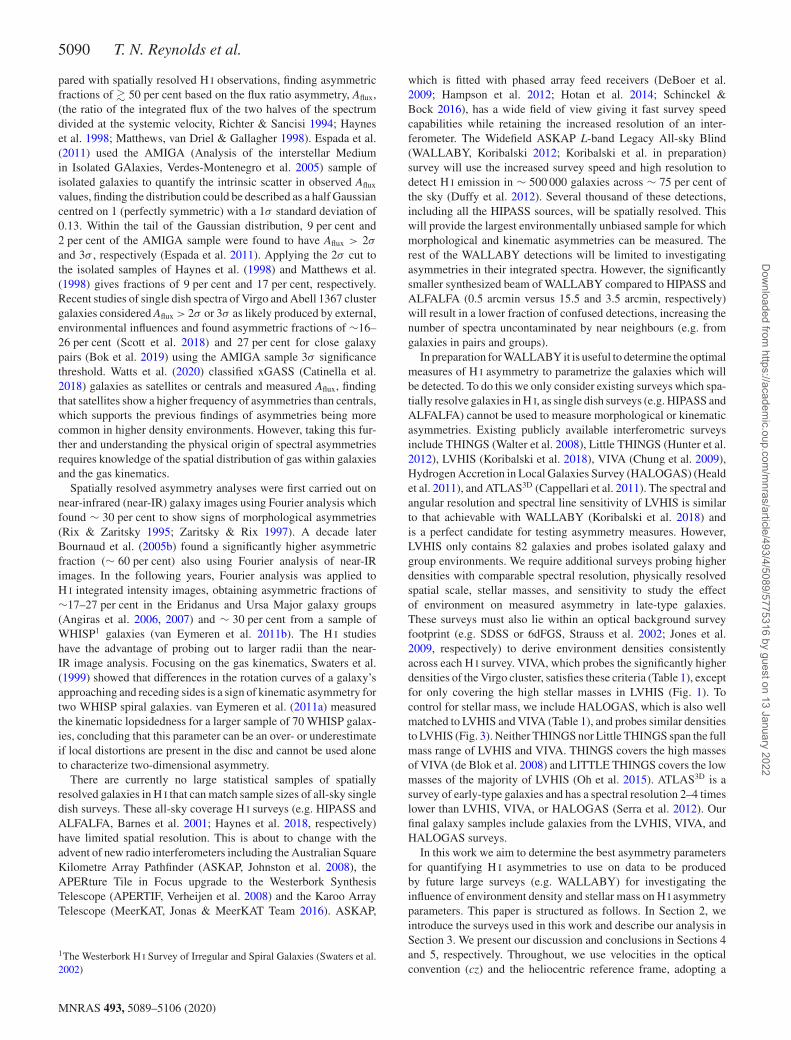
Figure 1. Stacked histograms of LVHIS (blue), VIVA (yellow), and HALOGAS (black) stellar and H I masses, 25th mag arcsec−2 B-band magnitude, specificstar formation rate (sSFR = SFR/M∗), the integrated H I detection signal-to-noise ratio (SNR) and the H I diameter (upper left, up per centre, upper right,lower left, lower centre, and lower right panels, respectively). B-band magnitudes and optical diameters are taken from the LVHIS, VIVA, and HALOGASoverview papers (Koribalski et al. 2018; Chung et al. 2009; Heald et al. 2011; respectively). LVHIS stellar masses are from Wang et al. (2017) and the VIVAand HALOGAS stellar mass calculates are described in Sections 2.2 and 2.3. SoFiA returns the integrated H I SNR, which we correct for the beam solid angle,and the H I diameter, which is computed by fitting an ellipse to the moment map, converted from an angular to physical size.
Table 1. Survey parameters summary. The galaxy sub-samples used in thiswork were selected to lie within the footprints of the 6dFGS (LVHIS) andSDSS (VIVA and HALOGAS) optical redshift catalogues and have publiclyavailable H I spectral line cubes. The number of galaxies for each surveysub-sample that are resolved by ≥3 beams is indicated in brackets. The 3σ
column density sensitivity is for a channel width of 10 km s−1.
Survey LVHIS VIVA HALOGAS
Telescope ATCA VLA WSRTTotal galaxies (N) 82 53 24Galaxy sub-samples (N) 73 (61) 45 (41) 18 (18)Distance (Mpc) <10 ∼16.5 <253σ column densitySensitivity (1019 cm−2) 0.4–7.4 0.9–9.0 0.2–0.6Stellar mass [log (M∗/M�)] 6–11 9–11 7.5–11
ResolutionSpectral (km s−1) 4–8 10 10Angular (arcsec) � 40 15 40Physical (kpc) 0.6–2.3 1.5 0.8–4.8
flat �CDM cosmology using H0 = 67.7, concordant with Planck(Planck Collaboration XIII 2016).
2 SAMPLE SELECTION
We use the Local Volume H I Survey (LVHIS, Koribalski et al.2018), the VLA Imaging of Virgo in Atomic Gas survey (VIVA,Chung et al. 2009), and the Hydrogen Accretion in Local Galaxiessurvey (HALOGAS, Heald et al. 2011) to investigate the influenceof environment density on measured morphological, kinematic, andspectral asymmetry parameters. Here we provide a brief overviewof each survey and direct the reader to the survey papers formore details. We present a summary of the survey parameters
in Table 1 and the stellar and H I mass distributions, B-bandmagnitude, specific star formation rate (sSFR = SFR/M∗), H I
detection signal-to-noise ratio (SNR) and the H I diameter in Fig. 1(panels ordered from upper left to lower right). We calculate the H I
masses for LVHIS, VIVA, and HALOGAS using a simplified formof equation (50) from Meyer et al. (2017)
MH I
M�∼ 2.35 × 10⁵
1 + z
(D
Mpc
)2 (Sint
Jy km s−1
), (1)
where Sint is the integrated flux and D is the galaxy distance.LVHIS star formation rates (SFRs) are computed in Shao et al.(2018) using IRAS 60 and 100μm fluxes, which for consistencywe use to compute the HALOGAS and VIVA SFRs followingequations 2–5 from Kewley et al. (2002). We note that the LVHISdwarf galaxy SFRs will be lower estimates due to lower dust opacity(e.g. Shao et al. 2018). Dwarf galaxy SFRs are more accuratelyderived by including UV and H α luminosities (e.g. Cluver et al.2017, and references therein), however we do not have UV and H α
luminosities for all of the three samples to consistently derive SFRs.For LVHIS and VIVA, H I properties are listed in the overviewpapers (Koribalski et al. 2018; Chung et al. 2009, respectively).However for consistency among the three surveys, we perform ourown source finding on the survey H I spectral line cubes (Section 3)and re-measure H I properties from the detected sources. We findgood agreement between the published properties and our values.
2.1 LVHIS
The Local Volume H I Survey (LVHIS, Koribalski et al. 2018) wascarried out on the Australia Telescope Compact Array (ATCA),observing H I in 82 nearby (<10 Mpc) gas-rich spiral, dwarf, andirregular galaxies. The majority of LVHIS galaxies are members
MNRAS 493, 5089–5106 (2020)
Dow
nloaded from https://academ
ic.oup.com/m
nras/article/493/4/5089/5775316 by guest on 13 January 2022
5092 T. N. Reynolds et al.
of local groups or pairs and have at least one close neighbour withan angular separation of <300 arcsec (e.g. projected separation<17 kpc) and a systemic velocity <800 km s−1 (group membershipand number of close neighbours are tabulated in Koribalski et al.2018). All galaxies were observed using a minimum of three ATCAconfigurations to provide good uv coverage and sensitivity to H I
gas on different spatial scales. We exclude galaxies which are notcovered by the 6dF Galaxy Survey due to incompleteness (seeSection 2.4). This reduces our sample to 73 LVHIS galaxies. We useLVHIS H I spectral line cubes made using natural weighting.2 TheLVHIS H I spectral line cubes have a 4 km s−1 spectral resolution,3
5 arcsec × 5 arcsec pixels and a synthesized beam of �40 arcsec ×40 arcsec. We use LVHIS stellar masses from Wang et al. (2017).
2.2 VIVA
The VLA Imaging of Virgo in Atomic Gas survey (VIVA, Chunget al. 2009) imaged 53 late-type galaxies in H I using the KarlG. Jansky Very Large Array (VLA) at an angular resolution of∼15 arcsec. Here we use a subsample of 45 galaxies for which thereduced H I spectral line cubes are available.4 The VIVA H I spectralline cubes have a 10 km s−1 spectral resolution and 5 arcsec × 5arcsec pixels. We calculate VIVA stellar masses using the empiricalrelation from Taylor et al. (2011),
log(M∗/M�) = a + b (g − i) − 0.4m + 0.4Dmod + 0.4Msol
− log(1 + z) − 2 log(h/0.7), (2)
where a, b = −1.197, 1.431 are empirically determined constantsbased on the chosen magnitude and colour from Zibetti, Charlot &Rix (2009), we use the SDSS g − i colour, m is the g-band apparentmagnitude, Dmod is the distance modulus, and Msol = 5.11 is theabsolute magnitude of the sun in the g band (Willmer 2018). SDSSmagnitudes have been corrected for foreground Galactic extinction(Kim et al. 2014). All VIVA physical parameters are calculatedassuming these galaxies are located at the distance of the Virgocluster (16.5 Mpc).
2.3 HALOGAS
The Hydrogen Accretion in Local Galaxies survey (HALOGAS,Heald et al. 2011) on the Westerbork Synthesis Radio Telescope(WSRT) imaged 24 spiral galaxies in H I at an angular resolutionof ∼40 arcsec. The HALOGAS sample is composed of galaxiesresiding in pairs and groups and includes both dominant and minorgroup members (group membership is tabulated in Heald et al.2011). Here we use a subsample of 18 galaxies5 which lie withinthe SDSS spectroscopic survey footprint (Strauss et al. 2002).Only 17 are specific HALOGAS targets, with the final galaxy,NGC 2537, lying within the same observed field as UGC 4278. Weuse the low-resolution H I spectral line cubes, which have a physicalresolution that is comparable to the LVHIS and VIVA observations.
2LVHIS H I spectral line cubes with natural weighting are publicly availablefor download at http://www.atnf.csiro.au/research/LVHIS/LVHIS-database.html.3Two LVHIS galaxies have a spectral resolution of 8 km s−1 (LVHIS 004and LVHIS 005) and one has a spectral resolution of 2 km s−1 (LVHIS 079).4VIVA H I spectral line cubes are publicly available for download at http://www.astro.yale.edu/cgi-bin/viva/observations.cgi.5HALOGAS H I spectral line cubes are publicly available for download athttp://www.astron.nl/halogas/data.php.
The HALOGAS H I spectral line cubes have a ∼5 km s−1 spectralresolution and 5 arcsec × 5 arcsec pixels. We also calculate theHALOGAS stellar masses using equation (2), replacing the g − icolour with the B − V colour and the g-band apparent magnitudewith the 2MASS J-band apparent magnitude. The constants for theB − V colour and J-band magnitude are a, b = −1.135, 1.267and the 2MASS absolute J-band magnitude of the sun Msol = 4.54(Zibetti et al. 2009; Willmer 2018, respectively).
2.4 Environment
We determine the local environment galaxy number density forthe galaxy samples using a 3D friends of friends (FOF) approachfor the Kth nearest neighbour (NN) method cross-matching withoptical redshift survey catalogues. We use the 6dF Galaxy Survey(6dFGS, Jones et al. 2009) for LVHIS, the Extended Virgo ClusterCatalogue (EVCC, Kim et al. 2014) for VIVA and the catalogueof Sloan Digital Sky Survey (SDSS) sources with spectroscopicredshifts (Strauss et al. 2002) for HALOGAS. The EVCC contains asubset of galaxies from the SDSS spectroscopic catalogue which aredetermined to be members of the Virgo cluster. For computing VIVAdensities, we assume a distance of 16.5 Mpc to the Virgo cluster(Mei et al. 2007) and give each VIVA galaxy a random distanceselected from a Gaussian distribution centred on 16.5 Mpc with astandard deviation of 1.72 Mpc, the virial radius of the Virgo cluster(Hoffman, Olson & Salpeter 1980). All densities calculated anddiscussed in this work are galaxy number densities (i.e. the numberof galaxies per Mpc3), not to be confused with the density of theIGM or intercluster medium (ICM), which is not easily measurable.
We calculate the weighted density to the Nth nearest neighbourfollowing the Bayesian metric of Cowan & Ivezic (2008)
ρN = CN∑N
i=1 d3i
, (3)
where CN is a constant, derived empirically, such that the meandensity agrees with the true density calculated on a uniform density,regular grid (e.g. for N = 10 nearest neighbours, C10 = 11.48) and∑N
i=1 d3i is the sum of the cubed luminosity distances, d, to the N
nearest neighbours. Equation (3) is sensitive to the distances to allN nearest neighbours and provides a better estimate of the localgalaxy density than using only the Nth nearest neighbour. Take asan example, the weighted number density of two galaxies for N =10 where one galaxy has the first nine neighbours within 0.5 Mpcand the 10th nearest galaxy is at 3 Mpc and the other galaxy only hastwo neighbours within 0.5 Mpc with the other eight neighbours at2.5–3 Mpc. The 10th nearest galaxy is at 3 Mpc in both cases, hencethe density to the 10th nearest neighbour will be the same as thisignores the inner nine neighbours. The weighted nearest neighbouron the other hand is sensitive to the distances to all 10 neighbours.It will return a higher number density for the first galaxy withmore weighting going to the inner nine galaxies compared withthe second galaxy which will return a lower density with moreweighting going to the more distant neighbours. The measureddensities for both galaxies will be higher than simply using the 10thnearest neighbour distance as the use of the inner nine neighboursin the calculation will more accurately describe the local density.
We calculate luminosity distances from galaxy redshifts usingthe PYTHON module ASTROPY function LUMINOSITY DISTANCE. Wetested measuring density to the 1st, 3rd, 6th, 10th, 12th, and 20thnearest neighbours. In each regime the relative difference in meanenvironment density remains nearly constant (see Fig. 2), whichis a good indication that VIVA is probing a different density
MNRAS 493, 5089–5106 (2020)
Dow
nloaded from https://academ
ic.oup.com/m
nras/article/493/4/5089/5775316 by guest on 13 January 2022
H I asymmetries in LVHIS, VIVA, and HALOGAS galaxies 5093
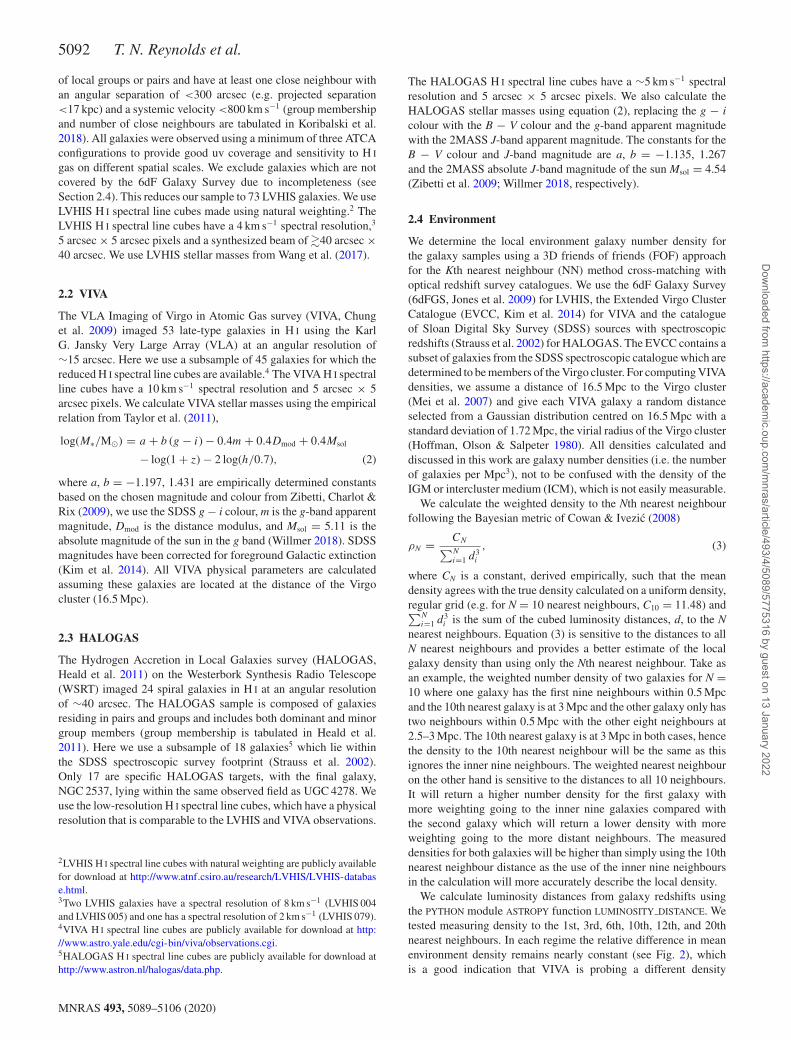
Figure 2. Mean environment density versus number of nearest neighboursused for calculation for LVHIS, VIVA, and HALOGAS (blue circle, yellowsquare, and black diamond, respectively). The shaded region indicates the1σ dispersion in the calculated density distributions.
Figure 3. Environment density versus physical distance. We show theweighted 10th nearest neighbour densities calculated using equation (3) aftercorrecting for survey completeness as described in Section 2.4. Distances forLVHIS and HALOGAS are taken from Koribalski et al. (2018) and Healdet al. (2011), respectively. For VIVA we assume a distance of 16.5 Mpc tothe Virgo cluster and give each VIVA galaxy a random distance selectedfrom a Gaussian distribution centred on 16.5 Mpc with a standard deviationof 1.72 Mpc, the distance to and virial radius of the Virgo cluster (Mei et al.2007; Hoffman et al. 1980, respectively).
environment than LVHIS and HALOGAS. The only exception tothis is for the 1st nearest neighbour, which also has the largestdispersion due to the random nature of the proximity of thenearest galaxy and hence does not provide a good indication ofthe local environment (e.g. field, group, or cluster galaxy numberdensities). We find using the 10 nearest neighbours (i.e. the samenumber of neighbours used by Cowan & Ivezic 2008) produceswell-defined density distributions with the dispersion in densityfor each survey ∼1 dex. Using less than 10 neighbours produceslarger dispersions in densities and using more than 10 neighboursresults in densities that are reduced by an order of magnitudecompared to the local density (Fig. 2). We show the environmentdensity (corrected for observational biases) distributions against thephysical distances of each galaxy in Fig. 3. The mean densities arelog(ρ10/Mpc−3) = −1.64, 0.88, and − 1.09 for LVHIS, VIVA,and HALOGAS, respectively. Throughout this work we refer toLVHIS and HALOGAS as low density relative to the high-densityVirgo cluster VIVA galaxies.
Both 6dFGS and SDSS have observational magnitude limits,resulting in fainter galaxies falling below the detection limit withincreasing distance. We correct for the bias this creates in thecomputed densities using a mock survey catalogue for which wecompute the measured density for the full mock and after applying
the magnitude limits for each survey (2MASS H = 12.95, J =13.75 and K = 12.65 for 6dFGS and SDSS r = 17.77 for SDSS).The mock survey is created using one of the simulation boxes fromthe Synthetic UniveRses For Surveys (SURFS, Elahi et al. 2018)N-body simulations denoted medi-SURFS (210 cMpc h−1 on a sideand 15363 dark matter particles). The dark matter haloes in this N-body simulation are populated with galaxies using the semi-analyticmodel SHARK (Lagos et al. 2018b). We then create a light-conefrom the simulation box using the STINGRAY code (Obreschkow, inpreparation), which uses an extension of the algorithm describedby Blaizot et al. (2005) and Obreschkow et al. (2009). We use thespectral energy distribution modelling codes PROSPECT6 (Robothamet al., submitted) and VIPERFISH7 (Lagos et al. 2019) to derivemagnitudes for the mock galaxies in the SDSS r-band filter andthe VISTA J-, H- and K-band filters. SHARK reproduces extremelywell the near-IR number counts reported by Driver et al. (2016)and the luminosity functions at different redshifts, which are shownby Lagos et al. (2019). This gives us confidence that we can useSHARK-based light-cones to inform us about necessary correctionsto our environmental density calculation. We convert the 2MASSJ-, H-, and K-band magnitude limits used in 6dFGS to VISTAbands using the calibration from Gonzalez-Fernandez et al. (2018).Medi-SURFS has a mass resolution limit of ∼ 108 M� (dark matterparticle mass resolution: 4.13 × 10⁷ M� h−1). We apply this masscut to the SDSS and 6dFGS catalogues to consistently calculatethe density correction factors based on the medi-SURFS mockcatalogue. We calculate SDSS stellar masses using equation (2)with SDSS g- and i-band magnitudes and 6dFGS stellar massesusing equation 1 from Beutler et al. (2013), log(M∗) = log(0.48 −0.59CbJ −rF ) + log(M sun
J − MJ )/2.5, where CbJ −rF is the 2MASSbJ − rF colour, MJ is the J-band absolute magnitude and M sun
J = 3.7is the J-band absolute magnitude of the sun (Worthey 1994).
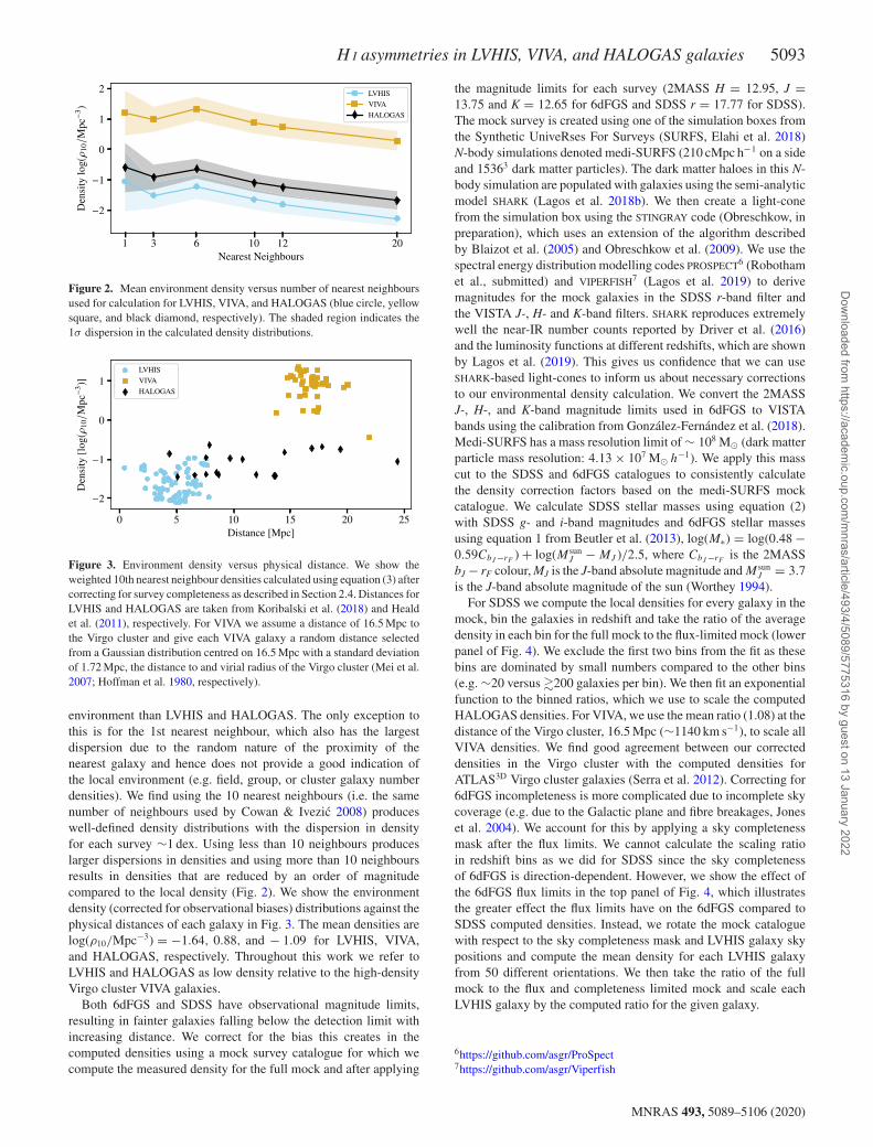
For SDSS we compute the local densities for every galaxy in themock, bin the galaxies in redshift and take the ratio of the averagedensity in each bin for the full mock to the flux-limited mock (lowerpanel of Fig. 4). We exclude the first two bins from the fit as thesebins are dominated by small numbers compared to the other bins(e.g. ∼20 versus �200 galaxies per bin). We then fit an exponentialfunction to the binned ratios, which we use to scale the computedHALOGAS densities. For VIVA, we use the mean ratio (1.08) at thedistance of the Virgo cluster, 16.5 Mpc (∼1140 km s−1), to scale allVIVA densities. We find good agreement between our correcteddensities in the Virgo cluster with the computed densities forATLAS3D Virgo cluster galaxies (Serra et al. 2012). Correcting for6dFGS incompleteness is more complicated due to incomplete skycoverage (e.g. due to the Galactic plane and fibre breakages, Joneset al. 2004). We account for this by applying a sky completenessmask after the flux limits. We cannot calculate the scaling ratioin redshift bins as we did for SDSS since the sky completenessof 6dFGS is direction-dependent. However, we show the effect ofthe 6dFGS flux limits in the top panel of Fig. 4, which illustratesthe greater effect the flux limits have on the 6dFGS compared toSDSS computed densities. Instead, we rotate the mock cataloguewith respect to the sky completeness mask and LVHIS galaxy skypositions and compute the mean density for each LVHIS galaxyfrom 50 different orientations. We then take the ratio of the fullmock to the flux and completeness limited mock and scale eachLVHIS galaxy by the computed ratio for the given galaxy.
6https://github.com/asgr/ProSpect7https://github.com/asgr/Viperfish
MNRAS 493, 5089–5106 (2020)
Dow
nloaded from https://academ
ic.oup.com/m
nras/article/493/4/5089/5775316 by guest on 13 January 2022
5094 T. N. Reynolds et al.
Figure 4. Variation of the ratio between the expected 10th nearest neighbourenvironment density for the full mock catalogue and the 10th nearestneighbour environment density computed after applying the optical surveyflux limits with velocity (cz) for 6dFGS and SDSS (upper and lower panels,respectively). The line in the lower panel is an exponential fit to the binneddata. We exclude the first two bins from the fit as these bins are dominated bysmall numbers compared to the other bins (e.g. ∼20 versus �200 galaxiesper bin). We only perform a fit for correcting SDSS as 6dFGS has theadditional issue of sky completeness, which is direction dependent.
3 A NA LY SIS
We use the Source Finding Application8 (SoFiA, Serra et al. 2015) toextract H I emission >3.5σ from the LVHIS, VIVA, and HALOGAScubes with default parameters for the Smooth+Clip (S+C) finder.The S+C finder smooths the cube over a number of spatial andspectral scales and identifies emission above the defined thresholdwhich are merged at the end. We set minimum merging sizes of 5pixels in both spatial and spectral dimensions and have reliabilityset to >0.7. SoFiA then creates integrated intensity (moment 0) andvelocity field (moment 1) maps, integrated spectra, and detectedsource properties.
3.1 Spectral asymmetries
The integrated spectrum of a galaxy provides global H I informationon a galaxy as a whole compared with spatially resolved maps,which provide more localized information of the distribution of H I
within a galaxy. Most galaxies that have been observed in H I andwill be observed by future surveys will be spatially unresolved,limiting studies of asymmetries in these galaxies to their integratedspectra. We present an example mock spectrum illustrating thespectral asymmetries in Fig. 5. We find spectral resolutions of4–10 km s−1 are sufficient to measure the spectral asymmetriesdescribed in this section.
3.1.1 Velocity differences
The H I systemic velocity can be measured in different ways. In thiswork we measure the systemic velocity using two definitions: theflux-weighted mean systemic velocity, Vsys,fwm, and the systemicvelocity defined as the mid-point of the spectrum at 50 per centof the spectrum’s peak height (i.e. based on the w50 line width),
8We use SoFiA v1.2.1, which can be found at https://github.com/SoFiA-Admin/SoFiA/.
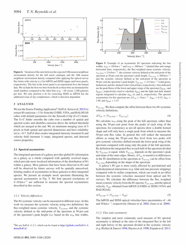
Figure 5. Example of an asymmetric H I spectrum indicating the linewidths, w20 = 184 km s−1 and w50 = 160 km s−1 (dashed blue and orangehorizontal lines, respectively), the flux-weighted mean systemic velocity,vsys,fwm = 214 km s−1, the systemic velocity defined as the mid-point of thespectrum at 20 per cent the spectrum’s peak height, Vsys,w20 = 209 km s−1
and the systemic velocity defined as the mid-point of the spectrum at50 per cent the spectrum’s peak height, Vsys,w50 = 211 km s−1 (solid green,dashed red, and dot–dashed violet vertical lines, respectively). Also indicatedare the peak fluxes of the lower and upper wings of the spectrum (Speak,1 andSpeak,2, respectively) used to calculate Apeak and the light and dark shadedregions integrated to calculate Aflux (I1 and I2, respectively). The spectralasymmetries for this spectrum are �Vsys = 3 km s−1, Aspec = 0.15, Aflux =1.09, and Apeak = 1.47.
Vsys,w50 . We then compute the offset between these two H I systemicvelocity definitions,
�Vsys = |Vsys,fwm − Vsys,w50 |. (4)
We calculate w50 using the peak of the full spectrum, rather thanusing the 50 per cent point from the peaks of each wing of thespectrum, for consistency as not all spectra show a double hornedshape and will only have a single peak from which to measure the50 per cent flux value. In general this will reduce the measuredoffsets as using the 50 per cent flux level from two peaks willgive systemic velocities shifted towards the lower peak wing of thespectrum compared with using only the peak of the full spectrum.By definition the integrated flux in each half of the spectrum dividedby Vsys,fwm is equal, while Vsys,w50 depends on the spectrum’s peakand slope of the outer edges. Hence, �Vsys is sensitive to differencesin the H I distribution in the spectrum as Vsys,w50 can be offset fromVsys, fwm depending on the shape of the spectrum.
A galaxy’s H I gas is more easily affected by gravitational andhydrodynamical interactions (e.g. tidal and ram pressure stripping)compared with its stellar component, which can result in an offsetbetween the systemic velocities measured from optical and H I
surveys. We calculate the difference between the flux weightedmean systemic velocity from the H I spectra, Vsys, fwm, and the opticalvelocity, Vopt, obtained from 6dFGS (LVHIS) or SDSS (VIVA andHALOGAS),
�Vsys,opt = |Vsys,fwm − Vopt|. (5)
The 6dFGS and SDSS optical velocities have uncertainties of ∼46and 30 km s−1, respectively (Strauss et al. 2002; Jones et al. 2009).
3.1.2 Flux ratio asymmetry
The simplest and most commonly used measure of H I spectralasymmetry is defined as the ratio of the integrated flux in the leftand right halves of the spectrum divided at the systemic velocity(e.g. Richter & Sancisi 1994; Haynes et al. 1998; Espada et al. 2011;
MNRAS 493, 5089–5106 (2020)
Dow
nloaded from https://academ
ic.oup.com/m
nras/article/493/4/5089/5775316 by guest on 13 January 2022
H I asymmetries in LVHIS, VIVA, and HALOGAS galaxies 5095
Scott et al. 2018)
Aflux = I1
I2=
∫ vsys,w20vlow
I dv∫ vhighvsys,w20
I dv, (6)
where I1 and I2 are the integrated fluxes in the lower and upper halvesof the spectrum (shaded regions in Fig. 5) integrated from vlow =vsys,w20 − w20/2 to vsys,w20 and from vsys,w20 to vhigh = vsys,w20 +w20/2, respectively. vsys,w20 is the systemic velocity defined as themid-point of the spectrum at the 20 per cent flux level (the w20 linewidth) and vlow and vhigh are the velocities at which the flux densitydrops to 20 per cent of the peak flux density. For channels bridgingthe edges of regions I1 and I2, the flux is assigned to I1 or I2 basedon the fraction of the channel within either region. For example, achannel centred on vsys,w20 will be evenly divided between I1 andI2. Similarly, only half the flux in a channel centred on vlow or vhigh
will contribute to I1 and I2, respectively). If the flux ratio Aflux < 1then the inverse is taken so that Aflux ≥ 1. A perfectly symmetricspectrum has Aflux = 1, with larger values indicating the spectrumis more asymmetric.
3.1.3 Peak flux ratio asymmetry
A related asymmetry parameter to Aflux, is taking the ratio betweenthe left and right peaks of the spectrum (e.g. the ‘height asymmetryindex’, Matthews et al. 1998)
Apeak = Speak,1
Speak,2, (7)
where Speak,1 and Speak,2 are the peak fluxes of the lower and upperwings of the spectrum (illustrated in Fig. 5). As with Aflux, if Apeak
< 1 we take the inverse such that Apeak ≥ 1. We note this is theinverse of the Matthews et al. (1998) definition. The peak flux ratiois limited to use on double horn profiles with defined peaks. Apeak issensitive to peaks in the noise and will not be reliably measurablefor noisy spectra. This does not affect our spectra which generallyhave high signal to noise ratios of SNR > 50.
3.1.4 Flipped spectrum residual
We also look for signs of asymmetry in the residual of the integratedspectrum, which has not been investigated in previous studies. Wedefine the spectrum residual as the sum of the absolute differencesbetween the flux in each channel of the spectrum and the flux in thespectral channel of the spectrum flipped about the systemic velocitynormalized by the integrated flux of the spectrum
Aspec =∑
i |S(i) − Sflip(i)|∑i |S(i)| , (8)
where S(i) and Sflip(i) are the fluxes in channel i of the original andflipped spectrum, respectively. Here we use the flux weighted meansystemic velocity, Vsys,fwm, so that the spectrum is flipped aroundthe centre of mass (COM) so that Aspec is sensitive to differences inthe spectral shape (e.g. higher flux peak or more extended, lowerflux on one side of the spectrum).
3.2 Spatially resolved asymmetries
Spatially resolved galaxies provide the additional information ofthe distribution of H I gas within the galaxies, down to the physicalscale resolved, and the gas kinematics. Morphological asymmetriesuse the two-dimensional information of the integrated intensity
(moment 0) map. The gas kinematics uses the full three-dimensionalinformation of the relative positions of the gas across the planeof the galaxy observed at different frequencies/velocities. Thereare a number of morphological parameters that are computed foroptical images of galaxies, including the concentration (Bershady,Jangren & Conselice 2000), asymmetry (Abraham et al. 1996;Conselice, Bershady & Jangren 2000), smoothness/clumpiness(Conselice 2003), M20 (Lotz, Primack & Madau 2004) and Gini(Abraham, van den Bergh & Nair 2003), which have been previouslyapplied to H I moment 0 maps (e.g. Holwerda et al. 2011a, b, c, d).Giese et al. (2016) found that the SNR affects the reliability ofthe optical parameters when applied to H I maps, with low-SNRdata not producing meaningful results. Accounting for SNR, Gieseet al. (2016) found the Conselice et al. (2000) asymmetry to bethe only parameter to provide useful information for measuringdeviations away from a symmetrical disc. Hence from the opticalmorphology parameters we only consider the Conselice et al.(2000) asymmetry. In this work we only measure morphologicaland kinematic asymmetries for galaxies resolved by ≥3 beams,as Giese et al. (2016) found that a galaxy needs to be resolvedby three or more beams to distinguish between differing levels ofasymmetry.
3.2.1 Moment 0 asymmetry
We use the asymmetry parameter, A, (first used by Abraham et al.1996) used for classification in optical studies to quantify themorphological asymmetry in the moment 0 map using the morerecent definition of Conselice et al. (2000), which includes a termto correct for bias due to noise and background
Amap =∑
i,j |I (i, j ) − I180(i, j )|2∑
i,j |I (i, j )| −∑
i,j |B(i, j ) − B180(i, j )|2∑
i,j |I (i, j )| ,
(9)
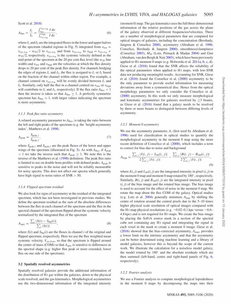
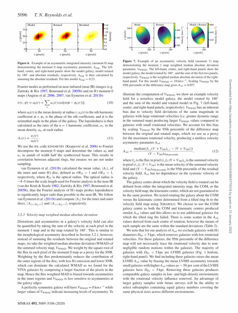
where I(i, j) and I180(i, j) are the integrated intensity in pixel (i, j) inthe moment 0 map and moment 0 map rotated by 180◦, respectively.Similarly, B(i, j) and B180(i, j) are the integrated intensity in pixel(i, j) of the bias image and the rotated bias image. The bias imageis used to account for the effect of noise in the moment 0 map. Werotate the map about the flux COM of the galaxy. Optical studies(e.g. Lotz et al. 2004) generally minimize Amap by shifting thecentre of rotation around the central pixels due to the 5–10 timeshigher physical scale resolution of optical images compared withthe H I map physical resolutions (e.g. ∼0.02–0.1 kpc versus ∼0.6–4.8 kpc) and is not required for H I maps. We create the bias imageby placing the SoFiA source mask in a section of the spectralcube not containing any H I signal and integrating the signal ineach voxel in the mask to create a moment 0 image. Giese et al.(2016) showed that the bias-corrected asymmetry, Amap, providesa lower limit on the intrinsic asymmetry and that the asymmetrycan be better determined using machine learning and a library ofmodel galaxies, however this is beyond the scope of the currentwork. We illustrate the calculation for a noiseless model galaxy,the model rotated by 180◦ and the absolute residuals which arethen summed (left-hand, centre and right-hand panels of Fig. 6,respectively).
3.2.2 Fourier analysis
We use a Fourier analysis to compute morphological lopsidednessin the moment 0 maps by decomposing the maps into their
MNRAS 493, 5089–5106 (2020)
Dow
nloaded from https://academ
ic.oup.com/m
nras/article/493/4/5089/5775316 by guest on 13 January 2022
5096 T. N. Reynolds et al.
Figure 6. Example of an asymmetric integrated intensity (moment 0) mapdemonstrating the moment 0 map asymmetry parameter, Amap. The left-hand, centre, and right-hand panels show the model galaxy, model rotatedby 180◦ and absolute residuals, respectively. Amap is then calculated bysumming the absolute residuals. For this model Amap = 0.23.
Fourier modes as performed on near-infrared (near-IR) images (e.g.Zaritsky & Rix 1997; Bournaud et al. 2005b) and on H I moment 0maps (Angiras et al. 2006, 2007; van Eymeren et al. 2011b)
σ (r, φ) = a0(r) +∑
n
an(r) cos[n(φ − φn(r))], (10)
where a0(r) is the mean density at radius r, an(r) is the nth harmoniccoefficient at r, φn is the phase of the nth coefficient, and φ is theazimuthal angle in the plane of the galaxy. The lopsidedness is thencalculated as the ratio of the n = 1 harmonic coefficient, a1, to themean density, a0, at each radius
A1(r) = a1(r)
a0(r). (11)
We use the IDL code KINEMETRY (Krajnovic et al. 2006) to Fourierdecompose the moment 0 maps and determine the values a0 anda1 in annuli of width half the synthesized beam. This results incorrelation between adjacent rings, but ensures we are not undersampling.
van Eymeren et al. (2011b) calculated the mean value, 〈A1〉, ofthe inner and outer H I disc, defined as r/R25 < 1 and r/R25 > 1,respectively, where R25 is the optical radius. The optical radius is∼4–5 times the scale length used for Fourier analysis in the near-IR(van der Kruit & Searle 1982; Zaritsky & Rix 1997; Bournaud et al.2005b), thus the Fourier analysis of H I maps probes lopsidednessto significantly larger radii than possible in the near-IR. We followvan Eymeren et al. (2011b) and compute 〈A1〉 for the inner and outerdiscs, 〈A1,r/R25<1〉 and 〈A1,r/R25>1〉, respectively.
3.2.3 Velocity map weighted median absolute deviation
Distortions and asymmetries in a galaxy’s velocity field can alsobe quantified by taking the sum of the velocity at each pixel in themoment 1 map and in the map rotated by 180◦. This is similar tothe morphological asymmetry described in Section 3.2.1, however,instead of summing the residuals between the original and rotatedmaps, we take the weighted median absolute deviation (WMAD) ofthe summed velocity map, VWMAD. We weight by the square root ofthe flux in each pixel of the moment 0 map as a proxy for the SNR.Weighting by the flux predominantly reduces the contribution ofthe outer regions of the disc, with less H I emission and lower SNR,which can dominate the calculated WMAD as we found for theVIVA galaxies by comprising a larger fraction of the pixels in themap. Hence the flux weighted MAD is biased towards asymmetriesin the inner regions and VWMAD is less sensitive to asymmetries atthe galaxy edges.
A perfectly symmetric galaxy will have VWMAD = 0 km s−1 whilelarger values of VWMAD indicate increasing levels of asymmetry. To
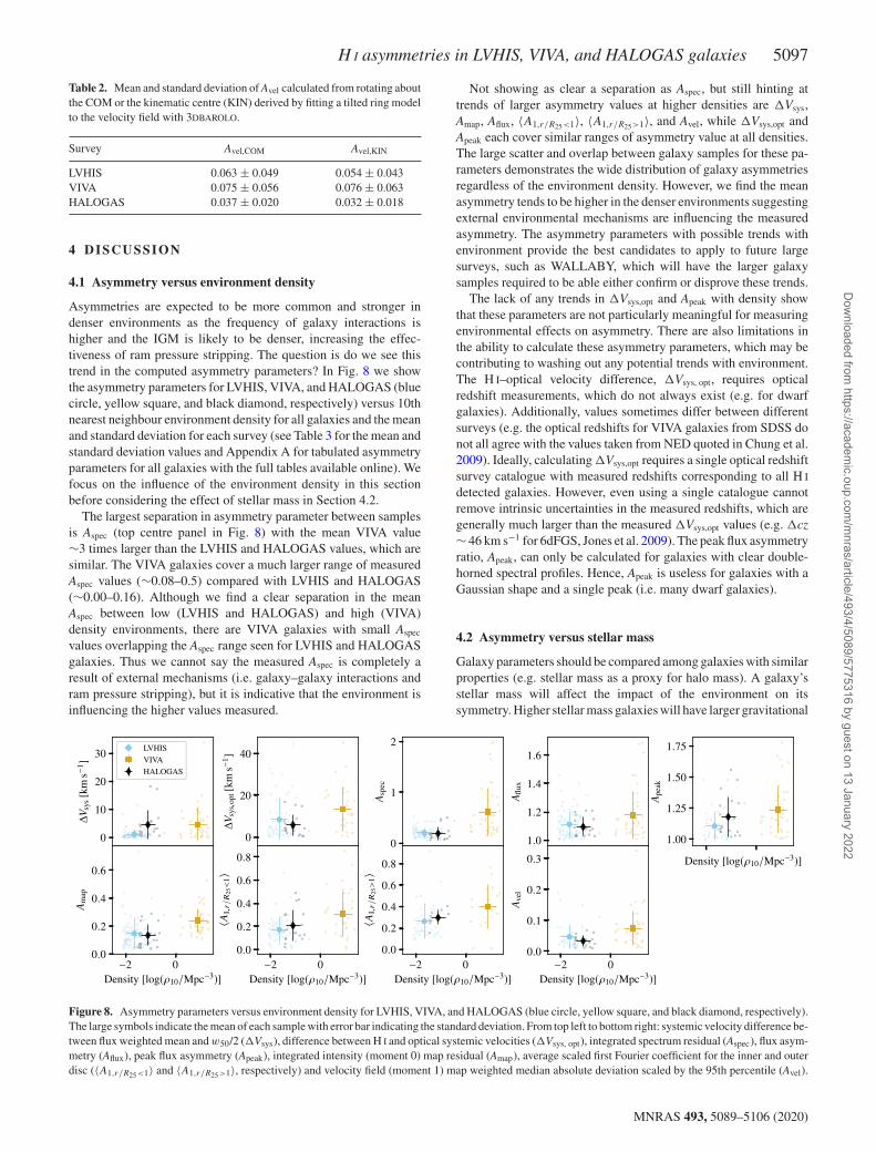
Figure 7. Example of an asymmetric velocity field (moment 1) mapdemonstrating the moment 1 map weighted median absolute deviationparameter, VWMAD. The left-hand, centre, and right-hand panels show themodel galaxy, the model rotated by 180◦, and the sum of the first two panels,respectively. VWMAD is the weighted median absolute deviation of the right-hand panel. For this model VWMAD = 18 km s−1. Scaling VWMAD by the95th percentile of the difference map gives Avel = 0.057.
illustrate the computation of VWMAD, we show an example velocityfield for a noiseless model galaxy, the model rotated by 180◦
and the sum of the model and rotated model in Fig. 7 (left-hand,centre, and right-hand panels, respectively). VWMAD has an inherentbias due to velocity field deviations of the same magnitude ingalaxies with large rotational velocities (i.e. greater dynamic rangein the summed map) producing larger VWMAD values compared togalaxies with small rotational velocities. We account for this biasby scaling VWMAD by the 95th percentile of the difference mapbetween the original and rotated maps, which we use as a proxyfor the maximum rotational velocity, producing a unitless velocityasymmetry parameter Avel
Avel = median(|Ii,j (V + V180)i,j − 〈V + V180〉|)(V − V180)95th percentile
, (12)
where Ii,j is the flux in pixel (i, j), (V + V180)i,j is the summed velocityin pixel (i, j), 〈V + V180〉 is the mean velocity of the summed velocityfield and (V − V180)95th percentile is the 95th percentile of the residualvelocity field. Avel has no dependence on the systemic velocity ofthe galaxy.
The galaxy centre about which the velocity field is rotated can bedefined from either the integrated intensity map, the COM, or thevelocity field map, the kinematic centre, which are not guaranteed tobe the same position. We tested rotating the galaxy about the COMversus the kinematic centre determined from a tilted ring fit to thevelocity field map using 3DBAROLO. We choose to use the COMgalaxy centre as both the COM and kinematic centres producedsimilar Avel values and this allows us to use additional galaxies forwhich the tilted ring fits failed. There is some scatter in the Avel
values derived from each centre of rotation, however the means ofeach sample are the same within the standard deviations (Table 2).
We note that for our analysis of Avel we exclude galaxies with H I
diameters DH I < 5 kpc, which removes galaxies with low rotationalvelocities. For these galaxies, the 95th percentile of the differencemap will not necessarily trace the rotational velocity due to non-negligible random motions within the galaxies. The majority ofgalaxies with DH I < 5 kpc are LVHIS galaxies (Fig. 1 bottom,right-hand panel). We find including these galaxies raises the meanLVHIS Avel value by biasing the mean LVHIS asymmetry towardssmall galaxies with higher Avel values as ∼ 50 per cent of the LVHISgalaxies have DH I < 5 kpc. Removing these galaxies producescomparable galaxy samples in low- and high-density environmentswith the rotational velocity influence removed. An advantage oflarger galaxy samples with future surveys will be the ability toselect subsamples containing equal galaxy numbers covering thesame physical sizes across different environments.
MNRAS 493, 5089–5106 (2020)
Dow
nloaded from https://academ
ic.oup.com/m
nras/article/493/4/5089/5775316 by guest on 13 January 2022
H I asymmetries in LVHIS, VIVA, and HALOGAS galaxies 5097
Table 2. Mean and standard deviation of Avel calculated from rotating aboutthe COM or the kinematic centre (KIN) derived by fitting a tilted ring modelto the velocity field with 3DBAROLO.
Survey Avel,COM Avel,KIN
LVHIS 0.063 ± 0.049 0.054 ± 0.043VIVA 0.075 ± 0.056 0.076 ± 0.063HALOGAS 0.037 ± 0.020 0.032 ± 0.018
4 D ISCUSSION
4.1 Asymmetry versus environment density
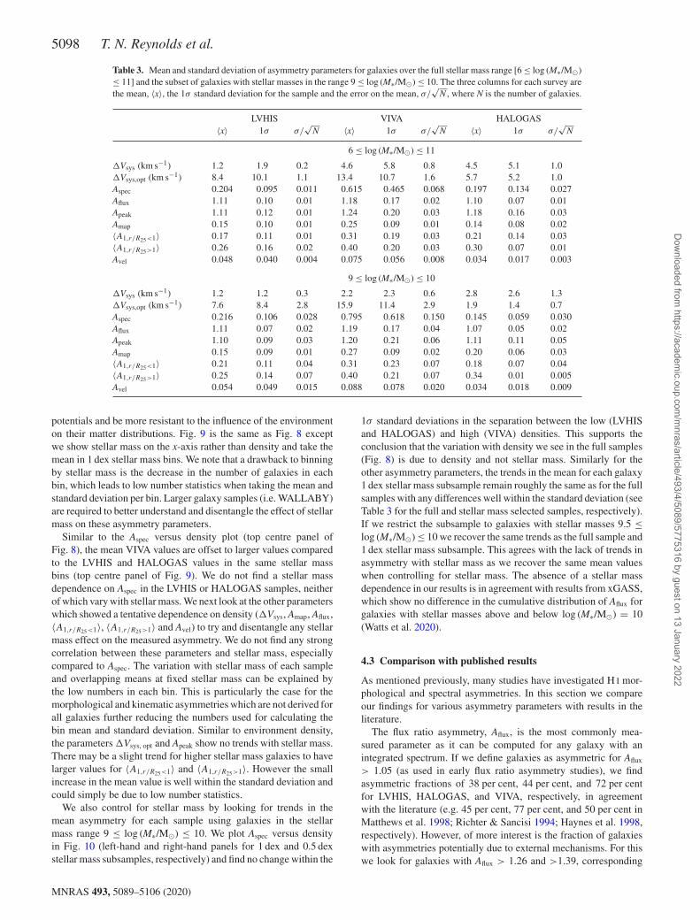
Asymmetries are expected to be more common and stronger indenser environments as the frequency of galaxy interactions ishigher and the IGM is likely to be denser, increasing the effec-tiveness of ram pressure stripping. The question is do we see thistrend in the computed asymmetry parameters? In Fig. 8 we showthe asymmetry parameters for LVHIS, VIVA, and HALOGAS (bluecircle, yellow square, and black diamond, respectively) versus 10thnearest neighbour environment density for all galaxies and the meanand standard deviation for each survey (see Table 3 for the mean andstandard deviation values and Appendix A for tabulated asymmetryparameters for all galaxies with the full tables available online). Wefocus on the influence of the environment density in this sectionbefore considering the effect of stellar mass in Section 4.2.
The largest separation in asymmetry parameter between samplesis Aspec (top centre panel in Fig. 8) with the mean VIVA value∼3 times larger than the LVHIS and HALOGAS values, which aresimilar. The VIVA galaxies cover a much larger range of measuredAspec values (∼0.08–0.5) compared with LVHIS and HALOGAS(∼0.00–0.16). Although we find a clear separation in the meanAspec between low (LVHIS and HALOGAS) and high (VIVA)density environments, there are VIVA galaxies with small Aspec
values overlapping the Aspec range seen for LVHIS and HALOGASgalaxies. Thus we cannot say the measured Aspec is completely aresult of external mechanisms (i.e. galaxy–galaxy interactions andram pressure stripping), but it is indicative that the environment isinfluencing the higher values measured.
Not showing as clear a separation as Aspec, but still hinting attrends of larger asymmetry values at higher densities are �Vsys,Amap, Aflux, 〈A1,r/R25<1〉, 〈A1,r/R25>1〉, and Avel, while �Vsys,opt andApeak each cover similar ranges of asymmetry value at all densities.The large scatter and overlap between galaxy samples for these pa-rameters demonstrates the wide distribution of galaxy asymmetriesregardless of the environment density. However, we find the meanasymmetry tends to be higher in the denser environments suggestingexternal environmental mechanisms are influencing the measuredasymmetry. The asymmetry parameters with possible trends withenvironment provide the best candidates to apply to future largesurveys, such as WALLABY, which will have the larger galaxysamples required to be able either confirm or disprove these trends.
The lack of any trends in �Vsys,opt and Apeak with density showthat these parameters are not particularly meaningful for measuringenvironmental effects on asymmetry. There are also limitations inthe ability to calculate these asymmetry parameters, which may becontributing to washing out any potential trends with environment.The H I–optical velocity difference, �Vsys, opt, requires opticalredshift measurements, which do not always exist (e.g. for dwarfgalaxies). Additionally, values sometimes differ between differentsurveys (e.g. the optical redshifts for VIVA galaxies from SDSS donot all agree with the values taken from NED quoted in Chung et al.2009). Ideally, calculating �Vsys,opt requires a single optical redshiftsurvey catalogue with measured redshifts corresponding to all H I
detected galaxies. However, even using a single catalogue cannotremove intrinsic uncertainties in the measured redshifts, which aregenerally much larger than the measured �Vsys,opt values (e.g. �cz∼ 46 km s−1 for 6dFGS, Jones et al. 2009). The peak flux asymmetryratio, Apeak, can only be calculated for galaxies with clear double-horned spectral profiles. Hence, Apeak is useless for galaxies with aGaussian shape and a single peak (i.e. many dwarf galaxies).
4.2 Asymmetry versus stellar mass
Galaxy parameters should be compared among galaxies with similarproperties (e.g. stellar mass as a proxy for halo mass). A galaxy’sstellar mass will affect the impact of the environment on itssymmetry. Higher stellar mass galaxies will have larger gravitational
Figure 8. Asymmetry parameters versus environment density for LVHIS, VIVA, and HALOGAS (blue circle, yellow square, and black diamond, respectively).The large symbols indicate the mean of each sample with error bar indicating the standard deviation. From top left to bottom right: systemic velocity difference be-tween flux weighted mean and w50/2 (�Vsys), difference between H I and optical systemic velocities (�Vsys, opt), integrated spectrum residual (Aspec), flux asym-metry (Aflux), peak flux asymmetry (Apeak), integrated intensity (moment 0) map residual (Amap), average scaled first Fourier coefficient for the inner and outerdisc (〈A1,r/R25<1〉 and 〈A1,r/R25>1〉, respectively) and velocity field (moment 1) map weighted median absolute deviation scaled by the 95th percentile (Avel).
MNRAS 493, 5089–5106 (2020)
Dow
nloaded from https://academ
ic.oup.com/m
nras/article/493/4/5089/5775316 by guest on 13 January 2022
5098 T. N. Reynolds et al.
Table 3. Mean and standard deviation of asymmetry parameters for galaxies over the full stellar mass range [6 ≤ log (M∗/M�)≤ 11] and the subset of galaxies with stellar masses in the range 9 ≤ log (M∗/M�) ≤ 10. The three columns for each survey arethe mean, 〈x〉, the 1σ standard deviation for the sample and the error on the mean, σ/
√N , where N is the number of galaxies.
LVHIS VIVA HALOGAS〈x〉 1σ σ/
√N 〈x〉 1σ σ/
√N 〈x〉 1σ σ/
√N
6 ≤ log (M∗/M�) ≤ 11
�Vsys (km s−1) 1.2 1.9 0.2 4.6 5.8 0.8 4.5 5.1 1.0�Vsys,opt (km s−1) 8.4 10.1 1.1 13.4 10.7 1.6 5.7 5.2 1.0Aspec 0.204 0.095 0.011 0.615 0.465 0.068 0.197 0.134 0.027Aflux 1.11 0.10 0.01 1.18 0.17 0.02 1.10 0.07 0.01Apeak 1.11 0.12 0.01 1.24 0.20 0.03 1.18 0.16 0.03Amap 0.15 0.10 0.01 0.25 0.09 0.01 0.14 0.08 0.02〈A1,r/R25<1〉 0.17 0.11 0.01 0.31 0.19 0.03 0.21 0.14 0.03〈A1,r/R25>1〉 0.26 0.16 0.02 0.40 0.20 0.03 0.30 0.07 0.01Avel 0.048 0.040 0.004 0.075 0.056 0.008 0.034 0.017 0.003
9 ≤ log (M∗/M�) ≤ 10
�Vsys (km s−1) 1.2 1.2 0.3 2.2 2.3 0.6 2.8 2.6 1.3�Vsys,opt (km s−1) 7.6 8.4 2.8 15.9 11.4 2.9 1.9 1.4 0.7Aspec 0.216 0.106 0.028 0.795 0.618 0.150 0.145 0.059 0.030Aflux 1.11 0.07 0.02 1.19 0.17 0.04 1.07 0.05 0.02Apeak 1.10 0.09 0.03 1.20 0.21 0.06 1.11 0.11 0.05Amap 0.15 0.09 0.01 0.27 0.09 0.02 0.20 0.06 0.03〈A1,r/R25<1〉 0.21 0.11 0.04 0.31 0.23 0.07 0.18 0.07 0.04〈A1,r/R25>1〉 0.25 0.14 0.07 0.40 0.21 0.07 0.34 0.01 0.005Avel 0.054 0.049 0.015 0.088 0.078 0.020 0.034 0.018 0.009
potentials and be more resistant to the influence of the environmenton their matter distributions. Fig. 9 is the same as Fig. 8 exceptwe show stellar mass on the x-axis rather than density and take themean in 1 dex stellar mass bins. We note that a drawback to binningby stellar mass is the decrease in the number of galaxies in eachbin, which leads to low number statistics when taking the mean andstandard deviation per bin. Larger galaxy samples (i.e. WALLABY)are required to better understand and disentangle the effect of stellarmass on these asymmetry parameters.
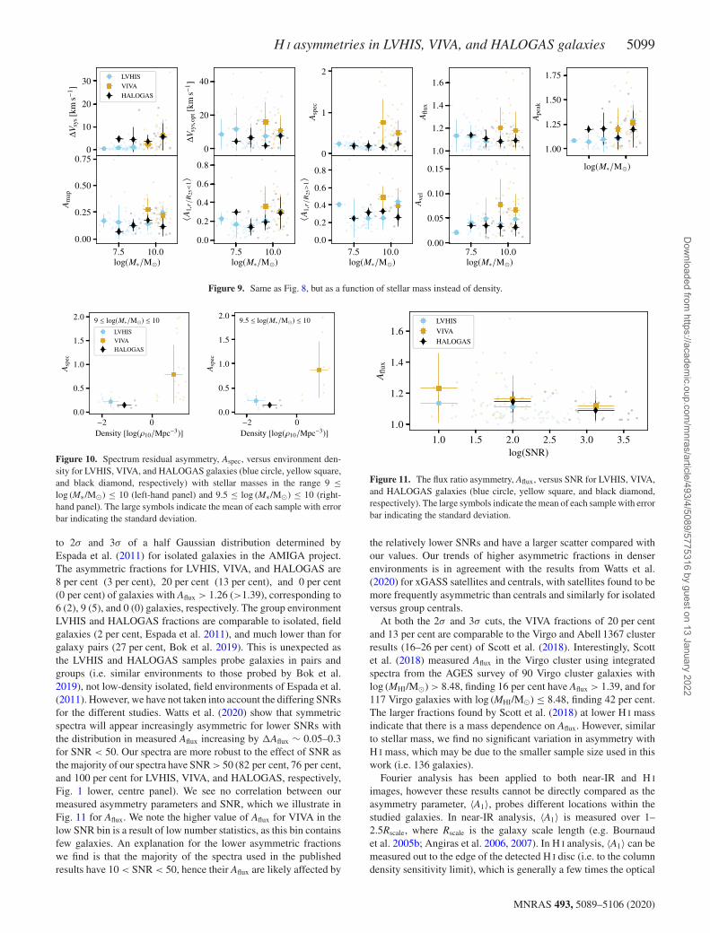
Similar to the Aspec versus density plot (top centre panel ofFig. 8), the mean VIVA values are offset to larger values comparedto the LVHIS and HALOGAS values in the same stellar massbins (top centre panel of Fig. 9). We do not find a stellar massdependence on Aspec in the LVHIS or HALOGAS samples, neitherof which vary with stellar mass. We next look at the other parameterswhich showed a tentative dependence on density (�Vsys, Amap, Aflux,〈A1,r/R25<1〉, 〈A1,r/R25>1〉 and Avel) to try and disentangle any stellarmass effect on the measured asymmetry. We do not find any strongcorrelation between these parameters and stellar mass, especiallycompared to Aspec. The variation with stellar mass of each sampleand overlapping means at fixed stellar mass can be explained bythe low numbers in each bin. This is particularly the case for themorphological and kinematic asymmetries which are not derived forall galaxies further reducing the numbers used for calculating thebin mean and standard deviation. Similar to environment density,the parameters �Vsys, opt and Apeak show no trends with stellar mass.There may be a slight trend for higher stellar mass galaxies to havelarger values for 〈A1,r/R25<1〉 and 〈A1,r/R25>1〉. However the smallincrease in the mean value is well within the standard deviation andcould simply be due to low number statistics.
We also control for stellar mass by looking for trends in themean asymmetry for each sample using galaxies in the stellarmass range 9 ≤ log (M∗/M�) ≤ 10. We plot Aspec versus densityin Fig. 10 (left-hand and right-hand panels for 1 dex and 0.5 dexstellar mass subsamples, respectively) and find no change within the
1σ standard deviations in the separation between the low (LVHISand HALOGAS) and high (VIVA) densities. This supports theconclusion that the variation with density we see in the full samples(Fig. 8) is due to density and not stellar mass. Similarly for theother asymmetry parameters, the trends in the mean for each galaxy1 dex stellar mass subsample remain roughly the same as for the fullsamples with any differences well within the standard deviation (seeTable 3 for the full and stellar mass selected samples, respectively).If we restrict the subsample to galaxies with stellar masses 9.5 ≤log (M∗/M�) ≤ 10 we recover the same trends as the full sample and1 dex stellar mass subsample. This agrees with the lack of trends inasymmetry with stellar mass as we recover the same mean valueswhen controlling for stellar mass. The absence of a stellar massdependence in our results is in agreement with results from xGASS,which show no difference in the cumulative distribution of Aflux forgalaxies with stellar masses above and below log (M∗/M�) = 10(Watts et al. 2020).
4.3 Comparison with published results
As mentioned previously, many studies have investigated H I mor-phological and spectral asymmetries. In this section we compareour findings for various asymmetry parameters with results in theliterature.
The flux ratio asymmetry, Aflux, is the most commonly mea-sured parameter as it can be computed for any galaxy with anintegrated spectrum. If we define galaxies as asymmetric for Aflux
> 1.05 (as used in early flux ratio asymmetry studies), we findasymmetric fractions of 38 per cent, 44 per cent, and 72 per centfor LVHIS, HALOGAS, and VIVA, respectively, in agreementwith the literature (e.g. 45 per cent, 77 per cent, and 50 per cent inMatthews et al. 1998; Richter & Sancisi 1994; Haynes et al. 1998,respectively). However, of more interest is the fraction of galaxieswith asymmetries potentially due to external mechanisms. For thiswe look for galaxies with Aflux > 1.26 and >1.39, corresponding
MNRAS 493, 5089–5106 (2020)
Dow
nloaded from https://academ
ic.oup.com/m
nras/article/493/4/5089/5775316 by guest on 13 January 2022
H I asymmetries in LVHIS, VIVA, and HALOGAS galaxies 5099
Figure 9. Same as Fig. 8, but as a function of stellar mass instead of density.
Figure 10. Spectrum residual asymmetry, Aspec, versus environment den-sity for LVHIS, VIVA, and HALOGAS galaxies (blue circle, yellow square,and black diamond, respectively) with stellar masses in the range 9 ≤log (M∗/M�) ≤ 10 (left-hand panel) and 9.5 ≤ log (M∗/M�) ≤ 10 (right-hand panel). The large symbols indicate the mean of each sample with errorbar indicating the standard deviation.
to 2σ and 3σ of a half Gaussian distribution determined byEspada et al. (2011) for isolated galaxies in the AMIGA project.The asymmetric fractions for LVHIS, VIVA, and HALOGAS are8 per cent (3 per cent), 20 per cent (13 per cent), and 0 per cent(0 per cent) of galaxies with Aflux > 1.26 (>1.39), corresponding to6 (2), 9 (5), and 0 (0) galaxies, respectively. The group environmentLVHIS and HALOGAS fractions are comparable to isolated, fieldgalaxies (2 per cent, Espada et al. 2011), and much lower than forgalaxy pairs (27 per cent, Bok et al. 2019). This is unexpected asthe LVHIS and HALOGAS samples probe galaxies in pairs andgroups (i.e. similar environments to those probed by Bok et al.2019), not low-density isolated, field environments of Espada et al.(2011). However, we have not taken into account the differing SNRsfor the different studies. Watts et al. (2020) show that symmetricspectra will appear increasingly asymmetric for lower SNRs withthe distribution in measured Aflux increasing by �Aflux ∼ 0.05–0.3for SNR < 50. Our spectra are more robust to the effect of SNR asthe majority of our spectra have SNR > 50 (82 per cent, 76 per cent,and 100 per cent for LVHIS, VIVA, and HALOGAS, respectively,Fig. 1 lower, centre panel). We see no correlation between ourmeasured asymmetry parameters and SNR, which we illustrate inFig. 11 for Aflux. We note the higher value of Aflux for VIVA in thelow SNR bin is a result of low number statistics, as this bin containsfew galaxies. An explanation for the lower asymmetric fractionswe find is that the majority of the spectra used in the publishedresults have 10 < SNR < 50, hence their Aflux are likely affected by
Figure 11. The flux ratio asymmetry, Aflux, versus SNR for LVHIS, VIVA,and HALOGAS galaxies (blue circle, yellow square, and black diamond,respectively). The large symbols indicate the mean of each sample with errorbar indicating the standard deviation.
the relatively lower SNRs and have a larger scatter compared withour values. Our trends of higher asymmetric fractions in denserenvironments is in agreement with the results from Watts et al.(2020) for xGASS satellites and centrals, with satellites found to bemore frequently asymmetric than centrals and similarly for isolatedversus group centrals.
At both the 2σ and 3σ cuts, the VIVA fractions of 20 per centand 13 per cent are comparable to the Virgo and Abell 1367 clusterresults (16–26 per cent) of Scott et al. (2018). Interestingly, Scottet al. (2018) measured Aflux in the Virgo cluster using integratedspectra from the AGES survey of 90 Virgo cluster galaxies withlog (MHI/M�) > 8.48, finding 16 per cent have Aflux > 1.39, and for117 Virgo galaxies with log (MHI/M�) ≤ 8.48, finding 42 per cent.The larger fractions found by Scott et al. (2018) at lower H I massindicate that there is a mass dependence on Aflux. However, similarto stellar mass, we find no significant variation in asymmetry withH I mass, which may be due to the smaller sample size used in thiswork (i.e. 136 galaxies).
Fourier analysis has been applied to both near-IR and H I
images, however these results cannot be directly compared as theasymmetry parameter, 〈A1〉, probes different locations within thestudied galaxies. In near-IR analysis, 〈A1〉 is measured over 1–2.5Rscale, where Rscale is the galaxy scale length (e.g. Bournaudet al. 2005b; Angiras et al. 2006, 2007). In H I analysis, 〈A1〉 can bemeasured out to the edge of the detected H I disc (i.e. to the columndensity sensitivity limit), which is generally a few times the optical
MNRAS 493, 5089–5106 (2020)
Dow
nloaded from https://academ
ic.oup.com/m
nras/article/493/4/5089/5775316 by guest on 13 January 2022
5100 T. N. Reynolds et al.
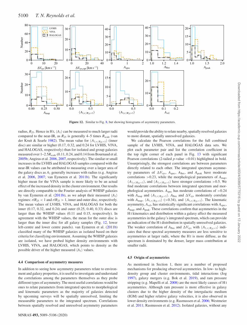
Figure 12. Similar to Fig. 8, but showing histograms of asymmetry parameters.
radius, R25. Hence in H I, 〈A1〉 can be measured to much larger radiicompared to the near-IR, as R25 is generally 4–5 times Rscale (vander Kruit & Searle 1982). The mean value for 〈A1,r/R25<1〉 (innerdisc) are similar or higher (0.17, 0.32, and 0.24 for LVHIS, VIVA,and HALOGAS, respectively) than for isolated and group galaxiesmeasured over 1–2.5Rscale (0.11, 0.24, and 0.14 from Bournaud et al.2005b; Angiras et al. 2006, 2007, respectively). The similar or smallincreases in the LVHIS and HALOGAS samples compared with thenear-IR values can be attributed to measuring over a larger area ofthe galaxy discs as A1 generally increases with radius (e.g. Angiraset al. 2006, 2007; van Eymeren et al. 2011b). The significantlyhigher mean for the VIVA sample is more likely to be an actualeffect of the increased density in the cluster environment. Our resultsare directly comparable to the Fourier analysis of WHISP galaxiesby van Eymeren et al. (2011b), as we adopt their measured 〈A1〉regimes: r/R25 < 1 and r/R25 > 1, inner and outer disc, respectively.The mean values of LVHIS, VIVA, and HALOGAS for both theinner (0.17, 0.32, and 0.24) and outer (0.25, 0.40, 0.33) discs arelarger than the WHISP values (0.11 and 0.15, respectively). Inagreement with the WHISP values, the mean for the outer disc islarger than the inner disc for all galaxy samples (Fig. 12, lowerleft-centre and lower centre panels). van Eymeren et al. (2011b)classified many of the WHISP galaxies as isolated based on theircriteria for classifying environment. Assuming the WHISP galaxiesare isolated, we have probed higher density environments withLVHIS, VIVA, and HALOGAS, which points to density as thepossible driver of the higher measured 〈A1〉 values.
4.4 Comparison of asymmetry measures
In addition to seeing how asymmetry parameters relate to environ-ment and galaxy properties, it is useful to investigate and understandthe correlations among the parameters themselves as they probedifferent types of asymmetry. The most useful correlations would beones to relate parameters from integrated spectra to morphologicaland kinematic parameters as the majority of galaxies detectedby upcoming surveys will be spatially unresolved, limiting themeasurable parameters to the integrated spectrum. Correlationsbetween spatially resolved and unresolved asymmetry parameters
would provide the ability to relate nearby, spatially resolved galaxiesto more distant, spatially unresolved galaxies.
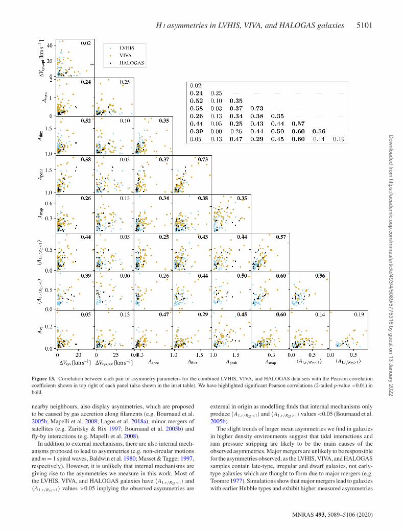
We calculate the Pearson correlations for the full combinedsample of the LVHIS, VIVA, and HALOGAS data sets. Weplot each parameter pair and list the correlation coefficient inthe top right corner of each panel in Fig. 13 with significantPearson correlations (2-tailed p-value <0.01) highlighted in bold.Unsurprisingly, the strongest correlations are between parametersdirectly related to each other. The integrated spectrum asymme-try parameters of �Vsys, Aspec, Aflux, and Apeak have moderatecorrelations >0.23, while the morphological parameters of Amap,〈A1,r/R25<1〉, and 〈A1,r/R25>1〉 have stronger correlations >0.5. Wefind moderate correlations between integrated spectrum and mor-phological asymmetries. Aspec has moderate correlations of >0.24with Amap and 〈A1,r/R25<1〉. Aflux and �Vsys moderately correlatewith Amap, 〈A1,r/R25<1〉 (>0.34), and 〈A1,r/R25>1〉. The kinematicasymmetry, Avel, has statistically significant correlations with Aspec,Amap, and Apeak. These correlations confirm that asymmetries in theH I kinematics and distribution within a galaxy affect the measuredasymmetries in the galaxy’s integrated spectrum, which can providean indication of the H I distribution in spatially unresolved galaxies.The weaker correlation of Aflux and �Vsys with 〈A1,r/R25>1〉 indi-cates that these spectral asymmetry measures are less sensitive toasymmetries at larger radii, where the H I is more diffuse, as thespectrum is dominated by the denser, larger mass contribution atsmaller radii.
4.5 Origin of asymmetries
As mentioned in Section 1, there are a number of proposedmechanisms for producing observed asymmetries. In low- to high-density group and cluster environments, tidal interactions (Jog1997), galaxy mergers (e.g. Bok et al. 2019), and ram pressurestripping (e.g. Mapelli et al. 2008) are the most likely causes of H I
asymmetries. Although ram pressure is more effective in galaxyclusters due to the higher density of the intergalactic medium(IGM) and higher relative galaxy velocities, it is also observed inlower density environments (e.g. Rasmussen et al. 2006; Westmeieret al. 2011; Rasmussen et al. 2012). Isolated galaxies, without any
MNRAS 493, 5089–5106 (2020)
Dow
nloaded from https://academ
ic.oup.com/m
nras/article/493/4/5089/5775316 by guest on 13 January 2022
H I asymmetries in LVHIS, VIVA, and HALOGAS galaxies 5101
Figure 13. Correlation between each pair of asymmetry parameters for the combined LVHIS, VIVA, and HALOGAS data sets with the Pearson correlationcoefficients shown in top right of each panel (also shown in the inset table). We have highlighted significant Pearson correlations (2-tailed p-value <0.01) inbold.
nearby neighbours, also display asymmetries, which are proposedto be caused by gas accretion along filaments (e.g. Bournaud et al.2005b; Mapelli et al. 2008; Lagos et al. 2018a), minor mergers ofsatellites (e.g. Zaritsky & Rix 1997; Bournaud et al. 2005b) andfly-by interactions (e.g. Mapelli et al. 2008).
In addition to external mechanisms, there are also internal mech-anisms proposed to lead to asymmetries (e.g. non-circular motionsand m = 1 spiral waves, Baldwin et al. 1980; Masset & Tagger 1997,respectively). However, it is unlikely that internal mechanisms aregiving rise to the asymmetries we measure in this work. Most ofthe LVHIS, VIVA, and HALOGAS galaxies have 〈A1,r/R25<1〉 and〈A1,r/R25>1〉 values >0.05 implying the observed asymmetries are
external in origin as modelling finds that internal mechanisms onlyproduce 〈A1,r/R25<1〉 and 〈A1,r/R25>1〉 values <0.05 (Bournaud et al.2005b).
The slight trends of larger mean asymmetries we find in galaxiesin higher density environments suggest that tidal interactions andram pressure stripping are likely to be the main causes of theobserved asymmetries. Major mergers are unlikely to be responsiblefor the asymmetries observed, as the LVHIS, VIVA, and HALOGASsamples contain late-type, irregular and dwarf galaxies, not early-type galaxies which are thought to form due to major mergers (e.g.Toomre 1977). Simulations show that major mergers lead to galaxieswith earlier Hubble types and exhibit higher measured asymmetries
MNRAS 493, 5089–5106 (2020)
Dow
nloaded from https://academ
ic.oup.com/m
nras/article/493/4/5089/5775316 by guest on 13 January 2022
5102 T. N. Reynolds et al.
during the merging process, while post-merger the final galaxybecomes more symmetric with lower measured asymmetries after∼1 Gyr (Walker, Mihos & Hernquist 1996; Bournaud, Jog &Combes 2005a; Bournaud et al. 2005b). However, minor mergersare still a possible cause. Gravitational interactions and minormergers produce asymmetries with longer life-times of ∼2–4 Gyr insimulations (Bournaud et al. 2005b), which can provide a time framefor a galaxy’s interaction history based on measured asymmetries.
Ram pressure likely has the greatest effect on the VIVA asym-metries as this sample probes the cluster environment of Virgo.However, several instances of likely tidal interactions causingasymmetries in VIVA galaxies have been identified (Chung et al.2009). Asymmetries in LVHIS and HALOGAS are likely predom-inantly caused by tidal interactions and possibly mergers as thesesamples probe pair and group environments. However, De Bloket al. (2014) and Westmeier et al. (2011) have also identified rampressure stripping as affecting galaxies in HALOGAS (NGC 4414)and LVHIS (NGC 300), respectively. Ram pressure would be morelikely to affect HALOGAS and LVHIS galaxies in larger groups(e.g. Sculptor and Coma I) with a denser IGM, more similar toin clusters, compared to the low-density IGM around the galaxypairs probed by these samples. The LVHIS, VIVA, and HALOGASgalaxy samples do not probe isolated galaxies, so gas accretionprobably has a small influence on the measured asymmetries asthere is likely less cold gas in higher density environments (e.g.Angiras et al. 2006). However, inflows could be responsible for theasymmetries measured in the lowest density LVHIS galaxies, asthese galaxies are unlikely to be undergoing tidal interactions andthe IGM is likely to be very low in density.
4.6 Implications for WALLABY
WALLABY will detect ∼ 500 000 galaxies in H I out to z ∼ 0.26across ∼ 75 per cent of the sky, enabling WALLABY to probeenvironment densities ranging from isolated, field galaxies to densecluster environments in statistically significant numbers. Comparedwith the analysis here, with WALLABY we will have sufficientnumbers of detections to more finely bin galaxies by density whilealso spanning a much larger range in environment densities.
To provide predictions for WALLABY, we create a mock surveycatalogue using the light-cone created from the medi-SURFSsimulation box described in Section 2.4. We also create a light-conefrom a smaller SURFS box, denoted micro-SURFS (40 cMpc h−1
on a side and 5123 dark matter particles), using the same methodas previously discussed. Micro-SURFS has a higher resolution thanmedi-SURFS (dark matter particle mass resolutions: 4.13 × 10⁷
and 2.21 × 10⁸ M� h−1 for micro- and medi-SURFS, respectively).To get the final mock survey catalogue we combine the micro-SURFS detections for z < 0.04 and M∗ > 106 M� with the medi-SURFS detections for z > 0.04 and M∗ > 108 M�, as micro-SURFS resolves smaller galaxies which will only be detectablewith WALLABY in the nearby Universe (the applied mass limitscorrespond to the resolution limits of each SURFS box). We thencreate H I emission for each mock galaxy using the H I emission linegenerator code9 presented in Chauhan et al. (2019). We estimatethe WALLABY detections by calculating the integrated flux ofeach mock galaxy, using the atomic mass estimated as an outputof SHARK and the distance from the light-cone, and comparing itwith the sensitivity of ASKAP (Duffy et al. 2012). We also find
9https://github.com/garimachauhan92/HI-Emission-Line-Generator
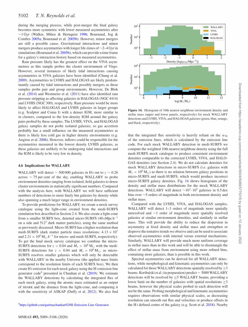
Figure 14. Histogram of 10th nearest neighbour environment density andstellar mass (upper and lower panels, respectively) for mock WALLABYdetections and LVHIS, VIVA, and HALOGAS galaxies (green, blue, orange,and black, respectively).
that the integrated flux sensitivity is heavily reliant on the w50
of the emission lines, which is calculated by the emission linecode. For each mock WALLABY detection in medi-SURFS wecompute the weighted 10th nearest neighbour density using the fullmedi-SURFS mock catalogue to produce consistent environmentdensities comparable to the corrected LVHIS, VIVA, and HALO-GAS densities (see Section 2.4). We do not calculate densities formock WALLABY detections in micro-SURFS (i.e. galaxies withM∗ < 108 M�) as there is no relation between galaxy positions inmicro-SURFS and medi-SURFS, which would produce incorrectmicro-SURFS galaxy densities. Fig. 14 shows histograms of thedensity and stellar mass distributions for the mock WALLABYdetections. WALLABY will detect ∼103–105 galaxies in 0.5 dexbins over ∼5 orders of magnitude in both environment density andstellar mass.
Compared with the LVHIS, VIVA, and HALOGAS samples,WALLABY will detect 1–3 orders of magnitude more spatiallyunresolved and ∼1 order of magnitude more spatially resolvedgalaxies at similar environment densities, and similarly in stellarmass. This will provide the ability to reduce the dispersion inasymmetry at fixed density and stellar mass and strengthen ordisprove the tentative trends we observe and can be used to associateobserved asymmetries with internal versus external mechanisms.Similarly, WALLABY will provide much more uniform coveragein stellar mass than in this work and will be able to disentangle theeffect of stellar mass from environment using more refined bins,containing more galaxies, than is possible in this work.
Spectral asymmetries can be derived for all WALLABY detec-tions, while morphological and kinematic asymmetries can only becalculated for those WALLABY detections spatially resolved by ≥3beams. Koribalski et al. (in preparation) predict ∼ 5000 WALLABYdetections will be resolved by ≥5 WALLABY beams, providing alower limit on the number of galaxies with spatial resolutions ≥3beams, however the physical scales probed in each detection willnot be the same. Probing morphological and kinematic asymmetriesrequires observations with similar physical scales, as decreasingresolution can smooth out flux and velocities or produce offsets inthe H I defined centre of the galaxy (e.g. Scott et al. 2018). Nearby
MNRAS 493, 5089–5106 (2020)
Dow
nloaded from https://academ
ic.oup.com/m
nras/article/493/4/5089/5775316 by guest on 13 January 2022
H I asymmetries in LVHIS, VIVA, and HALOGAS galaxies 5103
galaxies with higher physical scale resolution can be smoothedto match the lower resolutions of more distant galaxies, which willincrease the sample size for direct comparison of morphological andkinematic asymmetries and enable the comparison of galaxies at agreater range of distances. Even with this limitation, WALLABYwill still provide significantly larger samples covering a range ofresolved physical scales than past surveys.
5 SU M M A RY
In this work we have investigated the influence of environmentdensity and stellar mass on measured spectral asymmetry param-eters from integrated spectra and morphological and kinematicasymmetry parameters from spatially resolved images of galaxiesin the LVHIS, VIVA, and HALOGAS surveys. Our main results areas follows:
(i) We find a trend in the integrated spectrum residual withenvironment density and a hint of trends in the morphologicalasymmetry parameters, the weighted median absolute deviationof the velocity field, the flux ratio asymmetry, and the differencein measured H I systemic velocities with environment. The envi-ronmental dependence is also supported from comparison of mor-phological asymmetries presented here with previously publishedresults. However, larger galaxy samples are required to determineif these are true trends or artefacts of low-number statistics.
(ii) We find no correlations between H I asymmetries and eitherstellar or H I mass. The lack of correlation with H I mass is indisagreement with the results of Scott et al. (2018) for Virgo clustergalaxies. Scott et al. (2018) found a larger asymmetric fraction(42 per cent) of galaxies with H I masses log (MH I/M�) ≤ 8.48compared with 16 per cent with log (MH I/M�) > 8.48 (117 and 90galaxies, respectively) and is potentially due to the small samplesize used in this work (136 galaxies).
(iii) As expected, the strongest correlations are between relatedasymmetry measures (i.e. between spectral parameters). However,we also find moderate correlations of spectral asymmetries withmorphological and kinematic asymmetry parameters indicatingspatially resolved asymmetries influence the asymmetries measuredfrom integrated spectra.
(iv) We propose parametrizing integrated spectrum asymmetrieswith the spectrum residual (Aspec), H I systemic velocity difference(�Vsys), and flux ratio asymmetry (Aflux). For spatially resolvedgalaxies, we propose parametrizing morphological asymmetrieswith the integrated intensity map residual (Amap) and Fourier anal-ysis of the integrated intensity map (〈A1,r/R25<1〉 and 〈A1,r/R25>1〉)and kinematic asymmetries using the weighted median absolutedeviation of the velocity field scaled by the 95th percentile (Avel).
(v) Tidal interactions and ram-pressure stripping are the mostlikely mechanisms responsible for the measured asymmetries, whilegas inflows could cause the small measured asymmetries in theLVHIS galaxies at the lowest estimated environment densities. Thisis supported by LVHIS, VIVA, and HALOGAS galaxies identifiedas undergoing tidal interactions and ram-pressure stripping inprevious work. However, the statistical analysis we present herecannot be used to distinguish between tidal interactions and rampressure, which requires detailed, targeted studies of individualspatially resolved systems.
Upcoming surveys, such as WALLABY, will detect significantlylarger numbers of galaxies covering a wide range of environmentdensities and stellar masses. These surveys will provide singleuniform samples for which we can carry out the analysis presented
here. This will remove inherent differences between surveys, bematched to a single optical redshift catalogue for environmentestimation and remove the influence of low number statistics. Futurestudies will then be able to investigate correlations between H I
asymmetries with other galaxy properties in addition to environmentand stellar mass, such as H I deficiency and SFR.
AC K N OW L E D G E M E N T S
We thank B. Koribalski for providing helpful comments. We alsothank B. Holwerda for instructive discussions and comments. Thisresearch was conducted by the Australian Research Council Centreof Excellence for All Sky Astrophysics in 3 Dimensions (ASTRO3D), through project number CE170100013. This research wassupported by the Munich Institute for Astro- and Particle Physics(MIAPP) of the DFG cluster of excellence ‘Origin and Structureof the Universe’. This research has made use of the NASA/IPACExtragalactic Database (NED) which is operated by the Jet Propul-sion Laboratory, California Institute of Technology, under contractwith the National Aeronautics and Space Administration. The LocalVolume H I Survey H I 21-cm observations were obtained with theAustralia Telescope Compact Array which is part of the AustraliaTelescope National Facility that is funded by the Commonwealthof Australia for operations as a National Facility managed byCommonwealth Scientific and Industrial Research Organisation(CSIRO). This research made use of data from WSRT HALOGAS-DR1. The Westerbork Synthesis Radio Telescope is operated byASTRON (Netherlands Institute for Radio Astronomy) with supportfrom the Netherlands Foundation for Scientific Research NWO.This research used data from VIVA survey carried out on the KarlG. Jansky Very Large Array, which is part of the National RadioAstronomy Observatory. The National Radio Astronomy Observa-tory is a facility of the National Science Foundation operated undercooperative agreement by Associated Universities, Inc.
Funding for the Sloan Digital Sky Survey IV has been providedby the Alfred P. Sloan Foundation, the U.S. Department of EnergyOffice of Science, and the Participating Institutions. SDSS-IVacknowledges support and resources from the Center for High-Performance Computing at the University of Utah. The SDSS website is www.sdss.org.
SDSS-IV is managed by the Astrophysical Research Consor-tium for the Participating Institutions of the SDSS Collaborationincluding the Brazilian Participation Group, the Carnegie Institutionfor Science, Carnegie Mellon University, the Chilean Participa-tion Group, the French Participation Group, Harvard-SmithsonianCenter for Astrophysics, Instituto de Astrofısica de Canarias, TheJohns Hopkins University, Kavli Institute for the Physics andMathematics of the Universe (IPMU) / University of Tokyo, theKorean Participation Group, Lawrence Berkeley National Lab-oratory, Leibniz Institut fur Astrophysik Potsdam (AIP), Max-Planck-Institut fur Astronomie (MPIA Heidelberg), Max-Planck-Institut fur Astrophysik (MPA Garching), Max-Planck-Institut furExtraterrestrische Physik (MPE), National Astronomical Observa-tories of China, New Mexico State University, New York University,University of Notre Dame, Observatario Nacional / MCTI, TheOhio State University, Pennsylvania State University, ShanghaiAstronomical Observatory, United Kingdom Participation Group,Universidad Nacional Autonoma de Mexico, University of Arizona,University of Colorado Boulder, University of Oxford, University ofPortsmouth, University of Utah, University of Virginia, Universityof Washington, University of Wisconsin, Vanderbilt University, andYale University.
MNRAS 493, 5089–5106 (2020)
Dow
nloaded from https://academ
ic.oup.com/m
nras/article/493/4/5089/5775316 by guest on 13 January 2022
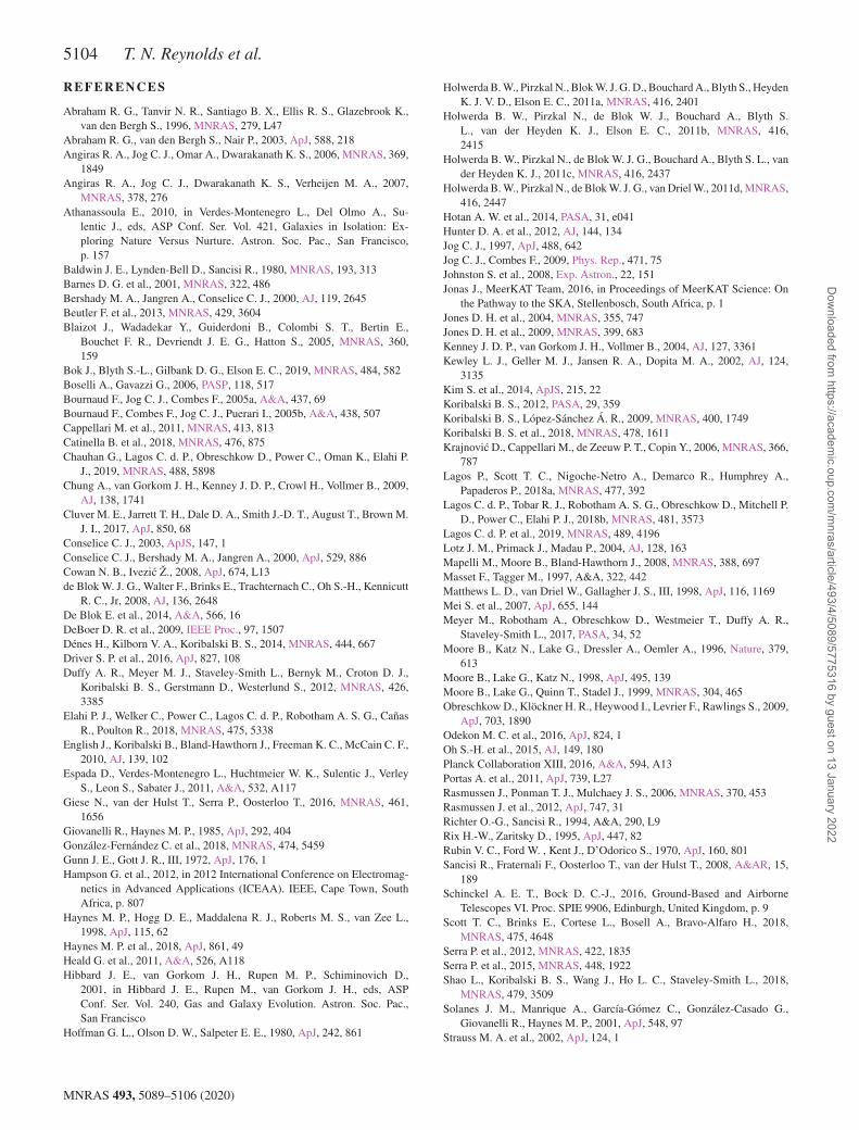
5104 T. N. Reynolds et al.
RE FERENCES
Abraham R. G., Tanvir N. R., Santiago B. X., Ellis R. S., Glazebrook K.,van den Bergh S., 1996, MNRAS, 279, L47
Abraham R. G., van den Bergh S., Nair P., 2003, ApJ, 588, 218Angiras R. A., Jog C. J., Omar A., Dwarakanath K. S., 2006, MNRAS, 369,
1849Angiras R. A., Jog C. J., Dwarakanath K. S., Verheijen M. A., 2007,
MNRAS, 378, 276Athanassoula E., 2010, in Verdes-Montenegro L., Del Olmo A., Su-
lentic J., eds, ASP Conf. Ser. Vol. 421, Galaxies in Isolation: Ex-ploring Nature Versus Nurture. Astron. Soc. Pac., San Francisco,p. 157
Baldwin J. E., Lynden-Bell D., Sancisi R., 1980, MNRAS, 193, 313Barnes D. G. et al., 2001, MNRAS, 322, 486Bershady M. A., Jangren A., Conselice C. J., 2000, AJ, 119, 2645Beutler F. et al., 2013, MNRAS, 429, 3604Blaizot J., Wadadekar Y., Guiderdoni B., Colombi S. T., Bertin E.,
Bouchet F. R., Devriendt J. E. G., Hatton S., 2005, MNRAS, 360,159
Bok J., Blyth S.-L., Gilbank D. G., Elson E. C., 2019, MNRAS, 484, 582Boselli A., Gavazzi G., 2006, PASP, 118, 517Bournaud F., Jog C. J., Combes F., 2005a, A&A, 437, 69Bournaud F., Combes F., Jog C. J., Puerari I., 2005b, A&A, 438, 507Cappellari M. et al., 2011, MNRAS, 413, 813Catinella B. et al., 2018, MNRAS, 476, 875Chauhan G., Lagos C. d. P., Obreschkow D., Power C., Oman K., Elahi P.
J., 2019, MNRAS, 488, 5898Chung A., van Gorkom J. H., Kenney J. D. P., Crowl H., Vollmer B., 2009,
AJ, 138, 1741Cluver M. E., Jarrett T. H., Dale D. A., Smith J.-D. T., August T., Brown M.
J. I., 2017, ApJ, 850, 68Conselice C. J., 2003, ApJS, 147, 1Conselice C. J., Bershady M. A., Jangren A., 2000, ApJ, 529, 886Cowan N. B., Ivezic Z., 2008, ApJ, 674, L13de Blok W. J. G., Walter F., Brinks E., Trachternach C., Oh S.-H., Kennicutt
R. C., Jr, 2008, AJ, 136, 2648De Blok E. et al., 2014, A&A, 566, 16DeBoer D. R. et al., 2009, IEEE Proc., 97, 1507Denes H., Kilborn V. A., Koribalski B. S., 2014, MNRAS, 444, 667Driver S. P. et al., 2016, ApJ, 827, 108Duffy A. R., Meyer M. J., Staveley-Smith L., Bernyk M., Croton D. J.,
Koribalski B. S., Gerstmann D., Westerlund S., 2012, MNRAS, 426,3385
Elahi P. J., Welker C., Power C., Lagos C. d. P., Robotham A. S. G., CanasR., Poulton R., 2018, MNRAS, 475, 5338
English J., Koribalski B., Bland-Hawthorn J., Freeman K. C., McCain C. F.,2010, AJ, 139, 102
Espada D., Verdes-Montenegro L., Huchtmeier W. K., Sulentic J., VerleyS., Leon S., Sabater J., 2011, A&A, 532, A117
Giese N., van der Hulst T., Serra P., Oosterloo T., 2016, MNRAS, 461,1656
Giovanelli R., Haynes M. P., 1985, ApJ, 292, 404Gonzalez-Fernandez C. et al., 2018, MNRAS, 474, 5459Gunn J. E., Gott J. R., III, 1972, ApJ, 176, 1Hampson G. et al., 2012, in 2012 International Conference on Electromag-
netics in Advanced Applications (ICEAA). IEEE, Cape Town, SouthAfrica, p. 807
Haynes M. P., Hogg D. E., Maddalena R. J., Roberts M. S., van Zee L.,1998, ApJ, 115, 62
Haynes M. P. et al., 2018, ApJ, 861, 49Heald G. et al., 2011, A&A, 526, A118Hibbard J. E., van Gorkom J. H., Rupen M. P., Schiminovich D.,
2001, in Hibbard J. E., Rupen M., van Gorkom J. H., eds, ASPConf. Ser. Vol. 240, Gas and Galaxy Evolution. Astron. Soc. Pac.,San Francisco
Hoffman G. L., Olson D. W., Salpeter E. E., 1980, ApJ, 242, 861
Holwerda B. W., Pirzkal N., Blok W. J. G. D., Bouchard A., Blyth S., HeydenK. J. V. D., Elson E. C., 2011a, MNRAS, 416, 2401
Holwerda B. W., Pirzkal N., de Blok W. J., Bouchard A., Blyth S.L., van der Heyden K. J., Elson E. C., 2011b, MNRAS, 416,2415
Holwerda B. W., Pirzkal N., de Blok W. J. G., Bouchard A., Blyth S. L., vander Heyden K. J., 2011c, MNRAS, 416, 2437
Holwerda B. W., Pirzkal N., de Blok W. J. G., van Driel W., 2011d, MNRAS,416, 2447
Hotan A. W. et al., 2014, PASA, 31, e041Hunter D. A. et al., 2012, AJ, 144, 134Jog C. J., 1997, ApJ, 488, 642Jog C. J., Combes F., 2009, Phys. Rep., 471, 75Johnston S. et al., 2008, Exp. Astron., 22, 151Jonas J., MeerKAT Team, 2016, in Proceedings of MeerKAT Science: On
the Pathway to the SKA, Stellenbosch, South Africa, p. 1Jones D. H. et al., 2004, MNRAS, 355, 747Jones D. H. et al., 2009, MNRAS, 399, 683Kenney J. D. P., van Gorkom J. H., Vollmer B., 2004, AJ, 127, 3361Kewley L. J., Geller M. J., Jansen R. A., Dopita M. A., 2002, AJ, 124,
3135Kim S. et al., 2014, ApJS, 215, 22Koribalski B. S., 2012, PASA, 29, 359Koribalski B. S., Lopez-Sanchez A. R., 2009, MNRAS, 400, 1749Koribalski B. S. et al., 2018, MNRAS, 478, 1611Krajnovic D., Cappellari M., de Zeeuw P. T., Copin Y., 2006, MNRAS, 366,
787Lagos P., Scott T. C., Nigoche-Netro A., Demarco R., Humphrey A.,
Papaderos P., 2018a, MNRAS, 477, 392Lagos C. d. P., Tobar R. J., Robotham A. S. G., Obreschkow D., Mitchell P.
D., Power C., Elahi P. J., 2018b, MNRAS, 481, 3573Lagos C. d. P. et al., 2019, MNRAS, 489, 4196Lotz J. M., Primack J., Madau P., 2004, AJ, 128, 163Mapelli M., Moore B., Bland-Hawthorn J., 2008, MNRAS, 388, 697Masset F., Tagger M., 1997, A&A, 322, 442Matthews L. D., van Driel W., Gallagher J. S., III, 1998, ApJ, 116, 1169Mei S. et al., 2007, ApJ, 655, 144Meyer M., Robotham A., Obreschkow D., Westmeier T., Duffy A. R.,
Staveley-Smith L., 2017, PASA, 34, 52Moore B., Katz N., Lake G., Dressler A., Oemler A., 1996, Nature, 379,
613Moore B., Lake G., Katz N., 1998, ApJ, 495, 139Moore B., Lake G., Quinn T., Stadel J., 1999, MNRAS, 304, 465Obreschkow D., Klockner H. R., Heywood I., Levrier F., Rawlings S., 2009,
ApJ, 703, 1890Odekon M. C. et al., 2016, ApJ, 824, 1Oh S.-H. et al., 2015, AJ, 149, 180Planck Collaboration XIII, 2016, A&A, 594, A13Portas A. et al., 2011, ApJ, 739, L27Rasmussen J., Ponman T. J., Mulchaey J. S., 2006, MNRAS, 370, 453Rasmussen J. et al., 2012, ApJ, 747, 31Richter O.-G., Sancisi R., 1994, A&A, 290, L9Rix H.-W., Zaritsky D., 1995, ApJ, 447, 82Rubin V. C., Ford W. , Kent J., D’Odorico S., 1970, ApJ, 160, 801Sancisi R., Fraternali F., Oosterloo T., van der Hulst T., 2008, A&AR, 15,
189Schinckel A. E. T., Bock D. C.-J., 2016, Ground-Based and Airborne
Telescopes VI. Proc. SPIE 9906, Edinburgh, United Kingdom, p. 9Scott T. C., Brinks E., Cortese L., Bosell A., Bravo-Alfaro H., 2018,
MNRAS, 475, 4648Serra P. et al., 2012, MNRAS, 422, 1835Serra P. et al., 2015, MNRAS, 448, 1922Shao L., Koribalski B. S., Wang J., Ho L. C., Staveley-Smith L., 2018,
MNRAS, 479, 3509Solanes J. M., Manrique A., Garcıa-Gomez C., Gonzalez-Casado G.,
Giovanelli R., Haynes M. P., 2001, ApJ, 548, 97Strauss M. A. et al., 2002, ApJ, 124, 1
MNRAS 493, 5089–5106 (2020)
Dow
nloaded from https://academ
ic.oup.com/m
nras/article/493/4/5089/5775316 by guest on 13 January 2022
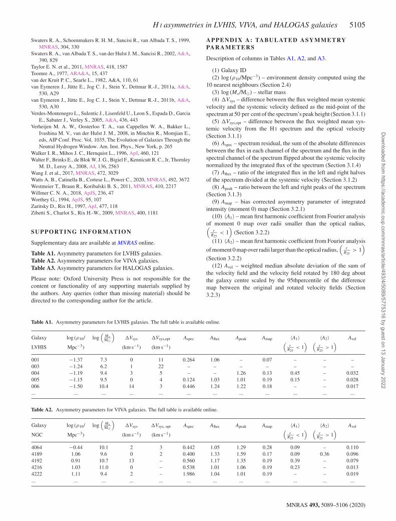
H I asymmetries in LVHIS, VIVA, and HALOGAS galaxies 5105
Swaters R. A., Schoenmakers R. H. M., Sancisi R., van Albada T. S., 1999,MNRAS, 304, 330
Swaters R. A., van Albada T. S., van der Hulst J. M., Sancisi R., 2002, A&A,390, 829
Taylor E. N. et al., 2011, MNRAS, 418, 1587Toomre A., 1977, ARA&A, 15, 437van der Kruit P. C., Searle L., 1982, A&A, 110, 61van Eymeren J., Jutte E., Jog C. J., Stein Y., Dettmar R.-J., 2011a, A&A,
530, A29van Eymeren J., Jutte E., Jog C. J., Stein Y., Dettmar R.-J., 2011b, A&A,
530, A30Verdes-Montenegro L., Sulentic J., Lisenfeld U., Leon S., Espada D., Garcia
E., Sabater J., Verley S., 2005, A&A, 436, 443Verheijen M. A. W., Oosterloo T. A., van Cappellen W. A., Bakker L.,
Ivashina M. V., van der Hulst J. M., 2008, in Minchin R., Momjian E.,eds, AIP Conf. Proc. Vol. 1035, The Evolution of Galaxies Through theNeutral Hydrogen Window. Am. Inst. Phys., New York, p. 265
Walker I. R., Mihos J. C., Hernquist L., 1996, ApJ, 460, 121Walter F., Brinks E., de Blok W. J. G., Bigiel F., Kennicutt R. C., Jr, Thornley
M. D., Leroy A., 2008, AJ, 136, 2563Wang J. et al., 2017, MNRAS, 472, 3029Watts A. B., Catinella B., Cortese L., Power C., 2020, MNRAS, 492, 3672Westmeier T., Braun R., Koribalski B. S., 2011, MNRAS, 410, 2217Willmer C. N. A., 2018, ApJS, 236, 47Worthey G., 1994, ApJS, 95, 107Zaritsky D., Rix H., 1997, ApJ, 477, 118Zibetti S., Charlot S., Rix H.-W., 2009, MNRAS, 400, 1181
SUPPORTING INFORMATION
Supplementary data are available at MNRAS online.
Table A1. Asymmetry parameters for LVHIS galaxies.Table A2. Asymmetry parameters for VIVA galaxies.Table A3. Asymmetry parameters for HALOGAS galaxies.
Please note: Oxford University Press is not responsible for thecontent or functionality of any supporting materials supplied bythe authors. Any queries (other than missing material) should bedirected to the corresponding author for the article.
APPENDI X A : TABULATED ASYMMETRYPA R A M E T E R S
Description of columns in Tables A1, A2, and A3.
(1) Galaxy ID(2) log (ρ10/Mpc−3) – environment density computed using the
10 nearest neighbours (Section 2.4)(3) log (M∗/M�) – stellar mass(4) �Vsys – difference between the flux weighted mean systemic
velocity and the systemic velocity defined as the mid-point of thespectrum at 50 per cent of the spectrum’s peak height (Section 3.1.1)
(5) �Vsys,opt – difference between the flux weighted mean sys-temic velocity from the H I spectrum and the optical velocity(Section 3.1.1)
(6) Aspec – spectrum residual, the sum of the absolute differencesbetween the flux in each channel of the spectrum and the flux in thespectral channel of the spectrum flipped about the systemic velocitynormalized by the integrated flux of the spectrum (Section 3.1.4)
(7) Aflux – ratio of the integrated flux in the left and right halvesof the spectrum divided at the systemic velocity (Section 3.1.2)
(8) Apeak – ratio between the left and right peaks of the spectrum(Section 3.1.3)
(9) Amap – bias corrected asymmetry parameter of integratedintensity (moment 0) map (Section 3.2.1)
(10) 〈A1〉 – mean first harmonic coefficient from Fourier analysisof moment 0 map over radii smaller than the optical radius,(
rR25
< 1)
(Section 3.2.2)
(11) 〈A2〉 – mean first harmonic coefficient from Fourier analysis
of moment 0 map over radii larger than the optical radius,(
rR25
> 1)
(Section 3.2.2)(12) Avel – weighted median absolute deviation of the sum of
the velocity field and the velocity field rotated by 180 deg aboutthe galaxy centre scaled by the 95thpercentile of the differencemap between the original and rotated velocity fields (Section3.2.3)
Table A1. Asymmetry parameters for LVHIS galaxies. The full table is available online.
Galaxy log (ρ10/ log(
M∗M�
)�Vsys �Vsys,opt Aspec Aflux Apeak Amap 〈A1〉 〈A2〉 Avel
LVHIS Mpc−3) (km s−1) (km s−1)(
rR25
< 1) (
rR25
> 1)
001 −1.37 7.3 0 11 0.264 1.06 – 0.07 – – –003 −1.24 6.2 1 22 – – – – – – –004 −1.19 9.4 3 5 – – 1.26 0.13 0.45 – 0.032005 −1.15 9.5 0 4 0.124 1.03 1.01 0.19 0.15 – 0.028006 −1.50 10.4 14 3 0.446 1.24 1.22 0.18 – – 0.017... ... ... ... ... ... ... ... ... ... ... ...
Table A2. Asymmetry parameters for VIVA galaxies. The full table is available online.
Galaxy log (ρ10/ log(
M∗M�
)�Vsys �Vsys, opt Aspec Aflux Apeak Amap 〈A1〉 〈A2〉 Avel
NGC Mpc−3) (km s−1) (km s−1)(
rR25
< 1) (
rR25
> 1)
4064 −0.44 10.1 2 3 0.442 1.05 1.29 0.28 0.09 – 0.1104189 1.06 9.6 0 2 0.400 1.33 1.59 0.17 0.09 0.36 0.0964192 0.91 10.7 13 – 0.560 1.17 1.35 0.19 0.39 – 0.0794216 1.03 11.0 0 – 0.538 1.01 1.06 0.19 0.23 – 0.0134222 1.11 9.4 2 – 1.986 1.04 1.01 0.19 – – 0.019... ... ... ... ... ... ... ... ... ... ... ...
MNRAS 493, 5089–5106 (2020)
Dow
nloaded from https://academ
ic.oup.com/m
nras/article/493/4/5089/5775316 by guest on 13 January 2022
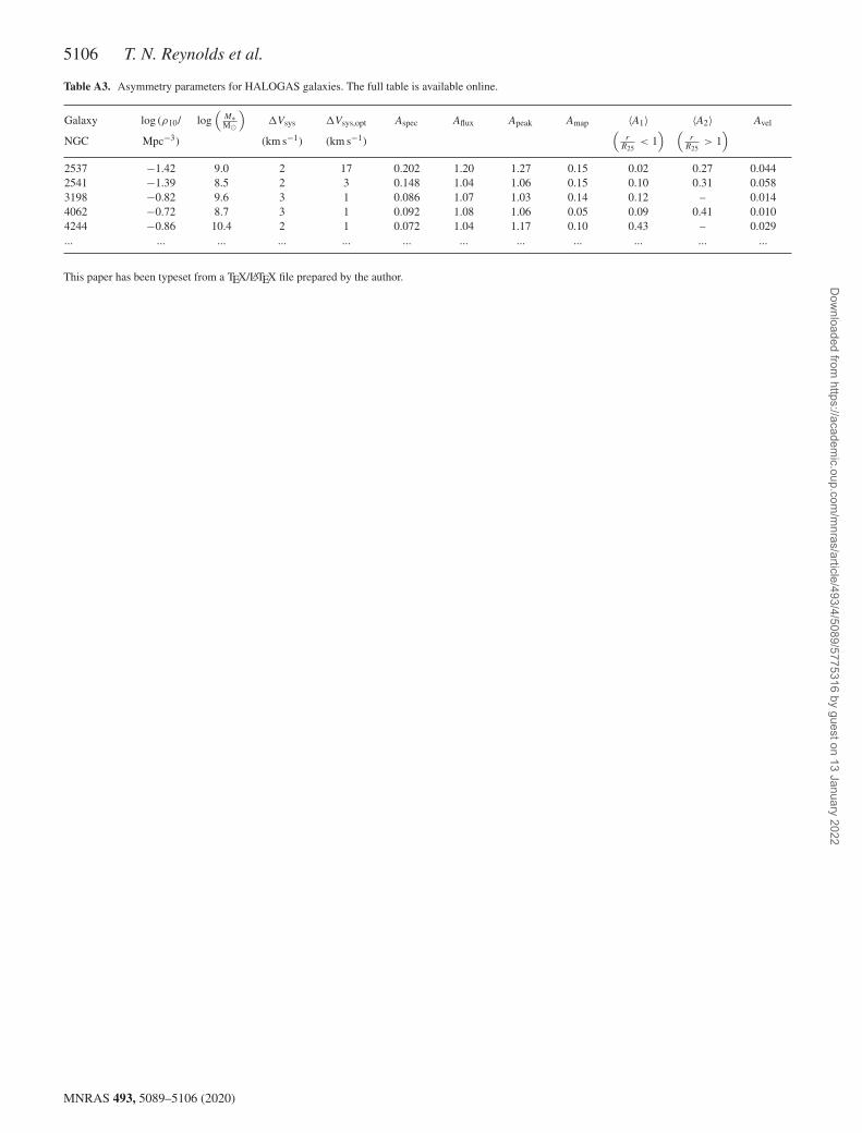
5106 T. N. Reynolds et al.
Table A3. Asymmetry parameters for HALOGAS galaxies. The full table is available online.
Galaxy log (ρ10/ log(
M∗M�
)�Vsys �Vsys,opt Aspec Aflux Apeak Amap 〈A1〉 〈A2〉 Avel
NGC Mpc−3) (km s−1) (km s−1)(
rR25
< 1) (
rR25
> 1)
2537 −1.42 9.0 2 17 0.202 1.20 1.27 0.15 0.02 0.27 0.0442541 −1.39 8.5 2 3 0.148 1.04 1.06 0.15 0.10 0.31 0.0583198 −0.82 9.6 3 1 0.086 1.07 1.03 0.14 0.12 – 0.0144062 −0.72 8.7 3 1 0.092 1.08 1.06 0.05 0.09 0.41 0.0104244 −0.86 10.4 2 1 0.072 1.04 1.17 0.10 0.43 – 0.029... ... ... ... ... ... ... ... ... ... ... ...
This paper has been typeset from a TEX/LATEX file prepared by the author.
MNRAS 493, 5089–5106 (2020)
Dow
nloaded from https://academ
ic.oup.com/m
nras/article/493/4/5089/5775316 by guest on 13 January 2022