RTO-EN-AVT-207 10 - 1

High Cyclic Fatigue

J. SZWEDOWICZ Switzerland

1.0 INTRODUCTION

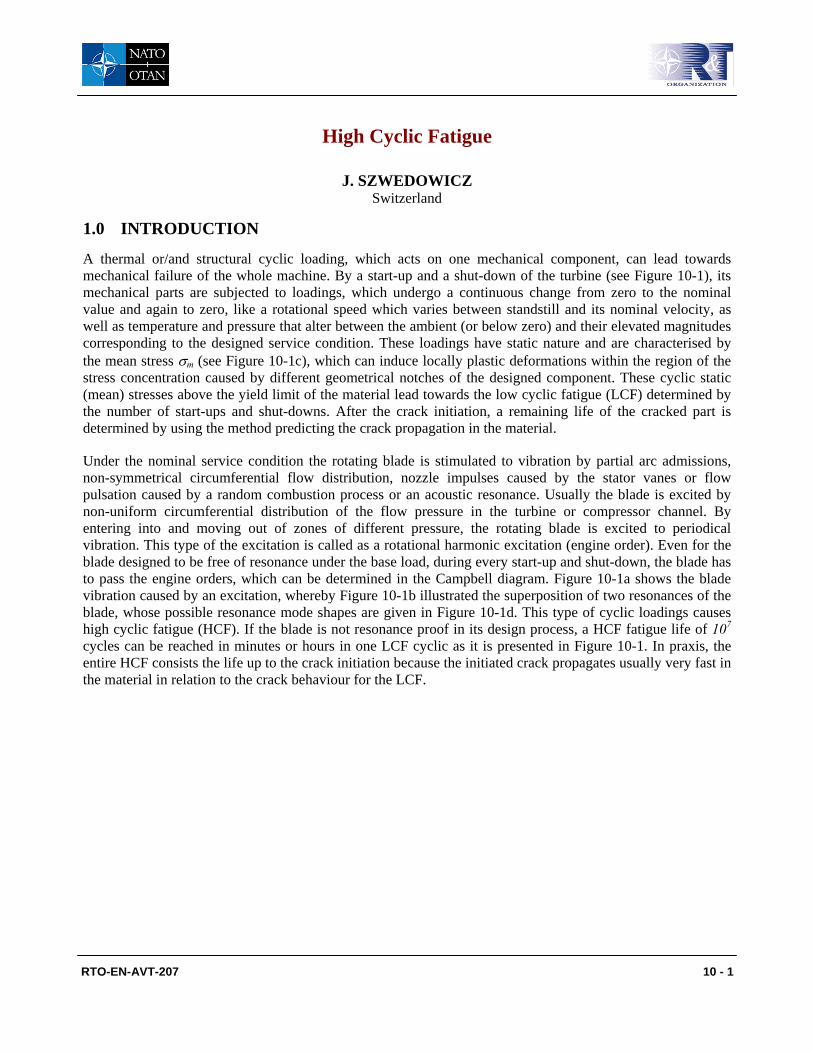
A thermal or/and structural cyclic loading, which acts on one mechanical component, can lead towards mechanical failure of the whole machine. By a start-up and a shut-down of the turbine (see Figure 10-1), its mechanical parts are subjected to loadings, which undergo a continuous change from zero to the nominal value and again to zero, like a rotational speed which varies between standstill and its nominal velocity, as well as temperature and pressure that alter between the ambient (or below zero) and their elevated magnitudes corresponding to the designed service condition. These loadings have static nature and are characterised by the mean stress σm (see Figure 10-1c), which can induce locally plastic deformations within the region of the stress concentration caused by different geometrical notches of the designed component. These cyclic static (mean) stresses above the yield limit of the material lead towards the low cyclic fatigue (LCF) determined by the number of start-ups and shut-downs. After the crack initiation, a remaining life of the cracked part is determined by using the method predicting the crack propagation in the material.

Under the nominal service condition the rotating blade is stimulated to vibration by partial arc admissions, non-symmetrical circumferential flow distribution, nozzle impulses caused by the stator vanes or flow pulsation caused by a random combustion process or an acoustic resonance. Usually the blade is excited by non-uniform circumferential distribution of the flow pressure in the turbine or compressor channel. By entering into and moving out of zones of different pressure, the rotating blade is excited to periodical vibration. This type of the excitation is called as a rotational harmonic excitation (engine order). Even for the blade designed to be free of resonance under the base load, during every start-up and shut-down, the blade has to pass the engine orders, which can be determined in the Campbell diagram. Figure 10-1a shows the blade vibration caused by an excitation, whereby Figure 10-1b illustrated the superposition of two resonances of the blade, whose possible resonance mode shapes are given in Figure 10-1d. This type of cyclic loadings causes high cyclic fatigue (HCF). If the blade is not resonance proof in its design process, a HCF fatigue life of 107 cycles can be reached in minutes or hours in one LCF cyclic as it is presented in Figure 10-1. In praxis, the entire HCF consists the life up to the crack initiation because the initiated crack propagates usually very fast in the material in relation to the crack behaviour for the LCF.

High Cyclic Fatigue

10 - 2 RTO-EN-AVT-207

Figure 10-1: Operation schedule including start-ups and shut-downs of the turbine as its LCF

loading with indicated vibrations under the service condition as HCF loading, where: a) vibrations due to one resonance excitation

b) vibrations as a superposition of two resonance excitations

c) stochastic vibration

d) mean centrifugal stresses in the steam turbine blade (Szwedowicz et al, 2006) and

e) its 3 lowest mode shapes excitable for engine orders k of 6, 11 and 12

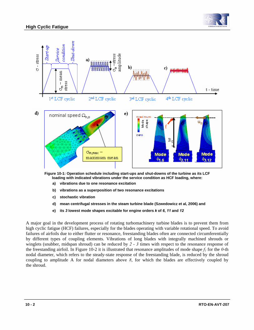
A major goal in the development process of rotating turbomachinery turbine blades is to prevent them from high cyclic fatigue (HCF) failures, especially for the blades operating with variable rotational speed. To avoid failures of airfoils due to either flutter or resonance, freestanding blades often are connected circumferentially by different types of coupling elements. Vibrations of long blades with integrally machined shrouds or winglets (snubber, midspan shroud) can be reduced by 2 - 3 times with respect to the resonance response of the freestanding airfoil. In Figure 10-2 it is illustrated that resonance amplitudes of mode shape f1 for the 0-th nodal diameter, which refers to the steady-state response of the freestanding blade, is reduced by the shroud coupling to amplitude A for nodal diameters above 8, for which the blades are effectively coupled by the shroud.

High Cyclic Fatigue

RTO-EN-AVT-207 10 - 3

Resonance amplitude Aof the blade entirely coupled by the shroud

Resonance amplitude Aorelating to the vibration of the freestanding blade

Figure 10-2: Effect of the shroud coupling on the response reduction of the turbine blade.

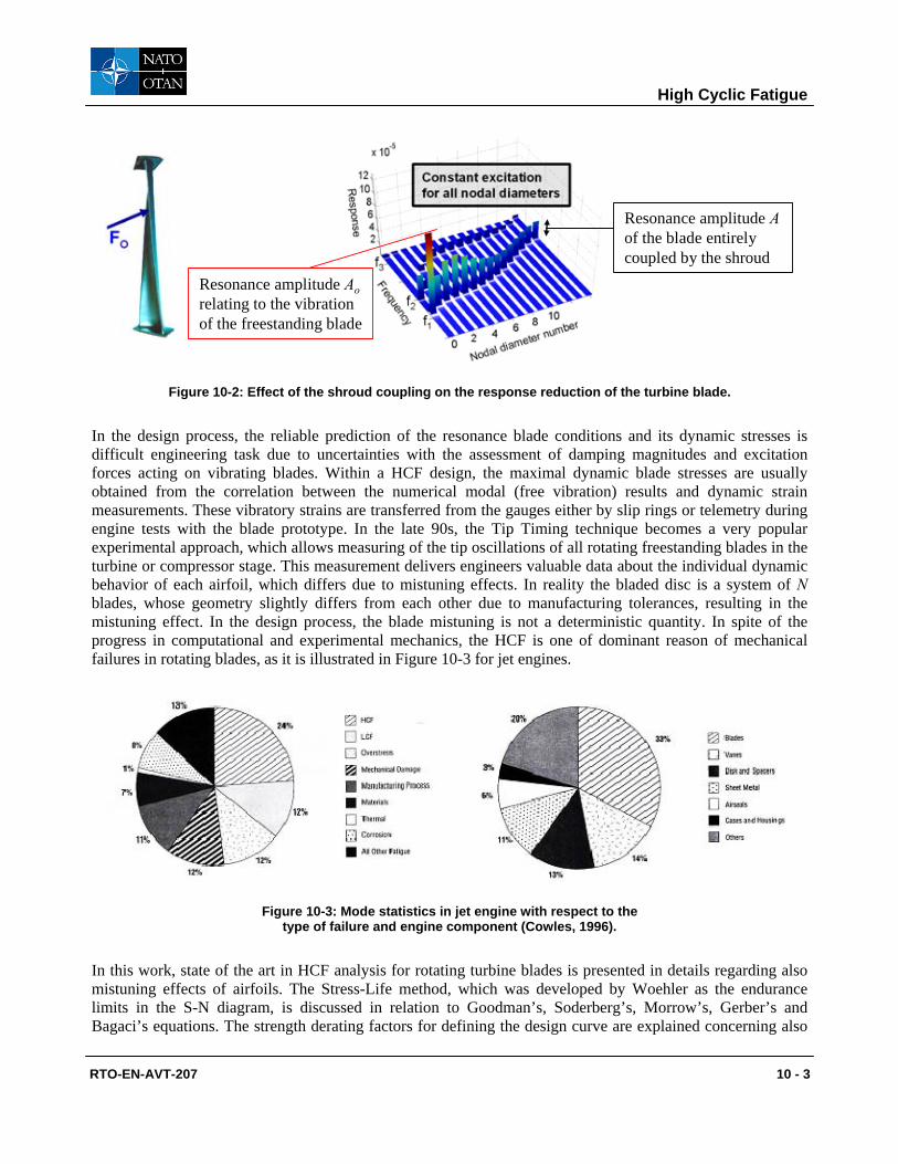
In the design process, the reliable prediction of the resonance blade conditions and its dynamic stresses is difficult engineering task due to uncertainties with the assessment of damping magnitudes and excitation forces acting on vibrating blades. Within a HCF design, the maximal dynamic blade stresses are usually obtained from the correlation between the numerical modal (free vibration) results and dynamic strain measurements. These vibratory strains are transferred from the gauges either by slip rings or telemetry during engine tests with the blade prototype. In the late 90s, the Tip Timing technique becomes a very popular experimental approach, which allows measuring of the tip oscillations of all rotating freestanding blades in the turbine or compressor stage. This measurement delivers engineers valuable data about the individual dynamic behavior of each airfoil, which differs due to mistuning effects. In reality the bladed disc is a system of N blades, whose geometry slightly differs from each other due to manufacturing tolerances, resulting in the mistuning effect. In the design process, the blade mistuning is not a deterministic quantity. In spite of the progress in computational and experimental mechanics, the HCF is one of dominant reason of mechanical failures in rotating blades, as it is illustrated in Figure 10-3 for jet engines.

Figure 10-3: Mode statistics in jet engine with respect to the type of failure and engine component (Cowles, 1996).

In this work, state of the art in HCF analysis for rotating turbine blades is presented in details regarding also mistuning effects of airfoils. The Stress-Life method, which was developed by Woehler as the endurance limits in the S-N diagram, is discussed in relation to Goodman’s, Soderberg’s, Morrow’s, Gerber’s and Bagaci’s equations. The strength derating factors for defining the design curve are explained concerning also

High Cyclic Fatigue

10 - 4 RTO-EN-AVT-207

the safety factor. Also the Strain-Life method contributing effects of the mean stress is described in this report. The Smith-Watson-Toper damage parameter with explanation of the local strain and stress concepts are discussed here. Essential information about the linear Palmgren-Miner, Corten-Dolan or Haibach concepts and non-linear Macro and Starkey, Shanley, or Henry hypotheses for the prediction of the cumulative damage are reminded briefly. Because the damage assessment depends on a characteristic of the alternating loading, which is based on the cyclic counting, the most popular Miner’s and the rain-flow approaches will be compared to each other regarding their disadvantages and benefits. Finally the evaluation of stochastic vibrations, determined as a narrow and a broad band process, is analyzed considering engineering needs for the design process.

2.0 STEADY-STATE DYNAMICS OF ROTATING BLADES

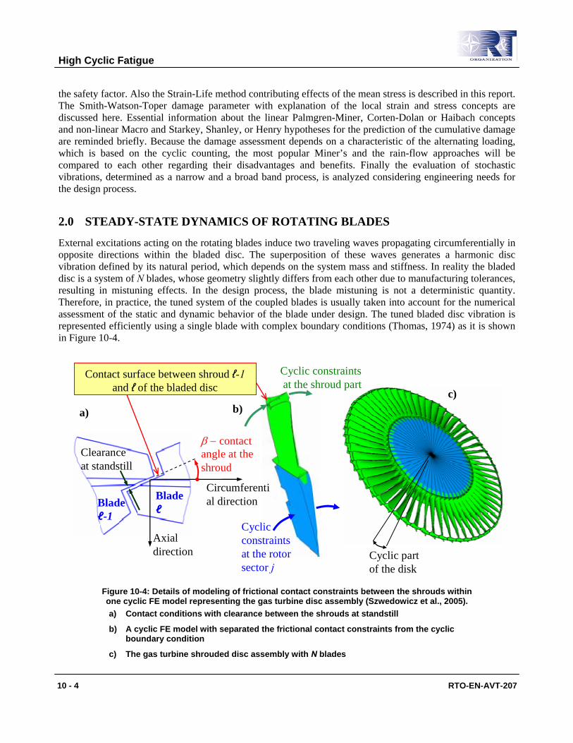
External excitations acting on the rotating blades induce two traveling waves propagating circumferentially in opposite directions within the bladed disc. The superposition of these waves generates a harmonic disc vibration defined by its natural period, which depends on the system mass and stiffness. In reality the bladed disc is a system of N blades, whose geometry slightly differs from each other due to manufacturing tolerances, resulting in mistuning effects. In the design process, the blade mistuning is not a deterministic quantity. Therefore, in practice, the tuned system of the coupled blades is usually taken into account for the numerical assessment of the static and dynamic behavior of the blade under design. The tuned bladed disc vibration is represented efficiently using a single blade with complex boundary conditions (Thomas, 1974) as it is shown in Figure 10-4.

Cyclic part of the disk

Cyclic constraintsat the shroud part

Cyclic constraints at the rotor sector j

b)c)

Circumferential direction

β − contact angle at the shroud

Axial direction

Clearance at standstill

Blade ℓBlade

ℓ-1

a)

Contact surface between shroud ℓ-1and ℓ of the bladed disc

Figure 10-4: Details of modeling of frictional contact constraints between the shrouds within one cyclic FE model representing the gas turbine disc assembly (Szwedowicz et al., 2005). a) Contact conditions with clearance between the shrouds at standstill

b) A cyclic FE model with separated the frictional contact constraints from the cyclic boundary condition

c) The gas turbine shrouded disc assembly with N blades

High Cyclic Fatigue

RTO-EN-AVT-207 10 - 5

For rotational speed Ω and given temperature distribution T, the well-known static matrix equation of the rotating turbine blade is expressed with the cyclic FE model (Figure 10-4b) by (Szwedowicz, 1999)

(1) ( )[ ]{ } { } ( ){ } { }ocA PFFqC,,q,T,K ++= ΩσΩ μ ,

where FA, F(Ω)c and Po denote the pre-assembly force, the centrifugal load and flow pressure acting on the blade, respectively. For the identical deformations on the circumferential sides of the rotor and shroud (Figure 10-4) and by including centrifugal stiffening effects, the stiffness matrix [K] depends on temperature T, rotational speed Ω, airfoil deformation q as well as friction shear coupling forces Cμ. By increasing the rotational speed, blades untwist themselves and are simultaneously coupled on their frictional interfaces on the shroud. Therefore, contact surfaces at the blade root and shroud, where frictional sliding can occur for the acting centrifugal load, should be modeled within the cyclic FE sector as it is illustrated in Figure 10-4. Then, the cyclic boundary conditions are separated from the contact constraints, what allows for more reliable numerical results. After exceeding a particular rotational speed Ωt, frictional contact forces join together all individual blades among each other in one integral disc assembly (Appendix 1).

At the rotational speed of interest by considering the sticking contact conditions on the blade interfaces and neglecting viscous damping, forced vibrations of the bladed disc excited by non-uniform pressure distribution P(α) along the circumferential direction α is represented for the n-th nodal diameter by

(2) ( )[ ] { }( )

{ }( )[ ] { }( )

{ }( ){ } 1j,P

qze,CK

qzeM

n

nN/n2j

n

nN/n2j −==⎪⎭

⎪⎬⎫

⎪⎩

⎪⎨⎧

+⎪⎭

⎪⎬⎫

⎪⎩

⎪⎨⎧

απμ

πll

&&

&&.

In Eq. (2), the nodes in vector {z}(ℓ), which are located on the ℓ-th circumferential side of the cyclic FE model, represent the boundary deformations between the ℓ-th and (ℓ+1)-th disc sectors with the cyclic constraint equations as

(3) ( ) ( ) N/n2j

boltbolt ezz1 πll

=+

, ( ) ( ) N/n2jrotorrotor ezz

1 πll

=+ ,

where the nodal diameter number n equals {0, 1, 2, …, N*/2} whereby N*=N-1 or N*=N for the odd or even number N of the blades in the stage, respectively. For each n-th nodal diameter, the global mass [M] and stiffness [K] matrices are arranged individually with respect to the generalized vector {φn}={{zn},{qn}}T of vibrations around the centrifugally deformed blade. For the considered steady-state dynamics, firstly the free vibrations need to be computed by neglecting the pressure {P(α)} and substituting harmonic responses {φi,n}exp(jωi,nt) in Eq.(2) from

(4) [ ] [ ]( ){ } 0)n(M)C,n,(K n,i2n,i =−∞= φωΩ μ ,

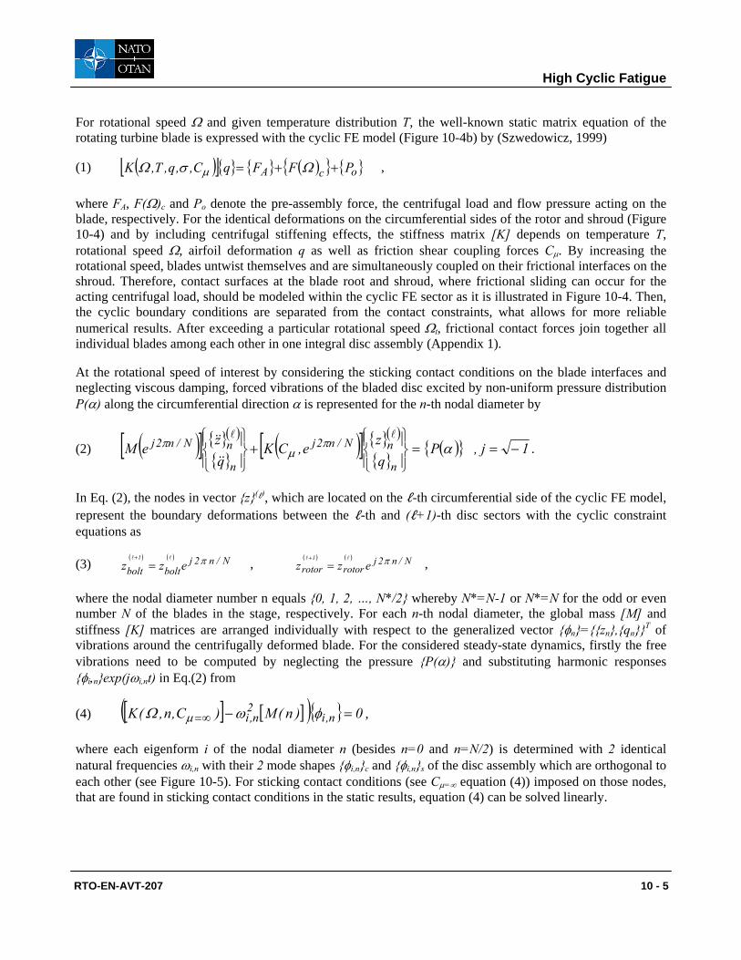
where each eigenform i of the nodal diameter n (besides n=0 and n=N/2) is determined with 2 identical natural frequencies ωi,n with their 2 mode shapes {φi,n}c and {φi,n}s of the disc assembly which are orthogonal to each other (see Figure 10-5). For sticking contact conditions (see Cμ=∞ equation (4)) imposed on those nodes, that are found in sticking contact conditions in the static results, equation (4) can be solved linearly.

High Cyclic Fatigue

10 - 6 RTO-EN-AVT-207

Rotor partLacing wire

resonance stress for ”bending” (real) blade oscillation

resonance stress for ”torsion” (imaginary) blade oscillation

A g

rey

colo

r cor

resp

onds

to t

he c

ompu

ted

vibr

atio

n fo

rm o

f the

dis

c as

sem

bly

Figure 10-5: Vibrations of the blades coupled by the lacing wire and the rotor with illustrated the real and imaginary mode shapes of von Mises stresses.

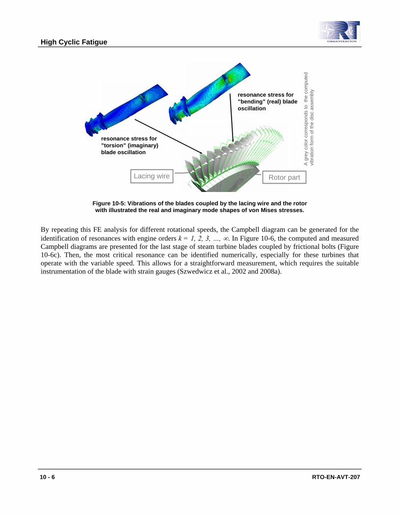
By repeating this FE analysis for different rotational speeds, the Campbell diagram can be generated for the identification of resonances with engine orders k = 1, 2, 3, …, ∞. In Figure 10-6, the computed and measured Campbell diagrams are presented for the last stage of steam turbine blades coupled by frictional bolts (Figure 10-6c). Then, the most critical resonance can be identified numerically, especially for these turbines that operate with the variable speed. This allows for a straightforward measurement, which requires the suitable instrumentation of the blade with strain gauges (Szwedwicz et al., 2002 and 2008a).

High Cyclic Fatigue

RTO-EN-AVT-207 10 - 7

Figure 10-6: The computed (solid lines) and measured (rot and blue colors denote the maximum and minimum strain amplitudes, respectively) Campbell diagrams of the last stage of the steam bladed

disc coupled by frictional bolts operating with variable speed (Szwedowicz et al., 2008a).

For the excitation amplitudes {Fk} and two FE eigenfrequencies ωi,n with their mass-normalized eigenforms {Φ°}i,n = {φ°i,n}c + j{φ°i,n}s, the forced response analysis of the coupled blade is performed in the modal domain for each nodal diameter n separately. Then, Eq. (2) is redefined with the modal steady-state response equation for resonance ωi,n and the modal damping ratio ξi,n by (Filsinger et al., 2002)

(5) tjkn,in,in,in,in,in,in,in,i efuku2um Ωξω =++ &&& ,

where ui,n is the modal displacement and

(6) { } { }αΦ ,kT*n,in,i Ff °= - modal force,

(7) { } ( )[ ]{ } 0.1nMm n,iT*n,in,i == °° ΦΦ - modal mass-normalized mass and

High Cyclic Fatigue

10 - 8 RTO-EN-AVT-207

(8) { } ( )[ ]{ } 2n,in,i

T*n,in,i C,n,Kk ωΦΩΦ μ == °

∞=° - modal stiffness

of the cyclic FE blade model and { } T*n,i

°Φ is the conjugate transposed vector. Finally the steady-state response

of all nodes representing the blade vibration of the n-th nodal diameter is calculated in the Cartesian system in the time domain from

(9) ( ){ } ( ){ }{ } { } ( )

( )( )tjkexp

k2jk

jexpFtqtq

I

1i n,in,i22

n,î

n,i,kT*n,i,n,iI

1in,in Ω

ΩωξΩω

γΦΨ αηδ

⎟⎟⎟

⎠

⎞

⎜⎜⎜

⎝

⎛

+−

−== ∑∑

=

°°

=

,

where the phase delay of the response for the disc mode i vibrating with the n-th nodal diameter is given by

(11) ( ) ⎟

⎟

⎠

⎞

⎜⎜

⎝

⎛

−= −

22n,î

n,in,i1n,i

k

k2tan

Ωω

Ωωξγ .

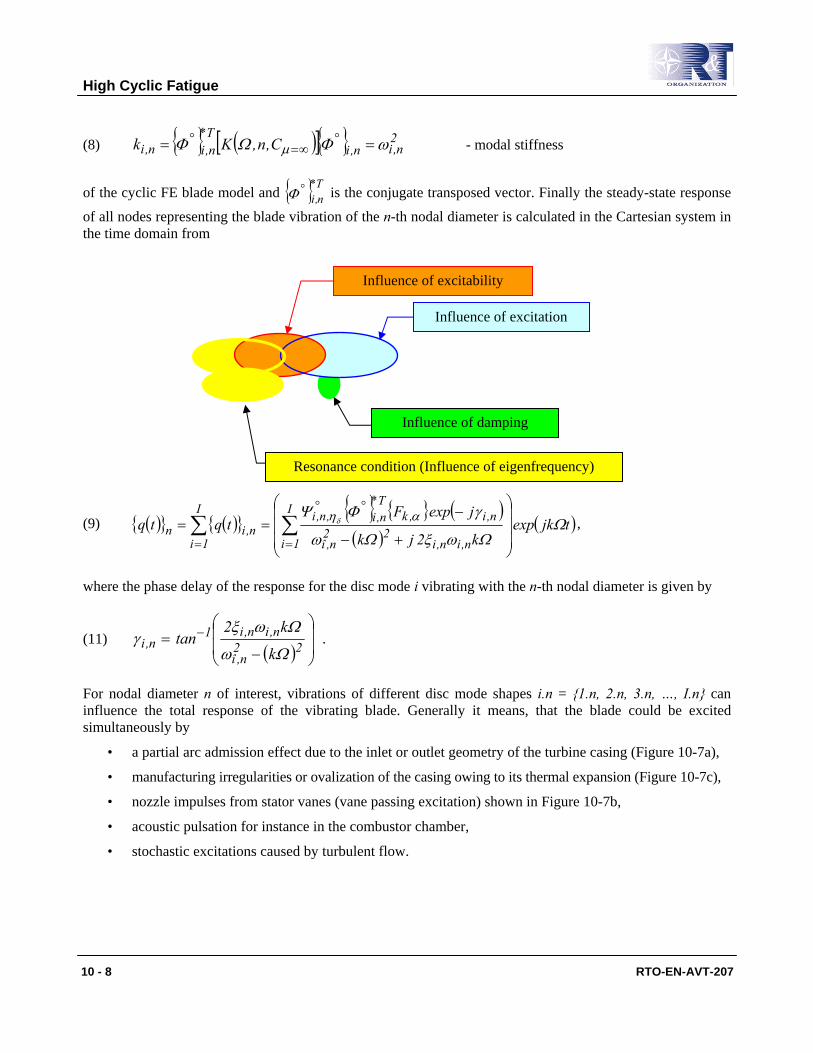
For nodal diameter n of interest, vibrations of different disc mode shapes i.n = {1.n, 2.n, 3.n, …, I.n} can influence the total response of the vibrating blade. Generally it means, that the blade could be excited simultaneously by

• a partial arc admission effect due to the inlet or outlet geometry of the turbine casing (Figure 10-7a),

• manufacturing irregularities or ovalization of the casing owing to its thermal expansion (Figure 10-7c),

• nozzle impulses from stator vanes (vane passing excitation) shown in Figure 10-7b,

• acoustic pulsation for instance in the combustor chamber,

• stochastic excitations caused by turbulent flow.

Influence of damping

Influence of excitability

Influence of excitation

Resonance condition (Influence of eigenfrequency)

High Cyclic Fatigue

RTO-EN-AVT-207 10 - 9

Figure 10-7: Usual sources of excitation for rotating bladed discs. a) Inlet partial arc admission b) Nozzle effects of stator vanes (Dzygadlo et al., 1982) c) Ovalization of the casing owing to its thermal expansion (Dzygadlo et al., 1982) d) FE acoustic mode shape in annular combustor

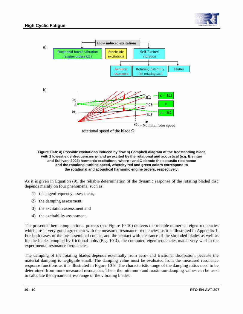
In praxis, the blade is stimulated mainly by one excitation source. However at one particular rotational speed the blade can be excited by two or even more harmonic excitations. In addition the rotating blade might be stimulated by acoustic resonance (see ε in Figure 10-8) induced for instance in a combustor cavity.

ΩΩ

Vortex excitation a) b)

c) d)

High Cyclic Fatigue

10 - 10 RTO-EN-AVT-207

Rotational forced vibration (engine orders kΩ)

Stochastic excitations

Self-Excited vibration

Acoustic resonance

Rotating instability like rotating stall

Flutter

Flow induced excitations

Rotational forced vibration (engine orders kΩ)

Stochastic excitations

Self-Excited vibration

Acoustic resonance

Rotating instability like rotating stall

Flutter

Flow induced excitations

Figure 10-8: a) Possible excitations induced by flow b) Campbell diagram of the freestanding blade

with 2 lowest eigenfrequencies ω1 and ω2 excited by the rotational and acoustical (e.g. Eisinger and Sullivan, 2002) harmonic excitations, where ε and Ω denote the acoustic resonance

and the rotational turbine speed, whereby red and green colors correspond to the rotational and acoustical harmonic engine orders, respectively.

As it is given in Equation (9), the reliable determination of the dynamic response of the rotating bladed disc depends mainly on four phenomena, such as:

1) the eigenfrequency assessment,

2) the damping assessment,

3) the excitation assessment and

4) the excitability assessment.

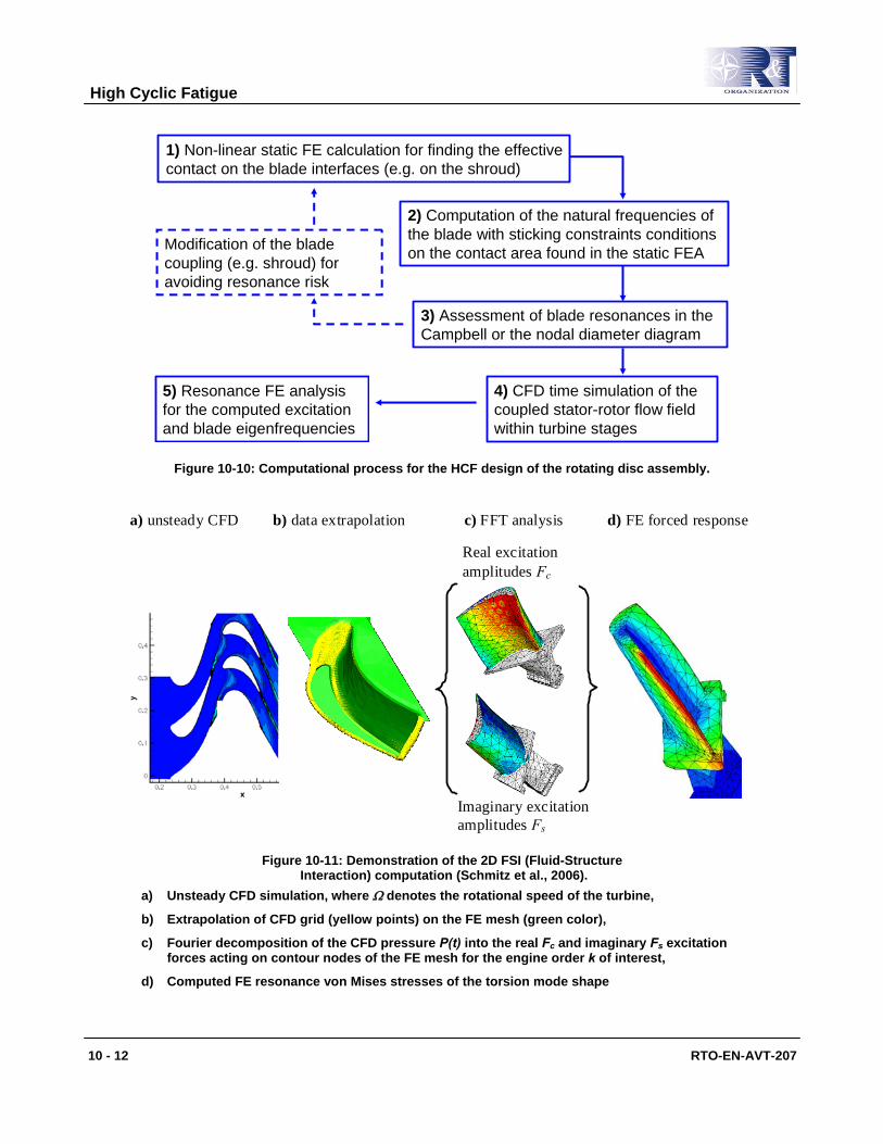
The presented here computational process (see Figure 10-10) delivers the reliable numerical eigenfrequencies which are in very good agreement with the measured resonance frequencies, as it is illustrated in Appendix 1. For both cases of the pre-assembled contact and the contact with clearance of the shrouded blades as well as for the blades coupled by frictional bolts (Fig. 10-4), the computed eigenfrequencies match very well to the experimental resonance frequencies.

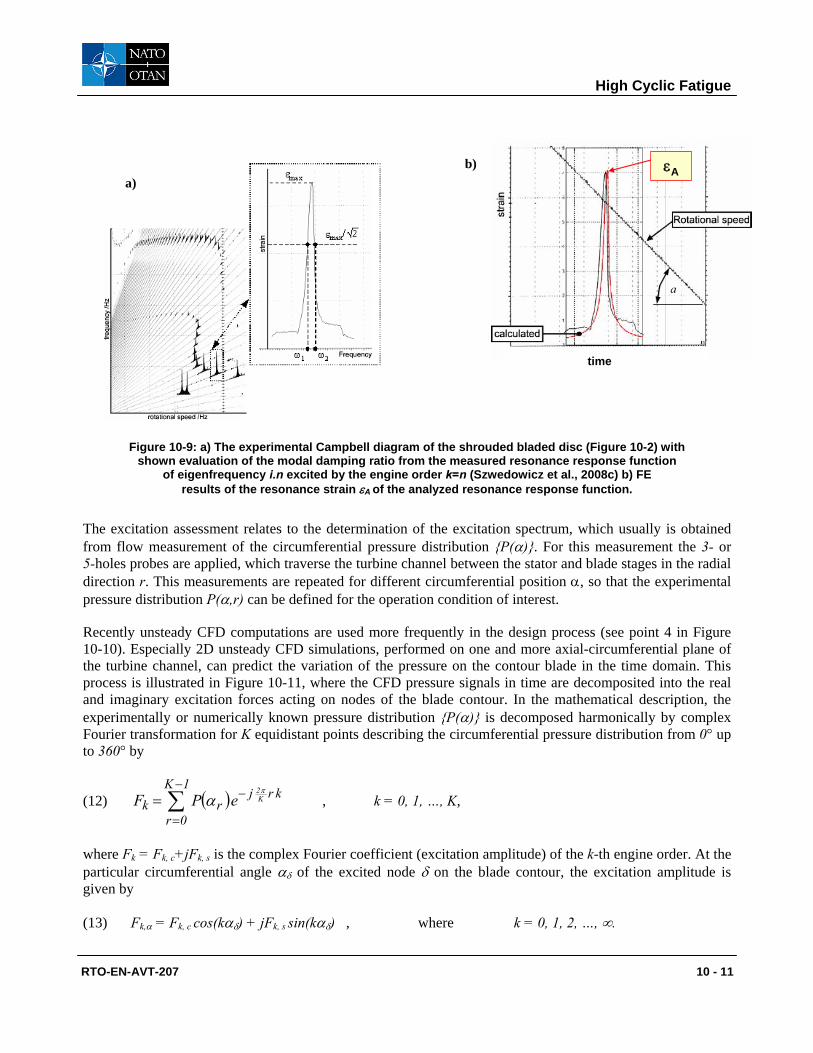
The damping of the rotating blades depends essentially from aero- and frictional dissipation, because the material damping is negligible small. The damping value must be evaluated from the measured resonance response functions as it is illustrated in Figure 10-9. The characteristic range of the damping ratios need to be determined from more measured resonances. Then, the minimum and maximum damping values can be used to calculate the dynamic stress range of the vibrating blades.

rotational speed of the blade Ω

ω2

ω1 1Ω

ΩN - nominal rotational spe

ε

ε - 1Ω

ε + 1Ω3Ωε2Ω

- Nominal rotor speed

a)

b)

High Cyclic Fatigue

RTO-EN-AVT-207 10 - 11

Figure 10-9: a) The experimental Campbell diagram of the shrouded bladed disc (Figure 10-2) with shown evaluation of the modal damping ratio from the measured resonance response function

of eigenfrequency i.n excited by the engine order k=n (Szwedowicz et al., 2008c) b) FE results of the resonance strain εA of the analyzed resonance response function.

The excitation assessment relates to the determination of the excitation spectrum, which usually is obtained from flow measurement of the circumferential pressure distribution {P(α)}. For this measurement the 3- or 5-holes probes are applied, which traverse the turbine channel between the stator and blade stages in the radial direction r. This measurements are repeated for different circumferential position α, so that the experimental pressure distribution P(α,r) can be defined for the operation condition of interest.

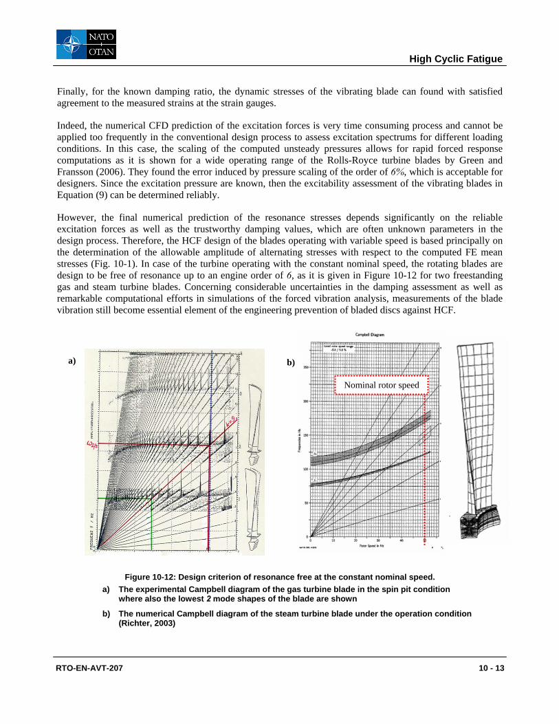
Recently unsteady CFD computations are used more frequently in the design process (see point 4 in Figure 10-10). Especially 2D unsteady CFD simulations, performed on one and more axial-circumferential plane of the turbine channel, can predict the variation of the pressure on the contour blade in the time domain. This process is illustrated in Figure 10-11, where the CFD pressure signals in time are decomposited into the real and imaginary excitation forces acting on nodes of the blade contour. In the mathematical description, the experimentally or numerically known pressure distribution {P(α)} is decomposed harmonically by complex Fourier transformation for K equidistant points describing the circumferential pressure distribution from 0° up to 360° by

(12) ( )∑−

=

−=1K

0r

krjrk K

2ePF

πα , k = 0, 1, …, K,

where Fk = Fk, c+jFk, s is the complex Fourier coefficient (excitation amplitude) of the k-th engine order. At the particular circumferential angle αδ of the excited node δ on the blade contour, the excitation amplitude is given by

(13) Fk,α = Fk, c cos(kαδ) + jFk, s sin(kαδ) , where k = 0, 1, 2, …, ∞.

a) b)

aa

time

εA

High Cyclic Fatigue

10 - 12 RTO-EN-AVT-207

2) Computation of the natural frequencies of the blade with sticking constraints conditions on the contact area found in the static FEA

3) Assessment of blade resonances in the Campbell or the nodal diameter diagram

Modification of the blade coupling (e.g. shroud) for avoiding resonance risk

4) CFD time simulation of the coupled stator-rotor flow field within turbine stages

5) Resonance FE analysis for the computed excitation and blade eigenfrequencies

1) Non-linear static FE calculation for finding the effective contact on the blade interfaces (e.g. on the shroud)

Figure 10-10: Computational process for the HCF design of the rotating disc assembly.

a) unsteady CFD b) data extrapolation c) FFT analysis d) FE forced response

Real excitation amplitudes Fc

Imaginary excitation amplitudes Fs

Figure 10-11: Demonstration of the 2D FSI (Fluid-Structure Interaction) computation (Schmitz et al., 2006).

a) Unsteady CFD simulation, where Ω denotes the rotational speed of the turbine,

b) Extrapolation of CFD grid (yellow points) on the FE mesh (green color),

c) Fourier decomposition of the CFD pressure P(t) into the real Fc and imaginary Fs excitation forces acting on contour nodes of the FE mesh for the engine order k of interest,

d) Computed FE resonance von Mises stresses of the torsion mode shape

High Cyclic Fatigue

RTO-EN-AVT-207 10 - 13

Finally, for the known damping ratio, the dynamic stresses of the vibrating blade can found with satisfied agreement to the measured strains at the strain gauges.

Indeed, the numerical CFD prediction of the excitation forces is very time consuming process and cannot be applied too frequently in the conventional design process to assess excitation spectrums for different loading conditions. In this case, the scaling of the computed unsteady pressures allows for rapid forced response computations as it is shown for a wide operating range of the Rolls-Royce turbine blades by Green and Fransson (2006). They found the error induced by pressure scaling of the order of 6%, which is acceptable for designers. Since the excitation pressure are known, then the excitability assessment of the vibrating blades in Equation (9) can be determined reliably.

However, the final numerical prediction of the resonance stresses depends significantly on the reliable excitation forces as well as the trustworthy damping values, which are often unknown parameters in the design process. Therefore, the HCF design of the blades operating with variable speed is based principally on the determination of the allowable amplitude of alternating stresses with respect to the computed FE mean stresses (Fig. 10-1). In case of the turbine operating with the constant nominal speed, the rotating blades are design to be free of resonance up to an engine order of 6, as it is given in Figure 10-12 for two freestanding gas and steam turbine blades. Concerning considerable uncertainties in the damping assessment as well as remarkable computational efforts in simulations of the forced vibration analysis, measurements of the blade vibration still become essential element of the engineering prevention of bladed discs against HCF.

Figure 10-12: Design criterion of resonance free at the constant nominal speed. a) The experimental Campbell diagram of the gas turbine blade in the spin pit condition

where also the lowest 2 mode shapes of the blade are shown

b) The numerical Campbell diagram of the steam turbine blade under the operation condition (Richter, 2003)

a) b)

Nominal rotor speed

High Cyclic Fatigue

10 - 14 RTO-EN-AVT-207

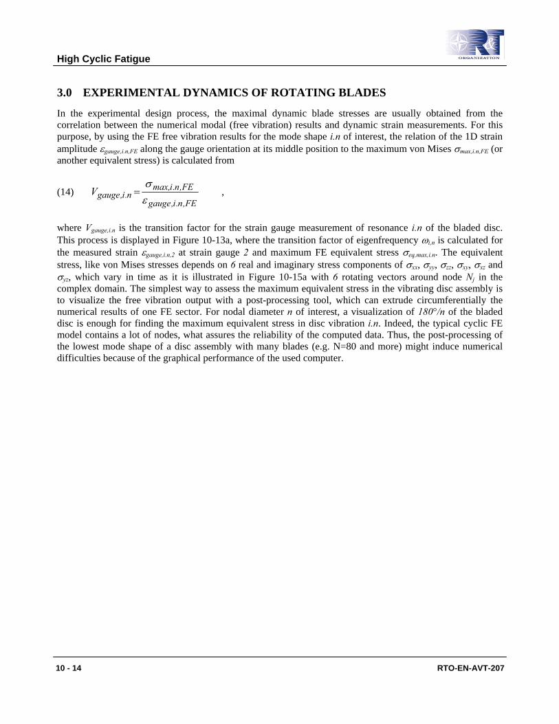
3.0 EXPERIMENTAL DYNAMICS OF ROTATING BLADES

In the experimental design process, the maximal dynamic blade stresses are usually obtained from the correlation between the numerical modal (free vibration) results and dynamic strain measurements. For this purpose, by using the FE free vibration results for the mode shape i.n of interest, the relation of the 1D strain amplitude εgauge,i.n,FE along the gauge orientation at its middle position to the maximum von Mises σmax,i.n,FE (or another equivalent stress) is calculated from

(14) FE,n.i,gauge

FE,n.imax,n.i,gaugeV

εσ

= ,

where Vgauge,i.n is the transition factor for the strain gauge measurement of resonance i.n of the bladed disc. This process is displayed in Figure 10-13a, where the transition factor of eigenfrequency ωi,n is calculated for the measured strain εgauge,i.n,2 at strain gauge 2 and maximum FE equivalent stress σeq,max,i.n. The equivalent stress, like von Mises stresses depends on 6 real and imaginary stress components of σxx, σyy, σzz, σxy, σxz and σyz, which vary in time as it is illustrated in Figure 10-15a with 6 rotating vectors around node Nj in the complex domain. The simplest way to assess the maximum equivalent stress in the vibrating disc assembly is to visualize the free vibration output with a post-processing tool, which can extrude circumferentially the numerical results of one FE sector. For nodal diameter n of interest, a visualization of 180°/n of the bladed disc is enough for finding the maximum equivalent stress in disc vibration i.n. Indeed, the typical cyclic FE model contains a lot of nodes, what assures the reliability of the computed data. Thus, the post-processing of the lowest mode shape of a disc assembly with many blades (e.g. N=80 and more) might induce numerical difficulties because of the graphical performance of the used computer.

High Cyclic Fatigue

RTO-EN-AVT-207 10 - 15

Figure 10-13: The vectorial illustration of 6 stress components “rotating” on the complex reference systems with the constant speed of eigenfrequency ωi.n at node Nj and Nk

at which the maximum resonance von Mises stresses σmax,i,n occur, a) Resonance von Mises stresses of the turbine blade instrumented with 2 strain gauges,

b) Resonance von Mises stresses and the mode shape of the turbine blade with illustration of the measuring plane at the airfoil tip for the Tip Timing Measurement, where ωi.n ≡ fi,n., t is the natural period of the vibration eigenfrequency ωi.n

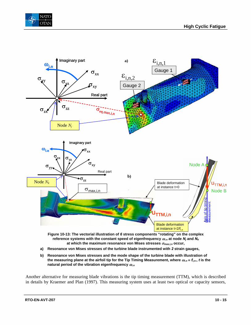
Another alternative for measuring blade vibrations is the tip timing measurement (TTM), which is described in details by Kraemer and Plan (1997). This measuring system uses at least two optical or capacity sensors,

uTTM,i,n

Node A

Axis

of t

ip ti

min

g m

easu

rem

ent

uTTM,i,n

Node A

Axis

of t

ip ti

min

g m

easu

rem

ent

σmax,i,n

uTTM,i,n

σmax,i,n

uTTM,i,nuTTM,i,n

Blade deformation at instance t=0

Blade deformation at instance t=2/fi.n

Node B

Real part

Imaginary part

σxx

σyy

σzz

σxy

σyzσzx

ωi.n

Imaginary part

σxx

σyy

σzz

σxy

σyzσzx

ωi.n

Gauge 1

Gauge 2

εi,n,1

εi,n,2

σeq.max,i,n

Imaginary part

σxxσyy

σzz

σxyσyz

σzx

ωi.n

Real part

Gauge 1

Gauge 2

εi,n,1

εi,n,2

σeq.max,i,n

Imaginary part

σxxσyy

σzz

σxyσyz

σzx

ωi.n

Real part

a)

Node Nj

b) Node Nk

High Cyclic Fatigue

10 - 16 RTO-EN-AVT-207

which are mounted in the turbine casing with circumferential distance αc. The distance αc is related to the circumferential vibration wave of the disc eigenfrequency ωi.n of interest. By monitoring the rotational speed of the turbine, the TTM measures the vibrations uTTM,i,n of all airfoil tips passing these two sensors. For this measurement, the relation between the FE response amplitude uTTM,i,n and the FE maximum stress von Mises σmax,i.n,FE (or another equivalent stress) needs to be calculated by

(15) FE,n.i,TTM

FE,n.imax,n.i,TTM u

Vσ

= ,

where VTTM,i.n is the transition factor for the tip timing measurement of resonance i.n of the bladed disc as it is shown in Figure 10-14a.

Figure 10-14: a) Laser beams from the optical sensors of the tip timing system and the measured blade vibration oscillations (Fuehrer et al., 1993) b) Blades

instrumented with the strain gauges and the measured vibratory strains in Campbell diagram for the spin pit condition (Szwedowicz et al., 2008).

For the measured response amplitude uexp,i.n (see Figure 10-14a) with the tip timing system, the real maximum resonance stress σmax,i.n of the blade is obtained from

(16) n.iexp,n.i,TTMn.imax, uV=σ .

In case of the measured strain amplitude εexp,i.n (see Figure 10-14b), the real maximum resonance stress σmax,i.n of the blade resonance ωi,n is determined in the similar form as

a) b)

High Cyclic Fatigue

RTO-EN-AVT-207 10 - 17

(17) n.iexp,n.i,gaugen.imax, V εσ = .

These vibratory strains are transferred from the gauges either by slip rings or telemetry during engine tests with the blade prototype. Vibrations of the blade can be characterized with an adequate number of strain gauges placed on the airfoil contour (see Figure 10-14b). In most papers given in literature, gauge locations and orientations are determined by using the numerical mode shapes (Kielb and Abhari, 2001) or from experimental stress analysis (e.g. Purcell, 1996). The strain gauge is then instrumented close to the peak stress location for the mode of interest. This qualitative technique may lead into data inaccuracy because of ambiguous mode identification occurring frequently for shrouded discs, blades assembled on flexible discs or high engine orders. The numerical manner for the calculation of the well-located gauges is provided by Szwedowicz et al. (2005), who utilized genetic algorithm optimization tool for an effective numerical search of suitable solutions of the defined optimization function. The typical goal function is based on 4 principles

a) sufficient strong signals of strain,

b) measuring of various mode shapes with a single gauge,

c) a good location for the instrumentation of gauges and

d) a good relation of the measured strain magnitude compared to the maximum resonance von Mises stress (see Eq. (14)).

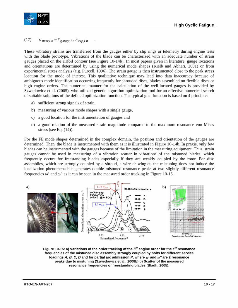
For the FE mode shapes determined in the complex domain, the position and orientation of the gauges are determined. Then, the blade is instrumented with them as it is illustrated in Figure 10-14b. In praxis, only few blades can be instrumented with the gauges because of the limitation in the measuring equipment. Thus, strain gauges cannot be used in measuring of a vibration scatter in vibrations of the mistuned blades, which frequently occurs for freestanding blades especially if they are weakly coupled by the rotor. For disc assemblies, which are strongly coupled by a shroud, a wire or winglet, the mistuning does not induce the localization phenomena but generates double mistuned resonance peaks at two slightly different resonance frequencies ω’ and ω” as it can be seen in the measured order tracking in Figure 10-15.

Figure 10-15: a) Variations of the order tracking of the 8th engine order for the 1st resonance frequencies of the mistuned disc assembly strongly coupled by bolts for different service

loadings A, B, C, D and for partial arc admission P, where ω’ and ω” are 2 resonance peaks due to mistuning (Szwedowicz et al., 2008b) b) Scatter of the measured

resonance frequencies of freestanding blades (Bladh, 2005).

a) b)

High Cyclic Fatigue

10 - 18 RTO-EN-AVT-207

In general, a vibration response of the mistuned blades is few times bigger than the computed resonance amplitudes of the tuned blades. This is because of spatial localization of the vibration energy (Whitehead, 1988). Certain airfoils, which are disordered by manufacturing and assembling tolerances as well as by divergences in material properties, might experience substantially larger oscillations than the numerical response amplitudes of the tuned bladed disc. Thus, the mistuned blades having high resonance amplitudes are the most critical for the HCF. This can be proved experimentally by using the tip timing system, which measures oscillation of each blade in the rotating bladed disc. In evaluation of the results from the tip timing measurement a certain difficulty can be with identification of the excited nodal diameter, what is an important piece of information in the HCF design. However, the tip timing system with at least 6 sensors provides the resonance frequencies and also enough detailed information about the forms of the excited vibration waves propagating in the rotating bladed disc. The strain gauge from the telemetry system provides continuous signals of the blade vibration, from which the detailed results about the mode shapes of the vibrating disc assembly can be evaluated. For both measuring systems, the numerical predication of the blade vibrations always is essential for the properly performed experimental dynamics.

4.0 RESONANCE PROOF OF ROTATING BLADES

The restricted frequency range of the blade eigenfrequencies below the 6th (see Figure 10-12) or even up to the 8th engine order is the most important criterion in the design of bladed disc assemblies operating with the constant nominal speed. For these blades, resonance loadings occur during start-ups and shot-downs of the turbine, when the blade eigenfrequencies are excited by lowest engine orders as it is shown in Figure 10-12.

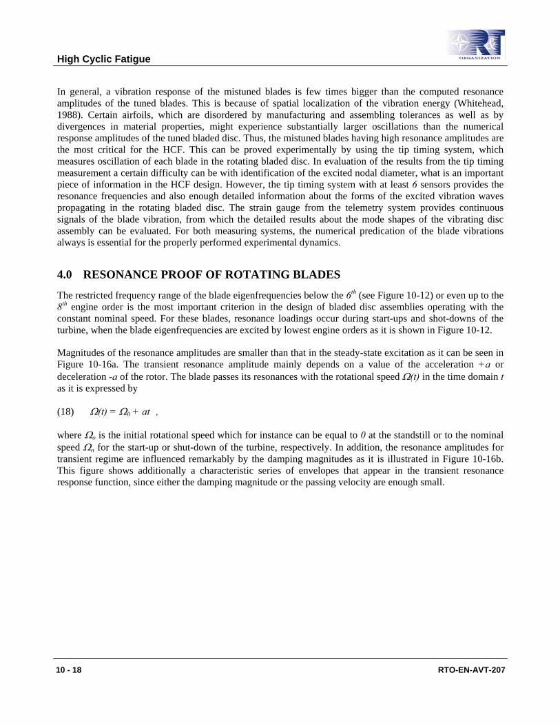
Magnitudes of the resonance amplitudes are smaller than that in the steady-state excitation as it can be seen in Figure 10-16a. The transient resonance amplitude mainly depends on a value of the acceleration +a or deceleration -a of the rotor. The blade passes its resonances with the rotational speed Ω(t) in the time domain t as it is expressed by

(18) Ω(t) = Ω0 + at ,

where Ωo is the initial rotational speed which for instance can be equal to 0 at the standstill or to the nominal speed Ωn for the start-up or shut-down of the turbine, respectively. In addition, the resonance amplitudes for transient regime are influenced remarkably by the damping magnitudes as it is illustrated in Figure 10-16b. This figure shows additionally a characteristic series of envelopes that appear in the transient resonance response function, since either the damping magnitude or the passing velocity are enough small.

High Cyclic Fatigue

RTO-EN-AVT-207 10 - 19

excitation / natural frequency

Res

pons

e am

plitu

deε(

t)

Transient response function

time

Steady-state response function

excitation / natural frequency

Res

pons

e am

plitu

deε(

t)

Transient response function

time

excitation / natural frequency

Res

pons

e am

plitu

deε(

t)

Transient response function

time

Steady-state response function

Δε

excitation / natural frequency

Res

pons

e am

plitu

deε(

t)

Transient response function

time

Steady-state response function

excitation / natural frequency

Res

pons

e am

plitu

deε(

t)

Transient response function

time

excitation / natural frequency

Res

pons

e am

plitu

deε(

t)

Transient response function

time

Steady-state response function

ΔεSDOFSDOFSDOF

Figure 10-16: a) Resonance Response Function (RRF) for the steady-state and transient excitation b) Behavior of the transient responses in terms of modal damping ratios ξ of 0.02% (a), 0.1%

(b) and 0.2% (c) computed with a single mass-spring system of one degree of freedom (SDOF) model of the rotating blade for the excitation amplitude and the

constant angular speed deceleration a of the rotor.

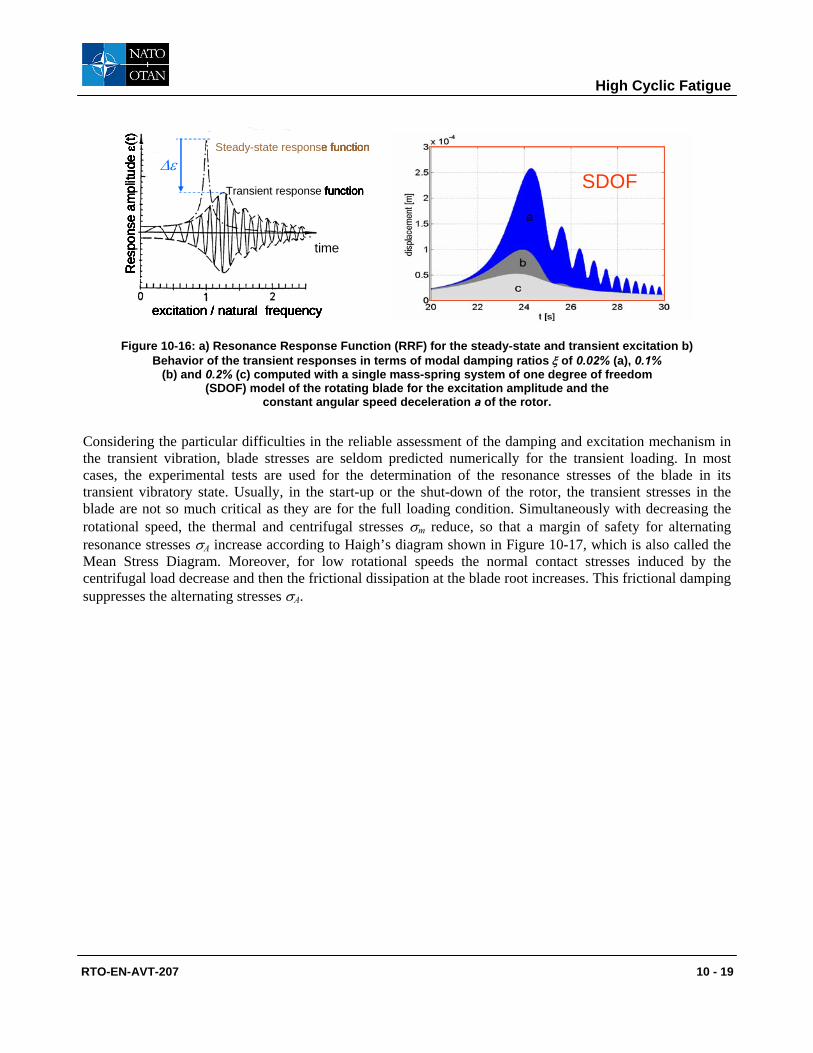
Considering the particular difficulties in the reliable assessment of the damping and excitation mechanism in the transient vibration, blade stresses are seldom predicted numerically for the transient loading. In most cases, the experimental tests are used for the determination of the resonance stresses of the blade in its transient vibratory state. Usually, in the start-up or the shut-down of the rotor, the transient stresses in the blade are not so much critical as they are for the full loading condition. Simultaneously with decreasing the rotational speed, the thermal and centrifugal stresses σm reduce, so that a margin of safety for alternating resonance stresses σA increase according to Haigh’s diagram shown in Figure 10-17, which is also called the Mean Stress Diagram. Moreover, for low rotational speeds the normal contact stresses induced by the centrifugal load decrease and then the frictional dissipation at the blade root increases. This frictional damping suppresses the alternating stresses σA.

High Cyclic Fatigue

10 - 20 RTO-EN-AVT-207

Figure 10-17: a) Haigh’s diagram as the most popular the Mean Stress Diagram in which green color means infinite life, whereby Rm ≡ Su is the ultimate tensile strength and σw ≡ σe ≡ Se

denotes the tensile endurance strength and U is the 1st bending mode shape of the resonance frequency ω1, b) Resonance Response Functions for the

steady-state excitation in terms of damping magnitude D ≡ ξ.

The most critical problems of the high cyclic fatigue occur for bladed discs operating with variable speed. Then, a disc assembly can be in resonance for long operation time. Therefore, these blades have to be resonance proof as the essential feature in the HCF design process. The blade can be in resonance, since the blade eigenfrequency ωi,n coincides with the excitation frequency, as it is expressed by

(19) ⎩⎨⎧

±=

ΩεΩ

ωk

kn,i , k = 0, 1, 2, 3, …, ∞ ,

where k is the engine order number, kΩ and (ε ± kΩ) denote the rotational and pulsation (acoustical) harmonic excitation, respectively. In Equation (19), ε can correspond to the acoustic resonance induced by the turbulent flow (see Figure 10-8b).

Besides the frequency condition given above, the excitability condition for the tuned bladed assembly has to be fulfilled. Due to the orthogonality condition between the disc mode φi,n and the circumferential pressure distribution Fk (see Equation (13)), the resonance occurs only, if the engine order k satisfies following conditions

(20) k = κ⋅N m n for the even number N,

(21) k = κ⋅(N+2) m n for the odd number N,

a) b)

High Cyclic Fatigue

RTO-EN-AVT-207 10 - 21

where κ=0, 1, … ∞ and N denotes the number of blades in the disc assembly. For the most common resonance problem of the rotational harmonic excitation kΩ and the lowest engine order k (for instance k<10), the Equation (9) can be simplified considering the resonance condition of ωi,n = kΩ and n = k. Then, the resonance response of node η is obtained from

(22) ⎟⎟

⎠

⎞

⎜⎜

⎝

⎛= °

2n,in,i

n,i,o,n,i,n.i

2

Fq

ωξΨ ηη ,

where according to Equation (13) the modal force Fo,i,n can be rewritten with

(23) { } { } { }( ) { } { } ( ){ } { } ( ){ }( )δδ ααΦΦ kcosFjksinFFjFF Tc,k

Ts,k

T*n,iC,kS,k

T*n,in,i,o +−=+−= °° .

In practice, the 3D excitation pressure of engine order k is usually unknown and the resonance response equation (22) needs to be simplified to

(24) ( ) ( )2n,in,i

,oo

,s,n,io

,c,n,iko,s,n,i

o,c,n,i2

n,in,i

,ok,n,i,n,i

2

Fjsj

2

fsq

ωξ

φφφφ

ωξΨ ΛΛΛ

ηηΛ

ηη+

+== ° ,

where Fo,Λ is the resulting static force of the steady-state flow imposed at point Λ of the airfoil (see Figure 10-16b). In Equation (24), sk is stimulus of the k-th engine order which is expressed empirically by

(25) o

kk F

Fs = , k = 1, 2, 3, …, ∞ ,

where Fo and Fk are the resulting static amplitude and excitation amplitude of the k-th engine order of the experimental excitation spectrum. This spectrum can be obtained from the Fourier Fast transformation of the measured flow pressure distribution by using for instance a 5-hole probe. In equation (24), the expression

o,s,n,i

o,c,n,i,n,i j ηηη φφΨ +=°

refers to the FE mass-normalized real and imaginary mode shape of the η–th degree of freedom of node n and eignefrequency i. These mode shapes can correspond to displacement, strain or stress in terms of needs in the HCF design process. For example, considering the real an imaginary FE mode shape of stress component σxx,i,n,c,η and σxx,i,n,s,η, the resonance stress σxx of the mode shape i,n at node η is determined with

(26) ( ) ( )2n,in,i

,oo

,s,n,io

,c,n,iko,s,n,i,xx

o,c,n,i,xx,n,i,xx

2

Fjsj

ωξ

φφσσσ ΛΛΛ

ηηη+

+= .

This uni-axial stress can be treated as the maximum resonance stress, if the blade dynamics is defined by the 1D formulation like Montoya’s or Timoshenko’s theory. For 3-dimensional stress state, equation (26) needs to be applied for all 6 components of the stress tensor of point η (see Figure 10-13) and then resonance von Mises stress (or another equivalent stress) can be computed.

High Cyclic Fatigue

10 - 22 RTO-EN-AVT-207

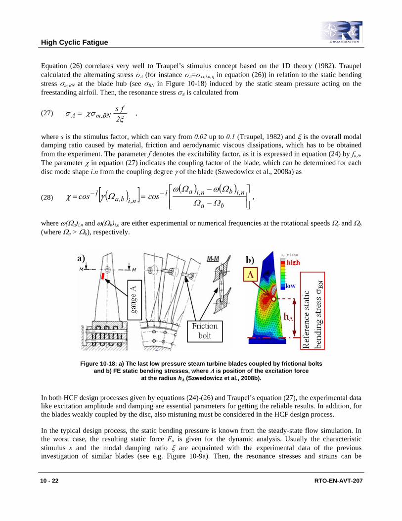
Equation (26) correlates very well to Traupel’s stimulus concept based on the 1D theory (1982). Traupel calculated the alternating stress σA (for instance σA=σxx,i,n,η in equation (26)) in relation to the static bending stress σm,BN at the blade hub (see σBN in Figure 10-18) induced by the static steam pressure acting on the freestanding airfoil. Then, the resonance stress σA is calculated from

(27) ξ

χσσ2

fsBN,mA = ,

where s is the stimulus factor, which can vary from 0.02 up to 0.1 (Traupel, 1982) and ξ is the overall modal damping ratio caused by material, friction and aerodynamic viscous dissipations, which has to be obtained from the experiment. The parameter f denotes the excitability factor, as it is expressed in equation (24) by fo,δ. The parameter χ in equation (27) indicates the coupling factor of the blade, which can be determined for each disc mode shape i.n from the coupling degree γ of the blade (Szwedowicz et al., 2008a) as

(28) ( )[ ] ( ) ( ),coscos

ba

n,ibn,ia1n,ib,a

1

⎥⎥⎦

⎤

⎢⎢⎣

⎡

−

−== −−

ΩΩ

ΩωΩωΩγχ

where ω(Ωa)i,n and ω(Ωb)i,n are either experimental or numerical frequencies at the rotational speeds Ωa and Ωb (where Ωa > Ωb), respectively.

Figure 10-18: a) The last low pressure steam turbine blades coupled by frictional bolts and b) FE static bending stresses, where Λ is position of the excitation force

at the radius hΛ (Szwedowicz et al., 2008b).

In both HCF design processes given by equations (24)-(26) and Traupel’s equation (27), the experimental data like excitation amplitude and damping are essential parameters for getting the reliable results. In addition, for the blades weakly coupled by the disc, also mistuning must be considered in the HCF design process.

In the typical design process, the static bending pressure is known from the steady-state flow simulation. In the worst case, the resulting static force Fo is given for the dynamic analysis. Usually the characteristic stimulus s and the modal damping ratio ξ are acquainted with the experimental data of the previous investigation of similar blades (see e.g. Figure 10-9a). Then, the resonance stresses and strains can be

High Cyclic Fatigue

RTO-EN-AVT-207 10 - 23

computed from the FE simulation and the maximum resonance strain εA,gauge,FE at the strain gauge is obtained for the assumed stimulus so and modal damping ratio ξo.

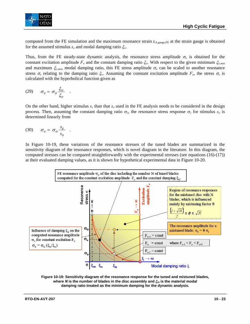
Thus, from the FE steady-state dynamic analysis, the resonance stress amplitude σo is obtained for the constant excitation amplitude Fo and the constant damping ratio ξo. With respect to the given minimum ξe,min and maximum ξe,max modal damping ratio, this FE stress amplitude σo can be scaled to another resonance stress σe relating to the damping ratio ξe. Assuming the constant excitation amplitude Fo, the stress σe is calculated with the hyperbolical function given as

(29) e

ooe ξ

ξσσ = .

On the other hand, higher stimulus se than that so used in the FE analysis needs to be considered in the design process. Then, assuming the constant damping ratio σo, the resonance stress response σe for stimulus so is determined linearly from

(30) o

eoe s

sσσ = .

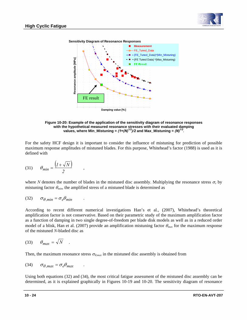
In Figure 10-19, these variations of the resonance stresses of the tuned blades are summarized in the sensitivity diagram of the resonance responses, which is novel diagram in the literature. In this diagram, the computed stresses can be compared straightforwardly with the experimental stresses (see equations (16)-(17)) at their evaluated damping values, as it is shown for hypothetical experimental data in Figure 10-20.

Figure 10-19: Sensitivity diagram of the resonance response for the tuned and mistuned blades, where N is the number of blades in the disc assembly and ξm is the material modal

damping ratio treated as the minimum damping for the dynamic analysis.

High Cyclic Fatigue

10 - 24 RTO-EN-AVT-207

Sensitivity Diagram of Resonance Responses

Damping value [%]

Res

onan

ce a

mpl

itude

[MPa

]

MeasurementFE_Tuned_Data(FE_Tuned_Data)*(Min_Mistuning)

(FE Tuned Data) *(Max_Mistuning)FE Result

Figure 10-20: Example of the application of the sensitivity diagram of resonance responses with the hypothetical measured resonance stresses with their evaluated damping

values, where Min_Mistuning = (1+(N)1/2)/2 and Max_Mistuning = (N)1/2.

For the safety HCF design it is important to consider the influence of mistuning for prediction of possible maximum response amplitudes of mistuned blades. For this purpose, Whitehead’s factor (1988) is used as it is defined with

(31) ( )

2N1

min+

=θ ,

where N denotes the number of blades in the mistuned disc assembly. Multiplying the resonance stress σe by mistuning factor θmin, the amplified stress of a mistuned blade is determined as

(32) minemin, θσσθ = .

According to recent different numerical investigations Han’s et al., (2007), Whitehead’s theoretical amplification factor is not conservative. Based on their parametric study of the maximum amplification factor as a function of damping in two single degree-of-freedom per blade disk models as well as in a reduced order model of a blisk, Han et al. (2007) provide an amplification mistuning factor θmax for the maximum response of the mistuned N-bladed disc as

(33) Nmax =θ .

Then, the maximum resonance stress σθ,max in the mistuned disc assembly is obtained from

(34) maxemax, θσσθ = .

Using both equations (32) and (34), the most critical fatigue assessment of the mistuned disc assembly can be determined, as it is explained graphically in Figures 10-19 and 10-20. The sensitivity diagram of resonance

FE result

High Cyclic Fatigue

RTO-EN-AVT-207 10 - 25

responses for the tuned and mistuned allows for straightforward correlation to the measured stresses. This diagram helps for finding the realistic variation of the alternating stresses σA with respect to uncertainties with excitation, damping and mistuning for the HCF life prediction.

5.0 STRESS-LIFE (S-N) METHOD

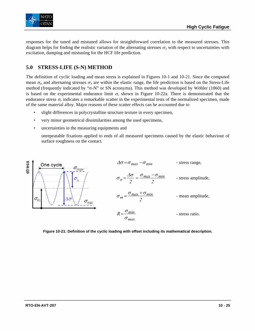
The definition of cyclic loading and mean stress is explained in Figures 10-1 and 10-21. Since the computed mean σm and alternating stresses σA are within the elastic range, the life prediction is based on the Stress-Life method (frequently indicated by “σ-N” or SN acronyms). This method was developed by Wöhler (1860) and is based on the experimental endurance limit σe shown in Figure 10-22a. There is demonstrated that the endurance stress σe indicates a remarkable scatter in the experimental tests of the normalized specimen, made of the same material alloy. Major reasons of these scatter effects can be accounted due to

• slight differences in polycrystalline structure texture in every specimen,

• very minor geometrical dissimilarities among the used specimens,

• uncertainties in the measuring equipments and

• unrepeatable fixations applied to ends of all measured specimens caused by the elastic behaviour of surface roughness on the contact.

minmax σσσΔ −= - stress range,

22minmax

aσσσΔσ −

== - stress amplitude,

2minmax

mσσσ +

= - mean amplitude,

max

minRσσ

= - stress ratio.

Figure 10-21: Definition of the cyclic loading with offset including its mathematical description.

High Cyclic Fatigue

10 - 26 RTO-EN-AVT-207

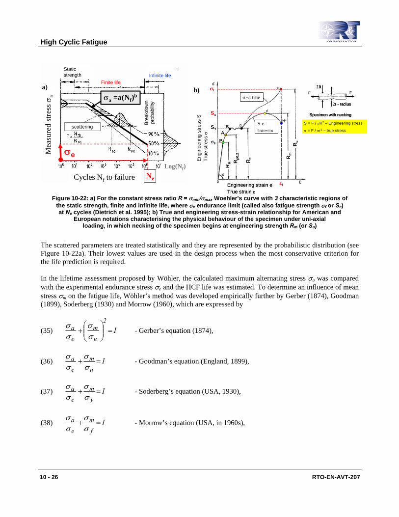
Figure 10-22: a) For the constant stress ratio R = σmin/σmax Woehler’s curve with 3 characteristic regions of the static strength, finite and infinite life, where σe endurance limit (called also fatigue strength σf or Se) at Ne cycles (Dietrich et al. 1995); b) True and engineering stress-strain relationship for American and

European notations characterising the physical behaviour of the specimen under uni-axial loading, in which necking of the specimen begins at engineering strength Rm (or Su)

The scattered parameters are treated statistically and they are represented by the probabilistic distribution (see Figure 10-22a). Their lowest values are used in the design process when the most conservative criterion for the life prediction is required.

In the lifetime assessment proposed by Wöhler, the calculated maximum alternating stress σa was compared with the experimental endurance stress σe and the HCF life was estimated. To determine an influence of mean stress σm on the fatigue life, Wöhler’s method was developed empirically further by Gerber (1874), Goodman (1899), Soderberg (1930) and Morrow (1960), which are expressed by

(35) 12

u

m

e

a =⎟⎟⎠

⎞⎜⎜⎝

⎛+

σσ

σσ

- Gerber’s equation (1874),

(36) 1u

m

e

a =+σσ

σσ

- Goodman’s equation (England, 1899),

(37) 1y

m

e

a =+σσ

σσ

- Soderberg’s equation (USA, 1930),

(38) 1f

m

e

a =+σσ

σσ

- Morrow’s equation (USA, in 1960s),

Static strength

Finite lifeInfinite life

scattering

Number of cycles

Mea

sure

d st

ress

Bre

akdo

wn

prob

abilit

y

Static strength

Finite lifeInfinite life

scattering

Number of cycles

Mea

sure

d st

ress

Bre

akdo

wn

prob

abilit

yσe

Cycles Nf to failureLog(Nf)

Mea

sure

d st

ress

σa

Ne

σa =a(Nf)bσf

Rm

Ru

Rp0

.2

εfEngineering strain eTrue strain ε

Eng

inee

ring

stre

ss S

True

stre

ss σ

Su

Re

RH

PσF

ABSY

S-eEngineering

σ−ε true

H*

σf

Rm

Ru

Rp0

.2

εfEngineering strain eTrue strain ε

Eng

inee

ring

stre

ss S

True

stre

ss σ

Su

Re

RH

PσF

ABSY

S-eEngineering

σ−ε true

H* S = F / πR2 – Engineering stress

σ = F / πr2 – true stress

Specimen with necking

2R

2r - radius

FF

Specimen with necking

2R

2r - radius

Specimen with necking

2R

2r - radius

FFa) b)

High Cyclic Fatigue

RTO-EN-AVT-207 10 - 27

where σy (called also Re, Sy) denotes yield stress (Figure 10-22b), σu (or Rm, Su) is ultimate stress (Figure 10-22b), σf corresponds to true fracture stress (Figure 10-22b) and σe (or σD, σW, Se) means endurance stress shown in Figure 10-22a.

The equations (35)-(38) predict a region of infinite life by combining the endurance strength σe (Figure 10-22a) with either the yield strength σy, ultimate strength σu, or true fracture stress σf known from monotonic uni-axial tensile test (Figure 10-22b). Therefore, these life equations ought to be applied only to tensile mean stresses. It is also characteristic, that for small mean loadings (R<<1) these methods do not differ among each too much. According to real data from field failures usually are reported between the Goodman and Gerber curves, where Goodman ones should be used for conservative design. If the ultimate strength approaches the true fracture stress like it is for hard steels showing brittle behavior, the Morrow and Goodman equations provide practically comparable life prediction.

In present design practice, Haigh’s equation becomes the most popular in engineering analyses. This method is developed from Goodman’s equation by considering the description of the Woehler curve for the range of finite life in Figure 10-22a as

(39) ( )bfa Na=σ .

By applying the number Nf=Ne of fully-reversing cycles (where Ne varies between 105 ÷ 107 cycles what depends on the strength and hardness of the alloys) into equation (39), the endurance stress σe is obtained, which is substituted into Goodman’s equation (36), Haigh’s equation is determined as

(40) ( ) ⎟⎟⎠

⎞⎜⎜⎝

⎛−=

u

mbea 1Na

σσσ ,

where a and b are empirical constants. In case of the absence of the experimental data, these constants can be estimated from

(41) ( )

e

2u90.0a

σσ

= and ⎟⎟⎠

⎞⎜⎜⎝

⎛=

e

u9.0log31b

σσ

,

where all stresses are expressed in (psi) unit. In addition, experiments show a linear relation between the endurance strength σe and ultimate stress σu, which for R=-1 (mean stress σm=0) are given exemplary in Table 10-1.

High Cyclic Fatigue

10 - 28 RTO-EN-AVT-207

Table 10-1: Relation between the endurance strength σe and ultimate stress σu, for R=-1 (mean stress σm=0) from Issler et al. (1995).

σe,R=-1 = (0.40 ÷ 0.45)σu steel under tensile loading mode σe,R=-1 = 0.436 Rp0,2 + 77 σe,R=-1 = 0.27 Rm + 85 cast steel under tensile loading mode σe,R=-1 = 0.27 Rm + 100 modular cast iron under tensile loading mode σe,R=-1 = 0.27 Rm + 110 anneal cast iron under tensile loading mode σe,R=-1 = 0.39 Rm grey cast iron under tensile loading mode σe,R=-1 = (0.25 ÷ 0.35)σu aluminium alloy under tensile loading mode σe,R=-1,Bending = (1.1 ÷ 1.4)σe,R=-1 ductile alloy under bending loading mode σe,R=-1,Torsion = 0.58σe,R=-1Bending brittle alloy under torsion loading mode

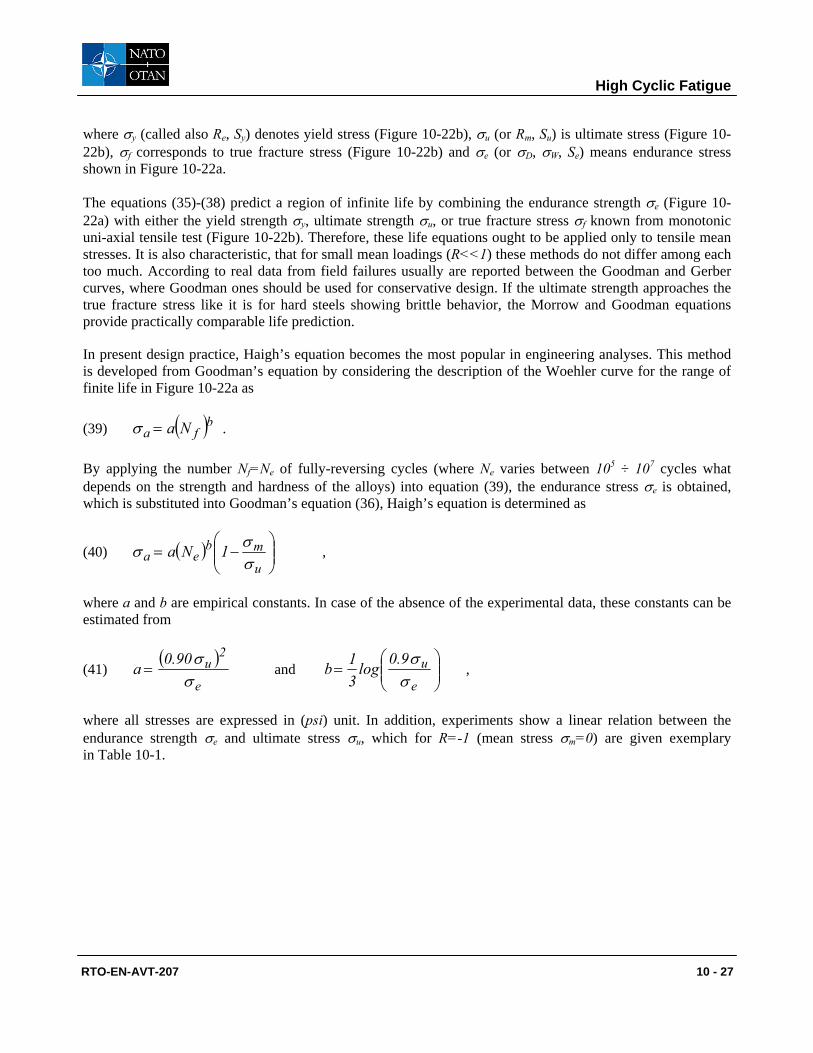
To create the Haigh’s diagram according to equation (40) a lot of data must be known from the experimental tests of specimen. This is demonstrated in Figure 10-23b, which shows additionally an influence of the mean stress σm on the endurance stress σe. The reduction of the endurance stress by increased tensile mean stress is less significant for ductile alloys in relation to brittle materials.

Figure 10-23: a) Graphical comparison of the most popular Mean Stress Diagrams; b) Relation between Wöhler (Fatigue-Strength-Diagram; FSD) curves and Haigh’s Diagram

with the indicated influence of the mean stress on the fatigue life.

In the design process, the simplified Haigh’s diagram is usually created by using two different endurance strength σe,R=0 and σe,R=-1 as well as yield stress σy (see Sy=Re in Figure 10-22b) and ultimate stress σu (see Rm=Su in Figure 10-22b). For these data, the construction of the Haigh’s diagram is explained in Figure 10-24a. Also in the engineering practise the Haigh’s diagram is extended by using an additional slope function defined with sensitivity factor M. As it is given in Figure 10-24b, the life curve fits in wider range of equation

σm

σa

σa

σaσa

σm=0

σm>0

σm<0

Ne σm=0 σm>0σm<0

σa

Rm

N=103

Soderberg

Mooorw

Gerber

Goodman

σy σu σf

σe

σm

σaFinite life region

a) b)

Wöhler (S-N) curves

Haigh diagram

High Cyclic Fatigue

RTO-EN-AVT-207 10 - 29

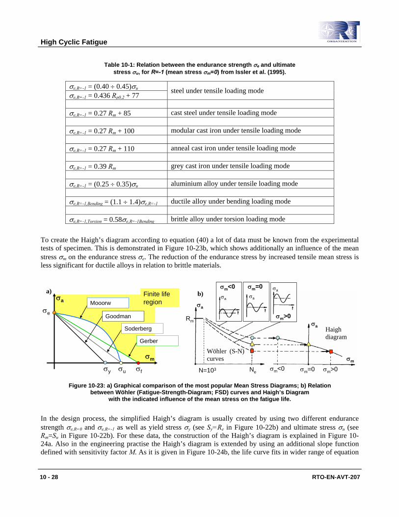
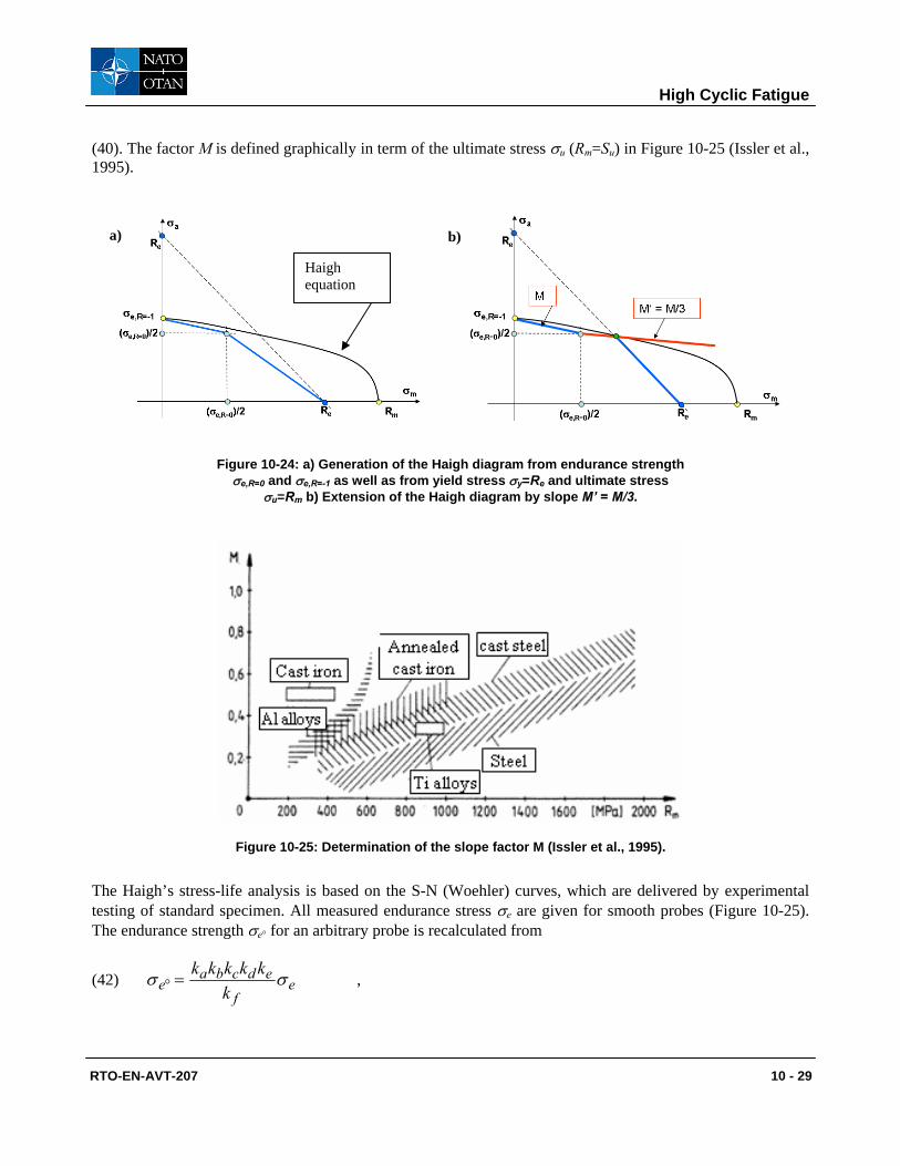
(40). The factor M is defined graphically in term of the ultimate stress σu (Rm=Su) in Figure 10-25 (Issler et al., 1995).

Figure 10-24: a) Generation of the Haigh diagram from endurance strength σe,R=0 and σe,R=-1 as well as from yield stress σy=Re and ultimate stress

σu=Rm b) Extension of the Haigh diagram by slope M’ = M/3.

Figure 10-25: Determination of the slope factor M (Issler et al., 1995).

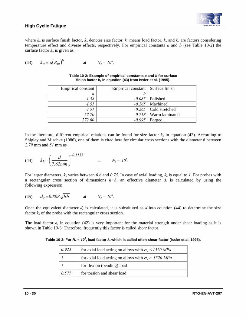
The Haigh’s stress-life analysis is based on the S-N (Woehler) curves, which are delivered by experimental testing of standard specimen. All measured endurance stress σe are given for smooth probes (Figure 10-25). The endurance strength σe° for an arbitrary probe is recalculated from

(42) ef

edcbae k

kkkkk σσ =° ,

Haigh equation

a) b)

High Cyclic Fatigue

10 - 30 RTO-EN-AVT-207

where ka is surface finish factor, kb denotes size factor, kc means load factor, kd and ke are factors considering temperature effect and diverse effects, respectively. For empirical constants a and b (see Table 10-2) the surface factor ka is given as

(43) ( )bma Rak = at Ne = 106.

Table 10-2: Example of empirical constants a and b for surface finish factor ka in equation (43) from Issler et al. (1995).

Empirical constant a

Empirical constant b

Surface finish

1.58 -0.085 Polished 4.51 -0.265 Machined 4.51 -0.265 Cold stretched

57.70 -0.718 Warm laminated 272.00 -0.995 Forged

In the literature, different empirical relations can be found for size factor kb in equation (42). According to Shigley and Mischke (1986), one of them is cited here for circular cross sections with the diameter d between 2.79 mm and 51 mm as

(44) 1133.0

b mm62.7dk

−⎟⎠⎞

⎜⎝⎛= at Ne = 106.

For larger diameters, kb varies between 0.6 and 0.75. In case of axial loading, kb is equal to 1. For probes with a rectangular cross section of dimensions h×b, an effective diameter de is calculated by using the following expression

(45) bh808.0de = at Ne = 106.

Once the equivalent diameter de is calculated, it is substituted as d into equation (44) to determine the size factor kb of the probe with the rectangular cross section.

The load factor kc in equation (42) is very important for the material strength under shear loading as it is shown in Table 10-3. Therefore, frequently this factor is called shear factor.

Table 10-3: For Ne = 106, load factor kc which is called often shear factor (Issler et al, 1995).

0.923 for axial load acting on alloys with σu ≤ 1520 MPa

1 for axial load acting on alloys with σu > 1520 MPa

1 for flexion (bending) load

0.577 for torsion and shear load

High Cyclic Fatigue

RTO-EN-AVT-207 10 - 31

Figure 10-26: Influence of surface ka and site kb factors on the behavior of Woehler curves for bending tests (a) and the Haigh’s diagram (b), where σe and σe° are endurance

strength of the standard and analysed probe, respectively.

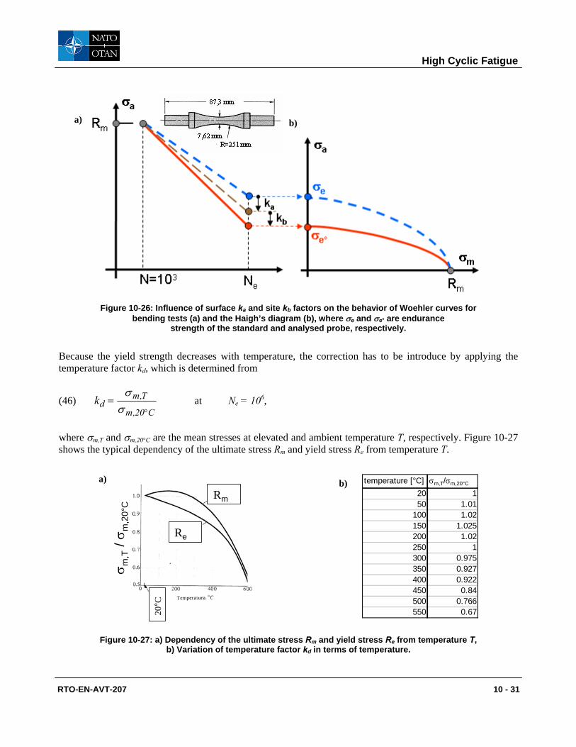
Because the yield strength decreases with temperature, the correction has to be introduce by applying the temperature factor kd, which is determined from

(46) C20,m

T,mdk

°=

σσ

at Ne = 106,

where σm,T and σm,20°C are the mean stresses at elevated and ambient temperature T, respectively. Figure 10-27 shows the typical dependency of the ultimate stress Rm and yield stress Re from temperature T.

Figure 10-27: a) Dependency of the ultimate stress Rm and yield stress Re from temperature T, b) Variation of temperature factor kd in terms of temperature.

Rm

Re

σ m,T

/ σm

,20°

C

20°C

temperature [°C] ST/SRT

20 150 1.01

100 1.02150 1.025200 1.02250 1300 0.975350 0.927400 0.922450 0.84500 0.766550 0.67

σm,T/σm,20°Ca) b)

a) b)

High Cyclic Fatigue

10 - 32 RTO-EN-AVT-207

For diverse effects, the factor ke can account for instance following environmental conditions:

• Corrosion can reduce the endurance strength to 0 (ke=0),

• An electrolytic metallic recoverment can reduce the endurance strength to 0.5 (ke=0.5),

• Metallisation by aspersion can reduce the endurance strength to 0.86 (ke=0.86),

• Fretting can reduce the endurance strength between 24% and 90% (ke=0.24 – 0.90).

Most vibration fatigue failures begin at locations of geometrical notches (e.g. radii, fillets, keyways etc.), which induce stress concentrations. Then, the fatigue stress concentration factor kf (called also a fatigue notch factor) in equation (42) is an essential feature of the reliable HCF life prediction. According to Peterson (1974), this factor corresponds proportionally to the geometrical stress concentration factor kt and is expressed by

(47) ( )1kq1k tf −+= at Ne = 106,

where q is a notch sensitivity factor, which by definition differs from 0 up to 1 and determines the sensitivity of discontinuity in the geometry. In general, the notch sensitivity factor q depends on

• the material property,

• the heat treatment of the material and

• the notch size.

The notch sensitivity factor q can be obtained from empirical Peterson’s equation

(48) a1k

1kq

n

n

t

f+

=−

−=

ρρ

,

where ρn radius (mm) at root of notch and a is material (Neuber’s) constant, given in (mm) unit, which for steels can be calculated from

(49) ( ) 8.1

mR300001.0a = for the ultimate stress Rm defined in ksi unit.

In equation (47), the geometrical stress concentration factor kt is measured with monotonic loading test for the notched specimen. Usually this factor kt ranges from 1.2 to 4 but it can be even higher. Peterson (1974) provides many analytically computed geometrical stress concentration factor kt. Also, from the static finite element analysis with a very fine mesh or sub-modeling around the notch, the geometrical stress concentration factor kt. might be computed in reliable manner. Although the FE computation is based on the isotropic and homogeneous assumption, the real material behavior with internal minor flaws tends to reduce the stress enlargement. Indeed, these effects are included in the fatigue stress concentration factor kf. Therefore, the most reliable assessment of this factor kf is the experimental manner. Then the fatigue notch factor kf is defined as the relation of the endurance stress σe° of the notched specimen to the endurance stress σe of the smooth specimen. This experimental manner is expressed with

High Cyclic Fatigue

RTO-EN-AVT-207 10 - 33

(50) °

=e

efk

σσ

.

It has to be noticed that for complex shapes components, the stress concentration (fatigue notch) factor kf. cannot be determined in reliable manner.

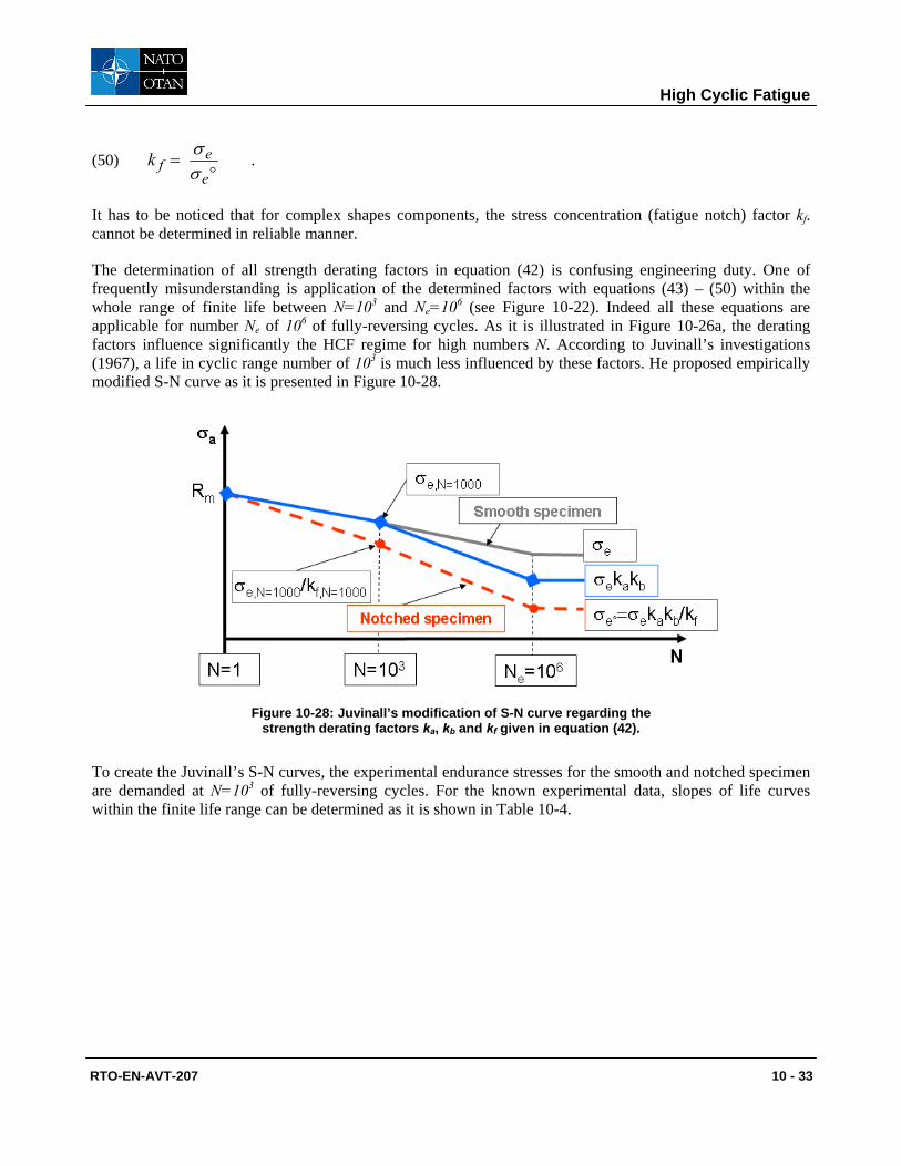
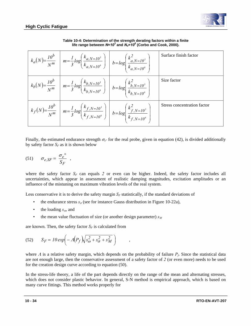
The determination of all strength derating factors in equation (42) is confusing engineering duty. One of frequently misunderstanding is application of the determined factors with equations (43) – (50) within the whole range of finite life between N=103 and Ne=106 (see Figure 10-22). Indeed all these equations are applicable for number Ne of 106 of fully-reversing cycles. As it is illustrated in Figure 10-26a, the derating factors influence significantly the HCF regime for high numbers N. According to Juvinall’s investigations (1967), a life in cyclic range number of 103 is much less influenced by these factors. He proposed empirically modified S-N curve as it is presented in Figure 10-28.

Figure 10-28: Juvinall’s modification of S-N curve regarding the strength derating factors ka, kb and kf given in equation (42).

To create the Juvinall’s S-N curves, the experimental endurance stresses for the smooth and notched specimen are demanded at N=103 of fully-reversing cycles. For the known experimental data, slopes of life curves within the finite life range can be determined as it is shown in Table 10-4.

High Cyclic Fatigue

10 - 34 RTO-EN-AVT-207

Table 10-4: Determination of the strength derating factors within a finite life range between N=103 and Ne=106 (Corbo and Cook, 2000).

( ) m

ba

N10Nk =

⎟⎟⎠

⎞⎜⎜⎝

⎛=

=

=6

3

10N,a

10N,akk

log31m

⎟⎟⎟

⎠

⎞

⎜⎜⎜

⎝

⎛=

=

=6

3

10N,a

210N,a

k

klogb

Surface finish factor

( ) m

bb

N10Nk =

⎟⎟⎠

⎞⎜⎜⎝

⎛=

=

=6

3

10N,b

10N,bkk

log31m

⎟⎟⎟

⎠

⎞

⎜⎜⎜

⎝

⎛=

=

=6

3

10N,b

210N,b

k

klogb

Size factor

( ) m

bf

N10Nk =

⎟⎟

⎠

⎞

⎜⎜

⎝

⎛=

=

=

6

3

10N,f

10N,fk

klog

31m

⎟⎟⎟

⎠

⎞

⎜⎜⎜

⎝

⎛=

=

=

6

3

10N,f

210N,f

k

klogb

Stress concentration factor

Finally, the estimated endurance strength σe° for the real probe, given in equation (42), is divided additionally by safety factor SF as it is shown below

(51) F

eSF,e S

°=

σσ ,

where the safety factor SF can equals 2 or even can be higher. Indeed, the safety factor includes all uncertainties, which appear in assessment of realistic damping magnitudes, excitation amplitudes or an influence of the mistuning on maximum vibration levels of the real system.

Less conservative it is to derive the safety margin SF statistically, if the standard deviations of

• the endurance stress sσ (see for instance Gauss distribution in Figure 10-22a),

• the loading sω, and • the mean value fluctuation of size (or another design parameter) sM

are known. Then, the safety factor SF is calculated from

(52) ( ) ⎟⎠⎞

⎜⎝⎛ ++−= 2

M22

fF sssPexp10S σωΛ ,

where Λ is a relative safety margin, which depends on the probability of failure Pf. Since the statistical data are not enough large, then the conservative assessment of a safety factor of 2 (or even more) needs to be used for the creation design curve according to equation (50).

In the stress-life theory, a life of the part depends directly on the range of the mean and alternating stresses, which does not consider plastic behavior. In general, S-N method is empirical approach, which is based on many curve fittings. This method works properly for

High Cyclic Fatigue

RTO-EN-AVT-207 10 - 35

• engineering type notch (e.g. groves, geometry change, etc.), • wrought steels (e.g. after Boushinger’s effect), • constant amplitude loading and • structures for them infinite life considered.

The S-N methods does not work accurately for • aluminum alloys, • loading modes with variable amplitudes, • low cyclic fatigue with plastic deformation, • mechanical systems with sever geometrical notches and • periodically overloaded systems.

The stress-life (S-N) approach is entirely acceptable engineering procedure for the prediction of the fatigue life, when mainly the infinite life is taken into consideration. On the other hand the S-N method tends to provide the conservative determination because of neglecting the ductility participation in the damage mechanism as well as of considering the endurance life up to 106 cycles.

6.0 STRAIN-LIFE (E-N) PREDICTION OF FATIGUE FAILURE

The Strain-Life method was developed by Coffin & Manson in 1950 for low cyclic fatigue problems of gas turbine and nuclear reactor components. In the 60’s, this method was improved by Morrow and Neuber as well as by other researchers considering different fatigue situations. In general the Strain-Life

• deals with plastic strains,

• considers notch geometries and multi-axial loading modes,

• accounts residual stresses,

• takes into consideration loading modes with variable amplitudes

• combines creep and relaxation for high temperature.

The application of this E-N method is more complicated in relation to the Stress-Life (S-N) approach and wide range of material data must be available.

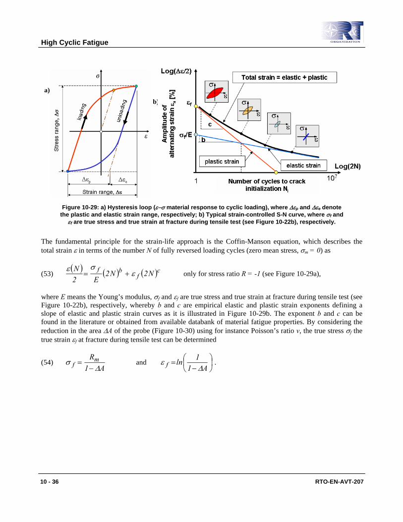
For the HCF regime, local cyclic plastic deformations are present in damage mechanism, which essentially depends on cyclic stresses and tensile stress. Once the local plastic deformation is needed in the assessment of fatigue failures, the strength and ductility must be considered in the analysis of the damage mechanism. This assures the strain-life (E-N) method, which calculates the total strain εT as a sum of elastic εE and plastic εP strain. In the HCF regime, the total strain is dominated by the elastic strain in relation to the participation of the plastic strain. This relationship is demonstrated very well in the typical strain-life curve in Figure 10-29b. Figures 10-29a shows area inside the hysteresis loop (ε−σ material response to cyclic loading), which determines energy per unit volume dissipated during one cycle. This energy represents plastic work, which is responsible for dislocation inside material and finally to crack imitation. For higher number N of cycles, this dissipation area minimizes itself what corresponds to HCF damage mechanism (Figure 10-22b).

High Cyclic Fatigue

10 - 36 RTO-EN-AVT-207

Figure 10-29: a) Hysteresis loop (ε−σ material response to cyclic loading), where Δεp and Δεe denote the plastic and elastic strain range, respectively; b) Typical strain-controlled S-N curve, where σf and

εf are true stress and true strain at fracture during tensile test (see Figure 10-22b), respectively.

The fundamental principle for the strain-life approach is the Coffin-Manson equation, which describes the total strain ε in terms of the number N of fully reversed loading cycles (zero mean stress, σm = 0) as

(53) ( ) ( ) ( )cf

bf N2N2E2

N εσε

+= only for stress ratio R = -1 (see Figure 10-29a),

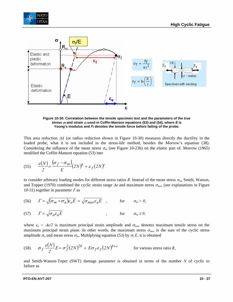
where E means the Young’s modulus, σf and εf are true stress and true strain at fracture during tensile test (see Figure 10-22b), respectively, whereby b and c are empirical elastic and plastic strain exponents defining a slope of elastic and plastic strain curves as it is illustrated in Figure 10-29b. The exponent b and c can be found in the literature or obtained from available databank of material fatigue properties. By considering the reduction in the area ΔA of the probe (Figure 10-30) using for instance Poisson’s ratio v, the true stress σf the true strain εf at fracture during tensile test can be determined

(54) A1

Rmf Δ

σ−

= and ⎟⎠⎞

⎜⎝⎛

−=

A11lnf Δ

ε .

a)

b)

High Cyclic Fatigue

RTO-EN-AVT-207 10 - 37

Figure 10-30: Correlation between the tensile specimen test and the parameters of the true stress σf and strain εf used in Coffin-Manson equations (53) and (54), where E is

Young’s modulus and Ff denotes the tensile force before failing of the probe.

This area reduction ΔA (or radius reduction shown in Figure 10-30) measures directly the ductility in the loaded probe, what it is not included in the stress-life method, besides the Morrow’s equation (38). Considering the influence of the mean stress σm (see Figure 10-23b) on the elastic part of, Morrow (1965) modified the Coffin-Manson equation (53) into

(55) ( ) ( )

( ) ( )cfbmf N2N2

E2N ε

σσε+

−=

to consider arbitrary loading modes for different stress ratios R. Instead of the mean stress σm, Smith, Watson, and Topper (1970) combined the cyclic strain range Δε and maximum stress σmax (see explanations in Figure 10-31) together in parameter Γ as

(56) ( ) EE amaxaam εσεσσΓ =+= , for σm > 0,

(57) EaaεσΓ = , for σm ≤ 0,

where εa = Δε/2 is maximum principal strain amplitude and σmax denotes maximum tensile stress on the maximum principal strain plane. In other words, the maximum stress σmax is the sum of the cyclic stress amplitude σa and mean stress σm. Multiplying equation (53) by σf E, it is obtained

(58) ( ) ( ) ( ) cb

ffb22

ff N2EN2E2N ++= εσσεσ for various stress ratio R,

and Smith-Watson-Toper (SWT) damage parameter is obtained in terms of the number N of cyclic to failure as

High Cyclic Fatigue

10 - 38 RTO-EN-AVT-207

(59) ( ) ( ) ( ) cbff

b22f N2EN2N ++= εσσΓ .

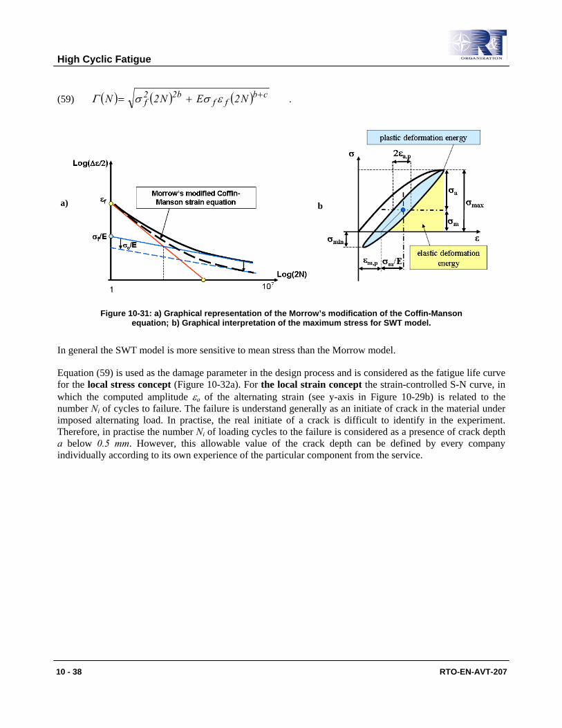
Figure 10-31: a) Graphical representation of the Morrow’s modification of the Coffin-Manson equation; b) Graphical interpretation of the maximum stress for SWT model.

In general the SWT model is more sensitive to mean stress than the Morrow model.

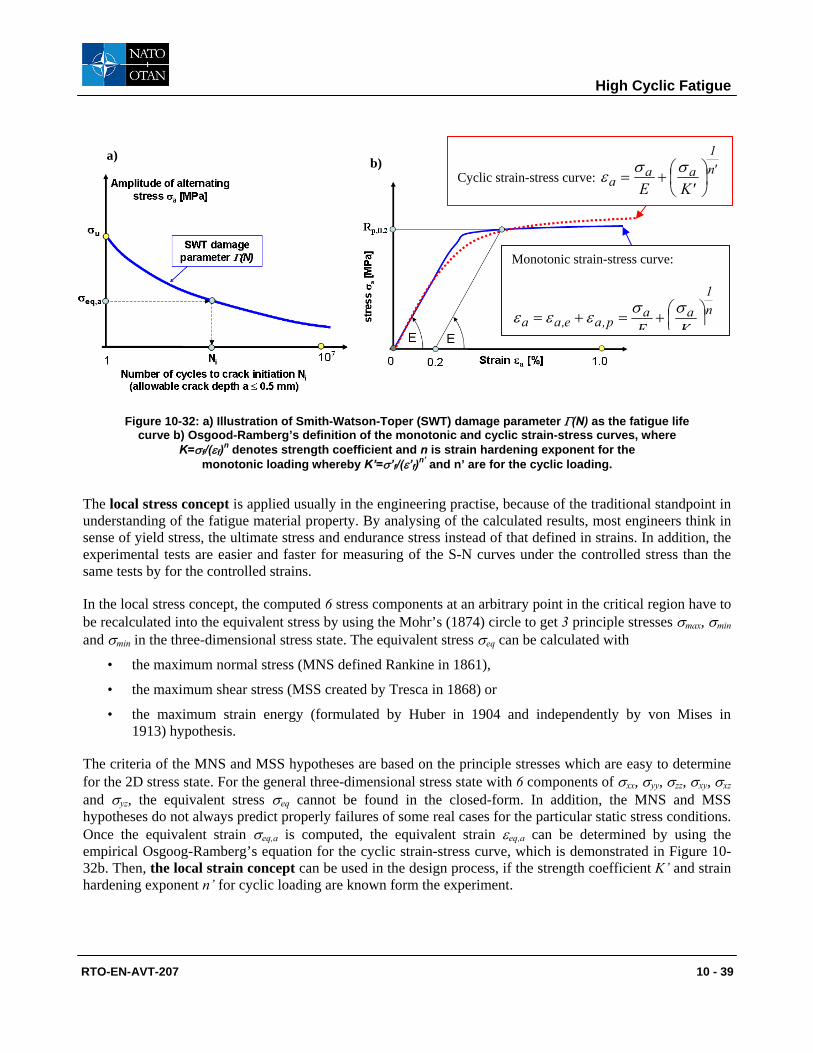
Equation (59) is used as the damage parameter in the design process and is considered as the fatigue life curve for the local stress concept (Figure 10-32a). For the local strain concept the strain-controlled S-N curve, in which the computed amplitude εa of the alternating strain (see y-axis in Figure 10-29b) is related to the number Ni of cycles to failure. The failure is understand generally as an initiate of crack in the material under imposed alternating load. In practise, the real initiate of a crack is difficult to identify in the experiment. Therefore, in practise the number Ni of loading cycles to the failure is considered as a presence of crack depth a below 0.5 mm. However, this allowable value of the crack depth can be defined by every company individually according to its own experience of the particular component from the service.

a) b)

High Cyclic Fatigue

RTO-EN-AVT-207 10 - 39

Figure 10-32: a) Illustration of Smith-Watson-Toper (SWT) damage parameter Γ(N) as the fatigue life curve b) Osgood-Ramberg’s definition of the monotonic and cyclic strain-stress curves, where

K=σf/(εf)n denotes strength coefficient and n is strain hardening exponent for the monotonic loading whereby K’=σ’f/(ε’f)n’ and n’ are for the cyclic loading.

The local stress concept is applied usually in the engineering practise, because of the traditional standpoint in understanding of the fatigue material property. By analysing of the calculated results, most engineers think in sense of yield stress, the ultimate stress and endurance stress instead of that defined in strains. In addition, the experimental tests are easier and faster for measuring of the S-N curves under the controlled stress than the same tests by for the controlled strains.

In the local stress concept, the computed 6 stress components at an arbitrary point in the critical region have to be recalculated into the equivalent stress by using the Mohr’s (1874) circle to get 3 principle stresses σmax, σmin and σmin in the three-dimensional stress state. The equivalent stress σeq can be calculated with

• the maximum normal stress (MNS defined Rankine in 1861),

• the maximum shear stress (MSS created by Tresca in 1868) or

• the maximum strain energy (formulated by Huber in 1904 and independently by von Mises in 1913) hypothesis.

The criteria of the MNS and MSS hypotheses are based on the principle stresses which are easy to determine for the 2D stress state. For the general three-dimensional stress state with 6 components of σxx, σyy, σzz, σxy, σxz and σyz, the equivalent stress σeq cannot be found in the closed-form. In addition, the MNS and MSS hypotheses do not always predict properly failures of some real cases for the particular static stress conditions. Once the equivalent strain σeq,a is computed, the equivalent strain εeq,a can be determined by using the empirical Osgoog-Ramberg’s equation for the cyclic strain-stress curve, which is demonstrated in Figure 10-32b. Then, the local strain concept can be used in the design process, if the strength coefficient K’ and strain hardening exponent n’ for cyclic loading are known form the experiment.

Monotonic strain-stress curve:

n1

aap,ae,aa KE

⎟⎠⎞

⎜⎝⎛+=+=

σσεεε

Cyclic strain-stress curve: 'n1

aaa 'KE

⎟⎠⎞

⎜⎝⎛+=

σσε

a) b)

High Cyclic Fatigue

10 - 40 RTO-EN-AVT-207

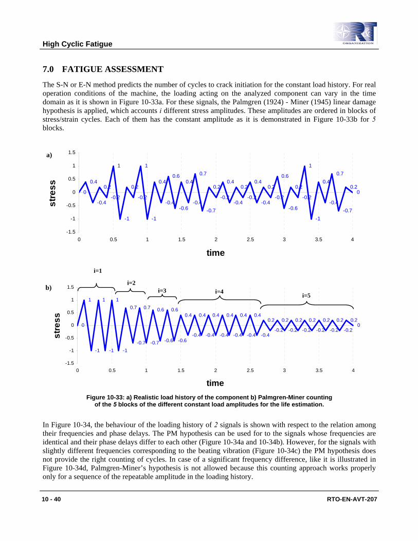
7.0 FATIGUE ASSESSMENT

The S-N or E-N method predicts the number of cycles to crack initiation for the constant load history. For real operation conditions of the machine, the loading acting on the analyzed component can vary in the time domain as it is shown in Figure 10-33a. For these signals, the Palmgren (1924) - Miner (1945) linear damage hypothesis is applied, which accounts i different stress amplitudes. These amplitudes are ordered in blocks of stress/strain cycles. Each of them has the constant amplitude as it is demonstrated in Figure 10-33b for 5 blocks.

0

0.4

-0.4

0.2

-0.2

1

-1

0.2

-0.2

1

-1

0.4

-0.4

0.6

-0.6

0.4

-0.4

0.7

-0.7

0.2

-0.2

0.4

-0.4

0.2

-0.2

0.4

-0.4

0.2

-0.2

0.6

-0.6

0.2

-0.2

1

-1

0.4

-0.4

0.7

-0.7

0.20

-1.5

-1

-0.5

0

0.5

1

1.5

0 0.5 1 1.5 2 2.5 3 3.5 4

time

stre

ss

0

1

-1

1

-1

1

-1

0.7

-0.7

0.7

-0.7

0.6

-0.6

0.6

-0.6

0.4

-0.4

0.4

-0.4

0.4

-0.4

0.4

-0.4

0.4

-0.4

0.4

-0.4

0.2

-0.2

0.2

-0.2

0.2

-0.2

0.2

-0.2

0.2

-0.2

0.2

-0.2

0.20

-1.5

-1

-0.5

0

0.5

1

1.5

0 0.5 1 1.5 2 2.5 3 3.5 4

time

stre

ss

Figure 10-33: a) Realistic load history of the component b) Palmgren-Miner counting

of the 5 blocks of the different constant load amplitudes for the life estimation.

In Figure 10-34, the behaviour of the loading history of 2 signals is shown with respect to the relation among their frequencies and phase delays. The PM hypothesis can be used for to the signals whose frequencies are identical and their phase delays differ to each other (Figure 10-34a and 10-34b). However, for the signals with slightly different frequencies corresponding to the beating vibration (Figure 10-34c) the PM hypothesis does not provide the right counting of cycles. In case of a significant frequency difference, like it is illustrated in Figure 10-34d, Palmgren-Miner’s hypothesis is not allowed because this counting approach works properly only for a sequence of the repeatable amplitude in the loading history.

i=1

i=3 i=2

i=5 i=4

a)

b)

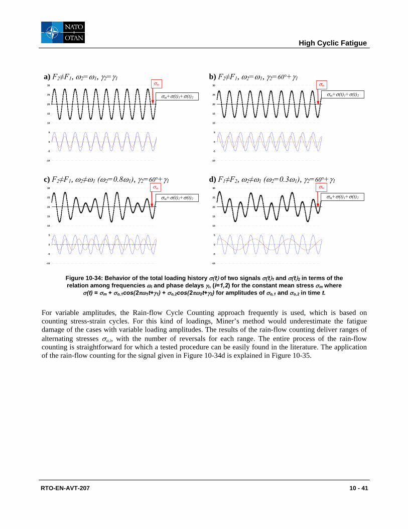
High Cyclic Fatigue

RTO-EN-AVT-207 10 - 41

a) F2≠F1, ω2=ω1, γ2=γ1 b) F2≠F1, ω2=ω1, γ2=60°+γ1

-10

-5

0

5

10

15

20

25

30

-10

-5

0

5

10

15

20

25

30

c) F2≠F1, ω2≠ω1 (ω2=0.8ω1), γ2=60°+γ1 d) F1≠F2, ω2≠ω1 (ω2=0.3ω1), γ2=60°+γ1

-10

-5

0

5

10

15

20

25

30

-10

-5

0

5

10

15

20

25

30

σm+σ(t)1+σ(t)2 σm+σ(t)1+σ(t)2

σm+σ(t)1+σ(t)2σm+σ(t)1+σ(t)2

σm σm

σm σm

Figure 10-34: Behavior of the total loading history σ(t) of two signals σ(t)1 and σ(t)2 in terms of the relation among frequencies ωi and phase delays γi, (i=1,2) for the constant mean stress σm where

σ(t) = σm + σo,1cos(2πω1t+γ1) + σo,2cos(2πω2t+γ2) for amplitudes of σo,1 and σo,2 in time t.

For variable amplitudes, the Rain-flow Cycle Counting approach frequently is used, which is based on counting stress-strain cycles. For this kind of loadings, Miner’s method would underestimate the fatigue damage of the cases with variable loading amplitudes. The results of the rain-flow counting deliver ranges of alternating stresses σa,i, with the number of reversals for each range. The entire process of the rain-flow counting is straightforward for which a tested procedure can be easily found in the literature. The application of the rain-flow counting for the signal given in Figure 10-34d is explained in Figure 10-35.

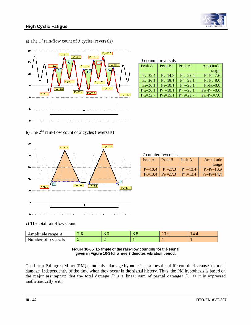
High Cyclic Fatigue

10 - 42 RTO-EN-AVT-207

a) The 1st rain-flow count of 5 cycles (reversals)

b) The 2nd rain-flow count of 2 cycles (reversals)

c) The total rain-flow count

Amplitude range Δ 7.6 8.0 8.8 13.9 14.4 Number of reversals 2 2 1 1 1

Figure 10-35: Example of the rain-flow counting for the signal given in Figure 10-34d, where T denotes vibration period.

The linear Palmgren-Miner (PM) cumulative damage hypothesis assumes that different blocks cause identical damage, independently of the time when they occur in the signal history. Thus, the PM hypothesis is based on the major assumption that the total damage D is a linear sum of partial damages Di, as it is expressed mathematically with

5 counted reversals Peak A Peak B Peak A’ Amplitude

range P2=22.4 P3=14.8 P’2=22.4 P2-P3=7.6 P6=26.1 P5=18.1 P’6=26.1 P6-P5=8.0 P8=26.1 P9=18.1 P’8=26.1 P8-P9=8.8

P10=26.1 P11=18.1 P’10=26.1 P10-P11=8.0 P14=22.7 P13=15.1 P’14=22.7 P14-P13=7.6

2 counted reversals Peak A Peak B Peak A’ Amplitude

range P7=13.4 P4=27.3 P’7=13.4 P4-P7=13.9 P9=13.4 P12=27.3 P’9=13.4 P12-P9=14.4

High Cyclic Fatigue

RTO-EN-AVT-207 10 - 43

(60) ∑∑==

==I

1i i

iI

1ii N

nDD ,

where ni is the number of cycles for the same alternating amplitude σa,i. In equation (60), the number of allowed cycles Ni for alternating amplitude σa,i for the accounted mean stress σm,i (see Figure 10-33) is calculated from

(61) ⎪⎩

⎪⎨

⎧

<∞

≥⎟⎟⎠

⎞⎜⎜⎝

⎛=

−

ei,a

ei,a

k

e

i,aei

for

forNNσσ

σσσ

σ ,

where σe is the endurance stress for the cycle number Ne under acting the mean stress σm,i at the temperature Ti. The exponent k depends on the material properties, quality of the manufacture and other conditions.

The number of the accounted cycles ni for the alternating stress σa,i is illustrated in Figure 10-36. According to the PM equation (60), the damage occurs if D ≥ 1. Indeed, the real damage can appear for the damage factor D, which might vary between 0.7 and 2. The acceptable magnitude of damage factor D depends on the type of specimen and its alloy which can be made of cast iron, steel, aluminum or titanium alloys (Schütz and Zenner, 1973). Usually in the conventional design concept, D is assumed to be equal to 1. Also, the entire loading history influences remarkably the life as it is presented in Figure 10-37. For real service loading with variable alternating stress and mean stresses, the real life of the loaded component can be found between the Wöhler’s and Gassner’s curves (Figure 10-36). The Gassner’s curve is arranged experimentally for different Gaussian variable amplitudes of the alternating stress σa.

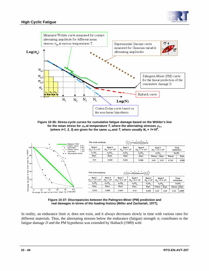
High Cyclic Fatigue

10 - 44 RTO-EN-AVT-207

Figure 10-36: Stress-cycle curves for cumulative fatigue damage based on the Wöhler’s line for the mean stress for σm at temperature T, where the alternating stresses σa,i,

(where i=1, 2, 3) are given for the same σm and T, where usually Ne = 1×106.

Figure 10-37: Discrepancies between the Palmgren-Miner (PM) prediction and real damages in terms of the loading history (Miller and Zachariah, 1977).

In reality, an endurance limit σe does not exist, and it always decreases slowly in time with various rates for different materials. Thus, the alternating stresses below the endurance (fatigue) strength σe contributes to the fatigue damage D and the PM hypothesis was extended by Haibach (1989) with

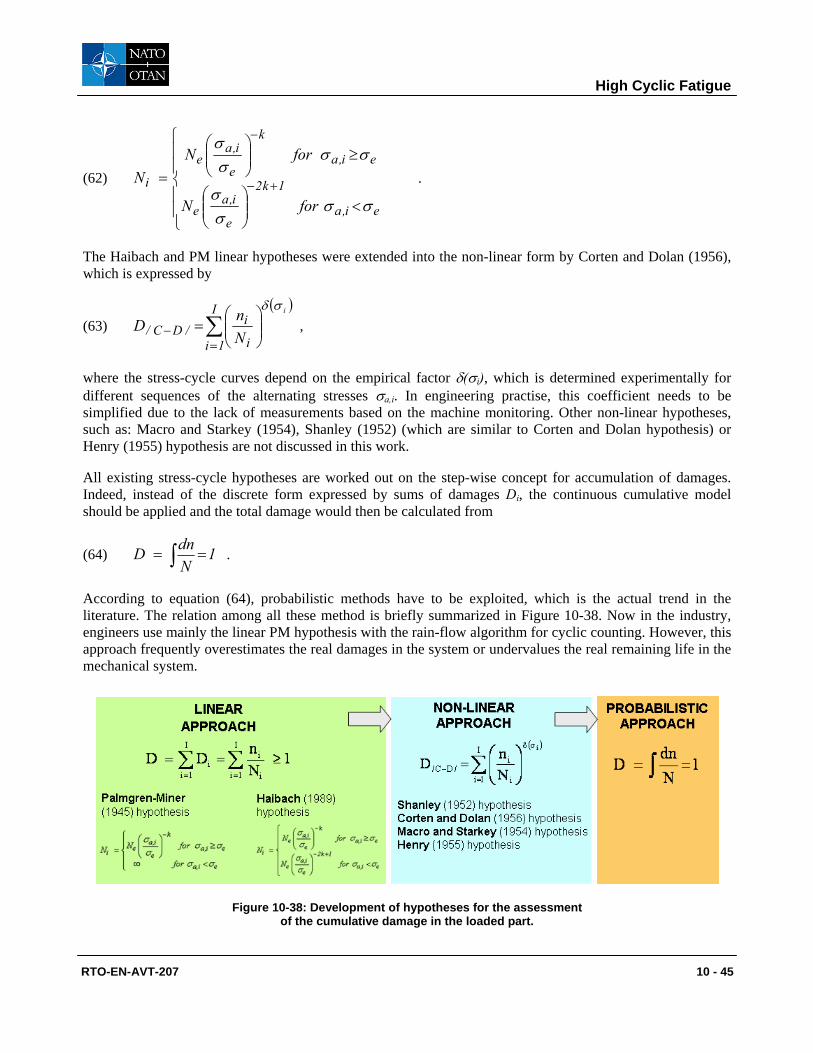
High Cyclic Fatigue

RTO-EN-AVT-207 10 - 45

(62)

⎪⎪

⎩

⎪⎪

⎨

⎧

<⎟⎟⎠

⎞⎜⎜⎝

⎛

≥⎟⎟⎠

⎞⎜⎜⎝

⎛

= +−

−

ei,a

1k2

e

i,ae

ei,a

k

e

i,ae

i

forN

forNN

σσσ

σ

σσσ

σ

.

The Haibach and PM linear hypotheses were extended into the non-linear form by Corten and Dolan (1956), which is expressed by

(63) ( )

∑=

− ⎟⎟⎠

⎞⎜⎜⎝

⎛=

I

1i i

i/DC/

i

NnD

σδ,

where the stress-cycle curves depend on the empirical factor δ(σi), which is determined experimentally for different sequences of the alternating stresses σa,i. In engineering practise, this coefficient needs to be simplified due to the lack of measurements based on the machine monitoring. Other non-linear hypotheses, such as: Macro and Starkey (1954), Shanley (1952) (which are similar to Corten and Dolan hypothesis) or Henry (1955) hypothesis are not discussed in this work.

All existing stress-cycle hypotheses are worked out on the step-wise concept for accumulation of damages. Indeed, instead of the discrete form expressed by sums of damages Di, the continuous cumulative model should be applied and the total damage would then be calculated from

(64) 1NdnD == ∫ .

According to equation (64), probabilistic methods have to be exploited, which is the actual trend in the literature. The relation among all these method is briefly summarized in Figure 10-38. Now in the industry, engineers use mainly the linear PM hypothesis with the rain-flow algorithm for cyclic counting. However, this approach frequently overestimates the real damages in the system or undervalues the real remaining life in the mechanical system.

Figure 10-38: Development of hypotheses for the assessment of the cumulative damage in the loaded part.

High Cyclic Fatigue

10 - 46 RTO-EN-AVT-207

8.0 STOCHASTIC VIBRATIONS

Regarding that the endurance limit does not exist in reality, even blades operating free-of-resonance stochastic vibration (see Figure 10-1c) can lead into fatigue failure. Therefore, the fatigue assessment should consider also for stochastic vibrations, which always occur in the real machine operation. Besides the white noise vibration, whose response amplitudes are usually negligible small1, the stochastic vibrations are divided into

• a narrow band process and

• a broad band process.

The narrow band vibration is built up by sinusoidal excitations, which cover only a narrow range of particular eigenfrequencies of the mechanical component. In the narrow band vibration, a characteristic amplitude modulation can be identified like it is in the “beat” vibration (see for instance Figure 10-34c). A freestanding turbine blade generally experiences the narrow band vibration what can be assessed from the measured frequency spectrum. As a rule of thumb, the frequency range of the response resonance spectrum is 10% smaller than a magnitude of the resonance frequency. Otherwise the stochastic vibration response might be treated as the broad band vibration, which is caused by many sinusoidal excitations over a broad range of the frequency domain of the analyzed component. This type of the stochastic vibration is quite difficult to identify in relation to the narrow band process. However, a time signal of the broad band vibration has characteristic positive and negative valleys (troughs) in its signals which are over or below the mean value level. For narrow band vibrations, there is always one zero crossing between a peak and a valleys. Peaks occur only above mean load and valleys below, respectively.

The fatigue vibration analysis of the narrow band vibration can relatively be easily performed. The Probability Density Function (pdf) of the Rain-Flow Ranges needs to be known as well as the number of the peaks E[P] and upward mean crossings E[0] which has to be extracted in the component’s vibration per second. According to Rice (1954), these numbers can be also calculated from spectral moments mn which are obtained directly from the Power Spectral Density (PSD) obtained as the squared modulus of the Fast Fourier Transformation (FFT) of the measured time history. In this case, it is necessary to apply the Hanning window for avoiding leaking effects of the processed time signal in the chosen time domain. Then, for the narrow band signals, whose peaks are described by a Rayleigh distribution R(σa) as it is given below,

(65) ( ) ⎟⎟⎠

⎞⎜⎜⎝

⎛=

0

2a

0

aa m8

expm4

R σσσ ,

In equation (65), the number ni of cycles of stress amplitude σa in time T, given in seconds, is computed (Bishop and Sherratt, 1989) from

(66) [ ] ( ) ⎟⎟⎠

⎞⎜⎜⎝

⎛==

0

2a

0

a

2

4aai m8

expm4

TmmRTPE)(n σσσσ ,

where m0, m2 and m4 are spectral moments obtained from

1 The stress range is below 0.5 MPa.

High Cyclic Fatigue

RTO-EN-AVT-207 10 - 47

(67) ( )∑=

=J

1jjj

njn dffGfm .

In equation (67), parameter J indicates the number of points tabularizing the Power Spectral Density G(f), where G(f)j and fj are values of the PSD function and frequency at point j whereby dfj = Δf/J is frequency width at point j for the considered frequency domain Δf. The determined cycle number ni is then used in Palmgren-Miner counting of the total life. If ni is equal to 1, then a crack is initiated in the structure.

Since the transfer function H(f) of the analyzed component is known from the Finite Element computation, the PSD response r(f) is determined at the arbitrary point of the structure from

(68) r(f) = G(f) H(f) ,

where G(f) is the Power Spectral Density at the monitoring point.

This procedure of the narrow band vibration gives a too conservative life estimation of the broad band signals. Therefore, the Rayleigh distribution R(σa) of peaks in the time signal in equation (65) is replaced by the empirical Dirlik’s function D2, which depends on the considered stress amplitude σa and m0, m1, m2, m4 spectral moments. Then, the number of cycles of stress amplitude σa in time T of the broad band signals is calculated from

(69) [ ] ( )4210aai m,m,m,m,DTPE)(n σσ = ,

where also the number of the peaks E[P] is determined for the known spectral moments m1 and m4 as

(70) [ ]2

4mmPE = .

From equation (66) or (69), the determined cycle numbers ni for all stress amplitudes σa,i that can be identified by the monitoring system are used in the prediction of the accumulated life of the analyzed component.

9.0 FINAL CONCLUSIONS

The whole HCF design process requires a lot of the numerical, experimental and laboratory engineering efforts. Therefore, the confident turbine design, which has accumulated many hours of reliable operation, is frequently scaled to sizes of the turbine unit demanded by market. The comparable scaling design philosophies have been developed independently by different companies like for GE gas turbines (Brandt and Wesorick, 1994) or for ALSTOM GT26 gas turbine (Eckardt and Rufli, 2002), scaled up from the GT24 unit designed for 60 Hz market, so that their compressors are principally identical on a 1.2 scale basis. The evaluation of the Siemens W501ATS from the W501 gas turbine (Diakunchak at al., 2002) is based on the scaling concept. Also Mitsubishi Heavy Industries shows good experiences with the upgraded M701G2 compressor, which is a scale-design of M501H unit (Maekawa et al., 2003). These modular concepts provide significant flexibility in the design process and fulfill customer’s demands for fast delivery periods and moderate prices with the proved performance and reliability.

2 All details of Dirlik’s function are given in the open literature.

High Cyclic Fatigue

10 - 48 RTO-EN-AVT-207

But too rapid scale-up/down of turbine components without sufficient numerical or experimental verification can lead to equipment failures and unexpected maintenance costs (see e.g. Swanekamp, 2000 or Wan, et al., 2002). Reimann (2000) presents a list of items and technical challenges, which have to be proved by scaling steam turbines. For the scaled-up low pressure last turbine stages, the bending pressure and excitation forces can be responsible for severe loading of the rotating airfoil, which should be validated in the design process.

The entire engineering concept for the HCF analysis is very well understood but it requires several physical parameters for its realistic application, especially the loading history. Nowadays, the reliable prediction of the resonance blade conditions can be attained with the 3D FE free vibration simulation considering sliding contact conditions. The realistic damping prediction becomes still an experimental and engineering challenge for assessing realistic resonance responses. On the other hand the newest applications of the technology based on friction dissipation seem to be well developed so that the blade vibrations can be controlled very well, but not all resonances. Numerical procedures of the fluid-structure interaction are being still developed, and they still do not assure effective predictions of the 3D excitation forces acting on the rotating blades with respect to different operation states of the engine.

Considering additional uncertainties with blade mistuning and unknown excitation level, monitoring systems are being intensively developed for better controlling of real blade dynamic behaviour as well as for recording the real loading history. This develops the diagnostic methods which are able to predict the remaining life of the parts in the service. By using the measured loading history, the blade HCF fatigue can be determined very realistically based on these information presented in this report. Naturally the monitoring systems increase costs of the engine operation, but they are generally lower than unexpected crash of the whole machine. Anyway, to avoid too much disaster, casings of the engine are frequently designed for containing all pieces of the broken rotating components.

10.0 REFERENCES

Bishop, N. W. M. and Sherratt, F., 1989, “Fatigue life prediction from power spectral density data”, Environmental Engineering, Vol.2

Bladh, R., 2005, “Mistuning Sensitivity Assessment of a Modern High-Pressure Turbine Blade”, CD-ROM Proceedings of the 12th Blade Mechanics Seminar, ZX CD #01998, ABB Turbo Systems Ltd., Baden, Switzerland, September 29

Brandt, D.E. and Wesorick, R.R., 1994, “GE Gas Turbine Design Philosophy”, GER-3434D GE Power Generation Marketing, 9/94 (500), pp. 1-21

Corbo, M., A. and Cook, C. F., 2000, “Torsional Vibration Analysis of Synchronous Motor-Driven Turbomachinery”, Proceedings of the 29th Turbomachinery Symposium, Turbomachinery Laboratory, Texas A&M University, College Station, Texas, USA, pp. 161-176

Cowles, B.A., 1996, “High Cycle Fatigue Failure in Aircraft Gas Turbines: An Industry Perspective,” International Journal of Fracture, 80, pp.147-163

Diakunchak, I.S., Gaul, G. R., McQuiggan, G. and Southall, L.R., 2002, “Siemens Westinghouse Advanced Turbine Systems Program Final Summary”, ASME Paper GT-2002-30654, Proceedings of ASME Turbo Expo 2002, Amsterdam, the Netherlands, June 2-6

High Cyclic Fatigue

RTO-EN-AVT-207 10 - 49

Dietrich, M., Kocanda, S., Korytkowski, B., Ozimowski, W., Stupecki, J. and Szopa, T., 1995, “Podstawy konstrukcji maszyn (Design Fundaments of Machines)”, Wydawnictwo Naukowo-Techniczne, ISBN 83-2004-1940-9, Part 1, Warszawa (in Polish)

Dzygadlo, Z., Lyzwinski, M., Otys, J., Szczecinski, S. and Wiatrek, R., 1982, “Zespoly wirnikowe silnikow turbinowych” (in Polish), Wydawnictwo Kominikacji I Lacznosci, ISBN 83-206-0217-3, Warszawa

Eckardt, D. and Rufli, P., 2002, “Advanced Gas Turbine Technology: ABB/BCC Historical Firsts”, Transactions of the ASME, Journal of Engineering for Gas Turbine and Power, Vol. 124, pp. 542-549, July

Eisinger, F., L. and Robert E. Sullivan, R. E., 2002, “Acoustically-Induced Structural Fatigue of Impeller Discs; A Brief Note”, ASME Paper GT-2002-30604, Proceedings of ASME TURBO EXPO 2002, June 3-6, 2002, Amsterdam, The Netherlands

Filsinger, D., Szwedowicz, J. and Schäfer, O., 2002, “Approach to Unidirectional Coupled CFD-FEM Analysis of Axial Turbocharger Turbine Blades”, Transactions of the ASME, Journal of Turbomachinery, Vol. 124, pp. 125-131

Fuehrer, K., Bloemers, D., Zuefle, E. and Wuethrich, C., 1993, „Monitoring Vibrations of Turbine Blades by Optical Means”, VGB Kraftwerkstechnik 73, No. 1, pp. 27-31

Green, J.S. and Fransson, T.H., 2006, „Scaling of turbine blade unsteady pressures for rapid forced response assessment”, ASME GT2006-90613, Proc. of ASME Turbo Expo, Barcelona, Spain, May 8-11

Haibach, E. and Lehrke, H.P., 1975, „Das Verfahren der Amplituden-Transformation”, LBF-Rep., No. FB-125, LBF, Darmstadt, Germany

Han, Y., Xiao, B. and Mignolet, M. P., 2007, “Expendient Estimation of the Maximum Amplification Factor in Damped Mistuned Bladed Disks”, ASME Paper GT2007- 27353, Proceedings of ASME Turbo Expo 2007, Montreal, Canada, May 14-17

Henry, D.L., 1955, “Theory of Fatigue Damage Accumulation in Steel”, ASME Trans., 77, pp. 913-921

Issler, L., Ruoss H. and Haefele P., 1995, “Festigkeitslehre - Grundlagen”, ISBN 3-540-58166-9 Srpinger-Verlag, Berlin Heidelberg New York

Juvinall, R., 1967, „Engineering Considerations of Stress, Strain and Strength”, New York, McGraw-Hill Inc.

Maekawa, A., Magoshi, R. and Iwasaki, Y., 2003, “Development and In-house Shop Load Test Results of M701G2 Gas Turbine”, IGTC2003, Tokyo-TS-100, Proc. of the Inter. Gas Turbine Congress, Tokyo, Nov., 2-7

Marco, S.M. and Starkey, W.L., 1954, “A Concept of Fatigue Damage”, ASME Trans., 76, pp. 627-636

Miller, K.J. and Zachariah, K.P., 1977, “Cumulative Laws for Fatigue Crack Initiation and Stage I Propagation”, Journal of Strain Analysis, Vol. 12, No 4, pp. 262 - 270

Miner, M. A., 1945, “Cumulative Damage in Fatigue”, Journal of Applied Mechanics, ASME, 12, pp. A-159-164

High Cyclic Fatigue

10 - 50 RTO-EN-AVT-207

Morrow, J., 1965, “Cyclic Plastic Strain Energy and Fatigue of Metals”, ASTM STP 378, pp. 45 - 87

Kielb, J. J. and Abhari, R. S., 2001, “Experimental Study of Aerodynamic and Structural Damping in a Full-Scale Rotating Turbine”, ASME Paper 2001-GT-0262

Kraemer, E. and Plan, E., 1997, “Optical vibration measuring system for long, free-standing LP rotor blades”, ABB Review, No. 5, pp. 4-9

Palmgren, A., 1924, “Die Lebensdauer von Kugellagern”, Zeitschrift des Vereins Duetscher, Ingenieure, 68, pp. 339-341

Peterson, R., E., 1974, “Stress Concentration Factors”, New York, John Wiley and Sons, ISBN 0-471-68329-9

Purcell, T. E., May 1996, “Dynamic Stress Analysis of Gas Turbine Rotor Airfoil Using Thermoelastic Techniques”, Experimental Techniques, 9-13

Reimann, P., 2000, “Stretching the size of geothermal steam turbines”, Proc. World Geothermal Congress 2000, Kyushu – Tohoku, Japan, May 28 – June 10, pp. 3283-3288

Richter, Ch.-H., 2003, “Structural design of modern steam turbine blades using ADINA”, Computers and Structures 81, pp. 919-927

Rice, S. O., 1954, “Mathematical analysis of random noise”, Dover, New York

Shanley, F.R., 1952, “A Theory of Fatigue Based on Unbonding during Reversed Slip”, The Rand Corporation, P-350

Shigley, J. E. and Mischke, C. R., 1986, “Standard Handbook of Machine Design”, New York, McGraw-Hill, Inc.

Smith, K. N., Watson, P. and Topper, T H., 1970, “A stress-strain function for the fatigue of materials”, Journal of Materials 5, pp. 767-775

Swanekamp, R., 2000, “Gas Turbines, Combined Cycles Harvest Record Orders”, Power Magazine, Vol. 144, No.2

Szwedowicz, J., Secall-Wimmel, T., Dünck-Kerst, P., Sonnenschein, A., Regnery, D. and Westfahl, M., 2008a, “Scaling Concept for Axial Turbine Stages with Loosely Assembled Friction Bolts: The Linear Dynamic Assessment”, Transactions of the ASME, Journal of Engineering for Gas Turbines and Power, Vol. 130, No. 032504, pp. 1 – 12, May

Szwedowicz, J., Secall-Wimmel, T. and Dünck-Kerst, P., 2008b, “Damping Performance of Axial Turbine Stages With Loosely Assembled Friction Bolts: The Nonlinear Dynamic Assessment”, Transactions of the ASME, Journal of Engineering for Gas Turbines and Power, Vol. 130, No. 032505, pp. 1 – 14, May

Szwedowicz, J., Slowik, S., Mahler, A. and Hulme, C.J., 2005, “Nonlinear Dynamic Analyses of a Gas Turbine Blade For Attainment of Reliable Shroud Coupling”, ASME Paper No. GT2005-69062, Proceedings of ASME Turbo Expo 2005, June 06-09, Reno-Tahoe, USA

High Cyclic Fatigue

RTO-EN-AVT-207 10 - 51

Szwedowicz, J., Senn, S.M. and Abhari, R.S., 2002, “Optimum Strain Gage Application to Bladed Assemblies”, Transactions of the ASME, Journal of Turbomachinery, Vol. 124, pp.606-613, ISSN 0889-504X, October

Szwedowicz, J., 1999, “Cyclic Finite Element Modelling of Shrouded Turbine Blades Including Frictional Contact”, ASME Paper No. 99-GT-92

Schmitz, M.B., Schaefer, O., Szwedowicz, J., Secall-Wimmel, T. and Sommer, T.P., 2006, „Axial Turbine Blade Vibrations Induced by the Stator Flow; Comparison of Calculations and Experiment”, „Unsteady Aerodynamics, Aeroacoustics and Aeroelasticity of Turbomachines”, Edited by K.C. Hall, R.E. Kielb & J.P. Thomas, Published by Springer, ISBN-10 1-4020-4267-1

Thomas, D. L., 1974, “Standing Waves in Rotationally Periodic Structures”, Journal of Sound and Vibration, Vol. 37, pp. 288-290

Traupel, W., 1982, “Thermische Turbomaschinen (Thermal Turbomachines)”, ISBN 3-540-10594-8, 3rd ed., Springer-Verlag New York Heidelberg Berlin

Wan, E.S, Crimi, P., Scheibel, J. and Viswanathan, R., 2002, “Combustion turbine F-class life Management of 1st stage turbine blades”, ASME Paper TE02, Proc. of ASME Turbo Expo, Amsterdam, June 3-6

Whitehead, D. S., 1988, “The Maximum Factor by Which Forced Vibration of Blades Can Increase Due to Mistuning”, ASME Journal of Engineering For Gas Turbines and Power, Vol. 120, pp. 115-119

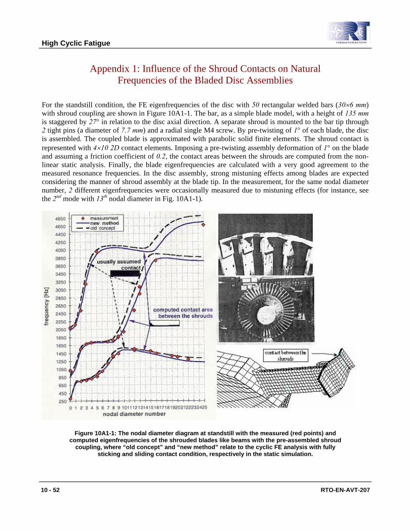
High Cyclic Fatigue

10 - 52 RTO-EN-AVT-207

Appendix 1: Influence of the Shroud Contacts on Natural Frequencies of the Bladed Disc Assemblies

For the standstill condition, the FE eigenfrequencies of the disc with 50 rectangular welded bars (30×6 mm) with shroud coupling are shown in Figure 10A1-1. The bar, as a simple blade model, with a height of 135 mm is staggered by 27° in relation to the disc axial direction. A separate shroud is mounted to the bar tip through 2 tight pins (a diameter of 7.7 mm) and a radial single M4 screw. By pre-twisting of 1° of each blade, the disc is assembled. The coupled blade is approximated with parabolic solid finite elements. The shroud contact is represented with 4×10 2D contact elements. Imposing a pre-twisting assembly deformation of 1° on the blade and assuming a friction coefficient of 0.2, the contact areas between the shrouds are computed from the non-linear static analysis. Finally, the blade eigenfrequencies are calculated with a very good agreement to the measured resonance frequencies. In the disc assembly, strong mistuning effects among blades are expected considering the manner of shroud assembly at the blade tip. In the measurement, for the same nodal diameter number, 2 different eigenfrequencies were occasionally measured due to mistuning effects (for instance, see the 2nd mode with 13th nodal diameter in Fig. 10A1-1).

Figure 10A1-1: The nodal diameter diagram at standstill with the measured (red points) and computed eigenfrequencies of the shrouded blades like beams with the pre-assembled shroud

coupling, where “old concept” and “new method” relate to the cyclic FE analysis with fully sticking and sliding contact condition, respectively in the static simulation.

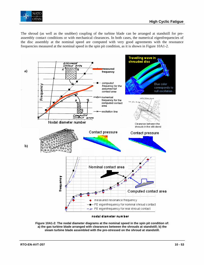
High Cyclic Fatigue

RTO-EN-AVT-207 10 - 53

The shroud (as well as the snubber) coupling of the turbine blade can be arranged at standstill for pre-assembly contact conditions or with mechanical clearances. In both cases, the numerical eigenfrequencies of the disc assembly at the nominal speed are computed with very good agreements with the resonance frequencies measured at the nominal speed in the spin pit condition, as it is shown in Figure 10A1-2.

Figure 10A1-2: The nodal diameter diagrams at the nominal speed in the spin pit condition of: a) the gas turbine blade arranged with clearances between the shrouds at standstill; b) the

steam turbine blade assembled with the pre-stressed on the shroud at standstill.

a)

b)

High Cyclic Fatigue

10 - 54 RTO-EN-AVT-207