Higher-Order Consistencies Through GAC on FactorVariables

Chavalit Likitvivatanavong, Wei Xia, and Roland H. C. Yap

School of Computing, National University of Singapore, Singapore{chavalit,xiawei,ryap}@comp.nus.edu.sg

Abstract. Filtering constraint networks to reduce search space is one of themain cornerstones of Constraint Programming and among them (Generalized)Arc Consistency has been the most fundamental. While stronger consistenciesare also the subject of considerable attention, none matches GAC’s and for thisreason it continues to advance at a steady pace and has become the popular choiceof consistency for filtering algorithms. In this paper, we build on the success ofGAC by proposing a way to transform a constraint network into another such thatenforcing GAC on the latter is equivalent to enforcing a stronger consistency onthe former. The key idea is to factor out commonly shared variables from con-straints’ scopes, form new variables, then re-attach them back to the constraintswhere they come from. Experiments show that this method is inexpensive andoutperforms specialized algorithms and other techniques when it comes to fullpair-wise consistency (FPWC).

1 Introduction

Generalized arc consistency (GAC) is one of the most studied filtering algorithms forconstraint satisfaction problems (CSPs) due to its simplicity and excellent performancein practice. Domain reduction interspersed with GAC during backtracking search hasbecome the foremost method for solving a general CSP [17]. GAC on positive tableconstraints, in particular, has received a great deal of attention in recent years [3, 4, 9,10, 12, 14]. These advances in turn provide a basis for many algorithms that enforceeven stronger consistencies than GAC to build on.

In [6] it was shown that a network is pairwise consistent (PWC) iff its dual CSP isarc consistent. PWC is a k-wise consistency [5] for the case where k = 2. This is oneof the earlier works that demonstrates how (G)AC can be used to achieve other types ofconsistencies. Consistencies of level/order higher than GAC are also the subject of manyrecent works [8, 11, 16]. Specifically, maxRPWC, PWC, and FPWC are investigated in[2, 11, 16]. Many of the algorithms that enforce these consistencies are based on well-established GAC algorithms. In [16], the authors extended the GACva algorithm [12] toenforce maxRPWC. Subsequently, STR2 was extended to cope with FPWC, resultingin eSTR2 [11] which gets improvement similar to how STR2 outperforms GACva.

As another area of focus in CSPs, researchers have studied how to transform non-binary constraint networks into equivalent binary constraint networks so that the algo-rithms and methods from the binary case can be applied [1, 18]. Two techniques emergeas a result: the hidden transformation and the dual transformation. Both rely on the dual

variable associated with each constraint, whose domain values have a one-to-one corre-spondence with the constraint’s tuples. Nevertheless, the benefits of the transformationdiminish as filtering algorithms for non-binary CSPs get better.

In this paper, we propose to transform a non-binary constraint network into anothernon-binary constraint network such that the latter is GAC if and only if the former isfull pairwise consistency (FPWC), which means both GAC and PWC. In this respect,our intention is similar to that of the authors of [13] who proposed another kind oftransformation. Like the transformation from non-binary to binary network, the one in[13] is based on dual variables. But here the dual variable is included into the scope ofthe constraint it is associated with. The pruning power comes from the join of tablesthat uses the dual variables as its scope so that propagation can be transmitted directlyto other constraints.

Our transformation works in a fundamentally different way. Instead of forming adual variable for each constraint, we factor out commonly shared variables among them.These variables form new compound variables that will be augmented to only the con-straints that are involved. For FPWC, no new constraints are created. We extend thistransformation to cover general k-wise consistency, adding new constraints reducedfrom the join of k tables. Preliminary experiments show that for FPWC our method isfaster than both [13] and a specialized FPWC algorithm. For k-wise consistency wherek ≥ 3, our transformation can lower the number of nodes visited during search but it ismore costly and thus of limited application unless the search reduction is large.

2 Preliminaries

A constraint network P is a (X , C) where X is a set of n variables {x1, . . . , xn} andC a set of e constraints {c1, . . . , ce}. D(x) is the domain of x ∈ X . During search,Dc(x) denotes the current domain of x. If a ∈ Dc(x), a is said to be present in D(x);otherwise a is absent from D(x). We use (x, a) to denote the value a ∈ D(x) (orsimply a when the context is clear). Each c ∈ C involves two components: a scope(scp(c)) which is an ordered subset of variables of X ; and a relation over the scope(rel(c)). Given scp(c) = {xi1 , . . . , xir}, rel(c) ⊆

∏rj=1 D(xij ) represents the set of

satisfying combinations of values for the variables in scp(c). We may also refer to cby c(xi1 , . . . , xir ) to emphasize the scope. A constraint’s scope can be made unique bycombining the constraint’s relation with relations from other constraints with the samescope through intersection. We assume a total ordering for every rel(c) and use ρ(c, i)to denote the ith tuple. The arity of c is |scp(c)|. Given an ordered set S ⊆ scp(c)and τ ∈ rel(c), the projection of τ on S (τ [S]) is the tuple consisting of only thecomponents of τ that correspond to the variables in S. A tuple τ = (aii , . . . , aik)where aij ∈ D(xij ) is said to be an tuple over {xi1 , . . . , xik}. The join of constraintsci and cj (ci 1 cj) is a constraint whose scope is scp(ci)∪scp(cj) and whose relation is{τ | τ is a tuple over scp(ci)∪ scp(cj)∧ τ [scp(ci)] ∈ rel(ci)∧ τ [scp(cj)] ∈ rel(cj)}.The join of tuples τi ∈ rel(ci) and τj ∈ rel(cj) (τi 1 τj) is the tuple τ over scp(ci) ∪scp(cj) such that τ [scp(ci)] = τi and τ [scp(cj)] = τj . When elements in rel(c) aregiven explicitly, c is called a positive table constraint. A tuple τ ∈ rel(c) is valid iffτ [x] ∈ Dc(x) for each x ∈ scp(c). Otherwise τ is invalid. A tuple τ ∈ rel(c) is a

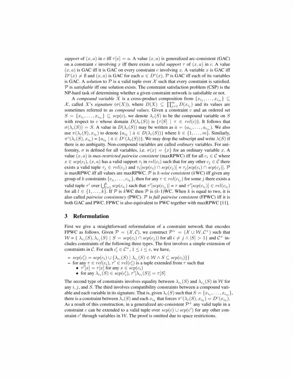
support of (x, a) in c iff τ [x] = a. A value (x, a) is generalized arc-consistent (GAC)on a constraint c involving x iff there exists a valid support τ of (x, a) in c. A value(x, a) is GAC iff it is GAC on every constraint c involving x. A variable x is GAC iffDc(x) 6= ∅ and (x, a) is GAC for each a ∈ Dc(x). P is GAC iff each of its variablesis GAC. A solution to P is a valid tuple over X such that every constraint is satisfied.P is satisfiable iff one solution exists. The constraint satisfaction problem (CSP) is theNP-hard task of determining whether a given constraint network is satisfiable or not.

A compound variable X is a cross-product composition from {xi1 , . . . , xim} ⊆X , called X’s signature (σ(X)), where D(X) ⊆

∏mj=1D(xij ) and its values are

sometimes referred to as compound values. Given a constraint c and an ordered setS = {xi1 , . . . , xim} ⊆ scp(c), we denote λc(S) to be the compound variable on Swith respect to c whose domain D(λc(S)) is {τ [S] | τ ∈ rel(c)}. It follows thatσ(λc(S)) = S. A value in D(λc(S)) may be written as a = (ai1 , . . . , aim). We alsouse π(λc(S), xik) to denote {aik | a ∈ D(λc(S))} where k ∈ {1, . . . ,m}. Similarly,πc(λc(S), xik) = {aik | a ∈ Dc(λc(S))}. We may drop the subscript and write λ(S) ifthere is no ambiguity. Non-compound variables are called ordinary variables. For uni-formity, σ is defined for all variables, i.e. σ(x) = {x} for an ordinary variable x. Avalue (x, a) is max-restricted pairwise consistent (maxRPWC) iff for all ci ∈ C wherex ∈ scp(ci), (x, a) has a valid support τi in rel(ci) such that for any other cj ∈ C thereexists a valid tuple τj ∈ rel(cj) and τi[scp(ci) ∩ scp(cj)] = τj [scp(ci) ∩ scp(cj)]. Pis maxRPWC iff all values are maxRPWC. P is k-wise consistent (kWC) iff given anygroup of k constraints {cii , . . . , cik}, then for any τ ∈ rel(cij ) for some j there exists avalid tuple τ ′ over

⋃kl=1 scp(cil) such that τ ′[scp(cij )] = τ and τ ′[scp(cil)] ∈ rel(cil)

for all l ∈ {1, . . . , k}. If P is kWC then P is (k-1)WC. When k is equal to two, it isalso called pairwise consistency (PWC). P is full pairwise consistent (FPWC) iff it isboth GAC and PWC. FPWC is also equivalent to PWC together with maxRPWC [11].

3 Reformulation

First we give a straightforward reformulation of a constraint network that encodesFPWC as follows. Given P = (X , C), we construct P+ = (X ∪ W, C+) such thatW = { λci(S), λcj (S) | S = scp(ci) ∩ scp(cj)) for all i 6= j ∧ |S| > 1} and C+ in-cludes constraints of the following three types. The first involves a simple extension ofconstraints in C. For each c′i ∈ C+, 1 ≤ i ≤ e, we have,

– scp(c′i) = scp(ci) ∪ {λci(S) | λci(S) ∈ W ∧ S ⊆ scp(ci)}}– for any τ ∈ rel(ci), τ ′ ∈ rel(c′i) is a tuple extended from τ such that• τ ′[x] = τ [x] for any x ∈ scp(ci)• for any λci(S) ∈ scp(c′i), τ ′[λci(S)] = τ [S]

The second type of constraints involves equality between λci(S) and λcj (S) inW forany i, j, and S. The third involves compatibility constraints between a compound vari-able and each variable in its signature. That is, given λc(S) such that S = {xi1 , . . . , xim},there is a constraint between λc(S) and each xik that forces πc(λc(S), xik) = Dc(xik).As a result of this construction, in a generalized arc-consistent P+ any valid tuple in aconstraint c can be extended to a valid tuple over scp(c) ∪ scp(c′) for any other con-straint c′ through variables inW . The proof is omitted due to space restrictions.

Theorem 1. P+ is GAC if and only if P is FPWC.

Next we show how P+ can be simplified while still preserving Theorem 1. Insteadof posting an equality constraint between every pair of compound variables with thesame signature, we unify all these compound variables into a single variable. Equalityconstraints are removed. Given P= (X , C) and P+= (X ∪W, C+), the factor encoding(FE) of P is the network P∗ = (X ∪W∗, C∗) where,

W∗ = {λ(S) | D(λ(S)) =⋃kD(λck(S)) for all k such that λck(S) ∈ W}

and for each c∗i ∈ C∗, 1 ≤ i ≤ e,– scp(c∗i ) = scp(ci) ∪ {λ(S) | λ(S) ∈ W∗ ∧ S ⊆ scp(ci)}}– for any τ ∈ rel(ci), τ∗ ∈ rel(c∗i ) is a tuple extended from τ such that• τ∗[x] = τ [x] for any x ∈ scp(ci)• for any λ(S) ∈ scp(c∗i ), τ∗[λ(S)] = τ∗[S](= τ [S]) (e1)

We call the compound variables in W∗ factor variables. P∗ is also referred to asfe(P). Given ck ∈ C, we may denote c∗k ∈ C∗ with fe(ck). We observe that the compat-ibility constraint in P+ can be decomposed into two conditions. Given λ(S) such thatS = {xi1 , . . . , xim}, we have,

(c1) a ∈ Dc(λ(S))⇒ ∀k ∈ {1, . . . ,m}, aik ∈ Dc(xik)(c2) a ∈ Dc(xik) for some k ∈ {1, . . . ,m} ⇒ ∃a ∈ Dc(λ(S)), aik = a

We will show that the compatibility constraints in P+ are actually implied and donot need to be posted explicitly.

Lemma 1 Enforcing GAC on fe(P) imposes the condition (c1) between a factor vari-able and each ordinary variable in its signature.

Proof Consider λ(S) where S = {xi1 , . . . , xim} and a ∈ Dc(λ(S)). Because fe(P)is GAC, for any fe(c) such that λ(S) ∈ scp(fe(c)), there is a valid support of a inrel(fe(c)). That is, ∃τ ∈ rel(fe(c)) such that τ [λ(S)] = a. Since τ [λ(S)] = τ [S],τ [xik ] = aik for 1 ≤ k ≤ m, which means aik also has a valid support in rel(fe(c)). 2

Lemma 2 Enforcing GAC on fe(P) imposes the condition (c2) between a factor vari-able and each ordinary variable in its signature.

Proof Assume aik /∈ πc(λ(S), xik) for some aik . This indicates that any a involving aikmust be absent from D(λ(S))). Due to propagation, every τ in every rel(fe(c)) suchthat λ(S) ∈ scp(fe(c)) and τ [λ(S)] = a would eventually become invalid. Becauseτ [S] = τ [λ(S)] = a, τ [xik ] = aik . That means such τ is not a valid support ofaik . Because D(λ(S)) contains every compound values involving aik from all c whosescope subsumes S, there is no other valid tuple τ ′ such that τ ′[xik ] = aik . Hence,aik /∈ Dc(xik) after the propagation converges. 2

Theorem 2. fe(P) is GAC if and only if P is FPWC.

Proof Follows from Theorem 1, and Lemma 1, and 2. 2

Theorem 3. fe(P) is GAC if and only if fe(P) is FPWC.

Proof As FPWC is both GAC and PWC, (⇐) is immediate. We will prove the (⇒)direction. Assume fe(P) is GAC. Let τi ∈ fe(ci). Now consider another constraintfe(cj) 6= fe(ci). If there is no factor variable in scp(fe(ci)) ∩ scp(fe(cj)), then PWC istrivial. Let f be the factor variable1 in scp(fe(ci))∩ scp(fe(cj)) such that scp(fe(ci))∩scp(fe(cj))\σ(f) = {f}. Since fe(P) is GAC, τi[f ] must have a valid support in fe(cj).Call it τj . Because τi and τj agree on f , by definition of factor variable they must agreeon σ(f) too, which means they agree on σ(f) ∪ {f} = scp(fe(ci)) ∩ scp(fe(cj)).As a result, τi 1 τj is well-defined as well as being a tuple extended from τi overscp(fe(ci)) ∪ scp(fe(cj)). Hence, fe(P) is PWC. 2

Let fek(P) denote fe(fe(. . . fe(P) . . .)) (the FE is applied k times in a row), then

Corollary 1 For all k ≥ 1, P is FPWC if and only if fek(P) is GAC.

Proof We consider k = 2 as other cases follow from induction. From Theorem 2 andTheorem 3, we have: P is FPWC iff fe(P) is FPWC. From this statement and the resultof another application of the FE on it we derive: P is FPWC iff fe(fe(P)) is FPWC.From Theorem 3, fe(fe(P)) is FPWC iff fe(fe(P)) is GAC. 2

This shows fek(P) for k ≥ 2 is no different than fe(P) so applying the FE more thanonce in succession is pointless. A localized version of this corollary is given as follows.

Corollary 2 Given any two constraints ci and cj , if there exists a factor variable f ∈scp(ci) ∩ scp(cj) such that scp(ci) ∩ scp(cj) \ σ(f) = {f} then adding the factorvariable f ′ whose signature is σ(f) ∪ {f} to the scopes of both constraints is futile.

Property 1 Running GAC on fe(P) can be O(e2) faster and use O(e2) smaller spacethan running eSTR2 on P .

Reasoning: eSTR2 [11] is an extension of STR2 [9] that enforces FPWC. The maindifference between enforcing GAC on the FE and enforcing eSTR2 on the original net-work is the space and time associated with factor variables vs. those associated with theadditional data structures for checking PWC in eSTR2. The overhead of running GACon the FE depends on factor variables, whose number can be lower than the number ofintersecting constraints. In eSTR2, the overhead depends on the number of intersectingconstraints. If P consists of only constraints such that a single factor variable is com-mon to all and that no other factor variable exists, the space and time complexity of theGAC on fe(P) is the same as those on P . By contrast, the space and time of eSTR2 onP would be at least an order of O(

(e2

)) = O(e2) larger. 2

Property 2 For any c ∈ C, |scp(c)| ≤ |scp(fe(c))| ≤ |scp(c)|+ |C| − 1.

The range is the result of the number of factor variables added. The lower bound is zero,when no other constraint’s scope overlaps on more than two variables with scp(c),whereas the upper bound is |C| − 1 when every intersection with another constraintproduces a new factor variable.

1 There may be multiple factor variables if P itself is the factor encoding of another constraintnetwork, which in turn is the factor encoding of another, and so on (see Corollary 1). Thefactor variable f is set to be the most recent one.

3.1 Example

We give an example of P∗ and trace some GAC propagation on P∗ in this section.Note that although relations in P∗ are an extension of those in P , the extension tofactor variables can be implicit. The expression τ [S] in (e1) can be given as a function(i.e. the projection) that takes an input S rather than the actual result of the projectionof τ on S. Such abstract extension of tuples is demonstrated in this section.

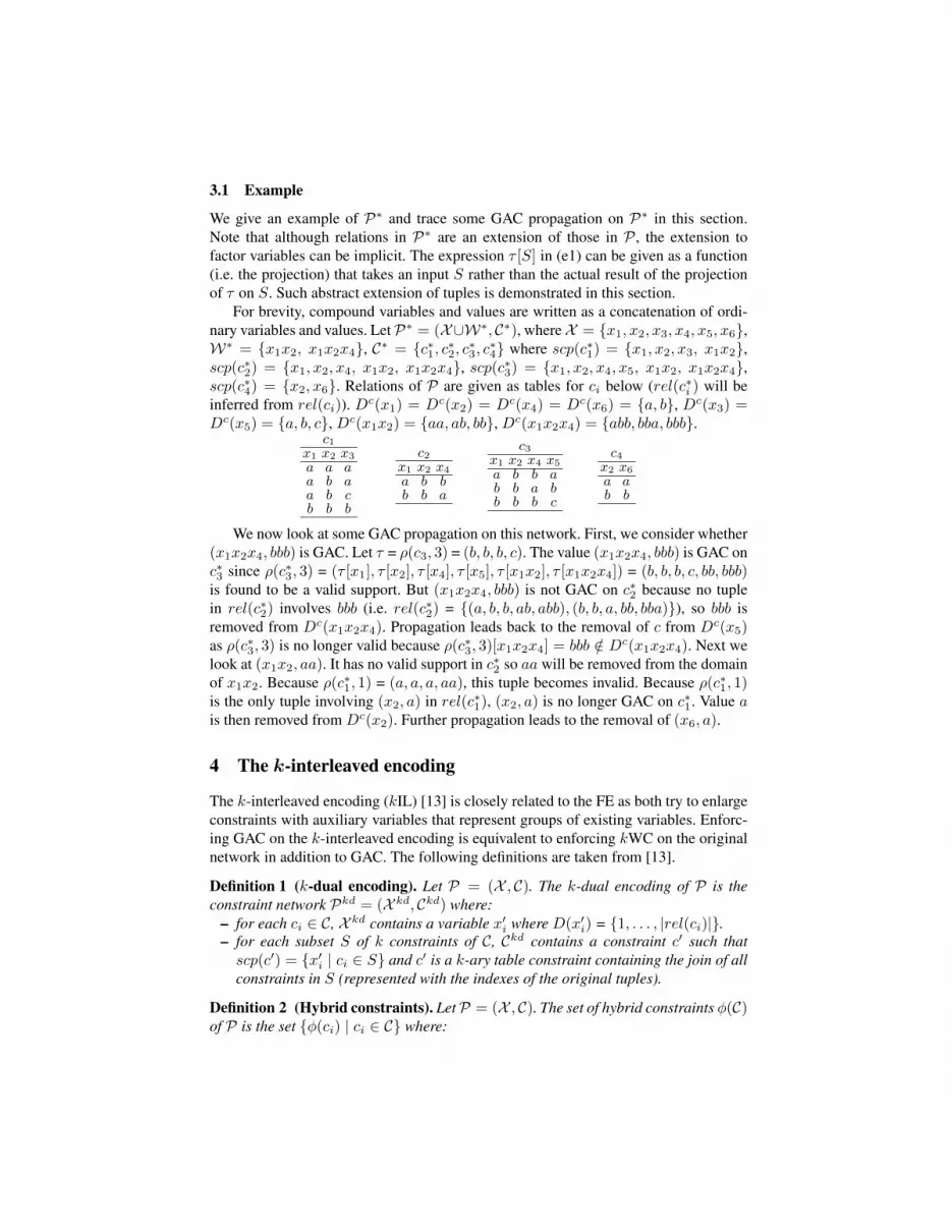
For brevity, compound variables and values are written as a concatenation of ordi-nary variables and values. LetP∗ = (X∪W∗, C∗), whereX = {x1, x2, x3, x4, x5, x6},W∗ = {x1x2, x1x2x4}, C∗ = {c∗1, c∗2, c∗3, c∗4} where scp(c∗1) = {x1, x2, x3, x1x2},scp(c∗2) = {x1, x2, x4, x1x2, x1x2x4}, scp(c∗3) = {x1, x2, x4, x5, x1x2, x1x2x4},scp(c∗4) = {x2, x6}. Relations of P are given as tables for ci below (rel(c∗i ) will beinferred from rel(ci)). Dc(x1) = Dc(x2) = Dc(x4) = Dc(x6) = {a, b}, Dc(x3) =Dc(x5) = {a, b, c}, Dc(x1x2) = {aa, ab, bb}, Dc(x1x2x4) = {abb, bba, bbb}.

c1x1 x2 x3

a a aa b aa b cb b b

c2x1 x2 x4

a b bb b a

c3x1 x2 x4 x5

a b b ab b a bb b b c

c4x2 x6

a ab b

We now look at some GAC propagation on this network. First, we consider whether(x1x2x4, bbb) is GAC. Let τ = ρ(c3, 3) = (b, b, b, c). The value (x1x2x4, bbb) is GAC onc∗3 since ρ(c∗3, 3) = (τ [x1], τ [x2], τ [x4], τ [x5], τ [x1x2], τ [x1x2x4]) = (b, b, b, c, bb, bbb)is found to be a valid support. But (x1x2x4, bbb) is not GAC on c∗2 because no tuplein rel(c∗2) involves bbb (i.e. rel(c∗2) = {(a, b, b, ab, abb), (b, b, a, bb, bba)}), so bbb isremoved from Dc(x1x2x4). Propagation leads back to the removal of c from Dc(x5)as ρ(c∗3, 3) is no longer valid because ρ(c∗3, 3)[x1x2x4] = bbb /∈ Dc(x1x2x4). Next welook at (x1x2, aa). It has no valid support in c∗2 so aa will be removed from the domainof x1x2. Because ρ(c∗1, 1) = (a, a, a, aa), this tuple becomes invalid. Because ρ(c∗1, 1)is the only tuple involving (x2, a) in rel(c∗1), (x2, a) is no longer GAC on c∗1. Value ais then removed from Dc(x2). Further propagation leads to the removal of (x6, a).

4 The k-interleaved encoding

The k-interleaved encoding (kIL) [13] is closely related to the FE as both try to enlargeconstraints with auxiliary variables that represent groups of existing variables. Enforc-ing GAC on the k-interleaved encoding is equivalent to enforcing kWC on the originalnetwork in addition to GAC. The following definitions are taken from [13].

Definition 1 (k-dual encoding). Let P = (X , C). The k-dual encoding of P is theconstraint network Pkd = (X kd, Ckd) where:

– for each ci ∈ C, X kd contains a variable x′i where D(x′i) = {1, . . . , |rel(ci)|}.– for each subset S of k constraints of C, Ckd contains a constraint c′ such thatscp(c′) = {x′i | ci ∈ S} and c′ is a k-ary table constraint containing the join of allconstraints in S (represented with the indexes of the original tuples).

Definition 2 (Hybrid constraints). LetP = (X , C). The set of hybrid constraints φ(C)of P is the set {φ(ci) | ci ∈ C} where:

– scp(φ(ci)) = scp(ci) ∪ {x′i}– for every jth tuple τ of rel(ci), τ ′ is a tuple in rel(φ(ci)) such that τ ′[x′i] = j andτ ′[x] = τ [x] for each x ∈ scp(ci)

Definition 3 (k-interleaved encoding). Let P = (X , C). The k-interleaved encod-ing of P is the constraint network Pki = (X ki, Cki) = (X ∪ X kd, φ(C) ∪ Ckd) where(X kd, Ckd) is the k-dual encoding of P and φ(C) the hybrid constraints of P .

For k = 2, enforcing GAC on the 2IL has the same pruning power as enforcingGAC on the FE, but the FE does not add any new constraint. We now look at an exam-ple from [13] for a comparison of the 2IL and the FE. Figure 1a shows three constraintsfrom the original network. Figure 1b shows the FE for these constraints. A factor vari-able’s domain of size d is normalized as {1, . . . , d}. As a result, Dc(xy) = Dc(uv) ={11, 00, 01, 10} = {1, 2, 3, 4}. After GAC is established,Dc(y) becomes {1} andDc(v)becomes {0}. Figure 1c shows the 2IL of 1a [13]. This example shows that while en-forcing GAC on the kIL gives identicalDc(y) andDc(v) to Figure 1b, the kIL can takea longer chain of propagation to do so.

x y u v

1 1 1 00 0 0 10 1 0 01 0 1 1

x y

1 10 00 1

u v

1 11 00 0

(a) Original

x y u v xy uv

1 1 1 0 1 40 0 0 1 2 30 1 0 0 3 21 0 1 1 4 1

x y xy

1 1 10 0 20 1 3

u v uv

1 1 11 0 40 0 2

(b) Factor encoding of (a)

x y u v x′1

1 1 1 0 10 0 0 1 20 1 0 0 31 0 1 1 4

x y x′2

1 1 10 0 20 1 3

u v x′3

1 1 11 0 20 0 3

x′1 x

′2

1 12 23 3

x′1 x

′3

1 23 34 1

(c) 2-interleaved encoding of (a)Fig. 1: Comparison of two encodings

We compare the complexity of the FE and the kIL as follows. For simplicity, weassume there are e constraints of arity r, each associated with a table containing t tuplesand that every pair of constraints shares at least two variables in their scopes.

Property 3 The extra cells added to the tables by the FE ranges from O(et) to O(e2t).

Proof In the best case there is only one factor variable. Each constraint will be extendedwith an extra column so the total extra space is O(et). In the worst case, every pair ofconstraint produces one additional factor variable. Each of these factor variables willappear in two different tables. Thus, the total is O(2t

(e2

)) = O(e2t). 2

Because an optimal GAC algorithm traverses every cell of every table in the worstcase, the worst-case time complexity of GAC on the FE is thus between O(ert) (i.e. noasymptotic difference) and O(ert+ e2t) = O(e2t) (i.e. assuming e > r).

Property 4 The extra cells added to the tables by the kIL is O((ek

)tk)

Proof Each constraint has an extra column for indexing so the space is et. For everysubset of C of size k, a join table of arity k is created. The total space is thereforeO(et+

(ek

)tk) = O(

(ek

)tk). 2

For k = 2, this space becomes O(e2t2). As far as GAC is concerned, the 2IL is thusa factor of t more expensive in the worst case than the FE.

5 Enforcing k-wise consistency through reduced join tables

Given fe(P), we may post additional constraints so that GAC may also enforce kWC.These new constraints are created from a group of existing constraints and this sectionstudies their effect on the consistency level.

Given C = {ci1 , . . . , cik} in P where k ≥ 3, we define the following notation:– mult(C) = {λ(S) | λ(S) ∈ W∗ ∧ S = scp(cij ) ∩ scp(cil) for 1 ≤ j < l ≤ k}– sing(C) = {x | x ∈ X ∧ {x} = scp(cij ) ∩ scp(cil) for 1 ≤ j < l ≤ k}– join(C) = rel(ci1) 1 . . . 1 rel(cik),

Definition 4. Given a set C of k constraints (k ≥ 3), the factor-reduced join of C(frj(C)) is a constraint constructed as follows. Let |mult(C)| = o, and |sing(C)| = p,

– scp(frj(C)) = mult(C) ∪ sing(C) = {λ(S1), . . . , λ(So)} ∪ {xj1 , . . . xjp}– rel(frj(C)) = {(τ [S1], . . . , τ [So], τ [xj1 ], . . . , τ [xjp ]) | τ ∈ join(C)}

The factor-reduced join is not a projection of join(C) as its scope may include factorvariables. Rather, it can be viewed as a projection of 1c∈C fe(c). In any case, since it isderived from the join of C, its pruning power cannot be greater.

It should be noted that frj(C) may end up having the same scope as another existingconstraint or another frj constraint. For instance, letC1 = {c1(x1, x2, x3), c2(x1, x2, x4),c3(x1, x5)} and C2 = {c4(x1, x2, x6), c5(x1, x2, x7), c3(x1, x5)}. Let y1 = x1x2, itfollows that scp(frj(C1)) = {x1, y1} = scp(frj(C2)). This can also happen in the casewhere no factor variables are formed by the FE. For instance, let C1 = {c1(x1, x2),c2(x2, x3), c3(x3, x4)}. Then scp(frj(C1)) = {x2, x3} = scp(c2). Both cases can behandled by merging constraints with the same scope afterwards.

We assume that every constraint in C must be relevant. Namely, given c ∈ C theremust exist at least one other c′ ∈ C such that |scp(c) ∩ scp(c′)| ≥ 1.

Property 5 The arity of frj(C) ranges from 2 to(|C|

2

).

The fe(P) with the additional constraints frj(C) for every groupC of size k is calledthe factor encoding of P for k-wise consistency (FKWC), also denoted by fkwc(P, k).Property 6 Enforcing GAC on fkwc(P ,k) is strictly weaker than enforcing both FPWCand kWC on P and strictly stronger than enforcing FPWC on P .

We show this by an example. Consider the constraints in Figure 2a and their factorencodings in Figure 2b, where y1 = x2x3. The networks in both figures are PWC. Thejoin of the three original constraints is given in Figure 2c. The projection of join(C)onto each of the original constraint makes the following tuples 3-wise inconsistent:(1, 1, 0, 0) ∈ rel(c1), (1, 0, 1) ∈ rel(c2), and (1, 0, 1) ∈ rel(c3). Now consider thefrj(C) in Figure 2d. GAC on {frj(C), fe(c1), fe(c2), fe(c3)} leads to the inconsistency of(1, 1, 0, 0, 2) ∈ rel(fe(c1)) and (1, 0, 1, 2) ∈ rel(fe(c2)), but not (1, 0, 1) ∈ rel(fe(c3)).

Although the fkwc(P ,k) encoding is only partial kWC, it subsumes fe(P) so FPWCis guaranteed by GAC. Together with the fact that kWC implies (k-1)WC, we haveProperty 7 Enforcing GAC on fkwc(P ,k) is strictly weaker than enforcing GAC on thekIL of P for k ≥ 3.

Theorem 4. Q = fe(fkwc(P, k))) is GAC if and only if P is FPWC and kWC.

c1x1 x2 x3 x4

0 0 0 00 0 1 11 1 0 0

c2x2 x3 x5

0 0 00 1 11 0 1

c3x4 x5 x6

0 0 01 0 11 1 0

(a) Original: C = {c1, c2, c3}

fe(c1)x1 x2 x3 x4 y10 0 0 0 00 0 1 1 11 1 0 0 2

fe(c2)x2 x3 x5 y10 0 0 00 1 1 11 0 1 2

fe(c3)x4 x5 x6

0 0 01 0 11 1 0

(b) Factor-encoded constraintsjoin(C)

x1 x2 x3 x4 x5 x6

0 0 0 0 0 00 0 1 1 1 0

(c) The join of constraints in C

frj(C)x4 y1 x5

0 0 01 1 1

(d) The factor-reduced join of Cfe(fe(c1))

x1 x2 x3 x4 y1 z10 0 0 0 0 00 0 1 1 1 11 1 0 0 2 2

fe(fe(c2))x2 x3 x5 y1 z20 0 0 0 00 1 1 1 11 0 1 2 2

fe(fe(c3))x4 x5 x6 z30 0 0 01 0 1 11 1 0 2

fe(frj(C))x4 y1 x5 z1 z2 z30 0 0 0 0 01 1 1 1 1 2

(e) The FE of (b) and (d) where fe(fe(ci)) denotes the FE of constraints from (b) with frj(C).

Fig. 2: The pruning power of GAC on (b) + (d) lies between FPWC and FPWC + 3-wiseconsistency on (a), whereas GAC on (e) is equal to FPWC + 3-wise consistency on (a).

Sketch of Proof: Consider C = {ci1 , . . . , cik}. It is clear that join(C) forces kWCon C through GAC. fe(frj(C)) ∈ Q represents all the articulation points of join(C)and we will show that both have the same restricting effect on the rest of the networkby showing that the “missing columns” can be “rebuilt” via GAC. The proof for (⇐)is omitted for lack of space. Assume Q is GAC. Let x be a variable in scp(join(C)) \(⋃λ(S)∈mult(C) S)\sing(C). It follows that there is exactly one constraint cij ∈ C such

that x ∈ scp(cij ). Suppose a ∈ Dc(x). BecauseQ is GAC, so is a. By definition, thereexists a valid tuple τij ∈ rel(fe(fe(cij ))) such that τij [x] = a. LetHij = scp(fe(cij ))∩scp(frj(C)), |Hij | ≥ 1. Because Q is a factor encoding, there exists a variable λ(Hij )in both scp(fe(fe(cij ))) and scp(fe(frj(C))) (λ(Hij ) is either an ordinary or a factorvariable). Since Hij too is GAC, τij is guaranteed to be extendable to fe(frj(C)). Let ϕbe such a tuple in fe(frj(C)) such that τij 1 ϕ is a tuple over scp(fe(cij ))∪scp(frj(C)).For each cil ∈ C \ {cij}, let Hil = scp(fe(cil)) ∩ scp(frj(C)). By the same argument,there exists a valid tuple τil in fe(fe(cil)) such that τil [Hil ] = ϕ[Hil ]. The join of ϕ,τij , and every such τil would become a valid support of a in J = (1c∈C fe(fe(c))) 1

fe(frj(C)). Because the projection of J on scp(join(C)) is join(C) and a is arbitrary,the column x in scp(join(C)) is thus the same as Dc(x). 2

Figure 2e shows another application of the factor encoding on top of fkwc(P, k),where z1 = x4y1, z2 = x5y1, and z3 = x4x5. GAC on this network would lead to theinconsistency of (1, 0, 1, 1) in the third table. Since x2x3y1 is redundant according toCorollary 2 we do not add it to scp(fe(fe(c1))) and scp(fe(fe(c2))).

Property 8 The arity of fe(frj(C)) ranges from 2 to(|C|

2

)+ |C|.

Proof The reasoning is similar to the one for Property 2, but here fe(frj(C)) is notnecessarily part of C so the bound on the number of constraints that it may interact withis |C| not |C| − 1. Coupled with Property 5, we have,

2 ≤ |scp(frj(C))| ≤ |scp(fe(frj(C)))| ≤ |scp(frj(C))|+ |C| ≤(|C|

2

)+ |C| 2

Figure 2e demonstrates: we have |C| = |C| = 3, so the upper bound on the arity offe(frj(C)) is

(|C|2

)+ |C| =

(32

)+3 = 6, which happens to be the actual arity of fe(frj(C)).

6 Experiments

In this section, we present experimental results on the effectiveness of the FE and theFKWC in comparison with the kIL and an FPWC algorithm. We will use kFE to denotefkwc(P, k). Benchmarks are drawn from the CSP solver competition2 in addition torandomly generated problems. The experiments were conducted on a 2.6GHz quad-core Intel Core i7 on OS X 10.8. The converters take an input in the XCSP format andoutput the result as another text file. As such, we are not restricted to any particular GACalgorithm and we shall test the encoding on multiple GAC algorithms. Like [7, 11], thesearch employed the dom/ddeg variable ordering heuristic and the lex value ordering.We used AbsCon [15] as the solver. Conversion time is limited to 30 minutes whilememory is limited to 8GB for both the converters and the solver.

Because the kIL and the FE augment the original constraints’ scope with new vari-ables, the location to which they are inserted has to be considered. Two natural choicesare the front and the back. The front leads to slightly faster running time in our experi-ments, with a big difference on some problem instances, such as when multi-valued de-cision diagrams (MDDs) are involved. To simplify the presentation, experiments there-fore involve only the front insertion. After the conversion the FE and FKWC convertersmay have to re-sort the tuples since the front insertion may disrupt the ordering of theinput that is already sorted. The reason is that AbsCon happens to need sorted rela-tions for some GAC algorithms such as MDDc [3]. The kIL conversion avoids thisoverhead because it maintains the tuple ordering of the input. For the 2IL any pair ofconstraints is joined only if their scopes share more than one variable. Unused dualvariables are discarded from the output. For instance, consider the 2IL comprising ofc1(x, y, z, v1), c2(x, y, w, v1), c3(w, z, v3), where v1, v2, v3 are the dual variables as-sociated with c1, c2, c3 and the rest are ordinary variables. Only v1 and v2 are joined toform a new constraint c4(v1, v2) as c1 and c2 share x and y. Because v3 is not involvedin any constraint it will be removed from X and c3.

Table 1 shows the mean results on some series of benchmarks while Table 2 showsthe results from selected instances. Five algorithms were tested: GACva [12], MDDc[3], STR3[10], STR2 [9], and an AbsCon’s implementation3 of FPWC based on STR,which we will call Fabs. Fabs is not eSTR2w [11] but can be regarded as a variant ofeSTRw (or FPWC-STRw). It exhibits a profile similar to that of eSTR2w when com-pared to STR2 on common benchmarks, except in a few cases where the difference inperformance with respect to STR2 is noticeably smaller (e.g. aim) or larger (e.g. rand-10-20-10). Among the four GAC algorithms, GACva and STR3 are generally slowerthan MDDc and STR2 so for succinctness they do not appear in the main results in

2 Available at http://www.cril.univ-artois.fr/CSC09. The modified renault problems with tables allpositive are taken from http://becool.info.ucl.ac.be/resources/positive-table-constraints-benchmarks.

3 Available in AbsCon 1.418.

Table 1. Their performance on some representative instances can be seen in Table 2.All algorithms were run on the original instance and its two encodings for FPWC: theFE and the 2IL. There are three variants depending on how variables are handled dur-ing search. FE-O and 2IL-O (pref-orig) force the variable ordering heuristic to choosefrom the set of original variables until all of them are instantiated before choosing fromthe set of auxiliary (compound) variables. FE-A and 2IL-A (pref-aux) are the opposite,where preference is given to the auxiliary variables. FE-E and 2IL-E (pref-equal) giveequal treatment to all variables with respect to dom/ddeg.

In both tables, tC gives the running time of the converters in seconds, while nV isthe number of the variables, e.g. there are 100 ordinary variables in a2, 99 extra factorvariables in its FE, and 127 extra dual variables in its 2IL. Best times and nodes are set inbold. A node count of zero means unsatisfiability is detected before the search starts. InTable 1, SS stands for solving strategy, the combination of GAC algorithm and encoding(if applicable). STR2 is the main GAC algorithm for solving various encodings unlessspecified otherwise (MDDc is ill-suited to the encodings as will be explained later). (#n)is the number of instances tested in the series. Instances that were not solved within 60minutes by STR2 (the baseline) or exceeded the memory limit on any solving strategyare excluded, otherwise there is no time limit. Trivial instances (solved within 1 second)of the modified renault benchmark (modRenault) are also excluded (17 out of 50). Themdd-r-n-d series are randomly generated, based on the RD model [19], by building anMDD in a post-order manner with probability 0.5 that a previously created sub-MDDis reused [3]. The parameters are: arity (r), number of variables (n), and domain size(d). In Table 2, ENC is the encoding used. The columns GACva, MDDc, STR3, STR3,and Fabs give their running times. As Fabs reaches the same node count as GAC on therespective FE/2IL encoding, cells on these rows are left blank.

It is worth mentioning that dom/ddeg may not produce the same search tree in boththe original network and in its encoding, even when only the ordinary variables are in-stantiated. Because the dynamic degree counts the number of constraints in which thereare at least two uninstantiated variables, the fact that an encoding’s scopes have morevariables may steer dom/ddeg to pick a different variable than in the original problem.As a result, a weaker consistency may generate lower nodes than a stronger one (e.g.Fabs’s node count on r19 is lower than GAC’s on the FE-O and the 2IL-O). Anothersource of the difference in node count lies in how AbsCon explicitly instantiates allvariables, even the ones that are already singletons. For example, both encodings for a2are backtrack-free for GAC, but the node count for the FE is 199 because there are 99more variables, while the 2IL’s is 277 because there are 127 additional dual variables.

We make the following observations on these data:– The FE’s conversion time is mostly inconsequential compared to the solver’s runningtime whereas the 2IL’s can be a lot more expensive as it is based on the join of tables.The conversion time of the FE can be improved since we have not made an attemptto optimize our converter. For one thing, it always re-sorts relations before writing theoutput regardless of the solver’s requirement.– The fastest GAC on the original problem is either MDDc or STR2. The best variant ofthe FE largely improves the running time of STR2 and STR3, while it may help or hurtMDDc and Fabs. The 2IL has mixed results and the conversion can be very slow due

series SS tC nV time nodesrand-3-20-20-fcd STR2 – 20 39.61 130,327(#50) MDDc – 20 21.00 130,327

Fabs – 20 34.28 37,727FE-O 0.21 +45 22.07 40,289FE-A 0.21 +45 32.94 71,568FE-E 0.21 +45 22.82 36,1952IL-O 2.83 +55 68.79 40,2992IL-A 2.83 +55 105.40 59,8852IL-E 2.83 +55 73.09 36,227

rand-3-20-20 STR2 – 20 83.27 256,958(#50) MDDc – 20 40.94 256,958

Fabs – 20 74.39 83,529FE-O 0.22 +45 41.76 74,825FE-A 0.22 +45 54.85 108,696FE-E 0.22 +45 42.53 66,8502IL-O 2.89 +55 130.38 74,8302IL-A 2.89 +55 269.64 137,3012IL-E 2.89 +55 129.68 66,853

dubois STR2 – 71 528.45 100.27M(#8) MDDc – 71 541.67 100.27M

Fabs – 71 298.35 75.20M

STR2

FE-O 0.00 +2 92.88 41.78MFE-A 0.00 +2 198.42 66.85MFE-E 0.00 +2 63.91 16.71M

Fabs + FE-E 0.00 +2 50.90 16.71MMDDc + FE-E 0.00 +2 64.63 16.71M

2IL-O 0.00 +4 96.74 41.78M2IL-A 0.00 +4 196.88 66.85M2IL-E 0.00 +4 73.79 16.71M4FE-O 0.08 +2 81.88 41.78M4FE-A 0.08 +2 194.64 66.85M4FE-E 0.08 +2 192.52 66.85M4IL-O 0.08 +47 89.80 29.25M4IL-A 0.08 +47 76.61 20.89M4IL-E 0.08 +47 65.68 8.36M

aim-200 STR2 – 200 45.54 637,085(#6) MDDc – 200 32.95 637,085

Fabs – 200 25.42 377,682FE-O 0.03 +354 3.85 32,354FE-A 0.03 +354 0.85 1,767FE-E 0.03 +354 2.96 11,3972IL-O 0.03 +551 4.36 32,5522IL-A 0.03 +551 3.45 22,9682IL-E 0.03 +551 3.72 11,5943FE-O 79.03 +354 1.39 5,5613FE-A 80.52 +354 2.79 19,0023FE-E 79.23 +354 1.00 1,4343IL-O 31.32 +769 34.73 4,8543IL-A 31.28 +769 8.32 6903IL-E 31.64 +769 7.73 683

instance SS tC nV time nodesrand-8-20-5 STR2 – 20 12.50 101,301(#20) MDDc – 20 22.26 101,301(2IL T/O) Fabs – 20 32.74 18,709

FE-O 5.87 +130 12.57 5,302FE-A 5.87 +130 22.64 3,111FE-E 5.87 +130 12.73 4,985

mdd-5-15-7 STR2 – 15 18.48 50,402(#30) MDDc – 15 5.95 50,402(e = 42) Fabs – 15 36.26 3,996(t = 8403) FE-O 1.05 +175 11.80 1,569(2IL M/O) FE-A 1.05 +175 13.63 1,816

FE-E 1.05 +175 12.33 1,512mdd-7-25-4 STR2 – 25 79.18 231,364(#10) MDDc – 25 26.19 231,364(e = 50) Fabs – 25 287.36 34,636(t = 8192) FE-O 1.85 +466 79.95 12,037(2IL M/O) FE-A 1.85 +466 71.90 39,366

FE-E 1.85 +466 73.99 10,523mdd-9-30-3 STR2 – 30 73.16 349,073(#10) MDDc – 30 39.00 349,073(e = 47) Fabs – 30 396.88 66,109(t = 9,841) FE-O 2.80 +723 83.68 12,963(2IL M/O) FE-A 2.80 +723 79.79 23,578

FE-E 2.80 +723 84.28 10,603rand-10-20-10 STR2 – 20 0.64 830(#20) MDDc – 20 2.06 830

Fabs – 20 0.60 0FE-O 0.24 +10 0.69 0FE-A 0.24 +10 0.69 0FE-E 0.24 +10 0.70 02IL-O 4.37 +5 1.41 02IL-A 4.37 +5 1.45 02IL-E 4.37 +5 1.45 0

dag-rand STR2 – 23 17.48 57,969(#25 ) MDDc – 23 123.83 57,969

Fabs – 23 12.56 0(2IL T/O) FE-O 14.07 +120 9.45 0

FE-A 14.07 +120 9.30 0FE-E 14.07 +120 9.12 0

modRenault STR2 – 110 317.18 6.40M(#12) MDDc – 110 295.45 6.40M

Fabs – 110 2.19 30FE-O 0.71 +102 1.19 54FE-A 0.71 +102 1.22 58FE-E 0.71 +102 1.20 532IL-O 81.16 +148 158.40 662IL-A 81.45 +148 159.93 10232IL-E 80.96 +148 159.14 2411

Table 1: Mean results for selected benchmarks. T/O indicates the converter was timedout. M/O is out-of-memory failure. M stands for millions. For the mdd series, e is thenumber of constraints while t is the number of tuples in a relation.

instance ENC tC nV nodes GACva MDDc STR3 STR2 Fabs nodesrand-3-20-20-60-632-19 None – 20 252,803 49.15 36.59 82.39 73.05 64.94 74,509(abbrv. as “r19”) FE-O 0.22 +47 87,674 119.53 197.73 90.55 49.78 226.84

FE-A 0.22 +47 145,296 145.12 296.61 128.35 73.93 301.83FE-E 0.22 +47 77,483 125.08 197.09 97.32 53.58 207.952IL-O 3.03 +57 87,674 258.08 341.64 222.87 143.26 218.482IL-A 3.03 +57 147,978 416.86 488.22 340.66 230.14 395.932IL-E 3.03 +57 77,483 245.40 355.73 222.59 156.22 243.80

rand-3-20-20-60-632-26 None – 20 442,871 74.65 67.24 147.71 127.00 35.34 29,765(abbrv. as “r26”) FE-O 0.21 +48 34,200 53.73 82.02 32.71 19.54 72.07

FE-A 0.21 +48 23,498 24.58 52.54 17.64 10.95 40.86FE-E 0.21 +48 30,957 53.02 85.44 32.94 19.37 72.552IL-O 2.73 +57 34,209 117.34 159.62 97.49 62.93 93.672IL-A 2.73 +57 31,907 117.13 156.49 112.07 66.98 90.202IL-E 2.73 +57 30,966 117.26 159.61 98.58 63.29 92.36

dag-rand-1 None – 23 43,994 74.37 109.04 259.00 15.52 11.68 0(2IL T/O) FE-O 14.28 +120 0 18.44 15.39 12.30 9.14 20.57

FE-A 14.28 +120 0 18.66 15.53 12.54 9.24 21.91FE-E 14.28 +120 0 18.74 15.65 13.79 9.91 20.47

rand-8-20-5-18-800-7 None – 20 11,063 4.75 4.94 32.95 4.43 8.81 980(2IL T/O) FE-O 5.71 +128 573 22.77 M/O 10.82 5.98 M/O

FE-A 5.71 +128 177 6.79 M/O 5.93 4.47 M/OFE-E 5.71 +128 546 23.00 M/O 11.40 6.27 M/O

aim-100-1-6-sat-2 None – 100 95.79M 498.67 446.68 1015.90 577.23 163.12 23.11M(abbrv. as “a2”) FE-O 0.01 +99 199 0.43 0.50 0.48 0.45 0.47

FE-A 0.01 +99 199 0.44 0.50 0.46 0.43 0.45FE-E 0.01 +99 199 0.44 0.49 0.46 0.46 0.472IL-O 0.00 +127 227 0.47 0.48 0.52 0.49 0.512IL-A 0.00 +127 227 0.47 0.48 0.49 0.48 0.522IL-E 0.00 +127 227 0.46 0.47 0.52 0.49 0.51

mdd-5-15-7-inst-1 None – 15 9,975 3.56 2.13 10.39 4.33 8.88 694(2IL M/O) FE-O 1.05 +190 594 16.58 91.49 5.84 4.11 52.74

FE-A 1.05 +190 1,383 35.54 201.29 12.10 9.33 155.91FE-E 1.05 +190 572 16.50 88.07 6.01 4.35 52.40

Table 2: Results from selected instances.

to the join. The FE clearly outperforms the 2IL on the same variant and benchmark, butenforcing MDDc on the original problems is frequently faster than any solving strat-egy (e.g. rand-3-20-20 and the fcd variation). The implication here is that switchingGAC algorithm may improve the running time better than equipping a GAC algorithmwith stronger consistency. Experiments in previous works [11, 13, 16] neither consid-ered MDDc nor included more than one GAC algorithm in the same study.

– For MDD compression, a larger scope is associated with lower probability of gettingwell-compacted MDDs. Any transformation which enlarges the scope may be unfa-vorable to MDDc. This is especially true with the kIL, which interferes directly withthe compression by assigning different index to different tuples. The FE too causes thesame problem, but to a lesser extent. However, the pruning from FPWC can more thancompensate for this drawback in many cases (e.g. dubois, dag-rand-1), although it isnot enough to win over STR2 on the same encoding. Since auxiliary variables are put

in front of the scope, they will be placed on top of the MDDs by MDDc and this makesthe pruning from FPWC more effective. By comparison, putting auxiliary variables inthe back of the scope lessens the impact of FPWC to the point where running MDDcon an encoding is always worse off.– Due to stronger consistency, maintaining Fabs leads to a lower node count than main-taining GAC during search, but the lower number of nodes does not always translate tofaster running time. Fabs can be faster or slower than STR2. By contrast, all variants ofthe FE are faster than Fabs although the node count can be higher.– When a problem does not present an opportunity for additional pruning beyond GAC,running a stronger algorithm is counterproductive. Given that FPWC is both GAC andPWC, as the FE and the 2IL already builds in PWC propagation into the encoding, theportion of an FPWC algorithm that administers PWC becomes useless and simply in-curs overhead when executed. Running an FPWC algorithm on the encoding thereforegets the same number of nodes as running any GAC algorithm on the encoding. It isinteresting that the FE can make Fabs faster in some cases. The reason is that Fabs en-forces only partial FPWC while the encoding provides complete FPWC. When Fabs’spruning capability happens to reach the level of complete FPWC on the original prob-lem (i.e. its node count is already the lowest or not too much higher) running it on theFE would be slower (e.g. r19, dag-rand-1). Otherwise if Fabs’s node count is consider-ably larger, that means there is still room for improvement and running Fabs on the FE(or 2IL) could make it faster (e.g. dubois, a2). On dubois, the combination of Fabs andFE-E is the fastest, offering an order-of-magnitude improvement over STR2.– Variable preferences have a strong influence on the performance: the best can be twiceas fast and/or halves the node count of the worst. Wide fluctuation also exists within thesame series (e.g. in Table 2 FE-A is the best on r26 but the worst on r19). Generallypref-equal has an advantage over pref-orig, while pref-aux is consistently the worst(FE-A on aim is the exception). This pattern holds for both the FE and the 2IL.– As is the case with Fabs, the node count of various encodings does not correlate wellwith the running time. However, too many overlapping constraints or factor variablesclearly has an adverse effect on the running time. The three mdd series illustrate. As ar-ity and number of variable increases, so does the number of overlapping constraints andfactor variables. Keep in mind that the latter’s number can be lower than the former’s.For example, the instance mdd-9-30-3-inst-1 has 47 relations, so the maximum numberof intersecting constraints is

(472

)= 1081, whereas the actual number is 930 and the

number of factor variables in the FE is 718. The ratio of the number of factor variablesto the number of original variables goes from 11.67 for mdd-5-15-7 to 18.64 for mdd-7-25-4 to 24.1 for mdd-9-30-3. The ratio of Fabs’s running time to STR2’s increasesaccordingly from 1.96 to 3.63 to 5.42. The ratio of the FE’s running time increases too,but at a lower pace of 0.54, 0.93, and 1.51 respectively. We also experimented withrestricting the number of factor variables allowed in the FE for the mdd series but thisdoes not improve the running time.

We have performed initial experiments with the FKWC and compare it with the kIL.For k ≥ 3, [13] suggested the cycle heuristic to reduce the number of constraints: eachconstraint must share at least one variable with the previous and the next constraint in acircular manner. Our converters for the kIL and the FKWC employ this heuristic. Both

the kIL and the FKWC are not practical beyond small k (3 or 4) since they are based onjoin which suffers from exponential growth in computation. The 3IL and 3FE are eithertimed out or ran out of memory on all the benchmarks in Table 1 except for dubois andaim-200. On dubois, no new constraint is created by the 3IL and the only constraintscreated by the 3FE are universal (where every combination of value is allowed) so theyare useless and ignored. The 4FE does not improve on the FE. The 4IL is better thanthe 2IL and has the best node count but it is still slower than the FE. Similarly, the 3FEand the 3IL brings down the node count for aim but does not improve the running time.We also tried other benchmarks from the solver competition but most exceeded time ormemory limit for conversion. Some benchmarks, such as pret or ramsey, produce onlyuniversal constraints for the 3FE. For the benchmarks that can be converted, we foundthe FKWC to be slower than the FE although the node count is lower.

7 Conclusion

We have introduced a new encoding for non-binary constraint networks that enablesstronger consistencies to be acquired through GAC. Thus, this allows stronger consis-tencies to be incorporated into existing (state-of-the-art) CP solvers. Our experimentssuggest FE to be the better method for achieving FPWC than both the 2IL and AbsCon’sFPWC algorithm. Unlike specialized FPWC algorithms which are usually slower thanGAC when there is little or no overlapping constraint, the preprocessors like the FEor the 2IL converter do not suffer from such computational overhead. Unlike the 2ILwhich joins constraints to achieve PWC, the FE is more precise and does not requireany new constraint to be posted. As a converter, the FE benefits from flexibility: anysolver using any GAC algorithm can be used as long as it is able to read the file inthe specified format. At the same time, passing information to the solver this way canbecome a significant expense when large files are involved. Integrating the converterwith the solver would eliminate this problem. As for the encodings for general kWC,we found they are not as effective as the FE. Similar to the kIL, the FKWC encodinghas limited practical benefits due to the high cost of joins in both time and space andthe need for good heuristics that pick only the useful pieces from the large number ofpossible joins. Success hinges on fine-tuning these heuristics and implementing betterjoin algorithms. Constructing the frj constraints directly through search [8] instead ofderiving them from join is also less expensive and could be examined in future works.

The MDDc algorithm is faster than STR2 on some sets of benchmarks but its per-formance on the FE is generally poor due to the factor variable’s larger domains andthe drop in compression rate as arity increases. Modifying the MDDc algorithm itselfto make it aware of factor variables is a promising direction.

Acknowledgments

We thank Christophe Lecoutre for the permission to use AbsCon in our experiment.This work has been supported by grant MOE2012-T2-1-155.

References

1. Fahiem Bacchus, Xinguang Chen, Peter van Beek, and Toby Walsh. Binary vs. non-binaryconstraints. AIJ, 140(1–2):1–37, 2002.

2. Christian Bessière, Kostas Stergiou, and Toby Walsh. Domain filtering consistencies fornon-binary constraints. Artificial Intelligence, 172(6–7):800–822, 2008.

3. Kenil C. K. Cheng and Roland H. C. Yap. An MDD-based generalized arc consistency al-gorithm for positive and negative table constraints and some global constraints. Constraints,15(2):265–304, 2010.

4. Ian P. Gent, Chris Jefferson, Ian Miguel, and Peter Nightingale. Data structures for gener-alised arc consistency for extensional constraints. In Proceedings of AAAI-07, pages 191–197, Vancouver, Canada, 2007.

5. Marc Gyssens. On the complexity of join dependencies. ACM Transactions on DatabaseSystem, 11(1):81–108, 1986.

6. P. Janssen, P. Jegou, B. Nouguier, and M. C. Vilarem. A filtering process for generalconstraint-satisfaction problems: Achieving pairwise-consistency using an associated binaryrepresentation. In Proceedings of IEEE Workshop on Tools for Artificial Intelligence, pages420–427, 1989.

7. Shant Karakashian, Robert Woodward, Berthe Y. Choueiry, Steven Prestwich, and Eugene C.Freuder. A partial taxonomy of substitutability and interchangeability. In CP-10 Workshopon Symmetry in Constraint Satisfaction Problems, 2010.

8. Shant Karakashian, Robert Woodward, Christopher Reeson, Berthe Y. Choueiry, and Chris-tian Bessiere. A first practical algorithm for high levels of relational consistency. In Pro-ceedings of AAAI-10, pages 101–107, 2010.

9. Christophe Lecoutre. STR2: Optimized simple tabular reduction for table constraints. Con-straints, 16(4):341–371, 2011.

10. Christophe Lecoutre, Chavalit Likitvivatanavong, and Roland H. C. Yap. A path-optimalGAC algorithm for table constraints. In Proceedings of ECAI-12, pages 510–515, France,2012.

11. Christophe Lecoutre, Anastasia Paparrizou, and Kostas Stergiou. Extending STR to a higher-order consistency. In Proceedings of AAAI-13, pages 576–582, Washington, U.S., 2013.

12. Christophe Lecoutre and Radoslaw Szymanek. Generalized arc consistency for positive tableconstraints. In Proceedings of CP-06, pages 284–298, 2006.

13. Jean-Baptiste Mairy, Yves Deville, and Christophe Lecoutre. Domain k-wise consistencymade as simple as generalized arc consistency. In Proceedings of CPAIOR-14, pages 235–250, 2014.

14. Jean-Baptiste Mairy, Pascal Van Hentenryck, and Yves Deville. Optimal and efficient filter-ing algorithms for table constraints. Constraints, 19(1):77–120, 2014.

15. S. Merchez, C. Lecoutre, and F. Boussemart. AbsCon: a prototype to solve CSPs with ab-straction. In Proceedings of CP-01, pages 730–744, Paphos, Cyprus, 2001.

16. Anastasia Paparrizou and Kostas Stergiou. An efficient higher-order consistency algorithmfor table constraints. In Proceedings of AAAI-12, pages 535–541, 2012.

17. D. Sabin and E.C. Freuder. Contradicting conventional wisdom in constraint satisfaction. InProceedings of CP-94, pages 10–20, Seattle WA, 1994.

18. Nikolaos Samaras and Kostas Stergiou. Binary encoding of non-binary constraint satisfac-tion problems: Algorithms and experimental results. JAIR, 24:641–684, 2005.

19. Ke Xu, Frederic Boussemart, Fred Hemery, and Christophe Lecoutre. Random constraintsatisfaction: easy generation of hard (satisfiable) instances. AIJ, 171(8–9):514–534, 2007.