Embed Size (px)
Citation preview

ISSN 1835-9728
Environmental Economics Research Hub
Research Reports
How Ambitious are China and India’s
Emissions Intensity Targets?
David I Stern and Frank Jotzo
Research Report No. 51
March 2010
About the authors
David Stern is a Hub Researcher based at the Arndt-Corden Division of Economics, Crawford School of Economics and Government, Australian National University, and Centre for Applied Macroeconomic Analysis, Canberra, ACT 0200, AUSTRALIA.
E-mail: [email protected], Phone: +61-2-6161-3977.
Frank Jotzo is a Research Fellow in Resource Management in the Asia Pacific, Crawford School of Economics and Government, Australian National University, Canberra ACT 0200, AUSTRALIA E-mail: [email protected], +61 2 6125 4367

2
Environmental Economics Research Hub Research Reports are published by The
Crawford School of Economics and Government, Australian National University, Canberra
0200 Australia.
These Reports present work in progress being undertaken by project teams within the
Environmental Economics Research Hub (EERH). The EERH is funded by the Department
of Environment and Water Heritage and the Arts under the Commonwealth Environment
Research Facility.
The views and interpretations expressed in these Reports are those of the author(s) and should
not be attributed to any organisation associated with the EERH.
Because these reports present the results of work in progress, they should not be reproduced
in part or in whole without the authorisation of the EERH Director, Professor Jeff Bennett
Crawford School of Economics and Government
THE AUSTRALIAN NATIONAL UNIVERSITY
http://www.crawford.anu.edu.au

3
Table of Contents
Abstract 4
1. Introduction 5
2. Econometric model 8
3. Data 11
4. Econometric results 14
5. Business as Usual Projections vs. Country Targets 17
6. Alternative Policy Scenarios for China 20
7. Comparing Developed and Developing Country Targets 21
8. Discussion and Conclusions 23
References 24

4
Abstract:
Several developing economies have announced carbon emissions targets for 2020 as part of the negotiating process for a post-Kyoto climate policy regime. China and India’s commitments are framed as reductions in the emissions intensity of the economy by 40-45% and 20-25% respectively between 2005 and 2020. How feasible are the proposed reductions in emissions intensity for China and India, and how do they compare with the targeted reductions in the US and the EU? In this paper, we use a stochastic frontier model of energy intensity to decompose energy intensity into input and output mix, climate, and a residual technology variable. We use the model to produce emissions projections for China and India under a number of scenarios regarding the pace of technological change and changes in the share of non-fossil energy. We find that China is likely to need to adopt ambitious carbon mitigation policies in order to achieve its stated target, and that its targeted reductions in emissions intensity are on par with those implicit in the US and EU targets. India’s target is less ambitious, and might be met with only limited or even no dedicated mitigation policies.
Key Words: carbon emissions, climate change, developing countries, projections
JEL Codes: O13, Q54, Q56, Q58
Acknowledgements: This project was funded by the Australian Commonwealth Department of Environment, Water, Heritage and the Arts through the CERF Environmental Economics Research Hub.

5
1. Introduction
Several developing economies including China, India, Brazil, Indonesia, Mexico, and South
Africa have announced voluntary carbon emissions reduction targets as part of the
negotiating process for a post-Kyoto climate policy regime (UNFCCC, 2010). The majority
of developing country target commitments to date are framed as reductions in emissions from
their business-as-usual (BAU) level in 2020 (the assumed levels of which are yet to be
defined). However, the targets put forth by China and India – the two most important
developing countries – are framed as reductions in the emissions intensity of their economies
(CO2 per unit of GDP) over time: for China, a 40-45% reduction from 2005 to 2020 (Xinhua,
2009), and for India a 20-25% reduction over the same period (Dasgupta and Sethi, 2009).
China also has a goal of ensuring the share of renewable and nuclear energy in total energy
use is 15% by 2020 (Xinhua, 2009).1 It stands to reason that other developing countries might
follow China’s and India’s examples and define their commitments in terms of the emissions
intensity of their economies, at least for fossil fuel use. Intensity targets have been criticized
because they can be used to obfuscate the fact that a targeted reduction in intensity can mean
a continued increase in absolute levels, but they have valuable properties in managing
economic uncertainty, and focus the target formulation on structural and technological
change, rather than GDP growth, which itself is not a policy variable (Jotzo and Pezzey
2007).
The energy intensity (aggregate energy use per unit of GDP) of the Chinese economy was
essentially unchanged from 2002 to 2008 (Figure 1), after a long period of declining energy
intensity that started with the economic opening of the late 1970s came to an end at the turn
of the century. Energy intensity rose from 2000 to 2005 before falling by 11% from 2005 to
2008. China has a commitment in place to reduce the energy intensity of its economy by 20%
from 2005 to 2010 (NDRC 2006). This will be difficult to achieve, as preliminary figures
(Xinhua, 2010) show only a 2.2% decline in energy intensity in 2009. Meanwhile, the carbon
1 According to IEA data, primary (i.e. renewable and nuclear) electricity and biomass accounted for 12% of Chinese energy consumption in 2007. The IEA World Energy Outlook 2007, however, projects this falling to 11% in 2020 according to our linear interpolation of their 2015 and 2030 forecasts. Therefore, the 15% goal represents an additional 4 percentage points of primary energy supply derived from non-fossil sources in 2020.

6
Figure 1: China Historical Energy, Emissions, and Carbon Intensity
Data sources: I.E.A. database and Penn World Table (1971-2007), World Development Indicators (World Bank) and U.S. E.I.A. (2007-2008 growth rates). Left-hand scale is for energy and carbon intensity, right-hand scale for emissions intensity.
intensity of energy supply (carbon/energy use) has increased since the year 2000, leading to a
slower decline in emissions intensity than in energy intensity in recent years.2
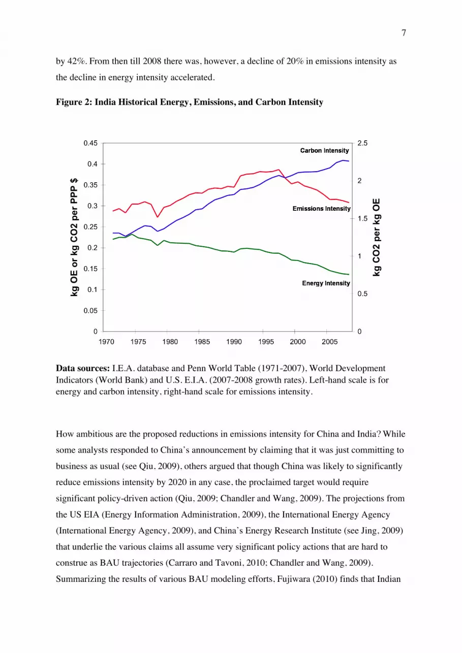
India shows a different pattern of change over time (Figure 2). While the energy intensity of
the Indian economy has declined over time, though at a slower pace than China, the carbon
intensity of energy supply has risen substantially, more than offsetting the improved energy
intensity until the mid to late 1990s. This was due to a pronounced shift of the fuel mix away
from biomass towards coal and other fossil fuels. From 1971 to 1997 emissions intensity rose
2 Data sources: I.E.A. database and Penn World Table (1971-2007), World Development Indicators (World Bank) and U.S. E.I.A. (2007-2008 growth rates).
7
by 42%. From then till 2008 there was, however, a decline of 20% in emissions intensity as
the decline in energy intensity accelerated.
Figure 2: India Historical Energy, Emissions, and Carbon Intensity
Data sources: I.E.A. database and Penn World Table (1971-2007), World Development Indicators (World Bank) and U.S. E.I.A. (2007-2008 growth rates). Left-hand scale is for energy and carbon intensity, right-hand scale for emissions intensity.
How ambitious are the proposed reductions in emissions intensity for China and India? While
some analysts responded to China’s announcement by claiming that it was just committing to
business as usual (see Qiu, 2009), others argued that though China was likely to significantly
reduce emissions intensity by 2020 in any case, the proclaimed target would require
significant policy-driven action (Qiu, 2009; Chandler and Wang, 2009). The projections from
the US EIA (Energy Information Administration, 2009), the International Energy Agency
(International Energy Agency, 2009), and China’s Energy Research Institute (see Jing, 2009)
that underlie the various claims all assume very significant policy actions that are hard to
construe as BAU trajectories (Carraro and Tavoni, 2010; Chandler and Wang, 2009).
Summarizing the results of various BAU modeling efforts, Fujiwara (2010) finds that Indian

8
emissions intensity is expected to fall by 3% p.a. till 2030, implying a 36% reduction
between 2005 and 2020. On this basis, India’s 20-25% pledge is well within business as
usual, but, again, the modeled BAU scenarios take into account existing energy and carbon
efficiency actions.
In this paper, we use a stochastic frontier model of energy intensity to decompose energy
intensity into the effects of input mix, output mix, climate, and a residual technology or
underlying energy efficiency variable. Underlying energy efficiency then measures what
energy intensity would be in each country if they had the same values of the structural
variables. In other words, it is a standardized measure of energy efficiency that takes into
account countries’ differing circumstances. We then evaluate what business as usual
trajectories of energy intensity might be, and how feasible various reductions to 2020 would
be.
The paper is organized as follows. The next two sections detail our econometric model and
data. Following these we present the econometric results, a comparison of the BAU
projections to the announced targets, a discussion of alternative policy scenarios, a
comparison of developed and developing country targets, and finally a conclusion.
2. Econometric Model
This section provides a basic description of our model, which is described in more detail in
Stern (2010). In that paper, a stochastic frontier model of energy intensity is developed. The
model is estimated using averages over the period 1971-2007 for 85 countries. The model is
given by:
€
ln Ei
Yi= −α0 −αK ln
Ki
Yi−αH ln
Hi
Yi−αWWi − β je ji + γ k yki
k=2
4
∑j=2
5
∑ + lnui + lnvi
lnui ~ N+ Γ'z i,σ u
2( )lnvi ~ N 0,σ v
2( )
(1)
where:
the ej are the shares of the five energy vectors: Coal, oil, natural gas, biomass, and primary
electricity; in total energy use, E, in country i. The coefficient of oil is set to zero so that oil is
the default fuel.

9
Y is GDP. The yk are the shares in GDP of the four industrial sectors: Agriculture, mining and
utilities, manufacturing, and services. The coefficient of manufacturing is set to zero so that
manufacturing is the default industry.
K is capital stock and H is human capital;
W is average winter temperature.
v is a normally distributed random error term assumed to represent measurement error. u is
the state of underlying energy efficiency in country i with lower levels of u implying higher
energy efficiency. The best practice frontier is defined by lnu = 0. The logarithm of u is a
random variable that can only take non-negative values. As shown in Figure 3, it is modeled
as the non-negative part of a normal distribution with mean
€
Γ'z i.
€
Γ
is a vector of coefficients
that will be estimated and
€
z i is a vector of additional explanatory variables. As
€
z i
varies
across countries, this distribution is different in each country - some countries are more likely
and others less likely to be close to the best practice frontier.
Figure 3: Truncated Normal Distribution
The vector z contains the following variables:

10
ln TFP: Log of total factor productivity calculated as: lnTFP = lnY - 0.3lnK - 0.7lnH.
ln K/T: Log of the ratio of capital stock to land area. This expresses the potential for
environmental disruption in the absence of mitigating technology.
ln PPP: Log of the ratio of the market exchange rate to the purchasing power parity exchange
rate.
ln Openness: Log of the ratio of exports and imports to GDP.
Corruption: Transparency International’s Corruption Perception Index. The index takes the
value of zero in a perfectly corrupt country and ten in the least corrupt country.
Energy Reserves/GDP: Size of fossil fuel energy reserves relative to GDP
Dummy variables for German/Scandinavian and French legal origin and a dummy for current
and former Communist states. English legal origin is the default.
The model is estimated via a maximum likelihood procedure (Kumbhakar et al., 1991; Hadri
et al., 2003). Estimation of the model using the “between estimator” – estimation on a cross-
section of means has some advantages and disadvantages. Stern (2009) provides a detailed
discussion. Among the advantages are that it does not impose any structure on the evolution
of underlying energy efficiency over time or on short-run dynamics associated with
investment etc. The state of technology in each year in each country can be derived in two
steps as follows. First a residual series is computed according to:
€
ln ˆ u it = ln Eit
Yit
+ ˆ α 0 + ˆ α K ln Kit
Yit
+ ˆ α H ln Hit
Yit
+ ˆ α WWi + ˆ β je jit − ˆ γ k ykitk= 2
4
∑j= 2
5
∑ − ln ˆ v i (2)
where, the measurement error, vi, is estimated via the maximum likelihood procedure.
€
ln ˆ u it
undoubtedly also includes fluctuations due to short-run dynamics and measurement errors.
We assume that these additional errors are stationary and apply the Hodrick-Prescott filter
(Hodrick and Prescott, 1997) to extract the long-run technology component. Note that these
time trends can take negative values. Negative values simply imply that underlying energy
efficiency is better than what the average of best practice across the whole 1971-2007 time
period was.
11
3. Data
Details of the data sources used in estimating the econometric model are given in Stern
(2010). The econometric model was estimated using data for 1971-2007. Some data for
China and India was updated to 2008 from a variety of sources. Carbon emissions data for
1971 to 2006 are taken from the IEA database and updated to 2008 using the growth rates
implied by the U.S. Energy Information Administration database. Data for energy use for
1971-2007 are taken from the IEA database and updated to 2008 using the growth rates from
the U.S. E.I.A. database. GDP data for 1971-2007 is from the Penn World Table. Updating to
2008 is based on the growth rates in the World Bank’s World Development Indicators.
In order to generate a business as usual scenario for energy intensity, we need to project the
explanatory variables in (1) over the commitment horizon. These projected growth rates
allow us to use equation (1) to project business as usual energy intensity. The projection of
the energy shares allows us to also project business as usual carbon intensity. We obtain the
carbon coefficients for each fuel from the US EIA.
For technological change we use three different scenarios. The first scenario is the one we
believe to be most likely. We estimate the forward growth rate using a convergence approach
described below. For China, the rate of change in underlying energy efficiency declines from
4.9% per annum in 2008 to 4.2% p.a. in 2020. For India, the rate of change in underlying
energy efficiency declines from 4.3% per annum in 2008 to 3.7% p.a. in 2020. As a
sensitivity analysis, we make two further projections for both China and India:
Scenario 2: The forward growth rate is equal to a regression estimate of the mean rate of
growth over the 2000-2007 period. This yields a rate of 5.5% p.a. for China and 3.9% for
India. Note that we find the rate of improvement in underlying energy efficiency to still
be fast in the 21st century in China despite the stalling in energy intensity.
Scenario 3: The forward growth rate is equal to a regression estimate of the mean rate of
growth over the 1971-2007 period. For China this yields the highest rate of change (6.1%
p.a.) and for India the lowest (1.5%).
We also make a number of other projections for China alone, which are discussed below.
Projections for the shares of fuels in energy use for 2020 are based on the 2007 World Energy
Outlook (IEA, 2007) reference scenario (p119). We interpolated the shares of each fuel
linearly between 2008 and 2015 and 2015 and 2030. In China biomass use declines from 10%

12
to 7% over the forecast horizon, oil use increases from 18% to 20% and the other fuels
change by one percentage point or less. For India coal increases from 41% to 44%, biomass
declines from 27% to 20%, and the other fuels change by one percentage point or less. As a
consequence, carbon intensity rises from 2.28 kg CO2 per kgOE to 2.47 over the forecast
horizon in India, while in China carbon intensity only increases from 3.05 to 3.08.
To project future industrial structure we used the following methods. For China, we use
Downes’ (2010) estimates for the agricultural sector. We do not use his estimates for the non-
agricultural sectors directly, because with the exception of agriculture, the baseline is slightly
different to the World Bank data we used to estimate the model. We use the growth in the
service sector used in the IEA reference scenario (43% in 2015 and 47% in 2030). Downes’
projection of the share of manufacturing is roughly constant over time so we assume that the
share of manufacturing is constant over the period. Mining and utilities are treated as the
residual category. For India, we estimate the share of share of agriculture in GDP by
assuming the real value of output continued to grow at its historical rate of growth of 2.7%
p.a. We then take the projected economic growth rates for India from Garnaut, Howes, Jotzo,
and Sheehan (2008) to project total GDP over this period. The ratio of agricultural output to
this projected GDP gives the projected share of agriculture in GDP. As a result agriculture
falls to 9.9% of GDP in India by 2020 while it falls to 5.9% of GDP in China. We assume
that India’s shares of mining and utilities and manufacturing will grow at their regression
estimated growth rate for the 1971-2007 period. Then the share of services is computed as the
residual.
We project capital and human capital intensities to grow at their regression estimated growth
rate for the 1971-2007 period. We assume that temperature is constant over the forecast
period as we do not have a time series for temperature to estimate any trend with.
Stern (2010) finds that the panel as a whole exhibits β-convergence (Quah, 1996) of energy
efficiency. But a general convergence model will probably not be very informative about
India and China specifically. Figure 5 shows that the US and Germany have had similar
levels of energy efficiency and that progress has been fairly smooth over time. Given this and
the fact that the US is the world’s largest economy and the technology leader (Kumar and
Russell, 2002) we model convergence of energy efficiency towards the US. The model is the
following error correction model:

13
€
Δ ln ˜ u it − ln ˜ u USAt( ) = −β i ln ˜ u it−1 − ln ˜ u USAt−1( ) + εit (3)
where the change in gap between the smoothed technology state
€
ln ˜ u it in country and i and the
US is a linear function of the gap itself. Assuming that the error is zero, Figure 4 presents the
time-varying estimate
€
− ˆ β it = Δ ln ˜ u it − ln ˜ u USAt( ) / ln ˜ u it−1 − ln ˜ u USAt−1( ) . The percentage of the gap
in technology between China and the US eliminated each year rose to a peak of about 4.1%
per annum in the late 1990s and subsequently stabilized around 2.5%. India only recently
reached these levels after a later start. The rate of change begins to accelerate in each country
after liberalization. China began to liberalize at the end of the 1970s but initially only the
Special Economic Zones were open to foreign investment. Reform in India too was phased in
gradually starting in 1991.
Figure 4: Convergence Rates
Using data from the entire 1971-2007 period to estimate (3) as a regression model would
underestimate the current rate of convergence. In order to construct Scenario 1, we assume
that the rate of convergence in each country over 2008-2020 is equal to the most recent rate
and that the recent rate of technical progress in the U.S. (2.3% p.a.) also continues until 2020.

14
4. Econometric Results
Parameter estimates for the model (1) are presented in Table 1. The parameters for the
deterministic model measure the effect on distance from the best practice frontier of each of
the variables. The coefficients of capital and human capital are positive, which is
theoretically consistent with substitutability between these inputs and energy. Countries with
warmer winter temperatures are further from the frontier, ceteris paribus, because they
should be able to use less energy per dollar of GDP the warmer their climate. The four fuels
all have lower energy quality (see Stern, in press) than oil, the default fuel.
Table 1. Econometric Results
Deterministic Model Stochastic Model Constant 11.454 Constant 9.278 (1.16) (1.59) Capital 0.292 ln TFP -1.296 (1.15) (-1.63) Human Capital 0.589 ln K/T -0.012 (1.05) (-0.32) Winter 0.011 ln PPP 0.884 (1.32) (5.79) Coal -0.485 ln Open 0.113 (-1.28) (1.38) Natural Gas -0.416 Transparency -0.050 (-0.87) (-1.47) Primary Electricity -0.732 Fossil Res. 0.008 (-1.50) (1.42) Biomass -0.867 German/Scand L.O. -0.251 (-3.48) (-1.22) Agriculture -0.225 French L.O. -0.107 (-0.21) (-1.23) Mining 0.144 Former Comm. 0.538 (0.13) (2.17) Services -0.850
€
συ 0.220 (-0.96) (3.04)
€
σu 0.011 (0.01) t-statistics in parentheses

15
Countries with a lower share of oil in energy use and higher shares of these fuels are,
therefore, for a given energy intensity more efficient. The signs of coefficients of the
industrial sectors have the opposite interpretation to those of the fuels and temperature. A
positive coefficient means that the sector is more energy intensive than the default sector,
manufacturing. A country with a larger share of GDP in energy intensive sectors is, ceteris
paribus, closer to the frontier. None of the effects of the industrial sectors are statistically
significant but the signs of the mining and services sectors are as would be expected.
Looking at the factors that explain the level of technology or underlying energy efficiency,
we see that countries with higher TFP are more energy efficient, ceteris paribus, as would be
expected. The elasticity is quite large. A 1% increase in TFP results in a 1.30% improvement
in energy efficiency as lower levels of the technology term, u, imply greater energy
efficiency. On the other hand, a higher exchange rate relative to the PPP level results in less
energy efficiency. The elasticity here is 0.88. It appears that the cost of imported fuel is the
key factor here. Relatively poor countries with low exchange rates can potentially be quite
energy efficient. Over the course of economic development rising exchange rates may offset
the gains from increased levels of general productivity and result in less improvements in
energy efficiency than one might naively expect. This makes sense, as globally, outside of the
poorest countries there is no strong relationship between energy intensity and the level of
GDP per capita (both measured in PPP terms). This has potentially important implications for
China (and India) as its currency is revalued over time. This will lower the effective price of
energy, encourage consumption, discourage energy efficient investments, and so act against
official energy efficiency goals unless energy taxes are simultaneously raised on petroleum
etc.
The more open an economy is the less energy efficient it will be. This counters the usual idea
that opening to trade will allow the adoption of more energy efficient technologies. Possibly,
more open economies have more of their economic activity in energy intensive industries.
The transparency indicator is scored so that zero is the most corrupt and ten the least corrupt
country. More corrupt countries are somewhat less energy efficient in line with theory on this
issue (e.g. Lopez and Mitra, 2000). Countries with greater fossil fuel reserves relative to the
size of their economies are less energy efficient. Countries of Scandinavian, German, and
French legal origin are more energy efficient, ceteris paribus, than those of English legal
origin, which is the default. Former and current communist countries have substantially lower

16
energy efficiency.
€
σ u is insignificantly different from zero indicating that there is little
unexplained variation in the technology variable, u.
Figure 5: China, India, and Four Developed Economies: Underlying Energy Efficiency
Figure 6: China, India, and Four Developing Economies: Underlying Energy Efficiency

17
Using (2) we can derive the underlying energy efficiency trends for each country. Figure 5
presents these for India, China, and several developed economies: U.S.A., Australia,
Germany, and Japan, while Figure 6 compares China and India to four developing economies
that have proposed reductions in emissions relative to BAU: Brazil, Indonesia, Mexico, and
South Africa. Again, the very different histories of China and India are illustrated. Rapid
improvements in energy efficiency are seen in both countries following economic reform,
which came in China in the 1980s and in India only recently. In the 1970s China was one of
the most inefficient countries in the world. India had an intermediate level of efficiency.
Many developing economies were more efficient than the developed economies. However,
on the whole, they have not improved as much since then as the developed economies have
and some are less efficient today than in the 1970s.
China, like other post-communist states has converged particularly rapidly to the more energy
efficient countries. The average rate of efficiency improvement in China over the entire
period (1971-2007) is 5.3% p.a. while in the U.S. it is 2.3%, Germany 2.4%, Australia 1.7%,
Japan 1.3%, India 1.7%, Indonesia 0.7%, and South Africa 0.1%. Brazil 0.6% saw a
reduction in efficiency of 0.2% p.a. and Mexico 1.2%. China’s performance over the entire
period and India’s recent rapid rate of improvement in energy efficiency are, however, not so
anomalous in the developing country context when we take into account their rapid rate of
economic growth and initial high level of inefficiency.
5. Business as Usual Projections vs. Country Targets
Table 2 presents the reductions in emissions intensity that we find under the three scenarios
for China and India. The implications for energy and emissions intensity are also shown in
Figures 7 and 8. None of the scenarios look inherently unreasonable in the figures except
perhaps Scenario 3 for India. The initial jump upwards in this scenario is due to the model
having negative residuals in recent years and the sudden slowing of the rate of technological
change implied by this scenario.
Scenario 1 – our preferred scenario – results in a 24% reduction in emissions intensity in
China. These results for China are comparable with an analysis by Garnaut, Jotzo, and Howes
(2008), whose projections for GDP growth, energy use and carbon intensity imply a 21%
reduction in BAU emissions intensity for China from 2005 to 2020. Scenario 3 – continuation

18
Table 2. BAU and Alternative Policy Scenarios:
Change in Emissions Intensity 2005-2020
China India
BAU Scenario 1 (Convergence to US in underlying energy efficiency)
-24% -29%
BAU Scenario 2 (2000-2007 rate of tech change)
-33% -28%
BAU Scenario 3 (1971-2007 rate of tech change)
-38% -2%
Scenario 1 + 15% Non-Fossil Fuel Energy Target
-26%
Scenario 1 + 20% Non-Fossil Fuel Energy Target
-29%
Scenario 1 + 25% Non-Fossil Fuel Energy Target
-32%
US Average Energy Efficiency Applied to New Investment
-46%
US Marginal Energy Efficiency Applied to New Investment
-56%
of the historic 1971-2007 rate of improvement in energy efficiency – results in a 38%
reduction in emissions intensity. This almost meets China’s proposed target of a 40-45%
reduction. But continuation of this rate of change seems unlikely a priori. The period of 1979
to 2000 represents a catching up with higher energy efficiency levels in other countries. Since
2000 the rate of progress in China has slowed down. Scenario 2, which assumes this recent
rate of technological progress results in a 33% reduction in emissions intensity. But if there
truly is convergence between China and other countries we would expect the rate of progress
to slow down even further as modeled in Scenario 1. Therefore, it is hard to see Scenarios 2
and 3 as realistic BAU scenarios for China.

19
Figure 7: BAU Scenarios for China
Figure 8: BAU Scenarios for India
For India, Scenario 1 results in a slightly greater reduction in emissions intensity than in
China of 29%. This and Scenario 2 (28% reduction) meet India’s goal of a 20-25% in
20
emissions intensity by 2020. Hence, India’s goal could be considered as “business as usual”.
But the long-run historic rate of improvement in energy efficiency in India was low and,
therefore, Scenario 1 results in only a 2% decrease in emissions intensity by 2020. In this
scenario, improvement in energy efficiency is offset by substitution of energy for human
capital and shift in the fuel mix. In interpreting these BAU projections, it is important to note
that in all scenarios we use IEA projections for fuel shares, and thus change in carbon
intensity of energy supply. To the extent that these IEA projections already include policies
that shift the energy mix towards lower-carbon fuels (e.g. substitution from coal to gas, or
increased renewable electricity generation), the “true” BAU projection would yield lower
reductions in emissions intensity.
In conclusion, it is likely that China will need to implement ambitious policies aimed at
reducing carbon emissions, in order to meet its announced emissions intensity goal. Even if
the rapid historical rate of improvement in energy efficiency could be again attained, the
target would not quite be reached. For India the conclusion is less clear-cut, as India’s target
might be met with only limited or even no dedicated mitigation policies.
6. Alternative Policy Scenarios for China
China also has a policy of increasing the share of energy derived from non-fossil sources to
15% by 2020. How much impact will this existing policy have? Under BAU primary
electricity and biomass provide 11.3% of China’s energy in 2020. We assume the gain comes
entirely from increasing the contribution of primary electricity while not changing the share
of biomass (and decreasing the shares of the three fossil fuels proportionally to make up for
the increase non-fossil energy). This means increasing the share of non-fossil fuel fired
electricity from 4.1% to 7.8% of the primary energy supply in 2020. The non-fossil target
itself reduces emissions intensity in 2020 by only an additional 2%. Increasing the non-fossil
target to 20% reduces emissions intensity by a further 3% and a 25% non-fossil target by an
incremental 3%. This appears to be the limit of feasible shifts towards non-fossil electricity.3
3 According to the IEA (2007), by 2020 41% of China’s primary energy supply will be used to produce electricity, which will result in a tripling of electricity generation between 2005 and 2020. Therefore, 27 percentage points of 2020 primary energy use will be due to electricity generating capacity installed from 2005-2020. A 25% non-fossil target represents

21
Thus, a policy aimed at reaching the 40% target must depend on a faster rate of improvement
in underlying energy efficiency. An interesting question to ask is how much improvement in
emissions intensity China could achieve if all new investment going forward was at the same
efficiency level as the US. We find the level of energy efficiency of new US investment, z,
from this equation:
€
Zt =ztIt + Zt−1(1−δ)Kt−1
It + (1−δ)Kt−1
(4)
where Z is the energy efficiency of installed capacity, K is the capital stock, I is investment,
and δ is the rate of depreciation assumed to be 6%. We assume that US investment grows at
the historic rate of 1.4% p.a. We project future US energy efficiency using the historic 1971-
2007 rate of improvement. For the growth of Chinese investment we assume the share of
investment in GDP remains constant in the future so that investment grows at the rate of
economic growth. This scenario results in a 56% improvement in energy efficiency over the
projection horizon of 2005-2020. However, if new investment in China is only of the same
efficiency as US overall existing capacity in that year (Z), energy efficiency improves by
46% over the projection horizon.
In conclusion, achieving the goal through improving the energy efficiency of new investment
alone would require reaching close to the average level in the leading developed economy in
new investment in China. Some combination of a non-fossil fuel goal of 15% or more
combined with a less stringent energy efficiency goal could also, of course, meet the goal.
7. Comparing Developed and Developing Country Targets
Following the Kyoto blueprint, developed country targets have been framed in terms of
absolute reductions of carbon emissions as a percentage of emissions in a base year such as
1990, 2000, or 2005. By contrast, China’s and India’s unilaterally declared targets have been
14 percentage points of 2020 primary energy being sourced from primary electricity rather than fossil fuels relative to business as usual. In other words, half of the new generating capacity would have to be in the form of primary electricity rather than fossil fired electricity. The 40% emissions intensity reduction goal could only be achieved with the Scenario 3 growth rate if all new electricity generating capacity from 2005-2020 was primary electricity. This is of course, impossible given existing developments from 2005 to 2010.

22
framed in terms of percentage reductions in emissions intensity at 2020 relative to 2005
emissions intensity, while some other developing countries have defined their commitments
as absolute reductions relative to a BAU trajectory. Among others, the US has proposed a
reduction of 17% relative to 2005, the EU either 20% to 30% relative to 1990, and Australia
5-25% relative to 2000. Australia’s target, like those of Brazil and Indonesia includes a large
amount of emissions from forestry and land-use change, which does not fit into our
framework of analysis.
Absolute and intensity targets can be compared on a common basis. The comparison depends
on making an assumption about the rate of economic growth in the developed economies
over the commitment period. This allows us to convert the developed country emissions
reduction target into an emissions intensity target. The relationship between emissions
reduction and emissions intensity targets is:
€
(1− I) =1− E1+G
(5)
where I is the intensity reduction target, E is the emissions reduction target (positive
numbers) and G is the total percentage growth of the economy over the commitment period.
The United States currently proposes to reduce emissions by 17% in 2020 relative to 2005.
China proposes to reduce its emissions intensity by 40-45% in 2020 relative to 2005. For the
US commitment to yield the same reduction in emissions intensity over the period, the
growth of the US economy over the period must be 44% or 2.5% per year. According to the
Penn World Table, the U.S. economy grew at 2.7% from 2000 to 2007. GDP declined over
2008 and 2009. A growth rate of 2.5%, therefore, may be a realistic growth rate for 2005-
2020. With that economic growth rate, the US and Chinese targets are then identical in terms
of reductions in emissions intensity.
Next, we compare the mid-point of the EU’s 20-30% target range with the mid-point of the
Chinese target range. A 25% reduction in emissions relative to 1990 implies a reduction in
carbon emissions of 23% relative to 2005, as aggregate emissions in EU-27 countries fell by
around 2% from 1990 to 2005 (with a significant contribution from collapse of low-
efficiency, high-carbon socialist economies). For this to translate into the same reduction in
emissions intensity as under China’s target, economic growth would need to be 1.8% p.a.
from 2005-20. The EU(27) economy has grown at a rate of just over 2% p.a. since 1990. A

23
continuation of this growth rate, combined with the weaker EU target, implies the same
reduction in emissions intensity as the weaker Chinese target, while the stricter EU target is
somewhat stricter than the stricter Chinese target.
8. Discussion and Conclusions
In this paper, we have shown that China’s emissions intensity target for 2020 is feasible but
ambitious. Chinese energy efficiency has converged towards that in developed and other
developing economies in recent years and its rate of improvement has slowed down. Given
this, a reasonable BAU scenario for China is a 24% reduction in emissions intensity. In no
way is a 40-45% reduction in emissions intensity “business as usual”, as has been claimed by
some observers.
China’s existing non-fossil energy goal will only contribute an additional 2% reduction in
emissions intensity by itself. Even drastic shifts towards low-carbon electricity sources, and
fast displacement of direct use of fossil fuels with electricity, by themselves would not be
enough to meet the emissions intensity target. Achieving China’s goal through maximizing
the energy efficiency of new investments alone would require China to come close to the
average energy efficiency of the US in all new investments. Hence, it is likely that policy
action in all aspects of the energy sector and all parts of the economy will be needed to
achieve the target.
India could achieve its goal of a 20-25% cut in emissions intensity if the recent rate of
progress in energy efficiency is maintained. Active policies such as increasing the energy
efficiency of new investments or increasing the share of electricity generated by non-fossil
technologies would obviously help India achieve its goal, but may not be necessary.
Comparing the targets for absolute emissions put forward by the US and the EU, we show
that the rate of reduction in emissions intensity implicit in their targets is similar to the
Chinese target. A comparison of rates of change of emissions intensity is informative and
relevant, as it strips away the “emissions dampening” effect of relatively slow economic
growth in the advanced economies, which is certainly not the effect of any deliberate policy
intervention.

24
Seen in this light, the EU and US targets would seem no more ambitious than China’s in
terms of the move towards low-carbon and high-efficiency energy technologies. Conversely,
it stands to reason that making the same rate of progress is more difficult in countries that are
already more efficient (in particular many EU countries). It can also be argued that it is
harder in a slow-growing economy to achieve the same rate of emissions intensity reductions
because the new capital stock added routinely each year is a smaller share of the total than in
fast-growing countries, so it requires especially efficient or low-carbon investment, and/or
premature scrapping of existing facilities.
But such arguments ignore that developed countries, going back to the Rio Convention of
1992, explicitly agreed to put in greater effort than developing countries in mitigating climate
change.
The debate now is no longer over whether developed countries should do ‘something’ while
developing countries continued to do ‘nothing’ for climate change mitigation. Rather, it
appears that countries’ targets on the table since Copenhagen, despite all the disagreements
over their legal status, can be the starting point for a serious debate about who does how
much, and how.
References
Carraro, C. and M. Tavoni (2010) Looking ahead from Copenhagen: How challenging is the
Chinese carbon intensity target? VOX: Research-Based Policy Analysis And Commentary
From Leading Economists, 5th January 2010.
Chandler, W. and Y. Wang (2009) Memo to Copenhagen: Commentary is Misinformed –
China’s Commitment is Significant, Carnegie Endowment for International Peace.
Dasgupta, S. and N. Sethi (2009) India offers to cut carbon intensity by 20-25%, The Times
of India, 28th November.
Downes, P. (2010) Forecasting Chinese Industrial Production, Presentation to Informal
Workshop: China Climate Change Policy and Research, Australian National University, 3
February.
EIA (2009) International Energy Outlook 2009, Washington DC.

25
Fujiwara, N. (2010) The political economy of India’s climate agenda, CEPS Working
Document 325/March 2010, Centre for European Policy Studies.
Garnaut, R., F. Jotzo, and S. Howes (2008) China’s rapid emissions growth and global
climate change policy, in Ligang Song and Wing The Woo (eds), China’s Dilemma:
Economic Growth, the Environment and Climate Change, China Update 2008, ANU e-press,
Canberra.
Garnaut, R., S. Howes, F. Jotzo, and P. Sheehan (2008) Emissions in the Platinum Age: the
implications of rapid development for climate change mitigation, Oxford Review of Economic
Policy 24, 377-401.
Hadri, K., C. Guermat, and J. Whittaker (2003) Estimation of technical inefficiency effects
using panel data and doubly heteroscedastic stochastic production frontiers, Empirical
Economics 28, 203-222.
Hodrick, R. and E. C. Prescott (1997) Postwar U.S. business cycles: An empirical
investigation, Journal of Money, Credit, and Banking 29, 1-16.
International Energy Agency (2007) World Energy Outlook 2007: China and India Insights,
Paris.
IEA (2009) World Energy Outlook 2009, Paris.
Jing, F. (2009) Emissions to peak at 2030: Report, China Daily 18th August 2009.
Jotzo, F. and J. Pezzey (2007), ‘Optimal intensity targets for greenhouse emissions trading
under uncertainty’, Environmental and Resource Economics 38(2), 259–284.
Kumar, S. and R. R. Russell (2002) Technological change, technological catch-up, and
capital deepening: Relative contributions to growth and convergence, American Economic
Review 92(3), 527-548.
Kumbhakar, S. C., S. Ghosh, and J. T. McGuckin (1991) A generalized production frontier
approach for estimating determinants of inefficiency in U.S. dairy farms, Journal of Business
and Economic Statistics 9(3), 279-286.
López, R. and S. Mitra (2000) Corruption, pollution and the Kuznets environment curve,
Journal of Environmental Economics and Management, 40, 137-150.

26
National Development and Reform Commission (NDRC), 2006. Overview of the 11th Five
Year Plan for National Economic and Social Development. Beijing: NDRC.
Quah, D. T. (1996) Empirics for economic growth and convergence, European Economic
Review 40(6), 1353-1375.
Qiu, J. (2009) China’s climate target: is it achievable? Nature 462(3), 550-551.
Stern D. I. (2009) Between estimates of the environmental Kuznets curve, Environmental
Economics Research Hub Research Report 34.
Stern, D. I. (in press) Energy quality, Ecological Economics.
Stern, D. I. (2010) Modelling international trends in energy efficiency and carbon emissions,
Environmental Economics Research Hub Research Report.
UNFCCC (2010), ‘Information provided by non-Annex I Parties relating to Appendix II of
the Copenhagen Accord (nationally appropriate mitigation actions of developing country
Parties)’, http://unfccc.int/home/items/5265.php, accessed 3 March 2010.
Xinhua (2009) Press Release, 26th November.
Xinhua (2010) Press Release, 26th February.


