Embed Size (px)
Citation preview

Ecological Complexity 16 (2013) 31–40
Original research article
How much complexity is needed to describe the fluctuations observed in denguehemorrhagic fever incidence data?
Maıra Aguiar a,b,*, Bob W. Kooi c, Filipe Rocha a, Peyman Ghaffari a, Nico Stollenwerk a
a Centro de Matematica e Aplicacoes Fundamentais da Universidade de Lisboa, Avenida Prof. Gama Pinto 2, 1649-003 Lisboa, Portugalb Fundacao Ezequiel Dias, Servico de Virologia e Riquetisioses, Laboratorio de dengue e febre amarela, Rua Conde Pereira Carneiro 80, 30510-010 Belo Horizonte, MG, Brazilc Vrije Universiteit, Faculty of Earth and Life Sciences, Department of Theoretical Biology, De Boelelaan 1087, NL 1081 HV Amsterdam, The Netherlands
A R T I C L E I N F O
Article history:
Received 5 February 2012
Received in revised form 5 July 2012
Accepted 3 September 2012
Available online 6 October 2012
Keywords:
Multi-strain
Dengue fever
Temporary cross-immunity
Chaos
Predictability
A B S T R A C T
Different extensions of the classical single-strain SIR model for the host population, motivated by
modeling dengue fever epidemiology, have reported a rich dynamic structure including deterministic
chaos which was able to mimic the large fluctuations of disease incidences. A comparison between the
basic two-strain dengue model, which already captures differences between primary and secondary
infections including temporary cross-immunity, with the four-strain dengue model, that introduces the
idea of competition of multiple strains in dengue epidemics shows that the difference between first and
secondary infections drives the rich dynamics more than the detailed number of strains to be considered
in the model structure. Chaotic dynamics were found to happen in the same parameter region of interest,
for both the two and the four-strain models, able to describe the fluctuations observed in empirical data
and shows a qualitatively good agreement between empirical data and model simulation. The
predictability of the system does not change significantly when considering two or four strains, i.e. both
models present a positive dominant Lyapunov exponent giving approximately the same prediction
horizon in time series. Since the law of parsimony favors the simplest of two competing models, the two-
strain model would be the better candidate to be analyzed, as well the best option for estimating all
initial conditions and the few model parameters based on the available incidence data.
� 2012 Elsevier B.V. All rights reserved.
Contents lists available at SciVerse ScienceDirect
Ecological Complexity
jo ur n al ho mep ag e: www .e lsev ier . c om / lo cate /ec o co m
1. Introduction
Dengue is a viral mosquito-borne infection, a leading cause ofillness and death in the tropics and subtropics. There are fourantigenically distinct but closely related dengue viruses, designat-ed DEN-1, DEN-2, DEN-3, and DEN-4. Infection by one serotypeconfers life-long immunity to that serotype and a short period oftemporary cross-immunity to other serotypes. Two forms of thedisease exist: dengue fever (DF), and dengue hemorrhagic fever(DHF) which has been associated with secondary dengue infectiondue to the antibody-dependent enhancement (ADE) process,where the pre-existing antibodies to previous dengue infectioncannot neutralize but rather enhance the new infection. In the firstdengue infection virus particles are captured and processed by so-called antigen presenting cells. T-cells become activated, likewiseB-cells that produce antibodies used to inactivate the viruses. In a
* Corresponding author at: Centro de Matematica e Aplicacoes Fundamentais da
Universidade de Lisboa, Avenida Prof. Gama Pinto 2, 1649-003 Lisboa, Portugal.
E-mail addresses: [email protected] (M. Aguiar), [email protected] (B.W. Kooi),
[email protected] (F. Rocha), [email protected] (P. Ghaffari),
[email protected] (N. Stollenwerk).
1476-945X/$ – see front matter � 2012 Elsevier B.V. All rights reserved.
http://dx.doi.org/10.1016/j.ecocom.2012.09.001
secondary infection the antibodies from the first infection attach tothe virus particles but do not inactivate them. The antibody–viruscomplex suppresses innate immune responses, increasing intra-cellular infection and generating inflammatory citokines andchemokines that, collectively, result in enhanced disease (Hal-stead, 1982; Guzman et al., 2010; Dejnirattisai et al., 2010).
Dengue fever dynamics is well known to be particularlycomplex with large fluctuations of disease incidences. Severalmathematical models found in the literature have been formulatedto describe the transmission of dengue fever. Multi-straindynamics are generally modeled with extended SIR-type models,and have demonstrated to show critical fluctuations with powerlaw distributions of disease cases exemplified in meningitis(Stollenwerk and Jansen, 2003b) and in dengue (Massad et al.,2008). Dengue models including multi-strain interactions via ADEbut without a temporary cross immunity period have showndeterministic chaos when strong infectivity on secondary infectionwas assumed (Ferguson et al., 1999; Schwartz et al., 2005; Billingset al., 2007). In these models, the recovered individuals could beimmediately infected with another strain.
The combination of biological aspects such as temporary cross-immunity and ADE have been studied by several authors (Wearingand Rohani, 2006; Nagao and Koelle, 2008; Recker et al., 2009)

M. Aguiar et al. / Ecological Complexity 16 (2013) 31–4032
where four strains are involved, but again limiting the effect of ADEto increase the contribution of secondary cases to the force ofinfection. Aguiar et al. (2008) have investigated a two-straindengue model, initially suggested and preliminarily analyzed inFerguson et al. (1999), where deterministic chaos was found in awider parameter regions when including temporary cross-immunity (Aguiar et al., 2008), not needing to restrict theinfectivity on secondary infection to one or another region inparameter space.
The two-strain model captures the essential differencesbetween primary and secondary infections where the notion oftwo different strains is enough to describe primary infections, amostly harmless form of illness, and secondary infection,associated with the severe form of the disease. It is a lowerdimensional model as opposed to the multiple strain models,easier to be analyzed and still can attempt to estimate all initialconditions as well as the few model parameters.
In this manuscript we compare the basic two-strain denguemodel with the four-strain dengue model, that introduces the idea ofcompetition of multiple strains in dengue epidemics. Observe thatthere are two different model formulations leading to the same set ofmathematical equations. In the first interpretation, we have twocoexisting strains and two infections episodes per individual areallowed. In the other interpretation there are four strains and thecompartments of the SIR type model consists of primarily and thesecondarily infected individuals. Hence all individuals primarily(secondarily) infected by each one of the four strains form onecompartment of the primary (secondary) infections.
This formulation has the advantage that the results can directlybe compared with the available DHF incidence data from hospitalssince secondary infection dengue patients may evolve into severedisease due to ADE, which will be probably hospitalized (Aguiaret al., 2011).
We perform a qualitative study in order to show how muchcomplexity we really need to add into epidemiological models tobe able to describe the fluctuations observed in empirical denguehemorrhagic fever incidence data. The parameter description andrespective values used to modeling dengue fever epidemiology aregiven in Table 1, if not otherwise explicitly stated. This is a first steptoward model selection. Next steps will be parameter estimationand model fine-tuning and finally usage for prediction based onmonitoring data (Stollenwerk et al., 2012).
This manuscript is organized as follows. In Section 2 wecompare the basic two-strain dengue model with SIR compart-ments for primary and secondary infections, with the four-straindengue model with separate SIR compartments for each strain,where only two recurrent infections are allowed. In Section 3 wecompare the long-term dynamics of the two models by comparingsimulation results, by using bifurcation analysis when thedynamics is a steady-state or periodically fluctuating and alsoLyapunov exponents calculation when the dynamics is chaotic. Theintroduction of a cross-immunity period appears to be important
Table 1Parameter set for the basic multi-strain models.
Par. Description Values
N Population size 1.6 � 106
m Birth and death rate 1/65 y
g Recovery rate 52 y�1
b Infection rate 2�g
h Degree of seasonality 2[0, 0.35]
r Import parameter 2[0, 10�10
a Temporary cross-immunity rate 2[2, 52] y
f Ratio of secondary infections
Contributing to force of infection 2[0, 3]
when combined with different forces of infection, in primary andsecondary infection. In Section 4 a time series analysis is performedwhere seasonality and import of infected are introduced in bothmodels. The predictions are compared with empirical DHFincidence data.
2. Multi-strain models: a dimensional problem
A basic n-strain epidemiological model with primary andsecondary infections can be written as follows:
S ¼ m N � Sð Þ �Xn
i¼1
bN
S Ii þ r � N þ fXn
j¼1; j 6¼ i
Iji
0@
1A
0@
1A (1)
and for i = 1, . . ., n
Ii ¼bN
Ii þ r � N þ fXn
j¼1; j 6¼ i
Iji
0@
1A
0@
1A� g þ mð ÞIi (2)
Ri ¼ gIi � a þ mð ÞRi (3)
Si ¼ aRi �Xn
j¼1; j 6¼ i
bN
Si I j þ r � N þ fXn
k¼1;k 6¼ j
Ikj
0@
1A
0@
1A� mSi (4)
and for i = 1, . . ., n and j = 1, . . ., n with j 6¼ i
˙Iij ¼bN
Si I j þ r � N þ fXn
k¼1;k 6¼ j
Ikj
0@
1A
0@
1A� g þ mð ÞIij (5)
and finally
R ¼ gXn
i¼1
Xn
j¼1; j 6¼ i
Iij
0@
1A� mR : (6)
The parameter r is the import factor, related to the possibility ofan individual to get infected outside the studied population and thenbring the infection into the population to which this individualbelongs to, mimicking the imported cases of the disease in a definedpopulation. Equivalently, an infected visitor to the region underconsideration who passes the infection to a susceptible in thepopulation of size N has the same effect on the studied population.Hence, we do not need to distinguish these two scenarios ofsusceptibles traveling outside or infected traveling inside the regionunder consideration. In total, this captures the imported infectionthat comes from an external source.
For constant population size, the susceptibles individualswithout a previous experienced dengue infection (S) become
Ref.
World Population (2008)
World Health Organization (2009) and Centers for Disease
Control and Prevention (2011)
Ferguson et al. (1999)
Aguiar et al. (2011)
] Aguiar et al. (2011)�1 Matheus et al. (2005)
Aguiar et al. (2008)

M. Aguiar et al. / Ecological Complexity 16 (2013) 31–40 33
infected for the first time with a given dengue strain (Ii) with twopossible infection rates, depending on who (individual on hisprimary or secondary infection) is transmitting the infection. Therelevant difference concerning disease transmissibility is that theforce of infection varies accordingly to the number of previousinfections which the hosts have experienced. Note that the numberof dengue cases caused by a third or fourth dengue virus infectionis extremely low and once confirmed, the risk for DHF relative to DFwas not different for those experiencing third or fourth denguevirus infections over those experiencing a second dengue virusinfection (Endy et al., 2002; Gibbons et al., 2007; Halstead, 2008).Therefore, individuals in a primary infection transmit the diseasewith a force of infection bI/N whereas in a secondary infection thetransmission is given with a force of infection fbI/N where f can belarger or smaller than unit, i.e. increasing or decreasing thetransmission rate, due to the ADE effect. Individuals infected forthe first time become recovered and life long immune to that givenstrain (Ri), with a recovery rate g and after a period of temporarycross-immunity a, are again susceptible with a previous experi-enced infection (Si). Individuals only get infected for the secondtime with a different strain than the one acquired during the first
a)
-30
-25
-20
-15
-10
-5
0
5
10
0 0.5 1 1.5 2 2.5 3
ln(I
)
φ
c)
-5
-2.5
0
2.5
0 0.5 1 1.5 2 2.5 3
ln(I
)
φ
Fig. 1. Bifurcation diagram comparison between multi-strain models. In red the non-s
neglecting temporary cross-immunity period (a = 52 y�1 or one week) we observe comple
strain model and in (b) the four-strain model. For assuming temporary cross-immunity
appears. In (c) the two-strain model, previously studied in Aguiar et al. (2008, 2011) and in
legend, the reader is referred to the web version of the article.)
infection (Iij), again with two possible infection rates, depending onwho (individual on his primary or secondary infection) istransmitting the infection. Finally, they recover from the secondaryinfection (R) with recovery rate g. The death rates m coming out ofall classes go into the class of susceptible without experiencingprevious dengue infection as a birth rate.
The n-strain SIR-type model can be understood as a mean fieldapproximation of a stochastic system, which is a good approxima-tion to be used in order to understand better the behavior of thestochastic systems in certain parameter regions, where thedynamics of the mean quantities are approximated by neglectingcorrelations (Stollenwerk and Jansen, 2011; Aguiar et al., 2012).
2.1. The two-strain model versus the four-strain model
Concerning data availability, long term epidemiologicalinformation come from the Ministry of Public Health in Thailandand consist on monthly incidences of hospitalized DHF cases. Forsuch a data scenario, models that are able to generate bothprimary and secondary infection cases (with a different strain),without the need of considering differences on the dynamics of
b)
-30
-25
-20
-15
-10
-5
0
5
10
0 0.5 1 1.5 2 2.5 3
ln(I
)
φ
d)
-5
-2.5
0
2.5
0 0.5 1 1.5 2 2.5 3
ln(I
)
φ
easonal two-strain model and in green the non-seasonal four-strain model. When
x dynamics restricted to the parameter region f � 1 for both models, in (a) the two-
period (a = 2 y�1 or six months) a new chaotic window a rich dynamical behavior
(d) the four-strain model. (For interpretation of the references to color in this figure
M. Aguiar et al. / Ecological Complexity 16 (2013) 31–4034
different co-circulating dengue serotypes, have show a goodqualitative agreement between empirical data and model output(Aguiar et al., 2011), just by considering ADE and temporary cross-immunity.
The two-strain model with temporary cross-immunity is a 9dimensional system where the population N is divided into tenclasses. For two different strains, named strain 1 and strain 2, welabel the SIR classes for the hosts that have seen the individualstrains, without epidemiological asymmetry between strains, i.e.infections with strain one followed by strain two or vice versacontribute in the same way to the force of infection. The completesystem of ordinary differential equations (ODEs) for the two-strainepidemiological model can be written as follows.
S ¼ mðN � SÞ � bðtÞN
SðI1 þ r � N þ fI21Þ
�bðtÞN
SðI2 þ r � N þ fI12Þ(7)
˙I1 ¼bðtÞ
NSðI1 þ r � N þ fI21Þ � ðg þ mÞI1 (8)
˙I2 ¼bðtÞ
NSðI2 þ r � N þ fI12Þ � ðg þ mÞI2 (9)
R1 ¼ gI1 � ða þ mÞR1 (10)
R2 ¼ gI2 � ða þ mÞR2 (11)
˙S1 ¼ aR1 �bðtÞ
NS1ðI2 þ r � N þ fI12Þ � mS1 (12)
˙S2 ¼ aR2 �bðtÞ
NS2ðI1 þ r � N þ fI21Þ � mS2 (13)
˙I12 ¼bðtÞ
NS1ðI2 þ r � N þ fI12Þ � ðg þ mÞI12 (14)
˙I21 ¼bðtÞ
NS2ðI1 þ r � N þ fI21Þ � ðg þ mÞI21 (15)
R ¼ gðI12 þ I21Þ � mR : (16)
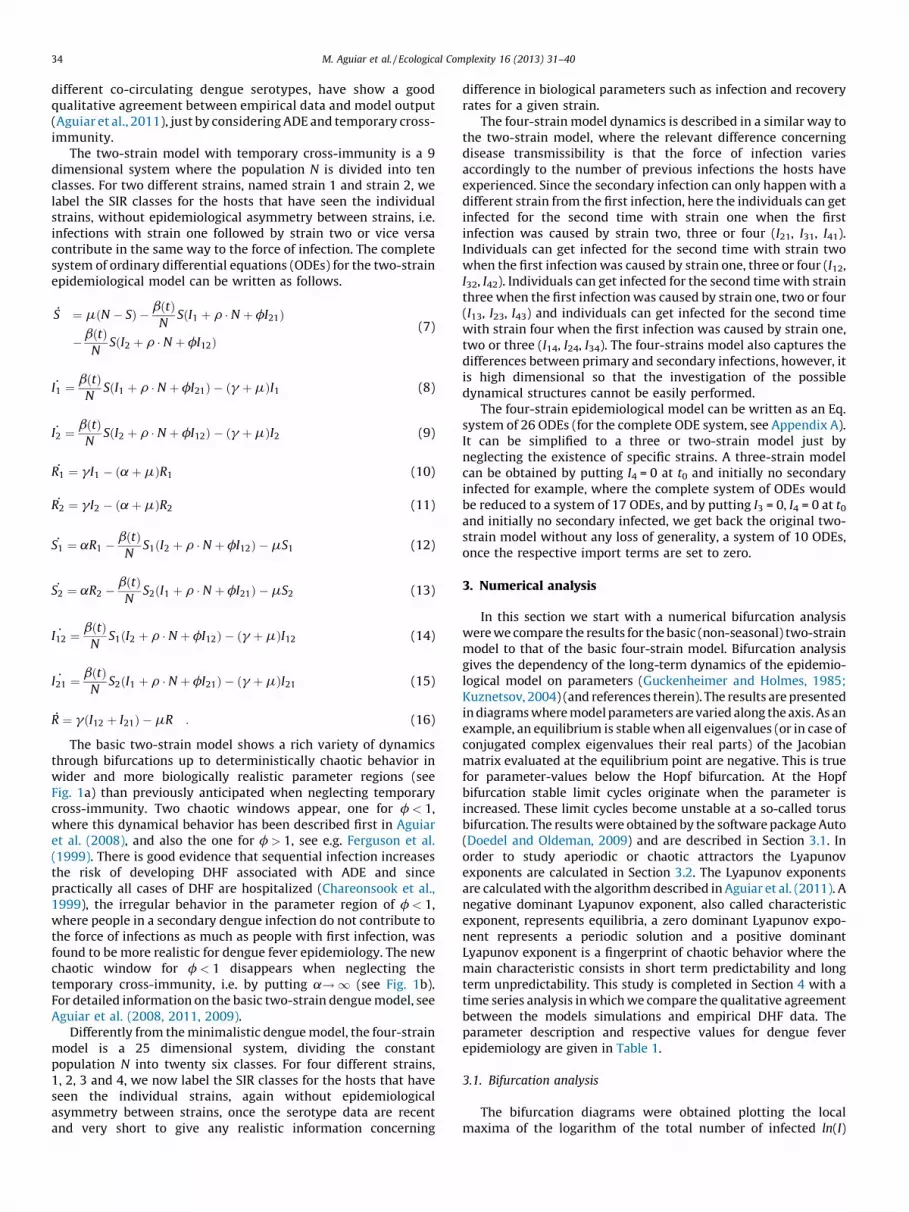
The basic two-strain model shows a rich variety of dynamicsthrough bifurcations up to deterministically chaotic behavior inwider and more biologically realistic parameter regions (seeFig. 1a) than previously anticipated when neglecting temporarycross-immunity. Two chaotic windows appear, one for f < 1,where this dynamical behavior has been described first in Aguiaret al. (2008), and also the one for f > 1, see e.g. Ferguson et al.(1999). There is good evidence that sequential infection increasesthe risk of developing DHF associated with ADE and sincepractically all cases of DHF are hospitalized (Chareonsook et al.,1999), the irregular behavior in the parameter region of f < 1,where people in a secondary dengue infection do not contribute tothe force of infections as much as people with first infection, wasfound to be more realistic for dengue fever epidemiology. The newchaotic window for f < 1 disappears when neglecting thetemporary cross-immunity, i.e. by putting a! 1 (see Fig. 1b).For detailed information on the basic two-strain dengue model, seeAguiar et al. (2008, 2011, 2009).
Differently from the minimalistic dengue model, the four-strainmodel is a 25 dimensional system, dividing the constantpopulation N into twenty six classes. For four different strains,1, 2, 3 and 4, we now label the SIR classes for the hosts that haveseen the individual strains, again without epidemiologicalasymmetry between strains, once the serotype data are recentand very short to give any realistic information concerning
difference in biological parameters such as infection and recoveryrates for a given strain.
The four-strain model dynamics is described in a similar way tothe two-strain model, where the relevant difference concerningdisease transmissibility is that the force of infection variesaccordingly to the number of previous infections the hosts haveexperienced. Since the secondary infection can only happen with adifferent strain from the first infection, here the individuals can getinfected for the second time with strain one when the firstinfection was caused by strain two, three or four (I21, I31, I41).Individuals can get infected for the second time with strain twowhen the first infection was caused by strain one, three or four (I12,I32, I42). Individuals can get infected for the second time with strainthree when the first infection was caused by strain one, two or four(I13, I23, I43) and individuals can get infected for the second timewith strain four when the first infection was caused by strain one,two or three (I14, I24, I34). The four-strains model also captures thedifferences between primary and secondary infections, however, itis high dimensional so that the investigation of the possibledynamical structures cannot be easily performed.
The four-strain epidemiological model can be written as an Eq.system of 26 ODEs (for the complete ODE system, see Appendix A).It can be simplified to a three or two-strain model just byneglecting the existence of specific strains. A three-strain modelcan be obtained by putting I4 = 0 at t0 and initially no secondaryinfected for example, where the complete system of ODEs wouldbe reduced to a system of 17 ODEs, and by putting I3 = 0, I4 = 0 at t0
and initially no secondary infected, we get back the original two-strain model without any loss of generality, a system of 10 ODEs,once the respective import terms are set to zero.
3. Numerical analysis
In this section we start with a numerical bifurcation analysiswere we compare the results for the basic (non-seasonal) two-strainmodel to that of the basic four-strain model. Bifurcation analysisgives the dependency of the long-term dynamics of the epidemio-logical model on parameters (Guckenheimer and Holmes, 1985;Kuznetsov, 2004) (and references therein). The results are presentedin diagrams where model parameters are varied along the axis. As anexample, an equilibrium is stable when all eigenvalues (or in case ofconjugated complex eigenvalues their real parts) of the Jacobianmatrix evaluated at the equilibrium point are negative. This is truefor parameter-values below the Hopf bifurcation. At the Hopfbifurcation stable limit cycles originate when the parameter isincreased. These limit cycles become unstable at a so-called torusbifurcation. The results were obtained by the software package Auto(Doedel and Oldeman, 2009) and are described in Section 3.1. Inorder to study aperiodic or chaotic attractors the Lyapunovexponents are calculated in Section 3.2. The Lyapunov exponentsare calculated with the algorithm described in Aguiar et al. (2011). Anegative dominant Lyapunov exponent, also called characteristicexponent, represents equilibria, a zero dominant Lyapunov expo-nent represents a periodic solution and a positive dominantLyapunov exponent is a fingerprint of chaotic behavior where themain characteristic consists in short term predictability and longterm unpredictability. This study is completed in Section 4 with atime series analysis in which we compare the qualitative agreementbetween the models simulations and empirical DHF data. Theparameter description and respective values for dengue feverepidemiology are given in Table 1.
3.1. Bifurcation analysis
The bifurcation diagrams were obtained plotting the localmaxima of the logarithm of the total number of infected ln(I)

M. Aguiar et al. / Ecological Complexity 16 (2013) 31–40 35
against the ratio of the contribution of the secondary infections fto the force of infection (see Fig. 1 for example). Fixed points appearas one dot per parameter value, limit cycles appear as two dots,double-limit cycles as four dots, more complicated limit cycles asmore dots, and chaotic attractors as continuously distributed dotsfor a single f value (Ruelle, 1989).
The dynamics predicted by the two models are compared withrespect to dependency of the qualitative long-term dynamicbehavior on one parameter f, which describes the secondaryinfection contribution to the force of infection. The parametervalues where this qualitative behavior (steady state, periodic orchaotic) are called bifurcation points.
For both models, only one chaotic window is observed whenneglecting the temporary cross-immunity period (see Fig. 1a andb). Here, the complex dynamics are restricted to the parameterregion f � 1, where individuals in the secondary dengue infectionwould contribute much more to the force of infection thanindividuals in the first infection. Consideration of temporary cross-immunity (see Fig. 1c and d) brings a new chaotic window with arich dynamical behavior from fixed point to limit cycles untilcompletely irregular behavior for a more biologically realisticparameter region f < 1, in addition to the previously found chaotic
a)
-16
-14
-12
-10
-8
-6
-4
-2
0
0 0.2 0.4 0.6 0.8 1
ln(I
)
φ
c)
-14
-12
-10
-8
-6
-4
-2
0
0 0.2 0.
ln(I
)
Fig. 2. Numerical bifurcation diagram comparison. In (a) the bifurcation diagram for the t
torus bifurcation at f = 0.551. In (b) the bifurcation diagram for the four-strain model. A
that occurs at f = 0.311. The Hopf bifurcation and the torus bifurcation points were p
exponents in Fig. 3c. In (c) we show the bifurcation diagram comparison between multi-s
and in green the four-strain model. (For interpretation of the references to color in thi
window for f > 1. Note that the addition of seasonal forcing and/orpopulation noise brings complex behavior also for the regionwhere only periodic dynamics are observed. For more informationon the seasonal two-strain model, see Aguiar et al. (2011).
In Fig. 2 we present the bifurcation diagram comparison, forboth two-strain and four-strain model, in the relevant parameterregion of f < 1, when dengue patients in its secondary infectionmay evolve to a severe disease due the Antibody-dependentEnhancement phenomenon. The hospitalized individuals (DHFcases) contribute less to the force of infection, and not more, asprevious models suggested. For the two-strains model a Hopfbifurcation was found to occur at f = 0.1133 and a torusbifurcation, as a route to the chaotic behavior, was found to occurat f = 0.551 whereas for the four-strain model, the Hopfbifurcation was predicted by AUTO to occur at f = 0.267 followedby a torus bifurcation that occurs at f = 0.311. Qualitatively, thebifurcation points appear to happen at similar parameter regions,well below the region of interest of f � 1. In both cases the chaoticdynamics which are able to describe the fluctuations observed inempirical data are found to happen at the same parameter regionof interest and not only when assuming strong infectivity onsecondary infection.
b)
-10
-9
-8
-7
-6
-5
-4
-3
-2
-1
0 0.2 0.4 0.6 0.8 1
ln(I
)
φ
4 0.6 0.8 1
φ
wo-strains dengue model. A Hopf bifurcation was found to occur at f = 0.1133 and a
Hopf bifurcation was predicted to occur at f = 0.267 followed by a torus bifurcation
redicted very well by AUTO when comparing the results given by the Lyapunov
train models for the parameter region of interest f < 1. In red the two-strain model
s figure legend, the reader is referred to the web version of the article.)
M. Aguiar et al. / Ecological Complexity 16 (2013) 31–4036
We continue our analysis with the calculation of the Lyapunovexponent spectrum, where the dynamics on or beyond a torus isclassified as periodic, when one Lyapunov exponent is zero,aperiodic when two Lyapunov exponents are zero, and chaoticwhen one Lyapunov exponent is zero and at least one positive (Ott,1993).
3.2. Lyapunov exponents and predictability
In this section, the Lyapunov spectrum for both multi-strainmodels are shown and compared concerning the predictionhorizon of the monthly peaks in the time series. The so-calleddominant Lyapunov exponent (DLE) is the exponent with thelargest magnitude. The set of Lyapunov exponents is called theLyapunov spectrum which can be calculated for all parametervalues (see Fig. 3). The Lyapunov exponents were calculated usingan iteration technique using the QR decomposition algorithm viaHouseholder matrices (see Aguiar et al., 2008, 2011; Ruelle, 1989;Holzfuss and Lauterborn, 1989; Holzfuss and Parlitz, 1991).
a)
-0.1
-0.05
0
0.05
0.1
0.15
0 0.2 0.4 0.6 0.8 1 1.2
λi
φ
b
c)
-0.1
-0.05
0
0.05
0.1
0.15
0 0.2 0.4
ln(I
)
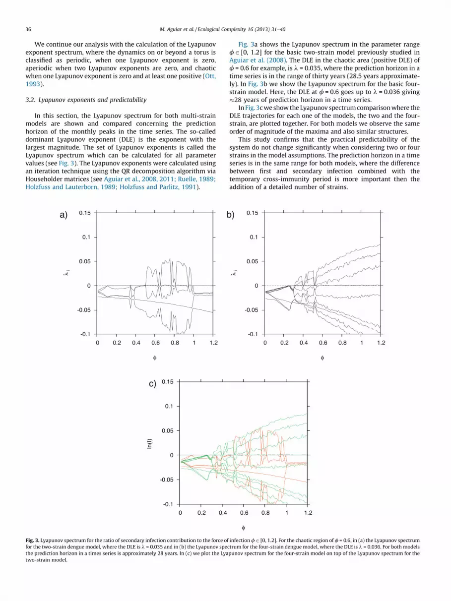
Fig. 3. Lyapunov spectrum for the ratio of secondary infection contribution to the force of
for the two-strain dengue model, where the DLE is l = 0.035 and in (b) the Lyapunov spec
the prediction horizon in a times series is approximately 28 years. In (c) we plot the Lya
two-strain model.
Fig. 3a shows the Lyapunov spectrum in the parameter rangef 2 [0, 1.2] for the basic two-strain model previously studied inAguiar et al. (2008). The DLE in the chaotic area (positive DLE) off = 0.6 for example, is l = 0.035, where the prediction horizon in atime series is in the range of thirty years (28.5 years approximate-ly). In Fig. 3b we show the Lyapunov spectrum for the basic four-strain model. Here, the DLE at f = 0.6 goes up to l = 0.036 giving�28 years of prediction horizon in a time series.
In Fig. 3c we show the Lyapunov spectrum comparison where theDLE trajectories for each one of the models, the two and the four-strain, are plotted together. For both models we observe the sameorder of magnitude of the maxima and also similar structures.
This study confirms that the practical predictability of thesystem do not change significantly when considering two or fourstrains in the model assumptions. The prediction horizon in a timeseries is in the same range for both models, where the differencebetween first and secondary infection combined with thetemporary cross-immunity period is more important then theaddition of a detailed number of strains.
)
-0.1
-0.05
0
0.05
0.1
0.15
0 0.2 0.4 0.6 0.8 1 1.2
λi
φ
0.6 0.8 1 1.2
φ
infection f 2 [0, 1.2]. For the chaotic region of f = 0.6, in (a) the Lyapunov spectrum
trum for the four-strain dengue model, where the DLE is l = 0.036. For both models
punov spectrum for the four-strain model on top of the Lyapunov spectrum for the

a)
-14
-12
-10
-8
-6
-4
-2
0
2 4 6 8 10 12 14 16 18 20
ln(I
)
α
b)
-14
-12
-10
-8
-6
-4
-2
0
2 4 6 8 10 12 14 16 18 20
ln(I
)
α
c)
-14
-12
-10
-8
-6
-4
-2
0
2 4 6 8 10 12 14 16 18 20
ln(I
)
α
d)
0
0.01
0.02
0.03
0.04
0.05
37.5 38 38.5 39 39.5 40 40.5 41 41.5 42 42.5
seco
ndar
y in
fect
ions
susceptibles without previous infection
e)
0
0.01
0.02
0.03
0.04
0.05
36 36.5 37 37.5 38 38.5 39 39.5 40 40.5 41
seco
ndar
y in
fect
ions
susceptibles without previous infection
f)
0
0.01
0.02
0.03
0.04
0.05
35.5 36 36.5 37 37.5 38 38.5 39 39.5 40
seco
ndar
y in
fect
ions
susceptibles without previous infection
g)
0
0.02
0.04
0.06
0.08
0.1
0.12
0.14
0 5 10 15 20 25 30 35 40 45 50
seco
ndar
y in
fect
ions
time
h)
0
0.02
0.04
0.06
0.08
0.1
0.12
0.14
0 5 10 15 20 25 30 35 40 45 50
seco
ndar
y in
fect
ions
time
i)
0
0.02
0.04
0.06
0.08
0.1
0.12
0.14
0 5 10 15 20 25 30 35 40 45 50
seco
ndar
y in
fect
ions
time
Fig. 4. Similarities between the basic multi-strain models. For f = 0.6, in (a) we show the bifurcation diagram for the two-strain model, in (b) the bifurcation diagram for the
three-strain model and in (c) the bifurcation diagram for the four-strain model. Here, the local maxima of the logarithm of the total number of infected ln(I) is plotted against
the temporary cross-immunity period parameter a. By fixing the temporary cross-immunity period a = 2 y�1, we show the state space plots in (d) for the two-strain model, in
e) for the three-strain model and in (f) for the four-strain model. In (g) we show the time series for the two-strain model, in (h) the time series for the three-strain model and in
(i) the time series for the four-strain model.
M. Aguiar et al. / Ecological Complexity 16 (2013) 31–40 37
In order to illustrate the similarities on the dynamical behaviorof the basic multi-strain models better, we show in Fig. 4, themodel dynamics when assuming two, three and four-strainsrespectively. We use bifurcation diagram, state space plots andtime series plots to compare the models behavior toward complexdynamics that would be able to mimic the available DHF incidencedata. For the bifurcation diagram the temporary cross-immunityperiod a is the varying parameter. For the time series and the statespace plots we fixed the ratio of secondary infection contributionto the force of infection to f = 0.6, where chaotic behavior wasconfirmed to happen in the non-seasonal models with two, threeand four-strains. For more information on the quantification ofunpredictability via Lyapunov exponents, see Aguiar et al. (2008,2011).
Fig. 4 presents a qualitative study on the similarities betweenthe basic multi-strain models. In Fig. 4a–c, we analyze the role ofthe temporary cross-immunity combined with the ADE affect inrespect of the detailed number of strains to be included in themodel structure. The numerical bifurcation diagram, where the
temporary cross-immunity period a is the varying parameter,shows that complex dynamics appears only when assuming thebiological relevant temporary cross-immunity period (between 3and 9 months, i.e. for a < 5). This finding appears to happen for allpossible multi-strain dengue models, the two-strain (see Fig. 4a),the three-strain (see Fig. 4b) and the four-strain model (see Fig. 4c).The time series and its state space plots are shown in Fig. 4d–f forthe two, three and the four-strain models respectively and showthe similarities between the multi-strain models where thecombination of temporary cross-immunity and ADE effect is aessential feature to be considered in the structure of the model inorder to understand the dynamics of dengue fever epidemiology. Infact, the differences between first and secondary infection(different forces of infections due to the hospitalization of thesevere cases of the disease), combined with temporary cross-immunity aspect (to be assumed between recurrent infections) aredriving the complex dynamics in multi-strain models more thanthe specific number of strains to be considered in the modelassumptions.

M. Aguiar et al. / Ecological Complexity 16 (2013) 31–4038
4. Time series analysis
This study is completed with a time series analysis where wecompare the matching between time series simulations (for thetwo-strain model as well for the four-strain model) and empiricalDHF data. The addition of seasonal forcing and import of infectedare needed to be included in order to describe the fluctuationsobserved in the available DHF incidence data (Aguiar et al., 2011).
Frequently the time series of empirical data are used as aqualitative check on model output, however, fitting every detail ofthe chaotic model to that of the empirical data is not possible(Stollenwerk et al., 2012). In Fig. 5 we match empirical DHFincidence data for the Province of Chiang Mai in the North ofThailand with model simulations. For both models a qualitativelygood result were obtained. Comparing empirical DHF data andmodel simulation, where patterns of the irregular data occurs, waspredicted by the models.
The effective dimension of the two strain model is 9 while of thefour strain model 25. The law of parsimony that recommendsselecting the hypothesis that makes the fewest assumptions,implies that the 9 dimensional two-strain model would be thebetter candidate than the 25 dimensional four-strain model to beanalyzed, capturing the essential differences of primary versussecondary infection without needing to restrict the ADE effect toone or another region in parameter space.
The two-strain model in its simplicity is a good model to beanalyzed, giving the expected complex behavior to mimic thefluctuations observed in empirical data, and would be indeed thebest option to be used for parameter estimation, which isnotoriously difficult for chaotic time series, based on the availableincidence data (Stollenwerk et al., 2012). Only the two-strain
a)
0
500
1000
1500
2000
2500
3000
1984 1988 1992 1996 2000 2004 2008 2012
Sec
onda
ry In
fect
ions
t
two-strain model simulation dhf empirical data
b)
0
500
1000
1500
2000
2500
3000
1984 1988 1992 1996 2000 2004 2008 2012
Sec
ond.
Infe
ctio
ns
t
four-strain model simulation dhf empirical data
Fig. 5. Using the same parameter set, empirical DHF incidence data (in black) for the
Province of Chiang Mai in the North of Thailand, with a population size
N = 1.6 � 106, are matched with simulations (in red) for the seasonal multi-
strain models with import of infected. In (a) two-strain model and in (b) the four-
strain model. The parameter b is given explicitly by b(t) = b0 � (1 + h � cos(v � t))where b0 is the infection rate and h is the degree of seasonality. Here, the degree of
seasonality is h = 0.35 and the import factor r = 10�10. The other parameter values
are given in Table 1. (For interpretation of the references to color in this figure
legend, the reader is referred to the web version of the article.)
model could attempt to estimate all initial conditions as well as thefew model parameters, as opposed of the four-strain model.
5. Discussion and remarks
In this manuscript we presented the results obtained from aqualitative analysis of multi-strain dynamical system motivated bydengue fever epidemiology. The comparison between the basictwo-strain dengue model, which already captures differencesbetween primary and secondary infections, with the four-straindengue model, that introduces the idea of competition of multiplestrains in dengue epidemics have shown that the differencebetween first and secondary infection combined with thetemporary cross-immunity period is driving more the complexdynamics, which is able to mimic the large fluctuations observed inthe empirical DHF incidence data, than the detailed number ofstrains to be considered in the model assumptions.
The numerical bifurcation analysis has shown that chaoticdynamics appear to happen at the same parameter region ofinterest, i.e. when assuming temporary cross-immunity periodbetween 3 and 9 months, for all of the considered multi-strainmodels, and the addition of seasonal forcing and import of infectedhave shown a qualitatively good result when comparing empiricalDHF data and simulation results, where patterns of the databehavior were similarly found to happen, for both models, in thetime series simulations.
Frequently the time series of empirical data are used as aqualitative check on model output, however, fitting every detail ofthe chaotic model to that of the empirical data is not possible.Parameter estimation based on empirical data to estimate initialconditions and model parameters have received great attentionand is notoriously difficult for chaotic time series. Temporally localapproaches are possible using iterated filtering algorithms (Ionideset al., 2006; He et al., 2010; Stollenwerk et al., 2012), and at themoment only minimalistic models would have a chance to bequalitatively understood well and eventually tested againstexisting data (Ionides et al., 2006; He et al., 2010; Stollenwerket al., 2012).
The two-strain model in its simplicity is a good model to beanalyzed, giving the expected complex behavior to explain thefluctuations observed in empirical data. It is minimalistic in thesense that it can capture the essential differences of primary versussecondary infection without needing to restrict the ADE effect toone or another region in parameter space. For future parameterestimation only the two-strain model could attempt to estimate allinitial conditions as well as the few model parameters. The two-strain model showed a qualitatively good result when comparingempirical DHF data and model simulations, giving insights into therelevant parameter values purely on topological information of thedynamics, and these relevant parameter values can be used forfurther refinement in formal parameter estimation based on theavailable data.
Acknowledgments
Maıra Aguiar acknowledge the financial support from the FCTgrants with reference SFRH/BD/43236/2008. This work has beenfurther supported by the European Union under FP7 in theEPIWORK and the DENFREE projects and the Portuguese FCTproject PTDC/MAT/115168/2009.
Appendix A. Unpacking the n-strain model into a four-strainmodel
The basic n-strain epidemiological model motivated by dengue
fever epidemiology, capturing difference between primary and
M. Aguiar et al. / Ecological Complexity 16 (2013) 31–40 39
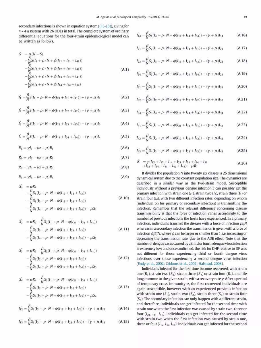
secondary infections is shown in equation system ((1)–(6)), giving for
n = 4 a system with 26 ODEs in total. The complete system of ordinary
differential equations for the four-strain epidemiological model can
be written as follows.
S ¼ mðN � SÞ
�bN
SðI1 þ r � N þ fðI21 þ I31 þ I41ÞÞ
�bN
SðI2 þ r � N þ fðI12 þ I32 þ I42ÞÞ
�bN
SðI3 þ r � N þ fðI13 þ I23 þ I43ÞÞ
�bN
SðI4 þ r � N þ fðI14 þ I24 þ I34Þ
(A.1)
˙I1 ¼bN
SðI1 þ r � N þ fðI21 þ I31 þ I41ÞÞ � ðg þ mÞI1 (A.2)
˙I2 ¼bN
SðI2 þ r � N þ fðI12 þ I32 þ I42ÞÞ � ðg þ mÞI2 (A.3)
˙I3 ¼bN
SðI3 þ r � N þ fðI13 þ I23 þ I43ÞÞ � ðg þ mÞI3 (A.4)
˙I4 ¼bN
SðI4 þ r � N þ fðI14 þ I24 þ I34ÞÞ � ðg þ mÞI4 (A.5)
R1 ¼ gI1 � ða þ mÞR1 (A.6)
R2 ¼ gI2 � ða þ mÞR2 (A.7)
R3 ¼ gI3 � ða þ mÞR3 (A.8)
R4 ¼ gI4 � ða þ mÞR4 (A.9)
˙S1 ¼ aR1
�bN
S1ðI2 þ r � N þ fðI12 þ I32 þ I42ÞÞ
�bN
S1ðI3 þ r � N þ fðI13 þ I23 þ I43ÞÞ
�bN
S1ðI4 þ r � N þ fðI14 þ I24 þ I34ÞÞ � mS1
(A.10)
˙S2 ¼ aR2 �bN
S2ðI1 þ r � N þ fðI21 þ I31 þ I41ÞÞ
�bN
S2ðI3 þ r � N þ fðI13 þ I23 þ I43ÞÞ
�bN
S2ðI4 þ r � N þ fðI14 þ I24 þ I34ÞÞ � mS2
(A.11)
˙S3 ¼ aR3 �bN
S3ðI1 þ r � N þ fðI21 þ I31 þ I41ÞÞ
�bN
S3ðI2 þ r � N þ fðI12 þ I32 þ I42ÞÞ
�bN
S3ðI4 þ r � N þ fðI14 þ I24 þ I34ÞÞ � mS3
(A.12)
˙S4 ¼ aR4 �bN
S3ðI1 þ r � N þ fðI21 þ I31 þ I41ÞÞ
�bN
S4ðI2 þ r � N þ fðI12 þ I32 þ I42ÞÞ
�bN
S4ðI3 þ r � N þ fðI13 þ I23 þ I43ÞÞ � mS4
(A.13)
˙I12 ¼bN
S1ðI2 þ r � N þ fðI12 þ I32 þ I42ÞÞ � ðg þ mÞI12 (A.14)
˙I13 ¼bN
S1ðI3 þ r � N þ fðI13 þ I23 þ I43ÞÞ � ðg þ mÞI13 (A.15)
˙I14 ¼bN
S1ðI4 þ r � N þ fðI14 þ I24 þ I34ÞÞ � ðg þ mÞI14 (A.16)
˙I21 ¼bN
S2ðI1 þ r � N þ fðI21 þ I31 þ I41ÞÞ � ðg þ mÞI21 (A.17)
˙I23 ¼bN
S2ðI3 þ r � N þ fðI13 þ I23 þ I43ÞÞ � ðg þ mÞI23 (A.18)
˙I24 ¼bN
S2ðI4 þ r � N þ fðI14 þ I24 þ I34ÞÞ � ðg þ mÞI24 (A.19)
˙I31 ¼bN
S3ðI1 þ r � N þ fðI21 þ I31 þ I41ÞÞ � ðg þ mÞI31 (A.20)
˙I32 ¼bN
S3ðI2 þ r � N þ fðI12 þ I32 þ I42ÞÞ � ðg þ mÞI32 (A.21)
˙I34 ¼bN
S3ðI4 þ r � N þ fðI14 þ I24 þ I34ÞÞ � ðg þ mÞI34 (A.22)
˙I41 ¼bN
S4ðI1 þ r � N þ fðI21 þ I31 þ I41ÞÞ � ðg þ mÞI41 (A.23)
˙I42 ¼bN
S4ðI2 þ r � N þ fðI12 þ I32 þ I42ÞÞ � ðg þ mÞI42 (A.24)
˙I43 ¼bN
S4ðI3 þ r � N þ fðI13 þ I23 þ I43ÞÞ � ðg þ mÞI43 (A.25)
R ¼ gðI12 þ I13 þ I14 þ I21 þ I23 þ I24 þ I31
þI32 þ I34 þ I41 þ I42 þ I43Þ � mR(A.26)
It divides the population N into twenty six classes, a 25 dimensional
dynamical system due to the constant population size. The dynamics are
described in a similar way as the two-strain model. Susceptible
individuals without a previous dengue infection S can possibly get the
primary infection with strain one (I1), strain two (I2), strain three (I3) or
strain four (I4), with two different infection rates, depending on whom
(individual on his primary or secondary infection) is transmitting the
infection. Remember that the relevant difference concerning disease
transmissibility is that the force of infection varies accordingly to the
number of previous infections the hosts have experienced. In a primary
infection, individuals transmit the disease with a force of infection bI/N
whereas in a secondary infection the transmission is given with a force of
infection fbI/N, where f can be larger or smaller than 1, i.e. increasing or
decreasing the transmission rate, due to the ADE effect. Note that the
number of dengue cases caused by a third or fourth dengue virus infection
is extremely low and once confirmed, the risk for DHF relative to DF was
not different for those experiencing third or fourth dengue virus
infections over those experiencing a second dengue virus infection
(Endy et al., 2002; Gibbons et al., 2007; Halstead, 2008).
Individuals infected for the first time become recovered, with strain
one (R1), strain two (R2), strain three (R3) or strain four (R4), and life
long immune to the given strain, with a recovery rate g. After a period
of temporary cross-immunity a, the first recovered individuals are
again susceptible, however with an experienced previous infection
with strain one (S1), strain two (S2), strain three (S3) or strain four
(S4). The secondary infection can only happen with a different strain,
and therefore, individuals can get infected for the second time with
strain one when the first infection was caused by strain two, three or
four (I21, I31, I41). Individuals can get infected for the second time
with strain two when the first infection was caused by strain one,
three or four (I12, I32, I42). Individuals can get infected for the second

M. Aguiar et al. / Ecological Complexity 16 (2013) 31–4040
time with strain three when the first infection was caused by strain
one, two or four (I13, I23, I43) and individuals can get infected for the
second time with strain four when the first infection was caused by
strain one, two or three (I14, I24, I34). Finally, the individuals recover
from the second infection (R) with recovery rate g. The death rates m
coming out of all classes go into the class of susceptible without
experiencing previous dengue infection as a birth rate. The model
also captures the differences between primary and secondary
infections, however, it is high dimensional so that the investigation
of the possible dynamical structures cannot be easily performed.
References
Aguiar, M., Kooi, B.W., Stollenwerk, N., 2008. Epidemiology of Dengue Fever: AModel with Temporary Cross-Immunity and Possible Secondary InfectionShows Bifurcations and Chaotic Behaviour in Wide Parameter Regions. Mathe-matical Modelling of Natural Phenomena 4, 48–70, http://dx.doi.org/10.1051/mmnp:2008070.
Aguiar, M., Stollenwerk, N., Kooi, B.W., 2009. Torus bifurcations, isolas and chaoticattractors in a simple dengue model with ADE and temporary cross-immunity.International Journal of Computer Mathematics 86, 1867–1877, http://dx.doi.org/10.1080/00207160902783532.
Aguiar, M., Ballesteros, S., Kooi, B.W., Stollenwerk, N., 2011. The role of seasonalityand import in a minimalistic multi-strain dengue model capturing differencesbetween primary and secondary infections: complex dynamics and its implica-tions for data analysis. Journal of Theoretical Biology 289, 181–196, http://dx.doi.org/10.1016/j.jtbi.2011.08.043.
Aguiar, M., Kooi, B.W., Stollenwerk, N., 2012. Infectious diseases dynamics: denguefever, a case study modeling infectious diseases dynamics: dengue fever, a casestudy. In: Epidemiology Insights, Maria de Lourdes Ribeiro de Souza da Cunha,Brazil, ISBN 979-953-307-754-2.
Billings, L., Schwartz, I.B., Shaw, L.B., Marie McCrary, Burke, D.S., Cummings, D.A.T.,2007. Instabilities in multiserotype disease models with antibody-dependentenhancement. Journal of Theoretical Biology 246, 18–27, http://dx.doi.org/10.1016/j.jtbi.2006.12.023.
Centers for Disease Control and Prevention, 2011. Dengue. Retrieved from http://www.cdc.gov/dengue/.
Chareonsook, O., Foy, H.M., Teeraratkul, A., Silarug, N., 1999. Changing epidemiology ofdengue hemorrhagic fever in Thailand. Epidemiology and Infection 122, 161–166.
Dejnirattisai, W., et al., 2010. Cross-reacting antibodies enhance dengue virusinfection in humans. Science 328, 745–748, http://dx.doi.org/10.1126/sci-ence.1185181.
Doedel, J.E., Oldeman, B., 2009. AUTO 07P—Continuation and bifurcation softwarefor ordinary differential equations. Technical Report: Concordia University,Montreal, Canada. Retrieved from http://indy.cs.concordia.ca/auto/.
Endy, T.P., et al., 2002. Spatial and temporal circulation of dengue virus serotypes: aprospective study of primary school children in Kamphaeng Phet, Thailand.American Journal of Epidemiology 156, 52–59, http://dx.doi.org/10.1093/aje/kwf006.
Ferguson, N., Anderson, R., Gupta, S., 1999. The effect of antibody-dependentenhancement on the transmission dynamics and persistence of multiple-strainpathogens. Proceedings of the National Academy of Sciences of the UnitedStates of America 96, 790–794.
Gibbons, V.R., et al., 2007. Analysis of repeat hospital admissions for dengue toestimate the frequency of third or fourth dengue infections resulting in admis-sions and dengue hemorrhagic fever, and serotype sequences. American Journalof Tropical Medicine and Hygiene 77, 910–913.
Guckenheimer, J., Holmes, P., 1985. Nonlinear Oscillations, Dynamical Systems andBifurcations of Vector Fields, volume 42 of Applied Mathematical Sciences, 2nded. Springer-Verlag, New York.
Guzman, M.G., et al., 2010. Dengue: a continuing global threat. Nature ReviewsMicrobiology 8, S7–S16, http://dx.doi.org/10.1038/nrmicro2460.
Halstead, S.B., 1982. Immune enhancement of viral infection. Progress in Allergy 31,301–364.
Halstead, S.B., 2008. Tropical Medicine: Science and Practice. In: Halstead, S.B.(Ed.), Dengue, volume 5. Imperial College Press (Chapter 7).
He, D., Ionides, E.L., King, A.A., 2010. Plug-and-play inference for disease dynamics:measles in large and small populations as a case study. Journal of the RoyalSociety Interface 7, 271–283 (DOI:10.1098/rsif.2009.0151).
Holzfuss, J., Lauterborn, W., 1989. Liapunov exponents from a time series of acousticchaos. Physical Review A 39, 2146–2152.
Holzfuss, J., Parlitz, U., 1991. Liapunov exponents from time series. Lecture Notes inMathematics 1486, 263–270.
Ionides, E., Breto, C., King, A.A., 2006. Inference for nonlinear dynamical systems.Proceedings of the National Academy of Sciences of the United States of America103, 18438–18443 (DOI:10.1073.pnas.0603181103).
Kuznetsov, Yu.A., 2004. Elements of Applied Bifurcation Theory, volume 112 ofApplied Mathematical Sciences, 3rd ed. Springer-Verlag, New York.
Massad, E., Ma, S., Chen, M., Struchiner, C.J., Stollenwerk, N., Aguiar, M., 2008. Scale-free network of a dengue epidemic. Applied Mathematics and Computation 195,376–381, http://dx.doi.org/10.1016/j.amc.2007.04.102.
Matheus, S., et al., 2005. Discrimination between primary and secondary denguevirus infection by an immunoglobulin G aviditnoy test using a single acute-phase serum sample. Journal of Clinical Microbiology 43, 2793–2797.
Nagao, Y., Koelle, K., 2008. Decreases in dengue transmission may act to increase theincidence of dengue hemorrhagic fever. Proceedings of the National Academy ofSciences 105, 2238–2243, http://dx.doi.org/10.1073/pnas/0709029105.
Ott, E., 1993. Chaos in Dynamical Systems, 2nd ed. Cambridge University Press,Cambridge.
Recker, et al., 2009. Immunological serotype interactions and their effect on theepidemiological pattern of dengue. Proceedings of the Royal Society B 276,2541–2548, http://dx.doi.org/10.1098/rspb.2009.0331.
Ruelle, D., 1989. Chaotic Evolution and Strange Attractors. Cambridge UniversityPress, Cambridge.
Schwartz, I.B., Shaw, L.B., Cummings, D.A.T., Billings, L., Marie McCrary, Burke, D.S.,2005. Chaotic desynchronization of multi-strain diseases. Physical Review E 72,066201–066206, http://dx.doi.org/10.1103/PhysRevE.72.066201.
Stollenwerk, N., Jansen, V.A.A., 2003b. Evolution towards criticality in an epidemio-logical model for meningococcal disease. Physics Letters A 317, 87–96.
Stollenwerk, N., Jansen, V., 2011. Population biology and criticality. Imperial CollegePress, London.
Stollenwerk, N., Aguiar, M., Ballesteros, S., Boto, J., Kooi, W.B., Mateus, L., 2012.Dynamic noise, chaos and parameter estimation in population biology. Inter-face Focus 2, 156–169, http://dx.doi.org/10.1098/rsfs.2011.0103.
Wearing, H.J., Rohani, P., 2006. Ecological and immunological determinants ofdengue epidemics. Proceedings of the National Academy of Sciences of theUnited States of America 103, 11802–11807 DOI:10.1073.pnas.0602960103.
World Health Organization, 2009. Dengue and Dengue Hemorrhagic Fever. Fact sheet117. Retrieved from http://www.who.int/mediacentre/factsheets/fs117/en/.
World Population Prospects: The 2008 Revision. Population Database. Retrievedfrom http://esa.un.org/unpp/index.asp?panel=2.


