Embed Size (px)
Citation preview

HYPERSONICAND
PLANETARY ENTRYFLIGHT MECHANICS
Nguyen X. Vinh
Adolf Busemann
Robert D. Cu/p
ANN ARBORTHE UNIVERSITY OF MICHIGAN PRESS

Copyright by The University of Michigan 1980All rights reserved
ISBN 0-472-09304-5Library of Congress Catalog Card No. 79-57117
Published in the United States of America byThe University of Michigan Press and simultaneously
in Rexdale, Canada, by John Wiley & Sons Canada, LimitedManufactured in the United States of America

Preface
The advent of the space shuttle and the prospect of several decades ofregular low-altitude earth orbital activity have focused attention on high-speed atmospheric trajectories exemplified by the space shuttle entry.The hypersonic flight mechanics of these trajectories represents a uniquefield, in that a combination of orbital mechanics and atmospheric flightmechanics is required.
For more than a decade we have worked together in this field, pursuingresearch under the sponsorship of the National Aeronautics and SpaceAdministration and the United States Air Force, and in teaching variousaspects of the subject to advanced undergraduate and graduate students atthe University of Michigan and the University of Colorado. During thistime, interest in this topic has grown steadily until the demand for suchmaterial led to this book.
We have endeavored to make this text valuable as a research tool andreference for current experts in the field, and also as a learning source forengineers and scientists in related fields who want to become involved inentry dynamics. Taken as a whole, this book is a comprehensive and self-contained treatment of hypersonic flight trajectories and atmospheric entryflight mechanics, leading the reader through the classical theories and end-ing with our modem, unified theory. Every topic is written so as to standalone; the reader can enter the text at any point to obtain the analysis ofparticular interest. Every chapter is followed by a list of references whichenables a researcher to trace the roots of the subject.
As a textbook, this book is designed to be used in several ways. Thefirst nine chapters serve as a text at the introductory level for senior stu-dents interested in orbital and entry flight mechanics. For students with afirm background in aerospace engineering, including aerodynamics, pro-pulsion, and orbital mechanics, this book can be used as the text for aspecialized course in atmospheric entry. For these advanced undergraduateand graduate students, chapter 2 and chapters 6 through 13 comprise asuitable text for such a one-semester course. Chapter 18 can be includedas time permits. The entire text covers a two-semester sequence at thesenior or first-year graduate level which brings the student to a sophisti-cated understanding of the subject. Finally, used as a textbook for a short
Preface
course on entry flight mechanics for engineers working in the space pro-gram, the following reading sequence is sufficient: chapter 2 and chapters10 through 18.
At both the University of Michigan and the University of Colorado,parts of this book have been used as the text for several courses at boththe advanced undergraduate and graduate levels. This favorable experiencehas enabled us to bring out the text in this final form suitable as a usefultool for both research and education. Several of our doctoral studentshave contributed to the development of a unified theory for planetaryentry covered in the second half of the book. It is a pleasure to acknowl-edge here their collective research efforts. Each individual contribution isfully accounted for in the text. During the whole period of the prepara-tion of this book, from its inception in 1972 until its completion in 1980,Professor Adolf Busemann has provided his eminent leadership, assistedby his gracious wife, Magda. To them this book is dedicated.
It is with gratitude that we acknowledge the support of the NASALangley Research Center, sponsor of much of the research work whichwent into this book. Dr. John E. Duberg, at a very early stage, shared ouropinion that further basic research on entry trajectories needed to bedone. As technical monitors from Langley, Mr. Robert W. Rainey andMr. Robert S. Dunning have provided enlightening comments on severaltechnical papers and NASA contractor reports generated under NASAresearch grants. Professor Robert M. Howe, Chairman of the Departmentof Aerospace Engineering at the University of Michigan, and also theChairman of the Department of Aerospace Engineering Sciences at theUniversity of Colorado have provided us with much encouragement forthis work. It is a pleasure to acknowledge their hospitality during ourfrequent visits to each other's campus to carry out our teamwork.
The excellent typing of the preliminary manuscript was done by Ms.Shirley Iverson while the final camera-ready copy was professionally pre-pared by Ms. Ann Gee. Their perseverance and dedication to this workare much appreciated.
We would like to express our deep appreciation to Magda Busemann,Joan Vinh, and Betty Culp for their continual love and encouragementduring these years.
Contents
Preface
Chapter 1. Planetary Atmospheres and Aerodynamic Forces
1- 1 Introduction 1
1-2 Fundamental Assumptions1 -2.1 Assumption of Spherical Symmetry 2
1-2.2 Assumption of Nonrotating Atmosphere 3
1-2.3 Assumption of Exponential Atmosphere 4
1 -3 The Earth's Atmosphere 5
1-4 Hypersonic Flow 10
1-5 Newtonian Flow 11
1-6 The Drag Polar 13
1-7 The Busemann Formula 15
References 17
Chapter 2. Equations for Flight Over a Spherical Planet
2-1 Introduction 19
2-2 Relative Angular Motion 19
2-3 Basic Equations of Motion 21
References 28
Chapter 3. Performance in Extra-Atmospheric Flight
3-1 Introduction 293-2 The Trajectory Equation 30
3-3 Characteristic Values of a Trajectory 33
3-4 Time of Flight Along the Orbit 383-5 The Elements of the Orbit in Terms of the Initial Condition 423-6 Minimum-Energy Orbit 443-7 Effects of Variations of the Initial Condition in the Elements at Entry .. . 49
References 54
Contents
Chapter 4. Powered Phase
4-1 Introduction4-2 The Equations of Motion4-3 Ascending Trajectory at Constant Flight Path Angle4-4 Optimum Staging
4-4.1 All the Propulsion Systems are Similar4-4.2 The Propellant Used is the Same for All Stages4-4.3 The Structural Ratios are the Same for All Stages
References
Chapter 5. Return to the Atmosphere
5- 1 Introduction5-2 Descent Trajectory for Given Entry Speed5-3 Minimum Impulse for Entry at Given Speed5-4 Descent Trajectory for Given Entry Angle5-5 Minimum Impulse for Entry at Given Angle5-6 Descent Trajectory for a Given Entry Position .5-7 Minimum Impulse for Entry at Given Position.References
Chapter 6. Basic Equations for Planar Entry Trajectories
6-1 Introduction6-2 Energy Discussion of the Trajectory in Phase Space.6-3 The Fundamental EquationsReferences
Chapter 7. Analysis of First-Order Planetary Entry Solutions
7-1 Introduction7-2 Gliding Entry at Small Flight Path Angles7-3 Gliding Entry at Medium and Large Flight Path Angles7-4 Ballistic Entry at Large Flight Path Angles
7-4.1 Analysis Neglecting Gravity7-4.2 Analysis Including Gravity
7-5 Skip EntryReferences
Chapter 8. Loh's Second-Order Theory for Entry Trajectories
8-1 Introduction8-2 Unified Solution for Entry8-3 Second-Order Solution for Entry
55
55
6266
7071
72
72
73
75
81
84
8994
98
99
100100
106
107
108
110113
.117117
121
123
126
128
129
1328-4 Reduction of the Second-Order Solution to First-Order Solutions 133
Contents ix
8-4.1 Gliding Entry at Small Flight Path Angles 1348-4.2 Gliding Entry at Medium and Large Flight Path Angles 1368-4.3 Ballistic Entry at Large Flight Path Angles 1368-4.4 Skip Entry at Large Flight Path Angles 137
References 138
Chapter 9. Aerodynamic Heating
9-1 Introduction 139
9-2 Heat Flow into the Vehicle 141
9-3 Dimensionless Variables 143
9-4 Entry of a Ballistic Vehicle 1449-5 Entry of a Glide Vehicle 1499-6 Entry of a Skip Vehicle 1509-7 Comparative Analysis of the Performance of Hypervelocity Vehicles. . . . 152
References 156
Chapter 10. Yaroshevskii's Theory for Entry into Planetary Atmospheres
10-1 Introduction 15710-2 Second-Order Nonlinear Differential Equation for Entry Trajectory .. . . 158
10-3 Atmospheric Entry at Constant Lift-to-Drag Ratio 161
10-4 Series Solutions of the Basic Nonlinear Differential Equations 164
10-4.1 Ballistic Decay from Satellite Orbits 164
10-4.2 Ballistic Entry With Various Initial Flight Path Angles 166
10-4.3 Lifting Entry from Circular Speed 172
10-4.4 Gliding Trajectory 174
References 177
Chapter 11. Chapman's Theory for Entry into Planetary Atmospheres
11-1 Introduction 178
11-2 Development of the Nonlinear Differential Equation 178
11 -3 The ZFunctions and Related Quantities 183
11-4 Some Approximate Analytical Solutions 187
11-4.1 Yaroshevskii'sSolution 187
11-4.2 Solution for Ballistic Entry 188
11-4.3 Solution for Glide Entry 18911 -4.4 Solution for Skip Trajectory 189
11-5 Numerical Results 19011-5.1 Entry from a Decaying Orbit for Various Lift-to-Drag Ratios .. . 190
11-5.2 Ballistic Entry from Circular Speed with Various InitialFlight Path Angles 191
11-5.3 Lifting Entry from Circular Speed with Various InitialFlight Path Angles 193
11 -5.4 Entry from Super Circular Speed 194
Contents
11-6 Effect of Lift on Entry 196
11-6.1 Effect of Lift on Deceleration11-6.2 Effect of Lift on Heating Rate11-6.3 Effect of the Initial Flight Path Angle
References
Chapter 12. Entry Corridor
Introduction 205
Basic Differential Equations 208
The Periapsis Parameter 210Chapman's Results for the Entry Corridor 214
Influence of Aerodynamic Lift on the Corridor Boundaries 218
12-5.1 Overshoot Boundary with Lift 219
12-5.2 Undershoot Boundary with Lift 222References 225
Chapter 13. Unified Theory for Entry into Planetary Atmospheres
13-1 Introduction 226
13-2 Universal Equations for Three-Dimensional Entry Trajectories 227
13-3 Reduction to Classical Solutions13-3.1 Keplerian Solution13-3.2 Chapman's Equations13-3.3 Yaroshevskii's Equation13-3.4 Loh's Second-Order Solution .
13-4 Numerical Results13-5 The Entry Corridor
13-5.1 Definition of the Entry Point .13-5.2 Trajectories with Several Passes.13-5.3 Chapman's Periapsis Parameter,13-5.4 The Entry Corridor
References
Chapter 14. Solution of the Exact Equations .Using Directly MatchedAsymptotic Expansions
14-1 Introduction 25414-2 The Dimensionless Equations of Motion14-3 Integrations by Directly Matched Asymptotic Expansions.
14-3.1 Outer Expansions (Keplerian Region)14-3.2 Inner Expansions (Aerodynamic-Predominated Region) 26014-3.3 Asymptotic Matching and Composite Expansions 261
14-3.4 Solution for the Planar Case 26514-4 Applications 266References 272
197
198
200204
12-112-212-312-412-5
232232235238239241
244246247248
.251253
254259
259
Contents Xi
Chapter 15. Orbit Contraction Due to Atmospheric Drag
15-1 Introduction 27315-2 Forces on a Satellite in Orbit 27415-3 The Equations of Motion 27615-4 The Perturbation Equations 28015-5 OrbitDecay 283
15-5.1 The Averaged Equation 28315-5.2 Integration by Poincaré's Method of Small Parameters 28615-5.3 Explicit Formulas for the Orbital Elements 291
15-5.4 The Contraction of Orbits 29415-5.5 Contraction of Highly Eccentric Orbits 294
15-6 Lifetime of the Satellite 298References 305
Chapter 16. Flight with Lift Modulation
16-1 Introduction 30716-2 The DragPolar 30816-3 Unified Equations with Varying Lift Coefficient and Bank Angle 311
16-4 Trajectory in the Phase Space 31316-4.1 Flight at Constant Flight Path Angle 314
16-4.2 Flight at Constant Rate of Descent 314
16-4.3 Flight at Constant Speed 315
16-4.4 Flight at Constant Dynamic Pressure 315
16-4.5 Flight at Constant Heating Rate 315
16-5 Flight Subject to Constraints on State Variables 316References 320
Chapter 17. Lift Modulation with Constraints on Speed and Flight Path Angle
17-1 State and Constraint Equations 321
17-2 Flight at Constant Flight Path Angle 323
17-2.1 The Lift Control Law 323
17-2.2 The Characteristic Curves 323
17-2.3 The Behavior of the Trajectory 32717-2.4 The Variation of the Angle of Attack 32917-2.5 The Variation of the Dynamic Pressure 334
17-3 Flat Earth Transformation 335
17-4 Flight at Constant Sinking Speed 33717-4.1 The Lift Control Law 337
17-4.2 Domain of Flight in the ('1, X)Space 337
17-4.3 Glide at Very High Sinking Speed 341
17-4.4 Glide at High Sinking Speed 341
17-4.5 Glide at Low Sinking Speed 342
17-5 Conclusions 343
References 344
Contents
Chapter 18. Lateral Maneuvers
18-1 Introduction 34518-2 Equilibrium Glide Condition 34618-3 Maximum Lateral Range 34718-4 Footprint of Reentry Vehicle 355References 356
Chapter 1
Planetary Atmospheres andAerodynamic Forces
1-1. INTRODUCTION
To study the effects of aerodynamic forces on trajectories atorbital speeds, it is necessary to model the planetary atmospheres inwhich the flights take place.Because of the nature of the aerodynamicforces on orbiting and entry vehicles, only a very thin layer of atmo-sphere near the planet's surface need be considered.This is conve-nient, for in these lower reaches of the atmosphere the modeling ismuch simpler.
Many of the more complicated aspects of planetary atmospheresare of no consequence in aerodynamic calculations.For instance,though the atmosphere is composed of a mixture of a number of gases,it may be treated as a uniform gas of unvarying composition throughoutthe aerodynamically important altitudes.
In fact, the overriding feature of the atmosphere, as far as itseffect on the spacecraft is concerned, is the density.The particularcomposition of the atmosphere can have an important influence on theaerodynamic heating of the vehicle because of the details of the disso-ciation of the gas after passing through the vehicle's bow shock wave,but the manner in which this is treated in this text accounts for thisvery simply. Once a particular reference value of aeroheating isdetermined, the other values are proportional.
The effect of composition on aerodynamic force is negligible.Hence, the concern in modeling the atmosphere will be to convenientlyand accurately represent the density.
1-2. FUNDAMENTAL ASSUMPTIONS
There are several important assumptions which may be madewith respect to any planetary atmosphere.These assumptions will beconsidered with the goal of providing an analytical representation whichlends itself to ease of manipulation while maintaining reasonable accu-racy. For high accuracy, tables of density such as in Ref.1 and de-tailed models as discussed in Ref. 2 and 3 may be used for particularnumerical cases.
ATMOSPHERES AND AERODYNAMIC FORCES Ch. 1
1-2. 1. Assumption of Spherical Symmetry
By far the greatest simplification in analytical atmosphericmodeling is achieved by assuming that the atmospheric density is afunction only of radial distance, r, from the center of the planet—theassumption of spherical symmetry.Actually, a much better assump-tion is that the density is a function only of altitude.If the planet'ssurface were a sphere, then these assumptions would be identical.But the basic figure of all the planets is an oblate spheroid, which hasan elliptical cross- section along any meridian.For example, theEarth's ellipticity, the eccentricity of this cross-sectional ellipse, is0.00335, Table 1-1.
This oblateness of the atmosphere is the greatest deviationfrom spherical symmetry.However, the tremendous analytical advan-tages of this assumption justifies this penalty in accuracy.This short-coming can be easily corrected when necessary.The sphericallysymmetric model atmosphere is presented as a function of the altitudeabove the planet's mean sphere.This same density variation is thenused as a function of the altitude above the planet's basic oblate spher-oid.
This is almost equivalent to assuming the density is constant onsurfaces of spheroids with the same ellipticity as that of the planet,and similarly aligned. For example, for Earth if the density at 300kilometers altitude is referred in this manner to the surface spheroid,it will deviate from a similar spheroid by less than a kilometer (beinghigh at the poles, and conversely low at the equator).
For planets with small ellipticity, the reference spheroid canbe conveniently approximated with error E2 by
(1-1)
where rE is the equatorial radius,is the ellipticity, and 4 is thelatitude.
For particular cases, the oblateness of the atmosphere can beincluded in this way. However, the complications introduced are se-vere, and general results are obscured.This approach can be seen inRef. 4.
Another source of deviation from spherical symmetry is the re-action of the atmosphere to solar activity.At extremely high altitudesthe density increases drastically in response to solar radiation.Thisshows up in several ways— as a diurnal hump of dense atmospherewhich follows the Sun as the Earth rotates, as a seasonal density in-crease which follows summer north and south, as a 27 day cycle re-sponding to a particular solar flare on the rotating surface of the Sun,and as a long period variation corresponding to the eleven year sunspotcycle.
Only rarely do any of these effects descent below 250 kilometersaltitude. Since aerodynamic forces are of short-term importance onlybelow about 150 kilometers, these effects are negligible except whenconsidering the slow decay of a high altitude satellite.
Ch. 1 ATMOSPHERES AND AERODYNAMIC FORCES
1-2.2. Assumption of Nonrotating Atmosphere
The atmosphere which the space vehicle encounters is not sta-tionary, but rotates with the planet.For Earth and Mars the aero-dynamic forces have immediate effects only at low altitudes, very nearthe surface. At these altitudes the atmosphere rotates with approxi-mately the angular velocity of the planet.Venus has a denser atmo-sphere with a much greater effective thickness, but its angular velocityis almost nil, and the rotation of the atmosphere is minuscule.Onlyon Jupiter and Saturn, of the readily reachable planets, with their fan-tastic rotational speed, turbulent atmosphere, and lack of a well-de-fined surface, would the rotating atmosphere deserve special treat-ment. For the other planets, the speed of the atmosphere past thevehicle contributed by the rotation of the atmosphere is a small per-centage of the total speed, Table 1-1.
For example, for Earth, the maximum rotational speed of theatmosphere, encountered at the equator, is about six percent of thecircular orbital velocity at low altitude.Thus, the aerodynamic forcedue to atmospheric rotation has a maximum value of about twelve per-cent of the aerodynamic force due to the vehicle's speed.In mostcircumstances it would be far less than this.
It is possible to treat this effect analytically.However, justas for the oblateness of the atmosphere, the rotational effect woulddepend on the latitude of the vehicle at all times.In addition, it woulddepend heavily on the inclination of the trajectory to the equator.In-clusion of such detail in an analytical study would do more to obscurethan reveal general trends and effects.
An example of such treatment is well-presented in Ref. 4.Theeffects are so slight, however, that they may easily be accounted forby slight changes in the coefficients of lift and drag for a vehicle.In-deed, the errors in such coefficients probably would already exceedthe error caused by neglecting the rotation of the atmosphere.
For all of these reasons, it is usual to assume a nonrotatingatmosphere. The assumption is certainly justifiable.
Table 1-1. Relative effects of oblateness and rotation of the atmo-sphere on aerodynamic force.
Ellipticity ofbasic spheroid,
surface rotationalspeed—circular o rbital speedat surface
Venus 0. 0%
Earth 0.0034 6%
Mars 0.0052 7%
Jupiter 0.062 30%
Saturn 0.096 40%
ATMOSPHERES AND AERODYNAMIC FORCES Ch. 1
1-2. 3. Assumption of Exponential Atmosphere
A powerful assumption, greatly simplifying atmospheric analy-ses, which is frequently made, is that the atmospheric density de-creases exponentially with altitude.There are several nuances to thisassumption which are worth investigating.
There are two basic equations governing the density as a func-tion of altitude. The is the familiar equation of state for theatmosphere relating its pressure p, density p and temperature T
p= p (1-2)
3. 0where R is the universal gas constant, 8. 31439 x 10 joules/kg- K,and M is the mean molecular weight of the atmosphere. The secondbasic equation expresses that the rate of change of pressure mustequal the increased weight of the atmosphere supported, as the altitudechanges.
dp = - pg dr (1-3)
where g is the acceleration of the gravity.
From the equation of state comes
= - (1-4)p p T
which, combined with Eq. (1-3), gives
-[ dr (1-5)RT
This equation can be rewritten as
dr (1-6)
where p, defined as the bracketed term in Eq. (1-5), is the reciprocalof the scale height.
At this point several specific types of density atmospheres,corresponding to different assumptions on p, are to be considered.a) The locally exponential atmosphere.
If the coefficient can be considered constant over some smallaltitude interval, the integrated density function is
-ç3(r.r )
= e (1-7)p0
from which the character of 1 / as a scale height is apparent.Thecoefficient is evaluated at the initial, or reference, point indicatedby subscript zero.
b) The strictly exponential atmosphere.If 3 can be considered constant throughout the atmosphere,
Ch. 1 ATMOSPHERES AND AERODYNAMIC FORCES
Eq. (1-7) holds for all r. In this case the reference level is commonlytaken to be the surface of the planet.
c) The isothermal atmosphere.If the temperature can be considered constant through an alti-
tude interval of the atmosphere, dT/ dr0, and 3 is given by
= (1-8)R T
Since for an inverse-square gravitational force field
g , (1-9)
the quantity 3 r2 is constant in an isothermal atmosphere.Again, thedensity is given by the exponential function, Eq. (1-7).
d) The pr-constant atmosphere.In several studies of atmospheric entry (Ref. 5, 6), it has been
convenient to consider the dimensionless quantity 3 r as constant.Forall the planets this is a large quantity, usually of the order 1000,Table 1—2. In this case, the difference introduced into Eq. (1-6) isadditive, of the order of r. Thus, the exponential atmosphere maybe retained while considering 3 r to be constant.
For Earth, the scale height at altitudes below 120 km, staysbetween about 5 km and 14 km, with a weighted mean value of about7. 1 km. The quantity r varies from 750 to 1300, with a weightedaverageof 900.
Table 1-2. Scale heights of the planets.
Average scale height,1 / 11 Average pr
Venus 6- 15km 500-900
Earth 7. 1 km 900
Mars 10.6 km 350
Jupiter 25 km ? 3000 ?
1-3. THE EARTHtS ATMOSPHERE
Of course, the primary interest must be focused on the Earth'satmosphere. In order to make an analytic study of orbital trajectoriesencountering the Earth's atmosphere, it is necessary to have a simple,but accurate, expression for the density as a function of r.For numer-ical calculations for particular cases, using a high speed computer,detailed tables, such as those in Ref. 1, or polynomial representations,are used. For detailed computations for a specific vehicle, such an
ATMOSPHERES AND AERODYNAMIC FORCES Ch. 1
approach is valuable.However, the intimate knowledge of the Earth'satmosphere which such references make available can be used to gen-erate more easily used functions.In particular, it is convenient toproduce piecewise exponential functions, Ref.7.
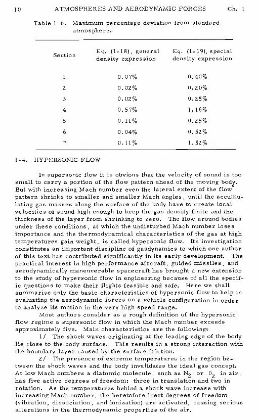
An accurate density function can be obtained by considering theeffects on density of the variation in scale height, H1 / , and mole-cular scale temperature,TM.
The molecular scale temperature accounts for both temperatureand molecular weight changes with altitude.
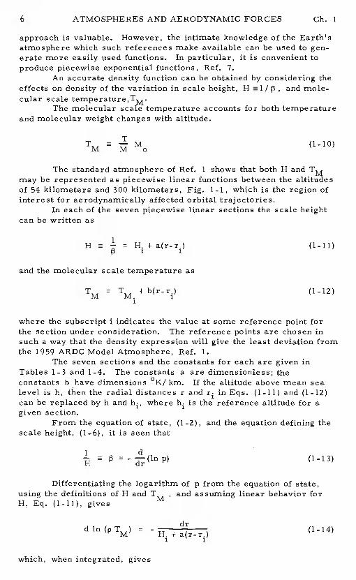
TM M (1-10)
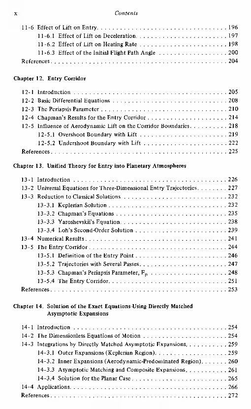
The standard atmosphere of Ref.1 shows that both H and TMmay be represented as piecewise linear functions between the altitudesof 54 kilometers and 300 kilometers, Fig. 1-1, which is the region ofinterest for aerodynamically affected orbital trajectories.
In each of the seven piecewise linear sections the scale heightcan be written as
H = H. + (1-11)
and the molecular scale temperature as
TM = TM. + b(r_r.) (1-12)
where the subscript i indicates the value at some reference point forthe section under consideration.The reference points are chosen insuch a way that the density expression will give the least deviation fromthe 1959 ARDC Model Atmosphere, Ref.1.
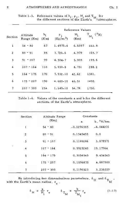
The seven sections and the constants for each are given inTables 1-3 and 1-4.The constants a are dimensionless; theconstants b have dimensions °K/ km.If the altitude above mean sealevel is h, then the radial distances r and r1 in Eqs. (1-11) and (1-12)can be replaced by h and where is the reference altitude for agiven section.
From the equation of state, (1-2), and the equation defining thescale height, (1-6), it is seen that
d= - p) (1-13)
Differentiating the logarithm of p from the equation of state,using the definitions of H and TM ,and assuming linear behavior forH, Eq. (1-11), gives
d in (p TM) = - H. + a(r-r.) (1-14)
which, when integrated, gives
Ch. 1 ATMOSPHERES AND AERODYNAMIC FORCES
PTM H.i/a
inpiTM
)= in
H.+a(r-r1)(1-15)
i
or, what is the same,
r TM ir H 11/a
= +b(r-r) ''H +a(r-r)(1-16)
M JLii
where the linear behavior of TM, Eq. (1-1Z), is assumed.
MOLECULARSCALE TEMPERATURE (K°)0 200 500 1000 1500 2000
I I I I
300 - 60.29 1878/ 300
//
250- ///
49.22 /1577 207w 200 - 4.972
I 4.987I-6.968 40.75 .—'1323 - 64
150
44.11 J1427 - 175
/-II
1230.2 0700
(65.7 — SCALE HEIGHT91
80 - U65.7 —-— MOLECULAR-SCALE 80TEMPERATURE
60 . \28o.21 - 548.3416
I I40o 20 40 60 80 100SCALE-HEIGHT (KM)
Fig. 1-1. The scale height and molecular scale temperatureversus altitude. The values at the endpoints of thesections are noted.
ATMOSPHERES AND AERODYNAMICS Ch. 1
Table 1-3. Reference values of h.p. H. and T for1 i. M.the different sections of the Earth's'atmosphere.
Reference Values
Table 1-4. Values of the constants a and b for the differentsections of the Earth's atmosphere.
Section
1
2
3
4
5
6
7
Altitude Range(Kxri)
54 80
80 91
91 107
107 — 164
164 — 175
175 —207
207 300
6TM
Constants
b, °K/km-4. 044231
0. 0
3. 878571
19. 17964
9.454545
4. 687500
3. 236559
.Section AltitudeRange (Km)
p
(Kg/rn3)H1
(Km)TM
1 54 80 67 1.4975-4 6.6597 222.8
2 80 — 91 85 7. 726-6 4.979 165. 7
3 91 —107 99 4. 504-7 5.905 195.6
4 107—164 110 5. 930-8 8.731 288.2
5 164 —175 170 7.932-10 42.62 1381.
6 175 207 190 4.680-10 46.51 1498.
7 207 300 254 1.149-10 54. 78 1730.
a
-0. 1296385
0. 1545455
0.1189286
0. 5925240
0. 3054545
0.1596875
0.1190323
By introducingwith the Earth's mean
two dimensionless parameters, 8and 6Tradius r Me'
k (1-1 7)
Ch. 1 ATMOSPHERES AND AERODYNAMIC FORCES
one arrives at the basic density equation which takes into account thevariation of scale height and molecular scale temperature:
r ii 1/a= 1
r-r. (1-18)P [1 + 8
TM iLl + 8H r1
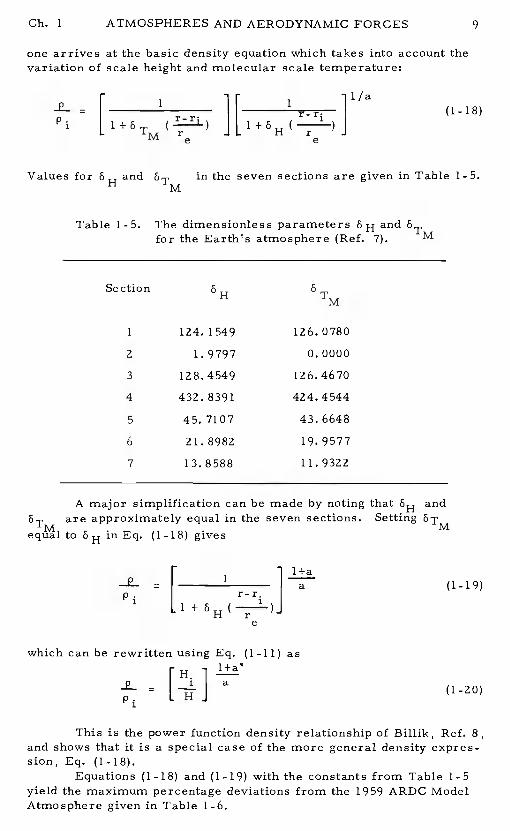
Values forH and 5T in the seven sections are given in Table 1-5.
M
Table 1-5. The dimensionless parameters 5H andfor the Earth's atmosphere (Ref.7). M
Section 6TM
1 124. 1549 126. 0780
2 1.9797 0.0000
3 128.4549 126.4670
4 432.8391 424.4544
5 45.7107 43.6648
6 21.8982 19.9577
7 13.8588 11.9322
A major simplification can be made by noting that 8H and5TM are approximately equal in the Seven sections. Setting
equal to 5H in Eq. (1-18) gives
1+a= 1
a (1-19)p. r-r.
1 l+SH(
which can be rewritten using Eq. (1-11) asrH. 1[1] a (1-20)
This is the power function density relationship of Billik, Ref. 8,and shows that it is a special case of the more general density expres-sion, Eq. (1-18).
Equations (1-18) and (1-19) with the constants from Table 1-5yield the maximum percentage deviations from the 1959 ARDC ModelAtmospheregiven in Table 1-6.
ATMOSPHERES AND AERODYNAMIC FORCES Ch. 1
Table 1-6. Maximum percentage deviation from standardatmosphere.
Eq. (1-18) general Eq. (1-19) specialSection density expression density expression
1 0.07% 0.40%
2 0.02% 0.20%
3 0. 02% 0. 25%
4 0.57% 1.16%
5 0.11% 0.25%
6 0.04% 0.52%
7 0.11% 1.52%
1-4. HYPERSONIC FLOW
In supersonic flow it is obvious that the velocity of sound is toosmall to carry a portion of the flow pattern ahead of the movingBut with increasing Mach number even the lateral extent of the flowpattern shrinks to smaller and smaller Mach angles, until the accumu-lating gas masses along the surface of the body have to create localvelocities of sound high enough to keep the gas density finite and thethickness of the layer from shrinking to zero.The flow around bodiesunder these conditions, at which the undisturbed Mach number losesimportance and the the rmodynamical characteristics of the gas at hightemperatures gain weight, is called hypersonic flow.Its investigationconstitutes an important discipline of gasdynamics to which one authorof this text has contributed significantly in its early development.Thepractical interest in high performance aircraft, guided missiles, andaerodynamically maneuverable spacecraft has brought a new extensionto the study of hypersonic flow in engineering because of all the specif-ic questions to make their flights feasible and safe.Here we shallsummarize only the basic characteristics of hypersonic flow to help inevaluating the aerodynamic forces on a vehicle configuration in orderto analyze its motion in the very high speed range.
Most authors consider as a rough definition of the hypersonicflow regime a supersonic flow in which the Mach number exceedsapproximately five. Main characteristics are the following:
1/ The shock waves originating at the leading edge of the bodylie close to the body surface.This results in a strong interaction withthe boundary layer caused by the surface friction.
2/ The presence of extreme temperatures in the region be-tween the shock waves and the body invalidates the ideal gas concept.At low Mach numbers a diatomic molecule, such as N2 or 02in air,has five active degrees of freedom: three in translation and two inrotation. As the temperatures behind a shock wave increase withincreasing Mach number, the heretofore inert degrees of freedom(vibration, dissociation, and ionization) are activated, causing seriousalterations in the thermodynamic properties of the air.
Ch. 1 ATMOSPHERES AND AERODYNAMIC FORCES
Such complex phenomena create challenging problems.Earlyreports of their investigations can be found in many specialized texts,such as Refs. 9 and 10.Here we shall be mainly concerned with thepractical importance with respect to determining the forces acting onbodies at hypersonic speeds using the most simplifying assumptions.
1-5. NEWTONIAN FLOW
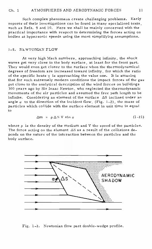
At very high Mach numbers, approaching infinity, the shockwaves get very close to the body surface, at least for the front part.They would even get closer to the surface when the thermodynamicaldegrees of freedom are increased toward infinity, for which the ratioof the specific heats y is approaching the value one.It is amazingthat for such extremely modern conditions the impact forces of the gasget close to the analytical description of the wind forces on buildings300 years ago by Sir Isaac Newton, who neglected the thermodynamicmovements of the air particles and assumed the free path length to beinfinite. Considering an element of the surface AS inclined under anangle a to the direction of the incident flow, (Fig. 1-2), the mass ofparticles which collide with the surface element in unit time is equalto
Am = pASV sine (1-21)
where p is the density of the medium and V the speed of the particles.The force acting on the element AS as a result of the collisions de-pends on the nature of the interaction between the particles and thebody surface.
Fig. 1-Z. Newtonian flow past double-wedge profile.
MIC
ATMOSPHERES AND AERODYNAMIC FORCES Ch. 1
For gases Newton assumed an elastic reflection of the particleson a smooth wall, reversing the normal velocity component V sin awhile retaining the tangential component V cos a .However, for whathe calls a "continuous medium" (water, oil, and mercury), Newtonestimated the normal force to be diminished by one-half, because "thebody does not immediately strike against all particles, but pressesonly the particles that lie next to it, which press the particles beyond,which press other particles and so on.This value is exactly theresult for M -. and 1 , when the free path is small and nothermodynamical particle movements existed before the collision withthe body (M = oo) nor would be created at the collision by the energyloss according to the disappearing velocity component V sin a becauseof the infinite number of degrees of freedom sharing its heat equivalent(y = 1). Dropping simply the normal velocity component V sin a duringthe collision creates a normal force on the surface element
2 .2= Vsina pV sin a (1-22)
Hence we have the Newtonian formula for the pressure coefficient:
C = 2 sin2 a (1-23)p
It was first observed by Lees (Ref. 11), that a substantial improve-ment in the agreement of the Newtonian calculations with experimentaldata for symmetric two-dimensional and axisymmetric flow can beobtained by modifying the formula as
C = sina(1-24)
p p .2Sin a0
where is the value of the pressure coefficient at the leading edgeor nosegf the body, found from the theory of supersonic flow of anideal gas, and a is the angle between the tangent to the body contourand the free- stream direction.For bodies with blunt noses, we haveobviously sin a = 1 while as a function of the Mach number Mpand the ratio of the constant specific heats 'ycan be obtained with theaid of the normal shock relations and the Bernoulli integral as
2 +1 2 +1 1C = —i
I Z'yM-','+l J
For , we have
y/(y-l) 1/('y_l)
= (1±1) (Y..±L) (126)p y 2 2y
If the simple Newtonian impact theory is used, where anystatic pressure and skin friction are neglected, the force on the ele-ment is the impact pressure force.Newton's theory implies
Ch. 1 ATMOSPHERES AND AERODYNAMIC FORCES
that only those frontal surfaces exposed to the flow can contribute tothe aerodynamic force, and pressure forces on rear surfaces in theaerodynamic shadow are negligible, (Fig. 1-2).Now if we divide theforces acting normal on every exposed surface elementinto posi-tive drag components in the direction of the free- stream velocity andlifting components orthogonal to it, then using the simple pressurefrom Eq. (1-23) at the surface element inclined at an angle a withrespect to the incident velocity, we have
(C ) = C sin a = 2 sin a (1-27)pD p
(C ) = C cos a = 2 sin2 a cos a (1-28)pL p
For this simple body or, integrated over the surface of a com-plicated body, Eqs. (1-27) and (1-28) give the drag and lift coefficients,CD and CL, respectively.
1-6. THE DRAG POLAR
On the basis of the simple formulas derived from Newton im-pact theory, we can determine the hypersonic aerodynamic character-istics of wedges or cone-like bodies when a high degree of accuracyis not required.
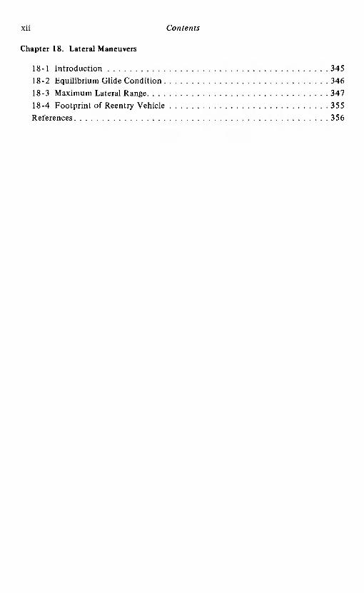
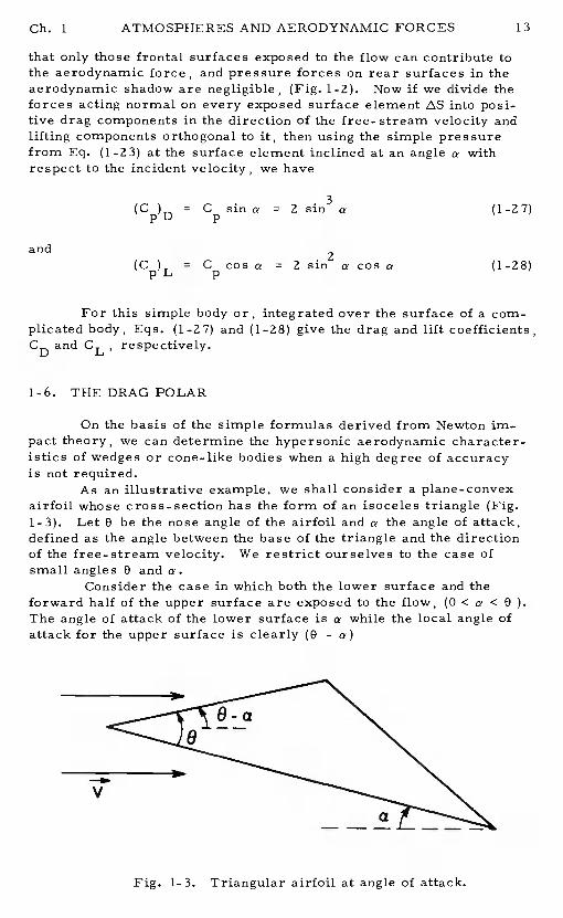
As an illustrative example, we shall consider a plane_convexairfoil whose cross-section has the form of an isoceles triangle (Fig.1-3). Let e be the nose angle of the airfoil and a the angle of attack,defined as the angle between the base of the triangle and the directionof the free-stream velocity. We restrict ourselves to the case ofsmall angles 0 and a.
Consider the case in which both the lower surface and theforward half of the upper surface are exposed to the flow, (0 <a < 0 ).The angle of attack of the lower surface is a while the local angle ofattack for the upper surface is clearly (0- a)
and
3
V
a
Fig. 1-3. Triangular airfoil at angle of attack.
ATMOSPHERES AND AERODYNAMIC FORCES Ch. 1
The lower surface is a flat plate at an incidence a. The liftand drag coefficients are respectively
CL = 2a2
CD = 2a3 (1-29)
The total lift and drag coefficients for the airfoil are evaluatedusing the area of the lower surface as a reference area.Since thefront area of the upper surface is practically equal to half of the areaof the lower surface for small B, the contributions of the lift and dragcoefficients from the upper surface, considered as a flat plate at anincidence (0 - a), are
CL = -(0-a2
C = (0 - a)3 (1-30)
The total lift and drag coefficients for the complete airfoil are found bysimply adding the separate contributions of the individual surface, aslong as 0< a < B
CL = 2a2 - (0 - a)2(1-31)
CD = 2a3 + (0 - a)3
In hypersonic flow, a useful small parameter i-, called the thicknessratio of the body, is defined as the maximum value of the angle between
surface of the forward portion of the body and the free- streamdirection. Here, we define 0/2 , and write the Eqs. (1-31)
= (2-i)T (1-32)
C 3= 2(s)
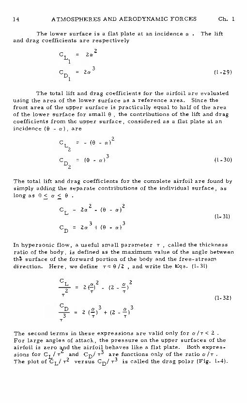
The second terms in these expressions are valid only for a/T < 2For large angles of attack, the pressure on the upper surfaces of theairfoil is zero the airfoil behaves like a flat plate.Both expres-sions for CL! T and CD! are functions only of the ratio a /TThe plot of CL! T2 versus CD! is called the drag polar (Fig. 1-4).
Ch. 1 ATMOSPHERES AND AERODYNAMIC FORCES 15
10 -
c'J
-J0
0
-50 0 20 30
CD Ir
Fig. 1-4. Drag polar for triangular airfoil in hypersonicflow.
1-7. THE BUSEMANN FORMULA
For the case of a flow over a wedge or axisymmetric cone, thegas particles move along straight lines in an infinitely thin layer adja-cent to the surface in which the density of the gas is infinitely large.The pressure on the surface of the wedge and cone coincides with thepressure behind the shock wave and is determined by the Newtonianformula
2.2p p1V sin (1-33)
with subscript 1 denoting the free- stream condition.On a curvedbody, a particle is constrained within the continuum flow in the shocklayer to follow a curved path and the forces required to curve the tra-jectories of the particles must be taken into consideration.Theresult is a pressure difference across the shock layer equal to themomentum flow in the layer times the curvature of the layer.Theinclusion of this centrifugal force was first proposed by Busemann whogave formulas for the correction (Ref. 12, pp. 276-277).
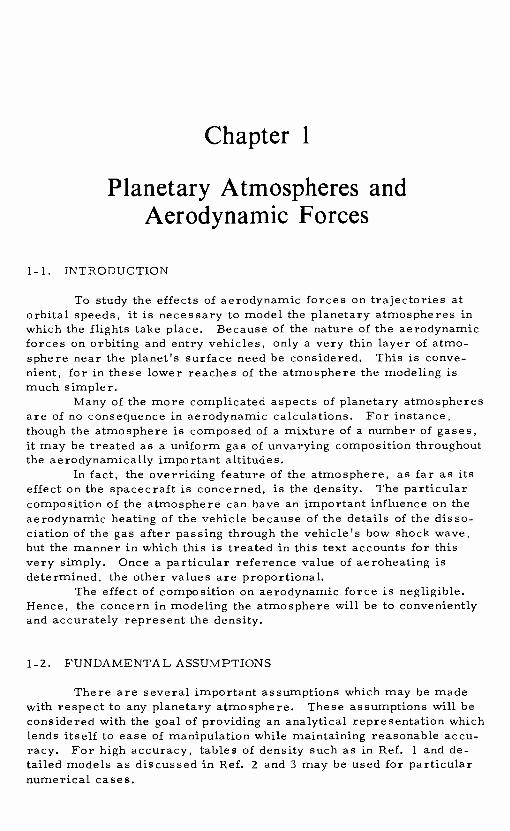
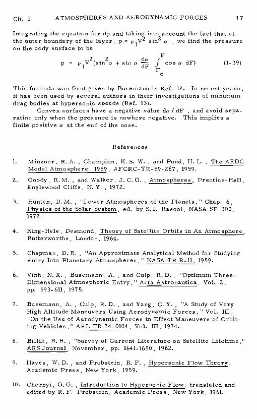
Based on the assumptions of inelastic collisions,= 1 , andthe absence of frictional forces, we may assume that the speed of eachparticle remains unchanged after its collision with the surface and thatthe particles move along the geodesic lines of the surface.Underthis assumption, we refer to Fig. 1-5 for the evaluation of the pres-sure difference in the layer for two-dimensional and axisymmetricflows.
Let us follow the motion of the particles along the surface ofthe body after collision. These particles move within an infinitelythin layer depicted in the figure by the body contour and the dashed
I I
ATMOSPHERES AND AERODYNAMIC FORCES Ch. 1
line. At the point x , measured along the body contour, the pressuredifference dp in the infinitesimal layer composed of particles whichhave collided with the surface near the point and which have thevelocity u(x!) , is equal to
dpp(x,xT)u2(xl)
dnR(x) (1-34)
where R(x) is the radius of curvature of the body at the point x, anddn the thickness of the infinitesimal layer of the deviated gas particles,evaluated along the outward normal to the surface.
Let F be the cross-sectional area of the body in a plane normalto the direction of the free-stream flow.By consideration of theconservation of mass in the layer, we have
R = - = - (1-36)da sina da
dadp = - p1V sin a u(x ) dF(x') (1-37)
= u(x') i(x) dn
V
— —
R(x)
(1-3 5)
u (x)
Fig. 1-5. Curved trajectories of gas particles aftercollisions.
For two-dimensional flow, I (x) = 1 , and for axisymmetric flowI (x) = 2ir r(x) where r is the radial coordinate for the body of revolu-tion.
The radius of curvature R(x) of the body at the point x is
Using Eqs. (1- 35) and (1- 36) in Eq. (1-34), we obtain
Since the velocity component of a particle tangential to the body surfaceis unaltered by the collision, u(x') =V cos [a (x')] . Hence,
dp = - p1 sin a Cos a(xT) dF(x') (1-38)
Ch. 1 ATMOSPHERES AND AERODYNAMIC FORCES
Integrating the equation for dp and into account the fact that atthe outer boundary of the layer, p =p sin2 a , we find the pressureon the body surface to be
Fp = p1V2(sin2a + sin a fcos a dF) (1-39)
This formula was first given by Busemann in Ref. 12.In recent years,it has been used by several authors in their investigations of minimumdrag bodies at hypersonic speeds (Ref. 13).
Convex surfaces have a negative value da /dF , and avoid sepa-ration only when the pressure is nowhere negative.This implies afinite positive a at the end of the nose.
References
1. Minzner, R. A. , Champion, K. S. W. , and Pond, H. L. , The ARDCModel Atmosphere, 1959, AFCRC-TR-59-267, 1959.
2. Goody, R.M. , and Walker, J.C.G. ,Atmospheres, Prentice-Hall,Englewood Cliffs, N. Y. , 1972.
3. Hunten, D.M. , "Lower Atmospheres of the Planets," Chap. 6,Physics of the Solar System, ed. by S. I. Rasool, NASA SP- 300,1972.
4. King-Hele, Desmond, Theory of Satellite Orbits in An Atmosphere,Butterworths,London, 1964.
5. Chapman,D. R. , "An Approximate Analytical Method for StudyingEntry Into Planetary Atmospheres, "NASA TR R-ll, 1959.
6. Vinh, N.X., Busemann, A., and Cuip, R.D. , "Optimum Three-Dimensional Atmospheric Entry," Acta Astronautica, Vol. 2,pp. 593-611, 1975.
7. Busemann, A. ,Gulp, R.D. ,and Yang, C.Y. ,"A Study of VeryHigh Altitude Maneuvers Using Aerodynamic Forces," Vol. III,"On the Use of Aerodynamic Forces to Effect Maneuvers of Orbit-ing Vehicles," ARL TR 74-0104, Vol. III, 1974.
8. Billik, B. H. , "Survey of Current Literature on Satellite LifetimeARS Journal, November, pp. 1641-1650, 1962.
9. Hayes, W.D. ,and Probstein, R.F. ,Hypersonic Flow Theory,Academic Press, New York, 1959.
10. Chernyi, G. G. ,Introduction to Hypersonic Flow, translated andedited by R. F. Probstein, Academic Press, New York, 1961.
ATMOSPHERES AND AERODYNAMIC FORCES Ch. 1
11. Lees, L. ,Hypersonic Flow, Proc. 5th International AerodynamicsConference, Los Angeles.Institute of Aerospace Sciences, NewYork, 1955.
12. Busemann, A. ,Flüssigkeits-und-Gasbewegung, Handwt5rterbuchder Naturwissenschaften,Vol. IV, 2nd Edition, pp. 244-279,GustavFischer, Jena, 1933.
13. Miele, A. , Editor, Theory of Optimum Aerodynamic Shapes,Academic Press, New York, 1965.
Chapter 2
Equations for FlightOver a Spherical Planet
2-i. INTRODUCTION
In this chapter we shall derive the equations of motion of a ve-hicle considered as a point mass of mass m flying inside a planetaryatmosphere. The motion of the vehicle is defined by
= position vectorV(t) = velocity vector (2-1)
m(t) = mass
At each instant, it is subject to a total force F composed of thetational force mg , the aerodynamic force A and a thrusting force Tprovided by the propulsion system.
F T +A + mg (a-a)
With respect to an inertial system, we have the vector equation
F (2-3)
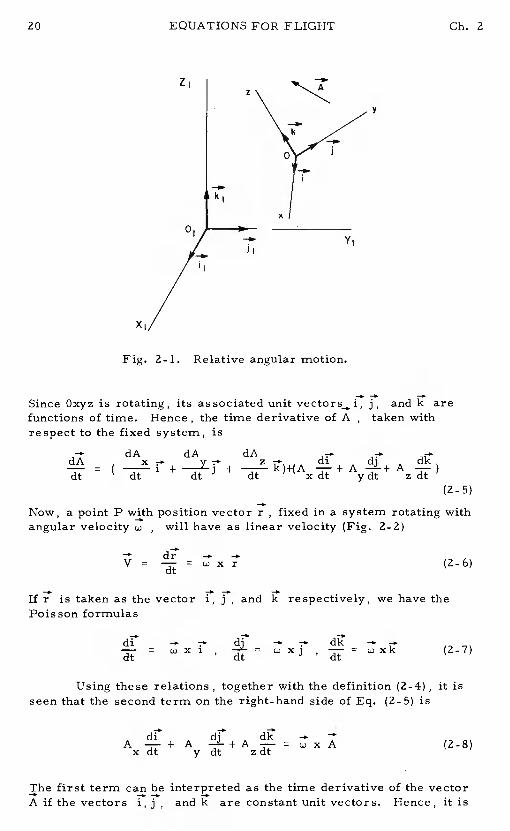
2-2. RELATIVE ANGULAR MOTION
Consider a fixed system 0 X1Y1Z, and another system Oxyzwhich is with respect to fixed1 system.
Let i, j , and k be the unit vectors along the axes of the
rotating system. Let A be any arbitrary vector with components Aand along the rotating axes.Then
A=A j+AIc (2-4)x y z
19
dA — dA
+ + + A Adt ydt zdt
—V = = x r
A + A + A = x Axdt y dt zdt
ZI
Oi
ii
Yl
XI
EQUATIONS FOR FLIGHT Ch. 2
y
Fig. 2-1. Relative angular motion.
Since Oxyz is rotating, its associated unit j, and k arefunctions of time. Hence, the time derivative of A ,taken withrespect to the fixed system, is
— dAdA x—
=
(2.5)
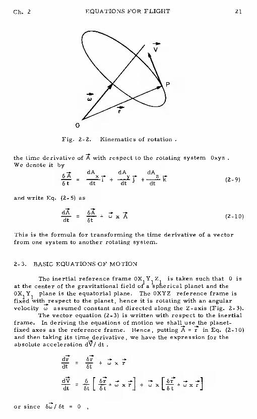
Now, a point P with position vector r, fixed in a system rotating withangular velocity o , will have as linear velocity (Fig. 2-2)
(2-6)
If is taken as the vector J, and respectively, we have thePoisson formulas
dl' —' -= dt ,
(2.7)
Using these relations, together with the definition (2-4) ,it isseen that the second term on the right-hand side of Eq. (2-5) is
(2-8)
The first term can be interpreted as the time derivative of the vectorA if the vectors i, j , and k are constant unitvectors. Hence, it is
0
Fig. 2-2. Kinematics of rotation
the time derivative of A with respect to the rotating system OxyzWe denote it by
- dA dA- 1 + dt
dAz
+ k
and write Eq. (2-5) as
=(2-10)
This is the formula for transforming the time derivative of a vectorfrom one system to another rotating system.
2-3. BASIC EQUATIONS OF MOTION
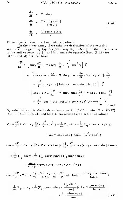
The inertial reference frame OX Y1Z is taken such that 0 isat the center of the gravitational fieldof1 a planet and the0X1Y1 plane is the equatorial plane.The OXYZ reference frame isfixed with respect to the planet, hence it is rotating with an angularvelocity .ü assumed constant and directed along the Z-axis (Fig. 2-3).
The vector equation (2-3) is written with respect to the inertialframe. In deriving the equations of motion we shall use the planet-fixed axes as the reference frame.Hence, putting A r in Eq. (2-10)and then taking its timederivative, we have the expression for theabsolute acceleration dV/ dt
dr ôr -=
+ x r
Ch. 2 EQUATIONS FOR FLIGHT
P
(2-9)
dv — —1 — Ioi' — —=
L+ w x rJ + + X r
or since öt = 0
52;
St
EQUATIONS FOR FLIGHT Ch. 2
dv 52r -. Sr -. -. — (2-11)
The vector equation (2-3) now becomes, with the planet-fixed systemusedas the reference frame,
F - 2mw x - mw x (w xr) (2-12)
For convenience, we change the notation for the time derivative andwrite it as
= F-Zmwx (2-13)
with V being the velocity with respect to the planet, and the timederivative taken with respect to planet-fixed axes.
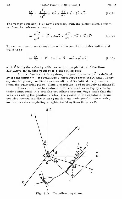
In this planetocentric system, the position vector r is definedby its magnitude r, its longitude 0 (measured from the X-axis, in theequatorial plane, positively eastward), and its latitude(measuredfrom the equatorial plane, along a meridian, and positively northward).
It is convenient to evaluate different vectors in Eq. (2-13) bytheir components in a rotating coordinate system Oxyz such that thex- axis is along the position vector, the y- axis in the equatorial planepositive toward the direction of motion and orthogonal to the x- axis,and the z-axis completing a right-handed system (Fig. 2-3).
z
z
V
•1'
x
x
Fig. 2-3. Coordinate systems.
Ch. 2 EQUATIONS FOR FLIGHT
Let be the angle between the local horizontal plane (that is,the plane passing through the vehicle and orthogonal to the vectorand the velocity V . The angle y is termed the flight path angle and ispositive when V is above the horizontal plane.Let Lj be the anglebetween the local parallel of latitude and the projection of V on thehorizontal plane. The angle is termed the heading and is measuredpositively in the right-handed direction about the x-axis.Let i,j, andk be the unit vectors along the axes of the rotating system Oxyz .Wehave
r = ri (2-14)
and
V = (Vsiny)r+ (Vcosycos4i) (2-15)
On the other hand, the angular velocitycan be represented by
= sink) r + (2-16)
Hence
cdxV = - i _cosysin4, sini4.)r
(2-17)
and— -. — 2 2 — 2
= -w r cos i +w r sin4, cos4 k (2-18)
In the force F, the gravity force is simply
mg = - mg(r) i (2-19)
The aerodynamic force Acan be decomposed into a drag forceD opposite to the velocity vector V and a lift force L orthogonal to it.In symmetric flight the thrust vector T is always in the lift- dragLet c be the angle between the velocity vector V and the thrust T.Then, we can decompose the thrust into a component T cos Ealong thevelocity and a component T sinE along the lift force.It is convenientfor the derivation of the equations to group the components of aerody-namic and propulsive force and define
FT = T cos E - D
FN = TsinE +L (2-20)
where F1 is the component of the aerodynamic and propulsive forcesalong the velocity vector and FN is their component orthogonal to it inthe lift-drag plane. In vector form, since FT is along V ,we canrefer to Eq. (2-15) to write
= 1 + + k (2-21)
EQUATIONS FOR FLIGHT Ch. 2
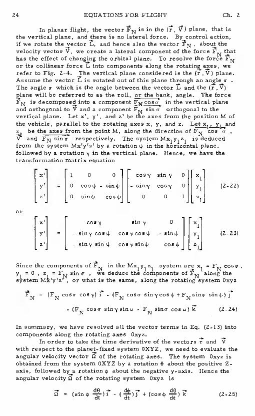
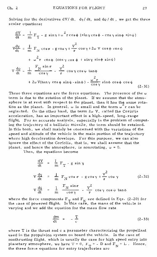
In planar flight, the vector FN is in the plane, that isthe vertical plane, and there is no lateral force.By control action,if we rotate the vector L, and hence also the vector FN ,about thevelocity vector V, we create a lateral component of the force FN thathas the effect of changing the orbital plane.To resolve the force FNor its collinear force L into components along the werefer to Fig. 2-4. The vertical plane considered is the (r, V) plane.Assume the vector L is rotated out of this plane through anThe angle which is the angle between the vector L and the (r ,V)plane will be referred to as the roll, or the bank, angle.The forceFN is decomposed into a component FN coso-in the vertical planeand orthogonal to V and a component FN orthogonal to thevertical plane. Let y' , and z' be the axes from the position M ofthe vehicle, parallel to the rotating axes x, y, and z.Let
be the axes from the point M, along the direction of FN cosa-
V and FN sin a- respectively. The system Mx1y1z1is deducedfrom the system MxIy?zI by a rotation in the horizontal plane,followed by a rotation in the vertical plane. Hence, we have thetransformation matrix equation
1 0 0 cos'j 0 x1
y' = 0 cos4i - sin4i - siny cosy 0 y1 (2-22)
z1 0 sin4i cos4i 0 0 1 z1
orcosy 0 x1
= - siny cos i4 cosy cos - y1 (2-23)
zi - siny sin4i cosysini4i cos4 z1
Since the components of FN in the Mx1y1z1 system are x1 =FNy1 = 0 , z1 = sin a- , we deduce the components of FN along thesystem MxTylz , or what is the same, along the rotating system Oxyz
FN = (FN cosa- cosy) i0- (FN cosa- +FNsina- f'
- (FN coso- sinysin4i -FN sino- cos4i) Ic (2-24)
In summary, we have resolved all the vector terms in Eq. (2-13) intocomponents along the rotating axes Oxyz.
In order to take the time derivative of the vectors r and Vwith respect to the planet-fixed system OXYZ, we need to evaluate theangular velocity vector of the rotating axes.The system Oxyz isobtained from the system OXYZ by a rotation 9 about the positive Z.axis, followed bya rotation about the negative y-axis.Hence theangular velocity of the rotating system Oxyz is
. dO—..= - dt
)j + (cos4 ..)k (2-25)
Ch. 2 EQUATIONS FOR FLIGHT 25
0y
Fig. 2-4. Aerodynamic forces and thrust components.
We use Eqs. (2-7) with instead of to deduce the time derivativeofr, j, andk
d dO
dt dt
. — dO dO -.dt
xj = - (cos j i + (sin4 k (2-26)
dk — dO= = j
If we take the time derivative of r, as given by Eq. (2-14), using thefirst of the Eqs. (2-26) for the derivative of i we have
dr= ( 1 + (r j + (r dt ) k (2-27)
Identifying this equation with Eq. (2-15) yields three scalar equations
VERTICALPLANE
H OR ZON TA LPLANE
y,
EQUATIONS FOR FLIGHT Ch. 2
dr= V sin'1
= V cos cos (2-28)dt
-dt -
These equations are the kinematic equations.On the other hand, if we take the derivative of the velocity
vector V , as given by Eq. (2-15), using Eqs. (2-26) for the derivativesof the unit vectors i , j , and k , and subsequently Eqs. (2-28) fordO/dt and d4/dt, we have
dv F. dV V2 2= + Vcosy dt
- —cos YJ 1
I dV . .
+ - V cos4idt
- Vcosy
+ cos'lcosij.(sin'l -
I . dV . . d+ - V dt + V cos'1 cosL)J dt
+ cos + cos2 kr (2-29)
By substituting into the basic vector equation (2-13), using Eqs. (2-17),(2-18), (2-19), (2-21) and (2-24), we obtain three scalar equations
dV V2 2 1 . 1COS'1 dt - 51fl'1 +_FN C051T CO5'1- g
+ 2w V
cos tan -
1 1
= FT cos'y coso sln'1+FNslna
-sin4i)
+
F sina-1 1 . N cos'1s1n4=—F -—(F coso- )- 2w Vm T m N tan4 taniji
- w 2r cos(2- 30)sin
Ch. 2 EQUATIONS FOR FLIGHT 27
Solving for the derivatives dv! dt, dt, and d4 /dt , we get the threescalar equations:
= - g -cos'jsin4
V
cos +
V = - — cosycos4 tan4dt m cosy r2
+ cos4,- C (2-31)
These three equations are the force equations.The presence of theterm is due to the rotation of the planet.If we assume that the atmo-sphere is at rest with respect to the planet, then it hassame rota-tion as the planet. In general, w is small and the termr can beneglected. On the other hand, the termV, called the Coriolisacceleration, has an important effect in a high-speed, long-rangeflight. For an accurate analysis, especially in the problem of comput-ing the trajectory of a ballistic missile, the term should be retained.In this book, we shall mainly be concerned with the variations of thespeed and altitude of the vehicle in the main portion of the trajectorywhere high deceleration develops.For this purpose, we can alsoignore the effect of the Coriolis, that is, we shall assume that theplanet, and hence the atmosphere, is nonrotating, u =0.
Then, the equations become
dV 1= —F-gsiny
v dt = — FN cos a- - gcosy +— cos y (2-32)
V = — - — cosydt m cosy r
where the force components Fand FN are defined in Eqs. (2-20) forthe case of powered flight. case, the mass of the vehicle isvarying and we add the equation for the mass flow rate
= _i (2-33)dt c
where T is the thrust and c a parameter characterizing the propellantused in the propulsion system on board the vehicle.In the case ofnonthrusting flight, which is usually the case for high speed entry intoplanetary atmosphere, we have T =0, = - D and FN = L . Hence,the three force equations for entry trajeclories are
EQUATIONS FOR FLIGHT Ch. 2
dV D
= L COS - g cos y + cos (2-34)
Lsino VV = - — cos y cos tan $dt mcosy r
References
1. Lass, H., Vector and Tensor Analysis, McGraw-Hill Book Co.,Inc. , New York, 1950.
2. Busemann, A. , Vinh, N. X., andGulp, R. D., Solution of the
Exact Equations for Three-Dimensional Atmospheric Entry UsingDirectly Matched Asymptotic Expansions, "NASA CR-2643, 1976.
3. Greenwood, D. T., Principles of Dynamics, Prentice-Hall, Inc.,Englewood Cliffs, New Jersey, 1965.
Chapter 3
Performance in Extra-Atmospheric Flight
3-1. INTRODUCTION
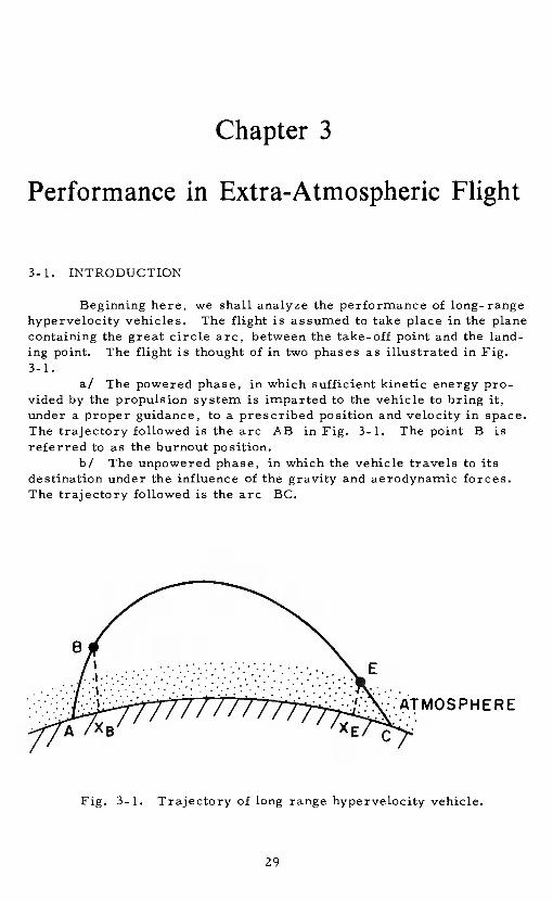
Beginning here, we shall analyze the performance of long-rangehypervelocity vehicles. The flight is assumed to take place in the planecontaining the great circle arc, between the take-off point and the land-ing point. The flight is thought of in two phases as illustrated in Fig.
a/ The powered phase, in which sufficient kinetic energy pro-vided by the propulsion system is imparted to the vehicle to bring it,under a proper guidance, to a prescribed position and velocity in space.The trajectory followed is the arc AB in Fig. 3-1.The point B isreferred to as the burnout position.
b/ The unpowered phase, in which the vehicle travels to itsdestination under the influence of the gravity and aerodynamic forces.The trajectory followed is the arc BC.
B'I . E
HERE
Fig. 3-1. Trajectory of long range hypervelocity vehicle.
29
EXTRA ATMOSPHERIC FLIGHT Ch. 3
The powered phase is generally short, and the correspondinglongitudinal range during launch,XE , is small compared to theradius of the Earth.Hence, the trajectory can be analyzed using theflat Earth assumption.This is done in Chapter 4.For a short rangeflight, the unpowered phase is performed entirely in the dense layer ofthe atmosphere.For long range flight,if the total energy imparted tothe vehicle at the burnout position B is sufficiently high, with a properorientation of the burnout velocity, the trajectory followed will have aportion entirely outside the dense layer of the atmosphere.This por-tion of the trajectory is represented by the arc BE in Fig. 3-1.Thecorresponding contribution to the range,(XE - XB) , may be large.This is one of the most interesting features in hypersonic flight.Forlong-range operation, hypervelocity vehicles may reduce the cost infuel consumption since the range (XE- XB) can be made infinite withfinite energy input. In this respect, Sãnger and Bredt were among thefirst to recognize the favorable connection between speed and range(Ref. 1). The idea leads to the concept of present-day shuttle vehicleswhere, after the powered phase, the subsequent trajectory is entirelyflown outside the atmosphere for several days and the required missionis accomplished without additional energy input.When it comes timeto return to the Earth a rocket may be fired to deflect the trajectorysuch that it intersects the atmosphere of the Earth at a certain pointE called the entry position.The subsequent trajectory is called thereentry trajectory. This portion of the trajectory is illustrated by thearc EC in Fig. 3-1.
In this chapter, we shall be concerned with the eXtra-atmo-spheric portion of the flight trajectory, namely the arc BE. Weshall assume that space is completely free of atmosphere.Hence,from classical orbital mechanics, the trajectory is a Keplerian conic.The reentry phasewill be analyzed in subsequent chapters.
3-2. THE TRAJECTORY EQUATION
In the plane of motion, the position of the vehicle, consideredas a point mass represented by the point M ,is defined in polar coor-dinates by its radial distancer from the center of the Earth 0, andthe angle 0 between the vectors 5ffand öTh (Fig. 3-2). With theaerodynamic force neglected, the vehicle is subject only to the gravi-tational attraction which, for a spherical earth, is directed towardthe center owith a force per unit mass
F= - (3-1)m 2
r
where m is the mass of the vehicle, and a positive constant
Is = Gm (3-2)
me is the mass of the Earth and G a universal constant. This yields
a value of i for Earth:
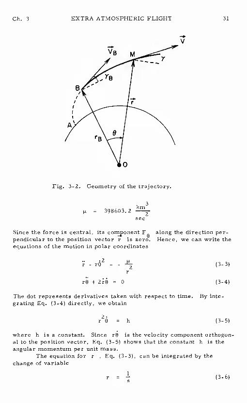
Fig. 3-2. Geometry of the trajectory.
= 398603.2sec
Since the force is central, its F0 along the direction per-pendicular to the position vector ris zero. Hence, we can write theequations of the motion in polar coordinates
.2r-rO = -
rO + 2r0 = 0 (3-4)
The dot represents derivatives taken with respect to time.By inte-grating Eq. (3-4) directly, we obtain
r2e = h (3-5)
where h is a constant.Since rO is the velocity component orthogon-al to the position vector, Eq. (3-5) shows that the constant h is theangular momentum per unit mass.
The equation for r , Eq. (3-3), can be integrated by thechange of variable
r=! (3-6)
Ch. 3 EXTRA ATMOSPHERIC FLIGHT 31
-0V
)9
A,'
0
2r(3-3)
EXTRA ATMOSPHERIC FLIGHT Gb. 3
Using 0 as the new independent variable to replace the time gives
drdO d 1 0 dsr = = 0 (—) = - (3-7)
Since, from Eqs. (3-5) and (3-6)
B hs2 (3-8)
we can write Eq. (3-7) as
(3-9)
Therefore,2 2ds dO ZZdsr = - h = - h s (3-10)
dO dO
Making these substitutions into Eq. (3-3) we obtain the linear equationin S
a
+ s = (3-li)do2 h2
The general solution of this equation is
s = —s- + cos (0-0 ) (3-12)h2
where C and 0 are two constants of integration.Returning to thevariable r , we write
r= 1 + e (0- (3-13)
where by definition
p (3-14)
and
e (3-15)
Equation (3-13) represents a family of conic sections.The center ofattraction 0 is a common focus for the family.The dimensionlessparameter eis called the eccentricity of the conic, and the parameterp , which has the dimension of length, is the semilatus rectum, or theconic parameter.The polar equation involves three constants,p , e
and 00. These constants are specified by the values of the radialdistance rB ,the speed VB and the flight path angle at the burn-
Ch. 3 EXTRA ATMOSPHERIC FLIGHT 33
out position B . The flight path angle along the trajectory is mea-sured positive upward from the local horizontal to the velocity vectorV.
3-3. CHARACTERISTIC VALUES OF A TRAJECTORY
Once the initial values rB, V and are specified, thetrajectory followed by the vehicle is wee-determined.With eachtrajectory, there are associated a number of characteristic valueswhich are constants of the motion.In this section, we shall definethese values and interpret their physical meanings.
First, using Eq. (3-5), we rewrite Eq. (3-3) as
1. = - J±. (3-16)
Multiplying the equation by , we have
or equivalently
=Zdt 2 dtrr
2 2. 2By integrating and replacing hby (r 0) , we obtain
+ -=
(3-17)
where & is a constant of integration.If V is the radial componentand V0 the transverse component of the vefocity,Vr = andV0 = r0 , and
V2 = V2 + V 2 = .2+ (rÔ)2 (3-18)
Hence Eq. (3-17) can be written as
+ v2- r (3-19)
At each point along its trajectory, the vehicle has, per unit mass, akinetic energy equal to(l/ 2) V2and a potential energy from which isderived the gravitational force.Since the gravitational force per unitmass has the magnitude p/ r2, the potential energy at a distanceris - r , if we select the level of the potential energy such that it
34 EXTRA ATMOSPHERIC FLIGHT Ch. 3
has the value zero at infinity.Heoce, relation (3-19) states that thetotal energy per unit mass, along the trajectory, is constant.Theequation is called the energy integral or the vis-viva integral.
Next, by a rotation of the direction of reference, we cao make= 0 and e > 0 in the polar equation (3-13) for the trajectory.
Hence we consider
pr =1 + e cos 0 (3-20)
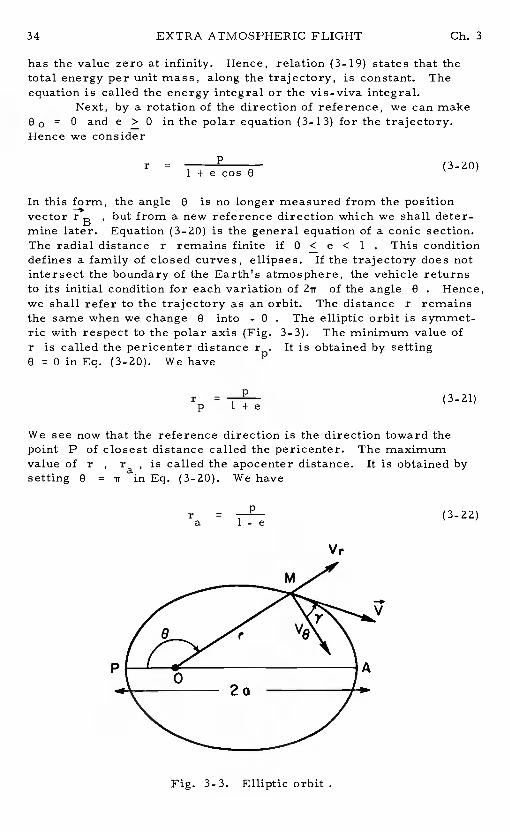
In this form, the angle0 is no longer measured from the positionvector rB but from a new reference direction which we shall deter-mine later. Equation (3-20) is the general equation of a conic section.The radial distance r remains finiteif 0 C e C 1 . This conditiondefines a family of closed curves, ellipses.If the trajectory does notintersect the boundary of the Earth's atmosphere, the vehicle returnsto its initial condition for each variation of Zrof the angle 0 . Hence,we shall refer to the trajectory as an orbit.The distancer remainsthe same when we change0 into - 0 . The elliptic orbit is symmet-ric with respect to the polar axis (Fig. 3-3).The minimum value ofr is called the pericenter distance r. It is obtained by setting0 = 0 in Eq. (3-20). We have
r =p l+e (3-21)
We see now that the reference direction is the direction toward thepoint P of closest distance called the pericenter.The maximumvalue of r , ra , is called the apocenter distance.It is obtained bysetting 0 = r in Eq. (3-20). We have
r =a 1-e
Fig. 3-3. Elliptic orbit
(3-2 2)
-eV
Ch. 3 EXTRA ATMOSPHERIC FLIGHT 35
The point of farthest distance, the point A, is called the apocenter.For the Earth, the point P and the point A are also called the peri-gee and the apogee, respectively.They are the apses of the ellipticorbit, and the line joining P and A is called the line of apses.Thedistance Za between the apses is defined as the major axis of theellipse. Hence
p p Zp2a = r + r = + — = (3-23)p a 1+e l-e (l-e2)
This gives the relation for the semi-latus rectum
p = a(1 - e2) (3-24)
Therefore, in terms ofa and e , the expression for r and r canbe written as p a
r = a(l - e), ra = a(1 + e) (3-25)
Now, by taking the derivative of Eq. (3-20), we have
— pesinO d8- 2 dt(1 + e case)
Using Eqs. (3-5) and (3-20) and noticing that Vr = , we have
V = — e sine (3-26)r p
On the other hand, in evaluatingV0 = r0 , we have
hV = — (1+ecos0) (3-27)
0 p
The Eqs. (3-26) and (3-27) give the expressions for the radial andtransverse components of the velocity along the orbit as functions ofthe polar angle. The magnitude of V is given by Eq. (3-18) writtenas
V tJi + e2 + Ze cos 0 (3-28)
Since h2 = by Eq. (3-14), using the relation (3-24) we can rewritethis expression as
V =2
+ e2 + 2e cos 0 (3-29)a(1 - e
This equation gives the magnitude of the velocity along the orbit as afunction of 0 . It passes through a maximum at the pericenter,
36 EXTRA ATMOSPHERIC FLIGHT Ch. 3
0 = 0 , and a minimum at the apocenter,0 = . We have
v = / ,
= - e) (3-30)a(1-e) a Va(l+e)
The flight path angle at each point along the orbit is given by
siny = , cos y = , tany = (3-31)
Hence, using the Eqs. (3-26) - (3-28), we have
esinO l+ecos0siny = , cosy =
+ e2 + 2e cos 0 + e2 + Ze cos 0
e sinOtany = (3-32)1 + e cos 0
If we use r = , and V = VP to evaluate the constant energy 8inthe vis-viva integral, (3-19), we have
& = -—a- (333)2a
This shows that the total energy of the orbit is a function solely of themajor axis. With this value for t we rewrite the energy integral
= (2 1) (334)
This very important relation expresses the speed along the ellipticalorbit in terms of the radial distancer
We have defined the elliptic orbit as an orbit with an eccentricitysuch that 0 < e < 1 . The two limiting cases are the cases wheree=0 , and e 1.
When e = 0 , the Eq. (3-20) shows that the radial distance isconstant. The orbit is circular. From the Eqs. (3-26) and (3-27)with e = 0 , we see that the radial component of the velocity is zero,while the normal component of the velocity is constant.This compon-ent, which is tangential to the circular orbit, is called the circularspeed. The circular speed can also be obtained from Eq. (3-34) byputting a = r . Thus,
V . = (3-35)dr V r
The other limiting case is obtained by making e —1 . FromEq. (3-23), we see that, holding the semilatus rectum pconstant,
Ch. 3 EXTRA ATMOSPHERIC FLIGHT 37
when e 1 , the major axis of the ellipse tends to infinity.We saythat in the limiting casee = 1 , the orbit is a parabola. The equa-tion of the conic, Eq. (3-20) ,with e = 1 , becomes
r= 1 + cosO
= p2o
(3-36)2cos
The closest distance is obtained forB = 0
r = (3-37)p 2
The farthest distance, when 0= , is infinite. Since the trajectoryhas an infinite branch, the vehicle along a parabolic flight path escapesto infinity, though it takes infinite time.For this reason, the speedalong a parabolic trajectory is called the escape speed. From Eq.(3-34) we see in the limiting case, when a , the escape speed is
V = (3-38)escape r
It is obvious that, at any distancer , the condition for a circularorbit is that Eq. (3-35) holds, together with the condition that the direc-tion of the velocity is perpendicular to the position vector.In contrast,for a parabolic orbit, condition (3-38) is necessary and sufficient.
Now Eq. (3-5) can be written
A = h (339)
The quantity A is called the areal velocity.It represents the rate atwhich the position vector sweeps out area.We see that this rate isconstant for a given orbit.For an elliptic orbit, if we integrate theequation over a full period T we obtain
= = Areaof ellipse (3-40)
But from the Eqs. (3-14) and (3-24)
h = = (3-41)
Therefore the period is
T = (3-42)
Just as is the energy , the period, T , in elliptical motion is afunction solely of the major axis.
38 EXTRA ATMOSPHERIC FLIGHT Ch. 3
3-4. TIME OF FLIGHT ALONG THE ORBIT
Consider the Eq. (3-39) written as
dt = r2 dO (3-43)
Using the polar equation (3-20) forr , we have the time of flight fromthe pericenter to a position M defined by the polar angle9
2 9 2r dO - p
— h 2 — 23/20 (l+ecos9) h(l-e
or
t = 5(0) (3-44)
where the function S(0) is given by
S(0)= e 0 + 2 arc tan tan (3-45)
Let M1 and M2 be two points along the orbit with polar angle0
and 02
The time of flight for the vehicle to travel the arc M1M2 is
- t1 [S(o2) - S(01)J (3-46)
Using Eq. (3-42) we can writet2—t
1= [S(e ) - S(0 )] (3-47)
T 2 1
The time of flight along an elliptic orbit can also be obtained by simplegeometric considerations.First we shall give some properties relatedto an ellipse.
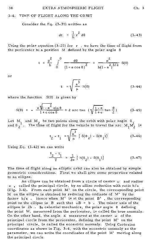
An ellipse can be obtained from a circle of center uand radiusa , called the principal circle, by an affine reduction with ratio b/a(Fig. 3-4). From each point M' on the circle, the corresponding pointM on the ellipse is obtained by reducing the ordinate of M' by thefactor b/a . Hence when M' is at the point B', the correspondingpoint on the ellipse isB such that = b . The minor axis of theellipse is 2b . In celestial mechanics, the polar angle0 definingthe point M, measured from the pericenter, is called the true anomaly.On the other hand, the angle E measured at the centerof theprincipal circle from the pericenter, defining the point M' on theprincipal circle, is called the eccentric anomaly.Using Cartesiancoordinates as shown in Fig. 3-4, with the eccentric anomaly as theparameter, we can write the coordinates of the point M' moving alongthe principal circle
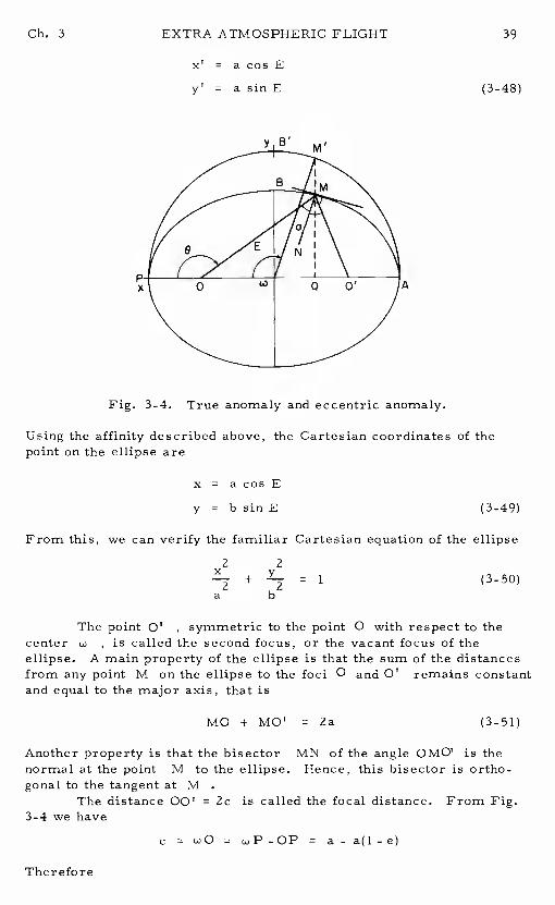
Ch. 3 EXTRA ATMOSPHERIC FLIGHT 39
x' = a cos E
y• = a sinE
Fig. 3-4. True anomaly and eccentric anomaly.
(3-48)
Using the affinity described above, the Cartesian coordinates of thepoint on the ellipse are
x = a cos E
y = b sin E (3-49)
From this, we can verify the familiar Cartesian equation of the ellipse2 2
x y
a b(3-50)
The point 0' , symmetric to the point 0with respect to thecenter , is called the second focus, or the vacant focus of theellipse. A main property of the ellipse is that the sum of the distancesfrom any point M on the ellipse to the foci 0 and 0' remains constantand equal to the major axis, that is
MO + MO' = 2a (3-51)
Another property is that the bisector MN of the angle OMO' is thenormal at the point M to the ellipse. Hence, this bisector is ortho-.gonal to the tangent at M
The distance 00' =2c is called the focal distance. From Fig.3-4 we have
Therefore
c = wO = wP-OP = a-a(1-e)
EXTRA ATMOSPHERIC FLIGHT Ch. 3
c = ae (3-52)
On the other hand, since OB =a , from the triangle OBw
2 2 2b = a -c
orb = a - e2 (3-53)
The ellipse can be considered as the projection of the principal circle,the angle abetween the planes containing the circle and the ellipse,respectively, being such that cos a= b/a . We have shown that thetime of flight from the pericenter P to the point M is proportionalto the area POM swept by the radius vector OMBy using the nota-tion Area POM = (POM) , we write
t = K • (POM)
where K is a coefficient of proportionality.But
(POM) =
= [(PwM') -
b 2 2= esinE]
Hence
t = E - e sin E] (3-54)
The coefficient K is obtained by taking E =2ir , which correspondsto the time t equal to a full period of revoluation T. Hence
T = Kabir (3-55)
Compared with Eq. (3-42)
= (3-56)
Hence, the time of flight from the pericenter in terms of the eccentricanomaly E is given by
M = E - e sin E (3-57)
where M is a non-dimensional time
EXTRA ATMOSPHERIC FLIGHT
M = kt (3-58)
Equation (3-57) is the well-known Kepler's equation.The variable Mexpressed in radians, is called the mean anomaly.
Finally, it is easy to derive relations between the true anomaly0 and the eccentric anomaly E. From Fig. 3-4, we have
OQ = + wQ
(1 - e2) cos 0 cosE-e1 + e cos 0
From this,
cos E -ecosO = 1-ecosEe + cOs 0cos E =
1 + e cos 0 (3-60)
Also,
- e2 sinEsinO =
1 - e cos FsinOsinE =
I + e cos 0(3-61)
2 0 1-cosOtan — = =
2 l+cos0
That is,
(I + e) (1 — cos E)(1 — e) (1 + cos E)
_(1+e) ZEtan —— (l-e) 2
etan=
tan (3-62)
Quite often, we use the expression for the radial distancer in termsof the eccentric anomaly E. Using Eq. (3-60) in Eq. (3-59), wehave
r = a(1 - e cos E) (3-63)
Ch. 3 41
r cos 0 = - ae + a cos E (3-59)
Using Eq. (3-20) for r * with p = a(l - e2) , we have
Hence,
EXTRA ATMOSPHERIC FLIGHT Ch. 3
3-5. THE ELEMENTS OF THE ORBIT IN TERMS OF THE INITIALCONDITION
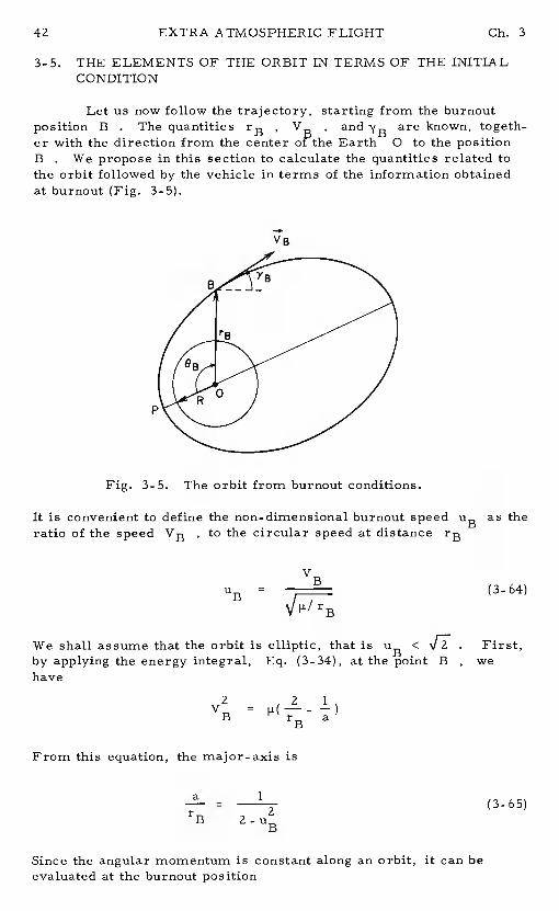
Let us now follow the trajectory, starting from the burnoutposition B . The quantities rB , , and are known, togeth-er with the direction from the center orthe Earth0 to the positionB . We propose in this section to calculate the quantities related tothe orbit followed by the vehicle in terms of the information obtainedat burnout (Fig. 3-5).
It is convenient to define the non-dimensional burnout speed UB as theratio of the speed VB, to the circular speed at distance rB
VB
U =B
(3- 64)
We shall assume that the orbit is elliptic, that is uB < . First,by applying the energy integral,Eq. (3-34), at the point B, wehave
=rB
From this equation, the major-axis is
Since the angular momentum is constant along an orbit, it can beevaluated at the burnout position
(3-65)
V8
Fig. 3-5. The orbit from burnout conditions.
Ch. 3 EXTRA ATMOSPHERIC FLIGHT 43
h = rBVB COS (3-66)
Using Eq. (3-41), with the major-axis obtained from Eq. (3-65), wehave for the eccentricity
e = - - 4) cos 2 (3-67)
or
____________________________
/.2 22 2e + _uB) COS (3-68)
From Eqs. (3-65) and (3-68) for aarid e , we have for the apocenterdistance and the pericenter distance from Eq. (3-25)
= [ 1 + (1-u2)2 COSYB] (3-69)B
and
-+ (1-4)2 (3-70)
The condition for the orbit to intersect the Earthrs atmosphere, assum-ed to be spherical, with a finite radius R, is that < R . Hence,in terms of the initial conditions, we have the condition for intersection
R 1 22 2
2 1- Vsin (l_uB) cos (3_71)B
The orientation of the orbit is given by the angle0 Bbetween the direc-
tion to the pericenter and the direction to the burnout position BThis angle is obtained by replacing in Eq. (3-20)r and 0 by rB and0B We have
cos 0B = 
/ 2 2 2
V
1 a 2= ;[ ) - 1]
44 EXTRA ATMOSPHERIC FLIGHT Ch. 3
2.UB
S1flOB = (3-73)
and
2UBS1fl
tanOB = 2 2(3-74)
UB - 1
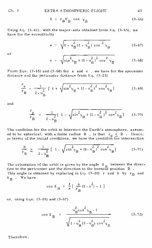
3-6. MINIMUM-ENERGY ORBIT
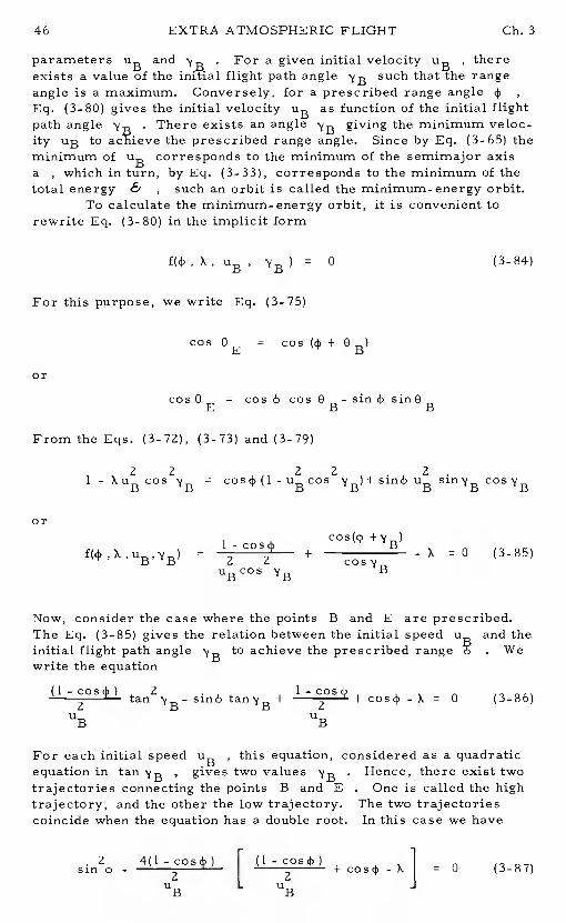
Let us consider the case where the vehicle, after ascending tothe highest altitude, at the apocenter A, returns and intersects theEarth's atmosphere at the entry point E at a distance R from thecenter of attraction 0 (Fig. 3-6).This is the case where the inequality ( 3-7 1) for intersection is satisfied.The angle between thepositions B and E, measured at the center of attraction 0, iscalled the range angle.From Fig. 3-6, it is seen that
= - (3-75)
where 0Eis the polar angle defining the entry position E. The
angle 0B
is given by Eq. (3-7 2). The angleE is obtained by
replacing in the Eq. (20)r and 0 by R and E• We have
(3-7 6)
A
Fig. 3-6. The range angle
Ch. 3 EXTRA ATMOSPHERIC FLIGHT 45
Using Eq. (3-65) for the semi-major axis we have
=
=
(377)
wherer
X = (3-78)
is the ratio of the radial distances to the point B and E, respectively.Hence,
2 2XuBcos NB1
cos 0 = (3-79)E I 2 2 2
V 1 - UB - UB) NB
The range angle is then
1 2 2 12 2= arc cos_(XuBcos NB') - arccos_(uBcos NB')
(3-80)
where e is given by Eq. (3-67). We notice that when the point B isat the top of the atmosphere,rB = R , and X = 1 . Since the pointE is beyond the apocenter,0E = 2ir - 0 B and Eq. (3-80) becomes
12 2= 2[ ii - arc cos _(uB cos NB -1)] (3-81)
The range can be evaluated when the trajectory intersects the Earth'satmosphere. In the limiting case, where we have an equality in con-dition (3-71), the trajectory is tangent at its pericenter to the circlewith center 0 and radius Rrepresenting the atmosphere in theplane of the motion. The flight path angle at the point of tangency,which is also the limiting position of the entry point E, is zero. Thetrajectory is called the grazing trajectory.By simple geometric con-siderations, it is seen that the range angle for the grazing trajectoryis given by = 2w - 9B Hence, from Eq. (3-74),
2.UB Sin NB coSNB
= 2 2(3-82)
This equation can be written as
- = 0 (3-83)
Equation (3-80) for the range givesc1 as a function of two
46 EXTRA ATMOSPHERIC FLIGHT Ch. 3
parameters UB and For a given initial velocity UB , thereexists a value of the initial flight path angle such that the rangeangle is a maximum. Conversely, for a prescribed range angleEq. (3-80) gives the initial velocity u8 as function of the initial flightpath angle . There exists an angle giving the minimum veloc-ity uB to acTiieve the prescribed range angle.Since by Eq. (3-65) theminimum of uB corresponds to the minimum of the semirnajor axisa , which in turn, by Eq. (3-33), corresponds to the minimum of thetotal energy & , such an orbit is called the minimum-energy orbit.
To calculate the minimum-energy orbit, it is convenient torewrite Eq. (3-80) in the implicit form
1(4, X, UB = 0 (3-84)
For this purpose, we write Eq. (3- 75)
cos 0E cos (4 +
cos 0E
= cos 4) cosB
- sin 4) sinOB
From the Eqs. (3-72), (3-73) and (3-79)
1 - XUB = UB SiflyB
or1 osA cos(4)
=
z+ - X = 0 (3-85)
uBcos '1B B
Now, consider the case where the points B and E are prescribed.The Eq. (3-85) gives the relation between the initial speed uand theinitial flight path angle to achieve the prescribed range . Wewrite the equation
(1- cos4)) sin4 +1- COS4 + cos4) -X = 0 (3-86)
UB UB
For each initial speed uB, this equation, considered as a quadraticequation in tan , gives two values Hence, there exist twotrajectories connecting the points B and E. One is called the hightrajectory, and the other the low trajectory.The two trajectoriescoincide when the equation has a double root.In this case we have
sin24)- 4(1 -cos4)
[+ cos4) -X] = 0 (3-87)
Ch. 3 EXTRA ATMOSPHERIC FLIGHT 47
We notice that if we consider Eq. (3-85) as an implicit equationgiving as function of for a prescribed range angle 4then by taking its derivative with respect to
8UB
The minimum of UB with respect to YB corresponds to du/ dYB = 0
that is, 0f/ 8YB = , which is the same condition as for (3-86)to have a double root. Hence Eq. (3-87), when solved, provides theminimum speed UB for a prescribed range angle 4, with an initialdistance ratio X . Solving for UB , we have by taking the positiveroot
4 =- X +1] (3-88)
cos2
The corresponding flight path angle is given by the double root ofEq. (3-86). We have
4tan = (3-89)
2 tan2
In the simple case where the point B is at the top of the atmosphere,we have X = 1 . The Eqs. (3-88) and (3-89) are reduced to
2 Zsin*UB = .
(3-90)1 + sin
and
cos
tan YB = .= (3-91)
1 + sin2
That is,- (3-92)
We see that, for the case of the minimum-energy orbit, when the burn-out and the entry positions are at the same distance from the center ofattraction, the initial speed and the initial flight path angle are givenby simple expressions in terms of the range angle 4. In this case,the other elements of the flight path can also be expressed in terms ofthe range angle.
For the semi-major axis, using Eq. (3-65) with rE =Rand Eq. (3-90) we have
48 EXTRA ATMOSPHERIC FLIGHT Ch. 3
= (3-93)
For the eccentricity, we write Eq. (3-67)
r 2 2Ie =\/l_ (3-94)
V l+tan
Using Eqs. (3-90) and (3-91), we have, after simplification
2e = , 1 - e = (3-95)
We notice from Eq. (3-91) that
e = tan (3-96)
The apocenter distance of the trajectory can be seen to be
= (1 + sin + cos (3-97)
For the time of flight between the two points B and E, we useKepler's equation, Eq. (3-57).Let E1 and E2 be the eccentricanomalies corresponding to the point B and E, respectively. Thenthe time of flight is given by
(t2-t1) E2-E1 - e(sinE2-sinE1)
Obviously, when X = 1 , the points B and E are symmetric withrespect to the line of apses.Hence
E2 = Zir -
Therefore,
- t1) = 2(r -E1+e sinE1) (3-98)
On the other hand, ife1
is the true anomaly of the point B
01 = - 2sin = sin , cos 01 = 2 (3-99)
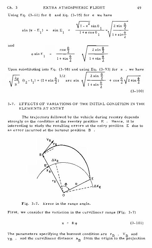
Ch. 3 EXTRA ATMOSPHERIC FLIGHT
Using Eq. (3-61) for 8 and Eq. (3-95) fore we have
sin (ii - E1) =
- e2 sinG1sinE1
= 1+ecosO1
-
+ sin3
Upon substituting into Eq. (3-98) and using Eq. (3-93) for awe have
(t-t) = arc sin +
(3-100)
3-7. EFFECTS OF VARIATIONS OF THE INITIAL CONDITION IN THEELEMENTS AT ENTRY
The trajectory followed by the vehicle during reentry dependsstrongly on the condition at the reentry position E. Hence, it isinteresting to study the resulting errors at the entry position E due toan error incurred at the burnout position B
Fig. 3-7. Error in the range angle.
First, we consider the variation in the curvilinear range (Fig. 3-7)
a = R4, (3-101)
The parameters specifying the burnout condition are rB, VB andNB , and the curvilinear distance from the origin to the projection
49
and
e sin E—
cos3
- i+sin3/
V8
0
EXTRA ATMOSPHERIC FLIGHT Ch. 3
of the burnout position B on the top of the atmosphere.It is apparentthat, from the rotational symmetry of the force field, any error inlinear range , incurred at the burnout position will be translatedinto an equal error of the range
(3-102)
We shall now evaluate the error , or equivalently the errorin the range as function of an error , or incurred
at the burnout position.For this purpose we rewrite Eq. (3-85) withthe velocity VB appearing explicitly
cos
= R-co
+ = 0 (3-103)_XVBCOS B
Then, the differential off is
= .
+ +B
+ = 0
Holding VB and constant, the change in the range , due toa change in the ratio of the radial distance is
= - 8f/ ax (3-104)af/
Similarly,
&f/ av=
- B (3-105)aVE
and
3f!— B (3-106)-
By evaluating the partial derivatives, we have the following formulaefor computing the error in the range angle
+
x [ sin4
2(1 - cos4
VB[(3-107)
Ch. 3 EXTRA ATMOSPHERIC FLIGHT-2(1 - cos4)) + UB5ln4)
(3-107)sin4)
Now, consider the quantity in the square brackets in the denominatorsof the Eqs. (3-107)
= sin4 _4sin(4 (3-108)
= 0 when
sin 4) - 4 sin (4) cos = 0 (3-109)
This is the same as Eq. (3-83) for grazing trajectory.Hence, in gen-eral, a is not vanishing and keeps the same sign which we can easilyverify as the positive sign.Since 1 - cos 4) > 0 , from the first twoequations (3-107), we see that the ratio a/ and a4 / aVB arepositive. Any increase in the initial altitude, or in the initial speed,provides an increase in the range. On the other hand, from the thirdequation (3-107), the ratio / changes its sign when
2(l-cos4)) = 4sin4) cosyB
2uB
tan2
This equation is the same as Eq. (3-89) for the minimum-energy tra-jectory. Along a minimum-energy trajectory, the variation of a4)isalways negative, and is of the second order in a.YB. We have
= + Lf ... (3-111)
By taking the derivative of the third of equations (3-10 7) with respect toNB and using the relations for the minimum-energy trajectory, wehave
22 4sin
=- 2
2 (3-112)a cos
Now, using Eq. (3-89) for a minimum-energy trajectory we have
52 EXTRA ATMOSPHERIC FLIGHT Ch. 3
= sin 4) - 4 sin (4)
F ±= Zsin2 [COS2 -Co S
± 2= Ztan
{cos
2cos 2sin
- 2 sin COS sin cos
or= 2
Therefore, a perturbation in the initial flight path angle, along aminimum-energytrajectory, corresponds to an error in the rangeangle given by
- sin4)(3-113)
Zcos YBCOS
In this case, using Eq. (3-89) in the first two of equations (3-107), wehave for the error in the range angle with respect to an error in theinitial altitude and in the initial speed, along a minimum-energytrajectory
sin4) +X
2(3-114)
2X cos
and
sin 42
VBCOS
In the special case where the point B is at the top of the
atmosphere, rB = R , and
22 cos + = 1 + cos +
But from Eq. (3-92),
2 cos2 + = - sin (3-116)
Ch. 3 EXTRA ATMOSPHERIC FLIGHT 53
The Equations (3-113) -(3-115) become
= - 4 tan (3-117)
= 1sin (3-118)
cos
= tan (3-119)
Now, let us consider the variations in the entry speed VE andthe entry flight path angle . From the energy integral, Eq. (3-19),we have the relation connecting the elements at the burnout position Band the entry position E
! v2 - = ! v2 - (3-120)2 B rB 2 E R
On the other hand, by evaluating the angular momentum at these points,we have
rBVB cos = RVE (3-121)
The differentials of Eqs. (3-120) and (3-121) give
+2 = (3-122)
rB
and
(VB COS + (rB COS (rBVB
= (RcosVE) - (3-123)
For an error in the burnout speed alone, the correspondingerror in the entry speed is given by Eq. (3-122) withrB = 0
LW =(3-124)
From Eq. (3-123) the error in the entry angle is obtained by putting0 and
54 EXTRA ATMOSPHERIC FLIGHT Ch. 3
V2
=- 1 (3-125)
B VE
For an error in the initial altitude, the error in the entry speed is
E=
B (E_) L_VE rB rB
In terms of X and UB , this is
- 1
- 2) (3-12
E [
The corresponding error in the entry angle is
2u +2X-3(tan
- 2 (r (3-127)UB + 2X - 2
Finally, for an error in the initial flight path angle alone, there isno error in the entry speed.The error in the entry angle is given by
(tan = (tan (3-128)
We notice from Eqs. (3-125), (3-127) and (3-128)that the entryangle is particularly sensitive for a grazing trajectory, = 0
References
1. Singer, E., and Bredt, J., Rocket Drive for Long RangeBombers," Translation No. CGD-32, Bureau of Aeronautics, NavyDepartment, 1944.
2. Anthony, M. L. , 'Free Flight Missile Trajectories, "Vistas inAstronautics, Vol. II, Pergamon Press, New York, 1959.
3. Dunning, R. S., "The Orbital Mechanics of Flight Mechanics,NASA SP-325, 1973.
4. Arora, K. L., and Vinh, N. X., "Maximum Range of BallisticMissiles, "SIAM Review, Vol. 7, No. 4, 1965.
Chapter 4
Powered Phase
4-1. INTRODUCTION
In this chapter, we shall analyze the trajectory of the vehiclefrom the launching pad, point A, to the burnout position, point BDuring the thrusting phase, the energy provided by the propellant istransformed into potential energy through the increase in the altitude ofthe vehicle, and kinetic energy through its increase in speed.Also, apart of the energy provided by the propulsion system is dissipated in theform of heat by action of the aerodynamic drag.The powered phase isthe phase during which it is possible to have a guidance system to con-trol the trajectory such that at the end of the thrusting program, thevehicle reaches a prescribed position.B, specified by the position vec-tor rB , and a prescribed velocity VB. We have seen in the pre-ceding chapter that the trajectory required by the mission may be com-pletely specified by these conditions at burnout.
The guidance is achieved by the following modes of control.a! Control of the thrusting force T. This control is performed
by the direction of the vector thrust.Its magnitude can also be control-led by the variation of the mass flow rate.
b/ Besides the main engine, the vehicle can be equipped withseveral small rockets providing lateral thrusting forces for its guidance.We shall assume that the resultant thrusting force of all the engines isrepresented by the vector thrust T.
c/ Control of the aerodynamic force A. This control is per-formed by varying the angle of attack of the vehicle and possibly byvarying its aerodynamic configuration.In three-dimensional flight.the aerodynamic force is also a function of the bank angle.
4-2. THE EQUATIONS OF MOTION
To write the equations of motion, we shall assume that the tra-jectory lies in the plane of the great circle containing the launch pointA and the burnout position B. Hence, it is necessary that all theforces involved be contained in that plane.This leads to the assump-tion that the vehicle has a plane of symmetry and that the velocityvector V , the aerodynamic force A and the thrusting force T are
55
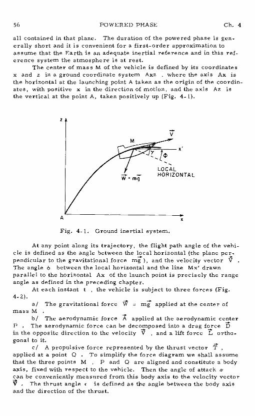
POWERED PHASE Ch. 4
all contained in that plane.The duration of the powered phase is gen-erally short and it is convenient for a first-order approximation toassume that the Earth is an adequate inertial reference and in this ref-erence system the atmosphere is at rest.
The center of mass M of the vehicle is defined by its coordinatesx and z in a ground coordinate system Axz, where the axis Ax isthe horizontal at the launching point A taken as the origin of the coordin-ates, with positive x in the direction of motion, and the axis Az isthe vertical at the point A, taken positively up (Fig. 4-i).
z
LOCALHORIZONTAL
A
Fig. 4-1. Ground inertial system.
At any point along its trajectory, the flight path angle of the vehi-cle is defined as the angle between the local horizontal (the plane per-pendicular to the gravitational force mg ),and the velocity vector VThe angle 4 between the local horizontal and the line Mx' drawnparallel to the horizontal Ax of the launch point is precisely the rangeangle as defined in the preceding chapter.
At each instantt , the vehicle is subject to three forces (Fig.
a! The gravitational force W = applied at the center ofmass M
b/ The aerodynamic force A applied at the aerodynamic centerP . The aerodynamic force can be decomposed into a drag force Din the opposite direction to the velocity V , and a lift force L ortho-gonal to it.
c/ A propulsive force represented by the thrust vector Tapplied at a point 0. To simplify the force diagram we shall assumethat the three points M, P and 0 are aligned and constitute a bodyaxis, fixed with respect to the vehicle.Then the angle of attack acan be conveniently measured from this body axis to the velocity vectorV . The thrust angle E is defined as the angle between the body axisand the direction of the thrust.
M
V
x.
'C
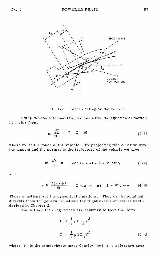
POWERED PHASE
Fig. 4-2. Forces acting on the vehicle.
Using secondin vector form
law, we can write the equation of motion
= (4-1)
where m is the mass of the vehicle.By projecting this equation intothe tangent and the normal to the trajectory of the vehicle we have
and
dV (4-2)
(4-3)
These equations are the dynamical equations.They can be obtaineddirectly from the general equations for flight over a spherical Earthderived in Chapter 2.
The lift and the drag forces are assumed to have the form
L = ZPSCLV
D = ZPSCDV (4-4)
where p is the atmospheric mass density, and S a reference area.
Ch. 4 57
L BODY AXIS
V
LOCALHORIZONTAL
58 POWERED PHASE Ch. 4
The coefficients CL and CD are lift and drag coefficients.They arefunctions of the angle of attack a, the Mach number M and the Rey-nolds number Re
CL = M, Re)
CD = CD (a, M, Re) (4-5)
The longitudinal range x, and the altitude z are obtained from thekinematic relations
tx = f V cos (y-4)) dt (4-6)
0
t
= f V sin - 4)) dt (4 7)
0
Finally we have the pitching moment equation, describing the motion ofthe vehicle about the center of mass
- M - K a (4-8)q dt
where B is the moment of inertial of the vehicle about an axis passingthrough the center of mass and perpendicular to the plane of symmetry,
the distance between P and M and the distance between 0and M . The term Mq is the aerodynamic pitching moment, and theterm Kd(y+a -4)/dt represents the moment due to the mass flow ofthe gas ejected from the propulsion system.
The thrust can be written as
= - + (p -p ) A (4-9)re e o e e
where - dm/ dt is the overall mass flow,Vre the average rela-tive velocity, Pe theaverage pressure and Ae the area over theexit of the engine. It is assumed that the tangential stress over theexit area is negligible. The unit vector 0e normal to the area Ae ispositively directed inward. Finally, p is the average free streampressure. For simplicity, we may assume that the vectors in Eq. (4-9)are all collinear and write the one dimensional equation as
T = Vre + Ae (4-10)
Ch. 4 POWERED PHASE 59
We define the effective exhaust velocityc as
c = Vre +-
(4-11)
Hence, the expression for the thrust magnitude is simply
T = nc-c- (4-12)
This equation gives the thrust in terms of the mass flow rate and theparameter cwhich can be characterized as a function of the propellantused in the propulsion system on board the vehicle.In engineeringpractice, we may use the specific impulse as an alternate para-meter which specifies the thrust performance.It is defined as thethrust impulse per unit mass of propellant or
I = - = (4-13)sp dm p
From the last two equations, it is seen that the specific impulseImay be alternatively defined as the thrust obtained per unit masswhich is precisely the same as the effective exhaust velocity.But it isa common practice to use different units for and c through therelationship p
c = gI (4-14)
where g is the acceleration of gravity.Therefore, while c is givenin meters per second,I is given in seconds.
Using Eqs. (4-11) (4-14) we have
V (p -p)I =
o eA (4-15)sp g gp e
The mass flow rate can be computed from
p = CpA (4-16)
where
= mass flow coefficient, function of the propellant
PC= average pressure in the combustion chamber.This
pressure is also called the operating pressure.
A = area of the throat of the nozzleC
Hence
POWERED PHASE Ch. 4
V (p -p) A=
a e e (4-17)sp g A
The ratio of the areas Ae/ Acan be expressed in terms of the expan-sion factor as C
_E =
1
(1- (4-18)
where k is the ratio of the specific heats.From these relations, we see that the specific impulse is a func-
tion of the following four factors
1. The nature of the propellant, Vre k
2. The operating pressure p
3. The expansion factor'ac"
4. The altitude of flight (g and p are functions of the altitude).
For a given type of propellant, we can evaluate its specific impulseunder some reference conditions.These conditions are:
For a solid propellant, p 70 atm. , 1 at sea level.For a liquid propellant, p = 25 atm. = 25/ 1 at sea level.
Let the specific impulse of the given propellant evaluated at thesereference conditions be denoted(I ) . Then we define the coefficientsp 0
I (4-19)sp 0
This dimensionless coefficient characterizing the propellant under theactual operating condition is now a function of four parameters--theratio of the specific heats k, the altitude z , the pressure in thecombustion chamber and the expansion ratio . If we assumethat the ratio of the specific heats is the same for all propellants, thenthe function is = f(z, can be tabulated for practical refer-ence.
For an anlytical integration of the equations of motion, we shallassume that, under normal operational conditions, the specific impulse
or equivalently the effective exhaust velocityc , is constant.Finally, if R is the radius of the Earth, then the range angle
is seen to be given by
tan4= R+z (4-20)
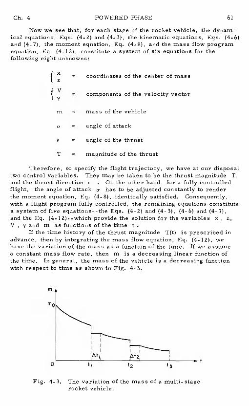
Ch. 4 POWERED PHASE 61
Now we see that, for each stage of the rocket vehicle, the dynam-ical equations, Eqs. (4-2) and (4-3), the kinematic equations, Eqs. (4-6)and (4-7), the moment equation, Eq. (4-8), and the mass flow programequation, Eq. (4-12), constitute a system of six equations for thefollowing eight unknowns:
1X
= coordinates of the center of mass(z
{
'V= components of the velocity vector
m = mass of the vehicle
a = angle of attack
e = angle of the thrust
T = magnitude of the thrust
Therefore, to specify the flight trajectory, we have at our disposaltwo control variables. They may be taken to be the thrust magnitudeT,and the thrust directione . On the other hand, for a fully controlledflight, the angle of attack ahas to be adjusted constantly to renderthe moment equation, Eq. (4-8), identically satisfied.Consequently,with a flight program fully controlled, the remaining equations constitutea system of five equations--the Eqs. (4-2) and (4-3), (4-6) and (4-7),and the Eq. (4-l2)--which provide the solution for the variables x ,z,V , and m as functions of the timet
If the time history of the thrust magnitude T(t)is prescribed inadvance, then by integrating the mass flow equation, Eq. (4-12), wehave the variation of the mass as a function of the time.If we assumea constant mass flow rate, then m is a decreasing linear function ofthe time. In general, the mass of the vehicle is a decreasing functionwith respect to time as shown in Fig. 4-3.
m
Ht2
Fig. 4-3. The variation of the mass of a multi-stagerocket vehicle.
POWERED PHASE Gb. 4
The figure represents the variation of the mass of a multi-stagerocket. The first stage of the rocket is operating between the initialtime and the time . At t1 the first stage is released providing adiscontinuity in the mass of the vehicle.If a lapse of time at1existsbefore the engine in the second stage is ignited, during that time thevehicle is in coast flight with constant mass.Next m continues todecrease between the time(t1 + t1t1) and t2 and so on.In the subse-quent analysis, we shall assume that all the are zero.
The remaining control variable can be selected either as the angleof attack a , or the thrust anglec or a combination of both by speci-fying a relation between these variables and possible other variablesalso. With this selection the ascending program is completely specified.
In general, in considering an ascending program, we are trying toobtain the optimum of some performance criterion.For example, fora preprogrammed motor, we would like to select a time history for thethrust orientation such that the range achieved is a maximum. Prob-lems like these involve the calculus of variations or the equivalentmodern control theory and will not be discussed here.From anengineering standpoint, the selection of a best flight control program isseverely restricted by other technical constraints.For example, for athrusting flight giving the maximum range, it can be shown, upon usingnot unrealistic assumptions, that the flight must be at maximum lift-to-drag ratio, with the thrust directed orthogonally to the aerodynamicforce, and hence making a constant angle with the velocity vector.Butthe thrust angleE , due to the technical construction of the propulsionsystem, cannot deviate at a large angle from the axis of the vehicle.Ingeneral E is constrained by a maximum anglec max of a few degreesfrom the main thrusting line.
Another factor to be considered is the normal acceleration.Ingeneral, due to structural constraints, this acceleration is severelylimited. Hence, for practical purposes, we are led to adopt somesimple ascending program which is satisfactory for the analysis duringthe preliminary stage of the design project.The simplifying hypotheseswill provide an analytical solution to the problem considered.Theanalytical solution has the advantage that it displays explicitly the manyrelationships among the different variables allowing a global analysis.For example, the solution will give the approximate size of the engine,and the weight of the propellant required to launch a certain given pay-load (final weight of the vehicle) into a prescribed final orbit.Fromthese approximate data, with the aid of high speed computers, we mayupdate the numerical results to obtain the exact solution to the problem.
4-3. ASGENDING TRAJEGTORY AT GONSTANT FLIGHT PATH ANGLE
The equations of motion derived in section 4-2 cannot be integratedanalytically. For a prescribed initial condition, and a specified thrust-ing program, numerical integration using high speed computers has tobe performed in order to obtain the variables describing the dynamicalsystem as functions of the time.
For advanced planning purposes, it is useful to adopt some simpli-fying assumptions in order to obtain an analytical solution of the ascen-
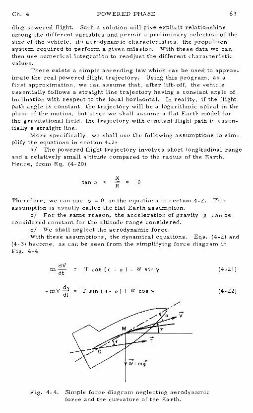
Ch. 4 POWERED PHASE 63
ding powered flight. Such a solution will give explicit relationshipsamong the different variables and permit a preliminary selection of thesize of the vehicle, its aerodynamic characteristics, the propulsionsystem required to perform a given mission.With these data we canthen use numerical integration to readjust the different characteristicvalues.
There exists a simple ascending law which can be used to approx-imate the real powered flight trajectory.Using this program, as afirst approximation, we can assume that, after lift-off, the vehicleessentially follows a straight line trajectory having a constant angle ofinclination with respect to the local horizontal.In reality, if the flightpath angle is constant, the trajectory will be a logarithmic spiral in theplane of the motion, but since we shall assume a flat Earth model forthe gravitational field, the trajectory with constant flight path is essen-tially a straight line.
More specifically, we shall use the following assumptions to sim-plify the equations in section 4-2:
a! The powered flight trajectory involves short longitudinal rangeand a relatively small altitude compared to the radius of the Earth.Hence, from Eq. (4-20)
tan4 0
Therefore, we can use4 0 in the equations in section 4-2.Thisassumption is usually called the flat Earth assumption.
b/ For the same reason, the acceleration of gravity g can beconsidered constant for the altitude range considered.
c/ We shall neglect the aerodynamic force.With these assumptions, the dynamical equations,Eqs. (4-2) and
(4-3) become, as can be seen from the simplifying force diagram inFig. 4-4
= Tcos(E -a)-Wsin'y (4-21)
= T sin ( E- a) + W cos y (4-22)
Fig. 4-4. Simple force diagram neglecting aerodynamicforce and the curvature of the Earth.
I
64 POWERED PHASE Ch. 4
Since we assume that = constant, then d'y/ dt = 0 . Hence,from Eq. (4_22) we have the relation between the thrust and the weight
T sin (a - = W cos (4-23)
In general, for rocket flight the thrust is large as compared to theweight. Hence from this equation we see that the angle( a- e ) isnecessarily small and we can take cos (E - a) 1 in Eq. (4-21).Then we have the simplified equation
= T - W (4-24)
Using Eq. (4-12) for the thrust we rewrite this equation, using the rela-tion W=mg
dV = - c - g sin y dt (4-25)
To integrate this equation for a multi-stage rocket vehicle, we refer tothe Fig. 4-3 and assume that all the time intervals between theseparation of the ith stage and the engine ignition of the(1+ 1)th stageare zero. Then by integrating Eq. (4-25) starting from the timet.of the separation of the(i- l)th stage, we have during the ofthe ith stage
rn.(t)V(t) = - c.log 1 - g sin yt' (4-26)
10where
V(t) = instantaneous speed at the timetV.1 = speed at the initial time of burning of the ith stagec. = effective exhaust velocity of the ith stage
m(t) instantaneous mass at the timetm. mass at the initial time of burning of the ith stage
0t' = -
- 1time interval from the initial time of
burdIng of the ith stage
Now, consider the operation of one single stage.For example,let us assume that the vehicle is a single-stage rocket.At the burnouttime t1 of this stage, the change in the speed is
mV1 - V0 = c log - gt1 sin y (4-27)
where c is the effective exhaust velocity of the stage considered,= m1 is the initial mass and m1 =m1(t1) is the final mass of the
vehicle. 01f we neglect the gravitational force, we have for the changein the speed
Ch. 4 POWERED PHASE 65
= c log (4-28)
We see that, in this case, can be used as a measure of the fuelconsumption. This quantity is called the characteristic velocity of themaneuver. From this simple formula, we can see thatmust havea certain upper limit. The exhaust velocity has an upper limit whichdepends on the propulsion system used.For example, ordinary chem-ical propulsion systems currently provide exhaust velocities up to3000 m/ sec, with a theoretical maximum in the neighborhood of4000 m/ sec. On the other hand, the ratio of the masses m /m1 alsocannot be made arbitrarily large.Let = in0 - m1 be mass ofthe fuel spent. Then we define the fuel ratio
£ = 1 - (4-29)in0 m0
so that we can write Eq. (4-28)
AV = c log (4-30)
It is obvious that f can never approach unity, since any amount of fuelalways requires a certain provision of structure for its operation.Therefore, the characteristic velocity for a single stage is limited dueto technological constraints.Some optimistic predictions advance afigure in the neighborhood of 9000 in!sec for its ultimate value.
Equation (4-30) gives the performance of a single stage rocket inthe hypothetical situation of gravity-free, vacuum space.If we includethe gravitational force, the increase in the speed during a thrustingphase of a stage is given by Eq. (4-27).The term gt1 siny character-izes the losses due to the gravitational force.Because of this compo-nent, the performance of a single stage rocket is further limited.Therefore, to obtain high final speed, one must use a multi-stagerocket.
Let ,- be the total burning time for a rocket vehicle having nstages. By repeated application of Eq. (4-26), we have the final speedat burnout, assuming a zero initial speed.
VB= - [
c. - gT siny (4-31)
where is the ratio of the masses of the ith stage, defined as
mass of the vehicle at burnout of ith stageF.L1n _ ...
iO mass of the vehicle at initial time of ith stage(4-32)
66 POWERED PHASE Ch. 4
For the range and the altitude at the end of the powered phase, we usethe Eqs. (4-6) and (4-7) with4 = 0 , and y = constant. We have
XE =
V(t) dtcosy
=
dt (4-33)
Using V(t) as given by Eq. (4-26)to evaluate the integral, we have, forthe case of constant mass flow p, (p n - dm1 dt)
XE = cos'l log it.)]- f gi-2 sin'y
1. 1 1 (434)
where 7. is the burning time of the ith stage.The final altitude issimply 1
= tan (4-35)
4-4. OPTIMUM STAGING
The final speed of a rocket vehicle, having a prescribed numberof stages is given by Eq. (4-31).This expression for VB is a functionof the characteristic parametersc. and of the different stages, ofthe constant flight path angle y and the total burning time'r of thepowered phase. By these considerations one may ask the followingquestion:
"Is there an optimum distribution of the masses of different stagessuch that, for a prescribed burnout speed VB, the ratio mL/ mF ofthe initial mass at launching to the final mass at the end of the poweredphase is a minimum? IT
If such a solution exists, it therefore gives the lightest rocket fora prescribed payload (final mass mF) for a prescribed final speed
B In solving this problem, we write the ratio of the masses
(4-36)
where to ease the notation, in this section, we have used the subscriptsas follows
- total mass of the vehicle at the initial burning time1 of the ith stage. This mass is also referred to as
the gross mass of the ith stage.
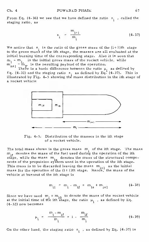
Ch. 4 POWERED PHASE 67
From Eq. (4-36) we see that we have defined the ratios. , called thestaging ratio, as
s.=
(437)
We notice that s. is the ratio of the gross mass of the (i+ 1)thstageto the gross mass of the ith stage, the masses are all evaluated at theinitial burning time of the corresponding stage.Also it is seen thatm1 = mL is the initial gross mass of the rocket vehicle, while
mF is the resulting payload of the operation.There is a basic difference between the ratio p..as defined by
Eq. (4-32) and the staging ratios. as defined by Eq. (4-37).This isillustrated by Fig. 4-5 showing the mass distribution in the ith stage ofa rocket vehicle
m1f ms
Fig. 4-5. Distribution of the masses in the ith stageof a rocket vehicle.
The total mass shown is the gross mass m• of the ith stage.The massm•1 denotes the mass of the fuel used during the operation of the ithstage, while the mass m1denotes the mass of the structural compo-nents of the propulsion system used in the operation of the ith stage.This mass is to be discarded leaving the mass m.+1 as the initialmass for the operation of the (i+ l)th stage.Hence, the mass of thevehicle at burnout of the ith stage is
- m• = m• + (4-38)al i if is i+l
Since we have used = rn.0 to denote the mass of the rocket vehicleat the initial time of the ratio p.. , as defined by Eq.(4-32) now becomes
=i if
1- (4-39)
On the other hand, the staging ratios. , as defined by Eq. (4-37) is
68 POWERED PHASE Gb. 4
m (m. +m.=
= 1 -is
(4—40)
We define the structural ratio for the propulsion system used in theoperation of the ith stage as
=(4-41)
Using this relation in Eq. (4-40) we have
= 1- 1 (4-42)i (l-w.)
By eliminating (m.f/m.) between the Eqs. (4-39) and (4-42), we havethe relation 1
-1 1 (449)
11
We can now formulate the optimizatioo problem as follows.The final speed V , the climb angle y and the total burning
time r are given. ThJis, we have from Eq. (4-31)
ilc.log = V0
where V0 is therefore prescribed. We write this equation as a con-straining relation
a c. log + V0 = 0 (4-44)
The number of stages n, the different propellant characteristicsc.and the different structural ratios w.are also given. Fiod a massdistribution shch that the following function
n 0 (F'. -w.)
= i=l= (445)
is a maximum. This is equivalent to minimizing the product of 1 /In solving this problem, we introduce a Lagrange multiplier to
form the augmented function
Ch. 4 POWERED PHASE 69
a + (4-46)
The solution to the problem is obtained by solving the system of (n+ 1)equations
= 0 , = 0 (4-47)
for the (n+ 1) unknowns '"' and X Explicitly, wewrite the first n equations
= 1 fl + X = 0 (4-48)(1
- j=l (1 -
For each of the n equations(4-48), we have
c.(p..-w.) - n1 1
Since the right-hand side is the same for all equations, it is a constantand we introduce a new constant K to replace the Lagrange multiplier
FL.1
a — (4-49)-w.) K11 1
These n equations can also be put into the form
=(4-50)
The problem is then to evaluate the constant K. Using this expressionin the constraining relation (4-44), we have
c. log=
- (4-51)
The sum of the logarithms can be written as the logarithm of a productC.
log1
( )
1 =
- (4-52)
POWERED PHASE Ch. 4
That is,n cw C -vIl l ii i 0
= e
1=1 1
Or finally, by separating the unknown K
n n
(c._K)c.
= eVO (453)
This equation can be solved for K, and subsequently the mass distri-bution , is obtained from Eq. (4-50).Obviously theequation can only be solved numerically.To obtain an explicitsolution, simplifying assumptions have to be made. We have thefollowing special cases.
4-4. 1. All the Propulsion Systems are Similar
If we assume that all the stages use the same propellant, andregardless of the difference in size, it is possible to achieve the samestructural ratio for all the stages, we have
C = c = ... = C = c1 2 n
(.) = = ... = = (4-54)1 2 n
Then, by Eq. (4-50), the mass distribution is the same for each stage.We have
= = = = c-K (4_55)
The equation (4-53) for K becomesVnc 0 nc(c_ K) = e (cu)
Solving for KVol
K = c[ ] (4-56)
Using this solution in Eq. (4-55), we have for the common mass ratio-V0/nc
(4-5 7)
We notice, by Eq. (4-43) ,that the staging ratios are also the same
-wS = S = ... = S = S =
1 2 n
or, explicitly in terms of the given characteristics
Ch. 4 POWERED PHASE 71
-V0/nc= (a) e - 1 (4-58)l-oL.
The final payload is then obtained in terms of the gross mass of the ve-hicle at launching
-v Inc= mL()[ - ]n
Finally, from Eq. (4-31), we have the final speed
VB = - gvsin'y (4-60)
The special case we have analyzed is highly hypothetical.Never-theless, the solution is obtained in closed form and it provides a firstestimation of the distribution of the masses for different stages.
4-4. 2. The Propellant Used is the Same for All Stages
If we assume that the propellant used is the same for all stages,but because of technological construction, the structural ratios are alldifferent, then we have the simplification
c = c = ... = c c (4-61)1 2 n
Equation (4-53) for K becomes
(c_K)nc = e0 cnc . (4-62)
Solving for KV /
K = c [ 1 - e0 (4-63)
The mass distribution is given by Eq. (4-50).
-Vs/nc=
1e (4-64)
1 1/n(w1w2.
We notice that the ratiop..! is the same for all stages.On theother hand, by Eq. (4-43), the staging ratio is
r -V/nc(ii. I 0
1 I e5. = I - 1 (4-65)
1 (l-w.)L
1/n1 (w a) . . . w )12 n
POWERED PHASE Ch. 4
The final payload is-v Incr o in n
mF = mL[
e
1/n IJ( (4-66)) 112 n i=1
Finally, we have for the final speed
VB = - C log FL. - gT sin y (4-6 7)
It is easy to verify that the equations in this section are reducedto the equations derived in the preceding section if we putw U).
1 2 n
4-4. 3. The Structural Ratios are the Same for All Stages
The special case considered in the previous section is very closeto the practical realization of a multi-stage rocket vehicle.Thereexists another special case, namely when technological realizationallows a common structural ratio for all the stages although differentpropellants are used.Then we have the simplification
= = ... = = (4-68)1 2 n
In this case the equation (4-53) cannot be solved explicitly for K .Themass ratio is here
=(4-69)
It is seen thatIL. is a decreasing function ofc. . Therefore, if thepropellants used are such thatc < c , we have FL1 > . Thestaging ratio is given by Eq.(4_4]3) as
= (1(4-70)
We see that it varies in the same direction as
References
1. Dorleac, B. , and Poggi, J. , "Performances et Structures duMissile Ealisti4ue, "Lecture notes, Ecole Nationale de
et de l'Espace, 1960.2. Schurmann, E. E. H., "Optimum Staging Technique for Multistaged
Rocket Vehicles, "ARS Journal, Vol. 27, No. 8, 1957.
Chapter 5
Return to the Atmosphere
5-1. INTRODUCTION
In Chapter 3, the trajectory for flight outside the atmosphere,assumed to be spherical with a finite radius R, was considered. Wehave seen that, if the burnout position B, (Fig. 3-1), is outside theatmosphere, the resulting trajectory is a Keplerian conic until theatmosphere is reencountered.In the case of an elliptic trajectory, ifthe periapsis distance is less than the radius R of the atmosphere,a condition expressed by the inequality (3-71), the trajectory will inter-sect the atmosphere at a point E, the entry position. In the casewhere inequality (3-71) is not satisfied, the vehicle will be in an ellipticorbit around the Earth ifthe initial speed is less than the escape speed,that is if
VB<
(5-1)
After the mission has been accomplished, to bring back the vehi-cle, one must perform a series of maneuvers to change the initialorbit, designated by , to a final orbit, , intersecting theatmosphere at the entry position E (Fig. 5-1).From this point on,the vehicle is in the atmosphere and follows a flight path subject to thegravitational and atmospheric forces.The flight path from the entryposition E to the landing point C is called the reentry flight path andits analysis is the subject of several later chapters.In this chapter,we shall be concerned with the maneuver performed to change the non-intersecting orbit into the intersecting orbit . In general,the means of accompfishing a change of orbit, or transfer, will be byfiring the rocket on board the vehicle to change its velocity, thus pro-pelling the vehicle into a new orbit.If the rocket engine provides ahigh thrust, the burning time is generally short, compared to the orbitalperiod. Hence, it can be assumed that, during a thrusting phase,the
position of the vehicle remains essentially unchanged while the velocityundergoes a change impulsively.Furthermore, we shall be concernedwith the last orbital change before reentry.Hence the orbit
1is the
final nonintersecting orbit resulting from a series of maneuvers.At apoint D in this orbit, referred to as the deorbit position, a velocity
73
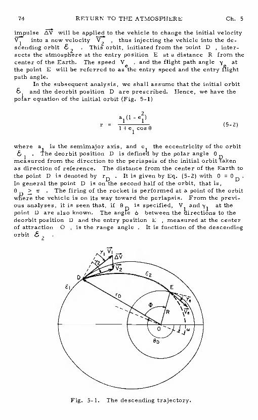
-r =
1 + e1 cos 8
74 RETURN TO THE ATMOSPHERE Gb. 5
impulse will be applied to the vehicle to change the initial velocityV1 into a new velocity V2 , thus injecting the vehicle into the de-scending orbit
2This orbit, initiated from the point D, inter-
sects the atmosphere at the entry position E at a distance R from thecenter of the Earth.The speed Ve and the flight path angle'y atthe point E will be referred to as the entry speed and the entry flightpath angle.
In the subsequent analysis, we shall assume that the initial orbit£ and the deorbit position D are prescribed.Hence, we have thepofar equation of the initial orbit (Fig. 5-1)
(5-2)
where a is the semimajor axis, and e1the eccentricity of the orbit& . he deorbit position D is defined by the polar angle 0
measured from the direction to the periapsis of the initial orbit Qakenas direction of reference.The distance from the center of the Earth tothe point D is denoted by rD. It is given by Eq. (5-2) with 0
=In general the point D is on the second half of the orbit, that is,O > it . The firing of the rocket is performed at a point of the orbitwPere the vehicle ison its way toward the periapsis. From the previ-ous analyses, it is seen that, if is specified, V1 and at the
point D are also known. The angre between the directions to thedeorbit position D and the entry position E , measured at the centerof attraction 0 , is the range angle. It is function of the descendingorbit
Fig. 5-1. The descending trajectory.
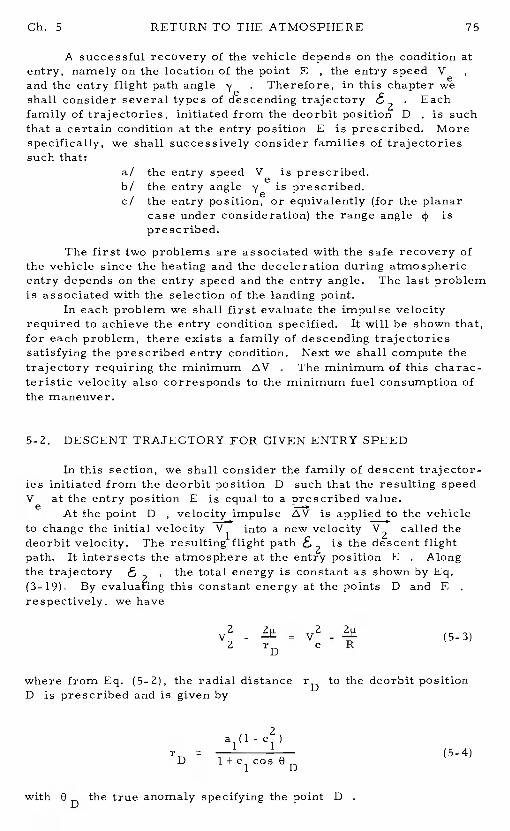
Ch. 5 RETURN TO THE ATMOSPHERE 75
A successful recovery of the vehicle depends on the condition atentry, namely on the location of the point E, the entry speed Vand the entry flight path angle y . Therefore, in this chaptershall consider several types of descending trajectory . Eachfamily of trajectories, initiated from the deorbit position D, is suchthat a certain condition at the entry position E is prescribed. Morespecifically, we shall successively consider families of trajectoriessuch that:
a/ the entry speed Ve is prescribed.b/ the entry angle is prescribed.c/ the entry position, or equivalently (for the planar
case under consideration) the range angle4, isprescribed.
The first two problems are associated with the safe recovery ofthe vehicle since the heating and the deceleration during atmosphericentry depends on the entry speed and the entry angle.The last problemis associated with the selection of the landing point.
In each problem we shall first evaluate the impulse velocityrequired to achieve the entry condition specified.It will be shown that,for each problem, there exists a family of descending trajectoriessatisfying the prescribed entry condition.Next we shall compute thetrajectory requiring the minimum . The minimum of this charac-teristic velocity also corresponds to the minimum fuel consumption ofthe maneuver.
5-2. DESCENT TRAJECTORY FOR GIVEN ENTRY SPEED
In this section, we shall consider the family of descent trajector-ies initiated from the deorbit position D such that the resulting speedVe at the entry position E is equal to a prescribed value.
At the point D , velocity impulse is applied to the vehicleto change the initial velocity V1 into a new velocity V2 called thedeorbit velocity. The resulting flight path E
2is the descent flight
path. It intersects the atmosphere at the entry position E. Alongthe trajectory , the total energy is constant as shown by Eq.(3-19). By evaluating this constant energy at the points D and Erespectively, we have
- = - (5-3)2 rD e R
where from Eq. (5-2), the radial distance rD to the deorbit positionD is prescribed and is given by
-r (5-4)
D l+elcosOD
with the true anomaly specifying the point D
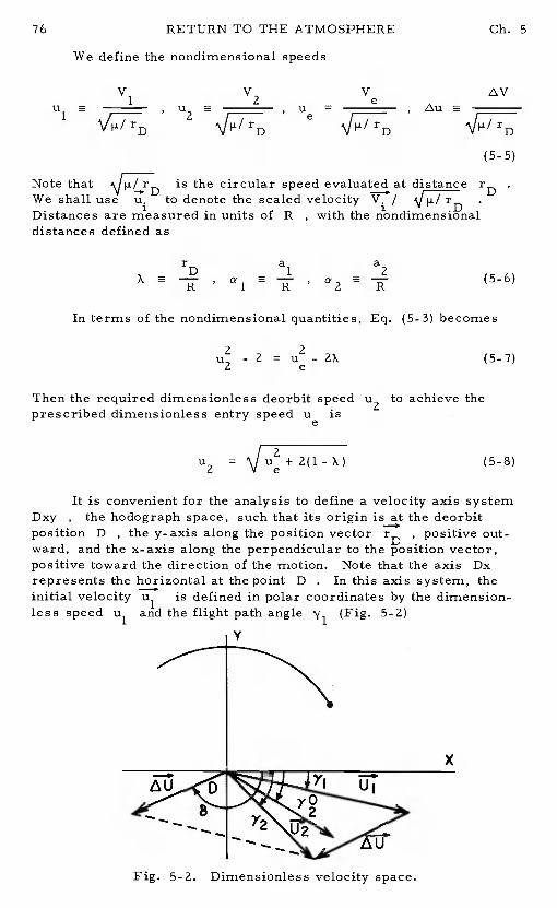
76 RETURN TO THE ATMOSPHERE Ch. 5
V V V1 2 e
U C U , U C , C1 1— 2 e r
(5-5)
Note that is the circular speed evaluated at distance rDWe shall use u. to denote the scaled velocityV. / rDDistances are measured in units of R, with the nondimensionaldistances defined as
r a aD 1 2
X a , a1 a , a2 —- (5-o)
u2 -2 = u2-2X (5-7)2 e
Then the required dimensionless deorbit speed u2 to achieve theprescribed dimensionless entry speed UiS
u2 = + 2(1 - X) (5-8)
It is convenient for the analysis to define a velocity axis systemDxy the hodograph space, such that its origin isat the deorbitposition D , the y-axis along the position vector rU, positive out-ward, and the x- axis along the perpendicular to the position vector,positive toward the direction of the motion.Note that the axis Dxrepresents the horizontal at the point D. In this axis system, theinitial velocity u1 is defined in polar coordinates by the dimension-less speed u1and the flight path angle'y1 (Fig. 5-2)
Fig. 5-2. Dimensionless velocity space.
We define the nondimensional speeds
In terms of the nondimensional quantities, Eq. (5-3) becomes
Y
x
Ch. 5 RETURN TO THE ATMOSPHERE 77
Since the initial orbit is given and the deorbit position prescribed,u1and are known quantities.From
2 2 1V = —)
1 rD a1
comes[20! X
u = (5-9)1 v
The flight path angle is given by Eq. (3-32).
1 + e1 cosD
=
Using Eqs. (5-4) and (5-6),we can write
/ (1-cos
V X(2e1 -
-
= ± V X(2a1 - X)(5-10)
Now consider Eq. (5-8) for the deorbit speed u. Since u and Xare prescribed, it is seen that uis constant all possib?e descenttrajectories. Hence, the locus the terminus of the velocity u2in the hodograph space is a circle centered at D and having a givenradius u2 as given by Eq. (5-8).For each direction of this velocity,defined by the flight path angle , we have a vector u2 . Therequired velocity impulse is such that
U1 + = U2
Its magnitude is obtained by applying the law of cosines to the velocitytriangle in Fig. 5-2. Thus,
= + - 2u1u2 cos (5-11)
The direction of is defined by the angle 6 from the horizontalDx . Applying the law of sines to the velocity triangle in Fig. 5-2, wehave
Usin (6
=(5-12)
78 RETURN TO THE ATMOSPHERE Ch. 5
From Eq. (5-11) and (5- 12) it is apparent that the deorbit flightpath angle for the descending trajectory can be used as a parameter.To each angle corresponds an impulse velocity , and hence, atrajectory . The elements of this trajectory can be obtained byusing the derived in Section 3-5, with the subscript B re-placed by subscript2 , and rB by r
We have for the semimajor axis OP
a
=
or =
(5-13)
For the eccentricity of the descending trajectory, by using Eq. (3-67)we have
e2 = - (2X - u2){u2+2(1 - X)] (5-14)
The periapsis distance is given by
r- - (2X - u2) [u2+2(1 - X)]—= e e
(5-15)rD 2X-u2
e
Hence we have the condition for the trajectory £2to intersect theatmosphere
1 [u2+2(1- X)}
Solving for , we have the condition
U
cos e (5-16)
+2(1-X)y e
This condition restricts the locus of the terminus of the vector in
the velocity space to an arc of a circle (Fig. 5-2).The entry angle at the entry position is obtained by writing that
the angular momentum is constant along the descent orbit.We have,by evaluating this constant at the point D and at the point E, respec-tively
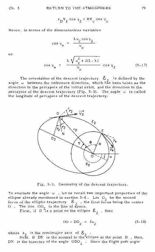
e
The orientation of the descent trajectory2
is defined by theangle between the reference direction, which has been taken as thedirection to the periapsis of the initial orbit, and the direction to theperiapsis of the descent trajectory (Fig. 5-3).The angle is calledthe longitude of periapsis of the descent trajectory.
Fig. 5-3. Geometry of the descent trajectory.
To evaluate the angle , let us recall two important properties of theellipse already mentioned in section 3-4 .Let 02 be the secondfocus of the elliptic trajectory E. , the first focus being the center0 . The line 00 is the line of apses.
First, if D is a point on the ellipse , then
DO + DO2 = 2a2 (5-18)
where a2 is the semimajor axisofNext, if DN is the normal to the ellipse at the point D, then,
DN is the bisector of the angle 0D02. Since the flight path angle
Ch. 5 RETURN TO THE ATMOSPHERE 79
rDVZ cos = RVe
Hence, in terms of the dimensionless variables
Xu2
cos cos (5-17)U
RETURN TO THE ATMOSPHERE Ch. 5
at the point D is defined as the angle between the horizontal at Dw?hich is perpendicular to the position vector OD, and the velocityV2 , which is tangent to the ellipse at the point Dthis property isexpressed by the relation
0D02 = (5-19)
Now let be the angle between the vectors OD and 002(Fig. 5-3). Using the law of sines in the triangle 0D02 and the prop-erty expressed by Eq. (5-19) we have
DO2 — 002— OD
sin sin —
But 007 = 2a2e2 and by the property expressed by Eq. (5-18)DO2 = �a2 - rD . Hence,
2a -r 2ae r2 D = 2 2 D (5-20)sin sin
Therefore, the first equation (5-20) gives
(202-X)sin1 =
2
or2[u + 2(1 - X)Isln 2y2
sin 1C (5-21)
2 - (2X - u2)[
U2 + 2(1 - X )} cos2
Another expression for 1 is obtained by using the second equation(5-20). We have
(2a2 - rD) sin (Za2
- X) sin
tan =rD - (2a2- rD) X - (2cy2- X)
[ U2 + 2(1 - X )} sin Z'y2
2 2(2X
- u) - [ Ue + 2(1 - X)J cos
2
2 2(5-22)
[ (2X -1) - Ue] +tan
Gb. 5 RETURN TO THE ATMOSPHERE
The longitude of periapsis of the descending trajectory is thengiven by
=- (5-23)
Finally, the range angle from the deorbit position to the entryposition is given by Eq. (3-80), written as
= arc cos 1) - arc -1)
(5-24)
5-3. MINIMUM IMPULSE FOR ENTRY AT GIVEN SPEED
We have seen in the preceding section that,if the entry speedalone is specified, then there exists a family of descent trajectorieswhich is a function of the deorbit angle . To each angle v2correspQxlds a descent trajectory, and hence an impulsive change,in the velocity. The magnitude of this impulse, the characteristicvelocity, is a measure of the fuel consumption for the maneuver.Inthis section we shall compute this particular descent trajectory suchthat is a minimum.
Let be the limiting value of the angle selected as theparameter for optimization.This value is given by the equalitysign in condition (5-16). Then from Fig. if , tomin-imize , we must select
=The velocity impu1lse is
tangential to the initial orbit, the deorbit point D , to reduce thespeed from u1 to u2 . Hence, we have the condition for optimumtangential deorbit for a given entry speed
ue> cos (5-25)— 1
Using Eq. (5- 10) for cos we can write this condition
22X (X - 1) (1-
e— X(l- 2a1+X
This condition expresses that, for a given initial orbit with a prescrib-ed deorbit position, the prescribed entry speed umust be less thana certain value for an optimum tangential deorbitbe possible.
For tangential optimum deorbit, we have the following resultsobtained by putting
=in the general expressions for the descent
trajectory derived in previous section.First,
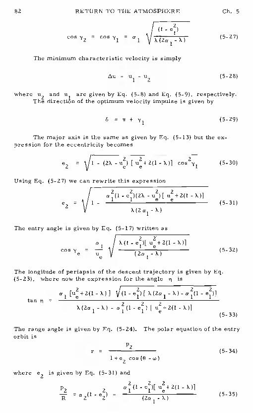
RETURN TO THE ATMOSPHERE Ch. 5
/ (1 -cosy2 =
=(5-27)
The minimum characteristic velocity is simply
= u1 - U2 (5-28)
where u2 and u1are given by Eq. (5-8) and Eq. (5-9), respectively.The direction of the optimum velocity impulse is given by
6 = ir + (5-29)
The major axis is the same as given by Eq. (5-13) but the ex-pression for the eccentricity becomes
e2 = - (2X -u2) [u2+2(1- X)] (5-30)
Using Eq. (5-27) we can rewrite this expression
/ e (5-31)V X(2a1-X)
The entry angle is given by Eq. (5-17) written as
al u2+2(1-X)ICOS
= 11e V (2a.i -(5-32)
The longitude of periapsis of the descent trajectory is given by Eq.(5-23), where now the expression for the angle is
fu2+2(l-X)]tanii
2 2 2
(5-33)
The range angle is given by Eq. (5-24).The polar equation of the entryorbit is
p2r = (5-34)
1+e2 cos(8
where e2 is given by Eq. (5-31) and2 2 2
p2 2(1- e1)[ Ue+2(l- x)]
— = (1 - e ) = (5-35)R 2 2 (Zcy1-X)
2u-Xee2
=
Gb. 5 RETURN TO THE ATMOSPHERE 83
The entry position E is defined by the polar angleeE
= 4) (5-36)
where 4) is the range angle.0 Ecan also be computed from Eq. (5-34)
with rR and 0=0A tangential is optimum when the entry velocity is small
as constrained by the inequality (5-26).When this inequality is notsatisfied, the minimum deorbit angle y,for the descent trajectory tointersect the atmosphere is larger thaninitial flight path angle
(Fig. 5-4).
Fig. 5-4. Minimum velocity impulse when >
In this case, as can be seen in Fig. 5-4, the minimumcor-reponds to . Since the limiting value of is given by theequality sign in ( we have
Ue
cos 'y =
______________
(5- 37)2 '2XVu +2(1-X)
e
The minimum characteristic velocity is given by Eq. (5-11), and itsdirection by Eq. (5-12) with the value of obtained from Eq. (5-37).Using Eq. (5- 37) in Eq. (5-17) we see thatcos = Hence, theentry is grazing
= 0 (5-38)
The eccentricity of the descending orbit is given by Eq. (5-14), whichby virtue of Eq. (5-37), becomes
(5-39)
84 RETURN TO THE ATMOSPHERE Ch. 5
The longitude of periapsis of the descent orbit is given by Eq. (5-23).To evaluate the angle , we notice from Eqs. (5-14), (5-21) and(5-22) that
(2K -u2) -[ u2+2(1 -K)]cos = e
Ze(5-40)
2
From Eq. (5-37)
2 2 2
2u (2_K )-ZK (1-K)
cos = 2 cos -= e
2K [u +2(1_K)]
Hence, upon substituting into Eq. (5-40), with the aid of Eq. (5-39) wehave
2 2K -uecos
= 2(5-41)
K(u -K)e
The polar equation of the entry orbit is
r= 1+e2:os(8 (5-42)
where now, by using Eqs. (5-13) and (5-39)2
p2 2 Ueo2(1-e2) = (5-43)
The position of entry is given by the polar angle0 EIt is obtained
by putting r = R , and 0 in Eq. (5-42).
5-4. DESCENT TRAJECTORY FOR GIVEN ENTRY ANGLE
In this section we shall consider the family of descending tra-jectories initiated from the deorbit position D, such that the result-ing flight path angle y at the entry position Eis equal to a prescrib-ed value. e
The notation used is the same as in the previous sections.Wenow write the equations for the conservation of energy and conservationof angular momentum, Eqs. (5-7) and (5-17), using the dimensionlessvariables defined by Eqs. (5-5) and (5-6).
U2 2 = Ue - 2K (5-44)
and
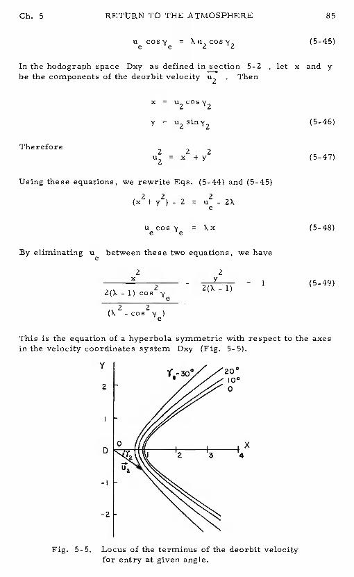
(x2+ y2) - 2 = U2 - ZX
u cosy = Xx (5-48)e e
This is the equation of a hyperbola symmetric with respect to the axesin the velocity coordinates system Dxy (Fig. 5-5).
Fig. 5-5. Locus of the terminus of the deorbit velocityfor entry at given angle.
Ch. 5 RETURN TO THE ATMOSPHERE 85
Ue = (5-45)
In the hodograph space Dxy as defined in section 5-2, let x and ybe the components of the deorbit velocity u2. Then
x u2cosy2
y = u2siny2 (5-46)
Therefore2 2 2
u2 x +y (5-47)
Using these equations, we rewrite Eqs. (5-44) and (5-45)
By eliminating Ue between these two equations, we have
22x y
- 2(X-1)2(X- 1) cos2y
(X -
= 1 (5-49)
200lOG0
Y
2
D
—l
-2
x4
86 RETURN TO THE ATMOSPHERE Ch. 5
The equation expresses that, for a deorbit from a prescribedposition D , at a given distance X , in such a way that the entry angle
equal to a prescribed value, the terminus of the deorbit velocityu2 must be on a branch of a hyperbola defined by Eq. (5-49).Each
hyperbola corresponds to a specified entry angle'y . In particular,when the entry is grazing,cos = , and we the limitinghyperbola
2-
= 1 (5-50)
(X +1)
Figure 5-5 gives the plots of several hyperbolas, loci of the terminusof the deorbit velocity u2 , for several values of y , and for aninitial distance ratio X = 1. 18.
To each prescribed value , we have a branch of an hyperbola.When the terminus of the vectoru moves along this hyperbola, itgenerates a family of descent
a a the prescribed entry angleThe deorbit angle can be used as a parameter for the
If the entry speed is also prescribed, then the magnitude of u2is prescribed as given by Eq. (5-8).The descending orbit is obtainedby finding the intersection of the circle of radius uand the hyperbolagiven by Eq. (5-49). We have, by using the Eqs. and (5-46)
x2 = [ u2 + 2(1 - X)]
= [ U2 + 2(1 - X)] (5-51)
To simplify the notation, we rewrite Eq. (5-49) as
Ax2 - By2 1 (5-52)
where2 2
X -cosA
22(X - 1) cos
B a 2(X-1) (5-53)
By substituting the Eqs. (5-51) into Eq. (5-52) and solving for , wehave
Ue ecos (5-54)
+ 2(1 - X)
Ch. 5 RETURN TO THE ATMOSPHERE 87
The branch of the hyperbola corresponding to the velocity pointingin the same direction as the motion along the initial orbit correspondsto a solution providing two points of intersection, hence two values for
One solution > 0 , gives a high descent orbit, while theother, < 0 , gives a low descent orbit. The solutions are realwhen
Ue e
< 1 (5-55)—
or, that is, when
Ue >2(X - (5-56)
X -cos
For a given entry angle , there exists a lower bound for a pre-determined entry speed an entry trajectory to be physically possible.On the other hand, we can write Eq. (5-55) in terms of a condition on
+ Z(l - X)cos (5-57)e— u
e
Hence, if the entry speed is prescribed, there exists a lower bound forthe entry angle , for an entry trajectory to be physically possible.
By both and u , for a given initial orbit, thatis, for a given and e , we caen alsovary the deorbit position,by varying X , to satisfy physical constraints on the entry.Tostudy the influence of X on the condition for entry, we rewrite thecondition (5- 56)
Ve > -1) (5-58)x -cos
With fixed, the right hand side of the inequality (5- 58) is an in-creasing function of X . Hence its minimum corresponds to the posi-tion of deorbit at the periapsis of the initial orbit.
X = a1(1-e1) (5-59)
We conclude that, when Ve and'y are both prescribed, for a giveninitial orbit, single-impulse is always possible if the followingcondition is satisfied
88 RETURN TO THE ATMOSPHERE Ch. S
Ve /2a1(l- e1) [a1(l- e1) -1]> (5-60)
— V
We now return to the case where only the entry angle yisprescribed. Then, there exists a family of deorbitinitiating from a prescribed deorbit position D. Using the deorbitflight path angle as a parameter for this family, we can calculatethe elements of the descent trajectory selected.This can be obtainedby expressing the entry speed uin terms of the variablesand and then substitutingintoetheequations obtained in section 5-2.For Ue we have from Eq. (5-54)
Ue =- 1)
2cos (5-61)
X cos 'y2 -
The deorbit speed u2is given by Eq. (5-45).
=2
2(X -1)2
cos (5-62)X coS - cos
The magnitude of the velocity impulse • and its direction öare given by the Eqs. (5-li) and (5-12) respectively, with the initialspeed given by Eq. (5-9) and the initial flight path angle by Eq. (5-10).The dimensionless semimajor axis of the descending trajectory isgiven by Eq. (5-13), written with the v:lue of ugiven by Eq. (5-61)
X cos - cos
= 2 2(5-63)
2(Xcos
The eccentricity of the descending trajectory is given by Eq. (5-14).In terms of X
,
and this is
1 2 2 2 2
/4X(X - 1)(X cos cos COS
e2 = \/1_2 2 2 2
V (X cos - cos(5- 64)
The longitude of periapsis of the descent trajectory is given by Eq.(5-23), where now the angle is given in terms of the selected vari-ables as
Gb. 5 RETURN TO THE ATMOSPHERE 89
22(X - l)costan
= 2 2 2 2(5-65)
X - (2X - 1) cos - cos
The polar equation of the entry trajectory is
r= 1+e2cos(O (5-66)
where e2 is given by Eq. (5-64) and2 2
p 2X(X - 1) cos cos2 e 2
R 2 2 2 -X cos
The position of entry E is defined by its polar angleE which isobtained by putting r = R , and 0
= 0E in the polar Eq. (5-66).
5-5. MINIMUM IMPULSE FOR ENTRY AT GIVEN ANGLE
We have seen in the preceding section that, for an entry at aprescribed angle initiating from a prescribed deorbit position, thereexists a family of descent trajectories which is a function of the deorbitangle 'y, . These trajectories are such that the terminus of the de-orbit vetocity u2 is on a hyperbola defined by Eq. (5-52).In thissection we shall select from among the descent trajectories in thisfamily the one that results in a minimum characteristic velocityThat particular trajectory is called the optimum deorbit trajectory fora prescribed entry angle.
In the hodograph space (Fig. 5-6), consider a hyperbola, thelocus of the terminus of u for ajiven entry angle
'1eIn this hodo-
graph space, the initial u1 is prescribed. Let x and y1be the projections of on the axes of the coordinates DxyWe have from Eqs. and (5-10)
I 2
/-
xi = u1= v
-y = u sin'y = +
1 1 1 — (5-68)
The minus sign for y1 is taken if the point D is on the second half ofthe initial orbit.
The minimum is obtained by finding the shortest distancefrom the point with coordinates(x1 , y ) to the hyperbola. Let super-script (*) denote the optimum The point with coordinates
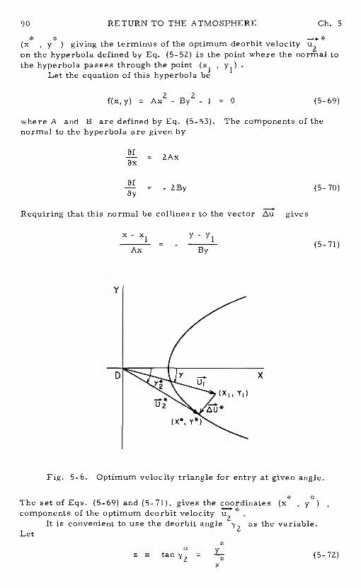
f(x, y) Ax2 - By2 - 1 =
where A and B are defined by Eq. (5-53).The components of thenormal to the hyperbola are given by
af— = 2Ax
= -2By
Requiring that this normal be collinear to the vector gives
x-xl -Ax - - By
Fig. 5-6. Optimum velocity triangle for entry at given angle.
The set of Eqs. (5-69)and (5-71), gives the coordinates(x' , y)components of the optimum deorbit velocity u2*
It is convenient to use the deorbit angle as the variable.Let
RETURN TO THE ATMOSPHERE Ch. 5
—...—-+ *(x
, y ) giving the terminus of the optimum deorbit velocity u2on the hyperbola defined by Eq. (5-52) is the point where the normal tothe hyperbola passes through the point (x1, y1)
Let the equation of this hyperbola be
(5-69)
(5-70)
(5-71)
Y
x
(x*,
z = (5-72)
Ch. 5 RETURN TO THE ATMOSPHERE 91
be the tangent of the optimum deorbit angle.Then from Eqs. (5-71)and (5-72) we have
Ay1 + Bx1 zX
= (A+B)z
* - Ay1+Bx1z
— (A+B) (5-73)
Upon substituting into Eq. (5-69) we have a quartic equation inz
A0z4 + A1z3 + A2z2 + A3z + A4 0 (5-74)
where the coefficients A.are given by
A0 E
A1 2AB2x1y1
A2 - + (A+ B)2
A3 - ZA2Bx1y1
A4 a - (5-75)
Hence, the optimum deorbit flight path angle is obtained by solving aquartic equation. In general, this equation gives four roots correspon-ding to four normals drawn from the point(x1 , y1) to the hyperboladefined by Eq. (5-69). One of these roots corresponds to the minimumof
The elements of the optimum deorbit trajectory can be easilyobtained in terms ofz by using the general equations derived in thepreceding section.
First the components of the deorbit velocity u2are given byEq. (5- 73). Next, the minimum characteristic velocity is simply
= -x1)2 + (y (5-76)
The direction of is the direction of the normal to the hyperbolawhich has componepts (Ax', - By") . Hence, if 8 is the opti-mum angle of , measured from the x-axis, we have
2B
zcoStan 6 = - =
- 2 2(5-77)
X -cos
The entry speed is given by Eq. (5-61). Since
RETURN TO THE ATMOSPHERE Ch. 5
2* 1 1
= 2 * = 21+tan l+z
then
* I 2(X-1)Ue =
2 2 2(5-78)
V X -(1+z )cos
The optimum deorbit speed is given by Eq. (5-62) written as
U22
- 1)(1COSYe (579)
X -(1+z )cos
The dimensionless semimajor axis of the optimum deorbit trajectory isgiven by Eq. (5-63).We have
2 2 2* X -(1+z )cos
= 2 2
e (5-80)2[X-(1+z ) cos
The eccentricity of this orbit is
* / 4X(X - l)[ X -(1e2
= V1
- - (1 + z2) 2 (5-81)
The longitude of periapsis of the optimum deorbit trajectory is given byEq. (5-23) with the angle expressed in terms of X, and z
2(X - 1)
= 2 2 2 2(5-82)
[ X - (2X - 1) cos - cos
The polar equation of the entry orbit is given by Eq. (5-66) where e2is given by Eq. (5-81) and
p2 2X(X- l)cosR = 2 2 2
(5-83)X _(1+z )cos
The position of entry E is defined by its polar angleE which isobtained by putting r = R and 0
= 0E in the polar Eq. (5-66).
Ch. 5 RETURN TO THE ATMOSPHERE 93
The formulae (5-78) -(5-83) are expressed in terms of the vari-able z = tan '4 , solution of the 9uartic equation (5-74).By using,instead of z , the components x and y* of the optimum deorbitvelocity u2 as given by the Eqs. (5-73), we have the following alter-nate formulae.
The optimum deorbit speed is* / *2 *2
U2 = +y (5-84)
Hence, we have from Eq. (5-44) for the entry speed
* *2 *2Ue = x + y + Z(X - 1) (5-85)
Also, from Eq. (5-13)
= * *2 (5-86)Z-(x +y
The eccentricity is obtained from Eq. (5-14).With the aid of Eqs.(5-51) and (5-85), it is seen that
* I 2 *2*2e2 = -1) + x y (5-87)
For the angle in the evaluation of the longitude of periapsis of theoptimum deorbit trajectory through Eq. (5-23), we rewrite Eq. (5-22)
2u2 tan= 2(1-u2)+tan
Then, using the Eqs. (5-72) and (5-84) to simplify the expression
tan= i
(5-88)
Finally,
* *=
a2 (l-e2
or using Eqs. (5-86) and (5-87),
*p2 *2
= Xx (5-89)
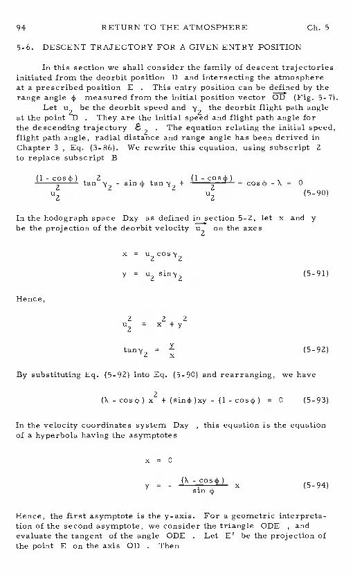
94 RETURN TO THE ATMOSPHERE Ch. 5
5-6. DESCENT TRAJECTORY FOR A GIVEN ENTRY POSITION
In this section we shall consider the family of descent trajectoriesinitiated from the deorbit position D and intersecting the atmosphereat a prescribed position E. This entry position can be defined by therange angle measured from the initial position vector OD (Fig. 5-7).
Let u be the deorbit speed and the deorbit flight path angleat the point2D . They are the initial speed and flight path angle forthe descending trajectory 8
2The equation relating the initial speed,
flight path angle, radial distance and range angle has been derived inChapter 3 , Eq. (3-86). We rewrite this equation, using subscript 2to replace subscript B
2 .tan - + + -x = 0
u2 u2 (5-90)
In the hodograph space Dxy as defined in section 5-2, let x and ybe the projection of the deorbit velocity u2on the axes
x =
u2 (5-91)
Hence,
2 2 2= x +y
z (5-92)
By substituting Eq. (5-92) into Eq. (5-90) and rearranging, we have
(X - x2 + - (1- = 0 (5-93)
In the velocity coordinates system Dxy, this equation is the equationof a hyperbola having the asymptotes
x0y =
- (X x (5-94)
Hence, the first asymptote is the y-axis.For a geometric interpreta-tion of the second asymptote, we consider the triangle ODE, andevaluate the tangent of the angle ODE. Let E' be the projection ofthe point E on the axis OD. Then
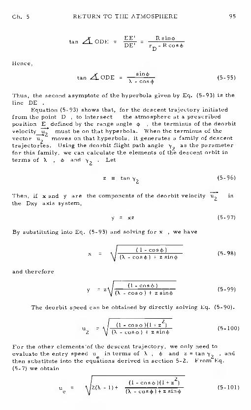
Gb. 5 RETURN TO THE ATMOSPHERE 95
tan = EE' Rsin4,DE
Hence,
tan = (595)X - cos4
Thus, the second asymptote of the hyperbola given by Eq. (5-93) is theline DE
Equation (5-93) shows that, for the descent trajectory initiatedfrom the point D , to intersect the atmosphere at a prescribedposition E defined by the range angle4 , the terminus of the deorbitvelocityu2 must be on that hyperbola. When the terminus of thevector moves on that hyperbola, it generates a family of descenttrajectories. Using the deorbit flight path angle as the parameterfor this family, we can calculate the elements of the descent orbit interms of X , and . Let
tan (5-96)
Then, if x and y are the components of the deorbit velocity u2inthe Dxy axis system,
y = xz (5-97)
By substituting into Eq. (5-93) and solving for x, we have
Fx = . (5-98)
(X - cos + z(599)
The deorbit speed can be obtained by directly solving Eq. (5-90).
- - )(l + z2)5 100)U2 -
(X - + -
For the other elements of the descent trajectory, we only need toevaluate the entry speed Uin terms of X , 4 and z = tan , andthen substitute into the equations derived in section 5-2.From Eq.(5-7) we obtain
(1 - )(l + z2)u = \/2(X - l)+ (5-101)
e v
96 RETURN TO THE ATMOSPHERE Ch. 5
Fig. .5- 7. The hyperbola which is the locus of the terminusof the deorbit velocity for entry at given position.
Fig. 5-8. Optimum velocity triangle for entry atgiven position.
Y
D
Y
E
Ch. 5 RETURN TO THE ATMOSPHERE 97
The impulsive change in the velocity , and its direction 6 , aregiven by Eqs. (5-11) and (5-12), respectively, with the initial speedgiven by Eq. (5-9) and the initial flight path angle by Eq. (5-10).
The entry flight path angle is given by Eq. (5-17). We have
2+2(1X)K I ecos'y
= \ I (5-102)e V (1+z)
where U is given by Eq. (5-101). The dimensionless semimajoraxis of the descent orbit is given by Eq. (5-13), written with the valueof Ue given by Eq. (5-101) as
a2 = X[ (K + zsin2
(5-103)(2K -1) - cos4 - (1- z
The eccentricity of the descent orbit is given by Eq. (5-14).
e = V2(1 - z2+ 2(K - +(K - 1)2 (5-104)2
[ (K -
The longitude of periapsis of the descent orbit is given by Eq. (5-23)where now the angle is given in terms of the selected variables as
(1 - cos4 ) ztan ii= (K -
(5-105)
The polar equation of the entry orbit is
p2r = (5-106)1+e2cos(0 -w)
where e2 is given by Eq. (5-104) and
p2 X'l— = - (5 107)R (K - cos 4) + z
The position of entry E is, of course, specified by the prescribedrange angle4
98 RETURN TO THE ATMOSPHERE Gh. 5
5-7. MINIMUM IMPULSE FOR ENTRY AT GIVEN POSITION
We have seen in the preceding section that, for an entry at a pre-scribed position, initiating from a given point D on the initialorbit,there exists a family of descent trajectories which is a function of thedeorbit flight path angle . These trajectories are such that theterminus of the deorbit vel2ocity is on a branch of hyperbola definedby Eq. (5-93). In this section we shall select from among the descenttrajectories in this family the one that results in a minimum character-istic velocity . That particular trajectory is called the optimumdeorbit trajectory for a prescribed entry position.
In the hodograph space (Fig. 5-8), consider the hyperbola whichis the locus of the terminus of u2for a given entry position definedby the range anglej . In this hodograph space, the initial velocityu1 is prescribed. Its projections x1 and y1 on the axis systemDxy are given by Eq. (5-68).
As for the problem of minimum impulse for entry at a given anglesolved in section 5-5, we obtain the minimum of by finding theshortest distance from the point with coordinates(x1
, y1 ) to thehyperbola defined by Eq. (5-93).
Again, let superscript (*)denote the optimum elements.Thepoint with coordinates(x* y* )on the hyperbola giving the terminusof the optimum deorbit velocity is the point where the normal tothe hyperbola passes through the point(x1 y1) . We write the equationof this hyperbola
f(x,y) = (X - x2 + xy - (1- = 0 (5-108)
The components of the normal to the hyperbola are given by
f 2(X - x+y
= x s1n4 (5-109)
Requiring that this normal be collinear to the vector gives
X-x1 - y-y10- (5h1
* *The set of equations (5-108) and (5-110) gives tlie coordinates (x, y )
components of the optimum deorbit velocity u2. It is convenient touse the variablez as defined by Eq. (5-96). Then the components ofthe vector are given in terms ofz by Eqs. (5-98) and (5-99).Upon substituting these equations into Eq. (5-110) and rearranging wehave a quartic equation in z
Bz4 + B1z3 + B2z2 + B3z + B4 0 (5-111)
Ch. 5 RETURN TO THE ATMOSPHERE 99
where the coefficientsB. are1
B0 (1 - S1fl4
B1 a 4(1 - - -
a 2(1 - -1)
+ 2x1y1 - (X -
B3 a - 4(1 - )(X - sink -
+6x1y1 (X - - (X -
B4 a
+ 4x1y1(X - )2- (X
)3
(5-112)
Hence, the optimum deorbit flight path angle is obtained by solvinga quartic equation. In general, this equation gives four roots corre-sponding to four normals drawn from the point(x1 , y1) to the hyper-bola given by Eq. (5-93).One of these roots corresponds to the mini-mum of
The elements of the optimum deorbit trajectory are obtained byusing the value ofz computed from the quartic equation (5-111) in thegeneral equations for descending trajectory derived in the previoussection.
By using, instead ofz , the components and of theoptimum deorbit velocity u2 as computed from Eqs. (5-98) and (5-99),we also can calculate the elements of the descending trajectory usingthe alternate formulas, Eqs. (5-84) -(5-89).
References
1. Fosdick, G.E. ,and Anthony, M. L. , "Three-Dimensional PulseOptimization for Vehicles Disorbiting from Circular Orbits,Research Report No. R-61-13, The Martin Company, Denver, 1961.
2. Vinh, N. X. , "A Geometrical Study of Re-Entry Transfer Orbits,ARL Report, TJSAF, No. 63-241, December 1963.
3. Busemann, A. ,Vinh, N. X. , and Gulp, R. D. , "Geometric Con-straints of the Disorbit Problem," AAS preprint No. 66-122, FirstSpace Flight Mechanics Specialist Conference, Denver, July 1966.Conference Proceedings, Vol.11 in the AAS Series in Sciencesand Technology.
4. Busemann, A. ,and Vinh, N. X. , "Geometric Theory of OptimumDisorbit Problems, "NASA GR-750, April 1967.
Chapter 6
Basic Equations forPlanar Entry Trajectories
6-1. INTRODUCTION
In Chapter 5 we considered the trajectory of the vehicle from thedeorbit position D to the entry position E. This point E is assumedto be at the top of the sensible atmosphere.Thus, until now, the tra-jectory has been analyzed for flight in a vacuum. From here on, thistext will treat the portion of the flight path beyond the point E, re-ferred to as the entry trajectory.
Along the entry trajectory, the aerodynamic force is no longernegligible. In fact, it plays an important role as a braking force toreduce the speed of the vehicle to the point such that the terminal phaseof the flight before landing can be conducted as a vertical free fall usinga system of parachutes for soft landing for vehicles with no lift capa-bility, or as a gliding flight at low speed as an ordinary airplane forvehicles which can generate aerodynamic lift.
6-2. ENERGY DISCUSSION OF THE TRAJECTORY IN PHASE SPACE
The equations of motion of a vehicle flying in a Newtonian gravi-tational force field and subject to thrust and aerodynamic force werederived in Chapter 2, Eqs. (2-28)and (2-32). We shall assume thatalong the fundamental part of the entry trajectory where the decelera-tion undergoes rapid change, the engine is shut off at all times.Hence,with T = 0 , and using Eqs. (4-4) for the lift and drag forces, wehave the planar equations of motion in the plane of a great circle(Fig. 6-1).
2
dV pSCDVdt = - Zm
- g(r)
pSC V2 2
= Zrn - [ g(r) - cos'1
= (6-1)
100
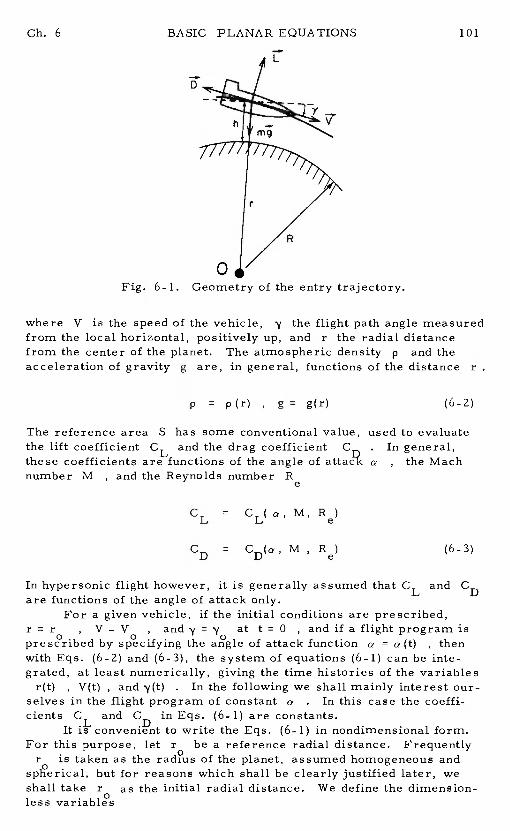
Gb. 6 BASIC PLANAR EQUATIONS 101
where V is the speed of the vehicle, the flight path angle measuredfrom the local horizontal, positively up, andr the radial distancefrom the center of the planet.The atmospheric densityp and theacceleration of gravity g are, in general, functions of the distancer
p = p(r) , g = g(r) (6-2)
The reference area S has some conventional value, used to evaluatethe lift coefficient CL and the drag coefficientC . In general,these coefficients are functions of the angle of a , the Machnumber M , and the Reynolds number Re
CL = CL( a, M, Re)
GD = CD(a, M , Re) (6-3)
In hypersonic flight however, it is generally assumed that CL and CDare functions of the angle of attack only.
For a given vehicle, if the initial conditions are prescribed,r=r , V=V , at t0 ,andifaflightprogramisprescribed by specifying the angle of attack function a =a(t) , thenwith Eqs. (6-2) and (6-3), the system of equations (6-1) can be inte-grated, at least numerically, giving the time histories of the variables
r(t) , V(t) , and . In the following we shall mainly interest our-selves in the flight program of constant a. In this case the coeffi-cients CL and CD in Eqs. (6-1) are constants.
It is convenient to Write the Eqs. (6-1) in nondimensional form.For this purpose, letr be a reference radial distance.Frequently
r is taken as the rad?us of the planet, assumed homogeneous andspherical, but for reasons which shall be clearly justified later, weshall take r as the initial radial distance. We define the dimension-less
L
D
V
R
0Fig. 6-i. Geometry of the entry trajectory.
BASIC PLANAR EQUATIONS Ch. 6
2 rz a (6-4)Zgr r00
where u is the dimensionless kinetic energy, and, for a Newtonianforce field, a is the negative of the potential energy.The accelera-tion of gravity is then
g = g0 (6-5)
where g is the acceleration of the gravity at the reference distance.With r as the initial distance, the initial value ofz is z = 1
a as the new independent variable, we the timeand rewrite Eqs. (6-1) as
du - rPSCDU2. +1
mz sinyr pSC
1= o L + (6-6)dz 2 z 2u2mz
where
4, a cos'y (6-?)
The system of Eqs. (6-6) constitutes the exact equations for flight in aNewtonian force field, subject to aerodynamic forces.Its integrationrequires specifying the law of variation for the atmospheric density,p , as a function of the independent variablea
The system of Eqs. (6-6) is exact.Hence, for flight in a vacuumthat is when p — 0 , we expect to obtain the trajectory in the form ofa Keplerian orbit. Putting p = 0 in the Eqs. (6-6), we have thesystem
dudz
a = (!J..)4, (6-8)dz a 2u
Integrating the first equation yields the vis viva integral
u = z+C (6-9)
where C is a constant representing the total energy.Substituting thisrelation into the second equation (6-8) and integrating gives
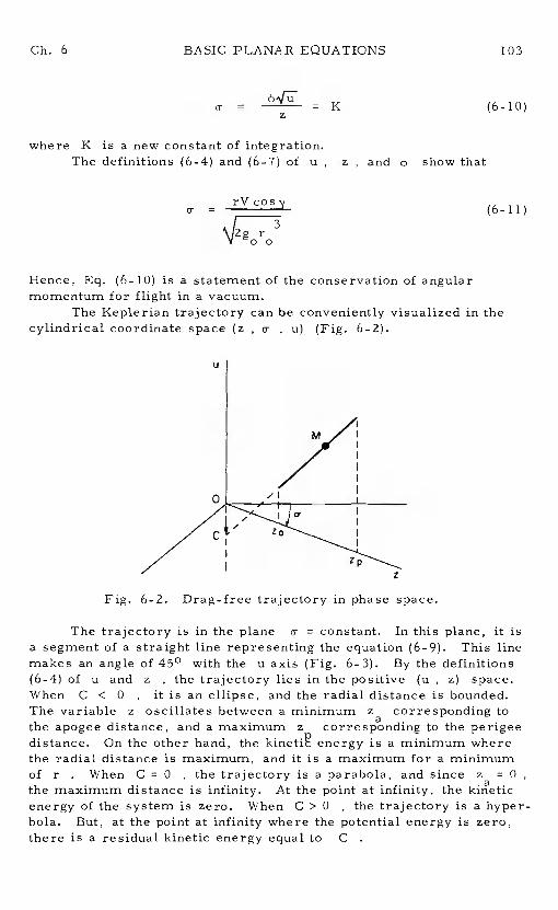
Ch. 6 BASIC PLANAR EQUATIONS 103
a = K (6-10)
where K is a new constant of integration.The definitions (6-4)and (6-7) of u , z , and show that
=rVcosy (6-11)
g r3
Hence, Eq. (6- 10) is a statement of the conservation of angularmomentum for flight in a vacuum.
The Keplerian trajectory can be conveniently visualized in thecylindrical coordinate space (z, , u) (Fig. 6-2).
Fig. 6-2. Drag-free trajectory in phase space.
The trajectory is in the planea- = constant. In this plane, it isa segment of a straight line representing the equation (6-9).This linemakes an angle of 45° with the u axis (Fig. 6-3).By the definitions(6-4) of u and z , the trajectory lies in the positive(a , z) space.When C < 0 , it is an ellipse, and the radial distance is bounded.The variable z oscillates between a minimum zcorresponding tothe apogee distance, and a maximum zcorresponding to the perigeedistance. On the other hand, the kinetiP energy is a minimum wherethe radial distance is maximum, and it is a maximum for a minimumof r . When C = 0 , the trajectory is a parabola, and sincez = 0
the maximum distance is infinity.At the point at infinity, the kineticenergy of the system is zero.When C > 0 , the trajectory is a hyper-bola. But, at the point at infinity where the potential energy is zero,there is a residual kinetic energy equal toC
Li
0
zpz
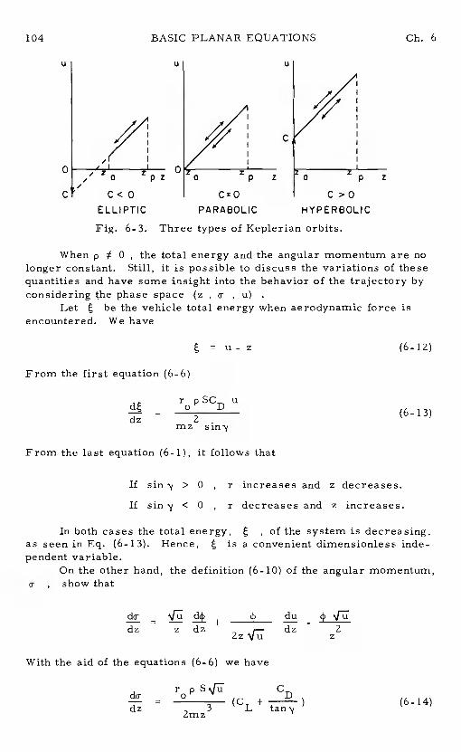
104 BASIC PLANAR EQUATIONS Ch. 6
U U U
/ // zo zpz za zp Z
C C<O C>OELLIPTIC PARABOLIC HYPERBOLIC
Fig. 6-3. Three types of Keplerian orbits.
When p 0 , the total energy and the angular momentum are nolonger constant. Still, it is possible to discuss the variations of thesequantities and have some insight into the behavior of the trajectory byconsidering the phase space(z , a- , u)
Let be the vehicle total energy when aerodynamic force isencountered. We have
= u- z (6-12)
From the first equation (6-6)
r pSC u— o D
13dz — 2.mz
From the last equation (6- 1),it follows that
If sin > 0 , r increases and z decreases.
If sin 'y < 0 , r decreases and z increases.
In both cases the total energy, , of the system is decreasing,as seen in Eq. (6-13). Hence, is a convenient dimensionless inde-pendent variable.
On the other hand, the definition (6-10) of the angular momentum,a- , show that
dz z dz ,— dz 22zVu z
With the aid of the equations (6-6) we have
d CD= (C + )
(6-14)dz 3 L tanyZmz
p z
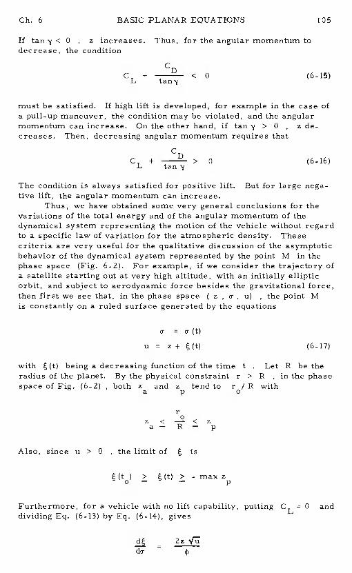
Ch. 6 BASIC PLANAR EQUATIONS 105
If tan < 0 , z increases. Thus, for the angular momentum todecrease, the condition
C+ D
< 0 (6-15)L tan'y
must be satisfied.If high lift is developed, for example in the case ofa pull-up maneuver, the condition may be violated, and the angularmomentum can increase. On the other hand, if tan> 0 , z de-creases. Then, decreasing angular momentum requires that
CC +
D> 0 (6-16)L
The condition is always satisfied for positive lift.But for large nega-tive lift, the angular momentum can increase.
Thus, we have obtained some very general conclusions for thevariations of the total energy and of the angular momentum of thedynamical system representing the motion of the vehicle without regardto a specific law of variation for the atmospheric density.Thesecriteria are very useful for the qualitative discussion of the asymptoticbehavior of the dynamical system represented by the point M in thephase space(Fig. 6-2). For example, if we consider the trajectory ofa satellite starting out at very high altitude, with an initially ellipticorbit, and subject to aerodynamic force besides the gravitational force,then first we see that, in the phase space( z , , u) , the point Mis constantly on a ruled surface generated by the equations
= o(t)
u = z+ (6-17)
with (t) being a decreasing function of the timet . Let R be theradius of the planet.By the physical constraint r > R, in the phasespace of Fig. (6-2), both z and z tend to r / R with
a p o
rz < —i < za— R — p
Also, since u > 0 , the limit of is
(t) > (t) > - max z
Furthermore, for a vehicle with no lift capability, putting CL =0 anddividing Eq. (6-13) by Eq. (6-14), gives
do- -
BASIC PLANAR EQUATIONS Ch. 6
which is, using definition (6-10)
= (6-18)
This shows that the angular momentuma- (t) is also decreasing.
6-3. THE FUNDAMENTAL EQUATIONS
The system of nonlinear differential equations (6-6) can be inte-grated for any specified vehicle from a prescribed initial condition,once the law of variation of the atmospheric density is known. We shallassume an exponential atmosphere of the form
p = (6-19)
where h is the altitude above the surface of the planet
h = r- R (6-20)
with R being the radius of the planet. is the reciprocal of the scaleheight and p is the atmospheric density at the surface.Using anaverage value forp in the altitude range of interest, we can treat itas essentially a constant.
For an analytic integration of the equations of motion, we intro-duce an altitude variable proportional to the atmospheric density
P 5%TI = (6-21)Zmp
Then using the exponential law, Eq. (6-19)
o— = - )3 dr = dz (6-22)Ti z
With this change of variable Eqs. (6-6) are transformed into2du = Zu
+
a =- Z (_L2-)4 (6-23)
dii CD j3nn 2u z
This system is the fundamental system of equations for planar entrytrajectories. The system is exact in the sense that the equations arevalid for flight in a Newtonian force field.The atmosphere is specifiedby prescribing the value of as shown in Table 1-2 (e.g.,
= 900 for the Earth's The flight parameter isspcified by the constant lift-to-drag ratio,CL! CD . For the
Ch. 6 BASIC PLANAR EQUATIONS 107
integration of the entry equations, the valuesu , and at theinitial time are given. Rigorously speaking, z 2 r/ rin the equations can be expressed in terms of the atmospheric density
through Eq. (6-21). This will require the specification of the dragparameter, that is the value of SCD/ mp. A simplification can bemade by noticing that in the fundamental equations, Eq. (6-23),thevariable ri which is proportional to the atmospheric density undergoesstrong variation while within the relatively thin layer of the atmosphere,as compared to the radius of the planet, we have for all practical pur-pose z =r / r 1 . Mathematically, this can be clearly seen in
(6-22) %y noticing that the value ofp r is large, of the order of10 . With this simplification, we are led to the basic equations foratmospheric entry
du Zu 1= +
n-ri sinv pm
=- pr'ii (6-24)
One characteristic feature with these equations is that for entry fromvery high altitude, we have11 = 0 . Hence, besides the values forthe atmospheric parameter,3°r , and lift-to-drag ratio, CL! CDwe only need to specify the initia?l valuesu and 'y for the integra-tion without regard to other physical characteristics°of the vehicle.Inother words, for a given planetary atmsophere, using the same lift-to-drag ratio C , with the same initial condition in u andthe relationships 9etweenu, and il are the same r°egardless ofthe mass, size and shape of the vehicle.The only difference is thatthe actual altitude during entry, for any specified vehicle, is ultimatelycomputed by Eq. (6-21) for the corresponding drag parameter.
The basic equations we have derived are adequate for a prelimi-nary analysis of the phenomena encountered during atmospheric entryof a hypervelocity vehicle. This will be done in Chapters 7,8 and 9.In Chapter 7, first order solutions for planetrary entry will be obtained.A second order theory for entry trajectories as developed by Loh willbe the subject of Chapter 8.Chapter 9 concerns the aerodynamic heat-ing during entry. The rest of the text will be devoted to more sophisti-cated theories for planetary entry.
References
1. Vinh, N.X., and Brace, F.,'An Energy Approach to AtmosphericEntry, " Lecture notes, University of Michigan, 1972.
2. Vinh, N. X., Busemann, A., and Cuip, R. D.,'Optimum Three-Dimensional Atmospheric Entry,Acta Astronautica, Vol. 2,pp. 593-611, 1975.
3. Loh, W. H. T. , Dynamics and Thermodynamics of Planetary Entry2Prentice Hall, Inc., Englewood Cliffs, New Jersey, 1963.
Chapter 7
Analysis of First-OrderPlanetary Entry Solutions
7-1. INTRODUCTION
To help in the understanding of the basic physical phenomenaencountered by a vehicle during its descent through a planetary atmo-sphere, in this chapter we shall derive several first-order solutionsfor planetary entry by making, separately for each case, the necessaryphysical assumptions.Each type of trajectory will be analyzed indetail. In particular, we shall be concerned with the variations duringthe entry of the altitude, the speed, and the acceleration of the vehicle.Other physical quantities associated with the dynamic pressure over thevehicle, and the heating phenomena will be analyzed in Chapter 9.Thestudy of the physical quantities associated with an entry trajectory isimportant since not only the knowledge of the variations of these quanti-ties is of great assistance in the preliminary planning of the design ofa specific type of entry vehicle, but also it provides the basic informa-tion with which one can construct new and accurate theories for analyz-ing entry trajectories.
For convenience, we recall the basic equations for entry trajec-tories in the plane of a great circle
+
= - 1 (.L (7-1C 2u
D o
where r is a constant and by definition
1u , (7-2)
while r is the initial distance from the center of the planet and gis the of gravity at this reference level.Thewere obtained by assuming that, at each instant,r = R + h rwhere R is the radius of the planet and h is the flight Thealtitude is obtained through the variation of the density of the atmosphere
108
Ch. 7 FIRST-ORDER SOLUTIONS 109
which is related to the dimensionless variable by the relation
SCDP
Zmp e (7-3)
It is generally assumed, in first-order theory, that the componentof the gravity along the tangent to the flight path can be neglected com-pared to the drag.This is equivalent to neglecting the second term onthe right-hand side of the first equation (7-1).Hence, we write it as
du 2u-
The second equation (7-1) is maintained in its general form. We re-write it with the physical meaning of each term
= - 1 (7-5)C Zu0/ \
lift gravity centrifugalforce force force
Two quantities of interest along an entry trajectory are the distancetraveled, and the deceleration.First, we have
= V (7-6)
where s is the arc length travelled since the initial time.On the otherhand, the equation for the speed V with the tangential component ofthe gravity g sin , neglected is
=-
(77)
Hence,pSC V
dV D 78ds - - 2m -
Using the definitions (7-2) and (7-3) for u and , we have
— 7du'r Zpr -0 0
This equation, upon integration, gives the distance travelled along theflight path. The tangential deceleration is simply
a = - (7-10)
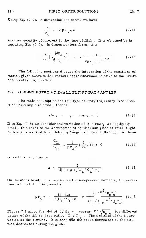
FIRST-ORDER SOLUTIONS Ch. 7
Using Eq. (7-7), in dimensionless form, we have
= (7-11)
Another quantity of interest is the time of flight.It is obtained by in-tegrating Eq. (7-7). In dimensionless form, it is
= - 1
3/2 (7-12)
The following sections discuss the integration of the equations ofmotion given above under various approximations relative to the natureof the entry trajectories.
7-2. GLIDING ENTRY AT SMALL FLIGHT PATH ANGLES
The main assumption for this type of entry trajectory is that theflight path angle is small, that is
, cos'j 1 (7-13)
If in Eq. (7-5) we consider the variation of 4= cos y as negligiblysmall, this leads to the assumption of equilibrium glide at small flightpath angles as first formulated by Sänger and Bredt (Ref.1). We have
+ -= 0 (7-14)
Solved for u , this is
1(7-15)
2[ 1 + j3 rO(CL/ CD)
On the other hand, if u is used as the independent variable, the varia-tion in the altitude is given by
(1 - 2u)1 - (112/ gr)
2'- 'c = 2(7-16)° C CU (C/C )(V/gr)
L D 00
Figure 7-1 gives the plot of1/ versus V/ for differentvalues of the lift-to-drag ratio,C / C . The ordinate of the figurevaries as the altitude.It is seentkat tke speed decreases as the alti-
tude decreases during the glide.
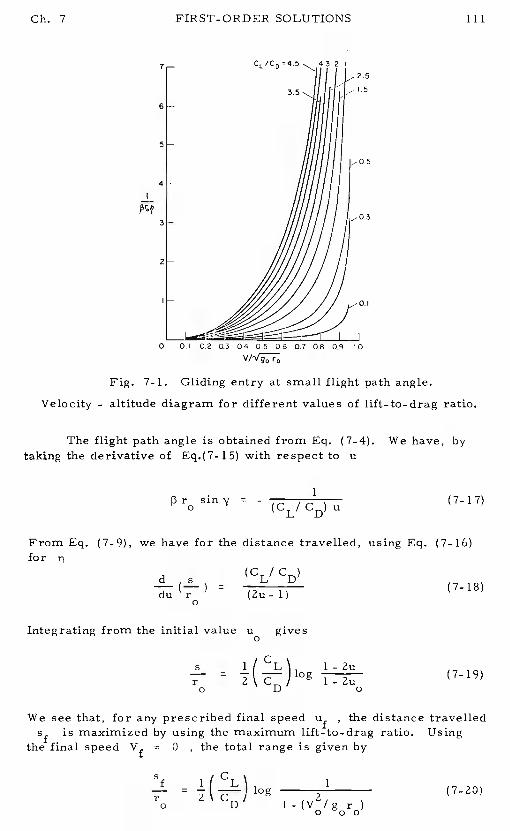
Ch. 7 FIRST-ORDER SOLUTIONS 111
2! !UL' 1
r 7o D r
0 00
7 CL/CD
3.5.
2.5
'.5
-0.5
-0.3
-0.I
P4
0 0.1 0.2 0.3 0.4 0.5 0.6 17 0.8 0.9 .0
Fig. 7-1. Gliding entry at small flight path angle.Velocity - altitude diagram for different values of lift-to-drag ratio.
The flight path angle is obtained from Eq. (7-4).We have, bytaking the derivative of Eq.(7- 15) with respect to u
siny =- (CL/CD) u (7-17)
From Eq. (7-9), we have for the distance travelled, using Eq. (7-16)for
d (CL/CD)= (7-18)
du r (Zu- 1)0
Integrating from the initial value u gives
s 1, LI 1-Zu— = (7-19)0 D o
We see that, for any prescribed final speed ufthe distance travelledis maximized by using the maximum lift-to-drag ratio.Using
the final speed Vf U , the total range is given by
(7-20)
FIRST-ORDER SOLUTIONS Ch. 7
The total range (s /speed VI
r ) is plotted in Fig. 7-2 in terms of the initialdifferent values of lift-to-drag ratio.
Srr0
1.0
Fig. 7-2. Gliding entry at small flight path angle.Total range in terms of initial speed
The time of flight is obtained by integrating Eq. (7-12).first by substituting Eq. (7-16) into Eq. (7-12)
Integrating from the initial value u gives
We have,
For any prescribed final speed Ufthe total time of flight tf ismaximized by using the maximum lift-to-drag ratio.Using Uf 0
we have the total flying time.
[_1+V/Li-vi0 VOO
CL/CD'4
0.3
v0 /
1
CD / (2u- 1) U 1/2
t- 1 (CL- log
Li-
(7-21)
(7-22)
1 ( CL\= (7-23)
Ch. 7 FIRST-ORDER SOLUTIONS 113
Finally, from Eq. (7-11) we have the deceleration along the glidingentry trajectory
21 - (V /g r
a 1-2u 00g - (CL/CD) - (CL/CD)
(7-24)
As the speed decreases, the deceleration increases continuously alongthe descending trajectory and it is minimized by using the maximumlift-to-drag ratio.
The first-order solution of this section is known as the first-ordersolution of Eggers, Allen and Neice (Ref. 2).
7-3. GLIDING ENTRY AT MEDIUM AND LARGE FLIGHT PATHANGLES
When the flight path angle is not small, the condition of equilibri-um glide is no longer maintained.On the right-hand side of Eq. (7-5)the lift force is predominant while the difference between the centrifugalforce and the gravity force remains small.Hence, we have the simpli-fied equation
= (7-25)
and upon integrating from the initial timeC
cos - cos = (ii - (7-26)
Combining the Eqs. (7-4) and (7-25) to eliminate we have
,C ',,
u = - (7-27)du 2 CD/
which integrates to
1_2(YU I 0— = exp I
(7-28)U L(C/C)
o L D
Equations (7-26) and (7-28) constitute the first-order solution of Leesfor gliding entry at medium positive lift-to-drag ratio and medium flightpath angle (Ref.3).
Using Eq. (7-11), with the solution (7-26) for and (7-28) for
u , we have for the deceleration, by taking
Zpr u _y)
= (CL/CD)(cosy - cosy) exp (7-29)
FIRST-ORDER SOLUTIONS Ch. 7
Since, by this expression,"a" is a function of alone, the maximumdeceleration occurs at a value of obtained by solving the equation
. We have
sin = cos - cos (7-30)
This equation can be written as a quadratic equation in tan (y/2)
(1 tan2-
tan - (1- = 0 (7-31)
The equation has two roots, one positive and one negative.For adescending trajectory, we take the negative root
tan= 2(l+cosy) [ —
(7-32)
Using this critical value for y in Eqs. (7-28) and (7-29), we have thecorresponding speed and the maximum deceleration.The altitude atwhich the maximum deceleration occurs is given by Eq. (7-26) with yas given by Eq. (7-32).Let subscript (*) denote the condition at thepoint of maximum deceleration.We have
ICL\ IICL\- = cos - cos
-sin
Therefore
- =— (733)
2 '1*1+tan
Another form of this equation is obtained by combining it with Eq.(7-31)
(1
- no = —
2+(CL/CD) tan
Using the solution (7-32), we have explicitly for the critical altitudewhere the maximum deceleration occurs, in terms of the lift-to-dragratio (CL/CD) , and the initial flight path angle
\J(CL/CD)+ - (CL/CD)
2 24+[(CL/CD)/(1 + )}[(CL/CD) +4 sin
(7-34)
Gb. 7 FIRST-ORDER SOLUTIONS
When the initial flight path angle is small
.24 sin<< 1
(CL/CD)
and the square root can be approximated by
+1+
(CL/CD)2]
The expression for becomes2Zsin
- = (C IC )
(7_35)L D
In this case, the critical flight path angle, as given by Eq. (7-32),be come s
22 sin=
- 'C IC (7-36)L D'
If the flight path angle is not too large, we have the approximate rela-tion
2
= - 0 (737)(CL/CD)
In this case, we obtain from Eq. (7-28) the critical speed where maxi-mum deceleration occurs
V
-v = expC
(7-38)o L D
The maximum deceleration is simply
a
= (CL/CD)exp (CLI0CD) (739)
The solution obtained by Lees applies to circular speed entry.For supercircular speed entry, it has been generalized by Ting (Ref. 4).In this case, the second term on the right-hand side of Eq. (7-5) is notnegligible since for large values of u, the difference [ (1/2u) - 1] isnot small. To obtain the expression for the flight path angle Ting usedthe approximation
FIRST-ORDER SOLUTIONS Ch.7
- -s-—- 1
Then, we have the equation
= - 1 (_L - 1) (7-40)CD Zu
Upon integrating and using the initial conditions, we have
= -1)log (7-41)
For small flight path angles, we have Ting's first-order solution forentry at supercircular speed
1/2=
-- 2 - 1) log (7-42)
Next, we write Eq. (7-5)
C- sin =
- 1- 1) (7-43)
dii CD clnii
Combining this equation with Eq. (7-4) to eliminate , we have
dii - dy (744)U
1
2 LCD - pnii 2u -
Considering the denominator on the right-hand side of this equation asconstant, we have, upon integrating
ULog — = (7-45)
i[ 1 _L1
-
Equations (7-42) and (7-45)constitute Ting's solution for entry fromsupercircular speed (Ref. 4).
Ch. 7 FIRST-ORDER SOLUTIONS
7-4. BALLISTIC ENTRY AT LARGE FLIGHT PATH ANGLES
When the aerodynamic force is in the form of pure drag, we haveballistic entry. For ballistic entry, CL = 0 . The general assumptionis that ballistic entry involves short range so that the assumption offlat Earth applies. In Eq. (7-5), if we neglect the centrifugal force, wehave
- u (7-46)
From this equation, because of the small factor1/2 , it is seenthat for relatively steep trajectories, the dimensionless atmosphericdensity will quickly become finite and the right-hand side can be putequal to zero. Since the term is the gravity term, this is equivalent toneglecting the gravity force compared with the drag force which is largeduring the fundamental portion of a steep ballistic entry trajectory.We shall first conduct the investigation under this assumption and latermodify the solution to include the effect of the gravitational force.
7-4. 1. Analysis Neglecting Gravity
If gravity is neglected, the integration of Eq. (7-46), with theright-hand side put equal to zero, yields
cos = cos (7-47)
We conclude that, for ballistic entry, the flight path angle remainsnearly constant and the trajectory is essentially a small portion of aspiral. Using this solution, Eq. (7-4) can be integrated to give
)i= exp I
. °I (7-48)
U L slay J0 0
Equations (7-47) and (7-48) constitute the first-order solution forballistic entry at large flight path angles as given by Gazley (Ref.5),Allen and Eggers (Ref. 6) and Chapman (Ref.7).
Equation (7-48), with 0 , can be written as
= exp ( siny (749)
It is seen that V decreases as the radius of a logarithmic spiral(Fig. 7-3).
In the figure, the angle is measured in radians.Let o bethe constant angle between V and the tangent to the spiral.We have
tan a- = sin < 0 (7-50)
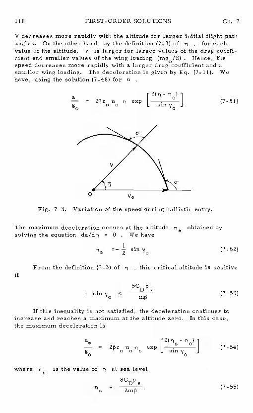
FIRST-ORDER SOLUTIONS Ch. 7
V decreases more rapidly with the altitude for larger initial flight pathangles. On the other hand, by the definition (7-3) of1 , for eachvalue of the altitude, is larger for larger values of the drag coeffi-cient and smaller values of the wing loading (mg/S) .Hence, thespeed decreases more rapidly with a larger drag coefficient and asmaller wing loading. The deceleration is given by Eq. (7-il).Wehave, using the solution (7-48) for u
rZ(n-1a
i o— = Zfir u expI
. (7-51)g o o L sin'v
0 0
Fig. 7-3. Variation of the speed during ballistic entry.
The maximum deceleration occurs at the altitude obtained bysolving the equation da/d1= 0 . We have
siny (7-52)
From the definition (7-3) of1 , this critical altitude is positive
5%- sin'y < (7-53)
o —
If this inequality is not satisfied, the deceleration continues toincrease and reaches a maximum at the altitude zero.In this case,the maximum deceleration is
a,1— = u exp I . I (7-54)
g 0 0 5 I.. siny J0 0
where is the value of at sea level
SCDP= Zm)3
(7-55)
0 V0
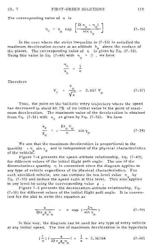
Ch. 7 FIRST—ORDER SOLUTIONS 119
The corresponding value of u is
1u = u exp I
° (7-56)0 L J0
In the case where the strict inequality in (7-53) is satisfied themaximum deceleration occurs at an altitude above the surface ofthe planet. The corresponding value ofil is given by Eq. (7-52).Using this value in Eq. (7-48) with 0 we have
— 1
U e0
ThereforeV
v = __2. = 0.607 V (7-57)* o
Thus, the point on the ballistic entry trajectory where the speedhas decreased to about 60. 7% of its initial value is the point of maxi-mum deceleration. The maximum value of the deceleration is obtainedfrom Eq. (7-51) with i-1 as given by Eq. (7-52). We have
a, pr u=
- 0 0 (7-58)g e 0
0
We see that the maximum deceleration is proportional to thequantity - u sin 'i and is independent of the physical characteristicsof the °
Figure 7-4 presents the speed-altitude relationship, Eq. (7-49),for different values of the initial flight path angle.The use of thedimensionless quantity is convenient since the diagram applies toany type of vehicle regardless of its physical characteristics.Foreach specified vehicle, one can compute its sea level valuebyEq. (7-55) and deduce the speed ratio at this level.This also appliesto any level by using the corresponding valuep -
Figure 7-5 presents the deceleration-altitude relationship, Eq.(7-51) for different values of the initial flight path angle.It is conven-ient for the plot to write this equation as
a =exp ( ) (7-59)2)3rgu sin
In this way, the diagram can be used for any type of entry vehicleat any initial speed. The line of maximum deceleration is the hyperbola
(!)(
a = = 0.36788 (7-60)2)3 rgu e
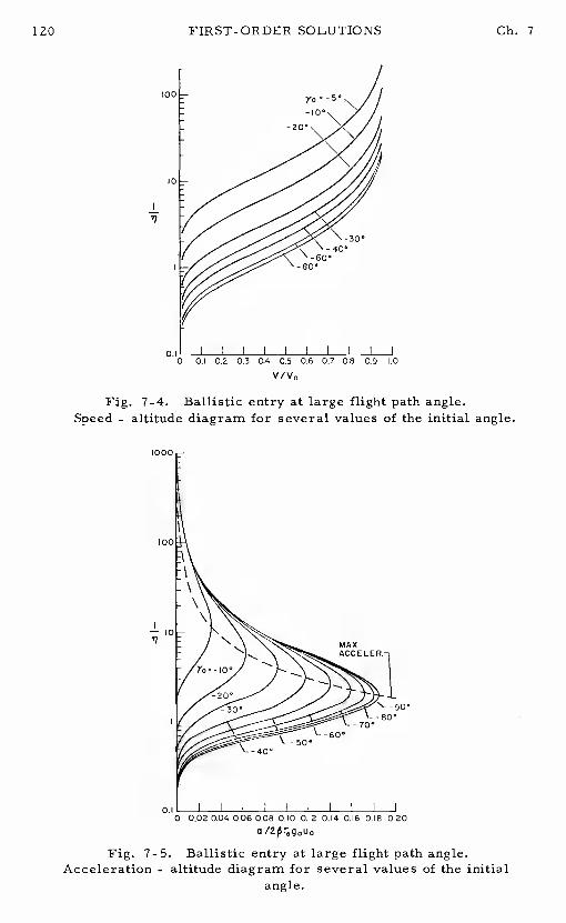
'7
FIRST-ORDER SOLUTIONS
1.0
Gb. 7
Fig. 7-4. Ballistic entry at large flight path angle.Speed -altitude diagram for several values of the initial angle.
Fig. 7-5. Ballistic entry at large flight path angle.Acceleration -altitude diagram for several values of the initial
angle.
.1 0.2 0.3 0.4 0.5 0.6 0.7 0.8
V / V0
'1
0.I
MAXACCE LE
0.02 0.04 0.06 008 0.10 0.12 0.14 0.16 0.18 0.20a
Ch. 7 FIRST-ORDER SOLUTIONS 121
7-4. 2. Analysis Including Gravity
The results in the previous section are obtained by neglecting thegravitational force. If the effect of gravitational force is retained,then for ballistic entry, under the flat Earth assumption, the Eqs. (7-1)are reduced to
du = 2u+
1
= - (7-61)2priiu
The first of these equations is now integrated under the assumptionthat the flight path angle is nearly constant and can be put equal to itsinitial value. Hence we have the linear equation
du 2u — 1 762- -
Using a new dimensionless atmospheric density asuch that
a = - (7-63)sin0
we can write the solution of Eq. (7-62) as (Ref. 8)
u = exp ( -a)[ Ei(a)+C] (7-64)
where C is a constant of integration and the exponential-integralfunction Ei(a) is defined as
Ei(a)= f dt (7-65)
This integral function is tabulated in Ref. 9.The constant of integra-tion C in Eq. (7-64) is evaluated using the initial condition.It isseen from this equation that the kinetic energy of the vehicle, orequivalently its speed, passes through a maximum for a falue of asatisfying the equation
Ei(a) + C =exp(a) (7-66)
If the constant of integration C has been obtained from the initialcondition, this equation can be solved for a. Upon substituting backinto Eq. (7-64) we have the value for the maximum kinetic energy
122 FIRST-ORDER SOLUTIONS Ch.7
u=
(7-67)a
0
Now, using Eq. (7-11), we have for the deceleration
- g= a exp (-a)[ Ei(a) + C] (7-68)
The deceleration has a maximum at the altitude where
Ei(a) + C = exp(a) (7-69)a-iAgain, if the constant C has been evaluated, using the initial
condition, this equation can be solved for aand, by the definition(7—63), for , yielding the altitude where maximum decelerationoccurs. Combining the last two equations, we have the maximumdeceleration
a* a- . = (7-70)gsin'j a - 1
where a is obtained by solving Eq. (7-69). Maximum decelerationoccurs at a positive altitude if
exp(a)Ei(a )+ C - > 0 (7-71)
5 a -l5
where a is the value of a at sea level, that isS
SCDPa = — = - (7-72)
s sin m13 sin
If the vehicle's physical characteristics are such that inequality (7-71)is not satisfied, then the deceleration monotonically increases duringthe balistic entry and reaches its highest level at sea level.Thismaximum deceleration is given by
a,- a exp (-a ) [Ei(a ) + C] (7-73)
g sin'1 s 5 50 0
From Eq. (7-64) the constant of integration C is given by
C = u exp (a) -Ei(a) . (7-74)
Ch. 7 FIRST-ORDER SOLUTIONS 123
where
a = — (7-75)0
On the other hand, a series expansion of the exponential function is
Ei(a) = loga + E (7-76)
where = 0.577215... is the Euler constant.Hence, for entryfrom altitude, a 0 and an approximate expression for C
C = 13r u(1 +a) - a-
- log a (7-77)
7-5. SKIP ENTRY
A trajectory of interest for a lifting hypervelocity vehicle is theskip trajectory. In the skipping phase, the vehicle enters the atmo-sphere, negotiates a turn, and is ejected from the atmosphere.Thistype of maneuver can be used to achieve a change in the orbital plane.Only the maneuver at constant lift-to-drag ratio in a vertical plane willbe analyzed in this section.The skip trajectory involves a short long-itudinal range. Hence the flat Earth assumption will be used; that is,we shall neglect the centrifugal force.Furthermore, since the gravi-tational force is, on the average, much smaller than the aerodynamicforce, we can neglect completely the gravitational force in the equationsof motion.
With these assumptions, we deduce from the general equations(7-1), the equations of motion governing a skip trajectory.
du — Zud,1 -
= (7-78)
The second equation can be integrated to giveC
cos - cos -(7-79)
D
The vehicle exits at a final altitude level equal to the initialaltitude . Hence,
'Yf = -(7-80)
124 FIRST-ORDER SOLUTIONS Ch. 7
This shows that, for a skip maneuver at constant angle of attack, theejection angle is equal to the absolute value of the entry angle.
At the lowest point of a skip trajectory, = 0 . The minimumaltitude is then
1 -
=(7-81)'L D
For this altitude to be positive, it is necessary that
1 - cos SCDP
(CL/CD) <
where the condition 0 has been assumed. We can write thecondition as
2sin — (7-82)2 4ç3(mg/S)
This provides the safety limit on the entry angle for a vehicle with speci-fied lift capability and wing loading condition.
To obtain the velocity distribution along a skip trajectory, wecombine the two equations (7-78) to obtain
= - (7-83)du 2u CD
Integration gives
exp (7-84)
or in terms of V
V 1= exp
[(CL/CD)](7-85)
Hence, since =-
the final velocity is
Vf ( 2yexp C /C ) (7-86)
o L D
Equations (7-79) and (7-85) constitute the first-order solution for askip trajectory as originally derived by Eggers, Allen and Neice (Ref. 2).
Ch. 7 FIRST-ORDER SOLUTIONS 125
The distance travelled is given by Eq. (7-9) which, combined withEq. (7-83), provides
(7-87)
Using the solution (7-79) for (CL/CD) , we can write this equa-tion
d 1
— = (7-88)dy
where the modified initial angle y.is defined by
cos = cos-
(7-89)
The integration of Eq. (7-88) is simple. We have
1)3s = log (7-90)siny.
1
using y. with its positive argument.If we consider the range x, then by the differential relation
dx = cos y ds (7-91)
the equation to be integrated is
= cos (7-92)(cos y - cos
Integration from the initial distance x= 0 gives the solution
r tan + tan tan - tan= y-y+ cOt'y. log
y.
(7-9 3)
The tangential deceleration is given by Eq. (7-11), written with sub-script t , as
(7-94)g0 0
FIRST-ORDER SOLUTIONS Ch. 7
It is informative to follow Miele, (Ref. 8), in considering also thenormal deceleration
= !_ I = Zpr (795)
Hence, the total deceleration is
=+
2pr (7-96)
The total deceleration and its two components are proportional toAll pass through their respective maxima at the same time.We needonly consider
u ig
== (CL/CD) exP[(C /C)] (797)
The analytical solution for and u , as well as the expression forthe deceleration have the same mathematical form as the expressionsobtained by Lees for gliding entry at medium and large flight path anglesas derived in Section 7-3.Hence, the discussion for the maximum de-celeration is identical to that in Section 7-3.The pertinent remark tobe added here is that, from Eq. (7-36), one can see that the peak decel-erationoccurs during the descending phase.
Furthermore, it should be noted that although for the two casesthe resulting differential equations are identical, hence, providing
identical solutions, the physical assumptions are different.For theskip trajectory, if we return to Eq. (7-5)with the different forceslabelled, each of the gravity force and the centrifugal force is smallcompared to the lift force, since it will require a relatively high lift-to-drag ratio to negotiate a skip trajectory.On the other hand, for glidingflight at medium and large flight path angles, one uses a moderate lift-to-drag ratio. The gravity force and the centrifugal force, consideredseparately, may have the same order of magnitude as the lift force.The assumption used is that their combined effect is negligible compar-ed to the effect due to the lift, hence the combined term may be putequal to zero. To retain this effect, instead of putting it equal to zero,we may hold it constant for the integration.In doing so, we used theso-called Loh's assumption.Loh's theory for the entry trajectory,which is a second-order theory, will be presented in Chapter 8.
References
1. Singer, E. , and Bredt, J., "A Rocket Drive for Long RangeBombers," Translation No. CGD-32, Technical Information Branch,Navy Dept. , 1944.
Ch. 7 FIRST-ORDER SOLUTIONS 127
2. Eggers, A. J., Allen, H. J. , and Neice, S. E. , "A ComparativeAnalysis of the Performance of Long-Range Hypervelocity Vehicles,NACATN4O46, 1957.
3. Lees, L. , Hastwig, F. W. , and Cohen, C. B., "Use of AerodynamicLift During Entry into the Earth's Atmosphere, "ARS Journal, pp.633-641, September, 1959.
4. Ting, L. , and Wang, K. "An Approximate Analytic Solution ofRe-Entry Trajectory with Aerodynamic Forces,ARS Journal, pp.565-566, June, 1960.
5. Gazley, C. , "Deceleration and Heating of a Body Entering a Plane-tary Atmosphere from Space, "The RAND Corporation ReportP-955. February 1957.
6. Allen, H.J. , and Eggers, A.J. , "A Study of the Motion and Aero-dynamic Heating of Missiles Entering the Earth's Atmosphere atHigh Supersonic Speeds," NACA TR 1381, 1958.
7. Chapman, D. R. ,"An Approximate Analytical Method for StudyingEntry into Planetary Atmospheres, "NASA Technical Report R-1l,1959.
8. Miele, A. , Flight Mechanics, Vol. 1, Addison-Wesley PublishingCompany Inc., Reading, Massachusetts, 1962.
9. National Bureau of Standards, Tables of Sine, Cosine andnential Integrals, Vols.1 and 2, 1940.
Chapter 8
Loh's Second-Order Theory forEntry Trajectories
8-1. INTRODUCTION
In Chapter 6, we derived the dimensionless exact equations forentry at constant lift-to-drag ratio in the plane of a great circle.Theset of fundamental equations of entry are not solvable analytically, evenwith the usual assumption considering the acceleration of gravity con..stant. However, upon restricting the solution to a limited region ofapplication, one can obtain several first-order approximate analyticalsolutions as presented in Chapter 7.Each of these solutions is thenvalid for one type of entry.On the other hand, Loh has derived a moregeneral solution which covers the entire range of lift-to-drag ratiosand initial flight path angles (Ref.1). We shall refer to his solution asLoh's second-order solution.
Loh's theory is empirical, and is based on data from extensivenumerical integration of entry trajectories.Nevertheless, it provesto be very accurate, even for trajectories with varying lift-to-dragratio (Ref. 2).
In formulating Loh's assumption, we consider the fundamentalequations, Eqs. (6-23)
2du = 2u z+
= - (i_. !) (8-1C 2u z
D o
where, as before,2 r
u a , z a , cosy (8-2)
with r the initial radial distance.The variable is proportional tothe atmospheric density, and is defined as
128
Ch. 8 LOWS SECOND-ORDER THEORY 129
5%= p (8-3)
Loh's first assumption is to takez = 1 in the fundamental equa-tions, Eqs. (8-1). Thus, we have the basic equations for planetaryentry
= +
- 1 8-4C
D o
Loh considered this system as the system of exact equations for entry,but, as seen here, it is obtained by neglecting the altitude as comparedto the reference radial distance.
Let
C a 1)4 (8-5)
Although the right-hand side of this equation is a function of the vari-ables , u and 4 , all varying with the time, Loh observed throughextensive numerical integration for different types of entry trajectories,that the term remains nearly constant for each trajectory.Therefore,he used the assumption that C is constant for the purpose of integra-tion with respect to either or 'y . A possible interpretation of thisphenomenon can be seen by observing that the expression for C is thedifferencebetween the gravity force and the centrifugal force along thenormal to the flight path. For curvilinear flight over a spherical Earth,this difference remains nearly constant.In keeping this term, theseeffects are retained in the solution, with any resulting error from theassumption coming entirely from the fluctuation between the two forces.Such fluctuation is small.
8-2. UNIFIED SOLUTION FOR ENTRY
With C considered as constant, the second Eq. (8-4) is written
= —h-C (8-6)CD
where, for constant lift-to-drag ratio, the right-hand side of thisequation is constant, The integration is immediate,
rCcos - cos
=- Gjk - (8-7)
D
LOHtS SECOND-ORDER THEORY Ch. 8
This equation can be rearranged to give the expression for the flightpath angle in terms of and u
-COS
= - (1/Zu)- 1] (8-8)
To integrate the first equation (8-4), Eq. (8-6) is rewritten as
C_siny = - G (8-9)
CD
Then, with y as the independent variable of integration, Eq. (8-4) is
du Zu - siny+ I - - - GJ
Using the solution (8-7) to rearrange the right-hand side of this equa-tion gives
du Zu - sinydy [ (CL/CD)_G] - — }
Since 0 , the final equation for u is
+2u - silly
(8 10)dy — )3r0(cosy_cosy) -
Let
Ku (8-11)
and
f(y)= (8-12)r(cos y - cosy)
The equation for u is a non-homogeneous, linear equation:
+ Ku = f(y) (8-13)
If we treat G as essentially constant,K is a constant for constantlift-to-drag ratio entry. Then Eq. (8-13) can be integrated:
Ch. 8 LOWS SECOND-ORDER THEORY
u = C e - v + F(V) (8-14)
where C is the constant of integration, and F(V) represents theintegral
F(V) a e dV (8-15)
The constant of integration C can be evaluated by using the initialconditions
V = V0 u = u ' = (8-16)
It should be noted that, although K is treated essentially as a constantfor the purpose of integration, when the solution is obtained explicitlyin the form (8-14), both terms on the right-hand side of this solutionare now functions of u, V and through the definitions (8-5) and(8-11) of G and K . Hence, in evaluating the constant of integrationC , one may choose either to consider K as a function of u ,V and
or as a constant evaluated at some specific point along the trajectory.If C is evaluated by considering K as varying, then
(K V -KV) (K V -KV)u = ue °
+ [ e° (8-17)
where
K[ (1/Zu)- 1]
(8-18)
The two equations (8-8) and (8-17) constitute Lohts unified solution forentry. In general, the function F(V)as given by the integral (8-15)cannot be expressed in terms of elementary functions, but series solu-tions are available(Ref. 1). The equations can be solved for any twoof the three variables u' V and in terms of the remaining one.From the value of , one can recover the real altitude through thedefinition (8-3) written as
e-ph (8-19)
The drag parameter of the vehicle is involved only at this step.Hence,as far as the relationship between the dimensionless kinetic energy uand the flight path angle is concerned, it is dependent on the value ofthe drag parameter only through the initial value . Practically,for entry from very high altitude11 is zero. Thus, the relationshipbetween u and Vis completely in8ependent of the drag parameter.In this case the value Kas defined by (8-18) should be evaluated atsome intermediate point of the trajectory other than the initial point toavoid the singularity caused by taking = 0
LOWS SECOND-ORDER THEORY Ch. 8
8-3. SECOND-ORDER SOLUTION FOR ENTRY
In general, the unified solution as presented by Loh is too tediousto use since the two governing equations, Eqs. (8-8) and (8-17) aretranscendental in the variables u ,y and . But the second term inthe expression (8-17) for u contains the factorl/)3r by the definition(8-12) of the function , which is generally small. For the Earth,
= 900 , and according to Table 1-2 ,the values of for theplanets Venus, Mars and Jupiter are 500, 350 and 3000 respectively.Therefore, except for the cases where extreme accuracy at the termi-nal phase of flight is desired or for the cases involving planetary at-mospheres in which the values of are unforeseeably small, onecan omit the term with the factor in the expression (8-17) for
u . In this case, the solution becomes
cos= ° (8-20)
(1/2u)- 1]
and
log= I (1/2u) - 1]
(8-21)
Equations (8-20) and (8-21) form the basic second-order solution asderived by Loh. From these two equations, any two of the three vari-ables u , and can be determined in terms of the remaining one.The equations are still transcendental in the variables.To ease thenumerical computation, whenever << 1 , Eq. (8-20) can beapproximated by
cosy +(CL/CD)cos = ° (8-22)
1+(l/pr)[(l/2u) — 1]
On the other hand, Eq. (8-21) ,when solved for , gives
(1/pr){ (l/2u)- 1] cosylog(u/u)
- (CL! CD) log (u/u) -Z(y - y)(8 23)
Eliminating between the last two equations yields
IC1
1 + [1 -(8-24)
This transcendental equation can be solved for y in terms of uSubsequently, the corresponding value ofcan be obtained fromEq. (8-23), or more accurately from Eq. (8-20), rewritten as
Ch. 8 LOWS SECOND-ORDER THEORY 133
CL1 1
=
For In << 1, the right-hand side can be simplified.This givesthe dimensionless atmospheric density representing
the variation of the altitude
IC=
+ [ +
D ° (8-25)
Loh has shown that the second-order solution, as derived, is veryaccurate compared with the exact numerical solution (Ref.1). However,it should be noted that the exact equations as considered by Loh are theequations (8-4) obtained by takingz = 1 . The theory is based on com-putational experience showing that, during the process of integration,the term G is nearly constant.This explains the accuracy of thetheory. A physical explanation of this phenomenon will be given in thenext section when we show how the second-order solution is reduced todifferent first-order solutions.
8-4. REDUCTION OF THE SECOND-ORDER SOLUTION TO FIRST-ORDER SOLUTIONS
As presented in Chapter 7, several authors have obtained first-order solutions for different cases of entry trajectories. The proce-dures followed in deriving these solutions are the same.First, thetype of entry trajectory is examined, and then approximations are madebased on physical reasoning, and the basic equations for entry aresimplified allowing simple integrations to obtain the solution in closedform. Each of the solutions is then only valid for a specified type of
entry trajectory. The second-order solution obtained by Loh is a unifiedsolution in the sense that itis valid for all types of entry trajectories.Hence, upon appropriate simplifications, it should be reducible to thedifferent types of entry solutions if the empirical observation made byLoh is consistent with the physical entry phenomena.
The second-order solution derived by Loh as presented in theprevioussection is reproduced here for convenience of discussion.
cos = (8-26)l+(1/pr)(l
- nI-n)[ (l/2u)- 1]
I u 2(.y-,y)log
= (CL/CD) - r (1/Zu) -.1] cos'y(8-27)
An alternate expression is
134 LOWS SECOND-ORDER THEORY Ch. 8
u [ 1 [(1/2u)-1} -= - [1 - (cos'j/cosy)J
(8-28)
The solution has been derived based on the assumption that a combinedgravity and centrifugal term G is constant.This G term is defined
G (—2—-l)cosy (8-29)2u
0
As has been observed, this term represents the difference between thegravity force and the centrifugal force along the normal to the flightpath. We shall derive the different first-order solutions from Loh'ssecond-order solution and at the same time try to justify his empiricalas sumption.
8-4. 1. Gliding Entry at Small Flight Path Angles
When the flight path angle is small,cos cos 1 . Thus,Eq. (8-26) becomes,with 0
1 1 (CL\i— (-i-- - 1)
=(8-30)
Or, solving for u
u = 2[ (CL/CD)(8-31)
which is identical to the first-order solution, Eq. (7-18), for glidingentry derived in Chapter 7. Now, Eq. (8-29) with cos 'y 1 canbe written as
(km. I) = (8-32)
By comparing the two Eqs. (8-30) and (8-32), we see that the nearlyconstant term 0 is, in this case, nearly equal to the constant lift-to-drag ratio. It also can be seen in Eq. (8-6) that, for gliding entry atsmall flight path angles,4 = cos is nearly unity and the right-handside of this equation is nearly zero.The condition
CL 1 1— - ( — - 1) cos = 0 (8-33)CD tlrri 2u
Gb. 8 LOWS SECOND-ORDER THEORY 135
is called the condition of equilibrium glide.That is, there is nearlyexact balancing among the lift force, the gravitational force and thecentrifugal force along the flight path for'y 0 . This assumptionwas first formulated by Sänger and Bredt in Ref.3.
Now Eq. (8-28) is written as- V (l/2)(CL/GD) log (u/u)
cos - cos; — (cos y - cos 'q) + (l/flr)[ (l/2u) - 1] cos
/GL\ u 1 -l— 1,,—) log (—) (— - 1) (8-34)2 C u 2u
D o
The left-hand side of this equation, for'y , can be approximated
- 1 1
1 sin'v0 sxn1(y+V)
On the other hand, for entry from near circular speed, 2u 1 , andthe logarithm term on the right-hand side of Eq. (8-34) is 2pproximatedby
u 1 1
=- +...
With these approximations, Eq. (8-34) is reduced to the final resultfor the small flight path angle in the form
)3r sin =- (CL/GD) u (8-35)
which is identical to Eq. (7-17) derived in Chapter 7.Equations (8-31)and (8-35) form the first-order solution of Eggers, Allen and Neice(Ref. 4) for gliding entry at small flight path angle.The derivation ofEq. (8-35) directly from the second-order solution is somewhat deli-cate because it involves the ratio of small quantities.A more directway is to use the first Eq. (8-4) with the second term on the right-handside neglected. This is equivalent to assuming that the component ofthe gravity force on the tangent to the flight path is negligible comparedto the drag force. Then,
du 2udi-1 - siny
Using the first-order solution (8-31) to evaluate the derivative du/dtiyields directly Eq. (8-35)
136 LOWS SECOND-ORDER THEORY Gb. 8
8-4. 2. Gliding Entry at Medium and Large Flight Path Angles
When the flight path angle is not small, we neglect the terms withcoefficient 1/ç3r in Loh!s second-order solution.Then the Eqs. (8-26)and (8-27) are reduced to
Ccos - cos = - (8-36)
and
1— = expL (C IC ) j (8-37)
o L D
Equations (8-36) and (8-37) are the first-order solutions of Eggers,Allen and Neice (Ref. 4) and Lees (Ref.5) for skip entry and glidingentry at medium and large flight path angles.They have been derivedby different approaches in Chapter 7.In the present analysis, thiscase corresponds to considering the term 0 as negligibly small.Hence, Loh's assumption, the empirical assumption of considering Gas nearly constant, is essentially correct.
8-4. 3. Ballistic Entry at Large Flight Path Angles
For ballistic entry, CL = 0 . This, along with neglecting theterm with coefficient 1/ in Eq. (8-26), gives
cos = cos (8-38)
Since the flight path angle is nearly constant, the trajectory is essen-tially a spiral in the plane of the great circle.If we keep the term1/13 r in Eq. (8-26) to retain the small variation in the flight pathangle, then
(8-39)
Now Eq. (8-27), with the constant term cosas unity, is
I u 1
- 'y)=—
log(—) 1) (8-40)
The ratio of the last two equations yields
1 u 2log(—) =U siny
Gb. 8 LOWS SECOND-ORDER THEORY 137
The last step in approximating the equation above is accomplished byusing as done previously.Hence, the expression for the veloc-ity is
r 2(n - n0) 1— = exp
J(8-41)
u L siny J
Equations (8-38) and (8-41) form the first-order solution of Gazley (Ref.6), Allen and Eggers (Ref. 7) and Chapman (Ref.8) for ballistic entryat large flight path angles.Since they are here derived from Lob'ssecond-order solution, they involve his assumed nearly constant 0the combined gravity and centrifugal force.Let us examine the validityof this conjecture of Lob.Comparing the two equations (8-29) and (8-39)we see that
cos'j(cos'y -cosy)0 = ° (8-42)
(n -
Hence, except along the initial portion of the trajectory, this term canbe considered as small ify y . In fact, as has been presented inChapter 7, for the direct derivat?on of the first-order solution forballistic entry we put CL = 0 , 0 = 0 in the second Eq. (8-4) and haveupon integration
cos y = cos
Hence the constancy of the term 0 ,being small in this case, is explain-
8-4. 4. Skip Entry at Large Flight Path Angles
Along a skip trajectory, the vehicle enter the atmosphere, nego-tiates a turn in the vertical plane and returns to the vacuum.Hence, ifthe flight continues under the action of the gravity, each portion ofatmospheric flight is joined to the next by a ballistic arc.lo Chapter 7,it has been seen that the original solution was developed by Eggers,Allen and Neice (Ref. 4) with the assumption that, in the turning process,the aerodynamic lift is the predominant force and the gravity force canbe neglected. While the original derivation considers a flat Earth model,we can retain the curvature of the Earth in the combined Lob's0term and set it equal to zero compared to the lift term.That is, thesecond Eq. (8-4) now becomes
Ca = (8-43)CD
Integration gives the solutionCL
cos y - cos = - no) (8-44)
138 LOH'S SECOND-ORDER THEORY Ch. 8
This equation can also be obtained from second-order solution,Eq. (8-26) by neglecting the term G in it.Using the same assumptionin Eq. (8-27) we have for the speed
r2N0-v) 1— = exp [(CL/CD) j (8-45)
References
1. Loh, W. H. T., Dynamics and Thermodynamics of Planetary Entry,Prentice Hall, Inc. ,Englewood Cliffs, New Jersey, 1963.
2. Speyer, J. ,and Womble, M., "Approximate Optimal AtmosphericEntry Trajectories, "J. of Spacecraft and Rockets, Vol. 8, pp.1120-1126, Nov. -Dec. , 1971.
3. Sänger, E. , and Bredt, J. , "A Rocket Drive for Long RangeBombers," Translation CGD - 32, Technical Information Branch,Navy Dept., 1944.
4. Eggers, A. J. ,Jr. , Allen, H. J. , and Neice, S. E. , "A Compara-tive Analysis of the Performance of Long-Range HypervelocityVehicles, " NACA TN 4046, 1957.
5. Lees, L. , Hastwig, F. W., and Cohen, C. B. ,"Use of AerodynamicLift During Entry into the Earth's Atmosphere, "ARS Journal, pp.633-641, September 1959.
6. Gazley, C., "Deceleration and Heating of a Body Entering a Plan-etary Atmosphere from Space, "The RAND Corporation Report,P-955, February 1957.
7. Allen, H. J. , and Eggers, A. J., "A Study of the Motion and Aero-dynamic Heating of Missiles Entering the Earth's Atmosphere atHigh Supersonic Speeds," NACA TR 1381, 1958.
8. Chapman, D. R., "An Approximate Analytical Method for StudyingEntry into Planetary Atmospheres, "NASA Technical Report R-l1,1959.
Chapter 9
Aerodynamic Heating
9-1. INTRODUCTION
The various first-order solutions developed in Chapter 7 are nowemployed to analyze the thermal problems encountered in hypersonicflight. The study is of fundamental interest to scientists and engineersinvolved in design of space vehicles and in planning flight operationsfor a given mission. In space-flight, achieving a maximum payload isalways a factor of prime consideration.A relatively important fractionof this payload is used in the protection and cooling process duringentry if the spacecraft is to be recovered.During entry the total heattransferred to a spacecraft from the environment must be absorbed bysome coolant material or radiated away.But any heat absorbing mater-ial has a maximum allowable temperature and therefore can acceptonly a given amount of heat per unit weight.Hence, the total heat in-put to the vehicle must be kept as low as possible.
On the other hand, often the coolant material is simply the pro-tective wall of the vehicle exposed to the oncoming airstream, and itfollows that the selection of this material is dictated by the requiredstructural strength and rigidity for the vehicle.An important criter-ion determining the required structural performance of the vehicle isthe dynamic pressure encountered, which is a function of the entrytrajectory flown. In structural analysis, it is known that the strengthof the structure is a function of the stresses induced by the temperaturegradients within the material.Since these temperature gradients areproportional to the time rate of heat input, the maximum time rate ofheat input is also a parameter of prime interest in the design of thevehicle. Hence, three of the most important parameters of the entrytrajectory are the total heat input along the trajectory, the maximumrate of aerodynamic heating and the maximum dynamic pressure.
This mechanism of heat flow into a vehicle during entry was in-vestigated at an early time by Allen and Eggers (Ref.1). Since then,because of the many possible combinations of speed regimes and aero-dynamic shapes, numerous technical papers have been published.Butthe basic aspects of the aerodynamic heating during entry are still thesame. Only numerical factors for different heat transfer formulas andtheir validity in terms of the regime of the speed vary with the differentauthors. Hence, in this chapter, we shall follow Allen and Eggers (Ref.1) in analyzing the three most important aspects of aerodynamic heating
139
140 AERODYNAMIC HEATING Ch. 9
during entry; namely,
1. The total heat input, Q
2. The time rate and maximum time rate of average heat inputper unit area, q = dH /dt andav av
= (dH /dt)av max3. The time rate and maximum time rate of local stagnation
region heat input per unit area,q = dH /dt and(q ) = (dH /dt) S $
s max s max
For easy reference, the notation introduced in this chapter issummarized below:
A surface area,
CF equivalent skin-, friction coefficient
C specific heat of atmosphere at constant pressure,k cal/kgm °K
h convective heat transfer coefficient,k cal/rn2 sec °KH convective heat transfer per unit area,k cal/rn2k fraction of the heating rate at any point to the heating rate
at stagnation pointK stagnation point heat-transfer equation,
k cal/rn sec
q time rate of heat input per unit area,k cal/m2 secq dimensionless qQ convective heat transferred,k calR radius of curvature of body surface at stagnation point, mT temperature ,
Subscript
o conditions at reference, initial conditionav average values
f final conditions
local conditions
e exit conditions
r recovery conditions
s stagnation conditions, also conditions at sea levelw wall condition
Ch. 9 AERODYNAMIC HEATING
9-2. HEAT FLOW INTO THE VEHICLE
A vehicle entering a planetary atmosphere possesses a largeamount of total energy. When it encounters the atmosphere at highspeed, a shock wave system will form ahead of the part of the vehicleexposed to the oncoming airstream.The resulting deceleration of theflow induces the formation of a high temperature region in the inviscidflow between the shock system and the body.In addition, the velocityof the stream relative to the vehicle vanishes at the surface (zero-slipcondition), producing a further increase in the static enthalpy of thefluid. Therefore, if the temperature at a small distance from the bodyis higher than the surface temperature, thermal energy flows into thebody. The heat transfer is made up of two basic processes:
a! convective heating associated with the transport processesin the boundary layer,
b/ radiant heating associated both with the radiation from thehigh-temperature gas to the vehicle, and the radiation away from thehot surface of the vehicle.
To simplify the analysis, Allen and Eggers have assumed that:1. Convective heat transfer predominates and radiation effects
could be ignored.2. Real gas effects may be neglected.3. Shock-wave boundary-layer interaction may be neglected.4. Reynolds analogy is applicable.5. The Prandtl number is unity.Of the first assumption, the radiation effects that are neglected
include the radiation from the surface of the body and the radiation tothe body from the high-temperature disturbed air between the shockwave and the surface.The first simplification is based on the fact thatthe maximum allowable surface temperature will be about the same fora variety of entry vehicles, regardless of shape, and as a consequencethe radiation away from the surface will be approximately the same.Hence, neglecting this form of heat transfer should not alter the quali-tative effect of the relative heating investigated.The second simplifi-cation, namely neglecting the radiative heat transfer from the disturbedair, is purely for qualitative evaluation and is not applicable to veryblunt and heavy shapes at entry speeds about 3,000 m/sec
In the second assumption, the neglect of real-gas effects in theflow, particularly dissociation, on convective heat transfer is a goodassumption for entry speeds up to3,000 m/sec . In any case, it is aconservative assumption resulting in heating rates higher than actualrates.
In the third assumption, it has been shown by Lees and Probstein(Ref. 2), and by Li and Nagamatsu (Ref.3), that shock-wave boundary-layer interaction may significantly increase laminar skin-friction co-efficients on a flat plate at zero incidence and at Mach numbers in ex-cess of about 10. Hence, this assumption should not be used for highentry speed of the order of6, 000 m/sec or higher.
AERODYNAMIC HEATING Ch. 9
The assumptions of Reynolds analogy and constant Praridtl num-ber taken as unity also restricts the entry speed to the range of lessthan 3,000 rn/sec. It is for the purpose of simplifying the analysisthat these assumptions were made.Hence, they should be removedfor an accurate quantitative evaluation of the aerodynamic heating dur-ing entry of a specific vehicle.Nevertheless, the qualitative and ex-plicit results obtained with these a3sumptions remain generally validfor an estimate of heat transport phenomena as a function of the aero-dynamic shape of the vehicle, and the type of entry trajectory.
On the basis of the foregoing assumptions, for large Mach num-bers, the difference between the local recovery temperature of the air,T , and the wall temperature,T , can be expressed asr w
(Tr - T)1=
(9-1)
where the subscript! denotes local conditions at a point on the bodysurface.
Now, by Reynolds analogy, the local heat-transfer coefficient, for the assumed Prandtl number of unity, is
h1= f (9-2)
where CF1 is the local skin-friction coefficient based on conditionsjust outside the boundary layer.
The time rate of convective heat transfer from the air to anyelement of surface of the body may be expressed by
= h (T -T ) (9-3)dt I r wI
Hence,
dH V2= (CF p1V1) (9-4)
p 1 1
Equation (9-4) can be integrated over the surface A of a body toyield the time rate of heat input
= f dA = CFApV3 (9-5)
where assuming Cp p
1(p1\ (V1\
CF = A CF dA (9-6)
Ch. 9 AERODYNAMIC HEATING 143
The parameter CF is termed the "equivalent skin-friction co-efficient" and will be assumed constant at a mean value for a particularvehicle (Refs. 4-5).
The time rate of average heat input per unit area may be obtainedfrom Eq. (9-5) as
dHav 1 dQ 1 3
= dt = =(9-7)
Consider next the local convective heat transfer at a stagnationpoint in the region of the foremost part of the body.According to Lees(Ref. 6), the heating rate at any point on a body is a fraction
k = —s- (9-8)
of the heating rateq at a stagnation point of radius of curvature R
, /
q = (-_a ) (9.9)5
where K is a constant. The constant exponents n and m depend onthe type of boundary-layer flow.For laminar flow, we have n =1/2and under the assumptions that the viscosity coefficient varies as thesquare root of the absolute temperature and that flow between the bowshock wave and the stagnation point is incompressible we can use thevalue m = 3 (Ref. 1).
Hence, we shall consider
= (9-10)
9-3. DIMENSIONLESS VARIABLES
With the expressions obtained for different thermal quantities interms of the atmospheric densityp and the speed V• we are now ina position to study the heating during entry using the first-order solu-tions derived in Chapter 7.The dimensionless variables introduced fordeveloping first-order solutions are
1 V2 SCD
,
'1 p (9-1')
where the subscript zero denotes a reference condition, usually theinitial condition.
It is convenient for the analysis to write the thermal quantities
144 AERODYNAMIC HEATING Ch.9
in terms of these dimensionlessvariables. Using definitions (9-11) inEq. (9-7), the time rate of average heat input per unit area is
3/2
= [(gr) CFJ (9-12)
where
3/2q = ii u (9-13)av
The expression for the time rate oflocal heat per unit area, Eq.(9-10), is
/ 14
-VSCDPO
where
1/2 3/2= 11 u (9-15)
Finally, the total heat input is obtained by integrating Eq. (9-5).It is advantageous to integrate this equation with respect to u, thoughthe relation (7-12) of Chapter 7, written as
-(9-16)
Hence, we can write the equation forQ
AC=
- 2
F) gr (9-17)
Integrating from u to u
Q = gr(u-u) (9-18)
9-4. ENTRY OF A BALLISTIC VEHICLE
For ballistic entry, the solution obtained in Chapter 7 is
u {— = exp I . (9-19)U L sin'y J0 0
Ch. 9 AERODYNAMIC HEATING 145
Hence, with 00
AC F mQ = — (—) g r u Ii - exp . (9-20)
2 SCD 000 L
Since u = (1/2) V2/g r , the fraction of the initial kineticenergy which t8 the vehicle in the form of heat can bewritten as
= exp
For a relatively light vehicle >> 1 and since sin < 0
the ratio is reduced to
Qf - i(ACF1 2 — 2
(9-22)—mV D2 o
where subscript f denotes the final condition.To minimize the heat convected to the vehicle, the ratio of the
skin-friction coefficient CF to the total drag coefficient CD must bemade as small as possible.This is achieved by a blunt body.Since alight vehicle is subject to sharply decreasing speed due to the aero-dynamic force, Eq. (9-22) can also be obtained directly from Eq. (9-18)by taking Uf 0 . For a relatively dense ballistic vehicle, issmall and
SCDPf1—exp . — . = —
Sin Sifl sin
Hence,
Qf - PfACF
1 2 — - 2m)3 sin (9-23)—mV o2 o
The skin-friction coefficient must be minimized to have the smallesttotal heat transferred.
With the solution (9-19) the dimensionless time rate of averageheat input per unit area, Eq. (9-13), was found to be
— 3/2q = u exp ( . ) (9-24)av o siny
0
The expression has a maximum value when
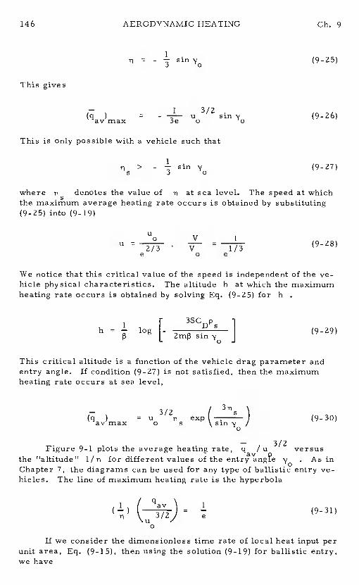
146 AERODYNAMIC HEATING Ch. 9
TI = - sin (9-25)
This gives
— 1 3/2.(q ) = - — u sin (9-26)avmax 3e o o
This is only possible with a vehicle such that
TI > - sin (9-27)s 3 o
where denotes the value of ii at sea level. The speed at whichthe maximum average heating rate occurs is obtained by substituting(9-25) into (9-19)
Uo V 1
U— e2h13 = e'
(9-28)
We notice that this critical value of the speed is independent of the ve-hicle physical characteristics.The altitude h at which the maximumheating rate occurs is obtained by solving Eq. (9-25) for h
r 3SCDP 1h — log _ I (9-29)
P L j
This critical altitude is a function of the vehicle drag parameter andentry angle. If condition (9-27) is not satisfied, then the maximumheating rate occurs at sea level,
(q ) u 3/2TI exp( ) (9-30)avmax o 5 siny
Figure 9-1 plots the average heating rate,q /u 312 versusthe 1Taltitude" 1/TI for different values of the y . Ps inChapter 7, the diagrams can be used for any type of ballistic entry ve-hicles. The line of maximum heating rate is the hyperbola
1 ( 1
=— (9-31)
If we consider the dimensionless time rate of local heat input perunit area, Eq. (9-15), then using the solution (9-19) for ballistic entry,we have
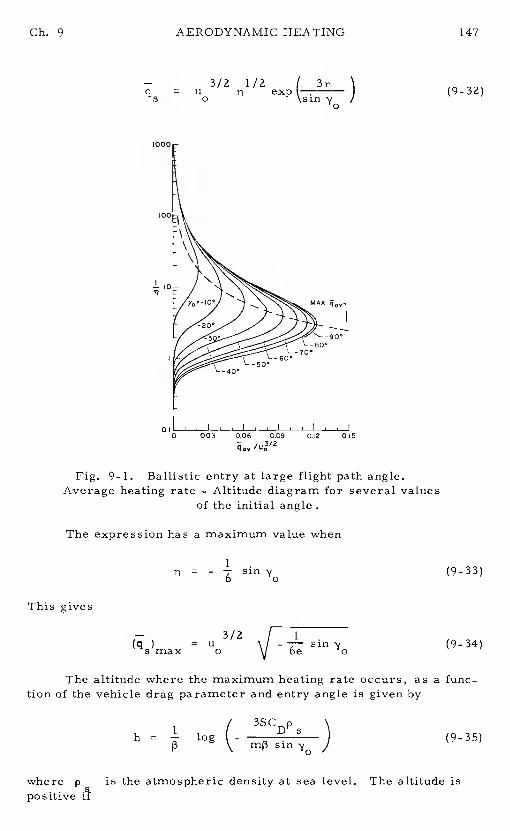
— 3/2 1/2
______
q u exp)5 0
0
Ch. 9 AERODYNAMIC HEATING 147
'7
(9-32)
Fig. 9-1. Ballistic entry at large flight path angle.Average heating rate -Altitude diagram for several values
of the initial angle.
The expression has a maximum value when
Ti = - sin (9-33)
This gives
— 3/2 I 1= U (9-34)
The altitude where the maximum heating rate occurs, as a func-tion of the vehicle drag parameter and entry angle is given by
1 / 3SCDP \h = — log ( -
Sj (935)
p J
where p is the atmospheric density at sea level.The altitude ispositive
0.09 0.12 0.15
148 AERODYNAMIC HEATING Ch. 9
sin y06
(9-3 6)
If the inequality is not satisfied, the maximum heating rate occurs atsea level and has the value
— 3/2 1/2(q) = u exptsmax o \sin'y0
Fig. 9-2. Ballistic entry at large flight path angle.Heating-rate -Altitude diagram for several values
of the initial angle.
(9-37)
— 3/2Figure 9-2 plots the heating rateq/ufor different values of the entry angle'y
used for any type of ballistic entry vehicl?e.ing rate is the curve
— 2
1 ( q51
=
versus the altitudeThe diagrams can be
The line of maximum heat-
(9-38)
too
10
-90
0.15 0.20 0.25/u03'2
Gb. 9 AERODYNAMIC HEATING 149
9-5. ENTRY OF A GLIDE VEHICLE
For gliding entry, the solution obtained in Chapter 7is
(1- Zu)= (CL/CD) u
(939)
The heat transfer to the vehicle is given by Eq. (9-18) which,for uf 0 is reduced to the same expression (9-22) as given for alight ballistic entry vehicle.
The time rate of average heat input per unit area is obtained bysubstituting solution (9-39) into Eq. (9-13)
1/2— (1-Zu) uq = (9-40)av 213r(CL/CD)
It follows that the maximum average heat input rate occurs at
1 Vu =, / =
(9-41)r
V 00
This value of the speed is independent of the lift-to-drag ratio andvehicle physical characteristics.The corresponding maximum valueof the average heat input rate is
(q )1 (9-42)av max
Pr(CL/ CD)
If we consider the dimensionless time rate of local heat input perunit area, Eq. (9-15), then using the solution (9-39) for gliding entry,we have
1/2— = (1 - 2u) u (943)S
(CL/GD)
The maximum time rate of local heat input occurs at
, = (944)
Again, this value of the speed is independent of the lift-to-drag ratioand vehicle physical characteristics. The corresponding maximumvalue of the local heating rate is
AERODYNAMIC HEATING Gb. 9
(945)CD)
9-6. ENTRY OF A SKIP VEHICLE
For skip entry, the solution obtain in Chapter 7 isC
cos y - cos y = (ii - (9-46)D
for the altitude andi
= expL c°/C i (9-47)
o L D
for the speed. The flight path angle is used as the independent var-iable.
First, for the total heat input, the integral (9-18) is valid.Let U;be the value of u at the first exit.The resulting heat flow after
the first skipping phase Q1is
AC ,Ft m= —i-— gr (u-u1) (9-48)
After a free flight in space, the vehicle reenters for another skippingphase with the same entry speed u. Then, if u is the exit speedat the end of the nth skip, the total 1heat input is
Q = gr (949)
It is clear that we have finally
ACQ = gr (9-50)
if u is the initial value of u and u1is its final value.°One may be led to believe that the final valueu is small. In
general, a skipping trajectory is possible for high val1ues of Ccoupled with a small flight path angle . For constantthe skipping phase may end at a relatively high value of uf re-maining portion of atmospheric flight is effected as a glide trajectoryat high lift-to-drag ratio. In any case, since the integral (9-18) isvalid for all types of entry trajectories, and for lifting entry uf0
Ch. 9 AERODYNAMIC HEATING 151
the resulting total heat input for a skip trajectory is
____
1 2 = 2 ) (9-51)—mV D2 o
which is identical to the result obtained for light ballistic vehicle entry,Eq. (9-22) , and also for gliding entry.
Now, using the Eqs. (9-46) and (9-47) in the expression (9-13)for the time rate of average heat input per unit area, we have
— 3/2(cos - cos y) I -
= u(CL! CD) exp L (CL! CD) J
(9-52)
The maximum heating rate occurs when dq/dy =0
3(cos cos + sin y = 0 (9-53)
As in Chapter 7,we can write this equation as a quadratic equation intan Upon solving we have the critical value of where themaximum heating rate occurs
tan 1 = (CL/CD) - VCL/CD)2 + sin20 (954)
2 3(1+cos'y)
In general, a skip trajectory is effected at high lift-to-drag ratios andsmall entry angles such that
9 sin<< 1 (9-55)
(CL/CD)
so that, in this case, the critical y can be evaluated from
1 3 .2tan - sin-j—
(9-56)(CL/CD)
In terms of the flight path angle, the time rate of local heat inputper unit area, Eq. (9-15), is
— 3/2(cos
1q = u
(CL! CD)l/2exp
(CL/CD)J(957)
AERODYNAMIC HEATING Ch. 9
At the point of maximum heating rate
6(cos - cos y) sin y = 0 (9-58)
Solving for this equation, we have
(CL/CD) - VCL/C&2 + 36 sin2ytan
= 6(1 + cos y)°
In the case where assumption (9-55) is valid, we have approximately
6 2tan- (CL/CD)
sin (9-60)
The maximum values for and q are obtained by using thecorresponding critical values of y. fri the case where the small2angleapproximation is used, since the critical yis of the order ofwe have explicitly
3/2 2u r 3y
— 0 0I (9-61)avmax
2(CL/CD)
and3/2u
Ns)max= V2CL/CD
exp]
(9-62)
9-7. COMPARATIVE ANALYSIS OF THE PERFORMANCE OFHYPERVELOCITY VEHICLES
Any detailed analysis of the performance would require variation-al theory and hence is not within the stated goal of this work.Never-theless, since some of the performance criteria such as range, time offlight, speed and design parameters, such as convective heat and heatrate, are obtained in explicit form, it is possible to have some quali-tative appraisal of the performance of a hypervelocity vehicle usingdifferent entry modes.In the past, space vehicles were designed fora specified entry mode.In the beginning, they were all of the ballisticentry type vehicles. A new generation of space vehicles has liftingcapability. Through attitude control the lift coefficient can be modu-lated in the range from CL =0 to CL = CL . Correspondingly,
maxfor a specified lifting vehicle, with a prescribed drag polar, the lift-to-drag ratio can be modulated from zero to (C1 /Cn)max. We shallrestrict ourselves to performance at constant liE-to-drag ratio.Lift-
AERODYNAMIC HEATING 153
modulation to achieve prescribed constraints will be examined in thefinal chapters.
Since we consider a versatile lifting vehicle, it is proper to dis-cuss entry modes rather than entry vehicles.The three entry modesthat have been discussed are:
1. Ballistic entry.
2. Glide entry.
3. Skip entry.
Any vehicle considered is supposed to have the capability ofentering a planetary atmosphere in any of these three modes or usingany combination of modes in following an overall, composite trajectory.
First, from the range standpoint, ballistic entry is the leasteffective mode. For skip entry, the range for each separate skippingphase is short but each atmospheric portion of the flight trajectory isfollowed by a Keplerian portion in space adding significant distance tothe total range. As a matter of fact, with a high initial entry speed, askip trajectory can achieve infinite range while a glide trajectory total-ly immersed in the atmosphere is condemned to a finite range.Thus,there exists an initial speed such that there is equal range for skipentry and glide entry, with gliding flight achieving the longer range atlower initial speed.
From considerations of aerodynamic heating, with the possibleexception of the relatively dense vehicle in the ballistic mode, in allthree modes, the hypervelocity vehicle expends the major part of itskinetic energy in flight and receives in exchange heat by convectionaccording to the simplified formula
Q= (9-63)
To minimize this fraction, that is to reduce the total heat transfer byconvection, it is necessary to determine how the ratio of friction forceto total drag force can be reduced.This matter was discussed in de-tail in Ref. 1 in connection with a purely ballistic vehicle and it wasdemonstrated that the ratio could be reduced by employing high pres-sure-drag shapes, that is, blunted shapes.On the other hand, in theskip and glide modes the geometric configuration of the vehicle will beslender and the above ratio may reach the order of 0. 1which is quitehigh for vehicle materials to absorb.In skip or glide modes one must,therefore, consider the possibility of the vehicleradiating a signifi-cant part of this heat back to the surrounding atmosphere.This prob-lem has been discussed in Ref. 4, and it is found that in a high lift- to-drag ratio glide mode, if the surface temperature is allowed to reacha high level, the vehicle can radiate heat at a rate equal to the maxi-mum average convective heat transfer rate.Furthermore, in the gli-ding mode the vehicle may require less coolant than in the ballisticmode. The reason for this is that although in the gliding mode thesame vehicle will receive more heat, the gliding time is much longer,by a factor of perhaps one hundred.Therefore, with a sufficiently
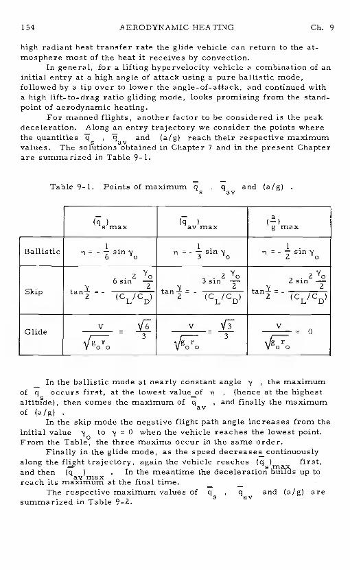
154 AERODYNAMIC HEATING Ch. 9
high radiant heat transfer rate the glide vehicle can return to the at-mosphere most of the heat it receives by convection.
In general, for a lifting hypervelocity vehicle a combination of aninitial entry at a high angle of attack using a pure ballistic mode,followed by a tip over to lower the angle-of-attack, and continued witha high lift_to-drag ratio gliding mode, looks promising from the stand-point of aerodynamic heating.
For manned flights, another factor to be considered is the peakdeceleration. Along an entry trajectory we consider the points wherethe quantities
'and (a/g) reach their respective maximum
values. The solutions obtained in Chapter 7 and in the present Chapterare summarized in Table 9-i.
Table 9-1. Points of maximum , q and (a/g)
Ballistic !.— - sin6 o
!•— - sin3 o
!.— - sin2 o
Skip
26siri
- (CL/CD)
3sin
- (CL/CD)
2sjn —tan2
=- (CL/CD)
Glide=
V 00
v0
Vo o
— In the ballistic mode at nearly constant angle'y , the maximumof q occurs first, at the lowest value_of , (hence at the highest
then comes the maximum ofq , and finally the maximumof (a/g)
In the skip mode the negative flight path angle increases from theinitial value y to = 0 when the vehicle reaches the lowest point.From the Table, the three maxima occur in the same order.
Finally in the glide mode, as the speed decreases continuouslyalong the flight trajectory, again the vehicle reaches (q) first,and then (q ) . In the meantime the deceleration up toreach its at the final time. — —
The respective maximum values ofq , q and (a/g) aresummarized in Table 9-2.
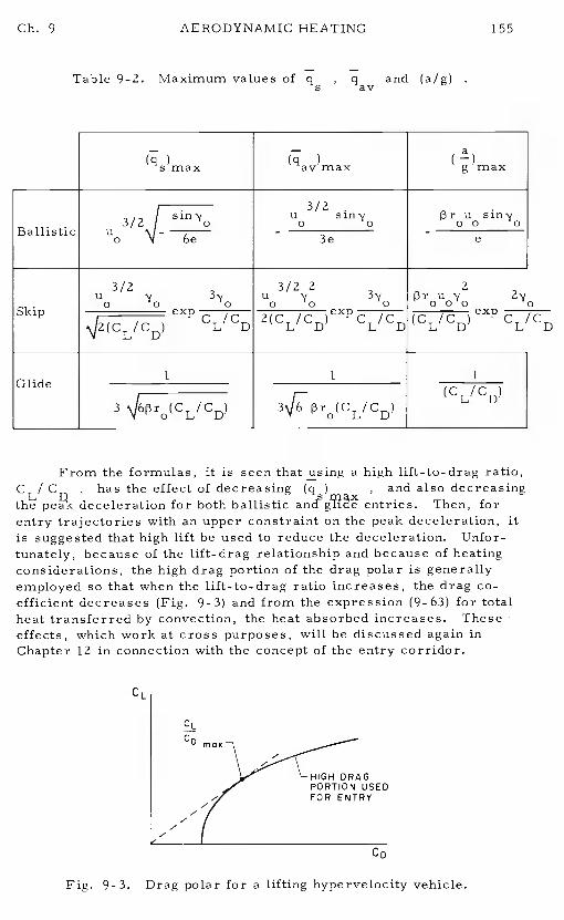
Ch. 9 AERODYNAMIC HEATING
Table 9-2. Maximum values of q , q and (a/g)S av
Glide 1 1 1
(CL/CD)3 (CL/CD) (CL/CD)
From the formulas, it is seen that using a high lift-to-drag ratio,CL! C , has the effect of decreasing(q ) , and also decreasingthe deceleration for both ballistic entries. Then, forentry trajectories with an upper constraint on the peak deceleration, itis suggested that high lift be used to reduce the deceleration.Unfor-tunately, because of the lift-drag relationship and because of heatingconsiderations, the high drag portion of the drag polar is generallyemployed so that when the lift-to-drag ratio increases, the drag co-efficient decreases (Fig. 9-3) and from the expression (9-63) for totalheat transferred by convection, the heat absorbed increases.Theseeffects, which work at cross purposes, will be discussed again inChapter 12 in connection with the concept of the entry corridor.
CL
Fig. 9-3. Drag polar for a lifting hype rvelocity vehicle.
155
max g 'max
Ballistic u2
o '4
o6e
3/2U
-0
3e
.
0U
-00 0
e
Skip
3(2U
2
expCL/CD
-D
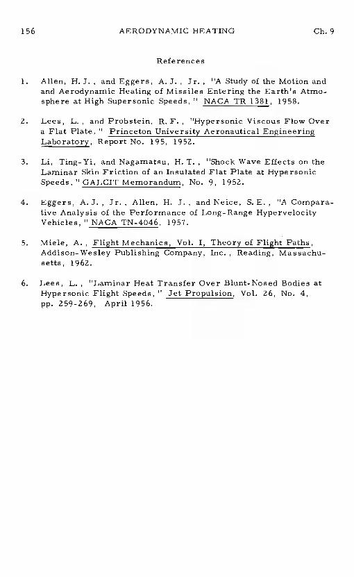
156 AERODYNAMIC HEATING Ch. 9
References
1. Allen, H. J. , and Eggers, A. J. ,Jr. , 'A Study of the Motion andand Aerodynamic Heating of Missiles Entering the Earth's Atmo-sphere at High Supersonic Speeds,' NACA TR 1381, 1958.
2. Lees, L. , and Probstein, R. F. ,"Hypersonic Viscous Flow Overa Flat Plate, "Princeton University Aeronautical
Report No. 195, 1952.
3. Li, Ting-Yi, and Nagamatsu, H. T. ,"Shock Wave Effects on theLaminar Skin Friction of an Insulated Flat Plate at HypersonicSpeeds," GALCIT Memorandum, No. 9, 1952.
4. Eggers, A. J., Jr. , Allen, H. J. , and Neice, S. E. ,"A Compara-tive Analysis of the Performance of Long-Range HypervelocityVehicles, "NACA TN-4046, 1957.
5. Miele, A. , Flight Mechanics, Vol. I, Theory of Flight Paths,Addison-Wesley Publishing Company, Inc., Reading, Massachu-setts, 1962.
6. Lees, L. , "Laminar Heat Transfer Over Blunt-Nosed Bodies atHypersonic Flight Speeds, "Jet Propulsion, Vol. 26, No. 4,pp. 259-269, April 1956.
Chapter 10
Yaroshevskii's Theory for Entry intoPlanetary Atmospheres
10-1. INTRODUCTION
The analytical development in Chapters 7,8 and 9 presents theclassical theories for entry into a planetary atmosphere.The simpleresults given are adequate for the purpose of a preliminary estimateof the variations of the trajectory variables along an entry flight pathand the different physical characteristics expressed as functions ofthese entry variables.Beginning in this chapter, we shall presentvarious modern theories for planetary entry.
First, with the physical understanding of the phenomena associ-ated with an entry trajectory as presented in the previous chapters,scientists and engineers are led to formulating very general assumptionswhich are valid for nearly all types of entry trajectories.This resultsin a set of equation of motion valid for all types of entry trajectories ofpractical interests. Furthermore, if these equations can be presentedin dimensionless form, in the same way as has been done in the pre-vious chapters for first-order analysis, the results obtained can beapplied to any entry vehicle regardless of its physical characteristics.This type of approach is illustrated by Yaroshevskii's theory presentedin this chapter, and Chapman's theory in Chapters 11 and 1Z.
Next, if the restrictive assumptions introduced are removedwhile the universal character of the entry equations is still preserved,the exact dimensionless equations of motion for planetary entry areobtained and they are valid for all types of entry trajectories of anyentry vehicle regardless of its mass, size and aerodynamic character-istics. Furthermore, the trajectory considered can be completelyimmersed inside the atmosphere or can be partly outside of it in theform of Keplerian arcs. This also will include orbital motion ofsatellites at very high altitude subject to Newtonian gravitational attrac-tion and infinitesimally small atmospheric drag.This analysis will beconsidered in the following chapters.
Finally, one may consider the case where the aerodynamic con-trols in the form of the lift-to-drag ratio and the bank angle are notconstant but can be modulated according to a certain law in order toachieve a specific purpose.This type of trajectories will be analyzedin the last chapters.
157
158 YAROSHEVSKII'S THEORY Ch. 10
Yaroshevskii's theory for entry trajectory is a semi-analyticaltheory. Using some simplifying assumptions, he derived a nonlinear,second-order differential equation which can be integrated analyticallyby using series expansions.To some extent, Yaroshevskii's theory isa special case (Refs. 1, 2) of a more sophisticated theory developed byChapman (Ref.3). Because his theory has some features of merit, weshall present it in this chapter.Chapman's theory will be developed inthe next chapter, and the connection between the two theories will beexamined.
10-2. SECOND-ORDER NONLINEAR DIFFERENTIAL EQUATION FORENTRY TRAJECTORY
Consider the basic equations for planar entry derived in Chapter
dV PSCDV2dt = - 2m
-gslny2pSCV 2
L VVdt = 2m
V sin 'y (10-1)
Strictly speaking, as was mentioned in Section 6-2, the lift andthe drag coefficients are functions of the angle of attack a, of theMach number M , and the Reynolds numberR . For constantangle of attack, Yaroshevskii assumed that thecoefficient CLand the drag coefficientC are functions of the Mach number. Foran isothermal atmosphere, is just a function of the speed,V
If, in the equation for V , we neglect the tangential componentof the gravity force, and in the equation for and r we use theapproximation of small flight path angle, we can write the Eqs. (10-1)as
=- p SCD(V) V2
d pSCL(V) V2V—1dt Zm r
= (10-2)
The first of these equations can be used to change the independentvariable to V
Ch. 10 YAROSHEVSKII'S THEORY 159
dV - - PSCD(V) V
2
V2
+2
(10-3)D PSCD(V) V
2
To derive his second-order nonlinear differential equation forentry into a planetary atmosphere, Yaroshevskii used an independentvariable x , and a dependent variable y defined as
V C (1) dVr Dx j
1 CD(V) V
C (1) Sy Dam (10-4)
where r is the radius of the planet and V is the dimensionlessspeed
V a (10-5)
At this point the following remarks are in order:a! The altitude h is small compared to the radiusr of the
planet. Hence, g is approximately constant.b/ For the same reason, can be considered as the cir-
cular speed at the entry altitude.Hence, if the entry is from circularspeed, the initial value of V is unity, and from the definition (10-4)of the independent variable x, this variable increases monotonicallyfrom the initial value x =0
If a strictly exponential atmosphere is used, then
= - )Sdr (10-6)p
where p is constant. Hence, from the definition of y
= - (10-7)
On the other hand
YAROSHEVSKII 'S THEORY Ch. 10
C (1) — C (1)dx D dV 13 (10-8)
C13(V) V C13(V)
With these differential relations, and the definition (10-4) of x and ythe Eqs. (10-3) are
C [V(x)] —2= L - 1-V (x) (10-9)
dx C13(l) yV2 (x)
where in the equation for'y , the approximation of small altitude,r = r , has been used.
°Eliminating 'y between the two equations above, we obtain asingle equation of the second-order
2 C [V(x)] —z -=
- C13(i)+ V (x) (10-10)
This equation is nonlinear, second-order differ-ential equation for studying entry into a planetary atmosphere.Thequantity f3r is constant, and for the Earth's atmosphere we can take
as abgut 900. The equation takes into account the effect ofthe R4ach number on the lift and the drag coefficients at constant angleof attack. In general, this equation has to be integrated numerically.In the special case where and C are independent of the Machnumber, the equation can be integrates using some appropriate seriesexpansions, depending on the type of entry trajectory.
Once the variable yis known as a function of the independentvariable x , other quantities of interest can be evaluated.
First, the flight path angle is given by the first of the Eqs. (10-9)For the time of flight, we write the first of the Eqs. (10-2) in
terms of x and y
= y V(x) (10-11)
Hence, the time is obtained by performing the quadrature= 1x dx (10-12)
yV(x)1
Ch. 10 YAROSHEVSKII'S THEORY 161
where x. is the initial value of x . The distance travelled, s , asprojected on the surface of the planet, is given by the kinematic rela-tion
ds dOr
— = rdt o dt r
Hence, for small flight path angles, and with the approximation ofsmall flight altitude relative tor , we have
0
= V(x) (10-13)
Using Eq. (10-11), it is seen that the distance travelled is given by theintegral
s
=
(10-14)o
The deceleration along the trajectory, during entry, is-(dV/dt)Using the first of the Eqs. (10-2), and the definitions (10-4) and (10- 5),we have
dV GD{ V(x)] —z- =
CD(1y V (x) (10.15)
Other physical quantities of interest, such as the heating rate and thetotal heat absorbed, will be given in the immediately following sectionwhen we consider entry at constant lift-to-drag ratio.
10-3. ATMOSPHERIC ENTRY AT CONSTANT LIFT-TO-DRAG RATIO
In practice, the simplest and most interesting case is that obtain-ed for constant lift and drag coefficients.This case is commonly en-countered along the main part of the entry trajectory where, at highMach number, the lift and the drag coefficients are independent of MIt is also along this portion of the trajectory that the deceleration andthe heating rate reach their maxima.
From the definition of x , Eq. (10-4), it is seen that when CDis independent of the Mach number
x = log , V = e (10-16)
The basic nonlinear differential equation, Eq. (10-10), is reduced to
= - +1 (10-17)
YAROSHEVSKII'S THEORY Ch. 10
This equation can be integrated by using an appropriate series expan-sion, depending on the type of trajectory.
While the distance travelled, Eq. (10-14), remains the same, inthe case of constant lift-to-drag ratio entry, the expression for the timeof flight and the deceleration, Eqs. (10-12) and (10-15) become
!_x (10-18)
and
a = - = (10-19)
In the numerical computation, we can use the following approximatecharacteristic values of the Earth
7000m,
30
26.5 sec 212 kmVP
V=
7850 m/ sec (10-20)circular 0
For a strictly exponential atmosphere, the dependent variable y issimply proportional to the atmospheric densityp . With the approx-imate value given above,
y 1.04 x lO6Bp (10-21)
where B is the drag parameter
SCD 2B a m /kg (10-22)mg
The aerodynamic heating rate per unit area on a body reaches its max-imum at a stagnation point of radius of curvature R, and is given by(Refs. 4-6)
= (10-23)
where the constants C, n and m depend on the type of boundarylayer. For laminar flow, n = 1/2 , and the value of m has beengiven by various authors as3. 1< m<3.25 . For his numerical
computation Yaroshevskii adopted the following formula as given by
Gb. 10 YAROSHEVSKII'S THEORY 163
Kemp and Riddell, (Ref. 7),for the stagnation point heat transfer rate:
= 8.8 x 1O4 v
)kcal (10-24)m sec
For a constant drag coefficient, for which the relations (10-16) and(10-21) apply, this formula becomes
0.5 -3.25xe kcal
— 0.5 0.5 2(10-25)
R B m sec
If there is a turbulent boundary layer, the aerodynamic heating rateper unit area reaches its maximum at the section where the transitionthrough the speed of sound takes place, (Ref. 8).The formula (10-25)for laminar flow is replaced by, (Ref.1),
0.8 -3.19x— 25y e kcal
20.2 0.8 2 -R B m sec
for the heat transfer rate at the turbulent sonic point.Another quantity of interest in aerodynamic heating is the total
heat absorbed per unit area
= f q dt (10-27)
where A is the whole surface wetted by the boundary layer, and qis given by Eq. (10-25) for laminar flow, and Eq. (10-26) for turbulentflow. The integration with respect tot can be changed into the inte-gration with respect to x , by the use of Eq. (10-18),
Q x -2.25xS 2250 e e kcal
A = 0. 5 5 Jdx —i (10-28)
R B
x -2.19xt 665 e kcalA 0.2 0.8 0.2 dx (10-29)
R B y m
It is seen that, if the basic nonlinear differential equation forconstant lift-to-drag ratio entry, Eq. (10-17), can be integrated, thevariable y is obtained as function of the independent variable xThe deceleration during entry is given by Eq. (10-19), while the timeof flight, the heating rate and the heat absorbed are obtained explicitlyor by quadratures through Eqs. (10-18), (10-25) -(10.26), and (10-28)-
(10-29), respectively.
164 THEORY Ch. 10
10-4. SERIES SOLUTIONS OF THE BASIC NONLINEAR DIFFEREN-TIAL EQUATION
The basic nonlinear differential equation for constant lift-to-dragratio entry, Eq. (10- 17), can be integrated approximately by usingseries solutions. We shall integrate this equation in the followingcases.
10-4. 1. Ballistic Decay From Satellite Orbits
For ballistic entry trajectory, CL/CD 0 , and Eq. (10-17)is reduced to
2 Zx= e - 1 (10-30)
dx2
Under the action of atmospheric drag, acting primarily at periapsis, ahigh altitude satellite orbit tends to a circular orbit before effectiveentry. Hence, in this case, for the portion of the trajectory whereeffective entry is achieved, Eq. (10-30) is integrated with the initialconditions
x. = 0 , y(0) = 0 , y'(O) = 0 (10-31)
where the prime denotes the derivative taken with respect to x . Thedifferential equation (10-30) has a singularity at y =0 . To removethis singularity, we notice that, in the neighborhood of x =0 , theequation becomes
yy" 2x (10-32)
This equation has the solution
3/2y (10-33)
satisfying the initial condition (10-31). Hence, we can seek a solutionof the differential equation (10-30) in the form
y = (a0 + a1x + a2x2 +a3x3 + ... ) (10-34)
Writing Eq. (10-30)
24324yy" = 2x+ 2x +jx + ... (10-35)
substituting the series (10- 34), and equating coefficients of like powersin x , we obtain for the coefficients ak
Gb. 10 YAROSHEVSKIIS THEORY 165
1 1 47a0 = 1 , a1 , a2 , a3 = , . . . (10-36)
The recurrence formula for computing the coefficients akis
k- 1
2 - (2m+l)(2m+3)a a(k + 1)! 3 m=1 m k-rnak (2k+l)(Zk+3) (10-37)
1+
It can be seen that
akl < (10-38)
Therefore, the radius of convergence of the series is not less than1. 5 . The series solution is sufficiently accurate to evaluate the max-imum deceleration and heat transfer rate which occurs during the fun-damental part of the entry trajectory where the main assumptions usedfor the derivation of the nonlinear differential equation are valid.
For x < 1 , we need only three terms of the series, and thetruncated y function for ballistic entry from circular orbit is
y3/2 (10-39)
From Eq. (10-19), the deceleration is
5/2 7/2-
= V°
+ + e2X (10-40)
The peak deceleration is obtained by taking the derivative of this equa-tion with respect to x and setting it equal to zero.The resultingequation is
4x3 + 9x2 + 76x - 72 = 0 (10-41)
The solution of this equation gives the conditions at maximum deceler-ation:
x = 0.835 , = 0.434
y = 1.45 , = 0.277 (10-42)
Substitution of the solution (10-39) into Eqs. (10-25) and (10-26) yieldsthe expression for the aerodynamic heating rate per unit area for lam-inar flow, (at the stagnation point), and turbulent flow, (at the sonicpoint), respectively. The maximization of these functions provides:
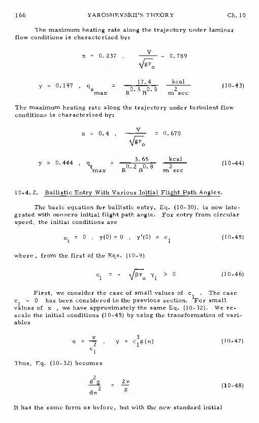
166 YAROSHEVSKII'S THEORY Ch. 10
The maximum heating rate along the trajectory under laminarflow conditions is characterized by:
x = 0.237 ,
= 0.789
y = 0. 197 , q5= 0
kcal (10-43)max B msec
The maximum heating rate along the trajectory under turbulent flowconditions is characterized by:
x = 0.4 V= 0.670
y = 0.444 '=
kcal(10—44)
max R B m sec
10-4. 2. Ballistic Entry With Various Initial Flight Path Angles.
The basic equation for ballistic entry, Eq. (10-30), is now inte-grated with nonzero initial flight path angle.For entry from circularspeed, the initial conditions are
= 0 , y(O) = 0 , y1(O) = c1 (10-45)
where , from the first of the Eqs. (10-9)
- > 0 (10-46)
First, we consider the case of small values ofc . The case= 0 has been considered in the previous section. kFor small
values of x , we have approximately the same Eq. (10-32).We re-scale the initial conditions (10-45) by using the transformation of vari-ables
ii = 4 , y = (10-47)
Thus, Eq. (10-32) becomes
(10-48)g
It has the same form as before, but with the new standard initial
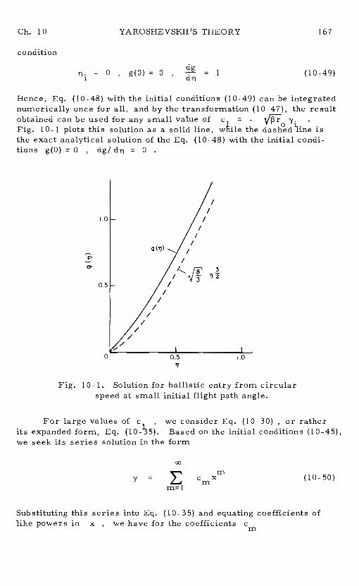
Gb. 10 YAROSHEVSKII'S THEORY 167
condition
= 0 , g(0) = 0 , = 1 (10-49)
Hence, Eq. (10-48) with the initial conditions (10-49) can be integratednumerically once for all, and by the transformation (10-47), the resultobtained can be used for any small value of = -Fig. 10-1 plots this solution as a solid line, the dashed 1line isthe exact analytical solution of the Eq. (10-48) with the initial condi-tions g(0) = 0 , dg/ = 0
Fig. 10-1. Solution for ballistic entry from circularspeed at small initial flight path angle.
For large values ofc , we consider Eq. (10-30), or ratherits expanded form, Eq. Based on the initial conditions (10-45),we seek its series solution in the form
cc
yr
cx
Substituting this series into Eq. (10-35) and equating coefficients oflike powers in x , we have for the coefficientscm
.0
//
/
/
0.5
3'72
17
(10-50)
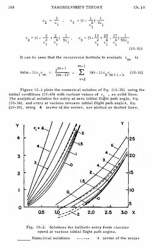
1 1C2 = — , C3ci ci
21C4 = (1-
9c1Cl Cl
10 20 17C5 = + - 90c1
C1 C1 C1
(10-51)
It can be seen that the recurrence formula to evaluatec
2m- 1m(m-1)c c =im (rn-I)!
m is
Figure 10-2 plots the numerical solution of Eq. (10-30) using theinitial conditions (10-45) with various values of c1, as solid lines.The analytical solution for entry at zero initial flight path angle, Eq.(10-34), and entry at various nonzero initial flight path angles, Eq.(10-50), using 4 terms of the series, are plotted as dashed lines.
V
4
3
2
0
Fig. 10-2. Solutions for ballistic entry from circularspeed at various initial flight path angles.
Numerical solutions 4 terms of the series
168 YAROSHEVSKII'S THEORY Ch. 10
rn-i
k(k_l)ckc+lk (10-52)
k= 2
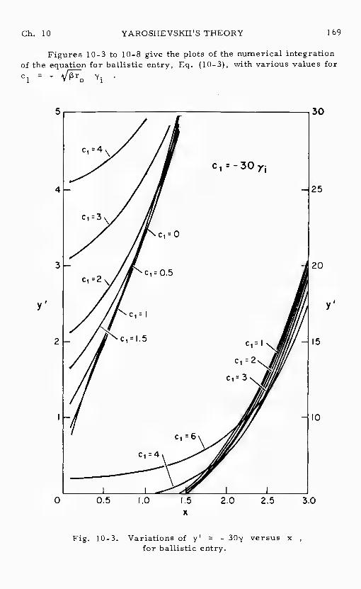
Ch. 10 YAROSHEVSKII'S THEORY 169
Figures 10-3 to 10-8 give the plots of the numerical integrationof the equation for ballistic entry, Eq. (10-3), with various values forc1 = -
Fig. 10-3. Variations of y' = - 30yfor ballistic entry.
versus x
y, ys
0 0.5 P.O 1.5 2.0 2.5 3.0x
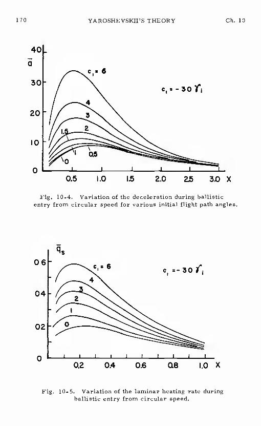
170 YAROSHEVSKIITS THEORY Ch. 10
I0
0
Fig. 10-4. Variation of the deceleration during ballisticentry from circular speed for various initial flight path angles.
0
Fig. 10-5. Variation of the laminar heating rate duringballistic entry from circular speed.
4'
acs 6
20
= - 30
0.5 1.0 15 2.0 2.5 3.0 X
q5
c= 606
04
02
C, 30
0.2 0.4 0.6 Q8 I.OX
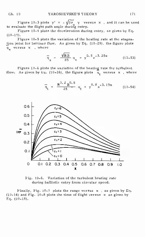
Ch. 10 YAROSHEVSKII'S THEORY 171
Figure 10-3 plots y' = - versus x , and it can be usedto evaluate the flight path angle during entry.
Figure 10-4 plots the deceleration during entry, as given by Eq.(10-19).
Figure 10-5 plots the variation of the heating rate at the stagna-tion point for laminar flow. As given by Eq. (10-25), the figure plotsq versus x , where
— 0.5 -3.25x= 85
q = y e (10- 53)
Figure 10-6 plots the variation of the rate for turbulentflow. As given by Eq. (10-26), the figure plots versus x , where
0.6
0.5
0.4
0.3
0.2
0.I
R°2B°8 0.8 -3.19x25 e
0 0.1 0.2 0.3 0.4 0.5 0.6 0.7 0.8 0.9x
Fig. 10-6. Variation of the turbulent heating rateduring ballistic entry from circular speed.
(10- 54)
Finally, Fig. 10-7 plots the range versus x, as given by Eq.(10-14) and Fig. 10-8 plots the time of flight versus x as given byEq. (10-18).
LO
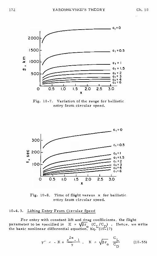
C1 :0.5
ci = I
1500
C1 1.5
c1 2C1: 3
= 46
0 0.5 1.0 1.5 2.0 2.5 3.0x
C,:C1 1.5
:2C, 3c, 4c,:6
y" = - K+ 1 (10-55)
YAROSHEVSKU'S THEORY Ch. 10
0
E
V)
1000
500
2000
(n
4-
Fig. 10-7. Variation of the range for ballisticentry from circular speed.
C,: 0
c,:0.5
0 0.5 .0 .5 2.0 2.5x
3.0
Fig. 10-8. Time of flight versus x for ballisticentry from circular speed.
10-4. 3. Lifting Entry From Circular Speed
For entry with constant lift and drag coefficients, the flightparameter to be specified isK = (CL/CD) . Hence, we writethe basic nonlinear differential equation, Eq. (10-17)
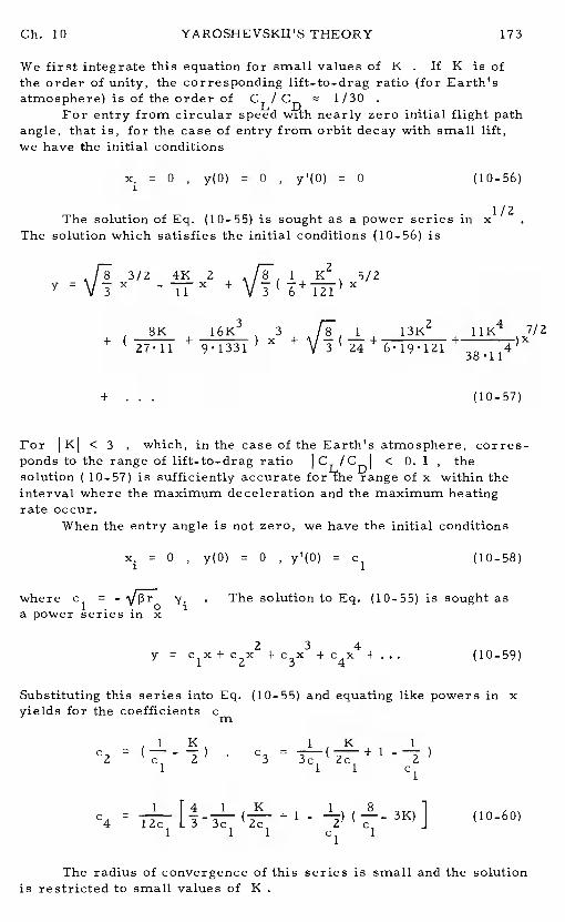
Ch. 10 YAROSHEVSKII'S THEORY 173
We first integrate this equation for small values of K. If K is ofthe order of unity, the corresponding lift-to-drag ratio (for Earth'satmosphere) is of the order ofCL! CD 1/30
For entry from circular speed with nearly zero initial flight pathangle, that is, for the case of entry from orbit decay with small lift,we have the initial conditions
= 0 , y(0) = 0 , y'(O) = 0 (10-56)
The solution of Eq. (10-55) is sought as a power series inThe solution which satisfies the initial conditions (10-56) is
3/2 4K 2 1 K2 5/2+
8K 16K3 3 1 13K2 ilK4 7/2+ )x + )x
2711 V 3 24
+ . . . (10-57)
For IKI < 3 , which, in the case of the Earth's atmosphere, corres-ponds to the range of lift-to-drag ratio CT ICDI < 0. 1 , thesolution (10-57) is sufficiently accurate range of x within theinterval where the maximum deceleration and the maximum heatingrate Occur.
When the entry angle is not zero, we have the initial conditions
= 0,
y(O) 0 , y'(O) c1 (10-58)
where c1 = - . The solution to Eq. (10-55) is sought asa power series in x
y c1x + c2x2 + c3x3 + c4x4 + ... (10-59)
Substitutingthis series into Eq. (10-55) and equating like powers in xyields for the coefficientscm
1 K 1 K 1
c2 = (—- c3 = 1
1 1 1
c4 + 1 - 3K)] (10-60)1 1 1 c1 1
The radius of convergence of this series is small and the solutionis restricted to small values of K
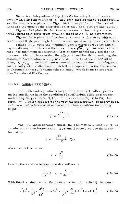
174 YAROSHEVSKII'S THEORY Ch. 10
Numerical integration of Eq. (10-55) for entry from circularspeed withdifferent values of c1 has been carried out by Yaroshevskii,and the results are plotted in Figs. 10-9 through 10-11. The dashedlines are the plots of the analytical solutions, Eqs. (10-57) and (10-59).
Figure 10-9 plots the function y versus x for entry at zeroinitial flight path angle from circular speed using K as parameter.
Figure 10-10 plots the function y versus x for entry with non-zero initial flight path angle from circular speed using K as parameter.
Figure 10-11 plots the maximum deceleration versus the initialflight path angle. It is seen that, as c = - increases fromzero, the maximum deceleration firstsfightly and then in-creases. Also, it is seen that the effect of positive lift in reducing themaximum deceleration is very powerful.Effects of the lift-to-dragratio, CL/CD , on maximum deceleration and maximum heating rateduring entry will be discussed in detail in Chapter 11 in the discussionof Chapman's theory for atmospheric entry, which is more accuratethan Yaroshevskii's theory.
10-4.4. Gliding Trajectory
If the lift-to-drag ratio is large while the flight path angle re-mains small, we have the condition of equilibrium glide as first for-mulated by Sanger (Refs. 9, 10).In this case, in Eq. (10-55), theterm y" , which represents the vertical acceleration, is nearly zero,and the equation is reduced to the equilibrium condition for glidingflight
y=
1 (10-61)
When the speed becomes small, the assumption of small verticalacceleration is no longer valid.For small speed, we use the trans-formation
y= e- 1
f(z) (10-62)
where we definez as
z (10-63)
Hence, the relation between the derivatives is
= ) (10-64)
With this transformation, the basic equation, Eq. (10-55), becomes
22 1 d2f 2 1 df 2 1z (z z(5z -.—+4z f -1 (10-65)
K dz KZ
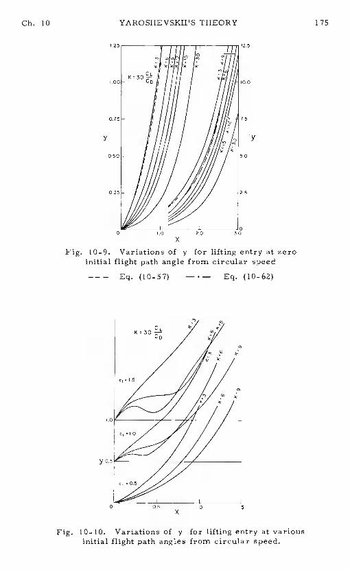
x
Fig. 10-9. Variations of y for lifting entry at zeroinitial flight path angle from circular speed
Eq. (10-57) Eq. (10-62)
y 0,5
0 05 1.0 1,5x
Fig. 10-10. Variations of y for lifting entry at variousinitial flight path angles from circular speed.
Ch. 10 YAROSHEVSKII'S THEORY 175
yy
0 10 20 30
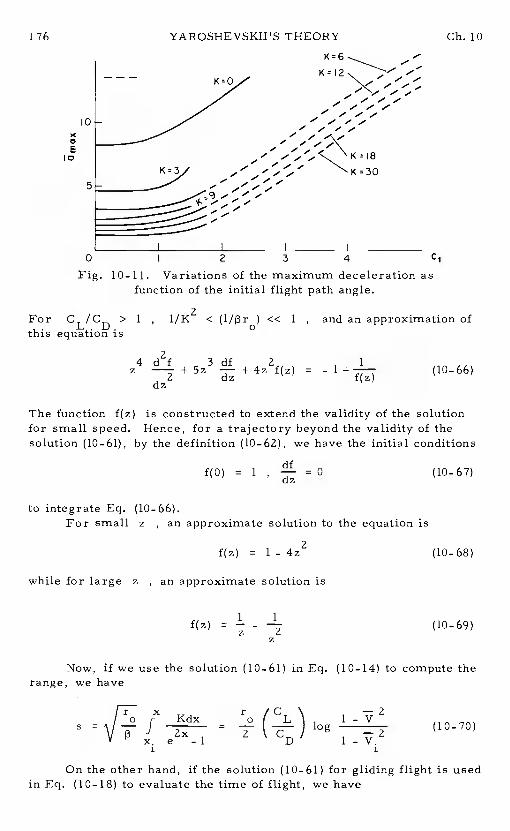
176 YAROSHEVSKIIS THEORY Gb. 10
0 I 2 3 4 C1
Fig. 10-11. Variations of the maximum deceleration asfunction of the initial flight path angle.
For CL/CD > 1 , 1/K2 < (1/pr) << 1 , and an approximation ofthis equation is
4 d2f 3 df 2f() = - 1 + (10-66)+5z —+4z2 dz f(z)
dz
The function f(z) is constructed to extend the validity of the solutionfor small speed. Hence, for a trajectory beyond the validity of thesolution (10-61), by the definition (10-62), we have the initial conditions
f(0) = 1 , = 0 (10-67)
to integrate Eq. (10-66).For small z , an approximate solution to the equation is
f(z) = 1- 4Z2 (10-68)
while for large z , an approximate solution is
f(z) = - -4 (10-69)
Now, if we use the solution (10-61) in Eq. (10-14) to compute therange, we have
I0
CE
10
5
z
/T x
i
Kdx2x
e -1
r
2
'C ' —2L\ 1-V1V2D
On the other hand, if the solution (10-61) for gliding flight is usedin Eq. (10-18) to evaluate the time of flight, we have
(10-70)
Ch. 10 YAROSHEVSKII'S THEORY 177
1KeXdx
1(CL\ [1-V]t =
1 =
(10—71)
These are the first-order solutions for gliding entry obtained in Chap-ter 7
References
1. Yaroshevskii, V.A., "The Approximate Calculation of Trajec-tories of Entry Into the Atmosphere.I", Translated fromKosmicheskie Issledovaniya, Vol. 2, No. 4, 1964.
2. Yaroshevskii, V. A., "The Approximate Calculation of Trajec-tories of Entry Into the Atmosphere.II" , Translated fromKosmicheskii Issledovaniya, Vol.2, No. 5, 1964.
3. Chapman, D. B.., "An Approximate Analytical Method for StudyingEntry Into Planetary Atmospheres," NASA TB R-11, 1959,
4. Lees, L. , "Laminar Heat Transfer Over Blunt- Nosed Bodies atHypersonic Flight Speeds, "Jet Propulsion, Vol. 26, No. 4,pp. 259-269, 1956.
5. Lees, L. , "Recovery Dynamics -Heat Transfer at HypersonicSpeeds in a Planetary Atmosphere," Chapter 12 of Space
ed. by H. S. Seifert, John Wiley and Sons, N. Y., 1959.
6. Fay, J. A. , and Riddell, F. R. , "Theory of Stagnation Point HeatTransferin Dissociated Air, "J. of Aeronautical Sciences, Vol.25, No. 2, pp. 73-85, 1958.
7. Kemp, N. H. , and Riddell, F. R. , "Heat Transfer to SatelliteVehicles Reentering the Atmosphere, "Jet Propulsion, Vol. 27,No. 2, 1957.
8. Sibulkin, M. , "Estimation of Turbulent Heat Transfer at theSonic Point of a Blunt-Nosed Body, "Jet Propulsion, Vol. 28,No. 8, pp. 548-554, 1958.
9. Sãnger, E, ,Raketen-Flugtechnik, R. Oldenbourg, Berlin, 1933.
10. Sänger, E., and Bredt, J., "A Rocket Drive for Long RangeBombers, " Translation CGD-32, Technical Information Branch,Navy Department, 1944.
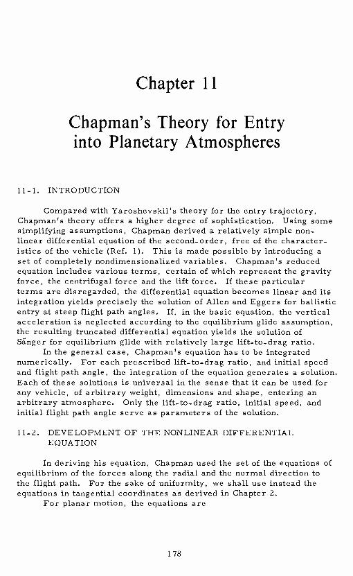
Chapter 11
Chapman's Theory for Entryinto Planetary Atmospheres
11-1. INTRODUCTION
Compared with Yaroshevskii's theory for the entry trajectory,Chapma&s theory offers a higher degree of sophistication.Using somesimplifying assumptions, Chapman derived a relatively simple non-linear differential equation of the second-order, free of the character-istics of the vehicle (Ref.1). This is made possible by introducing aset of completely nondimensionalized variables.Chapman's reducedequation includes various terms, certain of which represent the gravityforce, the centrifugal force and the lift force.If these particularterms are disregarded, the differential equation becomes linear and itsintegration yields precisely the solution of Allen and Eggers for ballisticentry at steep flight path angles.If, in the basic equation, the verticalacceleration is neglected according to the equilibrium glide assumption,the resulting truncated differential equation yields the solution ofSänger for equilibrium glide with relatively large lift-to-drag ratio.
In the general case, Chapman's equation has to be integratednumerically. For each prescribed lift-to-drag ratio, and initial speedand flight path angle, the integration of the equation generates a solution.Each of these solutions is universal in the sense that it can be used forany vehicle, of arbitrary weight, dimensions and shape, entering anarbitrary atmosphere.Only the ratio, initial speed, andinitial flight path angle serve as parameters of the solution.
11-2. DEVELOPMENT OF THE NONLINEAR DIFFERENTIALEQUATION
In deriving his equation, Chapman used the set of the equations ofequilibrium of the forces along the radial and the normal direction tothe flight path. For the sake of uniformity, we shall use instead theequations in tangential coordinates as derived in Chapter 2.
For planar motion, the equations are
1 78
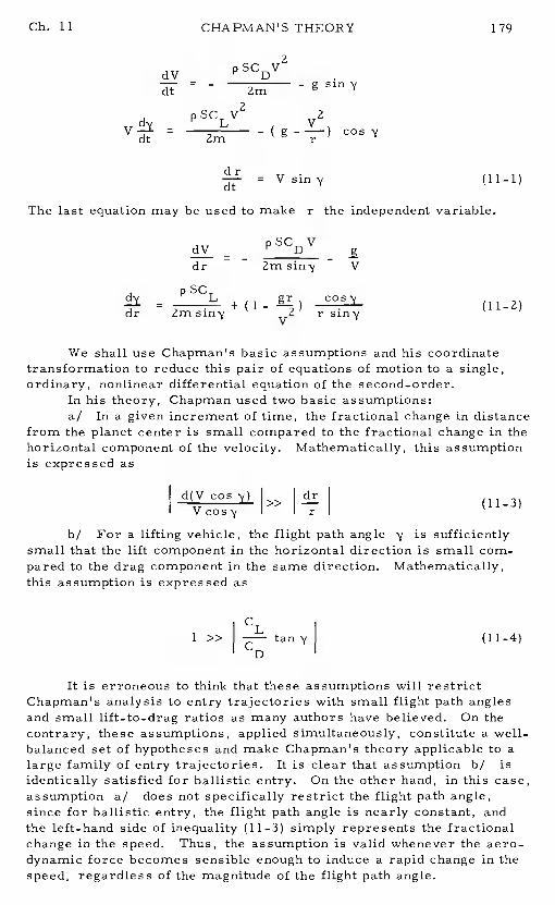
Ch. 11 CHAPMAN'S THEORY 179
dV pSCDV2dt = - Zm
2pSCV 2L V
Vdt = 2m -(g-——)
= V sin'y (11-1)
The last equation may be used to make rthe independent variable.
dr - - V
p SC= L + (1- (11-2)dr r
We shall use Chapman's basic assumptions and his coordinatetransformation to reduce this pair of equations of motion to a single,ordinary, nonlinear differential equation of the second-order.
In his theory, Chapman used two basic assumptions:a! In a given increment of time, the fractional change in distance
from the planet center is small compared to the fractional change in thehorizontal component of the velocity.Mathematically, this assumptionis expressed as
d(Vcos'j) (11-3)Vcos'j r
b/ For a lifting vehicle, the flight path angle is sufficiently
small that the lift component in the horizontal direction is small com-pared to the drag component in the same direction.Mathematically,this assumption is expressed as
1 >> tany (11-4)
It is erroneous to think that these assumptions will restrictChapman's analysis to entry trajectories with small flight path anglesand small lift-to-drag ratios as many authors have believed.On thecontrary, these assumptions, applied simultaneously, constitute a well-balanced set of hypotheses and make Chapman's theory applicable to alarge family of entry trajectories.It is clear that assumption b/isidentically satisfied for ballistic entry.On the other hand, in this case,assumption a! does not specifically restrict the flight path angle,since for ballistic entry, the flight path angle is nearly constant, andthe left-hand side of inequality (11-3) simply represents the fractionalchange in the speed.Thus, the assumption is valid whenever the aero-dynamic force becomes sensible enough to induce a rapid change in thespeed, regardless of the magnitude of the flight path angle.
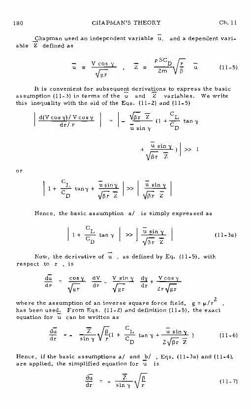
180 CHAPMAN'S THEORY Ch. 11
Chapman used an independent variable u,and a dependent vari-able Z defined as
p SC— Vcosy u (11-5)
It is convenient for subsequent derivations to express the basicassumption (11-3) in terms of the u and Z variables. We writethis inequality with the aid of the Eqs. (11-2) and (11—5)
d(Vcosy)/Vcosy - Z
dr/r - —— .
anyusiny D
U sin+ _) >>1
L usiny usiny1 + — tany + >>CD
Hence, the basic assumption a! is simply expressed as
C —.1 + tan y
>> U Sifly (1l_3a)CD
Now, the derivative of u , as defined by Eq. (11-5), withrespect to r , is
du = cosy dV V siny Vcosydr / dr dr
where the assumption of an inverse square force field, g = IL/r2has been used. From Eqs. (11-2) and definition (11-5), the exactequation for u can be written as
= - Z+ tany +
U siny (11-6)dr siny r CD
Hence, if the basic assumptions a! and b/ ,Eqs. (l1-3a) and (11-4),
are applied, the simplified equation for uis
= - (11-7)dr siny r
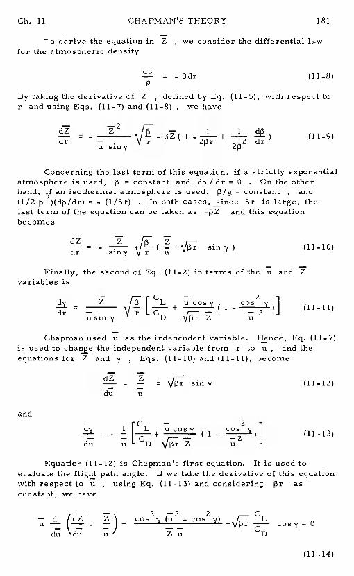
CHAPMAN'S THEORY
To derive the equation in Z, we consider the differential lawfor the atmospheric density
= - f3dr (11-8)p
By taking the derivative of Z , defined by Eq. (11-5), with respect tor and using Eqs. (11-7) and (11-8), we have
V r 2132 dr
dr — . VrU Sin
dZ Z 1—— - — = v13r sln'ldu u
2cos—2U
2cos—2U
(11—10)
Equation (11-12) is Chapman's first equation.It is used toevaluate the flight path angle.If we take the derivative of this equationwith respect to u , using Eq. (11-13) and considering13r as
constant, we have
— d /dZ z cos2 —2 2
u—I—— — +-cos
du\ducosy = 0
(11.14)
Ch. 11 181
dZ .12
dr —U
(11-9)
Concerning the last term of this equation, if a strictly exponentialatmosphere is used,
13= constant and d13 / dr = 0 . On the other
hand, if an isothermal atmosphere is used,ç3/g = constant , and(1/2 = - (1/13r) . In both cases, since13r is large, thelast term of the equation can be taken as_13Z and this equationbecomes
dZ Z— = - / ( — sindr siny yr u
Finally, the second of Eq. (11-2) in terms of the u and Zvariables is
FCL
L CD+
u as the independent variable.Hence, Eq. (11.7)is used to chan1e the independent variable from rto u , and theequations for Z and y, Eqs. (11-10) and (11-11), become
and
=- 1
—+
ucosy (1du
(11-12)
(11-13)
CHAPMAN'S THEORY Ch. 11
This equation is equivalent to Chapman's second-order nonlinear dif-ferential equation with Z as the dependent variable and u as theindependent variable.In this equation, cos y = \Ii - sin2 y can beexpressed in terms of u ,Z and dZ/du through Eq. (11-12).
To obtain the equation in the form identical to the one given byChapman in his classical paper (Ref.1), we write it as
--
(1-u2) cos4y cos3y
— 2 .2+
ucosysinz
With the aid of Eq. (11-12), we consider the sum of the terms
+uco ysiny cosy sin2y
siny [i_-
The last step is a result of applying the basic assumptions a!and b/Eqs. (l1_3a) and (11-4).This is equivalent to neglecting the termscontaining sin2 y in Eq. (11-15), yielding
(1-u2) 4 ,..... CL 3—— COS y - — cos yZu D
This equation is the second Chapman equation.Following Chapman,we have identifiedthe different components of the force as labelled.Another form is
— d /dZ \ 4 CL 3u — —- — ) =—— cos y _Vpr -a--- cos y
du\du u' Zu D(11_16a)
In general, this nonlinear differential equation has to be integratednumerically. For a nonlifting vehicle, CL! CD = 0 , the equation isapplicable to large flight path angles, as well as small angles.Forlifting vehicles, it is applicable when (CL! CD) tan yis small.
CL 2— cosysin y = 0CD
(11-15)
- (dz - z
\du U
Vertical Vertical component Gravity minus Liftacceleration of drag force centrifugal force force
(11—16)
Ch. 11 CHAPMAN'S THEORY 183
11-3. THE Z FUNCTIONS AND RELATED QUANTITIES
As mentioned in the introductory section of this chapter, Chap-man's equation, Eq. (11-16), is universal in the sense that it is free ofthe physical characteristics of the vehicle.Hence, it is applicable toany type of entry vehicle regardless of its weight, dimensions andshape.
_For an entry trajectory, since Z. 0 , only initial conditionson u. and need be given. The parameter CL/ CD and the
the atmosphere, , must, of course, be specified.For each planetary atmosphere, the average value for pris
known to a greater or lesser degree of accuracy, as was discussed inChapter 1. For Earth, is 30 . Thus, Eq. (11-16) can be inte-grated numerically starting from the initial valueu. _of the independentvariable, using the initial conditions on Z. and dZ/ du.. For anentry trajectory,
0 (11—17)
Since the basic nonlinear equation has a singularity at Z =0 , thefirst step in the numerical integration must be handled analytically byusing an approximate value for Z in the initial portion of the trajectory,depending on the type of entry.Some approximate Z functions will begiven in the next section.If y. is given, the initial value for dZ/du.is given by Eq. (11-12) as 1 1
=siny. + sin y. (1l_18)
For each flight program_and entry condition, the resulting vari-ation of Z as a function of u can be tabulated.These Tables,known as the Tables of the Z Functions (Ref. 2), can be used to analyzethe entry of any arbitrary vehicle.
In some instances, these Tables, computed for entry into theEarth's atmosphere, can be extrapolated for use with other planetaryatmospheres.
First, for a shallow entry at very small flight path angle, Eq.(11-16) is reduced to
— — —2 C— d dZ Z 1-u / Lu — ( — - —) - —— + Vpr = 0 (11-19)
du du u Zu D
with the initial condition for a prescribed
Z(u.) = 0
,
= 0 (11-20)
Hence, in this case, Tables of the Z functions can be used for anyplanetary atmosphere, for entry with the same prescribed flight para-meter (CL/CD) , as far as the variations of Z and u are
184 CHAPMAN'S THEORY Ch. 11
concerned. For the flight path angle, using subscript efor the Earth,and subscript P for any other planet, from Eq. (11-12) comes
= k
k is the conversion factor.The condition discussed above is,in particular, true for a decaying orbit for various lift-to-drag ratios.In this case, u. = 1
Next, the'extrapolation can be extended to the cases of smallentry angle. Equation (11-19) is still valid, but with the initial condi-tions
Z(u) = 0 ,= y. (11-22)
1du.
1
Hence, the Tables can be used for any planetary atmosphere, for entrywith the same (CL/CD) and . Under these condi-tions, the Z and u variations are the same, while the'y variationis obtained from Eq. (11-21).
In all cases, the validity of the application is restricted to thepart of the trajectory where the flight path angle remains small.
Several useful quantities during entry can be constructed fromthe Tables of the Z functions.
The first quantity of interest is the deceleration during entry.The deceleration along the flight trajectory is simply dV/dtThefirst of Eqs. (11-1), and definitions (11-5) of u andZ , yields
—=
+ (11_23)cos
For small flight path angles,
IdV \ ,———— Z u (11-24)
and the deceleration is simply to the product Z u. Refer-ence 1 gives several plots of Z u versus u for different typesof entry. Some of these plots are reproduced in_Section 11-5 of thischapter. They are useful in locating the speed uand the altitude Zwhere the deceleration reaches its maxima and minima during entry.
The deceleration due to the combined lift and drag forces, as feltby the pilot or an accelerometer during entry, is
=
(—fl- = A / (11-25)g
V CD
Ch. 11 CHAPMAN'S THEORY 185
Hence, for entry at small angles, the deceleration due to aerodynamicforce is obtained simply by multiplying the vehicle deceleration, givenby Eq. (11-24), by the constant factor + (CL/CD)2
The Z function provides the flight altitude of the vehicle oncethe drag parameter(SCD/2m) is specified. For an arbitrary atmo-sphere, the altitude is most conveniently expressed in terms of thelocal atmospheric densityp . Let subscript s denote the conditionat sea level. From the definition (11-5) of Z , we have
.a.(
2m(11-26)
p SC rp —s Dss u
Hence, for a strictly exponential atmosphere, the altitude h is given
riSC rp —1 Il uh = — log I t (11—27)L\ 2m
Another quantity of interest is the dynamic pressure exerted onthe vehicle.
=Zu (11-28)
Hence, the dynamic pressure is proportional to the deceleration of thevehicle.
The free-stream Reynolds number per unit length is
Re = = (rn)
=Z (11-29)
I SCD SCD
where is the atmospheric dynamic viscositL.Thus, the Reynoldsnumber per unit length is proportional to the Zfunction.
Relatively simple expressions can also be obtained for the aero-dynamic heating rate per unit area,q , and the total heat absorbedper unit area, Q/A
According to the local similarity law of Lees, (Refs. 3,4), theheating rate q at any point on a body is equal to a fraction of theheating rate q at a stagnation point of radius of curvature R . Thus,the local heating rate is expressed as
(11—30)
where the heating rate in hypersonic flow at a stagnation point,qcan be expressed as
CHAPMAN'S THEORY Ch. 11
n — mC u 2
q = — ( ) (—) kcal/m sec (11—31)
where the constants C, n , and m depend on the type of boundarylayer flow. For laminar flow, n = 1/2 . A simple power law,m = 3 , for the speed, together with the expression (11-26) for thedensity ratio, gives the expression for the laminar convective heattransfer rate in terms of theZ and u variables
q =
J
kcalr p D cos y m sec
0 0 (11-32)where
-11/2 — 5/2 (11-33)
The expression for the heat transfer rate has been written in the formof the product of three factors.The first factor represents the effecton heat flux of the particular planetary atmosphere.The second factorrepresents the effect of the physical characteristics of the vehicles,that is, the mass, dimensions and shape of the vehicle.which for flight at small flight path angles is reduced toZrepresents the effect of the particular type of entry trajectory.
Although Eq. (11-32) for heating rate is useful in studying vehiclesdesigned to operate at radiation equilibrium temperatures, an equationfor the total heat absorbed, Q, during entry is of more interest forheat-sink type vehicles.This is expressed in the form of an integral
Q = ffqdtdA = fJ'k1qdtdA (11-34)
where A is the whole surface wetted by the boundary layer.Let
fk1dA = *J'_adA (11-35)
where k2 is the factor which takes into account the variations in heatflux over the whole surface A, For a hemisphere, we have thenIs2 0.5
Q = k2AJ'qdt (11-36)
Using the expression (11-32) for q = q/k1 in this integral, we have
Q = [C rç dt (11-37)
Ch. 11 CHAPMAN'S THEORY 187
The integration with respect to the independent variable u can beaccomplished if the simplified expression (11-7) for du/dr is rewrittenwith respect to t
du du dr /—= = - cos (11-38)
This equation gives the time of flight between U1and u as
- 1
3
Zu
Substitution of (11-38) into (11-37), yields the expression for the totalheat absorbed between and
Q =z
(11-40)
whereU1 —3/2du
= 1 —1/2 2(11-41)
— ZU
11-4. SOME APPROXIMATE ANALYTICAL SOLUTIONS
The ultimate purpose of the Chapman formulation is the numericalintegration and tabulation of theZ functions, as generated by Eq.(11-16), for use in the preliminary design of the entry vehicle and itsmission planning. Although Chapman's equation is only approximate,the assumptions made are general enough so that the basic nonlinearequation ,Eq. (11-16), contains all the principal effects of the forcesacting on the vehicle during entry.Hence, under various assumptionsto simplify this equation, Chapman's reduced equation should providethe other first-order solutions discussed previously.In this section,we shall consider several such cases.
11-4.1. Yaroshevskii's Solution
For constant lift-to-drag ratio entry, Yaroshevskii's second-order nonlinear differential equation, discussed in Chapter 10, is sim-ply a case of Chapman's equation.
For constant lift and drag coefficients, Yaroshevskii's variablesare (Ref. 5)
x a log , y a p (11-42)
188 CHAPMAN'S THEORY Ch. 11
where the subscript o denotes the condition at a reference level.In the more sophisticated definition of Chapman's variables, Eqs.
(11-5), if a constant reference value forr is used, and a very smallflight path angle is assumed, then
— v — SCDPu = , Z = u (11-43)2m $3
Hence, the relations between the two sets of variables are
= y , = (11-44)U
The corresponding relation between the derivatives is
d xd I d— ( ) = - e ( ) = - — ) (11-45)du u
Transformations (11-44) and (11-45) applied to Chapman's simplifiedequation for entry at very small flight path angles, Eq. (11-19), gives
+1
= 0 (11-46)
This equation is identical to Yaroshevskii's equation, Eq. (10-17), andits analytical solutions for various entry trajectories have been pre-sented in Chapter 10.
11-4.2. Solution for Ballistic Entry
For ballistic entry, using Allen and Eggers assumption (Ref.6),we disregard the gravity, centrifugal and lift force in Chapman'sequation, Eq. (11-16), and write it as
( - ) = 0 (11-47)du du u
This, and Eq. (11- 12), shows that the flight path angle remains constant.The integral of Eq. (11-47) can be written
- (11-48)
A second integration, along with the initial conditions, produces thesolution for ballistic entry
Ch. 11 CHAPMAN'S THEORY 189
= u log (11-49)
The Z1 function provides an approximate solution for the motion andheating identical to the solution of Allen and Eggers for ballistic entry.
11-4. 3. Solution for Glide Entry
For glide entry, using Sknger's assumption (Ref.7), we neglectthe vertical acceleration and vertical component of the drag force inChapman's equation.Chapman's equation, along with Eq. (11-12),shows that this amounts to considering the glide angle as negligiblysmall, cos 1 . Hence, Eq. (11-16) is reduced to the condition forequilibrium glide
—2= I - U (11-50)
II
The function corresponds to equilibrium gliding flight as dis-cussed by Sänger and Bredt.
11-4.4. Solution for Skip Trajectory
For skip trajectories, using Eggers, Allen, and Neice's assump-tion (Ref. 8), we neglect the gravity and centrifugal force in Chapman'sequation. Thus,
u-
= (11-51)
By using an average value for on the right-hand side of thisequation, and using Eq. (11-12), we may integrate this and apply theinitial conditions to obtain
C —
sin sin - cos 'y log (ll_52)
This equation gives the flight path angle in terms of the flight speed.The Z function for skip trajectories may be obtained by combiningEqs. (11-52) and (11-12):
- sin y. - co S3 log ( (11- 53)du u
1D u.
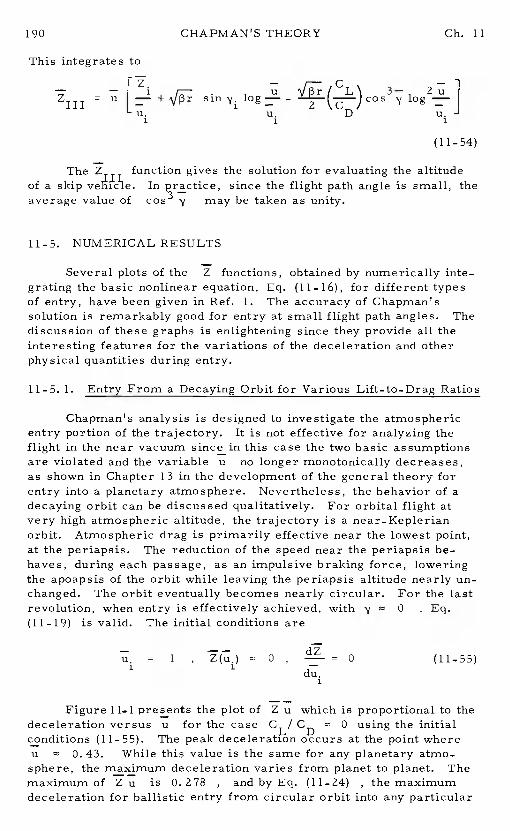
190 CHAPMAN'S THEORY Ch. 11
This integrates to
iiii =
(11-54)
The Z function gives the solution for evaluating the altitudeof a skip In practice, since the flight path angle is small, theaverage value of cos3 may be taken as unity.
11-5. NUMERICALRESULTS
Several plots of the Z functions, obtained by numerically inte-grating the basic nonlinear equation, Eq. (11- 16), for different typesof entry, have been given in Ref.1. The accuracy of Chapman'ssolution is remarkably good for entry at small flight path angles.Thediscussion of these graphs is enlightening since they provide all theinteresting features for the variations of the deceleration and otherphysical quantities during entry.
11-5. 1. Entry From a Decaying Orbit for Various Lift-to-Drag Ratios
Chapman's analysis is designed to investigate the atmosphericentry portion of the trajectory.It is not effective for analyzing theflight in the near vacuum since in this case the two basic assumptionsare violated and the variable uno longer rnonotonically decreases,as shown in Chapter 13 in the development of the general theory forentry into a planetary atmosphere.Nevertheless, the behavior of adecaying orbit can be discussed qualitatively.For orbital flight atvery high atmospheric altitude, the trajectory is a near-Keplerianorbit. Atmospheric drag is primarily effective near the lowest point,at the periapsis.The reduction of the speed near the periapsis be-haves, during each passage, as an impulsive braking force, loweringthe apoapsis of the orbit while leaving the periapsis altitude nearly un-changed. The orbit eventually becomes nearly circular.For the lastrevolution, when entry is effectively achieved, with y 0 , Eq.(11-19) is valid. The initial conditions are
U = 1 , Z(u.) = 0 , = 0 (11-55)1 1
du.1
Figure 11..l presents the plot of Z u which is proportional to thedeceleration versus ufor the case CL! CD =0 using the initialconditions (11-55). The peak deceleration occurs at the point whereu 0. 43. While this value is the same for any planetary atmo-sphere, the maximum deceleration varies from planet to planet.Themaximum of Z u is 0. 278 , and by Eq. (ll-Z4) , the maximumdeceleration for ballistic entry from circular orbit into any particular
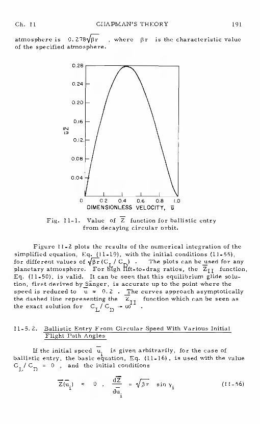
Ch. 11 CHAPMAN'S THEORY 191
atmosphere is 0. , where is the characteristic valueof the specified atmosphere.
Fig. 11-1. Value of Z function for ballistic entryfrom decaying circular orbit.
Figure 11-2 plots the results of the numerical integration of thesimplified equation, Eq. (11—19), with the initial conditions (11—55),for different values of (CL! . The plots can be used for anyplanetary atmosphere.For high ratios, the Z11 function,Eq. (11-50), is valid. It can be seen that this equilibrium glide solu-tion, first derived is accurate up to the point where thespeed is reduced tou 0. 2 . The curves approach asymptoticallythe dashed line representing theZ11 function which can be seen asthe exact solution for CL! CD
11-5. 2. Ballistic Entry From Circular Speed With Various InitialFlight Path Angles
If the initial speed u. is given arbitrarily, for the case ofballistic entry, the basic equation, Eq. (11-16), is used with the valueCL! CD = 0 , and the initial conditions
o=
siny. (11-56)du.
IN
0.28
0.24
0.20
0.16
0.12.
0.08
0.04
0 0.2 0.4 0.6 0.8 1.0
DIMENSIONLESS VELOCITY, U
Z(u.)
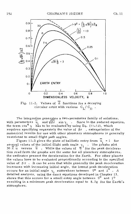
Fig. 11-2. Values of 21 functions for a decayingcircular orbit with various CL!
The integration generates a two-parameter family of solutions,with parameters u• and sin . Since in the reduced equation,the term cos4 'y to be evaluated by using Eq. (11-12), whichrequires specifying separately the value of , extrapolation of thenumerical results for use with other planetary atmospheres is generallyrestricted to small flight path angles. —
Figure 11-3 gives the plots of ballistic entry from ui= 1 forseveral values of the initial flight path angle . The graphs plot30 Z u versus ii . While the values of U for the peak decelera-tion read from the graphs are the same for all planetary atmospheres,the ordinates present the deceleration for the Earth.For other planetsthe values have to be evaluated proportionally according to the specifiedvalue of r . It can be seen that while generally the peak decelerationincreases with increasing initial angle, the lowest peak decelerationoccurs for an initial angle somewhere between 00 and 20 . Adetailed analysis, using the exact equations developed in Chapter 13,shows that this occurs for a small entry angle between 00 and 1oresulting in a minimum peak deceleration equal to8. 2g for the Earth'satmosphere.
CHAPMAN'S THEORY Ch. 11
0.9
0.8
0.7
0.6IN
0.5
-JI° 0.4
0.3
0.2
0.I
0 0.2 0.4 0.6 0.8DIMENSIONLESS VELOCITY, U
1.0
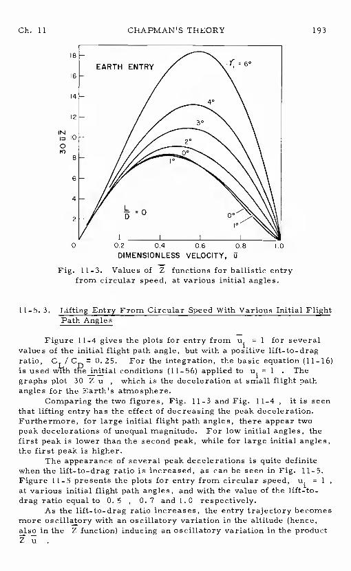
Ch. 11 CHAPMAN'S THEORY 193
8
6
4
2
IN0
08
6
4
2
0 0.2 0.4 0.6 0.8 .0DIMENSIONLESS VELOCITY, 0
Fig. 11-3. Values of Z functions for ballistic entryfrom circular speed, at various initial angles.
11-5.3. Lifting Entry From Circular Speed With Various Initial FlightPath Angles
Figure 11-4 gives the plots for entry from u.= 1 for severalvalues of the initial flight path angle, but with a positive lift-to-dragratio, CL/C = 0.25. For the integration, the basic equation (11-16)is used with initial conditions (11-56) applied tou. = 1 . Thegraphs plot 30 Z u, which is the deceleration at small flight pathangles for the Earth's atmosphere.
Comparing the two figures, Fig. 11-3 and Fig. 11-4it is seenthat lifting entry has the effect of decreasing the peak deceleration.Furthermore, for large initial flight path angles, there appear twopeak decelerations of unequal magnitude.For low initial angles, thefirst peak is lower than the second peak, while for large initial angles,the first peak is higher.
The appearance of several peak decelerations is quite definitewhen the lift_to-drag ratio is increased, as can be seen in Fig. 11-5.Figure 11-5 presents the plots for entry from circular speed,u. = 1
at various initial flight path angles, and with the value of the lift-to-drag ratio equal to0. 5 0. 7 and 1.0 respectively.
As the lift-to-drag ratio increases, the entry trajectory becomesmore oscillatory with an oscillatory variation in the altitude (hence,also in the Z function) inducing an oscillatory variation in the productZu
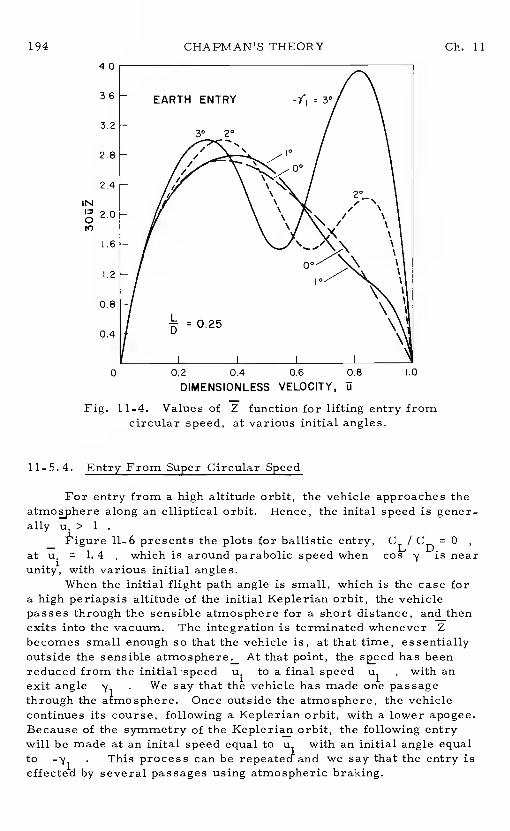
IN
0
194 CHAPMAN'S THEORY Ch. 114.0
3.6
3.2
2.8
2.4
2.0
LB
1.2
0.8
0.4
0 0.2 0.4 0.6 0.8 1.0
DIMENSIONLESS VELOCITY, U
Fig. 11-4. Values of Z function for lifting entry fromcircular speed, at various initial angles.
11-5.4. Entry From Super Circular Speed
For entry from a high altitude orbit, the vehicle approaches thealong an elliptical orbit. Hence, the inital speed is gener-
ally u. > 1
— tigure 11-6 presents the plots for ballistic entry,CL! CD = 0
at u. = 1.4 , which is around parabolic speed whencns y is nearunity', with various initial angles.
When the initial flight path angle is small, which is the case fora high periapsis altitude of the initial Keplerian orbit, the vehiclepassesthrough the sensible atmosphere for a short distance, and thenexits into the vacuum. The integration is terminated whenever Zbecomes small enough so that the vehicle is, at that time, essentiallyoutside the sensible atmosphere. At that point, the speed has beenreduced from the initial speed u. to a final speed u1 , with anexit angle . We say that the vehicle has made one passagethrough the atmosphere. Once outside the atmosphere, the vehiclecontinues its course, following a Keplerian orbit, with a lower apogee.Because of the symmetry of the Keplerian orbit, the following entrywill be made at an inital speed equal to uwith an initial angle equalto This process can be and we say that the entry iseffected by several passages using atmospheric braking.
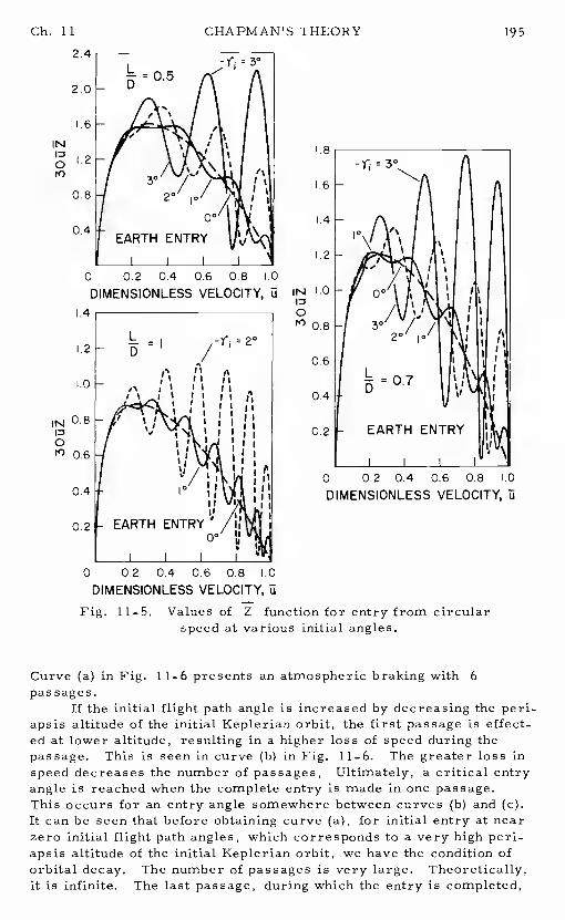
Ch. 11 CHAPMAN'S THEORY 195
0 0.2 0.4 0.8 '.0DIMENSIONLESS VELOCITY, U
.4
0.2
0 0.2 0.4 0.6 0.8 .0
DIMENSIONLESS VELOCITY, U
0 0.2 0.4 0.6 0.8 .0
DIMENSIONLESS VELOCITY, U
Fig. 11-5. Values of Z function for entry from circularspeed at various initial angles.
Curve (a) in Fig. 11-6 presents an atmospheric braking with6
passages.If the initial flight path angle is increased by decreasing the pen-
apsis altitude of the initial Keplerian orbit, the first passage is effect-ed at lower altitude, resulting in a higher loss of speed during thepassage. This is seen in curve (b) in Fig. 11—6.The greater loss inspeed decreases the number of passages,Ultimately, a critical entryangle is reached when the complete entry is made in one passage.This occurs for an entry angle somewhere between curves (b) and (c).It can be seen that before obtaining curve (a), for initial entry at nearzero initial flight path angles, which corresponds to a very high pen-apsis altitude of the initial Keplerian orbit, we have the condition oforbital decay. The number of passages is very large.Theoretically,it is infinite. The last passage, during which the entry is completed,
IN
0
1.2
1.0
IN 0.8ID0ro 0.6
0.4
.8
.6
.4
.2
IN 1.0ID0
0.8
0.6
0.4
0.2
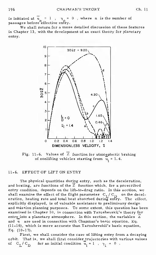
196 CHAPMAN'S THEORY Ch. 11
is initiated at u = 1 , = 0 , where n is the number ofpassagesbeforeneffective enPry.
We shall return for a more detailed discussion of these featuresin Chapter 13, with the development of an exact theory for planetaryentry.
I0
8
7
6
IN
0K)
4
3
2
0
Fig. 11-6. Values of Z function for atmospheric brakingof nonlifting vehicles starting from u. =1. 4.
11-6. EFFECT OF LIFT ON ENTRY
The physical quantities during entry, such as the deceleration,and heating, are functions of the Z function which, for a prescribedentry condition, depends on the lift-to-drag ratio.In this section, weshall examine the effect of the flight parameter CL! Con the decel-eration, heating rate and total heat absorbed during enfty.The effect,explicitly displayed, is of valuable assistance to preliminary designand mission planning purposes.To some extent, this question has beenexamined in Chapter 10, in connection with Yaroshevskii's theory forentry into a planetary atmosphere.In this section, the variables Zand u are used in connection with Chapman's basic equation, Eq.(11-16), which is more accurate than Yaroshevskii's basic equation,Eq. (10-17).
First, we shall consider the case of lifting entry from a decayingorbit. That is, we shall first consider trajectories with various valuesof C IC foraninitialcondition u.=1 , y. = 0L D 1
9
0.2 0.4 0.6 0.8 1.0 .2 1.4
DIMENSIONLESS VELOCITY, V
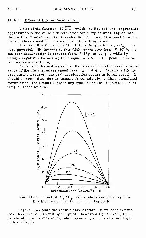
Ch. 11 CHAPMAN'S THEORY 197
11-6. 1. Effect of Lift on Deceleration
A plot of the function 30 Z u which, by Eq. (11-24), representsapproximately the vehicle deceleration for entry at small angles intothe Earth's atmosphere, is presented in Fig. 11-7, as a function of thedimenionless speed ufor various lift-to-drag ratios.
It is seen that the effect of the lift-to-drag ratio,C / CD , isvery powerful. By increasing this flight parameter from to 0. 1the peak deceleration is reduced from 8. 38g to4. 9g , while byusing a negative lift-to-drag ratio equal to-0. 1 , the peak decelera-tion increases to 12. 8g
For small lift-to-drag ratios, the jeak deceleration occurs in therange of the dimensionless speed nearu = 0. 4 , When the lift-to-drag ratio increases, the peak deceleration occurs at lower speed.Itshould be noted that, due to Chapman's completely nondimensionalizedformulation, the graphs apply to any type of vehicle, regardless of itsweight, shape or size.
4
12U,
a,
2100I-.4a:w-JLu0Lu0-J
20Na:0t
2
0
Fig. 11-7. Effect of CL! C on deceleration for entry intoEarth's atmosphere Rom a decaying orbit.
Figure 11-7 plots the vehicle deceleration.If we consider thetotal deceleration, as felt by the pilot, then from Eq. (11-25), thisdeceleration at its maximum, which generally occurs at small flightpath angles, is
8
6
4
0.2 0.4 0.6 0.8 .0DIMENSIONLESS VELOCITY, U
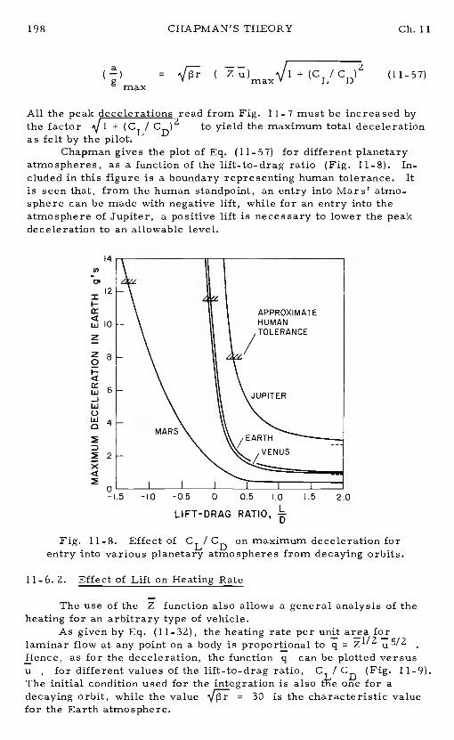
( ( AJ1 + (CL/CD)2max
All the peak decelerations read from Fig. 11-7 must be increased bythe factor + (CL! CD) to yield the maximum total decelerationas felt by the pilot.
Chapman gives the plot of Eq. (11-57) for different planetaryatmospheres, as a function of the lift-to-drag ratio(Fig. 11-8). In-cluded in this figure is a boundary representing human tolerance.Itis seen that, from the human standpoint, an entry into MarsT atmo-sphere can be made with negative lift, while for an entry into theatmosphere of Jupiter, a positive lift is necessary to lower the peakdeceleration to an allowable level.
LIFT-DRAG RATIO,
Fig. 11-8. Effect of CL/CD on maximum deceleration forentry into various planetary atmospheres from decaying orbits.
11-6. 2. Effect of Lift on Heating Rate
The use at theZ function also allows a general analysis of theheating for an arbitrary type of vehicle.
As given by Eq. (11-32), the heating rate per unit area forlaminar flow at any point on a body is proportional to q = u5/2Hence, as for the deceleration, the function qcan be plotted versusu , for different values of the lift-to-drag ratio,C / CD (Fig. 11-9).The initial condition used for the integration is also one for adecaying orbit, while the value = 30 is the characteristic valuefor the Earth atmosphere.
198 CHAPMAN'S THEORY Ch.ll
(11-57)
U,
zF—
LU
zz0
LU-jUiC.)Ui0
x
-1.5 -1.0 -0.5 0 0.5 1.0 .5 2.0
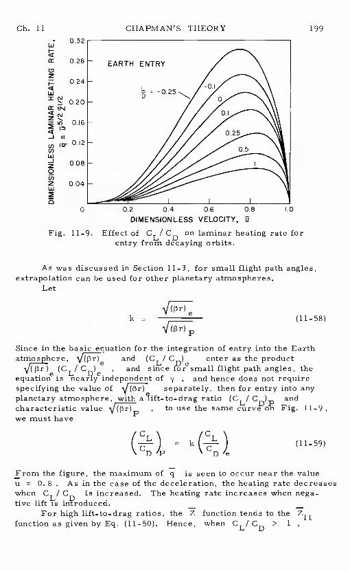
U
2
U
INz....
_J
(I,U)U-Jz0U)2Lu
Ch. 11 CHAPMAN'S THEORY 199
0 0.2 0.4 0.6 0.8DIMENSIONLESS VELOCITY, U
I.0
Fig. 11-9. Effect of CL/CD on laminar heating rate forentry from decaying orbits.
As was discussed in Section 11-3, for small flight path angles,extrapolation can be used for other planetary atmospheres.
Let
ek a
______
(11-58)
Since in the basic equation for the integration of entry into the Earthatmosphere, and (CL/ C ) enter as the product
(CL! , and since flight path angles, theequation is nearly independent of , and hence does not requirespecifying the value of separately, then for entry into anyplanetary atmosphere, with ratio (CL! CD)P andcharacteristic value , to use the same curve on Fig. 11-9,we must have
fC \ fC '\) = k ) (11-59)
\
From the figure, the maximum of qis seen to occur near the valueu = 0. 8 . As in the case of the deceleration, the heating rate decreaseswhen CL! C is increased. The heating rate increases when nega-tive lift is in1?roduced. — —
For high lift-to-drag ratios, the Z function tends to theZ11function as given by Eq. (11-50).Hence, when CL/CD > 1
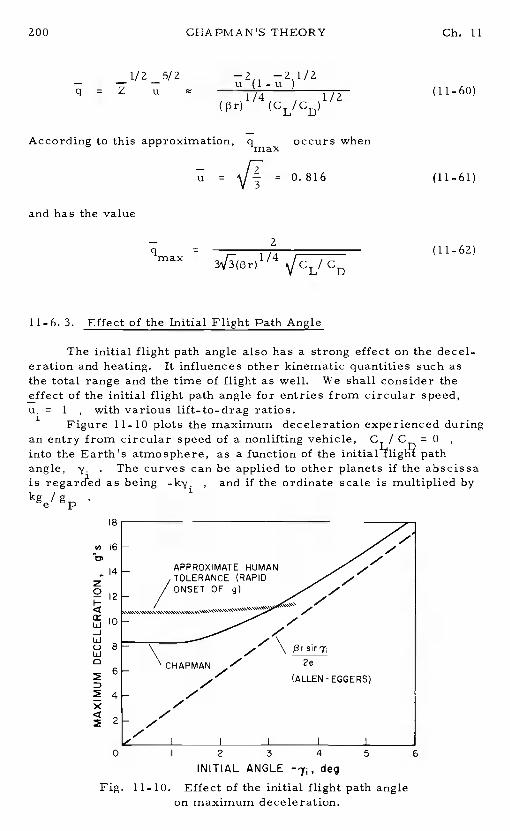
CHAPMAN'S THEORY Ch. 11
— —2 —21/2u (1-u— 1/4 1/2(pr) (CL/CD)
11-6. 3. Effect of the Initial Flight Path Angle
The initial flight path angle also has a strong effect on the decel-eration and heating.It influences other kinematic quantities such asthe total range and the time of flight as well.We shall consider theeffect of the initial flight path angle for entries from circular speed,ui = 1 , with various lift-to-drag ratios.
Figure 11-10 plots the maximum deceleration experienced duringan entry from circular speed of a nonlifting vehicle,C1 / CD = 0
into the Earth's atmosphere, as a function of the initialtight pathangle, . The curves can be applied to other planets if the abscissais regarcted as being -ky., and if the ordinate scale is multiplied by
1
Fig. 11-10. Effect of the initial flight path angleon maximum deceleration.
1/2 5/2q = Z u
According to this approximation,q occurs whenmax
= = 0.816
and has the value
VCL/CD
(11-60)
(11—61)
(11-62)
'o IS
C'
20F-Clxw-JLii0LiiC
xC
2 3 4
INITIAL ANGLE deg
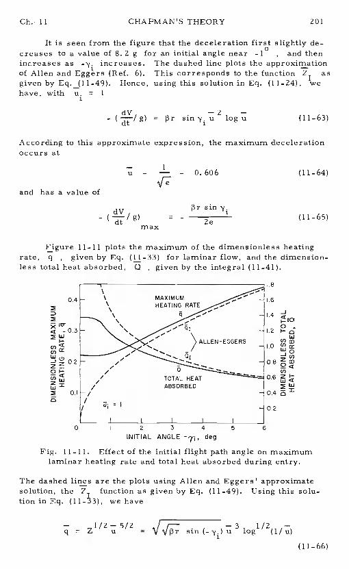
increases as increases.of Allen and Eggers (Ref.6).given by Eq. (11-49). Hence,have, with u. = 1
dV —2 —- g) = 3r sin u log u (11—63)
expression, the maximum deceleration
U 0.606 (11-64)
max
sin= - (11-65)
2e
Figure 11-11 plots the maximum of the dimensionless heatingrate, q , given by Eq. (11-33) for laminar flow, and the dimension-less total heat absorbed,Q , given by the integral (11-41).
-JKY0.
i_cDw
Fig. 11-11. Effect of the initial flight path angle on maximumlaminar heating rate and total heat absorbed during entry.
The dashed lines are the plots using Allen and Eggers' approximatesolution, the ZT function asgiven by Eq. (11-49). Using this solu-tion in Eq. we have
= 5/2 sin logl/2(1/u)
Ch.• 11 CHAPMAN'S THEORY 201
It is seen from the figure that the deceleration first slightly de-creases to a value of8.2 g for an initial angle near , and then
The dashed line plots the approximationThis corresponds to the function Z1 asusing this solution in Eq. (11-24), we
According to this approximateoccurs at
and has a value of
dV-
2 3 4
INITIAL ANGLE deg
(11-66)
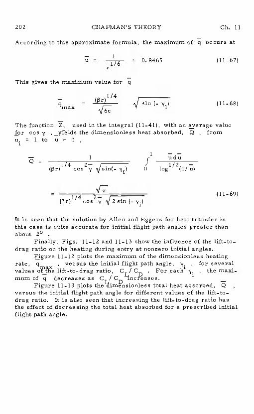
CHAPMAN'S THEORY Ch. 11
According to this approximate formula, the maximum of q occurs at
=0.8465 (11-67)
This gives the maximum value for q
1/4I
q = sin (- (11-68)max
The function used in the integral (11-41), with an average valuefor cos , yields the dimensionless heat absorbed, Q, fromu. = 1 to u = 0
3.
—- 1 udu— 1/4 2— j . J 1/2 —
(13r) cos Vsin(_ 0 log (1/u)
1/4 2—(11—69)
(13r) cos 2 sin (_ 'y.)
It is seen that the solution by Allen and Eggers for heat transfer inthis case is quite accurate for initial flight path angles greater thanabout 20
Finally, Figs. 11-12 and 11—13 show the influence of the lift-to-drag ratio on the heating during entry at nonzero initial angles.
Figure 11-12 plots the maximum of the dimensionless heatingrate, q , versus the initial flight path angle, , for severalvalues lift-to-drag ratio, CD . For each1 , the maxi-mum of q decreases as C/ CD increases. —
Figure 11-13 plots total heat absorbed, Qversus the initial flight path angle for different values of the lift-to-drag ratio. It is also seen that increasing the lift-to-drag ratio hasthe effect of decreasing the total heat absorbed for a prescribed initialflight path angle.
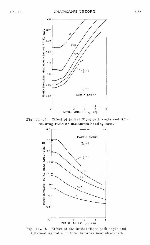
Ch. 11 CHAPMANTS THEORY
Fig. 11-12. Effect of initial flight path angle and lift-to-drag ratio on maximum heating rate.
4.0
I0
Liim
0Cd,
I-w
-J 2.0I-0I-C')C')w-J20(1)zUi
0
Fig. 11-13. Effect of the initial flight path angle andlift-to-drag ratio on total laminar heat absorbed.
2 3 4
INITIAL ANGLE deg
0 2 3 4
INITIAL ANGLE deg
CHAPMAN'S THEORY Ch. 11
References
1. Chapman, D. R., "An Approximate Analytical Method for StudyingEntry Into Planetary NASA TR R-ll, 1959.
2. Chapman, D. R., and Kapphahn, A. K., "Tables of Z Functionsfor Atmsopheric Entry Analyses," NASA TR R_106, 1961.
3. Lees, L. , " Laminar Heat Transfer Over Blunt-Nosed Bodies atHypersonic Flight Speeds, "Jet Propulsion, Vol. 26, No. 4,pp. 259-269, 1956.
4. Lees, L., "Recovery Dynamics -Heat Transfer at HypersonicSpeeds in a Planetary Atmosphere," Chapter 12 of Spacenology, ed. by H. S. Seifert, John Wiley and Sons, N. Y., 1959.
5. Yaroshevskii, V.A., "The Approximate Calculation of Trajector-ies of Entry Into the Atmosphere.I', Translated fromKosmicheskie Issledovaniya, Vol. 2, No. 4, 1964.
6. Allen, H. J. , and Eggers, A. J. ,Jr., "A Study of the Motion andAerodynamic Heating of Missile Entering the Earth's Atmosphereat High Supersonic Speeds," NACA Report No. 1381, 1958.
7. Singer, E. , and Bredt, J. , "A Rocket Drive For Long RangeBomber, " Translation No. CGD-32, Technical InformationBranch, Navy Department, 1944.
8. Eggers, A.J. ,Jr., Allen, H.J. , and Neice, S. E. ,"A Compar-ative Analysis of the Performance of Long-Range HypervelocityVehicles, " NACA TN 4046, 1957.
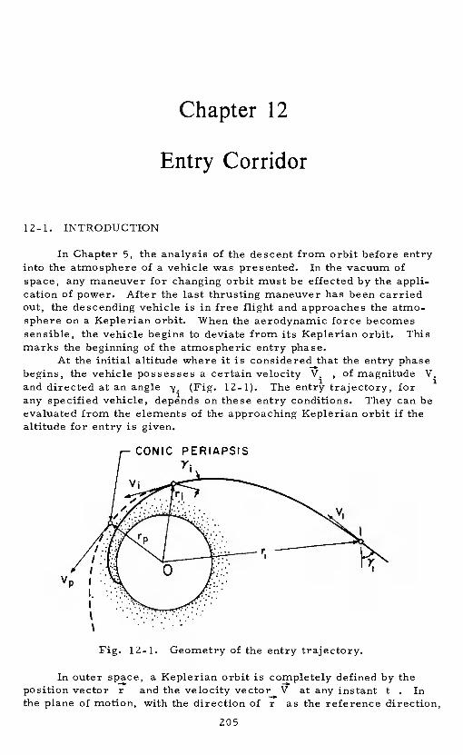
12-1. INTRODUCTION
Chapter 12
Entry Corridor
In Chapter 5, the analysis of the descent from orbit before entryinto the atmosphere of a vehicle was presented.In the vacuum ofspace, any maneuver for changing orbit must be effected by the appli-cation of power. After the last thrusting maneuver has been carriedout, the descending vehicle is in free flight and approaches the atmo-sphere on a Keplerian orbit.When the aerodynamic force becomessensible, the vehicle begins to deviate from its Keplerian orbit.Thismarks the beginning of the atmospheric entry phase.
At the initial altitude where it is considered that the entry phasebegins, the vehicle possesses a certain velocity V., of magnitude V.and directed at an angle (Fig. 12-1). The trajectory, forany specified vehicle, on these entry conditions.They can beevaluated from the elements of the approaching Keplerian orbit if thealtitude for entry is given.
Fig. Geometry of the entry trajectory.
In outer space, a Keplerian orbit is completely defined by theposition vector r and the velocity vector Vat any instantt . Inthe plane of motion, with the direction of ras the reference direction,
205
CONIC PERIAPSIS'-I
I
206 ENTRY CORRIDOR Ch. 12
the three scalar quantitiesr , V and y suffice to specify the orbit.This has been studied in detail in Chapter 3.In the following, we shallconsider three particular positions for defining the approachingKeplerian orbit:
it The first point is an arbitrary point on the orbit, at very highaltitude where the vehicle is still in the vacuum (Fig. 12-1).Thequantities associated with this point arer1 , V1 and y
ii! The second point is the entry point and the associ-ated with this point arer. , V. and y. . Theoretically, the defini-tion of this point involves a certain degrbe of arbitrariness.One mayconsider the distancer. as the distance to the top of the sensibleatmosphere. Another of the entry point is that point wherethe deceleration due to atmospheric force has reached a certain frac-tion, say one per cent, of the local gravitational force so that the vehi-cle has just begun its nonKeplerian trajectory.Obviously, in this casethe corresponding initial distancer. depends on the drag coefficientSCDtm of the vehicle, the initial V. and the initial flight pathangle y. . We shall return to this question in Chapter 13.Whateverthe used, for all practical computation, the entry point willbe considered the last point on the approaching Keplerian orbit.
iiit The third point to be used for the definition of the Kepleriantrajectory is its pericenter.This point is the lowest point on thenominal Keplerian trajectory.It is the pericenter of the conic trajec-tory which the vehicle would have followed had there been nosphere around the planet.In the case where the Keplerian orbit inter-sects the planet, the trajectory is extended to lead to a pericenter in-side the planet. The quantities associated with this point arerV andy =0. p
p pThe entry speed from a close orbit is near circular speed at the
entry altitude, while entry from a high altitude orbit is effected atsupercircular speed.In particular, for a moon flight return to theEarth's atmosphere, the entry speed is near parabolic speed.In thecase of an entry following an interplanetary flight, the vehicle entersthe planetary atmosphere at hyperbolic speed.For a safe recovery ofa ballistic vehicle, one must select the entry conditions, the speed V.and the flight path angley. at the distancer. , such that the subse-quent trajectory generates deceleration and heating conditions withinacceptable limits. For a lifting hypervelocity vehicle, the entry posi-tion must also be selected such that, near the end of the atmosphericentry trajectory, the vehicle is in the correct presentation in the posi-tion vector and the velocity vector for effectively performing thelast aerodynamic and thrusting maneuver phase for making a safeapproach and landing at the previously selected airfield.
While thrusting maneuvers in space can always be programmedto bring the vehicle to a prescribed entry condition, the resulting fuelconsumption may become prohibitive.Savings in fuel consumptionwill increase the useful payload, cargo, life support equipment andmanpower onboard the vehicle, thus providing more flexibility in mis-sion planning.
Ch. 12 ENTRY CORRIDOR 207
On the other hand, there exist constraints on the entry conditionas illustrated in Fig. 12-2.Let us assume that a physical constraint,say the maximum deceleration, has been advanced in the selection ofan entry trajectory. This is obviously one of the constraints in mannedflights. For a given vehicle, with a certain ballistic coefficient, usinga prescribed lift-to-drag ratio, all approach orbits, having a prescrib-ed periapsis speed Vat the fictitious pericenter, can be divided intotwo families. In one ?amily, the resulting atmospheric entry trajec-tories generate a peak deceleration exceeding the prescribed maximumdeceleration. The boundary of this family will be referred to as theundershoot boundary and the resulting periapsis distance isr(Fig. 12-2). In general an undershoot trajectory, that is atrajectory leading to an unacceptable peak deceleration, has its pen-apsis distance less than this minimum acceptable periapsis distance.
Fig. 12-2. The entry corridor.
On the other hand, among the trajectories of the remaining fam-ily of Keplerian orbits, not all can be considered as entry trajectories.This is because if the periapsis distance of the nominal Keplerianconic considered is too large, the atmospheric force encountered istoo small and after a short flight inside the atmosphere the vehicle willescape into space and entry is not completed during the first pass.Theboundary of these escaping trajectories is called the overshoot bound-ary and the resulting periapsis distance is . In general, anovershoot trajectory, that is a trajectory OV leading to an exit intospace, has a peniapsis distance larger than this maximum periapsisdistance.
The portions representing excessive overshoot and undershootin the figure are excluded as not representing the intended maneuver.This leads to a narrow corridor through which the vehicle must beguided. The difference = r - r will be referred to as the
OVERSHOOT
208 ENTRY CORRIDOR Ch. 12
corridor width. For a successful entry during the first pass, withinthe limit of the physical constraint imposed upon the trajectory, thevehicle must be guided during its Keplerian phase into this narrowcorridor. Flight from circular or elliptical orbit is somewhat tolerantof guidance errors. An undershoot trajectory can be readily correctedby application of a thrust at a large distance before entry. An over-shoot trajectory can be similarly corrected. If necessary, one canuse an aerodynamic maneuver during the skipping phase to have acorrect presentation on the next return.
In contrast, entry at hyperbolic speed from outer space isunforgiving of guidance errors. For an undershoot trajectory, becauseof the high approach speed, thrusting correction may be prohibitivebecause of the fuel consumption, and an insufficiently corrected under-shoot trajectory may cause destruction of the vehicle during entry.On the other hand, an overshoot trajectory, if inadequately corrected,may result in a hyperbolic departure leading the vehicle into a home-less exit into space, or a highly elliptic ejection prolonging dangerous-ly the lapse time until the next return.
The concept of an entry corridor was first formulated byChapman (Ref.1). Before we continue with the presentation of thisoutstanding formulation, one fundamental comment is in order.
The introductory notion given above is related to a prescribedvehicle, with a given ballistic coefficient following different Kepleriantrajectories, all leading to the same fictitious periapsis speed VMore clearly, for a given ballistic coefficient, with the same con?cperiapsis speed V , for the entry to be accomplished during the firstpass, within the maximum deceleration, the periapsis dis-tance of the approaching Keplerian orbit should be aimed betweenr and rpun
A novel feature introduced in Chapman's original paper (Ref.1)is a dimensionless periapsis parameter combining certain character-istics of the vehicle with certain quantities associated with the conicpericenter. With this parameter, the analysis can be applied to avehicle of arbitrary weight, shape and size, entering an arbitraryplanetary atmosphere.
12-2. BASIC DIFFERENTIAL EQUATIONS
Chapman developed his theory of the entry corridor for smallflight path angles. Hence, the fundamental second-order nonlineardifferential equation to be used is Eq. (11-19) written as
= CL(12-1)
where
Ch. 12 ENTRY CORRIDOR 209
— Vcos'vu=&— pSC cz
=u (12-2)
— The integration of the equation requires two initial conditions onZ and Z = dZ/ du at the initial time, u =
Z(u.) = , Z (u.) = Z. (12-3)1 1 1 1
To evaluate Z we use Eq. (11-12) reproduced here for convenience
dZ Z C- = = vpr sin'y (12-4)
du u
Hence, the initial conditions are
='
=
+siny. (12-5)
The kinematic elements at entry arer1 V. and y. . Hence,we can form the dimensionless entry speedV.Then = V. cos y. , y. and the additional Z.will pro\ride stlfficieAt initib conditions for the integration of thelinear equation (12-1).Subsequently, the flight path angle is given byEq. (12-4) and the deceleration, the heating rate or any other physicalquantity at any instant can be obtained fromZ , u , and 'y ashas been presented!n Chapter 11.
Now, since Z, can be taken as approximately zero, oranaly-tically by using the f?rst-order solutions, it is seen that only V.andy. need be prescribed.Then, the analysis of the deceleration, orw1hatever physical quantity is considered, determines whether or notthe trajectory is an undershoot trajectory while the correspondingZfunction is used to assess if a trajectory is a skip trajectory, Zf = Z.or a descending trajectory, Z > Z. . Several hundred solutionsfor different entry trajectories were computed by Chapman and theresults presented in his report (Ref. 1).A very convenient parameter,the periapsis parameter, was introduced to present the results in acompletely dimensionless form applicable to any type of vehicle, ofarbitrary weight, shape and size, entering an arbitrary planetaryatmosphere.
ENTRY CORRIDOR Ch. 12
12-3. THE PERIAPSIS PARAMETER
It was explained in Chapter 11 that the use of Chapman's vari-ables Z and u has the advantage of eliminating the specificationof the entry altitudeh. and the ballistic coefficient . Thecharacteristics of the planet's atmosphere enter the basic equation(12-1) in the dimensionless parameter iJjT. From Eq. (12-5), itfollows that, for shallow entry at a high altitude, where the initialvalues of Z are negligible compared to subsequent values duringentry, the second initial condition can be written as
Z(u=
(12-6)
The initial flight path angle should be taken at the beginningof the sensible atmosphere.Theoretically, from Fig. 12-1, it is seenthat, once the Keplerian approach orbit is known, this anglecanbe evaluated for any distancer. chosen as the radius of the sensibleatmosphere. But this distancer. is not well-defined. From a physi-cal standpoint, if the entry altituäe is defined as the altitude whereaerodynamic force begins to take effect, then this altitude obviouslydepends on the drag parameter SC /m, the entry speed V. andthe angle 'y. itself. For very trajectories grazing the edgeof the atmosphere, a precise evaluation of'y. is therefore cumber-some.
A convenient parameter for the analysis of the entry corridor,the periapsis parameter, was introduced by Chapman.This parameteris associated with the hypothetical periapsis distance of the approachconic orbit (Fig. 12-1) . The relation between this periapsis distancer , and the elements r, V and y at any arbitrary point on thel&eplerian orbit was given in Chapter 3,Eq. (3_70). This equationcan be rewritten in the current notation as
2 —2 —2 . 2= 1- V(V -1) +V (2-V )sin 'y (127)r a-V2
where
V == co''y (12-8)
For shallow entries for which the flight path angle is small,
V2(2-V2) sin2y << 1
(V2 - 1)2
and Eq. (12-7) for supercircular entries(V2 - 1) > 0 , with thearbitrary point taken as the entry point, can be approximated as

Ch. 12 ENTRY CORRIDOR
—z 2r V. sin_2i_ 1
r1 2(v.2 — 1)
Hence,—2 2r• - r V. 'j.
1 p 1 1
r — 2(12-9)
1 2W. - 1)1
Chapman introduced a periapsis parameter defined as
F= PP:CD
(12-10)
where r is the hypothetical periapsis distance andp is the atmo-spheric evaluated at this distance.For an at#iosphere whichis strictly exponential between the initial point and the pericenter,
-13(h - h.) p(r. - r)p = p.e = p1e (12-11)
On the other hand, from the definition (12-2) of the Z function
p.SCz. = 1 D
u. (12-12)1 2m V 1
so that,
z. /TF
=
e1 p (12-13)
For shallow entries,u.2 = V.2 cos2'y. V.2 , and the ratior I can be set equatto consis1tent w?th the approximationn?ade in deriving Eq. (12-9).Hence, the approximate expression forF is
p
r V.2( )2
]F = — exp —2 (12-14)V. L 2(V. — 1)
This is the form given by Chapman (Ref.1). For the case of shallowentry
2(V.2-1) V.
=
log (_i (12-15)
ENTRY CORRIDOR Ch. 12
That is, ','. is a function only of V. , Z. and F . Conse-quently, the inktiai conditions Z. and Z. , imposedat on the basic nonlinear Eq.(12-t), can be replaced by the equivalent two,Z. and F , imposedatV.. 1 p
To explain the usefulness and generality of the periapsis para-meter F in a clear and satisfactory way, let us consider the case ofballistic C / CD = 0 , at parabolic speed,V. = 1.4 , intothe Earth's atmosp¼ere.The basic equation to be is
— dZ Id \ —2u —2 - - —) = —— (12-16)
du 'du u1 uZ
The initial conditions required for the integration are
= V. = 1.4 , Z(u.) Z. , = (12-17)
A nonzero value Z. is obtained analytically as explained in Chapman'sRef. 2, while, of y. as a scanning parameter togenerate different entry is used as an arbitraryscanning parameter and Vp.r. is obtained from Eq. (12-15) tobe used in the second initial bJndition (12-17).For each parabolicentry trajectory into the Earth's atmosphere, the peak deceleration isplotted versus the corresponding value Fin Fig. 12-3. The curveends at the valueF = 0. 06 . For F smaller than this value,
p pthe vehicle will pass through the atmosphere, exit into space, andthen return fnr at least a second pass before the entry is completed.Hence, this value of F corresponds to the overshoot boundary forsingle-pass entries.how, let us assume that 10 gis the maximumdeceleration allowed for this particular case of parabolic entry intothe Earth's atmosphere. From the graph, the corresponding valuefor F is F = 0. 31. Hence, for single-pass entries limited atlOg for
F < 0.31p—The result thus obtained is independent of the entry vehicle.In prac-tice, when the drag parameter of the vehicle and the characteristicsof the atmosphere have been specified, with F= 0. 06 , andF = 0. 31 , the equation (12-10) can be solvPd for a maximum anda ?ninimum value of the periapsis distance.For a successful entry,the parabolic returning trajectory should be aimed so that its periapsisdistance is between these limits.
In general, let us consider the ratioPp / of thevalues of the atmnspheric density at the two ov limiting pen-apsis distances
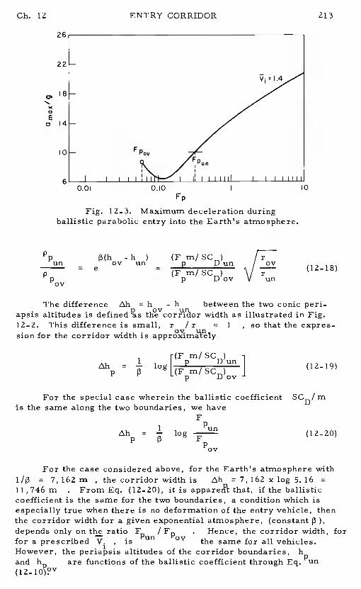
Ch. 12 ENTRY CORRIDOR 213
26
I
0.01 0.10 I 10
Fp
Fig. 12-3. Maximum deceleration duringballistic parabolic entry into the Earth's atmosphere.
Pp 3(h -h ) (F mISC )un= e
ov un - p D Ufl I 12 18p — (F rn/SC ) \/ r
p Dov V un
The difference = h - h between the two conic pen-apsis altitudes is width as illustrated in Fig.12-2. This difference is small,r / r 1 , so that the expres-sion for the corridor width is
(F rn/SC= log
]
For the special case wherein the ballistic coefficientSCD/ rnis the same along the two boundaries, we have
F1
p= log (12-20)
For the case considered above, for the Earth's atmosphere with= 7,162 ru , the corridor width is = 7,162 x log 5.16
11,746 rn . From Eq. (l2_20), it is apparex?t that, if the ballistic
coefficient is the same for the two boundaries, a condition which isespeciallytrue when there is no deformation of the entry vehicle, thenthe corridor width for a given exponential atmosphere, (constant 3),depends only on the ratio / . Hence, the corridor width, forfor a prescribed V. , is Ufl OV the same for all vehicles.However, the periapsis altitudes of the corridor boundaries,
h are functions of the ballistic coefficient through Eq. un
214 ENTRY CORRIDOR Ch. 12
12-4. CHAPMAN'S RESULTS FOR THE ENTRY CORRIDOR
To ease the discussion, Fig. 12-3 has been presented for para-bolic entry into the Earth's atmosphere.With the purpose of present-ing his results in a completely dimensionless form, applicable to anyarbitrary vehicle regardless of its weight, size and shape, entering anarbitrary planetary atmosphere, Chapman used a tech-nique.
From Eq. of Chapter 11, the dimensionless decelerationfor a shallow entry is
=Z u \Jl + (CL! CD)2 (12-21)
Now, in integrating Eq. (12-1), instead of specifying the twovalues and (CL! CD) separately, one can specify only thesingle parameter (CL! CD) . Then, for any specified planetaryatmosphere (i. e. ,given ) the actual lift-to-drag ratio flowncan be deduced.Next, let us assume that for a prescribed value
X = (CL/CD) , and for a certain prescribed condition onentry, a function Z has been generated with the corresponding valueu . Then we can evaluate the deceleration for the case of the Earth(subscript e ) and the deceleration for the case of an arbitrary planet(no subscript) as
=Z
+ (Pt)e
= Z u + (12-22)
Since X is prescribed for the computation of theZ function,we can construct the dimensionless deceleration function
I 2
G = 30 Z u 1 + (12-23)
Since for the Earth's atmosphere = 900 , it is seen thatthis function is simply the dimensionless deceleration, in Earth g'sfor entry into the Earth's atmosphere. From the Eqs. (12-22) and(12-23), itis seen that, through the use of the dimensionless universalfunction Z , all the decelerations reach their respective maximumvalues at the same values for Z, and u . Hence, if the functionGmax is used for the diagram, Gmax versus , for differentvalues of the dimensionless entry speedV. , it represents the pointof peak deceleration for entry of any arbitra'ry vehicle into any arbitraryplanetary atmosphere.The diagram can be used directly for evalua-tion of the entry corridor for entry into the Earth's atmosphere. Forentry into any other planetary atmosphere, from Eq. (12- 22), the
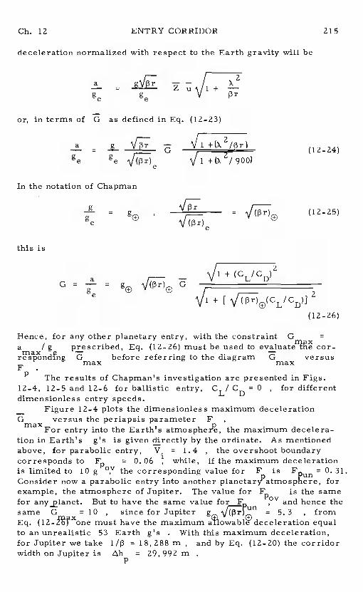
Ch. 12 ENTRY CORRIDOR 215
deceleration normalized with respect to the Earth gravity will be
=3r
or, in terms of G as defined in Eq. (12-23)
a - g +(x2/pr(12 24)
— +x2i 9001 -
In the notation of Chapman
= ,
e
=(12-25)
this is
+ (C /ca — v L DG = — = g0 Ge
+2
(12—26)
Hence, for any other planetary entry, with the constraint Gmx =a / g prescribed, Eq. (12-26) must be used to evaluate cor-max e — —responding G before referring to the diagram0 versusF max max
The results of Chapman's investigation are presented in Figs.12-4, 12-5 and 12-6 for ballisticentry, CL! CD = 0 , for differentdimensionless entry speeds.— Figure 12-4 plots the dimensionless maximum decelerationG versus the periapsis parameterF
maxForentry into the Earth's the maximum decelera-tion in Earth's g's is given directly by the ordinate.As mentionedabove, for parabolic entry, V. = 1.4 , the overshoot boundarycorrespondsto 0. 06 while, if the maximum decelerationis limited to 10 g °v the corresponding value forF is Fpun = 0. 31Consider now a parabolic entry into another forexample, the atmosphere of Jupiter.The value for is the samefor But to have the same value for F and hence thesame 0 = 10 , since for Jupiter = 5. 3 , fromEq. one must have the maximum deceleration equalto an unrealistic 53 Earth g's. With this maximum deceleration,for Jupiter we take1/ç3 = 18, 288 m , and by Eq. (12-20) the corridorwidth on Jupiter is = 29, 992 m
p
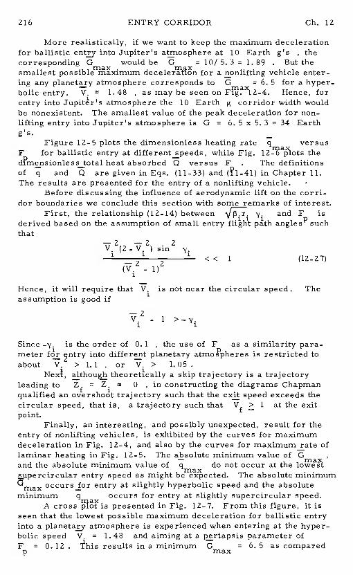
216 ENTRY CORRIDOR Ch. 12
More realistically, if we want to keep the maximum decelerationfor ballistic into Jupiter's atmosphere at10 Earth g's , thecorrespondingG would be G = 10/5.3 = 1.89 . But the
max .smallest possible maximum deceleration for a nonlifting vehicle enter-ing any planetaryatmosphere corresponds to G
a= 6. 5 for a hyper-
bolic entry, V. 1.48 , as may be seen on Hence, forentry into atmosphere the10 Earth g corridor width wouldbe nonexistent. The smallest value of the peak deceleration for non-lifting entry into JupiterTs atmosphere is G =6. 5 x 5. 3 = 34 Earthg's.
Figure 12-5 plots the dimensionless heating rateq versusF for ballistic entry at different speeds, while Fig. thed?mensionless total heat absorbed Qversus F . The definitionsof q and Q are given in Eqs. (11-33) and (?l_41) in Chapter 11.The results are presented for the entry of a nonlifting vehicle.
Before discussing the influence of aerodynamic lift on the corri-dor boundaries we conclude this section with some remarks of interest.
First, the relationship (12- 14) betweenv'i. and F isderived based on the assumption of small entry path suchthat
—2 —2 2V (2_V.
)sin
—2' 2 '< < 1 (12-27)
(V. - 1)
Hence, it will require that V. is not near the circular speed.Theassumption is good if
V12 - i
Since ...y. is the order of 0. 1, the use of F as a similarity para-meter into different planetary atmospheres is restricted toabout V. > 1. 1 , or V. > 1. 05
Next, theoretically a skip trajectory is a trajectoryleading to Zf = Z. 0 , in constructing the diagrams Chapmanqualified an overshoot trajectory such that theexit speed exceeds thecircular speed, that is,a trajectory such thatVf > 1 at the exitpoint.
Finally, an interesting, and possibly unexpected, result for theentry of rionlifting vehicles, is exhibited by the curves for maximumdeceleration in Fig. 12-4, and also by the curves for maximum rate oflaminar heating in Fig. 12-5.The absolute minimum value of Gand the absolute minimum value ofq do not occur at the
entry speed as might The absolute minimumGmax occurs for entry at slightly hyperbolic speed and the absoluteminimum q a
occurs for entry at slightly supercircular speed.A cross presented in Fig. 12—7. From this figure,it is
seen that the lowest possible maximum deceleration for ballistic entryinto a atmosphere is experienced when entering at the hyper-bolic speed V. = 1.48 and aiming at a periapsis parameter ofF = 0. 12 . results in a minimum G = 6. 5 as comparedp max
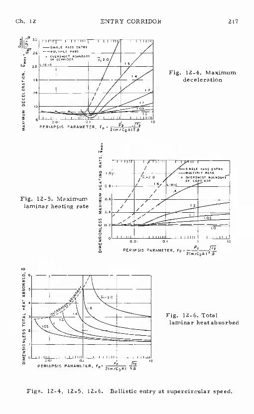
2aI—4a:UI-JUIC-)
Liia
x4
I-4a:
C,2C—
4U)I
Fig. 12-5. Maximumlaminar heating rate
COU,lii-J
z0(02w
a
Fig. 12-6. Totallaminar heat absorbed
Gb. 12 ENTRY CORRIDOR
Fig. 12-4. Maximumdeceleration
EIa:
I C
o 8
E
11111
Iml
— SINGL.6 PASS ENTRY
11111
PASSOVEROCCOOT ROUNDARY
/ OF
./ 1.6/
"-7HI I liii] I
1.0
,, -,, '2
010 01
PER IPSIS PARAMETER, Fp
0
0
0DY
4I-4UII-J4I—0C—
('I(0UI-ia:
0CO
zUI
C
Figs. 12-4, 12-5, 12-6.Ballistic entry at supercircular speed.
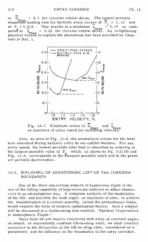
218 ENTRY CORRIDOR Ch. 12
to U = 8. 3 for circular orbital decay. The lowest possibleheating rate for ballistic entry occurs atV. = 1. 12 and
at F = 0.018 . This results in a minimum q = 0. 19 as corn-pares to = 0. 22 for circular orbital An enlighteningphysical reason to explain the phenomena has been provided by Chap-man in Ref. 1.
— SINGLE-PASS ENTRIES0.6 —— MULTIPLE-PASS ATM 12
BRAKING
U.
::0.1- 2
,-, I I I
1.0 .2 1.4 .6 .8
ENTRY VELOCITY, V
Fig. 12-7. Minimum values of U and qas functions of entry speed for non'HMng
Also, as seen in Fig. 12- 6,the normalized curves for the totalheat absorbed during ballistic entry do not exhibit minima. For anyentry speed, the lowest possible total heat is absorbed by entering atthe largest possible value of Fwhich, as shown by Eq. (12- 15) andFig. 12-4, corresponds to the possible entry and to the great-est possible deceleration.
12-5. INFLUENCE OF AERODYNAMIC LIFT ON THE CORRIDORBOUNDARIES
One of the most interesting aspects of hypersonic flight is theuse of the lifting capability of hypervelocity vehicles to effect maneu-vers in an advantageous way. A complete analysis of the modulationof the lift, and possibly the bank angle, as functions of time, to achievethe maximization of a certain quantity, called the performance index,would require the tools of modern optimization theory.Such a subjectwill be discussed in a forthcoming text entitled, 'Optimal Trajectoriesin Atmospheric Flight.
Since here we are mainly concerned with entry at constantof-attack, or equivalently constant lift-to-drag ratio, we shall restrictourselves to the discussion of the lift-to-drag ratio, considered as aparameter, and its influence on the boundaries of the entry corridor.
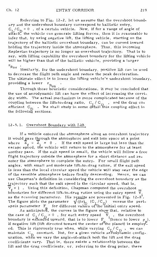
Ch. 12 ENTRY CORRIDOR 219
Referring to Fig. 12-2, let us assume that the overshoot bound-ary and the undershoot boundary correspond to ballistic entry,C /CD = 0 , of a certain vehicle. Now, if for a range of angle of
the vehicle can generate lifting forces, then it is reasonable toinfer that, by using negative lift, the lifting vehicle, starting on thetrajectory of the ballistic overshoot boundary, can be curved inwardholding the trajectory inside the atmosphere.Thus, this incomingKeplerian trajectory is no longer an overshoot trajectory.That is tosay, with lifting capability the overshoot boundary for the lifting vehiclewill be higher than that of the ballistic vehicle, providing a largerrpov
Similarly, for the undershoot boundary, positive lift can be usedto decrease the flight path angle and reduce the peak deceleration.The ultimate effect is to lower the lifting vehicle's undershoot boundary,providing a lower r
PunThrough these heuristic considerations, it may be concluded thatthe use of aerodynamic lift can have the effect of increasing the corri-dor width. The actual mechanism is more complicated because of thecoupling between the lift-to_drag ratio,C / C , and the drag co-efficient CD . We shall study in some coupling effect inthe following sections.
12-5. 1. Overshoot Boundary with Lift
If a vehicle entered the atmosphere along an overshoot trajectoryit through the atmosphere and exit into space at a pointwhere Zf = 0 . If the exit speed is large but less than theescape speed, tike vehicle will return to the atmosphere for at leastanother pass.If the exit speed is small, the vehicle will follow a freeflight trajectory outside the atmosphere for a short distance and re-enter the atmosphere to complete the entry.For small flight pathangles, with small and moderate lift-to-drag ratios, if the exit speedis less than the local circular speed the vehicle will stay near the edgeof the sensible atmosphere before finally descending.Hence, we canuse Chapman's definition in considering the overshoot boundary as thetrajectory such that the exit speed is the circular speed, that is,Vf = 1 . Using this definition, Chapman computed the overshoot—boundaries for different lift-to-drag ratios using the entry speed V.as the scanning parameter.His results are presented in Fig. 12_81.The figure plots the parameter (C1 lCD) versus the pen-apsis parameter F for different values oCthe initial entry speed.
As anticipated, the curves in the figure show that, relative tothe case of C / C = 0 , for each entry speed V. , the overshootboundary is upward, that is to lower F 1(hence to lower p ),
if negative lift (lift directed toward the center planet) ised. This is rigorously true when, while varying CL! CD, we canmaintain CD constant.But, for a given vehicle aerodynamic config-uration, when we vary the angle-of-attack both the lift and the dragcoefficients vary. That is, there exists a relationship between thelift and the drag coefficients, or, referring to the drag polar, there
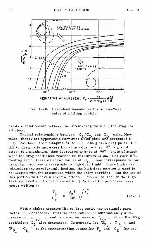
ENTRY CORRIDOR Ch. 12
0
Fig. 12-8. Overshoot boundaries for single-passentry of a lifting vehicle.
exists a relationship between the lift-to-drag ratio and the drag co-efficient.
Typical relationships betweenCL/C and CD using New-tonian theory for hypersonic flow over a flaPplate are presented inFig. 12-9 taken from Chapman's Ref.1. Along each drag polar, thelift-to-drag ratio increases from the value zero at00
a maximum, then decreases to zero at 900angle of attackwhen the drag coefficient reaches its maximum value.For each lift-to-drag ratio, there exist two values of CD, one corresponds to lowdrag flight and one corresponds to high drag flight.Since high dragminimizes the aerodynamic heating, the high drag portion is used inconnection with the attempt to widen the entry corridor.But the use ofthis portion will have a reverse effect.This can be seen in the Figs.12-8 and 12-9 and from the definition (12_b) of the periapsismeter written as
F pS ITT= (12-28)
CD 2m p
With a higher negative lift-to-drag ratio, the periapsis para-meter F decreases.But this does not induce automatically a de-crease p , and hence an increase inr , since the drag
Pov Povcoefficient C also decreases.In general, let (F
, CD ) andD p1
1(F , C ) be the corresponding values for Fand C for two
P2 ID2 p D
10—2
PpPERIAPSIS PARAMETER,
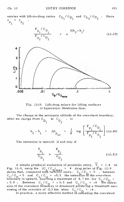
Ch. 12 ENTRY CORRIDOR
entries with lift-to-drag ratiosr r
p1 p2
F ICp1 D1
F ICp2
Fig. 12-9. Lift-drag polars for lifting surfacesin hypersonic Newtonian flow.
The extension is upward, if and only if
p2
1>-sA simple graphical evaluation of parabolic entry,V. = 1.4 on
Fig. 12-8, using the (C / C ) 4 drag polar of 12-9shows that, compared entry, CL! CD = 0 , betweenCL! CD = 0 and CL! C = -0. 5 the extension of the overshootboundary is upward, reac'?iing a maximum of9. 7 km for C /CD =- 0. 5 . Between CL! C = - 0. 5 and CL! CD = -4 exten-sion of the overshoot is downward producing a maximum nar-rowing of the corridor of 11.3 km when CL! C -4
In practice, a more effective method of expending the overshoot
CL/CD and CL/CD . Since
p(h2 - h1)= e (12-29)
4
3
-J
0
.002 .01
CD/CDmax
The change in the periapsis altitude of thewhen we change from CD to CD , is
1 2
overshoot boundary,
h -h =2 1 pov
- 1D1
log
F !C
1(12-30)- F/Cp2 D2
FFp1
CD(l2_3l)
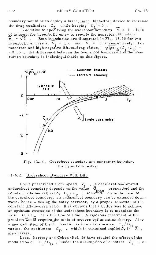
ENTRY CORRIDOR Ch. 12
boundary would be to deploy a large, light, high-drag device to increasethe drag coefficient CD while keeping C = 0 . —
In addition to specifying the Vf = 1 , it isof interest for hyperbolic entry to specify the nonreturn boundaryVf = . Both boundaries are illustrated in Fig. 12-10 for twohyperbolic entries atV. = 1. 6 and V. = 2. 0 respectively. Formoderate and high lift-to-drag (C1 /CD) <- 0. 05 , the difference between the overshoot boundary non-.return boundary is indistinguishable on this figure.
(LID)overshoot boundary
0
-2
-3
Fig. 12-10. Overshoot boundary and nonreturn boundaryfor hyperbolic entry.
12-5. 2. Undershoot Boundary With Lift
For a prescribed entry speedV. , a deceleration-limitedundershoot boundary depends on the val'ue0 prescribed and theconstant lift_to_drag ratio,C / C As in the case ofthe overshoot boundary, an boundary can be extended down-ward, hence widening the entry corridor, by a proper selection of theconstant lift-to-drag ratio. It is obvious that a better way to achievean optimum extension of the undershoot boundary is to modulate theratio CL! C as a function of time. A rigorous treatment of theproblem require the tools of modern optimization theory.Alsoa new definition of the Z function is in order since asC / CD —varies, the coefficient CD , which is contained in Zalso varies.
Lees, Hartwig and Cohen (Ref.3) have studied the effect of themodulation of CL! CD , under the assumption of constantCD , On
Hyperbolicexit
nonreturn boundary
Single pass entry
Gb. 12 ENTRY CORRIDOR 223
the maximum deceleration during entry.They show that by modulatingCL! C in a manner such that largeCL! CD values are employedin the first portion of the entry trajectory where the longitudinal decel-eration is small, the resultant deceleration can build up to its maxi-mum under conditions where the transverse component is dominant.Then, by maintaining this constant resultant valueG through de-creasing the transverse component while increasing the longitudinalcomponent, the entry with modulated lift can be completed without re-quiring large negative C ! CD at any stage. In this way, the under-shoot boundary for C / CD can be extended considerablyfrom the value for constantCL/'tD , provided the value of C /CDat entry is relativejy high. They found that the ratio ofG axmodulated lift to G for constant lift was essentiallymaxof V. and y. , and dependent only on the initial value of CL! CDat entry. Their result is presented in Fig. 12-11.
::
0.4 - -
S S
0.2 -
0 2 3
LID AT ENTRY
Fig. 12-11. Effect of modulated liftin reducing peak deceleration.
On the other hand, Chapman studied the effect of constantC1 / CD on the undershoot boundary for deceleration-limited entry.
diagram showing his results is presented in Fig. 12-12 forparabolic entry, V. = 1.4 . The diagram plots the normalizedmaximum deceleration, G , versus log F . From thefigure, it is apparent that in C !dD up to about 2
can extend considerably the undershoot for a given Gsince it leads to higherF , hence lower r forIt should be noted that a high ratio may lead to askip trajectory. Hence, the constantC / C program used is onlymaintained until the flight path is essentiklly Rorizontai,'y
NCE
z0I—
LiJ-JwUw0
x
ENTRY CORRIDOR Ch. 12
near the point where maximum deceleration is reached.After thispoint the lift-to-drag ratio is modulated to maintain the flight insidethe atmosphere in order to complete entry in a single pass.
0 2 4 6 8 10
10910
Fig. 12-12. Normalized maximum decelerationfor various lift-to-drag ratio entries at parabolic speed.
4
3
2
0—I
— LID
,' ---mod. L/DI/
L/D> 0 - — -- --
—— V,=I.4
3
logI 0 ,,/
a
0
Gmax
16
0 5 I0 15
Fig. 12-13. Overshoot and undershoot boundariesas function of lift-to_drag ratio and maximum deceleration.
Gb. 12 ENTRY CORRIDOR 225
The overshoot boundary with negative lift, and the undershootboundary with positive lilt for various prescribedG are plottedin Fig. 1Z-13 for entry at parabolic speed,V.
= and entryat slightly hyperbolic speed, V. = 1.6 . curve in Fig. 12-li isused for obtaining the extensionthe undershoot boundaries for mod-ulated CL! CD from curves calculated for constantC / CWith a given G the improvement using 8L' CDis insignificant in of C / CD less than about 0. 5. AtC / GD greater than about1 , ke undershoot boundaries with modu-la1Ced CL! GD are considerably extended beyond those for constant
CL! C . Since a constant CD has been assumed and the abscis-sa is p1?otted in log10 F , the corridor width is proportional to thehorizontal spacing between the overshoot boundary and the undershootboundary.
References
1. Chapman, D. R., "An Analysis of the Corridor and GuidanceRequirements for Supercircular Entry into Planetary Atmo-spheres,Y NASA Technical Report R-55, 1960.
2. Chapman, D. R., "An Approximate Analytical Method foring Entry into Planetary Atmospheres, "NASA Technical ReportR-1l, 1959.
3. Lees, L., Hartwig, F. W. ,and Cohen, C. B., "The Use ofAerodynamic Lift During Entry Into the Earth's Atmosphere,STL Report GM— TR-0165-00519, 1958.
Chapter 13
Unified Theory for Entryinto Planetary Atmospheres
13-1. INTRODUCTION
The classical theories for planar entry into planetary atmosphereshave been presented in Chapters 6through 12. Except for Loh's second-order theory which gives a high degree of accuracy, the application ofall theories is severely restricted.Each theory is applicable to oneparticular type of entry trajectory because of the assumptions intro-duced to facilitate the integration of the equations of motion.Loh'stheory itself is empirical. To alleviate this heuristic aspect, inChapter 8 we offered a physical explanation to justify his theory.
This book is designed primarily as a textbook.However, it isalso intended to present a complete account of the present state of theart of the problem of evaluating the performance of a lifting hyper-velocity vehicle entering a planetary atmosphere along asional path.
Up to this point, the first objective has been fulfilled.Entrytheories have been presented with their appropriate simplifications torender explicit the dynamic characteristics of each type of entry tra-jectory. Simple but accurate first-order solutions have been obtained.They are of valuable assistance in analyzing the effect of the gravityforce and the aerodynamic force, the two main forces considered inthis volume, on the entry trajectories.Furthermore, the closed formsolutions obtained lead to explicit forms for physical quantities ofinterest during entry, such as the deceleration and the heating rate.These data are of utmost importance for the preliminary design ormission planning of entry vehicles.
In the last quarter of this century, a new direction for spaceexploration is formulated.Frequent flights weekly or even daily toEarth orbit are planned.This introduces a new generation of spacevehicles, a versatile lifting hypervelocity vehicle used both as a satel-lite and as a winged atmospheric vehicle with airplane aerodynamicmaneuverability. This requires a unified theory for studying atmo-spheric entry, a theory that is applicable to all types of entry evenwith lift and bank modulation. The second objective of this book is theformulation of such a theory and the presentation of it in a complete
226
Ch. 13 UNIFIED THEORY FOR PLANETARY ENTRY 227
but readable form to assist engineers and scientists working on thespace program in understanding the complexity associated with hyper-velocity flight.
A unified theory that enables one to study the performance of ageneral type of lifting vehicle, regardless of its weight, shape and size,entering an arbitrary planetary atmosphere, would require a set ofuniversal equations.In turn, this requires universal variables, freeof the physical characteristics of the vehicle.In this respect, thebest theory available is undoubtedly Chapman's theory for analysis ofplanetary entry (Ref. 1-2).Chapman's theory for planetary entry waspresented in Chapters 11 and 12.Just as most other first-ordertheories, it is restricted to planar entries.This restriction is ofminor inconvenience since it can be easily removed. A major defi-ciency in Chapman's theory is that, because of his two main assump-tions, the equations are only approximate and the applications arerestricted to entry trajectories with small flight path angles, or smalllift-to-drag ratios.
In this chapter, Chapman's restrictive assumptions are removedand the results extended to three-dimensional entry trajectories,while all the distinctive features in Chapman1s classical analysis areconserved. Furthermore, it will be shown that, from the exact equa-tions, all the known first and second-order solutions can be obtained,thus displaying a certain universality for the present theory.
13-2. UNIVERSAL EQUATIONS FOR THREE-DIMENSIONAL ENTRYTRAJECTORIES
The equations of motion of a nonthrusting, lifting vehicle, enter-ing a planetary atmosphere were derived in Chapter 2:
dr=
V cos cosdt r cos4
-
-— = - -dt
pSCLV V22m cos o - (g - — ) cos
d PSCLV= sino - — (13-1)
dt r
The first three equations are simply the kinematic relations.The last three equations are the momentum equations.The planet andits atmosphere are assumed to be spherical and noorotating.The
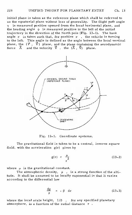
228 UNIFIED THEORY FOR PLANETARY ENTRY Gb. 13
initial plane is taken as the reference plane which shall be referred toas the equatorial plane without loss of generality.The flight path angle
is measured positive upward from the local horizontal plane, andthe heading angle is measured positive to the left of the initialtrajectory in the direction of the North pole (Fig. 13-1).The bankangle a- is taken such that, for positivea- , the vehicle is turningto the left. This angle is defined as the angle between the local verticalplane, the , V) plane, and the plane containing the aerodynamicforce A and the velocity V , the (A , V) plane.
The gravitational field is taken to be a central, inverse squarefield, with the acceleration g(r)given by
g(r) =
r(13.2)
where is the gravitational constant.The atmospheric density,p , is a strong function of the alti-
tude. It shall be assumed to be locally exponential in that it variesaccording to the differential law
= drp
(13-3)
where the local scale height, , for any specified planetaryatmosphere, is a function of the radial distancer
Fig. 13-1. Coordinate systems.
Ch. 13 UNIFIED THEORY FOR PLANETARY ENTRY Z29
In his classical2aper (Ref.1), Chapman introduced two dimen-sionless variables, u and Z , defined as
pSC r—(13-4)Zm VP
It has been found more convenient for the present theory to usethe modified variables
u , zp:CD 4jj (13-5)
Chapman used the variable uas the independent variable.UnderChapman s assumption this variable is monotonically decreasing.Itwill be shown later that, at high altitude,u is purely periodic. Toavoid this difficulty, in deriving the exact three-dimensional entryequations, we shall use the following dimensionless variable as the in-dependent variable
tS E J cos dt (13-6)
0
This variable is strictly increasing as long ascos y > 0 , a con-dition which is always satisfied for entry with constant lift and dragcoefficients. With this independent variable Eqs. (13-1) become
dO - cos4ids -
=
dV2 rp SCDV2= -
ds mcos'yrpSC coso
Lds - Zmcos
d rpSCLsino= - cos 4i (13-7)
Zmcos y
The differential relation between rand s is
r tan (13-8)
As in Chapman's theory, the variableV2 is replaced by u, whilethe radial distancer , or equivalently the altitude, is replaced bythe variable Z
230 UNIFIED THEORY FOR PLANETARY ENTRY Ch. 13
The derivative of u with respect tos , with u as defined inEq. (13—5), is
du = - Zu+ cos a- tan y +
](13-9)
S COSVD
The derivative of Z with respect to s, with the differential law forp , Eq. (13—3), is
= - 3r(1 - + Z tany (13-10)
Finally, the differential equations for y and , written interms of the dimensionless variables, are
=z
cos a- +C05 - )] (13-11)
ds LCD u
and
= - COSqJ tan4]
(13-12)cos D Z
These dimensionless equations are exact.In particular, they reduceto the equations for Keplerian motion when Z0
In Eq. (13-10) for Z , if a strictly exponential atmosphere isused = constant, and /dr = 0 . On the other hand, if an iso-
thermal atmosphere is considered, p /g = constant, and(1/2p2)(dp /dr) - . In both cases, in the equations of motion,the variables and r enter as the product . For the Earth,for altitudes below 120kilometers, the mean value is large. In this
same region 3r varies from a low of about 750 to a high of about1300 . It is, however, a better assumption to use a mean value for
than simply to put constant and use the simple exponentialatmosphere in the computation.This development will follow Chap-man's lead and put13r constant. Also, because of the large value for
the quantity inside the brackets in Eq. (13- 10) is practicallyunity. This minor assumption concerning the product 3r does notalter the asymptotic behavior of the trajectory at very high altitudeswhere the equation in Z becomes inoperative.
In summary, the equations of motion for three-dimensionalentry trajectories are
Ch. 13 UNIFIED THEORY FOR PLANETARY ENTRY 231
dZ=
du = - Zu+ +
sinds L Z
= ZE X +
COS(1
- COSyds cos'y L u
-ds — cos4
=
=z
[- cos
](13-13)
z
where
L LX — coso , 6 sina (13-14)
CD D
The equations (13-13) were first derived by Vinh and Brace (Ref.3). In view of the definition (13- 5)of Z , they are restricted toflight at constant lilt-to-drag ratio, CL! CD = constantand for flight with a completely free modulation in the bank angle.Extension of these equations to the case of free modulation in the co-efficients CD and CL and in the bank angleo- for the study ofthree-dimensional optimal trajectories in atmospheric, hypervelocityflight has been obtained by Vinh, Busemann and Gulp (Ref. 4).
The equations derived can be considered as the exact equationsfor entry into a planetary atmosphere.Just as Chapman's simplifiedequations, they are completely free of the characteristics of the vehicle.Hence, they can be used to analyze the motion of an arbitrary vehicleregardless of its weight, size and shape.The characteristics of theatmosphere enter the equations in the form of the parameter
Once the atmosphere has been specified through, for anyprescribed lift-to-drag ratio,CL! CD , and bank angle, o , andwith a prescribed set of initial conditions, the universal function Zcan be generated, and different physical quantities during entry can beevaluated and analyzed exactly as in Chapman's theory, described inChapters 11 and 12.It may be thought at first glance that, to integrateChapman's simplified equation, Eq. (11- 16) of Chapter 11, only theproduct (C ! CD) need be prescribed and not and
(CL! CD) That is, Chapman's analysis appears to applyto any arbitrary atmosphere.But this is not rigorously true sincein evaluating the flight path angle , using Chapman's first equation,
UNIFIED THEORY FOR PLANETARY ENTRY Ch. 13
Eq. (11- 12) of Chapter 11, the parameter needs to be prescribed.A normalizing technique to obtain a similarity solution for an arbitraryatmosphere requires sacrificing the accuracy in evaluating the univer-sal Z function and the flight path angle'y , and restricting the analy-sis to a small class of entry trajectories.
13-3. REDUCTION TO CLASSICAL SOLUTIONS
The equations derived are the universal equations in the sense ofChapman since they produce the universal Z functions for analyzingthe motion, deceleration and heating of an arbitrary vehicle.Further-more, they are the exact equations for flight of a vehicle in a Newton-ian gravitational field subject to aerodynamic force.In particular,they provide the Keplerian solution for flight in a vacuum and all otherclassical solutions when appropriate assumptions are introduced.These particuiar solutions can be obtained as follows.
13-3. 1. Keplerian Solution
For flight in the vacuum, letZ 0 . The first of Eqs. (13- 13)is inoperative. It is replaced by Eq. (13-8). Using this equation tochange the independent variable froms to r , we rewrite the otherEqs. (13-13)
du - udr - r
— 1 cosv)dr — rtany' - u
-dr — r tan cos
dr - rtan'y
= cos 4 tan (13 15)dr -
Integrating the first of these equations yields
u = (13-16)
where p is a constant of integration.Next, combining the first twoequations to eliminater gives
2=
— 1 (1 — cos y (13—17)du utany u
Ch. 13 UNIFIED THEORY FOR PLANETARY ENTRY 233
By the change of variable
F (13—18)cos
this becomes the linear equation
+ = (13-19)du U 2
U
which integrates to- 2u + constant
2U
For reasons that will be clear later this solution is written
22 ucos
= 2(13-20)
Zu - (1 - e
where e is a constant of integration.Combining the last two equations (13-15), we obtain
=— tan
(13—21)di4 tan4
The integration is immediate:
cos cos = cos I (13-22)
where I is a new constant of integration.The equation for 0 can be written with as the independent
variable.
= - 1 (13-23)sin4
Using the solution (13- 22) for 4
= - cos (13-24)d4i
2V cos - cos I
The quadrature gives
sin = sin I cos (0 — c2) (13—25)
where £2 is another constant of integration.
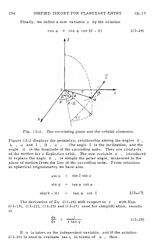
234 UNIFIED THEORY FOR PLANETARY ENTRY
Finally, we define a new variable aby the relation
cos a cos 4 cos (8 -
Fig. 13-2. The osculating plane and the orbital elements.
sin4 = sinlsina
sin9 = tan4 cota
sin(0-Q) = tan4 cot I
dr - rtan'y
If u is taken as the independent variable, and if the solution(13-20) is used to evaluate tan in terms of u , then
Ch. 13
z
(13—26)
V
0y
x
Figure 13-2 displays the geometric relationship among the angles0
4 , 9 and I , 12 , a . The angle I is the inclination, and theangle £2 is the longitude of the ascending node.They are constantsof the motion for a Keplerian orbit.The new variablea , introducedto replace the angle0 , is simply the polar angle, measured in theplane of motion from the line of the ascending node. From relationsin spherical trigonometry we have also
(13—27)
The derivative of Eq. (13-26) with respect tor , with Eqs.(13-15), (13—22), (13—25) and (13-27) used for simplification, results
(13—28)
Ch. 13 UNIFIED THEORY FOR PLANETARY ENTRY 235
=- 1 (13-29)du
2 2U -F 2u - (1 - e
This integrates to
u = 1 + e cos - (13-30)
where w is the last constant of integration.It defines the argumentof periapsis. From the solutions (13-16) and (13-30) we can identifye as the eccentricity of the orbit and p as the conic parameter.
For subsequent discussions, for Keplerian motion, we will takethe plane of motion as the reference plane, with the reference directionalong the pericenter.Then the equations of interest become
u = 1 + e cos e = (13-31)
and
=— u2
2(13-32)
2u - (1 - e
We see that, outside the atmosphere,u varies periodicallybetween u =1 - e and u = 1 + e . Hence, for flight with atmosphericdrag involving several passages through the1atmo sphere, the variableu , and hence Chapman's variable u 12
, is oscillatory. Itis, therefore, more convenient to replace it as independent variableby the dimensionless variables as defined by Eq. (13-6).
13_3. 2. Chapman's Equations
In deriving his equations, Chapman introduced two basic assump-tions as has been explained in Chapter 11.
a! The percentage change in the radial distance is small com-pared to the percentage change in the horizontal component of thevelocity.
d(V cos y) >>drr
In terms of the variables u and Z, this basic assumption isex-pressed as
CL1 + — tan >> (13_33)
236 UNIFIED THEORY FOR PLANETARY ENTRY Ch. 13
b/ For lifting vehicles, the flight path angle yis sufficientlysmall that the lift component in the horizontal direction is small com-pared to the drag component in the same direction.
C1>> tan (13-34)
D
Before we continue with the derivation of Chapman's equationsfrom our formulation, the following remark is pertinent.
Most of the published analytical works on the theory concernplanar entry. For nonpianar entry, as far as the altitude, speed andflight path angle are concerned, we only need to consider the firstthree of Eqs. (13-13).These equations govern the three-dimensionalvariation of Z , u , and y , upon specification of the initial con-ditions for these variables, and the three-dimensional flight parameterX (CT / CD) cos . Hence, throughout the rest of this chapter,we shaltconsider only the three equations
= _pr z tany
du = - Zu (1 + Xtan'y + V
ds cosy z
Z [ +cos (1 - COSy
ds cosy L u
(13-3 5)
They are valid for three-dimensional entry at constant lift-to-dragratio, and constant bank angle.For comparison with the classicalsolutions for planar entry we simply consider Xas being C / CD
Now, applying Chapman's basic assumptions, Eqs. (l3Ji) and(13-34), to the equation for u, we have the reduced equation
du — Zu (13 36ds — - cosy -
These assumptions automatically restrict the validity of Chapman'stheory to the portion of trajectory where u is monotonically decreas-ing. Using this equation to change the independent variable froms tou , we rewrite the equations for Z and y
= V (13-37)
and
= - x +COS V
(1 V )1 (13-38)du Zu L u
Ch. 13 UNIFIED THEORY FOR PLANETARY ENTRY 237
It is convenient for concordance to return to Chapman's original vari-ables u and Z . From definitions (13-4) and (13-5),
uE u2 , Z (13-39)U
Hence, in terms of Chapman's variables, Eqs. (13-37) and (13-38)become
- = (13-40)
and
= +U cos (1 - 1 (13-41)
du
Equation (13-40) is Chapman's first equation.It is used to evaluate theflight path angle. If we take the derivative of this equation with respectto u , using Eq. (13-41), we have
-+
cos2 - cos2= 0
(13-42)
This equation is equivalent to Chapman's second-order nonlinear dif-ferential equation with Z as the dependent variable and uas theindependent variable.To obtain the equation in the form identical tothe one given by Chapman in his classical paper (Ref.1), we write it as
U Xcos3y
+ + = 0
z(13-43)
With the aid of Eq. (13-40), we consider the sum of the terms
- - )+
sin2+ x cos sin2
= - sin [i - cos2 tan -cos2 ysin y
]
siny
UNIFIED THEORY FOR PLANETARY ENTRY
The last step is obtained by applying Chapman's basic assumptions,Eqs. (13-33) and (13-34).We see that this is equivalent to neglectingthe terms containing sin2 in Eq. (13-43). Thus,
d2Z(
Chapman derived this same equation for planar entry by repeatedlyapplying his two basic assumptions.
13-3. 3. Yaroshevskii's Equation
Yaroshevskii's theory, (Ref. 5), is closely related to Chapman'stheory. It can be shown that, for constant lift-to-drag ratio entry,Yaroshevskii's second-order nonlinear differential equation is a specialcase of Chapman's equation.
Yaroshevskii used an independent variable,x , and a dependentvariable, y , defined as
where the subscript zero denotes the condition at a reference level.In the more sophisticated definition of variables,
Eq. (13-4), if we use a constant value forr , and the assumption ofa very small flight path angle, cos 'y1 , we have
— V(13—46)
Hence, we have the relations between the two sets of variables
z — -x— = y , U = e
u
do x d- =-edu
- 1 do— dxU
(13-48)
On the other hand, for very small flight path angles, Chapman's equa-tion, Eq. (13-44), is reduced to
d (Z) (13-49)
238 Ch. 13
—2Z 1-u 4= - cos
- (13-44)
xelogSC r
D 0y p (13-45)
The corresponding relation in the derivatives is
(1 3_47)
Ch. 13 UNIFIED THEORY FOR PLANETARYENTRY 239
Using the transformations (13-47) and (13-48) in this equation, we haveYaroshevskii's equation
+-
+ = 0 (13-50)dx
13-3.4. Loh's Second-Order Solution
There exist several first-order solutions.The assumptionsintroduced concern the equation for'y , the third of the basic Eqs.(13-35). We write it as
= (X + G)ds cos
where
Gcos
[ 1- cos2 y
] (13-52)
represents the combined gravity and centrifugal acceleration along thenormal to the flight path.
For skip trajectories, Eggers, Allen and Neice neglect the Uterm compared to the liftX , (Ref. 6). For equilibrium glide withnearly zero flight path angle, the correct assumption by yieldsX + G = 0 (Ref. 7). This leads Loh to conjecture, based on exten-sive numerical analysis, that the G term is nearly constant duringthe integration (Ref. 8).
The equations for and u , written with Z as the independentvariable, are
=- (X + G) (13 53dZ
VPr
and
du 2u= (1 + X tan y + ) (13-54)
With assumption of constant C, the integration of Eq.(13-53) is immediate. We have
(X + G)cos — cos 'y. = (Z — z1) (13—55)
where subscripti denotes the initial condition.To assess the effectof each of the entry variables, in the final equation, Eq. (13-55),Cis to be replaced by its definition, Eq. (13-52).
240 UNIFIED THEORY FOR PLANETARY ENTRY Ch. 13
Equation (13-54) for u has a singularity for Z =0 . To avoidthis difficulty, we rewrite it as
[log u - log z] = 2 (1 + X tan (13-56)sin 'j
Dividing this equation by Eq. (13-53), we have
+ 0)-cf—
[log u - log z] -(1 tan (13-57)
Integrating and using the initial conditions, we have
(X+G) u (X+G) ZX log
- 2log — + Zpr (13-58)
Equations and (13-58), derived with the present dimensionlessvariables, constitute what Loh has called the unified solution of entrydynamics (Ref. 8). The last term in Eq. (13-58) is the higher-ordereffect term. It has been given only in approximate form by Loh.Furthermore, the equations used in Loh's analysis assume constantgravity. Neglecting the last term in Eq. (13-58) we have Loh's second-order solution.
cosy (X+G) u-
= X log- 2
log— (13-59)
For ballistic entry, X = 0 . Thus, to the first order, byneglecting the gravity and centrifugal force, we have from this equation
y. . Keeping the G term, we combine this equation with Eq,(13—55) to obtain
(Z - Z.) / ucos y - cos sin
/ log — =- 2(y
-y.) 2
The last simplifying step has been shown in Section 8-4. 1.This givesthe classical first-order solution for ballistic entry (Refs.1, 9)
Z1 = Z. + siny. log a (13-60)
For gliding entry the flight path angle is small and nearly constant andhence X + G 0 , cos y 1 . Thus, from the definition (13-52)of G
Z = - U (13-61)IIXii
Ch. 13 UNIFIED THEORY FOR PLANETARY ENTRY 241
This is the first-order solution originally derived by Singer (Ref.7).For skip entry, G 0 , and Eq. (13-59) is reduced to
1/21/2 U•U = exp
') (13-62)
X /
while, from Eq. (13-55), we have the solution for Z(cos - cos
Z111 = Z. + (13-63)
For small flight path angles the equations become
- = log (13-64)
and
Z111 = Z. + - (13-65)
Using Eq. (13-64) we can rewrite this solution
Z111 = Z. + y. log log2 —a (13-66)
This is the solution for skip trajectories obtained by Chapman (Ref. 1).The analysis in this section has shown that all the known first-
order and second-order solutions for entry dynamics can be obtainedfrom the present formulation including the exact limiting case fororbital flight outside the atmosphere.Another second-order theorycan be constructed by matching the Keplerian solution with one of thefirst-order solutions as has been done by Shi and Pottsepp for planartrajectories (Ref. 10).Such a matched asymptotic solution for three-dimensional entry trajectories using the present formulation will bepresented in Chapter 14.
13-4. NUMERICAL RESULTS
One outstanding feature of Chapman's approach is the constructionof the Z - Tables for atmospheric entry (Ref. 11).For each initialspeed u. , entry angle and lift-to-drag ratio CL! CD thesetables gi've the among the variables , u and Zduring entry. From these we can calculate other physical quantities ofinterest. The tabulation is valid for any entry vehicle.The onlydifference is the actual altitude which also can be calculated for anyspecified drag parameter SCD/ m
242 UNIFIED THEORY FOR PLANETARY ENTRY Ch. 13
But there are restrictions to the use of Chapman's tables due tohis two basic assumptions.In the present analysis, we have removedthese two restrictive assumptions and the basic equations (13-35) can beintegrated using the same entry data u.
,and (C11 C ) cos o to
generate more accurate tables.One additional benefit is tRat the dataobtained are also valid for three-dimensional entry at constant lift-to-drag ratio and bank angle since they are tabulated in terms of the flightparameter X = (CL! CD) cos o . Several Z functions, using theexact equations, have been computed by Brace (Ref. 12).Some select-ed trajectories are reproduced here and compared withcomputed Z functions. They are chosen to display the quantitativeaspect of Chapman's assumptions.
In order to meaningfully compare Chapman's original results withthe results of the numerical integration of the exact equations the samevalue = 900 has been used.Furthermore, the same integrationprogram and the same method for selecting the initial valueZ. _havebeen used. The results for Z and u are converted intoZ , uthrough Eq. (13-39), and the diagrams are presented in terms of thedeceleration Z u versus u as in Chapman's Ref.1 for easycomparison.
Chapman's basic assumptions concern the coefficient A, thequantity in parentheses in Eq. (13-35) for u
A = 1 + A1 + A2 (13-67)
where
A1 a X tan'j (13-68)
A a (13-69)2
As has been shown in Eqs. (13-35) and (13-36), Chapman's assumptionsconsist of taking A = 1 . Hence, Chapman's theory is accurate when-ever IA l<< 1 and lA2l<< 1 , or more generally whenever
A1 + A2 I<< 1 . It is therefore informative, for each compari-
son, to also plot the functions A1, A2 and A . In every case,the results of the numerical integration support the hypotheses regard-ing the accuracy of Chapman's solution.Along trajectories where A1and A2 remain reasonably close to zero, Chapman's solution followsthe exact solution.Along trajectories where Ais either discontinuousor does not remain close to unity, there are discrepancies betweenChapman'stheory and the present exact theory.
The best agreement between the exact analysis and Chapman'sresults is evidenced in the case of steep angle ballistic entry as shownin Fig. 13-3. A1 is identically zero since CL =0 , and A2remains close to zero over most of the trajectory.This can be pre-dicted by inspection of Eq. For steep ballistic entry,sin y is nearly constant while Z/u , which is proportional top , quickly becomes finite and large.This leads to near zero valuefor A2
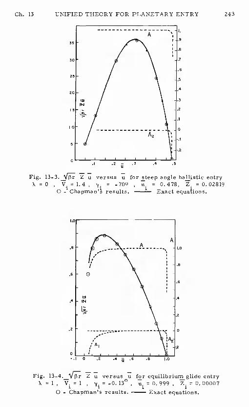
Ch. 13 UNIFIED THEORY FOR PLANETARY ENTRY 243
Fig. Z u versus u for steep angle ballistic entryX = 0 , V. = 1.4 , = _7Ø0 , u. = 0.478, Z. = 0.02819
0 _' results. ' Exact equations.
0 .2 .4 .6 .8 1.0
Fig. Z u versus u for equilibrium glide entryX = 1 , V. = 1 , y. = -0. 13° , u. = 0. 999 , Z. = 0. 00007
1 1 1 1
0 - Chapman's results. —Exact equations.
.1 .2 — .3 .4 .5
.8
A
0
.4 IN
I.0
.8
.6
.4
.2
0
2
.2
0
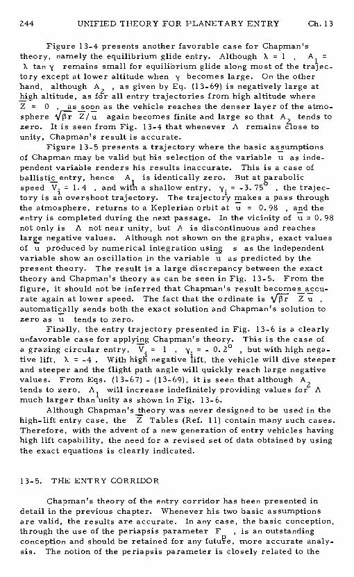
244 UNIFIED THEORY FOR PLANETARY ENTRY Ch. 13
Figure 13-4presents another favorable case for Chapman'stheory, namely the equilibrium glide entry.Although K = 1 , A1 =
K tan 'y remains small for equilibrium glide along most of the trajec-tory except at lower altitude when becomes large. On the otherhand, although A2 , as given by Eq. (13-69) is negatively large athigh altitude, as for all entry trajectories from high altitude whereZ 0 , as soon as the vehicle reaches the denser layer of the atmo-sphere Z/ u again becomes finite and large so that A? tends tozero. It is seen from Fig. 13-4 that whenever A remains tounity, Chapman's result is accurate.
Figure 13-5 presentsa trajectory where the basic assumptionsof Chapman may be valid but his selection of the variable u as inde-pendent variable renders his results inaccurate.This is a case ofballistic entry, hence A is identically zero. But at parabolicspeed = 1.4 , and a shallow entry, y. = 750
, the trajec-tory is an overshoot trajectory.The trajector'y makes a pass throughthe atmosphere, returns to a Keplerian orbit at u =0. 98 , and theentry is completed during the next passage.In the vicinity of u =0. 98not only is A not near unity, but A is discontinuous and reacheslar&e negative values.Although not shown on the graphs, exact valuesof u produced by numerical integration usinjs as the independentvariable show an oscillation in the variable u as predicted by thepresent theory. The result is a large discrepancy between the exacttheory and Chapman's theory as can be seen in Fig. 13-5. From thefigure, it should not be inferred that Chapman's result becomes accu-rate again at lower speed.The fact that the ordinate is Z uautomatically sends both the exact solution and Chapman's solution tozero as u tends to zero.
Finally, the entry trajectory presented in Fig. is a clearlyunfavorable case for applying Chapman's theory.This is the case ofa grazing circular entry,V. = 1 , = - 0. 2° , but with high nega-tive lift, K = -4 . With high negative lift, the vehicle will dive steeperand steeper and the flight path angle will quickly reach large negativevalues. From Eqs. (13-67) -(13-69), it is seen that although A2tends to zero, A1 will increase indefinitely providing values for Amuch larger than unity as shown in Fig. 13-6.
Although Chapma&s theory was never designed to be used in thehigh-lift entry case, the Z Tables (Ref. 11) contain many such cases.Therefore, with the advent of a new generation of entry vehicles havinghigh lift capability, the need for a revised set of data obtained by usingthe exact equations is clearly indicated.
13-5. THE ENTRY CORRIDOR
Chapman's theory of the entry corridor has been presented indetail in the previous chapter.Whenever his two basic assumptionsare valid, the results are accurate.In any case, the basic conception,through the use of the periapsis parameter F, is an outstandingconception and should be retained for any more accurate analy-sis. The notion of the periapsis parameter is closely related to the
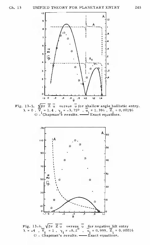
Ch. 13
Fig. 13—5.X =0
UNIFIED THEORY FOR PLANETARY ENTRY 245
Z u versus u for shallow angle ballistic entry.V. = 1.4 , = -3. 750
, u. = 1.396 , Z. = 0.001960 _'Chapman"s results. 'Exact equati'ons.
110
90
70
50
30
10
0—.10 .1
U.7 .9 1.1
60
50
40
30
20
I0
C)
Fig. 13_6. Zu versus u for negative lift entryX -4 , V. 1, u.0.999, Z.0.00016
1 1 1 10 - Chapman1s results. —Exact equations.
-.1 0 .2 .4 .6 — . 8 .0 1.2 .4U
A,
'A
0
IN
It':
UNIFIED THEORY FOR PLANETARY ENTRY Ch. 13
definition of the entry altitude which, in turn, is the basis for thecomputation of the overshoot and undershoot boundaries.These notionsare revised in this section, in light of the exact equations as a tool forcomputing accurate entry trajectories.
13-5. 1. Definition of the Entry Point
To some extent, any definition of an entry point is arbitrary,since from a strictly mathematical standpoint, the process of changingfrom a Keplerian orbit to an atmospheric flight orbit is a continuouslyvarying process.
For the numerical integration of his equation, Chapman chosethe starting value of'y as the initial value of y, and the startingvalue of u for the first 2pint as 0. 995 . Then, since the equa-tion has a singularity at Z =0 , the value of Z is obtainedby an approximate method.This choice of the starting value of uclearly assumes that u is decreasing at the entry point.If we areinterested in effective entry trajectories, along which the heating rateand the deceleration build up, then we can use Chapman's definition ofan entry point as the point where u starts to decrease.In this case,the initial value of Z can be obtained from the equation
sin y.A = 1 + K tan y. +
1= 0 (13—70)
since with this value du/ ds = 0
If a broader class of trajectories is considered, especially tra-jectories with several passages through the atmosphere, then it isnatural to consider the point where atmospheric flight is initiated asthe point where the acceleration caused by the aerodynamic force hasreached a selected small fraction,f , of, the local gravity force. Theexpression for the acceleration due to aerodynamic force is
= a = u+ (CL! CD)Z (13-71)
cos
Hence, for a given u. and , Z. is obtained from
a. —
,'— z v' +(CL/CD) —f (13-72)
1
The manner in which f is chosen determines the accuracy withwhich the atmospheric portionof a trajectory may be interfaced withthe Keplerian portion. As f becomes smaller, the entry point movesbackward along the trajectory, and the two portions of the trajectoryare more accurately matched.However, a too small value of f
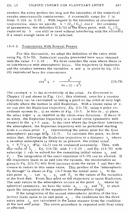
Ch. 13 UNIFIED THEORY FOR PLANETARY ENTRY 247
renders the entry portion too long and the tabulation of the numericalresults unnecessarily cumbersome. A reasonable range forf isfrom 0. 005 to 0. 05 . With regard to the tabulation of noncoplanartrajectories, since we specifyX (C / CD) cos a- for economyof parameters, the definition (13_72) entry point, with CL/CDreplaced by X can still be used without interfering with the accuracyif a small enough value of fis selected.
13-5.2. Trajectories With Several Passes
For this discussion, we adopt the definition of the entry pointusing Eq. (l3_72). Numerical results presented here were obtainedwith the value f = 0. 05 . We first consider the case where there isno interference with atmospheric force.The trajectory is Keplerianand the relation between the variables u andis given by Eq. (13-20) reproduced here for convenience
cos2 =
2(13-73)
2u — (1 - e
The constant eis the eccentricity of the orbit.As discussed inChapter 12 and shown in Fig. 12-1, this element, even for a reentrytrajectory can be calculated by taking a point on the orbit at very highaltitude where the motion is still Keplerian.With a known value ofe,we can plot the Keplerian trajectory, Eq. (13-73), using a polar co-ordinate system (u
,as shown in Fig. 13-7. In this (u , y) plane,
the polar angle is negative in the clock-wise direction.If there isno entry, the Keplerian trajectory is a closed curve symmetric withrespect to the = 0 axis. In the case where the trajectory intersectsthe atmosphere, the Keplerian trajectory will be perturbed startingfrom a certain point i
1representing the initial point for the first
atmospheric passage (Fig. 13-7) .To calculate this point, we firstnotice that, following the Keplerian trajectory to a distancer. wherea sensible atmosphere is likely to be present, the initial valueu. = V.2/ (Fig. 12-1) can be evaluated accurately.Then, withthis u. , Eq. (13-72) with f= 0.05 , and Eq. (13-73) withsubscript i can be solved for the remaining initial values andZ. . The integration of the exact equations (13-35) can be started.Ifthe trajectory leads to an exit into the vacuum, the deceleration asgiven in Eq. (13-71) will first increase from the valuef and then de-crease to return to this same value.This portion of the "atmosphericfly through" is shown in Fig. 13-7 from the initial pointi to theexit point e1 . Let u
.and Z be the values of variables
at the first exit. From point on the trajectory is again Keplerian.The next return to the atmosphere occurs at the pointi2 where byspherical symmetry, we have the value u
,and Z1 to start
again the integration of the equations for flight.If the integration of the second atmospheric portion of the tra-
jectory leads again to an exit point e2, the conditions for the thirdentry point i are calculated in the same manner from the conditionat the last point. The above procedure is repeated until final entryis effected.
PPSCDF a
p 2m V 13
zF
p1
exp
2
i vi']2(V
2-i
Hence F can be used as an alternate parameter replacing'y.Before a more accurate formula forF for use in thischapter, we notice that, by the definition (13-5) ?f our Z variable,we have F = Z . Hence, from now on, we shall use the notationz to rep?ace ? to designate the periapsis parameter.
For an which is essentially exponential between theinitial entry point and the conic periapsis, we have
Z 1T -13(r -r.)
248 UNIFIED THEORY FOR PLANETARY ENTRY Ch. 13
0
13-5.3. Chapman's Periapsis Parameter, F
It has been shown in Chapter 12 that Chapman's periapsis para-meter is used to define the entry condition.
He defined the periapsis parameter as
(1 3— 74)
where r is the hypothetical periapsis distance andp is the atmo-spheric evaluated at this periapsis altitude. a very smallentry angle
's'.and for a supercircular speedV. V.! > 1. 05
an approximate relation between y.and F has givenman as p
(13—75)
Fig. 13-7. Representation in the (u, y) planeof an entry trajectory with several passes.
(13— 76)
Ch. 13 UNIFIED THEORY FOR PLANETARY ENTRY 249
Now, if the value f in Eq. (13-72) is selected small enough, theentry point can be considered as a point on the initial Keplerian orbit(Fig. 13-7). Hence, Eqs. (13-31) and (13-32) apply.We have byevaluating the constant p ande at the entry point and hypotheticalperiapsis
r u.
= (13-77)1 p
and2
- Zu. = U2 - 2u (13-78)cos
Using Eq. (13- 77) in Eq. (13-76), we obtain the expression forthe periapsis parameter in terms of Z. and the ratioU
-
z = e
up(13-79)
p 1 u
There are many possible computing schemes using the formulas justderived. For computation and tabulation of accurate Z functions wecan follow Chapman using V., 'j. and (CL! CD) as entry data,andZ as an auxiliary parameter. uniformity, a of fsly f = 0. 05 , is selected. Then, we have u. = V. cos . Thenu is obtained from Eq. (13-78),Z. from Eq. and1finally
from Eq. (13-79). The of the equations starts fromtl?e values u. , 'v'. and Z. . For tabulation we can use either themodified (Z 1,
u) or the original Chapman variables(Z , u).
In practical application, for a given vehicle with a prescribeddrag parameter, approaching a planetary atmosphere, sometimes it isdifficult to obtain an accurate evaluation of the entry angle, ashas been pointed out by Chapman.In this case, since the Keplerianapproachorbit is known, its drag-free periapsis distance r can beeasily evaluated. Hence, if the atmosphere is known, we havep . For a prescribed draj parameter, Fis evaluated from Eq.(?3_74). The entry speed V.can be accurltely evaluated from ele-ments of the Keplerian orbit \lsing a distancer. representing the radi-us of the atmosphere.This is because V.is not as sensitive to vari-ation of r. as is . Since the Z Tables haveV. and Z as entrydata, together with 1CL/ CD, the entry trajectory 'can be i?entified.
Finally, Chapman used Eq. (l3_75) to obtain an explicit formulafor in terms of F , Z. and V. . Written in terms of ZZ. V. this is p 1 1
1 1
2log (13-80)
UNIFIED THEORY FOR PLANETARY ENTRY Ch. 13
The use of this explicit formula is restricted to very smallangles and V. > 1. 05 . An informative derivation of an improv-ed formula for as follows.
Letz u.
E_ (13-81)i p
From Eq. (13- 77) it may be seen that(1 - x) is a very small positivequantity. Thus, Eq. (13-79), which is
1/2y = x e (13-82)
or
log y = log x + - x) (13-83)
may be expanded for x near unity as2x-1 1logx=—+—( i +.,.x 2' x /
Thus,
log y = (1 - x) [Pr - +(1-x) -
],
That is, for large value of
1-x = (13-84)
Now, since u = u1/x , Eq. (13- 78) becomes
2x(1 - x) cos2 y. —2 2U
= 2 2
1= V. cos (13-85)
cos - x
Hence, solving for sin2'y. in terms of x and
2sin—2
(13-86)V.
1
where x is given by (13_84). This formula may be written as
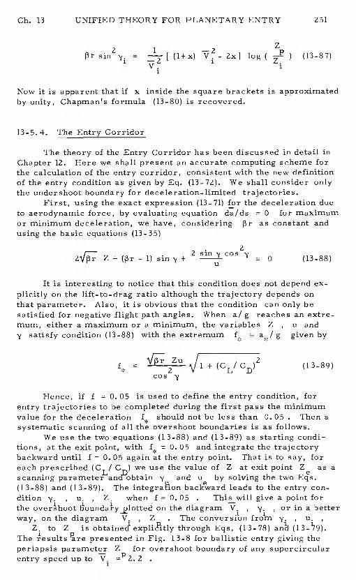
Ch. 13 UNIFIED THEORY FOR PLANETARY ENTRY 251
1z
= [ (l+x) log ( ) (13-87)1 1
1
Now it is apparent that if x inside the square brackets is approximatedby unity, Chapman's formula (13-80) is recovered.
13-5.4. The Entry Corridor
The theory of the Entry Corridor has been discussed in detail inChapter 12. Here we shall present an accurate computing scheme forthe calculation of the entry corridor, consistent with the new definitionof the entry condition as given by Eq. (13-72).We shall consider onlythe undershoot boundary for deceleration-limited trajectories.
First, using the exact expression (13- 71) for the deceleration dueto aerodynamic force, by evaluating equation da/ds= 0 for maximumor minimum deceleration, we have, consideringç3r as constant andusing the basic equations (13-35)
2= 0 (13-88)
It is interesting to notice that this condition does not depend ex-plicitly on the lift-to-drag ratio although the trajectory depends onthat parameter.Also, it is obvious that the condition can only besatisfied for negative flight path angles. When a! g reaches an extre-mum, either a maximum or a minimum, the variables Z, u andy satisfy condition (13-88) with the extremumf a,,! g given by
=Zu
+ (CL! CD) (13-89)cos 'y
Hence, if f = 0. 05 is used to define the entry condition, forentry trajectories to be completed during the first pass the minimumvalue for the decelerationf, should not be less than0. 05 . Then asystematic scanning of all the overshoot boundaries is as follows.
We use the two equations (13-88) and (13-89) as starting condi-tions, at the exit point, withf,, = 0. 05 and integrate the trajectorybackward until f = 0. 05 again at the entry point.That is to say, foreach prescribed (CL! C) we use the value of Zat exit point Ze as ascanning parameter ancPobtain and Ue by solving the two Eqs.(13-88) and (13-89). The integration backward leads to the entry con-dition 'i. u, , when £ = 0. 05 . This will give a point forthe on the diagram V. , or in a betterway, on the diagram V. , Z . The conversfon from y. , u.
Z. to Z is obtained through Eqs. (13-78) (13)79).The presented in Fig. 13-8 for ballistic entry giving theperiapsis parameter Zfor overshoot boundary of any supercircularentry speed up toV. 2
UNIFIED THEORY FOR PLANETARY ENTRY Ch. 13
Fig. 13-8. Overshoot and undershoot boundariesentries into the Earth's atmosphere.
Similarly, the undershoot boundary for any prescribed maximumdeceleration f = f can be obtained in the same way.The twoequations are used for the starting conditions atthe point of peak deceleration, f . Then Z is used as ascanning parameter for an to the entry pointwhere f = 0. 05 . The resulting value , u. and Z. providesthe entry condition for a peak deceleration f . It has beenfound that many ballistic entry trajectories have decelerations.The region where they occur and a comparison of their magnitudesare shown in Fig. 13-8 depicting the undershoot boundaries for differ-ent values of f . As has been mentioned in Chapter 12, forballistic entry circular speed, there is a minimum value forthe peak deceleration if the entry is completed during the first pass.Using the exact equations, it has been found that the smallest possiblepeak deceleration is6. 5 g which occurs for a slightly hyperbolicentry V. = 1.466 with Z = 0.13.
1 p
vi
• 001 .002 .004 .01 .02 .04 .1 .a •4 Zp i.
for ballistic
Ch. 13 UNIFIED THEORY FOR PLANETARY ENTRY 253
References
1. Chapman, D. R., "An Approximate Analytical Method for StudyingEntry Into Planetary Atmospheres, "NASA TR-R-11, 1959.
2. Chapman, D. R., "An Analysis of the Corridor and GuidanceRequirements for Supercircular Entry Into Planetary Atmo-spheres, "NASA TR-R-55, 1960.
3. Vinh, N. X., and Brace, F. C., "Qualitative and QuantitativeAnalysis of the Exact Atmospheric Entry Equations Using Chap-man's Variables, "LkF paper No. 74-010, presented at theXXVth Congress of the International Astronautical Federation,Amsterdam, The Netherlands, October 1974.
4. Vinh, N. X., Busemann, A., and Cuip, R. D.. 'Optimum Three-Dimensional Atmospheric Entry, "Acta Astronautica, Vol. 2,pp. 593-611, 1975.
5. Yaroshevskii, V. A. , "The Approximate Calculation of Traject-ories of Entry into the AtmosphereI, " translated fromKosmicheskie Issledovaniya, Vol. 2, No. 4, 1964.
6. Eggers, A. J. ,Jr. , Allen, H. J. , and Neice, S. E. ,"A Corn-paritive Analysis of the Performance of Long-Range Hyper-velocity Vehicles, "NACA TN 4046, 1957.
7. Singer, E., Raketen-Flugtechnik, R. Odenbourg, Berlin, 1933.
8. Loh, W. H. T., Dynamics and Thermodynamics of PlanetaryEntry, Prentice-Hall, Inc. ,Englewood Cliffs, New Jersey, 1963.
9. Allen, H.J., and Eggers, A.J., Jr., "A Study of the Motion andAerodynamic Heating of Missiles Entering the Earth's Atmosphereat High Supersonic Speed, " NACA TN 4047, 1957.
10. Shi, Y. Y., and Pottsepp, L. , "Asymptotic Expansion of a Hyper-velocity Atmospheric Entry Problem, "AIAA Journal, Vol.7,
No. 2, 1969.
11. Chapman, D.R., and Kapphahn, A.K., "Tables of Z Functionsfor Atmospheric Entry Analyses, "NASA TR-R-l06, 1961.
12. Brace, F. C., "An Improved Chapman Theory for Studying EntryInto Planetary Atmospheres, "Ph. D. Thesis, The Universityof Michigan, 1974.
Chapter 14
Solution of the Exact Equations UsingDirectly Matched Asymptotic Expansions
14-1. INTRODUCTION
The dimensionless universal equations for atmospheric entrywere derived in the previous chapter.The modified Chapman's vari-ables were introduced primarily to generate numerically the Z func-tions appropriate for analyzing entries of arbitrary vehicles.First-order solutions were also obtained.As presented in Chapter 13,thetheory is semi-analytical.In this chapter, a higher-order, analyticalsolution is presented.It is obtained by using the method of directlymatched asymptotic expansions applied to the exact equations for three-dimensional entry. The two-regime approach of directly matchedasymptotic expansions has proved to be feasible and effective in somerestricted cases (Refs.1 - 4). This chapter will follow the recent,complete integration of the exact universal equations, (Ref. 5).
14-2. THE DIMENSIONLESS EQUATIONS OF MOTION
If an isothermal atmosphere is used, the universal equations,derived in Chapter 13, have the form
dZ 3= - - Z tan
=- Zu{ fly
ds cosy
- z cosy1
cos2yds — cosy L - u
d9 -ds
= (14-1)
254
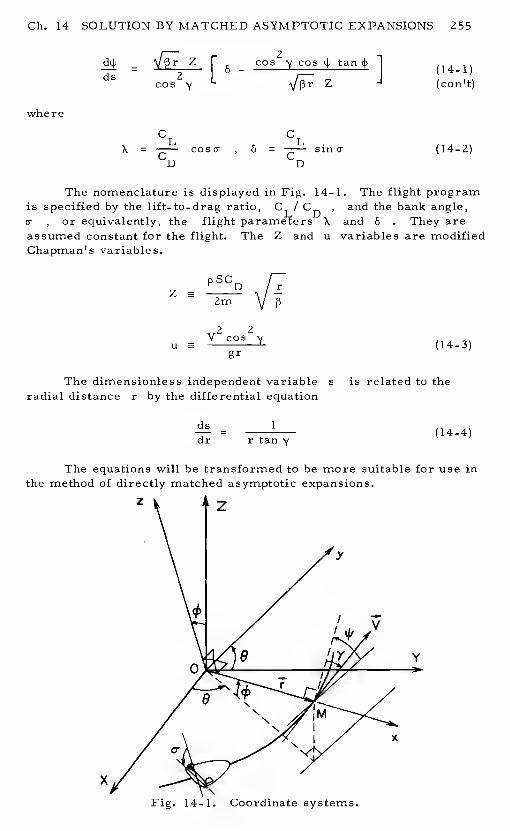
Cli. 14 SOLUTION BY MATCHED ASYMPTOTIC EXPANSIONS 255
= Z
[
- cO5'y COS
](14-1)
cos y (con't)
whereC CL
X = cosa , 6 = sinq- (14-2)D D
The nomenclature is displayed in Fig. 14-1.The flight programis specified by the lift-to-drag ratio,C / CD and the bank angle,a- , or equivalently, the flight parame1ters X and 6 . They areassumed constant for the flight.The Z and u variables are modifiedChapman'svariables.
a-
pS%Zm
2 2
u acos
(14-3)gr
The dimensionless independent variables is related to theradial distance r by the differential equation
ds = 1 (14-4)dr rtanN
The equations will be transformed to be more suitable for use inthe method of directly matched asymptotic expansions.
x
z z
V
'1'
x
256 SOLUTION BY MATCHED ASYMPTOTIC EXPANSIONS Ch.l4
In this method, the solutions are obtained separately for an outerregion, where the gravity force is predominant, and for an innerregion, near the planetary surface, where the aerodynamic force ispredominant. Hence, the altitude is the appropriate independent vari-able selected for the integration.
Let y be the altitude and let subscripts denote the referencealtitude, for example, sea level.Then
r = r + y = r(l + h) (14-5)
where the dimensionless altitude h is defined as
h = (14-6)
The differential relation betweens and r , Eq. (14-4), becomes
ds= (1 + h)tan'y (14-7)
For the integration, we adopt a strictly exponential atmosphere, butthe general method can be applied to any more realistic atmospheresuch as, for example, the one proposed in Ref. 1.For an exponentialatmosphere
p = = (14-8)
where
(14-9)
Since the constant is large, e. g. ,for the Earth atmosphere13r 900 , the parameter c is a small quantity. By the defini-tion (14—3) of Z
=e
h/c (14-10)
We define the ballistic coefficient
SCDPsB (14-11)Zmp
For each vehicle, B is specified and the variable Zis obtainedfrom
Z = B e_hk (14-12)
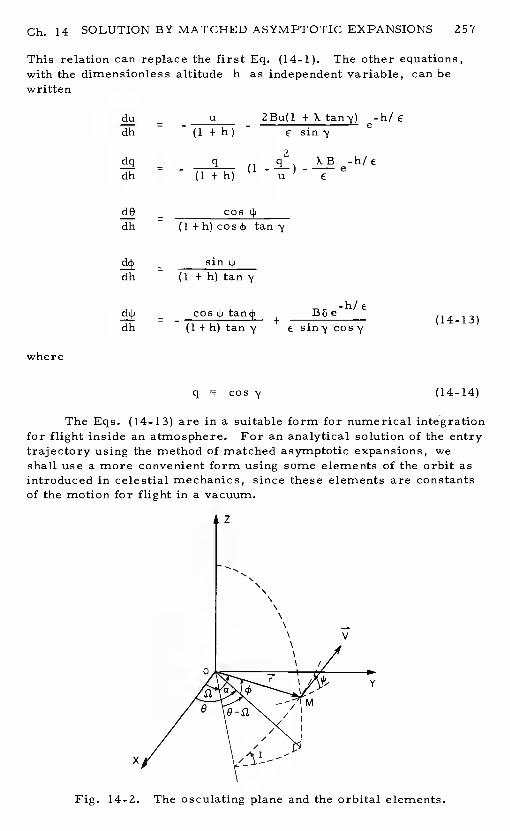
- sini4idh —
Ch. 14 SOLUTION BY MATCHED ASYMPTOTIC EXPANSIONS 257
This relation can replace the first Eq. (14-1).The other equations,with the dimensionless altitude h as independent variable, can bewritten
du - u 2Bu(l + X tan'y)dh - (1+h) - E siny
— q(1
dh - - (1+h) - E
-dh - tany
=-
+Böe (14-13)
dh (1 +h) tan
cos y (14-14)
The Eqs. (14-13) are in a suitable form for numerical integrationfor flight inside an atmosphere.For an analytical solution of the entrytrajectory using the method of matched asymptotic expansions, weshall use a more convenient form using some elements of the orbit asintroduced in celestial mechanics, since these elements are constantsof the motion for flight in a vacuum.
z
\
V
0Y
Fig. 14-2. The osculating plane and the orbital elements.
258 SOLUTION BY MATCHED ASYMPTOTIC EXPANSIONS Ch. 14
As seen in Fig. 14-2, ifI is the inclination of the plane of theosculating orbit, that is, the(r , V) plane, the longitude of theascending node, anda the angle between the line of the ascendingnode and the position vector, the following pertinent relations fromspherical trigonometry hold:
CoS4
cos cos cos (0 - (14-15)
These relations are independent. We can easily deduce
sin4, = sinlsinatan4
=tan a
sin sin I cos (0 - c2) (14-16)
Using these relations, we replace the variables0 , 4, , and withthe new variables a, , and I . The Eqs. (4-13) now become
du - u ZBu(1 + X tan y) -h/Edh - (l+h) - E siny e
- q(1dh - (l+h) E
cia - 1 B6 sinadh — (1+h)tany€tanlsinycosy e
B6 sin adh sin I sin y cos e
dl B5 cos a— = e (14-17)dh
The Eqs. (14-17) are most suitable for an integration using themethod of matched asymptotic expansions. We notice that, once theelements a , , and I are known, we obtain the original variableso , 4, , and from
tan (0 - Ii) = cos I tan a
= sinlsina
tan L4i = cos a tan I (14-18)
Gb. 14 SOLUTION BY MATCHED ASYMPTOTIC EXPANSIONS 259
14-3. INTEGRATION BY DIRECTLY MATCHED ASYMPTOTICEXPANSIONS
14-3. 1. Outer Expansions (Keplerian Region)
The Eqs. (14-17) are expressed in terms of the outer variables.The outer expansions are introduced to study the limiting conditions ofthe solution in the outer region where the gravitational force is pre-dominant. They are obtained by repeated application of the outer limit,which is defined as the limit when 0 with the variable h andother dimensionless quantities held fixed.
We assume the following expansions
u = u0(h)+€u(h) +.
q = q0(h) + €q1(h) +.
a = a0(h) + €a1(h) + .
= + +.
I = + E11(h) + . . . (14-19)
From Eqs. (14-17), the differential equations with zero order ofare
du0 u0
dh - (1+h)2
dq0 q0 q0
- 1
dh (l+h)tany0
dl= 0 (14-20)
The solution of this system is
u0(1 + h) = C1
1 — 2(1+h) 2
2 - C-C2(1+h)
q0 1
(14-21)
260 SOLUTION BY MATCHED ASYMPTOTIC EXPANSIONS Ch. 14
u0 = 1 + - cos (a0 - C3)
= C4
I = C (14-21)0 (con't)
where the C are constants of integration.The first-order and higher-order solutions are all equal to zero because at high altitude, in thelimit the atmospheric density is zero and the motion is Keplerian.
14-3. 2. Inner Expansions (Aerodynamic-Predominated Region)
The inner expansions are introduced to study the limiting condi-tion of the solution near the planetary surface where the aerodynamicforce is predominant. They are obtained by repeated application of theinner limit, which is defined as the limit when 0 with the newstretched altitude
(14-22)
and the other dimensionless quantities held fixed.We assume the following expansions
u u0(h)+cu1(h)+.
q = q0(h)+€q1(h)+.
a = a0(h)+€a1(h)+.
£2 = c20(h)+€c21(h)+.
I = 10(h) + €I1(h) +. . . (14-23)
From Eqs. (14-17), the differential equations with zero order of Care
du0 - 2Bu0(1 + X tan 'q0)
dh sin'q0
dq0— = -XBedh
da0 = -__B6 sin0
dh tan 1o sin cos
(14-24)
Ch. 14 SOLUTION BY MATCHED ASYMPTOTIC EXPANSIONS 261
sin
dh sjnl0sin'y0 cosy0
d10 Bô cos a0— — e (1.4-24)dh sin COS (con't)
The solution of this system is
— -2 ru0 = C1q0 exp —r
q0 = XBe_h +
sin sin = sin
cos = cos C3
cos j log [tan( + -i)] +
(14-25)
where the C are constants of integration.
14-3. 3. Asymptotic Matching and Composite Expansions
The constants of integration C in the inner expansions will be
determined by matching with the expansions. In this problem,matching is accomplished by expanding the inner solutions for largeh , expressing the results in terms of the outer variables and match-ing with the outer solutions for small h
The outer solutions, Eqs. (14-21), becomefor small h
U0 = C1
Iq0=v 2-C1C2
r C -1 1= cos_l I
1I + c
3
= C4
10 = C5 (14-26)
262 SOLUTION BY MATCHED ASYMPTOTIC EXPANSIONS Ch. 14
On the other hand, the inner solutions, Eqs. (14-25), become for largeh
— ——2 r 2 -l-u0 C1C2 exp
L-COS C2
=
C
cos = cos C3 cos (C4-
- 6 1 —1 —cos = cos C3 C2)J + C5 }
(14-2 7)
Matching Eqs. (14-27) with Eqs. (14-26) provides the constants Cin terms of the constants C . We have n
n
= (2 - C1C2) exp- I
C2= _C1C2
— I C-isin C = sin C sin cos 1 + Ci / 2
/
V1 - C1 C2
C4 cosC1 1
+ c3] /cos C3 } + C4
- Cl CZ
C5 = cos' [cos c51cos -
(14-28)
Hence, the constants Care expressed explicitly in terms of theconstants Cn into Eqs. (14-25) gives the inner solu-tions. It is convenient to use the following notation to write thesesolutions in a symmetric form.Let
Ch. 14 SOLUTION BY MATCHED ASYMPTOTIC EXPANSIONS 263
u* = Cl
__________
/ Cl
V 2 - C1C2
sin sin [1 C1 1
+ c3]- Cl Cz
= os + +
C2
= C5 (14-29)
The constants with subscript *are explicit functions of the constantsC . Then the inner solutions are
n
U0 COS '10 12=
expcos
cos = cos + XBeh
0sin 10 = *
COS = COS cos-
-1cos I coscos 4,,! \cos4,,
ir it
= log [tan + tan(T+ -i-)] (14-30)
From the Eqs. (14- 15) and (14-16) the meaning of the starredconstants can be seen.The Eqs. (14-30) show that during the phase ofaerodynamic turning, the latitude4, and the longitudee remainconstant. The last equation gives the change in the headingduringthat phase.
The composite expansions, uniformly valid everywhere, can beconstructed by the method ofadditive composition. The additive com-position is obtained by taking the sum of the inner and the outer expan-sions, Eqs. (14-30) and (14-21), and subtracting the part they have incommon (the inner limit of the outer expansions or the outer limit ofthe inner expansions), Eqs. (14-26) and (14-27). Thus, for the vari-ables u and '1 using subscript cfor the composite solution,
264 SOLUTION BY MATCHED ASYMPTOTIC EXPANSIONS Ch. 14
u— h 12
u - (1 +h) +2 exp k (14-31)
cos
and
cos = cos /2
-h/E+ X Be
V 2 cos +h)+(u, -2(14-32)
For the angular variables a, and I , the composite solutionsare
a=
+ --
C1-iC
=C
I = I +1 -C (14-33)0 0 5C
Hence, from Eq. (14-21), = and I = I From the lastof the Eqs. (14-30) c 0 c 0
CosI cos cos cos'(c
11 IF
+ log [tan( —1)/tan (14-34)
For the angle = , the second Eq. (14-15) yieldsc 0
tan= - (tan ) (14-35)
C
where I is given by Eq. (14-34)the angle a is given by
c
u,,-1
(sin-1 r
2
- ijja sinI
I
c sinc L
-l r- 1)
- C05[
+ (1 - (14—36)
Ch. 14 SOLUTION BY MATCHED ASYMPTOTIC EXPANSIONS 265
The composite solutions are expressed explicitly in terms of thefive constants of integration 4) and . For com-putation in terms of the independent variable h, the angle isfirst calculated from the second Eq. (14-30). Subsequently, we obtainu and I and finally c� and
c c c c c
14-3.4. Solutionfor the Planar Case
When 6 = 0 , the motion is planar. The trajectory remainsin the equatorial plane and the variable ais the same as the longitude0
The composite solutions for u and y, Eqs. (14-31) and (14-32), remain valid. The composite solutions for0 can be seen fromEq. (14-36) to be
cos / u*cos(0
/ 1+h'V u* + (1 - cos (14-37)
where w is a constant of integration.The three constants of integra-tion , and in Eqs. (14-31), (14-32) and (14-37) for theplanar case are evaluated using the initial conditionsu. , y. and0. ath.. 1
It obvious that when CL 0 , (X = 0) , then 6 = 0 and theballistic entry is planar. To show thatsolution is valid for all rangesof X we shall obtain the solution for ballistic entry using a limitingprocess. The second of the Eqs. (14-30) shows that, when X -0
Hence we write that equation in the limit-- .
cos - COS sin2 ) sin (
2Be
=2
=
By substituting in Eq. (14-31), we have the solution for ballistic entry,x -.0
uc h r2Be 1— - + exp I . I (14-38)(1+h) L
This solution can also be obtained by reintegrating the innerequations with X =0 and then matching with the outer solutions.
266 SOLUTION BY MATCHED ASYMPTOTIC EXPANSIONS Ch. 14
14-4. APPLICATIONS
For the initial conditions to be satisfied identically, the fiveconstants of integration C , or equivalently the five constants withsubscript * , as Eqs. (14-29), are to be evaluated byusing the composite solutions.Let the conditions ath. be
u = u. y = y. a = a. 1I. (14-39)1 1 1 1 1
With these conditions in the composite solutions, the constants u*'and are obtained by solving a set of transcendental
equations which can only be done numerically.Another obstacle ariseswhen, as is a common practice, in order to reduce the number ofprescribed initial values, one takes the initial (r.,V.) plane as thereference OXY plane with the axis OX along . In doing soa. = 0 and I. = 0 . But when I = 0 , the longitude1of the ascendingnJde £2 is not defined, as evidenced by Eq. (14-35).This singularitycan always be avoided by rotating theOXY plane through a fixed andarbitrary angle, say 45°, about the axis. Then the initialconditions at h. are
1
u = =a. = 0 , £2 0 Ii
= 450 (14-40)
The equivalent conditions for the variables0 , , and 4i are
(14-41)
This method of directly matched asymptotic expansions has pro-vided highly accurate and useful solutions to less gencral atmospherictrajectory equations, Ref. 1.In that work, extensive numerical cal-culations demonstrated the accuracy compared with exact numericalsolutions. The method was also proven valid for some restrictedproblems in Refs. 2-4.The present development which is based onRef. 5 has accomplished the wedding of the exact atmospheric trajec-tory equations, using the powerful modified Chapman variables, withthe method of directly matched asymptotic expansions.Numericalexperiments using the composite solutions obtained show that the re-sulting solution is accurate and reliable.Thus, this analytical solu-tion for atmospheric entry trajectories, in many ways completes thesearch for explicit, analytic, and yet accurate, solutions to this broadclass of problems.
Before we close this chapter, one pertinent remark is in order:In using the method of directly matched asymptotic expansions,
the logical choice for the independent variable is the dimensionlessaltitude h . From the composite solutions, it is seen that the ballis-tic coefficient B , defined by Eq. (14-11) , has to be prescribed.Hence, it seems that the solutions apply to a particular vehicle andthe generality of Chapman'sZ variable is lost. This is true for thepreviously developed solutions concerning restricted cases (Refs. 1-4).
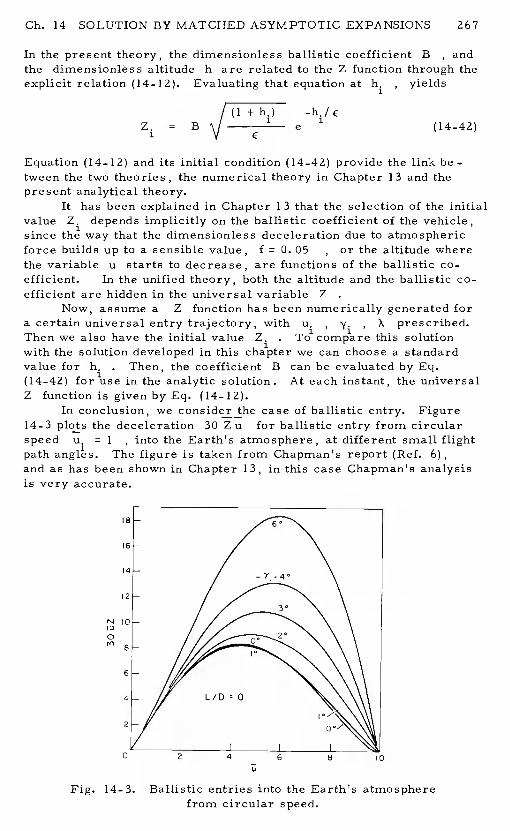
Ch. 14 SOLUTION BY MATCHED ASYMPTOTIC EXPANSIONS 267
In the present theory, the dimensionless ballistic coefficient B, andthe dimensionless altitude h are related to the Z function through theexplicit relation (14-12). Evaluating that equation ath. , yields
1(1 +h.) -h./cZ. = B V e
1 (14-42)
Equation (14-12) and its initial condition (14-42) provide the link be -tween the two theories, the numerical theory in Chapter 13 and thepresent analytical theory.
It has been explained in Chapter 1 3 that the selection of the initialvalue Z. depends implicitly on the ballistic coefficient of the vehicle,since the way that the dimensionless deceleration due to atmosphericforce builds up to a sensible value,f = 0. 05 , or the altitude wherethe variable u starts to decrease, are functions of the ballistic co-efficient. In the unified theory, both the altitude and the ballistic co-efficient are hidden in the universal variable Z
Now, assume a Z function has been numerically generated fora certain universal entry trajectory, withu. , y. X prescribed.Then we also have the initial valueZ. . Tb' compare this solutionwith the solution developed in this chapter we can choose a standardvalue for h. . Then, the coefficient B can be evaluated by Eq.(14-42) for use in the analytic solution.At each instant, the universalZ function is given by Eq. (14-12).
In conclusion, we consider the case of ballistic entry.Figure14-3 plots the deceleration 30 Z ufor ballistic entry from circularspeed u. = 1 , into the Earth's atmosphere, at different small flightpath The figure is taken from Chapman's report (Ref. 6),and as has been shown in Chapter 13, in this case Chapman's analysisis very accurate.
NJ':3
0'0
Fig. 14-3. Ballistic entries into the Earth's atmospherefrom circular speed.
U
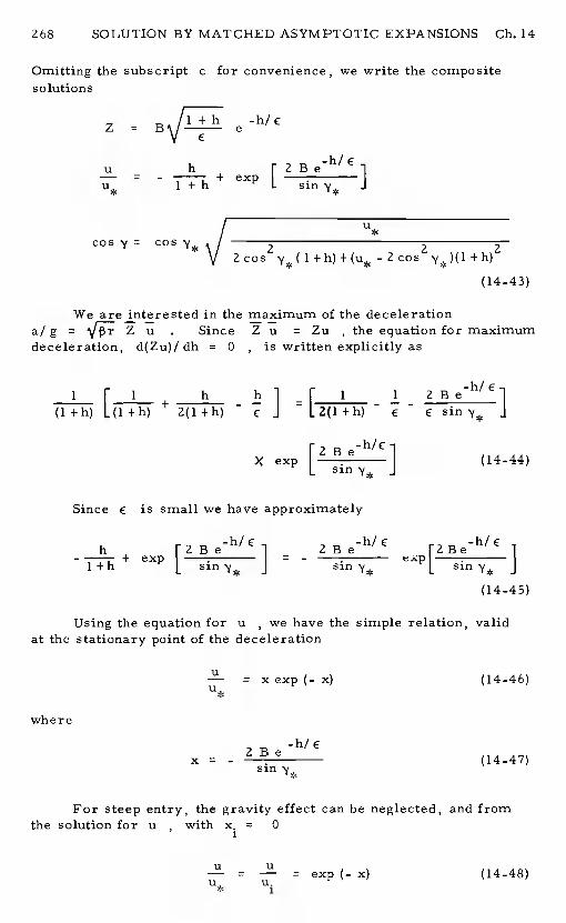
268 SOLUTION BY MATCHED ASYMPTOTIC EXPANSIONS Gb. 14
Omitting the subscript cfor convenience, we write the compositesolutions
Z =
-h/cu h I2Be— = 1+h L
I UI *
cosy=2 2 2
V
(14-43)
We are interested in the maximum of the decelerationa! g = Z u . Since Z u = Zu , the equation for maximumdeceleration, d(Zu)/ dh = 0 , is written explicitly as
1 1 h h 1 - [ 1 1 2 B e_hI'E(1+h) Lu+h + 2(1+h) - J — 12(l+h) - E - E
r -h/c2Be)( exp
I. (14-44)
L
Since is small we have approximately
h IZEe 1 ZBe i2Be- + exp I . I = - .l+h L J L
(14—45)
Using the equation for u* we have the simple relation, validat the stationary point of the deceleration
U— = x exp (_ x) (14-46)u*
where
-h/c=
- 2Be (14-47)sin '1*
For steep entry, the gravity effect can be neglected, and fromthe solution for u with x• 0
i
U U— = — = exp (_ x) (14-48)U U.* 1
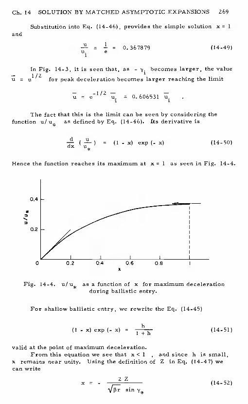
*
Fig. 14-4. u/ as a function of x for maximum decelerationduring ballistic entry.
For shallow ballistic entry, we rewrite the Eq. (14-45)
(1 - x) exp (_ x)= 1 h (14-51)
valid at the point of maximum deceleration.From this equation we see that x C1 , and since h is small,
x remains near unity.Using the definition of Z in Eq. (14-47) wecan write
x = - (14-52)sin
Ch. 14 SOLUTION BY MATCHED ASYMPTOTIC EXPANSIONS 269
Substitution into Eq. (14-46), provides the simple solution x =1
and
= = 0. 367879 (14-49)
In Fig. 14-3, it is seen that, as-
y. becomes larger, the valueu = uU"2 for peak deceleration becomes larger reaching the limit
= = 0.606531
The fact that this is the limit can be seen by considering the
function u/ut as defined by Eq. (14-46).Its derivative is
= (1 -x) exp(-x) (14-50)
Hence the function reaches its maximum at x =1 as seen in Fig. 14-4.
0.4
0.2
0 0.2 0.4 0.6 0.8x
270 SOLUTION BY MATCHED ASYMPTOTIC EXPANSIONS Ch. 14
Now, from Eq. (14-1), with X = 0 , we have the condition atthe point where maximum deceleration occurs, d(Zu)/ ds =0
1 =-
(14-53)sin y
From this equation, for maximum deceleration,
x=
(14-54)sin
which should be compared with Eq. (14-52).This relation sheds lighton the meaning of the constant . It is not the initial flight pathangle, but it is the angle near which the maximum deceleration occurs,and is in general larger than
The constants of integration and are calculated byapplying the initial conditions to the solution (14-43) at h =h. . Sincethe selection of h. is rather arbitrary the initial conditions may notprovide a solution and . For example, we consider thecase where = 0 . Then
2
u + h.) (14-55)* 1 1
For to be real
2(1 + h.) h.
2 + h. 1 + (14-56)
for small h. . Since by Eq. (14-43)
u.1
—1 — 1
U - l+h. - 1+h.1 1
we have the condition
u. < 1 - (14-57)1 2
For grazing entry with deceleration building up, that is, one-passballistic entry, the entry speed must be subcircular.
Strictly speaking, for y. = U , u, = 1 , Z. 0 the entryprocess is by orbital decay. topic be discussed in detail inChapter 15. For the last phase of entry we can integrate directly theEqs. (14_I), with = 0 , X = 0
Ch. 14 SOLUTION BY MATCHED ASYMPTOTIC EXPANSIONS 271
= -çlr
=- Zu
= U - 1 (14-58)ds u
Changing the independent variable tou
du - 2u
= 1 - U (14-59)du 1_12
Using a monotonically increasing variable by the transformation
u = (14-60)
we obtain
dZ = - y
1 - (14-61)
By eliminating y2dZ - e -1
2 - Z1-
with the initial conditions
Z(0) = 0 , Z'(O) = 0 (14-63)
This is precisely Yaroshevskii's formulation as discussed in Chapter10. It has been found that, in this case, the peak deceleration occursat
= 0. 835 = = 0.434 (14-64)
which is consistent with Chapman's numerical calculation in Fig. 14-3.
272 SOLUTION BY MATCHED ASYMPTOTIC EXPANSIONS Gb. 14
References
1. Yang, Ching-Yew, "On the Use of Aerodynamic Forces to EffectManeuvers of Orbiting Vehicles," Ph. D. Thesis, University ofColorado, August 1972.
2. Shi, Y. Y. , and Pottsepp, L. ,"On the Asymptotic Expansionsof a Hypervelocity Atmospheric Entry Problem," AIAA Journal,Vol. 7, No. 2, pp. 353-355, 1969.
3. Shi, Y. Y. , Pottsepp, L. , and Eckstein, M. C. , "A MatchedAsymptotic Solution for Skipping Entry into Planetary Atmo-sphere," AIAA Journal, Vol. 9, No. 4, pp. 736-738, 1971.
4. Shi, Yun-Yuan, "Matched Asymptotic Solutions for OptimumLift Controlled Atmospheric Entry," AIAA Journal, Vol.9,No. 11, pp. 2229-2238, 1971.
5. Busemann, A. ,Vinh, N. X. , and Gulp, R. D. , "Solution of theExact Equations for Three-Dimensional Atmospheric EntryUsing Directly Matched Asymptotic Expansions," NASA ReportCR-2643, 1976.
6. Chapman, D. R., "An Approximate Analytical Method For Study-ing Entry Into Planetary Atmospheres," NASA Report R-1l,1959.
Chapter 15
Orbit ContractionDue to Atmospheric Drag
15-1. INTRODUCTION
In Chapters 10-13, we have considered, among different typesof trajectories, the special case of the trajectory of a vehicle subjectto pure aerodynamic drag.If the periapsis altitude of the initialorbit is high anough, the vehicle will make several passes through theatmosphere before completing its entry.
On the other hand, for very high periapsis altitude the vehiclewill stay aloft for several days, weeks or even years before the effectof aerodynamic drag has reduced the lowest altitude far enough intothe sensible atmosphere to effectively initiate the entry trajectory.During this time the trajectory of the vehicle is essentially a Kepler-ian orbit subject to a small perturbing effect due to the resistance ofa tenuous atmosphere.The analysis of such a trajectory is the sub-ject of the present chapter.
In the early days, development of the theory of flight nearorbital speed inside an atmosphere was conducted in two separatedaspects. On the one hand, researchers analyzed the small perturba-tions of satellite orbits at very high altitude.The mathematical toolsare perturbation theories in celestial mechanics based on Lagrange'sequations for the variations of orbital elements.The space vehicle,usually referred to as a satellite, is not intended for recovery.Themain subjects of concern are first, its life expectancy, and second,the slow variations of its orbital elements.The variables of interestare primarily the major axis and the eccentricity of the osculatingorbit. On the other hand, engineers and scientists who were concern-ed with the safe recovery of an entry vehicle concentrated their efforton the study of the deceleration and heating during entry.The elementsof prime consideration are the position and the velocity of the vehicle,both varying rapidly. The nice behavior of the near-Keplerian orbitis no longer available, and strong physical assumptions were made tosuch an extent that, although describing the same phenomenon, namely,flight of an object inside a planetary atmosphere, the equations be-came totally different. The gap got wider as the two theories becamemore and more sophisticated.Now the two groups, one consistingmostly of mathematicians, and one consisting mostly of physicists,seldom reference the other group's work.
273
274 ORBIT CONTRACTION Ch. 15
With the objective of providing a unified theory for flight insidea planetary atmosphere, we have formulated a set of universal, exactequations in Chapter 13.These equations have been successfullyapplied to the study of planetary entry of a space vehicle (Refs. 1-2),and to optimization of such an entry (Refs. 3-4).In this chapter weshall present the necessary transformation such that the equations canbe used for analyzing the slow variations of the orbital elements whilethe vehicle is still in the near vacuum.This successful wedding isnecessary since future space vehicles are designed to stay for anextended period in orbit as satellites, and also to be recovered safelyafter a fiery entry which is followed by a glide, an approach, and alanding on an airfield.
15-2. FORCES ON A SATELLITE IN ORBIT
The satellite and the planet are assumed in two-body relativemotion. For a spherical planet, the gravitational force is an inversesquare force of attraction with acceleration
g(r) = (15-1)
where r is the distance from the satellite to the center of the planetand the planet gravitational constant.
The atmospheric force is in the form of drag acting in a directionopposite to the velocity VA of the satellite relative to the ambientatmosphere
DA = PSCDVA
We shall use a strictly exponential law for the density of the atmosphere
-r)p = p e (15-3)
p0
where 3 is now considered as a constant
= (15-4)
The quantity H which has the dimension of a length, is the scaleheight, and subscript pdenotes the initial periapsis condition.
The equations of motion are written with respect to an inertialframe with origin at the center of the planet.Let V be the absolutevelocity of the satellite
V = V + V (15-5)A e
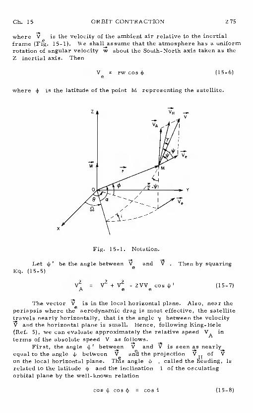
Ch. 15 ORBIT CONTRACTION Z75
where V is the velocity of the ambient air relative to the inertialframe (Fieg. 15-1). We shall assume that the atmosphere has a uniformrotation of angular velocity w about the South-North axis taken as theZ inertial axis. Then
V = rwcos4)e
(15- 6)
where 4) is the latitude of the point M representing the satellite.
Fig. 15-1. Notation.
Y
Let 4)' be the angle between V and V . Then by squaringEq. (15-5)
V is in the local horizontal plane.Also, near theperiapsis wherethee aerodynamic drag is most effective, the satellitetravels nearly horizontally, that is the angle y between the velocityV and the horizontal plane is small.Hence, following King-Hele(Ref. 5), we can evaluate approximately the relative speed VA interms of the absolute speed V as follows.
First, the angle4)' between V and V is seen as nearlyequal to the angle4i between V aned the projection VH of V
on the local horizontal plane. angle 4) , called the heading, isrelated to the latitude4) and the inclination i of the osculatingorbital plane by the well-known relation
cos 4) cos 4) = cos i (15-8)
z
w
V
VA
/
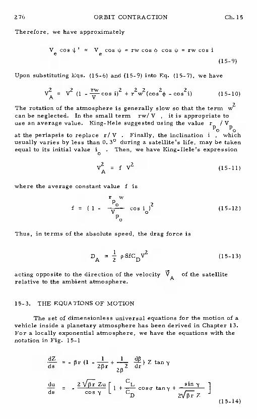
276 ORBIT CONTRACTION Ch. 15
Therefore, we have approximately
Ve cos Ve cos = rw cos cos = rw cos i(15-9)
Upon substituting Eqs. (15-6) and (15-9) into Eq. (15-7), we have
= V2 (1 - cosj)2
+ - cos2i) (15-10)
The rotation of the atmosphere is generally slow so that the term w2can be neglected.In the small term rw/ V , it is appropriate touse an average value.King-Hele suggested using the valuer / V
p0 p0at the periapsis to replace r/ V. Finally, the inclination i , whichusually varies by less than 0. 3° during a satellite's life, may be takenequal to its initial valuei . Then, we have King-Hele's expression
= f V2 (15-11)
where the average constant valuef isr w
p 2f = ( 1-
cos i) (15-12)p0
Thus, in terms of the absolute speed, the drag force is
DA 2 pSfCDV2 (15-13)
acting opposite to the direction of the velocity VAof the satelliterelative to the ambient atmosphere.
15-3. THE EQUATIONS OF MOTION
The set of dimensionless universal equations for the motion of avehicle inside a planetary atmosphere has been derived in Chapter 13.For a locally exponential atmosphere, we have the equations with thenotation in Fig. 15-1
du CL SiflV— = - I 1 +—coso- tan's' +ds cosy L CD
(15-14)
- cosq)ds —
ORBIT CONTRACTION
The variables u and Z are the modified Chapman's variables
2 2V cosungr
The independent variables is the dimensionless arc length from theinitial time
t—r
0
(15-16)
The variable 8 is the longitude, and the angleo- , the "bank angle,is the angle between the vertical plane passing through the velocity, the(r, V) plane, aridthe plane containing the aerodynamic force and thevelocity, the (VA , V) plane. As has been mentioned above, the aero-dynamic force is in the direction opposite to the velocity VA, therelative velocity of the satellite with respect to the ambient air.Finally, C and CD denote the coefficients of the aerodynamicforces in the direction perpendicular and parallel to the abso-lute velocity V
The equations (15-14) are convenient for analyzing the entryportion of the trajectory. For satellite orbits, it is more advantageousto use the orbital elements.First, we use the relations from sphericaltrigonometry
cos4,
cos 4 cos
cos (8 - (15-17)
to transform the last three equations (15- 14) into
Ch. 15
=
ds cosyr CL
cosCD
2cos ya +
(1cosu]
ds=
=ds 2coS y
ICL sifla -
277
(15-14)(con't)
(15-15)
tan4
rZE D
Zm
cos a
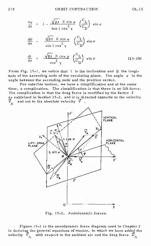
278 ORBIT CONTRACTION Ch. 15
= 1- Zsinatan i cos y
I sin a-
df2 = CL
2sina-
sinicos 'y
di - Z cos a sin2cos y
From Fig. 15-1, we notice thati is the inclination and c�the longi-tude of the ascending node of the osculating plane.The angle a is theangle between the ascending node and the position vector.
For satellite motion, we have a simplification and at the sametime, a complication. The simplification is that there is no lift force.The complication is that the drag force is modified by the factorfas explained in Section 15-2, and it is directed opposite to the velocityVA and not to the absolute velocity V
ZI
VERTICALPLANE
HORIZONTALPLANE
y,
0y
Fig. 15-2. Aerodynamic forces.
Figure 15-2 is the aerodynamic force diagram used in Chapter 2in the general equations of motion, to which we have added thevelocity VA with respect to the ambient air and the drag force DA
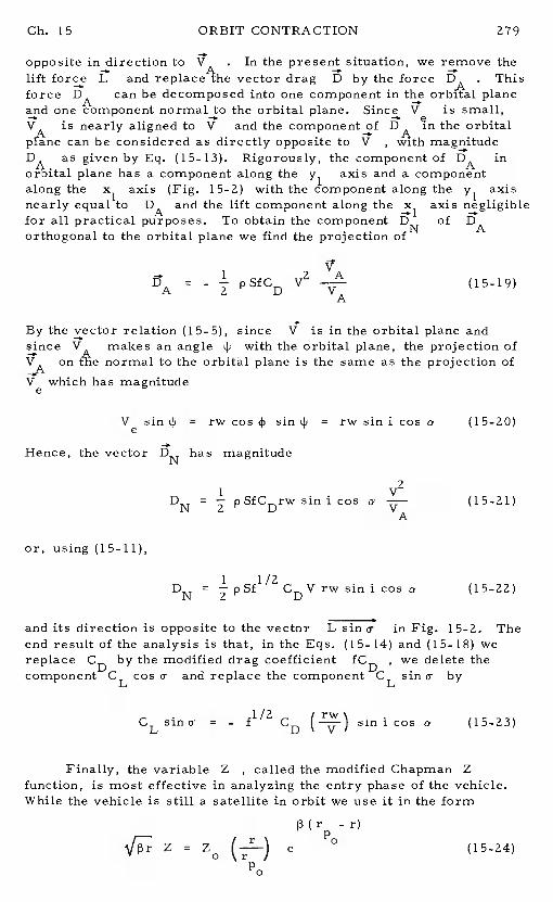
Ch. 15 ORBIT CONTRACTION 279
opposite in direction to VA . In the present situation, we remove thelift force L and replace the vector dragD by the force DA . Thisforce DA can be decomposed into one component in the orbital planeand one component normal to the orbital plane,Since V is small,-. -b Cis nearly aligned to V and the component of DA in the orbitalprane can be considered as directly opposite to V, with magnitude
as given by Eq. (15-13).Rigorously, the component of DA inorMtal plane has a component along they1 axis and a componentalong the x1 axis (Fig. 15-2) with the component along they1 axisnearly equal to DA and the lift component along the axis negligiblefor all practical purposes.To obtain the component DN of DAorthogonal to the orbital plane we find the projection of
DA = 2 PSfCD V2 (15-19)
By the vector relation (15-5), sinceV is in the orbital plane andsince makes an angle4 with the orbital plane, the projection of
on £he normal to the orbital plane is the same as the projection ofVe which has magnitude
V sin 4, = rw cos 4) sin 4i = rw sin i cos a (15-20)
Hence, the vector DN has magnitude
V2DN = pSfCDrw sin i cos a (15-21)
A
or, using (15-11),
DN = pSfh/2 CDV rw sin i cos a (15-22)
and its direction is opposite to the vectorL sin a in Fig. 15-2. Theend result of the analysis is that, in the Eqs. (15-14) and (15-18) wereplace CD by the modified drag coefficientfCD , we delete thecomponent CL cos aand replace the component CL sin aby
1/2CL sina = - f CD sini cos a (15-23)
Finally, the variable Z , called the modified Chapman Zfunction, is most effective in analyzing the entry phase of the vehicle.While the vehicle is still a satellite in orbit we use it in the form
p(r ..r)Z Z
(—i--)e
0 (15-24)p0
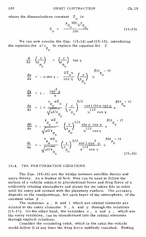
p Sf C rp Dp
0 0z = (15-25)0 2m
r wZp 0
- 0
-
r wZp 0
di2 — 0
-0
r wZdi - °
-
15-4. THE PERTURBATION EQUATIONS
r)p0
The Eqs. (15-26) are the bridge between satellite theory andentry theory. As a matter of fact, they can be used to follow themotion of a vehicle subject to gravitational force and drag force of auniformly rotating atmosphere and planet for its entire life in orbituntil its entry and contact with the planetary surface.The accuracydepends on the readjustment, for each layer of the atmosphere, of theconstant value
The variables a , and i which are orbital elements arerelated to the entry elements0 , and through the relations(15-17). On the other hand, the variablesr , u and 'y , which arethe entry variables, can be transformed into the orbital elementsthrough explicit relations.
Consider the osculating orbit, which is the orbit the vehiclewould follow if at any time the drag force suddenly vanished.Putting
280 ORBIT CONTRACTION Ch. 15
where the dimensionless constantZ is0
We can now rewrite the Eqs. (15-14) and (15-18), introducingthe equation for r/ r to replace the equation forZ
p0
d (rds \r
p0=
p0
duds
ds
= -utan'y-
2
= 1- cosU
p0
ZZu0 fr
5/2(rp0
5/2(rp0
j3(r -r)p0
e
cOsiSifla COSa1/2
U
sin a cos1/2 e
u cos'y
13(r - r)p0
e
/ .. 5/2 . 2sin i cos a/ 1/2
p0 u
3(r - r)p0
e
(15- 26)
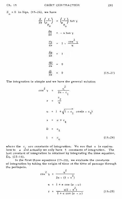
Ch. 15 ORBIT CONTRACTION 281
Z = 0 in Eqs. (15-26), we have
d fr\ fr\k—) =
p0 p0
du=
= 1-
1ds
ds
= 0 (15-27)
The integration is simple and we have the general solution2
2 ucos Zu - c
C2r = —
U
u = 1 + - c1 cos(s -c3)
5 =
= c5
i = C6 (15-28)
where the c. are constants of integration.We see thats is equiva-lent to and actually we only have5 constants of integration.Thelast constant of integration is obtained by integrating the time equation,Eq. (15-16).
In the first three equations (15-28), we evaluate the constantsof integration by taking the origin of time at the time of passage throughthe periapsis.
22 u
Cos= 22u - (1 - e
u = 1 + e cos2
r = a(1 - e (15-29)1 + e cos -
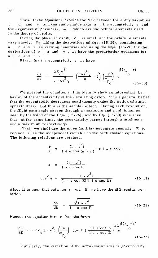
ORBIT CONTRACTION Ch. 15
These three equations provide the link between the entry variablesr , u and y and the semi-major axis a, the eccentricity e andthe argument of periapsis, , which are the orbital elements usedin the theory of orbits.
During the phase in orbit,Z is small and the orbital elementsvary slowly. By taking the of Eqs. (15-29), consideringa , e and u as varying quantities and using the Eqs. (15-26) for thederivatives of r , u and y , we have the perturbation equations fora , e and
First, for the eccentricity e we have
2 _r)d
- U (coseds - 3 u I
e cos (15-30)
We present the equation in this form to show an interesting be-havior of the eccentricity of the osculating orbit.It is a general beliefthat the eccentricity decreases continuously under the action of atmo-spheric drag. But this is the secular effect.During each revolution,the flight path angle passes through a maximum and a minimum asseen by the third of the Eqs. (15-26), and by Eq. (15-30) it is seenthat, at the same time, the eccentricity passes through a minimumand a maximum respectively.
Next, we shall use the more familiar eccentric anomalyE toreplace s as the independent variable in the perturbation equations.The following relations are obtained.
r (1-e)— = 1-ecosEa
1 - e cos E
cos y = — (15-31)(1 - e cos E)(1 + e cos E)
Also, it is seen that between$ and E we have the differential re-lation
ds —
1532dE — 1-ecosE -
Hence, the equation for e has the form13(r - r)
de 2 / a\ l+ecosE p0— = -2Z(1-e)i—j cosE( ) edE o / 1-ecosE
p0 (15-33)
Similarly, the variation of the semi_major axis is governed by
Ch. 15 ORBIT CONTRACTION 283
2 3/2 - r)
= - 2 a (l+ecosE)e (15-34)dE or 1/2
p (1-ecosE)
Under the same transformation, the last three equations of theEqs. (15-26) become
2 2Z ! ip(r -r)- e sin E(1-e cos E)2(l+e cos E)2e 0
]dE dE 1-ecosE e rp0
5 5 1r wZ — -r)° /aY 2 2 p(1-ecosE) coscye
5 5 1r wZ — — — 13(r -r)
p o 2 2 2 pdi 0 fa\ 2 o— = - I—) (1-ecosE) (1+ecosE) sinicos aedE f— \ r
p0 (15-35)
15-5. ORBIT DECAY
The equations (15-33) -(15-35) give the slow variation of the fiveorbital elements a, e , , and i . In the present chapter weare concerned with the variation of the semi_major axisa and theeccentricity e of the osculating orbit.As seen from Eqs. (15-33)and (15-34), under the dissipative effect of the drag, the major axisdecreases continuously while the eccentricity, although having anoscillatory behavior, also decreases secularly with the time. Wesay that the orbit undergoes a contraction and ase decreases,tendsto circularize itself. We shall use the method of averaging for theintegration of the equations.
15-5.1. The Averaged Equation
First, we have for the radial distance
r a(l - e cos E)
r = a (1 - e ) (15-36)p0 0 0
With this we write the exponential function in the equations
284 ORBIT CONTRACTION Ch. 15
exp = E] (15-37)
Along each revolution, a is nearly constant while the varyingquantity cos E provides the fluctuation in the air density.Thisleads to a natural choice of the variable
x a pae (15-38)
to replace the eccentricity e, (Ref. 5).By taking the derivative of Eq. (15-38) using the Eqs. (15-33)
and (15-34) we have the equation forx
2Z 3a2 2 13(r -r)dx o 1+ecosE p=- r (e+cosE)( e (15-39)
p0
The new dimensionless variable x behaves like the eccentricity ethat is, during each revolution x passes through stationary valueswhen cos E = - e , but, on the average, x decreases with the time.Since the decaying process is slow we can use an averaging technique(Ref. 6) applied to the right-hand sides of Eqs. (15-34) and (15-39)
for a and xFor the equation for a , we have the averaged equation
2 Zir 3/2
= - ZZ —f—(1+e cos E)
exp(xcos E) dE
p 0 (1-ecosE)0 (15-40)
For small eccentricity, the integrand can be expanded in powerseries in e . Upon integrating, we have
2
= -p0
+ + 0(e4)] (15-41)
where 1(x) is the Bessel function of the first kind and of imaginaryargument, of order n
1(x) =
ZrnE exp (xcos E) dE (15-42)
Similarly, the averaged equation for x is
Ch. 15 ORBIT CONTRACTION 285
= -p0
(15-43)
The Eqs. (15-41) and (15-43) were given by Cook, King-Hele andWalker. As shown in Ref.5, they truncated the equations to the ordere4 , formed the equation da/dxand integrated it separately for thecases where x is very large and x very small. We shall integratethe equation without making that asymptotic simplification, thus ob-taining the solution uniformly valid for any x
First, by dividing Eq. (15-41) by Eq. (15-43) and expanding theratio in power series ine , we have
da 1 2 1 2 2p —s-— y0+ y0y2)+-ge [2y0(3y0+y2) - 29y0
2 2 3 4+2y2+6y0y3+2y0y2y3-2y0(3y0+y2)]
+ O(e(1 5-44)
where we have defined the ratios of the Bessel functions
y a , n 1 (15-45)
For x> 3 , Cook, King-Hele and Walker integrated thisequation by using the asymptotic expansions of the functionyn(x)In this case, the right-hand side of Eq. (15-44) has a very simpleform and the major axisa is obtained by quadrature.Mathematically,the method of integration they used is not rigorous since on the right-hand side, the eccentricity eis a function of x and a by definition(15-38), so that the equation is actually anonlinear equation in aWe shall arrange the equation in a form where the Poincare methodof perturbations can be applied (Ref. 7).
The Bessel functions satisfy the recurrence formula
I (x) - I (x) = I (x) (15-46)n-i n+l x n
Hence, any function y(x) can be expressed in terms of y0(x) andx . For example,
286 ORBIT CONTRACTION Ch. 15
2y2(x) = y0 - —
8 4y3(x) = 1 + - —
8 48 24y4(x) = - — - + y0 + y0
(15—47)
Let
z (15-48)
be the dimensionless semi-major axis.Then, from Eq. (15-38) wehave for the eccentricity
e = E (15-49)
where
—i— (15-50)a
is a small quantity of the order of . Then, we can write Eq.(15-44) as an equation inz = a/a
2y 2 '7ydz 2x 0 2 3x 1 0 3
= y0 + —(2+—- 2y0) + e - 8y0 - — + By02z
2 3
4 2 "0 4+E 10— +4—s - +20—-16y0)2z x x x
+ (15-51)
We see that the true nature of the equation is a nonlinear equation.Since is a very small quantity we need not go further with the ex-pansion, and to the order of included, the solution of this equationcan be considered as the exact solution of Eq. (15-44), truncated tothe order e4
15-5. 2. Integration by Poincare's Method of Small Parameters
method for integration of a nonlinear differentialequation containing a small parameter is a rigorous mathematical
Ch. 15 ORBIT CONTRACTION 287
technique, proven to be convergent for small values of the parameter• We assume a solution fora of the form
= t0(15-52)
Upon substituting into Eq. (15-51) and equating coefficients oflike powers in we have the equations forzk(x)
dz
dx
dz1
—;i; =
dz yz x 0 2
dx a0 x 0
2dz3 xz1a x2 1 3
-a-—=-—-y(Z+—-2y0)+—-7(—-8y0--——+8y0)
a0 2z0
2 2 2dz4 XZ1
1 3 x 2— -——-—(— -8y -—+8y )-1-—(2+--—-2y )(—dx x 0 a 0 a x 0 2
a0 0 a0
2 3
x3 1 2Joy0 4y0 5y0 20y0
+ —i - - + - by0)2a x a x
0 (15-53)
We also have the initial conditions.
z0(x) = 1 z1(x) = a2(x) ... = 0 (15-54)
The integration of Eqs. (15-53) is accomplished by successivequadratures. Its success depends on whether or not the integrals canbe expressed in terms of known functions.It has been found that thefollowing recurrence formula is useful.
fp(x) =- + fp(x) f 2113)] dx
(15-55)
where n 0 and p(x) is any arbitrary function. To derive thisformula, we use the well-known relation
288 ORBIT CONTRACTION Ch. 15
xl' (x) + nI (x) = xl (x) (15-56)n n n—i
For n=1 I'= + (15-57)
andfor n=O
= 1(x) (15—58)
Therefore, if y0 =
10 loll 2Yb = -
= 1 + — - (15-59)
Now, consider
fp(x)
fp(x) = dx
Rearranging this equation, we have the recurrence formula (15-55).Using these relations we proceed with the integrations of the Eqs.(15-53), using the initial conditions (15-54).
First, we havez0(x) = 1 (15-60)
andbyEq. (15-57)
xI(x)z1 = log
x I (x )
(15-61)ol 0
where x = 3a e is the initial value of xz0 01
, the equation for z2 is
dz22Zx+y0-2xy0
Integrating
z2 = x2 + log x11(x) - dx (15-62)
Ch. 15 ORBIT CONTRACTION 289
But, by the recurrence formula (15-55) with p(x) =x , n = 1
dx = - xy0 + 2 log x 11(x) (15-63)
so that using in Eq. (15-62) with its initial condition, we havex11(x)
z2 = 2x y0(x ) - 3 log (x )(15-64)
ol 0
The integrations for obtainingz3 and are performed the sameway but they are much more laborious. is found that the zk(x) canbe expressed in terms of two functions
Io(x)A(x) E x = xy0(x)
B(x) log [ x11(x)] (15-65)
We have the final solution
z0(x) = 1
z (x) B - B1 0
z (x) = Z(A - A)
- 3(B - B
Z:(X) = j - A0) - Z(A2 -A2)
+ 13(B - B ) - 2A(B - B ) + (B - B)2
o o 2 o
z4(X) = - - x2) + (A - A) + 3 (A2 - A2) + (A3 - A3)
+ 4A(A - A) - Z(x2A - x2A)
- (69 + 6A + 7x2 - 19A - 4A2)(B - B)
- - B)2 - (B - B)3 + ZA(B - B)2 (15-66)
where A and B are the values of A and B evaluated at x =xaxis of the orbit under contraction is
a 2 3 4— = 1 + cz + e z + E z + z (15-67)a 1 2 3 4
0
Using x as a parameter, we easily express the other quantitiesof interest. The eccentricity e is given by Eq. (15-49), while the
290 ORBIT CONTRACTION Ch. 15
drop in the periapsis is obtained from
r -rr- a(l-e)] = - pa(l+cz1+...)
r -rp p 2 3
°H = (x-x) - (z+(z-fc z3+E z4) (15-68)
The ratio of the eccentricity is given by
9 = (15-69)
During the process of orbit contraction, the drag force is most signifi-cant along the lower part of the trajectory, near the periapsis.Thisresults in a strong braking force at the periapsis which has the effectof reducing drastically the apoapsis distance while the periapsis dis-tance remains nearly constant.To show this effect we can calculatethe ratios of the apsidal distances as function of the variable x. Wehave
= a(l-e) = Z-EX (15-70)r a(l-e)p0 o 0 0
Similarly, for the ratio of the apoapsis distances, we have
= a(l+e) = z+Ex (15-71r a(l+e) (l+e)a o 0 0
0
If we want to calculate the drop in the apoapsis, we can use the formula
r -ra
= a(l+e) - a(1+e)] =
a= (x - x) - (z +cz2 +E2z3+c3z4) (15-72)
Finally, the orbital period is simply3/2 3/2
T a= (—) z (x) (15-73)
Ch. 15 ORBIT CONTRACTION 291
For each initial value c = Hf a , and initial eccentricity ewe can calculate the initial valuex e = e 1€ . Then, wecan compute the expressionsa! a 0 0
, T7 T , etc. , asfunctions of x . Subsequently, can in any com-bination.
Since the quantitiesa , e , T are all easily observable, andthe integration has been performed to the order of e4, for smalleccentricity (which is the case for most scientific Earth satellites) theequations can be used to verify the assumption made on the atmosphere.In general, it can be, as a first approximation, assumed to be locallyexponential. That is to say, the parameter , or H = i/p , can beassumed constant for each layer of the atmosphere.Since the valueof enters analytically in the solution, by adjusting for concordancebetween the theory and the observation, determination of pcan bemade.
The theory can be modified to take into account the oblateness ofthe planet and the atmosphere, as has been done by King-Hele (Ref. 5).
15-5. 3. Explicit Formulas For the Orbital Elements
For small eccentricity, e < 0. 2 , the solutions obtained, Eqs.(15- 66) - (15-73), are very accurate.They are in parametric form,and for each pair of values and x they can be used to cross plotthe relationship between any pair of or°bital elements.
It would be useful to derive explicit formulas between any pairof orbital elements. This amounts to eliminating x between any twoof the equations (15- 67) -(15-7 3). Because of the transcendental natureof the solutions, the task is cumbersome.In this respect, King-Hele,(Ref. 5), used an asymptotic expansion for the Bessel function 1(x)Since the asymptotic expansion isonly valid for x> 3 which approxi-mately correspondsto e > 0.02, it was necessary to divide the pro-cess of orbit contraction into two phases. In the first phase, 0. 02 <
e < 0. 2 , asymptotic expansions can be used. Somewhat heuristically,an accurate and explicit expression for the major axis was obtained interms of the eccentricity. In the second phase,e < 0. 02 , byneglecting higher order terms ine , the solution z(x) , identicalto the present theory, but only to the order of€2 , was obtained.Explicit formulas for the second phase are not available.Since thepartition of the process of orbit contraction into two phases is ratherartificial, we shall offer an accurate theory uniformly valid for allvalues of the eccentricity in the range0 < e < 0. 2 . For very smallvalues of e the theory is no longer valid, but by then the satelliteis only a few revolutions before effective entry into the planetaryatmosphere.
To derive the explicit expression for the major axis in terms ofthe eccentricity, we write the equation (15—67) as
z= p+E4(z) (15-74)
where, by observing that
ORBIT CONTRACTION Ch. 15
x =
we can writex = (15-75)
with
a a xk , k (15-76)
Then, explicitly
= z1(az) + EZ2(aZ) + €2z3(az) + ... (15-77)
Equation (15-74) is in the form to which a Lagrange expansion can besuccessfully applied. We have, (Ref. 8),
z = p+ (15-78)
If we carry out the expansion and then put p =1 , we shall have to theorder of E4
z = 1 + €h1(a) +€2h2(a)+ + €4h4(a) (15-79)
where
h = B-B1 o
= 2(A - A) + (A - 3)(B - B)
h3 = - x2) - (ZA + )(A - A )+(13+ 2a2 -4A - - B)
+ B)Z
h4 = (35+4A-7A)
)(213+42A +16A2+12a2-9A+4A A-8A2)6 o o o o
-
+ Z(A-A )(B-B )(3+a2+A-A2)
- - B:)3 (6 - :2 + 2a2A + 3A2 - 2A3) (1 5_80)
Ch. 15 ORBIT CONTRACTION 293
with the definition
B log [a11(a)} (15—81)
Since a =3ae , the solution, as given by Eqs. (15-79) -(15-81)provides an explicit expression of the variation of the dimensionlessmajor axis a/a in terms of the eccentricity.
The other orbital elements can also be expressed in terms ofeThe drop in the periapsis is seen to be
r -rp p 2 3
°H (a -x)-(l-e)(h1+Eh2+E h3+E h4) (15-82)
For the apoapsis, we have
r -ra
= (x-a)-(1+e)(h1+Eh2+E2h3+E3h4) (15-83)
By replacing x by az in Eq. (15-70), we have the ratio of the pen-apsis distances
p = (1-Ea) z (15-84)r (1_ep0 0
where z is given by the Eqs. (15-79) and (15-80).For the ratio of the apoapsis distances, we have
a = (1 + Ea)z (15-85)r (1+e)
a o0
The orbital period is now
T 3/2= z (a) (15-86)
which is a function of the eccentricity.As pointed out by King- Hele,this equation provides a powerful method of verifying the assumptionmade on the atmosphere from two of the most accurate and easilymeasured orbital parameters, namely the period of revolution and theeccentricity.
294 ORBIT CONTRACTION Ch. 15
15-5.4. The Contraction of Orbits
The solution (15-66) can be considered as the exact analyticalsolution of the nonlinear differential equation (15-51).Both this solu-tion and the explicit solution in terms of the eccentricity, Eq. (15-80),have been computed for a number of orbits and they provide aboutnearly identical results.As illustrative examples, we consider thefollowing initial orbits
Orbit 1 = 0. 008 , e = 0. 2 — x = 25o o
Orbit 2 : 0. 009 , e = 0. 225 — x 25o 0
Figure 15-3 plots the variation of the major axis versus theeccentricity using the explicit solution, uniformly valid for all eccen-tricities. In this figure and in the following figures the circles repre-sent the exact solution.
Figure 15-4 plots the variation of the orbital period while Fig.15-5 presents the drop in the periapsis.It is seen that the decreasein the periapsis is very slow.This can be seen clearly in Fig. 15-6where the ratiosr / r and r / r are plotted versus the eccen-
p p a a
tricity. When e/ e = 0. 1 the calculated values for orbit 1 arer /r = 0.987l6cY and r /r = 0. 684968 and the correspondingp p a a
values for orbit 2 are found to be r / r = 0.985136 and r / r =p p a a
0. 651941.
15-5. 5. Contraction of Highly Eccentric Orbits
For the case of orbits with large eccentricities, sincex =a — , x becomes very large and the asymptotic
expression for Bessel's ratio y0(x)is
y0 = 1 + +
= ... (15-87)
Using this form in Eq. (15-51) we have
2 3 42dz 1 E Ex Exc (1 + i—) - — + —i-- - —i-— + ... (15-88)
an equation which can be seen as the development of
= €(l-
(15-89)
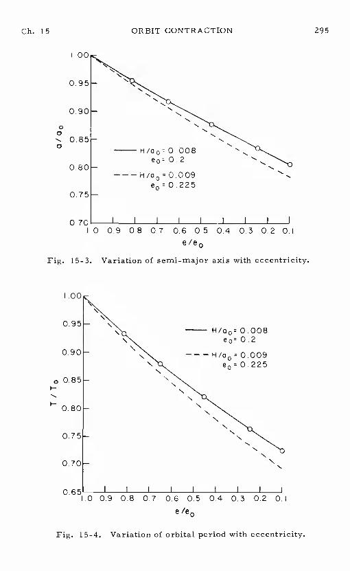
Ch. 15 ORBIT CONTRACTION 295
00 -
0.90
0 95
00
0.85-
0
00 0.7 0.6 0.5 0.4 0.3 0.2 0.1
e/e0
Fig. 15-3. Variation of semi-major axis with eccentricity.
I .00 -
\0.95— \ \ H/a0rO.008
\0.90 - \ —— — H/a0 0.009
NN
p0.85-H N
NH 0.80- N
NN
0.75-N
NN
0.70- N
0.65 I I I
1.0 0.9 0.8 0,7 0.6 0.5 0 4 0.3 0.2 0.1
e /e0
Fig. 15-4. Variation of orbital period with eccentricity.
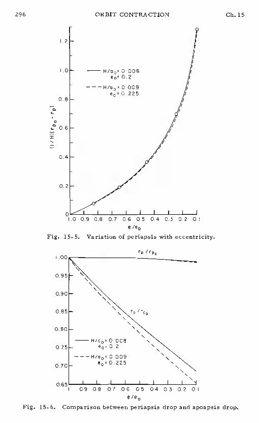
296 ORBIT CONTRACTION Ch. 15
1.2 —
.0 —- ———H/00r0009
0.8—
/
a. 0.6 -±
/
0.4 -
0.2 -
C I I I I I
1.0 0.9 0.8 0.7 06 0.5 04 0.2 0.1
e /e0
Fig. 15-5. Variation of periapsis with eccentricity.
rp /rp0I .00
\
0.85-
0.80-
\075 -
::: - I
I 0.9 0.8 07 06 05 0.4 0.3 0.2 0.1
e /e0
Fig. 15-6. Comparison between periapsis drop and apoapsis drop.
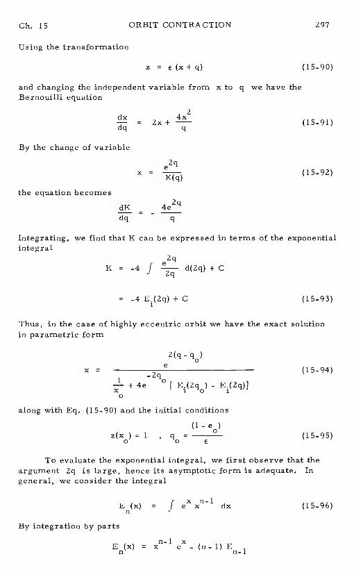
Ch. 15 ORBIT CONTRACTION 297
Using the transformation
z = (x + q) (15-90)
and changing the independent variable from x toq we have theBernouilli equation
2dx 4x— = 2x+ (15-91)dq q
By the change of variable2q
x = (15-92)
the equation becomesdK
- 42qdq - - q
Integrating, we find that K can be expressed in terms of the exponentialintegral
2qK = -4 f d(2q) + C
= -4 E.(2q) + C (15-93)
Thus, in the case of highly eccentric orbit we have the exact solutionin parametric form
2(q - q)= e (15-94)-2q
+ 4e ° [ E.(2q) - E.(2q)]
along with Eq. (15-90) and the initial conditions(1 - e
z(x) 1 , q° (15-95)
To evaluate the exponential integral, we first observe that theargument 2q is large, hence its asymptotic form is adequate.Ingeneral, we consider the integral
E(x) = f dx (15-96)
By integration by parts
E (x) = n-l ex - (n- 1) En n-i
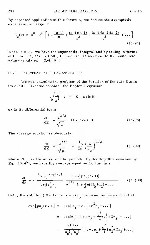
298 ORBIT CONTRACTION Ch. 15
By repeated application of this formula, we deduce the asymptoticexpansion for large x
En(X) = [1 - (n-l) + (n-l)(n-2)-
+ ...](15-97)
When n =0 , we have the exponential integral and by taking6 termsof the series, for x> 50 ,the solution is identical to the numericalvalues tabulated in Ref. 9
15-6. LIFETIME OF THE SATELLITE
We now examine the problem of the duration of the satellite inits orbit. First we consider the Kepler's equation
t = E-esinE
or in its differential form3/2dt a— = (1 - ecosE) (15-98)
The average equation is obviously
3/2 T 3/2dt = a = o(a 1599dE -
0
where T is the initial orbital period. By dividing this equation byEq. (l5_z?3), we have the average equation for the time
Tr exp(x)op o (z-1)J— = - ° °
(15-100)dx
z the exponential
exp[pa(z-1)] = exp[z1 + EZ2+E Z3+...
= exp(z1){ l+€z2+ + ...}
xI(x) 22
= x I(x )ol o
Ch. 15 ORBIT CONTRACTION 299
Next, we define the dimensionless time Tas
Zrpa2p SfCDT m T
x11(x)[exp(_x)]t (15-101)
Then, the dimensionless time equation has the form
di- 2 2 (15-102)dx €2x2
If z is replaced by its expression and then the binomial expansion isapplied, we have to the order of€2 , inclusively,
= _x[ + 11x2-x2y3+18xy0z1
+ 12xy0z2-4xy2z2
+ 4z -4zz+4z2+ 8z3)J (15-103)
Finally, if the functions z.(x) as given by the solution (15-66)are sub-stituted into this equation, 1the time-r is obtained by quadrature.Explicitly, by letting
T = T0+ET1+ €T2 (l5_l04)
we have the following equations
T0 = - x
T = (2A )1 o 2 o
=
-(10+ 7A )(B - B ) x - x(B_ B)2 (15-105)
0 o 8 o
with ( ) = d ( )/dx Integrating the first equation fromx , wehave
T0 = (15-106)
ORBIT CONTRACTION Ch. is
For the other two equations some of the quadratures cannot be expres-sed in terms of elementary functions.For an accurate treatment, wecan tabulate these integrals.But, to obtain an explicit expressionfor the time, an approximation has to be used.
For elliptic orbits, when e > 0.02 (which corresponds approxi-mately to x> 3 ), we have the following asymptotic expansion for theBessel function I (x)
1(x) = expx[
(1)m(42- 12)(4n2- 32)...[ 4n2_(2m_ 1)2]
m=0 m! (8x) (15-107)
In particular, we have for x> 3
expx 1 910(x) = + +
128x2+
Ii(x)= - - 128x2 -
• (15-108)
Using these expansions, we have to the order of l/x
10(x)3
A = x— = x+—+---—+11(x) 2 8x
xl (x)1
3(x-xB - B = log 1
(x- x ) + — log—f- +°
+o xI(x) o 2 x 8xxol 0 0 0
(15— 109)
With the expansions substituted into the equation for , we haveafter integration
21 1 7 33 2 2=
73 3 72 x- - x )
log (15-110)
For the equation in T2 , we take approximately
2 2xy0 = x
A = xo o
2 2A x +xo o 0
B-B = (x-x)0 0
Ch. 15 ORBIT CONTRACTION 301
to have
T2 = (15-111)
Integrating, we obtain
1 22 2 1 3 3 794 4T2 = - -j-g(4x - 1 1x0)(x0 - x
) - - 4)(x0 - x) + - x
(15-112)
The solution(15_104) with T.(x) as given by the Eqs. (15-106), (15-110)and (15-112) , gives the dimensionless time T as a function of x forlarge x . Although it is valid for x > 3 , we can have a goodestimate of the time the satellite remains in orbit by evaluating thelifetime TL obtained by putting e = 0 , or equivalently x =0
Then, we have the lifetime given as:Ee 2
2 1 2 5 23 2 7 o 9EETL (15-113)
As with the orbital elements, it is possible to express the timein terms of the eccentricity.For this purpose, we use the relationx = x zk to write the expression for the time,
E2T = - z2k2)[ 1 + - €)e e2 +jE-
-
+ - Ee(l-zk) log(zk) (15-114)
Since z has been obtained explicitly in terms of k =e/e throughthe Eqs. (15-79) and (15-80), this expression gives the dimensionlesstime in terms of the eccentricity.To be consistent with the approxi-mation used in deriving Eq. (15-114), we shall use the expression forz in its asymptotic expansion form.Then, to the order of E
z = 1+€[B(a)-B}a'
= 1 + E( a'- x )+ —log —0 2 x
0
or
z = 1 - e (1-k) + log k (15-115)0 2
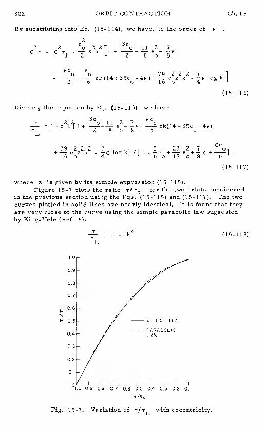
302 ORBIT CONTRACTION Ch. 15
By substituting into Eq. (15-114), we have, to the order of2
2 2e 3e 112 7
T = TL_7Z k Ll+
- zk(14+35e log k]
(15- 116)
Dividing this equation by Eq. (15-113), we have
3e ce= zk(14+35e -4€)
TL 2 808 6 o
Ee79222 7 5 232 7 ok - /[
(15- 117)
where z is given by its simple expression (15-115).Figure 15-7 plots the ratio TIT for the two orbits considered
in the previous section using the Eqs. and (15-117). The twocurves plotted in solid lines are nearly identical.It is found that theyare very close to the curve using the simple parabolic law suggestedby King-Hele (Ref. 5).
= 1 - k2 (15-118)TL
I.0
0.9
0.8 /07 //
//
Eq. (15- 17)
PARABOLIC0.4 LAW
03
02
0.1
0 I I I
1.0 0.9 0.8 07 0.6 0.5 0,4 0.3 02 0,1e /e0
Fig. 15-7. Variation of T/TL with eccentricity.
Ch. 15 ORBIT CONTRACTION 303
In practice, the solution (15-117) is valid down to an eccentricityof about e 0. 02 . When this eccentricity is reached, solution byasymptotic expansions is no longer valid.The equation (15-103) hasto be integrated again using a different approximation.This is alsothe case where the initial orbit is nearly circular.Since e is verysmall, the value of x is also small, with x <3 , and we only needto consider the solution for T and T1 . The solution for isexact, as given by Eq. (15-109>).For the equation in T1, thesecondof the Eqs. (15-105), we have the series expansion of the Besselfunction I (x) for small x
n
1n+2m
x)1(x) m!(n+m)! (15-119)
In particular, we have
2 4 6
10= 1 + + + 2304 +
2 4 6
= ) (15-120)
Therefore,
A = xy0 = 2 - + ... (15-121)
This series is obtained by the binomial expansion and its convergencerequires that x > I1(x) , that is, x < 2.4 . To extend its validity,King- Hele sugge the empirical formula
A = xy0 = 2
which, although less accurate than the exact expansion, (15-121), forsmall x , never has an error more than 0. 07 for larger values of
We now write the equation for T1
(15-123)
Using the approximation (15-122) for A and A , we have,upon integrating the equation from x
= (15-124)
Hence, for small eccentricity, the expression for the dimension-less time is
304 ORBIT CONTRACTION Ch. 15
0 ° (15-125)
This expression is identical to the one given in Ref. 5, sincethat analysis corresponds to the present theory up through the orderof . Beyond this order, the integration in Ref. 5 involves someheuristic steps which have been avoided in the present development.By putting x = 0 in the equation above, we obtain the lifetime of thesatellite from the initial eccentricity,e , assumed smalL
02
e2 o €92TL = 1- 1)] (15-126)
By dividing Eq. (15-125) by Eq. (15-126), retaining only theorder we have
2 22 2 (x-x)
v x 7 x o= 1- [ 20
-(B-B)]L x x (15-127)
0 0
Now, ifwewrite x=xkzxk_cxk(B -B) , wecanputthe0 0 0 0equation in the form
= 1-k2 +jck2 (15-128)
where the argument of B is x =x kz = az . But, to the orderthe solution 0
z = 1 - €(B- B) (15-129)
is the same for both arguments x and a =xk . Hence, to the orderof Eqs. (15-128) gives the explicit expression for the ratior/ in terms of k where
B = log [a 11(a)J , a = xk (15-130)
Considering the fact that both xand B are about 3 , the contri-bution of the term in Eq. is and for small eccentri-city, the parabolic law as given by Eq. (15-118) is still valid.
Equation (15-128) is of the form (15-74) where p= 1 - T/TL andthe function to be found isk2 . Hence, applying the Lagrange expan-sion to find k2 and then taking the square root, we can express theeccentricity as a function of the time:
= [1 -2S(B -B) (15-131)e v TLL 80 °TL
Ch. 15 ORBIT CONTRACTION 305
where
B = log x11(x)
B = log[x I(xL ° TL 1 TL (15-132)
Numerical computation has been done for several orbits and itis found that the parabolic law is adequate.Hence, Fig. 15-7 can beused for any elliptic orbit up to e 0. 2.
A higher order analysis of the theory has been presented inRef. 10. Using the same approach, the theory has been extended tothe case of an oblate planet and oblate atmosphere in Ref. 12.
References
1. Vinh, N. X., and Brace, F. C., "Qualitative and QuantitativeAnalysis of the Exact Atmospheric Entry Equations UsingChapman's Variables, "IAF paper No. 74-010, XXVthCongressof the International Astronautical Federation, Amsterdam,October 1974.
2. Busemann, A., Vinh, N. X., and Culp, R. D., "Solutionof theExact Equations for Three-Dimensional AtmosphericEntry UsingDirectly Matched Asymptotic Expansions, "NASA ReportCR-2643, 1976.
3. Vinh, N. X., Busemann, A., and Culp, R. D., 'OptimumThree-Dimensional Atmospheric Entry, "Acta Astronautica, Vol. 2,pp. 593-611, 1975.
4. Frostic, F., and Vinh, N. X., "Optimal Aerodynamic ControlBy Matched Asymptotic Expansions, "Acta Astronautica, Vol.3, pp. 319-332, 1976.
5. King-Hele, D. , Theory of Satellite Orbits in An Atmosphere,Butterworths, London, 1964.
6. Bogoliubov, N. N., and Mitropoisky, Y. A., Asymptotic Methodsin the Theory of Non-Linear Oscillations, Gordon and BreachSc. Publishers, Inc. ,New York, 1961.
7. Poincare, H., Les Nouvelles de laCeleste, Vol. 2, Dover reprint, 1957.
8. Bellman, R., Perturbation Techniques in Mathematics, Physicsand Engineering, Holt, Rinehart and Winston, Inc. ,New York,1964.
9. Abramowitz, M. , and Stegun, I. A., Handbook of MathematicalFunctions, Dover Publications, Inc., New York, 1972.
306 ORBIT CONTRACTION Ch. 15
10. Longuski, J.M. , "Analytic Theory of Orbit Contraction andBallistic Entry into Planetary Atmopsheres, "Ph.D. thesis, TheUniversity of Michigan, 1979.
11. Vinh, N.X., Longuski, J.M., Busemann, A. and Culp, R.D.,"Analytic Theory of Orbit Contraction Due to Atmospheric Drag,Acta Astronautica, Vol. 6, pp. 697-723, 1979.
12. Chen, W. T. , "Satellite Orbits under the Influence of Air Drag,Rotating Oblate Atmosphere and Planet's Oblateness, "Ph. D.thesis, University of Colorado, 1977.
Chapter 16
Flight with Lift Modulation
16-1. INTRODUCTION
Until now we have considered entry trajectories with constantangle of attack and constant bank angle. A space vehicle entering aplanetary atmosphere and having control devices allowing modulationof the lift coefficient and the bank angle will have more flexibility inthe selection of the appropriate trajectory.For a highly maneuverablevehicle, lift and bank controls can guide the vehicle along a prescribedtrajectory to a correct presentation for making the final approach andlanding. Also, as has been shown in Chapter 9 and Chapter 12, liftcontrol can be performed to reduce the overall heating or the peakdeceleration. It can be used to widen the entry corridor,Lift andbank controls, used in an optimally coordinated manner, may reduceto a strict minimum the fuel consumption for an orbital maneuver ofa lifting vehicle (Ref. 1).
For these reasons, starting with this chapter, we shall analyzethe motion of an entry vehicle having the capability of controlling thelift program along its trajectory.
We shall first modify the universal equations, developed inChapter 13 for constant angle of attack and bank angle, put them in theform where the lift coefficient and the bank angle are variable, andthen use these equations to study successively the following entrytrajectories:
1. Entry at constant flight path angle.2. Entry at constant rate of descent.3. Entry at constant speed.4. Entry at constant dynamic pressure.5. Entry at constant heating rate.The equations with lift and bank modulation are derived in this
chapter. Different constraints imposed upon the state of the vehiclewill be discussed and a theory of flight path control for satisfying theseconstraints will be presented.Examples of flight subject to constraintsas mentioned above will be analyzed later.
The examples considered above are selected solely to presentsome fascinating aspects of entry with aerodynamic maneuveringcapabilities, but the equations derived can be used to analyze entry
307
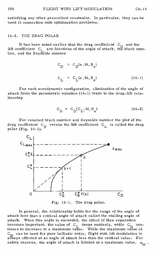
308 FLIGHT WITH LIFT MODULATION Ch. 16
satisfying any other prescribed constraint.In particular, they can beused in connection with optimization problems.
16-2. THE DRAG POLAR
It has been noted earlier that the drag coefficient CD and thelift coefficient CL are functions of the angle of attack, the Mach num-ber, and the Reynolds number
CD =
CL CL(o,M,R) (16-1)
For each aerodynamic configuration, elimination of the angle ofattack from the parametric equation (16-1) leads to the drag-lift rela-tions hip
CD = (16-2)
For constant Mach number and Reynolds number the plot of thedrag coefficient CD versus the lift coefficient CL is called the dragpolar (Fig. 16-1).
Xmox
0 C CD
Fig. 16-1. The drag polar.
In general, the relationship holds for the range of the angle ofattack less than a critical angle of attack called the stalling angle ofattack. When this angle is exceeded, the effect of flow separationbecomes important; the value of C1drops suddenly, while con-tinues to increase to a maximum vaiie.While the maximum value ofC can be used for pure ballistic entry, flight with lift modulation is
effected at an angle of attack less than the critical value.Forsafety reasons, the angle of attack is limited at a maximum value, aM
Ch. 16 FLIGHT WITH LIFT MODULATION 309
near the stalling angle of attack,aS . To this value, corresponds amaximum value of the lift coefficient,CL
An important parameter in the vehicles is thelift-to-drag ratio, or aerodynamic efficiency
CLE = — (16-3)
CD
As are the lift and the drag coefficients, the aerodynamic efficiencyis a function of the angle of attack, the Mach number and the Reynoldsnumber. For constant Mach number and Reynolds number, E varieswith the angle of attack; as a increases, E increases, reaches amaximum value E* , and then decreases.
The drag coefficient CD can be decomposed into two parts, thezero-lift drag coefficient CD and the induced drag coefficient CD(Ref. 2). o i
CD = CD + CD (16-4)
For most vehicle aerodynamic configurations, the induced drag co-efficient can be represented in the form
CDi = K CLn (16-5)
Hence, we write the lift-drag relationship
CD = CD + K (16-6)
This is a modeling form of the general relationship (16-2).Hence, thezero-lift drag coefficient CD , the induced drag factor K, and also
the exponent n are functions°of the Mach number and the Reynoldsnumber. For constant Mach and Reynolds number these coefficientsare constants and can be selected to best represent the drag polarobtained through wind tunnel measurements.For subsonic flight, theapproximation n =2 can be used and the drag polar is called the para-bolic polar. For thin-winged vehicles operating in the hypervelocityregime, n is about 3/2.
With the assumed form, (16—6),the lift_to-drag ratio is
CE L (16-7)
CD + K CLn
E reaches its maximum when dEldCL = 0 , that is when
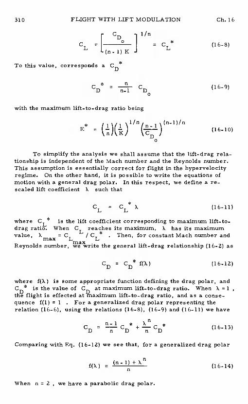
310 FLIGHT WITH LIFT MODULATION Ch. 16
r CD
CL= L(n 1)K -1
= CL* (16-8)
To this value, corresponds a CD*
CD*=
(16-9)
with the maximum lift-to-drag ratio being
*E = (16-10)
n K CD
To simplify the analysis we shall assume that the lift-drag rela-tionship is independent of the Mach number and the Reynolds number.This assumption is essentially correct for flight in the hypervelocityregime. On the other hand, it is possible to write the equations ofmotion with a general drag polar.In this respect, we define a re-scaled lift coefficient X such that
CL = CL* X (16-11)
where CL* is the lift coefficient corresponding to maximum lift-to-drag ratio. When CL reaches its maximum, K has its maximumvalue, K = C / C *
. Then, for constant Mach number andmax L LReynolds number, the general lift-drag relationship (16-2) as
CD = CD* f(X) (16-12)
where 1(X) is some appropriate function defining the drag polar, andCD* is the value of CD at maximum lift-to-drag ratio.When K =1
the flight is effected at maximum lift-to-drag ratio, and as a conse-quence f(l) =1 . For a generalized drag polar representing therelation (16-6), using the relations (16-8), (16-9) and (16-11) we have
C - C*
+ -h-— C * (16 13)D n D n D -
Comparing with Eq. (16-12) we see that, for a generalized drag polar
f(X)= (n-l)+X (16-14)
When n =2 , we have a parabolic drag polar.
Ch. 16 FLIGHT WITH LIFT MODULATION 311
16-3. UNIFIED EQUATIONS WITH VARYING LIFT COEFFICIENTAND BANK ANGLE
The dimensionless equations, using modified Chapman's vari-ables, have been derived in Chapter 13.The equations can be used toanalyze motion with modulation of the lift coefficient and the bank angleif we assume that the drag coefficient remains unchanged.Thissimplification has been used by various authors, but, as has beenpointed out in Chapter12 on the entry corridor, strong couplingbetween the drag and the lift coefficients has important effects onentry physical quantities.Thus, the lift-drag relationship must beconsidered for accurate analysis.
We recall the equations for constant lift coefficient and bank anglederived in Chapter 13.We have
dZ=
du = - r1+ cosotany+ds cosv L CD
2= Z
+cosy (1 - cos
ds cosy LCD
dO -ds —
=
= z [CL - cos2 y tan4](16-15)
cosy D
where in spherical coordinates, the position of the vehicle is definedby its altitude, through the variable Z, longitude 0 and latitudeThe velocity vector is specified by the variable u, the flight pathangle y and the heading angle . The angle o- is the bank angle.
The variable Z and u , called Chapman's modified variablesare defined as
PSCD
= Zm
2 2
uV cos (16-16)gr
while the independent variables is the dimensionless arc length
s = f .! cos y dt (16-17)
FLIGHT WITH LIFT MODULATION Ch. 16
For flight with lift modulation, since the drag coefficient CD is vary-ing, in the definition of the variable Z, we replace CD by theconstant CL* , that is
pSCz 2mL (16-18)
Also, it has been found convenient to replace u by the variable vdefined as
= U2 (16-19)cos y
Hence the variable v is the square of the dimensionless speed.Withthese modifications, and using Eqs. (16-11) and (16-12), it is seenthat the new equations are
dZ= Ztany
dv - Z vf(X)- (2-v)
ds E* cos
= +cos'y
(1 _!)ds v
dO -ds — cos4
= sin4i
Z X- cos tan
cos
where E = is the maximum lift-to-drag ratio.Equations (1 6-20) are in the form suitable for the analysis of
entry with lift and bank modulation (Refs. 3-4) and even for the optimi-zation of such entry trajectories (Ref s.5_7).
With lift and bank modulation, the entry trajectory can be control-led in such a way that a certain requirement can be satisfied.Forexample, one may control the glide angle to be constant or the rate ofdescent, also called the sinking speed, to have a predetermined value.The required lift modulation to keep the vehicle along such a trajectorywill be analyzed in the next chapter.In the following section we shalldiscuss the characteristics of each family of trajectories satisfying aspecified condition.
Ch. 16 FLIGHT WITH LIFT MODULATION 313
16-4. TRAJECTORY IN THE PHASE SPACE
We shall consider lift-modulated entry trajectories in the planeof a great circle. Hence, taking o = 0 , the equations of interestare
dZ=
dv = - Zvf(X)do
= + 1 - (16-21)dO cosv v
where, as in Chapter 13, the quantity 3r will be considered asconstant with = 900 for the Earth's atmosphere.In planar entrythe independent variables becomes the range angle0 . Here thevariable Z and v are defined by the Eqs. (16-18) and (16-19) respec-tively.
it is convenient for the representation and visualization of thetrajectory to use a cylindrical coordinate system (v, y, w) where
w= 1 (16-22)
In this way, w varies in the same direction as the altitude (Fig. 16-2).
wu
0
Fig. 16-2. Trajectory in the phase space.
314 FLIGHT WITH LIFT MODULATION Ch. 16
Let us assume that the entry trajectory is such that a certainrelationship exists among the three variables, speed, flight path angle,and altitude
F(v , y, w) = 0 (16-23)
Then, in the phase space the totality of entry trajectories satisfyingEq. (16-23) forms a two-dimensional surface.Hence, if two differentconstraints must be satisfied simultaneously, the trajectory, ifphysically possible, is in general unique, being the intersection of twoconstraining surfaces. We shall consider these constraining surfacesin the following cases:16-4. 1. Flight at Constant Flight Path Angle
In this flight program, we have constantly
=(16_24)
where is the initial flight path angle.In the phase space, thetrajectory must lie on the vertical plane defined by Eq. (16-24).Inthe (v, plane the trajectory is a straight line while in the physicalplane of the great circle it is a logarithmic spiral.
16-4.2. Flight at Constant Rate of Descent
The rate of descent, or sinking speed V, is the verticalcomponent of the velocity
V = V sin y (16-25)
In dimensionless form, by expressing that the sinking speed is con-stant, we have the relation
v sin2 y = C (16-26)
where C is a constant.In the phase space, the trajectory must lieon a cylinder whose projection in the(v, y) plane is the curve definedby Eq. (16-26).
A geometric construction of this curve is as follows.In thev , y) plane, we draw a circle with center at the origin and radiusC.
Since C is the square of the dimensionless sinking speed, this circleis small if the sinking speed is small.At the point P on the circle,defined by the polar angle y, we draw the perpendicular PQ to theradius OP and then the perpendicular QR to OQ as shown in Fig.16-3. The intersection R of this perpendicular and the radius OPis on the curve. The point R describes the curve as given by Eq.(16-26) in dashed line as the point P moves on the circle.
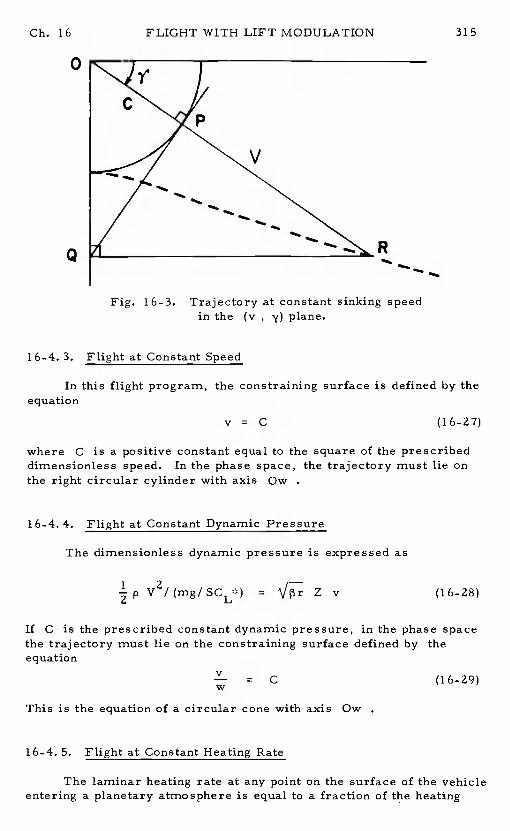
Ch. 16 FLIGHT WITH LIFT MODULATION 315
Fig. 16-3. Trajectory at constant sinking speedin the (v , 'y) plane.
16-4.3. Flight at Constant Speed
In this flight program, the constraining surface is defined by theequation
v = C (16-27)
where C is a positive constant equal to the square of the prescribeddimensionless speed. In the phase space, the trajectory must lie onthe right circular cylinder with axis Ow
16-4.4. Flight at Constant Dynamic Pressure
The dimensionless dynamic pressure is expressed as
p (mgi SCL*) = V (1 6-28)
If C is the prescribed constant dynamic pressure, in the phase spacethe trajectory must lie on the constraining surface defined by theequation
= C (16-29)
This is the equation of a circular cone with axis Ow
16-4.5. Flight at Constant Heating Rate
The laminar heating rate at any point on the surface of the vehicleentering a planetary atmosphere is equal to a fraction of the heating
0
Q
V
R
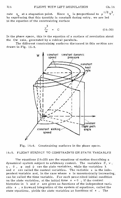
316 FLIGHT WITH LIFT MODULATION Ch. 16
rate q at a stagnation point. Since q is proportional to p V3by expressing that this quantity is constant during entry, we are ledto the equation of the constraining surface
3
= Cw
(16- 30)
In the phase space, this is the equation of a surface of revolution aboutthe Ow axis, generated by a cubical parabola.
The different constraining surfaces discussed in this section aredrawn in Fig. 16-4.
Fig. 16-4. Constraining surfaces in the phase space.
16-5. FLIGHT SUBJECT TO CONSTRAINTS ON STATE VARIABLES
The equations (1 6-20) are the equations of motion describing adynamical system subject to arbitrary control.The variables Z, v
U , and are the state variables, while the variables Xand o are called the control variables.The variable s is the inde-pendent variable and, in the case wheres is monotonically increasing,can be called the time variable.For each prescribed initial conditionon the state variables, at the initial times 0 , if the controlhistories in X and o- are given as functions of the independent vari-able s , a forward integration of the system of equations, called thestate equations, yields the state variables as functions ofs . The
constantspeed
Ch. 16 FLIGHT WITH LIFT MODULATION 317
plot of the state variables in the phase space will be called the trajec-tory.
In general, we consider an n-dimensional dynamical systemgoverned by the system of differential equations
= f. t) (16—31)
j=l,2 n
where x is the n-dimensional state vector
= (x1 ,x) (16-32)
and u is the rn-dimensional control vector
u = (u , u u ) (16-33)1 2 m
In general u is an element of U, where U is the bounded, m-dimensional control space.For example, in the Eqs. (16-20), we cantake u1 =X and u2 = . If the lift coefficient X and the bankangle are bounded, U is defined by
x— max
1o1 < o (l6_34)— max
where X is the maximum rescaled lift coefficient anda-max maxis the maximum allowable bank angle.In the previous section, we gave examples where some of the
state variables are related by certain equation which must be satisfiedalong the trajectory. These equations impose constraints on the tra-jectory. In general, if the relations are independent of the controls,they are of the form
Fk(x , t) = 0 (16-35)
k=1,2 p.Each of the p relations (16-35), if it is time independent, defined a(n_1)_dimensional surface in the n-dimensional phase space.Thetrajectory satisfying the relation must lie on this constraining surface.In particular, the initial point must be taken on the surface itself.When the relation depends on the time, we can still consider it asdefining a varying constraining surface.However, in this presentanalysis we shall invariably consider time independent state equations
318 FLIGHT WITH LIFT MODULATION Ch. 16
= f.R, (16-36)
j=l,2 . n.
and time independent constraining relations
= 0 (16-37)
k=l,2 ,..., p.Consider the casep = 1 , and the constraining surface F1 =0
in the n-dimensional spaceE° (Fig. 16-5 ). Let I be the initialpoint taken on the constraining surface.The trajectory starting from
the surface. Using the constraining relationF1(x) = 0 , we can express one of the state variables, say x, interms of the remaining (n-i) variables.Hence, we can delete theequation for x from the system (16-36).Furthermore, the conditionfor the trajectory to lie on the constraining surface requires that, ateach instant, the tangent to the trajectory is also a tangent of the sur-face. That is, it is orthogonal to the normal N of the surface at thepoint. Mathematically, this is expressed by taking the differential ofthe Eq. (16-37)
DF DF DFdx + —h- dx + . . . + dx = 0 (16-38)
Dx 1 Dx 2 Dx n1 2 n
This equation expresses the of the vector velocityV = (dx.! dt) and the normal N =(aFk/ Dx.)
Usi1ng the state equations (16-36), we can3write this equation as
8Fk— f. (x , u) = 0 (16-39)
• Dx. jj=l j
At each instant, Eq. (16-39) can be satisfied by a proper selectionof the vector control u in its bounded space.The trajectory cannotbe generated if u cannot be found within its bound.If p = 1 , and ifu has only one component u1, then from Eq. (16-39) , u1 can beobtained in terms of the remaining (n-i) state variables.Substitutinginto the remaining (n-i) state equations and integrating from the initialconditions, we generate a unique trajectory.(In some instances,Eq. (16- 39) provides more than one solution for u1and the properselection of the control is dictated by physical considerations.
In general, the number of constraints cannot exceed the numberof controls, that isp < m • If p < m , then, from the p equations(16..39), (rn- p) components of the control vector ucan be selectedarbitrarily in some manner in the bounded space U
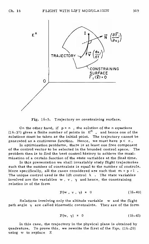
Ch. 16 FLIGHT WITH LIFT MODULATION 319
On the other hand, if p =n , the solution of the n equations(1 6-37) gives a finite number of points in En, and hence one of thesolutions must be taken as the initial point.The trajectory cannot begenerated as a continuous function.Hence, we must have p <n
In optimization problems, there is at least one free componentof the control vector to be selected in the bounded control space.Theproblem then is to find the best control history to achieve the maxi-mization of a certain function of the state variables at the final time.
In this presentation we shall invariably study flight trajectoriessuch that the number of constraints is equal to the number of controls.More specifically, all the cases considered are such that m =p = 1
The unique control used is the lift control X. The state variablesinvolved are the variables w ,v , y and hence, the constrainingrelation is of the form
F(w , v , = 0 (16-40)
Relations involving only the altitude variablew and the flightpath angle 'y are called kinematic constraints.They are of the form
F(w, 'i') = 0 (16-41)
In this case, the trajectory in the physical plane is obtained byquadrature. To prove this, we rewrite the first of the Eqs. (16-20)using w to replace Z
0
Fig. 16-5. Trajectory on constraining surface.
FLIGHT WITH LIFT MODULATION Ch. 16
= wtan'y (16-42)
From Eq. (16-41) we obtain y as function of w, to be used inEq. (16-42). Thus, w is obtained by quadrature.
This provides the equations for the trajectory in the physicalplane.
= f1(0)
= (16-43)
On the other hand, constraining relations involving only thespeed v and the flight path angley give directly the trajectory inthe ( v, y ) plane. Such trajectory constraints will be analyzed inChapter 17. General relations such as Eq. (16-40) are dynamicconstraints.
References
1. Busemann, A., Vinh, N. X., and Culp, R. D.,OptimumManeuvers of Hypervelocity Vehicles Using Thrust and/or Aero-dynamic Force, ' ARL Report No. TR-74-0104, Vol. IV, USAF,1974.
2. Miele, A., Flight Mechanics, Vol.1, Theory of Flight Paths,Addison-Wesley Publishing Company, Inc. ,Reading, Massa-chusetts, 1962.
3. Bletsos, N.A., 'Performance and Control with Lift Modulationof Hypervelocity Entry Vehicles, "Ph.D. thesis , The Univer-sity of Michigan, 1976.
4. Vinh, N. X., Bletsos, N. A., Busemann, A., and Cuip, R. D.,"Flight with Lift Modulation Inside a Planetary Atmosphere,"AIAA Journal, Vol. 15, No. 11, pp. 1617-1623, 1977.
5. Vinh, N. X., Bus emann, A., and Culp, R. D., 'Optimum Three-Dimensional Atmospheric Entry, "Acta Astronautica, Vol. 2,pp. 593-611, 1975.
6. Frostic, F., and Vinh, N.X., "Optimal Aerodynamic Control byMatched Asymptotic Expansions, "Acta Astronautica, Vol. 3,pp. 319-332, 1976.
7. Vinh, N. X., and Chern, J. S., "Three-Dimensional OptimumManeuvers of a Hypervelocity Vehicle, "IAF paper No. 79-F-184, presented at the XXXth Congress of the InternationalAstronautical Federation, Munich, September 1979.
Chapter 17
Lift Modulation with Constraintson Speed and Flight Path Angle
17-1. STATE AND CONSTRAINT EQUATIONS
The equations for flight with variable lift and bank control werederived in Chapter 16.For flight along a great circle, with the vari-ables
pSC 1—v — ,
= L (17-1)gr 2m
the state equations are
dZ=
dv = Zvf(X)dO E cosy
=Z X
+ - (l7_Z)dO cosy v
The rescaled lift coefficient X is used as a control and has beendefined as
CLX = (17-3)
CL
where CL* is the lift coefficient corresponding to maximum lift-to-drag ratio, E* = (LID) . Hence, when X = 1 the flight is atmaximum lift-to-drag The lift coefficient is bounded by anupper limit and proportionally we have the constraint on the lift control
!X1 < X (17-4)— max
321
LIFT MODULATION WITH CONSTRAINTS Ch. 17
The function f(X) = CD! CD* is the resealed drag coefficient.Itsform is dictated by the drag polar.In particular, for a parabolicdrag polar
f(X)= 1 X2 (17-5)
For planar entry, to visualize the trajectory in the phase space,in Chapter 1 6, it has been found convenient to change the variable Zinto the variable w such that
w = 1 (17-6)
In this way, since w is the inverse of the density of the atmosphere,it varies in the same direction as the altitude.Then, we have theequations of motion in the variables w, v and'y , using a parabolicdrag polar
dwd8 = 3r wtany
dv v(1+X= - - (Z-v)tany
E* w cos
= x+ - (17-7)
w cos y
In Chapter 16, we have seen that if a constraint of the form
F(v , , w) = 0 (17-8)
is imposed upon the entry variables, then it is possible to deduce thelift control law to flight the vehicle along this constraint.Once acertain constraint is prescribed, it is of interest to study the behaviorof the lift control along the flight. The analysis would be valuable tomission planning and design of guidance system.Several trajectoriesof practical interest have been analyzed in Ref. 1.In this chapter thefollowing flight trajectories will be considered:
a! Flight at constant flight path angle.The constraining relation is simply
=(17-9)
where 'y. is the initial flight path angle.b! at constant sinking speed.
The constraining relation in this case is
vsin2.y = C (17_b)
Ch. 17 LIFT MODULATION WITH CONSTRAINTS 323
where the constant C is the square of the dimensionless sinking speed.For each flight program, the lift control required to satisfy the
constraining relation will be derived.The variation of the state vari-ables and the behavior of the trajectory in the phase space will beanalyzed. Pertinent properties of the flight path will be displayedexplicitly.
17-2. FLIGHT AT CONSTANT FLIGHT PATH ANGLE
In this flight program, it is required to keep the entry angleconstant throughout the portion of trajectory under consideration.Thisscheme is most attractive during the initial phase of descent, and alsoat a later phase during an approach before landing.
17-2.1. The Lift Control Law
The constraining relation is Eq. (17-9).Hence, dy/ dO = 0
and from Eq. (17-7), in terms of the variables v and w, the liftcontrol is given by
w cos y. (1 -v)X = (17-11)
The lift is positive for subcircular speed flight,v < 1 . Athigher speed, when v > 1, negative lift should be used to hold constantglide angle. Since y is constant, the first of the Eqs. (17-7) can beintegrated.
w = w. exp [ ( tan y1) 0 J (17-12)
In the plane of motion, the trajectory is a logarithmic spiral and, foran entry trajectory, < 0 , the haltitudeu w decreases accordingto the law (17-12)
17-2. 2. The Characteristic Curves
In the (v ,y) plane, the trajectory is the ray y =y. . In thephase space, the trajectory lies in the vertical plane(v , w) . Asimplification can be made by using the modified variable
Y w cos (17-13)
and the modified parameter
E. - E* tany. > 0 (17-14)
to replace w and E* respectively.The lift control is simply
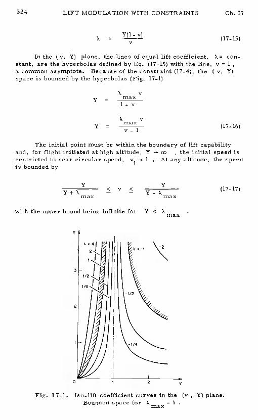
Y(1- v)(17-15)
In the (v, Y) plane, the lines of equal lift coefficient,X= con-stant, are the hyperbolas defined by Eq. (17-15) with the line, v =1
a common asymptote.Because of the constraint (17-4), the( v, Y)space is bounded by the hyperbolas (Fig. 17-1)
x= max
1-v
Y <V <Y+x — —max
Y
Y- X max(17-17)
with the upper bound being infinite forY C X
Fig. 17-1. Iso-lift coefficient curves in the(v , Y) plane.Bounded space for A = 1max
324 LIFT MODULATION WITH CONSTRAINTS Ch. U?
A vY = (17-16)
The initial point must be within the boundary of lift capabilityand, for flight initiated at high altitude, Y —w , the initial speed isrestricted to near circular speed,v. —. 1 . At any altitude, the speedis bounded by
V
max
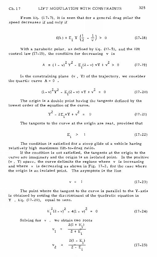
Ch. 17 LIFT MODULATION WITH CONSTRAINTS 325
From Eq. (17-7), it is seen that for a general drag polar thespeed decreases if and only if
f(X) + E. Y - —) > 0 (17-18)
With a parabolic polar, as defined by Eq. (17- 5), and the liftcontrol law (17_IS), the condition for decreasing v is
A (1 - v)2 Y2 - E.(2 - v) vY + V2 > 0 (17-19)
In the constraining plane(v , Y) of the trajectory, we considerthe quartic curve A =0
(1- v)2Y2 - E.(Z - v) vY + v2 = 0 (17_20)
The origin is a double point having the tangents defined by thelowest order of the equation of the curve.
- ZE.vY + V2 0 (17-21)
The tangents to the curve at the origin are real, provided that
E. > 1 (17—22)
The condition is satisfied for a steep glide of a vehicle havingrelatively high maximum lift-to-drag ratio.
If the condition is not satisfied, the tangents at the origin to thecurve are imaginary and the origin is an isolated point.In the positive(v , Y) space, the curve delimits the regions where vis increasingand where v is decreasing as shown in Fig. 17-2, for the case wherethe origin is an isolated point.The asymptote is the line
v = 1 (17-23)
The point where the tangent to the curve is parallel to the Y-axisis obtained by setting the discriminant of the quadratic equation inY , Eq. (17_20), equal to zero.
E.2(2 - v)2 - 4(1 - v)2 = 0 (17-24)
Solving for v , we obtain two roots2(1 + E.)
= 2+E.1
2(1 - E.)
= 2 - E.(17_25)
326 LIFT MODULATION WITH CONSTRAINTS Ch. 17
The first root is always positive and larger than1 . It givesthe point to the right of the asymptote with the value for Y
2(1 + E.)
1 E.1 (17-26)
This point is above the point
v3 = 1 , Y3 = (17-27)
where the curve intersects the asymptote. As expected, if the originis an isolated point,1 - E. > 0 , the second root is also positive.The corresponding value Y is
2(1 - E.)
= E.(17-28)
This point (v2 , Y2) is below the point (v1 , Y ) . It is above thepoint (v3 , Y ) if and only if 1 - ZE, > 0 . 'ike can verify that thepoint (v1 , is on the iso-lift coefficient hyperl5ola with x =-1,and the point (v2, Y2) is on the hyperbola with X =1
The point where the tangent to the curve is parallel to the v-axisis given by the value of Y
2= 1 -E.
(17-29)
It is positive if the origin is an isolated point.The correspond-ing value of v is
= 1 - (17-30)
The point (v4, Y4) is on the iso-lift coefficient hyperbola withthe value for X
X = E. (17-31)1
In the (v , Y) plane, the curves X =± X intersect thecurve A = 0 between the points v and v ifmtx < 1 . The
1 2 max—intersections are outside whenX > 1
The sense of variation of the19M coefficient along the trajectoryis given by the sign of the derivativedX /de . From Eq. (17-15) forX and using the state equations, Eqs. (17-7), we have
dX A= 3r X tan •y. + (17- 32)
Ev
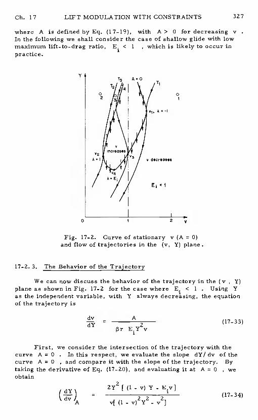
Ch. 17 LIFT MODULATION WITH CONSTRAINTS 327
where A is defined by Eq. (17-19),with A> 0 for decreasing vIn the following we shall consider the case of shallow glide with lowmaximum lift-to-drag ratio, E. < 1 , which is likely to occur inpractice.
Fig. 17-2. Curve of stationary v (A =0)and flow of trajectories in the(v, Y) plane.
17-2. 3. The Behavior of the Trajectory
We can now discuss the behavior of the trajectory in the (v ,Y)plane as shown in Fig. 17-2 for the case where E. <1 . Using Yas the independent variable, with Y always decreasing, the equationof the trajectory is
dv A2
(17-33)E.Y v
First, we consider the intersection of the trajectory with theA = 0 . In this respect, we evaluate the slope dY/ dv of theA = 0 , and compare it with the slope of the trajectory.Bythe derivative of Eq. (17-20), and evaluating it at A =0 , we
2Y2 [(1 -v)Y
v[ (1 - v) Y - V
02
Y
0
—t
v decraa5esV2
< I
0 2 v
curvecurvetakingobtain
f dY \dv
(17-34)
328 LIFT MODULATION WITH CONSTRAINTS Ch. 17
where subscript A means that (dY/ dv)A is the slope of the curve ALikewise the slope of the trajectory T is
E.Y2v(17-35)
Note that it is infinite at A =0 ; that is, at the intersection of thetrajectory and the curve A. Using Eq. (17-15) we can rewriteEq. (17- 34) as
dY2X2(X - E.)
= (X2 -1) (1-(17-36)
Moving clockwise around the curve A from infinity, see thatbetween the points v =1 + and v1 , X < 0 , X - 1 > 0 , andthe slope of the curve A=0is negative. Between the points v1 and
x 2 - < , X - E. < 0 and the slope is positive.Similarly,we see that the slope is between v4 and v2 and becomespositive between v7 and v =1 - The trajectory, in the caseE. < 1 of Fig. , can only intersect vertically the curve A =0afways in the decreasing direction of Y, as shown by the arrows. Weimmediately have the following properties:
a! The speed can only have one relative minimum and one rela-tive maximum with the relative minimum occurring first.
b/ Once through a relative maximum, the speed continues todecrease.
To discuss the behavior of the trajectory in terms of the initialpoint (v. , Y.) , we introduce the limiting trajectories T1, T2 andT3 as showA in Fig. 17-2.The trajectory T1 is obtained by integra-ting Eq. (17-33) forward and backward from the point(v1 , Y1) . Like-wise, the trajectories T2 and T3 are obtained by integrating forwardand backward from the points (v2, Y2) and (v3 , Y3 ) , respectively.By the existence and uniqueness of the solution of Eq. (17-33), thelimiting trajectories partition the flow of the trajectories in the(v, Y)space.
From the figure, the type of the trajectory can be classified interms of the initial point. For example, the trajectories initiated frompoints 1 and 2will have the speed continuously decreasing.The tra-jectories initiated from points 3 and 4 will have the speed decreasingfirst and then increasing after passing through a minimum.After theminimum, the speed will increase, pass through a maximum, andthen decrease again until the end.Speed along the trajectory initiatedfrom point 3 will remain subcircular, while the speed along the tra-jectory initiated from point 4 will go from subcircular to supercircular
be noted that the trajectory must remain within the iso-lift coefficient hyperbolas X =j Xmax and above the level Y =Y =
w w evaluated at sea
Gb. 17 LIFT MODULATION WITH CONSTRAINTS 329
Hence, the trajectory must be such thatK. < K . It terminateseither at the point whereIX = K whe're the lift capa-bility is reached, or at
=the vehicle has reached sea
level.
17-2. 4. The Variation of the Angle of Attack
It is interesting to follow the variation of the angle-of-attack alongthe trajectory. In this respect the lift control Kis useful. It variesin the same direction as the angle of attack, and furthermore, forK = 1 , the corresponding angle of attack is the one giving maximumlift-to-drag ratio for the case where K > 1 . In the case whereK < 1 , the maximum lift-to-drag ratio is reached at K =K
Eq. (17-32), the lift coefficient is increasing if and only ifmax
B - E.Xv3 + A > 0 (17-37)
In the (v, Y) plane, the curve B =0 delimits the region whereK is increasing (outside the curve) and where Kis decreasing (insidethe curve). The curve B =0 is plotted in Fig. 17-3 for the casewhere E. < 1 . Since B = 0 when K = 0 and A = 0 simultaneously,the curve A =0 and B = 0 have their intersection at the point (v3, Y3).Furthermore since B <0 when K > 0 and A < 0 , the portion ofthe curve A =0 on the left of the asymptote v =1 is entirely in theregion B< 0. Similarly, since B> 0 when K <0 and A> 0the portion of the curve A =0 on the right of the asymptote is entirelyin the region B > 0 . As a consequence, we have the followingproperties:
a! In the subcircular speed regime, the angle-of-attack passesthrough its stationary value with decreasing speed.
b/ In the supercircular speed regime, the angle-of-attackpasses through its stationary value with increasing speed.
This theorem can be made stronger by specifying that, in bothcases, the stationary value is a minimum, as we shall prove.Explicit-ly, we write the equation of the curve B =0
B = (l-v)2Y2_E1 [2 + (pr_l) v - v2]vY + v2 = 0
(17-38)
Like the curve A =0 , this quartic curve has the line v =I asthe vertical asymptote.The origin is a double point, and it is anisolated point if E. < 1 . The tangent to the curve is parallel to theY-axis when
[ 2 + ( 1) v- 13r v2} 2 - 4(1_v)2 = 0 (17-39)
The equation can be factored into two quadratic equations
330 LIFT MODULATION WITH CONSTRAINTS Ch. 17
E.v2 v-2(1+E.) 0
pr E.v2 - { - 1) E. + 2] v+ 2(1 - E.) = 0 (17-40)
The first equation provides one positive and one negative root.In the case where1 - E.> 0 , that is when the origin is an isolated
the second equation provides two positive roots, one root is lessthan 1 and the other root is larger than1 . If we write this secondequation as
- E.[ 2+ ( = 2(v_1)
we see that taking the root v >1 will make the coefficient of Y inEq. (17-38) positive hence providing a negative value for Y. Hence,the two positive roots of interest in the Eqs. (17_40) are the positiveroot of the first equation and the smaller positive root of the secondequation,
_________________________
2] + E.+212+v5 = (17—41)
2 E.
andE. + 2]- E.- +
= (17-42)2 E.
The root v5 is larger than1 and corresponds to the pointinside the A =0 curve. The corresponding value of Y is the doubleroot of the Eq. (17-38).Hence
V
= -l (17-43)5 v5-l
andVL
Y = , X = I (17-44)6 1-v6
If we rewrite the Eq. (17-38) as a cubic equation inv, thepoint where the tangent to the curve B =0 is parallel to the v-axis isthe point providing a double root in v. It can be shown that this isthe point
2X = E.(2 + v2) (17_45)
The point is in the range
Ch. 17 LIFT MODULATION WITH CONSTRAINTS 331
E. < X < 1 (17-46)
On the other hand, using Xto replace Y , we rewrite theequation (17-38) as
2X
- 1+ 1 = 0 (17-47)
(1 - v)
By eliminating X between the two equations (17-45) and (17.47) wehave a quintic equation to evaluate the value of v =v7 where thetangent to the curve B =0 is parallel to the v-axis.
E.)2v5 - E.)2v4 + + 1) -
4 (1 - = 0 (17-48)
Let us now consider the intersection of the trajectory with thecurve of stationary value for X, B 0 . Using the condition B =0
in Eq. (17-33) we have the slope of the trajectory at the point ofintersection
= = x(17 49)v(1-v) (1.v)2
On the other hand, if we evaluate the slope of the curve B =0
using Eq. (17-38), we have, after simplification
IdY' x2{zx -= (17-50)
1B (X2 - 1)(l - v)2
Referring to Fig. 17.3, we move along the curve B =0 from thepoint v = i + to the point v = 1 - in the clockwise direction.Between the point v =1 + E and the point v5 , X < - 1 , both thetwo slopes are negative, and
(dY\ > (dY\B
We find that this condition leads to
X 0 . Hence we have the possible intersectionindicated.
Between the point v5 and the point v3, X is negative and
332 LIFT MODULATION WITH CONSTRAINTS Ch. 17
< 1 , the slope (dY/dv)T is negative while the slope (dY/dv)Bis positive and again we have the trajectory going from inside thecurve B = 0 to outside the curve asa indicated by the arrows.Betweenthe point v3 and the point v7, X < 1 and
0 < ZX < E.(Z+13rv2)
Hence, the two slopes are positive.The condition
(dY\ (dY\
>
leads to
- v2) X + 1 > 0
Since the point is on the curve B =0 , Eq. (17-47) applies and we havethe condition
v 1)2 + 1]>
(1 - v)
This condition is satisfied since(1 - v) > 0
Similar arguments lead to the direction of intersection alwaysfrom inside the curve B =0 to outside the curve as shown in Fig.17-3. Hence, the intersection is always from dX / de <0 todX / d8 > 0 . The angle of attack considered as an algebraic quantitynever passes though a relative maximum and can only pass through arelative minimum once. More specifically, for positive a, thestationary value is a minimum while for negative a, the stationaryvalue is amaximum in absolute value.
The discussion is more enlightening if we plot the trajectory andthe curve A =0 and B = 0 in the (v , X) plane. In this plane, theequation of the curve A =0 is
2E.(2-v)X
-+ 1 = 0 (17-51)(1 - v)
The line v =1 is the vertical asymptote. The curve passesthrough the point X = 0 , v = 1 with a slope at that point equal to
= - (17-52)
For any v , the product of the roots of Eq. (17- 51) is = 1
Hence, the points where the tangent is vertical are the where= X2 =+ 1 . We have the values and v2 for v as found
previously in Eq. (17_25). In the (v , X) plane, the equation of the
Fig. 17-3. Curve of stationary K (B =0)and flow of trajectories in the (v, Y) plane.
curve B =0 has been given in Eq. (17- 47).The line v = 1 is thevertical asymptote. The curve also passes through the point K =0
v = 1 and has at that point the same tangent as the curve A =0 . Thepoints with vertical tangent also occur at K =± 1 , with the valuesv5 and v6 as given in Eq. (17-41) and (17-42).
Figure 17-4 presents the plots of the curves in the(v, K) plane.The limiting trajectories T1 , T, and T3 , as depicted in Fig. 17-2are also replotted in this figure. "Using these trajectories, we candescribe the behavior of the trajectory and the variation of the angle ofattack in terms of the initial condition.
For example, the trajectory starting from the point1 , atsupercircular speed begins with negative lift with the speed alwaysdecreasing and the lift coefficient always increasing.The trajectoryterminates whenever K =K or Y = Y
For the trajectory from the 2 , we first observethat by the uniqueness of the solution, it cannot cross the trajectoryT2 . Since the point 2 is on the left of the curve A =0 , and on theright of the curve B = 0 , the speed decreases continuously until theend while the angle of attack first decreases and then increases afterthe trajectory has intersected the curve B = 0
The trajectory starting from the point3 will be bounded by thetrajectory and the trajectory . Hence, the speed remainssubcircular w'hile the lift coefficient is always positive.The speedalong the trajectory will first increase to a maximum, and then de-crease. The lift coefficient will decrease to a minimum value and thenincrease to K at the end if the vehicle has not reached groundlevel. We that the maximum speed is reached before thelift coefficient attains its minimum value.
Ch. 17 LIFT MODULATION WITH CONSTRAINTS 333
B'
stationary
\A'O
V
Yo
increases
E1 < I
2
334 LIFT MODULATION WITH CONSTRAINTS Ch. 17
Fig. 17-4. Variations of the angle of attack and flowof trajectories in the(v , X) plane.
The trajectory starting from the point 4 will go supercircular.The lift coefficient decreases first, reaches a minimum with negativevalue, and then increases to X . The speed increases first andpasses through a maximum to its final value. Wealso notice that the maximum speed is reached after the point ofminimum lift coefficient.
It should be mentioned that the point v =1 , X = 0 must beconsidered as an accumulation point for all trajectories passing throughcircular speed, and not the point of intersection of the trajectories.At that point each trajectory has a different value of Y. In particular,the trajectory T , which has a cusp at the accumulation point, hasthe value Y =l?E.
3 1
17-2. 5. The Variation of the Dynamic Pressure
In general, along the entry trajectory at constant flight pathangle, the dynamic pressure increases continuously and reaches itsmaximum value either at ground level or at some critical altitude.Athorough discussion of the variation of the dynamic pressure for thistype of trajectory is given in Ref.1. Here we mention briefly a fewcharacteristics of the phenomenon.
The dimensionless dynamic pressure can be represented as
T3
4.
a
—1
< I
B • 0'A •
T1
Ch. 17 LIFT MODULATION WITH CONSTRAINTS 335
2(l/2)pV —(17 53)mgcos - -
Hence, in the (v , Y) plane, the lines with constant dynamicpressureare the rays passing through the origin. As a consequence,when the vehicle passes through the point of maximum dynamic pres-sure, in the (v , Y) plane, the tangent to the trajectory passes throughthe origin. We obtain the equation of the curve of stationary dynamicpressure by writing
- = 0 (17-54)
Using Eq. (17- 33) we get the condition for increasing dynamic pressure
Cn A - E. Yv2 < 0 (17-55)
Hence, the dynamic pressure increases in the region where the speedincreases (A < 0) . In the (v , Y) plane, if we plot the curve ofstationary dynamic pressure,C = 0 , the curve is entirely outsidethe curve A 0 On the other hand, from Eq. (17-3 7) and (17- 55),by writing
B = C + prE.Yv3 (17-56)
we see that for B =0 , C < 0 . The curve C =0 is entirely outsidethe curve of stationary X, B = 0 . As a consequence, minimum liftcoefficient is reached while the dynamic pressure is increasing.
As a final remark for this case of entry at constant flight pathangle, we should mention that, for a typical entry vehicle, the ofw (or equivalently Y ) is rather small, of the order of 2 x l0 at15 km , reaching 2 at 30 km and 1. 29 at 60 km. For prac-tical applications, in the(v , Y) plane, the region of interest is theregion at subcircular speed below the curve A = 0 where the speeddecreases along the trajectory.
The case of vertical entry, y. =- 900 is trivial. The case of
constant altitude, coasting flight, y. = 0 has many interesting charac -teristics. This case has been discu1ssed in detail by the authors inRef. 2
FLAT EARTH TRANSFORMATION
In the second specific example, the rate of descent, or sinkingspeed, is kept at a constant value.This is a flight program of practi-cal interest during the approach phase.The speed is relatively small;hence, an analysis using a flat planet model is adequate.
It must be emphasized here that the general equations (17- 7),which are exact equations, can be used but to the scale of altitude and
336 LIFT MODULATION WITH CONSTRAINTS Ch. 17
range considered, it is better to change the variables, say the rangeangle 8 in radians, into dimensionless linear range and disregardterms that are trivially small.In this purpose, instead of startingwith the equations for flight over a flat planet and introducing theappropriate dimensionless transformation, it is enlightening to performthe transformation directly on the basic equations (17-7).
For a flat planet model, we define the dimensionless linear range
x a 8 (17-57)
and use the new altitude and speed variables
2mpz a w
PSCL
V a (17-58)
Using these definitions in Eqs. (17-7), we have
dz=
— 2 —dv v(l+X ) v— = - _(2_—)tanydx E*zcosy
= X - + (17-59)dx zcosy v f3r
Now, for nearly all planetary atmospheres, is large and in thescale of speed considered v is now of the order of unity. Hence, itis trivial that the term 1 / is negligibly small, and we have thedimensionless equation for flight over a flat planet.
dz= ztany
dv v(1 + X2)— = - -2tanydx zcosy
X- (17-60)dx zcosy v
We obtain identical equations by starting from equations for flight overa flat planet. One interesting fact is that the new equations are freeof the characteristic of the atmosphere although we continue to referto the planet as the Earth.
Ch. 17 LIFT MODULATION WITH CONSTRAINTS 337
17-4. FLIGHT AT CONSTANT SINKING SPEED
For this flight program, we write the constraining relation(17—10) as
sin2 = K2 (17-61)
where K is a positive constant representing the absolute value of thedimensionless sinking speed.
17-4.1. The Lift Control Law
By taking the derivative of Eq. (17-61) using the state equations(17-60), we have the lift control law
siny - 2E* X cosy + sin y +(2E* z sin2 y/ K2) = 0 (17-62)
At each instant, the lift coefficient required to maintain constant sink-ing speed K is obtained by solving this quadratic equation in XSince sin < 0 , then if
z > - K2! 2E* sin 'y (17-63)
we have a positive and a negative lift coefficient.Positive lift shouldbe selected to reduce deceleration. When condition (17-63) is reversed,both roots are negative and low negative root must be selected.
Since the altitude is decreasing, the flight is terminated when-ever the variablez reaches the ground level valuez or whenIX = X or when Eq. (17-62) no longer has real Fromthis the condition for real roots is
2.2 2 2- K (sin y - E* cos 'y) (17-64)
2E* sin 'y
17-4. 2. Domain of Flight in the (y , X) Space
The discussion of the variation of the angle of attack, or equiva-lently the lift coefficient, along the descending trajectory with constantsinking speed can be explicitly carried out in the (y, X) space.
In this space, the constraint on maximum lift capability is repre-sented by the linesX = + X . On the other hand, the boundaryfor real roots, as given by sign in Eq. (17-64), with zobtained from Eq. (17- 62) is simply
X = E*coty (17-65)
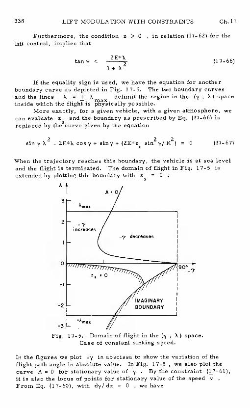
338 LIFT MODULATION WITH CONSTRAINTS Ch. 17
Furthermore, the conditionz > 0 , in relation (17-62) for thelift control, implies that
ZE*Xtany<a1+ X
(17-66)
If the equality sign is used, we have the equation for anotherboundarycurve as depicted in Fig. 17-5. The two boundary curvesand the lines X = + X delimit the region in the (y , K) spaceinside which the flight is possible.
More exactly, for a given vehicle, with a given atmosphere, wecan evaluatez and the boundary as prescribed by Eq. (17-66) isreplaced by the curve given by the equation
sin'j K2 - ZE*X cosy + siny + (ZE*z sin2y/1C2) = 0 (17-6 7)
When the trajectory reaches this boundary, the vehicle isand the flight is terminated.The domain of flight in Fig.extended by plotting this boundary with z= 0
Fig. 17-5. Domain of flight in the (y , K) space.Case of constant sinking speed.
at sea level17-5 is
In the figures we plot -yin abscissa to show the variation of theflight path angle in absolute value.In Fig. 17-5 , we also plot thecurve A = 0 for stationary value of y. By the constraint (17-61),it is also the locus of points for stationary value of the speed vFrom Eq. (17-60), with dy/dx =0 • we have
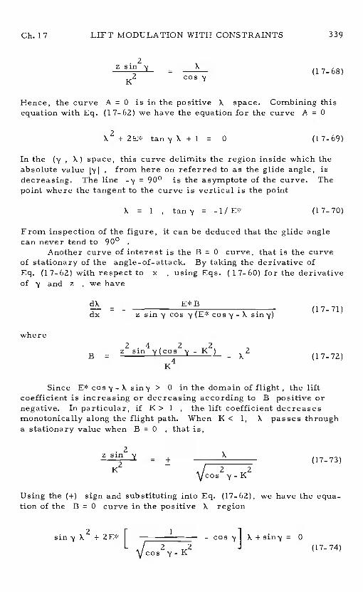
Ch. 17 LIFT MODULATION WITH CONSTRAINTS 339
.2zsin = x (1768)K2 -
Hence, the curve A =0 is in the positive X space. Combining thisequation with Eq. (17-62) we have the equation for the curve A =0
+ tan y X + 1 = 0 (17-69)
In the ('s' , X) space, this curve delimits the region inside which theabsolute value M from here on referred to as the glide angle, isdecreasing. The line -'s' = 900 is the asymptote of the curve.Thepoint where the tangent to the curve is vertical is the point
X 1 , tan = _1/E* (17—70)
From inspection of the figure, it can be deduced that the glide anglecan never tend to 900
Another curve of interest is the B =0 curve, that is the curveof stationary of the angle-of-attack.By taking the derivative ofEq. (17-62) with respect tox , using Eqs. (17-60) for the derivativeof 'y and z , we have
dX -7 7dx - - z sin'y cos (1 - 1)
where 2.4 2 2
B= z sin \l(cos - K ) - (17-72)
K
Since E* cos y -X siny > 0 in the domain of flight, the liftcoefficient is increasing or decreasing according to B positive ornegative. In particular, if K> I , the lift coefficient decreasesmonotonically along the flight path.When K < 1, X passes througha stationary value when B =0 , that is,
.2z sin y= +
X (17-73)K2 — I 2 2y-K
Using the (+) sign and substituting into Eq. (17-62), we have the equa-tion of the B = 0 curve in the positive X region
y + 2E* [ 1 - y1 + siny = 0L / 2 2 J (17-74)y-K
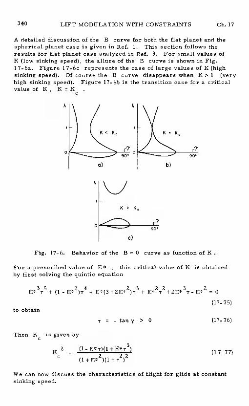
340 LIFT MODULATION WITH CONSTRAINTS Ch. 17
A detailed discussion of the B curve for both the flat planet and thespherical planet case is given in Ref. 1.This section follows theresults for flat planet case analyzed in Ref. 3.For small values ofK (low sinking speed), the allure of the B curve is shown in Fig.l7-6a. Figure 17-6c represents the case of large values of K (highsinking speed). Of course the B curve disappears when K> 1 (veryhigh sinking speed).Figure l7-6b is the transition case for a criticalvalueof K, KK
KC
K >
90
c)
Fig. Behavior of the B =0 curve as function of K
For a prescribed value of E*, this critical value of K is obtainedby first solving the quintic equation
E*3T5 + (1 - E*Z)r4 + E*(3 + + E*2T2 + 2E*3r_ E*2 = 0
(17- 75)
to obtain
T = - > 0 (17-76)
Then K is given by
K2 - (17 77)
C - (1+E*2)(1+T2)2 -
We can now discuss the characteristics of flight for glide at constantsinking speed.
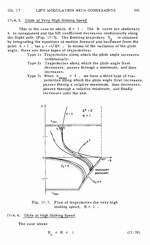
Ch. 17 LIFT MODULATION WITH CONSTRAINTS 341
1 7-4. 3. Glide at Very High Sinking Speed
This is the case in which K >1 . The B curve for stationaryX is nonexistent and the lift coefficient decreases continuously alongthe flight path (Fig. 17- 7). The limiting trajectory T1 is obtainedby integrating the equations of motion forward and backward from thepoint X = 1 , tan 'y = -1/ E* . In terms of the variation of the glideangle, there are three types of trajectories:
Type 1: Trajectories along which the glide angle increasescontinuously.
Type 2: Trajectories along which the glide angle firstdecreases, passes through a minimum, and thenincreases.
Type 3: When X > 1 , we have a third type of tra-which the glide angle first increases,
passesthroug a relative maximum, then decreases,passes through a relative minimum, and finallyincreasesuntil the end.
Fig. 17-7. Flow of trajectories for very highsinking speed, K> 1
17-4. 4. Glide at High Sinking Speed
The case where
K < K < 1 (17-78)
0
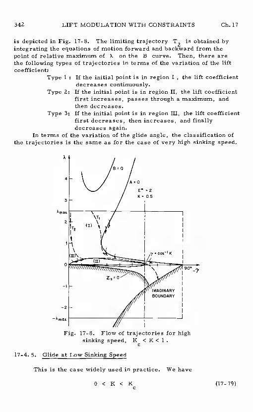
LIFT MODULATION WITH CONSTRAINTS Ch. 17
is depicted in Fig. 17-8. The limiting trajectory T2 is obtained byintegrating the equations of motion forward and backward from thepoint of relative maximum of Xon the B curve. Then, there arethe following types of trajectories in terms of the variation of the liftcoefficient:
Type 1: If the initial point is in region I, the lift coefficientdecreases continuously.
Type 2: If the initial point is in region II, the lift coefficientfirst increases, passes through a maximum, andthen decreases.
Type 3: If the initial point is in region Ill, the lift coefficient
first decreases, then increases, and finallydecreases again.
In terms of the variation of the glide angle, the classification of
the trajectories is the same as for the case of very high sinking speed.
Amax
—1
—2
Fig. 17-8. Flow of trajectories for high
sinking speed, Kc < K C 1.
17-4. 5. Glide at Low Sinking Speed
This is the case widely used in practice. We have
0< K< Kc
(17-79)
0
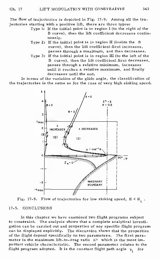
Ch. 17 LIFT MODULATION WITH CONSTRAINTS 343
The flow of trajectories is depicted in Fig. 17-9.Among all the tra-jectories starting with a positive lift, there are three types:
Type 1: If the initial point is in region I (to the right of theB curve), then the lift coefficient decreases contin-uous ly.
Type 2: If the initial point is in region II (inside the Bcurve), then the lift coefficient first increases,passesthrough a maximum, and then decreases.
Type 3: If the initial point is in region Ill (to the left of theB curve), then the lift coefficient first decreases,passes through a relative minimum, increasesuntil it reaches a relative maximum, and finallydecreases until the end.
In terms of the variation of the glide angle, the classification ofthe trajectories is the same as for the case of very high sinking speed.
Fig. 17-9. Flow of trajectories for low sinking speed, K <K
17-5. CONCLUSIONS
In this chapter we have examined two flight programs subjectto constraint. The analysis shows that a complete analytical investi-gation can be carried out and properties of any specific flight programcan be displayed explicitly.The discussion shows that the propertiesof the flight depend specifically on two parameters.The first para-meter is the maximum lift-to-drag ratio E* which is the most im-portant vehicle characteristic.The second parameter relates to theflight program adopted. It is the constant flight path angle for
Amax
Amax
344 LIFT MODULATION WITH CONSTRAINTS Ch. 17
the first problem and the constant sinking speed K for the secondproblem. The types of trajectories are classified according to eitherthe variation of a state variable, speed or flight path angle, or thevariation of the control variable, the lift coefficient.The variations ofthese variables along the trajectory depend on the initial condition.
Two accessory parameters are involved in the discussion,namely, the maximum rescaled lift coefficient X and the vehiclesea-level parameter wor z . These have no influenceon the behavior of the They only limit the domain of flighteither in the physical plane or in the control plane.
References
1. Bletsos, N.A., 'Performance and Control with Lift Modulationof Hypervelocity Entry Vehicles, "Ph.D. thesis, The Universityof Michigan, 1976.
Z. Bus emann, A., Vinh, N. X., and Culp, R. D., "Optimum Altitudefor Coasting Flight of a Hypervelocity Vehicle, 'The Journal ofthe Astronautical Sciences, Vol. XXI, No. 1,pp. 32-48, 1973.
3. Vinh, N. X., Bletsos, N. A., Bus emann, A., and Cuip, R. D.,"Flight with Lift Modulation Inside a Planetary Atmosphere,Paper No. 76.105, 27th International Astronautical Congress,Anaheim, California, U.S.A., 1976.Also, AIAA Journal,Vol. 15, No. 11, pp. 1617-1623, 1977.
Chapter 18
Lateral Maneuvers
18-1. INTRODUCTION
One interesting aspect of lifting entry is that the vehicle can rotatethe lift force out of the vertical plane, thus creating a lateral componentwhich can be used to change the heading.In this final chapter we shallconsider such lateral maneuver.Of particular interest is the maximumlateral range which can be attained from a prescribed entry condition.Further consideration will be given to a maximum area on the surfaceof the planet which can be reached by the entry vehicle.
For convenience, we reproduce the dimensionless equations ofmotion for entry into a nonrotating spherical atmosphere derived inChapter 16, using a parabolic drag polar. We have
dZ= - I3rZtany
dv - Zv (1+X2)- (2-v) tands E*cosV
=I X coso + (1-!)
ds cosy L V
- cos4ids —
coscos
where by definition
345
346 LATERAL MANEUVERS Ch. 18
z- PSCL* r= 2m VP
2
v (18-2)gr
The product characterizing the atmosphere will be considered asconstant with the value = 900 for the Earth. The controls are thebank angle and the rescaled lift coefficient
CLX = (18-3)
L
where CL* is the lift coefficient corresponding to maximum lift-to-drag ratio E* . For a hypervelocity entry vehicle Etis in therange 1-3 . The independent variable s is the dimensionless arclength
ts
= J'X. cos 'y dt . (18-4)
0
18-2. EQUILIBRIUM GLIDE CONDITION
For entry from low altitude orbit, the initial speed is nearlycircular. Furthermore, for moderate lift, the flight path angle can bekept small and nearly constant.This is the condition of equilibriumglide discussed previously.Hence, we shall take y 0 and havethe reduced equations
dv - Z v(l+X2)ds - -
dO cos4,ds - cos$
= sin4i
-p Z X sing- - cos iji (18-5)
We recall that 0 is the longitudinal range,4 is the lateral range, orlatitude if the reference plane is taken as the equatorial plane.Theangle i4i is the heading angle measured from the reference plane.Theequation for y becomes the equilibrium equation
Xcosg- = (l-v) (18-6)
Ch. 18 LATERAL MANEUVERS 347
This equation shows that the vertical component of the lift force is usedto balance the combined gravity and centrifugal force.The equation isused to evaluate the "altitude'Z in terms of the kinetic energy vUpon substituting into Eqs. (18-5), we have
dv - (l-v)(l+X2)ds — - E*X cos o
dO -ds — cos4,
=
= (lv_v)
tan o- - cos tan (18-7)
18-3. MAXIMUM LATERAL RANGE
The equations (18-7) constitute the state equations for the fourmain variables v ,0 , and . For equilibrium glide from circu-lar speed we have at the initial time
1 , B = 0, = 0 , = 0 (18-8)0 0 0 0
It is proposed to use lift and bank control, in the variables Xand rto achieve a maximum lateral range when the speed has reduced to afinal low speed Vf = 0 . A full treatment will require the tool ofmodern optimum control theory and we refer to Ref. 1.A sub-optimumcontrol law will be discussed in this chapter.
First, from the equation for v, it is seen that the speeddecreasescontinuously. In atmospheric maneuvers at high speed, thekinetic energy is an important element since itcan be used for an ex-change with the potential energy, hence gaining the necessary altitudeto extend both longitudinal and lateral ranges.Then, for a given bankangle, to minimize the decrease in the speed, we minimize the right-hand side of the equation for v, the first of Eqs. (18-7), with respectto the lift control X . This gives
X = 1 (18-9)
The optimal glide should be performed at maximum lift-to-drag ratio.To achieve a maximum lateral range, the bank angle must be
modulated in an optimum manner.In general, for maximum lateralrange the optimum bank angle varies as a function of the time from amaximum permissible value,a- = a- , at the initial time, to thevalue zero at the final time (Refs.1 , shall assume that thereexists a certain average constant value for the bank angle providingcomparable performance.Furthermore, in order to obtain an analyticintegration of the equations of motion, we shall assume that both the
348 LATERAL MANEUVERS Ch. 18
changes in the heading4i , and latitude 4 are small so that
tan , cos 1 , sin 4i , cos 4i 1 (18-10)
With these simplifications and using X =1 in Eqs. (18-7) we have
dv = 2(1-v)ds - E'I'cosa
ds
= (h.v) tana- - (18_li)
We note that, for small and , dO / ds 1 , and the variables becomes the range angle0
For constant bank angle, the first of the Eqs.(18-11) can beintegrated immediately. We have
r Zs 1
v 1 - (1-v)
exp I (18-12)0
From this formula, it is seen that we must takev 1 to avoid theindetermination. For all practical purpose, we v = 0.995For entry from circular speed, this is the point where thehas become sensible such that lifting force is effective.The expres-sion (18-12) can be substituted into the equation fori)i and this equa-tion and the equation for4 can be integrated as has been done inRef. 2. Here, we shall follow Ref. 3 and rewrite the two equationsusing the speed v as independent variable.Then, we have the equa-tions
=-
dv 2(1-v)
=- sina
+E*coscr
(18 13)dv Zv 2(l_v)
By taking the derivative of the first equation, using the second equationof this system, we have a linear second-order differential equationfor the lateral range
2 2 2 2- 1
+E* cos = E* sino coso
(18-14)
dv2(1-v) dv 4v(1_v)
By the change of independent variable
Ch. 18 LATERAL MANEUVERS 349
1 — v = r (18—15)
and dependent variable
= 2(18-16)
E* sino-
we put the equation in the simpler form
+ ! +E*2cos2o- 1 (18-17)
2 T dT 2 4T(l-T)d-r
The homogeneous equation
2— — 2 2
+ ! +E* cos
° 4) = 0 (18-18)2 T dT 2
di- 4T
is an Euler equation and the change of variable
T = (18-19)
transforms it into a linear equation with constant coefficient
+E*2cos2o
4) = 0 (18-20)
Hence, we have the general solution of the homogeneous equation
— I E*cosr 1 .
4) = cosL 2
log T] + SlflL 2
log i-
(18—21)
where c1 and c2 are two arbitrary constants of integration.Toobtain a particular solution of Eq. (18-17), since by the definition(18-15) , -r < 1 , we can use binomial expansion to write the equa-tion as
2—" —' 2 2 — 2 34) + 4T4) + E* cos a- 4) = T+T +T + . (18-22)
where the prime denotes derivative with respect tor . A particularsolution to this equation can be constructed in the form of a powerseries
4) = aT (18-23)
350 LATERAL MANEUVERS Ch. 18
By substituting this series into Eq. (18-22) and equating coefficientsof like powers in i- , it is found that
a= ,2
1
2(18-24)
cos o-f-4n
In summary, the solution for the latitude is
rE*coso rE*cosa=
L 2+ C2 Slfl L 2
log TE sinacosa
+ (E*coso)2+
2(18-25)
By using the initial condition, T = T , = 0 , = 0 wecan evaluate the constants of c1 and c2 and obtain thesolution for as function of the kinetic energy v
aD
2 4 /E* sin acoso n=1 (E*coso \ 2
2
nI
- I cosi log —/ \2 IL 2 T(E*coso-\ 2 j o
2 ) +n
n -,
1 I
flTI coso T
- ZE*cosoL n1 ]
sin2
log —
(18-26)
This formula is to be used for entry at any arbitrary speed,T = 1 - vprovided that the equilibrium glide condition is realized.Forfrom near circular speed i- 0 , and we can neglect the contri-bution of the harmonic terms.Furthermore, for low final speedVf 0 , Tf = 1 - 1 , we have the expression for the finalrange as given in Ref.
2 2
(18-27)
n1 n + — cos o
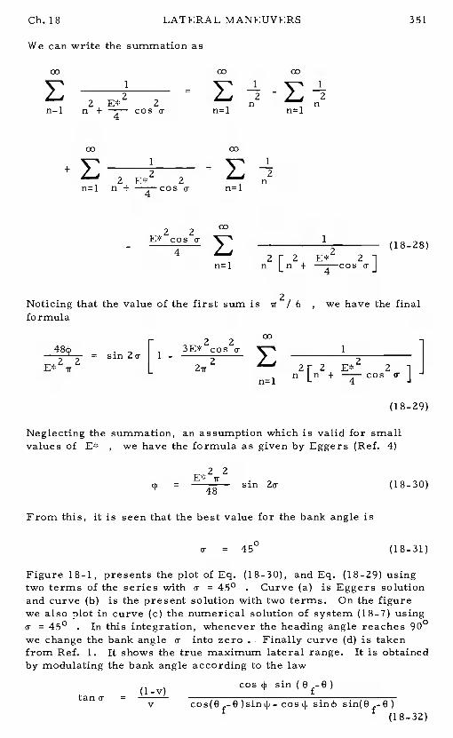
2 E*2 2+ COS cr
1
zr 2 E*2 2+ a-
Neglecting the summation, an assumption which is valid for smallvalues of E* , we have the formula as given by Eggers (Ref. 4)
=sin 2a- (18-30)
From this, it is seen that the best value for the bank angle is
a- = 45° (18-31)
Figure 18-1, presents the plot of Eq. (18-30), and Eq. (18-29) usingtwo terms of the series witha- = 450 Curve (a) is Eggers solutionand curve (b) is the present solution with two terms. On the figurewe also plot in curve (c) the numerical solution of system (18-7) using
= 450. In this integration, whenever the heading angle reaches 900
we change the bank anglea- into zero . Finally curve (d) is takenfrom Ref. 1. It shows the true maximum lateral range.It is obtainedby modulating the bank angle according to the law
cos4 sin(Of_9)cos(Of-O)sinI4J-cos4i sin(Of_O)
(18_32)
We can write the summation as
Ch. 18 LATERAL MANEUVERS 351
w1 1
n - n2n1
+ E2 E*2 2n1
,2 2cos a-4
(18-28)
Noticing that the value of the first sum isv 6
formula
4842 2
= sin 2a-E*
r ,2 2I
cos a-1
2L
we have the final
zr 2 E*2 2nzrl n
(18-29)
(1-v)tana- =V
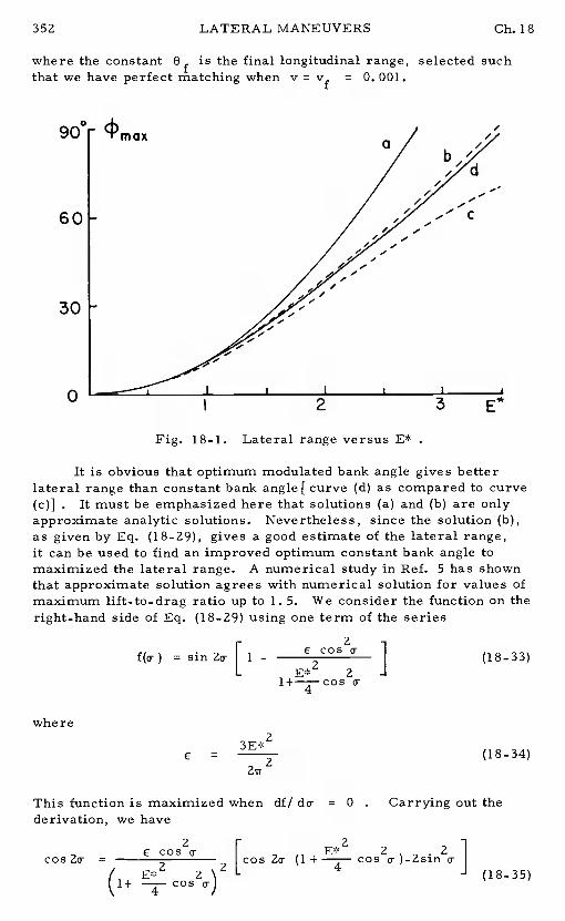
22 2C cOS 0cos2o- =
(E*2 2
22o (1 + cos o )_2sin
1+ —i— cos
352 LATERAL MANEUVERS Ch.18
where the constant is the final longitudinal range, selected suchthat we have perfect matching when v =Vf = 0. 001.
maxa
/60
30
0
,///
Fig. 18-1. Lateral range versus E*
3
It is obvious that optimum modulated bank angle gives betterlateral range than constant bank angle [curve (d) as compared to curve(c)] . It must be emphasized here that solutions (a) and (b) are onlyapproximate analytic solutions.Nevertheless, since the solution (b),as given by Eq. (18-29), gives a good estimate of the lateral range,it can be used to find an improved optimum constant bank angle tomaximized the lateral range. A numerical study in Ref. 5 has shownthat approximate solution agrees with numerical solution for values ofmaximum lift-to-drag ratio up to 1. 5.We consider the function on theright-hand side of Eq. (18-29) using one term of the series
r 2I ECOSO
f(o-) = sin2o- 1 - (18-33)L 2
o
where
= (18-34)
This function is maximized when df/ do- 0 . Carrying out thederivation, we have
(18-35)
Ch. 18 LATERAL MANEUVERS 353
Let
a = cog2 a (18-36)
We write the equation as
a = - [3 - (4 a - 2
] (18-37))2
For low maximum lift-to-drag ratio, is small, and to the zero order,= 0 , we have the solution
1 2 oa = cos a- , a-45
For higher order, Eq. (18-37)is of the form
a = p + E g(a) (18-38)
and by Lagrange's expansion, we have the solution
a = +
0(18-39)
To the order of we have the solution
cos2a- - E*2)5
E*4)
- 648
E*8)(1+
8 (18-40)
This expression shows that the optimum constant bank angle is greaterthan 450 This explicit solution is accurate for values of E* up to3. For large values of E* , we can solve the exact equation (18-37)which is a cubic equation in awritten as
- + E*2(l-
(1 - aZ
+ 1 ] a -1 = 0 (18-41)
354 LATERAL MANEUVERS Ch. 18
Another approximate solution to this equation can be obtained by putting
= + 5 , 6 << 1 (18-42)
Then, by series expansions and to the order of62 included
=152)
a =
a = (1- 45 + 452)
a = (1- 66 + 1252) (18-43)
Upon substituting into Eq. (18-41), we have a quadratic equation inS
2
2
2ir -6
b = 26 (18-45)-6
Upon solving, we have the solution
6 =+
[1- -
)2]
(18-46)
This solution is identical to the approximate solution obtained byShkadov in Ref. 2. He used the Eq. (18-42) to expand the function f(o-)as given by Eq. (18-33) in series in6 before maximizing.
The exact solution for the optimum bank angle obtained bysolving the cubic equation (18-41) is plotted in Fig. 18-2 versus themaximum lift-to-drag ratio. In the range of E* considered,
< 3. 5, both the explicit solutions (18-40) and (18-46) are inexcellent agreement with the exact solution.
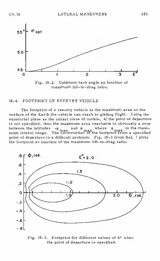
Ch. 18 LATERAL MANEUVERS 355
55!
50
45
Fig. 18-2. Optimum bank angle as function ofmaximum lift-to-drag ratio.
18-4. FOOTPRINT OF REENTRY VEHICLE
The footprint of a reentry vehicle is the maximum area on thesurface of the Earth the vehicle can reach in gliding flight.Using theequatorial plane as the initial plane of motion, if the point of departureis not specified, then the maximum area reachable is obviously a zonebetween the latitudes_4 and 4 where is the maxi-max maxmum lateral range.The construction 01the footprint trom a specifiedpoint of departure is a difficult problem.Fig. 18-3 from Ref.1 plotsthe footprint as function of the maximum lift-to-drag ratio.
.8
.6
.4
.2
0
-.2
-.4
-.6
-.8
Fig. 18-3. Footprint for different values of E* whenthe point of departure is specified.
opt
0 I 2 3
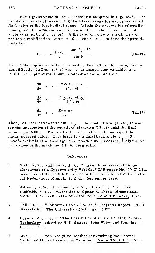
LATERAL MANEUVERS Ch. 18
For a given value of E*, consider a footprint in Fig. 18-3. Theproblem consists of maximizing the lateral range for each prescribedfinal value of the longitudinal range.Within the assumption of equilib-rium glide, the optimum control law for the modulation of the bankangle is given by Eq. (18-32).If the lateral range is small, we canuse the simplification sin 4, 0 , cos 4, 1 to have the approxi-mate law
tan(0 -0)(l-v) Itana- . (18-47)v sin4i
This is the approximate law obtained by Fave (Ref. 6).Using Fave'ssimplification in Eqs. (18-7) with v as independent variable, andX = 1 for flight at maximum lift-to-drag ratio, we have
dO — E*coso- cos4idv - - 2(l-v)
— E*coso sin9dv - - 2(1-v)
d4i — E*sino-(18 48)dv - Zv -
Then, for each estimated value , the control law (18-47) is usedfor the integration of the equations of motion (18-48) until the finalvalue vf = 0.001. The final value of 0 obtained must equal theinitial guessed value.This leads to the final bank angle o 0
analysis is in good agreement with pure numerical analysis forlpw values of the maximum lift-to-drag ratio.
References
1. Vinh, N.X., and Chern, J.S., "Three-Dimensional OptimumManeuvers of a Hypervelocity Vehicle, "IAF paperNo. 79-F-184,presented at the XXXth Congress of the International Astronauti-cal Federation, Munich, F. R. C., September 1979.
2. Shkadov, L. M., Bukhanova, R. S., Illarionov, V. F., andPlokhikh, V. P., "Mechanics of Optimum Three-DimensionalMotion of Aircraft in the Atmosphere, "NASA TT F-777, 1975.
3. Cell, D.A., "Optimum Lateral Range, "Progress Report, Ph.D.dissertation, The University of Michigan, 1979.
4. Eggers, A.J. ,Jr., "The Possibility of a Safe Landing, "SpaceTechnology, edited by H. S. Seifert, John Wiley and Son, Inc.,Ch. 13, 1959.
5. Slye, R. E., "An Analytical Method for Studying the LateralMotion of Atmosphere Entry Vehicles, "NASA TN D-325, 1960.
Ch. 18 LATERAL MANEUVERS 357
6. Fave, J., "Approche Analytique du du DomairieAccessible un Planeur Orbital, "La Recherche Ae'rospatiale,No. 124, pp. 3-11, 1968.