Hyperspectral imaging based biomass and nitrogen contentestimations from light-weight UAV

Polonen I.a, Saari H. b, Kaivosoja J. c, Honkavaara E. d and Pesonen L. c

aDepartment of Mathematical Information Technology, University of Jyvaskyla, Mattilanniemi2, 40100 Jyvskyla, Jyvskyla, Finland;

bVTT Technical Research Center of Finland, Tietotie 02150, Espoo, FinlandcMTT Agrifood Research Finland, Vakolantie 55, 03400 Vihti, Vihti, Finland

dFinnish Geodetic Institute, Geodeetinrinne 2, 02430 Masala, Kirkkonummi, Finland

ABSTRACT

Hyperspectral imaging based precise fertilization is challenge in the northern Europe, because of the cloudconditions. In this paper we will introduce schemes for the biomass and nitrogen content estimations fromhyperspectral images. In this research we used the Fabry-Perot interferometer based hypespectral imager thatenables hyperspectral imaging from lightweight UAVs. During the summers 2011 and 2012 imaging and flightcampaigns were carried out on the Finnish test field. Estimation mehtod uses features from linear and non-linearunmixing and vegetation indices. The results showed that the concept of small hyperspectral imager, UAV anddata analysis is ready to operational use.

Keywords: Hyperspectral imaging, UAV, biomass, nitrogen, unmixing

1. INTRODUCTION

Hyperspectral imaging is fast developing and growing multidisciplinary field of science. Growing amount ofresearch papers is published every year. A paper count of hyperspectral topics is now in same level as radarpapers.1 Basic concept in hyperspectral imaging has been combine spectral and spatial information in to theone data source as illustrated in figure 1. Each pixel in hyperspectral image cube forms also spectrum troughthe cube.

Climate in northern Europe makes utilization of hyperspectal imaging for the precision agriculture challenging.Cloud conditions combined with short growing seasons makes traditional satellite and airborne hyperspecralimaging almost useless. In recent years fast developing in unmanned aerial vehicles (UAV) and hyperspectralimagers has created totally new aspects for this problem.

VTT has developed lightweight and small sized hyperspectral imager (HSI), which is capable to take imagesfrom UAV’s. Unlike regular push broom based hyperspectral scanners VTT’s HSI takes whole 2D-plane atonce. This enables photogrammetric processing of imaged data. Our research consortium has performed fieldstudies in UASI -project with this HSI. Field studies have been in different application like forestry and precision

Further author information: (Send correspondence to Ilkka Polonen)Ilkka Polonen: E-mail: ilkka.polonen@jyu.fi, Telephone: +358 400 248 140

Figure 1. Illustration of hyperspectral image. Each pixel in the image forms spectrum trough imaged wavebands.

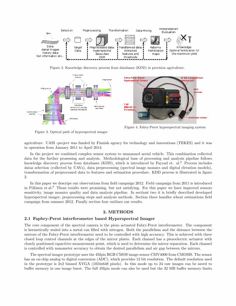
Figure 2. Knowledge discovery process from databases (KDD) in precision agriculture.

Figure 3. Optical path of hyperspectral imager

Figure 4. Fabry-Perot hyperspectral imaging system

agriculture. UASI -project was funded by Finnish agency for technology and innovations (TEKES) and it wasin operation from January 2011 to April 2013.

In the project we combined complex sensor system to unmanned aerial vehicle. This combination collecteddata for the further prosessing and analysis. Methodological base of processing and analysis pipeline followsknowledge discovery process from databases (KDD), which is introduced by Fayyad et. al.2 Process includesdatas selection (collected by UAVs), data preprocessing (spectral image mosaics and digital elevation models),transformation of preprocessed data to features and estimation procedure. KDD process is illustrated in figure2.

In this paper we descripe our observations from field campaign 2012. Field campaign from 2011 is introducedin Polonen et.al.3 Those results were promising, but not satisfying. For this paper we have improved sensorssensitivity, image mosaics quality and data analysis pipeline. In sectiont two it is briefly described developedhyperspectral imager, preprocessing steps and analysis methods. Section three handles wheat estimations fieldcampaign from summer 2012. Finally section four outlines our results.

2. METHODS

2.1 Fapbry-Perot interferometer based Hyperspectral Imager

The core component of the spectral camera is the piezo actuated Fabry-Perot interferometer. The componentis hermetically sealed into a metal can filled with nitrogen. Both the parallelism and the distance between themirrors of the Fabry-Perot interferometer need to be controlled with high accuracy. This is achieved with threeclosed loop control channels at the edges of the mirror plates. Each channel has a piezoelectric actuator withclosely positioned capacitive measurement point, which is used to determine the mirror separation. Each channelis controlled with nanometer accuracy to obtain the desired parallelism and air gap between the mirrors.

The spectral imager prototype uses the 4Mpix RGB CMOS image sensor CMV4000 from CMOSIS. The sensorhas an on-chip analog to digital conversion (ADC), which provides 12 bit resolution. The default resolution usedin the prototype is 2x2 binned XVGA (1024x648 pixels). In this mode up to 24 raw images can be saved tobuffer memory in one image burst. The full 4Mpix mode can also be used but the 32 MB buffer memory limits

the number of images to three for each image burst. This mode can be used if only a small set of wavelengthbands is required. Full description in detail for the FPI-HSI is in the article of Makynen et. al.4

2.2 Data Preprocessing

Steps from spectral images to whole mosaic is described briefly in conference paper of Honkavaara et. al.5 withfollowing steps:

1. System corrections of the images using the laboratory calibration, spectral correction and dark signalcorrection. These parameters and algorithms are provided by VTT.6

2. Image quality assessment, signal-to-noise ratio calculation (SNR).

3. Pixel transformation from 32 bit float format to 16 bit unsigned integer format.

4. Matching of layers to form spectral data cubes of individual images.

5. Determination of image orientations of reference layers using a self-calibrating bundle block adjustment.7,8

6. Optionally also a DSM can be calculated.8

7. Determination of radiometric imaging model to compensate atmospheric and illumination influences, andview (or illumination) related nonuniformity, as well as reflectance transformation. A radiometric blockadjustment method is being developed to determine optimal parameters by utilizing the overlapping im-ages.7,9

8. Calculation of output products, which include 3D spectral point clouds, digital surface models, spectro-metric image mosaics and object bidirectional reflectance data.9

The processing is implemented at the FGI in a processing environment based on BAE Systems SOCET SETand GXP photogrammetric software. The system corrections are developed by VTT (step 1) and the softwarefor layer matching and radiometric processing is developed by FGI (steps 2-4, 7, 8).

2.3 Feature Extraction

Spectral feature extraction can be divided to three different categories: spectral indices, spectral unmixing andspatial features. Vegetation indices are the easiest and computationally cheapest way to extract features fromthe spectral data. Basically, vegetation index is for example a spectral band divided by another. For exampleclassical Normalized Difference Vegetation Index (NDVI)10 is calculated in a following way

RNDV I =Rnir −Rred

Rnir +Rred. (1)

NDVI emphasize the density to green vegetation density. Used wavebands for Rnir = 816 nm and Rred = 690nm. For the Chlorophyll there is vegetation index called MCARI11

RMCARI = ((R700 −R670)− 0.2 ∗ (R700 −R550) ∗ R700

R670. (2)

One efficient way to extract feature information is spectral unmixing. This technique assumes that pixelcontent in the hyperspectral image is a mixture of different substances. Unmixing can be divided in three differentmodels: linear, bilinear and non-linear. We utilized linear12 and non-linear13 models for the feature extraction.Let y = (y1, y2, . . . yL)T be observed spectrum with L wavebands. Let assume that we are looking for N purespectra from image, which are also called endmembers. Endmembers form L × N matrix X = (x1,x2 . . .xN).Now we can assume that M = (m1,m2 . . .mN )T is (1×N) abundance vector of endmembers L to the observedspectrum y.

Linear model can be formulated

Figure 5. Illustration of the projection of high dimensional convex data set in to the two dimensional simplex.

y = XM + n (3)

where n is noise. General non-linear model is

y = Ψ(X) + n (4)

where Ψ in non-linear function which descripes connection between endmembers and obtained spectrum.Thus, in linear model unknown parameter is M and in non-linear model unknown function is Ψ. It is quiteclear that linear unmixing model can be solved multiple ways. Classical solution for the problem is least squaresmethod. One fast way to solve problem is use filter vector algorithm,14 which is linear way to solve inverseproblem. Linear models have been examined widely, when non-linear models haven’t been that actractive.Recently there has published more research, which has concentrated on non-linear unmixing. We tested K-Hypealgorithm, which is developed by Chen et. al.13 K-Hype is kernel -based approach to solve non-linear unmixingproblem. Abundance matrix M and results of function Ψ can be used as features in estimation process.

The unmixing models required knowledge about pure spectra. Spectra are known from the libraries or theseare perceived from hyperspectral data itself. There are algorithms like N-Finder or Vertex Component Analysis(VCA)15 , which are looking for pure spectra from data cube. VCA is widely used in hyperspectral remote sensing.Main assumption in VCA is that there is pure spectra X precence in observed data set Y = (y1,y2, . . .yd),where d is number of spectra in the image. VCA basically determinate in projected subspace extreme pointsof data set Y and these points are selected to endmembers. In Figure 5 is illustration of projected subspace.Extreme points of this convex hull are marked with star.

Feature selection can be based on correlation between extracted features and measured test plots or it ispossible to use all extracted features. If we use all extracted features, then manifold learning approach can beutilized. We utilized quite new dimensional reduction method called diffusion maps.16 It finds a low-dimensionalrepresentation using the singular value decomposition of a transition probability matrix based on some chosendistance function. Thus, the high-dimensional data points become embedded in a lower-dimensional space. Thedimensionality reduction yields a space where the Euclidean distance corresponds to the diffusion distance in theoriginal space.16,17

If we consider a feature set, which consist feature vectors i.e. digits extracted from spectral data. LetX = {x1,x2, . . . ,xn} be feature set and xi ∈ Rp is feature vector lenght of p. As described in Nieminen et. al.18

diffusion map is kernel method, which utilize gaussian kernel matrix W ,

Wij = exp

(−dist(xi, xj)

ε

), (5)

Barley Voitto

Barley Saana

Wheat Kruunu Wheat Anniina

Fertilizing stripes

Barley

Wheat

0 - 60 - 60 -120-120-180-180-120-120- 0 - 120-120- 60 - 60- 80 - 80 - 80- 80 - 0

S S S S

Variety:

Fert. amount:

110 kg/ha

80 kg/ha

150%

50% 150%

50%

50%

0%

0%

Spring fertilization plan 2012

kg/ha

100%

100%

Seeding plan 2012

0%

100 m

S = sprayer track

S

0 kg/ha

Figure 6. Seeding and fertilizing plan for the field at Vihti(Finland 2012)

Figure 7. Used microcopter

where dist(xi, xj) is Euclidean distance. Matrix W is normalized P = D−1W , where Dii =∑n

j=1Wij , i ∈1 . . . n. The matrix represents the transition probabilities between the data points. To determinate the eigenval-ues of P the conjugate matrix P = D

12PD− 1

2 is calculated. From this we get

P = D− 12WD− 1

2 . (6)

This is normalized graph Laplacian19 and it maintain the eigenvalues.17 Singular value decomposition (SVD)P = UΛU∗ is used to find the eigenvalues Λ = diag([λ1, λ2, . . . , λn]) and eigenvectors U = [u1, u2, . . . , un] for

P . The eigenvalues for P are the same as for P . The eigenvectors for P are found with V = D− 12U .17 The

low-dimensional coordinates Φ are created using Φ = V Λ.

2.4 Estimation

To estimate biomass and nitrogen content on the field we use machine learning approach. Because extractedfeatures aren’t continuous data as spectrum is, it is possible to use just simple K nearest neighbour (KNN) inclassification. Selected method and approach needs training data with appriori information. In our case thetraining data was gathered as test samples from the test field and measured in the laboratory. These labelledsamples can be also used in verification of estimation results. KNN calculates distance between points in trainingdata set and points en, which are needed to be estimated (n = 1, ..., d). Algorithm selects k data points, whichEuclidean distance to point en is shortest. With selected k = 5 we calculated five nearest neighbours in Euclideanspace from trained data set. Estimate e is calculated from label values li of these five neighbours with following

e =

∑ki=1 lik

. (7)

3. EMPIRICAL TESTS

3.1 Test field and flight campaign

Our test field at Vihti is located to southern Finland. Flight and imaging campaign was executed in mid-summer2012 just before tillering. In Finland usually there is only one extra fertilization due to short growing season.Seeding and fertilization had been done in May. As figure 6 indicates there was two types of wheat and barleyseeded. Also different amount seed and nitrogen was given. All together 50 spots, size of one square meter, wereselected. Spots accurate location was taken with GPS. All vegetation in those spots were taken and measuredin the laboratory. Measured values were dry-weight, moisture, nitrogen content

Flight campaign was operated by lightweight microcopter (Figure 7). Microcopter has an autopilot system,which enables to fly in advance determinated path. Microcopters payload is appoximate one kg.

Figure 8. Manually selected non-linear features for thebiomass.

Figure 9. Manually selected non-linear features for nitrogen.

3.1.1 Estimation results

After the flight data was preprocessed as described in section 2.2. Linear and non-linear unmixing was performedfor the data. NDVI and MCARI indices were also calculated as reference for the biomass and nitrogen estimation.In table 1 is presented correlation between biomass and nitrogen content to calculated features. From non-linearand and linear abundance maps only highest correlations are shown.

Table 1. Correlations

Correlation between Biomass Nitrogen

NDVI 0.639 0.69

FVA (linear) 0.814 0.72

K-Hype (non-linear) 0.779 0.665

MCARI 0.807 0.552

Closer examination revealed that there were endmembers, linear and non-linear, which abundance maps hadhigh correlation with measured test plots values. We can use feature selection with some criteria or use allextracted features. If we for example take closer look to the non-linear abundance maps we found out that therewere two, which correlation with nitrogen was high and three for the biomass. In figures 8 and 9 we can seescatter plots of these non-linear abundance maps with the labeled test plots. From figures 8 and 9 it is clearthat there is structured manifold, which can be used for the estimation. It also success that there is possible toset up threshold for the feature selection.

Labelled test spots are divided for the training and testing randomly in ratio 1:1. KNN estimator is trainedwith other half and tested with other half. Results are seen in figure 10 and 11. Normalized root mean squareerror for the biomass estimation is 18.08 % and for the nitrogen content estimation 19.73 %. These results aren’tstraight comparable to the results in literature. Satellite and normal airborne hyperspectral data has muchlarger land pixel, hence data is also much more averaged and doesn’t include that much variance. Estimation ofwhole data is illustrated in figures 12 and 13. Based on these figures it is possible to create fertilization task asdescribed in Kaivosoja et. al.20

Manifold learning approach seems to give similar answer for estimation of biomass. Figure 14 illustratesresults of diffusion map dimension reduction. We used all extracted features (NDVI, MCARI, linear and non-linear unmixing) in the feature space. With diffusion maps we can lower this 52 dimensional space to two

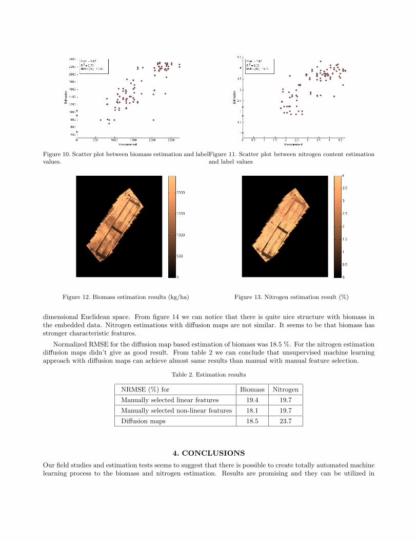
Figure 10. Scatter plot between biomass estimation and labelvalues.

Figure 11. Scatter plot between nitrogen content estimationand label values

Figure 12. Biomass estimation results (kg/ha) Figure 13. Nitrogen estimation result (%)

dimensional Euclidean space. From figure 14 we can notice that there is quite nice structure with biomass inthe embedded data. Nitrogen estimations with diffusion maps are not similar. It seems to be that biomass hasstronger characteristic features.

Normalized RMSE for the diffusion map based estimation of biomass was 18.5 %. For the nitrogen estimationdiffusion maps didn’t give as good result. From table 2 we can conclude that unsupervised machine learningapproach with diffusion maps can achieve almost same results than manual with manual feature selection.

Table 2. Estimation results

NRMSE (%) for Biomass Nitrogen

Manually selected linear features 19.4 19.7

Manually selected non-linear features 18.1 19.7

Diffusion maps 18.5 23.7

4. CONCLUSIONS

Our field studies and estimation tests seems to suggest that there is possible to create totally automated machinelearning process to the biomass and nitrogen estimation. Results are promising and they can be utilized in

Figure 14. Low dimensional embedding of the test plots labelled with biomass amount (kg/ha).

precision agriculture. But there is still some open questions. Campaign was utilized in one location, mainlywith wheat and in one year. Are the results easily generalized? Is trained features depended on location? Is itpossible to calibrate training data so, that it is usefull in many years? Vegetation indices are robust estimatesand when we compare estimation results with correlation values in table 1 it is indicating that our approach isn’ttoo adaptating. Alltogether combination of UAV, HSI-FPI and modern data analysis gives us results, which areexploitable in practice.

ACKNOWLEDGMENTS

This research has been funded by Finnish agency for innovations and technology (TEKES, grants 40035/11,40036/11, 40037/11 and 40038/11).

REFERENCES

[1] Bioucas-Dias, J., Plaza, A., Camps-Valls, G., Scheunders, P., Nasrabadi, N., and Chanussot, J., “Hyper-spectral remote sensing data analysis and future challenges,” Geoscience and Remote Sensing Magazine,IEEE 1(2), 6–36 (2013).

[2] Fayyad, U., Piatetsky-Shapiro, G., and Smyth, P., “The kdd process for extracting useful knowledge fromvolumes of data,” Commun. ACM 39, 27–34 (Nov. 1996).

[3] Polonen, I., Salo, H., Saari, H., Kaivosoja, J., Pesonen, L., and Honkavaara, E., “Biomass estimator for nirimage with a few additional spectral band images taken from light uas,” in [Sensing for Agriculture andFood Quality and Safety IV ], Proc. SPIE 8369 (2012).

[4] Makynen, J., Holmlund, C., Saari, H., Ojala, K., and Antila, T., “Multi- and hyperspectral uav imagingsystem for forest and agriculture applications,” 8374 (2012).

[5] Honkavaara, E., Hakala, T., Kirjasniemi, J., Lindfors, A., Makynen, J., Nurminen, K., Ruokokoski, P.,Saari, H., and Markelin, L., “New light-weight stereosopic spectrometric airborne imaging technology forhigh-resolution environmental remote sensing case studies in water quality mapping,” XL-1/W1 (2013).

[6] Makynen, J., Holmlund, C., Saari, H., Ojala, K., and Antila, T., “Unmanned aerial vehicle (uav) operatedmegapixel spectral camera,” 8186 (2011).

[7] Honkavaara, E., Hakala, T., Saari, H., Markelin, L., Makynen, J., and Rosnell, T., “A process for radiometriccorrection of uav image blocks,” Photogrammetrie, Fernerkundung, Geoinformation (PFG) , 115–127 (22012).

[8] Rosnell, T. and Honkavaara, E., “Point cloud generation from aerial image data acquired by a quadrocoptertype micro unmanned aerial vehicle and a digital still camera,” Sensors 12, 453–480 (2012).

[9] Honkavaara, E., Kaivosoja, J., Makynen, J., Pellikka, I., Pesonen, L., Saari, H., Salo, H., Hakala, T.,Markelin, L., and Rosnell, T., “Hyperspectral reflectance signatures and point clouds for precision agricul-ture by light weight uav imaging system,” ISPRS Annals of Photogrammetry, Remote Sensing and SpatialInformation Sciences I-7, 353–358 (2012).

[10] Rouse, J. W., Haas, R. H., Schell, J. A., and Deering, D. W., “Monitoring vegetation systems in the greatplains with erts,” Third ERTS Symposium, NASA SP-351 1, 309–317 (1973).

[11] Daughtry, C. S., Walthall, C. L., Kim, M. S., de Colstoun, E. B., and McMurtrey, J. E., “Estimatingcorn leaf chlorophyll concentration from leaf and canopy reflectance.,” Remote Sensing of Environment 74,229–239 (2000).

[12] Keshava, N. and J., M., “Spectral unmixing,” IEEE Signal Processing Mag. 19(1), 44–57 (2002).

[13] Chen, J., Richard, C., Bermudez, J.-C., and Honeine, P., “A modified non-negative lms algorithm and itsstochastic behavior analysis,” ASILOMAR 11, 6-9 November (2011).

[14] Bowles, J., Palmadesso, P., Antoniades, J., Baumback, M., and Rickard, L., “Use of filter vectors in hyper-spectral data analysis,” 148157 (1995).

[15] Nascimento, J. and Dias, J., “Vertex component analysis: A fast algorithm to unmix hyperspectral data,”IEEE Transactions on Geoscience and Remote Sensing 34(4), 898–910 (2005).

[16] Coifman, R. R. and Lafon, S., “Diffusion maps,” Applied and Computational Harmonic Analysis 21(1),5–30 (2006).

[17] Nadler, B., Lafon, S., Coifman, R., and Kevrekidis, I. G., “Diffusion maps – a probabilistic interpreta-tion for spectral embedding and clustering algorithms,” in [Principal Manifolds for Data Visualization andDimension Reduction ], Barth, T. J., Griebel, M., Keyes, D. E., Nieminen, R. M., Roose, D., Schlick, T.,Gorban, A. N., Kegl, B., Wunsch, D. C., and Zinovyev, A. Y., eds., Lecture Notes in Computational Scienceand Engineering 58, 238–260, Springer (2008).

[18] Nieminen, P., Polonen, I., and Sipola, T., “Research literature clustering using diffusion maps,” Journal ofInformetrics (2013).

[19] Chung, F. R. K., [Spectral Graph Theory ], 2, AMS Press (1997).

[20] Kaivosoja, J., Pesonen, L., Kleemola, J., Polonen, I., Salo, H. A., Honkavaara, E., Saari, H., Makynen,J. H., and Rajala, A., “A case study of a precision fertilizer application task generation for wheat based onclassified hyperspectral data from uav combined with farm history data,” in [Remote Sensing for Agriculture,Ecosystems, and Hydrology XV ], Proc. SPIE 8887 (2013).