A Gravitational Origin of the Arrows of Time

Julian Barbour,1,2 Tim Koslowski,3 and Flavio Mercati,4

1College Farm, South Newington, Banbury, Oxon, OX15 4JG UK,

2Visiting Professor in Physics at the University of Oxford, UK.

3 University of New Brunswick, Fredericton, NB, E3B 5A3 Canada,

4Perimeter Institute for Theoretical Physics, 31 Caroline Street North,

Waterloo, ON, N2L 2Y5 Canada,

December 16, 2013

Abstract

The only widely accepted explanation for the various arrows of time that every-where and at all epochs point in the same direction is the ‘past hypothesis’: theUniverse had a very special low-entropy initial state. We present the first evidencefor an alternative conjecture: the arrows exist in all solutions of the gravitationallaw that governs the Universe and arise because the space of its true degrees of free-dom (shape space) is asymmetric. We prove our conjecture for arrows of complexityand information in the Newtonian N -body problem. Except for a set of measurezero, all of its solutions for non-negative energy divide at a uniquely defined pointinto two halves. In each a well-defined measure of complexity fluctuates but growsirreversibly between rising bounds from that point. Structures that store dynamicalinformation are created as the complexity grows. Recognition of the division is akey novelty of our approach. Each solution can be viewed as having a single pastand two distinct futures emerging from it. Any internal observer must be in one halfof the solution and will only be aware of one past and one future. The ‘paradox’of a time-symmetric law that leads to observationally irreversible behaviour is fullyresolved. General Relativity shares enough architectonic structure with the N -bodyproblem for us to prove the existence of analogous complexity arrows in the vacuumBianchi IX model. In the absence of non-trivial solutions with matter we cannotprove that arrows of dynamical information will arise in GR, though they have inour Universe. Finally, we indicate how the other arrows of time could arise.

1

arX

iv:1

310.

5167

v1 [

gr-q

c] 1

8 O

ct 2

013

Contents

1 Introduction 3

1.1 Doubts about existing approaches . . . . . . . . . . . . . . . . . . . . . . . . . 3

1.2 Our conceptual framework and main results . . . . . . . . . . . . . . . . . . . . . 4

2 Time Asymmetry in Particle Dynamics 6

2.1 Generic solutions . . . . . . . . . . . . . . . . . . . . . . . . . . . . . . . . . . 6

2.2 Definition and growth of the complexity . . . . . . . . . . . . . . . . . . . . . . 7

2.3 Definition and growth of information . . . . . . . . . . . . . . . . . . . . . . . . 10

2.4 Dynamical similarity . . . . . . . . . . . . . . . . . . . . . . . . . . . . . . . . 11

2.5 Homothetic solutions and the topography of shape space . . . . . . . . . . . . . . 13

2.6 The 3-body problem in shape space . . . . . . . . . . . . . . . . . . . . . . . . . 16

2.7 Dissipation in particle dynamics . . . . . . . . . . . . . . . . . . . . . . . . . . 18

2.8 Shape-dynamic explanation of 3- and N -body behaviour . . . . . . . . . . . . . . . 22

2.9 On structure emergence . . . . . . . . . . . . . . . . . . . . . . . . . . . . . . 23

2.10 Remarks on time . . . . . . . . . . . . . . . . . . . . . . . . . . . . . . . . . . 24

3 Time Asymmetry in Dynamical Geometry 25

3.1 Shape space for dynamical geometry . . . . . . . . . . . . . . . . . . . . . . . . 25

3.2 Shape Dynamics in conformal superspace . . . . . . . . . . . . . . . . . . . . . . 28

3.3 Spacetime construction . . . . . . . . . . . . . . . . . . . . . . . . . . . . . . 30

3.4 The emergence of rods and clocks . . . . . . . . . . . . . . . . . . . . . . . . . 31

3.5 The Mixmaster model . . . . . . . . . . . . . . . . . . . . . . . . . . . . . . . 33

3.6 Complexity in geometrodynamics . . . . . . . . . . . . . . . . . . . . . . . . . . 37

4 Possible Quantum Implications 39

4.1 A time-dependent Planck constant . . . . . . . . . . . . . . . . . . . . . . . . . 39

4.2 Metrogenesis and hylogenesis . . . . . . . . . . . . . . . . . . . . . . . . . . . . 43

5 Conclusions and Outlook 43

A Appendices 46

A.1 Growth of complexity in the N -body problem . . . . . . . . . . . . . . . . . . . . 46

A.2 Phase-space reduction for the 3-body problem . . . . . . . . . . . . . . . . . . . . 47

A.3 Positive energy N -body system . . . . . . . . . . . . . . . . . . . . . . . . . . . 50

A.4 The monotonicity of York time . . . . . . . . . . . . . . . . . . . . . . . . . . . 51

A.5 Metriplectic Formalism: A Definition of Bulk Entropy . . . . . . . . . . . . . . . . 52

2

1 Introduction

“It seems to me that the idea of trying to obtain a universe in the form we know it byapplying time-symmetric physics to a generic unconstrained initial state is basicallymisconceived.” R. Penrose [1].

1.1 Doubts about existing approaches

Most discussions of the various arrows of time concentrate on the growth of entropy. Thisis natural; the entropy arrow was the first that attracted widespread interest. It is also theone most readily observed, as when we drop a glass and know it cannot be reassembled.However, we question whether the entropy concept and statistical mechanics, which areundoubtedly excellent for characterizing and understanding subsystems of the Universe,are appropriate for the Universe as a whole. These are some of our reasons:

1. Boltzmann and Gibbs developed the entropy concept to describe non-gravitatingparticles in a confined space, e.g., a box, and based it on phase-space volume. Arethe italicized aspects appropriate for the Universe? Gravity dominates it, no wallsconfine it, and volume presupposes an external scale.

2. By assuring probability conservation, Liouville’s theorem for ensembles in phase spaceprovides the foundation of statistical mechanics for dynamical systems evolving wrtan external time. But the Universe is a unique system with a unique history and allphysical clocks are subsystems of it.

3. Self-gravitating systems are ‘anti-thermodynamic’. They have negative heat capac-ity and cannot equilibrate. Instead of making non-uniform systems more uniform,gravity fosters clustering, i.e., complexity. This has long been recognized, but to thebest of our knowledge no one has hitherto quantified the effect. We shall.

4. Although black holes and other solutions of Einstein’s equations with horizons haveremarkable thermodynamic properties and suggest an intimate connection betweengravity, entropy and quantum dynamics, the general covariance of GR has defeatedattempts to define gravitational entropy in generic situations.

5. The entropy concept is often illustrated in configuration space Q alone, e.g., atomsinitially confined to a small region then spread out over a complete box. In the greatmajority of the naturally occurring far-from-equilibrium objects in the Universe, themomenta are effectively random and the disequilibrium is manifested almost entirelyin Q, which may therefore be more relevant than phase space.

These are the main reasons why we seek a new way to understand the arrows of time.Specifically, we suggest that three-dimensional (3D) scale-invariant configurational com-plexity is the fundamental concept that should be studied in the first place. We definesuch a concept for Newtonian gravity and show that it exhibits striking irreversible be-haviour. We also propose a candidate analogue for GR and indicate how our frameworkcould explain not only the Universe’s manifest complexity arrow but also the other arrows.

3

Our approach has similarities to the Weyl curvature hypothesis of Penrose [2, 1], differingmainly in seeking a notion of 3D complexity rather than 4D entropy. We do also think hisbelief quoted above may be too pessimistic.

1.2 Our conceptual framework and main results

Our fundamental assumptions are:

1. The Universe is a closed dynamical system. In Newtonian gravity (NG), this meansan ‘island universe’ of N point particles. In general relativity (GR), the Universemust be spatially closed. This is not in conflict with current observations.

2. A notion of universal simultaneity exists. This is built into NG. In GR, we rely onthe theory of Shape Dynamics (SD), discussed below, to supply this notion.

3. Since all measurements are relational, only shapes are physical. We will define thecomplexity, denoted CS, of any complete shape of the Universe. It is a pure number.

Our basic arena is shape space, denoted S. In NG, it is obtained by quotienting thestandard Newtonian configuration space Q by Euclidean translations, rotations and dilata-tions, i.e., wrt the similarity group. Then for the N -body problem its 3N -dimensional Qis replaced by the 3N − 7-dimensional S. Shape space for GR will be introduced later.

The guiding principle of SD is to abstract from dynamics all external structures. InNG, these are position, orientation and size in an inertial frame and also an external time.A dynamical history is then simply an unparametrized curve c in S. The equations of bothNG and GR are time-reversal symmetric, so they define no orientation on c. This is whythe entropy and other arrows are a problem. However, for NG we show that its generic1

solutions for non-negative energy, E ≥ 0, exhibit ‘two-sided’ time asymmetry, namely, theydivide into two halves in each of which CS fluctuates but overall grows irreversibly froma common minimum. Moreover, structures that store dynamical information are createdas CS grows. In our Universe, we identify the direction to the future with the arrowsof increasing complexity and information. On this basis, since the minimum divides thesolution effectively into distinct halves, two ‘directions of time’, pointing away from theminimum, exist in all generic NG solutions. We are not aware that this ‘one-past–two-futures’ structure has hitherto been noted or related to the arrows of time.

We first demonstrate the structure in conventional Newtonian terms and then derivethe equations that determine the evolution curve in S. We believe this provides strongevidence that shape space is the arena in which to study all the arrows of time. Ourlong-term aim is to show that the past hypothesis (that the arrows of time can only beexplained by an exceptionally low-entropy birth of the Universe) is unnecessary. Instead,we shall suggest that the arrows all have their origin in an asymmetry of shape space S.

1Throughout the paper, we use generic to denote the sets of solutions that are not of measure zero.

4

We see support for our conjecture in the form of the evolution in S in each of the abovehalves, which is asymmetric in time and dissipative2 in the naturally defined directionof increasing complexity. This is so despite the absence of ‘hidden’ microscopic degreesof freedom of the kind that normally give rise to irreversible behaviour. We think thetime-asymmetric evolution could be related to the deterministic laws of black hole ther-modynamics found in classical GR in the late 1960s. It might also be a manifestationof hidden degrees of freedom and an entropic origin of gravity. Whatever the truth, thedissipation is a mathematical fact and a direct consequence of our fundamental ontology,in accordance with which only shape evolution is physical.

We should like to emphasize here that in both NG and GR the physical degrees offreedom (dofs) with which we are concerned are heterogeneous in nature. There are purelydimensionless shape dofs and one dimensionful scale dof.3 Moreover, under a physicallyreasonable restriction, its conjugate momentum, unlike all the momenta of the shape dofs,is monotonic along the solution curve. Its existence as a unique Lyapunov function in theN -body problem has long been known. It has an equally striking counterpart in GR, calledthe York time. The direction of increase of these two Lyapunov functions is conventional,so their existence does not conflict with the time-reversal symmetry of the laws that definethem.

However, since the scale dof is unique and, being dimensionful, can only be given avalue if an external scale is present, it literally ‘cries out’ for a role distinct from the shapedofs. Through the operation of deparametrization, which we explained in detail in [15], wetransform the scale variable into the Hamiltonian and its monotonic conjugate momentuminto the evolution parameter. We are left with the minimal set of variables needed todescribe the Universe objectively. Any attempt to remove more would bring down thewhole structure.

The transition to this optimal (fully reduced) description automatically removes fromthe system the scale kinetic energy present in the conventional description and explainswhy the dynamics in S is dissipative. The potential significance of our result stands or fallswith our ontology. We ask readers who suspect we have created an artefact by tamperingwith hallowed principles to bear in mind that Einstein was led to create GR precisely inorder to eliminate external background structures from physics. We are suggesting thatone last step needs to be taken: the elimination of external scale.

In Sec. 3, we consider GR. For reasons that we shall spell out, we cannot as yet ob-tain results as definitive as for the N -body problem. However, we find enough similaritiesto encourage us to believe that in this much more realistic context the route to an un-derstanding of the arrows of time is through study of the problem in a suitably definedshape space. The main argument and the novel aspects of our approach can be understoodwithout reading Sec. 3 which discusses the application to dynamical geometry. However,for readers unfamiliar with GR in its Hamiltonian formulation, we briefly introduce somebackground in Sec. 3.1.

2Irreversibility of the dynamics of the true conformal degrees of freedom of GR, manifested as monotonicdecrease of the reduced Hamiltonian, has been noticed before, and was exploited by Fischer and Moncriefin a study of attractors of the motion [3]. In vacuum GR we actually find anti-dissipation (Sec. 3).

3Machian arguments allow us to eliminate translational and rotational degrees of freedom.

5

2 Time Asymmetry in Particle Dynamics

2.1 Generic solutions

We here review facts about the N -body problem4 as formulated in the ‘scaffolding’ ofan inertial reference frame, external clock and reference scale. We call this the coordina-tized description and contrast it with the objective description. This latter is obtained byabstracting away everything that is not unambiguously intrinsic to the system. All that re-mains are the dimensionless mass ratios of the particles and the successive shapes throughwhich the system passes in shape space.5 The elimination of the strictly redundant partof the coordinatized description reveals effective asymmetry in S.

We begin with the qualitative behaviour of the 3-body problem in the coordinatizeddescription. Since we use this as a toy model for the Universe, we limit ourselves onMachian grounds to the zero-angular momentum, Jtot = 0, and zero-energy, E = 0, case.By Galilean invariance, we can always assume that the momentum Ptot vanishes.6

All generic three-body solutions with E = Jtot = 0 have a period of nontrivial three-body interaction that develops asymptotically in both time directions into hyperbolic–elliptic escape in which a pair of particles (not necessarily the same in the two time direc-tions) separates from the third. As the pair becomes more and more isolated, its motion isever better approximated by elliptical Keplerian motion. In the meantime, the third par-ticle, the ‘escapee’, tends to increasingly undisturbed inertial motion directed away fromthe pair. This behaviour is illustrated in Fig. 1.

Being time-reversal symmetric, Newton’s equations do not define any temporal orderingon the complete orbit. However, we shall show that there exists a unique point on it atwhich the dilatational momentum7

D =3∑

a=1

rcm

a · pacm , (1)

where rcma and pacm are the centre-of-mass coordinate and momentum vectors of the particles,

vanishes. This point divides the orbit into two halves and, as we shall show, serves as a‘past’ for each half, both of which have an infinitely distant ‘future’ as the Kepler pair andescapee drift forever apart.8 Thus every generic E = Jtot = 0 solution has ‘one past andtwo futures’. This is also true of all generic N -body solutions with E = Jtot = 0. We deferdiscussion of the residual measure-zero solutions, which exhibit quite different behaviour.

4See Chenciner’s [4] for a rigorous review. Marchal [5] treats the 3-body problem in detail. Sundman[6] first established the 3-body behaviour described below.

5This is the conceptual framework of Shape Dynamics. For details, including its origin in Machianconsiderations, see [7, 8, 9, 10, 11, 12, 13, 14, 15, 16, 17].

6Best matching (see [16, 17] for details) shows that the conditions Ptot = Jtot = 0 ensure overalltranslation and rotation of the Universe make no contribution to its action, as Mach’s principle requires.

7Coined in [18] by analogy with angular momentum, which has the same dimensions. It has not beennamed in the N -body literature, but is generally denoted by J , probably for Jacobi.

8Since only ratios have meaning in shape space, the objective fact is that the ratio between the semi-major axis of the pair and the distance of the third particle from the pair tends to infinity.

6

x

y

Figure 1: Orbits of the three particles in a pair exchange process in the centre-of-mass inertialframe. Because we assume Jtot = 0 and consider the 3-body problem, the motion is planar. Theorientation of the axes and the units are arbitrary. Time-reversal symmetry makes it possible toread two ‘pair-swapping’ stories in one picture. With the option shown by the arrows, a boy (red,coming from bottom left) meets a Kepler pair dancing in from the top right, grabs the girl (green)and goes off with her bottom right, ensuring momentum conservation if not happiness for thejilted boy (blue). But reverse the arrows, and the blue boy gets the girl. The cameo story showshow illusory it is to say some initial condition ‘causes’ what happens later. For a time-symmetricsystem, the solutions do not have an initial condition. They each have their own overall structureencoded equally well in any phase-space point along the solution.

2.2 Definition and growth of the complexity

We wish to define the complexity CS as a scale-invariant, and hence dimensionsless, functionon S. A simple way is to make CS the ratio of two ‘democratically’ mass-weighted lengths.If ma is the mass of particle a, and ra is its position vector, an obvious candidate for oneis the root-mean-square length `rms:

`rms :=1

mtot

√∑a<b

mamb r2ab, mtot =

N∑a=1

ma, rab = ‖rb − ra‖. (2)

Another is the mean harmonic length `mhl:

1

`mhl

:=1

m2tot

∑r<a

mamb

rab. (3)

Then the complexity, a pure number that depends only on N and the mass ratios, is

CS :=`rms

`mhl

. (4)

7

D

Icm

CS

tD0

Figure 2: The moment of inertia Icm (red), dilatational momentum D (blue), and complexityCS (black) as functions of the Newtonian time for the solution of the 3-body problem shown inFig. 1. The different heights of the fluctuations on the two sides of the figure reflect the differentorbital elements of the corresponding Kepler pairs and escapees. Note that in the asymptoticregions, where the orbital parameters stabilize, numerical calculation of the evolution in eithertime direction is relatively easy but becomes much harder when the three-body interactions becomenon-trivial. Given asymptotic data on one side, it is not easy to predict with any accuracy thebehaviour on the other. The two sides are effectively different worlds.

We are not aware of an earlier proposal for this purpose, but it is easy to see that CS isa good measure of non-uniformity and hence complexity. Even for relatively small N , `rms

(2) changes little if two particles approach each other or even coincide. In contrast, `mhl

is sensitive to any clustering and tends to zero if that happens. Moreover, while CS growswith clustering, Battye et al’s [19] numerical calculations show that the minima of CS upto N ≈ 104 correspond to extraordinarily uniform (super-Poissonian) shapes.9

Apart from the division by 1/m2tot and the absence of the constant G, `mhl is, of course,

the Newton potential. Less obvious is that `rms is, the normalization apart, the square rootof the centre-of-mass moment of inertia Icm. This follows from the identity

1

mtot

∑r<a

mambr2ab ≡

N∑a=1

ma‖ra − rcm‖2 := Icm, rcm =N∑a=1

ma

mtotra. (5)

Thus, the complexity is formed from the two most fundamental quantities in Newtoniangravitational dynamics. Note also that D (1) is half the time derivative of Icm.

9Conceptually at least, our definition bears no obvious resemblance to Kolmogorov complexity definedby the number of binary digits needed in an algorithm to generate a given distribution. It is obvious thatone could define more sophisticated measures of complexity than (4), e.g., ones that take into accountalignments, but (4) appears to be the most appropriate as a measure for a self-gravitating universe.

8

CS

tFigure 3: The complexity CS vs. Newtonian time for a typical solution with N ∼ 1000. Theinitial state was a Gaussian distribution of all coordinates and velocities around the origin. Itclearly exhibits a linear growth, and, as was to be expected from the increase in N , the fluctua-tions due to the eccentricity of the Keplerian orbits average each other, giving a smoother curve.Time reversal (implemented by reversing the initial velocities but not shown) leads to qualitativelysimilar behaviour on either side of the minimum of CS (as in Fig. 2).

Figure 2 gives a first hint why we study CS. It fluctuates but has a clear tendency toincrease between growing bounds either side of the central region of minimal Icm. It is easyto see why: first, the escapee’s increasing separation leads to asymptotic linear growthof Icm; second, the Kepler pair forms with eccentricity, and the varying separation of itsconstituents causes VNew to fluctuate. Behind the behaviour of CS =

√IcmVNew we directly

see the cause. It is not some initial condition but the effect of law.

The fluctuations in CS for the N -body problem with large N are much weaker (Fig. 3).An initial cluster of particles ‘evaporates’ (in both time directions), forming quasi-boundfew-particle systems and some stable Kepler pairs. As the system disperses, `rms growssteadily, while the Kepler pairs and quasi-bound systems, whose phases are uncorrelated,ensure that |VNew| = `−1

mhl declines to a more or less stable asymptotic value.10

Marchal and Saari [20] obtained rigorous results which show that this must happen.Subject to certain caveats (see Appendix A.1), the basic reason is that the N -body systembreaks up into subsystems whose centres of mass separate linearly with the Newtoniantime t in the asymptotic limit. Each subsystem consists of individual particles and clusterswhose constituents remain close to each other. The separations within a subsystem are

10The deterministic manifestation of ‘two-sided’ arrows of time described here should be compared withBoltzmann’s suggestion, made in a non-gravitational context, of rare deep fluctuations out of statisticalequilibrium, in which intelligent beings can only exist near the bottom of an entropy fluctuation. Ifpresent on both sides, each would regard the entropy minimum as lying to their past. Note that theBoltzmann fluctuations reoccur infinitely often, whereas there is just one pair of arrows of time in eachof the deterministic solutions we consider. Moreover, the entropy arrow points to a ‘heat-death’ future,whereas the complexity arrow points in the direction of greater structure.

9

bounded by O(t2/3). Thus, if particle a belongs to cluster J , we have 11

ra = cJ t + O(t2/3), if a ∈ J , (6)

where cJ ∈ R3 is a constant vector. It follows immediately that√Icm must grow linearly

with t, while VNew declines not faster than t−2/3, so that their product CS grows on averageat least as t1/3. In fact, the formation of at least one asymptotically stable Kepler pair willensure that VNew asymptotes to a constant average, so that CS grows linearly.

Although we have as yet only shown how CS grows asymptotically in Newtonian gravity,it seems to be an excellent candidate measure of complexity in our actual Universe, inwhich non-gravitational forces also play an important role. The protons and other nucleitogether with possible dark matter particles can be taken to represent the bulk of theinhomogeneously distributed matter in the Universe. Suppose that at each instant of cosmictime since last scattering of the CMB the shortest spatial geodesic distances between all ofthem were determined in spacelike hypersurfaces12 in which the CMB is at rest on average.Let the obtained values be inserted as the inter-particle distances rab in the expression (4)for the complexity CS. Even allowing for uncertainty about the fate of matter in blackholes, it will surely be the case that this CS for the Universe will have increased on averagemonotonically to an extremely good accuracy from last scattering to the present epoch.

2.3 Definition and growth of information

We now want to suggest that an arrow of information growth also emerges generically. Ofcourse, we must first define information. We adhere to the ideas sketched by one of us inthe essay [22] and assume that all kinds of information (factual, semantic and Shannon)have a physical basis and that their existence is tied to the availability of an adequatelyrich physical substrate. Here we are concerned with deterministic processes, so we leavethe discussion of Shannon information, which is about probabilities, for later studies.

For the purposes of this paper, the results that we have so far obtained lead us naturallyto an information-theoretical identification of complexity as ‘the necessary condition for asystem to store recognizable local information’. This enables us to synthesize the conceptsof complexity and information, in the sense that ‘complexity is potential information’. TheN -body problem provides a chance to test this conjecture using our intuitive (and quanti-tative!) notion of configurational complexity as defined by CS. Indeed, we now conjecturethat there is an equally intuitive notion of dynamical information. This is suggested by thedynamics of the system, which, evolving in the direction of our arrow of time, can spon-taneously create subsystems that, as Marchal and Saari [20] show, become increasinglyisolated from the rest of the Universe. As this happens, the subsystems develop (approx-imate) Galilean symmetries with which there are associated seven conserved quantities:the linear and angular momenta PJ , JJ , and the energy EJ of the clusters (the index Jidentifies the cluster). On Machian grounds, the whole Universe is constrained to have a

11 If N > 3, there can also be super-hyperbolic solutions, a well known example of which is Xia’s 5-bodysolution [21], in which four particles reach infinity in finite time. However, as Edward Anderson pointedout to us, these are not compatible with special relativity, so we do not consider them.

12Assumed to foliate the complete Universe, taken to be spatially closed.

10

vanishing value for these quantities in an inertial frame, but subsystems are not, so thatany non-zero value of PJ , JJ and EJ has to be compensated by an equal and oppositevalue of the same quantities for the rest of the Universe.

The key observation is that when a subsystem becomes isolated, it develops the sevensymmetries and corresponding conserved quantities EJ , PJ and JJ that, as shown in [20],are more and more accurately conserved. With time both the number n of clusters J =1, ..., n and the number of ‘frozen’ digits of (E1,P1,J1, ..., En,Pn,Jn) increases, implyingthat the number of digits reliably stored in subsystems increases. We propose that thetotal amount of data ‘saved’ in the ‘frozen’ digits measures the information content of thesystem. By the results of [20], this increases in time together with the measure CS ofconfigurational complexity.

Moreover, one can also say that physical rods and clocks emerge spontaneously in theform of Kepler pairs. If they are to have utility, rods must remain mutually congruentand clocks must remain in phase – they must march in step [23]. This is what happenswhen Kepler pairs form. Their semi-major axes become mutually fixed with ever greaterprecision and therefore serve as rods, while the areas swept out by the major axes measuretime concordantly in accordance with Kepler’s second law. Both information and themeans to measure it emerge dynamically and generically.

Of course, Kepler pairs do not meet all the criteria of metrology since two such pairswould disrupt each other when in close proximity and the very essence of measurementis the bringing of a rod and the measured interval into overlap. Metrology now relies onquantum mechanics and the great weakness of gravity compared with the other forces. Wereturn to this question in Sec. 3.4.

2.4 Dynamical similarity

We now want to understand, at the most basic level, the behaviour described in the previoussubsections and shown in Figs. 2 and 3. The characteristic features are the U-shaped graphof Icm and the fluctuating growth of CS either side of D = 0.

The behaviour of Icm is easily explained and has long been known. As the first qualitativeresult in dynamics, Lagrange discovered it over 200 years ago. It relies on two architectonicproperties of the Newton potential.

The first is homogeneity : if for any dynamical system and any real constant k thepotential satisfies V (α ra) = αk V (ra), then it is homogeneous of degree k and dynamicalsimilarity holds: the equations of motion permit a series of geometrically similar paths([24], p. 22), in which the times between corresponding points satisfy t′/t = (l′/l)1−k/2 ifthe distances are scaled as l′/l. The best known example of this is Kepler’s third law,13

for which 1− k/2 = 3/2 and the periods of planets of the same eccentricity (and thereforeshape) but different semi-major axes a scale as a3/2. The dynamical similarity in the N -body problem will be crucial below: it shows that, if (as for a dynamically closed universe)external standards of duration and scale are unavailable, then a one-parameter family ofsolutions in the coordinatized description collapses to a single curve in S.

13Dynamical similarity is also the basis of the virial theorem [24].

11

The homogeneity of degree k of any potential also leads to the relation

Icm = 4E − 2(k + 2)V , (7)

which is often called the Lagrange–Jacobi relation. Its derivation uses Newton’s secondlaw and Euler’s homogeneous function theorem.

We now come to the second important property of VNew. Besides having k = −1, it isalso negative definite. These two properties enable us to particularize (7) as follows:

Icm = 4E − 2(k + 2)V =⇒ 4E − 2VNew > 0 if E ≥ 0. (8)

Thus, if E ≥ 0 it follows that Icm = 2D is positive [D is defined in (1)]. Then Icm isconcave upward, D is positive and D, whose sign is conventional, is monotonic.14 SinceFigs. 2 and 3 are based on calculations with E = 0, this immediately explains the U-shapedbehaviour of Icm, which is also bound to occur if E > 0.

Deferring for a moment the exceptional case in which Icm reaches zero, it follows fromits upward concavity that Icm must tend to infinity in both time directions. This requireseither one particle to recede infinitely far from the other two, which leads to the hyperbolic–elliptic escape described above, or all inter-particle separations to tend to infinity at thesame time. This is also an exceptional case and will be considered below. As for thebehaviour of CS in Fig. 2, we have seen that this is directly due to the formation of Keplerpairs and escape of the third particle: the generic behaviour of the 3-body problem withE ≥ 0 is inevitable. Appendix A.1 shows this is also true for the N -body problem.

Let us here say something about our Machian assumption that the Universe has E =Ptot = Jtot = 0 (in its centre-of-mass inertial frame). We noted in footnote 6 that theconditions Ptot = Jtot = 0 ensure that translation and rotation of the Universe as a wholemake no contribution to its action. Moreover, solutions with E = Jtot = 0 are importantin N -body theory because they are scale invariant : if E or Jtot is non-vanishing, its valuechanges under a change of units, but zero is obviously invariant. Of greater relevance tous is a corresponding reduction in the number of degrees of freedom. The exact numberis important, so we do a count. We start with 3N . By Galilean relativity, the centre-of-mass coordinates have no effect on the inter-particle separations, so that brings us downto 3N − 3. Next Jtot = 0 eliminates two,15 so we reach 3N − 5. Dynamical similarity andthe condition E = 0 enable us to make the final reduction below to 3N − 7 shape dofs anda time variable based on the dilatational momentum.

One more comment. Newton’s equations have the same form in Q independently ofthe values of E and Jtot, but the objective equations in S are very different. The readermay think E = Jtot = 0 is merely a special initial condition ‘put in by hand’. However,we treat the N -body problem as a model ‘island Universe’. It is important that theUniverse, as opposed to subsystems of it, is unique. The equations that describe such auniverse objectively in S have different, significantly more complicated forms if E,Jtot 6= 0as compared with the case Jtot = E = 0. Above all, if E and Jtot are non-vanishing

14If k = −2, then Icm = 0. This case, studied in [18, 25], also plays a role below.15Not three because the rotation group is non-Abelian: there are only two commuting quantum angular-

momentum observables.

12

the Universe in its evolution responds not only to the structure of S but also to externalstructures. Moreover, this case matches the basic structure of closed-space vacuum GR(which we show in Sec. 3) and provides a reasonably realistic toy model for at least thematter-dominated evolution of our Universe (see, e.g., [26]).

2.5 Homothetic solutions and the topography of shape space

Here we first wish to describe the structure of S. To this end we note that a mere signchange turns the complexity CS into the shape potential VS introduced in [25, 15]:

VS :=√IcmVNew, VNew = −

∑a<b

mamb

rab. (9)

The absence of the Newton constant from VNew will be discussed below. We call VS theshape potential16 because its factor

√Icm removes the scale dependence from VNew, so forces

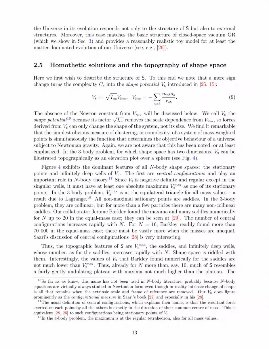
derived from VS can only change the shape of the system, not its size. We find it remarkablethat the simplest obvious measure of clustering, or complexity, of a system of mass-weightedpoints is simultaneously the function that determines the objective behaviour of a universesubject to Newtonian gravity. Again, we are not aware that this has been noted, or at leastemphasized. In the 3-body problem, for which shape space has two dimensions, VS can beillustrated topographically as an elevation plot over a sphere (see Fig. 4).

Figure 4 exhibits the dominant features of all N -body shape spaces: the stationarypoints and infinitely deep wells of VS. The first are central configurations and play animportant role in N -body theory.17 Since VS is negative definite and regular except in thesingular wells, it must have at least one absolute maximum V max

S as one of its stationarypoints. In the 3-body problem, V max

S is at the equilateral triangle for all mass values – aresult due to Lagrange.18 All non-maximal sationary points are saddles. In the 3-bodyproblem, they are collinear, but for more than a few particles there are many non-collinearsaddles. Our collaborator Jerome Barkley found the maxima and many saddles numericallyfor N up to 20 in the equal-mass case; they can be seen at [29]. The number of centralconfigurations increases rapidly with N . For N = 16, Barkley readily found more than70 000 in the equal-mass case; there must be vastly more when the masses are unequal.Saari’s discussion of central configurations [28] is very interesting.

Thus, the topographic features of S are V maxS , the saddles, and infinitely deep wells,

whose number, as for the saddles, increases rapidly with N . Shape space is riddled withthem. Interestingly, the values of VS that Barkley found numerically for the saddles arenot much lower than V max

S . Thus, already for N more than, say, 10, much of S resemblesa fairly gently undulating plateau with maxima not much higher than the plateau. The

16So far as we know, this name has not been used in N -body literature, probably because N -bodyequations are virtually always studied in Newtonian form even though in reality intrinsic change of shapeis all that remains when the extrinsic scale and frame of reference are removed. Our VS does figureprominently as the configurational measure in Saari’s book [27] and especially in his [28].

17The usual definition of central configurations, which explains their name, is that the resultant forceexerted on each point by all the others is exactly in the direction of their common centre of mass. This isequivalent [28, 26] to such configurations being stationary points of VS.

18In the 4-body problem, the maximum is at the regular tetrahedron, also for all mass values.

13

Figure 4: The shape sphere of the three-body problem, with an elevation plot of VS (9) on itssurface. The equator corresponds to collinear configurations; at three points on it there are two-body coincidences, where VS is singular with infinitely deep wells. Between them, at the azimuthalangles φab, there are the Euler configurations, saddle points of VS. The triangles corresponding topoints with the same longitude and opposite latitude are mirror images. For all values of the massratios, the absolute maximum of VS is at the equilateral triangle. The figure shows the equal-masscase, for which φab =

(π, π3 ,−

π3

).

wells occupy a relatively small ‘area’ of the plateau. Moreover, the shapes on the plateauhave rather uniform, low complexity particle distributions. We have already mentionedthe result of Battye et al [19] that for N ≈ 104 the particle distribution at the minimumof CS – and thus maximum of VS – is extraordinarily smooth19 for equal-mass particles.

We say shape space is asymmetric because, through the level surfaces of VS, it acquiresthe structure with plateau and infinitely deep wells just described. It is certain that shapespace with any potential will lack symmetry.

The central configurations are important because they are associated with central col-lisions, when all the particles collide at once at their centre of mass and Icm hits zero. Thisbrings us to the zero-measure solutions of the N -body problem deferred earlier.

First, there are homothetic (unchanging shape) solutions: if the system is ‘held’ at restat a central configuration and released, it will fall homothetically until all the particlescollide in a central collison at the centre of mass, beyond which the solution cannot be

19Super-Poissonian. We believe study of the equal-mass case is justified because it best approximatesfield theory, modelling high field values by high particle densities.

14

continued (a noteworthy result). The centre-of-mass position vector of each particle is

rcm

a = caf(t− t0), t > t0, (10)

where ca is a constant vector. Thus, all interparticle separations and their distances fromthe centre of mass are proportional to a common function of the time f(t − t0) until thecentral collision. In Newtonian terms, the complete set of Jtot = 0 homothetic solutionscorresponds to the system either hitting or exploding out of the centre of mass and behavingin one of three ways. If E < 0, the system can only reach a finite size before collapsingback to a central collision; the solution exists only for a finite time interval. If E = 0, thesystem can ‘just’ escape to infinity, its scale increasing throughout as (t− t0)2/3. Finally, ifE > 0 the system ‘reaches infinity’ with the scale increasing asymptotically as t − t0; thesystem has escaped the effect of gravity and is ‘coasting’ inertially.

All the homothetic solutions (10) exist as mere points in S. Much more interesting arethe solutions that become homothetic only asymptotically, terminating at a central colli-sion or escaping to infinity. In fact, central collisions can only occur if the solution doesterminate at a central configuration [4]. In S, these asymptotically homothetic solutionsterminate at one end at a central configuration or, very exceptionally, at both ends. How-ever, in all solutions that are asymptotically homothetic at one end the other end will bedrawn forever down a well of VS. Since, as we noted, the complexity at saddles is typicallylow but tends to infinity in the wells, such solutions will exhibit clear complexity growthfrom one ‘past’ to one ‘future’. As with the ‘two-sided’ solutions, complexity arrows aredue to the law alone. Moreover, all E ≥ 0 solutions of the N -body problem except thefully homothetic ones, which are mere points in S, have the arrows. They are generic.

It might be argued that we have only been able to make this claim by an artificial‘marriage’ of two physically distinct things to make CS: the (square root of the) momentof inertia and the Newton potential. But a closed dynamical system must be characterizedin dimensionless terms: CS is the real thing and splitting it into

√Icm and VNew is artificial.

The objectively true arena in which a dynamically closed universe exists is like Fig. 4.

This is the point for a preliminary summary, which we begin with a reiteration of thetwo main novelties of our approach. The first is consistent passage from the dimensionfulcoordinatized description in Q to the dimensionless S. Second, as we stressed in the captionto Fig. 1, one should not be thinking about initial states but rather the structure ofcomplete solutions, both the zero-measure and generic ones. Only the behaviour of aquantity like the complexity allows pragmatic identification of points on the solutions thatcan be termed ‘initial’ or to lie in a ‘past’. In the generic E ≥ 0 solutions to the N -bodyproblem, this criterion places the ‘initial’ point in the middle of the solution.

This leads us to suggest that the puzzle of time asymmetry may have arisen becausedynamics has been considered in the wrong arena. At least in the case of the N -bodyproblem, there is a time-symmetric dynamical law in the coordinatized representation, butin the objective description in S a seemingly time-symmetric generic solution becomes, forall practical purposes, two time-asymmetric solutions that are independent. The fact is thatany attempt to evolve, however accurately, asymptotic N -body data back in the direction ofdecreasing complexity will always lead to a more uniform state. Moreover, magnificationof computational errors will mean that the overwhelming majority of retrodictions will

15

make it seem that such a universe emerged from a very special, highly uniform state.Returning to Penrose’s comment at the start of the paper, we see this as first tentativeevidence that an explanation for the existence of “a universe in the form we know it” couldbe obtained provided we pass from the time-symmetric coordinatized representation in Qto the dimensionless, scale-invariant and time-asymmetric representation in S. Then nospecial initial condition – no past hypothesis – would be needed.

We end this part of the paper with a question: since we can only observe and measureratios, e.g., red shifts, why do we say the Universe is expanding? This is often illustrated byblowing up a balloon onto which coins, taken to represent galaxies, are glued: the distancesbetween the coins grow relative to their diameters. We find this a misleading analogy, whichlimps on two crutches (‘rigid’ coins and ‘expansion’ between them). We think the N -bodyproblem provides a much more illuminating dynamical picture of crutch-free ‘expansionwithout expansion’: once Kepler pairs form, the distances between them (and to otherparticles) increase relative to the semi-major axes, whose ratios remain unchanged. Thebehaviour of the true actors – the ratios – underlies the complexity growth and ‘expansion’.We will now show that deeper understanding of N -body dynamics is gained if we respondto the ‘cry’ of change of scale to play a role distinct from that of shape.

2.6 The 3-body problem in shape space

We have here one aim: to express everything intrinsically on S. This is appropriate ifwe treat the 3-body problem, the simplest nontrivial system, as a toy universe, for whichexternal non-dynamical influences are manifestly questionable. Following our aim consis-tently, we are led ineluctably to a dissipative structure on S that exists identically in theN -body problem and in anti-dissipative form in vacuum GR.

We first mention a scale-invariant model [18] in which VNew is replaced by a potentialhomogeneous of degree −2, V = I−1/2

cm VNew. This simplest choice for dynamics on S isgeodesic and for large N reproduces Newtonian gravity to good accuracy in small subsys-tems, but there is no secular growth of complexity, so the long-term Newtonian behaviouris not reproduced.20 The model serves as a useful reference to characterize the Newtoniandissipative behaviour by the deviation from a geodesic on S.

We now make the reduction to the 3-body shape space. For three particles, S is thetwo-dimensional space of triangle shapes. To arrive at it, we start with the 9D spaceR

9 of particle positions ra = (xa, ya, za), a = 1, 2, 3, and quotient wrt the 3D similaritygroup Sim of rigid rotations, translations and rescalings. Montgomery [30] gives the details,Appendix A.2 the phase-space reduction in our notation. The resulting space, to whichthe 3-body collision (not a shape) does not belong,21 is topologically a sphere with threepiercings as shown in Fig. 4 with centre at the origin of a Cartesian space with coordinatesw = (w1, w2, w3).22 The square of the sphere’s radius is

||w||2 = w21 + w2

2 + w23 =

I2cm

4. (11)

20Dirac quantization of the model leads to an anomaly [25] that suggests holographic emergence of time.21Denial of ontology to scale has consequences for the ‘Big Bang’, modelled in the 3-body problem by

triple coincidence of the particles. The only candidate to replace it in S is the equilateral triangle, themost uniform shape.

22The w coordinates are nontrivially related to the Cartesian coordinates ra, see Appendix A.2.

16

The three coordinates w permit full description of a Newtonian history, including thechanging size of the three-body triangle as measured by Icm. Quotienting wrt rescalingsw→ ϕw, ϕ > 0, is the final step to S.

To get there and exhibit the effect of the assumption E = 0, we use Jacobi’s principle,according to which (as Lanczos [31] shows) the Newtonian orbits for each fixed value of Eand any potential V are found as geodesics in Q. The Jacobi action is

SJacobi = 2

∫ds

√(E − V )

∑a

ma

2

drads· dra

ds. (12)

This is a good first step: Newton’s extraneous time is eliminated. But there is aproblem since (12) is invariant under the reparametrization s→ s′(s). In a generic geodesicprinciple, there is no obvious choice of a unique evolution parameter. Taking of one of thecoordinates involves an arbitrary choice and in general will only work over a limited interval:generic dofs are not monotonic – such a ‘clock’ can stop and run backward.

This is where the split into scale and shape dofs is decisive [15]. There can be arbitrarilymany shape dofs, but there is always only a single scale dof. Moreover, its derivative D ismonotonic in the N -body problem if E ≥ 0. If we take it to be the independent variable,we ‘kill two birds with one stone’. We get a monotonic ‘time’ and remove scale from amongthe dofs. Shape-dynamic purity is achieved.

At this point it is best to make the Legendre transformation from Lagrangian to Hamil-tonian dofs and introduce canonical momenta. Because SJacobi is reparametrization invari-ant, these are homogeneous of degree zero in the velocities and satisfy the constraint[16, 17, 8, 25, 15] 23

H =∑a

pa · pa

2µa+ VNew =

1

2I−1

cm ‖z‖2 + VNew = 0 , µa = ma

mtot, (13)

where the momenta z = (z1, z2, z3) are conjugate to w, {wi, zj} = δij, pa = (pax, pay, p

az) are

the Cartesian momenta and VNew(w) is the Newton potential

VNew = −∑a<b

(µa µb)32 (µa + µb)

− 12√

‖w‖ − w1 cos φab − w2 sin φab. (14)

The azimuthal angles φab on the w3 = 0 plane identify the direction of the two-bodycoincidences between particles a and b. Their explicit expressions are

φ12 = π , φ23 = arctan

(2

√m1m2m3(m1+m2+m3)

m2(m1+m2+m3)−m1 m3

), (15)

φ13 = − arctan

(2

√m1m2m3(m1+m2+m3)

m1(m1+m2+m3)−m2 m3

),

which reduce to φ12 = π, φ23 = π3, φ13 = −π

3in the equal-mass case.

23At this point we set E = 0. We will later show the effect on the equations in S if it is retained. TheN -body problem with E = 0 is a good toy model of vacuum GR.

17

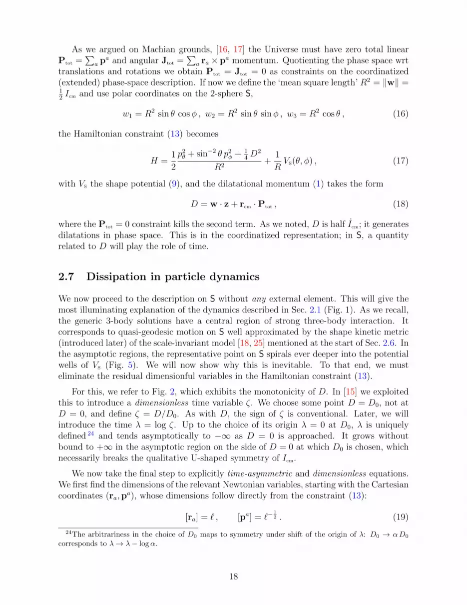
As we argued on Machian grounds, [16, 17] the Universe must have zero total linearPtot =

∑a pa and angular Jtot =

∑a ra×pa momentum. Quotienting the phase space wrt

translations and rotations we obtain Ptot = Jtot = 0 as constraints on the coordinatized(extended) phase-space description. If now we define the ‘mean square length’ R2 = ‖w‖ =12Icm and use polar coordinates on the 2-sphere S,

w1 = R2 sin θ cosφ , w2 = R2 sin θ sinφ , w3 = R2 cos θ , (16)

the Hamiltonian constraint (13) becomes

H =1

2

p2θ + sin−2 θ p2

φ + 14D2

R2+

1

RVS(θ, φ) , (17)

with VS the shape potential (9), and the dilatational momentum (1) takes the form

D = w · z + rcm ·Ptot , (18)

where the Ptot = 0 constraint kills the second term. As we noted, D is half Icm; it generatesdilatations in phase space. This is in the coordinatized representation; in S, a quantityrelated to D will play the role of time.

2.7 Dissipation in particle dynamics

We now proceed to the description on S without any external element. This will give themost illuminating explanation of the dynamics described in Sec. 2.1 (Fig. 1). As we recall,the generic 3-body solutions have a central region of strong three-body interaction. Itcorresponds to quasi-geodesic motion on S well approximated by the shape kinetic metric(introduced later) of the scale-invariant model [18, 25] mentioned at the start of Sec. 2.6. Inthe asymptotic regions, the representative point on S spirals ever deeper into the potentialwells of VS (Fig. 5). We will now show why this is inevitable. To that end, we musteliminate the residual dimensionful variables in the Hamiltonian constraint (13).

For this, we refer to Fig. 2, which exhibits the monotonicity of D. In [15] we exploitedthis to introduce a dimensionless time variable ζ. We choose some point D = D0, not atD = 0, and define ζ = D/D0. As with D, the sign of ζ is conventional. Later, we willintroduce the time λ = log ζ. Up to the choice of its origin λ = 0 at D0, λ is uniquelydefined 24 and tends asymptotically to −∞ as D = 0 is approached. It grows withoutbound to +∞ in the asymptotic region on the side of D = 0 at which D0 is chosen, whichnecessarily breaks the qualitative U-shaped symmetry of Icm.

We now take the final step to explicitly time-asymmetric and dimensionless equations.We first find the dimensions of the relevant Newtonian variables, starting with the Cartesiancoordinates (ra,p

a), whose dimensions follow directly from the constraint (13):

[ra] = ` , [pa] = `−12 . (19)

24The arbitrariness in the choice of D0 maps to symmetry under shift of the origin of λ: D0 → αD0

corresponds to λ→ λ− logα.

18

Figure 5: The pair-exchange process of Fig. 1 as seen from shape space S. The red and theyellow part of the orbit are distinguished by belonging, respectively, to the (nominal) past and thefuture of the point at which the dilatational momentum D is zero and the centre-of-mass momentof inertia Icm is at its minimum. This point is shown as an ‘x’ at the back of S, where the orbitis dashed.

In their turn, the Poisson brackets have dimension [action]−1, in our terms [{· , ·}] = `−12 .25

The partially reduced coordinates w (16) are manifestly translation- and rotation-invariantand, being quadratic in ra, they and their conjugate momenta z have dimensions

[w] = `2 , [z] = `−32 . (20)

Finally, after the last phase-space splitting between dimensionless shape variables (θ, φ)and the ‘rms length’ [R] = `, the momenta have the dimensions

[pθ] = [pφ] = [D] = `12 . (21)

This last trace of ‘coordinatization’, the dimensionality of the shape momenta (pθ, pφ), willdisappear below. Mass dimensions do not occur because (on rescaling of the action by mtot

[17]) we have only the dimensionless ‘geometrical’ masses µa = ma

mtot.

After these preliminaries, we first, as in [15], express the dynamics purely on S by using

25In (13) the Newton constant G has been absorbed into the definition of the momenta. Both in NGand in vacuum GR, G is unphysical and absent if one attributes no dimensions to time. See [17] for aderivation of these results from an action principle.

19

ζ = D/D0 as a time label.26 We also rescale the momenta πi = pi/D0 to make themdimensionless. The shape Hamiltonian, generating evolution wrt ζ, is

H = log

(1

2

π2θ + sin−2 θ π2

φ

CS(θ, φ)+

1

8

ζ2

CS(θ, φ)

), (22)

where we have introduced the complexity CS = −VS ≥ 0. The equations of motion are

dθ

dζ=

2 πθπ2θ + sin−2 θ π2

φ + 14ζ2,

dφ

dζ=

2 sin−2 θ πφπ2θ + sin−2 θ π2

φ + 14ζ2, (23)

dπθdζ

=2 sin−3 θ cos θ π2

φ

π2θ + sin−2 θ π2

φ + 14ζ2

+∂ logCS

∂θ,

dπφdζ

=∂ logCS

∂φ.

As we noted, CS is a simple measure of shape complexity and, remarkably, as we seeexplicitly in these equations, − logCS is the potential that governs Newtonian gravity repre-sented objectively on S. At this point we want to compare the time-dependent Hamiltonian(22) of NG on S with the geodesic model of [18]. To this end, consider the ‘complexity’metric, conformally related to the round metric, that assigns to a surface element d cos θ dφon S the measure [25] CS(θ, φ) d cos θ dφ. This metric is

gij =

(CS 00 sin2 θ CS

). (24)

The non-reparametrization invariant action

S =1

2

∫ds gij

dqids

dqjds

, (25)

whose canonical Hamiltonian (with gij the inverse metric) is

Hgeo = pi qi − L =1

2gij p

i pj =1

2

p2θ + sin−2 θ p2

φ

CS(θ, φ), (26)

generates affinely parametrized geodesics wrt the metric (24). Comparison with (22) showsthat its ζ2 term leads to deviation from geodesics on S – and, as we shall now show, todissipative behaviour in accordance with our formalism.

To achieve a fully dimensionless description, initially for the 3-body problem, we intro-duce the logarithmic time λ = log ζ and make a non-canonical transformation:

λ = log ζ , ωθ =πθζ, ωφ =

πφζ. (27)

26This ‘deparametrization’ procedure, described in detail in [15], consists of identifying the conjugatevariable to D, which is logR where R =

√Icm, and solving the Hamiltonian constraint (13) for it. The

resulting expression for logR in terms of the other dofs (which are all shape dofs) is the Hamiltonian Hwhich generates D-translations.

20

The equations of motion for these variables are autonomous,27

dθ

dλ=

2ωθω2θ + sin−2 θ ω2

φ + 14

,dφ

dλ=

2 sin−2 θ ωφω2θ + sin−2 θ ω2

φ + 14

, (28)

dωθdλ

= −ωθ +2 sin−3 θ cos θ ω2

φ

ω2θ + sin−2 θ ω2

φ + 14

+∂ logCS

∂θ,

dωφdλ

= −ωφ +∂ logCS

∂φ.

This system is dissipative: the equations for the momenta contain the terms −ωθ and −ωφand therefore do not conserve phase-space volume (conserving phase-space volume is thenecessary condition for non-dissipative dynamics). The equations of motion can be thoughtas being generated by the time-independent Hamiltonian

H0 = log

(ω2θ + sin−2 θ ω2

φ + 14

CS(θ, φ)

)(29)

and the dimensionless canonical structure

{{θ, ωθ}} = 1 , {{θ, ωφ}} = 0 , {{φ, ωφ}} = 1 , {{φ, ωθ}} = 0 , (30)

but with deformed, non-Hamiltonian equations of motion:

dθ

dλ= {{θ,H0}} ,

dφ

dλ= {{φ,H0}} , (31)

dωθdλ

= {{ωθ, H0}} − ωθ ,dωφdλ

= {{ωφ, H0}} − ωφ .

The dimensionless Poisson brackets, [{{ ·, · }}] = 1, are related to the dimensionful {·, ·} by

{{ ·, · }} =1

ζ D0

{ ·, · } ≡ D−1{ ·, ·} . (32)

We now extend our treatment to the N -body problem. The 3-body model is particu-larly suited to build intuition because one can explicitly perform the configuration spacereduction to S. This is not possible for N > 3 because quotienting by rotations, unliketranslations and scale, cannot be done explicitly. Luckily, the main interest arises fromscale quotienting, and we can work with a partially reduced configuration space, ‘pre-shapespace’ PS = R

3N/Dil×Transl. We will skip the intermediate step of obtaining the shapemomenta πa, which we derived in [15]. Instead we introduce directly the dimensionlessand dissipative description with ωa, the dimensionless shape momenta:

σa =√µa

rcma

R, ωa =

1õa

R

Dpacm − σa , (33)

R = I1/2cm , D =

∑a

rcm

a · pacm ,

rcm

a = ra −N∑b=1

µb rb , pacm = pa − 1

N

N∑b=1

pb .

27For the purposes of this paper, an autonomous dynamical system is one in which the equations ofmotion take the form xα = fα(x), where xα are the phase-space variables, and fα does not dependexplicitly on the independent variable.

21

These coordinates on PS satisfy the constraints∑a

σa · σa = 1 ,∑a

σa · ωa = 0 , (34)∑a

√µa σa = 0 ,

∑a

√µaωa = 0 .

The dimensionless Hamiltonian generating the dynamics on PS is

H0 = log

(N∑a=1

ωa · ωa + 1

)− logCS , (35)

and the equations of motion are

σa = {{σa, H0}} ,

ωa = {{ωa, H0}} − ωa ,(36)

where the dimensionless Poisson brackets have the symplectic structure

{{σia, ωjb}} = δba δ

ij − σia σ

jb ,

{{ωai , ωbj}} = σia ωbj − σ

jb ω

ai ,

{{σai , σjb}} = 0 .

(37)

An analogous dissipative representation exists for any shape-dynamic (particle or field-theoretic) model of the Universe provided the conditions assumed above hold: 1) thegenerator of scale transformations, here D and in GR an analogous variable (the Yorktime), is monotonic, allowing deparametrization wrt it; 2) the generator of dynamics,which takes the form of a Hamiltonian constraint, can be solved for log(R), which convertsits conjugate momentum D into a time variable and yields the physical Hamiltonian.

In the introduction we noted that there is no obvious explanation (like microscopic de-grees of freedom) for the dissipation we find in SD. We conjectured a possible connectionwith the deterministic laws of black-hole thermodynamics found in the late 1960s. What-ever the truth, we mention here that there exists a ‘metriplectic’ formalism which makesit possible to introduce a formal entropy in cases when one has dissipative equations. Wedescribe this formalism and apply it to shape-dynamic gravity in Appendix A.4.

2.8 Shape-dynamic explanation of 3- and N-body behaviour

Much of the long-known generic 3-body hyperbolic–elliptic behaviour when E = 0 (Sec. 2.1and Fig. 1) can be directly ‘read off’ the plot of VS in Fig. 4 knowing that the system isdissipative. Equations (28) describe a particle moving in S under the influence of thepotential VS but subject to friction; the solutions have a transparent intuitive explanation.Locally the orbits are well approximated by geodesic motion wrt the metric (24), but inthe long run the momenta get depleted by friction, and the orbits are drawn inescapablyever deeper into the potential wells.

22

The dissipative picture on S provides an even more powerful intuition for the remainingmeasure-zero solutions (Sec. 2.5). These end either with a central collision or escape ofall three particles (no Kepler pair formed) and always tend asymptotically to homotheticmotion (the shape freezes); the final shape can only be a central configuration. From theNewtonian coordinatized point of view, this behaviour is not obvious, but on S it is. Thecentral configurations are the stationary points of VS, so the system can only end up notchanging its shape if the derivatives of VS vanish: at points where ∇VS = 0. Because ofthe dissipation, there will be orbits that reach these stationary points with exactly zerovelocity (wrt the logarithmic time λ). But all the stationary points of VS are unstableequilibria: the Euler configurations are saddles, the equilateral triangle a maximum. Thatthese are measure-zero solutions is therefore also readily explained: the initial conditionsmust be doubly fine-tuned, to reach a stationary point and to arrive with zero velocity.

The difference between the solutions with E = 0 and E 6= 0 is particularly interesting.As we show in Appendix A.3, the effect of E > 0 on shape space S is to add a time-dependent effective potential to VS. This flattens the total potential and allows the solutioncurve in S to asymptote as λ → ∞ to points away from central configurations. Anyscalene end shape of the triangle is possible. This shows that, in contrast to the caseE 6= 0, the topography defined on S by VS completely determines the E = 0 solutions:they can asymptote only to its singularities (potential wells) or stationary points. Thereis a complete explanation for what happens in any E = 0 solution, but not in the E 6= 0case, which violates the principle of sufficient reason.28

This is also true for the E = 0 solutions of the N -body problem for all N ≥ 3 andhas a bearing on the ‘is-the-Universe-expanding’ question raised at the end of Sec. 2.5. Asjudged by the simplicity criterion of the amount of initial data needed to determine theevolution (a point and, respectively, direction or velocity), the two simplest theories on Sare the geodesic theory with Hamiltonian (26) and Newtonian theory with E = Jtot = 0.The latter is not quite ‘pure shape’ in having an independent variable, but it is in giving allshapes independently specifiable velocities. In fact, as we have seen, the resulting dynamics‘clings’ to S more perfectly than the geodesic dynamics, which allows the representativepoint in S to ‘roam’ more or less freely. We obtain a closed description of the Universe onS without any external notion of scale or expansion. We next make some comments ontheir intrinsic emergence.

2.9 On structure emergence

We have illustrated above a description of the dynamics in intrinsic terms, as a law generat-ing curves on S, without any external ‘props’ (scale, location, orientation). This descriptioncontains all the physical information that is contained in the Newtonian ‘coordinatized’ de-scription. The extra props needed for the standard Newtonian description can actually beconstructed from pure shape data as shown in [16, 17]. A notion of scale can be generatedstarting from the dynamical curve on S by inverting the process that brought us from thera, pa variables to the dimensionless ones, σa, ω

a, which essentially consists in solving the

28Einstein [32] made powerful use of this principle to argue against a dynamical role of absolute spacein his famous example of two fluid bodies in relative rotation. No genuine cause could be given why oneshould be spherical, the other an ellipsoid of revolution.

23

Hamiltonian constraint for Icm. Newtonian time can be abstracted from a measure of thechange that the physical dofs undergo along the dynamical curve, called ephemeris time.Similarly one can abstract a notion of equilocality29 and inertial frames of reference fromthe physical data. This is obtained through the mechanism of best-matching, in which apreferred orientation and location of the center of mass of the Universe is identified at eachinstant through a minimization process.

The result of this process is the definition of an invisible, purely mathematical frame-work, consisting of an inertial frame, in which the whole Universe has vanishing totalmomentum and angular momentum, evolving in a time parametrization which conservesthe total energy, and Newton’s laws hold. This will be true at any epoch in a given solution.The Machian conditions lead to what may be called metrogenesis (an emergent notion ofscale) and chronogenesis (an emergent notion of duration).

However, away from the two asymptotic regions there will not be any clearly definedsystems in which this structure created by the Machian law of the Universe is manifest.We have to ‘await’ the asymptotic emergence of Kepler pairs and other bound systmes forthat to be clearly revealed. Following Aristotle, let us call this process hylogenesis (ὕλη(hyle) means ‘stuff’, and to the extent that bound systems are stable they warrant such adesignation).

2.10 Remarks on time

Ellis and Gibbons [26] criticize our identification of dissipation in gravity as “an artefact ofan unphysical choice of the time parameter”, noting that one could obtain anti-dissipationby a mere change of sign of our parameter λ and that “standard physics ... results onlyif one restricts oneself to affine transformations of the standard time function t”. Butthis confuses physics in the laboratory with the physics of the whole Universe, for whichdifferent criteria apply. Correctly interpreted in Machian terms, it is the Universe that, aswe have just shown, creates local inertial frames, rods and clocks and with them ‘standardphysics’.

When we work in shape space, as opposed to the emergent inertial frames just described,we are led to replace t by ζ by first principles: all external structures and dimensionfulquantities are to be eliminated. To arrive at λ, we then require the Hamiltonian to beautonomous and time to increase with complexity. These are ‘gauge choices’ but autonomyis the closest one can get to ‘standard physics’ and distinguishes the choice λ = log ζ. Anda ‘mere’ reversal of its direction would make the Universe become less complex with time.Moreover, as we noted at the end of Sec. 1.2, the real reason why dissipation appears isthat in S only shape kinetic energy is physical. We have used the Newtonian dilatationalmomentum to define our evolution parameter λ. This removes the corresponding kineticenergy from the Hamiltonian and explains why our equations are dissipative.

The evolution parameter must be dimensionless in order to define the velocity of therepresentative point in the dimensionless S. Any such variable, based ultimately on themonotonicity of D, cannot ‘march in step’ with Newtonian time, though it can on averagein the asymptotic regimes and with better accuracy as N increases. We find it particularly

29‘Equilocality’ means the ability to say a given point is at the same place at different times.

24

interesting that when a Kepler pair forms asymptotically it becomes a naturally createdsystem that serves simultaneously as a rod (through its semi-major axis) and clock rela-tive to which the escaping particle is found to be moving inertially with ever increasingaccuracy.30 Thus, there are two times in the theory: one dimensionless and fundamental,the other emergent. They only march in step in the asymptotic limit.

That the dimensionless time is fundamental is underlined by an analogy with standardNewtonian dynamics. In its variational formulation, one determines a solution by specifyingtwo configurations and the difference t2−t1 between the times at them. In shape space, onespecifies, as the absolutely minimal data, two shapes 1 and 2 and the ratio D2/D1 of thedilatational momenta at them.31 Being dimensionful, Newtonian time cannot be specifiedin S. Since D2/D1 determines the objective behaviour, it is fundamental. Newtonian timeis emergent in the behaviour of subsystems.

3 Time Asymmetry in Dynamical Geometry

In this section we will show that closed-space Einstein vacuum gravity exhibits several keysimilarities to the features of Newtonian gravity discussed in Sec. 2. First and foremost, ithas both dynamical similarity and a monotonic time variable. In vacuum gravity, there isalso, although not so unambiguously identifiable as in Newtonian gravity, a candidate fora measure of complexity; we believe it can be generalized to include matter.

There is however a feature of Einstein gravity that cannot be ignored: in its coordina-tized (spacetime) description the expansion-of-space kinetic energy has the opposite signto the change-of-shape kinetic energy. This is a unique feature of GR and arises directlyfrom the form of the Einstein–Hilbert action. Although we regard the size (volume) of theUniverse as a gauge variable, this structural feature of the spacetime description appearsprominently in the shape-space description: whereas Newtonian gravity is dissipative inthe direction of increasing complexity in shape space, vacuum Einstein gravity is anti-dissipative. This does not take into account matter. The inclusion of matter is subtle:gravitational waves experience anti-dissipation, while matter degrees of freedom experi-ence dissipation, as we already saw in the Newtonian limit. We thus still expect the arrowof time to agree with the direction of complexity growth in the matter sector.

3.1 Shape space for dynamical geometry

For readers unfamiliar with the Hamiltonian formulation of vacuum GR due to Diracand Arnowitt, Deser and Misner (ADM) [34, 35], we begin with a brief review of thisimportant work. Einstein introduced spacetime as a block with four-dimensional metricgµν satisfying the field equations Gµν = (4)Rµν − 1

2(4)Rgµν = 0.32 These apparently frozen

30In this connection, Einstein admitted to a ‘sin’ in his Autobiographical Notes [33]: rods and clocksappear as independent external elements in GR and not as structures created through the equations of thetheory. The spontaneous formation of Kepler pairs, seen clearly in the time-asymmetric behaviour in S,appears to be a first step to a satisfactory completion of Einstein’s theory. We return to this in Sec. 3.4.

31Note that D2

D1= eλ2−λ1 , which underlines the analogy and exhibits translational invariance wrt λ.

32Here, Gµν is the Einstein tensor, (4)Rµν is the 4D Ricci tensor, and (4)R is the 4D Ricci scalar (whilehere and henceforth R denotes the 3D Ricci scalar curvature).

25

equations are hyperbolic, and for dynamical purposes GR is better treated as the evolutionof three-dimensional Riemannian metrics gab (3-metrics). In the ADM formalism, theseare regarded as canonical coordinates and have canonical momenta pab. In terms of them,Einstein’s G00 = 0 and G0a = 0 equations become the ADM constraints

1√g(pab p

ab − 12p2)−√g R = 0 , (38)

∇bpab = 0 , (39)

where p = gabpab, g = det gab and ∇ denotes covariant differentiation using the Levi-Civita

connection of gab. The quadratic, or Hamiltonian, constraint (38) is analogous to the onethat arises from Jacobi’s principle when E = 0, but crucially there is one such constraintat each space point (with consequences we come to in a moment). This is also true ofthe linear momentum constraint (39), which, like the conditions Ptot = Jtot = 0 in particledynamics, can be derived as (Machian) constraints [8].

The ADM system is fully constrained with total Hamiltonian

H =

∫Σ

d3x{N(

1√g(pab p

ab − 12p2)−√g R

)− 2Na∇bp

ab}

(40)

with multipliers N (the lapse) and Na (shift) that are arbitrary functions of the label timeand position. Variation wrt them enforces the constraints (38)–(39), but N and Na arethemselves freely specifiable in advance. If one has initial data that satisfy (38)–(39), theevolution in accordance with (40) preserves them. The hard task, to which we shall come,is finding data that do satisfy (38)–(39).

A spacetimeM is built up as follows. The 3-manifold on which gab and pab are definedbecomes a spacelike hypersurface embedded in M. The momentum pab is related to theextrinsic curvature Kab of the hypersurface by pab =

√g (K gab−Kab). The 4-dimensional

line element is related to gab, the lapse N and the shift Na by

ds2 = gµν dxµ dxν = (−N2 + gabNaN b) (dx0)2 + 2Na dxa dx0 + gab dxa dxb . (41)

Specification of the shift Na as a function of the label time and position determines howthe coordinates will be laid out on the successive spacelike hypersurfaces ofM as they arecreated by the dynamics. The critical issue is the role of the lapse N , which determines afoliation ofM. Choosing lapses with different dependences on the label time and position,one creates the same M but with different foliations on it.

Before we proceed, we introduce the three geometrodynamic spaces that correspond tothe Cartesian Q, the relational configuration space QR (the quotient of Q wrt translationsand rotations), and shape space S.

Let Σ be a 3D manifold (with manifold at this stage we mean a topological manifold,without any metric structures on it) that is compact (closed) without boundary. Forsimplicity,33 we take this to be S3. The space of all Riemannian 3-metrics defined on Σ isRiem(Σ). This matches Q. The quotient of Riem(Σ) wrt 3D diffeomorphisms is superspace

33One may also argue against topologically more complicated compact manifolds, constructed by iden-tifications, on the grounds that they “do not appear to be natural”, as Wald comments [41], p. 95.

26

Sup(Σ),34 each point of which is a 3-geometry. This matches QR. The final step is toquotient wrt 3D conformal transformations defined as follows:35

gij → φ4gij, φ > 0, (42)

where φ is a smooth function of position. The resulting space, the quotient of Riem wrt3D diffeomorphisms and (42), is conformal superspace CS(Σ). It is analogous to S. Eachpoint of CS(Σ) is a conformal three-geometry, represented as a joint diffeomorphism andconformal equivalence class of 3-metrics.

The passage to conformal 3-geometries changes the ontology of gravity. The determi-nant g = det gab of a 3-metric is generally regarded as a physical dof: the local scale of the3-geometry. The two remaining dofs define the conformal geometry and determine anglesbetween intersecting curves in the manifold. In SD, the dimensionful g is a gauge dof; onlythe two angle-determining dofs are physical.36

We note here an important difference between dilatations and 3D conformal transforma-tions. The former merely change a single global scale, while the latter do two things. The1D subgroup φ = const contains transformations that are like the dilatations and changethe local scales (det g) by a common factor and thus change the volume V =

∫Σ

d3x√g

without altering the relative distribution of scale. The infinitely many remaining transfor-mations have no particle counterpart and redistribute the local scales freely while leavingV unchanged. These are volume-preserving conformal transformations (VPCTs) [11].

It is now time to describe Shape Dynamics proper. SD provides a dual representation ofGR by replacing37 almost all of the ADM-Hamiltonian constraints (38) with the followinglinear constraint:

p√g

= 〈p〉 = V −1

∫Σ

d3x p = 32τ = const. (43)

This constraint generates VPCTs [12]. In fact p = gab pab generates full conformal trans-

formations, but removing its average p − 〈p〉√g deprives the constraint of its ability tochange the global volume. Besides this simple geometrical interpretation, (43) has also aninterpretation in spacetime terms: it foliates M with spacelike hypersurfaces of spatiallyconstant mean extrinsic curvature K = const (called CMC surfaces). The CMC constraint(43) replaces almost all of (38) precisely because of its volume-preserving property: onesingle global linear combination of the Hamiltonian constraints (38), which we will callHglobal = 0, is kept among the constraints. Now, the meaning of Hglobal = 0 is perfectly

34No relation to supersymmetry: the term ‘superspace’ has been coined by Wheeler [36].35 The fourth power of φ in (42) is chosen for mathematical convenience to make the transformation of

the 3D scalar curvature R = gabRab take the simplest form, which is R→ φ−4R− 8φ−5∇2φ.

36By virtue of the ADM constraints (38)–(39), there was never any doubt that gravity has only twophysical degrees of freedom, but the relativity of simultaneity (refoliation invariance) made it impossibleto identify them among the three dofs in a 3-geometry. In SD the physical degrees of freedom are identifiedand have a simple geometric characterization as the angle-determining part of the metric.

37For readers familiar with gauge theory, by ‘replacing’ we mean the following: first a gauge-fixing whichleads to ADM gravity in CMC gauge. This is followed by the observation that the gauge-fixed system canbe obtained as a gauge-fixing of a different theory which has Weyl (conformal) gauge symmetries. Theprecise meaning of ‘replacing’ is to be found in the more advanced concept of ‘symmetry trading’ [12] or,in a BRST setting, ‘symmetry doubling’ [37].

27

analogous to that of the Hamiltonian constraint (13) of the N -body problem: it generatesreparametrizations of the time label.

Through its preferred foliation, SD restores simultaneity and with it history to theUniverse: the solutions of SD are arbitrarily parametrized curves in the reduced configu-ration space CS(Σ) ×R+. Adoption of the VPCT gauge group makes all the local scalesinto gauge dofs, while the volume V , the R+ part of the configuration sapce, can initiallybe retained as a physical dof just like the moment of inertia in the particle model. Themomentum conjugate to V is the so-called York time τ = 2

3〈p〉.

The pair of variables V , τ is closely analogous to the Icm, D pair in the particle model.In particular the York time is monotonic whenever the spacetime is CMC foliable, as weprove in Appendix A.4. Moreover, due to dynamical similarity [15], V and τ form onlya single Hamiltonian dof, i.e., half a Lagrangian dof, just like Icm and D in the N -bodyproblem . Thus, as there we can deparametrize wrt the York time τ [15], transforming thevolume V into a physical Hamiltonian and τ into a monotonic time variable. The reducedconfiguration space is then CS(Σ). In this respect, the parallel with the particle model isessentially perfect. What makes conformal geometrodynamics so much more interesting isthe added richness that the local scales introduce. We now turn to the details.

3.2 Shape Dynamics in conformal superspace

In exact analogy with the particle model, we seek to formulate a theory in CS(Σ) in whichan initial shape, i.e., a conformal 3-geometry, and a shape velocity uniquely determine theevolution. For the moment, we restrict ourselves to the matter free case. The theory isencoded in the two constraints

∇bpab = 0 , p = 0 (44)

together with the analogue of (22), the Shape Dynamics Hamiltonian, which generatesevolution with respect to τ . It is defined in [14], used in [15] and is

HSD[gab, πcd, τ ] =

∫Σ

d3x√g φ6[gab, π

cd, τ ;x) , (45)

where φ6[hab, πcd, τ ;x) is the (unique) positive solution to the Lichnerowicz–York (LY)

equation:

φ−12

ggac gbd (pab − 1

3p gab)(pcd − 1

3p gcd)− φ−4(R− 8φ−1∇2φ)− 3

8τ 2 = 0 . (46)

The Hamiltonian (45) is invariant under infinitesimal diffeomorphisms, which act on themetric and the momenta as δgab = ∇aξb +∇bξa, δp

cd = ∇c(ξcpab)−∇cξ

apcb −∇cξbpac

φ[gab + δgab, pcd + δpcd, τ ;x) = φ[gab, p

cd, τ ;x) + ξc∇cφ[gab, pcd, τ ;x)

⇓HSD[gab + δgab, p

cd + δpcd, τ ] = HSD[gab, pcd, τ ] ,

(47)

28

and therefore commutes with the constraint ∇bpab. Moreover, it is invariant under confor-

mal transformations gab → ω4gab, pcd → ω−4pab:

φ[ω4gab, ω−4pab, τ ;x) = ω−1 φ[gab, p

cd, τ ;x)

⇓HSD[ω4gab, ω

−4pab, τ ] = HSD[gab, pcd, τ ] ,

(48)

and therefore commutes with the conformal constraint gabpab. We have a conformally- and

diffeo-invariant Hamiltonian generating evolution with respect to the York time τ . If wechoose initial data satisfying the constraints (44), then HSD will evolve them in a way thatpreserves the constraints. HSD generates a curve in conformal superspace CS(Σ).

A note on dimensional analysis: we follow Dicke’s convention [38], in which the 3-metric has dimensions of an area [gab] = `2, while the coordinates (and, accordingly, spacederivatives) are dimensionless labels for points. The momenta are dimensionless, [pab] =1, and the York time is [τ ] = `−1. So the phase-space variables are dimensionful, andthe Hamiltonian (45) is time-dependent. As in the particle model, we can rectify thesetwo defects simultaneously by changing variables to the dimensionless unimodular metric[hab] = 1, with inverse hab, and traceless momenta [ωab] = 1 rescaled by the York time,

hab = g−1/3 gab , hab = g1/3 gab , ωab = τ 2 g1/3(pab − 13p gab) . (49)

In terms of those variables, the Lichnerowicz–York equation reads

Θ−12 hac hbd ωab ωcd −Θ−4(R− 8 Θ−1∇2

hΘ)− 38

= 0 , (50)

where now Θ = τ 1/2 φ g1/12 is a density of weight 1/6 (so Θ6 is a scalar density which canbe used as integration measure), ∇a

h is the covariant derivative associated to hab and Θ isrelated to the SD Hamiltonian by

HSD[hab, ωcd, τ ] = τ−3H0[hab, ω

cd] = τ−3

∫Σ

d3xΘ6[hab, ωcd;x) , (51)

We have thus introduced the dimensionless SD Hamiltonian H0 = H0[hab, ωcd], which does

not depend on the York time. Everything can now be described intrinsically in CS(Σ).The introduction of the dimensionless Poisson brackets

{{ ·, · }} =1

τ 2{ ·, · } (52)

makes the equations of motion autonomous and dissipative if expressed in terms of thelogarithm of the York time λ = log τ/τ0,

dhabdλ

= {{H0, hab}} ,dωab

dλ= 2ωab + {{H0, ω

ab}} . (53)

W have obtained a theory that, given a point in CS(Σ) and a tangent vector to it, generatesa curve in CS(Σ). But now, from this curve, we can reconstruct a spacetime.

29

3.3 Spacetime construction

We have shown above how to generate a curve on CS(Σ), parametrized by the dimensionlesslabel λ, starting from purely dimensionless shape degrees of freedom, namely a unimodularmetric hab and a dimensionless TT-tensor density ωab. These data are sufficient to constructa whole spacetime. In fact the solution Θ of the dimensionless version (50) of the LYequation produces a local notion of size from the dimensionless conformally-invariant datahab, ω

ab. To give everything its dimensions, we introduce a λ-dependent spatial constantτ = τ0 e

λ with dimensions of length−1 and define the dimensionful 3-metric38

Gab = τ−2 Θ4hab , Gab = τ 2 Θ−4hab ,√G = τ−3 Θ6 , (54)

the (still dimensionless) constant-trace momentum

Πab = Θ−4ωab + 12

Θ2 hab , Π = Gab Πab = 32τ√G , (55)

and the constant-trace extrinsic curvature Kab = 1√G

(12

ΠGab − Πab),

Kab = 14τ 3 Θ−4 hab −Θ−10 τ 3 ωab , K = GabK

ab = 12τ . (56)

These derived quantities automatically solve the first Gauss–Codazzi equation,

GacGbdKabKcd − 1

2K2 −R[G;x) = 0 . (57)

The transversality of ωab wrt hab translates into transversality of Kab −KGab wrt Gab,

∇Gb (Kab −KGab) = 0 , (58)

which is the second Gauss–Codazzi equation. These two equations guarantee that the3-metric gab and the extrinsic curvature can be embedded as initial data on a spacelikehypersurface of constant mean extrinsic curvature (CMC) in a 4-dimensional Lorentzianmetric whose 4D Einstein tensor is zero (or determined by the matter terms if present).

We obtain the 4D metric by solving two other equations, the lapse-fixing equation:

∇2GN −

(R[G;x) + 9

16τ 2)N −

∫Σ d3x

√G(∇2

GN−(R[G;x)+

916

τ2)N)

∫Σ d3x

√G

= 0 , (59)

and the equation for the shift Na, found by York to solve the diffeo constraint [39, 17]:

∇Gb

(∇aGN

b +∇bGN

a − 23gab∇G

c Nc)

= ∇Gb

(Kab − 1

3K gab

). (60)

These two equations can be used only after the LY equation has been solved for Θ to obtainGab from hab. Like the LY equation, the two equations above have a unique solution Nand Na (the latter modulo conformal Killing vectors of Gab, but this is unimportant here).

Thus, starting only from hab and ωab, and having deduced Θ[hab, σab;x), N [hab, σ

ab,Θ;x)and Na[hab, σ

ab;x), we can build the 4-dimensional (dimensionful) spacetime metric

gµν =

(−N2 +GabN

aN b Na

Nb Gab

)=

(−N2 + τ−2 Θ4habN

aN b Na

Nb τ−2 Θ4hab

), (61)

38Here Gab is not to be confused with the Einstein tensor.

30

which is defined in a open neighbourhood of the initial Cauchy hypersurface. In fact, usingthe full set of Einstein equations, one can always generate a ‘slab’ of spacetime in CMCfoliation once the conformal data hab and ωab have been produced. We are not in a positionto say how far such data can be evolved since that depends on difficult issues of long-termevolution, but for the purposes of this paper we shall make the ‘physicist’s assumption’that such evolution is possible.

We conclude this part of the discussion by noting that the above ‘construction of space-time’ is by no means an essential part of SD, which at the fundamental ontological levelis solely concerned with the evolution curve in CS(Σ). Spacetime is emergent, as are rodsand clocks, which we now consider. We will return to the status of spacetime in Sec. 4.2

3.4 The emergence of rods and clocks

In Sec. (2), we saw Machian constraints and dynamics create a (Newtonian) spacetime,in which lengths and times are always defined, but how only in the asymptotic regime isthere emergence of well-defined Kepler pairs that physically realize the lengths and times.In the light of the above equations, we now consider the situation in dynamical geometry.This will highlight the way in which local lengths and times emerge.

We start with conformal 3-geometries and 3D matter fields defined in them. In thisontology, there is no notion of distance, time or equilocality. Among the normally acceptedattributes of spacetime geometry, only spatial angles are present. What we find remarkableand just showed is this: given a shape and shape velocity (or momentum), the hiddenconformal law in Einstein’s equations creates all the additional spacetime attributes: localproper time, local proper distance and equilocality39 all have their origin in law. There isno need to presuppose spacetime ontology. We can rely on conformal dynamics to create astructure in which length and duration (proper time) are ‘there’ to be measured. But wedo not yet have rods and clocks to measure the distances and times.

In footnote (30), we commented on Einstein’s ‘sin’ in not creating a proper theory ofrods and clocks. It is worth citing the passage [33]:

It is striking that the theory (except for four-dimensional space) introduces twokinds of physical things, i.e., (1) measuring rods and clocks, (2) all other things,e.g., the electromagnetic field, material point, etc. This, in a certain sense,is inconsistent; strictly speaking measuring rods and clocks would have to berepresented as solutions of the basic equations... not, as it were, as theoreticallyself-sufficient entities.

Probably because he was convinced quantum mechanics should play a central role,Einstein never attempted to rectify the ‘sin’ and develop a proper theory of rods andclocks. However, at the non-quantum level our N -body model does precisely this: the

39In the context of conformal dynamics, this means a given point in one conformal 3-geometry can besaid to be at the same position as a uniquely defined point in another conformal 3-geometry. For oncethe 4D spacetime has been constructed, equilocal points are determined by the spacetime normals to theCMC spacelike hypersurfaces.

31

generic orbit, far from the D = 0 point, spontaneously forms measuring rods and clocksin the way we described earlier. We now want to consider what we can say about thesituation in GR.

First, all metrology relies on the degrees of freedom provided by matter. Gravitationaldofs are not suited to ‘make’ rods and clocks, as we shall see below. Therefore, the theorythat Einstein did not supply will certainly need to include matter fields and seek solutions inwhich the requisite objects emerge as they do in the N -body problem. This is the crucialprocess, about which we can unfortunately say little at present because of the intricatemanner in which matter fields interact with geometry. However, the Universe does seemto be very well described by GR and we do know that natural rods and clocks, for examplethe Earth, which has a diameter and a rotation period, have been created. Thus, it seemsthat a solution at the classical level is in principle possible.

To some extent it does already exist, namely one knows how stable objects, once formed,will interact with 4D gravity. Assume we have a solution of the equations of motion hab(λ)in CS, with the inclusion of matter. This describes the real physics, from which, in themanner described above, we can construct a complete spacetime. If a ‘test rod–clock’system like a Kepler pair does form and is sufficiently light that its backreaction on thegeometry can be ignored, one can show that it moves along the geodesics of the 4D metricgµν shown in (61), and the proper time

ds2 = (−N2 + τ−2 Θ4 habNaN b) (dx0)2 + 2Na dxa dx0 + τ−2 Θ4 hab dxa dxb , (62)

turns out to be the time it ticks along its worldline. A collection of such test systems willalso keep mutual congruence in the way the Kepler pairs do in the N -body problem. In fact,because gravity is so vastly weaker than the other forces, relatively massive subsystemsof the Universe (planets, stars, galaxies, and even cluster of galaxies) will exert only asmall backreaction on the underlying conformal geometry and conspire to form a mutuallyconsistent picture of a background spacetime in which these systems exist.

This picture of the reaction of test objects to a pre-existing spacetime is non-trivial andwas, of course, known to relativists, including Einstein, from the 1920s. The new elementin the above account, implicit but not explicit in York’s work, is the demonstration of theemergence of spacetime itself from conformal data alone. Two things remain to be doneto complete the theory of rods and clocks: 1) At the classical level, show how test rodsand clocks emerge as solutions of the full conformal equations with matter terms included.This will parallel the classical emergence of Kepler pairs in the N -body problem. 2) Createa truly modern theory of metrology based on quantum mechanics. The gap that needs tobe filled is the lack of rods and clocks with identical lengths and periods, respectively. Inthe N -body problem, we obtain rods and clocks that remain mutually concordant but donot have a common length or period. Only quantum mechanics applied to systems withquantized charges can do that. Modern metrology relies on the caesium clock and theselection of a transition with fixed frequency that can be reproduced everywhere and atall epochs. Thus, the final step to a satisfactory theory of rods and clocks, together withthe creation of information that can be read by them, awaits the unification of quantummechanics with the conformal dynamics of geometry and matter fields. We make a tentative– and very speculative – first step in that direction in Sec. 4.1.

32

3.5 The Mixmaster model

We here explore the similarities and differences of the particle model and the shape-dynamics description of gravity in the simplest non-trivial model that can be worked outin detail: the vacuum Bianchi IX model, also known as the mixmaster Universe [40]. Beingspatially homogeneous, it allows us to perform all steps of our construction analytically,and to build the shape-dynamic description in analogy with the N -body problem for E = 0.

The model describes the evolution of diagonal homogeneous metrics on S3. Usingcoordinates (0 ≤ θ ≤ π, 0 ≤ φ ≤ 2π, 0 ≤ χ ≤ 4π), we can parametrize the homogeneousmetrics on S3 as

ds2 =(α cos2 χ+ β sin2 χ

)dθ2 + γ cos θ dφ dχ

+[(α sin2 χ+ β cos2 χ) sin2 θ + γ cos2 θ

]dφ2

+γ dχ2 + 2(α− β) cosχ sinχ sin θ dθ dφ .

(63)

where α, β and γ parametrize the three components of the metric. The total volume of theCauchy surface S3 is V = 16π2 v = 16 π2

√αβγ, so it is useful to split the metric degrees

of freedom into v and the shape degrees of freedom40

x =1

2logαβ , y =

√12 log

α

β, (64)

and denote the momenta conjugate to x, y by πx, πy41 and the momentum conjugate to v

by τ . This allows us to write the Hamilton constraint as

H =1

2

(π2x + π2

y −9

4τ 2 v2

)+ 12 v4/3 VS ≈ 0, (65)

(notice the minus sign in front of the dilatational kinetic energy 94τ 2 v2), where the shape

potential VS depends only on x and y,

VS =1

2

[e−4x − 4 e−x cosh(

√3 y) + 2 e2x

(cosh(

√12 y)− 1

)]. (66)

The shape potential is a multiple of the three-dimensional Yamabe invariant,42

Y = infφ

{∫d3x√g (φ2R− 8φ∇2φ)∫d3x√g φ6

}, (67)

which, at least in this model, provides a natural candidate for a measure of shape com-plexity in geometrodynamics. The potential (66) is plotted in Fig. 6.

We prove now that York time τ is monotonic. Its derivative wrt parameter time43

τ = {τ,H} =9

4τ 2v − 16 v

13 VS , (68)

40They determine the extent to which space has a ‘cigar’ or ‘pancake’ shape.41Notice that these momenta are not pab, the ones conjugate to the metric, which are dimensionless. πi

correspond to the quantities g1/3(pab − 13p g

ab) which are conjugate to the unimodular part of the metric

hab = g−1/3gab.42We shall discuss its interesting properties below.43With ‘parameter time’ we mean the foliation label obtained by choosing a constant unit lapse.

33

Figure 6: Bianchi IX shape potential in the x, y-plane. The thick white line delimits the regionwhere the potential becomes negative. The circle at the centre surrounds the point x = y = 0.

can be shown to be positive by using the Hamiltonian constraint (65):

τ =3

4τ 2v +

2

3v−1

(π2x + π2

y

)≥ 0 . (69)

Now comes the important difference between Bianchi IX and the 3-body problem, whichcarries forward to full GR and the N -body problem: the derivative of v is

v = {v,H} = −9

4τ v2 =⇒ ˙(v−1) = − v

v2=

9

4τ , (70)

so it is v−1 that is concave upwards, and not v, as the parallel with the N -body problemwould suggest. This obviously means that v is concave downwards. The reason for thisdifference, which we discuss in more detail below, is ultimately traced back to the negativesign of the dilatational kinetic energy in the Hamiltonian constraint (65) (which in turnderives from the form of the Einstein–Hilbert action). The corresponding term in theN -body Hamiltonian constraint has the opposite (positive) sign.

Now recall the dimensional analysis shown in Sec. 3.2: the 3D metric has dimensionsof an area [gab] = `2. Then the volume obviously has dimensions [v] = `3, and the shapemomenta and York time, as can be read off Eq. (65), have

[πx] = [πy] = `2 , [τ ] = `−1 . (71)

The shape potential is of course dimensionless.

34

As in the particle model, we can now pass to an autonomous Hamiltonian with, however,anti-dissipation. The SD Hamiltonian HSD is the conformal York Hamiltonian, which isthe positive root of (65) if considered as an equation for v. It generates evolution in Yorktime τ , which we treat as our time variable from now on. Using the dimensionless quantityz := τ 2 v2/3, we obtain HSD = τ−3 z

3/2+ , where z+ is the positive root of

z3 − u z2 − k = 0 , u = 323VS , k = 8

9τ 4(π2

x + π2x) . (72)

The discriminant of Eq. (72) is

∆ = −k(27 k + 4u3

)= −k δ , (73)

and u is bounded from below by u ≥ −16. Therefore, whenever u ≥ 0 or u is negative but27 k > −4u3 we have a unique real and positive root,

HSD =1

3τ 3

[u+

(1− 1

2δ u3 + 3

√3

2

√δ) 1

3+(

1− 12δ u3 + 3

√3

2

√δ)− 1

3

]. (74)

If u is negative and 27 k ≤ −4u3 we have three real roots, but two of them are negative,and the positive one has still the form (74).

Dimensional analysis shows that equation (72) still holds after the simultaneous rescal-ings z → λ2 x, u→ λ2 u, k → λ6 k. This implies that the non-canonical transformation

ωx := τ 2 πx , ωy := τ 2 πy , (75)

allows us to express the Hamiltonian in time-independent form as

HSD(x, y, πx, πy; τ) = τ−3HSD(x, y, τ 2 πx, τ2 πy; 1)

=: τ−3H0(x, y, ωx, ωy) .(76)

Using H0, the dimensionless Poisson-bracket {{f, g}} := τ−2{f, g} and the logarithmic timeλ := ln(τ/τ0), we find the non-canonical equations of motion

ddλf(x, y) = {{f(x, y), H0}} ,

dωi

dλ= {{ωi, H0}}+ 2ωi .

(77)

Study of the solutions of these equations shows that the behaviour of Bianchi IX (andfull GR) differs in important ways from Newtonian gravity. First, the potential (Fig. 6) isvery different from VS (Fig. 4). It has a single minimum at the most homogeneous shapex = y = 0 (the round metric on the 3-sphere) and diverges at infinity in all directions,apart from the three symmetry axes with polar angles 0, 2π/3 and 4π/3 (in the x, y-plane). It has triangular symmetry and is negative inside the thick white line. The ‘walls’around the centre are extremely steep, as can be seen in the section at y = 0, whereVS(x, 0) = 1

2(e−4x − 4 e−x). It grows as e4 |x| for negative x and shrinks as −e−|x| for

positive x. The walls around the central region all grow exponentially, apart from three‘gorges’ along the three symmetry axes, which tend to zero exponentially. As a dynamicalsystem on shape space, this is like a particle in a triangular funnel with three thin inletswhose bottoms remain at zero elevation.

35

(a)

τ

CS

v

(b)

Figure 7:(a) Plot of the trajectory in shape space (the x,y-plane) of a typical Bianchi IX orbit. Nearthe τ = 0 point the motion remains close to the minimum of the potential and within the three‘gorges’. Far from τ = 0, when the momenta grow at an exponential rate, the motion is mostly onstraight lines (because the momenta are so large that they are not affected by the potential walls),with sudden ‘bounces’ when the representative point climbs far enough up the potential walls.(b) Plot of the dilatational momentum τ (in blue), which grows monotonically, together with thespatial volume v (in red), which is ‘pyramid-shaped’, and the ‘complexity function’ CS (in black),which grows (on average) away from the point τ = 0.

The behaviour in parameter time is anti-dissipative: the term +2ωi in Eq. (77) has theopposite sign wrt the analogous term −ωi in (31). Therefore, the momenta tend to growwhen the system leaves the turning point τ = 0. The typical orbit has a central region nearτ = 0, where the system spends most of the time near the bottom of the potential (close tothe most homogeneous shape), and two branches ‘before’ and ‘after’ the central region (inparameter time), where the kinetic energy grows exponentially. The representative pointof the system behaves like a particle that initially has little kinetic energy and remainsnear the bottom of the funnel. It is then accelerated exponentially and bounces repeatedlyoff the funnel walls, reaching ever greater elevations and speeds. It can happen (as in theorbit depicted in Fig. 7a) that the particle, when in the central region of the orbit, getstrapped in an inlet and bounces back and forth between its walls, but it will eventuallyescape into another arm due to its ever-increasing kinetic energy.

As we have noted, Bianchi IX (and with it, empty-space GR) differs substantially fromthe Newtonian 3-body (and N -body) problem in crucial signs. It will be helpful to reviewthem together with other differences.

The dilatational kinetic energy is non-positive in Bianchi IX, non-negative in the 3-body problem. The shape potential is bounded from below in Bianchi IX, from above inthe 3-body problem. Finally, the shape momenta have the dimensions of the inverse ofthe dilatational momentum squared in Bianchi IX but of the dilatational momentum inthe 3-body problem. Taken together, these differences make the behaviour anti-dissipative

36

in the direction of growing τ in Bianchi IX, dissipative in the N -body problem. Table 1summarizes the differences.

Bianchi IX 3-body problem

Kinetic term 12

(π2x + π2

y − 94τ 2 v2

)12R−2

(p2θ + sin2 θ p2

φ + 14D2)

Potential VS ∈ [−32,∞) VS ∈ (−∞, 0)

Dissipation dωi

dλ= {{ωi, H0}}+ 2ωi dωi

dλ= {{ωi, H0}} − ωi

Table 1: Sign differences between Bianchi IX and the 3-body problem.

The upshot is that in both models complexity grows with τ , but in coordinatized BianchiIX this is accompanied by a shrinking volume; in the 3-body problem the size (Icm) growswith τ . A further difference is that the complexity fluctuations in the 3-body problem arebounded below by a monotonically growing function, but in Bianchi IX only by zero.

As a final difference, we note that, besides the anti-dissipation, Bianchi IX fails toparallel the 3-body problem in that there is no emergence and ‘storing’ of dynamicalinformation like that associated with the formation and stabilization of Kepler pairs. Aproblem here is that, unlike the passage from the 3-body problem to the N -body problem,there is no easy generalization from Bianchi IX to full vacuum SD. Even if there were, wedo not think stable storage of dynamical information should emerge. For this we believethat matter must be present, but here too we are thwarted by the sheer difficulty of findingnon-trivial solutions in GR. However, we think we can make a plausible suggestion for thedefinition of complexity. To this we now turn.

3.6 Complexity in geometrodynamics

A major achievement of 20th-century mathematics was the proof of the Yamabe conjecture:any Riemannian metric gij on a compact manifold Σ can be conformally transformed to ametric of constant scalar curvature R. This enables one to define the Yamabe invariant ofany conformal 3-geometry on Σ. To do this, one considers all 3-metrics in the equivalenceclass it defines and finds the infimum of R wrt all volume-preserving (ensured by the 1/3rdpower of the volume in the denominator of (78)) conformal transformations:

Y = infφ

∫d3x√g φ(Rφ− 8∇2φ)(∫d3x√g φ6

) 13

. (78)

From our perspective, it is encouraging that there is at least a partial analogy betweenCS in particle dynamics and Y in vacuum GR:

1. Y is a function of the conformal geometry only.

37

2. Y appears in the shape-dynamic description of GR in a way that partially resemblesthe way VS does in the N -body problem: the Hamiltonian constraints (13) and (38)reveal a clear analogy between VNew and R and hence between VS and Y . We willexpand on ‘partially’ below.

3. Y takes all values from −∞ to its absolute maximum at the round metric (the mostuniform shape) on S3 and is therefore a measure of the ‘distance’ from the roundmetric. This analogy with CS suggests that Y could serve as a measure of ‘howstructured a conformal geometry’ is.

The caveat ‘partially’ in point 2. is necessary because the Hamiltonian constraint (38)is local, in contrast to the global Hamiltonian (35) of the particle model. Thus, whereas VS

is truly the potential that governs the particle dynamics, the local nature of the constraintsin conformal geometry makes it impossible, except in homogeneous models like Bianchi IX,to separate potential and kinetic energy for the system as a whole. We can at best saythat Y is an ‘average’ gravitational shape potential energy.

Despite the caveat, we think the analogies between CS and Y are sufficiently close towarrant further investigation. The most important thing will be to generalize Y to includematter degrees of freedom. The way to attempt this is clear, since the local Hamiltonianconstraints are then augmented by potential-type matter terms, for example, the squareof the curl of the three-dimensional vector potential in the case of coupling to the Maxwellfield. The generalization of (78) to include matter terms is therefore straightfoward, thoughthe existence of an infimum must of course be studied.

In fact, since up to the present epoch gravitational waves appear to have been veryweak, at least far from the most violent gravitational events, it seems possible that anexpression of the kind suggested at the end of Sec. 2.2 will be a relatively good measure ofthe complexity of the Universe and reflect the formation and increasing relative separationof gravitationally bound systems.

In this connection, our inclination is to keep identifying the arrow of time with thedirection of growing complexity in the matter sector, because any measuring device, in-cluding one to observe geometry, is built from matter. We deduce our notion of time frommaterial records of the past, not from gravitational waves.

One thing at least is secured by observation: the Universe has been getting ever morestructured at least since the surface of last scattering. Now in Newtonian theory, whichis a good model of GR for virtually everything that has happened gravitationally sincethe CMB epoch, we can understand very well how this happens. All generic solutions willseem to have evolved from near the most uniform shapes the Universe can have (at whichCS has its minimum), into the kind of universe we currently observe. This suggests to usthat for much of the history of the Universe dissipative gravitational behaviour of matteroutweighs the anti-dissipative behaviour of vacuum gravity.

We conclude this section with a comparison of our approach to the various attemptsthat have been made to define gravitational entropy since Penrose’s initial suggestion [2, 1]that near the big bang the Universe had near zero Weyl curvature. In one way or another,they all invoke gravitationally induced ‘clumpiness’, defined through a 4D scalar,44 which

44An obvious candidate is the ratio of the Weyl and Ricci curvatures considered in [42].

38

may be integrated over a 4D volume or a 3D hypersurface. This is very natural in the lightof Penrose’s suggestion. All such proposals to use a 4D scalar clearly respect the spirit of4D general covariance. There is a useful discussion of the proposals (none of which arefound to be fully satisfactory) of [42, 43, 44, 45] in [46]. Although the ‘clumpiness’ idea isobviously shared, our proposal differs in several respects.

First, for the reasons given in Sec. 1.1, we question whether it is appropriate to tryto define entropy for the Universe, as opposed to subsystems of it. However, we do notrule out some connection with an entropy-like quantity. For this, we would regard thecomplexity (CS or the Yamabe invariant) as a macroscopic variable analogous to pressureor temperature for which, given a suitably defined metric and coarse graining on shapespace, one could define an ‘entropy’ through the logarithm of the corresponding number ofshapes that have the given complexity. However, as of now, we regard complexity as theprimary quantity of interest.

Second, where we differ most strongly, our proposal is three dimensional. We do notneed to repeat the arguments that led us to this position, but we would like to point outthat it yields a well-defined integral quantity at each instant of cosmic history, whereasintegrals of 4D scalars inevitably depend on arbitrary choices of a 4D volume or a 3Dspacelike hypersurface.

There is one respect in which our ideas, extended to GR with matter, will be ratherclose to Penrose’s original suggestion, which was that near the big bang the geometryhad exceptionally low entropy but the matter was in thermal equilibrium. Now the topo-graphical ideas we took over above from the N -body problem to vacuum GR clearly needextension to include matter. Then uniform geometry on S3 will appear in shape spacealongside structure that represents matter. If our ideas are a move in the right direction,this further structure must give rise to matter thermal equilibrium while the 3D conformalgeometry still remains ‘on the plateau’ of very uniform geometry.

Finally, we are not aware of any attempt to use the N -body problem as heuristic guideto the arrows of time in GR, though it is in [26] as a cosmology model. We think the closeparallels in their key architectonic features, in accordance with which two shapes and justone dimensionless number fix a solution, give strong support to our approach. It suggeststhat the entire incredibly rich structure of the Universe arises from the presence of thatone extra number. We now want to consider the role it might play in quantum gravity.

4 Possible Quantum Implications

4.1 A time-dependent Planck constant

Shape space quantities are dimensionless. As shown above, gravitational dynamics can beequivalently formulated in S as a theory of evolving dimensionless conformally-invariantdegrees of freedom. The dynamics on S is naturally described in terms of dimensionlessPoisson brackets {{· , ·}}, and the coordinatized, dimensionful description is recovered, bothin the Newtonian and the GR case, in the form

{f, g} = Da {{f, g}} , a = −1 (Newton) , a = 2 (GR) , (79)

39

where D is a fixed function of the dissipative time λ, D = D0 exp λ, and D0 is a conven-tional dimensionful constant with dimensions (action)

1a . It can be seen immediately that

Da plays a role analogous to that of ~, in that it transforms dimensionless brackets (likethe commutators of quantum mechanics) into the familiar, dimensionful Poisson brackets.

Many observations indicate that the Planck constant is (over a large time interval,at least) an epoch-independent constant of nature. This means that in the coordinatizeddescription the quantization rule for a set of elementary phase space functions is

{f, g} → 1

i ~[f , g] . (80)

This gives quantum mechanics an intrinsic scale. But scale has only a relative meaning,and the dynamics of the Universe unfolds on shape space. Therefore there should be alaw acting on a deeper level than (80) that determines the magnitude of quantum effectsin shape space and such that they appear to be controlled by an unchanging scale in thecoordinatized description.

To construct a quantum theory on S, it is natural to start with the dimensionlessPoisson brackets {{· , ·}} and the quantization rule

{{f, g}} → 1

i ~S

[f , g] , (81)

where ~S is a dimensionless c-number.45 Using now Eq. (79)

{f, g} → Da

i ~S

[f , g] , (82)

and comparing with Eq. (80) we get

~ =~S

Da. (83)

Thus, since Da is epoch dependent, the dimensionless constant in the quantization rulein S must be time dependent if the Planck constant in the coordinatized description isto be (at least to the observed accuracy) unchanging. If the shape-dynamic conceptualframework is accepted, this is a direct consequence of dimensional analysis and suggests asimple unified picture of evolution of the Universe, which we shall now briefly outline.

We note first that a commonly employed measure of the ‘size of the Universe’ is theratio of the Hubble radius, assumed to be epoch dependent, divided by the Planck length,assumed to be constant. This ratio is currently ≈ 1061 and is said to be ‘increasing becausethe Universe is expanding’. But only the dimensionless ratio ≈ 1061 corresponds to anobjective fact, so the interpretation in terms of expansion is questionable. Shape Dynamicssuggests an alternative, namely, that all change in the Universe, including its ‘expansion’,arises for just one reason: a dimensionless epoch-dependent quantity ~S determines thestrength of quantum effects on S.

45M. Lostaglio and two of us already noted [25] that SD applied consistently requires the magnitude ofthe quantum effects on S to be controlled by a dimensionless ‘Planck constant’ ~S.

40

We can give heuristic arguments for this based on our toy model: the N -body problem.We have seen that, classically, clustering occurs spontaneously and causes CS to grow,typically linearly with time. This corresponds rather accurately to ‘expansion’ of theNewtonian Universe as it inescapably sinks ever lower into its shape potential VS. Thepoint is that bound systems like Kepler pairs keep the same size relative to each otherwhile the distance between them, measured by these ‘rods’, grows linearly. This veryclosely matches what we observe in our Universe.

Now let us consider quantum mechanics. The quantization procedure is by no meansunique: there is a large class of quantum theories that admit the same classical limit.Reducing this ambiguity to the bare minimum, one is left with a one-parameter familyof quantum theories that generate the same semiclassical trajectory: they are the ones inwhich the momenta are represented as pi = −i ~S

∂∂si

with different values of ~S. These theo-ries generate different quantum wavefunctions that spread out from the classical trajectoryto different degrees. This fact is inevitable, and is present even if one ignores all otherquantization ambiguities (like ordering issues). It is related to the fact that to generalizea curve to a wavefunction we need at least one ‘scale’.46 Our ~2

S determines the analogueof a ‘Bohr radius’ on S; it is still a dimensionless and relational concept, but it expresses‘over what portion of shape space the wavefunction is spread out’.

In [25], it was pointed out that there seems to be no reason why the dimensionlessnumber ~S should have one value rather than another. We have also noted that there is anambiguity inherent in quantum theories on S. We now suggest tentatively that attemptingto fix this ambiguity might be a mistake, that all values are realized successively, and thatsuch change in the value of ~S is the sole cause of all change in the Universe.

Let us first consider, for example, the model of [25], which is the simplest theory onecan build on S: the Hamiltonian is

HS = p2θ + sin−2 θ p2

φ − CS(θ, φ) . (84)

The natural quantization of this Hamiltonian is

HS = −~2S∇2 − CS(θ, φ) , (85)

where ∇2 is the Laplacian on the 2-sphere. We see that ~S determines the relative weightof the kinetic vs. the potential term. If ~S is allowed to change, it goes from ~S →∞ wherethe kinetic term dominates, and the operator is basically identical to the Laplacian, withits positive-definite spectrum ~2

S l (l+1), l ∈ N, to ~S → 0, where the Hamiltonian becomesthe multiplicative operator −CS(θ, φ), which has a negative-definite continuum spectrumthat is bounded from above but not below.

In the above we started from the simplest (geodesic) quantum theory on S with adimensionless Planck constant ~S. Let us now, more realistically, consider the Newtonian(non-geodesic) 3-body problem on S. Its quantization could start from the time-dependentHamiltonian (22), which we reproduce here with D explicitly shown:

H = log

(1

2

p2θ + sin−2 θ p2

φ + 14D2

D0CS(θ, φ)

). (86)

46From a wavefunction one can calculate variances around the mean values, like 〈(si − 〈si〉)2〉, whichhave a magnitude related to ~2S. With ‘scale’ in this particular model we mean a dimensionless portion ofshape space, as measured by the natural metric on S.

41

H generates D-translations and pis generate si-translations. Recall that pis are still dimen-sionful at this stage, and the dynamics is generated by dimensionful Poisson brackets. Wemight naively quantize this system with the rules

H = −i ~ ∂

∂Dpis = −i ~ ∂

∂si, (87)

where ~ is the dimensionful Planck constant, which, by what we said above, should beexpected to be constant in time. Then the D-evolution of the wavefunction on S would begenerated by the Schrodinger equation (notice that we chose a definite particularly simpleordering choice)

− i ~ ∂ψ∂D

= log

(− ~2∇2 + 14D2

2D0

)ψ − log (CS(θ, φ))ψ . (88)

Here, D0 is conventional and has the same dimensions as ~. Thus, it is mere conventionto choose D0 = ~. Now, calling ζ = D/D0 = D/~, we obtain

− i ∂ψ∂ζ

= log

(−1

2∇2 +

1

8ζ2

)ψ − log(CS)ψ . (89)

We obtain a kind of ‘time-dependent Schrodinger equation’ that contains no arbitraryconstant, and, through the presence of the ζ2/8 term, has an unconventional form.

Despite this, we should like to explain why we find the idea of a single dimensionlessindependent variable which generates all change and, in a certain sense, simultaneouslyplays the role of both time and the strength of quantum effects appealing. It is wellknown that quantum probability tends to collect in dimensionful potential wells until theHeisenberg uncertainty principle halts too deep a descent (which is the reason why thehydrogen atom is stable). If we examine (85), the simpler of the two ‘quantum’ equationsconsidered above, we see that 1/~2

S measures the strength of the potential CS relative tothe kinetic Laplacian. For greater strengths of the potential, we would expect the quantumprobablity density of the wave function of the Universe to sink deeper into the wells of thedimensionless shape potential VS. This matches what happens in the classical theory, inwhich the evolution trajectories pass ever further down the potential wells. Increasing thevalue of 1/~S is like increasing the resolution of a dimensionless analogue of a ‘microscope’used to examine shape space S on ever finer scales.

This would then be the reason why the ratio of the distance between hydrogen atoms inthe Galaxy and a very distant galaxy divided by the Bohr radius is increasing. Moreover,1/~S is then not a function of time but time itself. All change in the Universe, manifestedas increasing complexity and growth in the ratio of certain length scales,47 arises from itsmonotonic increase. The so-called expansion of the Universe would not be a classical effectbut the dominant macroscopic manifestation of the fundamental quantum nature of theUniverse.

47In the N -body problem, the ratio of the distance between Kepler pairs in subsystems (models ofclusters of galaxies as Saari suggests [28]) to the distance between subsystems.

42

4.2 Metrogenesis and hylogenesis

In Sec. 2.9 we intoduced the notions of metrogenesis and hylogenesis. In geometrodynamics,the same notions are appropriate and arise in a much more sophisticated way than inparticle dynamics. We saw that for metrogenesis in Sec. 3.3. A point we should like tomake here is that we live in a universe in which hylogenesis has taken place with massiveconsequences. Near and far, all the structures that we see around us in the Universe owetheir origin to it. This leads us to ask how safe it is to apply techniques and results obtainedin our epoch to epochs significantly before the surface of last scattering, which reveals tous the CMB. We suspect the methods in which we have gained trust will fail somewheretowards the ‘past’ of our curve on shape space. In the N -body problem this happens whenthe universe is very homogeneous and no rods and clocks can be formed. We see no reasonto suppose it will be any different in GR. The need to develop new concepts and techniquesmight arise much closer to us than the Planck era. Indeed, we think the very definitionof the Planck era may need re-examination. For example, how is one to think about thePlanck units in shape space?

The shape-dynamic approach may also be important for our ideas about singularities, atleast some of which can be seen to be mere artifacts of taking spacetime as the fundamentalontology.

5 Conclusions and Outlook

Numerous arrows of time can be identified. Perhaps the four most fundamental are en-tropy growth, retarded potentials in electrodynamics, wave-function collapse in quantummechanics, and complexity growth. We do not wish to make any exaggerated claims forthis paper. What we have done is show that two-sided growth of complexity and informa-tion is generic in NG and used that result to identify a candidate measure of complexityin GR with and without matter. We think we have also made a plausible case that ir-reversibility in the Universe should be studied in the first place through the evolution ofits three-dimensional shapes. The shape-dynamic identification of a distinguished notionof simultaneity in Einstein gravity makes this a defensible position. But there is clearly along way to go. In this final section, we give some indication of how we look to explain themost fundamental arrows in an approach based on shape-space ontology.

1. Because all the arrows are observed to point in the same direction everywhere and atall epochs, many earlier discussions have conjectured that they have a common cause in theexpansion of the Universe. We seek a deeper explanation. On S the most predictive law,with minimal initial data, is geodesic: a shape and direction in S determine the evolution.But such a theory is dull; it leads to no secular growth of complexity. Next in predictivepower are the theories we have considered; for them the initial data are a shape and a shapevelocity. At least in NG, either two- or one-sided complexity growth is inevitable. One ofits manifestations is emergent ‘expansion’ of the Universe as measured by equally emergentrods and clocks. Thus, expansion, assumed as a primary cause in many earlier discussions,is one and the same thing as growing complexity, and both emerge solely through the law.

2. Our approach may cast light on cosmology. Ellis and Gibbons [26] note that N -body homothetic solutions are models of FLRW solutions. Both belong to measure-zero

43

sets and pose “an intriguing fine-tuning problem” ([26], Sec. 3.4) because “we currently seea FLRW type homothetic expansion. But in order to get such a flow, the initial positionsof the particles must be constrained to satisfy [the central configuration condition].” Theexplanation “for such a fine tuning [is] presumably to be sought in an initial relativisticstate that results at late times in such a Newtonian configuration.” This is the standardpast-hypothesis approach: a special initial condition creates a FLRW solution that is thenperturbed into the kind of universe we observe today. If our conjecture is correct, thepast hypothesis is redundant: the generic solutions of the law will all resemble perturbedFLRW.48 We see this as an indication of how a shape-dynamic perspective could inform anew approach to cosmology, shifting attention from the search for special initial conditionsto the structure of shape space and its effect on the solution asymptotics. We have seenhow this structure is the true cause of striking time-asymmetric effects.

3. The SD perspective also suggests a new approach to the retarded-potential enigma.The most popular attempts, originated by Wheeler and Feynman [47, 48], rely on expansionof the Universe and conditions which ensure absorbtion of all advanced radiation, but theseideas have not gained wide acceptance. All we will note is that this approach relies onspecial structure within an arena provided by an individual spacetime. The problem mighttake a very different form in shape space, as we have already seen for complexity growth.

4. As regards entropy growth, we will have to show that it emerges generically insubsystems of the universe. We cannot begin to attack this problem before our shape-dynamic formalism has been fully developed to include realistic matter fields, whose forcesare so vastly greater than gravity. Since the era of primordial nucleosynthesis, there hasbeen significant degradation of energy through fission in stars. We have to explain thecreation of the low-entropy hydrogen and helium. Equally pressing: how did the Universeget into a state as close to radiative thermal equilibrium as we observe in the CMB at thesurface of last scattering? Our best hope at the moment is the importance of shape-spacetopography in SD, as noted in the penultimate paragraph of Sec. 4.2. In the discussion ofour putative quantum equation (89), we likened increasing the value of 1/~S, and with itmoving time forward, to sharpening the resolution of a ‘microscope’ that examines S toever greater depths of the potential. We also noted that the N -body S has the topographyof an undulating plateau dotted with deep wells. The points on the plateau have lowcomplexity and high uniformity. At least in the N -body problem, the first ‘features’ thatthe ‘microscope’ will discern and assign Born amplititude, i.e., probablility, will be thoseon the plateau, so the quantum state will correspond to a superposition of many nearlyuniform matter distributions. Thus, the isotropy and homogeneity of the CMB, whichinflation cannot explain, could arise of necessity from a quantum law of the form (89) andthe topography of S. Of course, a caveat must here be made: it remains to be shown whattopography, if it can be meaningfully defined, exists on the appropriate shape space withmatter fields included.

5. We noted that a classical Machian universe has gauge symmetries, but that inthe asymptotic regime subsystems arise for which there are global symmetries (rotations,

48We also wonder about the proposal in [26] to consider, in a follow-up paper, perturbation of homotheticsolutions. The problem we see is that in S both the homothetic N -body solutions and the FLRW solutionsare mere points. There cannot be a small perturbation from a point to a complete solution curve. Moreover,all curves that emanate from a central configuration, which is an unstable equilibrium point, rapidly becomeeffectively indistinguishable from generic solutions and inevitably tend to FLRW behaviour.

44

spatial and time translations. In accordance with Noether’s first theorem, the latter leadto conserved quantities, whereas all these must be exactly zero for the Universe. Given thecentral role conserved quantities play in quantum mechanics (QM), this suggests that, justas with classical physics, the quantum Universe can be expected to behave in a qualitativelyvery different way compared with its subsystems. We have already made suggestions alongthese lines in Sec. 4.1. To conclude the paper, we will consider implications for the quantummeasurement problem and its time asymmetry.

With Bohm and Bell and in full accord with our shape-space ontology, we assume thatconfigurations are fundamental. We now recall the concept of a time capsule, introducedin [49, 50]. This is a static configuration whose structure suggests it has arisen throughsome historical process governed by definite laws. A single ‘snapshot’ of the Universe atthe present epoch reveals just such a remarkable structure with many similar substructuresembedded within it, for example hundreds of planetary systems around stars in our region ofthe Galaxy. Already the asymptotic N -body problem gives rise to instantaneous structuresthat ‘call for dynamical explanation’, namely statistically unlikely close pairs.

Quantum mechanics as we know it in the laboratory is capable of creating the mostremarkable time capsules. Indeed, Mott’s explanation of why α-particles make straighttracks in cloud chambers is a famous early example [51]: Gamow had recently explainedradioactivity through QM tunneling, but this led to a wave function spreading out isotropi-cally in 3D space. This seemed to be in the most flagrant contradiction with cloud chamberexperiments, which always led to α detection at individual points. Only statistically didan isotropic distribution build up. Mott resolved the problem with the remark “The dif-ficulty that we have in picturing how it is that a spherical wave can produce a straighttrack arises from our tendency to picture the wave as existing in ordinary three dimen-sional space, whereas we are really dealing with wave functions in the multispace formedby the coordinates both of the α-particle and of every atom in the Wilson chamber.” Mottthen showed that the complete wave function would be concentrated on time capsules asdefined above. Bell’s discussion [52] of Mott’s paper in his gloss of Everett’s many-worldsinterpretation of QM is illuminating.

A remarkable aspect of the Mott example is its ‘snapshot-within-snapshot’ aspect.When the cloud chamber is examined and its wave function ‘collapsed’ (according to theCopenhagen interpretion), it reveals a complete track with multiple ionizations at whichthe α-particle undergoes small-angle deflections in accordance with the appropriate QMprobabilities for single-particle scattering. Each ionization can be interpreted as a mea-surement process that is simultaneously a state-preparation process for the next ionization.The complete track is a snapshot that contains within it multiple records of state measure-ments preceded by records of the state preparation. Moreover, any complete track exhibitsa pronounced arrow of time, since the α-particle loses energy on each ionization, and itsdeflection angles become greater.

Although the Mott example and others like it are striking, they are still not fullysatisfactory from our point of view since they rely on a perturbative expansion in which anarrow of time is effectively put into the zeroth approximation by hand: the radioactive atomis excited, all atoms of the cloud chamber are in their ground state, and the cloud chamberitself is in a metastable state.49 We suspect many mysteries observed in the laboratory

49To amplify a tiny quantum disturbance into a macroscopic effect, all detectors must be in such a state.

45

arise from special conditions created there by both the Universe, which is responsible forlocal inertial frames and finite-parameter symmetry groups, and experimentalists. We havealready seen how an arrow of time and time capsules in the form of statistically unlikelyshapes arise generically in the classical N -body problem. We think our toy ‘wave equationof the universe’ could do the same in the quantum domain. If it does, the ultimate reasonwill surely be same as in the N -body problem: the asymmetric structure of shape spaceand the fact that a law is defined on it in a way that fully respects its intrinsic structure.

A Appendices

A.1 Growth of complexity in the N-body problem

Let us summarize the main results of [20] concerning the final state of the NewtonianN -body problem. For non-negative energy there are a number of interesting non-genericcases, i.e., cases that require initial conditions within lower-dimensional strata in phasespace. Non-generic behaviour includes superhyperbolic escape and point particle collisions.We will focus our attention on the generic case. A rough description of it is as follows:The N -body system breaks up into subsystems, which are defined as groups of particleswhose separations are bounded by O(t2/3) in Newtonian time. Let us introduce the indexJ ⊂ N identifying the subsystem. A particle with label a ∈ N will belong to J if a ∈ J .These subsystems are composed of clusters, whose constituents remain close to each other.Subsystems have a number of interesting properties, including the following:

1. The centres of mass of the subsystems separate asymptotically linearly with New-tonian time, giving the subsystem J an asymptotically conserved linear momentumPJ . This implies that particle a ∈ J satisfies asymptotically

ra = cJ t + O(t2/3), if a ∈ J , (90)

where cJ ∈ R3 is a constant vector.

2. Each subsystem J has asymptotically conserved quantities: energy EJ and angularmomentum JJ , which satisfy bounds

EJ = E0J +O(t−5/3) , JJ = J0

J +O(t−2/3) . (91)

3. A subsystem with E0J = 0 tends to a central configuration; the deviation from a

central configuration is bounded by

ma

t2(ra −RJ ) +

∂VJ∂ra

= o(t−4/3) , (92)

where RJ denotes the centre of mass of subsystem J and VJ its Newtonian potential.

The generic final state of the E = 0 Newtonian N -body problem (i.e. except for lower–dimensional strata in phase space), develops at least two distinct subsystems (which maycontain only one particle or may be clusters). This means in particular that there are at

46

least two distinct cJ . One can thus show that the generic E = 0 evolution of CS exhibitssecular growth if at least one negative energy subsystem forms, i.e. if at least one E0

J < 0for a subsystem with at least two particles.

To show this we write CS as the product of the weighted mean square distance m2 =√∑a<bwabr

2ab of the particles and the inverse of their weighted mean harmonic distance

1/m−1 =∑

a<bwab

rab. According to (90), we find after some time t0J that there is a constant

rJ such that all constituent particles of subsystem J are within a ball of center cJ t andradius rJ t

2/3. Hence after time tI,J = max{8((rI + rJ )/‖cI − cJ ‖)3, t0I , t0J } the smallest

separation of a particle of subsystem I from a particle of subsystem J , which we denoteby rI,J , will be t

2‖cI − cJ ‖. Since we exclude point-particle collisions, we can estimate

m2 < const. t ‖cI − cJ ‖ . (93)

To estimate 1/m−1, we use the assumption that at least one E0I < 0. Since we exclude

superhyperbolic escape, we find the estimate

1/m−1 <wI,I

const., (94)

where wI,I = min{wab : a, b ∈ I}, after some time t0. Combination of these two estimatesresults in a bound

CS > tA after time T, (95)

where A is a constant. However, CS is finite since we exclude superhyperbolic escape andpoint-particle collisions for all finite t. The bound thus implies secular growth of CS, i.e.,for every t > T there exists in particular ∆ = ∆(t) such that CS(t+ ∆(t)) > CS(t).

A.2 Phase-space reduction for the 3-body problem

In this appendix we will show how the coordinates w = (w1, w2, w3) used in section 2.6and their conjugate momenta z = (z1, z2, z3) are defined.

We will follow Montgomery [30] in the phase space reduction. The first simplificationcomes from the fact that, because the total angular momentum J is zero, the problem isplanar,50 so we can gauge fix two out of three angular momentum constraints plus onetranslational constraint by fixing the plane in which the motion unfolds. We are left withthree two-component vectors r1, r2 and r3 that define the position of the three bodieson this plane. Then we gauge fix the two remaining translation constraints by going tomass-weighted Jacobi coordinates [25, 53]:

ρ1 =

√m1m2

m1 +m2

(r2 − r1) , (96)

ρ2 =

√m3 (m1 +m2)

m1 +m2 +m3

(r3 −

m1 r1 +m2 r2

m1 +m2

), (97)

ρ3 =m1 r1 +m2 r2 +m3 r3√

m1 +m2 +m3

. (98)

50If the total angular momentum is nonzero and it is not orthogonal to the plane identified by the threeparticles, then the motion is not planar.

47

The transformation is linear and invertible,

ρa = Mab rb , detM =

√m1m2m3 , (99)

and therefore it is easy to find a canonical extension for it, which transforms the momentawith the inverse matrix,

κa = (M−1)ab pb . (100)

Note that the inverse matrix has the form

(M−1)ab =1

3

−m2√

m1m2(m1+m2)− m3√

(m1+m2+m3)(m1+m2)m3

1√m1+m2+m3

m1√m1m2(m1+m2)

− m3√(m1+m2+m3)(m1+m2)m3

1√m1+m2+m3

0 m1+m2√(m1+m2+m3)(m1+m2)m3

1√m1+m2+m3

, (101)

and has a constant column, namely, the column of κ3,

κ3 =1√

m1 +m2 +m3

3∑a=1

pa ∝ Ptot ≈ 0 , (102)

which is therefore proportional to the momentum constraint and vanishes. The coordinatesρ3 can consequently be discarded (they are the coordinates of the centre of mass). Theother two momenta are

κ1 =m1 p2 −m2 p1√m1m2(m1 +m2)

,

κ2 =(m1 +m2)p3 −m3 p1 −m3 p2√

(m1 +m2 +m3)(m1 +m2)m3

. (103)

The above is a canonical transformation, leaving the Poisson brackets unchanged:

{ρia, κbj} = δij δba , (104)

and it diagonalizes the kinetic term in terms of the new momenta κa,

T =3∑

a=1

pa · pa

2ma

=3∑

a=1

3∑b,c=1

MabMa

c

2ma

κb · κc . (105)

Remembering that κ3 ≈ 0, it is easy to verify that

3∑a=1

3∑b,c=1

MabMa

c

2ma

κb · κc ≈3∑

a=1

2∑b,c=1

MabMa

c

2ma

κb · κc

=1

2

(‖κ1‖2 + ‖κ2‖2

). (106)

The centre-of-mass moment of inertia is also diagonal in these coordinates, as can beexplicitly verified:

Icm =3∑

a=1

ma ‖ra − rcm‖2 = ‖ρ1‖2 + ‖ρ2‖2 . (107)

48

We are left with four coordinates ρ1, ρ2 and momenta κ1, κ2, and a single angularmomentum constraint,

Jtot =3∑

a=1

ra × pa ≈2∑

a=1

ρa × κa ≈ 0 , (108)

to reduce. The coordinates

w1 =1

2

(||ρ1||2 − ||ρ2||2

), (109)

w2 = ρ1 · ρ2 , w3 = ρ1 × ρ2 ,

are invariant under the remaining rotational symmetry and therefore give a complete co-ordinate system on the reduced configuration space [30]. The norm of the vector w isproportional to the square of the moment of inertia

||w||2 =1

4

(||ρ1||2 + ||ρ2||2

)2=I2

cm

4, (110)

so the angular coordinates in the three-space (w1, w2, w3) coordinatize shape space, whichhas the topology of a sphere [30].

The momenta conjugate to w are

z1 =ρ1 · κ1 − ρ2 · κ2

‖ρ1‖2 + ‖ρ2‖2, z2 =

ρ2 · κ1 + ρ1 · κ2

‖ρ1‖2 + ‖ρ2‖2, z3 =

ρ1 × κ2 − ρ2 × κ1

‖ρ1‖2 + ‖ρ2‖2; (111)

they are rotationally invariant as well. Notice that the kinetic energy decomposes as

T =1

2

(‖κ1‖2 + ‖κ2‖2

)=

1

2

(Icm ‖z‖2 +

‖Jtot‖2

Icm

), (112)

so we finally reduced the phase space to the cotangent bundle of Q3R, the relative configu-

ration space.

To obtain the Newton potential, we now write the Hamiltonian in the coordinates(w, z). To do this we need the distance formula51

‖ra − rb‖2 =ma +mb

mamb

(‖w‖ −w · bab) , (113)

where bab is the unit vector corresponding to the ray in Q3R associated to the binary collision

between particle a and b. Notice that all of these unit vectors lie in the plane w3 = 0, whichis the plane of collinear configurations (called “syzygy plane” in [30]). Then the equationabove can be rewritten

‖ra − rb‖2 =ma +mb

mamb

(‖w‖ − w1 cos φab − w2 sin φab) ,

51Eq. (4.3.14) of [30]; its proof is not trivial. A sketch of it goes like this: a dynamical trajectory startingfrom any configuration in Q3

R and moving the particles a and b along the straight line connecting themuntil they collide is a geodesic in Q3

R and is everywhere perpendicular to the orbits of the Euclidean group.Then, by another theorem, the corresponding curve in shape space S3 is a geodesic as well, and the lengthof a geodesic connecting a point in S3 with a binary collision is that given in the equation above.

49

and the Newton potential takes the form

VNew = −∑a<b

(mamb)32 (ma +mb)

− 12√

‖w‖ − w1 cos φab − w2 sin φab. (114)

Here, φab are the angles identifying the two-body collisions (between body a and body b)on the equator. They can be explicitly calculated in the generic-mass case by imposingra = rb and transforming to the w coordinates:

• collision 1− 2:

ρ1 = 0 , ρ2 =

√m3 (m1 +m2)

m1 +m2 +m3

(r3 − r1) ∈ R2 , (115)

w1 = −1

2||ρ2||2 , w2 = w3 = 0 , ⇒ θ =

π

2, φ12 = π , (116)

• collision 1− 3: √m2m3 ρ1 +

√m1(m1 +m2 +m3) ρ2 = 0 (117)

w1 =1

2||ρ1||2

(1− m2m3

m1(m1 +m2 +m3)

), w2 = −||ρ1||2

√m2m3

m1(m1 +m2 +m3),

w3 = 0 ,

⇒ θ =π

2, φ13 = − arctan

(2

√m1m2m3(m1 +m2 +m3)

m1(m1 +m2 +m3)−m2m3

), (118)

• collision 2− 3: √m1m3 ρ1 −

√m2(m1 +m2 +m3) ρ2 = 0 (119)

w1 =1

2||ρ1||2

(1− m1m3

m2(m1 +m2 +m3)

), w2 = ||ρ1||2

√m1m3

m2(m1 +m2 +m3),

w3 = 0 ,

⇒ θ =π

2, φ23 = arctan

(2

√m1m2m3(m1 +m2 +m3)

m2(m1 +m2 +m3)−m1m3

). (120)

A.3 Positive energy N-body system

The shape-dynamical description of the N -body system with E > 0 is similar to thedescription of the N–body problem with E = 0, but with one important difference: thedynamics on S can be described by an effective shape potential CS that is time-dependent,and is identical to CS only at the initial instant. The energy being positive, CS becomesweaker with time. The energy E defines a time scale E−

12 that controls the weakening of

50

CS. This leads to a qualitatively new final state: asymptotic freeze-out on shape space,which can be explained as follows: If the dynamics avoids the valleys of CS long enoughthen the secular flattening of the plateaus of CS ‘outruns’ dissipation. In this case, thedynamics asymptotes to a generic point in S, not only to a critical point of CS. This isbecause the entire potential CS becomes critical in the limit of infinite Newtonian time.The interpretation of this phenomenon in the coordinatized Newtonian representation isthat the system undergoes homothetic expansion at late Newtonian times.

Let us look at the derivation of the Shape Dynamics Hamiltonian to see how the seculardecay of the shape potential comes about. The time-dependent Hamiltonian is

H = log

[1

2

CS

E

(1−

√1 +

2D2 + 4KS

CS

E

)], (121)

where KS is the shape kinetic energy. We see that the shape potential appears only in thecombination VS

E. We now use dynamical similarity, i.e. the simultaneous rescaling KS →

KS = KS D−2, E → E = D2E, to make the kinetic term autonomous, i.e. independent of

dilatational time D, and make the description of the system dimensionless.

H = log

[1

2

CS

E

(1−

√1 +

2 + 4 KS

CS

E

)], (122)

The shape potential thus enters the description only through CS

D2 E, which shows how the

secular flattening of the shape potential comes about.

A.4 The monotonicity of York time

We will prove here that the CMC evolution of York time is monotonic. For this purposeit is useful to introduce the quantities

V =

∫Σ

d3x√g , τ = 2

3〈p〉 = 2

3V −1

∫Σ

d3x p , (123)

gab = V −2/3gab , pab = V 2/3(pab − 1

3〈p〉√g gab

). (124)

The York time τ Poisson-commutes with gab and πab and is the momentum canonicallyconjugate to V . The CMC-condition becomes

gab pab = 0 , (125)

which can be used to simplify the ADM-Hamiltonian constraints to

1

V√ggac gcd (pab − 1

3p gab)(pcd − 1

3p gcd)− 3

8τ 2 V

√g − V 1/3 , R

√g = 0, (126)

where R denotes the Ricci scalar derived from gab. Let the solution to the CMC lapseequation (59) be NCMC. Then the Hamiltonian constraints imply the identity

V 1/3

∫Σ

d3xNCMCR√g =V −1

∫Σ

d3xNCMC√

g(pab − 1

3p gab)(pab − 1

3p gab)

− 38τ 2V

∫Σ

d3xNCMC

√g .

(127)

51

Using the CMC-Hamiltonian

HCMC =

∫Σ

d3xNCMC

(1√g

(pab − 13p gab)(pab − 1

3p gab)− 3

8τ 2V 2√g − V 4/3R

√g

), (128)

we find the equations of motion for τ as

τ ={τ,HCMC}

=34V τ 2

∫Σ

d3xNCMC

√g + 4

3V 1/3

∫Σ

d3xNCMCR√g

+

∫Σ

d3x{τ,NCMC}(

1√g

(pab − 13p gab)(pab − 1

3p gab)− 3

8τ 2V 2√g − V 4/3R

√g

)=1

4V τ 2

∫Σ

d3xNCMC

√g + V −1

∫Σ

d3xNCMC√

g(pab − 1

3p gab)(pab − 1

3p gab) ≥ 0 ,

(129)

where in the last line the constraint (126) implies the vanishing of the term multiplied by{τ,NCMC}, and we used the identity (127) and the fact that NCMC > 0 as well as V > 0,τ 2 ≥ 0, (pab − 1

3p gab)(pab − 1

3p gab) ≥ 0 for any physical configuration.

Thus, Eq. (129) shows that τ is positive: York time is monotonic.

A.5 Metriplectic Formalism: A Definition of Bulk Entropy

The metriplectic formalism introduced by Kaufman and Morrison [54, 55] allows one todescribe dissipative systems in a language very close to the canonical formalism. To dothis, one extends phase space with a new canonical variable S, which is a Poisson Casimir,meaning that it Poisson commutes with everything,

{{S, f}} = 0 , (130)

and is usually interpreted as a (formal) entropy. To be able to describe conversion of energy

into heat, one introduces an internal energy U(S) and denotes T := ∂U(S)∂S

, which defines aformal temperature through Clausius’ relation. The total Hamiltonian is Htot = H0+U(S).The metriplectic time-evolution equations are

df

dλ= 〈〈f, F 〉〉 = {{f, F}} − ((f, F )) , (131)

where F := Htot − S denotes the free energy and 〈〈., .〉〉 := {{., .}} − ((., .)) is the metriplecticbracket; 〈〈., .〉〉 is the sum of the dimensionless Poisson bracket and a metric bracket ((., .)),defined as

((f, g)) := GAB ∂f

∂zA∂g

∂zB, (132)

where zA runs over the extended set of canonical variables (including S) and GAB de-notes a metric on extended phase space that encodes the dissipative nature of the system.Moreover, the formalism requires the metric bracket to be energy-conserving, that is

((Htot, f)) = 0 , (133)

52

which implies, for f = S (using the fact that U is assumed to be a function of S only),

((Htot, S)) = ((H0, S)) + ((U, S)) = ((H0, S)) + T ((S, S)) = 0 . (134)

Then the total energy is conserved and, if the metric GAB is positive semidefinite theentropy grows monotonically:

dHtot

dλ= 〈〈Htot, F 〉〉 = {{Htot, Htot}} = 0 ,

dS

dλ= 〈〈S, F 〉〉 = ((S, S)) ≥ 0 . (135)

We can of course also describe any conservative canonical system in the metriplecticformalism by choosing GAB = 0, which removes all dissipation and ensures that S is non–dynamical, i.e., dS/dλ = 0. The metriplectic equations of motion reduce for this choice tothe canonical equations of motion, df/dλ = 〈〈f, F 〉〉 = {{f,H}}.

To apply this formalism to our prototype system, we need the symmetric bracket (( ·, · ))to reproduce the non-canonical term −aωi in the equations of motion for πi. This isachieved by setting

((ωi, S)) = −aωi , (136)

which determines some of the elementary round brackets. In addition, there is no non-canonical term for the shape coordinates, so

((si, S)) = 0 . (137)

The other defining condition (133) can be solved for a subset of the round brackets betweenthe original phase space variables, and the bracket ((S, S)) is determined as − 1

T((H0, S)) by

Eq. (134). Note that this procedure leaves the metric GAB underdetermined. This is amild non-uniqueness, since the equations of motion are unaffected by a different choice ofthe dissipation GAB. We have focused on a non-canonical transformation that makes thedescription of the system dimensionless, scale-invariant and autonomous. This procedurefixes the Hamiltonian. We would have encountered a qualitatively different source of non-uniqueness had we just looked for a pair H, GAB that produces the equations of motion.

Metriplectic formalism for the 3- and N-body problem

We now apply what we wrote in the last subsection to the 3-body problem. We intro-duce a formal entropy S as a Poisson-commuting extension of phase space and postulate theproduction of internal energy U(S) to compensate the nonconservation of the Hamiltonian:

dU

dλ= −dH0

dλ=∂H0

∂ωθωθ +

∂H0

∂ωφωφ = 2

ω2θ + sin−2 θ ω2

φ

ω2θ + sin−2 θ ω2

φ + 14

. (138)

Define Ξ = ω2θ + sin−2 θ ω2

φ + 14. The formal temperature is T = ∂U

∂S, which yields

dS

dλ=

2

T

Ξ− 14

Ξ. (139)

We now have to find round brackets that satisfy the requirements of the formalism,

((ωi, S)) = −ωi

T, ((si, S)) = 0 , ((S, S)) = − 1

T((H0, S)) , (140)

((H0, f)) = −T ((S, f)) , f = f(θ, φ, ωθ, ωφ) ,

53

and produce the non–canonical equations of motion. A solution is

GAB =

0 0 0 0 00 0 0 0 00 0 −T Ξ

20 −ωθ

0 0 0 −T Ξ2

sin2 θ −ωφ0 0 −ωθ −ωφ 1−4 Ξ

2T Ξ

, (141)

where the order of the entries is θ, φ, ωθ, ωφ, S.

This description of the 3-body problem on shape space can straightforwardly be gener-alized to the N -body problem on pre-shape space (i.e., the Newtonian configuration spacequotiented wrt translations and scale transformations). The description of this system asa dissipative dynamics on pre-shape space is completely analogous to the 3-body problem.

Metriplectic formalism for dynamical geometry

Bianchi IX. Following the mechanism shown above, we absorb the extra 2ωi of Eq. (77)in the round bracket

((ωi, S)) = 2ωi, i = x, y . (142)

The Hamiltonian H0 is not preserved by the equations of motion, instead

∂H0

∂λ= 2

∑i=x,y

ωi∂H0

∂ωi6= 0, (143)

which is compensated by the change of internal energy U(S) if we choose the remainingparts of the round bracket such that 〈〈Htot, F 〉〉 = 0. The change of H0 then differs from

the change of entropy only by a factor of formal temperature T = ∂U(S)∂S

.

Full GR. The analogue of Eq. (142) in full GR is

((ωab(x), S)) = 2ωab(x) . (144)

In complete analogy to Bianchi IX, the Hamiltonian H0 is not conserved, but

∂H0

∂λ= 2

∫Σ

d3xδH0

δωab(x)ωab(x) 6= 0, (145)

which is again compensated by the change in internal energy U(S).

Some considerations

Let us conclude this section with the remark that we do not have a physical inter-pretation of the formal bulk entropy S. We do know that it is forced upon us by therequirement that we want to describe gravity as an autonomous dimensionless evolution ofspatial conformal geometry, as is dictated by the shape-dynamics ontology. Moreover, wedo not know whether this entropy can be related to the familiar black hole entropy of Beck-enstein and Hawking. At least formally S, which is associated with change in the spatialconformal metric, seems more closely related to Penrose’s proposal that the bulk entropyof GR should be related to the conformal geometry, but we want to caution that S couldbe a completely unrelated entity that simply expresses the irreversibility of dynamics onshape space. It should also be noted that Penrose’s proposal relates to the four-dimensionalconformal geometry, while ours is tied to three-dimensional conformal geometry in a CMCfoliation.

54

Acknowledgements

JB thanks Alain Albouy, Alain Chenciner, Christian Marchal, and Richard Montgomeryfor discussions over many years; we all thank AA, AC and CM for recent discussions;TK thanks Viqar Husain; FM and TK thank Niayesh Ashfordi; we all thank Lee Smolin,Phillipp Hohn and Brendan Foster; finally special thanks to Jerome Barkley for his nu-merical calculations and permission to show some of his results. TK was supported in partthrough NSERC. Perimeter Institute is supported by the Government of Canada throughIndustry Canada and by the Province of Ontario through the Ministry of Economic De-velopment and Innovation. This research was also partly supported by grants from FQXiand the John Templeton Foundation.

References

[1] R. Penrose, “Difficulties with Inflationary Cosmology,” Ann. NY Acad. Sci. 571no. 1, (1989) 249–264.

[2] R. Penrose, “Singularities and time-asymmetry,” in General Relativity: An EinsteinCentenary Survey, S. W. Hawking and W. Israel, eds., ch. 12, pp. 581–638.Cambridge University Press, 1979.

[3] A. E. Fischer and V. Moncrief, “The phase portrait of the reduced Einsteinequations,” Int. J. Mod. Phys. D10 no. 6, (2001) 825–831.

[4] A. Chenciner, “Collisions totales, mouvements completement paraboliques etreducion des homotheties dans le probleme des n corps,” Reg. Chaot. Dyn. 3 (1998)93–106.

[5] C. Marchal, The three-body problem. Elsevier, 1990.

[6] K. F. Sundman, “Memoire sur le probleme des trois corps,” Acta. Math. 36 (1913)105–179.

[7] J. Barbour, “Relative-distance Machian theories,” Nature 249 (1974) 328–329.

[8] J. Barbour and B. Bertotti, “Mach’s principle and the structure of dynamicaltheories,” Proc. R. Soc. A 382 no. 1783, (1982) 295–306.

[9] J. Barbour, B. Z. Foster, and N. O’Murchadha, “Relativity without relativity,”Class. Quant. Grav. 19 (2002) 3217–3248, arXiv:gr-qc/0012089.

[10] J. Barbour and N. O’Murchadha, “Classical and quantum gravity on conformalsuperspace,” arXiv:gr-qc/9911071.

[11] E. Anderson, J. Barbour, B. Z. Foster, B. Kelleher, and N. O’Murchadha, “Thephysical gravitational degrees of freedom,” Class. Quant. Grav. 22 (2005)1795–1802, arXiv:gr-qc/0407104.

55

[12] H. Gomes, S. Gryb, and T. Koslowski, “Einstein gravity as a 3D conformallyinvariant theory,” Class. Quant. Grav. 28 (2011) 045005, arXiv:1010.2481[gr-qc].

[13] H. Gomes and T. Koslowski, “The Link between General Relativity and ShapeDynamics,” Class.Quant.Grav. 29 (2012) 075009, arXiv:1101.5974 [gr-qc].

[14] T. Koslowski, “Observable equivalence between general relativity and shapedynamics,” arXiv:1203.6688 [gr-qc].

[15] J. Barbour, T. Koslowski, and F. Mercati, “The solution to the problem of time inshape dynamics,” arXiv:1302.6264 [gr-qc].

[16] J. Barbour, “Shape dynamics. An introduction,” in Quantum Field Theory andGravity. Proc. Conference at Regensburg 2010, F. Finster, ed. Birkhauser, 2012.arXiv:1105.0183 [gr-qc].

[17] F. Mercati, “A Shape Dynamics Tutorial,”. to appear soon on the arXiv.

[18] J. Barbour, “Scale-invariant gravity: particle dynamics,” Class. Quant. Grav. 20(2003) 1543–1570, arXiv:gr-qc/0211021.

[19] R. Battye, G. Gibbons, and P. Sutcliffe, “Central Configurations in ThreeDimensions,” Proc. R. Soc. A459 (2003) 911–943, arXiv:hep-th/0201101.

[20] C. Marchal and D. Saari, “On the final evolution of the n-body problem,” J. Diff.Equ. 20 no. 1, (1976) 150–186.

[21] Z. Xia, “The Existence of Noncollision Singularities in Newtonian Systems,” Ann.Math. 135 (1992) 411–468.

[22] J. Barbour, “Bit from It,” FQXi Essay Contest - Is Reality Digital or Analog?(2011) . http://fqxi.org/data/essay-contest-files/Barbour_Wheeler.pdf.

[23] J. Barbour, “The Nature of Time,” FQXi Essay Contest - The Nature of Time(2009) , arXiv:0903.3489 [gr-qc].

[24] L. D. Landau and E. M. Lifshitz, Course of theoretical physics, vol. 1: Mechanics,ch. II, sec. 10. Pergamon Press, Oxford, 1976.

[25] J. Barbour, M. Lostaglio, and F. Mercati, “Scale anomaly as the origin of time,”Gen. Rel. Grav. 45 (2013) 911–938, arXiv:1301.6173 [gr-qc].

[26] G. W. Gibbons and G. F. R. Ellis, “Discrete Newtonian Cosmology,”arXiv:1308.1852 [astro-ph.CO].

[27] D. G. Saari, Collisions, rings, and other newtonian N-body problems. AmericanMathematical Society, Providence, RI, 2005.

[28] D. G. Saari, “Central configuration – A problem for the twenty-first century,”.www.math.uci.edu/~dsaari/BAMA-pap.pdf.

56

[29] J. Barkley, July, 2013. http://www.nbi.dk/~barkley/shapeDynamics/.

[30] R. Montgomery, “Infinitely Many Syzygies,” Arch. Rational Mech. Anal. 164no. 2002, 311–340.

[31] C. Lanczos, The Variational Principles of Mechanics. University of Toronto Press,Toronto, 1949.

[32] A. Einstein, “Die Grundlage der allgemeinen Relativitatstheorie,” Ann. Phys. 49(1916) 769–822. http://www.physik.uni-augsburg.de/annalen/history/einstein-papers/1916_49_769-822.pdf.

[33] A. Einstein, Autobiographical Notes. Open Court, 1949.

[34] P. A. M. Dirac, “Generalized Hamiltonian dynamics,” Proc. R. Soc. A 246 (1958)326–332.

[35] P. A. M. Dirac, “Fixation of coordinates in the Hamiltonian theory of gravitation,”Phys. Rev. 114 (1959) 924–930.

[36] C. W. Misner, K. S. Thorne, and J. A. Wheeler, Gravitation (Physics Series). W. H.Freeman, first edition ed., Sept., 1973.

[37] H. Gomes and T. Koslowski, “Symmetry Doubling: Doubly General Relativity,”arXiv:1206.4823 [gr-qc].

[38] R. Dicke, Relativity, groups, and topology. Gordon and Breach, NY, 1964.

[39] J. James W. York, “Conformally invariant orthogonal decomposition of symmetrictensors on Riemannian manifolds and the initial value problem of general relativity,”J. Math. Phys. 14 (1973) 456–464.

[40] C. W. Misner, “Mixmaster Universe,” Physical Review Letters 22 (1969) 1071–1074.

[41] R. M. Wald, General relativity. University of Chicago press, 1984.

[42] J. Wainwright and P. J. Anderson, “Isotropic singularities and isotropization in aclass of Bianchi type-V Ih cosmologies,” Gen. Rel. Grav. 16 no. 7, (1984) 609–624.

[43] Ø. Grøn and S. Hervik, “Gravitational entropy and quantum cosmology,” Class.Quant. Grav. 18 (2001) 601–618, arXiv:gr-qc/0011059 [gr-qc].

[44] R. A. Sussman, “Invariant characterization of the growing and decaying densitymodes in LTB dust models,” Class. Quant. Grav. 30 (2013) 235001,arXiv:1305.3683 [gr-qc].

[45] T. Clifton, G. F. Ellis, and R. Tavakol, “A Gravitational Entropy Proposal,” Class.Quant. Grav. 30 (2013) 125009, arXiv:1303.5612 [gr-qc].

[46] K. Bolejko and W. R. Stoeger, “Intermediate homogenization of the Universe andthe problem of gravitational entropy,” Phys. Rev. D88 (2013) 063529,arXiv:1309.5695 [astro-ph.CO].

57

[47] J. Wheeler and R. P. Feynman, “Interaction with the Absorber as the Mechanism ofRadiation,” Rev. Mod. Phys. 17 no. 2-3, (1945) 157–181.

[48] J. A. Wheeler and R. P. Feynman, “Classical electrodynamics in terms of directinterparticle action,” Rev. Mod. Phys. 21 no. 3, (1949) 425–433.

[49] J. Barbour, “The Emergence of Time and Its Arrow from Timelessness,” in Physicalorigins of time asymmetry, J. J. Halliwell, J. Perez-Mercader, and W. H. Zurek, eds.,ch. 27, pp. 405–414. Cambridge University Press, 1996.

[50] J. Barbour, “The end of time: The next revolution in physics,”. Oxford UniversityPress, UK.

[51] N. F. Mott, “The wave mechanics of α-ray particles,” Proc. R. Soc. Lond. A126(1929) 79–84.

[52] J. S. Bell, “Quantum mechanics for cosmologists,” in Speakable and Unspeakable inQuantum Mechanics: Collected papers on quantum philosophy, J. S. Bell andA. Aspect, eds., ch. 15, pp. 117–138. Cambridge university press, 1987.

[53] C. C. Lim, “Binary trees, symplectic matrices and the Jacobi coordinates of celestialmechanics,” Archive for rational mechanics and analysis 115 no. 2, (1991) 153–165.

[54] A. N. Kaufman, “Dissipative hamiltonian systems: A unifying principle,” Phys. Lett.A100 (1984) 419–422.

[55] P. J. Morrison, “A Paradigm for Joined Hamiltonian and Dissipative Systems,”Physica 18D (1986) 410–419.

58