Embed Size (px)
Citation preview

ENOC-2005, Eindhoven, Netherlands, 7-12 August 2005
IDENTIFICATION OF PRE-SLIDING AND SLIDINGFRICTION
K. Worden, C.X. WongUniversity of Sheffield
Dept. of Mechanical Engineering,Mappin Street, Sheffield S1 3JD, U.K.
U. Parlitz, A. Hornstein, D. EngsterDrittes Physikalisches Institut
Universitat Gottingen,Burgerstraße 42-44
D-37073 Gottingen, [email protected]
T. Tjahjowidodo, F. Al-BenderK.U. Leuven
Dept. of Mechanical EngineeringDivision P.M.A.
Celestijnenlaan 300B3001 Heverlee (Leuven), Belgium.
S.D. Fassois, D. RizosDept. of Mechanical & Aeronautical Engineering
University of PatrasGR 265 00 Patras, [email protected]
AbstractThe nonlinear dependence of pre-sliding and slid-
ing friction forces on displacement and velocity ismodelled using different physics-based and black-boxapproaches including various Maxwell-slip models,NARX models, neural networks, nonparametric (local)models and recurrent networks. The efficiency and ac-curacy of these identification methods is compared foran experimental time series where the observed fric-tion force is predicted from the measured displacementand velocity. All models, although varying in their de-gree of accuracy, show good prediction capability offriction. Finally, it is shown that better results can beachieved by using an ensemble of the best models forprediction.
1 IntroductionFriction is a complex nonlinear phenomenon that ex-
ists in mechanical systems. It is the result of interac-tions between two neighbouring surfaces and is depen-dent on many parameters, such as: surface topographyand materials, presence and type of lubrication and rel-ative motion. The friction phenomenon can usually bedivided into two operating regimes, presliding frictionand gross sliding friction. Presliding friction is largelydependent on the elastic and plastic deformations ofasperities. Gross sliding friction is due to the shear-ing resistance of the asperities. In reality, the transitionbetween these two regimes in the friction process is acontinuous one and a good model should reflect this. Amore detailed explanation about friction and its manymodelling techniques can be found in various worksin literature [Armstrong-Helouvry et al., 1994; Olsson,
1996; Swevers et al., 2000].
The problems caused by friction such as limit cy-cles, tracking error and stick-slip motion have beenstudied extensively in engineering. This nonlinearity(and other usually less severe - or possibly, easier tomodel - nonlinearities, i.e. backlash, motor satura-tion etc.) poses a problem in the control of mecha-nisms that require a high degree of dynamic accuracyand performance. Many different compensation tech-niques exist for dealing with friction in mechanisms.Some are non-model based [Popovic et al., 1995; Yangand Tomizuka, 1988], while others are model-basedmethods. Many researchers have proposed severalfriction models. Dahl’s model [Dahl, 1968], simu-lates the symmetric hysteresis loops observed in fric-tion small-amplitude sinusoidal forcing. An improve-ment of this model has been implemented in the LuGremodel [Canudas de Wit et al., 1995]. The LuGre in-cludes other effects, such as those associated with thesliding of lubricated contacts (e.g. the Stribeck effect).The Leuven model [Swevers et al., 2000], was basedon the experimental finding that the friction force in thepre-sliding regime is a hysteresic function of the posi-tion with non-local memory, which was only approxi-mated by the former models. A model based compen-sation scheme is described in [Eriksson, 1996]. In thepresent work, time-domain data is used to construct afriction model for the ultimate purpose of model-basedcompensation. Because the models are constructed onthe basis of measured experimental data, the work fallswithin the field of system identification.
System identification is usually accomplished not onlyby processing measured data, but also by applying

a priori knowledge. According to [Sjoberg et al.,1995], different types of models are distinguished bythe amount of physical prior knowledge they incorpo-rate. These are:
White-box models;Grey-box models;Black-box models.
White-box models are distinguished by the fact thatthey are perfectly specified by prior knowledge andphysical insight. Grey-box models are obtained whenless physical insight is available and fall into two sub-classes: physical models and semiphysical models.The former occurs when prior knowledge is sufficientto supply a model form, but is insufficient to providevalues of the model parameters and these must be es-timated from data. The latter group of models oc-curs when prior knowledge is only sufficient to suggestwhich nonlinear combinations of measured data willbe relevant for the model, these combinations are thenused in a black-box model. A black-box model can beobtained in the absence of a priori physical knowledgeor insight and is usually formed from a known basis ofmodel terms which is sufficiently flexible to representa broad range of behaviours.In the case of the friction processes considered here,
all three levels of modelling are feasible. However,while some of the authors have proposed a white-box(or largely white) model in [Al-Bender et al., 2004],this paper is mainly concerned with grey and black-box models. The paper also concentrates on the regimewhere both pre-sliding and sliding friction are present,a previous paper having covered the case of pre-slidingfriction alone [Parlitz et al., 2004].The work described here was carried out by a consor-
tium of participants from: The Katholieke Universityof Leuven (KUL), Belgium, The University of Patras(UP), Greece, The University of Gottingen (UG), Ger-many and the University of Sheffield (US), UK. Thisis reflected in the organisation of the paper. After asection describing the test set-up and data acquisition,the work of the participants is presented sequentially:first the grey-box models are described (KUL and UP),then the black-box models (UG and US). This is fol-lowed by a summary section which also describes thework on ensemble modelling. The paper is completedby discussion and conclusions.
2 Test Set-up and Data CaptureThe experimental data for system identification was
obtained from a tribometer at KUL, a schematic isshown in Figure 1. The rig was constructed on thebasis of design rules expressed in [Nakazawa, 1991].A detailed discussion of the design and commission-ing of the tribometer can be found in [Lampaert et al.,2004], a description of how the rig was used to obtainpre-sliding data is given in [Parlitz et al., 2004]. Forthe sake of completeness, a brief description of the rig
normal forcecontact line fixed
mirror (8)sensor (3)force
mirror (7)moving
friction block (5)
actuator block (6)
actuator (10)Lorenz
joint (4)elastic
Figure 1. Schematic of Experiment.
is given here. The objective is to measure the frictionforce in the sliding interface between the friction blockand the actuator block (Figure 1). The instrument canbe roughly divided into three parts: an actuator part, afriction part and a loading part. The different parts aredecoupled as much as possible, the actuation part andfriction part are only coupled by the friction interfaceunder consideration and the loading part and frictionpart are completely separated by an air-bearing whichensures that all the tangential forces are directed to theforce sensor.The actuator part consists of three main parts: a
Lorentz actuator, a moving block and a displacementsensor. The Lorentz actuator linearly forces, by meansof a stinger, the moving block which makes contactwith the friction block. The displacement of the themoving block is obtained using a Renishaw laser in-referometer which measures the distance between amirror fixed to the moving block and a mirror fixed tothe frame. The Lorentz actuator is current driven andby feeding back the position signal into a controller adesired displacement can be obtained; therefore the setup is capable of imposing forces or desired displace-ment trajectories.The friction part is the critical part of the tribometer
and has two important components: the friction blockon which the friction force acts, and a force cell, whichmeasures the friction force. There is an elastic joint be-tween the friction block and the force cell which con-sists of two pairs of elastic hinges. The purpose of thehinges is to set off small vertical, lateral and rotationalalignment errors of the friction block (all perpendicularto the direction of displacement) caused by positioningthe friction block on the moving block.The force and displacement signals were measured on
a Dspace system with an accuracy of 24 bits and a sam-pling frequency of 2500 Hz. In excess of 110 000 sam-ple points were recorded. It was established that, as aresult of the low level of excitation, there was a sub-stantial quantisation noise component on the positionsignal. This was therefore low-pass filtered using aButterworth filter implemented via the MatLab func-tion filtfilt.m. In order to preserve the phase of the po-sition signal, which is critical to the identification, thisfunction passes the data through the filter in both theforward and reverse directions in series. This type oftreatment can clearly only be carried out off-line.

The identification exercise here was to produce a pre-dictive model for the force based on the position sig-nal. However, it is well-known that although the fric-tion force is dependent on the displacement in the pre-sliding regime, the main dependence in gross slidingis on velocity. The velocity signal was obtained by aprocess of discrete differentiation.The identification problem was posed as follows: 110
000 points of force and displacement data were madeavailable. The first 90 000 points were to be used fortraining and validation in whatever proportion the par-ticipants saw fit, the remaining 20 000 points of datawere reserved as a test set in order to validate the iden-tified models. As an objective measure of performance,the normalised mean-square-error (MSE), was selecteddefined by,
MSE(F ) =100Nσ2
F
N∑i=1
(Fi − Fi)2 (1)
where F is the friction force, σ2F is the force variance
and the caret denotes an estimated quantity. If the meanof the output signal F is used as the model (i.e. Fi =F for all i), the MSE is 100. On past experience an,MSE of less than 5.0 indicates a good fit, while one ofless than 1.0 indicates an excellent fit. In addition tothe MSE, the normalised maximum errors on the testset were determined for the different models, this wasdefined by,
MAX(F ) =1
σ2F
maxi=1,N
(|Fi − Fi|) (2)
3 Grey-Box Modelling I: Katholieke University ofLeuven
3.1 IntroductionIn this section, two grey-box models of friction will
be considered, namely the LuGre and GeneralisedMaxwell Slip (GMS) models.The Generalised Maxwell-Slip (GMS) friction model
is an extension of the Leuven model [Lampaert et al.,2002]. This model is based on three main compo-nents: a Stribeck curve for constant velocities, a hys-teresis function with non-local memory in the pre-sliding regime, and frictional memory in the slidingregime. The hysteretic part with non-local memoryfor the pre-sliding regime is represented by Maxwell-Slip elements. Lampaert et al. [Lampaert et al., 2002],have merged the hysteretic property with the non-localmemory property of the friction force in the pre-slidingregime, represented by Maxwell-Slip elements, in theoriginal Leuven model. The friction force is given asthe summation of the outputs of N elementary statemodels.
3.2 The LuGre modelTwo sets of 40000 points each were used for training
and validation purposes in the friction identification us-
ing the LuGre model. The model is described by thefollowing equations,
dz
dt= v − |v|
s(v)z (3)
Ff = σ0z + σ1dz
dt+ σ2 (4)
where σ0 is a viscous friction coefficient, σ1 is calledthe micro-viscous friction coefficient, and σ2 is adamping coefficient. The steady state characteristic orStribeck curve s(v) was simply assumed to have an ex-ponential structure of the form,
s(v) = FC + (FS − FC)e−| vvS
|δ (5)
This assumption was made due to the fact that in thesteady state, the friction force as a function of velocityis bounded by a static force FS and Coulomb force FC .Identification was carried out using a nonlinear regres-
sion with the Nelder-Mead Downhill Simplex Algo-rithm, which has a major advantage in its short runningtime. It converges very rapidly when it finds a min-imum. This algorithm also has the advantage that itdoes not require derivatives; however, it requires morefunction evaluations than some other algorithms suchas the Levenberg-Marquardt algorithm.The identification was successful and showed that
the LuGre model exhibited an acceptably low error of1.02% MSE on the testing set. The maximum error ob-tained was 0.2345.
3.3 Generalized Maxwell-Slip (GMS) modelIn the GMS model, as an improvement of the Leuven
model, the hysteretic property of non-local memory ofthe friction force in the pre-sliding regime, representedby Maxwell-Slip elements, was incorporated into theoriginal Leuven model. The friction force is given asthe summation of the outputs of N elementary statemodels.The friction behavior of each elementary model can
be written as,
dFi
dt= kvi (6)
if the model is sticking, or,
dFi
dt= sgn(v)C
(αi +
Fi
s(v)
)(7)
if the model is slipping.

Once the model is slipping, it remains slipping untilthe direction of movement is reversed back or its ve-locity approaches a zero value.By using the same number of points of training and
validation sets and also the same optimisation algo-rithm, the result of this identification method were ob-tained utilizing 4 Maxwell-Slip elements. This GMSmodel yielded a better MSE value compared to the re-sult of LuGre model, the MSE for the testing set was0.45%, while the maximum error was 0.64. The majorimprovement of the GMS model compared to the Lu-Gre model was in the reduction of ’spikes’ in the fric-tion force which correspond to velocities near zero. Asmoother transition between the sliding and pre-slidingregimes is captured with this model.
4 Grey Box Modelling II: University of Patras4.1 Identification of Physics-Based ModelsThe friction identification problem is currently ad-
dressed via three ‘physics-based’ methods. The firstuses the LuGre model again [Canudas de Wit etal., 1995], which accounts for most of the observedfrictional characteristics [Armstrong-Helouvry et al.,1994]. The other two, designated as NLR (NonLinearRegression) and DNLRX (Dynamic NonLinear Regres-sion with direct application of eXcitation), are basedupon the Maxwell Slip model structure and are thuscapable of representing the presliding hysteresis withnon-local memory [Lampaert et al., 2002; Rizos andFassois, 2004] (a feature not present in the LuGremodel [Swevers et al., 2000]). Among the methods’main advantages are simplicity and a direct physicalinterpretation.All three methods attempt identification via the min-
imisation of a quadratic cost function of the form,
J �N∑
t=λ
e2(t) (8)
where N is the length of the available signals, λ ≡ 1 forthe LuGre and NLR methods and λ ≡ max{n, nx}+ 1(with n and nx defined in subsection 4.3 in the sequel)for the DNLRX method. e(t) is the model error definedas the difference between the measured, F (t), and thecorresponding model provided, F (t), friction,
e(t) � F (t) − F (t) (9)
For a more elaborate description and analysis of themethods the reader is referred to References [Rizos andFassois, 2004; 2005].
4.2 The LuGre MethodThis method incorporates the LuGre model structure
given by equations (3) and (4), which contain an un-measurable state variable (z) which represents the av-erage deflection of an array of elastic bristles. The time
evolution of z is provided by the following differentialequation (3), while the friction is represented by (4).Within this section, the Stribeck curve s(v) is selectedas follows,
s(v) = a1 +a2
1 +(
|v|vs
)µ (10)
with,
a1 =Fc
σ0, a2 =
Fs − Fc
σ0(11)
where Fc and Fs are the Coulomb and Static frictionforces, respectively, vs the Stribeck velocity, and µ anextra parameter for providing additional flexibility inthe dynamics.In view of equation (4), the LuGre model may be ex-
pressed as,
FLG(t) = θTLG ·
[z(t)
dz(t)dt
v(t) 1]T
+e(t) (12)
subject to equations (3) and (4). The vectors g and θLG
incorporate the model parameters to be estimated,
g � [z(1) a1 a2 vs µ]T ,
θLG � [σ0 σ1 σ2 b]T (13)
where z(1) denotes the initial value of the unmeasur-able state variable z(t) and b is an extra parameter ac-counting for experimental friction offset.
4.3 NLR/DNLRX MethodsBoth the NLR and DNLRX methods are based upon the
Maxwell Slip model structure [Lampaert et al., 2002].This model consists of M massless elasto-slide ele-ments in parallel configuration (all get excited by thesame displacement x(t) - see Figure 2. Each elementi (i = 1, . . . , M) is subject to Coulomb friction andis characterized by stiffness a ki. The element’s posi-tion is designated as xi(t), the spring deformation asδi(t) � x(t) − xi(t) and the maximum spring defor-mation (threshold) as ∆i (this is the deformation be-fore the i-th element starts slipping). In mathematicalterms, the normalized (with respect to ∆i) i-th springdeformation δi(t) is given as follows [Lampaert et al.,2002],
if |δi(t)| < ∆i
⎧⎨⎩
δi(t) = δi(t)∆i
xi(t + 1) = xi(t)︸ ︷︷ ︸Stick

1k
k i
1
i
∆
∆
M
k MM
∆
x
i
1
x
x
. . .. . . x
(t)
(t)
(t)
(t)
Figure 2. Schematic representation of the Maxwell Slip model
structure.
if |δi(t)| ≥ ∆i
⎧⎨⎩
δi(t) = sgn(δi)
xi(t + 1) = x(t) − sgn(δi) · ∆i︸ ︷︷ ︸(14)
Slip
Two friction force representation are employed: thefirst is provided by the NLR method, in which the fric-tion is approximated as the summation of all the ele-mental spring forces, while the second by the DNLRXmethod. In the latter case, the friction force is producedby driving the exerted displacement x(t) through a Fi-nite Impulse Response (FIR) filter of order nx and co-efficients cr (r = 0, . . . , nx), and the normalized springdeformation vector δ(t), defined as,
δ(t) �[δ1(t) . . . δM (t)
]Tthrough an M -dimensional FIR filter of order n withvector coefficients θr (r = 0, . . . , n).Thus, the NLR and DNLRX model classes are of the
following respective forms,
FNLR(t) =M∑i=1
ki · ∆i · δi(t) + b + e(t) (15)
FDNLRX(t) =nx∑r=0
cr · x(t − r)
+n∑
r=0
θTr · δ(t − r) + b + e(t) (16)
where e(t) is the corresponding model error, while d,θM and θEM are the vectors containing the unknown
parameters of the corresponding models,
d � [∆1 . . . ∆M ]T , θM � [k1 . . . kM b]T and
θEM �[c0 . . . cnx
θT0 . . . θT
n b]T
(17)
4.4 Parameter EstimationAll three types of models [LG, NLR(M ) and
DNLRX(M,n, nx)] are nonlinear in the parameters.As a consequence, minimization of the cost functionJ (equation (8)) leads to a nonlinear regression typeof estimator for the corresponding unknown parame-ters. Within this study, the estimation of each modelis based upon a two-phase, hybrid, nonlinear optimisa-tion scheme [Rizos and Fassios, 2004; 2005]. The firstinitial optimisation) phase utilizes a Genetic Algorithm(GA) ([Nelles, 2001]) in order to explore large areas ofthe parameter space and locate regions where global orlocal minima may exist. The second (fine-optimisation)phase utilizes the Nelder-Mead Downhill Simplex al-gorithm ([Nelles, 2001]) for locating the exact globalor local minima within the previously obtained regions.The Nelder-Mead algorithm makes use of cost functionevalutions but not of derivatives, which, for the NLRand DNLRX cases, are not defined everywhere as thecost function is nonsmooth in the parameter space.This two-phase scheme has been shown to be effective
in locating the true global minimum of the cost functionand circumvents problems associated with local min-ima, which are otherwise quite common (especially inconnection with the NLR and DNLRX methods [Rizosand Fassois, 2004; 2005])
4.5 Identification ResultsThe model training data was set as points 3550 to
18549 and the validation set was taken as points 18550to 90000. However, the LG method requires the veloc-ity signal (equations (3) and (4)) which is unavailable.The velocity signal is thus obtained via first-order dif-ferencing of a low-pass filtered version of the displace-ment signal. Regarding the NLR and DNLRX methods,the number M of the incorporated elements and theorders n and nx of the FIR filters [see equations (14)and (15)] should be selected. A way of doing this isby considering the Mean Square Error (MSE) of can-didate NLR(M ) and DNLRX(M,n, nx) models withinthe aforementioned part of the data [Rizos and Fassois,2004; 2005]. This procedure leads to the selection ofan NLR(3) and a DNLRX(5, 4, 2) model, respectively.A comparative performance assessment of the Lu-
Gre, NLR(3) and DNLRX(5, 4, 2) models indicatedexcellent fits for all of them. Comparing the threemodels, it is however noticed that the DNLRX(5, 4, 2)model achieves an MSE of 0.29%, which is signifi-cantly smaller than that of the LuGre model (1.04%)and the NLR(3) model (0.76%). The price paid for the

improved performance of the DNLRX(5, 4, 2) model isits increased parametric complexity (that is the numberof the estimated parameters), which is almost three andfour times higher than that of the LuGre and NLR(3)model, respectively (34 parameters compared to 9 and7, respectively).
5 Black-Box Modelling I: The University ofGottingen
5.1 NARX ModelsThe discussion now turns to black-box models starting
with NARX models which are a nonlinear extensionsof the well known ARX (AutoRegressive with eXo-geneous inputs) models [Billings et al., 1989; Aguirreand Billings, 1995; Billings and Coca, 1999; Aguirreet al., 1999]. In the regression formalism the modelform is described by some arbitrary nonlinear functionyi = f(xi |θ) where the input vector xi includes pastvalues of the time series {ut} and values of the exoge-nous input {wt}.How the parameters θ = (θ1, . . . , θM ) enter into the
model function is not defined. Practical aspects adviseto choose f as a linear sum of so-called basis functionsφj ,
f(xi |θ) =M∑
j=1
θjφj(xi) . (18)
In this way the parameters θj contribute only quadrat-ically to the sum of squared errors,
V (θ) =N∑
i=1
(yi − f(xi |θ))2 , (19)
reducing the least squares fit to a simple convex mini-mization problem with a well defined solution.Theoretically any function type can serve as basis
function. Nevertheless it should meet two require-ments. First of all the basis functions have to be suf-ficiently flexible and complex. A combination of themshould be able to approximate the potentially complexrelationship between the inputs xi and the outputs yi.Obviously for nonlinear regression this implies that thebasis functions have to be also nonlinear in some way.The second requirement is contrary to the first and
states that the basis functions should be as simple aspossible. This is partly a matter of practicability as sim-ple basis functions reduce computational efforts. How-ever it also refines the control of the complexity of themodel. Every basis function φj with a correspond-ing nonzero coefficient θj increases the complexity ofthe model by a small amount. Choosing an appro-priate number M of basis functions effectively deter-mines the trade–off between accuracy and complexityof the model (see the Forward Orthogonal Regression[Billings et al., 1989]).
In the models considered here, monomials are used forbasis functions
φ(x) =d∏
i=1
xpi
i for the input x ∈ Rd (20)
with the maximum degree p =∑
i pi. Other popularchoices are radial basis functions, rational functions,and wavelets.
5.2 Local ModelsIn contrast to the global models discussed so far, lo-
cal models do not use any training data until queriedwith some point x. A small neighborhood of x is lo-cated in the training set and a simple model using onlythe training points lying in this neighborhood is con-structed [Atkeson et al., 1997].The most common choice for the neighborhood is to
locate the k nearest neighbors xnn1 , . . . , xnnk of x(fixed mass), i.e. the k points in the training set whichhave the smallest distance to the query point accord-ing to some arbitrary metric ‖ · ‖ (usually Euclidean).To find the nearest neighbors a fast algorithm calledATRIA is used, which relies on a binary search tree builtin a preprocessing stage [Merkwith et al., 2000].The model used in the neighborhood of the query
point is usually fairly simple. A locally constant modelcomputes a weighted average of the images of the near-est neighbors,
f(x) =∑k
i=1 wiynni∑ki=1 wi
. (21)
Besides their speed of computation, locally constantmodels are very robust, as their predictions always re-main in the data range given by the nearest neighbors.The weights wi are usually drawn from a monotoni-cally decreasing weight function, so that the influenceof the furthest nearest neighbors is decreased. Other-wise, the model output becomes discontinious, as shift-ing the query point x results in points suddenly enter-ing or leaving the neighborhood.A locally linear model fits a linear function,
f(x) = aT · x + a0 = aT · x (22)
(with a = [a; a0] and x = [x; 1]) in the neighborhoodof the query point by minimizing the weighted sum ofsquared errors,
V (a, a0) =k∑
i=1
w2i (ynni − aT · x)2 . (23)
The solution for a is given by,
a = (XTW XW )−1XT
W · yW = X†W · yW , (24)

where XW = W · X , yW = W · y, X =[xT
nn1, . . . , xT
nnk]T, y = [ynn1 , . . . , ynnk ]T and
W = diag([w1, . . . , wk]) [McNames, 1999]. The termX†
W denotes the pseudoinverse of XW , which can becalculated using the singular value decomposition.Locally linear models give usually more accurate esti-
mations than locally constant ones, but they need an ad-ditional regularization method to secure stability. Onepopular approach for regularization is the truncatedprincipal component regression (TPCR). During thecalculation of the pseudoinverse X†
W small singularvalues in the diagonal matrix S are set to zero. Thiscan be further improved by soft thresholding, wheresingular values lying in a specific interval [s1, s2] aresmoothly weighted down to zero [McNames, 1999].For locally linear models, four types of parameters
must be chosen: the number of nearest neighbors k andthe metric used to locate these, the weighting functionfor the weights wi, and the regularization parameterss1, s2. Additionally, one must also find good valuesfor the embedding parameters. Instead of the usuallychosen delay embedding with the two parameters di-mension and delay, a nonuniform embedding is used,which allows varying delays between the componentsof the input vector.For finding good parameter values, one can use a
training procedure like cross validation. Here, the dataset is split into a training and a test set which are usedfor training and validating the model, respectively. Lo-cal models allow an “extreme” form of this procedure,the leave-one-out cross validation (LOOCV), wherethe test set is reduced to one single point. Such an im-plementation is possible because local models are lazylearners, which delay any model calculations until theyare queried. Of course, one has to repeat this valida-tion procedure with enough different test points to geta good estimation of the actual model error.A genetic algorithm which minimizes the LOOCV er-
ror is used for optimising the delays of the embeddingand the number of nearest neighbors.For the other parameters a simple type of cyclic opti-
mization is used, where all parameters are successivelyoptimised with a semi-global line search [McNames,1999]. Although these optimization procedures do notnecessarily lead to the global minimum in parameterspace, they are usually able to improve prediction ac-curacy compared to manually chosen parameters.
5.3 Recurrent Neural NetworksAll methods introduced in the previous subsections re-
quire a delay vector as an input. An alternative are Re-current Neural Networks (RNN) [Jaeger, 2001; Maasset al., 2002] that are trained to generate a specificoutput signal when driven by the corresponding inputsignal. The nonlinear functional relation between in-put and output is here an emergent feature of general-ized synchronization [Parlitz et al., 2004] between theRNNS differ from memoryless models (like NARX,Local Models or feed-forward Neural Networks) that
operate on vector valued input and provide (static)functions between input–output pairs (xi, yi). In orderto use the latter for prediction purposes one has to intro-duce an external memory by the embedding techniquedescribed above. In contrast RNNs do not depend onthis technique. They preserve information from thepast in the states of their internal elements and can useit for dynamic tasks like prediction or classification.The local dynamics of the elements in the RNN used
here for friction modelling follow the equation,
xi(t) = αixi(t − 1) + σ(Ii(t)) (25)
with the local input,
Ii(t) = wi0 +∑j �=i
wijxj(t − 1) + viu(t) (26)
where xi(t) is the state of the i–th element at time stept, wij is the connection strength of the output from thej–th element to the i–th element, wi0 the bias of thei–th element, vi the connection strength of the externalinput signal u(t) to the i–th element and σ(·) a sigmoidactivation function,
σ(z) = tanh(z) . (27)
There are many ways to define the topology of a RNN.For current purposes a constructive approach was usedthat included two phases, an optimisation phase and agrowing phase. Starting with a network consisting of20 elements the parameters αi, vi, and wij were cho-sen randomly. The values for the weights of the inter-nal connections wij were set sparse. That means thatonly about 10% of the connections had a nonvanish-ing value. This percentage of connectivity was held atthe same level throughout the whole construction of thenetwork.Following the random initialization, the parameteres
were adjusted in the optimisation phase. For the opti-mization purpose a non–gradient–based algorithm wasused, which was a mixture of simulated annealing andthe Nelder–Mead simplex search. The optimizationwas repeated until it showed no improvements on thevalidation set. After the optimisation phase the size ofthe network was increased in the growing phase. Fiveextra elements were added to the network with randomconnections to the old structure. Then again the optimi-sation phase was started followed by a growing phase,and so on. The whole procedure was stopped whenno significant improvements on the validation set wereachieved between two growing phases.The output of the network was represented by a linear
superposition of the elemental states
y(t) =N∑
i=1
θixi(t) + θ0 ,

where the weights θi, i = 0, . . . , N were computed onthe training data set with the usual least squares methodas already described for NARX Models.
5.4 Identification results5.4.1 NARX Model The NARX model (Section
5.1) is a polynomial of degree five (including 84 mono-mials) with a 5–dimensional input vector x(t) =(P (t), P (t − 16), P (t − 66), P (t − 67), F (t − 19))and output y(t) = F (t). The prediction obtained withthis method gave a MSE of 0.44%.
5.4.2 Local Models A prediction was made for alocally linear model (LM) based on 260 nearest neigh-bors and a linear weight function. For regularisation,a truncated principal component regression with softthresholding was used.The genetic optimisation of the nonuniform embed-
ding led to a 5-dimensional input vector x(t) =(P (t), P (t − 16), P (t − 66), P (t − 67), F (t − 19)),consisting of four components from the position andone component from past force values. The MSE of themodel was 1.01%.
5.4.3 Recurrent Neural Networks A predictionwas made using a Recurrent Neural Network (RNN).The final RNN consisted of 45 elements with 225 in-ternal connections, which is a level of connectivity ofabout 11%. Three inputs were used, the original inputsignal, a lagged version with a delay of 80 samples andanother lagged version with a delay of 160 samples.The prediction accuracy obtained with this method wasvery high with a MSE of 0.13%.
6 Black-Box Modelling II: The University ofSheffield
6.1 Generalised Shunting Neural NetworkThe shunting inhibition mechanism has been used ex-
tensively to model visual and cognitive processes. Itcame about as a plausible explanation in sensory neuralinformation processing [Furman, 1965]. Basically, theshunting inhibition mechanism describes how an exci-tatory signal into a cellular system is mediated by othersignals in the system to deal with the problem of noiseand saturation. The cells in this case would be neuronsof an artificial neural network.In the shunting inhibitory network, there exist two
ways for information (all the excitatory signals) to ar-rive to a single neuron; either the feedforward or recur-rent path. In the feedforward method, all the input sig-nals are passed into each neuron directly. In the recur-rent method, each input signal would only pass througha single neuron, after which the neuron would send sig-nals to the other neurons. The activity of each neuronfor the feedforward case can be written in a nonlinear
differential equation,
dxj
dt= Ij −ajxj − g
(∑i
cjiIi + cj0
)xj + bj (28)
where xj is the output of the jth neuron; Ij and Ii arethe inputs to the ith and jth neuron respectively; aj
is the passive decay rate of the neuron (positive con-stant); cji is the connection weight from the ith inputto the jth neuron; bj represents the bias; and g is anactivation function. For the recurrent case, the inputsIi are replaced by xi , the activity of the other neuronsin the network. Bouzerdoum and colleagues [Bouzer-doum, 1999], utilised the feedforward method in deriv-ing a static version of the shunting inhibitory network,leading to the so-called SIANN (Shunting InhibitoryArtificial Neural Network). The static version enablesthe optimisation of the model using backpropagation-type methods without the numerical solution of equa-tion (28). This was done by acquiring the steady statesolution of equation,
xj =Ij + bj
aj + g (∑
icjiIi + cj0)(29)
The state of a static shunting neuron of SIANN wouldthen be explained by equation (29). However, it can beseen from equation (29) that there would be as manyneurons in the network as there are the number of in-puts. This might result in a large network that is diffi-cult to train. In order to solve this problem, a modifiedneuron was proposed, the Generalised Shunting Neu-ron (GSN) [Arulampalam and Bouzerdoum, 2003].In the GSN, all the excitatory input is summed and
passed through an activation function similarly to a per-ceptron neuron. The state of a GSN is therefore givenas,
xj =bj + f (
∑iwjiIi + wj0)
aj + g (∑
icjiIi + cj0)(30)
where f is an activation function, bj the bias and wji
and wj0 the connection weights. The GSN is actually asuperset of both the static shunting neuron and the per-ceptron neuron of a MLP (Multi-Layered-Perceptron)network. The network constructed using the GSN istherefore a superset of both the SIANN and the MLP.A wide variety of activation functions can be imple-
mented in the GSNN. However for this preliminarystudy, a restriction is made to that of a hyperbolic tan-gent numerator function, with a denominator functionof either a logarithmic sigmoid, an exponential or thehyperbolic tangent. The structure of the GSNN is alsorestricted to a 3-layer format with a linear output func-tion, utilising between 1 to 3 neurons. Memory is intro-duced into the system externally via the NARX (Non-

linear AutoRegressive with eXogeneous inputs) formu-lation. The output of the GSNN is given as,
y =∑
j
djxj + d0 (31)
where the inputs to the neurons are the original inputs,the delayed inputs (exogeneous inputs), and the de-layed outputs (autoregressive terms) of the model. Theoriginal inputs in this case would be the displacement,velocity and acceleration (the derivatives being calcu-lated using the stable Al-Alaoui IIR filters [Al-Alaoui,1993]).
6.2 Optimisation RoutineOptimisation of ANNs is usually performed using gra-
dient descent based techniques. One of the most ro-bust techniques is the second order based Levenberg-Marquardt (LM) algorithm [Bates and Watts, 1988]. Avariation of the Levenberg-Marquardt algorithm, theOptimised Levenberg-Marquardt with Adaptive Mo-mentum (OLMAM) is used [Ampazis and Perantonis,2002], utilizing simple weight decay [Krogh and Hertz,1992]. The iterative update rule of OLMAM withweight decay is given by,
wt+1 = wt− λ1
2λ2(JT
t Jt+(µt+m)I)−1(JTt Et−mwt)
+1
2λ2(wt − wt−1) (32)
where w is the weight vector, J is the Jacobian (the par-tial derivative matrix of the network error with respectto the weights), µ is an adaptive parameter that reflectsthe degree of ’trust’ the LM algorithm employs in us-ing second order information. λ1 and λ2 are adaptivehyperparameters, m is a small parameter that penaliseslarge weights, is a unit identity matrix and E is thenetwork error. The subscript t denotes the current iter-ation.The optimisation of the NARX GSNN is slightly more
complicated than the NARX MLP model. Details canbe found in [Wong and Worden, 2005].The Jacobian matrix required by the OLMAM algo-
rithm can be easily derived using extensive use of thechain rule of differentiation, just as in the case of stan-dard backpropagation. The Nonlinear Output Error(NOE) method considers the fact that the Jacobians arefunctions of previous errors as well, caused by the au-toregressive terms. The teacher forced technique (stan-dard backpropagation utilising measured data for theautoregressive terms) ignores this, as all the autoregres-sive terms would be fixed. The Jacobian computed by
the NOE is given as:
∂E(t)∂w
=∂K(t)∂w
+ny∑i=1
[∂K(t)
∂E(t − i)
]T∂E(t − i)
∂w(33)
where ∂K(t)/∂w is the Jacobian calculated using theteacher forced technique.
6.3 Identification ResultsA wide variety of activation functions can be imple-
mented in the GSNN. However for this preliminarystudy, the networks have been restricted to that of ahyperbolic tangent numerator function, with a denomi-nator function of either a logarithmic sigmoidal, an ex-ponential or the hyperbolic tangent. The structure ofthe GSNN is also restricted to that of a 3-layer formatwith a linear output function, utilising between 1 to 3neurons. The autoregressive order was constrained be-tween 1 to 6 and the delays of the exogeneous inputsbetween 1 to 3. An exhaustive search conducted withinthis constrained region was used to produce the finaloptimised architecture of the GSNN (4 autoregressiveorder, no delays of the inputs, 3 neurons with hyper-bolic tangent numerator and logarithmic sigmoidal de-nominator). The prediction accuracy produced throughthe model was 0.38% MSE. The normalised maximumerrors are 0.64.
7 Summary and Ensemble ModellingThe overall results of the identification exercise are
summarised in Table 1, which gives the MSE and MAXerrors for each model. A comparison between the
Model MSE MAX
LuGre (exp. Stribeck) 1.02 1.27
GMS 0.45 0.64
LuGre 1.04 1.35
NLR 0.76 0.90
DNLRX 0.29 0.90
NARX 0.44 0.90
Local Model 1.01 1.53
RNN 0.13 0.50
GSNN 0.35 0.64
Table 1. Summary of model prediction accuracies.
worst and the best individual models is given in Fig-ure 3. All the individual models are accurate for a widerange of the data. Accuracy of the model is mostly
0 200 400 600 800 1000 1200 1400 1600 1800 2000−1.8
−1.6
−1.4
−1.2
−1
−0.8
−0.6
−0.4
Sampling instant
For
ce
MeasuredLuGreRNN
Figure 3. Comparison showing best and worst individual models.
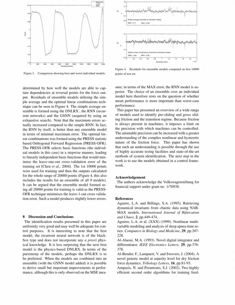
determined by how well the models are able to cap-ture dependencies at reversal points for the force out-put. Residuals of ensemble models utilising the sim-ple average and the optimal linear combinations tech-nique can be seen in Figure 4. The simple average en-semble is formed using the DNLRX , the RNN (recur-rent networks) and the GSNN (acquired by using anexhaustive search). Note that the maximum errors ac-tually increased compared to the simple RNN. In fact,the RNN by itself, is better than any ensemble modelin terms of minimal maximum error. The optimal lin-ear combinations was formed using the PRESS statisticbased Orthogonal Forward Regression (PRESS-OFR).The PRESS-OFR selects basis functions (the individ-ual models in this case) in a stepwise manner, leadingto linearly independent basis functions that would min-imise the leave-one-out cross-validation error of thetraining set [Chen et al., 2004]. The 1st 10000 pointswere used for training and then the outputs calculatedfor the whole range of 20000 points (Figure 4, this alsoincludes the results for an ensemble of all 9 models).It can be argued that the ensemble model formed us-ing all 20000 points for training is valid as the PRESS-OFR technique minimises the leave-1-out cross valida-tion error. Such a model produces slightly lower errors.
8 Discussion and ConclusionsThe identification results presented in this paper are
uniformly very good and may well be adequate for con-trol purposes. It is interesting to note that the bestmodel, the recurrent neural network is of the black-box type and does not incorporate any a priori phys-ical knowledge. It is less surprising that the next bestmodel is the physics-based DNLRX. In terms of theparsimony of the models, perhaps the DNLRX is tobe preferred. When the models are combined into anensemble (with the GSNN model added) it is possibleto derive small but important improvements in perfor-mance, although this is only observed on the MSE mea-
0 0.2 0.4 0.6 0.8 1 1.2 1.4 1.6 1.8 2
x 104
−0.2
−0.1
0
0.1
Sampling instant
−0.2
−0.1
0
0.1
0.2
e
Simple Average Ensemble (3 individual models)
MSE = 0.11 MAX = 0.60
Optimal Linear Combinations Ensemble (9 individual models)
MSE = 0.08 MAX = 0.56
(a)
(b)
e
Figure 4. Residuals for ensemble models computed on first 10000
points of test set.
sure; in terms of the MAX error, the RNN model is su-perior. The choice of an ensemble over an individualmodel here therefore rests on the question of whethermean performance is more important than worst-caseperformance.This paper has presented an overview of a wide range
of models used to identify pre-sliding and gross slid-ing friction and the transition regime. Because frictionis always present in machines, it imposes a limit onthe precision with which machines can be controlled.The attainable precision can be increased with a greaterunderstanding of the complex nonlinear and hystereticnature of the friction force. This paper has shownthat such an understanding is possible through the useof highly accurate tesing facilities and state-of-the-artmethods of system identification. The next step in thework is to use the models obtained in a control frame-work.
AcknowledgementThe authors acknowledge the Volkswagenstiftung for
financial support under grant no. 1/76938.
ReferencesAguirre, L.A. and Billings, S.A. (1995). Retrievingdynamical invariants from chaotic data using NAR-MAX models. International Journal of Bifurcationand Chaos, 2, pp.449-474.Aguirre, L.A. et al. (XXX) (1999). Nonlinear multi-variable modeling and analysis of sleep apnea time se-ries. Computers in Biology and Medicine, 29, pp.207-228.Al-Alaoui, M.A. (1993). Novel digital integrator anddifferentiator. IEEE Electronics Letters, 29, pp.376-378.Al-Bender, F., Lampaert, V. and Swevers, J. (2004). Anovel generic model at asperity level for dry frictionforce dynamics. Tribology Letters, 16, pp.81-93.Ampazis, N. and Perantonis, S.J. (2002). Two highlyefficient second order algorithms for training feed-

forward networks. IEEE Transactions on Neural Net-works, 13 pp.XXX-XXX.Armstrong-Helouvry, B., Dupont, P. and Canudas deWit, C. (1994). A survey of models, analysis tools andcompensation methods for the control of machineswith friction. Automatica, 30, pp.1083-1183.Arulampalam, G. and Bouzerdoum, A. (2003). A gen-eralized feedforward neural network architecture forclassification and regression. Neural Networks, 16,pp.561-568.Atkeson, C.G. et al. (XXX) (1997). Locally weightedlearning. Artificial Intelligence Review, 11, pp.11-73.Bates, D.M. and Watts, D.G. (1988). Nonlinear Re-gression and Its Applications. New York: Wiley.Billings, S.A. et al. (XXX) (1989). Identification ofMIMO non-linear systems using a forward-regressionorthogonal estimator. International Journal of Con-trol, 6, pp.2157-2189.Billings, S.A. and Coca, D. (1999). Discrete waveletmodels for identification and qualitative analysis ofchaotic systems. International Journal of Bifurcationand Chaos, 7, pp.1263-1284.Bouzerdoum, A. (1999). A new class of high-orderneural networks with nonlinear decision boundaries.Proceedings of the Sixth International Conference onNeural Information Processing (ICONIP’99), Perth,Australia, pp.1004-1009.Canudas de Wit, C., Olsson, H., Astrom, K.J. andLischinsky, P. (1995). A new model for control of sys-tems with friction. IEEE Transactions on AutomaticControl, 40, pp.419-425.Chen, S., Hong, X., Harris, C.J. and Sharkey, P.M.(2004). Sparse modelling using orthogonal forwardregression with PRESS statistic and regularization.IEEE Transactions on System, Man, and Cybernetics,Part B, 34, pp.898-911.Dahl, P.R. (1968). A solid friction model. TheAerospace Corporation, El Segundo, CA, TOR-158.Eriksson, B. (1996). Optimal force control to improvehydraulic drives. Licentiate Thesis, Damek ResearchGroup, Department of Machine Design, Royal Insti-tute of Technology, KTH, Sweden.Furman, G.G. (1965). Comparison of models for sub-tractive and shunting lateral-inhibition in receptor-neuron fields. Kybernetik, 2, pp.257-274.Jaeger, H. (2001) The echo state approach toanalysing and training recurrent neural networks.GMD Report German National Research Center forInformation Technology, 148.Krogh, A. and Hertz, J.A. (1992). A simple weightdecay can improve generalisation. Advances in NeuralInformation Processing Systems, 4, pp.951-957.Lampaert, V., Swevers, J. and Al-Bender F. (2002).Modification of the Leuven integrated friction modelstructure. IEEE Transactions on Automatic Control,47, p.683-XXX.Lampaert, V., Al-Bender, F. and Swevers, J. (2004).Experimental characterisation of dry friction at lowvelocities on a developed tribometer set-up for macro-
scopic measurements. Tribology Letters, 16, pp.95-105.Maass, W., Natschlager, T. and Markram, H. (2002).Real-time computing without stable states: a newframework for neural computation based on perturba-tions. Neural Computation, 14, pp.2531-2560.McNames, J. (1999). Innovations in local modelingfor time series prediction. Ph.D. thesis, Stanford Uni-versity.Merkwirth, C. et al. (XXX) (2000). Fast nearest-neighbor searching for nonlinear signal processing.Physical Review E, 62, pp.2089-2097.Nakazawa, H. (1991). Principles of Precision Engi-neering. Oxford University Press, Oxford.Nelles, O. (2001). Nonlinear System Identification:From Classical Approaches to Neural Networks andFuzzy Models. Springer-Verlag, Berlin.Olsson, H. (1996). Control system with friction. Ph.D.thesis, Department of Automatic Control, Lund Insti-tute of Technology, Sweden.Parlitz, U., Hornstein, A., Engster, D., Al-Bender, F.,Lampaert, V., Tjahjowidodo, T., Fassois, S.D., Ri-zos, D., Wong, C.X., Worden, K. and Manson, G.(2004). Identification of pre-sliding friction dynam-ics. Chaos: An Interdisciplinary Journal of NonlinearScience, 14, pp.420-430.Popovic, M.R., Gorinevsky, D.M. and Goldenbery,A.A. (1995). Accurate positioning of devices withnonlinear friction using fuzzy logic pulse controller.Proceedings of International Symposium on Experi-mental Robotics, pp.331-342.Rizos, D.D. and Fassois, S.D. (2003). Presliding fric-tion identification based upon the Maxwell slip modelstructure. 4th International Symposium on Investiga-tions of Non-Linear Dynamics Effects in ProductionSystems, Chemmintz, Germany.Rizos, D.D. and Fassois, S.D. (2004). Presliding fric-tion identification based upon the Maxwell slip modelstructure. Chaos: An Interdisciplinary Journal ofNonlinear Science, 14, pp.431-445.Rizos, D.D. and Fassois, S.D. (2005). Friction iden-tification based upon the LuGre and Maxwell-slipModels. Submitted to IFAC World Congress 2005.Sjoberg, J., Zhang, Q., Ljung, L., Beneviste, A., De-lyon, B., Glorennec, P.-Y., Hjalmarsson, H. and Ju-ditsky, A. (1995). Nonlinear black-box modelling insystem identification: a unified overview. Automatica,31, pp.1691-1724.Swevers, J., Al-Bender, F., Ganseman, C.G. and Pra-jogo, T. (2000). An integrated friction model structurewith improved presliding behavior for accurate fric-tion compensation. IEEE Transactions on AutomaticControl, 45, pp.675-675.Wong, C.X. and Worden, K. (2004) Identification offriction models using a genaralised shunting neuralnetwork. Submitted to Mechanical Systems and Sig-nal Processing.Yang, S. and Tomizuka, M. (1988). Adaptive pulsewidth control for precise positioning under the influ-

ence of stiction and Coulomb friction. ASME Journalof Dynamic Systems, Measurements and Control, 110,pp.211-227.


