Identification of volcanic rootless cones, ice mounds, and

2 Identification of volcanic rootless cones, ice mounds, and impact

3 craters on Earth and Mars: Using spatial distribution as a remote

4 sensing tool

5 B. C. Bruno,1 S. A. Fagents,1 C. W. Hamilton,1 D. M. Burr,2 and S. M. Baloga3

6 Received 16 June 2005; revised 29 March 2006; accepted 10 April 2006; published XX Month 2006.

7 [1] This study aims to quantify the spatial distribution of terrestrial volcanic rootless8 cones and ice mounds for the purpose of identifying analogous Martian features. Using a9 nearest neighbor (NN) methodology, we use the statistics R (ratio of the mean NN distance10 to that expected from a random distribution) and c (a measure of departure from11 randomness). We interpret R as a measure of clustering and as a diagnostic for12 discriminating feature types. All terrestrial groups of rootless cones and ice mounds are13 clustered (R: 0.51–0.94) relative to a random distribution. Applying this same14 methodology to Martian feature fields of unknown origin similarly yields R of 0.57–0.93,15 indicating that their spatial distributions are consistent with both ice mound or rootless16 cone origins, but not impact craters. Each Martian impact crater group has R � 1.00 (i.e.,17 the craters are spaced at least as far apart as expected at random). Similar degrees of18 clustering preclude discrimination between rootless cones and ice mounds based solely on19 R values. However, the distribution of pairwise NN distances in each feature field20 shows marked differences between these two feature types in skewness and kurtosis.21 Terrestrial ice mounds (skewness: 1.17–1.99, kurtosis: 0.80–4.91) tend to have more22 skewed and leptokurtic distributions than those of rootless cones (skewness: 0.54–1.35,23 kurtosis: �0.53–1.13). Thus NN analysis can be a powerful tool for distinguishing24 geological features such as rootless cones, ice mounds, and impact craters, particularly25 when degradation or modification precludes identification based on morphology alone.

26 Citation: Bruno, B. C., S. A. Fagents, C. W. Hamilton, D. M. Burr, and S. M. Baloga (2006), Identification of volcanic rootless

27 cones, ice mounds, and impact craters on Earth and Mars: Using spatial distribution as a remote sensing tool, J. Geophys. Res., 111,

28 XXXXXX, doi:10.1029/2005JE002510.

30 1. Introduction

31 [2] The objective of this research is to refine and apply32 the nearest neighbor (NN) technique used by Bruno et al.33 [2004] to distinguish among different origins for small34 (less than a few km), circular to elongate, positive-relief35 mounds and cones, for the purposes of understanding the36 local geology and, ultimately, constructing a historical37 volatile inventory for our study sites on Mars. Geologic38 features that form in the presence of water or ice are of39 key interest because they provide information about the40 abundance and spatial distribution of volatiles on Mars at41 the time of feature formation. Such features include42 volcanic rootless cones, subglacial volcanoes, rampart43 craters, pingos, and other types of ice mounds [Carr et44 al., 1977; Allen, 1979a, 1979b; Frey et al., 1979;45 Lucchitta, 1981; Frey and Jarosewich, 1982; Mouginis-

46Mark, 1987; Cabrol et al., 2000; Chapman and Tanaka,472001]. Water-rich localities on Mars not only represent48potential niches for past biological development, but they49are also prospective sources of water for future Mars50missions.51[3] Rootless volcanic cones are an important diagnostic52of ice distribution in the near-surface regolith [Greeley and53Fagents, 2001; Lanagan et al., 2001; Fagents et al., 2002;54Fagents and Thordarson, 2006]. They were first identified55in Viking Orbiter imagery [Allen, 1979a; Frey et al., 1979;56Frey and Jarosewich, 1982], and more recently from data57acquired by both the Thermal Emission Imaging System58(THEMIS) on Mars Odyssey and the high-resolution (Nar-59row-Angle) Mars Orbiter Camera (MOC-NA) aboard Mars60Global Surveyor. Rootless cones, found in abundance in61Iceland, form when lava flowing in an inflating pahoehoe62flow field interacts explosively with water or ice contained63within the substrate [Thorarinsson, 1951, 1953]. Successive64explosive pulses eject fragments of lava and substrate from65the explosion site to build a cratered cone of ash, scoria,66spatter, and clastic substrate sediments. Once activity at a67given explosion site wanes (due to volatile depletion or a68cessation of lava supply), explosive interactions typically69initiate nearby. The result is a group containing tens to

JOURNAL OF GEOPHYSICAL RESEARCH, VOL. 111, XXXXXX, doi:10.1029/2005JE002510, 2006ClickHere

for

FullArticle

1Hawaii Institute of Geophysics and Planetology, University of Hawaii,Honolulu, Hawaii, USA.

2SETI Institute, Mountain View, California, USA.3Proxemy Research, Bowie, Maryland, USA.

Copyright 2006 by the American Geophysical Union.0148-0227/06/2005JE002510$09.00

XXXXXX 1 of 16

http://dx.doi.org/10.1029/2005JE002510

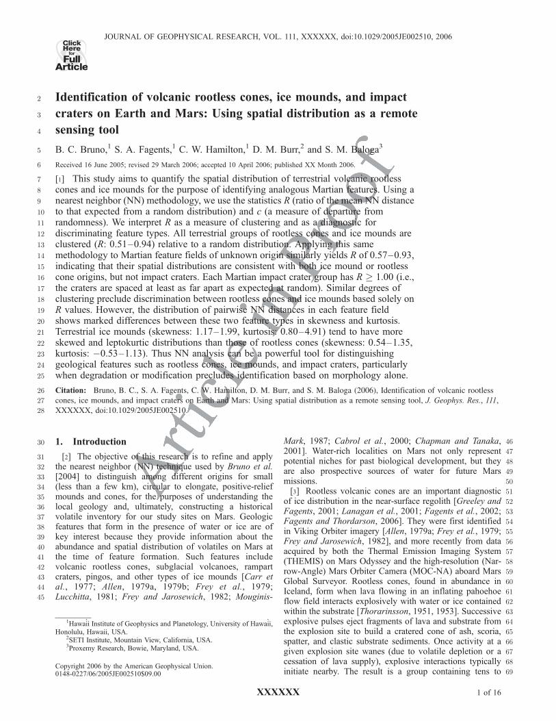
70 hundreds of cones [Thordarson et al., 1998; Thordarson,71 2000].72 [4] Rootless volcanic cones are distinct from primary73 scoria cones, which form over a volcanic conduit more74 deeply rooted in the crust to a magma source. Unlike75 primary cones, rootless cones are not the source of lava76 flows (although they can feed rheomorphic flows that can77 be difficult to distinguish from primary lava flows).78 Figures 1a and 1b show a typical rootless cone group within79 the 1783-84 Laki lava flow in Iceland. The morphology and80 spatial density of rootless cones provide an indication of the81 quantity and location of water in the substrate at the time of82 cone formation; modeling the dynamics of cone-forming83 explosions permits assessment of the vapor mass and84 pressure required to produce cones of the observed numbers85 and sizes [Greeley and Fagents, 2001]. If rootless cones can86 be unequivocally identified on Mars, we will have a87 powerful means to gauge the amount, distribution, and88 evolution of near-surface volatiles in the regolith.89 [5] Similarly, the putative identification of pingos and90 other ice mounds on Mars implies the presence of volatiles91 in the Martian regolith [Lucchitta, 1981; Parker et al., 1993;92 Cabrol et al., 2000; Burr et al., 2005; Soare et al., 2005]. A93 pingo is a type of ice cored mound, common in periglacial94 environments within Alaska, Canada, and Russia. Like95 rootless cones, pingos can grow up to several hundreds of96 meters in basal diameter and up to tens of meters in height97 [Washburn, 1973].98 [6] In general, pingos form when the overburden is99 domed above a segregated ice body that grows either by100 (1) intrusion and subsequent freezing of liquid water101 injected into permafrost; (2) progressive underplating of102 an ice cored mound as an underlying water reservoir103 freezes; or (3) a combination of both these processes104 [Washburn, 1973; Mackay, 1987]. Depending on their105 formation mechanism, pingos are divided into two main106 categories: hydrostatic and hydraulic.107 [7] The majority of terrestrial pingos are hydrostatic108 (‘‘closed-system’’) pingos and form in response to the109 draining of ephemeral ponds and lakes which exposes the110 unfrozen basin to subfreezing temperatures [Porsild, 1938;111 Muller, 1959; Mackay, 1962, 1973, 1979, 1998; Washburn,112 1973]. Progradation of the freezing front both from the113 ground surface downward and the underlying permafrost114 upward pressurizes the residual pore water. In transmissive115 sediments, this pore water flows ahead of the freezing front116 toward the basin center, the usual site of minimal permafrost117 growth. Continued flow and freezing of this expelled pore118 water, in addition to a small effect from volumetric expan-119 sion, domes up the overlying permafrost layer to form a120 mound [Mackay, 1998; Burr et al., 2005]. Continued121 growth can produce radial tension fractures from the sum-122 mit and circumferential compression fractures at the mar-123 gins. Pingo collapse may occur when the summit ruptures124 and the remaining liquid water below the ice mound125 escapes. Collapsed pingos typically form a depression126 surrounded by a raised ring of residual sediment.127 Figures 1c and 1d show hydrostatic pingos from the128 Tuktoyaktuk Peninsula, Canada.129 [8] Hydraulic (‘‘open-system’’) pingos tend to form in130 narrow valleys or on slopes in areas of discontinuous (or131 locally thinner) permafrost. In these cases, artesian pressure

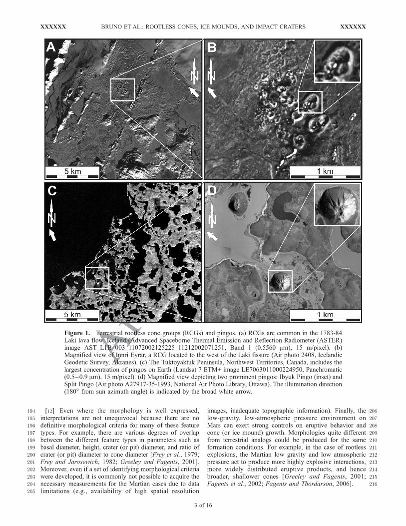
132forces water to intrude into shallow permafrost. Upon133freezing, the water ice uplifts the overburden to form134mounds [Washburn, 1973]. Hydraulic pingos may also135grow as a result of hydraulic lift, where low artesian136pressure is amplified through confinement under a pingo137[Muller, 1959; Holmes et al., 1968]. When discussing ice138cored mounds of uncertain origin, we use the general term139‘‘ice mound’’ (rather than the specific term ‘‘pingo’’) to140include other segregated ice bodies such as palsas, hydro-141laccoliths, icings, and ice hummocks. (SeeWashburn [1973]142for a comprehensive description of these features.) We143reserve the term ‘‘pingo’’ for ice cored mounds of known144hydraulic or hydrostatic origin.145[9] On Mars, potential rootless volcanic cones have been146identified in the northern lowland plains (Figure 2a),147including Acidalia, Amazonis, Isidis, and Elysium Planitiae148[Allen, 1979a; Frey and Jarosewich, 1982; Greeley and149Fagents, 2001; Lanagan et al., 2001; Fagents et al., 2002].150Possible Martian ice mounds have been identified in Gusev151Crater, Athabasca Valles and the Cerberus Plains (Figure 2b)152as defined by Plescia [1990], and Chryse, Acidalia, and153Utopia Planitiae [Lucchitta, 1981; Parker et al., 1993;154Cabrol et al., 2000; Burr et al., 2005; Soare et al., 2005;155Page and Murray, 2006].156[10] Historically, Martian pingos have been difficult to157identify on the basis of Viking Orbiter data, in part because158of limited availability of high-resolution images, but also159because only the most mature pingos exhibit distinctive160morphologies. Younger and/or smaller pingos are typically161expressed as low-relief mounds. Only once the mound is162sufficiently upheaved does its surface begin to rupture,163thereby exposing the interior ice, which melts or sublimes164to form crevices and pits at or near the summit [Washburn,1651973;Mackay, 1979]. Moreover, these morphologies are apt166to be confused with those of rootless cones, and the167presence of pingos or other ice mounds on Mars remains168equivocal [Theilig and Greeley, 1979; Lucchitta, 1981;169Rossbacher and Judson, 1981; Squyres et al., 1992; Parker170et al., 1993; Cabrol et al., 2000].171[11] Geological context is therefore of key importance in172identifying rootless cones and ice mounds. Interpretation of173a volcanic origin is relatively straightforward for pristine174cones lying on surfaces with clear textural indications of175lava flow morphology [Lanagan et al., 2001]. However, in176areas where the cones and/or the underlying surface are177degraded or mantled by dust, or for which image resolution178is a limiting factor, it becomes harder to identify the origins179on the basis of morphology alone. Ambiguities arise be-180cause, under these adverse conditions, other small, circular,181pitted cones or mounds can resemble rootless cones. In182addition to the ice mound hypothesis, other possibilities183include (1) secondary (Figure 2c) or pedestal (Figure 2d)184impact craters, the latter having resistant ejecta armoring a185more easily eroded substrate; (2) mud volcanoes produced186by gas- or water-charged eruptions of clastic sediments187[Tanaka, 1997; Farrand et al., 2005]; (3) primary scoria188cones; (4) gravity craters, produced when blocks of ice189transported by jokulhlaups (glacial outburst floods) settle190into soft sediments [Gaidos and Marion, 2003]; and (5)191kettle holes, which are formed when sediment-laden ice192blocks are partially buried and subsequently melted [Gaidos193and Marion, 2003].

XXXXXX BRUNO ET AL.: ROOTLESS CONES, ICE MOUNDS, AND IMPACT CRATERS

2 of 16

XXXXXX

194 [12] Even where the morphology is well expressed,195 interpretations are not unequivocal because there are no196 definitive morphological criteria for many of these feature197 types. For example, there are various degrees of overlap198 between the different feature types in parameters such as199 basal diameter, height, crater (or pit) diameter, and ratio of200 crater (or pit) diameter to cone diameter [Frey et al., 1979;201 Frey and Jarosewich, 1982; Greeley and Fagents, 2001].202 Moreover, even if a set of identifying morphological criteria203 were developed, it is commonly not possible to acquire the204 necessary measurements for the Martian cases due to data205 limitations (e.g., availability of high spatial resolution

206images, inadequate topographic information). Finally, the207low-gravity, low-atmospheric pressure environment on208Mars can exert strong controls on eruptive behavior and209cone (or ice mound) growth. Morphologies quite different210from terrestrial analogs could be produced for the same211formation conditions. For example, in the case of rootless212explosions, the Martian low gravity and low atmospheric213pressure act to produce more highly explosive interactions,214more widely distributed eruptive products, and hence215broader, shallower cones [Greeley and Fagents, 2001;216Fagents et al., 2002; Fagents and Thordarson, 2006].

Figure 1. Terrestrial rootless cone groups (RCGs) and pingos. (a) RCGs are common in the 1783-84Laki lava flow, Iceland (Advanced Spaceborne Thermal Emission and Reflection Radiometer (ASTER)image AST_L1B_003_11072002125225_11212002071251, Band 1 (0.5560 mm), 15 m/pixel). (b)Magnified view of Innri Eyrar, a RCG located to the west of the Laki fissure (Air photo 2408, IcelandicGeodetic Survey, Akranes). (c) The Tuktoyaktuk Peninsula, Northwest Territories, Canada, includes thelargest concentration of pingos on Earth (Landsat 7 ETM+ image LE7063011000224950, Panchromatic(0.5–0.9 mm), 15 m/pixel). (d) Magnified view depicting two prominent pingos: Ibyuk Pingo (inset) andSplit Pingo (Air photo A27917-35-1993, National Air Photo Library, Ottawa). The illumination direction(180� from sun azimuth angle) is indicated by the broad white arrow.


3 of 16

XXXXXX

217 [13] Given these interpretive difficulties, Bruno et al.218 [2004] developed and applied a suite of nonmorphological219 statistical criteria to quantify the distribution of small,220 circular structures within a feature field on the basis of221 NN analysis and linear alignment detection techniques.222 They applied these techniques to rootless cone groups in223 Iceland, candidate rootless cone groups on Mars, and impact224 craters on Mars of probable secondary origin. They found225 that the spatial relationships of Martian candidate rootless226 cones are indistinguishable from those of Icelandic rootless227 cones (i.e., they both show similar degrees of clustering228 within their groups), but are markedly different from those229 of Martian impact craters (which show no evidence of230 intrafield clustering). This suggests that we can have some

231confidence in distinguishing rootless cones from impact232craters in images where morphology is not well defined233due to degradation, modification or sediment cover. Other234investigators have similarly investigated clustering of pri-235mary volcanic cones, on the basis of qualitative observa-236tions, cluster analysis and related NN-based techniques237[Carr, 1976; Settle, 1979; Heming, 1980; Walker, 1981;238Hasenaka and Carmichael, 1985a, 1985b; Connor, 1990;239Connor et al., 1992; Connor and Hill, 1995], but we are not240aware of any other comparable published studies that relate241to the feature types included in this study.242[14] We recognize some limitations of the NN technique243as applied by Bruno et al. [2004]. First, the NN technique244requires that an envelope be drawn to enclose the feature

Figure 2. Feature fields on Mars. (a) Candidate rootless cone group (RCG) southeast of Phlegra Montes(MOC-NA image M08-01962, 4.52 m/pixel). (b) Candidate Martian group (may represent rootlesscones or ice mounds) in western Cerberus Planitia (MOC-NA image E10-01384, 3.09 m/pixel).(c) Secondary impact craters northeast of Mars Pathfinder site in Ares Vallis (MOC-NA image R10-05447, 3.13 m/pixel). (d) Pedestal craters east of Acidalia Planitia (THEMIS visible image V1358002,19 m/pixel). The illumination direction (180� from sun azimuth angle) is indicated by the broad whitearrow. Note: Figures 1a, 1c, and 2d; Figures 1b, 1d, and 2a–2c; and insets for Figures 1b, 1d, and 2a–2dare represented to the same scale, respectively.


4 of 16

XXXXXX

245 field. Bruno et al. [2004] used the best fitting rectangle to246 enclose all cones or craters in a given group, but there are a247 number of reasons why this is not the best approach (as248 discussed below). Second, features which occur along the249 border of an image were fully included as members of the250 group. However, our inability to assess their nearest neigh-251 bors (which might be beyond the edge of the image)252 suggests that they should be selectively excluded from the253 analysis. The third issue is group definition. Several feature254 fields contain subclusters within them, and treating all255 features as a single group can considerably affect NN256 results. Finally, and perhaps most important, standard NN257 methodology reduces all the information of a feature field to258 two statistics (R and c), and much important information is259 lost in this process.260 [15] In this paper we present refinements to standard NN261 methodology in the areas outlined above, and this leads to a262 more objective assessment of spatial distribution. We apply263 our methodology to the same data set studied by Bruno et264 al. [2004], as well as to terrestrial ice mounds, candidate265 Martian ice mounds, and Martian pedestal craters for the266 first time. Finally, we outline a skewness-kurtosis analysis267 which, when combined with the standard NN statistics R268 and c, proves useful in separating feature types.269 [16] Throughout this paper, we use the term ‘‘random.’’270 Spatial randomness is defined for a set of points on a given271 area as follows: ‘‘any point has had the same chance of272 occurring on any subarea as any other point; that any273 subarea of specified size has had the same chance of274 receiving a point as any other subarea of that size, and that275 the placement of each point has not been influenced by that276 of any other point’’ [Clark and Evans, 1954]. Thus spatial277 randomness is intimately connected with a Poisson proba-278 bility distribution of points in a plane of infinite extent. In279 this work, we are concerned only with spatial randomness280 resulting from an underlying Poisson distribution and its281 corresponding probability distribution of nearest neighbor282 distances. Therefore we use the term ‘‘random’’ as a283 convenient shorthand for these concepts.

284 2. Data

285 2.1. Icelandic Rootless Cones (8 Groups)

286 [17] For our first data set, we apply our refined NN287 methodology to the same three Icelandic lava flow fields

288(Laki, Eldgja, and Leitin) previously considered by Bruno et289al. [2004]. Within these three flow fields are multiple290distinct rootless cone groups, of which we analyze eight291(Table 1). Two of these (Hnuta North and Hnuta South)292were previously considered to be a single group; Bruno et293al. [2004] listed only seven rootless cone groups. However,294our refined NN technique (detailed below) requires that295these two groups be considered separately because they are296physically separated by a scarp.297[18] These volcanic cone groups have all been unambigu-298ously determined from field investigations to be rootless299cones formed by hydrovolcanic explosions and constructed300on top of the host lava flow [Thoroddsen, 1894;Thorarinsson,3011951; 1953]. In all cases, locations of rootless cones were302determined from stereo aerial photographs at scales of3031:37000 (Laki, Eldgja) and 1:16000 (Leitin). Cone morphol-304ogy and dimensions vary considerably, as does the spatial305distribution of cones within a cone group. Cone basal306diameters lie in the 5–450 m range, and cone heights are3072–40 m [Thorarinsson, 1953; Thordarson et al., 1992;308Thordarson and Hoskuldsson, 2002].

3092.2. Ice Mounds in Canada and Alaska (7 Groups)

310[19] Our second data set comprises seven groups of ice311mounds in Canada and Alaska (Table 2). These mounds312have been mapped by previous authors from stereo aerial313photographs and through field investigations, and our314analysis is based on their published maps in three locations:315Tuktoyaktuk Peninsula area, Northwest Territories, Canada316[Mackay, 1998]; Tanacross, central Alaska [Holmes et al.,3171968] and Prudhoe Bay, northern Alaska [Walker et al.,3181985]. The sizes of ice mounds are comparable to those of319rootless cones. Basal diameter and height ranges are respec-320tively �5–600 m and �3–70 m [Washburn, 1973].321[20] In the Tuktoyaktuk Peninsula area, the type locality322for hydrostatic pingos, nearly 1400 pingos of greatly323varying sizes are divided into three geographic groups,324whose boundaries are determined by the peninsular coast-325line. Basal diameters range from 30 to 600 m and heights326range from 3 to �50 m [Holmes et al., 1968]. In contrast,327the Tanacross ice mounds (which are treated as one group)328are hydraulic pingos. They can be circular, elliptical or329irregularly shaped. With basal diameters of 15–450 m and330heights of 3–30 m, the Tanacross pingos do not attain the331sizes of the largest Tuktoyaktuk pingos [Holmes et al.,

t1.1 Table 1. Terrestrial Rootless Cone Groups, Icelanda

Air Photo Number and Position of Feature Field Air Photo Scale Locationt1.2

Laki Lava Flow (1783–84)t1.3Blagil 1869 – Just NE of center 1:37000 64.0�N, 18.4�Wt1.4Innri Eyrar (Figure 1) 2408 – Just E of center 1:37000 64.2�N, 18.2�Wt1.5Hnuta (North) 1870 – Eastern 1/3 of image 1:37000 64.0�N, 18.4�Wt1.6Hnuta (South) 1870 – Eastern 1/3 of image 1:37000 64.0�N, 18.4�Wt1.7Trollhamar 2408 – Northern edge of image 1:37000 64.2�N, 18.2�Wt1.8Stakafell 2409 – Just SW of center 1:37000 64.2�N, 18.2�Wt1.9

t1.10Eldgja Lava Flow (1.1 kybp)t1.11

Landbrot 1413 – Northern half of image 1:37000 63.7�N, 18.1�Wt1.12t1.13

Leitin Lava Flow (4.6 kybp)t1.14Raudholar 264 – Center of image 1:16000 64.1�N, 21.7�Wt1.15

aAir photos obtained from Geodetic Survey of Iceland.t1.16


5 of 16

XXXXXX

332 1968]. Yet the average size (10 or 15 m high, 150 or 200 m333 wide) of the two groups appears to be about the same334 [Stager, 1956]. Most of the Tanacross pingos lie along335 gentle to moderate south-facing slopes or on very gently336 sloping valley floors. None are observed in drained or337 shallow lake basins, despite an abundance of such basins338 on the valley floor [Holmes et al., 1968].339 [21] At Prudhoe Bay, Walker et al. [1985] distinguished340 between steep-sided hydrostatic pingos (mean height 4 m,341 mean diameter 72 m, mean slope 7�) and broad-based342 mounds (mean height 5 m, mean diameter 242 m, mean343 slope 3�). Whether these broad mounds represent pingos is344 unclear, but drilling suggests at least the larger ones are ice345 cored [Brockett, 1982]. Walker et al. [1985] observed that346 the steep-sided pingos appear to be fairly randomly distrib-347 uted in both the flat and gently rolling thaw-lake plains,348 whereas the broad-based mounds are clustered into regions349 of higher density within the gently rolling thaw-lake plains.350 We note two main groupings of these broad mounds,

351located to the east and west of the flat plains. We consider352the steep-sided pingos as a third, separate group for NN353analysis.

3542.3. Candidate Martian Rootless Cones and/or Ice355Mounds (10 Groups)

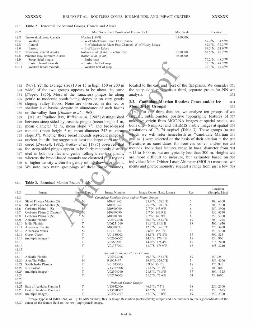
356[22] For our third data set, we analyze ten groups of357circular, subkilometer, positive topographic features of358unknown origin from MOC-NA images at spatial resolu-359tions of 3–6 m/pixel and THEMIS visible images at spatial360resolutions of 17–74 m/pixel (Table 3). These groups (to361which we will refer henceforth as ‘‘candidate Martian362groups’’) were selected on the basis of their citation in the363literature as candidates for rootless cones and/or ice364mounds. Individual features range in basal diameter from365�15 to 1000 m, but are typically less than 300 m. Heights366are more difficult to measure, but estimates based on367individual Mars Orbiter Laser Altimeter (MOLA) measure-368ments and photoclinometry suggest a range from just a few

t2.1 Table 2. Terrestrial Ice Mound Groups, Canada and Alaska

Map Source and Position of Feature Field Map Scale Locationt2.2

Tuktoyaktuk area, Canada Mackay [1998] 1:1000000t2.3Western – W of Mackenzie River East Channel 69.2�N, 134.5�Wt2.4Central – E of Mackenzie River East Channel; W of Husky Lakes 69.5�N, 132.3�Wt2.5Eastern – E of Husky Lakes 69.5�N, 131.0�Wt2.6

Tanacross, central Alaska Holmes et al. [1968] – entire map 1:870000 63.5�N, 142.2�Wt2.7Prudhoe Bay, northern Alaska Walker et al. [1985] 1:670000t2.8

Steep-sided pingos – Entire map 70.2�N, 148.5�Wt2.9Eastern broad mounds – Eastern half of map 70.1�N, 147.7�Wt2.10Western broad mounds – Western half of map 70.3�N, 149.4�Wt2.11

t3.1 Table 3. Examined Martian Feature Fieldsa

Image Image Type Image Number Image Center (Lat., Long.) Res.Location

(Sample, Line)t3.2

Candidate Rootless Cone and/or Pingo Groupst3.3SE of Phlegra Montes (S) M M0801962 25.9�N, 170.3�E 5 300, 6100t3.4SE of Phlegra Montes (N) M M0801962 25.9�N, 170.3�E 5 200, 7700t3.5Cerberus Plains 1 (S) M M0800090 2.7�N, 143.9�E 6 250, 3900t3.6Cerberus Plains 2 (Central) M M0800090 2.7�N, 143.9�E 6 150, 4550t3.7Cerberus Plains 3 (N) M M0800090 2.7�N, 143.9�E 6 250, 5300t3.8Acidalia Planitia T V05393016 40.3�N, 353.1�E 19 700, 1225t3.9Isidis Planitia T V06251019 11.6�N, 84.8�E 18 500, 1650t3.10Amazonis Planitia M M0700373 12.2�N, 196.3�E 3 225, 3400t3.11Athabasca Valles M E1001384 9.6�N, 156.1�E 3 350, 5700t3.12Gusev Crater T V01580003 14.5�S, 175.8�E 17 500, 825t3.13(multiple images) T V02666002 14.1�S, 176.1�E 18 550, 900t3.14

T V05662001 14.0�S, 176.4�E 18 215, 2400t3.15T V03777003 13.7�S, 175.9�E 18 455, 3210t3.16

t3.17Secondary Impact Crater Groupst3.18

Acidalia Planitia T V05393016 40.3�N, 353.1�E 19 25, 925t3.19Ares/Tiu Valles M R1005447 19.9�N, 326.7�E 3 350, 4500t3.20South Isidis Planitia T V01033003 3.9�N, 85.5�E 18 375, 925t3.21Nili Fossae T V13927008 21.4�N, 76.3�E 37 300, 800t3.22(multiple images) T V02394010 21.8�N, 76.3�E 37 300, 1325t3.23

T V02756003 21.3�N, 76.6�E 74 75, 1600t3.24t3.25

Pedestal Crater Groupst3.26East of Acidalia Planitia 1 T V13942006 46.3�N, 7.5�E 38 250, 2100t3.27East of Acidalia Planitia 2 T V13580002 47.5�N, 10.3�E 19 350, 1675t3.28(multiple images) T V04993017 47.7�N, 10.0�E 19 550, 2300t3.29

aImage Type is M (MOC-NA) or T (THEMIS Visible); Res. is Image Resolution (meters/pixel); sample and line numbers are the x,y coordinates of thecenter of the feature field on the raw (unprojected) image.t3.30


6 of 16

XXXXXX

369 meters at Athabasca Valles to close to 100 m at Gusev370 Crater [Cabrol et al., 2000; Burr et al., 2005; Soare et al.,371 2005].372 [23] Two of these candidate Martian groups are located373 southeast of Phlegra Montes and west of Amazonis Planitia374 (MOC-NA image M0801962). Here, features have been375 interpreted as rootless cones on the basis of a variety of376 criteria, including distinct conical morphology and well377 defined summit craters, stratigraphic position atop a lava378 flow having a pristine platy-ridged surface texture, the lack379 of association with eruptive fissures, and an absence of lava380 flows issuing from the cones [Greeley and Fagents, 2001;381 Lanagan et al., 2001]. Three candidate Martian groups are382 located in the region Plescia [1990, 1993, 2003] called the383 Cerberus plains (MOC-NA image M0800090). These fea-384 tures have similarly been interpreted as rootless cones on385 the basis of distinctive morphologies and geologic relations386 [Lanagan et al., 2001].387 [24] The morphologies of cone-like features in the Cydo-388 nia region of Acidalia Planitia (THEMIS image389 V05393016) and within Isidis Planitia (THEMIS image390 V06251019) are less pristine. These two groups contain391 degraded, positive-relief, conical features with subdued392 summit craters (e.g., Figure 2a) that are quite distinct from393 the impact craters located within the same images. Cones394 and mounds in these areas were interpreted as rootless cones395 on the basis of Viking Orbiter imagery [Frey et al., 1979;396 Frey and Jarosewich, 1982]. The surfaces on which the397 features reside appear considerably older than those in398 MOC-NA images M0800090 and M0801962, as evidenced399 by the higher density of impact craters. One possibility is400 that the cones formed on a sedimentary surface, in which401 case they could not be volcanic, let alone rootless. Alterna-402 tively, the original surface prior to mantling may have been403 lava that, in combination with a volatile-rich substrate,404 would admit the possibility of rootless cone formation.405 The Isidis cones have also been interpreted as pingos; their406 cratered expression has been attributed to ablation of ice407 cores within ice mounds [Rossbacher and Judson, 1981;408 Grizzaffi and Schultz, 1989]. However, the influx into the409 basin of voluminous flows from Syrtis Major (immediately410 to the west) suggests that significant lava resurfacing once411 took place and may have provided conditions favorable for412 rootless cone formation.413 [25] In Amazonis Planitia, the confluence of recent vol-414 canism and recent fluvial activity allows for the possibility415 of both pingo growth and rootless cone formation [Burr et416 al., 2002a, 2002b]. MOC-NA image M0700373 shows a417 group of mounds and cones lying on an older, degraded418 surface. Lanagan et al. [2001] interpreted these mounds to419 be rootless cones.420 [26] Recently acquired high-resolution MOC-NA images421 have revealed possible pingo forms in great detail. One422 particular group of features in Athabasca Valles (Figure 2b)423 has been imaged at resolutions as high as 1.5–3 m/pixel.424 Basal diameters lie in the range 15–128 m; heights are in425 the range 1.5–24 m [Burr et al., 2005]. The continuum of426 morphologies exhibited in this image, ranging from circular427 mounds and pitted cones to irregularly shaped depressions428 with positive relief margins, is less characteristic of rootless429 volcanic cones. Furthermore, the association of these fea-430 tures with a sedimentary substrate in an outflow channel has

431been cited as corroborating evidence that these features are432pingos, collapsing pingos, and residual pingo scars [Burr et433al., 2005]. An alternate interpretation for the low, rimmed434depressions is that they are kettle holes or gravity craters435[Gaidos and Marion, 2003].436[27] The final candidate Martian group is located along437the margins of Thira Crater, located to the east of the Mars438Exploration Rover, Spirit, landing site within Gusev Crater439(Figure 3). On the basis of geomorphological interpretation440of Viking Orbiter imagery, Cabrol et al. [2000] proposed441these enigmatic mounds are pingos that formed shortly after442the impact that created Thira Crater. Using higher resolution443THEMIS visible imagery (V01580003; V02666002;444V05662001; V03777003), we are able to identify 93 such445mounds, almost three times the number originally identified446by [Cabrol et al., 2000].

4472.4. Martian Impact Craters (6 Groups)

4482.4.1. Martian Secondary Impact Craters (4 Groups)449[28] Of the six groups of Martian impact craters in our450analysis, four represent probable secondary impact cratering451events: Ares/Tiu Valles (imaged by MOC-NA at a resolu-452tion of 13 m/pixel), Acidalia Planitia, Nili Fossae, and south453Isidis Planitia (all imaged by THEMIS at resolutions of 17–45474 m/pixel) (Table 3). The largest craters are found at Nili455Fossae, with diameters ranging up to 1.5 km. In the other456three groups, craters are subkilometer in diameter. These457features have been identified as probable secondary impact458craters on the basis of their impact morphologies, occur-459rence in tight groupings and a qualitative inspection of their460size-frequency distributions.4612.4.2. Martian Pedestal Craters (2 Groups)462[29] The final two groups of Martian impact craters463included in this analysis have been previously identified464as pedestal craters by other investigators [e.g., Carr, 1981].465Both groups are located just east of Acidalia Planitia, and466were analyzed from THEMIS images at resolutions of 19–46738 m/pixel (Table 3). Pedestal craters are believed to take on468a highstanding expression when the surrounding surface469undergoes substantial eolian erosion: the crater ejecta470armors the underlying material, thereby protecting it from471erosion. In some cases, pedestal crater ejecta take on472broad, pancake-like morphologies. However, smaller exam-473ples with less extensive ejecta blankets are more conical,474and hence more apt to be confused with volcanic cone475structures.476[30] The six secondary and pedestal crater groups are477included in this study to determine whether the spatial478distributions of either or both impact crater types can be479remotely distinguished from rootless cones and/or ice480mounds. If the spatial distributions of these impact crater481types are found to be statistically different from those of482rootless cones and/or ice mounds, then NN analysis can be483used to distinguish rootless cones and/or ice mounds from484impact craters in images where morphology is not well485defined due to degradation, modification or sediment cover.486This assumes, however, that any such modification would487not completely obliterate any feature or cause crater satu-488ration, which would likely affect the spatial statistics. (See489Squyres et al. [1997] for a discussion of the effect of crater490saturation and obliteration on spatial statistics.)


7 of 16

XXXXXX

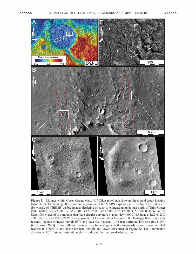
Figure 3. Mounds within Gusev Crater, Mars. (a) MOLA relief map showing the mound group location(white box). The landing ellipse and initial position of the MARS Exploration Rover Spirit are indicated.(b) Mosaic of THEMIS visible images depicting circular to elongate mounds just north of Thira Crater(V02666002, V03777003, V05662001, V12327003, V13238003, V14773003, V15085003). (c and d)Magnified views of two mounds that have circular curvature in plan view (MOC-NA images R22-01237,2.98 m/pixel, and M02-02129, 5.96 m/pixel). (e) Lava inflation features in the Hrutagja flow, southwestIceland, include elongate tumuli (ET) and lava-rise plateaus (LR) that surround lava-rise pits (LRP)[Oskarsson, 2005]. These inflation features may be analogous to the irregularly shaped, positive-relieffeatures in Figure 3b and in the left-hand margin and lower left corner of Figure 3c. The illuminationdirection (180� from sun azimuth angle) is indicated by the broad white arrow.


8 of 16

XXXXXX

491 [31] We note that other layered ejecta craters (e.g., single-492 layer, double-layer, or multiple-layer ejecta craters) [Barlow493 et al., 2000], which are thought to form by emplacement of494 fluidized ejecta flows due to the presence of volatiles in the495 substrate [Carr et al., 1977; Gault and Greeley, 1978;496 Mouginis-Mark, 1987] or through atmospheric effects497 [Schultz and Gault, 1979; Schultz, 1992; Barnouin-Jha498 and Schultz, 1996, 1998], typically exceed 4 km in diameter499 and exhibit quite distinctive morphologies. These craters are500 therefore unlikely to be mistaken for the subkilometer scale501 of rootless cones, pingos, and other ice mounds, and are not502 included in our analysis.

504 3. Methodology

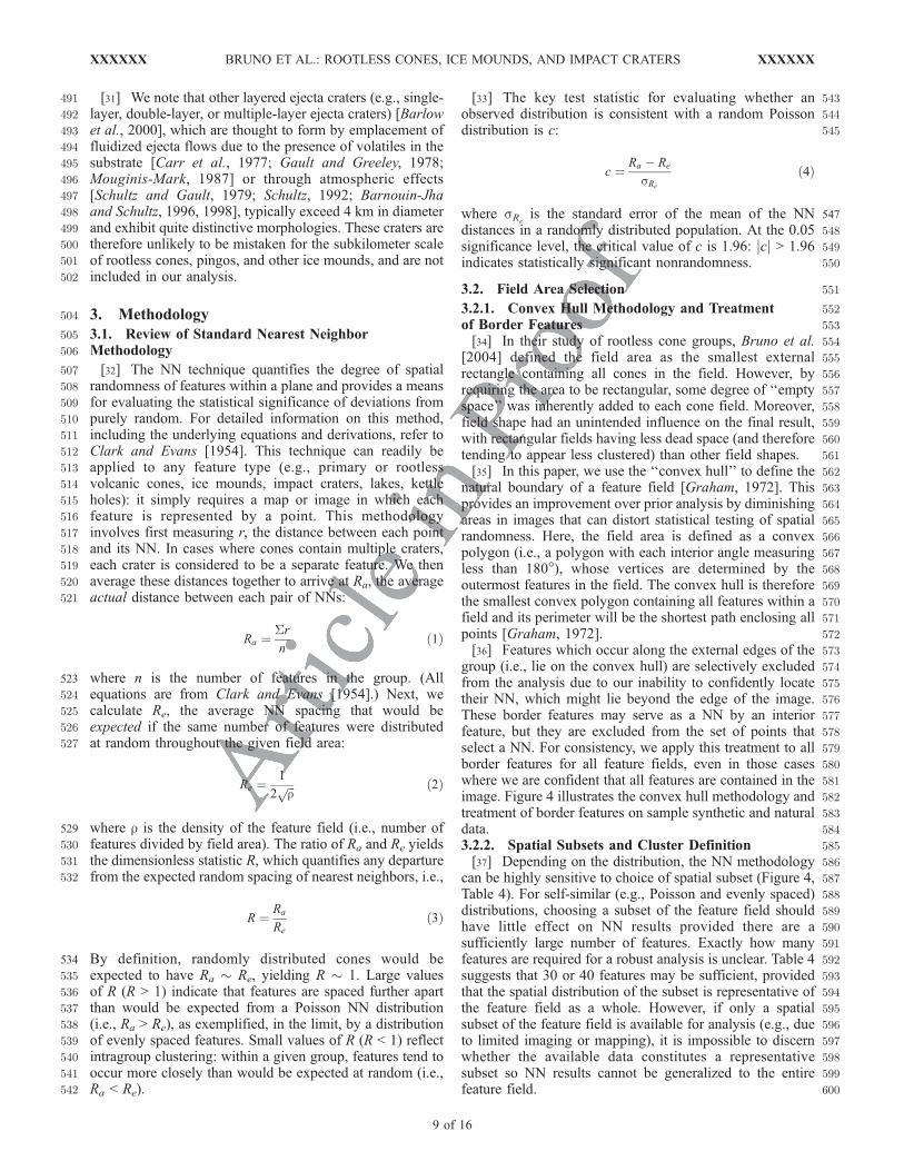
505 3.1. Review of Standard Nearest Neighbor506 Methodology

507 [32] The NN technique quantifies the degree of spatial508 randomness of features within a plane and provides a means509 for evaluating the statistical significance of deviations from510 purely random. For detailed information on this method,511 including the underlying equations and derivations, refer to512 Clark and Evans [1954]. This technique can readily be513 applied to any feature type (e.g., primary or rootless514 volcanic cones, ice mounds, impact craters, lakes, kettle515 holes): it simply requires a map or image in which each516 feature is represented by a point. This methodology517 involves first measuring r, the distance between each point518 and its NN. In cases where cones contain multiple craters,519 each crater is considered to be a separate feature. We then520 average these distances together to arrive at Ra, the average521 actual distance between each pair of NNs:

Ra ¼Srn

ð1Þ

523 where n is the number of features in the group. (All524 equations are from Clark and Evans [1954].) Next, we525 calculate Re, the average NN spacing that would be526 expected if the same number of features were distributed527 at random throughout the given field area:

Re ¼1

2ffiffiffir

p ð2Þ

529 where r is the density of the feature field (i.e., number of530 features divided by field area). The ratio of Ra and Re yields531 the dimensionless statistic R, which quantifies any departure532 from the expected random spacing of nearest neighbors, i.e.,

R ¼ Ra

Re

ð3Þ

534 By definition, randomly distributed cones would be535 expected to have Ra � Re, yielding R � 1. Large values536 of R (R > 1) indicate that features are spaced further apart537 than would be expected from a Poisson NN distribution538 (i.e., Ra > Re), as exemplified, in the limit, by a distribution539 of evenly spaced features. Small values of R (R < 1) reflect540 intragroup clustering: within a given group, features tend to541 occur more closely than would be expected at random (i.e.,542 Ra < Re).

543[33] The key test statistic for evaluating whether an544observed distribution is consistent with a random Poisson545distribution is c:

c ¼ Ra � Re

sRe

ð4Þ

547where sReis the standard error of the mean of the NN

548distances in a randomly distributed population. At the 0.05549significance level, the critical value of c is 1.96: jcj > 1.96550indicates statistically significant nonrandomness.

5513.2. Field Area Selection

5523.2.1. Convex Hull Methodology and Treatment553of Border Features554[34] In their study of rootless cone groups, Bruno et al.555[2004] defined the field area as the smallest external556rectangle containing all cones in the field. However, by557requiring the area to be rectangular, some degree of ‘‘empty558space’’ was inherently added to each cone field. Moreover,559field shape had an unintended influence on the final result,560with rectangular fields having less dead space (and therefore561tending to appear less clustered) than other field shapes.562[35] In this paper, we use the ‘‘convex hull’’ to define the563natural boundary of a feature field [Graham, 1972]. This564provides an improvement over prior analysis by diminishing565areas in images that can distort statistical testing of spatial566randomness. Here, the field area is defined as a convex567polygon (i.e., a polygon with each interior angle measuring568less than 180�), whose vertices are determined by the569outermost features in the field. The convex hull is therefore570the smallest convex polygon containing all features within a571field and its perimeter will be the shortest path enclosing all572points [Graham, 1972].573[36] Features which occur along the external edges of the574group (i.e., lie on the convex hull) are selectively excluded575from the analysis due to our inability to confidently locate576their NN, which might lie beyond the edge of the image.577These border features may serve as a NN by an interior578feature, but they are excluded from the set of points that579select a NN. For consistency, we apply this treatment to all580border features for all feature fields, even in those cases581where we are confident that all features are contained in the582image. Figure 4 illustrates the convex hull methodology and583treatment of border features on sample synthetic and natural584data.5853.2.2. Spatial Subsets and Cluster Definition586[37] Depending on the distribution, the NN methodology587can be highly sensitive to choice of spatial subset (Figure 4,588Table 4). For self-similar (e.g., Poisson and evenly spaced)589distributions, choosing a subset of the feature field should590have little effect on NN results provided there are a591sufficiently large number of features. Exactly how many592features are required for a robust analysis is unclear. Table 4593suggests that 30 or 40 features may be sufficient, provided594that the spatial distribution of the subset is representative of595the feature field as a whole. However, if only a spatial596subset of the feature field is available for analysis (e.g., due597to limited imaging or mapping), it is impossible to discern598whether the available data constitutes a representative599subset so NN results cannot be generalized to the entire600feature field.


9 of 16

XXXXXX

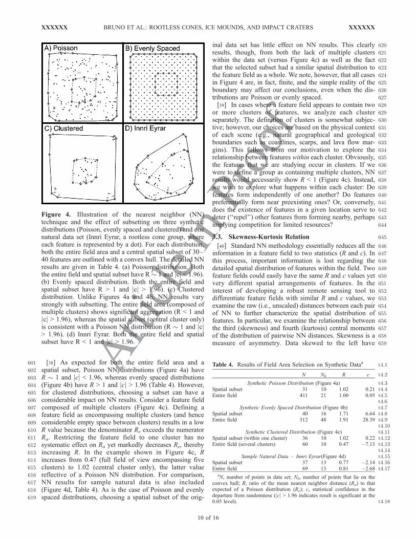
601 [38] As expected for both the entire field area and a602 spatial subset, Poisson NN distributions (Figure 4a) have603 R � 1 and jcj < 1.96, whereas evenly spaced distributions604 (Figure 4b) have R > 1 and jcj > 1.96 (Table 4). However,605 for clustered distributions, choosing a subset can have a606 considerable impact on NN results. Consider a feature field607 composed of multiple clusters (Figure 4c). Defining a608 feature field as encompassing multiple clusters (and hence609 considerable empty space between clusters) results in a low610 R value because the denominator Re exceeds the numerator611 Ra. Restricting the feature field to one cluster has no612 systematic effect on Ra yet markedly decreases Re, thereby613 increasing R. In the example shown in Figure 4c, R614 increases from 0.47 (full field of view encompassing five615 clusters) to 1.02 (central cluster only), the latter value616 reflective of a Poisson NN distribution. For comparison,617 NN results for sample natural data is also included618 (Figure 4d, Table 4). As is the case of Poisson and evenly619 spaced distributions, choosing a spatial subset of the orig-

620inal data set has little effect on NN results. This clearly621results, though, from both the lack of multiple clusters622within the data set (versus Figure 4c) as well as the fact623that the selected subset had a similar spatial distribution to624the feature field as a whole. We note, however, that all cases625in Figure 4 are, in fact, finite, and the simple reality of the626boundary may affect our conclusions, even when the dis-627tributions are Poisson or evenly spaced.628[39] In cases where a feature field appears to contain two629or more clusters of features, we analyze each cluster630separately. The definition of clusters is somewhat subjec-631tive; however, our choices are based on the physical context632of each scene (e.g., natural geographical and geological633boundaries such as coastlines, scarps, and lava flow mar-634gins). This follows from our motivation to explore the635relationship between features within each cluster. Obviously,636the features that we are studying occur in clusters. If we637were to define a group as containing multiple clusters, NN638results would necessarily show R < 1 (Figure 4c). Instead,639we wish to explore what happens within each cluster: Do640features form independently of one another? Do features641preferentially form near preexisting ones? Or, conversely,642does the existence of features in a given location serve to643deter (‘‘repel’’) other features from forming nearby, perhaps644implying competition for limited resources?

6453.3. Skewness-Kurtosis Relation

646[40] Standard NN methodology essentially reduces all the647information in a feature field to two statistics (R and c). In648this process, important information is lost regarding the649detailed spatial distribution of features within the field. Two650feature fields could easily have the same R and c values yet651very different spatial arrangements of features. In the652interest of developing a robust remote sensing tool to653differentiate feature fields with similar R and c values, we654examine the raw (i.e., unscaled) distances between each pair655of NN to further characterize the spatial distribution of656features. In particular, we examine the relationship between657the third (skewness) and fourth (kurtosis) central moments658of the distribution of pairwise NN distances. Skewness is a659measure of asymmetry. Data skewed to the left have

t4.1Table 4. Results of Field Area Selection on Synthetic Dataa

N Nb R c t4.2

Synthetic Poisson Distribution (Figure 4a) t4.3Spatial subset 31 10 1.02 0.21 t4.4Entire field 411 21 1.00 0.05 t4.5

t4.6Synthetic Evenly Spaced Distribution (Figure 4b) t4.7

Spatial subset 40 16 1.71 6.64 t4.8Entire field 312 48 1.91 28.39 t4.9

t4.10Synthetic Clustered Distribution (Figure 4c) t4.11

Spatial subset (within one cluster) 36 10 1.02 0.22 t4.12Entire field (several clusters) 60 10 0.47 �7.13 t4.13

t4.14Sample Natural Data – Innri Eyrar(Figure 4d) t4.15

Spatial subset 37 13 0.77 �2.14 t4.16Entire field 69 13 0.81 �2.68 t4.17

aN, number of points in data set; Nb, number of points that lie on theconvex hull; R, ratio of the mean nearest neighbor distance (Ra) to thatexpected of a Poisson distribution (Re); c, statistical confidence in thedeparture from randomness (jcj > 1.96 indicates result is significant at the0.05 level). t4.18

Figure 4. Illustration of the nearest neighbor (NN)technique and the effect of subsetting on three syntheticdistributions (Poisson, evenly spaced and clustered) and onenatural data set (Innri Eyrar, a rootless cone group, whereeach feature is represented by a dot). For each distribution,both the entire field area and a central spatial subset of 30–40 features are outlined with a convex hull. The detailed NNresults are given in Table 4. (a) Poisson distribution. Boththe entire field and spatial subset have R � 1 and jcj < 1.96).(b) Evenly spaced distribution. Both the entire field andspatial subset have R > 1 and jcj > 1.96). (c) Clustereddistribution. Unlike Figures 4a and 4b, NN results varystrongly with subsetting. The entire field area (composed ofmultiple clusters) shows significant aggregation (R < 1 andjcj > 1.96), whereas the spatial subset (central cluster only)is consistent with a Poisson NN distribution (R � 1 and jcj> 1.96). (d) Innri Eyrar. Both the entire field and spatialsubset have R < 1 and jcj > 1.96.


10 of 16

XXXXXX

676 negative skewness, whereas data skewed to the right have677 positive values. Kurtosis is the degree of peakedness of a678 distribution; higher values indicate distributions with simul-679 taneously sharper peaks and fatter tails. As these moments680 distinguish standard distributions from each other, this681 aspect of the methodology is designed to rapidly differen-682 tiate the NN distributions from each other without a683 detailed analysis of the full histogram of NN distances.684 There are a variety of formulae to estimate the skewness685 and kurtosis of distributions. We use the following fairly686 standard formulations:

Skewnessn

n� 1ð Þ n� 2ð ÞXni¼1

ri � Ra

s

� �3

ð5Þ

Kurtosisn nþ 1ð Þ

n� 1ð Þ n� 2ð Þ n� 3ð ÞXni¼1

ri � Ra

s

� �4" #

� 3 n� 1ð Þ2

n� 2ð Þ n� 3ð Þ ð6Þ

690 where ri is the pairwise NN distance (computed for each691 feature in the field), Ra is the average NN distance in the692 feature field and S is the sample standard deviation. Using693 these definitions, a Gaussian distribution has skewness = 0694 (i.e., is symmetric) and kurtosis = 0 (the peakedness of a695 bell-shaped curve). Before applying these formulae, pair-696 wise NN data are trimmed by 5%, to minimize the influence697 of extreme high-end values, as discussed below.

699 4. Results

700 [41] Nearest neighbor results are summarized in Table 5701 for terrestrial data sets and Table 6 for Martian data sets and702 are detailed below.

7034.1. Terrestrial Data Sets

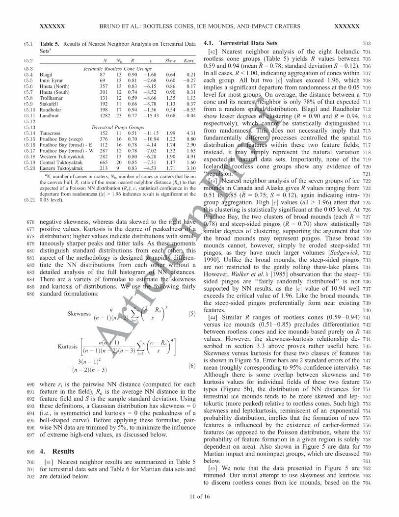
704[42] Nearest neighbor analysis of the eight Icelandic705rootless cone groups (Table 5) yields R values between7060.59 and 0.94 (mean R = 0.78; standard deviation S = 0.12).707In all cases, R < 1.00, indicating aggregation of cones within708each group. All but two jcj values exceed 1.96, which709implies a significant departure from randomness at the 0.05710level for most groups. On average, the distance between a711cone and its nearest neighbor is only 78% of that expected712from a random spatial distribution. Blagil and Raudholar713show lesser degrees of clustering (R = 0.90 and R = 0.94,714respectively), which cannot be statistically distinguished715from randomness. This does not necessarily imply that716fundamentally different processes controlled the spatial717distribution of features within these two feature fields;718instead, it may simply represent the natural variation719expected in natural data sets. Importantly, none of the720Icelandic rootless cone groups show any evidence of721‘‘repulsion.’’722[43] Nearest neighbor analysis of the seven groups of ice723mounds in Canada and Alaska gives R values ranging from7240.51 to 0.85 ( R = 0.75; S = 0.12), again indicating intra-725group aggregation. High jcj values (all > 1.96) attest that726this clustering is statistically significant at the 0.05 level. At727Prudhoe Bay, the two clusters of broad mounds (each R =7280.78) and steep-sided pingos (R = 0.70) show statistically729similar degrees of clustering, supporting the argument that730the broad mounds may represent pingos. These broad731mounds cannot, however, simply be eroded steep-sided732pingos, as they have much larger volumes [Sedgewick,7331990]. Unlike the broad mounds, the steep-sided pingos734are not restricted to the gently rolling thaw-lake plains.735However, Walker et al.’s [1985] observation that the steep-736sided pingos are ‘‘fairly randomly distributed’’ is not737supported by NN results, as the jcj value of 10.94 well738exceeds the critical value of 1.96. Like the broad mounds,739the steep-sided pingos preferentially form near existing740features.741[44] Similar R ranges of rootless cones (0.59–0.94)742versus ice mounds (0.51–0.85) precludes differentiation743between rootless cones and ice mounds based purely on R744values. However, the skewness-kurtosis relationship de-745scribed in section 3.3 above proves rather useful here.746Skewness versus kurtosis for these two classes of features747is shown in Figure 5a. Error bars are 2 standard errors of the748mean (roughly corresponding to 95% confidence intervals).749Although there is some overlap between skewness and750kurtosis values for individual fields of these two feature751types (Figure 5b), the distribution of NN distances for752terrestrial ice mounds tends to be more skewed and lep-753tokurtic (more peaked) relative to rootless cones. Such high754skewness and leptokurtosis, reminiscent of an exponential755probability distribution, implies that the formation of new756features is influenced by the existence of earlier-formed757features (as opposed to the Poisson distribution, where the758probability of feature formation in a given region is solely759dependent on area). Also shown in Figure 5 are data for760Martian impact and nonimpact groups, which are discussed761below.762[45] We note that the data presented in Figure 5 are763trimmed. Our initial attempt to use skewness and kurtosis764to discern rootless cones from ice mounds, based on the

t5.1 Table 5. Results of Nearest Neighbor Analysis on Terrestrial Data

Setsa

N Nb R c Skew. Kurt.t5.2

Icelandic Rootless Cone Groupst5.3Blagil 87 13 0.90 �1.68 0.64 0.21t5.4Innri Eyrar 69 13 0.81 �2.68 0.60 �0.27t5.5Hnuta (North) 357 13 0.83 �6.15 0.86 0.17t5.6Hnuta (South) 301 12 0.74 �8.52 0.90 0.31t5.7Trollhamar 131 12 0.59 �8.66 1.35 1.13t5.8Stakafell 192 11 0.66 �8.78 1.13 0.37t5.9Raudholar 198 17 0.94 �1.56 0.54 �0.53t5.10Landbrot 1282 23 0.77 �15.43 0.68 �0.04t5.11

t5.12Terrestrial Pingo Groupst5.13

Tanacross 152 11 0.51 �11.15 1.99 4.31t5.14Prudhoe Bay (steep) 376 16 0.70 �10.94 1.22 0.80t5.15Prudhoe Bay (broad) - E 112 16 0.78 �4.14 1.74 2.90t5.16Prudhoe Bay (broad) - W 287 12 0.78 �7.02 1.32 1.63t5.17Western Tuktoyaktuk 282 13 0.80 �6.28 1.90 4.91t5.18Central Tuktoyaktuk 665 20 0.85 �7.31 1.17 1.60t5.19Eastern Tuktoyaktuk 213 9 0.83 �4.53 1.71 3.10t5.20

aN, number of cones or craters; Nb, number of cones or craters that lie onthe convex hull; R, ratio of the mean nearest neighbor distance (Ra) to thatexpected of a Poisson NN distribution (Re); c, statistical confidence in thedeparture from randomness (jcj > 1.96 indicates result is significant at the0.05 level).t5.21


11 of 16

XXXXXX

765 entire (i.e., untrimmed) NN distribution, yielded ambiguous766 results. For rootless cones, kurtosis ranged from 2.89 to767 60.36 (mean kurtosis = 14.32; s = 19.39) and skewness768 ranged from 1.35 to 5.20 (mean skewness = 2.52, s = 1.20).769 The respective ranges for ice mounds are 3.49 to 39.85770 (mean kurtosis = 19.19, S = 14.85) and 1.82 to 5.31 (mean771 skewness = 3.56, S = 1.40). As the statistical distribution of772 geologic features reflects the physical processes that influ-773 enced feature formation [Bruno et al., 2004; Glaze et al.,774 2005], the NN distribution should bear some resemblance to

775classical probability distributions such as those associated776with random processes, population growth and resource777utilization. For comparison, the normal distribution has778skewness and kurtosis values each of zero; the exponential779distribution has corresponding values of two and six,780respectively. Other classical probability distributions gener-781ally have similarly modest values of skewness and kurtosis.782However, many of the feature fields included in this783analysis have anomalously high values of skewness and784kurtosis due to the influence of extreme high-end values.785[46] Extreme values suggest that features have been786included in the data sets that belong to different statistical787populations and/or were formed under different physical788conditions. Visual inspection of the extreme values in the789feature fields included in this analysis suggests they tend to790be larger than average, and therefore may have caused a791more pronounced depletion of local resources required for792feature formation. Alternatively, they may have formed793during different time periods, different ambient settings or794by different physical processes that cannot be determined by795a statistical analysis. Regardless, including extreme values796inhibits our ability to distinguish feature types on the basis797of skewness and kurtosis, as reflected in similar mean798values and high standard deviations for rootless cones and799ice mounds. Consequently, we have investigated these800statistics using trimmed NN distributions. Statistical trim-801ming is a standard technique [e.g., Hoaglin et al., 1983] and802is particularly useful in applications where influential fac-803tors have not been completely eliminated or controlled, as is804clearly the case in the spatial distribution of geological805features. We have found that excluding the highest 5% of806values yields a remarkable separation between terrestrial ice807mounds and impact craters, and thus provides an important808tool for interpreting the Martian data sets.

8094.2. Martian Impact Crater Groups

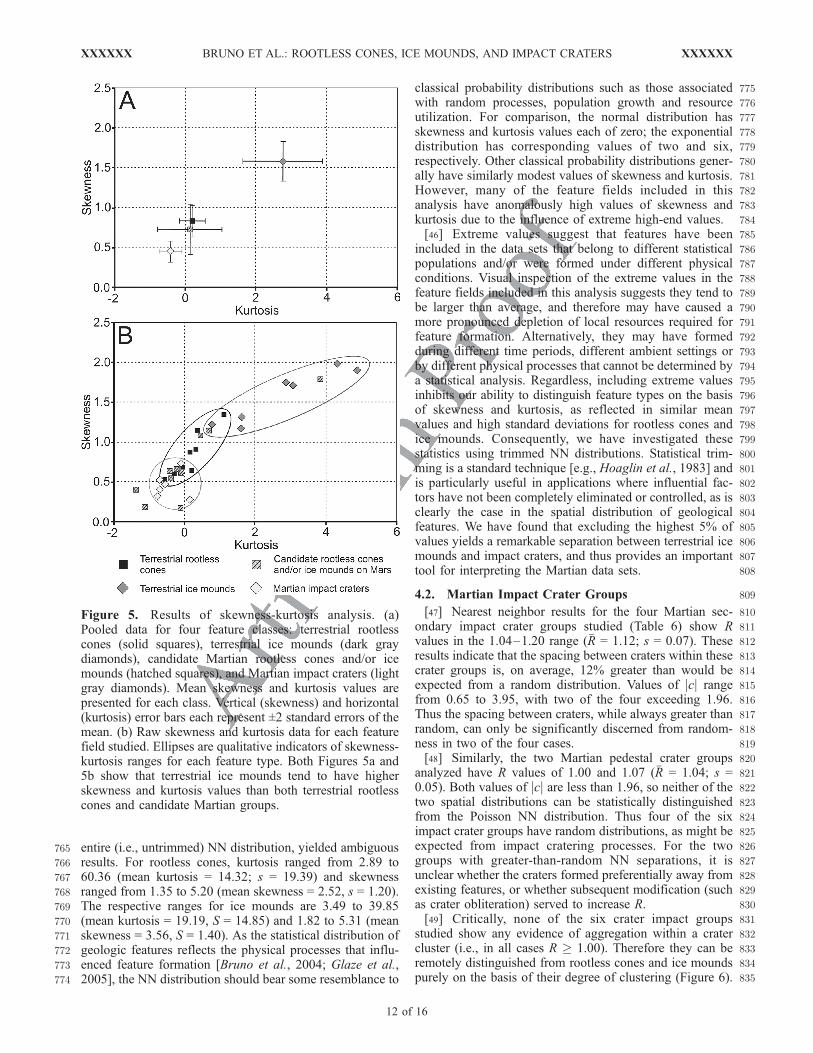
810[47] Nearest neighbor results for the four Martian sec-811ondary impact crater groups studied (Table 6) show R812values in the 1.04–1.20 range ( R = 1.12; s = 0.07). These813results indicate that the spacing between craters within these814crater groups is, on average, 12% greater than would be815expected from a random distribution. Values of jcj range816from 0.65 to 3.95, with two of the four exceeding 1.96.817Thus the spacing between craters, while always greater than818random, can only be significantly discerned from random-819ness in two of the four cases.820[48] Similarly, the two Martian pedestal crater groups821analyzed have R values of 1.00 and 1.07 ( R = 1.04; s =8220.05). Both values of jcj are less than 1.96, so neither of the823two spatial distributions can be statistically distinguished824from the Poisson NN distribution. Thus four of the six825impact crater groups have random distributions, as might be826expected from impact cratering processes. For the two827groups with greater-than-random NN separations, it is828unclear whether the craters formed preferentially away from829existing features, or whether subsequent modification (such830as crater obliteration) served to increase R.831[49] Critically, none of the six crater impact groups832studied show any evidence of aggregation within a crater833cluster (i.e., in all cases R � 1.00). Therefore they can be834remotely distinguished from rootless cones and ice mounds835purely on the basis of their degree of clustering (Figure 6).

Figure 5. Results of skewness-kurtosis analysis. (a)Pooled data for four feature classes: terrestrial rootlesscones (solid squares), terrestrial ice mounds (dark graydiamonds), candidate Martian rootless cones and/or icemounds (hatched squares), and Martian impact craters (lightgray diamonds). Mean skewness and kurtosis values arepresented for each class. Vertical (skewness) and horizontal(kurtosis) error bars each represent ±2 standard errors of themean. (b) Raw skewness and kurtosis data for each featurefield studied. Ellipses are qualitative indicators of skewness-kurtosis ranges for each feature type. Both Figures 5a and5b show that terrestrial ice mounds tend to have higherskewness and kurtosis values than both terrestrial rootlesscones and candidate Martian groups.


12 of 16

XXXXXX

836 This would be particularly useful for feature fields where837 morphology is not well-defined due to degradation, modi-838 fication, or sediment cover.

839 4.3. Martian Candidate Rootless Cone and/or Ice840 Mound Groups

841 [50] The ten candidate Martian groups studied have R842 ranging from 0.57 to 1.18 ( R = 0.81; s = 0.17). The only843 feature field with R > 1.00 is found within Gusev Crater.844 Nearest neighbor results for these Gusev mounds (R = 1.18,845 c = 3.31) are markedly different from those of all other846 candidate Martian groups, as well as from the terrestrial847 groups of rootless cones and ice mounds. Unlike the848 rootless cones and ice mounds, which tend to cluster near849 each other, the Gusev mounds tend to form preferentially850 away from preexisting features. This ‘‘repulsion’’ is signif-851 icantly different from random, as jcj exceeds 1.96. Nearest852 neighbor results for the Gusev mounds fall within the range853 of the Martian impact crater groups studied in terms of both854 R (1.00–1.20) and c (0.07–3.95).855 [51] Excluding the Gusev mounds leaves an R range of856 0.57–0.93 ( R = 0.77; s = 0.11), with all but one jcj value857 exceeding 1.96. These values are nearly identical to those858 obtained for both the Icelandic rootless cones ( R = 0.78; s =859 0.12) and the terrestrial ice mounds ( R = 0.75; s = 0.12), yet860 show no overlap with the R range of the Martian impact861 crater groups studied (1.00–1.20). These NN results,862 summarized in Figure 6, lend support to the argument that863 the candidate Martian groups (except the Gusev mounds)864 may be rootless cones and/or ice mounds, but R and c865 values alone cannot be used to discriminate between these866 two possible origins. Thus, as in section 4.1 above, we867 examine the relationship between skewness and kurtosis.868 [52] Skewness and kurtosis values for both individual869 feature fields and Mars candidate groups as a feature type

870are shown in Figure 5, alongside the terrestrial data.871Immediately apparent from Figure 5a is the strong overlap872in the skewness-kurtosis relationship between the candidate873Martian groups and the terrestrial rootless cones, although874the Martian data have more variance. The near coincidence875of the mean skewness and kurtosis values of these two876groups suggests they are drawing from the same population877(i.e., that the candidate Martian groups are rootless cones).878Detailed examination of the skewness-kurtosis relation of879individual candidate Martian groups (Figure 5b; Table 6)880reveals a somewhat more complex picture. One candidate881Martian group (Cerberus Plains 1) has skewness and kur-882tosis values falling well within the range of terrestrial ice883mounds. Two others (Cerberus Plains 2 and Isidis Planitia)884have values intermediate between terrestrial rootless cones885and ice mounds. Four groups (SE of Phlegra Montes N,886Cerberus Plains 3, Athabasca Valles, and Acidalia Planitia)887have skewness and kurtosis values well within the rootless888cone range. This result, together with the R and c values of889Table 6, suggests these four groups represent rootless cones.890The same argument may hold for Amazonis Planitia and SE891of Phlegra Montes (S), as their low skewness and kurtosis892values suggest an ice mound origin is unlikely; however893their skewness and kurtosis values are lower than any894terrestrial rootless cone group. The final group (Gusev)895has skewness and kurtosis values comparable to those of896Martian impact craters, which further suggests that these897mounds may represent modified impact craters (as dis-898cussed below).

9005. Discussion

9015.1. Improved Methodology

902[53] Using an improved NN methodology, we have903examined the spatial distribution of rootless cones in Ice-

Figure 6. Summary of NN results for the four data setsstudied in this analysis. All groups of terrestrial rootlesscones and ice mounds show clustering (R < 1.0), whereas allMartian impact craters show spacing greater than or equal tothat expected of a random distribution (R � 1.0). With asingle exception, the NN results for the candidate Martiangroups mirror those of the two terrestrial data sets. Theexception (Gusev) has a distribution that is statisticallyindistinguishable from the impact craters.

t6.1Table 6. Results of Nearest Neighbor Analysis on Martian Data

Setsa

N Nb R c Skew Kurt t6.2

Candidate Martian Rootless Cone and/or Pingo Groups t6.3SE of Phlegra Montes (S) 149 14 0.93 �1.66 0.19 �1.16 t6.4SE of Phlegra Montes (N) 282 17 0.86 �4.37 0.67 �0.24 t6.5Cerberus Plains 1 159 11 0.68 �7.54 1.79 3.83 t6.6Cerberus Plains 2 90 9 0.85 �2.63 1.09 0.45 t6.7Cerberus Plains 3 104 6 0.76 �4.64 0.63 �0.12 t6.8Acidalia Planitia 386 20 0.81 �6.91 0.64 �0.39 t6.9Isidis Planitia 247 13 0.66 �9.94 1.14 0.68 t6.10Amazonis Planitia 32 11 0.57 �3.78 0.41 �1.35 t6.11Athabasca Valles 891 15 0.83 �9.69 0.56 �0.41 t6.12Gusev Crater 104 11 1.18 3.31 0.19 �0.11 t6.13

t6.14Martian Secondary Impact Crater Groups t6.15

Acidalia Planitia 67 14 1.11 1.54 0.34 �0.76 t6.16Ares/Tiu Valles 196 17 1.15 3.95 0.48 �0.56 t6.17Nili Fossae 154 11 1.20 4.49 0.72 �0.08 t6.18South Isidis Planitia 94 9 1.04 0.65 0.29 0.18 t6.19

t6.20Martian Pedestal Crater Groups t6.21

East of Acidalia Planitia 1 257 15 1.00 0.07 0.51 �0.67 t6.22East of Acidalia Planitia 2 98 10 1.07 1.28 0.41 �0.70 t6.23

aN, number of cones or craters; Nb, number of cones or craters that lie onthe convex hull; R, ratio of the mean nearest neighbor distance (Ra) to thatexpected of a Poisson NN distribution (Re); c, statistical confidence in thedeparture from randomness (jcj > 1.96 indicates result is significant atthe 0.05 level); Skew and Kurt, skewness and kurtosis, respectively, of thedistribution of pairwise NN distances. t6.24


13 of 16

XXXXXX

904 land, ice mounds in Canada and Alaska, candidate rootless905 cones and ice mounds on Mars, and pedestal and secondary906 impact craters on Mars. Our approach invokes four spatial907 statistics (R, c, skewness, and kurtosis) and provides sys-908 tematic methods for defining the cluster boundary (i.e.,909 choosing a logical area and then constructing a convex910 hull) and treating border features (i.e., selectively excluding911 those features that lie on the hull boundary). We have shown912 that R and c values (the standard NN statistics) separate913 impact craters from rootless cones and ice mounds, but914 similar degrees of clustering preclude differentiation be-915 tween the latter two feature types (Figure 6). This is where916 the skewness-kurtosis relation proves useful. The skewness917 and kurtosis of the NN distribution provides a remarkable918 segregation and grouping of terrestrial and Martian features919 for a trivial amount of computation. What is most signifi-920 cant is that this segregation and grouping emerges without921 the need for the postulation of an underlying probability922 distribution.923 [54] The R values presented in this paper, on the basis of924 the refined methodology, are generally consistent with (but925 somewhat higher than) those of Bruno et al. [2004] for the926 identical data sets (Table 7). The slight differences are927 largely attributed to using the convex hull to define a cluster928 boundary, which eliminates empty space surrounding a929 feature field. Empty space increases Re and therefore tends930 to decrease R; thus the elimination of space via the convex931 hull would conversely tend to increase R. A sensitivity932 analysis has shown that our selective treatment of border933 features had a much less pronounced effect on R, presum-934 ably because of the relatively large ratio of interior to border935 features which characterize these reasonably large data sets.

936 5.2. Interpretation of Martian Data Sets

937 [55] With a single exception, nearest neighbor results for938 the candidate Martian groups show R < 1, mirroring the939 results of terrestrial rootless cone and ice mound groups.940 These candidate Martian groups do not appear to represent941 impact craters, as all Martian secondary and pedestal impact942 crater groups studied have R � 1. Instead, these results943 suggest that, purely on the basis of their spatial distribution,944 these candidate Martian groups resemble ice mounds or945 rootless cones. Further discrimination between these two946 feature types is suggested on the basis of the relationship947 between skewness and kurtosis, as ice mounds tend to have948 higher values of both central moments. We do not attempt to949 argue convincingly that the candidate Martian groups are950 clusters of ice mounds or rootless cones, or whether ice951 mounds would even be expected on Mars. We simply note952 that both theories of origin are consistent with the results of

953our analysis, and warrant further examination in conjunction954with other lines of evidence such as morphology, geological955context (e.g., identifiable lava surface texture or water-956bearing sediments), and physical constraints on their for-957mation and preservation.958[56] The sole exception is the Gusev Crater mounds,959whose NN results (R, c, skewness and kurtosis) are statis-960tically indistinguishable from the Martian impact crater961groups studied. These mounds were initially identified as962pingos on the basis of geomorphological interpretation of963Viking Orbiter imagery [Cabrol et al., 2000]. However,964more recent, higher-resolution THEMIS and MOC-NA965imagery has failed to resolve any morphological character-966istics that are diagnostic of pingos (Figures 3a–3d). Mellon967et al. [2004] demonstrated that near-surface ground ice is968currently unstable in the Gusev Crater region and the969Mars Exploration Rover Spirit has revealed basalt to be970the dominant surface lithology [Squyres et al., 2004].971Martınez-Alonso et al. [2005] noted that both the morphol-972ogy and dimensions of the Gusev mounds are consistent973with those of inflated lava flows. Combining statistical and974morphological lines of evidence, we speculate that the975Gusev mounds may represent topographic inversion of976impact craters due to lava flow inflation. Sites of localized977inflation often originate as topographic lows into which lava978concentrates [Hon et al., 1994]. Continued accumulation of979lava causes the surface of the flow to swell upward and may980create features such as tumuli, lava-rise plateaus, and lava-981rise pits [Walker, 1991]. These lava inflation features may982be analogous to the Gusev mounds in that they initiated in983topographic lows and topographically inverted the land-984scape into a series of circular to elongate ridges and plateaus985(Figure 3e). In any case, the geospatial statistics and986morphologies of the Gusev mounds distinguish them from987rootless cones and ice mounds, thus suggesting a different988formation mechanism.

9895.3. Implications for Nonrandom Processes

990[57] All 15 groups of terrestrial ice mounds and rootless991cones studied show intragroup aggregation (all R < 1), i.e.,992features are more closely spaced than would be expected993from a random spatial distribution. In all but two cases, this994departure from randomness is statistically significant on the995basis of an evaluation of c. This clustering implies that996nonrandom processes systematically control the spatial997distribution of rootless cones and ice mounds within their998respective groups.999[58] For rootless cones, a likely control is the geometry of1000preferred lava pathways, evidenced by the presence of1001significant linear cone alignments and supported by field1002observations of Icelandic rootless cones [Bruno et al.,10032004]. Heterogeneous subsurface hydrology may also play1004a role in controlling cone distribution. Rootless cones form1005in lake basins, river floodplains, and glacial outwash plains1006[Fagents et al., 2002], which presumably contain abundant1007water. If water was heterogeneously distributed within the1008substrate (e.g., by structural, lithological or hydrological1009controls) then this would limit the potential locations at1010which cones could form and influence broader-scale group-1011ings within a flow field.1012[59] Hydraulic pingos, such as those found in Tanacross,1013tend to form in narrow valleys or on slopes where perma-

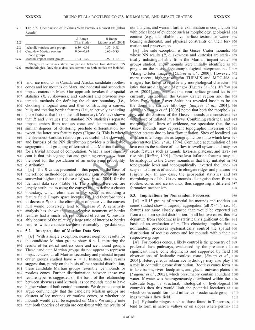
t7.1 Table 7. Comparison of RValues With Previous Nearest Neighbor

Resultsa

R Range(This Study)

R Range[Bruno et al., 2004]t7.2

Icelandic rootless cone groups 0.59–0.94 0.57–0.88t7.3Candidate Martian rootlesscone groups

0.66–0.93 0.66–0.85t7.4

Martian impact crater groups 1.04–1.20 0.92–1.17t7.5aRanges of R values show comparison between two different NN

methodologies. Only those data sets common to both studies are included.t7.6


14 of 16

XXXXXX

1014 frost is discontinuous or locally thinner. Thus a clustered1015 distribution may simply reflect preferred locations of dis-1016 continuous or locally thinner permafrost. For hydrostatic1017 pingos (e.g., Prudhoe Bay and Tuktoyaktuk Peninsula)1018 which form following rapid drainage of lakes, a clustered1019 distribution could either reflect (1) a nonrandom distribution1020 of thaw-lake basins (e.g., thaw-lake locations could be1021 controlled by the presence of drainage networks and drain-1022 age barriers) and/or (2) a nonrandom process that affects1023 which thaw-lakes are capable of generating pingos (e.g.,1024 variable basin substrates may locally favor or prohibit the1025 hydrological conditions required for pingo growth).

1027 6. Conclusions

1028 [60] We have shown that the spatial statistics of geologic1029 features can be an effective supplement to geologic context1030 and morphologic diagnostics to remotely differentiate be-1031 tween feature types such as rootless cones, ice mounds, and1032 impact craters. Our method is based in part on the two1033 statistics of the conventional nearest neighbor approach, R1034 and c, which alone distinguish impact craters from the other1035 two feature types. With a single exception, the R and c1036 values of candidate Martian groups mirror those of terres-1037 trial rootless cones and ice mounds. To further differentiate1038 between these two feature types, we invoke the skewness-1039 kurtosis relation, as ice mounds tend to have higher values1040 of both central moments.1041 [61] The skewness-kurtosis statistic generally favors a1042 rootless cone origin for the candidate Martian groups,1043 although ice mounds remain a viable possibility for1044 several groups. On the basis of NN results (as well as1045 morphology), these Martian groups are clearly not clusters1046 of impact craters: impact craters have distinctly different1047 spatial distributions. The sole exception is the Gusev1048 Crater mounds, which have R, c, skewness, and kurtosis1049 values that are indistinguishable from those of Martian1050 impact craters.1051 [62] In summary, we have developed an improved method1052 for characterizing the spatial distribution of rootless cones1053 and ice mounds on Mars and quantitatively comparing them1054 with terrestrial analogs. These results provide a basis for1055 detailed physical modeling of the processes that form fields1056 of these features and wider systematic applications may1057 provide improvements in our understanding of the volatile1058 inventory and evolution on Mars.

Notation

c statistical measure of confidence in the departure fromrandomness.

n number of features in the feature field.r distance between a feature and its nearest neighbor,

[L].R statistical measure of departure from randomness of

spatial distribution, = Ra/Re. R average R value (for multiple feature fields).Ra average distance between nearest neighbors, [L].Re average nearest neighbor spacing expected for a

spatially random distribution [L].s sample standard deviation [L].r spatial density of features within a field, [L�2].

sRestandard error of the mean of nearest neighbordistances in a randomly distributed population [L].

1086[63] Acknowledgments. We thank all those who shared their knowl-1087edge and provided insights, including T. Thordarson (rootless cones and1088lava inflation), E. Pilger (programming), and S. Still (clustering). Thorough1089reviews by L. Glaze and P. Lanagan led to significant improvements in this1090manuscript. This work was supported in part by NASA Mars Data Analysis1091Program grant NAG5-13458 to S.A.F. This paper is HIGP contribution10921436 and SOEST contriubtion 6774.

1093References1094Allen, C. C. (1979a), Volcano-ice interactions on Mars, J. Geophys. Res.,109584, 8048–8059.1096Allen, C. C. (1979b), Volcano-ice interactions on the Earth and Mars, Ph.D.1097thesis, 131 pp, Univ. of Arizona, Tucson.1098Barlow, N. G., J. M. Boyce, F. M. Costard, R. A. Craddock, J. B. Garvin,1099S. E. H. Sakimoto, R. O. Kuzmin, D. J. Roddy, and L. A. Soderblom1100(2000), Standardizing the nomenclature of Martian impact crater1101morphologies, J. Geophys. Res., 105, 26,733–26,738.1102Barnouin-Jha, O. S., and P. H. Schultz (1996), Ejecta entrainment by im-1103pact-generated ring vortices: Theory and experiments, J. Geophys. Res.,1104101, 21,099–21,115.1105Barnouin-Jha, O. S., and P. H. Schultz (1998), Lobateness of impact ejecta1106deposits from atmospheric interactions, J. Geophys. Res., 103, 25,739–110725,756.1108Brockett, B. E. (1982), Modification of and experience with a portable drill,1109Prudhoe Bay, Alaska, spring 1982, 14 pp., memorandum, Cold Regions1110Res. and Eng. Lab., U.S. Army Corps of Eng., Hanover, N. H.1111Bruno, B. C., S. A. Fagents, T. Thordarson, S. M. Baloga, and E. Pilger1112(2004), Clustering within rootless cone groups on Iceland and Mars:1113Effect of nonrandom processes, J. Geophys. Res., 109, E07009,1114doi:10.1029/2004JE002273.1115Burr, D. M., J. A. Grier, A. S. McEwen, and L. P. Keszthelyi (2002a),1116Repeated aqueous flooding from the Cerberus Fossae: Evidence for very1117recently extant, deep groundwater on Mars, Icarus, 159, 53–73.1118Burr, D. M., A. S. McEwen, and S. E. H. Sakimoto (2002b), Recent aqu-1119eous floods from the Cerberus Fossae, Mars, Geophys. Res. Lett., 29(1),11201013, doi:10.1029/2001GL013345.1121Burr, D. M., R. J. Soare, and J.-M. Wan Bun Tseung (2005), Young (late1122Amazonian), near surface, ground ice features near the equator, Athabas-1123ca Valles, Mars, Icarus, 178, 56–73.1124Cabrol, N. A., E. A. Grin, and W. H. Pollard (2000), Possible frost mounds1125in an ancient Martian lake bed, Icarus, 145, 91–107.1126Carr, M. H. (1981), The Surface of Mars, 232 pp., Yale Univ. Press, New1127Haven, Conn.1128Carr, M. H., L. S. Crumpler, J. A. Cutts, R. Greeley, J. E. Guest, and1129H. Masursky (1977), Martian impact craters and emplacement of ejecta1130by surface flow, J. Geophys. Res., 82, 4055–4065.1131Carr, M. J. (1976), Underthrusting and Quaternary faulting in northern1132Central America, Geol. Soc. Am. Bull., 87, 825–829.1133Chapman, M. G., and K. L. Tanaka (2001), Interior trough deposits on1134Mars: Subice volcanoes?, J. Geophys. Res., 106, 10,087–10,100.1135Clark, P. J., and F. C. Evans (1954), Distance to nearest neighbor as a1136measure of spatial relationships in populations, Ecology, 35, 445–453.1137Connor, C. B. (1990), Cinder cone clustering in the TransMexican volcanic1138belt: Implications for structural and petrologic models, J. Geophys. Res.,113995, 19,395–19,405.1140Connor, C. B., and B. E. Hill (1995), Three nonhomogeneous Poisson1141models for the probability of basaltic volcanism: Application to the Yucca1142Mountain region, Nevada, J. Geophys. Res., 100, 10,107–10,125.1143Connor, C. B., C. D. Condit, L. S. Crumpler, and J. C. Aubele (1992),1144Evidence of regional structural controls on vent distribution: Springer-1145ville Volcanic Field, Arizona, J. Geophys. Res., 97, 12,349–12,359.1146Fagents, S. A., and T. Thordarson (2006), Rootless volcanic cones in Ice-1147land and on Mars, in The Geology of Mars: Evidence From Earth-Based1148Analogues, edited by M. G. Chapman and I. P. Skilling, Cambridge Univ.1149Press, New York, in press.1150Fagents, S. A., P. D. Lanagan, and R. Greeley (2002), Rootless cones1151on Mars: A consequence of lava-ground ice interaction, in Volcano-Ice1152Interaction on Earth and Mars, edited by J. L. Smellie and M. G.1153Chapman, Geol. Soc. Spec. Publ., 202, 295–317.1154Farrand, W. H., L. R. Gaddis, and L. Keszthelyi (2005), Pitted cones and1155domes on Mars: Observations in Acidalia Planitia and Cydonia Mensae1156using MOC, THEMIS, and TES data, J. Geophys. Res., 110, E05005,1157doi:10.1029/2004JE002297.1158Frey, H., and M. Jarosewich (1982), Subkilometer Martian volcanoes:1159Properties and possible terrestrial analogs, J. Geophys. Res., 87, 9867–11609879.


15 of 16

XXXXXX

1161 Frey, H., B. L. Lowry, and S. A. Chase (1979), Pseudocraters on Mars,1162 J. Geophys. Res., 84, 8068–8075.1163 Gaidos, E., and G. Marion (2003), Geological and geochemical legacy of a1164 cold early Mars, J. Geophys. Res., 108(E6), 5055, doi:10.1029/1165 2002JE002000.1166 Gault, D. E., and R. Greeley (1978), Exploratory experiments of impact1167 craters formed in viscous-liquid targets: Analogs for Martian rampart1168 craters?, Icarus, 34, 486–495.1169 Glaze, L. S., S. W. Anderson, E. R. Stofan, S. Baloga, and S. E. Smrekar1170 (2005), Statistical distribution of tumuli on pahoehoe flow surfaces:1171 Analysis of examples in Hawaii and Iceland and potential applications1172 to lava flows on Mars, J. Geophys. Res., 110, B08202, doi:10.1029/1173 2004JB003564.1174 Graham, R. (1972), An efficient algorithm for determining the convex hull1175 of a finite planar point set, Info. Proc. Lett., 1, 132–133.1176 Greeley, R., and S. A. Fagents (2001), Icelandic pseudocraters as analogs1177 to some volcanic cones on Mars, J. Geophys. Res., 106, 20,527–1178 20,546.1179 Grizzaffi, P., and P. H. Schultz (1989), Isidis Basin: Site of ancient volatile-1180 rich debris layer, Icarus, 77, 358–381.1181 Hasenaka, T., and I. S. E. Carmichael (1985a), The cinder cones of1182 Michoacan-Guanajuato, central Mexico: Their age, volume, distribution1183 and magma discharge rate, J. Volcanol. Geotherm. Res., 25, 105–124.1184 Hasenaka, T., and I. S. E. Carmichael (1985b), A compilation of location,1185 size and geomorphological parameters of volcanoes in the Michoacan-1186 Guanajuato volcanic field, Mexico, Geofis. Int., 24, 577–608.1187 Heming, R. F. (1980), Patterns of Quaternary basaltic volcanism in the1188 northern North Island, New Zealand, N. Z. J. Geol. Geophys., 23,1189 335–344.1190 Hoaglin, D. C., F. Mosteller, and J. W. Tukey (1983), Understanding1191 Robust and Exploratory Data Analysis, 447 pp., John Wiley, Hoboken,1192 N. J.1193 Holmes, G., D. Hopkins, and H. Foster (1968), Pingos in Central Alaska,1194 40 pp., Geol, Surv. Bull. 1241-H, U.S. Dept. of the Interior, Washington,1195 D. C.1196 Hon, K., J. Kauahikaua, R. Denlinger, and K. Mackay (1994), Emplace-1197 ment and inflation of pahoehoe sheet flows: Observations and measure-1198 ments of active lava flows on Kilauea Volcano, Hawaii, Geol. Soc. Am.1199 Bull., 106, 351–370.1200 Lanagan, P. D., A. S. McEwen, L. P. Keszthelyi, and T. Thordarson (2001),1201 Rootless cones on Mars indicating the presence of shallow equatorial1202 ground ice in recent times, Geophys. Res. Lett., 28, 2365–2368.1203 Lucchitta, B. K. (1981), Mars and Earth: Comparison of cold climate1204 features, Icarus, 45, 264–303.1205 Mackay, J. R. (1962), Pingos of the Pleistocene Mackenzie Delta area,1206 Geogr. Bull. 18, pp. 21–63, Geogr. Branch, Mines and Tech. Surv.,1207 Ottawa, Canada.1208 Mackay, J. R. (1973), The growth of pingos, western Arctic coast, Canada,1209 Can. J. Earth Sci., 10, 979–1004.1210 Mackay, J. R. (1979), Pingos of the Tuktoyaktuk Peninsula area, Northwest1211 Territories, Geogr. Phys. Quat., 33, 3–61.1212 Mackay, J. R. (1987), Some mechanical aspects of pingo growth and fail-1213 ure, western Arctic coast, Canada, Can. J. Earth Sci., 24, 1108–1119.1214 Mackay, J. R. (1998), Pingo growth and collapse, Tuktoyaktuk Peninsula1215 Area, western Arctic coast, Canada: A long-term field study, Geogr. Phys.1216 Quat., 52, 271–323.1217 Martınez-Alonso, S., B. M. Jakosky, M. T. Mellon, and N. E. Putzig (2005),1218 A volcanic interpretation of Gusev Crater surface materials from thermo-1219 physical, spectral, and morphological evidence, J. Geophys. Res., 110,1220 E01003, doi:10.1029/2004JE002327.1221 Mellon, M. T., W. C. Feldman, and T. H. Prettyman (2004), The presence1222 and stability of ground ice in the southern hemisphere of Mars, Icarus,1223 169, 324–340.1224 Mouginis-Mark, P. J. (1987), Water or ice in the Martian regolith?: Clues1225 from rampart craters seen at very high resolution, Icarus, 71, 268–1226 286.1227 Muller, F. (1959), Meddeleser on Grønland (in German), 153(3), 127 pp.1228 (translated by D. A. Sinclair, Natl. Res. Counc. of Can, Ottawa, Ont., 1171229 pp., 1963).1230 Oskarsson, B. V. (2005), Lava-rise structures in pahoehoe and aa: Examples1231 from the Hrutagja lava shield and Kapelluhraun aa flow field on the1232 Reykjanes Peninsula, B.Sc. thesis, Univ. of Iceland, Reykjavik.1233 Page, D. P., and J. B. Murray (2006), Stratigraphic and morphological1234 evidence for pingo genesis in the Cerberus plains, Icarus, doi:10.1016/1235 j.icarus.2006.01.017, in press.

1236Parker, T. J., D. S. Gorsline, R. S. Saunders, D. C. Pieri, and D. M.1237Schneeberger (1993), Coastal geomorphology of the Martian northern1238plains, J. Geophys. Res., 98, 11,061–11,078.1239Plescia, J. B. (1990), Recent flood lavas in the Elysium region of Mars,1240Icarus, 88, 465–490.1241Plescia, J. B. (1993), An assessment of volatile release from recent volcan-1242ism in Elysium, Mars, Icarus, 104, 20–32.1243Plescia, J. B. (2003), Cerbereus Fossae, Elysium, Mars: A source of lava1244and water, Icarus, 164, 79–95.1245Porsild, A. E. (1938), Earth mounds in unglaciated Arctic northwestern1246America, Geogr. Rev., 28, 46–58.1247Rossbacher, L. A., and S. Judson (1981), Ground ice on Mars; inventory,1248distribution, and resulting landforms, Icarus, 45, 39–59.1249Schultz, P. H. (1992), Atmospheric effects on ejecta emplacement, J. Geo-1250phys. Res., 97, 11,623–11,662.1251Schultz, P. H., and D. E. Gault (1979), Atmospheric effects on Martian1252ejecta emplacement, J. Geophys. Res., 84, 7669–7687.1253Sedgewick, R. (1990), Algorithms in C, 657 pp., Addison-Wesley Long-1254man, Boston, Mass.1255Settle, M. (1979), The structure and emplacement of cinder cone fields, Am.1256J. Sci., 279, 1089–1107.1257Soare, R. J., D. M. Burr, and J.-M. Wan Bun Tseung (2005), Possible1258pingos and a periglacial landscape in northwest Utopia Planitia, Icarus,1259174, 373–382, doi:310.1016/j.icarus.2004.1011.1013.1260Squyres, S. W., S. M. Clifford, R. O. Kuzmin, J. R. Zimbelman, and F. M.1261Costard (1992), Ice in the Martian regolith, in Mars, edited by H. H.1262Kieffer et al., pp. 523–554, Univ. of Ariz. Press, Tucson.1263Squyres, S. W., C. Howell, M. C. Liu, and J. J. Lissauer (1997), Investiga-1264tion of crater ‘saturation’ using spatial statistics, Icarus, 125, 67–82.1265Squyres, S. W., et al. (2004), The Spirit Rover’s Athena science investiga-1266tion at Gusev crater, Mars, Science, 305, 794–799.1267Stager, J. K. (1956), Progress report on the analysis of the characteristics1268and distribution of pingos east of the Mackenzie delta, Can. Geogr., 7,126913–20.1270Tanaka, K. L. (1997), Sedimentary history and mass flow structures of1271Chryse and Acidalia Planitiae, Mars, J. Geophys. Res., 102, 4131–4419.1272Theilig, E., and R. Greeley (1979), Plains and channels in the Lunae Pla-1273num–Chryse Planitia region of Mars, J. Geophys. Res., 84, 7994–8010.1274Thorarinsson, S. (1951), Laxargljufur and Laxarhraun. A tephrochronolo-1275gical study, Geogr. Ann., H1–2, 1–89.1276Thorarinsson, S. (1953), The crater groups in Iceland, Bull. Volcanol., 14,12773–44.1278Thordarson, T. (2000), Rootless eruptions and cone groups in Iceland:1279Products of authentic explosive water to magma interactions, in Volca-1280no/Ice Interactions on Earth and Mars, Abstract Volume, edited by V. C.1281Gulick and M. T. Gudmundsson, p. 48, Univ. of Iceland, Reykjavik.1282Thordarson, T., and A. Hoskuldsson (2002), Iceland, Terra, Harpenden,1283Hertfordshire, U. K.1284Thordarson, T., D. J. Miller, and G. Larsen (1998), New data on the1285Leidolfsfell cone group on south Iceland, Jokull, 46, 3–15.1286Thordarson, T., M. M. Morrissey, G. Larsen, and H. Cyrusson (1992),1287Origins of rootless cone complexes in S. Iceland, in The 20th Nordic1288Geological Winter Meeting, edited by A. Geirsdottir, H. Norddahl, and1289G. Helgadottir, p. 169, Icelandic Geol. Soc., Reykjavik.1290Thoroddsen, T. (1894), Ferd un Vestur Skaftafellssyslu sumarid 1893 (Tra-1291velogue from Western Skaftafellshire in the summer of 1893), Andvari,129219, 44–161.1293Walker, D., M. Walker, K. Everett, and P. Webber (1985), Pingos of the1294Prudhoe Bay Region, Alaska, Arctic Alpine Res., 17, 321–336.1295Walker, G. P. L. (1991), Structure, and origin by injection of lava under1296surface crust, of tumuli, ‘‘lava rises’’, ‘‘lava rise pits’’, and lava inflation1297clefts in Hawaii, Bull. Volcanol., 53, 546–558.1298Walker, J. (1981), Petrogenesis of lavas from cinder cone fields behind the1299volcanic front of Central America, J. Geol., 89, 721–739.1300Washburn, A. L. (1973), Periglacial Processes and Environments, 320 pp.,1301Edward Arnold, London.

��1303S. M. Baloga, Proxemy Research, 20528 Farcroft Lane, Bowie, MD130420882, USA.1305B. C. Bruno, S. A. Fagents, and C. W. Hamilton, Hawaii Institute of1306Geophysics and Planetology, University of Hawaii, 1680 East West1307Road,POST 504, Honolulu, HI 96822, USA. ([email protected])1308D. M. Burr, SETI Institute, 515 North Whisman Road, Mountain View,1309CA 94043, USA.


16 of 16

XXXXXX

Documents

Identification of volcanic rootless cones, ice mounds, and