Identifying Monotonic and Non-Monotonic Relationships

Shlomo Yitzhaki1; Edna Schechtman2 1Central Bureau of Statistics, and Hebrew University. 2Dept. of Industrial Engineering and Management, Ben-Gurion University. E-mail: yitzhaki@cbs.gov.il; ednas@bgu.ac.il 1. Introduction One of the basic assumptions in linear regression analysis is that the relationships between the dependent and the independent variables are monotonic over the entire range. The aim of this paper is to analyze the implications of using several common practices in econometrics (to be detailed below) on the signs of the estimated regression coefficients. Hopefully, this will lead us to define standard reporting procedures that will make it easier for the reader to understand the effects of those practices on the estimates. We note that we do not detail the estimation procedures and the calculations of the variances of the estimators in this paper. The interested reader can find them in Schechtman, Yitzhaki and Artzev (2008) and Schechtman et al (2008).

Our method is partially based on the fact that the regression coefficient can be presented as a weighted

average of slopes based on any grouping of observations. This point presents a simple methodological

contribution of this paper.

STC

PM

sS

essi

ons

T

The paper suggests methods for performing a sensitivity analysis with respect to the following actions:

1. Throwing extreme observations.

2. Throwing irrelevant observations, and using only a subgroup of the population – e.g., bounds on

observations that participate in the regression.

3. Substituting a continuous variable by a discrete one with the data entries taken to be either mid-points or

averages. Referred to as binning (Wainer, 2006).

4. Applying a monotonic non-decreasing transformation to the independent variable.

While throwing observations sounds suspicious, using a transformation seems natural and is being used in

practice quite often.

Note that under (1) and (2) observations are omitted, which means that all variables participating are

affected, while under (3) and (4) only the specific variables are affected. Also, (3) can be viewed as a special

case of (4).

The reason for stressing sign change is that it may reverse the conclusion reached. Instead of positive

(negative) effect it may turn the effect into a negative (positive) one.

STC

PM

sS

essi

ons

T

The structure of the paper is the following: in Section 2 we analyze the effects of several commonly used

actions on the sign of the simple regression coefficients. Section 3 analyzes the effect of applying monotonic

transformation to a variable on the regression coefficient, while Section 4 illustrates our analyses using wage

equation. Section 5 concludes and suggests directions for further research.

2. Sensitivity Analysis – The Simple Regression Case

The discussion below is based on the decomposition of the regression coefficient. The regression coefficients

we are dealing with are the Ordinary Least Squares (OLS) and Gini regression coefficients (Schechtman,

Yitzhaki and Artzev, 2008). Let (Y,X) be a bivariate random variable.

The least squares regression coefficient is given by

X)cov(X,X)cov(Y,βOLS

Y.X =

and the Gini regression coefficient is given by

F(X))cov(X,F(X))cov(Y,βG

Y.X = ,

where F(X) is the cumulative distribution of X.

STC

PM

sS

essi

ons

T

Assume that the observations are partitioned into M disjoint groups, denoted by m=1,…,M and let pm = nm/n

be the relative size of group m.

It can be shown that the OLS regression coefficient can be decomposed as follows:

(1) BBM

1m mm βwβwβ ∑ =+=

where X) cov(X,X)(X,covpw m

m m= , =mβ X) (X,covX) (Y,cov

m

m , X)cov(X,

)X,X(covw m.m.B

B = , =Bβ ),cov(),cov(

mm

mm

XXXY

and

m.X denotes the vector of group means. The Appendix presents the equivalent development in a Gini

regression framework. Equation (1) presents the effect of different groups of observations. Using this

decomposition, we can now evaluate the effect of the different actions listed in the introduction on the

estimates in the simple regression framework. The effect in a multiple regression framework can be

evaluated through the relationship between the coefficients of the simple regression and the multiple

regression coefficients (see the suggestions for further research). We note that we are only interested in the

possibility to change the sign of the coefficient. The magnitude itself is of no interest. The decomposition (1)

is based on 4 types of components: the group's weight, the group's regression coefficient, the between-group

weight and the between-group regression coefficient. In what follows we detail which component(s) is (are)

affected by each action. The direction of the effect, obviously, depends on the particular change.

STC

PM

sS

essi

ons

T

2.1 Omitting Extreme Observations.

Omitting a group of observations will affect the weighted sum of slopes (one slope will be missing, and the

remaining weights will be adjusted) and the between-group component. (The case of omitting one extreme

observation can be handled as a special case by forming a group with one observation).

The effect on the weighting scheme depends on the variability measure used (variance in OLS or Gini),

while the effect on the regression coefficient is determined by the slopes in the data as well as by the

regression method used.

For example, consider the case of grouping of observations as in the case of Wald estimator. The Wald

estimator is actually the between-group regression coefficient (Wald, 1940; Pakes, 1982). One possibility is

that the grouping is intended to reduce the variability in order to achieve a higher portion of explained

variability. Another possibility is that the grouping results in omitting some negating effects that happen to

occur in the sub-group. The decomposition proposed here enables the reader to see which effect has led to

the result: is it the innocent need to make the results more robust, or is it caused by an overzealous

investigator who wants to prove his point.

STC

PM

sS

essi

ons

T

2.2 Omitting Irrelevant Observations from the Regression

This case is similar to case (1) except that the observations omitted follow a certain criterion (like being

above a given threshold). In this case, the decomposition will be into two groups: the omitted one and the

remaining one. Decomposing the overall regression coefficient into the two subgroups and the between

group component enables the reader to learn about the effect of omitting the group from the regression.

Whether omitting irrelevant observations can change the sign of the regression coefficient depends on the

data and it cannot be detected a-priori. Presenting the results of the decomposition can shed some light on

whether there was a change in the sign, and on the reasons why it has happened.

2.3 Substituting a Continuous Variable by a Discrete One

This action is referred by Wainer (2006) as binning. Some econometricians tend to transform a continuous

variable into a discrete one (binning) or even a binary one, indicating participating or non-participating in a

program. See, among others, the survey by Angrist and Krueger (1999) concerning random assignment. In

this case, all intra-group components are omitted and we are left with the between-group component. If the

sign of the between-group component is different from the sign of the overall regression coefficient then this

action causes a sign change. The same procedure can be applied to an Instrumental Variable (IV) estimator.

In that case, it can totally change the direction in which one variable influences the other (Heckman, Urzua

STC

PM

sS

essi

ons

T

and Vytlacil , 2006a,b; Heckman, Stixrud and Urzua ,2006; Heckman and Urzua, 2009; Yitzhaki and

Schechtman, 2004), which makes the effect on the sign of the regression coefficient even more difficult to

analyze.

3. Applying a Monotonic Transformation to a Variable – The Simple Regression Case.

In this section we rely on the fact that the regression coefficient can be presented as a weighted sum of slopes

defined between adjacent observations (Yitzhaki, 1996; Heckman, Urzua and Vytlacil, 2006a,b; Heckman,

Stixrud and Urzua, 2006). While the covariance decomposition can be applied without constraints on the

grouping, here the groups are limited to be based on sections of the range of the independent variable. The

reason for abandoning the covariance decomposition by groups in favor of the slopes defined between

adjacent observations is that when decomposing a covariance by groups one cannot get rid of the effect of

the regression method used on the intra-group and inter-group regression coefficients. Whenever the group

includes more than two observations, that is, more than one slope, then one has to aggregate them, an action

influenced by the methodology used. The adjacent observations decomposition is based on the basic slopes

defined by the data, which are identical for the two methods of regression. Therefore they enable a "pure"

decomposition into: (a) slopes, which are identical for both methods, and (b) weighting schemes, which are

specific for each method. Hence, changing the methodology of the regression means substituting one

STC

PM

sS

essi

ons

T

weighting scheme applied to the slopes by another. There are common features to the weighting schemes.

Both of them are derived from an Absolute Concentration Curve (ACC) or a transformation of ACC. Also,

properties of ACC determine whether a monotonic transformation of a variable, either dependent or

independent, can change the sign of a regression coefficient in OLS and Gini regressions (to be shown later).

We first present the properties of ACC in general, adjust the curve to simplify the detection of the segments

contributing to the Gini regression coefficient, and link the results to the decomposition of the regression

coefficient. The reader who is not interested in the theory can skip directly to the next section.

3.1 The Concentration and LMA Curves

Concentration curves are mainly used in the area of income distribution or stochastic dominance.

Mahalanobis (1960) and Iyengar (1960) seem to be the first accessible published papers on using

concentration curves to estimate a regression coefficient. Mahalanobis (1960) refers to the derivative of the

absolute concentration curve as fractile graphical analysis and on p-327 there is a detailed explanation on

how to construct them for weighted and random samples. Iyengar (1960) restricts the distributions to be

lognormal. One famous descendent member of the family is the Lorenz curve. For a general discussion of the

properties of concentration curves and the connection to inequality measures see Kakwani (1977), Nygård and

Sandström (1981), and Yitzhaki and Olkin (1991). Yitzhaki (1990) suggests using them to detect the

STC

PM

sS

essi

ons

T

sensitivity of the sign of a regression coefficient to monotonic transformations. The present paper offers an

improvement over this methodology. Yitzhaki and Schechtman (2004) show that the weighting scheme of

Gini and OLS regression coefficients can be derived from the concentration curves. In this section we follow

Yitzhaki and Olkin (1991) and list the properties of concentration curves used in this paper.

In the regression context there seems to be two potential uses for concentration curves. The first use is to learn

about the curvature of the simple regression curve and the second use is to learn about the weighting scheme.

(See Heckman, Urzua, and Vytlacil (2006a,b) for the derivation of weighting schemes for many different

econometric models).

Let g(x) = E{Y|X=x} be the conditional expectation of Y given X. We will refer to it as the regression curve.

We start with three definitions.

Definition of ACC: The absolute concentration curve (ACC) of Y with respect to X denoted by AYoX(p) is

∫∞−

=pX

X )t(dF p , where X∫∞−

=pX

XXY (t)dFg(t)(p)A o p is implicitly defined by .

A special case of the ACC curve is the Absolute Lorenz Curve - AYoY(p).

STC

PM

sS

essi

ons

T

For simplicity of exposition, we write ACC instead of AYoX(p) for the absolute concentration curve.

Definition of LOI: Connect the points (0,0) and (μY, 1) by a straight line; Yitzhaki and Olkin (1991) call this

line the line of independence (LOI). (If Y and X are independent, then the ACC curve coincides with the LOI).

Because we are interested in “deviations from independence” we will be interested in a curve which is the LOI

minus the ACC.

Definition of LMA: LMAYoX(p) = μY p - AYoX(p) is defined as the LOI minus the absolute concentration curve

of Y with respect to X.

The properties of ACC and LMA, relevant for this paper, are as follows:

(a) The ACC passes through the points (0, 0) and (μY, 1).

Property (a) enables us to define a variation of the ACC that will make the analysis of the regression curve

easier.

(b) The derivative of the LMA with respect to p (at Xp) is μY - EY(Y|X = Xp). This follows directly from the

definition of the LOI and ACC. As a consequence the LMAYoX(p) is increasing (decreasing, constant ) if and

only if μY - g(Xp) > (<, =) 0.

(c) The LMA is concave at p (convex, straight line) if and only if ∂g(xp)/∂xp > (<, = ) 0.

STC

PM

sS

essi

ons

T

(d) If X and Y are independent then AYoX(p) is a straight line which coincides with the LOI, and the LMA curve

coincides with the horizontal axis.

Properties (c) and (d) enable the user to identify sections with constant, increasing and decreasing slopes of the

regression curve: linearity of LMA implies constant slope of the regression curve, concavity of LMA means an

increasing slope, while convexity means a decreasing slope.

(e) The area between the LMA and the horizontal axis is equal to cov(Y, FX(X)) (Yitzhaki, 1990). Note that if

the curve intersects the horizontal axis then the sign of cov(Y, FX(X)) depends on the magnitudes of the areas

above and below the horizontal axis.

(f) The LMA is above the horizontal axis for all F if and only if cov(Y, T(X)) > 0 for all continuous

differentiable monotonically increasing functions T(X).

The advantage of using the LMA (instead of the ACC) is that it is easy to detect what will happen to

cov(Y,F(X)) (and hence to the sign of the regression coefficient) if sections of observations of X are omitted

from the regression, as will be illustrated later.

For the purpose of analyzing the effect on the OLS regression coefficient one needs a modified LMA curve

for which the area beneath it will be equal to COV(Y,X). It is shown in Yitzhaki (1998) that a simple

transformation can make the curve applicable to OLS: if one substitutes the horizontal axis to be X instead of

FX, then the area between the new curve and the horizontal axis will be equal to COV(Y,X). However, the

STC

PM

sS

essi

ons

T

nature of the curve changes and further research is needed to study its properties. For our purposes it is

sufficient that property (f) holds in the transformed curve, hence one can change the sign of a regression

coefficient in a Gini regression if and only if there is a monotonic transformation that can change the sign of

the regression coefficient in an OLS regression.

3.2 Gini Regression Coefficients and Concentration Curves

The Gini regression coefficient is a ratio of two covariances (Olkin and Yitzhaki, 1992):

F(X))cov(X,F(X))cov(Y,βG

Y.X = .

It resembles Durbin's (1954) estimator. The denominator is always positive hence the sign of the regression

coefficient is determined by the numerator. By property (e) of the LMA curve one can analyze the

implication of applying a monotonic transformation to X on the sign of the regression coefficient. Also, one

can see whether there are sections with different signs. To ease the analysis of the effect on a regression

coefficient, we normalize the LMA curve by dividing it by cov(X, F(X)). We call the curve NLMA

(Normalized Line Minus ACC). The additional property of this curve is that the area between the curve and

the horizontal axis is equal to the Gini regression coefficient.

Because the analysis is relatively simple, we will do it by an illustration.

STC

PM

sS

essi

ons

T

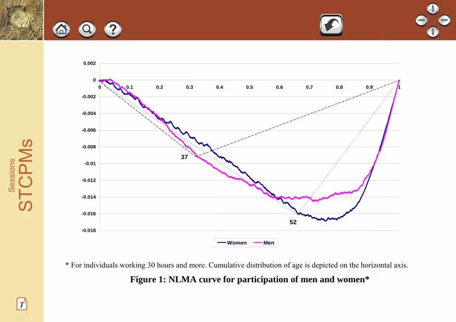
4. An Illustration: Labor Force Participation by Gender and Age

Figure 1 presents the Normalized Line (of independence) Minus the Absolute concentration curve (NLMA)

which is the LMA divided by cov(X, F(X)). As discussed above, the total area enclosed by the curve and the

horizontal axis is equal to the Gini regression coefficient. The horizontal axis depicts the cumulative

distribution according to age, while the vertical axis depicts the difference between the cumulative value of

participation in the labor force would participation be independent of age (i.e., LOI) and the actual

cumulative value of participation, divided by the Gini of the age distribution. The data are taken from

Income Survey, 2005, conducted by the Israeli Central Bureau of Statistics. Similar results were obtained

for the years 2003-2004.

Figure 1 is based on 12,685 observations for women and 11,213 for men. The curve enables us to detect

regions with positive or negative slopes according to whether the curve is concave or convex, and according

to whether the regression coefficient of each section is contributing positively or negatively to the overall

regression coefficient. If the curve is above (below) the horizontal axis then this range has a positive

(negative) contribution to the regression coefficient. In addition a concave (convex) section implies that

would we take this section alone we will find a positive (negative) regression coefficient. Table 1 presents

the regression coefficients in each section.

STC

PM

sS

essi

ons

T

-0.018

-0.016

-0.014

-0.012

-0.01

-0.008

-0.006

-0.004

-0.002

0

0.002

0 0.1 0.2 0.3 0.4 0.5 0.6 0.7 0.8 0.9 1

Women Men

37

52

* For individuals working 30 hours and more. Cumulative distribution of age is depicted on the horizontal axis.

Figure 1: NLMA curve for participation of men and women*

STC

PM

sS

essi

ons

T

Table 1: Regression coefficients of participation on age in different sections.

GINI OLS

Females Males Females Males

Section I 0.0170.0008 0.0007 0.017

Section II 0.034- 0.034-0.013- 0.014-

All 0.009- 0.010-0.009- 0.010-

As can be seen from Figure 1 and Table 1 the overall Gini and OLS regression coefficients are negative,

while the curve is concave for males for the lower 30 percent of the observations (up to age 37) and for

females for the 65 percent of the observations with smallest ages (up to age 52). As a result in these sections

the regression coefficients of both OLS and Gini regressions are positive. On the other hand, in the second

section the curves are convex, hence the regression coefficients in this section are negative. Note, however,

that the curves do not cross the horizontal axis, implying that the contributions of the two sections are adding

up to the overall regression coefficients. Also, note that for the Gini regression we can evaluate, by adding

and subtracting positive and negative areas, how many additional observations of the "wrong" sign we can

add without changing the sign of the regression coefficient. We note that the regression coefficients obtained

STC

PM

sS

essi

ons

T

by the two methods are similar. However, using the Gini method and the figures which are derived from the

Gini enable the user to make the partition into sections as shown above.

-0.4

-0.3

-0.2

-0.1

0

0.1

0.2

0.3

0.4

0.5

0 0.1 0.2 0.3 0.4 0.5 0.6 0.7 0.8 0.9 1

Women Men * For individuals working 30 hours and more

Figure 2: NLMA curve for monthly hours of work and age by gender*

46

39

STC

PM

sS

essi

ons

T

Figure 2 presents the NLMA of the regressions of monthly hours of work on age for men and women who

work 30 hours or more per week. The curve for men can be divided into two region: for the 45 percent of

observations with younger ages (up to age 39) the regression coefficient is positive and every monotonic

transformation of it will yield a positive coefficient, while for the 55 percent with older ages (ages from 39

up to 70) the regression coefficient for every monotonic transformation of it is negative. Table 2 confirms

this result. Because the curve intersects the horizontal axis at this point, the Gini between group regression

coefficient is zero. (It is close to zero due to the fact that the empirical distribution is discrete). A monotonic

transformation that extends (shrinks) the range of age at low values of age, relative to high values of age will

change the overall regression coefficient to be positive (negative) (e.g., using log(age) will increase the value

of the regression coefficient while using exp(age) will decrease it to be negative). The case of women is

more interesting. Here we can divide the age into three age groups: up to 40, 40 to 46, and over 46. In each

of those groups the regression coefficient is negative, but the overall coefficient is positive. Table 2 confirms

this result. As can be seen from the graph and the table, the between-group component is positive, leading to

an overall positive regression coefficient. Clearly, monotonic transformation of age may affect the sign of the

regression coefficient. Finally, note that for women, the OLS and Gini regressions result in an overall

positive effect of age on working hours, while for men, the sign depends on the regression method used (the

difference may be statistically insignificant).

STC

PM

sS

essi

ons

T

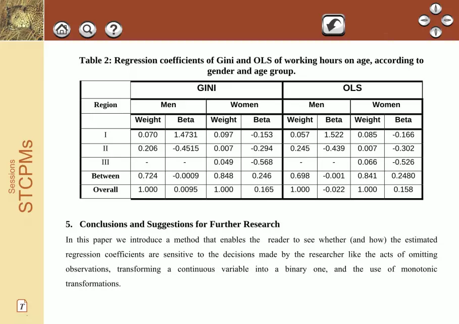
Table 2: Regression coefficients of Gini and OLS of working hours on age, according to gender and age group.

GINI OLS

Region Men Women Men Women

Weight Beta Weight Beta Weight Beta Weight Beta

I 0.070 1.4731 0.097 -0.153 0.057 1.522 0.085 -0.166

II 0.206 -0.4515 0.007 -0.294 0.245 -0.439 0.007 -0.302

III - - 0.049 -0.568 - - 0.066 -0.526

Between 0.724 -0.0009 0.848 0.246 0.698 -0.001 0.841 0.2480

Overall 1.000 0.0095 1.000 0.165 1.000 -0.022 1.000 0.158

5. Conclusions and Suggestions for Further Research

In this paper we introduce a method that enables the reader to see whether (and how) the estimated

regression coefficients are sensitive to the decisions made by the researcher like the acts of omitting

observations, transforming a continuous variable into a binary one, and the use of monotonic

transformations.

STC

PM

sS

essi

ons

T

The major advantage of using the Gini regression is its ability to enable the reader and the researcher to see

which (and how) sections contribute to the regression coefficient.

Applying the decomposition of the regression coefficient into intra and inter group components with the

weights depending on the variability measures of the independent variable simplifies the presentation of the

regression coefficient as a weighted average of slopes. It can be presented as a weighted average of groups'

regression coefficients so that it can be performed without a need for special software.

We also check whether the relationship between the dependent and the independent variable is monotonic,

and provided that we find that it is not, then it means that a monotonic transformation can change the sign of

the regression coefficient, both for Gini and OLS regressions.

Further theoretical and empirical researches are needed. The theoretical research that is needed is to translate

the effects on the simple regression coefficients to the effect in a multiple regression framework. The

empirical research needed is to develop the appropriate software and the diagnostic system that can transmit

to the reader, in a concise way, the influence of the many decisions made by the researcher to derive the

STC

PM

sS

essi

ons

T

estimated coefficients. A first step in this direction of extension to multiple regression is taken in Yitzhaki

and Schechtman (2009).

REFERENCES

[1] Angrist, J.D. and A.B. Krueger (1999). Empirical strategies in labor economics, Ch. 23 in O.

Ashenfelter & D. Card (ed.), Handbook of Labor Economics, Elsevier, edition 1, volume 3, number 3.

[2] Durbin, J. (1954). Errors in Variables. Review of International Statistical Institute, 23-32.

[3] Frick, R. J., J. Goebel, E. Schechtman, G. G. Wagner and S. Yitzhaki (2006). Using analysis of Gini

(ANOGI) for detecting whether two sub-samples represent the same universe: The German Socio-

Economic Panel study (SOEP) experience. Sociological Methods and Research, 34, 4, May, 427-468.

[4] Heckman, J.J., J. Stixrud and S. Urzua (2006). The effect of cognitive and noncognitive skills on labor

market outcomes and social behavior. Journal of Labor Economics, 24, 3, 411-481.

[5] Heckman, J.J., S. Urzua and E. Vytlacil (2006a). Understanding instrumental variables in models with

essential heterogeneity. Review of Economics and Statistics, LXXXVIII, 3, (August), 389-432.

[6] Heckman, J.J., S. Urzua and E. Vytlacil (2006b). Supplement to "Understanding instrumental variables in

models with essential heterogeneity". WEBAPPENDIX. March,

http://jenni.uchicago.edu/underiv/webappendix.pdf

STC

PM

sS

essi

ons

T

[7] Heckman, J.J. and S. Urzua (2009). Comparing IV with Structural Models: What Simple IV Can or

Cannot Identify, IZA DP No. 3980.

[8] Iyengar, N.S. (1960). On a method of computing Engel elasticities from concentration curves.

Econometrica, 28, 4, (October), 882-891.

[9] Kakwani, N.C. (1977). Applications of Lorenz curves in economic analysis. Econometrica, 45: 719-

727.

[10] Mahalanobis, P.C. (1960). A method of fractile graphical analysis. Econometrica, 28, 2, (April), 325-

351.

[11] Nygård, F. and A. Sandström (1981). Measuring Income Inequality. Stockholm: Almqvist & Wiksell

International.

[12] Olkin, I. and S. Yitzhaki (1992). Gini regression analysis. International Statistical Review, 60, 2, 185-

196.

[13] Pakes, A. (1982). On the asymptotic bias of Wald-type estimators of a straight line where both variables

are subject to error. International Economic Review, 23, 2, June, 491-497.

[14] Schechtman, E.; A. Shelef; S. Yitzhaki and R. Zitikis (2008). Testing hypotheses about absolute

concentration curve and marginal conditional stochastic dominance. Econometric Theory, 24, 4, 1044-

1062.

STC

PM

sS

essi

ons

T

[15] Schechtman, E., S. Yitzhaki and Y. Artzev (2008). Who does not respond in the household

expenditure survey: An exercise in extended Gini regressions. Journal of Business & Economic

Statistics. 26, 3, pp. 329-344.

[16] Wainer, H. (2006). Finding what is not there through the unfortunate binning of results: The Mendel

effect. Chance, 19, 1, 49-52.

[17] Wald, A. (1940). The fitting of straight lines if both variables are subject to errors. The Annals of

Mathematical Statistics, 11, 3, (September), 284-300.

[18] Yitzhaki, S. (1990). On the sensitivity of a regression coefficient to monotonic transformations.

Econometric Theory, 6, No. 2, 165-169. [19] Yitzhaki, S. (1996). On using linear regression in welfare economics. Journal of Business & Economic

Statistics, 14, 4, October, 478-86.

[20] Yitzhaki, S. (1998). More than a dozen alternative ways of spelling Gini. In Research on Economic

Inequality, 8, 13-30.

[21] Yitzhaki, S. (2003). Gini’s mean difference: A superior measure of variability for non-normal

distributions. Metron, LXI, 2, 285-316.

STC

PM

sS

essi

ons

T

[22] Yitzhaki, S. and I. Olkin. (1991). Concentration indices and concentration curves. In K. Mosler and M.

Scarsini (eds.) Stochastic Orders and Decisions under Risk, Institute of Mathematical Statistics: Lecture-

Notes Monograph Series, 19, 1991, 380-392.

[23] Yitzhaki, S. and E. Schechtman (2004). The Gini instrumental variable, or the "double instrumental

variable" estimator. Metron, LXII, 3, 287-313.

[24] Yitzhaki, S. and E. Schechtman (2009). The effects of some common practices on estimates in

covariance based regressions. Mimeo.

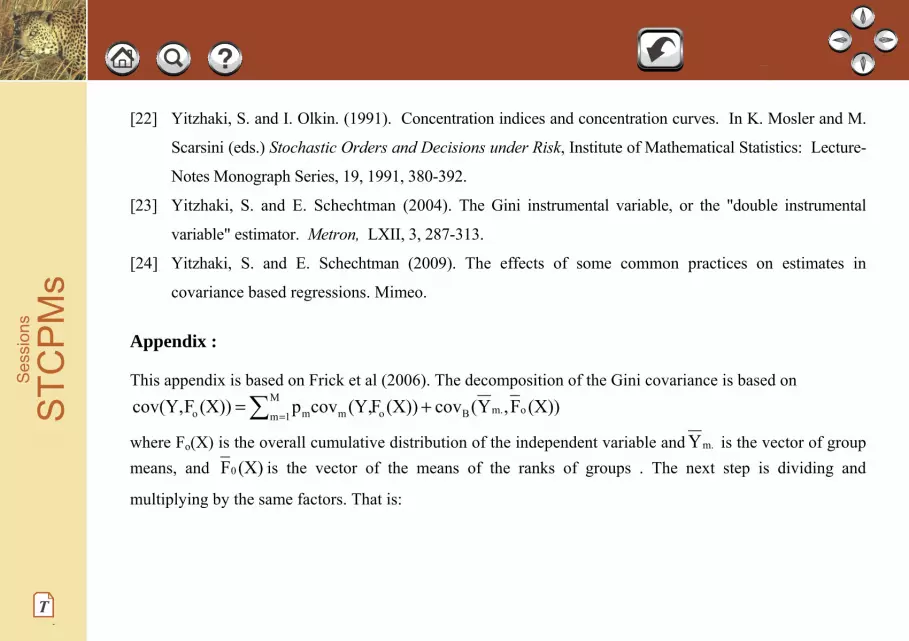
Appendix :

This appendix is based on Frick et al (2006). The decomposition of the Gini covariance is based on (X))F,Y(cov(X))F(Y,covp(X))Fcov(Y, om.Bo

M

1m mmo +=∑ =

where Fo(X) is the overall cumulative distribution of the independent variable and m.Y is the vector of group means, and (X)F0 is the vector of the means of the ranks of groups . The next step is dividing and

multiplying by the same factors. That is:

STC

PM

sS

essi

ons

T

(X))F.,X(cov(X))F,Y(cov(X))F,X(covGO

(X))F(X,cov(X))F(Y,covp

(X))F,Y(cov

(x))F(x,cov(x))F(x,cov(X))F(x,cov

(x))F(x,cov(X))F(y,covp(X))Fov(Y,

omB

om.Bom.B

M

1m mmom

omm

om.B

mM

1m mmm

om

om

ommo

+=

=+

=

∑

∑

=

=c

where ))(,(cov))(,(cov

XFXXFXO

mm

omm = is the overlapping between group k and the overall population.,

is (a quarter of ) the Gini Mean Difference of X))(,(cov XFXG mmm = m, while ))(,(cov))(,(cov

0

0

XFXXFY

m

mm =β is

a kind of Gini regression coefficient. Using the above notation we get:

))(,(cov))(,(cov

.

.

1 XFXXFYww

omB

omBB

M

m mm +=∑ =ββ

STC

PM

sS

essi

ons

T

where G

GOpw mmmm = is the contribution of the group to overall variability, G=cov(X,F(X)) is (one forth)

of Gini's Mean Difference of X and ))(,cov(

))(,(cov .

XFXXFXw omB

B = .

It is easy to see that if the grouping is according to non-intersecting sections of X, then the decomposition of the GMD is identical in structure to the decomposition of the variance. On the other hand, whenever there is overlapping between the groups according to X, then the share of between group Gini can be totally different from the share of between group variance. It can be easily shown (Frick et al, 2006) that the higher the overlapping the lower is the share of between group in the overall Gini, while the share of between group in the variance decomposition remains unaffected. S

TCP

Ms

Ses

sion

s

T