Embed Size (px)
Citation preview
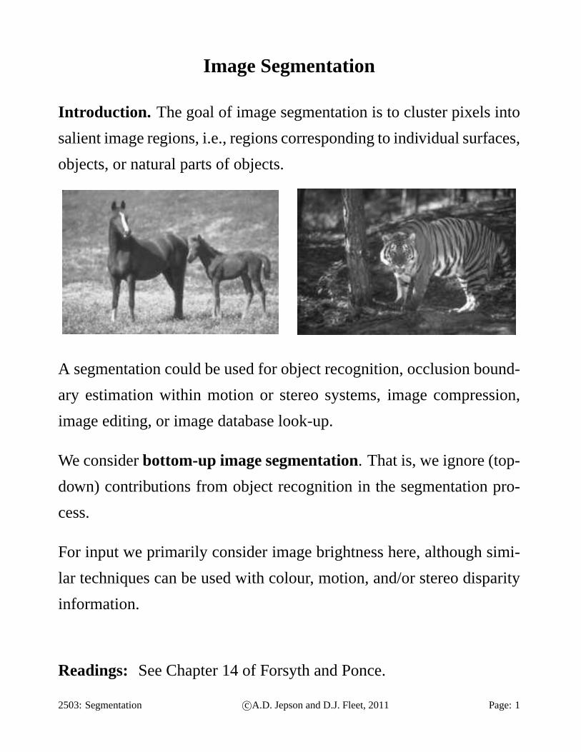
Image Segmentation
Introduction. The goal of image segmentation is to cluster pixels into
salient image regions, i.e., regions corresponding to individual surfaces,
objects, or natural parts of objects.
A segmentation could be used for object recognition, occlusion bound-
ary estimation within motion or stereo systems, image compression,
image editing, or image database look-up.
We considerbottom-up image segmentation. That is, we ignore (top-
down) contributions from object recognition in the segmentation pro-
cess.
For input we primarily consider image brightness here, althoughsimi-
lar techniques can be used with colour, motion, and/or stereodisparity
information.
Readings: See Chapter 14 of Forsyth and Ponce.
2503: Segmentation c©A.D. Jepson and D.J. Fleet, 2011 Page: 1
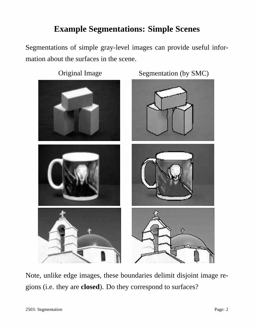
Example Segmentations: Simple Scenes
Segmentations of simple gray-level images can provide useful infor-
mation about the surfaces in the scene.
Original Image Segmentation (by SMC)
Note, unlike edge images, these boundaries delimit disjointimage re-
gions (i.e. they areclosed). Do they correspond to surfaces?
2503: Segmentation Page: 2
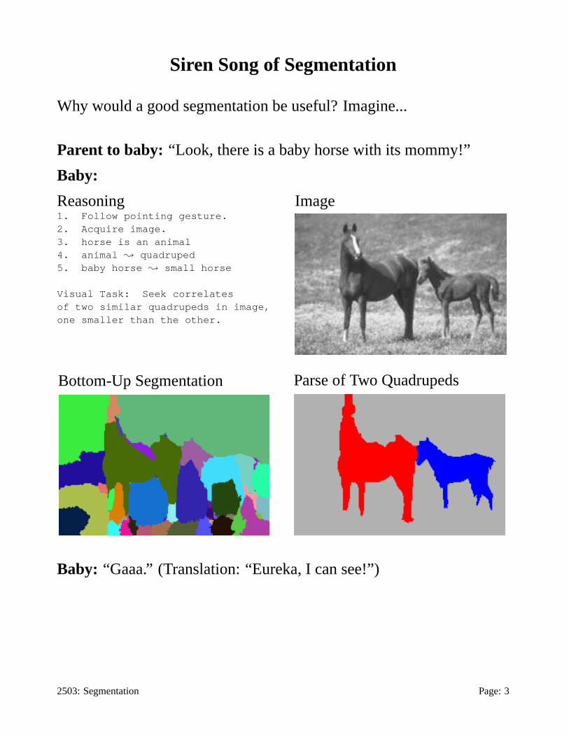
Siren Song of Segmentation
Why would a good segmentation be useful? Imagine...
Parent to baby: “Look, there is a baby horse with its mommy!”
Baby:
Reasoning1. Follow pointing gesture.2. Acquire image.3. horse is an animal4. animal ; quadruped5. baby horse ; small horse
Visual Task: Seek correlatesof two similar quadrupeds in image,one smaller than the other.
Image
Bottom-Up Segmentation Parse of Two Quadrupeds
Baby: “Gaaa.” (Translation: “Eureka, I can see!”)
2503: Segmentation Page: 3

Key Questions
1. How well can we expect to segment images without recognizing
objects (i.e. bottom-up segmentation)?
2. What determines a segment?
How can we pose the problem mathematically?
3. How do we solve the specified problem(s)?
4. How can we evaluate the results?
2503: Segmentation Page: 4
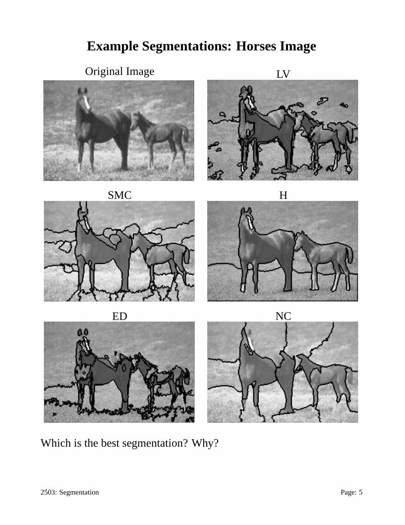
Example Segmentations: Horses Image
Original Image LV
SMC H
ED NC
Which is the best segmentation? Why?
2503: Segmentation Page: 5
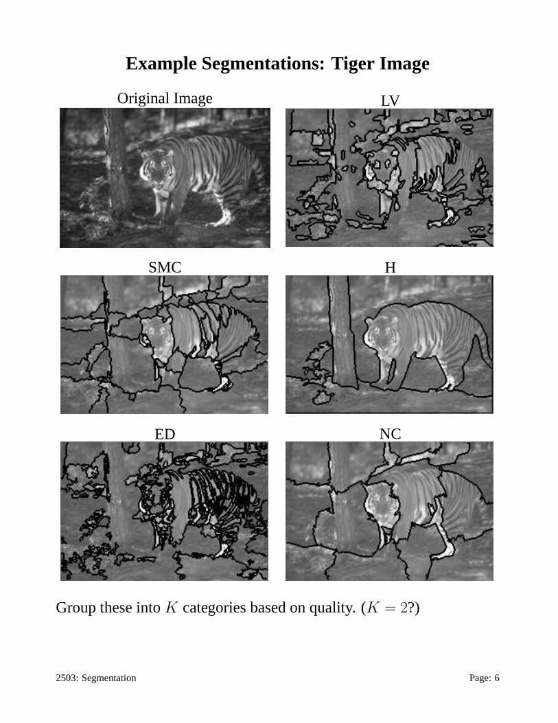
Example Segmentations: Tiger Image
Original Image LV
SMC H
ED NC
Group these intoK categories based on quality. (K = 2?)
2503: Segmentation Page: 6
Observations on Example Segmentations
The previous segmentations were done by
LV: local variation algorithm [8],
SMC: spectral min-cut [7],
H: human [10, 9],
ED: edge-augmented mean-shift [5, 4],
NC: normalized cut [12, 6].
Remarks:
• The quality of the segmentation depends on the image. Smoothly
shaded surfaces with clear gray-level steps between different sur-
faces are ideal for the above algorithms.
• For simple images (p. 2) it is plausible that machine segmentations
like those above are useful for visual tasks, e.g., object recognition.
• For more complex images (pp. 5, 6), machine segmentations pro-
vide a less reliable indicator for surface boundaries, and theirutility
for subsequent processing is questionable.
• While many algorithms work well with simple images, they break
down with clutter and camouflage. The assessment of segmenta-
tion algorithms therefore needs to be done on standardized datasets.
• Humans probably use object recognition in conjunction with seg-
mentation, while the machine algorithms above do not.
2503: Segmentation Page: 7

Current Goals
• Provide a brief introduction to the current image segmentation lit-
erature, including:
– Feature space clustering approaches.
∗ EDISON
– Graph-based approaches.
∗ Total Variation
∗ Ncut
∗ Spectral Min Cut
• Discuss the inherent assumptions different approaches make about
what constitutes a good segment.
• Emphasize general mathematical tools that are promising.
• Discuss metrics for evaluating the results.
2503: Segmentation Page: 8
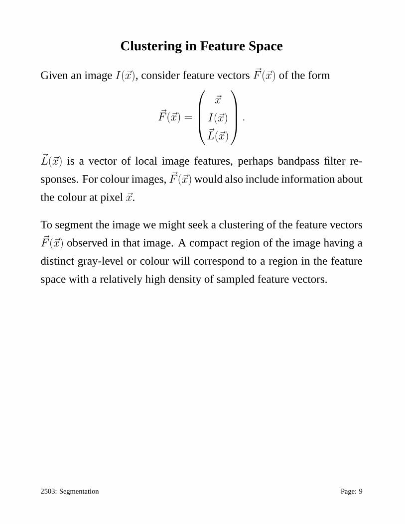
Clustering in Feature Space
Given an imageI(~x), consider feature vectors~F (~x) of the form
~F (~x) =
~x
I(~x)
~L(~x)
.
~L(~x) is a vector of local image features, perhaps bandpass filter re-
sponses. For colour images,~F (~x) would also include information about
the colour at pixel~x.
To segment the image we might seek a clustering of the feature vectors~F (~x) observed in that image. A compact region of the image having a
distinct gray-level or colour will correspond to a region in the feature
space with a relatively high density of sampled feature vectors.
2503: Segmentation Page: 9
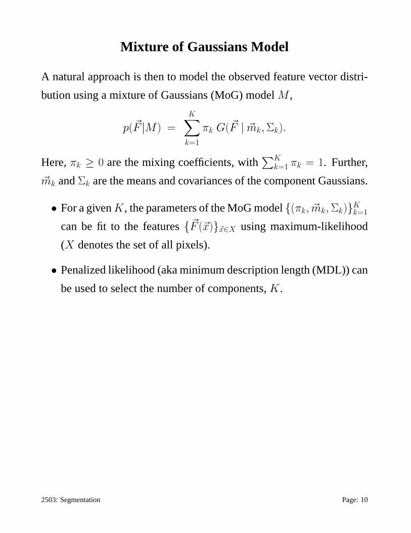
Mixture of Gaussians Model
A natural approach is then to model the observed feature vector distri-
bution using a mixture of Gaussians (MoG) modelM ,
p(~F |M) =
K∑
k=1
πk G(~F | ~mk, Σk).
Here,πk ≥ 0 are the mixing coefficients, with∑K
k=1 πk = 1. Further,
~mk andΣk are the means and covariances of the component Gaussians.
• For a givenK, the parameters of the MoG model{(πk, ~mk, Σk)}Kk=1
can be fit to the features{~F (~x)}~x∈X using maximum-likelihood
(X denotes the set of all pixels).
• Penalized likelihood (aka minimum description length (MDL)) can
be used to select the number of components,K.
2503: Segmentation Page: 10
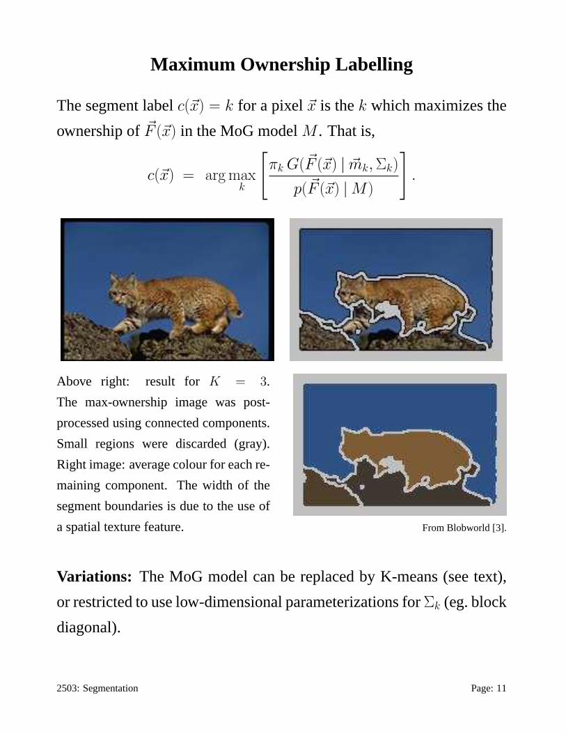
Maximum Ownership Labelling
The segment labelc(~x) = k for a pixel~x is thek which maximizes the
ownership of~F (~x) in the MoG modelM . That is,
c(~x) = arg maxk
[
πk G(~F (~x) | ~mk, Σk)
p(~F (~x) | M)
]
.
Above right: result for K = 3.
The max-ownership image was post-
processed using connected components.
Small regions were discarded (gray).
Right image: average colour for each re-
maining component. The width of the
segment boundaries is due to the use of
a spatial texture feature. From Blobworld [3].
Variations: The MoG model can be replaced by K-means (see text),
or restricted to use low-dimensional parameterizations forΣk (eg. block
diagonal).
2503: Segmentation Page: 11
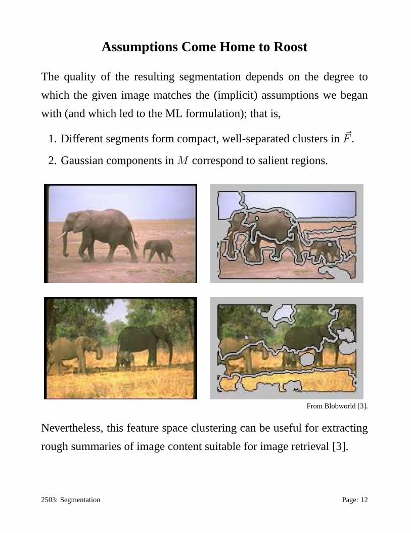
Assumptions Come Home to Roost
The quality of the resulting segmentation depends on the degree to
which the given image matches the (implicit) assumptions we began
with (and which led to the ML formulation); that is,
1. Different segments form compact, well-separated clusters in~F .
2. Gaussian components inM correspond to salient regions.
From Blobworld [3].
Nevertheless, this feature space clustering can be useful for extracting
rough summaries of image content suitable for image retrieval [3].
2503: Segmentation Page: 12
Mean-Shift Segmentation
The mean-shift segmentation algorithm [5] also considers the probabil-
ity density of feature vectors~F (~x) obtained from a given image. How-
ever, anon-parametric density model is used instead of an MoG.
Given features~Fj ≡ ~F (~xj), the kernel-density estimate is
pK(~F ) ≡1
|X|
|X|∑
j=1
K(~Fj − ~F ) , with ~F ∈ RD ,
whereX is the set of all pixels in the image,|X| is the number of
pixels, andK(~e) is a kernel (which integrates to unity).
Common choices forK(~e) are functions of a (covariance) matrixΣ
and the squared deviations ≡ ~e TΣ−1~e ≥ 0. That is,
K(~e) = k(~e TΣ−1~e) , (1)
wherek(s) is a concave decreasing function ofs. For example,
k(s) = ce−s/2 , for a Gaussian kernel, (2)
k(s) = cb1 − sc+ , for an Epanechnikov kernel. (3)
Here,c = c(Σ) is a normalizing constant, andbzc+ denotes positive
rectification, i.e.bzc+ ≡ max(z, 0) .
We show an example next.
2503: Segmentation Page: 13
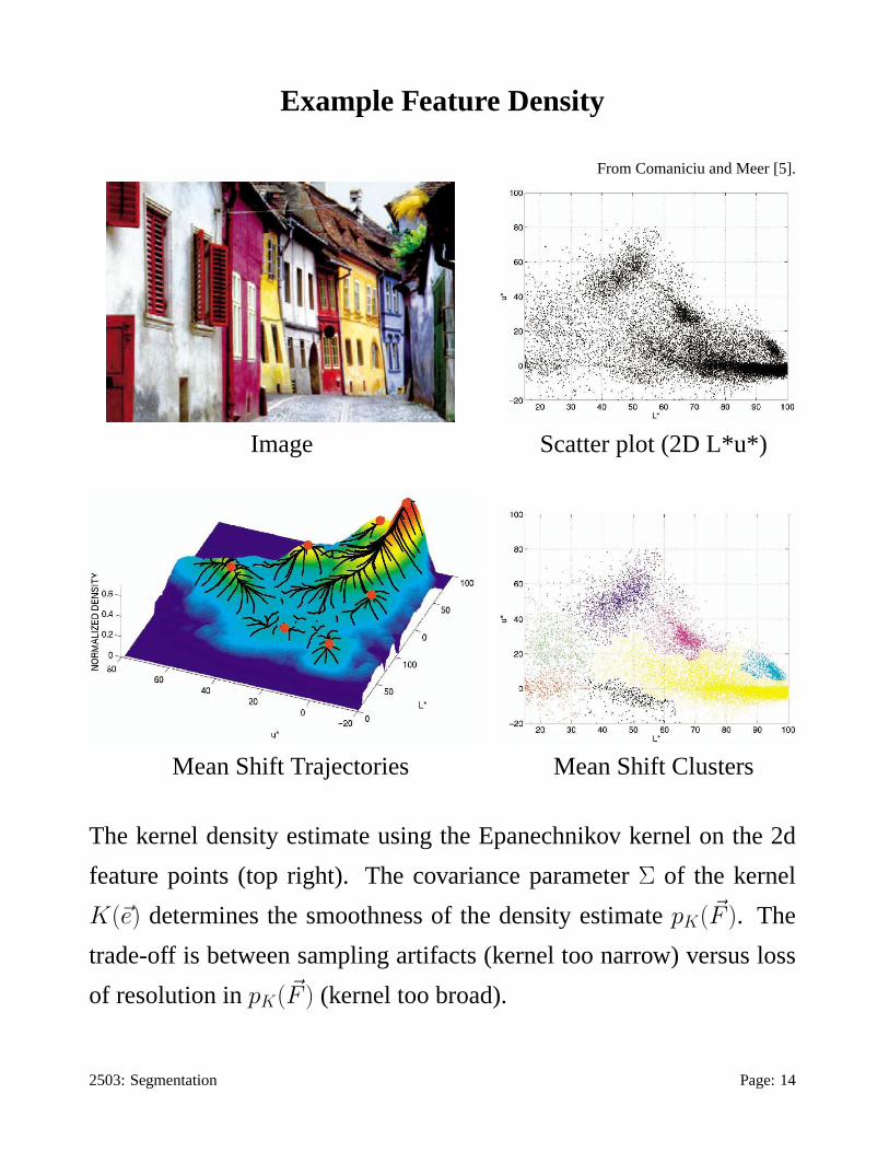
Example Feature Density
From Comaniciu and Meer [5].
Image Scatter plot (2D L*u*)
Mean Shift Trajectories Mean Shift Clusters
The kernel density estimate using the Epanechnikov kernel on the 2d
feature points (top right). The covariance parameterΣ of the kernel
K(~e) determines the smoothness of the density estimatepK(~F ). The
trade-off is between sampling artifacts (kernel too narrow) versus loss
of resolution inpK(~F ) (kernel too broad).
2503: Segmentation Page: 14
Mean-Shift Iterations
We will use the modes (i.e. peaks) ofpK(~F ) to be segmentation labels,
replacing the use of the component labels in the previous MoG model.
That is, we wish to locally solve
~F∗ = arg max~F
pK(~F ) .
This is similar to robust M-estimation, but here we are maximizing the
objective functionpK(~F ), not minimizing it. A similar derivation to
the one for M-estimation shows~F∗ must satisfy
~F∗ =
∑
j w(~Fj − ~F∗) ~Fj∑
j w(~Fj − ~F∗),
wherew(~e) = −k′(~e TΣ−1~e) andk′(s) = dkds(s). In words, ~F∗ must be
the weighted mean of~Fj using the weightsw(~Fj− ~F∗) centered on~F∗.
The analogue of the iterative reweighting idea used in M-estimation is
to solve for~F∗ here by iterating themean-shiftequation
~F (t+1) =
∑
j w(~Fj − ~F (t)) ~Fj∑
j w(~Fj − ~F (t)). (4)
Note ~F (t+1) is just the weighted mean of the feature points~Fj, with the
weightsw(~Fj− ~F (t)) centered on the previous guess~F (t).
2503: Segmentation Page: 15
Details of Mean-Shift Iterations
Let ~Fj ≡ ~F (~xj) be the feature vector at pixel~xj. We define a kernel density estimate for the distribution
of the image features~F as follows:
p(~F ) =1
|X|
|X|∑
j=1
k(sj(~F )) , (5)
where|X| is the number of pixels in the image,k be a non-negative kernel function, and, given a
positive definite matrixC,
sj(~F ) ≡ (~F − ~Fj)T C−1(~F − ~Fj) (6)
measures the scaled deviation between~F and ~Fj. We further assume that the kernel integrates to one
in order for (5) to be a valid density function. And letw(s) = dkds
(s) ≡ k′(s) be the kernel derivative.
The goal of the mean-shift iterations is to find a trajectory to local maxima ofp(~F ), beginning at an
arbitrary point in the feature space. A necessary conditionfor a local maxima of the kernel density
estimate is that the gradient be zero. That is, for~F ∗ to be a critical point it must satisfy
∂pk
∂ ~F(~F ∗) = ~0 . (7)
Thus, to find critical points let’s look at the form of the derivative of the feature distribution:
∂pk
∂ ~F(~F ) =
1
|X|
∑
j
∂k
∂ ~F(sj(~F ))
=1
|X|
∑
j
∂k
∂s
∣
∣
∣
s=sj
∂sj
∂ ~F
=1
|X|
∑
j
w(sj(~F ))[
2C−1 ~F − 2C−1 ~Fj
]
(8)
With some algebraic simplification, we find that that the critical points satisfy[
∑
j
w(sj(~F ∗))
]
~F ∗ =∑
j
w(sj(~F ∗)) ~Fj . (9)
To find a critical point, given an initial guess,~F (t), we compute the weights using~F (t). Then, holding
the weights fixed we solve for the next point on the trajectorytoward the critical point; i.e.,[
∑
j
w(sj(~F (t)))
]
~F (t+1) =∑
j
w(sj(~F (t))) ~Fj, (10)
from which we obtain (4).
2503: Segmentation Notes: 16
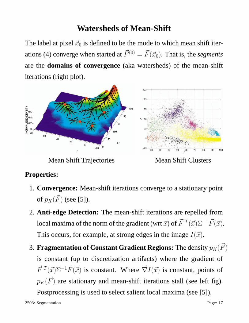
Watersheds of Mean-Shift
The label at pixel~x0 is defined to be the mode to which mean shift iter-
ations (4) converge when started at~F (0) = ~F (~x0). That is, thesegments
are thedomains of convergence(aka watersheds) of the mean-shift
iterations (right plot).
Mean Shift Trajectories Mean Shift Clusters
Properties:
1. Convergence:Mean-shift iterations converge to a stationary point
of pK(~F ) (see [5]).
2. Anti-edge Detection:The mean-shift iterations are repelled from
local maxima of the norm of the gradient (wrt~x) of ~F T (~x)Σ−1 ~F (~x).
This occurs, for example, at strong edges in the imageI(~x).
3. Fragmentation of Constant Gradient Regions:The densitypK(~F )
is constant (up to discretization artifacts) where the gradient of~F T (~x)Σ−1 ~F (~x) is constant. Where~∇I(~x) is constant, points of
pK(~F ) are stationary and mean-shift iterations stall (see left fig).
Postprocessing is used to select salient local maxima (see [5]).
2503: Segmentation Page: 17
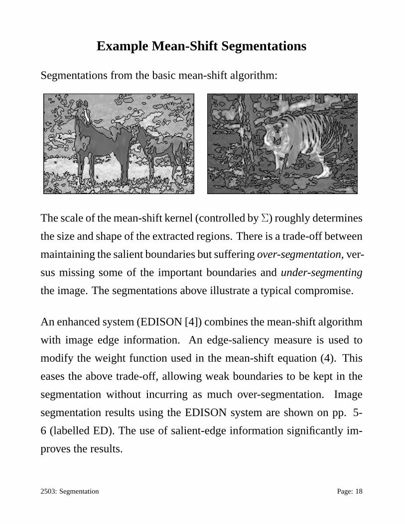
Example Mean-Shift Segmentations
Segmentations from the basic mean-shift algorithm:
The scale of the mean-shift kernel (controlled byΣ) roughly determines
the size and shape of the extracted regions. There is a trade-off between
maintaining the salient boundaries but sufferingover-segmentation, ver-
sus missing some of the important boundaries andunder-segmenting
the image. The segmentations above illustrate a typical compromise.
An enhanced system (EDISON [4]) combines the mean-shift algorithm
with image edge information. An edge-saliency measure is used to
modify the weight function used in the mean-shift equation (4). This
eases the above trade-off, allowing weak boundaries to be kept inthe
segmentation without incurring as much over-segmentation. Image
segmentation results using the EDISON system are shown on pp. 5-
6 (labelled ED). The use of salient-edge information significantly im-
proves the results.
2503: Segmentation Page: 18
Similarity Graph Based Methods
Graph-based methods provide an alternative to feature space clustering.
A weighted undirected graphG = (V, E) is formed, with the set of
verticesV corresponding to the pixels~x in the image. EdgesE in the
graph occur between any two pixels~xi and~xj within a small distance
of each other.
The edge weightw(~xi, ~xj) ≥ 0 reflects the dissimilarity (alternatively,
the similarity) between the two image neighbourhoods centeredon pix-
els~xi and~xj. A common form of the weight function is to usew(~xi, ~xj) =
1 − a(~xi, ~xj) where the affinitya(~xi, ~xj) is given by
a(~xi, ~xj) ≡ exp
(
−1
2(~F (~xi) − ~F (~xj))
TΣ−1(~F (~xi) − ~F (~xj))
)
.
As above,~F (~x) is a feature vector associated with pixel~x, for example:
1. ~F (~x) = I(~x), so the affinity is determined only by the grey-level
difference between neighbouring pixels,
2. ~F (~x) = ~I(~x), the RGB values for a colour image, or some mapping
of the RGB values to a more uniform colour space (eg. L*u*v*).
3. ~F (~x) includes texture primitives, such as local filter responses,
along with the brightness and/or colour at pixel~x.
2503: Segmentation Page: 19
Connected Components (Not Robust)
A simple approach is to delete all edges between dissimilar pixels (i.e.,
with weightsw(~xi, ~xj) > τ ), and then seek connected components
(CCs) in the remaining graph.
An efficient way to do CC clustering, with a variableτ , is to first build
a minimal spanning tree (MST) of the graph.Kruskal’s Algorithm is
a greedy approach that is guaranteed to give an optimal MST:
• Begin with the completely disconnected graph.
• Add edges one at a time in increasing order of their weights, so
long as adding an edge does not introduce cycles in the sub-graph.
The CCs of the decimated graph (with edges havingw(~xi, ~xj) > τ
removed) are then efficiently computed by deleting these same edges
from the MST. The trees in the resulting forest provide the desired CCs.
Note that a single edge withw(~xi, ~xj) ≤ τ would be sufficient to cause
two desired regions to be merged. Therefore CCs are not robust to stray
links (aka “leaks”) between regions. The consequence is that there is
often no suitable value ofτ that gives a useful segmentation.
A modified version of Kruskal’s algorithm is considered next.
2503: Segmentation Page: 20
Local Variation Method
Felzenszwalb and Huttenlocher [8] introduce a simple but effective
modification of Kruskal’s algorithm. As in Kruskal’s algorithm,
• it begins with the completely disconnected graph,
• edges are added one at a time in increasing order of their weights,
• it maintains a forest of MSTs for its current components.
During processing, each MSTCi is associated with a threshold
T (Ci) = w(Ci) +k
|Ci|, (11)
wherew(Ci) is the maximum weight in the spanning treeCi (i.e. the
local variation of Ci). Also k > 0 is a constant, and|Ci| is the number
of pixels inCi.
Suppose the edge(~xk, ~xl) is to be processed next, and its two endpoints
are in two separate MSTsCi andCj. Then these MSTs are merged by
adding the edge(~xk, ~xl) only if
w(~xk, ~xl) ≤ min(T (Ci), T (Cj)) . (12)
As the size ofCi increases, (11) and (12) dictate an increasingly tight
upper boundT (Ci) (compared to the largest weightw(Ci) in Ci) for the
acceptable affinity of an edge mergingCi with another region.
2503: Segmentation Page: 21
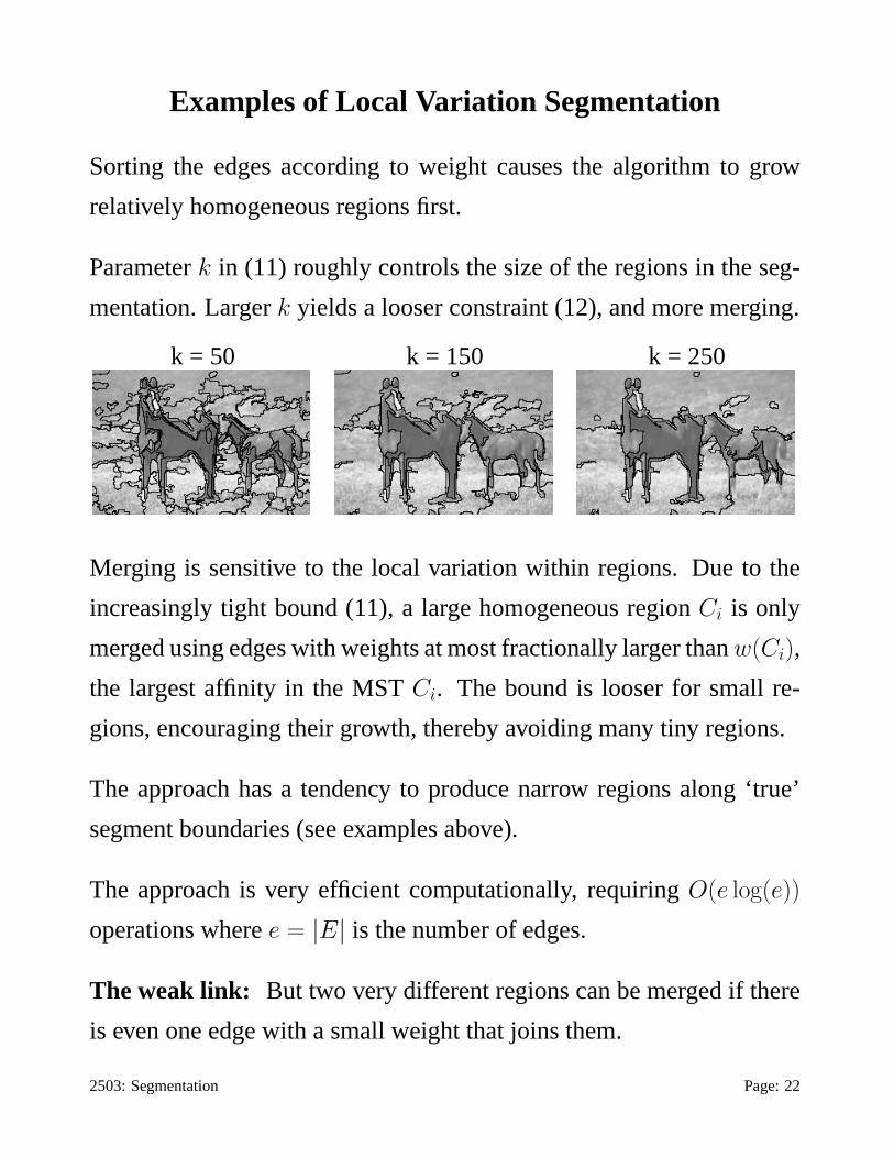
Examples of Local Variation Segmentation
Sorting the edges according to weight causes the algorithm to grow
relatively homogeneous regions first.
Parameterk in (11) roughly controls the size of the regions in the seg-
mentation. Largerk yields a looser constraint (12), and more merging.
k = 50 k = 150 k = 250
Merging is sensitive to the local variation within regions. Due to the
increasingly tight bound (11), a large homogeneous regionCi is only
merged using edges with weights at most fractionally larger thanw(Ci),
the largest affinity in the MSTCi. The bound is looser for small re-
gions, encouraging their growth, thereby avoiding many tiny regions.
The approach has a tendency to produce narrow regions along ‘true’
segment boundaries (see examples above).
The approach is very efficient computationally, requiringO(e log(e))
operations wheree = |E| is the number of edges.
The weak link: But two very different regions can be merged if there
is even one edge with a small weight that joins them.
2503: Segmentation Page: 22

Graph Cuts
Graph partitioning formulations are intended to be more robust to small
leaks, since the objective criteria naturally take into account the entire
boundary of a hypothetical segment.
Suppose we want to partition (i.e., cut) the graph into two parts,F and
G = V − F . Further, we only want to cut edges with small affinities
(ie keep similar nodes together in the same partition). Thus, one might
measure the cost of the cut using
L(F, G) =∑
~xi∈F, ~xj∈G
a(~xi, ~xj) , (13)
wherea(·, ·) is the affinity function described above.
Problem: Optimal cuts often result inF (or G) containing one node.
Solution: Formulate more suitable objective functions or graph con-
structions to place constraints onF andG.
2503: Segmentation Page: 23
Normalized Cut
The normalized cut approach of Shi and Malik [12] avoided trivialpar-
titions of the affinity weighted graph with the use of thenormalized cut
criterion. They proposed that the optimal partition of the graph intoF
andG = V − F should minimize
N(F, G) ≡ L(F, G)
(
1
L(F, V )+
1
L(G, V )
)
, (14)
whereL is the linkage defined in (13); i.e.,L(A, B) is the sum of the
affinities for all edges having one end inA and the other inB.
Properties:
• The cut cost decreases when edges connecting nodes inF andG
have small affinities (i.e., for smallL(F, G)).
• L(F, V ) is sum of affinities on edges withinF , and those connect-
ing F to the rest of the graph. And similarly forL(G, V ).
• Other things being equal, the cut cost decreases when the affinities
on edges withinF andG are larger (i.e., forhomogeneous regions).
Problem: Unfortunately, the resulting graph partitioning problem,
F = arg minF⊂V
N(F, V − F ), (15)
is computationally intractable [12]. Therefore we must seek algorithms
that provide approximate solutions of (15).
2503: Segmentation Page: 24
Normalized Cut (cont)
Shi and Malik [12] prove that (15) is equivalent to the discrete opti-
mization problem, for labelling~y = (y1, ..., yN)T with N = |X| ,
arg min~y
~y T (D − A)~y
~y TD~y, subject toyi ∈ {1,−b} and ~d T~y = 0 . (16)
Here,
• A is theN×N symmetric matrix of affinities,a(~xi, ~xj), arranged
(say) according to the raster ordering of the pixels;
• ~d = A~1, where~1 is theN -vector comprisingN ones;
• D is the diagonal matrix withDi,i = di ;
• b > 0.
Given a solution~y of (16), the corresponding solution for partitionF
of (15) is then obtained by settingF = {~xi | yi > 0} . And, vice versa,
givenF we setyi = 1 for each~xi ∈ F , and set the other elements of~y
to−b, whereb > 0 is chosen such that~d T~y = 0.
Shi and Malik [12] proposed to relax the discrete problem. They first
find a real-valued solution to (16), for which they ignore the binary
constraint thatyi ∈ {1,−b}. Then they threshold the result to produce
a discrete (approximate) solution.
2503: Segmentation Page: 25
Rayleigh Quotient
Equation (16) is a discrete version of a standard eigenvector formulation, namely the Rayleigh quotient.
By way of background, the matrixD − A is known as the Laplacian matrix. Among its generalized
eigenvectors,~y, satisfying
(D − A) ~y = µ D ~y , (17)
the eigenvector corresponding to the smallest eigenvectoris known to be the solution to the following
problem:
arg min~y
~y T (D − A)~y
~y T D~y. (18)
It is well-known that becauseD − A is symmetric, real, positive semidefinite, that (1)D − A has
orthogonal eigenvectors, and (2) that the associated eigenvalues must be greater than or equal to zero.
More specifically the vector of all ones~1 is known to be an eigenvector ofD − A, with eigenvalue0.
Now consider the relaxation of (16), in which we ignore the constraint thatyi ∈ {1,−b}, and therefore
treat~y as real-valued. Further consider the transformation~y = D−1/2~u, for which the relaxed problem
becomes
arg min~u
~u T (I − B)~u
~u T~u, subject to~d T/2~u = 0 , (19)
for symmetric matrixB = D−1/2AD−1/2, and real-valued~u. This is a standard eigenvalue problem in
linear algebra. In particular, it can be shown that
• ~u = ~d 1/2 is an eigenvector ofB with eigenvalue1, so it must also be an eigenvector ofI − B
with eigenvalue0;
• sinceD − A is symmetric positive semidefinite, so isI − B, and therefore all the eigenvalues
associated withI − B are greater than or equal to zero, and the corresponding eigenvectors are
orthogonal;
• all the eigenvalues ofI − B are in the interval[0, 2].
Hence, from (19) it follows that the linear constraint on~u simply says that~u must be orthogonal to the
eigenvector ofI −B having the smallest eigenvalue. Accordingly, the vector minimizing the Rayleigh
Quotient and orthogonal to~d 1/2 is simply the eigenvector ofI−B with thesecond smallest eigenvalue.
2503: Segmentation Notes: 26
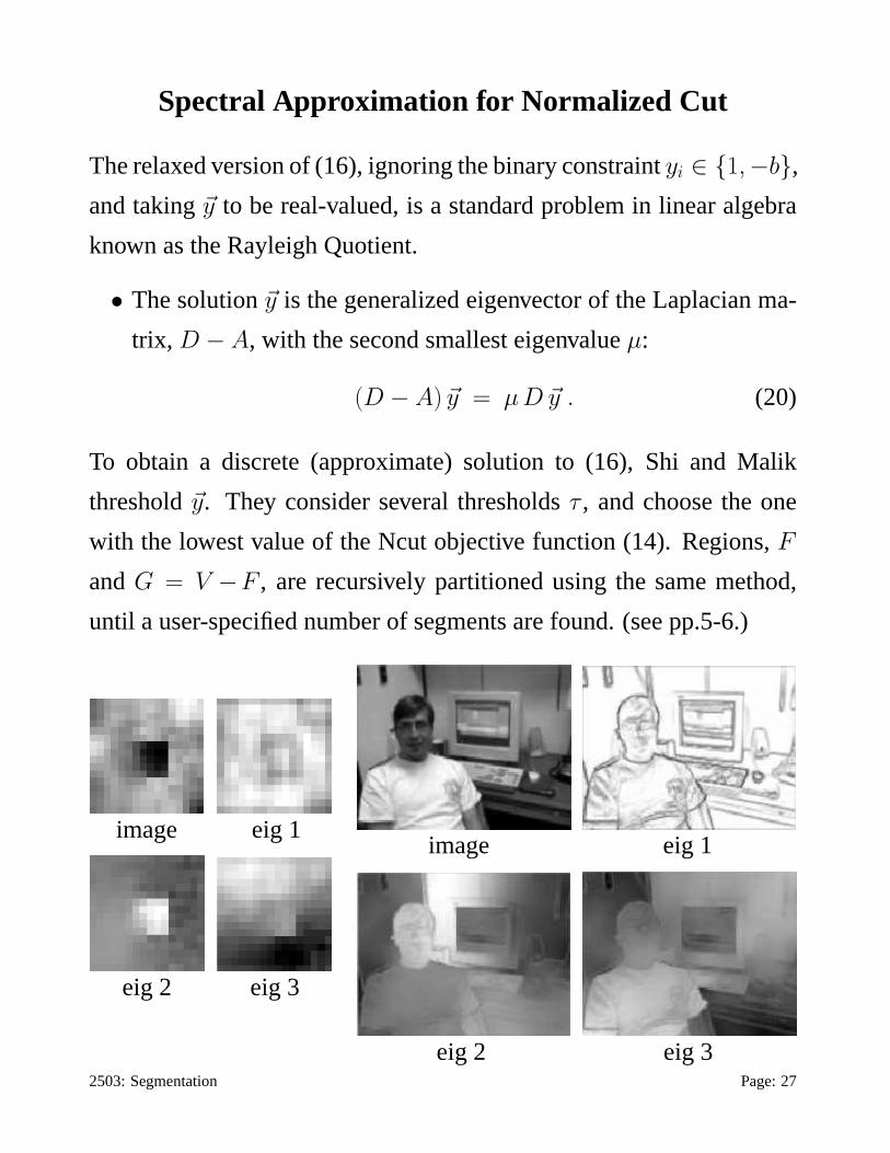
Spectral Approximation for Normalized Cut
The relaxed version of (16), ignoring the binary constraintyi ∈ {1,−b},
and taking~y to be real-valued, is a standard problem in linear algebra
known as the Rayleigh Quotient.
• The solution~y is the generalized eigenvector of the Laplacian ma-
trix, D − A, with the second smallest eigenvalueµ:
(D − A) ~y = µ D ~y . (20)
To obtain a discrete (approximate) solution to (16), Shi and Malik
threshold~y. They consider several thresholdsτ , and choose the one
with the lowest value of the Ncut objective function (14). Regions,F
andG = V −F , are recursively partitioned using the same method,
until a user-specified number of segments are found. (see pp.5-6.)
image eig 1
eig 2 eig 3
image eig 1
eig 2 eig 32503: Segmentation Page: 27
Remarks on Ncuts
The step of thresholding the second largest eigenvector to provide a
partitioning proposal is a key limitation. In practice, the approximation
only appears to be consistently reliable when there is just one clear
way to partition the data. Yu and Shi [13] attempt to alleviate this
problem by extractingK segments from the subspace spanned by the
K eigenvectors ofI − B with the smallest eigenvalues.
Ncuts can be very slow for large images since the matrix becomes pro-
hibitively large. Efficient approximations to the eigenvector problem
have also been proposed.
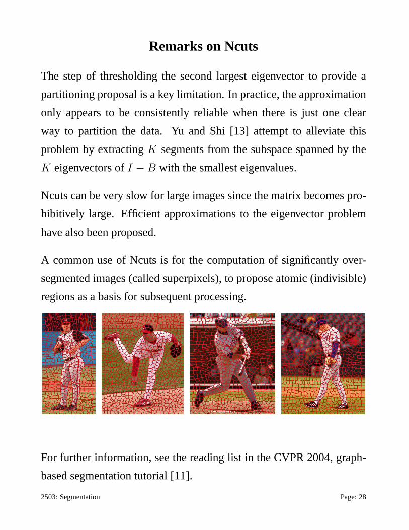
A common use of Ncuts is for the computation of significantly over-
segmented images (called superpixels), to propose atomic (indivisible)
regions as a basis for subsequent processing.
For further information, see the reading list in the CVPR 2004, graph-
based segmentation tutorial [11].
2503: Segmentation Page: 28
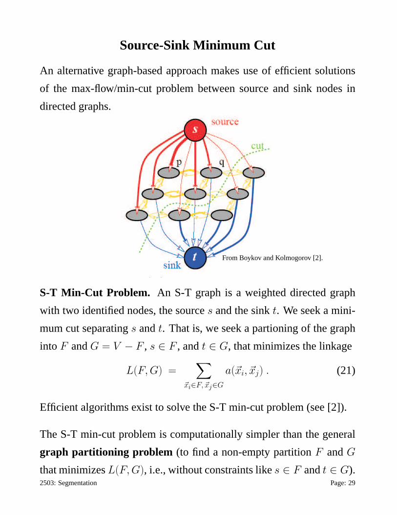
Source-Sink Minimum Cut
An alternative graph-based approach makes use of efficient solutions
of the max-flow/min-cut problem between source and sink nodes in
directed graphs.
From Boykov and Kolmogorov [2].
S-T Min-Cut Problem. An S-T graph is a weighted directed graph
with two identified nodes, the sources and the sinkt. We seek a mini-
mum cut separatings andt. That is, we seek a partioning of the graph
into F andG = V − F , s ∈ F , andt ∈ G, that minimizes the linkage
L(F, G) =∑
~xi∈F, ~xj∈G
a(~xi, ~xj) . (21)
Efficient algorithms exist to solve the S-T min-cut problem (see [2]).
The S-T min-cut problem is computationally simpler than the general
graph partitioning problem (to find a non-empty partitionF andG
that minimizesL(F, G), i.e., without constraints likes ∈ F andt ∈ G).2503: Segmentation Page: 29

Source-Sink Minimum Cut (Cont.)
To take advantage of efficient solutions to the S-T min-cut problem, we
first need to construct an S-T graph.
Given two disjoint sets of pixelsS andT , we form a weighted directed
graph as follows:
• For each edge(~xi, ~xj) in the previous undirected graphs, we in-
clude two directed edges〈~xi, ~xj〉 and〈~xj, ~xi〉. Both are weighted
by the affinitya(~xi, ~xj).
• Two additional nodess andt are created, namely the source and
sink nodes, respectively.
• Infinitely weighted directed links〈s, ~xi〉 and 〈~xj, t〉 are included
for each~xi ∈ S and~xj ∈ T . This ensures that nodes inS andT
can never be cut froms andt.
The resulting S-T min-cut then provides theglobally, minimum-cost
cut between the sets of pixelsS andT .
2503: Segmentation Page: 30

Seed Regions for S-T Min Cut
SetsS andT (nodes connected to source and sink) should satisfy:
1. EachS andT generated must be sufficiently large (otherwise the
minimum cut is eitherS andV − S, or T andV − T ),
2. EachS andT should be contained within different ‘true’ segments
(due to the infinite weights, neitherS or T will be partitioned),
3. Enough pairsS andT should be generated to identify most of the
salient segments in the image.
Interactive Min-Cut:
Spectral Min-Cut: One suitable generation process is discussed in
Estrada et al. [7]. It is based on spectral properties of a matrix repre-
senting the affinities. Sample results are given by theSpectral Min-
Cut technique (SMC on pp. 5,6). The process is much more compu-
tationally intensive than the previous ones. Several hundred min-cut
problems are typically solved for differentS, T .
2503: Segmentation Page: 31
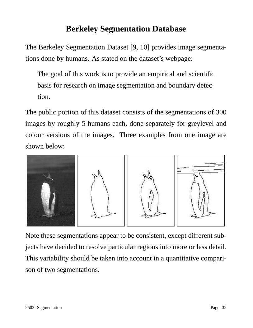
Berkeley Segmentation Database
The Berkeley Segmentation Dataset [9, 10] provides image segmenta-
tions done by humans. As stated on the dataset’s webpage:
The goal of this work is to provide an empirical and scientific
basis for research on image segmentation and boundary detec-
tion.
The public portion of this dataset consists of the segmentations of 300
images by roughly 5 humans each, done separately for greylevel and
colour versions of the images. Three examples from one image are
shown below:
Note these segmentations appear to be consistent, except different sub-
jects have decided to resolve particular regions into more or less detail.
This variability should be taken into account in a quantitative compari-
son of two segmentations.
2503: Segmentation Page: 32
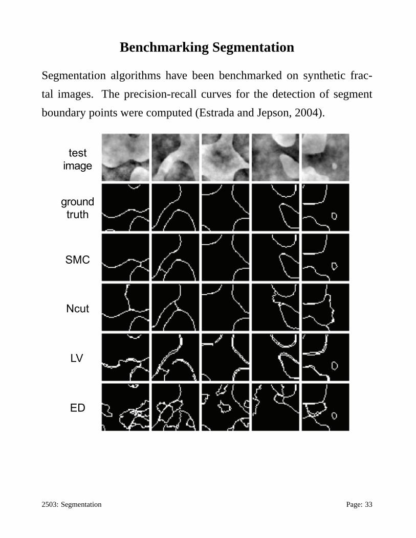
Benchmarking Segmentation
Segmentation algorithms have been benchmarked on synthetic frac-
tal images. The precision-recall curves for the detection of segment
boundary points were computed (Estrada and Jepson, 2004).
testimage
ground truth
SMC
Ncut
LV
ED
2503: Segmentation Page: 33
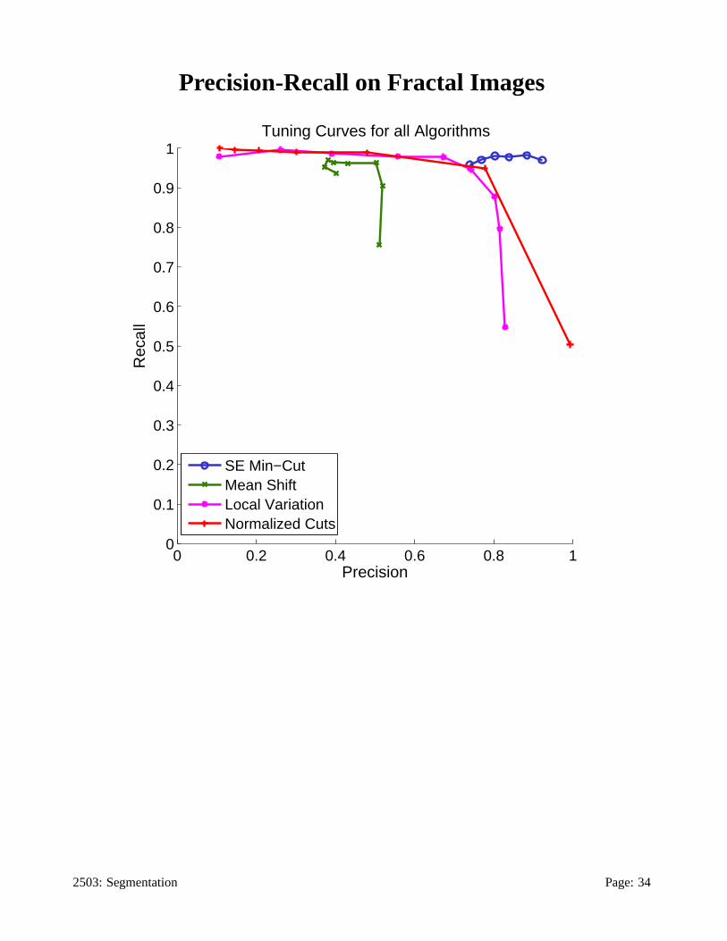
Precision-Recall on Fractal Images
0 0.2 0.4 0.6 0.8 10
0.1
0.2
0.3
0.4
0.5
0.6
0.7
0.8
0.9
1
Precision
Rec
all
Tuning Curves for all Algorithms
SE Min−CutMean ShiftLocal VariationNormalized Cuts
2503: Segmentation Page: 34
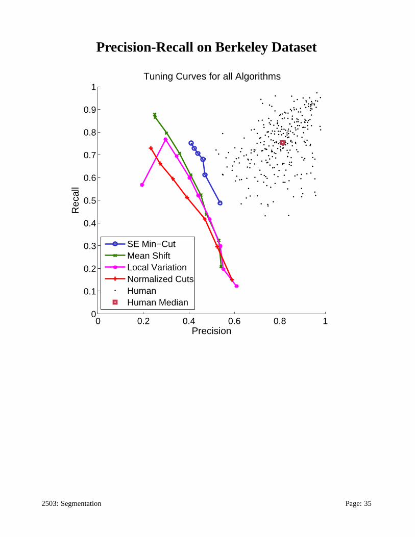
Precision-Recall on Berkeley Dataset
0 0.2 0.4 0.6 0.8 10
0.1
0.2
0.3
0.4
0.5
0.6
0.7
0.8
0.9
1
Precision
Rec
all
Tuning Curves for all Algorithms
SE Min−CutMean ShiftLocal VariationNormalized CutsHumanHuman Median
2503: Segmentation Page: 35
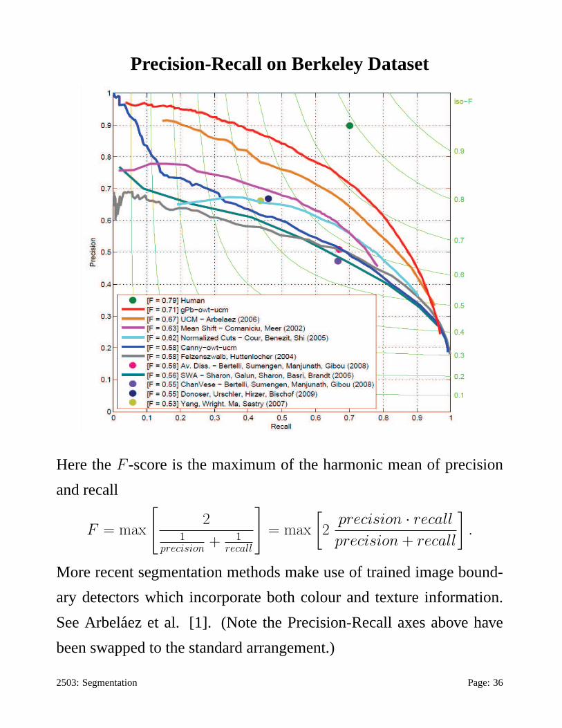
Precision-Recall on Berkeley Dataset
Here theF -score is the maximum of the harmonic mean of precision
and recall
F = max
[
21
precision + 1recall
]
= max
[
2precision · recall
precision + recall
]
.
More recent segmentation methods make use of trained image bound-
ary detectors which incorporate both colour and texture information.
See Arbelaez et al. [1]. (Note the Precision-Recall axes above have
been swapped to the standard arrangement.)
2503: Segmentation Page: 36
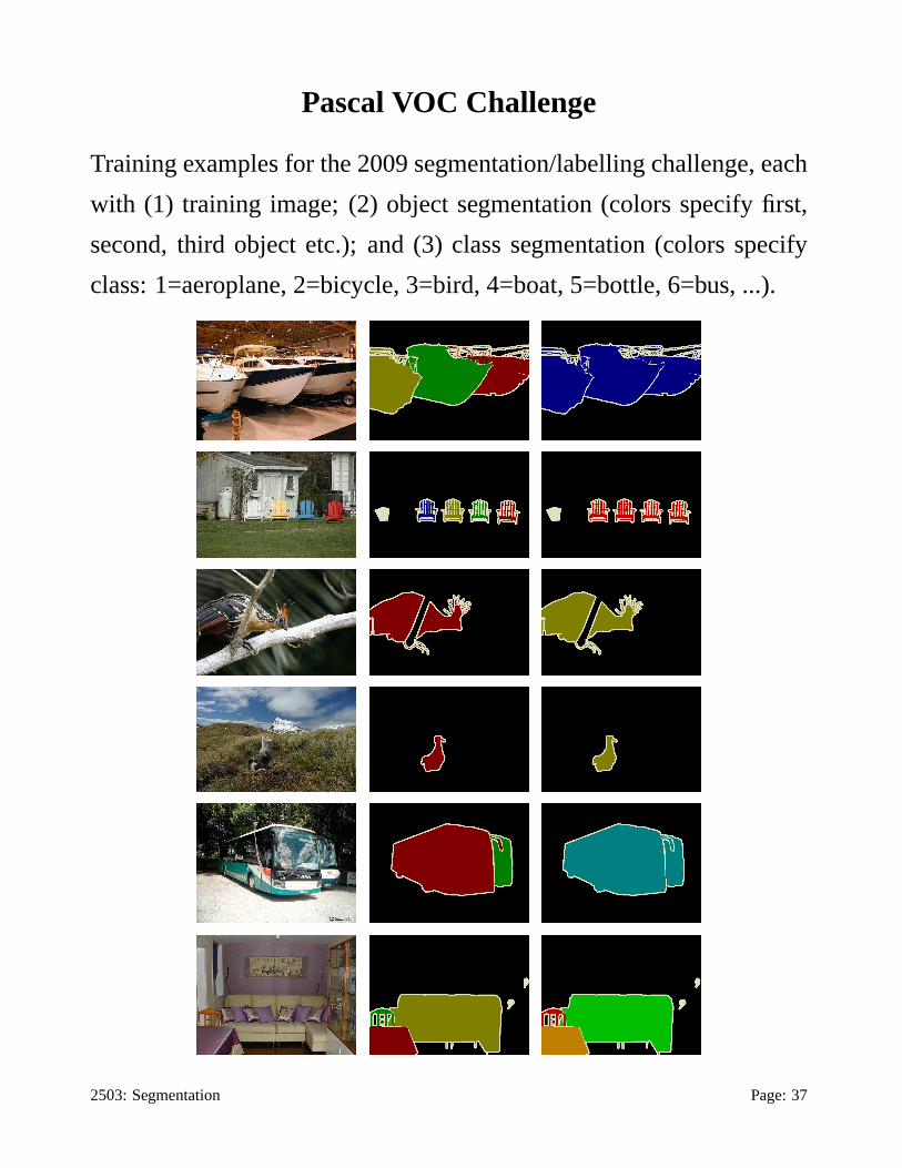
Pascal VOC Challenge
Training examples for the 2009 segmentation/labelling challenge, each
with (1) training image; (2) object segmentation (colors specify first,
second, third object etc.); and (3) class segmentation (colors specify
class: 1=aeroplane, 2=bicycle, 3=bird, 4=boat, 5=bottle, 6=bus, ...).
2503: Segmentation Page: 37
References
[1] P. Arbelaez, M. Maire, C. Fowlkes, and J. Malik. Contour detection and hierarchical image seg-mentation.IEEE Trans. PAMI, 33(5):898–916, 2011. Seehttp://www.eecs.berkeley.edu/Research/Projects/CS/vision/grouping/resources.html .
[2] Y. Boykov and V. Kolmogorov. An experimental comparison of min-cut/max-flow algorithmsfor energy minimization in vision.IEEE Trans. PAMI, 26(9):1124–1137, 2004.
[3] C. Carson, S. Belongie, H. Greenspan, and J. Malik. Blobworld: Image segmentation usingexpectation-maximization and its application to image querying. IEEE Trans. PAMI, 24(8):1026–1038, 2002.
[4] C. M. Christoudias, B. Georgescu, and P. Meer. Synergism in low level vision. InInternationalConference on Pattern Recognition., Quebec City, Canada, volume IV, pages 150–155, 2002.
[5] D. Comaniciu and P. Meer. Mean shift: A robust approach toward feature space analysis.IEEETrans. PAMI, 24:603–619, 2002.
[6] T. Cour, S. Yu, and J. Shi. Normalized cuts matlab code. Computer and Information Sci-ence, Penn State University. Code available athttp://www.cis.upenn.edu/ ˜ jshi/software/ .
[7] F.J. Estrada, A.D. Jepson, and C. Chennubhotla. Spectral embedding and min-cut for imagesegmentation. InBritish Machine Vision Conference, 2004.
[8] P.F. Felzenszwalb and D.P. Huttenlocher. Efficient graph-based image segmentation.IJCV,59(2):167–181, 2004.
[9] D. Martin and C. Fowlkes.The Berkeley Segmentation Dataset and Benchmark. 2007. http://www.cs.berkeley.edu/projects/vision/grouping/segbench/ .
[10] D. Martin, C. Fowlkes, D. Tal, and J. Malik. A database of human segmented natural imagesand its application to evaluating segmentation algorithmsand measuring ecological statistics. InIEEE ICCV, volume 2, pages 416–423, 2001.
[11] J. Shi, C. Fowlkes, D. Martin, and E. Sharon. Graph based image segmentation tutorial. IEEECVPR 2004.http://www.cis.upenn.edu/ ˜ jshi/GraphTutorial/ .
[12] J. Shi and J. Malik. Normalized cuts and image segmentation. IEEE Trans. PAMI, 22(8):888–905, 2000.
[13] S. Yu and J. Shi. Multiclass spectral clustering. InIEEE ICCV, 2003.
2503: Segmentation Notes: 38


