Impact of Different Interest Rate Models on Bond Value Measures

IT IS

ILLE

GAL

TO R

EPRODUCE T

HIS A

RTICLE

IN A

NY FO

RMAT

DECEMBER 2001 THE JOURNAL OF FIXED INCOME 41

In the last 10 to 15 years an increasingnumber of different interest rate modelshave become available. All are commonlyused to price bonds with embedded

options. The models have different features,which makes the choice of the correct modelconfusing for both practitioners and academi-cians alike. They often provide different val-ues for securities with contingent claimcharacteristics. Not surprisingly, then, theygenerate different sensitivity measures such aseffective duration (ED), effective convexity(EC), and option-adjusted spreads (OAS).

We document the differences and try toshed some light on their determinants—a phe-nomenon that has not been documented before.Interest rates are commonly modeled usingstochastic differential equations (SDEs). Themost common types of models are one-factorand two-factor interest rate models. One-factormodels use an SDE to represent the short-termrate, and two factor models use an SDE for boththe short-term rate and the long-term rate. TheSDEs chosen to model interest rates capturesome of the more desirable properties of inter-est rates such as mean reversion and/or a volatil-ity term that depends on the level of interest rates.

There are two distinct approaches toimplement the SDEs in a term structuremodel: equilibrium and no-arbitrage. Eachcan be used to value bonds and interest ratederivatives. Each approach starts with similarSDEs, but applies the SDE under a differentframework to price securities.

Equilibrium models start with an SDEmodel and develop pricing mechanisms forbonds under an equilibrium framework. Someof the most common models that use thisapproach are Vasicek [1977], Brennan andSchwartz [1979, 1982], Cox, Ingersoll, and Ross[1985], Longstaff [1989, 1992], and Longstaff andSchwartz [1992].

No-arbitrage models begin with thesame or similar SDE models, but use marketprices to generate an interest rate lattice. Thelattice produces an array of interest rates thatresult in prices of bonds that are the same asthose observed in the market and follow thebehavioral characteristics of the SDEs. Someof the most well-known models that use thisapproach are Ho and Lee [1986], Black, Der-man, and Toy [1990], Hull and White [1990,1993], Black and Karasinski [1991], and Heath,Jarrow, and Morton [1992].

No-arbitrage models are the preferredframework to value interest rate derivatives.This is because they minimally ensure that themarket prices for bonds are exact. Equilib-rium models do not price bonds exactly, whichcan have significant effects on the corre-sponding contingent claims.

Cheyette [1997] offers an excellentreview of how to select the appropriate model;he suggests that one must consider the char-acteristics of the security to be evaluated inorder to select the best model. Cheyette alsoillustrates empirically that some models maybetter capture actual interest rate dynamics, but

Impact of Different Interest Rate Models on Bond Value MeasuresGERALD W. BUETOW, JR., BERND HANKE, AND FRANK J. FABOZZI

GERALD W.BUETOW, JR.,is president of BFRCServices, LLC inCharlottesville, [email protected]

BERND HANKE

is a doctoral candidateat the London Business School, Institute of Financeand Accounting [email protected]

FRANK J. FABOZZI

is adjunct professor of finance, School of Management atYale University inNew Haven, [email protected]

Copyright © 2002 Institutional Investor, Inc. All Rights Reserved

Copyright @ Institutional Investor, Inc. All rights reserved.

he readily notes that the empirical evidence is far fromconclusive.

We examine differences in the effective duration,effective convexity, and the option-adjusted spread result-ing from different one-factor no-arbitrage interest ratemodels. The models considered are: the Ho and Lee(HL) [1986] model; the Kalotay, Williams, and Fabozzi(KWF) [1993] model; the Black, Derman, and Toy (BDT)[1990] model; the Hull and White (HW) [1994] model;and the Black and Karasinski (BK) [1991] model.1

I. NO-ARBITRAGE INTEREST RATE MODELS

The interest rate models we examine assume that theshort-term interest rate follows a certain process that canbe represented by a stochastic differential equation. All theinterest rate models are special cases of the general formof changes in the short-term rate:

(1)

where f and g are suitably chosen functions of the short-termrate and are the same for most models presented here, θ willbe shown to be the drift of the short-term rate, and ρ is themean reversion term to an equilibrium short-term rate. Theterm σ is the local volatility of the short-term rate, and zis a normally distributed Wiener process that captures therandomness of future changes in the short-term rate.

Equation (1) is a one-factor model that gives onlythe short-term rate (one factor).2 Its first component(the dt term) is the expected or average change in theshort-term rate over a short period of time. The secondcomponent is the risk term, as it includes the randomcomponent dz. All the interest rate models we considerare special cases of Equation (1).

The Ho-Lee Model

The Ho-Lee model assumes that changes in the short-term rate can be modeled using Equation (1) by setting f(r)= r and ρ = 0, so that the process for the short-term rate is:

(2)

Since dz is a normally distributed Wiener process,the HL process is a normal process for the short-term

��

��

rate. As can be seen from Equation (2), the short-termrate may become negative if the random term is largeenough to dominate the drift term (dt). This is a seri-ous shortcoming of the HL model, although it is arguedthat as long as the HL model provides good prices forbonds with embedded options, it does not matter ifsome of its assumptions are unrealistic. Another possi-ble drawback of the model, however, is that the volatil-ity of the short-term rate does not depend on the levelof the rate, and the short-term rate does not mean-revert to a long-term equilibrium rate, as many practi-tioners believe would hold in reality.

Some of these restrictive assumptions are relaxed inthe other models. Note that the distributional propertieswill have a tendency to bias the values of the embeddedcontingent claim.

The simplicity of the HL model combined with thefact that it provides reasonable prices under many cir-cumstances makes it a very popular interest rate model.

The Kalotay-Williams-Fabozzi Model

The Kalotay-Williams-Fabozzi model assumes thatchanges in the short-term rate can be modeled usingEquation (1) by setting f(r) = ln (r) (where ln is the nat-ural logarithm) and ρ = 0. Making these adjustments toEquation (1) produces the short-term rate process:

(3)

Comparing Equation (3) to Equation (2), it can beseen that the KWF model is directly analogous to the HLmodel, except that now the change in the natural log-arithm of the short-term rate is modeled instead of thechange in the short-term rate itself. Since ln(r) followsa normal process, r itself follows a lognormal process, andthe KWF model is therefore a lognormal interest ratemodel. Hence, although ln(r) may become negative if therisk component in Equation (3) dominates the driftcomponent, r itself will never be negative as r = e ln(r).Therefore, the KWF model eliminates the problem ofnegative short-term rates that can occur in the HLmodel.

The actual KWF model does not explicitly incor-porate the drift term. As a result, it does not always havea solution for the binomial tree.

While the KWF model is able to avoid negative short-term rates, it still does not capture mean reversion in theshort-term rate.

� ��

42 IMPACT OF DIFFERENT INTEREST RATE MODELS ON BOND VALUE MEASURES DECEMBER 2001


It is illegal to reproduce this article in any format. Email [email protected] for Reprints or Permissions.


The Black-Derman-Toy Model

One of the main advantages of the Black-Derman-Toy model is that it is a lognormal model that is able tocapture a realistic term structure of interest rate volatili-ties. To accomplish this feature, the short-term rate volatil-ity is allowed to vary over time, and the drift in interestrate movements depends on the level of rates.

While interest rate mean reversion is not modeledexplicitly, this property is introduced through the termstructure of volatilities. Hence, the extent to which thedrift term depends on the level of rates depends on thelocal volatility process. In other words, the mean rever-sion is endogenous to the model. Therefore, no additionaldegree of freedom is required for the mean reversionterm, and the BDT SDE can be relatively easily approx-imated using the binomial tree approach.

The BDT model is obtained from Equation (1) by set-ting f(r) = ln(r) and g(r) = ln(r). Therefore, the short-termrate in the BDT model follows the lognormal process:

(4)

The mean reversion term ρ(t) depends on theinterest rate local volatility as follows:

which gives

(5)

Comparing Equation (5) with Equation (3), weobserve that if the volatility term structure is flat so thatσ(t) is constant, then σ´(t) = 0 and ρ(t) = 0, so that theBDT model reduces to the KWF model. In this sense, theKWF model is a special case of the BDT for constant localvolatility. When the local volatility term structure isdecreasing, i.e., if σ´(t) < 0, the BDT model will exhibitmean reversion. If σ´(t) > 0, i.e., if the local volatility termstructure is increasing, the BDT model will not exhibitmean reversion. Hence, the mean reversion dependsentirely on the shape of the local volatility term structure.

While some researchers believe that the mean rever-sion in the BDT model will be more representative of the

� ��

�

��

��

��

��

�

��

� ��

market since it is endogenous to the model, others arguethat it might be more appropriate to model mean rever-sion independently of the volatility process. This can beaccomplished only in the framework of a binomial modelthrough the use of varying time steps (as in the Hull-White and Black-Karasinski binomial trees), which com-plicates both the numerical solution and the applicabilityof the model substantially.

The Hull-White Model

Similar to the Ho-Lee model, the Hull-White modelassumes a normal process for the short-term rate. The modelcan be obtained from Equation (1) by setting f(r) = g(r) = rand ρ = –φ. The process for the short-term rate is thus:

(6)

where θ is the long-term equilibrium mean rate, and φis the mean reversion term. Note that if φ = 0, the HWprocess reduces to the HL process. The HL model istherefore a special case of the HW model when there isno mean reversion.

The HW model explicitly models mean reversionby specifying a central tendency for the short-term rateand by specifying the speed at which the short-term ratereverts to that central tendency. The mean reversion coef-ficient allows correction for uncontrolled growth ordecline in the HW model. The coefficient thereforereduces the probability of negative interest rates, althoughit does not completely rule out negative interest rates,which makes the HW model subject to the same criti-cism as the HL model.

Since mean reversion is modeled explicitly, solvingthe HW SDE numerically using a binomial tree is com-plicated by the fact that an additional degree of freedomis required. In a binomial framework, this additionaldegree of freedom can be obtained only by using time stepsof varying length, which complicates the analysis. Alter-natively, a trinomial lattice may be used for the numeri-cal solution, which is the approach we follow.

The Black-Karasinski Model

In order to obtain the Black-Karasinski short-termrate process we set f (r) = ln(r), ρ = –φ, and g(r) = ln(r) inEquation (1), which results in the short-term rate process:

��





(7)

Inspection shows that the BK model is simply thelogarithmic analogue to the HW model. In the BK model,ln(r) has the same properties as r in the HW model. As inthe KWF model, however, r cannot become negativebecause r = e ln(r), which is always positive. This is the advan-tage of the BK model over the HW model.

Therefore, we see that the BK model is an exten-sion of the KWF process in the same way as the HW pro-cess is an extension of the HL process. In fact, as φ = 0,the KWF model is obtained.

The BK model explicitly models mean reversion byspecifying a central tendency for the short-term rate andthe speed at which the short-term rate reverts to that cen-tral tendency. Like the HW model, which also includesa mean reversion term, the BK SDE is solved numeri-cally in the most straightforward way by using a trino-mial tree approach.

II. NUMERICAL SOLUTION OF INTEREST RATE MODELS

The models may be solved numerically by eitherbinomial or trinomial methods.

Binomial SDE Approximations

The binomial method models the short-term ratein a geometrically analogous manner as equities in Cox,Ross, and Rubinstein [1979]. That is, the short-termrate for the next period can have only one of two possi-ble values, ru or rd where ru > rd. Continuing in this man-ner for a number of future time periods results in abinomial tree whose number of nodes increases by twonodes for each time step. As a result, the number of nodesquickly increases over time.

To reduce the number of nodes for computationaltractability, a restriction is imposed on the algorithm,namely, the recombination condition, which forces an upmove followed by a down move to result in the same futureinterest rate as a down move followed by an up move. Thismakes the binomial method more computationallytractable since the number of nodes at each time stepincreases by only one node.

An up move in the short-term interest rate has aprobability q, so the corresponding down move has aprobability of 1 – q. We use q = 0.5. It should be notedthat setting the up and down probabilities to 0.5 is merely

� �� an artificial device to ensure risk-neutrality in solution ofthe short-term rate SDEs. It by no means implies that theactual probability for an interest rate increase or decreaseis equal to 0.5.3

Trinomial SDE Approximations

The trinomial method is similar in spirit to thebinomial tree, except that there are three possible statesinstead of two. From each time we call the upward movethe up move, the downward move the down move, andthe center move the middle move. Again, we have to makesure that the interest rate lattice possesses the recombina-tion property in order for it to be computationallytractable. From any node in the trinomial lattice an upmove followed by a down move will get to the same nodeas two successive middle moves and as a down move fol-lowed by an up move. This ensures that the number ofnodes in the trinomial lattice increases by only two nodesat each time step.

For the probabilities of an up move, middle move,and down move, we solve both the HW model and theBK model using the Hull and White method (HW ver-sion). In each of the two versions the probabilities for anup move, middle move, and down move are given by q1,q2, and q3 with q1 + q2 + q3 = 1.

The Hull and White methodology for generatingHW and BK trinomial lattices lets the probabilities dependon the mean-reversion term. In order to assure positiveprobabilities, Hull and White truncate the upper andlower branches of their lattice at a certain maximum andminimum. Below the minimum and above the maxi-mum, they apply a new branching procedure with dif-ferent probabilities.

III. EFFECTIVE DURATION, EFFECTIVECONVEXITY, AND OPTION-ADJUSTED SPREAD

Modified duration measures the percentage bondprice change from an absolute yield change. It can alsobe interpreted as the negative of the slope (first deriva-tive) of the price-yield relationship divided by the price.Similarly, convexity is interpreted as the curvature of theprice-yield relationship (i.e., the second derivative).

Since modified duration and convexity do not con-sider that the cash flows for a bond with an embedded optionmay change due to exercise of the option, they do not pro-vide satisfactory results for bonds with embedded options.Effective duration and convexity do take into consideration





how changes in interest rates in the future may alter the cashflows due to exercise of an embedded option.

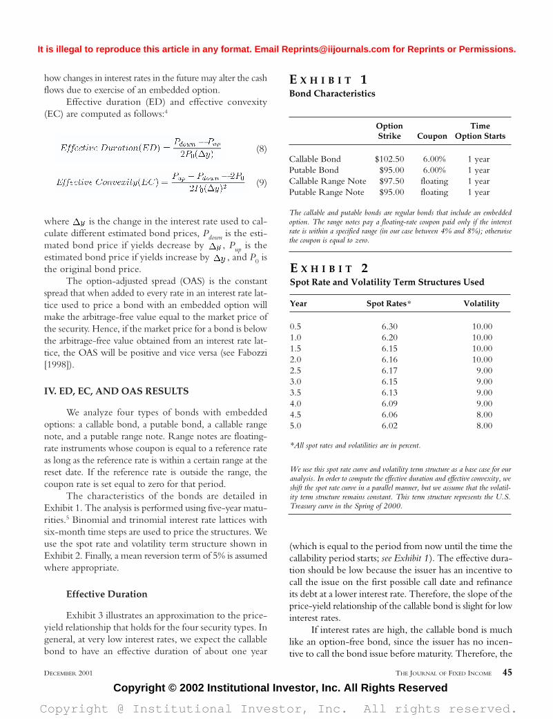
Effective duration (ED) and effective convexity(EC) are computed as follows:4

(8)

(9)

where is the change in the interest rate used to cal-culate different estimated bond prices, Pdown is the esti-mated bond price if yields decrease by , Pup is theestimated bond price if yields increase by , and P0 isthe original bond price.

The option-adjusted spread (OAS) is the constantspread that when added to every rate in an interest rate lat-tice used to price a bond with an embedded option willmake the arbitrage-free value equal to the market price ofthe security. Hence, if the market price for a bond is belowthe arbitrage-free value obtained from an interest rate lat-tice, the OAS will be positive and vice versa (see Fabozzi[1998]).

IV. ED, EC, AND OAS RESULTS

We analyze four types of bonds with embeddedoptions: a callable bond, a putable bond, a callable rangenote, and a putable range note. Range notes are floating-rate instruments whose coupon is equal to a reference rateas long as the reference rate is within a certain range at thereset date. If the reference rate is outside the range, thecoupon rate is set equal to zero for that period.

The characteristics of the bonds are detailed inExhibit 1. The analysis is performed using five-year matu-rities.5 Binomial and trinomial interest rate lattices withsix-month time steps are used to price the structures. Weuse the spot rate and volatility term structure shown inExhibit 2. Finally, a mean reversion term of 5% is assumedwhere appropriate.

Effective Duration

Exhibit 3 illustrates an approximation to the price-yield relationship that holds for the four security types. Ingeneral, at very low interest rates, we expect the callablebond to have an effective duration of about one year

��

��

��

(which is equal to the period from now until the time thecallability period starts; see Exhibit 1). The effective dura-tion should be low because the issuer has an incentive tocall the issue on the first possible call date and refinanceits debt at a lower interest rate. Therefore, the slope of theprice-yield relationship of the callable bond is slight for lowinterest rates.

If interest rates are high, the callable bond is muchlike an option-free bond, since the issuer has no incen-tive to call the bond issue before maturity. Therefore, the


E X H I B I T 1Bond Characteristics

Option TimeStrike Coupon Option Starts

Callable Bond $102.50 6.00% 1 year Putable Bond $95.00 6.00% 1 year Callable Range Note $97.50 floating 1 year Putable Range Note $95.00 floating 1 year

The callable and putable bonds are regular bonds that include an embeddedoption. The range notes pay a floating-rate coupon paid only if the interestrate is within a specified range (in our case between 4% and 8%); otherwisethe coupon is equal to zero.

E X H I B I T 2Spot Rate and Volatility Term Structures Used

Year Spot Rates* Volatility

0.5 6.30 10.001.0 6.20 10.001.5 6.15 10.002.0 6.16 10.002.5 6.17 9.003.0 6.15 9.003.5 6.13 9.004.0 6.09 9.004.5 6.06 8.005.0 6.02 8.00

*All spot rates and volatilities are in percent.

We use this spot rate curve and volatility term structure as a base case for ouranalysis. In order to compute the effective duration and effective convexity, weshift the spot rate curve in a parallel manner, but we assume that the volatil-ity term structure remains constant. This term structure represents the U.S.Treasury curve in the Spring of 2000.




effective duration in a high interest rate environment isapproximately equal to the effective duration of a corre-sponding option-free bond.

Exhibit 3 shows that the slopes for the option-freebond and the callable bond are approximately the samefor high interest rates and diverge at low interest rates.

Employing similar intuition, the opposite should holdfor a putable bond. If interest rates are low, bondholders haveno incentive to redeem the bond before maturity. There-fore, the effective duration of the putable bond will beapproximately the same as the effective duration of a corre-sponding option-free bond in a low interest rate environ-

ment (the slopes of the price-yield relation-ships for the two bonds are equal in Exhibit 3for low interest rates).

At high interest rates, bondholders willredeem the bond early because they are ableto get a higher return on an alternative invest-ment. So the effective duration of the putablebond should be low at high interest rates, i.e.,about one year in our case (since the bond canbe redeemed only after one year from now).As Exhibit 3 illustrates, for high interest ratesthe putable bond price has a lower boundbecause of the putability. Therefore, the slopeof the price-yield relationship is less steep thanfor a corresponding option-free bond.

Exhibit 3 shows that the slopes for theoption-free bond and the putable bond areapproximately the same for low interest ratesand diverge at high interest rates.

For the range notes, this relationship ismore complicated. The range note graph inExhibit 3 includes the price-yield curve forthe corresponding zero-coupon callable andputable bonds with the same strike pricesand the same callability periods. The rangenotes differ from these zero-coupon bondsonly in that they pay a floating-rate couponwhenever the interest rate is between thelower and the upper interest rate limits of 4%and 8%. When the interest rate is outsidethis range, the coupon is set equal to zero.

As a result, the callable range note mustbe worth the same or more than the corre-sponding zero-coupon callable bond, and theputable range note must be worth the same ormore than the corresponding zero-couponputable bond. Consequently, the duration pat-tern of the range notes at different interest rate

levels differs from that for the corresponding zero-couponbonds only when the interest rate is within the range wherea floating-rate coupon is paid. The durations of the rangenotes are similar to the durations of the correspondingzero-coupon bonds when interest rates are substantiallyoutside this range.

In general, there are two interest rate effects forrange notes that work in the same direction at very highinterest rates and in the opposite direction at very lowinterest rates. If interest rates are very high, the range notes’redemption value is discounted at a higher interest rate,


E X H I B I T 3Price-Yield Relationships

The two graphs illustrate the pricing behavior over a spectrum of yields for the regular callable andputable bond and the callable and putable range note. The purpose of the two graphs is to providea general intuition for the ED and EC pattern over different yield levels, i.e. for the original termstructure provided in Exhibit 2 and the parallel shifts of ±250 bp and ±500 bp. In addition tothe regular callable and putable bond, the first graph shows the price-yield relationship for an option-free bond with the same characteristics. The second graph shows the price-yield curve for a callablezero-coupon bond as well as a putable zero-coupon bond, both with the same characteristics as thecorresponding range notes. These two securities are shown for reference only, because they providea lower bound for the callable and the putable range note prices.

8 0

9 0

1 0 0

1 1 0

1 2 0

- 5 0 0 b p - 2 5 0 b p Original +2 5 0 b p +5 0 0 b p

Yield Term Structures

Option-Free Bond Callable Bond Putable Bond

5 5

6 5

7 5

8 5

9 5

- 5 0 0 b p - 2 5 0 b p Original +2 5 0 b p +5 0 0 b p

Yield Term Structures

Callable Range Note Putable Range Note

Callable Bond Putable Bond

Pric

ePr

ice




and therefore its present value will be low. If interest ratesare high enough so that they exceed the upper limit ofthe interest rate range (8% in our example), then bond-holders will receive no coupon. Both effects depress therange note value to the bondholder, and there is noincentive to redeem the putable range note. Similarly, theissuer has no incentive to call the callable range notebefore maturity under such a scenario.

When interest rates are low, however, the two inter-est rate effects work in the opposite direction. On the onehand, the redemption value is discounted at a lower rate,and therefore its present value is high. On the other hand,the interest rate might fall below the lower limit of theinterest rate range (4% in our case) so the range note hasa zero coupon. For the issuer, this provides cheap financ-ing, so there is no incentive to call the callable range noteas long as the coupon is equal to zero. The range noteholder may have a strong incentive to redeem the putablerange note before maturity under such a scenario.

These characteristics will have a significant influenceon the effective duration of the range notes. At very highinterest rates, the effective duration of the callable range notewill be high, and the effective duration of the putable rangenote will be very low. At very low interest rates, the effec-tive duration will be high for the callable range note andlow for the putable range note. This is seen in Exhibit 3.

The slope of the price-yield relationship is high inabsolute value for the callable range note in high interest rateenvironments, and it is low in absolute value for the putablerange note. The same pattern holds for low interest rates.Here, the slope is relatively high in absolute value for thecallable range note and low for the putable range note.

The range notes exhibit this peculiarly non-mono-tonic price-yield relationship because of the imposedboundary conditions from the interest rate ranges. Forexample, if interest rates increase from below the lowerlimit of the range (where the coupon is zero) to a rate thatis within the range (so that the coupon jumps from zeroto the floating rate level), the value of the range note toits holder increases. Under this scenario, the range noteprice increases if the interest rate rises, for both the callableand the putable range note.

This pattern is a result of the note becoming acoupon-paying security, and this has more influence overthe value of the note than the lower discount factors.Therefore, the coupon effect dominates the present valueeffect so that the range note value increases and the effec-tive duration will be negative near the lower limit of theinterest rate range.

Exhibit 3 illustrates this phenomenon through thepositively sloped price-yield relationship, indicating anegative effective duration. The value of the range notethen reaches a maximum somewhere between the lowerand the upper limit of the interest rate range. Beyond thisinterest rate level, the value decreases again with increas-ing interest rates.

The range note price sensitivity to interest ratechanges is especially high close to the upper limit of theinterest rate range (here 8%), since the coupon jumps fromthe floating-rate level to zero above the upper limit. Thepresent value effect of higher interest rates further depressesthe range note value, so the effective duration is relativelyhigh close to the upper interest rate limit (especially forthe callable range note). This can be seen in Exhibit 3.The slope of the price-yield relationship is relatively highin absolute value close to the upper interest rate limit.

Exhibit 4 shows the effective duration results for theHL, the KWF, and the BDT models. We computed theeffective duration for the original term structures shownin Exhibit 2 using a yield change of 50 basis points.The results are no different for any yield change of lessthan 100 bp. We then shift the original term structure upand down in a parallel manner by ±250 basis points andby ±500 basis points.

The KWF and the BDT effective duration esti-mates are very similar, while the HL model sometimesproduces substantially different estimates. This is to beexpected; the HL model is a normal interest rate model,while the KWF and BDT models are lognormal interestrate models.

While the KWF model does not incorporate inter-est rate mean-reversion, the BDT model includes animplicit mean reversion term introduced through the termstructure of local volatilities. The differences in their effec-tive duration estimates are relatively minor, especially forthe more extreme interest rate term structures. Therefore,the impact of the implicit mean-reversion term on theeffective duration estimate in the BDT model is minor.

For the HL model, the effective duration does notvary much with the level of interest rates. The HL modelproduces ED estimates that are not as representative of theprice-yield properties as the estimates resulting from thelognormal models. For example, when interest rates areextremely low, as in the first column of Exhibit 4 (–500bp), the callable bond should have a very short effectiveduration. In fact, the one-year delayed call should dictatean effective duration close to 1.0. The KWF and BDTmodels are in line with this estimate, but the HL model

��





produces an effective duration estimate of more than twoyears (more than a 100% difference). The same is true forthe HL model estimate for the putable bond in an envi-ronment of extremely high interest rates.

Since our HL model does not truncate the returnsat zero, the results in Exhibit 4 should not be surprising.At the very low interest rates (i.e., –500 bp and –250 bp),the HL model will have a large number of negative ratesin the lattice. Combine this with the hyperbolic nature ofvalue with respect to the discount rate, and the higher EDvalues are easily explained. Small changes in rates ( )will produce greater price differentials for the HL modelthan any of the other models, which results in higher EDvalues. If we were to truncate the values at zero, this resultwould be reduced somewhat.6

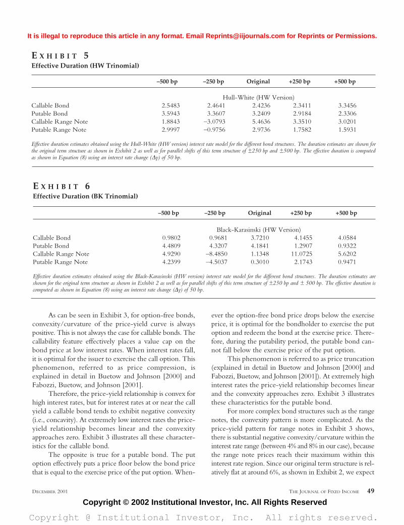
Exhibits 5 and 6 present the effective duration estimatesproduced by the trinomial versions of the HW and BK mod-els. As we have noted, both the HW and the BK modelsare able to explicitly incorporate mean reversion. Recall thatthe HW model is a normal interest rate model and the BKmodel is a lognormal interest rate model. In this sense, we

��

can make a similar comparison between normal and log-normal models as we do in explaining Exhibit 4.

The HW model, as a normal model, produces effec-tive duration estimates that vary less with interest rate lev-els than the BK effective duration estimates. As for the HLmodel, the HW model produces an effective duration esti-mate for the callable bond that is high at very low interestrates and low at very high interest rates. The reverse is truefor the putable bond. The BK effective duration estimatesare more variable for different interest rate levels and seemto be more in line with theoretical reasoning.

A comparison of Exhibits 5 and 6 shows that theduration estimates for the two models can be substantiallydifferent, especially for more complex securities such asthe range notes.

Effective Convexity

Effective convexity (EC) is an approximation to thesecond derivative (the curvature) of the price-yield rela-tionship while taking the embedded option into account.


E X H I B I T 4Effective Duration (Binomial)

–500 bp –250 bp Original +250 bp +500 bp

Ho-LeeCallable Bond 2.1843 2.5365 2.4526 2.5544 3.0556 Putable Bond 3.4528 3.2383 2.8964 2.7253 2.4569 Callable Range Note 4.3656 –1.7185 2.2345 4.2559 2.7632Putable Range Note 4.4676 –0.0342 1.9460 1.9601 0.6527

Kalotay-Williams-FabozziCallable Bond 0.9802 0.9680 3.6940 4.1764 4.0875Putable Bond 4.4452 4.3552 4.1643 1.4121 0.9322 Callable Range Note 4.4769 –7.3821 1.9101 12.1257 6.0632Putable Range Note 4.2303 –3.8566 0.5662 3.3333 0.9470

Black-Derman-ToyCallable Bond 0.9802 0.9680 3.8620 4.1765 4.0875 Putable Bond 4.4453 4.3552 4.2656 1.2215 0.9322Callable Range Note 4.4768 –7.5520 1.1107 13.9608 5.7683Putable Range Note 4.2419 –3.5625 0.5573 3.6847 0.9470

Effective duration estimates obtained using the Ho-Lee, Kalotay-Williams-Fabozzi, and the Black-Derman-Toy interest rate models for the different bond struc-tures. The duration estimates are shown for the original term structure as shown in Exhibit 2 as well as for parallel shifts of this term structure of ±250 and ±500bp. The effective duration is computed as shown in Equation (8) using an interest rate change (∆y) of 50 bp.




As can be seen in Exhibit 3, for option-free bonds,convexity/curvature of the price-yield curve is alwayspositive. This is not always the case for callable bonds. Thecallability feature effectively places a value cap on thebond price at low interest rates. When interest rates fall,it is optimal for the issuer to exercise the call option. Thisphenomenon, referred to as price compression, isexplained in detail in Buetow and Johnson [2000] andFabozzi, Buetow, and Johnson [2001].

Therefore, the price-yield relationship is convex forhigh interest rates, but for interest rates at or near the callyield a callable bond tends to exhibit negative convexity(i.e., concavity). At extremely low interest rates the price-yield relationship becomes linear and the convexityapproaches zero. Exhibit 3 illustrates all these character-istics for the callable bond.

The opposite is true for a putable bond. The putoption effectively puts a price floor below the bond pricethat is equal to the exercise price of the put option. When-

ever the option-free bond price drops below the exerciseprice, it is optimal for the bondholder to exercise the putoption and redeem the bond at the exercise price. There-fore, during the putability period, the putable bond can-not fall below the exercise price of the put option.

This phenomenon is referred to as price truncation(explained in detail in Buetow and Johnson [2000] andFabozzi, Buetow, and Johnson [2001]). At extremely highinterest rates the price-yield relationship becomes linearand the convexity approaches zero. Exhibit 3 illustratesthese characteristics for the putable bond.

For more complex bond structures such as the rangenotes, the convexity pattern is more complicated. As theprice-yield pattern for range notes in Exhibit 3 shows,there is substantial negative convexity/curvature within theinterest rate range (between 4% and 8% in our case), becausethe range note prices reach their maximum within thisinterest rate region. Since our original term structure is rel-atively flat at around 6%, as shown in Exhibit 2, we expect


E X H I B I T 5Effective Duration (HW Trinomial)


Hull-White (HW Version)Callable Bond 2.5483 2.4641 2.4236 2.3411 3.3456Putable Bond 3.5943 3.3607 3.2409 2.9184 2.3306Callable Range Note 1.8843 –3.0793 5.4636 3.3510 3.0201Putable Range Note 2.9997 –0.9756 2.9736 1.7582 1.5931

Effective duration estimates obtained using the Hull-White (HW version) interest rate model for the different bond structures. The duration estimates are shown forthe original term structure as shown in Exhibit 2 as well as for parallel shifts of this term structure of ±250 bp and ±500 bp. The effective duration is computedas shown in Equation (8) using an interest rate change (∆y) of 50 bp.

E X H I B I T 6Effective Duration (BK Trinomial)


Black-Karasinski (HW Version)Callable Bond 0.9802 0.9681 3.7210 4.1455 4.0584Putable Bond 4.4809 4.3207 4.1841 1.2907 0.9322 Callable Range Note 4.9290 –8.4850 1.1348 11.0725 5.6202Putable Range Note 4.2399 –4.5037 0.3010 2.1743 0.9471

Effective duration estimates obtained using the Black-Karasinski (HW version) interest rate model for the different bond structures. The duration estimates areshown for the original term structure as shown in Exhibit 2 as well as for parallel shifts of this term structure of ±250 bp and ± 500 bp. The effective duration iscomputed as shown in Equation (8) using an interest rate change (∆y) of 50 bp.




the curvature/convexity of the price-yield relationship inExhibit 3 to be negative around the original term structure.

Exhibit 3 shows that the prices of the callable andputable range notes have a lower bound that is equal to theprice of the corresponding zero-coupon callable or putablebond, respectively. As can be seen in the graph, the price-yield curves of the range notes approach their lower boundsasymptotically for interest rates that are substantially belowor above their coupon interest rate range. As a result, theconcavity within the coupon interest rate range has to beoffset by higher (positive) convexity above and below theconcavity range in order for the range note price-yieldcurves to converge to their lower bounds. This pattern isillustrated in the second graph of Exhibit 3.

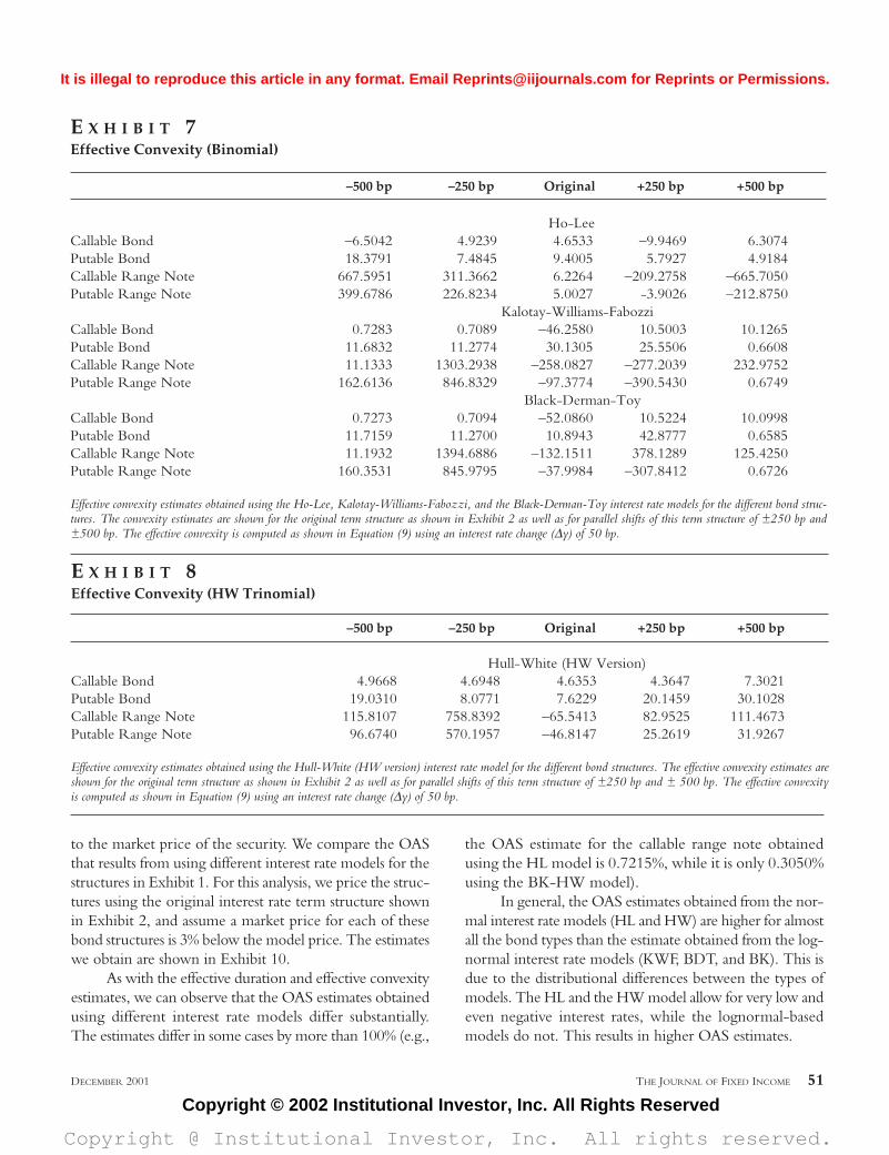
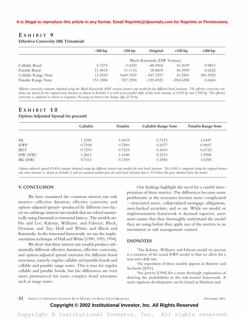
Exhibit 7 shows the EC estimates resulting from theHL, KWF, and BDT models. Exhibit 8 shows the EC esti-mates produced by the HW (HW version) model. TheEC estimates for the BK (HW version) models are shownin Exhibit 9.

For the callable bond, once again the three lognor-mal models (KWF, BDT, and BK) show a distinctive ECpattern. The EC tends to be relatively high and positivefor high interest rates; it then turns into concavity formedium interest rates and is fairly linear for low interestrates (i.e., the EC is close to zero). Therefore, the possi-bility that the callable bond might be called if interest ratesdrop is already anticipated at medium interest rates (forthe original term structure), and the EC therefore becomesnegative (i.e., concave) at this interest rate level.

The HL model (as a normal interest rate model)shows a somewhat different EC pattern with concavity athigh interest rates (+250 bp) and very low interest rates(–500 bp). It suffers from EC estimates that do not matchthe necessary pricing behavior.

EC estimates for putable bonds are all positive asrequired by the pricing behavior. Most normal interest ratemodels tend to produce EC estimates that are relativelyhigh at all interest rate levels. The lognormal models pro-duce EC patterns that are more representative of the pric-ing behavior. The EC is generally highest for intermediateinterest rate levels, but in all cases becomes close to zero(i.e., a linear relationship between yields and bond prices)for very high interest rates, which again is due to theputability at high interest rates.

The EC pattern for range notes is substantially morevolatile than for regular callable and putable bonds. Thisis due to the boundary effects of the interest rate range(4% and 8% in our case) that determine the amount of thecoupon and whether a coupon will be paid or not.

At low interest rates, we expect positive convexity(–500 bp and –250 bp). Convexity should be highestaround the level of the lower interest rate range limit,which coincides approximately with our –250 bp shift.Our results in Exhibits 7, 8, and 9 confirm this expecta-tion, especially for the callable range note.

It is interesting to observe that in all cases the log-normal models produce a significantly higher convexity atthis interest rate level than the normal interest rate models.For the callable range note, the convexity estimate rangesbetween 311.37 (HL) and 1669.74 (BK-HW version).

The range notes achieve their price maximumwithin the interest rate range between 4% and 8%. There-fore, we expect the price-yield curve to be concave withinmost of this region, which is confirmed by most of ourresults. Here again, this pattern is more pronounced forthe lognormal models than for the normal interest ratemodels. Beyond the maximum range note price, theprice-yield curve returns to its lower bound—the corre-sponding callable or putable zero-coupon bond—forhigher interest rates. Therefore, concavity should turn intoconvexity for higher rate levels.

There are substantial differences among the interestrate models, however. The HL model, for example, stillshows a concave price-yield relationship for the +500 bpterm structure shift for both the callable and the putablerange note, while the BDT and BK (HW) models gen-erate price-yield relationships that quickly revert to con-vexity for the callable range note and seem to produceresults that are most consistent with the pricing behavior.For high interest rates, there is no clearly distinguishablepattern between normal and lognormal interest rate mod-els as was the case for lower interest rate levels.

In general, Exhibits 7, 8, and 9 illustrate that theextent of the convexity estimates is strongly influenced bythe interest rate model used. Differences can be signifi-cant. In some cases, different interest rate models yield con-vexity estimates for the same bond that are of large absolutevalue but opposite sign. This is true not only for morecomplex structures such as the range notes that we exam-ine but also for the regular bonds with embedded options.The BDT and the BK (HW) models seem to generate esti-mates that are consistent with the pricing behavior.

Option-Adjusted Spread

The option-adjusted spread (OAS) is the constantspread that when added to every rate in an interest rate lat-tice used to price a security will make the model price equal





to the market price of the security. We compare the OASthat results from using different interest rate models for thestructures in Exhibit 1. For this analysis, we price the struc-tures using the original interest rate term structure shownin Exhibit 2, and assume a market price for each of thesebond structures is 3% below the model price. The estimateswe obtain are shown in Exhibit 10.

As with the effective duration and effective convexityestimates, we can observe that the OAS estimates obtainedusing different interest rate models differ substantially.The estimates differ in some cases by more than 100% (e.g.,

the OAS estimate for the callable range note obtainedusing the HL model is 0.7215%, while it is only 0.3050%using the BK-HW model).

In general, the OAS estimates obtained from the nor-mal interest rate models (HL and HW) are higher for almostall the bond types than the estimate obtained from the log-normal interest rate models (KWF, BDT, and BK). This isdue to the distributional differences between the types ofmodels. The HL and the HW model allow for very low andeven negative interest rates, while the lognormal-basedmodels do not. This results in higher OAS estimates.


E X H I B I T 7Effective Convexity (Binomial)


Ho-LeeCallable Bond –6.5042 4.9239 4.6533 –9.9469 6.3074Putable Bond 18.3791 7.4845 9.4005 5.7927 4.9184Callable Range Note 667.5951 311.3662 6.2264 –209.2758 –665.7050Putable Range Note 399.6786 226.8234 5.0027 -3.9026 –212.8750

Kalotay-Williams-FabozziCallable Bond 0.7283 0.7089 –46.2580 10.5003 10.1265Putable Bond 11.6832 11.2774 30.1305 25.5506 0.6608Callable Range Note 11.1333 1303.2938 –258.0827 –277.2039 232.9752Putable Range Note 162.6136 846.8329 –97.3774 –390.5430 0.6749

Black-Derman-ToyCallable Bond 0.7273 0.7094 –52.0860 10.5224 10.0998Putable Bond 11.7159 11.2700 10.8943 42.8777 0.6585Callable Range Note 11.1932 1394.6886 –132.1511 378.1289 125.4250Putable Range Note 160.3531 845.9795 –37.9984 –307.8412 0.6726

Effective convexity estimates obtained using the Ho-Lee, Kalotay-Williams-Fabozzi, and the Black-Derman-Toy interest rate models for the different bond struc-tures. The convexity estimates are shown for the original term structure as shown in Exhibit 2 as well as for parallel shifts of this term structure of ±250 bp and±500 bp. The effective convexity is computed as shown in Equation (9) using an interest rate change (∆y) of 50 bp.

E X H I B I T 8Effective Convexity (HW Trinomial)


Hull-White (HW Version)Callable Bond 4.9668 4.6948 4.6353 4.3647 7.3021Putable Bond 19.0310 8.0771 7.6229 20.1459 30.1028Callable Range Note 115.8107 758.8392 –65.5413 82.9525 111.4673Putable Range Note 96.6740 570.1957 –46.8147 25.2619 31.9267

Effective convexity estimates obtained using the Hull-White (HW version) interest rate model for the different bond structures. The effective convexity estimates areshown for the original term structure as shown in Exhibit 2 as well as for parallel shifts of this term structure of ±250 bp and ± 500 bp. The effective convexityis computed as shown in Equation (9) using an interest rate change (∆y) of 50 bp.




V. CONCLUSION

We have examined the common interest rate riskmetrics—effective duration, effective convexity, andoption-adjusted spread—produced by different one-fac-tor no-arbitrage interest rate models that are solved numer-ically using binomial or trinomial lattices. The models are:Ho and Lee; Kalotay, Williams, and Fabozzi; Black,Derman, and Toy; Hull and White; and Black andKarasinski. In the trinomial framework, we use the imple-mentation technique of Hull and White [1990, 1993, 1994].

We show that these interest rate models produce sub-stantially different effective duration, effective convexity,and option-adjusted spread estimates for different bondstructures, namely, regular callable and putable bonds andcallable and putable range notes. This is true for regularcallable and putable bonds, but the differences are evenmore pronounced for more complex bond structuressuch as range notes.

Our findings highlight the need for a careful inter-pretation of these metrics. The differences become moreproblematic as the structures become more complicated—structured notes, collateralized mortgage obligations,asset-backed securities, and so on. While no model orimplementation framework is deemed superior, usersmust ensure that they thoroughly understand the modelthey are using before they apply any of the metrics in aninvestment or risk management context.

ENDNOTES

1The Kalotay, Williams, and Fabozzi model we presentis a variation of the actual KWF model in that we allow for anon-zero drift rate.

2An exposition of these models appears in Buetow andSochacki [2001].

3See Jarrow [1996] for a more thorough explanation ofderiving the probabilities in the risk-neutral framework. Amore rigorous development can be found in Harrison and


E X H I B I T 9Effective Convexity (BK Trinomial)


Black-Karasinski (HW Version)Callable Bond 0.7575 0.6920 –48.5904 10.3039 9.9813Putable Bond 11.4815 11.1116 18.8605 45.3959 0.6522Callable Range Note 13.3549 1669.7437 –247.1297 10.2581 200.2952Putable Range Note 151.1884 937.3596 –120.4923 –204.6208 0.6660

Effective convexity estimates obtained using the Black-Karasinski (HW version) interest rate model for the different bond structures. The effective convexity esti-mates are shown for the original term structure as shown in Exhibit 2 as well as for parallel shifts of this term structure of ±250 bp and ±500 bp. The effectiveconvexity is computed as shown in Equation (9) using an interest rate change (∆y) of 50 bp.

E X H I B I T 1 0Option-Adjusted Spread (in percent)

Callable Putable Callable Range Note Putable Range Note

HL 1.2350 1.0619 0.7215 1.0447KWF 0.7598 0.7509 0.5077 0.9697BDT 0.7270 0.7219 0.3610 0.6732HW (HW) 1.2661 1.0186 0.5219 1.5998BK (HW) 0.7413 0.7359 0.3050 1.0255

Option-adjusted spread (OAS) estimate obtained using the different interest rate models for each bond structure. The OAS is computed using the original interestrate term structure as shown in Exhibit 2 and an assumed market price for each bond structure that is 3% below the price obtained from the model.




Kreps [1979] and Harrison and Pliska [1981]. A q = 0.5 alsoensures that the moments of the distribution are matched.

4This is illustrated in Buetow and Johnson [2000] and inFabozzi, Buetow, and Johnson [2001].

5Results for the ten-year maturities are available atwww.bfrcservices.com.

6The effective duration results for the truncated HL modelare as follows for the original term structure: Callable bond =2.2980, putable bond = 1.4166, callable range note = 1.7095,putable range note = 0.4263. In general, the ED estimate for thecallable bond is mainly a function of the call option delay (oneyear in our example). If there is no delay, the callable price can-not exceed the call price at any time, and the ED should be lowfor all models. As the delay increases, the HL ED estimate willbe even higher.

REFERENCES

Black, F., E. Derman, and W. Toy. “A One-Factor Model ofInterest Rates and its Application to Treasury Bond Options.”Financial Analysts Journal, January/February 1990, pp. 33-39.

Black, F., and P. Karasinski. “Bond and Option Pricing whenShort-Term Rates are Lognormal.” Financial Analysts Journal,July/August 1991, pp. 52-59.

Brennan, M. and E. Schwartz. “A Continuous Time Approachto the Pricing of Bonds.” Journal of Banking and Finance, 3(1979), pp. 133-155.

——. “An Equilibrium Model of Bond Pricing and a Test ofMarket Efficiency.” Journal of Financial and Quantitative Analy-sis, 17 (1982), pp. 301-329.

Buetow, G.W., and R. Johnson. “A Primer on Effective Dura-tion and Effective Convexity.” In F.J. Fabozzi, ed., ProfessionalPerspectives on Fixed Income Portfolio Management, Volume 1.New Hope, PA: Frank J. Fabozzi Associates, 2000.

Buetow, G.W., and J. Sochacki. “No-Arbitrage BinomialModels.” AIMR Research Foundation, 2001.

Cheyette, O. “Interest Rate Models.” In F.J. Fabozzi, ed.,Advances in Fixed Income Valuation Modeling and Risk Manage-ment. New Hope, PA: Frank J. Fabozzi Associates, 1997.

Cox, J., J. Ingersoll, and S. Ross. “A Theory of the Term Struc-ture of Interest Rates.” Econometrica, 53 (1985), pp. 385-408.

Cox, J., S. Ross, and M. Rubinstein. “Option Pricing: A Sim-plified Approach.” Journal of Financial Economics, 7 (1979), pp.229-264.

Fabozzi, F. J., ed. Valuation of Fixed Income Securities and Deriva-tives, 3rd Edition. New Hope, PA: Frank J. Fabozzi Associates,1998.

Fabozzi, F.J., G.W. Buetow, and R. Johnson. Measuring Inter-est Rate Risk: The Handbook of Fixed Income Securities, 6th Edi-tion. New York: McGraw-Hill, 2001.

Harrison, J., and D. Kreps. “Martingales and Arbitrage in Mul-tiperiod Securities Markets.” Journal of Economic Theory, 20(1979), pp. 381-408.

Harrison, J., and S. Pliska. “Martingales and Stochastic Integralsin the Theory of Continuous Trading.” Stochastic Processes andTheir Applications, 1981, pp. 215-260.

Heath, D., R. Jarrow, and A. Morton. “Bond Pricing and theTerm Structure of Interest Rates: A New Methodology.”Econometrica, 60 (1992), pp. 77-105.

Ho, T., and S. Lee. “Term Structure Movements and PricingInterest Rate Contingent Claims.” Journal of Finance, 41 (1986),pp. 1011-1029.

Hull, J., and A. White. “Numerical Procedures for Imple-menting Term Structure Models I: Single-Factor Models.”The Journal of Derivatives, Fall 1994, pp. 7-16.

——. “One-Factor Interest Rate Models and the Valuation ofInterest Rate Derivative Securities.” Journal of Financial andQuantitative Analysis, 28 (1993), pp. 235-254.

——. “Pricing Interest Rate Derivative Securities.” Review ofFinancial Studies, 3 (1990), pp. 573-590.

Jarrow, R. Modeling Fixed Income Securities and Interest RateOptions. New York: McGraw-Hill, 1996.

Kalotay, A., G. Williams, and F. Fabozzi. “A Model for the Val-uation of Bonds and Embedded Options.” Financial Analysts Jour-nal, May/June 1993, pp. 35-46.

Longstaff, F., “A Non-Linear General Equilibrium Model ofthe Term Structure of Interest Rates.” Journal of Financial Eco-nomics, 23 (1989), pp. 195-224.

Longstaff, F. “Multiple Equilibria and Term Structure Mod-els.” Journal of Financial Economics, 32 (1992), pp. 333-344.

Longstaff, F., and E. Schwartz. “Interest Rate Volatility andthe Term Structure: A Two-Factor General EquilibriumModel.” Journal of Finance, 47 (1992), pp. 1259-1280.

Vasicek, O. “An Equilibrium Characterization of the Term Structure.” Journal of Financial Economics, 5 (1977), pp. 177-188.

To order reprints of this article please contact Ajani Malik [email protected] or 212-224-3205.





Documents

Impact of Different Interest Rate Models on Bond Value Measures