IEEE TRANSACTIONS ON GEOSCIENCE AND REMOTE SENSING, VOL. 51, NO. 9, SEPTEMBER 2013 4633

Impact of the Local Oscillator Calibration Rate onthe SMOS Measurements and Retrieved Salinities

Carolina Gabarró, Verónica González-Gambau, Ignasi Corbella, Senior Member, IEEE,Francesc Torres, Senior Member, IEEE, Justino Martínez, Marcos Portabella, and Jordi Font

Abstract—The local oscillators (LOs) of the Soil Moisture andOcean Salinity mission payload are used to shift the operatingfrequency of the 72 receivers to an optimal intermediate frequencyneeded for the signal processing. The LO temperature variationsproduce phase errors in the visibility, which result in a blurring ofthe reconstructed brightness temperature (Tb) image. At the endof the commissioning phase, it was decided to calibrate the LOevery 10 min while waiting for a more in-depth analysis. Duringshort periods of time, the LO calibration has been performed every2 min to assess the impact of a higher calibration rate on thequality of the data. In this paper, by means of a decimation ex-periment, the relative errors of 6- and 10-min calibration intervaldata sets are estimated using the 2 min as a reference. A noticeablesystematic across- and along-track pattern of amplitude ±0.3 K isobserved for Tb differences between 10 and 2 min, whereas this isreduced between 6 and 2 min. A simulation experiment confirmsthat the nature of such systematic pattern is due to the visibilityphase errors induced by the LO calibration rate. Such pattern ispropagated into the sea surface salinity (SSS) retrievals. Overall,the SSS error increase (relative to the 2 min SSS data) is about 0.39and 0.14 psu for the 10- and 6-min data sets, respectively. Thispaper shows that a LO calibration rate of at least 6 min wouldnoticeably improve the SSS retrievals.

Index Terms—Brightness temperature, calibration, interfer-ometry, Microwave Imaging Radiometer by Aperture Synthesis(MIRAS), radiometer, salinity, Soil Moisture and Ocean Salinity(SMOS).

I. INTRODUCTION

THE DISTRIBUTION and variability of salinity in theworld’s oceans is a key parameter to understand the role

of the oceans in the climate system. Until very recently, globalsea surface salinity (SSS) measurements have been availableonly from climatology (i.e., a data set only based on in situmeasurements) [1]. Over the last decade, the Argo floats pro-gram (http://www.argo.ucsd.edu) has contributed to increasethe spatial and temporal sampling for salinity observations.However, the sampling is still rather sparse and is not fullyglobal (e.g., lack of coverage at high latitudes, coastal areas,

Manuscript received July 13, 2012; revised October 29, 2012; acceptedDecember 2, 2012. Date of publication February 11, 2013; date of currentversion August 30, 2013. This work was supported by the Spanish NationalR+D Plan for the SMOS Barcelona Expert Center on Radiometric Calibrationand Ocean Salinity (http://www.smos-bec.icm.csic.es) activities under ProjectAYA2010-22062-C05 and previous Grants.

C. Gabarró, V. González-Gambau, J. Martínez, M. Portabella, and J. Fontare with the Institut de Ciències del Mar, ICM-CSIC, and the SMOS BarcelonaExpert Centre, 08003 Barcelona, Spain (e-mail: cgabarro@icm.csic.es).

I. Corbella and F. Torres are with the Universitat Politècnica de Catalunya,08034 Barcelona, Spain.

Color versions of one or more of the figures in this paper are available onlineat http://ieeexplore.ieee.org.

Digital Object Identifier 10.1109/TGRS.2012.2233744

Fig. 1. MIRAS payload architecture from [7].

etc.). Moreover, Argo salinity observations are well below thesurface (up to 3- to 5-m depth), therefore leaving a gap for SSSobservations.

With the aim of filling this gap, the Soil Moisture and OceanSalinity (SMOS) mission was launched on 2nd November 2009[2]–[5]. The SMOS’ payload consists of the Microwave Imag-ing Radiometer by Aperture Synthesis (MIRAS) instrument,which is a Y-shaped synthetic aperture radiometer with 72receivers (see Fig. 1) [6], [7]. Over the ocean, SMOS providesglobal SSS maps for climate and large-scale ocean circulationstudies. The mission accuracy requirement for SSS maps is0.1 psu at a spatial resolution of 100 (200) km every 30 (10)days in open ocean.

MIRAS measures the cross correlation of the signals col-lected by each pair of receivers (k, j), giving the samples ofthe so-called visibility function, Vkj . These visibility measure-ments transform into a brightness temperature map by means ofa Fourier-like integral transformation [8]. Therefore, visibilityphase errors are translated into an image distortion (pixel bias)through the image reconstruction process.

During the instrument on-ground characterization, the vis-ibility phase showed to be significantly dependent on thephysical temperature variations [9]. The origin of the phasevariation was found in the local oscillators (LO) and not in eachparticular receiver. MIRAS has a LO per segment (commonto six receivers), which synthesizes a frequency in order toshift the working radio-frequency band of each receiver toan intermediate frequency. This shift of frequency is neces-sary to perform the digital signal processing. A method totrack visibility phase errors due to temperature gradients was

0196-2892 © 2013 IEEE

4634 IEEE TRANSACTIONS ON GEOSCIENCE AND REMOTE SENSING, VOL. 51, NO. 9, SEPTEMBER 2013

developed to increase the intercalibration period [10], thus max-imizing the coverage. However, physical temperatures were notmeasured with enough accuracy, since temperature sensors arenot close enough to the LO. Therefore, visibility phase errorswere slightly above the required accuracy (1◦) [11], mainly forthose receivers located in the hub (central structure shown inFig. 1). For this reason, an alternative phase calibration proce-dure has been operationally implemented in SMOS: frequentLO phase tracking calibrations along the orbits by correlatednoise injection to the receivers [12]. To track the phase, aspline interpolation is performed between calibration events,producing the best data near the calibration time and the worstdata in between calibrations.

The LO calibration sequence lasts 6 s, which means that fivesnapshots of data are lost during each calibration. As such, thecalibration rate (also called calibration frequency within theSMOS team) is a tradeoff between the very accurate brightnesstemperature measurements needed for ocean salinity retrievalsand the not as much accurate measurements but with fewer gaps(i.e., the lower the calibration rate, the lower the number ofacquisitions lost) needed for soil moisture retrievals.

The rate of the LO phase calibration sequences was assessedduring the SMOS commissioning phase when the instrumentwas set to operate at different LO calibration periods. A firstagreement established the MIRAS LO calibration interval to10 min at the end of the commissioning phase (20-May 2010).However, it was also agreed to revisit the agreement when morein-depth studies about the impact of the LO calibration rate onthe geophysical retrievals become available.

In this paper, the impact of different LO calibration rates onTb and SSS is analyzed. For such purpose, data from 25th to27th March 2010, in which the LO calibration interval wasset to 2 min, are used. A decimation study has been carriedout using the 2-min calibration events to retrieve the Tb mea-surements at LO calibration rates larger than 2 min, i.e., 6 and10 min, respectively. Please note that a LO calibration rate of nminutes is hereafter referred as n min.

In Section II, the SMOS data and processors used aredescribed. Section III shows the impact of the different LOcalibration rates on the reconstructed Tbs. In Section IV, atheoretical analysis of the LO calibration rate effect on the Tbswas presented. Section V analyzes the impact on the retrievedSSS. Finally, concluding remarks can be found in Section VI.

II. METHODOLOGY

From the 16th to the 30th of March 2010, the MIRASinstrument was set to perform the LO calibration every 2 min.At the SMOS Barcelona Expert Center, data from 24th to 26thMarch (85 half-orbits) were processed with the official SMOSLevel 1 Prototype Processor v5.00 up to Level 1c products(geolocated Tbs) [13]. The SMOS Level 2 Ocean SalinityPrototype Processor (L2OSPP) v5.00 [14] was used to processthe L1c Tbs up to retrieved SSS products (L2OS). The L2processing is performed using an ISEA4H8 grid (32-km spatialresolution), which is half of the default grid size used by theL2OSPP in operations (ISEA4H9), to reduce the size of thedata files.

Fig. 2. Differences between Tb calibrated at (left) 10 and 2 min and betweenTb calibrated at (right) 6 and 2 min, in (top) H-pol and (bottom) V-pol forincidence angles between 38◦ and 40◦ and EAF-FOV.

The data were processed at three different LO phase calibra-tion rates, namely, 2, 6, and 10 min. The last two correspondto the decimated data, i.e., from the original data (2 min),only LO phase calibrations every 6 and 10 min were used toprocess the 6- and 10-min data, respectively. The advantageof the decimation is that it allows a comparison of exactlythe same orbits with three different calibration intervals. Thisavoids errors related to different geophysical conditions (e.g.,different Sun effects, different galactic noise conditions, etc.)to play a role in the analysis. The comparison between the threedata sets is performed using the 2 min one as a reference. It isassumed that the higher the calibration rate, the lower the LOphase errors, and, therefore, the more accurate the reconstructedTbs and retrieved SSS.

III. IMPACT ON BRIGHTNESS TEMPERATURES

This section analyzes and quantifies the impact of the LOcalibration rate on the Tb quality. The difference betweenthe Tb obtained with a given LO calibration rate (10 and6 min) and the reference Tb (corresponding to 2-min), forone SMOS half-obit, is shown in Fig. 2. The horizontal(H-pol) and vertical polarization (V-pol) Tbs are plotted forincidence angles between 38◦ and 40◦ and for the ExtendedAlias Free-Field of View (EAF-FOV). One can clearly see that10-min Tbs suffer higher degradation than 6-min Tbs. More-over, V-pol Tbs show a higher degradation than H-pol, since the

GABARRÓ et al.: LO CALIBRATION RATE ON THE SMOS MEASUREMENTS AND RETRIEVED SALINITIES 4635

Fig. 3. Scatter plots of Tb differences between 10 and 2 min for (top)H-pol and (bottom) V-pol. Only incidence angles between 38◦ and 40◦ areconsidered. Points of lower dispersion correspond to LO calibration events.

Fig. 4. Scatter plots of Tb differences between 6 and 2 min for (top) H-pol and(bottom) V-pol. Only incidence angles between 38◦ and 40◦ are considered.Points of lower dispersion correspond to LO calibration events.

former has larger signal amplitude [15] than the latter, which,in turn, produces a larger LO phase error. A similar patternis observed when analyzing Tb differences at other incidenceangle ranges (not shown). Note that coincident calibration timesbetween 10- and 2-min calibrations (also between 6 and 2 min)are clearly discernible, which correspond to areas of minimumdifferences (see green areas in Fig. 2). This is an expected effectsince at such moments, both data sets are calibrated at the sametime, and therefore, very similar Tbs are expected.

The left plots of Fig. 2 also show a clear spatial pattern ofrelatively strong differences (up to ±0.7 K) both along andacross-tracks (see red and blue stripes). Since they cannot beassociated with any geophysical signal, these patterns must beartifacts induced by the increasing phase errors with decreasing

Fig. 5. Histogram of Tb differences at V-pol for incidence angles between 38◦

and 40◦. (a) Tb_10 min minus Tb_2 min. (b) Tb_6 min minus Tb_2 min.

Fig. 6. (Left) Observation measurements over the Pacific used to compute(right) the average image used as a reference.

LO calibration rate, i.e., additional errors in the 10-min Tbswith respect to 2-min Tbs. Moreover, these patterns changealong the orbit every 10 min (see four distinct patterns in thealong-track direction), further confirming this hypothesis. Inthe right plots, these artifacts are hardly visible, indicating that

4636 IEEE TRANSACTIONS ON GEOSCIENCE AND REMOTE SENSING, VOL. 51, NO. 9, SEPTEMBER 2013

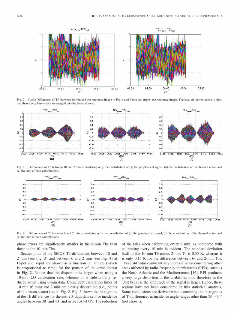
Fig. 7. (Left) Differences of TB between 10 min and the reference image in Fig. 6 and 2 min and (right) the reference image. The level of thermal noise is high,and therefore, phase errors are merged into the thermal noise.

Fig. 8. Differences of Tb between 10 and 2 min, considering only the contribution of (a) the geophysical signal, (b) the contribution of the thermal noise, and(c) the sum of both contributions.

Fig. 9. Differences of Tb between 6 and 2 min, considering only the contribution of (a) the geophysical signal, (b) the contribution of the thermal noise, and(c) the sum of both contributions.

phase errors are significantly smaller in the 6-min Tbs thanthose in the 10-min Tbs.

Scatter plots of the SMOS Tb differences between 10 and2 min (see Fig. 3) and between 6 and 2 min (see Fig. 4) atH-pol and V-pol are shown as a function of latitude (whichis proportional to time) for the portion of the orbit shownin Fig. 2. Notice that the dispersion is larger when using a10-min LO calibration rate, whereas it is substantially re-duced when using 6-min data. Coincident calibration times of10 min (6 min) and 2 min are clearly discernible (i.e., pointsof minimum scatter), as in Fig. 2. Fig. 5 shows the histogramsof the Tb differences for the entire 3-days data set, for incidenceangles between 38◦ and 40◦ and in the EAF-FOV. The reduction

of the tails when calibrating every 6 min, as compared withcalibrating every 10 min is evident. The standard deviation(std) of the 10-min Tb minus 2-min Tb is 0.55 K, whereas itis only 0.15 K for the difference between 6- and 2-min Tbs.These std values substantially increase when considering otherareas affected by radio-frequency interferences (RFIs), such asthe North Atlantic and the Mediterranean [16]. RFI producesa very large distortion in the visibilities (and therefore in theTbs) because the amplitude of the signal is larger. Hence, theseregions have not been considered in this statistical analysis.Same conclusions are derived when examining the histogramsof Tb differences at incidence angle ranges other than 38◦−40◦

(not shown).

GABARRÓ et al.: LO CALIBRATION RATE ON THE SMOS MEASUREMENTS AND RETRIEVED SALINITIES 4637

IV. THEORETICAL ANALYSIS

The along- and across-track patterns observed in the10- (and 6 min) versus 2-min Tb differences (shown inSection III) have been theoretically analyzed. The MIRASTesting Software (MTS), which is an independent software thatfully processes the SMOS raw data up to brightness temperatureimages [17], has been used to perform this analysis.

Using a decimation scheme, the thermal noise (or radiomet-ric sensitivity) in the measurements is correlated for the threecases (2, 6, and 10 min), since the measurements are exactly thesame, and only the different LO phase calibration processing isperformed. In order to assess the thermal noise, a reference Tbimage is computed by averaging 5-min brightness temperaturedata over the Pacific (see Fig. 6). The difference between the10-min Tb (2-min Tb) and the reference image has been per-formed to obtain the thermal noise, as shown in Fig. 7.

Visibility phase errors have been assessed for the differentLO calibration rates [19]. Maximum values of 2.5◦, 1◦, and0.3◦ have been found when calibrating the LO every 10, 6,and 2 min, respectively. Moreover, the sensitivity of Tb toreceiver phase errors is 0.27 K/◦ [20], [21]. Therefore, theimpact of the visibility phase errors on the Tb yields, i.e.,0.27 K/◦ ∗ 2.5◦ ∗

√2 = 0.95 K (10 min), 0.38 K (6 min), and

0.11 K (2 min). The factor√2 takes into account that maximum

phase errors have been found per baseline (difference of tworeceivers’ phases), whereas the sensitivity of Tb to phase errorsis given per receiver.

From these results, it is noticeable that phase errors aremerged into a high level of thermal noise (see Fig. 7). For thisreason, a theoretical simulation has been performed in order toseparately analyze the geophysical signal contribution from thethermal noise.

The calibrated visibility with a LO calibration every n min-utes can be expressed following [22], [23], as:

V(n)kj =

√TsyskTsysj ·

Mkj

|Gkj |· ejφn . (1)

In (1), the term Mkj stands for the normalized complexcorrelations during the observation measurements computedfrom the correlator counts after the self-calibration procedure[24]. The terms, Tsysk, Tsysj, correspond to the system tem-peratures measured by the power measurement system of eachreceiver. Gkj corresponds to the fringe washing function termat the origin that takes into account the spatial decorrelationeffects due to the limited noise bandwidth of the receiver filters[25]. The phase of visibility Vkj is taken into account by theterm ejφn , which is affected by the LO phase drifts due totemperature swings [10].

Differences between the calibrated visibilities using the LOcalibration every n min (where n corresponds to 10 or 6) withrespect to the 2 min are given by

V(n)kj − V

(2)kj = V

(2)kj ·

(ej(φn−φ2) − 1

). (2)

The visibility measurement can be expressed as the sumof the noise from the geophysical signal, i.e., V scene

kj and

Fig. 10. Differences of Tb between (left) 10 and 2 min and (right) 6 and 2 minfor an incidence angle range of 0◦−40◦ and AF-FOV. Both thermal noise andphase errors have been taken into account in the simulation. Spatial structuresacross and along tracks can be appreciated, as in the real data in Fig. 2 (althoughin this case, the incidence angle range is only 38◦−40◦ and for the EAF-FOV).

the thermal noise component, i.e., ΔV . Hence, (2) can bewritten as

V(n)kj −V

(2)kj =V scene

kj ·(ej(φn−φ2)−1

)+ΔV ·

(ej(φn−φ2)−1

).

(3)

In this theoretical analysis, the contribution from the geo-physical signal [the first term in (3)] has been simulated usingan average of the visibilities from the measurements shown inFig. 6 and the corresponding phase terms calibrating the LOevery 2, 6, and 10 min. On the other hand, the thermal noisecontribution [the second term in (3)] has been simulated usinga normal distribution with the std of the visibilities previouslydescribed. This term is also affected by the visibility phaseerrors.

After the image reconstruction procedure [26], the differencebetween n min and 2-min Tbs can be expressed as the sumof the geophysical signal Tb (ΔTbscene) and the thermal noise(ΔTbnoise) contributions, i.e.,

Tb(n) − Tb(2) = ΔTbscene +ΔTbnoise. (4)

The results for the simulated Tb differences are shown inFig. 8 (10 min minus 2 min) and Fig. 9 (6 min minus 2 min).Note that the impact of the LO phase errors on Tb is of thesame order of magnitude in both the geophysical signal [seeFigs. 8(a) and 9(a)] and thermal noise [see Figs. 8(b) and 9(b)]contributions. Figs. 8(c) and 9(c) correspond to the Tb differ-ence between the 10 min (6 min) and the 2 min, consideringboth contributions. Only V-pol plots are shown here, since theypresent a larger scatter than H-pol, as observed with real data.Note that these plots are very similar to those in Figs. 3 and 4,

4638 IEEE TRANSACTIONS ON GEOSCIENCE AND REMOTE SENSING, VOL. 51, NO. 9, SEPTEMBER 2013

Fig. 11. Differences of Tb between (left) 10 and 2 min and (right) 6 and 2 min using real data. An average of 125 snapshots over the Pacific has been performed.Spatial structures in the brightness temperatures at the antenna frame can be clearly observed due to the imperfect cancellation of LO phase errors.

further confirming that the origin of the observed Tb differencesis the visibility phase errors induced by the different calibrationrates.

Since the SSS inversion uses multiple incidence angle infor-mation, it is relevant to check whether the LO phase errors arecancelled out by averaging measurements at different incidenceangles or not. Fig. 10 shows an image of the (left) 10-min minus2-min Tbs and (right) 6-min minus 2-min Tbs after averagingall Tbs between 0◦ and 40◦ incidence angles in the AliasFree-Field of View (AF-FOV). This image shows a similaralong- and across-track patterns to that of Fig. 2, thereforeindicating that LO phase errors do not cancel out when aver-aging over a wide range of incidence angles, thus are expectedin the retrieved SSS fields. From the previous results, it canbe concluded that simulated data confirm the experimentalresults.

Moreover, the impact of the LO phase calibration rate onthe brightness temperatures has been analyzed at the antennaframe using real data (half-orbit over the Pacific). Fig. 11shows the differences of Tb between (left) 10 and 2 minand (right) 6 and 2 min. An average of 125 snapshots overthe Pacific has been performed. From this figure, it can beclearly observed that LO phase errors, at visibility level, trans-late into brightness temperature systematic errors, appearingas spatial structures at the antenna frame. In summary, thevisibility phase errors induce noticeable systematic patternsin the spatial Tb distribution, which are translated into SSSretrievals.

V. IMPACT ON RETRIEVED SALINITY

In this section, the impact of the phase errors (induced bythe LO calibration rate) on the retrieved SSS is assessed usingreal data. The decimated data sets are used to retrieve SSS atLevel 2 (SSS retrievals at the satellite swath grid) and Level 3(spatio-temporally averaged Level 2 SSS data in a griddedglobal map). The L2PP is used to generate Level 2 SSS data,and the Spanish operational SMOS Levels 3 and 4 ProductionCentre (CP34) processor is used to generate Level 3 SSS maps[27]. Note that measurements in the entire EAF-FOV have been

used to retrieve the SSS since this is the default mode of theoperational L2PP and CP34.

The impact of the different LO calibration rates on the re-trieved SSS is shown in Fig. 12. The figure shows the retrievedL2 SSS difference (top) between the 10- and 2-min data setsand (bottom) between the 6- and 2-min data sets for the 3 days.Similar to the results obtained at Tb level, Fig. 12 shows that thelower the calibration rate, the lower the quality of the retrievedSSS. Note that, as for the Tb differences analysis, the 2-minSSS data set is used as a reference. An along- and across-track error pattern is observed in the SSS differences, similarto that observed in the Tb differences. The North Atlantic areais evidently the noisiest due to the large RFI sources present inthe region, as previously explained.

Fig. 13 shows the histograms for the retrieved SSS differ-ences, excluding regions with high RFI contamination, suchas the North Atlantic. The std for 10-min minus 2-min SSSdifferences is 0.39 psu, whereas for the 6-min and 2-min SSSdifferences the std is 0.15 psu.

Table I shows the percentage of points for which the SSSdifference between the 10 min (6 min) and 2 min is higher thana certain threshold, i.e., 0.2, 0.5, and 1 psu. The table highlightsthe impact of calibrating the LO too sparsely (every 10 min) onthe quality of the retrieved SSS. About 10% of the points havean additional salinity error above 0.5 psu at 10 min with respectto 2 min. Moreover, about 30% of the points have an additionalerror above 0.2 psu.

The impact of calibrating the LO every 10 min relative to2 min has been also assessed at Level 3 maps. SSS maps areproduced by averaging the Level 2 SSS data into 1◦ × 1◦ boxesfor the 3 days data set. Separate SSS maps have been producedusing the 10- and 2-min data sets. The top plot of Fig. 14 showsthe difference between the 10- and 2-min SSS maps. This mapwas obtained with a very strict quality control that yields areduction in the number of valid data. The bottom plot of Fig. 14shows the mean value of 10-min minus 2-min SSS as a functionof latitude, which shows a nonnegligible bias. In the regionbetween 45◦ S and 30◦ N, the mean value of the SSS differencesis 0.05 psu, whereas the std is 0.12. On the other hand, largervalues are observed in the Southern ocean. The sensitivity of Tb

GABARRÓ et al.: LO CALIBRATION RATE ON THE SMOS MEASUREMENTS AND RETRIEVED SALINITIES 4639

Fig. 12. Retrieved SSS differences (a) between 10 and 2 min and (b) between6 and 2 min data sets at L2 level.

to SSS changes decreases with Sea Surface Temperature (SST)[15]. As such, in the Southern region, where the SST is verylow, small errors in Tb are translated into large retrieved SSSerrors.

Note that the decimation does not account for the samplingeffect. That is, the lower the calibration rate, the larger thenumber of available measurements, and, in turn, the largerthe error reduction due to increased sampling. Therefore, onewould expect a decrease in SSS quality at 2 min, as comparedwith 10 min due to data loss.

The impact of losing snapshots for calibrating the LO hasbeen assessed. Note that a total of five snapshots are usedevery LO calibration sequence. For one semiorbit (50 min,2500 snapshots), the reduction of usable snapshots at 2 min(6 min), as compared with 10 min (current calibration rate)is 4.0% (0.72%). Taking into account that at nadir, a total of140 Tb measurements are used in the SSS inversion (if noinvalid measurements), and assuming that the Tb errors (radio-metric accuracy) are Gaussian, the relative error (std) decreases

Fig. 13. Histogram of retrieved SSS differences (a) between 10 and 2 min and(b) between 6 and 2 min data sets.

TABLE IPERCENTAGE OF POINTS WHERE THE DIFFERENCES BETWEEN SSS

AT 10 min MINUS AT 2 min AND BETWEEN 6 AND 2 minIS HIGHER THAN A CERTAIN THRESHOLD

due to the loss of five snapshots (in the case of calibrating every2 min) is

√140/

√135 = 1.018, i.e., 1.8%. However, at the

edges of the swath (or if many measurements are consideredinvalid), the number of available Tbs are substantially reduced.In the worst case, i.e., when only 40 Tb measurements areavailable (below this number, the retrieved SSS is considerednot reliable and therefore flagged by L2PP), the relative error(std) decrease is

√45/

√40 = 1.061, i.e., 6.1%. Assuming a

SSS retrieved error is about 1.2 psu (requirements), the relative

4640 IEEE TRANSACTIONS ON GEOSCIENCE AND REMOTE SENSING, VOL. 51, NO. 9, SEPTEMBER 2013

Fig. 14. (Top) Differences between SSS maps at 10 and 2 min. (Bottom) Aforementioned differences averaged by longitudinal cuts as a function of latitude.

error impact is about 0.02 psu at nadir and 0.07 psu at the edgeof the swath. As such, the sampling effect is at least one orderof magnitude smaller than the expected increase in data qualityfor increasing calibration rates shown in this paper (0.39 psu).

VI. CONCLUSION AND PERSPECTIVE

Using a LO calibration rate of 10 min results in substantialdegradation of the reconstructed Tb (larger in V-pol than H-pol)and retrieved SSS quality, much larger than that for 6-mindata, as compared with 2-min data. Tb and SSS differencesbetween 10 and 2 min are up to 0.8 K and 1.5 psu, respectively.When calibrating the LO every 6 min instead, the Tb and SSSerrors are substantially reduced. The std of salinity differencesbetween 10 and 2 min is about 0.39 psu, whereas between6 and 2 min is about 0.14 psu. An additional reduction isnoticeable when calibrating every 4 min (not shown here butpresented in [28]).

These results have been confirmed with theoretical study.The simulation results further emphasize that the LO phaseerrors negatively impact the Tb and produce systematic patterns

in the Tb images, which do not correspond to geophysicalpatterns.

It is important to note that the Tb and SSS errors induced bythe LO calibration rate choice are added to a list of other errorsthat have been identified since the beginning of the mission.Some of the known errors are systematic errors caused by an-tenna pattern errors [29], [30], long- and short-term drifts [18],[31], forward model errors [32]–[34], among others, which atthe moment are hard to remove or mitigate.

Although the LO phase errors represent only a small contri-bution to the SMOS measurement errors, they are indeed sig-nificant and furthermore systematic (i.e., they follow a spatialpattern), thus hard to reduce with spatio-temporal averaging, asshown in Sections IV and V.

In contrast with other sources of error, these LO phase errorscan be easily reduced by simply increasing the LO calibrationrate. It is also shown that the measurement loss due to increas-ing the calibration rate to 2 min is small and marginally impactsthe SSS retrieval quality. In consequence, it is recommendedto increase the SMOS MIRAS LO calibration rate to at least6 min.

GABARRÓ et al.: LO CALIBRATION RATE ON THE SMOS MEASUREMENTS AND RETRIEVED SALINITIES 4641

ACKNOWLEDGMENT

The SMOS Level 2 Prototype Processor developmentwas funded by the European Space Agency under differentcontracts.

REFERENCES

[1] S. Levitus, T. P. Boyer, M. E. Conkright, T. O’Brien, J. Antonov,C. Stephens, L. Stathoplos, D. Johnson, and R. Gelfeld, “NOAA AtlasNESDIS 18, World Ocean Database 1998,” U.S. Gov. Printing Office,Washington, DC, USA, 1998, vol. 1, Introduction.

[2] Y. H. Kerr, P. Waldteufel, J. P. Wigneron, J. M. Martinuzzi, J. Font, andM. Berger, “Soil moisture from space: The soil moisture and ocean salin-ity (SMOS) mission,” IEEE Trans. Geosci. Remote Sens., vol. 39, no. 8,pp. 1729–1735, Aug. 2001.

[3] Y. H. Kerr, P. Waldteufel, J. P. Wigneron, S. Delwart, F. Cabot, J. Boutin,M. J. Escorihuela, J. Font, N. Reul, C. Gruhier, S. Juglea, M. Drinkwater,A. Hahne, M. Martín-Neira, and S. Mecklenburg, “The SMOS mission:New tool for monitoring key elements of the global water cycle,” Proc.IEEE, vol. 98, no. 5, pp. 666–687, May 2010.

[4] S. Mecklenburg, N. Wright, C. Bouzinac, and S. Delwart, “Gettingdown to business—SMOS operations and products,” ESA Bull., vol. 137,pp. 25–30, 2009.

[5] J. Font, A. Camps, A. Borges, M. Martín-Neira, J. Boutin, N. Reul,Y. H. Kerr, A. Hahne, and S. Mecklenburg, “SMOS: The challenging seasurface salinity measurement from space,” Proc. IEEE, vol. 98, no. 5,pp. 649–665, May 2010.

[6] M. Martin-Neira and J. M. Goutoule, “MIRAS: A two dimensional aper-ture synthesis radiometer for Soil Moisture and Ocean Salinity observa-tions,” ESA Bull., vol. 92, pp. 95–104, Nov. 1997.

[7] K. D. McMullan, M. A. Brown, M. Martin-Neira, W. Rits, S. Ekholm,J. Marti, and J. Lemanczyk, “SMOS: The payload,” IEEE Trans. Geosci.Remote Sens., vol. 46, no. 3, pp. 594–605, Mar. 2008.

[8] I. Corbella, N. Duffo, M. Vall-llossera, A. Camps, and F. Torres, “Thevisibility function in interferometric aperture synthesis radiometry,” IEEETrans. Geosci. Remote Sens., vol. 42, no. 8, pp. 1677–1682, Aug. 2004.

[9] M. Martin-Neira, “Analysis of LO phase drift calibration,” ESA-ESTEC,Noordwijk, The Netherlands, Tech. Rep. ESA-ESTEC SO-TN-ESA-PLM-6052, 2008.

[10] V. González-Gambau, F. Torres, and N. Duffo, “Phase calibration temper-ature track in interferometric radiometers devoted to Earth observation,”in Proc. SPIE, 2008, pp. 71061U-1–71061U-8 .

[11] “SMOS system requirements document,” Paris, France, Tech. Rep. ESASO-RS-ESA-SYS-0555, 2003.

[12] M. A. Brown, F. Torres, I. Corbella, and A. Colliander, “SMOS calibra-tion,” IEEE Trans. Geosci. Remote Sens., vol. 46, no. 3, pp. 646–658,Mar. 2008.

[13] A. Gutierrez, J. Barbosa, N. Almeida, N. Catarino, J. Freitas,M. Ventura, and J. Reis, “SMOS L1 Processor prototype: From digi-tal counts to brightness temperatures,” in Proc. IEEE IGARSS, 2007,pp. 3626–3630.

[14] S. Zine, J. Boutin, J. Font, N. Reul, P. Waldteufel, C. Gabarró, J. Tenerelli,F. Petitcolin, J. L. Vergely, M. Talone, and S. Delwart, “Overview ofthe SMOS sea surface salinity prototype processor,” IEEE Trans. Geosci.Remote Sens., vol. 46, no. 3, pp. 621–645, Mar. 2008.

[15] C. Swift, “Passive microwave remote sensing,” Boundary-layer Meteo-rol., vol. 18, pp. 25–54, 1980.

[16] R. Oliva, E. Daganzo, Y. H. Kerr, S. Mecklenburg, S. Nieto, P. Richaume,and C. Gruhier, “SMOS radio frequency interference scenario: Sta-tus and actions taken to improve the RFI environment in the 1400–1427-MHz passive band,” IEEE Trans. Geosci. Remote Sens., vol. 50,no. 5, pp. 1427–1439, May 2012.

[17] I. Corbella, F. Torres, N. Duffo, V. González, A. Camps, andM. Vall-llossera, “Fast processing tool for SMOS data,” in Proc. IEEEIGARSS, 2008, vol. 2, pp. II-1152–II-1155.

[18] I. Corbella, F. Torres, N. Duffo, V. González-Gambau, M. Pablos,I. Durán, and M. Martín-Neira, “MIRAS calibration and perfor-mance: Results from the SMOS in-orbit commissioning phase,”IEEE Trans. Geosci. Remote Sens., vol. 49, no. 9, pp. 3147–3155,Sep. 2011.

[19] UPC team, “LO calibration track assessment in electrical stability tests,”Universitat Politècnica de Catalunya, Technical Note SO-TN-UPC-PLM-0130, Barcelona, 2011.

[20] I. Corbella, F. Torres, A. Camps, J. Bara, N. Duffo, and M. Vall-Ilossera,“L-band aperture synthesis radiometry: Hardware requirements and sys-tem performance,” in Proc. IEEE IGARSS, 2000, vol. 7, pp. 2975–2977.

[21] F. Torres, I. Corbella, A. Camps, N. Duffo, and M. Vall-llossera, “Errorbudget map to SRD (PRS),” Universitat Politècnica de Catalunya, Tech-nical Note SO-TN-UPC-PLM-0007, Barcelona, 2007.

[22] I. Corbella, F. Torres, A. Camps, A. Colliander, M. Martín-Neira,S. Ribó, K. Rautiainen, N. Duffo, and M. Vall-llossera, “MIRAS end-to-end calibration: Application to SMOS L1 processor,” IEEE Trans. Geosci.Remote Sens., vol. 43, no. 5, pp. 1126–1134, May 2005.

[23] F. Torres, I. Corbella, A. Camps, N. Duffo, M. Vall-llossera, S. Beraza,C. Gutierrez, and M. Martín-Neira, “Denormalization of visibilities forin-orbit calibration of interferometric radiometers,” IEEE Trans. Geosci.Remote Sens., vol. 44, no. 10, pp. 2679–2686, Oct. 2006.

[24] M. Martín-Neira, S. Ribó, and K. Rautianen, “0-1 correction of compara-tor threshold in 1-bit interferometric radiometers,” in Proc. IEEE 8th Spec.Meeting MicroRad, 2004, p. 93.

[25] R. Butora, M. Martín-Neira, and A. L. Rivada-Antich, “Fringe-Washingfunction calibration in aperture synthesis microwave radiometry,” RadioSci., vol. 38, no. 2, pp. 15-1–15-5, 2003. DOI: 10.1029/2002RS002695.

[26] I. Corbella, F. Torres, A. Camps, N. Duffo, and M. Vall-llossera, “Bright-ness temperature retrieval methods in synthetic aperture radiometers,”IEEE Trans. Geosci. Remote Sens., vol. 47, no. 1, pp. 285–294, Jan. 2009.

[27] J. Font, J. Ballabrera-Poy, A. Camps, I. Corbella, N. Duffo,I. Duran, M. Emelianov, L. Enrique, P. Fernández, C. Gabarró,C. González, V. González, J. Gourrion, S. Guimbard, N. Hoareau, A. Julià,S. Kalaroni, A. Konstantinidou, L. Aretxabaleta, J. Martínez, J. Miranda,A. Monerris, S. Montero, B. Mourre, M. Pablos, F. Pérez, M. Piles,M. Portabella, R. Sabia, J. Salvador, M. Talone, F. Torres, A. Turiel,M. Vall-llossera, and R. Villarino, “A new space technology for oceanobservation: The SMOS mission,” Sci. Mar., vol. 76, no. S1, pp. 249–259,2012.

[28] C. Gabarró, V. González, J. Martínez, I. Corbella, M. Portabella, N. Duffo,F. Torres, and J. Font, “Assessment of the local oscillator calibrationfrequency impact on the SMOS sea surface salinity,” in Proc. IGARSS,2012, pp. 2613–2616.

[29] J. Gourrion, R. Sabia, M. Portabella, J. Tenerelli, S. Guimbard, andA. Camps, “Characterization of the SMOS Instrumental Error PatternCorrection Over the Ocean,” IEEE Geosci. Remote Sens. Lett., vol. 9,no. 4, pp. 793–797, Jul. 2012.

[30] F. Torres, I. Corbella, W. Lin, N. Duffo, J. Gourrion, J. Font, andM. Martin-Neira, “Minimization of image distortion in SMOS brightnesstemperature maps over the ocean,” IEEE Geosci. Remote Sens. Lett.,vol. 9, no. 1, pp. 18–22, Jan. 2012.

[31] I. Corbella, F. Torres, N. Duffo, and M. Martin-Neira, “Stability of theMIRAS amplitude calibration,” in Proc. 12th Spec. Meeting MicroRad,Mar. 5–9, 2012, pp. 1–3.

[32] S. Guimbard, J. Gourrion, M. Portabella, A. Turiel, C. Gabarró, andJ. Font, “SMOS semi-empirical ocean forward model adjustment,” IEEETrans. Geosci. Remote Sens., vol. 50, no. 5, pp. 1676–1687, May 2012.

[33] J. E. Tenerelli, N. Reul, A. A. Mouche, and B. Chapron, “Earth- view-ing L-band radiometer sensing of sea surface scattered celestial skyradiation—Part I: General characteristics,” IEEE Trans. Geosci. RemoteSens., vol. 46, no. 3, pp. 659–674, Mar. 2008.

[34] N. Reul, J. Tenerelli, N. Floury, and B. Chapron, “Earth-viewingL-band radiometer sensing of sea surface scattered celestial skyradiation—Part II: Application to SMOS,” IEEE Trans. Geosci. RemoteSens., vol. 46, no. 3, pp. 675–688, Mar. 2008.

Carolina Gabarró was born in Barcelona, Spain, in1974. She received the B.Eng. degree in telecom-munications engineering and the Ph.D. degreein ocean science from the Universitat Politèc-nica de Catalunya, Barcelona, in 1998 and 2004,respectively.

From 1997 to 1999, she was with theEuropean Space Research and TechnologyCentre, EuropeanSpace Agency, Noordwijk, TheNetherlands, where she worked on ocean-colorremote sensing (for the ENVISAT mission). Since

2000, she has been with the Physical Oceanography Department, Institut deCiencies del Mar, Consejo Superior de Investigaciones Cientificas, Barcelona,Spain, where she has been working on the Soil Moisture and Ocean Salinity(SMOS) mission. She is currently a Member of the SMOS Barcelona ExpertCentre, Barcelona. Her work was focused on the retrieval of salinity fromSMOS images. Her research interest includes microwave remote sensing.

4642 IEEE TRANSACTIONS ON GEOSCIENCE AND REMOTE SENSING, VOL. 51, NO. 9, SEPTEMBER 2013

Verónica González-Gambau was born in Huesca,Spain, in 1981. She received the M.S. and Ph.D.degrees in telecommunication engineering from theSchool of Telecommunication Engineering, Univer-sitat Politècnica de Catalunya (UPC), Barcelona,Spain, in 2006 and 2012, respectively.

In 2006, she joined the Passive Remote SensingGroup of the Signal Theory and CommunicationsDepartment, Universitat Politècnica de Catalunya(UPC), Barcelona, where she was involved in theSoil Moisture and Ocean Salinity (SMOS) payload

on-ground characterization in the framework of SMOS Precommissioningactivities. She was collaborating with the SMOS Level 1 software developmentand data analysis of the Microwave Imaging Radiometer by Aperture Synthesisinstrument validation campaigns. Since 2007, she has been a Member ofthe SMOS Barcelona Expert Center on Radiometric Calibration and OceanSalinity, Barcelona, where she is currently working on advanced Level 1 errorcorrection techniques and in-orbit validation procedures.

Ignasi Corbella (S’78–M’82–SM’08) was born inBarcelona, Spain, in 1955. He received the Telecom-munication Engineer and Dr. Eng. degrees fromthe Universitat Politècnica de Catalunya (UPC),Barcelona, Spain, in 1977 and 1983, respectively.

In 1976, he was with the School of Telecom-munication Engineering, Universitat Politècnica deCatalunya (UPC), Barcelona, as a Research Assis-tant in the Microwave Laboratory, where he workedon passive microwave integrated-circuit design andcharacterization. In 1979, he was with Thomson-

CSF, Paris, France, working on microwave oscillators design. In 1982, he wasan Assistant Professor; in 1986, he was an Associate Professor; and in 1993, hewas a Full Professor with UPC, where he is currently teaching basic microwavesand antennas at the undergraduate level and graduate courses on nonlinearmicrowave circuits. From 1993 to 1997, he was the Academic Director of theSchool of Telecommunications Engineering. From 2001 to 2003, he was theDirector of the Department of Signal Theory and Communications, UPC. From1998 to 1999, he was with the NOAA/Environmental Technology Laboratory asa Guest Researcher developing methods for total-power radiometer calibrationand data analysis. Since 1993, he has been actively participating as a researcherwith the European Space Agency (ESA) Soil Moisture and Ocean Salinity(SMOS) mission in the frame of several contracts, directly with ESA, orwith the payload prime contractor European Aeronautic Defense and Space-Construcciones Aeronáuticas Sociedad Anónima Espacio or other companiesinvolved in the SMOS mission. His expertise in this field includes, amongothers, fundamentals of interferometric aperture synthesis radiometry, imagereconstruction algorithms, onboard calibration, hardware specification, andpayload characterization. From 2004 to 2009, he was a Member of the SMOSScience Advisory Group and from 2009 to present, he was a Member of theSMOS Quality Working Group. Since 2007, he has been a Member of theSMOS Barcelona Expert Centre (BEC), Barcelona. From 1999 to 2007, hewas the Scientific Coordinator of a Dictionary of Telecommunication termsin Catalan language, with more than 4000 entries, published in March 2007.Dr. Corbella was the General Chairman of the 2007 International Geoscienceand Remote Sensing Symposium (IGARSS’07), Barcelona, from July 22 to 27,2007.

Francesc Torres (S’88–M’96–SM’06) was born inIbiza, Spain, in 1962. He received the Ingenieroand Doctor Ingeniero degrees in telecommunica-tion engineering from the Universitat Politècnica deCatalunya (UPC), Barcelona, Spain, in 1988 and1992, respectively.

From 1988 to 1989, he was a Research Assis-tant with the RF System Division, European SpaceAgency, Holland, where he was devoted to mi-crowave device testing and characterization. In 1989,he joined the Signal Theory and Communications

Department, UPC, as an Assistant Professor on microwave circuits and systemsand, currently, as Full Professor. Since 1995, as part of the UPC Passive RemoteSensing Group, he has been participating in a number of projects related to

the Soil Moisture and Ocean Salinity (SMOS) mission by the European SpaceAgency. From 2005 to 2006, he held a sabbatical stage at the MicrowaveSystems Section, Jet Propulsion Laboratory, Pasadena, CA, USA, where he wasinvolved in the GeoSTAR pilot project, a passive microwave interferometricgeosounder. He is a Member of the SMOS Barcelona Expert Centre onRadiometric Calibration and Salinity, Barcelona.

Justino Martínez was born in Girona, Spain, in1966. He received the B.Sc. and Ph.D. degrees inphysics from Autonomous University of Barcelona,Barcelona, Spain, in 1991 and 1995, respectively.

He is currently working as a Scientific Pro-grammer in the Physical Oceanography Department,Institut de Ciencies del Mar, Consejo Superior deInvestigaciones Cientificas, Barcelona. He is also aMember of the Soil Moisture and Ocean SalinityBarcelona Expert Centre, Barcelona, and he is in-volved in the L3 and L4 SMOS products generation

and validation.

Marcos Portabella was born on October 14, 1970,in Spain. He received the B.Sc. and Ph.D. degrees inphysics from the University of Barcelona, Barcelona,Spain, in 1994 and 2002, respectively, and the M.Sc.degree in remote sensing from the Institute of SpaceStudies of Catalonia, Catalonia, Spain, in 1995.

He is currently with the Institut de Ciències delMar, Consejo Superior de Investigaciones Cientificas(ICM-CSIC), Barcelona, Spain, working on satelliteremote sensing. In particular, he is involved in scat-terometry and L-band radiometry.

Jordi Font received the B.Sc. and Ph.D. degrees inphysics from the University of Barcelona, Barcelona,Spain, in 1973 and 1986, respectively.

He is a Research Professor at the PhysicalOceanography Department, Institut de Ciències delMar (Spanish Research Council, Consejo Superiorde Investigaciones Cientificas), Barcelona. He is aMember of several international societies and com-mittees. He is a Participant in 42 oceanographiccampaigns. He has authored or coauthored 300 com-munications to scientific symposia and 260 pub-

lished papers (75 in SCI journals). He is an Adviser of nine Ph.D. Theses. PI inseveral Spanish and European research contracts. His research interests includeOcean remote sensing: determination of sea surface salinity by microwaveradiometry; Physical oceanography of the Mediterranean Sea: water masses,circulation, and climate change; Ocean circulation: operational measurementsof ocean currents, technological improvements; and Mesoscale dynamics:fronts, eddies, topographic interactions, and physical–biological processescoupling. He is currently the Co-Lead Investigator for ocean salinity with theEuropean Space Agency Soil Moisture and Ocean Salinity (SMOS) mission.Until May 2010, he was the Chairman of the Ocean Physics and ClimateCommittee of the International Commission for the Scientific Exploration ofthe Mediterranean Sea CIESM. He received the National Arts Award 2011 ofthe Catalan Government in the category of Thought and Scientific Culture.