Embed Size (px)
Citation preview

47D. Zilberman and G.R. Timilsina (eds.), The Impacts of Biofuels on the Economy, Environment, and Poverty, Natural Resource Management and Policy 41, DOI 10.1007/978-1-4939-0518-8_4, © Springer Science+Business Media New York 2014
4.1 Introduction
For the first time since the Green Revolution, food and fuel commodity prices began to rise in 2001 and reached peak levels in 2008 (FAO 2008; Peters et al. 2009; Trostle 2008a, b). As primary food commodities (e.g., corn, wheat) doubled in price, the bio-fuel industry expanded manifold within this same period (e.g., ethanol from corn and sugarcane doubled to 65 billion liters; biodiesel from soybean, oil palm, and rapeseed reached 12 billion liters or six times 2001 levels (Martinot and Sawin 2009). Popular opinion has linked biofuel production to the shock in food prices in 2008. Yet, much of the biofuel demand by the US and EU was driven by government mandates and subsi-dies, which aim to reduce the demand for oil and increase demand for agricultural goods (Hochman et al. 2010). In high-income households and countries, a smaller percentage of crop prices is reflected in the final food price (due to food processing, packaging services). In low-income households and countries, however, crop prices have much larger share of the final food price.
Hochman et al. (2011) identify and quantify the major factors in food commodity prices and also report the importance of the ability to store certain feedstock and of inventory relative to the consumption levels. It is argued that price shock for food
Chapter 4Impacts of Biofuels on Food Prices
Gal Hochman, Deepak Rajagopal, Govinda R. Timilsina, and David Zilberman
[AU1]
G. Hochman • D. Rajagopal
G.R. Timilsina (*) The World Bank, 1818 H Street, N.W., Washington, DC 20433, USAe-mail: [email protected]
D. Zilberman Department of Agricultural and Resource Economics, College of Natural Resources, University of California, Berkeley, Giannini Hall 206, Berkeley, CA 94720-3310, USAe-mail: [email protected]
[AU2]
1
2
3
4
5
6
7
8
9
10
11
12
13
14
15
16
17
18
19
20
21

48
commodities in 2008 was partly caused by the declining stock-to-use ratio since 1985 (Trostle 2008a, b).
Historical lows in inventory caused societies to experience greater price sensitivity. Other notable factors in the food crisis included global economic growth, population growth, energy price inflation, exchange rate fluctuations, adverse weather, and trade policy. Economic growth created new demand for luxury foods and meats (which heighten production costs) by rising income households. Energy price inflation moti-vated many farmers to convert agricultural plots to biofuel feedstock plantations. In 2008, the US dollar depreciated relative to major world currencies (Abbott et al. 2008)—thus raising commodity prices for many nations in trade with the United States and inciting currency speculation during the exchange rate flux (Rosegrant 2008). Adverse weather patterns experienced in key grain-producing regions caused high pro-duction costs and shortage of crop output. Many of these factors prompted govern-ments to ensure their own food supply by stalling grain trades, consequently straining regions relying on food imports (Timmer 2008). In addition, cumulative underinvest-ment in agricultural research and technology stagnated agriculture’s productivity growth (Schnepf 2004).
4.2 Prior Research
Economic assessments of the food crisis have been categorized as based on partial or general equilibrium models. Partial equilibrium models—e.g., IMPACT, AGLINK/COSMO, FAPRI, and FASOM—utilize supply and demand equations to represent the economic behavior within select markets (Alston et al. 2009). Disadvantages arise from partial equilibrium analyses, because it is not comprehensive enough to gauge restraints on budget. Computable general equilibrium (CGE) models—e.g., GTAP, LINKAGE, and USAGE—could correct some disadvantages, but would require much more robust data and complexity. CGE is a numerical technique based on Walrasian theory that was formalized by Arrow and Debrew to model supply, demand, and prices across a set of markets. Tables 4.1 and 4.2 summarize a range of studies that estimated commodity price effects.
As biofuels are increasingly used to substitute crude oil for energy uses, many have studied the impact that feedstock prices have on the market (Zilberman et al. 2012). The food crisis of 2007–08 has given further cause for research—wherein the most pessimistic of estimates attributed 75 % of the food price shock to the biofuel industry (Mitchell 2008). The IMF and other bodies of scholars have suggested factors such as: depreciation of the dollar, global changes in production such as weather shocks, changes in patterns of food consumption, trade policies, government incentives, and the role of biofuels in commodity price increases. The USDA had reported greater demands for grains among world consumers, while production gains in technology had slowed in growth rate.
Macroscopically, food prices had been in the decline with the ongoing development of farming techniques from cropland rotation to the Green Revolution. Then, the increase of trade via globalization presented higher rates of capital flow that ampli-
G. Hochman et al.
22
23
24
25
26
27
28
29
30
31
32
33
34
35
36
37
38
39
40
41
42
43
44
45
46
47
48
49
50
51
52
53
54
55
56
57
58
59
60
61
62
63

49
Table 4.1 Quantitative estimates of impact of biofuel on food commodity prices
Source Estimate (%) Commodity Time period
Mitchell (2008) 75 Global food index Jan 2002–Feb 2008Rosegrant (2008) 39 Corn 2000–2007
21–22 Rice and wheat 2000–2007OECD-FAO (2008) 42 Coarse grains 2008–2017
34 Vegetable oils 2008–201724 Wheat 2008–2017
Collins et al. (2008) 25–60 Corn 2006–200819–26 US retail food 2006–2008
Glauber (2008) 23–31 Commodities Apr 2007–Apr 200810 Global food index Apr 2007–Apr 2008 4–5 US retail food Jan–Apr 2008
Lampe et al. (2006) 35 Corn Mar 2007–Mar 2008 3 Global food index Mar 2007–Mar 2008
Rajagopal et al. (2009) 15–28 Global corn price 2007–200810–20 Global soy price 2007–2008
Hochman et al. (2011) 20–30 Corn 2002–2007 5–10 Soybeans 2002–2007
Fischer et al. (2009) 11–51 Coarse grains 2008De Hoyos and Medvedev (2009) 6 Global food index 2005–2007
Table 4.2 Impacts of increased biofuel production on food prices
Study Coverage and key assumptionsKey impacts of biofuels on food
prices
Abbott et al. (2008)
Rise in corn price from about US$2–6 per bushel accompanying the rise in oil price from US$40 in 2004 to US$120 in 2008
US$1 of the US$4 increase in corn price (25 %) due to the fixed subsidy of 51-cents per gallon of ethanol
Baier et al. (2009)
24 months ending June 2008; historical crop price elasticities from academic literature; bivariate regression estimates of indirect effects
Global biofuel production growth responsible for 17, 14, and 100 % of the rises in corn, soybean, and sugar prices, respectively, and 12 % of the rise in the IMF’s food price index
Banse et al. (2008)
2001–2010; Reference scenario without mandatory biofuel blending, 5.75 % mandatory blending scenario (in EU member states), 11.5 % mandatory blending scenario (in EU member states)
Price change under reference scenario, 5.75 % blending, and 11.5 % blending, respectively
Cereals: −4.5, −1.75, +2.5 %Oilseeds: −1.5, +2, +8.5 %Sugar: −4, −1.5, +5.75 %
Collins (2008) 2006/2007–2008/2009; Two scenarios considered: (1) normal and (2) restricted, with price inelastic market demand and supply
Under the normal scenario, the increased ethanol production accounted for 30 % of the rise in corn price; Under the restricted scenario, ethanol accounted for 60 % of the expected increase in corn prices.
(continued)
4 Impacts of Biofuels on Food Prices
t1.1
t1.2
t1.3
t1.4
t1.5
t1.6
t1.7
t1.8
t1.9
t1.10
t1.11
t1.12
t1.13
t1.14
t1.15
t1.16
t1.17
t1.18
t1.19
t1.20
t1.21
t2.1
t2.2
t2.3
t2.4
t2.5
t2.6
t2.7
t2.8
t2.9
t2.10
t2.11
t2.12
t2.13
t2.14
t2.15
t2.16
t2.17
t2.18
t2.19
t2.20
t2.21
t2.22
t2.23
t2.24
t2.25
t2.26

50
fied energy demands. As oil prices spiked in the 1970s, the global market was challenged to deal with the scale of energy demand and the scale of supply alterna-tives (Graff et al. 2009). The alternative of biofuel will favor or even revive the agricultural sector. Baka and Roland-Holst (2009) argue that, in the case of Europe, biofuel production will reduce trade rivalries and heighten energy security. Agricultural biotechnology and its markets vary given regional natural resources, competitive advantages, industry set up costs, institutional regulations, and other economic considerations.
Study Coverage and key assumptionsKey impacts of biofuels on food
prices
Fischer et al. (2009)
(1) Scenario based on the IEA’s WEO 2008 projections
Increase in prices of wheat, rice, coarse grains, protein feed, other food, and non-food, respectively, compared to reference scenario:
(2) Variation of WEO 2008 scenario with delayed second gen biofuel deployment
(3) Aggressive biofuel production target scenario
(1) +11, +4, +11, −19, +11, +2 %
(4) and variation of target scenario with accelerated second gen deployment
(2) +13, +5, +18, −21, +12, +2 %(3) +33, +14, +51, −38, +32, +6 %(4) +17, +8, +18, −29, +22, +4 %
Glauber (2008)
12 months ending April 2008 Increased US biofuel production accounted for 25 % of the rise in corn prices and 10 % of the rise in global food prices
IMF (2008) Estimated range covers the plausible values for the price elasticity of demand
Range of 25–45 % for the share of the rise in corn prices attributable to ethanol production increase in the US
Lazear et al. (2008)
12 months ending March 2008 US ethanol production increase accounted for 20 % of the rise in corn prices
Lipsky (2008) and Johnson (2008)
2005–2007 Increased demand for world biofuels accounts for 70 % of the increase in corn prices
Mitchell (2008)
2002-mid-2008; ad hoc methodology: impact of movement in dollar and energy prices on food prices estimated, residual allocated to the effect of biofuels
70–75 % of the increase in food commodity prices was due to world biofuels and the related consequences of low grain stocks, large land-use shifts, speculative activity, and export bans
Rosegrant et al. (2008)
2000–2007; Scenario with actual increased biofuel demand compared to baseline scenario where biofuel demand grows according to historical rate from 1990 to 2000
Increased biofuel demand accounted for 30 % of the increase in weighted average grain prices, 39 % of the increase in real corn prices, 21 % of the increase in rice prices and 22 % of the rise in wheat prices
Source: Timilsina and Shrestha (2011) [AU4]
Table 4.2 (continued)
[AU3]
G. Hochman et al.
64
65
66
67
68
69
70
71
t2.27
t2.28
t2.29
t2.30
t2.31
t2.32
t2.33t2.34
t2.35
t2.36
t2.37
t2.38
t2.39
t2.40
t2.41
t2.42
t2.43
t2.44
t2.45
t2.46
t2.47
t2.48
t2.49
t2.50
t2.51
t2.52
t2.53
t2.54
t2.55
t2.56
t2.57
t2.58
t2.59
t2.60
t2.61
t2.62
t2.63
t2.64
t2.65
t2.66
t2.67
t2.68

51
4.3 Historical Price Trends
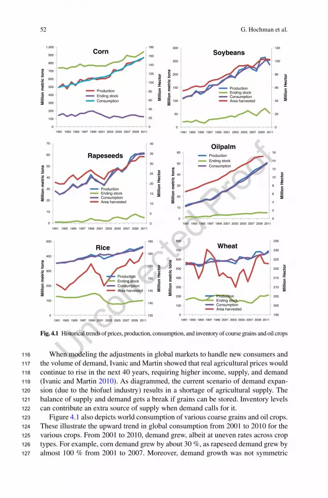
For centuries, economic development has improved agricultural efficiency and allowed for resources to shift to sectors such as manufacturing. Inasmuch, the expan-sion of consumption and production—biased toward manufacturing and against agriculture—raised food prices (Sexton et al. 2009). From a partial equilibrium per-spective, this mechanism would also heighten food demand and further boost food prices. An interesting case in point is China: 20 % of the world’s population (the world’s largest consumer and producer of food) produces agricultural products at only 20–33 % of the rate that it produces non-agricultural goods (Alston et al. 2009). On a more global scale, economic development has afforded higher population and income levels. This shifts the lifestyle and consumption habits of people on an exceptionally larger scale, considering developing countries. The historical trends of production, consumption, inventory, and prices of major grains—corn, wheat, rice, soybeans, rapeseed, oil palm (see Fig. 4.1) show that crop prices have been countercyclical to their inventory levels. Consumption levels of wheat have decreased since 2004, while consumption levels of coarse grains and rice have increased. The higher demand for coarse grains mostly comes from US demand for corn for ethanol production. The higher demand for rice is concentrated in Asian countries, which have increased their consumption levels from 61.5 to 85.9 kg/capita. Rice crops are characteristically pro-duced by nations for domestic consumers, under segmented and protected markets.
It is notable that, outside the agricultural industry, other commodity prices were also on the rise (e.g., minerals, metals, energy). Between January 2002 and July 2008, the IMF price indices showed that food prices rose 130 % and crude oil prices rose 590 %, contrasted against 330 % rise in commodity prices in general. The impact of biofuel demand on food prices manifests in two ways: allocation of land (for which biofuel feedstock compete with food products, thus increasing aggregate demand for agricultural commodities) and the level of energy prices (which affects production costs and output level of agricultural commodities).
When comparing allocation rate of corn, soybean, and rapeseed crops toward biofuel production, rapeseed has the highest share of its total supply allocated to biofuel, thus signifying that biofuel has become an important factor for the increas-ing demand and prices of rapeseed. While corn and soy also experienced rising biofuel allocation per total supply, biofuel appears less important a demand to affect corn and rice prices.
The food price shock was not instantaneous. On the demand side, consumption of agricultural products was rising across the world. On the supply side, production technologies were making less gains and growth had been sluggish. Agricultural output in developing nations had been almost half of their GDP growth for the past two decades. During this time period in which demand outpaced supply, stockpiles of grain commodities diminished with use. In fact, stock-to-use ratios declined by more than 50 % since 1985, making regional markets more sensitive to changes in grain prices. Depicted in Fig. 4.2, the observed correlation between price and inven-tory is graphed for major grain crops. Stock-to-use of the world’s grain and oilseeds were recorded at 35 % in 1985 and at less than 15 % in 2005.
[AU5]
[AU6]
4 Impacts of Biofuels on Food Prices
72
73
74
75
76
77
78
79
80
81
82
83
84
85
86
87
88
89
90
91
92
93
94
95
96
97
98
99
100
101
102
103
104
105
106
107
108
109
110
111
112
113
114
115
52
When modeling the adjustments in global markets to handle new consumers and the volume of demand, Ivanic and Martin showed that real agricultural prices would continue to rise in the next 40 years, requiring higher income, supply, and demand (Ivanic and Martin 2010). As diagrammed, the current scenario of demand expan-sion (due to the biofuel industry) results in a shortage of agricultural supply. The balance of supply and demand gets a break if grains can be stored. Inventory levels can contribute an extra source of supply when demand calls for it.
Figure 4.1 also depicts world consumption of various coarse grains and oil crops. These illustrate the upward trend in global consumption from 2001 to 2010 for the various crops. From 2001 to 2010, demand grew, albeit at uneven rates across crop types. For example, corn demand grew by about 30 %, as rapeseed demand grew by almost 100 % from 2001 to 2007. Moreover, demand growth was not symmetric
0
20
40
60
80
100
120
140
160
180
0
100
200
300
400
500
600
700
800
900
1,000
1991 1993 1995 1997 1999 2001 2003 2005 2007 2009 2011
Mill
ion
Hec
tor
Mill
ion
met
ric
ton
s
Corn
Production
Ending stock
Consumption
0
20
40
60
80
100
120
0
50
100
150
200
250
300
1991 1993 1995 1997 1999 2001 2003 2005 2007 2009 2011
Mill
ion
Hec
tor
Mill
ion
met
ric
ton
s
Soybeans
ProductionEnding stockConsumptionArea harvested
0
5
10
15
20
25
30
35
40
0
10
20
30
40
50
60
70
1991 1993 1995 1997 1999 2001 2003 2005 2007 2009 2011
Mill
ion
Hec
tor
Mill
ion
met
ric
ton
s
Rapeseeds
ProductionEnding stockConsumptionArea harvested
135
140
145
150
155
160
165
0
100
200
300
400
500
1991 1993 1995 1997 1999 2001 2003 2005 2007 2009 2011
Mill
ion
Hec
tor
Mill
ion
met
ric
ton
s
Rice
Production
Ending stock
Consumption
Area harvested
195
200
205
210
215
220
225
230
235
0
100
200
300
400
500
600
700
800
1991 1993 1995 1997 1999 2001 2003 2005 2007 2009 2011
Mill
ion
Hec
tor
Mill
ion
met
ric
ton
s
Wheat
ProductionEnding stockConsumptionArea harvested
0
2
4
6
8
10
12
14
16
0
10
20
30
40
50
60
1991 1993 1995 1997 1999 2001 2003 2005 2007 2009 2011
Mill
ion
Hec
tor
Mill
ion
met
ric
ton
s
OilpalmProduction
Ending stock
Consumption
Fig. 4.1 Historical trends of prices, production, consumption, and inventory of course grains and oil crops
G. Hochman et al.
116
117
118
119
120
121
122
123
124
125
126
127

53
across regions. Whereas globally consumption of all crops increased with income (at the world level, income is positively correlated with consumption, and world income grew throughout the period investigated), in some regions consumption of certain crops decreased. For example, corn, rice, and wheat consumption in China went down by 12.7 %, 23.7 %, and 20.9 %, respectively, although global consump-tion increased by 24.0 %, 3.2 %, and 4.3 %, respectively. Although the global reces-sion of 2008 hampered the food-commodity price inflation of 2007/2008, in 2009/2010 consumption returned to display an upward trend and so did food- commodity prices. Further, between 2011 and 2017, corn prices are expected to rise 14 % and soybean oil prices are expected to be more stable with only a 5 % rise (Zilberman et al. 2010). Timilsina and Shrestha argue that Ethanol production might be sustainable without support if gasoline prices remain above US$3/gal (Timilsina and Shrestha 2011). Then, even if ethanol production was doubled, corn prices would still remain at about US$4/bushel.
4.4 Methodology
Grain storability and its inventory level would soften a grain’s price volatility on the market. With this intuition, the authors have developed a new model to capture more accurately biofuels’ impact on the agricultural commodities market. Assuming that the demand function follows on historical data on prices and inventory levels, any anticipation of future inventory decisions affects current behavior and is constrained by the fact that one cannot borrow from future inventory (e.g., inventory cannot be negative) (Williams and Wright 1991). Graphical results of this demand function depict that when market demand exceeds the harvest of crops, prices will rise if stocks are too low. The inventory function would present a significant buffer to demand, thus suggesting that a model neglecting grain inventory would overesti-mate price effects of biofuel (Hochman et al. 2011).
y = 3E+06x -0.84
R2 = 0.54417
y = 4E+07x -1.041
R2 = 0.62125
y = 5022.5x -0.325
R2 = 0.04127
y = 2E+06x -1.058
R2 = 0.99955
y = 1. 0093x0.509
R2 = 0.26548
0
50
100
150
200
250
300
350
400
450
0 50000 100000 150000 200000 250000
Wor
ld p
rice
in $
/ ton
ne
Year ending stock (in Thousand metric tonnes)
Rice
Wheat
Maize
Rapeseed
Soybean
Fig. 4.2 The observed correlation between price and inventory
4 Impacts of Biofuels on Food Prices
128
129
130
131
132
133
134
135
136
137
138
139
140
141
142
143
144
145
146
147
148
149
150
151
152
153

54
4.4.1 Multi-market Analysis
For a multiple market analysis, methodology differs from the partial equilibrium and general equilibrium models. An important aim is to disaggregate markets in order to accurately portray, explain, and predict price impacts from policies regulating specific markets. Disaggregation of the “vertical structure” (the chain of production) would distinguish between supply interactions and the different end-uses—whether for food processing or energy production. Disaggregation of the “horizontal structure” (across different staple crops) assesses the input prices and the feedback effects between different markets. GTAP, FAPRI, and IFPRI models have utilized multi-market in various studies, though none has included grain inventory before.
Horizontal Structure: Since different staple crops compete for the same inputs (e.g., land, labor, resources), there is negative cross-price elasticity between different staple crops. For example, higher demand for Chinese soybeans may trigger shifts in resources from corn cultivation to soybean cultivation. Consequently, the strong growth rate of soybeans in China causes other competitive crops to lessen in pro-duction rate. A similar comparison can be made between agricultural production of biofuel to food. If the demand rises for corn-ethanol allocates more land to corn specifically for ethanol, then resources are detracted from food production from corn or other crops. Thus, biofuel also has a negative cross-price elasticity with respect to food. Yet, biofuel can sometimes replace one feedstock with another—thus, rendering different crops complementary and not substitutable goods. To properly disaggregate the horizontal structure, it is critical to determine the domi-nant forces between demand of agricultural inputs (e.g., land, energy) and end-use (e.g., food consumption, energy).
Vertical Structure: The vertical structure highlights the supply chain interactions. Production level would be determined by existing markets and introduction of new markets (e.g., ethanol, biodiesels). Differences in willingness to pay will incentivize suppliers to develop for one market over another. For example, farmers switched crops from food to biofuel feedstock and limited the sale to food markets. The verti-cal structure of production is likewise influenced by inputs (e.g., land, energy) and demand of end product (e.g., food, biofuel).
4.4.2 Numerical Model
Combining the horizontal and vertical structure intuition, the authors (Hochman et al. 2011) extend the empirical model for a single region, single crop to a multi- market with five major grain crops (corn, soybean, rapeseed, rice, wheat). They divide the world into seven major regions, namely, Argentina, Brazil, China, European Union (EU-27 countries), India, United States, and an aggregate that rep-resents the rest of the world (ROW), and focus on the time period between the year 2001 and the year 2007.
G. Hochman et al.
154
155
156
157
158
159
160
161
162
163
164
165
166
167
168
169
170
171
172
173
174
175
176
177
178
179
180
181
182
183
184
185
186
187
188
189
190
191
192
193

55
To determine the level of inputs used, crop consumption minus the quantity of a co-product, which may be returned as an input. Biofuel from corn, soybean, and rapeseed is jointly produced along with a co-product that is itself a substitute for the raw grain or the oilseed. For instance, in the case of corn, 1 bushel (56 lb) of corn yields approximately 2.75 gal of ethanol and 18 lb of distiller grains, which is a substitute for corn grain. A fraction of the quantity of original crop used for biofuel is replaced in the form of co-product. Therefore, for these three crops, we compute an effective demand of the particular crop for biofuel, which equals the crop con-sumption for biofuel minus the quantity of a co-product. In the case of corn, the effective demand of corn is 0.68 = (1 − 18/56) bushels per 2.75 gal of ethanol. Assume that biofuel production function is of Leontief (fixed-proportion) type. Further, when biofuel production is determined through a mandate, the derived crop demand for biofuel is simply a fixed proportion of the mandate.
With the exception of the demand for inventory, assume a linear structure for supply and demand. The linear structure generally serves as a good approximation for small disturbances or shocks. Crop demand for inventory is represented as a nonlinear function of price and follows Carter et al. (2008). For details regarding the calibration of the numerical model and the calculations made for various shocks, see Hochman et al. (2011).
4.4.3 Numerical Scenarios
Given the cumulative change in a variable with respect to the year 2001, use the mar-ket-clearing condition to derive a counterfactual equilibrium world price for each crop for the various shocks for each year. Repeating this process for four different alterna-tive scenarios which either differ in the assumed range for elasticities used in calibra-tion of supply and demand functions, or differ in the specification of the demand for food/feed (whether GDP per capita is explicitly represented in demand) or differ in parameters of the inventory demand function. Given the challenge of estimating a point estimate for the various elasticities, as well as the inventory parameters, we simulated these alternative scenarios to determine the robustness of our results.
The first scenario, which the authors henceforth refer to as the baseline scenario, is one in which used the range of price and income elasticities reported in the litera-ture, namely, that mentioned in the USDA’s database of elasticities and in the FAPRI database. Under this scenario, the parameters for the inventory demand function are those estimated using the specification of Carter et al (2008). As mentioned earlier, perform 100 simulations of this scenario for the various shocks for each crop and for each time period but report the mean value of these outcomes.
In the second scenario, the inelastic scenario, assume a narrower range for elas-ticities, which is on average more inelastic compared to the baseline scenario and follows Gardner (1987). This scenario further differs from the baseline in that we employ a demand specification that does not include income. The reason for exclud-ing income is that some of the elasticities reported in the literature were based on models that did not include income.
4 Impacts of Biofuels on Food Prices
194
195
196
197
198
199
200
201
202
203
204
205
206
207
208
209
210
211
212
213
214
215
216
217
218
219
220
221
222
223
224
225
226
227
228
229
230
231
232
233
234
235
56
Finally, to test the robustness of the inventory demand parameters, simulate a fourth scenario using Carter et al.’s (2008) estimates for the inventory demand func-tion as opposed to the original estimates of this study. Note that Carter et al. (2008) estimated the inventory demand based on US data for 2006–2008, while the original results drew from world data in 2001–2008.
4.5 Results
The authors report two different price changes: First, reduction of commodity price if key variables would have stayed at 2001 levels, ΔPt,i. Technically, this is the per-centage difference between the actual price in a given year and the counter-factual price for the same year, and secondly, the increase of the commodity price attributed to a change in one of the variables (income, biofuel mandate, exchange rate , energy prices) between 2001 and the specific year, ΔPt/2001,i, where i ∈ {bio-fuel, income growth, energy prices, exchange rate}. Technically, this is the percent-age difference between counter-factual price for a given year and the price in 2001. The simulations compute ΔPt,i. The authors then compute ΔPt/2001,i as follows: let ΔPt
a denote the total percentage price change between the year t and year 2001; then,
D D D DP P P Pt i t i t
ata
/ , , /2001 1= +( ) (4.21)
Total change in price from year t to year 2001 that is explained by this model equals the sum of ΔPt/2001,i over all the shocks. The figures depict ΔPt,i—namely, the food commodity price reduction attributed to a shock that eliminates one of the fac-tors that caused prices to change after 2001, whereas the tables show ΔPt/2001,i—namely, the increase in commodity prices from 2001 attributed to one of the factors that caused prices to change after 2001. In both cases, the authors report the mean outcome of 100 simulations, where each trial draws upon a number from a range of plausible values (for price, income, and supply elasticities) and compute the coun-terfactual outcome. When presenting prices for different crops, the authors distin-guish between two different specifications: one with inventory demand function and another without inventory demand. For each crop, the authors show the impact of these shocks one at a time.
The analysis includes five simulated scenarios for each of the five crops, namely, corn, soybeans, rapeseed, rice, and wheat. The baseline scenario’s outcome is con-trasted with alternative specifications to evaluate robustness of the relative and abso-lute value of the numerous shocks. The alternative scenarios illustrate the robustness of the results presented with respect to relative impact, but the absolute impact usu-ally becomes larger as elasticities become smaller. Some but not all scenarios include an income term in the demand specification for food and feed. Introducing an income term reduces the biofuel impact. While for the first four scenarios the authors estimated an inventory demand function, for the fifth scenario, the authors
G. Hochman et al.
236
237
238
239
240
241
242
243
244
245
246
247
248
249
250
251
252
253
254
255
256
257
258
259
260
261
262
263
264
265
266
267
268
269
270
271
272
273

57
relied on the parameters from Carter et al. as a constant. The estimated parameters suggest, on average, more elastic inventory demand, and thus less fluctuation in prices. The authors conclude this section by qualitatively discussing the role of trade policy and speculation and the role of inventory management for limiting the impact of future shocks.
4.5.1 The Baseline Scenario
The observed prices for the different crops are shown in Fig. 4.3. A clear upward trend, on average, emerges for all crops, albeit some prices increase more than oth-ers. Whereas the price of corn and soybeans increased from 2002 to 2006 by about 63 %, the price of wheat increased by more than 74 %. Furthermore, while some crops like rice and wheat experienced an upward trend throughout the period, others such as soybeans declined in 2005 and 2006 only to increase by 39 % in 2007. Inventory theory predicts that prices decline when inventory accumulates and vice versa. The data confirm these predictions, except for soybeans, and show similar trends for stock-to-use ratio (see Fig. 4.3). If, however, dropping 2007 (a year where soybean prices spiked), then such a pattern is also observed for soybeans.
Inventory serves as a buffer and affects prices as long as inventory levels are suf-ficiently large. However, as these levels become small, prices become more volatile and sensitive to the numerous specific factors affecting crop prices. Less fluctuation
Fig. 4.3 Average annual crop prices (in 2005 USD per ton)
4 Impacts of Biofuels on Food Prices
274
275
276
277
278
279
280
281
282
283
284
285
286
287
288
289
290
291
292

58
is observed if inventory demand is explicitly added to the analysis. The aggregate demand curve becomes much more elastic for large inventory levels, and thus pre-dicts less price volatility (Fig. 4.4).
The annual increase in corn and soybean prices is largest toward the end of the sample period (i.e., between 2006 and 2007). One explanation for the observed price fluctuation in corn and soybeans is that consumption of corn for biofuel became significant around 2006, when the federal government began implementing biofuel mandates. Although biofuel subsidies have been in effect for several decades, mandates are the main cause for the recent increase in biofuel production. Furthermore, land allocated to corn replaces soybean land, resulting in higher soy-bean prices (not modeled explicitly, because we do not have data on land use). This complements the upward pressure on soybean prices attributed to biodiesel produc-tion. On the other hand, economic growth results in structural changes to demand in countries like China, where increased demand for feed led to larger demand for soybeans considerable growth of about 20 % between 2000 and 2008 was also observed for pork (Trostle 2008a, b).
Since it was assumed that rice and wheat are not utilized for biofuels in any sig-nificant quantities, and since land growing rice and wheat do not generally compete with corn, sugarcane, and oilseeds, the data reflect that the prices of rice and wheat are not influenced by biofuels. However, a general equilibrium framework, in con-trast to the multi-market framework presented here, may identify indirect linkages between biofuel production and rice and wheat (Mitchell 2008). When the market for storage is excluded, higher price fluctuations are documented (Fig. 4.5 and
[AU7]
Stock to use and prices
Corn
Rice Wheat
0
.12
.15 .2 .25 .3 .15 .2 .25 .3
.14 .14.16 .16.18 .18stock_use stock_use
stock_usestock_use
Price Fitted values
Price Fitted values Price Fitted values
Price Fitted values
.2 .2.22
100
200
300
0100
200
300
0100
200
300
0100
200
300
Soybean
Fig. 4.4 Crop prices and the stock-to-use ratio
G. Hochman et al.
293
294
295
296
297
298
299
300
301
302
303
304
305
306
307
308
309
310
311
312
313
314
315

59
Table 4.3). Graphing the standard deviation of prices for five crops for a represented shock, in Fig. 4.5, the shock caused prices to fluctuate more when inventory is not modeled explicitly. This picture emerges for all shocks. Inventory specification mat-ters. Introducing inventory demand alters outcomes. Now, since inventories are observed and found significant by the numerical model, the following sections present exogenous shocks and simulate the impacts upon inventory demand.
4.6 Sensitivity Analysis
Because the empirical estimation of the demand and supply parameters as well as the demand for inventory are challenging but are key steps to accurately measuring the factors causing the food inflation of 2007–2008, two additional scenarios were numerically simulated to further check the robustness of this study’s conclusion.
4.6.1 Inelastic Scenario
Key parameters in our analysis and in simulation-based models in general are the elasticities, which are used to calibrate the demand and supply curves. The alter-native specification, denoted the inelastic scenario, assumes lower elasticities.
Fig. 4.5 The implication of demand and supply shocks on prices with and without inventory
4 Impacts of Biofuels on Food Prices
316
317
318
319
320
321
322
323
324
325
326
327
328
329
330
60
The elasticities used in the baseline scenario were obtained from well-known and widely used sources such as the FAPRI elasticity database and the USDA elasticity database.1 However, according to several other researchers, the elasticities of supply and demand for agriculture are more inelastic than those reported in the above data-bases (Gardner (1987). In order that the elasticities are on average lower than those in the baseline scenario and also conservative, we chose own-price supply elastici-ties in the range 0.2–0.3 and own- price demand elasticities in the range −0.3 to −0.2. Employing these elasticities, we find that the main qualitative conclusions regarding the importance of the different shocks from the baseline scenario hold.2
1 http://www.ers.usda.gov/Data/InternationalFoodDemand/.2 To this end, using world data on four major crops, namely, corn, soybeans, wheat, and rice from 1960 to 2007, Roberts and Schlenker (2010 estimate that short-term, own-price elasticity of supply and demand for calories from these crops is less than 0.15 and greater than −0.1, respectively.
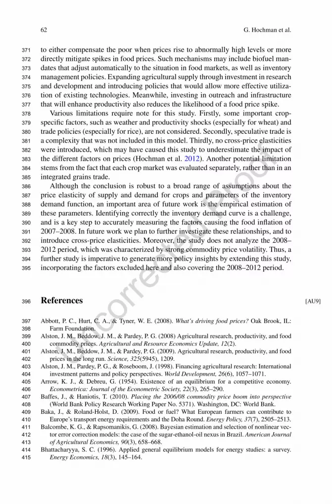
Table 4.3 Contribution of various factors on increased price of selected food commodities (% price increase from counterfactual scenario in a given year)
Crop
With inventory Without inventory
Year Year
2005 (%) 2006 (%) 2007 (%) 2005 (%) 2006 (%) 2007 (%)
Biofuel shockCorn 4.40 6.80 9.80 5.50 7.40 9.80Soybean 1.00 1.80 3.40 1.50 2.60 4.10Rice 0.00 0.00 0.00 0.00 0.00 0.00Wheat 0.00 0.00 0.00 0.00 0.00 0.00
Income shockCorn 7.90 12.20 15.30 12.40 16.70 19.50Soybean 6.30 8.90 14.70 12.10 15.60 22.10Rice 11.60 13.50 16.10 20.90 27.90 35.10Wheat 11.10 16.00 21.20 15.10 21.40 27.70
Exchange rate shockCorn 3.50 5.00 7.60 4.60 6.20 9.40Soybean 1.00 2.40 5.30 1.40 3.80 7.90Rice 3.30 4.00 6.50 6.70 8.30 14.40Wheat 6.60 7.30 11.00 8.10 8.90 13.10
Energy price shockCorn 2.20 2.90 2.90 3.30 3.60 3.60Soybean 1.90 2.40 2.40 3.60 4.00 4.00Rice 3.00 3.00 3.00 2.40 2.60 2.60Wheat 2.80 3.10 3.10 3.60 4.00 4.00
Aggregate effect of all four shocksCorn 18 27 36 26 34 42Soybean 10 15 26 19 26 38Rice 18 20 26 30 39 52Wheat 20 26 35 27 34 45
G. Hochman et al.
331
332
333
334
335
336
337
338
339
t3.1
t3.2
t3.3
t3.4
t3.5
t3.6
t3.7
t3.8
t3.9
t3.10
t3.11
t3.12
t3.13
t3.14
t3.15
t3.16
t3.17
t3.18
t3.19
t3.20
t3.21
t3.22
t3.23
t3.24
t3.25
t3.26
t3.27
t3.28

61
Comparing the baseline scenario to the inelastic scenario results in the price changes summarized in Table 4.4. This comparison emphasizes the importance of obtaining good elasticity estimates. The more inelastic scenario results in a larger impact.
Finally, we simulate the model using the inventory demand parameters estimated in Carter et al. (2008). Results confirm the conclusions derived for the baseline sce-nario. The price effect now is marginally smaller for all shocks. This is because the estimates of the parameters of the inventory demand employed in the elastic sce-nario imply an inventory demand function that is on average more elastic compared to that suggested by parameters estimated by Carter et al. (2008).
4.7 Conclusions
This chapter has focused on four major factors widely agreed to be responsible for food commodity price increases—economic growth, biofuel expansion, exchange rate fluctuations, and energy price change. The study also captures the effect of inventory adjustments. Incorporating an empirically estimated inventory demand function into the market-clearing condition shows that the impact of inventory on prices increases as the level of inventory diminishes. In the absence of shocks attrib-utable to the four factors mentioned above, in 2007 the prices of corn, soybean, rapeseed, rice, and wheat would have been 26–36 % lower than the observed prices in that year. On the other hand, if inventory demand was to be ignored, in 2007 the prices would have been 38–52 % lower than the observed prices in that year. Abstracting from considerations of inventory responses leads to predictions of larger price changes.
Because key parameters in this analysis included the elasticities used to calibrate the demand and supply curves, the authors performed several sensitivity analyses on these values. In these alternative scenarios, many inelastic curves were introduced and compared against a demand curve based on the inventory parameters from Carter et al. (2008). It is concluded that although the percentage changes vary between scenarios, the main conclusion is that the inventory matters do not change. The relative magnitude of the various shocks also does not change.
From a policy standpoint, the food crisis emphasizes both the importance of a proactive inventory management policy and the need for mechanisms. Policies need
[AU8]
Table 4.4 Comparison of results between main and sensitivity analysis (% change as compared to the counterfactual scenario in 2007)
Shock CropMain analysis (%)
Sensitivity analysis (%)
Biofuel Corn 9.8 12.7Soybean 3.4 3.7
Income growth Corn 15.3 20.3Soybean 14.7 16.0Rice 16.1 17.2Wheat 21.1 25.8
4 Impacts of Biofuels on Food Prices
340
341
342
343
344
345
346
347
348
349
350
351
352
353
354
355
356
357
358
359
360
361
362
363
364
365
366
367
368
369
370
t4.1
t4.2
t4.3
t4.4
t4.5
t4.6
t4.7
t4.8
t4.9
t4.10
t4.11
t4.12
t4.13
t4.14
62
to either compensate the poor when prices rise to abnormally high levels or more directly mitigate spikes in food prices. Such mechanisms may include biofuel man-dates that adjust automatically to the situation in food markets, as well as inventory management policies. Expanding agricultural supply through investment in research and development and introducing policies that would allow more effective utiliza-tion of existing technologies. Meanwhile, investing in outreach and infrastructure that will enhance productivity also reduces the likelihood of a food price spike.
Various limitations require note for this study. Firstly, some important crop- specific factors, such as weather and productivity shocks (especially for wheat) and trade policies (especially for rice), are not considered. Secondly, speculative trade is a complexity that was not included in this model. Thirdly, no cross-price elasticities were introduced, which may have caused this study to underestimate the impact of the different factors on prices (Hochman et al. 2012). Another potential limitation stems from the fact that each crop market was evaluated separately, rather than in an integrated grains trade.
Although the conclusion is robust to a broad range of assumptions about the price elasticity of supply and demand for crops and parameters of the inventory demand function, an important area of future work is the empirical estimation of these parameters. Identifying correctly the inventory demand curve is a challenge, and is a key step to accurately measuring the factors causing the food inflation of 2007–2008. In future work we plan to further investigate these relationships, and to introduce cross-price elasticities. Moreover, the study does not analyze the 2008–2012 period, which was characterized by strong commodity price volatility. Thus, a further study is imperative to generate more policy insights by extending this study, incorporating the factors excluded here and also covering the 2008–2012 period.
References
Abbott, P. C., Hurt, C. A., & Tyner, W. E. (2008). What’s driving food prices? Oak Brook, IL: Farm Foundation.
Alston, J. M., Beddow, J. M., & Pardey, P. G. (2008) Agricultural research, productivity, and food commodity prices. Agricultural and Resource Economics Update, 12(2).
Alston, J. M., Beddow, J. M., & Pardey, P. G. (2009). Agricultural research, productivity, and food prices in the long run. Science, 325(5945), 1209.
Alston, J. M., Pardey, P. G., & Roseboom, J. (1998). Financing agricultural research: International investment patterns and policy perspectives. World Development, 26(6), 1057–1071.
Arrow, K. J., & Debreu, G. (1954). Existence of an equilibrium for a competitive economy. Econometrica: Journal of the Econometric Society, 22(3), 265–290.
Baffes, J., & Haniotis, T. (2010). Placing the 2006/08 commodity price boom into perspective (World Bank Policy Research Working Paper No. 5371). Washington, DC: World Bank.
Baka, J., & Roland-Holst, D. (2009). Food or fuel? What European farmers can contribute to Europe’s transport energy requirements and the Doha Round. Energy Policy, 37(7), 2505–2513.
Balcombe, K. G., & Rapsomanikis, G. (2008). Bayesian estimation and selection of nonlinear vec-tor error correction models: the case of the sugar-ethanol-oil nexus in Brazil. American Journal of Agricultural Economics, 90(3), 658–668.
Bhattacharyya, S. C. (1996). Applied general equilibrium models for energy studies: a survey. Energy Economics, 18(3), 145–164.
[AU9]
G. Hochman et al.
371
372
373
374
375
376
377
378
379
380
381
382
383
384
385
386
387
388
389
390
391
392
393
394
395
396
397
398
399
400
401
402
403
404
405
406
407
408
409
410
411
412
413
414
415

63
Birur, D. K., Hertel, T.W., & Tyner, W. E. (2007). Impact of biofuel production on world agricul-tural markets: a computable general equilibrium analysis. The Annual conference on global equilibrium analysis, Purdue University, West Lafayette, IN.
Burniaux, J. M., Martin, J. P., Nicoletti, G., & Martins, J. O. (1991). GREEN–A multi-region dynamic general equilibrium model for quantifying the costs of curbing CO2 emissions: A technical manual (OECD Economics Department Working Paper No. 116). OECD: Paris, France.
Carter, C., Rausser, G., & Smith, A. (2008). Causes of the food price boom. Agricultural and Resource Economics Update, 12(2), 7.
Collins, K. (2008, June 19). The role of biofuels and other factors in increasing farm and food prices: A review of recent developments with a focus on feed grain markets and market pros-pects. Written as supporting material for a review conducted by Kraft Foods Global, Inc. of the current situation in farm and food markets.
De Hoyos, R. E., & Medvedev, D. (2009). Poverty effects of higher food prices—a global perspec-tive. World Bank Policy Research Working Paper(4887).
Demeke, M., Pangrazio, G., & Maetz, M. (2009). Country responses to the food security crisis: Nature and preliminary implications of the policies pursued. Initiative on soaring food prices.
Dixon, P. B., Osborne, S., & Rimmer, M. T. (2007). The economy-wide effects in the United States of replacing crude petroleum with biomass. Energy & Environment, 18(6), 709–722.
Dixon, P. B., & Parmenter, B. R. (1996). Computable general equilibrium modelling for policy analysis and forecasting. Handbook of Computational Economics, 1, 3–85.
FAO. (2008, July). Crop prospects and food situation. Food and Agriculture Organization, (3) FAO. (2008). The State of Food and Agriculture—Biofuels: Prospects, risks and opportunities.
Food and Agricultural Organization.Fischer, G., Hizsnyik, E. Prieler, S., Shah, M., & van Velthuizen, H. (2009, May) Biofuels and food
security. Prepared by the International Institute for Applied Systems Analysis (IIASA) for OPEC Fund for International Development (OFID).
Food and Agriculture Organization (FAO). (2009). Policy responses to rising commodity prices in selected countries. In The state of agricultural commodity markets. Rome, Italy: Economic and Social Development Department, FAO.
Fuglie, K., & Schimmelpfennig, D. (2010). Introduction to the special issue on agricultural pro-ductivity growth: a closer look at large, developing countries. Journal of Productivity Analysis, 33(3), 169–172.
Gardner, B. L. (1987). The economics of agricultural policies. New York: Macmillan.Glauber, J. (2008). Testimony of USDA Chief Economist Joseph Glauber before the Joint Economic
committee of Congress on May 1.Gohin, A., & Moschini, G. (2008). Impacts of the European biofuel policy on the farm sector:
A general equilibrium assessment. Review of Agricultural Economics, 30(4), 623–641.Goldemberg, J., & Guardabassi, P. (2009). Are biofuels a feasible option? Energy Policy, 37(1), 10–14.Graff, G., Hochman, G., & Zilberman, D. (2009). The political economy of agricultural biotech-
nology policies. AgBioForum, 12(1), 34–46.Graff, G., Zilberman, D., & Bennett, A. B. (2009). The contraction of product quality innovation
in agricultural biotechnology. Nature Biotech, 27(8), 702–704.Hertel, T. W. (2002a). Applied general equilibrium analysis of agricultural and resource policies.
Handbooks in Economics, 18(2A), 1373–1420.Hertel, T. W. (2002b). Applied general equilibrium analysis of agricultural and resource policies.
Handbook of Agricultural Economics, 2, 1373–1419.Hochman, G., Kaplan, S., Rajagopal, D., & Zilberman, D. (2012). Biofuel and food-commodity
prices. Agriculture, 2(3), 272–281.Hochman, G., Rajagopal, D., Timilsina, G., & Zilberman, D. (2011) Quantifying the causes of the
global food commodity price crisis. World Bank Policy Research Working Paper.Hochman, G., Rajagopal, D., & Zilberman, D. (2010a). The effect of biofuels on crude oil markets.
Agbioforum, 13(2), 112–118.Hochman, G., Rajagopal, D., & Zilberman, D. (2010b). Are biofuels the culprit: OPEC, food, and
fuel. American Economic Review: Papers and Proceedings, 100(2), 183–187.
4 Impacts of Biofuels on Food Prices
416
417
418
419
420
421
422
423
424
425
426
427
428
429
430
431
432
433
434
435
436
437
438
439
440
441
442
443
444
445
446
447
448
449
450
451
452
453
454
455
456
457
458
459
460
461
462
463
464
465
466
467
468
469
470

64
Hochman, G., Rausser, G., & Zilberman, D. (2009a). US versus E.U. biotechnology regulations and comparative advantage: Implications for future conflicts and trade.
Hochman, G., Sexton, S., & Zilberman, D. (2008). The economics of biofuel policy and biotech-nology. Journal of Agricultural & Food Industrial Organization, 6(2), 8.
Hochman, G., Sexton, S., & Zilberman, D. (2009b). Food and biofuel in a global environment. Handbook of bioenergy economics and policy.
Hochman, G., Sexton, S., & Zilberman, D. (2010). The economics of trade, biofuel, and the envi-ronment (CUDARE Working Papers Series 1100). Berkeley, CA: Department of Agricultural and Resource Economics and Policy, University of California at Berkeley.
IMF. (2008). Food and fuel prices: Recent developments, macroeconomic impact, and policy responses. Report prepared by the Fiscal Affairs, Policy Development and Review, and Research Departments.
Ivanic, M., & Martin, W. (2010). Promoting global agricultural growth and poverty reduction.Khanna, M., Hochman, G., Rajagopal, D., Sexton, S., & Zilberman, D. (2009). Sustainability of
food, energy and environment with biofuels. CAB Reviews: Perspectives in Agriculture, Veterinary Science, Nutrition and Natural Resources, 4(28), 1–10.
Koh, L. P., & Ghazoul, J. (2008). Biofuels, biodiversity, and people: Understanding the conflicts and finding opportunities. Biological Conservation, 141(10), 2450–2460.
Lampe, M. (2006). Agricultural market impacts of future growth in the production of biofuels. Paris, France: Working party on Agricultural Policies and Markets.
Lazear, E. P. (2008, May 14). Testimony of Edward P. Lazear Chairman, Council of Economic Advisers Before the Senate Foreign Relations Committee Hearing on “Responding to the Global Food Crisis.”
Mabiso, A., & Weatherspoon, D. (2008). Fuel and food trade-offs: A preliminary analysis of South African food consumption patterns. In Selected paper prepared for presentation at the American Agricultural Economics Association Annual Meeting (pp. 27–29).
Martin, W., & Mitra, D. (2001). Productivity growth and convergence in agriculture versus manu-facturing*. Economic Development and Cultural Change, 49(2), 403–422.
Martinot, E., & Sawin, J. (2009). Renewables global status report: 2009 update. Washington, DC: REN21 Renewable Energy Policy Network/Worldwatch Institute.
Mitchell, D. (2008). A note on rising food prices (Policy Research Working Paper #4682, Development Prospects Group). Washington, DC: World Bank.
Msangi, S., Sulser, T., Rosegrant, M., Valmonte-Santos, R., & Ringler, C. (2007). Global scenarios for biofuels: Impacts and implications. Farm Policy Journal, 4(2), 1–9.
Nielsen, C. P., & Anderson, K. (2001). Global market effects of alternative European responses to genetically modified organisms. Review of world economics, 137(2), 320–346.
Nin-Pratt, A., Yu, B., et al. (2010). Comparisons of agricultural productivity growth in China and India. Journal of Productivity Analysis, 33(3), 209–223.
Organization for Economic Co-operation and Development/Food and Agriculture Organization of the United Nations (OECD-FAO). (2008). OECD/FAO agricultural outlook 2008/2017. Author: Rome, Italy.
Peters, M., Langley, S., & Westcott, P. (2009). Agricultural commodity price spikes in the 1970s and 1990s: Valuable lessons for today. Amber Waves, 7, 16–23.
Rajagopal, D. (2008). Implications of India’s biofuel policies for food, water and the poor. Water Policy, 10(1), 95–106.
Rajagopal, D., Sexton, S., Hochman, G., Roland-Holst, D., & Zilberman, D. (2009). Biofuel and the food versus fuel trade-off. California Agriculture, 63(4), 20.
Rajagopal, D., & Zilberman, D. (2008). Environmental, economic and policy aspects of biofuels. Foundations and Trends® in Microeconomics, 4(5), 353–468.
Rathmann, R., Szklo, A., & Schaeffer, R. (2009). Land use competition for production of food and liquid biofuels: An analysis of the arguments in the current debate. Renewable Energy, 35, 14–22.
Regmi, A., Deepak, M. S., Seale, J. L., Jr., & Bernstein, J. (2001). Cross-country analysis of food consumption patterns. Changing structure of global food consumption and trade (pp. 14–22).
[AU10]
[AU11]
G. Hochman et al.
471
472
473
474
475
476
477
478
479
480
481
482
483
484
485
486
487
488
489
490
491
492
493
494
495
496
497
498
499
500
501
502
503
504
505
506
507
508
509
510
511
512
513
514
515
516
517
518
519
520
521
522
523
524

65
Roberts, M. J., & Schlenker, W. (2010, March 4–5). The US biofuel mandate and the world food prices: An econometric analysis of the demand and supply of calories. Presented at the National Bureau of Economic Research Agricultural Economics Conference.
Rosegrant. M. W. (2008). Biofuels and grain prices: impacts and policy response. Testimony for the US Senate Committee on Homeland Security and Governmental Affairs. Washington, DC: IFPRI.
Schnepf, R. (2004). Energy use in agriculture: Background and issues. Report of the US Congressional Research Service and The Library of Congress.
Serra, T., Zilberman, D., Gil, J. M., & Goodwin, B. K. (2009). Price transmission in the US ethanol market. Handbook of bioenergy economics and policy (pp. 55–72).
Sexton, S., Zilberman, D., Rajagopal, D., & Hochman, G. (2009). The role of biotechnology in a sustainable biofuel future. AgBioForum, 12(1), 1–11.
Subramanian, S., & Deaton, A. (1996). The demand for food and calories. The Journal of Political Economy, 104(1), 133–162.
The 2007/08 agricultural price spikes: Causes and policy implications. Report by the Department for Environment, Food and Rural Affairs, HM Government, UK, 2010.
The 2007/08 Agricultural price spikes: Causes and policy implications. Report by the Department for Environment. Food and Rural Affairs, HM Government, UK (2010).
The 2007/08 agricultural price spikes: causes and policy implications. Report by the Department for Environment, Food and Rural Affairs, HM Government, UK, 2010.
The World Bank. (2008). World development report 2008: Agriculture for development. Author: Washington, DC.
Timilsina, G. R., & Shrestha, A. (2011). How much hope should we have for biofuels? Energy, 36, 2055–2069.
Timmer. C. P. (2008). Causes of high food prices (Asian Development Bank Economics Working Paper, 128).
Trostle, R. (2008a). Fluctuating food commodity prices a complex issue with no easy answers. Amber Waves, 6(5), 10–17.
Trostle, R. (2008, May) Global agricultural supply and demand: factors contributing to the recent increase in food commodity prices (Outlook Report No. WRS-0801). Economic Research Service, US Department of Agriculture.
von Braun, J. (2008). Rising food prices: What should be done? EuroChoices, 7(2), 30–35 (Special Section on the Common Agricultural Policy at Fifty and a Focus on World Food Commodity Prices).
Williams, J. C., & Wright, B. D. (1991). Storage and commodity markets. Cambridge, MA: Cambridge University Press.
Wing, I. S. (2007). Computable general equilibrium models for the analysis of energy and climate policies. In L. C. Hunt & J. Evans (Eds.), International handbook of energy economics. Cheltenham, England: Edward Elgar.
Yang, H., Zhou, Y., & Liu, J. (2009). Land and water requirements of biofuel and implications for food supply and the environment in China. Energy Policy, 37(5), 1876–1885.
Zilberman, D., Hochman, G., Rajagopal, D., Sexton, S., & Timilsina, G. (2012). The impact of biofuels on commodity food prices: assessment and findings. American Journal of Agriculture Economics, 95(2), 275–281.
Zilberman, D., Khanna, M., & Scheffran, J. (Eds.). (2010). Handbook of bioenergy economics and policy. New York: Springer Science + Business Media.
[AU12]
[AU13]
[AU14]
[AU15]
4 Impacts of Biofuels on Food Prices
525
526
527
528
529
530
531
532
533
534
535
536
537
538
539
540
541
542
543
544
545
546
547
548
549
550
551
552
553
554
555
556
557
558
559
560
561
562
563
564
565
566
567
568
569
570

Author QueriesChapter No.: 4 0002112942
Queries Details Required Author’s Response
AU1 Govinda R. Timilsina has been treated as the corresponding author. Please check.
AU2 Please provide affiliation details for the authors “Gal Hochman, Deepak Rajagopal”.
AU3 Please provide reference details for the citations Lipsky (2008), Johnson (2008).
AU4 Please confirm whether we need to retain the source or not in Table 4.2.
AU5 Please check the edit made in the following sentence:“Consumption levels of wheat…”
AU6 Please check the edit made in the sentence:“When comparing allocation rate of corn…”
AU7 The citation “Trostle 2008” (original) has been changed to “Trostle (2008a, b)”. Please check if appropriate.
AU8 Please check the edit made in the following sentence:“It is concluded that although the percentage…”
AU9 Following references are not cited in text: DEFRA (2010), Alston et al. (1998, 2008), Baffes and Haniotis (2010), Balcombe and Rapsomanikis (2008), Bhattacharyya (1996), Birur et al. (2007), Burniaux et al. (1991), Demeke et al. (2009), Dixon et al. (2007), Dixon and Parmenter (1996), Fuglie and Schimmelpfennig (2010), FAO (2009), Gohin and Moschini (2008), Goldemberg and Guardabassi (2009), Hertel (2002a, b), Hochman et al. (2008, 2009a, b, 2010), Khanna et al. (2009), Koh and Ghazoul (2008), Mabiso and Weatherspoon (2008), Martin and Mitra (2001), Msangi et al. (2007), Nielsen and Anderson (2001), Nin-Pratt et al. (2010), Rajagopal (2008), Rajagopal and Zilberman (2008), Rathmann et al. (2009), Regmi et al. (2001), Roberts and Schlenker (2010), Serra et al. (2009), Subramanian and Deaton (1996), von Braun (2008), Wing (2007), Yang et al. (2009). Please cite.
AU10 Please provide publisher details fro ref. “Ivanic and Martin (2010).
AU11 Please provide the publisher details for ref. Regmi (2001).
AU12 Please provide the publisher and editor details for refs. Hochman et al. (2009b), Serra et al. (2009).
AU13 Please provide the author names for this reference.
AU14 Please provide author names for this reference.
AU15 Please provide the author names for this reference.


