Implementing random scan Gibbs samplers

Computational Statistics (2005) 20:177-196

Implementing Random Scan Gibbs Samplers I

Richard A. Levine 2, Zhaoxia Yu 3, Will iam G. Hanley 4, and John J. Nitao 4

2 Department of Mathematics and Statistics, San Diego State University, San Diego, CA 92182, USA 3 Department of Statistics, Rice University, PO Box 1892, MS- 138, Houston, TX 77251 USA 4 Lawrence Livermore National Laboratory, 7000 East Avenue, Livermore, CA 94551, USA

Summary

The Gibbs sampler, being a popular routine amongst Markov chain Monte Carlo sampling methodologies, has revolutionized the application of Monte Carlo methods in statistical computing practice. The performance of the Gibbs sampler relies heavily on the choice of sweep strategy, that is, the means by which the components or blocks of the random vector X of interest are visited and updated. We develop an automated, adaptive algorithm for implementing the optimal sweep strategy as the Gibbs. sampler traverses the sample space. The decision rules through which this strategy is chosen are based on convergence properties of the induced chain and precision of statistical inferences drawn from the generated Monte Carlo samples. As part of the development, we analytically derive closed form expressions for the decision criteria of interest and present computationally feasible implementations of the adaptive random scan Gibbs sampler via a Gaussian approximation to the target distribution. We illustrate the results and algorithms presented by using the adaptive random scan Gibbs sampler developed to sample multivariate Gaussian target distributions, and screening test and image data.

178

Keywords : Markov chain Monte Carlo, Gaussian approximation, adaptive algorithms, optimal sweep strategies, convergence rate, asymptotic risk

1 Introduct ion

Markov chain Monte Carlo methods (MCMC) have had an enormous im- pact on the development and application of statistical methodologies. The Gibbs sampler, as introduced to the statistics literature by Gelfand and Smith (1990), is one of the most popular implementations within this class of Monte Carlo methods. The Gibbs sampler provides the practitioner with samples of a multivariate random vector X = {X(1) , . . . , X(d)}' distributed according to some distribution 7r(X), difficult if not impossible to sample directly, by generating random variates from each of the full conditional distributions. In particular, the algorithm iteratively visits each component Xi (or block of components of X) and updates that component (or block) with a sample from the distribution conditioned on the most recently simulated values of all the other coordinates (blocks) excluding Xi (or excluding the given block). Un- der general regularity conditions, in the limit over the number of iterations, the random variates approach samples from the distribution 7r(X).

The original MCMC method introduced by Metropolis et al. (1953) as well as the groundbreaking Gibbs sampler work of Geman and Geman (1984) uses a random sweep strategy whereby the selection of coordinates or blocks of X to update at each iteration is made at random. Convergence properties of this MCMC implementation are dependent on the frequency at which the coordinates or blocks of X are visited (Levine and Casella, 2003; Liu et al., 1995). In this paper we develop automated routines for optimal implementations of the random scan strategy in the Gibbs sampler.

We approach the problem of optimal implementation of the random scan Gibbs sampler from two angles: convergence of the induced chain to the stationary distribution (convergence rate) and precision in inferences drawn from the Monte Carlo sample (variance). We develop these decision criteria in closed form, however implementation of these criteria for optimizing the random scan Gibbs sampler in general is hindered by computational com- plexity. We thus introduce an automated algorithm for choosing the optimal random sweep strategy through the application of Gaussian approximations to the chain of interest. This algorithm is distinguished by an adaptive rule whereby the visitation strategy is constructed as the chain progresses through the sample space. The result is a routine feasible in practice that does not require much more coding hardship nor computational expense than a random scan Gibbs sampler with predetermined visitation rule, though providing at least a near-optimal sweep strategy with respect to the criteria of interest.

1 Research by RL and ZY supported in part by a US National Science Foundation FRG grant 0139948 and a grant from Lawrence Livermore National Laboratory, Livermore, California, USA.

179

Mira (2001) and Besag et al. (1995) observe that implementations of MCMC samplers that optimize convergence rate are different than those that optimize with respect to a variance decision criterion due to the role played by the eigenvalues of the transition kernels in each case. Our implementation strategies lead us to the same conclusions and, consequently, a recommendation of applying different random sweep strategies during the burn-in and post-processing phases of the Gibbs sampler. We discuss and illustrate this option as part of the automated random scan Gibbs sampler proposed.

The paper unfolds as follows. In Section 2, we formalize the random scan Gibbs sampler and develop the convergence rate and variance decision criteria with respect to which we propose to choose the optimal visitation strategy for the sampler. In Section 3, we present the decision criteria for the associated chain with approximate Gaussian target distribution. In Section 4, we present the pseudocode for various implementations of the adaptive random scan Gibbs sampler. In Section 5, we illustrate the algorithms developed when the target distribution is truly Gaussian, in a screening test problem, and in a Bayesian image analysis problem. In each case, we compare our optimal random scan Gibbs sampler to the typical implementation of the random scan Gibbs sampler, namely a sampler with equal probability of visiting a given component or block of X. We also study the effect of decision criteria, be it convergence rate or variance, on the choice of visitation strategy.

2 R a n d o m scan Gibbs s a m p l e r

Assume we wish to simulate X = {X(1), . . . , X(d)}', a continuous random d-vector with distribution lr(X). Further suppose all full conditional distributions r(X(i) [ X-i) , i = 1, . . . ,d , where X- i = {Z(j) : j ~ i}, are available in the sense that a sample can readily be drawn from the distributions. The Gibbs sampler is an iterative scheme which constructs a Markov chain through these easy to simulate full conditionals with 7r(X) as the equilibrium distribution.

Formally, the Gibbs sampler updates components X(i) of X with a sample from the distribution 7r(X(i) I X-i ) conditioned on the current states of the other components. The order in which the components are visited may vary. The most common sweep strategy is the random scan, where the visiting order is random. In the next subsections, we will briefly detail the random scan Gibbs sampler, the convergence theory for this sampler focusing on the convergence rate, the variance of estimators derived from the random variates generated by the sampler, and the adaptive random scan Gibbs sampler.

2 .1 R a n d o m s c a n

The random scan Gibbs sampler randomly chooses at each step the sequence in which states or the d components of X are visited. Let ( a l , . . . , Old} be the

180

set of selection probabilities of visiting a component. Assume 0 < ai < 1 for all i e {1, . . . , d} and ~ ai = 1. The random scan Gibbs sampling algorithm can be stated as follows.

A l g o r i t h m 2.1 R a n d o m scan

1. Se lec t an initial point X (~ and selection probabilities a .

2. On the tth iteration

a. Randomly choose i E {1,. . . ,d} with probability ai;

b. Generate X(t)(i) ~ T(X(i) [ X(_t?l)).

3. Repeat step two until reaching equilibrium.

Note that on each iteration, j, a single component X(i) is updated so X~ I --= X(_t~- 1).

The chain {X (i))~-1 induced by the random scan Gibbs sampler is Markov with invariant distribution 7r. The transition function is a weighted sum of the full conditional probabilities P (Y I X) -- E/d=1 O/i 7i'(Y I X_i) since, as seen in step two of Algorithm 2.1, any component may be updated during a given iteration. The weights, ai, are the probabilities a component i is visited during an iteration. The forward operator is FRs -- E(. [ X) -- E[E(. I i ,X) [ X] d = ~-~'~i=1 i E(. [ X- i ) . If Ai -- E(. [ X- i ) represents the operation of mapping the current state X to its expected value upon updating component i during a given iteration, then FR8 is a weighted sum of these operators.

2 .2 C o n v e r g e n c e r a t e a n d m a x i m a l c o r r e l a t i o n

The Markov chain induced by the random scan Gibbs sampler visits every state infinitely often. Liu et al. (1995) show that under mild regularity conditions, the chain is reversible and ergodic with geometric convergence rate the spectral radius of the forward operator, IIFRslI.

These convergence issues are closely related to the p-mixing condition and the notion of maximal correlation in the Markov chain literature. A Markov chain {X(i)}n=o is p-mixing if Pn = supt,seL~(~r) corr{t(X(~ s(X(n))} converges to zero as n approaches infinity. Note that the p-mixing coefficient p~ is defined as the maximal correlation between the nth step of the chain, X (~), and the initial state, X (~ denoted 7(X (~ X(n)). Therefore, elements further apart in a p-mixing chain have smaller maximal correlation with the value decreasing as a function of distance. See Bradley (1986) for more about p-mixing.

An interesting connection can be drawn between the random scan Gibbs sampler convergence rate and the p-mixing or maximal correlation term.

181

T h e o r e m 2.1 A Markov chain {X(i)}~_0 induced by the random scan Gibbs sampling strategy has convergence rate ARs = pl = 3'(X(~ Further- more, for a positive integer k, IJFRsl[ 2k = suptEL~(~ ) COV{t(X(0)),t(X(2k))} -

The proof is a consequence of the definition of the operator norm and reversibility of the random scan Gibbs chain.

Theorem 2.1 provides expressions for the convergence rate for the random scan through the maximal correlation and k-lag covariances. We note too that the theorem may be stated in terms of functions on L2(Tr) without restricting the mean to zero. The same consequences hold under this more general restriction.

2 . 3 A s y m p t o t i c v a r i a n c e

An important characterization of the Gibbs sampler, in addition to the convergence rate, is the variance of estimators derived from the generated random variates. In particular, we will need the variance as a function of the selection probabilities a . In this subsection, we will present the asymptotic variance of an estimator, as the number of samples generated approaches infinity.

Assume a random d • 1 vector X with distribution 7r(X) is generated by a random scan Gibbs sampler. The sampler generates a (Markov) chain {X (i) }n_ 0 with stationary distribution 7r. Suppose interest lies in estimating # = E~{h(X)~ where h e L2(Tr). The natural estimator for/~ is the sample mean ft = ~ t = l h(X( t ) ) / t based on the samples generated by the random scan Gibbs sampler. The asymptotic variance is then

t - -1

cov{ h(X(~ h(X(i) ) }. lira t - - + ~ t --+(x~ i = 1

(1) Assume h E L~(Tr) from here onward. All the preceding definitions hold

for this subspace of L2(Tr). The restriction of zero mean is the same as that assumed in earlier sections and is required for future results. Levine and Casella (2003) prove the following result for the asymptotic variance (1). Define rl(h(X),ij) = E ( . . . E ( E ( h ( X ) I X - , , ) I X - i 2 ) I " " I X - i j ) and Qt(a) = cov{h(X(~ h(X(t))} where { i l , . . . i j } is a set of integers iq e {1 , . . . , d}; q = 1 , . . . , j . These t-lag covariances can be expressed as follows.

T h e o r e m 2.2 (Levlne a nd Casel la , 2003) For the Markov chain {X(i)}n=0 induced by the random scan Gibbs sampler, the t-lag autocovariances with r -- t /2 and s -- (t + 1)/2 can be represented by

d

Qt(c~) = ~ ( a i , ' " a i~ )2VAR.{r l (h (X) , i r )} Q,...,i~=l

182

d d

+ E E ~176176176 il ,...,i,:1 ml ..... re,----l; ij =#rnj ,Vj

x coy {~?(h(X), it), ~?(h(X), mr)}

if t is even and

if t is odd.

d

E (ai ' " "a / , -1 )2a i , VARr 41 ,...,i.=1

d d d

+ E ~ E E ~176176 i j= l il ..... i j - l = l rnl,...,rn~-x=l;ij:fimj,Vj

• cov{~?(h(X), is), ~(h(X), ms)}

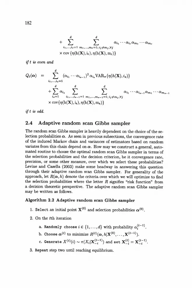
2 .4 A d a p t i v e r a n d o m s c a n G i b b s s a m p l e r

The random scan Gibbs sampler is heavily dependent on the choice of the selection probabilities a . As seen in previous subsections, the convergence rate of the induced Markov chain and variances of estimators based on random variates from this chain depend on a . How may we construct a general, automated routine to choose the optima/random scan Gibbs sampler in terms of the selection probabilities and the decision criterion, be it convergence rate, precision, or some other measure, over which we select these probabilities? Levine and Casella (2003) make some headway in answering this question through their adaptive random scan Gibbs sampler. For generality of the approach, let R(cz, h) denote the criteria over which we will optimize to find the selection probabilities where the letter R signifies "risk function" from a decision theoretic perspective. The adaptive random scan Gibbs sampler may be written as follows.

A l g o r i t h m 2.2 A d a p t i v e r a n d o m scan Gibbs s a m p l e r

1. Se lec t an initial point X (~ and selection probabilities ct(~


a. Randomly choose i 6 {1, . . . , d} with probability ~ t -1) .

b. Choose a(t) to minimize R (t) (cz, h]X(~ X(t-1)).

c. Generate X(O(i) ~ ~(Xi[X~ -I)) and set X(_t~ -- X~i -I).


183

In words, the adaptive random scan Gibbs sampler in Algorithm 2.2 estimates the risk function R(a, h) and chooses a each iteration using previous Gibbs samples generated. In this sense, the random scan learns from and adapts to the random variates as the Markov chain traverses the sample space.

We propose to study two alternative objective functions or optimization criteria R(a, h) when implementing adaptive random scan Gibbs samplers: convergence rate and asymptotic variance. The convergence rate and asymptotic variance describe speed of convergence to the stationary distribution and precision of estimates from the Monte Carlo samples respectively. Mira (2001) and Besag et al. (1995) argue that the convergence rate is of impor- tance for determining an appropriate burn-in of the chain. Variance con- siderations are relevant for posterior inferences following the burn-in period. Thus we may use both of these criteria during different parts, pre and post burn-in, of our Gibbs sampling, for choosing a .

3 Gauss ian target d i s tr ibut ion

In this section, we will characterize the convergence rate and asymptotic variance of Sections 2.2 and 2.3 in the case of Gaussian target distributions. The motivation is that in many situations, the Gibbs sampler of interest may be well approximated by a Gibbs chain with an appropriate Gaussian target distribution. We may thus study the convergence rate and asymptotic variance of the induced Markov chain of interest through the approximate chain with Gaussian stationary distribution. The first subsection discusses the Gaussian approximation theory. The remaining subsections derive the convergence rates and asymptotic variance for a random scan Gibbs sampler for a Gaussian target distribution.

3 .1 G a u s s i a n approximation Normal approximations to posterior distributions has a long history dating back to the work of Laplace in the 18th and early 19th centuries (see Chap- ter 5.3 of Bernardo and Smith, 1994, for relevant historical references from the time of Laplace to the present). The literature focuses on regularity conditions under which such an approximation holds. We require conditions under which not only the posterior distribution of interest is approximately normal, but the properties of the Markov chain induced by our Gibbs sampler is well approximated by the convergence properties of the Markov chain Monte Carlo for sampling from the Gaussian approximation. We first introduce some notation in order to formally clarify this idea.

Assume interest lies in a d-dimensional parameter X characterizing a probability model p(Y[X) from which we observe the n data points Y1, �9 �9 �9 Y~. We consider the case of implementing a Gibbs sampler to generate random variates from the posterior distribution of interest pn(X[Y). The Gibbs sam-

184

pler induces a Markov chain with stationary distribution p(XlY ) by suc- cessively sampling the full conditional distributions pn(X( i ) lX_ i ,Y ). We subscript the distributions with an n to signify the dependence on a data set of size n.

Roberts and Sahu (2001) provide the conditions under which we may apply a Gaussian approximation in our setting. In particular, under regularity conditions as presented in Bernardo and Smith (1994; page 289), if for all i the full conditional distributions pn(X(i)lX_i, Y) converge pointwise and in L 1 to normal distributions, then the posterior distribution pn(O[x) is approximately normal. Furthermore, the convergence properties of the Gibbs sampler with stationary distribution pn(XIY ) may be approximated by the Gibbs sampler with the approximating normal distribution as the stationary distribution.

The regularity conditions of Bernardo and Smith (1994) and Roberts and Sahu (2001) place restrictions on the "steepness," "smoothness," and "concentration" of the posterior distribution. That is, in a neighborhood of the posterior mean, the function pn(X]Y) becomes highly peaked and behaves like a normal density. Outside this neighborhood, the probability mass must be negligible. We note too that many other regularity conditions exist for application of a asymptotic Gaussian distribution. See for example Yee et al. (2002) for references and alternative sufficient conditions.

3 .2 G a u s s i a n c a s e : R a n d o m s c a n G i b b s s a m p l e r

Let ~r(X) be a d-dimensional normal density N(0, ~E) with dispersion ]E and, without loss of generality, mean 0. The conditional distributions required by the Gibbs samplers are easily shown (Amit and Grenander, 1991) to be

X(i) [ X - i "~ N ( - Z riJ x (J) ' 1/rii) (2) rii jr

where rij is the ( i , j ) th element of R = ~-1. The Gibbs sampler discussed in Algorithm 2.1 updates each component

of X by generating a random variate from the conditional distributions X(i) l X_i , i = 1, . . . ,d . Let Di = diag(O,...,O, 1/rii,O,...,O), a d x d diagonal matrix with all entries zero except for the ith diagonal element which is 1/rii. The transition kernel and convergence of the random scan Gibbs Markov chain is described by the following theorem, a result easily proved using (2) and the theoretical construct of Liu et al. (1995). Denote the spectral radius of the transition operator F by p(F).

T h e o r e m 3.1 The Markov chains {X(i)}~=o induced by the random scan Gibbs sampler has normal transition dis tr ibut ion P(X (k) I x(k-1)) with mean

d d

~ns = ~ H a i ~ ( I - D i ~ R ) . . . ( I - D i ~ R ) X (k.1) (3) il,...,id=l j=l

185

! and dispersion E - ttRS•ttRS. Under these transition laws, the Markov chain converges geometrically to the stationary distribution N(O, ~) at rate p(FRs) where FRs corresponds to the transition operator]or the random scan scheme.

3.3 G a u s s i a n c a s e : C o n v e r g e n c e r a t e v i a m a x i m a l c o r -

r e l a t i o n

Theorem 3.1 proves geometric convergence of the Markov chain induced by the random scan Gibbs sampler, but does not provide analytic expressions for the convergence rates. The mixing properties and maximal correlation discussed in Section 2.2 establish analytic representations for these rates.

The maximal correlation

7(X(~ sup corr{t(X(~

is easily determined under normality for the random scan Gibbs sampler after noting the following. First, Sarmanov and Zaharov (1960) show that the supremum over t and s is attained by linear functions when the distribution of X (~ and X (n) is normal. Second, the covariance of two linear functions is concisely determined by the following lemma.

L e m m a 3.1 I] t(X) --- a 'X and s(X) = b ' X for some a, b E IR d, then ]or a Markov chain {X(i)}~=o with transition operator F and stationary distribution ~r -- N(O, E), cov~{t(X(~ s(X(n))} -- a 'E (Fn) 'b .

Proof: Note that E~{t(X)} = E ,{a 'X} = 0 and Er{s(X)} = E . {b 'X} -- 0. Hence covr{t(X(~ = E,{t(X(~ �9 siX(n))} = Er{t(X(~ �9 F~s(X(~ = E . { a ' X (~ (X(~ -- a 'E(F '~) 'h where the second equality follows from the definitions of the operator F and the iterative expected value (see Liu et al., 1995).

[]

The one-lag maximal correlation for the random scan Gibbs sampler, and thus the convergence rate, is as follows. Let A(A) denote the largest eigenvalue of the matrix A.

T h e o r e m 3.2 The convergence rate ]or the random scan Gibbs sampler with transition operator FRS is ARS 2 = )~(E-1/2FRsEFRsTE-1/2).

This result follows directly from a constrained maximization over the one-lag covariance term in Theorem 2.1 using Lemma 3.1. Note that the expression for ARS in Theorem 3.2 is independent of the iteration count. This fact is a consequence of reversibility of the Markov chain induced under the random sampling scheme.

Recall from Theorem 2.1, for linear functions t(X) = a 'X where a E ]R d, Ans 2 -- supa,~a= 1 corr(a'X (~ a 'X (2)), a quantity based on one coefficient a.

186

This expression may provide an alternative specification for Arts than the one derived in Theorem 3.2 where the maximum covariance with respect to two coefficients a and b is utilized�9 However, the following theorem, proven analogously to Theorem 3.2, shows no additional information is attained from this formulation.

Theo rem 3.3 I f {X(i)}~=0 is a Markov chain induced by the random scan Gibbs sampler with transition operator FRS, then for some a E ~d suPa,~a= 1 corr(a,X(0), alX(2))2 _ ~(~- I /2FRs]EFI~sT~-I /2 ) .

3.4 G a u s s i a n c a s e : C o n v e r g e n c e r a t e v i a s p e c t r a l r a d i i

The convergence rate expression obtained in Theorem 3.2 is still difficult to compute and study due to the reliance on the currently unspecified operator Fns. However, the maximal correlations are attained by linear functions corresponding to the eigenspace of the largest eigenvalue of the operator Fns. Therefore, computations utilizing these operators can be restricted to the space of linear functions. For example, the random scan operator updates X (~ to obtain a new s t a t e X (1), say, through X (1) = FRS t ( X (0)) =

d d a' ~-~il ..... id=l I-Ij=lai~ (I - D / , R ) . . . (I - DidR ) X (~ = aP/~RsX(0)�9 Since the maximum eigenvalue of FRs occurs in the space of linear functions, the

�9 d d convergence rate may then be written ARS = p ( ~ i l ..... id=l l-[j=1 ai~ ( I - D / , R ) . . . ( I - DidR)). See Amit and Grenander (1991) and Roberts and Sahu (1997) for more formal proofs of this convergence rate. This expression may be simplified through matrix manipulations�9 Amit (1996) and Roberts and Sahu (1997) find the convergence rate for the random scan under equal selection probabilities, al -- 1/d for all i, is

~ R s = p { ( 1 - dsq) d} (4)

where S = diag(1/r11,..., 1/rdd) and I is a d x d identity matrix�9 This result may be generalized to random scans with arbitrary selection probabilities�9

Theo rem 3.4 I f ~ -- diag(al , . . . ,ad), ~d__ 1 ai ---- 1, contains the selection probabilities for the random scan Gibbs sampler, then

~Rs = p{(I - ~SR)~} . (5)

Proof: The transition operator for the random scan for a single update is, according to (2), ~=, ~/(I-D/R) = I - ~ = , ~ / D i R = I - � 9 ~ = , D~R = I - @SR. Since there are d updates each iteration, the transition operator for the random Gibbs scan restricted to linear functions is (I - ~2SR) d. []

The expression for ARs in Theorem 3.4 may be more easily manipulated than the formulation in Theorem 3.2 as dependence on a is isolated to the single diagonal matrix ~ . Its application will be seen later�9

187

3 . 5 G a u s s i a n c a s e : A s y m p t o t i c v a r i a n c e

Consider a d-dimensional Ganssian random vector X with mean /z and dispersion ~ with R -- ~E -1. Let #i denote the mean for the ith component. We denote the (i, j ) t h element of ~E and R by sij and rij respectively. Let A = I - diag(r111, . . . ,rddl)R with ( i , j ) t h element A i j . Under this Ganssian distribution, we may derive the covariance lags Q k ( a ) . In this section, we will derive the first four covariance lags, k -- 1,2, 3, 4, under the assumption that interest lies in a linear function h(X) -- l~X with d-vector of coefficients 1. As we will discuss in Section 5, an order four expansion of Q(c~) reasonably balances the tradeoff of approximation accuracy and computational cost in calculating the asymptotic variances of Section 2.3. The choice of linear functions h(X) is made partially for simplicity and partially due to the optimality results of Kagan et al. (1973) for Gaussian distributions, which we will exploit in later sections.

The first four covariance lags follow directly from Theorem 2.2. Using the notation of Section 2.3, we have that

d

QI (or) -- Z aiVAR[r/(h(x), i)] i----1

d

---- Z a / l ' { I - eie~(I - A ) } ' E { I - eie~(I - A)}I i = 1

where ei = (0 , . . . 0, 1 ,0 , . . . , 0) ~ with the ith element equal to one. Addition- ally,

Ot i ,

= { a ' l l ' - a 'd iag (1 ) ( I - A)}lE{ct ' l l ' - o~'diag(1)(I - A)} '

where 1 is a d-vector of ones. The odd and even covariance lags are now easily computed by expanding

out the first two covariance lags. In particular, we have that

Q3(ol) = Z VAR ailr](h(x),i2) 12----1 i l m l

d

-- Z a j [ l ' { I + ( a j e j e ~ - d i a g ( a ) - eje~)(I - A)}] j----1

Z[I ' { I + ( a j e j e ~ - diag(ot) - eje~)(I - A)}] '

188

and

Q4( ) / dd } = VAR Z E al, ai~(h(x),i2)

kil----1 i2--~1

-- [l'{I + diag(a 2 - 2a)(I - A) - diag(o~)Adiag(c~)(I - A)}]Z

[l'{I + diag(a 2 - 2c~)(I - A) - diag(c~)Adiag(o~)(I - A)}]'

where c~ 2 represents the squaring of each element of a. 4

In the following sections, we will approximate Q(a) ~ ~-~k=1 Qk(c~) and use this function as a decision criterion to choose optimal selection probabilities in the adaptive scan.

4 Implementing the adaptive random scan Gibbs sampler

Sections 3.4 and 3.5 show that under Gaussian target distributions, the convergence rate of the induced Markov chain is available in closed form and precision measures such as the asymptotic variance (1) are computationally feasible. If the Gibbs sampler of interest may be reasonably approximated by a Markov chain with a Ganssian stationary distribution, we may use these measures to, in some sense, optimally choose selection probabilities for implementing the random scan Gibbs sampler as well as study convergence properties of the induced Markov chain. In this section, we address implementation of the random scan Gibbs sampler through development of an adaptive random scan Gibbs sampler which chooses selection probabilities a "on-the-fly." Such an algorithm automates the task of implementing the random scan Gibbs sampler and, as far as the asymptotic results of Section 3.1 takes us, will find the optimal random scan Gibbs sampler with respect to the decision criteria of choice.

The mean and dispersion of the approximating normal distribution are the mode and Hessian, evaluated at the mode, of the target distribution 7r(X) respectively. Of course, in practice, the posterior mode is typically not available to us, thus the need for MCMC estimation routines in the first place. The EM algorithm, which has been shown to have an intimate connection with the Gibbs sampler (Sahu and Roberts, 1999), presents quick methods for computing these quantities however. We thus propose the following strategy for finding the optimal random scan Gibbs sampler. In all subsequent algorithms, we will suppress dependence of conditional distributions on the observed data Y for clarity of presentation.

A lgor i thm 4.1 Adapt ive r andom scan Gibbs sampler using Gaus- sian approximations

1. Selec t an initial point X (~ and selection probabilities c~ (~

189


a. Choose c~(~) to minimize R(t)(a, hlX(~ X (t-l), N(~ (t), E(t))).

b. Randomly choose i E {1, . . . , d} with probability al t).

c. Generate X(~)(i) ~ ~ ( Z ( i ) l X ~ 7 1 ) ) and s e t X(J~ = X(J71)


The conditioning arguments in the risk function in step 2a implies that the risk function is constructed under the approximating Gaussian distribution whose parameters, the mean vector tt(t) and the dispersion E(t), are computed at the tth iteration using perhaps all random variates {X (D }j generated to that point.

Two simple modifications of Algorithm 4.1 lead to practical implementations of the routine. For the first implementation, note that, following Roberts and Sahu (2001), we can estimate the asymptotic Gaussian distribution independent of the random variates generated by the Gibbs sampler. In such a scenario, we may modify the random scan Gibbs sampler as follows.

Algor i thm 4.2 Adapt ive r a n d o m scan Gibbs sampler via Rober t s and Sahu (2001)

1. Obtain the posterior mode, X* using the EM algorithm.

2. Obtain the Hessian matrix H -- -02 log{~r(X)}/aX �9 0 X I x = x . .

3. Se lec t an initial point X (~ and selection probabilities ~(0)


a. Choose c~ (t) to minimize R (t) (o 4 hlX(~ X (t-l) , N(X*, H -1)).

b. Randomly choose i E {1,.. . ,d} with probability a~t).

c. G e n e ~ t ~ x(~)(~) ~ ~ ( x ( i ) l x ~ 7 1 ) ) and . ~ t x(J~ = x(J71~


For the second implementation, note that we do not need to perform an adaptive random scan if the objective function or decision criteria R(t) (~, hlX(0) . . . , X(t- 1), N(t t ( t ) ]E(t))) is computable independent of the random variates {X (j) }j. The idea is that we use the Gibbs sampler with approximate normal stationary distribution, for which we can compute the decision criteria, to choose the selection probabilities and then implement the Gibbs sampler of interest using these pre-selected selection probabilities. In such a scenario, we may modify the random scan Gibbs sampler as follows.

190

Algorithm 4.3 R a n d o m scan via a Gaussian approximation

1. Obtain the posterior mode, X* using the EM algorithm.

2. 0b ta in the Hessian matrix H = -02 log{r (X)} /0X, a S I X = X . .

3. Choose (~(t) to minimize R(~, hlN(X*, H- l ) ) .

4. Se l ec t an initial point X (~


a. Randomly choose i E {1,. . . ,d} with probability ai;

b. Generate Z(t)(i) ,,~ 7r(Z(i)lX~[ 1)) and se t X(_~ -- X(t~ -1).


5 Examples In this section, we illustrate our results and adaptive random scan Gibbs sampler on three examples: sampling from Gaussian target distributions, studying a screening test problem, and performing Bayesian image analysis. In each case we implement a random scan with equal selection probabilities (ERS), a random scan with selection probabilities chosen to optimize the convergence rate (RRS), and a random scan with selection probabilities chosen to optimize the asymptotic variance (VRS). ERS is the sweep strategy typically used in applications of the random scan Gibbs sampler. The implementations of VRS assume a linear function of interest as in Section 3.5. This assumption is reasonable from an optimality viewpoint as linear functions are optimal among unbiased estimators of linear estimands under Gaussian target distributions (Kagan et al., 1973, Section 7.6). However, we may lift this assumption to consider alternative functions of interest. See Levine et al. (2003).

In each example, we compare the three scan strategies, ERS, RRS, and VRS, with respect to convergence rate and asymptotic variance. We also put forth the idea of implementing RRS during the burn-in phase of the Gibbs sampler and VRS during the post-processing (statistical inference) phase of the sampler.

5 .1 G a u s s i a n t a r g e t d i s t r i b u t i o n s

5.1.1 Bivariate Gaussian variates

Consider sampling from a bivariate normal distribution with mean vector zero, variances a 2 and a 2, and covariance ~-. By Theorem 3.4, the random scan Gibbs sampler has convergence rate ARs ----- ( ~ / 2 + a 2 /2+a l (~2~ -2 / (a2a~)+

191

. ~ 3/2 3/2 0 . 5 a 1 2 a 2 2 (0~1 + 0~2 -- z) a 1 a 2 �9 { 4 ~ 1 a 2 T2 + 02a22(~1 + ~ 2 ) } 1/2. T h e b e s t

random scan can be calculated by minimizing ARS over ~1 and a2 under the constraint a l + c~2 = 1. The resulting optimal random scan is the strategy with equal selection probabilities, ch -- a2 = 0.5. When the selection probabilities are equal, A R s = 0.25{1 + r / ( a x a y ) } 2 = 0.25(1 + A s s + 2 ~x/~-~s).

5.1.2 Independent Gaussian variates

Consider sampling from a d-variate normal distribution with independent components, mean vector zero, and variances al 2, a22,..., a~. Since the components are independent, the Gibbs sampler obtains samples directly from the marginal distribution. The random scan, the way we are implementing it, is penalized for not guaranteeing an update of every component each iteration. This statement can be shown as follows. Note that ARs = p{(I - ~ I I S R ) d} - -

p{(I - ~)d} since R - - E - 1 --- S -1 in this situation. Thus, the best random scheme has rate A R s = maxa{(1 - ai) d : ai E (0, 1), ~-~ai = 1} = d - d > O.

5.1.3 Equicorrelated Gaussian variates

Consider a trivarate Ganssian variable X = {X(1) ,X(2) ,X(3)} I with zero mean vector, variances (100,10,1), and covariance -0.125. We are interested in drawing inferences about h(X) 3 = ~-~i=l X ( i ) . In this section, we find the set of selection probabilities that induces a random scan Gibbs sampler with the smallest convergence rate as well as the set that induces a random scan Gibbs sampler with the smallest asymptotic variance. Unlike the derivations in last two subsections, closed form manageable expressions of the spectral radius in equation (4) and the asymptotic variance (1) are unavailable for analytic optimization. Nonetheless, we may optimize the convergence rate numerically over r

The selection probabilities that minimize the convergence rate is a R R S =

(0.32, 0.33, 0.34) for the RRS strategy. The selection probability that mini- mizes the asymptotic risk is a v R s -- (0.80, 0.10, 0.10). We take the asymptotic risk as put forth in Section 3.5 being a four term expansion of Q(a) . Our simulations indicate that the remainder term beyond this fourth term is negligible towards optimizing the random scan Gibbs sampler. We thus find that the convergence rate under VRS, RRS, and ERS is 0.74, 0.31, and 0.32 respectively. The asymptotic risk under VRS, RRS, and ERS is 226.37, 471.57, and 463.45 respectively.

Note that the RRS and ERS algorithms produce similar scans. We find this result true in all simulations and applications we have performed using the optimal random scan with respect to a convergence rate criterion. In fact, we find and postulate that (1 + AERS)(1 -- A R R S ) / { ( 1 -- AERS)(1 +

ARRS)} < 1.5. While this result is based on empirical evidence, it suggests that the ERS is sufficient for optimizing the convergence rate in that the gain in convergence speed does not outweigh the cost in finding RRS. However,

192

the asymptotic variance can be substantially reduced, even in this simple example, by applying VRS. In this case, the risk reduction between VRS and ERS is about 52%.

Our proposal in practice is then to burn-in the Gibbs sampler using ERS, in which the goal is convergence to the stationary distribution in as few iterations as possible. After burn-in, when precise inferences are of interest, apply VRS to minimize the variance of estimators of interest.

We next consider a Ganssian target distribution with equicorrelated variates studied by Roberts and Sahu (1997), in our case illustrating VRS under four dispersion structures. We assume that the mean vector in each case is zero and define B = diag{ lO, 5, ones ( l , 8)}, C = diag{ lO0, 10, ones ( l , 8)}, 5 -- {0,0.05,0.10,. . . ,0.95}, k = { -0 .95 ,0 .90 , . . . , 0 ) , and J as a matrix of all ones. The four dispersion matrices we consider are 511 = B - J / (10 + 5), 512 = B + k J / (10 + 1), 513 -- C - J / (10 + 5), and 514 = C + k J / (10 + 1). We consider the risk for estimating the linear function h(X) = ~~d=l X ( i ) .

Figure 1 displays the asymptotic variance (risk) as a function of 5 or k for each of these four scenarios. Note that VRS significantly improves upon ERS and RRS. Though not displayed here, the convergence rates for ERS and RRS differ by less than a factor of 1.5. Thus the recommendation of using random scans with equal selection probabilities put forth by Roberts and Sahu (1997) is recommended for the burn-in process as convergence to the stationary distribution is not significantly improved by alternative scan strategies. However, for drawing statistical inferences, the random scan with equal selection probabilities is not preferred in terms of estimator precision.

We finally illustrate the performance of the three scan strategies for a larger dimensional Gaussian target distribution with mean vector zero and dispersion matrix E5 = B - J / (100 + 5) where B -- dia9{lO0, ones(99, 1)}. We find that the convergence rate under VRS, RRS, and ERS is 1.00, 0.61, and 0.61 respectively. VRS is definitely not desirable in the burn-in phase and again, RRS and ERS are not different enough to warrant use of RRS. The asymptotic risk under VRS, RRS, and ERS is 5881.46, 21994.27, 25204.25 respectively. VRS shows a 73% improvement in risk over RRS.

5.2 Screening Test Problem

Joseph et al. (1995) considers the evaluation of two diagnostic tests for the determination of Strongyloides infection status among patients in which no gold standard is available. Out of 162 subjects, we observe y n -- 38 positive cases under both tests, Y12 -- 87 positive cases only under diagnostic test one, y21 = 2 positive cases only under diagnostic test two, and Y22 ---- 35 negative cases under both tests. The model assumes the number of cases under each test of these four scenarios is multinomially distributed with parameters p~j = /~i~j + (1 - /3 ) (1 - 0i)(1 - 0j), i , j = 1,2. Following Joseph et al. (1995), the five unknown parameters are assumed to have independent beta prior distributions with parameters (al , , bl~) -- (21.96, 5.49),

193

170

160

150

140

130

\ x

\ \ �9 \

0

1200

0.2 0.4 0.6 0.8

8

1150

1100

1050

1000

950

\ \

\ x

�9 . \

�9 x

, x

�9 x

�9 �9 x �9 x

0 0.2 0.4 0.6 08

200

180

160 I

1 4 0

"~ 1201

100

80

r

-1 -0.8 -0.6 -0.4 -0.2

10001

900 ]

8001

7001

8001

500 I

4OO I

300 I -1 -0.8 -0.6 - 0 4 -0.2

Figure l: Risk comparison between the three random scan strategies ERS (dotted), RRS (dashed), and VRS (solid)�9 The subplots from upper left to lower right apply these scans to ten-dimensional Ganssian target distributions with zero mean vectors and dispersions, being functions of either 5 or k, ]E1 = B - J / (10 + (f), ]E 2 = B + kJ/(10 + 1), Z3 = C - J / (10 + (f), and ]E4 = C + k J / ( 1 0 + 1) where B = diag{lO, 5, ones(1,8)} and C = diag{ lO0,10, ones(l, 8)}�9

(a2o, b2n) = (4.44,13.31), (a,o, blo) = (4.1, 1.76), (a2o, b2o) = (71.25,3.75), (a~, bE) = (1, 1). A Gibbs sampler for drawing Monte Carlo posterior inferences is easily obtained by augmenting the data with the actual disease status, categorized similarly to the observed data as z = (z11, z12, z21, z22).

Yee et al. (2002) shows that the Gaussian distribution serves as an approximate target distribution for this Gibbs sampler. We apply the routine of Section 4 to this data�9 For drawing statistical inferences, we use VRS in which we obtain a 55% reduction in risk over ERS. Interestingly, the VRS strategy draws more precise inferences than the Gibbs sampling routine of Yee et al. (2002), though we do not present the results here due to space limitations�9

194

5 .3 B a y e s i a n i m a g e a n a l y s i s

In this example, we consider dimension reduction as a means of implementing the VRS for analyzing image data. We consider modeling a temperature image over the globe from Jones et al. (1999). Our goal is to illustrate our algorithm, though the implications towards analysis of images, and high dimensional data, is apparent.

Let 0 be the true image and y be the observed image. An Ising model type of prior distribution on the p • p lattice with the inverse temperature fl > 0

is assumed where lr(0) ~ exp {-/~ )-~[ij] (0i - 0j)2}, [i, j] specifies i and J a s

in the image. Here {-/~ )-~[i,j](0i - 0j)2 } can be expressed as the neighbors

quadratic form {-/~'W/~}, where if i -- j , W(i , j) is the number of neighbors of i; if [i - J l - - 1, W ( i , j ) -- -1 ; otherwise W ( i , j ) -- O.

Each pixel i is assumed to follow an independent Gaussian distribution with mean 0i and variance a 2. Hence the posterior distribution is of the form (61y) (e)exv{-0.5 Ei(e - 2} e x v { - 0 . 5 ( o - - where E = (2/~W + I /a2) -1.

We may draw posterior inferences through an application of the random scan Gibbs sampler. Determining optimal selection probabilities through the algorithms of Section 4 may be computationally intensive for high-dimensional images. However, our experience shows that even a slight deviation from random scans with equal selection probabilities may lead to significant improvement in Monte Carlo precision, even if the scan strategy is not optimal. We thus use the structure of the image to suggest dimension reduction strategies for which implementation of VRS is computationally inexpensive.

The pairwise difference prior of Besag et al. (1995) forces symmetry in the parameters depending on their location in the image. In particular, the model assumes the covariance structure for points with the same number of neighbors are equal. We thus may group pixels into four groups depending on whether the pixel is on a corner, caddy-corner, edge, or center (see Figure 2).

We thus define four selection probabilities according to the four groups within which a pixel may lie. Assuming/~ = 0.0002 and ~ estimated from the standard deviation of our climate data, the optimal scan probabilities for the four groups based on a random scan Gibbs sampler fit to the Ising model are a = (0.08, 0.03, 0.02, 0.001). The corresponding asymptotic risk is 17032.98 improving upon ERS by 20%. This problem is small enough that we can optimize the risk over the 64 dimensional space of selection probabilities. The resulting gain in risk is minimal (less than 1%) with a substantial increase in cost (1 second versus 10 minutes). The user must be aware then of the tradeoff between computational expense and efficiency in larger dimensional problems. For a given level of coding skill, the efficiency gain may not be worth the loss in computational expense without reducing the dimension of the space of selection probabilities.

195

1 2 . * * . 2 1 2 * * * * * * 2 . . | 1 7 4 1 7 4 1 7 4 . . | 1 7 4 1 7 4 1 7 4 . . @ | . . | 1 7 4 1 7 4 1 7 4

2 . . . . . . 2 1 2 . * * . 2 1

Figure 2: Grouping of pixels according to location in an 8 • 8 image.

References

Amit, Y. (1996). Convergence Properties of the Gibbs Sampler for Perturba- tions of Gaussians. Annals of Statistics 24, 122-140.

Amit, Y. and Grenander, U. (1991). Comparing Sweep Strategies for Stochas- tic Relaxation. Journal of Multivariate Analysis 37, 197-222.

Bernardo, J. M. and Smith, A. F. M. (1994). Bayesian Theory. Wiley, New York.

Besag, J., Green, P., Higdon, D., and Mengersen, K. (1995). Bayesian Com- putation and Stochastic Systems. Statistical Science 10, 3-41.

Bradley, R. C. (1986). Basic Properties of Strong Mixing Conditions. In De- pendence in Probability and Statistics, E. Eberlein and M. S. Taqqu (Eds.). Birkhafiser. Boston.

Gelfand, A. E. and Smith, A. F. M. (1990). Sampling-Based Approaches to Calculating Marginal Densities. Journal of the American Statistical Association 85, 398-409.

Geman, S. and Geman, D. (1984). Stochastic Relaxation, Gibbs Distribu- tions, and the Bayesian Restoration of Images. IEEE Transactions on Pattern Analysis and Machine Intelligence 6, 721-741.

Jones, P. D., New, M., Parker, D. E., Martin, S., and Rigor, I. G. (1999). Surface air temperature and its changes over the past 150 years. Review of Geophysics 37, 173-199.

Joseph, L., Gyorkos, T. W., and Coupal, L. (1995). Bayesian Estimation of Disease Prevalence and Parameters for Diagnostics Tests in the Absence of a Gold Standard. American Journal of Epidemiology 141,263-272.

196

Kagan, A. M., Linnik, Yu. V., Rao, C. (1973). Characterization problems in mathematical statistics, translated from the Russian by B. Ramachan- dran. Wiley, New York.

Levine, R. A. and Casella, G. (2003). Optimizing Random Scan Gibbs Sam- plers. Lawrence Livermore National Laboratory, Livermore, CA, UCRL- JC-145679.

Levine, R. A., Yu, Z., Hanley, W. G., and Nitao, J. J. (2003). Implement- ing Componentwise Hastings Algorithms. Lawrence Livermore National Laboratory, Livermore, CA, UCRL-JC-145678.

Liu, J., Wong, W. H., and Kong, A. (1995). Correlation Structure and Con- vergence Rate of the Gibbs Sampler with Various Scans. Journal of the Royal Statistical Society, B 57, 157-169.

Metropolis, N., Rosenbluth, A. W., Rosenbluth, M. N., Teller, A. H., and Teller, E. (1953). Equation of State Calculations by Fast Computing Machines. The Journal of Chemical Physics 21, 1087-1092.

Mira, A. (2001). Ordering and Improving Performance of Monte Carlo Markov Chains. Statistical Science 16, 340-350.

Roberts, G. O. and Sahu, S. K. (2001). Approximate Predetermined Conver- gence Properties of the Gibbs Sampler. Journal of Computational and Graphical Statistics 10, 216-229.

Roberts, G. O. and Sahu, S. K. (1997). Updating Schemes, Correlation Struc- ture, Blocking and Parameterization for the Gibbs Sampler. Journal of the Royal Statistical Society, B 59 291-317.

Sahu, S. K. and Roberts, G. O. (1999). On Convergence of the EM Algorithm and the Gibbs Sampler. Statistics and Computing 9, 55-64.

Sarmanov, O. V. and Zaharov, V. K. (1960). Maximum Coefficients of Mul- tiple Correlation. Doklady Akademii Nauk SSSR 29, 269-271.

Yee, J., Johnson, W. 0., and Samaniego, F. J. (2002). Asymptotic Approx- imations to Posterior Distributions via Conditional Moment Equations. Biometrika 89, 755-767.

Documents

Implementing random scan Gibbs samplers