Embed Size (px)
Citation preview

c© 2011 Phong Vu Viet Le
EXPANSION OF BIOENERGY CROPS IN THE MIDWESTERN UNITED STATES:IMPLICATIONS FOR THE HYDROLOGIC CYCLE UNDER CLIMATE CHANGE
BY
PHONG VU VIET LE
THESIS
Submitted in partial fulfillment of the requirementsfor the degree of Master of Science in Civil Engineering
in the Graduate College of theUniversity of Illinois at Urbana-Champaign, 2011
Urbana, Illinois
Adviser:
Professor Praveen Kumar
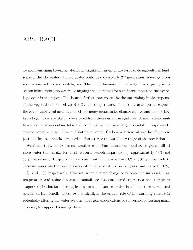
ABSTRACT
To meet emerging bioenergy demands, significant areas of the large-scale agricultural land-
scape of the Midwestern United States could be converted to 2nd generation bioenergy crops
such as miscanthus and switchgrass. Their high biomass productivity in a longer growing
season linked tightly to water use highlight the potential for significant impact on the hydro-
logic cycle in the region. This issue is further exacerbated by the uncertainty in the response
of the vegetation under elevated CO2 and temperature. This study attempts to capture
the eco-physiological acclimations of bioenergy crops under climate change and predict how
hydrologic fluxes are likely to be altered from their current magnitudes. A mechanistic mul-
tilayer canopy-root-soil model is applied for capturing the emergent vegetation responses to
environmental change. Observed data and Monte Carlo simulations of weather for recent
past and future scenarios are used to characterize the variability range of the predictions.
We found that, under present weather conditions, miscanthus and switchgrass utilized
more water than maize for total seasonal evapotranspiration by approximately 58% and
36%, respectively. Projected higher concentration of atmospheric CO2 (550 ppm) is likely to
decrease water used for evapotranspiration of miscanthus, switchgrass, and maize by 12%,
10%, and 11%, respectively. However, when climate change with projected increases in air
temperature and reduced summer rainfall are also considered, there is a net increase in
evapotranspiration for all crops, leading to significant reduction in soil-moisture storage and
specific surface runoff. These results highlight the critical role of the warming climate in
potentially altering the water cycle in the region under extensive conversion of existing maize
cropping to support bioenergy demand.
ii

...to my family
iii

ACKNOWLEDGMENTS
I would first like to thank my advisor, Prof. Praveen Kumar, whose valuable thoughts and
vision have made this thesis possible. His guidance and encouragement are also a powerful
inspiration to me. I would like to thank Dr. Darren Drewry for his advices and comments
on this thesis. I am also thankful to our team members, Prof. Murugesu Sivapalan, Sayo
Chaoka, Ciaran Harman, Hongyi Li, Juan Quijano, Venkatraman Srinivasan, Sheng Ye, and
Mary Yeager for their invaluable discussions and comments. I appreciate the support of
Prof. Carl Bernacchi and Andy VanLoocke for providing me an opportunity to gain field
experience at the Energy Farm. Thanks to the wonderful people in Hydrosystem Lab for
their friendship and supports. Finally, thanks to my family members for all their endless
love and encouragement. This thesis is dedicated to them.
This work is supported by Vietnam Education Foundation (VEF) and National Science
Foundation (grant ATM 06-28687).
iv

TABLE OF CONTENTS
LIST OF TABLES . . . . . . . . . . . . . . . . . . . . . . . . . . . . . . . . . . . . . vii
LIST OF FIGURES . . . . . . . . . . . . . . . . . . . . . . . . . . . . . . . . . . . . viii
LIST OF ABBREVIATIONS . . . . . . . . . . . . . . . . . . . . . . . . . . . . . . . xi
LIST OF SYMBOLS . . . . . . . . . . . . . . . . . . . . . . . . . . . . . . . . . . . . xii
CHAPTER 1 INTRODUCTION . . . . . . . . . . . . . . . . . . . . . . . . . . . . 1
CHAPTER 2 METHODS AND DATA DESCRIPTIONS . . . . . . . . . . . . . . . 52.1 Multi-layer canopy root soil model . . . . . . . . . . . . . . . . . . . . . . . . 52.2 Weather Generator . . . . . . . . . . . . . . . . . . . . . . . . . . . . . . . . 92.3 Data sets . . . . . . . . . . . . . . . . . . . . . . . . . . . . . . . . . . . . . 92.4 Climate change projections . . . . . . . . . . . . . . . . . . . . . . . . . . . . 132.5 Water balance . . . . . . . . . . . . . . . . . . . . . . . . . . . . . . . . . . . 142.6 Calculation of albedo . . . . . . . . . . . . . . . . . . . . . . . . . . . . . . . 14
CHAPTER 3 GRAPHIC USER INTERFACE FOR MLCAN . . . . . . . . . . . . . 153.1 Introduction . . . . . . . . . . . . . . . . . . . . . . . . . . . . . . . . . . . . 153.2 Graphic User Interface for MLCan . . . . . . . . . . . . . . . . . . . . . . . 163.3 Summary . . . . . . . . . . . . . . . . . . . . . . . . . . . . . . . . . . . . . 25
CHAPTER 4 RESULTS AND DISCUSSIONS . . . . . . . . . . . . . . . . . . . . . 274.1 MLCan model validation . . . . . . . . . . . . . . . . . . . . . . . . . . . . . 274.2 Weather Generator validation . . . . . . . . . . . . . . . . . . . . . . . . . . 304.3 Within-canopy vertical variation . . . . . . . . . . . . . . . . . . . . . . . . . 364.4 Impacts of crop type on energy balance . . . . . . . . . . . . . . . . . . . . . 384.5 Vegetation response to elevated CO2 and increased air temperature . . . . . 404.6 Sensitivity to Seasonal Variation in Photosynthetic Capacity . . . . . . . . . 414.7 Impacts on hydrology . . . . . . . . . . . . . . . . . . . . . . . . . . . . . . . 434.8 Discussion . . . . . . . . . . . . . . . . . . . . . . . . . . . . . . . . . . . . . 46
CHAPTER 5 CONCLUSIONS AND FUTURE WORKS . . . . . . . . . . . . . . . 49
CHAPTER 6 REFERENCES . . . . . . . . . . . . . . . . . . . . . . . . . . . . . . 52
v

APPENDIX A WEATHER GENERATOR . . . . . . . . . . . . . . . . . . . . . . . 57A.1 Precipitation . . . . . . . . . . . . . . . . . . . . . . . . . . . . . . . . . . . 60A.2 Cloud cover . . . . . . . . . . . . . . . . . . . . . . . . . . . . . . . . . . . . 61A.3 Shortwave radiation . . . . . . . . . . . . . . . . . . . . . . . . . . . . . . . . 63A.4 Air temperature . . . . . . . . . . . . . . . . . . . . . . . . . . . . . . . . . . 67A.5 Humidity . . . . . . . . . . . . . . . . . . . . . . . . . . . . . . . . . . . . . 68A.6 Wind speed . . . . . . . . . . . . . . . . . . . . . . . . . . . . . . . . . . . . 70
APPENDIX B SIMULATIONS FOR OTHER LOCATIONS IN MIDWESTERNUNITED STATES . . . . . . . . . . . . . . . . . . . . . . . . . . . . . . . . . . . 71B.1 Ozark Forest, Missouri . . . . . . . . . . . . . . . . . . . . . . . . . . . . . . 74B.2 Brookings, South Dakota . . . . . . . . . . . . . . . . . . . . . . . . . . . . . 76
vi

LIST OF TABLES
2.1 Projected climate change scenarios for Midwestern U.S. for 2050 during the
summer for driving MLCan model predictions [33] . . . . . . . . . . . . . . . . . 13
4.1 Value of model parameters for maize, miscanthus, and switchgrass used in the
multilayer canopy-root-soil model (MLCan) . . . . . . . . . . . . . . . . . . . . 294.2 Parameters used in the Weather Generator. . . . . . . . . . . . . . . . . . . . . 314.3 Comparison of total evapotranspiration (ET) and its component contribution
maize, miscanthus, and switchgrass under present climate condition in 2005 . . . 384.4 Comparisons of total evapotranspiration (ET) alterations (mm) under climate
change between maize, miscanthus, and switchgrass . . . . . . . . . . . . . . . . 414.5 Change of total evapotranspiration (ET ) and specific surface runoff (R) for the
two cases shown in Figure 4.11 . . . . . . . . . . . . . . . . . . . . . . . . . . . 45
A.1 Parameters for precipitation model . . . . . . . . . . . . . . . . . . . . . . . . . 57A.2 Parameters of the wind speed model . . . . . . . . . . . . . . . . . . . . . . . . 58A.3 Parameters for cloud cover, air temperature, and humidity model . . . . . . . . . 59
B.1 Comparison of total evapotranspiration (ET) and its component contribution
maize, miscanthus, and switchgrass under present climate condition in 2005 at
three locations . . . . . . . . . . . . . . . . . . . . . . . . . . . . . . . . . . . 73
vii
LIST OF FIGURES
2.1 Schematic of the canopy, root, and soil system model . . . . . . . . . . . . . . . 62.2 Leaf-level model component coupling . . . . . . . . . . . . . . . . . . . . . . . 82.3 Application of Weather Generator for developing a forcing ensemble in Bondville, IL 92.4 Ameriflux tower at Bondville, Illinois, USA. (A) Map of Ameriflux tower located
at Bondville, Central Illinois; (B) 10-meter eddy covariance flux tower in Bondville 102.5 Key meteorological forcing data observed in 2005 overlaid on an ensemble ob-
tained using the stochastic weather generator . . . . . . . . . . . . . . . . . . . 112.6 Normalized canopy leaf area density profiles (A) and normalized root fraction
in each soil layer (B) for miscanthus and switchgrass . . . . . . . . . . . . . . . 12
3.1 Main window of MLCan graphic user interface. The GUI is organized by func-
tion and task on the left. Corresponding instructions for each sub-components
are presented on the right of the main window . . . . . . . . . . . . . . . . . . . 173.2 View of Model Setup in MLCanFace. The Model Setup is comprised of 3 subsec-
tions: (i) Specifying site information; (ii) Root structure; (iii) Canopy structure.
The root and canopy structure windows are graphically supported . . . . . . . . 193.3 View of model Options in MLCanFace . . . . . . . . . . . . . . . . . . . . . . . 203.4 View of model Forcing and Initial Conditions in MLCanFace . . . . . . . . . . . 213.5 View of Leaf & Canopy (A) and Soil & Radiation (B) parameters in MLCanFace . 233.6 View of Photosynthesis (A) and Conductance & Respiration (B) parameters in
MLCanFace . . . . . . . . . . . . . . . . . . . . . . . . . . . . . . . . . . . . 243.7 Result viewer in MLCanFace . . . . . . . . . . . . . . . . . . . . . . . . . . . . 25
4.1 Comparison of half-hourly net photosynthetic leaf CO2 uptake (An) of upper
canopy sunlit leaves for miscanthus and switchgrass modeled by MLCan and
observed data . . . . . . . . . . . . . . . . . . . . . . . . . . . . . . . . . . . . 284.2 Observed and simulated mean monthly rainfall at Bondville, Illinois . . . . . . . 304.3 Observed and simulated cloud cover distribution at Bondville, Illinois . . . . . . . 334.4 Observed and simulated daily cycles of air temperature in 12 months at Bondville,
Illinois . . . . . . . . . . . . . . . . . . . . . . . . . . . . . . . . . . . . . . . 344.5 Diurnally averaged observed and simulated air temperature over 10 years (1997-
2006) at Bondville, Illinois . . . . . . . . . . . . . . . . . . . . . . . . . . . . . 354.6 The histogram of hourly wind speed from the observed and simulated data over
10 years (1997-2006) at Bondville, Illinois . . . . . . . . . . . . . . . . . . . . . 35
viii
4.7 Diurnally averaged profiles of photosynthetic rate An; latent heat LE; sensi-
ble heat H; total absorbed shortwave included photosynthetically active and
near-infrared bands Qabs; and stomatal conductance for vapor gsv for maize,
miscanthus and switchgrass under present climate condition in August 2005 . . . 374.8 Diurnal variation of mean canopy temperatures (A), temperature difference be-
tween the top layers and mean canopy (B), and albedo during the day (C) for
maize; miscanthus; and switchgrass in August 2005. Diurnally averaged change
of net-canopy fluxes and variables obtained from the MLCan model with ver-
tical bars representing ± SD over growing season of Photosynthetic rate ∆An(D); Latent heat ∆LE (E); Sensible heat ∆H (F); Leaf temperature ∆Tl (G);
Stomatal conductance for vapor ∆gsv (H) for miscanthus and switchgrass . . . . . 394.9 Diurnally averaged net-canopy fluxes and variables obtained from MLCan model
with vertical bars representing ± one SD over one growing season of (A) Pho-
tosynthetic rate An; (B) Latent heat LE; (C) Sensible heat H; (D) Leaf tem-
perature Tl; and (E) Stomatal conductance for vapor gsv for miscanthus and
switchgrass under present climate condition in 2005 . . . . . . . . . . . . . . . . 424.10 To understand the impact of seasonality of leaf photosynthetic capacity on the
results presented earlier, Vmax for maize was varied as shown here . . . . . . . . . 434.11 Diurnally averaged change of net-canopy fluxes and variables obtained for maize
during 2005 using the MLCan model with vertical bars representing ± one SD
over one growing season of (A) Photosynthetic rate An; (B) Latent heat LE;
(C) Sensible heat H; (D) Leaf temperature Tl; and (E) Stomatal conductance
for vapor gsv . . . . . . . . . . . . . . . . . . . . . . . . . . . . . . . . . . . . 444.12 Weekly mean water balance, soil water storage change, and total specific surface
runoff for 3 crops in several weeks in growing season 2005 under present CO2
condition (370 ppm) . . . . . . . . . . . . . . . . . . . . . . . . . . . . . . . . 474.13 Ensemble of total evapotranspiration (A), total soil water storage change (B),
and total specific surface runoff (C) for maize (green), miscanthus (red), and
switchgrass (blue) under present climate and eight combinations of climate
change scenarios involving expected CO2 concentration, higher air tempera-
ture, and altered precipitation magnitudes [33] . . . . . . . . . . . . . . . . . . 48
A.1 Flowchart of the dependence of variables in the Weather Generator. . . . . . . . . 58
B.1 Map of Ameriflux towers located Bondville, Illinois (red point); Ozark, Missouri
(blue point); and Brooking, South Dakota (green point) in Midwestern U.S. . . . 72B.2 Key meteorological forcing data observed in 2005 at Ameriflux tower located in
Ozark, Missouri. . . . . . . . . . . . . . . . . . . . . . . . . . . . . . . . . . . 74B.3 Diurnally averaged profiles of photosynthetic rate An; latent heat LE; sensi-
ble heat H; total absorbed shortwave included photosynthetically active and
near-infrared bands Qabs; and stomatal conductance for vapor gsv for maize,
miscanthus and switchgrass in Ozark, Missouri under present climate condition
in August 2005 . . . . . . . . . . . . . . . . . . . . . . . . . . . . . . . . . . . 75B.4 Key meteorological forcing data observed in 2005 at Ameriflux tower located in
Brookings, South Dakota. . . . . . . . . . . . . . . . . . . . . . . . . . . . . . 76
ix

B.5 Diurnally averaged profiles of photosynthetic rate An; latent heat LE; sensi-
ble heat H; total absorbed shortwave included photosynthetically active and
near-infrared bands Qabs; and stomatal conductance for vapor gsv for maize,
miscanthus and switchgrass in Brookings, South Dakota under present climate
condition in August 2005 . . . . . . . . . . . . . . . . . . . . . . . . . . . . . . 77
x

LIST OF ABBREVIATIONS
ET Evapotranspiration
FACE Free Air CO2 Enrichment
GUI Graphical User Interface
HR Hydraulic Redistribution
LAD Leaf Area Density
LAI Leaf Area Index
MLCan Multilayer canopy-root-soil model
NIR Near-infrared Radiation
PAR Photosynthetically Active Radiation
RHC Root Hydraulic Conductivity
RuBP Ribulose-1,5-bisphosphate
Rubisco RuBP carboxylase-oxygenase
SD Standard Deviation
U.S. United States
UV Ultraviolet band
VIS Visible band
WG Weather Generator
xi
LIST OF SYMBOLS
Roman
a, b Shape parameters of beta distribution
An [µmol·m−2·s−1] Photosynthetic leaf CO2 uptake
b [mol·m−2·s−1] Stomatal intercept parameter in Ball Berry model
bi (i = 0, 1, ...4) regression coefficients for deterministic hourly
temperature increment
C [mm] Condensation on the foliage
Ca [ppm] Atmospheric CO2 concentration
Ci [µmol·mol−1] Internal CO2 concentration
do [m] Leaf width
E [mm] Evaporation from the canopy
ET [mm] Total evapotranspiration
ea [kPa] Vapor pressure
fsunlit Sunlit fraction
fshaded Shaded fraction
gbh [mol·m−2·s−1] Boundary layer conductance for heat
gbv [mol·m−2·s−1] Boundary layer conductance for vapor
gs [mol·m−2·s−1] Stomatal conductance
gsv [mol·m−2·s−1] Stomatal conductance for vapor
H [W·m−2] Sensible heat
h [mm] Storm depth
hcan [m] Canopy height
Jmax,25 [µmol·m−2·s−1] maximum rate of electron transport at 25◦C
Kd Diffuse extinction coefficient
xii
k4 [mol·m−2·s−1] Initial slope of C4 photosynthetic CO2 response
kn Decay coefficient for leaf nitrogen content
LE [W·m−2] Latent heat
LWnet [W·m−2] Net longwave energy
LWP0 [g·m−2] Cloud total liquid water path for overcast conditions
M0 Mean of fair weather cloudiness
m Stomatal slope parameter in Ball Berry model
N(t) Cloud cover
P ∗ann [mm] Precipitation index in dew temperature model
PPT [mm] Precipitation
R [mm] Total specific surface runoff (per unit area)
Rd [µmol·m−2·s−1] Reference value fo leaf respiration
Rg [MJ·m−2·day−1] Global radiation
Rlw [MJ·m−2·day−1] Incident longwave radiation from atmosphere
Q10,4 Temperature sensitivity of temperature-dependent C4 pa-
rameters
Q(abs) [W·m−2] Total absorbed shortwave radiation
S [mm] Soil water storage
SE [mm] Soil evaporation
SW [W·m−2] Shortwave radiation
So [W·m−2] Solar constant
Sp [mm] Seepage
sf [MPa−1] Stomatal sensitivity parameter
Ta [◦C] Air temperature
Tl [◦C] Leaf temperature
TR [mm] Transpiration
tb [hour] Time between two successive storms
tr [hour] Storm duration
U [m·s−1] Wind speed
uo [cm] Ozone amount in a vertical column
Vmax [µmol·m−2·s−1] Reference value for substrate saturated Rubisco capacity
xiii
Ws [m·s−1] Mean wind speed
x Leaf angle distribution parameter
z [m] Vertical coordinate
Greek
α Albedo
α4 [mol·mol−1] Intrinsic quantum yield C4 photosynthesis
αL−PAR Leaf absorptivity to photosynthetic active radiation
αL−NIR Leaf absorptivity to near-infrared
β Angstrom turbidity parameter
δT [◦C] Mean of random temperature deviates
εv Leaf emissivity
γs(t) Skewness of wind speed
µb [hour] Mean time between storms
µd [mm] Mean storm depth
µr [hour] Mean storm duration
ωAi Aerosol single-scattering albedos (VIS and NIR band)
Ψf [MPa] Ψl at which half potential gs is lost
Ψl [MPa] Leaf water potential
ρg Spatial average regional albedo
ρm Lag-1 autocorrelation of fair weather cloudiness
ρs(1) Lag-1 autocorrelation of wind speed
ρδT Lag-1 autocorrelation of random temperature deviates
σ2m Variance of fair weather cloudiness
σ2δT [◦C] Variance of random temperature deviates
σ2s [m2·s−2] Variance of wind speed
τ [hour] Time lag
θ [m3·m−3] Soil moisture
ς, γ [hour−1] Cloudiness decay rate from the end of rainfall to fairweather
xiv
CHAPTER 1
INTRODUCTION
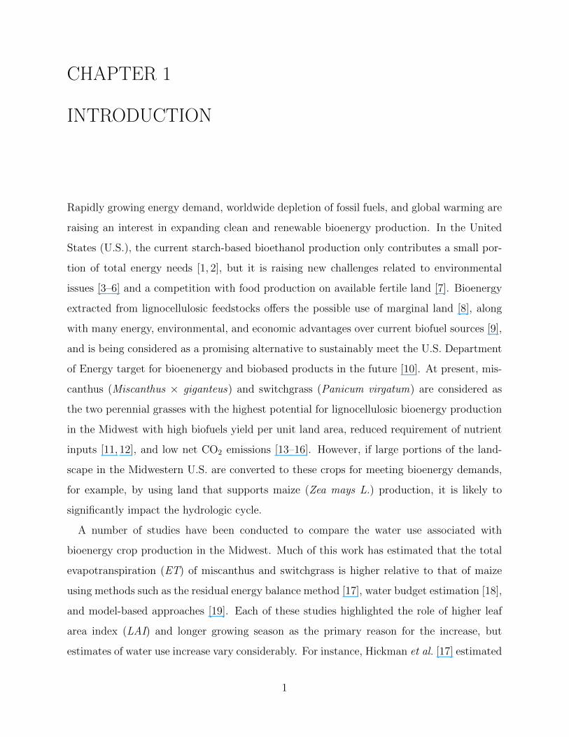
Rapidly growing energy demand, worldwide depletion of fossil fuels, and global warming are
raising an interest in expanding clean and renewable bioenergy production. In the United
States (U.S.), the current starch-based bioethanol production only contributes a small por-
tion of total energy needs [1, 2], but it is raising new challenges related to environmental
issues [3–6] and a competition with food production on available fertile land [7]. Bioenergy
extracted from lignocellulosic feedstocks offers the possible use of marginal land [8], along
with many energy, environmental, and economic advantages over current biofuel sources [9],
and is being considered as a promising alternative to sustainably meet the U.S. Department
of Energy target for bioenenergy and biobased products in the future [10]. At present, mis-
canthus (Miscanthus × giganteus) and switchgrass (Panicum virgatum) are considered as
the two perennial grasses with the highest potential for lignocellulosic bioenergy production
in the Midwest with high biofuels yield per unit land area, reduced requirement of nutrient
inputs [11, 12], and low net CO2 emissions [13–16]. However, if large portions of the land-
scape in the Midwestern U.S. are converted to these crops for meeting bioenergy demands,
for example, by using land that supports maize (Zea mays L.) production, it is likely to
significantly impact the hydrologic cycle.
A number of studies have been conducted to compare the water use associated with
bioenergy crop production in the Midwest. Much of this work has estimated that the total
evapotranspiration (ET) of miscanthus and switchgrass is higher relative to that of maize
using methods such as the residual energy balance method [17], water budget estimation [18],
and model-based approaches [19]. Each of these studies highlighted the role of higher leaf
area index (LAI) and longer growing season as the primary reason for the increase, but
estimates of water use increase vary considerably. For instance, Hickman et al. [17] estimated
1
that miscanthus and switchgrass increase total growing season ET by 343 and 153 mm
relative to maize, respectively, while McIsaac et al. [18] showed that miscanthus increases
total ET by 104 mm relative to maize, with switchgrass and maize having comparable
total ET.
The present study evaluates potential impacts of biofuel-based land use changes on the
hydrologic cycle through simultaneous considerations of (i) above-ground canopy structure
and function as a result of changes in crop type, and (ii) vegetation response to climate
change as manifested through elevated atmospheric CO2, higher temperature, and altered
precipitation magnitude. Land use conversion from maize to bioenergy crops significantly
modifies above-ground canopy structure, affecting surface hydrological cycling in several
ways. Higher LAI allows these perennial crops to intercept more rainfall before reaching
the soil, which is then lost through evaporation, in combination with evaporative losses of
increased condensation moisture on leaf surfaces [20,21]. Denser foliage will also modify the
canopy radiative regime and within-canopy micro-climate [22], impacting ET, for example,
by way of reduced soil-evaporation as a result of the reduced energy flux reaching the ground
surface [23]. While alterations in canopy structure affect energy and water partitioning above
ground, climate change is expected to trigger acclimatory responses in vegetation that lead
to the modification of eco-hydrological responses [23]. In the context of the plant acclimation
categorization presented by Drewry et al. [23], these C4 crops do not show any significant
structural (leaf area) or biochemical acclimation (photosynthetic down-regulation), with the
primary response to elevated CO2 being ecophysiological acclimation (decreased stomatal
conductance), and associated decreases in canopy-scale transpiration. This conclusion is
drawn based on Free Air CO2 Enrichment (FACE) experiments which have demonstrated a
lack of response of photosynthesis, biomass accumulation, and yield of maize under elevated
CO2 [24,25]. These experiments have also shown insensitivity of key photosynthetic enzymes
of this C4 crop to elevated CO2 [24], and have pointed to the alleviation of water stress as the
primary impact of elevated CO2 on maize productivity [26, 27], in agreement with previous
hypotheses on the impact of elevated CO2 on the functioning of C4 plants [28]. Published
results for response of miscanthus and switchgrass to elevated CO2 are not yet available. We
have therefore adopted maize response as prototypical of all three crops. Increases in air
2

temperature will likely increase ET losses, potentially offsetting the conservative impact of
reduced stomatal conductance on transpiration. The combined impact of these counteracting
effects is a complex function of the biophysical functioning of each crop type, resulting
in potentially significant changes in canopy-integrated water and heat exchange with the
atmosphere.
In this thesis, we explore the potential hydrologic change associated with simultaneous
land use conversion to bioenergy crops and projected climate change in the U.S. Midwest.
Specifically, we contrast the eco-hydrological responses of maize, the main feedstock for
current starch-based biofuel production, with miscanthus and switchgrass, through the ap-
plication of a vertically-resolved model of canopy biophysical processes. The simulations
are conducted by parameterizing a multi-layer canopy model (MLCan; [22, 23]) to account
for canopy structural and biophysical functional characteristics of miscanthus and switch-
grass. This work is performed in four stages. First, the model is run for the year 2005 when
field observations of leaf photosynthetic CO2 uptake (An), strongly correlated with water
utilization [29, 30], is available for miscanthus and switchgrass, providing data for model
validation. Second, we examine the alterations in the energy balance and canopy temper-
ature that result from the land use conversion from maize to miscanthus and switchgrass
under present climate in 2005. Third, as a single year of data does not capture the entire
range of meteorological variability in the recent past, we use a stochastic Weather Generator
(WG; [31,32]) to provide an ensemble of forcing for the model. This ensemble enables us to
examine the range of crop responses to potential meteorological forcing. In the fourth stage,
meteorological forcing ensembles are generated which capture climate variability associated
with a number of climate change scenarios projected for the U.S. Midwest for 2050 [33]. The
model is forced using each of the climate scenarios to produce variability range correspond-
ing to the hydrologic predictions associated with these future climate scenarios. We then
estimate the water use of bioenergy crops and the impact on the hydrologic cycle which is
characterized through the change in soil-water storage and specific surface runoff (runoff per
unit area).
This thesis is organized in five chapters:
3

• Chapter 2 describes the methods, models and datasets utilized in this study. We briefly
review the theoretical background of the MLCan model [22] and the WG [31, 32].
Climate change projection for Midwest region for 2050 and data are also discussed in
this chapter.
• Chapter 3 presents a graphic user interface (MLCanFace) designed for facilitating the
use of MLCan model and making it easy to use for all interested users. We show
features and processing steps in this interface to conduct simulations in MLCan.
• In Chapter 4, numerical results of the WG and MLCan model for bioenergy crops
are presented. We discuss the simultaneous impacts of land use conversion, eco-
physiological acclimation of bioenergy crops under climate change associated with
climate variability on hydrologic cycle in the Midwest.
• Chapter 5 concludes with summary and research contribution of this thesis, including
open questions that can be addressed in future work.
4
CHAPTER 2
METHODS AND DATA DESCRIPTIONS
This chapter reviews the materials and methods used in this study. In the first section
formulation of multi layer canopy-root-soil model (MLCan) described by Drewry et al. [22]
is briefly summarized and discussed. This model has been extensively validated for both
ambient and elevated CO2 conditions for maize (C4) and soybean (C3) [22,23] and is applied
for bioenergy crops throughout this research. The aim is to resolve accurately the vertical
light and thermal regimes within the canopy and representing the tight coupling between the
leaf ecophysiology, energy balance and soil moisture state required to predict the vegetation
response to environmental perturbations. We then discuss the use of a stochastic Weather
Generator (WG; [31,32]) to deal with the variability in climate. Following the presentation
of the WG, a description of data sets used for model forcing, validation and structural
information for canopy and root systems is presented. In the last three sections, climate
change projection for the Midwest for 2050 and methods for water balance and albedo
estimation are discussed.
2.1 Multi-layer canopy root soil model
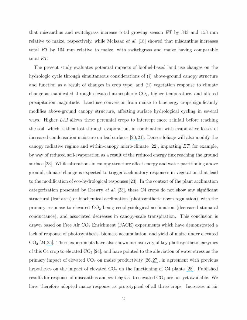
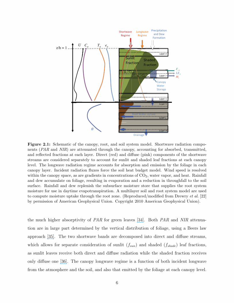
The multi layer canopy-root-soil model (MLCan) resolves the canopy radiation and meteo-
rological microenvironment and leaf-level ecophysiological states at multiple canopy levels to
determine canopy-atmosphere scalar fluxes (See [22] for further details). The model is driven
by above-canopy observations of shortwave (Rg) and longwave (Rlw) incident radiation, air
temperature (Ta), vapor pressure (ea), ambient CO2 concentration (Ca), wind speed (U)
and precipitation (PPT ) as shown in Figure 2.1. Consideration of photosynthetically ac-
tive (PAR) and near-infrared (NIR) shortwave bands separately is required to account for
5
U
!"#$%&'()*
+),-.)*
/#0,&'()*
+),-.)*
z/h = 1!Ca! Ta! ea!
!"'1)1*
2$'3%-#0*
4$'-0',)*
+##%*5'%)$*67%'8)*
/'9)$*!"
/'9)$*#"
Fc,i!
LE,i!
Hi!
/'9)$*:*
/'9)$*;*
<$)3-7-%'%-#0*
'01*4)&*
2#$.'%-#0*
/'9)$*.*
/'/'
='0#79**
5'%)$*
!%#$',)*
=
/'9)$*:*
"!
!"
2$'
!>0?-%*
2$'3%-#0*
@$%*A*,B*A*&!CB>0"
@$%*A*,B*A*&!CB"'1)"
/'9)$*:*
##%*5'%%%%)$*6666667%%%%'88888)*
/'/'99)$*;*)$*;
###%%%%%% 555555#+#++++++#
/'/'999)$*.*)$*.
Figure 2.1: Schematic of the canopy, root, and soil system model. Shortwave radiation compo-nents (PAR and NIR) are attenuated through the canopy, accounting for absorbed, transmitted,and reflected fractions at each layer. Direct (red) and diffuse (pink) components of the shortwavestreams are considered separately to account for sunlit and shaded leaf fractions at each canopylevel. The longwave radiation regime accounts for absorption and emission by the foliage in eachcanopy layer. Incident radiation fluxes force the soil heat budget model. Wind speed is resolvedwithin the canopy space, as are gradients in concentrations of CO2, water vapor, and heat. Rainfalland dew accumulate on foliage, resulting in evaporation and a reduction in throughfall to the soilsurface. Rainfall and dew replenish the subsurface moisture store that supplies the root systemmoisture for use in daytime evapotranspiration. A multilayer soil and root system model are usedto compute moisture uptake through the root zone. (Reproduced/modified from Drewry et al. [22]by permission of American Geophysical Union. Copyright 2010 American Geophysical Union).
the much higher absorptivity of PAR for green leaves [34]. Both PAR and NIR attenua-
tion are in large part determined by the vertical distribution of foliage, using a Beers law
approach [35]. The two shortwave bands are decomposed into direct and diffuse streams,
which allows for separate consideration of sunlit (fsun) and shaded (fshade) leaf fractions,
as sunlit leaves receive both direct and diffuse radiation while the shaded fraction receives
only diffuse one [36]. The canopy longwave regime is a function of both incident longwave
from the atmosphere and the soil, and also that emitted by the foliage at each canopy level.
6
The net gain in longwave energy (LWnet) at each canopy layer is the difference between the
absorbed and emitted longwave flux magnitudes.
Canopy-top observation of wind speed, air temperature and vapor pressure are applied
as upper boundary conditions for the solution of the within-canopy environment. Water
storage on foliage, as a function of dew or rainfall interception, is likewise considered [22].
Energy intercepted by wet surfaces is used for evaporation, requiring separate consideration
of the energy balance of wet leaves. Throughfall and soil surface evaporation provide the
surface flux boundary condition for the solution of soil moisture [22].
MLCan model incorporates explicit coupling between leaf-level ecophysiological processes
(photosynthesis and stomatal conductance), physical processes (energy balance and bound-
ary layer conductance), and below-ground water status which incorporates a hydraulic redis-
tribution (HR) model [37] (Figure 2.2). The dashed arrow connecting stomatal conductance
and photosynthesis signifies that this connection may not generally be important for the
determination of An in C4 plants, due to the CO2 concentrating mechanism of C4 physiology
that effectively decouples An from gs across a wide range of conditions typically experienced.
Net leaf fluxes at each canopy level are calculated as a weighted average of the sunlit and
shaded leaf fluxes and those from the wet leaf fraction. Photosynthetic capacity, as repre-
sented by the maximum rates of ribulose-1,5-bisphosphate (RuBP) regeneration and RuBP
carboxylase-oxygenase (Rubisco) catalyzed carboxylation at 25◦C (Jmax,25 and Vcmax,25, re-
spectively), declines exponentially through the canopy, affecting An and leaf respiration at
each canopy level. Canopy-scale fluxes are computed through the vertical integration over
each of the foliage layers [22].
Moisture uptake from the soil by the root system provides water for transpiration, with
soil water deficits acting to constrain leaf-level fluxes through a control on leaf water po-
tential (Ψl) that results in decreased stomatal conductance and plant gas exchange. Root
system structure, in particular the distribution of conductive elements through the soil col-
umn, acts in concert with the vertical distribution of soil moisture to determine the avail-
ability of moisture to the plant. MLCan utilizes a vertically resolved soil column, with root
conductivity distributed according to observed profiles of root biomass. Radial root con-
ductivities determine the ability of the root system to absorb moisture from the soil. The
7
Met
Forcing Fluxes
An, LE, H
Leaf EnergyBalance
Boundary Layer Conductance
BiochemicalPhotosynthesis
StomatalConductance
Leaf Ecophysiology
Tl
An
Ci
gbvgbh
Leaf Physics
Root Water Uptake
gbvTl
gs
P
Rg, Rlw
ea, Ta, U
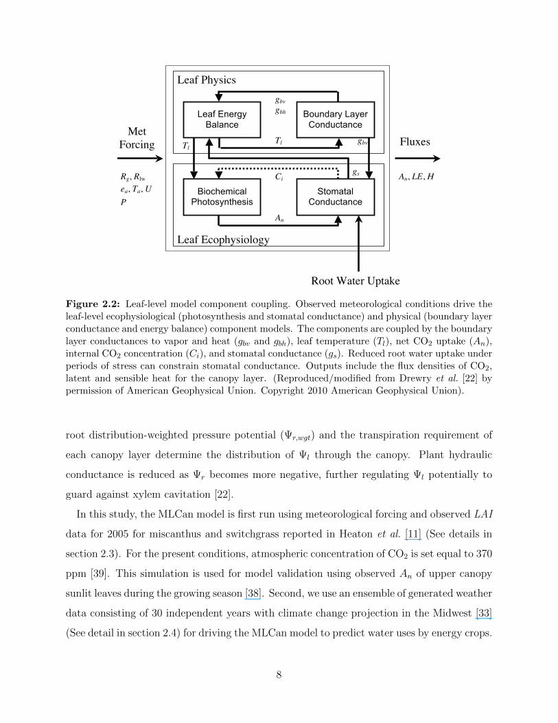
Figure 2.2: Leaf-level model component coupling. Observed meteorological conditions drive theleaf-level ecophysiological (photosynthesis and stomatal conductance) and physical (boundary layerconductance and energy balance) component models. The components are coupled by the boundarylayer conductances to vapor and heat (gbv and gbh), leaf temperature (Tl), net CO2 uptake (An),internal CO2 concentration (Ci), and stomatal conductance (gs). Reduced root water uptake underperiods of stress can constrain stomatal conductance. Outputs include the flux densities of CO2,latent and sensible heat for the canopy layer. (Reproduced/modified from Drewry et al. [22] bypermission of American Geophysical Union. Copyright 2010 American Geophysical Union).
root distribution-weighted pressure potential (Ψr,wgt) and the transpiration requirement of
each canopy layer determine the distribution of Ψl through the canopy. Plant hydraulic
conductance is reduced as Ψr becomes more negative, further regulating Ψl potentially to
guard against xylem cavitation [22].
In this study, the MLCan model is first run using meteorological forcing and observed LAI
data for 2005 for miscanthus and switchgrass reported in Heaton et al. [11] (See details in
section 2.3). For the present conditions, atmospheric concentration of CO2 is set equal to 370
ppm [39]. This simulation is used for model validation using observed An of upper canopy
sunlit leaves during the growing season [38]. Second, we use an ensemble of generated weather
data consisting of 30 independent years with climate change projection in the Midwest [33]
(See detail in section 2.4) for driving the MLCan model to predict water uses by energy crops.
8
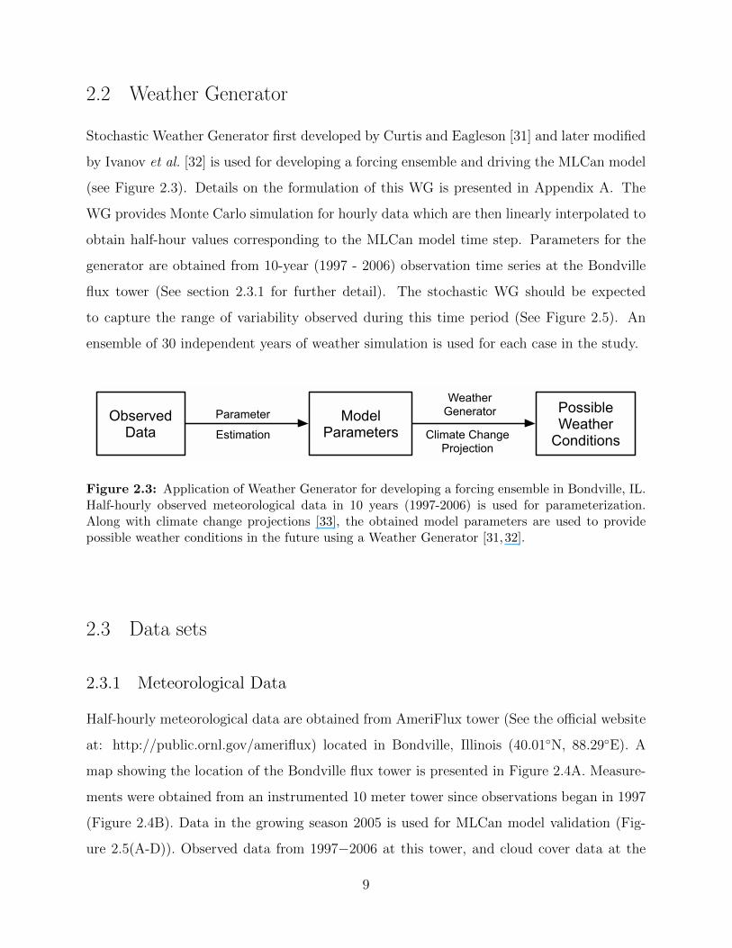
2.2 Weather Generator
Stochastic Weather Generator first developed by Curtis and Eagleson [31] and later modified
by Ivanov et al. [32] is used for developing a forcing ensemble and driving the MLCan model
(see Figure 2.3). Details on the formulation of this WG is presented in Appendix A. The
WG provides Monte Carlo simulation for hourly data which are then linearly interpolated to
obtain half-hour values corresponding to the MLCan model time step. Parameters for the
generator are obtained from 10-year (1997 - 2006) observation time series at the Bondville
flux tower (See section 2.3.1 for further detail). The stochastic WG should be expected
to capture the range of variability observed during this time period (See Figure 2.5). An
ensemble of 30 independent years of weather simulation is used for each case in the study.
Observed Data
Model Parameters
Possible Weather Conditions
Parameter
WeatherGenerator
Climate ChangeProjection
Estimation
Figure 2.3: Application of Weather Generator for developing a forcing ensemble in Bondville, IL.Half-hourly observed meteorological data in 10 years (1997-2006) is used for parameterization.Along with climate change projections [33], the obtained model parameters are used to providepossible weather conditions in the future using a Weather Generator [31,32].
2.3 Data sets
2.3.1 Meteorological Data
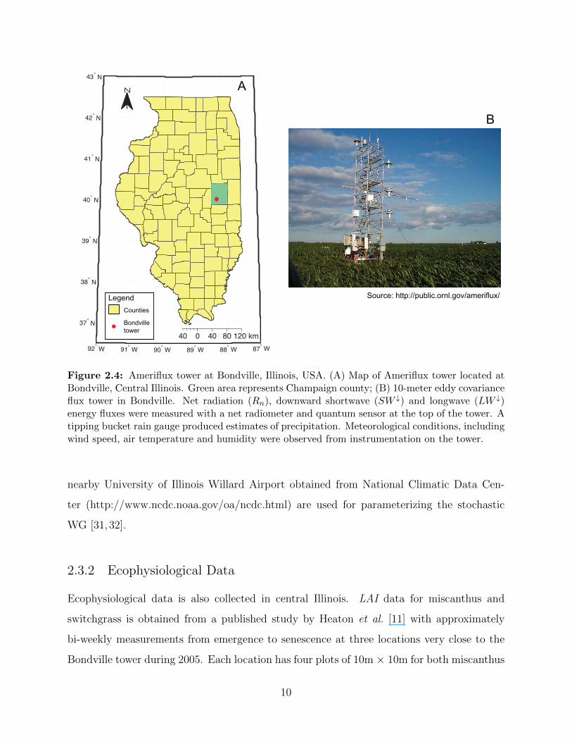
Half-hourly meteorological data are obtained from AmeriFlux tower (See the official website
at: http://public.ornl.gov/ameriflux) located in Bondville, Illinois (40.01◦N, 88.29◦E). A
map showing the location of the Bondville flux tower is presented in Figure 2.4A. Measure-
ments were obtained from an instrumented 10 meter tower since observations began in 1997
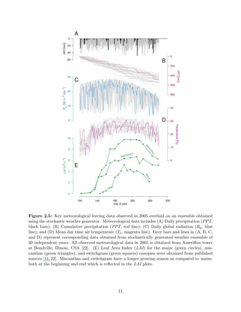
(Figure 2.4B). Data in the growing season 2005 is used for MLCan model validation (Fig-
ure 2.5(A-D)). Observed data from 1997−2006 at this tower, and cloud cover data at the
9
0 40 80 120 km40
92° W 91
° W 90
° W 89
° W 88
° W 87
° W
37° N
38° N
39° N
40° N
41° N
42° N
43° N
Legend
Counties
Bondville
tower
B
A
Source: http://public.ornl.gov/ameriflux/
Figure 2.4: Ameriflux tower at Bondville, Illinois, USA. (A) Map of Ameriflux tower located atBondville, Central Illinois. Green area represents Champaign county; (B) 10-meter eddy covarianceflux tower in Bondville. Net radiation (Rn), downward shortwave (SW ↓) and longwave (LW ↓)energy fluxes were measured with a net radiometer and quantum sensor at the top of the tower. Atipping bucket rain gauge produced estimates of precipitation. Meteorological conditions, includingwind speed, air temperature and humidity were observed from instrumentation on the tower.
nearby University of Illinois Willard Airport obtained from National Climatic Data Cen-
ter (http://www.ncdc.noaa.gov/oa/ncdc.html) are used for parameterizing the stochastic
WG [31,32].
2.3.2 Ecophysiological Data
Ecophysiological data is also collected in central Illinois. LAI data for miscanthus and
switchgrass is obtained from a published study by Heaton et al. [11] with approximately
bi-weekly measurements from emergence to senescence at three locations very close to the
Bondville tower during 2005. Each location has four plots of 10m × 10m for both miscanthus
10
0
20
40
60
[mm
]
0
200
400
600
800
[mm
]P
PT
0
10
20
30
[M
J m
−2 d
ay−
1]
0
10
20
30
40
Tem
pera
ture
[ oC]
100 140 180 220 260 300
0
2
4
6
8
10
Miscanthus
Switchgrass
Maize
[m2 m
−2]
Day of year
PP
TR
gLA
I
A
E
B
D
C
Figure 2.5: Key meteorological forcing data observed in 2005 overlaid on an ensemble obtainedusing the stochastic weather generator. Meteorological data includes (A) Daily precipitation (PPT,black bars); (B) Cumulative precipitation (PPT, red line); (C) Daily global radiation (Rg, blueline); and (D) Mean day time air temperature (Ta, magenta line). Grey bars and lines in (A, B, C,and D) represent corresponding data obtained from stochastically generated weather ensemble of30 independent years. All observed meteorological data in 2005 is obtained from Ameriflux towerat Bondville, Illinois, USA [22]. (E) Leaf Area Index (LAI) for the maize (green circles), mis-canthus (green triangles), and switchgrass (green squares) canopies were obtained from publishedsources [11, 22]. Miscanthus and switchgrass have a longer growing season as compared to maize,both at the beginning and end which is reflected in the LAI plots.
11
and switchgrass. Observations for An of upper canopy sunlit leaves are obtained from another
published study [38]. These observations were made at 2 hour intervals from pre-dawn to
post-dusk on 8 separate days across the growing season in 2005 in the same plots as studied
by Heaton et al. [11].
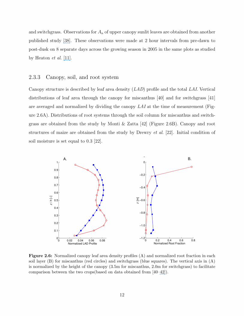
2.3.3 Canopy, soil, and root system
Canopy structure is described by leaf area density (LAD) profile and the total LAI. Vertical
distributions of leaf area through the canopy for miscanthus [40] and for switchgrass [41]
are averaged and normalized by dividing the canopy LAI at the time of measurement (Fig-
ure 2.6A). Distributions of root systems through the soil column for miscanthus and switch-
grass are obtained from the study by Monti & Zatta [42] (Figure 2.6B). Canopy and root
structures of maize are obtained from the study by Drewry et al. [22]. Initial condition of
soil moisture is set equal to 0.3 [22].
0 0.02 0.04 0.06 0.080
0.1
0.2
0.3
0.4
0.5
0.6
0.7
0.8
0.9
1
[−]
Normalized LAD Profile
A.
z /
h
0 0.2 0.4 0.6 0.8−1.2
−1.0
−0.8
−0.6
−0.4
−0.2
0
Normalized Root Fraction
[m]
B.
z
Miscanthus Switchgrass
Figure 2.6: Normalized canopy leaf area density profiles (A) and normalized root fraction in eachsoil layer (B) for miscanthus (red circles) and switchgrass (blue squares). The vertical axis in (A)is normalized by the height of the canopy (3.5m for miscanthus, 2.0m for switchgrass) to facilitatecomparison between the two crops(based on data obtained from [40–42]).
12
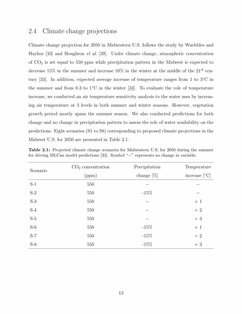
2.4 Climate change projections
Climate change projection for 2050 in Midwestern U.S. follows the study by Wuebbles and
Hayhoe [33] and Houghton et al. [39]. Under climate change, atmospheric concentration
of CO2 is set equal to 550 ppm while precipitation pattern in the Midwest is expected to
decrease 15% in the summer and increase 10% in the winter at the middle of the 21st cen-
tury [33]. In addition, expected average increase of temperature ranges from 1 to 3◦C in
the summer and from 0.3 to 1◦C in the winter [33]. To evaluate the role of temperature
increase, we conducted an air temperature sensitivity analysis to the water uses by increas-
ing air temperature at 3 levels in both summer and winter seasons. However, vegetation
growth period mostly spans the summer season. We also conducted predictions for both
change and no change in precipitation pattern to assess the role of water availability on the
predictions. Eight scenarios (S1 to S8) corresponding to proposed climate projections in the
Midwest U.S. for 2050 are presented in Table 2.1.
Table 2.1: Projected climate change scenarios for Midwestern U.S. for 2050 during the summerfor driving MLCan model predictions [33]. Symbol “−” represents no change in variable.
ScenarioCO2 concentration Precipitation Temperature
(ppm) change [%] increase [◦C]
S-1 550 − −
S-2 550 -15% −
S-3 550 − + 1
S-4 550 − + 2
S-5 550 − + 3
S-6 550 -15% + 1
S-7 550 -15% + 2
S-8 550 -15% + 3
13

2.5 Water balance
Change in soil water storages is important for evaluating the impact of different land covers
on the hydrologic cycle. It is given as:
dS
dt= P + C − TR − E − SE − SP −R (2.1)
where P , C, TR, E, SE , SP , and R represent precipitation, condensation, transpiration,
evaporation, soil evaporation, seepage, and specific surface runoff. All variables are in the
dimensions of [L / T].
2.6 Calculation of albedo
For the whole spectrum, the reflection coefficient of a natural surface is often called the
albedo [34, 43]. Its values are very important in shaping local and global climates through
the radiation budget. Albedo for each crop in this study is estimated based on the ratio of
total outgoing and incoming shortwave radiation during the daytime.
α =
∫SW ↓>40(W ·m−2)
SW ↑dt∫SW ↓>40(W ·m−2)
SW ↓dt(2.2)
α: albedo [dimensionless];
SW↓: downward or incoming shortwave radiation [W·m−2];
SW↑: upward or outgoing shortwave radiation [W·m−2].
14

CHAPTER 3
GRAPHIC USER INTERFACE FOR MLCAN
3.1 Introduction
In the previous chapter, we have described the formulation of multi layer canopy-root-soil
model (MLCan) which couples above ground ecophysiological processes with below ground
coupled soil-root moisture transport. Drewry et al. [22,23] also demonstrated the important
role of environmental driver and model skill of MLCan in capturing variability in canopy-
atmosphere fluxes exchange. Biological data (LAI) and high resolution of a range of me-
teorological data are required for driving the model. Moreover, the MLCan model requires
specification of structural characteristic of the canopy, root and soil systems to simulate
accurately the vertical variation in radiative states and scalar fluxes [22].
The lack of a friendly graphic user interface (GUI) and visualization capabilities, however,
is often a barrier to process raw input data and setup the MLCan model, and it is not
easy for an ecohydrologist with no specific training in MLCan model or a novice user to
operate it. Throughout this Chapter 3, we present a GUI that works as an additional
preprocessor for MLCan model. The aim of this GUI is to provide a better visualization
tool and to simplify significantly the processing steps in this model for all users. We show
important features of this GUI as well as basic steps to process and transfer raw input data
to the MLCan model. An independent interface that works as a post-processor for viewing
numerical results obtained from original MLCan model is also presented.
15

3.2 Graphic User Interface for MLCan
The GUI for multi layer canopy root-soil-model, MLCanFace, is developed and linked to
the original model code [22] in MATLAB (2009a, Mathworks, Natick, MA, U.S.) that can
be executed in many operating systems (e.g. Linux, Windows, Mac OS). It uses interactive
visualizations as an interface which supports MLCan users to organize data, and save and
load their work more easily. When data processing is completed, a set of processed data and
required parameters will be saved and transferred to the original MLCan model. Finally,
the MLCan model is activated to implement simulations.
The main window of MLCanFace is illustrated in Figure 3.1, showing five important sub-
components on the left side of the interface: (i) Model setup for providing general simulation
and vertical structure information; (ii) Options for selecting sub-models and simulation
modes; (iii) Forcings & Initial conditions for processing input data and initial conditions
required in MLCan model; (iv) Parameters for providing a diverse set of parameters required;
and (v) Result viewer for displaying simulation results in graphical modes. Additional menu
bar and toolbar are also integrated, providing other convenient ways for running the model.
To support new users, a short instruction summarizing basic steps in MLCanFace is presented
on the right of the main window (Figure 3.1). For further detail instructions, users can open
Help section on the menu bar.
3.2.1 Model Setup
The Model setup is comprised of 3 subsections, one for specification of geographic location
and simulation periods by mean of a threshold value in LAI data, and the other two for the
specification of root and canopy structures with plotting capabilities (Figure 3.2).
Specify Site Information
• Vegetation name: The name of simulated vegetation is provided in the Vegetation
name text box. Vegetation name is required and used for saving output files of the
MLCan model later.
16
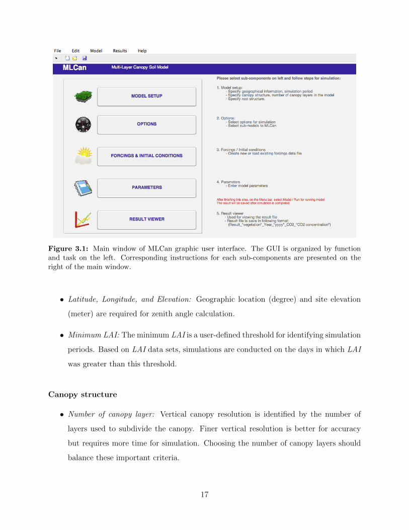
Figure 3.1: Main window of MLCan graphic user interface. The GUI is organized by functionand task on the left. Corresponding instructions for each sub-components are presented on theright of the main window.
• Latitude, Longitude, and Elevation: Geographic location (degree) and site elevation
(meter) are required for zenith angle calculation.
• Minimum LAI: The minimum LAI is a user-defined threshold for identifying simulation
periods. Based on LAI data sets, simulations are conducted on the days in which LAI
was greater than this threshold.
Canopy structure
• Number of canopy layer: Vertical canopy resolution is identified by the number of
layers used to subdivide the canopy. Finer vertical resolution is better for accuracy
but requires more time for simulation. Choosing the number of canopy layers should
balance these important criteria.
17
• Leaf Area Density (LAD) layer: LAD layer is used to describe the observed, vertical
canopy structure. The observed structure is then interpolated to match the number of
canopy layer provided above
• Input LAD profile: Users can input observed LAD profile in two different ways. The
first (manual) way is using designed table built in the interface. The second (automatic)
way is importing observed data from supporting files. The supporting files include:
Text (*.txt), Comma-separated values (*.csv), and Microsoft Excel (*.xls) files.
Root structure
• Number of root layer: Similar to canopy structure, vertical root structure is identified
by the number of root layers in the soil. Choosing the number of root layer should also
balance the accuracy and simulation time criteria.
• Input root profile: The distribution of root through the soil column is provided via two
methods. First, a logistic dose-response curve used by Schenk and Jackson [44] can be
applied. The two parameters representing 50% and 95% cumulative root distribution
and one parameter for the maximum root are required for root distribution estimation.
Second, observed data can be imported to describe the root distribution. This method
uses the same procedure including two different ways to input raw data as shown in
the Input LAD profile.
3.2.2 Options
Simulation modes and sub-models are selected in Options windows (Figure 3.3). The Pho-
tosynthesis panel allows flexibility in the choice of photosynthetic pathways, C3 or C4, in
the MLCan model. The Linear option in the Root Hydraulic Conductivity panel represents
the linear increase of root hydraulic conductivity (RHC) with soil depth. If this option is
not selected, no increase of RHC along the soil depth is applied. The Root Numerical Model
is used for selecting numerical finite difference scheme in root model. Users can select either
18

Figure 3.2: View of Model Setup in MLCanFace. The Model Setup is comprised of 3 subsections:(i) Specifying site information; (ii) Root structure; (iii) Canopy structure. The root and canopystructure windows are plotting supported.
Explicit or Implicit scheme [45] for the root model. Ca is input in the CO2 concentration
panel. Two default values for ambient condition (370 [ppm]) and elevated condition (550
[ppm]) are given for reference. However, user can easily modify Ca for their specific uses.
There are five sub-models shown in the Models panel located at the bottom-left side of the
Options window. Each sub-model is activated by checking the corresponding box. Soil Heat
Model is used for simulating the heat transfer in the soil system. The Turbulence model is
used to calculate the turbulence transport of micro-environment using a first-order canopy
closure model. Hydraulic Redistribution (HR) model simulates the nocturnal transfer of
water by roots from moist to dry regions of the soil profile. The last two Nutrient models
(Carbon and Nitrogen) are used to simulate the nutrient dynamics in soil and plant in
MLCan model. These two models are temporarily unavailable.
3.2.3 Forcings and Initial conditions
Processing input data and setting up initial conditions are most important steps in model-
ing. The Forcing & Initial conditions interface is designed to support and facilitate these
processes in MLCan model. This interface is designed in two separate tab-pages (Figure 3.4):
19
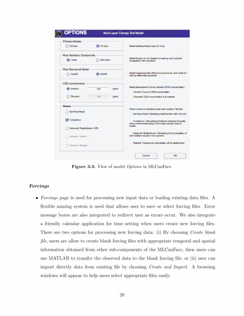
Figure 3.3: View of model Options in MLCanFace.
Forcings
• Forcings page is used for processing new input data or loading existing data files. A
flexible naming system is used that allows user to save or select forcing files. Error
message boxes are also integrated to redirect user as errors occur. We also integrate
a friendly calendar application for time setting when users create new forcing files.
There are two options for processing new forcing data: (i) By choosing Create blank
file, users are allow to create blank forcing files with appropriate temporal and spatial
information obtained from other sub-components of the MLCanFace, then users can
use MATLAB to transfer the observed data to the blank forcing file; or (ii) user can
import directly data from existing file by choosing Create and Import. A browsing
windows will appear to help users select appropriate files easily.
20
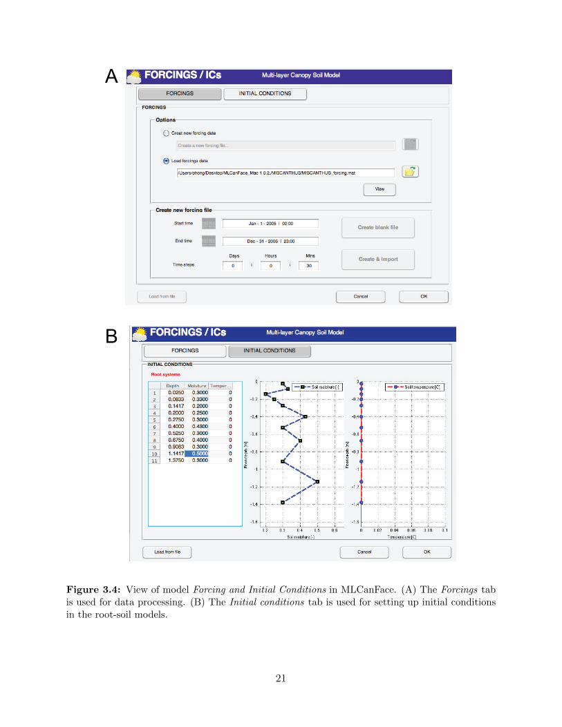
A
B
Figure 3.4: View of model Forcing and Initial Conditions in MLCanFace. (A) The Forcings tabis used for data processing. (B) The Initial conditions tab is used for setting up initial conditionsin the root-soil models.
21

• Initial conditions page is used to set up initial conditions for soil moisture and heat in
the root-soil model. The spatial discretization in the soil is obtained from the verti-
cal root profile shown in Model setup section. Users can either input initial conditions
manually or import automatically from existing data files. The supporting files also in-
clude: Text (*.txt), Comma-separated values (*.csv), and Microsoft Excel (*.xls) files.
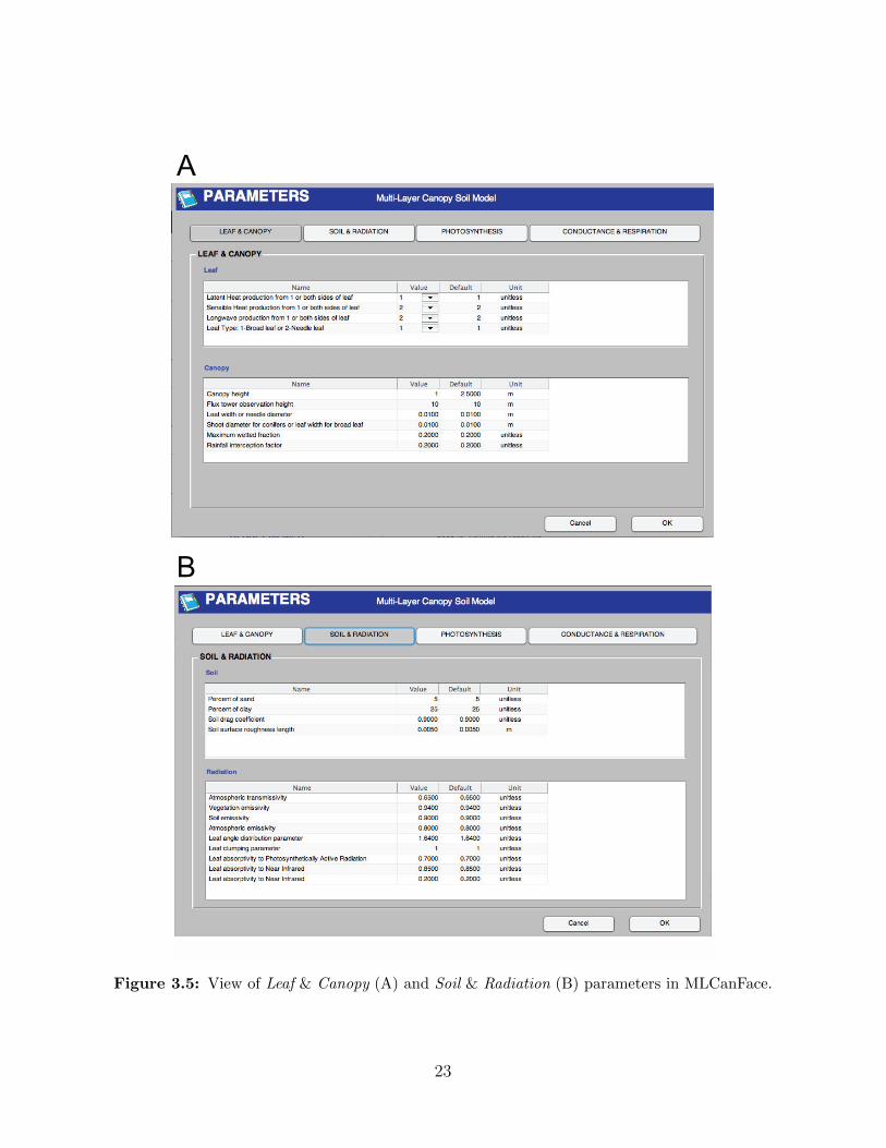
3.2.4 Parameters
Users must provide the parameters that control the simulation processes. In fact, the MLCan
model requires a large number of parameters in several categories. The Parameters window
in MLCanFace is provided to support this process in the model.
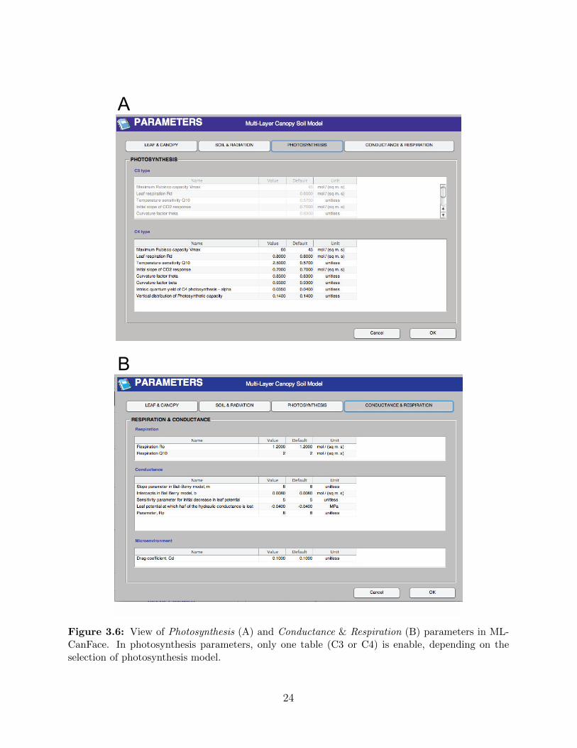
More than 40 parameters required for MLCan model are classified in four major groups:
(i) Leaf & Canopy; (ii) Soil & Radiation; (iii) Photosynthesis; and (iv) Conductance & Res-
piration (See Figure 3.5 and Figure 3.6). Each group is shown in a separate tab-page located
on the top of the interface. For example, the view of Photosynthesis parameters for both C3
and C4 plants are shown in Figure 3.5A. Only one table in photosynthesis tab-page is enable,
depending on the user’s selection for photosynthesis model in Options (See section 3.2.2). A
list of parameters used for MLCan model is described comprehensively by Drewry et al. [22].
We refer interested users to that paper for further information on model parameters.
3.2.5 Result Viewer
Presenting and plotting result are important for evaluating model simulations. An inde-
pendent Result Viewer is developed for supporting users to present the numerical results
obtained from MLCan model easily. For convenience, it is also integrated directly to the
MLCanFace (Figure 3.1).
The window of Result viewer in MLCanFace is presented in Figure 3.7. At the top of
the interface, a browsing windows is designed to allows users to select result files easily.
Information in the Load result file panel shows the name of the working file, time step, and
time that simulation is started and ended (Figure 3.7).
22
A
B
Figure 3.5: View of Leaf & Canopy (A) and Soil & Radiation (B) parameters in MLCanFace.
23
A
B
Figure 3.6: View of Photosynthesis (A) and Conductance & Respiration (B) parameters in ML-CanFace. In photosynthesis parameters, only one table (C3 or C4) is enable, depending on theselection of photosynthesis model.
24
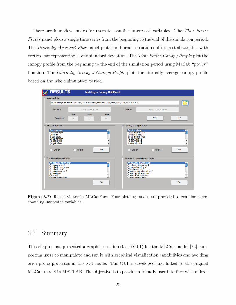
There are four view modes for users to examine interested variables. The Time Series
Fluxes panel plots a single time series from the beginning to the end of the simulation period.
The Diurnally Averaged Flux panel plot the diurnal variations of interested variable with
vertical bar representing ± one standard deviation. The Time Series Canopy Profile plot the
canopy profile from the beginning to the end of the simulation period using Matlab “pcolor”
function. The Diurnally Averaged Canopy Profile plots the diurnally average canopy profile
based on the whole simulation period.
Figure 3.7: Result viewer in MLCanFace. Four plotting modes are provided to examine corre-sponding interested variables.
3.3 Summary
This chapter has presented a graphic user interface (GUI) for the MLCan model [22], sup-
porting users to manipulate and run it with graphical visualization capabilities and avoiding
error-prone processes in the text mode. The GUI is developed and linked to the original
MLCan model in MATLAB. The objective is to provide a friendly user interface with a flexi-
25

bility in the choice of operating systems. Indeed, users can run the MLCanFace in Microsoft
Windows, Linux, or Mac OS environments.
The designed GUI works as a preprocessor as well as a post-processor for the MLCan
model. First, raw input data and parameters required are classified and processed in separate
sub-components of the GUI. General information, processed data and parameters are saved
and transferred to the original MLCan model in appropriately formatted files. The original
MLCan model is then activated to conduct simulations. Second, the GUI are also used to
analyze output files obtained from the MLCan model. Numerical results, saved in Matlab
format (*.mat) files, are loaded and transferred easily to the GUI for graphical presentations
and analyses.
There are five main sub-components in the MLCanFace, accounting for different tasks and
functions. The Model setup is used for providing general information and vertical structure
information. The second component, Options interface, is designed to select simulation
modes and sub-models. Third, the Forcing & Initial conditions interface is provided to
support input data processing and initial conditions setting. Next, the Parameters is used
to provide model parameters that control the simulation processes. Finally, the Result viewer
is designed to facilitate the result processing with four plotting modes. Each sub-component
is designed to simplify manipulations in MLCan model, avoid the error-prone process in the
text mode, and decrease the time needed to build simulations for novice users.
In general, the application of coupled canopy, leaf, root and soil processes resolved ver-
tically through the canopy and soil domains are important for simulating the vegetation
responses to climate states and perturbation. This work requires an enormous and con-
certed effort for data processing and model setup. It is expected that the MLCanFace will
be used as an useful visualization for facilitating the modeling work in MLCan model.
26
CHAPTER 4
RESULTS AND DISCUSSIONS
In this chapter, we evaluate the applications of MLCan model [22] through its GUI, pre-
sented in the previous one, for exploring the simultaneous impacts of land use conversion,
eco-physiological acclimation of bioenergy crops under climate change associated with cli-
mate variability on hydrologic cycle in Central Illinois, characterizing much of the Midwest-
ern U.S., based on collected data described in Chapter 2. We first validate the MLCan
model for two bioenergy crops and the WG [31, 32] for Ameriflux Bondville tower site, Illi-
nois. Within-canopy vertical variation and impacts of crop type on energy balance are then
discussed. We try to understand the impact of land use change to the canopy-atmosphere
exchange and energy balance. In the next section, the vegetation response to elevated CO2
and increased air temperature are examined to evaluate the impact of climate change on
vegetation response to environmental perturbations. Finally, we explore the water use of
bioenergy crops and their impacts on hydrologic cycle which is characterized through the
change in soil-water storage and specific surface runoff.
Simulations for maize, miscanthus and switchgrass for growing season in the year 2005 at
two other locations in the Midwest region: (i) Ozark, Missouri (38.74 ◦N, 92.20 ◦E) and (ii)
Brookings, South Dakota (44.34 ◦N, 96.84 ◦E) are also conducted for comparison. Details
and simulation results for those two additional sites are presented in Appendix B.
4.1 MLCan model validation
Comparisons of modeled and observed (data obtained from [38]) photosynthetic leaf CO2
uptake (An) for several days demonstrate the ability of the MLCan model to capture the
ecophysiological functioning of both miscanthus and switchgrass throughout the growing
27
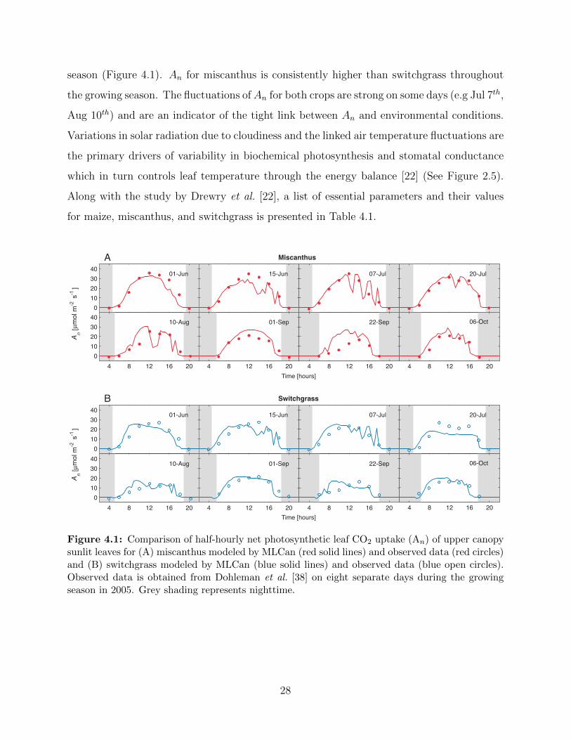
season (Figure 4.1). An for miscanthus is consistently higher than switchgrass throughout
the growing season. The fluctuations ofAn for both crops are strong on some days (e.g Jul 7th,
Aug 10th) and are an indicator of the tight link between An and environmental conditions.
Variations in solar radiation due to cloudiness and the linked air temperature fluctuations are
the primary drivers of variability in biochemical photosynthesis and stomatal conductance
which in turn controls leaf temperature through the energy balance [22] (See Figure 2.5).
Along with the study by Drewry et al. [22], a list of essential parameters and their values
for maize, miscanthus, and switchgrass is presented in Table 4.1.
0
10
20
30
4001-Jun
An [µ
mo
l m
-2 s
-1]
A Miscanthus
15-Jun 07-Jul 20-Jul
4 8 12 16 20
0
10
20
30
4010-Aug
4 8 12 16 20
01-Sep
4 8 12 16 20
22-Sep
4 8 12 16 20
06-Oct
Time [hours]
0
10
20
30
4001-Jun
An [µ
mo
l m
-2 s
-1]
B Switchgrass
15-Jun 07-Jul 20-Jul
4 8 12 16 20
0
10
20
30
4010-Aug
4 8 12 16 20
01-Sep
4 8 12 16 20
22-Sep
4 8 12 16 20
06-Oct
Time [hours]
Figure 4.1: Comparison of half-hourly net photosynthetic leaf CO2 uptake (An) of upper canopysunlit leaves for (A) miscanthus modeled by MLCan (red solid lines) and observed data (red circles)and (B) switchgrass modeled by MLCan (blue solid lines) and observed data (blue open circles).Observed data is obtained from Dohleman et al. [38] on eight separate days during the growingseason in 2005. Grey shading represents nighttime.
28
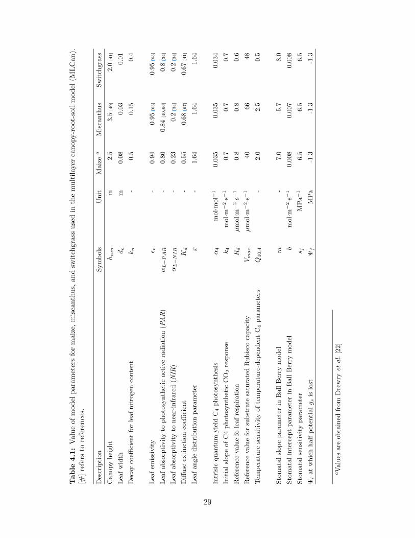
Table
4.1:
Valu
eof
mod
elp
ara
met
ers
for
mai
ze,
mis
canth
us,
and
swit
chgr
ass
use
din
the
mu
ltil
ayer
can
opy-r
oot
-soi
lm
od
el(M
LC
an).
[#]
refe
rsto
refe
ren
ces.
Des
crip
tion
Sym
bols
Un
itM
aiz
ea
Mis
canth
us
Sw
itch
gra
ss
Can
opy
hei
ght
hcan
m2.5
3.5
[40]
2.0
[41]
Lea
fw
idth
do
m0.0
80.0
30.0
1
Dec
ayco
effici
ent
for
leaf
nit
roge
nco
nte
nt
kn
-0.5
0.1
50.4
Lea
fem
issi
vit
yε v
-0.9
40.9
5[65]
0.9
5[65]
Lea
fab
sorp
tivit
yto
ph
otos
ynth
etic
acti
vera
dia
tion
(PAR
)αL−PAR
-0.8
00.8
4[40,66]
0.8
[34]
Lea
fab
sorp
tivit
yto
nea
r-in
frar
ed(N
IR)
αL−N
IR
-0.2
30.2
[34]
0.2
[34]
Diff
use
exti
nct
ion
coeffi
cien
tK
d-
0.5
50.6
8[67]
0.6
7[41]
Lea
fan
gle
dis
trib
uti
onp
aram
eter
x-
1.6
41.6
41.6
4
Intr
isic
quan
tum
yie
ldC
4p
hot
osynth
esis
α4
mol·m
ol−
10.0
35
0.0
35
0.0
34
Init
ial
slop
eof
C4
ph
otos
ynth
etic
CO
2re
spon
sek4
mol·m
−2·s−
10.7
0.7
0.7
Ref
eren
ceva
lue
fole
afre
spir
atio
nR
dµ
mol·m
−2·s−
10.8
0.8
0.6
Ref
eren
ceva
lue
for
sub
stra
tesa
tura
ted
Ru
bis
coca
paci
tyVm
ax
µm
ol·m
−2·s−
140
66
48
Tem
per
ature
sen
siti
vit
yof
tem
per
atu
re-d
epen
den
tC
4p
ara
met
ers
Q10,4
-2.0
2.5
0.5
Sto
mat
alsl
ope
par
amet
erin
Bal
lB
erry
mod
elm
-7.0
5.7
8.0
Sto
mat
alin
terc
ept
par
amet
erin
Bal
lB
erry
mod
elb
mol·m
−2·s−
10.0
08
0.0
07
0.0
08
Sto
mat
alse
nsi
tivit
yp
aram
eter
s fM
Pa−1
6.5
6.5
6.5
Ψl
atw
hic
hh
alf
pot
enti
alg s
islo
stΨ
fM
Pa
-1.3
-1.3
-1.3
aV
alu
esar
eob
tain
edfr
omD
rew
ryet
al.
[22]
29
4.2 Weather Generator validation
The performance of the WG are validated by reproducing hourly observations at Ameriflux
tower located in Bondville, Illinois. Statistics derived from hydrometeorological observed
data are compared with those obtained from a 10-year (1997-2006) simulation period by
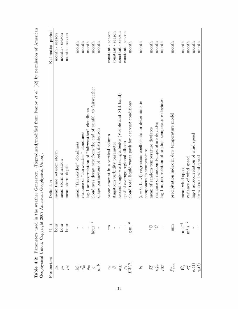
the WG. A list of model parameters used in the WG adapted from [32] is summarized in
Table 4.2. Interested readers are also referred to the study by Ivanov et al. [32] for further
details on the WG parameter information. The values of these parameters obtained from
observed data in Bondville are presented in Appendix A.
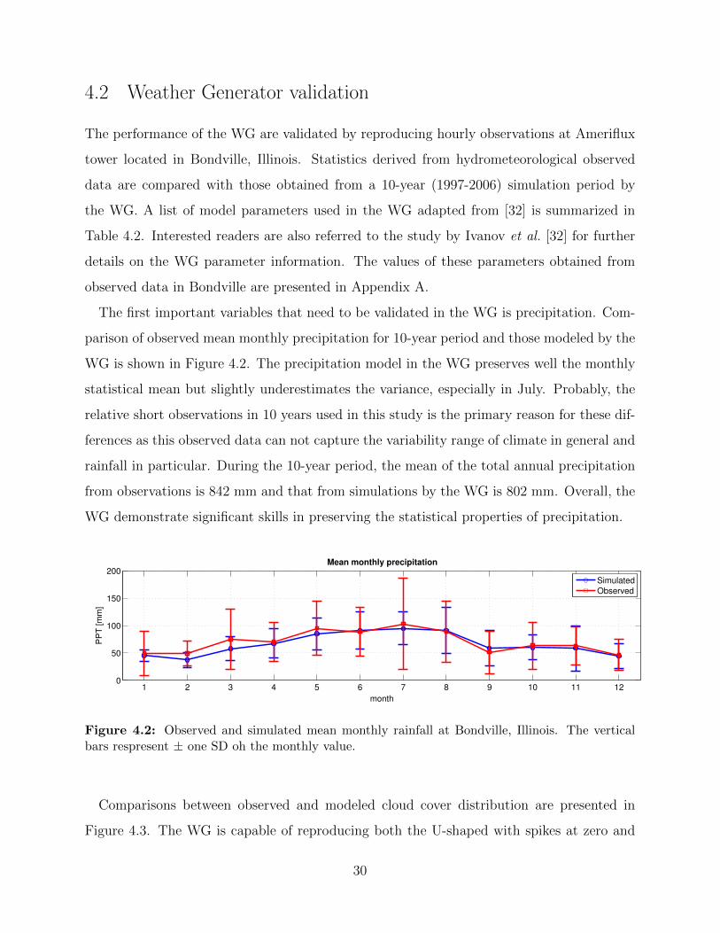
The first important variables that need to be validated in the WG is precipitation. Com-
parison of observed mean monthly precipitation for 10-year period and those modeled by the
WG is shown in Figure 4.2. The precipitation model in the WG preserves well the monthly
statistical mean but slightly underestimates the variance, especially in July. Probably, the
relative short observations in 10 years used in this study is the primary reason for these dif-
ferences as this observed data can not capture the variability range of climate in general and
rainfall in particular. During the 10-year period, the mean of the total annual precipitation
from observations is 842 mm and that from simulations by the WG is 802 mm. Overall, the
WG demonstrate significant skills in preserving the statistical properties of precipitation.
1 2 3 4 5 6 7 8 9 10 11 120
50
100
150
200
month
PP
T [m
m]
Mean monthly precipitation
Simulated
Observed
Figure 4.2: Observed and simulated mean monthly rainfall at Bondville, Illinois. The verticalbars respresent ± one SD oh the monthly value.
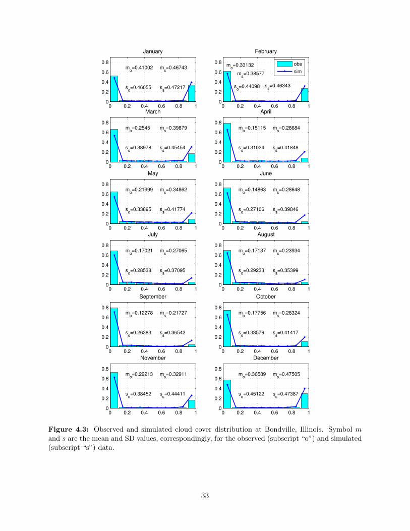
Comparisons between observed and modeled cloud cover distribution are presented in
Figure 4.3. The WG is capable of reproducing both the U-shaped with spikes at zero and
30
Table
4.2:
Para
met
ers
use
din
the
wea
ther
Gen
erat
or.
(Rep
rod
uce
d/m
od
ified
from
Ivan
ovet
al.
[32]
by
per
mis
sion
ofA
mer
ican
Geo
physi
cal
Un
ion
.C
opyri
ght
2007
Am
eric
anG
eop
hysi
cal
Un
ion
).
Para
met
ers
Un
itD
efin
itio
nE
stim
atio
np
erio
d
µb
hou
rm
ean
tim
eb
etw
een
stor
mm
onth
-se
ason
µr
hou
rm
ean
stor
md
ura
tion
mon
th-
seas
onµd
hou
rm
ean
stor
md
epth
mon
th-
seas
on
M0
-m
ean
”fai
rwea
ther
”cl
oud
ines
sm
onth
σ2 m
-va
rian
ceof
”fai
rwea
ther
”cl
oud
ines
sm
onth
ρm
-la
g-1
auto
corr
elat
ion
of”f
airw
eath
er”
clou
din
ess
mon
thς
hou
r−1
clou
din
ess
dec
ayra
tefr
omth
een
dof
rain
fall
tofa
irw
eath
erm
onth
a,b
-sh
ape
par
amet
ers
ofb
eta
dis
trib
uti
onm
onth
uo
cmoz
one
amou
nt
ina
vert
ical
colu
mn
con
stan
t-
seas
onβ
-A
ngs
trom
turb
idit
yp
aram
eter
con
stan
t-
seas
onωAi
-ae
roso
lsi
ngl
e-sc
atte
rin
gal
bed
os(V
isib
lean
dN
IRb
and
)co
nst
ant
-se
ason
ρg
-sp
atia
lav
erag
ere
gion
alal
bed
oco
nst
ant
-se
ason
LWP
0g·
m−
2cl
oud
tota
lli
quid
wat
erp
ath
forovercast
con
dit
ion
sm
onth
b i(i
=0,
1,...4
)re
gres
sion
coeffi
cien
tsfo
rdet
erm
inis
tic
mon
thco
mp
onen
tin
tem
per
atu
reδT
◦ Cm
ean
ofra
nd
omte
mp
erat
ure
dev
iate
sm
onth
σ2 δT
◦ Cva
rian
ceof
ran
dom
tem
per
atu
red
evia
tes
mon
thρδT
-la
g-1
auto
corr
elat
ion
ofra
nd
omte
mp
erat
ure
dev
iate
sm
onth
P∗ ann
mm
pre
cip
itat
ion
ind
exin
dew
tem
per
atu
rem
od
elm
onth
Ws
m·s−
1m
ean
win
dsp
eed
mon
thσ
2 sm
2·s−
2va
rian
ceof
win
dsp
eed
mon
thρs(1
)-
lag-
1au
toco
rrel
atio
nof
win
dsp
eed
mon
thγs(t
)-
skew
nes
sof
win
dsp
eed
mon
th
31

one as well as the seasonality of the process, showing a generally good agreement between
observed and modeled data. However, the WG appears to overestimate cloud cover in late
spring and early summer months (Mar to Jun) as overcast condition decreases strongly. This
discrepancy was noted by Ivanov [46] as passing atmospheric precipitation systems sometimes
does not necessarily result in rainfall at a given location. The cloud cover, however, is non-
stationary during such periods and the estimated mean can be significantly affected [46].
Simulation of air temperature should be able to capture the diurnal cycle and average
daily variability. Figure 4.4 illustrated the comparisons of simulated and observed diurnally
averaged air temperature in 12 months. The model simulates well the daily air temperature
fluctuation and seasonality. It slightly underestimates air temperature in the afternoon for
summer months, but constantly overestimates for December. The model also underestimates
the variance, especially in winter months. At monthly scale, the air temperature statistics
are well reproduced as shown in Figure 4.5, showing small discrepancy as presented in
Figure 4.4. A reasonable explanation for this discrepancy is the short observations in data
used for parameter estimation. Generally, the WG reproduces well the air temperature
during growing season for bioenergy crops which mostly spans in the summer.
Comparisons of wind speed histograms computed from observed and modeled data are
shown in Figure 4.6. The frequency distribution of wind speed data is positively skewed [32].
Both the skewness properties and the first two moments of the distribution are preserved
well in the WG.
32
0 0.2 0.4 0.6 0.8 10
0.2
0.4
0.6
0.8m
o=0.41002
so=0.46055
January
ms=0.46743
ss=0.47217
0 0.2 0.4 0.6 0.8 10
0.2
0.4
0.6
0.8m
o=0.33132
so=0.44098
February
ms=0.38577
ss=0.46343
0 0.2 0.4 0.6 0.8 10
0.2
0.4
0.6
0.8m
o=0.2545
so=0.38978
March
ms=0.39879
ss=0.45454
0 0.2 0.4 0.6 0.8 10
0.2
0.4
0.6
0.8m
o=0.15115
so=0.31024
April
ms=0.28684
ss=0.41848
0 0.2 0.4 0.6 0.8 10
0.2
0.4
0.6
0.8m
o=0.21999
so=0.33895
May
ms=0.34862
ss=0.41774
0 0.2 0.4 0.6 0.8 10
0.2
0.4
0.6
0.8m
o=0.14863
so=0.27106
June
ms=0.28648
ss=0.39846
0 0.2 0.4 0.6 0.8 10
0.2
0.4
0.6
0.8m
o=0.17021
so=0.28538
July
ms=0.27065
ss=0.37095
0 0.2 0.4 0.6 0.8 10
0.2
0.4
0.6
0.8m
o=0.17137
so=0.29233
August
ms=0.23934
ss=0.35399
0 0.2 0.4 0.6 0.8 10
0.2
0.4
0.6
0.8m
o=0.12278
so=0.26383
September
ms=0.21727
ss=0.36542
0 0.2 0.4 0.6 0.8 10
0.2
0.4
0.6
0.8m
o=0.17756
so=0.33579
October
ms=0.28324
ss=0.41417
0 0.2 0.4 0.6 0.8 10
0.2
0.4
0.6
0.8m
o=0.22213
so=0.38452
November
ms=0.32911
ss=0.44411
0 0.2 0.4 0.6 0.8 10
0.2
0.4
0.6
0.8m
o=0.36589
so=0.45122
December
ms=0.47505
ss=0.47387
obs
sim
Figure 4.3: Observed and simulated cloud cover distribution at Bondville, Illinois. Symbol mand s are the mean and SD values, correspondingly, for the observed (subscript “o”) and simulated(subscript “s”) data.
33
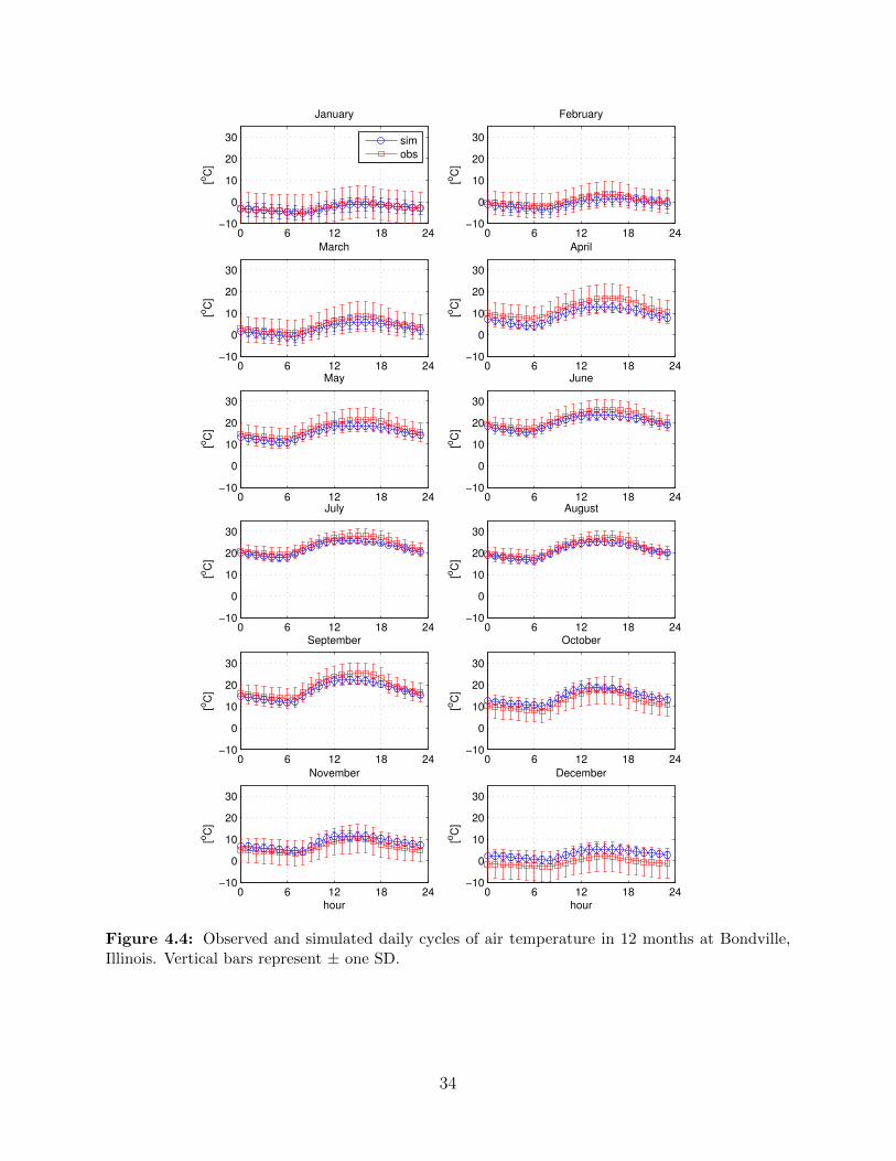
0 6 12 18 24−10
0
10
20
30
January
[oC
]
sim
obs
0 6 12 18 24−10
0
10
20
30
February
[oC
]
0 6 12 18 24−10
0
10
20
30
March
[oC
]
0 6 12 18 24−10
0
10
20
30
April
[oC
]
0 6 12 18 24−10
0
10
20
30
May
[oC
]
0 6 12 18 24−10
0
10
20
30
June
[oC
]
0 6 12 18 24−10
0
10
20
30
July
[oC
]
0 6 12 18 24−10
0
10
20
30
August
[oC
]
0 6 12 18 24−10
0
10
20
30
September
[oC
]
0 6 12 18 24−10
0
10
20
30
October
[oC
]
0 6 12 18 24−10
0
10
20
30
November
[oC
]
hour0 6 12 18 24
−10
0
10
20
30
December
[oC
]
hour
Figure 4.4: Observed and simulated daily cycles of air temperature in 12 months at Bondville,Illinois. Vertical bars represent ± one SD.
34
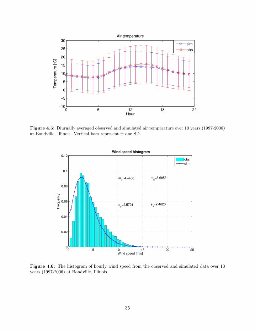
0 6 12 18 24−10
−5
0
5
10
15
20
25
30Air temperature
Hour
Te
mp
era
ture
[oC
]
sim
obs
Figure 4.5: Diurnally averaged observed and simulated air temperature over 10 years (1997-2006)at Bondville, Illinois. Vertical bars represent ± one SD.
0 5 10 15 20 250
0.02
0.04
0.06
0.08
0.1
0.12
mo=4.4468
so=2.5701
Wind speed histogram
Fre
qu
en
cy
Wind speed [m/s]
ms=3.6053
ss=2.4626
obs
sim
Figure 4.6: The histogram of hourly wind speed from the observed and simulated data over 10years (1997-2006) at Bondville, Illinois.
35
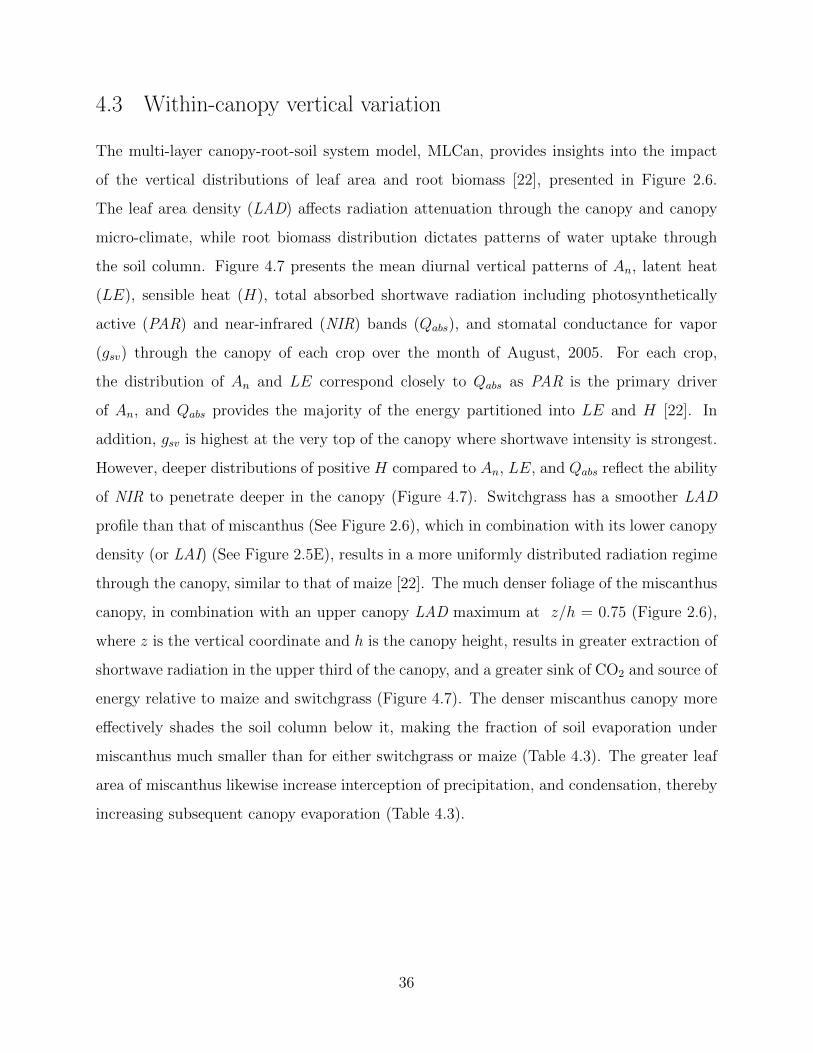
4.3 Within-canopy vertical variation
The multi-layer canopy-root-soil system model, MLCan, provides insights into the impact
of the vertical distributions of leaf area and root biomass [22], presented in Figure 2.6.
The leaf area density (LAD) affects radiation attenuation through the canopy and canopy
micro-climate, while root biomass distribution dictates patterns of water uptake through
the soil column. Figure 4.7 presents the mean diurnal vertical patterns of An, latent heat
(LE), sensible heat (H), total absorbed shortwave radiation including photosynthetically
active (PAR) and near-infrared (NIR) bands (Qabs), and stomatal conductance for vapor
(gsv) through the canopy of each crop over the month of August, 2005. For each crop,
the distribution of An and LE correspond closely to Qabs as PAR is the primary driver
of An, and Qabs provides the majority of the energy partitioned into LE and H [22]. In
addition, gsv is highest at the very top of the canopy where shortwave intensity is strongest.
However, deeper distributions of positive H compared to An, LE, and Qabs reflect the ability
of NIR to penetrate deeper in the canopy (Figure 4.7). Switchgrass has a smoother LAD
profile than that of miscanthus (See Figure 2.6), which in combination with its lower canopy
density (or LAI) (See Figure 2.5E), results in a more uniformly distributed radiation regime
through the canopy, similar to that of maize [22]. The much denser foliage of the miscanthus
canopy, in combination with an upper canopy LAD maximum at z/h = 0.75 (Figure 2.6),
where z is the vertical coordinate and h is the canopy height, results in greater extraction of
shortwave radiation in the upper third of the canopy, and a greater sink of CO2 and source of
energy relative to maize and switchgrass (Figure 4.7). The denser miscanthus canopy more
effectively shades the soil column below it, making the fraction of soil evaporation under
miscanthus much smaller than for either switchgrass or maize (Table 4.3). The greater leaf
area of miscanthus likewise increase interception of precipitation, and condensation, thereby
increasing subsequent canopy evaporation (Table 4.3).
36
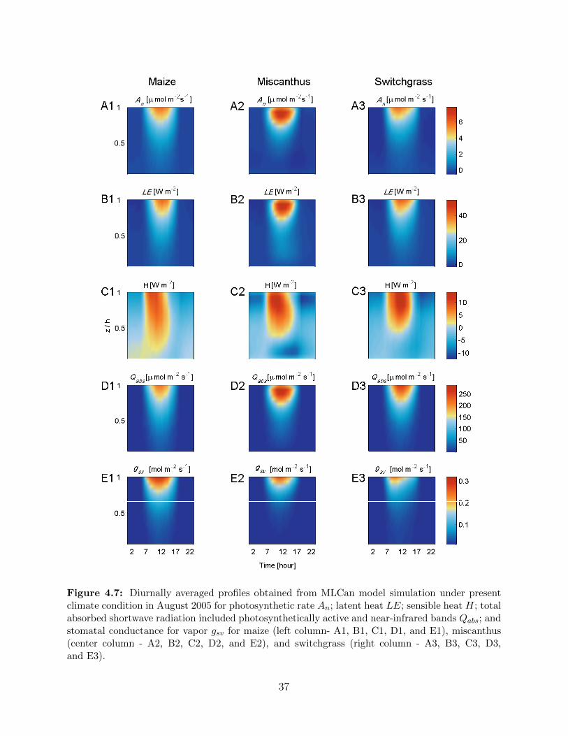
Figure 4.7: Diurnally averaged profiles obtained from MLCan model simulation under presentclimate condition in August 2005 for photosynthetic rate An; latent heat LE; sensible heat H; totalabsorbed shortwave radiation included photosynthetically active and near-infrared bands Qabs; andstomatal conductance for vapor gsv for maize (left column- A1, B1, C1, D1, and E1), miscanthus(center column - A2, B2, C2, D2, and E2), and switchgrass (right column - A3, B3, C3, D3,and E3).
37
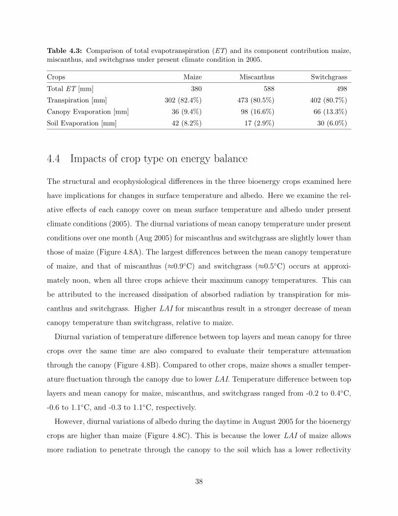
Table 4.3: Comparison of total evapotranspiration (ET) and its component contribution maize,miscanthus, and switchgrass under present climate condition in 2005.
Crops Maize Miscanthus Switchgrass
Total ET [mm] 380 588 498
Transpiration [mm] 302 (82.4%) 473 (80.5%) 402 (80.7%)
Canopy Evaporation [mm] 36 (9.4%) 98 (16.6%) 66 (13.3%)
Soil Evaporation [mm] 42 (8.2%) 17 (2.9%) 30 (6.0%)
4.4 Impacts of crop type on energy balance
The structural and ecophysiological differences in the three bioenergy crops examined here
have implications for changes in surface temperature and albedo. Here we examine the rel-
ative effects of each canopy cover on mean surface temperature and albedo under present
climate conditions (2005). The diurnal variations of mean canopy temperature under present
conditions over one month (Aug 2005) for miscanthus and switchgrass are slightly lower than
those of maize (Figure 4.8A). The largest differences between the mean canopy temperature
of maize, and that of miscanthus (≈0.9◦C) and switchgrass (≈0.5◦C) occurs at approxi-
mately noon, when all three crops achieve their maximum canopy temperatures. This can
be attributed to the increased dissipation of absorbed radiation by transpiration for mis-
canthus and switchgrass. Higher LAI for miscanthus result in a stronger decrease of mean
canopy temperature than switchgrass, relative to maize.
Diurnal variation of temperature difference between top layers and mean canopy for three
crops over the same time are also compared to evaluate their temperature attenuation
through the canopy (Figure 4.8B). Compared to other crops, maize shows a smaller temper-
ature fluctuation through the canopy due to lower LAI. Temperature difference between top
layers and mean canopy for maize, miscanthus, and switchgrass ranged from -0.2 to 0.4◦C,
-0.6 to 1.1◦C, and -0.3 to 1.1◦C, respectively.
However, diurnal variations of albedo during the daytime in August 2005 for the bioenergy
crops are higher than maize (Figure 4.8C). This is because the lower LAI of maize allows
more radiation to penetrate through the canopy to the soil which has a lower reflectivity
38
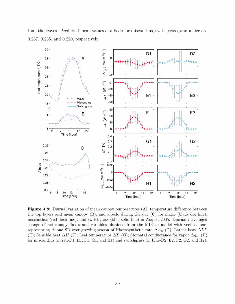
than the leaves. Predicted mean values of albedo for miscanthus, switchgrass, and maize are
0.237, 0.235, and 0.220, respectively.
−2
−1
0
1
[µm
ol m
−2s
−1]
D1 D2
−90
−60
−30
0
[W m
−2]
E1 E2
0
30
60
90
[W m
−2]
F1 F2
−0.1
0
0.1
0.2
0.3
0.4
[oC
] G1 G2
2 7 12 17 22
−0.04
−0.02
0
0.02
Time [hour]
[mol m
−2s
−1]
H1
2 7 12 17 22
Time [hour]
H2
18
20
22
24
26
28
30
A
[oC
]Leaf te
mpera
ture
Tl
2 7 12 17 22−1
0
1 B
Time [hour]
∆A
n∆
LE
∆H
∆T
l
∆g
sv
6 8 10 12 14 160.2
0.21
0.22
0.23
0.24
0.25
0.26C
Alb
edo
Time [hour]
Maize
Miscanthus
Switchgrass
Figure 4.8: Diurnal variation of mean canopy temperatures (A), temperature difference betweenthe top layers and mean canopy (B), and albedo during the day (C) for maize (black dot line);miscanthus (red dash line); and switchgrass (blue solid line) in August 2005. Diurnally averagedchange of net-canopy fluxes and variables obtained from the MLCan model with vertical barsrepresenting ± one SD over growing season of Photosynthetic rate ∆An (D); Latent heat ∆LE(E); Sensible heat ∆H (F); Leaf temperature ∆Tl (G); Stomatal conductance for vapor ∆gsv (H)for miscanthus (in red-D1, E1, F1, G1, and H1) and switchgrass (in blue-D2, E2, F2, G2, and H2).
39
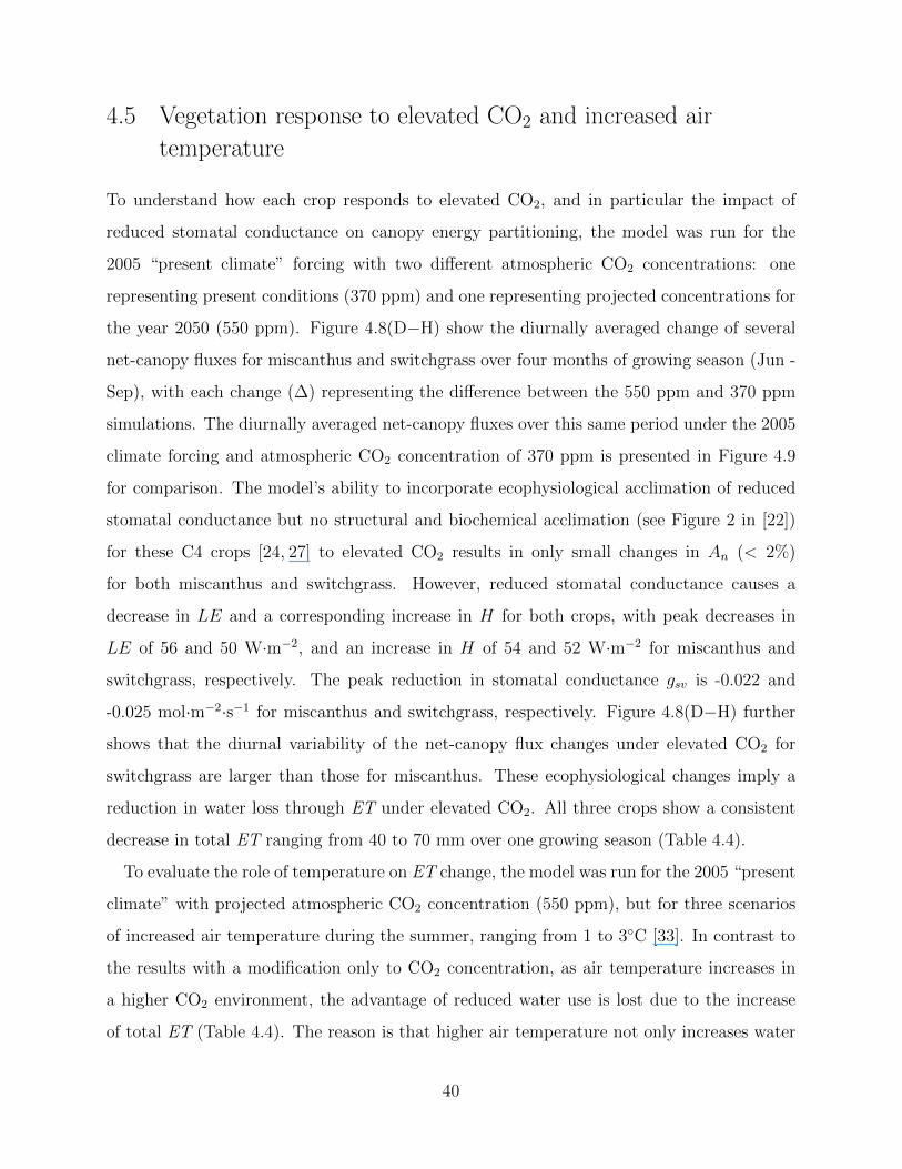
4.5 Vegetation response to elevated CO2 and increased air
temperature
To understand how each crop responds to elevated CO2, and in particular the impact of
reduced stomatal conductance on canopy energy partitioning, the model was run for the
2005 “present climate” forcing with two different atmospheric CO2 concentrations: one
representing present conditions (370 ppm) and one representing projected concentrations for
the year 2050 (550 ppm). Figure 4.8(D−H) show the diurnally averaged change of several
net-canopy fluxes for miscanthus and switchgrass over four months of growing season (Jun -
Sep), with each change (∆) representing the difference between the 550 ppm and 370 ppm
simulations. The diurnally averaged net-canopy fluxes over this same period under the 2005
climate forcing and atmospheric CO2 concentration of 370 ppm is presented in Figure 4.9
for comparison. The model’s ability to incorporate ecophysiological acclimation of reduced
stomatal conductance but no structural and biochemical acclimation (see Figure 2 in [22])
for these C4 crops [24, 27] to elevated CO2 results in only small changes in An (< 2%)
for both miscanthus and switchgrass. However, reduced stomatal conductance causes a
decrease in LE and a corresponding increase in H for both crops, with peak decreases in
LE of 56 and 50 W·m−2, and an increase in H of 54 and 52 W·m−2 for miscanthus and
switchgrass, respectively. The peak reduction in stomatal conductance gsv is -0.022 and
-0.025 mol·m−2·s−1 for miscanthus and switchgrass, respectively. Figure 4.8(D−H) further
shows that the diurnal variability of the net-canopy flux changes under elevated CO2 for
switchgrass are larger than those for miscanthus. These ecophysiological changes imply a
reduction in water loss through ET under elevated CO2. All three crops show a consistent
decrease in total ET ranging from 40 to 70 mm over one growing season (Table 4.4).
To evaluate the role of temperature on ET change, the model was run for the 2005 “present
climate” with projected atmospheric CO2 concentration (550 ppm), but for three scenarios
of increased air temperature during the summer, ranging from 1 to 3◦C [33]. In contrast to
the results with a modification only to CO2 concentration, as air temperature increases in
a higher CO2 environment, the advantage of reduced water use is lost due to the increase
of total ET (Table 4.4). The reason is that higher air temperature not only increases water
40
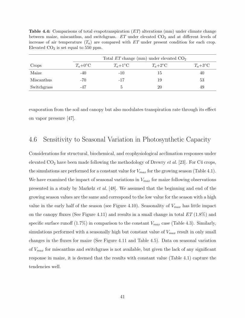
Table 4.4: Comparisons of total evapotranspiration (ET) alterations (mm) under climate changebetween maize, miscanthus, and switchgrass. ET under elevated CO2 and at different levels ofincrease of air temperature (Ta) are compared with ET under present condition for each crop.Elevated CO2 is set equal to 550 ppm.
Total ET change (mm) under elevated CO2
Crops Ta+0◦C Ta+1◦C Ta+2◦C Ta+3◦C
Maize -40 -10 15 40
Miscanthus -70 -17 19 53
Switchgrass -47 5 20 49
evaporation from the soil and canopy but also modulates transpiration rate through its effect
on vapor pressure [47].
4.6 Sensitivity to Seasonal Variation in Photosynthetic Capacity
Considerations for structural, biochemical, and ecophysiological acclimation responses under
elevated CO2 have been made following the methodology of Drewry et al. [23]. For C4 crops,
the simulations are performed for a constant value for Vmax for the growing season (Table 4.1).
We have examined the impact of seasonal variations in Vmax for maize following observations
presented in a study by Markelz et al. [48]. We assumed that the beginning and end of the
growing season values are the same and correspond to the low value for the season with a high
value in the early half of the season (see Figure 4.10). Seasonality of Vmax has little impact
on the canopy fluxes (See Figure 4.11) and results in a small change in total ET (1.8%) and
specific surface runoff (1.7%) in comparison to the constant Vmax case (Table 4.3). Similarly,
simulations performed with a seasonally high but constant value of Vmax result in only small
changes in the fluxes for maize (See Figure 4.11 and Table 4.5). Data on seasonal variation
of Vmax for miscanthus and switchgrass is not available, but given the lack of any significant
response in maize, it is deemed that the results with constant value (Table 4.1) capture the
tendencies well.
41
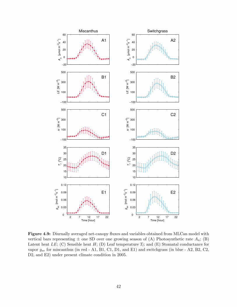
−20
0
20
40
60
[µm
ol m
−2s
−1]
Miscanthus
A1
An
−20
0
20
40
60
[µm
ol m
−2s
−1]
Switchgrass
A2
An
−100
100
300
500
[W m
−2]
B1
LE
−100
100
300
500
[W m
−2]
B2
LE
−100
100
300
500
[W m
−2]
C1
H
−100
100
300
500
[W m
−2]
C2
H
10
15
20
25
30
35
[oC
]
D1
Tl
10
15
20
25
30
35
[oC
]
D2
Tl
2 7 12 17 220
0.03
0.06
0.09
0.12
Time [hour]
[mol m
−2s
−1]
E1
gsv
2 7 12 17 220
0.03
0.06
0.09
0.12
Time [hour]
[mol m
−2s
−1]
E2
gsv
Figure 4.9: Diurnally averaged net-canopy fluxes and variables obtained from MLCan model withvertical bars representing ± one SD over one growing season of (A) Photosynthetic rate An; (B)Latent heat LE; (C) Sensible heat H; (D) Leaf temperature Tl; and (E) Stomatal conductance forvapor gsv for miscanthus (in red - A1, B1, C1, D1, and E1) and switchgrass (in blue - A2, B2, C2,D2, and E2) under present climate condition in 2005.
42
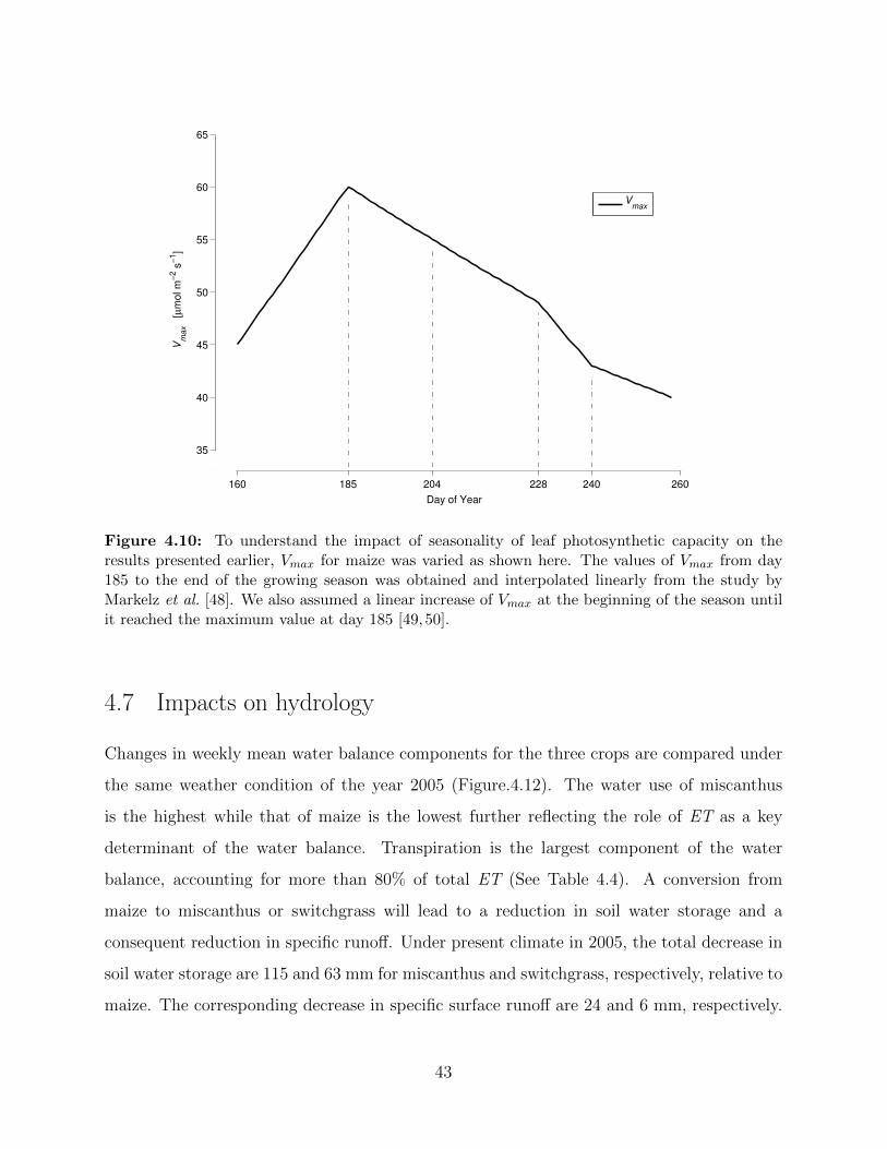
160 185 204 228 240 260
35
40
45
50
55
60
65
Day of Year
[µm
ol m
−2 s
−1]
Vm
ax
Vmax
Figure 4.10: To understand the impact of seasonality of leaf photosynthetic capacity on theresults presented earlier, Vmax for maize was varied as shown here. The values of Vmax from day185 to the end of the growing season was obtained and interpolated linearly from the study byMarkelz et al. [48]. We also assumed a linear increase of Vmax at the beginning of the season untilit reached the maximum value at day 185 [49,50].
4.7 Impacts on hydrology
Changes in weekly mean water balance components for the three crops are compared under
the same weather condition of the year 2005 (Figure.4.12). The water use of miscanthus
is the highest while that of maize is the lowest further reflecting the role of ET as a key
determinant of the water balance. Transpiration is the largest component of the water
balance, accounting for more than 80% of total ET (See Table 4.4). A conversion from
maize to miscanthus or switchgrass will lead to a reduction in soil water storage and a
consequent reduction in specific runoff. Under present climate in 2005, the total decrease in
soil water storage are 115 and 63 mm for miscanthus and switchgrass, respectively, relative to
maize. The corresponding decrease in specific surface runoff are 24 and 6 mm, respectively.
43
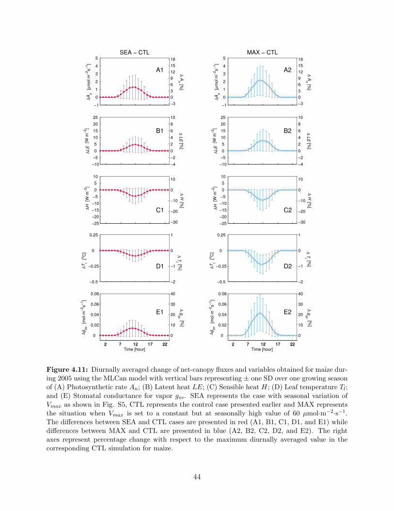
−1
0
1
2
3
4
5
[µm
ol m
−2s
−1]
SEA − CTL
A1
[%]
∆A
n
−3
0
3
6
9
12
15
18
∆ A
n
−1
0
1
2
3
4
5
[µm
ol m
−2s
−1]
MAX − CTL
A2
[%]
∆A
n
−3
0
3
6
9
12
15
18
∆ A
n
−10
−5
0
5
10
15
20
25
[W m
−2]
B1
[%]
∆L
E
−4
−2
0
2
4
6
8
10
∆ L
E
−10
−5
0
5
10
15
20
25
[W m
−2]
B2
[%]
∆L
E
−4
−2
0
2
4
6
8
10
∆ L
E
−25
−20
−15
−10
−5
0
5
10
[W m
−2]
C1[%
]
∆H
−30
−20
−10
0
10
∆ H
−25
−20
−15
−10
−5
0
5
10
[W m
−2]
C2
[%]
∆H
−30
−20
−10
0
10
∆ H
−0.5
−0.25
0
0.25
[oC
]
D1
[%]∆
Tl
−2
−1
0
1
∆ T
l
−0.5
−0.25
0
0.25
[oC
]
D2
[%]
∆T
l
−2
−1
0
1
∆ T
l
2 7 12 17 22
0
0.02
0.04
0.06
0.08
Time [hour]
[mo
l m
−2s
−1]
E1
[%]
∆g
sv
2 7 12 17 22
0
10
20
30
40
∆ g
sv
2 7 12 17 22
0
0.02
0.04
0.06
0.08
Time [hour]
[mo
l m
−2s
−1]
E2
[%]
∆g
sv
2 7 12 17 22
0
10
20
30
40
∆ g
sv
Figure 4.11: Diurnally averaged change of net-canopy fluxes and variables obtained for maize dur-ing 2005 using the MLCan model with vertical bars representing ± one SD over one growing seasonof (A) Photosynthetic rate An; (B) Latent heat LE; (C) Sensible heat H; (D) Leaf temperature Tl;and (E) Stomatal conductance for vapor gsv. SEA represents the case with seasonal variation ofVmax as shown in Fig. S5, CTL represents the control case presented earlier and MAX representsthe situation when Vmax is set to a constant but at seasonally high value of 60 µmol·m−2·s−1.The differences between SEA and CTL cases are presented in red (A1, B1, C1, D1, and E1) whiledifferences between MAX and CTL are presented in blue (A2, B2, C2, D2, and E2). The rightaxes represent percentage change with respect to the maximum diurnally averaged value in thecorresponding CTL simulation for maize.
44
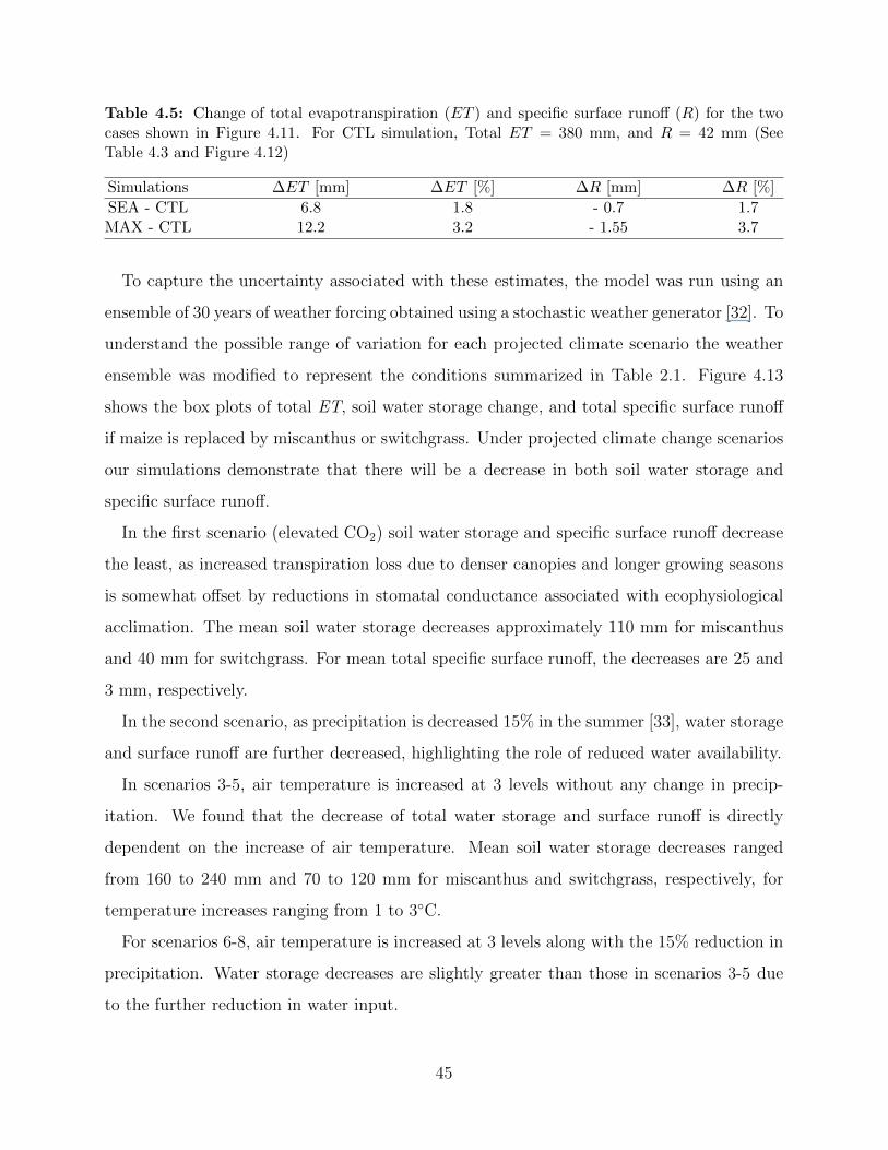
Table 4.5: Change of total evapotranspiration (ET ) and specific surface runoff (R) for the twocases shown in Figure 4.11. For CTL simulation, Total ET = 380 mm, and R = 42 mm (SeeTable 4.3 and Figure 4.12)
Simulations ∆ET [mm] ∆ET [%] ∆R [mm] ∆R [%]
SEA - CTL 6.8 1.8 - 0.7 1.7MAX - CTL 12.2 3.2 - 1.55 3.7
To capture the uncertainty associated with these estimates, the model was run using an
ensemble of 30 years of weather forcing obtained using a stochastic weather generator [32]. To
understand the possible range of variation for each projected climate scenario the weather
ensemble was modified to represent the conditions summarized in Table 2.1. Figure 4.13
shows the box plots of total ET, soil water storage change, and total specific surface runoff
if maize is replaced by miscanthus or switchgrass. Under projected climate change scenarios
our simulations demonstrate that there will be a decrease in both soil water storage and
specific surface runoff.
In the first scenario (elevated CO2) soil water storage and specific surface runoff decrease
the least, as increased transpiration loss due to denser canopies and longer growing seasons
is somewhat offset by reductions in stomatal conductance associated with ecophysiological
acclimation. The mean soil water storage decreases approximately 110 mm for miscanthus
and 40 mm for switchgrass. For mean total specific surface runoff, the decreases are 25 and
3 mm, respectively.
In the second scenario, as precipitation is decreased 15% in the summer [33], water storage
and surface runoff are further decreased, highlighting the role of reduced water availability.
In scenarios 3-5, air temperature is increased at 3 levels without any change in precip-
itation. We found that the decrease of total water storage and surface runoff is directly
dependent on the increase of air temperature. Mean soil water storage decreases ranged
from 160 to 240 mm and 70 to 120 mm for miscanthus and switchgrass, respectively, for
temperature increases ranging from 1 to 3◦C.
For scenarios 6-8, air temperature is increased at 3 levels along with the 15% reduction in
precipitation. Water storage decreases are slightly greater than those in scenarios 3-5 due
to the further reduction in water input.
45
The fractions of soil water storage and specific surface runoff change during the overlapping
and longer growing season (with respect to maize) in both bioenergy crops are also different.
For miscanthus, 87% of soil water storage change occurred during the overlapping period of
the growing season, and 13% due to water utilization during the longer growing season. For
switchgrass, these estimates are 83% and 17%, respectively. However, both crops showed a
92% decrease of specific surface runoff during the overlapping period of growing season, and
8% decrease in the longer growing season.
4.8 Discussion
National policies and economic viability is likely to foster a shift in agricultural practices
from maize to bioenergy crops such as miscanthus and switchgrass [51]. The differences of
miscanthus and switchgrass from maize in the density (LAI) and architecture (LAD) of above
ground foliage results in increased transpiration. This also facilitates larger interception of
rainfall and condensation leading to increased direct evaporation from the foliage. Attenua-
tion of radiation through the denser canopy reduces the radiation reaching the soil thereby
increasing the albedo as more light is reflected from the more reflective foliage and reducing
the soil evaporation. All these impact both the energy and water balance. Elevated atmo-
spheric CO2 concentrations lead to an ecophysiological reduction in stomatal conductance
of the C4 plants which results in a suppression of transpiration and a corresponding increase
in soil-water storage and specific runoff. However, this conservation is not sufficient to offset
the reductions induced by the land use change from maize to miscanthus and switchgrass.
When expected increase in air temperature and reductions in rainfall are further included,
the conservative advantage of elevated CO2 is lost resulting in large reductions of both soil
water storage and specific runoff. Miscanthus, by virtue of its significantly larger LAI, has
the larger impact among the two bioenergy crops. Additionally, the longer growing season
adds to the net reduction in storage and runoff but this accounts for roughly 15% of the
change while the remainder is due to the structural differences in the vegetation foliage. As
illustrated in Figure 4.13, the increase in evapotranspiration, and reductions in soil water
storage and specific surface runoff is quite large, but these per unit area estimates need to
46
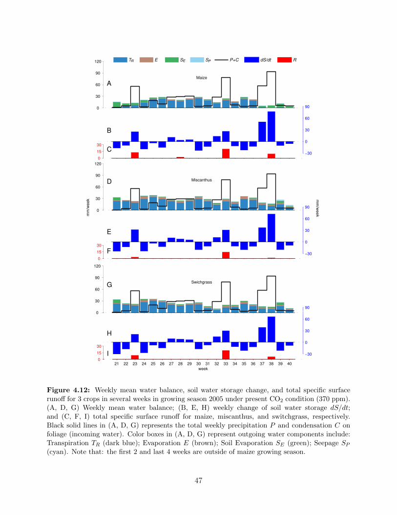
0
30
60
90
120
Maize
T E S S P+C
−30
0
30
60
90
dS/dt
0
15
30
R
0
30
60
90
120
mm
/week
Miscanthus
−30
0
30
60
90
mm
/week
0
15
30
0
30
60
90
120
Swichgrass
−30
0
30
60
90
21 22 23 24 25 26 27 28 29 30 31 32 33 34 35 36 37 38 39 400
15
30
week
I
E
A
C
F
D
G
B
H
R E P
Figure 4.12: Weekly mean water balance, soil water storage change, and total specific surfacerunoff for 3 crops in several weeks in growing season 2005 under present CO2 condition (370 ppm).(A, D, G) Weekly mean water balance; (B, E, H) weekly change of soil water storage dS/dt;and (C, F, I) total specific surface runoff for maize, miscanthus, and switchgrass, respectively.Black solid lines in (A, D, G) represents the total weekly precipitation P and condensation C onfoliage (incoming water). Color boxes in (A, D, G) represent outgoing water components include:Transpiration TR (dark blue); Evaporation E (brown); Soil Evaporation SE (green); Seepage SP(cyan). Note that: the first 2 and last 4 weeks are outside of maize growing season.
47
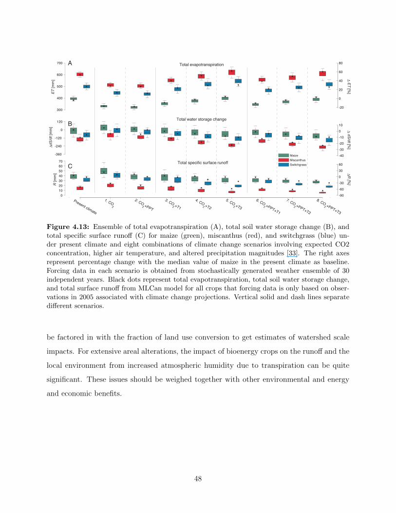
300
400
500
600
700
ET
[m
m]
Total evapotranspirationA
-20
0
20
40
60
80
∆ E
T [%
]
-360
-240
-120
0
120
∆d
S/d
t [m
m]
Total water storage change
B
Maize
Miscanthus
Switchgrass
-40
-30
-20
-10
0
10
∆ d
S/d
t [%]
0
10
20
30
40
50
60
70
R [m
m]
Total specific surface runoffC
-90
-60
-30
0
30
60
∆R
[%]
Present climate
1. CO2
2. CO2 +PPT
3. CO2 +T1
4. CO2 +T2
5. CO2 +T3
6. CO2 +PPT+T1
7. CO2 +PPT+T2
8. CO2 +PPT+T3
Figure 4.13: Ensemble of total evapotranspiration (A), total soil water storage change (B), andtotal specific surface runoff (C) for maize (green), miscanthus (red), and switchgrass (blue) un-der present climate and eight combinations of climate change scenarios involving expected CO2concentration, higher air temperature, and altered precipitation magnitudes [33]. The right axesrepresent percentage change with the median value of maize in the present climate as baseline.Forcing data in each scenario is obtained from stochastically generated weather ensemble of 30independent years. Black dots represent total evapotranspiration, total soil water storage change,and total surface runoff from MLCan model for all crops that forcing data is only based on obser-vations in 2005 associated with climate change projections. Vertical solid and dash lines separatedifferent scenarios.
be factored in with the fraction of land use conversion to get estimates of watershed scale
impacts. For extensive areal alterations, the impact of bioenergy crops on the runoff and the
local environment from increased atmospheric humidity due to transpiration can be quite
significant. These issues should be weighed together with other environmental and energy
and economic benefits.
48

CHAPTER 5
CONCLUSIONS AND FUTURE WORKS
This thesis addresses the potential impacts of large-scale land cover change, possibly arising
from a shift in agricultural practices from maize to bioenergy crops such as miscanthus and
switchgrass, on the hydrologic cycle in Midwestern U.S. under climate change. Several model
modifications and significant improvements in model interfaces were performed to conduct
this research. The goal of this work was to integrate a vertically-resolved model of canopy
biophysical processes [22] with a stochastic Weather Generator [31, 32] and climate change
projections in the Midwest [33] for capturing the eco-physiological acclimations of bioenergy
crops and characterizing the variability range of crop responses to potential meteorological
forcing. The study revealed important insights into the water use of bioenergy crops and
impact on the hydrologic cycle which was characterized through the change in soil-water
storage and specific runoff.
Throughout this study, a mechanistic multi layer canopy-root-soil model (MLCan; [22])
was applied to contrast the eco-hydrological response of maize, the main feedstock for current
starch-based biofuel production, with miscanthus and switchgrass. For each crop, MLCan
model resolves vertically the light and thermal regimes within the canopy and provide pre-
dictions of photosynthetic CO2 assimilation and respiratory losses, as well as latent and
sensible heat fluxes for each canopy layer, through consideration of energy balance for both
sunlit and shaded leaf fraction. Water storage on foliage, as a function of dew or rainfall in-
terception, and soil moisture states are likewise considered to estimate water use, soil-water
storage change, and specific surface runoff.
The major limitation of the MLCan model was the lack of a friendly graphic user interface
(GUI) used for simplifying the modeling steps. This shortcoming was fully resolved by a
GUI developed and linked to the original model in MATLAB that can be executed in many
49

operating systems. The GUI takes advantage of built-in functions and Image Processing
packages in MATLAB to provides a visualization tool with plotting capabilities for the
MLCan model. Our tests for different crops demonstrated that the GUI may contribute
significantly to the MLCan simulations by ways of reducing time for model processing and
avoiding error-prone processes in the text modes.
The stochastic Weather Generator (WG; [31,32]) was used to provide an ensemble forcing
that captures the range of climate variability observed in recent past. The WG was also
included climate change projections in the Midwest [33] to provides Monte Carlo simulation
at hourly scale for: precipitation, total cloud cover, incoming shortwave and longwave radi-
ations, air temperature, humidity, and wind speed. Those variables are then interpolated to
obtain half-hour values and used for driving the MLCan model.
Lignocellulosic bioenergy is considered as a potential alternative for fossil fuel in term of
energy, economic, and environmental advantages. However, higher biomass production of
these bioenergy crops also require more water for their physical and biological functioning.
The work contained in this thesis showed that, under present climate in 2005, miscanthus
and switchgrass utilized more water than maize for total seasonal ET by approximately
58% and 36%, respectively. Elevated atmospheric CO2 concentrations (550 ppm) lead to an
eco-physiological reduction in stomatal conductance of the C4 plants which results in a sup-
presion of transpiration and a corresponding increase in soil-water storage and specific runoff.
However, this conservation is not sufficient to offset the reductions induced by the land use
change from maize to miscanthus and switchgrass, resulted from significant differences in
the density (LAI) and architecture(LAD). When expected increase in air temperature and
reductions in rainfall are further included, the conservative advantage of elevated CO2 is lost
resulting in large reduction of both soil water storage and specific runoff, highlighting the
critical role of warming air temperature in climate change.
A view from the multi layers canopy root soil model (MLCan) showed that the increase
in ET and reduction in soil water storage and specific runoff is quite large, but these per
unit area estimate need to be factored with fraction of land use conversion to get estimate
of water scale impacts. For extensive areal alteration, it is important to recognize that we
have to prepare for the impact of bioenergy crop on runoff and the local environment for
50

achieving sustainable development.
In the next step of this study, we will expand the application of MLCan model for bioenergy
crops to larger spatial scales. The integration of MLCan with watershed models will provide
important insights to watershed scale impacts of land use conversion as well as climate
change to hydrologic cycle.
51
CHAPTER 6
REFERENCES
[1] Ragauskas AJ, et al. (2006). The path forward for biofuels and biomaterials. Science311:484–489.
[2] Wall JD, Harwood CS, Demain AL (2008). Bioenergy. (ASM Press, Washington, DC).
[3] Kladivko EJ (2001). Tillage systems and soil ecology. Soil Till Res 61:61–76.
[4] Donner SD (2007). Surf or turf: A shift from feed to food cultivation could reducenutrient flux to the Gulf of Mexico. Global Environ Chang 17:105–113.
[5] Schnoor JL, et al. (2008). Water implications of biofuels production in the United States.(National Academies Press, Washington, DC).
[6] Costello C, Griffin WM, Landis AE, Matthews HS (2009). Impact of biofuel cropproduction on the formation of hypoxia in the Gulf of Mexico. Environ Sci Technol43:7985–7991.
[7] Tilman D, Hill J, Lehman C (2006). Carbon-negative biofuels from low-input high-diversity grassland biomass. Science 314:1598–1600.
[8] Cai X, Zhang X, Wang D (2011). Land Availability for Biofuel Production. EnvironSci Technol 45:334–339.
[9] Schmer M, Vogel K, Mitchell R, Perrin R (2008). Net energy of cellulosic ethanol fromswitchgrass. Proc Natl Acad Sci USA 105:464–469.
[10] Hess JR, Thomas DF, Hoskinson R, Thompson D (2003). Roadmap for agriculturebiomass feedstock supply in the United States. DOE/NE-ID-11129. (U.S. Departmentof Energy, Washington, DC).
[11] Heaton EA, Dohleman FG, Long SP (2008). Meeting US biofuel goals with less land:the potential of Miscanthus. Glob Change Biol 14:2000–2014.
[12] Heaton EA, Voigt T, Long SP (2004). A quantitative review comparing the yields of twocandidate C4 perennial biomass crops in relation to nitrogen, temperature and water.Biomass Bioenergy 27:21–30.
52
[13] Dondini M, Groenigen KJV, Galdo ID, Jones MB (2009). Carbon sequestration undermiscanthus: a study of 13c distribution in soil aggregates. Glob Change Biol Bioenergy1:321–330.
[14] Liebig MA, Schmer MR, Vogel KP, Mitchell RB (2008). Soil carbon storage by switch-grass grown for bioenergy. Bioenerg Res 1:215–222.
[15] Clifton-Brown JC, Breuer J, Jones MB (2007). Carbon mitigation by the energy crop,miscanthus. Glob Change Biol 13:2296–2307.
[16] Ma Z, Wood CW, Bransby DI (2000). Soil management impacts on soil carbon seques-tration by switchgrass. Biomass Bioenergy 18:469–477.
[17] Hickman GC, Vanloocke A, Dohleman FG, Bernacchi CJ (2010). A comparison ofcanopy evapotranspiration for maize and two perennial grasses identified as potentialbioenergy crops. Glob Change Biol Bioenergy 2:157–168.
[18] McIsaac GF, David MB, Mitchell CA (2010). Miscanthus and Switchgrass Productionin Central Illinois: Impacts on Hydrology and Inorganic Nitrogen Leaching. J EnvironQual 39:1790–1799.
[19] Vanloocke A, Bernacchi CJ, Twine TE (2010). The impacts of Miscanthus × giganteusproduction on the Midwest US hydrologic cycle. Glob Change Biol Bioenergy 2:180–191.
[20] Pieruschka R, Huber G, Berry JA (2010). Control of transpiration by radiation. ProcNatl Acad Sci USA 107:13372–13377.
[21] Sauer TJ, Singer JW, Prueger JH, DeSutter TM, Hatfield JL (2007). Radiation balanceand evaporation partitioning in a narrow-row soybean canopy. Agric Forest Meteorol145: 206-214.
[22] Drewry DT, et al. (2010a). Ecohydrological responses of dense canopies to environmen-tal variability: 1. Interplay between vertical structure and photosynthetic pathway. J.Geophys. Res. 115, G4, G04022.
[23] Drewry DT, et al. (2010b). Ecohydrological responses of dense canopies to environmen-tal variability: 2. Role of acclimation under elevated CO2. J. Geophys. Res. 115, G4,G04023.
[24] Leakey ADB, et al. (2006). Photosynthesis, productivity, and yield of maize are notaffected by open-air elevation of CO2 concentration in the absence of drought. PlantPhysiol 140:779–790.
[25] Long SP, Ainsworth EA, Rogers A, Ort DR (2004). Rising atmospheric carbon dioxide:Plants FACE the Future*. Annu. Rev. Plant Biol. 55: 591-628.
[26] Leakey ADB, et al. (2009). Elevated CO2 effects on plant carbon, nitrogen, and waterrelations: six important lessons from FACE. J Exp Bot 60: 2859-2876.
53
[27] Leakey ADB, Bernacchi CJ, Dohleman FG, Ort DR, Long SP (2004). Will photosynthe-sis of maize (Zea mays) in the US Corn Belt increase in future [CO2] rich atmosphere?An analysis of diurnal courses of CO2 uptake under free-air concentration enrichment(FACE). Glob Change Biol 10:95–962.
[28] Ghannoum O, von Caemmerer S, Ziska LH, Conroy JP (2000). The growth responseof C-4 plants to rising atmospheric CO2 partial pressure: a reassessment. Plant CellEnviron 23:931–942.
[29] Knapp AK, Hamerlynck EP, Owensby CE (1993). Photosynthetic and Water RelationsResponses to Elevated CO2 in the C4 Grass Andropogon gerardii. Int J Plant Sci154:459-466.
[30] Nobel PST (1980). Water Vapor Conductance and CO2 Uptake for Leaves of a C4Desert Grass, Hilaria Rigida. Ecology 6:252-258.
[31] Curtis DC, Eagleson PS (1982). Constrained stochastic climate simulation. Tech. Rep.274, Mass. Inst. of Technol., Dep. of Civ. and Environ. Eng., Ralph M. Parson Lab.,Cambridge.
[32] Ivanov VY, Bras RL, Curtis DC (2007). A weather generator for hydrological, ecological,and agricultural applications. Water Resour Res 43:W10406.
[33] Wuebbles DJ, Hayhoe K (2004). Climate change projections for the United StatesMidwest. Mitig. Adapt. Strategies Glob. Chang. 9:335–363.
[34] Campbell GS, Norman JM (1998). An introduction to environmental biophysics(Springer-Verlag, New York).
[35] Goudriaan J (1977). Crop micrometeorology: A simulation study (Cent. for Agric. Publ.and Doc., Wageningen, Netherlands).
[36] Spitters C (1986). Separating the diffuse and direct component of global radiation andits implications for modeling canopy photosynthesis. II: Calculation of canopy photo-synthesis. Agric. For. Meteorol. 38:231–242.
[37] Amenu GG, Kumar P (2008). A model for hydraulic redistribution incorporating cou-pled soil-root moisture transport. Hydrol Earth Syst Sc 12: 55–74.
[38] Dohleman FG, Heaton EA, Leakey ADB, Long SP (2009). Does greater leaf-level pho-tosynthesis explain the larger solar energy conversion efficiency of miscanthus relativeto switchgrass? Plant Cell Environ 32:1525–1537.
[39] Houghton JT, et al. (2001). Climate Change 2001: The Scientific Basis (CambridgeUniversity Press, Cambridge, U.K).
[40] Kromdijk J, et al. (2008). Bundle sheath leakiness and light limitation during C4 leafand canopy CO2 uptake. Plant Physiol. 148:2144–2155.
54
[41] Madakadze IC, et al. (1998). Leaf area development, light interception, and yield amongswitchgrass populations in a short-season area. Crop Sci. 38:827–834.
[42] Monti A, Zatta A (2009). Root distribution and soil moisture retrieval in perennial andannual energy crops in northern Italy. Agr Ecosyst Environ 132:252–259.
[43] Monteith JL, Unsworth MH (1990). Principles of environmental physics. (EdwardArnold Publishers, London).
[44] Schenk H, Jackson R (2002). The global biogeography of roots. Ecol. Monogr. 72:311–328.
[45] Durran DR (1999). Numerical Methods for Wave Equations in Geophysical Fluid Dy-namics. (Springer-Verlag, New York).
[46] Ivanov VY (2006). Effects of dynamic vegetation and topography on hydrological pro-cesses in semi-arid areas. Ph.D. Thesis, Mass. Inst. of Technol., Cambridge.
[47] Hopkins WG, Huner NPA (2009). Introduction to plant physiology (John Wiley & Son,Inc.).
[48] Markelz RJC, Strellner RS, Leakey ADB (2008). Impairment of C4 photosynthesis bydrought is exacerbated by limiting nitrogen and ameliorated by elevated [CO2] in maize.J Exp Bot 62:3235–3246.
[49] Wilson KB, Baldocchi DD, Hanson PJ (2000). Spatial and seasonal variability of photo-synthetic parameters and their relationship to leaf nitrogen in a deciduous forest. TreePhysiol 20:565–578.
[50] Xu L, Baldocchi DD (2003). Seasonal trends in photosynthetic parameters and stomatalconductance of blue oak (Quercus douglasii) under prolonged summer drought and hightemperature. Tree Physiol 23:865–877.
[51] Chen X, Huang H, Khanna M, Onal H (2011). Meeting the Mandate for Biofuels:Implications for Land Use, Food and Fuel Prices. National Bureau of Economic ResearchWorking Paper No. 16697 (Natl. Bureau Econ. Res., Cambridge, MA).
[52] Dermody O, Long S, DeLucia E (2006). How does elevated CO2 or ozone affect the leafarea index of soybean when applied independently? New Phytol 169:145–155.
[53] Dermody O, O’Neill B, Zangerl A, Berenbaum M, DeLucia E (2008). Effects of ele-vated CO2 and O3 on leaf damage and insect abundance in a soybean agroecosystem.Arthropod-Plant Inte 2:125–135.
[54] Grayman WM, Eagleson PS (1969). Streamflow record length for modeling catchmentdynamics. Tech. Rep. 114, Mass. Inst. of Technol., Dep. of Civ. and Environ. Eng.,Ralph M. Parson Lab., Cambridge.
55

[55] Eagleson PS (2002). Ecohydrology: Darwinian Expression of Vegetation and FormFunction. (Cambridge University Press, Cambridge, U.K).
[56] Gueymard C (1989). A 2-band model for the calculation of clear sky solar irradiance,illuminance, and photosynthetically active radiation at the earth’s surface. Sol. Energy43, 253–265.
[57] Becker S (2001). Calculation of direct solar and diffuse radiation in Israel. Int. J. Clim.21, 1561–1576.
[58] Thomas GE, Stamnes K (1999). Radiative Transfer in the Atmosphere and Ocean.(Cambridge University Press, Cambridge, U.K).
[59] Slingo A, Schrecker HM (1982). On the shortwave radiative properties of stratiformwater clouds. Q. J.R. Meteorol. Soc 108, 407–426.
[60] Stephens GL (1978). Radiation profiles in extended water clouds. 2. Parameterizationschemes. J. Atmosph. Sci. 35, 2123–2132.
[61] Slingo A (1989). A GCM parameterization for the shortwave radiative properties ofwater clouds. J. Atm. Sci. 46, 1419–1427.
[62] Han Q, Rossow WB, Lacis AA (1994). Near-global survey of effective droplet radii inliquid water clouds using ISCCP data. J. Clim. 7, 465–497.
[63] Kimball JS, Running SW, Nemani R (1997). An improved method for estimating surfacehumidity from daily minimum temperature. Agric. For. Meteorol. 85, 87–98.
[64] Priestley CHB, Taylor RJ (1972). On the assessment of surface heat flux and evaporationusing large-scale parameters. Mon. Weather Rev. 100, 81–92.
[65] Brutsaert W (1982). Evaporation into the Atmosphere : Theory, History, and Applica-tions. (D. Reidel, London).
[66] Farage PK, Blowers D, Long SP, Baker NR (2006). Low growth temperatures modifythe efficiency of light use by photosystem II for CO2 assimilation in leaves of twochilling-tolerant C4 species, Cyperus Longus l. and Miscanthus × Giganteus. PlantCell Environ, 29:720–728.
[67] Clifton-Brown JC, Neilson B, Lewandowski I, Jones MB (2000). The modelled produc-tivity of Miscanthus × Giganteus (Greef et deu) in Ireland. Ind Crop Prod, 12:97–109.
[68] Maass A, Hufschmidt MM, Dorfman R, Thomas Jr, HA, Marglin SA, Fair GM (1962).Design of water-resources systems. (Harvard Univ. Press, Cambridge, Mass).
56
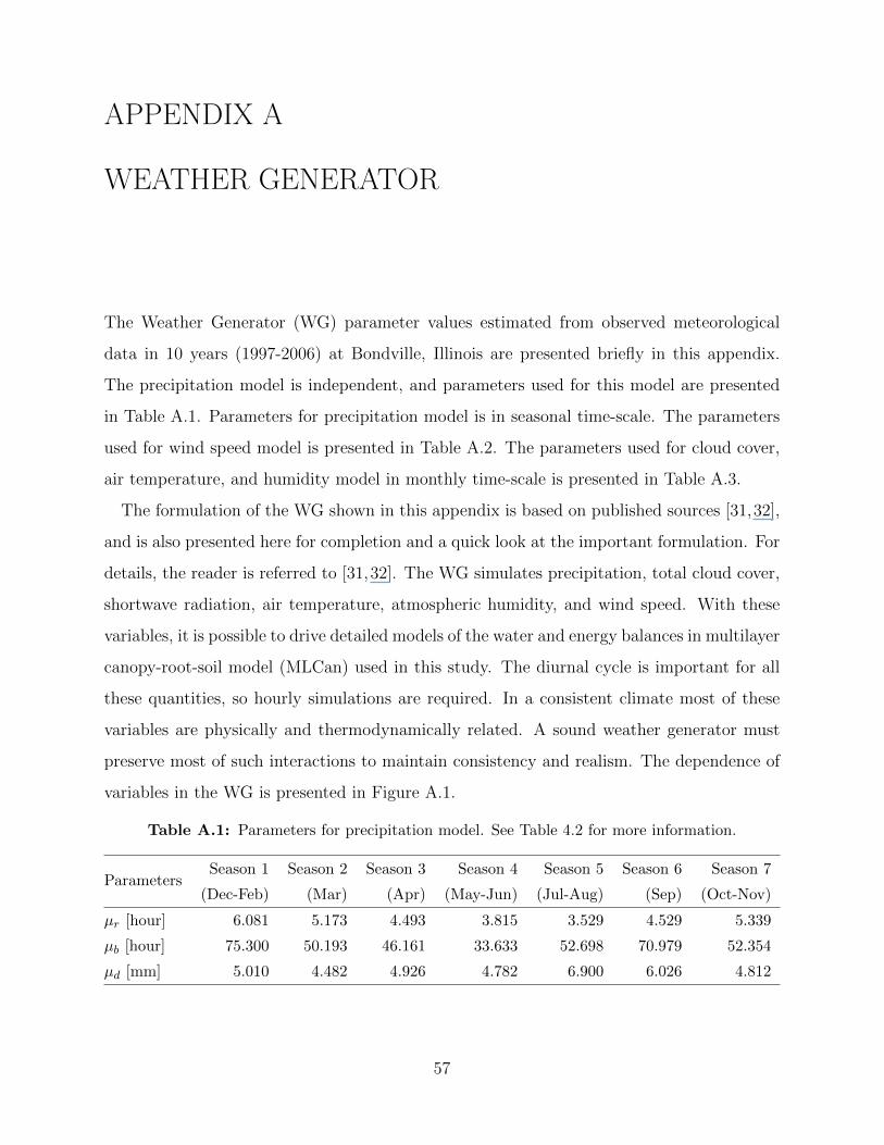
APPENDIX A
WEATHER GENERATOR
The Weather Generator (WG) parameter values estimated from observed meteorological
data in 10 years (1997-2006) at Bondville, Illinois are presented briefly in this appendix.
The precipitation model is independent, and parameters used for this model are presented
in Table A.1. Parameters for precipitation model is in seasonal time-scale. The parameters
used for wind speed model is presented in Table A.2. The parameters used for cloud cover,
air temperature, and humidity model in monthly time-scale is presented in Table A.3.
The formulation of the WG shown in this appendix is based on published sources [31,32],
and is also presented here for completion and a quick look at the important formulation. For
details, the reader is referred to [31,32]. The WG simulates precipitation, total cloud cover,
shortwave radiation, air temperature, atmospheric humidity, and wind speed. With these
variables, it is possible to drive detailed models of the water and energy balances in multilayer
canopy-root-soil model (MLCan) used in this study. The diurnal cycle is important for all
these quantities, so hourly simulations are required. In a consistent climate most of these
variables are physically and thermodynamically related. A sound weather generator must
preserve most of such interactions to maintain consistency and realism. The dependence of
variables in the WG is presented in Figure A.1.
Table A.1: Parameters for precipitation model. See Table 4.2 for more information.
ParametersSeason 1 Season 2 Season 3 Season 4 Season 5 Season 6 Season 7
(Dec-Feb) (Mar) (Apr) (May-Jun) (Jul-Aug) (Sep) (Oct-Nov)
µr [hour] 6.081 5.173 4.493 3.815 3.529 4.529 5.339
µb [hour] 75.300 50.193 46.161 33.633 52.698 70.979 52.354
µd [mm] 5.010 4.482 4.926 4.782 6.900 6.026 4.812
57
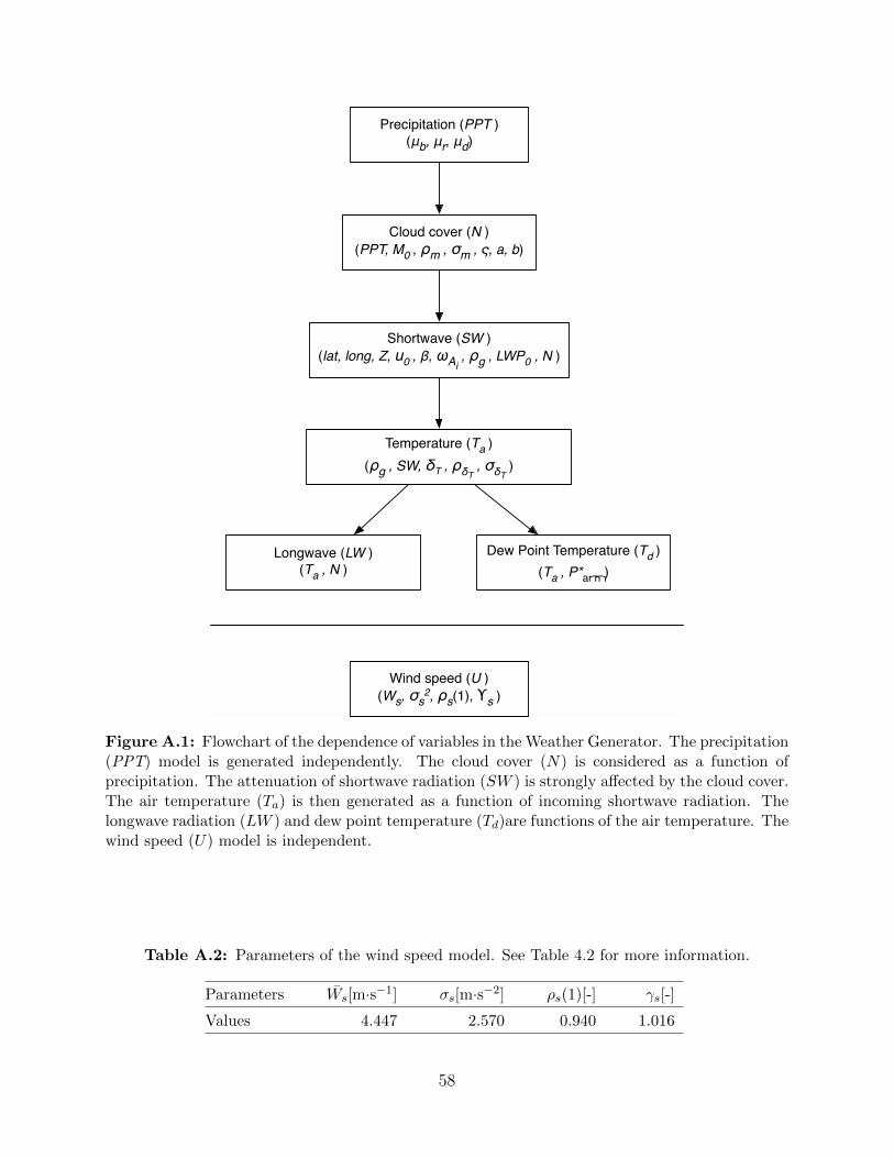
Precipitation (PPT )
(μb, μr, μd)
Cloud cover (N )
(PPT, M0 , ρm , σm , , a, b)
Shortwave (SW )
(lat, long, Z, u0 , β, ωAi , ρg , LWP0 , N )
Temperature (Ta )
(ρg , SW, δT , ρδT , σδT )
Longwave (LW )
(Ta , N )
Dew Point Temperature (Td )
(Ta , P*ann
)
Wind speed (U )
(Ws, σs2, ρs(1), ϒs )
Figure A.1: Flowchart of the dependence of variables in the Weather Generator. The precipitation(PPT) model is generated independently. The cloud cover (N) is considered as a function ofprecipitation. The attenuation of shortwave radiation (SW ) is strongly affected by the cloud cover.The air temperature (Ta) is then generated as a function of incoming shortwave radiation. Thelongwave radiation (LW ) and dew point temperature (Td)are functions of the air temperature. Thewind speed (U) model is independent.
Table A.2: Parameters of the wind speed model. See Table 4.2 for more information.
Parameters Ws[m·s−1] σs[m·s−2] ρs(1)[-] γs[-]
Values 4.447 2.570 0.940 1.016
58
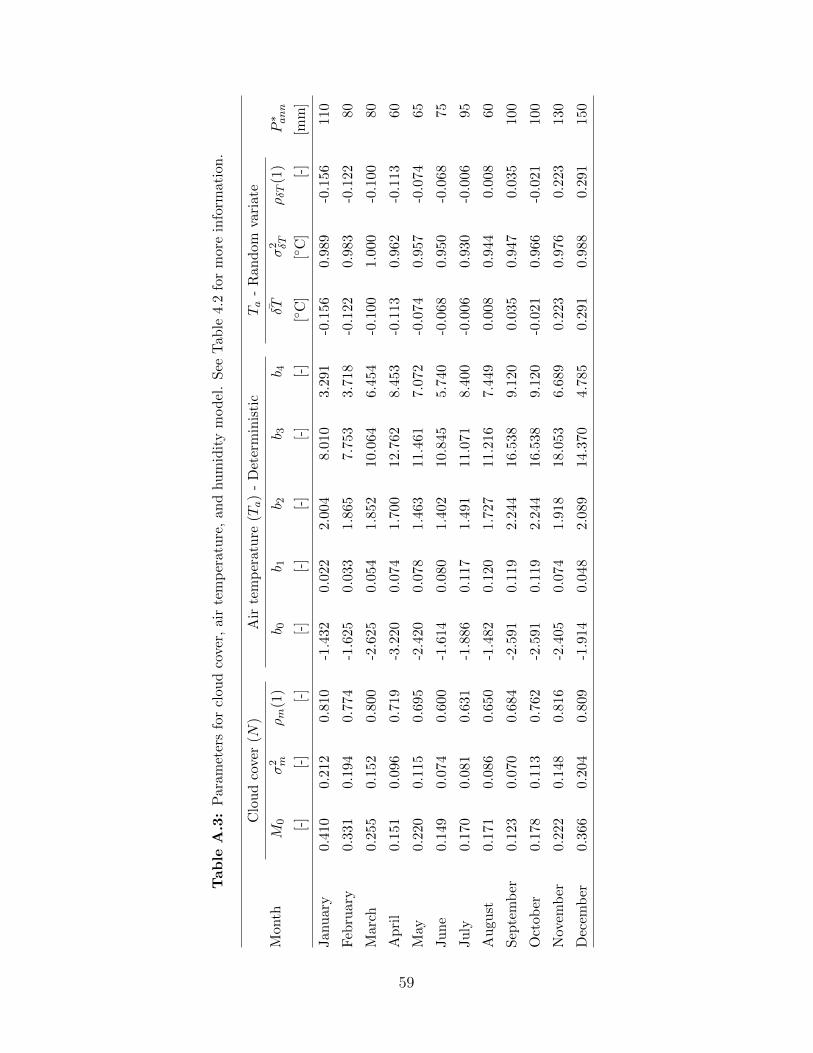
Table
A.3:
Par
amet
ers
for
clou
dco
ver
,ai
rte
mp
erat
ure
,an
dhu
mid
ity
mod
el.
See
Tab
le4.
2fo
rm
ore
info
rmat
ion.
Mon
th
Clo
ud
cove
r(N
)A
irte
mp
erat
ure
(Ta)
-D
eter
min
isti
cTa
-R
and
omva
riat
e
M0
σ2 m
ρm
(1)
b 0b 1
b 2b 3
b 4δT
σ2 δT
ρδT
(1)
P∗ ann
[-]
[-]
[-]
[-]
[-]
[-]
[-]
[-]
[◦C
][◦
C]
[-]
[mm
]
Jan
uar
y0.4
100.
212
0.81
0-1
.432
0.02
22.
004
8.01
03.
291
-0.1
560.
989
-0.1
5611
0
Feb
ruar
y0.
331
0.1
940.7
74-1
.625
0.03
31.
865
7.75
33.
718
-0.1
220.
983
-0.1
2280
Mar
ch0.2
550.1
520.8
00
-2.6
250.
054
1.85
210
.064
6.45
4-0
.100
1.00
0-0
.100
80
Ap
ril
0.1
510.
096
0.71
9-3
.220
0.07
41.
700
12.7
628.
453
-0.1
130.
962
-0.1
1360
May
0.22
00.
115
0.6
95-2
.420
0.07
81.
463
11.4
617.
072
-0.0
740.
957
-0.0
7465
Ju
ne
0.14
90.
074
0.6
00-1
.614
0.08
01.
402
10.8
455.
740
-0.0
680.
950
-0.0
6875
Ju
ly0.1
700.0
810.6
31-1
.886
0.11
71.
491
11.0
718.
400
-0.0
060.
930
-0.0
0695
Au
gust
0.1
710.0
860.
650
-1.4
820.
120
1.72
711
.216
7.44
90.
008
0.94
40.
008
60
Sep
tem
ber
0.12
30.0
700.6
84-2
.591
0.11
92.
244
16.5
389.
120
0.03
50.
947
0.03
510
0
Oct
ob
er0.1
780.
113
0.76
2-2
.591
0.11
92.
244
16.5
389.
120
-0.0
210.
966
-0.0
2110
0
Nov
emb
er0.2
220.1
480.8
16-2
.405
0.07
41.
918
18.0
536.
689
0.22
30.
976
0.22
313
0
Dec
emb
er0.
366
0.20
40.
809
-1.9
140.
048
2.08
914
.370
4.78
50.
291
0.98
80.
291
150
59

A.1 Precipitation
Precipitation is the most crucial meteorological variable for many applications. Its pres-
ence or absence also affects statistics of many other hydrometeorological variables. Storm
durations and interstorm times could be treated as independent events [54]. Thus, the pre-
cipitation model can be expressed by successive sampling from the fitted probability density
functions. For example, time between two successive storms tb [hour] follows the exponential
distribution (by definition of the Poisson arrival process):
f(tb) =1
µbe− 1µbtb (A.1)
where µb [hour] is the mean time between storms. The storm duration tr [hour] is also
simulated using the exponential distribution [54]:
f(tr) =1
µre−
1µrtr (A.2)
where µr [hour] is the mean storm duration. Grayman and Eagleson [54] showed that storm
depth were highly dependent on storm durations. Storm depth h [mm] were found to follow
a gamma distribution conditioned by storm duration:
f
(h| trµr
)=
1
µd
hµd
trµr−1e− h
µd
Γ( trµr
)(A.3)
where µr [mm] is the mean storm depth. The two-paramter gamma distribution has been
shown to satisfactorily preserve the rainfall statistical characteristics [31].
The following procedure is used to simulate rainfall. At some initial time t0, an interstorm
duration tb is generated from the fitted exponential distribution. The period [t0, t0 + tb] is
considered dry. When the time reaches [t0 + tb], the storm duration tr is generated. Using
the value set for tr, a storm depth h is generated from the gamma distribution. The period
[t0 + tb, t0 + tb + tr] is then considered wet. When time reaches [t0 + tb + tr] the process is
repeated to determine the next storm-interstorm sequence. The adopted method assumes
the model of rectangular pulses that considers a uniform rainfall intensity throughout the
60
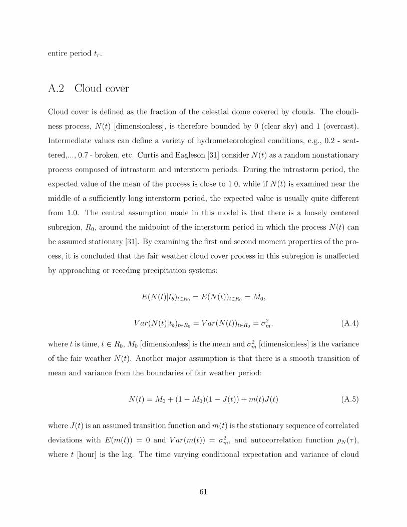
entire period tr.
A.2 Cloud cover
Cloud cover is defined as the fraction of the celestial dome covered by clouds. The cloudi-
ness process, N(t) [dimensionless], is therefore bounded by 0 (clear sky) and 1 (overcast).
Intermediate values can define a variety of hydrometeorological conditions, e.g., 0.2 - scat-
tered,..., 0.7 - broken, etc. Curtis and Eagleson [31] consider N(t) as a random nonstationary
process composed of intrastorm and interstorm periods. During the intrastorm period, the
expected value of the mean of the process is close to 1.0, while if N(t) is examined near the
middle of a sufficiently long interstorm period, the expected value is usually quite different
from 1.0. The central assumption made in this model is that there is a loosely centered
subregion, R0, around the midpoint of the interstorm period in which the process N(t) can
be assumed stationary [31]. By examining the first and second moment properties of the pro-
cess, it is concluded that the fair weather cloud cover process in this subregion is unaffected
by approaching or receding precipitation systems:
E(N(t)|tb)t∈R0 = E(N(t))t∈R0 = M0,
V ar(N(t)|tb)t∈R0 = V ar(N(t))t∈R0 = σ2m, (A.4)
where t is time, t ∈ R0, M0 [dimensionless] is the mean and σ2m [dimensionless] is the variance
of the fair weather N(t). Another major assumption is that there is a smooth transition of
mean and variance from the boundaries of fair weather period:
N(t) = M0 + (1−M0)(1− J(t)) +m(t)J(t) (A.5)
where J(t) is an assumed transition function and m(t) is the stationary sequence of correlated
deviations with E(m(t)) = 0 and V ar(m(t)) = σ2m, and autocorrelation function ρN(τ),
where t [hour] is the lag. The time varying conditional expectation and variance of cloud
61

cover under this assumption are obtained as [31]:
E(N(t)|tb) = M0 + (1−M0)(1− J(t))
V ar(N(t)|tb) = σ2mP
2(t) (A.6)
where t ∈ tb. The autocorrelation structure of the cloud cover process (Eq. A.5) is
not affected by J(t) and is identical to the autocorrelation function of the process m(t):
ρN(τ) = ρm(τ) [31]. The transition function J(t) is assumed to be of an exponential form:
J(t) = (1− e−ς(t−t0))(1− e−γ(t0+tb−t)) (A.7)
where ς and γ [hour−1] are decay coefficients controlling the transition rates from the bound-
aries (end/beginning of precipitation events) to/from the region R0. These rates are assumed
to be equal in the current model implementation. As follows from Eq. (A.7), for t ∈ R0:
limtb→∞
N(t) = M0 +m(t) (A.8)
J(t) reaches a value close to 1.0 for all reasonable values of the decay coefficients and
therefore the fair weather cloudiness is essentially simulated as:
limtb→∞
N(t) = M0 +m(t) (A.9)
The stationary deviations process, m(t), is taken to be a firstorder Markov process:
m(t) = ρm(1)m(t− 1) + ε(t)σm√
1− ρ2m(1) (A.10)
where ε(t) is a random deviate. In the model of Curtis and Eagleson [31], ε(t) is assumed
to be a normally distributed variable, N(0, 12). However, a modification is introduced here
and ε(t) is simulated as a random deviate from the Beta probability distribution.
Beta(y) =Γ(a+ b)
Γ(a)Γ(b)
1
(y2 − y1)a+b−1(y − y1)a−1(y2 − y)b−1 (A.11)
62

where y1 and y2 are the lower and upper bounds of the Beta distribution for independent
variable y and a and b are the distribution shape parameters (a > 0, b > 0). The lower and
upper bounds (y1, y2) are found from Eq. (A.5) and (A.10) at every simulation step, i.e., the
knowledge of m(t− 1) and J(t) at every time t allows one to derive y1 and y2 by imposing
the requirement for the cloud cover N(t) to be in the range [0, 1]. The Beta distribution
shape parameters a and b are estimated based on conditioning by the cloudiness value at
(t − 1) (see Ivanov et al. [32] for more detail). Sampling of deviate ε(t), performed in this
manner, allows one to avoid the truncation of values of N(t) and preserve the moments and
shape of the cloud cover distribution.
A.3 Shortwave radiation
For all practical purposes, the Sun radiates its energy at a constant rate. Outside the
atmosphere, at the mean solar distance, the beam irradiance, also known as the solar constant
So, is 1367 [W·m−2]. The Earth’s orbit is slightly eccentric and the Sun-Earth distance varies
throughout the year. To allow for the varying solar distance, a correction, a ratio of the
actual Earth-Sun to the mean Earth-Sun Distance, r [-], is introduced so that:
S ′o =Sor2
(A.12)
r = 1.0 + 0.017 cos
[2π
365(186− JDay)
](A.13)
where JDay is the Julian day. Several other variables defining the Sun’s position with
respect to a location on Earth are used in the following. See Ivanov et al. [32] for further
information.
The model considers two wide bands of solar spectrum: the ultraviolet (UV) and vis-
ible (VIS) band, BΛ1 [0.29 µm ÷ 0.70 µm], where ozone absorption and molecular scat-
tering are concentrated, and the infrared in near- and short-wavelength range (NIR), BΛ2,
[0.70 µm ÷ 4.0 µm], where water and mixed gases absorptions are concentrated. The spec-
trum separation into two bands facilitates the transmittance modeling of beam and diffuse
63
clear sky irradiances because overlap between scattering and selective absorption is lim-
ited [56]. In the presence of clouds, the chosen spectral limits are also convenient due to the
above differences in absorption properties by water droplets. Moreover, separate treatment
of these two bands allows one to explicitly compute PAR, which is used in the process of
leaf photosynthesis. According to Slingo [61], the energy contained in the two bands, BΛ1
and BΛ2, is 46.6% and 53.4% of So, respectively. These fractions are applied to obtain the
extraterrestrial flux densities in the two bands: SoΛ1 and BoΛ2 [W·m−2].
A.3.1 Clear Sky
Direct Beam Irradiance
It is assumed that direct rays entering the atmosphere encounter extinction processes, which
are limited to the effects of ozone (’O’), uniformly mixed gases (’G’), water vapor (’W’), and
aerosol absorption (’A’), and Rayleigh and aerosol scattering (’R’) [56]. For the transmit-
tances TX due to an extinction process X (X = ’O’, ’G’, ’W’, ’A’, ’R’), see Ivanov et al. [32]
for more detail. In this model, separate extinction layers are considered, so that the total
direct beam flux at the ground at normal incidence is
SµbΛi = SoΛi∏X
TX,i (A.14)
Sµb = SµbΛ1 + SµbΛ2 (A.15)
where T [-] is transmittances and i (i = 1, 2) is used to denoted the considered bands.
Diffuse Irradiance
The diffuse irradiance at the ground level is modeled as a combination of three components
IdX corresponding to (the X index) the two scattering layers (molecules and aerosols) and
to a backscattering process between ground and sky (See Ivanov et al. [32] for more detail).
64
The total diffuse flux at the ground is therefore:
SµdΛi =∑X
IdX,i (A.16)
Sd = SdΛ1 + SdΛ2 (A.17)
A.3.2 Cloudy Sky
Clouds alter transmission and reflection properties of the atmosphere. Therefore the effects
of cloud cover need to be carefully accounted for. Cloud parameterizations provided in
hydrological literature typically use empirical functions of the fractional cloud cover [57] or
specify fixed bulk properties. However, cloud radiative characteristics strongly depend on
cloud type, structure, and density [58]. Also, different spectral intervals exhibit distinct
absorption and scattering characteristics [59].
The framework used here relies on parameterizations developed by Stephens [60] and
Slingo [61]. On the basis of both observational and theoretical evidence, these studies infer
that the cloud radiative properties are mainly determined by the cloud total vertical liquid
water path, LWP [g·m−2]. Stephens [60] showed that the broadband optical thickness is
essentially the same for clouds of different types that have the same LWP . Slingo [61]
introduced an additional independent relationship between cloud radiative properties and
the effective radius of drop size distribution. The advantage of using LWP is that this
quantity can be obtained by satellite microwave radiometry [62] and allows the introduction
of seasonality effects in the cloud properties.
The approach developed by Stephens [60] is used here to derive the effective radius of drop
size distribution based on LWP. The four-band model of Slingo [61] is then used to derive
the cloud transmittances and reflectances for the incident clear sky direct SµbΛi and diffuse
SµdΛi fluxes (assumed to be incident on top of clouds).
65
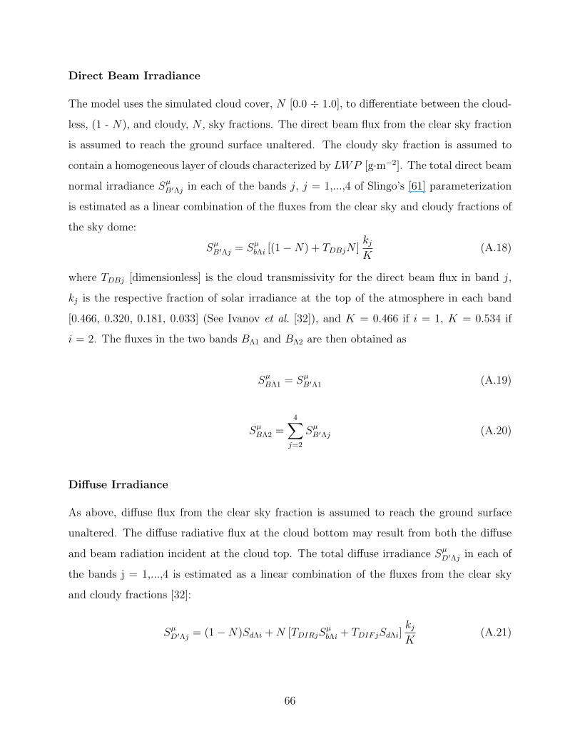
Direct Beam Irradiance
The model uses the simulated cloud cover, N [0.0 ÷ 1.0], to differentiate between the cloud-
less, (1 - N), and cloudy, N , sky fractions. The direct beam flux from the clear sky fraction
is assumed to reach the ground surface unaltered. The cloudy sky fraction is assumed to
contain a homogeneous layer of clouds characterized by LWP [g·m−2]. The total direct beam
normal irradiance SµB′Λj in each of the bands j, j = 1,...,4 of Slingo’s [61] parameterization
is estimated as a linear combination of the fluxes from the clear sky and cloudy fractions of
the sky dome:
SµB′Λj = SµbΛi [(1−N) + TDBjN ]kjK
(A.18)
where TDBj [dimensionless] is the cloud transmissivity for the direct beam flux in band j,
kj is the respective fraction of solar irradiance at the top of the atmosphere in each band
[0.466, 0.320, 0.181, 0.033] (See Ivanov et al. [32]), and K = 0.466 if i = 1, K = 0.534 if
i = 2. The fluxes in the two bands BΛ1 and BΛ2 are then obtained as
SµBΛ1 = SµB′Λ1 (A.19)
SµBΛ2 =4∑j=2
SµB′Λj (A.20)
Diffuse Irradiance
As above, diffuse flux from the clear sky fraction is assumed to reach the ground surface
unaltered. The diffuse radiative flux at the cloud bottom may result from both the diffuse
and beam radiation incident at the cloud top. The total diffuse irradiance SµD′Λj in each of
the bands j = 1,...,4 is estimated as a linear combination of the fluxes from the clear sky
and cloudy fractions [32]:
SµD′Λj = (1−N)SdΛi +N [TDIRjSµbΛi + TDIFjSdΛi]
kjK
(A.21)
66
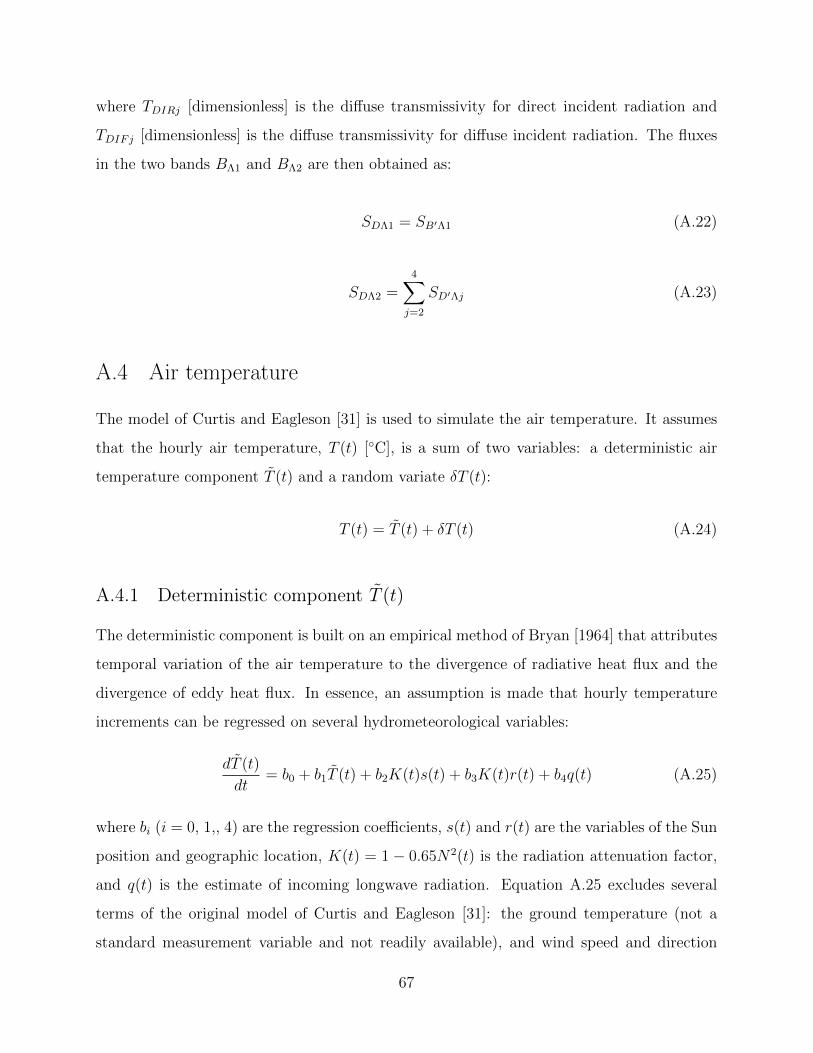
where TDIRj [dimensionless] is the diffuse transmissivity for direct incident radiation and
TDIFj [dimensionless] is the diffuse transmissivity for diffuse incident radiation. The fluxes
in the two bands BΛ1 and BΛ2 are then obtained as:
SDΛ1 = SB′Λ1 (A.22)
SDΛ2 =4∑j=2
SD′Λj (A.23)
A.4 Air temperature
The model of Curtis and Eagleson [31] is used to simulate the air temperature. It assumes
that the hourly air temperature, T (t) [◦C], is a sum of two variables: a deterministic air
temperature component T (t) and a random variate δT (t):
T (t) = T (t) + δT (t) (A.24)
A.4.1 Deterministic component T (t)
The deterministic component is built on an empirical method of Bryan [1964] that attributes
temporal variation of the air temperature to the divergence of radiative heat flux and the
divergence of eddy heat flux. In essence, an assumption is made that hourly temperature
increments can be regressed on several hydrometeorological variables:
dT (t)
dt= b0 + b1T (t) + b2K(t)s(t) + b3K(t)r(t) + b4q(t) (A.25)
where bi (i = 0, 1,, 4) are the regression coefficients, s(t) and r(t) are the variables of the Sun
position and geographic location, K(t) = 1− 0.65N2(t) is the radiation attenuation factor,
and q(t) is the estimate of incoming longwave radiation. Equation A.25 excludes several
terms of the original model of Curtis and Eagleson [31]: the ground temperature (not a
standard measurement variable and not readily available), and wind speed and direction
67
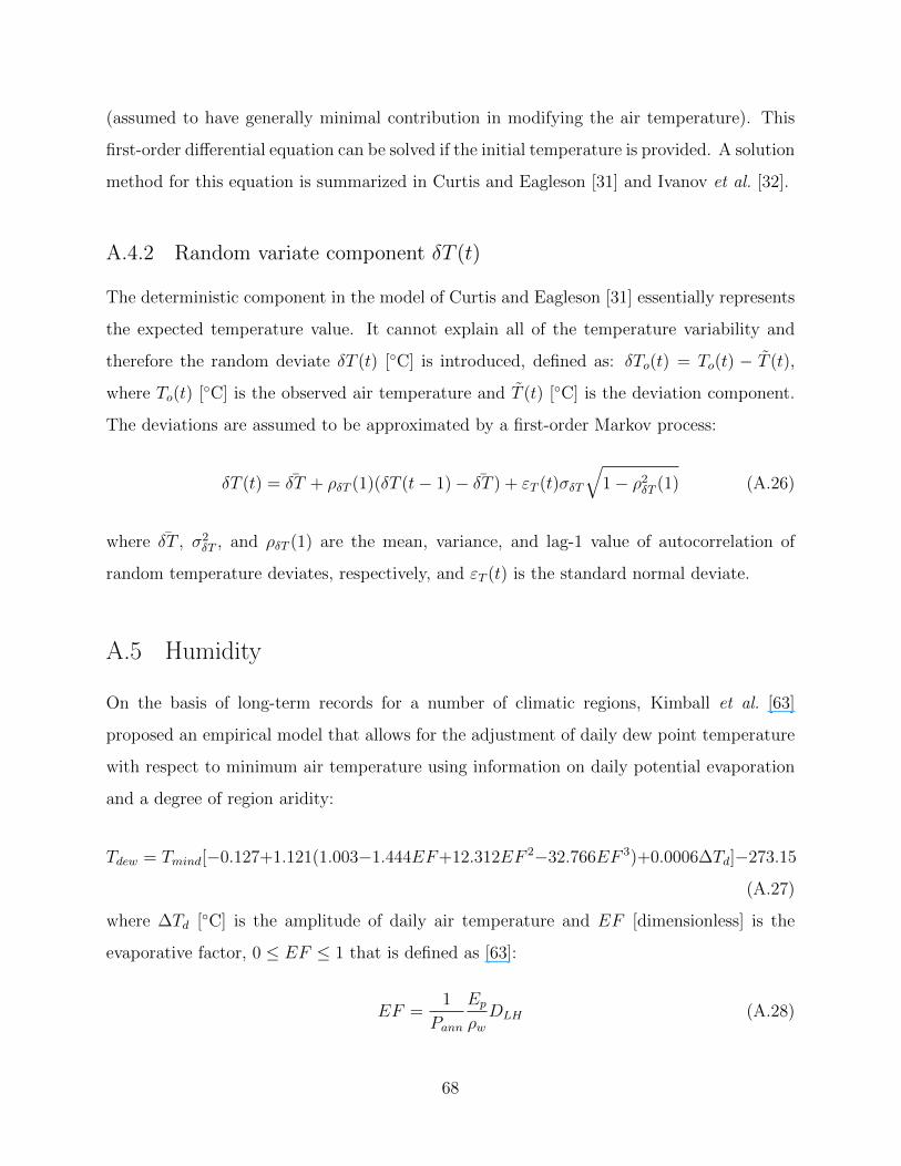
(assumed to have generally minimal contribution in modifying the air temperature). This
first-order differential equation can be solved if the initial temperature is provided. A solution
method for this equation is summarized in Curtis and Eagleson [31] and Ivanov et al. [32].
A.4.2 Random variate component δT (t)
The deterministic component in the model of Curtis and Eagleson [31] essentially represents
the expected temperature value. It cannot explain all of the temperature variability and
therefore the random deviate δT (t) [◦C] is introduced, defined as: δTo(t) = To(t) − T (t),
where To(t) [◦C] is the observed air temperature and T (t) [◦C] is the deviation component.
The deviations are assumed to be approximated by a first-order Markov process:
δT (t) = δT + ρδT (1)(δT (t− 1)− δT ) + εT (t)σδT
√1− ρ2
δT (1) (A.26)
where δT , σ2δT , and ρδT (1) are the mean, variance, and lag-1 value of autocorrelation of
random temperature deviates, respectively, and εT (t) is the standard normal deviate.
A.5 Humidity
On the basis of long-term records for a number of climatic regions, Kimball et al. [63]
proposed an empirical model that allows for the adjustment of daily dew point temperature
with respect to minimum air temperature using information on daily potential evaporation
and a degree of region aridity:
Tdew = Tmind[−0.127+1.121(1.003−1.444EF+12.312EF 2−32.766EF 3)+0.0006∆Td]−273.15
(A.27)
where ∆Td [◦C] is the amplitude of daily air temperature and EF [dimensionless] is the
evaporative factor, 0 ≤ EF ≤ 1 that is defined as [63]:
EF =1
Pann
EpρwDLH (A.28)
68
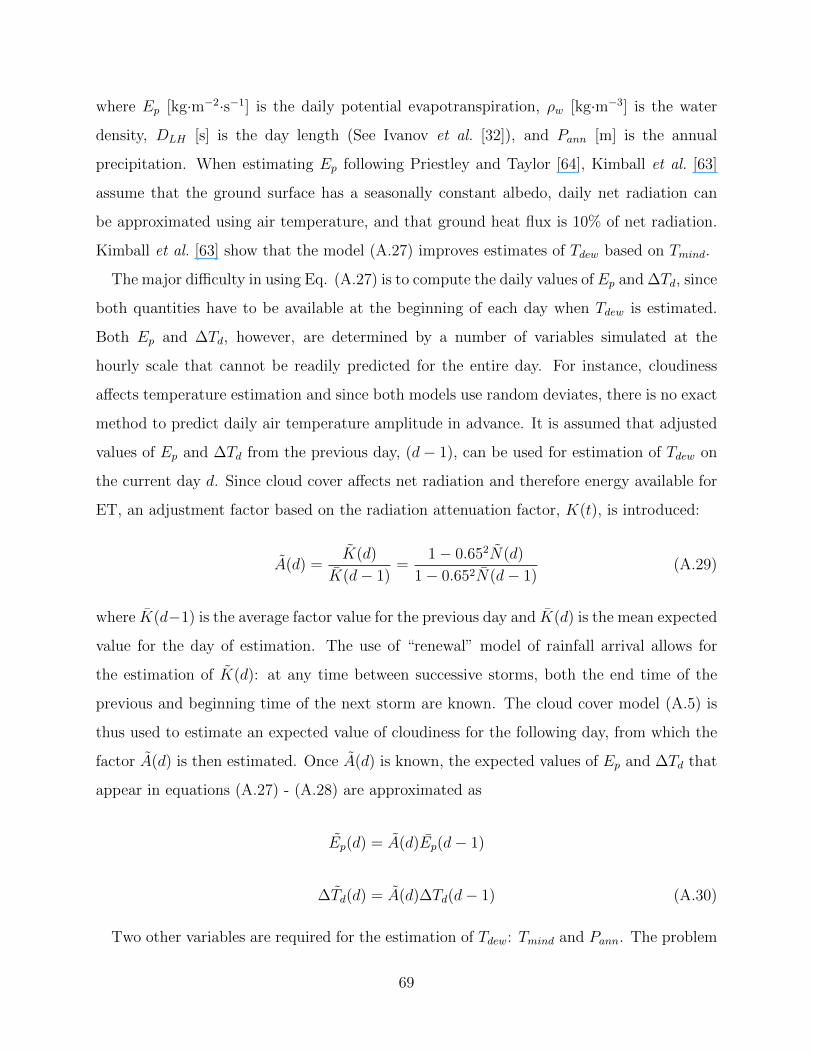
where Ep [kg·m−2·s−1] is the daily potential evapotranspiration, ρw [kg·m−3] is the water
density, DLH [s] is the day length (See Ivanov et al. [32]), and Pann [m] is the annual
precipitation. When estimating Ep following Priestley and Taylor [64], Kimball et al. [63]
assume that the ground surface has a seasonally constant albedo, daily net radiation can
be approximated using air temperature, and that ground heat flux is 10% of net radiation.
Kimball et al. [63] show that the model (A.27) improves estimates of Tdew based on Tmind.
The major difficulty in using Eq. (A.27) is to compute the daily values of Ep and ∆Td, since
both quantities have to be available at the beginning of each day when Tdew is estimated.
Both Ep and ∆Td, however, are determined by a number of variables simulated at the
hourly scale that cannot be readily predicted for the entire day. For instance, cloudiness
affects temperature estimation and since both models use random deviates, there is no exact
method to predict daily air temperature amplitude in advance. It is assumed that adjusted
values of Ep and ∆Td from the previous day, (d− 1), can be used for estimation of Tdew on
the current day d. Since cloud cover affects net radiation and therefore energy available for
ET, an adjustment factor based on the radiation attenuation factor, K(t), is introduced:
A(d) =K(d)
K(d− 1)=
1− 0.652N(d)
1− 0.652N(d− 1)(A.29)
where K(d−1) is the average factor value for the previous day and K(d) is the mean expected
value for the day of estimation. The use of “renewal” model of rainfall arrival allows for
the estimation of K(d): at any time between successive storms, both the end time of the
previous and beginning time of the next storm are known. The cloud cover model (A.5) is
thus used to estimate an expected value of cloudiness for the following day, from which the
factor A(d) is then estimated. Once A(d) is known, the expected values of Ep and ∆Td that
appear in equations (A.27) - (A.28) are approximated as
Ep(d) = A(d)Ep(d− 1)
∆Td(d) = A(d)∆Td(d− 1) (A.30)
Two other variables are required for the estimation of Tdew: Tmind and Pann. The problem
69

of computing Tmind is similar to the one described above. Air temperature at the hour
preceding sunrise can be usually associated with Tmind. Hence the air temperature from
(A.24) at the hour preceding sunrise is taken as Tmind and used in the estimation of Tdew.
Kimball et al. [63] used the mean annual precipitation Pann for all days throughout the year.
Here, it is assumed that a monthly basis is more appropriate since different months/seasons
have different degree of dryness. Therefore Pann is considered as a precipitation parameter
for each month, Pann∗.
A.6 Wind speed
To simulate the wind speed, Curtis and Eagleson [31] used the AR(1) model, where the
random term forces skewness on the results of the autoregressive model, leading to an ap-
proximately Gamma distribution of wind speed [68].
Ws(t) = Ws + ρs(1)(Ws(t− 1)− Ws) + εtσs√
1− ρ2s(1) (A.31)
where Ws [m·s−1], σ2s [m2·s−2], and ρs(1) [dimensionless] are the mean, variance, and lag-1
value of the autocorrelation of wind speed, respectively. And the term εt(t) is:
εt =2
γε
[1 +
γεψt6− γ2
ε
36
]3
− 2
γε(A.32)
where ψt is a standard normal deviate and γs(t) is the skewness of εt(t):
γε =(1− ρ3
s)γs(1− ρ2
s)1.5
(A.33)
where γs(t) is the skewness determined from the wind speed data.
70
APPENDIX B
SIMULATIONS FOR OTHER LOCATIONS INMIDWESTERN UNITED STATES
MLCan simulations for maize, miscanthus and switchgrass for growing season in the year
2005 at two other locations in the Midwest area: (i) Ozark, Missouri (38.74 ◦N, 92.20 ◦E)
and (ii) Brookings, South Dakota (44.34 ◦N, 96.84 ◦E) are presented in this appendix for
reference. First, results obtained from MLCan simulations for these two additional sites
and for Bondville, Illinois under present climate conditions are compared to understand the
role of meteorological forcing on the water use of energy crops in Midwestern U.S. In the
next sections, further details and descriptions of the two additional sites, input data, and
simulation results are presented.
A map showing the locations of Ameriflux towers located at Bondville, Ozark, and Brook-
ings is presented in Figure B.1. The Ozark site is located in the University of Missouri Baskett
Wildlife Research area, situated in the region of central Missouri. The site is uniquely located
in the ecologically important transitional zone between the central hardwood region and the
central grassland region of the U.S. (See official website at http://public.ornl.gov/ameriflux/
for details). The Brookings site is located in a private pasture, consisting of a mixture of C3
and C4 species actively used for grazing. Belonging to the Northern Great Plains Rangelands,
the grassland is representative of many in the north central United States, with seasonal win-
ter conditions and a wet growing season (See official website at http://public.ornl.gov/ameriflux/
for further details). For these two additional sites (Ozark and Brookings), the meteorological
forcing data is also collected at the nearby eddy-covariance flux towers in Ameriflux network
(See section 2.3.1 for further information). However, there is no observation of LAI data for
maize, miscanthus, and switchgrass in these locations, the biological data (LAI) is therefore
obtained from the study by Heaton et al. [11] and Drewry et al. [22] in central Illinois as
shown in Chapter 2.
71
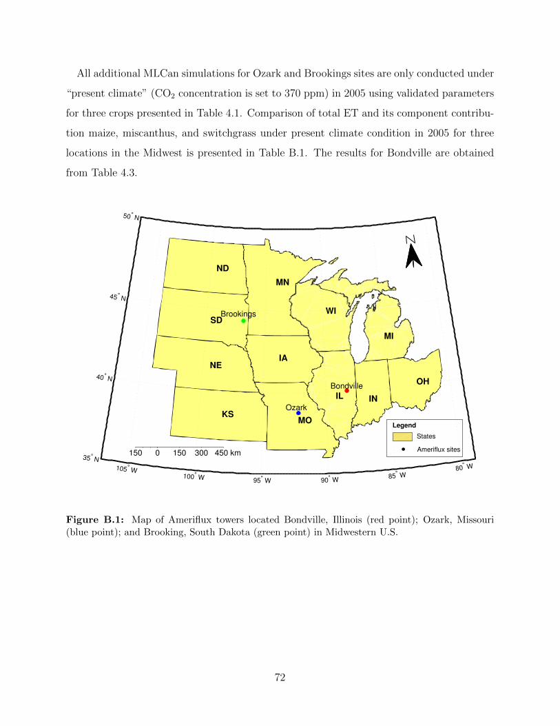
All additional MLCan simulations for Ozark and Brookings sites are only conducted under
“present climate” (CO2 concentration is set to 370 ppm) in 2005 using validated parameters
for three crops presented in Table 4.1. Comparison of total ET and its component contribu-
tion maize, miscanthus, and switchgrass under present climate condition in 2005 for three
locations in the Midwest is presented in Table B.1. The results for Bondville are obtained
from Table 4.3.
IL IN
IA
KS
MI
MN
MO
NE
ND
OH
SDWI
0 150 300 450 km150
Bondville
Ozark
Brookings
105° W
100° W 95
° W 90
° W 85
° W 80
° W
35° N
40° N
45° N
50° N
Legend
States
Ameriflux sites
Figure B.1: Map of Ameriflux towers located Bondville, Illinois (red point); Ozark, Missouri(blue point); and Brooking, South Dakota (green point) in Midwestern U.S.
72
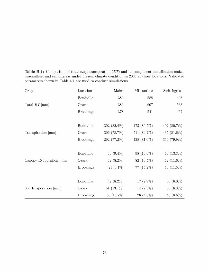
Table B.1: Comparison of total evapotranspiration (ET) and its component contribution maize,miscanthus, and switchgrass under present climate condition in 2005 at three locations. Validatedparameters shown in Table 4.1 are used to conduct simulations.
Crops Locations Maize Miscanthus Switchgrass
Bondville 380 588 498
Total ET [mm] Ozark 389 607 533
Brookings 378 541 462
Bondville 302 (82.4%) 473 (80.5%) 402 (80.7%)
Transpiration [mm] Ozark 306 (78.7%) 511 (84.2%) 435 (81.6%)
Brookings 292 (77.2%) 438 (81.0%) 369 (79.9%)
Bondville 36 (9.4%) 98 (16.6%) 66 (13.3%)
Canopy Evaporation [mm] Ozark 32 (8.2%) 82 (13.5%) 62 (11.6%)
Brookings 23 [6.1%] 77 (14.2%) 53 (11.5%)
Bondville 42 (8.2%) 17 (2.9%) 30 (6.0%)
Soil Evaporation [mm] Ozark 51 (13.1%) 14 (2.3%) 36 (6.8%)
Brookings 63 [16.7%] 26 (4.8%) 40 (8.6%)
73
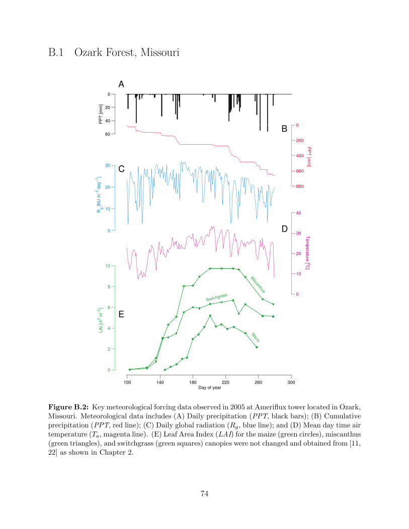
B.1 Ozark Forest, Missouri
0
20
40
60
PP
T [m
m]
0
200
400
600
800
PP
T [m
m]
0
10
20
30
Rg [M
J m
−2 d
ay−
1]
0
10
20
30
40
Tem
pera
ture
[ oC]
100 140 180 220 260 300
0
2
4
6
8
10
Miscanthus
Switchgrass
Maize
LA
I [m
2 m
−2]
Day of year
A
B
D
C
E
Figure B.2: Key meteorological forcing data observed in 2005 at Ameriflux tower located in Ozark,Missouri. Meteorological data includes (A) Daily precipitation (PPT, black bars); (B) Cumulativeprecipitation (PPT, red line); (C) Daily global radiation (Rg, blue line); and (D) Mean day time airtemperature (Ta, magenta line). (E) Leaf Area Index (LAI) for the maize (green circles), miscanthus(green triangles), and switchgrass (green squares) canopies were not changed and obtained from [11,22] as shown in Chapter 2.
74
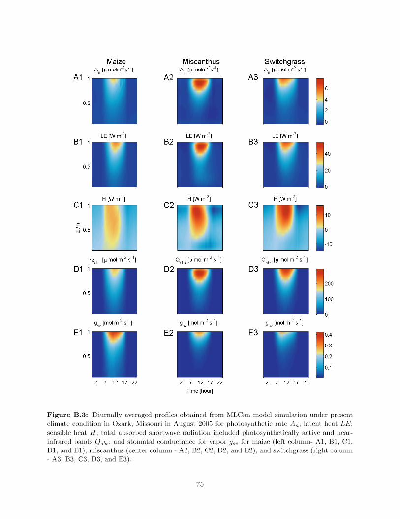
Figure B.3: Diurnally averaged profiles obtained from MLCan model simulation under presentclimate condition in Ozark, Missouri in August 2005 for photosynthetic rate An; latent heat LE;sensible heat H; total absorbed shortwave radiation included photosynthetically active and near-infrared bands Qabs; and stomatal conductance for vapor gsv for maize (left column- A1, B1, C1,D1, and E1), miscanthus (center column - A2, B2, C2, D2, and E2), and switchgrass (right column- A3, B3, C3, D3, and E3).
75
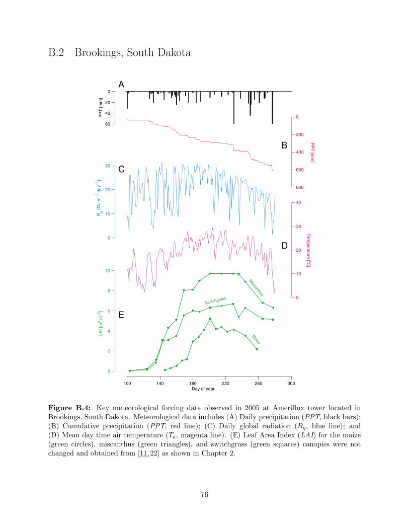
B.2 Brookings, South Dakota
0
20
40
60
PP
T [
mm
]
0
200
400
600
800
PP
T [m
m]
0
10
20
30
Rg [M
J m
−2 d
ay−
1]
0
10
20
30
40
Tem
pera
ture
[ oC]
100 140 180 220 260 300
0
2
4
6
8
10
Miscanthus
Switchgrass
Maize
LA
I [m
2 m
−2]
Day of year
E
C
A
B
D
Figure B.4: Key meteorological forcing data observed in 2005 at Ameriflux tower located inBrookings, South Dakota. Meteorological data includes (A) Daily precipitation (PPT, black bars);(B) Cumulative precipitation (PPT, red line); (C) Daily global radiation (Rg, blue line); and(D) Mean day time air temperature (Ta, magenta line). (E) Leaf Area Index (LAI) for the maize(green circles), miscanthus (green triangles), and switchgrass (green squares) canopies were notchanged and obtained from [11,22] as shown in Chapter 2.
76
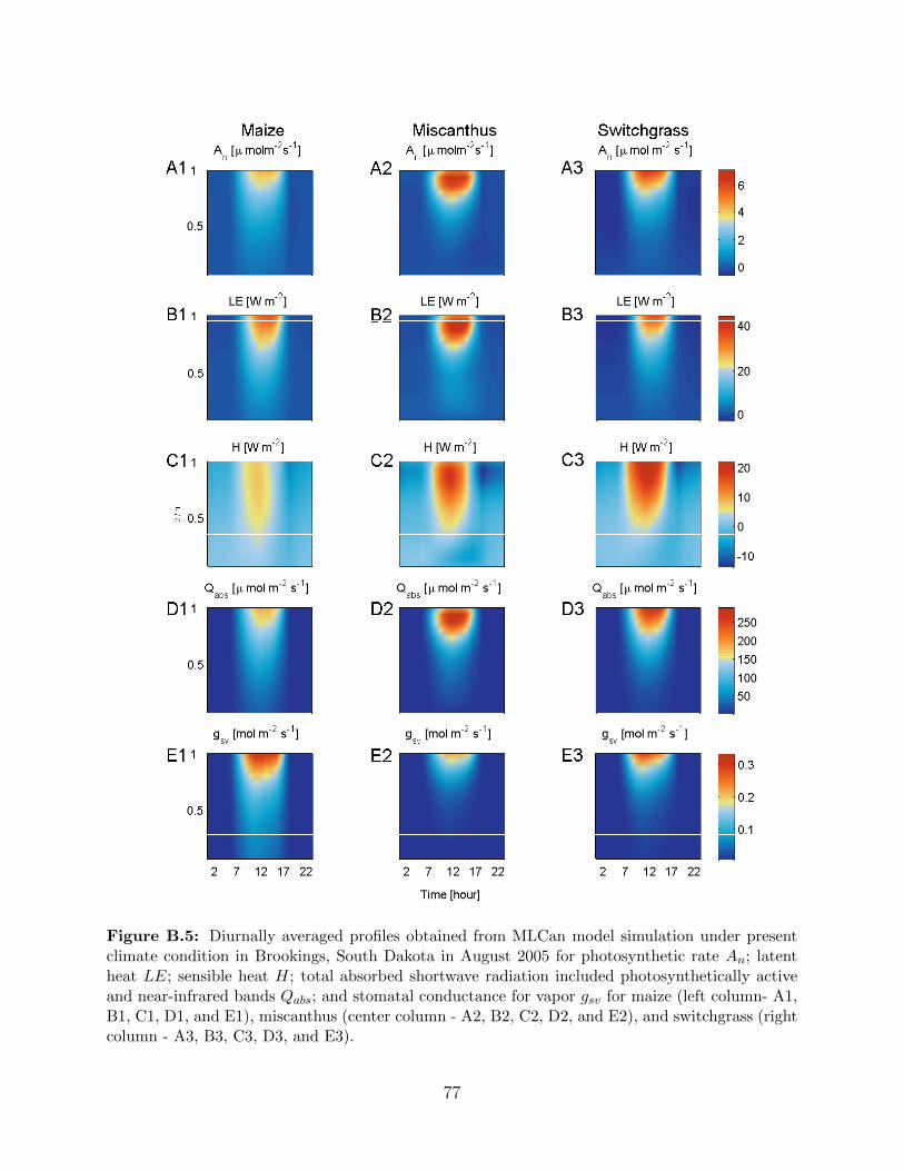
Figure B.5: Diurnally averaged profiles obtained from MLCan model simulation under presentclimate condition in Brookings, South Dakota in August 2005 for photosynthetic rate An; latentheat LE; sensible heat H; total absorbed shortwave radiation included photosynthetically activeand near-infrared bands Qabs; and stomatal conductance for vapor gsv for maize (left column- A1,B1, C1, D1, and E1), miscanthus (center column - A2, B2, C2, D2, and E2), and switchgrass (rightcolumn - A3, B3, C3, D3, and E3).
77


