Improved Multi-Core Nested Depth-First Search

Sami Evangelista1, Alfons Laarman2, Laure Petrucci1, and Jaco van de Pol2

1 LIPN, CNRS UMR 7030 — Universite Paris 13, France2 Formal Methods and Tools, University of Twente, The Netherlands

Abstract. This paper presents CNDFS, a tight integration of two earlier multi-core nested depth-first search (NDFS) algorithms for LTL model checking. CNDFS

combines the different strengths and avoids some weaknesses of its predecessors.We compare CNDFS to an earlier ad-hoc combination of those two algorithmsand show several benefits: It has shorter and simpler code and a simpler correct-ness proof. It exhibits more robust performance with similar scalability, while atthe same time reducing memory requirements.The algorithm has been implemented in the multi-core backend of the LTSMIN

model checker, which is now benchmarked for the first time on a 48 core ma-chine (previously 16). The experiments demonstrate better scalability than otherparallel LTL model checking algorithms, but we also investigate apparent bottle-necks. Finally, we noticed that the multi-core NDFS algorithms produce shortercounterexamples, surprisingly often shorter than their BFS-based counterparts.

1 Introduction

Model checking is a resource demanding task that can be performed by a systematic ex-ploration of a huge directed graph representing the dynamic behaviour of the analysedsystem. Although memory is usually the major bottleneck, execution times can alsooften exceed acceptable limits. For instance the exploration of a 109 states graph at ahigh exploration rate of 105 states per second would take more than a day. This remainsacceptable but becomes problematic when increasing the number of system configu-rations and properties analysed. Hence, model checking has gained a renewed interestwith the advent of multi-core architectures that can help tackle this time explosion.

Some properties like safety properties rely on a complete enumeration of systemstates and can thus be easily parallelised since they do not ask for a specific search or-der. However, the problem is harder when it comes to the verification of Linear Timetemporal Logic (LTL) properties. LTL model checking can be reduced to a cycle detec-tion problem and state-of-the-art algorithms [8,9,11] proceed depth-first since cycles aremore easily discovered using this search order. However, this characteristic also makesthem unsuitable for parallel architectures since DFS is inherently sequential [20].

One approach to address this issue is to sacrifice the optimal linear complexity pro-vided by DFS algorithms and switch to BFS-like algorithms, which are highly scalableboth theoretically and experimentally. We compare our approach to the best representa-tive of that family. More recently, two algorithms (LNDFS from [13] and ENDFS from[10]) adapted the well known Nested DFS (NDFS) algorithm [8] to multi-core architec-tures. They share the principle of launching multiple instances of NDFS that synchronise

themselves to avoid useless state revisits. Although they are heuristic algorithms in thesense that, in the worst case, they reduce to spawn multiple unsynchronised instancesof NDFS, the experiments reported in [13,14] show good practical speedups.

The contribution of this paper is an improvement to both the LNDFS and ENDFSalgorithms, called CNDFS. This new algorithm is both much simpler and uses lessmemory, making it more compatible with lossy compression techniques such as treecompression [17] that can compress large states down to two integers. We also pursue athorough experimental evaluation of this algorithm on the models of the BEEM database[18] with an implementation of this algorithm on top of the LTSMIN toolset [16]. Theoutcome of these experiments is threefold. Firstly, CNDFS exhibits a similar speedupto its predecessors, but achieves this more robustly, with smoother speedup lines, whileusing less memory. Second, it combines nicely with heuristics limiting the amount ofredundant work performed by individual threads. Finally, in the presence of bugs, it re-ports counterexamples that are usually much shorter than those reported by NDFS and,more importantly, this length tends to decrease as more working threads get involvedin the verification. This property is quite appreciable from a user perspective as it easesthe task of error correction.

The outline of this paper is the following. In Section 2 we formally express the LTLmodel checking problem and review existing (sequential and parallel) algorithms thataddress it. CNDFS, our new algorithm, is introduced and formally proven in Section 3.Our experimental evaluation of this algorithm is summarised in Section 4. Finally, Sec-tion 5 concludes our paper and explores some research perspectives to this work.

2 Background

We give in this section the few ingredients that are required for the understanding ofthis paper and briefly review existing works in the field of explicit parallel LTL modelchecking based on the automata theoretic approach.

2.1 The Automata Theoretic Approach to LTL Model Checking

LTL model checking is usually performed following the automata-based approach orig-inating from [22] that proceeds in several steps. In this paper we focus only on the laststep of the process that can be reduced to a graph problem: given a graph representingthe synchronised product of the Buchi property automaton and the state space of thesystem, find a cycle containing an accepting state. Any such identified cycle determinesan infinite execution of the system violating the LTL formula. In this paper we will onlyreason on automaton graphs that result from the product of a Buchi property automatonand a system graph describing the dynamic behaviour of the modelled system.

Definition 1 (Automaton graph). An automaton graph is a tuple G = (S ,T ,A ,s0),where S is a finite set of states; T ⊆ S × S is a set of transitions; A ⊆ S is the set ofaccepting states; and s0 ∈ S is an initial state.

Notations. Let (S ,T ,A ,s0) be an automaton graph. For s ∈ S the set of its successorstates is denoted by succ(s) = {s′ ∈ S | (s,s′)∈ T }. (s,s′)∈ T is also denoted by s→ s′.

2

s→+ s′ (s→∗ s′) denotes the (reflexive) transitive closure of T , i.e. the fact that s′ isreachable from s. A path is a state sequence s1, . . . ,sn with si→ si+1, ∀i∈{1, . . . ,n−1},a cycle is a path s1, . . . ,sn with s1 = sn and a cycle C ≡ s1, . . . ,sn is an accepting cycleif C∩A 6= /0. An accepting run is an accepting cycle reachable from the initial state:s0, . . . ,si, . . . ,sn where si = sn. The LTL model checking problem consists of findingan accepting run in an automaton graph. An LTL model checking algorithm proceedson-the-fly if it can report an accepting run without visiting all transitions.

2.2 Sequential LTL Model Checking Algorithms

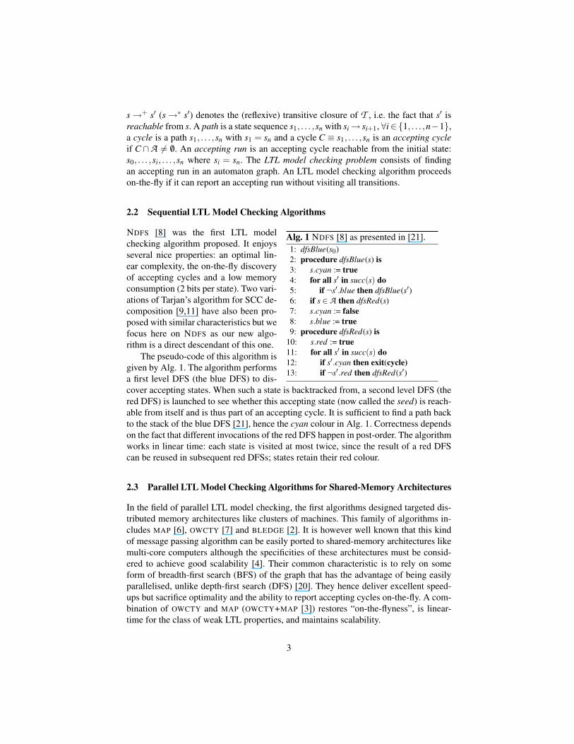
Alg. 1 NDFS [8] as presented in [21].1: dfsBlue(s0)2: procedure dfsBlue(s) is3: s.cyan := true4: for all s′ in succ(s) do5: if ¬s′.blue then dfsBlue(s′)6: if s ∈ A then dfsRed(s)7: s.cyan := false8: s.blue := true9: procedure dfsRed(s) is

10: s.red := true11: for all s′ in succ(s) do12: if s′.cyan then exit(cycle)13: if ¬s′.red then dfsRed(s′)

NDFS [8] was the first LTL modelchecking algorithm proposed. It enjoysseveral nice properties: an optimal lin-ear complexity, the on-the-fly discoveryof accepting cycles and a low memoryconsumption (2 bits per state). Two vari-ations of Tarjan’s algorithm for SCC de-composition [9,11] have also been pro-posed with similar characteristics but wefocus here on NDFS as our new algo-rithm is a direct descendant of this one.

The pseudo-code of this algorithm isgiven by Alg. 1. The algorithm performsa first level DFS (the blue DFS) to dis-cover accepting states. When such a state is backtracked from, a second level DFS (thered DFS) is launched to see whether this accepting state (now called the seed) is reach-able from itself and is thus part of an accepting cycle. It is sufficient to find a path backto the stack of the blue DFS [21], hence the cyan colour in Alg. 1. Correctness dependson the fact that different invocations of the red DFS happen in post-order. The algorithmworks in linear time: each state is visited at most twice, since the result of a red DFScan be reused in subsequent red DFSs; states retain their red colour.

2.3 Parallel LTL Model Checking Algorithms for Shared-Memory Architectures

In the field of parallel LTL model checking, the first algorithms designed targeted dis-tributed memory architectures like clusters of machines. This family of algorithms in-cludes MAP [6], OWCTY [7] and BLEDGE [2]. It is however well known that this kindof message passing algorithm can be easily ported to shared-memory architectures likemulti-core computers although the specificities of these architectures must be consid-ered to achieve good scalability [4]. Their common characteristic is to rely on someform of breadth-first search (BFS) of the graph that has the advantage of being easilyparallelised, unlike depth-first search (DFS) [20]. They hence deliver excellent speed-ups but sacrifice optimality and the ability to report accepting cycles on-the-fly. A com-bination of OWCTY and MAP (OWCTY+MAP [3]) restores “on-the-flyness”, is linear-time for the class of weak LTL properties, and maintains scalability.

3

SWARM verification [12] consists of spawning multiple unsynchronised instances ofNDFS each exploring the graph in a random way. Accepting cycles are expected to bereported faster thanks to randomised parallel search, but in the absence of such cyclesparallelisation does not help. This pragmatic strategy however targets graphs that are toolarge in any case to be explored in reasonable time. The purpose is then to maximisethe graph coverage in a given time frame and thereby increase confidence in the model.

Two recent multi-core algorithms follow the principle of the SWARM technique butdeviate from it in that working threads executing NDFS are synchronised through thesharing of some state attributes. In the first one, LNDFS [13], workers share the outcomeof the red (nested) search which can then also be used to prune the blue search. Sincethe blue flags are not shared among threads, the red searches are still invoked in theappropriate DFS postorder. The ENDFS algorithm [10] also allows the sharing of blueflags, but a sequential emergency procedure is triggered if the appropriate invocationorder of the red DFS is not respected. Moreover, to maintain correctness, informationon a red DFS in progress cannot be transmitted in “real time” to other threads: the statesvisited by a red DFS are only marked globally red after it has returned.

A thorough experimental comparison of ENDFS and LNDFS [14] led to the mainconclusion that ENDFS and LNDFS complement each other on a variety of models:the larger amount of information shared by ENDFS can potentially yield a better workdistribution, but LNDFS is to be preferred when ENDFS threads often launch unfruitfulemergency procedures. Since this emergency procedure launches the sequential NDFSalgorithm, large portions of the graph may then be revisited, in the worst case by allworkers. Hence, a combination of ENDFS and LNDFS was proposed [14] to remedythe downsides of the two algorithms. The principle of that parallel algorithm (calledNMCNDFS) is to run ENDFS but replace its sequential emergency procedure by a par-allel LNDFS. Experiments show that this combination pays off: NMCNDFS is alwaysat least as fast as ENDFS or LNDFS.

While NMCNDFS combines the strengths of both earlier algorithms in terms ofperformance, it also conjoins their memory usage. LNDFS requires 2P + log2(P) + 1bits per state (2 local colours for all P workers, a synchronisation counter and a globalred bit) and ENDFS 4P+3 (2 local colours plus another 2 for the repair procedure and3 global bits: {dangerous,red,blue}). Next to more than doubling the memory usage,the conglomerated algorithm is long and complex.

3 A New Combination of Multi-Core NDFS

To mitigate the downsides of NMCNDFS, we present a new algorithm, CNDFS, shownin Alg. 2. Like the previous multi-core algorithms, it is based on the principle of SWARMworker threads (indicated by subscript p here), sharing information via colours stored inthe visited states, here: blue and red. After randomly (shuffleblue

p ) visiting all successors(l.13–l.15), a state is marked blue at l.16 (meaning “globally visited”) and causing the(other) blue DFS workers to lose the strict postorder property.

If the state s is accepting, as usual, a red DFS is launched at l.19 to find a cycle.At this point, state s is called “the seed”. All states visited by dfsRedp are collectedin Rp. If no cycle is found in the red DFS, we can prove that none exists for the seed

4

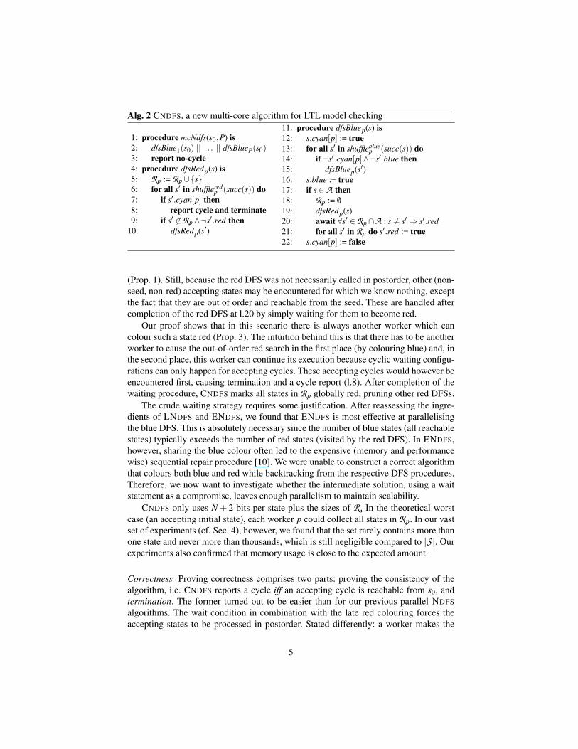
Alg. 2 CNDFS, a new multi-core algorithm for LTL model checking

1: procedure mcNdfs(s0,P) is2: dfsBlue1(s0) || . . . || dfsBlueP(s0)3: report no-cycle4: procedure dfsRedp(s) is5: Rp := Rp∪{s}6: for all s′ in shufflered

p (succ(s)) do7: if s′.cyan[p] then8: report cycle and terminate9: if s′ 6∈ Rp∧¬s′.red then

10: dfsRedp(s′)

11: procedure dfsBluep(s) is12: s.cyan[p] := true13: for all s′ in shuffleblue

p (succ(s)) do14: if ¬s′.cyan[p]∧¬s′.blue then15: dfsBluep(s′)16: s.blue := true17: if s ∈ A then18: Rp := /0

19: dfsRedp(s)20: await ∀s′ ∈ Rp∩A : s 6= s′⇒ s′.red21: for all s′ in Rp do s′.red := true22: s.cyan[p] := false

(Prop. 1). Still, because the red DFS was not necessarily called in postorder, other (non-seed, non-red) accepting states may be encountered for which we know nothing, exceptthe fact that they are out of order and reachable from the seed. These are handled aftercompletion of the red DFS at l.20 by simply waiting for them to become red.

Our proof shows that in this scenario there is always another worker which cancolour such a state red (Prop. 3). The intuition behind this is that there has to be anotherworker to cause the out-of-order red search in the first place (by colouring blue) and, inthe second place, this worker can continue its execution because cyclic waiting configu-rations can only happen for accepting cycles. These accepting cycles would however beencountered first, causing termination and a cycle report (l.8). After completion of thewaiting procedure, CNDFS marks all states in Rp globally red, pruning other red DFSs.

The crude waiting strategy requires some justification. After reassessing the ingre-dients of LNDFS and ENDFS, we found that ENDFS is most effective at parallelisingthe blue DFS. This is absolutely necessary since the number of blue states (all reachablestates) typically exceeds the number of red states (visited by the red DFS). In ENDFS,however, sharing the blue colour often led to the expensive (memory and performancewise) sequential repair procedure [10]. We were unable to construct a correct algorithmthat colours both blue and red while backtracking from the respective DFS procedures.Therefore, we now want to investigate whether the intermediate solution, using a waitstatement as a compromise, leaves enough parallelism to maintain scalability.

CNDFS only uses N + 2 bits per state plus the sizes of R. In the theoretical worstcase (an accepting initial state), each worker p could collect all states in Rp. In our vastset of experiments (cf. Sec. 4), however, we found that the set rarely contains more thanone state and never more than thousands, which is still negligible compared to |S |. Ourexperiments also confirmed that memory usage is close to the expected amount.

Correctness Proving correctness comprises two parts: proving the consistency of thealgorithm, i.e. CNDFS reports a cycle iff an accepting cycle is reachable from s0, andtermination. The former turned out to be easier than for our previous parallel NDFSalgorithms. The wait condition in combination with the late red colouring forces theaccepting states to be processed in postorder. Stated differently: a worker makes the

5

effects of its dfsRedp(s) globally visible (via the red colouring), only after all smaller(in postorder) accepting states t have been processed by some dfsRedp′(t). This is ex-pressed by Lemma 3. In Theorem 1, we finally show that, if the algorithm terminateswithout reporting a cycle, all accepting states must be red and consequently cannot lieon a cycle. Proof of termination was already discussed briefly and is detailed in Prop. 3.

In the following proofs, the graph colouring and the process counter of Alg. 2 areviewed as state properties of the execution. When writing dfsBluep(s)@19, we refer tothe point in the execution at which a worker p is about to call dfsRed on a state s at l.19,within the execution of dfsBluep(s). Graph colourings are denoted as follows: s ∈ Redmeans that the red flag of s is set to true and similarly s ∈ Blue means that the blueflag is set. For local flags we use s ∈ Cyanp. Also, we use the modal operator s ∈ �X ,to express ∀s′ ∈ succ(s):s′ ∈ X . We show that our propositions hold in the initial state(∀s ∈ S : s 6∈ Red∧ s 6∈ Blue∧∀p ∈ {1 . . .P} : s 6∈ Cyanp) and inductively that they aremaintained by execution of each statement in the algorithm, considering only lines thatcan influence the truth value of the proposition. Here an important assumption is thatall lines of Alg. 2 are executed atomically.

Lemma 1. Red states have red successors: Red ⊆�Red.

Proof. Initially, there are no red states, hence the lemma holds.States are coloured red when dfsBluep@21 and are never uncoloured red. The set of

states Rp that is coloured at l.21 contains all states reachable from the seed s, but not yetred, since dfsRedp(s) performed a DFS from s over all non-red states. For the red statesreachable from s, the induction hypothesis can be applied, hence there are no non-redstates reachable from s that are not in Rp. ut

Lemma 2. At l.20, the set Rp invariably contains (1) the seed s, (2) all non-red statesreachable from s and also (3) all states in the set are reachable from the seed s:dfsBluep(s)@20⇒ (s ∈Rp∧ (∀s′ 6∈ Red : s→∗ s′⇒ s′ ∈Rp)∧ (∀s′′ ∈Rp⇒ s→∗ s′′)).

Proof. At l.5, we have s ∈ Rp. For the rest, see proof of Lemma 1. ut

Lemma 3. The only accepting state that can be coloured red at l.21 (for the first time)is the current seed s itself: dfsBluep(s)@21⇒ (Rp∩A)\Red ⊆ {s}.

Proof. Assume dfsBluep(s)@21 and ∃a ∈ (A \{s}) : a ∈ Rp. We show that a ∈ Red.By Lemma 2, Rp contains at least s and the non-red states reachable from s. After

l.20, all non-seed accepting states in Rp are red: (Rp ∩ (A \ {s})) ⊆ Red. Since, a ∈Rp∩ (A \{s}), we have: a ∈ Red. ut

Proposition 1. The initial invocation of dfsRedp(s) at l.19 of Alg. 2 reports a cycle ifand only if the seed s belongs to a cycle.

Proof. ⇔ is split into two cases: Case ⇒: Every state s′ ∈ Cyanp can reach the seedfrom dfsBluep(s)@19 by properties of the DFS stack. Similarly, when dfsRedp(s′′)@8,s′′ is reachable from the seed s. Therefore, there is a cycle: s′′→ s′→∗ s→∗ s′′.

Case⇐: assume dfsRedp(s) at l.19 finishes normally (without cycle report), whiles lies on a cycle C. We show this leads to a contradiction. Since dfsRed avoids only red

6

states (l.9), there would have to be some r ∈C∩Red obstructing the search. The stater can only be coloured red at l.21 by a worker. W.l.o.g. we investigate the first workerdfsRedp′ to have coloured r red. p′ started for an s′ ∈ A (dfsBluep′(s′)@l.19).

Since r is not yet red, by Lemma 1 C ∩Red = /0. Before r is coloured red, it isfirst stored in Rp′ . By Lemma 2, we also have C ⊆ Rp′ . Either s′ ∈ C, then the cyclethrough s′ would have been detected since s′ ∈ Cyanp′ . Or else s′ 6∈C, and then we have{s} ⊆ (Rp′ \Red) when dfsBluep′(s′)@21, contradicting Lemma 3. ut

Proposition 2. Red states never lie on an accepting cycle.

Proof. Initially, there are no red states, hence the proposition holds.When dfsBluep(s)@21, the set of states Rp is coloured red. The only accepting state

to be colored red is the seed s (Lemma 3). By Prop. 1, this state s does not lie on anaccepting cycle. Hence, Prop. 2 is preserved. ut

Lemma 4. Blue states have blue or cyan successors: Blue⊆S

p �(Blue∪Cyanp).

Proof. Initially there are no blue states, hence the lemma holds.Only at l.16, states are coloured blue, after each successor t has been skipped at l.14

(t ∈ Cyan∪Blue), or processed by dfsBluep at l.15 (leading to t ∈ Blue). States can beuncoloured cyan (l.22), but only after they have been coloured blue (l.16). ut

Lemma 5. A blue accepting state, that is not also Cyanp for some worker p, must bered: ∀a ∈ (Blue∩A) : (∀p ∈ {1 . . .P} : a 6∈ Cyanp)⇒ a ∈ Red.

Proof. Assume s ∈ (A ∩Blue) and ∀p ∈ {1 . . .P} : s 6∈ Cyanp. We show that s ∈ Red.State s can only be coloured blue when dfsBluep(s)@16. There, it still retains its

cyan colouring from l.12, it only loses this colour at l.22. But, since s ∈ A , l.21 wasreached and there a ∈ Rp by Lemma 2. Hence, s ∈ Red at l.22. ut

Proposition 3. Algorithm 1 always terminates with a report.

Proof. The individual DFSs cannot proceed indefinitely due to a growing set of red andblue states. So eventually a cycle (l.8) or no cycle is reported (l.3). However, progressmay also halt due to the wait statement at l.20. We now assume towards a contradictionthat a worker p is waiting indefinitely for a state a∈A to become red: dfsBluep(s)@20,s 6= a and a ∈ Rp. We will show that either a will be coloured red eventually, or a cyclewould have been detected, contradicting the assumption that p keeps waiting.

By Lemma 2, a is reachable from s: s→+ a. And by l.16, s ∈ Blue. Induction onthe path s→∗ a, using Lemma 4, tells us that: either all states are blue (1) or there is acyan state on this path (2):

1. a ∈ Blue∧∀p ∈ {1 . . .P} : a 6∈ Cyanp: by Lemma 5, a ∈ Red, which contradicts theassumption that p is waiting for a to become red.

2. ∃c ∈ Cyanp′ : s→+ c→∗ a, then depending on the identity of worker p′, we have:A) p = p′: but then dfsRedp(s) would have terminated on cycle detection (C ≡

s→+ c→+ s), except when dfsRedp did not reach c in presence of a red statelying on C. However, this would contradict Prop. 2.

7

B) p 6= p′: we show that either p′ is executing or going to execute dfsRedp′(a).To eventually colour state a red, worker p′ must not end up itself in a waitingstate: dfsBluep′(a′)@20. First, consider the case a′ 6= a. We also have a′ ∈Rp: Ifa′ ∈ Red, then by Prop. 2 all its reachable states are red and it cannot be waitingfor a non-red reachable accepting state (Lemma 2). Therefore, a′ 6∈ Red andsince also s→+ c→∗ a′ (stack Cyanp), we have: a′ ∈Rp (Lemma 2). Therefore,we can assume w.l.o.g. that a = a′ and only consider dfsBluep′(a)@20. We canrepeat the reasoning process of this proof, with p ≡ p′ and s ≡ a. But sincethere are finitely many workers, the chain of processes waiting for each othereventually terminates, except the hypothetical configuration of a cyclic waitingdependency, which we consider finally.

To exclude cyclic dependencies, assume n ≥ 2 workers are simultaneously wait-ing for each other’s seed to be coloured red at l.20. We have: dfsBlue1(s1)@20∧ . . .∧dfsBluen(sn)@20∧s2 ∈R1∧ . . .∧s1 ∈Rn. This is only possible if s1→+ sn∧ . . .∧sn→+

s1, hence there is a cycle: s1 →+ . . .→+ sn →+ s1. However, this contradicts that thered DFSs (which terminate anyway) would have detected this cycle (Prop. 1). ut

Theorem 1. Alg. 2 reports an accepting cycle if and only if one is reachable from s0.

Proof. By Prop. 3, the algorithm is guaranteed to terminate with some report, formingthe basis for two cases: Case⇒: dfsRedp(s)@8 implies a cycle (Prop. 1).

Case ⇐: At l.3, we have s0 ∈ Blue and Cyan = /0 by properties of DFS. Now, byLemma 4, we have: ∀s ∈ G : s0→∗ s⇒ s ∈ Blue. Hence, all reachable accepting statesmust be red by Lemma 5 and do not lie on cycles by Prop. 2. ut

4 Experimental Evaluation

Our previously reported experiments [15,14,13] were performed on 16-core machines.Meanwhile, in accordance with Moore’s law applied to parallelism, we obtained ac-cess to a 48-core machine (a four-way AMD OpteronTM 6168). The added parallelismputs extra stress on the scalability of our algorithms and therefore also forces a repeatof some of our previous reachability experiments [15]. We investigated the cause forthe performance difference between various algorithms: NMCNDFS [14], CNDFS (thispaper), OWCTY+MAP [5] (the best representant of parallel BFS-based algorithms [13])and reachability from [15]. Work duplication due to overlapping stacks can cause slow-downs for all multi-core NDFS variants, as can long await cycles in CNDFS. We intro-duced counters to measure and study these effects. Initially, we focus on models withoutcycles, the hardest case for these algorithms. Later we move on to show that CNDFS ex-hibits the same on-the-fly performance as existing multi-core NDFS variants [14].

We have used models from the BEEM database [18].1 From each type of model, weselected the variants with more than 9 million states. Our CNDFS algorithm is imple-mented in the multi-core backend of the LTSMIN model checking tool set [16], basedon a dedicated scalable lock-free hash table and an off-the-shelf load balancer [15].

1 All results are available at http://fmt.cs.utwente.nl/tools/ltsmin/atva-2012/.

8

For a fair comparison with previous algorithms, we also implemented some NDFS opti-mizations [13, Sec. 4.4], all-red and early cycle detection. All-red colours a state s red,if all its successors are red after l.15 of Alg. 2; correctness follows from Prop. 2. Earlycycle detection detects certain accepting cycles already in the blue search.

LTSMIN 1.92 was compiled with GCC 4.4.2 (with optimisation -O2) and ran with:dve22lts-mc --threads=N -s28 --state=table --strategy=name, where namecan be cndfs or endfs,lndfs, representing the different algorithms [14]. We used Di-VinE 2.5.2 [5] as OWCTY+MAP implementation, compiled and run with equivalent pa-rameters. Since LTSMIN reuses its next-state function, both tools are comparable [15].

4.1 Models without Accepting Cycles

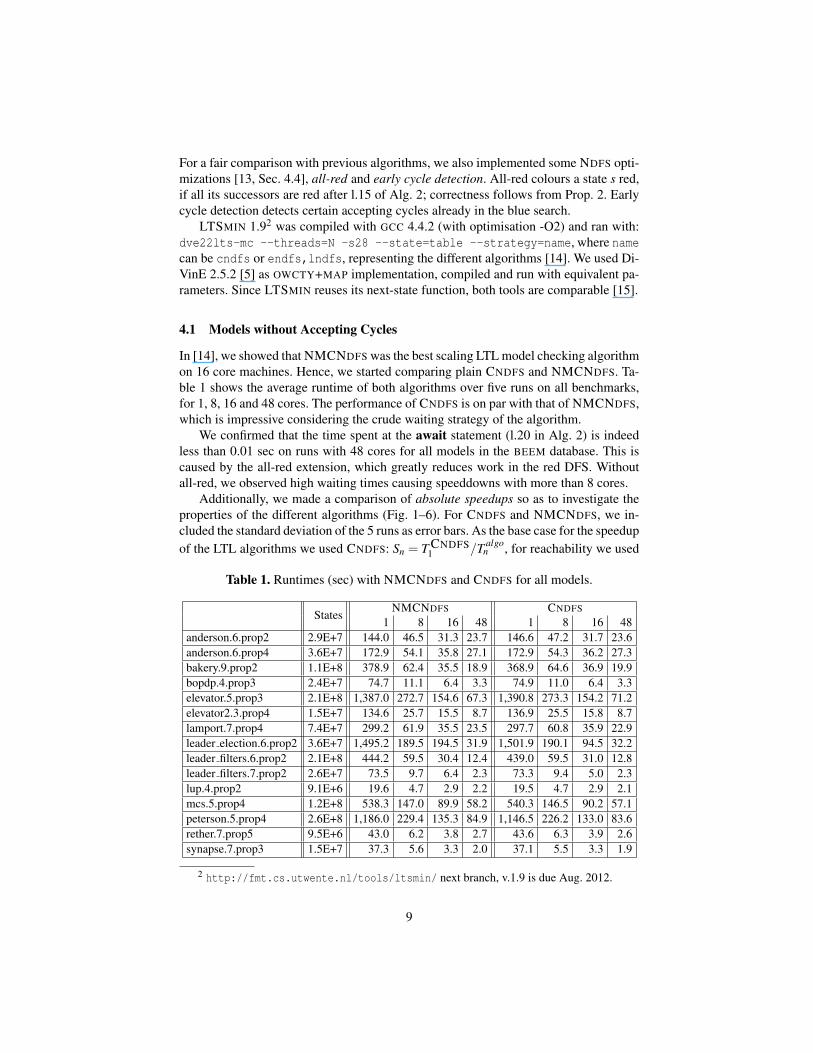
In [14], we showed that NMCNDFS was the best scaling LTL model checking algorithmon 16 core machines. Hence, we started comparing plain CNDFS and NMCNDFS. Ta-ble 1 shows the average runtime of both algorithms over five runs on all benchmarks,for 1, 8, 16 and 48 cores. The performance of CNDFS is on par with that of NMCNDFS,which is impressive considering the crude waiting strategy of the algorithm.

We confirmed that the time spent at the await statement (l.20 in Alg. 2) is indeedless than 0.01 sec on runs with 48 cores for all models in the BEEM database. This iscaused by the all-red extension, which greatly reduces work in the red DFS. Withoutall-red, we observed high waiting times causing speeddowns with more than 8 cores.

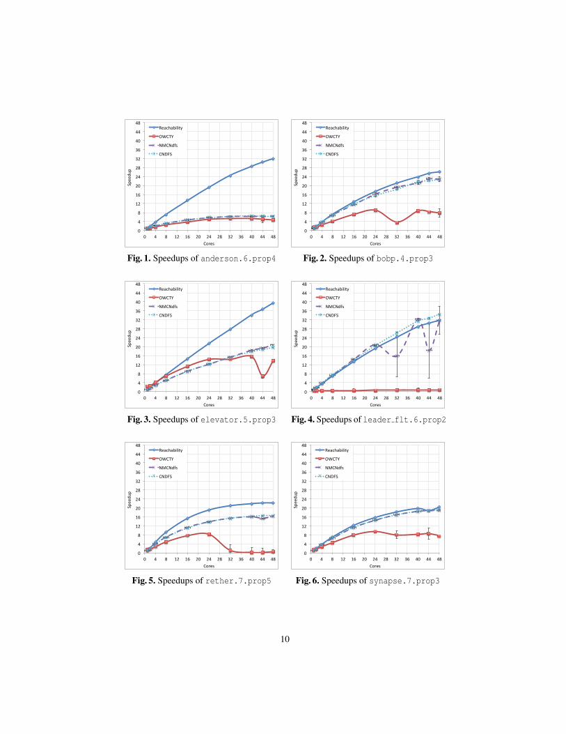
Additionally, we made a comparison of absolute speedups so as to investigate theproperties of the different algorithms (Fig. 1–6). For CNDFS and NMCNDFS, we in-cluded the standard deviation of the 5 runs as error bars. As the base case for the speedupof the LTL algorithms we used CNDFS: Sn = T CNDFS

1 /T algon , for reachability we used

Table 1. Runtimes (sec) with NMCNDFS and CNDFS for all models.

StatesNMCNDFS CNDFS

1 8 16 48 1 8 16 48anderson.6.prop2 2.9E+7 144.0 46.5 31.3 23.7 146.6 47.2 31.7 23.6anderson.6.prop4 3.6E+7 172.9 54.1 35.8 27.1 172.9 54.3 36.2 27.3bakery.9.prop2 1.1E+8 378.9 62.4 35.5 18.9 368.9 64.6 36.9 19.9bopdp.4.prop3 2.4E+7 74.7 11.1 6.4 3.3 74.9 11.0 6.4 3.3elevator.5.prop3 2.1E+8 1,387.0 272.7 154.6 67.3 1,390.8 273.3 154.2 71.2elevator2.3.prop4 1.5E+7 134.6 25.7 15.5 8.7 136.9 25.5 15.8 8.7lamport.7.prop4 7.4E+7 299.2 61.9 35.5 23.5 297.7 60.8 35.9 22.9leader election.6.prop2 3.6E+7 1,495.2 189.5 194.5 31.9 1,501.9 190.1 94.5 32.2leader filters.6.prop2 2.1E+8 444.2 59.5 30.4 12.4 439.0 59.5 31.0 12.8leader filters.7.prop2 2.6E+7 73.5 9.7 6.4 2.3 73.3 9.4 5.0 2.3lup.4.prop2 9.1E+6 19.6 4.7 2.9 2.2 19.5 4.7 2.9 2.1mcs.5.prop4 1.2E+8 538.3 147.0 89.9 58.2 540.3 146.5 90.2 57.1peterson.5.prop4 2.6E+8 1,186.0 229.4 135.3 84.9 1,146.5 226.2 133.0 83.6rether.7.prop5 9.5E+6 43.0 6.2 3.8 2.7 43.6 6.3 3.9 2.6synapse.7.prop3 1.5E+7 37.3 5.6 3.3 2.0 37.1 5.5 3.3 1.9

2 http://fmt.cs.utwente.nl/tools/ltsmin/ next branch, v.1.9 is due Aug. 2012.

9

0"

4"

8"

12"

16"

20"

24"

28"

32"

36"

40"

44"

48"

0" 4" 8" 12" 16" 20" 24" 28" 32" 36" 40" 44" 48"

Speedu

p"

Cores"

Reachability"

OWCTY"

NMCNdfs"

CNDFS"

Fig. 1. Speedups of anderson.6.prop4

0"

4"

8"

12"

16"

20"

24"

28"

32"

36"

40"

44"

48"

0" 4" 8" 12" 16" 20" 24" 28" 32" 36" 40" 44" 48"

Speedu

p"

Cores"

Reachability"

OWCTY"

NMCNdfs"

CNDFS"

Fig. 2. Speedups of bobp.4.prop3

0"

4"

8"

12"

16"

20"

24"

28"

32"

36"

40"

44"

48"

0" 4" 8" 12" 16" 20" 24" 28" 32" 36" 40" 44" 48"

Speedu

p"

Cores"

Reachability"

OWCTY"

NMCNdfs"

CNDFS"

Fig. 3. Speedups of elevator.5.prop3

0"

4"

8"

12"

16"

20"

24"

28"

32"

36"

40"

44"

48"

0" 4" 8" 12" 16" 20" 24" 28" 32" 36" 40" 44" 48"

Speedu

p"

Cores"

Reachability"

OWCTY"

NMCNdfs"

CNDFS"

Fig. 4. Speedups of leader flt.6.prop2

0"

4"

8"

12"

16"

20"

24"

28"

32"

36"

40"

44"

48"

0" 4" 8" 12" 16" 20" 24" 28" 32" 36" 40" 44" 48"

Speedu

p"

Cores"

Reachability"

OWCTY"

NMCNdfs"

CNDFS"

Fig. 5. Speedups of rether.7.prop5

0"

4"

8"

12"

16"

20"

24"

28"

32"

36"

40"

44"

48"

0" 4" 8" 12" 16" 20" 24" 28" 32" 36" 40" 44" 48"

Speedu

p"

Cores"

Reachability"

OWCTY"

NMCNdfs"

CNDFS"

Fig. 6. Speedups of synapse.7.prop3

10

its own base case. We included reachability from [15] to serve as a reference point forCNDFS. We were primarily interested to see whether the scalability of CNDFS keepsup with our parallel reachability implementation. After all, sequential NDFS visits eachstate at most twice; once in the blue DFS and possibly once in the red DFS.

We notice that NMCNDFS and CNDFS are always faster than OWCTY+MAP. Theerror bars show less robust runtimes for NMCNDFS as they fluctuate greatly (e.g.leader filters). Upon investigation it turned out that NMCNDFS sometimes launchesa repair search even though we also fitted its ENDFS search with all-red. When only fewworkers enter this repair search, it cannot be parallelized. In these cases, CNDFS turnsto waiting, a much better strategy, since in total it waits less than 0.01 sec. Also, reach-ability scales sometimes twice as good as CNDFS; anderson even scales 5 times better.

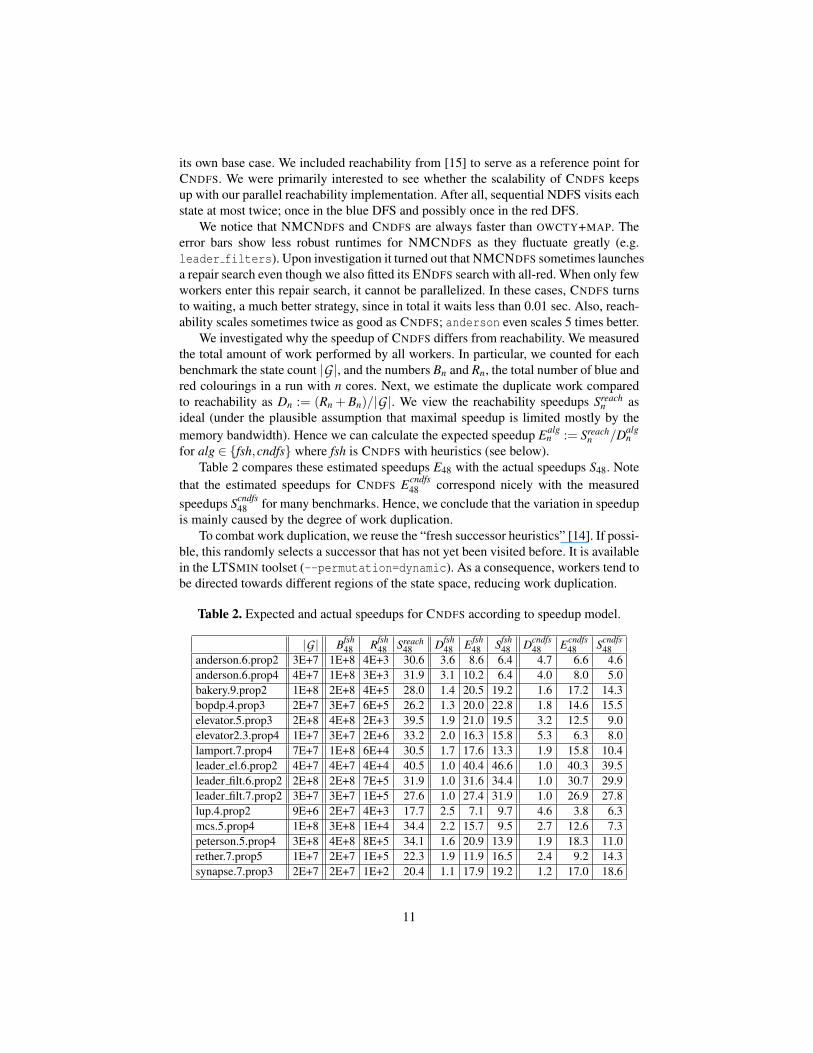
We investigated why the speedup of CNDFS differs from reachability. We measuredthe total amount of work performed by all workers. In particular, we counted for eachbenchmark the state count |G |, and the numbers Bn and Rn, the total number of blue andred colourings in a run with n cores. Next, we estimate the duplicate work comparedto reachability as Dn := (Rn + Bn)/|G |. We view the reachability speedups Sreach

n asideal (under the plausible assumption that maximal speedup is limited mostly by thememory bandwidth). Hence we can calculate the expected speedup Ealg

n := Sreachn /Dalg

nfor alg ∈ {fsh,cndfs} where fsh is CNDFS with heuristics (see below).

Table 2 compares these estimated speedups E48 with the actual speedups S48. Notethat the estimated speedups for CNDFS Ecndfs

48 correspond nicely with the measuredspeedups Scndfs

48 for many benchmarks. Hence, we conclude that the variation in speedupis mainly caused by the degree of work duplication.

To combat work duplication, we reuse the “fresh successor heuristics” [14]. If possi-ble, this randomly selects a successor that has not yet been visited before. It is availablein the LTSMIN toolset (--permutation=dynamic). As a consequence, workers tend tobe directed towards different regions of the state space, reducing work duplication.

Table 2. Expected and actual speedups for CNDFS according to speedup model.

|G | Bfsh48 Rfsh

48 Sreach48 Dfsh

48 E fsh48 Sfsh

48 Dcndfs48 Ecndfs

48 Scndfs48

anderson.6.prop2 3E+7 1E+8 4E+3 30.6 3.6 8.6 6.4 4.7 6.6 4.6anderson.6.prop4 4E+7 1E+8 3E+3 31.9 3.1 10.2 6.4 4.0 8.0 5.0bakery.9.prop2 1E+8 2E+8 4E+5 28.0 1.4 20.5 19.2 1.6 17.2 14.3bopdp.4.prop3 2E+7 3E+7 6E+5 26.2 1.3 20.0 22.8 1.8 14.6 15.5elevator.5.prop3 2E+8 4E+8 2E+3 39.5 1.9 21.0 19.5 3.2 12.5 9.0elevator2.3.prop4 1E+7 3E+7 2E+6 33.2 2.0 16.3 15.8 5.3 6.3 8.0lamport.7.prop4 7E+7 1E+8 6E+4 30.5 1.7 17.6 13.3 1.9 15.8 10.4leader el.6.prop2 4E+7 4E+7 4E+4 40.5 1.0 40.4 46.6 1.0 40.3 39.5leader filt.6.prop2 2E+8 2E+8 7E+5 31.9 1.0 31.6 34.4 1.0 30.7 29.9leader filt.7.prop2 3E+7 3E+7 1E+5 27.6 1.0 27.4 31.9 1.0 26.9 27.8lup.4.prop2 9E+6 2E+7 4E+3 17.7 2.5 7.1 9.7 4.6 3.8 6.3mcs.5.prop4 1E+8 3E+8 1E+4 34.4 2.2 15.7 9.5 2.7 12.6 7.3peterson.5.prop4 3E+8 4E+8 8E+5 34.1 1.6 20.9 13.9 1.9 18.3 11.0rether.7.prop5 1E+7 2E+7 1E+5 22.3 1.9 11.9 16.5 2.4 9.2 14.3synapse.7.prop3 2E+7 2E+7 1E+2 20.4 1.1 17.9 19.2 1.2 17.0 18.6

11

These results are also shown in Table 2: Dfsh48 , E fsh

48 and Sfsh48 together with the mea-

sured amount of blue and red colourings: Bfsh48 and Rfsh

48 . The heuristic approach showsquite some improvement, sometimes halving work duplication and doubling speedup(see elevator). Still we see duplications as high as 3.6 (see anderson). Note that theearlier speedups in Fig. 1–6 already include the benchmarks with this heuristic.

0"

0.5"

1"

1.5"

2"

2.5"

3"

3.5"

4"

4.5"

5"

0" 4" 8" 12" 16" 20" 24" 28" 32" 36" 40" 44" 48"

anderson.6.prop2"anderson.6.prop4"bakery.9.prop2"bopdp.4.prop3"bopdp.4.prop4"elevator.5.prop3"elevator2.3.prop4"lamport.7.prop4"leader_elec>on.6.prop2"leader_filters.6.prop2"leader_filters.7.prop2"lup.4.prop2"mcs.5.prop4"peterson.5.prop4"rether.7.prop5"synapse.7.prop3"

Fig. 7. Work duplication per core per model

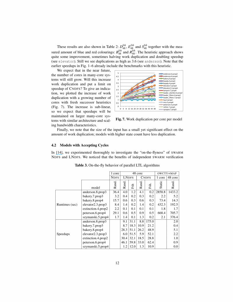
We expect that in the near future,the number of cores in many-core sys-tems will still grow. Will this increasework duplication and put a limit onspeedup of CNDFS? To give an indica-tion, we plotted the increase of workduplication with a growing number ofcores with fresh successor heuristics(Fig. 7). The increase is sub-linear,so we expect that speedups will bemaintained on larger many-core sys-tems with similar architecture and scal-ing bandwidth characteristics.

Finally, we note that the size of the input has a small yet significant effect on theamount of work duplication; models with higher state count have less duplication.

4.2 Models with Accepting Cycles

In [14], we experimented thoroughly to investigate the “on-the-flyness” of SWARMNDFS and LNDFS. We noticed that the benefits of independent SWARM verification

Table 3. On-the-fly behavior of parallel LTL algorithms

1 core 48 core OWCTY+MAP

NDFS LNDFS CNDFS 1 core 48 core

model Ran

d.

Ran

d.

Fsh

Ran

d.

Fsh.

Stat

ic

Ran

d.

Runtimes (sec)

anderson.8.prop3 36.4 4.0 1.2 4.1 0.2 2858.8 1433.2bakery.7.prop3 3.2 0.4 0.2 0.3 0.2 2.2 5.2bakery.8.prop4 15.7 0.6 0.3 0.6 0.3 73.4 14.3elevator2.3.prop3 8.4 1.4 0.2 1.4 0.2 432.3 192.5extinction.4.prop2 2.2 0.1 0.1 0.1 0.1 1.8 1.7peterson.6.prop4 29.1 0.6 0.5 0.9 0.5 668.4 705.7szymanski.5.prop4 1.7 1.4 0.1 1.3 0.2 2.1 376.4

Speedups

anderson.8.prop3 9.1 31.1 8.8 175.0 2.0bakery.7.prop3 8.7 18.3 10.9 21.2 0.4bakery.8.prop4 28.3 51.1 26.2 48.9 5.1elevator2.3.prop3 6.0 51.5 5.9 52.1 2.2extinction.4.prop2 30.4 32.1 18.5 28.8 1.0peterson.6.prop4 46.1 59.8 33.0 62.4 0.9szymanski.5.prop4 1.2 12.0 1.3 10.9 0.0

12

is limited, on average only yielding a speedup of 2-8 on 16 core machines. LNDFShowever yielded speedups from 4 to 14. Combined with the fresh successor heuristicspeedups became often superlinear. This is not surprising [19], because we verified thatin those cases there are many cycles, distributed evenly over the state space.

We performed the same experiments again with CNDFS on a 48 core machine. Theresults in Table 3 show that CNDFS exhibits the same desirable on-the-fly behaviour asLNDFS, scaling up to 48 cores. We conclude that our new multi-core CNDFS algorithmscales well also for models with bugs.

For completeness, we also included the runtimes and speedups with OWCTY+MAPin the table. While the heuristic on-the-fly behavior seems to work well for some mod-els, for others it does not. It must however be mentioned that the on-the-fly capabilitiesof this algorithm have recently been improved by changing its exploration order to bemore DFS-like [1]. In [1], performance is reported on par with the LNDFS algorithm.Unfortunately, we do not have the means (a GPGPU) to reproduce any results here.

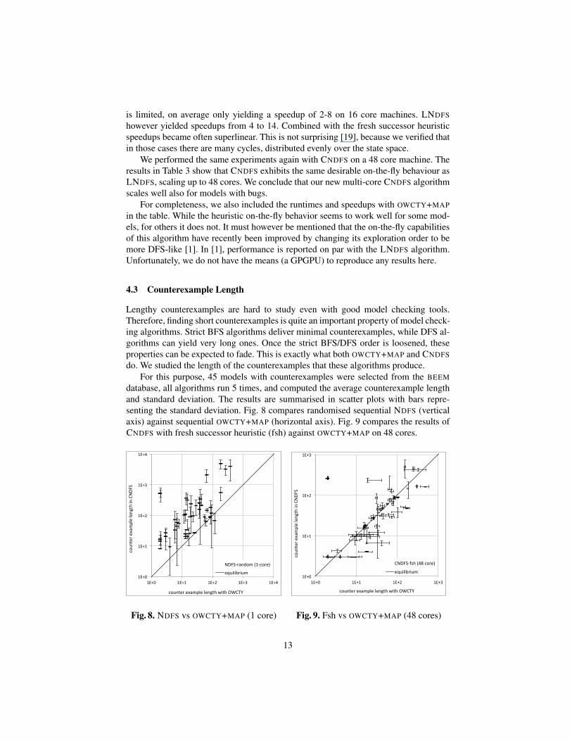
4.3 Counterexample Length

Lengthy counterexamples are hard to study even with good model checking tools.Therefore, finding short counterexamples is quite an important property of model check-ing algorithms. Strict BFS algorithms deliver minimal counterexamples, while DFS al-gorithms can yield very long ones. Once the strict BFS/DFS order is loosened, theseproperties can be expected to fade. This is exactly what both OWCTY+MAP and CNDFSdo. We studied the length of the counterexamples that these algorithms produce.

For this purpose, 45 models with counterexamples were selected from the BEEMdatabase, all algorithms run 5 times, and computed the average counterexample lengthand standard deviation. The results are summarised in scatter plots with bars repre-senting the standard deviation. Fig. 8 compares randomised sequential NDFS (verticalaxis) against sequential OWCTY+MAP (horizontal axis). Fig. 9 compares the results ofCNDFS with fresh successor heuristic (fsh) against OWCTY+MAP on 48 cores.

1E+0%

1E+1%

1E+2%

1E+3%

1E+4%

1E+0% 1E+1% 1E+2% 1E+3% 1E+4%

coun

ter%e

xample%length%in%CNDF

S%

counter%example%length%with%OWCTY%

NDFSBrandom%(1Bcore)%

equilibrium%

Fig. 8. NDFS vs OWCTY+MAP (1 core)

1E+0%

1E+1%

1E+2%

1E+3%

1E+0% 1E+1% 1E+2% 1E+3%

coun

ter%e

xample%length%in%CNDF

S%

counter%example%length%with%OWCTY%

CNDFSAfsh%(48%core)%

equilibrium%

Fig. 9. Fsh vs OWCTY+MAP (48 cores)

13

In the sequential case, most bars are above the equilibrium so, as expected, NDFSproduces long counterexamples of variable size compared to OWCTY+MAP (which wecould not randomise). The parallelism of a 48 core run, however, greatly stabilises andreduces counterexample lengths for CNDFS, while the randomness added by parallelismintroduces variable results for OWCTY+MAP (horizontal bars). In many cases, CNDFScounterexamples become shorter than those of OWCTY+MAP, a surprising result con-sidering the BFS-like order of this algorithm. The one extreme outlier in this case is theplc.4 model. All our NDFS algorithms consistently find a counterexample of length216, while OWCTY+MAP finds one of length 2!

5 Conclusion

We presented CNDFS, a new multi-core NDFS algorithm. It can detect accepting cycleson-the-fly, and its worst case execution time is linear in the size of the input graph. Weshowed that CNDFS is considerably simpler than its predecessor NMCNDFS, becauseof the deep integration of ENDFS and LNDFS. Experiments show that CNDFS deliversperformance and scalability similar to its predecessors, but achieves this more robustly.Hence CNDFS is currently the fastest multi-core LTL model checking algorithm in prac-tice. Moreover, CNDFS halves the memory requirements per state per worker thread; animportant factor since the total number of cores keeps growing.

Experiments revealed that the main bottleneck for perfect scalability of CNDFS iscurrently the work duplication due to overlapping stacks. Forcing workers to favour“fresh” successor states already decreases duplication. The same experiments indicatethat work duplication grows only linearly in the number of cores, and decreases forlarger input sizes. From this we conjecture that CNDFS will scale even beyond 48 cores.

CNDFS shares global information only during or even after backtracking, whichleads to potential work duplication. In the worst case, every worker could visit the wholegraph, blocking any speedup. During our extensive experiments with the entire BEEMdatabase we have not found such cases. However, we did observe work duplication offactor 3 on 48 cores, so there is room for improvement.

Designing a provably scalable, linear-time algorithm remains an open question.Such an algorithm should cause negligible duplicate work and avoid synchronisationby await statements. So far, we have not been able to come up with a correct algorithmwithout await statements or a repair procedure. An improvement might be to invent asmart work stealing scheme, in which workers can cooperate instead of waiting.

Finally, we demonstrated that counterexamples in CNDFS become shorter with moreparallelism, even shorter than counterexamples in parallel BFS-based OWCTY+MAP.This is an interesting and desirable property for a model checking algorithm. It is in-triguing that our parallel DFS based algorithm shows good scalability and short coun-terexamples, usually attributed to BFS algorithms, while still maintaining the linear-time and on-the-fly properties expected from a DFS algorithm.

References1. J. Barnat, P. Bauch, L. Brim, and M. Ceska. Designing Fast LTL Model Checking Algorithms

for Many-Core GPUs. Journal of Parallel and Distributed Computing, (0):–, 2011.

14

2. J. Barnat, L. Brim, and J. Chaloupka. Parallel Breadth-First Search LTL Model-Checking.In ASE’03, pages 106–115. IEEE Computer Society, 2003.

3. J. Barnat, L. Brim, and P. Rockai. A Time-Optimal On-the-Fly Parallel Algorithm for ModelChecking of Weak LTL Properties. In ICFEM’09, volume 5885 of LNCS, pages 407–425.Springer, 2009.

4. J. Barnat, L. Brim, and P. Rockai. Scalable shared memory LTL model checking. STTT,12(2):139–153, 2010.

5. J. Barnat, L. Brim, M. Ceska, and P. Rockai. DiVinE: Parallel Distributed Model Checker(Tool paper). In PDMC 2010, pages 4–7. IEEE, 2010.

6. L. Brim, I. Cerna, P. Moravec, and J. Simsa. Accepting Predecessors Are Better than BackEdges in Distributed LTL Model-Checking. In FMCAD’04, volume 3312 of LNCS, pages352–366. Springer, 2004.

7. I. Cerna and R. Pelanek. Distributed Explicit Fair Cycle Detection (Set Based Approach). InSPIN’03, volume 2648 of LNCS, pages 49–73. Springer, 2003.

8. C. Courcoubetis, M. Y. Vardi, P. Wolper, and M. Yannakakis. Memory Efficient Algorithmsfor the Verification of Temporal Properties. In CAV’1990, volume 531 of LNCS, pages 233–242. Springer, 1990.

9. J.-M. Couvreur. On-the-Fly Verification of Linear Temporal Logic. In FM’1999, volume1708 of LNCS, pages 253–271. Springer, 1999.

10. S. Evangelista, L. Petrucci, and S. Youcef. Parallel Nested Depth-First Searches for LTLModel Checking. In ATVA’2011, volume 6996 of LNCS, pages 381–396. Springer, 2011.

11. J. Geldenhuys and A. Valmari. Tarjan’s Algorithm Makes On-the-Fly LTL Verification MoreEfficient. In TACAS’04, volume 2988 of LNCS, pages 205–219. Springer, 2004.

12. A. Groce G.J. Holzmann, R. Joshi. Swarm Verification Techniques. Transactions on Soft-ware Engineering, 37(6):845–857, 2011.

13. A.W. Laarman, R. Langerak, J.C. van de Pol, M. Weber, and A. Wijs. Multi-Core NestedDepth-First Search. In ATVA’2011, volume 6996 of LNCS, pages 321–335. Springer, 2011.

14. A.W. Laarman and J.C. van de Pol. Variations on multi-core nested depth-first search. InJ. Barnat and K. Heljanko, editors, PDMC, volume 72 of EPTCS, pages 13–28, 2011.

15. A.W. Laarman, J.C. van de Pol, and M. Weber. Boosting multi-core reachability perfor-mance with shared hash tables. In N. Sharygina and R. Bloem, editors, FMCAD’10, Lugano,Switzerland, USA, October 2010. IEEE Computer Society.

16. A.W. Laarman, J.C. van de Pol, and M. Weber. Multi-core LTSmin: Marrying modularityand scalability. In M. Bobaru, K. Havelund, G. Holzmann, and R. Joshi, editors, NFM 2011,Pasadena, CA, USA, volume 6617 of LNCS, pages 506–511, Berlin, July 2011. Springer.

17. A.W. Laarman, J.C. van de Pol, and M. Weber. Parallel Recursive State Compression forFree. In A. Groce and M. Musuvathi, editors, SPIN 2011, LNCS, pages 38–56, London, July2011. Springer.

18. R. Pelanek. BEEM: Benchmarks for Explicit Model Checkers. In SPIN’07, volume 4595 ofLNCS, pages 263–267. Springer, 2007.

19. V. N. Rao and V. Kumar. Superlinear speedup in parallel state-space search. In FSTTCS’88,pages 161–174, London, UK, UK, 1988. Springer.

20. J.H. Reif. Depth-first Search is Inherently Sequential. Information Processing Letters,20(5):229–234, 1985.

21. S. Schwoon and J. Esparza. A Note on On-the-Fly Verification Algorithms. In N. Halbwachsand L.D. Zuck, editors, TACAS’05, volume 3440 of LNCS, pages 174–190. Springer, 2005.

22. M.Y. Vardi and P. Wolper. An Automata-Theoretic Approach to Automatic Program Verifi-cation. In LICS’1986, pages 332–344. IEEE Computer Society, 1986.

15