Journal of Communication and Computer, 2 (2013) 234-251

Improving the Texture Spectrum Model Using a Compact

Texture Unit Descriptor

Abdelmounaime Safia, Dong-Chen He

Centre for Research and Applications in Remote Sensing, Sherbrooke University, Sherbrooke 2500, Canada

Received: October 22, 2012 / Accepted: November 26, 2012 / Published: February 28, 2013.

Abstract: Existing texture models tend to emphasize either the spectral properties, or the spatial organization of texture. However, both texture components are important for texture characterization. Here we have improved the texture spectrum model in order to enhance its performance for the analysis of both spectral and spatial organization texture components. This was achieved by introducing a general solution for the codification of non-ordered texture units. This improved version is computationally very efficient compared to the original model because it uses a drastically reduced number of texture units. The improved model uses a new descriptor named the Compact Texture Unit, that is rotation invariant in addition to grayscale invariance inherited from the original model. The new descriptor is very simple to generate and allows the implementation of fast algorithms. We validated the proposed descriptor for different applications, including texture classification, rotation invariant image retrieval, and rotation invariant texture classification. Results clearly showed the benefits of detailed analysis of both the spectral and spatial organization texture components, and robust texture characterization was obtained for all of experiments. Key words: Texture Spectrum, texture classification, Image retrieval, rotation invariant, grayscale Invariant

1. Introduction

Texture analysis is very active field of research

[1],[2],[3],[4] and a valuable source of information for

many applications, particularly when spectral attributes

alone are insufficient to discriminate between object of

interest in the image[5], [6], [7], [8], [9], [10]. Even if

there is no universal definition of the concept of texture

[11], there is general agreement that texture is

characterized by the spectral properties of local pixels

and the spatial organization of these pixels [12].

Conceptually, texture analysis is based on two

parameters that describe its spectral and spatial

organization aspects. The first is the spectral resolution

(M), which refers to the effective spectral range of the

pixels being used to analyze the spectral aspect of

Corresponding author: Abdelmounaime Safia, PhD candidate,

research fields: remote sensing, texture analysis and pattern recognition. Email: A.Safia@Usherbrooke.ca.

Dong-Chen He, Ph.D., professor, research fields: texture analysis, pattern recognition, geomatics and remote sensing.

texture. The second is the spatial resolution (N), which

refers to the number of pixels and directions

(orientations) being analyzed simultaneously to

characterize the spatial organization. Both of these

texture aspects are important to characterize texture, yet

existing texture analysis methods tend to emphasize one

or the other of these aspects. Based on these two

parameters, texture analysis methods can be divided into

two categories: methods that maximize the spectral

resolution (M) and methods that maximize the spatial

resolution (N).

One of the most representative texture models that

maximizes M is the Gray Level Co-occurrence Matrix

(GLCM) proposed by Haralick [12]. The GLCM uses

the full spectral range of an image to transform each

neighborhood into a 256 x 256 matrix (for an 8-bit

image) that contains the occurrence of all the pairs of

two pixels in the neighborhood separated by a fixed

distance in a given unique direction. The use of the full

spectral range provides the GLCM with a maximum

Improving the Texture Spectrum Model Using a Compact Texture Unit Descriptor

spectral resolution of M=256 (for an 8-bit image).

However, as only two pixels are analyzed at the same

time, the GLCM has a spatial resolution (N) equal to 2,

which is the minimum spatial resolution that a given

texture model can have. The autocorrelation and the

variogram models [13], [14] for example are very

similar to the GLCM model because texture analysis is

performed in a fixed direction and displacement step.

Signal processing based texture analysis methods such

as Fourier and wavelet transforms [6], [15] have also an

important spectral resolution compared to their spatial

resolution.

On the other hand, the texture spectrum model

proposed by He and Wang [16] is the most

representative of the models that maximize the spatial

resolution (N). In this model, texture is extracted by

analyzing all the pixels in a neighborhood

simultaneously in all directions. This strategy gives the

texture spectrum model a maximum spatial resolution N

equal to the number of pixels in the neighborhood. The

spectral resolution of the texture analysis process, in this

model, is fixed by the number of intervals used to

multi-threshold a neighborhood by the gray level value

of its central pixel. This step is a quantization of the

spectral variability of texture and the number of

threshold intervals, defines the spectral resolution (M)

of the texture spectrum model. In theory, the texture

spectrum model allows the use of any number of

thresholding intervals [17]; however, in practice, only

limited numbers can be used because of the

computational overhead. This tends to reduce the

spectral resolution of the texture spectrum model.

Another texture model that maximizes spatial resolution

is the structural element model [18], [19], which is

based on structural element matching.

In the case of texture with complex structures

(complex spatial interaction), the GLCM may fail to

capture all of its characteristics, whereas the texture

spectrum model may provide insufficient texture

characterization in the case of texture with rich spectral

variability content. A potentially important

improvement in texture analysis is to develop a new

model to take full advantage of both the spectral and

spatial resolutions. In addition to theoretical and

methodological difficulties, the computational

complexity of such a model should also be addressed.

Here, we propose a generalized solution for the texture

spectrum model which allows a detailed analysis of both

spectral and spatial texture properties. In this new

solution all the texture units that have the same codes,

regardless the position of these codes in the

neighborhood are compacted into a single texture unit

named the Compact Texture Unit (C-TU). This results on

a drastically reduced number of texture units, compared

to the original model. The proposed solution uses a new

codification system that insures unique identification for

each compact texture unit. Using these new codes we

proposed the C-TU based descriptor that allows

simultaneous maximization of spectral (M) and spatial

(N) resolutions of the texture spectrum model. Our

results indicate that even with using less texture units, the

texture spectrum model preserves its texture

discrimination capability. The reason is that the C-TU

descriptor allows increasing the spectral resolution (M),

which balances the decrease of its spatial resolution due

the fact that the order is not considered in the C-TU

codification. In addition, the new C-TU descriptor makes

the texture model rotation invariant.

The paper is organized as follows. In section 2 we

present the texture spectrum background and its limits.

Section 3 introduces the proposed Compact Texture Unit

based solution. Section 4 presents a set of three

experiments using the C-TU descriptor dealing with

texture classification, rotation invariant image retrieval

and rotation invariant texture classification. Conclusions

are drawn in Section5.

2. Texture spectrum background

In this section we presents the texture spectrum model

using a different notation that the original one. The

Improving the Texture Spectrum Model Using a Compact Texture Unit Descriptor

reason is to make the notations simpler when using large

numbers of spectral and spatial resolutions. The texture

spectrum model transforms each local neighborhood Ψ

from the grayscale domain to M-tuple texture units in

the textural domain T [16]. This transformation is

conducted with a maximum spatial resolution and a

reduced spectral resolution [1]. For a given local region

of Ψ0,N=v1,v2,v3,…vN of N pixels centered on (vo), this

transformation is a multi-threshold of the (vi - vo)

measures[17].

We define Ω as the definition domain of these

differences (vi - vo). For an 8-bit image, for example, it

would be Ω = [-255,255]. We can define ∆kk=1,2…M as

a set of M regular subdivisions of Ω (disjoint

subintervals), and we associate each subinterval with a

unique code Ek:

k

kk

E

and, (1)

N in Eq. 1 is the set of natural numbers. The

multi-threshold transformation function ζ can then be

applied to each pixel (vi) in order to transform Ψ0,N from

the grayscale domain to the textural domain Ŧ:

kikii

MN

)v(vEvv

EEEE

0

321,0

if)(

...,,,:

(2)

The number of subintervals ∆k defines the spectral

resolution of the texture spectrum model.

2.1 Defining the threshold values

When the set Ω is estimated for an entire image using a

small neighborhood Ψ, it provides information related to

the spatial variation contained in the image. The way this

set (Ω) is handled defines how the process of texture

characterization is conducted for its spectral component

(spectral resolution). To illustrate this, Fig. 1 shows the

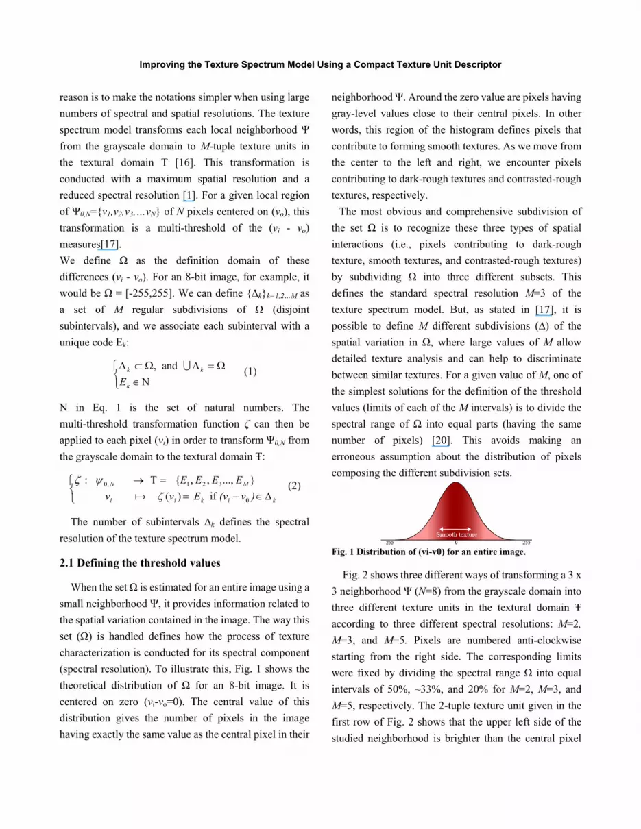
theoretical distribution of Ω for an 8-bit image. It is

centered on zero (vi-vo=0). The central value of this

distribution gives the number of pixels in the image

having exactly the same value as the central pixel in their

neighborhood Ψ. Around the zero value are pixels having

gray-level values close to their central pixels. In other

words, this region of the histogram defines pixels that

contribute to forming smooth textures. As we move from

the center to the left and right, we encounter pixels

contributing to dark-rough textures and contrasted-rough

textures, respectively.

The most obvious and comprehensive subdivision of

the set Ω is to recognize these three types of spatial

interactions (i.e., pixels contributing to dark-rough

texture, smooth textures, and contrasted-rough textures)

by subdividing Ω into three different subsets. This

defines the standard spectral resolution M=3 of the

texture spectrum model. But, as stated in [17], it is

possible to define M different subdivisions (∆) of the

spatial variation in Ω, where large values of M allow

detailed texture analysis and can help to discriminate

between similar textures. For a given value of M, one of

the simplest solutions for the definition of the threshold

values (limits of each of the M intervals) is to divide the

spectral range of Ω into equal parts (having the same

number of pixels) [20]. This avoids making an

erroneous assumption about the distribution of pixels

composing the different subdivision sets.

Fig. 1 Distribution of (vi-v0) for an entire image.

Fig. 2 shows three different ways of transforming a 3 x

3 neighborhood Ψ (N=8) from the grayscale domain into

three different texture units in the textural domain Ŧ

according to three different spectral resolutions: M=2,

M=3, and M=5. Pixels are numbered anti-clockwise

starting from the right side. The corresponding limits

were fixed by dividing the spectral range Ω into equal

intervals of 50%, ~33%, and 20% for M=2, M=3, and

M=5, respectively. The 2-tuple texture unit given in the

first row of Fig. 2 shows that the upper left side of the

studied neighborhood is brighter than the central pixel

Improving the Texture Spectrum Model Using a Compact Texture Unit Descriptor

whereas the lower right side is darker. As higher spectral

resolutions were used, the 3-tuple and 5-tuple texture

units given in the second and third rows revealed more

nuanced spectral information.

2.2 Labeling texture units

The texture units defined in Eq. 2 are organized in an

M-tuple system. He and Wang [16] proposed the

following equation to ensure a unique label for each

texture unit:

N

i

iiTU MvvN

1

10 )(

(3)

The last column in Fig. 2 shows how NTU can be

obtained for three spectral resolutions (2, 3, and 5). The

histogram of texture units is referred to as the texture

spectrum (TS) [16], where the abscissa indicates the NTU

and the ordinate represents its occurrence frequency.

This histogram reveals texture information similar to the

histogram of gray-level values that reveals spectral

information. TS can be estimated for an entire image for

image retrieval [21], or locally using a moving window

for image segmentation and classification [17], [22],

[23].

Fig. 2 Calculation of the original ordered texture unit for M=2, M=3, and M=5 as proposed in [16] [17].

2.3 Limitations of the M-tuple labeling system

The power-based labeling system produces very

different NTU for very similar neighborhoods. Fig. 3

shows two 2-tuple texture units in (a) and (b) and two

3-tuple texture units in (c) and (d). The two texture units

in (a) and (b) are very similar (both have only one pixel

higher than the central pixel). In a set of available labels

ranging from 0 to 255, these two texture units were

attributed very different labels: 1 and 128. The

similarity between these two texture units was not

reflected in their corresponding labels. The same effect

is observed for the 3-tuple texture units in (c) and (d).

Another drawback of the power-based labeling system

is that the number of possible texture units increases

rapidly with M and N (MN different texture units). In

theory, it is possible to label all the texture units provided

by any spectral and spatial resolution. But, in practice,

only a few combinations of M and N can be used to keep

the calculations manageable. This is a serious limitation

of the texture spectrum model.

To explore high spectral and spatial resolutions in

practice, we must reduce the number of bins for the

resulting histograms. The main drawback of reducing the

histogram bins is that there is no control on how texture

information is compressed. This is due to the fact that the

Improving the Texture Spectrum Model Using a Compact Texture Unit Descriptor

relative locations of the resulting texture units (NTU

values) in the histogram do not reflect their similarities.

Fig. 3 Power-based codification. 2-tuple (a, b) and 3-tuple (c, d), produce very different texture numbers (NTU) for similar texture situations.

3. Proposed Compact Texture Unit

An ordered texture unit provides information about the

occurrence of the different M threshold situations in the

neighborhood and the relative position of each of these

situations. The two 3-tuple texture units in Fig. 3(c) and

(d), for example, differ from each other by the position

of the pixel that has a value higher than the central

pixel. The occurrence of the three threshold situations is

the same for both of the 3-tuple texture units: both have

six pixels with values less than the central pixel, one

pixel close to the value of the central pixel, and, finally,

one pixel higher than the central pixel. The same

observations can be made for the 2-tuple texture units in

Fig. 3(a) and (b). If only the occurrence is retained,

these two texture unit pairs will be identical. And, if an

appropriate labeling system is adopted to identify these

non-ordered texture units, then the problem reported in

Section 2 related to the NTU value that does not reflect

texture unit similarity will be solved.

To develop this solution, we were inspired by our

previous work [20] that aimed to reduce the texture

spectrum redundancy caused by the M-tuple encoding

system reported in [24]. A solution was proposed for

labeling non-ordered texture units for the particular case

of M=3 and N=4. Here, we propose a general solution

for labeling non-ordered texture units, for different

spectral and spatial resolutions. Specifically, we

attribute to each threshold interval special codes that

change according to the spectral and spatial resolutions

being used. These codes were generated using a high

performance processing grid facility. Specifically we

used a grid of 109073 cores during 24 hours. These

codes are summarized in Fig. 4. The labeling strategy

used these special codes in a sum-based formula given

in Eq. 4. Using this solution (Fig. 4 and Eq. 4), all

texture units having the same occurrence of the different

threshold values, regardless of their positions in the

neighborhood, are identified with the same unique label

referred to as (NC-TU). In this solution, all ordered texture

units are automatically “compacted” to form a unique

non-ordered texture unit. We propose to call these

non-ordered texture units Compact Texture Units

(C-TU).

N

i iTUC vvN1 0 )(

(4)

Fig. 4 Compact Texture Units codes for different radiometric and spatial resolutions.

Table 1 Number of C-TU for different values of N and M.

Spectral resolution (M) N 2 3 5 7 9 4 5 15 70 210 495 6 7 28 210 924 3003 8 9 45 495 3003 12870 12 13 91 1820 18564 16 17 153 4845 74613 24 25 325 20475

In Fig. 4, each texture analysis scenario, which uses

fixed spectral and spatial resolutions M and N, needs to

use its specific codes to identify the M-related

thresholds. These specific codes ensure that Eq. 4 will

Improving the Texture Spectrum Model Using a Compact Texture Unit Descriptor

provide a unique label (NC-TU) for each of the resulting

C-TU. The total number of C-TU for each scenario is

given in Table 1. The analysis of texture using, for

example, a spectral resolution of M=3 and a

neighborhood size of N=8 needs the codes 1, 2, and 10

to attribute unique labels to the resulting 45 C-TU. If a

higher spatial resolution of N=24 is needed, the resulting

325 C-TU have to be labeled using the following codes:

1, 2, and 26.

The proposed solution (Fig. 4 and Eq. 4) attributes

different NC-TU to each of the generated C-TU.

Consequently, the NC-TU can be used exactly as

generated by Eq. 4 for texture characterization without

any post-processing. However, in order to have C-TU

labeled with successive digits to form histograms with

continuous bins, the NC-TU need to be re-coded. This

supplementary step, if needed, can be performed with a

small lookup table because it does not use the original

ordered texture units.

Fig. 5 Calculation of the proposed Compact Texture Unit for M=2, M=3, and M=5).

In Fig. 5 we showed the different steps needed to

transform a fixed neighborhood into a C-TU using the

proposed codification system. In Figs. 6(a) and 4(b), we

explicitly presented the different C-TU and their

corresponding NC-TU for two different circular

neighborhoods, N=4 and N=8, for a spectral resolution

of M=3. Viewed as compact texture units, the two

texture units in Fig. 3(c) and (d) are identical because

both have six dark pixels, one flat pixel, and one bright

pixel. These two 3-tuple texture units are represented by

a single C-TU shown in the fifth column of the first row

in Fig. 6.

For a neighborhood of N pixels and a spectral

resolution of M, there are only: (M+N-1)! / (N!*(M-1)!)

different C-TU. This greatly reduces the total number of

combinations compared to the original ordered texture

units. In Table 2 we give the reduction achieved by our

solution compared to the original M-tuple system

(number of M-tuple texture units by the number of

C-TU). It is exactly this drastic reduction that allowed

the texture analysis process to be scalable even for high

spatial and spectral resolutions.

Table 2 Ratio of the total number of ordered texture units to the number of C-TU.

Spectral resolution (M) N 2 3 5 7 9 4 3 5 9 11 13 6 9 26 74 127 177 8 28 146 789 1920 3345

12 315 5840 1.E+05 7.E+05 16 3855 281351 3.E+07 4.E+08 24 7.E+05 9.E+08 3.E+12

Improving the Texture Spectrum Model Using a Compact Texture Unit Descriptor

Fig.6 The 15 Compact Texture Units for the case of M=3, N=4 (a) and, the 45Compact Texture Units for the case of M=3 and N=8 (b). These same configurations produce 81

Another important characteristic of the C-TU

descriptor is that it is rotation invariant by definition. The

original model did not have this characteristic. It can be

useful in many applications because in the real word

textures appear with different orientations. In addition,

the C-TU descriptor keeps the grayscale invariance of the

original model. From a computational complexity point

of view, these tow invariance as well as the non-ordered

constraint, are straightforward to achieve without any

post-processing. In addition, the C-TU use a sum-based

formula (Eq. 4), which is simpler to calculate than the

power-based one (Eq. 3). All of these advantages help to

develop faster algorithms. The theoretical framework for

compact texture units, which was introduced in this

section, describes more than a new descriptor. It is a

general and practical solution for texture analysis using a

wide range of spatial and spectral resolutions. It is

probably one of the rare texture analysis solutions that

allow, in practice, the simultaneous maximization of

spatial and spectral resolutions. In this sense, it can be

seen as a combination of the co-occurrence matrix

(which maximizes M) and the texture spectrum (which

maximizes N).

4. Experiments

Different texture aspects can be revealed and analyzed

using the proposed C-TU solution. This includes: 1) the

effect of increasing the spectral resolution in relation to

intra-texture variation, 2) the effect of using different

spatial resolutions in relation to the nature of texture

(macro and micro textures), and 3) the way that these two

parameters interact when combined in order to find

optimum combinations for specific applications and a

given type of texture. Addressing all of the texture

aspects is beyond the scope of this paper. However, all

these research topics are interrelated to the two

fundamental questions: Does the drastic reduction of the

number of texture units affect texture discrimination?

How efficient is the rotation invariance of the C-TU? The

following experiments focused on these two fundamental

characteristics that make the C-TU descriptor very

attractive for texture analysis. Among the solutions

provided in Fig. 4, we tested 27 different scenarios that

used three different spectral resolutions (i.e., M=2, M=3,

and M=5) and 9 different circular neighborhoods (having

different radii and different pixel sizes). These 27

scenarios were tested in three experiments dealing with

different image analysis topics.

Experiment #1 dealt with the texture classification of a

texture mosaic. Experiment #2 dealt with rotation

invariant texture image retrieval. Finally, Experiment #3

dealt with rotation invariant texture classification. These

experiments used 22 different texture images in total

(Fig. 7) from the Brodatz album [25].

4.1 Classification algorithm

In these experiments, we used a supervised

classification scheme. Among metrics used to evaluate

the similarity between two histograms we used a simple

Improving the Texture Spectrum Model Using a Compact Texture Unit Descriptor

integrated absolute difference. It has the advantage of

being efficient and very simple to estimate. It is given by:

M

iSRxR iTSiTSTSTSD

1

)()(),( (5)

where M is the number of texture spectrum bins. TSR is

the reference texture spectrum of a given texture, and TSS

is the sample texture spectrum at a given position in the

processed texture using a moving window.

We note here that for all experiments we made the

choice of using the effective number of texture units

provided by each tested descriptor, without any

histogram bin reduction. The aim was to perform an

effective assessment of the discriminative value of each

of the studied descriptors without any alteration. Along

the same logic, and in order to conduct a rigorous

evaluation of the intrinsic textural value of the developed

descriptor and those used for comparison, the

classification process was conducted with only these

descriptors as input and without any additional or

complementary information.

Fig. 7 The 22 Brodatz texture images used for validation.

4.2 Experiment #1: Texture classification

4.2.1 Experimental setup

This experiment involved the classification of a

mosaic formed by 12 different textures organized as

shown in Fig. 8. Each texture image was 640 x 640

pixels. There were several aims in this experiment. The

first aim was to analyze the texture discrimination

performance of the proposed C-TU descriptor using

different values for the spectral and spatial resolutions.

The test of the new descriptor using different spectral

and spatial resolutions was practically possible because

the C-TU descriptor used a reasonable number of

combinations. The second aim was to compare the

proposed C-TU descriptor with the original texture unit

descriptor [16] in order to evaluate how the drastic

reduction of the number of texture units achieved by the

C-TU could affect the texture discrimination

performance. Finally we introduced a comparison with

the GLCM method [12]. We found this test very

interesting because it introduced a comparison between

two different principles of texture analysis. The

following GLCM features were used: mean, variance,

homogeneity, contrast, dissimilarity, entropy, second

moment, and correlation.

Fig. 8 Locations of the 12 Brodatz textures of Experiment #1.

During the classification process, the size of the

moving window used to construct TSS needs to be small

enough to avoid texture confusion, but at the same time it

needs to be large enough to contain discriminative

information. To set the size of the classification moving

window, we adopted the strategy proposed in [20]. Each

of the twelve textures was divided into 100

non-overlapping windows of a fixed size and uniformly

distributed on the image. Then, the average similarity

between these 100 windows and the whole texture image

(640 x 640 pixels) was estimated using Eq. 5. This

process was iterated for 26 different window sizes

ranging from 11 to 59 pixels (26 x 100 distances were

estimated for each texture). The window that minimized

the distance in Eq. 5 among the 26 tested sizes

corresponded to the window size that best represented the

analyzed texture. An optimum window size of 33 x 33

pixels was selected for the classification. To construct the

reference TSR for each of the 12 textures, we

systematically took a sample of about 97 x 97 pixels at

the center of each texture. Selecting a reference window

Improving the Texture Spectrum Model Using a Compact Texture Unit Descriptor

larger than the classification window helped to deal with

intra-texture variations. In our case, the use of a reference

window of 97 x 97 pixels for classifier training

physically covered only ~2.2% of the area of each

texture. The classification and reference windows

produced histograms with only 1,089 and 9,409 entries

respectively, which was fairly reasonable.

4.2.2 Experimental Results

The textural content of the mosaic in Fig. 8 was

analyzed using the proposed C-TU descriptor. We

conducted 27 different classifications with different

C-TU configurations. Table 3 summarizes the

classification rate of each of the 12 textures for the 27

classifications.

Table 3 shows that for a fixed spectral resolution,

decreasing the spatial resolution tended to increase the

overall classification rate. For example, when the spatial

resolution was reduced from N=24 to N=8, the overall

classification rate increased by 11% for M=5 and by

4.5% for M=3. This suggests that the benefit of using

small spatial resolution is more important when

combined with high spectral resolution. To the contrary,

when used with its minimum spectral resolution M=2, the

increase of the spatial resolution of the C-TU improved

the overall classification rate. This particular case of M=2

recorded the lowest classification rate compared to M=3

and M=5 for all spatial resolutions (Table 3). This is

evidence of the limitation of using minimum spectral

resolution and thus increasing the spatial resolution was a

mean to partially compensate for this limitation.

The effect of varying spatial resolution when C-TU

used high spectral resolution M=5 was very visible for

two textures D4 and D57. Indeed, the classification rates

of these textures dropped by about 50%, when the spatial

resolution was increased from N=8 to N=24. This can be

explained by the combined effects of using high spectral

and spatial resolutions in relation to the type of texture.

This effect was more visible for texture D4 where

attentive visual analysis showed that this texture has

important intra-texture variation that physically separates

roughly this texture into two parts. The combination of

high spectral and spatial resolutions revealed these

differences and one of these parts was classified as D24.

From the spectral resolution point of view, the results

showed that increasing the spectral resolution of the

texture analysis process increased the overall

classification rate. For each of the nine tested

neighborhood configurations (different sizes and radii),

the binary subdivision of the spectral variation (M=2)

provided the lowest classification rate. Increasing the

spectral resolution to M=3 provided an improvement of

the overall classification rate by 17% in average

compared with the binary subdivision. This improvement

was more than 50% for some textures such as D77, D57,

and D83. Among the 27 tested configurations, the

highest classification rate of 97.5% was achieved by the

use of N=8, r=1, and M=5. It seemed that minimum

spatial resolution and maximum spectral resolution are

the optimum parameters for the C-TU descriptor to

discriminate between different textures in the same

image. This result indicated that the C-TU descriptor

was more sensitive to the spectral resolution than the

spatial resolution for the case of mosaic classification

(local estimation of C-TU). This is in contrast to the

original model, which is more sensitive to the spatial

resolution [24].

The results of the original ordered texture unit

descriptor are summarized in Table 4. As no histogram

bin reduction was performed, only a few values of M and

N can be explored. As for the C-TU descriptor, the use of

a high spectral resolution improved the classification

rate. The best classification rate provided by the original

model was 99%. It was achieved by the use of the

classical configuration using (M=3, N=8) that produced

6,561 ordered texture units. This is equivalent to the

classification of an image of 6,561 bands. The C-TU

achieved similar classification rate using only 495

different combinations. This reduced 13 times the

computational complexity.

Improving the Texture Spectrum Model Using a Compact Texture Unit Descriptor

For some applications such as remote sensing the

classification rate of 95% can be judged very

satisfactory. The original model achieved this

classification rate when it used M=2 and N=24, which is

equivalent to the processing of an image of 65,536 bands

(224). The C-TU descriptor achieved this classification

rate with highly reduced complexity equivalent to the

processing of an image of only 45 bands (M=3 and N=8).

Compared to the original model, the C-TU descriptor

provided results with an excellent balance between the

classification rate and the computational efficiency.

Table 3 Experiment #1 - Classification accuracy (%) using the C-TU descriptor. Algorithm N , r M D4 D57 D24 D16 D77 D53 D83 D14 D29 D52 D22 D17 Aver

C-TU

2 49.6 79.9 59.5 99.6 47.0 96.2 56.1 90.2 85.5 97.2 91.7 64.9 76.4 8, 1 3 87.0 97.2 98.4 99.3 96.8 97.2 86.3 97.9 94.4 99.5 99.0 91.3 95.4

5 89.6 96.4 98.5 99.6 97.4 98.4 95.1 99.3 99.2 99.6 99.7 96.7 97.5 2 38.8 76.2 71.3 99.1 36.0 91.2 26.9 88.3 70.0 95.6 92.7 79.9 72.0

8, 1.5 3 79.5 96.8 95.0 99.6 97.1 96.6 80.3 94.3 92.7 99.1 99.0 90.7 93.4 5 79.8 97.5 97.3 99.6 97.6 97.1 97.1 97.3 99.3 99.4 99.6 95.0 96.4 2 40.7 73.5 87.7 99.6 45.7 93.8 49.8 89.5 70.3 96.6 94.1 81.6 76.8

12, 1.5 3 83.1 97.1 94.9 99.8 97.1 95.9 88.1 95.9 94.1 98.9 99.0 91.8 94.6 5 75.5 97.5 97.7 99.9 97.6 97.6 98.3 97.7 99.1 99.6 99.7 94.5 96.2 2 51.0 60.8 73.4 99.8 70.5 92.6 40.9 83.5 59.9 95.5 97.7 74.8 75.0

12, 2 3 80.1 97.2 93.5 99.7 96.8 95.0 83.9 95.0 94.0 97.1 99.1 90.4 93.5 5 72.3 97.4 96.2 99.9 98.0 96.6 97.5 95.7 99.7 99.3 99.6 93.7 95.5 2 48.6 66.4 86.4 99.9 64.9 93.0 51.7 90.2 53.3 96.1 96.9 71.9 76.6

16, 2 3 77.1 96.8 94.2 99.7 96.8 94.7 86.4 94.5 94.7 97.2 99.0 90.4 93.5 5 57.3 95.2 97.2 100 97.1 97.8 93.7 94.3 99.7 99.6 99.8 93.3 93.8 2 49.9 55.6 88.1 99.5 70.6 94.2 38.3 88.0 59.1 94.6 97.0 70.5 75.4

16, 2.5 3 75.8 97.3 94.3 99.5 93.6 92.4 80.6 94.1 93.5 96.0 98.9 90.0 92.2 5 56.6 93.5 97.7 99.6 87.2 97.0 92.0 93.5 99.2 99.4 99.6 93.5 92.4 2 59.0 62.4 87.2 99.8 66.8 93.6 58.3 88.2 57.9 95.4 97.3 71.5 78.1

24, 2 3 78.6 96.7 93.1 99.8 97.4 94.5 87.7 94.3 94.2 98.1 99.1 90.4 93.7 5 34.8 67.6 99.4 100 92.8 98.5 85.4 94.8 99.2 99.9 99.6 95.0 88.9 2 61.6 58.6 92.9 99.6 66.7 94.8 45.9 92.4 76.9 90.0 98.1 75.5 79.3

24, 2.5 3 74.7 97.4 94.4 99.5 95.2 93.0 82.2 93.6 91.4 97.2 99.0 90.3 92.3 5 39.2 69.7 99.0 100 77.1 98.7 79.4 92.6 98.4 99.8 99.6 94.7 87.3 2 69.0 41.4 86.2 93.2 86.7 92.2 27.3 92.9 71.1 93.4 97.3 76.7 77.2

24, 3 3 74.0 95.4 93.7 91.7 90.6 93.2 82.8 94.2 93.6 93.5 98.7 89.6 90.9 5 39.5 48.4 98.2 95.7 92.4 98.9 87.6 85.4 98.4 99.8 99.7 95.6 86.5

Table 4 Experiment #1 - Classification accuracy using the ordered texture units descriptor and using the GLCM.

Algorithm N , r M D4 D57 D24 D16 D77 D53 D83 D14 D29 D52 D22 D17 Aver

Original Texture

Spectrum model

M=2 96.2 97.3 98.5 99.8 96.6 99.4 95.3 99.4 87.4 99.7 75.9 72.0 93.2 N=8, r=1 M=3 98.5 99.7 99.9 100 99.1 100 98.7 99.5 95.1 100 99.0 98.5 99.0

M=2 97.9 97.0 97.3 100 96.6 99.4 95.1 98.0 94.4 99.1 73.2 69.1 93.2 N=8, r=1.5 M=3 98.7 99.8 99.7 100 99.4 100 98.4 98.0 93.3 100 99.4 99.5 98.8

N=12, r=1.5 M=2 98.5 96.9 98.5 100 98.0 99.8 97.0 97.3 82.5 99.5 77.3 80.9 93.9 N=12, r=2 M=2 98.0 97.7 95.0 99.9 99.4 100 98.3 97.5 76.2 100 84.0 90.2 94.7 N=16, r=2 M=2 98.0 95.5 94.4 99.9 98.7 100 97.8 97.2 57.9 100 85.1 92.5 93.1

N=16, r=2.5 M=2 97.5 96.4 93.9 99.7 99.7 100 97.2 96.9 86.2 100 88.0 95.0 95.9 GLCM 95.1 86.5 79.3 67.1 79.6 51.9 82.5 94.2 92.0 78.9 92.8 56.0 79.7

The comparison between the classification rates of the

original model and the C-TU, obtained individually for

the 12 textures revealed some interesting results. For

example, texture D29 was better identified using C-TU

with a classification rate of 99.2% than using the original

texture spectrum model which recorded a classification

Improving the Texture Spectrum Model Using a Compact Texture Unit Descriptor

rate of 95.1%. The parts of D29 that were erroneously

classified as D52 by the original model are mainly dark

spots which are spectrally close to texture D52. The use

of a spectral resolution M=3 was probably not sufficient

for the original model to detect subtle spectral differences

between these spots and some regions in texture D52.

These spots were correctly classified by the C-TU when

using higher spectral resolution M=5. The case of the two

textures D4 and D57 was better classified by the original

model that uses a spectral resolution M=3. This

resolution seemed to be optimum to identify these two

textures as it delivered also the most stable classification

rates in case of C-TU descriptor.

The last row of Table 4 provides the results of the

GLCM feature. The C-TU recoded an improvement of

the overall classification rate of 17.8% over the GLCM.

The GLCM recorded important confusions; in particular,

40% of texture D53 was classified as D24. Another

important confusion was also caused by D17, where 20%

and 15% of this texture were classified as D53 and D29

respectively. The low classification rate of the GLCM

can be attributed to the limitation of using a minimum

spatial resolution (N=2). We show in Fig. 9 the best

classifications provided by the three tested methods.

Fig. 9 Classification results for the mosaic in Fig.8. (a) C-TU (M=5, N=8, r =1), (b) Original model (M=3, N=8, r=8), and (c) co-occurrence matrix.

4.3 Experiment #2: Rotation invariant texture

retrieval

This experiment was initially proposed by Porter and

Canagarajah [26]. In this paper, we used a modified

version of this experiment as proposed in [27], which is

referred to as Contrib_TC00001. This modified version

introduced the problem of retrieving texture images that

were rotated by angles different than those used to train

the classifier.

4.3.1 Experimental setup

This experiment involved 16 different texture classes

(the first 16 images from the top right in Fig. 7). Each of

the 16 texture classes was presented with 8 different

images called source images (180 x 180 pixels each),

where one source image was used for training and the 7

others for building the database for retrieval

performance evaluation. Each source image of a given

texture class was rotated by 10 different angles (0°, 20°,

30°, 45°, 60°, 70°, 90°, 120°, 135°, and 150°). To build

the training data set, the authors divided each of the 10

rotated versions of the selected training source image

(180 x 180 pixels) into 121 disjoint subimages (16 x 16

pixels each). This provided 10 angles for each of the

121 subimages for each texture class. To form TSR of a

given texture class at a given orientation, the histograms

of each of the 121 subimages were added to form one

big histogram. This resulted in TSR of 121 x (16-2r)2

entries, where r is the radius of the circular

neighborhood. The set of images to be classified was

formed by rotating each of the 7 other source images of

a given texture class by the same 10 different rotation

angles. This gave a total of 1,120 images (7 source

images x 10 orientations x 16 texture classes). As this

experiment dealt with image retrieval, each image in

this set was classified as a whole by estimating a unique

TS with (180-2r)2 entries. The retrieval process was

trained using one rotation angle and tested using the

nine remaining rotation angles.

4.3.2 Experimental Results

The retrieval process was applied 10 times. Each

time, we used training data from one angle to retrieve

the 1,008 images that have different rotations (7 source

images x 9 orientations x 16 texture classes). The results

Improving the Texture Spectrum Model Using a Compact Texture Unit Descriptor

obtained for the 10 retrieval testes are summarized in

Table 5.

Table 5 shows that when C-TU was used with M=2,

five of the nine tested neighborhood configurations

produced average retrieval rates less than 90%. When it

is used with higher spatial resolutions it provided better

results (98.2% with N=24 and r=2).

Table 5 Experiment #2 - Image retrieval accuracy (Contrib_TC00001) using the C-TU.

Training angle Algorithm N and r M 0° 20° 30° 45° 60° 70° 90° 120° 135° 150° Aver

M=2 66.6 81.4 84.5 74.5 86.5 81.8 66.3 85.3 72.2 85.7 78.5 N=8, r=1 M=3 68.7 87.5 86.3 85.0 88.3 88.5 67.8 87.1 86.0 90.3 83.5 M=5 68.0 89.7 90.9 86.6 93.0 87.6 65.3 91.8 86.1 93.2 85.2 M=2 79.3 90.1 90.7 87.4 88.2 89.8 80.3 91.7 86.0 88.4 87.2 N=8, r=1.5 M=3 91.3 92.6 93.8 92.0 97.1 92.7 92.0 96.1 93.1 97.0 93.8 M=5 93.2 94.5 95.5 92.9 96.3 92.9 91.9 96.9 91.5 97.8 94.3 M=2 80.0 93.6 95.1 88.1 94.2 91.2 79.1 94.8 87.8 94.3 89.8 N=12, r=1.5 M=3 94.5 99.0 97.9 98.9 98.1 99.0 96.3 97.5 98.3 98.0 97.8 M=5 97.6 99.7 98.1 98.5 99.5 99.1 98.0 99.0 96.7 99.7 98.6 M=2 83.5 86.6 95.9 84.0 96.8 91.2 82.8 94.9 86.8 94.2 89.7 N=12, r=2 M=3 92.4 99.6 96.8 97.8 97.3 100 91.8 95.5 97.4 97.2 96.6 M=5 92.0 100 97.8 98.4 99.3 99.1 93.8 98.0 98.4 97.6 97.5

C-TU M=2 83.5 97.2 94.0 92.9 96.2 98.5 82.6 92.6 92.9 94.8 92.5 N=16, r=2 M=3 94.2 100 98.5 98.3 100 100 94.9 98.0 97.2 99.9 98.1 M=5 95.7 100 98.4 98.5 98.6 100 95.4 98.4 98.6 98.6 98.2 M=2 93.5 95.3 92.1 92.5 96.1 98.9 94.3 92.3 88.6 95.7 93.9 N=16, r=2.5 M=3 99.0 98.9 99.4 98.9 99.5 99.6 99.2 99.3 98.4 99.4 99.2 M=5 100 99.7 99.6 99.2 99.8 99.6 100 99.3 99.4 99.4 99.6 M=2 93.8 99.7 99.9 99.8 100 98.8 93.2 99.0 97.8 100 98.2 N=24, r=2 M=3 96.8 100 99.8 99.7 99.9 100 97.4 99.5 99.3 99.8 99.2 M=5 100 100 99.9 99.8 100 100 100 99.6 99.9 100 99.9 M=2 92.5 99.6 95.7 96.4 98.7 96.8 96.8 94.9 98.4 97.8 96.8 N=24, r=2.5 M=3 98.6 100 99.8 97.9 99.8 100 100 99.3 98.8 99.8 99.4 M=5 100 99.8 99.8 99.3 99.7 99.5 100 99.4 99.6 99.4 99.7 M=2 73.1 93.4 95.3 91.9 94.2 93.7 80.9 91.6 94.3 88.8 89.7 N=24, r=3 M=3 100 98.2 98.2 97.8 98.7 99.4 100 97.6 96.8 98.6 98.5 M=5 99.9 98.9 99.0 97.0 99.4 98.9 100 99.1 99.1 98.2 99.0

The use of a higher spectral resolution, i.e., M>2

showed significant improvement and more stable

results. Indeed, eight of the nine neighborhood sizes

produced average retrieval rates higher than 93.8%.

When the C-TU descriptor was used with a

neighborhood configuration equal to or larger than

(N=16, r=2.5), it produced an excellent retrieval rate

higher than 99%. Almost a perfect retriavl rate of 99.9%

was obtained by the C-TU when used with a

neighborhood of 24 pixels and r=2.

The proposed C-TU descriptor was able to deliver

robust measures for texture characterization that can be

generalized to physically different textures and different

rotation angles. When the overall retrieval rate of

individual training angles was analyzed, we noticed that

a perfect retrieval rate of 100% was obtained 27 times,

and 24 of them were obtained when a high spectral

resolution was used (M>2).

These results showed the very good stability of the

C-TU, particularly for large neighborhoods. This helped

us to draw the partial conclusion that, in the context of

image retrieval, the use of large neighborhoods seems to

provide better results.

It is fair to compare our results with those obtained by

the LBP-riu2 descriptor using exactly the same

experimental setup with the exactly the same data

(Contrib_TC00001) and reported in [27]. We recall here

that the LBP-riu2 uses the texture spectrum model to

produce rotation invariant and uniform texture units for

the case of N=2 which is referred to in [28] as the local

Improving the Texture Spectrum Model Using a Compact Texture Unit Descriptor

binary pattern (LBP). The results in this study [27],

reported that the LBP-riu2 recorded a maximum retrieval

rate of 98.5%, which was achieved by using a

neighborhood of 24 pixels. To further improve their

results, the authors combined three LBP-riu2 descriptors

estimated on three different neighborhoods (8, 16, and

24), and each of them was combined with local variance

as an additional local measure of contrast. Even with

these additional features, the C-TU descriptor had a

higher retrieval rate based on its basic form without any

additional information.

4.4 Experiment #3: Rotation invariant texture

classification

This experiment tested the ability of the proposed

C-TU descriptor to recognize texture that appears in the

same image in different orientations. This kind of

problem is in fact very common in various fields, such as

the earth sciences where the same land cover theme can

appear in a satellite image with random orientations. This

is a challenging problem as it deals with both

intra-texture and inter-texture variations combined with

the rotation invariance effect. In addition, texture

descriptors should be generated locally using a moving

window which brings the problem of histograms

stability.

4.4.1 Experimental setup

In this experiment, we used the 12 textures in Fig. 8. These textures were rotated by six different angles: 0°, 15°, 30°, 45°, 60°, and 75° resulting on a data set of 72 images. Each rotated image was 400 x 400 pixels. These images were than grouped into a single big mosaic of 4,800 x 2,400 pixels. As the six rotated images of each texture needed to be recognized as the same texture, they were placed in a way that they did not have common borders. This made the problem of texture recognition more difficult at texture borders as these borders need to be identified. Fig. 10. shows the location of each of the 72 images in the mosaic. The classification process was conducted as in Experiment #1. To increase the

difficulty, the classifier was trained at each time using only one orientation angle among the six orientations.

Fig.10 Location of the 72 images in the mosaic used in Experiment #3.

4.4.2 Experimental Results

Table 6 shows that the case of C-TU using a minimum

spectral resolution (M=2) provided the lowest rates. The

use of a minimum spectral resolution made this case

special, and it needed to be analyzed differently than the

other spectral resolutions. Indeed, for this case,

increasing the spatial resolution partially balanced the

lack of spectral resolution. Table 6 shows that the lowest

overall classification rate of 44% was recorded by the use

of the standard neighborhood configuration (N=8), and

increasing the neighborhood size improved the overall

classification rate. But even with the large neighborhood,

the classification rate still remained relatively low at only

72.9%. Experiment #3, as well as the other two

experiments, showed the limitations of using a minimum

spectral resolution in complex texture analysis problems.

From Fig. 11 (derived from Table 6) we can notice that

the advantage of increasing the spectral resolution (M) of

the C-TU descriptor was very significant. Indeed, an

average improvement of 22.7% was obtained when

increasing M=2 to M=3. For this case (M=3) the

maximum improvement (37%) was obtained using the

standard neighborhood configuration (N=8 and r=1).

This standard neighborhood recorded also the maximum

improvement when the spectral resolution increased

from M=3 to M=5.

The effect of increasing the spatial resolution (in terms

of the number of pixels and radii), in the context of

Improving the Texture Spectrum Model Using a Compact Texture Unit Descriptor

rotation invariant texture classification, was very

informative (see C-TU curves in Fig. 12). Indeed, outside

the particular case of the M=2, large neighborhoods gave

relatively low classification rates. Increasing, for

example, the neighborhood size from N=16 pixels with

r=2 to N=24 with r=3 decreased the classification rate.

Also, for large neighborhoods, even when increasing

only the radius, the classification rate decreased. This

was the case, for example, for the (M=3, N=16) and

(M=5, N=16) configurations when tested for r=2 and

r=2.5. The same effect was also observed for the (M=3,

N=24) and (M=5, N=24) configurations when tested for

r=2, r=2.5, and r=3.

Table 6 Experiment #3 - Classification rate using the C-TU.

Algorithm N and r M 0° 15° 30° 45° 60° 75° Aver M=2 30.3 49.4 51.4 37.4 46.9 48.8 44.0 8 pixels, r=1 M=3 69.2 82.6 85.9 78.4 86.5 83.7 81.1 M=5 75.3 90.1 92.6 84.5 91.6 90.2 87.4 M=2 46.6 64.8 62.9 62.3 62.6 63.4 60.4 8 pixels, r=1.5 M=3 78.0 90.2 91.7 89.7 91.3 91.1 88.6 M=5 80.9 93.6 94.3 92.9 94.1 94.1 91.6 M=2 47.8 69.9 67.8 64.6 68.2 68.4 64.4 12 pixels, r=1.5 M=3 79.7 91.3 91.8 90.3 91.7 91.8 89.5 M=5 82.3 94.0 94.0 92.8 94.1 93.9 91.9 M=2 59.6 68.8 69.5 66.7 69.3 69.0 67.2 12 pixels, r=2 M=3 79.0 90.4 91.3 90.3 90.8 91.2 88.9 M=5 81.0 93.4 93.9 93.1 93.9 93.4 91.4

C-TU M=2 57.2 68.7 67.1 64.9 66.6 67.5 65.3 16 pixels, r=2 M=3 79.9 90.7 90.6 90.2 91.0 91.3 88.9 M=5 81.1 91.3 93.0 92.3 92.4 91.8 90.3 M=2 58.1 73.0 73.3 72.5 74.7 73.3 70.8 16 pixels, r=2.5 M=3 78.2 89.4 90.0 89.4 90.0 90.2 87.9 M=5 78.0 90.2 90.8 90.8 90.9 90.1 88.5 M=2 63.2 72.7 72.0 69.6 72.2 72.4 70.4 24 pixels, r=2 M=3 80.9 91.3 91.2 91.2 91.6 91.6 89.6 M=5 80.9 86.6 88.3 88.6 88.4 87.1 86.7 M=2 62.7 74.7 74.4 75.8 74.1 75.8 72.9 24 pixels, r=2.5 M=3 81.9 89.7 90.4 89.8 90.2 90.4 88.7 M=5 76.6 86.9 89.4 89.5 88.9 87.6 86.5 M=2 58.5 70.0 72.8 71.3 74.0 71.7 69.7 24 pixels, r=3 M=3 77.8 87.7 88.3 88.3 88.8 89.1 86.7 M=5 76.2 87.5 88.7 88.6 89.1 87.9 86.3

Table 7 Experiment #3 - Classification rate using the LBP-riu2.

Algorithm N and r 0° 15° 30° 45° 60° 75° Aver 8 pixels, r=1 28.0 46.0 47.5 38.0 49.7 45.6 42.5 8 pixels, r=1.5 52.2 66.1 65.3 63.7 63.7 65.4 62.7 12 pixels, r=1.5 51.1 68.3 67.4 64.1 67.1 66.7 64.1 12 pixels, r=2 63.7 69.9 70.0 67.8 68.3 68.2 68.0

LBP-riu2 16 pixels, r=2 59.2 70.6 70.1 69.2 69.4 67.9 67.8 16 pixels, r=2.5 67.2 70.6 71.4 71.8 73.6 70.7 70.9 24 pixels, r=2 60.6 72.3 71.6 71.1 70.4 70.6 69.4 24 pixels, r=2.5 68.1 73.0 73.1 75.4 75.1 73.3 73.0 24 pixels, r=3 66.1 73.6 74.0 74.8 74.3 73.7 72.8

Journal of Communication and Computer, 2 (2013) 234-251

Fig. 11 Effect of increasing the spectral resolution (M) on

the classification rate of the mosaic in Fig. 10. This Figure

was derived from Table 6.

The high classification rate obtained by small

neighborhood was in agreement with Experiment #1,

but was in contrast to Experiment #2. The reason is

related to the bases of the texture spectrum model,

particularly that this model uses two different windows

at two different levels. The first window is used to

estimate the texture numbers (Eq. 3 for ordered texture

units and Eq. 4 for C-TU), which are the cornerstones

of texture characterization. This window can be seen as

a tool for sampling texture (sampling step). The second

window (larger than the first one) is used to estimate

the distribution of these cornerstones. The size of the

first window is linked to the second one in such a way

that the first window must deliver representative entries

(texture units) to the second one. In image retrieval as

in Experiment #2, texture analysis is performed at the

macro level as the second window is taken as the whole

image. Consequently, the use of relatively large

windows to build these cornerstones tends to produce

representative entries to the second window. By

contrast, in texture classification, as in Experiments# 1

and 3, the second window is exactly the moving local

window used for classification. Consequently,

extraction of representative texture cornerstones is

better achieved using small windows.

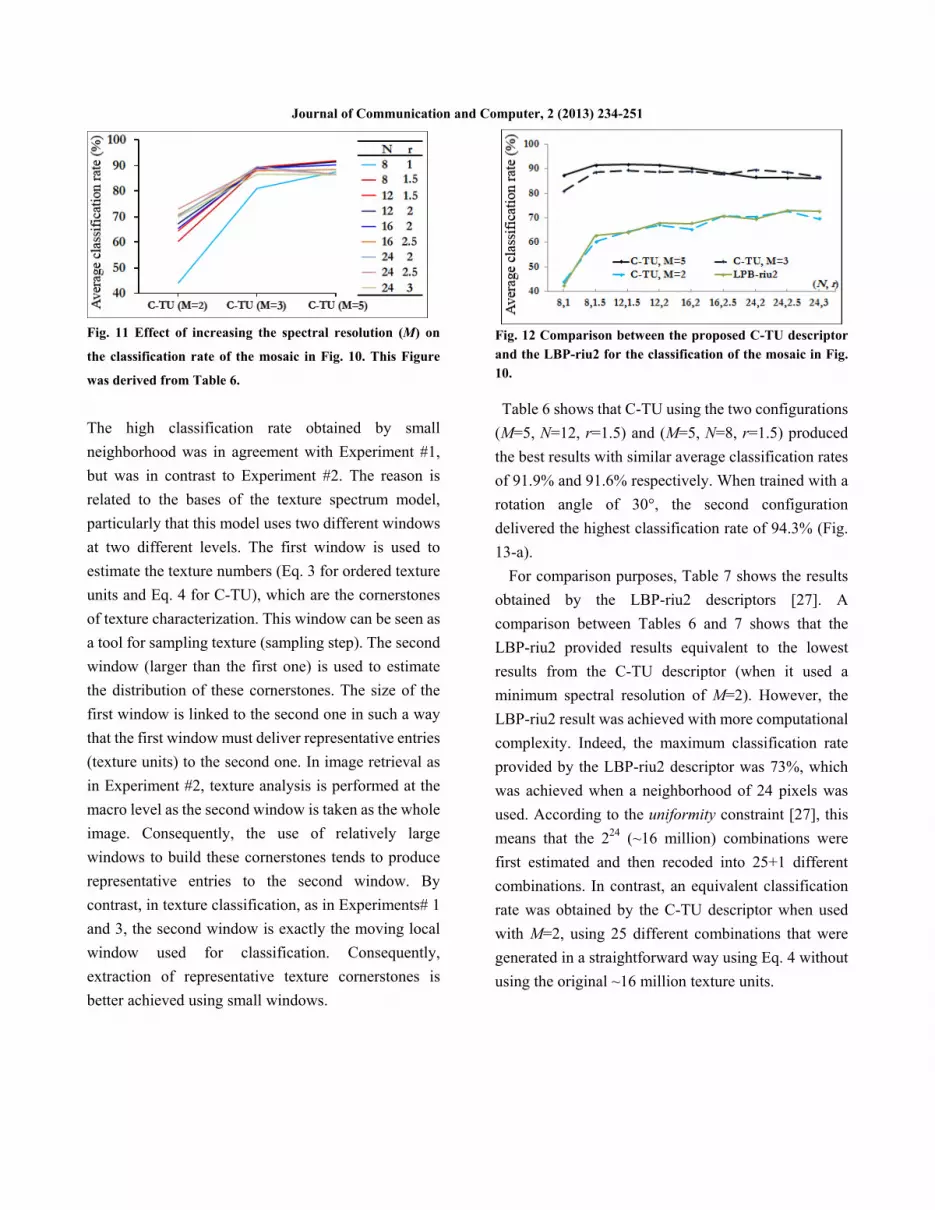
Fig. 12 Comparison between the proposed C-TU descriptor and the LBP-riu2 for the classification of the mosaic in Fig. 10.

Table 6 shows that C-TU using the two configurations

(M=5, N=12, r=1.5) and (M=5, N=8, r=1.5) produced

the best results with similar average classification rates

of 91.9% and 91.6% respectively. When trained with a

rotation angle of 30°, the second configuration

delivered the highest classification rate of 94.3% (Fig.

13-a).

For comparison purposes, Table 7 shows the results

obtained by the LBP-riu2 descriptors [27]. A

comparison between Tables 6 and 7 shows that the

LBP-riu2 provided results equivalent to the lowest

results from the C-TU descriptor (when it used a

minimum spectral resolution of M=2). However, the

LBP-riu2 result was achieved with more computational

complexity. Indeed, the maximum classification rate

provided by the LBP-riu2 descriptor was 73%, which

was achieved when a neighborhood of 24 pixels was

used. According to the uniformity constraint [27], this

means that the 224 (~16 million) combinations were

first estimated and then recoded into 25+1 different

combinations. In contrast, an equivalent classification

rate was obtained by the C-TU descriptor when used

with M=2, using 25 different combinations that were

generated in a straightforward way using Eq. 4 without

using the original ~16 million texture units.

Improving the Texture Spectrum Model Using a Compact Texture Unit Descriptor

Fig. 13 Classification of Fig.10: (a) C-TU (M=5, N=8, r =1, angle 30°), (b) LBP-riu2 (N=24, r=2.5, angle 45°)

When the C-TU was computed with a higher spectral

resolution, Tables 6 and 7 clearly show that the C-TU

descriptor outperformed the LBP-riu2 descriptor. For

example, when the C-TU used a spectral resolution of

M=3 it provided an important improvement of 38.5 %

over the LBP-riu2. This improvement reached 44.9%

when the C-TU was used with M=5. In Fig. 12 we

summarize the average classification rates obtained by

the C-TU and the LBP-riu2 descriptors for the six

orientations and for the nine neighborhood

configurations. For visual comparison, Fig. 13 shows

the best-classified mosaic provided by the C-TU and

LBP-riu2 descriptors.

5. Discussion and conclusion

We presented an improvement to the texture

spectrum model [16] in order to allow the analysis of

both spectral properties and spatial organization

components of texture information. This improvement

allowed texture analysis using high spectral and

spatial resolutions. To the best of our knowledge,

among existing texture models, this improved version

is probably the only one that provides practical tools

for the simultaneous analysis of texture with high

spectral and spatial resolutions.

This improved version was based on Compact

Texture Units (C-TU), which are non-ordered texture

units. The number of compact texture units needed to

describe texture is drastically reduced compared to the

original model.

The improved model used a new descriptor, referred

to as C-TU. This new descriptor can be generated

using a simple sum-based formula. It inherited from

the original model a robust invariance to grayscale

[29]. In addition it was also rotation invariant by

definition. The grayscale and rotation invariance was

achieved using the process of generating the C-TU

descriptor itself, without any additional

post-processing. This makes the proposed solution

computationally very attractive particularly for

applications using large volumes data, such as the

geosciences and applications performing real-time

analyses.

This new descriptor was extensively tested in

different applications, including texture classification

(Experiments #1), rotation invariant texture image

retrieval (Experiment #2), and rotation invariant

texture classification (Experiment #3).

The comparison with the original texture spectrum

model and the co-occurrence matrix features

confirmed that the C-TU was a valuable improvement

to the original model. It effectively reduced its

complexity and preserved its texture discrimination

performance. The different experiments showed also

excellent ability of the proposed C-TU descriptor to

produce discriminative information for physically

different textures.

The three experiments showed the benefit of using a

descriptor that allows a flexible analysis of texture

with a wide range of spectral and spatial resolutions.

Experiment #3, in particular, confirmed what was

observed in the two first experiments concerning the

advantage of using a high spectral resolution in texture

Improving the Texture Spectrum Model Using a Compact Texture Unit Descriptor

analysis. Our results showed that it was advantageous

to maximize the spatial resolution in the context of

image retrieval. And, when it comes to recognizing

textures in the same image, it was advantageous to

minimize the spatial resolution.

The rotation invariance of the C-TU was extensively

tested for both image retrieval and texture

classification. The descriptor showed a robust

performance when recognizing textures that were

rotated with different angles from the one used to

generate the descriptor.

This paper presents the first evaluation of the

proposed C-TU descriptor. This descriptor introduced

here has been tested using basic conditions. Its

performance can be improved by using simple

schemes, including the combination of multiple spatial

and spectral resolutions in the same texture

discrimination process. For more fundamental texture

analysis issues, understanding how the spectral and

spatial resolutions interact with each other in relation

to the texture types being analyzed is an important

area to be explored.

Acknowledgment

The authors are grateful to the Natural Sciences and

Engineering Research Council of Canada (NSERC) for

sponsoring this research through the Postgraduate

Scholarship (PhD) awarded to Abdelmounaime Safia

and the Discovery Grant awarded to Dong-Chen He.

The authors are grateful to Huizhong Lu, for using

high-performance computing facility.

References

[1] D.E. Ilea, P.F. Whelan, Image segmentation based on the

integration of colour–texture descriptors—A review.

Pattern Recognit 44 (2011) 2479-2501. doi: DOI:

10.1016/j.patcog.2011.03.005.

[2] D. Cremers, M. Rousson, R. Deriche, A Review of

Statistical Approaches to Level Set Segmentation:

Integrating Color, Texture, Motion and Shape. 72 (2007)

195-215. doi: 10.1007/s11263-006-8711-1.

[3] J. Zhang, T. Tan, Brief review of invariant texture analysis

methods. Pattern Recognit 35 (2002) 735-747. doi: DOI:

10.1016/S0031-3203(01)00074-7.

[4] T.R. Reed, J.M.H. Dubuf, A Review of Recent Texture

Segmentation and Feature Extraction Techniques.

CVGIP: Image Understanding 57 (1993) 359-372. doi:

DOI: 10.1006/ciun.1993.1024.

[5] L.R. Sarker, J.E. Nichol, Improved forest biomass estimates

using ALOS AVNIR-2 texture indices. Remote Sens.

Environ. 115 (2011) 968-977. doi: DOI:

10.1016/j.rse.2010.11.010.

[6] Xin Wang, N.D. Georganas, E.M. Petriu, Fabric Texture

Analysis Using Computer Vision Techniques.

Instrumentation and Measurement, IEEE Transactions on

60 (2011) 44-56.

[7] Kassnera,A. b. and Thornhilla, b., Texture Analysis: A

Review of Neurologic MR Imaging Applications. AJNR

31 (2010) 816. doi: 10.3174/ajnr.A2061.

[8] J.R. Smith, Ching-Yung Lin, M. Naphade, Video texture

indexing using spatio-temporal wavelets. Image

Processing. 2002. Proceedings. 2002 International

Conference on 2 (2002) II-437-II-440 vol.2.

[9] W. Phillips III, M. Shah, N. da Vitoria Lobo, Flame

recognition in video. Pattern Recog. Lett. 23 (2002)

319-327. doi: 10.1016/S0167-8655(01)00135-0.

[10] R.C. Nelson, R. Polana, Qualitative recognition of motion

using temporal texture. CVGIP: Image Understanding 56

(1992) 78-89. doi: 10.1016/1049-9660(92)90087-J.

[11] R.M. Haralick, Statistical and structural approaches to

texture. Proc IEEE 67 (1979) 786-804.

[12] R.M. Haralick, K. Shanmugam, I. Dinstein, Textural

Features For Image Classification. IEEE Transactions on

Systems, Man and Cybernetics SMC-3 (1973) 610-621.

[13] A. Rosenfeld, E.B. Troy, Visual texture analysis. (1970).

[14] C.E. Woodcock, A.H. Strahler, D.L.B. Jupp, The use of

variograms in remote sensing: I. Scene models and

simulated images. Remote Sens. Environ. 25 (1988)

323-348. doi: 10.1016/0034-4257(88)90108-3.

Improving the Texture Spectrum Model Using a Compact Texture Unit Descriptor

[15] I.J. Sumana, Guojun Lu, Dengsheng Zhang, Comparison

of Curvelet and Wavelet Texture Features for Content

Based Image Retrieval. Multimedia and Expo (ICME),

2012 IEEE International Conference on (2012) 290-295.

[16] D. He, L. Wang, Texture Unit, Texture Spectrum, And

Texture Analysis. Geoscience and Remote Sensing, IEEE

Transactions on 28 (1990) 509-512.

[17] D. He, L. Wang, Unsupervised textural classification of

images using the texture spectrum. Pattern Recognit 25

(1992) 247-255. doi: DOI:

10.1016/0031-3203(92)90108-U.

[18] L. Vincent, Morphological grayscale reconstruction in

image analysis: Applications and efficient algorithms.

Image Processing, IEEE Transactions on 2 (1993)

176-201.

[19] Yong Xia, Dagan Feng, Rongchun Zhao,

Morphology-based multifractal estimation for texture

segmentation. Image Processing, IEEE Transactions on

15 (2006) 614-623.

[20] D. He, L. Wang, Simplified texture spectrum for texture

analysis. Journal of Communication and Computer 7

(2010) 44-53.

[21] L. Wang, D. He, A New Statistical Approach for Texture

Analysis. PE&RS 56 (1990) 61247-66.

[22] D. He, L. Wang, Texture features based on texture

spectrum. Pattern Recognit 24 (1991) 391-399. doi: DOI:

10.1016/0031-3203(91)90052-7.

[23] D. He, L. Wang, Textural filters based on the texture

spectrum. Pattern Recognit 24 (1991) 1187-1195. doi:

DOI: 10.1016/0031-3203(91)90144-T.

[24] L. Wang, Vector choice in the texture spectrum approach.

Int. J. Remote Sens. 15 (1994) 3823.

[25] P. Brodatz, Testures: A Photographic Album for Artists &

Designers, Dover Publications, New York, 1966.

[26] R. Porter, N. Canagarajah, Robust rotation-invariant

texture classification: wavelet, Gabor filter and GMRF

based schemes. Vision, Image and Signal Processing,

IEE Proceedings - 144 (1997) 180-188.

[27] T. Ojala, M. Pietikainen, T. Maenpaa, Multiresolution

gray-scale and rotation invariant texture classification

with local binary patterns. Pattern Analysis and Machine

Intelligence, IEEE Transactions on 24 (2002) 971-987.

[28] T. Ojala, M. Pietikäinen, D. Harwood, A comparative

study of texture measures with classification based on

featured distributions. Pattern Recognit 29 (1996) 51-59.

[29] W. Li, D. He, Texture classification using texture

spectrum. Pattern Recognit 23 (1990) 905-910. doi: DOI:

10.1016/0031-3203(90)90135-8.