Embed Size (px)
Citation preview

iii
© Ayman Jamal Alazazmeh
2016

iv
In the name of Allah, most gracious, most
merciful

v
Dedicated to
My Beloved Mother, Father,
Wife, Daughters and sons.

vi
ACKNOWLEDGEMENT
This thesis represents not only my work at the keyboard, it is a milestone in
more than one decade of work and specifically within the Space Systems of
air conditioning. The work presented in this thesis would not been possible
without support of my family, friends, and colleagues. I would like to thanks
a few people in particular.
First and foremost, I would like to thank my advisor Prof. Esmail Mokheimer
and express my deepest appreciation for all time and effort he has put into
helping me with my work. I really appreciate your willingness to be my
mentor and to provide professional supervision that can support my journey
which is a very challenging one.
I would like also to express my deep appreciation to my committee
members, Prof. Ahmet Ziyaettin Şahin and Dr. Abdul Khaliq, for their
constant help and encouragement.
Finally, I would like to thank my father, my wife, my son, my daughter, my
brothers, and my sisters who always support me with their love, patience
encouragement and constant prayers throughout my study.
vii
TABLE OF CONTENTS
ACKNOWLEDGEMENT…………………………………………….......vi
TABLE OF CONTENTS…………………………………...……………vii
ABSTRACT……………………………………………………………….xii
ARABIC ABSTRACT…………………………......…………………….xiii
LIST OF FIGURES……………………………………………….……..xiv
LIST OF TABLES………………………………………...……………..xxii
LIST OF ABBREVIATIONS ………………………………….………..xxiv
CHAPTER 1: INTRODUCTION
1.1 Background. …………………………………………….……...1
1.2 Solar Cooling Technologies Classification…………………..2
1.3 Solar Cooling Technologies Application and Temperature
ranges…………………………...……………………..……..….3
1.4 Concentrated Solar Power Technologies ………...………...4
Parabolic Trough Reflector…………………………….6
Fresnel Reflector…………….………………………….7
Central Receiver System (Solar Tower)……………...8
Solar Dish System…………………………………..…10
Solar Power Technologies Comparison……….…….12
CSP Water Requirement…………………..……….…13
1.5 Solar Energy Component and Angle Definition
Direct Normal Insolation (DNI)…………………….....13
Angle of Incidence (θ) and Declination Angle (δ)…..13
Hour Angle (ω) and Solar Time………………………....16
Zenith Angle (θz)………………………………………..…18
Incidence Angle Modifier (IAM)…………………..……….18
viii
CHAPTER 2: SOLAR COOLING TECHNOLOGIES DESCRIPTION
and LITERATURE REVIEW
2.1 Solar Electrical Cooling System………………….….………….21
Thermo-electric Cooling System………...………..…….22
Vapor Compression Cooling System ………………..…24
Stirling Refrigeration System……………………….……25
2.2 Solar Thermal Cooling System………………………………...31
Open Sorption Cycles…………………………...…….…….31
� Liquid Desiccant System………………………….…32
� Solid Desiccant System……………….………….....34
Closed Sorption Cycles………………….…………….…….37
� Absorption System…………………….…………..….37
� Adsorption System………………………………...….45
� Chemical Reaction System……………………….…..50
� Energy Storage in Solar Cooling System……….….....51
� Solar Radiation System…………………………..…..52
� Solar Refrigerant Cooling System………………..….52
Thermo-mechanical System………………………………...53
� Ejector Cooling System……………….…………..….53
� Solar Combined Power/Cooling Systems………..…56
� Combined Rankine and Vapor Compression System....57
� Triple-effect Refrigeration Cycle………………….….58
2.3 Solar Cooling Technologies Comparison Based on Driving
Temperature ……………………………………………………………..…..59
ix
CHAPTER 3: OBJECTIVE, METHODOLOGY and APPROACH.
3.1 Objective…………………………………………………………….62
3.2 Approach……………………………………………….……………..63
3.3 Problem Statement ……………………………………………………..64
3.4 Methodology…………………………………………….....…….65
CHAPTER 4: TRIPLE EFFECT REFRIGERATION CYCLE
MODELING.
4.1 Description of The Triple Effect Refrigeration Cycle….……...66
4.2 Main Assumption of The Triple Effect Refrigeration Cycle…..71
4.3 Triple-effect Refrigeration Cycle Working Fluid ………….…..72
4.4 Desirable Properties of Working Fluids…………………….……..73
4.5 Hot Molten Salt Properties…………………….………………………..74
4.6 Triple-effect Refrigeration Cycle Working Fluid Characteristic…....75
CHAPTER 5: FIRST & SECOND LAW of THERMODYNAMIC
ANALYSIS.
5.1 Energy Analysis and First Law of Thermodynamics…………78
5.2 Exergy Analysis and Second Law of Thermodynamics………..…81
5.3 Energy, Exergy Analysis & Mathematical Formulation…..
� Solar System (Heliostat & Central Receiver)………...…88
� Steam Rankine Cycle……..…………………………….93
� HRVG…………………………………………………………….….93
� Turbine …………………………………………………….……….94
� Pump 1 ………………………………………………………….….96
� Ejector Refrigeration Cycle…………………….…………..98
� Ejector……………………………………………………….………98
� Entrainment Ratio……………………………………………….100
x
� Condenser-1 (C1)…………………………..………….……….112
� Throttling Valve-1(TV-1)………………………..…………….114
� Evaporator-1 (E1)………………………………………..…….115
� Absorption Refrigeration Cycle..............................117
� Generator………………………………………………………….120
� Condenser-2 (C2)……………………………....…………..….123
� Throttling Valve-2(TV-2)………………………..…………….125
� Evaporator-2 (E2)……………………………………………….126
� Absorber (A)……………………………………...………………129
� Pump 2 ………………………………………………...………….131
� Solution Heat Exchanger (SHX)……………...……..….….132
� Throttling Valve-3 (TV-3)…………………..……..……….….135
� Cascade Refrigeration Cycle ………….…………………137
� Compressor-2 (Comp-2)..……………………………………138
� Internal Heat Exchanger-2 (IHX-2)…………………..…....140
� Cascade Heat Exchanger (CHX)………………….......…..141
� Throttling Valve-5 (TV-5)…………………………….……….142
� Compressor-1 (Comp-1)..……………………………………143
� Condenser-3 (C3)………………………………..……………. 144
� Internal Heat Exchanger-1 (IHX-1)…………….………… 146
� Throttling Valve-4 (TV-4)……………………………….…….147
� Evaporator-2 (E2)………………………………………...…….148
CHAPTER 6: RESULT and DISCUSSION.
6.1 Main Operating Parameter of the proposed Cycle……......….153
6.2 Result Validation……………………………………….…..…..154
6.3 Power Cycle Analysis and Central Receiver Performance
……………………………………………………...……......…….162
xi
6.4 Central Receiver Performance Variation with Incident Solar
Isolation………………………………………………………………..…166
6.5 Central Receiver Performance Variation with Aperture Area
…………………………………………………………………….…….….169
6.6 Central Receiver Performance Variation with Emissivity
………………………………………………………………….....….…….171
6.7 Central Receiver Performance Variation with Reflectivity
……………………………………………………………….….....……….172
6.8 Sun’s Exergy Distribution for Triple-effect Refrigeration
cycle………………………..………………………….………174
6.9 Variation of The Refrigeration Output and Efficiencies of the
Proposed Cycle with Influential Parameter…..………..….….176
Hot Molten Salt Outlet Temperature …………………………...176
Inlet Turbine Pressure ……………………………………………...179
Turbine Back Pressure …………………………………………….181
Evaporator-1 (E1) Temperature ………………………………...183
Evaporator-3 (E3) Temperature ………………………………...184
Compressors Discharge Pressure …………………………......186
6.10 Variation of The Refrigeration Output of The Proposed Cycle
with Changing of Average Daily and Hourly Solar
Radiation……………………………………………………...188
CHAPTER 7: CONCLUSIONS and RECOMMENDATION.
7.1 Conclusions………………………………………………………………..203
7.2 Recommendation and Future Work...............................................206
References …………………………………………………….…….….….…………209
Appendix-A.…………………………………………….……………………......……223
Vitae.…………………………………………….……………………...............………229
xii
ABSTRACT
Full Name : Ayman Jamal Abdel Majid Alazazmeh
Thesis Title : Solar Assisted Multi-Effect Refrigeration System.
Major Field : Mechanical Engineering
Date of Degree : May, 2016.
The main purpose of the present research is to investigate the
thermodynamic performance (based on the first and second law analysis) of
a proposed multi-effect refrigeration cycle driven by concentrated solar
power (CSP) system consisting of heliostat field and central receiver which
uses molten salt as heat transfer fluid.
The proposed cycle is an integration of solar energy with different cooling
technologies that can supply refrigeration effect at different temperature
ranges and magnitude to serve wide range of applications.
All components of exergy destruction have been analyzed and hence
thermodynamic imperfection has been identified.
The effects of some influenced parameters such as pressure, temperature,
fluid flow rate and fluid types were investigated.

xiii
ةملخص الرسال
األسم الكامل : أيمن جمال عبد المجيد العزازمة. عنوان الرسالة : .يعمل بالطاقة الشمسية األستخدام د متعددنظام التبري
التخصص : الهندسة الميكانيكية. التخرجتاريخ : 1437.شعبان
كفmmmmmmmmاءة الديناميكيmmmmmmmmةهmmmmmmmmو دراسmmmmmmmmة ال الرسmmmmmmmmالة هالغmmmmmmmmرض الرئيسmmmmmmmmي مmmmmmmmmن هmmmmmmmmذ
متعmmmmmmددة لمقترحmmmmmmةا لmmmmmmدائرة التبريmmmmmmد )القmmmmmmانون األول والثmmmmmmانيب(متمثلmmmmmmة الحراريmmmmmmة
واالسmmmmmmتخدام وتشmmmmmmمل هmmmmmmذه الدراسmmmmmmة كmmmmmmذلك اسmmmmmmتخدام الطاقmmmmmmة الشمسmmmmmmية اتتmmmmmmأثيرال
متمثلmmmmmmة بmmmmmmالبرج الشمسmmmmmmي وحقmmmmmmول األسmmmmmmتقبال الحmmmmmmراري المركزيmmmmmmة والتmmmmmmي تقmmmmmmوم
الmmmmmmذي بتسmmmmmmليط وعكmmmmmmس االشmmmmmmعة الشمسmmmmmmية الmmmmmmى مسmmmmmmتقبل مثبmmmmmmت اعلmmmmmmى البmmmmmmرج
ومن ثmmmmmmmmم تmmmmmmmmوفير الطاقmmmmmmmmة لmmmmmmmmح المصmmmmmmmmهور كسmmmmmmmmائل نقmmmmmmmmل الحmmmmmmmmرارةيسmmmmmmmmتخدم الم
الحرارية الالزمة لتشغيل الدائرة المقترحة في هذه الدراسة
للطاقmmmmmة الشمسmmmmmية مmmmmmع تقنيmmmmmات التبريmmmmmد المختلفmmmmmة التmmmmmييعmmmmmرض دمجmmmmmا البحmmmmmث هmmmmmذا
الحmmmmmmرارة ات درجmmmmmmالمطلmmmmmmوب علmmmmmmى مسmmmmmmتويات مختلفmmmmmmة مmmmmmmن التبريmmmmmmد زودنmmmmmmا بت
مmmmmmmmmmmmmmmmmmmmmن التطبيقmmmmmmmmmmmmmmmmmmmmات.مجموعmmmmmmmmmmmmmmmmmmmmة واسmmmmmmmmmmmmmmmmmmmmعة والتmmmmmmmmmmmmmmmmmmmmي تخmmmmmmmmmmmmmmmmmmmmدم
اجmmmmmmmراء دراسmmmmmmmة وتحليmmmmmmmل لجميmmmmmmmع االجmmmmmmmزاء المكونmmmmmmmة لهmmmmmmmذة الmmmmmmmدائرة لقmmmmmmmد تmmmmmmmم و
بالتmmmmmmالي سmmmmmmيتم تحديmmmmmmد االجmmmmmmزاء التmmmmmmي تقلmmmmmmل كفmmmmmmاءة هmmmmmmذة الmmmmmmدائرة ثالثيmmmmmmة التmmmmmmأثير
واالستخدام.
مثmmmmmل الضmmmmmغط المmmmmmؤثرة فmmmmmي هmmmmmذا المشmmmmmروعدراسmmmmmة بعmmmmmض العناصmmmmmر كمmmmmmا تmmmmmم
.وتأثيرها على هذة الدائرة ئلوأنواع السواتدفق ودرجة الحرارة ومعدل
xiv
List of Figures
Figure 1.1 Solar Cooling Technology…………………………………….….2
Figure 1.2 Solar Cooling System and Application Temperature Ranges…..…..3
Figure 1.3 Concentrated Solar Power Technologies…………………….….….5
Figure 1.4 Parabolic Trough Solar Collectors Schematic……………..……6
Figure 1.5 Fresnel Reflector Solar Collector Schematic……………….….….7
Figure 1.6 Solar Tower Schematic…………………………………………………...8
Figure 1.7 Solar Dish Schematic…………………………………………………….11
Figure 1.8 Declination angle due to Earth's Tilt……………………….….……..14
Figure 1.9 Declination Angle Variation by Month……………………..……..…15
Figure 1.10 Equation of Time vs Month of the Year…………………………...17
Figure 2.1 Peltier Cooling System………………………………………..…….22
Figure 2.2 Thermoelectric Refrigeration System……………………………….23
Figure 2.3 Solar Powered Vapor Compression Cycle……………………..….25
Figure 2.4 Stirling Refrigerator Schematic………………………………………..26
Figure 2.5 P-V Diagram for Stirling Refrigerator……………………………….27
Figure 2.6 Solar Thermal Cooling………………………………………………..….31
Figure 2.7 Process of Moisture Transfer by Desiccant……………………….33
Figure 2.8 Schematic of Liquid Desiccant System…………………………….34
Figure 2.9 Schematic of a Solid Descant Cooling System………………….35
Figure 2.10 Psychometric Chart of a Solid Desiccant System Process...37
xv
Figure 2.11 Schematic of a Solar Absorption System…………………….….38
Figure 2.12 Schematic of Solar Adsorption System…………………….…….45
Figure 2.13 Difference Between Absorption and Adsorption……………....47
Figure 2.14 Schematic of Solar Refrigerant Cooling System………………52
Figure 2.15 Schematic of Ejector Refrigeration System……………………..53
Figure 2.16. Combined Rankine and Vapor Compression Cycle………….57
Figure 2.17 Solar Collector Temp. Ranges for Solar Cooling Application……60
Figure 2.18 Solar Collector Temp. Ranges for Different Cooling
Cycles………………………………………………………………………………….60
Figure 2.19 COP of Different Solar Cooling Technologies and Hot Water
Temperature …………………………………………………………….….….61
Figure 4.1 Solar Assisted Triple-effect Refrigeration Cycle………………….70
Figure 5.1 Solar Tower with Steam Rankine Cycle Schematic…...…....….86
Figure 5.2 T-S Diagram of the steam Rankine Cycle with Ejector
Refrigeration Cycle………………………………………………………………………..87
Figure 5.3 Schematic Diagram for Heat Recovery Vapor Generator….…93
Figure 5.4 Schematic Diagram for Turbine…………………………………….…94
Figure 5.5 Actual and Isentropic Process of the Steam Turbine………..….96
Figure 5.6 Schematic Diagram for Pump (P1)…………………………………...97
Figure 5.7 Schematic Diagram for Ejector…………………………………..…….98
Figure 5.8 Detailed Schematic Diagram for Ejector……..…….…..……….…99
Figure 5.9 the Structure and Working Process of Ejector…...……………..100
xvi
Figure 5.10 Variation in Stream Pressure and Velocity as a Function of Location
Along The Ejector………………………………………………………………………….102
Figure 5.10 a h-s Diagram for Ejector Working Processes………….....111
Figure 5.11 Schematic Diagram for Condenser (C1)…………………...112
Figure 5.12 T-Q Diagram for Condenser (C-1)………………………..…..….113
Figure 5.13 Schematic Diagram for Throttling Valve (TV1)………..……..114
Figure 5.14 Schematic Diagram for Ejector Cooling Evaporator (E1)....115
Figure 5.15 T-Q Diagram for Evaporator (E1)………………………………...116
Figure 5.16 P-T Diagram for Absorption Refrigeration Cycle (ARC)..…117
Figure 5.17 Real T-S Diagram for Absorption Refrigeration Cycle……..119
Figure 5.18 Schematic Diagram for Generator…………….......................120
Figure 5.19 T-Q Diagram for Generator……………………………………..….122
Figure 5.20 Schematic Diagram for Condenser (C-2)……………...……….123
Figure 5.21 T-Q Diagram for Condenser (C-2)…………………………….….124
Figure 5.22 Schematic Diagram for Throttling Valve (TV2)……………….125
Figure 5.23 Schematic Diagram for Evaporator (E2)………………………..126
Figure 5.24 T-Q Diagram for Evaporator (E2)………………………………….128
Figure 5.25 Schematic Diagram for Absorber (A)…………………………….129
Figure 5.26 T-Q Diagram for Absorber (A)……………………………...………130
Figure 5.27 Schematic Diagram for Pump (P2)…………………………...…..131
Figure 5.28 Schematic Diagram for Solution Heat Exchanger (SHX)…..132
Figure 5.29 Concurrent and Countercurrent Heat Exchanger Temperature
Profile……………………………………………………………………………………..….133
xvii
Figure 5.30 Schematic Diagram for Throttling Valve (TV3)…………….….135
Figure 5.31 T-S Diagram for Cascaded Refrigeration Cycle……………….136
Figure 5.32 P-h Diagram for Cascaded Refrigeration Cycle…………...…..136
Figure 5.33 Schematic Diagram for Compressor 2 (Comp-2)……….........138
Figure 5.34 Actual and Isentropic Process of the Compressor………..….139
Figure 5.35 Schematic Diagram for Internal Heat Exchanger (IHX-2)…140
Figure 5.36 Schematic Diagram for Cascaded Heat Exchanger (CHX)..141
Figure 5.37 Schematic Diagram for Throttling Valve (TV5)…………..……142
Figure 5.38 Schematic Diagram for Compressor 1 (Comp-1)……….....143
Figure 5.39 Schematic Diagram for Condenser-3 (C-3) …………………...144
Figure 5.40 T-Q diagram for Condenser (C-3)…………….……………….....146
Figure 5.41 Schematic Diagram Internal Heat Exchanger (IHX1)……...146
Figure 5.42 Schematic Diagram Throttling Valve (TV4)……………………147
Figure 5.43 Schematic Diagram for Evaporator (E3)…………………….…..148
Figure 5.44 T-Q Diagram for Evaporator (E3)………………………………….150
Figure 6.1 Validation for CR Surface Temperature Variation with Aperture
Area for Present Model and Jameel et al. Model…………….……………155
Figure 6.2 Validation for CR Surface Temperature Variation with Hot Molten
Salt Outlet Temperature for Present Model and Jameel et al. Model
……………………………………………………………………….…….….156
Figure 6.3 Validation for CR Thermal Efficiency Variation with Hot Molten
Salt Outlet Temperature for Present Model and Jameel et al. Model
…………………………………………………………………………………..156
xviii
Figure 6.4 Validation for Ejector Cycle Refrigeration Output Variation with
Hot Molten Salt Outlet Temperature for Present Model and Kumar et al.
model…………………………………………………………………………...157
Figure 6.5 Validation for Ejector Cycle Refrigeration Output Variation with
Turbine Inlet Pressure for Present Model and Kumar et al.
model……………………………………………………………………….…..158
Figure 6.6 Validation for Absorption Cycle Refrigeration Output Variation
with Hot Molten Salt Outlet Temperature for Present Model and kumar et al.
model………………………………………………………………………..….159
Figure 6.7 Validation for Absorption Cycle Refrigeration Output Variation
with Turbine Inlet Pressure for Present Model and kumar et al.
model…….................................................................................................160
Figure 6.8 Validation for Cascade Cycle Refrigeration Output Variation with
Hot Molten Salt Outlet Temperature for Present Model and kumar et al.
model............................................................................................…….....161
Figure 6.9 Validation for Cascade Cycle Refrigeration Output Variation with
Turbine Inlet Pressure for Present Model and kumar et al.
model……………………………………………………………………….…..161
Figure 6.10 Energy Losses in the Solar Tower and Rankine
Cycle………………………………………………………………………………….……....163
Figure 6.11 Exergy Losses in the Solar Tower and Rankine
Cycle………………………………………………………….……………………………....164
Figure 6.12 Effect of the variation of Hot Molten Salt Outlet Temperature on
the Receiver Efficiency and Surface Temperature……………….……………..165
Figure 6.13 The Relationship between Outlet Molten Salt Temperature and
Different Types of Receiver Heat Losses…………………………………………..166
Figure 6.14 Effect of the Incident Solar Radiation on the Energy Efficiency
and Surface Temperature of the Receiver …………………………………...….167
xix
Figure 6.15 Effect of the Incident Solar Radiation on the Surface
Temperature of the Receiver ……………………………………………………...….168
Figure 6.16 Relationship between Incident Solar Radiations with Different
Types of Receiver Heat Losses…………………………………………………..….168
Figure 6.17 Central Receiver Aperture and Surface Area……………..…169
Figure 6.18 The Relationship Between CR Thermal Efficiency, Surface
Temperature with CR Aperture Area………………………………………………..170
Figure 6.19 the Relationship Between CR Surface Temperature with CR
Aperture Area……………………………………………………………………..………..170
Figure 6.20 The Relationship between CR Heat Losses with CR Aperture
Area……………………………………………………………………..……………...……..171
Figure 6.21 The Relationship between CR Thermal Efficiency & Heat
Losses with Emissivity………………………………………………...……….……..…172
Figure 6.22 The Relationship between CR Thermal Efficiency and Heat
Losses with Reflectivity………………………………………….…………….…….….173
Figure 6.23 Sun’s Exergy Distribution in Output and Destruction for triple-effect Refrigeration Cycle……………………………………………………………….175
Figure 6.24 Variation of Refrigeration Output for Triple-effect Refrigeration Cycle with Hot Molten Salt Outlet Temperature……………….…………..……176
Figure 6.25 Variation First and Second Law Efficiency for Triple-effect Refrigeration Cycle with Hot Molten Salt Outlet Temperature. ……...……..178
Figure 6.26 Refrigeration Output for Triple-effect Refrigeration Cycle with Turbine Inlet Pressure……………………………………………………………...……179
Figure 6.27 First and Second Law Efficiency for Triple-effect Refrigeration Cycle with Turbine Inlet Pressure……………………………………………………180
Figure 6.28 Refrigeration Output for Triple-effect Refrigeration Cycle with Turbine Back Pressure………………………………………………………….………182
Figure 6.29 First and Second Law Efficiency for Triple-effect Refrigeration Cycle with Turbine Back Pressure………………………………………….……….182
xx
Figure 6.30 Refrigeration Output for Triple-effect Refrigeration Cycle with Evaporator-1 (E1) temperature………………………………………………....……183
Figure 6.31 First and Second Law Efficiency for Triple-effect Refrigeration Cycle with Evaporator-1 (E1) Temperature………………………………………184
Figure 6.32 Refrigeration Output for Triple-effect Refrigeration Cycle with
Evaporator-3 (E3) Temperature………………………………………………………185
Figure 6.33 First and Second Law Efficiency for Triple-effect Refrigeration Cycle with Evaporator-3 (E3) Temperature……………………………….…...…185
Figure 6.34 First and Second Law Efficiency for Cascade Refrigeration Cycle with Compressors Discharge Pressure……………………………….…..187
Figure 6.35 Refrigeration Output of ERC, ARC, CRC and Combined Cycle With Variation of Average Daily Solar Radiation………………………….….…191
Figure 6.36 Ejector Refrigeration Cycle Output Variation with Average Daily
Solar Radiation…………………………………………………………..…………………191
Figure 6.37 Absorption Refrigeration Cycle Output Variation with Average
Daily Solar Radiation. ……………………………………………………….……..……192
Figure 6.38 Cascade Refrigeration Cycle Output Variation with Average
Daily Solar Radiation. ……………………………………………………………………192
Figure 6.39 Combined Refrigeration Cycle Output Variation with Average
Daily Solar Radiation. ……………………………………………………………………193
Figure 6.40 Refrigeration Output of Proposed Cycle with Variation of
Average Daily Solar Radiation Annually. …....……………………………………194
Figure 6.41 Refrigeration Output of ERC, ARC, CRC and Combined Cycle
with Variation of Average Hourly Solar Radiation-June 11. ... ………...……196
Figure 6.42 Refrigeration output of ERC, ARC, CRC and Combined Cycle
with Variation of Average Hourly Solar radiation-December 10.……..……196
Figure 6.43 Ejector Refrigeration Cycle Output Variation with Average
Hourly Solar Radiation-June 11………………………………..………….……197
xxi
Figure 6.44 Absorption Refrigeration Cycle Output Variation with Average
Hourly Solar Radiation-June 11. ……………………………….…………………...197
Figure 6.45 Cascade Refrigeration Cycle Output Variation with Average Hourly Solar Radiation-June 11…………………………….…………………..…...198
Figure 6.46 Cascade Refrigeration Cycle Output Variation with Average Hourly Solar Radiation-June 11…………………………….…………………….....198
Figure 6.47 Refrigeration Output of ERC, ARC, CRC and Combined Cycle
with Variation of Average Hourly Solar Radiation-June 11. ………………...199
Figure 6.48 Ejector Refrigeration Cycle Output Variation with Average Hourly Solar Radiation-December 10…………….………………….………..…...200
Figure 6.49 Absorption Refrigeration Cycle Output Variation with Average Hourly Solar Radiation-December 10 ………………….…………………….…...200
Figure 6.50 Cascade Refrigeration Cycle Output Variation with Average Hourly Solar Radiation-December 10…………….………………….….………...201
Figure 6.51 Combined Refrigeration Cycle Output Variation with Average Hourly Solar Radiation-December 10…………….…………………………...…...201
Figure 6.52 Refrigeration output of ERC, ARC, CRC and combined cycle
with Variation of Average Hourly Solar Radiation-December 10. …..…....202
xxii
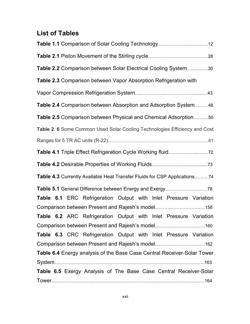
List of Tables
Table 1.1 Comparison of Solar Cooling Technology………………..….……….12
Table 2.1 Piston Movement of the Stirling cycle……………………….…………28
Table 2.2 Comparison between Solar Electrical Cooling System……....…..30
Table 2.3 Comparison between Vapor Absorption Refrigeration with
Vapor Compression Refrigeration System………………..…………………..……43
Table 2.4 Comparison between Absorption and Adsorption System………48
Table 2.5 Comparison between Physical and Chemical Adsorption……….50
Table 2. 6 Some Common Used Solar Cooling Technologies Efficiency and Cost
Ranges for 5 TR AC units (R-22)…………………………………………………………..61
Table 4.1 Triple Effect Refrigeration Cycle Working fluid………………..…….72
Table 4.2 Desirable Properties of Working Fluids……………….......................73
Table 4.3 Currently Available Heat Transfer Fluids for CSP Applications……... 74
Table 5.1 General Difference between Energy and Exergy………………….……78
Table 6.1 ERC Refrigeration Output with Inlet Pressure Variation
Comparison between Present and Rajesh’s model……………………………158
Table 6.2 ARC Refrigeration Output with Inlet Pressure Variation
Comparison between Present and Rajesh’s model……………………………160
Table 6.3 CRC Refrigeration Output with Inlet Pressure Variation
Comparison between Present and Rajesh’s model……………………………162
Table 6.4 Energy analysis of the Base Case Central Receiver-Solar Tower
System……………………………………………………………………………………....163
Table 6.5 Exergy Analysis of The Base Case Central Receiver-Solar
Tower…………………………………………………………………………………..…….164

xxiii
Table 6.6 Weather Data and Average Daily Solar Radiation at Dhahran
City. ………………………………………………………………………………….………189
Table 6.7 Hourly Solar Radiation at Dhahran City on June 11 and December
10. ……………………………………………………….…..…………………..………190
xxiv
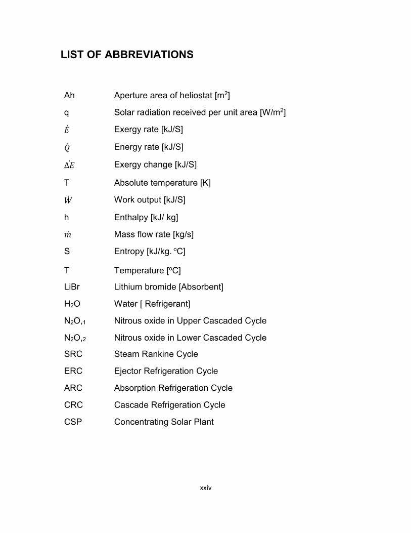
LIST OF ABBREVIATIONS
Ah Aperture area of heliostat [m2]
q Solar radiation received per unit area [W/m2]
�� Exergy rate [kJ/S]
�� Energy rate [kJ/S]
�� Exergy change [kJ/S]
T Absolute temperature [K]
�� Work output [kJ/S]
h Enthalpy [kJ/ kg]
�� Mass flow rate [kg/s]
S Entropy [kJ/kg. oC]
T Temperature [oC]
LiBr Lithium bromide [Absorbent]
H2O Water [ Refrigerant]
N2O,1 Nitrous oxide in Upper Cascaded Cycle
N2O,2 Nitrous oxide in Lower Cascaded Cycle
SRC Steam Rankine Cycle
ERC Ejector Refrigeration Cycle
ARC Absorption Refrigeration Cycle
CRC Cascade Refrigeration Cycle
CSP Concentrating Solar Plant
xxv
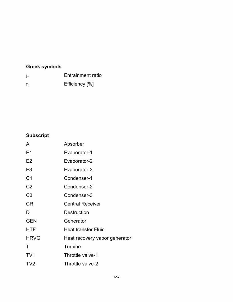
Greek symbols
μ Entrainment ratio
η Efficiency [%]
Subscript
A Absorber
E1 Evaporator-1
E2 Evaporator-2
E3 Evaporator-3
C1 Condenser-1
C2 Condenser-2
C3 Condenser-3
CR Central Receiver
D Destruction
GEN Generator
HTF Heat transfer Fluid
HRVG Heat recovery vapor generator
T Turbine
TV1 Throttle valve-1
TV2 Throttle valve-2
xxvi
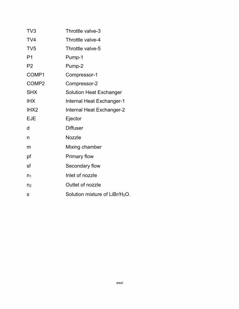
TV3 Throttle valve-3
TV4 Throttle valve-4
TV5 Throttle valve-5
P1 Pump-1
P2 Pump-2
COMP1 Compressor-1
COMP2 Compressor-2
SHX Solution Heat Exchanger
IHX Internal Heat Exchanger-1
IHX2 Internal Heat Exchanger-2
EJE Ejector
d Diffuser
n Nozzle
m Mixing chamber
pf Primary flow
sf Secondary flow
n1 Inlet of nozzle
n2 Outlet of nozzle
s Solution mixture of LiBr/H2O.
1
CHAPTER 1
INTRODUCTION
1.1 Background:
“Throughout the history of the human race, major advances in civilization
have been measured by the increase in the rate of energy consumption.
Today, energy consumption appears to be related to the life standard of
the population and the degree of industrialization of the countries.
However, the world today faces unfavorable condition of atmospheric
pollution on a scale that has not been faced earlier in human history
because of huge revolution in human use of fossil fuel in all activities, it
is also Global warning for further temperature increase by 1.4 - 4.5 oK up
to 2100 [1].
In order to avoid these unfavorable impact, we need to reduce the harmful
emission resulting from burning fossil fuel as a source of energy. This can
be achieved either by increasing energy conversion efficiency of the fossil
fuel based system or using renewable source of green energy. Among
these sources, solar energy is the most important and attractive source;
because of the solar energy universal abundance and unlimited nature
unlike many other renewable energy sources [2].
The attractive characteristic of solar energy is continues source being
unending even it is intermittent source during the day and night. In
addition, solar energy does not cause air pollution or affect the earth’s
surface as fossil fuel. Solar energy is easy to collect unlike the extraction
of fossil fuel.
In the field of solar thermal system, solar cooling has huge potential,
because the cooling demand reach its peak coincides with peak solar
energy availability.
2
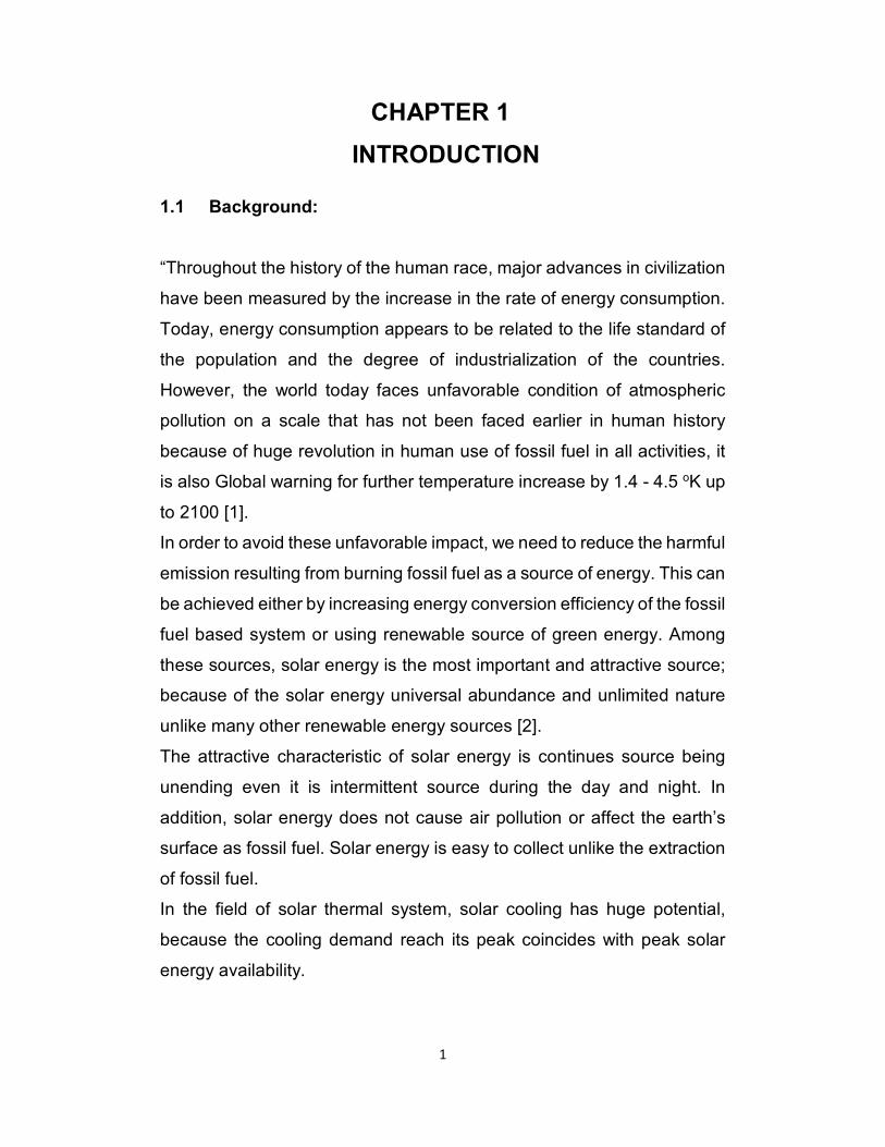
1.2 Solar Cooling technologies classification:
Solar Cooling technologies can be classified in three main categories:
solar electrical, thermal and combined power/cooling cycles as
illustrated in Figure 1.1:
Figure 1.1 Solar Cooling technology.
3
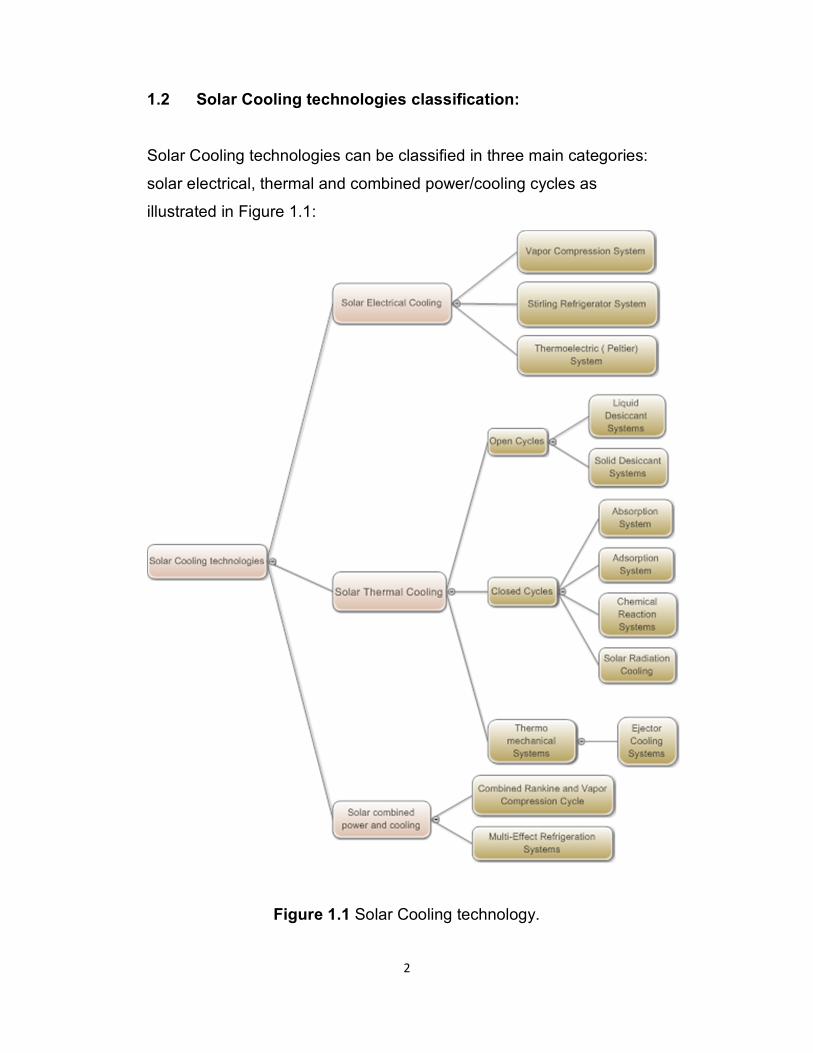
1.3 Solar Cooling System and Application Temperature Ranges
The solar cooling system can be divided into three major components;
solar energy collecting element, refrigeration cycles, and the application
at different temperature ranges.
The proper cycle for each application mainly can be selected based on
cooling demand and required temperature ranges. Figure 1.2 shows
different solar cooling technologies that could produce refrigeration effect
at different temperature ranges.
Figure 1.2. Solar Cooling System and Application Temperature Ranges.
Some applications require different range of cooling which cannot be
achieved by any single refrigeration cycle. The Multi-effect system is the
best way to achieve different magnitude of refrigeration effect and
temperature ranges by using solar energy that helps in eliminating
problems affecting the environment.
4
1.4 Concentrated Solar Power Technologies:
In this section, the concentrated solar power technologies will be
discussed.
For applications such as air conditioning, central power generation, and
numerous industrial heat requirements, flat plate collectors generally
cannot provide carrier fluids at temperatures sufficiently elevated to be
effective. They may be used as first-stage heat input devices; the
temperature of the carrier fluid is then boosted by other conventional
heating means. Alternatively, more complex and expensive concentrating
collectors can be used. These are devices that optically reflect and focus
incident solar energy onto a small receiving area. As a result of this
concentration, the intensity of the solar energy is magnified, and the
temperatures that can be achieved at the receiver (called the "target")
can approach several hundred or even several thousand degrees
Celsius. The concentrators must move to track the sun if they are to
perform effectively [3]
Concentrating, or focusing, collectors intercept direct radiation over a
large area and focus it onto a small absorber area. These collectors can
provide high temperatures more efficiently than flat-plate collectors, since
the absorption surface area is much smaller. However, diffused sky
radiation cannot be focused onto the absorber. Most concentrating
collectors require mechanical equipment that constantly orients the
collectors toward the sun and keeps the absorber at the point of focus.
Therefore; there are many types of concentrating collectors [4].
In Concentrating Solar Power (CSP) plants, mirrors concentrate sunlight
and produce heat and steam to generate electricity via a conventional
thermodynamic cycle or to drive thermal system. Unlike solar photo-
voltaic (PV), CSP uses only the direct component (DNI) of sunlight and
5
provides heat and power only in regions with high DNI (i.e. Sun Belt
regions like North Africa, the Middle East, the southwestern United States
and southern Europe).
CSP plants can be equipped with a heat storage system to generate
electricity even under cloudy skies or after sunset. Thermal storage can
significantly increase the capacity factor and dispatch ability of CSP
compared with PV and wind power. It can also facilitate grid integration
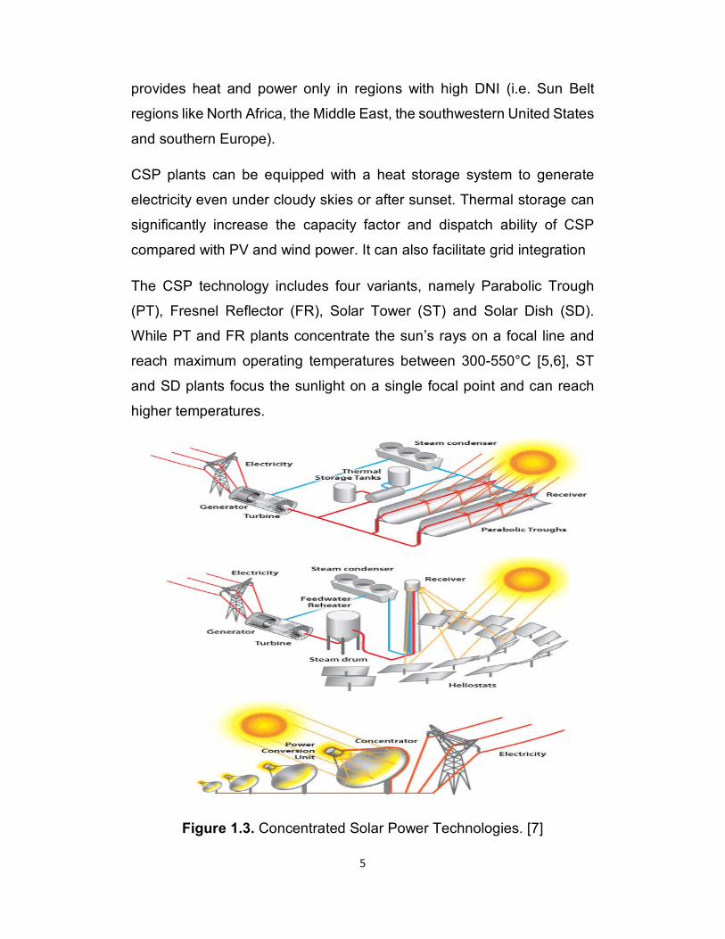
The CSP technology includes four variants, namely Parabolic Trough
(PT), Fresnel Reflector (FR), Solar Tower (ST) and Solar Dish (SD).
While PT and FR plants concentrate the sun’s rays on a focal line and
reach maximum operating temperatures between 300-550°C [5,6], ST
and SD plants focus the sunlight on a single focal point and can reach
higher temperatures.
Figure 1.3. Concentrated Solar Power Technologies. [7]
6
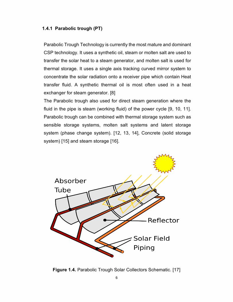
1.4.1 Parabolic trough (PT)
Parabolic Trough Technology is currently the most mature and dominant
CSP technology. It uses a synthetic oil, steam or molten salt are used to
transfer the solar heat to a steam generator, and molten salt is used for
thermal storage. It uses a single axis tracking curved mirror system to
concentrate the solar radiation onto a receiver pipe which contain Heat
transfer fluid. A synthetic thermal oil is most often used in a heat
exchanger for steam generator. [8]
The Parabolic trough also used for direct steam generation where the
fluid in the pipe is steam (working fluid) of the power cycle [9, 10, 11].
Parabolic trough can be combined with thermal storage system such as
sensible storage systems, molten salt systems and latent storage
system (phase change system). [12, 13, 14], Concrete (solid storage
system) [15] and steam storage [16].
Figure 1.4. Parabolic Trough Solar Collectors Schematic. [17]
7
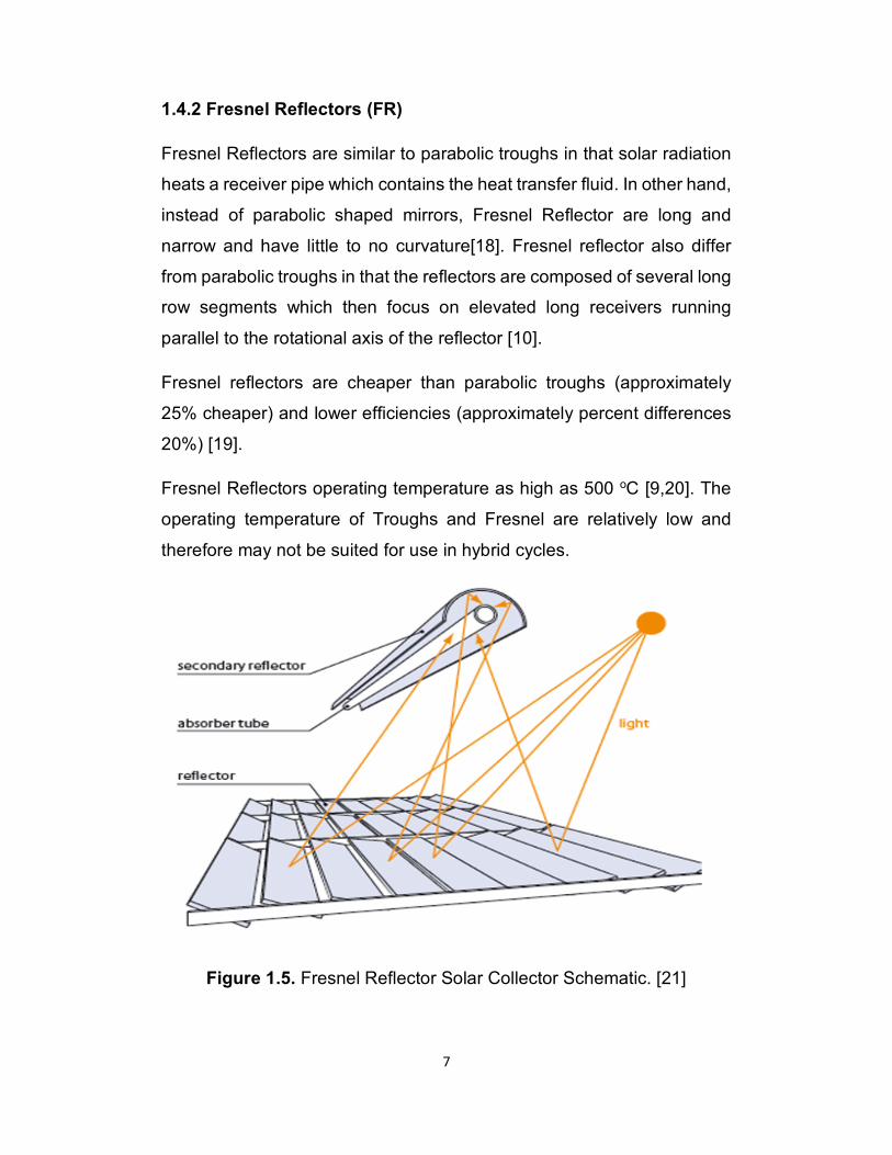
1.4.2 Fresnel Reflectors (FR)
Fresnel Reflectors are similar to parabolic troughs in that solar radiation
heats a receiver pipe which contains the heat transfer fluid. In other hand,
instead of parabolic shaped mirrors, Fresnel Reflector are long and
narrow and have little to no curvature[18]. Fresnel reflector also differ
from parabolic troughs in that the reflectors are composed of several long
row segments which then focus on elevated long receivers running
parallel to the rotational axis of the reflector [10].
Fresnel reflectors are cheaper than parabolic troughs (approximately
25% cheaper) and lower efficiencies (approximately percent differences
20%) [19].
Fresnel Reflectors operating temperature as high as 500 oC [9,20]. The
operating temperature of Troughs and Fresnel are relatively low and
therefore may not be suited for use in hybrid cycles.
Figure 1.5. Fresnel Reflector Solar Collector Schematic. [21]
8
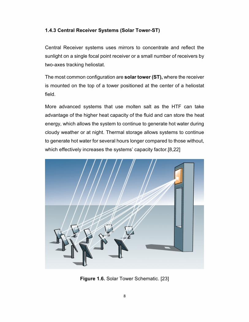
1.4.3 Central Receiver Systems (Solar Tower-ST)
Central Receiver systems uses mirrors to concentrate and reflect the
sunlight on a single focal point receiver or a small number of receivers by
two-axes tracking heliostat.
The most common configuration are solar tower (ST), where the receiver
is mounted on the top of a tower positioned at the center of a heliostat
field.
More advanced systems that use molten salt as the HTF can take
advantage of the higher heat capacity of the fluid and can store the heat
energy, which allows the system to continue to generate hot water during
cloudy weather or at night. Thermal storage allows systems to continue
to generate hot water for several hours longer compared to those without,
which effectively increases the systems’ capacity factor.[8,22]
Figure 1.6. Solar Tower Schematic. [23]
9
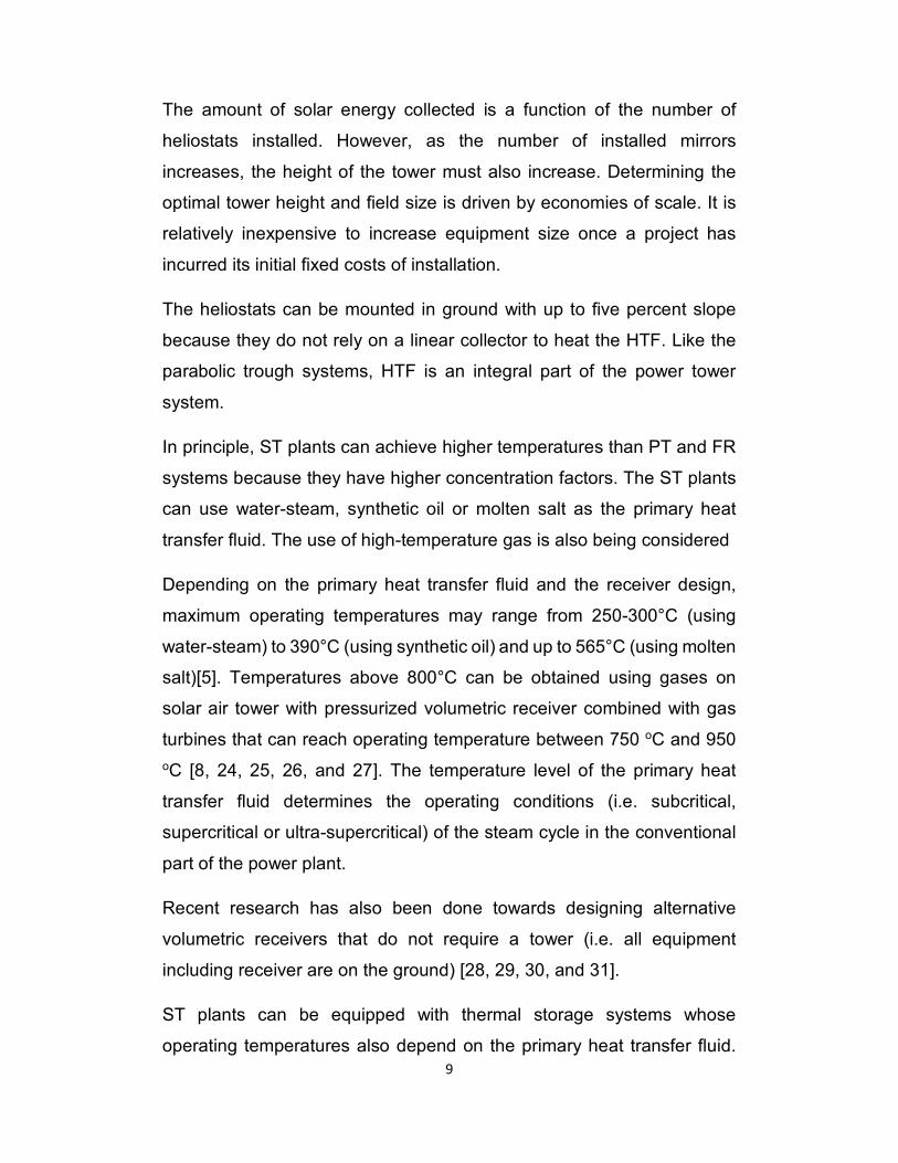
The amount of solar energy collected is a function of the number of
heliostats installed. However, as the number of installed mirrors
increases, the height of the tower must also increase. Determining the
optimal tower height and field size is driven by economies of scale. It is
relatively inexpensive to increase equipment size once a project has
incurred its initial fixed costs of installation.
The heliostats can be mounted in ground with up to five percent slope
because they do not rely on a linear collector to heat the HTF. Like the
parabolic trough systems, HTF is an integral part of the power tower
system.
In principle, ST plants can achieve higher temperatures than PT and FR
systems because they have higher concentration factors. The ST plants
can use water-steam, synthetic oil or molten salt as the primary heat
transfer fluid. The use of high-temperature gas is also being considered
Depending on the primary heat transfer fluid and the receiver design,
maximum operating temperatures may range from 250-300°C (using
water-steam) to 390°C (using synthetic oil) and up to 565°C (using molten
salt)[5]. Temperatures above 800°C can be obtained using gases on
solar air tower with pressurized volumetric receiver combined with gas
turbines that can reach operating temperature between 750 oC and 950
oC [8, 24, 25, 26, and 27]. The temperature level of the primary heat
transfer fluid determines the operating conditions (i.e. subcritical,
supercritical or ultra-supercritical) of the steam cycle in the conventional
part of the power plant.
Recent research has also been done towards designing alternative
volumetric receivers that do not require a tower (i.e. all equipment
including receiver are on the ground) [28, 29, 30, and 31].
ST plants can be equipped with thermal storage systems whose
operating temperatures also depend on the primary heat transfer fluid.
10
Today’s best performance is obtained using molten salt at 565°C for
either heat transfer or storage purposes. This enables efficient and cheap
heat storage and the use of efficient supercritical steam cycles.
High-temperature ST plants offer potential advantages over other CSP
technologies in terms of efficiency, heat storage, performance, capacity
factors and costs. In the long run, they could provide the cheapest CSP
electricity, and thermal energy but more commercial experience is
needed to confirm these expectations.
The receiver of a central solar tower power plant is located on the top of
the tower. As support of the receiver the tower is commonly with a height
of 80 to 100 m and is made of concrete or steel structure. A higher tower
is preferable for bigger and denser heliostats fields but it should avoid the
shades or objects that block the sun. At the same time, the technical
factors, e.g., tracking precision and the economic factors, e.g., tower
costs should also be considered in determining the height of the tower.
The receiver of solar tower power plant transforms the concentrated solar
energy into the thermal energy of working fluid. This working fluid could
be commonly water/steam or molten salts. In further research air is
applied for use in high temperature power towers. Water/steam receivers
are the most used receiver in solar tower power plants.
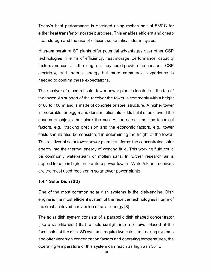
1.4.4 Solar Dish (SD)
One of the most common solar dish systems is the dish-engine. Dish
engine is the most efficient system of the receiver technologies in term of
maximal achieved conversion of solar energy [8].
The solar dish system consists of a parabolic dish shaped concentrator
(like a satellite dish) that reflects sunlight into a receiver placed at the
focal point of the dish. SD systems require two-axis sun tracking systems
and offer very high concentration factors and operating temperatures, the
operating temperature of this system can reach as high as 750 oC.
11
The Dish engine system is also the least mature of the receiver
technologies and is modular in design with a single dish limited to
capacity of 10-50 kW [5]. Therefore, at least in the near term future, solar
dish engine system are most likely to be used in smaller, high value
application rather than large scale solar driven plants.
Figure 1.7. Solar Dish Schematic. [32]
The main advantages of solar dish systems include high efficiency (i.e.
up to 30%) and modularity (i.e. 10-50 kW), which is suitable for distributed
generation [5].
Unlike other CSP options, solar dish systems do not need cooling
systems for the exhaust heat. This makes Solar dish suitable for use in
water-constrained regions, though at relatively high electricity generation
costs compared to other CSP options. Several Solar Dish prototypes
have successfully operated over the last ten years with capacities ranging
from 10-100 kW (e.g. Big Dish, Australian National University).
12
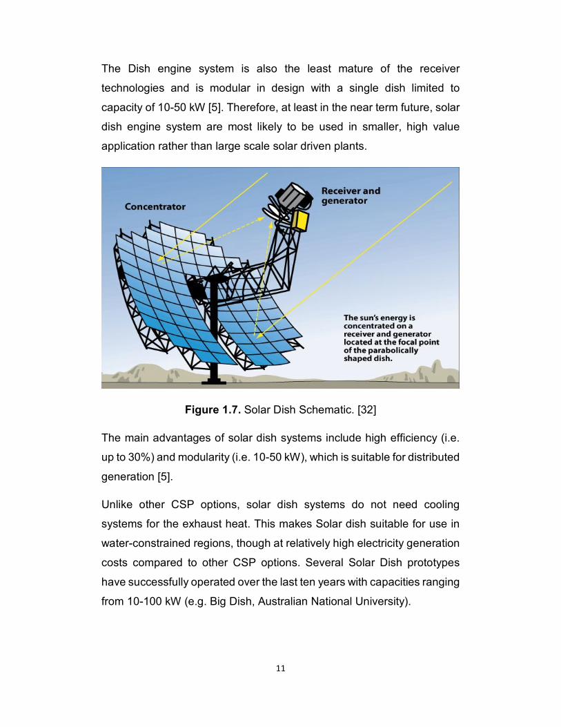
1.4.5 Comparison of Solar Cooling Technology
Table 1.1 Comparison of Solar Cooling Technology [33, 36]
Parabolic Trough Dish/Engine Power Tower
Size 30-320 MW 5-25 kW 10-200 MW
Operating
Temperature (ºC/ºF) 390/734 750/1382 565/1049
Annual Capacity
Factor 23-50 % 25 % 20-77 %
Peak Efficiency 20%(d) 29.4%(d) 23%(p)
Net Annual
Efficiency 11(d)-16% 12-25%(p) 7(d)-20%
Commercial Status
Commercially
Scale-up
Prototype
Demonstrati
on
Available
Demonstration
Technology
Development Risk Low High Medium
Storage Available Limited Battery Yes
Hybrid Designs Yes Yes Yes
Cost USD/W 2,7-4,0 1,3-12,6 2,5-4,4
(p) = predicted; (d) = demonstrated;
13
1.4.6 CSP Water Requirements
CSP plants using steam cycles (i.e. PT, FR and ST) require cooling (i.e.
2-3 m3 of water per MWh) to condense exhaust steam from the turbines;
the lower the efficiency, the higher the cooling needs. As water resources
are often scarce in Sun Belt regions, wet or dry cooling towers are often
needed for CSP installations. In general, dry (air) cooling towers are more
expensive and less efficient than wet towers. [34]
1.5 Solar Energy Component and Angle Definition:
1.5.1 Direct Normal Insolation (DNI)
Extraterrestrial solar radiation follows a direct line from the sun to the
Earth. Upon entering the earth’s atmosphere, some solar radiation is
diffused by air, water molecules, and dust within the atmosphere (Duffie
and Beckman). The direct normal insolation represents that portion of
solar radiation reaching the surface of the Earth that has not been
scattered or absorbed by the atmosphere. The adjective “normal” refers
to the direct radiation as measured on a plane normal to its direction.
1.5.2 Angle of incidence (θ) and Declination angle (δ)
Only the insolation that is directly normal to the collector surface can be
focused and thus be available to warm the absorber tubes. The angle of
incidence (θ) represents the angle between the beam radiation on a
surface and the plane normal to that surface. The angle of incidence will
vary over the course of the day (as well as throughout the year) and will
heavily influence the performance of the collectors.
14
Figure illustrates the angle of incidence between the collector normal and
the beam radiation on a solar tower. The angle of incidence results from
the relationship between the sun’s position in the sky and the orientation
of the collectors for a given location.
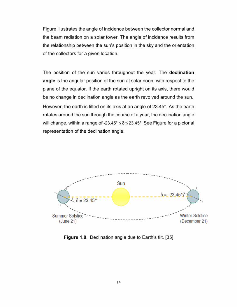
The position of the sun varies throughout the year. The declination
angle is the angular position of the sun at solar noon, with respect to the
plane of the equator. If the earth rotated upright on its axis, there would
be no change in declination angle as the earth revolved around the sun.
However, the earth is tilted on its axis at an angle of 23.45°. As the earth
rotates around the sun through the course of a year, the declination angle
will change, within a range of -23.45° ≤ δ ≤ 23.45°. See Figure for a pictorial
representation of the declination angle.
Figure 1.8. Declination angle due to Earth's tilt. [35]
15
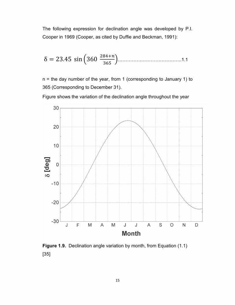
The following expression for declination angle was developed by P.I.
Cooper in 1969 (Cooper, as cited by Duffie and Beckman, 1991):
δ = 23.45 sin �360 �������� �…………………………………..1.1
n = the day number of the year, from 1 (corresponding to January 1) to
365 (Corresponding to December 31).
Figure shows the variation of the declination angle throughout the year
Figure 1.9. Declination angle variation by month, from Equation (1.1)
[35]

16
1.5.3 Hour Angle (ω ) and Solar Time.
The position of the sun depends on the hour angle, or the angular
displacement of the sun east or west of the local meridian. The hour angle
is negative when the sun is east of the local meridian (in the morning),
positive when the sun is west of the local meridian (afternoon), and zero
when the sun is in line with the local meridian (noon).
The hour angle comes as a result of the rotation on the earth, which spins
on its axis at a rate of 15° per hour:
⍵ = ������ � !" − 12% . 15�
ℎ� …………………...……1.2
Where ⍵ is the hour angle [deg] and SolarTime is the solar time [hr].
There is an important distinction between standard time and solar time.
In solar time, the sun aligns with the local meridian (ω = 0) at exactly
12:00, or “solar noon.” However, standard time is based not on the local
meridian, but on a standard meridian for the local time zone. The length
of the solar day also varies; this variation is due primarily to the fact that
the earth follows an elliptical path around the sun (Stine and Harrigan,
1985). As a result, the standard time must be adjusted to reflect the
current time of day in solar time. The relationship between solar time and
standard time, in hours, is:
����� � !" = �'()��) ' !" − 4 �*+, − *-./ % + 1………….1.3
Where
Lst = standard meridian for the local time zone [deg]
Lloc = the longitude of the location of collector site [deg]
E = equation of time [min]
E, the equation of time, accounts for the small irregularities in day length
that occur due to the Earth’s elliptical path around the sun. The equation
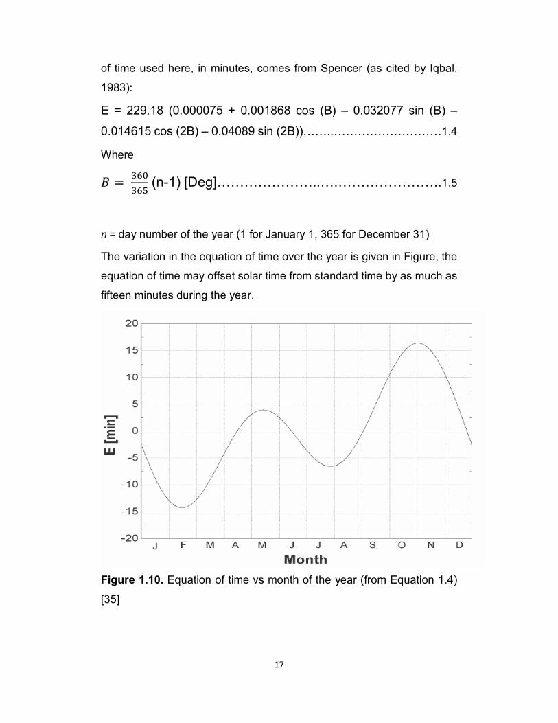
17
of time used here, in minutes, comes from Spencer (as cited by Iqbal,
1983):
E = 229.18 (0.000075 + 0.001868 cos (B) – 0.032077 sin (B) –
0.014615 cos (2B) – 0.04089 sin (2B))……..………………………1.4
Where
2 = ��3��� (n-1) [Deg]…………………..….…………………..1.5
n = day number of the year (1 for January 1, 365 for December 31)
The variation in the equation of time over the year is given in Figure, the
equation of time may offset solar time from standard time by as much as
fifteen minutes during the year.
Figure 1.10. Equation of time vs month of the year (from Equation 1.4)
[35]
18
1.5.4 Zenith Angle (θz)
The final angle required to solve for the angle of incidence is the zenith
angle. The zenith angle is the angle between the line of sight to the sun
and the vertical. Its complement, the angle between the line of sight to
the sun and the horizon, is the solar altitude angle. The zenith angle is
related to both the declination angle and the hour angle by the following
relationship (Duffie and Beckman, 1991):
4�567 = cos�:% cos�;% cos�⍵% + sin�:% sin �;%………..…1.6
Where,
δ = declination angle (see Equation 1.1)
ω = hour angle (see Equation 1.2)
φ = latitude location of the plant
1.5.5 Incidence Angle Modifier (IAM)
In addition to losses due to the angle of incidence, there are other losses
from the collectors that can be correlated to the angle of incidence. These
losses occur due to additional reflection and absorption by the glass
envelope when the angle of incidence increases [37]. The incidence
angle modifier (IAM) corrects for these additional reflection and
absorption losses. The incidence angle modifier is given as an empirical
fit to experimental data for a given collector type.
K = cos�θ% + 0.000884�θ% − 0.0005369�θ%�………………..1.7
Where θ, the incidence angle, is provided in degrees.
19
It is desirable to distinguish between losses in available radiation due to
the angle of incidence itself and the reflection/absorption corrections
empirically correlated to the angle of incidence.
For this purpose, the incidence angle modifier is defined for this work as
the incidence angle modifier defined by Dudley et al, divided by the
cosine of the incidence angle:
@AB = CDEF �G% ………………………………………………….…...1.8
The equation for the incidence angle modifier used in the solar field
component model is:”
@AB = 1 + 0.000884 . GDEF �G% − 0.00005369 . GH
DEF �G%…….……1.9

20
CHAPTER 2
SOLAR COOLING TECHNOLOGIES
DESCRIPTION AND LITERATURE REVIEW
Solar cooling is a clean and cost-effective technology, solar cooling offer
environmental benefits including reducing main grid demand and shift the
load during peak usage and reduced greenhouse gas emissions.
The main objective of this chapter is to review and analyze different solar
cooling technologies that can be used to provide the required cooling and
refrigeration effect from solar energy. This chapter is covering a wide
range of solar cooling technologies including solar electrical refrigeration
system, thermo-mechanical combined power and cooling systems and
advanced triple effect refrigeration cycles [38].
This chapter includes comparisons of different technologies highlighting
the advantages and disadvantages. This comparison would assist the
decision makers to select the proper solar cooling technology for specific
application.
21
Solar Cooling technologies can be classified in three main categories:
solar electrical, thermal and combined power/cooling cycles.
The solar cooling system can be divided into three major components;
solar energy collecting element, refrigeration cycles, and the application
at different temperature ranges.
The proper cycle for each application mainly can be selected based on
cooling demand and required temperature ranges.
Some applications require different range of cooling which cannot be
achieved by any single refrigeration cycle.
The Multi-effect system is the best way to achieve different magnitude of
refrigeration effect and temperature ranges by using solar energy that
helps in eliminating problems affecting the environment.
2.1 Solar Electrical Cooling:
A solar electrical cooling system consists of photovoltaic panel and
electrical refrigeration device. Photovoltaic cells transform light into
electricity through photoelectric effect. Many of solar electrical
refrigeration system are made for independent operation.
PV cells made of semiconductor materials, single crystalline thin films,
poly-crystalline and silicon-wafers represent the solar panel materials,
and the silicon is major component of PV cell in the market.
The efficiency of polycrystalline thin films is higher than that of silicon
wafer, the efficiency of polycrystalline thin films in range of 10 to 17 %
[39] and single crystalline thin file efficiency can reach 15 to 20 % by
using multi-junction cell structure, while as silicon wafer performance is
low and its cost are high compare the thin film technologies.
22
The produced power by solar photovoltaic cells is supplied either to the
thermo-electrical system, Stirling cycle or normal vapor compression
systems.
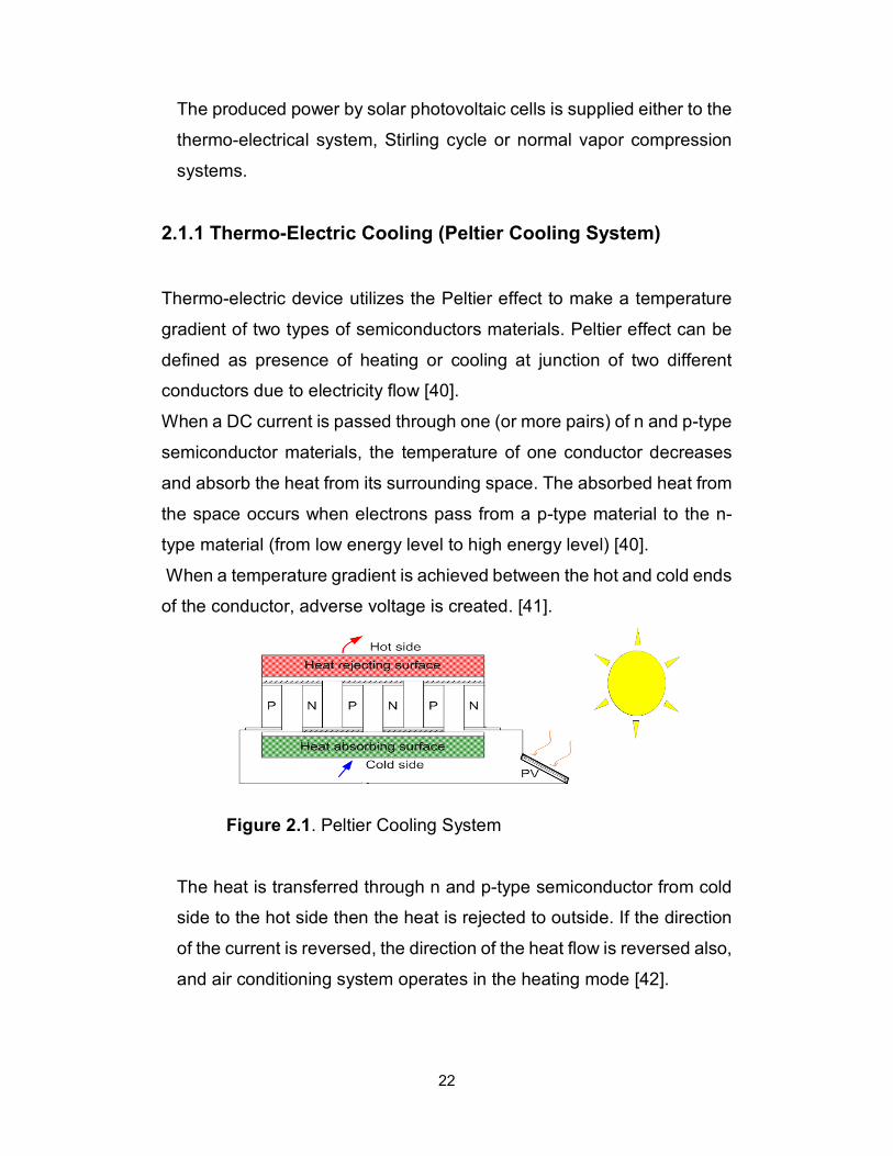
2.1.1 Thermo-Electric Cooling (Peltier Cooling System)
Thermo-electric device utilizes the Peltier effect to make a temperature
gradient of two types of semiconductors materials. Peltier effect can be
defined as presence of heating or cooling at junction of two different
conductors due to electricity flow [40].
When a DC current is passed through one (or more pairs) of n and p-type
semiconductor materials, the temperature of one conductor decreases
and absorb the heat from its surrounding space. The absorbed heat from
the space occurs when electrons pass from a p-type material to the n-
type material (from low energy level to high energy level) [40].
When a temperature gradient is achieved between the hot and cold ends
of the conductor, adverse voltage is created. [41].
Figure 2.1. Peltier Cooling System
The heat is transferred through n and p-type semiconductor from cold
side to the hot side then the heat is rejected to outside. If the direction
of the current is reversed, the direction of the heat flow is reversed also,
and air conditioning system operates in the heating mode [42].
23
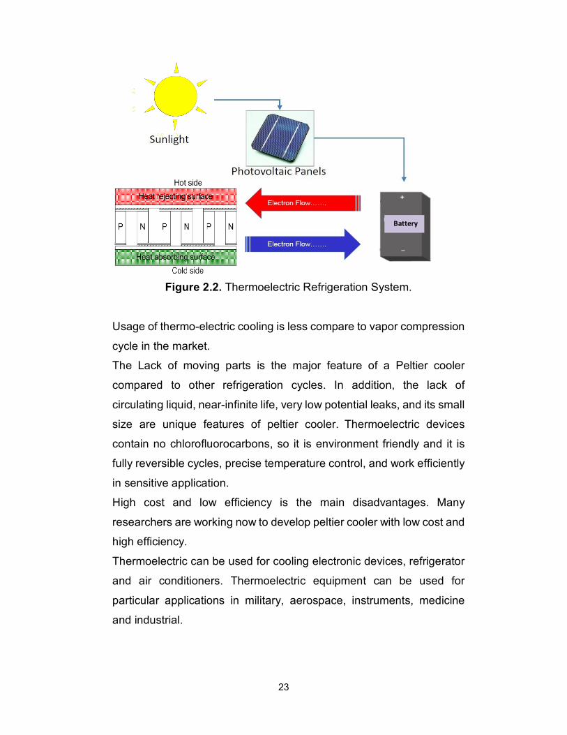
Figure 2.2. Thermoelectric Refrigeration System.
Usage of thermo-electric cooling is less compare to vapor compression
cycle in the market.
The Lack of moving parts is the major feature of a Peltier cooler
compared to other refrigeration cycles. In addition, the lack of
circulating liquid, near-infinite life, very low potential leaks, and its small
size are unique features of peltier cooler. Thermoelectric devices
contain no chlorofluorocarbons, so it is environment friendly and it is
fully reversible cycles, precise temperature control, and work efficiently
in sensitive application.
High cost and low efficiency is the main disadvantages. Many
researchers are working now to develop peltier cooler with low cost and
high efficiency.
Thermoelectric can be used for cooling electronic devices, refrigerator
and air conditioners. Thermoelectric equipment can be used for
particular applications in military, aerospace, instruments, medicine
and industrial.
Battery
24
Riffat et. al. [40] explained thermoelectric working principle and
materials used for thermoelectric and its application. They also
discussed thermoelectric devices application in refrigeration and power
generation, and as sensor in thermal energy, they discussed the
development of new materials that could improve the thermoelectric
devices for many applications.
The main disadvantage of thermo-electric is low COP but it does have
high potential in specific application, such as cooling electronic devices,
where thermo-electric is preferred due to small size and consume very
less electricity. [42]
2.1.2 Solar powered vapor compression cooling system
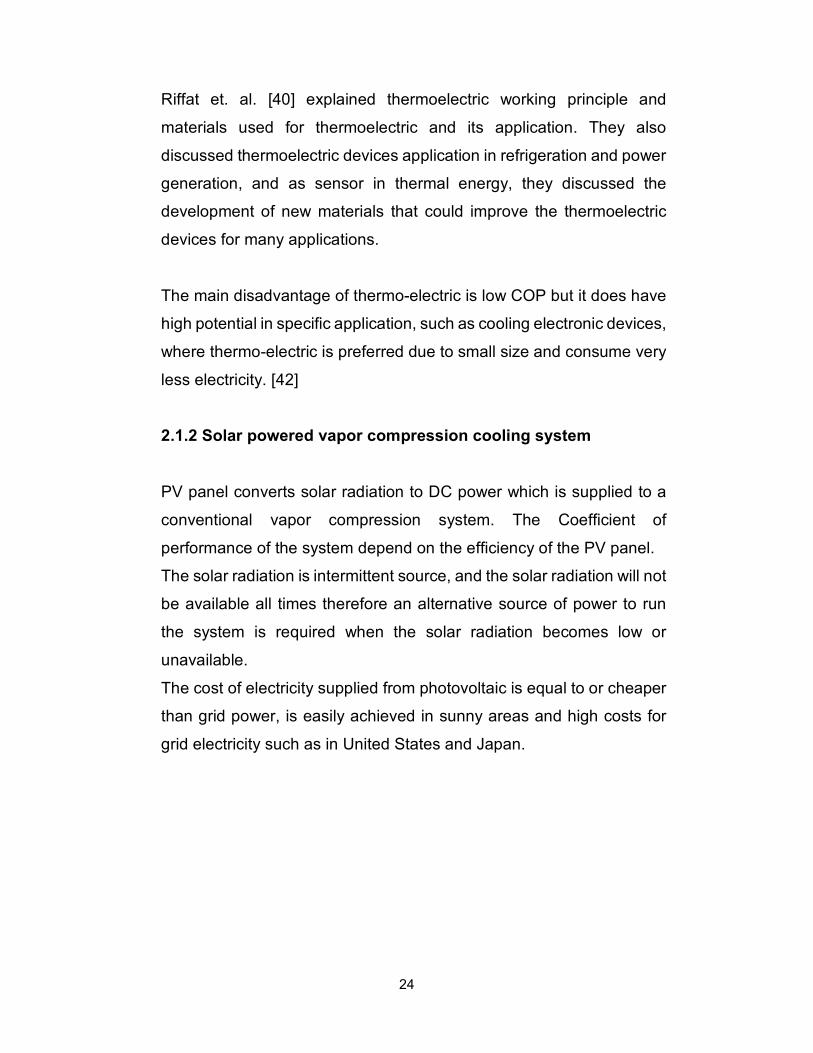
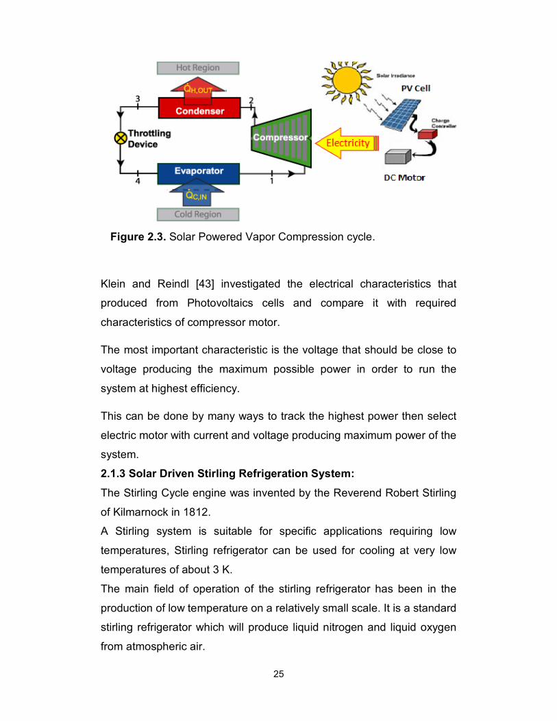
PV panel converts solar radiation to DC power which is supplied to a
conventional vapor compression system. The Coefficient of
performance of the system depend on the efficiency of the PV panel.
The solar radiation is intermittent source, and the solar radiation will not
be available all times therefore an alternative source of power to run
the system is required when the solar radiation becomes low or
unavailable.
The cost of electricity supplied from photovoltaic is equal to or cheaper
than grid power, is easily achieved in sunny areas and high costs for
grid electricity such as in United States and Japan.
25
Figure 2.3. Solar Powered Vapor Compression cycle.
Klein and Reindl [43] investigated the electrical characteristics that
produced from Photovoltaics cells and compare it with required
characteristics of compressor motor.
The most important characteristic is the voltage that should be close to
voltage producing the maximum possible power in order to run the
system at highest efficiency.
This can be done by many ways to track the highest power then select
electric motor with current and voltage producing maximum power of the
system.
2.1.3 Solar Driven Stirling Refrigeration System:
The Stirling Cycle engine was invented by the Reverend Robert Stirling
of Kilmarnock in 1812.
A Stirling system is suitable for specific applications requiring low
temperatures, Stirling refrigerator can be used for cooling at very low
temperatures of about 3 K.
The main field of operation of the stirling refrigerator has been in the
production of low temperature on a relatively small scale. It is a standard
stirling refrigerator which will produce liquid nitrogen and liquid oxygen
from atmospheric air.
26
Hydrogen is the most often and best gas to use in a stirling refrigerator
because of its low molecular weight while as nitrogen is used in
commercial and standard units as it is very cheap and safe.
Stirling refrigeration cycle principle is based on volume changes caused
by pistons, thus inducing changes in pressure and temperature of a gas
(no phase change). On the other hand, it yields very good performance
at large temperature increases [44].
The Main Concept of Stirling refrigerator is to convert mechanical energy
to thermal energy (Useful Cooling).
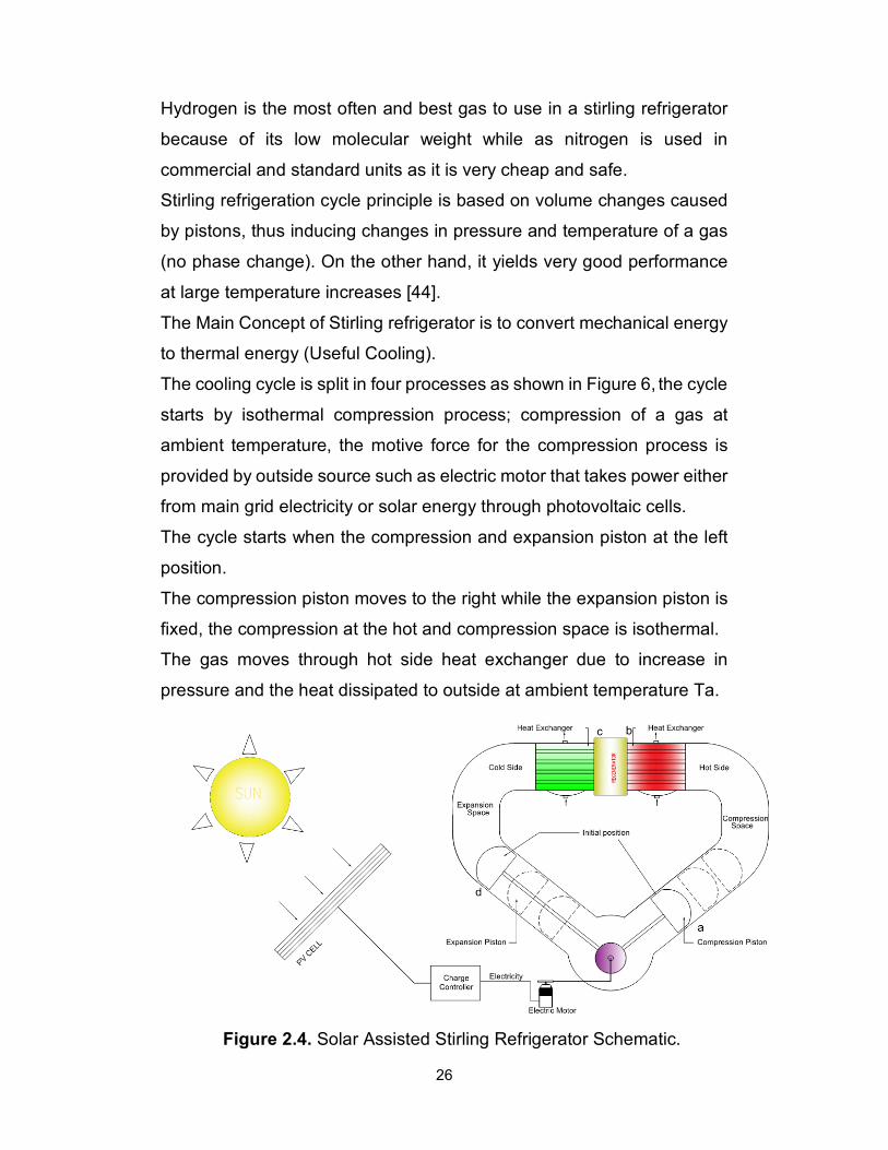
The cooling cycle is split in four processes as shown in Figure 6, the cycle
starts by isothermal compression process; compression of a gas at
ambient temperature, the motive force for the compression process is
provided by outside source such as electric motor that takes power either
from main grid electricity or solar energy through photovoltaic cells.
The cycle starts when the compression and expansion piston at the left
position.
The compression piston moves to the right while the expansion piston is
fixed, the compression at the hot and compression space is isothermal.
The gas moves through hot side heat exchanger due to increase in
pressure and the heat dissipated to outside at ambient temperature Ta.
Figure 2.4. Solar Assisted Stirling Refrigerator Schematic.
27
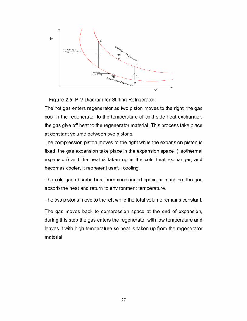
Figure 2.5. P-V Diagram for Stirling Refrigerator.
The hot gas enters regenerator as two piston moves to the right, the gas
cool in the regenerator to the temperature of cold side heat exchanger,
the gas give off heat to the regenerator material. This process take place
at constant volume between two pistons.
The compression piston moves to the right while the expansion piston is
fixed, the gas expansion take place in the expansion space ( isothermal
expansion) and the heat is taken up in the cold heat exchanger, and
becomes cooler, it represent useful cooling.
The cold gas absorbs heat from conditioned space or machine, the gas
absorb the heat and return to environment temperature.
The two pistons move to the left while the total volume remains constant.
The gas moves back to compression space at the end of expansion,
during this step the gas enters the regenerator with low temperature and
leaves it with high temperature so heat is taken up from the regenerator
material.
28
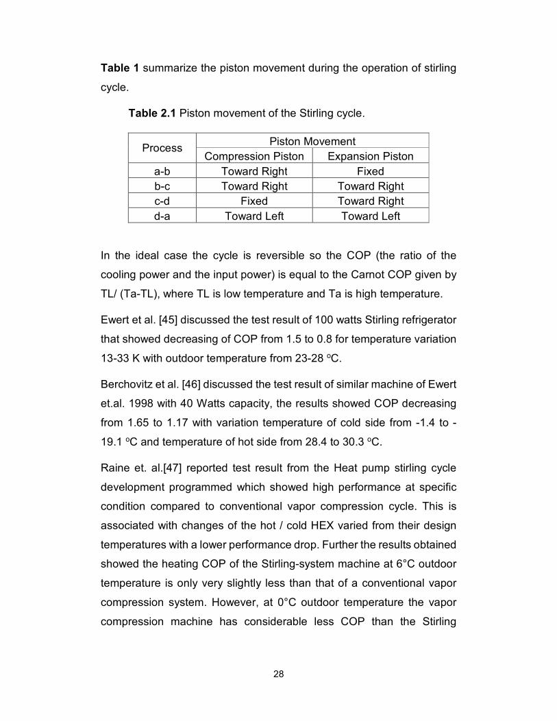
Table 1 summarize the piston movement during the operation of stirling
cycle.
Table 2.1 Piston movement of the Stirling cycle.
Process Piston Movement
Compression Piston Expansion Piston
a-b Toward Right Fixed
b-c Toward Right Toward Right
c-d Fixed Toward Right
d-a Toward Left Toward Left
In the ideal case the cycle is reversible so the COP (the ratio of the
cooling power and the input power) is equal to the Carnot COP given by
TL/ (Ta-TL), where TL is low temperature and Ta is high temperature.
Ewert et al. [45] discussed the test result of 100 watts Stirling refrigerator
that showed decreasing of COP from 1.5 to 0.8 for temperature variation
13-33 K with outdoor temperature from 23-28 oC.
Berchovitz et al. [46] discussed the test result of similar machine of Ewert
et.al. 1998 with 40 Watts capacity, the results showed COP decreasing
from 1.65 to 1.17 with variation temperature of cold side from -1.4 to -
19.1 oC and temperature of hot side from 28.4 to 30.3 oC.
Raine et. al.[47] reported test result from the Heat pump stirling cycle
development programmed which showed high performance at specific
condition compared to conventional vapor compression cycle. This is
associated with changes of the hot / cold HEX varied from their design
temperatures with a lower performance drop. Further the results obtained
showed the heating COP of the Stirling-system machine at 6°C outdoor
temperature is only very slightly less than that of a conventional vapor
compression system. However, at 0°C outdoor temperature the vapor
compression machine has considerable less COP than the Stirling
29
system, even the Stirling cycle machine is operating at an even lower
outdoor temperature of -5°C.
There is many challenges in designing efficient Stirling refrigerator as low
COP due to poor heat transfer between working fluid and ambient air [48].
Riffat et. al. [41] conducted a comparative study of the performance
between vapor compression cycle, the absorption cycle and the
thermoelectric refrigerator. The comparison showed that vapor
compression have high COP and low cost. However, some of refrigerant
used vapor compression system will be phase out due to their effect on
depletion of the ozone layer like system used R-12 or R-22.
Absorption cycle generally require large space and high initial cost but
consume very less electricity to run the pumps and fan as it depends on
waste energy source or solar energy to provide the required thermal
energy to generator, so the operational cost is very low, while as low
noise or almost very less vibration due to no moving parts, small size and
light weight are unique features of thermo-electric. Thermo-electric does
not require refrigerant so no effect on the environment.
30
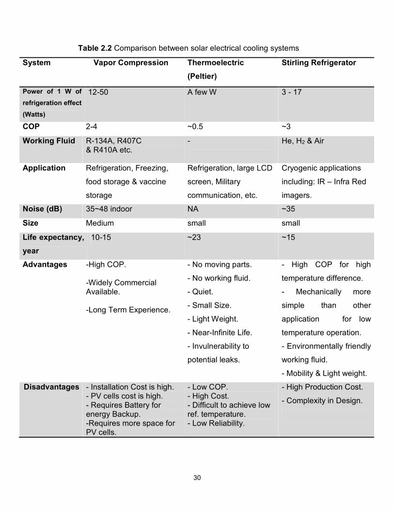
Table 2.2 Comparison between solar electrical cooling systems
System Vapor Compression Thermoelectric
(Peltier)
Stirling Refrigerator
Power of 1 W of
refrigeration effect
(Watts)
12-50 A few W 3 - 17
COP 2-4 ~0.5 ~3
Working Fluid R-134A, R407C & R410A etc.
-
He, H2 & Air
Application Refrigeration, Freezing,
food storage & vaccine
storage
Refrigeration, large LCD
screen, Military
communication, etc.
Cryogenic applications
including: IR – Infra Red
imagers.
Noise (dB) 35~48 indoor NA ~35
Size Medium small small
Life expectancy,
year
10-15 ~23 ~15
Advantages -High COP. -Widely Commercial Available.
-Long Term Experience.
- No moving parts.
- No working fluid.
- Quiet.
- Small Size.
- Light Weight.
- Near-Infinite Life.
- Invulnerability to
potential leaks.
- High COP for high
temperature difference.
- Mechanically more
simple than other
application for low
temperature operation.
- Environmentally friendly
working fluid.
- Mobility & Light weight.
Disadvantages - Installation Cost is high. - PV cells cost is high. - Requires Battery for energy Backup. -Requires more space for PV cells.
- Low COP. - High Cost. - Difficult to achieve low ref. temperature. - Low Reliability.
- High Production Cost.
- Complexity in Design.
31
2.2 Solar Thermal Cooling:
Solar energy conversion systems can be used to transform solar
thermal energy to cooling or heating through chemical or physical
Processes.
2.2.1 Open Sorption Cycle Solar Cooling.
It represents desiccant systems that are used in air conditioning
applications for humidification or dehumidification basically transfer
moisture from one air stream to another one. These cycles cab be used
as pre-cooling of other system and can be used to provide cooling for
specific application with special requirement.
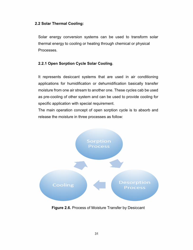
The main operation concept of open sorption cycle is to absorb and
release the moisture in three processes as follow:
Figure 2.6. Process of Moisture Transfer by Desiccant
32
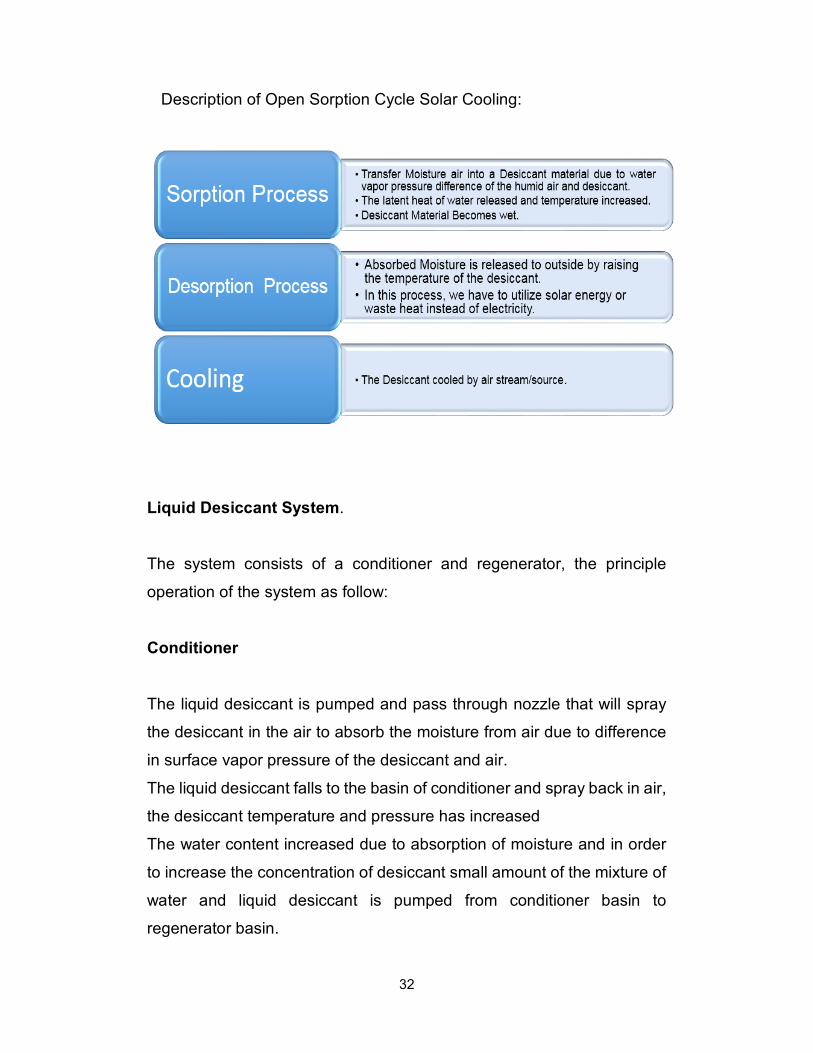
Description of Open Sorption Cycle Solar Cooling:
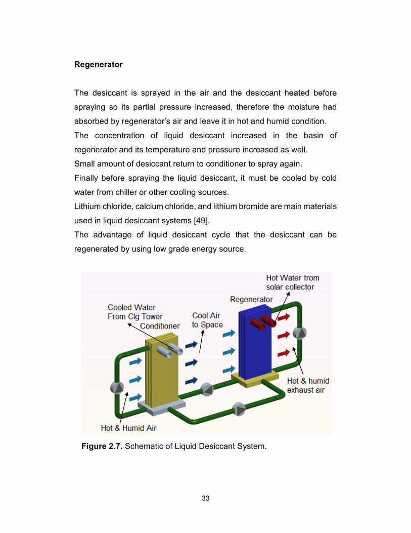
Liquid Desiccant System.
The system consists of a conditioner and regenerator, the principle
operation of the system as follow:
Conditioner
The liquid desiccant is pumped and pass through nozzle that will spray
the desiccant in the air to absorb the moisture from air due to difference
in surface vapor pressure of the desiccant and air.
The liquid desiccant falls to the basin of conditioner and spray back in air,
the desiccant temperature and pressure has increased
The water content increased due to absorption of moisture and in order
to increase the concentration of desiccant small amount of the mixture of
water and liquid desiccant is pumped from conditioner basin to
regenerator basin.
33
Regenerator
The desiccant is sprayed in the air and the desiccant heated before
spraying so its partial pressure increased, therefore the moisture had
absorbed by regenerator’s air and leave it in hot and humid condition.
The concentration of liquid desiccant increased in the basin of
regenerator and its temperature and pressure increased as well.
Small amount of desiccant return to conditioner to spray again.
Finally before spraying the liquid desiccant, it must be cooled by cold
water from chiller or other cooling sources.
Lithium chloride, calcium chloride, and lithium bromide are main materials
used in liquid desiccant systems [49].
The advantage of liquid desiccant cycle that the desiccant can be
regenerated by using low grade energy source.
Figure 2.7. Schematic of Liquid Desiccant System.
34
Gommed & Grossman [50] investigated solar assisted liquid desiccant
cooling system using Lithium chloride and water as working fluid, outside
temperature was the influencing factor that is having high effect on the
dehumidification process.
The result showed that the system supplied 16 kW of dehumidification
capacity with 0.8 coefficient of performance.
Davies [51] developed the liquid desiccant system based on Abu Dhabi
data weather with the solar collector for regenerative heating coil and the
adiabatic cooler to reduce inside condition in greenhouses. The result
revealed clearly the possibility of lower outside temperature by 5 oC as
cooling effect.
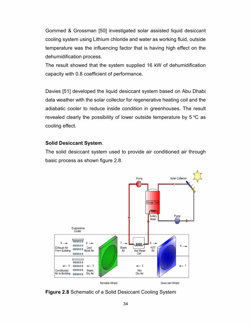
Solid Desiccant System.
The solid desiccant system used to provide air conditioned air through
basic process as shown figure 2.8.
Figure 2.8 Schematic of a Solid Desiccant Cooling System
35
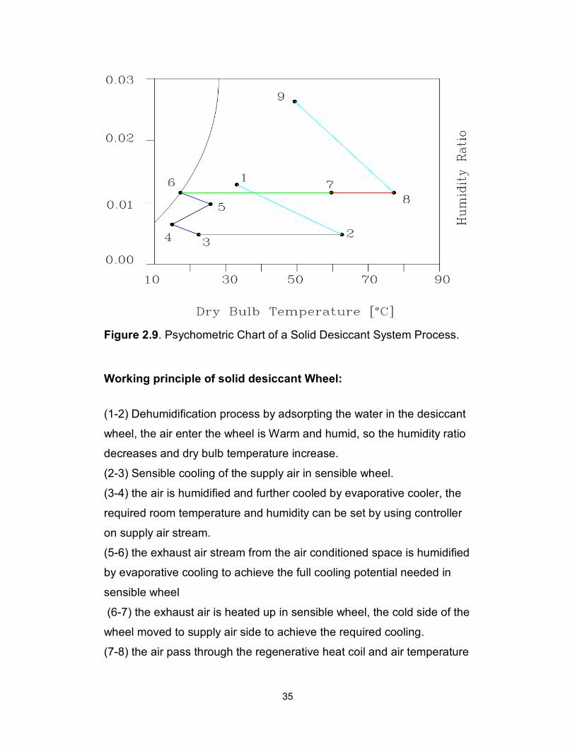
Figure 2.9. Psychometric Chart of a Solid Desiccant System Process.
Working principle of solid desiccant Wheel:
(1-2) Dehumidification process by adsorpting the water in the desiccant
wheel, the air enter the wheel is Warm and humid, so the humidity ratio
decreases and dry bulb temperature increase.
(2-3) Sensible cooling of the supply air in sensible wheel.
(3-4) the air is humidified and further cooled by evaporative cooler, the
required room temperature and humidity can be set by using controller
on supply air stream.
(5-6) the exhaust air stream from the air conditioned space is humidified
by evaporative cooling to achieve the full cooling potential needed in
sensible wheel
(6-7) the exhaust air is heated up in sensible wheel, the cold side of the
wheel moved to supply air side to achieve the required cooling.
(7-8) the air pass through the regenerative heat coil and air temperature

36
increased. The hot water received from dedicated solar collector in a
comparatively low temperature around 70 °C.
(8-9) the desiccant wheel has to be regenerated to keep the system
operate continuously for dehumidification process, so the humidity ratio
increased and dry bulb temperature decreases of the exhausted air.
The solar system consist of solar collectors and a hot water storage to
maximize the utilization of the solar system. Auxiliary water heater is
needed to maintain continuous operation during the night and when the
solar source is not available or enough.
Standard desiccant wheel might not be efficient in coastal areas where
the outdoor air is very hot and humid as the system will not be able to
reduce the humidity to level which evaporative cooling can work
efficiently. Therefore, more complex design can be implemented to
overcome this problem.
Henning [52], Simulated a solar assisted solid desiccant system with
solar collector (20 m2 Area) and storage tank (2 m3 volume). The results
showed that a 54% collector efficiency, 0.6 COP and 76% solar fraction
(auxiliary energy supplied).
Henning [53] Investigated a solid desiccant cooling system, the result
showed that the maximum COP was about 0.7.
37
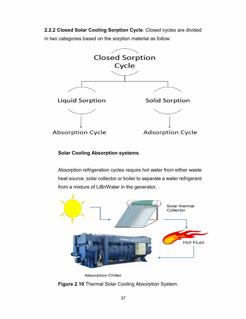
2.2.2 Closed Solar Cooling Sorption Cycle. Closed cycles are divided
in two categories based on the sorption material as follow:
Solar Cooling Absorption systems.
Absorption refrigeration cycles require hot water from either waste
heat source, solar collector or boiler to separate a water refrigerant
from a mixture of LiBr/Water in the generator.
Figure 2.10 Thermal Solar Cooling Absorption System.
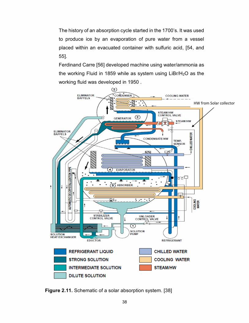
38
The history of an absorption cycle started in the 1700’s. It was used
to produce ice by an evaporation of pure water from a vessel
placed within an evacuated container with sulfuric acid, [54, and
55].
Ferdinand Carre [56] developed machine using water/ammonia as
the working Fluid in 1859 while as system using LiBr/H2O as the
working fluid was developed in 1950 .
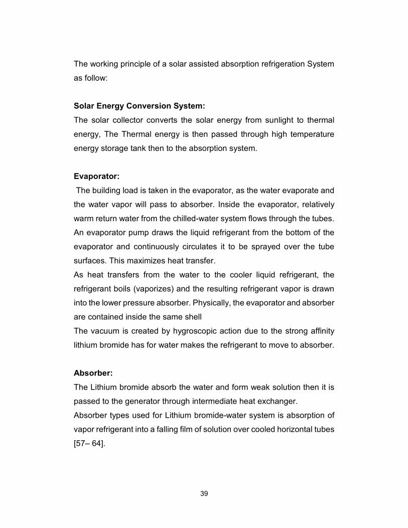
Figure 2.11. Schematic of a solar absorption system. [38]
HW from Solar collector
39
The working principle of a solar assisted absorption refrigeration System
as follow:
Solar Energy Conversion System:
The solar collector converts the solar energy from sunlight to thermal
energy, The Thermal energy is then passed through high temperature
energy storage tank then to the absorption system.
Evaporator:
The building load is taken in the evaporator, as the water evaporate and
the water vapor will pass to absorber. Inside the evaporator, relatively
warm return water from the chilled-water system flows through the tubes.
An evaporator pump draws the liquid refrigerant from the bottom of the
evaporator and continuously circulates it to be sprayed over the tube
surfaces. This maximizes heat transfer.
As heat transfers from the water to the cooler liquid refrigerant, the
refrigerant boils (vaporizes) and the resulting refrigerant vapor is drawn
into the lower pressure absorber. Physically, the evaporator and absorber
are contained inside the same shell
The vacuum is created by hygroscopic action due to the strong affinity
lithium bromide has for water makes the refrigerant to move to absorber.
Absorber:
The Lithium bromide absorb the water and form weak solution then it is
passed to the generator through intermediate heat exchanger.
Absorber types used for Lithium bromide-water system is absorption of
vapor refrigerant into a falling film of solution over cooled horizontal tubes
[57– 64].
40
Generator:
The hot water used to separate the weak solution form water vapor and
form strong lithium bromide solution, then the water vapor is passed to
the condenser.
The hot water provided from Low-grade heat source can be upgraded by
using solar energy [65], power plant waste heat or other industrial
application [66, 67]. The absorption heat source performance with
various working fluids has been investigated; LiBr/water [68], Dimethyl
Formamide (DMF)/R21 [69-74].
Heat Exchanger:
The strong solution of lithium bromide is passed to the absorber through
heat exchanger after the separation in the generator. The weak solution
from the absorber is pumped through the same heat exchanger to the
generator, so the temperature of weak solution increased while as the
strong solution temperature decreased.
Condenser:
The cold water from cooling tower used to remove the heat and
condensate the water vapor, then the liquid water will enter the expansion
valve.
Cooling water from cooling tower:
Cold water supplied from cooling tower used to remove the heat from
condenser and absorber then the heat is dissipated in the cooling tower
to outside.
Auxiliary heat source:
The auxiliary heat source is needed when sun is not shining or solar
energy source is not enough to main continuous operation.
41
Performance of Absorption Solar cooling system:
��� =������ ���� ��� �� ����������
���� ����� �� ��������� + ���� �������� �����
The performance of Absorption solar cooling system depends mainly on
thermodynamic properties of the working fluid [38].
Working Fluid in Absorption Solar cooling system:
The most common working Fluid are LiBr/H2O where Water is the
refrigerant and LiBr is the absorbent and H2O/ammonia are widely used
in absorption systems where ammonia (NH3) is refrigerant and Water is
the absorbent.
Marcriss discussed all possible working fluids that can be used in
absorption solar cooling systems, he found that there are 40 refrigerant
compounds and 200 absorbent compounds available to be used in
absorption refrigeration systems. [73].
H2O / NH3 thermodynamic properties can be obtained from [74–78].
LiBr/H2O thermodynamic properties can be obtained from [79–83]. A
corrosion inhibitor may be added to LiBr/H2O as [84–87] or to enhance
heat & mass transfer performance [88–92].
Many research has been carried out to investigate the thermodynamic
properties of new working fluid like fluorocarbon refrigerant with number
of organic solvents, Research on these kinds of working fluids may be
obtained from the literature [93–98].
Ghaddar [99] investigated a solar assisted absorption system located in
Beirut. The results showed a minimum collector Area for each ton
42
refrigeration is 23.3 m2 and with best water storage tank size varied from
1,000 to 1,500 L for seven hour of operation on solar energy.
Hammed and Zurigat [100] Studied the performance of solar assisted
absorption system with 1.5 ton cooling capacity, 14 m2 solar collector and
Shell and tube heat exchangers. The test carried on April and May in
Jordan and the test result showed actual COP around 0.55.
Florides [101], designed a solar cooling system to handle the house load
for whole year, the system consist of a solar collector storage tank, an
auxiliary water heater and a LiBr/water absorption system. Selection of
solar collector area can be decided through economic analysis without
compromising of the system performance.
Hammad and Audi [102] simulated the performance of a non-storage
solar assisted absorption system without storage tank. The results
showed a maximum ideal COP of the system to be equal to 1.6 while the
peak actual COP was 0.55.
Boehm [103] developed a solar assisted absorption system (single-effect
with ideal cooling capacity of 10 ton) with storage tank (0.45 m3), solar
collector (63.7 m2). Economic analysis was performed for this system and
the result showed reduction from $3,448 to $1,737 annually more than
the normal 8 ton vapor compression refrigeration system. The analysis
showed the payback periods is 1.5 to 3 years based on the performance
of the solar collector and rate of electricity difference. The system showed
capability to supply more than 5.5 ton of actual cooling continuously for 8
hours on a summer day.
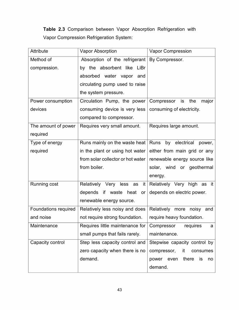
43
Table 2.3 Comparison between Vapor Absorption Refrigeration with
Vapor Compression Refrigeration System:
Attribute Vapor Absorption Vapor Compression
Method of
compression.
Absorption of the refrigerant
by the absorbent like LiBr
absorbed water vapor and
circulating pump used to raise
the system pressure.
By Compressor.
Power consumption
devices
Circulation Pump, the power
consuming device is very less
compared to compressor.
Compressor is the major
consuming of electricity.
The amount of power
required
Requires very small amount. Requires large amount.
Type of energy
required
Runs mainly on the waste heat
in the plant or using hot water
from solar collector or hot water
from boiler.
Runs by electrical power,
either from main grid or any
renewable energy source like
solar, wind or geothermal
energy.
Running cost Relatively Very less as it
depends if waste heat or
renewable energy source.
Relatively Very high as it
depends on electric power.
Foundations required
and noise
Relatively less noisy and does
not require strong foundation.
Relatively more noisy and
require heavy foundation.
Maintenance Requires little maintenance for
small pumps that fails rarely.
Compressor requires a
maintenance.
Capacity control Step less capacity control and
zero capacity when there is no
demand.
Stepwise capacity control by
compressor, it consumes
power even there is no
demand.
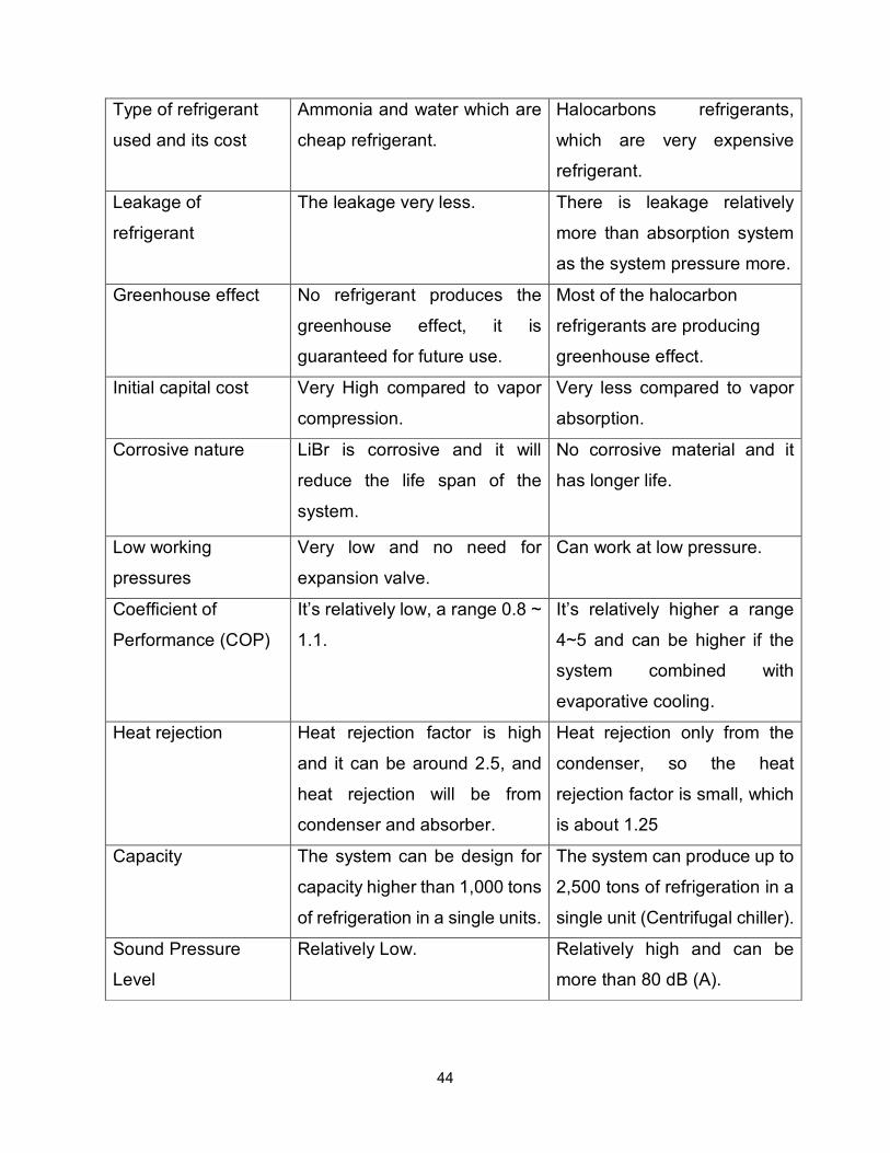
44
Type of refrigerant
used and its cost
Ammonia and water which are
cheap refrigerant.
Halocarbons refrigerants,
which are very expensive
refrigerant.
Leakage of
refrigerant
The leakage very less. There is leakage relatively
more than absorption system
as the system pressure more.
Greenhouse effect No refrigerant produces the
greenhouse effect, it is
guaranteed for future use.
Most of the halocarbon
refrigerants are producing
greenhouse effect.
Initial capital cost Very High compared to vapor
compression.
Very less compared to vapor
absorption.
Corrosive nature LiBr is corrosive and it will
reduce the life span of the
system.
No corrosive material and it
has longer life.
Low working
pressures
Very low and no need for
expansion valve.
Can work at low pressure.
Coefficient of
Performance (COP)
It’s relatively low, a range 0.8 ~
1.1.
It’s relatively higher a range
4~5 and can be higher if the
system combined with
evaporative cooling.
Heat rejection Heat rejection factor is high
and it can be around 2.5, and
heat rejection will be from
condenser and absorber.
Heat rejection only from the
condenser, so the heat
rejection factor is small, which
is about 1.25
Capacity The system can be design for
capacity higher than 1,000 tons
of refrigeration in a single units.
The system can produce up to
2,500 tons of refrigeration in a
single unit (Centrifugal chiller).
Sound Pressure
Level
Relatively Low. Relatively high and can be
more than 80 dB (A).
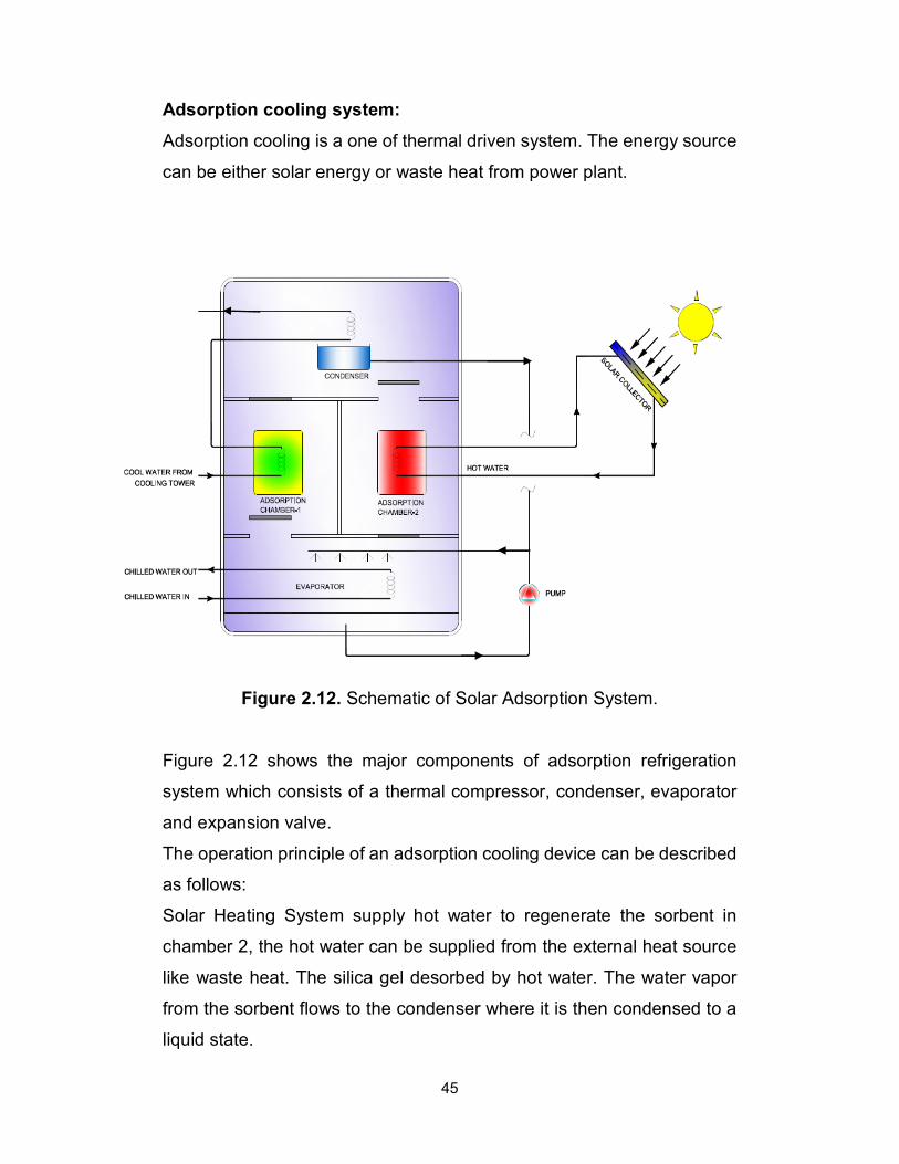
45
Adsorption cooling system:
Adsorption cooling is a one of thermal driven system. The energy source
can be either solar energy or waste heat from power plant.
Figure 2.12. Schematic of Solar Adsorption System.
Figure 2.12 shows the major components of adsorption refrigeration
system which consists of a thermal compressor, condenser, evaporator
and expansion valve.
The operation principle of an adsorption cooling device can be described
as follows:
Solar Heating System supply hot water to regenerate the sorbent in
chamber 2, the hot water can be supplied from the external heat source
like waste heat. The silica gel desorbed by hot water. The water vapor
from the sorbent flows to the condenser where it is then condensed to a
liquid state.
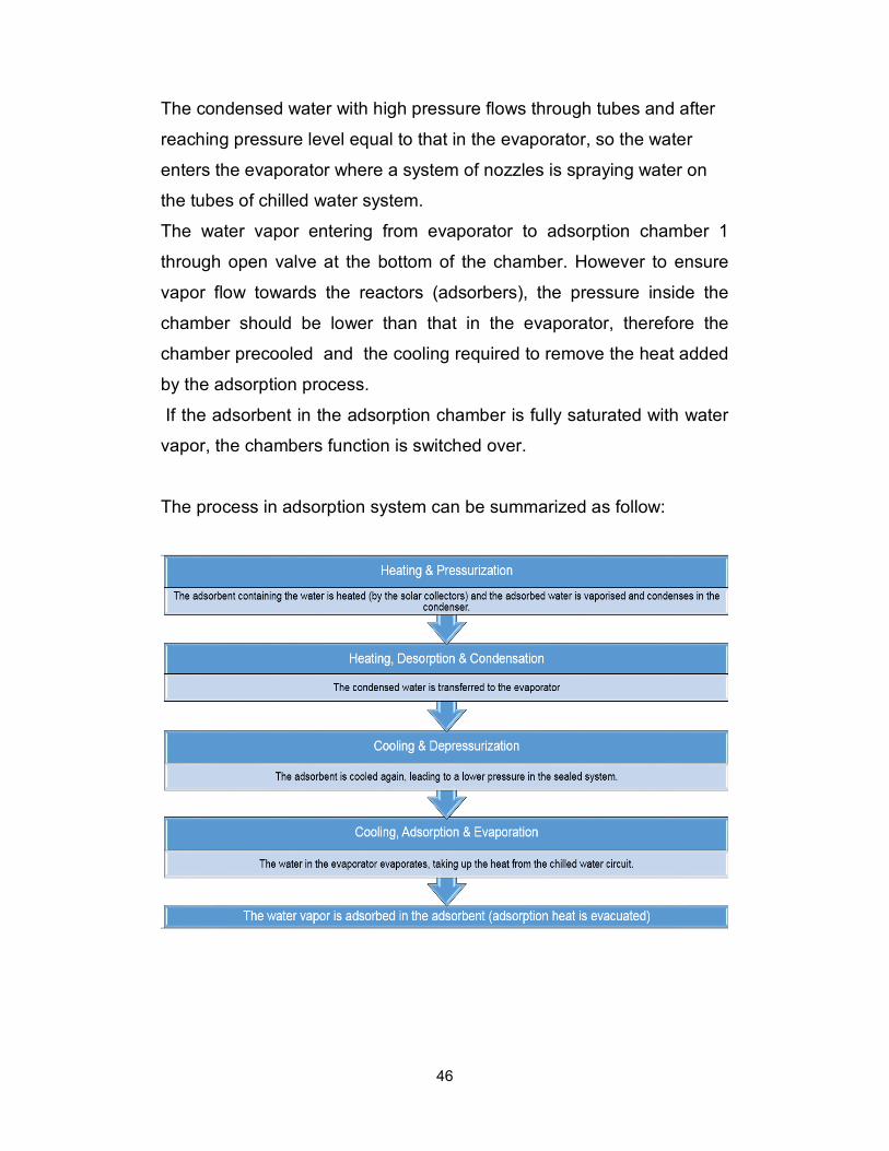
46
The condensed water with high pressure flows through tubes and after
reaching pressure level equal to that in the evaporator, so the water
enters the evaporator where a system of nozzles is spraying water on
the tubes of chilled water system.
The water vapor entering from evaporator to adsorption chamber 1
through open valve at the bottom of the chamber. However to ensure
vapor flow towards the reactors (adsorbers), the pressure inside the
chamber should be lower than that in the evaporator, therefore the
chamber precooled and the cooling required to remove the heat added
by the adsorption process.
If the adsorbent in the adsorption chamber is fully saturated with water
vapor, the chambers function is switched over.
The process in adsorption system can be summarized as follow:
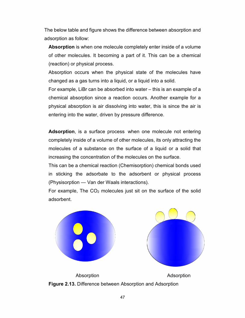
47
The below table and figure shows the difference between absorption and
adsorption as follow:
Absorption is when one molecule completely enter inside of a volume
of other molecules. It becoming a part of it. This can be a chemical
(reaction) or physical process.
Absorption occurs when the physical state of the molecules have
changed as a gas turns into a liquid, or a liquid into a solid.
For example, LiBr can be absorbed into water – this is an example of a
chemical absorption since a reaction occurs. Another example for a
physical absorption is air dissolving into water, this is since the air is
entering into the water, driven by pressure difference.
Adsorption, is a surface process when one molecule not entering
completely inside of a volume of other molecules, its only attracting the
molecules of a substance on the surface of a liquid or a solid that
increasing the concentration of the molecules on the surface.
This can be a chemical reaction (Chemisorption) chemical bonds used
in sticking the adsorbate to the adsorbent or physical process
(Physisorption — Van der Waals interactions).
For example, The CO2 molecules just sit on the surface of the solid
adsorbent.
Absorption Adsorption
Figure 2.13. Difference between Absorption and Adsorption
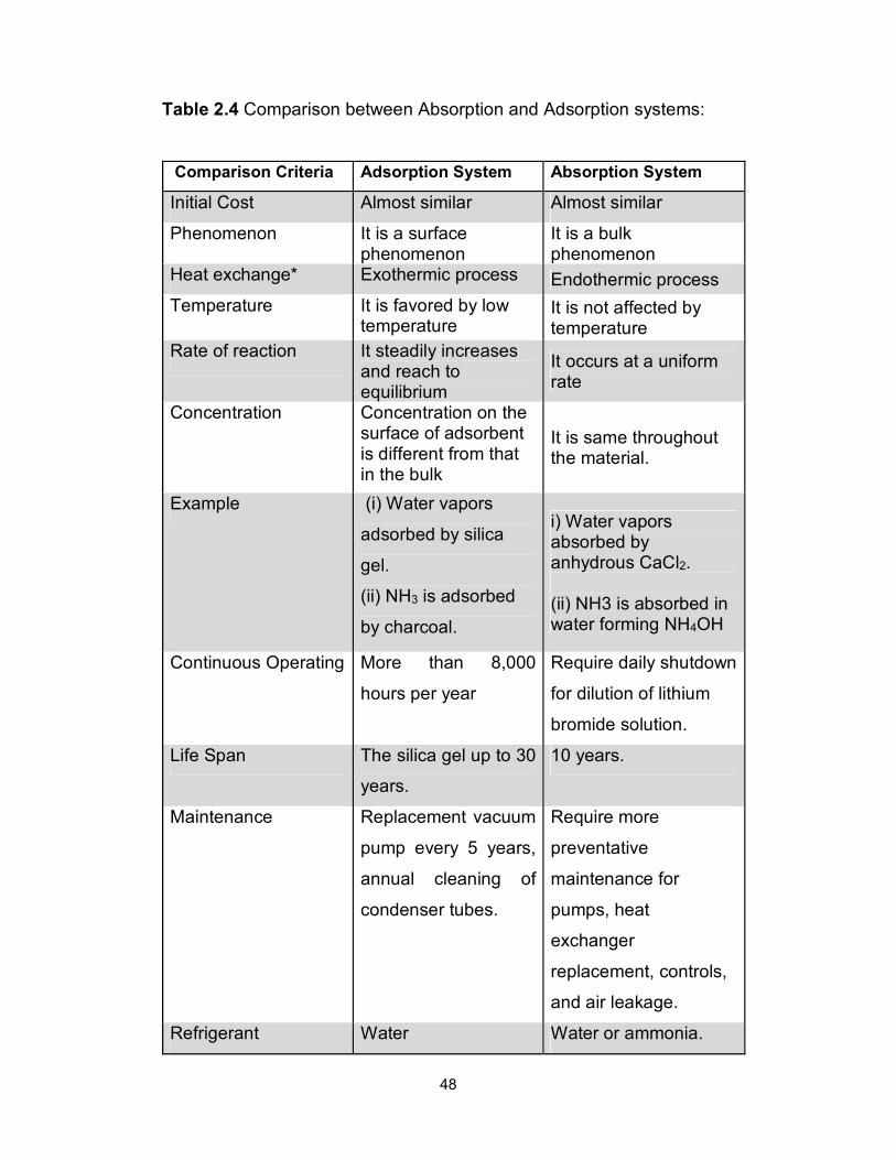
48
Table 2.4 Comparison between Absorption and Adsorption systems:
Comparison Criteria Adsorption System Absorption System
Initial Cost Almost similar Almost similar
Phenomenon It is a surface phenomenon
It is a bulk phenomenon
Heat exchange* Exothermic process Endothermic process
Temperature It is favored by low temperature
It is not affected by temperature
Rate of reaction It steadily increases and reach to equilibrium
It occurs at a uniform rate
Concentration Concentration on the surface of adsorbent is different from that in the bulk
It is same throughout the material.
Example (i) Water vapors
adsorbed by silica
gel.
(ii) NH3 is adsorbed
by charcoal.
i) Water vapors absorbed by anhydrous CaCl2. (ii) NH3 is absorbed in water forming NH4OH
Continuous Operating More than 8,000
hours per year
Require daily shutdown
for dilution of lithium
bromide solution.
Life Span The silica gel up to 30
years.
10 years.
Maintenance Replacement vacuum
pump every 5 years,
annual cleaning of
condenser tubes.
Require more
preventative
maintenance for
pumps, heat
exchanger
replacement, controls,
and air leakage.
Refrigerant Water Water or ammonia.
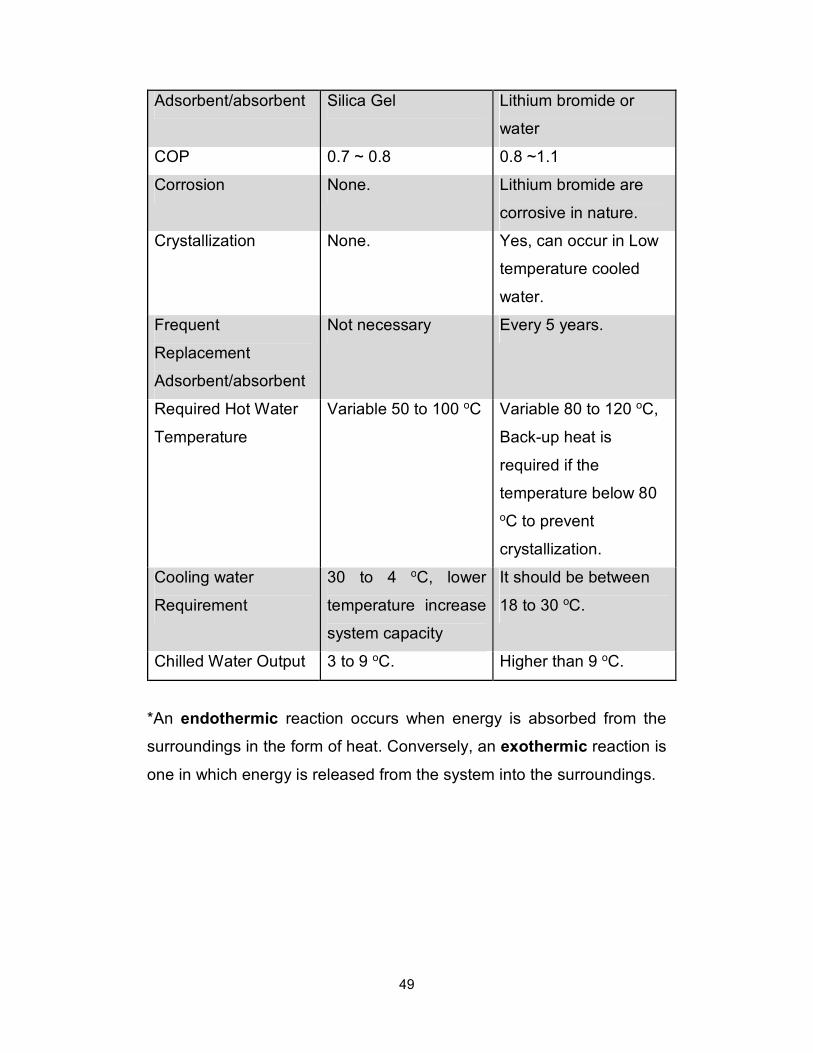
49
Adsorbent/absorbent Silica Gel Lithium bromide or
water
COP 0.7 ~ 0.8 0.8 ~1.1
Corrosion None. Lithium bromide are
corrosive in nature.
Crystallization None. Yes, can occur in Low
temperature cooled
water.
Frequent
Replacement
Adsorbent/absorbent
Not necessary Every 5 years.
Required Hot Water
Temperature
Variable 50 to 100 oC Variable 80 to 120 oC,
Back-up heat is
required if the
temperature below 80
oC to prevent
crystallization.
Cooling water
Requirement
30 to 4 oC, lower
temperature increase
system capacity
It should be between
18 to 30 oC.
Chilled Water Output 3 to 9 oC. Higher than 9 oC.
*An endothermic reaction occurs when energy is absorbed from the
surroundings in the form of heat. Conversely, an exothermic reaction is
one in which energy is released from the system into the surroundings.
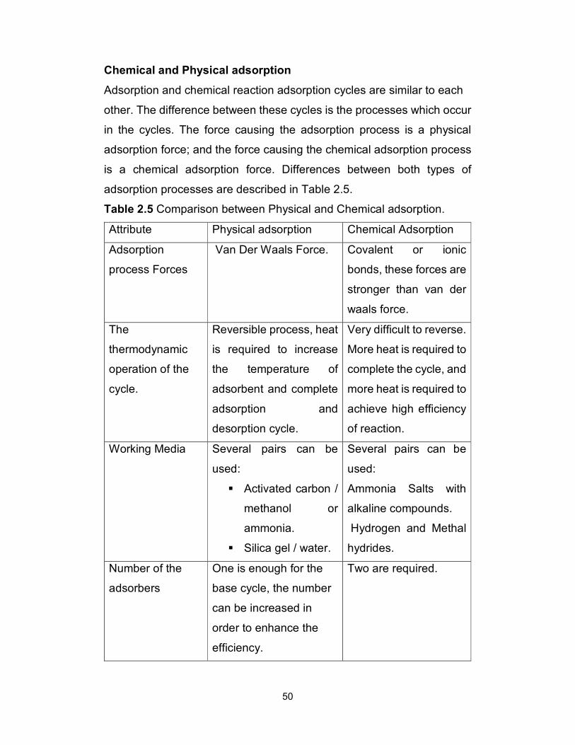
50
Chemical and Physical adsorption
Adsorption and chemical reaction adsorption cycles are similar to each
other. The difference between these cycles is the processes which occur
in the cycles. The force causing the adsorption process is a physical
adsorption force; and the force causing the chemical adsorption process
is a chemical adsorption force. Differences between both types of
adsorption processes are described in Table 2.5.
Table 2.5 Comparison between Physical and Chemical adsorption.
Attribute Physical adsorption Chemical Adsorption
Adsorption
process Forces
Van Der Waals Force. Covalent or ionic
bonds, these forces are
stronger than van der
waals force.
The
thermodynamic
operation of the
cycle.
Reversible process, heat
is required to increase
the temperature of
adsorbent and complete
adsorption and
desorption cycle.
Very difficult to reverse.
More heat is required to
complete the cycle, and
more heat is required to
achieve high efficiency
of reaction.
Working Media Several pairs can be
used:
� Activated carbon /
methanol or
ammonia.
� Silica gel / water.
Several pairs can be
used:
Ammonia Salts with
alkaline compounds.
Hydrogen and Methal
hydrides.
Number of the
adsorbers
One is enough for the
base cycle, the number
can be increased in
order to enhance the
efficiency.
Two are required.
51
No moving parts and low evaporation temperatures during operation is
the main advantages of chemical reaction cooling system. While as low
COP, high weight of adsorbent makes it not sufficient for large
application.
System design complexity due to adsorber volume change through
chemical reaction and difficulty to achieve system tightness during
operation at low pressure and temperature, all the above demerits limiting
its use.
Lemmini [104] investigated the performance of adsorptive solar assisted
cooling system and compare it with normal solid adsorption system. The
comparison proved that the performance of solar powered system highly
depends on the absorptivity of the solar collector and the insulation on
the back side of the solar collector.
Pons and Guilleminot [105] carried out a study on solar assisted solid
adsorption ice maker. The result revealed clearly the system COP is 0.12
which makes this machine one of the highest efficient solar ice makers.
Wang et. al. [106] investigated a solar assisted adsorption system with
activated carbon and water with solar collector ( area 2 m2), the result
showed that the system are able to produce daily 10 Kg of ice with 90°C
hot water ( around 60 kg).
Energy Storage in Solar Cooling System:
Schweigler et al. [107] modeled solar assisted absorption system with
phase change material (PCM) for latent heat storage in order to
guarantee a low operating temperature of the system. In the study, the
latent heat storage was based Calcium Chloride Hexahydrate, whose
melting temperature starting from 27°C up to 29°C. Standard lithium
bromide and water absorption system cannot provide cold chilled water
at 6°C/12°C with LiBr/Water system but in this system the condenser and
absorber were air cooled combined with PCM latent storage, so the
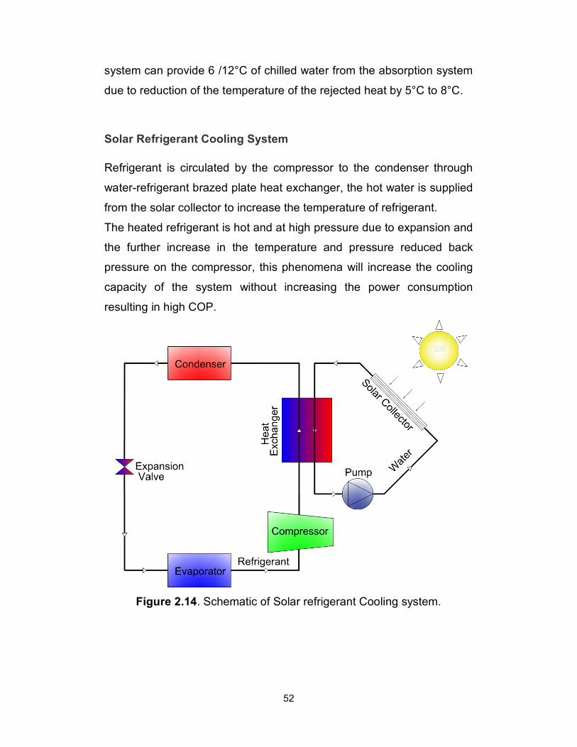
52
system can provide 6 /12°C of chilled water from the absorption system
due to reduction of the temperature of the rejected heat by 5°C to 8°C.
Solar Refrigerant Cooling System
Refrigerant is circulated by the compressor to the condenser through
water-refrigerant brazed plate heat exchanger, the hot water is supplied
from the solar collector to increase the temperature of refrigerant.
The heated refrigerant is hot and at high pressure due to expansion and
the further increase in the temperature and pressure reduced back
pressure on the compressor, this phenomena will increase the cooling
capacity of the system without increasing the power consumption
resulting in high COP.
Figure 2.14. Schematic of Solar refrigerant Cooling system.
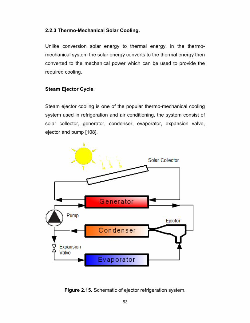
53
2.2.3 Thermo-Mechanical Solar Cooling.
Unlike conversion solar energy to thermal energy, in the thermo-
mechanical system the solar energy converts to the thermal energy then
converted to the mechanical power which can be used to provide the
required cooling.
Steam Ejector Cycle.
Steam ejector cooling is one of the popular thermo-mechanical cooling
system used in refrigeration and air conditioning, the system consist of
solar collector, generator, condenser, evaporator, expansion valve,
ejector and pump [108].
Figure 2.15. Schematic of ejector refrigeration system.
54
The working and operation principle of ejector cooling system are
described in Figure 17. The saturated vapor primary fluid (can be water
or other refrigerant) enters the nozzle of the ejector at high pressure and
temperature supplied from boiler or generator.
This primary fluid expand and leaves the nozzle at a very high velocity
and a low pressure which draws working fluid vapor (secondary fluid)
from the evaporator and maintains the vacuum necessary for operation.
When the mixing of the two streams is completed, the pressure increased
in the diverging section and the mixture slow down, the ejector will be
able to discharge the mixture of primary and secondary fluid at a pressure
that is higher than the entering pressure. So, the ejector is boosting the
pressure of the primary entering fluid.
A low energy grade energy source that can be used for this system and
low cost of operation and construction are the main advantages of steam
ejector solar cooling system, while as high initial cost, low COP,
complicated design of the ejector and the difficulty to operate in a wide
range of ambient temperatures are the challenges in this system.
Wang et. al. [109, 110] performed a study of ejector cooling system
consist of multi-function generator that provides the required hot water for
ejector cycle operation and can work as heat pump. In this study R141b
considered as working refrigerant and the ejector design modified to work
with other refrigerant like R365mfc to enhance COP of the system and
R141b phased out, and R365mfc ODP was close to zero. The ejector
cooling system with multifunction generator operating at full-cycle using
R141b and the cooling capacity of 0.75 kW, ejector area ratio of 7.73 at
90 oC generator temperature, condenser temperature 37 oC and
evaporator temperature 8.5 oC. Operating coefficient of performance can
reach 0.225 at full cycle while using R141b therefore it conclude that
55
R365mfc can replace R141b without affecting the system overall
efficiency and performance as long as the design of ejector optimized.
Pollerberg [111] investigated solar assisted steam ejector chiller for
whole year in Bochum, Germany. The system includes experimental step
with cooling capacity 1 kW and two types of collector a parabolic trough
(PTC) and a vacuum tube collector (VTC). The effect of the operating
temperatures and pressures on the efficiency of the solar collectors and
the COP of the system are studied. Then, the annual mean efficiency of
the solar collector, the annual mean COP of the solar ejector cooling
system are determined by using simulation tools as well the annual mean
total efficiency of the system for different locations worldwide are
investigated. The direct horizontal solar radiation reached maximum
value of 550-600 W/m2, absorber area of 10.5 m2, COP of the system
investigated based on condenser temperature ranging from 15-35 oC and
evaporator temperature of 7, 13 and 17 oC, with decreasing condenser
temperature and increasing evaporator temperature COP of the system
rises.
The simulation result showed that the PTC are more suitable for large
application and collector fields and the ratio of direct insolation to global
insolation for a particular zone had influenced on the economy aspect of
the system.
Many researchers carried out experimental study [112-122] to investigate
the performance of steam ejector refrigeration system with different
working fluids and characteristic. A numerical study [123,124] also
performed to find the optimum design condition of steam ejector
refrigeration system. Good results were obtained from these numerical
study such as better pressure recovery for small diffuser angle, the weight
fraction recovery was higher for low angle and smaller droplet size yield
to better diffuser performance.
56
Selvaraju et. al. [125] investigated the performance of vapor ejector
refrigeration system when the ejector operates at choking-mode. When
operating conditions are changed, the critical performance parameters of
the system get shifted to different critical values. The effect of factors
studied in this paper were a specific heat of the working fluid and friction
at the constant-area mixing chamber and internal irreversibility of the
ejector to validate the model, the effect of compression ratio, driving
pressure ratio on the critical entrainment ratio and critical COP of the
ejector system are studied. The result from simulation compared with the
experimental data from the literature, the effects of operational
parameters and ejector configurations of the system are studied and find
out the effect in the performance. The results showed decreasing the
entrainment ration and COP due to increase compression ration while as
entrainment ration and COP increases with rising driving pressure. Also,
comparison of performance of the system with environment friendly
refrigerants, R134a, R152a, R290, R600a and R717 is made. Among
working fluid considered, the system with R134a gives better
performance.
Solar Combined Power/Cooling Systems:
The solar energy can be converted to thermal energy that drive power
generation device therefore the produced power can be used to run
refrigeration cycle which provides the required cooling and refrigeration
effect.
Goswami and Lu [126] made first law efficiency analysis of the combined
power and refrigeration cycles, the system includes the solar collector
can supply hot water at 90°C temperature. The results showed that
thermodynamic efficiency (first law) reached maximum 15.7% and
minimum 10.5% based on the ambient temperature variation from 7°C-
27°C.
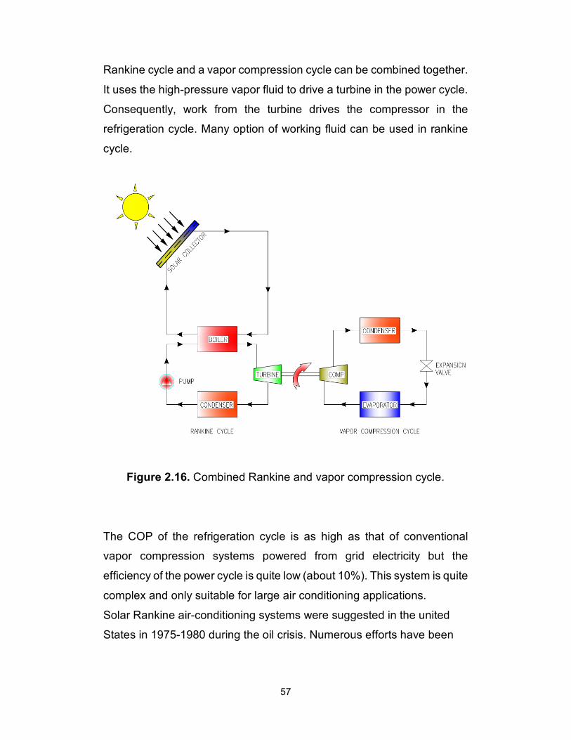
57
Rankine cycle and a vapor compression cycle can be combined together.
It uses the high-pressure vapor fluid to drive a turbine in the power cycle.
Consequently, work from the turbine drives the compressor in the
refrigeration cycle. Many option of working fluid can be used in rankine
cycle.
Figure 2.16. Combined Rankine and vapor compression cycle.
The COP of the refrigeration cycle is as high as that of conventional
vapor compression systems powered from grid electricity but the
efficiency of the power cycle is quite low (about 10%). This system is quite
complex and only suitable for large air conditioning applications.
Solar Rankine air-conditioning systems were suggested in the united
States in 1975-1980 during the oil crisis. Numerous efforts have been
58
made to develop similar solar cooling systems. The systems were not
economically competitive compared with conventional systems.
Wali, [127] suggested that only halocarbon compounds and the
fluorinated compounds fulfilled safety requirements. Subsequently, the
working media which were previously recommended, were found not to
be environmentally benign. Thus, the development of this system was
detained until interest returned in the 21st century with new proposed
cycles combining power and cooling cycles.
Kane, Larrain et al.,[128] proposed an Organic Rankine Cycle (ORC)
including a hermetic scroll expander-generator and solar tracking
equipment.
The advantages of Combined Rankine and vapor compression cycle are
suitable for high capacity systems and suitable for integration into poly
generation systems (heat, electricity and refrigeration).
High installation cost, large system and Regular maintenance required
due to complications and many moving parts reduce the demand of this
system.
Triple-Effect Refrigeration Cycle
Agrawal et. al.[129], investigated the triple effect refrigeration cycle with
a cascaded vapor compression cycle (N2O natural refrigerant),
absorption cycle (LiBr/Water system) with an ejector refrigeration cycle.
The main disadvantage of N2O is its higher GWP compared to other
refrigerant, however it is significantly more favorable in terms of toxicity.
The results showed that some influenced factors as waste flue gas
temperature, ejector evaporator temperature, turbine inlet and outlet
pressure and discharge pressure of the compressor are having
significant effects on the refrigeration outputs of proposed cycles in term
of exergy efficiency and thermal efficiency.
Fan et al. [130], investigated of a solar assisted ejector-absorption
technologies and shows the other feature that these cycle can be used
59
for, not only to provide the required cooling and refrigeration effect but
can be used for environmental protection.
Abdul Khaliq et al. [131], performed energy and exergy analyses of a
triple effect solar assisted refrigeration system. The results clearly
revealed that thermodynamic investigations based on energy analysis is
not enough and the exergy analysis must be considered to find out the
imperfection component and work it out to enhance the system overall
performance.
Rajesh Kumar et. al. [132], performed the thermodynamic analysis of a
solar assisted multi-effect refrigeration cycles. The result showed that
highest irreversibility occurs in the central receiver and the heliostat field
represents the second highest irreversibility. Furthermore, the first law
efficiency is 11.5% while as second law efficiency is 2%, these results
are another proof that the first law analysis is not accurate alone and
hence, more accurate analysis shall be considered the second law
analysis.
2.3 Solar Cooling Technologies Comparison based on driving
temperature:
The solar thermal cooling technologies performance change based on
the hot water temperature.
The Thermal-Driven system consists of three kinds of solar system types
including flat plate collector, delivering output temperature of around 70
oC to 100 oC, evacuated tube collector, delivering temperature in the
range of 100 oC to 150 oC, and Concentrating Solar Collector, delivering
temperature of over 150 oC. The heat generated by the panels will be
transmitted into the heat transformation cycle and produce two ranges of
temperature, 8 oC fits for air conditioning system and 0 oC to 8 oC which
is applicable for food and vaccine preservation as shown in figure 2.17.
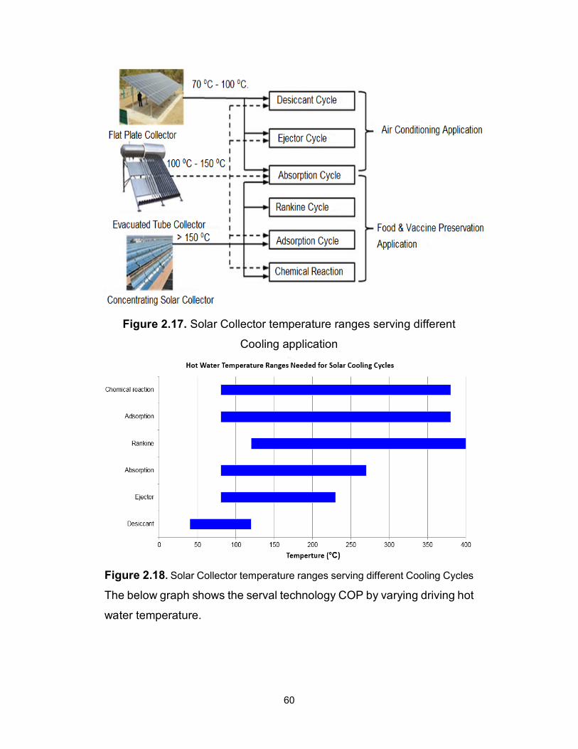
60
Figure 2.17. Solar Collector temperature ranges serving different
Cooling application
Figure 2.18. Solar Collector temperature ranges serving different Cooling Cycles
The below graph shows the serval technology COP by varying driving hot
water temperature.
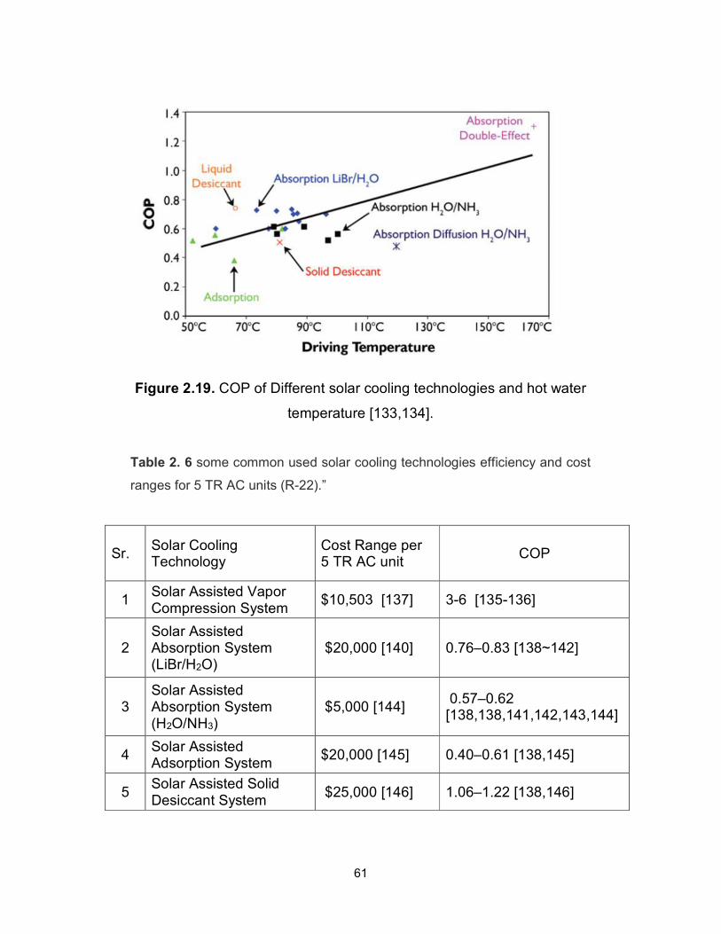
61
Figure 2.19. COP of Different solar cooling technologies and hot water
temperature [133,134].
Table 2. 6 some common used solar cooling technologies efficiency and cost
ranges for 5 TR AC units (R-22).”
Sr. Solar Cooling Technology
Cost Range per 5 TR AC unit
COP
1 Solar Assisted Vapor Compression System
$10,503 [137] 3-6 [135-136]
2 Solar Assisted Absorption System (LiBr/H2O)
$20,000 [140] 0.76–0.83 [138~142]
3 Solar Assisted Absorption System (H2O/NH3)
$5,000 [144] 0.57–0.62 [138,138,141,142,143,144]
4 Solar Assisted Adsorption System
$20,000 [145] 0.40–0.61 [138,145]
5 Solar Assisted Solid Desiccant System
$25,000 [146] 1.06–1.22 [138,146]
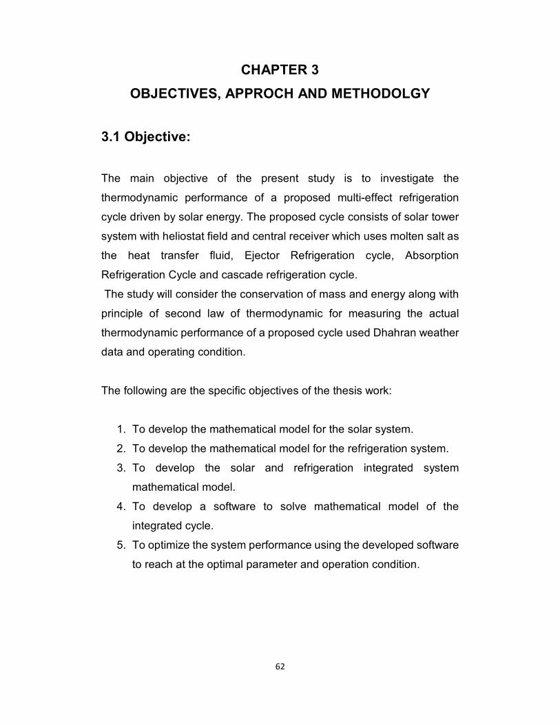
62
CHAPTER 3
OBJECTIVES, APPROCH AND METHODOLGY
3.1 Objective:
The main objective of the present study is to investigate the
thermodynamic performance of a proposed multi-effect refrigeration
cycle driven by solar energy. The proposed cycle consists of solar tower
system with heliostat field and central receiver which uses molten salt as
the heat transfer fluid, Ejector Refrigeration cycle, Absorption
Refrigeration Cycle and cascade refrigeration cycle.
The study will consider the conservation of mass and energy along with
principle of second law of thermodynamic for measuring the actual
thermodynamic performance of a proposed cycle used Dhahran weather
data and operating condition.
The following are the specific objectives of the thesis work:
1. To develop the mathematical model for the solar system.
2. To develop the mathematical model for the refrigeration system.
3. To develop the solar and refrigeration integrated system
mathematical model.
4. To develop a software to solve mathematical model of the
integrated cycle.
5. To optimize the system performance using the developed software
to reach at the optimal parameter and operation condition.

63
3.2 Approch:
The Mathematical model is developed for each component of the
proposed cycle.
To solve aforementioned mathematical model, the engineering equation
solver software (EES) was used to develop a software which will be to
assess different integrating models and cycles. The validation of these
models had been conducted against experimental data previously
published in the public literature and journal papers.
The parametric analysis conducted to reach optimal condition.

64
3.3 Problem Statement :
Investigation of the thermodynamic performance of a proposed multi-
effect refrigeration cycle had been conducted to point out the effect of
some influenced parameter on the overall efficiency of the solar assisted
triple effect refrigeration cycle.
The incident solar radiation is hourly and seasonally fluctuating, and as a
result the outlet energy from a solar field will also change over time. If
there is a need for a stable power outlet from solar thermal power, many
strategies may be used. Integrating a triple effect refrigeration cycle with
the solar system to provide a compensation effect is one of these
strategies.

65
3.4 Methodology:
A thermodynamic analysis is to be conducted to point out the effect of
some influenced parameters on the overall efficiency of the solar assisted
triple effect refrigeration system.
The analysis will be conducted by using EES software.
The following methodology will be followed to achieve the objective
aforementioned:
1. A complete mathematical model will be developed for each
individual component of the system based on first and second law
of thermodynamics.
2. Heat transfer model for different components will be developed
when needed.
3. A software code will be developed and used to solve the
developing mathematical model using the engineering equation
solver (EES)
4. The code will be validated against experimental data available in
the literature.
5. Detailed parametric analysis will be performed to reach the optimal
operation condition.
68
66
CHAPTER 4
TRIPLE EFECT REFRIGERATION SYSTEM MODELING
4.1 Description of the Triple-effect Refrigeration Cycle:
Solar Assisted triple effect refrigeration cycle consists of Solar Tower with
central receiver connected Steam Rankine Cycle (SRC) providing
thermal energy to (ERC) and (ARC), and (CRC) with only solar heat
source. Figure 4.1 shows the simplified SRC, ERC, ARC, and CRC cycle.
Solar radiation reflected from the mirror of heliostat field to the aperture
area of central receiver (CR) at the top of solar tower where molten salt
(a mixture of 60 wt% of sodium nitrate [NaNo3] and 40 wt% potassium
nitrate [KNo3]) used to absorb the solar energy.
The key advantage in using molten salt is that it is of a cheaper solution,
good thermal storage and can work effectively for 24 hour operation.
The molten salt is absorbing the thermal energy at central receiver so the
temperature of molten salt is increased up to 560 oC, then the molten salt
will pass through the heat recovery vapor generator (HRVG) (1–2), the
thermal energy transfer to ejector refrigeration cycle due to heat transfer
in HRVG between hot molten salt in the Rankine cycle and water
refrigeration in the ejector cycle.
The temperature of molten salt decreased to approximately 315 oC then
it is flowing to generator (2–12) to provide the required heat energy to
separate LiBr and water.
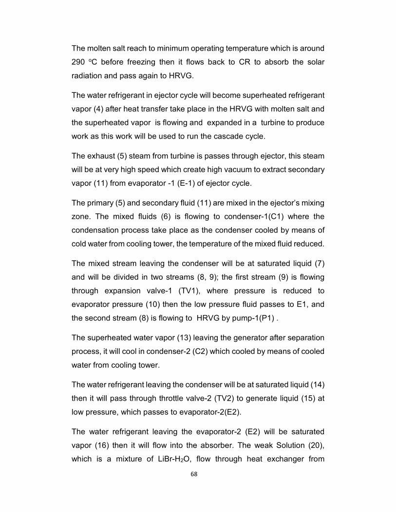
69
68
The molten salt reach to minimum operating temperature which is around
290 oC before freezing then it flows back to CR to absorb the solar
radiation and pass again to HRVG.
The water refrigerant in ejector cycle will become superheated refrigerant
vapor (4) after heat transfer take place in the HRVG with molten salt and
the superheated vapor is flowing and expanded in a turbine to produce
work as this work will be used to run the cascade cycle.
The exhaust (5) steam from turbine is passes through ejector, this steam
will be at very high speed which create high vacuum to extract secondary
vapor (11) from evaporator -1 (E-1) of ejector cycle.
The primary (5) and secondary fluid (11) are mixed in the ejector’s mixing
zone. The mixed fluids (6) is flowing to condenser-1(C1) where the
condensation process take place as the condenser cooled by means of
cold water from cooling tower, the temperature of the mixed fluid reduced.
The mixed stream leaving the condenser will be at saturated liquid (7)
and will be divided in two streams (8, 9); the first stream (9) is flowing
through expansion valve-1 (TV1), where pressure is reduced to
evaporator pressure (10) then the low pressure fluid passes to E1, and
the second stream (8) is flowing to HRVG by pump-1(P1) .
The superheated water vapor (13) leaving the generator after separation
process, it will cool in condenser-2 (C2) which cooled by means of cooled
water from cooling tower.
The water refrigerant leaving the condenser will be at saturated liquid (14)
then it will pass through throttle valve-2 (TV2) to generate liquid (15) at
low pressure, which passes to evaporator-2(E2).
The water refrigerant leaving the evaporator-2 (E2) will be saturated
vapor (16) then it will flow into the absorber. The weak Solution (20),
which is a mixture of LiBr-H2O, flow through heat exchanger from
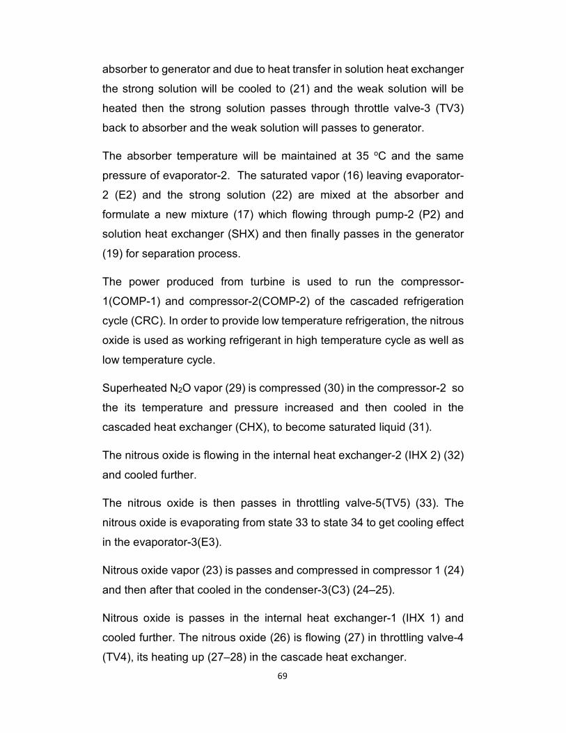
70
69
absorber to generator and due to heat transfer in solution heat exchanger
the strong solution will be cooled to (21) and the weak solution will be
heated then the strong solution passes through throttle valve-3 (TV3)
back to absorber and the weak solution will passes to generator.
The absorber temperature will be maintained at 35 oC and the same
pressure of evaporator-2. The saturated vapor (16) leaving evaporator-
2 (E2) and the strong solution (22) are mixed at the absorber and
formulate a new mixture (17) which flowing through pump-2 (P2) and
solution heat exchanger (SHX) and then finally passes in the generator
(19) for separation process.
The power produced from turbine is used to run the compressor-
1(COMP-1) and compressor-2(COMP-2) of the cascaded refrigeration
cycle (CRC). In order to provide low temperature refrigeration, the nitrous
oxide is used as working refrigerant in high temperature cycle as well as
low temperature cycle.
Superheated N2O vapor (29) is compressed (30) in the compressor-2 so
the its temperature and pressure increased and then cooled in the
cascaded heat exchanger (CHX), to become saturated liquid (31).
The nitrous oxide is flowing in the internal heat exchanger-2 (IHX 2) (32)
and cooled further.
The nitrous oxide is then passes in throttling valve-5(TV5) (33). The
nitrous oxide is evaporating from state 33 to state 34 to get cooling effect
in the evaporator-3(E3).
Nitrous oxide vapor (23) is passes and compressed in compressor 1 (24)
and then after that cooled in the condenser-3(C3) (24–25).
Nitrous oxide is passes in the internal heat exchanger-1 (IHX 1) and
cooled further. The nitrous oxide (26) is flowing (27) in throttling valve-4
(TV4), its heating up (27–28) in the cascade heat exchanger.

71
70
In the current project, a multi-mode thermodynamic cycle is presented for
solar power cooling which could produce refrigeration output at various
magnitudes at different level of temperature simultaneously.
The cycle can meet out the cooling demand for air conditioning (15oC –
22oC), refrigeration for food preservation (2 oC – 8 oC), deep freezing for
vaccine preservation and pharmaceutical plants (-50 oC to -80 oC).
This cycle employ solar tower technology which will use molten salt as a
heat transfer fluid (HTF) and integrates the heliostat field and central
receiver with the Steam Rankine Cycle (SRC), ERC, ARC, and CRC.
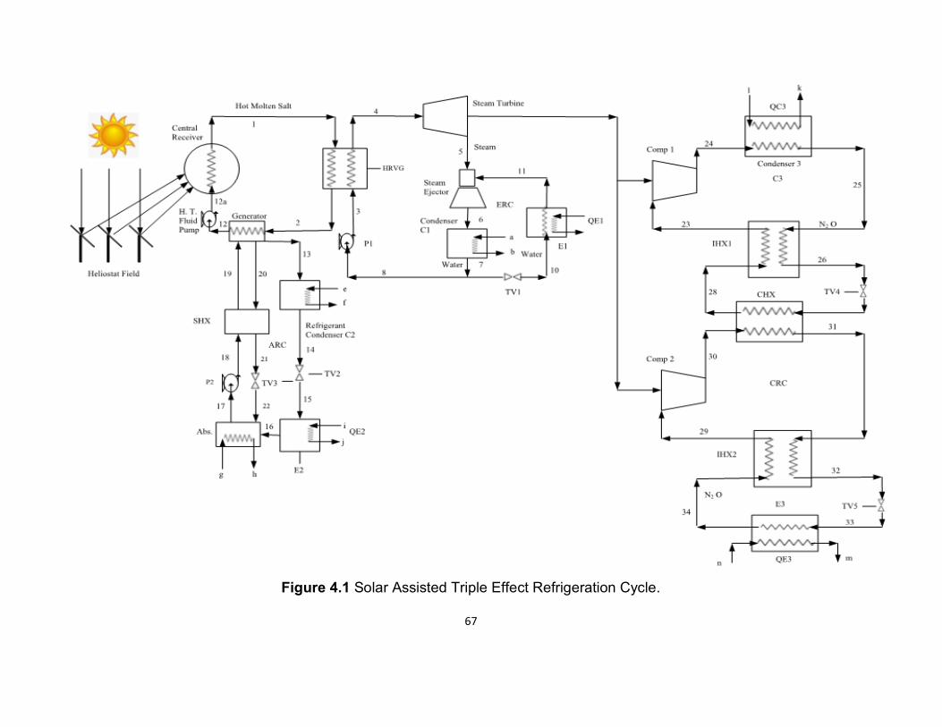
67
Figure 4.1 Solar Assisted Triple Effect Refrigeration Cycle.

71
4.2 Main assumption of the triple-effect refrigeration cycle:
Main assumptions have been as follow of the novel cycle.
(1) All components of the triple effect refrigeration cycle considered in
steady state.
(2) The pipes pressure drop in in the proposed triple effect refrigeration
cycle are neglected.
(3) The heat losses to the surrounding in the Heat recovery generator,
steam turbine, all condensers and all evaporators are neglected.
(4) The flow through the expansion valves are isenthalpic.
(5) The condenser leaving state considered as saturated liquid.
(6) The evaporator leaving state considered as saturated vapor.
(7) Solar heat source physical exergies are used only (chemical exergy
for solar heat source is negligible).
(8) Chemical exergies, Kinetic and potential of the material are not
taken into account in the analysis..
(9) We considered the solution of LiBr are in equilibrium in the generator
and absorber are in at standard temperature and pressure conditions.
(10) saturated condition of the solution leaving the absorber and the
generator.
(11) The compression process is considered to be adiabatic
(12) Isobaric considered in evaporator, condenser and internal/cascade
heat exchanger.
(13) one dimensional and steady state flow in the ejector .
(14) The ejector walls are well insulated.
(15) Saturated condition of the primary and secondary flow when
entering the ejector (states 5 and 11).
(16) All flow losses are taken into account by using isentropic
efficiencies in the nozzle (ηn), in the diffuser (ηd), as well as in the
mixing chamber (ηm).
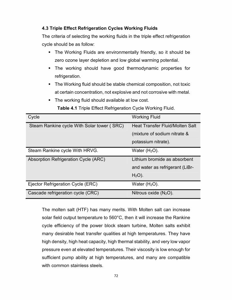
72
4.3 Triple Effect Refrigeration Cycles Working Fluids
The criteria of selecting the working fluids in the triple effect refrigeration
cycle should be as follow:
� The Working Fluids are environmentally friendly, so it should be
zero ozone layer depletion and low global warming potential.
� The working should have good thermodynamic properties for
refrigeration.
� The Working fluid should be stable chemical composition, not toxic
at certain concentration, not explosive and not corrosive with metal.
� The working fluid should available at low cost.
Table 4.1 Triple Effect Refrigeration Cycle Working Fluid.
Cycle Working Fluid
Steam Rankine cycle With Solar tower ( SRC) Heat Transfer Fluid/Molten Salt
(mixture of sodium nitrate &
potassium nitrate).
Steam Rankine cycle With HRVG. O).2Water (H
Absorption Refrigeration Cycle (ARC) Lithium bromide as absorbent
-refrigerant (LiBrand water as
O).2H
Ejector Refrigeration Cycle (ERC) O).2Water (H
Cascade refrigeration cycle (CRC) O).2Nitrous oxide (N
The molten salt (HTF) has many merits. With Molten salt can increase
solar field output temperature to 560°C, then it will increase the Rankine
cycle efficiency of the power block steam turbine, Molten salts exhibit
many desirable heat transfer qualities at high temperatures. They have
high density, high heat capacity, high thermal stability, and very low vapor
pressure even at elevated temperatures. Their viscosity is low enough for
sufficient pump ability at high temperatures, and many are compatible
with common stainless steels.
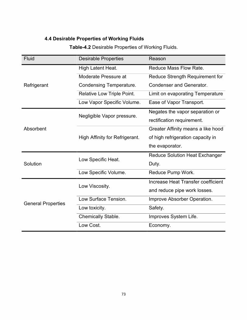
73
4.4 Desirable Properties of Working Fluids
Table-4.2 Desirable Properties of Working Fluids.
Fluid Desirable Properties Reason
Refrigerant
High Latent Heat. Reduce Mass Flow Rate.
Moderate Pressure at
Condensing Temperature.
Reduce Strength Requirement for
Condenser and Generator.
Relative Low Triple Point. Limit on evaporating Temperature
Low Vapor Specific Volume. Ease of Vapor Transport.
Absorbent
Negligible Vapor pressure. Negates the vapor separation or
rectification requirement.
High Affinity for Refrigerant.
Greater Affinity means a like hood
of high refrigeration capacity in
the evaporator.
Solution Low Specific Heat.
Reduce Solution Heat Exchanger
Duty.
Low Specific Volume. Reduce Pump Work.
General Properties
Low Viscosity. Increase Heat Transfer coefficient
and reduce pipe work losses.
Low Surface Tension. Improve Absorber Operation.
Low toxicity. Safety.
Chemically Stable. Improves System Life.
Low Cost. Economy.
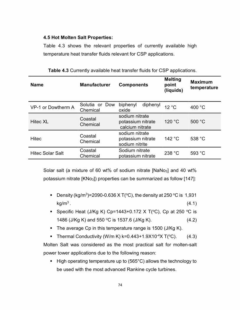
74
4.5 Hot Molten Salt Properties:
Table 4.3 shows the relevant properties of currently available high
temperature heat transfer fluids relevant for CSP applications.
Table 4.3 Currently available heat transfer fluids for CSP applications.
Name
Manufacturer
Components
Melting point (liquids)
Maximum temperature
VP-1 or Dowtherm A Solutia or Dow Chemical
biphenyl diphenyl oxide
12 °C 400 °C
Hitec XL Coastal Chemical
sodium nitrate potassium nitrate calcium nitrate
120 °C 500 °C
Hitec Coastal Chemical
sodium nitrate potassium nitrate sodium nitrite
142 °C 538 °C
Hitec Solar Salt Coastal Chemical
Sodium nitrate potassium nitrate
238 °C 593 °C
Solar salt (a mixture of 60 wt% of sodium nitrate [NaNo3] and 40 wt%
potassium nitrate [KNo3]) properties can be summarized as follow [147]:
� Density (kg/m3)=2090-0.636 X T(oC), the density at 250 oC is 1,931
kg/m3 . (4.1)
� Specific Heat (J/Kg K) Cp=1443+0.172 X T(oC), Cp at 250 oC is
1486 (J/Kg K) and 550 oC is 1537.6 (J/Kg K). (4.2)
� The average Cp in this temperature range is 1500 (J/Kg K).
� Thermal Conductivity (W/m K) k=0.443+1.9X10⁻⁴X T(oC). (4.3)
Molten Salt was considered as the most practical salt for molten-salt
power tower applications due to the following reason:
� High operating temperature up to (565°C) allows the technology to
be used with the most advanced Rankine cycle turbines.
75
� Lower cost of nitrate salts. However, while as main demerit with
Solar Salt is its high freezing point of 290°C compared to other
molten salt.
� Molten Salt can store thermal energy while it is in liquid state.
4.6 Triple-effect Refrigeration Cycle working fluid characteristic:
Water which has zero ODP and GWP will be used as working fluid in
Steam Rankine cycle (SRC), and as refrigerant in ejector refrigeration
cycle (ERC) and absorption refrigeration cycle (ARC), respectively, while
N2O which has zero ODP and moderate GWP will be used as a
refrigerant in the cascaded refrigeration cycle (CRC) to produce cooling
in the deep freezing range.
Nitrous oxide is selected as working fluid in cascade refrigeration cycle
as it has zero ozone depletion potential as well as moderate global
warming potential (GWP) in addition to that it is natural refrigerant and
can produce cooling in the range of - 60 to - 80oC which is necessary of
for some application like vaccine storage.
The main disadvantage of N2O its higher GWP compared to CO2,
however it is significantly more favorable in terms of toxicity.
The Lithium bromide and water (LiBr/H2O) solution is used as working
fluid in absorption refrigeration systems due to the following:
� It is non-volatile and non-toxic.
� Environmentally friendly.
� Low cost fluids.
� Easy handling are the advantages of using water as refrigerant
(despite its high freezing point).
While as the disadvantage of LiBr-H2O that

76
� Restricted to applications in cooling requirements are water
freezing point (0°C).
So LiBr chillers are mainly used for air-conditioning system rather than
refrigeration system. Another disadvantage is that crystallization will
occur if LiBr solution is of higher concentration and may damage the
machine.
Many control strategies are proposed to prevent crystallization.
Control the concentration of LiBr solution is one of the most important
strategy.
Increasing the chilled water temperature settings can avoid
crystallization, and the byproducts include improved cooling capacity
and COP.
77
CHAPTER 5
FIRST AND SECOND LAW OF
THERMODYNAMIC ANALYSIS OF THE
PROPOSED CYCLE
The thermodynamic analysis in term of energy, entropy, and exergy is
provided in this chapter. The heat input and rate of exergy can be found
by using mass, energy and exergy balances.
Applying exergy approach for solar assisted triple effect refrigeration
cycle can provide a better understanding for each component behavior
and enhanced tools for improving them.
Exergy analysis clearly indicates the location, nature and causes of
energy destruction in a process and therefore can help improve a process
or technology.
The primary objective of exergy balance is to provide meaningful
efficiency and the magnitude of exergy losses.
Exergy balance can quantify the quality of energy during heat transfer.
When exergy analysis is performed the thermodynamic imperfection can
be quantified as exergy destruction which represent losses in energy
quality or usefulness.
The exergy can be transported across the boundary of the system.
Important characteristic of exergy:
1. The rate of exergy in system will be raised with more relatively
deviation from surrounding.
2. Rate of Exergy in definition depends not only on the state of the
system or flow but also the state of the reference environment.
It is important to be aware of the difference between energy and exergy
in order to make the issue clear between exergy and traditional energy
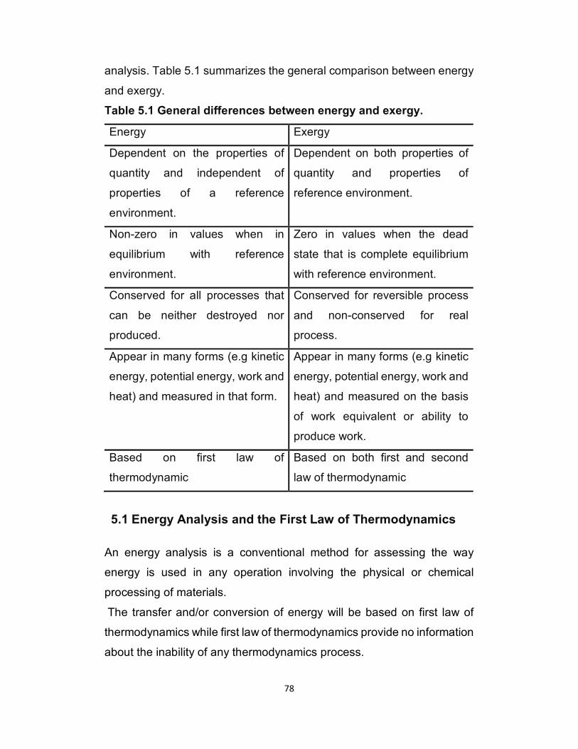
78
analysis. Table 5.1 summarizes the general comparison between energy
and exergy.
Table 5.1 General differences between energy and exergy.
Energy Exergy
Dependent on the properties of
quantity and independent of
properties of a reference
environment.
Dependent on both properties of
quantity and properties of
reference environment.
Non-zero in values when in
equilibrium with reference
environment.
Zero in values when the dead
state that is complete equilibrium
with reference environment.
Conserved for all processes that
can be neither destroyed nor
produced.
Conserved for reversible process
and non-conserved for real
process.
Appear in many forms (e.g kinetic
energy, potential energy, work and
heat) and measured in that form.
Appear in many forms (e.g kinetic
energy, potential energy, work and
heat) and measured on the basis
of work equivalent or ability to
produce work.
Based on first law of
thermodynamic
Based on both first and second
law of thermodynamic
5.1 Energy Analysis and the First Law of Thermodynamics
An energy analysis is a conventional method for assessing the way
energy is used in any operation involving the physical or chemical
processing of materials.
The transfer and/or conversion of energy will be based on first law of
thermodynamics while first law of thermodynamics provide no information
about the inability of any thermodynamics process.
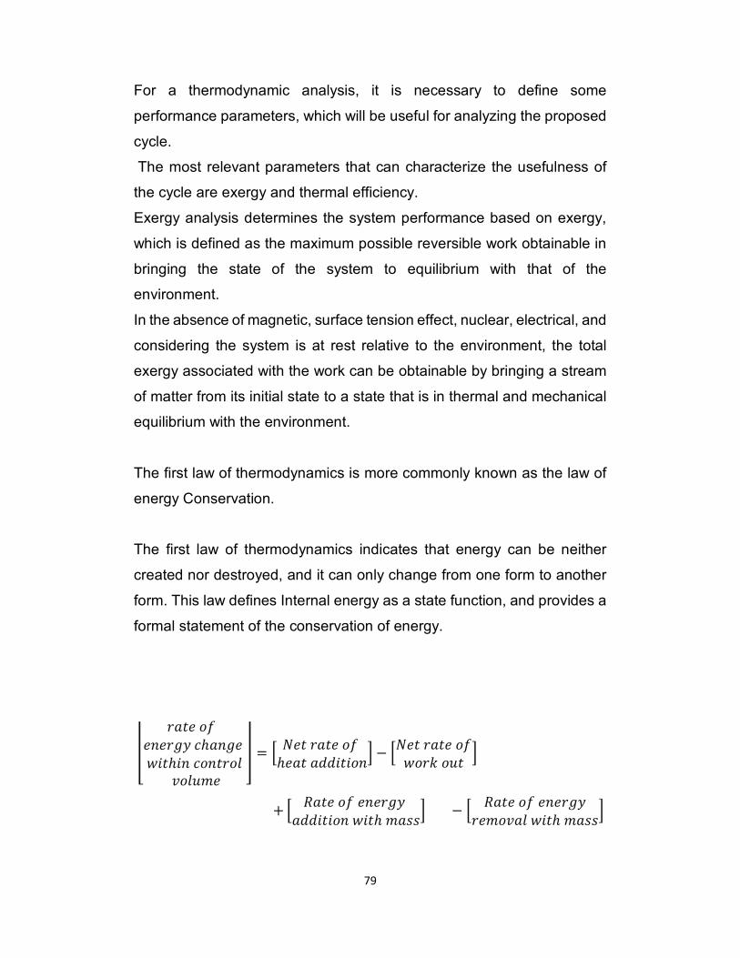
79
For a thermodynamic analysis, it is necessary to define some
performance parameters, which will be useful for analyzing the proposed
cycle.
The most relevant parameters that can characterize the usefulness of
the cycle are exergy and thermal efficiency.
Exergy analysis determines the system performance based on exergy,
which is defined as the maximum possible reversible work obtainable in
bringing the state of the system to equilibrium with that of the
environment.
In the absence of magnetic, surface tension effect, nuclear, electrical, and
considering the system is at rest relative to the environment, the total
exergy associated with the work can be obtainable by bringing a stream
of matter from its initial state to a state that is in thermal and mechanical
equilibrium with the environment.
The first law of thermodynamics is more commonly known as the law of
energy Conservation.
The first law of thermodynamics indicates that energy can be neither
created nor destroyed, and it can only change from one form to another
form. This law defines Internal energy as a state function, and provides a
formal statement of the conservation of energy.
� ���� �� ���� �ℎ�� ���ℎ� ������ ������ � = � ��� ���� �� ℎ��� �������� − ���� ���� ������ ��� � + � ���� �� ���� ������� ���ℎ ����� − � ���� �� ����������� ���ℎ �����
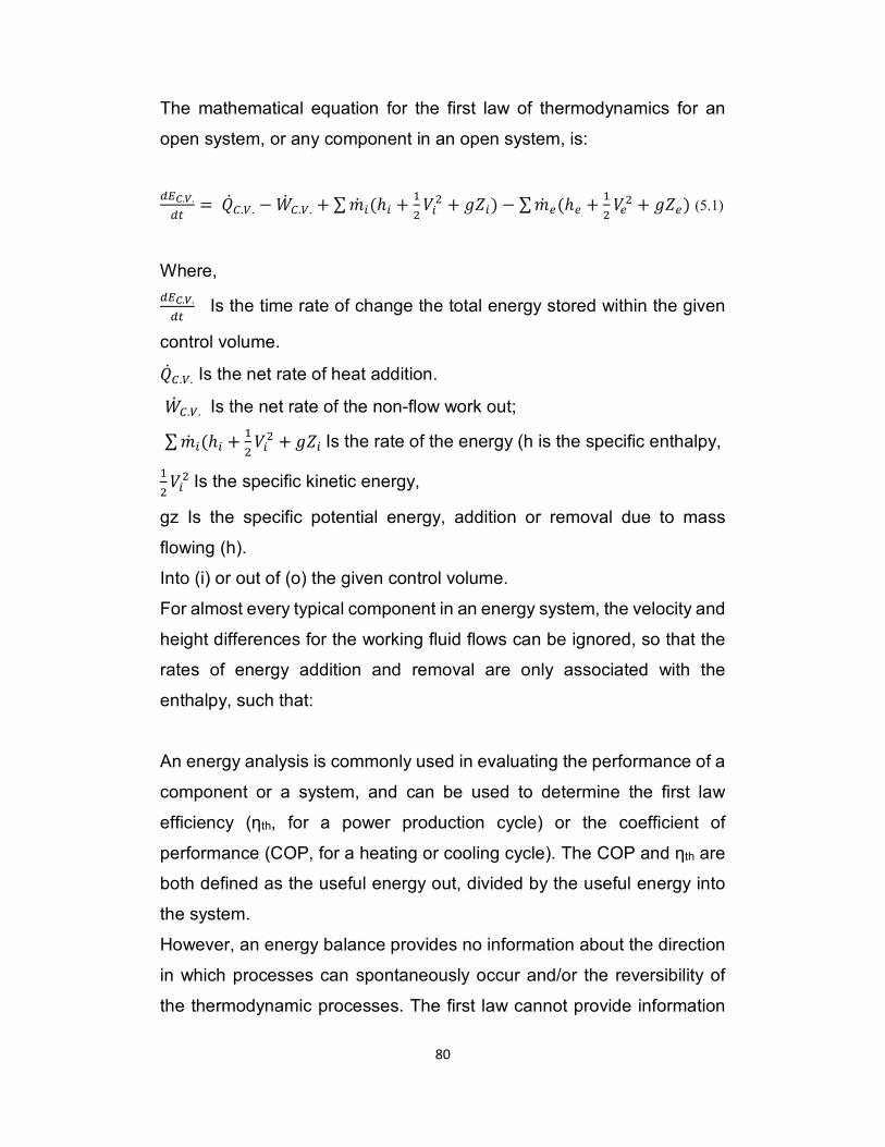
80
The mathematical equation for the first law of thermodynamics for an
open system, or any component in an open system, is:
� !.#.�$ = %&'.(. − )& '.(. + ∑ �& +(ℎ+ + -. /+. + 0+) − ∑ �& 2(ℎ2 + -. /2. + 02) (5.1)
Where, � !.#.�$ Is the time rate of change the total energy stored within the given
control volume. %&'.(. Is the net rate of heat addition.
)& '.(. Is the net rate of the non-flow work out;
∑ �& +(ℎ+ + -. /+. + 0+ Is the rate of the energy (h is the specific enthalpy,
-. /+. Is the specific kinetic energy,
gz Is the specific potential energy, addition or removal due to mass
flowing (h).
Into (i) or out of (o) the given control volume.
For almost every typical component in an energy system, the velocity and
height differences for the working fluid flows can be ignored, so that the
rates of energy addition and removal are only associated with the
enthalpy, such that:
An energy analysis is commonly used in evaluating the performance of a
component or a system, and can be used to determine the first law
efficiency (ηth, for a power production cycle) or the coefficient of
performance (COP, for a heating or cooling cycle). The COP and ηth are
both defined as the useful energy out, divided by the useful energy into
the system.
However, an energy balance provides no information about the direction
in which processes can spontaneously occur and/or the reversibility of
the thermodynamic processes. The first law cannot provide information
81
about the inability of any thermodynamic process to convert heat fully into
mechanical work, or any insight into why mixtures cannot spontaneously
separate themselves.
5.2 Exergy analysis and the Second Law of Thermodynamics
The second law of thermodynamics emphasizes on the quality, rather
than just the quantity, of different forms of energy, and explains the
reasons that some spontaneous processes can only occur in one
direction. Two well-known (and, ultimately, equivalent) statements of the
second law of thermodynamics are cited below.
Clausius statement:
"It is impossible for heat to move of itself from a lower-temperature
reservoir to a higher temperature reservoir. That is, heat transfer can only
occur spontaneously in the direction of temperature decrease. "
Kelvin-Planck statement:
"It is impossible for a system to receive a given amount of heat from a
high temperature reservoir and to provide an equal amount of work
output. While a system converting work to an equivalent energy transfer
as heat is possible, a device converting heat to an equivalent energy
transfer as work is impossible. "
The second law of thermodynamics defines entropy as the measurement
of the randomness within a system. Because entropy is a state property,
an expression of the second law of thermodynamics for an open system
can be developed in a similar manner to that of the first law, as below:
82
� ���� �� ����3� �������� ������ ������ � = 4 ��� ���� �� 5���3� 6������7� 8��� 9 + : ���� ��5���3� 6���������ℎ ���� ���� �;
− : ���� �� 5���3� ����������ℎ <��� ���� ���; + 4 ���� ��5���3� =��������� ������ ������ 9
The mathematical equation for the second law of thermodynamics for an
open system, or any component in an open system, is:
�>!.#.�$ = ∑ �& +?+ − ∑ �& @?@ + ∑ AB (5.2)
Where,
�>!.#.�$ Is the time rate of change of the entropy stored in the control
volume. ∑ � ? Is the rate of entropy (S) addition (i) or removal (O) from the
system due mass flow.
∑ AB Is the rate of entropy addition due to heat transfer.
An ideal process is a process with no entropy generation/production, so
that the system would operate at its best possible performance level.
Therefore, compared with the actual system performance, the second law
efficiency (isentropic efficiency, for a power production process such as
a turbine, for a power consumption process such as a pump) can be
determined.
To better understand and quantify these restrictions on the flow and
conversion of energy, it is necessary to combine the first law with the
second law of thermodynamics. The exergy analysis is based on this
combination and will be discussed in the next section.
83
Exergy is a measure of a system's ability to do useful work as it is brought
into thermal mechanical and chemical equilibrium with the environment.
It is derived from the combination of the first and second law of
thermodynamics.
Since exergy is more valuable than energy according to the second law
of thermodynamics, it is useful to consider both output and input in terms
of exergy. The amount of exergy supplied in the product to the amount of
exergy associated with the fuel is more accurate measure of the
thermodynamic performance of the system which is defined as the ratio
of exergy contained in the product to the exergy associated with the solar
energy input.
� ���� �� �C��� �ℎ�����ℎ� ������ ������ � = 4��� 5C��� �������7� 8��� 9 − 4��� 5C���D������ 7� ���� 9
+ 4 ���� �� �C��� ������� ���ℎ <��� 9 − 45C��� E������������ℎ� F����� ������ 9 Based on the definition and equations, energy is never destroyed during
a process; it only changes from one form to another. In contrast, exergy
accounts for the irreversibility of process due to the increase in entropy.
Exergy is always destroyed when a process involves a temperature
change. The system exergetic efficiency is defined as the useful exergy
out from the system, divided by the overall exergy supplied to the system.
It is important to understand the subdivision of contributions to the exergy
destruction within each component. Since a conventional exergy analysis
cannot provide the required information, a better approach concerning
this detailed exergy analysis is needed. One approach to accomplish this
is known as an advanced exergy analysis. In an advanced exergy
analysis, the exergy destruction within a component can be split into
unavoidable and avoidable parts. The unavoidable exergy destruction is
84
the exergy destruction that is not recoverable due to technological
limitations, and the remaining part is the avoidable exergy destruction,
which is recoverable and should be focused on by engineers to improve
system efficiency. Additionally, the exergy destruction within a
component can also be split into endogenous and exogenous parts.
The second law efficiency of the solar assisted triple effect refrigeration
cycle may be reported as ηHH = ∆ &JKL∆ &JML∆ &JN &OPQRS (5.3)
(
Where, 5&>@TUV is incoming exergy associate with solar radiation falling on
heliostat, ∆5& - is the change in exergy at ejector evaporator of ERC, ∆5& .
is the change in exergy at evaporator of ARC and ∆5& W is the change in
exergy at evaporator of CRC. ∆5& - = �& XY[(ℎ-[ − ℎ--) − D[(�-[ − �--)] (5.4)
∆5& . = �& V[(ℎ-] − ℎ-^) − D[(�-] − �-^)] (5.5) ∆5& W = �& _M`,.[(ℎWW − ℎWb) − D[(�33 − �34)] (5.6)
5&>@TUV = %&>@TUV e1 − BgBhi (5.7)
apparent sun temperature (equal to 4500 K).the is sWhere, T 5&- = �& j@T$2k >UT$[(ℎ- − ℎ[) − D[(�- − �[)] (5.8) 5&-. = �& j@T$2k >UT$[(ℎ-. − ℎ[) − D[(�-. − �[)] (5.9)
5&- is the exergy associated with incoming Molten Salt from receiver. 5&-. Is the exergy associated with outgoing Molten Salt from generator to
the CR.
Exergy analysis determines the system performance based on exergy,
which is defined as the maximum possible reversible work obtainable in
bringing the state of the system to equilibrium with that of the
85
environment. In the absence of magnetic, surface tension effect, nuclear,
electrical, and considering the system is at rest relative to the
environment, the total exergy associated with the work obtainable by
bringing a stream of matter from its initial state to a state that is in thermal
and mechanical equilibrium with the environment.
Mathematically, 5& = �& [(ℎ − ℎ[) − D[(� − �[)] (5.10)
The First Law efficiency of the solar assisted triple effect refrigeration
cycle is given by
ηH = A& JKLA& JMLA& JNA& OPQRS (5.11)
According to the Bejan [163], entropy generation over a control volume
is given by
?&l2k = �>�$ − ∑ A& mBmk+n[ − ∑ �& �+k + ∑ �& �@o$ ≥ 0 (5.12)
According to Gouy–Stodola theorem, the exergy destruction and
entropy generation are related as [161]
5&r,s = D[?&l2k (5.13)
Exergy for a specific state with reference to the environment is defined
as follows:
5&t = �& [(ℎ − ℎ[) − D@(� − �@)] (5.14)
The exergy destruction or irreversibility equation was defined as
5&s = ∑ 5C�+k+ − ∑ 5C�@o$ − )+ + ∑ (1 − BPBu)%vv (5.15)
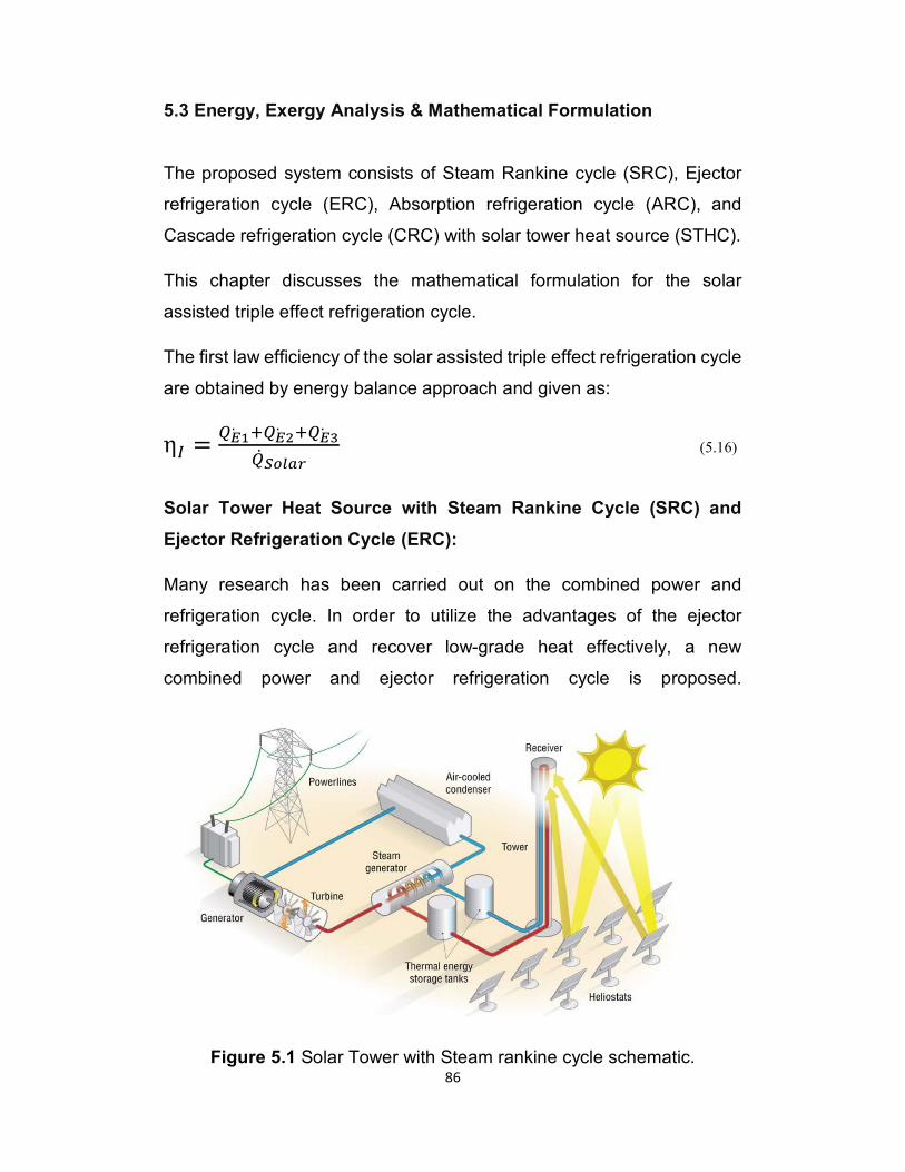
86
5.3 Energy, Exergy Analysis & Mathematical Formulation
The proposed system consists of Steam Rankine cycle (SRC), Ejector
refrigeration cycle (ERC), Absorption refrigeration cycle (ARC), and
Cascade refrigeration cycle (CRC) with solar tower heat source (STHC).
This chapter discusses the mathematical formulation for the solar
assisted triple effect refrigeration cycle.
The first law efficiency of the solar assisted triple effect refrigeration cycle
are obtained by energy balance approach and given as:
ηH = AJK. LAJM. LAJN.A& OPQRS (5.16)
Solar Tower Heat Source with Steam Rankine Cycle (SRC) and
Ejector Refrigeration Cycle (ERC):
Many research has been carried out on the combined power and
refrigeration cycle. In order to utilize the advantages of the ejector
refrigeration cycle and recover low-grade heat effectively, a new
combined power and ejector refrigeration cycle is proposed.
Figure 5.1 Solar Tower with Steam rankine cycle schematic.
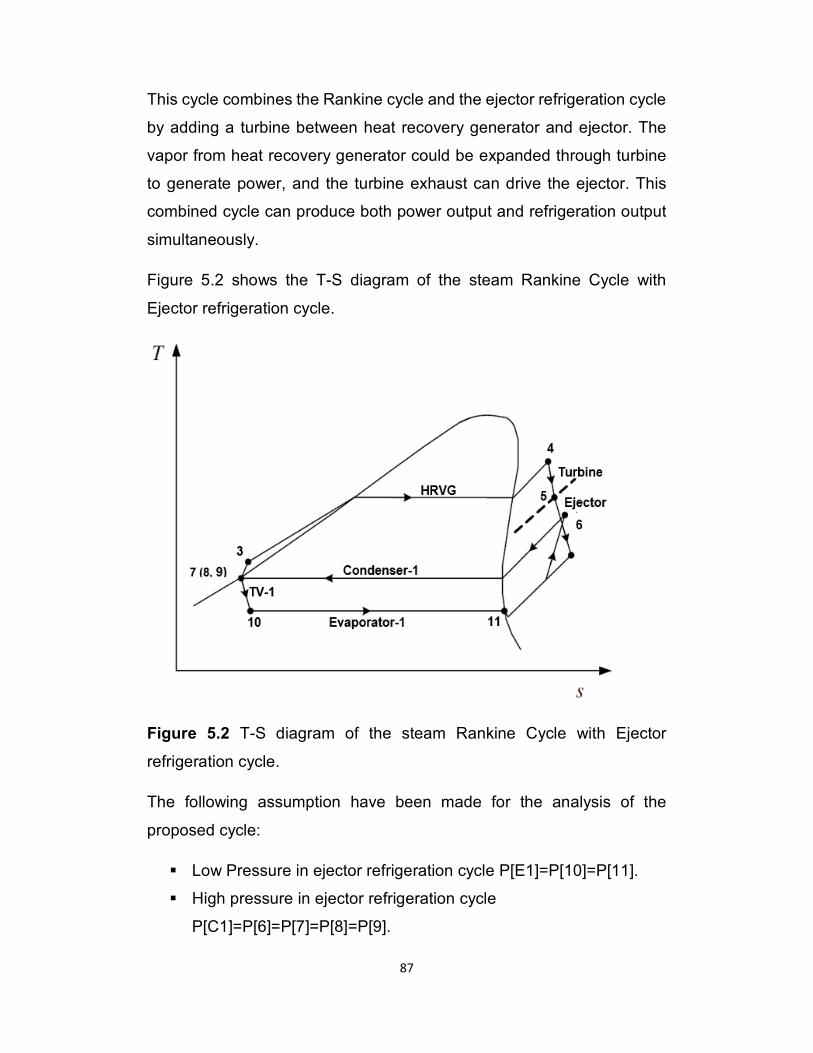
87
This cycle combines the Rankine cycle and the ejector refrigeration cycle
by adding a turbine between heat recovery generator and ejector. The
vapor from heat recovery generator could be expanded through turbine
to generate power, and the turbine exhaust can drive the ejector. This
combined cycle can produce both power output and refrigeration output
simultaneously.
Figure 5.2 shows the T-S diagram of the steam Rankine Cycle with
Ejector refrigeration cycle.
Figure 5.2 T-S diagram of the steam Rankine Cycle with Ejector
refrigeration cycle.
The following assumption have been made for the analysis of the
proposed cycle:
� Low Pressure in ejector refrigeration cycle P[E1]=P[10]=P[11].
� High pressure in ejector refrigeration cycle
P[C1]=P[6]=P[7]=P[8]=P[9].
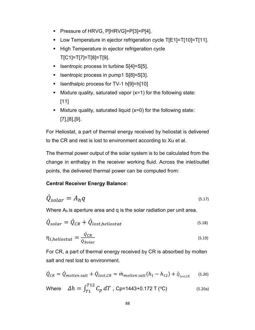
88
� Pressure of HRVG, P[HRVG]=P[3]=P[4].
� Low Temperature in ejector refrigeration cycle T[E1]=T[10]=T[11].
� High Temperature in ejector refrigeration cycle
T[C1]=T[7]=T[8]=T[9].
� Isentropic process in turbine S[4]=S[5].
� Isentropic process in pump1 S[8]=S[3].
� Isenthalpic process for TV-1 h[9]=h[10]
� Mixture quality, saturated vapor (x=1) for the following state:
[11]
� Mixture quality, saturated liquid (x=0) for the following state:
[7],[8],[9].
For Heliostat, a part of thermal energy received by heliostat is delivered
to the CR and rest is lost to environment according to Xu et al.
The thermal power output of the solar system is to be calculated from the
change in enthalpy in the receiver working fluid. Across the inlet/outlet
points, the delivered thermal power can be computed from:
Central Receiver Energy Balance:
%&X@TUV = 6wx (5.17)
area and q is the solar radiation per unit area. apertureis h Where A %&X@TUV = %&'y + %& T@X$,w2T+@X$U$ (5.18)
ηH,w2T+@X$U$ = A& !zA& OPQRS (5.19)
For CR, a part of thermal energy received by CR is absorbed by molten
salt and rest lost to environment.
%&'y = %&{@T$2k XUT$ + %& T@X$,'y = �& {@T$2k XUT$(ℎ- − ℎ-.) + %& ����,F� (5.20)
Where |ℎ = } F~B-.B- �D , Cp=1443+0.172 T (oC) (5.20a)
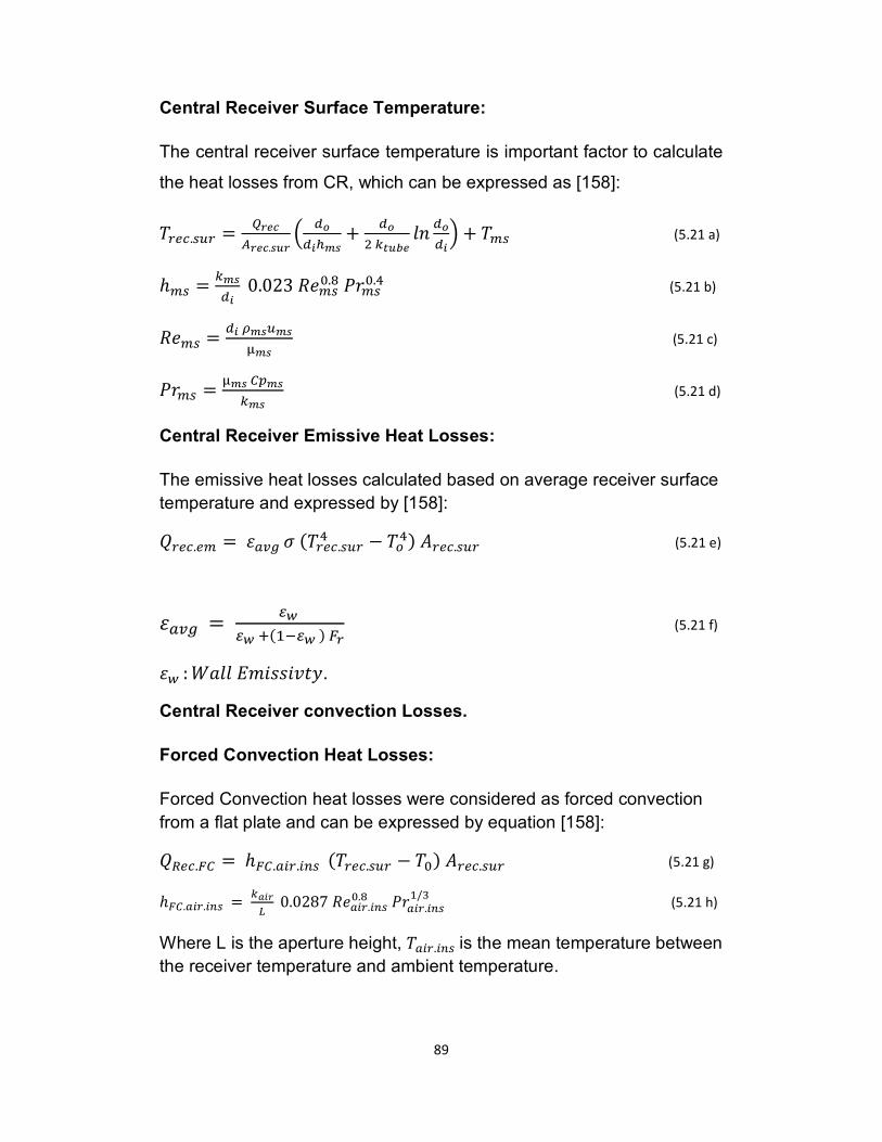
89
Central Receiver Surface Temperature:
The central receiver surface temperature is important factor to calculate
the heat losses from CR, which can be expressed as [158]:
DV2�.XoV = AS���S��.h�S e �P�mw�h + �P. ����� � �P�m i + D{X (5.21 a)
ℎ{X = ��h�m 0.023 ��{X[.� =�{X[.b (5.21 b)
��{X = �m ��ho�h��h (5.21 c)
=�{X = ��h '~�h��h (5.21 d)
Central Receiver Emissive Heat Losses:
The emissive heat losses calculated based on average receiver surface
temperature and expressed by [158]: %V2�.2{ = �U�l � (DV2�.XoVb − D@b) 6V2�.XoV (5.21 e)
�U�l = �� �� L(-��� ) �S (5.21 f)
�� : )��� 5��������.
Central Receiver convection Losses.
Forced Convection Heat Losses:
Forced Convection heat losses were considered as forced convection
from a flat plate and can be expressed by equation [158]: %y2�.�' = ℎ�'.U+V.+kX (DV2�.XoV − D[) 6V2�.XoV (5.21 g)
ℎ�'.U+V.+kX = �RmS� 0.0287 ��U+V.+kX[.� =�U+V.+kX-/W (5.21 h)
Where L is the aperture height, DU+V.+kX is the mean temperature between
the receiver temperature and ambient temperature.
90
Natural Convection Heat Losses:
The natural convection heat losses inside the central receiver can be
expressed as [158]: %y2�._' = ℎ_'.U+V.+kX (DV2�.XoV − D[) 6V2�.XoV (5.21 j)
ℎ_'.U+V.+kX = 0.81 (DV2�.XoV − D[)[.b.^ (5.21 k)
Central Receiver Reflective Heat Losses:
The reflective heat losses considering surface reflectivity and view
factor which can be expressed as [158]: %V2�.V2Y = %V2� �V ��� (5.21 L)
�V = �R���S��.h�S (5.21 m)
Central Receiver Conductive Heat Losses:
The conductive heat losses from the insulation layer considered and
can be expressed as follow [158]:
%V2�.�@k� = �m�h��m�h� (DV2�.XoV − D+kXo.�) 6V2�.XoV (5.21 n)
The combined convective heat transfer is taken into account to calculate
the heat transfer coefficient of the outer receiver insulation layer and can
be expressed as [158]:
�m�h��m�h� (DV2�.XoV − D+kXo.�) 6V2�.XoV = ����� 0.0239 �����.�0.805(0.785 D���.�D )0.21.167 =� ���, 0.45 (5.21 o)
91
Air Properties equations as a function of temperature [158]:
Density (Kg/m3):
¢U+V = W]-.££BRmS + Wbb.�bBRmSM (5.22 a)
Specific Heat for air (J/kg K):
F3U+V = 1030.5 − 0.19975 DU+V + 3.9734 ¤ 10�b DU+V. (5.22 b)
Thermal Conductivity for air (W/m K):
�U+V = ..WWb r -[¥N B RmSN/M-^b.]bLBRmS (5.22 c)
Absolute Viscosity for air (N S/m2):
μU+V = §-.b]£. B RmSNM-[£.-LBRmS ¨ X 10�^ (5.22 d)
The properties of Molten Salt as a function of temperature (a mixture of 60
wt% NaNO3 and 40 wt% KNO3 [158]:
Density (Kg/m3):
¢{X = 2090 − 0.636 D{X (5.23 a)
Specific Heat for molten salt (J/kg K):
F3{X = 1443 + 0.172 D{X (5.23 b)
Thermal Conductivity for molten salt (W/m K):
�{X = 0.443 + 1.9 ¤10�b D{X (5.23 c)
Absolute Viscosity for molten salt (N S/m2): μ{X = (22.714 − 0.12 D�� + 2.281 ¤ 10−4 D��2 − 1.474 ¤ 10−7 D��3 )¤ 10−6 (5.23 d)
92
The optical losses, heat radiation losses, and the convection heat losses
were considered for the calculation of the central receiver thermal
efficiency.
ηH,'y = A& ªPQ��� ORQ�A& !z (5.24)
Central Receiver Exergy Balance:
For Heliostat: A part of exergy received by Heliostat is delivered to the
CR and rest is lost to environment (Irreversibility),
5&>@TUV = 5&'y + 5&T@X$,w2T+@X$U$ (5.25)
So,
ηHH,w2T+@X$U$ = &!z &OPQRS (5.26)
For CR, a part of exergy received by CR is absorbed by molten salt and
rest is lost to the environment (Irreversibility),
5&'y = 5&j@T$2k >UT$ + 5&s2X$,'y (5.27) 5&'y = �& <���� ?��� (ℎ − D0 ?) + 5&s2X$,'y
= �& j@T$2k >UT$ �«,j@T$2k >UT$ �D- − D-. − D[ ln BKBKM� + 5&s2X$,'y (5.28)
ηHH,'y = & ªPQ��� ORQ� & !z (5.29)
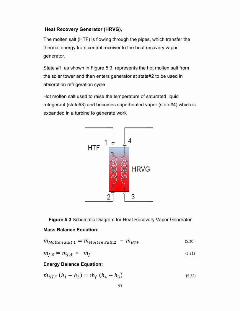
93
Heat Recovery Generator (HRVG),
The molten salt (HTF) is flowing through the pipes, which transfer the
thermal energy from central receiver to the heat recovery vapor
generator.
State #1, as shown in Figure 5.3, represents the hot molten salt from
the solar tower and then enters generator at state#2 to be used in
absorption refrigeration cycle.
Hot molten salt used to raise the temperature of saturated liquid
refrigerant (state#3) and becomes superheated vapor (state#4) which is
expanded in a turbine to generate work
Figure 5.3 Schematic Diagram for Heat Recovery Vapor Generator
Mass Balance Equation: �& j@T$2k >UT$,- = �& j@T$2k >UT$,. = �& ®B� (5.30) �& Y,W = �& Y,b = �& Y (5.31)
Energy Balance Equation: �& ®B� (ℎ- − ℎ.) = �& Y (ℎb − ℎW) (5.32)
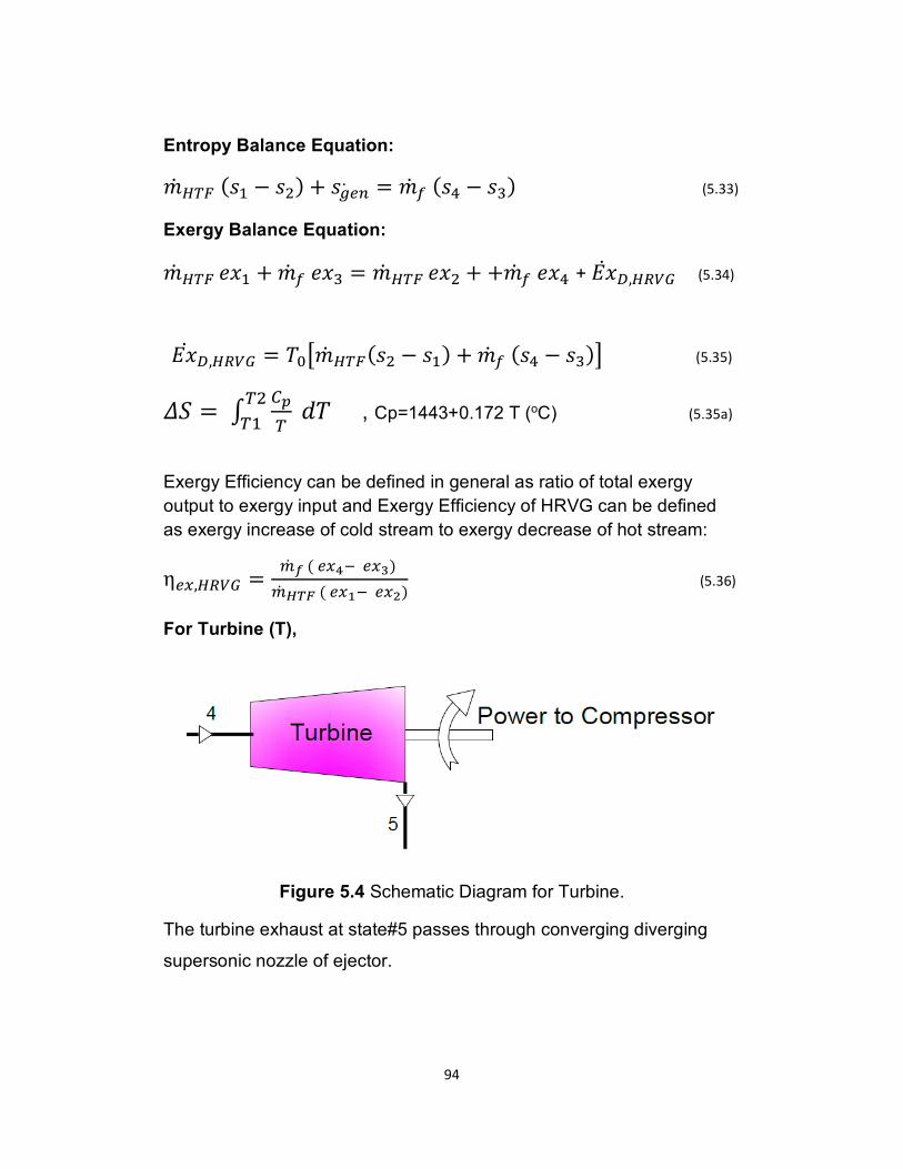
94
Entropy Balance Equation: �& ®B� (�- − �.) + �l2k. = �& Y (�b − �W) (5.33)
Exergy Balance Equation: �& ®B� �C- + �& Y �CW = �& ®B� �C. + +�& Y �Cb + 5C& s,®y(¯ (5.34)
5C& s,®y(¯ = D[°�& ®B�(�. − �-) + �& Y (�b − �W)± (5.35)
(5.35a) C) oT (p=1443+0.172 C, |? = } '�BB.B- �D)
Exergy Efficiency can be defined in general as ratio of total exergy
output to exergy input and Exergy Efficiency of HRVG can be defined
as exergy increase of cold stream to exergy decrease of hot stream:
η2t,®y(¯ = {& ² ( 2t³� 2tN) {& ´µ¶ ( 2tK� 2tM) (5.36)
For Turbine (T),
Figure 5.4 Schematic Diagram for Turbine.
The turbine exhaust at state#5 passes through converging diverging
supersonic nozzle of ejector.
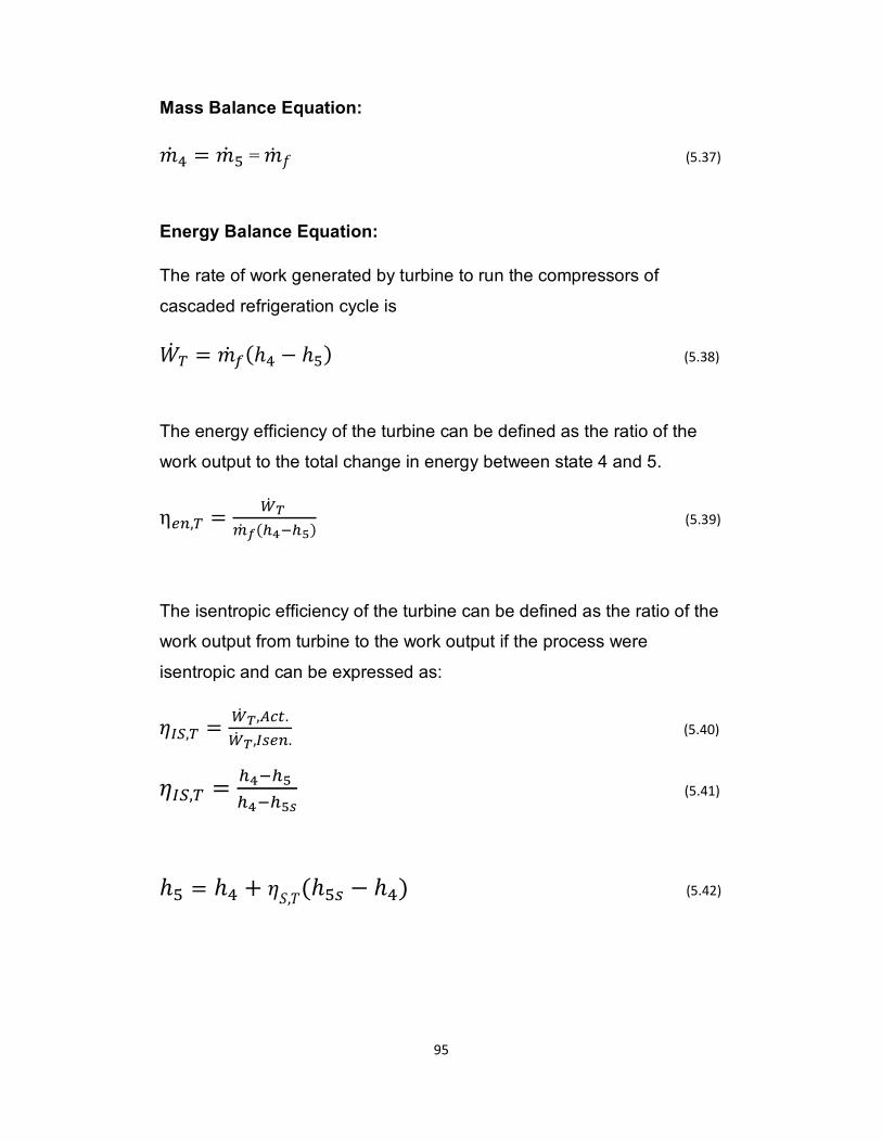
95
Mass Balance Equation:
�& b = �& ] = �& � (5.37)
Energy Balance Equation:
The rate of work generated by turbine to run the compressors of
cascaded refrigeration cycle is
)& B = �& Y(ℎb − ℎ]) (5.38)
The energy efficiency of the turbine can be defined as the ratio of the
work output to the total change in energy between state 4 and 5.
η2k,B = ·& µ {& ²(w³�w¸) (5.39)
The isentropic efficiency of the turbine can be defined as the ratio of the
work output from turbine to the work output if the process were
isentropic and can be expressed as:
¹H>,B = ·& µ,��$.·& µ,HX2k. (5.40)
¹H>,B = w³�w¸ w³�w¸h (5.41)
ℎ] = ℎb + ¹?,D(ℎ]X − ℎb) (5.42)
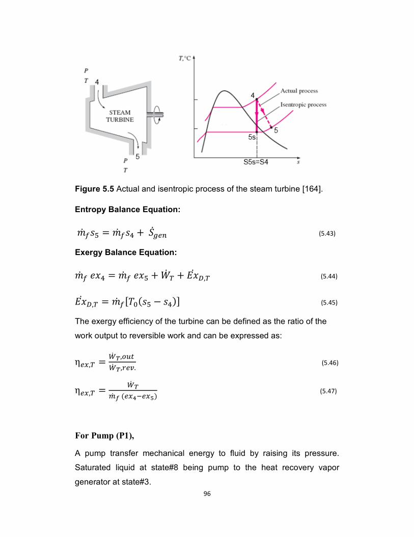
96
Figure 5.5 Actual and isentropic process of the steam turbine [164].
Entropy Balance Equation:
�& Y�] = �& Y�b + ?&l2k (5.43)
Exergy Balance Equation:
�& Y �Cb = �& Y �C] + )& B + 5C& s,B (5.44)
5C& s,B = �& Y[D[(�] − �b)] (5.45)
The exergy efficiency of the turbine can be defined as the ratio of the
work output to reversible work and can be expressed as:
η2t,B = ·& µ,@o$ ·& µ,V2�. (5.46)
η2t,B = ·& µ{& ² (2t³�2t¸) (5.47)
For Pump (P1),
A pump transfer mechanical energy to fluid by raising its pressure.
Saturated liquid at state#8 being pump to the heat recovery vapor
generator at state#3.
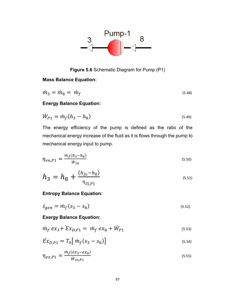
97
Figure 5.6 Schematic Diagram for Pump (P1)
Mass Balance Equation:
�& W = �& � = �& Y (5.48)
Energy Balance Equation:
)& «- = �& Y(ℎW − ℎ�) (5.49)
The energy efficiency of the pump is defined as the ratio of the
mechanical energy increase of the fluid as it is flows through the pump to
mechanical energy input to pump.
¹2k,«- = {& ²(wN�wº)·& m� (5.50)
ℎW = ℎ� + (ℎ3�−ℎ8)η»?,=1 (. (5.51) Entropy Balance Equation:
�&l2k = �& Y(�W − ��) (5.52)
Exergy Balance Equation: �& Y �CW+ 5C& s,«- = �& Y �C� + )& «- (5.53)
5C& s,«- = D[° �& Y(�W − ��)± (5.54)
η2t,«- = {& ²(2tN�2tº)·& m�,¼K (5.55)
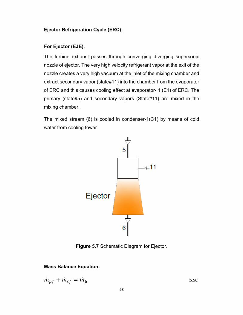
98
Ejector Refrigeration Cycle (ERC):
For Ejector (EJE),
The turbine exhaust passes through converging diverging supersonic
nozzle of ejector. The very high velocity refrigerant vapor at the exit of the
nozzle creates a very high vacuum at the inlet of the mixing chamber and
extract secondary vapor (state#11) into the chamber from the evaporator
of ERC and this causes cooling effect at evaporator- 1 (E1) of ERC. The
primary (state#5) and secondary vapors (State#11) are mixed in the
mixing chamber.
The mixed stream (6) is cooled in condenser-1(C1) by means of cold
water from cooling tower.
Figure 5.7 Schematic Diagram for Ejector.
Mass Balance Equation:
�& ~Y + �& XY = �& ^ (5.56)
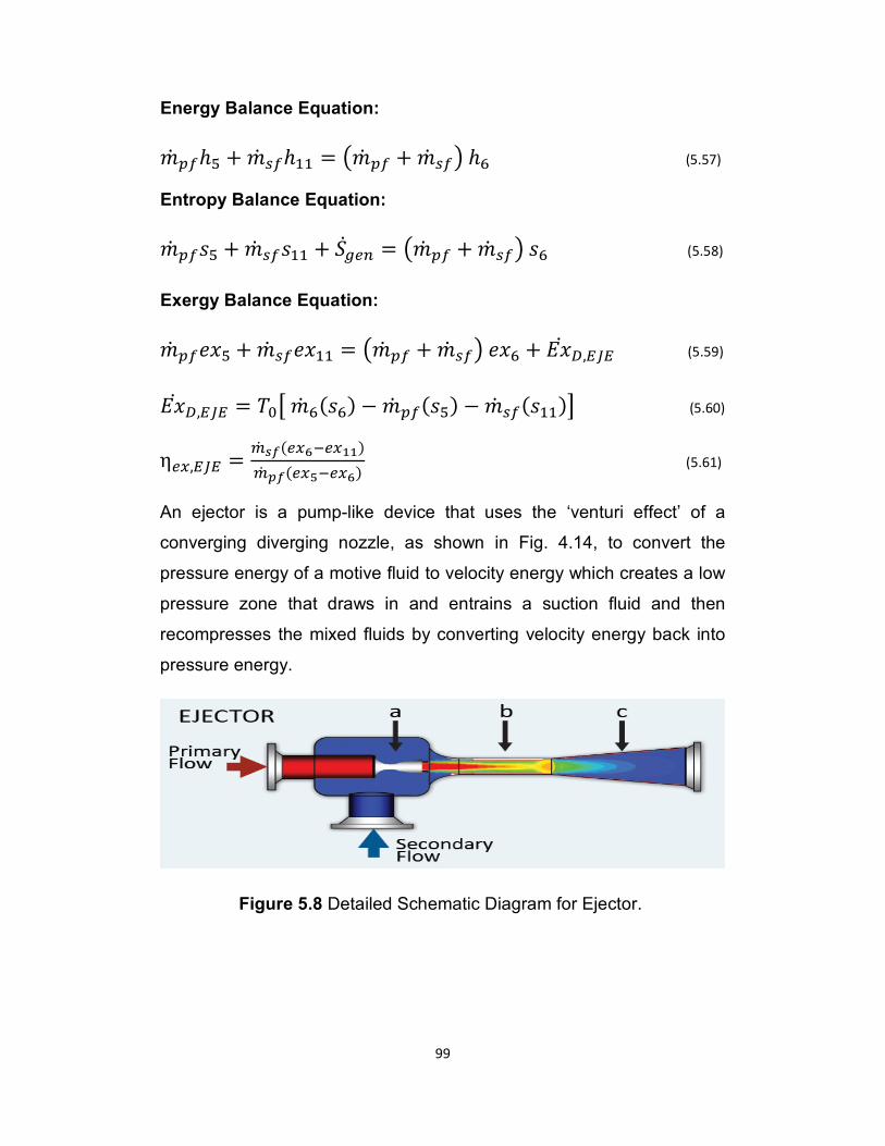
99
Energy Balance Equation:
�& ~Yℎ] + �& XYℎ-- = ½�& ~Y + �& XY¾ ℎ^ (5.57)
Entropy Balance Equation:
�& ~Y�] + �& XY�-- + ?&l2k = ½�& ~Y + �& XY¾ �^ (5.58)
Exergy Balance Equation:
�& ~Y�C] + �& XY�C-- = ½�& ~Y + �& XY¾ �C^ + 5C& s, ¿ (5.59)
5C& s, ¿ = D[° �& ^(�^) − �& ~Y(�]) − �& XY(�--)± (5.60)
η2t, ¿ = {& h²(2tÀ�2tKK){& �²(2t¸�2tÀ) (5.61)
An ejector is a pump-like device that uses the ‘venturi effect’ of a
converging diverging nozzle, as shown in Fig. 4.14, to convert the
pressure energy of a motive fluid to velocity energy which creates a low
pressure zone that draws in and entrains a suction fluid and then
recompresses the mixed fluids by converting velocity energy back into
pressure energy.
Figure 5.8 Detailed Schematic Diagram for Ejector.
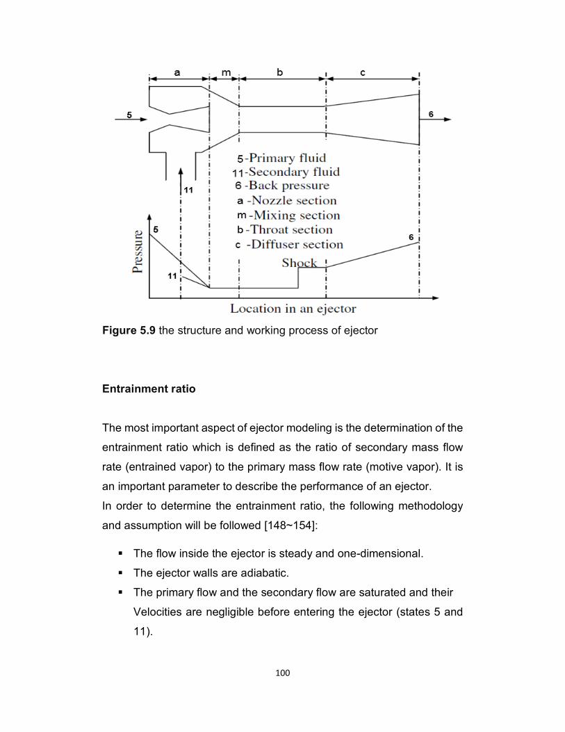
100
Figure 5.9 the structure and working process of ejector
Entrainment ratio
The most important aspect of ejector modeling is the determination of the
entrainment ratio which is defined as the ratio of secondary mass flow
rate (entrained vapor) to the primary mass flow rate (motive vapor). It is
an important parameter to describe the performance of an ejector.
In order to determine the entrainment ratio, the following methodology
and assumption will be followed [148~154]:
� The flow inside the ejector is steady and one-dimensional.
� The ejector walls are adiabatic.
� The primary flow and the secondary flow are saturated and their
Velocities are negligible before entering the ejector (states 5 and
11).
101
� The velocity of the mixed flow leaving the ejector (at state 6) is also
neglected.
� All flow losses are taken into account by using isentropic
efficiencies in the nozzle (ηn), in the diffuser (ηd), as well as in the
mixing chamber (ηm). The motive steam expands isentropically in
the nozzle. Also, the mixture of the motive steam and the entrained
vapor compresses isentropically in the diffuser.
� Constant isentropic expansion exponent and the ideal gas
behavior.
� The mixing of motive steam and the entrained vapor takes place in
the suction chamber.
� The motive steam and the entrained vapor have the same
molecular weight and specific heat ratio.
� The exist of the condenser is at saturated liquid state.
� The fluid at the exist of the evaporator is at saturated vapor state.
� The exist of the generator is at saturated vapor state.
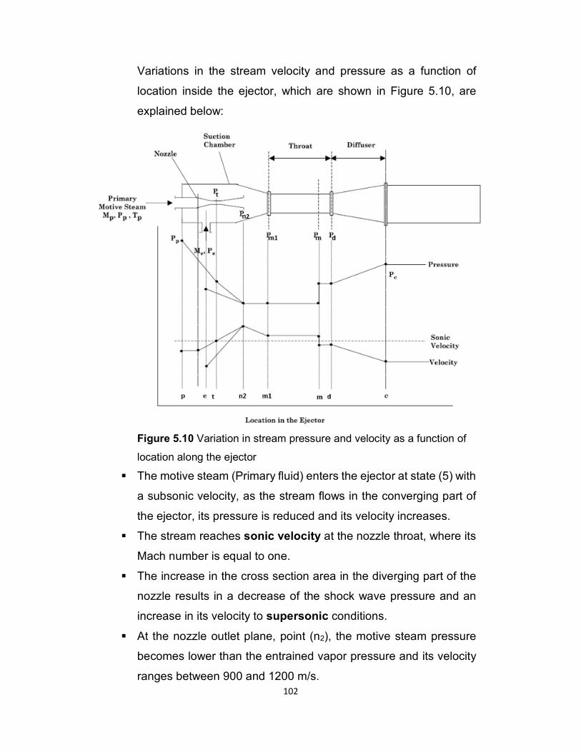
102
Variations in the stream velocity and pressure as a function of
location inside the ejector, which are shown in Figure 5.10, are
explained below:
Figure 5.10 Variation in stream pressure and velocity as a function of
location along the ejector
� The motive steam (Primary fluid) enters the ejector at state (5) with
a subsonic velocity, as the stream flows in the converging part of
the ejector, its pressure is reduced and its velocity increases.
� The stream reaches sonic velocity at the nozzle throat, where its
Mach number is equal to one.
� The increase in the cross section area in the diverging part of the
nozzle results in a decrease of the shock wave pressure and an
increase in its velocity to supersonic conditions.
� At the nozzle outlet plane, point (n2), the motive steam pressure
becomes lower than the entrained vapor pressure and its velocity
ranges between 900 and 1200 m/s.
103
� The entrained vapor at point (11) enters the ejector, where its
velocity increases and its pressure decreases to that of point (m1).
� The motive steam and entrained vapor streams may mix within the
suction chamber and the converging section of the diffuser or it
may flow as two separate streams as it enters the constant cross
section area of the diffuser, where mixing occurs.
� In either case, the mixture goes through a shock inside the
constant cross section area of the diffuser. The shock is associated
with an increase in the mixture pressure and reduction of the
mixture velocity to subsonic conditions, point (m). The shock
occurs because of the back pressure resistance of the condenser.
� As the subsonic mixture emerges from the constant cross section
area of the diffuser, further pressure increase occurs in the
diverging section of the diffuser, where part of the kinetic energy of
the mixture is converted into pressure. The pressure of the
emerging fluid is slightly higher than the condenser pressure, point
(c).
� Optimum ejector operation occurs at the critical condition. The
condenser pressure controls the location of the shock wave, where
an increase in the condenser pressure above the critical point
results in a rapid decline of the ejector entrainment ratio, since the
shock wave moves towards the nozzle exit. Operating at pressures
below the critical points has negligible effect on the ejector
entrainment ratio.
� At the critical condition, the ejector entrainment ratio increases at
lower pressure for the boiler and condenser. Also, higher
temperature for the evaporator increases the entrainment ratio.
104
Below, the thermodynamic model and mathematical equation of the
ejector processes, ideal gas behavior is assumed.
Primary flow through nozzle to m1 [165-167]:
The conservation of energy of the primary flow through nozzle n1 to n2:
�& ~Yℎ~Y,{- + {& �² o�²,�KM. = �& ~Yℎ] + {& �²oM̧. (5.62) ℎ~Y,{- = �~D~Y,{- From Ideal gas behavior, u5=0.
Recalling from thermodynamic the relationship for perfect gas �~ = � − �� (5.63) Divide the above equation by cv yields to:
�~ = Á yÁ�- (5.64)
The speed of sound can be obtained easily for the equation of state for
an ideal gas (also perfect gas as a sub set) because of a simple
mathematical expression.
The pressure for an ideal gas can be expressed as a simple function of
density, and a function “molecular structure” or ratio of specific heats, k
namely
= = ������ × ¢� (5.65)
F = � «� (5.66)
Remember that P/ρ is defined for an ideal gas as RT, and equation can
be written as:
F = √� � D (5.67) F. = Ä � D (5.68)
D = Á y'M (5.69)
105
Perfect gas is an ideal gas with a constant heat capacity, Cp. For perfect
gas equation is simplified into
�~ D~Y,{- + o�²,�KM. = �~D] + 0 (5.70)
Dividing the above equation by �~ D~Y,{- and substituting D = Á y'M
And utilizing the definition of Cp as function of R & K and inserting it into
equation () yields
1 + o�²,�KM. �� B�²,�K Å� = B̧B�²,�K (5.71)
1 + Á�- .Å� o�²,�KM'M = B̧B�²,�K (5.72)
Very useful to convert equation () into a dimensionless form and denote
Mach number as the ratio of velocity to speed of sound as
< = o� (5.73)
1 + Á�- .Å� <{-. = B̧B�²,�K (5.74)
The ratio of stagnation pressure to the static pressure can be expressed
as the function of the temperature ratio because of the isentropic
relationship as
= �� = F����� (5.75)
� = yB« (5.76)
= (yB« )Á = F����� (5.77)
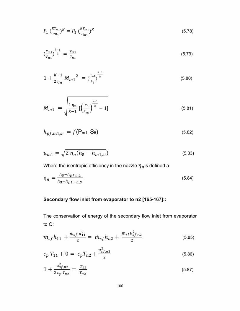
106
=- (yB�K«kK )Á = =. (yB�K«�K )Á (5.78)
(«�K«�K )Æ¥KÆ = B�KB�K (5.79)
1 + Á�- . Å� <{-. = (=�1=5 )�−1� (5.80)
<{- = Ç. Å���- [e =5=�1i�−1� − 1] (5.81)
ℎ~Y,{-,XÈ = �(Pm1, S5) (5.82)
�{- = É2 ¹k(ℎ] − ℎ{-,XÈ) (5.83)
Where the isentropic efficiency in the nozzle ¹kis defined a ηk = w¸�w�²,�Kw¸�w�²,�K,O, (5.84)
Secondary flow inlet from evaporator to n2 [165-167]::
The conservation of energy of the secondary flow inlet from evaporator
to O:
�& XYℎ-- + {& h² oKKM. = �& XYℎk. + {& h²oh²,�MM. (5.85)
�~ D-- + 0 = �~Dk. + oh²,�MM. (5.86)
1 + oh²,�MM. �� B�M = BKK B�M (5.87)
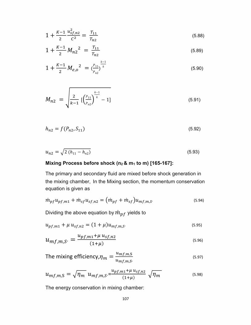
107
1 + Á�- . oh²,�MM'M = BKK B�M (5.88)
1 + Á�- . <k.. = BKK B�M (5.89)
1 + Á�- . <2,@. = (=11=2)�−1� (5.90)
<k. = Ç . ��- [e=11=2i�−1� − 1] (5.91)
ℎk. = �(=k., ?--) (5.92) �k. = É2 (ℎ11 − ℎ2) (5.93)
167]:-[165 to m) 1& m 2(nMixing Process before shock
The primary and secondary fluid are mixed before shock generation in
the mixing chamber, In the Mixing section, the momentum conservation
equation is given as �& ~Y�~Y,{- + �& XY�XY,k. = ½�& ~Y + �& XY¾�{Y,{,> , (5.94)
Dividing the above equation by �& ~Y yields to
�~Y,{- + Ê �XY,k. = (1 + Ê)�{Y,{,> , (5.95)
�{Y,{,>, = o�²,�KLË oh²,�M(-LË) (5.96)
The mixing efficiency,¹{ = o�²,�,Ìo�²,�,O, (5.97)
�{Y,{,Í = ɹ{ �{Y,{,>,=o�²,�KLË oh²,�M(-LË) ɹ{ (5.98)
The energy conservation in mixing chamber:
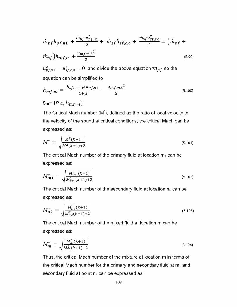
108
�& ~Yℎ~Y,k- + {& �² o�²,�KM. + �& XYℎXY,2,@ + {& h²oh²,�,PM
. = ½�& ~Y +�& XY¾ℎ{Y,{ + o�²,�,ÌM. (5.99)
�~Y,k-. = �XY,2,@. = 0 and divide the above equation �& ~Y so the
equation can be simplified to ℎ{Y,{ = wh²,KKL Ë w�²,�K -LË − o�²,�,ÌM. (5.100)
ℎ{Y,{),n2P( =mS
), defined as the ratio of local velocity to *The Critical Mach number (M
the velocity of the sound at critical conditions, the critical Mach can be
expressed as:
<∗ = Ï jM(�L-)jM(�L-)L. (5.101)
can be 1The critical Mach number of the primary fluid at location m
expressed as:
<{-∗ = Ï j�KM (�L-)j�KM (�L-)L. (5.102)
can be 2nfluid at location secondaryThe critical Mach number of the
expressed as:
<k.∗ = Ï j�MM (�L-)j�MM (�L-)L. (5.103)
The critical Mach number of the mixed fluid at location m can be
expressed as:
<{∗ = Ï j�M (�L-)j�M (�L-)L. (5.104)
Thus, the critical Mach number of the mixture at location m in terms of
and 1the critical Mach number for the primary and secondary fluid at m
can be expressed as: 2secondary fluid at point n
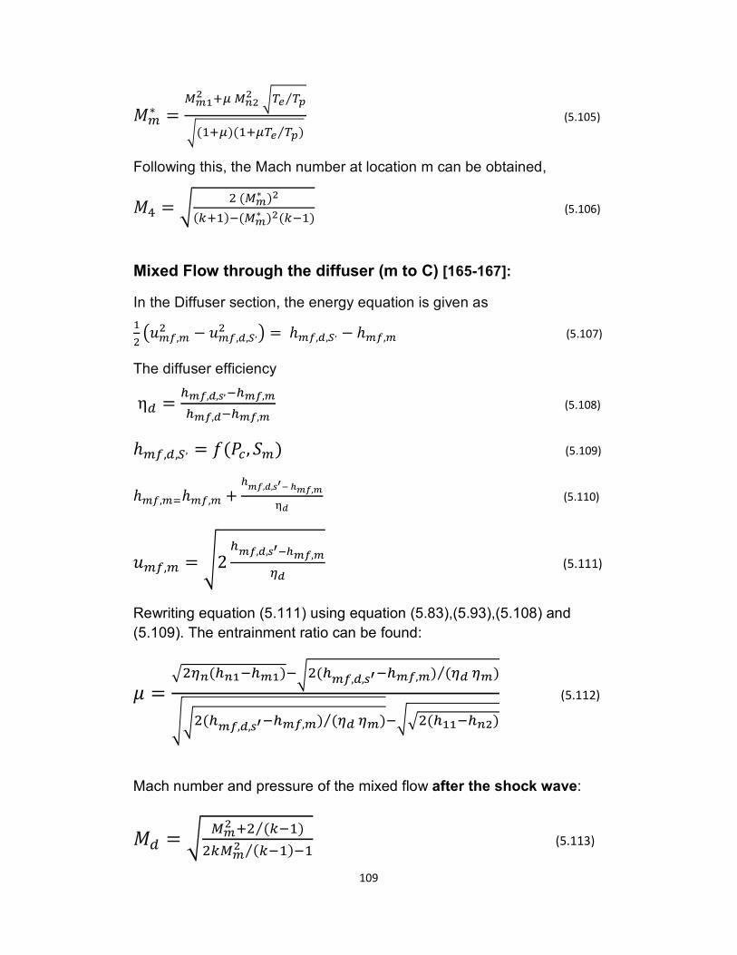
109
<{∗ = j�KM LË j�MM ÏB� B�⁄Ï(-LË)(-LËB� B�⁄ ) (5.105)
Following this, the Mach number at location m can be obtained,
<b = Ï . (j�∗ )M(�L-)�(j�∗ )M(��-) (5.106)
Mixed Flow through the diffuser (m to C) [165-167]:
In the Diffuser section, the energy equation is given as -. ½�{Y,{. − �{Y,�,> ,. ¾ = ℎ{Y,�,> , − ℎ{Y,{ (5.107)
The diffuser efficiency
η� = w�²,Ñ,h,�w�²,�w�²,Ñ�w�²,� (5.108)
ℎ{Y,�,> , = �(=�, ?{) (5.109)
ℎ{Y,{nℎ{Y,{ + w�²,Ñ,hÒ¥ Ó�²,�ÔÑ (5.110)
�{Y,{ = Ç2 w�²,Ñ,hÒ¥Ó�²,�ÅÑ (5.111)
Rewriting equation (5.111) using equation (5.83),(5.93),(5.108) and
(5.109). The entrainment ratio can be found:
Ê = É.Å�(w�K�w�K)�Ï.(w�²,Ñ,hÒ�w�²,�) (ÅÑ Å�)⁄ÇÏ.(w�²,Ñ,hÒ�w�²,�) (ÅÑ Å�)⁄ �ÏÉ.(wKK�w�M) (5.112)
Mach number and pressure of the mixed flow after the shock wave: <� = Ï j�M L. (��-)⁄.�j�M (��-)�-⁄ (5.113)
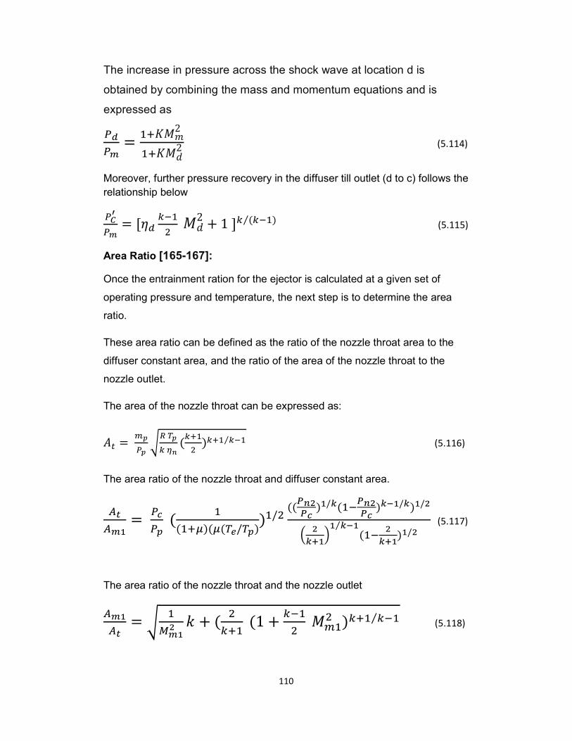
110
The increase in pressure across the shock wave at location d is
obtained by combining the mass and momentum equations and is
expressed as
«Ñ«� = -LÄ<�2-LÄ<�2 (5.114)
Moreover, further pressure recovery in the diffuser till outlet (d to c) follows the
relationship below
«!Ò«� = [¹� ��-. <�2 + 1 ]� (��-)⁄ (5.115)
Area Ratio [165-167]:
Once the entrainment ration for the ejector is calculated at a given set of
operating pressure and temperature, the next step is to determine the area
ratio.
These area ratio can be defined as the ratio of the nozzle throat area to the
diffuser constant area, and the ratio of the area of the nozzle throat to the
nozzle outlet.
The area of the nozzle throat can be expressed as:
6$ = {�«� Ïy B�� Å� (�L-. )�L- ��-⁄ (5.116)
The area ratio of the nozzle throat and diffuser constant area.
����K = «�«� ( -(-LË)(Ë(B�/B�))-/. ((¼�M¼� )K/Æ(-�¼�M¼� )Æ¥K/Æ)K/Me MÆÕKiK Æ¥K⁄ (-� MÆÕK)K/M (5.117)
The area ratio of the nozzle throat and the nozzle outlet
��K�� = Ï -j�KM � + ( .�L- (1 + ��-. <{-. )�L- ��-⁄ (5.118)
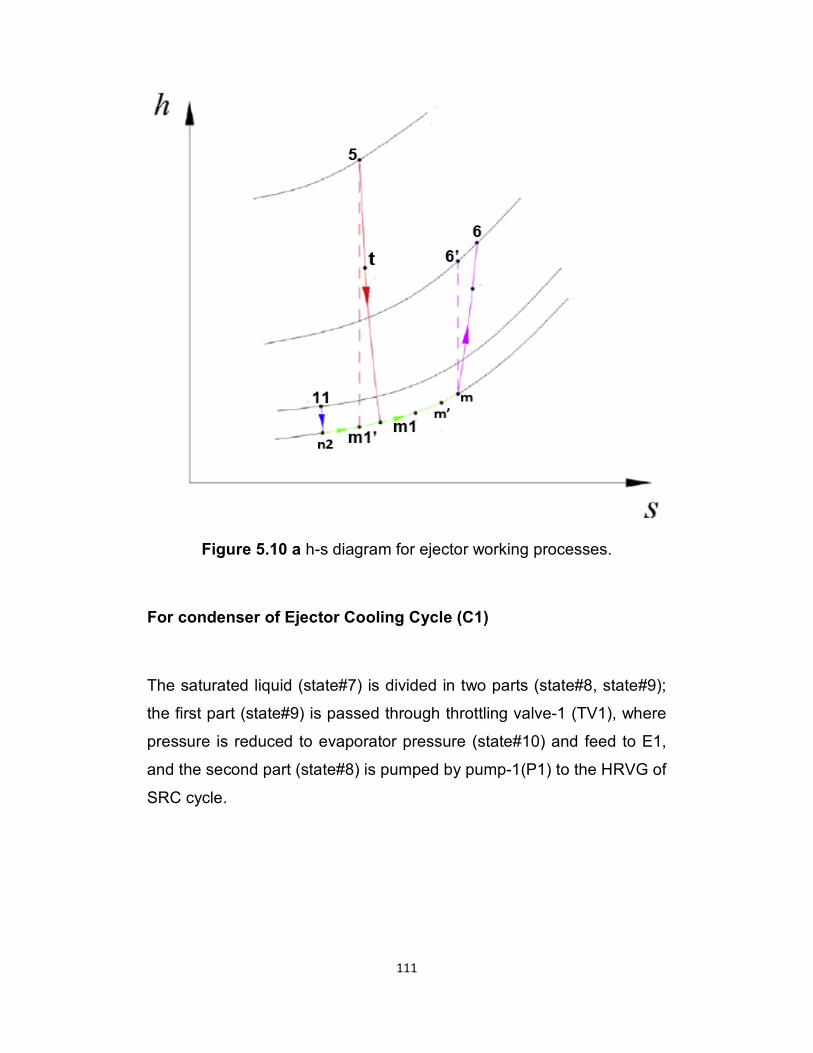
111
Figure 5.10 a h-s diagram for ejector working processes.
For condenser of Ejector Cooling Cycle (C1)
The saturated liquid (state#7) is divided in two parts (state#8, state#9);
the first part (state#9) is passed through throttling valve-1 (TV1), where
pressure is reduced to evaporator pressure (state#10) and feed to E1,
and the second part (state#8) is pumped by pump-1(P1) to the HRVG of
SRC cycle.
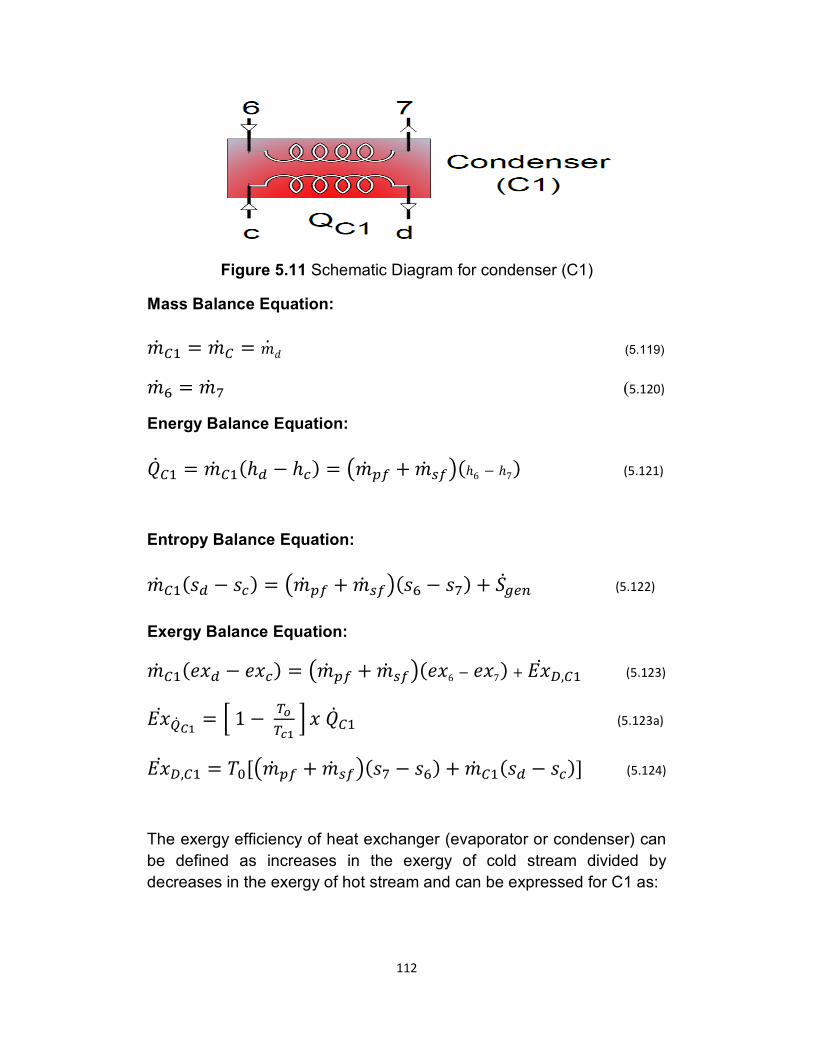
112
Figure 5.11 Schematic Diagram for condenser (C1)
Mass Balance Equation:
�& '- = �& ' = �& � (5.119) �& ^ = �& Ö (5.120)
Energy Balance Equation:
%&'- = �& '-(ℎ� − ℎ�) = ½�& ~Y + �& XY¾(ℎ6 − ℎ7) (5.121)
Entropy Balance Equation:
�& '-(�� − ��) = ½�& ~Y + �& XY¾(�^ − �Ö) + ?&l2k (5.122)
Exergy Balance Equation: �& '-(�C� − �C�) = ½�& ~Y + �& XY¾(�C6 − �C7) + 5C& s,'- (5.123)
5C& A& !K = � 1 − BPB�K � C %&'- (5.123a)
5C& s,'- = D[[½�& ~Y + �& XY¾(�Ö − �^) + �& '-(�� − ��)] (5.124)
The exergy efficiency of heat exchanger (evaporator or condenser) can
be defined as increases in the exergy of cold stream divided by
decreases in the exergy of hot stream and can be expressed for C1 as:
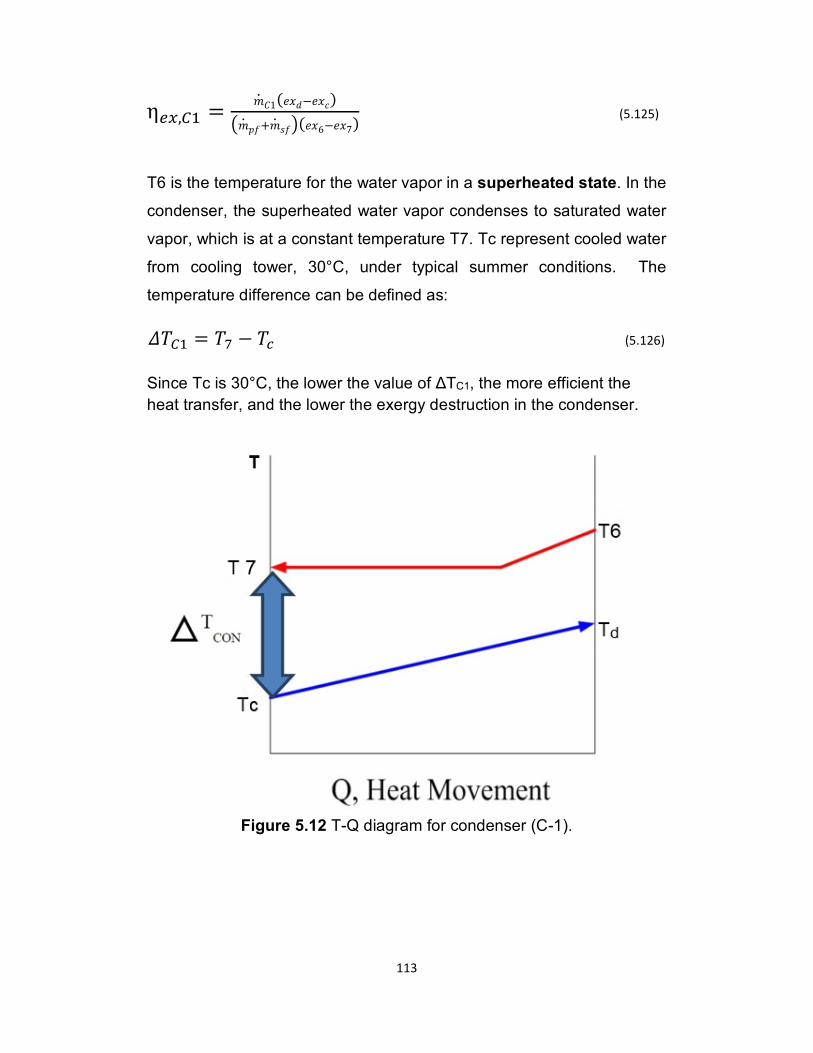
113
η2t,'- = �& F1(�C�−�C�)½�& 3�+�& ��¾(�C6−�C7) (5.125)
T6 is the temperature for the water vapor in a superheated state. In the
condenser, the superheated water vapor condenses to saturated water
vapor, which is at a constant temperature T7. Tc represent cooled water
from cooling tower, 30°C, under typical summer conditions. The
temperature difference can be defined as:
|D'- = DÖ − D� (5.126)
Since Tc is 30°C, the lower the value of ΔTC1, the more efficient the
heat transfer, and the lower the exergy destruction in the condenser.
Figure 5.12 T-Q diagram for condenser (C-1).
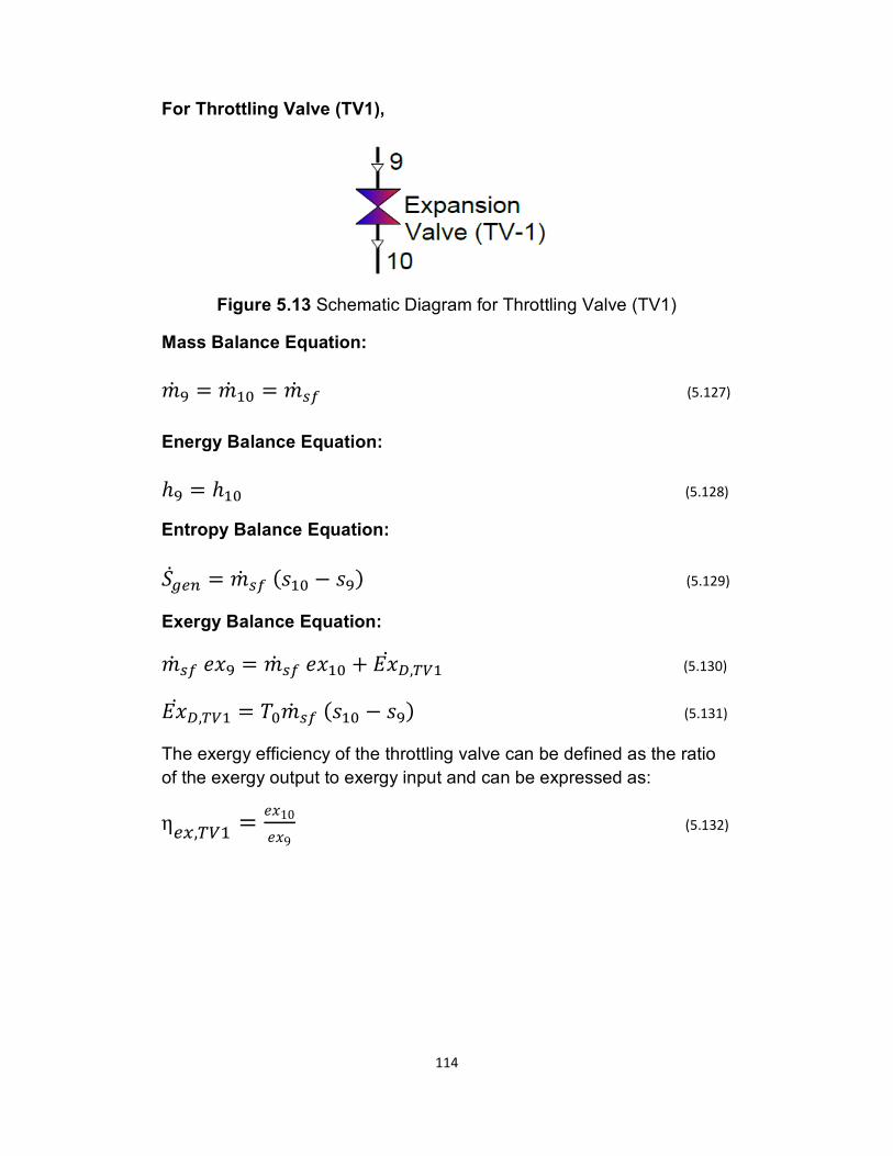
114
For Throttling Valve (TV1),
Figure 5.13 Schematic Diagram for Throttling Valve (TV1)
Mass Balance Equation:
�& £ = �& -[ = �& XY (5.127)
Energy Balance Equation:
ℎ£ = ℎ-[ (5.128)
Entropy Balance Equation:
?&l2k = �& XY (�-[ − �£) (5.129)
Exergy Balance Equation: �& XY �C£ = �& XY �C-[ + 5C& s,B(- (5.130)
5C& s,B(- = D[�& XY (�-[ − �£) (5.131)
The exergy efficiency of the throttling valve can be defined as the ratio
of the exergy output to exergy input and can be expressed as: η2t,B(- = �C10�C9 (5.132)
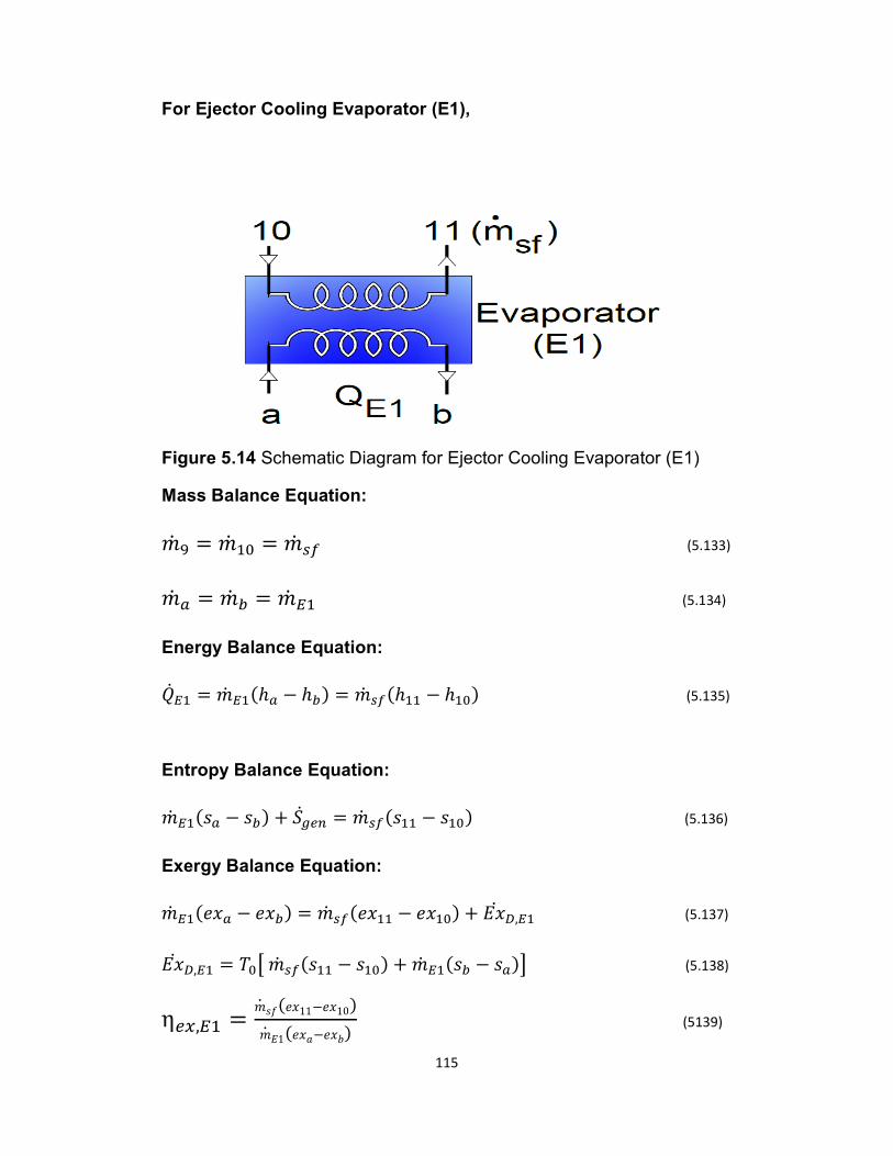
115
For Ejector Cooling Evaporator (E1),
Figure 5.14 Schematic Diagram for Ejector Cooling Evaporator (E1)
Mass Balance Equation:
�& £ = �& -[ = �& XY (5.133)
�& U = �& × = �& - (5.134)
Energy Balance Equation:
%& - = �& -(ℎU − ℎ×) = �& XY(ℎ-- − ℎ-[) (5.135)
Entropy Balance Equation:
�& -(�U − �×) + ?&l2k = �& XY(�-- − �-[) (5.136)
Exergy Balance Equation:
�& -(�CU − �C×) = �& XY(�C-- − �C-[) + 5C& s, - (5.137)
5C& s, - = D[° �& XY(�-- − �-[) + �& -(�× − �U)± (5.138)
η2t, - = �& ��(�C11−�C10)�& 51(�C�−�C7) (5139)
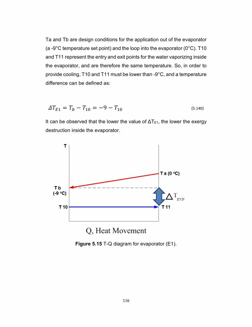
116
Ta and Tb are design conditions for the application out of the evaporator
(a -9°C temperature set point) and the loop into the evaporator (0°C). T10
and T11 represent the entry and exit points for the water vaporizing inside
the evaporator, and are therefore the same temperature. So, in order to
provide cooling, T10 and T11 must be lower than -9°C, and a temperature
difference can be defined as:
|D - = D× − D-[ = −9 − D-[ (5.140)
It can be observed that the lower the value of ΔTE1, the lower the exergy
destruction inside the evaporator.
Figure 5.15 T-Q diagram for evaporator (E1).
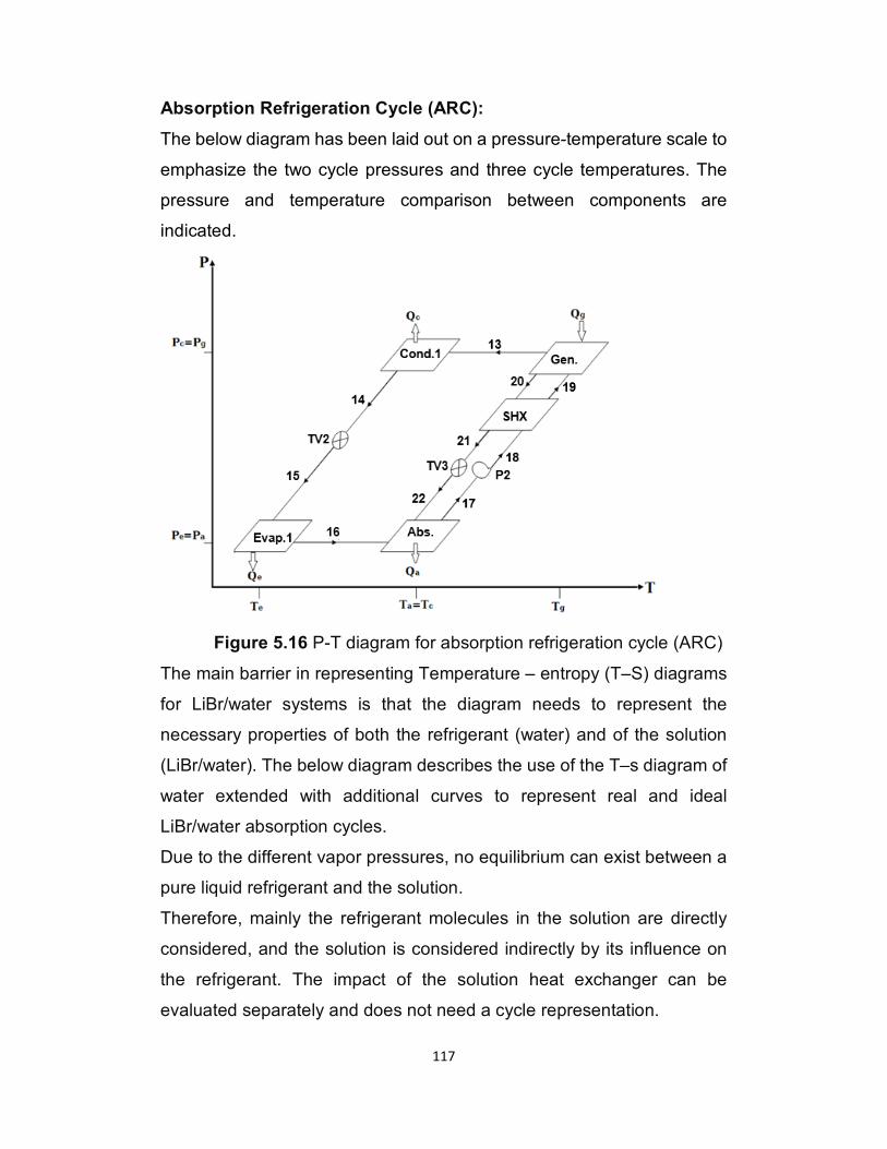
117
Absorption Refrigeration Cycle (ARC):
The below diagram has been laid out on a pressure-temperature scale to
emphasize the two cycle pressures and three cycle temperatures. The
pressure and temperature comparison between components are
indicated.
Figure 5.16 P-T diagram for absorption refrigeration cycle (ARC)
The main barrier in representing Temperature – entropy (T–S) diagrams
for LiBr/water systems is that the diagram needs to represent the
necessary properties of both the refrigerant (water) and of the solution
(LiBr/water). The below diagram describes the use of the T–s diagram of
water extended with additional curves to represent real and ideal
LiBr/water absorption cycles.
Due to the different vapor pressures, no equilibrium can exist between a
pure liquid refrigerant and the solution.
Therefore, mainly the refrigerant molecules in the solution are directly
considered, and the solution is considered indirectly by its influence on
the refrigerant. The impact of the solution heat exchanger can be
evaluated separately and does not need a cycle representation.
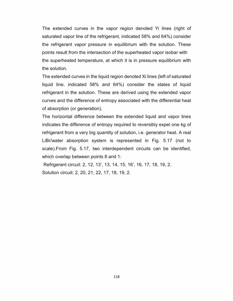
118
The extended curves in the vapor region denoted Yi lines (right of
saturated vapor line of the refrigerant, indicated 58% and 64%) consider
the refrigerant vapor pressure in equilibrium with the solution. These
points result from the intersection of the superheated vapor isobar with
the superheated temperature, at which it is in pressure equilibrium with
the solution.
The extended curves in the liquid region denoted Xi lines (left of saturated
liquid line, indicated 58% and 64%) consider the states of liquid
refrigerant in the solution. These are derived using the extended vapor
curves and the difference of entropy associated with the differential heat
of absorption (or generation).
The horizontal difference between the extended liquid and vapor lines
indicates the difference of entropy required to reversibly expel one kg of
refrigerant from a very big quantity of solution, i.e. generator heat. A real
LiBr/water absorption system is represented in Fig. 5.17 (not to
scale).From Fig. 5.17, two interdependent circuits can be identified,
which overlap between points 8 and 1:
Refrigerant circuit: 2, 12, 13’, 13, 14, 15, 16’, 16, 17, 18, 19, 2.
Solution circuit: 2, 20, 21, 22, 17, 18, 19, 2.
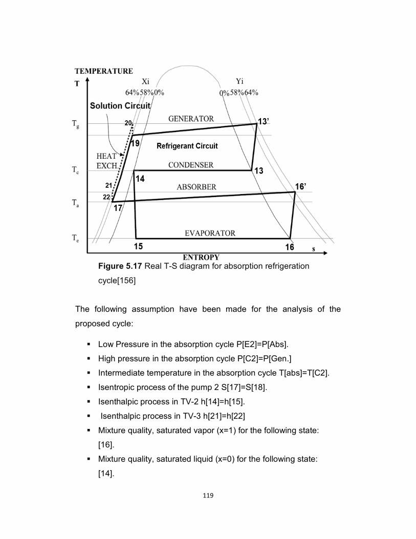
119
Figure 5.17 Real T-S diagram for absorption refrigeration
cycle[156]
The following assumption have been made for the analysis of the
proposed cycle:
� Low Pressure in the absorption cycle P[E2]=P[Abs].
� High pressure in the absorption cycle P[C2]=P[Gen.]
� Intermediate temperature in the absorption cycle T[abs]=T[C2].
� Isentropic process of the pump 2 S[17]=S[18].
� Isenthalpic process in TV-2 h[14]=h[15].
� Isenthalpic process in TV-3 h[21]=h[22]
� Mixture quality, saturated vapor (x=1) for the following state:
[16].
� Mixture quality, saturated liquid (x=0) for the following state:
[14].
120
For Generator (GEN),
The lithium bromide/water solution will be boiled off using a hot molten
salt supplied from the solar tower through heat recovery vapor generator.
The hot molten salt used to separate the water and lithium bromide.
State #2, as shown in Figure 5.18 represents the hot molten salt from
HRVG used in separation process then leaves it in liquid form at state#12
to return to central receiver.
The mixture of water and lithium bromide enters the generator at
state#19, once the weak lithium bromide and water solution is boiled,
which is designed to take place at a certain operating temperature and
pressure.
The mixture will release the water in vapor form at state #13 then it will
be condensed and exit as liquid water at state #14. The strong solution
of lithium bromide will return to solution heat exchanger at state#20.
Figure 5.18 Schematic diagram for generator.
Mass Balance Equation
�& . = �& -. = �& ®B� (5.141) �& -£ = �& -W + �& .[ (5.142)
121
Solute Mass Balance Equation:
�& X¤-£ = (�& X − �& V)¤.[ (5.143)
Where m is the mass flow rate (kg/s), X is the lithium bromide
concentration, S is weak solution and r is water refrigerant. The
circulation ratio can be defined as the ratio of the mass flow rate of the
solution through the pump to the mass flow rate of the working fluid. It
must be noted that f represents the required pumping energy. It can be
expressed in terms of concentrations as follows:
�& X = rMgrMg�rKØ �& V (5.144)
Energy Balance Equation:
%&¯ _ = �& ®B�(ℎ. − ℎ-.) (5.145) %&¯ _ = (�& � − �& �)ℎ20 + �& �ℎ13 − �& �ℎ19 (5.146)
Entropy Balance Equation:
�& ®B�(�. − �-.) + ��. = (�& � − �& �)�20 + �& ��13 − �& ��19 (5.147)
Exergy Balance Equation:
�& ®B�(�C. − �C-.) = (�& X − �& V)�C.[ + �& V�C-W − �& X�C-£ + 5C& s,¯ _ (5.148)
5C& s,¯ _ = D[[ �& V(�-W − �.[) + �& X(�.[ − �-£) + �& 8D�(�12 − �2)] (5.149)
η2t,¯2k. = 1 − D0[ �& �(�13−�20)+�& �(�20−�19)+�& �(�12−�2)]{& ´µ¶(2tM�2tKM) (5.150)
For the generator, from Figure 5.19, it can be seen that T2 and T12 are
the temperatures for the solar loop inlet and outlet, T19 is the temperature
of the dilute solution pumped into the Gen., and T20 is the temperature
of the strong solution leaving the Gen. T13 is not shown in the figure, it is
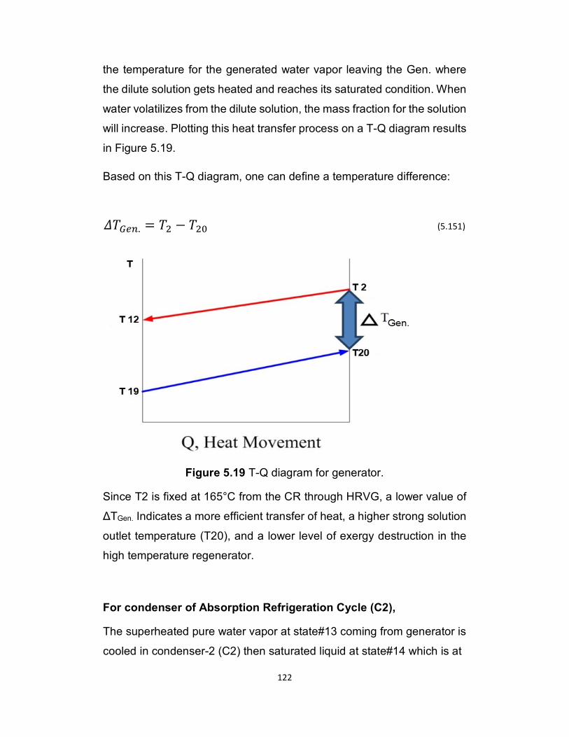
122
the temperature for the generated water vapor leaving the Gen. where
the dilute solution gets heated and reaches its saturated condition. When
water volatilizes from the dilute solution, the mass fraction for the solution
will increase. Plotting this heat transfer process on a T-Q diagram results
in Figure 5.19.
Based on this T-Q diagram, one can define a temperature difference:
|D̄ 2k. = D. − D.[ (5.151)
Figure 5.19 T-Q diagram for generator.
Since T2 is fixed at 165°C from the CR through HRVG, a lower value of
ΔTGen. Indicates a more efficient transfer of heat, a higher strong solution
outlet temperature (T20), and a lower level of exergy destruction in the
high temperature regenerator.
For condenser of Absorption Refrigeration Cycle (C2),
The superheated pure water vapor at state#13 coming from generator is
cooled in condenser-2 (C2) then saturated liquid at state#14 which is at
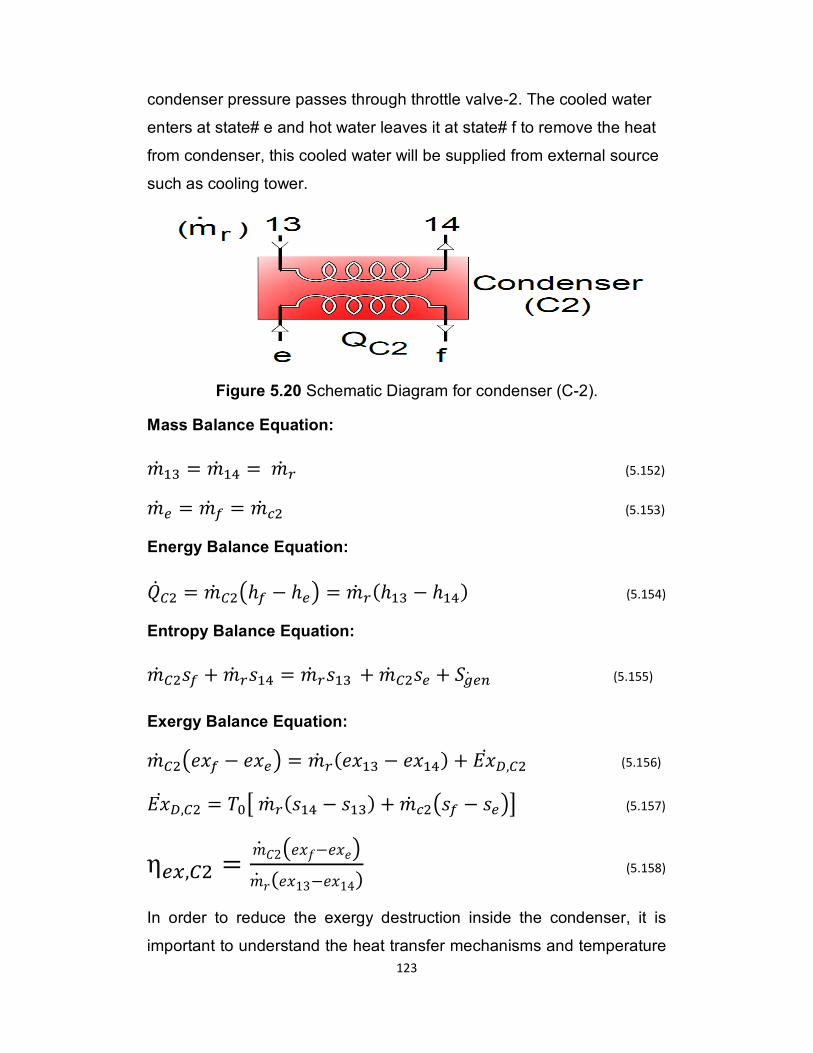
123
condenser pressure passes through throttle valve-2. The cooled water
enters at state# e and hot water leaves it at state# f to remove the heat
from condenser, this cooled water will be supplied from external source
such as cooling tower.
Figure 5.20 Schematic Diagram for condenser (C-2).
Mass Balance Equation:
�& -W = �& -b = �& V (5.152) �& 2 = �& Y = �& �. (5.153)
Energy Balance Equation:
%&'. = �& '.½ℎY − ℎ2¾ = �& V(ℎ-W − ℎ-b) (5.154)
Entropy Balance Equation:
�& '.�Y + �& V�-b = �& V�-W + �& '.�2 + ?l2k. (5.155)
Exergy Balance Equation: �& '.½�CY − �C2¾ = �& V(�C-W − �C-b) + 5C& s,'. (5.156) 5C& s,'. = D[° �& V(�-b − �-W) + �& �.½�Y − �2¾± (5.157)
η2t,'. = �& F2½�C�−�C�¾�& �(�C13−�C14) (5.158)
In order to reduce the exergy destruction inside the condenser, it is
important to understand the heat transfer mechanisms and temperature
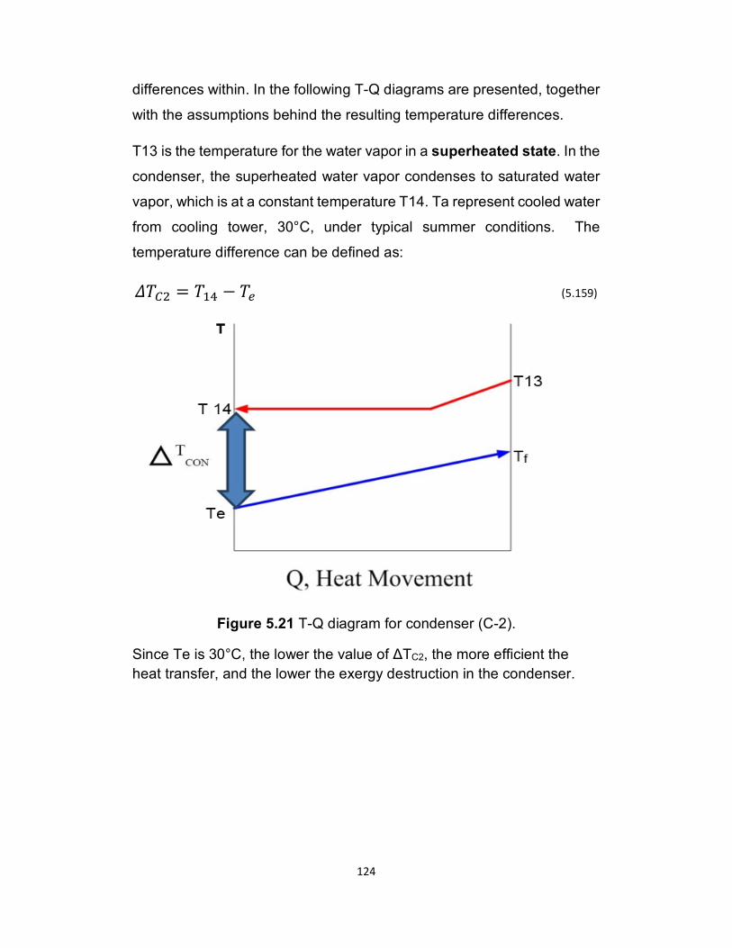
124
differences within. In the following T-Q diagrams are presented, together
with the assumptions behind the resulting temperature differences.
T13 is the temperature for the water vapor in a superheated state. In the
condenser, the superheated water vapor condenses to saturated water
vapor, which is at a constant temperature T14. Ta represent cooled water
from cooling tower, 30°C, under typical summer conditions. The
temperature difference can be defined as:
|D'. = D-b − D2 (5.159)
Figure 5.21 T-Q diagram for condenser (C-2).
Since Te is 30°C, the lower the value of ΔTC2, the more efficient the
heat transfer, and the lower the exergy destruction in the condenser.
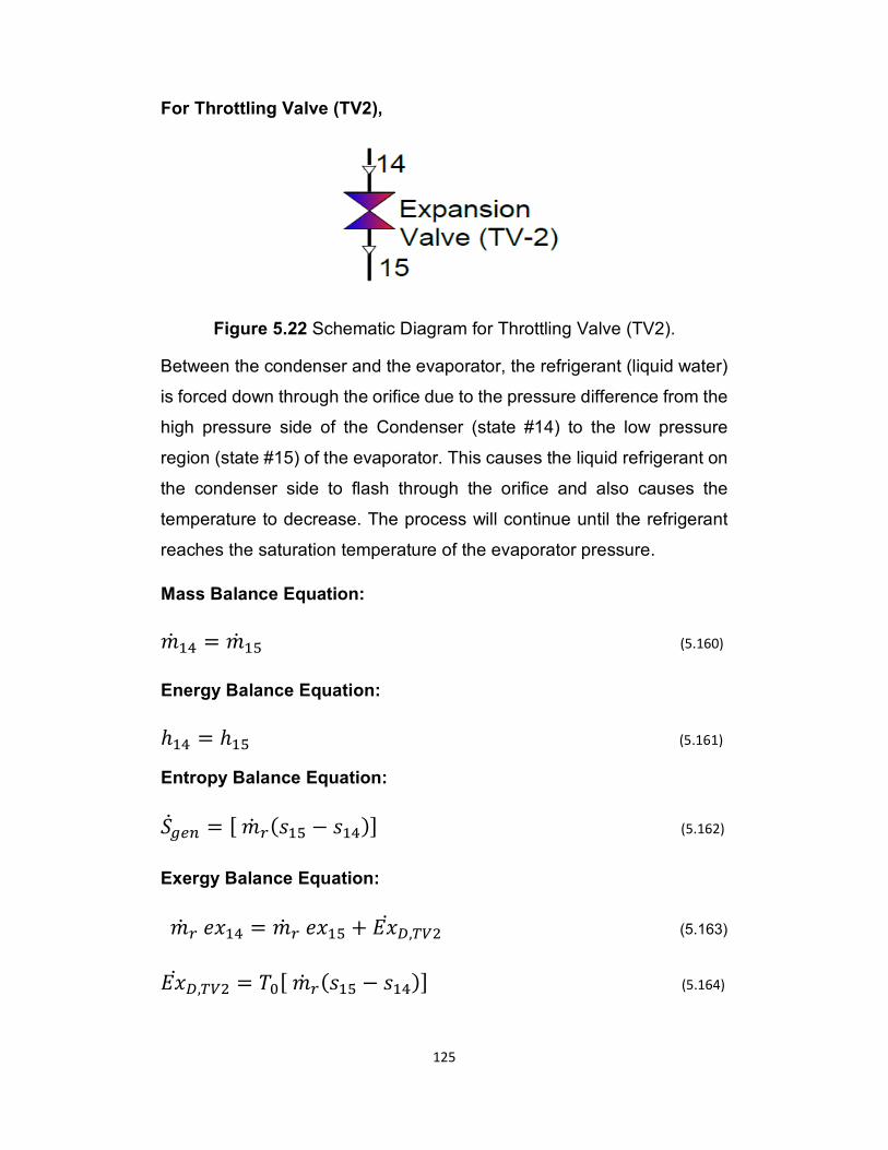
125
For Throttling Valve (TV2),
Figure 5.22 Schematic Diagram for Throttling Valve (TV2).
Between the condenser and the evaporator, the refrigerant (liquid water)
is forced down through the orifice due to the pressure difference from the
high pressure side of the Condenser (state #14) to the low pressure
region (state #15) of the evaporator. This causes the liquid refrigerant on
the condenser side to flash through the orifice and also causes the
temperature to decrease. The process will continue until the refrigerant
reaches the saturation temperature of the evaporator pressure.
Mass Balance Equation:
�& -b = �& -] (5.160)
Energy Balance Equation:
ℎ-b = ℎ-] (5.161)
Entropy Balance Equation:
?&l2k = [ �& V(�-] − �-b)] (5.162)
Exergy Balance Equation:
�& V �C-b = �& V �C-] + 5C& s,B(. (5.163)
5C& s,B(. = D[[ �& V(�-] − �-b)] (5.164)
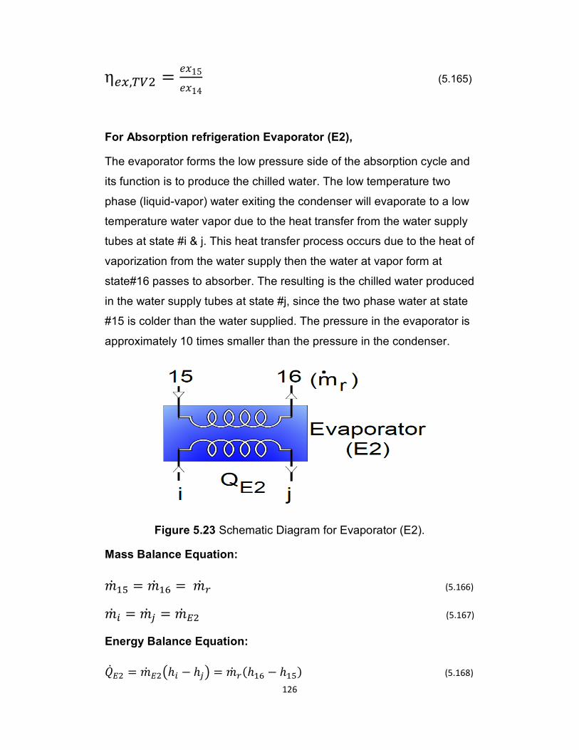
126
η2t,B(. = �C15�C14 (5.165)
For Absorption refrigeration Evaporator (E2),
The evaporator forms the low pressure side of the absorption cycle and
its function is to produce the chilled water. The low temperature two
phase (liquid-vapor) water exiting the condenser will evaporate to a low
temperature water vapor due to the heat transfer from the water supply
tubes at state #i & j. This heat transfer process occurs due to the heat of
vaporization from the water supply then the water at vapor form at
state#16 passes to absorber. The resulting is the chilled water produced
in the water supply tubes at state #j, since the two phase water at state
#15 is colder than the water supplied. The pressure in the evaporator is
approximately 10 times smaller than the pressure in the condenser.
Figure 5.23 Schematic Diagram for Evaporator (E2).
Mass Balance Equation:
�& -] = �& -^ = �& V (5.166) �& + = �& v = �& . (5.167)
Energy Balance Equation:
%& . = �& .½ℎ+ − ℎv¾ = �& V(ℎ-^ − ℎ-]) (5.168)
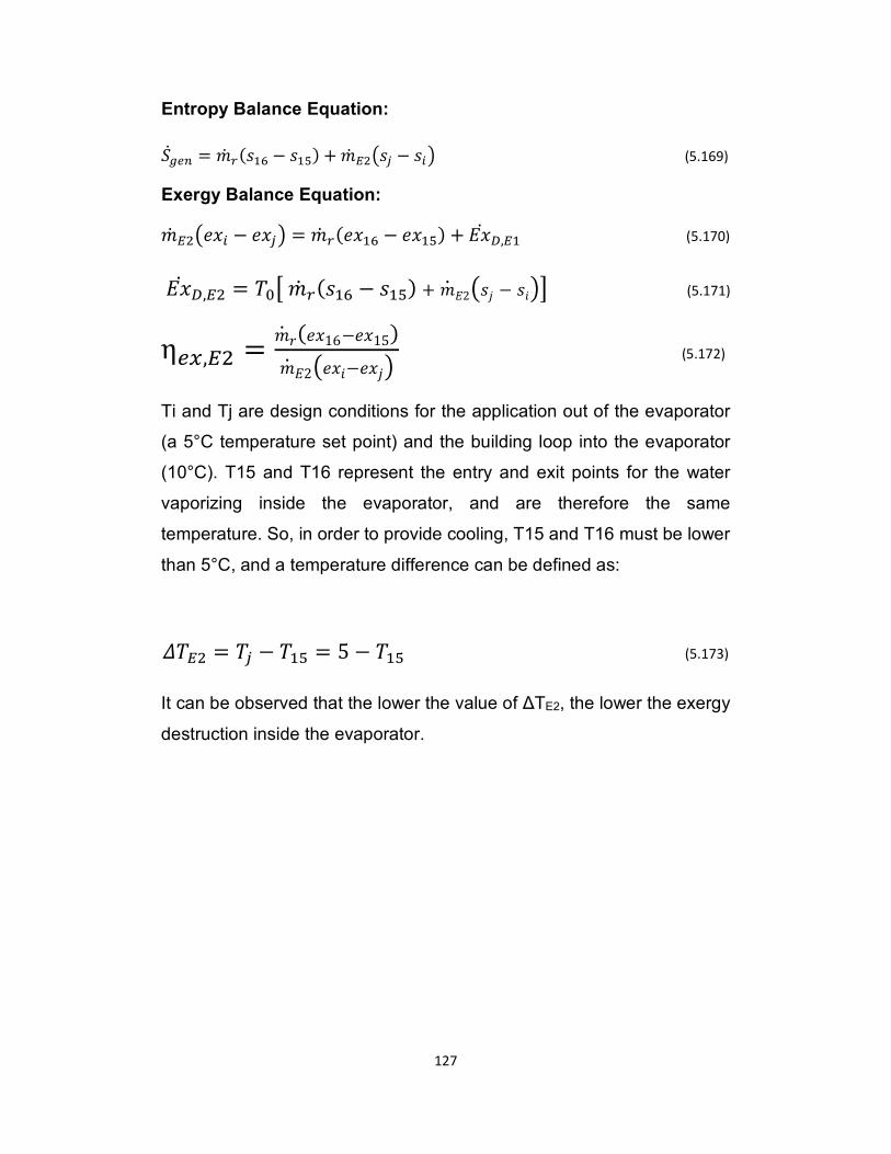
127
Entropy Balance Equation:
?&l2k = �& V(�-^ − �-]) + �& .½�v − �+¾ (5.169)
Exergy Balance Equation: �& .½�C+ − �Cv¾ = �& V(�C-^ − �C-]) + 5C& s, - (5.170)
5C& s, . = D[° �& V(�-^ − �-]) + �& 52½�Ù − ��¾± (5.171) η2t, . = �& �(�C16−�C15)�& 52½�C�−�CÙ¾ (5.172)
Ti and Tj are design conditions for the application out of the evaporator
(a 5°C temperature set point) and the building loop into the evaporator
(10°C). T15 and T16 represent the entry and exit points for the water
vaporizing inside the evaporator, and are therefore the same
temperature. So, in order to provide cooling, T15 and T16 must be lower
than 5°C, and a temperature difference can be defined as:
|D . = Dv − D-] = 5 − D-] (5.173)
It can be observed that the lower the value of ΔTE2, the lower the exergy
destruction inside the evaporator.
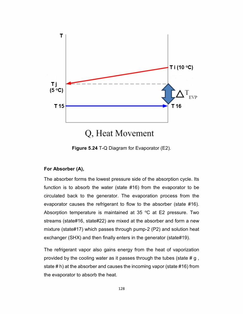
128
Figure 5.24 T-Q Diagram for Evaporator (E2).
For Absorber (A),
The absorber forms the lowest pressure side of the absorption cycle. Its
function is to absorb the water (state #16) from the evaporator to be
circulated back to the generator. The evaporation process from the
evaporator causes the refrigerant to flow to the absorber (state #16).
Absorption temperature is maintained at 35 oC at E2 pressure. Two
streams (state#16, state#22) are mixed at the absorber and form a new
mixture (state#17) which passes through pump-2 (P2) and solution heat
exchanger (SHX) and then finally enters in the generator (state#19).
The refrigerant vapor also gains energy from the heat of vaporization
provided by the cooling water as it passes through the tubes (state # g ,
state # h) at the absorber and causes the incoming vapor (state #16) from
the evaporator to absorb the heat.
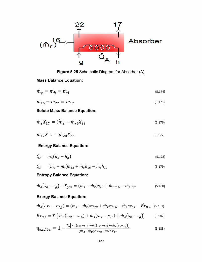
129
Figure 5.25 Schematic Diagram for Absorber (A).
Mass Balance Equation:
�& l = �& w = �& � (5.174) �& -^ + �& .. = �& -Ö (5.175)
Solute Mass Balance Equation:
�& X¤-Ö = (�& X − �& V)¤.. (5.176)
�& -Ö¤-Ö = �& .[¤.. (5.177)
Energy Balance Equation:
%&� = �& �½ℎw − ℎl¾ (5.178)
%&� = (�& X − �& V)ℎ.. + �& Vℎ-^ − �& Xℎ-Ö (5.179)
Entropy Balance Equation:
�& �½�w − �l¾ + ?&l2k = (�& X − �& V)�.. + �& V�-^ − �& X�-Ö (5.180)
Exergy Balance Equation: �& �½�Cw − �Cl¾ = (�& X − �& V)�C.. + �& V�C-^ − �& X�C-Ö − 5C& s,� (5.181)
5C& s,� = D[° �& V(�.. − �-^) + �& X(�-Ö − �..) + �& �½�w − �l¾± (5.182)
η2t,�×X. = 1 − D0° �& �(�22−�16)+�& �(�17−�22)+�& 6½�ℎ−�¾±({& h�{& S)2tMM�{& h2tKÚ (5.183)
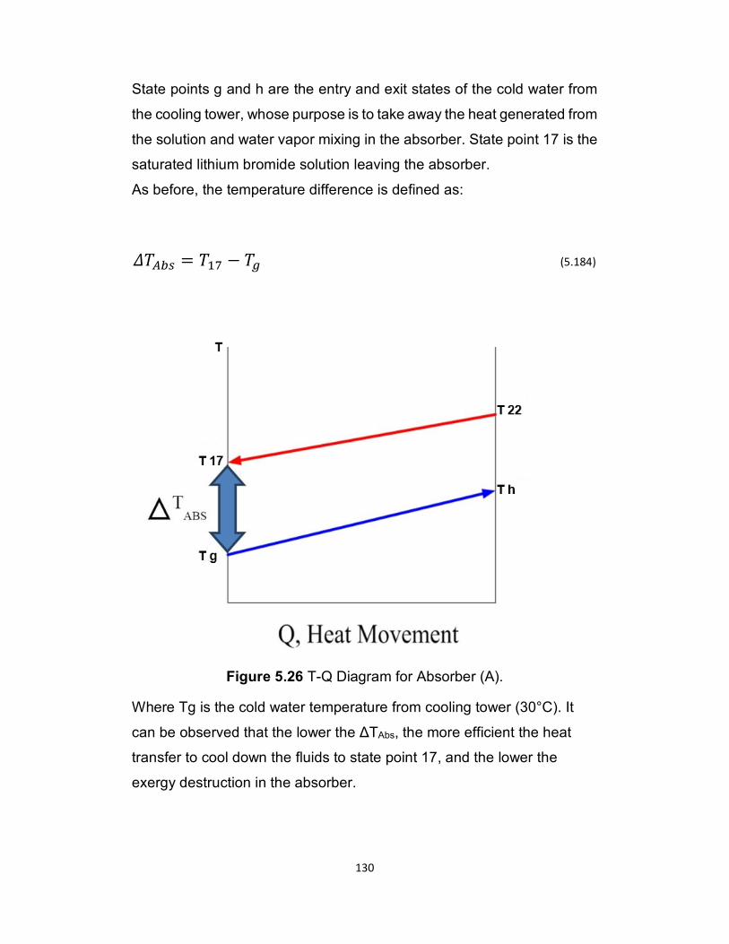
130
State points g and h are the entry and exit states of the cold water from
the cooling tower, whose purpose is to take away the heat generated from
the solution and water vapor mixing in the absorber. State point 17 is the
saturated lithium bromide solution leaving the absorber.
As before, the temperature difference is defined as:
|D�×X = D-Ö − Dl (5.184)
Figure 5.26 T-Q Diagram for Absorber (A).
Where Tg is the cold water temperature from cooling tower (30°C). It
can be observed that the lower the ΔTAbs, the more efficient the heat
transfer to cool down the fluids to state point 17, and the lower the
exergy destruction in the absorber.
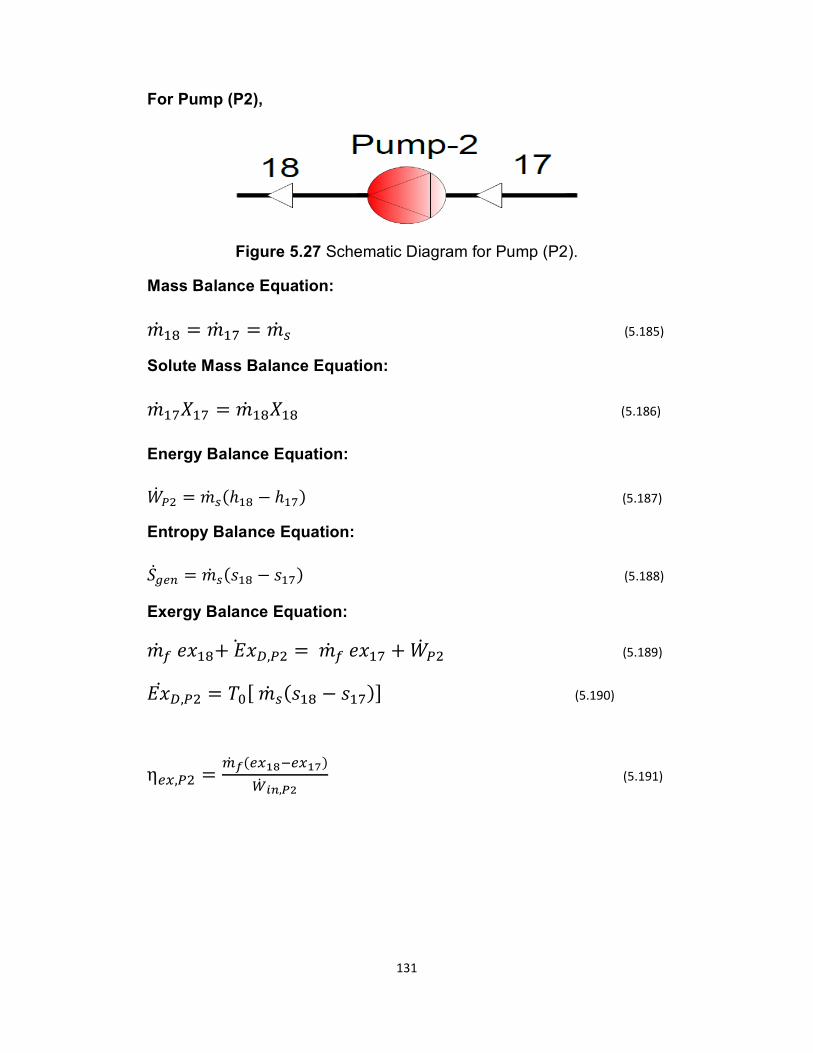
131
For Pump (P2),
Figure 5.27 Schematic Diagram for Pump (P2).
Mass Balance Equation:
�& -� = �& -Ö = �& X (5.185)
Solute Mass Balance Equation:
�& -Ö¤-Ö = �& -�¤-� (5.186)
Energy Balance Equation:
)& «. = �& X(ℎ-� − ℎ-Ö) (5.187)
Entropy Balance Equation:
?&l2k = �& X(�-� − �-Ö) (5.188)
Exergy Balance Equation: �& Y �C-�+ 5C& s,«. = �& Y �C-Ö + )& «. (5.189)
5C& s,«. = D[[ �& X(�-� − �-Ö)] (5.190)
η2t,«. = {& ²(2tKº�2tKÚ)·& m�,¼M (5.191)
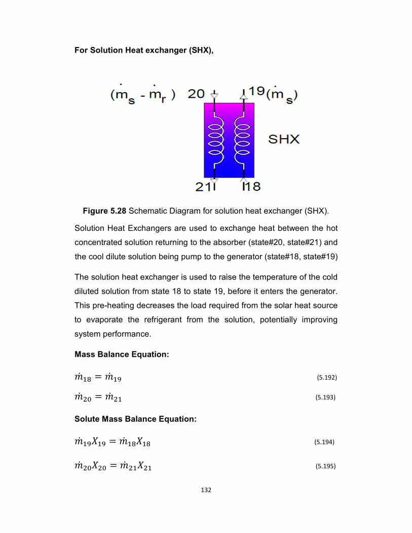
132
For Solution Heat exchanger (SHX),
Figure 5.28 Schematic Diagram for solution heat exchanger (SHX).
Solution Heat Exchangers are used to exchange heat between the hot
concentrated solution returning to the absorber (state#20, state#21) and
the cool dilute solution being pump to the generator (state#18, state#19)
The solution heat exchanger is used to raise the temperature of the cold
diluted solution from state 18 to state 19, before it enters the generator.
This pre-heating decreases the load required from the solar heat source
to evaporate the refrigerant from the solution, potentially improving
system performance.
Mass Balance Equation:
�& -� = �& -£ (5.192) �& .[ = �& .- (5.193)
Solute Mass Balance Equation:
�& -£¤-£ = �& -�¤-� (5.194)
�& .[¤.[ = �& .-¤.- (5.195)
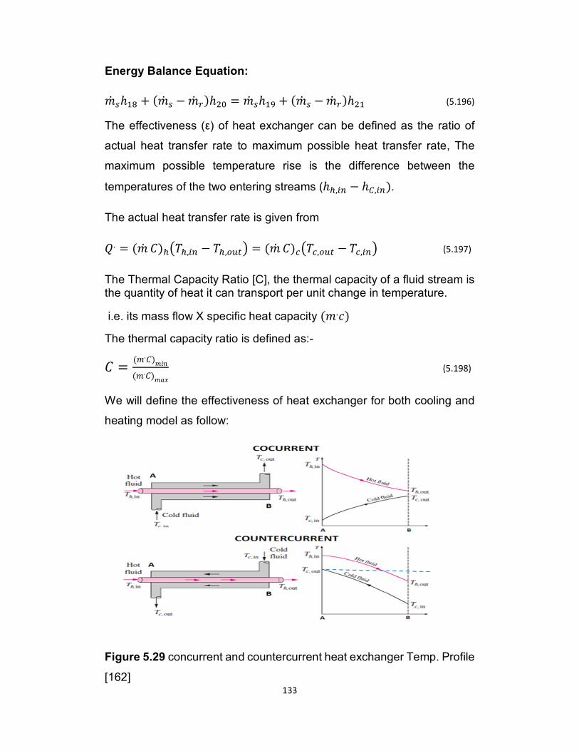
133
Energy Balance Equation:
�& Xℎ-� + (�& X − �& V)ℎ.[ = �& Xℎ-£ + (�& X − �& V)ℎ.- (5.196)
The effectiveness (ε) of heat exchanger can be defined as the ratio of
actual heat transfer rate to maximum possible heat transfer rate, The
maximum possible temperature rise is the difference between the
temperatures of the two entering streams (ℎw,+k − ℎ',+k).
The actual heat transfer rate is given from
%. = (�& .F)w½Dw,+k − Dw,@o$¾ = (�& .F)�½D�,@o$ − D�,+k¾ (5.197)
The Thermal Capacity Ratio [C], the thermal capacity of a fluid stream is the quantity of heat it can transport per unit change in temperature.
i.e. its mass flow X specific heat capacity (�.�). The thermal capacity ratio is defined as:- F = (�.F)��(�.F)��C (5.198)
We will define the effectiveness of heat exchanger for both cooling and
heating model as follow:
Figure 5.29 concurrent and countercurrent heat exchanger Temp. Profile
[162]
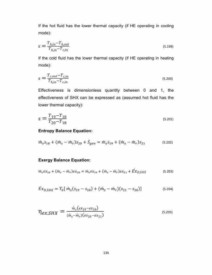
134
If the hot fluid has the lower thermal capacity (if HE operating in cooling
mode):
ε = Dℎ,�−Dℎ,���Dℎ,�−D�,� (5.199)
If the cold fluid has the lower thermal capacity (if HE operating in heating
mode):
ε = D�,���−D�,�Dℎ,�−D�,� (5.200)
Effectiveness is dimensionless quantity between 0 and 1, the
effectiveness of SHX can be expressed as (assumed hot fluid has the
lower thermal capacity):
ε = D19−D18D20−D18 (5.201)
Entropy Balance Equation:
�& X�-� + (�& X − �& V)�.[ + ?&l2k = �& X�-£ + (�& X − �& V)�.- (5.202)
Exergy Balance Equation:
�& X�C-� + (�& X − �& V)�C.[ = �& X�C-£ + (�& X − �& V)�C.- + 5C& E,?8¤ (5.203)
5C& s,>®r = D[[ �& X(�-£ − �-�) + (�& X − �& V)(�.- − �.[)] (5.204)
η2t,>®r = �& �(�C19−�C18)(�& �−�& �)(�C20−�C21) (5.205)
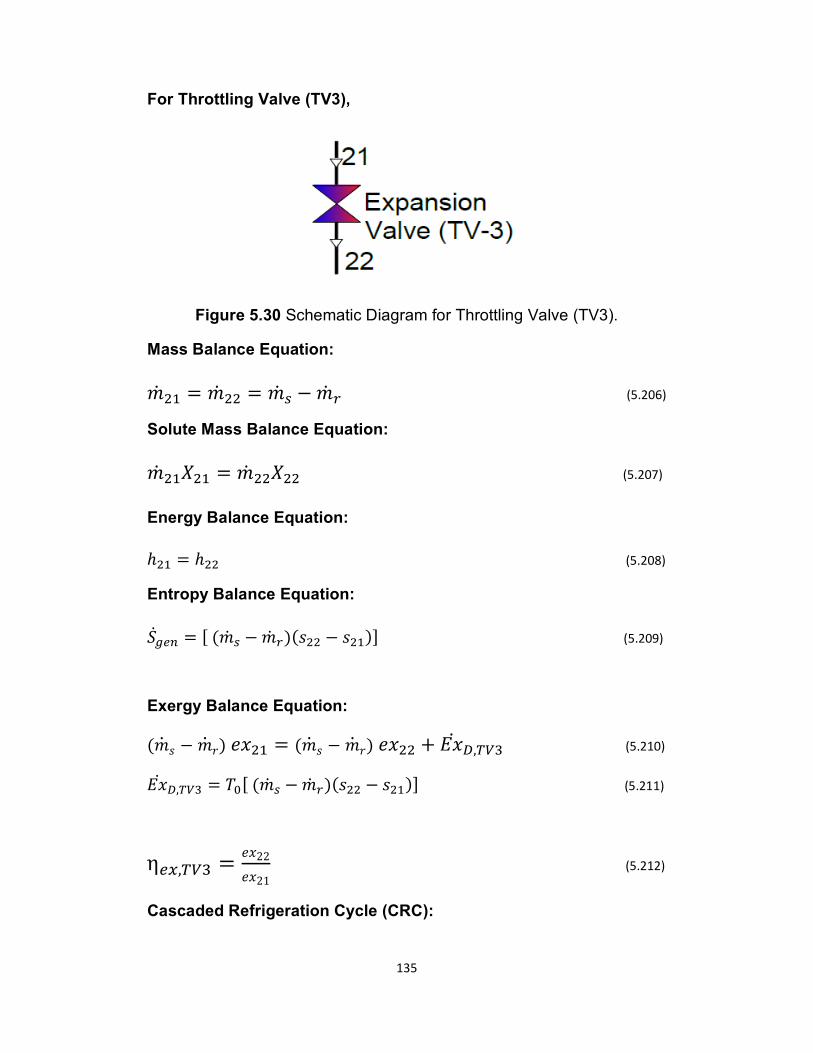
135
For Throttling Valve (TV3),
Figure 5.30 Schematic Diagram for Throttling Valve (TV3).
Mass Balance Equation:
�& .- = �& .. = �& X − �& V (5.206)
Solute Mass Balance Equation:
�& .-¤.- = �& ..¤.. (5.207)
Energy Balance Equation:
ℎ.- = ℎ.. (5.208)
Entropy Balance Equation:
?&l2k = [ (�& X − �& V)(�.. − �.-)] (5.209)
Exergy Balance Equation:
(�& � − �& �) �C.- = (�& � − �& �) �C.. + 5C& s,B(W (5.210)
5C& s,B(W = D[[ (�& X − �& V)(�.. − �.-)] (5.211)
η2t,B(W = �C22�C21 (5.212)
Cascaded Refrigeration Cycle (CRC):
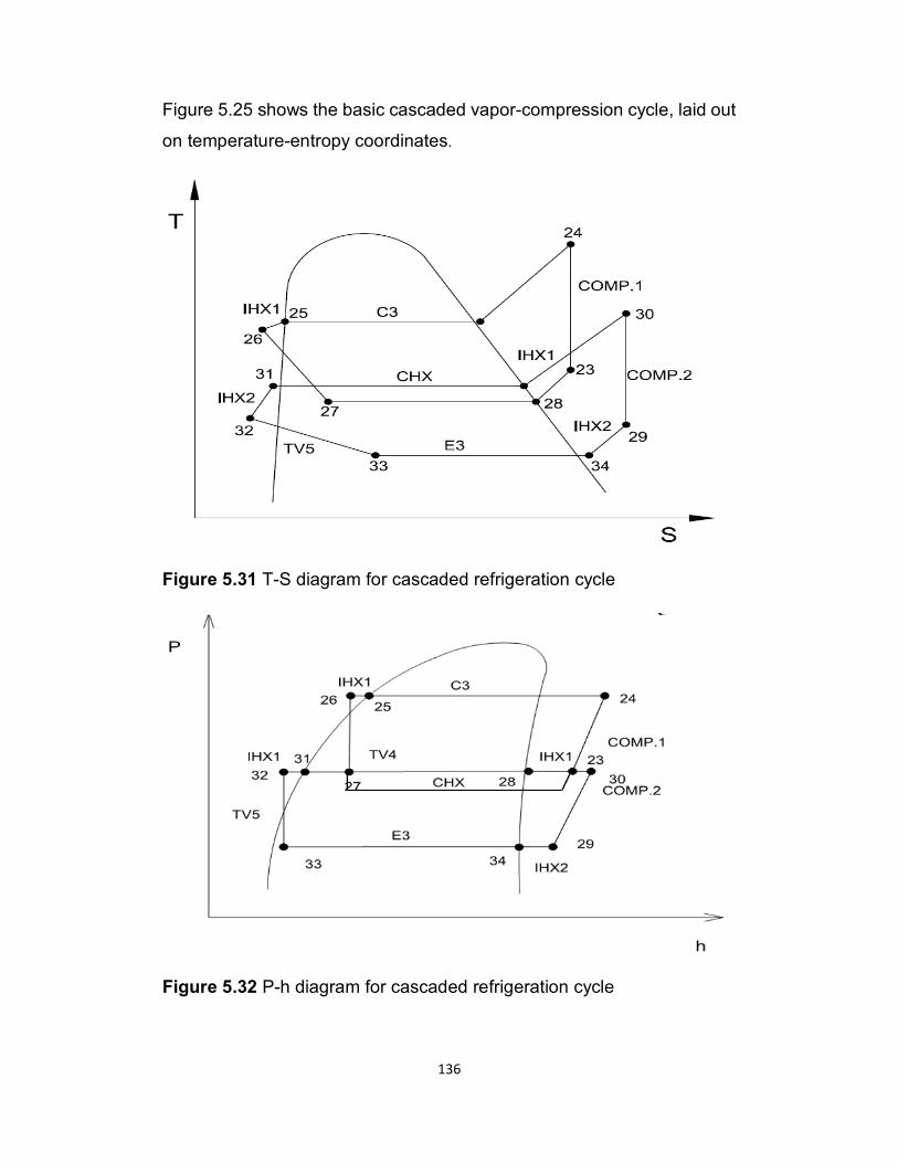
136
Figure 5.25 shows the basic cascaded vapor-compression cycle, laid out
on temperature-entropy coordinates.
Figure 5.31 T-S diagram for cascaded refrigeration cycle
Figure 5.32 P-h diagram for cascaded refrigeration cycle
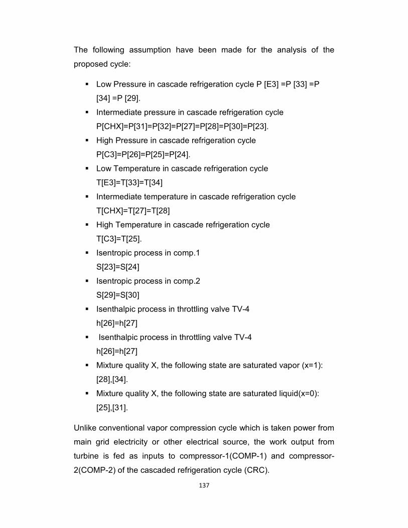
137
The following assumption have been made for the analysis of the
proposed cycle:
� Low Pressure in cascade refrigeration cycle P [E3] =P [33] =P
[34] =P [29].
� Intermediate pressure in cascade refrigeration cycle
P[CHX]=P[31]=P[32]=P[27]=P[28]=P[30]=P[23].
� High Pressure in cascade refrigeration cycle
P[C3]=P[26]=P[25]=P[24].
� Low Temperature in cascade refrigeration cycle
T[E3]=T[33]=T[34]
� Intermediate temperature in cascade refrigeration cycle
T[CHX]=T[27]=T[28]
� High Temperature in cascade refrigeration cycle
T[C3]=T[25].
� Isentropic process in comp.1
S[23]=S[24]
� Isentropic process in comp.2
S[29]=S[30]
� Isenthalpic process in throttling valve TV-4
h[26]=h[27]
� Isenthalpic process in throttling valve TV-4
h[26]=h[27]
� Mixture quality X, the following state are saturated vapor (x=1):
[28],[34].
� Mixture quality X, the following state are saturated liquid(x=0):
[25],[31].
Unlike conventional vapor compression cycle which is taken power from
main grid electricity or other electrical source, the work output from
turbine is fed as inputs to compressor-1(COMP-1) and compressor-
2(COMP-2) of the cascaded refrigeration cycle (CRC).
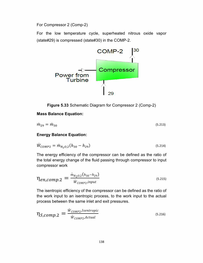
138
For Compressor 2 (Comp-2)
For the low temperature cycle, superheated nitrous oxide vapor
(state#29) is compressed (state#30) in the COMP-2.
Figure 5.33 Schematic Diagram for Compressor 2 (Comp-2)
Mass Balance Equation:
�& .£ = �& W[ (5.213)
Energy Balance Equation:
)& '`j«. = �& _M`,.(ℎW[ − ℎ.£) (5.214)
The energy efficiency of the compressor can be defined as the ratio of
the total energy change of the fluid passing through compressor to input
compressor work η2k,�@{~.. = �& �2 ,2(ℎ30−ℎ29))& F <=2 ,�3�� (5.215)
The isentropic efficiency of the compressor can be defined as the ratio of
the work input to an isentropic process, to the work input to the actual
process between the same inlet and exit pressures. η>,�@{~.. = )& F <=2 ,»�����3��)& F <=2 ,6����� (5.216)
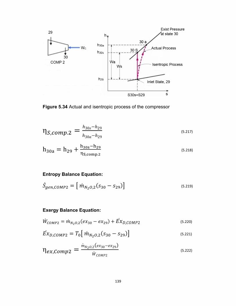
139
Figure 5.34 Actual and isentropic process of the compressor
η>,�@{~.. = ℎ30�−ℎ29ℎ30�−ℎ29 (5.217)
hW[Ý = h.£ + ÞNgß�ÞMØÔÌ,àáâã.M (5.218)
Entropy Balance Equation: ?&l2k,'`j«. = ° �& _M`,.(�W[ − �.£)± (5.219)
Exergy Balance Equation:
)& '`j«. = �& _M`,.(�CW[ − �C.£) + 5C& E,F <=2 (5.220) 5C& s,'`j«. = D[° �& _M`,.(�W[ − �.£)± (5.221)
η2t,'@{~. = �& �2 ,2(�C30−�C29))& F <=2 (5.222)
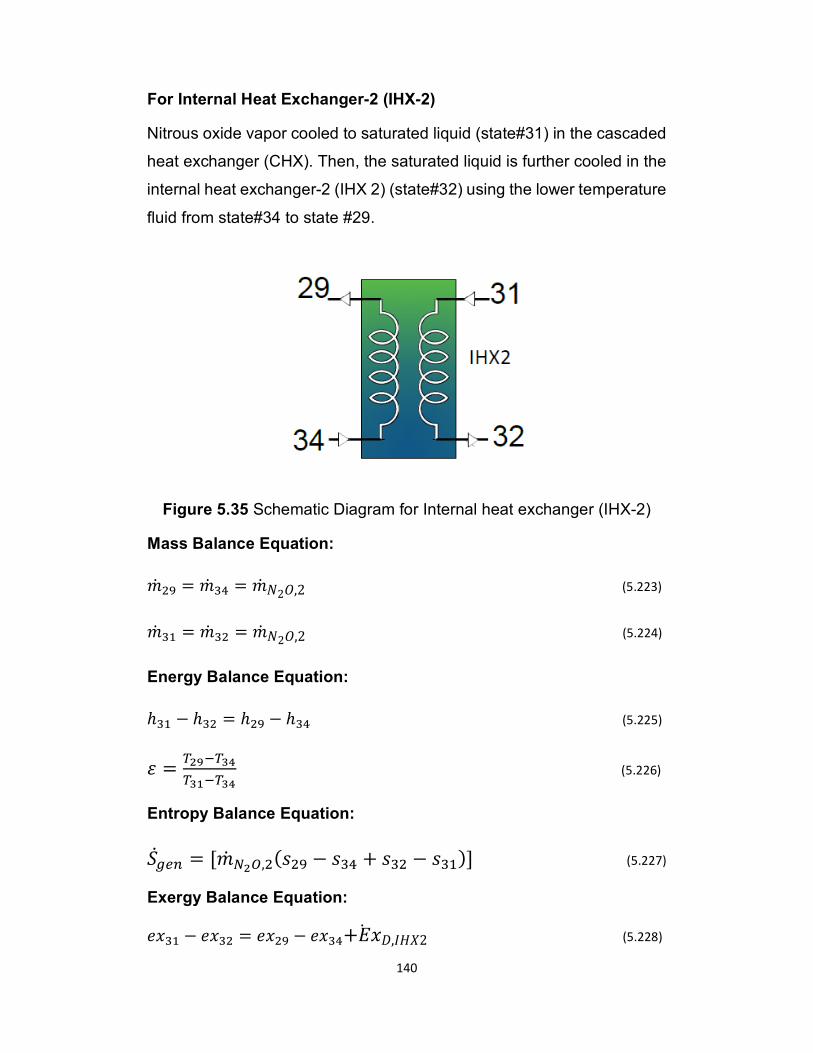
140
For Internal Heat Exchanger-2 (IHX-2)
Nitrous oxide vapor cooled to saturated liquid (state#31) in the cascaded
heat exchanger (CHX). Then, the saturated liquid is further cooled in the
internal heat exchanger-2 (IHX 2) (state#32) using the lower temperature
fluid from state#34 to state #29.
Figure 5.35 Schematic Diagram for Internal heat exchanger (IHX-2)
Mass Balance Equation:
�& .£ = �& Wb = �& �2 ,2 (5.223)
�& W- = �& W. = �& �2 ,2 (5.224)
Energy Balance Equation:
ℎW- − ℎW. = ℎ.£ − ℎWb (5.225)
� = BMØ�BN³BNK�BN³ (5.226)
Entropy Balance Equation:
?&l2k = [�& _M`,.(�.£ − �Wb + �W. − �W-)] (5.227)
Exergy Balance Equation:
�CW- − �CW. = �C.£ − �CWb+5C& E,»8¤2 (5.228)
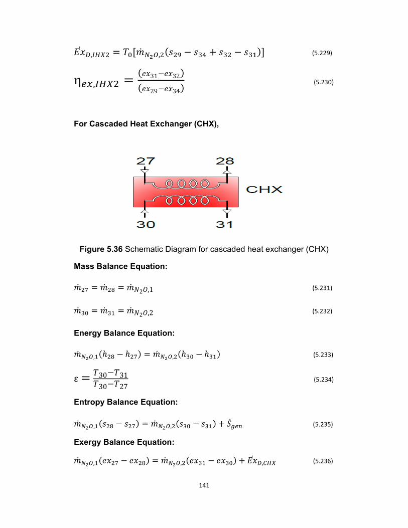
141
5C& s,H®r. = D[[�& _M`,.(�.£ − �Wb + �W. − �W-)] (5.229) η2t,H®r. = (�C31−�C32)(�C29−�C34) (5.230)
For Cascaded Heat Exchanger (CHX),
Figure 5.36 Schematic Diagram for cascaded heat exchanger (CHX)
Mass Balance Equation:
�& .Ö = �& .� = �& �2 ,1 (5.231)
�& W[ = �& W- = �& �2 ,2 (5.232)
Energy Balance Equation:
�& _M`,-(ℎ.� − ℎ.Ö) = �& _M`,.(ℎW[ − ℎW-) (5.233)
ε = D30−D31D30−D27 (5.234)
Entropy Balance Equation:
�& _M`,-(�.� − �.Ö) = �& _M`,.(�W[ − �W-) + ?&l2k (5.235)
Exergy Balance Equation: �& _M`,-(�C.Ö − �C.�) = �& _M`,.(�CW- − �CW[) + 5C& s,'®r (5.236)
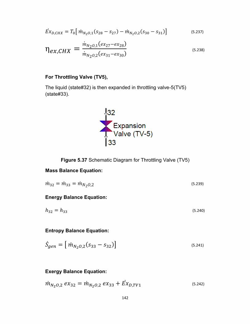
142
5C& s,'®r = D[° �& _M`,-(�.� − �.Ö) − �& _M`,.(�W[ − �W-)± (5.237)
η2t,'®r = �& �2 ,1(�C27−�C28)�& �2 ,2(�C31−�C30) (5.238)
For Throttling Valve (TV5),
The liquid (state#32) is then expanded in throttling valve-5(TV5)
(state#33).
Figure 5.37 Schematic Diagram for Throttling Valve (TV5)
Mass Balance Equation:
�& W. = �& WW = �& �2 ,2 (5.239)
Energy Balance Equation:
ℎW. = ℎWW (5.240)
Entropy Balance Equation:
?&l2k = ° �& _M`,.(�WW − �W.)± (5.241)
Exergy Balance Equation: �& _M`,. �CW. = �& _M`,. �CWW + 5C& s,B(- (5.242)
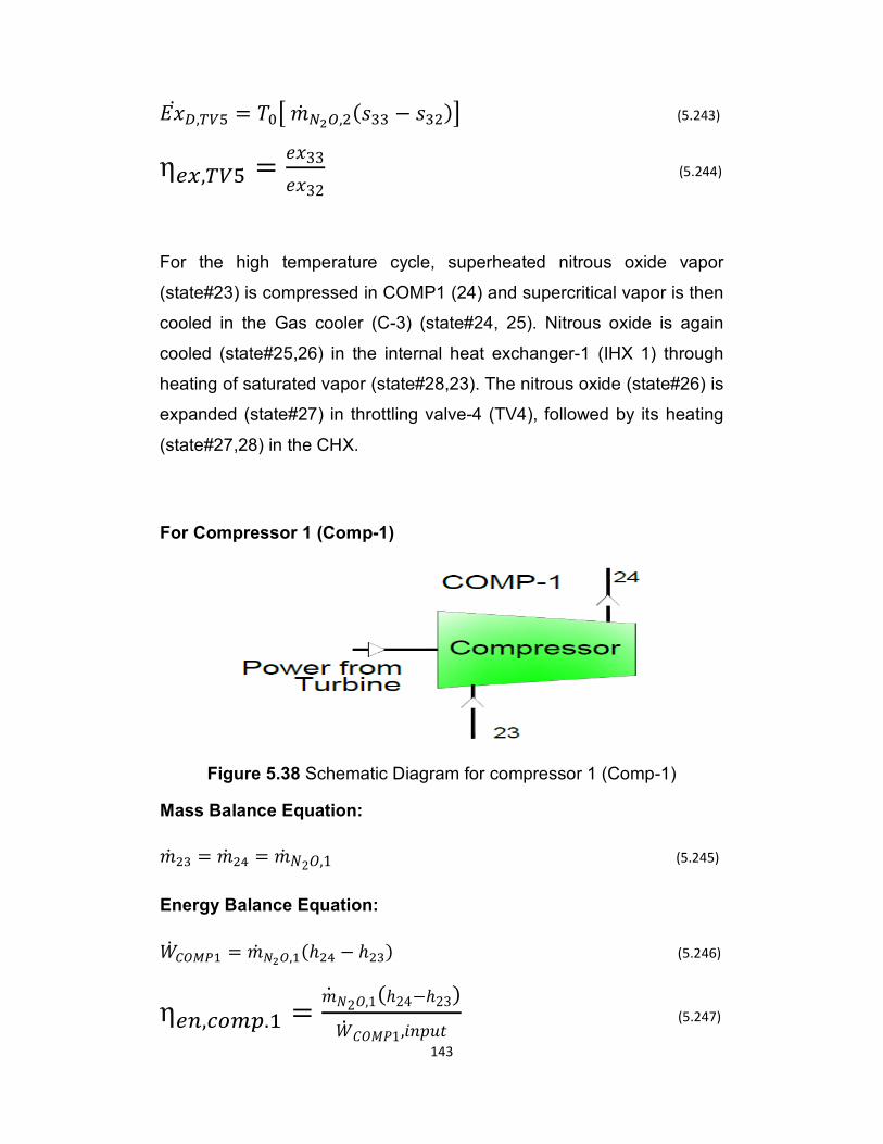
143
5C& s,B(] = D[° �& _M`,.(�WW − �W.)± (5.243) η2t,B(] = �C33�C32 (5.244)
For the high temperature cycle, superheated nitrous oxide vapor
(state#23) is compressed in COMP1 (24) and supercritical vapor is then
cooled in the Gas cooler (C-3) (state#24, 25). Nitrous oxide is again
cooled (state#25,26) in the internal heat exchanger-1 (IHX 1) through
heating of saturated vapor (state#28,23). The nitrous oxide (state#26) is
expanded (state#27) in throttling valve-4 (TV4), followed by its heating
(state#27,28) in the CHX.
For Compressor 1 (Comp-1)
Figure 5.38 Schematic Diagram for compressor 1 (Comp-1)
Mass Balance Equation:
�& .W = �& .b = �& �2 ,1 (5.245)
Energy Balance Equation:
)& '`j«- = �& _M`,-(ℎ.b − ℎ.W) (5.246) η2k,�@{~.- = �& �2 ,1(ℎ24−ℎ23))& F <=1,�3�� (5.247)
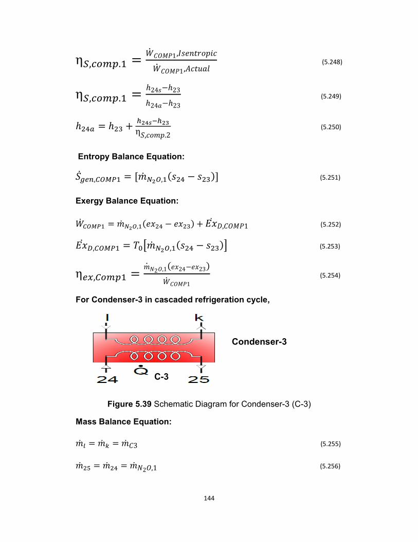
144
η>,�@{~.- = )& F <=1,»�����3��)& F <=1,6����� (5.248)
η>,�@{~.- = ℎ24�−ℎ23ℎ24�−ℎ23 (5.249)
ℎ.bU = ℎ.W + wM³h�wMNη?,���3.2 (5.250)
Entropy Balance Equation: ?&l2k,'`j«- = [�& _M`,-(�.b − �.W)] (5.251)
Exergy Balance Equation:
)& '`j«- = �& _M`,-(�C.b − �C.W) + 5C& E,F <=1 (5.252) 5C& s,'`j«- = D[°�& _M`,-(�.b − �.W)± (5.253)
η2t,'@{~- = �& �2 ,1(�C24−�C23))& F <=1 (5.254)
For Condenser-3 in cascaded refrigeration cycle,
Figure 5.39 Schematic Diagram for Condenser-3 (C-3)
Mass Balance Equation:
�& T = �& � = �& F3 (5.255)
�& .] = �& .b = �& �2 ,1 (5.256)
Condenser-3
C-3
145
Energy Balance Equation:
%&'W = �& _M`,-(ℎ.] − ℎ.b) = �& _M`,-(ℎ� − ℎT) (5.257)
Entropy Balance Equation:
�& 'W(�.] − �.b) = �& _M`,-(�T − ��) + ?&l2k (5.258)
Exergy Balance Equation: �& _M`,-(�C.] − �C.b) + 5C& E,F3 = �& _M`,-(�CT − �C�) (5.259) 5C& s,'W = D[�& _M`,-[ (�� − �T) + (�.] − �.b)] (5.260)
η2t,'W = �& F3(�C�−�C�)�& �2 ,1(�C24−�C25) (5.261)
T24 is the temperature for the Refrigerant vapor in a superheated state.
In the condenser, the superheated refrigerant vapor condenses to
saturated vapor, which is at a constant temperature T25. TL represent
cooled water from cooling tower, 30°C, under typical summer conditions.
The temperature difference can be defined as:
|D'W = D.] − D� (5.262)
Since TL is 30°C, the lower the value of ΔTC3, the more efficient the heat
transfer, and the lower the exergy destruction in the condenser.
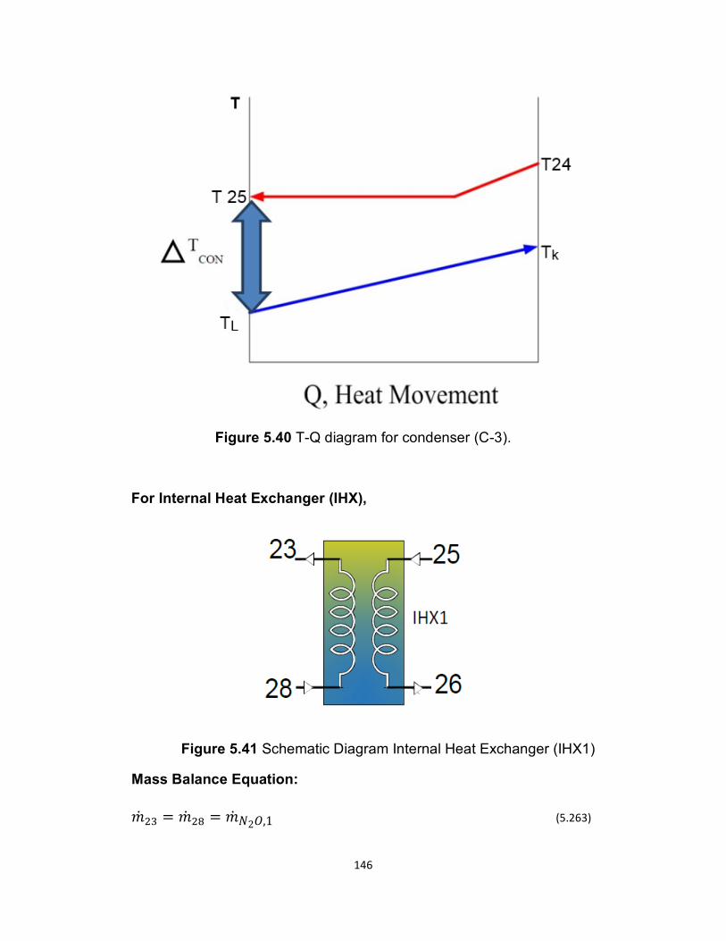
146
Figure 5.40 T-Q diagram for condenser (C-3).
For Internal Heat Exchanger (IHX),
Figure 5.41 Schematic Diagram Internal Heat Exchanger (IHX1)
Mass Balance Equation:
�& .W = �& .� = �& �2 ,1 (5.263)
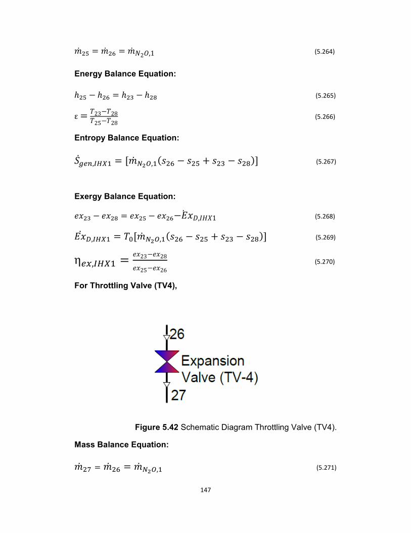
147
�& .] = �& .^ = �& �2 ,1 (5.264)
Energy Balance Equation:
ℎ.] − ℎ.^ = ℎ.W − ℎ.� (5.265)
ε = D23−D28D25−D28 (5.266)
Entropy Balance Equation:
?&l2k,H®r- = [�& _M`,-(�.^ − �.] + �.W − �.�)] (5.267)
Exergy Balance Equation:
�C.W − �C.� = �C.] − �C.^−5C& E,»8¤1 (5.268) 5C& s,H®r- = D[[�& _M`,-(�.^ − �.] + �.W − �.�)] (5.269) η2t,H®r- = �C23−�C28�C25−�C26 (5.270)
For Throttling Valve (TV4),
Figure 5.42 Schematic Diagram Throttling Valve (TV4).
Mass Balance Equation:
�& .Ö = �& .^ = �& _M`,- (5.271)
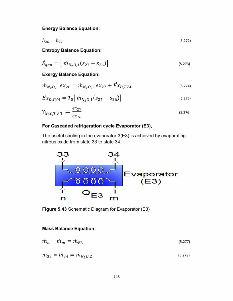
148
Energy Balance Equation:
ℎ.^ = ℎ.Ö (5.272)
Entropy Balance Equation:
?&l2k = ° �& _M`,-(�.Ö − �.^)± (5.273)
Exergy Balance Equation: �& _M`,- �C.^ = �& _M`,- �C.Ö + 5C& s,B(b (5.274)
5C& s,B(b = D[° �& _M`,-(�.Ö − �.^)± (5.275) η2t,B(- = �C27�C26 (5.276)
For Cascaded refrigeration cycle Evaporator (E3),
The useful cooling in the evaporator-3(E3) is achieved by evaporating
nitrous oxide from state 33 to state 34.
Figure 5.43 Schematic Diagram for Evaporator (E3)
Mass Balance Equation:
�& k = �& { = �& W (5.277)
�& WW = �& Wb = �& _M`,. (5.278)
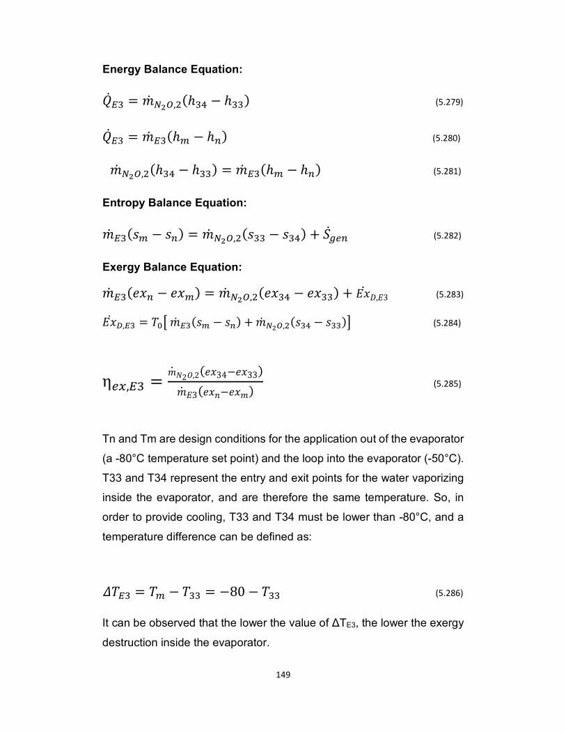
149
Energy Balance Equation:
%& W = �& _M`,.(ℎWb − ℎWW) (5.279)
%& W = �& W(ℎ{ − ℎk) (5.280)
�& _M`,.(ℎWb − ℎWW) = �& W(ℎ{ − ℎk) (5.281)
Entropy Balance Equation:
�& W(�{ − �k) = �& _M`,.(�WW − �Wb) + ?&l2k (5.282)
Exergy Balance Equation: �& W(�Ck − �C{) = �& _M`,.(�CWb − �CWW) + 5C& E,53 (5.283)
5C& s, W = D[° �& W(�{ − �k) + �& _M`,.(�Wb − �WW)± (5.284)
η2t, W = �& �2 ,2(�C34−�C33)�& 53(�C−�C�) (5.285)
Tn and Tm are design conditions for the application out of the evaporator
(a -80°C temperature set point) and the loop into the evaporator (-50°C).
T33 and T34 represent the entry and exit points for the water vaporizing
inside the evaporator, and are therefore the same temperature. So, in
order to provide cooling, T33 and T34 must be lower than -80°C, and a
temperature difference can be defined as:
|D W = D{ − DWW = −80 − DWW (5.286)
It can be observed that the lower the value of ΔTE3, the lower the exergy
destruction inside the evaporator.
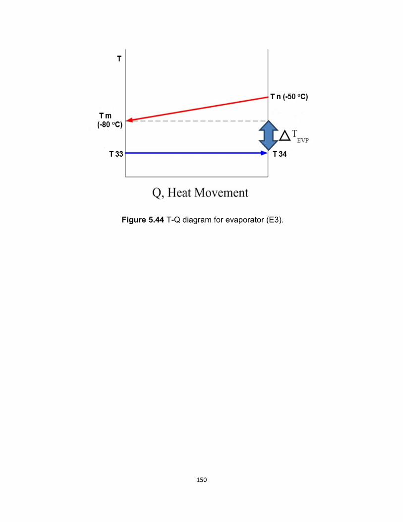
150
Figure 5.44 T-Q diagram for evaporator (E3).
151
CHAPTER 6
RESULT AND DISCUSSION
A thermodynamic analysis has been conducted to assess the
performance variation of the solar assisted triple effect refrigeration
system with varying some influential operating parameter.
Some of operating parameter will vary over a typical range of operation
to find out its effect on the overall cycle whereas values of other
parameters are kept constant at the level of base case values.
The first law efficiency and energy distribution of solar heat source are
obtained by energy balance approach or the first law analysis of the
cycle. However, the exergy destruction or irreversibility in each
component and the second law efficiency are obtained using the exergy
balance approach or the second law analysis of the cycle.
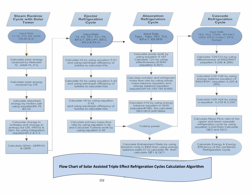
153
Flow Chart of Solar Assisted Triple Effect Refrigeration Cycles Calculation Algorithm
152
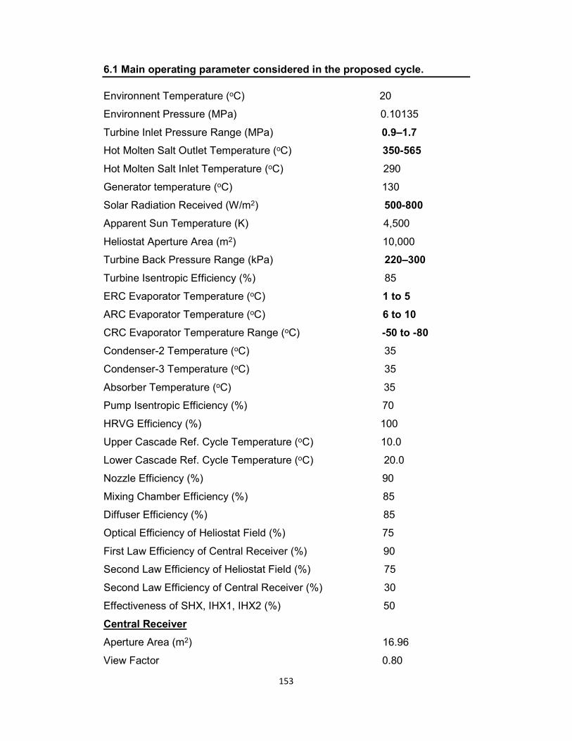
153
6.1 Main operating parameter considered in the proposed cycle.
20 C) oemperature (T Environnent
Environnent Pressure (MPa) 0.10135
Turbine Inlet Pressure Range (MPa) 0.9–1.7
565-503 ) Coemperature (Tutlet OHot Molten Salt
290 C) oemperature (Tnlet IHot Molten Salt
130 C) otemperature (Generator
008-500 )2eceived (W/mRadiation Solar R
Apparent Sun Temperature (K) 4,500
00010, ) 2(m reaAperture AHeliostat
Turbine Back Pressure Range (kPa) 220–300
Turbine Isentropic Efficiency (%) 85
5to 1 C) o(emperature Tvaporator E ERC
to 10 6 C) oemperature (TEvaporator ARC
80-50 to - C) oange (Remperature Tvaporator ECRC
35 C) oemperature (T2 -Condenser
C) 35oemperature (T3 -Condenser
35 C) oemperature (TAbsorber
Pump Isentropic Efficiency (%) 70
HRVG Efficiency (%) 100
10.0 C) oemperature (T ycleCUpper Cascade Ref.
0.02 C) oemperature (T ycleCLower Cascade Ref.
Nozzle Efficiency (%) 90
Mixing Chamber Efficiency (%) 85
Diffuser Efficiency (%) 85
Optical Efficiency of Heliostat Field (%) 75
First Law Efficiency of Central Receiver (%) 90
Second Law Efficiency of Heliostat Field (%) 75
Second Law Efficiency of Central Receiver (%) 30
Effectiveness of SHX, IHX1, IHX2 (%) 50
Central Receiver
96.61 )2rea (mAAperture
View Factor 0.80
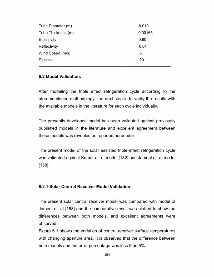
154
Tube Diameter (m) 0.019
Tube Thickness (m) 0.00165
Emissivity 0.80
Reflectivity 0.04
Wind Speed (m/s) 5
Passes 20 ____________________________________________________________
6.2 Model Validation:
After modeling the triple effect refrigeration cycle according to the
aforementioned methodology, the next step is to verify the results with
the available models in the literature for each cycle individually.
The presently developed model has been validated against previously
published models in the literature and excellent agreement between
these models was revealed as reported hereunder.
The present model of the solar assisted triple effect refrigeration cycle
was validated against Kumar et. al model [132] and Jameel et. al model
[158].
6.2.1 Solar Central Receiver Model Validation:
The present solar central receiver model was compared with model of
Jameel et. al [158] and the comparative result was plotted to show the
differences between both models, and excellent agreements were
observed.
Figure 6.1 shows the variation of central receiver surface temperatures
with changing aperture area. It is observed that the difference between
both models and the error percentage was less than 5%.
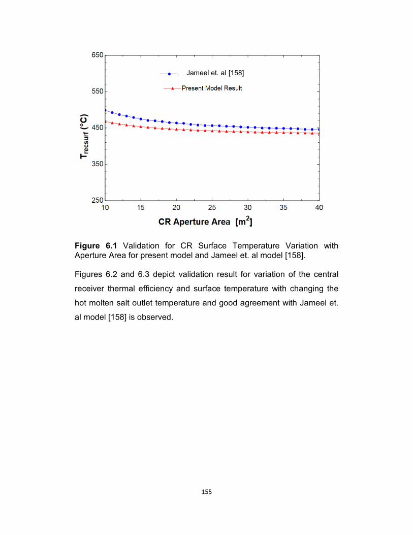
155
Figure 6.1 Validation for CR Surface Temperature Variation with Aperture Area for present model and Jameel et. al model [158]. Figures 6.2 and 6.3 depict validation result for variation of the central
receiver thermal efficiency and surface temperature with changing the
hot molten salt outlet temperature and good agreement with Jameel et.
al model [158] is observed.
]158[ Jameel et. al
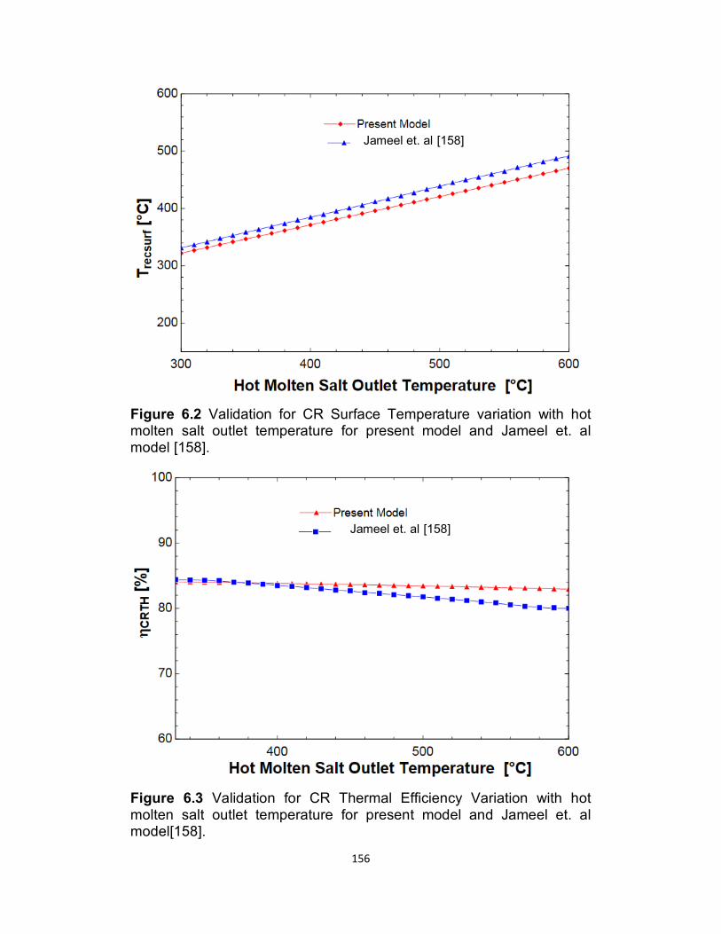
156
Figure 6.2 Validation for CR Surface Temperature variation with hot molten salt outlet temperature for present model and Jameel et. al model [158].
Figure 6.3 Validation for CR Thermal Efficiency Variation with hot molten salt outlet temperature for present model and Jameel et. al model[158].
]158[
Jameel’s Model [158]
Jameel’s Model [158]
]158[ Jameel et. al
]158[ Jameel et. al
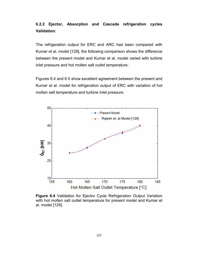
157
6.2.2 Ejector, Absorption and Cascade refrigeration cycles
Validation:
The refrigeration output for ERC and ARC had been compared with
Kumar et al. model [129], the following comparison shows the difference
between the present model and Kumar et al. model varied with turbine
inlet pressure and hot molten salt outlet temperature:
Figures 6.4 and 6.5 show excellent agreement between the present and
Kumar et al. model for refrigeration output of ERC with variation of hot
molten salt temperature and turbine inlet pressure.
Figure 6.4 Validation for Ejector Cycle Refrigeration Output Variation with hot molten salt outlet temperature for present model and Kumar et al. model [129].
Rajesh et. al Model [129]
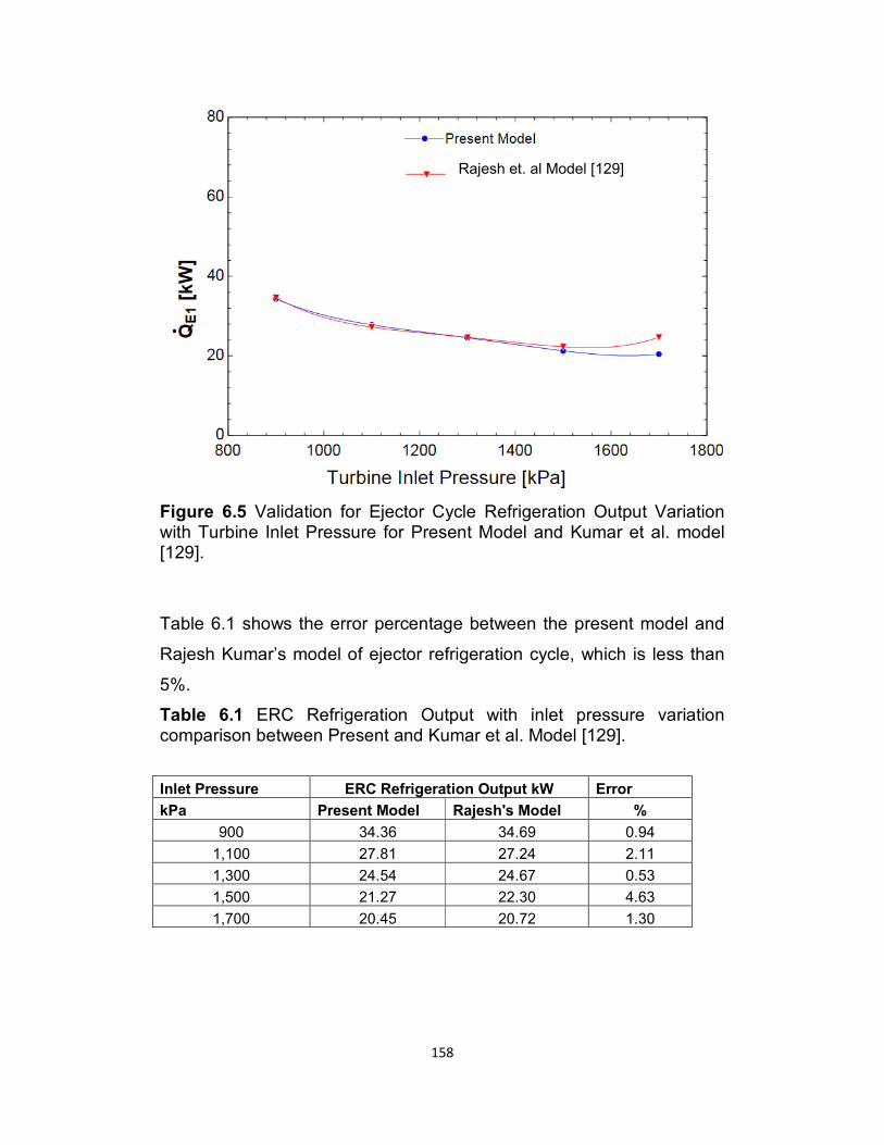
158
Figure 6.5 Validation for Ejector Cycle Refrigeration Output Variation with Turbine Inlet Pressure for Present Model and Kumar et al. model [129].
Table 6.1 shows the error percentage between the present model and
Rajesh Kumar’s model of ejector refrigeration cycle, which is less than
5%.
Table 6.1 ERC Refrigeration Output with inlet pressure variation comparison between Present and Kumar et al. Model [129].
Inlet Pressure ERC Refrigeration Output kW Error
kPa Present Model Rajesh's Model %
900 34.36 34.69 0.94
1,100 27.81 27.24 2.11
1,300 24.54 24.67 0.53
1,500 21.27 22.30 4.63
1,700 20.45 20.72 1.30
Rajesh’s Model [129] Rajesh et. al Model [129]
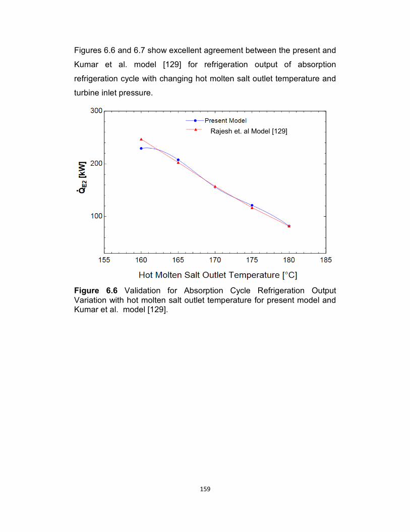
159
Figures 6.6 and 6.7 show excellent agreement between the present and
Kumar et al. model [129] for refrigeration output of absorption
refrigeration cycle with changing hot molten salt outlet temperature and
turbine inlet pressure.
Figure 6.6 Validation for Absorption Cycle Refrigeration Output Variation with hot molten salt outlet temperature for present model and Kumar et al. model [129].
Rajesh’s Model [129] Rajesh et. al Model [129]
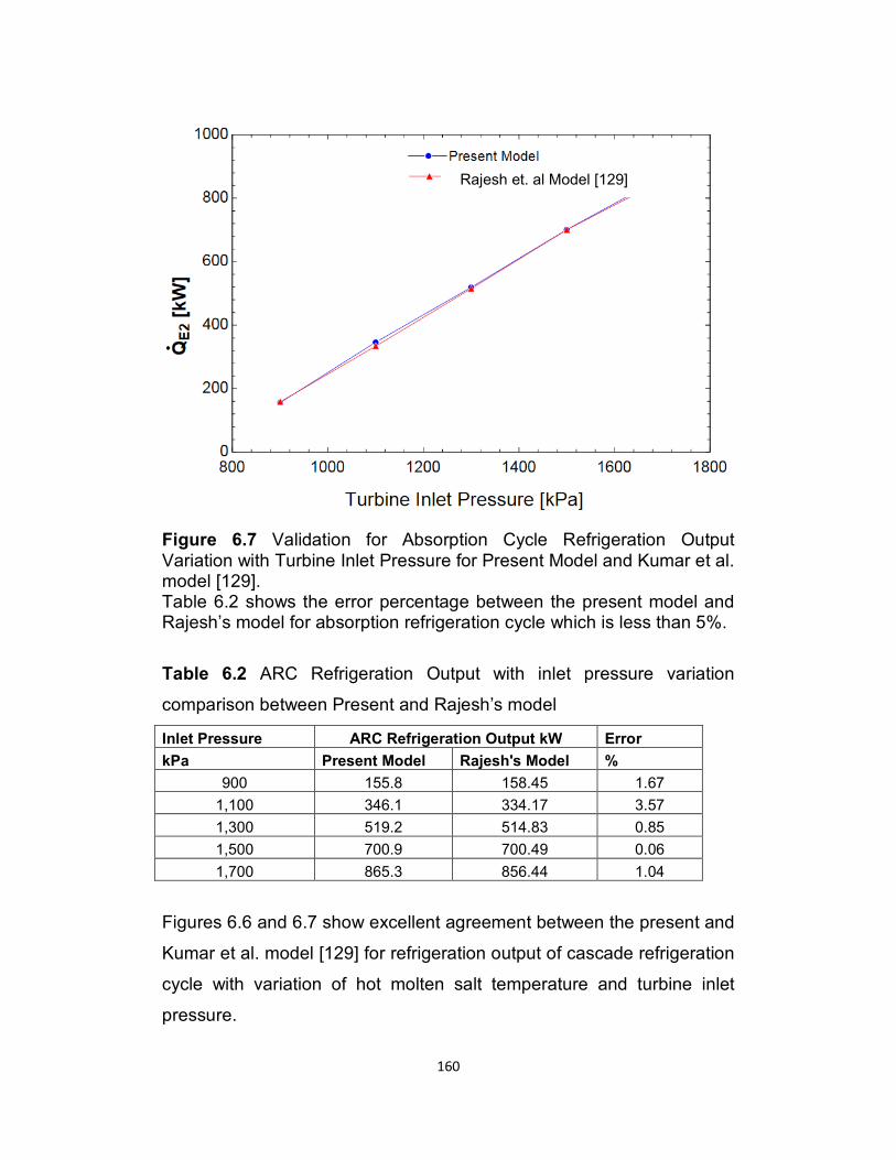
160
Figure 6.7 Validation for Absorption Cycle Refrigeration Output Variation with Turbine Inlet Pressure for Present Model and Kumar et al. model [129]. Table 6.2 shows the error percentage between the present model and Rajesh’s model for absorption refrigeration cycle which is less than 5%.
Table 6.2 ARC Refrigeration Output with inlet pressure variation
comparison between Present and Rajesh’s model
Inlet Pressure ARC Refrigeration Output kW Error
kPa Present Model Rajesh's Model %
900 155.8 158.45 1.67
1,100 346.1 334.17 3.57
1,300 519.2 514.83 0.85
1,500 700.9 700.49 0.06
1,700 865.3 856.44 1.04
Figures 6.6 and 6.7 show excellent agreement between the present and
Kumar et al. model [129] for refrigeration output of cascade refrigeration
cycle with variation of hot molten salt temperature and turbine inlet
pressure.
Rajesh’s Model [129] Rajesh et. al Model [129]
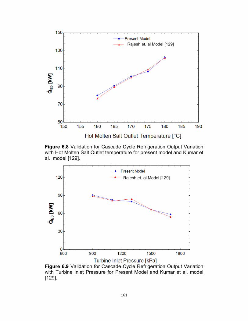
161
Figure 6.8 Validation for Cascade Cycle Refrigeration Output Variation with Hot Molten Salt Outlet temperature for present model and Kumar et al. model [129].
Figure 6.9 Validation for Cascade Cycle Refrigeration Output Variation with Turbine Inlet Pressure for Present Model and Kumar et al. model [129].
Rajesh’s Model [129]
Rajesh’s Model [129]
Rajesh et. al Model [129]
Rajesh et. al Model [129]
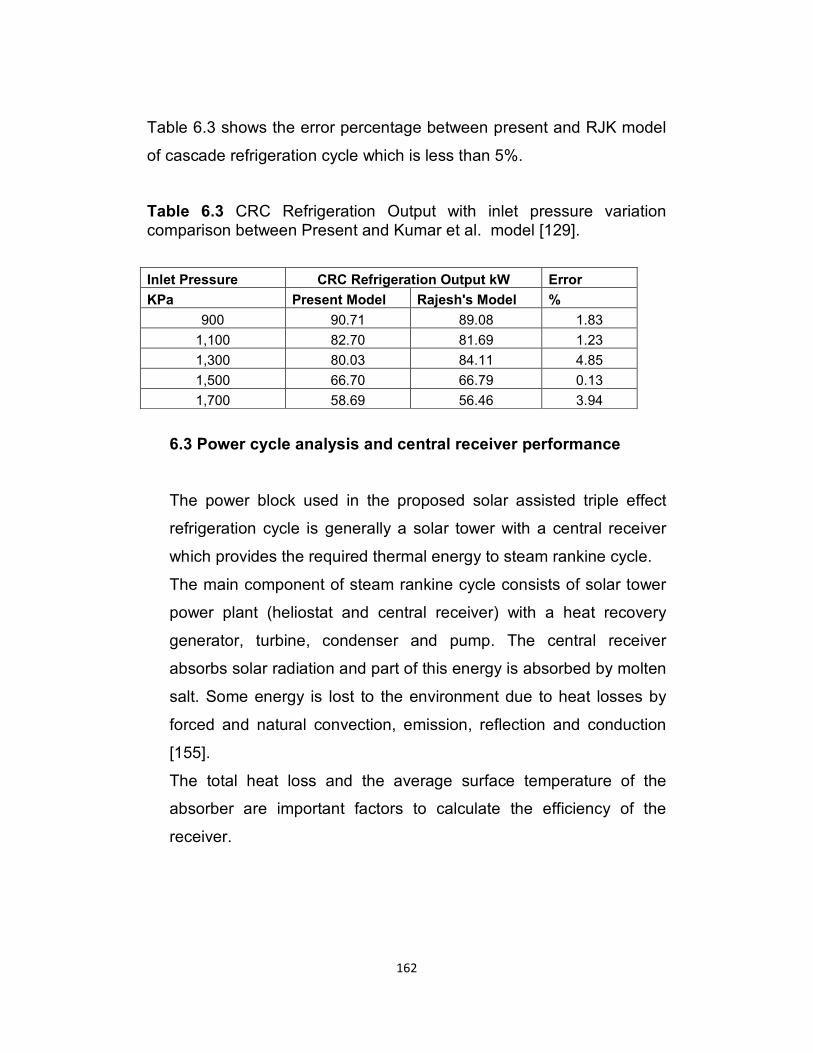
162
Table 6.3 shows the error percentage between present and RJK model
of cascade refrigeration cycle which is less than 5%.
Table 6.3 CRC Refrigeration Output with inlet pressure variation comparison between Present and Kumar et al. model [129].
Inlet Pressure CRC Refrigeration Output kW Error
KPa Present Model Rajesh's Model %
900 90.71 89.08 1.83
1,100 82.70 81.69 1.23
1,300 80.03 84.11 4.85
1,500 66.70 66.79 0.13
1,700 58.69 56.46 3.94
6.3 Power cycle analysis and central receiver performance
The power block used in the proposed solar assisted triple effect
refrigeration cycle is generally a solar tower with a central receiver
which provides the required thermal energy to steam rankine cycle.
The main component of steam rankine cycle consists of solar tower
power plant (heliostat and central receiver) with a heat recovery
generator, turbine, condenser and pump. The central receiver
absorbs solar radiation and part of this energy is absorbed by molten
salt. Some energy is lost to the environment due to heat losses by
forced and natural convection, emission, reflection and conduction
[155].
The total heat loss and the average surface temperature of the
absorber are important factors to calculate the efficiency of the
receiver.
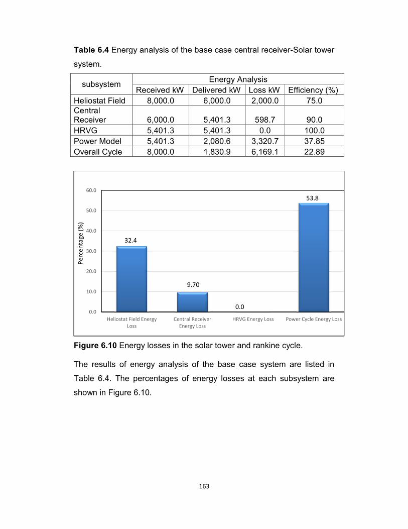
163
Table 6.4 Energy analysis of the base case central receiver-Solar tower
system.
subsystem Energy Analysis
Received kW Delivered kW Loss kW Efficiency (%)
Heliostat Field 8,000.0 6,000.0 2,000.0 75.0
Central Receiver 6,000.0 5,401.3 598.7 90.0
HRVG 5,401.3 5,401.3 0.0 100.0
Power Model 5,401.3 2,080.6 3,320.7 37.85
Overall Cycle 8,000.0 1,830.9 6,169.1 22.89
Figure 6.10 Energy losses in the solar tower and rankine cycle. The results of energy analysis of the base case system are listed in
Table 6.4. The percentages of energy losses at each subsystem are
shown in Figure 6.10.
0.0
10.0
20.0
30.0
40.0
50.0
60.0
Heliostat Field Energy
Loss
Central Receiver
Energy Loss
HRVG Energy Loss Power Cycle Energy Loss
32.4
0.0
53.8
Pe
rce
nta
ge
(%)
9.70
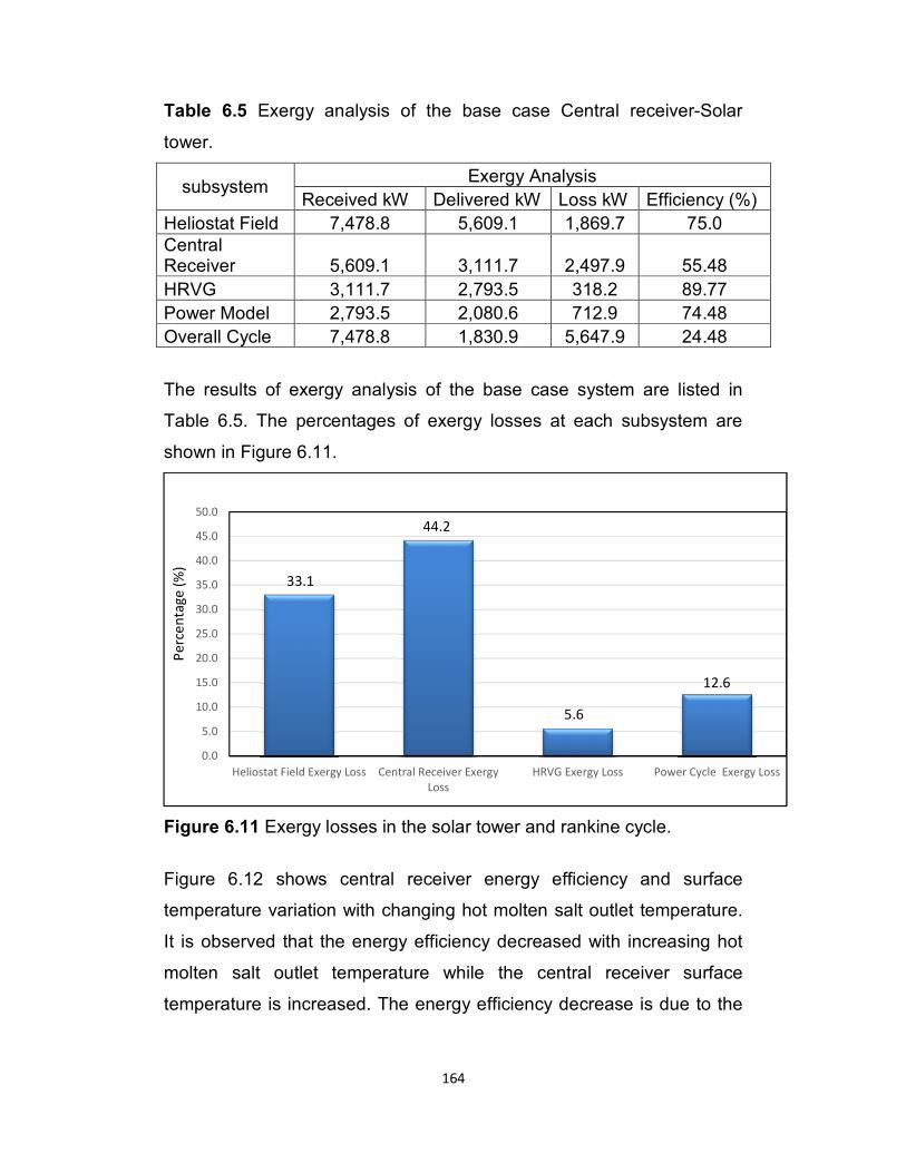
164
Table 6.5 Exergy analysis of the base case Central receiver-Solar
tower.
subsystem Exergy Analysis
Received kW Delivered kW Loss kW Efficiency (%)
Heliostat Field 7,478.8 5,609.1 1,869.7 75.0
Central Receiver 5,609.1 3,111.7 2,497.9 55.48
HRVG 3,111.7 2,793.5 318.2 89.77
Power Model 2,793.5 2,080.6 712.9 74.48
Overall Cycle 7,478.8 1,830.9 5,647.9 24.48
The results of exergy analysis of the base case system are listed in
Table 6.5. The percentages of exergy losses at each subsystem are
shown in Figure 6.11.
Figure 6.11 Exergy losses in the solar tower and rankine cycle.
Figure 6.12 shows central receiver energy efficiency and surface
temperature variation with changing hot molten salt outlet temperature.
It is observed that the energy efficiency decreased with increasing hot
molten salt outlet temperature while the central receiver surface
temperature is increased. The energy efficiency decrease is due to the
0.0
5.0
10.0
15.0
20.0
25.0
30.0
35.0
40.0
45.0
50.0
Heliostat Field Exergy Loss Central Receiver Exergy
Loss
HRVG Exergy Loss Power Cycle Exergy Loss
33.1
44.2
5.6
12.6
Pe
rce
nta
ge
(%)
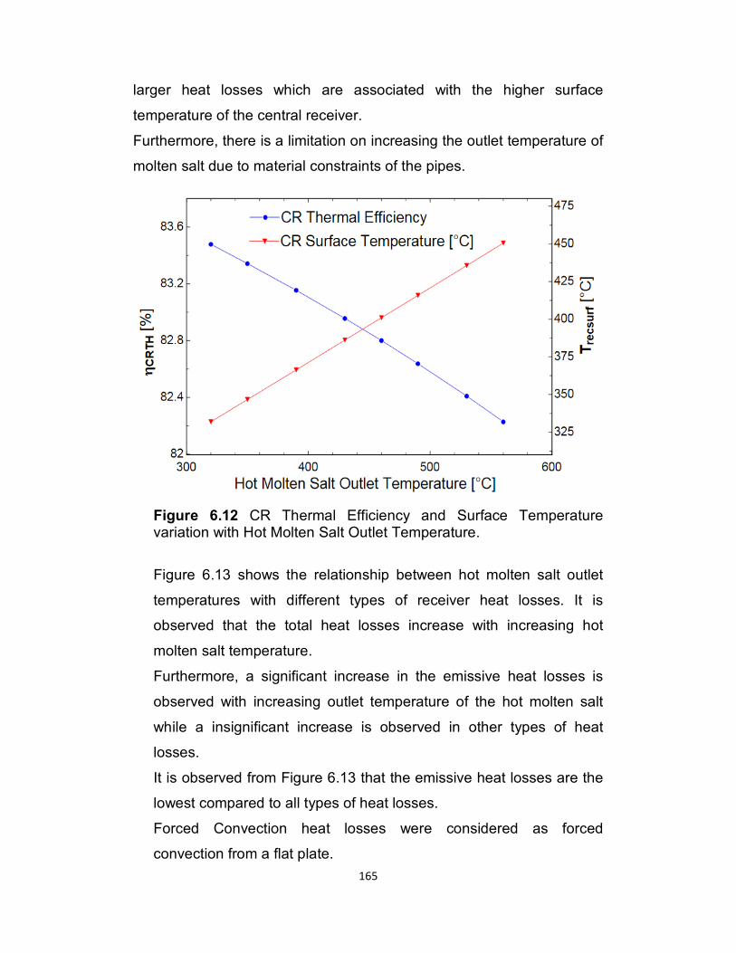
165
larger heat losses which are associated with the higher surface
temperature of the central receiver.
Furthermore, there is a limitation on increasing the outlet temperature of
molten salt due to material constraints of the pipes.
Figure 6.12 CR Thermal Efficiency and Surface Temperature variation with Hot Molten Salt Outlet Temperature.
Figure 6.13 shows the relationship between hot molten salt outlet
temperatures with different types of receiver heat losses. It is
observed that the total heat losses increase with increasing hot
molten salt temperature.
Furthermore, a significant increase in the emissive heat losses is
observed with increasing outlet temperature of the hot molten salt
while a insignificant increase is observed in other types of heat
losses.
It is observed from Figure 6.13 that the emissive heat losses are the
lowest compared to all types of heat losses.
Forced Convection heat losses were considered as forced
convection from a flat plate.
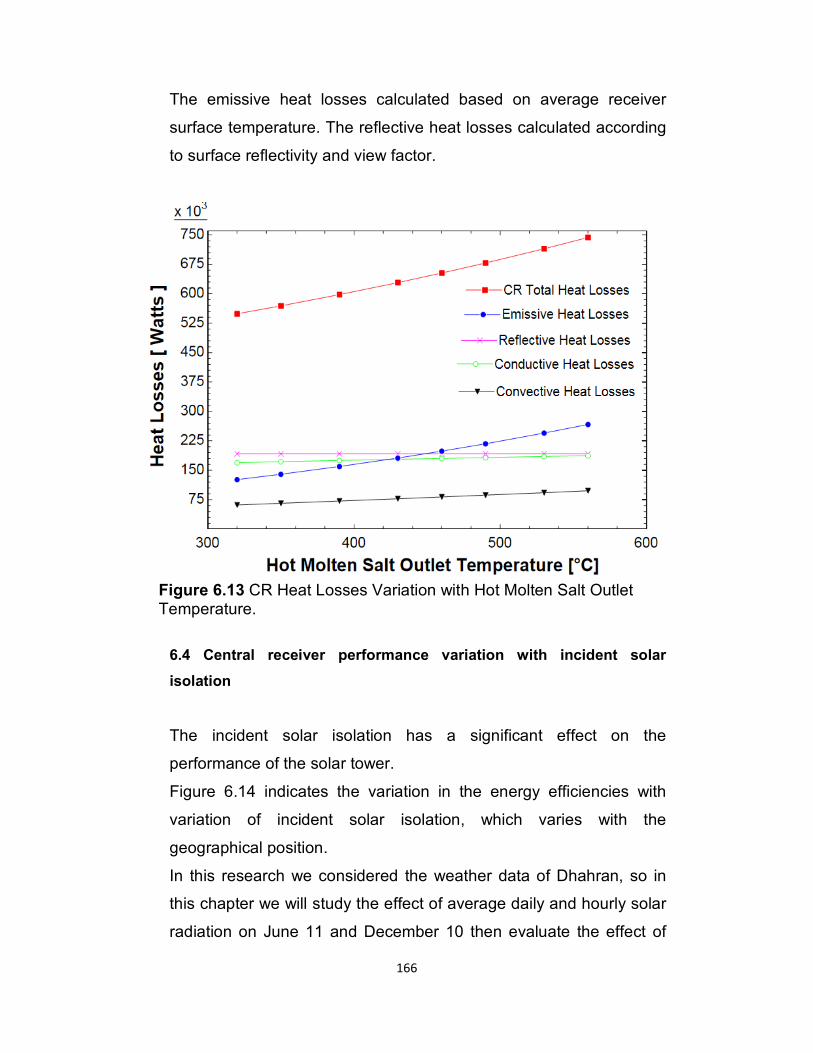
166
The emissive heat losses calculated based on average receiver
surface temperature. The reflective heat losses calculated according
to surface reflectivity and view factor.
Figure 6.13 CR Heat Losses Variation with Hot Molten Salt Outlet Temperature.
6.4 Central receiver performance variation with incident solar
isolation
The incident solar isolation has a significant effect on the
performance of the solar tower.
Figure 6.14 indicates the variation in the energy efficiencies with
variation of incident solar isolation, which varies with the
geographical position.
In this research we considered the weather data of Dhahran, so in
this chapter we will study the effect of average daily and hourly solar
radiation on June 11 and December 10 then evaluate the effect of
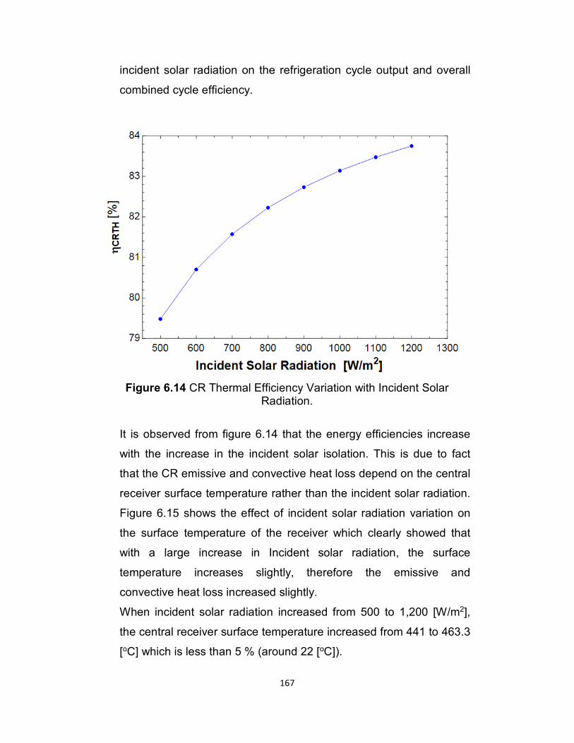
167
incident solar radiation on the refrigeration cycle output and overall
combined cycle efficiency.
Figure 6.14 CR Thermal Efficiency Variation with Incident Solar Radiation.
It is observed from figure 6.14 that the energy efficiencies increase
with the increase in the incident solar isolation. This is due to fact
that the CR emissive and convective heat loss depend on the central
receiver surface temperature rather than the incident solar radiation.
Figure 6.15 shows the effect of incident solar radiation variation on
the surface temperature of the receiver which clearly showed that
with a large increase in Incident solar radiation, the surface
temperature increases slightly, therefore the emissive and
convective heat loss increased slightly.
When incident solar radiation increased from 500 to 1,200 [W/m2],
the central receiver surface temperature increased from 441 to 463.3
[oC] which is less than 5 % (around 22 [oC]).
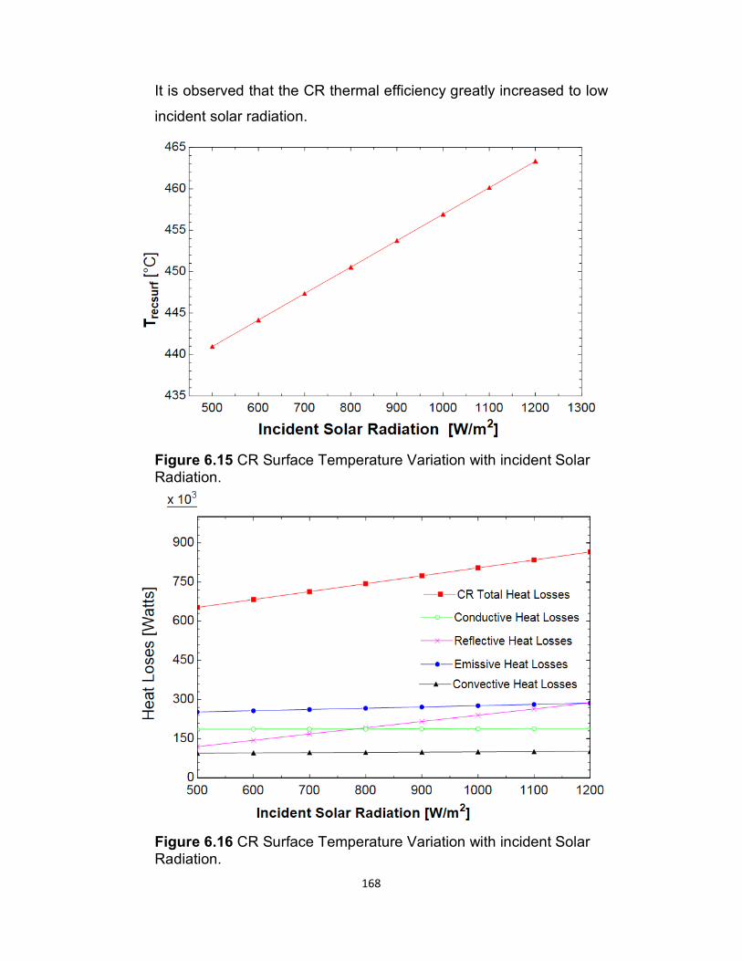
168
It is observed that the CR thermal efficiency greatly increased to low
incident solar radiation.
Figure 6.15 CR Surface Temperature Variation with incident Solar Radiation.
Figure 6.16 CR Surface Temperature Variation with incident Solar Radiation.
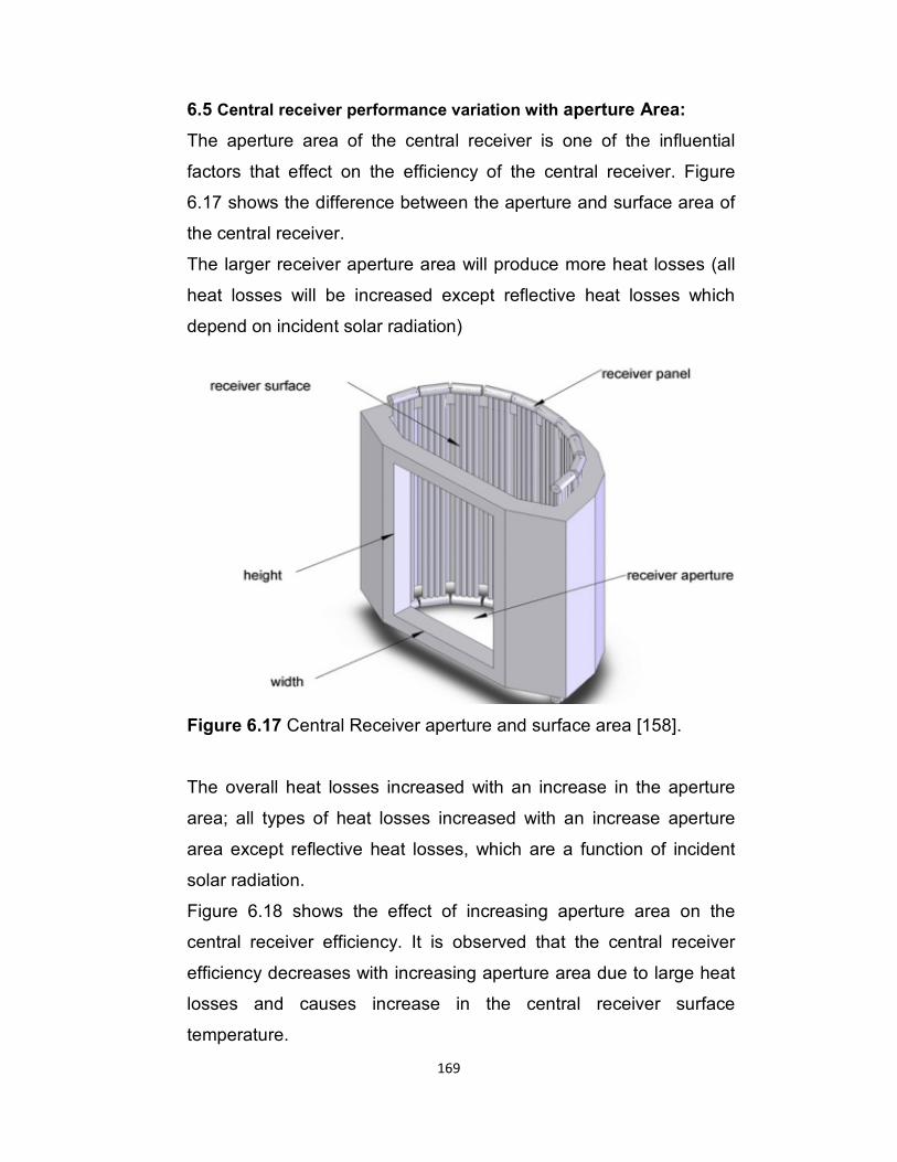
169
6.5 Central receiver performance variation with aperture Area:
The aperture area of the central receiver is one of the influential
factors that effect on the efficiency of the central receiver. Figure
6.17 shows the difference between the aperture and surface area of
the central receiver.
The larger receiver aperture area will produce more heat losses (all
heat losses will be increased except reflective heat losses which
depend on incident solar radiation)
Figure 6.17 Central Receiver aperture and surface area [158].
The overall heat losses increased with an increase in the aperture
area; all types of heat losses increased with an increase aperture
area except reflective heat losses, which are a function of incident
solar radiation.
Figure 6.18 shows the effect of increasing aperture area on the
central receiver efficiency. It is observed that the central receiver
efficiency decreases with increasing aperture area due to large heat
losses and causes increase in the central receiver surface
temperature.
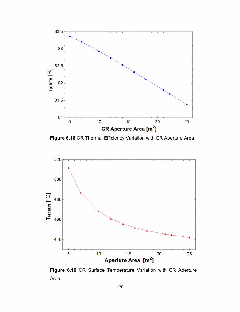
170
Figure 6.18 CR Thermal Efficiency Variation with CR Aperture Area.
Figure 6.19 CR Surface Temperature Variation with CR Aperture
Area.
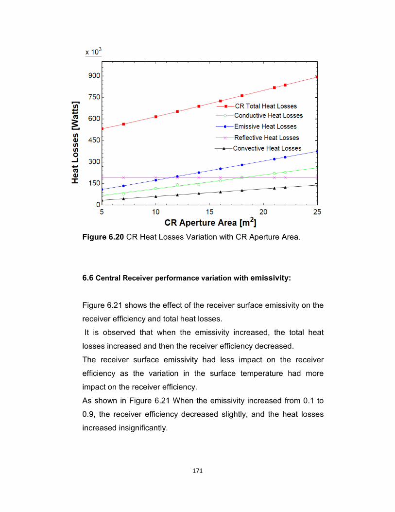
171
Figure 6.20 CR Heat Losses Variation with CR Aperture Area.
6.6 Central Receiver performance variation with emissivity:
Figure 6.21 shows the effect of the receiver surface emissivity on the
receiver efficiency and total heat losses.
It is observed that when the emissivity increased, the total heat
losses increased and then the receiver efficiency decreased.
The receiver surface emissivity had less impact on the receiver
efficiency as the variation in the surface temperature had more
impact on the receiver efficiency.
As shown in Figure 6.21 When the emissivity increased from 0.1 to
0.9, the receiver efficiency decreased slightly, and the heat losses
increased insignificantly.
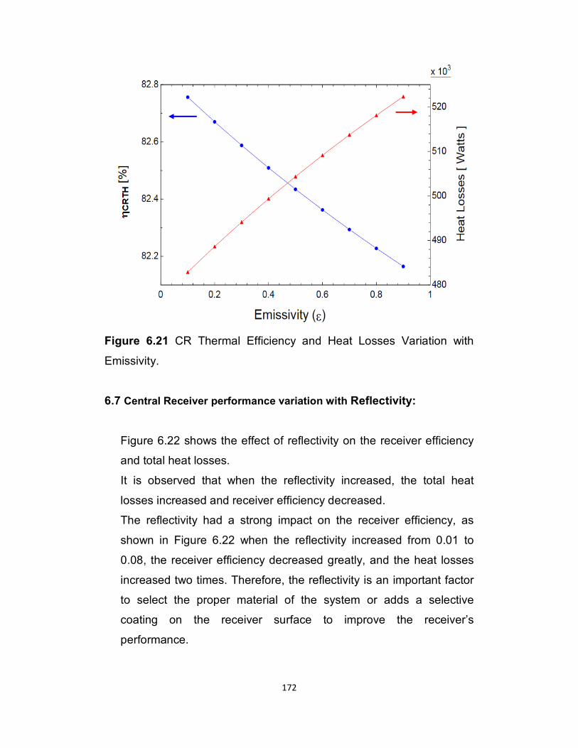
172
Figure 6.21 CR Thermal Efficiency and Heat Losses Variation with
Emissivity.
6.7 Central Receiver performance variation with Reflectivity:
Figure 6.22 shows the effect of reflectivity on the receiver efficiency
and total heat losses.
It is observed that when the reflectivity increased, the total heat
losses increased and receiver efficiency decreased.
The reflectivity had a strong impact on the receiver efficiency, as
shown in Figure 6.22 when the reflectivity increased from 0.01 to
0.08, the receiver efficiency decreased greatly, and the heat losses
increased two times. Therefore, the reflectivity is an important factor
to select the proper material of the system or adds a selective
coating on the receiver surface to improve the receiver’s
performance.
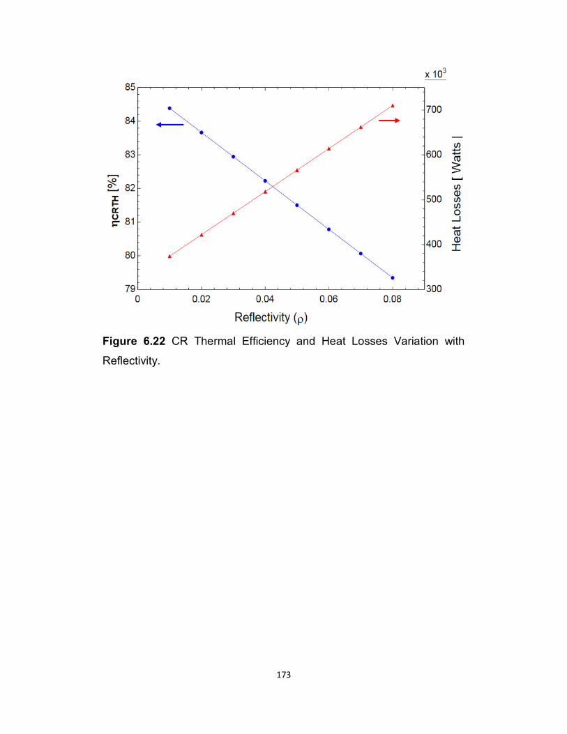
173
Figure 6.22 CR Thermal Efficiency and Heat Losses Variation with
Reflectivity.
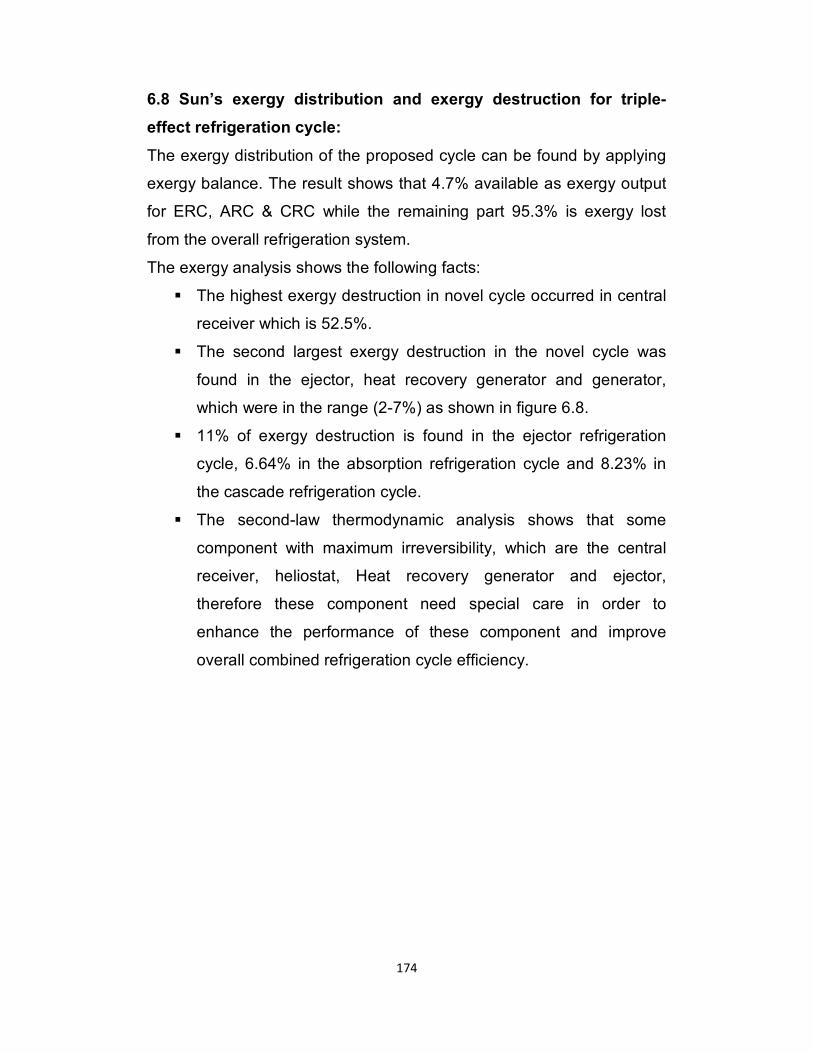
174
6.8 Sun’s exergy distribution and exergy destruction for triple-
effect refrigeration cycle:
The exergy distribution of the proposed cycle can be found by applying
exergy balance. The result shows that 4.7% available as exergy output
for ERC, ARC & CRC while the remaining part 95.3% is exergy lost
from the overall refrigeration system.
The exergy analysis shows the following facts:
� The highest exergy destruction in novel cycle occurred in central
receiver which is 52.5%.
� The second largest exergy destruction in the novel cycle was
found in the ejector, heat recovery generator and generator,
which were in the range (2-7%) as shown in figure 6.8.
� 11% of exergy destruction is found in the ejector refrigeration
cycle, 6.64% in the absorption refrigeration cycle and 8.23% in
the cascade refrigeration cycle.
� The second-law thermodynamic analysis shows that some
component with maximum irreversibility, which are the central
receiver, heliostat, Heat recovery generator and ejector,
therefore these component need special care in order to
enhance the performance of these component and improve
overall combined refrigeration cycle efficiency.
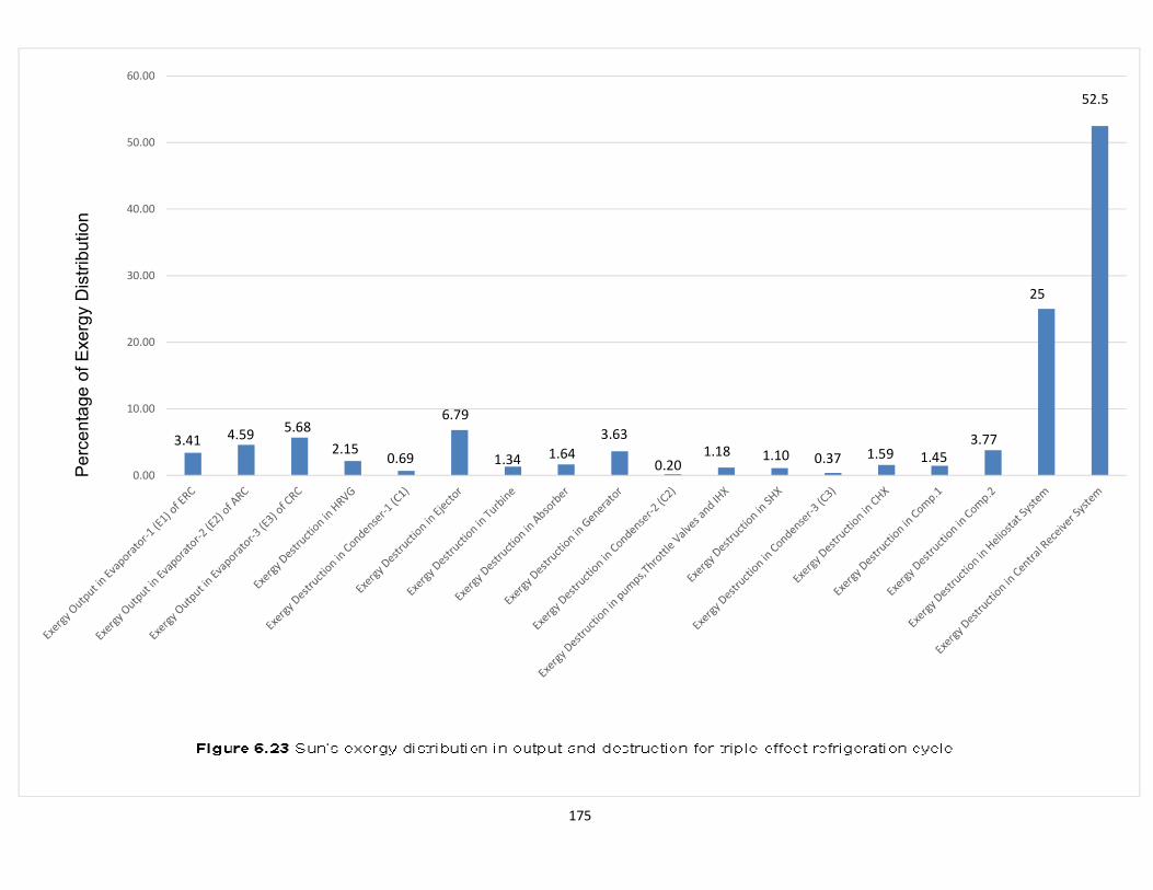
177
.
0.00
10.00
20.00
30.00
40.00
50.00
60.00P
erc
enta
ge o
f E
xerg
y D
istr
ibutio
n
3.411.590.37
25
52.5
1.101.180.20
3.63
1.641.34
6.79
0.692.15
5.684.59 3.77
1.45
175
176
6.9 Variation of the refrigeration output and efficiencies of the
proposed cycle with changing of influential parameter:
Figure 6.24 shows the variation refrigeration output of each
individual cycle and the overall combined refrigeration cycle of the
novel solar assisted multi effect refrigeration cycle with the variation
of hot molten salt outlet temperature.
Figure 6.24 Variation of refrigeration output for triple-effect
refrigeration cycle with hot molten salt outlet temperature.
Figure 6.24 shows that the refrigeration output of ERC and CRC
increases with the increase in hot molten salt outlet temperature
(T1). This is due to the fact that an increase in hot molten
temperature results in heat transfer in HRVG and improves the
thermodynamic properties of the refrigerant at turbine inlet and
leaving state. Therefore turbine power output increases so the
compressor will get more power which increases the mass flow rate
177
of N2O in cascade refrigeration cycle and increases the cooling effect
accordingly.
It is further observed that improving the thermodynamic properties of
vaporized refrigerant at the turbine outlet will increase the speed of
fluid leaving the nozzle of the ejector and increase the entrainment
ratio which caused negative pressure (vacuum) to entrain the
secondary fluid. Then, the mass flow rate of the secondary fluid in
ERC will be increased accordingly and the increment in secondary
mass flow will make more cooling effect in ERC.
It is further observed that increase in hot molten salt outlet
temperature causes a lower refrigerating effect at the evaporator of
absorption refrigeration system. This is because of the reason that
an increase in hot molten salt outlet temperature results in lower
temperature at the exit of HRVG that causes a low mass flow rate of
water refrigerant that goes to the C2 and hence, a lower refrigerating
effect at the evaporator of ARC. Because the refrigeration output of
ARC is much higher than the refrigeration output of ERC and CRC
cycle.
The overall combined cycle output is decreased with increasing hot
molten salt outlet temperature, and this is due to the cooling output
of ARC which is relatively higher than the cooling output of the
ejector and cascade refrigeration cycle. Therefore, ARC has a
significant effect on the total refrigeration output.
Figure 6.25 shows a significant reduction in energy efficiency with
increases of the hot molten salt outlet temperature, where as the
exergy efficiency increases insignificantly with increases of hot
molten salt outlet temperature. This is the reason why exergy output
of cascade refrigeration cycle is higher than the exergy output of
absorption and ejector refrigeration cycle.
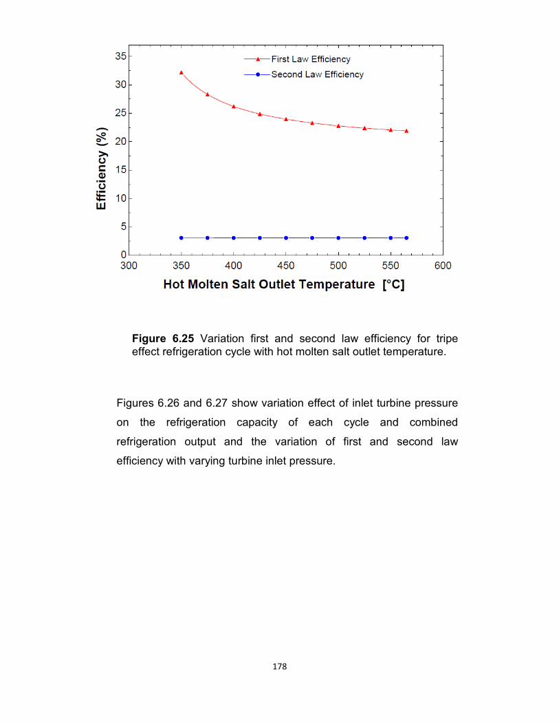
178
Figure 6.25 Variation first and second law efficiency for tripe effect refrigeration cycle with hot molten salt outlet temperature.
Figures 6.26 and 6.27 show variation effect of inlet turbine pressure
on the refrigeration capacity of each cycle and combined
refrigeration output and the variation of first and second law
efficiency with varying turbine inlet pressure.
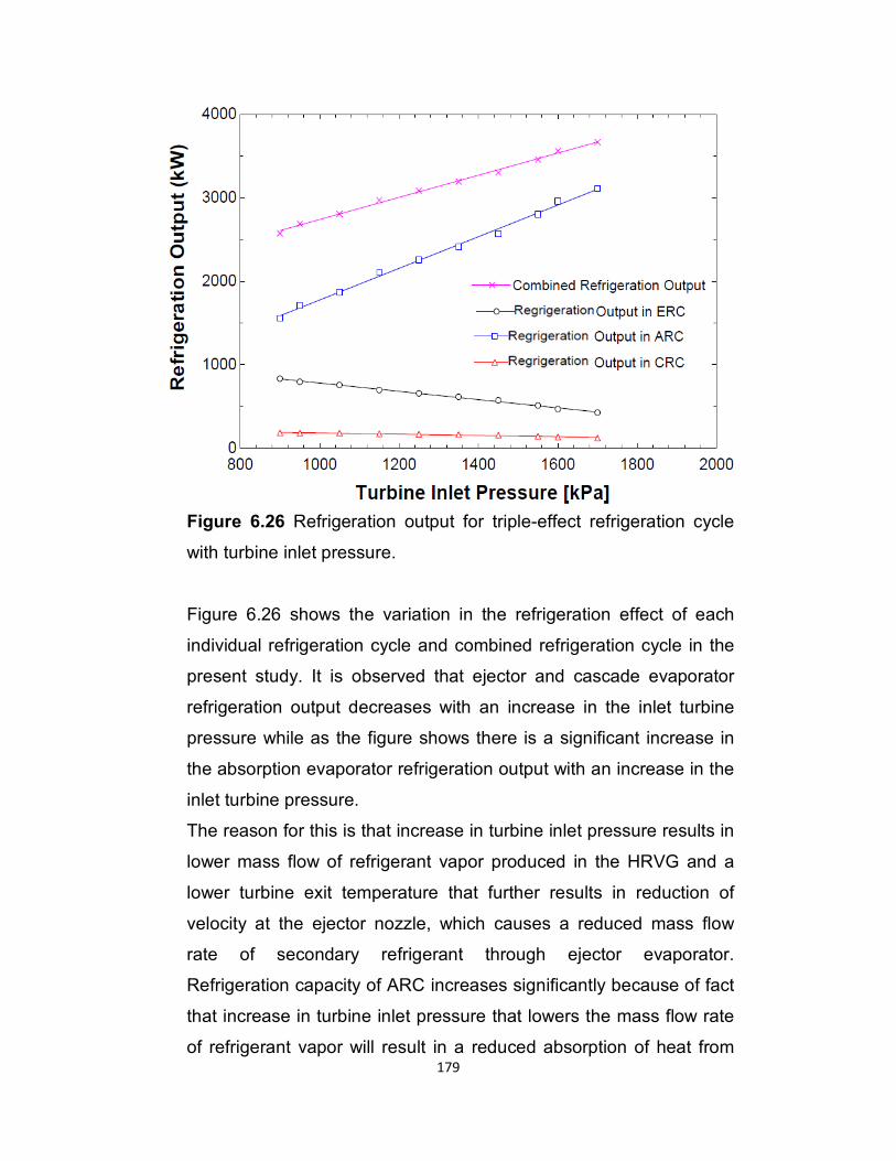
179
Figure 6.26 Refrigeration output for triple-effect refrigeration cycle
with turbine inlet pressure.
Figure 6.26 shows the variation in the refrigeration effect of each
individual refrigeration cycle and combined refrigeration cycle in the
present study. It is observed that ejector and cascade evaporator
refrigeration output decreases with an increase in the inlet turbine
pressure while as the figure shows there is a significant increase in
the absorption evaporator refrigeration output with an increase in the
inlet turbine pressure.
The reason for this is that increase in turbine inlet pressure results in
lower mass flow of refrigerant vapor produced in the HRVG and a
lower turbine exit temperature that further results in reduction of
velocity at the ejector nozzle, which causes a reduced mass flow
rate of secondary refrigerant through ejector evaporator.
Refrigeration capacity of ARC increases significantly because of fact
that increase in turbine inlet pressure that lowers the mass flow rate
of refrigerant vapor will result in a reduced absorption of heat from
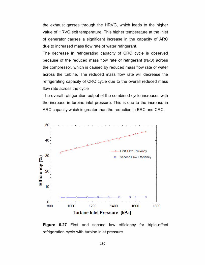
180
the exhaust gasses through the HRVG, which leads to the higher
value of HRVG exit temperature. This higher temperature at the inlet
of generator causes a significant increase in the capacity of ARC
due to increased mass flow rate of water refrigerant.
The decrease in refrigerating capacity of CRC cycle is observed
because of the reduced mass flow rate of refrigerant (N2O) across
the compressor, which is caused by reduced mass flow rate of water
across the turbine. The reduced mass flow rate will decrease the
refrigerating capacity of CRC cycle due to the overall reduced mass
flow rate across the cycle
The overall refrigeration output of the combined cycle increases with
the increase in turbine inlet pressure. This is due to the increase in
ARC capacity which is greater than the reduction in ERC and CRC.
Figure 6.27 First and second law efficiency for triple-effect
refrigeration cycle with turbine inlet pressure.
181
It is seen that the second law efficiency decreases with the increase
in turbine inlet pressure whereas the first law efficiency is increased
significantly with the increase in turbine inlet pressure.
Figure 6.28 shows the effect of turbine back pressure (P5) on the
refrigeration outputs of CRC, ERC, ARC and combined refrigeration
output. It is seen that the turbine power output decreases when
turbine back pressure increases, which will lower the compressor
work and cooling effect accordingly. It is also observed that the
ejector cycle cooling effect will increase with an increase in the
turbine back pressure. This is because, when the turbine back
pressure (P5) increases, causes significant increase in primary flow
velocity at the ejector nozzle and makes more vacuum, entrains
more secondary fluid, and increases the cooling effect accordingly.
It is found that there is no change in the ARC cooling effect due to
increase or decrease turbine back pressure (P5). This is due to the
inlet and outlet state of generator which is not affected by variation of
back pressure of the turbine.
The combined refrigeration outputs increase with increasing turbine
back pressure.
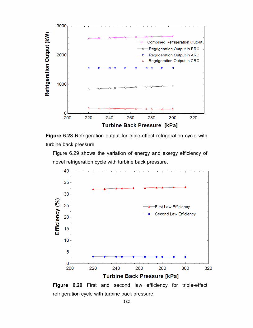
182
Figure 6.28 Refrigeration output for triple-effect refrigeration cycle with
turbine back pressure
Figure 6.29 shows the variation of energy and exergy efficiency of
novel refrigeration cycle with turbine back pressure.
Figure 6.29 First and second law efficiency for triple-effect
refrigeration cycle with turbine back pressure.
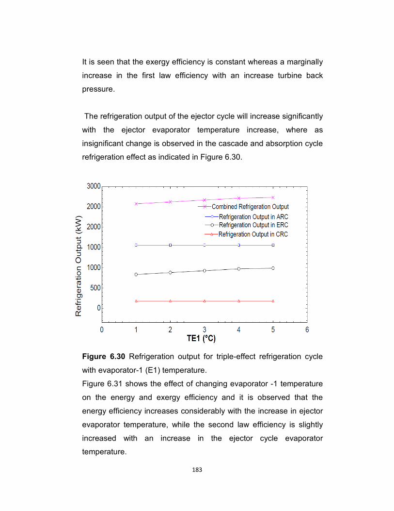
183
It is seen that the exergy efficiency is constant whereas a marginally
increase in the first law efficiency with an increase turbine back
pressure.
The refrigeration output of the ejector cycle will increase significantly
with the ejector evaporator temperature increase, where as
insignificant change is observed in the cascade and absorption cycle
refrigeration effect as indicated in Figure 6.30.
Figure 6.30 Refrigeration output for triple-effect refrigeration cycle
with evaporator-1 (E1) temperature.
Figure 6.31 shows the effect of changing evaporator -1 temperature
on the energy and exergy efficiency and it is observed that the
energy efficiency increases considerably with the increase in ejector
evaporator temperature, while the second law efficiency is slightly
increased with an increase in the ejector cycle evaporator
temperature.
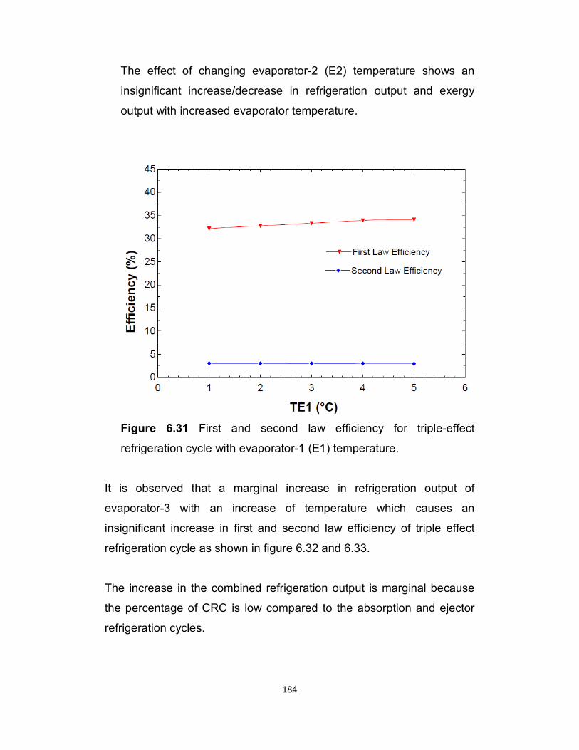
184
The effect of changing evaporator-2 (E2) temperature shows an
insignificant increase/decrease in refrigeration output and exergy
output with increased evaporator temperature.
Figure 6.31 First and second law efficiency for triple-effect
refrigeration cycle with evaporator-1 (E1) temperature.
It is observed that a marginal increase in refrigeration output of
evaporator-3 with an increase of temperature which causes an
insignificant increase in first and second law efficiency of triple effect
refrigeration cycle as shown in figure 6.32 and 6.33.
The increase in the combined refrigeration output is marginal because
the percentage of CRC is low compared to the absorption and ejector
refrigeration cycles.
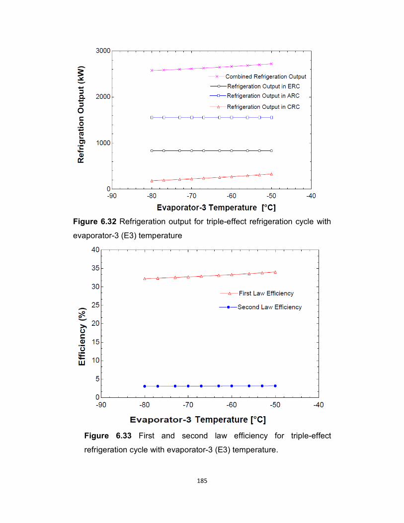
185
Figure 6.32 Refrigeration output for triple-effect refrigeration cycle with
evaporator-3 (E3) temperature
Figure 6.33 First and second law efficiency for triple-effect
refrigeration cycle with evaporator-3 (E3) temperature.

186
Figures 6.34 shows the effect of compressor discharge pressure
on the thermal and exergy efficiencies of triple effect refrigeration
cycle and show the effect of compressor discharge pressure on
the refrigeration outputs of CRC, ERC and ARC.
It can be observed that the refrigeration effect of CRC decreases
with an increase in the compressor discharge pressure.
Further, it is seen that the variation of refrigeration effect of CRC
has no effect on the refrigeration outputs of ERC and ARC.
The second law efficiency changes insignificantly with an
increase in the compressor discharge pressure whereas the first
law efficiency decreases as the compressor discharge pressure
increases.
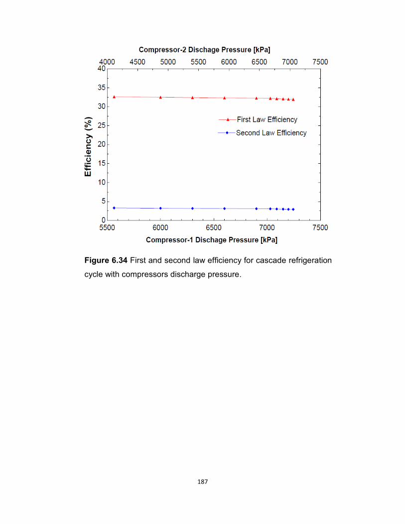
187
Figure 6.34 First and second law efficiency for cascade refrigeration
cycle with compressors discharge pressure.
188
6.10 Variation of the refrigeration output of the proposed cycle with
changing average daily and hourly solar radiation:
Figures 6.35 and 6.36 show the effect of average daily solar
radiation on the refrigeration outputs of CRC, ERC, ARC and
combined refrigeration output. It is seen that when the average daily
solar radiation increases, it increases the refrigeration output in ERC,
ARC, CRC and combined cycle.
The reason for the increase in the refrigeration output with increasing
average daily solar radiation is due to the following facts:
� When the average daily solar radiation increases, it will
increase HRVG thermal energy which will increase the mass
flow rate across the turbine (primary mass flow rate) and then
increase the secondary mass flow rate and the ejector cycle
refrigeration output accordingly.
� When the primary mass flow rate increases across the turbine,
this will increase the turbine output power, then the mass flow
rate in cascade refrigeration cycle and then the refrigeration
output in CRC.
� When the average daily solar radiation increases, it will
increase the hot molten salt mass flow rate in the generator of
absorption refrigeration cycle and the thermal energy in the
generator, which will increase the mass flow rate of
evaporator-2 and then increase the refrigeration output of
ARC.
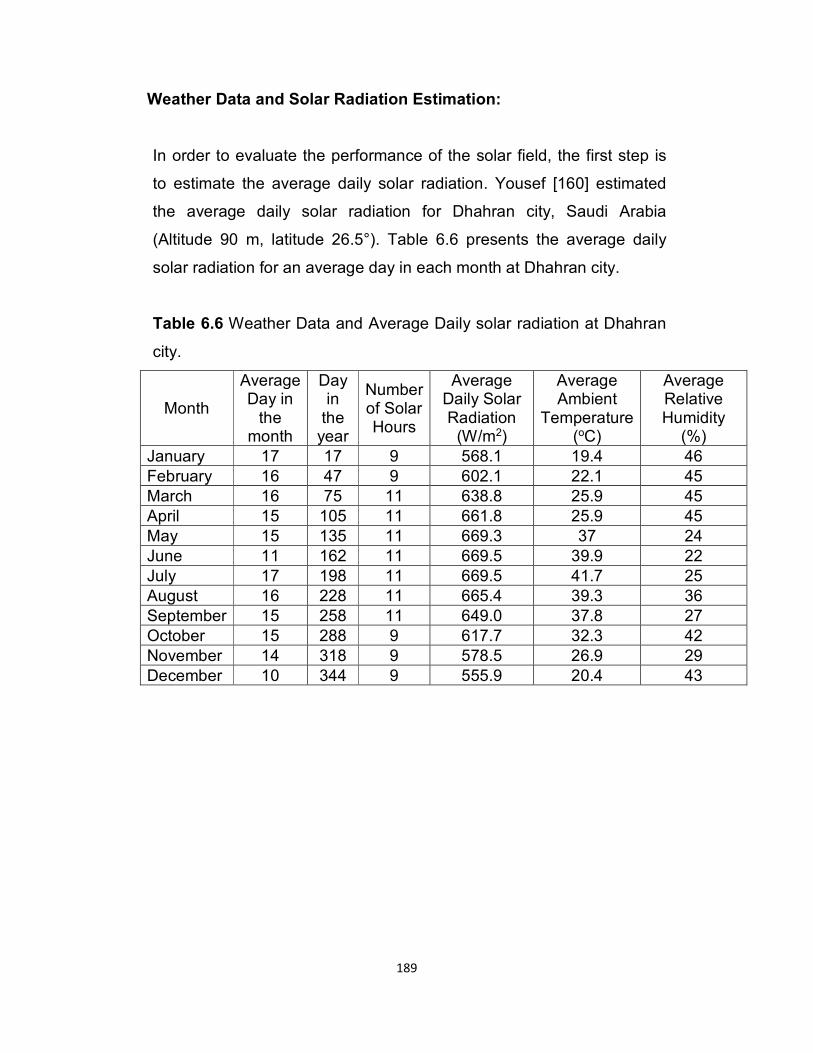
189
Weather Data and Solar Radiation Estimation:
In order to evaluate the performance of the solar field, the first step is
to estimate the average daily solar radiation. Yousef [160] estimated
the average daily solar radiation for Dhahran city, Saudi Arabia
(Altitude 90 m, latitude 26.5°). Table 6.6 presents the average daily
solar radiation for an average day in each month at Dhahran city.
Table 6.6 Weather Data and Average Daily solar radiation at Dhahran
city.
Month
Average Day in
the month
Day in
the year
Number of Solar Hours
Average Daily Solar Radiation
(W/m2)
Average Ambient
Temperature (oC)
Average Relative Humidity
(%)
January 17 17 9 568.1 19.4 46
February 16 47 9 602.1 22.1 45
March 16 75 11 638.8 25.9 45
April 15 105 11 661.8 25.9 45
May 15 135 11 669.3 37 24
June 11 162 11 669.5 39.9 22
July 17 198 11 669.5 41.7 25
August 16 228 11 665.4 39.3 36
September 15 258 11 649.0 37.8 27
October 15 288 9 617.7 32.3 42
November 14 318 9 578.5 26.9 29
December 10 344 9 555.9 20.4 43
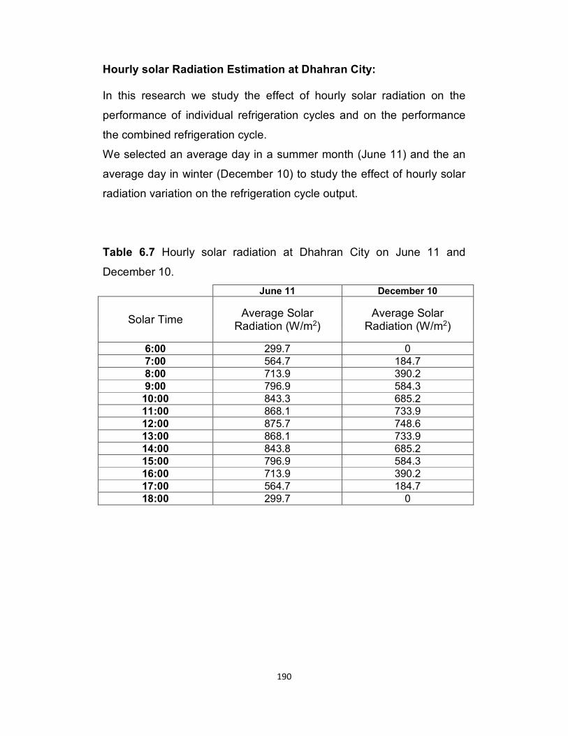
190
Hourly solar Radiation Estimation at Dhahran City: In this research we study the effect of hourly solar radiation on the
performance of individual refrigeration cycles and on the performance
the combined refrigeration cycle.
We selected an average day in a summer month (June 11) and the an
average day in winter (December 10) to study the effect of hourly solar
radiation variation on the refrigeration cycle output.
Table 6.7 Hourly solar radiation at Dhahran City on June 11 and
December 10.
June 11 December 10
Solar Time Average Solar
Radiation (W/m2) Average Solar
Radiation (W/m2)
6:00 299.7 0
7:00 564.7 184.7
8:00 713.9 390.2
9:00 796.9 584.3
10:00 843.3 685.2
11:00 868.1 733.9
12:00 875.7 748.6
13:00 868.1 733.9
14:00 843.8 685.2
15:00 796.9 584.3
16:00 713.9 390.2
17:00 564.7 184.7
18:00 299.7 0
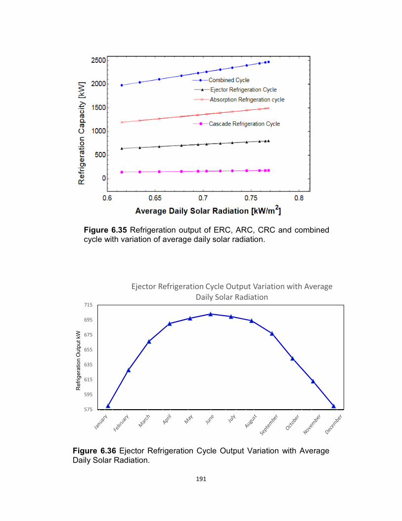
191
Figure 6.35 Refrigeration output of ERC, ARC, CRC and combined cycle with variation of average daily solar radiation.
Figure 6.36 Ejector Refrigeration Cycle Output Variation with Average Daily Solar Radiation.
575
595
615
635
655
675
695
715
Ejector Refrigeration Cycle Output Variation with Average
Daily Solar Radiation
Refr
igera
tio
n O
utp
ut kW
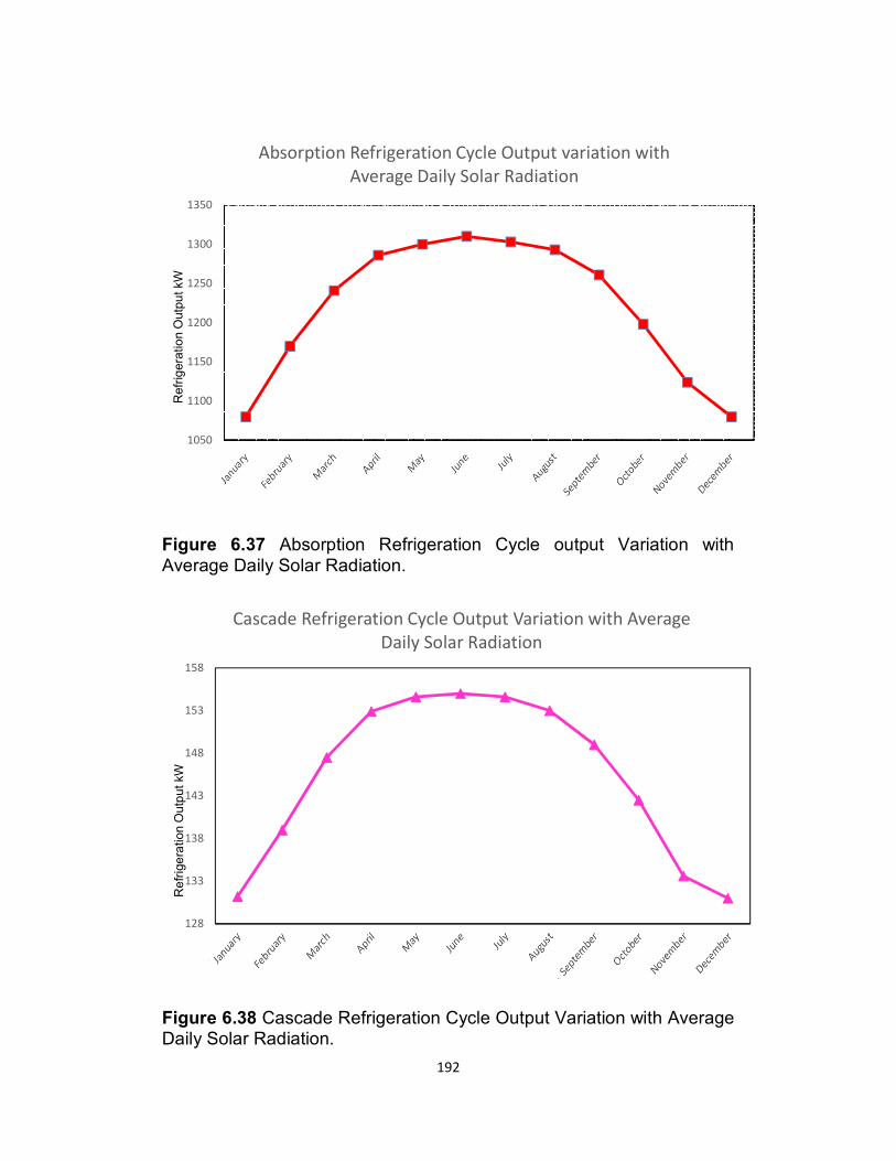
192
Figure 6.37 Absorption Refrigeration Cycle output Variation with Average Daily Solar Radiation.
Figure 6.38 Cascade Refrigeration Cycle Output Variation with Average Daily Solar Radiation.
1050
1100
1150
1200
1250
1300
1350
Absorption Refrigeration Cycle Output variation with
Average Daily Solar RadiationR
efr
igera
tio
n O
utp
ut kW
128
133
138
143
148
153
158
Cascade Refrigeration Cycle Output Variation with Average
Daily Solar Radiation
Re
frig
era
tion O
utp
ut kW
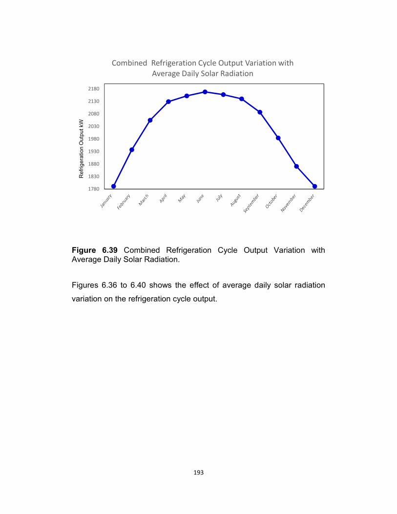
193
Figure 6.39 Combined Refrigeration Cycle Output Variation with Average Daily Solar Radiation.
Figures 6.36 to 6.40 shows the effect of average daily solar radiation
variation on the refrigeration cycle output.
1780
1830
1880
1930
1980
2030
2080
2130
2180
Combined Refrigeration Cycle Output Variation with
Average Daily Solar RadiationR
efr
igera
tion
Ou
tput kW
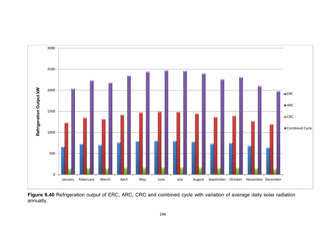
195
Figure 6.40 Refrigeration output of ERC, ARC, CRC and combined cycle with variation of average daily solar radiation annually.
0
500
1000
1500
2000
2500
3000
January Feberuary March April May June July August Sepetmber October November December
ERC
ARC
CRC
Combined Cycle
Refr
igera
tio
n O
utp
ut
kW
194

195
Figures 6.36 to 6.40 are showing the refrigeration output of ERC, ARC,
CRC and combined cycle with variation of average daily solar radiation
for the entire year from January to December. It can be seen that the
refrigeration output for all cycles reaches the maximum capacity with
peak solar energy availability.
The maximum average solar radiation was in June (768.2 W/m2) and
the refrigeration output reached the maximum capacity in this month, as
follows:
� 801.1 kW for Ejector refrigeration cycle.
� 1,493 kW for Absorption Refrigeration Cycle.
� 177.4 kW for Cascade Refrigeration Cycle.
� 2,471.5 kW for Combined Refrigeration Cycle.
The minimum average solar radiation was in December (615.1 W/m2)
and the refrigeration output was the minimum capacity in this month as
follow:
� 641.6 kW for Ejector refrigeration cycle.
� 1,195 kW for Absorption Refrigeration Cycle.
� 142.1 kW for Cascade Refrigeration Cycle.
� 1,978.7 kW for Combined Refrigeration Cycle.
Figures 6.41 to 6.47 (excluding 6.42) show the effect of average
hourly solar radiation on June 11 (11 hours from 6:00 to 18:00) on
the refrigeration outputs of CRC, ERC, ARC and combined
refrigeration output. It is seen that when the average hourly solar
radiation increases, it increases the refrigeration output in ERC,
ARC, CRC and combined cycle.
Figures 6.42 and 6.48 to 6.52 show the effect of average hourly solar
radiation on December 10 (9 hours from 7:00 to 17:00) on the
refrigeration outputs of CRC, ERC, ARC and combined refrigeration
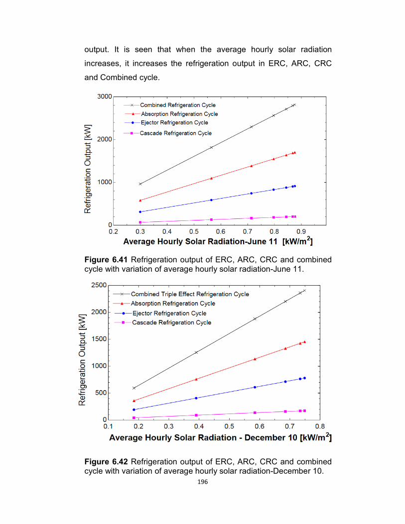
196
output. It is seen that when the average hourly solar radiation
increases, it increases the refrigeration output in ERC, ARC, CRC
and Combined cycle.
Figure 6.41 Refrigeration output of ERC, ARC, CRC and combined cycle with variation of average hourly solar radiation-June 11.
Figure 6.42 Refrigeration output of ERC, ARC, CRC and combined cycle with variation of average hourly solar radiation-December 10.
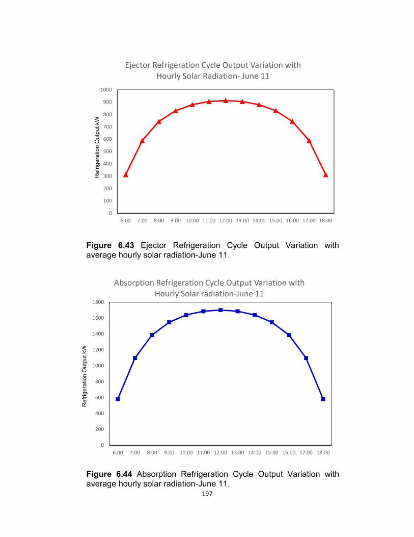
197
Figure 6.43 Ejector Refrigeration Cycle Output Variation with average hourly solar radiation-June 11.
Figure 6.44 Absorption Refrigeration Cycle Output Variation with average hourly solar radiation-June 11.
0
100
200
300
400
500
600
700
800
900
1000
6:00 7:00 8:00 9:00 10:00 11:00 12:00 13:00 14:00 15:00 16:00 17:00 18:00
Ejector Refrigeration Cycle Output Variation with
Hourly Solar Radiation- June 11
Refr
igera
tio
n O
utp
ut kW
0
200
400
600
800
1000
1200
1400
1600
1800
6:00 7:00 8:00 9:00 10:00 11:00 12:00 13:00 14:00 15:00 16:00 17:00 18:00
Absorption Refrigeration Cycle Output Variation with
Hourly Solar radiation-June 11
Refr
igera
tion
Ou
tput kW
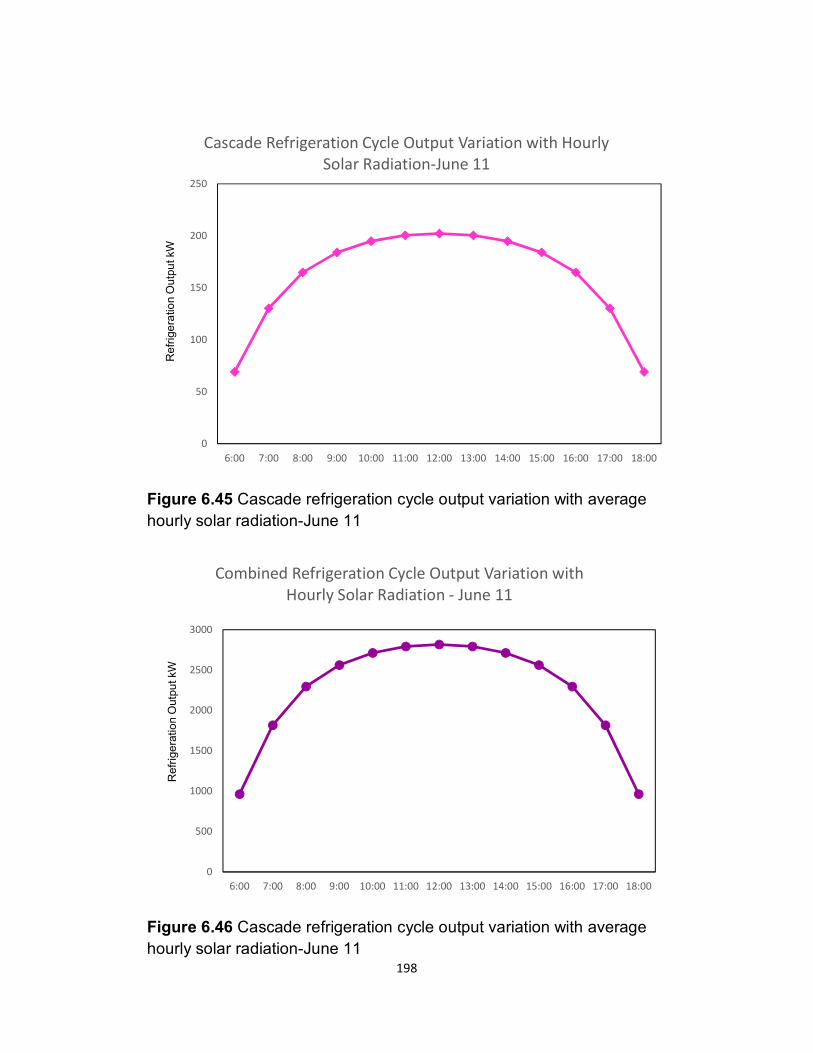
198
Figure 6.45 Cascade refrigeration cycle output variation with average
hourly solar radiation-June 11
Figure 6.46 Cascade refrigeration cycle output variation with average
hourly solar radiation-June 11
0
50
100
150
200
250
6:00 7:00 8:00 9:00 10:00 11:00 12:00 13:00 14:00 15:00 16:00 17:00 18:00
Cascade Refrigeration Cycle Output Variation with Hourly
Solar Radiation-June 11R
efr
ige
ratio
n O
utp
ut kW
0
500
1000
1500
2000
2500
3000
6:00 7:00 8:00 9:00 10:00 11:00 12:00 13:00 14:00 15:00 16:00 17:00 18:00
Combined Refrigeration Cycle Output Variation with
Hourly Solar Radiation - June 11
Refr
ige
ratio
n O
utp
ut kW
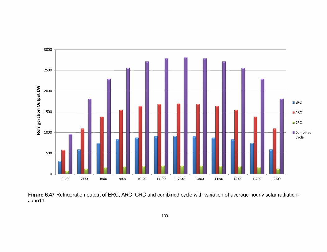
200
Figure 6.47 Refrigeration output of ERC, ARC, CRC and combined cycle with variation of average hourly solar radiation-June11.
0
500
1000
1500
2000
2500
3000
6:00 7:00 8:00 9:00 10:00 11:00 12:00 13:00 14:00 15:00 16:00 17:00
ERC
ARC
CRC
Combined
Cycle
Refr
igera
tio
n O
utp
ut
kW
199
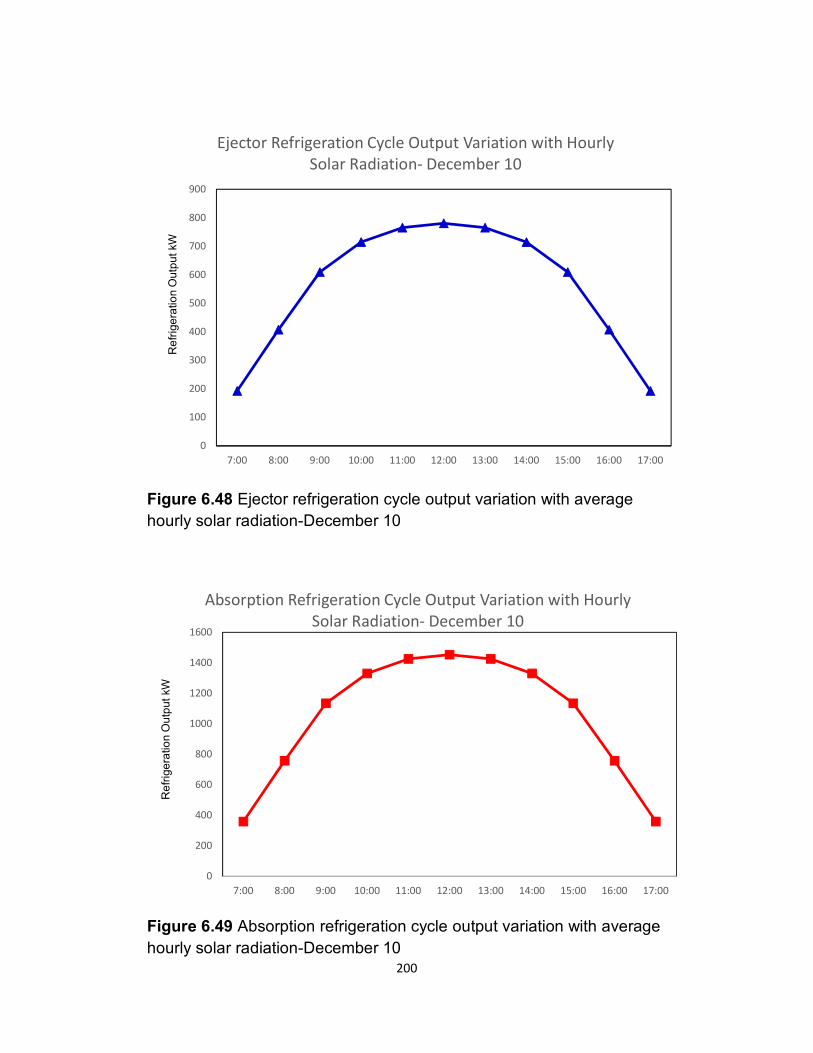
200
Figure 6.48 Ejector refrigeration cycle output variation with average
hourly solar radiation-December 10
Figure 6.49 Absorption refrigeration cycle output variation with average
hourly solar radiation-December 10
0
100
200
300
400
500
600
700
800
900
7:00 8:00 9:00 10:00 11:00 12:00 13:00 14:00 15:00 16:00 17:00
Ejector Refrigeration Cycle Output Variation with Hourly
Solar Radiation- December 10R
efr
ige
ratio
n O
utp
ut kW
0
200
400
600
800
1000
1200
1400
1600
7:00 8:00 9:00 10:00 11:00 12:00 13:00 14:00 15:00 16:00 17:00
Absorption Refrigeration Cycle Output Variation with Hourly
Solar Radiation- December 10
Re
frig
era
tio
n O
utp
ut kW
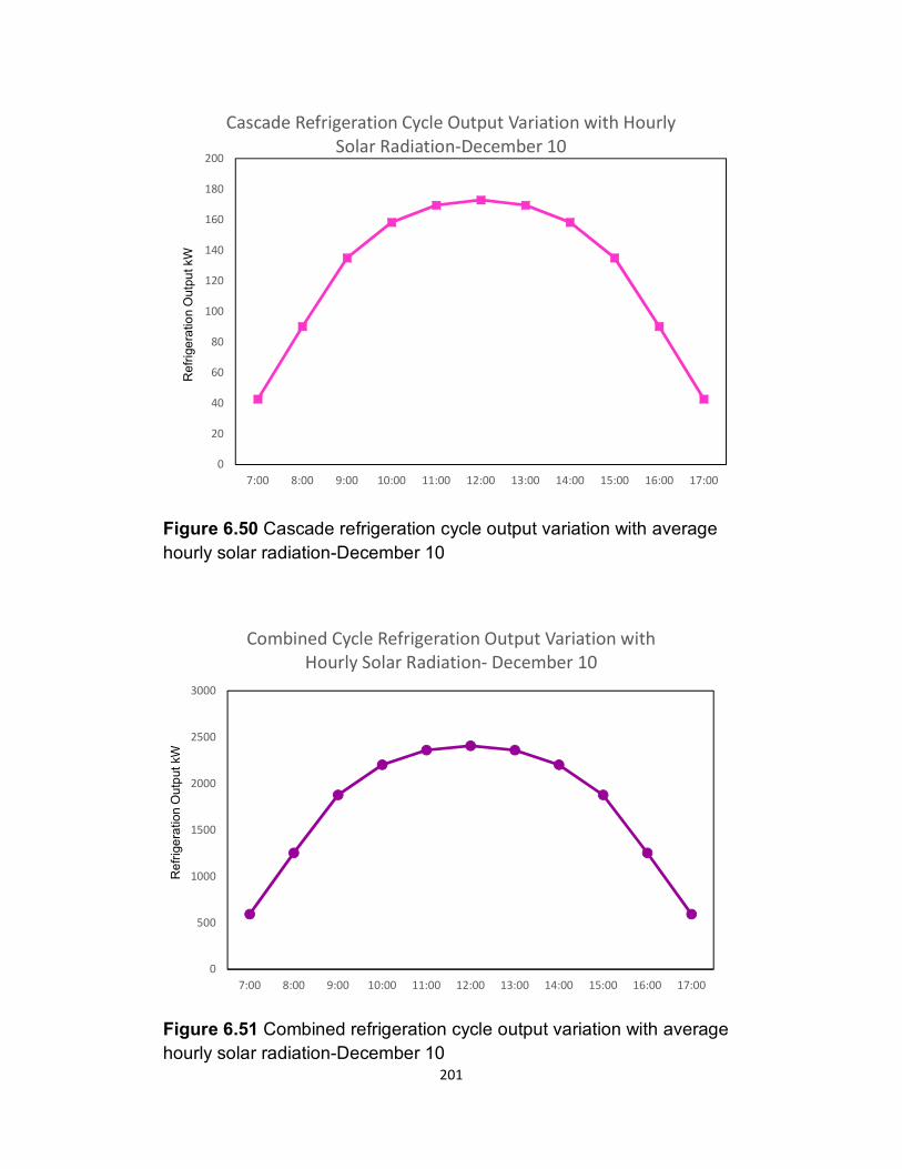
201
Figure 6.50 Cascade refrigeration cycle output variation with average
hourly solar radiation-December 10
Figure 6.51 Combined refrigeration cycle output variation with average
hourly solar radiation-December 10
0
20
40
60
80
100
120
140
160
180
200
7:00 8:00 9:00 10:00 11:00 12:00 13:00 14:00 15:00 16:00 17:00
Cascade Refrigeration Cycle Output Variation with Hourly
Solar Radiation-December 10
Refr
ige
ratio
n O
utp
ut kW
0
500
1000
1500
2000
2500
3000
7:00 8:00 9:00 10:00 11:00 12:00 13:00 14:00 15:00 16:00 17:00
Combined Cycle Refrigeration Output Variation with
Hourly Solar Radiation- December 10
Re
frig
era
tion
Outp
ut kW
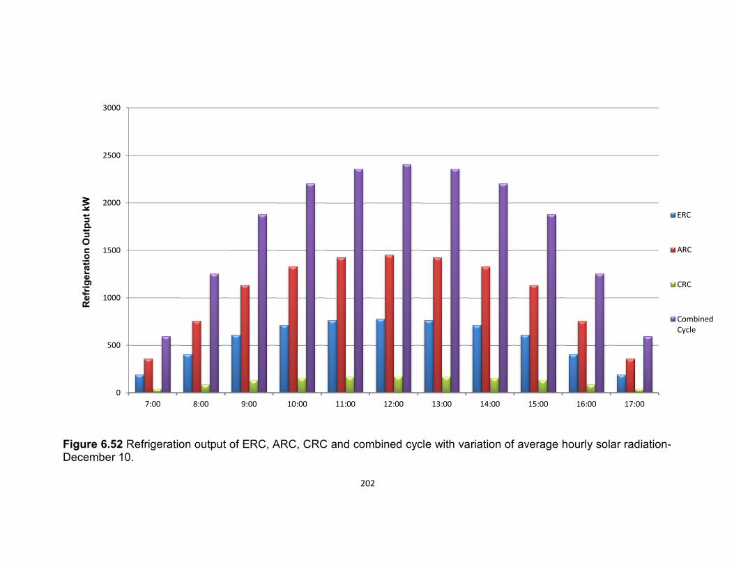
203
Figure 6.52 Refrigeration output of ERC, ARC, CRC and combined cycle with variation of average hourly solar radiation-December 10.
0
500
1000
1500
2000
2500
3000
7:00 8:00 9:00 10:00 11:00 12:00 13:00 14:00 15:00 16:00 17:00
ERC
ARC
CRC
Combined
Cycle
Refr
igera
tio
n O
utp
ut
kW
202
203
CHAPTER 7
CONCULUSION AND RECOMMENDATION
7.1 Conclusion:
Many solar energy technologies used to achieve refrigeration effect are
investigated in this research. This study provides the useful indicators of
these technologies performance.
A new solar driven triple-effect refrigeration cycle is proposed for the
production of cooling at different temperature ranges. The main conclusion
from this study can be summarized as follows:
� The largest contribution to cycle irreversibility comes from the CR
and heliostat field of 52.5 and 25%, respectively. The irreversibility of
the order of 2–7% is observed in the HRVG, ejector, and generator
of refrigeration cycle and this could be minimized by better design
consideration.
� Around 4.7% is available as useful exergy output where as 47.7% is
available as useful energy output. Exergy output was low because of
low temperature refrigerating effect of CRC.
� Both thermal and exergy efficiency are increased by increasing any
one of the following parameters i.e. turbine back pressure, turbine
inlet pressure, ejector evaporator temperature and cascade
evaporator temperature, whereas both thermal and exergy
efficiencies decreases with increase compressor discharge pressure,
hot molten salt outlet temperature. The optimization of above
parameters could be considered to improve the performance of the
cycle.
204
� The parametric study shows that hot molten salt outlet temperature,
turbine back pressure, turbine inlet pressure, and ejector evaporator
temperature and compressor delivery pressure have significant
effects on refrigeration outputs.
� The exergy destruction, which is happened in the generator and
absorber increases with the generator temperature as the
concentration difference between weak and strong solution
increases.
� The condenser and evaporator exergy losses are much less than
generator and absorber losses. The losses (within the condenser and
evaporator) are mainly due to heat of mixing in the solution which is
not present in pure fluid such as single refrigerant in vapor
compression cycle. The effects of exergy losses in the solution,
refrigerant pump and expansion valves on the total exergy losses are
small and considered negligible.
� The performance of the absorption refrigeration cycle is strongly
influenced by the operating temperatures. These results are very
important in the improvement of the absorption cycle performance.
The research presented the merits and demerits of the solar cooling
technologies, a number of observations can be made as follow:
� All sorption cycles including chemical sorption are in the beginning
process with research laboratory to the market, but much more work
is needed on cost minimization, design and packaging.
� Small-scale absorption cycles driven by solar thermal energy have
been recently launched in the market by several companies.
� Adsorption and chemical adsorption cycles appear to function well in
small scale applications such as small refrigerators; however, these
205
cycles need to solve refrigerant/ adsorbent problems due to corrosion
and crystallization.
� An interesting option for the future is to integrate the desiccant
cooling cycles into the ventilation system and rendering the system
to become more popular.
� The combined Rankine cycle is suitable for high cooling capacities
where a large number of moving parts in the cycle, and the implied
regular maintenance can be accepted.
� The ejector refrigeration cycle has the benefit of being simple, reliable
and feasible to operate with a low grade energy source. The cycle
COP is low, but only slightly lower than other heat operated cycles.
� The Multi effect refrigeration cycles are the best way to provide
cooling at different magnitude and temperature ranges using
renewable energy like solar energy that could produce required
refrigeration effect.
� Many researchers are working now to develop Peltier cooler with low
cost and high efficiency.
It is obvious that each refrigeration cycle described has its own niche in
application, advantages and disadvantages therefore a proper decision of
system selection must be taken according to aforementioned solar cooling
system merit and demerit.
Results obtained in the present study may be utilized by the engineers and
scientists for a suitable thermodynamic design of solar-assisted triple-effect
refrigeration system.
Based on the results obtained, it can be stated that the proposed cycle is a
promising triple effect refrigeration cycle for the production of wide range of
cooling simultaneously from thermodynamically and technical point of view.
206
7.2 Recommendation and Future Work:
This research presents the true fundamental life cycle solar energy and exergy
analysis for triple effect refrigeration cycle, and applies exergy/ exergy
analyses. The research contributions point to future research directions:
� A phase change storage device will be integrated with the current solar
tower heating system for continuous operation over the year.
� In this new cycle, high temperature energy solar source like the solar
tower is utilized to produce power using the high temperature availability
while supplying the required thermal energy to applications that require
low or medium temperature source like absorption and adsorption cycle.
� The thermal energy storage is introduced. Therefore, no auxiliary energy
source is needed.
� The system includes thermal energy storage and quadruple effect
refrigeration cycle which would provide cooling effect continuously when
the solar radiation is not available.
� The thermal storage system of molten salt consists of hot and cold molten
salt storage tank (direct type).
� An extra option of integrating waste energy heat source can be provided
with a minor modification in order to achieve continuous operation in case
of long periods of low solar radiation during cloudy winter days.
� An extra option can be provided to integrate the Steam Rankine cycle to
an electric generator. This electric generator is to be connected to the
utility grid to export electric energy to the grid in cases when, the very low
temperature cooling provided by the Cascade cycle is not need or the
power generated by the turbine is more than the load required by the
Cascade cycle.
207
� An extra option can be provided to integrate the compressors of the
Cascade cycle to electric motors that runs the compressors at nights and
this case the sizes thermal storage tanks would be reduced.
� An extra option can be introduced via providing a control panel making
proper control for the cycle exchange electric energy with the utility
grade. The cycle would supply electricity to the grid when there is high
solar radiation and there is a surplus in the power generated by the steam
turbine compared to the required work by the compressors. And vice
versa when there is low or no solar radiation and the size of the storage
tanks were minimized.
� An extra option can be introduced via providing control valve at HRVG
with bypass line (control valve is needed at bypass line) connected with
absorption cycle generator. This is to modulate the flow of molten salt
depending on the cooling demand at absorption and adsorption cycle
compared to the cooling demand at the ejector and cascade refrigeration
cycle. Thus, when the cooling demand is low at ejector and cascade
cycle, then part of molten salt can be bypassed directly to absorption-
adsorption cycle to increase the output cooling effect otherwise the
control valve will be closed, and normal operation takes place.
� Improve efficiency to lower the Entropy generation
The work gives researchers and engineers a thorough understanding
of all the losses within the system. This serves as the first step for the
improvement of the energy efficiency. The components with the highest
exergy destruction should be focused upon first, and the Lowering
entropy generation techniques should be applied to reduce the entropy
generation in those components.
That techniques includes reducing temperature difference for a heat
exchanger , and reducing the pressure drop and friction in pipes, this
is based on Bejan's work (1995).
208
� Thermoeconomic optimization for the overall system.
� Change the type of molten salt in order to improve the cycle efficiency.
� Change the type of refrigerant in cascade refrigeration cycle in order to
replace it with safe refrigerant.
� Improve the performance of absorption cycle and considering triple effect
refrigeration cycle.
� Study the performance of other mixture can be used in solar absorption
cooling system and this mixture should be high performance, safe, non-
toxic, environmentally friendly, non-corrosive, non-explosive, cheap and
available in the market.
209
References
1. M.M.EL-WAKIL., Power Plant Technology, McGraw-Hill.
2. Zekai Sen., 2002, Solar energy in progress and future research trends, Istanbul,
Turkey.
3. http://aloisiuskolleg.www.de/schule/fachbereiche/comenius/charles/solar.html
4. http://www.tpub.com/utilities/index.html
5. E.A. Demeo and J.F. Galdo. Renewable energy technology characterization.
Technical report , electrical power research institute (EPRI) and US dept of
energy, 1997.
6. H. Price, E.Lupfert, and D.Kearney . Advances in parabolic trough solar power
technology. Journal of solar energy engineering-Transaction of the
ASMe,124(2):109-125, 2002.
7. U.S. Department of Energy.http://www1.eere.energy.gov/solar.
8. F.Cavallaro. Multi-criteria descision aid to assess concentrated solar thermal
technologies. Renewable energy, 34(7):1678-1685, 2009.
9. J. Birnbaum, M. Eck, M. Fichtner, T. Hirsch, D.Lehmann, and G. Zimmermann.
A direct steam generation solar power plant with integrated storage. Journal of
solar energy engineering-Transaction of the ASME, 132(3):310-314, 2010.
10. D.Mills. Advances in solar thermal electricity technology. Solar energy 76(1-
3:19-31, 2004.
11. E. Zarza, M.E. Rojas, L. Gonzalez, J. Caballero , and F.Rueda. INDITEP: The
first pre- commercial DSG solar power plant. Solar energy, 80 (10):1270-1276,
2006.
12. M. J. Hale. Survey of thermal storage for parabolic trough power plants.
Technical report, NREL, 2000.
13. H. Herrmaan and D.W.Kearney. Survey of thermal storage for parabolic trough
power plants. Technical report, NREL, 2000. Journal of solar engineering –
transaction of the ASME,124 (2):145-152, 2002.
210
14. J.E. Pacheco, S. K. Showalter, and W. J. Kolb. Development of molten salt
thermocline thermal storage system for parabolic trough plants. Journal of solar
energy engineering transaction of the ASME, 124(2)153-159, 2002.
15. D. Laing, W.D. Steinmann, M. Fib, R. Tamme, T. Brand, and C. Bahl, Solid
Media thermal storage development and analysis of a modular storage operation
concept for parabolic trough power plant. Journal of solar energy engineering
transaction of the ASME, 130(1):011005-1-011005-5, 2008.
16. V.Mirisson, M.rady, E.Palomo, and E.Arquis. Thermal energy storage system
for electricity production using solar energy direct steam generation technology.
Chemical engineering and processing: Process intensification 47(3):499-507,
2008.
17. http://www.photofileit.com/Collection.htm
18. D.R. Mils and G.L. Morrison. Compact Linear Fresnel reflector Solar thermal
power plants. Solar energy, 68(3):263-283, 2000.
19. A. Lewandowski and D.Simms. An assessment of linear Fresnel lens
concentrator for thermal application. Energy, 12(3-4):333-338, 1987.
20. Novatec solars Fresnel collector generates superheated steam above 500c.
http://www.novatecsolar.com/86-1-novatec-solar-fresnel-collector-generates-
superheated-steam-above-500C.html
21. http://usmanali-views.blogspot.com
22. H. E. Reilly and G.J. Kolb. An evaluation of molten-salt power towers including
results of the solar two project. Technical report, sandia National Labs, 2001.
23. http://www.energy.siemens.com/co/en/fossil-power-generation/power-
plants/csp-power-block/
24. R. Buck, M. Abele, J. Kunberger, T.Denk, P.Heller, and E.Lupfert. Receiver for
solar-hybrid gas turbine and combined cycle system. Journal de
physique,9(3):537-544,1999.
25. R.Buk,T.Brauning, T.Denk,M.Pfander, P.Schwarzbozl, and F.Telles.
Solar Hybrid gas turbine based power systems (REFOS). Journal of solar energy
engineering transaction of the ASME,124(1):2-9, 2002.
211
26. M.Horn, H.Fuhring, and J. Rheinlander. Economic analysis of integrated solar
combined cycle power plants: A sample case: the economic feasibility of an ICCS
power plant in Egypt. Energy,29(5-6):935-945, 2004.
27. M. Romero, R. Buck, and J.Pacheco. an update on solar central receiver
systems, projects, and technologies. Journal of solar energy engineering –
Transaction of the ASME,124(2):98-108, 2002.
28. A. Chobeity, C.J. Noone, C.N. Papanicolas, and A. Mitsos. Optimal time invariant
operation of a power and water cogeneration solar thermal plant. Solar
energy,85(9):2295-2320,June 20, 2011.
29. C.J. Noone, A.Ghobeity, A.H. Slocum, G.Tzarntzis and A.Mitsos. Site Selection
for hillside central receiver solar thermal plant. Solar energy, 85(5):839-848,
2011.
30. A. H. Slocum, J. Buongiorno, C. W. Forsberg, D. S. Codd, and A. T. Paxson.
Concentrated solar power system. PCT patent Application PCT/US10/49474,
2009.
31. A. H. Slocum, D. S. Codd, J. Buongiorno, C. Forsberg, T. Mckrell, J. C. Nave,
C. N. Papanicolas, A.Ghobeity, C.J. Noone, S. Passerini, F. Rojas, and A.Mitsos.
Concentrated solar power on demand. Solar, 85(7):1519-1529, 2011.
32. http://www.boem.gov/Renewable-Energy-Program/Renewable-Energy-
Guide/Offshore-Solar-Energy.aspx .
33. http://www.geocities.com/dieret/re/Solar/solar.html
34. Nicole T. Carter, Richard J. Campbell, 2009. Water Issues of Concentrating Solar
Power (CSP) Electricity in the U.S. Southwest, Congressional Research Service
7-5700 www.crs.gov R40631.
35. Solar Engineering of Thermal Processes, 4th Edition John A. Duffie, William A.
Beckman.
36. J.Dersch, M.geyer, U.Herrmann, S.Jones, B.Kelly, R.Kistner, W.ortmannas,R.
Pitz-Paal, and H.Price. Through integration into power plants – A study on the
performance and economy of in integrated solar combined cycle system. Energy,
29(5-6):947-959, 2004.
212
37. S. A. Kalogirou. Solar energy engineering: Process and Systems. Elsevier,
2009.
38. Alazazmeh AJ, Mokheimer EM (2015) Review of Solar Cooling Technologies. J Appl
Mech Eng 4: 180. doi:10.4172/2168-9873.1000180
39. Wu, X., 2004. High-efficiency polycrystalline CdTe thin-film solar cells. Solar
energy 77(6):803-14.
40. Riffat, S. and Xiaoli, M., 2003. Thermoelectrics: a review of present and potential
applications. Applied Thermal Engineering 23 913–935.
41. Zemansky, M. and Dittman, R., Heat and Thermodynamic, Sixth ed., McGraw-
Hill Book Company, 1981, pp.431-442.
42. Riffat, S. and Xiaoli, M., 2004. Comparative investigation of thermoelectric air-
conditioners versus vapor compression and absorption air-conditioners. Applied
Thermal Engineering 24 1979–1993.
43. Klein, S. and Reindl, D., 2005 Solar refrigeration. ASHRAE Journal 47(9):S26-
S30.
44. Lundqvist, P., (1993). Stirling Cycle Heat Pumps and Refrigerators. Applied
Thermodynamics and Refrigeration. Stockholm, Royal Institute of Technology:
284.
45. Ewert, M., Agrella, M., DeMonbrun, D., Frahm, J., Bergeron, D., and Berchowitz,
D., 1998. Experimental evaluation of a solar PV refrigerator with thermoelectric,
Stirling, and vapour compression heat pumps. In: Proceedings of ASES Solar 98
Conference, Albuquerque, USA.
46. Berchovitz, D., McEntee, J. and Welty, S., 1999. Design and testing of a 40W
free-piston Stirling cycle cooling unit. In: Proceedings of 20th International
Congress of Refrigeration, Sydney, Australia.
47. Haywood, D., Raine, J. and Gschwendtner, M. Stirling-Cycle Heat-Pumps and
Refrigerators – a Realistic Alternative, Stirling Cycle Research Group,
Department of Mechanical Engineering, University of Canterbury, New
Zealand. http://www.mech.canterbury.ac.nz/research/stirling/stirling.htm
48. Kribus, A., 2002. Thermal integral micro-cogeneration systems for solar and
conventional use. Journal of Solar Energy Engineering 124, 189–197.
213
49. Ameel, T., Gee, K., and Wood, B., 1995. Performance predication of alternative,
low cost absorbents for open-cycle absorption solar cooling. Solar engineering
(2):65-73.
50. Gommed, K. and Grossman, G. 2007. Experimental investigation of a liquid
desiccant system for solar cooling and dehumidification solar energy 81(1) 131-
38.
51. Davies, P., 2005. A solar cooling system for greenhouse food production in hot
climate. Solar energy 79 (6):661-68.
52. Henning, H., T.Erpenbeck, C. Hindenburg and I.S.Santamaria. 2001. The
potential of solar energy use in desiccant cooling cycles. International journal of
refrigeration. 24 (3)220-29.
53. Henning, H., 2004. Solar-assisted Air-conditioning Handbook in Buildings: A
Handbook for Planners. Springer-Verlag, Wien, ISBN 3-211-00647-8.
54. Herold, K. and Radermacher, L. Absorption heat pump, Mech. Eng., Aug,
1989;68–73.
55. Gosney, W., Principle of refrigeration. Cambridge Uni. Press, 1982.
56. Srikhirin,P. and Aphornratana,S., Chungpaibulpatana,S., 2001. A review of
absorption refrigeration Technologies, Renewable and Sustainable Energy
Review 343–372.
57. Murphy, K. and Phillips, B. Development of residential gas absorption heat pump.
Int J Refrig 1984;7(1):56–8.
58. Choudhury, S., Hisajima, D., Ohuchi, T., Nishiguchi, A., Fukushima, T. and
Sakaguchi, S., Absorption of vapors into liquid films flowing over cooled
horizontal tubes. ASHRAE Trans 1993; 99:81–9.
59. Matsuda, A., Choi, K., Hada, K. and Kawamura, T., Effect of pressure and
concentration on performance of a vertical falling-film type of absorber and
generator using lithium bromide aqueous solutions. Int J Refrig 1994; 17(8):538–
42.
60. Cosenza, F. and Vliet, G., Absorption in falling water/LiBr films on horizontal
tubes. ASHRAE Trans 1990; 96:693–701.
214
61. Morioka, I. and Kiyota, M., Absorption of water vapor into a wavy film of an
aqueous solution of LiBr. JSME Int J, Series II 1991;34(2):183–8.
62. Kim, K., Berman, N., Chau, D. and Wood, B. Absorption of water vapour into
falling films of aqueous lithium bromide. Int J Refrig 1995; 18(7):486–94.
63. Benzeguir, B., Setterwall, F. and Uddholm, H., Use of wave model to evaluate
falling film absorber efficiency. Int J Refrig 1991;14:292–6.
64. Fujita, T., Falling liquid films in absorber machines. Int J Refrig 1993;16(4):282–
94.
65. Andberg, J.and Vliet, G., A simplified model for absorption of vapors into liquid
films flowing over cooled horizontal tubes. ASHRAE Trans 1987;93:2454–66.
66. Grossman, G., Absorption heat transformer for process heat generation from
solar ponds. ASHRAE Trans 1991;97:420–7.
67. Ikeuchi, M., Yumikura, T., Ozaki, E. and Yamanaka, G., Design and performance
of a high-temperature boost absorption heat pump. ASHRAE Trans
1985;90:2081–94.
68. Nakanishi, T., Furukawa, T. and Sato, N., Industrial high-temperature heat pump.
Hitachi zosen Tech Rev 1981;42(1):7–12.
69. Siddig, M., Performance studies on a reversed absorption heat pump. PhD
thesis, University of Salford, UK, 1982.
70. George, J. and Murthy, S., Influence of heat exchanger effectiveness on
performance of vapour absorption heat transformers. Int J Energy Res 1989;
13:455–7.
71. George, J. and Murthy, S., Influence of absorber effectiveness on performance
of vapour absorption heat transformers. Int J Energy Res 1989; 13:629–38.
72. Perez-Blanco, H. Absorption heat pump performance for different types of
solution. Int J Ref 1984; 7(2):115–22.
73. Marcriss, R., Gutraj, J. and Zawacki, T. Absorption fluid data survey: final report
on worldwide data, ORLN/sub/8447989/3, Inst. Gas Tech., 1988.
74. Park, Y. and Sonntag, R. Thermodynamic properties of ammonia-water mixtures:
a generalized equation-of-state approach. ASHRAE Trans 1990; 96:150–9.
215
75. El-Sayed, Y. and Tribus, M. Thermodynamic properties of water-ammonia
mixtures: theoretical implementation for use in power cycle analysis. ASME Pub
AES 1985; 1:89–95.
76. Ziegler, B. and Trepp, C., Equation of state for ammonia-water mixtures. Int J
Refrig 1984; 7(2):101–6.
77. Herold, K., Han, K. and Moran, M., a computer program for calculating the
thermodynamic properties of ammonia and water mixtures using a Gibbs free
energy formulation. ASME Pub AES 1988; 4:65–75.
78. Patek, J. and Klomfae, J., Simple function for fast calculations of selected
thermodynamic properties of ammonia-water system. Int J Refrig 1995;
18(4):228–34.
79. McNeely, L., Thermodynamic properties of aqueous solutions of lithium bromide.
ASHRAE Trans 1979; 85(2):413–34.
80. Patterson, M. and Perez-Blanco, H., Numerical fits of properties of lithium-
bromide water solutions. ASHRAE Trans 1988; 94(2):2059–77.
81. Lee, R., DiGuilio, R., Jeteter, S. and Teja, A., Properties of lithium bromide-water
solutions at high temperatures and concentrations-part II: density and viscosity.
ASHRAE Trans 1990; 96:709–14.
82. Jeter, S., Moran, J. and Teja, A., Properties of lithium bromide-water solutions at
high temperatures and concentrations-part III: specific heat. ASHRAE Trans
1992; 98:137–49.
83. Lenard, J., Jeter, S. and Teja, A. Properties of lithium bromide-water solutions at
high temperatures and concentrations-part IV: vapor pressure. ASHRAE Trans
1992; 98:167–72.
84. Modahl, R. and Lynch, P., Arsenic trioxide corrosion inhibitor for absorption
refrigeration system, US Patent No. 3609086, 1971.
85. Iyoki, S. and Uemura, T., Studies on corrosion inhibitor in water-lithium bromide
absorption refrigerating machine. Reito 1978; 53(614):1101–5.
86. Wen, T., Lin, S., Corrosion inhibitors the absorption system. J Chin Inst Chem
Eng 1992; 22:311–6.
216
87. Verma, S., Mekhjian, M., Sandor, G., Nakada, N., Corrosion inhibitor in lithium
bromide absorption fluid for advanced and current absorption cycle machines.
ASHRAE Trans 1999; 105(1):813–5.
88. Albertson, C. and Krueger R., Heat transfer additives for absorbent solution, US
Patent No.3580759, 1971.
89. Chang, W., Marcriss, R. and Rush, W., Secondary alcohol additives for lithium
bromide-water absorption refrigeration system, US Patent No. 3609087, 1971.
90. Elkassabgi, Y., Perez-Blanco, H., Experimental study of the effects of alcohol
additives in lithium bromide/water pool absorber. ASHRAE Trans 1991; 97:403–
5.
91. Daiguji, H., Hihara, E. and Saito, T., Mechanism of absorption enhancement by
surfactant. Int J Heat and Mass transfer 1997;40(8):1743–52.
92. Hihara, E. and Saito, T., Effect of surfactant on falling film absorption. Int J Refrig
1993; 16(5):339–46.
93. Aphornratana, S., Research on absorption refrigerators and heat pumps. Reric
Int Energy J 1995; 17(1):1–19.
94. Agarwal, R. and Bapat, S., Solubility characteristics of R22-DMF refrigerant-
absorbent combination. Int J Refrig 1985; 8:70–4.
95. Ando, E. and Takeshita, I., Residential gas-fired absorption heat pump based on
R22-DEGDME pair part I: thermodynamic properties of the R22-DEGDME pair.
Int J Refrig 1984; 7:181–5.
96. Bhaduri, S., Verma, H., P-T-X behavior of R22 with five different absorbents. Int
J Refrig 1986; 9:362–6.
97. Bhaduri, S., Verma, H., Heat of mixing of R22-absorbent mixture. Int J Refrig
1988; 11:92–5.
98. Fatouh, M., Murthy, S., Comparison of R22-absorbent pairs for vapour
absorption heat transformers based on P-T-X-H data. Heat Recovery Systems
and CHP 1993; 13(1):33–48.
99. Ghaddar, N., Shihab, M., Bdeir, F., Modeling and simulation of solar absorption
system performance in Beirut. Renewable Energy 1997; 10(4):539–58.
217
100. Hammad, M., Zurigat, Y., Performance of a second generation solar cooling
unit. Solar Energy 1998; 62(2):79–84.
101. Florides, G., Kalogirou, S., Tassou, S., Wrobel, L., Modeling and simulation
of absorption solar cooling system for Cyprus. Solar Energy 2002; 72(1):43–51.
102. Hammad, M., and Audi, M., (1992) Performance of a solar LiBr–water
absorption refrigeration system. Renew. Energy 2(3), 275–282.
103. Boehm, R., “The Development of a Model for a Solar-Fired, Single-Effect,
Absorption Chiller”, (ES2008-54186), 2008, ASME.
104. Lemmini, F., Buret Bahraoui, J., Pons, M., Meunier, F., Simulation des
performances d’un refrigerator solaire a adsorption: comparison des
performances pour deux types de charbonactif. Rev Int Froid 1992; 15(3):159.
105. Pons, M., Guilleminot, J., 1986. Design of experimental solar powered,
solid-adsorption ice maker. Journal of Solar Energy Engineering 108, 332–337.
106. Wang, R., Li, M., Xu, Y., Wu, J., 2000. An energy efficient hybrid system of
solar powered water heater and adsorption ice maker. Solar Energy 68, 189–
195.
107. Schweigler, C., Hiebler, S., Keil, C., kren, C., Kobel, H. and Mehling, H.,
2007. Low temperature heat storage for solar heating and cooling application,
ASHRAE Transaction 113 (1).
108. Chunnanond, K. and Aphornratana, S., "Ejectors: applications in
refrigeration technology," Renewable and sustainable energy reviews, vol. 8, pp.
129-155, 2004.
109. Wang,J., Wu,J., Hu,S. and Huang,B. "Performance of ejector cooling
system with thermal pumping effect using R141b and R365mfc," Applied
Thermal Engineering, Vol. 29, No. 10, pp. 1904-1912, 2009.
110. Huang,B., Chang,J., Petrenko,V. and Zhuk, K. "A solar ejector cooling
system using refrigerant R141b," Solar Energy, vol. 64, pp. 223-226, 1998.
111. Pollerberg, A., Ali,H. and Dotsch,C. "Solar driven steam jet ejector chiller,"
Applied Thermal Engineering, Vol. 29, No. 5-6, pp. 1245-1252, 2009.
112. George, J., Murthy, S., Influence of generator effectiveness on performance
of vapour absorption heat transformers. Int J Energy Res 1989;13:687–99.
218
113. Eames, I., Aphornratana, S., and Haider,H., "A theoretical and experimental
study of a small-scale steam jet refrigerator," International Journal of
Refrigeration, vol. 18, pp. 378-386, 1995.
114. Sun, W. "Experimental investigation of the performance characteristics of
a steam jet refrigeration system," Energy Sources, vol. 19, pp. 349-367, 1997.
115. Sankarlal, T. and Mani, A. "Experimental investigations on ejector
refrigeration system with ammonia," Renewable Energy, vol. 32, pp. 1403-1413,
2007.
116. Ma, X. , Zhang,W., Omer, S. and Riffat,S. "Performance testing of a novel
ejector refrigerator for various controlled conditions," International Journal of
Energy Research, vol. 35, pp. 1229-1235, 2011.
117. Sankarlal, T. and Mani, A. "Experimental studies on an ammonia ejector
refrigeration system," International communications in heat and mass transfer,
vol. 33, pp. 224-230, 2006.
118. Sriveerakul,T., Aphornratana,S. and Chunnanond,K. "Performance
prediction of steam ejector using computational fluid dynamics: Part 1. Validation
of the CFD results," International Journal of Thermal Sciences, vol. 46, pp. 812-
822, 2007.
119. Aphornratana, S., and Chunnanond, K. "Steam Ejector Refrigeration
Cycle."
120. Aphornratana, S., and Chunnanond, K. and Srikhirin,P., "Experimental
investigation of an ejector refrigerator: effect of mixing chamber geometry on
system performance," International journal of energy research, vol. 25, pp. 397-
411, 2001.
121. Aphornratana, S., and Chunnanond, K., "An experimental investigation of a
steam ejector refrigerator: the analysis of the pressure profile along the ejector,"
Applied Thermal Engineering, vol. 24, pp. 311-322, 2004.
122. Ma,X., Zhang,W., Omer, S. and Riffat,S. "Experimental investigation of a
novel steam ejector refrigerator suitable for solar energy applications," Applied
Thermal Engineering, vol. 30, pp. 1320-1325, 2010.
219
123. Khattab, N., "Optimum design conditions of farm refrigerator driven by solar
steam-jet system," International Journal of Sustainable Energy, vol. 24, pp. 1-17,
2005.
124. Levy,A. Jelinek, M. and Borde,I., "Numerical study on the design
parameters of a jet ejector for absorption systems," Applied Energy, vol. 72, pp.
467-478, 2002.
125. Selvaraju,A. and Mani,A., "Analysis of a vapour ejector refrigeration system
with environment friendly refrigerants," International Journal of Thermal
Sciences, vol. 43, pp. 915-921, 2004.
126. Lu,S., and Goswami,D., 2003. Optimization of a novel combined
power/refrigeration thermodynamic cycle, transaction of the ASME 125:212-17.
127. Wali, E. (1980). "Optimum Working Fluids for Solar Powered Rankine Cycle
Cooling of Buildings." Solar Energy 25(3): 235-241.
128. Kane, M., Larrain, D., Favrat, D. and Allani, Y. (2003). "Small Hybrid Solar
Power System." Energy 28(14): 1427-1443.
129. Agrawal, B., Karimi, M. .2012. Thermodynamic performance assessment
of a novel waste heat based triple effect refrigeration cycle. International journal of
refrigeration 35 1647-1656.
130. Fan, Y., Luo, L., and Souyri, B., 2007, “Review of Solar Sorption
Refrigeration Technologies: Development and Applications,” Renewable
Sustainable Energy Rev., 11, pp. 1758–1775.
131. Abdul Khaliq, A., Kumar,R., Dincer.I. and Khalid,F. 2014. Energy and
Exergy Analyses of a New Triple-Staged Refrigeration Cycle Using Solar Heat
Source. Journal of Solar Energy Engineering, Vol. 136 / 011004.
132. Agrawal, B., Kumar, R. and Abdul Khaliq, A., .2014. First and second law
investigations of a new solar-assisted thermodynamic cycle for triple effect
refrigeration, International Journal of energy research, 38:162–173.
133. Choudhury, B., Baran Saha, B., Chatterjee, P., and Prakas Sarkar, J. An
overview of developments in adsorption refrigeration systems towards a
sustainable way of cooling. Applied Energy 104(2013), 554-567. 11-19-2012.
220
134. Kalkan, N., Young, E., and Celiktas, A. Solar thermal air conditioning
technology reducing the footprint of solar thermal air conditioning. Renewable &
Sustainable Energy Reviews 16(2012), 6352-6383. 7-15-2012.
135. Anyanwu,E., Review of solid adsorption solar refrigerator II: an overview of
the principles and theory Energy Conversion and Management, 45 (2004), pp.
1279–1295.
136. Critoph, R., Performance limitations of adsorption cycles for solar cooling.
137. Ayyash,S., Sartawi,M., Economic comparison of solar absorption and
photovoltaic-assisted vapour compression cooling systems International Journal
of Energy Research, 7 (1983), pp. 279–288.
138. Gordon, J.M., Ng, K.C., 2000. High-efficiency solar cooling. Solar Energy 68,
23–31.
139. Kim, D.S., Ferreira, C.A.I., 2008. Solar refrigeration options – a state-of the art
review. International Journal of Refrigeration 31, 3–15.
140. Ton, D., Peek, G.H., Hanley, C., BOyes, J., 2008. Solar Energy Grid Integration
Systems – Energy Storage (SEGIS–ES). Sandia National Laboratories.
141. Itron, 2007. CPUC Self-generation Incentive Program – Solar PV Costs and
Incentive Factors.
142. Duffie, J.A., Beckman, W.A., 2006. Solar Engineering of Thermal Processes,
third ed. Wiley.
143. Choudhury, B., Chatterjee, P.K., Sarkar, J.P., 2010. Review paper on solar-
powered air-conditioning through adsorption route. Renewable and Sustainable
Energy Reviews 14, 2189–2195.
144. EnergyStar, Savings Calculator, 2010. Energy Star.
<http://www.energystar.gov/index.cfm?c=cac.pr_central_ac>.
145. Joshi, A.S., Dincer, I., Reddy, B.V., 2009. Performance analysis of photovoltaic
systems: a review. Renewable and Sustainable Energy Reviews 13, 1884–1897.
146. AET, 2011. Flat Plate Solar Thermal Collector Technical Information.
Alternative Energy Technology. http://www.aetsolar.com/ AEseries.html>.
147. Xu C, Wang Z, Li X, Sun F. Energy and exergy analysis of solar power tower
plants. Applied Thermal Engineering 2011; 31:3904–3913.
221
148. E.E. Ludwig, Applied Process Design for Chemical and Petrochemical Plants,
vol. 1, second ed, Gulf, Houston, TX, 1977.
149. R.B. Power, Hydrocarb. Proc. 43 (1964) 138.
150. H.T. El-Dessouky, H.M. Ettouney, Single effect thermal vapor compression
desalination process: thermal analysis, Heat Trans. Eng. 20 (1999) 52–68.
151. J.T. Munday, D.F. Bagster, A new ejector theory to steam jet refrigeration, IEC
16 (1977) 442–449.
152. D.W. Sun, I.W. Eames, Recent developments in the design theories and
applications of ejectors—a review, J. Inst. Energy 68 (1995) 65–79.
153. I.W. Eames, S. Aphornaratana, H. Haider, A theoretical and experimental study
of a small-scale steam jet refrigerator, Int. J.Refrig. 18 (1995) 378–385.
154. S. Aphornratana, I.W. Eames, A small capacity steam-ejector refrigerator:
experimental investigation of a system using ejector with moveable primary
nozzle, Int. J. Refrig. 20 (1997) 352–358.
155. X. Li, W.Q. Kong, Z.F. Wang, C. Chang, F.W. Bai, Thermal model and
thermodynamic performance of molten salt cavity receiver, Renewable Energy
35 (2010) 981e988.
156. R. Tozer, A.Syed, G. Maidment, Extended temperature–entropy (T–S)
diagrams for aqueous lithium bromide absorption refrigeration cycles,
International Journal of Refrigeration 28 (2005) 689–697.
157. N.E. Bergan, An external molten salt solar central receiver test, Solar
Engineering (1987).
158. M.S Jamel, Performance evaluation of molten salt cavity tubular solar central
receiver for future integration with existing power plants in Iraq, Australian
Journal of basic and applied sciences , 7(8):399-410, 2013.
159. B. J. Huang, J. M. Chang, C. P. Wang, and V. A. Petrenko, "A 1-D analysis of
ejector performance," International Journal of Refrigeration, Vol. 22, No. 5, pp.
354-364, 1999.
160. Development and Assessment of Solar-Assisted Gas Turbine Cogeneration
Systems in Saudi Arabia, Yousef Naji, 2013.
222
161. Irreversibility and Gouy-Stodola Theorem - Kostic-www.kostic.niu.edu
162. Çengel, Y. A and A. J. Ghajar, Heat and Mass Transfer: Fundamentals and
Applications, 4th edition, McGraw-Hill, 2011.
163. Adrian Bejan, Entropy Generation Minimization: The Method of
Thermodynamic Optimization of Finite-Size Systems and Finite-Time
Processes.
164. https://www.ohio.edu/mechanical/thermo/Intro/Chapt.1_6/Chapter6a.html.
165. B.J. Huang, J.M. Chang, C.P. Wang, V.A. Petrenko, A 1-D analysis of
ejector performance. International Journal of Refrigeration 22 (1999) 354–
364.
166. A.S. Hanafi, G.M. Mostafa, A. Waheed , A. Fathy 1-D Mathematical
Modeling and CFD Investigation on Supersonic Steam Ejector in MED-TVC.
Energy Procedia Volume 75, August 2015, Pages 3239-3252 Clean, Efficient
and Affordable Energy for a Sustainable Future: The 7th International
Conference on Applied Energy (ICAE2015).
167. W. Chen, C. Shi, S. Zhang, H. Chen, D. Chong, J. Yan. Theoretical analysis
of ejector refrigeration system performance under overall modes. Applied
Energy (2015)
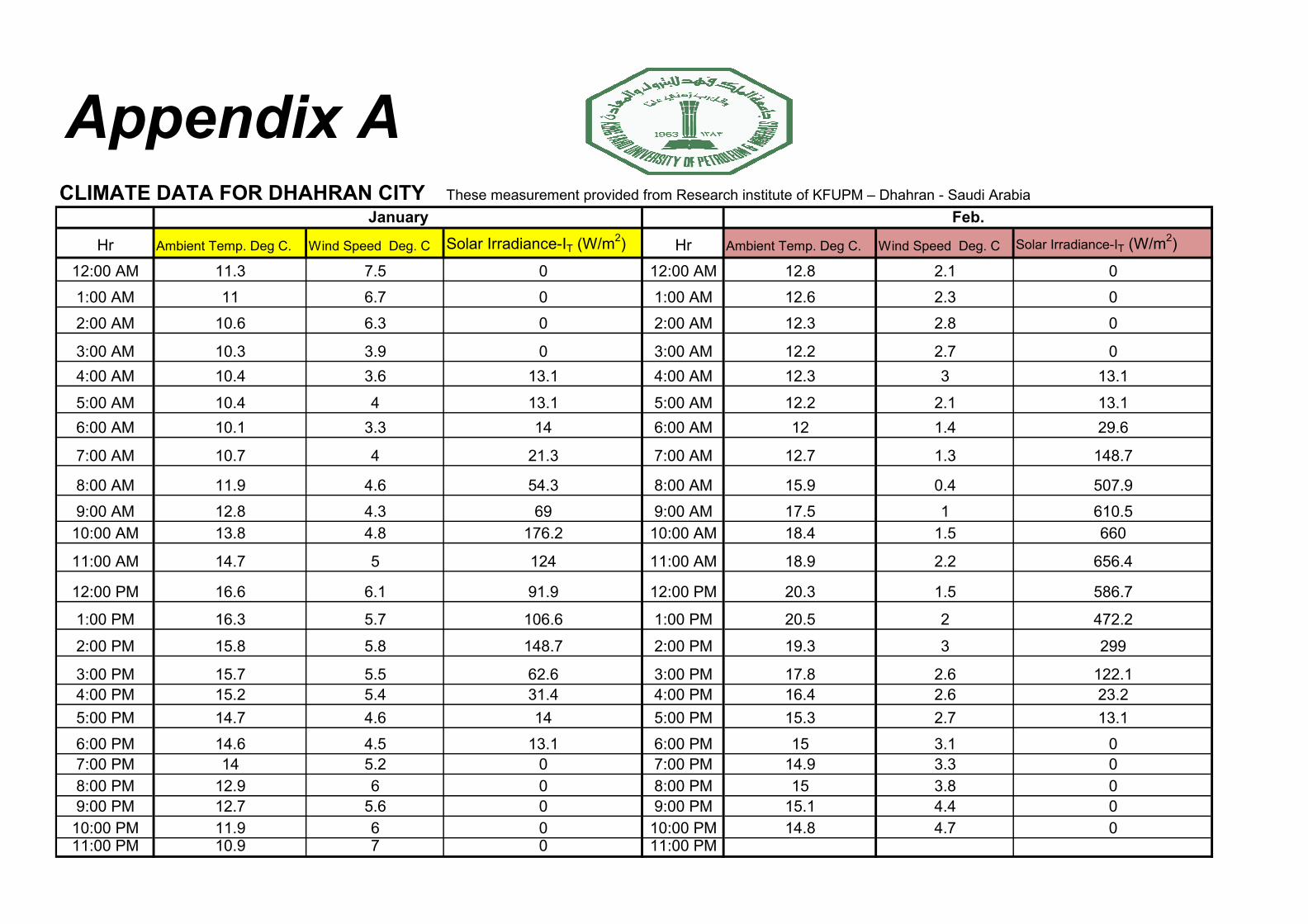
Hr Ambient Temp. Deg C. Wind Speed Deg. C Solar Irradiance-IT (W/m2) Hr Ambient Temp. Deg C. Wind Speed Deg. C Solar Irradiance-IT (W/m
2)
12:00 AM 11.3 7.5 0 12:00 AM 12.8 2.1 0
1:00 AM 11 6.7 0 1:00 AM 12.6 2.3 0
2:00 AM 10.6 6.3 0 2:00 AM 12.3 2.8 0
3:00 AM 10.3 3.9 0 3:00 AM 12.2 2.7 0
4:00 AM 10.4 3.6 13.1 4:00 AM 12.3 3 13.1
5:00 AM 10.4 4 13.1 5:00 AM 12.2 2.1 13.1
6:00 AM 10.1 3.3 14 6:00 AM 12 1.4 29.6
7:00 AM 10.7 4 21.3 7:00 AM 12.7 1.3 148.7
8:00 AM 11.9 4.6 54.3 8:00 AM 15.9 0.4 507.9
9:00 AM 12.8 4.3 69 9:00 AM 17.5 1 610.5
10:00 AM 13.8 4.8 176.2 10:00 AM 18.4 1.5 660
11:00 AM 14.7 5 124 11:00 AM 18.9 2.2 656.4
12:00 PM 16.6 6.1 91.9 12:00 PM 20.3 1.5 586.7
1:00 PM 16.3 5.7 106.6 1:00 PM 20.5 2 472.2
2:00 PM 15.8 5.8 148.7 2:00 PM 19.3 3 299
3:00 PM 15.7 5.5 62.6 3:00 PM 17.8 2.6 122.1
4:00 PM 15.2 5.4 31.4 4:00 PM 16.4 2.6 23.2
5:00 PM 14.7 4.6 14 5:00 PM 15.3 2.7 13.1
6:00 PM 14.6 4.5 13.1 6:00 PM 15 3.1 0
7:00 PM 14 5.2 0 7:00 PM 14.9 3.3 0
8:00 PM 12.9 6 0 8:00 PM 15 3.8 0
9:00 PM 12.7 5.6 0 9:00 PM 15.1 4.4 0
10:00 PM 11.9 6 0 10:00 PM 14.8 4.7 011:00 PM 10.9 7 0 11:00 PM
CLIMATE DATA FOR DHAHRAN CITY January Feb.
Appendix AThese measurement provided from Research institute of KFUPM – Dhahran - Saudi Arabia
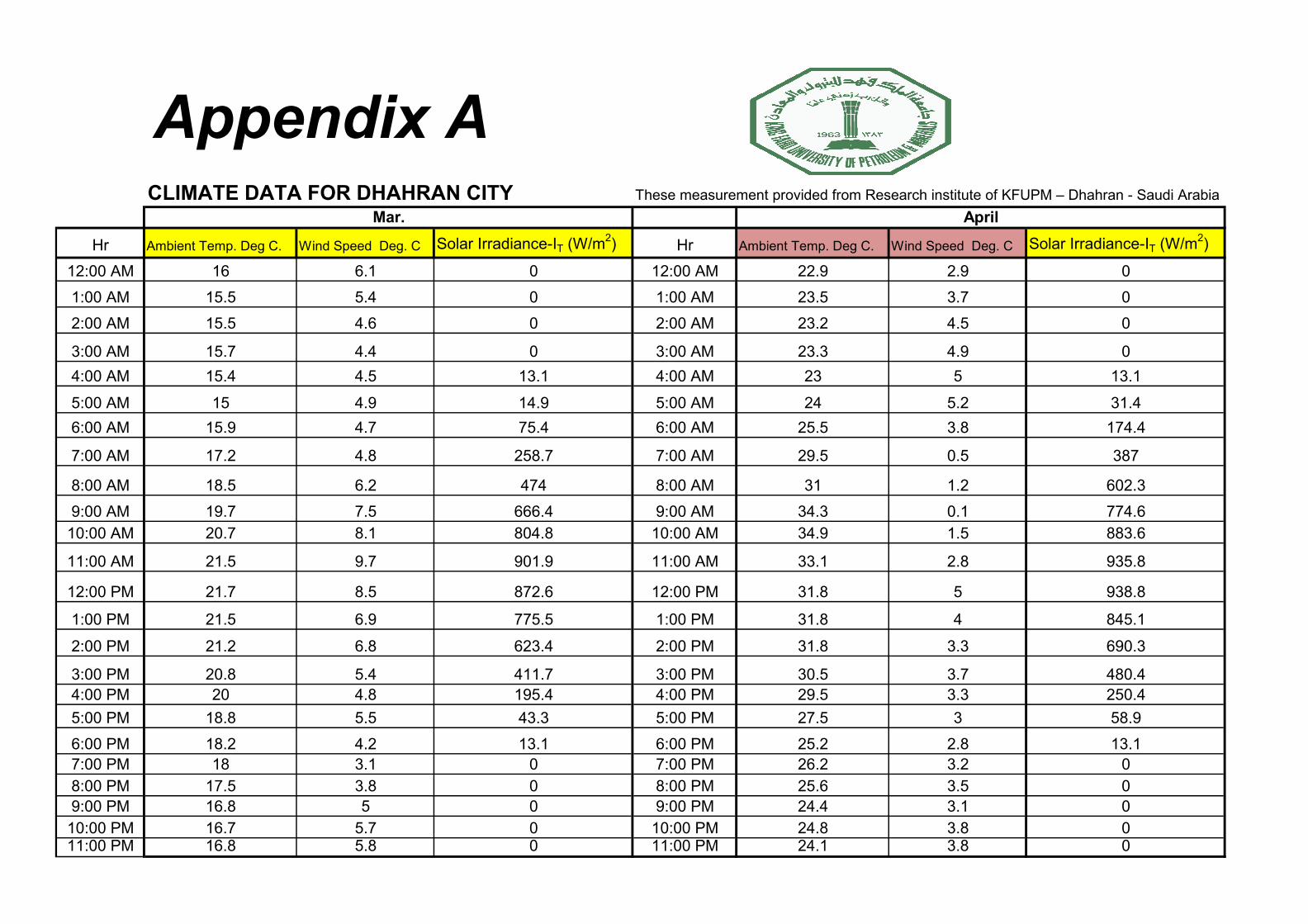
Hr Ambient Temp. Deg C. Wind Speed Deg. C Solar Irradiance-IT (W/m2) Hr Ambient Temp. Deg C. Wind Speed Deg. C Solar Irradiance-IT (W/m
2)
12:00 AM 16 6.1 0 12:00 AM 22.9 2.9 0
1:00 AM 15.5 5.4 0 1:00 AM 23.5 3.7 0
2:00 AM 15.5 4.6 0 2:00 AM 23.2 4.5 0
3:00 AM 15.7 4.4 0 3:00 AM 23.3 4.9 0
4:00 AM 15.4 4.5 13.1 4:00 AM 23 5 13.1
5:00 AM 15 4.9 14.9 5:00 AM 24 5.2 31.4
6:00 AM 15.9 4.7 75.4 6:00 AM 25.5 3.8 174.4
7:00 AM 17.2 4.8 258.7 7:00 AM 29.5 0.5 387
8:00 AM 18.5 6.2 474 8:00 AM 31 1.2 602.3
9:00 AM 19.7 7.5 666.4 9:00 AM 34.3 0.1 774.6
10:00 AM 20.7 8.1 804.8 10:00 AM 34.9 1.5 883.6
11:00 AM 21.5 9.7 901.9 11:00 AM 33.1 2.8 935.8
12:00 PM 21.7 8.5 872.6 12:00 PM 31.8 5 938.8
1:00 PM 21.5 6.9 775.5 1:00 PM 31.8 4 845.1
2:00 PM 21.2 6.8 623.4 2:00 PM 31.8 3.3 690.3
3:00 PM 20.8 5.4 411.7 3:00 PM 30.5 3.7 480.4
4:00 PM 20 4.8 195.4 4:00 PM 29.5 3.3 250.4
5:00 PM 18.8 5.5 43.3 5:00 PM 27.5 3 58.9
6:00 PM 18.2 4.2 13.1 6:00 PM 25.2 2.8 13.1
7:00 PM 18 3.1 0 7:00 PM 26.2 3.2 0
8:00 PM 17.5 3.8 0 8:00 PM 25.6 3.5 0
9:00 PM 16.8 5 0 9:00 PM 24.4 3.1 0
10:00 PM 16.7 5.7 0 10:00 PM 24.8 3.8 011:00 PM 16.8 5.8 0 11:00 PM 24.1 3.8 0
Mar. April
Appendix ACLIMATE DATA FOR DHAHRAN CITY These measurement provided from Research institute of KFUPM – Dhahran - Saudi Arabia
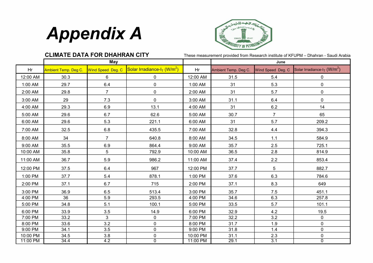
Hr Ambient Temp. Deg C. Wind Speed Deg. C Solar Irradiance-IT (W/m2) Hr Ambient Temp. Deg C. Wind Speed Deg. C Solar Irradiance-IT (W/m
2)
12:00 AM 30.3 6 0 12:00 AM 31.5 5.4 0
1:00 AM 29.7 6.4 0 1:00 AM 31 5.3 0
2:00 AM 29.8 7 0 2:00 AM 31 5.7 0
3:00 AM 29 7.3 0 3:00 AM 31.1 6.4 0
4:00 AM 29.3 6.9 13.1 4:00 AM 31 6.2 14
5:00 AM 29.6 6.7 62.6 5:00 AM 30.7 7 65
6:00 AM 29.6 5.3 221.1 6:00 AM 31 5.7 209.2
7:00 AM 32.5 6.8 435.5 7:00 AM 32.8 4.4 394.3
8:00 AM 34 7 640.8 8:00 AM 34.5 1.1 584.9
9:00 AM 35.5 6.9 864.4 9:00 AM 35.7 2.5 725.1
10:00 AM 35.8 5 792.9 10:00 AM 36.5 2.8 814.9
11:00 AM 36.7 5.9 986.2 11:00 AM 37.4 2.2 853.4
12:00 PM 37.5 6.4 967 12:00 PM 37.7 5 882.7
1:00 PM 37.7 5.4 878.1 1:00 PM 37.6 6.3 784.6
2:00 PM 37.1 6.7 715 2:00 PM 37.1 8.3 649
3:00 PM 36.9 6.5 513.4 3:00 PM 35.7 7.5 451.1
4:00 PM 36 5.9 293.5 4:00 PM 34.6 6.3 257.8
5:00 PM 34.8 5.1 100.1 5:00 PM 33.5 5.7 101.1
6:00 PM 33.9 3.5 14.9 6:00 PM 32.9 4.2 19.5
7:00 PM 33.2 3 0 7:00 PM 32.2 3.2 0
8:00 PM 33.6 3.2 0 8:00 PM 31.7 1.9 0
9:00 PM 34.1 3.5 0 9:00 PM 31.8 1.4 0
10:00 PM 34.5 3.8 0 10:00 PM 31.1 2.3 011:00 PM 34.4 4.2 0 11:00 PM 29.1 3.1 0
JuneMay
These measurement provided from Research institute of KFUPM – Dhahran - Saudi Arabia
Appendix ACLIMATE DATA FOR DHAHRAN CITY These measurement provided from Research institute of KFUPM – Dhahran - Saudi Arabia
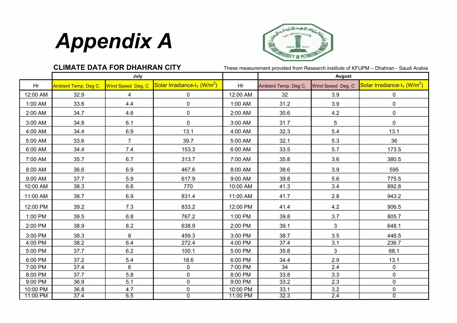
Hr Ambient Temp. Deg C. Wind Speed Deg. C Solar Irradiance-IT (W/m2) Hr Ambient Temp. Deg C. Wind Speed Deg. C Solar Irradiance-IT (W/m
2)
12:00 AM 32.9 4 0 12:00 AM 32 3.9 0
1:00 AM 33.6 4.4 0 1:00 AM 31.2 3.9 0
2:00 AM 34.7 4.6 0 2:00 AM 30.6 4.2 0
3:00 AM 34.8 6.1 0 3:00 AM 31.7 5 0
4:00 AM 34.4 6.9 13.1 4:00 AM 32.3 5.4 13.1
5:00 AM 33.6 7 39.7 5:00 AM 32.1 5.3 36
6:00 AM 34.4 7.4 153.3 6:00 AM 33.5 5.7 173.5
7:00 AM 35.7 6.7 313.7 7:00 AM 35.8 3.6 380.5
8:00 AM 36.6 6.9 467.6 8:00 AM 38.6 3.9 595
9:00 AM 37.7 5.9 617.9 9:00 AM 39.8 5.6 775.5
10:00 AM 38.3 6.6 770 10:00 AM 41.3 3.4 892.8
11:00 AM 38.7 6.9 831.4 11:00 AM 41.7 2.8 943.2
12:00 PM 39.2 7.3 833.2 12:00 PM 41.4 4.2 906.5
1:00 PM 39.5 6.8 767.2 1:00 PM 39.8 3.7 805.7
2:00 PM 38.9 8.2 638.9 2:00 PM 39.1 3 648.1
3:00 PM 38.3 8 459.3 3:00 PM 38.7 3.5 446.5
4:00 PM 38.2 6.4 272.4 4:00 PM 37.4 3.1 236.7
5:00 PM 37.7 6.2 100.1 5:00 PM 35.8 3 68.1
6:00 PM 37.2 5.4 18.6 6:00 PM 34.4 2.9 13.1
7:00 PM 37.4 6 0 7:00 PM 34 2.4 0
8:00 PM 37.7 5.8 0 8:00 PM 33.8 3.3 0
9:00 PM 36.9 5.1 0 9:00 PM 33.2 2.3 0
10:00 PM 36.8 4.7 0 10:00 PM 33.1 3.2 011:00 PM 37.4 6.5 0 11:00 PM 32.3 2.4 0
July August
These measurement provided from Research institute of KFUPM – Dhahran - Saudi Arabia These measurement provided from Research institute of KFUPM – Dhahran - Saudi Arabia
Appendix ACLIMATE DATA FOR DHAHRAN CITY
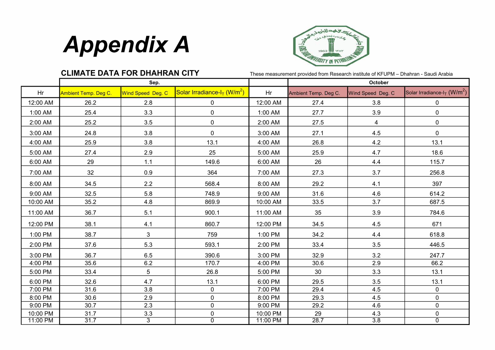
Hr Ambient Temp. Deg C. Wind Speed Deg. C Solar Irradiance-IT (W/m2) Hr Ambient Temp. Deg C. Wind Speed Deg. C Solar Irradiance-IT (W/m
2)
12:00 AM 26.2 2.8 0 12:00 AM 27.4 3.8 0
1:00 AM 25.4 3.3 0 1:00 AM 27.7 3.9 0
2:00 AM 25.2 3.5 0 2:00 AM 27.5 4 0
3:00 AM 24.8 3.8 0 3:00 AM 27.1 4.5 0
4:00 AM 25.9 3.8 13.1 4:00 AM 26.8 4.2 13.1
5:00 AM 27.4 2.9 25 5:00 AM 25.9 4.7 18.6
6:00 AM 29 1.1 149.6 6:00 AM 26 4.4 115.7
7:00 AM 32 0.9 364 7:00 AM 27.3 3.7 256.8
8:00 AM 34.5 2.2 568.4 8:00 AM 29.2 4.1 397
9:00 AM 32.5 5.8 748.9 9:00 AM 31.6 4.6 614.2
10:00 AM 35.2 4.8 869.9 10:00 AM 33.5 3.7 687.5
11:00 AM 36.7 5.1 900.1 11:00 AM 35 3.9 784.6
12:00 PM 38.1 4.1 860.7 12:00 PM 34.5 4.5 671
1:00 PM 38.7 3 759 1:00 PM 34.2 4.4 618.8
2:00 PM 37.6 5.3 593.1 2:00 PM 33.4 3.5 446.5
3:00 PM 36.7 6.5 390.6 3:00 PM 32.9 3.2 247.7
4:00 PM 35.6 6.2 170.7 4:00 PM 30.6 2.9 66.2
5:00 PM 33.4 5 26.8 5:00 PM 30 3.3 13.1
6:00 PM 32.6 4.7 13.1 6:00 PM 29.5 3.5 13.1
7:00 PM 31.6 3.8 0 7:00 PM 29.4 4.5 0
8:00 PM 30.6 2.9 0 8:00 PM 29.3 4.5 0
9:00 PM 30.7 2.3 0 9:00 PM 29.2 4.6 0
10:00 PM 31.7 3.3 0 10:00 PM 29 4.3 011:00 PM 31.7 3 0 11:00 PM 28.7 3.8 0
Sep. October
These measurement provided from Research institute of KFUPM – Dhahran - Saudi Arabia
Appendix ACLIMATE DATA FOR DHAHRAN CITY These measurement provided from Research institute of KFUPM – Dhahran - Saudi Arabia
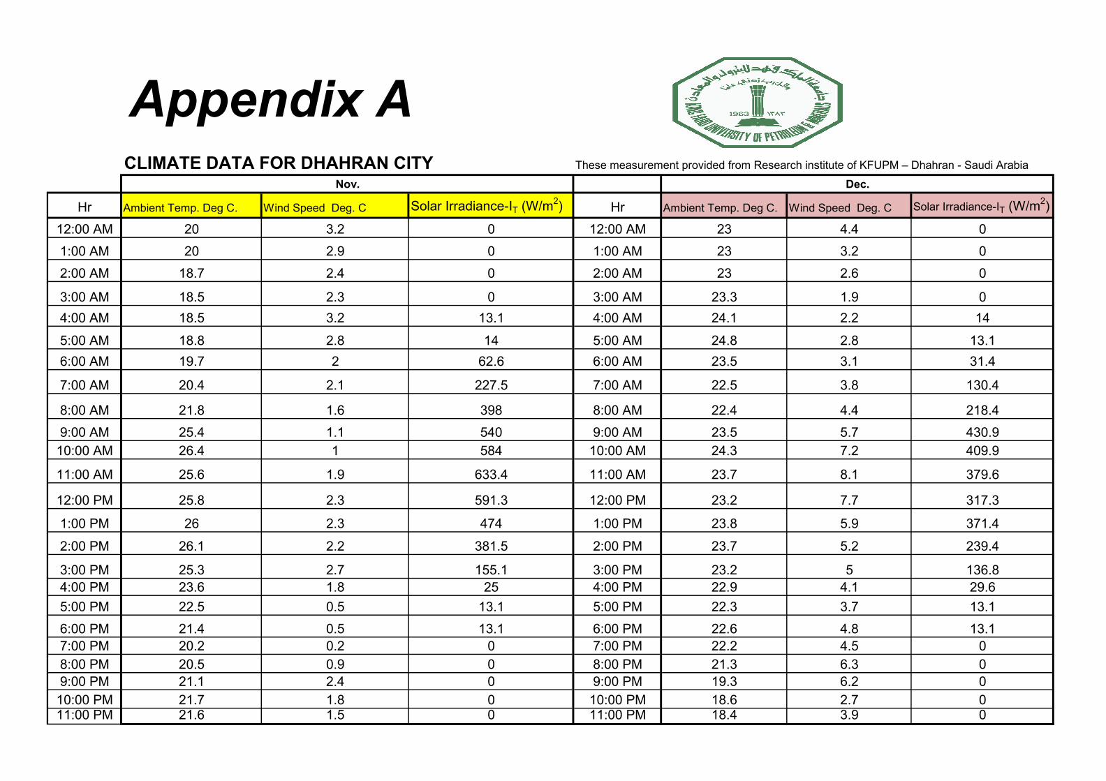
Hr Ambient Temp. Deg C. Wind Speed Deg. C Solar Irradiance-IT (W/m2) Hr Ambient Temp. Deg C. Wind Speed Deg. C Solar Irradiance-IT (W/m
2)
12:00 AM 20 3.2 0 12:00 AM 23 4.4 0
1:00 AM 20 2.9 0 1:00 AM 23 3.2 0
2:00 AM 18.7 2.4 0 2:00 AM 23 2.6 0
3:00 AM 18.5 2.3 0 3:00 AM 23.3 1.9 0
4:00 AM 18.5 3.2 13.1 4:00 AM 24.1 2.2 14
5:00 AM 18.8 2.8 14 5:00 AM 24.8 2.8 13.1
6:00 AM 19.7 2 62.6 6:00 AM 23.5 3.1 31.4
7:00 AM 20.4 2.1 227.5 7:00 AM 22.5 3.8 130.4
8:00 AM 21.8 1.6 398 8:00 AM 22.4 4.4 218.4
9:00 AM 25.4 1.1 540 9:00 AM 23.5 5.7 430.9
10:00 AM 26.4 1 584 10:00 AM 24.3 7.2 409.9
11:00 AM 25.6 1.9 633.4 11:00 AM 23.7 8.1 379.6
12:00 PM 25.8 2.3 591.3 12:00 PM 23.2 7.7 317.3
1:00 PM 26 2.3 474 1:00 PM 23.8 5.9 371.4
2:00 PM 26.1 2.2 381.5 2:00 PM 23.7 5.2 239.4
3:00 PM 25.3 2.7 155.1 3:00 PM 23.2 5 136.8
4:00 PM 23.6 1.8 25 4:00 PM 22.9 4.1 29.6
5:00 PM 22.5 0.5 13.1 5:00 PM 22.3 3.7 13.1
6:00 PM 21.4 0.5 13.1 6:00 PM 22.6 4.8 13.1
7:00 PM 20.2 0.2 0 7:00 PM 22.2 4.5 0
8:00 PM 20.5 0.9 0 8:00 PM 21.3 6.3 0
9:00 PM 21.1 2.4 0 9:00 PM 19.3 6.2 0
10:00 PM 21.7 1.8 0 10:00 PM 18.6 2.7 011:00 PM 21.6 1.5 0 11:00 PM 18.4 3.9 0
Dec.Nov.
These measurement provided from Research institute of KFUPM – Dhahran - Saudi Arabia
Appendix ACLIMATE DATA FOR DHAHRAN CITY
Vitae
Name : Ayman Jamal Abdel Majid Alazazmeh
Nationality : Jordanian.
Date of Birth : June 19, 1985.
Email : [email protected]
Address : Jordan - Amman
Academic Background : B.S (Mechanical Engineering)
August 2007
Hashemite University
……………………………. Alzarqa, Jordan.
Journal publications:
Alazazmeh AJ, Mokheimer EM (2015) Review of Solar Cooling
Technologies. J Appl Mech Eng .
Patent “Pat. Applied For":
EVAPORATIVE CONDENSER COOLING SYSTEM, Alazazmeh
AJ, Mokheimer EM (2015).


