atmosphere

Article

Increasing Neurons or Deepening Layers inForecasting Maximum Temperature Time Series?

Trang Thi Kieu Tran 1, Taesam Lee 1,* and Jong-Suk Kim 2,*1 Department of Civil Engineering, ERI, Gyeongsang National University, 501 Jinju-daero, Jinju 660-701,

Korea; trangtran281292@gmail.com2 State Key Laboratory of Water Resources and Hydropower Engineering Science, Wuhan University,

Wuhan 430072, China* Correspondence: tae3lee@gnu.ac.kr (T.L.); jongsuk@whu.edu.cn (J.-S.K.)

Received: 8 September 2020; Accepted: 7 October 2020; Published: 9 October 2020�����������������

Abstract: Weather forecasting, especially that of extreme climatic events, has gained considerableattention among researchers due to their impacts on natural ecosystems and human life.The applicability of artificial neural networks (ANNs) in non-linear process forecasting has significantlycontributed to hydro-climatology. The efficiency of neural network functions depends on the networkstructure and parameters. This study proposed a new approach to forecasting a one-day-aheadmaximum temperature time series for South Korea to discuss the relationship between networkspecifications and performance by employing various scenarios for the number of parametersand hidden layers in the ANN model. Specifically, a different number of trainable parameters(i.e., the total number of weights and bias) and distinctive numbers of hidden layers were comparedfor system-performance effects. If the parameter sizes were too large, the root mean square error(RMSE) would be generally increased, and the model’s ability was impaired. Besides, too manyhidden layers would reduce the system prediction if the number of parameters was high. The numberof parameters and hidden layers affected the performance of ANN models for time series forecastingcompetitively. The result showed that the five-hidden layer model with 49 parameters produced thesmallest RMSE at most South Korean stations.

Keywords: artificial neural network; neurons; layers; temperature; South Korea; deep learning

1. Introduction

An artificial neural network (ANN) is a system for information processing inspired by biologicalneural networks. The key element of this network is the huge amount of highly interconnectedprocessing nodes (neurons) that work together by a dynamic response to process the information.A neural network is useful for modeling the non-linear relation between the input and output of asystem [1]. Compared to other machine learning methods such as autoregressive moving averages(ARMA), autoregressive integrated moving averages (ARIMA), and random forest (RF), the ANNmodel showed better performance in regression prediction problems [2–4]. According to Agrawal [5],the ANN model predicted rainfall events more accurately than the ARIMA model. In another work,ANNs have been applied to forecast monthly mean daily global solar radiation [6].

Furthermore, the ANN model has also been employed to forecast climatological and meteorologicalvariables. Although it is known that the weather forecasting problem is challenging because of itschaotic and dynamic process, weather forecasting based on ANNs has been employing considerably inrecent years due to the success of the ANN’s ability. From some previous research, artificial neuralnetworks have been shown as a promising method to forecast weather and time series data due to theircapability of pattern recognition and generalization [7,8]. Smith et al. [9] developed an improved ANN

Atmosphere 2020, 11, 1072; doi:10.3390/atmos11101072 www.mdpi.com/journal/atmosphere

Atmosphere 2020, 11, 1072 2 of 18

to forecast the air temperature from 1 to 12 h ahead by increasing the number of samples in the training,adding additional seasonal variables, extending the duration of prior observations, and varying thenumber of hidden neurons in the network. Six hours of prior data were chosen as the inputs for thetemperature prediction since a network with eight prior observations performed worse than the sixhour network. Moreover, it is demonstrated that the models using one hidden layer with 40 neuronsperformed better than other models over repeated instantiations. In another study, the ANN modelsfor the maximum as well as minimum temperature, and relative humidity forecasting were proposedby Sanjay Mathur [10] using time series analysis. The multilayer feedforward ANN model with aback-propagation algorithm was used to predict the weather conditions in the future, and it was foundthat the forecasting model could make a highly accurate prediction. The authors in [11] employed theANN models to forecast air temperature, relative humidity, and soil temperature in India, showing thatthe ANN model was a robust tool to predict meteorological variables as it showed promising resultswith 91–96% accuracy for predictions of all cases. In this study, we also aimed to predict the airtemperature one day ahead of past observations using the ANN model.

The effectiveness of a network-based approach depends on the architecture of the network andits parameters. All of these considerations are complex, and the configuration of a neural networkstructure depends on the problem [12]. If unsuitable network architecture and parameters are selected,the results may be undesirable. On the other hand, a proper design of network architecture andparameters can produce desirable results [13,14]. However, little investigation has been conductedon the effect of parameters and architecture on the model’s performance. The selection of ANNarchitecture, consisting of input variables, the number of neurons in the hidden layer, and the numberof hidden layers is a difficult task, so the structure of the network is usually determined by a trial anderror approach and based on the experience of the modeler [5]. In another previous study, we comparedone-hidden layer and multi-hidden layer ANN models in maximum temperature prediction at fivestations in South Korea [15]. In addition, the genetic algorithm was applied to find the best architectureof models. It showed that the ANN with one hidden layer performed the most accurate forecasts.However, the effect of the number of hidden layers and neurons on the ANN’s performance in themaximum temperature time series prediction is not sufficient. It may expect that the model performsworse when the number of parameters decreases. However, what happens if we further increase thenumber of tunable parameters? There are two competing effects. On the one hand, more parameters,which mean more neurons, become available, possibly allowing for better predictions. On the otherhand, the higher the parameter number, the more overfitting the model is. Will the networks be robustif more trainable parameters than necessary are present? Is a one-hidden layer model always betterthan a multi-hidden layer model for maximum temperature forecasting in South Korea? Therefore,it is also apparently several problems related to the model proper architecture.

This paper proposed a new strategy that applied the ANNs using different learning parametersand hidden layers to empirically compare the prediction performance of daily maximum temperaturetime series. This study aimed to discuss the effect of parameters on the performance of ANN fortemperature time series forecasting.

The rest of the paper is structured as follows. Section 2 describes the data and methodology usedfor the experiments. Section 3 describes the results, and the final section provides conclusions anddirections for future work.

2. Data and Methods

In the current study, 55 weather stations that record maximum temperature in South Korea atthe daily timescale were employed. Most stations have a data period of 40 years from 1976 to 2015,except for Andong station (1983–2015) and Chuncheon station (1988–2015).

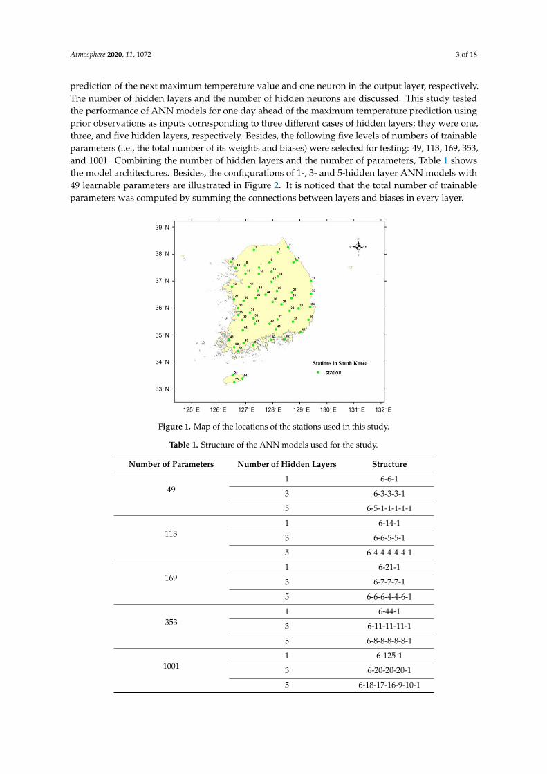
Figure 1 presents the locations of the stations at which the data were recorded. The forecastingmodel for the maximum temperature was built based on the neural network. There were six neuronsin the input layer, which corresponds to the number of previous days provided to the network for the

Atmosphere 2020, 11, 1072 3 of 18

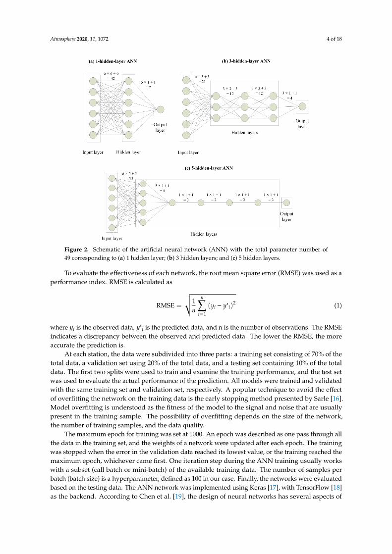
prediction of the next maximum temperature value and one neuron in the output layer, respectively.The number of hidden layers and the number of hidden neurons are discussed. This study testedthe performance of ANN models for one day ahead of the maximum temperature prediction usingprior observations as inputs corresponding to three different cases of hidden layers; they were one,three, and five hidden layers, respectively. Besides, the following five levels of numbers of trainableparameters (i.e., the total number of its weights and biases) were selected for testing: 49, 113, 169, 353,and 1001. Combining the number of hidden layers and the number of parameters, Table 1 showsthe model architectures. Besides, the configurations of 1-, 3- and 5-hidden layer ANN models with49 learnable parameters are illustrated in Figure 2. It is noticed that the total number of trainableparameters was computed by summing the connections between layers and biases in every layer.

Atmosphere 2020, 11, x FOR PEER REVIEW 3 of 18

respectively. The number of hidden layers and the number of hidden neurons are discussed. This

study tested the performance of ANN models for one day ahead of the maximum temperature

prediction using prior observations as inputs corresponding to three different cases of hidden layers;

they were one, three, and five hidden layers, respectively. Besides, the following five levels of

numbers of trainable parameters (i.e., the total number of its weights and biases) were selected for

testing: 49, 113, 169, 353, and 1001. Combining the number of hidden layers and the number of

parameters, Table 1 shows the model architectures. Besides, the configurations of 1-, 3- and 5-hidden

layer ANN models with 49 learnable parameters are illustrated in Figure 2. It is noticed that the total

number of trainable parameters was computed by summing the connections between layers and

biases in every layer.

Figure 1. Map of the locations of the stations used in this study.

Figure 2. Schematic of the artificial neural network (ANN) with the total parameter number of 49

corresponding to (a) 1 hidden layer; (b) 3 hidden layers; and (c) 5 hidden layers.

Figure 1. Map of the locations of the stations used in this study.

Table 1. Structure of the ANN models used for the study.

Number of Parameters Number of Hidden Layers Structure

491 6-6-1

3 6-3-3-3-1

5 6-5-1-1-1-1-1

1131 6-14-1

3 6-6-5-5-1

5 6-4-4-4-4-4-1

1691 6-21-1

3 6-7-7-7-1

5 6-6-6-4-4-6-1

3531 6-44-1

3 6-11-11-11-1

5 6-8-8-8-8-8-1

10011 6-125-1

3 6-20-20-20-1

5 6-18-17-16-9-10-1

Atmosphere 2020, 11, 1072 4 of 18

Atmosphere 2020, 11, x FOR PEER REVIEW 3 of 18

respectively. The number of hidden layers and the number of hidden neurons are discussed. This

study tested the performance of ANN models for one day ahead of the maximum temperature

prediction using prior observations as inputs corresponding to three different cases of hidden layers;

they were one, three, and five hidden layers, respectively. Besides, the following five levels of

numbers of trainable parameters (i.e., the total number of its weights and biases) were selected for

testing: 49, 113, 169, 353, and 1001. Combining the number of hidden layers and the number of

parameters, Table 1 shows the model architectures. Besides, the configurations of 1-, 3- and 5-hidden

layer ANN models with 49 learnable parameters are illustrated in Figure 2. It is noticed that the total

number of trainable parameters was computed by summing the connections between layers and

biases in every layer.

Figure 1. Map of the locations of the stations used in this study.

Figure 2. Schematic of the artificial neural network (ANN) with the total parameter number of 49

corresponding to (a) 1 hidden layer; (b) 3 hidden layers; and (c) 5 hidden layers.

Figure 2. Schematic of the artificial neural network (ANN) with the total parameter number of49 corresponding to (a) 1 hidden layer; (b) 3 hidden layers; and (c) 5 hidden layers.

To evaluate the effectiveness of each network, the root mean square error (RMSE) was used as aperformance index. RMSE is calculated as

RMSE =

√√1n

n∑i=1

(yi − y′i)2 (1)

where yi is the observed data, y′i is the predicted data, and n is the number of observations. The RMSEindicates a discrepancy between the observed and predicted data. The lower the RMSE, the moreaccurate the prediction is.

At each station, the data were subdivided into three parts: a training set consisting of 70% of thetotal data, a validation set using 20% of the total data, and a testing set containing 10% of the totaldata. The first two splits were used to train and examine the training performance, and the test setwas used to evaluate the actual performance of the prediction. All models were trained and validatedwith the same training set and validation set, respectively. A popular technique to avoid the effectof overfitting the network on the training data is the early stopping method presented by Sarle [16].Model overfitting is understood as the fitness of the model to the signal and noise that are usuallypresent in the training sample. The possibility of overfitting depends on the size of the network,the number of training samples, and the data quality.

The maximum epoch for training was set at 1000. An epoch was described as one pass through allthe data in the training set, and the weights of a network were updated after each epoch. The trainingwas stopped when the error in the validation data reached its lowest value, or the training reached themaximum epoch, whichever came first. One iteration step during the ANN training usually workswith a subset (call batch or mini-batch) of the available training data. The number of samples perbatch (batch size) is a hyperparameter, defined as 100 in our case. Finally, the networks were evaluatedbased on the testing data. The ANN network was implemented using Keras [17], with TensorFlow [18]as the backend. According to Chen et al. [19], the design of neural networks has several aspects of

Atmosphere 2020, 11, 1072 5 of 18

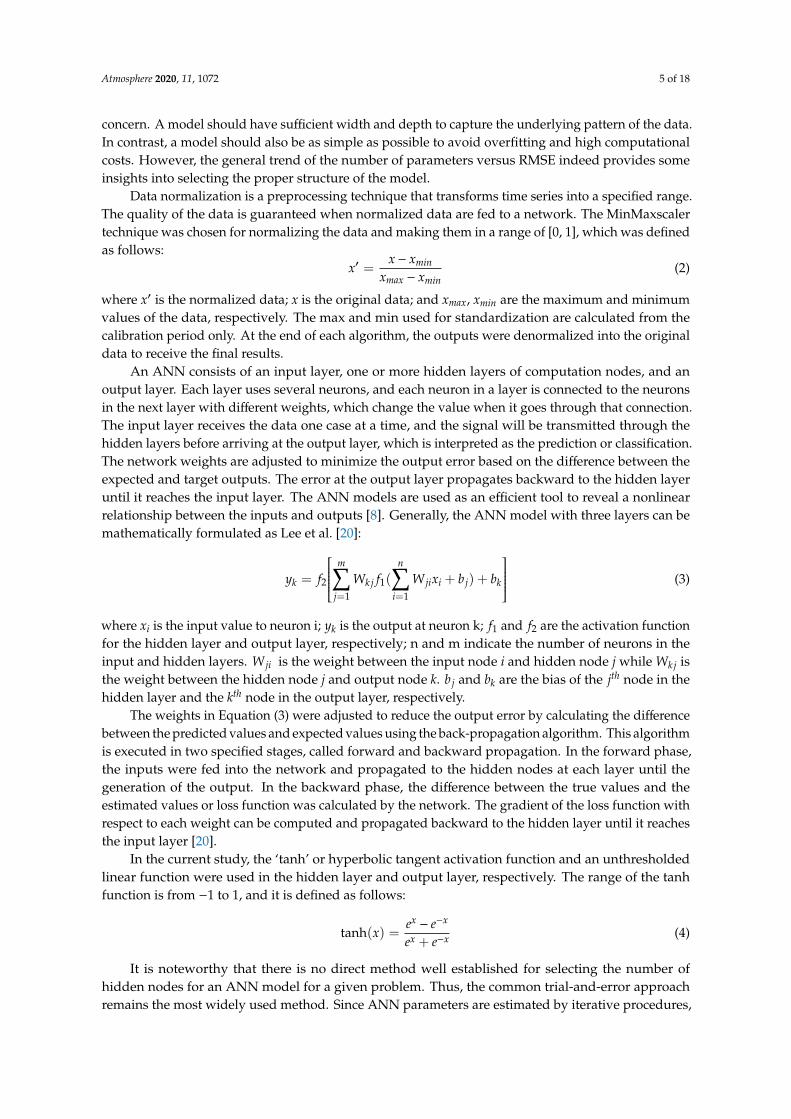
concern. A model should have sufficient width and depth to capture the underlying pattern of the data.In contrast, a model should also be as simple as possible to avoid overfitting and high computationalcosts. However, the general trend of the number of parameters versus RMSE indeed provides someinsights into selecting the proper structure of the model.

Data normalization is a preprocessing technique that transforms time series into a specified range.The quality of the data is guaranteed when normalized data are fed to a network. The MinMaxscalertechnique was chosen for normalizing the data and making them in a range of [0, 1], which was definedas follows:

x′ =x− xmin

xmax − xmin(2)

where x′ is the normalized data; x is the original data; and xmax, xmin are the maximum and minimumvalues of the data, respectively. The max and min used for standardization are calculated from thecalibration period only. At the end of each algorithm, the outputs were denormalized into the originaldata to receive the final results.

An ANN consists of an input layer, one or more hidden layers of computation nodes, and anoutput layer. Each layer uses several neurons, and each neuron in a layer is connected to the neuronsin the next layer with different weights, which change the value when it goes through that connection.The input layer receives the data one case at a time, and the signal will be transmitted through thehidden layers before arriving at the output layer, which is interpreted as the prediction or classification.The network weights are adjusted to minimize the output error based on the difference between theexpected and target outputs. The error at the output layer propagates backward to the hidden layeruntil it reaches the input layer. The ANN models are used as an efficient tool to reveal a nonlinearrelationship between the inputs and outputs [8]. Generally, the ANN model with three layers can bemathematically formulated as Lee et al. [20]:

yk = f2

m∑j=1

Wkj f1(n∑

i=1

W jixi + b j) + bk

(3)

where xi is the input value to neuron i; yk is the output at neuron k; f1 and f2 are the activation functionfor the hidden layer and output layer, respectively; n and m indicate the number of neurons in theinput and hidden layers. W ji is the weight between the input node i and hidden node j while Wkj isthe weight between the hidden node j and output node k. b j and bk are the bias of the jth node in thehidden layer and the kth node in the output layer, respectively.

The weights in Equation (3) were adjusted to reduce the output error by calculating the differencebetween the predicted values and expected values using the back-propagation algorithm. This algorithmis executed in two specified stages, called forward and backward propagation. In the forward phase,the inputs were fed into the network and propagated to the hidden nodes at each layer until thegeneration of the output. In the backward phase, the difference between the true values and theestimated values or loss function was calculated by the network. The gradient of the loss function withrespect to each weight can be computed and propagated backward to the hidden layer until it reachesthe input layer [20].

In the current study, the ‘tanh’ or hyperbolic tangent activation function and an unthresholdedlinear function were used in the hidden layer and output layer, respectively. The range of the tanhfunction is from −1 to 1, and it is defined as follows:

tanh(x) =ex− e−x

ex + e−x (4)

It is noteworthy that there is no direct method well established for selecting the number ofhidden nodes for an ANN model for a given problem. Thus, the common trial-and-error approachremains the most widely used method. Since ANN parameters are estimated by iterative procedures,

Atmosphere 2020, 11, 1072 6 of 18

which provide slightly different results each time they are run, we estimated each ANN 5 times andreported the mean and standard deviation errors in the figure.

The purpose of this study was not to find the best station-specific model, but to investigatethe effects of hidden layers and trainable parameters on the performance of ANNs for maximumtemperature modeling. We think that the sample size of 55 stations is large enough to infer some of the(average) properties of these factors to the ANN models.

3. Results

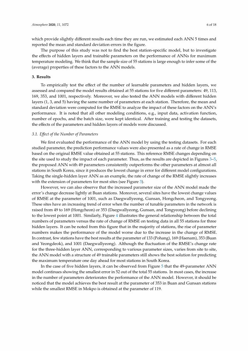
To empirically test the effect of the number of learnable parameters and hidden layers, weassessed and compared the model results obtained at 55 stations for five different parameters: 49, 113,169, 353, and 1001, respectively. Moreover, we also tested the ANN models with different hiddenlayers (1, 3, and 5) having the same number of parameters at each station. Therefore, the mean andstandard deviation were computed for the RMSE to analyze the impact of these factors on the ANN’sperformance. It is noted that all other modeling conditions, e.g., input data, activation function,number of epochs, and the batch size, were kept identical. After training and testing the datasets,the effects of the parameters and hidden layers of models were discussed.

3.1. Effect of the Number of Parameters

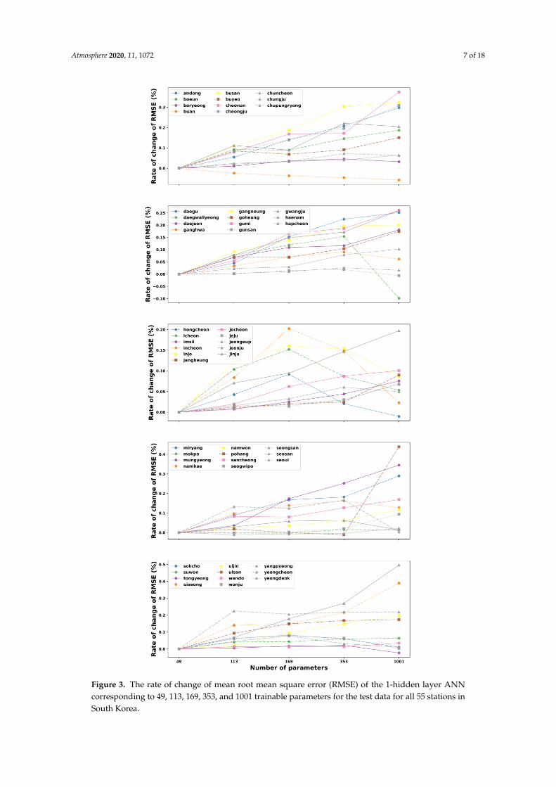
We first evaluated the performance of the ANN model by using the testing datasets. For eachstudied parameter, the prediction performance values were also presented as a rate of change in RMSEbased on the original RMSE value obtained at 55 stations. This reference RMSE changes depending onthe site used to study the impact of each parameter. Thus, as the results are depicted in Figures 3–5,the proposed ANN with 49 parameters consistently outperforms the other parameters at almost allstations in South Korea, since it produces the lowest change in error for different model configurations.Taking the single-hidden layer ANN as an example, the rate of change of the RMSE slightly increaseswith the extension of parameters for most sites (see Figure 3).

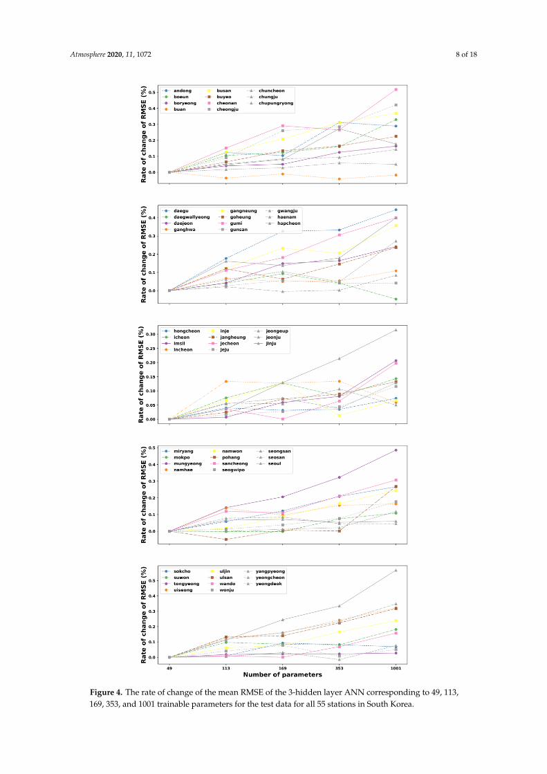
However, we can also observe that the increased parameter size of the ANN model made theerror’s change decrease lightly at Buan stations. Moreover, several sites have the lowest change valuesof RMSE at the parameter of 1001, such as Daegwallyeong, Gunsan, Hongcheon, and Tongyeong.These sites have an increasing trend of error when the number of tunable parameters in the network israised from 49 to 169 (Hongcheon) or 353 (Daegwallyeong, Gunsan, and Tongyeong) before decliningto the lowest point at 1001. Similarly, Figure 4 illustrates the general relationship between the totalnumbers of parameters versus the rate of change of RMSE on testing data in all 55 stations for threehidden layers. It can be noted from this figure that in the majority of stations, the rise of parameternumbers makes the performance of the model worse due to the increase in the change of RMSE.In contrast, few stations have the best results at the parameter of 133 (Pohang), 169 (Haenam), 353 (Buanand Yeongdeok), and 1001 (Daegwallyeong). Although the fluctuation of the RMSE’s change ratefor the three-hidden layer ANN, corresponding to various parameter sizes, varies from site to site,the ANN model with a structure of 49 trainable parameters still shows the best solution for predictingthe maximum temperature one day ahead for most stations in South Korea.

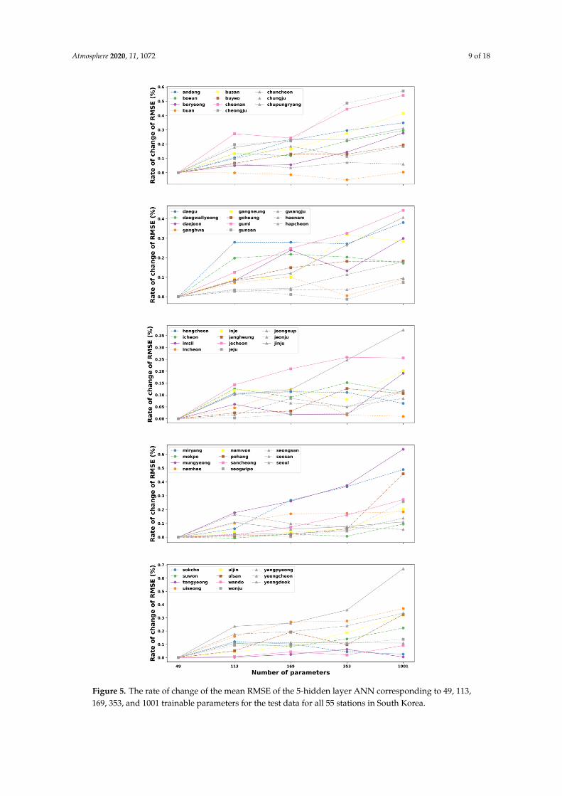
In the case of five hidden layers, it can be observed from Figure 5 that the 49-parameter ANNmodel continues showing the smallest error in 52 out of the total 55 stations. In most cases, the increasein the number of parameters deteriorates the performance of the ANN model. However, it should benoticed that the model achieves the best result at the parameter of 353 in Buan and Gunsan stationswhile the smallest RMSE in Mokpo is obtained at the parameter of 119.

Atmosphere 2020, 11, 1072 7 of 18Atmosphere 2020, 11, x FOR PEER REVIEW 7 of 18

Figure 3. The rate of change of mean root mean square error (RMSE) of the 1-hidden layer ANN

corresponding to 49, 113, 169, 353, and 1001 trainable parameters for the test data for all 55 stations in

South Korea.

Figure 3. The rate of change of mean root mean square error (RMSE) of the 1-hidden layer ANNcorresponding to 49, 113, 169, 353, and 1001 trainable parameters for the test data for all 55 stations inSouth Korea.

Atmosphere 2020, 11, 1072 8 of 18Atmosphere 2020, 11, x FOR PEER REVIEW 8 of 18

Figure 4. The rate of change of the mean RMSE of the 3-hidden layer ANN corresponding to 49, 113,

169, 353, and 1001 trainable parameters for the test data for all 55 stations in South Korea.

Figure 4. The rate of change of the mean RMSE of the 3-hidden layer ANN corresponding to 49, 113,169, 353, and 1001 trainable parameters for the test data for all 55 stations in South Korea.

Atmosphere 2020, 11, 1072 9 of 18Atmosphere 2020, 11, x FOR PEER REVIEW 9 of 18

Figure 5. The rate of change of the mean RMSE of the 5-hidden layer ANN corresponding to 49, 113,

169, 353, and 1001 trainable parameters for the test data for all 55 stations in South Korea.

Figure 5. The rate of change of the mean RMSE of the 5-hidden layer ANN corresponding to 49, 113,169, 353, and 1001 trainable parameters for the test data for all 55 stations in South Korea.

Atmosphere 2020, 11, 1072 10 of 18

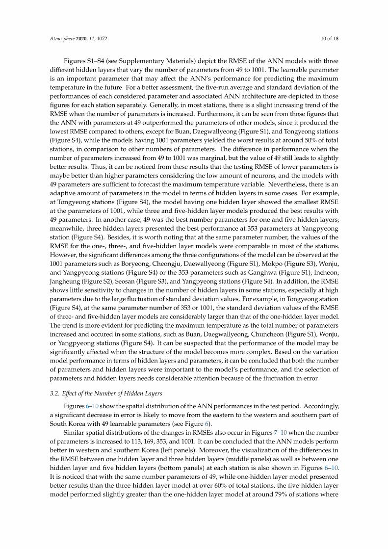
Figures S1–S4 (see Supplementary Materials) depict the RMSE of the ANN models with threedifferent hidden layers that vary the number of parameters from 49 to 1001. The learnable parameteris an important parameter that may affect the ANN’s performance for predicting the maximumtemperature in the future. For a better assessment, the five-run average and standard deviation of theperformances of each considered parameter and associated ANN architecture are depicted in thosefigures for each station separately. Generally, in most stations, there is a slight increasing trend of theRMSE when the number of parameters is increased. Furthermore, it can be seen from those figures thatthe ANN with parameters at 49 outperformed the parameters of other models, since it produced thelowest RMSE compared to others, except for Buan, Daegwallyeong (Figure S1), and Tongyeong stations(Figure S4), while the models having 1001 parameters yielded the worst results at around 50% of totalstations, in comparison to other numbers of parameters. The difference in performance when thenumber of parameters increased from 49 to 1001 was marginal, but the value of 49 still leads to slightlybetter results. Thus, it can be noticed from these results that the testing RMSE of lower parameters ismaybe better than higher parameters considering the low amount of neurons, and the models with49 parameters are sufficient to forecast the maximum temperature variable. Nevertheless, there is anadaptive amount of parameters in the model in terms of hidden layers in some cases. For example,at Tongyeong stations (Figure S4), the model having one hidden layer showed the smallest RMSEat the parameters of 1001, while three and five-hidden layer models produced the best results with49 parameters. In another case, 49 was the best number parameters for one and five hidden layers;meanwhile, three hidden layers presented the best performance at 353 parameters at Yangpyeongstation (Figure S4). Besides, it is worth noting that at the same parameter number, the values of theRMSE for the one-, three-, and five-hidden layer models were comparable in most of the stations.However, the significant differences among the three configurations of the model can be observed at the1001 parameters such as Boryeong, Cheongju, Daewallyeong (Figure S1), Mokpo (Figure S3), Wonju,and Yangpyeong stations (Figure S4) or the 353 parameters such as Ganghwa (Figure S1), Incheon,Jangheung (Figure S2), Seosan (Figure S3), and Yangpyeong stations (Figure S4). In addition, the RMSEshows little sensitivity to changes in the number of hidden layers in some stations, especially at highparameters due to the large fluctuation of standard deviation values. For example, in Tongyeong station(Figure S4), at the same parameter number of 353 or 1001, the standard deviation values of the RMSEof three- and five-hidden layer models are considerably larger than that of the one-hidden layer model.The trend is more evident for predicting the maximum temperature as the total number of parametersincreased and occured in some stations, such as Buan, Daegwallyeong, Chuncheon (Figure S1), Wonju,or Yangpyeong stations (Figure S4). It can be suspected that the performance of the model may besignificantly affected when the structure of the model becomes more complex. Based on the variationmodel performance in terms of hidden layers and parameters, it can be concluded that both the numberof parameters and hidden layers were important to the model’s performance, and the selection ofparameters and hidden layers needs considerable attention because of the fluctuation in error.

3.2. Effect of the Number of Hidden Layers

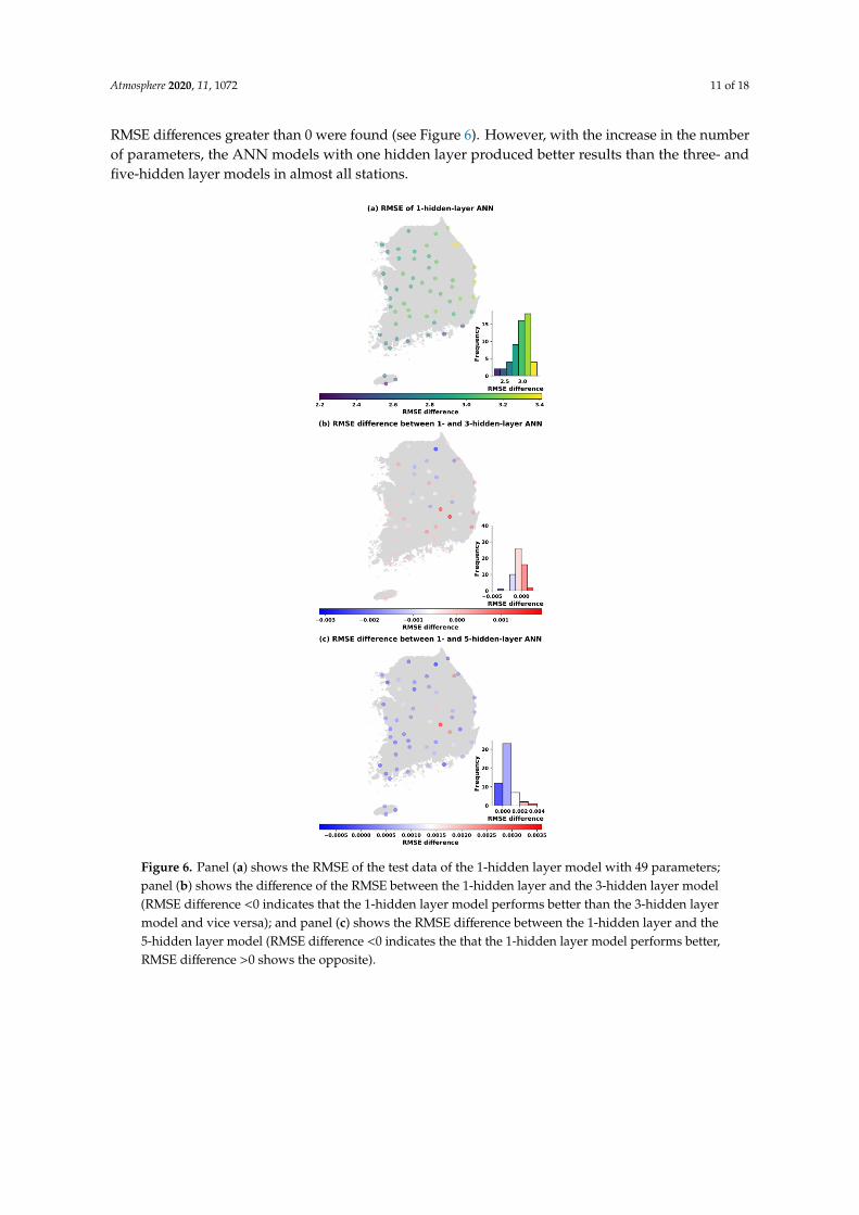
Figures 6–10 show the spatial distribution of the ANN performances in the test period. Accordingly,a significant decrease in error is likely to move from the eastern to the western and southern part ofSouth Korea with 49 learnable parameters (see Figure 6).

Similar spatial distributions of the changes in RMSEs also occur in Figures 7–10 when the numberof parameters is increased to 113, 169, 353, and 1001. It can be concluded that the ANN models performbetter in western and southern Korea (left panels). Moreover, the visualization of the differences inthe RMSE between one hidden layer and three hidden layers (middle panels) as well as between onehidden layer and five hidden layers (bottom panels) at each station is also shown in Figures 6–10.It is noticed that with the same number parameters of 49, while one-hidden layer model presentedbetter results than the three-hidden layer model at over 60% of total stations, the five-hidden layermodel performed slightly greater than the one-hidden layer model at around 79% of stations where

Atmosphere 2020, 11, 1072 11 of 18

RMSE differences greater than 0 were found (see Figure 6). However, with the increase in the numberof parameters, the ANN models with one hidden layer produced better results than the three- andfive-hidden layer models in almost all stations.Atmosphere 2020, 11, x FOR PEER REVIEW 11 of 18

Figure 6. Panel (a) shows the RMSE of the test data of the 1-hidden layer model with 49 parameters;

panel (b) shows the difference of the RMSE between the 1-hidden layer and the 3-hidden layer model

(RMSE difference <0 indicates that the 1-hidden layer model performs better than the 3-hidden layer

model and vice versa); and panel (c) shows the RMSE difference between the 1-hidden layer and the

5-hidden layer model (RMSE difference <0 indicates the that the 1-hidden layer model performs

better, RMSE difference >0 shows the opposite).

Similar spatial distributions of the changes in RMSEs also occur in Figures 7–10 when the

number of parameters is increased to 113, 169, 353, and 1001. It can be concluded that the ANN

models perform better in western and southern Korea (left panels). Moreover, the visualization of

the differences in the RMSE between one hidden layer and three hidden layers (middle panels) as

well as between one hidden layer and five hidden layers (bottom panels) at each station is also

shown in Figures 6–10. It is noticed that with the same number parameters of 49, while one-hidden

layer model presented better results than the three-hidden layer model at over 60% of total stations,

the five-hidden layer model performed slightly greater than the one-hidden layer model at around

79% of stations where RMSE differences greater than 0 were found (see Figure 6). However, with the

increase in the number of parameters, the ANN models with one hidden layer produced better

results than the three- and five-hidden layer models in almost all stations.

Figure 6. Panel (a) shows the RMSE of the test data of the 1-hidden layer model with 49 parameters;panel (b) shows the difference of the RMSE between the 1-hidden layer and the 3-hidden layer model(RMSE difference <0 indicates that the 1-hidden layer model performs better than the 3-hidden layermodel and vice versa); and panel (c) shows the RMSE difference between the 1-hidden layer and the5-hidden layer model (RMSE difference <0 indicates the that the 1-hidden layer model performs better,RMSE difference >0 shows the opposite).

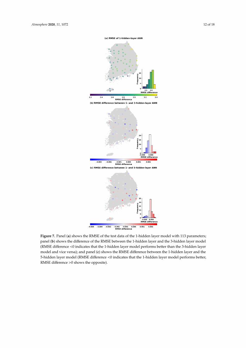
Atmosphere 2020, 11, 1072 12 of 18Atmosphere 2020, 11, x FOR PEER REVIEW 12 of 18

Figure 7. Panel (a) shows the RMSE of the test data of the 1-hidden layer model with 113 parameters;

panel (b) shows the difference of the RMSE between the 1-hidden layer and the 3-hidden layer model

(RMSE difference <0 indicates that the 1-hidden layer model performs better than the 3-hidden layer

model and vice versa); and panel (c) shows the RMSE difference between the 1-hidden layer and the

5-hidden layer model (RMSE difference <0 indicates that the 1-hidden layer model performs better,

RMSE difference >0 shows the opposite).

For example, Figure 7 indicates that, based on the RMSE of the testing sets, the one-hidden layer

model achieves a better performances at 42 and 41 stations, respectively, when the number of

parameters is 113, compared to the three- and five-hidden layer models. Similarly, at the parameter

number of 169, and from the histogram of RMSE differences (Figure 8), we can see that the

one-hidden layer structure generally obtained a smaller error than three and five hidden layers for

most sites. However, it was noted that the multi-hidden layer models improved the performance of

temperature prediction at some stations (17 stations with three hidden layers and 20 stations with

five hidden layers) in comparison to one hidden layer. Moreover, the number of sites that obtained a

smaller RMSE with multiple hidden layers decreased slightly when the number of parameters was

increased to 353 (Figure 9). Out of 55 stations, there were 12 stations with three hidden layers having

Figure 7. Panel (a) shows the RMSE of the test data of the 1-hidden layer model with 113 parameters;panel (b) shows the difference of the RMSE between the 1-hidden layer and the 3-hidden layer model(RMSE difference <0 indicates that the 1-hidden layer model performs better than the 3-hidden layermodel and vice versa); and panel (c) shows the RMSE difference between the 1-hidden layer and the5-hidden layer model (RMSE difference <0 indicates that the 1-hidden layer model performs better,RMSE difference >0 shows the opposite).

Atmosphere 2020, 11, 1072 13 of 18

Atmosphere 2020, 11, x FOR PEER REVIEW 13 of 18

smaller errors than one hidden layer, and 18 stations with five hidden layers had better performance

than one hidden layer. Finally, Figure 10 compares the ANN models in the test case in the name of

the RMSE and hidden layer with 1001 trainable parameters. As the results showed, the one-hidden

layer ANN generated a better result at almost every station than the three and five hidden layers.

The three- and five-hidden layer ANNs had higher RMSE than one hidden layer in five and three

stations out of 55 stations, respectively. The results were worth emphasizing that the deep ANN

with various parameters trained for all stations generated a certain number of basins with lower

performance than a single-hidden layer network, but the stations where this occurred were not

always the same.

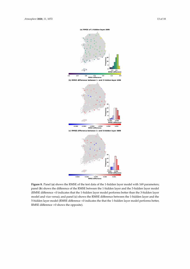
Figure 8. Panel (a) shows the RMSE of the test data of the 1-hidden layer model with 169 parameters;

panel (b) shows the difference of the RMSE between the 1-hidden layer and the 3-hidden layer model

(RMSE difference <0 indicates that the 1-hidden layer model performs better than the 3-hidden layer

model and vice versa); and panel (c) shows the RMSE difference between the 1-hidden layer and the

5-hidden layer model (RMSE difference <0 indicates the that the 1-hidden layer model performs

better, RMSE difference >0 shows the opposite).

Figure 8. Panel (a) shows the RMSE of the test data of the 1-hidden layer model with 169 parameters;panel (b) shows the difference of the RMSE between the 1-hidden layer and the 3-hidden layer model(RMSE difference <0 indicates that the 1-hidden layer model performs better than the 3-hidden layermodel and vice versa); and panel (c) shows the RMSE difference between the 1-hidden layer and the5-hidden layer model (RMSE difference <0 indicates the that the 1-hidden layer model performs better,RMSE difference >0 shows the opposite).

Atmosphere 2020, 11, 1072 14 of 18Atmosphere 2020, 11, x FOR PEER REVIEW 14 of 18

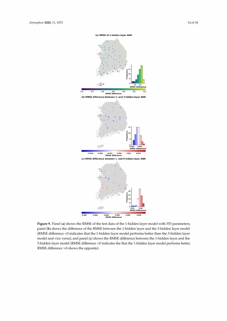
Figure 9. Panel (a) shows the RMSE of the test data of the 1-hidden layer model with 353 parameters;

panel (b) shows the difference of the RMSE between the 1-hidden layer and the 3-hidden layer model

(RMSE difference <0 indicates that the 1-hidden layer model performs better than the 3-hidden layer

model and vice versa); and panel (c) shows the RMSE difference between the 1-hidden layer and the

5-hidden layer model (RMSE difference <0 indicates the that the 1-hidden layer model performs

better, RMSE difference >0 shows the opposite).

Figure 9. Panel (a) shows the RMSE of the test data of the 1-hidden layer model with 353 parameters;panel (b) shows the difference of the RMSE between the 1-hidden layer and the 3-hidden layer model(RMSE difference <0 indicates that the 1-hidden layer model performs better than the 3-hidden layermodel and vice versa); and panel (c) shows the RMSE difference between the 1-hidden layer and the5-hidden layer model (RMSE difference <0 indicates the that the 1-hidden layer model performs better,RMSE difference >0 shows the opposite).

Atmosphere 2020, 11, 1072 15 of 18Atmosphere 2020, 11, x FOR PEER REVIEW 15 of 18

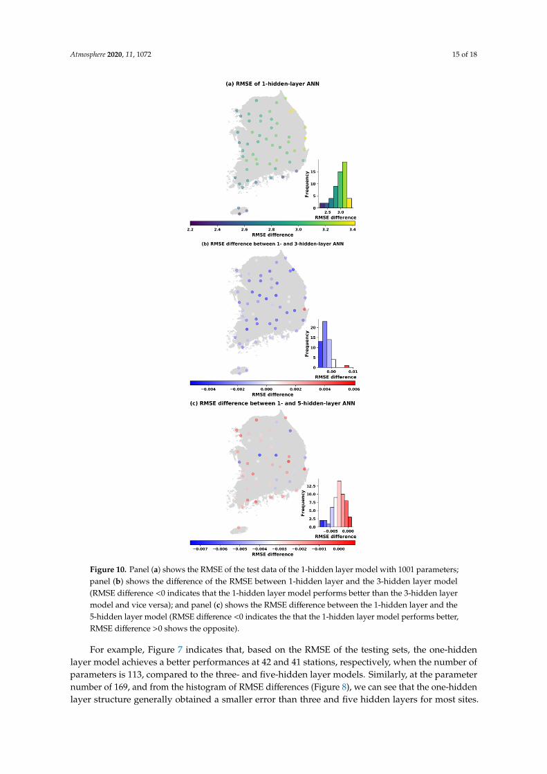
Figure 10. Panel (a) shows the RMSE of the test data of the 1-hidden layer model with 1001

parameters; panel (b) shows the difference of the RMSE between 1-hidden layer and the 3-hidden

layer model (RMSE difference <0 indicates that the 1-hidden layer model performs better than the

3-hidden layer model and vice versa); and panel (c) shows the RMSE difference between the

1-hidden layer and the 5-hidden layer model (RMSE difference <0 indicates the that the 1-hidden

layer model performs better, RMSE difference >0 shows the opposite).

4. Summary and Conclusions

In this study, different hidden layer ANN models with various interior parameters were

employed to forecast 1 day maximum temperature series over South Korea. This study aimed to

explore the relationship between the size of the ANN model and its predictive capability, revealing

that for future predictions of the time series of maximum temperature. In summary, the major

findings of the present study are as follows.

Figure 10. Panel (a) shows the RMSE of the test data of the 1-hidden layer model with 1001 parameters;panel (b) shows the difference of the RMSE between 1-hidden layer and the 3-hidden layer model(RMSE difference <0 indicates that the 1-hidden layer model performs better than the 3-hidden layermodel and vice versa); and panel (c) shows the RMSE difference between the 1-hidden layer and the5-hidden layer model (RMSE difference <0 indicates the that the 1-hidden layer model performs better,RMSE difference >0 shows the opposite).

For example, Figure 7 indicates that, based on the RMSE of the testing sets, the one-hiddenlayer model achieves a better performances at 42 and 41 stations, respectively, when the number ofparameters is 113, compared to the three- and five-hidden layer models. Similarly, at the parameternumber of 169, and from the histogram of RMSE differences (Figure 8), we can see that the one-hiddenlayer structure generally obtained a smaller error than three and five hidden layers for most sites.

Atmosphere 2020, 11, 1072 16 of 18

However, it was noted that the multi-hidden layer models improved the performance of temperatureprediction at some stations (17 stations with three hidden layers and 20 stations with five hiddenlayers) in comparison to one hidden layer. Moreover, the number of sites that obtained a smallerRMSE with multiple hidden layers decreased slightly when the number of parameters was increasedto 353 (Figure 9). Out of 55 stations, there were 12 stations with three hidden layers having smallererrors than one hidden layer, and 18 stations with five hidden layers had better performance thanone hidden layer. Finally, Figure 10 compares the ANN models in the test case in the name of theRMSE and hidden layer with 1001 trainable parameters. As the results showed, the one-hidden layerANN generated a better result at almost every station than the three and five hidden layers. The three-and five-hidden layer ANNs had higher RMSE than one hidden layer in five and three stations outof 55 stations, respectively. The results were worth emphasizing that the deep ANN with variousparameters trained for all stations generated a certain number of basins with lower performance than asingle-hidden layer network, but the stations where this occurred were not always the same.

4. Summary and Conclusions

In this study, different hidden layer ANN models with various interior parameters were employedto forecast 1 day maximum temperature series over South Korea. This study aimed to explore therelationship between the size of the ANN model and its predictive capability, revealing that for futurepredictions of the time series of maximum temperature. In summary, the major findings of the presentstudy are as follows.

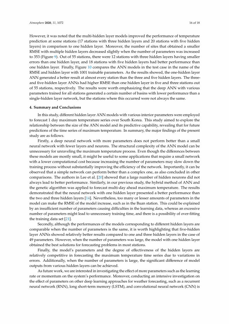
Firstly, a deep neural network with more parameters does not perform better than a smallneural network with fewer layers and neurons. The structural complexity of the ANN model can beunnecessary for unraveling the maximum temperature process. Even though the differences betweenthese models are mostly small, it might be useful to some applications that require a small networkwith a lower computational cost because increasing the number of parameters may slow down thetraining process without substantially improving the efficiency of the network. Importantly, it can beobserved that a simple network can perform better than a complex one, as also concluded in othercomparisons. The authors in Lee et al. [20] showed that a large number of hidden neurons did notalways lead to better performance. Similarly, in our previous study, the hybrid method of ANN andthe genetic algorithm was applied to forecast multi-day ahead maximum temperature. The resultsdemonstrated that the neural network with one hidden layer presented a better performance thanthe two and three hidden layers [14]. Nevertheless, too many or lesser amounts of parameters in themodel can make the RMSE of the model increase, such as in the Buan station. This could be explainedby an insufficient number of parameters causing difficulties in the learning data, whereas an excessivenumber of parameters might lead to unnecessary training time, and there is a possibility of over-fittingthe training data set [21].

Secondly, although the performances of the models corresponding to different hidden layers arecomparable when the number of parameters is the same, it is worth highlighting that five-hiddenlayer ANNs showed relatively better results compared to one and three hidden layers in the case of49 parameters. However, when the number of parameters was large, the model with one hidden layerobtained the best solutions for forecasting problems in most stations.

Finally, the model’s parameters and the degree of effectiveness of the hidden layers arerelatively competitive in forecasting the maximum temperature time series due to variations inerrors. Additionally, when the number of parameters is large, the significant difference of modeloutputs from various hidden layers can be achieved.

As future work, we are interested in investigating the effect of more parameters such as the learningrate or momentum on the system’s performance. Moreover, conducting an intensive investigation onthe effect of parameters on other deep learning approaches for weather forecasting, such as a recurrentneural network (RNN), long short-term memory (LSTM), and convolutional neural network (CNN) is

Atmosphere 2020, 11, 1072 17 of 18

a matter of interest for our future research. Besides, the sensitivity analysis or critical dependence ofone parameter on others may be involved for further research.

Supplementary Materials: The following are available online at http://www.mdpi.com/2073-4433/11/10/1072/s1,Figure S1: RMSE of different parameters ANN corresponding to 1, 3, and 5 hidden layers for test data Andong,Boeun, Boryeong, Buan, Busan, Buyeo, Cheonan, Cheongju, Chuncheon, Chungju, Chupungryong, Daegu,Daewallyeong, Daejeon, and Ganghwa stations. The dot and the vertical lines denote the mean and the standarddeviation of 5 repetitions, respectively, Figure S2: RMSE of different parameters ANN corresponding to 1, 3,and 5 hidden layers for test data at Gangneung, Goheung, Gumi, Gunsan, Gwangju, Haenam, Hapcheon,Hongcheon, Icheon, Imsil, Incheon, Inje, Jangheung, Jecheon, and Jeju stations. The dot and the vertical linesdenote the mean and the standard deviation of 5 repetitions, respectively, Figure S3: RMSE of different parametersANN corresponding to 1, 3, and 5 hidden layers for test data at Jeongeup, Jeonju, Jinju, Miryang, Mokpo,Mungyeong, Namhae, Namwon, Pohang, Sancheong, Seogwipo, Seongsan, Seosan, Seoul, and Sokcho stations.The dot and the vertical lines denote the mean and the standard deviation of 5 repetitions, respectively, Figure S4:RMSE of different parameters ANN corresponding to 1, 3, and 5 hidden layers for test data at Suwon, Tongyeong,Uiseong, Uljin, Ulsan, Wando, Wonju, Yangpyeong, Yeongchen, and Yeongdeok stations. The dot and the verticallines denote the mean and the standard deviation of 5 repetitions, respectively.

Author Contributions: Conceptualization, formal analysis, writing—original draft, T.T.K.T.; conceptualization,resources, methodology, writing—original draft, T.L.; conceptualization, writing—original draft, writing—reviewand editing, J.-S.K. All authors have read and agreed to the published version of the manuscript.

Funding: This work was supported by the National Research Foundation of Korea (NRF) grant funded by theKorean Government (MEST) (2018R1A2B6001799).

Acknowledgments: The authors appreciate the journal editors and the reviewers for their useful and valuablecomments for this study. We also thank the support of the State Key Laboratory of Water Resources andHydropower Engineering Science, Wuhan University.

Conflicts of Interest: The authors declare no conflict of interest.

References

1. Valverde Ramírez, M.C.; De Campos Velho, H.F.; Ferreira, N.J. Artificial neural network technique for rainfallforecasting applied to the São Paulo region. J. Hydrol. 2005, 301, 146–162. [CrossRef]

2. Umakanth, N.; Satyanarayana, G.C.; Simon, B.; Rao, M.C.; Babu, N.R. Long-term analysis ofthunderstorm-related parameters over Visakhapatnam and Machilipatnam, India. Acta Geophys. 2020,68, 921–932. [CrossRef]

3. Verma, A.P.; Swastika Chakraborty, B. Now casting of Orographic Rain Rate Using ARIMA and ANN Model.In Proceedings of the IEEE 2020, Aranasi, India, 12–14 February 2020. [CrossRef]

4. Berbic, J.; Ocvirk, E.; Carevic, D.; Loncar, G. Application of neural networks and support vector machine forsignificant wave height prediction. Oceanologia 2017, 59, 331–349. [CrossRef]

5. Agrawal, K. Modelling and prediction of rainfall using artificial neural network and ARIMA techniques.J. Ind. Geophys. Union 2006, 10, 141–151.

6. Ozoegwu, C.G. Artificial neural network forecast of monthly mean daily global solar radiation of selectedlocations based on time series and month number. J. Clean. Prod. 2019, 216, 1–13. [CrossRef]

7. Young, C.-C.; Liu, W.-C.; Hsieh, W.-L. Predicting the Water Level Fluctuation in an Alpine Lake UsingPhysically Based, Artificial Neural Network, and Time Series Forecasting Models. Math. Probl. Eng. 2015,1–11. [CrossRef]

8. Alotaibi, K.; Ghumman, A.R.; Haider, H.; Ghazaw, Y.M.; Shafiquzzaman, M. Future predictions of rainfalland temperature using GCM and ANN for arid regions: A case study for the Qassim region, Saudi Arabia.Water (Switzerland) 2018, 10, 1260. [CrossRef]

9. Smith, B.A.; Mcclendon, R.W.; Hoogenboom, G. Improving Air Temperature Prediction with Artificial NeuralNetworks. Int. J. Comput. Inf. Eng. 2007, 1, 3159.

10. Paras, S.; Kumar, A.; Chandra, M. A feature based neural network model for weather forecasting. World Acad.Sci. Eng. 2007, 4, 209–216.

11. Rajendra, P.; Murthy, K.V.N.; Subbarao, A.; Boadh, R. Use of ANN models in the prediction of meteorologicaldata. Model. Earth Syst. Environ. 2019, 5, 1051–1058. [CrossRef]

12. Tsai, C.Y.; Lee, Y.H. The parameters effect on performance in ANN for hand gesture recognition system.Expert Syst. Appl. 2011, 38, 7980–7983. [CrossRef]

Atmosphere 2020, 11, 1072 18 of 18

13. Hung, N.Q.; Babel, M.S.; Weesakul, S.; Tripathi, N.K. Hydrology and Earth System Sciences An artificial neuralnetwork model for rainfall forecasting in Bangkok, Thailand. Hydrol. Earth Syst. Sci. 2009, 13, 1413–1416.[CrossRef]

14. Tran, T.T.K.; Lee, T.; Shin, J.-Y.; Kim, J.-S.; Kamruzzaman, M. Deep Learning-Based Maximum TemperatureForecasting Assisted with Meta-Learning for Hyperparameter Optimization. Atmosphere 2020, 11, 487.[CrossRef]

15. Tran, T.T.K.; Lee, T. Is Deep Better in Extreme Temperature Forecasting? J. Korean Soc. Hazard Mitig. 2019,19, 55–62. [CrossRef]

16. Sarle, W.S. Stopped Training and Other Remedies for Overfitting. Proc. 27th Symp. Comput. Sci. Stat. 1995,17, 352–360.

17. Chollet, F. Home Keras Documentation. Available online: https://keras.io/ (accessed on 4 May 2020).18. Abadi, M.; Agarwal, A.; Barham, P.; Brevdo, E.; Chen, Z.; Citro, C.; Corrado, G.S.; Davis, A.; Dean, J.;

Devin, M.; et al. TensorFlow: Large-Scale Machine Learning on Heterogeneous Distributed Systems. arXiv2016, arXiv:1603.04467.

19. Chen, Y.; Tong, Z.; Zheng, Y.; Samuelson, H.; Norford, L. Transfer learning with deep neural networksfor model predictive control of HVAC and natural ventilation in smart buildings. J. Clean. Prod. 2020,254, 119866. [CrossRef]

20. Lee, J.; Kim, C.G.; Lee, J.E.; Kim, N.W.; Kim, H. Application of artificial neural networks to rainfall forecastingin the Geum River Basin, Korea. Water (Switzerland) 2018, 10, 1448. [CrossRef]

21. Alam, S.; Kaushik, S.C.; Garg, S.N. Assessment of diffuse solar energy under general sky condition usingartificial neural network. Appl. Energy 2009, 86, 554–564. [CrossRef]

Publisher’s Note: MDPI stays neutral with regard to jurisdictional claims in published maps and institutionalaffiliations.

© 2020 by the authors. Licensee MDPI, Basel, Switzerland. This article is an open accessarticle distributed under the terms and conditions of the Creative Commons Attribution(CC BY) license (http://creativecommons.org/licenses/by/4.0/).