Inequalities for Shannon entropy andKolmogorov complexity

Daniel HammerTechnische Universitat, Berlinhammer@math.tu-berlin.de

Andrei RomashchenkoMoscow State University

an@romash.mccme.ru

Alexander ShenInstitute of Problems of

Information Transmission, Moscowshen@landau.ac.ru, shen@mccme.ru

Nikolai VereshchaginMoscow State Universityver@mech.math.msu.su

Abstract

It was mentioned by Kolmogorov in [5] that the properties of algorithmiccomplexity and Shannon entropy are similar. We investigateone aspect ofthis similarity. Namely, we are interested in linear inequalities that are validfor Shannon entropy and for Kolmogorov complexity.

It turns out that

(1) all linear inequalities that are valid for Kolmogorov complex-ity, are also valid for Shannon entropy and vice versa;

(2) all linear inequalities that are valid for Shannon entropy, arevalid for ranks of finite subsets of linear spaces;

(3) the opposite statement is not true: Ingleton’s inequality ([3],see also [8]) is valid for ranks but not for Shannon entropy;

(4) for some special cases all three classes of inequalitiescoin-cide and have simple description.

We present an inequality for Kolmogorov complexity that implies Ingleton’sinequality for ranks; another application of this inequality is a new simpleproof of one of Gacs–Korner’s results on common information [1].

1

1 Shannon entropy and Kolmogorov complexity

Since the very beginning the notion of complexity of finite objects was con-sidered as an algorithmic counterpart to the notion of Shannon entropy. Kol-mogorov’s paper [4] was called “Three approaches to the quantitative definitionof information”; Shannon entropy and algorithmic complexity were among theseapproaches. Let us recall the main definitions.

Let α be a random variable with a finite rangea1; : : : ;an. Let pi be the proba-bility of the eventα = ai . Then the Shannon entropy ofα is defined as

H(α) =�∑i

pi logpi

(All logarithms in the paper are base 2 logarithms.) Using the convexity of thefunctionp 7! �plogp, one can prove that the Shannon entropy of a random vari-able does not exceed the logarithm of the cardinality of its range (and is equal toit only for uniformly distributed variables).

Let β be another variable with a finite rangeb1; : : : ;bk defined on the sameprobabilistic space asα is. We defineH(αjβ = b j) in the same way asH(α); theonly difference is thatpi is replaced by the conditional probability Pr[α = aijβ =b j ℄. Then we define the conditional entropy as

H(αjβ) = ∑j

Pr[β = b j ℄ �H(αjβ = b j):It is easy to check that

H(hα;βi) = H(β)+H(αjβ):Using the convexity of logarithm function, one can prove that

H(αjβ) � H(α);and thatH(αjβ) = H(α) if and only if α andβ are independent. This inequalitymay be rewritten as

H(hα;βi) � H(α)+H(β):The mutual information inα andβ is defined as

I (α : β) = H(β)�H(βjα) = H(α)+H(β)�H(hα;βi):2

The mutual informationI (α : β) is always non-negative and is equal to 0 if andonly if α andβ are independent. The conditional version of mutual information isdefined as

I (α : βjγ) = H(αjγ)+H(βjγ)�H(hα;βijγ)and is always non-negative, too. Indeed, for any possible value ci of γ we have

H(αjγ = ci)+H(βjγ = ci)�H(hα;βijγ = ci) � 0:Multiplying this inequality by Pr[γ = ci℄ and summing overi, we get the desiredinequality.All these notions have their counterparts in Kolmogorov complexity theory.

The Kolmogorov complexity of a binary stringa is defined as the minimallength of a program that generatesa. There are different refinements of this idea(calledsimpleKolmogorov complexity,monotonecomplexity,prefixcomplexity,decisioncomplexity, see [6], [7]). However, for our purposes the difference is notimportant, since all these complexity measures differ onlyby O(logm) wherem isthe length ofa. Therefore, in the sequel we denote Kolmogorov complexity of abinary stringa by K(a) not specifying which version we use, andall our equalitiesand inequalities are valid up to O(logm) term where m is the total length of allstrings involved.

The conditional complexityK(ajb) is defined as the minimal length of a pro-gram that producesa havingb as input; one can prove that

K(bja) = K(ha;bi)�K(a);(see [9]). Hereha;bi denotes the encoding of the paira;b by a binary string (dif-ferent computable encodings lead to complexities that differ only byO(logm)).As always,O(logm) additive term is omitted; the precise meaning of this equalityis: there exist constantsp;q such that

K(bja) � K(ha;bi)�K(a)+ plog(jaj+ jbj)+q;K(ha;bi)�K(a) � K(bja)+ plog(jaj+ jbj)+q

for all binary stringsa;b. The mutual information is defined as

I (a : b) = K(b)�K(bja):An equivalent (up toO(logm) term) symmetric definition is

I (a : b) = K(a)+K(b)�K(ha;bi):3

As for the Shannon case, the mutual information is always non-negative (up toO(logm) term). The conditional version of mutual information is defined as

I (a : bjc) = K(ajc)+K(bjc)�K(ha;bijc):The inequality

I (a : bjc) � 0

is valid up to a logarithmic term, that is,I (a : bjc)��O(log(jaj+ jbj+ jcj)). Thisinequality plays an important role in the sequel.

2 Inequalities

We have already mentioned several inequalities for Shannonentropy and Kol-mogorov complexity. Some others are known. For example, consider the inequal-ity

2K(ha;b;ci)� K(ha;bi)+K(ha;ci)+K(hb;ci) (1)

This inequality is equivalent in a sense to the following geometric fact: ifV is thevolume of the setA�R3 andSxy, Sxz andSyz are areas of its three projections (tothe coordinate planesOxy, OxzandOyz), then

V2� Sxy �Sxz�Syz

(see [2]).It turns out that the inequality (1), as well as all other known inequalities for

Kolmogorov complexity, is a corollary of the inequalities of type

I (P : QjR) � 0 (2)

used together with equalities

K(QjP) = K(hP;Qi)�K(P); (3)

I (P : QjR) = K(PjR)+K(QjR)�K(hP;QijR); (4)

that express mutual information and conditional complexity in terms of uncon-ditional complexity. (HereP;Q;R are some tuples (possibly empty) of binarystrings.)

4

Indeed, (1) is a consequence of the equality

2K(ha;b;ci) = K(ha;bi)+K(ha;ci)+K(hb;ci)�� I (a : bjc)� I (ha;bi : c) (5)

and inequalitiesI (a : bjc) � 0 andI (ha;bi : c) � 0. To check the equality (5) weexpress all the quantities in terms of unconditional complexity. For example, wereplaceI (a : bjc) by

K(ajc)+K(bjc)�K(ha;bijc)= K(ha;ci)�K(c)+K(hb;ci)�K(c)�K(ha;b;ci)+K(c)= K(ha;ci)+K(hb;ci)�K(ha;b;ci)�K(c);and so on.

Let us consider another example. Assume thata andb are two binary strings.Let us prove that the mutual informationI (a : b) is an upper bound for complex-ity K(x) of any stringx which has negligible conditional complexityK(xja) andK(xjb). Indeed, the following inequality holds for any three stringsa;b;x:

K(x) � K(xja)+K(xjb)+ I (a : b): (6)

This inequality is a consequence of the equality

K(x) = I (a : b)+K(xja)+K(xjb)�K(xjha;bi)� I (a : bjx)and inequalitiesK(xjha;bi) � 0 andI (a : bjx)� 0.

The inequalities of type (2) can be written in different equivalent forms:

I (P : QjR) � 0

K(PjR)+K(QjR) � K(hP;QijR)K(PjR) � K(PjhQ;Ri)

K(hP;Ri)+K(hQ;Ri) � K(hP;Q;Ri)+K(R)HereP, Q andR are strings or tuples of strings;hP;Ri denotes the union of tuplesP andR (it does not matter whether we list strings that are inP\R twice or not,the complexity does not change), etc.

The latter form does not involve conditional complexity. Ingeneral, we mayalways replace conditional complexity and mutual information by linear combi-nations of unconditional complexity using (3) and (4). Therefore, in the sequel weconsider inequalities containing only unconditional complexity. The same appliesto inequalities for Shannon entropy.

5

We call the inequalities

K(hP;Ri)+K(hQ;Ri) � K(hP;Q;Ri)+K(R) (7)

(for any tuplesP;Q;R) basic inequalities. Let us mention two special cases ofinequalities (7). IfP= Q, we get an inequality

K(hP;Ri)+K(hP;Ri) � K(hP;Ri)+K(R)or

K(hP;Ri) � K(R)(bigger tuple has bigger complexity) or

K(PjR) � 0

(conditional complexity is non-negative).Now we see that the inequalityK(xjha;bi) � 0 in our second example is also acorollary of basic inequalities (7). Another special case:if R is empty, we get theinequality

K(P)+K(Q) � K(hP;Qi)or

K(P) � K(PjQ)This inequalities imply that all unconditional complexities are non-negative, too.(Strictly speaking, inequalities imply that complexitiesare non-negative up to alogarithmic term, i.e.,K(P) ��O(logn) wheren is the length ofP.)

All inequalities mentioned in this section have counterparts that involve Shan-non entropy instead of Kolmogorov complexity. We would liketo know if (1)the same linear inequalities are true for Shannon entropy and Kolmogorov com-plexity and if (2) all linear inequalities valid for Shannonentropy (or Kolmogorovcomplexity) are consequences of basic inequalities. In next section, we obtain apositive answer to the first question (for the general case) and a positive answerto the second question in the case when at most three random variables (binarystrings) are involved.

6

3 Linear inequalities

Considern variablesa1; : : : ;an whose values are binary strings (if we considerKolmogorov complexity) or random variables with finite range (for Shannon en-tropy). There are 2n�1 nonempty subsets of the set of variables. Therefore, thereare 2n�1 tuples whose complexity (or entropy) may appear in the inequality. Weconsider only linear inequalities. Each inequality has 2n�1 coefficientsλW in-dexed by non-empty subsetsW of the setf1;2; : : : ;ng; for example, forn= 3 thegeneral form is

λ1K(a1)+λ2K(a2)+λ3K(a3)++λ1;2K(ha1;a2i)+λ1;3K(ha1;a3i)+λ2;3K(ha2;a3i)++λ1;2;3K(ha1;a2;a3i)� 0

Herea1;a2;a3 are binary strings; for Shannon entropy they should be replacedby random variables, andK should be replaced byH. For arbitraryn the generalform of a linear inequality is:

∑W

λWK(aW)� 0; (8)

where the sum is over all nonempty subsetsW� f1;2; : : : ;ng, andaW stands forthe tuple formed by allai for i 2W.

Now we consider the set of inequalities that are valid (up to aO(logm) term,as usual) for all binary strings. This set is a convex cone inR2n�1. We wantto compare this cone with the similar cone for Shannon entropies (of tuples ofrandom variables with finite range).

Theorem 1. Any linear inequality that is true for Kolmogorov complexity is alsotrue for Shannon entropy, and vice versa.

Proof [Kolmogorov! Shannon] Let an inequality of the form (8) be true forKolmogorov complexity (up toO(logm) term).

Let α = hα1; : : : ;αni be a tuple of random variables. We have to prove that

∑W

λWH(αW)� 0;where the sum is taken over all nonempty subsetsW�f1;2; : : : ;ng andαW standsfor the tuple formed by allαi for i 2W.

7

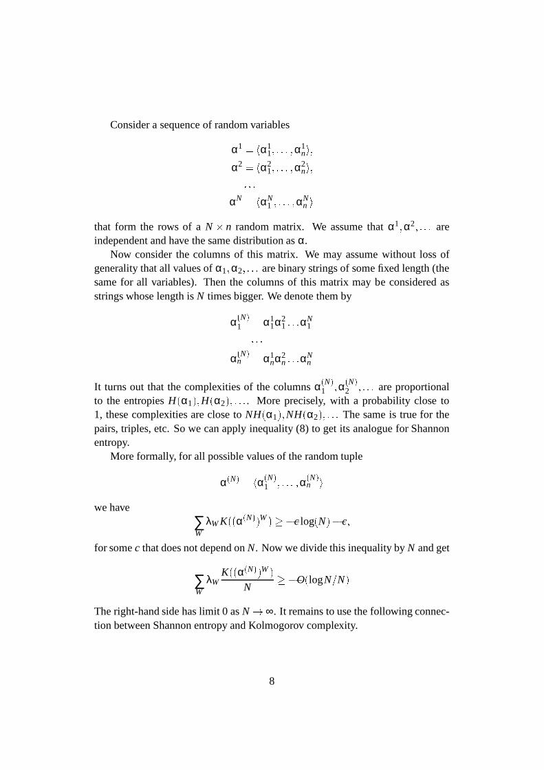
Consider a sequence of random variables

α1 = hα11; : : : ;α1

ni;α2 = hα2

1; : : : ;α2ni;: : :

αN = hαN1 ; : : : ;αN

n ithat form the rows of aN� n random matrix. We assume thatα1;α2; : : : areindependent and have the same distribution asα.

Now consider the columns of this matrix. We may assume without loss ofgenerality that all values ofα1;α2; : : : are binary strings of some fixed length (thesame for all variables). Then the columns of this matrix may be considered asstrings whose length isN times bigger. We denote them by

α(N)1 = α1

1α21 : : :αN

1: : :α(N)

n = α1nα2

n : : :αNn

It turns out that the complexities of the columnsα(N)1 ;α(N)

2 ; : : : are proportionalto the entropiesH(α1);H(α2); : : :. More precisely, with a probability close to1, these complexities are close toNH(α1);NH(α2); : : : The same is true for thepairs, triples, etc. So we can apply inequality (8) to get itsanalogue for Shannonentropy.

More formally, for all possible values of the random tuple

α(N) = hα(N)1 ; : : : ;α(N)

n iwe have

∑W

λWK((α(N))W) ��clog(N)�c;for somec that does not depend onN. Now we divide this inequality byN and get

∑W

λWK((α(N))W)

N��O(logN=N)

The right-hand side has limit 0 asN!∞. It remains to use the following connec-tion between Shannon entropy and Kolmogorov complexity.

8

Lemma 1. ([9], equation(5.18))Let τ be a random variable whose values arefinite binary strings of a fixed length. Consider the sequenceτ1;τ2; : : : of indepen-dent random variables, where eachτi has the same distribution asτ. Then

limN!∞

K(τ1 : : :τN)N

= H(τ)with probability1 (i.e., for almost all elements of the sample space where allτi

are defined).

We fixW and apply this lemma toτ = αW. It is easy to see thatK((α(N))W) isequal (up to aO(1) term) toK(τ1 : : :τN). Therefore,

limN!∞

K((α(N))W)N

= limN!∞

K(τ1 � � �τN)N

= H(αW)with probability 1. Hence the inequality∑W λWH(αW)� 0 is true.

[Shannon! Kolmogorov] Now we have to prove the converse: if the in-equality

∑W

λWH(αW)� 0;is true for any random variablesα1; : : : ;αn, then the inequality

∑W

λWK(AW)��O(logjAj)is true for any tuple of binary stringsA = ha1;a2; : : : ;ani, whereAW is a tupleformed by allai such thati 2W andjAj= ja1j+ ja2j+ � � �+ janj is the total lengthof A. (Please note that the constant hidden inO(logjAj) may depend onn.)

To prove this inequality, for a givenA we want to construct random variablesα1; : : :αn whose entropies are close to the complexities ofa1;a2; : : : ;an. We alsowant the entropies of all pairs, triples, etc. to be close to the complexities of thecorresponding pairs, triples, etc. of binary strings.

The following construction achieves this goal. Assume thata tuple A =ha1;a2; : : : ;ani is fixed. Consider the set of all tuplesB = hb1;b2; : : : ;bni thatsatisfy the following conditions: First, the complexity ofeachbi does not exceedthe complexity of the correspondingai . Moreover, the same is true for all pairs,triples, etc. Finally, the same should be true for all conditional complexities. For-mally, we consider the setB formed by all tuplesB = hb1;b2; : : : ;bni such thatK(BV jBW) � K(AV jAW) for any two subsetsV;W � f1;2; : : : ;ng. (Here the in-equality is understood literally, without any hidden constants or log-terms.)

9

The setB contains at least one point,A: This set has a simple description asan enumerable set: to generate its elements it is enough to know all conditionalcomplexitiesK(AV jAW), i.e., several integers not exceedingjAj. So the complex-ity of the program that enumeratesB is O(logjAj). (The constant hidden in theO-notation depends onn and grows exponentially, but we assumen to be fixed.)And any setX having a simple description (as an enumerable set) and having apointx with high complexity should have many elements. Indeed, anypoint inXmay be identified by its number (in the enumeration order) andthe enumerationprogram, soK(x) cannot be high ifjXj is small.

More formally, the following lemma gives the lower bound forthe cardinalityof B (denoted byjB j):Lemma 2. logjB j � K(ha1; : : : ;ani)�O(logjAj):Proof. Consider the program that printsha1; : : : ;ani and works as follows. ItenumeratesM; a tupleB = hb1; : : : ;bni is included in the enumeration after wehave found that its complexity is in the required range (looking for all programsthat printB and finding a short one); and, moreover, the conditional complexitiesare in the required ranges. The program counts the elements of B that were alreadygenerated; whenz elements are found, it printsz-th element and terminates. Herez is the number ofA (it is a compiled-in constant in the program). The length ofthis program does not exceed logz+O(logjAj) +O(1), since the program usesz, conditional complexities

�the total amount of information isO(logjAj)� and a

finite amount of other information. It remains to use thatz� jB j. �Now letα = hα1;α2; : : : ;αni be a random variable uniformly distributed inB .

We know that

∑W

λWH(αW)� 0;so we get the desired inequality for the complexities ofa1; : : : ;an, their pairs,triples, etc., if we show that their complexities are close to the correspondingentropies ofα1; : : : ;αn, their pairs, triples etc. Thus, we have to prove thatH(αW)is close toK(AW) for any nonemptyW� f1;2; : : : ;ng.

Let us fix a setW � f1;2; : : : ;ng. The random variableαW is close to therandom variable that is uniformly distributed in the set having 2K(AW) elements.Indeed, the cardinality of the setfbW j b2 Bgthat is the projection ofB ontoW-coordinates, is at most 2K(AW)+O(1), since allthe elements of this projection have a complexity not exceeding K(AW). ThereforeαW has no more than 2K(AW)+O(1) values andH(αW)� K(AW)+O(1).

10

To prove the converse inequality, let us note that if Pr[ξ = x℄ � p for allpossible valuesx of a random variableξ, thenH(ξ) � � logp. So it suffices toshow that Pr[αW = BW℄ � 2�K(AW)+O(logjAj) for any B = hb1; : : : ;bni in B . Wehave

Pr[αW = BW℄ = jfC2 B jCW = BWgj=jB j:The lower bound for the denominator is provided by the lemma we proved. Theupper bound for the numerator can be obtained as follows. Let:W be the com-plement ofW: :W = f1;2; : : : ;ngnW:All the pointsC counted in the numerator have the sameW-projectionCW anddiffer only by :W-projectionsC:W. By definition, the complexityK(C:WjCW)for C 2 B does not exceedK(A:WjAW). Therefore, the number of thoseC islimited; the logarithm of this number does not exceed

K(A:WjAW) = K(A)�K(AW)+O(logjAj)Combining this bound with the lower bound forB , we get the desired inequalityfor probabilities. �

Our next result is about the inequalities for ranks of finite subsets of linearspaces.

Assume that a linear spaceL over a finite field or overR is given. Letα1, : : :,αn be finite subsets ofL. For any subsetA �fα1; : : : ;αng consider the rank of theunion of allα 2 A . Now consider all linear inequalities that are valid for ranks ofthese subsets for allα1; : : : ;αn � L. For example, inequality of type (7) for rankssays that

rk(α1[α3)+ rk(α2[α3) � rk(α1[α2[α3)+ rk(α3)This inequality can be rewritten in terms of dimensions of subspaces: any setX of vectors generates a subspace, and the dimension of this subspace is rk(X).Replacing eachαi by a linear subspaceAi generated byαi , we get

dim(A1+A3)+dim(A2+A3) � dim(A1+A2+A3)+dim(A3)It is easy to verify that this inequality is true for any linear subspaces of any linearspace. So, all basic inequalities are true whenK(�) is replaced by rk(�) and stringsare replaced by vectors. Moreover, the following is true:

Theorem 2. Any linear inequality valid for Shannon entropy is valid forranks(dimensions) in any linear space over any finite field or overR.

11

Proof Assume thatA1; : : : ;An are subspaces of a finite-dimensional linear spaceL over a fieldF . It suffices to construct random variablesα1; : : : ;αn such thatH(αi) is proportional to dimAi , H(hαi ;α ji) is proportional to dim(Ai +A j ), : : :,H(hα1;α2; : : : ;αni) is proportional to dim(A1+A2+ � � �+An).

If F is finite, the construction is straightforward. Consider a random linearfunctionalα : L ! F . For any subspaceA� L consider the restrictionαjA. This isa random variable withjFjdimA values

�herejFj is the number of elements inF

�;

all values have equal probabilities, soH(αjA) = dimA � logjFj. If Ai andA j aretwo subspaces, the pairhαjAi ;αjA ji is equivalent to (and has the same distributionas)αjAi+A j . Therefore, the entropy of the pairhαjAi ;αjA j i is equal to dim(Ai +A j) � logjF j; the same is true for triples, etc.

Now consider the caseF =R. We may assume thatL is an Euclidean space.Let α be a random variable, uniformly distributed in the unit diskin L. For anysubspaceA, consider a random variableαA that is the orthogonal projection ofαontoA. This random variable has an infinite domain, so we need to digitize it. Foranyε > 0 and for any subspaceA� L we divideA into equal cubes of dimensiondimA and sizeε��� ��ε. By αA;ε we denote the variable whose value is the cubethat containsαA. Let us prove that

H(αA;ε) = log(1=ε) �dimA+O(1)(whenε ! 0).

If ε is small enough the numberkA;ε of the cubes which are possible values ofαA satisfies the inequality

kA;ε �C(1=ε)dimA

whereC is a constant slightly bigger than the volume of unit disk inA. Therefore,

H(αA;ε)� log(1=ε) �dimA+O(1):On the other hand, for any fixed cube the probability ofαA getting into it is atmost

cεdimA

wherec is a constant equal to the ratio of volumes of unit disks in Euclideanspaces of dimensions dimL�dimA and dimL.

HenceH(αA;ε)� log(1=ε) �dimA+O(1):

The projectionαA1+A2 is equivalent tohαA1;αA2i. This is not true forε-versions; the random variablesαA1+A2;ε andhαA1;ε;αA2;εi do not determine each

12

other completely. However, for any fixed value of one of thesevariables there existonly a finite number of possible values of the other one; therefore, the conditionalentropies are limited and the entropies differ byO(1).

Now we letε ! 0 and conclude that any inequality that is valid for Shannonentropy is valid for ranks. �

Therefore, we have a sequence of inclusions: (basic inequalities (7) and theirnon-negative linear combinations)� (inequalities valid for Kolmogorov complex-ity) = (inequalities valid for Shannon entropy)� (inequalities valid for ranks).

Forn= 1;2;3 all these sets are equal, as the following theorem shows:

Theorem 3. For n= 1;2;3 any inequality valid for ranks (dimensions) is a con-sequence(linear combination with non-negative coefficients) of basic inequali-ties(7).Proof The casesn= 1;2 are trivial. Let us consider the casen= 3.

Consider the following 9 basic inequalities:

dim(B+C) � dim(A+B+C)dim(A+C) � dim(A+B+C)dim(A+B) � dim(A+B+C)

dim(C)+dim(A+B+C) � dim(A+C)+dim(B+C)dim(B)+dim(A+B+C) � dim(A+B)+dim(B+C) (9)

dim(A)+dim(A+B+C) � dim(A+B)+dim(A+C)dim(A+B) � dim(A)+dim(B)dim(A+C) � dim(A)+dim(C)dim(B+C) � dim(B)+dim(C)

We claim that any valid linear inequality for dimA, dimB, dimC, dim(A+B),dim(A+C), dim(B+C), dim(A+B+C) is a non-negative linear combination ofthese nine ones (for instance, so are all other basic inequalities).

The inequalities (9) determine a convex coneC in the spaceR7 where variablesare

dim(A); dim(B); dim(C); dim(A+B); dim(B+C); dim(A+C); dim(A+B+C)Any three subspacesA;B;C determine a point insideC. Let us denote the set ofall points inC obtained in this way byC0. To prove Theorem 3 it is enough toshow that any point inC can be represented as a non-negative linear combinationof points fromC0. It is enough to consider 8 points inC0 shown on Figure 1.

13

subspaces (old) coordinates

A B C

dim

(A)d

im

(B)d

im

(C)d

im

(A+B)d

im

(A+C)d

im

(B+C)d

im

(A+B+C)fe1g 0 0 1 0 0 1 1 0 10 fe1g 0 0 1 0 1 0 1 10 0 fe1g 0 0 1 0 1 1 1fe1g fe1g 0 1 1 0 1 1 1 1fe1g 0 fe1g 1 0 1 1 1 1 10 fe1g fe1g 0 1 1 1 1 1 1fe1g fe1g fe1g 1 1 1 1 1 1 1fe1g fe2g fe3g 1 1 1 2 2 2 2

Figure 1. 8 points inC0.Heree1;e2;e3 are three pairwise independent vectors in 2-dimensional space;fug stands for the linear subspace generated byu. By 0 we denote the 0-dimen-

sional subspace.Let us show that any point inC can be represented as a non-negative linear

combination of those 8 points. To prove this it is convenientto consider anothercoordinate system inR7. We denote new coordinates by[a℄; [b℄; [c℄; [ab℄; [ac℄; [bc℄; [abc℄The relations between new and old variables are:

dim(A) = [a℄+ [ab℄+ [ac℄+ [abc℄;dim(A+B) = [a℄+ [b℄+ [ab℄+ [ac℄+ [bc℄+ [abc℄;

dim(A+B+C) = [a℄+ [b℄+ [c℄+ [ab℄+ [bc℄+ [ac℄+[abc℄:and similar formulae obtained by permutations of letters. (See Figure 2.) Or,equivalently,

14

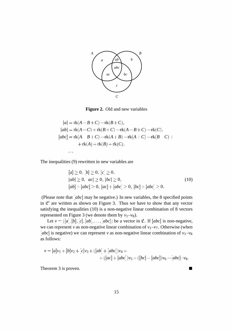
A B

C

c

ab

abc

bc

a b

ac

Figure 2. Old and new variables[a℄ = rk(A+B+C)� rk(B+C);[ab℄ = rk(A+C)+ rk(B+C)� rk(A+B+C)� rk(C);[abc℄ = rk(A+B+C)� rk(A+B)� rk(A+C)� rk(B+C)++ rk(A)+ rk(B)+ rk(C);: : :The inequalities (9) rewritten in new variables are[a℄� 0; [b℄� 0; [c℄� 0;[ab℄� 0; [ac℄� 0; [bc℄� 0; (10)[ab℄+ [abc℄� 0; [ac℄+ [abc℄� 0; [bc℄+ [abc℄� 0:(Please note that[abc℄ may be negative.) In new variables, the 8 specified pointsin C0 are written as shown on Figure 3. Thus we have to show that any vectorsatisfying the inequalities (10) is a non-negative linear combination of 8 vectorsrepresented on Figure 3 (we denote them byv1–v8).

Let v= ([a℄; [b℄; [c℄; [ab℄; : : : ; [abc℄) be a vector inC. If [abc℄ is non-negative,we can representv as non-negative linear combination ofv1–v7. Otherwise (when[abc℄ is negative) we can representv as non-negative linear combination ofv1–v8

as follows:

v= [a℄v1+[b℄v2+[c℄v3+([ab℄+ [abc℄)v4++([ac℄+ [abc℄)v5+([bc℄+ [abc℄)v6� [abc℄ �v8:Theorem 3 is proven. �

15

new coordinatesvector [a℄ [b℄ [c℄ [ab℄ [ac℄ [bc℄ [abc℄

v1 1 0 0 0 0 0 0v2 0 1 0 0 0 0 0v3 0 0 1 0 0 0 0v4 0 0 0 1 0 0 0v5 0 0 0 0 1 0 0v6 0 0 0 0 0 1 0v7 0 0 0 0 0 0 1v8 0 0 0 1 1 1 �1

Figure 3. 8 points inC0 in new coordinates.

4 Ingleton’s inequality

As we have seen in the preceding section, forn = 3 the same inequalities aretrue for Shannon entropy, Kolmogorov complexity and ranks,namely, the non-negative linear combinations of basic inequalities. However, for n= 4 the situa-tion becomes more complicated: there is an inequality that is true for ranks butnot for Shannon entropy.

A.W. Ingleton [3] established the following necessary condition for a matroidwith ground setSand rank functionr to be representable over a fieldF : for anysubsetsA, B, C, D of S there must hold

r(A)+ r(B)+ r(C[D)+ r(A[B[C)+ r(A[B[D)� r(A[B)+ r(A[C)+ r(A[D)+ r(B[C)+ r(B[D): (11)

In terms of dimensions of subspaces Ingleton’s inequality says that

dimA+dimB++dim(C+D)+dim(A+B+C)+dim(A+B+D) �� dim(A+B)+dim(A+C)+dim(B+C)++dim(A+D)+dim(B+D); (12)

It can be rewritten as follows:

I (A : B)� I (A : BjC)+ I (A : BjD)+ I (C : D) (13)

16

whereI (A : B) stands for dim(A) +dim(B)�dim(A+B), I (A : BjC) stands fordim(B+C)+dim(A+C)�dim(A+B+C)�dim(C), etc.

To prove inequality (13) one may interpretI (A : B) as the dimension of inter-sectionA\B, andI (A : BjC) as the dimension of the intersection ofA=C andB=C(i.e.,A andB factorized overC). See also Section 5 where Ingleton’s inequality isproved as a a consequence of Theorem 8.

The following example shows that Ingleton’s inequality is not always true forShannon entropy.

Theorem 4. There exist four random variablesα, β, γ, δ such that

I (α : β) > 0

I (α : βjγ) = 0

I (α : βjδ) = 0

I (γ : δ) = 0

In other terms,γ andδ are independent, andα andβ are independentfor anyfixed values ofγ andfor any fixed value ofδ; however,α andβ are dependent.

Proof of Theorem 4. Let the range of all four variablesα;β;γ;δ bef0;1g. Let γandδ be independent and uniformly distributed.

Any possible distribution ofα;β is determined by four non-negative realswhose sum is 1 (i.e., by the probabilities of all four combinations), so the dis-tribution can be considered as a point in a three-dimensional simplex S in R4.For any of the four possible values ofhγ;δi we have a point inS (whose coordi-nates are conditional probabilities). We denote these points byP00, P01, P10 andP11. What are the conditions we need to satisfy? LetQ be the subset ofS thatcorresponds to independent random variables;Q is a quadratic curve (the inde-pendence condition means that the determinant of the probabilities matrix is equalto zero). The conditionsI (α : βjγ) = 0 andI (α : βjδ) = 0 mean that midpoints ofsegmentsP00P01, P10P11, P00P10, P01P11 belong toQ . The inequalityI (α : β) > 0means that the point(P00+P01+P10+P11)=4 does not belong toQ . In otherterms, we are looking for a parallelogram (formed by midpoints) whose verticeslie on a quadratic curve but whose center does not, so almost any example willwork. Figure 4 shows one of them:

It is easy to check that all four conditional distributions (for conditionsγ = 0,γ = 1, δ = 0, δ = 1) satisfy the independence requirement. However, the uncondi-

17

0 1

0 0 01 0 1

0 1

0 1=8 3=81 3=8 1=8

0 1

0 1=8 3=81 3=8 1=8

0 1

0 1 01 0 0

γ = 0;δ = 0 γ = 1;δ = 0 γ = 0;δ = 1 γ = 1;δ = 1

Figure 4. Conditional probability distributions forhα;βitional distribution forhα;βi is

0 1

0 5=16 3=161 3=16 5=16

(14)

soα andβ are dependent.A simpler example, though not so symmetric, can be obtained as follows. Letγ

andδ be independent random variables with rangef0;1g and uniform distribution,α = γ(1�δ) andβ = δ(1� γ). For any fixed value ofγ or δ one of the variablesα and β is equal to 0, therefore they are independent. However,α and β arenot (unconditionally) independent, since each of them can be equal to 1, but theycannot be equal to 1 simultaneously. �

We see that forn= 4 not all the inequalities valid for ranks are valid for en-tropies, so the rank and entropy cases should be considered separately. For rankswe have the complete answer:

Theorem 5. For n= 4, all inequalities that are valid for ranks, are consequences(positive linear combinations) of basic inequalities and Ingleton-type inequal-ities (i.e., inequalities obtained from Ingleton’s inequality bypermutations ofvariables).Proof The systemF (+)

4 of all basic inequalities that involve at most four variables,together with the six Ingleton-type inequalities, determines a convex polyhedralconeC(+)

4 �R15.It is not hard to show that this cone is generated by (i.e., is the convex hull of)

the 35 points shown in Figure 5. Since it requires a great dealof (not very inter-esting) computation, we refrain from demonstrating this proof here. However, itcan be performed by hand (using, for instance, Fourier-Motzkin elimination) orwith the help of an appropriate software.

To prove the theorem, it remains to show that for each generator ρi there existsa quadruple of subspacesA;B;C;D that represents this point.

18

ρ1 (1;1;1;1;1;1;1;1;1;1;1;1;1;1;1) ρ19 (0;1;1;1;1;1;1;2;2;2;2;2;2;2;2)ρ2 (1;1;1;0;1;1;1;1;1;1;1;1;1;1;1) ρ20 (1;1;1;1;2;2;2;2;2;1;2;2;2;2;2)ρ3 (1;1;0;1;1;1;1;1;1;1;1;1;1;1;1) ρ21 (1;1;1;1;2;2;2;2;1;2;2;2;2;2;2)ρ4 (1;0;1;1;1;1;1;1;1;1;1;1;1;1;1) ρ22 (1;1;1;1;2;2;2;1;2;2;2;2;2;2;2)ρ5 (0;1;1;1;1;1;1;1;1;1;1;1;1;1;1) ρ23 (1;1;1;1;2;2;1;2;2;2;2;2;2;2;2)ρ6 (1;1;0;0;1;1;1;1;1;0;1;1;1;1;1) ρ24 (1;1;1;1;2;1;2;2;2;2;2;2;2;2;2)ρ7 (1;0;1;0;1;1;1;1;0;1;1;1;1;1;1) ρ25 (1;1;1;1;1;2;2;2;2;2;2;2;2;2;2)ρ8 (1;0;0;1;1;1;1;0;1;1;1;1;1;1;1) ρ26 (1;1;1;1;2;2;2;2;2;2;2;2;2;2;2)ρ9 (0;1;1;0;1;1;0;1;1;1;1;1;1;1;1) ρ27 (1;1;1;1;2;2;2;2;2;2;3;3;3;3;3)ρ10 (0;1;0;1;1;0;1;1;1;1;1;1;1;1;1) ρ28 (2;1;1;1;2;2;2;2;2;2;2;2;2;2;2)ρ11 (0;0;1;1;0;1;1;1;1;1;1;1;1;1;1) ρ29 (1;2;1;1;2;2;2;2;2;2;2;2;2;2;2)ρ12 (1;0;0;0;1;1;1;0;0;0;1;1;1;0;1) ρ30 (1;1;2;1;2;2;2;2;2;2;2;2;2;2;2)ρ13 (0;1;0;0;1;0;0;1;1;0;1;1;0;1;1) ρ31 (1;1;1;2;2;2;2;2;2;2;2;2;2;2;2)ρ14 (0;0;1;0;0;1;0;1;0;1;1;0;1;1;1) ρ32 (2;1;1;1;3;3;3;2;2;2;3;3;3;3;3)ρ15 (0;0;0;1;0;0;1;0;1;1;0;1;1;1;1) ρ33 (1;2;1;1;3;2;2;3;3;2;3;3;3;3;3)ρ16 (1;1;1;0;2;2;1;2;1;1;2;2;2;2;2) ρ34 (1;1;2;1;2;3;2;3;2;3;3;3;3;3;3)ρ17 (1;1;0;1;2;1;2;1;2;1;2;2;2;2;2) ρ35 (1;1;1;2;2;2;3;2;3;3;3;3;3;3;3)ρ18 (1;0;1;1;1;2;2;1;1;2;2;2;2;2;2)

Figure 5. The generators ofC(+)4 .

represented generator ofC(+)4

sub

spa

ce

ρ1 ρ2 ρ3 ρ4 ρ5 ρ6 ρ7 ρ8 ρ9 ρ10

A fe1g fe1g fe1g fe1g 0 fe1g fe1g fe1g 0 0B fe1g fe1g fe1g 0 fe1g fe1g 0 0 fe1g fe1gC fe1g fe1g 0 fe1g fe1g 0 fe1g 0 fe1g 0D fe1g 0 fe1g fe1g fe1g 0 0 fe1g 0 fe1g

represented generator ofC(+)4

sub

spa

ce

ρ11 ρ12 ρ13 ρ14 ρ15 ρ16 ρ17 ρ18 ρ19 ρ20

A 0 fe1g 0 0 0 fe1g fe1g fe1g 0 fe1gB 0 0 fe1g 0 0 fe2g fe2g 0 fe1g fe2gC fe1g 0 0 fe1g 0 fe3g 0 fe2g fe2g fe3gD fe1g 0 0 0 fe1g 0 fe3g fe3g fe3g fe3g

19

represented generator ofC(+)4

sub

spa

ce

ρ21 ρ22 ρ23 ρ24 ρ25 ρ26 ρ27 ρ28 ρ29

A fe1g fe1g fe1g fe1g fe1g fe1g f j1g fe1;e2g fe1gB fe2g fe2g fe2g fe2g fe1g fe2g f j2g fe2g fe1;e2gC fe3g fe2g fe3g fe1g fe2g fe3g f j3g fe3g fe3gD fe2g fe3g fe1g fe3g fe3g fe4g f j4g fe4g fe4g

represented generator ofC(+)4

sub

spa

ce

ρ30 ρ31 ρ32 ρ33 ρ34 ρ35

A fe1g fe1g f j1; j2g f j1g f j1g f j1gB fe2g fe2g f j3g f j2; j3g f j2g f j2gC fe1;e3g fe3g f j4g f j4g f j3; j4g f j3gD fe4g fe1;e4g f j5g f j5g f j5g f j4; j5g

It is easy to check that the above indicated quadruples of subspaces meet allnecessary requirements. Heree1, e2, e3, e4 are four pairwise independent vectorsin 2-dimensional space;j1, j2, j3, j4, j5 are five vectors in 3-dimensional spacesuch that any three of them are independent;fu; : : :g stands for the linear subspacegenerated byu; : : :. By 0 we denote the 0-dimensional subspace. �

For Shannon entropy (Kolmogorov complexity) we do not know the completeanswer. The only thing we know is the following conditional result.

Theorem 6. For n= 4 : if for any ε > 0 there exist random variablesα, β, γ, δand a real k such that

H(α) � H(β)� H(γ) � H(δ)� 2k;H(hα;βi) � H(hα;γi) � H(hα;δi)� H(hβ;γi) � H(hβ;δi)� 3k;H(hγ;δi) � 4k;H(hβ;γ;δi)� H(hα;γ;δi)� H(hα;β;δi)� H(hα;β;γi)� 4k;H(hα;β;γ;δi)� 4k;

where x� y means thatjx�yj � kε, then all the linear inequalities that are validfor Shannon entropy are consequences(positive linear combinations) of the basicinequalities.

20

Proof The systemF4 of all basic inequalities that involve at most four variablesdetermines a convex polyhedral coneC4�R15, and we haveC(+)

4 �C4. Moreover,it can be shown that the extreme pointsρ1; : : :;ρ35 of C(+)

4 together with the sixpoints:

ρ36 = (2;2;2;2;4;3;3;3;3;3;4;4;4;4;4)ρ37 = (2;2;2;2;3;4;3;3;3;3;4;4;4;4;4)ρ38 = (2;2;2;2;3;3;4;3;3;3;4;4;4;4;4)ρ39 = (2;2;2;2;3;3;3;4;3;3;4;4;4;4;4)ρ40 = (2;2;2;2;3;3;3;3;4;3;4;4;4;4;4)ρ41 = (2;2;2;2;3;3;3;3;3;4;4;4;4;4;4)

generate the coneC4. As in the case ofC(+)4 , it requires a rather long computation

that can be performed using standard analytic/geometric methods or with the helpof an appropriate software.

Now, for every extreme vectorρi we would like to find a quadruple of randomvariables whose entropies’ vector is proportional toρi . For the generatorsρ1,: : :, ρ35 this can be easily done: Using the method developed in the proof ofTheorem 2, construct for eachi = 1; : : : ;35 the required quadruple of randomvariables from the respective quadruple of subspacesA;B;C;D that representsρi.

However, one can prove that forρ36; : : :;ρ41 such a quadruple does not exist.Our assumption says that for everyε there is a quadruple of random variables thatgivesε-approximation to the required point.

From here follows the assertion of the theorem. Indeed, assume that thereexists a linear inequality that is valid for random variables but is not a positivelinear combination of the basic inequalities. Then, at least one of the extremepointsρi of C4 does not satisfy this inequality. Consequently, for someε, no pointin the ε-neighbourhood ofρi is represented by a quadruple of random variables— contradiction. �

We may also ask which inequalities are valid for ranks in arbitrary matroids(see [8]). In this case the extreme vector mentioned in Theorem 6 is representedby a Vamos matroid (see [8]), so we get the following

Theorem 7. For n = 4, all the inequalities that are valid for ranks in arbitrarymatroids, are consequences(positive linear combinations) of basic inequalities.

21

5 One more inequality for Shannon entropy

In this section we present one more inequality for entropy and show how it can beused to prove Ingleton’s inequality and Gacs–Korner result on common informa-tion.

Theorem 8. For any random variablesξ, α, β, γ andδ

H(ξ) � 2H(ξjα)+2H(ξjβ)+ I (α : βjγ)+ I (α : βjδ)+ I (γ : δ) (15)

Proof This inequality is a non-negative linear combination of basic inequalities.However, we present a proof that reflects the intuitive meaning of the inequality.

The intuitive meaning of (15) can be explained as follows. Aswe have seen,Ingleton’s inequality

I (α : β) � I (α : βjγ)+ I (α : βjδ)+ I (γ : δ)is not always true for entropies. However, (15) implies thatif a random variableξhas zero complexitiesH(ξjα) andH(ξjβ), then

H(ξ)� I (α : βjγ)+ I (α : βjδ)+ I (γ : δ)The inequality (15) can be proved as follows. As we know from Section 1,

inequality (6),H(ξ)� H(ξjγ)+H(ξjδ)+ I (γ : δ)

Now we use the conditional versions of this inequality,

H(ξjγ) � H(ξjhα;γi)+H(ξjhβ;γi)+ I (α : βjγ)H(ξjδ) � H(ξjhα;δi)+H(ξjhβ;δi)+ I (α : βjδ)

Recalling thatH(ξjhα;γi) � H(ξjα), H(ξjhα;δi)� H(ξjα), etc., and combininglast three inequalities, we get the inequality of Theorem 8. �

We present two corollaries of inequality (15). The first one is the generaliza-tion of Ingleton’s inequality. We formulate this corollaryfor Shannon entropy; thesimilar result is true for Kolmogorov complexity.

Let us call the random variableξ acommon informationfor random variablesα andβ if

H(ξjα) = 0

H(ξjβ) = 0

H(ξ) = I (α : β)22

Theorem 9. Let α, β, γ and δ be random variables. If there exists a randomvariable that is a common information forα and β, then Ingleton’s inequalityholds:

I (α : β) � I (α : βjγ)+ I (α : βjδ)+ I (γ : δ)The proof is easy: just apply the Theorem 8 to the random variable ξ that is

the common information ofα andβ. �The inequality of Theorem 8 is valid for dimensions (as a consequence of basic

inequalities). That is, for any linear spacesX;A;B;C;D, we have

dim(X)� 2dim(XjA)+2dim(XjB)+ I (A : BjC)+ I (A : BjD)+ I (C : D):Let X = A\B. Since dim(X) = I (A : B), dim(XjA) = dim(XjB) = 0, we obtainIngleton’s inequality.

Now we understand the reason why Ingleton’s inequality is true for ranks inlinear spaces (though it is not true for general matroids, Shannon entropy or Kol-mogorov complexity): There is an intersection operation onsubspaces that ex-tracts the common information!

The second corollary is an easy proof of one of the Gacs–Korner [1] resultson common information.

Let a andb be two binary strings. We look for the binary stringx that repre-sents the common information ina andb in the following sense (cf. the definitionfor the case of Shannon entropy above):K(xja) andK(xjb) are small andK(x) isclose toI (a : b). (As we know from Section 1, equation (6),K(x) cannot exceedI (a : b) significantly ifK(xja) andK(xjb) are small.)

Now we can read the Kolmogorov complexity version of the inequality ofTheorem 8 in the following way:If for given a and b one can find c and d suchthat I(a : bjc), I(a : bjd) and I(c : d) are small, then any x with small K(xja) andK(xjb) has small complexity.

However,I (a : b) may still be significant, and in this case we get an example oftwo strings with significant mutual information but with no common information.This can be done as follows.

Consider two coins (random variables)α andβ used in the proof of Theorem 4,see (14). Each coin has two equiprobable outcomes;α andβ are dependent:

Pr[β = α℄ = 5=8; Pr[β 6= α℄ = 3=8

23

Theorem 10. Consider the infinite sequence of independent trialshαi ;βii havingthis distribution. Let AN be the initial segmentα1α2 : : :αN; BN be the initialsegmentβ1β2 : : :βN. Then with probability1 we have

I (AN : BN) = cN+o(N)where c= I (α : β) > 0. At the same time the following is true with probability1 :For any sequence XN of binary strings of length O(N) such that K(XNjAN) = o(N)and K(XNjBN) = o(N), the complexity K(XN) is small: K(XN) = o(N).

Indeed, the first statement (I (AN : BN) = cN+o(N)) follows from Lemma 1above. To validate the second claim, consider four random variablesα;β;γ;δ usedin the proof of theorem 4 and the initial segmentsΓN = γ1 : : :γN and∆N = δ1 : : :δN

of independent trials (each trial involves all four variables). Lemma 1 implies thatI (AN : BNjΓN) = o(N) andI (AN : BNj∆N) = o(N) as well asI (ΓN : ∆N) = o(N).The inequality 15 (for Kolmogorov complexities) guarantees now that

H(XN) � 2H(XNjAN)+2H(XNjBN)+ I (AN : BNjΓN)+ I (AN : BNj∆N)+ I (ΓN : ∆N) == 2o(N)+2o(N)+o(N) = o(N):Theorem 10 is proved. �

This theorem is a very special case of Gacs–Korner results[1]; they prove theclaim of theorem 10 for any two random variablesα andβ such that there is norandom variableγ such thatH(γ)> 0 whileH(γjα) =H(γjβ) = 0. However, theirproof seems to be more technical.

Conclusions and open questions

The obtained results are summarized in the following picture: In the general casethe class of the basic inequalities (7) and their non-negative linear combinationsis a subclass of the class of all inequalities valid for Kolmogorov complexity orShannon entropy which is a subclass of the class of all inequalities valid for ranks(left side of Figure 6). The latter two classes are separatedby Ingleton’s inequality,and, hence, the inclusion is strict. Therefore, the area marked by* is nonempty.

Forn= 1;2;3 all these classes coincide (right side of Figure 6).

Many questions are still unsolved. Here are some of them:

24

Ranks of linear spaces

Shannon entropy =Kolmogorov complexities

basic inequalities

= Ranks of linear spaces

= Kolmogorov complexities

basic inequalities

= Shannon entropy?

*

(at most 3 variables are involved)(general case)

Figure 6. True linear inequalities� Is it true that all inequalities valid for Shannon entropy orKolmogorov com-plexity are consequences of basic inequalities? (See the right part of Fig-ure 6 where the respective area is labelled by a question-mark.)� Is it true that all inequalities valid for ranks are consequences of basic in-equalities and Ingleton-type inequalities?� What inequalities are true for ranks in arbitrary matroids?(For n = 4 theanswer is given by Theorem 7.)� The proof of Gacs–Korner’s result given above works only for a very specialα andβ; we cannot use it directly even if 3=8 and 5=8 are replaced, say, by1=8 and 7=8. (Some extension of our technique allows to cover this case,however.) It is possible to get a simple proof of Gacs–Korner’s result forgeneral case?

Acknowledgements.

The work of Moscow authors was supported in part by the INTAS project No93-0893. A. Shen thanks also the Volkswagen Foundation for support, and BonnUniversity and Prof. M. Karpinski for hospitality.

25

References

[1] P. Gacs and J. Korner. Common information is far less than mutual information.Problems of Control and Inform. Theory, 2:149–162, 1973.

[2] D. Hammer and A. Shen. A strange application of Kolmogorov complexity.Theoryof Computing Systems, 31(1):1–4, 1998.

[3] A.W. Ingleton. Representation of matroids. In: D.J.A. Welsh, editor.Combinatorialmathematics and its applications. Academic Press (London), 1971, pp. 149–167.

[4] A.N. Kolmogorov. Three approaches to the quantitative definition of information.Problems Inform. Transmission, 1(1):1–7, 1965.

[5] A.N. Kolmogorov. Logical basis for information theory and probability theory.IEEETrans. Inform. Theory, IT-14(5):662–664, 1968.

[6] M. Li and P. Vitanyi.An introduction to Kolmogorov complexity and its applications.Springer-Verlag, second edition, 1997.

[7] V.A. Uspensky and A. Shen. Relation between varieties ofKolmogorov complexi-ties.Mathematical Systems Theory, 29:271–292 (1996)

[8] D.J.A. Welsh.Matroid theory. Academic Press, 1976.

[9] A.K. Zvonkin and L.A. Levin. The complexity of finite objects and the developmentof the concepts of information and randomness by means of thetheory of algorithms.Russian Math. Surveys, 25(6):83–124, 1970

26