Inferences from Cross-Sectional,

Stochastic Frontier Models

Leopold Simar Paul W. Wilson∗

August 2008

Forthcoming, Econometric Reviews

Abstract

Conventional approaches for inference about efficiency in parametric stochastic fron-tier (PSF) models are based on percentiles of the estimated distribution of the one-sidederror term, conditional on the composite error. When used as prediction intervals, cov-erage is poor when the signal-to-noise ratio is low, but improves slowly as sample sizeincreases. We show that prediction intervals estimated by bagging yield much bettercoverages than the conventional approach, even with low signal-to-noise ratios. We alsopresent a bootstrap method that gives confidence interval estimates for (conditional)expectations of efficiency, and which have good coverage properties that improve withsample size. In addition, researchers who estimate PSF models typically reject mod-els, samples, or both when residuals have skewness in the “wrong” direction, i.e., in adirection that would seem to indicate absence of inefficiency. We show that correctlyspecified models can generate samples with “wrongly” skewed residuals, even when thevariance of the inefficiency process is nonzero. Both our bagging and bootstrap meth-ods provide useful information about inefficiency and model parameters irrespective ofwhether residuals have skewness in the desired direction.

∗Simar: Institut de Statistique, Universite Catholique de Louvain, Voie du Roman Pays 20, B 1348Louvain-la-Neuve, Belgium; email simar@stat.ucl.ac.be. Wilson: The John E. Walker Department ofEconomics, 222 Sirrine Hall, Clemson University, Clemson, South Carolina 29634–1309, USA; emailpww@clemson.edu. Research support from the “Inter-university Attraction Pole”, Phase V (No. P5/24)and Phase VI (No. P6/03) from the Belgian Government, and from the Clemson University Research Foun-dation is gratefully acknowledged. We are grateful for comments on earlier versions of this work from PeterSchmidt and from seminar participants at Florida State University, University of Kansas, University ofGeorgia, Georgia Institute of Technology, Michigan State University, and Texas A&M University, as well asparticipants at the European Productivity Workshop in Brussels, July 2005, and the Econometric SocietyEuropean Meetings in Vienna, August 2006. Any remaining errors are solely our responsibility.

1 Introduction

Parametric stochastic frontier (PSF) models introduced by Aigner et al. (1977) and Meeusen

and van den Broeck (1977) specify output, cost, etc. in terms of a response function and

a composite error term. The composite error term consists of a two-sided error represent-

ing random effects and a one-sided term representing technical inefficiency. Since their

introduction, several hundred papers, describing either methodological issues or empirical

applications of these models, have appeared in the literature. Bauer (1990), Greene (1993),

and Kumbhakar and Lovell (2000) provide overviews of developments in this area in varying

levels of detail.

PSF models are typically estimated by the maximum likelihood (ML) method. Bauer

(1990), Bravo-Ureta and Pinheiro (1993), and Coelli (1995) observe that most applied pa-

pers describe estimation of cross-sectional models with errors composed of normal and half-

normal random variables. Interest typically lies in obtaining information about (i) mean

technical efficiency; (ii) technical efficiency for individual firms, either real or hypothetical;

or (iii) marginal effects, returns to scale, or other features of the response function. In case

(i), information about mean technical efficiency is gleaned from estimates of unconditional

expectations of the efficiency process. In case (ii), when cross-sectional data are used, firm-

specific efficiency is unidentified; consequently, researchers typically estimate expectations

of efficiency, conditional on observed residuals, and often rank firms in terms of these es-

timated conditional expectations. In both cases, many papers have relied only on point

estimates, with no attempt at inference regarding either firm-specific technical efficiency or

mean technical efficiency.

Taube (1988) and Horrace and Schmidt (1996) provide an analytic approach that yields

prediction intervals for either firm-specific or mean technical inefficiency; we refer to these

as conventional prediction intervals. Their idea is based on percentiles of the estimated

distribution of the one-sided error term, conditional on the composite error. Horrace and

Schmidt as well as others (e.g., Greene, 1999; Giannakas et al., 2003) have noted that

use of the conventional prediction intervals involves replacing unknown parameters with

their estimates, and hence the resulting interval estimates understate the uncertainty that is

involved. Consequently, one might expect bootstrap methods to be useful in this situation.

1

However, as shown below, the presence of the one-sided error term in PSF models creates

even greater problems for conventional inference along the lines of Taube (1988) and Horrace

and Schmidt (1996).1

While we agree with the view of Horrace and Schmidt (1996, page 257) that “boot-

strapping procedures are an imperfect substitute for an adequately developed distributional

theory,” for reasons that become clear in the following sections, bootstrap methods offer some

useful tools for inference within the framework of PSF models. In particular, in this paper

we show how bootstrap aggregating, i.e., bagging, can be used to estimate prediction inter-

vals reflecting uncertainty about model parameters that have been replaced by estimates.

In addition, we obtain bootstrap estimates of confidence intervals for the quantities that

are actually estimated in stochastic frontier applications, namely conditional and uncondi-

tional expectations of the inefficiency process. We find, through Monte Carlo experiments,

that prediction intervals estimated by the bagging technique provide much better coverage

properties than prediction intervals estimated by the conventional method. In addition, we

similarly find that our bootstrap confidence intervals provide better coverage of both condi-

tional and unconditional expectations of inefficiency than intervals relying on the Hessian of

the log-likelihood function and constructed using the delta method.

The remainder of our paper unfolds as follows: notation and a PSF model are defined in

Section 2, with a brief review of quantities that are typically estimated in PSF studies. In

Section 3 we discuss some estimation issues that create problems for inference, particularly

when conventional approaches are used. Section 4 describes the prediction intervals suggested

by Taube (1988) and Horrace and Schmidt (1996) and how bagging techniques can be used

to estimate intervals that reflect uncertainty surrounding estimates of model parameters.

Section 5 discusses confidence intervals for the conditional and unconditional expectations

that are typically estimated in PSF applications, and describes how these can be estimated

by either the delta method or by bootstrap methods. Section 6 gives details of our Monte

Carlo experiments and a discussion of the results, while the final section concludes.

1Other inference-making methods have been proposed; examples include Horrace (2005) and Flores-Lagunes et al. (2007) in the panel-data context.

2

2 The Model

In typical cross-sectional applications where PSF models are estimated, researchers use a

set of n observed pairs of input and output quantities to estimate a production frontier,

technical efficiency, etc. To begin, we define a statistical model along the lines of what is

typically used in applications. Our model is comprised of two assumptions:

Assumption 2.1. The set of n observed pairs of input and output quantities, Sn =

{(xi, yi)}ni=1, with xi ∈ R

p+, yi ∈ R

1+ for each i, results from n independent draws from

a (p+ 1)-dimensional distribution function FXY (x, y).

Assumption 2.2. The distribution function FXY (x, y) is such that, conditional on X,

Y = g(X | β)eW (2.1)

where

W = V − U, (2.2)

V ∼ N(0, σ2V ), (2.3)

U ∼ N+(0, σ2U), (2.4)

and V and U are independent,

Additional assumptions (e.g., convexity of g(X | β) are sometimes made, but are not

important for purposes of the analysis that follows. Following standard practice, we use

upper case Roman letters (e.g., U , V , W , X, Y ) to denote random variables, and lower case

letters (e.g., u, v, w, x, y) to denote realizations of random variables or other non-stochastic

quantities.. Although we consider production functions in this paper, our discussion and

results extend to estimation of cost functions with some changes in notation; e.g., the minus

sign on the right-hand side of (2.2) could be changed to a plus sign to consider cost functions.

Taken together, Assumptions 2.1 and 2.2 imply that for an observed realization (xi, yi),

there are corresponding realizations vi, ui and hence wi, although these are not observed.

Note that even if wi were observed, neither vi nor ui would be identified; e.g., vi = 2, ui = 1

is indistinguishable from vi = 1.5, ui = 0.5 as well as infinitely many other pairs of values.

3

The distributional assumption in (2.3) is typical in applications. The half-normal as-

sumption in (2.4) is also common, but other assumptions are sometimes used for the dis-

tribution of the random term U , e.g., N+(µU , σ2U) with µU 6= 0, gamma, exponential, etc.2

Bauer (1990), Bravo-Ureta and Pinheiro (1993), and Coelli (1995) observe that most ap-

plied papers describe estimation of cross-sectional models with errors composed of normal

and half-normal random variables. Our qualitative results are unaffected by the choice of

one-sided distribution for the random variable U .

Given the conditions (2.2)–(2.4) in Assumption 2.2, the density of W can be found using

either the convolution theorem or characteristic functions, yielding

f(w | γ, σ2) =1

σ√

π2

[1 − Φ

(w

σ

√γ

1 − γ

)]exp

(− w2

2σ2

), (2.5)

where σ2 = σ2V +σ2

U , γ = σ2Uσ

−2, and Φ(·) denotes the standard normal distribution function.

Note that the variance of W is given by σ2W =

(π−2

π

)σ2

U + σ2V ; the term σ2 is only used to

re-parameterize the model.

Given an independent sample Sn = {(xi, yi)}ni=1 as described in Assumption 2.1, max-

imum likelihood estimates θ =[β σ2 γ

]′of the parameter vector θ =

[β σ2 γ

]′are

obtained by θ = argmaxθ

L(θ | Sn), where L(θ | Sn) is the log-likelihood function

L(θ | Sn) = −(n

2

)log

(π2

)−

(n2

)log σ2 +

n∑

i=1

log

[1 − Φ

([log yi − log g(xi | β)]γ1/2

σ(1 − γ)1/2

)]

− 1

2σ2

n∑

i=1

[log yi − log g(xi | β)]2 . (2.6)

ML estimates of σ2U and σ2

V can be recovered from the relationships σ2U = γσ2 and σ2

V =

σ2 − σ2U . Here, we use the parameterization of Battese and Corra (1977); alternatively,

(2.5) and (2.6) may be written in terms of σ2 and λ = σU

σV

, which was the parameterization

used by Aigner et al. (1977). Note that λ2 = γ1−γ

. The parameterization used here has the

advantage that γ ∈ [0, 1], while λ ∈ [0,∞); using γ simplifies numerical maximization of the

log-likelihood function.

2The choice of one-sided distribution is not innocuous. If the one-sided distribution for u can be made toresemble a normal distribution with certain parameter combinations, estimation can be very difficult withsample sizes commonly found in the literature. This was demonstrated for a normal-gamma convolution byRitter and Simar (1997), but the problem could also be expected if the distribution for u was specified astruncated normal, with the location parameter to be estimated (instead of constrained to zero, as in thehalf-normal distribution).

4

Now consider an arbitrary realization (x0, y0) ∈ Rp+×R

1+ from the data-generating process

(DGP) defined by Assumption 2.2; this point might be one of the observations in Sn, or some

other point of interest, perhaps representing input and output quantities of an hypothetical

firm. In any case, (x0, y0) is known with certainty. Associated with this point is a distance,

w0 = ω(θ | x0, y0) = log y0 − log g(x0 | β). (2.7)

Note that while w0 is written as a function of θ, dependence is only on the element β in

θ. Clearly, w0 gives distance in the direction of the y axis from the known point (x0, y0) to

the (unobserved) response function; w0 is non-stochastic, but unobserved. However, given a

consistent estimator θ of θ, w0 can be estimated consistently by

w0 = ω(θ | x0, y0), (2.8)

which amounts to replacing the unknown β on the right-hand side of (2.7) with a consistent

estimator β.

In addition, it is straightforward to show that the conditional density of U , given the

non-stochastic value w0, is

f(u | θ,x0, y0) =

{σ−1∗ φ

(u−µ∗

σ∗

) [1 − Φ

(−µ∗

σ∗

)]−1

∀ u ≥ 0;

0 otherwise,(2.9)

where

µ∗ = −w0σ2U

σ2= −w0γ, (2.10)

σ2∗ =

σ2Uσ

2V

σ2= σ2γ(1 − γ), (2.11)

and φ(·) denotes the standard normal density function. Here, the conditioning is on θ, x0,

and y0 due to the fact that in (2.7), w0 is merely a function of θ, x0, and y0. Note also that

the result in (2.9) reveals that, conditional on w0, U is distributed truncated normal, i.e.,

N+(µ∗, σ2∗).

Battese and Coelli (1988, p. 390) remark that

“It is important to clearly define the appropriate measure of technical efficiency

before reporting numerical values. It appears that there is a degree of confusion

in the literature on this point.”

5

Consequently, we attempt in the remainder of this section to define clearly what is known,

what is unknown, and what will be estimated.

Working in a panel-data context, Battese and Coelli (p. 389–390) define

“technical efficiency of a given firm as the ratio of its mean production (in original

units), given its realized firm effect, to the corresponding mean production if the

firm effect was zero... The suggested measure of technical efficiency for the ith

firm is thus e−ui.”

Unfortunately, as noted above and as Battese and Coelli recognize, the quantity e−ui cannot

be identified from the data in Sn. As an alternative, Battese and Coelli (1988, p. 389) define

“the mean technical efficiency of firms in the industry that corresponds to the measure of”

e−ui. For a fixed point (x0, y0), the measure introduced by Battese and Coelli corresponds

to

τ0 ≡ E(e−U | w0

)

= τ(θ | x0, y0)

=

[1 − Φ

(σ∗ −

µ∗

σ∗

)][1 − Φ

(−µ∗

σ∗

)]−1

exp

(−µ∗ +

σ2∗

2

). (2.12)

The last line of (2.12) follows after using (2.9) in the integration required to compute the

conditional expectation. The expression for τ0 in (2.12) appears in equation (8) of Battese

and Coelli.3 The quantity τ0 represents “mean technical efficiency” of a firm operating at

the point (x0, y0) in the space of inputs and outputs in the sense that it gives the expected

value of technical efficiency e−U for any firm operating at the point (x0, y0). Since w0 is

non-stochastic, τ0 is non-stochastic. Replacing the unknown parameters in (2.12) with their

corresponding ML estimates yields a ML estimate

τ0 = τ(θ | x0, y0) (2.13)

of τ(θ | x0, y0).

3Some authors have estimated exp [−E(U | w0)] instead of E(e−U | w0

). But, the expectation opera-

tor is linear, and consequently E(e−U | w0

)6= e−E(U|w0). The difference between exp [−E(U | w0)] and

E(e−U | w0

)can be substantial. For example, if σ2

U= σ2

V= 1, then e−E(U|w0)/E

(e−U | w0

)= 0.6644,

0.5255, and 0.3798 for w0 = −1, 0, and 1, respectively. Hence, we focus on the conditional expectationdefined in (2.12).

6

In the case of mean technical efficiency in the population of firms, we have

τ = E(e−U

)= τ (σ2

U) = 2e1

2σ2

U [1 − Φ(σU )] , (2.14)

which follows after multiplying e−U by the half-normal density in (2.4) and then integrating

with respect to U over [0,∞). The result in (2.14) is a function of the single model pa-

rameter σ2U . The quantity τ represents the mean level of technical efficiency throughout the

population, apart from the efficiency of a specific firm operating at a specific location. This

quantity too can be estimated consistently by the ML method by τ = τ (σ2U).

In applied studies, researchers often report point-estimates of technical efficiency corre-

sponding to the observed firms in Sn. In other words, researchers report estimates of τ0

defined in (2.12), replacing subscripts 0 with subscripts i. These estimates correspond to τ0

defined in (2.13), again replacing subscripts 0 with subscripts i. In addition, Researchers

sometimes report point-estimates of population mean efficiency τ .

Note that instead of conditioning on the non-stochastic value w0 in (2.12), one could

instead consider the quantity

T ≡ E(e−U |W

), (2.15)

where the conditioning is on the random variable W . In contrast to τ defined earlier in

(2.12), the quantity T is a random variable. Replacing the non-stochastic w0 in (2.10) with

the stochastic W , and then substituting for µ∗ in (2.12) yields

T =

[1 − Φ

(σ∗ +

Wγ

σ∗

)][1 − Φ

(Wγ

σ∗

)]−1

exp

(Wγ +

σ2∗

2

), (2.16)

illustrating that the random variable T defined in (2.15) is simply a function of model

parameters and the random variable W . Since the density of W is given by (2.5), it would

be straightforward, if tedious, to derive the density of T in terms of model parameters;

and one could then derive prediction intervals for T along the lines of Taube (1988) and

Horrace and Schmidt (1996). The result, however, would be different from the intervals

described by Taube and by Horrace and Schmidt. Alternatively, one could adapt the bagging

method described below in Section 4.2 to estimate prediction intervals for T . However, to

our knowledge, no applied studies have attempted to estimate prediction intervals for T .

Moreover, no realizations of T can be observed, since T is a function of unknown model

parameters.

7

Applying the law of iterated expectations, we have

E(T ) = EW

[E

(e−U |W

)]= E

(e−U

), (2.17)

and therefore E(T ) = τ given by (2.14). Although T cannot be estimated, because it is a

random variable, its expectation τ can be estimated, as noted above; as will also be discussed

below, confidence intervals for τ can be estimated.

To summarize the discussion so far, applied researchers are typically interested in esti-

mates of θ, τ(θ | x0, y0) for various points (x0, y0) (usually corresponding to each of the

observed input-output combinations in Sn), and perhaps τ , as well as confidence intervals

for these quantities. We next turn to a discussion of some estimation issues that affect

researchers’ ability to make inference about the quantities of interest in PSF models.

3 Boundary Problems

In order to better understand the simulation results that appear later in Section 6, it is

important to realize that the presence of a boundary in the support of U poses some problems

for conventional inference in PSF models. As will be seen, the bagging and bootstrap

methods introduced below in Sections 4 and 5 avoid some of these problems.

Lee (1993) derives the asymptotic distribution of the maximum likelihood estimator[β σ2

]for the case where γ = 0 (implying σ2

U = 0), and observes (i) that the information

matrix is singular in this case; (ii) that the likelihood ratio statistic for testing the null

hypothesis γ = 0 is asymptotically distributed as 12χ2(0) + 1

2χ2(1), i.e., as a mixture of a

degenerate chi-square distribution with a unit mass at zero and a chi-square distribution

with one degree of freedom; and (iii) the convergence rates of the estimators of the intercept

term and of γ are slower than the usual O(n−1/2

)parametric rate. For cases where γ > 0

but close to zero, Lee shows that the first-order normal approximation for γ can be poor as

γ approaches zero.4

Unfortunately, even if γ is not close to zero, similar problems arise in finite samples.

Aigner et al. (1977) noted that in some finite samples, the composite residuals in (2.1) may

have positive skewness. In such cases, the ML estimator γ of γ will be zero, while the ML

4Lee (1993) works in terms of the parameterization of Aigner et al. (1977), using λ instead of γ. However,the results described here hold after straightforward substitution.

8

estimators of β and σ2 will be equal to the corresponding OLS estimators in the case of a

linear response function, as noted by Waldman (1982). This was discussed briefly in Olson

et al. (1980) and confirmed in their Monte Carlo experiments. Both Aigner et al. (1977) and

Olson et al. (1980) as well as others have referred to this as a “failure” of the ML estimator,

but this terminology is misleading. As Lee (1993) notes, the estimators are identifiable, even

though the negative of the Hessian of the log-likelihood in (2.6) cannot be inverted when

γ = 0 (or when γ is replaced by an estimate γ = 0) due to singularity. The problem is not

a failure of the ML method per se, but rather a difficulty for inference.

A simple Monte Carlo experiment illustrates that the problem can be severe for reason-

able, plausible values of the model parameters. Table 1 shows, for various sample sizes n

and ratios λ2 = σ2U/σ

2V , the proportion among each set of 1,000 samples drawn from the

normal/half-normal convolution with density given by (2.5) that exhibit positive skewness

within a given sample. The results in Table 1 show, for example, that for λ2 = 1, almost

1/3 of samples of size n = 100 will have skewness in the “wrong” direction. Of course, the

problem goes away asymptotically, but at a rate that depends on the value of λ2. For the

case where λ2 = 1, even with n = 1, 000 observations, about 3.5 percent of samples will have

positive skewness. If λ2 = 0.5—which is far from implausible in applied studies—even with

1,000 observations, one should expect that about 22.5 percent of samples will have positive

skewness. For smaller values of λ2 the problem becomes even more severe. At λ2 = 0.1, even

with 100,000 observations, about 20 percent of samples will exhibit positive skewness.

The results in Table 1 imply that in finite samples, the sampling distribution of the

ML estimators for parameters in the model (2.1) are necessarily far from normal in many

cases. For example, if λ2 = 1 and n = 100, the sampling distribution of the ML estimator

γ will have a mass of approximately 0.3 at zero. Of course, the sampling distribution is

normal asymptotically provided γ is not equal to either 0 or 1. But, the results in Table 1

indicate that asymptotic normal approximations are, in many cases, not particularly useful

for inference about the parameters of the model when samples are finite, even if γ is not

very close to 0. In fact, conventional inference based on inverting the negative Hessian of

the log-likelihood in (2.5) is not possible whenever γ is replaced by an estimate equal to

zero due to singularity (although one can use the outer dot-product of the gradient of the

log-likelihood in such cases). Again for the case where λ2 = 1, n = 100, this problem can be

9

expected to arise in almost 1/3 of all cases. It is well-known that bootstrap methods often

outperform conventional methods in such situations, due to the fact that the bootstrap takes

account of higher moments, which typically matter when limiting normal distributions are

a poor approximation to finite-sample distributions.

As will be seen below in Section 6, the implications of these results for the conventional

methods of estimating prediction and confidence intervals are severe. Additional problems

are created, however, by conditioning that is imposed by some researchers, but without

accounting for the conditioning in the likelihood function. Apparently, when applied re-

searchers encounter residuals with the “wrong” skewness, many (if not all) typically either

(i) obtain a new sample, or (ii) re-specify the model. Indeed, the user’s manual for the

widely-used LIMDEP software package (Greene, 1995, Section 29.3) advises users that “If

this condition emerges, your model is probably not well specified or the data are inconsis-

tent with the model.” Moreover, we know of no published papers reporting an estimate of

zero for the variance parameter of the one-sided component in a stochastic frontier model.5

Yet, the results in Table 1 make clear that even when the PSF being estimated is the true

model, one should expect to sometimes obtain estimates γ = 0 (or an analogous result in

models where other one-sided distributions are specified; the problem is not unique to the

normal/half-normal convolution used here).

Presumably, the researcher estimating a model such as the one in (2.1)–(2.4) must be-

lieve that the model is at least a good approximation of the underlying DGP, if not the

correct specification. Otherwise, he would estimate a different model. Changing the model

specification simply because residuals are skewed in the wrong direction is likely to lead to

a mis-specification, particularly when the DGP produces finite samples yielding positively

skewed residuals with some non-zero frequency. Moreover, it is well-known that classical

inference assumes that the model specification is chosen independently of any estimates that

are obtained; specification-searching introduces problems of bias in both parameter estimates

as well as variance-covariance estimates (see Leamer, 1978 for discussion).

Note that if one were to discard estimates γ = 0 and draw a new sample without changing

5Of course, there are many published papers that specify a production or cost function with a two-sidederror term, but with no one-sided error term. Provided the expectation of the two-sided error is zero,the response functions in these specifications are interpreted as conditional mean functions. This is verydifferent from PSF models, where the response function is interpreted as the boundary of a production set.The boundary problems described here do not exist when conditional mean functions are estimated.

10

the model specification, until obtaining an estimate γ > 0, this would be tantamount to

imposing a complicated conditioning on the underlying model. This point is crucial. If the

true model is the one represented by (2.1)–(2.4), where the v and u are iid, then we have seen

that unless the variance ratio λ2 is sufficiently large, one should expect to sometimes draw

samples with positive skewness in the composite residuals with sample sizes of the same order

as those used in published applications. If one were to believe that the true model can only

generate finite samples with negatively-skewed residuals, then such a model would be very

different from the ones that have been estimated, and different from the one in (2.1)–(2.4).

Indeed, to ensure that only samples with negative skewness can be generated, one would

have to impose a complicated correlation structure that would ensure that whenever a large,

positive value v is drawn, a sufficiently large value of u is also drawn. We know of no instance

in the literature where such a model has been estimated. On the contrary, models such as

(2.1)–(2.4) have been estimated, and this model is clearly capable of generating samples with

positive skewness; moreover, it will do so with a frequency that depends on λ2 and n. More

importantly, values of λ2 and n that are plausible in applications result in relatively high

frequencies of samples with positive skewness.

If a model such as (2.1)–(2.4) is to be estimated, and the researcher has the bad luck to

draw a sample that yields positively-skewed residuals, a solution would be to increase the

sample size. In most applications, however, this option is likely not feasible. Nonetheless,

positively skewed residuals should not be taken as evidence that the model is misspecified.

Fortunately, as will be seen in Section 6 below, while conventional approaches to inference

break down when γ = 0, the bagging and bootstrap approaches provide useful information,

provided the true γ is strictly greater than 0.

As a practical matter, two software packages are commonly used to estimate stochastic

frontier models: (i) the commercial package known as LIMDEP (Greene, 1995), and (ii) a

free-ware package known as FRONTIER (Coelli, 1996); see Sena (1999) and Herrero and

Pascoe (2002) for reviews of these packages. The two packages are rather different in their

treatment of cases where composite residuals have the “wrong” skewness. In both packages,

ordinary least squares (OLS) estimates are first obtained to serve as starting values after

adjusting the intercept and variance terms using the modified OLS estimator. In the case of

LIMDEP, when the OLS residuals have positive skewness, the program stops with a message

11

stating, “Stoch. Frontier: OLS residuals have wrong skew. OLS is MLE.” While it is indeed

true that the ML parameter estimates of β and σ2 are equivalent to the OLS estimates in such

cases, the OLS standard error estimates that are reported should not be taken as estimates of

the standard error of the ML estimates. The OLS standard error estimates are conditioned

on γ = 0, and consequently understate the true standard errors since uncertainty about γ is

ignored.6 Indeed, conventional standard error estimates of the ML estimates are unavailable

due to singularity of the negative Hessian of the log-likelihood in this case. However, the

bootstrap and bagging methods remain valid when γ = 0, provided γ > 0.

With FRONTIER, estimation proceeds even if the OLS residuals have positive

skewness—even though with a linear response function, the OLS estimates of slope pa-

rameters and σ2 are equivalent to ML estimates as discussed by Waldman (1982). After the

OLS estimates have been obtained, a grid search procedure is used to find a starting value

for γ; then these starting values are used in the DFP algorithm (Davidon, 1959; Fletcher and

Powell, 1963). If the OLS residuals have positive skewness, FRONTIER returns a very small

estimate for γ, but typically not zero. In addition, FRONTIER does not use the inverse

negative Hessian to estimate the variance-covariance matrix, but rather the DFP direction

matrix, which is an approximation of the inverse negative Hessian. The DFP algorithm

is based in part on approximating the objective function by a quadratic; the accuracy of

the approximation of the Hessian by the DFP direction matrix will suffer if the algorithm

iterates only a few times or if the objective function is far from quadratic. Inattentive users

may be misled by the fact that FRONTIER returns estimates of variance for the parameter

estimates in all cases, even though these are clearly invalid when the OLS residuals have

positive skewness.7

The problems surrounding inference about model parameters also affect inferences about

technical efficiency, as demonstrated in the next section.

6Neither the output from the LIMDEP program nor the accompanying manual suggest that the OLSstandard error estimates should be taken as estimates of the standard error of the ML estimates when theOLS residuals are positively skewed. Nor do we know of any cases where one has done so; rather, as discussedearlier, we expect that many applied users are tempted to draw a new sample at this point, or to re-specifytheir model, even though residuals with positive skewness can easily arise when (2.1)–(2.4) is the correctspecification.

7The discussion here is not meant to imply that FRONTIER is not a useful program; in fact, aside fromthe problems mentioned here, it is easy to use for a wide variety of models, and typically runs very fast;moreover, its author has been kind to make the source code available, at zero price. One should, however,compute OLS residuals and check their skewness before using FRONTIER to estimate PSF models.

12

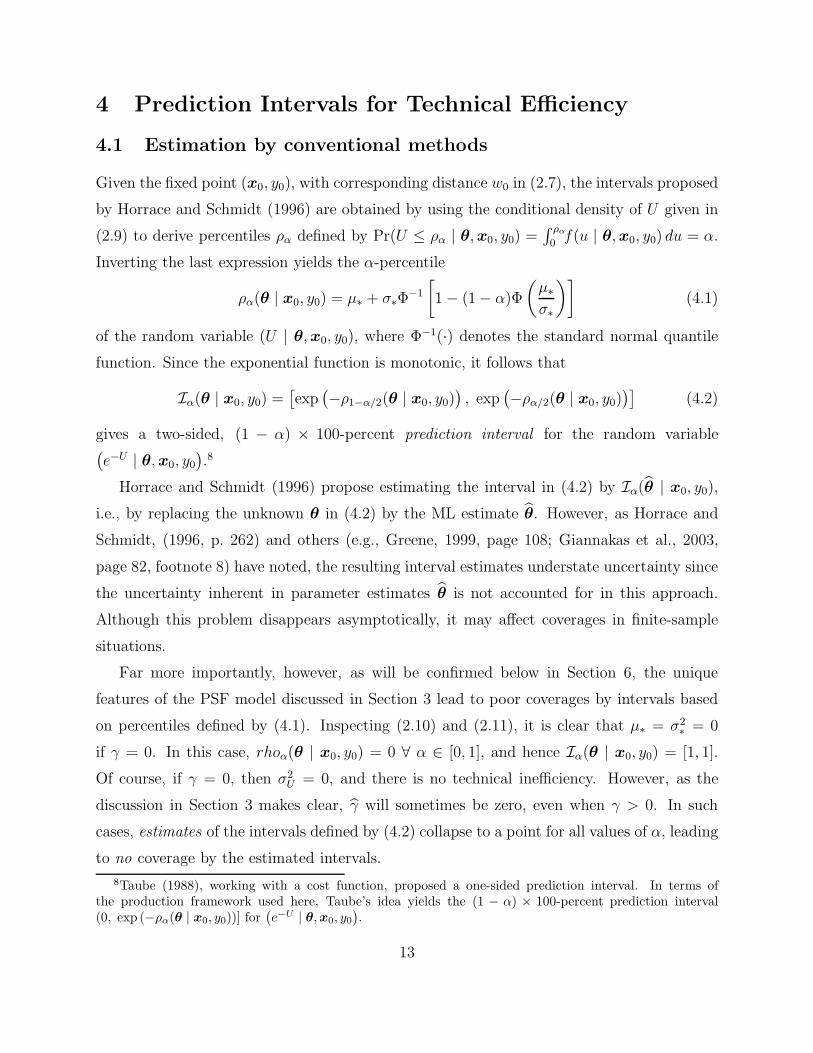
4 Prediction Intervals for Technical Efficiency

4.1 Estimation by conventional methods

Given the fixed point (x0, y0), with corresponding distance w0 in (2.7), the intervals proposed

by Horrace and Schmidt (1996) are obtained by using the conditional density of U given in

(2.9) to derive percentiles ρα defined by Pr(U ≤ ρα | θ,x0, y0) =∫ ρα

0f(u | θ,x0, y0) du = α.

Inverting the last expression yields the α-percentile

ρα(θ | x0, y0) = µ∗ + σ∗Φ−1

[1 − (1 − α)Φ

(µ∗

σ∗

)](4.1)

of the random variable (U | θ,x0, y0), where Φ−1(·) denotes the standard normal quantile

function. Since the exponential function is monotonic, it follows that

Iα(θ | x0, y0) =[exp

(−ρ1−α/2(θ | x0, y0)

), exp

(−ρα/2(θ | x0, y0)

)](4.2)

gives a two-sided, (1 − α) × 100-percent prediction interval for the random variable(e−U | θ,x0, y0

).8

Horrace and Schmidt (1996) propose estimating the interval in (4.2) by Iα(θ | x0, y0),

i.e., by replacing the unknown θ in (4.2) by the ML estimate θ. However, as Horrace and

Schmidt, (1996, p. 262) and others (e.g., Greene, 1999, page 108; Giannakas et al., 2003,

page 82, footnote 8) have noted, the resulting interval estimates understate uncertainty since

the uncertainty inherent in parameter estimates θ is not accounted for in this approach.

Although this problem disappears asymptotically, it may affect coverages in finite-sample

situations.

Far more importantly, however, as will be confirmed below in Section 6, the unique

features of the PSF model discussed in Section 3 lead to poor coverages by intervals based

on percentiles defined by (4.1). Inspecting (2.10) and (2.11), it is clear that µ∗ = σ2∗ = 0

if γ = 0. In this case, rhoα(θ | x0, y0) = 0 ∀ α ∈ [0, 1], and hence Iα(θ | x0, y0) = [1, 1].

Of course, if γ = 0, then σ2U = 0, and there is no technical inefficiency. However, as the

discussion in Section 3 makes clear, γ will sometimes be zero, even when γ > 0. In such

cases, estimates of the intervals defined by (4.2) collapse to a point for all values of α, leading

to no coverage by the estimated intervals.

8Taube (1988), working with a cost function, proposed a one-sided prediction interval. In terms ofthe production framework used here, Taube’s idea yields the (1 − α) × 100-percent prediction interval(0, exp (−ρα(θ | x0, y0))] for

(e−U | θ, x0, y0

).

13

Both of these problems can be alleviated by using bagging techniques.

4.2 Estimation by bagging

The idea of bootstrap aggregating was first used by Harris (1989); the name bagging was

given by Breiman (1996). The idea consists of generating replications of a predictor, and

then using the replicates to obtain an aggregated predictor. Theoretical properties of bagging

predictors have been examined by Friedman and Hall (1999), Buhlmann and Yu (2002), and

Fushiki et al. (2005). In particular, bagging predictors have been shown to provide substantial

improvements over conventional predictors (such as ML estimates of the intervals defined in

Section 4.1) when the conventional predictors are unstable in the sense that perturbations of

the learning set can cause significant changes in predictions. Due to the problems discussed

earlier in Section 3, this is precisely the case with ML estimates of the intervals defined above

in Section 4.1.

Recall that the interval Iα(θ | x0, y0) defined in (4.2) is determined by percentiles of the

conditional density f(u | θ,x0, y0) given in (2.9), which is estimated by f(u | θ,x0, y0). By

contrast, bagging determines a prediction interval based on percentiles of an estimate of

Ebθ

[f(u | θ,x0, y0)

]=

∫

Θ

f(u | θ,x0, y0)ψ(θ) dθ, (4.3)

where Θ is the parameter space and ψ(θ) is the sampling density of θ. The sampling density

ψ(θ) is unknown, but it can be approximated by bootstrap methods; the bagging technique

involves estimating the expectation in (4.3) by B−1∑B

b=1 f(u | θ∗

b ,x0, y0), where the θ∗

b are

bootstrap estimates of θ. Implementing the bagging estimator of the prediction interval in

(4.2) is straightforward; Fushiki et al. (2005) refer to the resulting interval estimate as a

“parametric bootstrap prediction interval.” The necessary steps are given below:

Algorithm #1:

[1] Maximize the log-likelihood function (2.6) to obtain ML estimates θ, Iα(θ | x0, y0),

and w0 = ω(θ | x0, y0); recover estimates σ2V , σ2

U from elements of θ.

[2] Set b = 1.

[3] For i = 1, . . . , n draw v∗i ∼ N(0, σ2V ) and u∗i ∼ N+(0, σ2

U), and compute y∗ib = g(xi |β)ev∗

i−u∗

i .

14

[4] Using the pseudo-data S∗b,n = {xi, y∗ib}n

i=1, compute bootstrap estimates θ∗

b =

argmaxθ

L(θ | S∗b,n) after replacing log yi with log y∗ib in (2.6).

[5] Draw u∗bk, k = 1, . . . , K, from f(u | θ∗

b ,x0, y0) obtained by replacing θ in (2.9) with

θ∗

b , and set ϕ∗bk = exp(−u∗bk) for each k = 1, . . . , K.

[6] Increment b by one.

[7] Repeat steps [3]–[6] B times, yielding a set U = {ϕ∗bk}B,K

b=1,k=1 of BK values.

[8] Form the set U∗ = {ϕ | ϕ ∈ U, ϕ 6= 1}.

The last step is necessary due to the fact that (as discussed previously in Section 3) some

bootstrap estimates in step [4] may yield estimates γ∗b —the bootstrap analog of γ—equal to

zero, causing the density f(u | θ∗

b ,x0, y0) to collapse to a probability mass at zero in step

[5]. This issue is explained further in Section 6. The realizations in U∗ can be sorted to find

α/2 and (1−α/2) quantiles of their empirical distribution, giving a bagging estimate of the

symmetric prediction interval Iα(θ | x0, y0) defined in (4.2) with nominal coverage (1 − α).

As an alternative, one might be tempted in step [5] of the above algorithm to simply

record quantiles of f(u | θ∗

b ,x0, y0), rather than drawing from this estimated density, and

then after step [7] to simply average the recorded quantiles over the Monte Carlo trials. This,

however, would be something other than bagging. In particular, (4.3) gives the expectation

of a density, rather than quantiles of the density. The number of deviates K drawn in step

[5] can be made to be very large, since draws cost little in terms of computational burden.

4.3 Bootstrap-adjusted interval estimates

As an alternative to the bagging method discussed in Section 4.2, bootstrap methods might

be used to adjust the nominal coverage of conventional estimates of the intervals defined in

Section 4.1 in an attempt to improve the realized coverage of conventional interval estimates.

The idea is similar to the approach described by Davison and Hinkley (1997, pages 243–245).

Iterated bootstrap procedures were introduced by Hall (1992) for the purpose of refining

the coverage of bootstrap estimates of confidence intervals. This idea has been used in the

context of nonparametric efficiency estimation with panel data by Hall et al. (1995), where

15

firm-specific efficiency was estimated as a fixed effect; the bootstrap was iterated to adjust

coverages when the two largest fixed effects were near each other, and in the context of

nonparametric efficiency estimation with cross-sectional data by Simar and Wilson (2001,

2004). The idea here is similar, except that conventional interval estimates are used in

the first stage, so that only one level of bootstrapping is needed. This greatly reduces

the computational burden that is incurred by more typical implementations of the iterated

bootstrap.

To briefly recap the discussion in Sections 2 and 4.1, the applied researcher is confronted

with some data in Sn and wishes to estimate the prediction interval given by (4.2) for the

random variable(e−U |, θ,x0, y0

)with a chosen, nominal coverage level (1−α). Let ξ denote

the random variable(e−U | θ,x0, y0

), where U has the probability density function given by

(2.9). In the case of the two-sided interval Iα(θ | x0, y0) defined in (4.2), the goal is to find

a value α such that Pr(ξ ∈ Ibα(θ | x0, y0

)≈ 1 − α.

Define a set of J values α1 < . . . < αJ , with 0 < αj < 1 for all j = 1, . . . , J . Since

the nominal value chosen for α to determine the coverage of prediction intervals is typically

small, αJ can be made well less than 1. Then the value α can be computed using the

following algorithm.

Algorithm #2:

[1] Maximize the log-likelihood function (2.6) to obtain estimates θ, Iα(θ), and w0 =

ω(θ | x0, y0); recover estimates σ2V , σ2

U from elements of θ.

[2] Set b = 1 and set C =[0 . . . 0

]′, a J-vector of zeros.

[3] For i = 1, . . . , n draw v∗i ∼ N(0, σ2V ) and u∗i ∼ N+(0, σ2

U), and compute y∗ib = g(xi |β)ev∗

i−u∗

i .

[4] Using the pseudo-data S∗b,n = {xi, y

∗ib}n

i=1, obtain bootstrap estimates θ∗

b =

argmaxθ

L(θ | S∗b,n) after replacing log yi with log y∗ib in (2.6).

[5] Compute J(θ∗

b) =[Iα1

(θ∗

b) . . . IαJ(θ

∗

b)]′

, a vector of intervals obtained by replacing

unknown parameters in (4.2) with elements of θ∗

b for each αj .

16

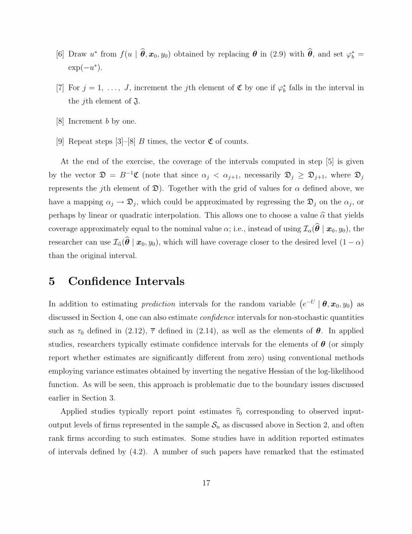
[6] Draw u∗ from f(u | θ,x0, y0) obtained by replacing θ in (2.9) with θ, and set ϕ∗b =

exp(−u∗).

[7] For j = 1, . . . , J , increment the jth element of C by one if ϕ∗b falls in the interval in

the jth element of J.

[8] Increment b by one.

[9] Repeat steps [3]–[8] B times, the vector C of counts.

At the end of the exercise, the coverage of the intervals computed in step [5] is given

by the vector D = B−1C (note that since αj < αj+1, necessarily Dj ≥ Dj+1, where Dj

represents the jth element of D). Together with the grid of values for α defined above, we

have a mapping αj → Dj, which could be approximated by regressing the Dj on the αj , or

perhaps by linear or quadratic interpolation. This allows one to choose a value α that yields

coverage approximately equal to the nominal value α; i.e., instead of using Iα(θ | x0, y0), the

researcher can use Ibα(θ | x0, y0), which will have coverage closer to the desired level (1−α)

than the original interval.

5 Confidence Intervals

In addition to estimating prediction intervals for the random variable(e−U | θ,x0, y0

)as

discussed in Section 4, one can also estimate confidence intervals for non-stochastic quantities

such as τ0 defined in (2.12), τ defined in (2.14), as well as the elements of θ. In applied

studies, researchers typically estimate confidence intervals for the elements of θ (or simply

report whether estimates are significantly different from zero) using conventional methods

employing variance estimates obtained by inverting the negative Hessian of the log-likelihood

function. As will be seen, this approach is problematic due to the boundary issues discussed

earlier in Section 3.

Applied studies typically report point estimates τ0 corresponding to observed input-

output levels of firms represented in the sample Sn as discussed above in Section 2, and often

rank firms according to such estimates. Some studies have in addition reported estimates

of intervals defined by (4.2). A number of such papers have remarked that the estimated

17

intervals are wide, and that firms’ efficiencies are not significantly different in a statistical

sense.9

While prediction intervals for the random variable(e−U | θ,x0, y0

)are certainly of in-

terest, such intervals are necessarily wider than confidence intervals for the non-stochastic

value τ0 defined in (2.12). Given that many papers report estimates of τ0 corresponding

to different firms, and that firms are typically ranked in terms of these estimates, it seems

reasonable to ask whether, and how, reasonable estimates of confidence intervals for τ0 might

be obtained.

In fact, it is straightforward to estimate confidence intervals for τ0 = τ(θ | x0,y0) given

in (2.12), as well as for τ(σ2U ) given in (2.14) using a parametric bootstrap. For the model

defined by Assumptions 2.1 and 2.2, a parametric bootstrap consists of the following steps:

Algorithm #3:

[1] Using the sample data Sn = {(xi, yi)}ni=1, maximize the log-likelihood in (2.6) to obtain

estimates θ; recover σ2V , σ2

U from elements of θ.

[2] For i = 1, . . . , n draw v∗i ∼ N(0, σ2V ) and u∗i ∼ N+(0, σ2

U), and compute y∗i = g(xi |β)ev∗

i−u∗

i .

[3] Using the pseudo-data S∗b,n = {xi, y∗i }n

i=1, compute bootstrap estimates θ∗

b =

argmaxθ

L(θ | S∗b,n) after replacing log yi with log y∗i in (2.6).

[4] Repeat steps [2]–[3] B times to obtain estimates B = {(θ∗

b)}Bb=1.

The estimates obtained in step [1] can be used to compute estimates τ0 = τ(θ | x0, y0)

and τ = τ(σ2U ) of τ0 = τ(θ | x0, y0) and τ (σ2

U), respectively. Similarly, the bootstrap

9The authors of Taube (1988) and Horrace and Schmidt (1996) are well aware that they provide predictionintervals for a random variable, even if they sometimes refer to their intervals as “confidence intervals”(Taube, writing in German, uses “Konfidenzintervall”). However, several published papers and perhaps alarger number of working papers contain clear, explicit statements indicating that the interval in (4.2) is usedas a confidence interval for the non-stochastic quantity τ0 defined in (2.12), rather than as a prediction intervalfor the random variable

(e−U | θ, x0, y0

). At the risk of being pedantic, a confidence interval is random set

covering an unknown population parameter with a certain probability, while a prediction interval involvesinference about a random variable, as opposed to a population parameter. A prediction interval is obtainedfrom knowledge of the distribution of the random variable whose future realizations one wishes to forecast,while a confidence interval requires information about the sampling distribution of an estimator. Precisedefinitions and additional discussion can be found in Stuart et al. (1999, pages 739–741), Shao (1999, pages99 and 432), Gourieaux and Monfort (1995, pages 373–374), or Neter et al. (1990, pages 78–83).

18

estimates obtained in B can be used to compute bootstrap estimates τ ∗b = τ(θ∗

b | x0, y0) and

τ∗

b = τ (σ∗2Ub) after recovering σ∗2

Ub from elements of θ∗

b . If one wishes to make inference about

σ2U and σ2

V , bootstrap estimates σ∗2Ub, σ

∗2V b can also be recovered from the bootstrap estimates

in B.

The bootstrap estimates in B (or the additional bootstrap estimates τ ∗B, τ∗

b) can be used

to estimate confidence intervals for the parameters of the model or for τ0 or τ in any of

several ways. We consider two possibilities. To illustrate, consider an initial estimate δ of

a quantity δ, and a corresponding set of bootstrap estimates {δ∗b}Bb=1. For nominal size α,

the percentile intervals discussed by Efron (1979, 1982) are given by(δ(α

2), δ( 1−α

2))

where

δ(α) denotes the α × 100-percentile of the elements of {δ∗b}Bb=1. Alternatively, bias-corrected

(BC) intervals described by Efron and Tibshirani (1993) are given (again, for nominal size

α) by(δ(α1), δ(α2)

)where α1 = Φ

(2z0 + z(α

2)), α2 = Φ

(2z0 + z(1−α

2)), z0 = Φ−1

(#{bδ∗

b<bδ}

B

),

and z(α) = Φ−1(α).

As an alternative to the bootstrap, confidence intervals for τ0 defined in (2.12) and τ

defined in (2.14) can also be obtained by noting that the theory of maximum likelihood

gives√n

(θ − θ

)d−→ N(0,Σ), (5.1)

where Σ is the variance-covariance matrix of θ. Since τ0 is simply a function of θ and of

x0, y0, the Slutsky theorem yields

√n (τ0 − τ0)

d−→ N(0, σ2

τ0

). (5.2)

The delta method gives the first-order approximation σ2τ0≈ ∇′

τ0Σ∇τ0 , where

∇τ0 =[

∂τ0∂β

∂τ0∂σ2

∂τ0∂γ

]′. (5.3)

Expressions for the necessary partial derivatives are given in the Appendix. In the case of

mean efficiency, the Slutsky theorem again provides

√n

(τ − τ

)d−→ N

(0, σ2

τ

), (5.4)

and the delta method gives σ2τ ≈ ∇′

τΣ∇τ where

∇τ =[

∂τ∂β

∂τ∂σ2

U

∂τ∂γ

]′. (5.5)

19

Again, the necessary partial derivatives are given in the Appendix.

Asymptotic confidence intervals for τ0 and τ can be constructed using the asymptotic

results in (5.2) and (5.4). For example, in the case of τ0, a (1− α)× 100-percent confidence

interval is given by (τ0 − στΦ

−1(α

2

), τ0 + στΦ

−1(1 − α

2

))(5.6)

where Φ−1(·) is the standard normal quantile function. A (1 − α) × 100-percent confidence

interval for τ can be constructed similarly by replacing στ with στ in (5.6). The variances

σ2τ and σ2

τ can be estimated by replacing unknown parameters with their ML estimates.

The bounds of the intervals obtained by the delta method are functions of θ. In order

to estimate the intervals, the unknown parameters must be replaced with estimates, just

as was the case with conventional estimation of prediction intervals as discussed in Section

4.1. Asymptotically this presents no problems, but in finite samples, one would expect that

the resulting interval estimates understate uncertainty about τ and τ , due to the failure

to account for uncertainty about the parameters that must be estimated. The bootstrap

method outlined in Section 5 avoids this problem.

6 Monte Carlo Evidence

6.1 Design of Experiments

In our Monte Carlo experiments, we take (2.1)–(2.4) as the “true” model, with g(X | β) =

eβ1Xβ2 and X ∼ N+(60, 10) so that X > 0. After taking logs, the model can be written as

log Y = β1 + β2 logX + V − U, (6.1)

with V and U distributed as described in (2.3)–(2.4). We set β1 = log(10) ≈ 2.3026 and β2 =

0.8. Olson et al. (1980) note that only two parameters among the set {σU , σV , σ2, γ, σ2

W}(where σ2

W = VAR(W ) =(π−2)σ2

U

π+ σ2

V ) are independent. Therefore, we set σ2W = 1 without

loss of generality, and consider six different values of the ratio λ2 =σ2

U

σ2

V

of shape parameters:

λ2 ∈ {0.1, 0.5, 1, 2, 10, 100}. These values correspond to γ = 0.0909, 0.3333, 0.5, 0.6667,

0.9091, and 0.9901, respectively. Figure 1 shows plots of the density of the composite error

term W given in (2.5) corresponding to the six values of λ2. For reference, plots of the

standard normal density, given by the dashed curves in Figure 1, are also shown.

20

Plausible values of the dependent variable in (6.1) vary across experiments, depending

on λ2. For each experiment, we use the true values of γ and σ2 to estimate (by Monte

Carlo) the 0.1, 0.3, 0.5, 0.7, and 0.9 quantiles of W = V − U ; denote these by w(q), q ∈Q = {0.1, 0.3, 0.5, 0.7, 0.9}. We then obtain log-output values for five hypothetical

firms by computing y(q) = exp(β1 + β2 log(60) + w(q)

), q ∈ Q. The input/output values for

these hypothetical firms are held constant across Monte Carlo trials, and across bootstrap

replications within each Monte Carlo trial, reflecting the fact that in applied settings, points

of interest in the input-output space are always taken as given.

On each Monte Carlo trial, we generate n ∈ {100, 1000} observations {(xi, yi)}ni=1 and

use these to estimate the parameters of the model by maximizing the log-likelihood (2.6).

We then use the parameter estimates to estimate mean efficiency τ defined in (2.14). We

also estimate inefficiency for a set of five “hypothetical” firms, which do not necessarily

correspond to any observations in our samples. For each of these hypothetical firms, the

input level is fixed at 60.10

Each experiment consisted of M = 2048 Monte Carlo trials.11 On each trial, we use

the conventional, bagging, and bootstrap-adjusted methods discussed in Section 4 to esti-

mate prediction intervals for(e−U | θ, x0 = 60, y(q)

), q ∈ Q. On each Monte Carlo trial,

the coverage of each estimated prediction interval can be computed exactly (in the sense

of not relying on Monte Carlo approximation or estimation) since the exact distribution of(e−U | θ, x0 = 60, y(q)

)is known from (2.9). Specifically, if a particular method yields pre-

diction interval estimates (am, bm) for each Monte Carlo trial m = 1, . . . , M , then the esti-

mated coverage is computed as M−1∑M

m=1 Fq(− log(am) | θ, x0 = 60, y(q)) − Fq(− log(bm) |θ, x0 = 60, y(q)), where Fq(·) is the distribution function for the truncated normal distribution

N+(µ∗, σ2∗), here with µ∗ obtained by substituting w(q) for w0 in (2.10).

In addition, confidence intervals for τ as well as for τ corresponding to each (x0, y(q)),

q ∈ Q, were estimated using both the delta method and the bootstrap method described in

Section 5. Estimated coverages for confidence interval estimates were computed by dividing

(i) the number of trials where confidence intervals estimated by a given method include the

10We experimented with other values for the input level, but found little difference among our results.11The Monte Carlo experiments were performed on a massively parallel machine, where the number of

processors for a particular job are conveniently and efficiently chosen as a power of 2. Choosing 211 = 2, 048Monte Carlo trials makes efficient use of the processors.

21

parameter of interest by (ii) M , the total number of Monte Carlo trials.

6.2 Coverages of estimated prediction intervals for(e−U | θ,x0, y0

)

Table 2 gives estimated coverages of two-sided prediction intervals estimated by the conven-

tional method, i.e., by replacing θ in (4.2) with ML estimates θ on each Monte Carlo trial,

for(e−U | θ, x0 = 60, y(q)

)(where q ∈ Q as described above in Section 6.1). For each sam-

ple size n ∈ {100, 1000}, Table 2 gives estimated coverages for six different signal-to-noise

ratios—corresponding to the six different values of λ2—as well as three nominal significance

levels and five different values of y0 determined by quantiles of W .

Coverages by the conventional prediction intervals reported in Table 2 generally improve

when the sample size increases from n = 100 to n = 1000, but are poor for smaller values

of λ2, even with n = 1000. Moreover, with n = 100, coverages across the six values of λ2

improve as λ2 increases from 0.1 to 10, but then become worse when λ2 is increased from 10

to 100. The poor performance of the conventional prediction intervals can be explained after

careful inspection of the interval in (4.2). To illustrate, consider the case where λ2 = 0.1; the

results in Table 1 indicate roughly 46 percent of samples of size n = 1000—about 942 of 2,048

Monte Carlo trials—will have residuals with positive skewness, ensuring that γ = 0 and hence

µ∗ = σ2U = 0. This is further confirmed by looking in Figure 1 at the panel corresponding to

λ2 = 0.1, where f(w | γ, σ2) is seen to be almost the same as the standard normal density.

Hence, for any value of α ∈ (0, 1), the estimate of the interval in (4.2) collapses to [1, 1]

in such cases. But, simple algebra confirms that when λ2 = 0.1 in our experiments, the

conditional density in (2.9) has strictly positive variance. Yet, prediction interval estimates

based on (4.2) will yield zero coverage in about 46-percent, or 942 of 2,048 Monte Carlo

trials, regardless of the significance level that is chosen. A similar phenomenon occurs when

γ = 1, which occurs in a number of trials when λ2 is increased to 100. Necessarily, prediction

intervals of zero-width have poor coverage when the true γ is neither zero nor one.12

12We know of only one other paper that has examined coverages of conventional prediction intervals similarto the interval in (4.2) proposed by Horrace and Schmidt (1996). Kumbhakar and Lothgren (1998) report, inTable 3a of their paper, coverages of e−U (as opposed to e−u | θ, x0, y0) for sample sizes ranging from n = 25

to n = 800, and eleven values of γ∗ = (π−2π

)σ2U

[(π−2

π)σ2

U+ σ2

V

]−1equal to 0.0, 0.1, ..., 1.0. They set σ2 = 1;

hence, their values of γ∗ correspond to λ2 = 0.0, 0.306, 0.688, 1.18, 1.83, 2.75, 4.13, 6.42, 11.01, 24.77,and +∞. Inspection of the results in their Table 3a reveals some problems. For example,with γ∗ = 0.1,implying λ2 = 0.306, Kumbhakar and Lothgren report average coverage equal to 0.743 at 95-percent atnominal significance in samples of size n = 100. Yet, as our results in Table 1 indicate, with n = 100 and

22

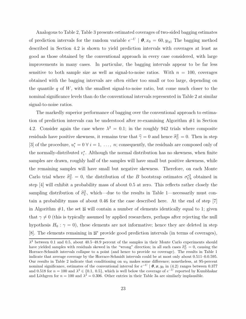
Analogous to Table 2, Table 3 presents estimated coverages of two-sided bagging estimates

of prediction intervals for the random variable e−U | θ, x0 = 60, y(q) The bagging method

described in Section 4.2 is shown to yield prediction intervals with coverages at least as

good as those obtained by the conventional approach in every case considered, with large

improvements in many cases. In particular, the bagging intervals appear to be far less

sensitive to both sample size as well as signal-to-noise ratios. With n = 100, coverages

obtained with the bagging intervals are often either too small or too large, depending on

the quantile q of W , with the smallest signal-to-noise ratio, but come much closer to the

nominal significance levels than do the conventional intervals represented in Table 2 at similar

signal-to-noise ratios.

The markedly superior performance of bagging over the conventional approach to estima-

tion of prediction intervals can be understood after re-examining Algorithm #1 in Section

4.2. Consider again the case where λ2 = 0.1; in the roughly 942 trials where composite

residuals have positive skewness, it remains true that γ = 0 and hence σ2U = 0. Then in step

[3] of the procedure, u∗i = 0 ∀ i = 1, . . . , n; consequently, the residuals are composed only of

the normally-distributed v∗i . Although the normal distribution has no skewness, when finite

samples are drawn, roughly half of the samples will have small but positive skewness, while

the remaining samples will have small but negative skewness. Therefore, on each Monte

Carlo trial where σ2U = 0, the distribution of the B bootstrap estimates σ∗2

Ub obtained in

step [4] will exhibit a probability mass of about 0.5 at zero. This reflects rather closely the

sampling distribution of σ2U , which—due to the results in Table 1—necessarily must con-

tain a probability mass of about 0.46 for the case described here. At the end of step [7]

in Algorithm #1, the set U will contain a number of elements identically equal to 1; given

that γ 6= 0 (this is typically assumed by applied researchers, perhaps after rejecting the null

hypothesis H0 : γ = 0), these elements are not informative; hence they are deleted in step

[8]. The elements remaining in U∗ provide good prediction intervals (in terms of coverages),

λ2 between 0.1 and 0.5, about 40.5–48.9 percent of the samples in their Monte Carlo experiments shouldhave yielded samples with residuals skewed in the “wrong” direction; in all such cases σ2

U= 0, causing the

Horrace-Schmidt intervals collapse to a point (and hence to provide no coverage). The results in Table 1indicate that average coverage by the Horrace-Schmidt intervals could be at most only about 0.511–0.0.595.Our results in Table 2 indicate that conditioning on w0 makes some difference; nonetheless, at 95-percentnominal significance, estimates of the conventional interval for e−U | θ, x, y0 in (4.2) ranges between 0.377and 0.518 for n = 100 and λ2 ∈ {0.1, 0.5}, which is well below the coverage of e−U reported by Kumbhakarand Lothgren for n = 100 and λ2 = 0.306. Other entries in their Table 3a are similarly implausible.

23

as demonstrated by the results in Table 3.

Before considering estimation of confidence intervals, we return to the conventional pre-

diction intervals with bootstrap adjustment described in Section 4.3. Estimates from our

Monte Carlo experiments for coverages achieved by this approach are shown in Table 4. The

results reveal that the bootstrap adjustment in Algorithm #2 provides some improvement

over coverages attained with the ordinary conventional approach in Table 2, but the cover-

ages in Table 4 remain poor when compared to the results obtained with bagging in Table

3. The bootstrap adjustment to the conventional intervals cannot overcome the problems

related to the collapse of the interval in (4.2) to a point whenever γ = 1.

6.3 Coverages of estimated confidence intervals for τ0 and τ

Using the expression in (2.12), the “true” values of θ in our Monte Carlo framework, and

the quantiles w(q), it is straightforward to compute τ(θ | x0, y0) (i.e., the “true” value) cor-

responding to quantiles w(q) considered in our Monte Carlo experiments as well as mean

efficiency τ using the expressions in (2.12) and (2.14). It is equally straightforward to com-

pute the proportion of Monte Carlo trials which yield intervals estimated using various

approaches that cover τ or τ .

In our experiments, the delta method provides no discrimination. In every case, the

method yielded intervals that always cover the true values of τ0. This should be of little sur-

prise, given that the delta method is based on a Taylor expansion of the log-likelihood; here,

where substantial nonlinearities exist, higher-order terms in the Taylor expansion that are

dropped by the delta method are important. This also suggests a situation where bootstrap

methods can be expected to give improved performance over more conventional methods of

inference.

Although it is clear that the interval Iα(θ | x0, y0) given in (4.2) is a prediction inter-

val for the random variable(e−U | θ,x0, y0

), a number of authors have used estimates of

Iα(θ | x0, y0) as confidence intervals for τ0. Table 5 presents estimated coverages of τ0 (cor-

responding to the quantiles w(q)) by estimates of conventional (prediction) intervals based

on Iα(θ | x0, y0) in (4.2). We stress that these results are obtained from a mis-use of predic-

tion intervals (for a random variable) as confidence intervals for a non-stochastic population

parameter, namely τ0; this is not what Horrace and Schmidt intended. Nonetheless, given

24

that the conventional, Horrace and Schmidt intervals have been mis-used by some authors

in this way, and given that one could plausibly expect prediction intervals for a random

variable to over-cover the mean of the same random variable, it is interesting to see what

the consequences of the mis-use might be.

Given that the conventional intervals are prediction intervals for a random variable, as

opposed to confidence intervals for its mean, one might plausibly expect that prediction

intervals would over-cover the mean when used as confidence intervals for τ0. Indeed, this

occurs in Table 5 for cases with n = 1000 and λ2 ≥ 2, where realized coverages range from

0.997 to 1.000 at each significance level that was considered. But, Table 5 also reveals the

opposite in many cases, particularly for sample size n = 100, but also when n = 1000 and

the signal-to-noise ratio is less than 1. In these cases, the intervals tend to under-cover. This

is due to the fact that the conventional interval estimates collapse to zero width whenever

γ = 0 or 1, as discussed above in Section 6.2. While one might have expected over-coverage,

that is not always the case.

Table 6 shows estimated coverages of bootstrap confidence intervals for τ0 (again, corre-

sponding to the quantiles w(q)) obtained from Algorithm #3. The results in Table 6 indicate

that the bootstrap method performs well in the sense that it yields coverages that are close

to nominal levels, except perhaps when λ2 is very small, although the coverages in Table 6

are not so bad even with λ2 = 0.1 and n = 100. With the smaller values of λ2, the realized

coverages shown in Table 6 are larger than the nominal significance levels. The results in-

dicate that coverages depend (not surprisingly) on the signal-to-noise ratio as reflected by

λ2. Coverages also depend, though less severely, on where the output value lies for a given

point of interest, as reflected by the quantiles w(q). The bootstrap intervals perform well

with the larger sample size (i.e., n = 1000) when λ2 ≥ 1. For smaller values of λ2, coverage

by the bootstrap intervals is too large for 90-percent and 95-percent nominal significance.

But, small values of λ2 represent low signal-to-noise ratios; in other words, when λ2 is small,

extracting information from a given body of data is necessarily more difficult than when

λ2 is larger. The bootstrap is neither magic nor a panacea, but it still out-performs the

conventional approach to inference regarding efficiencies of individual units.

As noted previously in Section 5, bootstrap estimates in the set B can be used to com-

pute bootstrap estimates τ∗

b ; these can be used to construct (percentile) bootstrap estimates

25

of confidence intervals for mean efficiency τ , analogous to how bootstrap confidence inter-

vals are constructed for τ0. Recall, however, that τ defined in (2.14) is a function of just

one model parameter, namely σ2U . Given the transformation-preserving property of the per-

centile bootstrap (e.g., see Efron and Tibshirani, 1993), the coverage of bootstrap confidence

intervals for τ will be identical to the coverage of bootstrap confidence intervals for σ2U at

the same significance levels. Results on coverages of bootstrap confidence intervals for σ2U

are given in Table 9 and are discussed below in Section 6.4. As will be seen, with sample

size n = 100, the bootstrap intervals perform well, though at .90 and .95 significance levels,

coverages are slightly too large at smaller values of λ2 and slightly too small at larger values

of λ2. At .99 significance, the bootstrap intervals have very good coverage. When the sample

size is increased to n = 1000, coverages by the bootstrap intervals improve in almost every

case.

6.4 Coverage of Intervals for Model Parameters

The bootstrap procedure (Algorithm #3) given in Section 5 can also be used to estimate con-

fidence intervals for the model parameters. Conventional inference about model parameters

meanwhile relies on the asymptotic normality result from the theory of maximum likeli-

hood, and typically employs the inverse negative Hessian of the log-likelihood function in

(2.6) as an estimator of the variance-covariance matrix. Alternatively, one can estimate the

variance-covariance matrix using the outer-dot product of the gradient of the log-likelihood,

sometimes called the OPG or BHHH (after Berndt et al., 1974); i.e., one can estimate Σ in

(5.1) by

Σ =[∇θ∇

′

θ

]−1

(6.2)

where

∇θ =[∇θ1 ∇θ2 . . . ∇θn

], (6.3)

∇θi =∂Li(θ | Sn)

∂θ

∣∣∣∣θ=bθ

, (6.4)

and Li(θ | Sn) is the contribution of the ith observation to the log-likelihood given in (2.6).

It is widely known (e.g., see Cameron and Trivedi, (2005)) that using the BHHH estimator

in (6.2) often leads to tests with poor finite-sample properties and large size distortions; on

the other hand, it can be computed even when the negative Hessian of the log-likelihood is

26

singular (it is this feature that leads to the guarantee of convergence in the maximization

algorithm of Berndt et al., 1974).

Although the model is parameterized in terms of β, σ2, and γ, straightforward algebra

yields estimators σ2V and σ2

V as functions of β, σ2, and γ; then variances of the the estimators

σ2V and σ2

U are given by O′V ΣOV and O

′UΣOU where Σ is the variance covariance matrix for

(β, σ2, γ) and OV and OU are vectors of derivatives of σ2V and σ2

U with respect to β, σ2,

and γ. Conventional variance estimates can be used to estimate confidence intervals in the

usual way.

Tables 7, 8, and 9 give estimated coverages of intervals estimated by the conventional

method (using the inverse of the negative Hessian in Table 7, and the BHHH estimator

in Table 8) and bootstrap method for model parameters with sample sizes n = 100 and

n = 1000, and significance levels .90, .95, and .99. The first row of Table 7 gives the

number of trials—out of 2,048—where confidence intervals for model parameters could be

estimated. Interval estimates could be computed for every trial using the BHHH estimator

and the bootstrap method, but the negative Hessian of the log-likelihood function is singular

whenever γ = 0 or 1. Due to the problems discussed in Section 6.2, γ = 0 with frequencies

similar to those in Table 1. In addition, with a sample size of only 100 observations, large

values of λ (10 and 100) yield small numbers of Monte Carlo trials with estimates γ = 1.

Of course, the conventional confidence interval estimates that use the inverse of the negative

Hessian cannot be computed whenever the negative Hessian is singular.

Estimated coverages in Table 7 for conventional intervals were computed by dividing the

number of instances where computed intervals covered the corresponding true values not by

the total number of Monte Carlo trials (2,048), but by the number of cases given in the first

row of the table where conventional intervals could be computed. Consequently, the coverage

estimates shown for conventional intervals in Table 7 may be overly optimistic. Although

coverage of the intercept and slope parameters (β1 and β2) by the conventional intervals is

close to nominal significance levels in Table 7, coverage of σ2, γ, σ2V , and σ2

U is poor for all

values of λ2. Moreover, the coverages do not improve when sample size is increased from

n = 100 to n = 1000. Similar observations can be made for coverages of intervals based on

the BHHH estimator, shown in Table 8, although with n = 100, coverages of β are too large

both when λ2 is small as well as when it is large. In both Tables 7 and 8, coverages of the

27

parameters other than β are very poor

Coverage by the bootstrap interval estimates shown in Table 9 is similar to that of the

conventional intervals based on the inverse of the negative Hessian for β1 and β2, and is

more accurate than with the conventional intervals for parameters σ2, γ, σ2V , and σ2

U . Unlike

the experience with the conventional intervals in Tables 7 and 8, coverages of the bootstrap

intervals in Table 9 are seen to improve when sample size is increased, except perhaps for

the smallest values of λ2. For the smallest values of λ2, coverage by bootstrap intervals for

σ2V is very accurate in Table 9 when n = 1000, but too large for σ2, γ, and σ2

U at significance

levels .90 and .95 when λ2 = 0.1 or 0.5. Coverages by the bootstrap intervals, however, are

closer to nominal values than coverages by the conventional intervals. Once again, when

the signal-to-noise ratio is low—reflected by small values of λ2—it is apparently difficult to

extract information about efficiency and noise from the model in 2.1.

7 Conclusions

In the context of cross-sectional PSF models, the term representing firm-specific inefficiency

is not identified; the point estimates that are typically reported are estimates of conditional

expectations. While one can estimate either prediction intervals for the random variable(e−U | w0

), or confidence intervals for the expectation of this random variable (i.e., for τ0

defined in (2.12)), prediction intervals for(e−U | w0

)are likely to be much wider than con-

fidence intervals for τ0. Where prediction intervals associated with individual firms have

been compared in the literature, it should be of little surprise that few, if any, significant

differences are found across firms.

Taube (1988) and Horrace and Schmidt (1996) derived prediction intervals for(e−U | w0

)

and proposed “conventional” estimators of their intervals based on replacing unknown model

parameters with consistent estimators. Unfortunately, the coverage properties of these con-

ventional interval estimates is poor, due in large part to the bounded support of the distri-

bution of the inefficiency term U , with the consequence that in finite samples, residuals may

have the “wrong” skewness, even if the model is correctly specified. By contrast, the bagging

method, using Algorithm #1 in Section 4.2, yields prediction interval estimates with much

better coverage properties.

In the case of confidence intervals for τ0, inappropriate use of the conventional prediction

28

intervals as confidence intervals leads (not surprisingly) to very poor coverage. While one

might expect that prediction intervals would over-cover when used as confidence intervals,

in fact the opposite occurs, again due to the boundary issues discussed in Sections 3 and 6.

Our simulation results demonstrate that a parametric bootstrap yields confidence intervals

for τ0 with good coverage properties, even when the signal-to-noise ratio is low.

It has been known for some time that PSF models sometimes yield residuals with the

“wrong” skewness. The implications of this phenomenon for inference, however, have not

been carefully considered. This paper makes clear that, depending on the signal-to-noise

ratio reflected by λ2, the problem can arise with alarming frequency, even when the model is

correctly specified. Consequently, “wrongly” skewed residuals in an observed sample do not

provide meaningful evidence of specification error. Common practice among practitioners,

however, has been to change the model specification whenever “wrongly” skewed residuals

are encountered.

Classical inference assumes that the model specification is chosen independently of any

estimates that are obtained; specification-searching introduces problems of bias in both pa-

rameter estimates as well as variance-covariance estimates. The bagging procedure described

in Section 4.2 and the bootstrap procedure given in Section 5 can be used to estimate predic-

tion intervals as well as confidence intervals with good coverage properties, and can extract

useful information about efficiency levels even from samples where residuals have the “wrong”

skewness. In such cases, one of course relies heavily on parametric assumptions, but this is

probably always true when PSF models are estimated.

A Technical Appendix

To evaluate ∇τ in (5.2) and (5.3), note that (2.12) can be rewritten as

τ = Φ

(µ∗

σ∗− σ∗

)Φ

(µ∗

σ∗

)−1

exp

(−µ∗ +

σ2∗

2

). (A.1)

Also note that the first term in ∇τ is given by

∂τ

∂β=

∂τ

∂µ∗

∂µ∗

∂w0

∂w0

∂β

=

(∂τ

∂µ∗

)γ

(∂ log g(x | β)

∂β

). (A.2)

29

Hence terms

∂τ

∂ζ= Φ

(µ∗

σ∗

)−1

exp

(−µ∗ +

σ2∗

2

)∂

∂ζΦ

(µ∗

σ∗− σ∗

)

+Φ

(µ∗

σ∗− σ∗

)exp

(−µ∗ +

σ2∗

2

)∂

∂ζΦ

(µ∗

σ∗

)−1

+Φ

(µ∗

σ∗− σ∗

)Φ

(µ∗

σ∗

)−1∂

∂ζexp

(−µ∗ +

σ2∗

2

)(A.3)

are needed, where ζ represents either µ∗, σ2 or γ.

The nine different partial derivatives needed in (A.3) are given by:

∂

∂µ∗Φ

(µ∗

σ∗− σ∗

)= σ−1

∗ φ

(µ∗

σ∗− σ∗

), (A.4)

∂

∂µ∗Φ

(µ∗

σ∗

)−1

= −σ−1∗ Φ

(µ∗

σ∗

)−2

φ

(µ∗

σ∗

), (A.5)

∂

∂µ∗exp

(−µ∗ +

σ2∗

2

)= − exp

(−µ∗ +

σ2∗

2

), (A.6)

∂

∂σ2Φ

(µ∗

σ∗− σ∗

)=

1

2φ

(µ∗

σ∗− σ∗

)γ1/2σ−1

[w0σ

−2γ−1 (1 − γ)−1/2 − (1 − γ)1/2], (A.7)

∂

∂σ2Φ

(µ∗

σ∗

)−1

= −1

2Φ

(µ∗

σ∗

)−2

φ

(µ∗

σ∗

)w0γ

1/2σ−3 (1 − γ)−1/2 , (A.8)

∂

∂σ2exp

(−µ∗ +

σ2∗

2

)=

1

2γ (1 − γ) exp

(−µ∗ +

σ2∗

2

), (A.9)

∂

∂γΦ

(µ∗

σ∗− σ∗

)= φ

(µ∗

σ∗− σ∗

) [σ2γ (1 − γ)

]−1/2

×{−w0 +

1

2(1 − 2γ)

[w0

(1 − γ)− σ2

]}, (A.10)

∂

∂γΦ

(µ∗

σ∗

)−1

=1

2Φ

(µ∗

σ∗

)−2

φ

(µ∗

σ∗

)w0σ

−1γ−1/2(1 − γ)−3/2 (A.11)

and∂

∂γexp

(−µ∗ +

σ2∗

2

)=

[w0 +

1

2σ2(1 − 2γ)

]exp

(−µ∗ +

σ2∗

2

). (A.12)

The terms appearing in ∇τ in (5.4) and (5.5) are given by

∂τ

∂β= 0, (A.13)

30

∂τ

∂σ2=

1

2γτ − e

1

2γσ2

γ1/2σ−1φ(γ1/2σ

), (A.14)

and∂τ

∂γ=

1

2σ2τ − e

1

2γσ2

γ−1/2σφ(γ1/2σ

). (A.15)

31

References

Aigner, D., Lovell, C. A. K., and Schmidt, P. (1977), “Formulation and estimation of stochas-tic frontier production function models,” Journal of Econometrics, 6, 21–37.

Battese, G. E., and Coelli, T. J. (1988), “Prediction of firm-level technical efficiencies witha generalized frontier production function and panel data,” Journal of Econometrics,38, 387–399.

Battese, G. E., and Corra, G. S. (1977), “Estimation of a production frontier model: Withapplication to the pastoral zone off eastern australia,” Australian Journal of AgriculturalEconomics, 21, 169–179.

Bauer, P. W. (1990), “Recent developments in the econometric estimation of frontiers,”Journal of Econometrics, 46, 39–56.

Berndt, E., B. Hall, R. Hall, and Hausman, J. (1974), “Estimation and inference in non-linearstructural models,” Annals of Economic and Social Measurement, 3, 653–665.

Bravo-Ureta, B. E., and Pinheiro, A. E. (1993), “Efficiency analysis of developing countryagriculture: A review of the frontier function literature,” Agricultural and ResourceEconomics Review, 22, 88–101.

Breiman, L. (1996), “Bagging predictors,” Machine Learning, 24, 123–140.

Buhlmann, P., and Yu, B. (2002), “Analyzing bagging,” Annals of Statistics, 30, 927–961.

Cameron, A. C., and Trivedi, P. K. (2005), Microeconometrics: Methods and Applications,Cambridge: Cambridge University Press.

Coelli, T. (1995), “Estimators and hypothesis tests for a stochastic frontier function: Amonte carlo analysis,” Journal of Productivity Analysis, 6, 247–268.

Coelli, Tim (1996), “A guide to frontier version 4.1: A computer program for stochasticfrontier production and cost function estimation,” CEPA working paper #96/07, Centrefor Efficiency and Productivity Analysis, University of New England, Arimidale, NSW2351, Australia.

Davidon, W. C. (1959), “Variable metric method for minimization,” Argonne NationalLaboratory Research and Development report #5990; reprinted in SIAM Journal onOptimization 1, 1–17 (1991).

Davison, A. C., and Hinkley, D. V. (1997), Bootstrap Methods and their Application, Cam-bridge, United Kingdom: Cambridge University Press.

Efron, B. (1979), “Bootstrap methods: another look at the jackknife,” Annals of Statistics,7, 1–16.

(1982), The Jackknife, the Bootstrap and Other Resampling Plans, Philadelphia: Societyfor Industrial and Applied Mathematics. CBMS-NSF Regional Conference Series inApplied Mathematics, #38.

Efron, B., and Tibshirani, R. J. (1993), An Introduction to the Bootstrap, London: Chapmanand Hall.

32

Fletcher, R., and Powell, M. J. D. (1963), “A rapidly convergent descent method for mini-mization,” Computer Journal, 6, 163–168.

Flores-Lagunes, A., Horrace, W. C., and Schnier, K. E. (2007), “Identifying technicallyefficient fishing vessels: A non-empty, minimal subset approach,” Journal of AppliedEconometrics, 22, 729–745.

Friedman, J. H., and Hall, P. (1999), “On bagging and nonlinear estimation,” Unpublishedworking paper, Department of Statistics, Stanford University.

Fushiki, T., Komaki, F., and Aihara, K. (2005), “Nonparametric bootstrap prediction,”Bernoulli, 11, 293–307.

Giannakas, K., Tran, K. C., and Tzouvelekas, V. (2003), “On the choice of functional formsin stochastic frontier modeling,” Empirical Economics, 28, 75–100.

Gourieaux, C., and Monfort, A. (1995), Statistics and Econometric Methods, vol. 1, Cam-bridge: Cambridge University Press. Translated by Quang Vuong.

Greene, W. H. (1993), “The econometric approach to efficiency analysis,” In The Measure-ment of Productive Efficiency, ed. H. O. Fried, C. A. K. Lovell, and S. S. Schmidt, NewYork: Oxford University Press pp. 68–119.

(1995), LIMDEP Version 7.0 User’s Manual, New York: Econometric Software, Inc.

Greene, W. H. (1999), “Frontier production functions,” In Handbook of Applied Econo-metrics, ed. H. Peseran and P. Schmidt, vol. II, Oxford, United Kingdom: BlackwellPublishers Ltd. chapter 3, pp. 81–166.

Hall, P. (1992), The Bootstrap and Edgeworth Expansion, New York: Springer-Verlag.

Hall, P., Hardle, W., and Simar, L. (1995), “Iterated bootstrap with application to frontiermodels,” The Journal of Productivity Analysis, 6, 63–76.

Harris, I. R. (1989), “Predicitve fit for natural exponential families,” Biometrika, 76, 675–684.

Herrero, I., and Pascoe, S. (2002), “Estimation of technical efficiency: A review of some ofthe stochastic frontier and dea software,” Computers in Higher Education EconomicsReview. Virtual edition (http://www.economics.ltsn.ac.uk/cheer.htm).

Horrace, W. C. (2005), “On ranking and selection from independent from independent trun-cated normal distributions,” Journal of Econometrics, 126, 335–354.

Horrace, W. C., and Schmidt, P. (1996), “Confidence statements for efficiency estimatesfrom stochastic frontier models,” Journal of Productivity Analysis, 7, 257–282.

Kumbhakar, S. C., and Lothgren, M. (1998), “A monte carlo analysis of technical inefficiencypredictors,” Working Paper Series in Economics and Finance, No. 229, StockholmSchool of Economics, P. O. Box 6501, S–113 83 Stockholm, Sweden.

Kumbhakar, S. C., and Lovell, C. A. K. (2000), Stochastic Frontier Analysis, Cambridge:Cambridge University Press.

33

Leamer, Edward E. (1978), Specification Searches: Ad Hoc Inference with NonexperimentalData, John Wiley & Sons, Inc.

Lee, L. F. (1993), “Asymptotic distribution of the maximum likelihood estimator for astochastic frontier function model with a singular information matrix,” EconomietricTheory, 9, 413–430.

Meeusen, W., and van den Broeck, J. (1977), “Efficiency estimation from Cobb-Douglasproduction functions with composed error,” International Economic Review, 18, 435–444.

Neter, J., Wasserman, W., and Kutner, M. H. (1990), Applied Linear Statistical Models,Homewood, Illinois: Richard D. Irwin, Inc.

Olson, J. A., Schmidt, P., and Waldman, D. M. (1980), “A monte carlo study of estimatorsof stochastic frontier production functions,” Journal of Econometrics, 13, 67–82.

Ritter, C., and Simar, L. (1997), “Pitfalls of normal–gamma stochastic frontier models,”Journal of Productivity Analysis, 8, 167–182.

Sena, V. (1999), “Stochastic frontier estimation: A review of the software options,” Journalof Applied Econometrics, 14, 579–586.

Shao, J. (1999), Mathematical Statistics, New York: Springer-Verlag New York, Inc.

Simar, L., and Wilson, P. W. (2001), “Aplicacion del ‘bootstrap’ para estimadores d. e. a.,”

In La Medicion de la Eficiencia y la Productividad, ed. A. Alvarez, Madrid: Piramide.Translation of Performance of the Bootstrap for DEA Estimators and Iterating thePrinciple, Discussion Paper No. 0002, Institut de Statistique, Universite Catholique deLouvain, Louvain-la-Neuve, Belgium.

(2004), “Performance of the bootstrap for DEA estimators and iterating the principle,”In Handbook on Data Envelopment Analysis, ed. W. W. Cooper, L. M. Seiford, andJ. Zhu, New York: Kluwer Academic Publishers, Inc. chapter 10, pp. 265–298.

Stuart, A., Ord, K., and Arnold, S. (1999), Kendall’s Advanced Theory of Statistics, sixthed., vol. 2A, London: Edward Arnold.

Taube, R. (1988), Moglichkeiten der Effizienzmessung von offentlichen Verwaltungen, Berlin:Duncker & Humbolt GmbH.

Waldman, D. (1982), “A stationary point for the stochastic frontier likelihood,” Journal ofEconometrics, 18, 275–279.

34

Table 1: Proportion of 1,000 Normal-Half Normal Samples with Positive Skewness

λ2 =σ2

U

σ2

V

n .01 .05 .1 .5 1 2 10 20 10025 0.517 0.510 0.512 0.464 0.390 0.320 0.114 0.048 0.02050 0.494 0.498 0.493 0.455 0.381 0.219 0.023 0.005 0.003

100 0.498 0.486 0.489 0.405 0.301 0.142 0.000 0.000 0.000200 0.475 0.509 0.465 0.372 0.228 0.060 0.000 0.000 0.000500 0.503 0.497 0.489 0.320 0.106 0.007 0.000 0.000 0.000

1,000 0.510 0.488 0.460 0.220 0.032 0.000 0.000 0.000 0.00010,000 0.513 0.458 0.386 0.004 0.000 0.000 0.000 0.000 0.000

100,000 0.498 0.379 0.215 0.000 0.000 0.000 0.000 0.000 0.0001,000,000 0.463 0.148 0.003 0.000 0.000 0.000 0.000 0.000 0.000

35

Table 2: Estimated Coverages of Prediction Intervals for(e−U | θ, x0 = 60, y0 = y(q)

)Estimated by Conventional Method

n = 100 n = 1000

λ2 =σ2

U

σ2

V

λ2 =σ2

U

σ2

V

quantile 0.1 0.5 1 2 10 100 0.1 0.5 1 2 10 100

(1 − α) = 0.90.1 0.315 0.424 0.508 0.629 0.796 0.609 0.436 0.643 0.808 0.879 0.893 0.8860.3 0.410 0.480 0.557 0.677 0.815 0.610 0.461 0.660 0.829 0.890 0.894 0.8860.5 0.439 0.496 0.575 0.701 0.826 0.611 0.470 0.667 0.837 0.894 0.895 0.8860.7 0.451 0.498 0.578 0.710 0.841 0.611 0.476 0.671 0.843 0.896 0.897 0.8860.9 0.456 0.493 0.573 0.708 0.839 0.615 0.482 0.675 0.847 0.896 0.896 0.890

(1 − α) = 0.950.1 0.382 0.469 0.556 0.686 0.857 0.644 0.478 0.686 0.864 0.934 0.944 0.9380.3 0.451 0.513 0.598 0.730 0.873 0.645 0.491 0.700 0.881 0.943 0.945 0.9380.5 0.466 0.524 0.611 0.750 0.882 0.646 0.497 0.706 0.888 0.945 0.946 0.9380.7 0.473 0.526 0.614 0.758 0.896 0.646 0.500 0.710 0.893 0.947 0.947 0.9380.9 0.476 0.523 0.611 0.756 0.892 0.654 0.503 0.714 0.897 0.947 0.947 0.942

(1 − α) = 0.990.1 0.461 0.522 0.612 0.753 0.923 0.684 0.513 0.728 0.918 0.983 0.988 0.9830.3 0.486 0.544 0.638 0.784 0.932 0.685 0.517 0.737 0.928 0.987 0.988 0.9830.5 0.490 0.548 0.645 0.798 0.940 0.685 0.518 0.741 0.933 0.988 0.989 0.9830.7 0.492 0.550 0.648 0.803 0.950 0.685 0.520 0.744 0.936 0.988 0.989 0.9830.9 0.493 0.550 0.648 0.803 0.945 0.695 0.521 0.748 0.939 0.989 0.989 0.986

36

Table 3: Estimated Coverages of Prediction Intervals for(e−U | θ, x0 = 60, y0 = y(q)

)Estimated by Bagging

n = 100 n = 1000

λ2 =σ2

U

σ2

V

λ2 =σ2

U

σ2

V

quantile 0.1 0.5 1 2 10 100 0.1 0.5 1 2 10 100

(1 − α) = 0.90.1 0.783 0.905 0.919 0.907 0.899 0.830 0.881 0.928 0.901 0.891 0.893 0.8870.3 0.871 0.919 0.905 0.883 0.892 0.829 0.907 0.920 0.897 0.892 0.893 0.8870.5 0.911 0.920 0.895 0.868 0.854 0.829 0.918 0.915 0.894 0.893 0.893 0.8870.7 0.932 0.913 0.885 0.866 0.827 0.693 0.926 0.909 0.893 0.894 0.895 0.8870.9 0.943 0.895 0.875 0.875 0.926 0.830 0.932 0.903 0.892 0.895 0.896 0.890

(1 − α) = 0.950.1 0.891 0.958 0.966 0.959 0.943 0.895 0.941 0.967 0.951 0.944 0.946 0.9420.3 0.935 0.961 0.952 0.936 0.941 0.895 0.953 0.963 0.948 0.945 0.945 0.9420.5 0.956 0.962 0.946 0.927 0.908 0.896 0.959 0.960 0.947 0.946 0.945 0.9420.7 0.967 0.958 0.939 0.925 0.898 0.794 0.963 0.957 0.946 0.946 0.947 0.9420.9 0.973 0.949 0.935 0.936 0.959 0.897 0.967 0.952 0.945 0.947 0.948 0.944

(1 − α) = 0.990.1 0.975 0.991 0.994 0.992 0.983 0.976 0.988 0.994 0.991 0.988 0.989 0.9890.3 0.987 0.992 0.990 0.983 0.981 0.979 0.991 0.994 0.990 0.988 0.988 0.9890.5 0.991 0.993 0.989 0.981 0.969 0.980 0.992 0.993 0.989 0.989 0.989 0.9890.7 0.993 0.992 0.986 0.980 0.968 0.964 0.993 0.992 0.989 0.989 0.989 0.9890.9 0.995 0.992 0.988 0.987 0.987 0.975 0.994 0.991 0.988 0.989 0.989 0.989

37

Table 4: Estimated Coverages of Prediction Intervals for(e−U | θ, x0 = 60, y0 = y(q)

)Estimated by Conventional Method

with Bootstrap Adjustment

n = 100 n = 1000

λ2 =σ2

U

σ2

V

λ2 =σ2

U

σ2

V

quantile 0.1 0.5 1 2 10 100 0.1 0.5 1 2 10 100

(1 − α) = 0.90.1 0.391 0.490 0.584 0.722 0.849 0.616 0.465 0.680 0.847 0.898 0.895 0.8870.3 0.428 0.503 0.589 0.720 0.840 0.614 0.469 0.673 0.842 0.896 0.895 0.8860.5 0.441 0.502 0.585 0.719 0.837 0.612 0.471 0.670 0.842 0.896 0.895 0.8860.7 0.453 0.498 0.578 0.714 0.845 0.611 0.477 0.671 0.843 0.896 0.897 0.8860.9 0.465 0.498 0.577 0.710 0.839 0.615 0.487 0.679 0.848 0.896 0.896 0.890

(1 − α) = 0.950.1 0.441 0.520 0.614 0.757 0.895 0.651 0.497 0.714 0.894 0.948 0.946 0.9380.3 0.463 0.530 0.622 0.763 0.891 0.648 0.497 0.710 0.891 0.947 0.946 0.9380.5 0.469 0.529 0.620 0.764 0.890 0.647 0.497 0.708 0.891 0.947 0.946 0.9380.7 0.475 0.526 0.615 0.760 0.899 0.646 0.501 0.710 0.893 0.947 0.947 0.9380.9 0.483 0.528 0.615 0.758 0.892 0.654 0.508 0.718 0.898 0.947 0.947 0.942

(1 − α) = 0.990.1 0.484 0.543 0.637 0.784 0.940 0.690 0.520 0.741 0.932 0.989 0.988 0.9830.3 0.491 0.551 0.648 0.800 0.941 0.687 0.520 0.742 0.933 0.989 0.988 0.9830.5 0.491 0.551 0.649 0.804 0.943 0.686 0.519 0.742 0.934 0.988 0.989 0.9830.7 0.493 0.550 0.648 0.804 0.951 0.685 0.520 0.744 0.936 0.988 0.989 0.9830.9 0.495 0.553 0.651 0.804 0.945 0.695 0.523 0.751 0.940 0.989 0.989 0.986

38

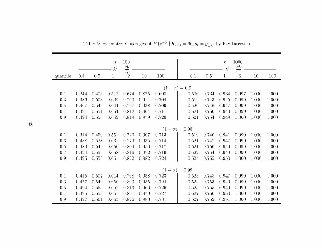
Table 5: Estimated Coverages of E(e−U | θ, x0 = 60, y0 = y(q)

)by H-S Intervals

n = 100 n = 1000

λ2 =σ2

U

σ2

V

λ2 =σ2

U

σ2

V

quantile 0.1 0.5 1 2 10 100 0.1 0.5 1 2 10 100

(1 − α) = 0.90.1 0.244 0.403 0.512 0.674 0.875 0.698 0.506 0.734 0.934 0.997 1.000 1.0000.3 0.386 0.508 0.609 0.760 0.914 0.704 0.519 0.743 0.945 0.999 1.000 1.0000.5 0.467 0.544 0.644 0.797 0.938 0.709 0.520 0.746 0.947 0.999 1.000 1.0000.7 0.491 0.551 0.654 0.812 0.964 0.711 0.521 0.750 0.949 0.999 1.000 1.0000.9 0.494 0.556 0.659 0.819 0.979 0.720 0.521 0.754 0.949 1.000 1.000 1.000

(1 − α) = 0.950.1 0.314 0.450 0.551 0.720 0.907 0.713 0.519 0.740 0.941 0.999 1.000 1.0000.3 0.438 0.528 0.631 0.779 0.935 0.714 0.521 0.747 0.947 0.999 1.000 1.0000.5 0.483 0.549 0.650 0.804 0.950 0.717 0.521 0.750 0.949 0.999 1.000 1.0000.7 0.494 0.555 0.658 0.816 0.972 0.719 0.522 0.754 0.949 0.999 1.000 1.0000.9 0.495 0.558 0.661 0.822 0.982 0.724 0.524 0.755 0.950 1.000 1.000 1.000

(1 − α) = 0.990.1 0.415 0.507 0.614 0.768 0.938 0.723 0.523 0.748 0.947 0.999 1.000 1.0000.3 0.477 0.549 0.650 0.800 0.955 0.724 0.524 0.753 0.949 0.999 1.000 1.0000.5 0.494 0.555 0.657 0.813 0.966 0.726 0.525 0.755 0.949 0.999 1.000 1.0000.7 0.496 0.558 0.661 0.821 0.979 0.727 0.527 0.756 0.950 1.000 1.000 1.0000.9 0.497 0.561 0.663 0.826 0.983 0.731 0.527 0.759 0.951 1.000 1.000 1.000

39

Table 6: Estimated Coverages of E(e−U | θ, x0 = 60, y0 = y(q)

)by Bootstrap Confidence Intervals

n = 100 n = 1000

λ2 =σ2

U

σ2

V

λ2 =σ2

U

σ2

V

quantile 0.1 0.5 1 2 10 100 0.1 0.5 1 2 10 100

(1 − α) = 0.90.1 0.942 0.943 0.936 0.930 0.850 0.899 0.953 0.952 0.894 0.893 0.885 0.9190.3 0.942 0.945 0.943 0.936 0.852 0.891 0.953 0.949 0.897 0.890 0.882 0.9160.5 0.942 0.948 0.948 0.933 0.853 0.883 0.953 0.950 0.897 0.887 0.883 0.9160.7 0.942 0.956 0.959 0.884 0.848 0.879 0.953 0.951 0.899 0.879 0.888 0.9150.9 0.977 0.959 0.814 0.704 0.828 0.850 0.953 0.956 0.895 0.870 0.894 0.911

(1 − α) = 0.950.1 0.967 0.970 0.967 0.958 0.906 0.964 0.978 0.976 0.975 0.943 0.938 0.9610.3 0.967 0.971 0.970 0.962 0.911 0.954 0.979 0.976 0.971 0.943 0.939 0.9600.5 0.967 0.971 0.974 0.964 0.912 0.950 0.979 0.977 0.967 0.943 0.938 0.9590.7 0.967 0.974 0.980 0.946 0.920 0.942 0.979 0.979 0.954 0.939 0.949 0.9600.9 0.993 0.981 0.892 0.794 0.886 0.910 0.979 0.980 0.946 0.928 0.940 0.957

(1 − α) = 0.990.1 0.988 0.991 0.992 0.982 0.971 0.991 0.998 0.996 0.993 0.987 0.984 0.9830.3 0.988 0.992 0.993 0.985 0.974 0.989 0.998 0.996 0.993 0.985 0.986 0.9830.5 0.988 0.994 0.993 0.989 0.976 0.988 0.998 0.995 0.994 0.985 0.988 0.9840.7 0.989 0.995 0.997 0.986 0.982 0.988 0.998 0.996 0.994 0.984 0.991 0.9840.9 1.000 0.997 0.958 0.918 0.950 0.962 0.998 0.997 0.990 0.976 0.982 0.989

40

Table 7: Estimated Coverages of Conventional Confidence Intervals for Model Parameters (using inverse of negative Hessianto estimate covariances)

n = 100 n = 1000

λ2 =σ2

U

σ2

V

λ2 =σ2

U

σ2

V

0.1 0.5 1 2 10 100 0.1 0.5 1 2 10 100

# 1030 1166 1384 1715 2035 1932 1084 1572 1956 2047 2048 2048

(1 − α) = 0.9β1 0.882 0.887 0.889 0.884 0.876 0.873 0.903 0.915 0.904 0.900 0.890 0.880β2 0.876 0.872 0.881 0.887 0.873 0.874 0.898 0.900 0.899 0.891 0.891 0.884σ2 0.579 0.625 0.655 0.628 0.152 0.024 0.735 0.798 0.790 0.522 0.140 0.023γ 0.963 1.000 1.000 1.000 1.000 1.000 0.798 0.983 1.000 1.000 1.000 1.000σ2

V 0.979 0.992 0.998 0.989 0.996 1.000 0.967 0.973 0.955 0.995 1.000 1.000σ2

U 0.976 0.997 1.000 0.997 0.974 0.982 0.873 0.972 0.990 0.980 0.997 0.999

(1 − α) = 0.95β1 0.935 0.937 0.941 0.939 0.925 0.911 0.940 0.950 0.949 0.945 0.939 0.938β2 0.931 0.937 0.934 0.939 0.926 0.914 0.948 0.949 0.948 0.944 0.940 0.941σ2 0.620 0.662 0.686 0.668 0.185 0.031 0.784 0.842 0.823 0.612 0.159 0.027γ 0.998 1.000 1.000 1.000 1.000 1.000 0.891 0.999 1.000 1.000 1.000 1.000σ2

V 0.987 0.997 0.999 0.995 0.996 1.000 0.989 0.983 0.967 0.997 1.000 1.000σ2

U 0.996 1.000 1.000 0.998 0.984 0.992 0.943 0.992 0.999 0.992 0.998 1.000

(1 − α) = 0.99β1 0.984 0.987 0.988 0.984 0.979 0.945 0.983 0.987 0.987 0.987 0.988 0.985β2 0.989 0.987 0.985 0.982 0.977 0.945 0.984 0.985 0.987 0.989 0.989 0.987σ2 0.674 0.716 0.726 0.714 0.247 0.041 0.863 0.896 0.883 0.767 0.212 0.037γ 1.000 1.000 1.000 1.000 1.000 1.000 0.982 1.000 1.000 1.000 1.000 1.000σ2

V 0.996 0.998 1.000 0.999 0.998 1.000 1.000 0.995 0.981 0.998 1.000 1.000σ2

U 1.000 1.000 1.000 1.000 0.997 0.997 0.994 1.000 1.000 1.000 1.000 1.000

41

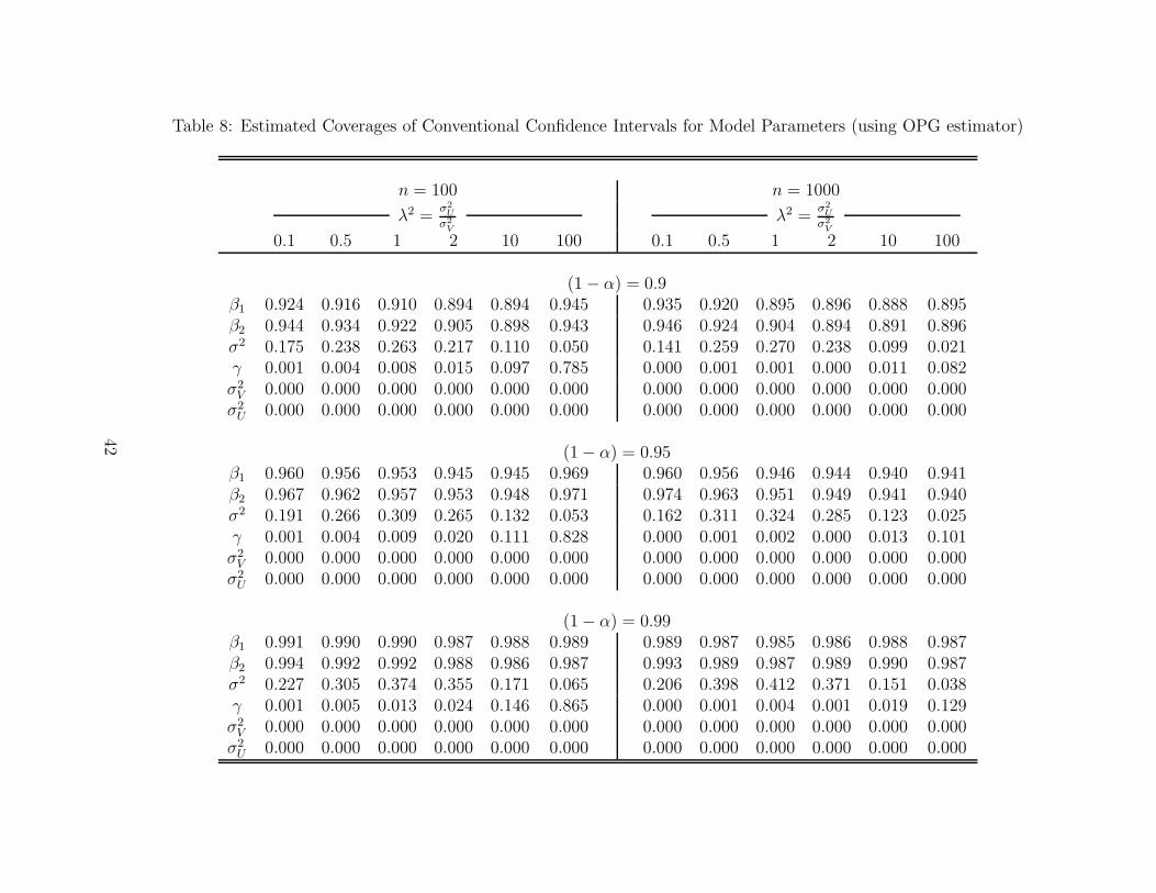
Table 8: Estimated Coverages of Conventional Confidence Intervals for Model Parameters (using OPG estimator)

n = 100 n = 1000

λ2 =σ2

U

σ2

V

λ2 =σ2

U

σ2

V

0.1 0.5 1 2 10 100 0.1 0.5 1 2 10 100

(1 − α) = 0.9β1 0.924 0.916 0.910 0.894 0.894 0.945 0.935 0.920 0.895 0.896 0.888 0.895β2 0.944 0.934 0.922 0.905 0.898 0.943 0.946 0.924 0.904 0.894 0.891 0.896σ2 0.175 0.238 0.263 0.217 0.110 0.050 0.141 0.259 0.270 0.238 0.099 0.021γ 0.001 0.004 0.008 0.015 0.097 0.785 0.000 0.001 0.001 0.000 0.011 0.082σ2

V 0.000 0.000 0.000 0.000 0.000 0.000 0.000 0.000 0.000 0.000 0.000 0.000σ2

U 0.000 0.000 0.000 0.000 0.000 0.000 0.000 0.000 0.000 0.000 0.000 0.000

(1 − α) = 0.95β1 0.960 0.956 0.953 0.945 0.945 0.969 0.960 0.956 0.946 0.944 0.940 0.941β2 0.967 0.962 0.957 0.953 0.948 0.971 0.974 0.963 0.951 0.949 0.941 0.940σ2 0.191 0.266 0.309 0.265 0.132 0.053 0.162 0.311 0.324 0.285 0.123 0.025γ 0.001 0.004 0.009 0.020 0.111 0.828 0.000 0.001 0.002 0.000 0.013 0.101σ2

V 0.000 0.000 0.000 0.000 0.000 0.000 0.000 0.000 0.000 0.000 0.000 0.000σ2

U 0.000 0.000 0.000 0.000 0.000 0.000 0.000 0.000 0.000 0.000 0.000 0.000

(1 − α) = 0.99β1 0.991 0.990 0.990 0.987 0.988 0.989 0.989 0.987 0.985 0.986 0.988 0.987β2 0.994 0.992 0.992 0.988 0.986 0.987 0.993 0.989 0.987 0.989 0.990 0.987σ2 0.227 0.305 0.374 0.355 0.171 0.065 0.206 0.398 0.412 0.371 0.151 0.038γ 0.001 0.005 0.013 0.024 0.146 0.865 0.000 0.001 0.004 0.001 0.019 0.129σ2

V 0.000 0.000 0.000 0.000 0.000 0.000 0.000 0.000 0.000 0.000 0.000 0.000σ2

U 0.000 0.000 0.000 0.000 0.000 0.000 0.000 0.000 0.000 0.000 0.000 0.000

42

Table 9: Estimated Coverages of Bootstrap Confidence Intervals for Model Parameters (Percentile Bootstrap)

n = 100 n = 1000

λ2 =σ2

U

σ2

V

λ2 =σ2

U

σ2

V

0.1 0.5 1 2 10 100 0.1 0.5 1 2 10 100

(1 − α) = 0.9β1 0.886 0.882 0.879 0.880 0.874 0.858 0.910 0.903 0.894 0.893 0.893 0.892β2 0.885 0.878 0.881 0.880 0.875 0.858 0.899 0.890 0.895 0.890 0.889 0.891σ2 0.938 0.961 0.957 0.905 0.868 0.867 0.938 0.960 0.897 0.885 0.891 0.895γ 0.942 0.941 0.938 0.928 0.838 0.720 0.953 0.952 0.893 0.894 0.888 0.913σ2

V 0.745 0.867 0.902 0.903 0.825 0.711 0.900 0.947 0.911 0.889 0.891 0.910σ2

U 0.943 0.948 0.949 0.939 0.865 0.876 0.953 0.950 0.895 0.893 0.891 0.899

(1 − α) = 0.95β1 0.940 0.942 0.940 0.936 0.930 0.922 0.952 0.947 0.943 0.940 0.939 0.944β2 0.935 0.940 0.939 0.939 0.931 0.919 0.949 0.946 0.945 0.943 0.940 0.945σ2 0.963 0.982 0.985 0.963 0.927 0.933 0.976 0.981 0.948 0.936 0.946 0.938γ 0.966 0.969 0.966 0.955 0.895 0.996 0.978 0.976 0.973 0.945 0.940 0.974σ2

V 0.824 0.910 0.936 0.938 0.884 0.990 0.944 0.976 0.965 0.949 0.940 0.977σ2

U 0.967 0.971 0.972 0.970 0.929 0.936 0.979 0.978 0.965 0.940 0.947 0.940

(1 − α) = 0.99β1 0.983 0.986 0.985 0.984 0.982 0.984 0.988 0.986 0.985 0.986 0.987 0.987β2 0.982 0.985 0.984 0.981 0.983 0.983 0.986 0.985 0.986 0.989 0.987 0.988σ2 0.992 0.998 0.997 0.993 0.980 0.976 0.998 0.997 0.996 0.985 0.985 0.984γ 0.987 0.991 0.990 0.981 0.959 0.999 0.998 0.995 0.994 0.986 0.984 0.994σ2

V 0.933 0.970 0.980 0.974 0.951 0.999 0.986 0.993 0.992 0.986 0.981 0.995σ2

U 0.988 0.992 0.993 0.989 0.984 0.980 0.998 0.996 0.994 0.986 0.984 0.983

43

Figure 1: Conditional Density of W , f(w | γ, σ2), Corresponding to Different Values of λ2

−4 −2 0 2 4

0.0

0.1

0.2

0.3

0.4

0.5

lambda^2= 0.1

epsilon

dens

ity

−4 −2 0 2 4

0.0

0.1

0.2

0.3

0.4

0.5

lambda^2= 0.5

epsilon

dens

ity

−4 −2 0 2 4

0.0

0.1

0.2

0.3

0.4

0.5

lambda^2= 1

epsilon

dens

ity

−4 −2 0 2 4

0.0

0.1

0.2

0.3

0.4

0.5

lambda^2= 2

epsilon

dens

ity

−4 −2 0 2 4

0.0

0.1

0.2

0.3

0.4

0.5

lambda^2= 10

epsilon

dens

ity

−4 −2 0 2 4

0.0

0.1

0.2

0.3

0.4

0.5

lambda^2= 100

epsilon

dens

ity

Note: Solid curves show f(w | γ, σ2); dashed curves show standard normal density.

44