Discussion Papers in Economics

Department of Economics

University of Surrey Guildford

Surrey GU2 7XH, UK Telephone +44 (0)1483 689380 Facsimile +44 (0)1483 689548 Web www.econ.surrey.ac.uk

ISSN: 1749-5075

INFORMALITY, FRICTIONS AND MONETARY POLICY

By

Nicoletta Batini (IMF and University of Surrey)

Paul Levine (University of Surrey) Emanuela Lotti

(University of Southampton) &

Bo Yang (University of Surrey)

DP 07/11

Informality, Frictions and Monetary Policy!

Nicoletta Batini

IMF and University of Surrey

Paul Levine

University of Surrey

Emanuela Lotti

University of Southampton

Bo Yang

University of Surrey

June 24, 2011

Abstract

How does informality in emerging economies a!ect the conduct of monetary pol-

icy? To answer this question we construct a two-sector, formal-informal new Keyne-

sian closed-economy. The informal sector is more labour intensive, is untaxed, has a

classical labour market, faces high credit constraints in financing investment and is

less visible in terms of observed output. We compare outcomes under welfare-optimal

monetary policy, discretion and welfare-optimized interest-rate Taylor rules building

the model in stages; first with no frictions in these two markets, then with frictions

in only the formal labour market and finally with frictions on both credit markets

and the formal labour market. Our main conclusions are first, labour and financial

market frictions, the latter assumed to be stronger in the informal sector, cause the

time-inconsistency problem to worsen. The importance of commitment therefore in-

creases in economies characterized by a large informal sector with the features we have

highlighted. Simple implementable optimized rules that respond only to observed ag-

gregate inflation and formal-sector output can be significantly worse in welfare terms

than their optimal counterpart, but are still far better than discretion. Simple rules

that respond, if possible, to the risk premium in the formal sector result in a significant

welfare improvement.

JEL Classification: J65, E24, E26, E32

Keywords: Informal economy, emerging economies, labour market, credit market,

tax policy, interest rate rules

!We acknowledge financial support for this research from the Foreign Commonwealth O!ce as a con-

tribution to the project “Building Capacity and Consensus for Monetary and Financial Reform” led by

the National Institute of Public Finance and Policy (NIPFP), New Delhi.

Contents

1 Introduction 1

2 Background Literature 3

3 The Model 6

3.1 The Model without Labour and Credit Market Frictions . . . . . . . . . . . 6

3.1.1 Households . . . . . . . . . . . . . . . . . . . . . . . . . . . . . . . . 6

3.1.2 Capital Producing Firms . . . . . . . . . . . . . . . . . . . . . . . . 7

3.1.3 Wholesale Firms . . . . . . . . . . . . . . . . . . . . . . . . . . . . . 8

3.1.4 Retail Firms . . . . . . . . . . . . . . . . . . . . . . . . . . . . . . . 9

3.1.5 Equilibrium . . . . . . . . . . . . . . . . . . . . . . . . . . . . . . . . 11

3.1.6 Monetary Policy and Government Budget Constraint . . . . . . . . . 12

3.1.7 Price Dispersion . . . . . . . . . . . . . . . . . . . . . . . . . . . . . 12

3.1.8 Functional Forms . . . . . . . . . . . . . . . . . . . . . . . . . . . . . 13

3.2 The Model with Labour and Credit Market Frictions . . . . . . . . . . . . . 14

4 Steady State Analysis and Model Calibration 15

4.1 Model Calibration . . . . . . . . . . . . . . . . . . . . . . . . . . . . . . . . 17

5 Optimal Stabilization Policy and Potential Gains from Commitment 22

5.1 LQ Approximation of the Optimization Problem . . . . . . . . . . . . . . . 23

5.2 Imposition of the ZLB Constraint . . . . . . . . . . . . . . . . . . . . . . . . 23

5.3 Gains from Commitment Compared Across Models . . . . . . . . . . . . . . 24

6 Optimized Taylor Commitment Rules 28

7 Conclusions 30

A Expressing Summations as Di!erence Equations 35

B The Model Set-up 35

C Quadratic Approximation of Welfare 37

C.1 The Hamiltonian Quadratic Approximation of Welfare . . . . . . . . . . 38

C.2 Small Distortions Approximation . . . . . . . . . . . . . . . . . . . . . . . . 39

1 Introduction

Relatively little has been written on the conduct of monetary policies in economies with

a large informal sector. The phenomenon, that we refer in our paper as ‘informality’ has

been discussed using di!erent terminology: unregistered, hidden, shadow, uno"cial un-

derground and, in a more restrictive sense black, economy. The term ‘hidden economy’ has

often been used with respect to advanced economies, whilst the term ‘informal economy’

has been usually been applied to developing economies.

As Figure 1 shows, a large informal sector is a reality in many emerging economies so

the study of informality can shed new light on the transmission mechanism of monetary

policy in these countries. At the same time, the long-existing debate over rules and

discretion in the conduct of monetary policy is still an on-going area of research with

important policy implications. Started with the pioneering contribution of Kydland and

Prescott (1977) and Barro and Gordon (1983), the credibility problem highlights the

economic gains, in welfare terms, of monetary commitment. The improvement in terms

of stabilization gains, summarized in Clarida et al. (1999) and quantified in Levine et al.

(2008b) are revisited here in an economy characterized by frictions in labour and credit

markets. Frictions are introduced in an asymmetric way to formalize the introduction of a

Asia Latin America Africa(North) Africa(SubSaharan)Transition Countries

10%

20%

30%

40%

50%

60%

70%

Contribution of Informal Sector to GDP

Figure 1: Contribution of Informal Sector to GDP: ILO (2002)

1

large informal sector and its impact on the conduct of monetary policy. The introduction

of new sources of sub-optimality, in addition to sticky prices and market power in the

good market, contributes to both the established discretion versus rule debate and the

understanding of the conduct of monetary policy in economies with a large informal sector.

It is possible to distinguish informality in the goods market, informality in the credit

market and informality in the labour market.1 We adopt a general equilibrium approach,

and study the impact of monetary policy in an economy where the size of the informal

sector is driven by the taxation regime and the di!ering frictions in the two sectors.

This model describes an economy with two sectors producing two di!erent goods. In

equilibrium, workers who do not find a job in the unionized formal labour market (i.e.

the sector with a higher labour standard), move to the informal sector. Public goods

are produced formally and the two sectors have di!erent technologies, the informal sector

being more labour intensive. Further distinctions are the introduction of a market friction

in the formal labour market, whilst the informal sector is frictionless in this respect, and

the presence of financial accelerators of di!ering impact in the two sectors. Thus we

capture some of the main characteristics of the informal sector: labour-intensiveness, lack

of public goods production, wage flexibility and credit constraints. Price stickiness is

added to both sector, but with the informal sector relatively flexible, to give us the New

Keynesian aspect and a model that can be used to investigate the flows between formal

and informal sectors.

The modelling approach captures the a priori ambiguous impact of informality. On

the one hand, the flexible and frictionless informal labour market reduces business cycle

costs. On the other hand, informality brings various costs due to the realistic assumption

that it lies outside the tax regime and it is often unobservable Batini et al. (2010b). The

model is calibrated based on observation of the formal and informal markets in selected

emerging economies.

Table 1: Characterizing Informality

Labour Market Credit Market Taxation Visibility Price Stickiness

F Sector frictions lower frictions taxed higher high

I Sector no frictions higher frictions untaxed lower low

We study optimal monetary policy and the questions we pose are first, what are the

1See Batini et al. (2010a) for details.

2

business cycle welfare costs associated with informality; second, what are the implications

of informality for the welfare gains from commitment and third, how does informality a!ect

the form of optimized Taylor commitment rules and their ability to mimic the optimal

commitment policy. We also consider, in relation to the conduct of monetary policy a

further dimension of informality: its lack of transparency. In particular we also consider

the extent to which the di"culty in fully observing the informal sector a!ects the e"cacy

of monetary policy.

The remainder of the paper is organized as follows. Section 2 shows how our general

equilibrium economy relates to similar theoretical frameworks within the DSGE and the

informal economy literatures. Section 3 sets out details of our model. Section 4 analyzes

steady-state properties and carries out the calibration based on this steady state. Section

5 studies optimal monetary policy with and without commitment. Section 6 examines sim-

ple Taylor-type commitment rules and their ability to mimic their optimal counterparts.

Section 7 concludes the paper.

2 Background Literature

A series of papers model informality using a general equilibrium approach. Conesa et al.

(2002) describes a simple RBC model with an informal sector. The authors introduce

a second sector into a standard Real Business Cycle (RBC) model that has a di!erent

technology, produces goods and services that could otherwise be produced in the formal

sector, but is not registered in NI accounts. The trade-o! between formal and informal

sectors are in terms of wage premium in the formal sector and labour indivisibilities in

the formal/registered sector. Households choose a probability of working in the informal

sector which can be interpreted as the purchase of lotteries in a perfectly insured market.

When a worker chooses the informal sector he/she enjoy more leisure at the price of a

smaller wage. In line with the RBC tradition, the authors use wage premium di!erentials

to explain the di!erent size of macroeconomic fluctuations in function of technological

shocks. The intuition is the following: countries with a smaller wage premium have a lower

opportunity cost to participate in the formal sector and so they have smaller participation

rates. In those countries, the e!ects of technological shocks are amplified. Ihrig and Moe

(2004) develop a simple dynamic general equilibrium framework and, in a deterministic

setting, show the evolution of the informal sector in function of tax rates and enforcement

policies.

A di!erent strand of literature introduces money in the analysis and look at the role

played by an informal sector where most of the transactions are cash-in-hands (Antunes

3

and Cavalcanti (2007) and Koreshkova (2006)). Within this framework, governments

usually can opt for an explicit tax (i.e. tax on income) or an implicit inflation tax .

Clearly the incidence of the two taxes di!erentiates the formal and the informal sector.

The literature shows how the extent of the informal sector may lead to di!erences in

optimal policy choices by governments. Aruoba (2010) and Aruoba and Schorfheide (2011)

di!erentiates a formal centralized sector from an informal decentralized one where money is

the only asset used as a medium of exchange. In Aruoba (2010) the search-based monetary

model is then used to show the stylized fact that lower taxes and higher inflation are usually

associated with a large informal sector: better institutions allow for higher taxes and in a

framework were taxes and monetary policy are endogenous, the link between institution,

taxes, inflation and size of the informal sector follow. In Aruoba and Schorfheide (2011)

the competitive formal sector is replaced by a NK one with standard price stickiness.

Mattesini and Rossi (2010) and Castillo and Montoro (2008) explore informality in a

DSGE New Keynesian model. Mattesini and Rossi (2010) model two sectors, one compet-

itive and one unionized and look at optimal monetary policies in the dual economy. The

paper shows that the level of output depends on the relative size of the two sectors. As in

our model, the divine coincidence does not hold due to distortions in the economy beside

the market structure and price stickiness. Optimal monetary policy under discretion is

then conducted. Respect to their work, we allow for various frictions in the labour and

credit markets and extend the analysis of the optimal monetary policy in a context with

financial frictions and commitment by the Central Bank. Castillo and Montoro (2008)

extends Blanchard and Gali (2007) by modelling a labour market economy with formal

and informal labour contracts within a New Keynesian model with labour market fric-

tions. This is the first paper that analyzes, together, the creation of informal jobs and

the interaction between the informal sector and monetary policy in a NK framework. In-

formality is a result of hiring costs, which are a function of the labour market tightness.

In equilibrium , firms in the wholesale sectors balance the higher productivity of a formal

production process with the lower hiring costs of the informal process. Marginal costs will

then become a function also of the proportion of informal jobs in the economy. The inter-

esting results of this theoretical framework is that during period of high aggregate demand

the informal sector expands due to lower hiring costs associated with this technology. This

creates a link between informality, the dynamics of inflation and the transmission mech-

anism of monetary policy. In particular, the authors show that “informal workers act

as a bu!er stock of labour that allows firms to expand output without putting pressure on

wages”. Castillo and Montoro (2008) allow for a voluntary decision where the marginal

worker is indi!erent between formal and informal sector. Labour market regulations may

4

reduce labour demand without introducing segmentation per se. While we recognize this

picture is realistic in many advanced economies and there is also evidence that shows the

existence of a voluntary, small firms sector in some developing countries (Perry/etal2007),

we believe that in the majority of the developing world informality is a result of segmen-

tation where workers turn to the informal labour market when they cannot find a job in

the formal sector. As in Satchi and Temple (2009) and Marjit and Kar (2008) we model

the idea that: “Unemployment is a luxury” and that “informal sector activities provide

an uno!cial safety-net in the absence of state-provided unemployment insurance”.

As in Zenou (2008), we allow for a frictionless informal labour market. We also in-

troduce labour market frictions in the formal sector, but we do not explicitly model the

matching process as in this paper. Rather we follow another modelling option favoured

in the literature by introducing a wage norm in the formal sector. While we explore the

general equilibrium features of informality, our model is in line with the Harris and Todaro

tradition (Harris and Todaro, 1970) in describing a very simple labour market structure

where labour in the formal sector is fixed at a higher than the market clearing level. See

also Marjit and Kar (2008) and Agenor and Montiel (1996) for a similar assumption. As

discussed in Satchi and Temple (2009) a richer labour market structure implies a wage in

the formal sector which is endogenously determined. While this can be a promising future

development we believe the simplifying assumption allows us to obtain interesting conclu-

sions without adding further complications to the already complex modelling framework.2

As clarified in Zenou’s paper “.. in the informal sector, either people are self-employed

or work with relatives or friends and thus do not apply formally for jobs posted in news-

papers or employment agency”. We follow Zenou and do not model this idea explicitly,

but our competitive informal labour market implies free-entry and an instantaneous hir-

ing process. In contrast to his paper which mainly focuses on the evaluation of various

labour market policies on the unemployment rate in economies with an informal sector,we

2In this respect, we should also mention that, following the critics on the inability of the search matching

model to generate the observed unemployment volatility as reported in Shimer (2005), a series of papers

depart from the flexible wage assumption in order to generate enough volatility in the unemployment

rate (see Blanchard and Gali (2007), Krause and Lubik (2007) and Christo!el and Linzert (2005)). The

introduction of a real wage norm in New Keynesian models has been described as one of the possible way

to reconcile the model with the data. However the introduction of such real wage rigidity is not immune

of critics. Thomas (2008) introduces staggered nominal wages and points to a series of advantages of his

approach with respect to the real wage norm assumption while Hornstein et al. (2005) and Pissarides (2008)

claim that wage rigidity needs to be accompanied by an unrealistic assumption on the labour share and

points instead at the introduction of demand shocks as a possible solution to the unemployment volatility

puzzle.

5

introduce NK features in a DSGE model.

Our paper contribution to this literature is as follows. We look at the e!cacy of mon-

etary policy and for this reason we require a more general framework where households’

consumption and leisure decisions are explicitly modelled in a DSGE model with price

rigidity. We introduce New Keynesian price rigidities in the usual way, as in Castillo

and Montoro (2008), 3 but then proceed to analyse the interaction of informal and for-

mal sectors and the implications for monetary policy. Our analysis of simple optimized

Taylor-type interest rate rules, the incorporation of zero-lower bound constraint and the

comparison between simple and optimal rules where one sector is unobserved are partic-

ularly novel features for the informal economy literature.

3 The Model

Consider a two-sector “Formal” (F) and “Informal” (I) economy, producing di"erent goods

with di"erent technologies which sell at di"erent retail prices, PF,t and PI,t, say. Labour

and capital are the variable factor inputs and the informal sector is less capital intensive.

In both F and I sectors competitive wholesale firms supply a homogeneous good (in that

sector) to a monopolistic retail sector. The latter convert the homogeneous good in a

di"erentiated product that is sold above its marginal cost. In a free-entry equilibrium,

monopolistic profits are driven down to the conversion costs so all firms, wholesale or

retail, F or I, make zero profits and are indi"erent as to which sector they operate.

Government services are provided from the formal sector and is financed by an employ-

ment tax as in Zenou (2008). In the general set-up this can be shared by the formal and

informal sectors giving us a framework in which the role of tax incidence can be studied

as one of the drivers of informalization. The other drivers in our model are the degree

of real wage rigidity in the formal sector and the credit constraints facing the informal

sector. But first we set out a model without these latter two frictions in the labour and

financial markets.

3.1 The Model without Labour and Credit Market Frictions

3.1.1 Households

A proportion nF,t of household members work in the formal sector. Hours hF,t and hours

hI,t are supplied in the F and I sectors respectively. Members who work in sector i = I, F

3Castillo and Montoro (2008) does not look at optimal monetary policy. Moreover, the authors focus

only on the labour market, while we characterize informality also in terms of access to credit, price stickiness

and observability

6

derive utility U(Ct, Li,t) where Ct is household shared consumption and leisure Li,t =

1! hi,t and we assume that4

UC > 0, UL > 0, UCC " 0, ULL " 0 (1)

. The representative household single-period utility is

!t = !(Ct, nF,t, hF,t, hI,t) = nF,tU(Ct, 1! hF,t) + (1! nF,t)U(Ct, 1! hI,t) (2)

We construct Dixit-Stiglitz consumption and price aggregates

Ct =

!w

1µC

µ!1µ

F,t + (1! w)1µC

µ!1µ

I,t

" µµ!1

(3)

Pt =#w(PF,t)

1!µ + (1! w)(PI,t)1!µ

$ 11!µ (4)

Then standard inter-temporal and intra-temporal decisions lead to

!C,t

Pt= !Et

!(1 +Rn,t)

!C,t+1

Pt+1

"(5)

CF,t = w

%PF,t

Pt

&!µ

Ct (6)

CI,t = (1! w)

%PI,t

Pt

&!µ

Ct (7)

where Rn,t is the nominal interest rate over the interval [t, t + 1] for riskless bonds set

by the central bank at the beginning of the period. Note that substituting (6) and (7)

into (3) gives (4), so that (4) or (3) are superfluous for the set-up. Total labour supply is

found by equating the marginal rate of substitution between labour and leisure with the

real wages for the two sectors:

ULI ,t

!C,t=

WI,t

Pt(8)

ULF ,t

!C,t=

WF,t

Pt(9)

For the moment there are no labour market frictions so we have WI,t = WF,t = Wt,

say. It follows from (8) that LI,t = LF,t and hI,t = hF,t = ht, say.

3.1.2 Capital Producing Firms

It is convenient to introduce capital producing firms that at time t convert It of output

into (1 ! S(Xt))It of new capital sold at a real price Qt. The law of motion of capital is

4Our notation is UC ! !U!C , UL ! !U(C,L)

!L , UCC ! !2U!C2 etc.

7

then given by

Kt+1 = (1! !)Kt + (1! S(Xt))It ; S!, S!! " 0 ; S(1 + g) = S!(1 + g) = 0 (10)

Xt # ItIt"1

(11)

Capital producing firms then maximize expected discounted profits

Et

#!

k=0

Dt,t+k [Qt+k(1! S (It+k/It+k"1))It+k ! It+k]

where Dt,t+k is the real stochastic discount rate. This results in the first-order condition

Qt(1! S(Xt)!XtS!(Xt)) + Et

"Dt,t+1Qt+1S

!(Xt+1)I2t+1

I2t

#= 1 (12)

Up to a first order approx this is the same as

Qt(1! S(Xt)!XtS!(Xt)) + Et

"1

(1 +Rt+1)Qt+1S

!(Xt+1)I2t+1

I2t

#= 1 (13)

3.1.3 Wholesale Firms

Wholesale output in the two sectors is given by a Cobb-Douglas production function

Y Wi,t = F (Ai,t, Ni,t,Ki,t), i = I, F (14)

where Ai,t are a technology, total labour supply Ni,t = ni,thi,t, i = I, F . Capital inputs

are Ki,t, i = I, F and we assume capital is accumulated from formal output only.

The first-order condition for labour demand are

PWF,tFNF ,t = WF,t + Pt"F,t (15)

PWI,tFNI ,t = WI,t + Pt"I,t (16)

(17)

where PWF,t and PW

I,t are wholesale prices, "F,t, "F,t are the employment real tax rates in

the formal sector and informal sectors respectively.

Demand for capital by firms must satisfy

Et[1 +Rt+1] =

Et

"PWF,t+1

PtFKF ,t+1 + (1! !)Qt+1

#

Qt# Et[1 +Rk

F,t+1]

=

Et

"PWI,t+1

PtFKI ,t+1 + (1! !)Qt+1

#

Qt# Et[1 +Rk

I,t+1] (18)

In (18) the right-hand-side is the expected gross return to holding a unit of capital in from

t to t+ 1 in the two sectors. The left-hand-side is the expected gross return from holding

bonds, the opportunity cost of capital.

8

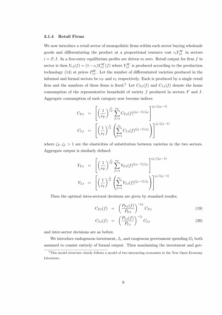
3.1.4 Retail Firms

We now introduce a retail sector of monopolistic firms within each sector buying wholesale

goods and di!erentiating the product at a proportional resource cost ciY Wi,t in sectors

i = F, I. In a free-entry equilibrium profits are driven to zero. Retail output for firm f in

sector is then Yi,t(f) = (1! ci)Y Wi,t (f) where Y

Wi,t is produced according to the production

technology (14) at prices PWi,t . Let the number of di!erentiated varieties produced in the

informal and formal sectors be !F and !I respectively. Each is produced by a single retail

firm and the numbers of these firms is fixed.5 Let CF,t(f) and CI,t(f) denote the home

consumption of the representative household of variety f produced in sectors F and I.

Aggregate consumption of each category now become indices

CF,t =

!

"#

1

!F

$ 1!F

!F%

f=1

CF,t(f)("F!1)/"F

&

'"F /("F!1)

CI,t =

!

"#

1

!I

$ 1!I

(

)!I%

f=1

CI,t(f)("I!1)/"I

*

+

&

'"I/("I!1)

where "F , "I > 1 are the elasticities of substitution between varieties in the two sectors.

Aggregate output is similarly defined:

YF,t =

!

"#

1

!F

$ 1!F

!F%

f=1

YF,t(f)("F!1)/"F

&

'"F /("F!1)

YI,t =

!

"#

1

!I

$ 1!I

(

)!I%

f=1

YI,t(f)("I!1)/"I

*

+

&

'"I/("I!1)

Then the optimal intra-sectoral decisions are given by standard results:

CF,t(f) =

#PF,t(f)

PF,t

$!"F

CF,t (19)

CI,t(f) =

#PI,t(f)

PI,t

$!"I

CI,t (20)

and inter-sector decisions are as before.

We introduce endogenous investment, It, and exogenous government spending Gt both

assumed to consist entirely of formal output. Then maximizing the investment and gov-

5This model structure closely follows a model of two interacting economies in the New Open Economy

Literature.

9

ernment expenditure indices as for the consumer in (19) we have

It(f) =

!PF,t(f)

PF,t

"!!F

It (21)

Gt(f) =

!PF,t(f)

PF,t

"!!F

Gt (22)

Using (19)–(22) it follows that total demands for each di!erentiated product are given

by

YF,t(f) = CF,t(f) + It(f) +Gt(f) =

!PF,t(f)

PF,t

"!!F

(CF,t + It +Gt) =

!PF,t(f)

PF,t

"!!F

YF,t

(23)

YI,t(f) = CI,t(f) =

!PI,t(f)

PI,t

"!!I

CI,t =

!PI,t(f)

PI,t

"!!I

YI,t (24)

Retail firms follow Calvo pricing. In sector i = F, I, assume that there is a probability

of 1 ! !i at each period that the price of each good f is set optimally to Pi,t(f). If the

price is not re-optimized, then it is held constant.6 For each producer f the objective is

at time t to choose Pi,t(f) to maximize discounted profits

Et

"#

k=0

!ki Dt,t+kYi,t+k(f)$Pi,t(f)! Pi,t+kMCi,t+k

%

where Dt,t+k is the discount factor over the interval [t, t+k], subject to a downward sloping

demand from consumers of elasticity "i given by (23) and (24), and MCi,t =PWi,t

Pi,tare real

marginal costs. The solution to this is

Et

"#

k=0

!ki Dt,t+kYi,t+k(f)

&Pi,t(f)!

"i("i ! 1)

Pi,t+kMCi,t+k

'= 0 (25)

and by the law of large numbers the evolution of the price index is given by

P 1!!ii,t+1 = !i (Pi,t)

1!!i + (1! !i)(Pi,t+1(f))1!!i (26)

These summations can be expressed as di!erence equations as follows. First define for

i = I, F , "i,t " Pi,t

Pi,t!1= #i,t + 1. Then from the Euler equation we have that Dt+k,t =

6Thus we can interpret 11!!i

as the average duration for which prices are left unchanged in sector

i = F, I.

10

!k UC,t+k

UC,t. Using this result we can derive the aggregate price dynamics for i = I, F as

Hi,t ! "i!Et[!!i!1i,t+1Hi,t+1] = Yi,tUC,t

Ji,t ! "i!Et[!!ii,t+1Ji,t+1] =

!1

1! 1!i

"Yi,tUC,tMSi,tMCi,t

Pi,t

Pi,tHi,t = Ji,t

1 = "i!!i!1t + (1! "i)

!Pi,t

Pi,t

"1!!i

where MSi,t is an exogenous mark-up shock in sector i = I, F .

3.1.5 Equilibrium

Assuming Cobb-Douglas technology in the wholesale sectors (see all functional forms be-

low) for each di"erentiated product in the F and I sectors we equate supply and demand

in the retail sectors to give

YF,t(f) = (1! ci)F (AF,t, NF,t(f),KF,t(f)) =

#PF,t(f)

PF,t

$!!F

YF,t (27)

YI,t(f) = (1! ci)F (AI,t, NI,t(f),KI,t(f)) =

#PI,t(f)

PI,t

$!!I

YI,t (28)

using (23) and (24). Then solving for Ni,t, i = F, I and defining aggregate employment-

hours in each sector by Ni,t =%"i

j=1Ni,t(j), i = F, I we arrive to the aggregate production

functions

Yi,t =(1! ci)Ai,tN

#ii,tK

1!#ii,t

#i,t; i = F, I (29)

where

#i,t ="i&

j=1

#Pi,t(f)

Pi,t

$! !i"i

(30)

is a measure of the price dispersion across firms in sector i = F, I. Then the aggregate

equilibrium conditions in each retail sector are

YF,t = CF,t + It +Gt

(1! S(Xt))It = Kt+1 ! (1! #)Kt

Kt = KF,t +KI,t

YI,t = CI,t

with aggregate production functions (29).

11

Given government spending Gt, technology Ai,t, mark-up shocks MSi,t, the nominal

interest rate Rn,t, the real wage norm RWt and choice of numeraire, the above system

defines a general equilibrium in Ct, Pt, Pi,t, PWi,t , Ci,t, hF,t, hI,t, WF,t, WI,t, ni,t, Yi,t =

(1! ci)Y Wi,t and Pi,t for i = I, F .

3.1.6 Monetary Policy and Government Budget Constraint

Monetary policy is conducted in terms of the nominal interest rate Rn,t set at the beginning

of period t. The expected real interest rate over the interval [t, t+ 1] is given by

Et[1 +Rt+1] = Et

!(1 +Rn,t)

Pt

Pt+1

"

In what follows we consider interest rate policy in the form of ad hoc Taylor-type rules,

optimized Taylor rules, optimal commitment rules and finally discretionary policy.

Fiscal policy for the moment assumes a balanced budget constraint in which and

employment tax on only formal firms, !t, finances government spending. This takes the

form

PF,tGt = Pt(nF,thF,t!F,t + nI,thI,t!I,t)

noting that government services are provided out of formal output. In general, a tax rule

!I,t = k!F,t ; k " [0, 1]

allows for the possibility that some tax can be collected in the informal economy.

3.1.7 Price Dispersion

Finally for second-order terms that a!ect the welfare, we need to include price dispersion

in the retail output. The production function for retail firm j in terms of its input of the

homogeneous wholesale good is given by

Yi,t(j) = (1! ci)YWi,t (j) = (1! ci)(Ai,tNi,t(j))

!iKi,t(j)1!!i ; i = I, F (31)

where Ni,t(j) and Ki,t(j) are labour and capital inputs into the wholesale sector required

to ultimately produce the variety j. From (18) we have

1 +Rki,t =

(1! "i)PWi,t

Pt

Y Wi,t (j)

Ki,t(j)+ (1! #)Qt

Qt!1

where we note that the return Rki,t and prices PW

i,t , Pt and Qt are all independent of j.

From (3.1.7) we can write the capital-output ratio as

KYi,t #Ki,t(j)

Y Wi,t (j)

=PWi,t

Pt

#(1 +Rk

i,t)Qt!1 ! (1! #)Qt

(1! "i)Qt!1

$(32)

12

which again is independent of j. Now we can write (31) as

Yi,t(j) = (1! ci)Ai,tNi,t(j))KY1!!i!i

i,t ; i = I, F

Using the Dixit-Stiglitz result for the demand for variety j:

Yi,t(j) =

!Pi,t(j)

Pi,t

"!!i

and defining total labour supply for sector i as Ni,t "#

j Ni,t(j) we arrive at the aggregate

production function

Yi,t =(1! ci)Ai,tNi,tKY

1!!i!i

i,t

!i,t; i = I, F (33)

where

!i,t ""i$

j=1

!Pi,t(j)

Pi,t

"!!i

(34)

is a measure of the price dispersion across firms in sector i = F, I. This can be shown to

be given by

!i,t = !i"!ii,t!i,t!1 + (1! !i)

!Ji,tHi,t

"!!i

In fact writing aggregate wholesale output as

Y Wi,t = (1! ci)(Ai,tNi,t)

#iK1!#ii,t ; i = I, F (35)

(33) simply becomes

Yi,t =(1! ci)Y W

i,t

!i,t; i = I, F

3.1.8 Functional Forms

We choose a Cobb-Douglas production function, AR(1) processes for labour-augmenting

productivity (LAP), government spending and mark-up shocks and a utility function con-

sistent with balanced growth:

F (Ai,t, Ni,t) = (Ai,tNi,t)#iK1!#i

i,t

logAi,t ! log Ai,t = "Ai(logAi,t!1 ! log Ai,t!1) + #Ai,t

logGt ! log Gt = "G(logGt!1 ! log Gt!1) + #G,t

Ut(Ct, Li,t) =[C1!$

t L$i,t]

1!% ! 1

1! $; $ > 1

= (1! %) logCt + % logLi,t ; $ = 1 (36)

log

%Ai,t

Ai,t!1

&= log

%Gt

Gt!1

&= 1 + g

S(X) = &X(Xt ! (1 + g))2

13

where !Ai,t, !Gi,t,! ID with zero mean. The choice of utility function in (36) is chosen to

be consistent with a steady state balanced growth path (henceforth BGP) where LAP At

and Gt are time-varying. As pointed out in Barro and Sala-i-Martin (2004), chapter 9,

this requires a careful choice of the form of the utility as a function of consumption and

labour e!ort. It is achieved by a utility function which is non-separable in consumption

and leisure unless " = 1. A utility function of the form (36) achieves this. The marginal

utilities are then then given by

"C,t = (1" #)C(1!!)(1!")!1t (nF,tL

!(1!")F,t + (1" nF,t)L

!(1!")I,t ) (37)

ULF ,t = #C(1!!)(1!")t L!(1!")!1

F,t

ULI ,t = #C(1!!)(1!")t L!(1!")!1

I,t

3.2 The Model with Labour and Credit Market Frictions

We allow in general for the the real wage in the F-sector to be a combination of an

exogenous real wage norm, RWt and the market-clearing real wage in the I-sector:

WF,t

Pt= RWt >

WI,t

Pt

From RWt >WI,t

Pt, it follows from ULL < 0 that the household will choose less leisure and

more work e!ort in the F-sector; i.e., hF,t > hI,F . Household members would prefer to

be employed in the F-sector at the higher wage rate; but all those who fail to do so find

employment at the the market-clearing wage rate in the I-sector.

We can model the risk premium rigorously by introducing a financial accelerator in

each sector. The main ingredient is an external finance premium #i,t # 1 such that the

expected cost of borrowing in sector i = I, F is given by

Et[1 +Ri,t+1] $ Et[#i,t+1(1 +Rt+1)] (38)

where

#i,t = si

!Ni,t

Qt!1Ki,t

"; s"(·) < 0 (39)

In (39), Ni,t is net worth in sector iandQt!1Ki,t"Ni,t is the external financing requirement.

Thus Qt!1Ki,t!Ni,t

Ni,tis the leverage ratio and thus (38) and (39) state that the cost of capital

is an increasing function of this ratio.

Assume that entrepreneurs in the sector i exit with a given probability 1 " $i. Then

the net worth accumulates according to

Ni,t+1 = $iVi,t + (1" $i)Di,t

14

where Di,t are transfers from exiting to newly entering entrepreneurs continuing, and Vi,t,

the net value carried over from the previous period, is given by

Vi,t = (1 +Rki,t)Qt!1Ki,t !!i,t(1 +Rt)(Qt!1Ki,t !Ni,t)

where Rki,t is the ex post return on capital in the i-sector given by

1 +Rki,t =

PWi,t

PtFKi + (1! !)Qt

Qt!1

Demand for capital in sector i = I, F is then given by

Et[1 +Ri,t+1] =

Et

!PWi,t+1

Pt+1FKi,t+1 + (1! !)Qt+1

"

Qt" Et[1 +Rk

i,t+1]

Finally exiting entrepreneurs consume the residual equity so that their consumption

Cei,t =

1! "i

"iNi,t

must be added to total consumption.

We choose the following functional form for s(·):

si

#Ni,t

QKi,t

$= RPStki

#Ni,t

QKi,t

$!!i

where RPSt is an exogenous risk premium shock that is common to both sectors.7

4 Steady State Analysis and Model Calibration

The zero-inflation balanced-growth deterministic steady state of the model economy is

given by

"C,t+1

"C,t" 1 + g!C =

!Ct+1

Ct

"(1!")(1!#)!1)

= (1 + g)((1!")(1!#)!1)

using (37). Thus from (5)

1 +Rn = 1 +R =(1 + g)1+(#!1)(1!")

#

7In a subsequent comparison of the models with and without financial frictions we will retain this shock

in the latter model as a ‘real interest rate shock’.

15

nI + nF = 1

P =!w(PF )

1!µ + (1! w)(PI)1!µ

" 11!µ

Yi,t = (1! ci)(nihiAi,t)!iK1!!i

I,t ; i = F, I

!Ct

(1! !)LF

#nF + (1! nF )

$LFLI

%"(#!1)& = WF,t

!Ct

(1! !)LI

#nF

$LILF

%"(#!1)+ 1! nF

& = WI,t

"iPWI Y W

i,t

Pnihi= Wi,t + #i,t " Wi,t(1 + #i,t) ; i = F, I

WF,t = ( ¯RW t)1!$(WI,t)

$

PKi,t

PWi Y W

i,t

=1! "i

Ri + $; i = I, F

It = ($ + g)(KI,t + KF,t)

Ni,t =(1! %i)DF,t

(1! %i(1 +Ri)); i = I, F (40)

1 +Ri = (1 +R) si

#Ni,t

Ki,t

&; i = I, F

Q = 1

Cei,t =

1! %i

%iNi,t

YI,t = CI,t = (1! w)

#PI

P

&!µ

(Ct + CeI,t + Ce

F,t)

YF,t = CF,t + Gt = w

#PF

P

&!µ

(Ct + CeI,t + Ce

F,t) + It + Gt

PF

PGt = nFhF #F,t + nIhI #I,t

#i,t = #iWi,t ; i = F, I

#I,t = k#F,t

Pi =1

1! 1%i

PWi

where consumption, technical LAP, the real wage and tax rates, and government spending

(all indicated by Xt) are growing at a common growth rate.

We impose a free entry condition on retail firms in this steady state which drives

monopolistic profits to zero. This implies that costs of converting wholesale to retail

16

goods are given by

ci = 1/!i

which implies that:

PiYi,t = PWi Y W

i,t ; i = F, I

Given exogenous trends for Ai,t and Gt, the tax rates and RWt, the above system

of equations give 21 relationships in 22 variables R, P, PF , PI , PWF , PW

I , Ct, CF,t, CI,t,

YF,t, YI,t, WI,t, WF,t, nI , nF , hI , hF , I , KF KI , "F,t, "I,t. One of the prices (it is conve-

nient to choose P ) can be chosen as the numeraire, so the system is determinate.

4.1 Model Calibration

Turning to the calibration, the idea is to assume an observed baseline steady state equi-

librium in the presence of some observed policy. We then use this observed equilibrium

to solve for model parameters consistent with this observation For this baseline and for

the purpose of calibration only, it is convenient to choose units of retail output such that

their prices are unitary. We can choose units of labour supply hI so that AI = 1, but the

choice of AF must be consistent with the choice of unitary prices.

Our baseline steady state can be described in terms of a vector X = f(#) of outcomes

where # is a vector of parameters. The calibration strategy is to choose a subset X1 of n

observed outcomes to calibrate a subset #1 of n parameters. Partition X = [X1, X2] and

# = [#1, #2]. Then #1 is then found by solving

[X1, X2] = f([#1, #2])

for X2 and #1, given X1 and #2. If such a solution exists for economically meaningful

parameter values for #1 then a successful calibration has been achieved.

We now calibrate the parameters #1 = [$,w,%,&I ] given observationsX1 = [nF ,YF,t

YI,t, hF , R].

The given the government share of formal output gyF , Gt is given by GtYF,t

! gyF . AF is

then determined by the normalization of unitary prices. Imposed parameters found from

micro-econometric studies are ', rw and ( and the long-run growth rate g chosen to

correspond to 5% per year. The results of this calibration are summarized in Table 1.

For the financial accelerator, we choose a functional form for sector i = I, F :

!i = si

!Ni,t

QKi,t

"= ki

!Ni,t

QKi,t

"!!i

(41)

Suppose we can obtain )i from econometric studies and we have data on the risk premium

!i =1+Ri1+R and leverage (= borrowing/net worth) in both sectors

*i =QKi "Ni

Ni=

QKi

Ni" 1 =

1

nk,i" 1

17

defining nk, ! NiQKi

. Then we can set the scaling parameter ki from (41) as

ki = !n!ik,i

Then in the baseline steady state used to calibrate parameters, we put Ni,t = nk,iKi,t and

calibrate Di from (40).

Data on emerging economies can be obtained from IMF, World Bank and ILO statis-

tics. As discussed in Neumeyer and Perri (2004), real interest rates in emerging economies

are very volatile and di"cult to calculate. Though nominal interest rate statistics are usu-

ally reported by local Central Banks, due to the high variability of inflation in emerging

economies, the calculation of the real interest rate in EMEs countries is often cumbersome.

Muinhos and Nakane (2006) report data on equilibrium real interest rate for various

emerging economies. Data on real interest rates as well as on the risk premium in the

formal sector can also be obtained from the World Development Indicators published by

the World Bank. We choose a real interest rate for selected emerging economies of 2% in

line with the information found in the sources discussed above. The risk premium in the

formal sector (i.e. the di#erence between the lending to the private formal sector and the

Treasury bill rate) is set equal to 1.05. 8. This risk premium is in line with Bose et al.

(2009) who report a risk premium in the formal sector of 1.067

Haugen (2005), in a study of default and informal lending in Nepal, shows that informal

rates vary from 0% to 84% with an average that is well above the formal interest rate.

Default rates range from 0 to 46% and by applying the following formula RI = [(1 +

RF )/(1" d)]" 1 where d is the default rate and RF the interest rate in the formal sector,

it is possible to predict the interest rate and so the risk premium in the informal sector.

Ngalawa and Viegi (2010) reports a probability of default of 0.15 in the informal sector

of quasi-emerging countries (African continent). We use this information and use a risk

premium in the informal sector of 1.17.

Various studies suggest that capital markets in emerging economies are less developed

relative to the ones in developed economies (see Gali and Gertler (2009)). Arellano et al.

(2010) looks at the link between financial development, financial choices and firms’ dy-

namics comparing economies with di#erent degree of financial development. The study

focus on developed and transitional European countries and we use the information on the

leverage in selected transitional economies as an upper bound of the degree of leverage in

emerging economies worldwide. The study also compare leverage ratio of small and large

firms and we use the firms’ size as a proxy for the informal and the formal sector. We

8It is obtained from selected emerging economies: Honk Kong, Mexico, Ghana, Malaysia, Egypt, Sin-

gapore, Venezuela, Sri Lanka, South Africa, Nepal and Pakistan

18

choose a leverage of 0.5 for the formal sector and of 0.3 for the informal sector. 9

We refer to LABSTAT (ILO) for the calculation of hours of work in emerging economies

and choose h=45/100 and to ILO (2002) for data on formal and informal output relobs =

7/3 as reported in table 2.8 of the ILO’s report. Data on government shares can be

obtained from di!erent sources such as IMF and World Bank. We choose World Bank

and calculate an average for selected EMEs countries to obtain a value equal to 15%. 10

For values of wage mark-up in the formal sector, we refer to Perry et al. (2007) where Latin

American data are reported. Table 3.1 shows that, on average, informal salaried workers

earn between 40 to 66 percent less than formal salaried workers. Looking at this figures,

we choose a mark-up of 50%. Finally, data on the formal sector employment as reported

in various ILO’s documents range from 60 percent to 35% in selected EMEs countries

with a particular low level of 15 percent in India. We choose a value of 50% which is also

consistent with Spatz (2003) for Bolivia (see table 4 of their working paper).

The World Development Indicators published by the World Bank show an annual

growth rate for 2007 of 5.8% for Latin American countries, 9.1% for India and 6% for

the Czech Republic (average selected EMEs countries = 7%). We choose a value of GDP

annual growth rate of 6% keeping in mind there are large di!erences among EMEs countries

and period considered.11

We also assume a higher degree of price stickiness in the formal sector due to the

presence of various contracts which are missing in the informal sector.

This completes the calibration of the parameters describing the deterministic parame-

ters. There are currently two exogenous shocks in the model to labour productivity in both

sectors and government spending. Again following the literature we assume AR(1) pro-

cesses with calibrated persistence parameters 0.7 for the technology and demand shocks.

Mark-up shocks are assumed to be transient. The standard deviations of the innovation

processes are taken to be unity, but later we examine more volatile economies with a

standard deviation k > 1. This completes the calibration; observations, imposed and

calibrated parameters are summarized in Table 1.

9Evidence from Arellano et al. (2010) shows that small firms have lower leverage ratio than large firms

in countries with limited financial development.10In general, government spending in emerging economies is lower than the one in developed economies.11Note that this is less than the steady-state real interest rate ensuring a binding intertemporal solvency

constraint for households and government.

19

Imposed Parameters Value

! 0.025

" 2.0

#F = #I 7.0

µ 1.5

g 0.015

$F 0.5

rw 0.5

gyF 0.15

%F 0.75

%I 0.50

&F 0.5

&I 0.3

!F 0.057

!I 1.17

'F = 'I 0.1

(F 0.96

(I 0.93

Observed Equilibrium Value

PF = PI = P 1

nF 0.5

hF 0.45

rel ! PFYFPIYI

7/3

R 0.02

Calibrated Parameters Value

$I 0.6821

) 0.9881

w 0.6304

* 0.6087

Rest of Equilibrium Value

KFYF

10.1742KIYI

3.2528IYF

0.2815CFYF

0.5685CFCI

1.7056

hI 0.2923

Table 1. Calibration

20

0 0.2 0.4 0.6 0.8 1

0.4

0.5

0.6

0.7

0.8

0.9

1

TAX PARAMETER k

SIZE

OF

FOR

MAL

SEC

TOR

nF

rw=0rw=0.25rw=0.5rw=0.75

Figure 2: The Size of Formal Sector and Tax Burden: k = Ratio of Informal-

Formal Tax Rates. rw =wage mark-up in the formal sector.

Figure 2 shows this process of informalization for di!erent degrees of wage rigidity and

illustrates how an increase in this friction coupled with a lack of tax-smoothing drives

down the size of the formal sector. For example, with k = 0 and no friction the size of

the formal sector is close to nF = 0.82. When rw = 0.75, this halves, falling to under

nF = 0.4.

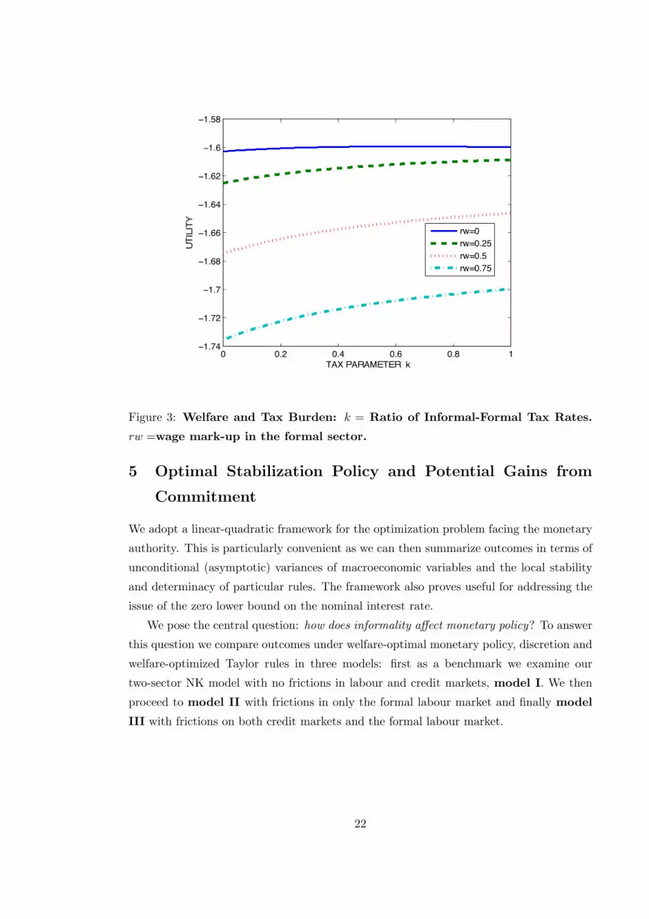
Figure 3 shows the welfare e!ects on a representative household as the tax burden is

smoothed over the two sectors. As k approaches unity the utility becomes very flat and

close to the optimum. We can work out the equivalent permanent increase in consumption

implied by this optimum by first computing the increase from a 1% consumption change

at any point on the balanced growth trend as nFU(1.01 ! Ct, LF ) + (1 " nF )U(Ct, LI)

at some time t = 0 say. In our best steady state equilibrium for rw = 0.5 at k = 1,

this works out as 0.0059, so any increase in welfare D" implies a consumption equivalent

ce = D!0.0059%. For the transition between k = 1 to k = 0 with rw = 0.5 in Figure 1 this

implies a utility loss ce = 4.38%.

21

0 0.2 0.4 0.6 0.8 1−1.74

−1.72

−1.7

−1.68

−1.66

−1.64

−1.62

−1.6

−1.58

TAX PARAMETER k

UTI

LITY

rw=0rw=0.25rw=0.5rw=0.75

Figure 3: Welfare and Tax Burden: k = Ratio of Informal-Formal Tax Rates.

rw =wage mark-up in the formal sector.

5 Optimal Stabilization Policy and Potential Gains from

Commitment

We adopt a linear-quadratic framework for the optimization problem facing the monetary

authority. This is particularly convenient as we can then summarize outcomes in terms of

unconditional (asymptotic) variances of macroeconomic variables and the local stability

and determinacy of particular rules. The framework also proves useful for addressing the

issue of the zero lower bound on the nominal interest rate.

We pose the central question: how does informality a!ect monetary policy? To answer

this question we compare outcomes under welfare-optimal monetary policy, discretion and

welfare-optimized Taylor rules in three models: first as a benchmark we examine our

two-sector NK model with no frictions in labour and credit markets, model I. We then

proceed to model II with frictions in only the formal labour market and finally model

III with frictions on both credit markets and the formal labour market.

22

5.1 LQ Approximation of the Optimization Problem

In our models there are three sets of distortions that result in the steady state output being

below the social optimum: namely, from monopolistic competition, from distortionary

taxes and from the labour and credit frictions. We cannot assume that these distortions

are small in the steady state and use the ‘small distortions’ (Woodford (2003)), quadratic

approximation to the household’s single period utility which is accurate in the vicinity of

our zero-inflation steady state. Our computations use the large distortions approximation

to this welfare function as described in Levine et al. (2008a) and summarized in Appendix

C. However it is instructive to see the form of the ‘small distortions’ approximation to the

loss function in a simpler case of the model without capital.

To work out the welfare in terms of a consumption equivalent percentage increase,

expanding U(C,L) as a Taylor series, a 1% permanent increase in consumption of 1 per cent

yields a first-order welfare increase UCC ! 0.01. Since standard deviations are expressed

in terms of percentages, the welfare loss terms which are proportional to the covariance

matrix (and pre-multiplied by 1/2) are of order 10!4. The losses reported in the paper

in the subsections that follow are scaled by a factor 1 " !. Letting !" be these losses

relative to the optimal policy, then ce = !"! 0.01%.

5.2 Imposition of the ZLB Constraint

We can modify welfare criterion so as to approximately impose an interest rate zero lower

bound (ZLB) so that this event hardly ever occurs. Our quadratic approximation to the

single-period loss function can be written as Lt = y"tQyt where y"t = [z"t, x"t]" and Q is a

symmetric matrix. As in Woodford (2003), chapter 6, the ZLB constraint is implemented

by modifying the single period welfare loss to Lt + wrr2n,t. Then following Levine et al.

(2008c), the policymaker’s optimization problem is to choose wr and the unconditional

distribution for rn,t (characterized by the steady state variance) shifted to the right about

a new non-zero steady state inflation rate and a higher nominal interest rate, such that

the probability, p, of the interest rate hitting the lower bound is very low.12 This is

implemented by calibrating the weight wr for each of our policy rules so that z0(p)"r < Rn

where z0(p) is the critical value of a standard normally distributed variable Z such that

prob (Z # z0) = p, Rn = 1!(1+guc )

" 1 + ## $ Rn(##) is the steady state nominal interest

rate, "2r = var(rn) is the unconditional variance and ## is the new steady state inflation

rate. Given "r the steady state positive inflation rate that will ensure rn,t % 0 with

12The idea that the ZLB should be avoided by choosing a long-run inflation rate rate so as increase the

corresponding long-run interest rate and make room for an active interest rate rule at all times has been

put forward recently by Blanchard et al. (2010).

23

probability 1! p is given by13

!! = max[z0(p)"r !Rn(0)" 100, 0] (42)

In our linear-quadratic framework we can write the inter-temporal expected welfare loss

at time t = 0 as the sum of stochastic and deterministic components, !0 = !0+ !0. Note

that !0 incorporates in principle the new steady state values of all the variables; however

the NK Phillips curve being almost vertical, the main extra term comes from the !2F,t

and !2I,t terms in the loss function seen clearly in (C.10) for the small distortions case.

By increasing wr we can lower "r thereby decreasing !! and reducing the deterministic

component, but at the expense of increasing the stochastic component of the welfare loss.

By exploiting this trade-o", we then arrive at the optimal policy that, in the vicinity of

the steady state, imposes the ZLB constraint, rt # 0 with probability 1! p.

5.3 Gains from Commitment Compared Across Models

We first assess the potential (maximum) gains from commitment by comparing the optimal

commitment policy with discretionary policy, both subject to the constraint that the ZLB

is reached with a very small probability p. In a quarterly model we choose p = 0.0025 or

an expected frequency of hitting the ZLB every 100 years. All shocks are AR(1) processes

and we calibrate their standard deviations in deviation form about the steady state as 1%

and the persistence parameters as 0.5.

Figures 4 and 5 show how the ZLB is imposed for commitment and discretion. In

the figures on the lhs we see that as the penalty on the nominal interest rate volatility

wr in the single-period loss function is increased, then unconditional variance "2r falls and

with it the steady-state inflation rate !! given by (42) also falls. The graphs on the right-

hand-side show the rising stochastic loss function that subtracts the interest rate penalty

how, the falling deterministic loss function arising from the positive steady state inflation

rate, and the sum of these two, !0, that falls and eventually reaches a minimum. This

minimum, together with "2r and !! is shown in table 3 for models I, II and III for both

commitment and discretion. The consumption equivalent percentage loss ce relative to

the best outcome, the model I commitment case, is also computed.

13If the ine!ciency of the steady-state output is negligible, then !! ! 0 is a credible new steady state

inflation rate. Note that in our LQ framework, the zero interest rate bound is very occasionally hit in

which case the interest rate is allowed to become negative.

24

4 6 8 10 12 14 16 18 200

0.5

1

1.5

2

2.5

3

3.5

4

4.5

WEIGHT wr

INFL

ATIO

N A

ND

VAR

IAN

CE

MODEL I

π*

σr2

4 6 8 10 12 14 16 18 200

100

200

300

400

500

WEIGHT wr

WEL

FAR

E LO

SS Ω

MODEL I

Total Welfare LossDeterministic Welfare LossStocastic Welfare Loss

Minimum at (18.5, 35.81)

4 6 8 10 12 14 16 18 200

0.5

1

1.5

2

2.5

WEIGHT wr

INFL

ATIO

N π

* AN

D V

ARIA

NC

E σ

r2

MODEL II

π*

σr2

4 6 8 10 12 14 16 18 200

20

40

60

80

100

120

140

160

WEIGHT wr

WEL

FAR

E LO

SS Ω

MODEL II

Total Welfare LossDeterministic Welfare LossStochastic Welfare Loss

1 1.5 2 2.5 3 3.5 4 4.5 5 5.5 60

0.5

1

1.5

WEIGHT wr

INFL

ATIO

N π

* AN

D V

ARIA

NC

E σ

r2

MODEL III

π*

σr2

1 1.5 2 2.5 3 3.5 4 4.5 5 5.5 60

20

40

60

80

100

120

140

WEIGHT wr

WEL

FAR

E L

OSS

ΩMODEL III

Total Welfare LossDerministic Welfare lossStochastic Welfare Loss

Figure 4: Commitment: Imposing the ZLB Constraint

25

30 35 40 45 50 55 60 650

0.5

1

1.5

2

2.5

3

WEIGHT wr

INFL

ATIO

N A

ND

VAR

IAN

CE

MODEL I

π*

σr2

30 35 40 45 50 55 60 650

50

100

150

200

250

300

350

400

WEIGHT wr

WEL

FAR

E L

OSS

Ω

MODEL I

Total Welfare Loss Deterministic Welfare LossStochastic Welfare Loss

Minimum at (64, 211.52)

30 35 40 45 50 55 60 650

0.5

1

1.5

2

WEL

FAR

E L

OSS

Ω

WEIGHT wr

MODEL II

π*

σr2

4 6 8 10 12 14 16 18 200

20

40

60

80

100

120

140

160

WEIGHT wr

WEL

FAR

E LO

SS Ω

MODEL II

Total Welfare LossDeterministic Welfare LossStochastic Welfare Loss

30 35 40 45 50 55 60 651.95

2

2.05

2.1

2.15

2.2

2.25

2.3

2.35

WEIGHT wr

INFL

ATIO

N A

ND

VAR

IAN

CE

MODEL III

π*

σr2

30 40 50 60 70 80 90100

150

200

250

300

350

400

WEIGHT wr

WEL

FAR

E L

OSS

ΩMODEL III

Total Welfare LossDeterministic Welfare LossStochastic Welfare Loss

Figure 5: Discretion: Imposing the ZLB Constraint

26

Model Policy Frictions !0 !2r "! ce(%)

I Commit Product 35.8 0.684 0.074 0

I Discretion Product 211.5 0.734 0.155 1.76

II Commit Product, Labour 60.3 0.678 0.064 0.25

II Discretion Product, Labour 185.0 0.680 0.068 1.49

III Commit Product, Labour, Credit 90.4 0.657 0.027 0.55

III Discretion Product, Labour, Credit 292.6 2.26 1.97 2.56

Table 2. Optimal Rules with and without Commitment

A number of notable results emerge from table 2. First, as noted in Levine et al.

(2008c) the gains from commitment with ZLB considerations are significant and vary be-

tween ce = 1.76% in model I with no labour or financial market frictions to ce = 2.26%

in model III with such frictions. Interestingly in model II where the real wage in the

F-sector is fixed at its real norm the gains from commitment actually fails. The intuition

here is straightforward: with the real wage in the F-sector fixed, the incentive to tackle

the product market friction by engaging in a surprise inflation that lowers the real wage

and increases output in the vicinity of a steady state that is below the e"cient output

level is less than in model I. In model III with credit market frictions the inability of the

policymaker lacking commitment and the ability to influence private sector behaviour with

promises of future interest rate changes becomes critical. The time inconsistency problem

worsens and with it the gain from commitment. The steady state inflation rate needed to

give room for interest rate changes rises to almost 2% per quarter, a level of inflation that

is typical of emerging economies. It should be stressed that these commitment gains are

for shocks with standard deviations all calibrated at 1%. If shocks are say 2%, then the

consumption equivalent figures will increase by at least fourfold, when the ZLB constraint

is imposed. Similarly if the persistence of shocks increases from it present calibration of

0.5 to 0.75, then welfare gains increase by at least a factor 1"0.52

1"0.752 = 1.714, so with a not

implausible calibration, these commitment gains can become quite considerable, especially

for model III.

Model aF,t (%) aI,t (%) gt (%) msF,t (%) msI,t (%) rpst (%) Total (%)

I 2.15 0.56 0.19 88.47 1.19 7.42 100

II 1.69 0.42 0.17 92.06 0.87 4.77 100

III 1.12 0.31 0.10 86.31 0.01 11.27 100

Table 3. Welfare Decomposition under Optimal Policy

27

Finally Table 3 shocks how six exogenous shocks contribute to the welfare loss under

optimal policy for the three models. By far the most important shock in this respect is the

mark-up shock in the F-sector, msF,t, then comes the risk premium shock rpst followed

by the technology shock in the F-sector aF,t. This decomposition contrasts with the RBC

model which is at the core of our NK model and arrived at by stripping the latter of its

nominal features with price stickiness. It is the latter and its e!ect on welfare that leads

to dominant e!ect of mark-up shocks that in e!ect are shocks to inflation.

6 Optimized Taylor Commitment Rules

We consider symmetrical and asymmetrical interest rate Taylor commitment rules that

respond to deviations of inflation and the output gap14 in both formal and informal sectors

and we allow for a degree of interest rate smoothing. Symmetrical rules are hypothetical

in the sense that they require the full visibility of inflation and output in the I-sector.

Asymmetrical rules require only data for F-sector output and aggregate inflation and are

implementable. The comparison between these two forms of rules enable us to assess the

welfare costs of the lack of visibility for the I-sector and these are part of the costs of

informality.15 We write the rules in log-linear form as:

rn,t = !rn,t!1 + "!F #F,t + "!I#I,t + "IyyI,t ; "!F , "!I , "Fy, "Iy > 0 (43)

rn,t = !rn,t!1 + "!#t + "FyyF,t ; "! > 0 (44)

and we compute optimal parameter values that optimize "0.

We now wish to address three questions. First can the optimized Taylor rule mimic

the fully optimal commitment rule? Second, what are the costs of being constrained to

an implementable asymmetric rule? Third, what form do the optimized rules take as

we proceed from model I with no labour and credit market frictions to model III with

these features? The results for the optimized Taylor rule are displayed in Table 4. The

consumption equivalent changes in utility are again measured relative to the best outcome

which is the optimal policy in model I. Thus ce = 0 in this case.

14In fact our measure of the output gap is simply the log-deviation about the steady state. We choose

this form of rules to avoid problems the monetary would have observing the true output gap. In fact some

experimentation suggests using the latter would make little di!erence to our results.15See Batini et al. (2010b) for a full assessment of the costs and benefits of informality.

28

Model Rule [!, "!F , "!I , "yF , "yI ] !0 #2r $! ce(%)

I Sym TR [1.00, 0.538, 0.000, 0.270, 0.161] 59.4 0.12 0 0.24

I Asym TR [0.953, 0.024, 0, 0.024, 0] 115.7 0.01 0 0.80

I Optimal Complex 35.8 0.684 0.074 0

II Sym TR [1.00, 0.428, 0.013, 0.400, 0.642] 86.4 0.14 0 0.51

II Asym TR [0.663, 0.337, 0, 0.000, 0] 127.8 0.42 0 0.92

II Optimal Complex 60.3 0.680 0.068 0.25

III Sym TR [0.732, 0.321, 0.027, 0.069, 0.042] 101.4 0.69 0.083 0.66

III Asym TR [0.871, 0.327, 0, 0.022, 0] 132.5 0.70 0.102 0.97

III Optimal Complex 90.4 0.657 0.027 0.55

Table 4. Optimized Taylor Rules Compared with Optimal Policy

The first result that emerges from table 4 is that the ZLB constraint does not bind

for our simple rules for models I and II without financial frictions. Simplicity restricts the

monetary authority from responding to all aspects of the economy and so keeps interest

rate volatility low, at least for models I and II. In response to the questions we have posed,

the costs of simplicity are measured as the di"erences between the optimal and simple rules

for each model. For the hypothetical symmetrical rule these are in the range 0.11! 0.24%

of consumption equivalent but rise to 0.42! 0.80% for implementable asymmetrical rules.

Interestingly the costs do not rise as frictions are added, and in fact fall. But again these

numbers depend on the calibration of the AR(1) shocks where modest standard deviations

of 1% and persistence parameters of 0.5 were chosen. A plausible higher choice of these

values would see these costs rising by at least a factor 4" 1.71 = 6.8 so costs of simplicity

and lack of visibility of the I-sector can be very high.

Turning to the form of the optimized implementable Taylor rules and how they change

with added frictions. Comparing the asymmetrical rules across the models it is of in-

terest to examine the long-term responses to aggregate inflation, "pi1"# and to output in

the F-sector, "y1"# . For model I these are 0.51 for both so that the Taylor principle is

violated - ceteris paribus real interest rate fall with a rise in inflation - but the economy

is stabilized by allowing the nominal interest rate to respond equally strongly to a rise in

output. When we introduce labour market frictions in model II the long-run responses to

inflation and output are 1.003 and 0.000 so the Taylor principle now just holds and there

is no significant response to output. Then adding financial frictions in model III the cor-

responding responses are 2.53 and 0.17 so now the Taylor principle is easily satisfied and

accompanied by a more modest response to output than in model I. The overall picture

is that frictions require an increasingly aggressive response of the interest rate to inflation

29

to mitigate shocks that are not dampened by changes in the real wage (model II) and to

o!set the financial accelerator e!ect in model III.

We finally seek an improvement on the asymmetric Taylor rule by allowing monetary

policy to also respond, data permitting, to the risk premium !F,t in the formal sector in

model III. The rule now takes the form

rn,t = "rn,t!1 + !!#t + !FyyF,t ! !F"!F,t ; !!, !Fy, !F" > 0 (45)

Model Rule [", !!F , !yF , !"F ] "0 $2r #" ce

III Asym TR [0.931, 0.169, 0.000, 0.076] 101.00 0.08 0 0.65

Table 5. Optimized Taylor Rule Responding to the F-sector Risk Premium

The result is shown in Table 5. We now have long-run responses to inflation, output

and the risk-premium of 2.45, 0.00 and 1.10 respectively. This more than one-to-one

long-run response of the nominal interest rate to changes in the risk-premium brings

about a significant welfare improvement in the outcome of ce = 0.32%. Again with less

conservative estimates for the size and persistence of the shocks, this improvement can

turn out as considerable.

7 Conclusions

Our main results for the implications of informality for the conduct of monetary policy are

as follows. First labour and financial market frictions, the latter assumed to be stronger

in the I-sector, cause the time-inconsistency problem to worsen. The importance of com-

mitment therefore increases in economies with a large informal sector with the features we

have highlighted. Simple implementable optimized rules that respond only to observed ag-

gregate inflation and F-sector output can be significantly worse in welfare terms than their

optimal counterpart, but are still far better than discretion. Simple rules that respond, if

possible, to the risk premium in the F-sector result in a significant welfare improvement.

We conclude by discussing a number of caveats and possible directions for future

research. Inevitably our results are dependent on our modelling strategy and choice of

calibration. Whilst some results not reported suggest that our conclusions are not too

sensitive to the latter, there remains the question of alternative models. We have chosen

to model labour market frictions as a real wage norm in the Harris-Todaro tradition, but

as we discuss in the review of the literature a search-match approach that endogenizes the

bargained real wage would pose an interesting alternative. Our model is closed - in the

open economy the issue of liability dollarization becomes an important issue giving the

financial accelerator more bite (see Batini et al. (2007) and Batini et al. (2009)).

30

Finally it would be desirable to estimate the model by Bayesian methods as is now

commonplace in the literature. This leads to the need to properly take into account the

lack of observability of this sector in solving for the rational expectations equilibrium and

the estimation. This is not done in this paper, nor indeed in the DSGE literature as a

whole.16 This caveat suggests another important direction for research.

References

Agenor, P. and Montiel, P. (1996). Development Macroeconomics. Princeton University

Press, New Jersey.

Antunes, A. and Cavalcanti, T. (2007). Start up costs, limited enforcement, and the

hidden economy. European Economic Review, 51, 203–224.

Arellano, C., Bai, Y., and Zhang, J. (2010). Firm Dynamics and Financial Development.

Mimeo Federal Reserve Bank of Minneapolis.

Aruoba, S. (2010). Informal Sector, Government Policies and Institutions. mimeo Univer-

sity of Maryland.

Aruoba, S. and Schorfheide, F. (2011). Sticky Prices versus Monetary Frictions: An

Estimation of Policy Trade-o!s. Americal Economic Journal, pages 60–90.

Barro, R. and Gordon, D. (1983). Rules, discretion, and reputation in a model of monetary

policy. Journal of Monetary Economics, 12(4), 101–120.

Barro, R. and Sala-i-Martin, X. (2004). Economic Growth. Second Edition, McGraw-Hill.

Batini, N., Levine, P., and Pearlman, J. (2007). Monetary Rules in Emerging Economies

with Financial Market Imperfections. Presented to the NBER Conference on Interna-

tional Dimensions of Monetary Policy, S’Agaro, Catalonia, Spain, June 11-13, 2007 and

NBER Conference Volume, International Dimensions of Monetary Policy, ed. J. Gali

and M. Gertler.

Batini, N., Levine, P., and Pearlman, J. (2009). Monetary and Fiscal Rules in an Emerging

Small Open Economy. IMF Working Paper, WP/09/22.

Batini, N., Kim, Y.-B., Levine, P., and Lotti, E. (2010a). Informal Labour and Credit

Markets: A Survey. IMF Working Paper, WP/10/42.

16Exceptions are Levine et al. (2007) and Levine et al. (2009).

31

Batini, N., Levine, P., and Lotti, E. (2010b). The Costs and Benefits of Informalization

in a Two-Sector New Keynesian Model. Department of Economics Discussion Papers

0211, University of Surrey.

Blanchard, O. and Gali, J. (2007). A New Keynesian Model with Unemployment. Centre

for Financial Studies WP No, 2007/08.

Blanchard, O., Giovanni, D., and Mauro, P. (2010). Rethinking Macroeconomic Policy.

IMF Sta! Position Note, SPN/10/03 .

Bose, N., Capasso, S., and Wurm, N. (2009). The Impact of Banking Development on the

Size of the Shadow Economies. mimeo University of Winsconsin.

Castillo, P. and Montoro, C. (2008). Monetary Policy in the Presence of Informal Labour

Markets. Mimeo, Banco Central de Reserva del Peru.

Christo!el, K. and Linzert, T. (2005). The Role of Real Wage Rigidities and Labor Market

Frictions for Unemployment and Inflation Dynamics. ECB Discussion Paper 556.

Clarida, R., Gali’, J., and Gertler, M. (1999). The science of monetary policy: a new

Keynesian perspective. Journal of Economic Literature, 37(4), 1661–1707.

Conesa, J. C., Diaz-Moreno, C., and Galdon-Sanchez, J. E. (2002). Explaining Cross-

Country Di!erences in Partication Rates and Aggregate Fluctuations. Journal of Eco-

nomic Dynamics and Control, 26, 333–345.

Gali, J. (2008). Monetary Policy, Inflation and the Business Cycle. Princeton University

Press.

Gali, J. and Gertler, M. (2009). International Dimensions of Monetary Policy. University

of Chicago Press, Chicago.

Haugen, N. (2005). The Informal Credit Market: A Study of Default in Informal Lending

in Nepal. Thesis, University of Bergen.

Hornstein, A., Krusell, P., and Violante, G. (2005). Unemployment and Vacancy Fluc-

tuations in the Matching Models: Inspecting the Mechanism. Federal Reserve Bank of

Richmond Economic Quarterly 91/3.

Ihrig, J. and Moe, K. (2004). Lurking in the Shadows: the Informal Sector and Government

Policies. Journal of Development Economics, 73, 541–557.

32

Koreshkova, T. (2006). A quantitative analysis of inflation as a tax on the underground

economy. Journal of Monetary Economy, pages 773–796.

Krause, M. and Lubik, T. (2007). The (Ir)relevance of Real Wage Rigidity in the New

Keinesyan Model with Search Frictions. Journal of Monetary Economics, 54(3), 706–

727.

Kydland, F. and Prescott, E. (1977). Rules rather than discretion: the inconsistency of

optimal plans. Journal of Political Economy, 85(4), 473–492.

Levine, P., Pearlman, J., and Perendia, G. (2007). Estimating DSGE Models under

Partial Information. Department of Economics, University of Surrey Discussion Paper

1607. Presented at the 14th International Conference on Computing in Economics and

Finance, Paris .

Levine, P., Pearlman, J., and Pierse, R. (2008a). Linear-Quadratic Approximation, E!-

ciency and Target-Implementability. Journal of Economic Dynamics and Control, 32,

3315–3349.

Levine, P., McAdam, P., and Pearlman, J. (2008b). Quantifying and sustaining welfare

gains from monetary commitment. Journal of Monetary Economics, 55(4), 1253–1276.

Levine, P., McAdam, P., and Pearlman, J. (2008c). Quantifying and Sustaining Welfare

Gains from Monetary Commitment. Journal of Monetary Economics, 55(7), 1253–1276.

Levine, P., Pearlman, J., Perendia, G., and Yang, B. (2009). Endogenous Persistence in an

Estimated New Keynesian Model under Imperfect Information. Presented at the annual

CDMA Conference, 2009, University of St Andrews, 2–4 September, and forthcoming

at the 2010 Royal Economic Society Conference, March 29 – 31, University of Surrey. .

Magill, M. (1977). A Local Analysis of Capital Accumulation under Uncertainty. Journal

of Economic Theory, 15(2), 211–219.

Marjit, S. and Kar, S. (2008). A Contemporary Perspective on the Informal Labor Market

- Theory, Policy and the Indian Experience. Mimeo, Centre for Studies in Social Science,

Calcutta.

Mattesini, F. and Rossi, L. (2010). Optimal Monetary Policy in Economies with Dual

Labour Markets. Department of Communication, Working Paper No 37, University of

Teramo.

33

Muinhos, M. and Nakane, M. (2006). Comparing Equilibrium Real Interest Rates: Di!er-

ent Apptoaches to Measure Brasilian Rates. Banco Central Do Brasil Working Paper

101.

Neumeyer, P. and Perri, F. (2004). Business Cycles in Emerging Economies: The Role of

Interest Rates. mimeo.

Ngalawa, H. and Viegi, N. (2010). Interaction of Formal and Informal Financial Markets

in Quasi-Emerging Market Economies. mimeo 2010.

Perry, G., Maloney, W., Arias, O., Fajnzylber, P., Mason, A., and Saavedra-Chanduvi

(2007). Informality: Exit and Esclusion. World Bank Report.

Pissarides, C. (2008). The Unemployment Volatility Puzzle: Is Wage Stickiness the An-

swer? mimeo CEP IZA CEPR.

Satchi, M. and Temple, J. (2009). Labor Markets and Productivity in Developing Coun-

tries. Review of Economic Dynamics, 26, 333–345.

Shimer, R. (2005). The cyclical Behaviour of Equilibrium Unemployment and Vacancies.

American Economic Review, 95(1), 25–49.

Spatz, J. (2003). The Impact of Structural Reforms on Wages and Employment: The Case

of Formal versus Informal Workers in Bolivia. Kiel Institute for World Economics WP

1186.

Thomas, C. (2008). Search and Matching Frictions and Optimal Policy. Journal of

Monetary Econsomic, pages 936–956.

Woodford, M. (2003). Foundations of a Theory of Monetary Policy. Princeton University

Press.

Zenou, Y. (2008). Job Search and Mobility in Developing Countries: Theory and Policy

Implications. Journal of Development Economics, 86, 336–355.

34

Appendix

A Expressing Summations as Di!erence Equations

In the first order conditions for Calvo contracts and expressions for value functions we are con-

fronted with expected discounted sums of the general form

!t = Et

! !"

k=0

!kXt,t+kYt+k

#(A.1)

where Xt,t+k has the properties Xt,t = 1 and Xt,t+k = Xt,t+1Xt+1,t+k (for example an inflation,

interest or discount rate over the interval [t, t+ k]).

Lemma

!t can be expressed as

!t = Yt + !Et [Xt,t+1!t+1] (A.2)

Proof

!t = Xt,tYt + Et

! !"

k=1

!kXt,t+kYt+k

#

= Yt + Et

! !"

k!=0

!k!+1Xt,t+k!+1Yt+k!+1

#

= Yt + !Et

! !"

k!=0

!k!Xt,t+1Xt+1,t+k!+1Yt+k!+1

#

= Yt + !Et [Xt,t+1!t+1] !

B The Model Set-up

For i = I, F the benchmark model without labour market or financial friction is

"t = "(Ct, LF,t, LI,t) =C(1"!)(1"")

t (nF,tL!(1"")F,t + (1! nF,t)L

!(1"")I,t )! 1

1! "(B.1)

(B.2)

"C,t = (1! #)C(1"!)(1"")"1t (nF,tL

!(1"")F,t + (1! nF,t)L

!(1"")I,t ) (B.3)

(B.4)

"Li,t = #C(1"!)(1"")t (Li,t)

!(1"")"1 (B.5)

"C,t = !Et [(1 +Rt+1)"C,t+1] (B.6)

"Li,t

"C,t=

Wi,t

Pt(B.7)

Li,t " 1! hi,t (B.8)

35

Y Wi,t = F (Ai,t, ni,t, hi,t,Ki,t) = (Ai,tni,thi,t)

!iK1!!ii,t (B.9)

nF,t + nI,t = 1 (B.10)

Yi,t = (1! ci)YWi,t (B.11)

PWi,t

PtFhi,t =

PWi,t

Pt

!iY Wi,t

hi,t=

Wi,t

Pt(1 + "i,t) (B.12)

Pi,t =1

1! 1"i

PWi,t (B.13)

Kt+1 = (1! #)Kt + (1! S(Zt))It (B.14)

Zt " ItIt!1

(B.15)

Qt(1! S(Zt)! ZtS"(Zt)) + Et

!1

(1 +Rt+1)Qt+1S

"(Zt+1)I2t+1

I2t

"= 1 (B.16)

S(Zt) = $Z(Zt ! (1 + g))2 (B.17)

Et[(1 +Ri,t+1)RPi,t+1] =

Et

!(1! !i)

PWi,t+1Y

Wi,t+1

Pt+1Ki,t+1+ (1! #)Qt+1

"

Qt" Et

!Xi,t+1

Qt

"(B.18)

YF,t = CF,t +Gt + It (B.19)

YI,t = CI,t (B.20)

CF,t = w

#PF,t

Pt

$!µ

Ct (B.21)

CI,t = (1! w)

#PI,t

Pt

$!µ

Ct (B.22)

PF,t

Pt=

1%w+ (1! w)T 1!µ

t

& 11!µ

(B.23)

PI,t

Pt=

1%wT µ!1

t + 1! w& 1

1!µ

(B.24)

Tt = Tt!1 +!I,t !!F,t (B.25)

Hi,t ! %i&Et[!"i!1i,t+1Hi,t+1] = Yi,t"C,t (B.26)

Ji,t ! %i&Et[!"ii,t+1Ji,t+1] =

'1

1! 1"i

(Yi,t"C,tMSi,tMCi,t (B.27)

1 = %i!"i!1i,t + (1! %i)

#Ji,tHi,t

$1!"i

(B.28)

MCi,t =PWi,t

Pi,t(B.29)

36

PF,t

PtGt = nF,thF,t!F,t

WF,t

Pt+ nI,thI,t!I,t

WI,t

Pt(B.30)

!I,t = k!F,t (B.31)

1 +Rt =1 +Rn,t!1

!t(B.32)

log

!1 +Rn,t

1 +Rn

"= " log

!1 +Rn,t!1

1 +Rn

"+ # log

!!t

!

"(B.33)

logAi,t ! log Ai,t = "Ai(logAi,t!1 ! log Ai,t!1) + $Ai,t (B.34)

logGt ! log Gt = "G(logGt!1 ! log Gt!1) + $G,t (B.35)

logMSi,t ! logMSi = "MSi(logMSi,t!1 ! logMSi) + $MSi,t (B.36)

logRPSi,t ! logRPSi = "RPSi(logRPSi,t!1 ! logRPSi) + $RPSi,t (B.37)

In the model without labour or credit market frictions we have

WF,t

Pt=

WI,t

Pt(B.38)

RF,t = RI,t = Rt (B.39)

It follows from the household FOC that LF,t = LI,t and hF,t = hI,t. This completes the model.

With labour and credit market frictions we have17

WF,t

Pt= RWt >

WI,t

Pt(B.40)

1 +Ri,t " "i,t(1 +Rt) (B.41)

"i,t = si

!Ni,t

Qt!1Ki,t

"; s"(·) < 0 (B.42)

Ni,t+1 = %iVi,t + (1! %i)Di,t (B.43)

Vi,t = (1 +Rki,t)Qt!1Ki,t !"i,t(1 +Rt)(Qt!1Ki,t !Ni,t)

1 +Rki,t =

Xi,t

Qt!1(B.44)

Cei,t =

1! %i

%iNi,t (B.45)

Caggt = Ct + Ce

I,t + CeF,t (B.46)

C Quadratic Approximation of Welfare

We first set out the ‘large distortions’ approximation of the welfare loss following the procedure of

Levine et al. (2008a). We then examine the form of the ‘small distortions’ approximation to the

loss function in a simpler case of the model without capital.

17The Dynare code for the full model is available from the authors on request.

37

C.1 The Hamiltonian Quadratic Approximation of Welfare

Consider the following general deterministic optimization problem

max!!

t=0

!tU(Xt"1,Wt) s.t. Xt = f(Xt"1,Wt) (C.1)

where Xt"1 is vector of state variables and Wt"1 a vector of instruments.18 There are given initial

and the usual tranversality conditions. For our purposes, we consider this as including models

with forward-looking expectations, so that the optimal solution to the latter setup is the pre-

commitment solution. Suppose the solution converges to a steady state X,W as t ! " for the

states Xt and the policies Wt. Define xt = Xt#X and wt = Wt#W as representing the first-order

approximation to absolute deviations of states and policies from their steady states.19

The Lagrangian for the problem is defined as,

!!

t=0

!t[U(Xt"1,Wt)# "Tt (Xt # f(Xt"1,Wt))] (C.2)

so that a necessary condition for the solution to (C.1) is that the Lagrangian is stationary at all

{Xs}, {Ws} i.e.

UW + "Tt fW = 0 UX # 1

!"Tt"1 + "T

t fX = 0 (C.3)

Assume a steady state " for the Lagrange multipliers exists as well. Now define the Hamiltonian

Ht = U(Xt"1,Wt) + "T f(Xt"1,Wt). The following is the discrete time version of Magill (1977):

Theorem: If a steady state solution (X,W,") to the optimization problem (C.1) exists, then

any perturbation (xt, wt) about this steady state can be expressed as the solution to

max1

2

!!

t=0

!t"xt"1 wt

# $ HXX HXW

HWX HWW

%$xt"1

wt

%s.t. xt = fXxt"1 + fWwt (C.4)

where HXX , etc denote second-order derivatives evaluated at (X,W ). This can be directly ex-

tended to the case incorporating disturbances.

Thus our general procedure is as follows:

1. Set out the deterministic non-linear problem for the Ramsey Problem, to maximize the

representative agents’ utility subject to non-linear dynamic constraints.

18An alternative representation of the problem is U(Xt,Wt) and Et[Xt+1] = f(Xt,Wt) where Xt

includes forward-looking non-predetermined variables and Et[Xt+1] = Xt+1 for the deterministic

problem where perfect foresight applies. Whichever one uses, it is easy to switch from one to the

other by a simple re-definition. Note that Magill (1977) adopted a continuous-time model without

forward-looking variables. As we demonstrate in Levine et al. (2008c), although the inclusion of

forward-looking variables significantly alters the nature of the optimization problem, these changes

only a!ect the boundary conditions and the second-order conditions, but not the steady state of

the optimum which is all we require for LQ approximation.19Alternatively xt = (Xt # X)/X and wt = (Wt # W )/W , depending on the nature of the

economic variable. Then the Theorem follows in a similar way with an appropriate adjustment to

the Jacobian Matrix.

38

2. Write down the Lagrangian for the problem.

3. Calculate the first order conditions. We do not require the initial conditions for an optimum

since we ultimately only need the steady-state of the Ramsey problem.

4. Calculate the steady state of the first-order conditions. The terminal condition implied by

this procedure is such that the system converges to this steady state.

5. Calculate a second-order Taylor series approximation, about the steady state, of the Hamil-

tonian associated with the Lagrangian in 2.

6. Calculate a first-order Taylor series approximation, about the steady state, of the first-order

conditions and the original constraints.

7. Use 4. to eliminate the steady-state Lagrangian multipliers in 5. By appropriate elimination

both the Hamiltonian and the constraints can be expressed in minimal form. This then

gives us the accurate LQ approximation of the original non-linear optimization problem in

the form of a minimal linear state-space representation of the constraints and a quadratic

form of the utility expressed in terms of the states.

C.2 Small Distortions Approximation

The small distortions approximation is found by approximating the utility function Ut =

U(Ct, Lt) in consumption, Ct and leisure Lt = 1 ! ht subject to the resource constraint.

We start with the Taylor Series expansion about the BGP steady state20

Ut = U + UCCct +1

2UCCC

2c2t + ULLlt +1

2ULLL

2l2t + higher order terms (C.5)

Next we write ct = wcF,t + (1 ! w)cI,t, lt = ! h1!h ht and use the linearized resource

constraints

yF,t = aF,t + !F (nF,t + ht)! dF,t = (1! gFy)cF,t + gFygt

yI,t = aI,t + !F (nI,t + ht)! dI,t = cI,t

where

di,t = log

!!i,t

!i

"; i = I, F (C.6)

and !i,t is the price dispersion e"ect given by (34). By standard results (see, for example,

Gali (2008), p88) di,t is a second order term given by

di,t ="i(!i + (1! !i)"i)

2!ivar(pi,t(j)) ; i = I, F (C.7)

and"#

t=0

#tvar(pi,t(j)) =$i

(1! #$i)(1! $i)

"#

t=0

#t%2i,t ; i = I, F (C.8)

20The BGP is time-varying but here we drop the bar and time-script in Ut, Ct etc.

39

Then using the linearized resource constraints and the properties of e!ciency in the

steady state: ULUC

= FNF = FNI the first order terms in ct and lt disappear in (C.5) and

we are left the quadratic approximation to the utility function

Ut = U+UCC

!! w

(1! gFy)dF,t ! (1! w)dI,t

"+1

2UCCC

2c2t+ULLlt+1

2ULLL

2l2t+higher order terms

(C.9)

Finally using the results (C.6)–(C.9) we can write the quadratic form of the intertem-

poral expected welfare loss at time t = 0 as

"0 =1

2Et

# !$

t=0

!t[wcc2t + whI h

2I + whF h

2F + w!F"

2F,t + w!I"

2I,t]

%(C.10)

where for our choice of utility function (36)

wc = !UCCC

UC= 1 + (# ! 1)(1! $)

wh = !ULLh2

UCC=

(1 + $(# ! 1))h2

(1! $)(1! h)2; h = hI , hF

w!F = w%F (&F + (1! &F )%F )

cFy&F'F

w!I =(1! w)%I(&I + (1! &I)%I)

&I'I

'i =(i

(1! !(i)(1! (i); i = F, I

40