Embed Size (px)
Citation preview
UNIVERSITY OF NAPLES FEDERICO II
DEPARTMENT OF INDUSTRIAL ENGINEERING
AEROSPACE SECTION
Ph.D. COURSE
IN INDUSTRIAL ENGINEERING
XXIX CYCLE
Infrared thermography to monitoring
mechanical tests on composite materials:
Experimental procedure and data analysis
Simone Boccardi
Research Supervisors:
Prof. Ing. Giovanni M. Carlomagno
Dr. Ing. Carosena Meola
The Chairman of the Ph.D. School:
Prof. Ing. Michele Grassi
2017

"Nil tam difficile est, quin
quaerendo investigari possit"
(Publio Terenzio)
Contents
Introduction 1
Chapter 1 Composite materials 3
Introduction 3
1.1. Some basics of composite materials 4
1.2. The matrices 5
1.2.1. Polymer types 5
1.3. Reinforcement for polymer-based composites 6
1.3.1. Glass fibres 7
1.3.2. Carbon fibres 8
1.3.3. Natural fibres 9
1.3.4. . Woven fabric architectures 10
1.4. Main types of deficiency in composites 10
1.4.1. Manufacturing defects. 11
1.4.2. In-service failures 12
1.4.2.1. Some hints on failure mechanisms 13
References to Chapter 1 15
Chapter 2 Infrared thermography 18
Nomenclature 18
Introduction 20
2.1. Some basics 20
2.2. Real objects radiation 22
2.2.1. Effects of interposed atmosphere 24
2.3. Infrared devices. 25
2.3.1. Thermal detectors 26
2.3.2. Photon Detectors 26
2.3.3. QWIP detectors technology 27
2.3.4. Detector performance 28
2.4. IR Image generation 30
2.4.1. Problems affecting infrared images 31
2.5. Calibration 32
2.6. Applications 33
References to Chapter 2 33
Chapter 3 Infrared cameras, temporal noise and
Reference Area Method 37
Nomenclature 37
Introduction 38
3.1. Characterization of QWIP SC6000 temporal noise 38
3.2. SC6000 camera electronic architecture and image construction 41
3.3. Black body monitoring with other detector types 43
3.4. The Reference Area Method 46
3.5. Application of the Reference Area Method to a real surface 51
3.6. Some effects of the Reference Area Method 58
3.7. Practical applications 60
References to chapter 3 60
Chapter 4 Cyclic bending tests 61
Nomenclature 61
Introduction 62
4.1. Some theoretical considerations 62
4.2. Some preliminary tests 65
4.3. New Investigation 68
4.3.1. Test setup and procedure 68
4.3.2. Description of specimens 71
4.4. Data post-processing 73
4.4.1. Description of the Area Method 73
4.4.2. Description of the Whole Width Method 77
4.5. Qualitative evaluation of ΔT on the rear specimen surface 78
4.6. Influence of the bending frequency 79
4.7. The effects of the matrix on ΔT values in thermoplastic specimens 83
4.8. A comparison between epoxy/resin and PP matrices in glass
reinforced specimens 88
4.9. The influence of fibres in thermoplastic matrix based specimens 89
4.10. Some bending coupled effects 90
4.10.1. Some considerations about the heating up effects 92
4.10.2. The influence of bending frequency on the heating up effect 93
4.11. Some remarks to Chapter 4 95
References to chapter 4 95
Chapter 5 Impact tests 98
Nomenclature 98
Introduction 100
5.1. Description of specimens 100
5.2. Conventional procedure for assessing impact resistance of new
composite materials 102
5.2.1. Lock-in thermography: test setup and procedure 103
5.2.2. PAUT test setup 104
5.2.3. Some results of LT inspection 105
5.2.4. Comparison of LT and PAUT results 107
5.3. The added value of online monitoring 109
5.4. Preliminary tests of impact monitoring 110
5.5. New investigation 114
5.5.1. Test setup and experimental procedure 114
5.5.2. Interpretation of infrared images recorded during impact tests 115
5.6. Analysis of impact dynamics 119
5.6.1. ΔT evolution under impact 119
5.6.2. Quantitative analysis of results 120
5.6.3. ΔT and Δt as clues of the impact damage 128
5.7. Measurement of Impact-Damaged Area 129 5.7.1. Estimation of the impact damage along horizontal and
vertical directions 131
5.8. Methods of warm area measurement 138
5.8.1. Description of the R method 139
5.8.2. Comparison of the R method with the Otsu's method. 141
5.8.3. Limitations of the R method and introduction of noise correction. 143
5.8.4. Some results obtained with the NCR method 146
5.9. Problems and future improvement of the NCR method 154
5.10. A summary to Chapter 5 155
References to Chapter 5 156
Conclusions 160
Acknowledgments 162
1
Introduction
Composite materials are increasingly used in an ever wider number of application fields such as in
the transport industry, in civil infrastructures, in chemical equipments, as well in the fabrication of
many objects for use in daily life Their success is mainly due to their high strength-to-weight ratio,
easy formability, and other properties that make them preferable to metals and other conventional
engineering materials. Then, the efforts are driven ever more towards the creation of materials of
superior characteristics by changing something in the matrix ingredients and/or by arranging the
fibres in particular ways, Besides the many advantages, there are also some disadvantages due to
their tendency to include defects during fabrication and their susceptibility to impact damage, at
least for those including a brittle matrix. Often, especially under impact at low energy, important
damage may occur inside the material thickness, without any surface sign, which may entail
considerable loss in strength, and possibly leading to catastrophic in-service failures. Moreover,
impact damaging of composites is a very complex mechanism involving matrix cracking, surface
buckling, delamination, fibre shear-out and fibre rupture, which are difficult to simulate numerically
and represent one of the major design concerns.
To get the best during the design phase, a lot of information about the material's properties and its
intended in-service performance should be available. This is practically impossible and then, once a
new material is created, it has to be subjected to many tests involving non-destructive evaluation,
chemical tests, mechanical tests, etc. Amongst them, especially for materials designed for aerospace
components, assessing the impact resistance is a primary requirement. This feature is assessed
through specific impact tests, which are intended to identify the energy that has caused
delamination of a given extension, the peak force, contact duration and other parameters. In
particular, some tests consist in impacting the laminate at a given energy, evaluating (in a non-
destructive way) the induced damage extension and go on to increasing impact energies until the
preset delamination has been reached. This is a long way on.
In recent years, at the University of Naples Federico II, it has been demonstrated that the use of an
infrared imaging device, to monitor the surface of the laminate precisely during the impact, may be
advantageous to get information on the extension of the occurred delamination. In fact, the damage
caused by the impact is related to the thermal signatures that develop, and can be visualized on-line,
on the laminate surface opposite to the impact. This approach appeared sudden fast and
advantageous. However, the evaluation of the extension of the delamination from the acquired
thermal images requires ad hoc post-processing of such thermal images.
The objective of this dissertation is to go on and to understand more through tests on many types of
composites and by developing specific post-processing procedures. In reality, the project is wider
including monitoring of composites during either impact, or cyclic bending tests. The latter is
involved with the measurement of very small temperature variations coupled with thermoelastic
effects, at the edge of the instrument resolution and strongly affected by the instrument temporal
noise. This noise, at least for the QWIP detector, is mainly constituted by random jumps, which
may completely disrupt the harmonic temperature variation coupled with cyclic bending.
Then, the attention of this thesis is focused on two types of tests: cyclic bending and impact tests,
dealing with the temporal detector noise. The innovative idea is to reduce, or eliminate, the
temporal noise through the use of a reference unloaded specimen.
2
The work is organized in five chapters.
Chapter 1 deals with a brief description of composite materials, involving the main types of matrix
and/or reinforcement. A section is dedicated to the description of the main types of defects which
may arise during manufacturing and/or in service. Particular attention is given to the impact
damage, which is of great concern within the industrial community.
Chapter 2 supplies some general hints on infrared thermography, infrared detectors and their
characteristics. The QWIP detector is more deeply described since is largely used during this work.
Chapter 3 is entirely devoted to the description of temporal noise correction with the developed
Reference Area Method. This correction approach, which is firstly experimentally investigated with
the help of a blackbody, is further implemented with either cyclic bending tests, or impact tests.
Chapter 4 is concerned with cyclic bending tests, which are performed on a single cantilever beam
configuration by means of a prototype machine suitably conceived and realised for the purpose.
Tests are carried out by changing the bending frequency, from 0.05 Hz up to 4 Hz, and the bending
configuration to perform bending in one direction, or in two directions. These cyclic bending tests
are performed with two purposes. One is to validate the Reference Area Method for correction of
the instrument temporal noise described in Chapter 3. The second one is to verify the possibility to
get, in a simple and fast way, information, which may be useful for the characterization of new
composite materials.
Chapter 5 is concerned with impact tests, which are carried out by means of a modified Charpy
pendulum, which allows enough room for positioning of the infrared camera to view the side
opposite to the impacted one. Tests are carried out by considering different types of composites and
different impact energies. The acquired sequences of thermal images are post-processed with
specific routines developed in the Matlab environment and aimed at extracting the desired
information. In particular, a method is developed to outline and evaluate the extension of the impact
damaged area, which can be of utmost importance to the aerospace industry.
The described activities have been carried out within a cooperation between the Department of
Industrial Engineering, the Department of Chemical, Materials and Production Engineering and two
research Centres, namely: the National Council of Research (CNR), in particular, the Institute for
Polymers, Composites and Biomaterials of CNR, and the Regional Centre for Energy, Materials,
Electronics and Industrial design (CRdC Tecnologie).
3
Chapter 1
Composite materials
Introduction
The Aerospace Industry has traditionally represented the engineering sector which has promoted
development and application of advanced materials. For aerospace applications, the large number of
requirements makes finding an appropriate material particularly challenging. An ‘ideal material’
should have the following properties: high strength, high stiffness, high toughness, low weight,
environmental resistance, high temperature capability, easy processing, and low cost. In particular,
weight/resistance ratio has always been a factor of great concern in aircraft technology.
At the beginning of the last century, during the pioneering phase, when aluminium was not yet
available at reasonable prices, wood (a composite material provided by the natural world) was the
cheapest and most readily available substance to be easily tailored into the desired shape and strong
enough to withstand flight loads. It was just with a wood-and-fabric biplane that the Wright brothers
made the first flight on 17 December, 1903, achieving the first milestone in the aviation era. A
second important step in aeronautics was the so-called structural revolution of 1930s, when wood
was replaced by metal, mostly aluminium; such a revolution was marked by the Boeing 247D and
the Douglas DC-3, even if, already in 1915, an all-metal construction was pioneered by Hugo
Junkers, driven by military purposes. Composites were first introduced in military aviation in 1960
and, about 10 years later, also in the civil aviation. Initially, the use of composites was confined to
the fabrication of secondary wing and tail components, such as rudder and wing trailing edge panels
involving directional reinforcement [1,2].
The limiting factors of composites that initially discouraged their widespread application, especially
in civil airframes, were the stringent safety requirements, which collided with the limited
experience within composites, and their high production costs.
A revolutionary exploitation of composites took place in the 2000s with the production of two big
airplanes, the Airbus A380 and the Boeing Dreamliner; in fact, in both of these airplanes,
composites have been extensively deployed in the primary load-carrying structure with fuel saving
and reduced CO2 emission [3]. They were followed by the A400, which is made almost entirely of
composites.
The success in the aircraft industry has paved nowadays the way to composite materials to an ever
more wide number of application fields (Fig. 1.1) such as transport industry involving also
automotive and naval, civil infrastructures, chemical equipments, as well the fabrication of many
objects for use in daily life [4].
To this regard in the last years, an increasing attention from both the industrial and academic
communities has been devoted also to composites based on thermoplastic matrix because of their
many advantages, compared with their thermoset counterparts, in terms of: potential recyclability
after life-cycle, chemical and environmental resistance, reduced moisture absorption and, usually,
faster production as well as reduced processes costs [5].
4
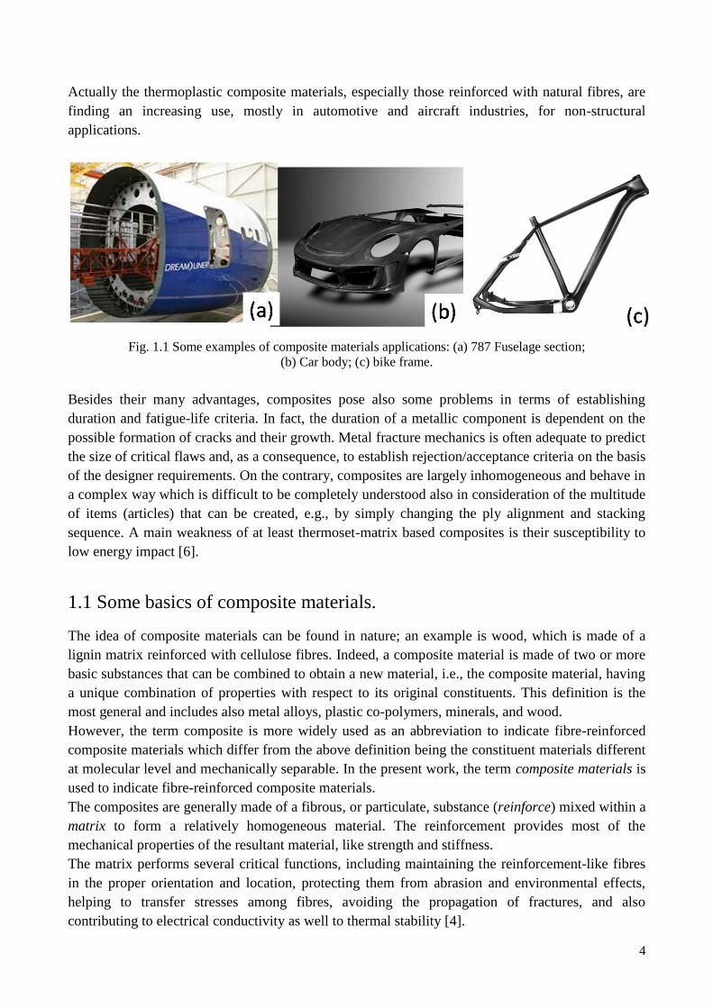
Actually the thermoplastic composite materials, especially those reinforced with natural fibres, are
finding an increasing use, mostly in automotive and aircraft industries, for non-structural
applications.
Fig. 1.1 Some examples of composite materials applications: (a) 787 Fuselage section;
(b) Car body; (c) bike frame.
Besides their many advantages, composites pose also some problems in terms of establishing
duration and fatigue-life criteria. In fact, the duration of a metallic component is dependent on the
possible formation of cracks and their growth. Metal fracture mechanics is often adequate to predict
the size of critical flaws and, as a consequence, to establish rejection/acceptance criteria on the basis
of the designer requirements. On the contrary, composites are largely inhomogeneous and behave in
a complex way which is difficult to be completely understood also in consideration of the multitude
of items (articles) that can be created, e.g., by simply changing the ply alignment and stacking
sequence. A main weakness of at least thermoset-matrix based composites is their susceptibility to
low energy impact [6].
1.1 Some basics of composite materials.
The idea of composite materials can be found in nature; an example is wood, which is made of a
lignin matrix reinforced with cellulose fibres. Indeed, a composite material is made of two or more
basic substances that can be combined to obtain a new material, i.e., the composite material, having
a unique combination of properties with respect to its original constituents. This definition is the
most general and includes also metal alloys, plastic co-polymers, minerals, and wood.
However, the term composite is more widely used as an abbreviation to indicate fibre-reinforced
composite materials which differ from the above definition being the constituent materials different
at molecular level and mechanically separable. In the present work, the term composite materials is
used to indicate fibre-reinforced composite materials.
The composites are generally made of a fibrous, or particulate, substance (reinforce) mixed within a
matrix to form a relatively homogeneous material. The reinforcement provides most of the
mechanical properties of the resultant material, like strength and stiffness.
The matrix performs several critical functions, including maintaining the reinforcement-like fibres
in the proper orientation and location, protecting them from abrasion and environmental effects,
helping to transfer stresses among fibres, avoiding the propagation of fractures, and also
contributing to electrical conductivity as well to thermal stability [4].
5
1.2 The matrices.
Several materials can be used as matrix and they include: polymers, cement, ceramics and metals.
Polymer-matrix and cement-matrix are the mostly used.
Cement matrix are widely exploited in civil engineering, especially as concrete products in which
sand, stones and steel act as reinforcement, embedded in the form of particles, or metal rods,
(reinforced concrete).
Ceramic matrix are particularly appreciated for their resistance to environmental effects like
corrosion and exposure to high temperature but they are extremely brittle. They are used in
applications where thermal protection is compulsory, especially in the aerospace field where
matrices of silicon carbide (SiC) are widely used [7].
Metal matrix are used in applications where high mechanical performances like enhanced specific
strength and stiffness, low density and high-temperature strength are demanded; aluminium alloys,
titanium and magnesium are the mostly employed [8].
Polymer matrix, thanks to their relative low-processing cost and weight, are the mostly used in
aircraft industry but they are finding ever larger application also in automotive and sport industries,
as well as to fabricate daily life objects. Polymer composites involving different types of polymers
and fibres are investigated in the next chapters.
1.2.1 Polymer types
The term polymer indicates a large molecule constituted of a long chain of reiterating units (small
molecules called monomers, or ‘mers’), bonded together through a so-called polymerization
chemical reaction. Polymerization requires at least two reaction points, or functional groups, for
each monomer. There are two types of polymerization: condensation polymerization and addition
polymerization. In the first, the chain development is accompanied by elimination of relatively
small molecules such as H2O or CH3OH; in the second, monomers react to form a polymer without
formation of by products, but, to get polymerization, the addition of catalysts is needed [9].
Owing to their behaviour under heating or cooling, polymers can be grouped into two categories:
thermosets and thermoplastics. Thermosets, before polymerization, behave like low-viscosity resin,
which gradually cures at a relatively low temperature (20-200°C) and cannot be reprocessed by
reheating. In a fully cured state, thermoset molecules are cross-linked and permanently insoluble
and infusible. These types of polymers are also known as cross-linked polymers. Thermosets
include unsaturated epoxies, polyesters and phenolics. Cured epoxy resins are reasonably stable to
chemical attack and are excellent adhesives having low shrinkage during curing (polymerization)
and no emission of volatile gases. Because of these characteristics, which result in a material with
high mechanical properties and high corrosion resistance (coupled with a quite simple curing
process), they are the most popular amongst composite matrices. In contrast, epoxies are quite
expensive, cannot be stored for a long time and so are mainly used in high technology applications.
It is worth noting that, polyester resins are quite easily accessible, cheaper and used in a wide range
of fields. Liquid polyesters can be stored at room temperature for months, sometimes even years,
and with the mere addition of a catalyst can cure within a short time; the cured polyester can be
rigid, or flexible, as the case may be, and transparent. They are mainly used in the automotive and
naval fields. Phenolics represent the first truly synthetic plastic (commercialized since 1905)
6
obtained combining formaldehyde and phenol. They are water and solvent resistant, can be used as
an electrical insulator (they were extensively used in circuit boards), but are generally brittle even if
they can be strengthened, to a certain extent, by fillers. Nowadays, they have been practically
superseded by modern plastics such as epoxy or polyester resins.
Thermoplastics are composed of chainlike molecules, and may be high-viscosity resins with
varying degrees of crystallinity; a number of them can be dissolved in certain liquids and they
soften, or melt, upon heating above their melting temperature (100-400 °C) for additional
processing. Some types of thermoplastic resins include polypropylene (PP), polyvinylchloride,
polyether imide (PEI), polyether ether ketone (PEEK), polystyrene and polyphenylene sulfide
(PPS). Thermoplastic matrices have recently become of great interest for their ductility and high-
processing speed, as well as for the greater choice of manufacturing techniques. In fact, their
processing can be selected by the scale and rate of production required and by the size of the
component. In addition, thermoplastic composites can be easily repaired because transition to the
softened phase can be accomplished any number of times by heating them up.
Due to the high strength/lightweight requirement, thermoset matrices (especially epoxy) are
generally preferred for aeronautical high technology applications, even if the use of thermoplastics
and natural fibres is significantly increasing in the last years for daily life applications [4].
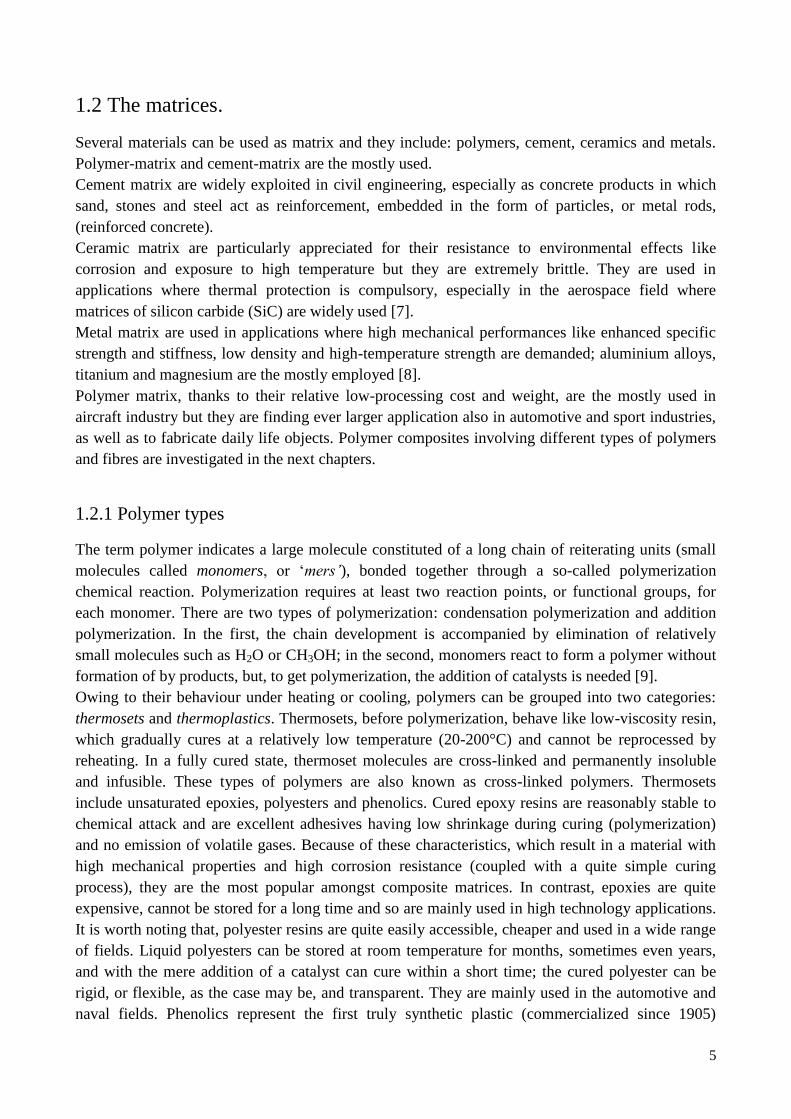
In Table 1.1, the most important mechanical characteristics of some polymers used as matrix are
collected.
MATRIX
Density (g/cm
3)
Elastic
modulus
(GPa)
Traction
resistance (MPa)
Breaking
deformation
(%)
Epoxy 1.1 - 1.4 2.75 - 4.10 55 - 130 1.5 - 8
Polyester 1.1 - 1.4 2.1 - 3.8 20 - 103.5 1 - 5
Phenolic 1.2-1.35 2.0-3.5 20-40 1.2-2.5
PP 0.90 1.2-1.6 25-35 40-70
LDPE 0.92 0.18-0.22 20-28 200-400
PEEK 1.30 - 1.32 3.2 100 50
PPS 1.36 3.3 83 2-20
PEI 1.27 3 105 60
PLA 1.24 3.4-3.8 50-60 2-5
Table 1.1. Most important polymer types used as matrix.
1.3 Reinforcement for polymer-based composites
Long small-diameter fibres are mostly used in the fabrication of composites because, a material
with a fibrous shape entails small and scarce defects and fibres can be oriented along the main
tensile stresses. Besides in a material with a fibrous shape, defects are present with a smaller size
and in a lower percentage and consequently the strength increases. In addition, small-diameter
fibres have greater flexibility and are more amenable to fabrication processes. High-performance
composites are generally made from continuous fibres (Fig. 1.2), but there are many applications
for which the requirements are less demanding and in these cases short fibres can be used in an
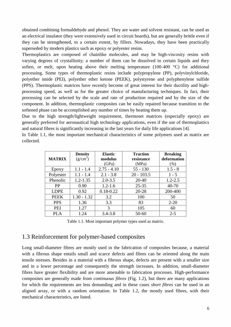
aligned array, or with a random orientation. In Table 1.2, the mostly used fibres, with their
mechanical characteristics, are listed.
7
FIBRES
Density (g/cm
3)
Elasticity
modulus (GPa)
Traction
resistance (GPa)
Specific
Modulus
(107 m
2/s
2)
E Glass 2.54 72.4 3.45 2.85
S Glass 2.49 86.2 4.58 3.46
Carbon HS 1.76 230 3.53 13
Carbon HM 1.87 405 3.10 21.7
Carbon UHM 2.15 572 1.86 29.2
Aramid 1.45 130 3.55 9.0
Boron 2.7 393 3.10 14.5
Aluminium 2.78 70 0.40 2.52
Steel 7.85 210 0.60 2.68
Jute 1.4 20 0.5 1.42
Table 1.2. Some of the mostly used reinforcement fibres
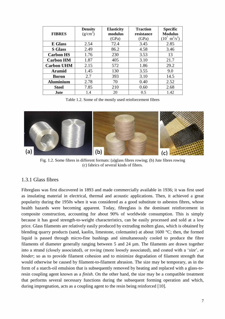
Fig. 1.2. Some fibres in different formats: (a)glass fibres rowing; (b) Jute fibres rowing
(c) fabrics of several kinds of fibres.
1.3.1 Glass fibres
Fibreglass was first discovered in 1893 and made commercially available in 1936; it was first used
as insulating material in electrical, thermal and acoustic applications. Then, it achieved a great
popularity during the 1950s when it was considered as a good substitute to asbestos fibres, whose
health hazards were becoming apparent. Today, fibreglass is the dominant reinforcement in
composite construction, accounting for about 90% of worldwide consumption. This is simply
because it has good strength-to-weight characteristics, can be easily processed and sold at a low
price. Glass filaments are relatively easily produced by extruding molten glass, which is obtained by
blending quarry products (sand, kaolin, limestone, colemanite) at about 1600 °C; then, the formed
liquid is passed through micro-fine bushings and simultaneously cooled to produce the fibre
filaments of diameter generally ranging between 5 and 24 µm. The filaments are drawn together
into a strand (closely associated), or roving (more loosely associated), and coated with a ‘size’, or
binder; so as to provide filament cohesion and to minimize degradation of filament strength that
would otherwise be caused by filament-to-filament abrasion. The size may be temporary, as in the
form of a starch-oil emulsion that is subsequently removed by heating and replaced with a glass-to-
resin coupling agent known as a finish. On the other hand, the size may be a compatible treatment
that performs several necessary functions during the subsequent forming operation and which,
during impregnation, acts as a coupling agent to the resin being reinforced [10].
8
By varying the ‘recipe’ (i.e., by adding chemicals to silica sand), different types of glass can be
produced:
A-glass (alkali glass) has good chemical resistance, but lower electrical properties.
C-glass (chemical glass) has very high chemical resistance.
E-glass (electrical glass) is an excellent insulator and resists attacks from water.
R-, S- and T-glass (structural glass) are optimized for mechanical properties; the different
letter identifies the manufacturer’s trade name for equivalent fibres.
D-glass (dielectric glass) has the best electrical properties but lacks in mechanical properties
when compared to electrical and structural glass.
M-glass (modulus) has high stiffness.
Electrical and structural glasses are, by far, the most common types used in composites because of
their good combination of chemical resistance, mechanical properties and insulating properties. In
particular, E-glass looks more attractive from the cost point of view, while structural glass offers
better mechanical performance [4].
1.3.2 Carbon fibres
Carbon has the highest strength and highest price of all reinforcement fibres today available for
composites. These fibres were produced in the United Kingdom in the early 1960s, even if Edison
had much earlier used them in lighting lamps. The most common method of making long carbon
fibres is the oxidation and thermal pyrolysis of an organic precursor, poly-acrylonitrile (PAN).
Through heating at correct conditions (2500-3000 °C), the non-carbon constituents evaporate away
with a resulting material having a 93-95% carbon content. Of course, the properties of carbon fibres
depend on the raw material and the manufacturing process; in fact, the relative amount of exposure
at high temperatures results in greater, orless, graphitization of the fibres. Higher degrees of
graphitization usually result in a stiffer fibre (higher modulus) with greater electrical and thermal
conductivity values.
The size, or thickness, of carbon tows is measured in ‘k’ or thousands of filaments. A 3k tow
contains 3000 filaments while a 12k has 12,000. Carbon fibres exhibit: substantially better strength
and stiffness values than all the others types for fibre reinforcement, outstanding temperature
performance and high electrical and thermal conductivities. Impact, or damage tolerance, of pure
carbon composite products can range from relatively low to higher depending on the processing
method. Despite that, when weight of a composite product is important, carbon fibres represent the
best reinforcement to be used because of the significant advantages retained by them:
high stiffness-to-weight ratio
high strength
corrosion resistant
fatigue resistant
high-energy absorption on impact
tailored material properties.
9
First of all, it has to be mentioned that carbon fibres are very light, resulting in lightweight
structures. Furthermore, one can chose between stiff, or strong, fibres depending on the composite
part being produced.
Another major advantage is that their thermal expansion is practically zero; this means that unlike
metals, which expand when heated, carbon fibres remain in their basic form with remarkable
benefits in specific projects where thermal stability is required. Moreover, the material can resist
very high temperatures (1000 °C), being essentially limited only by the matrix. If properly designed
and conceived, carbon fibre composite structures do not suffer any fatigue issues. Finally, carbon
fibres are permeable to X-ray and do not corrode, which is a huge concern with metals. The
material also has some disadvantages that need to be taken into consideration when planning a
project. For instance, carbon fibres are fairly expensive compared to other reinforcements even if
their price is steadily decreasing due to the progress of production technology. Moreover, carbon
fibre is an electric conductor and, as such, can reflect radio waves, which can be a disadvantage in
some cases. In addition, carbon fibres are brittle and material breakage can create debris, which can
fly in multiple directions with safety implications.
Finally, handling of carbon fibres may be difficult requiring specific protection. The material size
must be appropriately chosen since it must provide consistent handling, without swelling residues
on the processing equipment and without obstacles to the penetration of resin into the fibre bundle.
Owing to the different commercial carbon fibre surface features (i.e., smooth, striated, round or
kidney shaped), a different blend of physical characteristics, optimized for the fibre shape and
surface texture, is required. Size materials must also be compatible with the resin matrix; this
includes solubility in and/or reactivity with the formulated resin. This allows the resin to better
penetrate the fibre bundle and interact with the fibre surface [4].
1.3.3 Natural fibres
Natural fibres are grouped into three types: seed hair, bast fibres, and leaf fibres, depending upon
the source. Some examples are cotton (seed hairs), ramie, jute, and flax (bast fibres), and sisal and
abaca (leaf fibres). Of these fibres, jute, ramie, flax, and sisal are the most commonly used fibres for
polymer composites. Natural fibres in the form of wood flour have also been often used for
preparation of natural fibre composites.
Natural fibres themselves are cellulose fibre reinforced materials as they consist of microfibrils in
an amorphous matrix of lignin and hemicellulose. These fibres consist of several fibrils that run all
along the length of the fibre. The hydrogen bonds and other linkages provide the necessary strength
and stiffness to the fibres. The chemical composition of natural fibres varies depending upon the
type of fibre. Primarily, fibres contain cellulose, hemicellulose, pectin, and lignin. The properties of
each constituent contribute to the overall properties of the fibre. Hemicellulose is responsible for the
biodegradation, moisture absorption, and thermal degradation of the fibre as it shows least
resistance, whereas lignin is thermally stable but is subjected to UV degradation. The percentage
composition of each of these components varies for different fibres. Generally, the fibres contain
60–80% cellulose, 5–20% lignin, and up to 20% moisture [11,12].
10
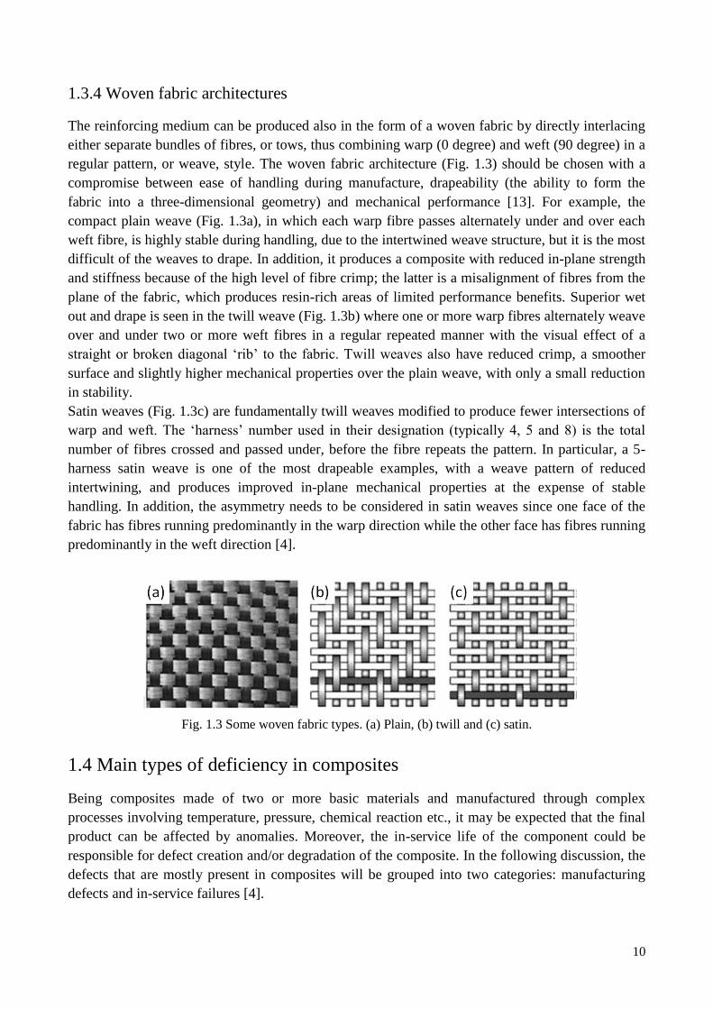
1.3.4 Woven fabric architectures
The reinforcing medium can be produced also in the form of a woven fabric by directly interlacing
either separate bundles of fibres, or tows, thus combining warp (0 degree) and weft (90 degree) in a
regular pattern, or weave, style. The woven fabric architecture (Fig. 1.3) should be chosen with a
compromise between ease of handling during manufacture, drapeability (the ability to form the
fabric into a three-dimensional geometry) and mechanical performance [13]. For example, the
compact plain weave (Fig. 1.3a), in which each warp fibre passes alternately under and over each
weft fibre, is highly stable during handling, due to the intertwined weave structure, but it is the most
difficult of the weaves to drape. In addition, it produces a composite with reduced in-plane strength
and stiffness because of the high level of fibre crimp; the latter is a misalignment of fibres from the
plane of the fabric, which produces resin-rich areas of limited performance benefits. Superior wet
out and drape is seen in the twill weave (Fig. 1.3b) where one or more warp fibres alternately weave
over and under two or more weft fibres in a regular repeated manner with the visual effect of a
straight or broken diagonal ‘rib’ to the fabric. Twill weaves also have reduced crimp, a smoother
surface and slightly higher mechanical properties over the plain weave, with only a small reduction
in stability.
Satin weaves (Fig. 1.3c) are fundamentally twill weaves modified to produce fewer intersections of
warp and weft. The ‘harness’ number used in their designation (typically 4, 5 and 8) is the total
number of fibres crossed and passed under, before the fibre repeats the pattern. In particular, a 5-
harness satin weave is one of the most drapeable examples, with a weave pattern of reduced
intertwining, and produces improved in-plane mechanical properties at the expense of stable
handling. In addition, the asymmetry needs to be considered in satin weaves since one face of the
fabric has fibres running predominantly in the warp direction while the other face has fibres running
predominantly in the weft direction [4].
Fig. 1.3 Some woven fabric types. (a) Plain, (b) twill and (c) satin.
1.4 Main types of deficiency in composites
Being composites made of two or more basic materials and manufactured through complex
processes involving temperature, pressure, chemical reaction etc., it may be expected that the final
product can be affected by anomalies. Moreover, the in-service life of the component could be
responsible for defect creation and/or degradation of the composite. In the following discussion, the
defects that are mostly present in composites will be grouped into two categories: manufacturing
defects and in-service failures [4].
11
1.4.1 Manufacturing defects
Several different types of defects may occur during fabrication of composites, the most common
being: fibre/play misalignment, broken fibres, resin or transversal ply cracks, voids, porosity, slag
inclusions, non-uniform fibre/resin volume ratio, disbonded interlaminar regions, kissing bonds,
incorrect cure and mechanical damage around machined holes and/or cuts.
The effective performance of a fibre is a function of its correct alignment with the stress/strain
direction. In fact, in the presence of fibre misalignment, the loading of the fibre may change from
straight tension/compression to shear loading of the weaker interface. This may result in a
considerable drop of the composite mechanical properties [14].
Slag inclusions such as dirt and debris, which may inadvertently contaminate the matrix or act as
local stress concentrators, leading to delamination either during the manufacturing process, or later
when the composite is in service.
The strength of a carbon-fibre-reinforced polymer (CFRP) component is strongly dependent on the
volume percentage of resin with respect to fibres. In fact, the presence of regions of fibres
unsupported by the matrix can induce local stress concentration (notch effect), with a consequent
severe degradation of strength and stiffness during the component’s in-service life [15].
Amongst the procedures that allow composite production, the most important is probably the resin
curing one. This process has to be optimized in order to get appropriate components responding to
the structural design requirements. In fact, resin curing is dependent on the temperature rate
increase, the temperature and duration of the curing plateau, the time at which pressure is applied
and the post-curing temperature and pressure. If something unexpected occurs in the process, the
typical consequence could be incomplete or inappropriate chemical reactions, uneven wetting of the
fibres, incorrect fibre volume ratio as well as formation of local matrix-rich pockets, or matrix-
starved regions. Moreover, the vacuum pressure, if not suitable, could affect the degassing of
contaminants with only partial removal of the gases developing during chemical reactions. This
may induce formation of voids (or porosity) within the matrix, between the plies or at the
fibre/matrix interface. The detrimental effects of porosity have been known since 1978 when it was
found that there was a decrease of the interlaminar shear strength by about 7% for each 1% of voids
up to a total void content of about 4% [16]. The decrease of other properties for the first 1% of
voids is reported as high as 30% (flexural strength), 9% (torsional shear), 8% (impact strength) and
3% (tensile properties).
The just described defects are the mostly recurrent ones; but, there are also some defects that are
peculiar to specific manufacturing processes. In particular, composites fabricated with pre-
impregnated layers may entail some specific defects due to the improper storage of pre-pregs, like:
out-of-date resin because of exposure to ambient temperature (higher than that required for
correct storage);
wrinkled surface because of an uneven positioning, which may result in resin-rich regions
within the laminate;
accumulation of debris, resulting in slag inclusions;
broken, or damaged, fibre tows, resulting in reduced strength of the laminate.
During processing in autoclave, some defects can occur in the laminate, mainly related to
imperfectly cured resin regions due to incorrect pressure/temperature reached values. Besides, lack
12
of bonding between layers, due to non-uniform pressure on the whole surface, may also occur.
Typical drawbacks of the resin transfer moulding (RTM) process are: formation of porosity due to
the volatilization of dissolved gases in the resin, mechanical entrapment of gas bubbles or a possible
evaporation of mould-release agents. The void formation can be influenced by many factors, such
as resin properties, moulding temperature, injection pressure and external pressure during curing.
Of course, whatever the type of defect, it may result in slight, or severe, variations of the material
properties with, in turn, a reduction of the predicted component life. In fact, these variations may act
as sites for the initiation of fatigue damage, or may facilitate the growth of a fatigue crack during
cyclic loading.
A comprehensive assessment of the quality of a composite material prior to putting it into service is
therefore as important as the monitoring of the levels of damage accumulated in a composite
structure during service [17]. This justifies the increasing attention toward development of:
effective non-destructive evaluation methods able to discover defects at an incipient stage;
aerospace design procedures aimed at achieving zero-growth thresholds for any type of
defect.
Theoretically, many defects may be avoided and the overall quality of a component may be
increased with the implementation of particular procedures and the use of specific instrumentation.
As an example, the use of computer-controlled tape-laying machines may assure construction of a
pre-preg stack for autoclaving to very high standards of quality and repeatability. Similarly, errors
of control in pressing can be avoided to some extent by the use of automated autoclaves with
pressure-temperature cycles. These cycles must be carefully programmed from detailed chemical
knowledge of the gelation and viscosity characteristics of the type of resin in use [17]. Of course,
this entails extra costs that remain an industrial decision.
A challenging question may arise concerning the real consequences of the presence of a defect. As
stated by Harris [17] in his comprehensive book, a few isolated spherical pores, a micron, or so, in
diameter, can have no effect on any physical property, and may not therefore affect the tensile or
flexural mechanical performance of a composite. But a distribution of innocuous-looking pores can
markedly reduce the interlaminar shear strength of a material and, by providing sites for
accumulation of moisture, may also decay the electrical or dielectric performance of the material.
A minor delamination between plies in a complex laminate may have no effect on the tensile
strength of the material, but such defect is frequently injurious to the compression performance of
laminates and, as previously indicated, can rapidly grow to eventually damage the composite under
cyclic-loading conditions. Therefore, to avoid unpredictable failure, it is important to use the most
effective non-destructive defects detection techniques and then establish the critical size with a
case-by-case approach, owing to the specific type of composite and the specific service conditions
for the given application [4].
1.4.2 In-service failures
The in-service failure of composite aircraft structures is primarily caused by impact strikes [18].
The weakness of composites, at least those based on a thermoset matrix, to impacts is well known,
especially to low-velocity/energies that may cause subsurface damage in the form of delamination,
cracks, as well as fibre breakage without appreciable surface signs. In fact, other than a small dent,
13
these impacts show no, or little visual evidence on the external surface as to the extent of the
delaminated area [19]. In particular, delamination in CFRP laminates reduces the strength,
particularly the compression strength, of the structure; if undetected and unrepaired, it may result in
reduction of ultimate load capability, or even inability to withstand design limit load in service life
[20,21]. Conversely, high velocity impact is accompanied by little structural response [21] and can
be identified with the naked eye. For safety issues, when impact damage occurs to an aircraft
structure, the latter must be able to ‘withstand reasonable loads without failure or excessive
structural deformation’ for the ‘operational life of the aircraft’ or ‘until the damage is detected’ [22].
Of course, for design purposes, it is of great importance to have knowledge of the failure
mechanisms.
1.4.2.1. Some hints on failure mechanisms
In the Griffith model [23], the fracture of homogeneous materials like metals is based on the stress-
intensity factor, K, and the associated strain-energy release rate, G, which is mainly related to the
material fracture toughness (material resistance to crack propagation) [17]. In real fibre composites,
the micro-structural inhomogeneity and anisotropy cause the failure process to be very complex
with also a combination of micro-failure events, which can often give rise to high levels of fracture
energy. In fact, unlike homogeneous materials, composites have crack-stopper ability inherent in
both types of interfaces at a microscopic level (between fibres and matrix) and at a macroscopic
level (between separate laminas). This gives rise to complex fracture mechanisms involving
breaking of fibres and matrix, delamination between fibres and matrix, and a combination of crack
deviations along interfaces (at both micro- and macroscopic levels).
In practice, the fracturing of a composite is driven by three factors: the matrix, the reinforcement
and the interface; it is important to consider the types of matrix and fibres, their mutual volumes and
the type of bonds in between them, meaning the curing process. Then, the toughness of a composite
is derived from many sources, and the relative magnitudes of the separate contributions depend not
only on the characteristics of the components but also on the manner in which they interact. Thus,
there is no simple recipe for predicting the toughness of all composites [17]. It follows that the
procedures based on classical fracture mechanics cannot be simply applied for design purposes of
composites. When fibres are incorporated into a matrix of any kind, the separate phases may be able
to contribute in an additive fashion their individual levels of toughness to the composite, or they
may not, depending on the kind of interaction that occurs and on the level of constraint that is set up
as a result of their different properties [17]; so, it is rather difficult, or even impossible, to predict
the way a composite will fail. This justifies the huge amount of literature on the subject [6, 19, 24-
47].
Since the introduction of composites in aircraft construction, one main interest of the scientific
community was to establish the delamination threshold load (DTL) under impact [24]. However,
notwithstanding the huge amount of available data coming from both numerical simulation and
experimental testing, a methodology to unambiguously establish the DTL has still not been
completely achieved. This is because the DTL depends on many factors, in primis, the effective
material mechanical characteristics as well as the geometry of the target [25,26] and of the impactor
[27]. The high variability of mechanical properties of composites derives also from the amount of
porosity that is induced by manufacturing processes and that is practically unavoidable [48]; the
14
voids content can be reduced but not completely suppressed. Perhaps this is the reason why
composite materials display a large variety of damaging ways under impact. In fact, as reported by
Abrate [28], some impacts produce plastic deformations in a small zone surrounding the impact
point, while others involve deformations of the entire structure. In some cases, a major portion of
the impact energy is transferred to the impacted plate, and in other cases, most of the energy is
returned to the impactor. In some circumstances, the indentation absorbs a significant amount of the
impact energy so that it must be adequately modelled in the analysis; in other cases, the effects of
indentation are practically negligible. It must also be considered that mainly in the aircraft industry
there is the habit to quantify impact threats in terms of impact energy, but, as observed by Olsson et
al. [47], this is not completely correct since a small mass and a large mass impactor may entail, at
the same impact energy, completely different responses. A contribution to solve this drawback was
given by Meola and Carlomagno [49] who proposed a relationship that links the damaged area to
the impact energy and the impactor dimension; this result was achieved while using infrared
thermography to investigate the response of composites to impact events [49,50].
Owing to the available literature within the last thirty years, it comes up that the prediction of the
impact response of composites to low energy impact has been widely addressed from analytical,
numerical and experimental approaches, but it is still an open question. This because the results
available in literature are generally restricted to particular cases, while new composite materials are
continuously developed, which require ad hoc testing. The problem seems of no solution
considering the many parameters involved (type of material, laminate thickness, testing machine,
boundary conditions, etc.) and complexity of the coupled physical phenomena, which make difficult
modelling as well the high costs involved with experimental tests.
As an important observation, the evaluation of new materials is generally performed owing to
criteria based on energy and force, or on a multiple parameters configuration [45]. The energy
based criterion involves damage maps, which are plots of damage area vs. impact energy or
dissipated energy, and Compression After Impact (CAI) curves, which are plots of the static
residual strength vs. impact or dissipated energy. The force criterion relies on the peak force
recorded during an impact event. The multiple parameters approach includes many tests in sequence
to get information about the most important parameters that characterize the impact behaviour of a
structure and practically includes both energy and force criteria. Amongst others, a main factor of
interest is the damage extension vs. the impact energy. Often, this feature is assessed through
specific impact tests, which are intended to identify the energy that has caused delamination of a
given extension. More specifically, such tests consist of impacting the laminate at a given energy,
evaluating, in a non-destructive way, the induced damage extension and go on to increasing impact
energies until the preset delamination has been reached. This is a long way on and often not very
accurate since the presence of very thin delamination is difficult to be discovered with the available
non-destructive testing techniques (NDT). In fact, it may happen that two layers of a thermoset
matrix based composite, which were separated by the impact, recommit themselves very tightly,
even if delaminated, once the impacting object went away and the surface has recovered its
undeformed configuration. It is also worth considering that, depending on the composite
architecture, delamination may propagate along tortuous pathways, which may complicate the
situation.
In recent years, at the University of Naples Federico II, it has been demonstrated that it is possible
to monitor the surface of the laminate directly during the impact with an infrared imaging device
[51] to get information on the extension of the occurred delamination [49,50]. In particular, they
15
proved that, with an infrared imaging device, it is possible to visualize the thermal effects that
develop under low-energy impact, and which may supply information about initiation and
propagation of the impact damage. By considering that during an impact event kinetic energy
passes from the impactor nose to the target, and that such energy is in part dissipated as heat, the
detection of thermal signatures developing under impact may be important for the comprehension
of failure modes. In fact, any form of damage (delamination and/or fibre breakage) is generally
accompanied by heat dissipation, which manifests itself through the appearance of hot spots/areas
over the material surface. In this regard, the use of infrared thermography has to be considered as
beneficial and unique.
Amongst the objectives of this dissertation, one is to go on that subject and to understand more
through tests on many types of composites and by developing post-processing procedures to
evaluate the extension of the occurred damage. This topic will be addressed in Chapter 5.
Another objective within composites is to investigate their behaviour under cyclic bending to search
for any likely information, which may be easily derived through monitoring with an infrared camera
and which may be helpful to characterize novel composite materials.
References to Chapter 1
[1]. R. Shütze, Aircraft wings. US Patent 5496002; 1996.
[2]. M. Piening, A. Pabsch, C. Sigle, Structural element of high unidirectional rigidity.US Patent
6355337; 2002.
[3]. P.M. Peeters, J. Middel, A. Hoolhorst, Fuel efficiency of commercial aircraft. An overview of
historical and future trends. Retrieved at
<http://www.transportenvironment.org/docs/Publications/2005pubs/2005-
12_nlr_aviation_fuel_efficiency.pdf>.
[4]. C. Meola, S. Boccardi, G.M. Carlomagno, Infrared Thermography in the Evaluation of Aerospace
Composite Materials, Elsevie & Woodhead publishing ISBN 978-1-78242-171-9, 2016
[5]. M.C. Collier, D.G. Baird, Separation of a thermotropic liquid crystalline polymer from
polypropylene composites. Polym Compos, 20, 423–35, 1999.
[6]. T.W. Shyr, Y.H. Pan, Impact resistance and damage characteristics of composite laminates.
Compos Struct, 62, 193–203, 2003.
[7]. D.J Landini, R.L.K. Matsumoto, D.M. Domanski, Processing of Sic/Sic Ceramic Matrix
Composites by Use of Colloidal Carbon Black, US 0035024 A1, 2006.
[8]. K.U. Kainer, Metal Matrix Composites. Custom-made Materials for Automotive and Aerospace
Engineering, Wiley-VCH, 2006.
[9]. M.A. Masuelli, Introduction of fibre-reinforced polymers polymers and composites: concepts,
properties and processes, in: M. Masuelli (Ed.), Fibre Reinforced Polymers - the Technology
Applied for Concrete Repair, InTech, 2013, ISBN 978-953-51-0938-9,
http://dx.doi.org/10.5772/54629.
[10]. A.C. Long (Ed.), Design and Manufacture of Textile Composites, Woodhead Publishing and CRC
Press LLC, 2005, ISBN 9781855737440.
[11]. H. Ku, H. Wang, N. Pattarachaiyakoop, M. Trada, A review on the tensile properties of natural
fibre reinforced polymer composites, Composites Part B, 42, 856-873, 2011.
[12]. D. Nabi Saheb, J. P. Jog, Natural Fibre Polymer Composite: A Review, Advances in Polymer
Technology, 18 (4), 352-363, 1999.
[13]. C.M. Pastore, D.W. Whyte, H. Soebruto, F.K. Ko, Design and analysis of multi axial warp knit
fabrics for composites, J. Ind. Fabrics, 5 (14) 4-14, 1986.
[14]. J. Summerscales, Manufacturing defects in fibre reinforced plastics composites, Insight, 36 (12)
936-942, 1994.
[15]. H.T. Yoshida, T. Ogasa, R. Hayashi, Statistical approach to the relationship between ILSS and void
content of CFRP, Comput. Sci. Tech. 25 (1) 3-18, 1986.
16
[16]. N.C.W. Judd, W.W. Wright, Voids and their effects on the mechanical properties of composites -
an appraisal, SAMPE J. 14 (1) 10-14, 1978.
[17]. B. Harris, Engineering Composite Materials, The Institute of Materials (IOM), London, 1999.
ISBN:1861250320, 9781861250322.
[18]. Civil Aviation Authority Safety Regulation Group, Reliability of Damage Detection in Advanced
Composite Aircraft Structures Paper 2013/03, 2013.
[19]. M.S. Sohn, X.Z. Hua, J.K. Kimb, L. Walker, Impact damage characterisation of carbon fibre/epoxy
composites with multilayer reinforcement, Composites: Part B, 31, 681-691, 2000.
[20]. Transportation Safety Board of Canada, Assessment of the Response from Transport Canada to
Aviation Safety Recommendation A06-05 Inspection Program of Rudder Assembly, 2007.
[21]. P.E. Irving, C. Soutis, Polymer Composites in the Aerospace Industry, Woodhead Publishing
Series in Composites Science and Engineering, ISBN 978-0-85709-523-7, 2014.
[22]. European Aviation Safety Agency, Certification Specifications for Large Aeroplanes CS-25,
Amendment 5, 2008.
[23]. A.A. Griffith, The phenomena of rupture and flow in solids, Philos. Trans. R. Soc. Lond. Ser. A
221, 163-198, 1920.
[24]. D.J. Elder, R.S. Thomson, M.Q. Nguyen, M.L. Scott, Review of delamination predictive methods
for low speed impact of composite laminates, Compos. Struct. 66, 677-683, 2004.
[25]. G.A. Schoeppner, S. Abrate, Delamination threshold loads for low velocity impact on composite
laminates, Composites: Part A, 31, 903-915, 2000.
[26]. W.J. Cantwell, Geometrical effects in the low velocity impact response of GFRP, Compos. Sci.
Technol. 67, 1900-1908, 2007.
[27]. T. Mitrevski, I.H. Marshall, R. Thomson, R. Jones, B. Whittingham, The effect of impactor shape
on the impact response of composite laminates, Compos. Struct. 67, 139-148, 2005.
[28]. S. Abrate, Modeling of impacts on composite structures, Compos. Struct. 51, 129-138, 2001.
[29]. W.J. Cantwell, J. Morton, Detection of impact damage in CFRP laminates. Compos Struct, 3, 241–
57, 1985.
[30]. K.N. Shivakumar, W. Elber, W. Illg, Prediction of Impact force and duration due to low-velocity
impact on circular composite laminates. J Appl Mech, 52, 674–80, 1985.
[31]. P. Sjo¨blom, T. Hartness, T.M. Corbell, On low velocity impact testing of composite materials. J
Compos Mater, 22 (1), 30–52, 1988.
[32]. G.A.O. Davies, X. Zhang, Impact damage prediction in carbon composite structure. Int J Impact
Eng, 16 (1), 149–70, 1994.
[33]. D. Delfosse, A. Poursartip, Energy-based approach to impact damage in CFRP. Compos Part A,
28A, 647–55, 1997.
[34]. G. Zhou, Effect of impact damage on the residual compressive strength of glass–fibre reinforced
polyester (GFRP) laminates. Compos Struct, 35, 171–81, 1996.
[35]. D. Liu, B.B. Raju, X. Dang, Size effects on impact response of composite laminates. Int J Impact
Eng, 21(10), 837–54, 1998.
[36]. C.F. Li, N. Hu, J.G. Cheng, H. Fukunaga, H. Sekine, Low velocity impact induced damage of
continuous fibre-reinforced composite laminates. Part II. Verification and numerical investigation.
Compos Part A, 33, 1063–72, 2002.
[37]. G. Belingardi, R. Vadori, Low velocity impact tests of laminate glass-fibre-epoxy matrix composite
material plates. Int J Impact Eng, 27, 213–29, 2002.
[38]. T. Mitrevski, I.H. Marshall, R.S. Thomson, R. Jones. Low-velocity impacts on preloaded GFRP
specimens with various impactor shapes. Composite Structures, 76, 209–217, 2006.
[39]. G. Caprino , V. Lopresto , C. Scarponi, G. Briotti. Infuence of material thickness on the response of
carbon-fabric/epoxy panels to low velocity impact. Comp. Sci. Technol. 59. 2279-2286, 1999.
[40]. W.C. Jackson, C.C. Poe, The use of impact force as a scale parameter for the impact response of
composite laminates. J Compos Technol Res, 15/4, 282–9, 1993.
[41]. A.T. Nettles, M.J. Douglas. A comparison of quasi-static indentation to low-velocity impact,
NASA TP-2000-210481, Aug.; 2003.
[42]. G. Caprino, V. Lopresto, The significance of indentation in the inspection of carbon fibre-
reinforced plastic panels damaged by low velocity impact. Compos Sci Tech, 60, 1003–12, 2000.
[43]. G. Caprino, A. Langella, V. Lopresto, Indentation and penetration of carbon fibre reinforced plastic
laminates. Compos Part B, 34(4), 319–25, 2003.
17
[44]. J.N. Baucoma, M.A. Zikryb. Low-velocity impact damage progression in woven E-glass composite
systems. Composites: Part A, 36, 658–664, 2005.
[45]. P. Feraboli, K.T. Kedward, A new composite structure impact performance assessment program,
Comp. Sci. Technol. 66, 1336–1347, 2006.
[46]. V. Lopresto, C. Leone, I. De Iorio. Mechanical characterisation of basalt fibre reinforced plastic.
Composites: Part B 42, 717-7123, 2011.
[47]. R. Olsson, M.V. Donadon, B.G. Falzon, Delamination threshold load for dynamic impact on plates,
Int. J. Solids Struct. 43, 3124-3141. 2006.
[48]. L. Liu, B.M. Zhang, D.F. Wang, Z.J. Wu, Effects of cure cycles on void content and mechanical
properties of composite laminates, Compos. Struct. 73, 303-309, 2006.
[49]. C. Meola, G.M. Carlomagno, Impact damage in GFRP: new insights with infrared thermography,
Composites: Part A 41, 1839-1847, 2010.
[50]. C. Meola, G.M. Carlomagno, F. Ricci, V. Lopresto, G. Caprino, Investigation of impact damage in
composites with infrared thermography, in: P. Mazal (Ed.), Proceedings of 6th NDT in Progress,
Prague (Czech Republic), 2011, pp. 175-182.
[51]. C. Meola, G.M. Carlomagno, Infrared thermography to impact-driven thermal effects, Applied
Physics A, 96, 759-762, 2009.

18
Chapter 2
Infrared thermography
Nomenclature
A,B,C Constants that accounts for the surface and atmosphere characteristics.
Adet Detector active area
Ae Electrical area
Ao Optical Area.
c Speed of light
D* Detectivity.
dw Wien’s displacement constant (dw 2898 μm K)
Ea Fraction of ETot Energy emitted by the atmosphere
Ed Detected radiationEb Total hemispherical radiation intensity
Eε Fraction of ETot emitted by the generic object
Eg Energy gap from the valence band and conduction band
Eλb Monochromatic (spectral) radiation intensity
Emc Incident Radiation.
Eph Photon energy
Eρ Fraction of ETot reflected by the generic object
ETot Total energy detected by the IR camera.
fph Photon Frequency
h Planck's constant (h = 6.6 x 10⁻³⁴
J s)
Iinc Incident energy over a surface.
Iout Reflected energy over a surface.
kb Boltzmann’s constant (kb = 1.38 x 10⁻²³
J/K)
NL rms noise level.
Nout Noise output.
Rv Responsivity
Sout Signal output.
T Absolute temperature
1/f Flicker noise or pink noise
Greek Symbols
α Total absorptance
α Monochromatic absorptance
β Angle formed by the Iout direction and the surface normal direction
Angle formed by the Iinc direction and the surface normal direction.
Δf Noise bandwidth
ΔSm Signal measured for the temperature ΔT
ΔT Temperature difference.
Emissivity coefficient.
ε Monochromatic emissivity coefficient.

19
ηq Quantum efficiency.
Wavelength
λc Cut-off wavelength.
λmax Wavelength at which is emitted the maximum radiation intensity of monochromatic
(spectral) radiation intensity Eλb.
ρ Total reflectance coefficient.
ρ Monochromatic reflectance coefficient
σ Stefan Boltzmann constant (σ = 5.67 x 10⁻⁸
W/m2 K
4)
τ Total transmittance
τ Monochromatic transmittance
Фb Photon flux density (also called dark current).
20
Introduction
Infrared thermography (IRT) is a discipline that relies on physical principles, theoretical basis and
practical approaches. Essentially, it includes an IR detecting device to sense the thermal energy that
is radiated from objects in the IR band; such energy, with the aid of specific software and basic
relationships, is transformed into a video signal and, finally, into the object surface temperature
map. Naturally, this is a simplified description; in reality, the way the final temperature map is
accomplished is a rather complex procedure that involves many disciplines like electromagnetism,
electronics, signal treatments, heat transfer, etc. IRT is being used in a broad number of application
fields and for many different purposes; definitely, any process that is temperature dependent may
benefit from the use of an IR device. Indeed, an IR imaging device should be considered as a
precious partner to consult for diagnostics and preventative purposes, for understanding of complex
fluid dynamics phenomena, or for material characterization and procedures assessment, which can
help improve design and fabrication of products. IRT may accompany the entire life of a product,
since it may be used to control the manufacturing process (online process control), to non-
destructively assess the final product integrity and to monitor the component in service.
Besides, IRT can be usefully exploited in all the applications in which the temperature in a key
parameter like: medicine, veterinary, electrics, electronics, video surveillance, astronomy, and many
other industrial fields [1-57]. Of course, for the success of any application, it is most important to
choose the most adequate IR camera and test procedure, as well image processing and data analysis
for the specific use required.
2.1 Some basics
Infrared thermography is based on the physical evidence that any body at temperature above 0 K
emits thermal radiation, due to molecular and atomic agitation associated with the internal energy of
the material. The radiant energy is carried by photons, generally regarded as a discrete particle
having zero mass, no electric charge, indefinitely long lifetime and moving in vacuum at the speed
of light c 3 x 10⁸ m/s. Each photon has energy Eph, which is equal to its frequency fph multiplied
the Planck’s constant (h = 6.6 x 10⁻³⁴
J s); such energy can be expressed, according to Einstein, in
terms of :
(2.1)
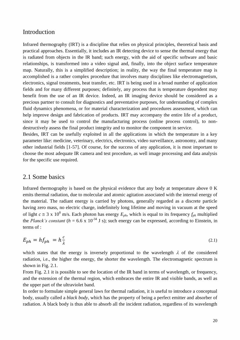
which states that the energy is inversely proportional to the wavelength of the considered
radiation, i.e., the higher the energy, the shorter the wavelength. The electromagnetic spectrum is
shown in Fig. 2.1.
From Fig. 2.1 it is possible to see the location of the IR band in terms of wavelength, or frequency,
and the extension of the thermal region, which embraces the entire IR and visible bands, as well as
the upper part of the ultraviolet band.
In order to formulate simple general laws for thermal radiation, it is useful to introduce a conceptual
body, usually called a black body, which has the property of being a perfect emitter and absorber of
radiation. A black body is thus able to absorb all the incident radiation, regardless of its wavelength
21
and direction, and is the body that, for a fixed temperature and wavelength, emits the maximum
possible amount of radiation.
Fig. 2.1. Representation of the electromagnetic spectrum (wave not to scale).
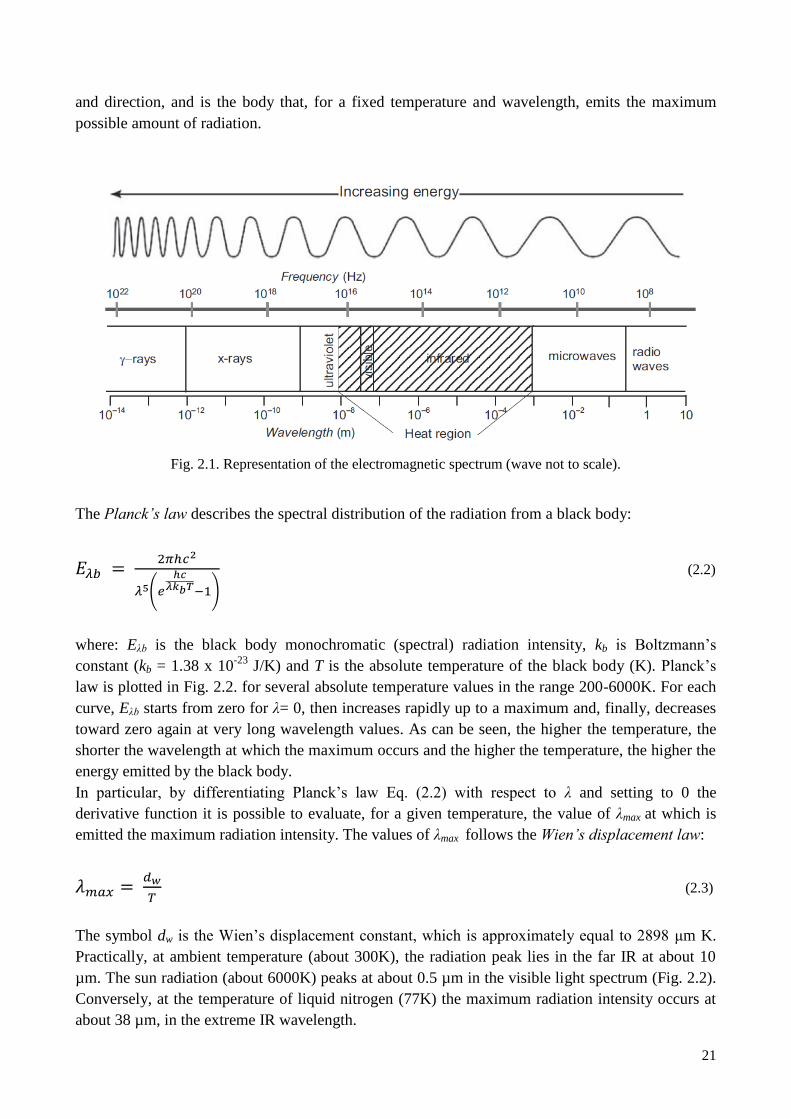
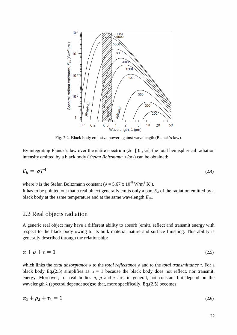
The Planck’s law describes the spectral distribution of the radiation from a black body:
(2.2)
where: Eλb is the black body monochromatic (spectral) radiation intensity, kb is Boltzmann’s
constant (kb = 1.38 x 10⁻²³
J/K) and T is the absolute temperature of the black body (K). Planck’s
law is plotted in Fig. 2.2. for several absolute temperature values in the range 200-6000K. For each
curve, Eλb starts from zero for λ= 0, then increases rapidly up to a maximum and, finally, decreases
toward zero again at very long wavelength values. As can be seen, the higher the temperature, the
shorter the wavelength at which the maximum occurs and the higher the temperature, the higher the
energy emitted by the black body.
In particular, by differentiating Planck’s law Eq. (2.2) with respect to λ and setting to 0 the
derivative function it is possible to evaluate, for a given temperature, the value of λmax at which is
emitted the maximum radiation intensity. The values of λmax follows the Wien’s displacement law:
(2.3)
The symbol dw is the Wien’s displacement constant, which is approximately equal to 2898 μm K.
Practically, at ambient temperature (about 300K), the radiation peak lies in the far IR at about 10
µm. The sun radiation (about 6000K) peaks at about 0.5 µm in the visible light spectrum (Fig. 2.2).
Conversely, at the temperature of liquid nitrogen (77K) the maximum radiation intensity occurs at
about 38 µm, in the extreme IR wavelength.
22
Fig. 2.2. Black body emissive power against wavelength (Planck’s law).
By integrating Planck’s law over the entire spectrum (λ [ 0 , ∞], the total hemispherical radiation
intensity emitted by a black body (Stefan Boltzmann’s law) can be obtained:
(2.4)
where σ is the Stefan Boltzmann constant (σ = 5.67 x 10⁻⁸
W/m2 K
4).
It has to be pointed out that a real object generally emits only a part E of the radiation emitted by a
black body at the same temperature and at the same wavelength Eλb.
2.2 Real objects radiation
A generic real object may have a different ability to absorb (emit), reflect and transmit energy with
respect to the black body owing to its bulk material nature and surface finishing. This ability is
generally described through the relationship:
(2.5)
which links the total absorptance α to the total reflectance ρ and to the total transmittance τ. For a
black body Eq.(2.5) simplifies as α = 1 because the black body does not reflect, nor transmit,
energy. Moreover, for real bodies α, ρ and τ are, in general, not constant but depend on the
wavelength λ (spectral dependence);so that, more specifically, Eq.(2.5) becomes:
(2.6)
23
It has to be observed that a surface may exhibit selective behaviour not only with respect to the
wavelength but also with respect to the direction of the propagating energy since the energy,
absorbed by a surface, may come mostly from certain directions.
By considering a generic wavelength λ, it is possible to demonstrate through the Kirchoff’s law that,
at thermodynamic equilibrium, the energy released by a surface is equal to the absorbed one:
(2.7)
where ε indicates the emissivity coefficient, which represents the fraction of the energy emitted by a
real body with respect to that emitted by the black body at the same temperature:
(2.8)
In other words, Eq.(2.7) states that, for a body at constant temperature, the rate at which it absorbs
energy is equal to the rate at which it emits energy; otherwise the object would warm, or cool, in
contrast with the assertion of thermodynamic equilibrium. It is general habit to use the symbol
without reference to the wavelength.
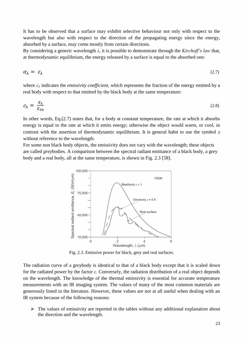
For some non black body objects, the emissivity does not vary with the wavelength; these objects
are called greybodies. A comparison between the spectral radiant emittance of a black body, a grey
body and a real body, all at the same temperature, is shown in Fig. 2.3 [58].
Fig. 2.3. Emissive power for black, grey and real surfaces.
The radiation curve of a greybody is identical to that of a black body except that it is scaled down
for the radiated power by the factor ε. Conversely, the radiation distribution of a real object depends
on the wavelength. The knowledge of the thermal emissivity is essential for accurate temperature
measurements with an IR imaging system. The values of many of the most common materials are
generously listed in the literature. However, these values are not at all useful when dealing with an
IR system because of the following reasons:
The values of emissivity are reported in the tables without any additional explanation about
the direction and the wavelength.
24
Tables present in literature include terms like: polished, cast, rolled, oxidized, heavily
oxidized etc that does not allow to uniquely identify the real surface under consideration.
Thus, the emissivity values reported in the tables does not allow to get accurate temperature
measurements. The better way is to directly measure the emissivity with the same IR camera
according to the standards [59]. This procedure consists simply in comparing the radiation emitted
by the material sample and that emitted by a black body at the same temperature. As last
observation to perform accurate thermographic measurements, it is preferable to work with high-
emissivity surfaces; to this end, it is possible to increase the surface emissivity of highly polished
metals, or reflectors, with deposition of thin films of dull paint or grease.
To allow for successful measurements with an IR imaging device, the object must be opaque (non
transparent) in the IR wavelength band and must have high emissivity. For an opaque material and
taking into account Eq. (2.7.), Eq. (2.6.) reverts to:
(2.9)
According to Eq. 2.9, all real surfaces reflect part of the incident radiation coming from the
surroundings that bounces off the target. Both ρ and ε depend on the considered material, surface
finishing and wavelength of the incident radiation.
A surface may reflect the incident radiation in two modes: specular and diffuse. When a surface is
very smooth and highly polished, almost all of the incident energy Iinc is thrown out of the surface
as Iout in a single direction, with the incident angle equal to the exit one β . In the case of rough
surfaces the incident energy Iinc is reflected almost uniformly in all directions .
The emissivity does not depend only on the bulk material and surface finishing but also on the
direction. In fact a real surface does not emit the same radiation in all directions; for non metallic
materials, the maximum emission generally occurs in the direction normal to the radiating surface
and decreases, becoming null for a direction parallel to that surface. Practically, a curved surface
must be subdivided into at least three sectors to obtain reliable temperature measurements [49].
2.2.1 Effects of interposed atmosphere
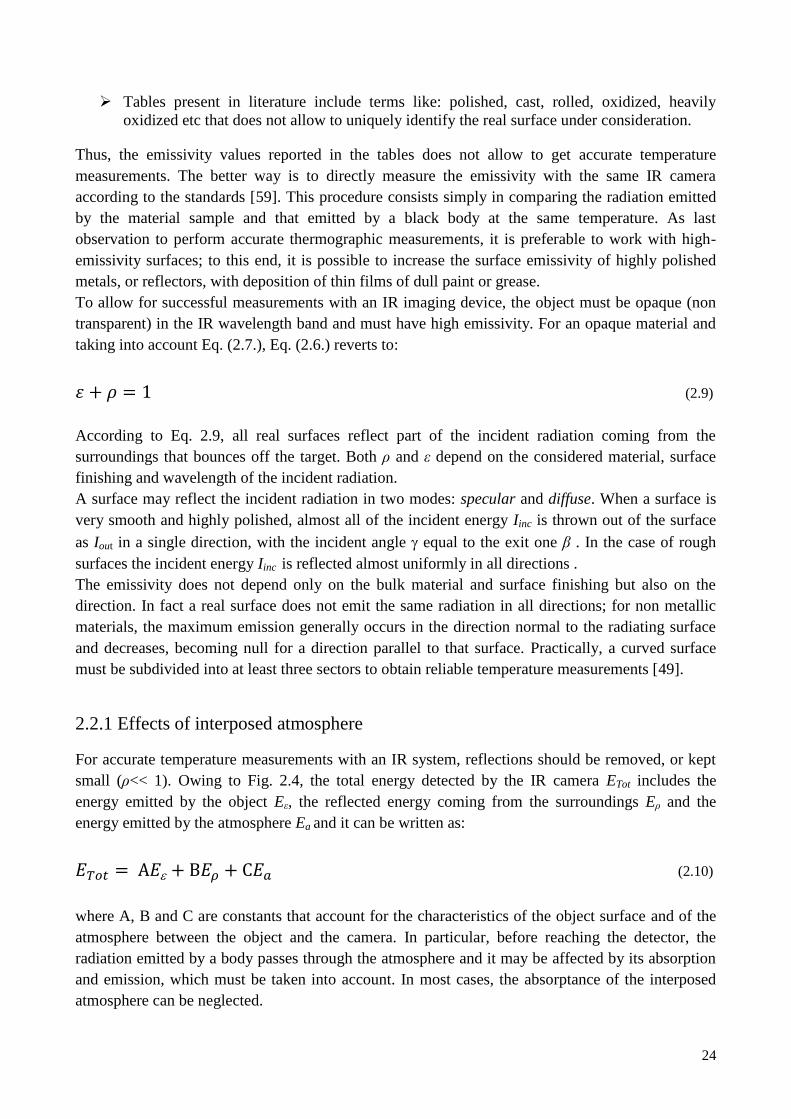
For accurate temperature measurements with an IR system, reflections should be removed, or kept
small (ρ<< 1). Owing to Fig. 2.4, the total energy detected by the IR camera ETot includes the
energy emitted by the object Eε, the reflected energy coming from the surroundings Eρ and the
energy emitted by the atmosphere Ea and it can be written as:
(2.10)
where A, B and C are constants that account for the characteristics of the object surface and of the
atmosphere between the object and the camera. In particular, before reaching the detector, the
radiation emitted by a body passes through the atmosphere and it may be affected by its absorption
and emission, which must be taken into account. In most cases, the absorptance of the interposed
atmosphere can be neglected.
25
Fig. 2.4. Components of energy reaching the infrared camera.
As a final point, to perform measurements of temperature starting from thermal radiation, it is
important to know exactly how much energy is emitted by the object and is captured by the IR
detector; it is worth noting that Eρ can be measured and accounted for.
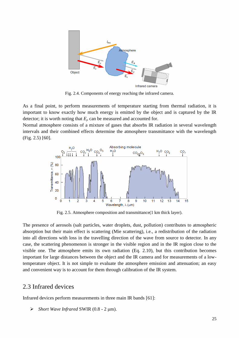
Normal atmosphere consists of a mixture of gases that absorbs IR radiation in several wavelength
intervals and their combined effects determine the atmosphere transmittance with the wavelength
(Fig. 2.5) [60].
Fig. 2.5. Atmosphere composition and transmittance(1 km thick layer).
The presence of aerosols (salt particles, water droplets, dust, pollution) contributes to atmospheric
absorption but their main effect is scattering (Mie scattering), i.e., a redistribution of the radiation
into all directions with loss in the travelling direction of the wave from source to detector. In any
case, the scattering phenomenon is stronger in the visible region and in the IR region close to the
visible one. The atmosphere emits its own radiation (Eq. 2.10), but this contribution becomes
important for large distances between the object and the IR camera and for measurements of a low-
temperature object. It is not simple to evaluate the atmosphere emission and attenuation; an easy
and convenient way is to account for them through calibration of the IR system.
2.3 Infrared devices
Infrared devices perform measurements in three main IR bands [61]:
Short Wave Infrared SWIR (0.8 - 2 μm).
26
Middle Wave Infrared MWIR (2 - 5.5 μm).
Long Wave Infrared LWIR (8 - 14 μm).
The detector is the kernel of any IR device; it absorbs the IR energy emitted by the object and
produce electrical signals proportional to the amount of incident radiation falling on it. The actual in
use infrared imager are based on the focal plane array (FPA) technology. The overall performance
of an IR imaging system is conventionally expressed through several parameters:
Thermal sensitivity- is expressed through the equivalent random noise level.
Frame rate- is the number of images per unit time.
Image resolution- is the number of independent measurement data points the image is
composed of.
Dynamic range or intensity resolution - is the number of intensity levels, which allows for
fine temperature differences.
The detectors mostly used for IR technology can be grouped into two main categories: thermal and
quantum (or photon) detectors.
2.3.1 Thermal detectors
These detectors are also called energy detectors, or photon absorbers, because they absorb the
incident energy and warm up; their temperature changes are measured through the variation of a
temperature-dependent property of the material such as the electrical resistance. The main
advantage is their response at room temperature and over a large band of the IR spectrum. The main
disadvantage is their relatively slow response time (of the order of milliseconds), which makes them
not suitable for high frequency events. Examples of detectors that belong to this family are:
thermopiles, bolometers, pyroelectric detectors and microcantilevers.
The microbolometer technology is based on the resistance change with temperature of a resistor
element and is the mostly employed in handheld IR systems. Basically, a microbolometer consists
of two platinum strips, covered with lampblack; one strip is shielded from the radiation and the
other one is exposed to it. The two strips form two branches of a Wheatstone bridge; the resistance
in the circuit varies when the strip, which is exposed to IR radiation, heats up and changes its
electrical resistance. Nowadays, advances in silicon micromachining have led to the
microbolometer technology, which includes a grid of vanadium oxide, or amorphous silicon heat
sensors, atop a porous silicon bridge as thermal insulator and a mechanical supporting structure.
The microbolometer grid is commonly found in different sizes: 160 x 120, 320 x 240, 640 x 512
and 1024 x 1024 arrays.
2.3.2 Photon Detectors.
Photon or quantum detectors generate free electrical carriers in response to photon absorption. Their
main advantage is a very short response time (of the order of microseconds). While a disadvantage
is the need of cooling them down to cryogenic temperature to avoid excessive dark current. In fact,
electrons can be excited from the valence to the conduction band by photons having an energy Eph

27
that is larger than the energy gap Eg between the bands. There exists a wavelength λc named cut-off
wavelength beyond which no emission occurs. The value of Eg varies from semiconductor to
semiconductor and tends to increase as temperature increases (cut-off wavelength decreases). Thus,
the detector must be maintained at low temperature.
Different cooling methods were developed through the history of infrared thermography. The
current mostly used method involves a Stirling pump that operates by cyclic compression and
expansion of the working fluid (generally helium gas). In modern cooled cameras, the detector focal
plane assembly is generally tightly attached to the cold side of a Stirling cooler to allow for
conductive heat exchange. The Stirling system removes heat from the cold finger and dissipates it at
the warm side. It has relatively low efficiency but it is adequate for cooling of the IR camera
detector and allows operation of the camera for a long time and in complex placements.
There are four main types of photon detectors: photovoltaic (PV), photoconductive, photo-emissive
and quantum well IR photodetector (QWIP). In particular, the PV and photoconductive types may
be intrinsic or extrinsic. The structure of a PV intrinsic (electromotive force generation) is based on
a p-n junction device (two dissimilar materials), which, under IR radiation, generates photocurrents.
These detectors are generally fabricated from silicon (Si), germanium (Ge), gallium arsenide
(GaAs), indium antimonide (InSb), indium gallium arsenide (InGaAs) and mercury cadmium
telluride (HgCdTe) (also called MCT).
In PV intrinsic detectors, the incident radiation, with energy greater than or equal to the energy
band-gap of the semiconductor, generates majority electrical carriers. The electric conductivity of
the material is improved; there is an internal photoelectric effect. Common materials are lead
sulfide (PbS), lead selenide (PbSe) and MCT (HgCdTe). Extrinsic detectors are similar to intrinsic
detectors. The difference lies in the fact that carriers are excited from the impurity levels and not
over the band-gap of the basic material; this is achieved by doping the semiconductor material. The
most-used materials are silicon and germanium doped with impurities such as boron, arsenic and
gallium. The spectral response of these detectors can be controlled by the doping level. Photo-
emissive detectors are bi-materials involving a metal layer superimposed to a semiconductor layer;
a typical example is platinum silicide (PtSi) on silicon (Si). The process, which is also called
external photoelectric effect, consists of the emission of carriers from the metal into the
semiconductor under photon absorption. The main advantage is a more uniform response since the
response depends on the characteristics of the metal. However, since the photon absorption is
proportional to the square of the wavelength, this type of detector is more indicated for long
wavelengths.
The QWIP generally consists of layers of thin gallium arsenide alternated to layers of aluminium
gallium arsenide (AlGaAs). The basic principle is similar to that of extrinsic detectors with the
peculiarity that the dopants are concentrated in microscopic regions and create the quantum wells.
The radiation is absorbed by the entire quantum well, not only by a single doping atom, and thus the
absorption is increased (so is the response) with respect to extrinsic detectors.
2.3.3. QWIP detectors technology
The Quantum Well Infrared Photodetector (QWIP) is a semiconductor device which is generally
made of layers of thin gallium arsenide (GaAs) alternated to layers of aluminium gallium arsenide
(AlGaAs). These quantum well devices have a number of potential advantages, including the use of

28
standard manufacturing techniques based on mature GaAs growth and processing technologies,
highly uniform and well-controlled molecular beam epitaxy growth on GaAs wafers greater than 6
in., high yield and thus low cost, more thermal stability, and extrinsic radiation hardness [62].
Conversely, QWIPs present some problems: low quantum efficiency (ηq< 50%, typical 20%),
lower operating temperature, high dark currents, complex light coupling schemes, narrow spectral
response that limits sensitivity in low-background conditions. As a fabrication drawback, photons
normally impinging are not absorbed (do not produce excitation) and so roughed surfaces are
needed to scatter photons inside the detector. The major source of noise in QWIPs is the dark
current (i.e., the current that flows through a biased detector in the dark with no photons impinging
on it). As reported by Rogalski [63], at low temperature (<40 K) the dark current is mostly caused
by defect related direct tunnelling, while in the medium range between 40 and 70 K the thermally
assisted tunnelling dominates. At temperature above 70 K, the dark current is mostly dominated by
classic thermionic emission (i.e., heat-induced flow of charge carriers) of ground state electrons
directly out of the well into the continuum. The choice of the detector operating temperature is
performed as a compromise between reducing the dark current and improving the sensitivity since
the two parameters are correlated. Generally, the choice falls on the value of 70 K opting for high
sensitivity. From a practical standpoint, QWIPs are suited for large arrays (640 x 512 pixels)
formats, low frame rates and large integration time.
2.3.4 Detector performance
The performance of a detector is evaluated through three parameters: responsivity Rv, noise
equivalent power (NEP) and detectivity D*. The responsivity Rv is a measure of the signal output
Sout (voltage, or current) per incident radiation Emc over the active area of the detector Adet:
(2.11)
The active area is determined as the ratio Adet = Ao/Ae between the optical area Ao and the actual
electrical area Ae. The NEP defines the intrinsic noise level of the detector, or better the detection
limit of the detector. It can be expressed by:
(2.12)
with Nout the noise output and Δf the noise bandwidth. The detectivity D* defines the resolving
power of the detector and is expressed in terms of the signal-to-noise ratio (Sout/Nout) with respect
to the incident power:
(2.13)
The noise that affects detection of IR radiation is of different types and comes from several sources
[63]. One major noise source is the electronic circuitry, which gives rise to two different types of

29
noise. One is thermal noise, also known as Johnson noise [64], or Johnson-Nyquist noise, which
refers to fluctuations in the electrical signal induced by thermal motion of free electrons in a
resistive element [65]. Thermal noise is important for thermal detectors while it is generally
negligible for photon detectors for which the detection limit is evaluated by accounting for the
background radiation. The other type of noise linked to the electronic circuitry is shot noise, first
described by Schottky in 1918 and often also named Schottky noise. From a general point of view,
since electrons share the particle-wave duality with photons, shot noise applies to both. As a
definition, shot noise is due to the fluctuations of the number of independent charge carriers
crossing a boundary (electrons in an electronic circuit, or photons in an optical device). It is a
random process following Poisson statistics (for which the mean squared fluctuation of the number
of emission events is equal to the average count (N) and the signal-to-noise ratio (SNR) takes the
expression:
(2.14)
Of course, shot noise dominates when the finite number of particles that carry energy is small
enough. As N increases, the Poisson distribution approaches the Gaussian one and shot noise
becomes insignificant. Shot noise is independent of frequency (white noise), but, unlike thermal
noise, it is also independent of temperature, meaning it cannot be eliminated by lowering the sensor
temperature. Generally, shot noise dominates at high frequency and is linearly proportional to the
current [66]. At low frequency (below 10 kHz), another type of noise dominates, which is related to
time dependent fluctuations; this noise is called flicker noise, or 1/f, or pink noise, and, in contrast
to the white noise (thermal and shot), is frequency dependent. Flicker noise occurs in virtually all
electronic components, as well as in many other physical items in everyday life from the earth’s
rotation to undersea currents [67,68]. There are two major theoretical hypotheses to its origin. One
refers to the fluctuation of the number of carriers caused by capture and emission of carriers into
trap centres close to the substrate/dielectric interface. The second hypothesis accounts for
fluctuations of the mobility of free carriers, since it is believed to be due to microscopic defects in
the semiconductor material.
As described in literature, when the area of the device is small, or the number of defects in the
device reduces to one or two, flicker noise becomes burst noise. This type of noise also got the
name of popcorn noise because the sound it makes when played over a speaker resembles the sound
of popcorn popping. Burst noise is described to look, on an oscilloscope, like a square wave of
constant magnitude but with random pulse widths. Recently this noise was also referred to as
random telegraph signal (RTS). In particular, Kleinpenning [69] showed that RTS noise exists with
devices with a small number of carriers, where a single electron can be captured by a single
trapping centre. RTS noise is present in sub-micrometer MOS transistors and in bipolar junction
transistors with defected crystal lattice, as well as in modern SiGe transistors. This type of noise is a
function of temperature, induced mechanical stress and radiation, and has significant effects at low
frequency (typically f < 1 kHz). It is described to manifest as a sudden step, or jump, in base current
on bipolar transistors, or a step in threshold voltage for FETs. Bursts can happen several times a
second or, in some rare cases, may take minutes to occur. They are believed to be caused by charge
traps or microscopic defects in the semiconductor material.
In IR detectors, noise comes from two main sources: the IR detector itself with its circuits and the
background fluctuations. The first contribution is generally negligible with respect to the second

30
one and then the detection limit is evaluated by accounting only for the background radiation. This
contribution is called background limited IR photodetection (BLIP). PV detectors are characterized
by a higher BLIP; in fact, the relationship for a PV detector is:
(2.15)
while for a photoconductive is:
(2.16)
Фb being the background photon flux density (also called dark current). The value of Фb received by
the detector depends on its responsivity to the wavelengths contained in the radiant source and on
its field of view of the background.
A relevant parameter for IR systems is the noise equivalent temperature difference; it can be
defined as the temperature change, for incident radiation, that gives an output signal equal to the
rms noise level NL:
(2.17)
where ΔSm is the signal measured for the temperature difference ΔT. In other words the NETD can
be considered as the amount of scene temperature difference that equals the internal noise. The
NETD can be improved by increasing the size of the detecting elements but, increasing the IFOV
would degrade the spatial resolution.
2.4 IR Image generation
A typical FPA can be described as a two-dimensional matrix of n columns by m rows of individual
cells, or pixels, with each pixel (detector) having micrometre-size dimensions. The interface circuit
(or driving circuit) of each cell, which converts the current from each photodiode to a voltage at
each pixel, is referred to as a readout integrated circuit (ROIC) unit cell. A control circuit is also
needed to synchronize the operation of the unit cells and converts the output of the IR pixels to a
stream of bits [70]. The main function of an ROIC is transforming the small diode incremental
current, generated by IR radiation, into a relatively large measurable output voltage; this is
commonly done by integrating the photocurrent in a capacitor during a fixed period of time. There
are two integration modes: the asynchronous integrate while read (AIWR) and the asynchronous
integrate then read (AITR). In the AIWR mode, the camera is able to integrate scene signals while
simultaneously reading out the previous frame. This mode allows for semi-independent control of
the camera’s frame rate and integration time snapshots taken per second; the integration time is the
length of time that each snapshot actually views the scene. However, the time required to read out
all of the pixels limits the maximum frame rate; the selection of a smaller window size allows the

31
maximum frame rate to increase The AITR mode is used in some radiometric cameras coupled with
specific calibrated windows [60,71]
The integration process is controlled by the Frame Synchronization (FSYNC) clock pulse. The
rising edge of the FSYNC clock pulse marks the beginning of the frame time; this is followed
immediately by a sequence of line synchronization (LSYNC) clock pulses that produce a readout
sequence. Each time the switch is closed, the capacitor discharges and when the switch is open the
integration starts again. The rate at which this switch is operated is called the sampling rate; such
sample & hold circuit acts in a sinusoidal fashion. The FSYNC clock remains high until the readout
sequence has been completed. The integration time occurs after the readout time, resulting in a
frame time that is approximately.
Two main signals that are used for time synchronization of the circuit are line synchronization
(LSYNC) and frame synchronization (FSYNC), which along with the master clock (CLK),
multiplex the provided array of the unit cell voltages to a serial stream, sequentially. The master
clock is the highest frequency clock and provides a reference for pixel readout; the other clocks
(FSYNC and LSYNC) are integral numbers of CLK periods. In particular, the LSYNC controls the
readout synchronization of each individual line of the array, while the FSYNC marks the beginning
of the frame time. Starting from the first cell of the first row, the outputs of all cells in the row go to
the column multiplexer. With each clock pulse, the multiplexer connects the output of one of the
cells in the first row to the output stage. After multiplexing the last cell in the row, the LSYNC
pulse triggers the row shift register and the second line is selected (the column shift register is also
reset). Similar to the first row, each column will again be selected sequentially by the clock pulse.
At the end of the frame, the FSYNC pulse resets both row and column shift registers and the pointer
returns to its initial position to start a new frame. The LSYNC and FSYNC pulses are generated
based on the ROIC operation mode (integrate-while read or integrate-then-read). More specifically,
in any case, the rising edge of the FSYNC triggers the beginning of the frame, but it is followed by
a sequence of LSYNC signals for every line change in the AIWR mode making the frame time
approximately equal to the read time. Conversely, in the AITR, the FSYNC signal remains high
until the end of the readout sequence, and the integration starts just after the readout, resulting in a
frame time that is approximately equal to the readout time plus the integration time [70].
2.4.1 Problems affecting infrared images
Every pixel in the sensor array is acting like a single element detector with its own thermal response
curve (offset and gain). This means that if we put in front of the camera an object with a uniform
temperature distribution, we would like to see each pixel of the array giving out the same signal, in
terms of digital level, or grey level or colour level. Instead, a raw image may appear affected by
non-uniformity and may be almost unusable without the due software corrections. Common effects
are:
Fixed pattern noise is due to spatial intensity values observed either as a grid like pattern or
as a striping pattern laid on the top of the true image. It is due to the pixel reading procedure
in the IR cameras that implement FPA.

32
Bad pixels, defined as anomalous pixels that can be distinguished in dead pixels,
permanently dark, and hot pixels, permanently white. A map of dead pixels is generally
known from the FPA manufacturer.
Vignetting, which appears as a darkening of the image corners while the centre remains
brighter. It is related to the gap between the temperature of the scene and the temperature of
the lens.
Different offset and gain of the pixels, which is almost unavoidable in the detector
production process.
All these effects deteriorate the image quality, hence, to get a good image out of a FPA detector, it
is necessary to go through the characterization of each array pixels. This process is the so-called
“Nonuniformity Correction” mapping (NUC).
This is part of the calibration procedure and in the microbolometer camera is factory prepared and
stored in the camera memory. For laboratory systems instead, this process can be either stored in the
camera memory or performed by the user according to the working conditions. The procedure
consists of placing in front of the camera two homogeneous black bodies, one at low temperature
and another one at higher temperature. All the image pixels are scanned by the software and
checked one by one for offset, gain and wrong response. Gain and offset values are identified and
then stored in file maps corresponding to the image size. The non responding pixels are instead
stored in another file map; the bad pixels will be replaced by the neighbours. Once calculated, these
maps will be applied on the fly to the raw image at camera scanning speed. Another problem may
be the camera’s ambient temperature drift, or better the radiation caused by the heating and cooling
of the camera itself, mainly of the internal electronic circuitry. Any swings in camera internal
temperature caused by changes in environment, or the heating and cooling of camera electronics,
will affect the radiation intensity at the detector. This is called parasitic radiation and can cause
inaccuracies in the camera output, especially with thermographically calibrated cameras. Certain IR
cameras have internal sensors that monitor changes in camera temperature and send feedback to the
camera processor. The camera output is then corrected for any parasitic radiation effects; this
functionality is commonly referred to as ambient drift compensation [72].
2.5 Calibration
As already said, the core of the camera is the infrared detector, which absorbs the IR energy emitted
by the object (whose surface temperature is to be measured) and converts it into electric voltage or
current. Every object emits energy proportional to its surface temperature. However, the energy
really detected (by the infrared detector) depends on the emissivity coefficient of the surface
under measurement and on the environment. In fact, a bright surface (low value) not only emits
less energy than a blackbody but also reflects part of the incident energy coming from the
surroundings (Fig.2.4). A fraction of such reflected energy falls in the detector optical pathway and
is added to the effective energy emitted by the object surface under measurement. Furthermore, the
infrared radiation measured by the detector can be affected by atmospheric damping. In fact, a
fraction of energy is absorbed by the atmosphere between the object and the camera; such a fraction
becomes important in presence of low-transmittance atmosphere. To take into account these factors,
calibration of the system by using a reference blackbody and by simulating real atmospheric
operating conditions has to be performed [17]. The calibration function:

33
(2.18)
relays the real amount of detected energy Ed to the blackbody temperature T through the calibration
constants A, B and C which take into account spurious quantities of energy from, or to, the
environment.
2.6 Applications
As already said at the beginning of this chapter, infrared thermography can be used in a wide range
of applications which are linked to thermal aspects, or in which the temperature is a parameter of
interest. Indeed, there is availability of a wide selection of infrared devices, which differentiate for
weight, dimensions, shape, performance and of course costs to fulfil with desires of users in a vast
variety of applications. However, within composite materials, infrared thermography has been used
mainly for non-destructive evaluation purposes to discover either manufacturing defects, or
artificially created defects, or impact damage. Different techniques have been developed: pulse,
long, or step pulse, lock-in, pulse phase, ultrasound lock-in, etc. With regard to the impact damage,
infrared thermography can also be used to monitor impact tests and get information helpful for
understanding the impact damaging mechanisms, as also said at the end of chapter 1. This work is
intended to pursue this objective with the obtained results being described in chapter 5.
References to Chapter 2
[1] M.P. Connolly, The measurement of porosity in composite materials using infrared thermography.
J. Reinf. Plast. Compos. 11, 1367–1375, 1992.
[2] D. Wu, A. Salerno, U. Malter, R. Aoki, R. Kochendörfer, P.K. Kächele, G. Busse, Inspection of
aircraft structural components using lockin-thermography. Quantitative infrared thermography,
QIRT, 96, 251-256, 1996.
[3] M.P. Luong Fatigue limit evaluation of metals using an infrared thermographic technique. Mech.
Mater. 28, 155–163, 1998.
[4] E. Grinzato, V. Vavilov, T. Kauppinen, Quantitative infrared thermography in buildings. Energy
Build. 29, 1–9, 1998.
[5] V. Vavilov, D. Almond, G. Busse, E. Grinzato, J. Krapez, X. Maldague, S. Marinetti, W. Peng, V.
Shirayev, D. Wu, Infrared thermographic detection and characterisation of impact damage in
carbon fibre composites: Results of the round robin test. Proceedings of the Eurotherm Seminar;
Lodz, Poland. September 1998; pp. 7–10.
[6] V. P. Vavilov, S. Marinetti, E. Grinzato, P. Bison, Thermal tomography characterization and pulse-
phase thermography of impact damage in CFRP, or why end users are still reluctant about practical
use of transient IR thermography. In Aerospace/Defense Sensing and Controls. International
Society for Optics and Photonics, 275-281, 1998.
[7] G. La Rosa, A. Risitano, Thermographic methodology for rapid determination of the fatigue limit
of materials and mechanical components. Int. J. Fatigue. 22, 65–73, 2000.
[8] X. Maldague, Applications of infrared thermography in nondestructive evaluation. Trends Opt.
Nondestruc. Test. 591–609, 2000.
[9] X. Maldague Theory and Practice of Infrared Technology for Nondestructive Testing. Wiley; New
York, NY, USA: 2001.
[10] S.M. Shepard Advances in pulsed thermography Proc. SPIE 4360, Thermosense XXIII, 511
(March 23, 2001); doi:10.1117/12.421032.
[11] E. Grinzato, P. Bison, S. Marinetti, Monitoring of ancient buildings by the thermal method. J.
Cultural Herit. 3, 21–29, 2002.

34
[12] C. Ibarra-Castanedo, F. Galmiche, A. Darabi, M. Pilla, M. Klein, A. Ziadi, S. Vallerand, J.F.
Pelletier, X.P. Maldague, Thermographic nondestructive evaluation: Overview of recent progress.
Proc. SPIE 5073. 2003 doi: 10.1117/12.485699.
[13] N.P. Avdelidis, B. Hawtin, D. Almond, Transient thermography in the assessment of defects of
aircraft composites. NDT& Int. 36, 433–439, 2003.
[14] S. M. Shepard, Advances in thermographic NDT. Proceedings of the AeroSense 2003.
International Society for Optics and Photonics; Orlando, FL, USA. 21 April 2003; pp. 882–887.
[15] C. Meola, G.M. Carlomagno, A. Squillace, G. Giorleo, The use of infrared thermography for
nondestructive evaluation of joints. Infrared Phys. Technol. 46, 93–99, 2004.
[16] N.P. Avdelidis, D.P. Almond, A. Dobbinson, B. Hawtin, C. Ibarra-Castanedo, X. Maldague,
Aircraft composites assessment by means of transient thermal NDT. Progr. Aerosp. Sci. 40, 143–
162, 2004.
[17] C. Meola, G.M. Carlomagno, Recent advances in the use of infrared thermography. Meas. Sci.
Technol. 15, R27-54, 2004.
[18] V.P. Vavilov, D.A. Nesteruk. Detecting water in aviation honeycomb structures: The quantitative
approach. Quant. InfraRed Thermogr. J. 1, 173–184, 2004.
[19] B. Wiecek, Review on thermal image processing for passive and active thermography. Proceedings
of the 27th Annual International Conference of the IEEE Engineering in Medicine and Biology;
Shanghai, China. 1–4 September 2005; pp. 686–689.
[20] M. Stewart, J. Webster, A. Schaefer, N. Cook, S. Scott, Infrared thermography as a non-invasive
tool to study animal welfare. Anim. Welf. 14, 319–325, 2005.
[21] A.R. Al-Kassir, J. Fernandez, F. Tinaut, F. Castro, Thermographic study of energetic installations.
Appl. Therm. Eng. 25, 183–190, 2005.
[22] C. Ibarra-Castanedo, M. Genest, J.M. Piau, S. Guibert, A. Bendada, X.P. Maldague, C. Chen.
Ultrasonic and Advanced Methods for Nondestructive Testing and Material Characterization. In:
Chen C.H., editor. Active Infrared Thermography Techniques for the Non-Destructive Testing of
Materials. World Scientific; Singapore, 2007. pp. 325–348.
[23] S.M. Shepard, Flash thermography of aerospace composites, in: Proceedings of the 4th Pan
American Conference for NDT, Buenos Aires, Argentina, October 2007. papers 132.
[24] R. Usamentiaga, D.F. García, J. Molleda. Real-time adaptive method for noise filtering of a stream
of thermographic line scans based on spatial overlapping and edge detection. J. Electron. Imaging.
17, 033012, 2008;.
[25] E.K. Ng, A review of thermography as promising non-invasive detection modality for breast tumor.
Int. J. Therm. Sci. 48, 849–859, 2009.
[26] C. Maierhofer, M. Roellig. Active thermography for the characterization of surfaces and interfaces
of historic masonry structures. Proceedings of the 7th International Symposium on Non-destructive
Testing in Civil Engineering (NDTCE); Nantes, France. 30 June–3 July 2009.
[27] C. Meola, G.M. Carlomagno. Recent Advances in Non-Destructive Inspection. Nova Science
Publisher Inc; New York, NY, USA: 2010.
[28] G.M. Carlomagno, G. Cardone, Infrared thermography for convective heat transfer measurements,
Experiments in Fluids, 49, 1187-1218, 2010.
[29] M. Vollmer, K.P. Möllmann, Infrared Thermal Imaging: Fundamentals, Research and
Applications. Wiley; Weinheim, Germany: 2011.
[30] G. Mayr, B. Plank, J. Sekelja, G. Hendorfer, Active thermography as a quantitative method for
non-destructive evaluation of porous carbon fiber reinforced polymers. NDT & Int. 44, 537–543,
2011.
[31] C. Ibarra-Castanedo, N.P. Avdelidis, E. Grinzato, P.G. Bison, S. Marinetti, C.C. Plescanu, X.P.
Maldague, Delamination detection and impact damage assessment of GLARE by active
thermography. International Journal of Materials and Product Technology, 41(1-4), 5-16, 2011.
[32] B. Lahiri, S. Bagavathiappan, T. Jayakumar, J. Philip, Medical applications of infrared
thermography: A review. Infrared Phys. Technol. 55, 221–235, 2012.
[33] R. Usamentiaga, P. Venegas, J. Guerediaga, L. Vega, I. López, Non-destructive inspection of
drilled holes in reinforced honeycomb sandwich panels using active thermography. Infrared Phys.
Technol. 55, 491–498, 2012.
[34] C. Meola, Infrared Thermography: Recent Advances and Future Trends. Bentham Science; New
York, NY, USA: 2012.

35
[35] U. Galietti, D. Palumbo, G. Calia, M. Pellegrini, Non destructive evaluation of composite materials
with new thermal methods. In 15th European Conference on Composite Materials: Composites at
Venice, ECCM (pp. 24-28), 2012.
[36] C. Ibarra-Castanedo, J.R. Tarpani, X.P. Maldague, Nondestructive testing with thermography. Eur.
J. Phys. 34, S91, 2013.
[37] X. Guo, V. Vavilov, Crack detection in aluminum parts by using ultrasound-excited infrared
thermography. Infrared Phys. Technol. 61, 149–156, 2013.
[38] S. Bagavathiappan, B. Lahiri, T. Saravanan, J. Philip, T. Jayakumar, Infrared thermography for
condition monitoring—A review. Infrared Phys. Technol. 60, 35–55, 2013.
[39] T. Astarita, G.M. Carlomagno, Infrared Thermography for Thermo-Fluid-Dynamics, Springer-
Verlag, Berlin-Heidelberg, 224 pages, 2013.
[40] C. Maierhofer, P. Myrach, M. Reischel, H. Steinfurth, M. Röllig, M. Kunert, Characterizing
damage in CFRP structures using flash thermography in reflection and transmission configurations.
Compos. Part B Eng. 57, 35–46, 2014.
[41] D. Palumbo, U. Galietti, Characterisation of steel welded joints by infrared thermographic
methods, Quantitative InfraRed Thermography Journal 11 (1), 29-42, 2014.
[42] D. Palumbo, F. Ancona, U. Galietti, Quantitative damage evaluation of composite materials with
microwave thermographic technique: feasibility and new data analysis, Meccanica 50 (2), 443-459,
2015.
[43] R. Marani, D. Palumbo, U. Galietti, E. Stella, T. D'Orazio, Automatic detection of subsurface
defects in composite materials using thermography and unsupervised machine learning. In
Intelligent Systems (IS), 2016 IEEE 8th International Conference on (pp. 516-521). IEEE, 2016.
[44] D. Palumbo, R. De Finis, P.G. Demelio, U. Galietti, A new rapid thermographic method to assess
the fatigue limit in GFRP composites Composites Part B: Engineering 103, 60-67, 2016.
[45] L.M. Serio, D. Palumbo, U. Galietti, L.A.C. De Filippis, A.D. Ludovico, Monitoring of the friction
stir welding process by means of thermography Nondestructive Testing and Evaluation 31 (4), 371-
383, 2016.
[46] D. Palumbo, U. Galietti, Mechanical Behaviour of Stainless Steels under Dynamic Loading: An
Investigation with Thermal Methods R De Finis, Journal of Imaging 2 (4), 32, 2016.
[47] C. Maierhofer, P. Myrach, R. Krankenhagen, M. Röllig, H. Steinfurth, Detection and
Characterization of Defects in Isotropic and Anisotropic Structures Using Lockin Thermography, J.
Imaging 2015, 1(1), 220-248; doi:10.3390/jimaging1010220
[48] C. Meola, S. Boccardi, G.M. Carlomagno, An Excursus on Infrared Thermography Imaging, J.
Imaging 2016, 2(4), 36; doi:10.3390/jimaging2040036.
[49] C. Meola, S. Boccardi, G.M. Carlomagno, Infrared Thermography in the Evaluation of
AerospaceComposite Materials, Elsevier& Woodhead publishing ISBN 978-1-78242-171-9, 2016.
[50] C. Meola, S. Boccardi, G.M. Carlomagno, N.D. Boffa, F. Ricci, G. Simeoli, P. Russo,
Characterization with infrared thermography, Compositi Magazine, 39, 25-29, 2016.
[51] C. Bonavolontà, C. Aramo, M. Valentino, G. Pepe, S. De Nicola, G. Carotenuto, A. Longo, M.
Palomba, S. Boccardi, C. Meola, Graphene–polymer coating for the realization of strain sensors,
Beilstein J. Nanotechnology, 8, 21–27, 2017.
[52] C. Bonavolontà, C. Camerlingo, G. Carotenuto, S De Nicola, A. Longo, C. Meola, S. Boccardi, M.
Palomba, G.P. Pepe, M. Valentino, Characterization of piezoresistive properties of graphene-
supported polymer coating for strain sensor applications, Sensors and Actuators A: Physical, 252,
26-34, 2016.
[53] L. Maio, M. Liberini, D. Campanella, A. Astarita, S. Esposito, S. Boccardi, C. Meola, Infrared
thermography for monitoring heat generation in a linear friction welding process of Ti6Al4V alloy,
Infrared Phys. Technol, 81, 325-338, 2017.
[54] C. Meola, G.M. Carlomagno, S. Boccardi, G. Simeoli, D. Acierno, P. Russo, Infrared
Thermography to Monitor Thermoplastic-matrix Composites Under Load, Proc. 11th ECNDT,
Prague (Czech Republic), 10p,. 2014.
[55] C. Meola, S. Boccardi, G.M. Carlomagno, G. Simeoli, P. Russo, Learning More on Thermoplastic
Composites with Infrared Thermography, Proc. 19th WCNDT, Munich (Germany),8p., 2016.
[56] S. Boccardi, N.D. Boffa, G.M. Carlomagno, C. Meola, F. Ricci, Visualization of impact damaging
of carbon/epoxy panels. Proc. AIP Conf. TOP & Composites Ischia (Italy), 4p., 2016.

36
[57] C. Meola, S. Boccardi, G.M. Carlomagno, N.D. Boffa, E. Monaco, F. Ricci, Experimental
Investigation of Impact Damaging of Carbon Fibre Reinforced Composites, Proc. 19th WCNDT,
Munich (Germany), 8p., 2016.
[58] F. Kreith, R.M. Manglik, M.S. Bohn Principles of Heat Transfer 7th Edition, 2009.
[59] ASTM E1933-14, Standard Test Methods for Measuring and Compensating for Emissivity Using
Infrared Imaging Radiometers, American Society for Testing and Materials, Pennsylvania, USA,
2014.
[60] Flir Systems SC6000 Manual.
[61] European Standards (EN 16714, part 1 to 3), 2016.
[62] A. Rogalski, Competitive technologies of third generation infrared photon detectors, Opto-
Electron. Rev. 14, 87–101, 2006.
[63] A. Rogalski, Infrared detectors: status and trends, Prog. Quantum Electron. 27, 59–210, 2003.
[64] J.B. Johnson, Thermal agitation of electricity in conductors, Am. Phys. Soc. 32, 97, 1928.
[65] E.L. Dereniak, D.G. Crowe, Optical Radiation Detectors, John Wiley & Sons, pp. 39-40, 1984.
[66] C. Beenakker, C. Schönenberge, Quantum shot noise, Phys. Today 56, 37-42, 2003.
[67] P. Dutta, P.M. Horn, Low-frequency fluctuations in solids: 1/f noise, Rev. Mod. Phys. 53, 497-516,
1981.
[68] A.A. Balandin, Noise and Fluctuations Control in Electronic Devices, American Scientific
Publishers, Los Angeles, 2002.
[69] T.G.M. Kleinpenning, On 1/f noise and random telegraph noise in very small electronic devices,
Physica B 164.
[70] M. Singh, M. Sadana, S. Sachdev, G. Pratap, Development of miniature Stirling cryocooler
technology for infrared focal plane array, Def. Sci. J. 63 (6) 571-580, 2013.
[71] N.Y. Aziz, R.F. Cannata, G.T. Kincaid, R.J. Hansen, J.L. Heath, W.J. Parrish, S.M. Petronio, J.T.
Woolaway, Standardized high performance 640 by 512 readout integrated circuit for infrared
applications, in: Proc. SPIE 3698, Infrared Technology and Applications XXV, vol. 766, July 26,
1999, http://dx.doi.org/10.1117/12.354577.
[72] http://www.flir.com/uploadedFiles/Thermography/MMC/Brochures/T559243/T559243_APAC.pdf
, (accessed on August 2014).

37
Chapter 3
Infrared cameras, temporal noise and Reference Area Method
Nomenclature
A Measuring Area.
Ai Generic Measuring Area.
AR Reference Area.
ARi Generic Reference Area.
FR Infrared camera frame rate.
i Row index.
j Column index.
m Generic number of pixels along a column.
n Generic number of pixels along a row.
T Temperature
t Image index in the sequence or time.
Greek Symbols
ΔTC Corrected ΔTR values.
ΔTN Temporal noise evaluated in the reference area.
ΔTR Raw Temperature difference.
ε Emissivity coefficient.
μ ΔT mean values over time relative to a specific signal.
μ(t) ΔT signal mean value evaluated amongst several signals at time t.
σ ΔT standard deviation over time relative to a specific signal.
σ(t) ΔT signal standard deviation evaluated amongst several signals at time t.

38
Introduction
The accuracy of measurement performed with infrared thermography depends on many factors
involving amongst others the instrument performance and the thermographer’s skill. Of course, the
magnitude of temperature differences to be measured is of great concern.
In fact, some limitations may arise when attempting to measure temperature variations that are very
small, in particular, at the edge of the instrument resolution. In this regard, a difficult task is to
perceive the temperature variations that are related to thermoelastic effects, e.g., developing under
relatively low loads. This is because of the presence of the detector noise; practically, the amplitude
of the signal to be measured may fall within the noise amplitude. In particular, some detectors may
exhibit random jumping noise that may mask the temperature variations to be measured. However,
some of the detector temporal noise may be accounted for and eliminated in a simple and effective
way with the use of a reference area.
This chapter is entirely devoted to the investigation of the temporal noise exhibited by several types
of infrared camera and the effectiveness of the Reference Area Method [1,2]. To this end,
measurements are carried out by considering either a black body, or real surfaces. In particular, the
temporal noise characterizing the infrared camera SC6000 equipped with the QWIP detector will be
analyzed more deeply being this camera the one mainly used within the applications reported in this
thesis. Indeed, this is the infrared camera available at the Gasdynamics Laboratoy where research
activities have been carried out; the others infrared cameras have been kindly provided by Flir
systems for a limited time period.
3.1 Characterization of QWIP SC6000 temporal noise.
The SC6000 QWIP LW is a radiometric cooled infrared camera developed by Flir Systems for
Research & Development (R&D). Its principal characteristics are listed below:
Detector QWIP working in the 8-9.2 μm electromagnetic band.
Cooling system: Linear Stirling cycle engine.
Maximal spatial resolution of 640x480 pixels.
Pixel size 25 μm.
Integration time 9 μs to full frame rate.
Operating temperature -40+55 °C.
Dynamic range 14 bit.
NETD < 35 mK.
Lens focal length 50 mm.
To try to characterize the SC6000 infrared camera temporal noise some specific tests are carried
out. In particular, the infrared camera is positioned to look at a blackbody (Fig. 3.1) that is
maintained at constant temperature being connected at a thermostatic bath. Of course, care was put
to wait that steady state conditions were reached for both infrared camera and thermostatic bath.
Two temperature values are considered: ambient temperature of about 25 °C and 30 °C; thermal
images in time sequence are acquired. by changing the frame rate from 1 up to 100 Hz. The use of
the blackbody assures getting free of any effects linked to emissivity variations and reflections from
the ambient.

39
Fig. 3.1. Test setup.
Then, the acquired sequences of thermal images are post-processed by using either the software
available within the infrared camera package (Flir Researcher, ResearchIR), or proper routines
developed in the Matlab environment. Firstly, sequences of ΔT images are created according to:
(3.1)
where i,j and t are the row, column and frame number respectively in the sequence and t=0 indicates
the first frame. Some ΔT plots versus time taken with varying the frame rate FR are reported in Fig.
3.2; in particular, each ΔT plot is obtained as average over at least 100 pixels. Being the black body
kept at constant temperature the measured ΔT over time should be perfectly equal to zero for each
pixel in the image, while as it is possible to see in Fig. 3.2. some irregularities are present over time
in the recorded signal.
Fig. 3.2. ΔT over time taken with the FlirSC6000 camera from a black body
at ambient temperature for varying the frame rate.

40
Moreover, it can be noticed that the ΔT irregularities depend on the chosen frame rate.
To allow for a direct comparison, all plots are represented with the same scale for both x (5 s) and y
(0.2 K, total amplitude) axes. In general, by considering also ΔT plots not shown herein, an almost
spiky sinusoidal pattern is often observed with random abrupt jumps which resembles the RTS
signal illustrated by Pavelka et al. [3] (see Fig. 14 of ref [3]).for UG = 0.66 V. This would mean that
the observed ΔT variations are mainly linked to the burst noise of the detector. On the other hand,
the QWIP detector suffers from dark current effects; of course, these manifest mostly as burst noise.
For some frame rate values, like 60 Hz (Fig. 3.2d) and all submultiples of 60, the ΔT plot losses the
sinusoidal distribution, while it retains the jumping fashion. To characterize the sinusoidal patter,
each ΔT sequence is subjected also to frequency analysis; some results are shown in Fig. 3.3. As
can be seen, a frequency-variable peak is observed to appear at certain frame rate values. More
specifically, such a peak shows dependence, in terms of frequency and amplitude, on the frame rate,
within the acquisition time interval; it is not present for FR = 30 Hz, 60 Hz and for other frame rate
values submultiples of 60.
Fig. 3.3. Frequency spectrum for some frame rate values of thermal image sequences taken with SC6000.
One may notice that this peak (about 15 mK) occurs at a frequency which either summed, or
subtracted, to the considered FR value leads to 60. The sinusoidal trend may be eliminated by
performing frequency correction. In particular starting from the raw signal spectrum it is possible to
identify and delete the peak relative to the sinusoidal pattern and then use the Fourier inverse
transform in order to reconstruct the signal over time without sinusoidal pattern (Fig. 3.4).

41
However, the frequency correction does not eliminate the alternate jump effect which, as already
discussed, is due to the random detector noise and some random environmental disturbance. This
effect can be eliminated only through correction by the use of an unloaded reference area.
It is very difficult to reduce the other sources of temporal noise from the signal spectrum without
compromising the physical information because they are not characterized by a specific value or
interval of frequencies.
The signal irregularities were also suspected to be introduced by the used camera data acquisition
software ThermaCAM(R) ResearcherTM 2.10. Then, to get accomplished with the signal behaviour
it is necessary to have a look at the camera electronic architecture and image construction [2].
Fig. 3.4. Example of sinusoidal pattern elimination for a frame rate of 34 Hz: (a) Original Signal, (b)
Original signal spectrum and identification of sinusoidal pattern frequency, (c) Signal spectrum without
sinusoidal pattern frequency, (d) Reconstructed temporal signal.
3.2 SC6000 camera: electronic architecture and image construction.
The main components of an infrared imaging system are the detector and the readout circuit. The
detector focal plane assembly, in the cooled camera, is tightly attached to the cold side of the
Stirling cooler to allow conductive heat exchange. The QWIP SC6000 camera is equipped with a
Stirling-cycle linear cryogenic cooler that is thermally coupled to the FPA via a cold finger. The
Stirling process removes heat from the cold finger and dissipates it at the warm side; it has
relatively low efficiency, but is adequate for cooling the IR camera detector. The cooler uses helium
as the working gas which is compressed by axial movement of a piston; the latter generates an axial
thrust, due to its inherent inertia, which in turn generates high vibrations and electromagnetic noise
in the cold region. The vibration export may cause line-of sight-jitter, low frequency noise, high
frequency microphones, etc. [4]. In addition, there are thermal losses in the regenerator, which
assume great importance in small capacity coolers [5].
As already described in Chapter 2, a typical FPA can be described as a two-dimensional matrix of n
columns by m rows of individual cells, or pixels, with each pixel (detector) having micrometer size

42
dimensions. The interface circuit (or driving circuit) of each cell, which converts the current from
each photodiode to a voltage, is referred to as ROIC (readout integrated circuit) Unit Cell. A control
circuit is also needed to synchronize the operation of the unit cell which converts the output of the
IR pixels to a stream of bits [5]. The main function of a ROIC is transforming the small diode
incremental current, generated by infrared radiation, into a relatively large measurable output
voltage, which is commonly done by integrating the photocurrent in a capacitor during a fixed
period of time. In particular, the standard integrated circuit ISC9803 of the LWIR QWIP SC6000 is
a 640 x 512 large format array with 25 µm pixel pitch and direct injection with up to 11 million
electron well capacity. The detector signal is integrated onto a capacitive trans-impedance amplifier
that includes two selectable capacitors and an anti-blooming transistor. In details, the detector
current flows through the input gate transistor and charges up the integration capacitor. The voltage
of the integration capacitor is sampled and multiplexed to the column amplifier (the column
amplifier is multiplexed to two output channels).
The anti-bloom gate keeps the input circuit from saturating, acting as global offset for the output
signal on top of a fixed background, or leakage current [6].
The standard mode of camera operation is the Asynchronous Integrate While Read (AIWR) mode,
meaning the camera is able to integrate scene signal while simultaneously reading out the previous
frame. This mode allows for semi-independent control of the camera’s frame rate and integration
time. The frame rate is the number of snapshots taken per second and the integration time is the
length of time that each snapshot actually views the scene. However, the ThermaCAM(R)
ResearcherTM software (herein used) does not allow the user to change integration time as this
would affect the factory calibration. In addition, the integration mode used by Researcher is the
Asynchronous Integrate Then Read (AITR) [6,7]. In any case, the time required to readout all of the
pixels limits the maximum frame rate; the selection of a smaller window size allows the maximum
frame rate to increase. There are several fixed window sizes to be used with the
ThermaCAM®ResearcherTM
.
The integration process is controlled by the Frame Synchronization (FSYNC) clock pulse. The
rising edge of the FSYNC clock pulse marks the beginning of the frame time; this is followed
immediately by a sequence of line synchronization (LSYNC) clock pulses that produce a readout
sequence. Each time the switch is closed, the capacitor discharges and when the switch is open the
integration starts again. The rate at which this switch is operated is called the sampling rate; such
sample & hold circuit acts in a sinusoidal fashion. The FSYNC clock remains high until the readout
sequence has been completed. The integration time occurs after the readout time, resulting in a
frame time that is approximately equal to the readout time plus the integration time. This results in a
lower maximum frame rate and integration time duty cycle for a given window size [7]. Since clock
timing and output modes determine the current required to slew and settle internal nodes, power
adjustment control is required to allow optimization of operation for the specific application. An
adjustment of the on chip master current is also provided to compensate for the temperature of
operation.
The detector bias voltage may be either controlled by a control register Digital to Analog Converter
in Command Mode or by applying a bias on the Vdet_adj pad when in Default Mode [7].
Then, it can be inferred that the observed ΔT variations may be ascribed to different causes. The
dominant one is the RTS noise which has its main source in the presence of defects in the
semiconductor material, but it is also driven by temperature related effects (thermionic emission)
depending on the Stirling cycle. Other causes have to be ascribed to the readout circuit and the

43
detector bias control which is a function of the chosen window size and frame rate, as well on the
camera ADC which in turn depends on any parasitic radiation due to either internal warming up, or
to ambient induced temperature variations. Of course, effects from different sources may sum up, or
cancel each other. From a practical point of view, a good practice may be to avoid the frame rate
values with presence of frequency peaks (Fig. 3.3) within the recording time, or the number of
frames, of interest. However, it has to be noted that for all the observed peaks the amplitude is
lower than 0.025 K which practically has no effects on the measurement of enough large
temperature variations. On the other hand, they may be easily eliminated through frequency
analysis and correction.
In addition, owing to the abrupt jumps (Fig. 3.2), it can be observed that the ΔT amplitude is quite
small reaching in the worst cases 0.1 K, which does not affect the measurement of enough large
temperature variations. Indeed, in most of the infrared thermography applications this condition is
satisfied. Instead, problems may arise when attempting to use the infrared camera in extreme
conditions such as in the measurement of very low temperature variations induced by thermo-
elastics effects or thermoplastic effects, which is the topic of the next chapters 4 and 5.
3.3 Black body monitoring with other detector types
The behaviour of tree other cameras, the MWIR X6540sc, the MWIR SC6800 and the un-cooled
T440, is analyzed by considering the same experimental setup and data analysis procedure already
described in section 3.1 for the SC6000 camera.
The MWIR X6540sc is equipped with InSb detector working in the 1.5–5.1 μm infrared
band, cooled by a rotary Stirling cycle engine, with NEDT < 25 mK, spatial resolution 640 x
512 pixels full frame and detector pitch 15 μm; the FlirResearchIR 3.4 MAX is used for
camera and image handling and the frame rate is 125 Hz full frame with integration time of
500 ns.
The MWIR SC6800 is equipped with InSb detector working in the 3–5 μm infrared band,
cooled by a rotary Stirling cycle engine, with NEDT < 20 mK, spatial resolution 640 x 512
pixels full frame and detector pitch 25 μm; the FlirResearchIR is used for camera and image
handling and the maximum frame rate at full frame is 565 Hz with integration time of 480
ns.
The hand-held T440 camera is equipped with a bolometer thermal detector, working in the
LWIR 8–12μm infrared band, NEDT 45 mK, 320 x 240 pixels, 30 Hz frame rate.
Sequences of thermal images are again acquired by looking at the blackbody by each of the tree
infrared cameras and by changing the frame rate from 20 up to 800 Hz for the MWIR X6540sc,
from 7.5 up to 970.75 Hz for the SC6800 and from 7.5 up to 30 Hz for the T440. Some of the data
obtained with the X6540sc are reported in Fig. 3.5 as plots of ΔT values against time. The first thing
that catches eyes is a low-amplitude ΔT randomly distributed without any well recognizable
sinusoidal trend and without jumps. Again, frequency analysis of the image sequences is performed
with results shown in Fig. 3.6. It is possible to note the appearance of small peaks, randomly
distributed at every frame rate, their amplitude being generally lower than 0.005 K.

44
Some data obtained with the infrared camera SC6800 are shown in Fig. 3.7. Also is this case, the
ΔT appears as randomly distributed without any well recognizable sinusoidal trend but differently
from the X6540sc it is possible to underline some abrupt jumps having an amplitude of about 0.02
K that occur at the frequencies of 30 and 69 Hz. No jumps are observed at 60 and 656.66 Hz.
Again, frequency analysis of the image sequences is performed with results shown in Fig. 3.8. It is
possible to note that no significative peaks appear.
As expected, the two infrared cameras equipped with InSb detector show very similar raw signals
even if small differences are present. As main differences, some jumps can be distinguished at some
frame rate values only for the SC6800, while no jumps are observed for the x6540 camera.
Conversely, unlike the SC6800 camera a small sinusoidal trend is displayed by data recorded with
the X6540sc.
Fig. 3.9. shows a plot of ΔT values against time for FR = 30 Hz taken with the un-cooled T440
camera. It is possible to see random ΔT variations due to the detector noise, which may be ascribed
to different sources either internal to the camera, or external. As expected, no frequency peaks are
found since the latter are mainly to be ascribed to the noise caused by the dark current which in turn
is linked to the Stirling cooler (not present in the T440 camera).
For all the infrared cameras, some temporal noise affects the acquired data which could influence
the measurements especially when the ΔT values to be measured are low and at the edge of the
instrument resolution. Of course the characteristics of temporal noise and its amplitude depend on
the whole infrared camera architecture. It is very simple to notice that the two cooled MW infrared
cameras exhibit a reduced temporal noise with respect to both the SC6000 and T440 ones. In
particular, no random jumps are recognized in the signals acquired with the two MW infrared
cameras equipped with InSb detector.
Fig. 3.5. ΔT distribution with time for different frame rate values
for the MWIR X6540sc camera.

45
Fig. 3.6. Frequency spectrum of thermal image sequences taken with the MWIR X6540sc camera
by varying the frame rate.
Fig. 3.7. ΔT distribution with time for different frame rate values
for the MWIR SC6800 camera.
It is worth noting that many factors must be considered when choosing an infrared camera, amongst
them, the thermal resolution plays a key role when discrimination of very small temperature
variations is required. In this context, it has been found that the InSb detector does not suffer from
the dark current noise as does the QWIP one, but it is not able to chase feeble temperature
variations [2,8]. Since the temporal noise can be significantly reduced in a simple manner by the
Reference Area Method (RAM), a noisy detector can be fruitfully used [1,9].

46
Fig. 3.8. Frequency spectrum of thermal image sequences taken with the MWIR SC6800 camera
by varying the frame rate.
Fig. 3.9. T distribution and frequency spectrum for the T440 camera at frame rate of 30 Hz.
3.4 The Reference Area Method
The Reference Area Method basically consists of the detraction from the acquired raw signal ΔTR of
the temporal noise ΔTN properly measured in a reference area. The reference area is a small portion
of space contained in the field of view which is not influenced or affected by the physical
phenomenon under investigation during tests. The corrected signal ΔTC is obtained by subtracting
the noise ΔTN from the raw signal according to:.
(3.2)
where i and j indicate row and column numbers in the image while t is the frame number in the
sequence. The quantity ΔTN is the mean value of ΔT evaluated in the reference area of m x n pixels
for each frame in the sequence.
The correction consists in the subtraction, for each value of time t, of the noise ΔTN from all pixels
in the image.
The Reference Area Method has been validated trough several experimental tests. As first step, it
has been applied to a blackbody with the used test setup sketched in Fig. 3.10.

47
Fig. 3.10. Setup for tests on a blackbody.
In Fig 3.10, A represents the measurements position (an area of m x n pixels) while AR is the
reference Area (an area of m1 x n1 pixels). The aim of the test is to measure the mean value of ΔT
over time inside the area A for a blackbody, which is kept at constant temperature; this means that
the measured ΔT should be zero over time.
The acquired sequences are post-processed following the already described procedure by applying
first Eq.(3.1) to create raw sequences of ΔTR (i,j,t) images. Then, the mean raw value of ΔTR (t) is
evaluated for each frame inside the Area A according to:
(3.3)
and the mean noise value of ΔTN (t) is evaluated for each frame inside the Area AR according to:.
(3.4)
As next step, the Reference Area Method is applied. and the corrected signal is obtained:
(3.5)
Same examples of ΔTR (t), ΔTN (t) and ΔTC (t) signals acquired with the infrared cameras Flir
SC6000, x6540sc, Sc6800 and T400 are reported in the following figures 3.11-3.14. Since the
maximum frame rate allowable for the T440 is 30Hz, for the sake of a comparison, sequences of
images are recorded at 30 Hz also for the cooled infrared cameras.
For each detector, ΔTR is similar to ΔTN even if they are evaluated in two different regions of space
including different pixels. For a direct comparison ΔTC plots of the four detectors are shown
superimposed in Fig. 3.15; in particular a magnification within the 6-8 s range is also supplied (left
side of Fig. 3.15).
To underline the effectiveness of the Reference Area Method, the signal mean value μ and its
standard deviation σ before (μR, σR) and after correction (μC, σC) are evaluated and reported in Table
3.1.
In relation to the raw signals, the lowest noise level is achieved by the InSb detectors, while the
highest one by the microbolometer. As can be seen, for all data reported in Table 3.1, the correction

48
with the Reference Area Method is effective to reduce the distance form ΔT = 0 and the standard
deviation [8].
(a) ΔTR.
(b) ΔTN.
(c) ΔTC.
Fig. 3.11. ΔTR (a), ΔTN (b) and ΔTC (c) signals taken with SC6000 camera.
(a) ΔTR.

49
(b) ΔTN.
(c) ΔTC.
Fig. 3.12. ΔTR (a), ΔTN (b) and ΔTC (c) signals taken with x6540sc camera.
(a) ΔTR.
(b) ΔTN.

50
(c) ΔTC.
Fig. 3.13. ΔTR (a), ΔTN (b) and ΔTC (c) signals taken with SC6800 camera.
(a) ΔTR.
(b) ΔTN.
(c) ΔTC.
Fig. 3.14. ΔTR (a), ΔTN(b) and ΔTC (c) signals taken with T440 camera.

51
Fig. 3.15. A comparison of ΔTC signals taken with the four cameras.
Camera FR(Hz) μR ΔT(K) σRΔT (K) μC ΔT(K) σC ΔT (K) σC/σR
T440
30 0.0282 0.0559 -0.0016 0.0083 0.1485
15 0.0456 0.0519 0.0044 0.0097 0.1869
7.5 0.0600 0.0408 0.0019 0.0098 0.2402
SC6000 30 0.0152 0.0347 0.0008 0.0032 0.0922
45 -0.0161 0.0238 0.0011 0.0059 0.2479
60 -0.0223 0.0184 0.0023 0.0022 0.1196
x6540sc 30 0.0135 0.0086 0.0008 0.0039 0.4535
57 -0.0086 0.0064 -0.0060 0.0034 0.5313
100 -0.0041 0.0056 0.0036 0.0031 0.5536
SC6800 30 -0.0105 0.0060 -0.0003 0.0037 0.6167
69 -0.0124 0.0098 0.0026 0.0035 0.3571
565.66 -0.0068 0.0053 -0.0006 0.0034 0.6415
Table 3.1. ΔT mean values and standard deviation for some raw and corrected signals.
3.5 Application of the Reference Area Method to a real surface.
The Reference Area Method is then applied by framing a real surface of a GLARE specimen (ε
0.9) at ambient temperature; thermal images are recorded with the infrared camera SC6000 at
sampling rate of 60 Hz.
A main problem when dealing with a real larger surface is the choice of the position of the reference
area as well the size of such an area (number of pixels inside the reference area). To investigate the
effects of the reference area position, 5 areas having the same dimension of 40 x 20 pixels are
considered along the specimen length (Fig. 3.16). An average ΔT over time (ΔTi (t)) is evaluated
inside each area frame by frame, obtaining 5 ΔTi (t) signals.
Then, the unbiased standard deviation over time σ(t) of the 5 ΔTi (t) signals is evaluated frame by
frame for each signal according to:
(3.6)

52
The subscript i is the area number, ΔTi (t) is the mean value of ΔT evaluated in the i-th area at time
t, k is the total number of areas (5 in the present case) and μ(t) is the ΔT mean value evaluated
amongst the 5 areas at time t by means of the following relationship:
(3.7)
The 5 ΔTi (t) signals over time evaluated inside each area and the standard deviation are shown in
Fig. 3.17.
Fig. 3.16. Distribution of 5 reference areas over the real surface.
Fig. 3.17. Data acquired in the five areas and the standard deviation over time. Figures (a) and (b) are relative
to a longer interval of time while in c and d only the first 10 seconds are considered.
As can be seen, the standard deviation value is low enough varying in the range from about 0.002 to
0.006K. Moreover, the mean value of the standard deviation (about 0.004 K) seems to be
independent of time. The smallness of bears witness for absence of significant spatial noise. This
reflexion allows to consider a generic ΔT(t) signal, measured in a generic area, as reference signal
to be used to correct all the other signals. An example of correction is shown in Fig. 3.18 in which
the area A1 is considered as reference area while the other four ΔTi (t) in A2, A3, A4 and A5 are the

53
signals to be measured. More specifically, the signal A1 is subtracted from each the other signals
according with Eq.(3.5).
As a result of good correction, all the corrected signals appear well overlapped; indeed, they differ
only by the third decimal digit.
As a next step, the effects of the size of reference and measuring areas are investigated. To this end,
10 reference areas ARi and 8 measuring area Ai of increasing size are considered and schematically
sketched in Fig. 3.19. Then, a mean ΔT(t) value is extracted inside each of them frame by frame. In
particular, the side of the square reference area varies from 1 to 10 pixels so that the total number of
pixels contained inside them varies from 1 up to 100. Also the measuring areas are concentric
squares, but they are chosen far away enough to avoid any interference with the reference areas (no
any pixel is shared between them). The side of the considered measuring areas includes the
following number of pixels: 1, 2, 3, 5, 10, 20, 40 so that the number of pixels contained in it varies
from 1 up to 1600. Besides, a rectangular measuring area of 20x40 pixels is considered too.
Fig.3.18. Example of correction; (a) and (c) show the original signal measured in A1while (b) and (d) show
the 5 corrected signals measured in A2, A3, A4, A5 (for all the mean values).
Fig. 3.19. Sketch of real surface with concentric Ai and ARi areas.

54
Some raw ΔT(t) signals evaluated inside the measuring areas are shown in Fig. 3.20 and 3.21, while
the signals mean μ and standard deviation σ values are collected in Table 3.2. It can be observed
that the abrupt jumps does not disappear with increasing the number of pixels inside the measuring
area, but they remain in the same position and with the same amplitude. This, as shown in Table
3.2, does not allow for a significant decrease of the standard deviation with the increase of the
number of pixels in the measuring area.
Some examples of corrected signals, which are obtained by using some measuring and reference
areas containing an increasing number of pixels, are shown in Fig. 3.22. The ΔT mean values μ,
standard deviation σ and the sum of mean value and standard deviation, in absolute value, for all the
tested conditions are reported in the following Tables 3.3, 3.4 and 3.5; the first row for AR = 0
indicates data relative to the uncorrected raw signal. The mean ΔT values μ evaluated inside the
measuring area A and the standard deviations σ with respect to the number of pixels in the
Reference Area AR are plotted in the following Figs. 3.23 and 3.24.
Fig. 3.20. Raw ΔT signals over time in measuring area A containing different pixels: (a)1 Pixel, (b) 4 Pixels
(c) 9 pixels, (d) 25 Pixels, (e) 100 pixels; (f) 400 pixel.

55
Fig. 3.21. Raw ΔT signals over time in measuring areas containing different pixels: (a)100 pixels, (b) 400
pixels, (c) 800 pixels, (d) 1600 pixels.
Fig. 3.22. Examples of corrected signals obtained by using measuring area and reference areas including a
different number of pixels: (a) A=1, AR=2, (b) A=4, AR=4, (c) A=9, AR=9, (d) A=25, AR=25,
(e) A=100, AR=100, (f) A=1600, AR=100.

56
Pixel μΔT(K) σΔT(K) dμ/Pixel dσ/Pixel
1 0.0138 0.0512 ----- -----
4 0.0076 0.0417 0.002067 0.0031667
9 0.0228 0.0400 -0.003040 0.0003400
25 0.0276 0.0392 -0.000300 0.0000500
100 0.0265 0.0388 0.000015 0.0000053
400 0.0267 0.0387 -0.000001 0.0000003
800 0.0272 0.0385 -0.000001 0.0000005
1600 0.0270 0.0385 0.000000 0.0000000
Table 3.2. Mean value μ and standard deviation σ of raw signals in measuring areas
containing a different number of pixels.
Looking at the corrected signals of figure 3.22, the following considerations can be done:
1. The abrupt jump disappears even if the Reference Area contains only one pixel.
2. The corrected signal mean value is about zero even when a small number of pixels is
considered inside the measuring and reference areas
3. The data dispersion around the mean value of the corrected signal decreases as the number
of pixels inside the reference and measuring areas increase.
4. The data dispersion around the mean decreases very quickly when only few pixels are
considered inside the areas A and AR and slows as the number of pixels increases.
AR\A 1 Pixel 4 9 25 100 400 800 1600
0 Pixel 0.0138 0.0076 0.0228 0.0276 0.0265 0.0267 0.0272 0.0270
1 -0.0148 -0.0210 -0.0057 0.0010 -0.0020 -0.0018 -0.0013 -0.0016
4 -0.0388 -0.0450 -0.0298 -0.0250 -0.0260 -0.0259 -0.0254 -0.0256
9 -0.0256 -0.0318 -0.0165 -0.0118 -0.0128 -0.0126 -0.0122 -0.0124
16 -0.0135 -0.0197 -0.0044 0.0003 -0.0007 -0.0005 0.0001 -0.0003
25 -0.0137 -0.0199 -0.0046 0.0001 -0.0009 -0.0007 0.0003 -0.0005
36 -0.0153 -0.0216 -0.0063 -0.0015 -0.0026 -0.0024 -0.0019 -0.0022
49 -0.0186 -0.0248 -0.0095 -0.0048 -0.0058 -0.0056 -0.0052 -0.0054
64 -0.0180 -0.0242 -0.0089 -0.0042 -0.0052 -0.0050 -0.0046 -0.0048
81 -0.0150 -0.0212 -0.0060 -0.0012 -0.0022 -0.0021 -0.0016 -0.0018
100 -0.0153 -0.0215 -0.0062 -0.0015 -0.0025 -0.0023 -0.0018 -0.0021
Table 3.3. Average corrected signal evaluated in the measuring area A by using the reference signal
measured in AR. The first raw shows original uncorrected values.

57
AR\A 1 Pixel 4 9 25 100 400 800 1600
0 Pixel 0.0512 0.0417 0.0400 0.0392 0.0388 0.0387 0.0385 0.0385
1 0.0438 0.0336 0.0315 0.0301 0.0297 0.0294 0.0294 0.0293
4 0.0361 0.0232 0.0200 0.0174 0.0166 0.0162 0.0161 0.0160
9 0.0341 0.0203 0.0164 0.0136 0.0126 0.0120 0.0119 0.0118
16 0.0334 0.0190 0.0147 0.0116 0.0100 0.0093 0.0092 0.0091
25 0.0331 0.0184 0.0138 0.0105 0.0088 0.0079 0.0078 0.0076
36 0.0328 0.0180 0.0133 0.0100 0.0079 0.0071 0.0069 0.0068
49 0.0328 0.0179 0.0130 0.0095 0.0074 0.0065 0.0064 0.0061
64 0.0327 0.0177 0.0128 0.0092 0.0069 0.0061 0.0059 0.0057
81 0.0327 0.0177 0.0128 0.0091 0.0066 0.0058 0.0056 0.0053
100 0.0327 0.0177 0.0127 0.0088 0.0064 0.0055 0.0053 0.0050
Table 3.4. Signal Standard deviation evaluated in the measuring area A by using the reference signal
measured in AR.. The first raw shows original uncorrected values.
AR\A 1 Pixel 4 9 25 100 400 800 1600
0 Pixel 0.0650 0.0493 0.0628 0.0668 0.0653 0.0654 0.0657 0.0655
1 0.0586 0.0546 0.0372 0.0311 0.0317 0.0312 0.0307 0.0309
4 0.0749 0.0682 0.0498 0.0424 0.0426 0.0421 0.0415 0.0416
9 0.0597 0.0521 0.0329 0.0254 0.0254 0.0246 0.0241 0.0242
16 0.0469 0.0387 0.0191 0.0119 0.0107 0.0098 0.0093 0.0094
25 0.0468 0.0383 0.0184 0.0106 0.0097 0.0086 0.0081 0.0081
36 0.0481 0.0396 0.0196 0.0115 0.0105 0.0095 0.0088 0.0090
49 0.0514 0.0427 0.0225 0.0143 0.0132 0.0121 0.0116 0.0115
64 0.0507 0.0419 0.0217 0.0134 0.0121 0.0111 0.0105 0.0105
81 0.0477 0.0389 0.0188 0.0103 0.0088 0.0079 0.0072 0.0071
100 0.0480 0.0392 0.0189 0.0103 0.0089 0.0078 0.0071 0.0071
Table 3.5. Sum of signal mean values and standard deviation absolute value evaluated in the measuring area
A by using the reference signal measured in AR. The first raw shows original uncorrected values.
Looking at Tables 3.3-3.5 and at Figs. 3.23 and 3.24, the following considerations can be made:
The mean ΔT value, relative to the original signal AR = 0, attempts to stabilize around the
value of 0.027 K as the number of pixels contained in the measuring area A increases.
Besides the standard deviation is seen to stabilize around the value of 0.0385 after an initial
fast decrease.
The mean absolute ΔT value displays a decreasing trend as the number of pixels in the
measuring area A increases for a given number of pixels inside the reference area AR; this
generally happens, except for some abnormal values within normal statistical fluctuations. It
is also possible to see a less clear decreasing trend of the ΔT mean value with increasing the
number of pixels inside the AR.

58
The standard deviation decreases as the number of pixels contained in A and in AR increase.
Moreover its value decreases quickly when the number of pixels contained in the measuring
Area A and in the reference area AR is small and tends to slow down when the number of
pixels increases.
Fig. 3.23. Distribution of μ against the number of pixels in AR.
Fig. 3.24. Distribution of σ against the number of pixels in AR.
3.6 Some effects of the reference area
This section is focused on the global effects of the Reference Area Method over the entire thermal
image and its evolution in time (the whole viewed scene), which means the whole distribution of
ΔT values in all the pixels contained in a set of consecutive images. To this end, a real surface at
ambient temperature is viewed by means of the infrared camera SC6000 and 101 consecutive
images are acquired at 83 Hz. According with equation 3.1. a sequences of 100 ΔT images (100 and
not 101 because in the first image all the pixels assumes the 0 ΔT value due the subtraction) is
created. Then, a reference area of 20x40 pixels is considered which is located on the top left corner

59
(Fig. 3.25) and the mean value of ΔTN is evaluated inside it frame by frame. Then, a corrected
sequence of ΔTC images is created according with Eq.(3.2). By subtracting the temporal noise ΔTN
measured in AR from all the pixels in the raw image ΔTR at a given time t. The ΔT distribution for
all the pixels contained in the 100 images considered before and after correction is shown in Fig.
3.26.
From the comparison between the two histograms before (Fig. 3.26a) and after correction (Fig.
3.26b), it is easy to understand the correction effectiveness. In fact, after correction the data
distribution becomes a Gaussian distribution with a mean value close to 0 and with a significant
reduction of the standard deviation. To better account for the correction effectiveness, only one
pixel for image is considered and its data distribution before and after correction are plotted in Fig.
3.27. Again. it is possible to see as a recovered Gaussian distribution (Fig. 3.27b).
Fig. 3.25. Scheme for data analysis.
Fig. 3.26. Data distribution relative to the all pixel in the image before (a) and after correction (b).
Fig. 3.27. Data distribution relative to only one pixel in each of the 100 image of Fig. 3.26,
before correction (a) and after correction (b).

60
3.7 Practical applications
This chapter has been concerned with the temporal noise, which is mainly introduced by the
instrument. A simple but effective correction method, which is based on a reference area, has been
described first with the help of a blackbody and after validated with a real surface. This method will
be used in the next chapters 4 and 5 to deal with measurements of thermo-elastic and thermoplastic
phenomena coupled with either cyclic bending, or impact tests.
References to chapter 3
[1]. C. Meola, S. Boccardi, G.M. Carlomagno, Infrared Thermography in the Evaluation of Aerospace
Composite Materials, Elsevie& Woodhead Publishing ISBN 978-1-78242-171-9, 2016.
[2]. C. Meola, S. Boccardi, G.M. Carlomagno, Measurements of very small temperature variations with
LWIR QWIP infrared camera, Infrared Physics & Technol., 72, 195-203, 2015.
[3]. J. Pavelka, J. Šikula, M. Tacano, M. Toita, Activation energy of RTS noise, Radioengineering 20,
194–199, 2011.
[4]. A. Veprik, H. Vilenchik, S. Riabzev, N. Pundak, Microminiature linear split stirling cryogenic
cooler for portable infrared applications, in: S.D. Miller, R.G.Ross Jr. (Eds.), Cryocoolers 14,
International Cryocooler Conference Inc.,Boulder, CO, 2007
[5]. M. Singh, M. Sadana, S. Sachdev, G. Pratap, Development of miniature stirling cryocooler
technology for infrared focal plane array, Defence Sci. J. 63, 571–580, 2013.
[6]. Flir Systems SC6000 Manual.
[7]. N.Y. Aziz, R.F. Cannata, G.T. Kincaid, R.J. Hansen, J.L. Heath, W.J. Parrish, S.M. Petronio, J.T.
Woolaway, Standardized high performance 640 by 512 readout integrated circuit for infrared
applications, in: Proc. SPIE 3698, Infrared Technology and Applications XXV, July 26, 1999, p.
766, http://dx.doi.org/10.1117/12.354577.
[8]. S. Boccardi, G.M. Carlomagno, C. Meola, The added value of infrared thermography in the
measurement of temperature-stress coupled effects, Sensors & Transducers, 201, 43-51, 2016.
[9]. S. Boccardi, G.M. Carlomagno, C. Meola, Basic temperature correction of QWIP cameras in
thermoelastic/plastic tests of composite materials, Applied Optics, 55, (34), D87-D94, 2016.

61
Chapter 4
Cyclic bending tests
Nomenclature
a,b Coefficients of the exponential law (4.13).
c Specific heat.
C% Percentage of compatibilizing agent.
E Flexural elastic modulus.
f Maximum deflection.
fb Bending frequency.
Fr Infrared camera frame rate.
h Specimen thickness.
I Momentum of inertia.
i Row index.
j Column index.
K Material thermo-elastic constant.
k Thermal conductivity.
L Specimen length under deflection.
M Bending moment.
P Concentrated force.
Rf Fr/fb.
T Temperature.
t Image index in the sequence or time.
Ta Absolute body temperature.
Tg Glass transition temperature.
x Spatial coordinate along the specimen length.
w Specimen width.
wt% Percentage by weigh.
Greek Symbols.
α Thermal diffusivity.
ρ Density.
Δσ Mean stress amplitude variation.
ΔT Temperature difference.
ΔTA Average maximum signal amplitude.
ΔTa1 ΔT values measured in a single bending test.
ΔTC Corrected ΔTR values.
ΔTN Temporal noise evaluated in the reference area.
ΔTR Raw Temperature difference ΔT.

62
Introduction
This chapter is concerned with on line monitoring of cyclic bending tests of different composite
materials and represents an important part of this dissertation. These tests are involved with small
temperature variations, which arise due to the thermo-elastic effect and are strongly affected by the
instrument temporal noise and are well suited for the validation of the Reference Area Method
described in Chapter 3.
Therefore, these cyclic bending tests are performed with two purposes. One is to validate the
Reference Area Method for correction of the instrument temporal noise described in Chapter 3. The
second one is to verify the possibility to get, in a simple and fast way, information, which may be
useful for the characterization of new composite materials.
Infrared thermography is used to monitor temperature variations which are linked to thermo-elastic
effects developing over the surface of a cantilever beam undergoing deflection under cyclic bending
tests. The deflection is carried out by means of an electromechanical prototype machine, properly
conceived and realized to perform the experimental tests. Indeed, this investigation builds on a
previous feasibility study, which supplied information useful for test setup and choice of testing
parameters.
As general information, one surface of the specimen is continuously viewed by the infrared imaging
device during deflection and a sequence of images is acquired. The results obtained by post-
processing of the acquired sequences and by exploiting the Reference Area Method already
described in the previous chapter 3, demonstrate the suitability of infrared thermography to
discriminate the small surface temperature variations, which are linked to the change of both matrix
and reinforcement in composite materials.
The attention is devised towards different types of composite materials, involving either a
thermoset, or a thermoplastic matrix, hybrid (Glare) ones and also towards the emergent natural
composites made of a poly(lactic acid) (PLA) matrix reinforced with jute fibres.
On the whole, this chapter can be regarded as subdivided in three main sections. The first one is
about some theoretical basis. The second section summarizes some previous attempts and feasibility
studies which have demonstrated the suitability of infrared thermography to account for the thermal
effects coupled with mechanical loading and have also supplied useful information about the related
problems to be solved. The last section, which also represents the core of this chapter, includes
several subsections and is concerned with description of test setup and specimens, post-processing
of the recorded sequences of images and discussion of results.
4.1 Some theoretical considerations
The thermo-elastic effect was first conceived by Lord Kelvin (W. Thomson) in 1878 [1]. Many
years later, in 1956 [2], Biot performed a thermodynamic analysis and formulated the classical
thermo-elastic equation, which expresses the change in temperature (T) of a solid in terms of the
change in the sum of the principal stresses (σ). The change in temperature is generally used to
perform thermo-elastic stress analysis tests (TSA) [3–6]. Under reversible and adiabatic conditions
(i.e., in the elastic regime and neglecting heat transfer within the body and to the environment), for
isotropic materials, the temperature variation can be written as:
(4.1)

63
where Ta is the absolute body temperature, Δσ is the mean stress amplitude variation, and K is the
material thermo-elastic constant. Practically, Eq. (4.1) relates the temperature local variations to the
volume variations. In particular, under adiabatic conditions, positive dilatation (tension) entails
cooling of the material and vice versa. In metals, the thermo-elastic limit is generally assumed [7] as
an indication for the yielding point. In orthotropic materials, as fibre-reinforced polymers (FRP),
Eq. (4.1) modifies as [4]:
(4.2)
with α1 and α2 the mean thermal expansion coefficients along the principal material directions.
Under certain conditions when the composite is made of plain weave fabric layers laid up to
produce a symmetric laminate, the thermo-elastic response can be approximated as originating from
the isotropic surface layer [6], making possible the use of the simpler Eq.(4.1).
In general, thermo-elastic effects are associated with the TSA technique, whose purpose being to
monitor the progression of damage in specific conditions, such as in presence of notched specimens
under cyclic tension compression tests. Owing to bending tests, Luong [8] reports on the use of
infrared thermography for detecting the onset of intrinsic dissipation, or damage indicator, owing to
the thermo-mechanical coupling. The adopted procedure was to acquiring a thermal image after a
fixed number of cycles. In all these cases, the analysis was driven towards the thermoplastic phase
in which the temperature variation is significant and then easy to be measured. A more difficult
point is to deal with measurements of temperature variations experienced by the material during the
elastic phase i.e., thermo-elastic effects. A way to exploit thermo-elastic effects is through
monitoring of sound specimens during cyclic bending. Under cyclic bending, the material
undertakes tension and/or compression with involved cooling/warming effects. For a cantilever
beam (Fig 4.1a) the temperature variations (Fig 4.1b) typically follow the bending moment trend
(Fig. 4.1c). Then, it is possible to acquire information on some material characteristics by simply
monitoring the thermo-elastic effects.
A question which may arise is if, and how, material properties interfere with thermo-elastic effects
and, in particular, if it is possible to discriminate any difference induced in the fibre and/or in the
matrix by simply visualizing thermo-elastic effects. In light of these considerations, the attention of
this chapter is focused on the use of an infrared imaging device for monitoring the thermal
response, under cyclic bending tests, of different types of composites involving change of matrix
and of fibres. To this end, a cantilever beam is considered and cyclic bending tests are performed on
it.
(a)

64
(b) (c)
Fig. 4.1. Sketch of a cantilever beam with concentrated force at its extreme (a) and a comparison of
temperature variations (b) and bending moment (c).
It is well known that for a cantilever beam with a concentrated force P at its end (Fig. 4.1a) the
following relationships apply:
(4.3)
(4.4)
where E is the material flexural elastic modulus and I is the momentum of inertia of the beam
transversal section that for a rectangular section can be expressed as:
(4.5)
It is possible to link the stress on the surface with the bending moment:
(4.6)
and then substitute the momentum of inertia expression in equation (4.6) to obtain the following
expression:
(4.7)
By substituting Eq.(4.7) in Eq.(4.1), the following relationship is found:
(4.8)

65
From Eq.(4.8), it is evident that ΔT depends on several quantities: the material elastic modulus E,
the thermoelastic constant K and some geometrical parameters like the beam length (L), thickness
(h) and the deflection under bending (f) as well.
Of course, what till now discussed refers to bending load without any secondary effect such as
shear stresses near the fixture [9], and other effects induced by cyclic load conditions.
4.2 Some preliminary tests
This research started few years ago with the pioneering work by Meola, et al. [10]. Indeed, the
obtained results have been promising and acted as breeding ground for the continuation of the
research through this Ph.D thesis.
The preliminary tests are carried out as feasibility tests to ascertain the capability of an infrared
imaging system to capture the weak signal associated with cyclic bending. Then, for quick testing a
simple tool is considered, which allows for two cyclic bending test configurations (A and B) as
sketched in Fig. 4.2. In the case of Configuration A (Fig. 4.2a), the specimen, a composite strip, is
fixed at one end and is in contact with a punch in its central zone. Bending arises under the action of
the force that is applied cyclically at the free end and is directed downside; the specimen
displacement is applied manually. Two infrared cameras (Flir Systems) are used, which are the
SC3000 and the SC6000, both equipped with a QWIP detector working in the 8-9 μm infrared band.
The used infrared camera is positioned to see the top surface of the strip.
Fig. 4.2. Setup for bending tests with manual force application [10].
(a) Bending with central punch, (b) cantilever beam.
In the case of configuration B (Fig. 4.2b), the specimen is again fixed at one extreme but the punch
is removed and then the configuration is that of a cantilever beam. Tests are performed with the
force acting cyclically in the direction upside-rest, downside-rest and upside-downside (downside-
upside). For each type of test the load is manually applied, while sequences of thermal images are
recorded by the infrared camera. Both surfaces (top and bottom) are monitored with the infrared
camera, the bottom surface being viewed with the aid of a mirror placed at 45 degrees underneath
the specimen. The results, in terms of ΔT amplitude over time, obtained with configuration A are

66
shown in Fig 4.3a for several measuring positions. From the shown data it is also possible to
recognize a good agreement between the bending moment and the ΔT over the span (Fig. 4.3b).
Several composite materials have been tested including glass fibres reinforced polymer (GFRP)
carbon fibres reinforced polymer (CFRP), a type of hybrid composite made of aluminium and
glass/epoxy (Glare).
(a)
b)
Fig. 4.3. Results with configuration A; T variation versus time in several areas located on the left and on
the right of the punch (a), comparison between ΔT distribution and bending moment diagram (b).

67
The main findings are [10]:
a quasi-sinusoidal trend that perfectly synchronizes with the cyclic displacement of the
specimen free end, with decrease/increase of temperature over the surface being in
tension/compression, respectively;
a general agreement with the momentum diagram along the specimen length with deviations
from the former being observed in presence of buried defects within the material.
The added value of Ref. [10] resides in the possibility to gain, in a fast and easy way through the
use of a simple hand-held mechanism and an infrared-imaging device, some information, which can
be usefully exploited for the material characterization. However, this study represents only a
preliminary approach; in fact, the manual application of the cyclic load poses some problems such
as the impracticality to change the load frequency as well as to assure overall test accuracy. This has
led to the necessity of different tests with power-driven load application allowing change of
parameters such as bending amplitude and frequency. Then, as a next step, a testing apparatus is
realized to allow for a power-driven load application with changing of both bending frequency and
amplitude. In addition, also the thermal image acquisition rate is varied in view of finding the
optimal values to perform tests in a quick and reliable way [11,12]. It has been found that by
introducing the parameter Rf as ratio between frame rate Fr and bending frequency fb:
(4.9)
the condition:
(4.10)
must be satisfied to assure chasing of thermoelastic effects developing under bending tests. This
condition corresponds to detecting not less than about seven frames, within a single loading cycle,
so as to capture average ΔT values with a certain confidence. However, as a main novelty of Ref.
[12], the noise correction method through the reference area is introduced for the first time.
The test setup of Ref. [12] as sketched in Fig. 4.4, consists of an apparatus, which includes
positioning of the specimen and application of the cyclic bending force with an electric motor, via a
piston rod and a loading arm (with a trench to insert the beam free end). More specifically, the
cantilever beam specimen is clamped on one side, while it is free to bend under the cyclic force
which is applied at the opposite end by the trench. The infrared camera SC6000 views the bottom
specimen surface by means of the mirror. positioned underneath (Fig. 4.4). Tests have been
performed on a Glare specimen by varying the bending frequency (fb) between 2 and 14 Hz. As
main finding, for all tests, a quasi-linear dependence of the temperature amplitude ΔT along the
cantilever beam (x/L) has been found. However, the intercept of the line with the x axis does not
exactly occur at x/L = 1 but at a value of about 0.9. This behaviour is most probably due to the small
moment induced by the trench where the specimen free end is inserted.

68
Fig. 4.4. Test setup of Ref [12].
4.3 New investigation
Drawing conclusions from preliminary tests has, from one side, encouraged the continuation of this
kind of testing and, from the other, demanded for a new test setup. Then, a new test setup is
arranged and different types of composites are considered for testing.
4.3.1 Test setup and procedure.
Cyclic bending tests are performed in cantilever beam configuration with the specimen clamped to a
fixture at its bottom side and free to bend at the opposite (upper) end where the cyclic harmonic
displacement is applied. Displacement is realized with a prototype bending machine properly
conceived and realised to perform cyclic bending tests (Fig. 4.5). The bending machine is composed
of an electro-mechanical actuator with a moving arm, two inextensible nylon wires, a small clip, a
return spring and a fixture suitable to lodge up to two specimens. The infrared camera SC6000 is
used to monitor the specimens surface during tests (see chapter 3 for camera specifications). The
two specimens are clamped together from one end in the fixture, but only one is subject to cyclic
deflection in response to the force applied to the other end; the other specimen remains unloaded
being the beam used as reference for correction of the camera temporal noise. The upper end of the
loaded specimen is inserted into the clip connected to the wire which forces the specimen to bend
under the wire alternate displacement. The clip is only a guide for the loaded specimen free end it
does not constraint it anyway; in fact, the clip can freely rotate around the wires and does not
transmit bending moment to the sample free edge (Fig. 4.6).

69
Fig. 4.5 Final test setup for cyclic bending tests.
Fig. 4.6. Clip details.
The loaded specimen end, connected to the clip, follows the harmonic displacement of the moving
arm; the bending frequency can be set through the electro-mechanical actuator control unit. The
total displacement imposed to the loaded specimen coincides with the total displacement of the
moving arm which is generally equal to 15 mm and cannot be changed. For each material under
investigation, several experimental tests have been performed by considering two testing
configurations (Fig. 4.7) and by changing the bending frequency. In configuration 1 (Fig. 4.7a) the
surface viewed by the infrared camera is subjected alternatively to tension and compression
conditions, with the imposed displacement being equal f =± 7.5 mm (7.5 mm in tension and then
7.5 mm in compression and viceversa). Instead, in configuration 2 (Fig. 4.7b) the viewed surface is
subjected only to tension with the total displacement being equal to -15 mm.
In particular, when the deflection is performed in configuration 2, the rear support of the clip is
removed in order to avoid bumping of the specimen against it with its free edge when returning to
its rest position after each load cycle.
The bending frequency fb has been varied in the range from 0.05 Hz up to 4 Hz. In particular, fb =
0.05 Hz is the minimum frequency value selectable, while at fb > 4 Hz the vibrations induced by the
electromechanical actuator becomes too much severe and hinders tests execution.

70
Fig. 4.7. Test configurations configuration 1 (a), configuration 2 (b).
In some tests a mirror (aluminium sheet) is introduced to visualize, in the same image and at the
same time, both front and rear specimen surfaces (Fig. 4.8). In particular, the mirror is placed 10
centimetres behind the specimens; the infrared camera looks at the specimen rear surface reflected
in the mirror. This allows to acquire information about the specimen rear surface. With this test
setup the infrared camera is focused on the specimen front surface, while the image reflected by the
mirror is not perfectly focused, but it appears a bit warped by the mirror effect. In reality, an
aluminium sheet has been used as mirror and without any calibration, the purpose being, not to
obtain quantitative data, but only to ascertain the correct functioning of the machine as well the
coherent response of specimens.
Fig. 4.8. Detail of mirror position behind the specimens (see also Fig. 4.5).
During each test, the infrared camera views the surface of both loaded and reference specimens and
acquires a sequence of images beginning few seconds before starting of bending in order to record
some images at ambient temperature. The sequences of thermal images are acquired at a frame rate
Fr = 60, 30 or 18 Hz during bending. The recorded sequences undergo post processing by using the
Researcher TM software (available from the Flir systems package) and specific routines developed
in the Matlab environment.

71
4.3.2 Description of specimens
Several different specimens are fabricated involving change of matrix and/or fibres; they are
summarized in Table 4.1 in terms of code, composition and thickness. Photos of some specimens
are shown in Fig. 4.9. In particular, three specimens, which are named PP, PC2 and PC5, are only
made of the basic matrix, which is polypropylene (PP grade MA712 from Unipetrol – Czech
Republic with ρ = 0.9 g/cc, MFI at 230 °C/2.16 Kg = 12g/10 min), either neat, or modified with the
addition of a given percentage (2%, or 5% by weight) of a common coupling agent, polypropylene
grafted maleic anhydride (PP-g-MA) that is commercialized under the trade name of Polybond
3200 (MFI 115 g/10 min, 1 wt% maleic anhydride, from Chemtura). The specimens identified with
codes: PPG, PGC2, PPJ, PJC2 and PJC5 include either a neat polypropylene matrix (PP), or a
compatibilized one at 2% (C2), or at 5% (C5) of the coupling agent Polybond 3200, and reinforced
with either glass (specimens with the letter G in their name), or jute fibres (specimens with the letter
J in their name). More specifically, plain weave type woven glass fabric (E-type glass fibres having
density of 2.54 g/cm3) with a specific mass of 204 g/m
2 [13] or jute plain weave type fabric with a
specific mass of 250 g/m2 and furnished by Deyute (Alicante, Spain) [14]. It is worth noting that
specimens reinforced with glass fibres include 20 balanced glass fibres layers, while the specimens
with jute fibres include 8 woven jute fibres layers; all layers are symmetrically arranged with
respect to the middle plane of the laminate. More specifically, PP layers were alternated with layers
of jute glass fabric, using the film stacking and compression moulding techniques to prepare sample
laminates.
Basically, the maleic anhydride coupling agent is used to improve adhesion between the
polypropylene PP matrix and fibres [15-28] and, in turn, to improve the composite mechanical
properties. In particular, glass fibres are usually pre-silanized and the added maleic anhydride
grafted polypropylene reacts with the amine group of the fibre glass surface; instead, jute fibres are
generally pre-dried before use and have a coarser texture warp which may entrap a larger amount of
matrix.
Specimens PLAJ include a matrix made of poly(lactic acid) (PLA) resin supplied by Nature Works
under the trade name Ingeo 7001D (ρ = 1.24 g/cc, MFI at 210 °C/2.16 Kg = 6g/10 min, Tg = 55-60
°C), reinforced with plain weave type jute fabric fibres by Deyute (also used to fabricate the
specimens with the PP matrix). More specifically, films of neat PLA were alternated with layers of
pre-dried jute fabric, using the film stacking and compression moulding techniques to prepare
sample laminates consisting of 8 balanced fabric layers 0°/90°, symmetrically arranged with respect
to the middle plane of the laminate [(0/90)4]s. Each laminate has an average thickness of 3.8 mm.
Specimens indicated with the GLARE code belong to a type of fibre metal laminate (FRML)
including 3 aluminium sheets with 2 glass/epoxy (GFRP) layers in between them. This type of
material is brand named Glare®. These specimens are 1.5 mm thick and are cut from a large plate,
which was fabricated following industrial standards with autoclave curing; their outside surface is
covered with a green aeronautical coating having an emissivity coefficient of about 0.9.
GFRP specimens include E glass fibres embedded in a low viscosity epoxy matrix. More
specifically, this type of specimen is obtained by hand layup of eight epoxy adhesive
preimpregnated unidirectional glass fibres and allowed to cure at ambient temperature. The stacking
sequence is [02/904]s with an overall specimen thickness h = 2.9 mm.

72
All the specimens used for cyclic bending tests have been cut from larger plates and have width of
25 mm (specimen involving PP and PLA as matrix), or of 30 mm (GFRP and GLARE), and total
length of 125 mm.
It is worth to underline that the specimen width of at least 25 mm, or 30 mm in some cases, has
been chosen in order to frame a wide enough portion of material under deflection. Besides, the
specimen length of 125 mm has been imposed by the maximum dimension of the plate from which
specimens were cut. Each specimen is inserted inside the fixture by 20 mm in order to assure a
perfect clamping, while 105 mm are free to bend under the harmonic solicitation. For almost all the
specimens under investigation, the width is lower than 25.4 mm, while the span-to-thickness ratio is
greater than 15 as prescribed by ASTM D747 − 10 [29].
Specimen Code Composition (Matrix – Reinforcement) Thickness (mm)
PP Neat PP - only matrix 4.0
PC2 Modified PP (2 wt% PP-g-MA) 4.0
PC5 Modified PP (5 wt% PP-g-MA) 4.0
PPG Neat PP - Woven glass fibres 3.0
PGC2
Modified PP (2 wt% PP-g-MA) Woven glass
fibres
3.0
PPJ Neat PP - Woven jute fibres 3.8
PJC2 Modified PP (2 wt% PP-g-MA) Woven jute
fibres
3.8
PJC5 Modified PP (5 wt% PP-g-MA) Woven jute
fibres
3.8
PLAJ Neat PLA-Woven glass fibres 3.8
GFRP Epoxy adhesive preimpregnated
unidirectional glass fibres [02/904]s
3.1
GLARE 3 aluminium sheets with 2 glass/epoxy
(GFRP) layers in between
1.5
Table 4.1. Some details of investigated specimens.
Fig. 4.9. Photos of some specimens.
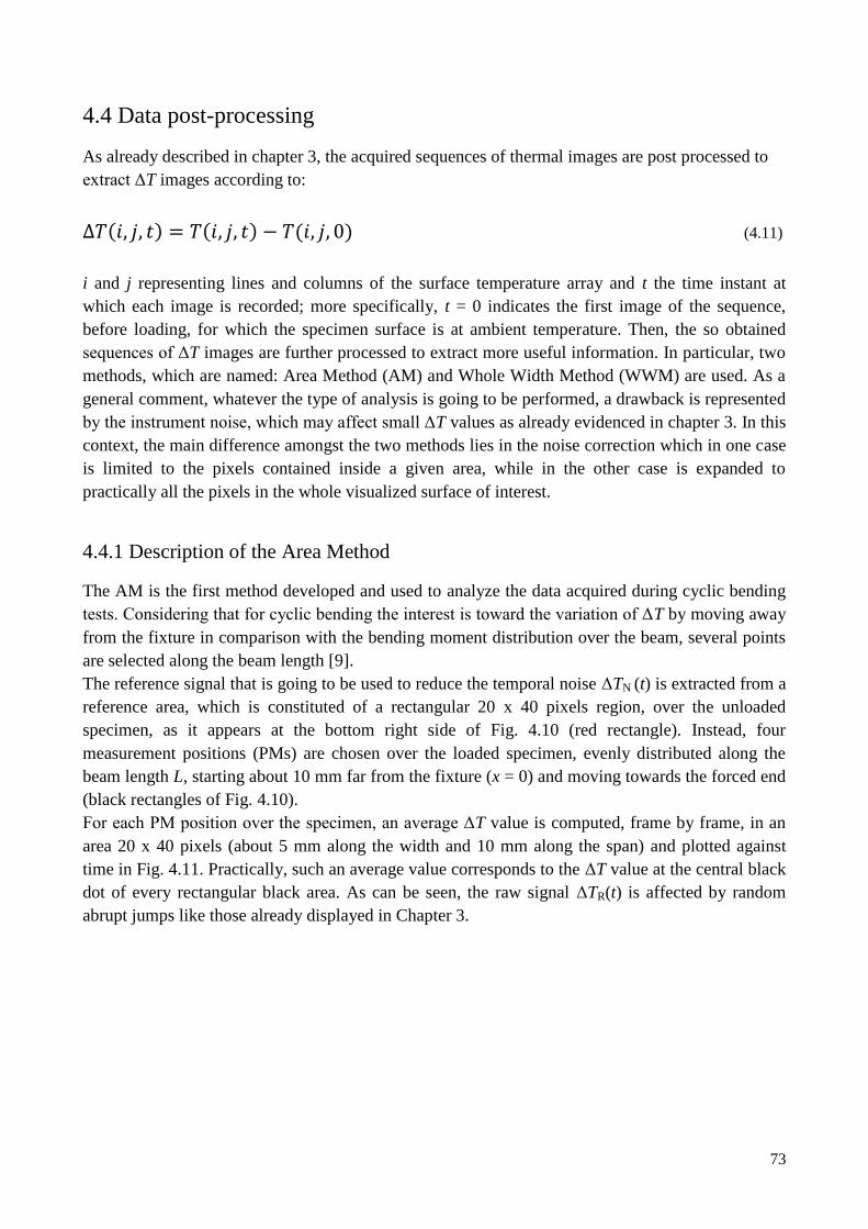
73
4.4 Data post-processing
As already described in chapter 3, the acquired sequences of thermal images are post processed to
extract ΔT images according to:
(4.11)
i and j representing lines and columns of the surface temperature array and t the time instant at
which each image is recorded; more specifically, t = 0 indicates the first image of the sequence,
before loading, for which the specimen surface is at ambient temperature. Then, the so obtained
sequences of ΔT images are further processed to extract more useful information. In particular, two
methods, which are named: Area Method (AM) and Whole Width Method (WWM) are used. As a
general comment, whatever the type of analysis is going to be performed, a drawback is represented
by the instrument noise, which may affect small ΔT values as already evidenced in chapter 3. In this
context, the main difference amongst the two methods lies in the noise correction which in one case
is limited to the pixels contained inside a given area, while in the other case is expanded to
practically all the pixels in the whole visualized surface of interest.
4.4.1 Description of the Area Method
The AM is the first method developed and used to analyze the data acquired during cyclic bending
tests. Considering that for cyclic bending the interest is toward the variation of ΔT by moving away
from the fixture in comparison with the bending moment distribution over the beam, several points
are selected along the beam length [9].
The reference signal that is going to be used to reduce the temporal noise ΔTN (t) is extracted from a
reference area, which is constituted of a rectangular 20 x 40 pixels region, over the unloaded
specimen, as it appears at the bottom right side of Fig. 4.10 (red rectangle). Instead, four
measurement positions (PMs) are chosen over the loaded specimen, evenly distributed along the
beam length L, starting about 10 mm far from the fixture (x = 0) and moving towards the forced end
(black rectangles of Fig. 4.10).
For each PM position over the specimen, an average ΔT value is computed, frame by frame, in an
area 20 x 40 pixels (about 5 mm along the width and 10 mm along the span) and plotted against
time in Fig. 4.11. Practically, such an average value corresponds to the ΔT value at the central black
dot of every rectangular black area. As can be seen, the raw signal ΔTR(t) is affected by random
abrupt jumps like those already displayed in Chapter 3.
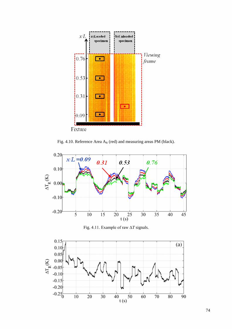
74
Fig. 4.10. Reference Area AR (red) and measuring areas PM (black).
Fig. 4.11. Example of raw ΔT signals.
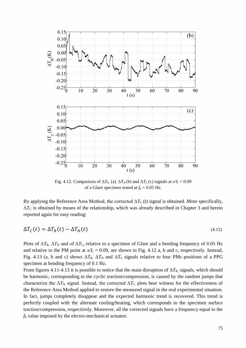
75
Fig. 4.12. Comparison of ΔTR (a), ΔTN (b) and ΔTC (c) signals at x/L = 0.09
of a Glare specimen tested at fb = 0.05 Hz.
By applying the Reference Area Method, the corrected ΔTC (t) signal is obtained. More specifically,
ΔTC is obtained by means of the relationship, which was already described in Chapter 3 and herein
reported again for easy reading:
(4.12)
Plots of ΔTR, ΔTN and of ΔTC, relative to a specimen of Glare and a bending frequency of 0.05 Hz
and relative to the PM point at x/L = 0.09, are shown in Fig. 4.12 a, b and c, respectively. Instead,
Fig. 4.13 (a, b and c) shows ΔTR, ΔTN and ΔTC signals relative to four PMs positions of a PPG
specimen at bending frequency of 0.1 Hz.
From figures 4.11-4.13 it is possible to notice that the main disruption of ΔTR, signals, which should
be harmonic, corresponding to the cyclic traction/compression, is caused by the random jumps that
characterize the ΔTN signal. Instead, the corrected ΔTC plots bear witness for the effectiveness of
the Reference Area Method applied to restore the measured signal in the real experimental situation.
In fact, jumps completely disappear and the expected harmonic trend is recovered. This trend is
perfectly coupled with the alternate cooling/heating, which corresponds to the specimen surface
traction/compression, respectively. Moreover, all the corrected signals have a frequency equal to the
fb value imposed by the electro-mechanical actuator.
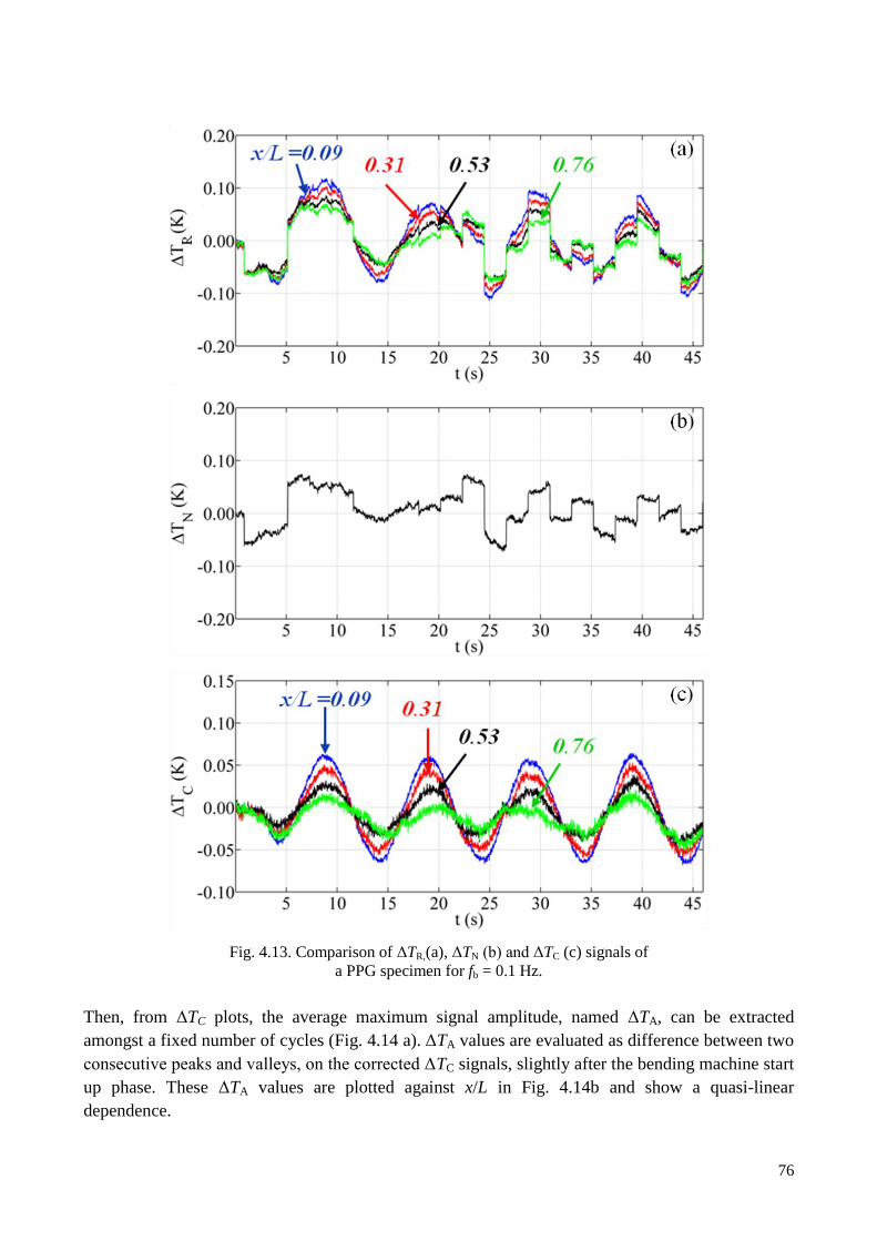
76
Fig. 4.13. Comparison of ΔTR,(a), ΔTN (b) and ΔTC (c) signals of
a PPG specimen for fb = 0.1 Hz.
Then, from ΔTC plots, the average maximum signal amplitude, named ΔTA, can be extracted
amongst a fixed number of cycles (Fig. 4.14 a). ΔTA values are evaluated as difference between two
consecutive peaks and valleys, on the corrected ΔTC signals, slightly after the bending machine start
up phase. These ΔTA values are plotted against x/L in Fig. 4.14b and show a quasi-linear
dependence.
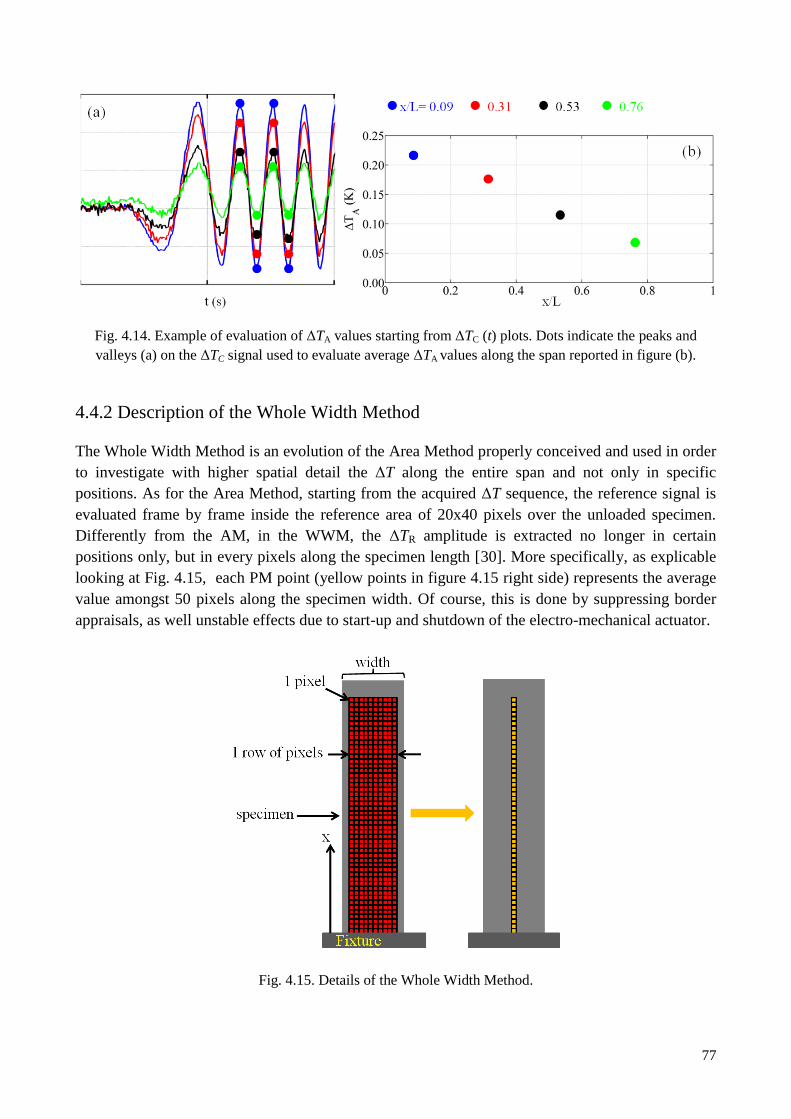
77
Fig. 4.14. Example of evaluation of ΔTA values starting from ΔTC (t) plots. Dots indicate the peaks and
valleys (a) on the ΔTC signal used to evaluate average ΔTA values along the span reported in figure (b).
4.4.2 Description of the Whole Width Method
The Whole Width Method is an evolution of the Area Method properly conceived and used in order
to investigate with higher spatial detail the ΔT along the entire span and not only in specific
positions. As for the Area Method, starting from the acquired ΔT sequence, the reference signal is
evaluated frame by frame inside the reference area of 20x40 pixels over the unloaded specimen.
Differently from the AM, in the WWM, the ΔTR amplitude is extracted no longer in certain
positions only, but in every pixels along the specimen length [30]. More specifically, as explicable
looking at Fig. 4.15, each PM point (yellow points in figure 4.15 right side) represents the average
value amongst 50 pixels along the specimen width. Of course, this is done by suppressing border
appraisals, as well unstable effects due to start-up and shutdown of the electro-mechanical actuator.
Fig. 4.15. Details of the Whole Width Method.

78
As a result, a distribution of ΔTR values over the specimen surface is reduced to a line of PM points
along the specimen length. Then, the Reference Area Method is applied to correct such ΔTR values
and to create a time sequence of ΔTC values in each PM point. Then, in each PM point an average
value is extracted amongst a certain number of load cycles, which ranges from 3 up to 8 depending
on the bending frequency (Fig. 4.16a). Finally, ΔTA values are evaluated from the average load
cycle as difference between peak and valley, as already described. The distribution of ΔTA along the
specimen length, as shown in Fig. 4.16b, is again quasi-linear and tending to zero for x/L → 1.
Fig. 4.16. Representation of ΔTC values; average load cycle (a); ΔTA values against x/L
obtained with WWM ( configuration 1) (b).
4.5 Qualitative evaluation of ΔT on the rear specimen surface
As already said in section 4.3.1, some tests have been performed by using a mirror (aluminium
sheet) to visualize also the rear specimen surface in order to gain information about the ΔT
evolution over this surface in comparison to what happens on the front surface. The acquired data
are post processed by means of the Area Method, previously described (Section 4.4.1), with the
only difference that also a PM point on the rear surface near to the fixture is considered (Fig 4.17).
Fig. 4.17. Details of specimens surface viewed with the aid of a mirror.

79
Some results obtained for specimens PPG and PJC2 solicited at a bending frequency of 0.5 Hz with
the test configuration 1 are shown in Fig. 4.18. In both plots, the red curve is relative to the PM
point over the front surface directly viewed by the infrared camera, while the black curve indicates
the ΔT evolution over the rear surface. It is worth noting that, due to the distortion effects
introduced by the mirror, the position of the PM point on the rear surface is about 0.1 mm far from
the fixture and not perfectly coincident with the position on the rear surface. Moreover, since care
was posed to focus the detector on the specimen front surface, the portion of image relative to the
back surface reflected by the mirror appears a bit blurred.
Fig. 4.18. A comparison of ΔTC plots at x/L = 0.1 and fb = 0.5 Hz on PPG (a) and
fb = 0.4 Hz on PJC2 (b) specimens.
It has to be noted that, for all the investigated specimens, the signal measured over the rear surface
(reflected by the mirror) is out of phase by 180° with respect to the signal measured over the front
surface. This is in agreement with the thermoelastic effect linked to the specimen oscillation; in
fact, when the front surface is in tension (cooling down), the rear one is in compression (heating up)
and viceversa, with an alternate cooling/heating effect. In addition, the signal reflected by the mirror
has a lower amplitude because of the absorption of the mirror and to defocusing effect; this effect
can be corrected through adequate calibration.
4.6 Influence of the bending frequency.
The frequency is a critical parameter in cyclic bending. Herein, the effects of bending frequency on
tests performed with configuration 1 are considered with the attention focused on plots of ΔTC
signals (Fig. 4.19) and mainly on the distribution of ΔTA against x/L (Fig. 4.20). In particular,
Fig.4.19 refers to ΔTC signals over time for the PLAJ specimen at different PM positions and
different bending frequencies from 0.1 Hz up to 2 Hz. Instead, Fig.4.20 shows examples of the
bending frequency effect on the distribution of ΔTA against x/L for some of the investigated
specimens.
Looking at Fig 4.19, some comments can be made. On the whole, ΔT displays harmonic variations,
which are perfectly coupled with the cyclic load. The ΔT amplitude increases with increasing the
bending frequency. The harmonic trend is more regular for the lowest x/L value, or better closest to
the specimen fixture (x/L = 0), where the bending moment reaches the highest value. As x/L
increases, i.e. moving towards the forced extremity, ΔT decreases mingling with the background
noise of the instrument. Moreover, from figure.4.20, it is possible to see that all ΔTA data lie over a

80
straight line with the maximum value achieved close to the fixture in agreement with the bending
moment.
Fig. 4.19. ΔTC over time for different fb values: (a) 0.1 Hz, (b) 0.3 Hz, (c) 0.5 Hz, (d) 2.0 Hz.
Test with configuration 1 on specimen PLAJ.

81
Fig. 4.20. Effect of bending frequency on ΔTA values for all the investigated specimens
(Test configuration 1).
To better investigate the role of the bending frequency in figure 4.21 are reported ΔTA values versus
fb for x/L=0.09 with the relative interpolation curves; these data are relative to Glare, GFRP and
PPG specimens.

82
Fig .4.21. ΔTA against fb at x/L = 0.09 for GLARE (a), GFRP (b),
PPG (c) and PLAJ (d) specimens. (Test configuration 1).
From Fig. 4.21 and by considering also values for others investigated specimens (not shown
herein), it seems that the ΔTA distribution is described by an exponential law:
(4.13)
with a and b, collected in Table 4.2, which seems to depend on the material characteristics. Of
course, more tests with a wider number of specimens is necessary to establish a correlation.
Specimen Code a (K) b (s)
GLARE 0.2388 -2.857
GFRP 0.1953 -30.740
PPG 0.1250 -25.56
PLAJ 0.2054 -16.33
Table 4.2. Values a and b relative to Eq. (4.13).
It has been observed that, in all the investigated cases, the bending frequency fb = 2 Hz guarantees
that the horizontal asymptotic value is reached. For this reason, the values of fb = 2.0 Hz is

83
considered as the best choice to compare the ΔTA values of different specimens. For lower values of
the bending frequency (fb = 0.05 Hz ÷ 0.1 Hz) the required adiabatic condition is not guaranteed
because there is enough time for the material under investigation to exchange heat with the
environment and through its thickness; this may cause a significant reduction of the measured ΔT
values. Of course, the minimum value of the bending frequency that allows to perform the cyclic
bending tests under adiabatic condition is not the same for all the investigated materials but depends
on their thermal diffusivity α, which is defined as:
(4.14)
where k, c and ρ are thermal conductivity, specific heat and density, respectively of the considered
material. In general, an average α value has to be considered for composite materials being them
composed of fibres and matrix that are characterized by different values of k, c and ρ.
4.7 The effects of the matrix on ΔT values in thermoplastic specimens
In this section, the effects of the matrix on ΔTA values are analyzed. This is done by considering
specimens that include a different matrix reinforced with the same type of fibres. In particular, Fig.
4.22a displays ΔTA values for four different specimens, which include the same jute fibres, but
embedded in a different type of matrix, which is:
neat polypropylene (PP)
polypropylene grafted with 2% of maleic anhydride (PC2)
polypropylene compatibilized with 5% of maleic anhydride (PC5)
poly lactic acid (PLA)
Instead, Fig. 4.22b displays ΔTA values for two specimens, which include glass fibres embedded in
either a neat polypropylene, or a 2% grafted one. The ΔTA values, reported in Fig. 4.22 (a) and (b)
are obtained with the test configuration 1 and fb =2 Hz.
From figure 4.22a it is evident that the specimens involving jute fibres embedded in a PLA matrix
exhibits higher values of ΔTA with respect to all the other specimens involving a PP matrix. As
second observation by comparing ΔTA values displayed by a specimen of pure polypropylene (e.g.,
PPJ) to those involving percentages of 2% (PJC2) and of 5% (PJC5) it is possible to see a
systematic increase of ΔTA with increasing the percentage of compatibilizing agent. For a direct
understanding of the influence of the compatibilizing agent, data taken with PP jute reinforced
specimens at fb = 2 Hz are plotted against the percentage of compatibilizing agent C% in Fig.4.23.
As can be seen, ΔTA displays an almost linear increase with C%.
Looking at figure.4.22b, which is relative to PP glass reinforced specimens, it appears that ΔTA
values decrease by increasing the percentage of the coupling agent. This is in contrast with what
showed by jute reinforced specimens. The coupling agent seems to have a different effect on ΔTA
values depending on the type of matrix-fibre combination. To better investigate the role played by
the coupling agent in specimens involving a PP matrix and to avoid any time-dependent effect, ΔTA
values are extracted from simple bending tests, which practically involve only the ΔTC values

84
relative to the first valley as indicated in Fig. 4.24. More specifically, these bending tests are
performed by applying to each specimen a simple bending of -7.5 mm, or -15 mm, starting from the
unloaded condition. These values, named ΔTa1, are plotted for x/L = 0.09 in Fig. 4.25.
Fig. .4.22. ΔTA against x/L for different thermoplastic composites; jute fibres reinforced (a) and glass fibres
reinforced (b). Results are relative to test configuration 1 and fb = 2 Hz.
Fig. 4.23. ΔTA against C% for fb = 2 Hz for specimens involving PP matrix
and reinforced with jute fibres. (Test configuration 1).

85
Fig. 4.24. A sketch of calculation of ΔTa1.
Fig. 4.25. ΔTa1 at x/L= 0.09 for the different specimens.
Looking at figure 4.25, it is possible to see that the amplitude (absolute value) attains a maximum
for specimens made of sole matrix and a minimum for specimens including jute fibres; for all
specimens the ∆Ta1 amplitude is practically proportional to the imposed deflection. It is also
possible to see that the grafted matrix entails increase of ∆Ta1 only for specimens made of either
sole matrix, or, to a certain extent, reinforced with jute fibres. On the contrary, ∆Ta1 seems to
decrease when a grafted matrix is reinforced with glass fibres. In particular, the increase of ∆Ta1 is
more significant in response to the addition of a percentage of 2% rather than to the 5% percentage.
In fact, the specimen PC5 displays a smaller ∆Ta1 increase with respect to the PC2 one, while a
small decrease is observed by comparing ∆Ta1 values of the PJC5 specimen to those of the PJC2
one.
To gain more insights about the role played by matrix and fibres, a comparison between the three
types of specimens: sole matrix, reinforced with glass fibres and reinforced with jute fibres is
analyzed and results are compared in Fig. 4.26. It is possible to see that the highest values of ΔTA
are achieved by the specimen PP (sole matrix) and the lowest ones by the PPJ (jute fibres); for each
specimen, all the points lie over an almost straight band in agreement with the bending moment
trend which attains a maximum near the fixture and decreases moving to the free edge. In
particular, the distribution of the PPJ specimen appears to display an up and down trend (Fig.
4.27a). These peaks seem to be driven by the fibres texture (Fig. 4.27b.) on the external layer

86
(viewed by the infrared camera). In fact, the down peaks appear located in correspondence of the
vertical jute bundles with amplitude variations linked to the step weaving.
Fig. 4.26. The compatibilizing agent effect on ∆TA from bending at fb = 2Hz (Test configuration 1)
of different types of specimens and obtained with the WWM method; specimens made of only
PP matrix (a); specimens made of PP reinforced with glass fibres (b) and jute fibres (c).
To be more accurate, we have to consider the effect of the jute fibres orientation with respect to the
direction of the applied load. In other words, the main difference between ΔTA ups and down peaks
seems to reside in the fact that the down peaks include the average value amongst pixels mostly
located all over jute fibres; conversely, the ups peaks include the average value amongst pixels

87
partly located over jute fibres (horizontal tracts) and partly over the matrix (i.e., the space between
two horizontal tracts). Thus, taking into account that, for a given load, it is expected that reinforcing
fibres are less deformed than the matrix, the expected reduction of the thermo-elastic effect in
correspondence of jute fibres and the increase of the same when the hosting matrix is partially
considered can easily explain the detected ups and down trend for ΔTA values.
Fig. 4.27. ΔTA against x/L for PPJ specimen at fb = 2 Hz: position of ups and down peaks (a)
with respect to fibres bundles (b).
The presence of 2% PP-g-MA (Fig. 4.26 a) affects significantly ΔTA values. In fact, the ΔTA values
of the PC2 specimen (sole matrix) displays a strong rise especially for small x/L values. Instead, to
an increase of the PP-g-MA content from 2% to 5% by weight corresponds a decrease of ΔTA. By
comparing Fig. 4.23b to Fig. 4.23c it is possible to see that, as an action of the grafted matrix, the
PGC2 ΔTA distribution has slipped down, while the PJC2 ΔTA distribution has moved up,
displaying an opposite thermal effect.
To deepen such a controversial behaviour we have to focus on two main aspects. One is the action
of the coupling agent within the specific matrix/fibre system, which is to improve adhesion between
fibres and matrix. The other one is the link between an improved interface (as consequence of
matrix grafting) and thermo-elastic effects. However, for a more comprehensive understanding, the
thermo-elastic effect, or better the Gough-Joule effect resulting from coupling of thermal and
mechanical fields [31,32] should be regarded from the atomic perspective [33]. In other words, it

88
should be considered the effects that the variations induced by the change of ingredients (addition
of PP-g-MA) in a pure matrix material, or at the interface of a composite material, may have on the
oscillation of individual particles.
4.8 A comparison between epoxy/resin and PP matrices in glass
reinforced specimens.
In this section the results obtained with GFRP, PPG and PGC2 specimens are compared to
underline the matrix effect on ΔT values. The specimens under investigation have almost the same
thickness and volumetric percentage of glass fibres. As difference between specimens, in PPG and
PGC2 the reinforcement consists in plain woven whilst in GFRP unidirectional layers at 0° and 90°
are arranged to obtain symmetrical and balanced laminates. This difference in fibres disposition is
not so important because a laminate having unidirectional fibres at 0 and 90 degrees can be
regarded as a composite material composed of plain woven having the same volumetric percentage
of fibres. The main difference consists in the used matrix and then in the interaction between fibre
and matrix at the interface. In Fig. 4.28 are reported the ΔTA values of these specimens obtained
with both methods AM (Fig. 4.28a) and WWM (Fig. 4.28b).
Fig. 4.28. Comparison between ΔTA values of specimens involving PP and epoxy/resin as matrix for test
configuration 1 at fb = 2 Hz; AM (a) and WWM (b).

89
From a comparison of ΔTA values, it is evident the different response of epoxy matrix based
specimens, which supply higher values. This is evident especially for data close to the fixture where
the ΔTA values of specimens involving the epoxy matrix are higher of about 0.05 K with respect to
the specimens having PP as matrix. This difference, looking at equation 4.8, may be ascribed to a
difference of the elastic modulus E that is higher for specimens involving the epoxy matrix.
4.9 The influence of fibres in thermoplastic matrix based specimens
In this section, to gain information about the role played by the fibres on ΔTA values, the results
obtained with specimens involving a neat PP as matrix reinforced with either glass, or jute are
compared. Notwithstanding the different thickness of the involved specimens, the obtained results
are compared in Fig. 4.29 because some interesting considerations can be made.
Fig. 4.29. A comparison of results for PPG and PP specimens. (Test configuration 1).
The ΔTA values for the PPG specimen are higher than those relative to the PPJ specimen; this is
probably due to the higher elastic modulus of the glass fibres with respect to that of the jute ones
(see Table 1.1 chapter 1). Quantitatively, the difference in terms of ΔTA is lower (about 0.02 K)
with respect to the difference in terms of elastic modulus. This can be explained by considering that
the PPG specimen is about 21% thinner than the PPJ one; in fact, from Eq.(4.8) it is possible to see

90
that ΔT varies linearly with the thickness h. Moreover, the differences in the fibres (glass and jute)
affects the thermo-elastic constant K.
4.10 Some bending coupled effects.
All the results till now showed are mostly relative to the test configuration 1 in which the specimen
is subjected to alternate tension/compression with a maximum deformation f of ±7.5 mm. In this
section, the results obtained with the two different test configurations (1 and 2) are compared in
order to investigate the influence of the test configuration on ΔT values. To this end, the cyclic
bending tests performed with f = ±7.5 mm (configuration 1) are compared with tests performed
with f = - 15 mm (configuration 2).
Looking at Eq.(4.3), it is clear that, for a given sample of given E and I values, if the deflection f
doubles also the applied concentrate force P doubles.
The results obtained with the different specimens PP, PC2, PPJ, PJC2, PPG, PGC2, at x/L = 0.1 for
the bending frequency of 2 Hz are shown in the following figures 4.30 - 4.32.
Fig. 4.30. ΔTC plots at x/L = 0.1 for bending tests performed at fb = 2 Hz on PP and PC2 specimens;
comparison between tests configurations 1 and 2.
First of all, looking at the plots (Figs. 4.30-4.32), it is possible to see that what already observed and
discussed in the previous sections for the test configuration 1 generally applies also for the test
configuration 2. In particular, also for configuration 2, it is possible to recognize a harmonic trend
over time whose frequency is equal to the applied bending frequency fb. The compatibilizing agent
has almost the same influence on the ΔT amplitude already described for each material tested with
configuration 1. However, some differences can be observed. First of all, for each specimen under
investigation the ΔT signal amplitude is higher for all the tests performed with configuration 2.
Moreover, for tests performed with configuration 2, a clear heating up effect can be noticed.

91
Fig. 4.31. ΔTC plots at x/L = 0.1 for bending tests performed at fb = 2 Hz on PPJ and PJC2 specimens;
comparison between tests configurations 1 and 2.
Fig. 4.32. ΔTC plots at x/L = 0.1 for bending tests performed at fb = 2 Hz on PPG and PGC2 specimens;
comparison between tests configurations 1 and 2.
In particular, for all the tests performed by means of configuration 2, ΔTA increases with the
number of cycles enclosed. This difference may be due to the different test dynamic. In fact, in
configuration 2 the specimen is subjected to a one side deflection of 15 mm which is higher with
respect to the 7.5 mm undergone on the same side under test configuration 1; this of course entails
also higher internal stresses. Moreover, in configuration 1 the observed surface is subjected to

92
alternate tension and compression conditions that causes ΔT variations from negative to positive
values, which may reduce the total ΔT amplitude. It is also worth noting that, in configuration 2, the
observed surface is subjected only to tension conditions that should cause only cooling linked to the
thermo-elastic effect. Instead, as already mentioned, even if the applied deflection remains constant,
ΔT tends to increase; this effect appears sudden after the first cycle, when the ΔT value does not
return to 0 as it should be, but becomes positive, with the specimen surface recovering its
undeformed condition. In addition, there is a positive increment of the ΔT amplitude after any cycle
of load as can be seen in Fig. 4.30-4.32 for test configuration 2. Besides, after a certain number of
cycles, only positive ΔT values are displayed as Fig. 4.33 shows.
It is clear that, as the distance from the fixture increases, the bending moment and the internal
stresses remain not constant along the beam but they decrease with the distance. Also, the afore
mentioned heating up effect decreases along the beam as shown in Fig. 4.33 in which ΔT signals
measured at three PM points along a PPG specimen for fb = 2 Hz (x/L = 0.1, 0.3, 0.5) are reported.
This may be explained by considering that the dissipated energy depends on internal stresses as will
be later explained.
Fig. 4.33. Heating up effect for varying the distance from the fixture
for specimen PPG under bending configuration 2
4.10.1 Some considerations about the heating up effects
The polymeric materials, especially the thermoplastic ones at temperature over the glass transition
one Tg, show a visco-elastic behaviour [34,35] rather than a pure elastic one like metals. The
polymeric materials, even if solicited in elastic conditions, dissipate a little amount of energy, which
is due to the internal friction between the polymeric macromolecules chains that, under
deformation, tend to move respectively. In composite materials, the internal energy dissipation is
not only due to the macromolecules interactions, but also to the friction at the interface between the
fibres and matrix. Of course, the higher is the total displacement f imposed to the specimen, higher
is the internal friction and much more important are the dissipative effects and in turn the dissipated
energy with temperature rise.
In particular, close to the clamp, where the stresses are the highest, the macromolecules,
constituting the matrix, are subjected to higher viscous interactions. Here, the relative displacement
attains a maximum, which promotes the dissipative phenomena and in turn temperature rise. Going

93
far from the fixture there is a gradual reduction of internal stresses with in turn a reduction of
displacement and dissipative phenomena and in turn lower temperature rise.
Of course, after each cycle of load, a small amount of energy is released by the dissipative
phenomena with an addition effect; this may justify the observed drift warming up effect in
configuration 2. In truth, this heating up effect is present also for bending tests in configuration 1,
but of reduced slope; indeed, this heating up effect becomes distinguishable only after a consistent
number of consecutive cycles of load (Fig. 4.34).
Fig. 4.34. ΔTC plots at x/L = 0.1 for bending tests performed at fb = 2 Hz
with configurations 1 and 2 on PPG and PPJ specimens.
Comparing the results obtained with the two test configurations 1 and 2 (Fig. 4.34), it is evident that
the slope of the heating up effect is higher for tests performed with configuration 2. Besides, for all
the tests performed by means of configuration 1, the heating up effect manifests itself like a ramp
having a small slope just starting from the first cycle. Whilst, in configuration 2, the heating up
effect starts with an abrupt increase which is later, after about 5s, followed by a gradual ramp.
These differences in the heating up effect observed for bending configurations 1 and 2 may mean
that something different is occurring inside the material when it is subjected to the different load
conditions.
In particular, focusing the attention on the bending configuration 2, the change in slope would mean
that initially, within the first few cycles, the amount of dissipated energy coupled with viscous
phenomena attains its maximum and then it decreases towards an almost constant value.
4.10.2 The influence of bending frequency on the heating up effect
It is well known that the visco-elastic behaviour of a material depends on the solicitation frequency
[34,35]. In this section, the dependence of the heating up effect from the bending frequency is
investigated for specimens involving the PP matrix. In particular, some T plots at x/L = 0.1,

94
obtained with bending configuration 2 on specimens PPG and PPJ are shown in Fig. 4.35. To allow
for a comparison, only five consecutive cycles of load are considered for each material; this because
at low fb values, data for only few cycles of load have been acquired, to avoid computer memory
overhead.
Fig. 4.35. The effect of the bending frequency fb on the heating up effect for
test performed on PPG (left) and PPJ (right) in configuration 2.

95
Looking at the plots of Fig. 4.35 it is possible to underline some differences relative to the heating
up effect with the bending frequency. In both of the cases for low values of the bending frequency
(fb = 0.05 and fb = 0.1 Hz) the ΔT signals are almost symmetric with respect to the 0 value; this
happens also when the bending is performed by means of configuration 2. This experimental
evidence might seem strange because in bending configuration 2 the observed surface undergoes
only tension and then, the cooling effect should prevail. Instead, for these values of fb the ΔT signal
appears almost symmetric with respect to 0 with its average value remaining almost equal to about
0 over time. This behaviour may be explained by considering that for low values of the bending
frequency the adiabatic condition is not fulfilled and the material under investigation has enough
time to exchange heat through its thickness and with the environment. Of course, it is worth
underlining that as fb increases the required adiabatic condition becomes ever more verified.
4.11 Some remarks to Chapter 4
As a main comment, the Reference Area Method has proved to be very effective in restoring all the
measured ΔT signals even when they were completely destroyed by the temporal noise.
For all the investigated materials ΔT attains its maximum value near the fixture and decreases
linearly to 0 at the free tip in agreement with the bending moment. In particular, the ΔT amplitude
depends on the bending frequency fb and it tends to assume a constant value for bending
frequencies equal to 2 Hz, or higher. This because the hypothesis of cyclic adiabatic condition for
low fb values is not fulfilled.
Besides, it has been noticed that the ΔT amplitude depends on the type of material employed,
meaning the type of matrix and/or reinforcement and on the likely presence of coupling agent,
which drives the internal stresses.
An heating up "ramp" effect has been observed mainly in thermoplastic matrix based materials and
especially for bending tests performed in configuration 2. This is due to materials internal
dissipations linked to viscoelastic effects and friction at the interface between the fibres and matrix.
Furthermore, the slope of the ramp seems to be dependent on the distance from the fixture, the
bending frequency and the material under investigation.
References to chapter 4
[1]. W. Thomson, On the thermoelastic, thermomagnetic and pyroelectric properties of matters. Phil
Mag 5, 4–27, 1978.
[2]. M.A. Biot, Thermoelasticity and irreversible thermodynamics. J Appl Phys,27, 240–53, 1956.
[3]. J.M. Dulieu-Barton, P. Stanley, Development and applications of thermoelastic stress analysis. J
Strain Anal, 33, 93–104, 1998.
[4]. P. Stanley, W.K. Chan, The application of thermoelastic stress analysis to composite materials. J
Strain Anal, 23, 137–42, 1988.
[5]. U. Galietti, D. Modugno, L. Spagnolo, A novel signal processing method for TSA applications.
Meas Sci Technol, 16, 2251–60, 2005.
[6]. T.R. Emery, J.M. Dulieu-Barton, J.S. Earl, P.R. Cunningham, A generalised approach to the
calibration of orthotropic materials for thermoelastic stress analysis. Compos Sci Technol, 68, 743–
522, 2008.
[7]. M.G. Beghi, C.E. Bottani, G. Caglioti, Irreversible thermodynamics of metals understress. Res
Mech, 19, 365–79, 1986.
[8]. M.P. Luong Fatigue limit evaluation of metals using an infrared thermographic technique. Mech
Mater, 28, 155–63, 1998.

96
[9]. S. Boccardi, G.M. Carlomagno, C. Meola, G. Simeoli, P. Russo, Infrared thermography to
evaluate thermoplastic composites under bending load, Composite Structures, 134, 900-904, 2015.
[10]. C. Meola, G.M. Carlomagno, C. Bonavolontà, M. Valentino, Monitoring composites under bending
tests with infrared thermography, Adv. Opt. Technol. 2012, 7 p. 2012.
[11]. S. Boccardi Master Thesis,Termografia all'infrarosso nel monitoraggio di materiali compositi sotto
carico di flessione, 2013.
[12]. S. Boccardi, G.M. Carlomagno, C. Bonavolontà, M. Valentino, C. Meola, Infrared thermography to
monitor Glare® under cyclic bending tests with correction of camera noise, in: Proc. QIRT 2014,
Bordeaux, France, July 2014, pp. 7-11 paper 215.
[13]. L. Sorrentino, G. Simeoli, S. Iannace, P. Russo, Mechanical performance optimization through
interface strength gradation in PP/glass fibre reinforced composites, Composites Part B, 76, 201-
208, 2015.
[14]. P. Russo, G. Simeoli, D. Acierno, V. Lopresto, Mechanical properties of virgin and recycled
polyolefin-based composite laminates reinforced with jute fabric, Polymer Composites 36, 2022-
2029, 2015.
[15]. H.A. Rijsdijk, M. Contant, A.A.J.M. Peijs, Continuous-glass-fibre-reinforced polypropylene
composites: I. Influence of maleic-anhydride-modified polypropylene on mechanical properties,
Compos. Sci. Technol., 48, 161–172, 1993.
[16]. E. Mäder, H.J. Jacobasch, K. Grundke, T. Gietzelt, Influence of an optimized interphase on the
properties of polypropylene/glass fibre composites, Compos. Part A 27, 907–912, 1996.
[17]. K.L. Pickering, M.G. Aruan Efendy, T.M. Le, A review of recent developments in natural fibre
composites and their mechanical performance, Compos. Part A 83, 98-112, 2016.
[18]. S.M.B. Nachtigall, G.S. Cerveira, and S.M.L. Rosa, New polymeric-coupling agent for
polypropylene/wood-flour composites, Polym.Test., 26, 619-628, 2007.
[19]. M. Sain, P. Suhara, S. Law, and A. Bouilloux, Interface modification and mechanical properties of
natural fiber-polyolefin composite products, J. Reinf. Plast. Compos., 24, 121-130, 2005.
[20]. M. Van den Oever, T. Peijs, Continuous-glass-fibre-reinforced polypropylene composites II.
Influence of maleic anhydride modified polypropylene on fatigue behavior. Compos Part A, 29,
227-239, 1998.
[21]. D. Bikiaris, P. Matzinos, A. Larena, V. Flaris, C. Panayiotou, Use of silane agents and
poly(propylene-g-maleic anhydride) copolymer as adhesion promoters in glass fibre/polypropylene
composites. J Appl Polym Sci, 81, 701-709, 2001.
[22]. L. Sorrentino, G. Simeoli, S. Iannace, P. Russo; Mechanical performance optimization through
interface strength gradation in PP/glass fibre reinforced composites, Composites part B, 76, 201-
208, 2015.
[23]. P. Russo, G. Simeoli, D. Acierno, V. Lopresto, Mechanical Properties of Virgin and
RecycledPolyolefin-Based Composite Laminates Reinforced With Jute Fabric, Polymer
Composites, 36, 2022-2029, 2015.
[24]. M.A. Kha, G. Hinrichsen, L.T. Drzal, Influence of novel coupling agents on mechanical properties
of jute reinforced J. Mater. Sci. Lett., 20, 1711-1713, 2001.
[25]. A.H. Haydaruzzaman, M.A. Khan, A. Hossain Mubarak, A. Khan Ruhul, M.A. Khnn Hakim,
Fabrication and Characterization of Jute Reinforced Polypropylene Composite: Effectiveness of
Coupling Agents, J. Comp. Mater., 44, 1945-1963, 2010.
[26]. S. Boccardi, C. Meola, G.M. Carlomagno, L. Sorrentino, G. Simeoli, P. Russo, Effects of Interface
Strength Gradation on Impact Damage Mechanisms in Polypropylene/Woven Glass Fabric
Composites, Composites Part B: Engineering, 90, 179-187, 2016.
[27]. S. Boccardi, G.M. Carlomagno, C. Meola, G. Simeoli, D. Acierno, S. Iannace, L. Sorrentino, P.
Russo, Lock-In Thermography (LT) for Investigation of Impact Damage Hibrid
Polypropylene/Glass composite, IEEE A&E System Magazine, 2016.
[28]. G. Simeoli, D. Acierno , C. Meola , L. Sorrentino, S. Iannace, P. Russo, The role of interface
strength on the low velocity impact behaviour of PP/glass fibre laminates, Composites: Part B,
62,88-94, 2014.
[29]. ASTM D747 − 10, Standard Test Method for Apparent Bending Modulus of Plastics by Means of a
Cantilever Beam.
[30]. S. Boccardi, G.M. Carlomagno, C. Meola, G. Simeoli, P. Russo, Visualization of Thermal Effects
in Polypropylene-Based Composites under Cyclic Bending Tests, International Symposium on

97
Dynamic Response and Failure of Composite Materials, DRAF 2016, Procedia Engineering, 167,
71-79,2016.
[31]. J. Gough, Memoirs of the Literary and Philosophical Society of Manchester, Second series 1, 288
1805.
[32]. J.P. Joule, On Some Thermo-Dynamic Properties of Solids, Phil. Trans. Roy. Soc. London 149, 91-
131, 1859.
[33]. B. Schweizer, J. Wauer, Atomistic explanation of the Gough-Joule-effect, The European Physical
Journal B, 23, 383-390, 2001.
[34]. J.D. Ferry, Viscoelastic Properties of Polymers, 1980, 3° edition, Wiley ISBN 978-0-471-04894-7.
[35]. H.F. Brinson, L.C. Brinson, Polymer Engineering Science and Viscoelasticity Springer, New York,
2015, ISBN: 978-1-4899-7484-3.

98
Chapter 5
Impact tests
Nomenclature
Ah Warm area.
DA Impact damage measured along the +45° direction.
Dav Impact damage average diameter.
DB Impact damage measured along the -45° direction.
DH Impact damage measured along the horizontal direction.
DV Impact damage measured along the vertical direction.
E Impact Energy.
Ea Total impact energy absorbed by the specimen.
Eb Amount of the impact energy absorbed as bending energy by the specimen.
Ed Amount of the impact energy absorbed as damage energy by the specimen.
Edb Amount of Ed used for fibre breakage.
Edd Amount of Ed used for delamination.
Em Amount of the impact energy absorbed as membrane energy by the specimen.
f Lock-in heating frequency.
FR Infrared camera frame rate.
i Row index.
j Column index.
K Frame number denoting the generic ΔT image in the sequence immediately after the end of
the cooling down effect
N Number of pixels having a given value of ΔT.
p Dept starting from the material surface.
Ph Number of pixels affected by the heating-up effect due to the impact.
sr Spatial resolution.
t Image index in the sequence or time.
tp Time to reach the ΔTMin.
T Temperature.
x Spatial coordinate along the horizontal direction.
y Spatial coordinate along the vertical direction.
Greek Symbols.
α Thermal diffusivity.
ΔT Temperature difference.
Δt Impact duration in time of the cooling effect.
∆Tb ΔT threshold value.
ΔtD Time to the heating onset.
TC Corrected ΔT values.
ΔTCRef Corrected ΔTRef image.

99
ΔTCw Corrected ΔTw image
ΔTMax Maximum absolute value of ΔT.
ΔTMin Minimum absolute value of ΔT.
∆TRN Temporal noise evaluated in the reference area.
ΔTRef Reference average Image immediately before the impact.
ΔTw Warm image; reference average Image after the impact the impact.
μ Thermal diffusion length.
Standard deviation.
ϕ Image phase angle.

100
Introduction
The weakness of composites, at least those based on a thermoset matrix, to impact load is a well
known problem [1-4]. Mostly dangerous is the impact at low energy, which does not produce
damage visible on the external surface but rather buried delamination between the layers. In
general, composites are able to absorb the impact energy within their polymeric matrix that
distributes the energy in the material; in this way, a low-energy (low-velocity) impact does not
produce perforation but delamination between the layers, with no visible surface manifestation,
whereas the structural integrity may be severely affected [5].
Indeed, the impact damage of composites happens through complex mechanisms and is still not
completely understood. This is mainly due to the multitude of materials that can be created by
changing any of their constituents: matrix, reinforcement, stacking sequence, curing process etc. In
fact, it is sufficient to add a new ingredient in the matrix, or change the orientation of a fibres layer
to develop a new material.
Since the introduction of composites in the construction of aircraft, a primary task was to establish
the delamination threshold load (DTL) [6-8]. However, notwithstanding the huge amount of
available data coming from both numerical simulation and experimental testing (see also references
to chapter 1), a methodology to unambiguously establish the DTL still has not been completely
achieved. This is because the DTL depends on many factors, first of all the material mechanical
characteristics but also the geometry of the target [8,9] and of the impactor [10].
Another problem within composites is linked to defects that can be accidentally induced during
their manufacturing processes. Indeed, these processes are probably primarily responsible for the
occurrence of defects, particularly for porosity formation. In fact, porosity typically forms during an
incorrect curing procedure due to uncontrolled or unexpected variations of the involved parameters,
such as temperature, pressure, duration etc. A certain percentage of gas may remain entrapped
within the material (essentially the matrix) and may give rise to formation of voids, which may
modify the material in service performance. In fact, the detrimental effects of voids on composites’
mechanical properties [11,12] are well recognized. Of course, the presence of porosity may also
affect the behaviour of the material under impact load, with amplification of the bulk material
weakness. Porosity is linked to manufacturing processes and can be reduced but not completely
eliminated [13]. Perhaps this is one of the reasons why composite materials display a large variety
of damaging behaviours under impact [14]. The negative effects of voids and other manufacturing
defects on the impact damage of glass/epoxy specimens were also observed by Meola and
Carlomagno [15] while using infrared thermography to investigate the response of composites to
impact events.
Thus, once a new material is created, it is mandatory to assess its impact damage resistance
especially if such material is predestined to an application sector which is highly exposed to impact
load.
5.1.Description of specimens
Several different specimens are considered, which involve different types of matrix and fibres. In
particular, owing to the type of matrix, the specimens are grouped into two families:

101
thermoplastic matrix based specimens
thermoset matrix based specimens.
This distinction is performed because of the dominant role played by the matrix in the material
damaging modality. It is worth noting that also an aluminium foam sandwich panel has been
investigated, which does not belong neither to the thermoplastic, nor to the thermoset, classification
made before. Each specimen is identified with a code involving the used matrix, fibres and other
most important characteristics. The specimens code with the most important details are collected in
Table 5.1.
Specimen Code Composition (Matrix – Reinforcement) Thickness (mm)
PPG Neat PP - Woven glass fibres 3.0
PGC2 Modified PP (2 wt% PP-g-MA) Woven Glass fibres 3.0
PPJ Neat PP - Woven jute fibres 3.8
PJC2 Modified PP (2 wt% PP-g-MA) Woven jute fibres 3.8
PLAJ Neat PLA-Woven glass fibres 3.8
PEF Neat PE-Unidirectional flax fibres at 0° 3.6
GFRP Epoxy adhesive preimpregnated
unidirectional glass fibres [02, 904]s
3.1
CFRPU Unidirectional carbon fibres [0/90°/+45/-45°]s
preimpregnated with epoxy resin
2.3
CFRPF Fabric carbon fibres [0/90°/+45/-45°]s
preimpregnated with epoxy resin
3.2
CFRPFU Fabric and unidirectional carbon fibres
[0/90°/+45/-45°]s preimpregnated with epoxy resin
5.0
CFRPNC Non-Crimp Fabrics (NCF), Multiaxial
Reinforcements (MR) and
5 Harness Satin Weave (HSW)
7.8
AFS Aluminium foam sandwich panel 10.0
Table 5.1. Some specimens details.
Some specimens, such as those identified with the codes:
PPJ
PJC2
PPG
PGC2
PLAJ
GFRP
were already described in chapter 4 and then, the reader is sent back there for more details. Instead,
more details for new specimens are listed below:
CFRPU includes a thermoset (epoxy resin) matrix reinforced with unidirectional carbon
fibres following the stacking sequence [0/45/90/-45]s. More specifically, 12 pre-

102
impregnated plies are overlaid by the hand lay-up technology and cured in autoclave.
Specimens are 150x100 mm2 and are 2.3 mm thick.
CFRPF is a panel of square side 500 mm. It is made of carbon fibres woven fabric layers
embedded in epoxy resin. The total numbers of overlapped plies allows to obtain a total
thickness of 3.2 mm.
CFRPFU is a panel of square side 500 mm and nominal thickness 5 mm. It is a multilayer
laminate reinforced with carbon and involving epoxy resin matrix. The fibres are oriented
following the stacking sequence [0/90/+45/-45]s; fibres are of both fabric and unidirectional
types.
CFRPNC has a complex architecture including Non-Crimp Fabrics (NCF), Multiaxial
Reinforcements (MR) and 5 Harness Satin Weave (HSW) and has a thickness of 7.8 mm
and square shape of side 485 mm. It is fabricated by the hand lay-up technology and
appropriate curing cycle in autoclave.
PEF is a square panel of 600x600 mm2 made of flax unidirectional fibres at 0 degrees
embedded in a Polyethylene (PE) matrix with a total thickness of 3.6 mm.
AFS is an aluminium foam sandwich panel consisting in a three-layer composite comprising
a foamable (containing TiH2 as a blowing agent) aluminium alloy sheet as a core layer and
two face sheets still in aluminium alloy on both sides. The AFS panel is 92 x 48 mm2 and
has a total thickness equal to 10 mm, with foam thickness of 8 mm and average cell size of
the foam bubbles of 2 mm. The surface viewed by the infrared camera was painted with
opaque paint in order to increase its emissivity.
It is worth noting that aluminium foam sandwiches (AFS) [16-18], obtained by combining metal
face sheets with a lightweight metal foam core, have peculiar properties (low specific weight,
efficient capacity of energy dissipation, high impact strength, acoustic and thermal insulation, high
damping), that make them interesting for a number of practical applications, such as the realization
of lightweight structures with high mechanical strength and good capacity of energy dissipation
under impacts. Core deformation and failure are decisive factors for the energy absorption
capability of sandwich structures. After fracture of the skin, the impacting object may damage and
penetrate into the core. With aluminium honeycomb cores, damage consists of crushing or
“buckling” of cell walls in a region surrounding the impact point, while, in foam cores, damage
looks more like a crack for low-energy impacts [19].
5.2. Conventional procedure for assessing impact resistance of new
composite materials.
The performance to impact of new composite materials is generally assessed through specific
impact tests [20]. Amongst other tests, it is generally required to draw damage maps, or plots of
damage area vs. impact energy. This also means to search for the impact energy that has caused a
damage of given size; this size is generally intended to include the whole extension of delamination
and is established through specific testing procedures. First of all, several specimens must be
fabricated of specific dimensions, according to the testing machine to be used. Specimens may be

103
relatively small to allow for one impact only, or quite large allowing for more than one impact, each
in a different place. Then, an initial value of the impact energy is chosen, according to current
knowledge and relaying to the behaviour of similar materials previously tested. The procedure
consists in a sequence of operation: A) put the panel in the impact machine, B) perform the impact,
C) remove the panel, D) perform non-destructive tests and evaluate the resulting extension of
delamination.
At this point, three cases may arise:
1. the requested size is found at the first attempt and tests stop;
2. the measured delamination is smaller than the prefixed value requiring more tests at
increasing energy;
3. the measured delamination is larger than the prefixed value requiring more tests at
decreasing energy.
However, it is generally unlikely to hit the imposed damage extension at the first attempt (point 1);
usually (points 2 and 3), many attempts are necessary with repetition of the operations at point A.
This involves removing and putting again the same, or another, specimen, in the impact machine for
another impact of different energy and so on. This also requires successive non-destructive testing
(NDT) and damage area measurement. Naturally, this procedure is time consuming and, sometimes,
not very accurate. In fact, the most commonly in use NDT techniques may fail to detect the actual
delamination extent essentially because of two main problems:
Two delaminated surfaces tend to tightly adhere once the impactor moves away.
Delamination propagates through tortuous pathways.
These problems may led to undetected delamination, or to underestimation of its real size with
obvious negative consequences on the component life.
Conversely, using infrared thermography, it is possible to recognize the type of arisen damage, from
the temperature rise and from the extension of the warm area, directly during online monitoring
with time saving. This is because the thermal signatures can be related to what occurred to the
material under load and help to understand the impact damage mechanisms, as well to estimate the
overall affected impact zone.
In the next section an example of inspection of impacted laminates is given by using two NDT
techniques: Lock-in thermography (LT) and Phased Array Ultrasonic (PAUT)
5.2.1 Lock in thermography: test setup and procedure
As shown in Fig. 5.1, the present test setup for LT includes the specimen, the infrared camera and
one or two halogen lamp (1 kW each) for thermal stimulation of the specimen; in particular, one
lamp is enough for small specimens, while two are used for larger ones. The heating source and the
infrared camera are positioned on the same side with respect to the observed surface (reflection
mode). The used infrared camera is the SC6000 (Flir systems). The distance of both camera and
lamp (lamps) to the specimen surface is varied between 0.5 and 1 m with care put to their mutual
orientation to avoid reflections. The camera is equipped with the Lock-in module that drives the

104
halogen lamp to generate a sinusoidal thermal wave of selectable frequency f and the IRLock-In©
software (supplied with the IR Lock-in package) for performing lock-in thermography analysis.
Lock-in thermography is well described in literature [21-30]. The thermal wave, delivered to the
specimen surface, propagates inside the material and gets reflected when it reaches zones where the
heat propagation parameters change. The reflected wave interacts with the surface wave producing
an oscillating interference pattern, which can be measured in terms of either temperature amplitude
or phase angle ϕ, and represented as amplitude, or phase, images, respectively. The basic link of the
thermal diffusion length μ to the heating frequency f and to the mean material thermal diffusivity
coefficient α is via the relationship:
(5.1)
The depth range for the amplitude image is given by μ, while the maximum depth p, which can be
reached for the phase image, corresponds to 1.8 μ [22-24]. In general, it is preferable to reduce data
in terms of phase image because of its insensitivity to both non uniform heating and local variations
of emissivity coefficient, over the monitored surface. Hence, the material thickness, which can be
inspected, depends on the wave period (the longer the period, the deeper the penetration) and on the
material thermal diffusivity. According to Eq.(5.1), the knowledge of the mean thermal diffusivity
is fundamental to evaluate the depth at which any detected anomaly is located, or to chose the
frequency value to check the material conditions at a given depth. To this end, the overall thermal
diffusivity α can be evaluated with the lock-in technique itself [31,32], or with flash thermography
[33,34].
Fig.5.1. Lock-in test setup.
5.2.2 PAUT test setup
PAUT tests are performed with an Olympus OmniScan SX flaw detector with a 16:64PR phased
array unit equipped also with a conventional UT channel for pulse-echo, pitch-catch, or TOFD
inspection [35,36]. Phased array elements are pulsed in such a way as to cause multiple beam
components to combine with each other and form a single wave front travelling in the desired
direction. Similarly, the receiver function combines the input from multiple elements into a single
presentation. Because phasing technology permits electronic beam shaping and steering, it is

105
possible to generate a vast number of different ultrasonic beam profiles from a single probe
assembly, and this beam steering can be dynamically programmed to create electronic scans.
Phased array ultrasonic instruments utilize high frequency sound waves to check for the internal
structure of a test piece, or measure its thickness, and rely on the same basic laws of physics that
govern sound wave propagation. The ability to generate multiple transducer paths within one probe
adds a powerful advantage in the detection, and naturally increases the ability to ‘‘visualize” an
inspection by creating an image of the inspected zone. Phased array imaging provides the user with
the ability to see relative point to point changes and multi-angular defect responses, which can assist
in flaw discrimination and sizing [37]. An encoded 5 MHz, 64 element linear array probe with a
straight wedge and by employing a specific gel as coupling medium has been used. Besides, no
calibration blocks are used, the measurement of the specimen thickness being taken as reference; it
is worth noting that it is generally difficult to fabricate reference blocks.
5.2.3 Some results of LT inspection
Some phase images of specimens, all impacted at 10 J, are shown in the following figures 5.2-5.4.
Fig.5.2 and Fig. 5.3 show phase images taken at different frequencies on the impacted surface of
PPG and PGC2 specimens, respectively.
From phase images and by knowing the spatial resolution of the used instrument (infrared detector
and lens), it is possible to measure the size of the damaged area; for present tests, the spatial
resolution is in the range 3–3.7 pixels/mm. Quantitative measurements are expressed in terms of the
two diameters DH and DV (along horizontal and vertical directions), which are reported on phase
images taken at f = 0.15 Hz (Figs. 5.1c and 5.2c) [38]; a threshold value according to Ref [28] has
been considered. DH and DV values are reported on Table 5.2.
Fig. 5.2. Phase images of specimen PPG impacted at E =10 J; (a) f =0.53 Hz; (b) f =0.36 Hz; (c) f =0.15 Hz.
Fig. 5.3. Phase images of specimen PGC2 impacted at E = 10 J;(a) f =0.53 Hz; (b) f =0.36 Hz; (c) f =0.15 Hz.

106
As can be seen, for the specimen PGC2 at f = 0.53 Hz (Fig. 5.3a), an almost circular dark zone,
which enlarges by decreasing the heating frequency to 0.15 Hz, is present. Such a variation of area
accounts for the damage progression through the specimen thickness. The damaged area assumes a
different shape for the specimen PPG (Fig. 5.2), showing a long branch along the horizontal
direction and a shorter one in the vertical direction. The presence of the two branches accounts for a
larger damaged zone; in particular, the different length of the two branches indicates a different
extension of the damage along the two directions [39].
The phase images taken from the rear surface (opposite to the impacted one) of the two specimens
CFRPU and GFRP, showing the largest detectable damage, are compared in Fig. 5.4 with their
characteristic dimensions DH and DV. As can be seen, the damage develops mostly along the fibres
direction [40]. In fact, a long horizontal stripe with smears along the fibres at 45° is visible for the
CFRP specimen (Fig. 5.4a); instead, an oblong structure with its longer side along the vertical
direction is visualized for the GFRP specimen (Fig. 5.4b). For both specimens it is also possible to
see the presence of other signs, like fibres orientation, presence of porosity and further details.
Particular consideration deserves the GFRP specimen being the material translucent in the visible
wavelength. In fact, after impact, a local permanent faded area is visible to the naked eye in
transparency, which corresponds to the damaged area and can be assumed as a reference. Such
visible area (Fig. 5.4c) well matches the damaged area detected by LT (Fig. 5.4a).
Fig. 5.4. Phase images showing the largest detectable damage for thermoset matrix specimens, taken from
the rear side at f=0.05 Hz; (a) GFRP; (b) CFRPU. (c) Visible image taken from the rear side GFRP.

107
Specimen DH (mm) (LT) DV (mm) (LT)
CFRPU 14 11
GFRP 7 13
PPG 30 15
PGC2 10 10
Table. 5.2. Comparison of DH and DV performed obtained with LT; impact at E = 10 J.
5.2.4 Comparison of LT and PAUT results
A comparison is made between results obtained with the specimen CFRPFU (see Table 5.3) that has
been impacted in three different places with three values of impact energy 18, 29 and 39 J,
respectively. The inspection with LT is performed by viewing the side opposite to impact (the same
viewed during impact monitoring) and by varying the heating frequency. A thermal diffusivity
equal to 0.0085 cm2/s was evaluated with lock-in thermography itself owing to a sound material
zone; of course, thermal diffusivity varies with the material being damaged. The three impacts are
distinguishable already at f = 0.88 Hz (depth of about 1 mm, evaluated from Eq.(5.1)), but the best
contrast is attained for f = 0.36 Hz. A phase image of the entire specimen is shown in Fig. 5.5 with
superimposed, for more details, also single images for each impacted zone.
The single images were taken with enhanced resolution (shorter distance) and refer to the same
frequency of 0.36 Hz of the whole image (depth p = 1.7 mm). From the phase images, it comes out
that the most important damage develops along the direction DB (along -45°). In particular, DB = 24,
32 and 34 mm for E = 18, 29 and 39 J, respectively. Some damage occurs along DA (i.e., +45°) but
it is milder and tends to get confused with the differences in the phase angle induced by the material
architecture.
Fig. 5.5. Phase image taken at f = 0.36 Hz, p = 1.7 mm.
C_scans and S_scans obtained with PAUT are reported in the following Figs. 5.6–5.8.The C-scan
images (Figs. 5.6a, 5.7a and 5.8a) show presence of surface damage. In particular, the central red
areolas, which increase in number with increasing of the impact energy, indicate indentation

108
damage, impact surface penetration and surface cracks. The surrounding yellow/blue areas, with a
lower signal amplitude, immediately suggest the presence of wider delaminations of different
orientations and at different depths through the thickness. From the circular C_scan view, it is
possible to measure an average diameter Dav that gives values equal to 24 mm (Fig. 5.6a), 32 mm
(Fig. 5.7a) and 34 mm (Fig. 5.8a) which practically coincide with DB values obtained from phase
images. However, the C_scan supplies a total view of the damage and does not allow for a direct
comparison with the phase image that is more selective in depth. Instead, a comparison with the
S_scan is feasible for locating the damage in depth. In fact, from the S_scans, it seems that, apart
from surface indentation, the most important damage is located between 1 and 1.6 mm from the
bottom. This is in general agreement with LT observations. Damage diameters obtained from LT
and PAUT images are reported in Table 5.3.
Fig. 5.6. PAUT results E = 18 J. C_scan (a), S-scan (b).
Fig. 5.7. PAUT results E = 29 J. C_scan (a), S-scan (b).
Fig. 5.8. PAUT results specimen E = 29 J. C_scan (a), S-scan (b).

109
E (J) DB (LT) Dav (PAUT)
18 24 24
29 32 34 39 34 34
Table 5.3 Quantitative data for damage extension.
Non-destructive testing with lock-in thermography and PAUT show a satisfactory agreement and
allow identification of impact damage [41-44]. Both LT and PAUT have their own advantages and
limitations. LT is fast to detect impact damage over large panels in non contact mode, but is
affected by loss of contrast in presence of deep defects. PAUT is more effective in the estimation of
the thickness and in the inspection of thick parts, but can be applied only over smooth surfaces and
requires a coupling medium. However, from an integrated analysis of C_scan, S_scan and phase
images it is possible to get useful information for a better evaluation of the material and for the
comprehension of some aspects, which may appear not understandable owing to the output of one
technique alone. In fact, the C_scan supplies a total view of the occurred damage, the S_scan helps
to locate the damage through the specimen thickness, while the phase images allow understanding
the evolution of the damage with respect to the fibre direction.
5.3. The added value of online monitoring
The scope of this section is to describe data obtained with online monitoring and to show as the use
of infrared thermography may be advantageous to get information, which are useful to estimate the
performance under impact of new composite materials. In particular, the main aim is to gain new
information about the damage mechanisms of several kinds of composites starting from the
sequences of thermal images acquired during the impact event. This is possible since the percentage
of impact energy, which produces the damage, is dissipated as heat with a local increase of
temperature. Then, the material damage can be associated with the surface temperature variation
visualized by the infrared camera.
It is worth noting that, during the impact event, the impact energy is in part elastically stored by the
material and returned back to the impactor, while the remaining part is mostly dissipated to produce
the damage. In particular, the specimen initially bends under the impactor pushing force and so, the
material surface opposite to the impacted one is subjected to a positive volume variation and
experiences a fast cooling down. This is due to the thermoelastic effect that vanishes once the
impactor pushing force is removed and the surface recovers its straight appearance. As will be
shown later, the cooling down effect, visualized by the infrared camera, can be used to obtain useful
information about the elastic energy stored by the material, the impact duration as well as the
overall extension of the impact affected area. Conversely, the material heating up can be exploited
to know more on its damaging under impact.
Different types of composites are considered, which involve change of either the matrix, or the
reinforcement.
The experimental investigation is conducted with two main purposes:

110
1. Analysis of impact dynamics - by visualizing the evolution in time and in space of thermo-
elastic/plastic phenomena arising during an impact event in order to get information useful
for a deeper understanding of the impact damaging mechanisms.
2. Evaluation of the impact damage - by developing a procedure to define the limit between
sound and damaged materials in order to outline and quantitatively measure the overall
extension of the impact affected area by using the acquired thermal images.
More specifically, the discussion will start with some qualitative considerations on the acquired
images and proceeds towards more quantitative outcomes with the two points 1 and 2, first,
separately addressed and, then, mutually considered since the outcomes of one point may help
dealing with the second one.
5.4 Preliminary tests of impact monitoring
The intention of this section is a brief excursus through the pioneering work performed by Meola,
Carlomagno and others that have inspired part of my research activity in focusing the attention on
monitoring of the impact tests with infrared thermography.
Throughout the past few years, the application of infrared thermography for monitoring of impact
tests was investigated at the University of Naples by varying the type of material, the impact
energy, the hammer nose diameter, the infrared camera and the acquisition frame rate as well [45-
51, 15]. The first impact tests have been carried out with the intention to ascertain the capability of
an infrared imaging system to follow the very fast impact dynamic and capture the thermal
phenomena associated to the impact [45]. To this end, some impact tests have been performed on a
glass/epoxy material transparent in the visible band to allow detection of impact damage with the
naked eye and comparison with thermographic images. It was sudden realized that impact tests
should be performed with a modified Charpy pendulum which involves enough room for
positioning of the infrared camera (Fig. 5.9). More specifically, in Fig. 5.9 the infrared camera is
positioned to view the surface opposite to that struck by the impactor, as better shown in Fig. 5.10.
Initially, the QWIP SC3000 LW infrared camera was used to acquire sequences of images at frame
rate FR = 900 Hz and 300 Hz. Afterwards, these sequences were post-processed by subtracting the
first image (t = 0 s) of the sequence, i.e. the specimen surface temperature (ambient) before impact,
to each subsequent image so as to generate a map of temperature difference ∆T:
(5.2)
i and j representing lines and columns of the surface temperature map.
Some examples of thermal images acquired during impact at 10 J on GFRP specimens are shown in
Fig. 5.11. It is worth noting that the field of view includes either 48, or 16, horizontal lines for 300
or 900 Hz, allowing visualization of only the thermal signatures evolving in the horizontal direction.
However, as can be seen from the plots of Fig. 5.12, the thermoelastic effect is very fast and can be
visualized only at high frame rate. In particular, Fig. 5.12 displays plots of T values in three points
over images taken during impact at 9.7 J on a GFRP specimen. It is possible to see that T starts
from zero, before the impact, decreases to negative values, as the specimen bends under the

111
impactor pushing force, and increases as the material undergoes some damage with the appearance
of hot spots. Apart from assessing feasibility of online impact monitoring, the preliminary tests with
the SC3000 camera, showed that important information can be derived which can help understand
more about the complex impact damaging of composites. However, it also soon appeared the need
of a wider field of view. This was in part fulfilled by viewing the specimen contemporaneously also
with another infrared camera (Cedip Jade III), which allowed, through its windowing option, to
view a larger enough surface to account for heating delamination coupled effects. A comparison
between online monitoring, non-destructive evaluation and visible inspection of a GFRP specimen
impacted at 9.7 J is reported in Fig. 5.13. In particular, the thermal image (Fig. 5.13b) was taken
during impact with the Jade III camera, the phase image (Fig. 5.13a) was taken with the SC3000
coupled with the lock-in option and the last (Fig. 5.13c) is a photo taken on the specimen surface
after impact. Being the surface translucent in the visible, it is possible to clearly see the damage
stain and compare it with infrared thermography thermal and phase images.
Fig. 5.9 Test setup for impact tests with a modified Charpy pendulum
Fig. 5.10. Sketch of impactor and infrared camera mutual position with respect to the impacted specimen.
Infrared camera
Specimen

112
Looking at figure 5.13, it is possible to see good agreement amongst results coming from the
different types of examination: visualization during impact, non-destructive inspection and visual
inspection. It is possible to see that three dots appearing in the phase image (b) correspond to the
three hot spots, which were observed during impact monitoring (a). Such spots may be assumed to
represent breakage loci. The delamination contour visualized by the phase image (b) practically
coincides with the largest hot zone, which develops during impact (a), and with the stain which
remains permanently on the specimen (c) after impact [48].
Later, the investigation was focused more on the evolution of the warming, or thermoplastic, phase
especially in presence of manufacturing defects with images taken at lower frequency (96 Hz) with
the QWIP SC6000 camera [15].
a) FR = 300 Hz
b) FR = 900 Hz
Fig. 5.11. Examples of thermal images acquired, during impact at E = 9.7 J on GFRP samples,
with the QWIP SC3000 camera at two frame rates. 300 Hz (a) and 900 Hz (b).
Fig. 5.12. Plots of ΔT values in three points over the zone impacted at E = 9.7 J.
Before impact
t = 0.0033s
t=0.01s
t= 0.02s
t=0.4s
t=0.903s
Before impact
t=0s
t=0.0011s
t=0.0033s
t=0.0056s
t=0.0111s
t=0.0189s
t=0.02s
t=0.0233s
t=0.25s
t=0.507s

113
Fig. 5.13. Comparison of images of a GFRP specimen impacted at 9.7 J; thermal image with the Jade III
camera (a), phase image at f = 0.14 Hz (b), visible image (c).
The most important results obtained within the first few years of investigation [15, 45-50] can be
summarized as:
Online monitoring of the thermal signatures helps gaining information on the impact
dynamics since hot spots coincide with the damage loci and the hot area with the overall
delaminated area. In particular, large ΔT values indicate occurrence of important
delamination and fibre breakage, while small ΔT values account for formation of
microcracks in the matrix and/or light delamination.
By comparing thermal images to the phase ones, it is possible to observe that the warm area
is similar to the damaged area detected through non-destructive evaluation. In addition, the
warm area seems to coincide with the stain, which is visible to the naked eye on a
translucent impacted material.
During impact, the monitored surface is seen to first cooling down due to thermo-elastic
effects and then heating up because of dissipation of the impact energy. In particular, within
the elastic phase, temperature variations occur during a very short time (fractions of a
second), and thus, their visualization is possible only with a high-frequency imaging device.
From temperature–time maps it is possible to perceive initiation of the damage phase.
It is possible to individuate initiation and propagation of the damage through measurements
of both temperature rising and warm area extension.
It seems there exists a correlation between the impact energy and the maximum positive ΔT.
The impactor geometry plays a key role and the effective contact area between the impactor
nose and the specimen surface must be considered for the evaluation of the impact damage
and, in turn, material impact resistance.
The obtained results demonstrate the suitability of infrared thermography to be used coupled with
impact tests for a faster evaluation of impact damage. However, the achieved results represent only
the first step in the investigation, which needs further tests with a wider assortment of specimens.
Besides, it is worth remembering that despite the huge amount of literature on the impact problem
(see also references to Chapter 1), no work seems to have been specifically concerned with heat
generation at damage onset. Moreover, the available quantitative data about initiation and
propagation of delamination with impact energy are mainly for some specific materials and for
specific test configurations which make difficult any comparison.

114
5.5. New investigation
From this point on, only the new impact tests carried out and the results achieved during the PhD
course are described.
5.5.1 Test setup and experimental procedure
Impact tests are carried out with a modified Charpy pendulum, which, as already said, allows
enough room for positioning of the infrared camera to view the rear specimen surface (i.e., opposite
to that struck by the hammer). Fig. 5.14 shows a sketch of the last setup which was modified to
include the reference specimen. Specimens are placed inside a special lodge which includes two
rigid plates, working as fixture and each having a window 12.5 cm x 7.5 cm to allow for the contact
with the hammer from one side and optical view (by the infrared camera) from the other one. The
hammer has a hemispherical nose 12.7 mm in diameter. The impact energy E is chosen between 2
and 60 J, depending on the specimen under test and is set by suitably adjusting the falling height of
the Charpy arm; the latter is set by means of an external control unit that allows to link the angle
between the pendulum oscillating arm and the vertical direction with the impact energy. In
particular, the values of the impact energy have been selected so as to have either barely visible
damage, or material breakage, but never a complete penetration of the sample. A reference
specimen is used for correction of the detector noise. More specifically, as shown in Fig. 5.14b, a
small sample (reference specimen) of the same material is attached over the specimen lodge so as to
be included in the camera field of view without undergoing percussion. This reference specimen is
mechanically separated from the impacted specimen and is not affected by the impact.
Fig. 5.14. Sketch of setup for impact tests (a) and details of the viewing frame (b).
During each test, the infrared camera visualizes both the impacted specimen and the reference
specimen and acquires a sequence of images starting few seconds before the impact and lasts some
time after in order to follow the evolution of surface thermal signatures.
The infrared camera mostly used is the Flir QWIP SC6000 LW, which was already described in
Chapter 3. In some tests, two infrared cameras of different characteristics are used to acquire
sequences at two different values of frame rate and to try to make the best amongst higher thermal

115
sensibility and higher frame rate. The second camera is the SC6800 MW already described in
Chapter 3. The integrated use of the two cameras, both managed with the ResearcherIR software
(supplied with the Flir package) at two different frame rate values FR = 83 Hz for the SC6000 and
FR = 960 Hz for the SC6800 and two different recording times, allows to contemporaneously
visualize thermoelastic and thermoplastic phenomena without either overloading the computer's
memory, or complicating post-processing.
Several impact tests have been performed, all at environmental temperature (15< T <25 °C), but at
several values of the impact energy. Depending on the specimen size, the several impacts have been
performed either on the same specimen, at different places, or on different specimens made of the
same material.
The acquired sequences of thermal images undergo post processing by using the Researcher TM
software (available from the Flir systems package) and specific routines developed in the Matlab
environment.
5.5.2 Interpretation of infrared images recorded during impact tests
Some ΔT images (Eq.5.2) recorded with the SC6800 camera are reported in the following figures
5.15- 5.20. In each figure, the first image (t = 0 s) refers to the surface T distribution before the
impact event, while the other images show variations at different instants during the impact.
From all of the showed figures, two main phenomena: cooling down (dark zones) and heating up
(light ones) with respect to the initial ambient temperature, can be observed. The analysis of these
two effects allows getting information about the impact damaging of the different tested specimens.
On the whole, the cooling down indicates that the viewed surface is under tension due to the impact
pushing force (thermoelastic effect), while the heating up is due to dissipation of the energy
absorbed by the specimen (thermoplastic effect).
In particular, the temperature increase is produced by the fraction of energy absorbed by the
material. The mechanism of energy absorption by the composite during impact depends on many
factors such as: impact velocity, geometrical parameters and material inherent characteristics (i.e.,
brittle, or ductile) [52,53]. For low-velocity impacts, the energy Ea absorbed by the specimen is
generally regarded as the sum of: membrane energy Em, bending energy Eb and damage energy Ed.
(5.3)
The importance of each component depends on the material properties. In particular, for a brittle
material, Ed includes two terms, one accounting for fibre breakage Edb and the other one for
delamination Edd. Instead, for a ductile material, the energy is predominantly spent in deformation
and delamination perpendicular to the impactor axis. Considering that most of the absorbed energy
is dissipated as heat, it is apparent that the sequence of thermal images, taken (at the rear side) with
the infrared camera during the impact event, can be usefully exploited for either a better
understanding, or validation, of previous hypothesis about the mechanisms of energy absorption. To
this end, it is important to take into account the material thermal properties and the involved heat
transfer mechanisms. As a general rule, the formation of micro-cracks is accompanied by small
energy dissipation, which in turn gives rise to small temperature increase. Conversely, a fibre
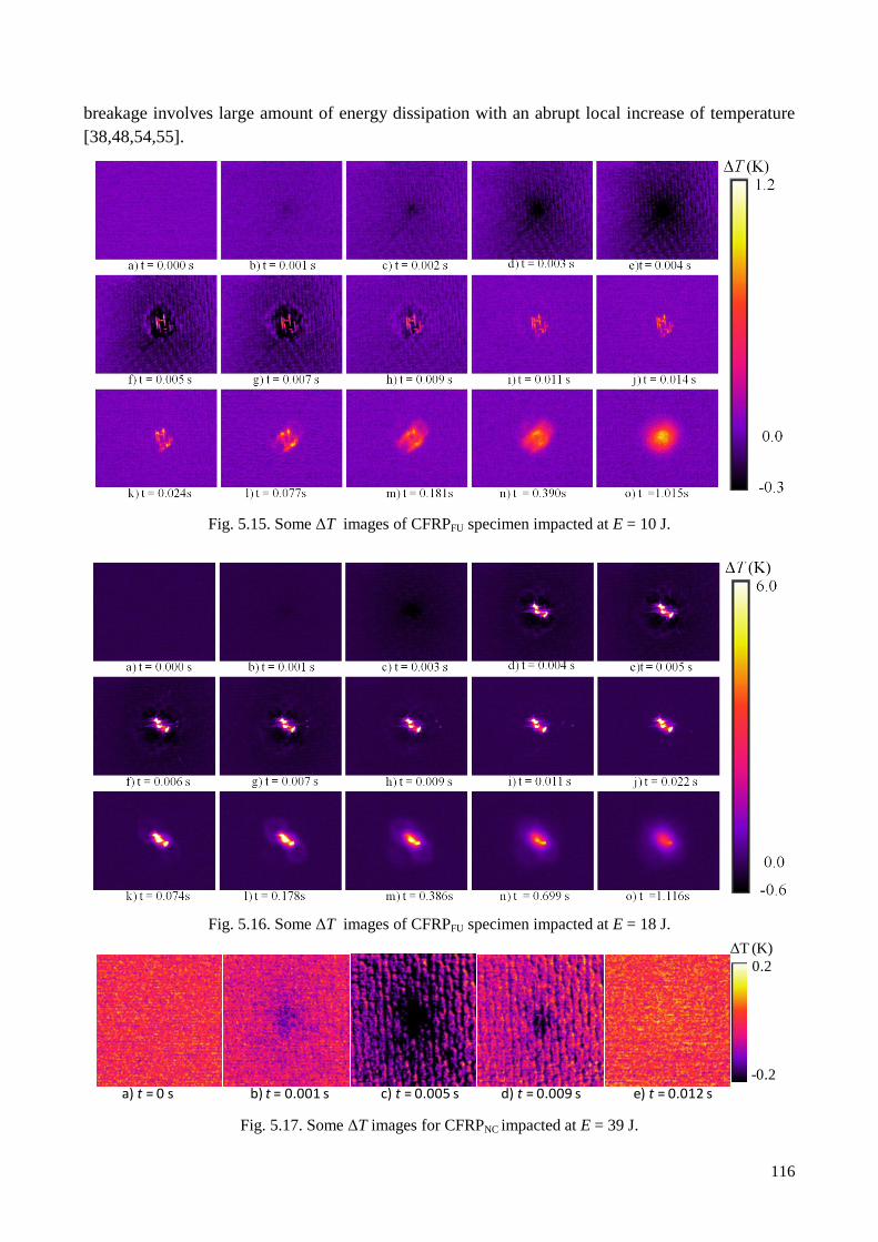
116
breakage involves large amount of energy dissipation with an abrupt local increase of temperature
[38,48,54,55].
Fig. 5.15. Some ΔT images of CFRPFU specimen impacted at E = 10 J.
Fig. 5.16. Some ΔT images of CFRPFU specimen impacted at E = 18 J.
Fig. 5.17. Some ΔT images for CFRPNC impacted at E = 39 J.
0.2
-0.2
ΔT (K)
a) t = 0 s b) t = 0.001 s c) t = 0.005 s d) t = 0.009 s e) t = 0.012 s
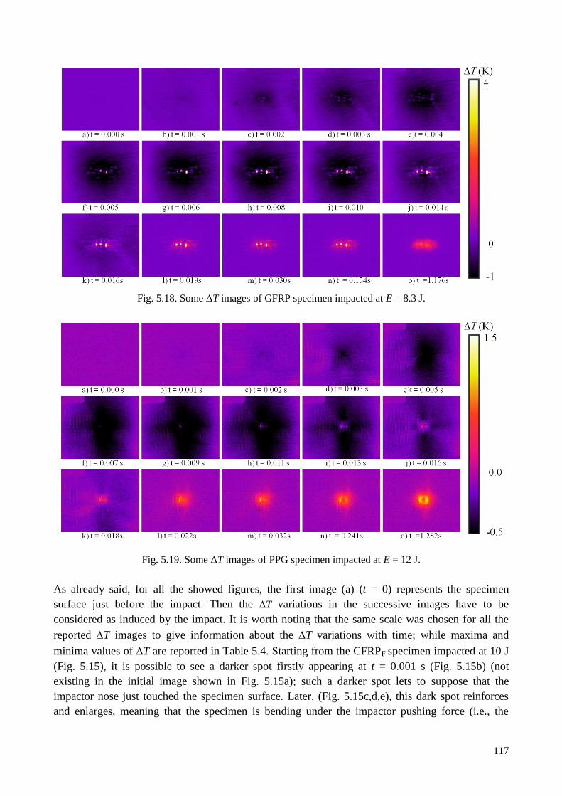
117
Fig. 5.18. Some ΔT images of GFRP specimen impacted at E = 8.3 J.
Fig. 5.19. Some ΔT images of PPG specimen impacted at E = 12 J.
As already said, for all the showed figures, the first image (a) (t = 0) represents the specimen
surface just before the impact. Then the ΔT variations in the successive images have to be
considered as induced by the impact. It is worth noting that the same scale was chosen for all the
reported T images to give information about the T variations with time; while maxima and
minima values of T are reported in Table 5.4. Starting from the CFRPF specimen impacted at 10 J
(Fig. 5.15), it is possible to see a darker spot firstly appearing at t = 0.001 s (Fig. 5.15b) (not
existing in the initial image shown in Fig. 5.15a); such a darker spot lets to suppose that the
impactor nose just touched the specimen surface. Later, (Fig. 5.15c,d,e), this dark spot reinforces
and enlarges, meaning that the specimen is bending under the impactor pushing force (i.e., the
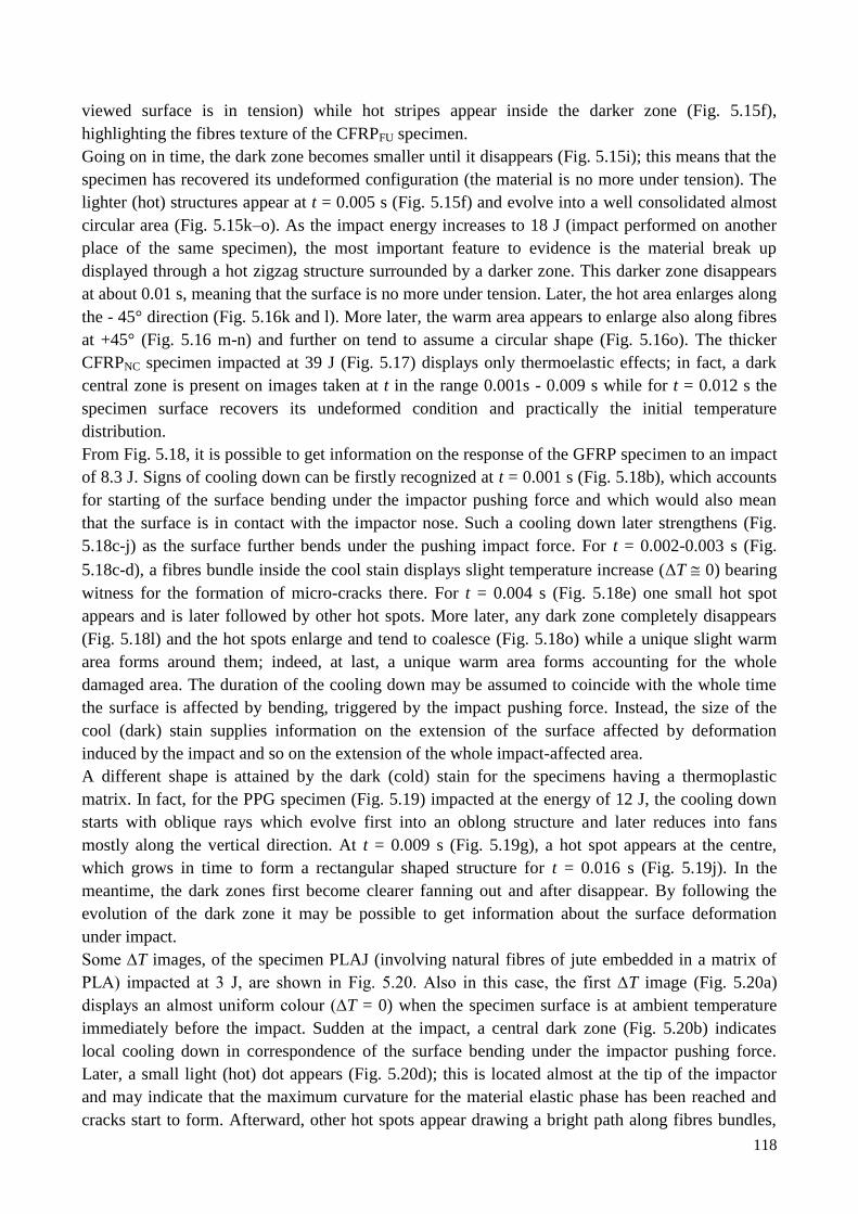
118
viewed surface is in tension) while hot stripes appear inside the darker zone (Fig. 5.15f),
highlighting the fibres texture of the CFRPFU specimen.
Going on in time, the dark zone becomes smaller until it disappears (Fig. 5.15i); this means that the
specimen has recovered its undeformed configuration (the material is no more under tension). The
lighter (hot) structures appear at t = 0.005 s (Fig. 5.15f) and evolve into a well consolidated almost
circular area (Fig. 5.15k–o). As the impact energy increases to 18 J (impact performed on another
place of the same specimen), the most important feature to evidence is the material break up
displayed through a hot zigzag structure surrounded by a darker zone. This darker zone disappears
at about 0.01 s, meaning that the surface is no more under tension. Later, the hot area enlarges along
the - 45° direction (Fig. 5.16k and l). More later, the warm area appears to enlarge also along fibres
at +45° (Fig. 5.16 m-n) and further on tend to assume a circular shape (Fig. 5.16o). The thicker
CFRPNC specimen impacted at 39 J (Fig. 5.17) displays only thermoelastic effects; in fact, a dark
central zone is present on images taken at t in the range 0.001s - 0.009 s while for t = 0.012 s the
specimen surface recovers its undeformed condition and practically the initial temperature
distribution.
From Fig. 5.18, it is possible to get information on the response of the GFRP specimen to an impact
of 8.3 J. Signs of cooling down can be firstly recognized at t = 0.001 s (Fig. 5.18b), which accounts
for starting of the surface bending under the impactor pushing force and which would also mean
that the surface is in contact with the impactor nose. Such a cooling down later strengthens (Fig.
5.18c-j) as the surface further bends under the pushing impact force. For t = 0.002-0.003 s (Fig.
5.18c-d), a fibres bundle inside the cool stain displays slight temperature increase (ΔT 0) bearing
witness for the formation of micro-cracks there. For t = 0.004 s (Fig. 5.18e) one small hot spot
appears and is later followed by other hot spots. More later, any dark zone completely disappears
(Fig. 5.18l) and the hot spots enlarge and tend to coalesce (Fig. 5.18o) while a unique slight warm
area forms around them; indeed, at last, a unique warm area forms accounting for the whole
damaged area. The duration of the cooling down may be assumed to coincide with the whole time
the surface is affected by bending, triggered by the impact pushing force. Instead, the size of the
cool (dark) stain supplies information on the extension of the surface affected by deformation
induced by the impact and so on the extension of the whole impact-affected area.
A different shape is attained by the dark (cold) stain for the specimens having a thermoplastic
matrix. In fact, for the PPG specimen (Fig. 5.19) impacted at the energy of 12 J, the cooling down
starts with oblique rays which evolve first into an oblong structure and later reduces into fans
mostly along the vertical direction. At t = 0.009 s (Fig. 5.19g), a hot spot appears at the centre,
which grows in time to form a rectangular shaped structure for t = 0.016 s (Fig. 5.19j). In the
meantime, the dark zones first become clearer fanning out and after disappear. By following the
evolution of the dark zone it may be possible to get information about the surface deformation
under impact.
Some ∆T images, of the specimen PLAJ (involving natural fibres of jute embedded in a matrix of
PLA) impacted at 3 J, are shown in Fig. 5.20. Also in this case, the first ∆T image (Fig. 5.20a)
displays an almost uniform colour (∆T = 0) when the specimen surface is at ambient temperature
immediately before the impact. Sudden at the impact, a central dark zone (Fig. 5.20b) indicates
local cooling down in correspondence of the surface bending under the impactor pushing force.
Later, a small light (hot) dot appears (Fig. 5.20d); this is located almost at the tip of the impactor
and may indicate that the maximum curvature for the material elastic phase has been reached and
cracks start to form. Afterward, other hot spots appear drawing a bright path along fibres bundles,
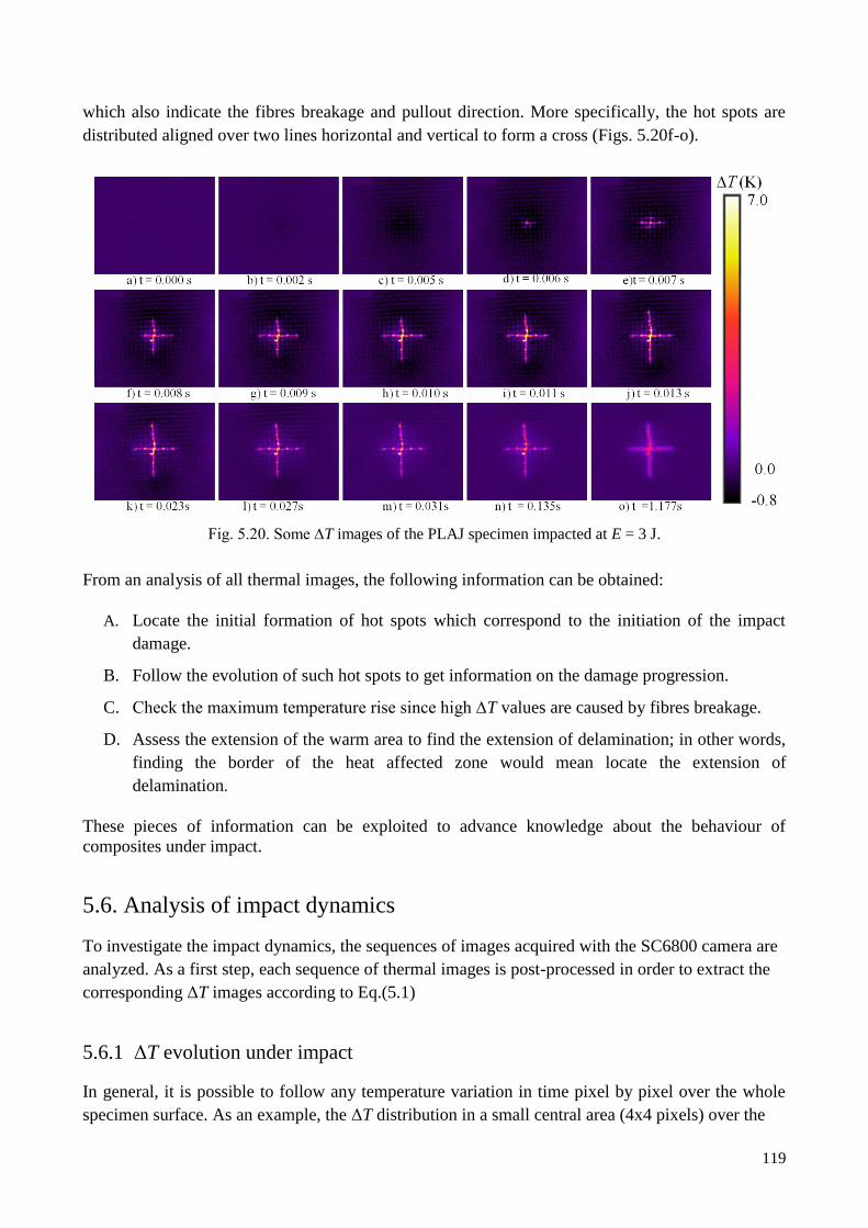
119
which also indicate the fibres breakage and pullout direction. More specifically, the hot spots are
distributed aligned over two lines horizontal and vertical to form a cross (Figs. 5.20f-o).
Fig. 5.20. Some ∆T images of the PLAJ specimen impacted at E = 3 J.
From an analysis of all thermal images, the following information can be obtained:
A. Locate the initial formation of hot spots which correspond to the initiation of the impact
damage.
B. Follow the evolution of such hot spots to get information on the damage progression.
C. Check the maximum temperature rise since high ∆T values are caused by fibres breakage.
D. Assess the extension of the warm area to find the extension of delamination; in other words,
finding the border of the heat affected zone would mean locate the extension of
delamination.
These pieces of information can be exploited to advance knowledge about the behaviour of
composites under impact.
5.6. Analysis of impact dynamics
To investigate the impact dynamics, the sequences of images acquired with the SC6800 camera are
analyzed. As a first step, each sequence of thermal images is post-processed in order to extract the
corresponding ΔT images according to Eq.(5.1)
5.6.1 ΔT evolution under impact
In general, it is possible to follow any temperature variation in time pixel by pixel over the whole
specimen surface. As an example, the ΔT distribution in a small central area (4x4 pixels) over the
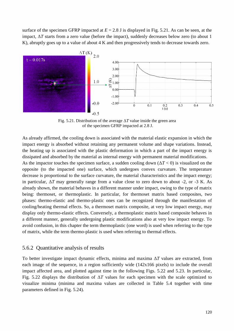
120
surface of the specimen GFRP impacted at E = 2.8 J is displayed in Fig. 5.21. As can be seen, at the
impact, ΔT starts from a zero value (before the impact), suddenly decreases below zero (to about 1
K), abruptly goes up to a value of about 4 K and then progressively tends to decrease towards zero.
Fig. 5.21. Distribution of the average ΔT value inside the green area
of the specimen GFRP impacted at 2.8 J.
As already affirmed, the cooling down is associated with the material elastic expansion in which the
impact energy is absorbed without retaining any permanent volume and shape variations. Instead,
the heating up is associated with the plastic deformation in which a part of the impact energy is
dissipated and absorbed by the material as internal energy with permanent material modifications.
As the impactor touches the specimen surface, a sudden cooling down (ΔT < 0) is visualized on the
opposite (to the impacted one) surface, which undergoes convex curvature. The temperature
decrease is proportional to the surface curvature, the material characteristics and the impact energy;
in particular, ΔT may generally range from a value close to zero down to about -2, or -3 K. As
already shown, the material behaves in a different manner under impact, owing to the type of matrix
being: thermoset, or thermoplastic. In particular, for thermoset matrix based composites, two
phases: thermo-elastic and thermo-plastic ones can be recognized through the manifestation of
cooling/heating thermal effects. So, a thermoset matrix composite, at very low impact energy, may
display only thermo-elastic effects. Conversely, a thermoplastic matrix based composite behaves in
a different manner, generally undergoing plastic modifications also at very low impact energy. To
avoid confusion, in this chapter the term thermoplastic (one word) is used when referring to the type
of matrix, while the term thermo-plastic is used when referring to thermal effects.
5.6.2 Quantitative analysis of results
To better investigate impact dynamic effects, minima and maxima ΔT values are extracted, from
each image of the sequence, in a region sufficiently wide (142x166 pixels) to include the overall
impact affected area, and plotted against time in the following Figs. 5.22 and 5.23. In particular,
Fig. 5.22 displays the distribution of ΔT values for each specimen with the scale optimized to
visualize minima (minima and maxima values are collected in Table 5.4 together with time
parameters defined in Fig. 5.24).
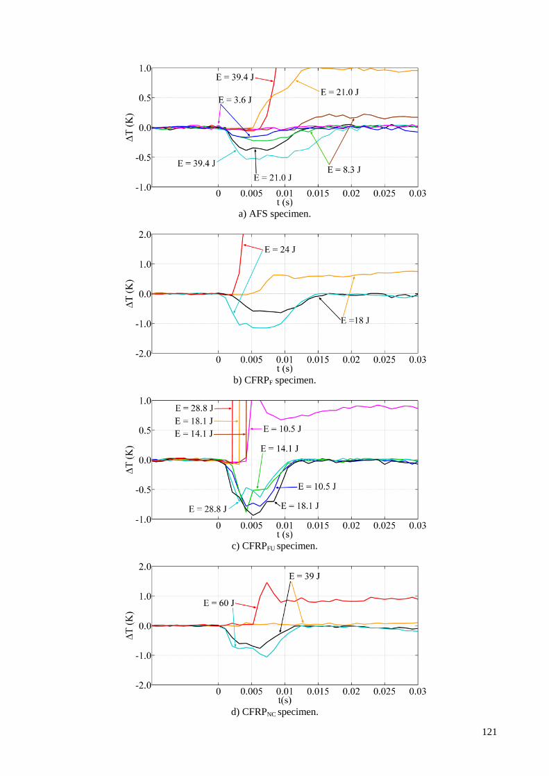
121
a) AFS specimen.
b) CFRPF specimen.
c) CFRPFU specimen.
d) CFRPNC specimen.
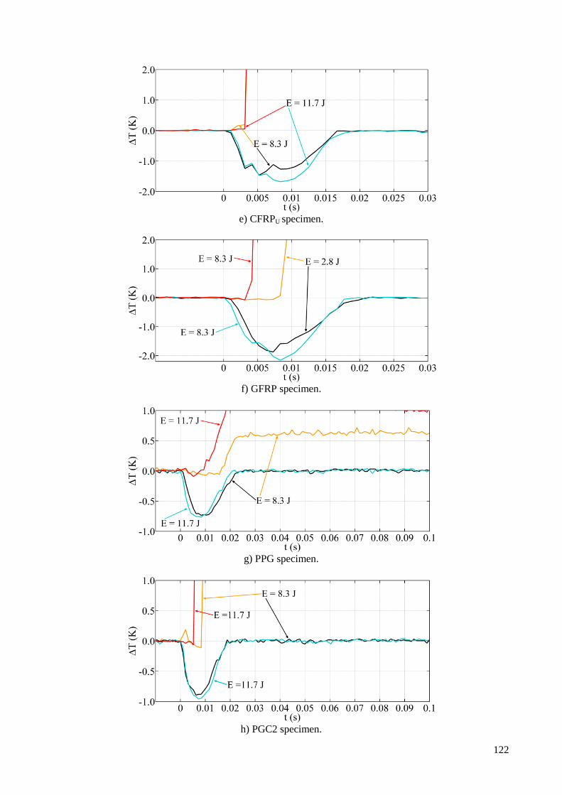
122
e) CFRPU specimen.
f) GFRP specimen.
g) PPG specimen.
h) PGC2 specimen.
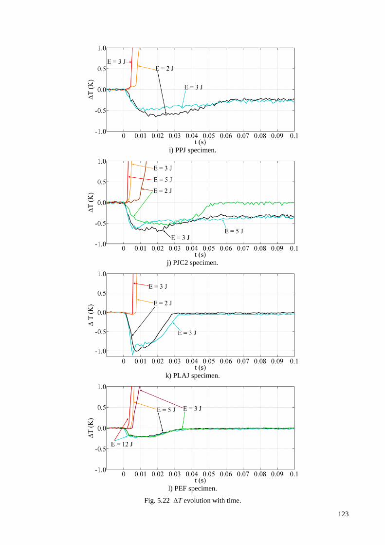
123
i) PPJ specimen.
j) PJC2 specimen.
k) PLAJ specimen.
l) PEF specimen.
Fig. 5.22 ΔT evolution with time.
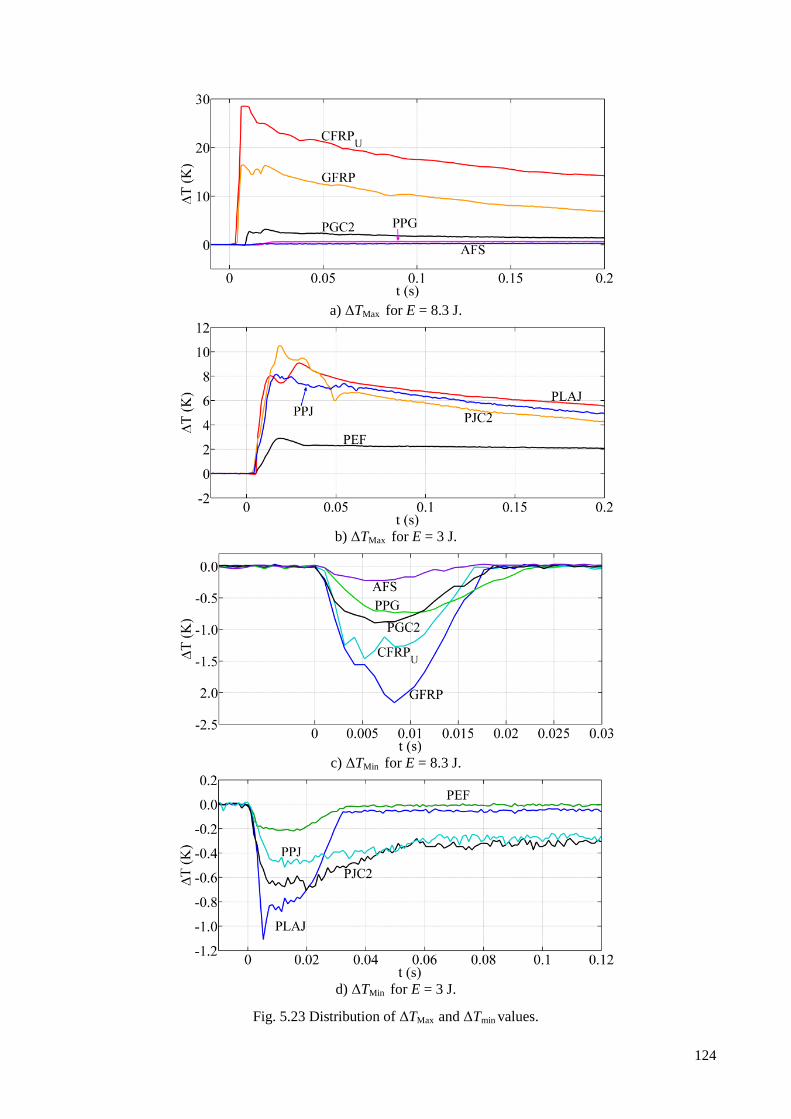
124
a) ΔTMax for E = 8.3 J.
b) ΔTMax for E = 3 J.
c) ΔTMin for E = 8.3 J.
d) ΔTMin for E = 3 J.
Fig. 5.23 Distribution of ΔTMax and ΔTmin values.
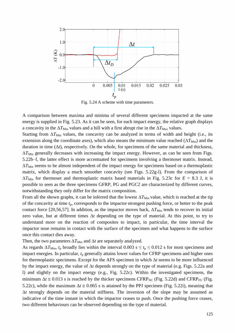
125
Fig. 5.24 A scheme with time parameters.
A comparison between maxima and minima of several different specimens impacted at the same
energy is supplied in Fig. 5.23. As it can be seen, for each impact energy, the relative graph displays
a concavity in the ΔTMin values and a hill with a first abrupt rise in the ΔTMax values.
Starting from ΔTMin values, the concavity can be analyzed in terms of width and height (i.e., its
extension along the coordinate axes), which also means the minimum value reached (ΔTMin) and the
duration in time (Δt), respectively. On the whole, for specimens of the same material and thickness,
ΔTMin generally decreases with increasing the impact energy. However, as can be seen from Figs.
5.22b–f, the latter effect is more accentuated for specimens involving a thermoset matrix. Instead,
ΔTMin seems to be almost independent of the impact energy for specimens based on a thermoplastic
matrix, which display a much smoother concavity (see Figs. 5.22g-l). From the comparison of
ΔTMin for thermoset and thermoplastic matrix based materials in Fig. 5.23c for E = 8.3 J, it is
possible to seen as the three specimens GFRP, PG and PGC2 are characterized by different curves,
notwithstanding they only differ for the matrix composition.
From all the shown graphs, it can be inferred that the lowest ΔTMin value, which is reached at the tip
of the concavity at time tp, corresponds to the impactor strongest pushing force, or better to the peak
contact force [20,56,57]. In addition, as the impactor moves back, ΔTMin tends to recover its initial
zero value, but at different times Δt depending on the type of material. At this point, to try to
understand more on the reaction of composites to impact, in particular, the time interval the
impactor nose remains in contact with the surface of the specimen and what happens to the surface
once this contact dies away.
Then, the two parameters ΔTMin and Δt are separately analyzed.
As regards ΔTMin, tp broadly lies within the interval 0.003 s ≤ tp ≤ 0.012 s for most specimens and
impact energies. In particular, tp generally attains lower values for CFRP specimens and higher ones
for thermoplastic specimens. Except for the AFS specimen in which Δt seems to be more influenced
by the impact energy, the value of Δt depends strongly on the type of material (e.g. Figs. 5.22a and
l) and slightly on the impact energy (e.g., Fig. 5.22c). Within the investigated specimens, the
minimum Δt 0.013 s is reached by the thicker specimens CFRPNC (Fig. 5.22d) and CFRPFU (Fig.
5.22c), while the maximum Δt 0.065 s is attained by the PPJ specimen (Fig. 5.22i), meaning that
Δt strongly depends on the material stiffness. The inversion of the slope may be assumed as
indicative of the time instant in which the impactor ceases to push. Once the pushing force ceases,
two different behaviours can be observed depending on the type of material.
tp
ΔtD
Δt
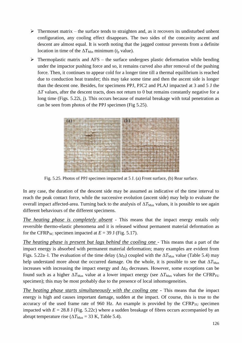
126
Thermoset matrix – the surface tends to straighten and, as it recovers its undisturbed unbent
configuration, any cooling effect disappears. The two sides of the concavity ascent and
descent are almost equal. It is worth noting that the jagged contour prevents from a definite
location in time of the ΔTMin minimum (tp value).
Thermoplastic matrix and AFS – the surface undergoes plastic deformation while bending
under the impactor pushing force and so, it remains curved also after removal of the pushing
force. Then, it continues to appear cold for a longer time till a thermal equilibrium is reached
due to conduction heat transfer; this may take some time and then the ascent side is longer
than the descent one. Besides, for specimens PPJ, PJC2 and PLAJ impacted at 3 and 5 J the
ΔT values, after the descent tracts, does not return to 0 but remains constantly negative for a
long time (Figs. 5.22i, j). This occurs because of material breakage with total penetration as
can be seen from photos of the PPJ specimen (Fig 5.25).
Fig. 5.25. Photos of PPJ specimen impacted at 5 J. (a) Front surface, (b) Rear surface.
In any case, the duration of the descent side may be assumed as indicative of the time interval to
reach the peak contact force, while the successive evolution (ascent side) may help to evaluate the
overall impact affected-area. Turning back to the analysis of ΔTMax values, it is possible to see again
different behaviours of the different specimens.
The heating phase is completely absent - This means that the impact energy entails only
reversible thermo-elastic phenomena and it is released without permanent material deformation as
for the CFRPNC specimen impacted at E = 39 J (Fig. 5.17).
The heating phase is present but lags behind the cooling one - This means that a part of the
impact energy is absorbed with permanent material deformation; many examples are evident from
Figs. 5.22a–l. The evaluation of the time delay (ΔtD) coupled with the ΔTMax value (Table 5.4) may
help understand more about the occurred damage. On the whole, it is possible to see that ΔTMax
increases with increasing the impact energy and ΔtD decreases. However, some exceptions can be
found such as a higher ΔTMax value at a lower impact energy (see ΔTMax values for the CFRPFU
specimen); this may be most probably due to the presence of local inhomogeneities.
The heating phase starts simultaneously with the cooling one - This means that the impact
energy is high and causes important damage, sudden at the impact. Of course, this is true to the
accuracy of the used frame rate of 960 Hz. An example is provided by the CFRPFU specimen
impacted with E = 28.8 J (Fig. 5.22c) where a sudden breakage of fibres occurs accompanied by an
abrupt temperature rise (ΔTMax = 33 K, Table 5.4).
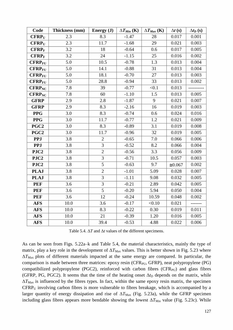
127
Code Thickness (mm) Energy (J) ∆TMin (K) ∆TMax (K) ∆t (s) ∆tD (s)
CFRPU 2.3 8.3 -1.47 28 0.017 0.001
CFRPU 2.3 11.7 -1.68 29 0.021 0.003
CFRPF 3.2 18 -0.64 0.6 0.017 0.005
CFRPF 3.2 24 -1.15 25 0.016 0.002
CFRPFU 5.0 10.5 -0.78 1.3 0.013 0.004
CFRPFU 5.0 14.1 -0.88 31 0.013 0.004
CFRPFU 5.0 18.1 -0.70 27 0.013 0.003
CFRPFU 5.0 28.8 -0.94 33 0.013 0.002
CFRPNC 7.8 39 -0.77 <0.1 0.013 ----------
CFRPNC 7.8 60 -1.10 1.5 0.013 0.005
GFRP 2.9 2.8 -1.87 9 0.021 0.007
GFRP 2.9 8.3 -2.16 16 0.019 0.003
PPG 3.0 8.3 -0.74 0.6 0.024 0.016
PPG 3.0 11.7 -0.77 1.2 0.021 0.009
PGC2 3.0 8.3 -0.89 3.1 0.019 0.008
PGC2 3.0 11.7 -0.96 32 0.019 0.005
PPJ 3.8 2 -0.65 7.0 0.066 0.006
PPJ 3.8 3 -0.52 8.2 0.066 0.004
PJC2 3.8 2 -0.56 3.3 0.056 0.009
PJC2 3.8 3 -0.71 10.5 0.057 0.003
PJC2 3.8 5 -0.63 9.7 0.067 0.002
PLAJ 3.8 2 -1.01 5.09 0.028 0.007
PLAJ 3.8 3 -1.11 9.08 0.032 0.005
PEF 3.6 3 -0.21 2.89 0.042 0.005
PEF 3.6 5 -0.20 5.94 0.050 0.004
PEF 3.6 12 -0.24 10.59 0.048 0.002
AFS 10.0 3.6 -0.17 <0.10 0.021 -------
AFS 10.0 8.3 -0.22 0.30 0.019 0.011
AFS 10.0 21 -0.39 1.20 0.016 0.005
AFS 10.0 39.4 -0.53 4.88 0.022 0.006
Table 5.4. ΔT and Δt values of the different specimens.
As can be seen from Figs. 5.22a–k and Table 5.4, the material characteristics, mainly the type of
matrix, play a key role in the development of ΔTMax values. This is better shown in Fig. 5.23 where
ΔTMax plots of different materials impacted at the same energy are compared. In particular, the
comparison is made between three matrices: epoxy resin (CFRPU, GFRP), neat polypropylene (PG)
compatibilized polypropylene (PGC2), reinforced with carbon fibres (CFRPU) and glass fibres
(GFRP, PG, PGC2). It seems that the time of the heating onset ΔtD depends on the matrix, while
ΔTMax is influenced by the fibres types. In fact, within the same epoxy resin matrix, the specimen
CFRPU involving carbon fibres is more vulnerable to fibres breakage, which is accompanied by a
larger quantity of energy dissipation and rise of ΔTMax (Fig. 5.23a), while the GFRP specimen
including glass fibres appears more bendable showing the lowest ΔTMin value (Fig. 5.23c). While
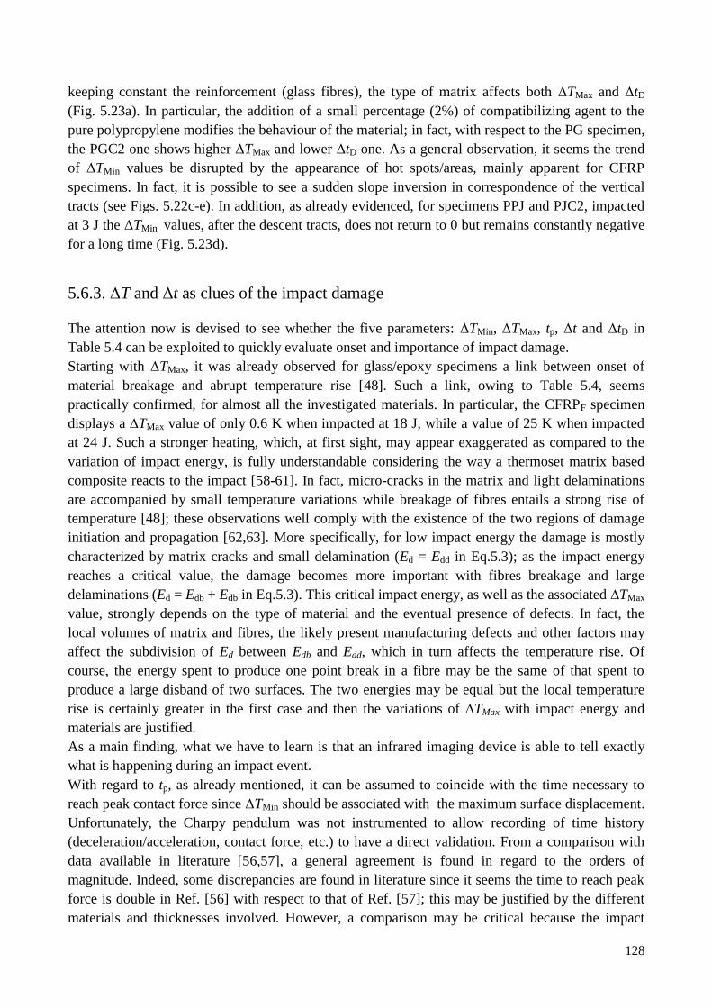
128
keeping constant the reinforcement (glass fibres), the type of matrix affects both ΔTMax and ΔtD
(Fig. 5.23a). In particular, the addition of a small percentage (2%) of compatibilizing agent to the
pure polypropylene modifies the behaviour of the material; in fact, with respect to the PG specimen,
the PGC2 one shows higher ΔTMax and lower ΔtD one. As a general observation, it seems the trend
of ΔTMin values be disrupted by the appearance of hot spots/areas, mainly apparent for CFRP
specimens. In fact, it is possible to see a sudden slope inversion in correspondence of the vertical
tracts (see Figs. 5.22c-e). In addition, as already evidenced, for specimens PPJ and PJC2, impacted
at 3 J the ΔTMin values, after the descent tracts, does not return to 0 but remains constantly negative
for a long time (Fig. 5.23d).
5.6.3. ΔT and Δt as clues of the impact damage
The attention now is devised to see whether the five parameters: ΔTMin, ΔTMax, tp, Δt and ΔtD in
Table 5.4 can be exploited to quickly evaluate onset and importance of impact damage.
Starting with ΔTMax, it was already observed for glass/epoxy specimens a link between onset of
material breakage and abrupt temperature rise [48]. Such a link, owing to Table 5.4, seems
practically confirmed, for almost all the investigated materials. In particular, the CFRPF specimen
displays a ∆TMax value of only 0.6 K when impacted at 18 J, while a value of 25 K when impacted
at 24 J. Such a stronger heating, which, at first sight, may appear exaggerated as compared to the
variation of impact energy, is fully understandable considering the way a thermoset matrix based
composite reacts to the impact [58-61]. In fact, micro-cracks in the matrix and light delaminations
are accompanied by small temperature variations while breakage of fibres entails a strong rise of
temperature [48]; these observations well comply with the existence of the two regions of damage
initiation and propagation [62,63]. More specifically, for low impact energy the damage is mostly
characterized by matrix cracks and small delamination (Ed = Edd in Eq.5.3); as the impact energy
reaches a critical value, the damage becomes more important with fibres breakage and large
delaminations (Ed = Edb + Edb in Eq.5.3). This critical impact energy, as well as the associated ∆TMax
value, strongly depends on the type of material and the eventual presence of defects. In fact, the
local volumes of matrix and fibres, the likely present manufacturing defects and other factors may
affect the subdivision of Ed between Edb and Edd, which in turn affects the temperature rise. Of
course, the energy spent to produce one point break in a fibre may be the same of that spent to
produce a large disband of two surfaces. The two energies may be equal but the local temperature
rise is certainly greater in the first case and then the variations of ∆TMax with impact energy and
materials are justified.
As a main finding, what we have to learn is that an infrared imaging device is able to tell exactly
what is happening during an impact event.
With regard to tp, as already mentioned, it can be assumed to coincide with the time necessary to
reach peak contact force since ΔTMin should be associated with the maximum surface displacement.
Unfortunately, the Charpy pendulum was not instrumented to allow recording of time history
(deceleration/acceleration, contact force, etc.) to have a direct validation. From a comparison with
data available in literature [56,57], a general agreement is found in regard to the orders of
magnitude. Indeed, some discrepancies are found in literature since it seems the time to reach peak
force is double in Ref. [56] with respect to that of Ref. [57]; this may be justified by the different
materials and thicknesses involved. However, a comparison may be critical because the impact
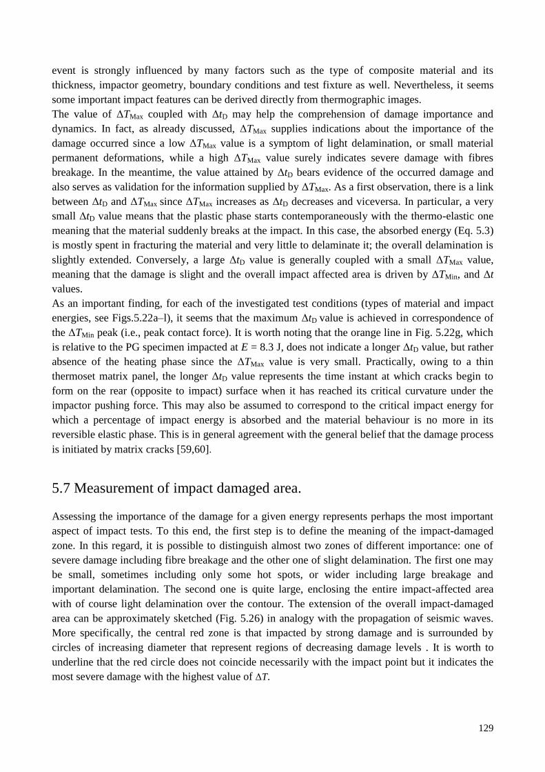
129
event is strongly influenced by many factors such as the type of composite material and its
thickness, impactor geometry, boundary conditions and test fixture as well. Nevertheless, it seems
some important impact features can be derived directly from thermographic images.
The value of ΔTMax coupled with ΔtD may help the comprehension of damage importance and
dynamics. In fact, as already discussed, ΔTMax supplies indications about the importance of the
damage occurred since a low ΔTMax value is a symptom of light delamination, or small material
permanent deformations, while a high ΔTMax value surely indicates severe damage with fibres
breakage. In the meantime, the value attained by ΔtD bears evidence of the occurred damage and
also serves as validation for the information supplied by ΔTMax. As a first observation, there is a link
between ΔtD and ΔTMax since ΔTMax increases as ΔtD decreases and viceversa. In particular, a very
small ΔtD value means that the plastic phase starts contemporaneously with the thermo-elastic one
meaning that the material suddenly breaks at the impact. In this case, the absorbed energy (Eq. 5.3)
is mostly spent in fracturing the material and very little to delaminate it; the overall delamination is
slightly extended. Conversely, a large ΔtD value is generally coupled with a small ΔTMax value,
meaning that the damage is slight and the overall impact affected area is driven by ΔTMin, and Δt
values.
As an important finding, for each of the investigated test conditions (types of material and impact
energies, see Figs.5.22a–l), it seems that the maximum ΔtD value is achieved in correspondence of
the ΔTMin peak (i.e., peak contact force). It is worth noting that the orange line in Fig. 5.22g, which
is relative to the PG specimen impacted at E = 8.3 J, does not indicate a longer ΔtD value, but rather
absence of the heating phase since the ΔTMax value is very small. Practically, owing to a thin
thermoset matrix panel, the longer ΔtD value represents the time instant at which cracks begin to
form on the rear (opposite to impact) surface when it has reached its critical curvature under the
impactor pushing force. This may also be assumed to correspond to the critical impact energy for
which a percentage of impact energy is absorbed and the material behaviour is no more in its
reversible elastic phase. This is in general agreement with the general belief that the damage process
is initiated by matrix cracks [59,60].
5.7 Measurement of impact damaged area.
Assessing the importance of the damage for a given energy represents perhaps the most important
aspect of impact tests. To this end, the first step is to define the meaning of the impact-damaged
zone. In this regard, it is possible to distinguish almost two zones of different importance: one of
severe damage including fibre breakage and the other one of slight delamination. The first one may
be small, sometimes including only some hot spots, or wider including large breakage and
important delamination. The second one is quite large, enclosing the entire impact-affected area
with of course light delamination over the contour. The extension of the overall impact-damaged
area can be approximately sketched (Fig. 5.26) in analogy with the propagation of seismic waves.
More specifically, the central red zone is that impacted by strong damage and is surrounded by
circles of increasing diameter that represent regions of decreasing damage levels . It is worth to
underline that the red circle does not coincide necessarily with the impact point but it indicates the
most severe damage with the highest value of ΔT.
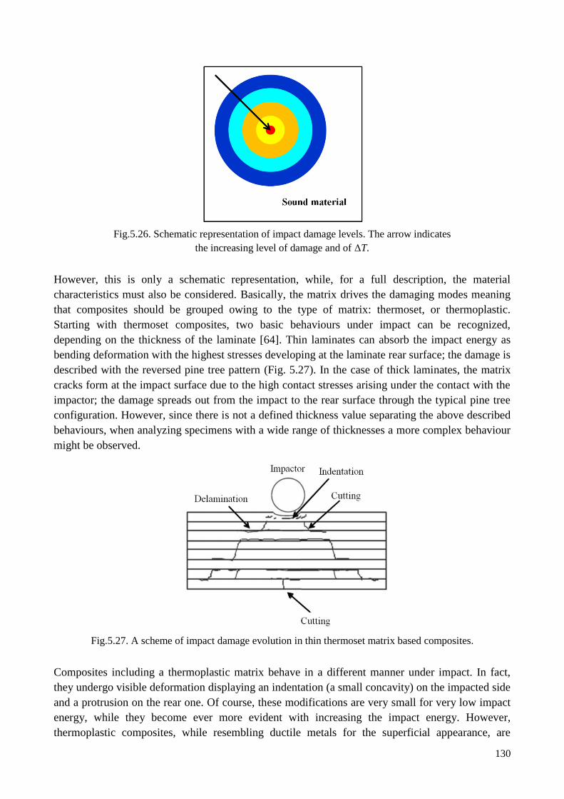
130
Fig.5.26. Schematic representation of impact damage levels. The arrow indicates
the increasing level of damage and of ΔT.
However, this is only a schematic representation, while, for a full description, the material
characteristics must also be considered. Basically, the matrix drives the damaging modes meaning
that composites should be grouped owing to the type of matrix: thermoset, or thermoplastic.
Starting with thermoset composites, two basic behaviours under impact can be recognized,
depending on the thickness of the laminate [64]. Thin laminates can absorb the impact energy as
bending deformation with the highest stresses developing at the laminate rear surface; the damage is
described with the reversed pine tree pattern (Fig. 5.27). In the case of thick laminates, the matrix
cracks form at the impact surface due to the high contact stresses arising under the contact with the
impactor; the damage spreads out from the impact to the rear surface through the typical pine tree
configuration. However, since there is not a defined thickness value separating the above described
behaviours, when analyzing specimens with a wide range of thicknesses a more complex behaviour
might be observed.
Fig.5.27. A scheme of impact damage evolution in thin thermoset matrix based composites.
Composites including a thermoplastic matrix behave in a different manner under impact. In fact,
they undergo visible deformation displaying an indentation (a small concavity) on the impacted side
and a protrusion on the rear one. Of course, these modifications are very small for very low impact
energy, while they become ever more evident with increasing the impact energy. However,
thermoplastic composites, while resembling ductile metals for the superficial appearance, are
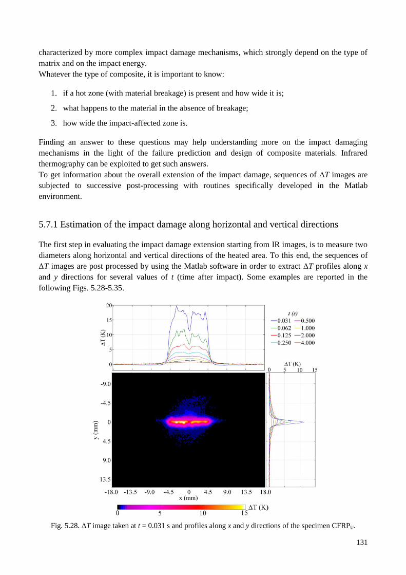
131
characterized by more complex impact damage mechanisms, which strongly depend on the type of
matrix and on the impact energy.
Whatever the type of composite, it is important to know:
1. if a hot zone (with material breakage) is present and how wide it is;
2. what happens to the material in the absence of breakage;
3. how wide the impact-affected zone is.
Finding an answer to these questions may help understanding more on the impact damaging
mechanisms in the light of the failure prediction and design of composite materials. Infrared
thermography can be exploited to get such answers.
To get information about the overall extension of the impact damage, sequences of ΔT images are
subjected to successive post-processing with routines specifically developed in the Matlab
environment.
5.7.1 Estimation of the impact damage along horizontal and vertical directions
The first step in evaluating the impact damage extension starting from IR images, is to measure two
diameters along horizontal and vertical directions of the heated area. To this end, the sequences of
ΔT images are post processed by using the Matlab software in order to extract ΔT profiles along x
and y directions for several values of t (time after impact). Some examples are reported in the
following Figs. 5.28-5.35.
Fig. 5.28. ΔT image taken at t = 0.031 s and profiles along x and y directions of the specimen CFRPU.
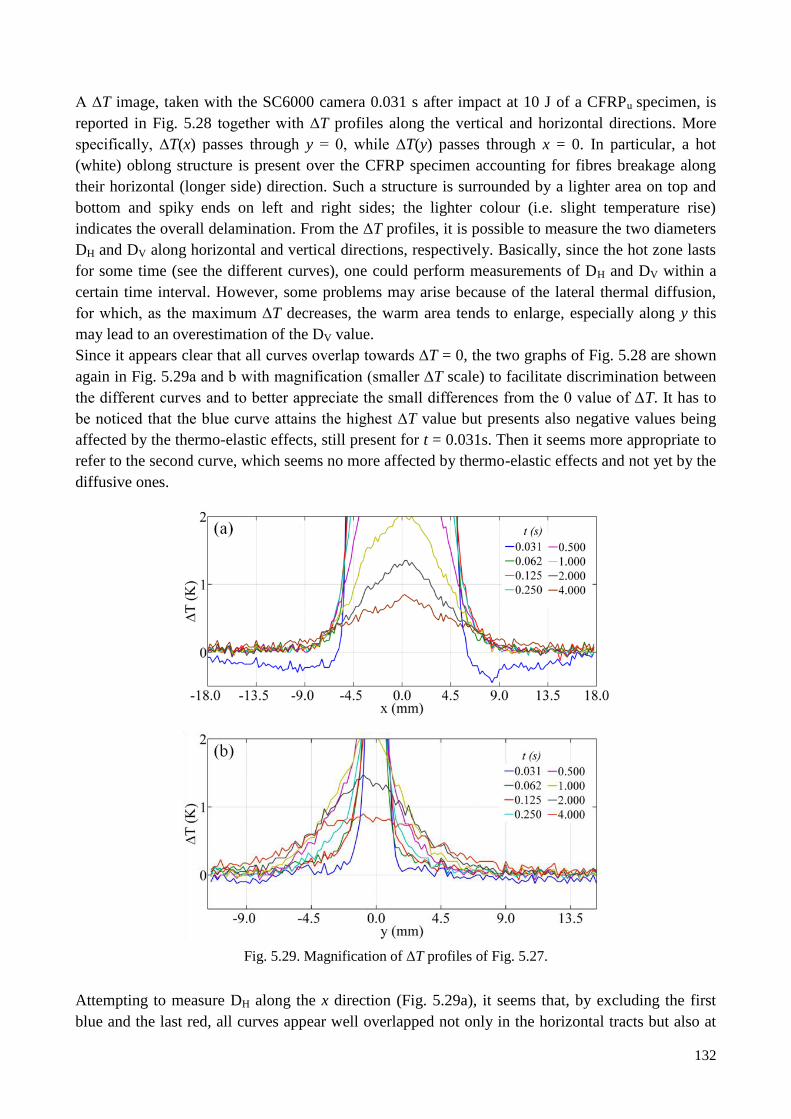
132
A ∆T image, taken with the SC6000 camera 0.031 s after impact at 10 J of a CFRPu specimen, is
reported in Fig. 5.28 together with ∆T profiles along the vertical and horizontal directions. More
specifically, ∆T(x) passes through y = 0, while ∆T(y) passes through x = 0. In particular, a hot
(white) oblong structure is present over the CFRP specimen accounting for fibres breakage along
their horizontal (longer side) direction. Such a structure is surrounded by a lighter area on top and
bottom and spiky ends on left and right sides; the lighter colour (i.e. slight temperature rise)
indicates the overall delamination. From the ΔT profiles, it is possible to measure the two diameters
DH and DV along horizontal and vertical directions, respectively. Basically, since the hot zone lasts
for some time (see the different curves), one could perform measurements of DH and DV within a
certain time interval. However, some problems may arise because of the lateral thermal diffusion,
for which, as the maximum ∆T decreases, the warm area tends to enlarge, especially along y this
may lead to an overestimation of the DV value.
Since it appears clear that all curves overlap towards ∆T = 0, the two graphs of Fig. 5.28 are shown
again in Fig. 5.29a and b with magnification (smaller ∆T scale) to facilitate discrimination between
the different curves and to better appreciate the small differences from the 0 value of ∆T. It has to
be noticed that the blue curve attains the highest ∆T value but presents also negative values being
affected by the thermo-elastic effects, still present for t = 0.031s. Then it seems more appropriate to
refer to the second curve, which seems no more affected by thermo-elastic effects and not yet by the
diffusive ones.
Fig. 5.29. Magnification of ΔT profiles of Fig. 5.27.
Attempting to measure DH along the x direction (Fig. 5.29a), it seems that, by excluding the first
blue and the last red, all curves appear well overlapped not only in the horizontal tracts but also at
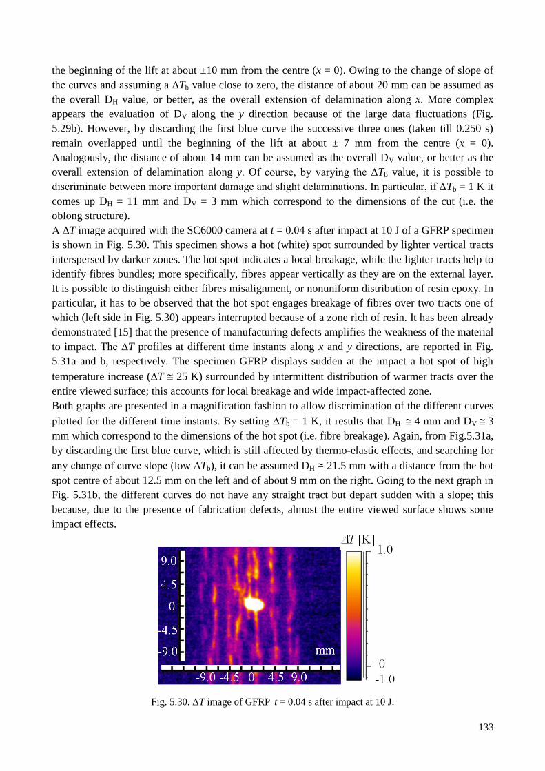
133
the beginning of the lift at about ±10 mm from the centre (x = 0). Owing to the change of slope of
the curves and assuming a ∆Tb value close to zero, the distance of about 20 mm can be assumed as
the overall DH value, or better, as the overall extension of delamination along x. More complex
appears the evaluation of DV along the y direction because of the large data fluctuations (Fig.
5.29b). However, by discarding the first blue curve the successive three ones (taken till 0.250 s)
remain overlapped until the beginning of the lift at about ± 7 mm from the centre (x = 0).
Analogously, the distance of about 14 mm can be assumed as the overall DV value, or better as the
overall extension of delamination along y. Of course, by varying the ∆Tb value, it is possible to
discriminate between more important damage and slight delaminations. In particular, if ∆Tb = 1 K it
comes up DH = 11 mm and DV = 3 mm which correspond to the dimensions of the cut (i.e. the
oblong structure).
A ∆T image acquired with the SC6000 camera at t = 0.04 s after impact at 10 J of a GFRP specimen
is shown in Fig. 5.30. This specimen shows a hot (white) spot surrounded by lighter vertical tracts
interspersed by darker zones. The hot spot indicates a local breakage, while the lighter tracts help to
identify fibres bundles; more specifically, fibres appear vertically as they are on the external layer.
It is possible to distinguish either fibres misalignment, or nonuniform distribution of resin epoxy. In
particular, it has to be observed that the hot spot engages breakage of fibres over two tracts one of
which (left side in Fig. 5.30) appears interrupted because of a zone rich of resin. It has been already
demonstrated [15] that the presence of manufacturing defects amplifies the weakness of the material
to impact. The ∆T profiles at different time instants along x and y directions, are reported in Fig.
5.31a and b, respectively. The specimen GFRP displays sudden at the impact a hot spot of high
temperature increase (ΔT 25 K) surrounded by intermittent distribution of warmer tracts over the
entire viewed surface; this accounts for local breakage and wide impact-affected zone.
Both graphs are presented in a magnification fashion to allow discrimination of the different curves
plotted for the different time instants. By setting ∆Tb = 1 K, it results that DH 4 mm and DV 3
mm which correspond to the dimensions of the hot spot (i.e. fibre breakage). Again, from Fig.5.31a,
by discarding the first blue curve, which is still affected by thermo-elastic effects, and searching for
any change of curve slope (low ∆Tb), it can be assumed DH 21.5 mm with a distance from the hot
spot centre of about 12.5 mm on the left and of about 9 mm on the right. Going to the next graph in
Fig. 5.31b, the different curves do not have any straight tract but depart sudden with a slope; this
because, due to the presence of fabrication defects, almost the entire viewed surface shows some
impact effects.
Fig. 5.30. ΔT image of GFRP t = 0.04 s after impact at 10 J.
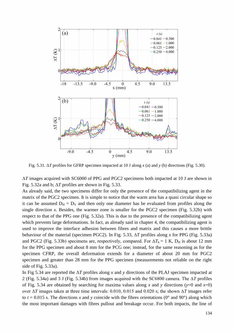
134
Fig. 5.31. ΔT profiles for GFRP specimen impacted at 10 J along x (a) and y (b) directions (Fig. 5.30).
ΔT images acquired with SC6000 of PPG and PGC2 specimens both impacted at 10 J are shown in
Fig. 5.32a and b; ΔT profiles are shown in Fig. 5.33.
As already said, the two specimens differ for only the presence of the compatibilizing agent in the
matrix of the PGC2 specimen. It is simple to notice that the warm area has a quasi circular shape so
it can be assumed DH = DV and then only one diameter has be evaluated from profiles along the
single direction x. Besides, the warmer zone is smaller for the PGC2 specimen (Fig. 5.32b) with
respect to that of the PPG one (Fig. 5.32a). This is due to the presence of the compatibilizing agent
which prevents large deformations. In fact, as already said in chapter 4, the compatibilizing agent is
used to improve the interface adhesion between fibres and matrix and this causes a more brittle
behaviour of the material (specimen PGC2). In Fig. 5.33, ∆T profiles along x for PPG (Fig. 5.33a)
and PGC2 (Fig. 5.33b) specimens are, respectively, compared. For ∆Tb = 1 K, DH is about 12 mm
for the PPG specimen and about 8 mm for the PCG one; instead, for the same reasoning as for the
specimen CFRP, the overall deformation extends for a diameter of about 20 mm for PGC2
specimen and greater than 28 mm for the PPG specimen (measurements not reliable on the right
side of Fig. 5.33a).
In Fig 5.34 are reported the ΔT profiles along x and y directions of the PLAJ specimen impacted at
2 (Fig. 5.34a) and 3 J (Fig. 5.34b) from images acquired with the SC6800 camera. The ∆T profiles
of Fig. 5.34 are obtained by searching for maxima values along x and y directions (y=0 and x=0)
over ∆T images taken at three time intervals: 0.010, 0.015 and 0.020 s; the shown ∆T images refer
to t = 0.015 s. The directions x and y coincide with the fibres orientations (0° and 90°) along which
the most important damages with fibres pullout and breakage occur. For both impacts, the line of
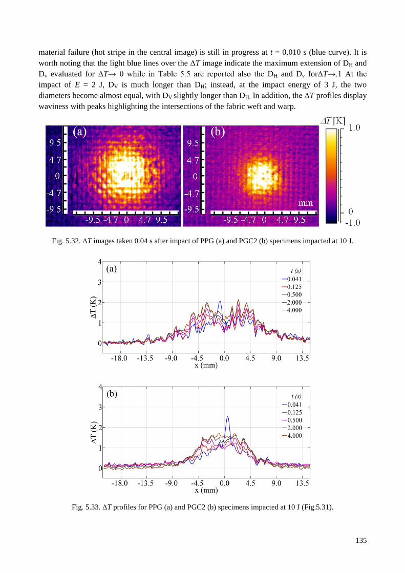
135
material failure (hot stripe in the central image) is still in progress at t = 0.010 s (blue curve). It is
worth noting that the light blue lines over the ΔT image indicate the maximum extension of DH and
Dv evaluated for ΔT→ 0 while in Table 5.5 are reported also the DH and Dv forΔT→.1 At the
impact of E = 2 J, DV is much longer than DH; instead, at the impact energy of 3 J, the two
diameters become almost equal, with DV slightly longer than DH. In addition, the ∆T profiles display
waviness with peaks highlighting the intersections of the fabric weft and warp.
Fig. 5.32. ΔT images taken 0.04 s after impact of PPG (a) and PGC2 (b) specimens impacted at 10 J.
Fig. 5.33. ΔT profiles for PPG (a) and PGC2 (b) specimens impacted at 10 J (Fig.5.31).
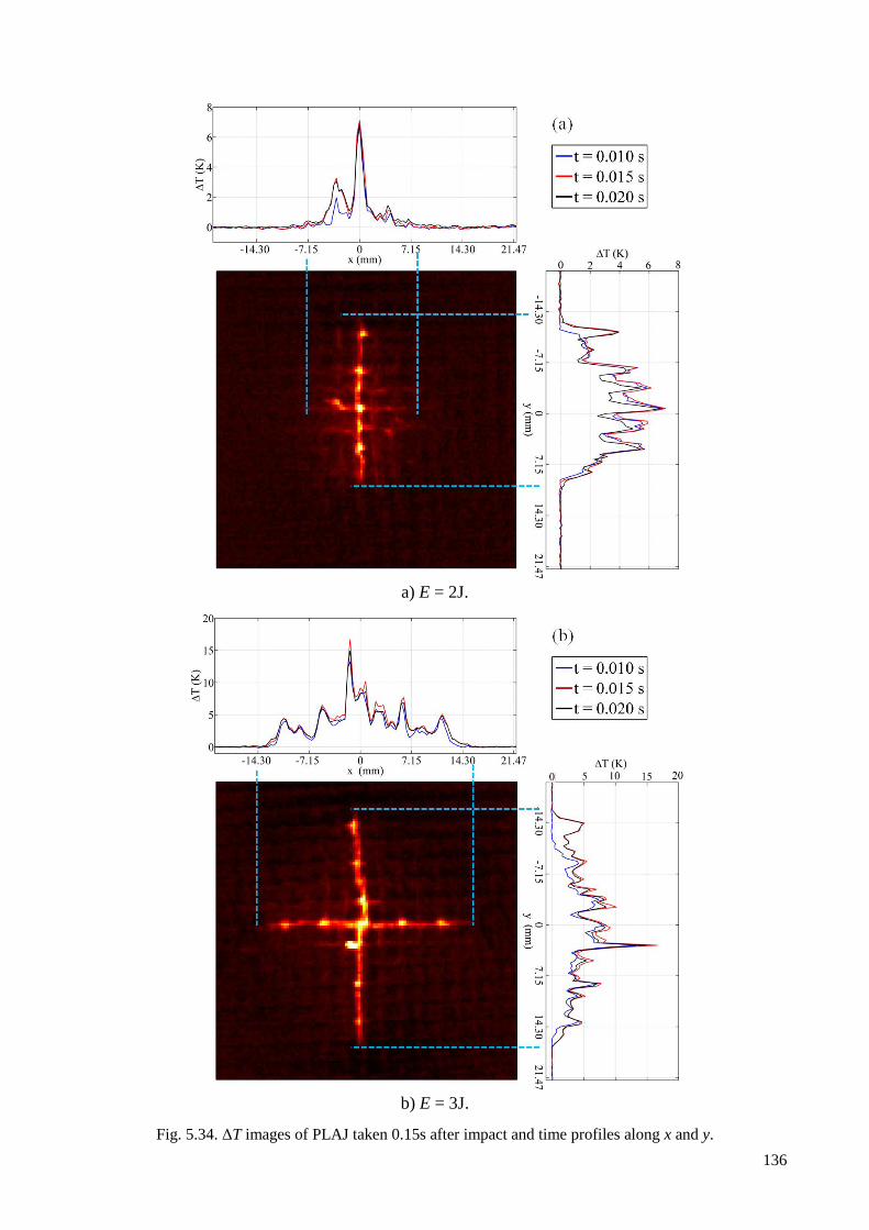
136
a) E = 2J.
b) E = 3J.
Fig. 5.34. ΔT images of PLAJ taken 0.15s after impact and time profiles along x and y.
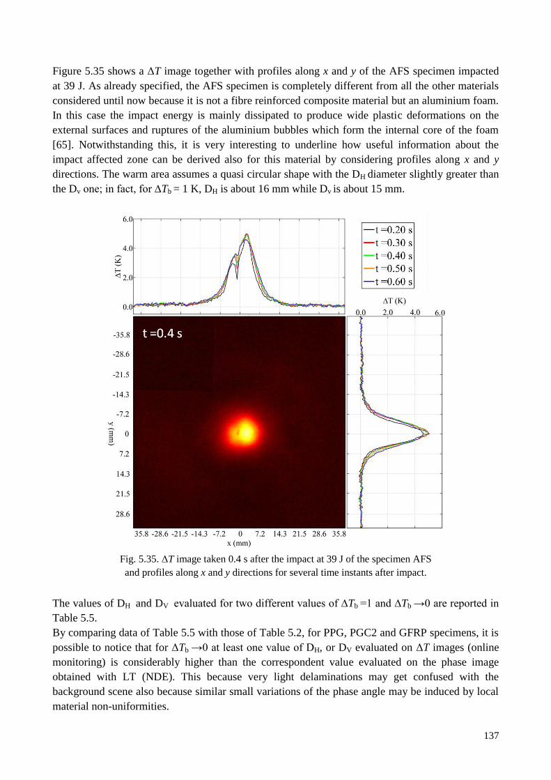
137
Figure 5.35 shows a ΔT image together with profiles along x and y of the AFS specimen impacted
at 39 J. As already specified, the AFS specimen is completely different from all the other materials
considered until now because it is not a fibre reinforced composite material but an aluminium foam.
In this case the impact energy is mainly dissipated to produce wide plastic deformations on the
external surfaces and ruptures of the aluminium bubbles which form the internal core of the foam
[65]. Notwithstanding this, it is very interesting to underline how useful information about the
impact affected zone can be derived also for this material by considering profiles along x and y
directions. The warm area assumes a quasi circular shape with the DH diameter slightly greater than
the Dv one; in fact, for ∆Tb = 1 K, DH is about 16 mm while Dv is about 15 mm.
Fig. 5.35. ΔT image taken 0.4 s after the impact at 39 J of the specimen AFS
and profiles along x and y directions for several time instants after impact.
The values of DH and DV evaluated for two different values of ∆Tb =1 and ∆Tb →0 are reported in
Table 5.5.
By comparing data of Table 5.5 with those of Table 5.2, for PPG, PGC2 and GFRP specimens, it is
possible to notice that for ΔTb →0 at least one value of DH, or DV evaluated on ΔT images (online
monitoring) is considerably higher than the correspondent value evaluated on the phase image
obtained with LT (NDE). This because very light delaminations may get confused with the
background scene also because similar small variations of the phase angle may be induced by local
material non-uniformities.
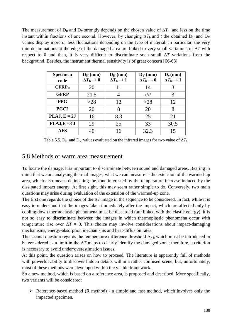
138
The measurement of DH and DV strongly depends on the chosen value of ∆Tb and less on the time
instant within fractions of one second. However, by changing ∆Tb and t the obtained DH and DV
values display more or less fluctuations depending on the type of material. In particular, the very
thin delaminations at the edge of the damaged area are linked to very small variations of ΔT with
respect to 0 and then, it is very difficult to discriminate such small ΔT variations from the
background. Besides, the instrument thermal sensitivity is of great concern [66-68].
Specimen
code
DH (mm)
ΔTb → 0
DH (mm)
ΔTb → 1
DV (mm)
ΔTb → 0
Dv (mm)
ΔTb → 1
CFRPU 20 11 14 3
GFRP 21.5 4 //// 3
PPG >28 12 >28 12
PGC2 20 8 20 8
PLAJ, E = 2J 16 8.8 25 21
PLAJ,E =3 J 29 25 33 30.5
AFS 40 16 32.3 15
Table 5.5. DH and DV values evaluated on the infrared images for two value of ΔTb.
5.8 Methods of warm area measurement
To locate the damage, it is important to discriminate between sound and damaged areas. Bearing in
mind that we are analysing thermal images, what we can measure is the extension of the warmed-up
area, which also means delineating the zone interested by the temperature increase induced by the
dissipated impact energy. At first sight, this may seem rather simple to do. Conversely, two main
questions may arise during evaluation of the extension of the warmed-up zone.
The first one regards the choice of the ΔT image in the sequence to be considered. In fact, while it is
easy to understand that the images taken immediately after the impact, which are affected only by
cooling down thermoelastic phenomena must be discarded (are linked with the elastic energy), it is
not so easy to discriminate between the images in which thermoplastic phenomena occur with
temperature rise over ΔT = 0. This choice may involve considerations about impact-damaging
mechanisms, energy-absorption mechanisms and heat-diffusion rates.
The second question regards the temperature difference threshold ΔTb which must be introduced to
be considered as a limit in the ΔT maps to clearly identify the damaged zone; therefore, a criterion
is necessary to avoid under/overestimation issues.
At this point, the question arises on how to proceed. The literature is apparently full of methods
with powerful ability to discover hidden details within a rather confused scene, but, unfortunately,
most of these methods were developed within the visible framework.
So a new method, which is based on a reference area, is proposed and described. More specifically,
two variants will be considered:
Reference-based method (R method) - a simple and fast method, which involves only the
impacted specimen.
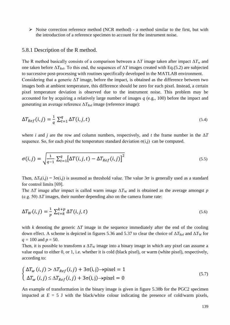
139
Noise correction reference method (NCR method) - a method similar to the first, but with
the introduction of a reference specimen to account for the instrument noise.
5.8.1 Description of the R method.
The R method basically consists of a comparison between a ΔT image taken after impact ΔTw and
one taken before ΔTRef. To this end, the sequences of ΔT images created with Eq.(5.2) are subjected
to successive post-processing with routines specifically developed in the MATLAB environment.
Considering that a generic ΔT image, before the impact, is obtained as the difference between two
images both at ambient temperature, this difference should be zero for each pixel. Instead, a certain
pixel temperature deviation is observed due to the instrument noise. This problem may be
accounted for by acquiring a relatively large number of images q (e.g., 100) before the impact and
generating an average reference ΔTRef image (reference image):
(5.4)
where i and j are the row and column numbers, respectively, and t the frame number in the ΔT
sequence. So, for each pixel the temperature standard deviation σ(i,j) can be computed.
(5.5)
Then, ΔTb(i,j) = 3σ(i,j) is assumed as threshold value. The value 3 is generally used as a standard
for control limits [69].
The ΔT image after impact is called warm image ΔTW and is obtained as the average amongst p
(e.g. 50) ΔT images, their number depending also on the camera frame rate:
(5.6)
with k denoting the generic ΔT image in the sequence immediately after the end of the cooling
down effect. A scheme is depicted in figures 5.36 and 5.37 to clear the choice of ΔTRef and ΔTW for
q = 100 and p = 50.
Then, it is possible to transform a ΔTW image into a binary image in which any pixel can assume a
value equal to either 0, or 1, i.e. whether it is cold (black pixel), or warm (white pixel), respectively,
according to:
σ
σ (5.7)
An example of transformation in the binary image is given in figure 5.38b for the PGC2 specimen
impacted at E = 5 J with the black/white colour indicating the presence of cold/warm pixels,
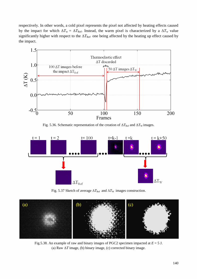
140
respectively. In other words, a cold pixel represents the pixel not affected by heating effects caused
by the impact for which ΔTw = ΔTRef. Instead, the warm pixel is characterized by a ΔTw value
significantly higher with respect to the ΔTRef one being affected by the heating up effect caused by
the impact.
Fig. 5.36. Schematic representation of the creation of ΔTRef and ΔTW images.
Fig. 5.37 Sketch of average TRef and TW images construction.
Fig.5.38. An example of raw and binary images of PGC2 specimen impacted at E = 5 J.
(a) Raw ΔT image, (b) binary image, (c) corrected binary image.
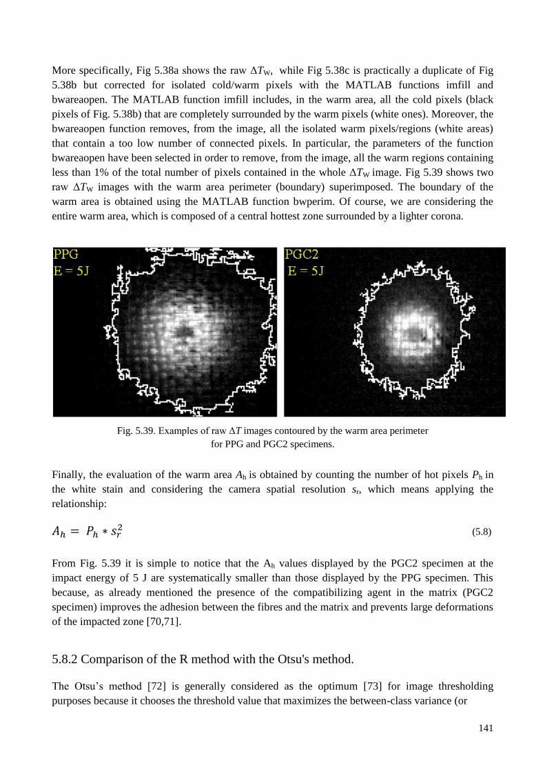
141
More specifically, Fig 5.38a shows the raw ΔTW, while Fig 5.38c is practically a duplicate of Fig
5.38b but corrected for isolated cold/warm pixels with the MATLAB functions imfill and
bwareaopen. The MATLAB function imfill includes, in the warm area, all the cold pixels (black
pixels of Fig. 5.38b) that are completely surrounded by the warm pixels (white ones). Moreover, the
bwareaopen function removes, from the image, all the isolated warm pixels/regions (white areas)
that contain a too low number of connected pixels. In particular, the parameters of the function
bwareaopen have been selected in order to remove, from the image, all the warm regions containing
less than 1% of the total number of pixels contained in the whole ΔTW image. Fig 5.39 shows two
raw ΔTW images with the warm area perimeter (boundary) superimposed. The boundary of the
warm area is obtained using the MATLAB function bwperim. Of course, we are considering the
entire warm area, which is composed of a central hottest zone surrounded by a lighter corona.
Fig. 5.39. Examples of raw ΔT images contoured by the warm area perimeter
for PPG and PGC2 specimens.
Finally, the evaluation of the warm area Ah is obtained by counting the number of hot pixels Ph in
the white stain and considering the camera spatial resolution sr, which means applying the
relationship:
(5.8)
From Fig. 5.39 it is simple to notice that the Ah values displayed by the PGC2 specimen at the
impact energy of 5 J are systematically smaller than those displayed by the PPG specimen. This
because, as already mentioned the presence of the compatibilizing agent in the matrix (PGC2
specimen) improves the adhesion between the fibres and the matrix and prevents large deformations
of the impacted zone [70,71].
5.8.2 Comparison of the R method with the Otsu's method.
The Otsu’s method [72] is generally considered as the optimum [73] for image thresholding
purposes because it chooses the threshold value that maximizes the between-class variance (or
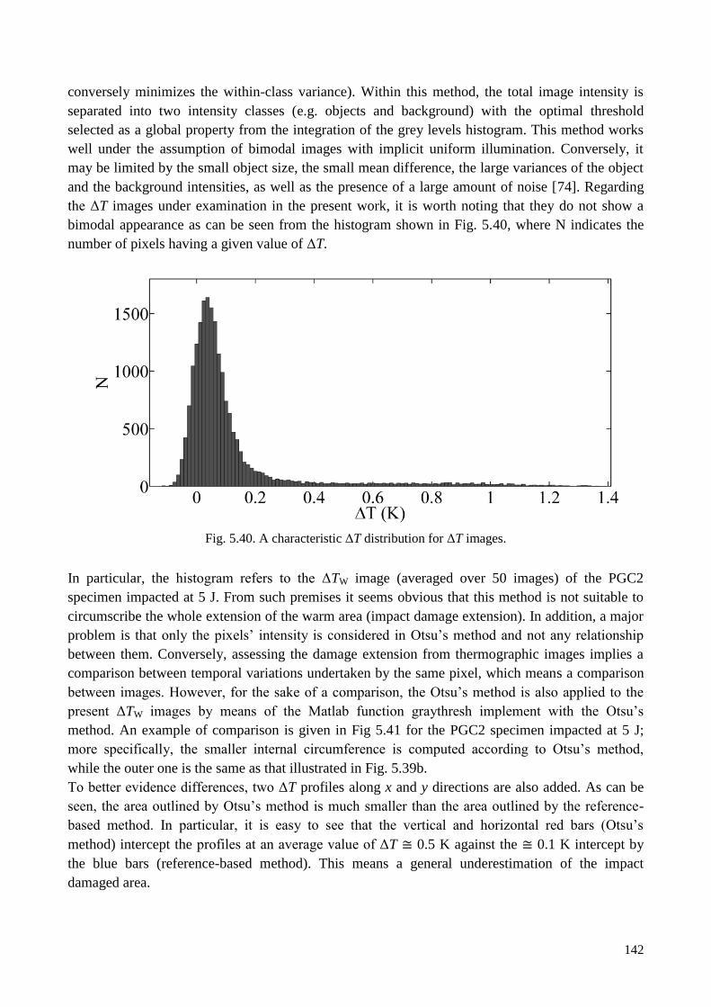
142
conversely minimizes the within-class variance). Within this method, the total image intensity is
separated into two intensity classes (e.g. objects and background) with the optimal threshold
selected as a global property from the integration of the grey levels histogram. This method works
well under the assumption of bimodal images with implicit uniform illumination. Conversely, it
may be limited by the small object size, the small mean difference, the large variances of the object
and the background intensities, as well as the presence of a large amount of noise [74]. Regarding
the ΔT images under examination in the present work, it is worth noting that they do not show a
bimodal appearance as can be seen from the histogram shown in Fig. 5.40, where N indicates the
number of pixels having a given value of ΔT.
Fig. 5.40. A characteristic ΔT distribution for ΔT images.
In particular, the histogram refers to the ΔTW image (averaged over 50 images) of the PGC2
specimen impacted at 5 J. From such premises it seems obvious that this method is not suitable to
circumscribe the whole extension of the warm area (impact damage extension). In addition, a major
problem is that only the pixels’ intensity is considered in Otsu’s method and not any relationship
between them. Conversely, assessing the damage extension from thermographic images implies a
comparison between temporal variations undertaken by the same pixel, which means a comparison
between images. However, for the sake of a comparison, the Otsu’s method is also applied to the
present ΔTW images by means of the Matlab function graythresh implement with the Otsu’s
method. An example of comparison is given in Fig 5.41 for the PGC2 specimen impacted at 5 J;
more specifically, the smaller internal circumference is computed according to Otsu’s method,
while the outer one is the same as that illustrated in Fig. 5.39b.
To better evidence differences, two ΔT profiles along x and y directions are also added. As can be
seen, the area outlined by Otsu’s method is much smaller than the area outlined by the reference-
based method. In particular, it is easy to see that the vertical and horizontal red bars (Otsu’s
method) intercept the profiles at an average value of ΔT ≅ 0.5 K against the ≅ 0.1 K intercept by
the blue bars (reference-based method). This means a general underestimation of the impact
damaged area.
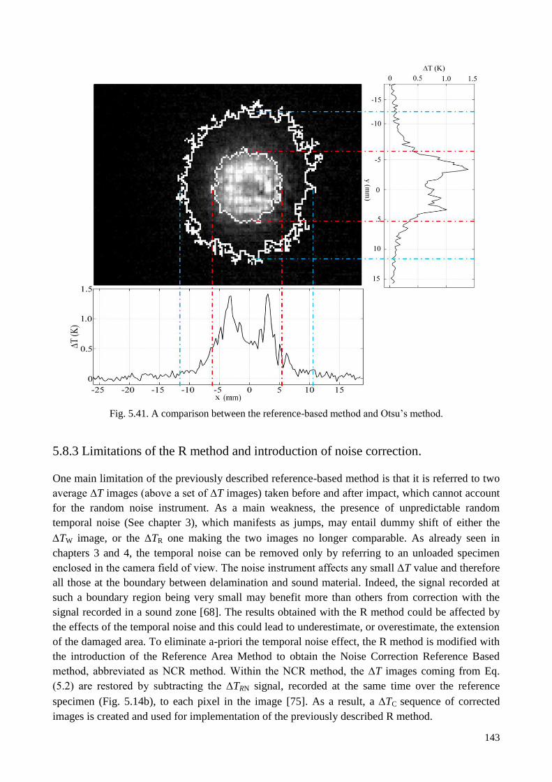
143
Fig. 5.41. A comparison between the reference-based method and Otsu’s method.
5.8.3 Limitations of the R method and introduction of noise correction.
One main limitation of the previously described reference-based method is that it is referred to two
average ∆T images (above a set of ∆T images) taken before and after impact, which cannot account
for the random noise instrument. As a main weakness, the presence of unpredictable random
temporal noise (See chapter 3), which manifests as jumps, may entail dummy shift of either the
TW image, or the TR one making the two images no longer comparable. As already seen in
chapters 3 and 4, the temporal noise can be removed only by referring to an unloaded specimen
enclosed in the camera field of view. The noise instrument affects any small ∆T value and therefore
all those at the boundary between delamination and sound material. Indeed, the signal recorded at
such a boundary region being very small may benefit more than others from correction with the
signal recorded in a sound zone [68]. The results obtained with the R method could be affected by
the effects of the temporal noise and this could lead to underestimate, or overestimate, the extension
of the damaged area. To eliminate a-priori the temporal noise effect, the R method is modified with
the introduction of the Reference Area Method to obtain the Noise Correction Reference Based
method, abbreviated as NCR method. Within the NCR method, the ∆T images coming from Eq.
(5.2) are restored by subtracting the ∆TRN signal, recorded at the same time over the reference
specimen (Fig. 5.14b), to each pixel in the image [75]. As a result, a TC sequence of corrected
images is created and used for implementation of the previously described R method.
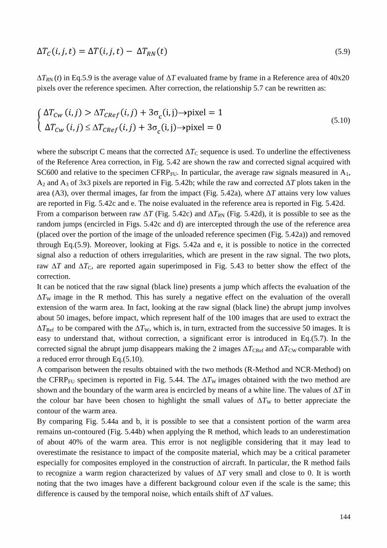
144
(5.9)
∆TRN (t) in Eq.5.9 is the average value of ΔT evaluated frame by frame in a Reference area of 40x20
pixels over the reference specimen. After correction, the relationship 5.7 can be rewritten as:
σ
σ
(5.10)
where the subscript C means that the corrected ΔTC sequence is used. To underline the effectiveness
of the Reference Area correction, in Fig. 5.42 are shown the raw and corrected signal acquired with
SC600 and relative to the specimen CFRPFU. In particular, the average raw signals measured in A1,
A2 and A3 of 3x3 pixels are reported in Fig. 5.42b; while the raw and corrected ΔT plots taken in the
area (A3), over thermal images, far from the impact (Fig. 5.42a), where ΔT attains very low values
are reported in Fig. 5.42c and e. The noise evaluated in the reference area is reported in Fig. 5.42d.
From a comparison between raw ΔT (Fig. 5.42c) and ΔTRN (Fig. 5.42d), it is possible to see as the
random jumps (encircled in Figs. 5.42c and d) are intercepted through the use of the reference area
(placed over the portion of the image of the unloaded reference specimen (Fig. 5.42a)) and removed
through Eq.(5.9). Moreover, looking at Figs. 5.42a and e, it is possible to notice in the corrected
signal also a reduction of others irregularities, which are present in the raw signal. The two plots,
raw T and TC, are reported again superimposed in Fig. 5.43 to better show the effect of the
correction.
It can be noticed that the raw signal (black line) presents a jump which affects the evaluation of the
ΔTW image in the R method. This has surely a negative effect on the evaluation of the overall
extension of the warm area. In fact, looking at the raw signal (black line) the abrupt jump involves
about 50 images, before impact, which represent half of the 100 images that are used to extract the
ΔTRef to be compared with the ΔTW, which is, in turn, extracted from the successive 50 images. It is
easy to understand that, without correction, a significant error is introduced in Eq.(5.7). In the
corrected signal the abrupt jump disappears making the 2 images ΔTCRef and ΔTCW comparable with
a reduced error through Eq.(5.10).
A comparison between the results obtained with the two methods (R-Method and NCR-Method) on
the CFRPFU specimen is reported in Fig. 5.44. The ΔTW images obtained with the two method are
shown and the boundary of the warm area is encircled by means of a white line. The values of ΔT in
the colour bar have been chosen to highlight the small values of ΔTW to better appreciate the
contour of the warm area.
By comparing Fig. 5.44a and b, it is possible to see that a consistent portion of the warm area
remains un-contoured (Fig. 5.44b) when applying the R method, which leads to an underestimation
of about 40% of the warm area. This error is not negligible considering that it may lead to
overestimate the resistance to impact of the composite material, which may be a critical parameter
especially for composites employed in the construction of aircraft. In particular, the R method fails
to recognize a warm region characterized by values of ΔT very small and close to 0. It is worth
noting that the two images have a different background colour even if the scale is the same; this
difference is caused by the temporal noise, which entails shift of ΔT values.
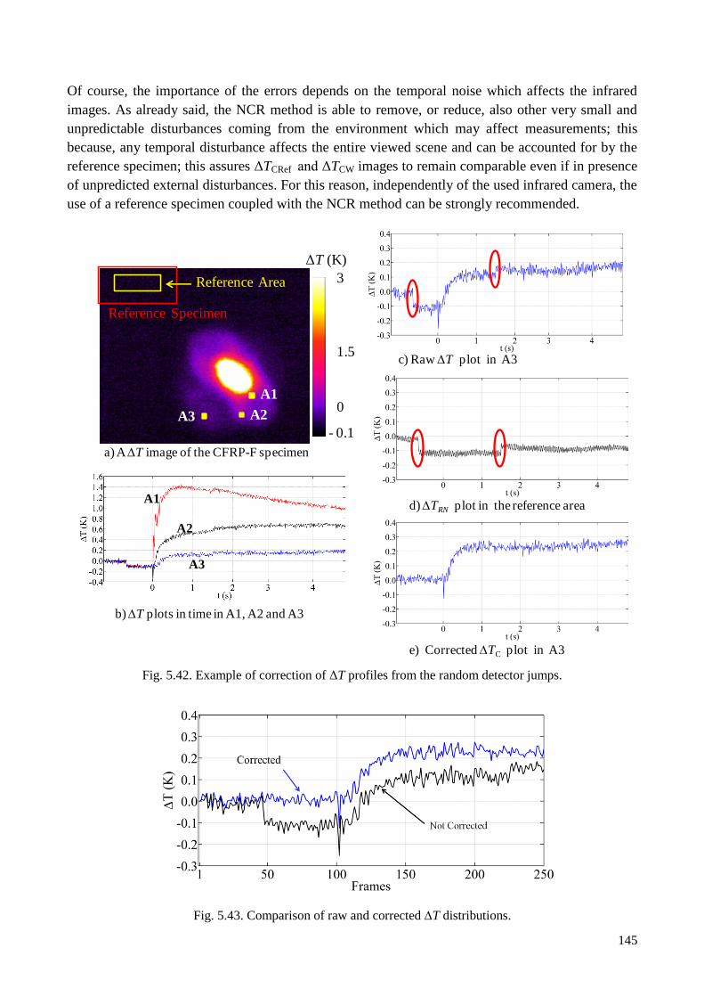
145
Of course, the importance of the errors depends on the temporal noise which affects the infrared
images. As already said, the NCR method is able to remove, or reduce, also other very small and
unpredictable disturbances coming from the environment which may affect measurements; this
because, any temporal disturbance affects the entire viewed scene and can be accounted for by the
reference specimen; this assures ΔTCRef and ΔTCW images to remain comparable even if in presence
of unpredicted external disturbances. For this reason, independently of the used infrared camera, the
use of a reference specimen coupled with the NCR method can be strongly recommended.
Fig. 5.42. Example of correction of ΔT profiles from the random detector jumps.
Fig. 5.43. Comparison of raw and corrected T distributions.
A3
Reference Area
Reference Specimen
- 0.1
3
1.5
0A2
A1
ΔT (K)
A1
A2
A3
a) AT image of the CFRP-F specimen
b) T plots in time in A1, A2 and A3
c) RawT plot in A3
d) TRN plot in the reference area
e) CorrectedTC plot in A3
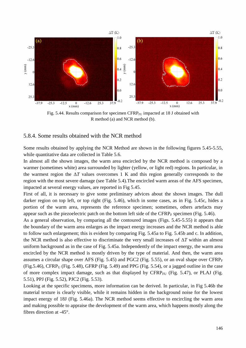
146
Fig. 5.44. Results comparison for specimen CFRPFU impacted at 18 J obtained with
R method (a) and NCR method (b).
5.8.4. Some results obtained with the NCR method
Some results obtained by applying the NCR Method are shown in the following figures 5.45-5.55,
while quantitative data are collected in Table 5.6.
In almost all the shown images, the warm area encircled by the NCR method is composed by a
warmer (sometimes white) area surrounded by lighter (yellow, or light red) regions. In particular, in
the warmest region the ΔT values overcomes 1 K and this region generally corresponds to the
region with the most severe damage (see Table 5.4).The encircled warm areas of the AFS specimen,
impacted at several energy values, are reported in Fig 5.45.
First of all, it is necessary to give some preliminary advices about the shown images. The dull
darker region on top left, or top right (Fig. 5.46), which in some cases, as in Fig. 5.45c, hides a
portion of the warm area, represents the reference specimen; sometimes, others artefacts may
appear such as the piezoelectric patch on the bottom left side of the CFRPF specimen (Fig. 5.46).
As a general observation, by comparing all the contoured images (Figs. 5.45-5.55) it appears that
the boundary of the warm area enlarges as the impact energy increases and the NCR method is able
to follow such enlargement; this is evident by comparing Fig. 5.45a to Fig. 5.45b and c. In addition,
the NCR method is also effective to discriminate the very small increases of ΔT within an almost
uniform background as in the case of Fig. 5.45a. Independently of the impact energy, the warm area
encircled by the NCR method is mostly driven by the type of material. And then, the warm area
assumes a circular shape over AFS (Fig. 5.45) and PGC2 (Fig. 5.55), or an oval shape over CFRPF
(Fig.5.46), CFRPU (Fig. 5.48), GFRP (Fig. 5.49) and PPG (Fig. 5.54), or a jagged outline in the case
of more complex impact damage, such as that displayed by CFRPFU (Fig. 5.47), or PLAJ (Fig.
5.51), PPJ (Fig. 5.52), PJC2 (Fig. 5.53).
Looking at the specific specimens, more information can be derived. In particular, in Fig 5.46b the
material texture is clearly visible, while it remains hidden in the background noise for the lowest
impact energy of 18J (Fig. 5.46a). The NCR method seems effective to encircling the warm area
and making possible to appraise the development of the warm area, which happens mostly along the
fibres direction at -45°.
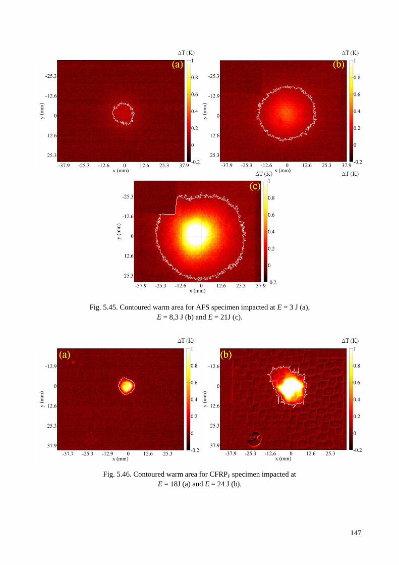
147
Fig. 5.45. Contoured warm area for AFS specimen impacted at E = 3 J (a),
E = 8,3 J (b) and E = 21J (c).
Fig. 5.46. Contoured warm area for CFRPF specimen impacted at
E = 18J (a) and E = 24 J (b).
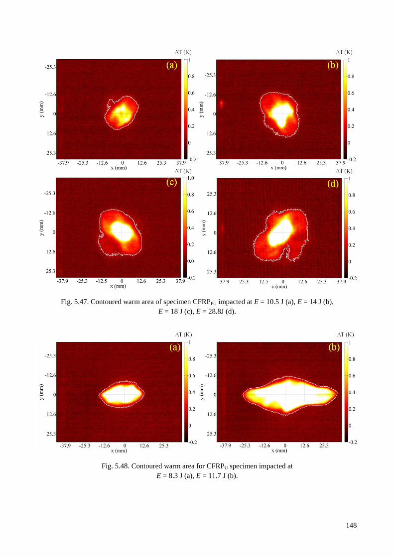
148
Fig. 5.47. Contoured warm area of specimen CFRPFU impacted at E = 10.5 J (a), E = 14 J (b),
E = 18 J (c), E = 28.8J (d).
Fig. 5.48. Contoured warm area for CFRPU specimen impacted at
E = 8.3 J (a), E = 11.7 J (b).
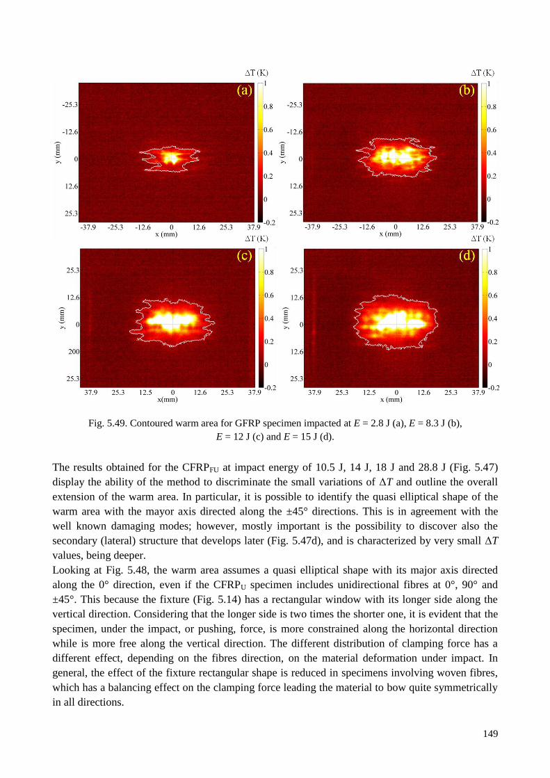
149
Fig. 5.49. Contoured warm area for GFRP specimen impacted at E = 2.8 J (a), E = 8.3 J (b),
E = 12 J (c) and E = 15 J (d).
The results obtained for the CFRPFU at impact energy of 10.5 J, 14 J, 18 J and 28.8 J (Fig. 5.47)
display the ability of the method to discriminate the small variations of ΔT and outline the overall
extension of the warm area. In particular, it is possible to identify the quasi elliptical shape of the
warm area with the mayor axis directed along the ±45° directions. This is in agreement with the
well known damaging modes; however, mostly important is the possibility to discover also the
secondary (lateral) structure that develops later (Fig. 5.47d), and is characterized by very small ΔT
values, being deeper.
Looking at Fig. 5.48, the warm area assumes a quasi elliptical shape with its major axis directed
along the 0° direction, even if the CFRPU specimen includes unidirectional fibres at 0°, 90° and
±45°. This because the fixture (Fig. 5.14) has a rectangular window with its longer side along the
vertical direction. Considering that the longer side is two times the shorter one, it is evident that the
specimen, under the impact, or pushing, force, is more constrained along the horizontal direction
while is more free along the vertical direction. The different distribution of clamping force has a
different effect, depending on the fibres direction, on the material deformation under impact. In
general, the effect of the fixture rectangular shape is reduced in specimens involving woven fibres,
which has a balancing effect on the clamping force leading the material to bow quite symmetrically
in all directions.
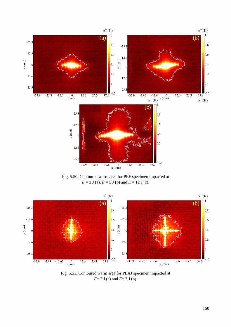
150
Fig. 5.50. Contoured warm area for PEF specimen impacted at
E = 3 J (a), E = 5 J (b) and E = 12 J (c).
Fig. 5.51. Contoured warm area for PLAJ specimen impacted at
E= 2 J (a) and E= 3 J (b).
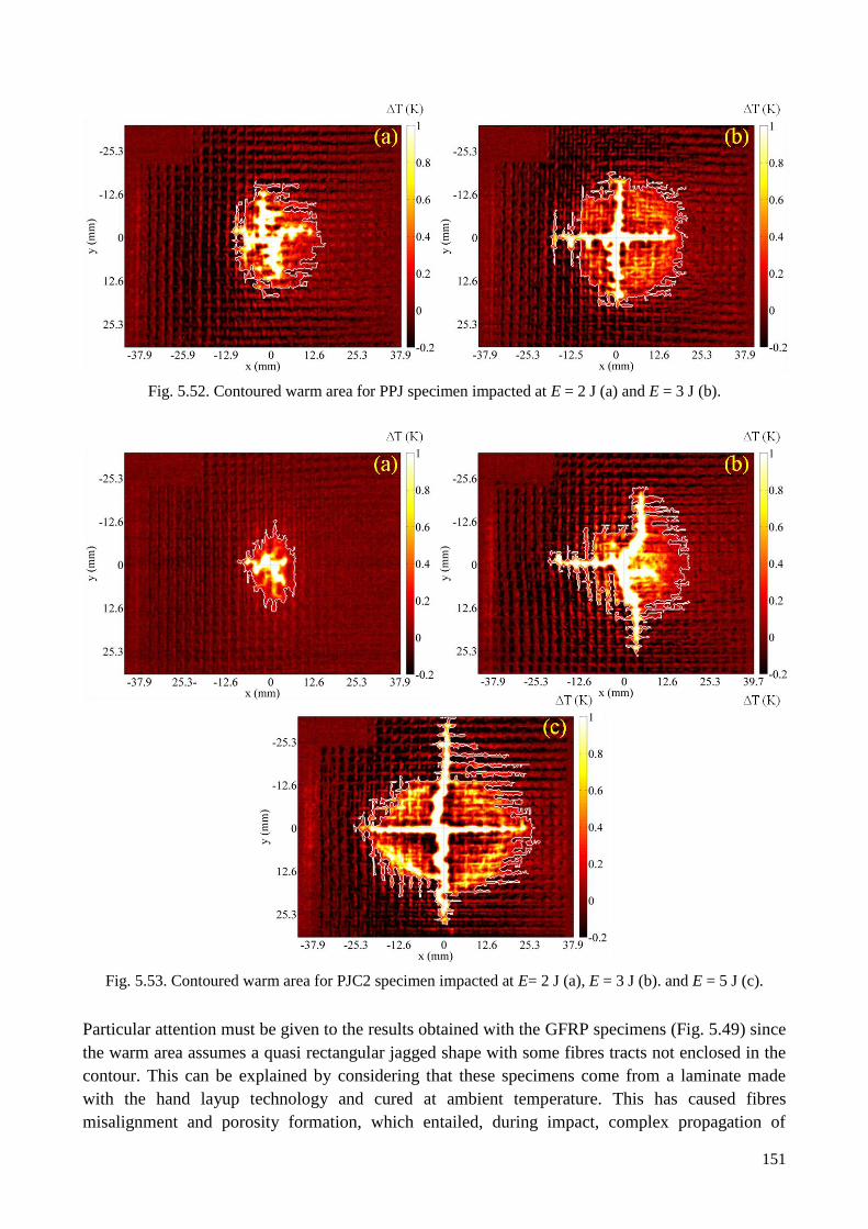
151
Fig. 5.52. Contoured warm area for PPJ specimen impacted at E = 2 J (a) and E = 3 J (b).
Fig. 5.53. Contoured warm area for PJC2 specimen impacted at E= 2 J (a), E = 3 J (b). and E = 5 J (c).
Particular attention must be given to the results obtained with the GFRP specimens (Fig. 5.49) since
the warm area assumes a quasi rectangular jagged shape with some fibres tracts not enclosed in the
contour. This can be explained by considering that these specimens come from a laminate made
with the hand layup technology and cured at ambient temperature. This has caused fibres
misalignment and porosity formation, which entailed, during impact, complex propagation of
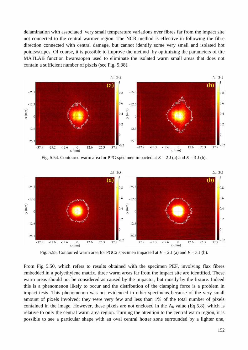
152
delamination with associated very small temperature variations over fibres far from the impact site
not connected to the central warmer region. The NCR method is effective in following the fibre
direction connected with central damage, but cannot identify some very small and isolated hot
points/stripes. Of course, it is possible to improve the method by optimizing the parameters of the
MATLAB function bwareaopen used to eliminate the isolated warm small areas that does not
contain a sufficient number of pixels (see Fig. 5.38).
Fig. 5.54. Contoured warm area for PPG specimen impacted at E = 2 J (a) and E = 3 J (b).
Fig. 5.55. Contoured warm area for PGC2 specimen impacted at E = 2 J (a) and E = 3 J (b).
From Fig 5.50, which refers to results obtained with the specimen PEF, involving flax fibres
embedded in a polyethylene matrix, three warm areas far from the impact site are identified. These
warm areas should not be considered as caused by the impactor, but mostly by the fixture. Indeed
this is a phenomenon likely to occur and the distribution of the clamping force is a problem in
impact tests. This phenomenon was not evidenced in other specimens because of the very small
amount of pixels involved; they were very few and less than 1% of the total number of pixels
contained in the image. However, these pixels are not enclosed in the Ah value (Eq.5.8), which is
relative to only the central warm area region. Turning the attention to the central warm region, it is
possible to see a particular shape with an oval central hotter zone surrounded by a lighter one,
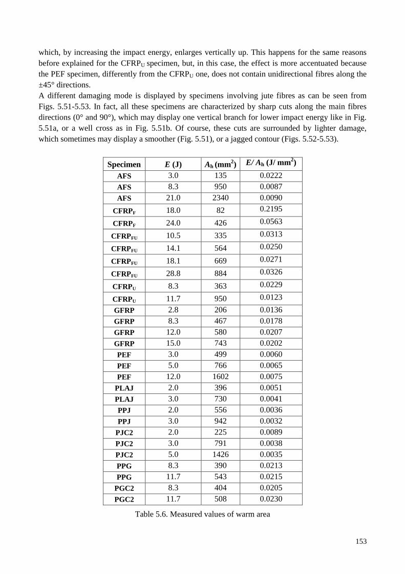
153
which, by increasing the impact energy, enlarges vertically up. This happens for the same reasons
before explained for the CFRPU specimen, but, in this case, the effect is more accentuated because
the PEF specimen, differently from the CFRPU one, does not contain unidirectional fibres along the
±45° directions.
A different damaging mode is displayed by specimens involving jute fibres as can be seen from
Figs. 5.51-5.53. In fact, all these specimens are characterized by sharp cuts along the main fibres
directions (0° and 90°), which may display one vertical branch for lower impact energy like in Fig.
5.51a, or a well cross as in Fig. 5.51b. Of course, these cuts are surrounded by lighter damage,
which sometimes may display a smoother (Fig. 5.51), or a jagged contour (Figs. 5.52-5.53).
Specimen E (J) Ah (mm2) E/ Ah (J/ mm
2)
AFS 3.0 135 0.0222
AFS 8.3 950 0.0087
AFS 21.0 2340 0.0090
CFRPF 18.0 82 0.2195
CFRPF 24.0 426 0.0563
CFRPFU 10.5 335 0.0313
CFRPFU 14.1 564 0.0250
CFRPFU 18.1 669 0.0271
CFRPFU 28.8 884 0.0326
CFRPU 8.3 363 0.0229
CFRPU 11.7 950 0.0123
GFRP 2.8 206 0.0136
GFRP 8.3 467 0.0178
GFRP 12.0 580 0.0207
GFRP 15.0 743 0.0202
PEF 3.0 499 0.0060
PEF 5.0 766 0.0065
PEF 12.0 1602 0.0075
PLAJ 2.0 396 0.0051
PLAJ 3.0 730 0.0041
PPJ 2.0 556 0.0036
PPJ 3.0 942 0.0032
PJC2 2.0 225 0.0089
PJC2 3.0 791 0.0038
PJC2 5.0 1426 0.0035
PPG 8.3 390 0.0213
PPG 11.7 543 0.0215
PGC2 8.3 404 0.0205
PGC2 11.7 508 0.0230
Table 5.6. Measured values of warm area
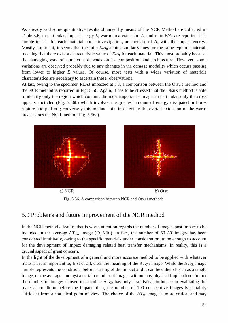
154
As already said some quantitative results obtained by means of the NCR Method are collected in
Table 5.6; in particular, impact energy E, warm area extension Ah and ratio E/Ah are reported. It is
simple to see, for each material under investigation, an increase of Ah with the impact energy.
Mostly important, it seems that the ratio E/Ah attains similar values for the same type of material,
meaning that there exist a characteristic value of E/Ah for each material. This most probably because
the damaging way of a material depends on its composition and architecture. However, some
variations are observed probably due to any changes in the damage modality which occurs passing
from lower to higher E values. Of course, more tests with a wider variation of materials
characteristics are necessary to ascertain these observations.
At last, owing to the specimen PLAJ impacted at 3 J, a comparison between the Otsu's method and
the NCR method is reported in Fig. 5.56. Again, it has to be stressed that the Otsu's method is able
to identify only the region which contains the most important damage, in particular, only the cross
appears encircled (Fig. 5.56b) which involves the greatest amount of energy dissipated in fibres
rupture and pull out; conversely this method fails in detecting the overall extension of the warm
area as does the NCR method (Fig. 5.56a).
a) NCR b) Otsu
Fig. 5.56. A comparison between NCR and Otsu's methods.
5.9 Problems and future improvement of the NCR method
In the NCR method a feature that is worth attention regards the number of images post impact to be
included in the average ΔTCW image (Eq.5.10). In fact, the number of 50 ΔT images has been
considered intuitively, owing to the specific materials under consideration, to be enough to account
for the development of impact damaging related heat transfer mechanisms. In reality, this is a
crucial aspect of great concern.
In the light of the development of a general and more accurate method to be applied with whatever
material, it is important to, first of all, clear the meaning of the ΔTCW image. While the ΔTCR image
simply represents the conditions before starting of the impact and it can be either chosen as a single
image, or the average amongst a certain number of images without any physical implication . In fact
the number of images chosen to calculate ΔTCR has only a statistical influence in evaluating the
material condition before the impact; then, the number of 100 consecutive images is certainly
sufficient from a statistical point of view. The choice of the ΔTW image is more critical and may
155
affect the final results. This implies the set of ΔT images used to calculate ΔTW to be chosen owing
to the material thermal diffusion time and its damaging way.
Owing to thermoset composites, in thick parts, the damage spreads out from the impact zone to the
opposite one through the typical pine tree configuration; conversely, in thin laminates the damage
starts from the rear surface (opposite to the impact) and evolves in the reversed pine tree pattern
[64]. The damaging way has to be taken into account for the interpretation of the hot stain
visualized over the viewed surface since it helps to be acquainted with what is responsible for
formation and/or enlargement of such a hot stain.
In thin parts, surface and/or shallow damage is accompanied by sudden temperature rise on the
opposite surface which is promptly captured by the infrared camera. Instead, surface temperature
variations linked to internal damage appear with delay; this because the heat produced by the
damage that branches through the thickness (reversed pine tree pattern) has to cross the thickness
moving backward towards the viewed surface. Of course, such a delay depends on the location of
the damage through the thickness and on the material characteristic diffusion time. Then, the warm
stain starts to form first very small, but very hot, at the tip of the impact (on the opposite side) and
after enlarges to cover the entire area affected by the reversed pine tree ramification. Unfortunately,
heat does not travel straight in one direction alone but it diffuses in all directions; this entails losses
and spreading with the consequence that the associated surface temperature (on the viewed side)
appears weaker and spread over a larger area. In the meantime, over the viewed surface, there is
lateral diffusion from hotter points/zones towards the colder ones. Of course, heat travels freely
along unidirectional fibres, while it is hindered by the fabric, as well other complex fibres
architecture. Then, for a specific material, it is important to know the characteristic diffusion time
through the thickness and between contiguous points over the viewed surface.
In thick parts, the damage starts close to the impacted surface and spreads in the pine tree
configuration. This would mean that the heat dissipated by the damage at the impact tip has to cross
the entire thickness before any temperature variation is visualized over the viewed surface.
Conversely, the outer damage branching in the pine tree pattern moves through the thickness
towards the opposite (viewed) surface Then, it is likely that the entire warm area may appear
outlined on the viewed surface sudden at the impact. Most likely, the warm area of a thicker part
may be less affected by lateral diffusion effects and then it might be more easily and accurately
outlined.
Thermoplastic matrix based composites behave differently under impact since they react to the
impact with visible permanent modifications, like metals, displaying an indentation (a small
concavity) on the impacted side and a protrusion on the rear one [39].
From these observations, the next step may be to find, for each material under investigation, a
characteristic time which allows to choose the number of images to be used to evaluate ΔTCW and
the time after impact from which extract such images.
5.10 A summary to Chapter 5
The obtained results show that monitoring the thermal signatures induced by an impact event
supplies information useful for the material characterization specifically for identifying initiation
and propagation of the impact damage. Through post-processing of the recorded images, it is
possible to get information useful for understanding more on the impact damaging mechanisms,
156
starting from the time interval the impactor remains in contact with the surface, the curvature
experienced by the different composites, as well the occurred plastic deformations. In particular,
from the time evolution of thermo-elastic effects it is possible to get information useful to establish
the time interval the impactor remains in contact with the specimen surface and to derive
knowledge about bending and deformation of the surface under the impactor pushing force.
Besides, the temperature rise with its time history allows getting information about the instant the
material starts to damage and the importance of the occurred damage. In addition, it was
demonstrated that applying the proposed NCR method it is possible to encircle and evaluate the
warm area, which accounts for the impact damaged area.
On the whole, as main findings, it has been shown that using infrared thermography it is possible to
get in a fast way different types of information about impact damaging of composites (impactor
peak contact, damage initiation and propagation, extension of delamination, etc.) which otherwise
require many different tests.
References to Chapter 5
[1] M.O.W. Richardson, M.J. Wisheart, Review of low-velocity impact properties of composite
materials. Composites Part A, 27, 1123-1131, 1996.
[2] R. Park, J. Jang, Impact behaviour of aramid/glass fiber hybrid composite: evaluation of four-layer
hybrid composites, J Mater Sci, 36, 2359-2367, 2001.
[3] T.W. Shyr, Y.H. Pan, Impact resistance and damage characteristics of composite laminates,
Compos Struct, 62, 193-203, 2003.
[4] S. Abrate, Impact on Composite Structures, Cambridge University Press, Cambridge, 1998.
[5] Baucom JN, Zikry MA. Low-velocity impact damage progression in woven E-glass composite
systems, Composites Part A, 36, 658-664, 2005.
[6] R. Olsson, M.V. Donadon, B.G. Falzon, Delamination threshold load for dynamic impact on plates,
Int. J. Solids Struct. 43, 3124-3141, 2006.
[7] D.J. Elder, R.S. Thomson, M.Q. Nguyen, M.L. Scott, Review of delamination predictive methods
for low speed impact of composite laminates, Compos. Struct. 66, 677-683, 2004.
[8] G.A. Schoeppner, S. Abrate, Delamination threshold loads for low velocity impact on composite
laminates, Compos. A 31, 903-915, 2000.
[9] W.J. Cantwell, Geometrical effects in the low velocity impact response of GFRP, Compos. Sci.
Technol. 67, 1900-1908, 2007.
[10] T. Mitrevski, I.H. Marshall, R. Thomson, R. Jones, B. Whittingham, The effect of impactor shape
on the impact response of composite laminates, Compos. Struct. 67, 139-148, 2005.
[11] H.S. Huang, R. Talreja, Effects of void geometry on elastic properties of unidirectional fiber
reinforced composites, Compos. Sci. Technol. 65, 1964-1981, 2005.
[12] P.O. Hagstrand, F. Bonjour, J.A.E. Månnson, The influence of void content on the structural
flexural performance of unidirectional glass fibre reinforced polypropylene composites, Compos. A
36, 705-714, 2005.
[13] L. Liu, B.M. Zhang, D.F. Wang, Z.J. Wu, Effects of cure cycles on void content and mechanical
properties of composite laminates, Compos. Struct. 73, 303-309, 2006.
[14] S. Abrate, Modeling of impacts on composite structures, Compos. Struct. 51, 129-138, 2001.
[15] C. Meola, G.M. Carlomagno, Infrared thermography to evaluate impact damage in glass/epoxy
with manufacturing defects, Int. J. Impact Eng. 67, 1-11, 2014.
[16] M. Ashby, A. Evans, N. Fleck, L. Gibson, J. Hutchinson, H. Wadley, Metal foams: a design guide,
referex engineering. Butterworth-Heinemann, 2000.
[17] G. Petrone, V. D’Alessandro, F. Franco, S. De Rosa, Numerical and Experimental investigations
on the acoustic power radiated by Aluminium Foam Sandwich panels, Composite Structure, 118,
170-177, 2014.
157
[18] V. D’Alessandro, G. Petrone, S. De Rosa, F. Franco, Modelling of aluminium foam sandwich
panels, Smart Struct Syst, 13(4), 615–636, 2014.
[19] L.J. Gibson; M.F. Ashby, Cellular Solids, 2nd ed.; Cambridge University Press: Cambridge, UK,
1997.
[20] P. Feraboli, K.T. Kedward, A new composite structure impact performance assessment program,
Composites Science and Technology, 66, 1336–1347, 2006.
[21] G.M. Carlomagno, P.G. Berardi, Unsteady thermotopography in non-destructivetesting, in: C.
Warren (Ed.), Proc. III Infrared Inform. Exch, AGA, St. Louis, MO, pp. 33-40, 1976.
[22] G. Busse, Optoacoustic phase angle measurement for probing a metal, Appl. Phys. Lett. 35, 759-
760, 1979.
[23] A. Letho, J. Jaarinen, T. Tiusanen, M. Jokinen, M. Luukkala, Magnitude and phase in thermal
wave imaging, Electron. Lett. 17, 364-365, 1981.
[24] J.-L. Beaudoin, E. Merienne, R. Danjoux, M. Egee, Numerical system for infrared scanners and
application to the subsurface control of materials by photothermal radiometry, Proc. SPIE 590,
287-292, 1985.
[25] G. Busse, D. Wu, W. Karpen, Thermal wave imaging with phase sensitive modulated
thermography, J. Appl. Phys. 71, 3962-3965, 1992.
[26] V. Vavilov, Thermal nondestructive testing: short history and state-of-art, in:D. Balageas, G.
Busse, G.M. Carlomagno (Eds.), Proceedings of the QIRT92,Eurotherm Series 27. EETI ed., pp.
179-193, 1992.
[27] X. Maldague, Introduction to NDT by active infrared thermography, Mater. Eval. 6, 1060-1073,
2002.
[28] C. Meola, G.M. Carlomagno Application of infrared thermography to adhesion science, Journal of
Adhesion Science and Technology, 20(7), 589-632, 2006.
[29] O. Breitenstein, W. Warta, M. Langenkamp, Lock-in Thermography: Basics and Use for
Evaluating Electronic Devices and Materials, Springer, 2nd. s.l., 2010.
[30] C. Maierhofer, P. Myrach, H. Steinfurth, M. Reischel, and M. Röllig, Development of standards for
flash thermography and lock-in thermography, Proceedings of the QIRT conference 2014.
[31] P.G. Bison, S. Marinetti, E. Grinzato, Measurement of thermal diffusivity by lock-in thermography.
Proc. QIRT 2000, 30-5, 2000.
[32] C. Meola, G.M. Carlomagno, A. Squillace, G. Giorleo, Non-destructive control of industrial
materials by means of lock-in thermography, Meas. Sci. Technol. 13, 1583-1590, 2002.
[33] W.J. Parker, R.J. Jenkins, C.P. Butler, G.L. Abbott, Flash Method of Determining Thermal
Diffusivity, Heat Capacity, and Thermal Conductivity, J. Appl. Phys., 32, 1679–84, 1961.
[34] C. Meola, C. Toscano, Flash thermography to evaluate porosity in carbon fiber reinforced polymer
(CFRPs). Materials, 7, 1483–501, 2014.
[35] Standard Practice for Ultrasonic Testing of Flat Panel Composites and Sandwich Core Materials
Used in Aerospace Applications ASTM E2580-07 2007.
[36] T.J. Batzinger, W. Li, R.S. Gilmore, E.J. Nieters, W.T. Hatfield, et al. Phased array ultrasonic
inspection method for industrial applications US6789427 (2004).
[37] Olympus manual: advances in phased array ultrasonic technology applications.
[38] C. Meola, S. Boccardi, G.M. Carlomagno, N.D. Boffa, F. Ricci, G. Simeoli, P. Russo, Impact
damaging of composites through online monitoring and non-destructive evaluation with infrared
thermography, NDT&E International, 85, 34-42, 2017.
[39] S. Boccardi, G.M. Carlomagno, C. Meola, P. Russo and G. Simeoli, Infrared thermography to
evaluate impact damaging of thermoplastic composites, Proc. QIRT 2014, Bordeaux, France, 7-11
July 2014. paper 214.
[40] C. Meola, S. Boccardi, N.D. Boffa, F. Ricci, G.M. Carlomagno Infrared thermography to evaluate
impact damaging of composites, Proc. of ECCM16 Seville (Spain) 22-26 June 2014, Paper 0318,
Program book: ISBN-10: 84-616-9798-7 and ISBN-13: 978-84-616-9798-4.
[41] C. Meola, S. Boccardi, G.M. Carlomagno, N.D. Boffa, E. Monaco, F. Ricci, Nondestructive
evaluation of carbon fibre reinforced composites with infrared thermography and ultrasonics.
Compos Structures, 134, 845–53, 2015.
[42] S. Boccardi, N.D. Boffa, G.M. Carlomagno, L. Maio, C Meola, F Ricci, Infrared thermography and
ultrasonics to evaluate composite materials for aeronautical applications, Journal of Physics,
Conference Series 658 (2015)
158
[43] L. Maio, V. Memmolo, S Boccardi, C. Meola, F. Ricci, N.D. Boffa, E. Monaco, Ultrasonic and IR
Thermographic Detection of a Defect in a Multilayered Composite Plate, Procedia Engineering,
167, 71-79, 2016. doi: 10.1016/j.proeng.2016.
[44] C. Meola, S. Boccardi, N.D. Boffa, M. Di Palma, L. Maio, G.M. Carlomagno, Impact Damaging of
Carbon Fibre-reinforced Composites: a Comparison between Infrared Thermography and
Ultrasonics, Proc. 11th ECNDT, Prague (Czech Republic), 10p, 2014.
[45] C. Meola, G.M. Carlomagno, Infrared thermography to impact-driven thermal effects, Applied
Physics A, 96, 759-762, 2009.
[46] C. Meola, G.M. Carlomagno, V. Lopresto, G. Caprino, Impact damage evaluation in composites
with infrared thermography, 3rd European Conference for Aerospace Science EUCASS, Versailles
(France) 6-9 July, 2009.
[47] C. Meola, G.M. Carlomagno, Health monitoring of composites with infrared thermography
ESMC2009 7th EUROMECH Solid Mechanics Conference Lisbon (Portugal) 7-11 September,
2009.
[48] C. Meola, G.M. Carlomagno, Impact damage in GFRP: new insights with Infrared Thermography,
Composites Part A, 41(12), 1839-1847, 2010.
[49] G.M. Carlomagno, C. Meola, F. Ricci, Infrared thermography and piezoelectric patches for impact
damage detection in composite structures, IWSHM 2011 - International Workshop on Structural
Health Monitoring 2011, Stanford University, Stanford, CA, September 13-15, 2011.
[50] C. Meola, G.M. Carlomagno, F. Ricci, V. Lopresto, G. Caprino, Investigation of Impact Damage in
Composites with Infrared Thermography, 6th NDT in Progress, Prague (Czech Republic) 10-12
October 2011, Ed. P. Mazal, pp. 175-182, 2011.
[51] C. Meola, G. M. Carlomagno and F. Ricci, Monitoring of impact damage in Carbon Fibre
Reinforced Polymers, QIRT 2012, Napoli, June 11-14, 2012, paper n. 374, pp.8.
[52] S. Abrate, Impact on laminated composite materials, Applied Mechanics Review, 44, 155-190,
1991.
[53] T.J. Kang, C. Kim, Impact Energy Absorption Mechanism of Largely Deformable Composites with
Different Reinforcing Structures, Fibers and Polymers, 1, 45-54, 2000.
[54] C. Meola, S. Boccardi, N.D. Boffa, F. Ricci, G. Simeoli, P. Russo, G.M. Carlomagno, New
perspectives on impact damaging of thermoset- and thermoplastic-matrix composites from
thermographic images, Composite Structures, 152, 746-754, 2016.
[55] C. Meola, S. Boccardi, G.M. Carlomagno, N.D. Boffa, E. Monaco, F. Ricci, The added value of
infrared thermography to impact damaging assessment of carbon fibre reinforced composites, NDT
WORLD, 19, (3), 49-53, 2016
[56] N.K. Naik, Y. Chandra Sekher, Sailendra Meduri, Damage in woven-fabric composites subjected
to low-velocity impact, Comp. Sci. Technol. 60, 731-744, 2000.
[57] N.K. Naik, R. Ramasimha, H. Arya, S.V. Prabhu, N. ShamaRao, Impact response and damage
tolerance characteristics of glass–carbon/epoxy hybrid composite plates, Composites Part B: Eng.,
32, 565–574, 2001.
[58] H.Y.T. Wu, F.K. Chang, Transient dynamic analysis of laminated composite plate subjected to
transverse impact. Comput Struct. 31, 453–66, 1989.
[59] H.Y. Choi, H.Y.T. Wu, F.K. Chang, A new approach toward understanding damage mechanisms
and mechanics of laminated composites due to low-velocity impact: part II––analysis. J Compos
Mater. 25, 1012–38, 1991.
[60] H.Y. Choi, F.K. Chang, A model for predicting damage in graphite/epoxy laminated composites
resulting from low-velocity point impact. J Compos Mater. 26, 2134–69, 1992.
[61] Z. Aslan, R. Karakuzu, B. Okutan, The response of laminated composite plates under low-velocity
impact loading Comp. Struct. 59, 119–127, 2003.
[62] Y. Perrot, C. Baley, Y. Grohens, P. Davies, Damage resistance of composites based on glass fibre
reinforced low styrene emission resins for marine applications. Appl Compos Mater 14, 67–87,
2007.
[63] G.P. Zhao, C.D. Cho, Damage initiation and propagation in composite shells subjected to impact.
Comp. Struct 78, 91–100, 2007.
[64] S. Abrate (Editor) Impact Engineering of Composite Structures, Springer Wien New York (2011).
159
[65] C. Meola, S. Boccardi, G. Petrone, N.D. Boffa, F. Ricci, G.M. Carlomagno, Infrared thermography
to an aluminium foam sandwich structure subjected to low velocity impact tests, Procedia
Engineering, 167, 23-29, 2016.
[66] C. Meola, S. Boccardi, G.M. Carlomagno, Measurements of very small temperature variations with
LWIR QWIP infrared camera, Infrared Physics & Technol. 72, 195-203, 2015.
[67] S. Boccardi, G.M. Carlomagno, C. Meola, The added value of infrared thermography in the
measurement of temperature-stress coupled effects, Sensors & Transducers, 201(6), 43-51, 2016.
[68] S. Boccardi, G.M. Carlomagno, C. Meola, Basic temperature correction of QWIP cameras in
thermo-elastic-plastic tests of composite materials, Applied Optics, 55(34), D87-D94, 2016.
[69] S.B. Vardeman, J.M. Jobe, Statistical Methods for Quality Assurance, second edition, Springer-
Verlag, New York, 2016.
[70] S. Boccardi, G.M. Carlomagno, C. Meola, P. Russo, G. Simeoli, Monitoring impact damaging of
thermoplastic composites, Journal of Physics: Conference Series 658 (2015).
[71] S Boccardi, GM Carlomagno, G Simeoli, P Russo, C Meola, Evaluation of impact-affected areas of
glass fibre thermoplastic composites from thermographic images. Measurement Science
&Technology, 27, 075602, 12p. 2016
[72] N. Otsu, A threshold selection method from gray-level histograms IEEE Trans. Syst. Man Cybern.
smc-9 62–6, 1979.
[73] R.C. Gonzales, R.E. Woods, S.L. Eddins, Digital Image Processing Using MATLAB 2nd edn
(USA: Gatesmark) 2009, ISBN 978-0-9820854-0-0.
[74] S.U. Lee, S.Y. Chung, R.H. Park, A comparative performance study of several global thresholding
techniques for segmentation Comput. Vis. Graph. Image Process. 52, 171–90, 1990.
[75] S. Boccardi, G.M. Carlomagno, C. Meola, Post-processing of time-sequences acquired during
impact tests with the aid of a reference area. Proc. QIRT 2016, Gdańsk (Poland), 126-134, 2016,
160
Conclusions
This thesis was concerned with the application of infrared thermography to monitoring composite
materials subjected to either cyclic bending, or impact tests. These tests were applied to different
types of composites involving either a thermoset, or a thermoplastic, matrix and different types of
fibres as reinforcement.
The main encountered problem to be solved has been the evaluation of the very small temperature
differences coupled with thermo-elastic and thermoplastic effects, which are at the edge of
instrument sensitivity, so strongly affected by noise.
At least for the QWIP detector, mostly used within this thesis, this noise is mainly constituted by
random jumps, which may completely disrupt the sinusoidal trend coupled with cyclic bending or
the detection of feeble delaminations. A solution to this problem has been devised in the use of a
reference specimen to account for temporal noise, which was successively eliminated from the
recorded sequences of images. To this end, also some simple post-processing algorithms have been
developed in the Matlab environment to handle the thermal images. This correction method, called
Reference Area Method, has also been applied to other infrared cameras with ad hoc experimental
tests, involving either a black body or a real surface, both kept at constant temperature.
In addition, some key parameters such as the dimension of the measuring area A, and of the
reference area AR, as well the influence of their relative positions have been considered; the
obtained results are shown in term of plots and/or Tables in Chapter 3. In all the test cases, the
Reference Area Method has proved its effectiveness in significantly reducing the temporal noise
and in particular abrupt jumps, sinusoidal patterns, drift and external disturbances due to the
environment. As an important result, it has been found that the Reference Area Method was able to
restore the signal coming from different cameras equipped with any type of tested detector: QWIP,
InSb and micro-bolometric.
Then, the Reference Area Method has been widely used coupled with both cyclic bending tests and
impact tests.
In particular, cyclic bending tests (Chapter 4) have been the litmus test of this method. In fact, the
Reference Area Method has been effective to restore the sinusoidal trend coupled with cyclic
bending tests, which, at low bending frequency, was completely disrupted by the random jumps
(e.g., Fig. 4.12).
Besides, the results obtained with the prototype machine setup (realized during doctorate and
described in chapter 4) show that, through simple tests, it was possible to get information useful for
the characterization of new composite materials, in particular, to discriminate the small variations of
T induced by any variation in the material such as the type of matrix, the reinforcement, or the
percentage of compatibilizing agent.
Of course, the obtained data cannot be considered exhaustive to characterize the specific behaviour
of the considered materials; other tests are required with also a comparison with conventional
mechanical tests made on the same materials.
The topic of chapter 5 has been the monitoring of impact tests, at low velocity/energy, on different
types of composites (different matrix, and/or reinforcement).
In particular, the efforts have been devoted towards two main aspects:
161
1. Get information about the impact dynamic through the analysis of image sequences acquired
at high frame rate (960 Hz).
2. Define a general criterion to measure the overall extension of the impact damage.
In relation to point 1, the obtained results showed that monitoring the thermal signatures, induced
by an impact event, supplied information useful for identifying, in a fast way, initiation and
propagation of the impact damage. However, more information were derived from post processing
of the recorded images, with ad hoc routines developed in the Matlab environment. In particular, it
was possible to get information useful for understanding more on the impact damaging
mechanisms, starting from the time interval the impactor remained in contact with the surface, the
curvature experienced by the different composites, as well the occurred plastic deformations. In
fact, from the time evolution of thermo-elastic effects, it was possible to get information useful to
establish the time interval the impactor remains in contact with the specimen surface and to derive
knowledge about bending and deformation of the surface under the impactor pushing force.
Besides, the temperature rise with its time history allowed getting information about the instant the
material started to damage and the importance of the occurred damage.
In addition, a procedure to measure the extension of the impact damage, from the warm area has
been proposed.
Such a procedure consisted in comparing two average ∆T images (above a set of ∆T images) taken
before and after impact and building a binary image, which highlighted the warm area. This
approach, which is named NCR, encloses the reference sample noise correction method. The
obtained results proved the capability of the NCR method to encircle the warm area accounting for
the extension of the impact affected area also in presence of complex materials architecture. The
effectiveness of the NCR method has been demonstrated also in comparison with the Otsu's
method.
It is worth noting that the NCR method was effective in measuring the overall extension of the
warmed area, but it still needs to be refined to get the real extension of the damaged area. In
particular, the introduction of a material characteristic diffusion time appears necessary to account
for heat diffusion related phenomena i.e. for a better choice of the number of thermal images to be
considered.

162
Acknowledgments
Today, April 4th 2017, I am in the Laboratory of Gasdynamics of the Department of Industrial
Engineering sat in front of the Desktop, which was with me along the Ph.D. adventure as a votary
friend, and I'm going to write the last part of my thesis: the acknowledgments.
I don't know the opinion of who has the difficult task to judge my work and all the other activities
performed in these 3 years Ph.D course, but just now, I need to thank all people who shared a little
step of this journey with me and encouraged me to go on, especially when dealing with life
problems, when deep sadness and despair obscure the brain and stop the heart.
My first thought goes, far away somewhere in the universe, to my mother Paola. Thanks Mom for
everything, I'll never forget your love and life lessons taught to me and to our family. The strength,
serenity and religious faith you have shown during the long illness and especially in your last days,
when also the last hopes vanished, have been a great example for everybody and will inspire forever
my life.
I want to thank my father Vincenzo, my brother Emanuele and in particular my young sister
Nicoletta who has tolerated me and my frequent absence. A special thank to my love Daniela, to my
brother's girlfriend Federica and to my aunts Maria and Silvana. Thanks to you all, without your
moral and material help everything would have been more and more difficult. Special thanks to
Antonio Rolfi for all the support he has given to me.
Rarely during the life, by chance, happens to meet uncommon people who have inside genius,
humanity and something special that I cannot' exactly explain, qualities joined in only one person. I
had the great luck to have as guides during the Ph.D travel two examples of this extraordinary
persons (sometimes I think it has been too much for an ordinary person like me). Dear Ing. Meola
and Prof. Carlomagno my only hope is having repaid at least a part of the trust you gave to me 3
years ago. Apart from your personal opinion about me and my activities, I want to tell you that I
have put in this adventure all myself and I have done everything that I could in order to honour the
opportunity you have offered to me. It is for you all my gratitude.
In particular, I thank you Carosena for all the time you have spent for me and for every single word
of encouragement and hope. You have been a great example for me because what you have taught
to me overcomes the pure academic activities and will remain forever in my life luggage. It is also
thanks to you if I never gave up.
My heartfelt thanks to my colleague, co-author and friend Ing. Giorgio Simeoli. Giorgio, during
these three years you have been as a big brother for me. Your advices about work and life problems
have been very precious for me. Your constant presence especially in the worst times has been
fundamental for me to keep on going on.
I thank Prof. Domenico Acierno and Pietro Russo who have made my Ph.D. possible and have
provided me with funds and all the necessary support and ever more in order to perform the
research activities.
I thank Prof. Michele Russo who has loaned me the electro-mechanical actuator to perform the
cyclic bending tests.
A particular thank to Ing. Francesco Messa (FLIR Systems) and Roberto Rinaldi (Infrared Training
Center) for the support in carrying tests with SC6800, X6540sc and T440 cameras and for fruitful
discussion.

163
I would thank the Evaluators Prof. Christiane Maierhofer and Prof. Vladimir Vavilov who patiently
read my work and supplied me fruitful and precious suggestions.
I thank all my co-authors, researchers and professors who have shared with me the experimental
activities and experiences, in particular: Prof. Fabrizio Ricci, Ing. Natalino Daniele Boffa, Ing.
Giuseppe Petrone and Ing. Leandro Maio.
I would say thank you to my colleagues, mates of adventure in the Gasdynamic Laboratory, for the
leisure hours spent together which have made the work less hard and for their support: Ing. Giusy
Castrillo, Ing. Carlo Salvatore Greco, Ing. Gerardo Paolillo, Ing. Cuono Massimo Crispo, Ing.
Mattia Contino, Ing. Francesco Avallone, Ing. Gioacchino Cafiero and Dott. Giuseppe Sicardi.
At last, but not least, I'm grateful to God. I am sure that without his help nothing of what happened
in my life till now would have been possible.
Naples, 04/04/2017
Simone Boccardi


