Integrated Nitrogen Management In China

International Institute for Applied Systems Analysis Registration number: ZVR 524808900

International Institute for Applied Systems Analysis Schlossplatz 1 A-2361 Laxenburg, Austria

Tel: +43 2236 807 342Fax: +43 2236 71313

E-mail: [email protected]: www.iiasa.ac.at

Interim Reports on work of the International Institute for Applied Systems Analysis receive only limited review. Views or opinions expressed herein do not necessarily represent those of the Institute, its National Member Organizations, or other organizations supporting the work.

Interim Report IR-09-005

Integrated nitrogen management in China T. Ermolieva W. Winiwarter G. Fischer G.-Y. Cao Z. Klimont W. Schöpp Y. Li W.A.H. Asman

Approved by Fabian Wagner Coordinator, GGI and Markus Amann Programme Leader, APD

August, 2009

ii

Contents

1 Introduction .................................................................................................................................... 1

1.1 Background ........................................................................................................................... 1

1.2 Objectives.............................................................................................................................. 2

1.3 A case study for China .......................................................................................................... 2

1.4 Methodology ......................................................................................................................... 3

2 The baseline development .............................................................................................................. 4

2.1 Economic growth .................................................................................................................. 5

2.2 Population.............................................................................................................................. 6

2.3 Land use ................................................................................................................................ 7

2.3.1 Demand for cereals and livestock products ...................................................................... 9

3 Sources of nitrogen: manure and mineral fertilizer ...................................................................... 13

3.1 Manure production .............................................................................................................. 13

3.2 Mineral fertilizer use ........................................................................................................... 15

4 Modeling the release of nitrogen compounds to the atmosphere and groundwater...................... 17

4.1 Leaching of nitrate .............................................................................................................. 17

4.2 Atmospheric emissions of N2O ........................................................................................... 21

4.3 Atmospheric emissions of ammonia ................................................................................... 22

5 Development of risk functions to minimize environmental effects.............................................. 26

6 Alternative scenarios of agricultural practice ............................................................................... 31

7 Exposure to environmental pressure............................................................................................. 37

7.1 Introduction to the concept.................................................................................................. 37

7.2 Performance review of reallocation .................................................................................... 40

7.3 Release of adverse compounds to the environment by scenario ......................................... 44

8 Comparing numerical results with literature data......................................................................... 47

9 Conclusions .................................................................................................................................. 49

iii

Abstract

Providing China’s growing population with higher quality food and a larger share of meat in diets can only be accomplished through increased agricultural productivity, which is usually achieved through higher input of nitrogen to soils. This can lead to nitrate leaching which affects the quality of drinking water, causes emissions of ammonia to the atmosphere, a contributor to the formation of atmospheric particles that are harmful to human health, and to the release of nitrous oxide (N2O), an important global greenhouse gas.

This report develops an integrated perspective on agricultural management measures that have multiple benefits on economic development, on the local environment and for global greenhouse gas emissions. The study estimates for the case of China that an integrated nitrogen management approach could increase agricultural production by up to 50 percent while keeping current levels of nitrogen discharge to soil, water and air at the local scale. Compared to the business as usual case, emissions of N2O greenhouse gas emissions would be 25 percent lower.

Developed as an activity of IIASA’s interdisciplinary Greenhouse Gas Initiative (GGI), the new integrated approach links population increase and demands on food quality with nitrogen fertilizer requirements in agriculture, and assesses undesired environmental effects of nitrogen at the local and global scales.

iv

Acknowledgments

This report describes results of an IIASA inter-program collaboration carried out under the umbrella of IIASA’s “Greenhouse Gas Initiative” (GGI).

The authors are grateful to their colleagues from numerous research programs at IIASA who have helped to develop the new integrated perspective on nitrogen management, and in particular to Geza Toth and Fabian Wagner for organizing and coordinating the GGI activities.

The authors acknowledge contributions of their research partners in China and Europe to this project, especially from the research projects on “Policy Decision Support for Sustainable Adaptation of China’s Agriculture to Globalization” (CHINAGRO) and the “Chinese Agricultural Transition: Trade, Social and Environmental Impacts” (CATSEI) project.

This work received financial support from the European Union through the INCO-DEV ICA-2000-20039 project and the ACCENT “Atmospheric Composition Change, the European Network of Excellence” of the 6th Framework Programme. Additional resources were provided by the Chinese and the Dutch governments, and from IIASA’s internal funds.

v

About the Authors

The authors are affiliated with the International Institute for Applied Systems Analysis, in the Land Use Change programme (T.E., G.F.), the Forestry programme (G.-Y.C.) and the Atmospheric Pollution and Economic Development programme (all other authors). W.W. also works at AIT, the Austrian Institute of Technology, Y.L. contributed during her involvement in IIASA’s Young Scientist’s Summer Programme, her permanent affiliation is the Chinese Academy of Agricultural Sciences, Beijing.

1

Integrated nitrogen management in China

T. Ermolieva, W. Winiwarter, G. Fischer, G.-Y. Cao, Z. Klimont, W. Schöpp, Y. Li, W.A.H. Asman

1 Introduction

1.1 Background

Providing the growing population in developing countries with higher quality food and a larger share of meat in diets can only be accomplished through higher agricultural productivity, which is usually achieved through larger input of nitrogen to soils.

However, this intensified application of nitrogen leads to a range of undesired effects on human health and the local, regional and global environment. At the local scale, excess input of nitrogen to soils can allow nitrate to leach into groundwater. Ingested nitrate (via conversion to nitrite) under conditions that result in endogenous nitrosation is probably carcinogenic to humans, leading to cancers e.g. of the digestive tract (Ward et al., 2005). Excess nitrogen in soils also causes volatilization of ammonia (NH3) and nitrogen oxides (NOx). Released to the atmosphere, they act as important precursor substances leading to the formation of fine particulate matter (PM2.5). Human exposure to PM2.5 causes premature mortality from cardiovascular and cardiopulmonary diseases (Pope et al., 2002). Excess nitrogen in surface water contributes to eutrophication of aquatic systems. Deposited on land, nitrogen in excess of the needs of plants threatens biodiversity and contributes to the acidification of ecosystems. The microbial conversion of soil nitrogen compounds also leads to emissions of nitrous oxide (N2O) to the atmosphere. This process accounts for about four percent of global anthropogenic greenhouse gas emissions (IPCC, 2001).

Among other factors, agricultural management practices do not only determine the crop yield, but they also have an important impact on the rates at which these environmental processes occur. Unfortunately, various trade-offs exist in the impacts of different measures on the various environmental endpoints.

An effective response to the full range of issues requires an integrated management of nitrogen in agriculture, and specifically of nitrogen in soil. Such a coherent approach is

2

even more important in developing countries in Asia where the rapidly growing economies with changing lifestyles and diets cause the release of increasing amounts of nitrogen into the environment. Challenges are further enhanced by ongoing climate change, which may compromise agricultural productivity especially in low-latitude developing countries (IPCC, 2007).

1.2 Objectives

In this report we explore how nitrogen could be managed to enable production of sufficient food while limiting negative impacts of excess nitrogen on human health, the local environment and on greenhouse gas emissions. Our work aims at a holistic perspective on nitrogen, bringing together the societal benefits of nitrogen application with its potentially negative environmental impacts. We explore alternative nitrogen management approaches that maintain agricultural productivity under possible future climatic conditions and reduce the release of nitrogen to the atmosphere and groundwater. Such approaches could facilitate a more comprehensive analysis of the options for mitigating N2O emissions from agriculture in developing countries, and allow exploring to what extent measures that help adapting agricultural production to climate change could at the same time reduce greenhouse gas emissions.

1.3 A case study for China

To illustrate our approach, we present a case study on nitrogen management in China. The rapid growth of the Chinese economy, associated urbanization, rising living standards, combined with continued population growth, have profoundly affected the agricultural sector in China. The rapid expansion of agricultural production to supply a sharply increased demand for livestock products has been achieved through an intensification of agricultural production and the introduction of industrial peri-urban and urban production systems. As the availability of additional agricultural land is limited, crop production has been significantly increased by higher application of chemical and livestock manure fertilizer.

Unfortunately, this pressure is not expected to diminish in the future. With current agricultural practices, agricultural production in China is limited by constraints on the availability of land with sufficient quality, on irrigation water and fertilizers. Increased production can only be achieved by enhanced efficiency in resource use and intensification through additional input of chemical fertilizers.

For this case study, we were able to benefit from existing information available at IIASA. We built on extensive detailed knowledge on the Chinese land use and

3

population development as available at the Land Use Change programme and at the Forestry programme. LUC’s CATSEI model (Fischer and Ermolieva, 2009a) provided spatially explicit, demand driven projections on the Chinese agricultural sector. Coupling this with the GAINS model (operated by the Atmospheric Pollution and Economic Development programme), which recently was updated for China (Amann et al., 2008), it became possible to link production and environmental impacts. This link allowed evaluating integrated measures to mitigate the environmental effects of agricultural nitrogen demand, which would not compromise food productivity.

1.4 Methodology

A methodology has been developed to assess the effects of agricultural management practices on productivity as well as on a range of environmental endpoints.

The approach starts from a “business-as-usual” projection of agricultural nitrogen application up to the year 2030, and explores a set of alternative nitrogen management options that do not compromise overall yields. The following management options have been explored:

• Sustainable reallocation: Spatial re-allocation of agricultural production so that a general environmental risk indicator is minimized

• Optimized fertilizer use: All manure that is available from livestock production is applied, and the remaining demand is covered by mineral fertilizer.

• Minimized emissions of ammonia (based on advanced technology options).

These management options have been analyzed along a set of indicators that reflect environmental and health risks that result from agricultural activities. The analysis is carried out in a geographically explicit way, which allows evaluating results both in terms of agricultural area and population exposure (where applicable).

A comparison of the scenarios provides indications about management options that will maintain productivity while minimizing negative health and environmental effects.

This report is organized as follows: Section 2 describes the baseline development used to set the scenarios. Section 3 estimates the current amounts of nitrogen that are applied to soils in China in the “business-as-usual” scenario, and Section 4 introduces risk indicators for nitrate leaching, NH3 and N2O emissions. The algorithm for the re-distribution of agricultural production is presented in Section 5. Section 6 analyzes the three policy options in terms of nitrate leaching, NH3 and N2O emissions, while their health impacts are explored in Section 7. Section 8 provides a brief literature review on agriculture-related N2O emissions, and conclusions are drawn in Section 9.

4

2 The baseline development To be of practical relevance, any assessment of alternative agricultural management options must consider the rapid economic development in China and the resulting implications on the agricultural system. A baseline scenario quantifies assumptions on important driving forces, environmental factors and policy variables that determine future agricultural production conditions. Inter alia, the development of a baseline scenario requires assumptions on the following aspects:

• What will be the demand for agricultural products in China, in particular for meat, under plausible economic, demographic and urbanization development paths to 2030?

• How will increased demand for feed and food translate into the livestock number and crop production?

• How much nitrogen will become available from livestock manure as a consequence of intensified livestock production? How much mineral fertilizer would be needed in addition to local supply of manure?

• What environmental loads, GHG emissions and water pollution through leaching are expected as a result of agricultural production intensification?

• Which improvements in productivity and environmental burden would result from an application of simple “good” agricultural practices at the different stages of agricultural production chain, i.e., from nutrients losses in livestock houses to emissions and nutrients losses on crop fields?

Our baseline scenario employs the ‘central’ national and regional economic, demographic projections developed for the CHINAGRO and CATSEI1 projects (Huang et al., 2003a) as the context in which the agricultural sector will operate.

We conduct our analysis at the county level, i.e., for about 2430 spatial units in China. Results are aggregated to 33 provinces or eight economic regions of China (Figure 1).

1 With support of the European Union (INCO-DEV ICA-2000-20039), support of the Chinese and Dutch governments, and support of IIASA, research partners in Europe and China have conducted a case study on “Policy Decision Support for Sustainable Adaptation of China’s Agriculture to Globalization” (hence the CHINAGRO project) and Chinese Agricultural Transition: Trade, Social and Environmental Impacts (CATSEI)

5

Figure 1. Provinces and economic regions of China

Incentives governing the demand for agricultural products are aggregated into the three main driving forces: economic growth, demographic development (population growth and urbanization), and land use. We distinguish different demand patterns for urban and rural areas in different geographical regions, which vary with income. In addition, agricultural development in China is also determined by the ongoing conversion of farmland due to economic as well as ecological reasons, and regionally severe land degradation.

2.1 Economic growth

Economic development is a key parameter driving any future development. In order to have a unique initial driver we single out growth rates of other sectors than agriculture. The level of agricultural activities will be determined by population growth and food quality. The growth rates resulting from the modeling performed by Huang et al. (2003) for each economic region as well as for total China are presented in Table 1. In the underlying economic model we differentiate three projections according to “low”, “medium” or “high” economic growth, but for most purposes it will be sufficient to refer to the “central” projection only.

6

Table 1. Non-farm production: regional growth rates in “central” projection

Annual growth rate (in %) at constant prices Region 1997-

2003 2003- 2010

2010- 2020

2020- 2030

2003- 2030

North 9.8 7.6 5.8 4.6 5.8 Northeast 8.6 6.2 5.1 3.8 4.9 East 9.8 8.0 6.2 5.0 6.2 Central 10.5 7.0 5.7 4.0 5.4 South 10.5 8.7 6.9 5.7 6.9 Southwest 7.8 6.0 5.1 3.8 4.8 Plateau 9.0 7.1 5.7 4.9 5.7 Northwest 9.5 6.5 5.6 4.3 5.4 CHINA 9.7 7.6 6.0 4.8 6.0

Source: Huang et al. (2003)

2.2 Population

Population growth and especially the share of people moving into cities (urbanization) is a function of the economic development. Table 2 lists our assumptions on population development derived from the “central” CATSEI projection. Starting from 1.275 billion people in 2000, population is assumed to rise to 1.39 billion people in 2015 and 1.46 billion people in 2030. At the same time, the share of population living in cities (urbanization) increases from 36 percent in 2000 to 58 percent in 2030.

Table 2. Population development and urbanization by region, central projection.

2000 2015 2030 Total Urban Total Urban Total Urban Region

(million) (%) (million) (%) (million) (%) North 311 33 337 45 348 48 Northeast 106 51 110 60 106 62 East 198 42 212 54 215 57 Central 167 31 175 42 172 45 South 130 50 176 59 221 62 Southwest 243 26 254 37 250 40 Plateau 8 26 9 36 11 38 Northwest 111 32 127 41 135 44 CHINA 1,275 36 1,400 47 1,459 58

Source: Toth et al. (2003); Liu et al. (2003).

7

Rural

Urban

0

200

400

600

800

1000

1200

1400

1600

2000 2005 2010 2015 2020 2025 2030

Population: central scenario

mill

ppl

Rural Urban

Figure 2. Assumed baseline development of urban and rural population

2.3 Land use

Arable land is considered the most important resource in China for food production. As a consequence of the rapid economic growth and urbanization, cultivated land has been threatened by degradation and by the expansion of non-agricultural land use. As currently unused land is mostly inappropriate for agricultural use, land loss cannot be compensated by adopting new area. The most important factors, which are causing loss of cultivated land, include: (i) conversion of marginal and steep-sloping farmland into forest and grassland areas (e.g., the Grain-for-Green program), (ii) expansion of built-up area, (iii) transformation of farmland into orchards and fishponds, and (iv) farmland losses due to environmental hazards.

Table 3 summarizes the changes in cultivated land for the three projections derived in CHINAGRO-CATSEI (Liu et al., 2003; Fischer and Ermolieva, 2009a, 2009b). Taking into account the above four major factors for losses of agricultural land and the assumed rates of GDP growth and urbanization (Figure 2), the “central” projection assumes a reduction of cultivated and horticulture land from 138 million hectares in 2000 to 127 million hectares in 2030. Table 3 and Table 4 present changes of cultivated and orchard land by regions for the central projection, and Figure 3 depicts the spatial distribution of cultivated land by Chinese counties.

8

Table 3. Cultivated land (106 ha) 2

Projection 2000 2015 2030 Change 2000-2030 (%)

Central 138 131 127 -8.1 High 139 130 125 -10.1 Low 139 132 129 -7.1

Table 4. Cultivated land by regions, central projection (106 ha).

Region 2000 2015 2030 Change 2000-2030 (%)

North 29.7 29.2 28.7 -3.4 Northeast 22.3 21.9 21.6 -3.1 East 14.6 13.9 13.2 -9.5 Central 13.0 12.3 12.1 -6.8 South 12.1 11.2 9.8 -18.7 Southwest 21.7 18.9 18.8 -13.4 Plateau 1.0 1.0 1.0 -2.6 Northwest 24.0 22.3 22.0 -8.5 CHINA 138.4 130.7 127.2 -8.1

0 (%)3-5 (%)6-10 (%)11-15 (%)16-20 (%)21-25 (%)26-30 (%)31-35 (%)36-40 (%)41-45 (%)46-50 (%)51-55 (%)56-60 (%)61-65 (%)66-70 (%)71-75 (%)76-80 (%)81-85 (%)86-90 (%)91-95 (%)96-100 (%)

Figure 3. Intensity of cultivated land (percent of total land in county) in 2000.

2 Cultivated land as available in Chinese statistics includes orchards.

9

2.3.1 Demand for cereals and livestock products

Despite the anticipated increase in population and welfare, total direct food consumption of cereals and other staple grains is expected to change only modestly between 2000 and 2030 (Huang et al., 2003). The explanation lies in two factors: first, food consumption levels in China are already high and there is a low or even negative propensity to spend extra income on food grains. Second, there are significant differences between rural and urban consumption patterns, with lower per capita consumption of cereals for urban lifestyles compared to rural diets. While urbanization is slowing down cereal consumption, it will likely accelerate increases in other food categories, in particular meat consumption. Urban diets include much higher consumption of meat than rural diets, and per capita meat demand and consumption is responding strongly to income growth (Huang et al., 2003).

The supply of livestock products has been considerably improved due to enhancements in the marketing sector, so that the potential demand can be met adequately, satisfactorily and more timely. Especially the expansion of retailer shops equipped with refrigerator facilities has significantly enlarged the market reach of milk and meat products.

In this report, incentives that govern the demand for livestock products are aggregated into three main driving forces: economic growth, urbanization, and demographic development. Demand patterns differ between urban and rural areas, between geographical regions, and vary with income. With increasing income higher quality low-fat meat, e.g., poultry is preferred. Figure 4 and 5 show that meat consumption is expected to almost double between 2000 and 2030 in the central projection – here presented by population segments and by broad meat categories.

Figure 4. Urban and rural meat demand Figure 5. Expected meat demand (central projection). by category (central projection).

Rural

Urban

0

20000

40000

60000

80000

100000

2000 2005 2010 2015 2020 2025 2030

1000

mt

Other meat

Pork

Poultry

0

20000

40000

60000

80000

100000

2000 2005 2010 2015 2020 2025 2030

1000

mt

10

Table 5 presents meat demand for the three projections, indicating that differences between the individual projections are insignificant compared to the overall changes. In each of the analyzed projections, the demand is expected to increase by about one hundred percent. The regional differentiation (Table 6) reflects the extent of further urbanization expected. In some regions, high current levels of urbanization limit further growth potentials.

Table 5. Meat demand (106 tons), by projection.

Projection 2000 2015 2030 Change 2000-2030 (%) Central 49.2 79.5 99.7 103 High 49.2 80.2 102.9 109 Low 49.2 78.6 96.2 96

Table 6. Meat demand (106 tons) by region, central projection.

Region 2000 2015 2030 Change 2000-2030 (%) North 8.7 14.5 18.3 110 Northeast 3.7 5.4 6.3 71 East 7.8 12.2 14.4 84 Central 7.0 11. 0 12.9 85 South 9.7 17.1 23.6 144 Southwest 9.2 14.1 17.2 88 Plateau 0.3 0.4 0.6 145 Northwest 2.8 4.8 6.3 124 CHINA 49.2 79.5 99.7 103

Our study projects livestock production at the county level, and then aggregates to the province level. Production is assumed to meet demand at the province level, i.e., no significant meat trading across provinces is expected. We consider supply of the meat demand by different livestock categories (poultry, pigs, dairy, cattle, buffaloes, yaks, sheep and goats, and other large animals such as horses, donkeys, and camels). We differentiate three management systems for livestock: traditional, specialized/industrial, and grazing. Shares are known at the county level for the base year. The following assumptions are taken to estimate the shares of each management systems beyond the base year:

• Livestock distribution of confined3 traditional systems is linked to the projected decrease in rural population.

3 Confined system may include post-harvest stubble grazing, as opposed to grazing systems relying on pastures.

11

• Confined specialized and industrial livestock systems have been modeled to meet demands for livestock products on the province level. For this reason, these systems compensate for decreases in traditional systems and evolve consistently with demand growth projected at provincial level.

• The geographical distribution of pastoral livestock has been projected in accordance with availability and productivity of grasslands.

Production of confined livestock is concentrated in the south and central regions, in the much of the northeast, and in part of north region. Density of confined livestock is shown in Figure 6 and Figure 7 in terms of livestock biomass4 per hectare cultivated land, by county.

01-150151-300301-600601-10001001-1500>1500

Figure 6. Density of confined livestock (livestock biomass in kg/ha cultivated land) in 2000.

4 Livestock biomass refers to summed live-weights of all types of livestock in a county.

12

01-150151-300301-600601-10001001-1500>1500

Figure 7. Density of confined livestock (livestock biomass in kg/ha cultivated land) projected for 2030 (central projection).

13

3 Sources of nitrogen: manure and mineral fertilizer

3.1 Manure production

The quantification of manure production and its nutrient composition is based on the nutrient balance calculation approach (NuFlux-AWI) developed in the context of the Livestock, Environmental and Development Initiative (LEAD). Results of applications of this approach for the Jiangsu province in China were consulted for the determination of conversion coefficients from livestock to manure (Menzi, 2001). Livestock excretion rates have been harmonized with NuFlux-AWI (Menzi, 2001) and the GAINS- methodology (Klimont and Brink, 2004). The assessment of manure nutrients requires distinguishing between animals in confined, grazing and traditional systems.

The composition of manure varies in terms of nutrients, contents of heavy metals and organic matter depending on livestock category5 and production system6 (Ermolieva et al., 2005, NuFlux-AWI: Menzi, 2001), applied manure management, feeding characteristics and manure type. Nutrients - comprising nitrogen (N), phosphate (P2O5) and potassium (K2O) - together account for an estimated 1.4 percent (in weight) of the total manure of confined animals in 2000; for pastoral livestock the average is estimated at about 1.1 percent. Nutrients in manure of confined livestock, calculated at county level, have been aggregated to provincial, regional and national levels. Quantities are expressed in tons as well as tons per hectare cultivated land. For China as a whole, the current amount of nutrients from manure of confined animals is estimated in the order of 8.0 million tons nitrogen, 3.9 million tons phosphates and 4.3 million tons potassium oxide (Table 8) or 57 kg nitrogen, 28 kg phosphates and 31 kg potassium oxide (Table 9), respectively, per hectare cultivated land.

5 Estimated stall-fed and otherwise confined livestock in 2000: pigs: 407 million, poultry: 3.8 billion, cattle: 94 million, sheep and goat: 290 million, and other large animals: 57 million. 6 Livestock production is typically structured in three categories of production systems: traditional backyard production, specialized livestock farms/households and industrial farms. The industrial farms are often situated in the vicinity of urban areas with insufficient land available to recycle livestock related waste and manure. In the worst cases, livestock manure is simply released into the water courses or is otherwise lost due to inadequate and inappropriate manure handling, that leads to manure components leaching into groundwater, run-off to surface water, overloading soils by nutrients, and emitting manure related gases to atmosphere.

14

Table 7. Manure nutrients from confined livestock (106 tons), by projection.

2000 2015 2030 Change 2000-2030 (%) Projection

N P2O5 K2O N P2O5 K2O N P2O5 K2O N P2O5 K2O Central 8.0 3.9 4.3 11.1 5.6 5.8 12.4 6.4 6.4 55 63 48 High 8.0 3.9 4.3 11.1 5.6 5.8 12.3 6.4 6.2 54 63 45 Low 8.0 3.9 4.3 11.1 5.6 5.8 12.5 6.4 6.5 57 63 50

Table 8. Manure nutrients from confined livestock (106 tons), by region, central projection.

2000 2015 2030 Region N P2O5 K2O N P2O5 K2O N P2O5 K2O

North 2.01 1.03 1.13 2.50 1.29 1.39 2.56 1.33 1.41 Northeast 0.64 0.32 0.34 0.82 0.41 0.44 0.89 0.46 0.47 East 0.88 0.46 0.44 1.14 0.60 0.56 1.25 0.67 0.63 Central 1.10 0.54 0.54 1.53 0.78 0.73 1.73 0.89 0.82 South 1.12 0.50 0.58 1.48 0.71 0.75 1.67 0.83 0.84 Southwest 1.61 0.77 0.85 2.29 1.14 1.16 2.55 1.30 1.26 Plateau 0.05 0.02 0.04 0.21 0.10 0.10 0.26 0.13 0.13 Northwest 0.56 0.27 0.38 1.12 0.57 0.65 1.46 0.77 0.81 CHINA 8.0 3.9 4.3 11.1 5.6 5.8 12.4 6.4 6.4

Table 9. Intensity of manure nutrients from confined livestock (kg nutrients/ha cultivated land) by region, central projection.

2000 2015 2030 Change 2000-2030 (%)Region7

N P2O5 K2O N P2O5 K2O N P2O5 K2O N P2O5 K2O North 67 34 37 85 44 47 89 46 49 34 36 31 Northeast 29 14 15 37 19 20 41 21 22 43 48 41 East 61 31 30 82 43 41 95 51 47 57 61 59 Central 85 42 42 124 63 60 143 74 68 69 76 63 South 93 42 48 132 63 67 171 84 86 84 103 80 Southwest 74 36 39 121 60 61 136 69 67 83 94 71 Northwest 23 11 16 50 26 29 67 35 37 187 211 130 CHINA 57 28 31 85 43 44 97 50 50 70 78 61

Projected increases of confined livestock coincide with a decrease of cultivated land available for nutrient recycling. This inevitably leads to a considerable increase of nutrient supply in manure per hectare of cultivated land. For the central projection, total amounts of nitrogen, phosphate, and potassium oxide increase in the range of 48-55 percent (see Table 7) in 2030, and in terms of nutrients per hectare of then available 7 The Plateau region (Xizang – Tibet – and Qinghai provinces) is mainly characterized by grass-based livestock systems and includes only very limited cultivated land, less than 0.05 percent of the region’s territory. Due to these special circumstances, results for confined livestock systems are irrelevant to judging environmental risks from livestock intensification and were omitted.

15

cultivated land China-wide by 61-78 percent (Table 9). These ranges become much larger when comparing across regions.

3.2 Mineral fertilizer use

In order to provide sufficient food, large amounts of nitrogen fertilizer are applied to agriculture. We assume that increased nitrogen fertilizer consumption will mainly occur in the most densely populated parts of the country, i.e., in the central, east, south-west and south (Figure 8 and Figure 9).

01-5051-150151-250251-350351-500>500

Figure 8. Fertilizer consumption (kg nitrogen/ha cultivated land) in 2000.

16

01-5051-150151-250251-350351-500>500

Figure 9. Fertilizer consumption (kg nitrogen/ha cultivated land) projected for 2030 (central projection).

Table 10. Fertilizer consumption (106 tons) by projection.

2000 2015 2030 Change 2000-2030 (%) Projection

N P2O5 K2O N P2O5 K2O N P2O5 K2O N P2O5 K2O Central 24.5 8.5 2.5 28.4 10.3 3.2 31.3 11.1 3.6 28 31 44 High 24.5 8.5 2.5 28.2 10.2 3.2 30.5 10.9 3.5 24 28 40 Low 24.5 8.5 2.5 28.6 10.4 3.2 31.8 11.3 3.7 30 33 48 Table 11. Fertilizer consumption (106 tons) by region, central projection.

2000 2015 2030 Region N P2O5 K2O N P2O5 K2O N P2O5 K2O

North 7.2 2.8 0.7 9.1 3.6 1.0 10.3 3.9 1.2 Northeast 2.2 0.6 0.2 2.8 1.0 0.3 3.3 1.2 0.4 East 4.4 1.3 0.3 4.6 1.5 0.4 4.8 1.6 0.5 Central 3.0 1.1 0.4 3.4 1.3 0.5 3.9 1.4 0.5 South 2.5 0.7 0.6 2.5 0.8 0.6 2.1 0.7 0.5 Southwest 2.9 1.0 0.2 3.3 1.2 0.2 3.9 1.3 0.3 Plateau 0.1 0.0 0.0 0.1 0.0 0.0 0.1 0.0 0.0 Northwest 2.3 0.9 0.1 2.6 1.0 0.2 3.0 1.1 0.2 CHINA 24.5 8.5 2.5 28.4 10.3 3.2 31.3 11.1 3.6

17

4 Modeling the release of nitrogen compounds Nutrient input to soil is not only consumed by the crop but may also leak into the environment. Excess nitrogen in soils may lead to nitrate leaching to groundwater and the release of compounds like ammonia, nitric oxide and nitrous oxide to the atmosphere.

Starting from current and future nitrogen inputs to soil, as derived according to agricultural and societal demands (see above) we are able to estimate the extent of this release, as a foundation of the environmental damage. Using the geographical resolution of input data, also leakage of nitrogen compounds can be assessed for each Chinese county. Estimates follow well proven but simple methodologies, fit for being applied to a large area like that of China.

4.1 Leaching of nitrate

Ammonium in soil will be immobilized, while nitrate remains transportable if soil water is available and then is leached into groundwater. For Europe, the MITERRA model has been developed to quantify this process (Velthof et al., 2009; Asman and Klimont, 2009, forthcoming). This model applies a simple combined water and nitrogen balance methodology to derive indicators of leaching for a broad range of soil types aggregated into seven representative classes (sandy, clay, gleyic, stagno-gleyic, peat, loam, and paddy soils) with different leaching characteristics. Soils are also distinguished by their type of management (irrigated vs. rain-fed). For each soil class, climate condition (e.g., precipitation, temperature) and land use type, the approach allows deriving the fraction of nitrogen surplus that is leached into the ground water, termed as the “leaching fraction”.

We apply this approach to the Chinese situation, taking advantage of the wealth of information on small-scale soil parameters available from the agricultural model used (Fischer and Ermolieva, 2009a). Only limited adaptations were possible, the most important of which refers to leaching from rice production (we assume that no leaching, only runoff can occur from rice production as rice paddies are sealed off the groundwater). Using the parametrisation developed mostly for Europe, the resulting leaching fractions for China are presented in Figure 10.

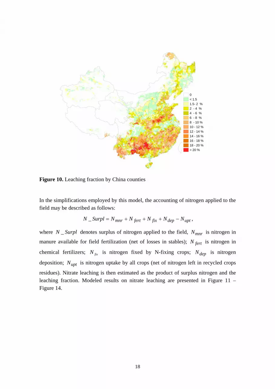
18

0 < 1.5 1.5- 2 %2 - 4 %4 - 6 %6 - 8 %8 - 10 %10 - 12 %12 - 14 %14 - 16 %16 - 18 %18 - 20 %> 20 %

Figure 10. Leaching fraction by China counties

In the simplifications employed by this model, the accounting of nitrogen applied to the field may be described as follows:

uptdepfixfertmnr NNNNNSurplN −+++=_ ,

where SurplN _ denotes surplus of nitrogen applied to the field, mnrN is nitrogen in

manure available for field fertilization (net of losses in stables); fertN is nitrogen in

chemical fertilizers; fixN is nitrogen fixed by N-fixing crops; depN is nitrogen

deposition; uptN is nitrogen uptake by all crops (net of nitrogen left in recycled crops

residues). Nitrate leaching is then estimated as the product of surplus nitrogen and the leaching fraction. Modeled results on nitrate leaching are presented in Figure 11 – Figure 14.

19

0 1 - 20 20 - 40 40 - 60 60 - 8080 - 100

Figure 11. Leaching kg / ha cultivated land, 2000.

0

200

400

600

800

1000

1200

1400

<1 <5 <10 <20 <40 <60 <80 <100 <120 More

Num

ber o

f cou

ntie

s

0%

20%

40%

60%

80%

100%

Figure 12. Leaching in severity classes by number of counties affected, kg / ha cultivated land, 2000, and cumulative fraction of counties.

20

0 1 - 20 20 - 40 40 - 60 60 - 8080 - 100

Figure 13. Leaching, kg / ha cultivated land, 2030.

0

200

400

600

800

1000

1200

1400

<1 <5 <10 <20 <40 <60 <80 <100 <120 More

Num

ber o

f cou

ntie

s

0%

20%

40%

60%

80%

100%

Figure 14. Leaching in severity classes by number of counties affected, kg / ha cultivated land, 2030, and cumulative fraction of counties.

21

4.2 Atmospheric emissions of N2O

Emissions of greenhouse gases (here: N2O) are estimated using the methodology compiled for IIASA’s Greenhouse gas–Air pollution INteractions and Synergies (GAINS) model (Winiwarter, 2005). Here N2O emissions are assessed as the product of emission factors times activity data. While far from reflecting the complex soil processes leading to N2O formation and release, this methodology is based on IPCC guidelines with IPCC default emission factors (IPCC, 2006). In GAINS the direct and indirect emissions have been combined into one factor, using IPCC default estimates for nitrogen losses for the respective pathways. The result of abatement measures to reduce N2O emissions is reflected in the choice of an alternative emission factor

∑=mji

ijmijmij EFXAON,,

2 ,

where ijA is location specific (indexed by i) activity data (indexed by j) (e.g., number of

livestock by types), which may apply different mitigation measures m at given shares of implementation ijmX (all shares X add up to 1) with emission factors ijmEF . For the

calculation of baseline emissions, the implementation rate of the “uncontrolled” case (based on the emission factors of IPCC) is considered. Results of calculations for China are presented in Figure 15 and Figure 16.

0 1 - 10 10 - 20 20 - 30 30 - 4040 - 50

Figure 15. N2O emissions from agricultural soils (kg N2O/ha cultivated land) in 2000, central projection.

22

0 1 - 10 10 - 20 20 - 30 30 - 4040 - 50

Figure 16. N2O emissions from agricultural soils (kg N2O/ha cultivated land) for the baseline projection in 2030.

4.3 Atmospheric emissions of ammonia

Reduced nitrogen components (e.g. urea, ammonium salts) make up an important fraction of nitrogen in agricultural activities. In contact with the atmosphere, these compounds easily may release gaseous ammonia (NH3).

Following the GAINS methodology (Klimont, 2001; Klimont and Brink, 2004), ammonia emissions comprise those from livestock production and from mineral fertilizer application (Figure 17 – Figure 20).

Emissions from livestock production are accounted at four major stages, i.e., in animal housing, during storage of manure, its application and during grazing periods. These stages are explicitly distinguished in the LUC model (Ermolieva et al., 2005; Fischer et al., 2007; Fischer et al., 2008). Again the accounting is based on parameters originally developed for Europe, but we are considering the impact of local manure management practice.

23

0

100

200

300

400

500

600

700

0 25 50 75 100 125 150 175 200 225 250 300 400 More

kg/ha cult land

Num

ber o

f cou

ntie

s

0%

20%

40%

60%

80%

100%

Figure 17. Ammonia emissions in size classes by number of counties affected, kg per ha of cultivated land, 2000, and cumulative fraction of counties.

0 1 - 25 25 - 50 50 - 75 75 - 100100 - 125125 - 150150 - 175175 - 200200 - 225 > 225

Figure 18. Ammonia emissions from agriculture (kg ammonia/ha cultivated land) in 2000, central projection.

<25 <50 <75 <100 <125 <150 <175 <200 <225 <250 <300 <400 <500 More

24

0

100

200

300

400

500

600

0 25 50 75 100 125 150 175 200 225 250 300 400 More

Num

ber o

f cou

ntie

s

0%

20%

40%

60%

80%

100%

kg/ha cult land

Figure 19. Ammonia emissions in size classes by number of counties affected, kg per ha of cultivated land, 2030, and cumulative fraction of counties.

0 1 - 25 25 - 50 50 - 75 75 - 100100 - 125125 - 150150 - 175175 - 200200 - 225 > 225

Figure 20. Ammonia emissions from agriculture (kg ammonia/ha cultivated land) in 2030, central projection.

<25 <50 <75 <100 <125 <150 <175 <200 <225 <250 <300 <400 <500 More

25

Emissions of ammonia from mineral fertilizer application depend on many factors, including the type of fertilizer applied, soil properties, meteorological conditions, time of application in relation to a crop canopy, and method of application. The nitrogen loss from fertilizer application is region-specific, and uncertainties of emission factors are high. Typically, N losses from synthetic fertilizers vary between one and four percent, with the exception of ammonium sulfate (eight percent), urea (15 to 25 percent) and ammonium bicarbonate (ABC) (20 to 30 percent). In China, a large proportion of total N-fertilizer use is represented by urea and ABC, estimated at about 50 and 40 percent, respectively. While nitrogen loss is expressed as a percentage of total nitrogen in the fertilizer, the results have been converted into mass of ammonia.

26

5 Development of risk functions to minimize environmental effects

Environmental problems are often multi-facetted, having a number of different causes and effects which can be only quantified to a limited extent. Mathematical modeling may provide meaningful results (a) to the extent input information is available, and (b) if ways can be derived how to combine input parameters. For an optimization, it is valuable to merge all environmentally adverse effects (or parameters representing such adverse effects) into one common “risk function”. Optimizing (minimizing or maximizing) this risk function will then provide the key to optimize the overall situation.

In this section we present the approach to derive risk functions that is used in Section 6. Developing the function requires choosing thresholds and weights of parameters according to empirical knowledge.

Spatial allocation of agricultural production commonly just minimizes transport costs, i.e., production will occur predominantly close to the demand (consumer). Here we add considerations on urbanization, share of built-up land, over-fertilization, and livestock biomass density (indicative for health risk, and for environmental burden of intensive production, respectively). The resulting risk function allows “penalizing” environmentally adverse agricultural production and thus minimizing environmental effects. The parameters chosen reflect data availability, its combination exhibits similarity with membership functions of the fuzzy logic theory.

The risk function related to a location’s urbanization share is defined as

,, ,0

],[ ),/()(, ,1

max

maxminminmaxmax

min1

⎪⎩

⎪⎨

⎧

>∈−−<

=ss

sssssssssif

R

k

kk

k

k

where ks is the location-specific urbanization share, k is a location. Here, critical

thresholds mins and maxs are assumed at 10 and 80 percent, respectively, in order to

disregard outliers. The implied risk function tells that a location with an urbanization share below mins may allocate livestock facilities with no constraints. In other words, there are no (population) risks associated with production expansion. In locations with urban population share in the interval [10, 80], losses associated with the allocation are increasing proportional to the share, and counties with an urbanization share beyond

27

80 percent are not allowed to increase their livestock production at all. In this case, the risk function is of linear segment-wise continuous form (Figure 21). Alternatively, the function may have a non-linear and even discontinuous shape.

% of urban pop. intotal pop. of county

0

1

8010

0.5

50

R1

0

1

8010

0.5

50

R1

Figure 21. Risk function related to urbanization level.

A health risk function can depend on more than one criterion. In some locations where the urban population share is high, there may still be land in abundance to justify expansion of livestock production. To include this consideration, we introduce a risk function associated with the amount of non-residential area suitable for production allocation, defined as (Figure 22):

⎪⎩

⎪⎨

⎧

>∈−−<

=

max

maxminminmaxmax

min2

,0],[),/()(

,1

bbbbbbbbb

bbifR

k

kk

k

k

where kb is the proportion of build-up area in total area of a location. Values of 25 and

50 percent were used for thresholds minb and maxb , respectively.

Accounting for health risks, the preference weights for allocating production increases by location are computed by adjusting profit-driven shares }~{~

iki Δ=Δ , with risk

function },max{ 212,1kkk RRR = , where ikΔ~ corresponds to ikq . The compound risk

28

function },max{ 212,1kkk RRR = combines two criteria. It may be viewed as a “union” of

two risk functions in the sense of fuzzy logic (Darbra et al., 2008).

0

1

10

0.5

5025% of total landin county

R2

Figure 22. Risk function related to the share of build-up area (as a percentage of total land in county).

In a similar way, we assume that environmental pollution and risks associated with agricultural production can be approximated by variables measuring excess nutrients. A risk function associated with nutrients in excess of crop uptake is defined as (Figure 23)

⎪⎪⎩

⎪⎪⎨

⎧

>∈−−⋅∈−−−+<

=

max

maxmaxmax

minminmin

min

3

,0],[),/()(5.0

],[),/())(15.0(1,1

uuuuuuuuu

uuuuuuuuuif

R

k

medkmedk

medkmedk

k

k

where minu , medu (median), and maxu were chosen as 90%, 110% and 150% of nutrients

supply, respectively, restricted to N only in relation to crop uptake in the location j. We assume that an undersupply of nutrients by 10% will not essentially affect yields. Therefore we allow allocating freely below 90% nutrients supply. Above the value, the risk function will give preference to areas of lower nutrients supply, with a maximum of 50% overfertilization (150% nutrients supply) permitted.

29

0.5

Ratio of nutrients supply to crop nutrients uptake

0

1

150110900

1

15011090

R3

Figure 23. Risk function related to the nutrients in excess of crop uptake as a ratio of nutrients supply to crop nutrients uptake.

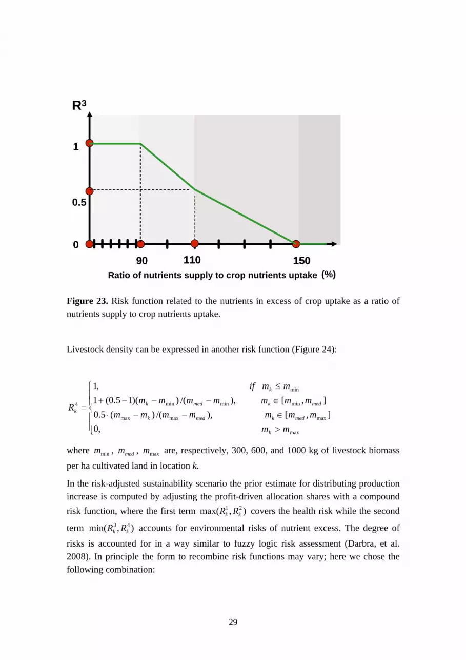
Livestock density can be expressed in another risk function (Figure 24):

⎪⎪⎩

⎪⎪⎨

⎧

>∈−−⋅∈−−−+≤

=

max

maxmaxmax

minminmin

min

4

,0],[),/()(5.0

],[),/())(15.0(1,1

mmmmmmmmm

mmmmmmmmmif

R

k

medkmedk

medkmedk

k

k

where minm , medm , maxm are, respectively, 300, 600, and 1000 kg of livestock biomass

per ha cultivated land in location k.

In the risk-adjusted sustainability scenario the prior estimate for distributing production increase is computed by adjusting the profit-driven allocation shares with a compound risk function, where the first term ),max( 21

kk RR covers the health risk while the second

term ),min( 43kk RR accounts for environmental risks of nutrient excess. The degree of

risks is accounted for in a way similar to fuzzy logic risk assessment (Darbra, et al. 2008). In principle the form to recombine risk functions may vary; here we chose the following combination:

(%)

30

),min(),max(),min( 432143)2,1(4,3)2,1(kkkkkkkk RRRRRRRR ∗== .

In optimization, the total value of 4,3)2,1(kR will be maximized (see Fischer et al., 2007,

for a detailed explanation of the calculation algorithm).

0

1

600300 11000

1

600300 1100kg animals biomass / ha cultivated land

R4

Figure 24. Risk function related to livestock biomass in relation to available cultivated land in county.

31

6 Alternative scenarios of agricultural practice Agricultural practice determines environmental impacts. Improvements can significantly reduce total fertilizer demand, the subsequent leaching of nutrients, and losses of excess nitrogen. Next to the use of fertilizer, the nitrogen cycle (and CH4 emissions) is also influenced by the handling and use of agricultural residues. In this study we use modeled environmental parameters as risk indicators for optimization. The following risk-adjusted scenarios have been developed and complement the projections on the current intensification trend (i.e., they are available for different target years, and have even been applied to the year 2000):

(i) An intensification scenario, representing the case in which the increase of production is allocated proportionally to demand increase, which is concentrated in the proximity to densely populated urban areas (“business as usual”),

(ii) a “sustainable reallocation” scenario that combines the demand driven preference structure of the first scenario with considerations of environmental and health norms, information on population densities and its vulnerability to environmental risks caused by agricultural production,

(iii) an “optimized” fertilizer use scenario, which uses mineral fertilizer only for filling the deficits after applying all available manure,

(iv) a combined consisting of optimized fertilizer use and specific technology options focused on ammonia abatement (“minimized ammonia” scenario).

(i). Business-as-usual allocation scenario.

Due to constraints from transport potential and transport costs, it is common practice to establish intensive livestock production in areas with good access to consumers, close to high demand and high population density (Fischer et al., 2007; 2008). In practical modeling the “profitability” of a location it has been standard practice to use a so-called market access function. The typical market access function measures the potential of location k as a weighted sum of purchasing power of all other locations in the vicinity of k . Weights are defined either as a function of distance or as a function of other factors, e.g., costs or losses. In the current study each county is characterized by its

market access ikΔ~ , Kk :1= , calculated as a weighted sum of demand for product i in

nearby counties within a vicinity kM : ∑ Δ=Δ∈ kMm

timkmik gf )()(~ , where

32

)1()()( −−=Δ timtimtim dd denotes the demand change in the location m and time t ,

)(timd is the demand for product i , and Kk :1= are counties. Weights )( kmgf are

equal to the inverse distance between locations k and m with a discounting factor α ,

kmkm ggf /)( α= , kmg is distance between k and m , 1)( =kkgf .

For each location the definition of the vicinity kM has to ensure the best coverage of

consumers. Optimal coverage can be derived either from rather complex spatial optimization models or from spatial estimation procedures, and sensitivity analysis.

Values ikΔ~ , Kk :1= , determine a profit-based prior probability ikq (allocation

preference structure) for allocation of demand increase among production units in locations. An example of a result is presented in Figure 25.

Figure 25. Concentration of demand for meat, demand-driven preference weights of locations (scale factor 1000).

(ii.) “Sustainable reallocation” scenario based on minimized risk functions. The objective of this scenario is to consider profitability of the agricultural production while

33

respecting health and environmental impacts. The main challenge in spatially-explicit planning regards the choice of adequate location-specific indicators to balance rural development within defined socio-economic and environmental objectives. While information on economic and livelihood conditions at a location may be available from statistics and census data, estimation of agricultural pollution and health risks is a more challenging task. As outlined in Section 5, we employ risk functions based on available surrogate data to reflect health and environmental impacts of excess nutrient application. Agricultural pollution is geographically disperse, thus also the risk function has been applied in a spatially explicit fashion.

(iii) An “optimizing” fertilizer use scenario (apply all available manure and match the remaining demand with mineral fertilizer). The scenario represents a simple feasible option to minimize nutrients fluxes into the environment in a least-cost way and to reduce the associated environmental risks. Substituting inorganic with organic (manure) nitrogen fertilizer, which is otherwise disposed as a waste product, will reduce the total amount of nitrogen in the system (and hence emissions). This scenario includes reallocation as defined in scenario (ii).

The practical application of manure, however, requires overcoming a couple of difficulties. Timing of manure application will influence, to different degrees, the loss pathways of manure nitrogen. Moreover, proper timing also requires the workforce (and machinery) to be available at the right point in time, which may be difficult to organize. Finally, other compounds included in manure (pathogens as well as drugs administered to fight such pathogens) may compromise the quality of manure as a fertilizer. As a consequence, there may be limitations in the applicability of this scenario.

(iv) A “minimized ammonia” scenario attempts to apply technology, in addition to balanced fertilization as in (iii), when nitrogen addition is limited to the amount of nutrient-N taken up by the crop. With manure injection the manure is placed in the soil as opposed to spreading it over the surface. This reduces ammonia emissions during application, however it may result in an increase in nitrous oxide emissions from agricultural soils. Substituting urea fertilizers with ammonium nitrate will further reduce ammonia emissions from synthetic fertilizer use, without an effect on nitrous oxide and methane.

The business-as-usual scenario (i) implicitly minimizes transportation costs as production concentrates in the vicinity of urban areas with high demand. In the alternative scenario (ii), production is shifted to more distant locations characterized by availability of cultivated land, lower livestock and population density, but at the expense of additional transportation. In contrast, scenario (iii) focuses on fertilizers saving, while scenario (iv) attempts to evaluate a scenario on drastic ammonia emission reductions.

34

Direct results of the four scenarios (business-as-usual plus three alternate scenarios) exhibit the expected environmental pressures, and, more importantly, their respective changes. Because of the mentioned limitations in applicability of scenarios (iii) and (iv), their benefits may not be directly comparable.

The results are presented in Table 12 - Table 15. Effects are quite different for different economic regions, but it is clear in all cases that current nitrogen pollution is prone to increase. Only the scenarios that provide considerable improvements are able, for all of China, to halt environmental deterioration and possibly even improve the situation somewhat compared to the base case of 2000.

Table 12. Environmental indicators and their expected change according to the business-as-usual scenario (by economic region, without Plateau region). Data in kt N.

2000 2030 Change 2000-2030 (%) Region

Lch N2O-N NH3-N Lch N2O-N NH3-N Lch N2O NH3 North 252 234 2133 444 367 3204 76 57 50 Northeast 25 74 662 40 106 915 60 43 38 East 117 124 1139 144 156 1380 23 26 21 Central 76 104 898 134 153 1321 75 47 47 South 116 91 794 143 120 1002 23 32 26 Southwest 95 133 1078 166 209 1706 74 57 58 Northwest 18 80 689 29 139 1151 58 74 67 CHINA 701 855 7469 1101 1282 10878 57 50 46

Table 13. Environmental indicators and their expected change according to the sustainable reallocation scenario (by economic region, without Plateau region). Data in kt N.

2000 2030 Change 2000-2030 (%) Region

Lch N2O-N NH3-N Lch N2O-N NH3-N Lch N2O NH3 North 252 234 2133 425 337 2965 68 44 39

Northeast 25 74 662 45 121 1062 78 69 61 East 117 124 1139 142 157 1385 22 26 22

Central 76 104 898 139 160 1376 82 54 54 South 116 91 794 154 136 1126 32 49 42

Southwest 95 133 1078 144 189 1540 51 42 43 Northwest 18 80 689 28 136 1126 52 70 64

CHINA 701 855 7469 1078 1278 10848 54 49 45

35

Note that the absolute values of environmental indicators do not change or may even slightly increase in the sustainable reallocation scenario in comparison to the business-as-usual scenario. Overall environmental and health impacts, measured in terms of population within different severity classes, decreases in the sustainable scenario because of production reallocation within imposed norms. This example illustrates disadvantages related to measuring impacts with only one value. It stresses the need for compound risk indicators, which combine multiple criteria and constraints.

Table 14. Environmental indicators and their expected change according to the optimization scenario (by economic region, without Plateau region). Change refers to scenario assumptions already introduced in 2000 (shaded figures). Data in kt N.

2000 2030 Change 2000-2030 (%) Region


Northeast 5 55 484 12 81 658 133 45 36 East 33 87 764 38 107 889 15 24 17

Central 34 85 709 46 121 986 37 42 39 South 36 66 543 50 96 740 38 46 37


CHINA 231 652 5426 321 956 7487 39 47 38

Table 15. Environmental indicators and their expected change according to the minimized ammonia scenario (by economic region, without Plateau region). Change refers to scenario assumptions already introduced in 2000 (shaded figures). Data in kt N.

2000 2030 Change 2000-2030 (%) Region


Northeast 5 56 458 12 81 610 133 44 33 East 33 87 730 38 108 833 17 23 14

Central 34 86 676 47 121 911 38 41 35 South 37 66 512 51 96 675 43 46 32


CHINA 232 654 5168 328 963 6884 39 46 33

Data for 2000 and changes between 2000 and 2030 as noted in Table 14 and Table 15 are presented for demonstrative purposes only, as it is assumed that the improved

36

scenarios would already have been implemented in 2000. In reality, such measures will lead to a significant decrease of current emissions (compare Table 12) and not to increases. But it is very interesting to note how production increase affects the emission pathways in different manners. The higher the pollution level of the starting conditions, the stronger will be the relative change in emissions. This points to the existence of some buffer capacity in the system, which is being used up with increasing environmental burden.

37

7 Exposure to environmental pressure

7.1 Introduction to the concept

We have presented environmental risk indicators as well as demands for agricultural products for administrative regions or normalized by area in previous sections of this report. For part of the environmental effects – especially regarding health – this may be misinterpreted as not the area, but the population is affected by the adverse situation. In order to estimate this risk, we need to assess the exposure of people. As population is not evenly distributed over the area, population-weighted risk may be considerably different to the area-based risk.

The scenarios (ii), (iii) and (iv) introduced in Section 6 reallocate agricultural production in a way to minimize overall risk. The risk function considers population density implicitly on the demand side but also in connection with health risks, and performs a reallocation away from population. Thus the altered distribution pattern of production alone will allow the exposure of population to decrease.

But even without optimization, a difference between population exposure and area- (or number-of-counties) based risk evaluation is evident. We will show here these differences for the “business as usual” scenario as an example. The risk parameter used is the spatial density of nitrogen losses8. Figure 26 displays the geographical distribution of this parameter for the year 2000.

8 Nitrogen losses are defined as the difference between the nutrients output (from livestock manure, inorganic fertilizers, crop residues, nitrogen fixation) and the uptake capacities of crops. Calculated total nutrients losses include: (i) nutrient losses from livestock housing, from manure storage facilities (ii) losses stemming from non-effective manure and fertilizers, (iii) losses due to over-supply of nutrients from fertilizers and manure to crops, plus (iv) non-effective manure nutrients produced by pastoral system

38

01-2526-5051-100101-150151-250>250

Figure 26. Spatial density of nitrogen losses (kg nutrients/ha total land), central projection, 2000.

Histograms in Figure 27 and 30 present the frequency distribution of the number of counties and the percentage of population exposed, respectively, as a function of spatial density of nitrogen losses. While a large number of counties in China (and also vast areas, especially in the west and the north of the country) are essentially unaffected, the situation is different for population. The unaffected counties and areas are at the same time also very sparsely populated. As may be expected, people tend to concentrate where agricultural conditions are favorable. Using the same argument, we may state that intensive agriculture – and coinciding with this also elevated environmental risk – occurs in the neighborhood of high population density. Thus the exposure of people to environmental risk is clearly less favorable than the distribution over the area. This situation is not expected to change by 2030. Basically the same data, again the “business as usual” scenario, is shown for 2030 in Figure 29 – 33.

39

0

400

800

1200

1600

2000

2400

1-25 26-50 51-100 101-150 151-250 >250

Intensity of nitrogen losses per unit land (kg/ha)

Num

ber

of c

ount

ies

0%

20%

40%

60%

80%

100%

0%

20%

40%

60%

80%

100%

1-25 26-50 51-100 101-150 151-250 >250


Perc

enta

ge o

f pop

ulat

ion

0%

20%

40%

60%

80%

100%

Cum

ulat

ive

perc

enta

ge o

f pop

ulat

ion

Figure 27. Distribution of counties by Figure 28. Distribution of population by density class of total nitrogen loss, 2000. density class of total nitrogen loss, 2000.

01-2526-5051-100101-150151-250>250

Figure 29. Spatial density of nitrogen losses (kg nutrients/ha total land), central projection, 2030.

40

0

400

800

1200

1600

2000

2400

1-25 26-50 51-100 101-150 151-250 >250


Num

ber o

f cou

ntie

s

0%

20%

40%

60%

80%

100%

Per

cent

age

of c

ount

ies

0%

20%

40%

60%

80%

100%

1-25 26-50 51-100 101-150 151-250 >250


Perc

enta

ge o

f pop

ulat

ion

0%

20%

40%

60%

80%

100%

Cum

ulat

ive

perc

enta

ge o

f pop

ulat

ion

Figure 30. Distribution of counties by Figure 31. Distribution of population by density class of total nitrogen loss, 2030 density class of total nitrogen loss, 2030.

Table 16. Share of population by spatial density class of total nutrient losses (percent).

2000 (kg nutrient loss/ha total land) 2030 (kg nutrient loss/ha total land)

<25 26-50 51-100

101-150

151-250 >250 <25 26-50 51-

100 101-150

151-250 >250

North 7 13 25 29 23 2 12 9 18 18 32 11 Northeast 38 32 20 8 2 0 32 23 29 13 3 0 East 7 13 35 21 19 5 14 17 27 16 23 2 Central 19 35 38 6 2 0 13 33 34 17 3 0 South 19 31 34 14 2 1 9 29 42 16 3 0 Southwest 19 31 41 8 1 0 11 26 36 19 8 0 Plateau 63 37 0 0 0 0 71 26 3 0 0 0 Northwest 60 16 9 5 8 1 52 23 16 6 3 1 CHINA 20 23 30 16 10 1 18 22 29 16 13 3

Results presented in Table 16 not only show an overall shift of population into areas of higher nutrient losses, but they also indicate clear differences between regions. While in the east the share of population exposed to the risk indicator “nutrient loss” even tends to decrease, the opposite is the case for the north. In 2030, the population of the northern region is expected to experience highest exposures.

7.2 Performance review of reallocation

A differentiation between area-based and population-based risk may be applied to any kind of risk indicator. Here we use indicators which resemble the parameters chosen to optimize allocation of agricultural production. Obviously, this is an opportunity to

41

review the performance of the spatial reallocation, when comparing the “business as usual” scenario to the “sustainable reallocation” scenario. Comparing to the other scenarios is not helpful as results will differ only marginally.

For this visualization purpose, counties were assigned into classes of “low”, “typical” and “high” exposure depending on the following overall risks criteria: (i) percentage of cultivated land in total land (i.e., less than 10 percent, 10 to 50 percent, and more than 50 percent of total county area), (ii) balance of livestock to crop land available, measured as total live weight of confined livestock per ha cultivated land (i.e., less than 300 kg/ha, 300 to 600 kg/ha, and more than 600kg/ha), and (iii) population density (i.e., less than 100 persons per square kilometer, 100 to 1000 persons per square kilometer, and more than 1000 persons per square kilometer). The resulting 27 risk classes were then further aggregated, and counties have been broadly classified into seven risks categories, which we define as classes of “environmental pressure”:

A. Counties in scarcely populated desert or mountain/plateau areas and with little confined livestock (No confined livestock).

B. Counties with substantial crop production but with little confined livestock (No environmental pressure).

C. Counties with low environmental pressure from confined livestock production (Slight environmental pressure).

D. Counties with moderate environmental pressure from confined livestock production (Moderate environmental pressure).

E. Counties with moderate urbanization and environmental pressure from confined livestock production (Environmental pressure).

F. Counties with moderate urbanization and high environmental pressure from livestock production (High Environmental pressure).

G. Counties with high degree of urbanization coinciding with high environmental pressure from confined livestock production (Extreme environmental pressure).

Figure 32 and Figure 33 present the occurrence of the above classes defining the environmental and health risks to human population from intensive agricultural production, for the years 2000 and 2030, respectively (business-as-usual scenario).

42

No confined livestockNo environmental pressureSlight environmental pressureModerate environmental pressureEnvironmental pressureHigh environmental pressureExtreme environmental pressure

Figure 32. “Environmental pressure” from confined livestock production, 2000.

No confined livestockNo environmental pressureSlight environmental pressureModerate environmental pressureEnvironmental pressureHigh environmental pressureExtreme environmental pressure

Figure 33. “Environmental pressure” from confined livestock production, 2030.

The classes chosen represent risk indicators alone; they do not contain any indication of emission fluxes. But even without considering emission fluxes these indicators provide first policy-relevant information, pointing to areas that require specific attention. The same classes can also be used to describe population exposure, and to compare the differences of risk indicators between the business-as-usual and the “sustainable

43

reallocation” scenario. Here both reallocation and visualization are based on risk indicators alone.

We assess the extent to which reallocation of agricultural activities due to risk factors improve the situation with regard to the risk factors – as noticeable to the population. Current conditions are presented in Figure 34 in absolute and relative population numbers. Risk factors allow consideration of spatial heterogeneity – the “sustainable reallocation” scenario (right panel in Figure 35) clearly represents lower risks to the population while having almost identical emission fluxes to the respective media (

Table 13). In contrast to the business-as-usual scenario (left panel), the environmental pressures occur in further distance to the population, decreasing exposure to the risk factors.

0

50

100

150200

250

300

350

N NE E C S SW NW

Extreme pressure

High pressure

Pressure

Moderate pressure

Slight pressure

No pressure

No confined

0.0 0.2 0.4 0.6 0.8 1.0

N

NE

E

C

S

SW

NW

Figure 34. Absolute (million people) and relative (share of total population) distribution of population according to classes of severity of environmental pressure from livestock, 2000. The label on the horizontal axis indicate China regions: N, NE, E, C, S, SW, NW stand for North, North-East, East, Center, South, South-West, North-West, respectively.

44

0.0 0.2 0.4 0.6 0.8 1.0

N

NE

E

C

S

SW

NW

0.0 0.2 0.4 0.6 0.8 1.0

N

NE

E

C

S

SW

NW

Figure 35. Share of total population exposed to different classes of severity of environmental pressure from livestock, 2030, by economic region (except for the sparsely populated “plateau” region): left panel, business-as-usual scenario; right panel, “sustainable reallocation” scenario; other scenarios are not presented as they would not show relevant differences.

7.3 Release of adverse compounds to the environment

Mathematically, no difference needs to be made on the type of indicator visualized. Nevertheless, in terms of interpretation it is of interest to provide risk parameters representative of an adverse situation when choosing an indicator.

Here we compare the population exposure in 2030, for the four scenarios developed, to the emissions of ammonia. This is a much more direct indicator than the use of structural agricultural parameters alone as presented in the previous example. Even considering that the underlying technical methodology has been developed for Europe and assumes European conditions, the result is of considerable interest and may be regarded much more robust than structural parameters alone could be.

Figure 36 presents population exposure to different classes of ammonia emissions in 2000. Figure 37 compares the same indicator for four alternative scenarios. The improvement of the situation, alleviating the environmental and health risk to population, becomes evident from comparing the incremental additional measures leading from the business-as-usual to the “minimized ammonia” scenario.

45

0.0

50.0

100.0

150.0

200.0

250.0

300.0

350.0

N NE E C S SW NW

> 300250 - 300200 - 250150 - 200100 - 15050 - 100< 50

0.0 0.2 0.4 0.6 0.8 1.0

N

NE

E

C

S

SW

NW

Figure 36. Absolute (million people) and relative (share of total population) distribution of population according to classes of severity of environmental pressure (measured in terms of kg nitrogen in ammonia emitted per ha cultivated land), 2000. The label on the horizontal axis indicate China regions: N, NE, E, C, S, SW, NW stand for North, North-East, East, Center, South, South-West, North-West, respectively.

46

0.0 0.2 0.4 0.6 0.8 1.0

N

NE

E

C

S

SW

NW

0.0 0.2 0.4 0.6 0.8 1.0

N

NE

E

C

S

SW

NW

0.0 0.2 0.4 0.6 0.8 1.0

N

NE

E

C

S

SW

NW

0.0 0.2 0.4 0.6 0.8 1.0

N

NE

E

C

S

SW

NW

Figure 37. Relative (share of total population) distribution of population according to classes of severity of environmental pressure, 2030, by economic region (except the sparsely populated “plateau” region): a. business-as-usual scenario, b. “sustainable reallocation” scenario: c. “optimization” scenario, d. “minimized ammonia” scenario. Color scale and labels are identical to Figure 36.

a) b)

c) d)

47

8 Comparing numerical results with literature data Using the approaches outlined in the previous sections, we arrive at model results describing fluxes of nitrogen compounds to environmental media under different scenarios. These model results may not fully reflect the real emission situation, especially as models and release factors not adjusted to the Chinese situation. While this does not compromise the usefulness of resulting emissions as indicators, it is important to compare results with other literature estimates.

Here we limit such a comparison to the emissions of the greenhouse gas N2O. Table 17 compares the resulting emission for the whole China with several national studies. We compare emissions from agricultural soils. As data presented in the literature are mostly limited to direct emissions, we used these figures and extrapolated GAINS results to cover direct emissions only, assuming that direct emissions account for 55% of total N2O emissions (following the GAINS emission factors, which in turn reflect the default parameterization of IPCC). Several of the studies refer to their own measurements for the provision of emission factors, reflecting specific Chinese situation.

Results demonstrate the importance of the local variability that may be expected for a compound like N2O. Also, the ranges (where given) are rather large. Still a trend becomes evident upon closer inspection: Studies referring to later base years tend to present higher values, reflecting agricultural dynamics. Furthermore, the more recent papers seem to more appropriately cover all input flows of reactive nitrogen to the system. Nevertheless, it is obvious that the result obtained in this study is highest, while being clearly within the margins of uncertainty. Only the original result of the GAINS model, largely relying on the same or similar input data, is almost identical. More work, especially regarding the biophysical conditions of Chinese soils, will be required to obtain a better understanding of the actual release of N2O. However, as this is characteristic for soil N2O emissions in general, this is beyond the scope of this report.

48

Table 17. Emissions of N2O from agricultural sources in China. Data in kt N2O-N, direct emissions only (for GAINS and this study, we account for 55% of total emissions as direct emissions).

Base year

N2O emission （Mg N2O-N）

range Emission

factor

Mineral fertilizer （Tg N）

Reference

1990 310 modeled 16.6 Li et al., 2001

1994 372 specific 18.8 PRC, 2004

1995 265 specific 17.6 Chen et al., 2000

1990s 275 59-650 specific 19.7

(28.9)* Zheng et al., 2004

1997 292 specific 21.2 Lu et al., 2006

2000 450 IPCC 24.5 GAINS (Amann et al., 2008; Li et al., 2009)

2000 470 IPCC 24.5 this study

2004 400 specific 28.1* Zheng et al., 2008

*) total reactive nitrogen (Nr) including manure, crop residues, biological fixation and atmospheric deposition

49

9 Conclusions Economic and demographic drivers continue to increase the demand for agricultural products in China. The resulting production expansion is constrained by limited land resources. As a consequence, an increase of environmental impacts needs to be expected. In this study we used demand-driven agricultural modeling (CATSEI model) and simulations of the fluxes to air and water (GAINS model and MITERRA model, respectively) to explore the relationship between agricultural demand and its impacts.

The drivers and trends of agricultural intensification were used to compile indicators of nitrogen leaching, and nitrous oxide and ammonia release into the environment in China. This allowed an assessment of the magnitude of environmental loads under alternative demographic or socio-economic scenarios and to provide policy suggestions on alternative pathways how to mitigate or minimize negative environmental and health risks from agriculture.

Some of the underlying technical parameters have been derived for European and not for Asian conditions. This means that the indicators will allow demonstrating a general trend, but not necessarily an absolute quantification of emission fluxes. A comparison of results obtained here with literature values on nitrous oxide emissions indicates general agreement, providing confidence to the approach. In principle, availability of appropriate data assumed, the approach should not be limited to a specific country or region.

Four scenarios were developed, including a business-as-usual scenario. Environmental sustainability aspects of these scenarios were compared with respect to agricultural area as well as with the share of people in China’s regions exposed to different categories of environmental risks. This enabled to also optimize measures on people instead of agricultural area only.

Results show (Table 18) that increasing demand will lead to higher nitrogen pressure on the Chinese environment, due to considerable increases in food demand (population growth is still to continue, coupled with increased meat share which adds to the amount of nitrogen fertilizer needed). In the baseline, the increase of leaching is expected to be stronger (more than 50% increase between 2000 and 2030) than that of the gaseous emissions. Leaching can be tackled most efficiently by optimizing and minimizing agricultural application of fertilizers.

50

Table 18. Environmental pressure indices for total China by scenario. Change refers to scenario assumptions already introduced in 2000 (shaded figures). Data in kt N.

in kt 2000 2015 2030 Change 2000-2030 (%)

Region Lch N2O-N NH3-N Lch N2O-N NH3-N Lch N2O-N NH3-N Lch N2O NH3 business-as-

usual 701 855 7469 953 1163 9822 1101 1282 10878 57 50 46

sustainable reallocation 701 855 7469 950 1162 9825 1077 1278 10848 54 49 45

optimization 231 652 5426 293 887 7003 321 956 7487 39 47 38 minimized ammonia 232 654 5168 298 897 6461 328 963 6884 43 46 33

In all scenarios and for all years considered, the major part of nitrogen loss is via the ammonia pathway. NH3 nitrogen emissions make up between 40 and 50% of total nitrogen application. Loss in form of N2O follows next, and it may seem somewhat surprising that nitrate leaching is even less important. This can be explained by the huge losses to the gas phase, while the leaching fractions (relatively small per se) apply only to the quantity of soil nitrogen not lost or used elsewhere, and also do not include nitrate runoff to surface water.

Comparing the scenarios, one finds that there is little influence of the “sustainable reallocation” scenario on the overall loss of nitrogen components – its advantage over the business-as-usual scenario is in terms of reallocation of risks away from the population centers. The full improvements presented for the “optimized” and “minimized ammonia” scenarios are possibly difficult to achieve as manure fertilizer may not be applicable under all circumstances (timing and quality issues, see above). Nevertheless it is interesting to see even for the “minimized ammonia” scenario, which has a higher emission factor that N2O emissions hardly change with respect to the “optimized” scenario. For a balanced fertilization scenario, the lack of NH3 losses strongly decreases the need of fertilizer. In consequence the additional amount of N2O formed is very small. Optimized application of nitrogen will lead to a no-regret situation, avoiding negative interactions between environmental pools.

Increased nitrogen pressure will call for action to reduce water and air pollution. In the scenarios developed here, simple spatial redistribution of agricultural activities (reallocation) will already somewhat relieve the situation of population exposure, but it will hardly affect overall balances. In contrast, further measures aimed at reducing leaching and ammonia pollution can simultaneously also mitigate greenhouse gas emissions: in the “optimized” scenario presented for the year 2030, reduction of nitrous oxide emissions from agricultural soils will be almost 25% compared to “business as usual”. This will be no improvement compared to 2000, but if efficient measures against

51

air and water pollution are taken at least the increase of nitrous oxide emissions can be minimized.

All measures are most effective with respect to leaching, and much less effective for atmospheric emissions. Leaching is considered to be roughly proportional to excess nitrogen, while ammonia and nitrous oxide emissions behave similar to nitrogen input. Improved efficiency of nitrogen use, which is the basis for the improvement scenarios, will diminish first of all excess nitrogen and therefore result in a much stronger decrease in nitrogen available for leaching. Nitrogen application as such will not be affected so strongly, unless specific measures (e.g., on ammonia abatement) come into play. Thus N2O emissions are still expected to increase by 2030 in all scenarios with regard to the baseline for 2000.

The work described in this report presents a framework that can be used to test further scenarios of agricultural activities and their related emissions. Such scenarios may include consequences of climate change on temperature, precipitation and agricultural productivity, once sufficiently detailed information will be available. This also comprises climate adaptation needs in order to safeguard agricultural production and its consequences on the nitrogen release to water and atmosphere, thus linking climate adaptation and mitigation related measures.

52

References

Amann M., Bertok I., Borken J., Chambers A., Cofala J., Dentener F., Heyes C., Hoglund L., Klimont Z., Purohit P., Rafaj P., Schöpp W., Texeira E., Toth G., Wagner F., Winiwarter W. (2008). GAINS ASIA – a tool to combat air pollution and climate change simultaneously. Methodology. International Institute for Applied Systems Analysis, Laxenburg, Austria.

Asman W.A.H., Klimont Z. (2009). Implementing leaching in GAINS. IIASA Interim Report IR-09-xxx. International Institute for Applied Systems Analysis, Laxenburg, Austria (in press)

Darbra, R.M., Demichela, M., Mure, S. (2008). Preliminary risk assessment of ecotoxic substances accidental releases in major risk installations through fuzzy logic, Process Safety and Environmental Protection 86, 103-111.

Ermolieva, T., G. Fischer, and H. van Velthuizen (2005). Livestock Production and Environmental Risks in China: Scenarios to 2030”, FAO/IIASA Research Report, International Institute for Applied Systems Analysis, Laxenburg, Austria.

Fischer, G., T. Ermolieva (2009a). CATSEI agricultural production model: A technical report. IIASA Interim Report IR-09-xxx. International Institute for Applied Systems Analysis, Laxenburg, Austria (forthcoming, available on request)

Fischer, G., T. Ermolieva (2009b). Environmental pressure from agricultural production: planning sustainable agriculture in China. A CATSEI report. IIASA Interim Report IR-09-xxx. International Institute for Applied Systems Analysis, Laxenburg, Austria (forthcoming, available on request)

Fischer, G., T. Ermolieva, Y. Ermoliev, L. Sun (2008). Risk-adjusted approaches for planning sustainable agricultural development. Stochastic Environmental Research and Risk Assessment, 1-10.

Fischer, G., T. Ermolieva, Y. Ermoliev, L. Sun (2007). Integrated risk management approaches for planning sustainable agriculture. In: Advances in Studies on Risk Analysis and Crisis Response, C. Huang, C. Frey, J. Feng (eds), Atlantis Press, Paris, France.

Huang, J., Zhang, L., Li, Q., and Qiu, H., (2003a). CHINAGRO project: National and Regional Economic Development Scenarios for China’s Food Economy Projections in the Early 21st Century. Center for Chinese Agricultural Policy, Chinese Academy of Sciences.

IPCC (2001). Climate Change 2001: The Scientific Basis. Contribution of Working Group I to the Third Assessment Report of the Intergovernmental Panel on Climate

53

Change. J.T. Houghton, Y. Ding, D.J. Griggs, M. Noguer, P.J. van der Linden, X. Dai, K. Maskell, C.A. Johnson (eds.), Cambridge University Press, Cambridge (UK).

IPCC (2006). 2006 IPCC Guidelines for National Greenhouse Gas Inventories. S. Eggleston, L. Buendia, K. Miwa, T. Ngara, K. Tanabe (eds.), IGES, Japan, Intergovernmental Panel on Climate Change.

IPCC (2007). Summary for Policymakers. In: Climate Change 2007: Impacts, Adaptation and Vulnerability. Contribution of Working Group II to the Fourth Assessment Report of the Intergovernmental Panel on Climate Change, M.L. Parry,

Klimont, Z. (2001). Current and Future Emissions of Ammonia in China. Paper presented at the 10th Annual Emission Inventory Conference: One Atmosphere, One Inventory, Many Challenges. May 1-3, Denver, CO, USA

Klimont Z, C. Brink (2004). Modeling of Emissions of Air Pollutants and Greenhouse Gases from Agricultural Sources in Europe. IIASA Interim Report IR-04-048. International Institute for Applied Systems Analysis, Laxenburg, Austria

Li, C., Y. Zhuang,M. Cao, P. Crill, Z. Dai, S. Frolking, B. Moore III, W. Salas, W. Song, X. Wang (2001). Comparing a process-based agro-ecosystem model to the IPCC methodology for developing a national inventory of N2O emissions from arable lands in China, Nutrient Cycling in Agroecosystems 60: 159–175.

Li, Y., E. Lin, W. Winiwarter. (2009). Modeling agriculture in China: N2O emissions and mitigation measures. Proceedings of the Fifth International NCGG Symposium, Wageningen, The Netherlands, 30 June - 3 July 2009. Non-CO2 Greenhouse Gases: Science, Reduction Policy and Implementation. Papers on USB stick coordinated by André van Amstel, paper 34_limai. VVM/MILCON, den Bosch, The Netherlands.

Liu, S., X. Li, M. Zhang (2003). Scenario Analysis of Urbanization and Rural-Urban Migration in China. IIASA Interim Report IR-03-036, International Institute for Applied Systems Analysis, Laxenburg, Austria.

Lu, Y., Y. Huang, J. Zou, X. Zheng (2006). An inventory of N2O emissions from agriculture in China using precipitation-rectified emission factor and background emission, Chemosphere 65, 1915–1924.

Menzi, H. (2001). Area-wide Integration (AWI) of Specialized Crop and Livestock Activities: Assessment of Nutrient Management and Environmental Impacts. Final Report of SCA contribution in China. Swiss College of Agriculture (SCA), Switzerland. Internal Document.

Pope C.A., R.T. Burnett, M.J. Thun, E. E. Calle D. Krewski K. Ito, G. D. Thurston (2002). Lung Cancer, Cardiopulmonary Mortality, and Long-term Exposure to Fine Particulate Air Pollution. JAMA 287(9), 1132-1141.

54

PRC (2004). Initial National Communication on Climate Change. The People’s Repub-lic of China, Beijing. Available at http://unfccc.int/resource/docs/natc/chnnc1e.pdf

Toth, F., G.-Y. Cao, and E. Hizsnyik (2003). Regional Population Projections for China. IIASA Interim Report IR-03-042, International Institute for Applied Systems Analysis, Laxenburg, Austria.

Velthof, G.L., Oudendag, D.A., Witzke, H.P., Asman, W.A.H., Klimont, Z., Oenema, O. (2009). Integrated assessment of nitrogen emissions from agriculture in EU27 using MITERRA-EUROPE. Journal of Environmental Quality 38, 1-16.

Ward, MH, de Kok TM, Levallois P, Brender J, Gulis G, Nolan BT, van der Slice J. (2005). Drinking water nitrate and health – Recent findings and research needs. Environ Health Perspect 113, 1607-1614.

Winiwarter, W., (2005). The GAINS Model for Greenhouse Gases-Version 1.0: Nitrous Oxide. IIASA Interim Report IR-05-55. International Institute for Applied Systems Analysis, Laxenburg, Austria.

Zheng, X., S. Han, Y. Huang, Y. Wang, and M. Wang, (2004). Re-quantifying the emission factors based on field measurements and estimating the direct N2O emission from Chinese croplands, Global Biogeochem. Cycles, 18, GB2018, doi:10.1029/2003GB002167.

Zheng X., C. Liu, S. Han (2008). Description and application of a model for simulating regional nitrogen cycling and calculating nitrogen flux. Description and Application of a Model for Simulating Regional Nitrogen Cycling and Calculating Nitrogen Flux. Advances In Atmospheric Sciences 25, 181-201.

Documents

Integrated Nitrogen Management In China