Research ArticleIntegration of High-Volume Molecular and Imaging Data forComposite Biomarker Discovery in the Study of Melanoma

Konstantinos Moutselos,1 Ilias Maglogiannis,2 and Aristotelis Chatziioannou3

1 Department of Computer Science and Biomedical Informatics, University of Thessaly, Papasiopoulou 2-4, 35100 Lamia, Greece2 Department of Digital Systems, University of Piraeus, Grigoriou Lampraki 126, 18532 Piraeus, Greece3Metabolic Engineering and Bioinformatics Programme, Institute of Biology, Medicinal Chemistry and Biotechnology,National Hellenic Research Foundation, 48 Vasileos Constantinou Avenue, 11635 Athens, Greece

Correspondence should be addressed to Aristotelis Chatziioannou; achatzi@eie.gr

Received 29 April 2013; Revised 28 September 2013; Accepted 12 October 2013; Published 16 January 2014

Academic Editor: Hesham H. Ali

Copyright © 2014 Konstantinos Moutselos et al.This is an open access article distributed under the Creative Commons AttributionLicense, which permits unrestricted use, distribution, and reproduction in anymedium, provided the originalwork is properly cited.

In this work the effects of simple imputations are studied, regarding the integration of multimodal data originating from differentpatients. Two separate datasets of cutaneous melanoma are used, an image analysis (dermoscopy) dataset together with atranscriptomic one, specifically DNA microarrays. Each modality is related to a different set of patients, and four imputationmethods are employed to the formation of a unified, integrative dataset. The application of backward selection together withensemble classifiers (random forests), followed by principal components analysis and linear discriminant analysis, illustrates theimplication of the imputations on feature selection and dimensionality reductionmethods.The results suggest that the expansion ofthe feature space through the data integration, achieved by the exploitation of imputation schemes in general, aids the classificationtask, imparting stability as regards the derivation of putative classifiers. In particular, although the biased imputation methodsincrease significantly the predictive performance and the class discrimination of the datasets, they still contribute to the studyof prominent features and their relations. The fusion of separate datasets, which provide a multimodal description of the samepathology, represents an innovative, promising avenue, enhancing robust composite biomarker derivation and promoting theinterpretation of the biomedical problem studied.

1. Introduction

Integration of multimodal and multiscale data is of knownimportance in the context of personalized medicine andfuture electronic health record management. The quest forsuitable data fusion schemes, which could ideally optimizethe exploitation of the information residing in compos-ite datasets, is an emergent area with numerous potentialapplications. In the context of Virtual Physiological Human(VPH), an integrated framework should promote the inter-connection of predictive models pervading different scales,with differentmethods, characterized by different granularity.Such a framework consolidates system level information andenables formulation and testing of hypotheses, facilitating aholistic approach [1].

In this work we propose a novel methodology on mul-timodal data fusion regarding separate datasets. As separate

we define datasets where each has been obtained from adifferent technological source and from a different set ofpatients. Even the number of patients participating in eachexamination is not the same. The only common determinantof separate datasets is that they refer to the same disease.Such datasets are not amenable to ordinary fusion methods,as all the known methods deal with the same set of patientsbeing examined by various instruments and techniques insequence, thus producing the multimodal data. However,the majority of open-accessible data refers to the unimodalresults of certain experiment relative to a specific disease.Thesuggested methodology is able to highlight biomarkers uti-lizing these separate unimodal outcomes and thus repurposethe existing data of accessible repositories.

As proof of concept, we focus on the fusion of twoseparate unimodal datasets, one of molecular and one ofimaging description, both concerned with the study of

Hindawi Publishing CorporationBioMed Research InternationalVolume 2014, Article ID 145243, 14 pageshttp://dx.doi.org/10.1155/2014/145243

2 BioMed Research International

cutaneous melanoma (CM). Application of feature selectionand dimensionality reduction algorithms on the producedunified dataset can contribute towards the extraction of betterbiomarkers, ruling out false positive findings coexisting, butwith no causal association, with the investigated disease.The procedure can be applied to various cases and tackleseparated datasets of other diseases as well.

This paper is organized as follows: Section 2 includesrelated work and background on information fusion meth-ods, the cutaneous melanoma disease, and the feature selec-tion techniques used in this work. Section 3 contains thepreprocessing steps for the preparation of the unimodaldatasets, the construction of the unified table with the use ofimputation methods, and the implementation details of thefeature selection methods regarding random forest, principalcomponent analysis, and linear discriminant analysis. Sec-tion 4 encloses the results of the feature selection proceduresregarding specific biomarkers and their performance andstability observed during repetitive runs. Finally, in Section 5we discuss the use of synthetic data via the simple classimputation methods, the multiple imbalances present at thejoined datasets, a comparison considering the modal originof the highlighted features, and biological implication of theproposed biomarker sets. The paper concludes with futurework.

2. Background and Related Work

2.1. Information Fusion. Information fusing algorithms canbe classified as belonging to one of the following categories:Combination of Data (COD) or Combination of Interpre-tations (COI) [2]; COD methods aggregate features fromeach source into a single feature vector before classification,while COI methods classify the data from each sourceindependently and then aggregate the results. Rohlfing etal. [2] compared the two methods to combine informationsources in different biomedical image analysis applications,whileHaapanen andTuominen [3] followed aCODapproachfor the combination of satellite image and aerial photographfeatures for higher accuracies at forest variable estimation.On the other hand, Jesneck et al. [4], on a COI path,optimized clinically significant performance measures in adecision-fusion technique combining heterogeneous breastcancer data. Lee et al. [5] proposed a Generalized FusionFramework (GFF) for homogenous data representation andsubsequent fusion in the metaspace, using dimensionalityreduction techniques. The metaspace comprises the pro-jections of the heterogeneous data streams transformed ina way that scale and alleviate dimensionality differences.Such metaspace representation approaches, which transformdata into a homogeneous space enabling direct combinationof modalities, are embedding projections and kernel spaceprojections [6]. For example, Hinrichs et al. [7] used mul-tikernel learning, while Gray et al. [8] used manifolds andrandom forests to exploitmultimodal datasets onAlzheimer’sdisease. The first work resulted in a multimodal diseasemarker to predict the progress of the disease, while the

second resulted in a model, which outperforms the predic-tions of the individual unimodal datasets. Golugula et al.[9] applied a specialised version of regularized canonicalcorrelation analysis on histologic imaging and proteomicsignatures regarding prostate cancer data, for the creation of ametaspace representation. Utilizing random forests they wereable to predict biochemical recurrence of the disease withsignificantly higher accuracy.

GFF algorithms assume that we have raw data fromsources 𝑆

𝑖(𝑥1, 𝑥2, . . . , 𝑥

𝑘), where 𝑥

1, 𝑥2, . . . , 𝑥

𝑘represent the 𝑘

observations in a study (i.e., rows in a dataset) and 𝑖 representsone of the𝑁 data sources, 𝑖 ∈ {1, 2, . . . , 𝑁}. While this couldbe the case for specific studies or electronic patient records,most available datasets are essentially unimodal. That is,there are single modal data for a set of patients and thenother available data of a different modality from observationson a different set of patients; both sets refer to the samedisease although possibly at different stage or phase of thedisease. Hence, there are other sources 𝑆

𝑗(𝑦1, 𝑦2, . . . , 𝑦

𝑙), 𝑗 ∈

{1, 2, . . . ,𝑀}, where in general 𝑙 = 𝑘 and𝑀 =𝑁. Nonetheless,the description conferred by each technological source 𝑆

𝑖,

𝑆𝑗characterizes the same disease, implying common pheno-

typic manifestations. Furthermore, associations underliningcausal biological actions could emerge due to associatedphysiological determinants. We name the datasets derivedfrom the sources 𝑆

𝑖and 𝑆𝑗as separate datasets.

2.2. Cutaneous Melanoma. Cutaneous melanoma (CM) isconsidered a complex multigenic and multifactorial diseasethat involves both environmental and genetic factors. Itis the most life-threatening neoplasm of the skin, and itsincidence andmortality are constantly increasing worldwide.CM tumorigenesis is often explained as a progressive trans-formation of normal melanocytes to nevi that subsequentlydevelop into primary cutaneous melanomas (PCM). How-ever, the molecular pathways involved have not been clearlyelucidated, although considerable progress has been made[10]. Despite the success of genomics in defining genomicmarkers or gene signatures for other kinds of cancers (suchas breast cancer), there has been no similar progress relatedto malignant melanoma.

The microarray studies that have been performed on CMby different groups exploit different microarray technologicalplatforms applied in highly heterogeneous patient cohortsand pathological sample collections [11]. These differenceshurdle significantly comparisons, yielding cohorts of reducedtotal size and diversity. Integration of independent cohortsfrom different studies bears significant challenges for anumber of reasons stemming from the technical design topurely biological ones [12].

Regarding the clinical methods for diagnosis of mela-noma, there exist several standard approaches for analysisand diagnosis of lesions, For example, the Menzies, scale,the Seven-point scale, the Total Dermoscopy Score based onthe ABCD rule, and the ABCDE rule (Asymmetry, Border,Color, Diameter, Evolution). In thesemethods, digital imagescan serve as a basis for the medical analysis and diagnosisof lesions under consideration. As human interpretation

BioMed Research International 3

of image content is fraught with contextual ambiguities,advanced computerized techniques can assist doctors inthe diagnostic process [13]. A review of image acquisitionand feature extraction methods utilized in the literatureregarding existing classification systems can be found in[14].

2.3. Feature Selection. Feature selection techniques do notalter the original representation of the input variables butmerely select a subset of them, a contrast to other dimen-sionality reduction techniques like those based on projection(e.g., principal components analysis) or compression (e.g.,using information theory).Thus, feature selection techniquespreserve the original semantics of the variables, enhancinginterpretability by a domain expert [15].

The main objectives of feature selection are (a) to avoidoverfitting and improve model performance, (b) to providefaster andmore cost-effectivemodels, and (c) to gain a deeperinsight into the underlying processes that generated thedata.

Regarding the applied feature selection procedures inthis study, at first, a wrapper type technique was employed(sequential backward elimination—SBE) using the randomforest (RF) algorithm [16], which utilizes ensembles ofdecision trees. SBE algorithm starts with the full set offeatures and iteratively removes the feature computed as leastimportant each time, until a required number of featuresremain. As an option, a multivariate filter was used to reducethe colinearity among features of the microarray dataset,prior to the application of the wrapper method. This filteringtogether with the imputation represents a transition from aCOD method towards a GFF approach, although here nofurther transformation is applied to the feature vectors.

The random forest algorithm, among other ensemblelearning methods, is reported to be successful in variancereduction, which is associated with reducing overfitting[17]. In addition, we used the option of stratifying thebootstrapped samples with equal number of cases per class[18]. This is compatible with the Balanced Random Forest(BRF) approach,which is computationallymore efficientwithlarge imbalanced data, since each tree only uses a smallportion of the training set to grow. Additionally it is lessvulnerable to noise (mislabelled class) than the WeightedRandom Forest (WRF) where a heavier penalty is placed onmisclassifications of the minority class [19]. BRF alleviatedthe class imbalance problem, a common problem in diseasediagnosis, where the disease prevalence entails that diseasecases are a small fraction of the total population. In our casedermoscopy and microarray data had class imbalance ratiosof disease to healthy samples: 70 : 972 and 45 : 18, respectively.The recognition goal is to detect people with the disease; thusa favorable classification model is one that supports higheridentification rates for the disease category. Additionally,the random forest algorithm was chosen for this study forone more reason: the method has only two optimizingparameters, the number of created trees as an ensemble andthe number of randomly tried features on each split as a tree iscreated.

Next, principal component analysis (PCA) and lineardiscriminant analysis (LDA) were employed to highlight topfeatures with larger coefficients as potential biomarkers. PCAis an unsupervised method and a data reduction techniquethat allows the major sources of variation in a multidimen-sional dataset to be analyzed without introducing inherentbias. PCA as a manifold provides an isomorphic, directmapping of high-dimensional data into a lower-dimensionalspace capturing and representing the information of theoriginal data incrementally. PCA defines new orthonormalin-between variables, consisting of linear combinations ofthe original variables such that the axis of the first principalcomponent (PC) highlights the dimension collinear to themost variation and the axis of the second component thedimension with the most of the remaining variation and soon. The coordinates of the samples in the new space createdby the PCs are called scores [20].

LDA uses class information to maximize the separationbetween various groups of observations. LDA presumesthat the classification variables follow a normal multivariatedistribution and the covariance matrices for the observationsof each class are equal (homoscedasticity). When theseworking assumptions are not considered plausible, LDA doesnot represent the optimal classifier. However, it can still beconsidered a valid and accurate method for the screen ofthe multidimensional solution space, when the objective isthe determination of separating hyperplanes that maximizediscrimination between different classes. This is so, becausethe hypotheses on the form of the data distributions do nothave any impact on the solution of the geometrical separationproblem [21].

3. Materials and Methods

3.1. Multimodal Data Fusion of Separate Datasets. The work-flow of the methodology is shown in Figure 1. At the initialphase (a) there are two unimodal separate datasets (imageand microarray data). Each table has different features (Ifand Mf) and different numbers of observations/rows (Ir andMr) obtained from different patients. The last column of thetables represents the response variable (rv). In our case itis a binary response variable with two classes: healthy ordisease. Next (b) the unimodal tables are merged to oneblock sparse matrix. The only column without nonavailablevalues is the one with the response variable. Subsequently,at step (c) simple biased imputations are performed perfeature and per class. These are depicted with dotted lines.The total number of rows and features of the unified tableis the sum of the rows and features of the two initial tables(Ur, Uf). Now the table is amenable to multivariate statisticalanalysis, and specific composite biomarkers can be extractedand studied for their performance contribution and stabilityin their appearance over repetitive runs of synthetic datacreation via the imputations.

All workflow programming was implemented in R [22].

3.1.1. Image Data. The dataset derived from skin lesionimages contained 972 instances of nevus skin lesions and

4 BioMed Research International

IfMfrv

If

Ir

rv

Mfrv

Ir Mr Mr

(b)

Uf = lf + Mfrv

Linear/nonlinearanalysis

(c)

(a)

(d)

(e)

Biomarkers(performance and stability)

Mr+

Ir=

Ur

Figure 1: Data fusion workflow for separate datasets: (a) separatedatasets, (b) unified sparse dataset, (c) unified dataset (class impu-tations), and (d) and (e) multivariate statistical analysis and featureselection. See text for details.

69 melanoma cases. Three types of features were analyzed:Border Features which cover the A and B parts of the ABCD-rule of dermatology, Color Features which correspond to theC rules, and Textural Features which are based on D rules.31 out of the initial set of 32 possible features were used;one feature was removed due to having zero variation acrossthe samples. The relevant preprocessing for all features isdescribed in [23]. The dimensions of the image dataset werethus 1041 (rows) × 31 (columns).

3.1.2. Microarray Data. The microarray dataset was takenfrom the Gene Expression Omnibus (GEO) [24], GDS1375.In that experiment, total RNA isolated from 45 primarymelanoma, 18 benign skin nevi, and 7 normal skin tissuespecimens was used for gene expression analysis, using theAffymetrix Hu133Amicroarray chip containing 22,000 probesets [25]. The dataset contains the MAS5-normalized signalintensities and is globally scaled so that the average intensityequals 600.

Data retrieval from GEO was performed using GEO-query [26] and concomitantly processed with limma [27]R packages from the Bioconductor project [28], followingthe proposed steps as listed in the R script produced bythe GEO2R tool [29]. The gene expression values across allcategories were log-transformed, and the mean values of allgenes in the normal skin were calculated. Subsequently, themean gene vector concerning the normal skin categorieswas subtracted from all replicate vectors of the other twocategories. In this way, the initial signal intensities provided

ratios of differential expression, calculated by dividing thesignal intensities of each category by the respective genevalue of the normal category. As all values have been log-transformed, the division is replaced with a subtraction.For the remaining analysis the differentially expressed genevalues of the melanoma versus skin and nevi versus skin wereexploited. 1701 genes from a linear model fit were extractedsetting FDR for multiple testing adjustment, 𝑃 value 0.001and 2-fold changes as thresholds. The dimensions of themicroarray dataset were thus 63 (rows) × 1701 (columns).

3.1.3. Data Integration. The two tables containing themicroarray and image data were merged to one block sparsematrix with dimensions 1104 rows × 1734 columns, markingthe unavailable values as NA. The rows contain the microar-ray and image data samples and the columns microarray andimage features plus one binary response variable (0 for nevusand 1 for melanoma).

3.1.4. Missing Values Imputation. Although there are severalsoftware packages implementing advanced imputationmeth-ods [30], they could not be utilized in this unified datasetwhere the multimodal data have only the class variablecolumn as complete. In this study we considered four simpleimputation methods applied per feature and per class:

(i) “mean value” imputation,(ii) “random normal” imputation,(iii) “uniform” imputation,(iv) “bootstrap” imputation.

In the second case, after estimating the mean value (m)and standard deviation (sd) of each feature (ignoring theNA values) per class, we randomly filled the missing valuessampling from an assumed normal distribution having asparameters: (m, sd). The “uniform” imputation is conductedby sampling uniformly within the range of each featureper class and the “bootstrap” imputation by independentbootstrap of each variable separately per class, until all theNA values are replaced. The last two imputation methods aresimilar to the way random forests construct synthetic data,in order to provide for a similarity measure [18]. For theefficient execution of the imputations, the plyr R packagewas employed [31].

3.2. Feature Selection with Random Forest. The first featureselection workflow was built, using the R package caret(classification and regression training) [32]. The search algo-rithm employed in caret uses the recursive feature elimina-tionmethod on predefined sets of predictors and in this studythe length of the variable subsets was defined as [1 to 10, 15, 20,25, 30, 35, 40, 45, 50], except for the image-only data, wherethe subsets were [1 to 10, 15, 20, 25, 30, 31] due to the numberof image predictors.

The setup of the insilico simulation involved the exam-ination of the reported selected feature subsets when (a)applying a colinearity removal filter to the microarray datasetprior to the execution of the selection algorithm (marked as

BioMed Research International 5

filtered/unfiltered), and (b) setting a 95% tolerance thresholdto the best-obtained performance criterion (Tolerance/Best).As noted at the caret documentation, the colinearity filtercomputes the correlations between the microarray featuresand then screens the correlation matrix, in order to removefeatures with high pairwise correlation. If two variables havea high correlation (0.75 is set by default as cut-off value), thefunction traces themean absolute correlation of each variableand removes the variable with the largest mean absolutecorrelation.The default cut-off value was empirically selectedas to reduce the number of high-correlated features (genes)up to a level where “enough” genes were left to continue withthe analysis (∼30%). The cut-off value is dataset dependent,as the correlation among the features of an experiment isinherent to the experiment itself. As to the tolerance-in-the-performance criterion, it allows the selection of a subsetsize that is small enough but without sacrificing too muchperformance and can yield good results with a performanceplateau for larger subset sizes. The combination of prior-filtering and tolerance-threshold resulted in the examinationof four distinct cases: “Filtered Tolerance,” “Filtered Best,”“Unfiltered Tolerance,” and “Unfiltered Best.”

For each of the four cases, a 10-fold cross-validationprocedure was performed with 50 repetitions on six differentdatasets:

(i) only the microarray data (marked as o.m),(ii) the unified dataset produced by themean imputations

(m.i),(iii) the unified dataset by normal random imputations for

the NA values (nr.i),(iv) the unified dataset by the “uniform” imputations (u.i),(v) the unified dataset by the “bootstrap” imputations

(b.i),(vi) only the image data (o.i).

Throughout all repetitions, the nr.i, u.i, and b.i datasetswere reimputed, thus providing more sampling variations.Prior to the application of the repetitions, the datasets werecentred and scaled.

For each of the 50 repetitions, the cardinality of theoptimum subset of predictors was recorded, along with thenames of the predictors and the performance attained. Thearea under the ROC curve (auc) was used as a performancemetric. The auc of a classifier is equivalent to the probabilitythat the classifier will rank a randomly chosen positiveinstance higher than a randomly chosen negative instance.This is equivalent to the Wilcoxon test of ranks and is alsoclosely related to the Gini coefficient [33].

3.3. Feature Selection Using Linear Multivariate StatisticalAnalysis. Statistical analysis was performed using multivari-ate techniques, specifically PCA, followed by LDA. For all thecases, the colinearity removal filter from the caret packagewas applied to the microarray data. PCA was performed bythe prcomp R function and LDA by the lda function fromthe MASS R package [21].

The lda function has two workingmodes: one having theparameter CV = False (the default), implying no applicationof cross-validation methods, meaning it can obtain an objectthat includes discriminant scores, and the other with CV =True, where predictions of class memberships are derivedfrom leave-one-out (LOO) cross-validation. In LOO CV amodel is trained iteratively with all the available observations(rows) but one each time, and a prediction is made as regardsthe response value of the left out observation.This procedureprovides an estimation of the overall performance of ourmodel.

Initially, we ran the lda function on each of the exam-ined datasets and retrieved the estimated scores as wellas the Singular Value Decomposition (SVD) parameters.SVD parameters provide the ratio of the in-between- andwithin-group standard deviations on the linear discriminantvariables.Their squares conform to the canonical F-statistics.The lda function (having CV = True) was executed 50 timeson each dataset (value imputations were applied each time tothe unified datasets), in order to assess the variability of theattained accuracy performance for the melanoma class. Next,the lda functionwas run again 100 times (having CV= False)on each dataset in order to assess the stability of the suggestedtop performing features.

Finally, the set of the 20-top scoring biomarkers wasderived, in order to assess the prediction performance for themelanoma case. The LDA (CV = True) and RF (stratified, 18samples per class) methods were applied 50 times on eachdataset using only the biomarkers’ columns and the class asresponse variable.TheRFperformancewas assessed using theout-of-bag (OOB) error estimation. OOB are the rows of thedataset that have not taken part in the creation of a decisiontree due to the bootstrap procedure, and therefore they can beused to assess the performance of the created decision tree.

4. Experiments and Results

4.1. Feature Selection with RF. The results of the tests regard-ing the feature selection process are depicted in Figure 2.All missing value imputation schemes applied onto theunified datasets yielded an almost perfect score as can besurmised from the median values of the area under curve(auc) estimates of those datasets. These median auc valuesare displayed in parentheses for each dataset at the data-labelboxes in Figure 2.

The unimodal dataset of the image data (o.i) exhib-ited lower performance scores together with the highercardinality of the selected features set. The application ofthe colinearity reduction filter to the microarray data hadlittle effect regarding the dispersion of the optimum subsetcardinality. The execution time in the condensed dataset,derived after the application of the filter, however, was 4times faster than before, in proportion with the reducednumber of remaining features after the use of the filter (482from the initial 1701 differentially expressed genes in themicroarray dataset). The results on the imputed datasetsof filtering demonstrated a drastic reduction regarding thenumber of features required to build the classifier, as well as

6 BioMed Research International

1.2

1.0

0.8

0.6

0.4

0.2

0.0

0 5 10 15 20

Den

sity

Filtered tolerance

o.m (1)m.i (1)nr.i (0.99)

u.i (1)b.i (1)o.i (0.8)

Selected features number, N = 50

Datasets

(a)

1.2

1.0

0.8

0.6

0.4

0.2

0.0

0 5 10 15 20D

ensit

y

Filtered best

Selected features number, N = 50

o.m (1)m.i (1)nr.i (0.99)

u.i (1)b.i (1)o.i (0.81)

Datasets

(b)

1.2

1.0

0.8

0.6

0.4

0.2

0.0

0 5 10 15 20

Den

sity

Unfiltered tolerance

Selected features number, N = 50

Datasetso.m (0.99)m.i (1)nr.i (1)

u.i (1)b.i (1)o.i (0.8)

(c)

1.2

1.0

0.8

0.6

0.4

0.2

0.0

0 5 10 15 20

Den

sity

Unfiltered best

Selected features number, N = 50

o.m (1)m.i (1)

u.i (1)b.i (1)o.i (0.81)

Datasets

nr.i (1)

(d)

Figure 2: Gaussian kernel density plots of the optimum features number from 50 repetitions.The six datasets are onlymicroarray (o.m),meanimputation (m.i), normal random imputation (nr.i), uniform imputation (u.i), bootstrap imputation (b.i), and only image (o.i). In parenthesesare the medians of the obtained performances (auc) for each dataset.

BioMed Research International 7

Table 1: Top features (genes) selected after 50 repetitions of the 10-fold cross-validation modeling for the best-filtered case in each ofthe tree datasets (o.m, m.i, and nr.i along with the frequencies ofappearance).

Feature Freq. Feature Freq. Feature Freq.(o.m) (o.m) (m.i) (m.i) (nr.i) (nr.i)CDC37L1 47 NEIL1 4 CDC37L1 49RRAS2 34 IFI16 3 RRAS2 2SLC7A8 18 CTDSPL 2HPCAL1 14 DLK2 2IFT81 8 NADK 2SSBP2 6 OR2A9P 2GIPC2 5 PIK3C2G 2CTDSPL 3

the constancy of the feature subsets, regarding the derivationof the classifier in the iterative framework.

The four imputed datasets, despite their different mecha-nism of imputed value generation, produced classifiers withsimilar cardinality. As shown in the feature of Tables 1 and2, the normal random imputation dataset (nr.i) resulted ina considerably more stable selection of features compared tothe mean imputation unified dataset (m.i). The same patternis observed for the unfiltered cases (data not shown). In theunfiltered cases, the nr.i dataset exhibited far better stabilityin the formation of the predictor set, outperforming eventhe unimodal transcriptomic (microarray-only) dataset. Thisimprovement supports the expediency of coming up with anextended integrative dataset as this approach stabilizes theperformance and tackles covariance effectively, managing torescue the critical information that enables correct classifica-tion.

The features from the mean-imputation unified datasetpresented higher instability than all other methods and soproved to be the least preferable approach for the imputationprocedure. All other imputation schemes (nr.i, u.i, and b.i)performed equally well in terms of stability.

The noted weaknesses in the use of solely performanceindicators for marker discovery, without considering thestability of the proposed marker set, has been raised in theliterature [34] and is in congruence with the findings of thisstudy. The imputations applied using the nr.i, u.i, and b.ischemes resulted in a balanced selection of the predictorset from the derived, unified dataset each time. This wasattained through the expansion of the feature set and thus theneater representation with respect to its stratification of thetotal information variation of the experiment. Consequently,this resulted in the retrieval of smaller optimum subsetsof features, encompassing at the same time a more stableselection of genes to be considered as candidate biomarkers.

4.1.1. Image-Derived Features Importance by RF. Notably,none of the image-derived features were present in thetop selected features of the unified datasets, as shown inTables 1 and 2. In order to assess the consistency of theranking of image features, 50 repetitions of the random forest

Table 2: Top features selected at the tolerance-filtered case.

Feature Freq. Feature Freq. Feature Freq.(o.m) (o.m) (m.i) (m.i) (nr.i) (nr.i)CDC37L1 45 PARD3 5 CDC37L1 40RRAS2 25 ACOT9 3 RRAS2 6SLC7A8 17 CYP4F3 3 HPCAL1. 2HPCAL1.1 10 FZD10 3 SSBP2 2IFT81 6 NEIL1 3GIPC2 5 ACADL 2CTDSPL 4 MTUS1 2NEIL1 4 PER3 2SSBP2 3 PPP2R3A 2SMAD5OS 2 SMAD5OS 2

algorithm were executed for each of the unified datasetsderived by the four imputation methods (m.i, nr.i, u.i, andb.i). Each of the resulting 50 lists of features was sortedby decreasing importance. Next, the positions of the imagefeatures in the lists were collected; the density plots for thefiltered/unfiltered cases are shown in Figure 3. Random forestexposes four importance measures [35] and in this case the“MeanDecrease Gini” criterion was chosen.The results usingthe other three criteria were similar (data not shown).

The majority of the image features were ranked as lessimportant when compared to the features from the microar-rays; this implies their lower informative power concerningthe total observed variation in the integrated dataset. Thelower informative power of the image features could beattributed to the phenotypic complexity of the image featurespace, as well as the technical covariance and the size ofits feature space. These factors mark their fingerprint in theintegration process, despite the application of normalizationtechniques, thus impacting the response vector of the disease.When using the nr.i, u.i, or b.i method, however, the imagefeatures perform better, demonstrated through their morefrequent presence in higher positions of the classifier’s vector.This contrasts with the results of the m.i method. The meanimputation process relegated all image features to the lowestpositions of the complete feature set, considering them lessinformative compared to the microarray features. In thissense, it is obvious that the three imputation methods,nr.i, u.i, and b.i, yield a more impartial effect. This canbe surmised from the improved score of the image relatedfeatures, providing practical value to its application in theintegration process. The simulated dataset thus derived hasa more balanced representation of features from the twomodalities (microarray and image).

In order to assess whether the small size of the image fea-tures (31 variables) compared to the 482 microarray features(after the colinearity filtering from the initial 1701 microarrayfeatures) is the reason that RF algorithm consistently favorsmicroarray predictors as the best performers, we performeda series of simulations similar to those described in Figure 3.This time, however, for the derivation of the unified datasetswe replicated the image features 10 times, so adding 310replicated image features, in order to balance the feature size

8 BioMed Research International

0.035

0.030

0.025

0.020

0.015

0.010

0.005

0.000

Den

sity

Filtered

100 300 500

Imputationnr.im.i

u.ib.i

Ranks of features’ importanceN = 50

(a)

0.035

0.030

0.025

0.020

0.015

0.010

0.005

0.000D

ensit

y

Unfiltered

400 800 1200 1600

Imputationnr.im.i

u.ib.i

Ranks of features’ importanceN = 50

(b)

Figure 3: Kernel density plots of importance ranks for image-derived features on the unified dataset. Ranking in the x-axis is in decreasingorder of importance.

effect with the microarray features. The results again showedthe same preference to the microarray features, excluding thecase that the behavior shown in Figure 3was due to the featuresize imbalance.

4.2. Feature Selection with PCA and LDA. In Figure 4the representation of the dataset (scores plot), using thefirst two principal components after the nr.i imputationmethod, is shown. The first principal component, whichdescribes the largest part of the data variation, can dis-criminate the melanoma/nonmelanoma classes quite well.Comparing the graphs of the PCA for all the cases (Sup-plementary 1 in Supplementary Material available online athttp://dx.doi.org/10.115/2014/145243) we note that while inunimodal image data more than 2 PCs are needed in orderto discriminate the two classes, in all other cases PC1 canseparate the classes, with the exception of 2-3 samples, allof which come from the microarray dataset (noncrossedsymbols). The three imputation methods (nr.i, u.i, and b.i)perform similarly regarding the extent of separation theyattain between classes, as well as the percentage of variationcaptured by the two PCs.

The plot of the scores after application of the LDA afterthe nr.i imputation method is shown in Figure 5. Comparingthe graphs of the LDAs, this time for all the datasets

100

0

5

10

PC1 (20.3%)

PC2

(1.8

%)

PCA with normal random imputation data

−30 −20 −10

−10

−5

Figure 4: Scores plot for the nr.i unified dataset. In parentheses is thepercentage of variation covered by each principal component. Withcircles are the melanoma samples (red), and crossed (either circlesor rectangles) are the image data points.

(Supplementary 2), it is obvious that the imputation processsignificantly increases the discrimination between the twoclasses, as denoted by the svd values. The mean imputation

BioMed Research International 9

0 200 400 600 800 1000Index

Scor

es (s

vd: 3

32.8

5)

LDA with normal random imputation data

0

−30

−10

−20

Figure 5: LDA scores plot for the nr.i dataset. With circles are themelanoma samples, and crossed (either circles or rectangles) are theimage data points.

o.m o.i m.i nr.i u.i b.i

0.3

0.4

0.5

0.6

0.7

0.8

0.9

1.0

Accuracies for melanoma class

Datasets

Accu

racy

(%)

Figure 6: LDACV accuracy for themelanoma class for each dataset(𝑁 = 50).

process yields the smallest increase of the SVD value relativeto nr.i, u.i, and b.i procedures.

The execution of the lda function 50 times in LOOcross-validation mode for each of the datasets (unimodal orintegrative according to the different imputation schemes)enables measurement of the accuracy of the predictive modelfor the case of melanoma class. The accuracy is measuredas the percentage of correct guesses in all predictions madeby the model related to the dataset. As it is shown inFigure 6, the accuracy for the nr.i, u.i, and b.i datasetsis very high (over 95%). The mean imputation of unifieddataset again underperforms compared to the other threeimputation methods. There is a significant improvement inthe attained LDA accuracy regarding the accuracy of theoriginal microarray-only and image-only datasets.

As with the high performing features derived by theapplication of the random forest algorithm, the stability of thefeatures suggested by the LDA is of high importance. In orderto test the stability of the features derived by the LDA, weexecuted the lda function 100 times without cross-validation

o.m

(LD

A)

o.m

(RF)

o.i (

LDA

)

o.i (

RF)

m.i

(LD

A)

m.i

(RF)

nr.i

(LD

A)

nr.i

(RF)

u.i (

LDA

)

u.i (

RF)

b.i (

LDA

)

b.i (

RF)

0.0

0.2

0.4

0.6

0.8

1.0Accuracies for melanoma class

Accu

racy

(%)

Figure 7: LDA LOO CV and RF OOB performance using u.i top-means biomarkers (𝑁 = 50).

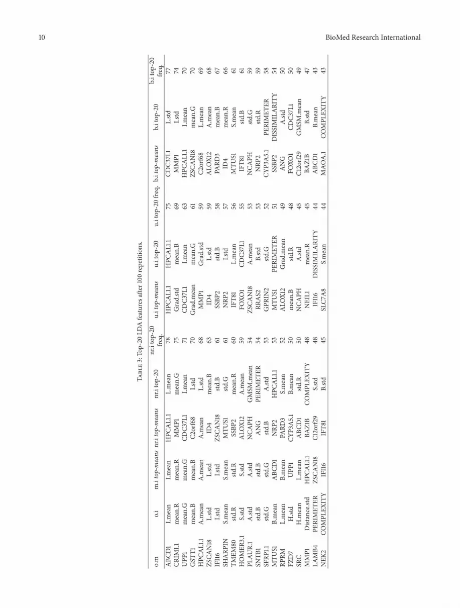
for each integrative dataset and recorded the LDA coefficients(loadings). Then we introduced two performance indicatorsthat rank feature performance as follows: the top-20 featureswith the largest mean coefficient (top-means) or the top-20features which appeared most of the times having the top-20largest coefficients (top-20). The results are shown in Table 3.

In Table 3 the three first columns (o.m, o.i, and m.i top-means) are retrieved after only one run, since there is novariation in the LDA coefficients as the dataset is stable inthese cases. The top-20 features for o.m, o.i, and m.i havebeen included so as to have a full view of the best variables ateach dataset. As it is obvious from the frequencies columns,the three imputation methods (nr.i, u.i, and b.i) show similardistributions. In order to assess the method which presentsthe better stability, we used as stability indicator (si), thenumber of common features between top-means and top-20columns for each method. The si for nr.i, u.i, and b.i was 2, 5,and 1, respectively.

As a last step, we assess the predictive performance ofthe top features (u.i top-means), looking at the LDA and RFalgorithms, to all the datasets. For the cases of the originaldatasets (o.m, o.i) only the relative part of the biomarkers wasused as predictors.The results are shown in Figure 7.Aperfectscore is achieved by random forests for all the datasets apartfrom the image-only original dataset. LDA reports an almostperfect score too, apart from the o.i dataset in which it cannotguess correctly any of the melanoma samples.

5. Discussion

In this work we propose the fusion of two separate datasets,concerning the same disease, as a new approach for theextraction of better biomarkers. The study extends theevaluation of the optimum set of predictors not only inlight of the attained performances but in relation to thestability of the resulted predictors as well. This is the firstattempt, to the best of our knowledge, to assess featureselection algorithms on integrative datasets retrieved from

10 BioMed Research International

Table3:To

p-20

LDAfeatures

after

100repetitions.

o.m

o.i

m.itop-means

nr.itop-means

nr.itop-20

nr.itop-20

freq.

u.itop-m

eans

u.itop

-20

u.itop

-20fre

q.b.itop-m

eans

b.itop

-20

b.itop

-20

freq.

ABC

D1

I.mean

I.mean

HPC

AL1.1

L.mean

78HPC

AL1.1

HPC

AL1.1

75CD

C37L

1L.std

77CR

IM1.1

mean.R

mean.R

MMP1

mean.G

75Grad.std

mean.B

69MMP1

I.std

74UPP

1mean.G

mean.G

CDC3

7L1

I.mean

71CD

C37L

1I.m

ean

63HPC

AL1.1

I.mean

70GST

T1mean.B

mean.B

C2orf68

I.std

70Grad.mean

mean.G

61ZS

CAN18

mean.G

70HPC

AL1.1

A.m

ean

A.m

ean

A.m

ean

L.std

68MMP1

Grad.std

59C2

orf68

L.mean

69ZS

CAN18

L.std

L.std

ID4

mean.B

63ID

4L.std

59ALO

X12

A.m

ean

68IFI16

I.std

I.std

ZSCA

N18

std.B

61SSBP

2std

.B58

PARD

3mean.B

67SH

ARP

INS.mean

S.mean

MTU

S1std

.G61

NRP

2I.std

57ID

4mean.R

66TM

EM80

std.R

std.R

SSBP

2mean.R

60IFT8

1L.mean

56MTU

S1S.mean

61HOMER

3.1

S.std

S.std

ALO

X12

A.m

ean

59FO

XO1

CDC3

7L1

55IFT8

1std

.B61

PLAU

R.1

A.std

A.std

NCA

PHGMSM

.mean

54ZS

CAN18

A.m

ean

53NCA

PHstd

.G59

SNTB

1std

.Bstd

.BANG

PERIMET

ER54

RRAS2

B.std

53NRP

2std

.R59

SFRP

1.1std

.Gstd

.Gstd

.BA.std

53GPR

IN2

std.G

52CY

P3A5.1

PERIMET

ER58

MTU

S1B.mean

ABC

D1

NRP

2HPC

AL1.1

53MTU

S1PE

RIMET

ER51

SSBP

2DISSIMILARITY

54RP

RML.mean

B.mean

PARD

3S.mean

52ALO

X12

Grad.mean

49ANG

A.std

50FZ

D7

H.std

UPP

1CY

P3A5.1

B.mean

50mean.B

std.R

48FO

XO1

CDC3

7L1

50SR

CH.m

ean

L.mean

ABC

D1

std.R

50NCA

PHA.std

45C1

2orf2

9GMSM

.mean

49MMP1

Distance.std

HPC

AL1.1

BAZ1B

COMPL

EXITY

48NEIL1

mean.R

45BA

Z1B

B.std

47LA

MB4

PERIMET

ERZS

CAN18

C12orf2

9S.std

48IFI16

DISSIMILARITY

44ABC

D1

B.mean

43NEK

2CO

MPL

EXITY

IFI16

IFT8

1B.std

45SLC7

A8

S.mean

44MAO

A.1

COMPL

EXITY

43

BioMed Research International 11

separate sources (modalities), where each source comes froma different set of patients, connected however by the samepathological mechanism. Although this study focused inthe CM disease, the method could be applied, in general,to any disease where separate datasets exist, such as thoseresiding in microarray expression, proteomic and genomicdata repositories. Of course, special care has to be given to theselection of matching experiments regarding the disease, sosamples, preparation methods, and the subsequent analysisare in the same context. In this work regarding CM, forinstance, the microarray experiment selected was carefullyscreened among dozens residing in the GEO related tomelanoma in order to match comparable state, progress, andtissue taken for the disease (e.g., no artificial cell lines, notonly metastatic tumours, etc.).

5.1. Use of Synthetic Data. The application of imputationmethods per feature and per class fills the gaps in the blocksparse matrix of the unified dataset and produces a datasetwhich is amenable for processing by multivariable machinelearningmethods.The imputation process as performed hereis class dependant and so inserts a significant bias at testingtime towards achieving high performance accuracies. As aheavy biased procedure still, it is able to integrate the differentdatasets at the data level and highlight features and relationsamongst them which would otherwise be impossible.

The three imputation methods (apart from the meanimputation), where each relies on a given statistical distribu-tion scheme, perform similarly (auc or accuracy) regardingthe predictor sets (biomarkers) they propose for the 2-class classification problem. These methods also performedequally well regarding the stability of the predictors, seenespecially in the RF results. In all cases the unified datasetswere able to produce biomarkers of higher predictive per-formance (with the exception of the RF case for the only-microarray data, which produces analogue results). In par-ticular, when the stability of the proposed biomarkers wastaken into account, the unified datasets had a superior perfor-mance, especially when compared with the solely microarrayrelated features.

5.2. Dataset Idiosyncrasies. The two joined datasets arecharacterised by class imbalance, features imbalance, andimbalance of the number of observations between themodes.An additional caveat is that the columns in both datasets arecovariant. The random forest algorithm, applied in stratifiedbootstrapped samples, was capable of tackling these issuesand performs almost perfectly in most cases, with the excep-tion of the image-only data, which had an auc score of 0.8.Thelinear approaches (PCA and LDA) did not perform highly inthe cases of the unimodal datasets (image or microarrays).For the unified datasets, however, both RF and LDA attainedtop scores.

5.3. Impact of the Unimodal Datasets. One of the noticeabledifferences in the proposed predictor sets between RF andLDA is the performance of the image features.RF indicates

that all image features score lower than the 100th position ofimportance for the filtered case or after the 350th positionfor the unfiltered case. In the linear analyses of PCA andLDA, however, presence of image features in the predictorsets is on a par with the microarray features. In addition,from the two used stability indicators on LDA, top-meansfavours microarray features (e.g., 17 to 3 for the u.i top-means), and top-20 favours image features (e.g., 2 to 18for the u.i top-20). Moreover, as surmised from the svdvalues (Supplementary 2) of the unimodal datasets, bothperform similarly and so the proposed top predictor setscontain variables from both modes. Additionally, in the samelinear perspective, the image data points present better classseparation in the unified datasets, as denoted by the crossedmarks in the PCA and LDA scores plots. The selection ofthe 20 u.i top-means set as biomarkers (as seen in Figure 7)resulted in an almost perfect performance on all the datasetsfor both methods (RF and LDA) apart from the image-onlycase. This is due to the fact that the selected u.i top-means setcontains only 3 image features. RF, however, needs between 5to 10 image features to reach the top performance as seen inFigure 2 for the two “best” cases.This is evenmore obvious forthe LDA method, which fails to predict any melanoma casefrom the 3 proposed image predictors, as seen in Figure 7.

These findings support the notion that the expansion ofthe feature set, through the use of the imputation meth-ods, benefits the classification process. Proposing geometricspaces where appropriate separating hyperplanes can bederived incurs good performance in a methodologically sim-ilar way with methods as the Support Vector Machines. It isworth noting the dramatic improvement of the predictor setsinferred by the unified datasets (although biased), in termsof classification performance as well as informational contentregarding the explained variation. Of paramount importanceis the fact that this superior performance is rescued even bysubsequent application of drastic data reduction techniques,such as the top-means or the top-20 formalisms. A possibleexplanation for this finding is that the transformation ofthe initial classification problem in a geometric space, whichalleviates features covariance, makes leeway for the inferenceof separating planes between classes that perform robustly.This improvement is therefore retained permanently, evenwhen the representation space is collapsing; a different,however, still robust combination of features that define thesignature set is feasible. Moreover, through the integrationof data from two different layers of organization of thebiological information (molecular and whole tissue), theeffect of noise, in the form of false positives in each layer ofdescription, is seriously limited. By transforming the initialdatasets into a unified phantom set the effect of arbitraryfeature covariance due to noise is confined in this layer oforganization, downgrading their impact in the unified datasetand thus disqualifying them fromcandidates for the predictorset.

5.4. Biological Implications of the Biomarker Sets. Theanalysisof the composite multimodal signature sets presented in

12 BioMed Research International

Table 3, according to the two different performing indi-cators, top-means and top-20, proposes equivalent featuresets capable of classifying robustly and accurately humansamples, probed either through molecular (gene expressionprofiling) or imaging (dermoscopic evaluation) examination.The fact that these signatures are top performers, not onlyin terms of efficiency in classification but also regarding theinformational content of the observed variation that theymanage to explain in the integrative dataset, renders themideal starting points for functional interpretation of criticaldeterminants of the CM pathophysiological mechanism.As previously said those signatures bear complementarityregarding the modules they select in order to performthe classification task, in terms of functional implication.Interestingly, the top-means indicator, which comprises the 20features with the largest mean coefficients, is heavily enrichedwith features coming from the molecular layer, while the top-20 is basically comprised of image features. The HPCAL1.1gene was encountered in all of the unified signatures with theexception of b.i, where CDC37L1 was observed.

Regarding the imaging features, they can contribute tothe construction of reliable operators, that consolidate thewealth of morphological information, critical for the task ofthe dynamic description of the undergoing transformationsof biological procedures in relation to disease manifesta-tion. Moreover they may represent reliable macroscopiccandidates for assessment of disease molecular subtypes,something that could be strengthened if covariance-basedassociation of those markers with the molecular markers isundertaken.However in order that this analysis is biologicallyinsightful and of practical use, large populations of cohortsare needed to check the consistency of the findings.

The molecular part of the feature set comprises geneswhich imply promotion of tumorigenesis, angiogensis, andprotein endoplasmic misfolding, that induces stress responserepair signals, xenobiotic metabolism, and so forth, namely,involvement of cellular modular functions. These func-tions are known to be associated with the carcinogenicaberrant course in particular for aggressive cancers like CM.Indicatively, FOX1 possesses an established role in myogenicgrowth, differentiation, and blood angiogenesis. Defectivefunction of FOX1 is incriminated for rhabdomyosarcomatype 2, a highly malignant tumour of striated muscle derivedfrom primitive mesenchymal cells, which is a cancer modelthat is evolutionary close to skin cells [36]. CDC37L1 is acochaperone that binds to numerous proteins and promotestheir interaction with Hsp70 and Hsp90, whose aberrantfunction suggests an endoplasmic reticulum stress responseas a result of protein misfolding stress [37]. MMP1 is impli-cated in the breakdown of extracellular matrix in normal,physiological processes, such as embryonic development,reproduction, tissue remodeling, and blood coagulation, aswell as in disease processes such as arthritis and themetastaticprocedure [38], for which melanoma cells present a highpotency. Interestingly, HPCAL1 encodes an extracellularprotein, which is a member of neuron-specific, calcium-binding, protein family, found in the retina and brain [39].

This finding is consistent with the fact that skin and neuralcells, especially the cancer ones that are dedifferentiated, havecommon progenitor lines.

5.5. Future Work. In this study, the direct comparisonbetween RF and the linear information-oriented methods,regarding the stability of the proposed predictor set forbiomarker discovery, was based on an empirical cut-off,namely, the top-20 features, as surmised by the LDAmethod.Subsequently, mode membership (image or microarrays) inthe 20 feature set was examined for the two schemes: top-means and top-20. Still, this approach could be further devel-oped to implement automated feature selection, exploitingstatistically derived decision cut-offs. It can also be extendedto enable juxtaposition with the automated filtering thatoccurs in the feature selection with RF, which is depicted atthe 3rd column of Tables 1 and 2. In addition, the signaturesderived by the unified datasets could be compared withclinical multimodal data stemming from the same set ofpatients. In this way, the impact of the imputationmethods inthe creation of the synthetic dataset could be cross-evaluated,with the performance of other data analysis methods, such ascanonical correlation analysis or variations of such methods.

Conflict of Interests

The authors declare that there is no conflict of interestsregarding the publication of this paper.

Acknowledgments

The authors would like to thank Dr. Max Kuhn, creator ofthe caret R package, for his support on the functionality ofthis software, and Dr. Joseph Ward for paper corrections.This work has been supported by the 12CHN 204 BilateralGreece-China Research Program of the Hellenic GeneralSecretariat of Research andTechnology and theChineseMin-istry of Research and Technology entitled “Personalizationof melanoma therapeutic management through the fusion ofsystems biology and intelligent data mining methodologies-PROMISE,” sponsored by the Program “Competitivenessand Entrepreneurship,” Priority Health of the PeripheralEntrepreneurial Program of Atticaki.

References

[1] J. W. Fenner, B. Brook, G. Clapworthy et al., “The EuroPhys-iome, STEP and a roadmap for the virtual physiological human,”Philosophical Transactions of the Royal Society A, vol. 366, no.1878, pp. 2979–2999, 2008.

[2] T. Rohlfing, A. Pfefferbaum, E. V. Sullivan, and C. R. Maurer,“Information fusion in biomedical image analysis: combinationof data vs. combination of interpretations,” Information Process-ing in Medical Imaging, vol. 19, pp. 150–161, 2005.

[3] R. Haapanen and S. Tuominen, “Data combination and featureselection for multi-source forest inventory,” PhotogrammetricEngineering and Remote Sensing, vol. 74, no. 7, pp. 869–880,2008.

BioMed Research International 13

[4] J. L. Jesneck, L. W. Nolte, J. A. Baker, C. E. Floyd, and J. Y. Lo,“Optimized approach to decision fusion of heterogeneous datafor breast cancer diagnosis,” Medical Physics, vol. 33, no. 8, pp.2945–2954, 2006.

[5] G. Lee, S. Doyle, J. Monaco et al., “A knowledge represen-tation framework for integration, classification of multi-scaleimaging and non-imaging data: preliminary results in predict-ing prostate cancer recurrence by fusing mass spectrometryand histology,” in Proceedings of the 6th IEEE InternationalConference on Symposium on Biomedical Imaging: From Nanoto Macro (ISBI ’09), pp. 77–80, Boston, Mass, USA, July2009.

[6] P. Tiwari, S. Viswanath, G. Lee, and A. Madabhushi, “Multi-modal data fusion schemes for integrated classification ofimaging and non-imaging biomedical data,” in Proceedings ofthe 8th IEEE International Symposium on Biomedical Imaging:From Nano to Macro (ISBI ’11), pp. 165–168, April 2011.

[7] C. Hinrichs, V. Singh, G. Xu, and S. C. Johnson, “Predictivemarkers for AD in a multi-modality framework: an analysis ofMCI progression in the ADNI population,”NeuroImage, vol. 55,no. 2, pp. 574–589, 2011.

[8] K. R. Gray, P. Aljabar, R. A. Heckemann, A. Hammers, and D.Rueckert, “Random forest-based similarity measures for multi-modal classification of Alzheimer’s disease,” NeuroImage, vol.65, pp. 167–175, 2013.

[9] A. Golugula, G. Lee, S. R. Master et al., “Supervised regularizedcanonical correlation analysis: integrating histologic and pro-teomic measurements for predicting biochemical recurrencefollowing prostate surgery,” BMC Bioinformatics, vol. 12, article483, 2011.

[10] M. Balazs, S. Ecsedi, L. Vızkeleti, and A. Begany, “Genomics ofhuman malignant melanoma,” in Breakthroughs in MelanomaResearch, Y. Tanaka, Ed., InTech, 2011.

[11] J. Tımar, B. Gyorffy, and E. Raso, “Gene signature of themetastatic potential of cutaneous melanoma: too much for toolittle?” Clinical and Experimental Metastasis, vol. 27, no. 6, pp.371–387, 2010.

[12] W. K. Martins, G. H. Esteves, O. M. Almeida et al., “Genenetwork analyses point to the importance of human tissuekallikreins in melanoma progression,” BMCMedical Genomics,vol. 4, article 76, 2011.

[13] M. Ogorzałek, L. Nowak, G. Surowka, and A. Alekseenko,“Modern techniques for computer-aided melanoma diagnosis,”in Melanoma in the Clinic—Diagnosis, Management and Com-plications of Malignancy, M. Murph, Ed., InTech, 2011.

[14] I. Maglogiannis and C. N. Doukas, “Overview of advancedcomputer vision systems for skin lesions characterization,” IEEETransactions on Information Technology in Biomedicine, vol. 13,no. 5, pp. 721–733, 2009.

[15] Y. Saeys, I. Inza, and P. Larranaga, “A review of feature selectiontechniques in bioinformatics,” Bioinformatics, vol. 23, no. 19, pp.2507–2517, 2007.

[16] L. Breiman, “Random forests,”Machine Learning, vol. 45, no. 1,pp. 5–32, 2001.

[17] Y. Sun, A. K. C. Wong, and M. S. Kamel, “Classification ofimbalanced data: a review,” International Journal of PatternRecognition and Artificial Intelligence, vol. 23, no. 4, pp. 687–719,2009.

[18] A. Liaw and M. Wiener, “Classification and regression byrandomForest,” R News, vol. 2, no. 3, pp. 18–22, 2002.

[19] C. Chen, A. Liaw, and L. Breiman, “Using random forest to learnimbalanced data,” 2004, http://stat-reports.lib.berkeley.edu/accessPages/666.html.

[20] W. N. Venables and B. D. Ripley,Modern Applied Statistics withS, Springer, New York, NY, USA, 2002.

[21] Z. Dıaz, M. J. Segovia, J. Fernandez, and E. M. d. Pozo,“Machine learning and statistical techniques. An applicationto the prediction of insolvency in spanish non-life insurancecompanies,” The International Journal of Digital AccountingResearch, vol. 5, no. 6, pp. 1–45, 2005.

[22] R. Development Core Team, “R: a language and environmentfor statistical computing,” http://www.R-project.org.

[23] M. Maragoudakis and I. Maglogiannis, “Skin lesion diagnosisfrom images using novel ensemble classification techniques,”in Proceedings of the 10th IEEE EMBS International Conferenceon Information Technology Applications in Biomedicine, Corfu,Greece, November 2010.

[24] T. Barrett, D. B. Troup, S. E. Wilhite et al., “NCBI GEO: archivefor functional genomics data sets-10 years on,” Nucleic AcidsResearch, vol. 39, no. 1, pp. D1005–D1010, 2011.

[25] D. Talantov, A. Mazumder, J. X. Yu et al., “Novel genes asso-ciated with malignant melanoma but not benign melanocyticlesions,” Clinical Cancer Research, vol. 11, no. 20, pp. 7234–7242,2005.

[26] D. Sean and P. S. Meltzer, “GEOquery: a bridge betweenthe Gene Expression Omnibus (GEO) and BioConductor,”Bioinformatics, vol. 23, no. 14, pp. 1846–1847, 2007.

[27] G. K. Smyth, “Limma: linear models for microarray data,” inBioinformatics andComputational Biology SolutionsUsing R andBioconductor, pp. 397–420, Springer, New York, NY, USA, 2005.

[28] R. C. Gentleman, V. J. Carey, D. M. Bates et al., “Bioconductor:open software development for computational biology andbioinformatics,” Genome Biology, vol. 5, no. 10, p. R80, 2004.

[29] NCBI GEO,“GEO2R,” http://www.ncbi.nlm.nih.gov/geo/info/geo2r.html.

[30] N. J. Horton and K. P. Kleinman, “Much ado about nothing:a comparison of missing data methods and software to fitincomplete data regression models,” American Statistician, vol.61, no. 1, pp. 79–90, 2007.

[31] H. Wickham, “The split-apply-combine strategy for data analy-sis,” Journal of Statistical Software, vol. 40, no. 1, pp. 1–29, 2011.

[32] M. Kuhn, S. Weston, A. Williams, C. Keefer, and A. Engel-hardt, “Caret: classification and regression training,” 2012,http://CRAN.R-project.org/package=caret.

[33] T. Fawcett, “An introduction to ROC analysis,” Pattern Recogni-tion Letters, vol. 27, no. 8, pp. 861–874, 2006.

[34] Z. He and W. Yu, “Stable feature selection for biomarkerdiscovery,” Computational Biology and Chemistry, vol. 34, no.4, pp. 215–225, 2010.

[35] L. Breiman, “Manual on setting up, using, and understand-ing random forests v3. 1,” 2002, http://oz.berkeley.edu/users/breiman/Using random forests V3.1.pdf.

[36] N. Galili, R. J. Davis, W. J. Fredericks et al., “Fusion of afork head domain gene to PAX3 in the solid tumour alveolarrhabdomyosarcoma,”Nature Genetics, vol. 5, no. 3, pp. 230–235,1993.

14 BioMed Research International

[37] J. Roiniotis, P. Masendycz, S. Ho, and G. M. Scholz, “Domain-mediated dimerization of the Hsp90 cochaperones Harc andCdc37,” Biochemistry, vol. 44, no. 17, pp. 6662–6669, 2005.

[38] R. M. Wenham, B. Calingaert, S. Ali et al., “Matrix metallo-proteinase-1 gene promoter polymorphism and risk of ovariancancer,” Journal of the Society for Gynecologic Investigation, vol.10, no. 6, pp. 381–387, 2003.

[39] M. Kobayashi, K. Takamatsu, M. Fujishiro, S. Saitoh, and T.Noguchi, “Molecular cloning of a novel calcium-binding pro-tein structurally related to hippocalcin from human brain andchromosomal mapping of its gene,” Biochimica et BiophysicaActa, vol. 1222, no. 3, pp. 515–518, 1994.