EPA 91 0/13-98-001 AlaskaUnited States Region 10 IdahoEnvironmental Protection 1200 Sixth Avenue OregonAgency SeattIeWA98lOl Washington

Office of Waste and Chemicals Management January 1998

SEPA Interim Final Guidance:

Developing Risk-Based Cleanup LevelsAt Resource Conservation and RecoveryAct Sites in Region 10

INTERIM FINAL GUThANCE: DEVELOPINGRISK-BASED CLEANUP LEVELS AT

RESOURCE CONSERVATION AND RECOVERY ACT SITES IN REGION 10

Prepared for

U.S. ENVIRONMENTAL PROTECTION AGENCYOffice of Waste and Chemicals Management

Seattle, WA 98101

Work Assignment No. : R10018EPA Region 10Date Prepared January 5, 1998Contract No. 068-W4-0004Prepared by Tetra Tech EM Inc.Tetra Tech EM Inc. Project Manager : Paul RacetteTelephone (206) 587-4646EPA Work Assignment Manager : Dr. Marcia BaileyTelephone : (206) 553-0684

DISCLA EM ER

This guidance document sets forth recommended approaches to conduct risk assessment andother activities which are integral to the process of developing risk-based cleanup levels at RCRAcorrective action facilities in Region 10 of the United States Environmental Protection Agency.Alternative approaches may be more appropriate at specific sites. Ml approaches used should bedescribed in hill in documents generated as part of the cleanup level decision-making process.This guidance is intended to be updated as scientific developments occur and U.S. EPA andstate rules and policies change. The user is encouraged to use the latest and best informationavailable for developing media cleanup levels, Users are also encouraged to submit suggestionsfor updates to the guidance, or to report any errors noted, to Marcia Bailey, U.S. EPA Region 10,at (206) 553-0684, or Bailey.marciaepamail.epa.gov.

This guidance is intended as guidance to U.S. EPA Region 10 personnel and to RCRA-regulatedfacilities undergoing corrective action or clean closures in Region 10. It does not constitute finalU.S. EPA action and does not constitute rulemaking. It is not intended, nor can it be relied upon,to create any rights enforceable by any party in litigation with the United States government. U.S.EPA officials may decide that the guidance provided in this document should be follwed, or maydecide to act at variance with the guidance, based on an analysis of specific site circumstances.US: EPA reserves the right to change the guidance at any time without public notice.

Chapter

ACRONYMS AND ABBREVIATIONS

Page

VIII

GLOSSARY XI

EXECUTIVE SUMMARY

INTRODUCTION

1.1 Statutory and Regulatory Authorities Overview1.2 Human Health and Ecological Risk Assessments:

An Overview1.3 Risk Characterization Principles

2 STATE PROGRAMS

ES-I

1—I

2-I

2.1 Alaska Department of Environmental Conservation2.2 Idaho Division of Environmental Quality2.3 Oregon Department of Environmental Quality2.4 Washington Department of Ecology

2-22-22-22-3

3.2.13.2.23.2.33.2.43.2.53.2.6

3-9

3-93-103-Il3-Il3-123-13

3-13

1-2

1-21-9

3 DATA COLLECTION TO CHARACTERIZE FACILITY AND DETERMINE HAZARDOUSCONSTITUENTS OF POTENTIAL CONCERN 3-I

3.1 Data Quality Objectives Process 3-I

3.1.1 Step 1: State the Problem 3-33.1.2 Step 2: ldenti& the Decision 3-33.1.3 Step 3: Identi’ the Inputs to the Decision 3-43.1.4 Step 4: Define Boundaries of the Study 3-43.1.5 Step 5: Develop a Decision Rule 3-53.1.6 Step 6: Speciv Tolerable Limits on Decision Errors 3-63.1.7 Step 7: Optimize the Design for Obtaining Data 3-8

3.2 Data Useability

Data SourcesDocumentationAnalytical Methods, Detection Limits, and Quantitation LimitsData Quality IndicatorsData ReviewReports from Sampling and Analysis

3.3 Data Quality Assessment

S REP4R WPDI2flIfl7N *,mne

CONTENTS (Continued)

Chanter

3.4 Identification of Hazardous Constituents ofPotential Concern 3-14

4 HUMAN HEALTH RISK ASSESSMENT PROCEDURES

4.1 Exposure Assessment: Identification of Exposure Pathways 4-24.2 Classification of Land Use 4-5

4.2.1 U.S. Environmental Protection Agency Land Use Policy andSoil Cleanup Levels 4-6

4.2.2 Region 10 State Land Use Policies and Soil Cleanup Levels 4-74.2.3 Land Use Policies and Other Media . 4-9

4.3 Identification of Promulgated Standards and Criteria . 4-13

4.3.1 Federal Standards and Criteria 4-134.3.2 State Standards and Criteria 4-13

4.4 Risk-based Screening 4-154.5 Exposure Assumptions 4-17

4.5.1 Dermal Absorption Factors 4-234.5.2 Fate and Transport Models 4-25

4.6 Toxicity Assessment 4-39

4.6.1 Dose-Response Information 4-394.6.2 U.S. Environmental Protection Agency Toxicity Factors 4-434.6.3 Chemicals or Exposure Pathways With No U.S. Environmental Protection

Agency Toxicity Values 4-45

4.7 Calculation of Risk-Based Concentrations .. . 4-57

4.7.1 Selection of Target Risks and Hazard Quotients 4-SB4.7.2 Risk-Based Concentration Calculation Equations 4-594.7.3 Examples of Risk-Based Concentration Calculations 4-664.7.4 Adjustment of Risk-Based Concentrations for

Multiple Hazardous Constituents 4-694.7.5 Risk-Based Concentrations Based on Hazardous

Constituent Migration 4-724.7.6 Cleanup Levels for Lead 4-73

S fPAI(NIIflASKS1flWSE3’PINAL1ASThk.WPD\j2flhf7rn jbm\ne II

Chapter

4.8 Uncertainty Analysis

CONTENTS (Continued)

Page

4-75

4.8.14.8.24.8.34.8.4

5.1.15.1.25.1.35.1.45.1.55.1.6

Data UncertaintyExposure Assessment UncertaintyToxicity Assessment UncertaintyCleanup Level Uncertainty

Preliminary Problem FormulationAnalysisPreliminary Risk CharacterizationEcological AdversityUncertainty AnalysisRisk-Based Corrective Action

4-764-774-794-81

5-I

5-4

5-65-155-225-265-275-27

6 PROBABILISTIC RISK ASSESSMENT . 6-I

6.1 Populations, Parameters, and Statistics6.2 Probabilistic Analysis

in Human Health

6.3 How to Conduct a Monte Carlo Simulation 6-10

6.3.16.3.26.3.3

Selection of an Appropriate Exposure ModelsSelection of Probability DistributionsRunning the Monte Carlo Simulation

6-Il6-126-20

6.4 Probabilistic Risk Assessment Case Study 6-21

6.4.16.4.26.4.3

Monte Carlo SimulationDeterministic Risk AssessmentSummary of Results

6-216-296-29

6.5 Work Plans. Reports, and Presentations

III

6-3!

5 ECOLOGICAL RISK ASSESSMENT PROCESS

5.1 Screening-Level Ecological Risk Assessment

6.2.1 Uncertainn’ and Variability6.2.2 Other Methods of Estimating Uncertainty

Risk Assessment and Ecological Risk Assessment6.2.3 Monte Carlo Simulation

6-26-5

6-6

6-86-9

S RLPARIEflIWTASKSREVlSE2flNALMASThR WP9\(V1(N 3m\slc

CONTENTS (Continued)

Chanter C)7 DETERMINATION OF COMPLIANCE WITH TARGET CLEANUP LEVELS 7-1

7.1 Data Quality Objective Steps 1 Through 3 7-17.2 Step 4: Study Boundaries 7-17.3 StepS: Develop Decision Rule 7-37.4 Step 6: Specify Tolerable Limits on Decision Errors 7-47.5 Step 7: Optimize the Design for Obtaining Data 7-57.6 Data Useability and Data Quality Assessment 7-77.7 Detection Limits 7-8

REFERENCES R- I

INDEX . I-I

ATTACHMENTS

A U.S. Environmental Protection Agency Carol Browner Memorandum on Risk Assessment

B RCRAJCERCLA Interface-Interim Final Guidance, EPA Region 10 Memorandum

C Examples of Data Quality Assessment Applications c:D Data Useability Worksheets

E U.S. Environmental Protection Agency Region 9 Preliminary Remediation Goals

F U.S. Environmental Protection Agency Region 8 Superfund Technical Guidance NumberRA-OJ: Evaluating and ldentiing Contaminants of Concern for Human Health

G U.S. Environmental Protection Agency Land Use Memorandum

H Soil Screening Guidance Chemical Properties Table C

Region 10 EPA Memorandum on Inorganic Arsenic

J World Health Organization Abstract on Dioxin Toxic Equivalency Factors

K EPA Region 1 Risk Updates, Revised Manganese Reference Dose

L An Approach for Determining Toxicity Values for Dermal Exposure, Oak Ridge NationalLaboratory Internal Paper

aS REPAR IIKjI7ASK5V15E2’flWAL1Aflfl.W?DIZflh,7flibm\M4 iv

CONTENTS (Continued)

ATTACHMENTS

M EPA Guidance for Calculating Exposure Point Concentrations

N A Bibliography Related to Ecological Risk Assessment

0 EPA Guidance and Policy for Probabilistic Risk Assessment

P Dealing with Data Below Detection Limits, Quality Assurance Course Module 492, EPANational Center for Environmental Research and Quality Assurance

EXHIBITS

Exhibit

1-1 Selection Process for Hazardous Constituents of Potential Concern . . . 1-5

1-2 Human Health Risk Assessment Resource Conservation and Recovery ActCleanup Level Development 1-7

1-3 Ecological Risk Assessment Risk-Based Corrective Action Flowchart 1-8

4-I Reduced Risk-Based Concentration Equations 4-62

4-2 Reduced Risk and Hazard Index Equations 4-64

4-3 Adjusting Cleanup Levels for Carcinogenic Compounds 4-7!

4-4 Adjusting Cleanup Levels for Noncarcinogenic Health Effects 4-72

4-5 Risk Assessment and Cleanup Level Determination Process 4-75

5-I Sources for Ecological Risk Assessment Methods 5-1

5-2 Ecological Risk Assessment Steps and Decision Points 5-2

5-3 Ecological Receptor Characterization 5-7

5-4 Exposure Pathway Examples 5-9

5-5 Sample Endpoints and Relationships 5-13

v

CONTENTS (Continued) C)EXHIBITS

Exhibit

5-6 Suggested Measurement Endpoints 5-14

5-7 Sample Intake Calculation for The Deer Mouse 5-19

5-8 Evaluation Criteria for Current and Future Ecological Adversity 5-26

5-9 Possible Uncertainties in Screening-level EcologicalRisk Assessment 5-28

6-I Common Probability Distributions 6-14

6-2 Probability Density Function Intervals-Latin Hypercube Sampling 6-21

6-3 Exposure Parameter Probability Density Functions - Adult 6-23

6-4 Exposure Parameter Probability Density Functions - Child 6-24

6-5 Case Study Probability Density Function for Benzo(a)pyrene Risk-BasedSoil Concentrations Region 10 RCRA Risk-Based Cleanup Level Guidelines 6-25

6-6 Case Study Sensitivity Chart for Exposure Parameters 6-27

S REM K ..pIxtAStkxEvSE,ENa,MArtR WpVIV1InP 1hmnc vi

CONTENTS (Continued)

TABLESTable

4-I Potential Exposure Pathways for Human Receptors 4-3

4-2 Standard Default Exposure Factors 4-18

4-3 U.S. Environmental Protection Agency Region 3 and Region 9Soil, Water, and Air Exposure Pathways 4-20

4-4 Washington State Model Toxics Control Act Cleanup Level Exposure Factors 4-21

4-5 Recommended Dermal Absorption Factors for Soil 4-24

4-6 Recommended Defaults for Dermal Exposure Factors 4-26

4-7 Derivation of The Volatilization Factor 4-28

4-8 Derivation of The Particulate Emission Factor 4-29

4-9 Dispersion Factor Values by Source Area, City, and Climatic Zone 4-31

4-10 Derivation of The Soil Saturation Limit 4-34

4-Il Ranges of Human Potency and Cancer Potency Factors for EnvironmentalMixtures of PCBs 4-53

6-I Descriptive Statistics for Benzo(a)pyrene Risk-Based Criteria ProbabilityDensity Function 6-28

6-2 Population Percentiles for Benzo(a)pyrene Risk-Based Criteria ProbabilityDensih Functions 6-29

6-3 Exposure Factors for Residential Exposure Ingestion of Soil 6-30

S REPAR HPIW TA5)R Rfl95E2’flWALMA5ThR WPDSIVIIfl7N 5jfl4 vii

0

(THIS PAGE INTENTIONALLY LEFT BLANK)

S REPAR ItI I rnTASKSflV1SE2F1NALMASThRWPDI S I-k IIXI I ILI7(SkIEI MO I .ZII*mlnc

ACRONYMS AND ABBREVIATIONS

2,4-D 2,4-Dichlorophenoxyacetic Acid40 CFR Title 40 of the Code of Federal Regulations95th UCL 95th upper confidence limit on the arithmetic meanAAC Alaska Administrative CodeABS Dermal absorption factorADD Average daily doseADEC Alaska Department of Environmental ConservationAr1254 Aroclor 1254ASTM American Society for Testing and MaterialsATSDR Agency for Toxic Substances and Disease RegistryAUF Area use factorAWQC Ambient water quality criteriaBDL Below detection limitCal/EPA California Environmental Protection AgencyCDD Chlorinated dibenzo-p-dioxinsCDF Chlorinated dibenzoftransCDI Chronic daily intakeCERCLA Comprehensive Environmental Response, Compensation, and Liability Act of 1980CMS Corrective measures studyCOPC Constituent of potential concernCPF Cancer potency factorCSGWPP Comprehensive state groundwater protection planCSM Conceptual site modelDDT DichlorodiphenyltrichloroethaneDEFT Decision error feasibility trialsDOD U.S. Department of DefenseDOE U.S. Department of EnergyDQA Data quality assessmentDQI Data quality indicatorsDQO Data quality objectivesEcology Washington Department of EcologyEDQL Ecological data quality levelsEPA U.S. Environmental Protection AgencyFR Federal RegisterHI Hazard indexBEAST Health Effects Assessment Summary TablesHHRA Human health risk assessmentHQ Hazard quotientHSWA Hazardous and Solid Waste Amendments of 1984IAC Idaho Administrative CodeIDEQ Idaho Division of Environmental QualityIEUBK Integrated exposure uptake biokinetic modelIRIS Integrated Risk Information SystemLADD Lifetime average daily doseLD50 Lethal dose 50

‘.REPA’R wrD\I1nIn7m 3flm\sae VIII

ACRONYMS AND ABBREVIATIONS (Continued)

L/day Liters per dayLOAEL Lowest-observable-adverse-effect-levelMg/dL Micrograms per deciliter

Micrograms per literm3/hr Cubic meter per hourMCL Maximum contaminant levelMCLG Maximum contaminant level goalMDEP Massachusetts Department of Environmental Protectionmg/kg Milligrams per kilogrammg/kg-day Milligrams per kilogram per dayMRL Minimal risk levelsMTCA Model Toxics Control ActNCEA National Center for Environmental AssessmentNOAA National Oceanic and Atmospheric AdministrationNOAEL No-observable-adverse-effect-levelOAR Oregon Administrative RulesODEQ Oregon Department of Environmental QualityPAR Polynuclear aromatic hydrocarbonPCB Polychiorinated biphenylPDF Probability density functionPEF Particulate emission factorPRA Probabilistic risk assessmentPRG Preliminary remediation goalQ/C Dispersion factorQA Quality assuranceQAPP Quality assurance project planQC Quality controlQMP Quality management planRAGS Risk Assessment Guidance for SuperfundRBC Risk-based concentrationRCRA Resource Conservation and Recovery ActRfC Reference concentrationsRfO Reference doseRFI RCRAfacility investigationRIIFS Remedial investigation and feasibility studyRME Reasonable maximum exposureSAP Sampling and analysis planSOP Standard operating proceduresSWMU Solid waste management unitSVOC Semivolatile organic compoundsTCDD 2,3,7,8-Tetrachlorodibenzo-p-dioxinTEF Toxicity equivalency factorsTEQ Toxic equivalentTPH Total petroleum hydrocarbonsTR Target risk

S REPAR (IIITASKS\REV1SE2FINA1&1ASThR.WPThI2RIfl7/S 1bmsae IX

ACRONYMS AND ABBREVIATIONS (Continucd)

TRV Toxicity reference valueTWA Time-weighted averageVF Volatilization factorVF Soil-to-air volatilization factorVF Groundwater-to-indoor air volatilization factorVOC Volatile organic compoundsWAG Washington Administrative Code

S REPAm I(K)IWTASK.mEW5E,FINAL4ASThR WPOSI2?UPflN ikmsn X

* a

(THIS PAGE INTENTIONALLY LEFT BLANK)

S REPA I•lItTASkKI9SE2flNAjfAflR I5I-RINlI7lM3flINWII Q

GLOSSARY

GENERAL RISK ASSESSMENT TERMS

absorbed dose: The amount of a substance penetrating the exchange boundaries of an organism aftercontact. Absorbed dose is calculated from the intake and the absorption efficiency. It usually isexpressed as mass of a substance absorbed into the body per unit body weight per unit time(e.g., mg/kg-day).

acute effects: Adverse human or ecological impacts caused by very short-term exposure to hazardousconstituents.

administered dose: The mass of a substance given to an organism and in contact with an exchangeboundary (e.g., gastrointestinal tract) per unit body weight per unit time (e.g., mg/kg-day).

carcinogenic risks: Incremental probability that an individual will develop cancer over a lifetime as aresult of exposure to a carcinogen.

chronic effects: Adverse human or ecological impacts caused by long-term exposure to hazardousconstituents.

cleanup levels: The hazardous constituent concentrations to which a contaminated environmentalmedium (e.g., soil, groundwater, surface water, sediment) must be remediated. EPA establishes cleanuplevels on a facility-by-facility basis during the remedy selection process. Determination of targetcleanup levels is a risk management decision.

conceptual site model: Schematic and/or narrative presentation of information about a facilityconditions including known and potential sources of releases of hazardous constituents, exposurepathways, receptors, and all available information about constituents of potential concern at the facility.

data quality objectives (DQOs): Qualitative and quantitative statements relevant to facility-specificcircumstances which are to ensure that sampling and analysis data of known, documented and adequatequality are obtained to support a risk assessment.

dose-response evaluations: The process of quantitatively evaluating toxicity information andcharacterizing the relationship between the dose of a hazardous constituent received and the incidence ofadverse health effects in the exposed population.

exposure pathways: The various ways a hazardous constituent in a given medium can come intocontact with a receptor. For example, possible exposure pathways for contaminated soil includeingestion of the soil, inhalation of the soil as dust, inhalation of volatile organics emanating from the soil,and dermal contact with the soil.

exposure route: The way an environmental hazardous constituent can enter an organism. The threeprimary routes are ingestion, inhalation, and dermal contact.

xi

RCRA hazardous constituent: Substances that have been shown in scientific studies to have toxic,carcinogenic, mutagenic, or teratogenic effects on humans or other life forms. RCRA hazardousconstituents used in 40 CFR 261, Appendix VIII.

CERCLA hazardous substance: Elements, compounds, mixtures, solutions, and substances, which,when released into the environment may present substantial danger to the public health or welfare or theenvironment. The terms means any substances designated under the federal water pollution control act.CERCLA, RCRA, the clean air act, and the toxic substances control act. CERCLA hazardous substanceare listed in 40 CFR 3024.

hazard index: An estimate of the risk associated with a specified exposure to a noncarcinogenichazardous constituent, expressed as the ratio of a substance exposure level over a specified time period toa reference dose for that substance derived from a similar exposure.

lifetime average daily intake: Exposure expressed as mass of a substance contacted per unit bodyweight per unit time, averaged over a lifetime.

linearized multistage model: One of a number of mathematical models and procedures used toextrapolate from carcinogenic responses observed at high doses to responses expected at low doses.

95 percent upper confidence limit (95 UCL) on the arithmetic mean: Value that, when calculatedrepeatedly for randomly drawn subsets of facility data, equals or exceeds the true mean 95 percent of thetime. Provides a conservative estimate of the average concentration.

quality assurance project plan (QAPP): Describes the policy, organization, functional activities, andquality assurance and quality control protocols necessary to achieve DQOs dictated by the intended useof the data.

receptor: An organism (human, plant, or animal) that is potentially exposed to chemical contaminationfrom a facility.

reference dose: An estimate (with uncertainty spanning an order of magnitude or greater) of a dailyexposure level for the human population, including sensitive subpopulations, that is likely to carry noappreciable risk of deleterious effects during a lifetime.

cancer potency factor: A plausible upper-bound estimate of the probability of an individual developingcancer as a result ofa lifetime of exposure to a particular level of potential carcinogen.

toxicity value: A numerical expression of a dose-response relationship for a particular substance. Themost common values used in EPA risk assessments are reference doses (for noncarcinogenic effects) andcancer potency factors (for carcinogenic effects).

weight-of-evidence classification: An EPA classification system for characterizing the extent to whichthe available data indicate that an agent is a human carcinogen. Recently, EPA has developed weight-ofevidence classification systems for some other kinds of toxic effects, such as development effects.

S REPASUlxlIITASKrflVISE2IY1NALMASflR WPDI1flIfl7I9 3km\in I

weight-of-evidence: Classification of evidence from human and animal studies into categories ofsufficient, limited, inadequate, no data, or no evidence of cancer effects.

ECOLOGICAL TERMS USED BY THE U.S. ENVIRONMENTAL PROTECTION AGENCY(1992f and 19941)

area use factor: The fraction ofan organism’s home range, breeding range, or foraging range to thearea of contamination or the facility area under investigation.

assessment endpoint: A clearly defined statement of the environmental value that is to be protected.

bioaccnmulation: General term describing a process by which chemicals are taken up by an organismeither directly from exposure to a contaminated medium or by consumption of food containing thechemical. EPA’s 19941 (and new 1997) Ecological RiskAssessment Guidance for Superfund: Processfor Designing and Conducting Ecological Risk Assessments.

bioavailability: The degree to which a material in environmental media is assimilated by an organism.

constituents of potential concern: Chemicals detected at a facility which have the potential toadversely affect ecological receptors because of their concentration, distribution, and mode of toxicity.

complete exposure pathway: Includes a source or release from a source, an exposure route (that is,soil), and an exposure point (that is, dermal contact). If the exposure point differs from the source,transport and exposure media are also included in the exposure pathway.

baseline ecological risk assessment: A comprehensive ecological risk assessment where uncertaintiesof the screening-level assessment are reduced, and nonfacility-specific TRVs are refined byincorporating data on facility-specific results from fate and transport modeling as well as exposure andecological effects analyses.

conceptual site model: The conceptual site model describes a series of working hypotheses of how astressor might affect ecological components. It also describes the ecosystem potentially at risk, therelationship between assessment endpoint and measurements and exposure scenarios.

ecological effect: An effect where the stressor acts directly on the ecological component of interest(direct effect). Also, an effect where the stressor acts on supporting ecological components of theecosystem, which in turn have an indirect effect on the ecological components of interest.

ecological niche: The functional position of an organism in its environment, comprising the habitat inwhich the organism lives, the periods of time during which it occurs and is active there, and the resourcesit obtains there.

ecological receptor: The biotic component (for example, organism, population, community) exposed toa stressor.

REPA’R Ir,IIW.TASKflXEV1SE1\FINALMASThR WPDI2fl Ifl7fl Th3msac xiii

ecological relevance: This term is typically used in the context of identif’ing assessment endpoints.Ecologically relevant assessment endpoints reflect important ecosystem components that are functionallyrelated to other ecosystem components and assessment endpoints

ecological risk assessment: The process that evaluates the likelihood that adverse ecological effectsmay occur or are occurring as a result of exposure to one or more stressors. -

ecosystem: The biotic community and the abiotic environment within a specified location in space andtime. The abiotic environment includes non-living environmental media (for example, water, soil,sediment) and associated physical and chemical influences (for example, light, temperature, pH,humidity).

ecotone: A narrow and fairly sharply defined transition zone between two or more different bioticcommunities. These “edge” communities are typically species-rich. Reference: Allaby, M., editor.1994. The Concise Oxford Dictionary of Ecology. Oxford University Press.

exposure: The contact or co-occurrence of a stressor with an ecological a receptor.

exposure area: A contaminated habitat where ecological receptors may be exposed to hazardousconstituents that may cause adverse ecological effects.

exposure point concentration: The concentration of a constituent that an ecological receptor is exposedto through exposure routes such as ingestion, dermal contact, inhalation.

exposure profile: The product of the exposure analysis step in the ecological risk assessment. Theexposure profile summarizes the magnitude and spatial and temporal patterns of exposure for the ()exposure scenarios described in the conceptual site model.

exposure scenario: A set of assumptions concerning how an exposure may occur, includingassumptions about the exposure setting, stressor characteristics, and activities that may lead to exposure.

guild: A group of species that share common ecological characteristics (for example, feeding behavior).Guilds are defined by guild descriptors (for example, feeding guild) that may be general or specific.Guilds may contain many or few species in response to the number of guild descriptors.

hazard index: A sum of hazard quotients for hazardous constituents of ecological concern with thesame ecological effect endpoint and/or the same mechanism of toxic effect.

hazard quotient: The ratio of a single exposure concentration or dose to a toxicity value selected for therisk assessment (for example. lowest observed adverse effect level or no observed adverse effect level).

keystone species: A species, the presence or abundance of which can be used to assess the extent towhich ecological components of an ecosystem are impacted.

lowest observed adverse effect level: The lowest level of a stressor evaluated in a test that causesstatistically significant differences from the controls.

S REPAfl IIrnI.\TASKSREWSE2’flNAL,MAflfl xiv

measurement endpoint: A measurable ecological characteristic that is indirectly related to theassessment endpoint.

no observed adverse effect level: The highest level of a stressor evaluated in a test that does not causestatistically significant differences from the controls.

population: A group of organisms of the same species, occupying a given area, and capable ofinterbreeding.

risk characterization: A phase of ecological risk assessment that integrates the results of the exposureand ecological effects analysis to evaluate the likelihood of adverse ecological effects associated withexposure to a stressor. The ecological significance of the adverse effects is discussed, includingconsideration of the types and magnitudes of the effects, their spatial and temporal patterns, and thelikelihood of recovery.

screening-level ecological risk assessment: Simplified assessments that can be conducted with limiteddata by assuming values for parameters for which data are lacking. Where data are lacking, assumedvalues are biased in the direction of overestimating risk so the assessment can provide a defensibleconclusion of no unacceptable ecological risk.

stressor: Any physical, chemical, or biological entity that can induce an adverse response.

subpopulation: A portion of the population known or likely to be exposed to hazardous constituents ator from the facility.

toxicological test: Tests used to evaluate relative potency of a chemical by comparing its effect onliving organisms with the effect of a standard preparation on the same type of organism.

trophic level: A functional classification of taxa within a community that is based on feedingrelationships (for example, aquatic and terrestrial plants make up the first trophic level, and herbivoresmake up the second).

xv

EXECUTIVE SUMMARY

This guidance document provides procedures for developing human and ecological risk-based cleanup

levels for facilities undergoing corrective action and clean closure under the Resource Conservation and

Recovery Act (RCR4). The procedures are intended for use by U.S. Environmental Protection Agency

(EPA) permit writers and regulatory compliance officials as well as RCRA-regulated facilities.

This guidance document references EPA Region 10 state RCRA corrective action programs and relevant

laws and regulations. EPA guidance on determining data quality objectives and performing a data quality

assessment is summarized. The major risk assessment steps, including data evaluation, exposure

assessment, toxicity assessment, and risk characterization, are described. Methods for determining human

and ecological risk-based cleanup levels using deterministic and probabilistic techniques are presented.

Screening-level ecological risk assessment methods are described. Procedures to follow when determining

compliance with cleanup levels are also described. Federal, state, and general literature references that

provide further details on the risk calculation processes are identified throughout the document.

Consultation with Region 10 human health scientists and ecologists is recommended if complex aspects of

the risk assessment process are encountered.

S WOISI.RIINII*lI7INflIflJflPI iS.mj.. —

INT

RO

DU

CT

ION

CHAPTER 1

INTRODUCTION

This guidance document provides procedures for developing human and ecological risk-based cleanup

levels for contaminated facilities undergoing corrective action and clean closure under the federal Resource

Conservation and Recovery Act (RCRA). The procedures are intended for use by permit writers and

enforcement officials as well as by RCRA-regulated facilities. The guidance is intended to enable RCRA

project managers to recommend cleanup level determinations based on risks posed to human health and the

environment by releases from the facility. The document also describes situations likely to require expert

technical assistance. A risk assessor or toxicologist should be involved at the beginning of the RCRA

facility investigation or corrective action order negotiation process.

This guidance document updates and supersedes the previous U.S. Environmental Protection Agency

(EPA) Interim Final Guidelines for Developing Risk-Based Cleanup Levels at RCRA Sites in Region 10

document (1992a). The document also complements RCRA Facility Investigation (RFI) Guidance

(EPA I 989a). The approach in this document is intended to be consistent with the Comprehensive

Environmental Response, Compensation, and Liability Act of 1980 (CERCLA), known as Superfund.

In circumstances where there are no RCRA-speciflc guidelines or rules, Superfund guidance should be

used. It is EPA Region 10’s objective that cleanup activities conducted under the auspices of either

Superfund or RCRA are comparably protective of human health and the environment (EPA 1994a).

Sections 1.1 through 1.3 provide overviews of (1) EPA’s statutory and regulatory authorities for

requiring corrective action, (2) processes for setting the human health and ecological cleanup levels, and

(3) risk characterization principles, respectively.

Additional sections of this guidance document summarize EPA Region 10 state programs (Chapter 2),data collection and useability issues (Chapter 3), human health risk-based methods for calculatingcleanup levels (Chapter 4), ecological screening-level risk assessment and cleanup levels (Chapter 5),probabilistic risk assessment methods and applications (Chapter 6), and determination of compliancewith cleanup levels (Chapter 7).

S REPAP IrPK’TASKR\REVISE3INAL1ASThR WPOSI5I.RI(P111071P512fl t,’17PJ kmsn —

1.1 STATUTORY AND REGULATORY AUTHORITIES OVERVIEW

Application of the procedures described in this guidance is intended for RCRA facilities where releases

of hazardous constituents require corrective action or where corrective action is necessary so that a

RCRA-regulated unit may be clean-closed. EPA derives its authority for compelling corrective action at

facilities regulated under RCRA Subtitle C by a variety of statutory provisions. Before the Hazardous

and Solid Waste Amendments of 1984 (HSWA) were passed, the RCRA corrective action authorities

were limited to Section 7003, which provides authority to compel action where solid or hazardous waste

may present an imminent and substantial endangerment to human health or the environment, and

Section 3013, which provides authority for requiring investigations where the presence of hazardous

waste or releases of hazardous waste may present a substantial hazard to human health or the

environment. HSWA substantially expanded corrective action authorities for both permitted RCRA

facilities and facilities operating under interim status. Section 3004(u) of HSWA requires that any

RCRA permit issued after November 8, 1984, address corrective action for releases of hazardous wastes

or hazardous constituents from any solid waste management unit. Section 3004(v) authorizes EPA to

require corrective action by permitted facilities beyond the facility boundary where appropriate.

Section 3008(h) provides the authority to require corrective action when there has been a release of

hazardous waste or hazardous constituents from a RCRA facility operating under interim status. EPA

authority for setting cleanup levels at closing units stems from RCRA Section 3004 with regulations

promulgated in Title 40 of the Code of Federal Regulations parts 264 and 265, subpart G, which require

that, among other things, the facility must be closed in a manner that “controls, minimizes or eliminates,

to the extent necessary to protect human health and the environment, post-closure escape of hazardous

waste, hazardous constituents, leachate, contaminated run-off, or hazardous waste decomposition

products to the ground or surface waters or to the atmosphere.” -

1.2 HUMAN HEALTH AND ECOLOGICAL RISK ASSESSMENTS: ANOVERVIEW

Human health risk assessment (HHRA) and ecological risk assessment methods can be used to either

(I) calculate the risk associated with exposure to a hazardous constituent or (2) calculate a risk-based

concentration (RBC) that represents a level of exposure to a hazardous constituent that is not expected to

result in unacceptable risks to human health or the environment health. RBCs may then be used as a

S WPDLSIR IIrnI,fl7(I\j2/, Ifl”.S 1am\nc —

basis for determining risk-based cleanup levels. As described in Chapter 5. screening-level ecological

risk assessments may be performed to determine the need for settings ecological RBCs. The human

health and ecological risk assessment processes are similar in that they involve the identification of

potential exposure pathways, the assessment of constituent toxicity, and the characterization of risk

based on exposure and toxicity information. The output of a risk assessment is typically an estimate of

the risk of getting cancer over a lifetime (for humans) or the likelihood of other toxic effects (referred to

as hazards) occurring in humans or ecological receptors. The direct calculation of cancer risks or hazards

can incorporate cumulative exposure occurring from more than one medium (for example, soil and

groundwater exposures). Risk assessments require that data of sufficient quantity and quality be

collected to determine the nature and magnitude of contamination released from a facility and the

resulting level of potential exposures to human and ecological receptors. Uncertainty associated with the

various risk assessment steps must be described, and in some cases, it may be quantified. When relevant,

both human and ecological procedures should be applied at each facility, and the processes can be

conducted either simultaneously or sequentially. For facilities where it has been decided that both

human and ecological receptors should be protected, the protective levels for each should be compared.

and the more stringent of the two should be proposed as the cleanup level.

When risk assessment methods are used to calculate RECs, the output is the concentration of a specific

hazardous constituent iii a specific medium (for example, soil) that will not cause unacceptable cancer

risks, systemic hazards, or ecological effects. For some hazardous constituents, federal standards or

criteria have been promulgated, such as maximum contaminant levels (MCL) under the federal Safe

Drinking Water Act. Criteria and standards consider exposure and toxicity information but may also

incorporate other factors such as cost, treatment technology, and available analytical methods. Criteria

and standards promulgated by both federal and state agencies should be considered when making

cleanup level decisions, but they may not be deemed sufficiently protective on a site-specific basis.

Chapter 2 summarizes state programs, while Chapters 4 and 5 provide additional details on federal and

state agency programs related to cleanup level determination methods.

Where promulgated criteria and standards are not available or are determined to be insufficiently

protective of human health or ecological components, RBCs should be calculated using risk assessment

methods. Hazardous constituents of potential concern (COPC), contaminated media, and important

S REPAR flkIITASKNREVISE3flNALM4STER WPD’I3I lIamsae —

exposure pathway information are first identified. Exposure assumptions and toxicity values are then

incorporated into risk assessment equations to derive RBCs for specific environmental media that do not

pose unacceptable cancer risks, hazards, or ecological risks. The RBCs can be used in the risk

management process to support the setting of cleanup levels.

A quantitative approach to deriving human health-based RBCs is presented in this guidance, while the

development of ecological RBCs usually involves a tiered approach including a screening-level

assessment (a qualitative assessment that is presented in this document) and a subsequent comprehensive

assessment. For a Fil-IRA, exposure and toxicity information is used to calculate specific constituent

RBCs for each environmental medium. As explained in Section 4.4, constituent screening can also be

performed using available human health risk-based concentrations that are based on significant exposure

pathways. The HHRA is concerned with just one type of receptor: the human populations potentially

affected by the facility. In an ecological risk assessment, there may be many potential ecological

receptors, including both aquatic and terrestrial organisms. A complex set of exposure pathways may be

associated with these receptors, based on how constituents may migrate through soil, water, sediment, air,

and the food chain. Each facility will have a specific set of conditions based on the types of habitat and

ecological receptors present in exposure areas. Ecological effects that may result from the complex

interrelationships among chemicals taken up by the ecological receptors must be weighed and assessed in

a series ofjudgements on the relative risks. In this way, one or more constituent-pathway-receptor

combinations are identified as the greatest threats to ecological health at a facility.

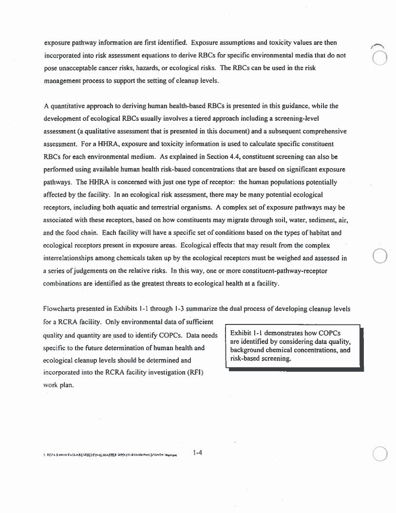
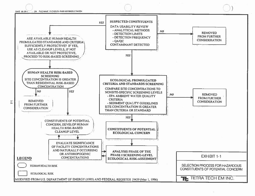
Flowcharts presented in Exhibits I-I through 1-3 summarize the dual process of developing cleanup levels

for a RCRA facility. Only environmental data of sufficient

______________________________________

quality and quantity are used to identi& COPCs. Data needs

specific to the future determination of human health and

ecological cleanup levels should be determined and

incorporated into the RCRA facility investigation (RH)

work plan.

0

Exhibit I - I demonstrates how COPCsare identified by considering data quality,background chemical concentrations, andrisk-based screening.

S REPARIIM’Iu\TASKrflVThE2’flNAL.4ASlR.WPDlI3I.RIwIIlflThIvII?9/9 S.mne 1-4

nDATE 08-26 UN FILE NME HCA25I-RIT6D7SEI.CTNDS4

ARE AVAILABLE HUMAN HEALTHPROMULGATED STANDARDS AND CRITERIA

SUFFICIENTLY PROTECTIVE? IF YES,USE AS CLEANUP LEVELS, IF NOTAVAILABLEORNOTPROTECTIVE, [

PROCEED TO RISK-BASED SCREEN1I%, /

hUMAN HEALTH RISK-BASEDSCREENING

SITE CONCENTRATION IS GREATERTHAN RESIDENTIAL RISK-BASED

-

CONCENTRATION

NO

REMOVEDFROM FURTHERCONSIDERATION

REMOVEDFROM FURTHER

CONSIDERATION

EXHIBIT 1-1

SELECTION PROCESS FOR HAZARDOUSCONSTITUENTS OF POTENTIAL CONCERN

0YES SUSPECTED CONSTITUENTS

DATA USABILITY REVIEW- ANALYTICAL METHODS- DETECTION LIMITS- DETECTION FREQUENCY-QA/QC

CONTAMINANT DETECTED

NO

YES

tr0 -

ECOLOGICAL PROMULGATEDCRITERIA AND STANDARDS SCREENING

COMPARE SITE CONCENTRATIONS TONONSITh-SPECIFIC SCREENING LEVELS

- EPA AMBIENT WATER QUALITYCRITERIA

- SEDIMENT QUALITY GUIDELINESSITE CONCENTRATION IS GREATERTHAN CRITERIA OR STANDARD

YES

REMOVEDFROM FURTHERCONSIDERATION

_______________-

- CONSTITUENTS OF POTENTIALCONCERN, DEVELOP HUMAN

HEALTH RISK-BASEDCLEANUP LEVEL

LEGEND

___

(Z) HUMAN HEALTH RISK

ECOLOGICAL RISK

YES 4,

t ‘fEVALUATE SIGNIFICANCE

OF FACILITY CONCENTRATIONSAND NATURALLY OCCURRING

OR ANTHROPOGENICCONCENTRATIONS

CONSTITUENTS OF POTENTIALECOLOGICAL CONCERN

4, -

ANALYSIS PHASE OF TIlEPHASE I SCREENING-LEVEL

ECOLOGICAL RISK-ASSESMENT

MODIFIED FROM U.S. DEPARTMENT OF ENERGY (1995) AND FEDERAL REGISTER 19439 (May I, 1996) TETRA TECH EM INC.

(

0

(THIS PAGE INTENTIONALLY LEFT BLANK)

S fPAJ I.IIrTASK.mEsErnNatR ThI3I.RHrnIInEnI2fl I7)I I 21am

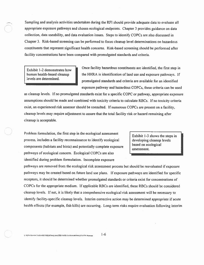
Sampling and analysis activities undertaken during the RFI should provide adequate data to evaluate all

appropriate exposure pathways and chosen ecological endpoints. Chapter 3 provides guidance on data

collection, data useability, and data evaluation issues. Steps to identit5’ COPCs are also discussed in

Chapter 3. Risk-based screening can be performed to focus cleanup level determinations on hazardous

constituents that represent significant health concerns. Risk-based screening should be performed after

facility’ concentrations have been compared with promulgated standards and criteria.

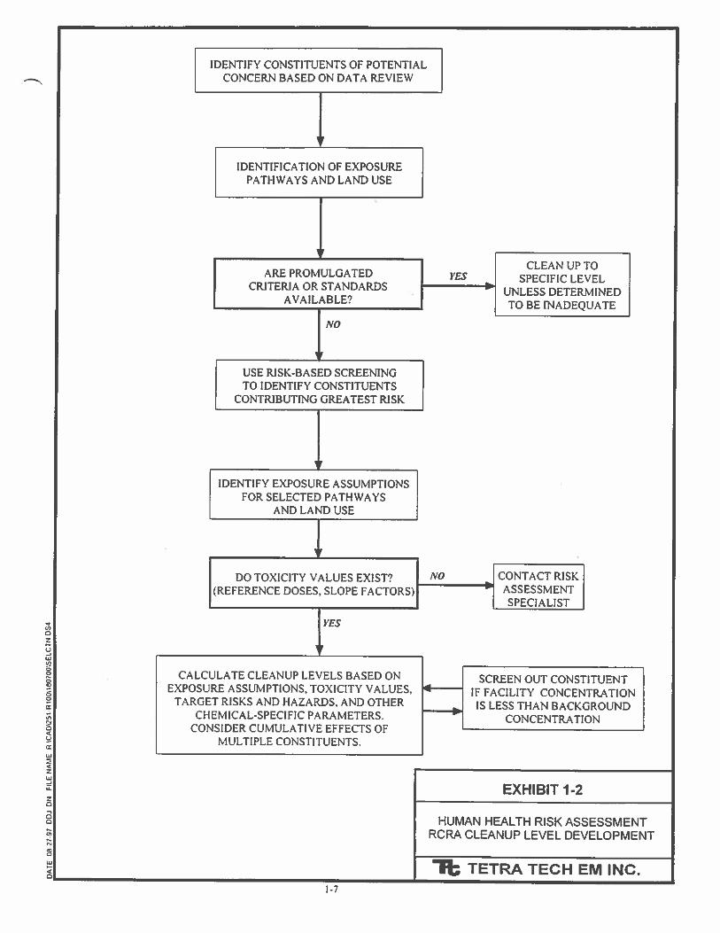
Once facility hazardous constituents are identified, the first step inExhibit 1-2 demonstrates howhuman health-based cleanup the HFWA is identification of land use and exposure pathways. Iflevels are determined. . .promulgated standards and criteria are available for an identified

exposure pathway and hazardous COPCs, these criteria can be used

as cleanup levels. If no promulgated standards exist for a specific COPC or pathway, appropriate exposure

assumptions should be made and combined with toxicity criteria to calculate RBCs. If no toxicity criteria

exist, an experienced risk assessor should be consulted. If numerous COPCs are present on a facility,

cleanup levels may require adjustment to assure that the total facility risk or hazard remaining after

cleanup is acceptable.

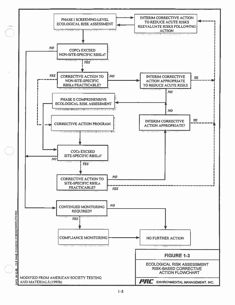
Problem formulation, the first step in the ecological assessmentExhibit 1-3 shows the steps in

process, includes a facility reconnaissance to identi& ecological developing cleanup levelsbased on ecologicalcomponents (habitats and biota) and potentially complete exposureassessment.

pathways of ecological concern. Ecological COPCs are also

____________________________

identified during problem formulation. Incomplete exposure

pathways are removed from the ecological risk assessment process but should be reevaluated if exposure

pathways may be created based on future land use plans. If exposure pathways are identified for specific

receptors, it should be determined whether promulgated standards or criteria exist for concentrations of

COPCs for the appropriate medium. If applicable RBCs are identified, these RECs should be considered

cleanup levels. If not, it is likely that a comprehensive ecological risk assessment will be necessary to

identify facility-specific cleanup levels. Interim corrective action may be determined appropriate if acute

health effects (for example, fish kills) are occurring. Long-term risks require evaluation following interim

S REPAR I I.TASKwREW5E3WJNAjIMASThR WPO\II.RICWIINII7ISI2fl I,’J7I Tha..Isn —

0

(THIS PAGE INTENTIONALLY LEFT BLANK)

S REPA R Ic.IIFtASKRESE1NALlAmR WPD’I5IjII.IIW7IMSI3rnlI I 31hm 0

r IDENTIFY CONSTITUENTS OF POTENTIALCONCERN BASED ON DATA REVIEW

IDENTIFICATION OF EXPOSUREPATH WAYS AND LAND USE

ARE PROMULGATEDCRITERIA OR STANDARDS

AVAILABLE?

NO

USE RISK-BASED SCREENINGTO IDENTIFY CONSTITUENTS

CONTRIBUTING GREATEST RISK

YESI,

CLEAN UP TOSPECIFIC LEVEL

UNLESS DETERMINEDTO BE INADEQUATE

______________1_____________

CALCULATE CLEANUP LEVELS BASED ONEXPOSURE ASSUMPTIONS, TOXICITY VALUES,

TARGET RISKS AND HAZARDS, AND OTHERCHEMICAL-SPECIFIC PARAMETERS.

CONSIDER CUMULATIVE EFFECTS OFMULTIPLE CONSTITUENTS.

TATRISKASSESSMENTSPECIALIST

EXHIBIT 1-2

HUMAN HEALTH RISK ASSESSMENTRCRA CLEANUP LEVEL DEVELOPMENT

IDENTIFY EXPOSURE ASSUMPTIONSFOR SELECTED PATH WAYS

L AND LAND USE

DO TOXICITY VALUES EXIST?(REFERENCE DOSES, SLOPE FACTORS)

YESU,CzULA]

00

C

00

C4U

-J-CCz

zC

CC

0

c,4

0

4n

SCREEN OUT CONSTITUENTIF FACILITY CONCENTRATION

IS LESS THAN BACKGROUND I

CONCENTRATION

R TETRA TECH EM INC.I-?

N

U

a

(THIS PAGE INTENTIONALLY LEFT BLANK)/

S REPARIIII TASKrnnSlSrl’nNALMASItR WPThLI.RINIIIO7(flhZflIfl7fiI 211.n1U -

ECOLOGICALRISKASSESSMEWr 4 REEVALUATEPJSKSFOLLOwING]ACTION

COPCs EXCEEDNON-SITE-SPECIFIC RBSLs?

YES CORRECTIVE ACTION TO JNO INTERIM CORRECTIVE jwj•- NON-SITE-SPECIFIC AON APPROPRIATE

RBSLs PRACTICABLE? TO REDUCE ACUTE RISKS

______________________________

No

PHASE II COMPREHENSIVEECOLOGICAL RISK ASSESSMENT

NO

INTERIM CORRECTIVE

CORRECTIVE

ACTION PROGRAM ACTION APPROPRIATE?

-•

COCs EXCEEDSITE-SPECIFIC RBSLs?

NO______________________

+CORRECTIVE ACTION TO

No

SITE-SPECIFIC RBSLsPRACTICABLE?

— CONTINUED MONITORING NO

REQUIRED?

YES

IANcEMONITo——— NO FURTHER ACTION

FIGURE 13

ECOLOGICAL RISK ASSESSMENTRISK-BASED CORRECTIVE

ACTION FLOWCHARTMODIFIED FROM AMERICAN SOCIETY TESTINGAND MATERIALS (1995b) pile ENVIRONMENTAL MANAGEMENT, INC.

1-8

0

(THIS PAGE INTENTIONALLY LEFT BLANK)

S npAI:MIIs\TAsKrnmE3NAL.AmR ?VI3I.RIm,I7INM1flIfl,,II 2 U

action; the focus of this guidance document is on long-term, chronic risks. Once all the necessary data are

collected and evaluated, cleanup levels can be determined.

13 RISK CHARACTERIZATION PRTh1CWLES

Data collected at a facility will typically be evaluated to determine whether corrective action is necessary

and appropriate. Where risks are deemed to be significant enough to trigger remediation, cleanup levels

must be determined. Risk characterization principles, which are summarized below, are an important part

of the risk assessment process including the determination and communication of corrective action

decisions.

Risk characterization is an important and requisite section of every risk assessment. Although the

principles of risk characterization should be evident throughout, a separate section must summarize risk

characterization. Risk characterization integrates information from the preceding components of the risk

assessment (primarily exposure and toxicity assessment components) and synthesizes information in a

manner that is complete, informative, and useful for risk managers, stakeholders, and the public. To

support quantitative and qualitative estimates of risk, it is critical to provide information to explain and

justify assumptions, methodologies used, and conclusions drawn. Risk characterizations should state and

explain why any potential COPCs or exposure pathways were eliminated from the risk assessment at any

time during the process. Risk characterizations should also discuss relative confidence in the

methodologies used, the potential impact of alternative choices, and the limitations of the analysis.

Particularly critical to complete risk characterization is a clear and complete discussion of the uncertainties

and variabilities associated with each of the components of the risk assessment. Uncertainty can be

defined as a qualitative or quantitative lack of precise knowledge about the truth. Uncertainty is typically

reducible through further measurement or study. Variability refers to the heterogeneity in a population

and is usually not reducible through further measurement or study. Uncertainty discussions help to

identify where additional information could contribute significantly to reducing uncertainties in risk

assessment and aid decision-makers in deciding whether reduced uncertainty would add value to the

overall objectives of the project. Sections 4.8 and 5.1.5 of this document identify specific risk assessment

uncertainty issues for human and ecological receptors, respectively.

S REPARI•ItTASKtRE9SE2WTNALM4STER WPTh)IRitNIflO7(ThI2flIN’N Ililnac —

In a 1995 memorandum and associated policy statement concerning the EPA Risk Characterization

Program (EPA 1995a and Attachment A), EPA Administrator Carol Browner stated that all risk

assessments and in particular, risk characterizations, must embrace the following fundamental values:

Transparency in decision making processClarity in communicationConsistency between EPA programsReasonableness of assumptions and policies

“Transparency” refers to the decision-making process; risks must be characterized fully and openiy. Risk

characterizations should disclose the scientific analyses, uncertainties, and assumptions (both science- and

policy-based) that underlie all decisions. “Clarity” refers to communication; the risk assessment process

should help the public better understand the relative significance of environmental risks. It is important to

note that risk characterization is a key component of risk communication, an interactive process involving

exchange of information and expert opinion among individuals, groups, and institutions. “Consistency”

and “reasonableness” refer to the core assumptions and scientific policies that are part of the risk

assessment process. Consistency among EPA risk assessments is an important goal of EPA’s risk

characterization policy. For example, CERCLA risk assessment guidance is considered appropriate for the

RCRA program, particularly because more detailed CERCLA guidance is often available. For RCRA

corrective actions and Superfund remedial actions, the actual environmental results achieved through

cleanup are expected to be environmentally equivalent. Further information on how the RCRA and

CERCLA programs overlap is documented in the EPA Region 10 (1994a) RCRA/CERCL4 Interface

Interim Final Guidance, which is included as Attachment B.

It is important that risk characterizations, like risk assessments themselves, be separate from risk

management decisions; scientific information should be selected, evaluated, and presented without

considering issues such as cost, feasibility, or how the scientific analysis might influence regulatory or

facility-specific decisions. In addition, the risk assessment process does not include decisions on the

public acceptability of risk levels, the value of reducing uncertainty by conducting further studies, and the

appropriate procedures for reducing facility-specific risks. The risk assessment process should delineate

both current and future risks because the time variable can impact site risks (for example, future risks may

S WPO;I1I.RI(,IR,)7,St2n inv, lRamsn 1— 10

be greater than current risks because of remedial activities and/or potential land usage at the site). Current

or future site risks for decision making should be selected during the risk management proceedings rather

than the risk characterization. The EPA (I 997g) Rules of Thumb for Superfluid Remedy Selection

identifies principles that should be consulted for risk assessments and risk management decisions. These

principles can be applied to RCRA corrective action programs.

S 1hmnc —

ST

AT

EP

RO

GR

AM

S

CHAPTER 2

STATE PROGRAMS

U.S. Environmental Protection Agency (EPA) may grant states the authority to administer Resource

Conservation and Recovery Act (RCRA) corrective action as part of their authorized RCRA permit

programs. States may promulgate their own regulations. For authorized programs, these regulations must

be at least as stringent as federal regulations, and EPA retains corrective action authority through statutory

enforcement orders in all states regardless of authorization status.

Facilities in states without authorized RCRA permit program regulations must comply with federal

regulations; however, according to the Federal Register 19457 (May 1, 1996), EPA recognizes that many

states have developed independent Superfund-like authorities and cleanup programs. Consequently, when

developing cleanup levels for a facility, the project manager should consider other promulgated state

standards or criteria, including those regarding land use classifications that may influence cleanup level

selection. Whether the corrective action is state-lead or EPA-lead, cleanup levels typically should be at

least as stringent as state standards or criteria to avoid the need for the state to revisit the corrective

measure taken at a facility. The burden is on the facility to ensure that both state and federal requirements

are met. Unlike the Comprehensive Environmental Response, Compensation, and Liability Act of 1980

(CERCLA), RCRA statutory language does not include requirements to follow state standards as

applicable or relevant and appropriate requirements. RCRA only requires that cleanups are “protective.”

The following sections summarize the authorization status of each Region 10 state RCRA program. Only

Washington State has specific regulations for an authorized RCRA corrective action program; however,

other non-RCRA state cleanup programs are also identified, and the state agency and phone number are

provided for obtaining further information. More specific information on state programs is included where

appropriate under the human health risk assessment (HHRA) and ecological risk assessment procedure

sections of this guidance. For example, state-promulgated human health standards and criteria are

described in more detail under Section 4.3, Identification of Promulgated Standards and Criteria.

S REPARIrnHSTASKWRflV1SE2W1NALQ.IASThR WPO\L5I.RI”11107’WMZflIPI7P) 3bm’sac —

2.1 ALASKA DEPARTMENT OF ENVIRONMENTAL CONSERVATION

The Alaska Department of Environmental Conservation (ADEC) has not applied for authorization to

manage any of the RCRA programs in lieu of EPA. ADEC is currently preparing cleanup standard

regulations for contaminated sites and associated guidance documents on HHRA, petroleum risk

evaluation methodology, and background calculation methodology. These cleanup regulations were

proposed for public comment on December 18, 1996. Current and proposed regulations are available for

download (http://www.state.ak.us/dec/dec-cal.htm#Regulation). The Contaminated Sites Remediation

Program may be contacted for further information at (907) 465-5390.

2.2 IDAHO DIVISION OF ENVIRONMENTAL QUALITY

The Idaho Division of Environmental Quality (IDEQ) is authorized to operate a RCRA hazardous waste

program; however, the state only has the authority to compel corrective action at RCRA facilities with

RCRA permits. Idaho has not promulgated specific rules for setting cleanup levels at RCRA facilities and

has followed EPA guidance. Idaho statutory language (Section 39-4404 of Idaho Code. Hazardous Waste

Management Act of 1983) prohibits IDEQ from promulgating rules more stringent than existing EPA

RCRA regulations. The IDEQ can be contacted at (208) 373-0502.

2.3 OREGON DEPARTMENT OF ENVIRONMENTAL QUALITY

The Oregon Department of Environmental Quality (ODEQ) is authorized to operate a RCRA hazardous

waste program, including the corrective action program. According to its corrective action authorization

application, ODEQ intends to rely on EPA risk assessment guidance documents and toxicological

databases to determine the appropriate cleanup levels for a given facility. Oregon has not promulgated

specific rules for setting cleanup levels at RCRA facilities. Facilities may calculate site-specific cleanup

levels that must be approved in advance by ODEQ.

In 1995, Oregon amended its statutory authority for environmental cleanup rules (Oregon Revised

Statutes 465.315 and 465.325), requiring that new rules be adopted for conducting risk assessments and

defining hot spots. The rules, adopted on January 10, 1997, establish protocols for HHRA and ecological

risk assessment that include deterministic and probabilistic methods. The rules apply to facilities subject

7S RLPA c.I,TAsKnRrv1sE2’nwALMA51rR WPDI SIR IIR)ixIpcmIWInpI 1NmLx — —

to the state’s Superfund-like program. These rules are not currently a part of the state-authorized RCRA

program. ODEQ’s Waste Management and Cleanup Division can be contacted at (503) 229-5913 or on

the Internet at http://www.deq.state.or.usf for further information on the state’s RCRA program.

2.4 WASHINGTON DEPARTMENT OF ECOLOGY

The Washington Department of Ecology (Ecology) is authorized to operate a RCRA hazardous waste

program, including the corrective action program. Washington’s Model Toxics Control Act (MTCA)

Cleanup Regulation, amended in January 1996 under Chapter 173-340 of the Washington Administrative

Code, establishes methods for calculating cleanup levels. Under the alternative authorities initiative of

Ecology’s corrective action authorization application, Ecology was authorized for a RCRA corrective

action program that allows for the option of incorporating a MTCA order into RCRA permits to fulfill the

RCRA Section 3004(u) and (v) requirements that all RCRA permits must include corrective action permit

conditions. As previously noted, however, EPA retains corrective action authority through statutory

enforcement orders regardless of Ecology’s authorization status. In February 1996, Ecology published a

MTCA Cleanup Levels and Risk Calculations (CL4RC II) Update reference document (Ecology 1996).

The MTCA cleanup regulation is described further in Chapter 4. Ecology has a comprehensive Internet

site where dozens of guidances and regulations are available for download, including those pertinent to the

Toxics Cleanup Program (http://www.wa.gov/ecology/tcp/cleanup.htm I). The Toxics Cleanup Program

can also be contacted toll-free at (800) 826-7716.

The Guidance for Clean Closure ofDangerous Waste Facilities (Ecology 1994) provides closure guidance

for interim and final status treatment, storage, and disposal facilities. The document provides direction for

demonstrating compliance with the clean closure performance standards and recommends the use of

MTCA residential cleanup standards.

S lIlm\Sae —

DA

TA

CO

LL

EC

TIO

N

CHAPTER 3

DATA COLLECTION TO CHARACTERIZE FACRITY AND DETERMINE HAZARDOUS

CONSTITUENTS OF POTENTIAL CONCERN

Site-specific data of sufficient quality must be collected to determine facility conditions and the extent of any

necessary cleanup. Guidance and reference documents that describe data collection and data review

methods are summarized in the following subsections. Many of the EPA documents cited are available on

the EPA Region 10 web site (http://www.epa.gov/rl Oearthloffice/oealrl Oqahome.htm). Two primary

issues are addressed in Chapter 3. The first issue is identifying what data must be collected to characterize a

facility. This issue can be addressed by following the data quality objectives (DQO) process defined by U.S.

Environmental Protection Agency (EPA). Section 3.1 summarizes the DQO process. The second issue is

identifying how the samples should be collected and analyzed to assure that the data meet useability

requirements. Issues that should be considered to address data useabitity are described in Section 3.2.

Following data generation, a data quality assessment is completed to assure that DQOs have been met.

Following this assessment, the data are then used to identify constituents of potential concern (COPC). The

data quality assessment and COPC identification steps are described in Sections 3.3 and 3.4, respectively.

Existing facility data that have been or can be validated should be considered during the DQO process as

well as used in COPC identification, risk assessment, and compliance determinations.

The DQO process must also be applied to determine whether compliance with cleanup goals has been

achieved following remediation. Determining compliance with cleanup goals is described in Chapter 7 of

this guidance.

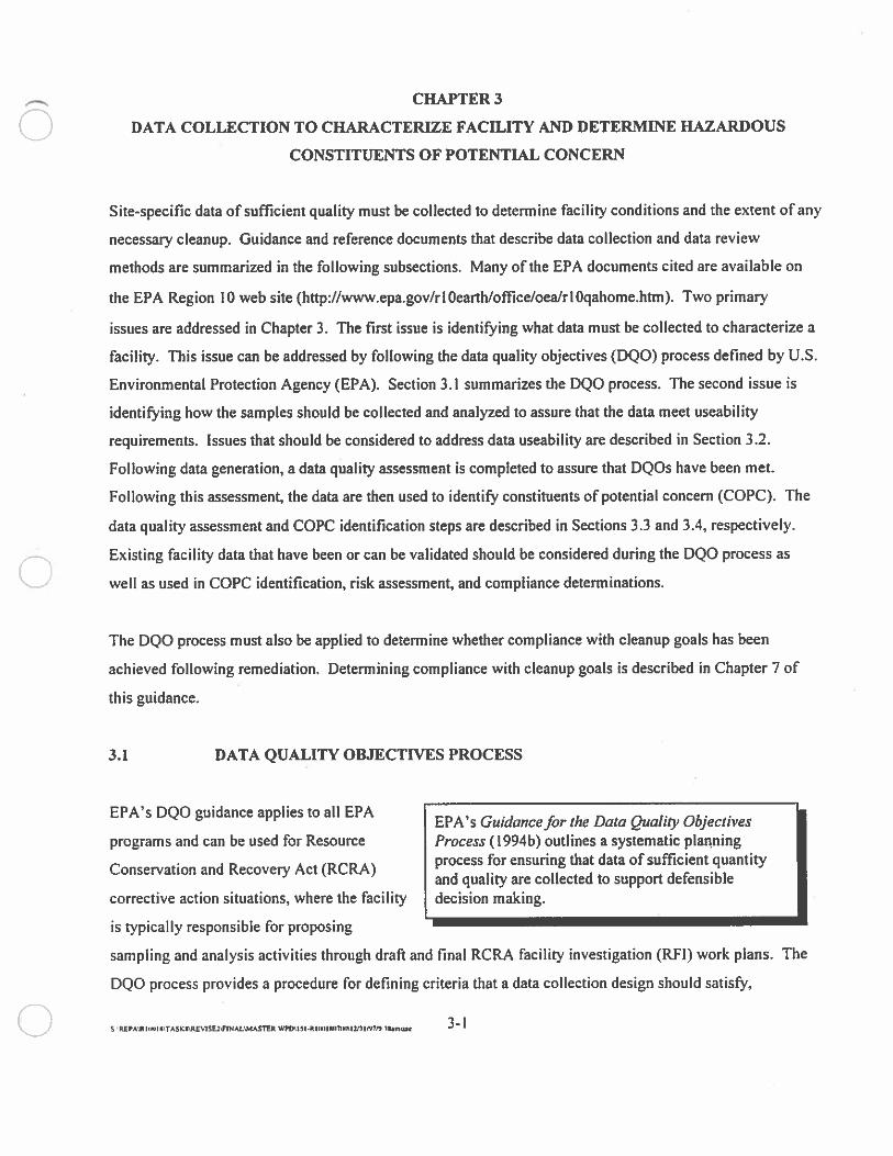
3.1 DATA QUALITY OBJECTIVES PROCESS

EPA’s DQO guidance applies to all EPA .

EPA’s Guidance for the Data Quality Objectivesprograms and can be used for Resource Process (1994b) outlines a systematic planning

process for ensuring that data of sufficient quantityConservation and Recovery Act (RCRA)

and quality are collected to support defensiblecorrective action situations, where the facility decision making.

is typically responsible for proposing

sampling and analysis activities through draft and final RCRA facility investigation (RFI) work plans. The

DQO process provides a procedure for defining criteria that a data collection design should satisfy,

S REPA jItwms.sRIvIsunNaNAsmR WPDHl.RIwIImI7tflL2fl fm’, lSam’sae —

including when, where, and how many samples to collect. The DQO guidance recommends the use of

statistical methods for identifying tolerable levels of decision errors (that is, type I and type 2 errors) and

the number of samples required to meet these decision error levels. DQOs are defined during the first six

steps of the process. The data collection design is thendeveloped in a seventh step, based on the DQOs.

All of the DQO steps should be specified in work plans submitted to the agency when sampling and

analyses are being proposed.

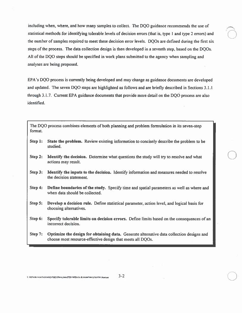
EPA’s DQO process is currently being developed and may change as guidance documents are developed

and updated. The seven DQO steps are highlighted as follows and are briefly described in Sections 3.1.1

through 3.1.7. Current EPA guidance documents that provide more detail on the DQO process are also

identified.

The DQO process combines elements of both planning and problem formulation in its seven-stepformat.

Step 1: State the problem. Review existing information to concisely describe the problem to bestudied.

Step 2: Identify the decision. Determine what questions the study will try to resolve and whatactions may result.

Step 3: Identify the inputs to the decision. Identify information and measures needed to resolvethe decision statement.

Step 4: Define boundaries of the study. Specify time and spatial parameters as well as where andwhen data should be collected.

Step 5: Develop a decision rule. Define statistical parameter, action level, and logical basis forchoosing alternatives.

Step 6: Specify tolerable limits on decision errors. Define limits based on the consequences of anincorrect decision.

Step 7: Optimize the design for obtaining data. Generate alternative data collection designs andchoose most resource-effective design that meets all DQOs.

c REPAR IIILU;TASK nSnENlAmR 3—2 - Q

3.1.1 Step 1: State the Problem

Step I requires that the problem be defined. This step will include summarizing existing facility

information, such as historical waste management activities and environmental data (including but not

limited to information in the RCRA facility assessment). In the ElI stage, the problem is typically

determining what additional data are required to characterize the type and concentration of hazardous

constituents associated with releases from solid waste management units (SWMU). The problem should

be defined as concisely as possible, focusing on such issues as the media of concern1 land use, location of

human and ecological receptors, and magnitude of contamination. A more specific problem may be what

data are needed to determine whether hazardous constituents are present at concentrations greater than

either preliminary background or risk-based screening concentrations.

A conceptual site model (CSM) is a useful tool for defining facility conditions and the types of data

collection that may be required. EPA Superfiind Guidance for Conducting Remedial Investigations and

Feasibility Studies Under CERCLA, Interim Final (EPA 1988) provides information on how a CSM can be

developed. As stated in that document, the CSM should include known and suspected sources of

contamination, types of constituents and affected media, known and potential routes of migration, and

known or potential human and environmental receptors. The American Society for Testing and Materials

(ASTM) Standard Guide for Developing Conceptual Site Models for Contaminated Sites also provides

guidance for developing a CSM (ASTM I995a). The CSM can be used to help identi6’ locations where

sampling is necessary. The CSM can also be used to identify the types of exposures that may result from

facility contamination and the cleanup levels required to address these potential exposures. Human health

and ecological exposure issues are further discussed in Chapters 4 and 5 of this cleanup level guidance.

3.1.2 Step 2: Identify the Decision

Step 2 requires that the principle study question be identified and a decision statement defined to link the

study question to possible alternative actions. The principle study question is defined by reviewing the

Step I problem. In the RFI, the study question is likely to be “are hazardous constituents present on a

SWMU at concentrations that exceed screening or preliminary background levels?” or a similar issue.

Possible alternative actions that may be taken are then identified, including the alternative that “no action”

is required. For example, theaction related to the principle study question may be “remediation is

S REPAR WPDU$I-R ICIIAfllMV1lAflfl lSim\sac —

required if the screening level is exceeded” or alternatively, “no remediation is required if the screening

level is not exceeded.” These alternative actions form the basis for defining decision performance criteria )in Step 6.

3.1.3 Step 3: Identify the Inputs to the Decision

In Step 3, the types of data or information that will be required to resolve the Step 2 decision statements

are identified. This includes determining whether environmental measurements are required and further

defining the types of measurement data. The sources of this information should be identified (for

example, historical data or new data collection). For the RFI, constituent concentration levels in the media

of concern will likely be required (for example, the average concentration of a constituent in soil). Other

measurements such as soil and hydrogeological parameters may also be required to support site

characterization through fate and transport information.

The basis for setting screening levels should also be defined in this step. Screening levels may be based on

existing standards and criteria (for example, groundwater maximum contaminant levels), risk-based

concentrations (RBC) (for example, soil RBCs based on residential land use), or preliminary site-specific

background data (for example, background metals data).

3.1.4 Step 4: Define Boundaries of the Study

Step 4 requires that the spatial and temporal boundaries of the problem be defined. Spatial boundaries

define the physical area to be studied and locations to collect samples. According to the Geosratistical

Sampling and Evaluaripn Guidance for Soils and Solid Media published by EPA in 1996, temporal

boundaries determine the time frame that the study data will represent and when samples should be

collected (EPA !996a).

The main purpose of this step is to identify, to the extent possible, a well defined data population that can

be statistically evaluated. In an RFI, sampling should be conducted to characterize the nature and extent of

contamination in areas where releases are suspected to have occurred. These study areas should focus on

waste management activities to define areas with similar contamination (for example, the concentration of

S REPAR WPThII.R(NIMfl7’EflI2BIMt 3hmn. —

a consti Went released from a single SWMU). In practice, areas of homogenous contamination may not be

present or readily identifiable. The EPA Soil Screening Guidance: User c Guide (1 996b) recommends

defining study areas by stratiing the site into known, suspected, and unlikely contaminated areas. The

study area can also be defined as an area where contamination may be present as a hot spot, and a

sampling program could provide acceptable probability that hot spots ofa specific size will be detected.

In addition to segregation by waste management activities, study boundaries may be defined by the type of

exposure that could occur. For example, if a large area of contaminated soil may be subdivided for future

residential development, it may be necessary to subdivide the SWMU into smaller “residential size”

exposure areas for data collection. Constituent releases that leave the SWMU area may enlarge the

boundary of the study area (for example, a groundwater contaminant plume). In this situation, monitoring

wells located along a plume’s center line may define the study boundaries. The average groundwater

concentration over a minimum of four calendar quarters of groundwater monitoring may define the

temporal boundaries of the study (EPA 1993a).

Chapter 3 of Methodsfor Evaluating the Attainment of Cleanup Standards, Volume I: Soils and Solid

Media (EPA 1989b) provides further information on the identification of discrete study areas to determine

cleanup decisions for soil. Section 2.3 of EPA’s Soil Screening Guidance: Users Guide (I 996b) also

provides guidance on identif’ing surface and subsurface soil study areas. EPA’s Supplemental Guidance

to RAGS: Estimating Riskfrom Groundwater Contamination (1993a) discusses approaches for delineating

groundwater exposure areas for Superfund risk assessments. Once study areas are defined, the areas will

be sampled to determine whether the constituent’s concentration exceeds a screening level or whether hot

spots are present.

3.1.5 StepS: Develop a Decision Rule

Step 5 requires that a decision rule be developed to define the conditions that would necessitate the choice

of an alternative action. The decision rule is formed from elements defined during previous DQO tasks.

including (I) the parameters of interest defined in Step 3, such as the avenge concentration of a

constituent in soil; (2) the screening levels defined in Step 3, such as the soil RBC; (3) the study boundary

defined in Step 4, such as soil located in a SWMU spill area; and (4) the principle study question and

alternative actions defined in Step 2. The decision rule is an “if. . . then” statement that incorporates the

S REPAR Ic,IIST45K,RESESINALMASThR WPThI5 I .R I IIRI7IXRIV1I/9I Ibmlsac —

previous information. For example, if the parameter of interest (average concentration of constituent

released to soil) within the study area (the SWMU spill area) is greater than the screening level (the soil

RBC), then alternative action A should be taken (for example, remove contaminated soil); otherwise,

alternative action B should be taken (for example, leave soil in place).

Step 3 requires that a general basis for defining facility conditions and screening criteria be defined. For

example, the facility parameter of interest may be the constituent concentration at a SWMU, while the

screening criteria may be a promulgated standard, a RBC, or a preliminary background level. In Step 5,

the facility parameter and screening criteria must be specifically defined and incorporated into the decision

rule. In the previous example, the average soil concentration of the constituent in a SWMU area is defined

as the specific facility parameter, while the screening criteria is defined as a specific soil RBC (for

example, residential land use RBC based on soil contact).

When determining the presence of hot spots, the decision rule must incorporate the size (radius) of the

potential hot spot that may exist in the study area and the distance between sampling locations within the

study area sampling grid.

More than one constituent may be present at a SWMU. For the purpose of SWMU characterization, the

constituent that will require the most significant data collection to determine whether a release has

occurred above screening levels should be identified and used in the decision rule. This constituent

typically will exhibit the highest variability in concentration or will be detected in a concentration closest

to the screening level.

3.1.6 Step 6: Specify Tolerable Limits on Decision Errors

Step 6 requires that the decisions maker’s tolerable limits on decision errors be specified. The true value

of the population parameter being measured (for example, the average constituent concentration) can

never be exactly defined based on sampling design and measurement design errors. An error may be made

during Step 5 since the decision is based on measurement data. A decision error occurs when the data

mislead the decision maker into concluding that the parameter of interest is on one side of a screening

level (for example, greater than the screening level) when it is actually on the other side (that is, less than

S REPA R IEMIW TASKRmEV1SE2PINAL’MASItR WPDSI5 II’17fl Jhm\n. —

the screening level). The possibility of decision errors can never be totally eliminated, but it can be

controlled. For example, a large number of samples may be collected to control sampling design errors.

Chapter 6 of Guidancefor the Data Quality Objectives Process (EPA 1994b) explains how the probability’

of decisions errors can be controlled by adopting a scientific approach that incorporates hypothesis testing.

The method includes (I) defining the two types of decision errors (that is, false positive [a] and false

negative [] decision errors), (2) evaluating the consequence of each error, (3) identifying the error with

more severe consequences near the cleanup level, (4) defining a null hypothesis that is equal to the true

state of nature that exists when the more severe decision error occurs, (5) estimating the range of

parameter values near the cleanup level where the consequences of decision errors are relatively minor

(defined as the grey area), and (6) assigning probability values to points above and below the grey area

that reflect the decision maker’s tolerable limits for making an incorrect decision.

For example, the decision maker may want to know whether a hazardous constituent is present in a

SWMU at an average concentration that exceeds a screening level. The decision maker may view the

consequence of deciding that the average concentration is less than the screening level when it is actually

greater than the screening level as the more severe decision error. The null hypothesis would then be that

the average concentration exceeds the screening level (enough data must now be collected to reject the null

hypothesis if it is false). A conclusion that the concentration is less than the screening level when it is

actually greater would be a false positive error, while a conclusion that the concentration is greater than

the screening level when it is actually less would be a false negative error. The decision maker then

establishes a grey area near the action level. The boundaries of the grey area are the action level and the

point below the action level where the consequences of a false negative error begin to become significant.

The actual grey area interval is the concentration range near the action level where the decision maker

determines it is not necessary or feasible to control the probability ofa false negative error (for example,

because the consequences of this error are minor, or because the costs of collecting enough samples are

prohibitively high). The decision maker then sets allowable decision error probabilities at points above

(false positive errors) and below (false negative errors) the screening level, starting at the boundaries of

the grey area where the consequences of errors are minor and/or expensive to control. The “tolerable

limits” are the intervals of concentration above or below the grey area where allowable decision errors are

set. Generally, the wider the interval, the lesser the decision error probability that will be accepted.

S REPA Ic’prnTASIS’REV1SE1flNAL’MASThR WpDII-RInhILflflI3nIrnn bmsae —

A similar DQO evaluation is performed when determining compliance with a cleanup level (see

Chapter 7). Detailed examples of DQO evaluations have been developed by EPA (Guidancefor the Data

Quality Objectives Process [I 994b], and Data Quality Objectives Decision Error Feasibility Trials

(DQO/DEFT) Users Guide [1994c]) and are included in Attachment C.

3.1.7 Step 7: Optimize the Design for Obtaining Data

As stated in the Guidancefor the Data Quality Objectives Process (EPA I 994b), DQOs are qualitative and

quantitative statements derived from the outputs of Steps I through 6 that help to accomplish the following

tasks:

• Clarify study objectives

• Define appropriate type of data to collect

• Determine conditions from which to collect the data

• Specify tolerable limits on decision errors to be used as the basis for establishing thequality and quantity of data needed to support the decision

0Step 7 includes identifying a resource-effective data collection (sampling) strategy for generating data that

are expected to satisfy the DQOs. The sampling strategy typically will focus on the sampling design, the

sample size, and the analytical methods required to meet the DQOs. A primary requirement of Step 7 will

be to define a statistical method for testing the Step 6 hypothesis and a sample size formula that

corresponds to the statistical method and the sample design. EPA has published several guidance

documents on the selection of appropriate statistical models for determining sample sizes and sample

designs. These documents are listed in the Chapter 7 discussion of compliance with cleanup levels.

Similar statistical models can be used in both site characterization and compliance determinations.

It is preferable to selected analytical methods that can be used to detect constituents at reasonable

concentrations well below the screening levels, to reduce the potential for false negatives, and to increase

confidence in the quantification of positive hits. A cost function that relates the number of samples to total

cost may also be defined. The cost function may be used to support the proposal of a cost-effective

S RLPAR I(”IM;TASKREV1SE3FINAL.IA5ThR WPO\I3I I,sni,wsiznimrn 3Sa,.iac —

sampling strategy that meets the DQOs. Generally, the lower the probability ofan error that the decision

maker is willing to accept, the greater the sampling effort and costs required to meet the DQOs.

The output of Step? will be a sampling strategy that defines sampling design, sample numbers, and

analytical methods. Section 3.2 further describes methods that should be followed to assure that the

sample data collected are of acceptable quality.

3.2 DATA USEABRITY

Sampling and analysis activities should provide adequate data to evaluate all appropriate exposure

pathways and chosen ecological endpoints. The sampling plan should be designed with all data uses

(human health, ecological, and others uses) in mind, including attainment of cleanup levels. Hence,

human health and ecological risk assessors and others must be involved in the designing of sampling

plans. These plans should ensure that the issues in the data useability work sheet (Attachment D) can be

adequately responded to after data have been collected.

The Final Guidance for Data Useability in Risk Assessment Part A The Final Guidancefor Data

(EPA I 992b) provides risk assessors and remedial project UseabilitY in Risk Assessment(Part A) (EPA l992b)

managers with nationally consistent procedures to plan and assess discusses the six datauseability criteria involved in

sampling and analysis of useable environmental data. planning an initial siteChapters 4 and 5 of EPA’s Risk Assessment Guidance for stigationi or an

investigation to determineSuperfund, Volume 1, Human Health Evaluation Manual (Part A) compliance with cleanup

levels: data sources,(EPA 1989c) discuss data collection and data evaluation, documentation, analyticalrespectively, methods and quantitation

limits, data quality indicators(DQI), data review, andreports to risk assessors.3.2.1 Data Sources

The data sources selected (for example, field screening, field analytical, fixed analytical) depend on the

type of data required and their intended use. The data sources must be comparable if data are combined

for quantitative use. For example, field screening and fixed laboratory data should not be combined for a

quantitative analysis. These separate data sources can, however, be used to complement one another.

Field screening data may be.used to delineate soil contamination, while fixed laboratory data would be

REP API EI I TASKX .REVISE2TSNAL\XIASThR wru’I 51 -R lIP’ RAflIXP I L’1 IfS/I SRm’sae —

used to quanti the contamination. If field analytical screening results are going to be used quantitatively,

it must be demonstrated that they are of sufficient quality to meet DQOs.

3.2.2 Documentation

Sample collection and analysis procedures must be fully and accurately documented to substantiate the

reliability of the dataderived from its analysis. The major types of documentation are quality assurance

project plans (QAPP), quality management plans (QMP), standard operating procedures, field and

analytical records, and chain-of custody records.

In addition, data quality indicators (DQI) (see Section 3.2.4) for assessing results against stated

performance objectives should be documented in the QAPP.

EPA policy requires that all environmental data used in decision making be supported by an approved

QAPP. A QAPP is required for each specific project or continuing operation. The QAPP documents how

quality assurance (QA) and quality control (QC) are applied to an environmental data operation to assure

that the results obtained are of the type and quality needed for a specific decision or use. QA is an

integrated system of management activities involving planning, implementation, assessment, reporting,

and quality improvement to ensure that a process, item, or service is of the type and quality needed and

expected. QC is the overall system of technical activities that measures the attributes and performance of

a process, item, or service against defined standards to veri& that they meet the stated requirements.

Current EPA requirements for QAPPs are presented in the Interim Guidelines and Specfficationsfor

Preparing Quality Assurance Project Plans (EPA 1980). Current EPA requirements for QMPs are

presented in the Guidelines and Spec4fications for Preparing Quality Assurance Program Plans

(EPA 1979). EPA is updating the QA/QC requirements. The updated document, EPA Requirements for

Quality Assurance Project Plans for Environmental Data Operations, is currently in the draft interim final

stage (EPA 1 994d). A draft interim final version of EPA Guidance on Quality Assurance Project Plans

(QA/G-5) is also available, as is the draft updated document, EPA Requirements for Quality Management

Plans (EPA 1994e) which will replace the quality assurance program plan guidelines. EPA Region 10’s

quality assurance office has indicated that use of the draft documents is preferable to the use of older

S RP\R Slm\ne —

documents, but ultimately that is the decision of the RCRA project manager. The EPA Region 10 web site

contains news about the finalization of the draft documents (hup://www.epa.gov/rloearth/office/oeal

rloqahome.htm). In addition, Federal Register 19445 (May 1, 1996) cites QualityAssurance Project

Plans for RCRA Ground-Water Monitoring and Corrective Action Activities (EPA I 993b) guidance for

information on incorporating DQOs in the decision-making process at RCRA facilities.

The Interim Guidelines and Specificationsfor Preparing Quality Assurance Project Plans (EPA 1980)

describe 16 elements that must be considered for inclusion in all QAPPs, recommend the format to be

followed, and specii’ how plans will be reviewed and approved. All QAPPs must describe procedures that

will be used to document and report precision, accuracy, and completeness of environmental

measurements. The 16 essential elements described must each be considered and addressed unless it is

documented that a particular element is not relevant to the project.

3.2.3 Analytical Methods, Detection Limits, and Quantitation Limits

Analytical methods selected should meet the required detection limits for metals and quantitation limits

for nonmetals that are at or below facility-specific screening or cleanup levels. If facility-specific cleanup

levels have yet to be determined, the EPA Region 9 preliminary remediation goals (PRG) described in

Section 4.5 and presented in Attachment E can be used to determine adequate detection and quantitation

limits for protection of human health (using a hazard quotient [HQ] of 0.1; Region 9 PROs are based on a

HQ of 1.0 ) (EPA 1996c). The term “PRO” has the same meaning as “risk based concentration (RBC).”

Appendix Ill of the Final Guidance for Data Useability in RiskAssessment (Part A) (EPA 1992b) lists

various analytical methods and associated detection and quantitation limits by chemical for human health.

Ecological data quality levels developed by EPA Region 5 (1995b) can be used to determine adequate

detection and quantitation limits for ecological health. A chemist should be consulted for assistance in

choosing an analytical method when those available have detection or quantitation limits near the cleanup

level or PRO.

3.2.4 Data Quality Indicators

DQIs are identified during the development of the DQOs to quantitatively measure the achievement ofQA

objectives. The five DQIs discussed by EPA (1992b) are completeness, comparability, representativeness,

S REPAR HWIIS\TASKSREV1SE2S1NALV3A5ThR WPO\t5I-R)SEflSS(.IZ/1Ifl7N Ibm\sa. —

precision, and accuracy. QA objectives for these DQIs should be listed in the QAPP. Precision is a

quantitative measure of variability, comparing facility samples to the mean. Results of QC samples (field

and/or laboratory duplicates) are used to calculate the precision of the analytical or sampling process.

Accuracy is a measure of the closeness of a reported concentration to the tme values. This measure is

usually expressed as bias (high or low) and is determined by calculating percent recovery from spiked

samples. Completeness is a measure of the amount ofuseable data resulting from what was planned for a

data collection effort. Representativeness is the extent to which data define the conditions at a facility.

Comparability refers to the ability to combine or compare results across sampling episodes and time

periods.

3.2.5 Data Review

DQOs dictate the level and amount of data review required. The level of data review refers to which

evaluation criteria are selected, ranging from generalized criteria (for example, holding time) to

analyte-specific criteria (for example, recovery of a surrogate spike for organic compounds or analyte

spike recovery for inorganic compounds). Analytical results, QC sample results, and raw data for

chemicals analyzed to determine compliance with cleanup levels should undergo a full data review. A full

data review is very labor intensive and includes checking the raw laboratory data against a number of data

review criteria and spot checking (recalculation) values reported by the laboratory. A partial data review

may only involve looking at the summary QC information reported by the laboratory. A full data review

minimizes false positives, false negatives, calculation errors, and transcription errors. EPA data review

guidance for Contract Laboratory Program data includes US. Environmental Protection Agency Contract

Laboratory Program National Functional Guidelines for Organic Data Review (1 994Q and US.

Environmental Protection Agency Contract Laboratory Program National Functional Guidelines for

Inorganic Data Review (I 994g). Data review criteria presented in these guidance documents must be

considered when developing the site-specific QAPP; however, some aspects of these documents may not

be applicable to a specific site or some types of analyses. Generalized and analyte-specific criteria must

be presented in the site-specific QAPP. When large numbers of samples (50 or more) are collected, the

amount of data to be reviewed should be determined based on expense, types of analyses, and historical

knowledge.

S .RFPAR,IrnIflTASKW,EV1SE,’flNAL’AlASrrR WPD%I5 IR I€RIIW)RRIV1 IflP*W.m,a —

The data review must provide a narrative summary describing specific sampling or analytical problems,

data qualification flags, level of review (full or partial and what was reviewed), detection and quantitation

limit definitions, and interpretation of QC data.

The decision maker must consider the completeness of the data and verify that detection and quantitation

limits were adequate to distinguish constituent concentrations from cleanup levels. All validated. useable

data should then be considered during the data quality assessment (Section 3.3) to determine whether the

sample design and the resulting validated data set are adequate for characterizing the facility and

determining compliance with cleanup levels.

3.2.6 Reports from Sampling and Analysis

Preliminary reports assist in identifying sampling or analytical problems early enough so that corrections

can be made during data collection and before sampling or analysis resources are exhausted.

3.3 DATA QUALITY ASSESSMENT

Data collected and validated in accordance with the QAPP must be assessed to determine whether the

DQOs have been satisfied. EPA Guidance for Data Quality Assessment (1 996d) describes data quality

assessment (DQA) methods. The primary objective is to determine whether the collected data meet the

DQO assumptions and whether the data user can then make a decision with the desired confidence. A

preliminary data review should also be performed to evaluate the structure of the data (for example,

common statistical parameters and data distribution type) and assess the accuracy of the sampling design.

Data characteristics should be consistent with statistical assumptions made during the DQO process (for

example, distribution type, nondetection frequency, variance). If the data do not support underlying

statistical assumptions, corrections must be performed to meet the decision maker’s needs. This may

include the selection of a different statistical approach or the need for additional data collection and a

revised sampling design. Once an appropriate statistical test has been identified, the DQO decision rule is

tested to reach a conclusion regarding compliance with the screening level (EPA 1996d).

S 1N71’) 1kamc —I 3

3.4 IDENTifICATION OF HAZARDOUS CONSTITUENTS OF POTENTIALCONCERN

COPCs should be identified so that a risk assessment or cleanup level determination can be focused on

hazardous constituents that pose the primary health threat. To identify COPCs, the data useability review

and DQA discussed in Sections 3.2 and 3.3 are first performed. Sampling data that have been validated

and determined to meet QAPP requirements should be considered, and all constituents detected should

initially be included as COPCs. All data should be summarized and submitted to regulatory agency

personnel. Deliverables should include the following information for all data including detected and non-

detection sample results: sampling date, sample location map, sample media, sample detection limits,

sample results, and sample qualifiers.

If the purpose of COPC identification is to perform a risk assessment, then risk-based screening is the next

step of the COPC identification process. Hazardous constituents in each medium present at maximum

concentrations which are below certain RBCs can be screened from further consideration. If the purpose

of the COPC identification is to calculate cleanup levels, the risk-based screening step should be

performed after promulgated standards and criteria have been considered for cleanup levels. As further

described in Section 4.3, available criteria and standards should be used as cleanup levels unless

determined on a facility-specific basis to be insufficiently protective of human health and the environment.

Since human health and ecological risk-based screening methods may vary, risk-based screening

approaches are described in Section 4.4 (human health) and Chapter 5 (ecological). Following data

evaluation and relevant risk-based screening, the remaining COPCs should be carried through the human

health risk assessment or considered in the cleanup level determination. Exhibit I-I presents the COPC

screening process relative to setting cleanup levels.

A preliminary background evaluation may be performed to determine whether the detected constituents

are related to the facility or potentially associated with background or ambient conditions. The

background evaluation is typically performed only for inorganic compounds that may naturally occur in

soil or water; however, the evaluation of organic constituents may also be performed on a case-by-case

basis if it can conclusively be determined that nonfacility-related organic contamination is prcsent.

Likewise, inorganic compounds associated with nonfacility-related anthropogenic sources may require

evaluation, such as releases of lead from leaded gasoline. The DQO process and associated guidance

S REPA’R I.,IN;TAsKKmEvmtnNALnASmRWpmI3I.RIIz,7,,,SIznIpn&1s.m\.n —

documents discussed in Section 3.1 and Chapter 7 should be followed when collecting data for facility and

background comparisons. The collected data are evaluated to determine that requirements specified in the

QAPP, including DQOs, have been met. The background data are then compared with site data using the

appropriate statistical tests identified during the DQO and DQA steps.

Elimination of constituents from the quantification of facility risks, based on claims or assumptions that

the constituents are not related to the facility, should not be allowed unless the following can be

demonstrated: adequate sampling, analyses, and statistical tests conducted following DQO and DQA

procedures should indicate that the constituents truly are not related to the facility. Any constituents that

are eliminated from the quantification of risk based on background conditions must be carried through to

the risk characterization section of the risk assessment, where they should be discussed qualitatively along

with a description of the justifications for the elimination. In the absence of sufficient evidence,

background screening should not be performed before risk assessment or cleanup level determinations.

Additional data may be collected if constituents suspected (but not adequately demonstrated) to be

nonfacility-related have a significant impact on cleanup level determinations (for example, if they are

present at concentrations above cleanup levels or if they have a significant effect on a cleanup level

incorporating risks from multiple constituents).

A generalized approach for comparing facility conditions with background is presented by the

EPA (1 994h) in the Region 8 Superfund Technical Guidance, RA-03: Evaluating and Identjfying

Contaminants ofConcernfor Human Health, included as Attachment F. In the guidance, EPA describes

two types of statistical comparisons that can be made between samples collected from background and

contaminated facilities: (I) distributional tests and (2) extreme value tests. EPA describes each

comparison type and recommends specific distributional tests. The distribution of the facility and

background data sets as well as the percent of detections in each data set are considered when selecting

appropriate tests. Attachment F should be consulted for further information on background statistical

testing. In addition, the following updated information should also be considered:

The Guidancefor Data Quality Assessment, Practical Methods for Data Analysis(EPA 1996d) provides information on summarizing data and performing statistical tests.EPA will also soon publish the “Data Quality Evaluation Statistical Toolbox(DATAQUEST)” software, which will include soffivare for running some statistical tests.

S WPDU3.RI(X)IP*)7INMV1iN7N Xam\s.e —

In addition to the Wilcoxon rank sum test and student’s t-test cited by EPA Region 8(1994h) for distributional tests, the quantile test can be used to check for extreme values.Other nonparametric (distribution free) outlier tests that are designed to test groups of datamay be substituted for the quantile test.

• At the decision points involving percent detections on Figure 2 in Attachment F (EPAl994h), if either data set (background or facility) is less than the criterion, use the ‘lessthan” or “yes” branch.

• If more than half of the results in either data set are nondetected, use a test of proportionswith a suitable choice of percentile (see Section 3.3.2.1 of EPA I 996d) instead of theWilcoxon rank sum or quantile tests. If the data set are not comparable (that is, there aremajor differences in the quantitation limits for the nondetected results), consult astatistician.

Additional reference information is presented in a letter regarding background comparison methods for

Rocky Flats Plant prepared by Richard 0. Gilbert, Ph.D. (1993). The letter identifies a variety of

statistical tests that can be used for background comparisons, including many of the tests identified in the

EPA documents cited in Chapters 3 and 7. The report describes a series of parametric and nonparametric

tests and also recommends that a “hot measurement” comparison be performed to identii’ hot spots

(extreme values). Examples of how to perform the statistical tests are presented. More detailed

information on statistical testing can be obtained from Statistical Methods for Environmental Pollution

Monitoring (Gilbert 1987).

The EPA Determination ofBackground Concentrations ofInorganics in Soils and Sediments at Hazardous

Waste Sites (1995c) report also provides guidance on technical issues that must be considered when

determining whether a site contains elevated levels of inorganic compounds relative to the local

background concentrations. Technical issues discussed include the selection of background sampling

locations, considerations in the selection of sampling procedures, and statistical analyses for determining

whether constituent levels are significantly different on a potential waste site and a background site.

S REPA’R IlN’I\TASKI\RE9SE2W1NAL’MA5TER WP I5I.RIIIIPJY,\I2Ifli7PJ iS.nisae — -

HU

MA

NH

EA

LT

H

CHAPTER 4

HUMAN HETH RISK ASSESSMENT PROCEDURES

Data collected during a Resource Conservation and Recovery (RCRA) facility investigation (RFI).

ongoing monitoring results, and any other available applicable and useful environmental sampling

information are used to assess risks to human health and the environment so it can be determined whether

there is a need for corrective action.

Four primary risk assessment steps: The data collection and evaluation step is described in

Chapter 3: relevant site data are collected, and the data• Data collection and

evaluation are determined to be of acceptable quality for risk

• Exposure assessment assessment. Exposure assessment, toxicity assessment,• Toxicity assessment . . .

• Risk characterization and risk characterization are described in this chapter.

The exposure assessment and toxicity assessment steps may

be performed concurrently. During the exposure assessment step, (1) constituent releases, (2) exposure

pathways into which constituents may then migrate, and (3) potential human exposures to constituents that

may occur are all identified. Constituent concentrations in exposure pathway media and resulting

constituent doses to humans are calculated during the exposure assessment. During the toxicity

assessment, toxicity factors are compiled. Toxicity factors represent the relationship between the

constituent dose received by a person and the resulting adverse response that may occur. The results of the

exposure and toxicity assessments are combined during the risk characterization step to characterize the

potential for adverse health effects to occur. During the risk characterization step, cancer risks and

noncancer hazards are estimated quantitatively where possible.

This chapter on human health procedures focuses on how to develop facility-specific media cleanup

standards for the protection of human health. The type of exposure pathways and land uses that may occur

on the facility must first be determined (Sections 4.1 and 4.2). Available media-specific criteria and

standards are then identified (Section 4.3) since they are frequently used as cleanup levels. When

promulgated standards and criteria do not exist, protective media cleanup standards can be developed

using the human health risk assessment (HHRA) method. Hazardous constituents can first be screened

using preliminary (that is, nonfacility-specific) risk-based concentrations (RBC) to identify constituents of

potential concerns (COPC) (that is, those constituents present at concentrations at or above concentrations

S REPA\k IIMPI\tASKS’REt1SE2’flNA1.’MASTER WPThI5I.R I€S)ISI73flI3)3Ifl, lkmsae —

that may be associated with significant health concern) (Section 4.4). Facility-specific RBCs are then

calculated for the COPCs using the exposure assessment, toxicity assessment, and risk characterization

steps. Exposure parameters and toxicity values are identified for COPCs (Sections 4.5 and 4.6). The

exposure and toxicity information is then combined to calculate a health-based RBC that correlates with a

target, or acceptable, risk level once that level has been determined (Section 4.7). Facility-specific RBCs

may then be used as the basis for setting risk-based cleanup levels. COPCs that may be nonfacility

related, such as naturally occurring metals, should be compared with background levels before final

cleanup level determinations are made. This process is discussed in Section 3.4.

4.1 EXPOSURE ASSESSMENT: IDENTifICATION OF EXPOSURE PATHWAYS

The steps of an exposure assessment include characterization of the exposure setting, identification of

exposure pathways, and quantification of exposure. In the first step, the facility is characterized with

respect to the general physical characteristics (for example, climate, vegetation, groundwater hydrology,

surface water) and the characteristics of the potentially exposed populations on or near the facility. This

section discusses the second step: identification of exposure pathways.

The third step, quantification of exposure, is discussed in Sections 4.5

through 4.7. For additional exposure.assessment discussions, see the ()U.S. Environmental Protection Agency (EPA) Exposure Assessment

Guidelines (1 992c), Risk Assessment Guidancefor Superfund,

Volume 1, Human Health Evaluation Manual (Part A), (RAGs)

Chapter 6 (I 989c), and the Exposure Factors Handbook (1 989d and

I 996e update).

Table 4-I summarizes potential exposure pathways (also called

exposure routes) for human receptors at a typical facility. The

identification of complete exposure pathways at a facility is necessary

to ensure that health-based cleanup levels protective of all potential

receptors can be developed. Any person who might be exposed to

facility-related constituents by one or more pathways is considered a

receptor.

a

Exposure is defined as thecontact of a person with achemical or physical agent.There are three primary routesby which hazardous constituentsreleased to the environment canenter the body: ingestion,inhalation, and dermal contact.Exposure pathways are thecourse a constituent takes from asource to an exposed organism(for example, soil ingestion, orinhalation of volatiles fromgroundwater). A completeexposure pathway consists ofthe following four elements:(I) a source and mechanism ofchemical release, (2) a retentionor transport medium, (3) a pointof potential human contact withthe contaminated medium, and(4) an exposure route (forexample, ingestion) at thecontact point.

S REPAR IIIISR TASXREVISE2’SINALMASThR WpDSI5I-RI(WSIlIlrnSILrJIfl7P1 3flmSsa. 4-2

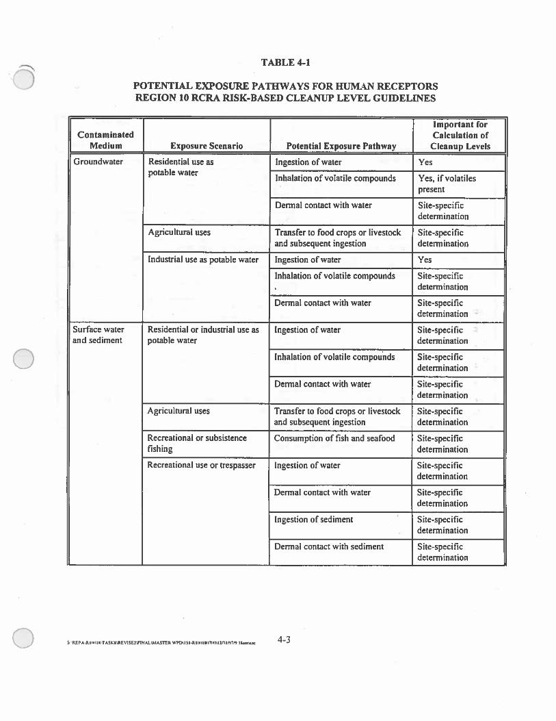
TABLE 4-1

POTENTIAL EXPOSURE PATHWAYS FOR HUMAN RECEPTORSREGION 10 RCRA RISK-BASED CLEANUP LEVEL GUIDELINES

Important forContaminated Calculation of

Medium Exposure Scenario Potential Exposure Pathway Cleanup Levels

Groundwater Residential use as Ingestion of water Yespotable water

Inhalation of volatile compounds Yes, if volatilespresent

Dermal contact with water Site-specificdetermination

Agricultural uses Transfer to food crops or livestock Site-specificand subsequent ingestion determination

Industrial use as potable water Ingestion of water Yes

Inhalation of volatile compounds Site-specific. determination

Dermal contact with water Site-specificdetermination

Surface water Residential or industrial use as Ingestion of water Site-specificand sediment potable water determination

Inhalation of volatile compounds Site-specificdetermination

Dermal contact with water Site-specificdetermination

Agricultural uses Transfer to food crops or livestock Site-specificand subsequent ingestion determination

Recreational or subsistence Consumption of fish and seafood Site-specificfishing determination

Recreational use or trespasser Ingestion of water Site-specificdetermination

Dermal contact with water Site-specificdetermination

Ingestion of sediment Site-specific. determination

Dermal contact with sediment Site-specificdetermination

S REPAR Il,IIN;TASK;E1SDflNAL’dASTtR ‘Pt?’? iRln,?nc

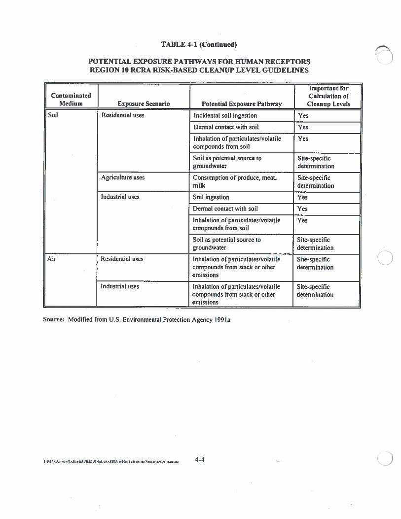
TABLE 4-1 (Continued)

POTENTIAL EXPOSURE PATHWAYS FOR HUMAN RECEPTORSREGION 10 RCRA RISK-BASED CLEANUP LEVEL GUIDELINES

Source: Modified from U.S. Environmental Protection Agency 199 Ia

a

0

Important forContaminated Calculation of

Medium Exposure Scenario Potential Exposure Pathway Cleanup Levels

Soil Residential uses Incidental soil ingestion Yes

Demial contact with soil Yes

Inhalation of paniculates/volatile Yescompounds from soil

Soil as potential source to Site-specificgroundwater determination

Agriculture uses Consumption of produce, meat, Site-specificmilk determination

Industrial uses Soil ingestion Yes

Dennal contact with soil Yes

Inhalation of particuiates/volatile Yescompounds from soil

Soil as potential source to Site-specificgroundwater determination

Air Residential uses Inhalation of paniculates/volatile Site-specificcompounds from stack or other determinationemissions

Industrial uses Inhalation of particulates/volatile Site-specificcompounds from stack or other determinationemissions

S WPfl\I5I.Rj(flhIPINflI2fl3NN 4-4

Exposure pathways are identified within each pertinent exposure scenario. Several exposure scenarios

may be applicable at a given facility. Those most commonly evaluated are the industrial and residential

exposure scenarios. Other scenarios, including agricultural, recreational, and trespasser. may be important

depending on facility location and identification of the most exposed individual. For example, if the

individual subject to the greatest exposure to facility-related constituents is a recreational user of a surface

water body, a recreational exposure scenario may be sufficiently protective. Classification of land use is

further discussed in Section 4.2.

Cleanup levels should be determined for all exposures to a specific medium, such as soil. The cleanup

level calculated for each medium should take into consideration all exposure pathways and all facility-

related constituents that contribute to risk or hazard. For example, the cleanup levels for soil should be

developed using all possible exposure routes for soil that are appropriate at a facility. It is recommended

that ingestion, dermal contact, and inhalation exposure routes be considered when developing cleanup

levels for all media. Where exposure may occur to a constituent in both soil and water, media-specific

cleanup levels may require further downward adjustment to assure that an acceptable cumulative target

risk level is met.

4.2 CLASSifICATION OF LAND USE

The evaluation of a facility to determine appropriate cleanup levels is based in part on the appropriate land

use scenario.

Depending on assumptions A residential scenario results in more conservative (that is, lower)

regarding future facility uses, cleanup levels, because it is assumed that adults and children liveeither a residential scenario or anindustrial scenario is typically on the site and are exposed to hazardous constituents 24 hours a

chosen. day. In the industrial scenario, exposure is assumed only for adults

______________________________

and only during working hours.

Selection of land use is most relevant when calculating cleanup levels that address direct contact with

soils. The following two subsections discuss EPA and Region 10 state policies or regulations regarding

land use and soil cleanup levels. An additional subsection discusses land use issues associated with setting

S ‘REPA’R I(’,IWT4SKWRE1SE3’flNAL’MASTtR wPD\I5IIcxH4,7nI2J1ImN $arn\Lae —

groundwater, surface water, and air cleanup levels. Later discussions in Section 4.3 identif3t specific

numerical standards and criteria that must be considered when setting cleanup levels.

Of the Region 10 states, only the Washington Model Toxics Control Act (MTCA) regulations have been

authorized for selling RCRA corrective action cleanup levels. Details of MTCA regulations relevant to

land use are therefore summarized. More general information on other state regulatory programs is also

presented because project managers and facilities are encouraged to take into consideration non-RCRA

state standards or criteria, including those regarding land use classifications that may influence cleanup

level selection. Consideration of state regulations and land use classifications will avoid the need for the

state to revisit the corrective measure taken at a facility. Overall, the most stringent land use requirement

that may apply to a facility should be used for risk assessment and selling cleanup levels.

4.2.1 U.S. Environmental Protection Agency Land Use Policy and Soil CleanupLevels

EPA’s policy is that “current and reasonable expected future land use and corresponding exposure

scenarios should be considered both in the selection and timing of remedial actions” (Federal Register

[FR] 19452, May 1, 1996). EPA’s May 25, 1995, directive, Land Use in the CERCL4 Remedy Selection

Process addresses land use consideration under the Comprehensive Environmental Response, ()Compensation and Liability Act of 1980 (CERCLA) process (directive is attached as Attachment G)

(EPA 1995d). The directive identifies sources and types of information that may aid EPA in determining

the reasonable anticipated future land use at a site. Examples of such information include zoning laws,

community master plans, site location in relation to current land uses and populations, groundwater

protection programs, and environmental justice issues. The directive recommends early discussions

between EPA and local land use planning authorities, local officials, and the public regarding reasonably

anticipated future land uses.

The principles identified in the directive are equally applicable to the RCRA corrective action program

(proposed Title 40 of the Code of Federal Regulations, Part 264 Subpart S Amendment, FR 19439, May I,

1996). Available information and local input may indicate that nonresidential land use assumptions are

appropriate for corrective action facilities if there is reasonable certainty that the facility will remain

industrial. Factors such as residential properties located adjacent to or on an industrialized facility or child

care areas operated on commercial and industrial facilities should be considered when determining land

S REPARIlMIIWT4SKMflV1SE2\flNAjIMASflR WPDI3I-RIoIIS1I(,IILqIrn, Wim\..e —

use. If the type of future land use cannot be reasonably predicted or if future residential land use (as well

as child care centers and recreational parks) cannot be reasonably ruled out, residential land use should be

assumed.

EPA is committed to ensuring that the public fully participates in all aspects of the RCRA corrective

action. EPA released a detailed guidance manual on public participation in RCRA programs (EPA 1993c)

and followed this guidance with a RCRA Expanded Public Participation Rule (FR 63417, December II,

1995). EPA regards public participation as an important activity that empowers all communities,

including minority and low income communities, to become actively involved in local waste management

activities. This should include public participation in making land use and exposure assumption decisions,

particularly for communities potentially impacted by waste management activities and the risk

management decisions associated with corrective action.

EPA expects that contaminated soils will be cleaned up as necessary to prevent the transfer of

unacceptable concentrations of hazardous constituents from soils, including subsurface soils, to other

media; therefore, the uses of groundwater and surface water potentially impacted by constituent migration

from soil must be considered when cleanup levels are set. Likewise, the location of adjacent or nearby

residents potentially exposed to airborne constituents must also be considered.

4.2.2 Region 10 State Land Use Policies and Soil Cleanup Levels

The Washington State MTCA cleanup regulations specify when cleanup levels may be based on

residential or industrial land uses and were amended in 1996 under Chapter 173-340 of the Washington

Administrative Code (WAC). WAC 173-340-740 requires that the residential land use scenario be

assumed unless a demonstration of nonapplicability can be made under subsection 740(1)(a). Industrial

property soil cleanup levels can be established as follows if the site meets the definition ofan industrial

property cited under the WAC 173-340-200:

S REPAR IRIX TASKXEV15E2F!NAL1ASThR WPD131.R mimi’s ‘V 1P17’) lAam\sat —

“Industrial properties” means properties that are or have been characterized by or are to be committed to traditionalindustrial uses such as processing or manufacturing of materials, marine terminal and transportation areas andfacilities, fabrication, assembly, treatment or distribution of manufactured products, or storage of bulk materials.One of the following statements is true for industrial properties:

• Zoned for industrial use by a city or county conducting land use planning under Chapter 36.70ARevised Code of Washinglon (RCW) (Growth Management Act)

• For counties not planning under Chapter 36.70A RCW (Growth Management Act) and the cilieswithin them, zoned for industrial use and adjacent to properties currently used or designated forindustrial purposes

WAC 173-340-745 provides additional criteria for determining whether a land use not specified in the

definition meets the “traditional industrial use” requirement or whether a land use zoning category meets

the requirement of being “zoned for industrial use.” In addition, WAC 173-340-745 requires an evaluation

of comprehensive plan text or zoning code to verify that only industrial land uses may occur on the site.

WAC 173-340-745 also requires that residential soil cleanup levels be used at industrial properties in close

proximity to (generally, within a few hundred feet) residential areas, schools, or child care facilities, unless

site or constituent inaccessibility and constituent immobility can be demonstrated. Likewise, residential

soil cleanup levels should be used for current or potential future residential areas adjacent to properties

currently used or designated for industrial purposes. State of Washington Guidancefor Clean Closure of

Dangerous Waste Facilities (Washington Department of Ecology [Ecology] 1994) specifies that according CDto WAC l73-303-610(2)(b)Q), numeric clean closure levels for soils, groundwater, surface water, and air

must be determined using residential exposure assumptions.

State of Oregon environmental cleanup law (Oregon revised Statutes 465.315 and 465.325), promulgated

on January 10, 1997, requires that current and reasonably anticipated future land uses be considered in risk

assessments and feasibility studies. As previously stated, this law (and the rules promulgated pursuant

thereto) is for state Superfund sites and is technically not part of the Oregon Department of Environmental

Quality authorized corrective action program for RCRA-regulated facilities. Idaho and Alaska have not

developed specific regulations or guidance documents that address land use issues. Idaho accepts the use

of cleanup levels based on residential and industrial land use (Tetra Tech 1996a). Land use is addressed in

proposed Alaska Cleanup Standard Regulations and Risk Assessment Guidance (proposed for public

comment on December 18, 1996) (Tetra Tech 1996b). State-specific rules and regulations, which are

evolving, should be consulted for further information.

S REPA IiNI,,;TASI.IR%V,5E2;rINAL,MA5ThR WPO’5I.RIIrnII1l,flh2flIN7f9 .ISimuc —

4.2.3 Land Use Policies and Other Media

Determination of cleanup levels for groundwater, surface water, and air is the same for all facilities

regardless of the site’s land use classification as industrial or residential. EPA Region 10 recommends that

residential exposures be assumed and that exceptions be made. only for extenuating circumstances.

Corrective actions for soil and groundwater media should assure that discharges from either media do not

exceed surface water, sediment, or air quality standards or risk-based criteria. Sections 4.2.3.2 (Surface

Water), 4.2.3.3 (Air), 4.3 (Standards and Criteria) and Chapter 5 (Ecological Sediment Criteria) provide

information on land use and standards and criteria for these media.

4.2.3.1 Groundwater

EPA expects to return useable groundwaters to their maximum beneficial uses wherever practicable.

When restoration of groundwater is not practicable, EPA expects to prevent or minimize further migration

of the plume, prevent exposure to the contaminated groundwater, and evaluate further risk reduction

(FR 19448, May 1, 1996). State-designated uses should be considered when setting cleanup levels. As

previously noted, however, although RCRA statutory language does not require nonauthorized state

standards to be followed, it does require cleanups to be protective of human health and the environment.

EPA has initiated a comprehensive state groundwater protection program (CSGWPP) to encourage each

state to coordinate its current and planned groundwater protection activities through a CSGWPP. EPA

remediation program personnel should be familiar with and utilize CSGWPPs (EPA 1997h). Washington

State has submitted a draft CSGWPP to EPA and was responding to EPA comments to the proposed plan

at this printing. No other Region 10 states have submitted a CSGWPP to EPA; however, Oregon and

Idaho have initiated CSGWPPs, and the following listed persons can be contacted regarding groundwater

use issues (for example, for information on groundwater classified as a source of drinking water or as

having significant ecological value).

S REPAR l.IIKSASK,REV1SErflNAL’MASThR WPD’ ‘I Ri,flsc —

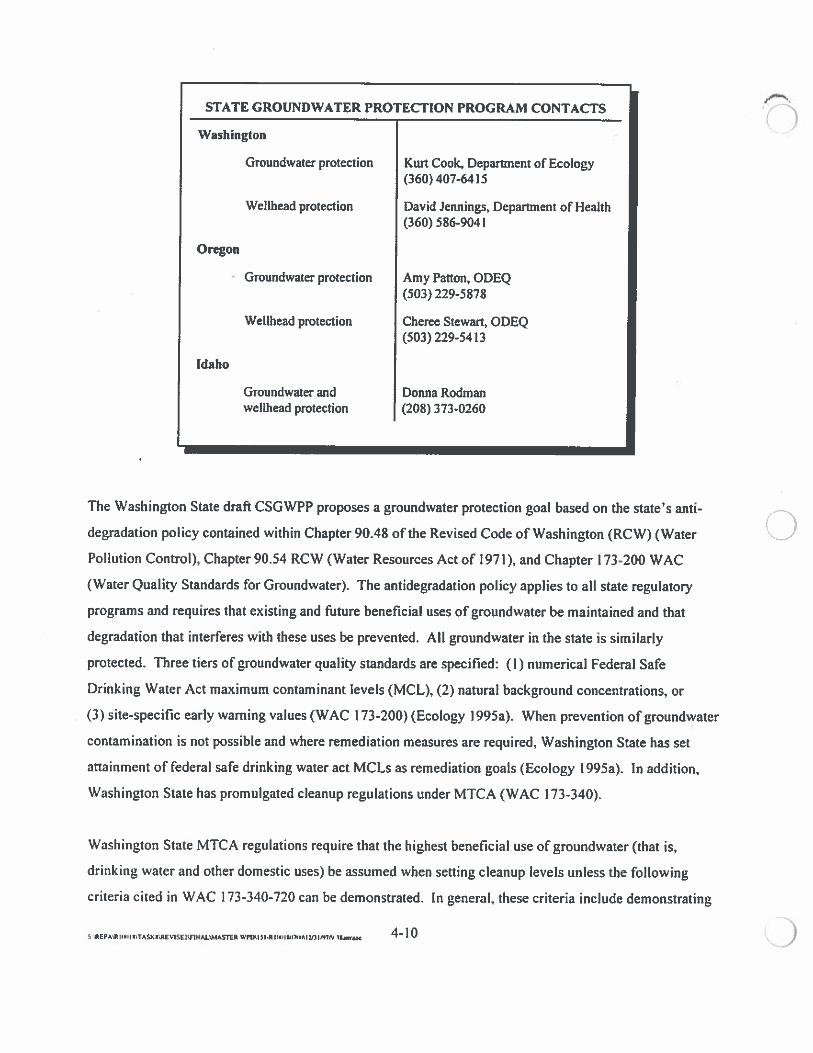
STATE GROUNDWATER pROTECTION PROGRAM CONTACTS )Washington

Groundwater protection Kurt Cook, Department of Ecology(360) 407-6415

Wellhead protection David Jennings. Department of Health(360) 586-9041

Oregon

Groundwater protection Amy Patton, ODEQ(503) 229-5878

Weithead protection Cheree Stewart, ODEQ(503) 229-5413

Idaho

Groundwater and Donna Rodmanwelihead protection (208) 373-0260

The Washington State draft CSGWPP proposes a groundwater protection goal based on the state’s anti-

degradation policy contained within Chapter 90.48 of the Revised Code of Washington (RCW) (Water

Pollution Control), Chapter 90.54 RCW (Water Resources Act of 1971), and Chapter 173-200 WAC

(Water Quality Standards for Groundwater). The antidegradation policy applies to all state regulatory

programs and requires that existing and future beneficial uses of groundwater be maintained and that

degradation that interferes with these uses be prevented. All groundwater in the state is similarly

protected. Three tiers of groundwater quality standards are specified: (I) numerical Federal Safe

Drinking Water Act maximum contaminant levels (MCL), (2) natural background concentrations, or

(3) site-specific early warning values(WAC 173-200) (Ecology 1995a). When prevention of groundwater

contamination is not possible and where remediation measures are required, Washington State has set

attainment of federal safe drinking water act MCLs as remediation goals (Ecology 1995a). In addition,

Washington State has promulgated cleanup regulations under MTCA (WAC 173-340).

Washington State MTCA regulations require that the highest beneficial use of groundwater (that is,

drinking water and other domestic uses) be assumed when setting cleanup levels unless the following

criteria cited in \VAC 173-340-720 can be demonstrated. In general, these criteria include demonstrating

S RERA’.R I(IItTASt\REV15E2w]NAjkMA57rR WPD\I IR ItRflhIIIRI;I3fl I/07P1 Ujj.ifl —

that the groundwater is not a current or future source of drinking water based on the following: (I) the

groundwater is present in insufficient quantity to yield water for a domestic well; (2) natural background

concentrations of organic or inorganic constituents are present and make use of the water for drinking not

practicable; and (3) the groundwater cannot technically be recovered for drinking water purposes based on

depth or location. It also must also be demonstrated that migration of contamination from an unusable

aquifer to a useable aquifer cannot occur. Information on specific MTCA cleanup goals is presented in

Section 4.3.2.

State of Alaska beneficial use regulations, applicable to both groundwater and surface water, are cited in

Title 18 Alaska Administrative Code (AAC) Chapter 70, “Water Quality Standards.” State of Oregon,

groundwater beneficial use regulations are cited in Oregon Administration Rules (OAR), Chapter 340,

Division 40, “Groundwater Quality Protection.” State of Idaho groundwater beneficial use regulations are

cited in the Idaho Administrative Code (JAC), Title 01, Chapter 02, Section 299, “Groundwater Quality

Standards.” The state-specific rules and regulations should be consulted for further information.

4.2.3.2 Surface Water

The proposed RCL& corrective action regulations recommend that state-designated uses of surface water

be considered when setting cleanup levels (proposed 40 CFR 264 Subpart S Amendment,

FR 30804, July 27, 1990). Promulgated state and federal drinking water standards or risk-based levels

based on water ingestion can be used as cleanup levels for surface water designated for drinking water use.

If surface water has been designated by a state for uses other than drinking water, the EPA may consider

the state-designated use when establishing cleanup levels (FR 30818, July 27, 1990). In any case, federal

Clean Water Act (CWA) prohibitions of releases of hazardous substances and oil to surface waters should

be considered when determining cleanup levels [(CWA 311(b) (3)].

Washington State MTCA regulations require that the highest beneficial use of surface water be assumed

when setting cleanup levels (WAC 173-340-730). Promulgated standards or risk-based levels based on

water ingestion should be used as cleanup levels for surface waters representing a source or potential

future source of drinking water. Risk-based standards based on human ingestion of fish or shellfish should

be considered when determining cleanup levels for surface waters that support or have the potential to

support fish or shellfish populations. Federal (CWA) (EPA 1986a) and state water quality criteria based

S EflMRII NTASKKREW5E2PINALMA5TER WPfl ihmae

on the protection of aquatic organisms must also be achieved. Washington State surface water beneficial

use and water quality standard regulations are cited in WAC 173-201.

As noted in Section 4.2.3.1, State of Alaska surface water beneficial use and water quality standards are

cited in Title IS, AAC, Chapter 70. Oregon surface water beneficial use and water quality standards are

cited in OAR, Chapter 340, Division 41, “State-Wide Water Quality Maintenance Plan, Beneficial Uses,

Policies.” Idaho surface water beneficial use standards are cited in IAC, Title 01, Chapter 02, Section 200,

“General Surface Quality Criteria.” The state-specific rules and regulations should be consulted for

further information.

4.233 Air

A residential exposure scenario is assumed when calculating air cleanup levels (FR 30831, July 27, 1990);

however, the location of the most exposed resident must be identified when determining compliance with

the cleanup level. The point where the maximum long-term human exposure to air releases would occur is

typically outside of a facility boundary. Under the corrective action process, the most exposed individual

is identified on a site-specific basis and may be identified as someone living across the street from the

facility, as a worker living on the site, or wherever else maximum long-term human exposure would occur

based on site characteristics (FR 30831, July 27, 1990). For clean closure, it is assumed that the most

exposed individual is at the unit boundary and that air constituent concentrations must be equal to or below

the health-based level at the unit boundary (EPA 1989e).

Alaska, Idaho, and Oregon do not have specific requirements for setting air cleanup standards at RCRA

facilities. Washington State MTCA regulations require that cleanup levels to protect air quality be based

on estimates of reasonable maximum exposure (RME) (WAC 173-340-750), the highest exposure that can

be reasonably expected to occur at a site under current or potential future uses. The cleanup level,

therefore, should be based on the residential scenario unless the criteria specified in WAC 173-340-750 for

nonresidential site uses can be demonstrated. The WAC 173-340-750 criteria generally require that no

current or future residential use of the site occur and that air emissions from the site not reduce the air

quality of adjacent residential areas. WAC 173-340-750 requires that ambient air cleanup levels for

nonresidential uses be established on a case-by-case basis.

‘REPAR 3II)IMTASKrRE9SE3ENALWAnR WPD’I5I-Rt,NpsI7IMp%Lrn Iflh/’J3flms.c 4—12

4.3 IDENTIFICATION OF PROMULGATED STANDARDS AND CRITERIA

When developing cleanup levels for a facility, promulgated standards or criteria for environmental media

contaminated by facility activities must be considered. Federal and state standards and criteria that should

be considered when developing cleanup levels are summarized in Sections 4.3. 1 (federal) and 4.3.2 (state).

The state and federal policies and regulations addressing land use discussed in Section 4.2 require

consideration when selecting appropriate standards and criteria.

4.3.1 Federal Standards and Criteria

Federal standards exist for drinking water supplies and surface water bodies. Under the federal Safe

Drinking Water Act, MCLs, maximum contaminant level goals (MCLG), and secondary MCLs are

established for a number of inorganic and organic chemicals in drinking water supplies. MCLs may be

used as cleanup levels for groundwaters and surface waters that are current or potential drinking water

resources, provided they are deemed to be sufficiently protective given the overall contamination at or

from the facility. In other words, it is discretionary to use risk-based levels rather than MCLs for i

determining cleanup levels which may impact drinking water because some MCLs are based on

technological barriers that no longer exist and/or do not consider additivity of risks when other chemicals

are present at levels of concern (see Section 4.7.4 for an example risk calculation where multiple

constituents with MCLs are present in groundwater). Other federal criteria for the protection of human

health include CWA ambient water quality criteria (AWQC), which are established for surface waters.

For the protection of human health, two types of AWQC have been established: (1) for the ingestion of

water and fish and (2) for the ingestion of fish only (EPA 1986a). The CWA prohibits the release of oil to

navigable surface waters in any quantity that causes a sheen, an emulsion, or a sludge, regardless of

cleanup standards that may be imposed and/or complied with [CWA 311(b) (3)]. This prohibition is

federally enforceable in all states.

4.3.2 State Standards and Criteria

Washington State has promulgated cleanup regulations under MTCA (WAG 173-340). As stated in

Chapter 2, Ecology was authorized for a corrective action program that uses MTCA regulations. MTCA

establishes cleanup levels for soil, groundwater, surface water, and air.

S \REPA\R IL flTASKI?flVISE2W1NALJ.lASThR WpO IL .R IILLI mI’INM 211 P)’?) Lbmsn —

MTCA requires that where groundwaters and surface waters are current or potential future sources of

drinking water, cleanup levels be at least as stringent as promulgated federal and state standards, including

federal MCLs and MCLGs, and Washington state MCLs published under WAC 248-54. In the absence of

promulgated standards, MTCA provides a method for calculating RBCs based on drinking water ingestion

(WAC 173-340-720).

For surface waters that support or have the potential to support fish or shellfish populations, MTCA

requires that human health cleanup levels be at least as stringent as federal AWQC established for the

protection of humans ingesting water and fish (WAC 173-340-730). In the absence of promulgated

standards, MTCA provides a method for calculating risk-based surface water cleanup levels based on fish

ingestion only (WAC 173-340-730).

MTCA requires that soil and air cleanup levels be at least as stringent as applicable state and federal laws.

MTCA provides methods for calculating soil RBCs based on soil ingestion (WAC 173-340-740) and air

RBCs based on inhalation (WAC 173-340-750). MTCA also requires that constituent concentrations in

soil not cause contamination of groundwater to concentrations that exceed groundwater cleanup levels.

MTCA provides three methods (A, B, and C) for determining risk-basedcleanup standards. Method A EDinvolves use ofa table that identifies conservative, default cleanup levels for a limited number of common

hazardous substances. Method B is applicable when there are more hazardous substances involved.

Method C is applicable when Methods A and B cleanup levels are technically impossible to achieve, lower

than background, or may cause more environmental harm than good. MTCA also defines a second

Method C procedure for determining when soil cleanup levels for industrial land use can be used and how

these cleanup levels should be calculated. Method B and Method C involve calculations of cleanup levels

based on defauLt exposure assumptions for different Land-use scenarios. At this printing Ecology is

preparing revised MTCA regulations and should be consulted for the latest regulatory update.

Washington State published a MTCA Cleanup Levels and Risk Calculations (CL4RC II) Update

(Ecology 1996) reference document. The doãument provides guidance on when Methods A, B, and C

should be used and provides tables of chemical-specific Methods B and C cleanup levels for hazardous

constituents in groundwater, surface water, and soils.

c RLPAR O.IIS’TASta’Efl5Ef1NAt’MASflR WPDISI.RI(EI!fl7€IWIi7J1SamSaC —

The ODEQ has no specific regulations for setting cleanup levels at RCRA facilities. As noted in

Chapter 2, ODEQ was authorized to include corrective action in RCRA permits using EPA risk assessment

guidance to determine cleanup levels for the corrective action program. Oregon does have rules that

address contamination at state Superflrnd sites and recently enacted statutory language that, among other

things, establishes target risk levels for cleanups and also requires development of a protocol for

probabilistic risk assessment (Oregon Revised Statutes 465.315 and 465.325). ODEQ promulgated rules

for these statutes on January 10, 1997. The state Superfund cleanup rules are not currently a part of

Oregon’s authorized RCRA corrective action program.

As noted in Chapter 2, Idaho and Alaska do not have authorized state-specific cleanup level regulations.

Alaska has not applied for authorization to manage RCRA programs in lieu of EPA. In accordance with

RCRA Section 3006 (b), Idaho’s authorized program must be equivalent to the federal RCRA program;

however, an Idaho statutory provision prohibits regulations more stringent than EPA’s (Idaho Code

Section 39-4404, Hazardous Waste Management Act of 1983.)

4.4 RISK-BASED SCREENING

When no promulgated standards or criteria are available for cleanup levels, facility-specific RBCs should

be calculated for the remaining COPCs. Before RBCs are calculated, hazardous constituents can be

screened from further consideration if they are present at concentrations below significant health concerns.

Generic RBCs calculated using residential scenario assumptions can be used to screen constituents. This

screening process should be performed as follows:

1. List maximum concentration of each constituent in each medium

2. List risk-based concentrations of each constituent, using PROscalculated by EPA Region 9 (described in Section 4.5 and includedin Attachment E) (EPA 1996c)

S REPASR I IN! I NSTASKNmEVISE21NALIASTER WItS 151-RI IN! I SIflINIS I Ui P5751 llNmSssc —

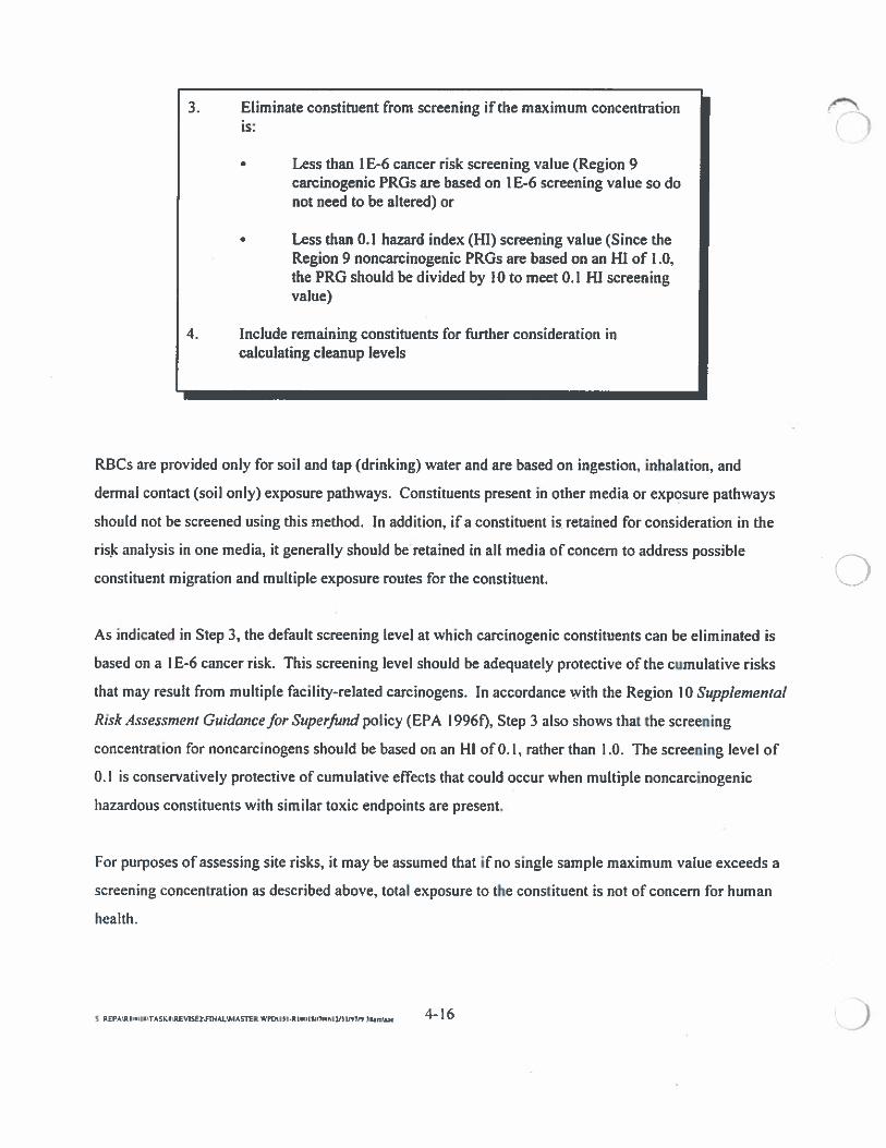
3. Eliminate constituent from screening if the maximum concentrationis:

/

Less than I E-6 cancer risk screening value (Region 9carcinogenic PRGs are based on I E-6 screening value so donot need to be altered) or

• Less than 0.1 hazard index (HI) screening value (Since theRegion 9 noncarcinogenic PRGs are based on an HI of 1.0,the PRG should be divided by 10 to meet 0.1 HI screeningvalue)

4. Include remaining constituents for flinher consideration incalculating cleanup levels

RBCs are provided only for soil and tap (drinking) water and are based on ingestion, inhalation, and

dermal contact (soil only) exposure pathways. Constituents present in other media or exposure pathways

should not be screened using this method. In addition, if a constituent is. retained for consideration in the

risk analysis in one media, it generally should be retained in all media of concern to address possible

constituent migration and multiple exposure routes for the constituent. Li

As indicated in Step 3, the default screening level at which carcinogenic constituents can be eliminated is

based on a I E-6 cancer risk. This screening level should be adequately protective of the cumulative risks

that may result from multiple facility-related carcinogens. In accordance with the Region 10 Supplemental

Risk Assessrnern Guidance for Superfund policy (EPA I 996fl, Step 3 also shows that the screening

concentration for noncarcinogens should be based on an HI of 0.1, rather than 1.0. The screening level of

0.1 is conservatively protective of cumulative effects that could occur when multiple noncarcinogenic

hazardous constituents with similar toxic endpoints are present.

For purposes of assessing site risks, it may be assumed that if no single sample maximum value exceeds a

screening concentration as described above, total exposure to the constituent is not of concern for human

health.

S REPA’ft IcflIrnTASK,flVlSE2flNAL’MAS1tR WPThII.RIlWPISSIIlSSIZflIfl7rn 3kmsac —

Aluminum, calcium, magnesium, potassium, and sodium are not associated with toxicity to humans

under normal circumstances. No quantitative toxicity information is available for these elements from

EPA sources. Unless these elements have promulgated standards or criteria or unless site-specific factors

dictate, they generally can be eliminated from consideration during development of cleanup levels.

4.5 EXPOSURE ASSUMPTIONS

The exposure assumptions presented in this

section are used to determine the magnitude of a

potential chemical dose, which is the amount of a

given chemical entering the human body during a

specified time.

The default residential and industrial exposure assumptions recommended in this document to calculate

RBCs are presented in Table 4-2. These exposure assumptions, which were primarily taken from EPA

guidance documents, address human health concerns and are consistent with current federal and Region 10

CERCLA guidance. With the exception of the dermal exposure factors, the Table 4-2 factors are

consistent with those recommended in the most recent version of the Region 9 PRGs (see Attachment E,

[EPA 1996c]). Region 9 PRGs are updated annually and are available on the World Wide Web at

http://www.epa.gov/regiono9/waste/sfiind/prg/indexlhtml and on the California Regional Water:Board’s

Bulletin Board System at (510) 286-0404 (PRG2ND96.ZIP).

Table 4-3 compares the exposure pathways considered in soil, water, and air risk-based concentration

calculations for EPA Regions 3 and 9. Region 3 has calculated risk-based concentrations for soil, water,

and air that are similar to the EPA Region 9 PRGs. The Region 3 values were previously recommended by

Region 10 for screening purposes; however, the use of Region 9 PRGs for risk-based screening is currently

being recommended, primarily because they are more comprehensive in that they take into account more

exposure pathways.

The exposure assumptions used to calculatecleanup levels include body weight,inhalation and ingestion rates, skin surfacearea, absorption fractions, exposurefrequency and duration, and volatilizationand particulate emission factors (PEF).

S REpAIcNIIwTASKRREvlSE3PlNALMAfltR WPOISII€w,Ifl*,7€xnI2flIfl7/) SK.m\sac 4-17

0

(THIS PAGE INTENTIONALLY LEFT BLANK)

S REPAR IC’)IWTA5KIflt15flNAjlAflR 2tbn

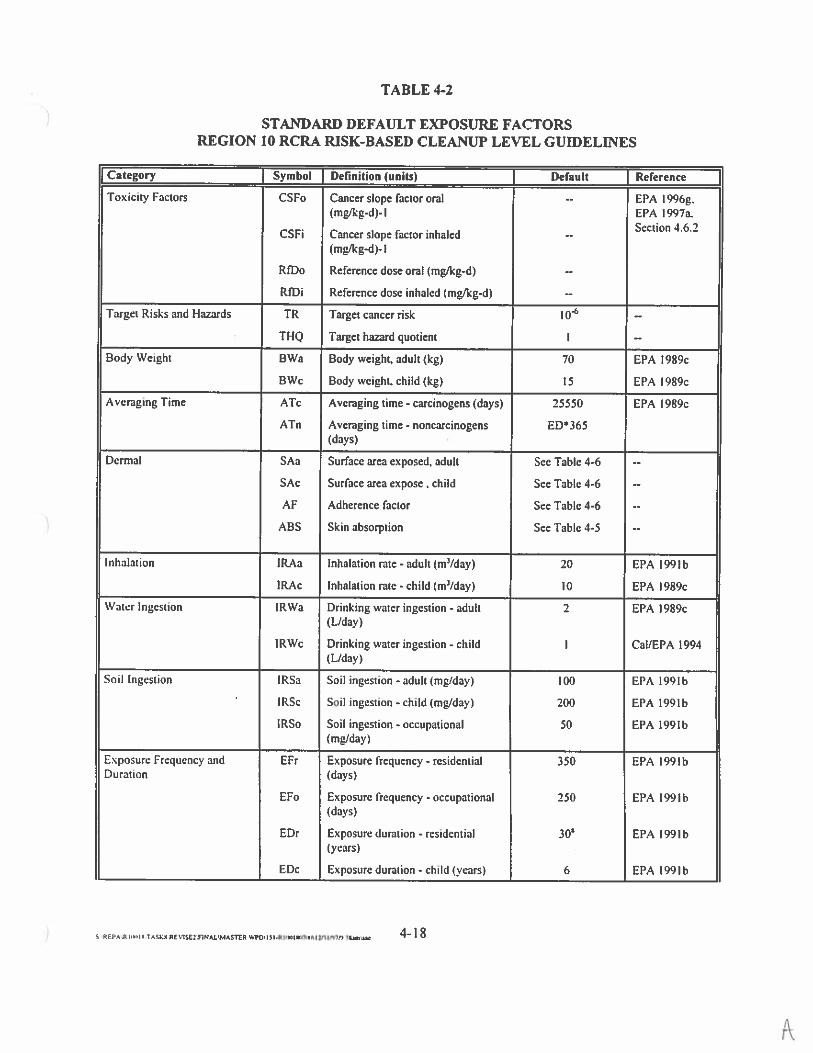
TABLE 4-2

) STANDARD DEFAULT EXPOSURE FACTORSREGION 10 RCRA RISK-BASED CLEANUP LEVEL GUIDELINES

Category Symbol Definition (units) Default Reference

Toxicity Factors CSFo Cancer slope factor oral -- EPA 1996g.(mØg-d)-l EPA 1997a.

. . Section 4.6.2CSFi Cancer slope factor inhaled --

(mg/kg-d)- I

RfDo Reference dose oral (mØg-d) --

RIDI Reference dnse inhaled (mg/kg-d) --

Target Risks and Hazards TR Target cancer risk io --

• THQ Target hazard quotient I --

Body Weight BWa Body weight, adult (kg) 70 EPA 1989c

BWc Body weight child (kg) 15 EPA I 989c

Avenging Time ATc Avenging time - carcinogens (days) 25550 EPA 1989c

ATn Avenging time - noncarcinogens ED’365(days)

Dermal SAa Surface area exposed, adult See Table 4-6 --

SAc Surface area expose, child See Table 4-6 --

AF Adherence factor See Table 4-6 --

ABS Skin absorption See Table 4-5 --

Inhalation IRAa Inhalation rate - adult (m3/day) 20 EPA 1991b

lRAc Inhalation rate - child (m3/day) 10 EPA I 989c

Water Ingestion IRWa Drinking waler ingestion - adult 2 EPA l989c(L/day)

IRWc Drinking water ingestion - child I Cal/EPA 1994(L/day)

Soil Ingestion IRSa Soil ingestion - adult (mg/day) 100 EPA l99lb

IRSc Soil ingestion - child (mglday) 200 EPA 199th

IRSo Soil ingestion - occupational 50 EPA 1991b(mgMay)

Exposure Frequency and EFr Exposure frequency - residential 350 EPA 1991bDuration (days)

EFo Exposure frequency - occupational 250 EPA 1991b(days)

EDr Exposure duration - residential 30 EPA 1991b(years)

EDc Exposure duration - child (years) 6 EPA 1991b

S LI’4fl TALK REV1SE2HNALMASThR WPD’J k ,rnLmo,nI2n 197’? I 4-I 8

ft

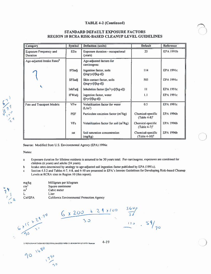
TABLE 4-2 (Continued)

STANDARD DEFAULT EXPOSURE FACTORSREGION 10 RCRA RISK-BASED CLEANUP LEVEL GUIDELINES

Category { Symbol Definition (units) Default Reference

Exposure Frequency and EDo Exposure duration - occupational 25 EPA 1991 bDuration (years)

Age-adjusted Intake Ratesb Age-adjusted factors forcarcinogens:

.—i lFSadj Ingestion factor, soils 114 EPA 1991c

( ([mgyrj/[kg-dJ)

‘ SFSadj Skin contact factor, soils 503 EPA 199 Ic

ç(mgyr]f[kg-d])

lnhFadj Inhalation factor ([m”yrJ/kg-dJ) II EPA 199 Ic

FFWadj Ingestion factor, water 1.1 EPA 199lc([I.yr/[kg-d])

Fate and Transport Models VFw Volatilization factor for water 0.5 EPA 199 Ic(Urn3)

PEF Particulate emission factor (m/kg) Chemical-specific EPA 1996b. (Table 4-Sf

VFs Volatilization factor for soil (m3&g) Chemical-specific EPA l996b(Table 4_7)C

sat Soil saturation concentration Chemical-specific EPA 1996b(mg/kg) (Table 4-IOf

Notes:

a Exposure duration for lifetime residents is assumed to be 30 years total. For carcinogens, exposures are combined forchildren (6 years) and adults (24 years).

b Intake rates determined by analogy to age-adjusted soil ingestion factor published by EPA (1991c).c Section 4.5.2 and Tables 4-7. 4-8. and 4-10 are presented in EPA’s Interim Guidelines for Developing Risk-based Cleanup

Levels at RCRA sites in Region 10 (this report).

567

2J

lo -

1 70

Source: Modified from U.S. Environmental Agency (EPA) 1996c

()

mg/kg Milligram per kilogramcrn Square centimeterrn Cubic meterL LiterCal/EPA California Environmental Protection Agency

1)zoo

--

S REPA,RI,m.INTAsa\REvIsm\rlNALMAcrfl WPO’IlI.RIlrnIAI<SSIlpflflIirn,5

aO

401’

4-19

‘1)0

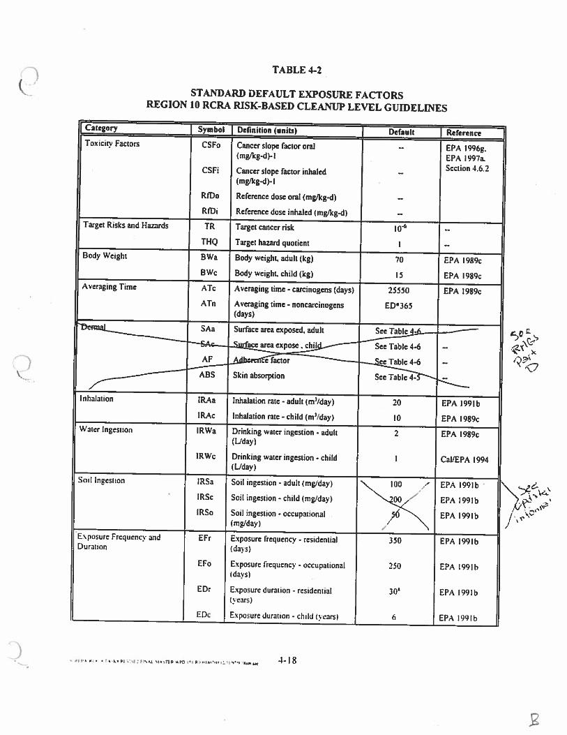
TABLE 4-2

[çtegory Symbol Definition (units) Default ReferenceToxicity Factors CSFo Cancer slope factor oral -- EPA 1996g.

(mg/kg-d)-l EPA 1997a,. Section 46.2CSFi Cancer slope Factor inhaled --

(mØg-d)-l

RIDo Reference dose oral (mg/kg-d) —

RtOi Reference dose inhaled (mg&g-d) --

Target Risks and Hazards TR Target cancer risk l0 —

THQ Target hazard quotient I —

Body Weight BWa Body weight, adult (kg) 70 EPA l9R9c

BWc Body weight child (kg) IS EPA 1989cAveraging Time ATc Averaging time - carcinogens (days) 25550 EPA I989c

ATn Averaging time - noncarcinogens ED’365(days)

SAa Surface area exposed, adult -

—SAc—-.. ace area expose. chil See Table 4-6 —

AF cefactor eeTable4-6

ABS Skin absorption See Table 4-

Inhalation lRAa Inhalation rate - adult (m’/day) 20 EPA 1991b

IRAc Inhalation rate - child (m’/day) 10 EPA I 989cWater Ingestion IRWa Drinking water ingestion - adult 2 EPA 1989c

(L/day)

IRWc Drinking water ingestion - child I Cal/EPA 1994( Uday

Soil Ingestion IRSa Soil ingestion - adult (mg/day) 100 7 EPA 1991b• IRSc Soil ingestion - child (mg/day) EPA l991b

IRSo Soil ingestion - occupational O N EPA 199 lb(mg/day) N

Exposure Frequency and EFr Exposure frequency - residential 350 EPA 1991bDuration (days)

EFo Exposure frequency - occupational 250 EPA 199Thdays)

EDr Exposure duration - residential 30 EPA I 99Th(‘ears)

EDc Exposure duration - child (‘ears) 6 EPA 1991h

STANDARD DEFAULT EXPOSURE FACTORSREGION 10 RCRA RISK-BASED CLEANUP LEVEL GUIDELINES

It

I ‘

1-18‘I: ;ls&L lk%flp\pn!’

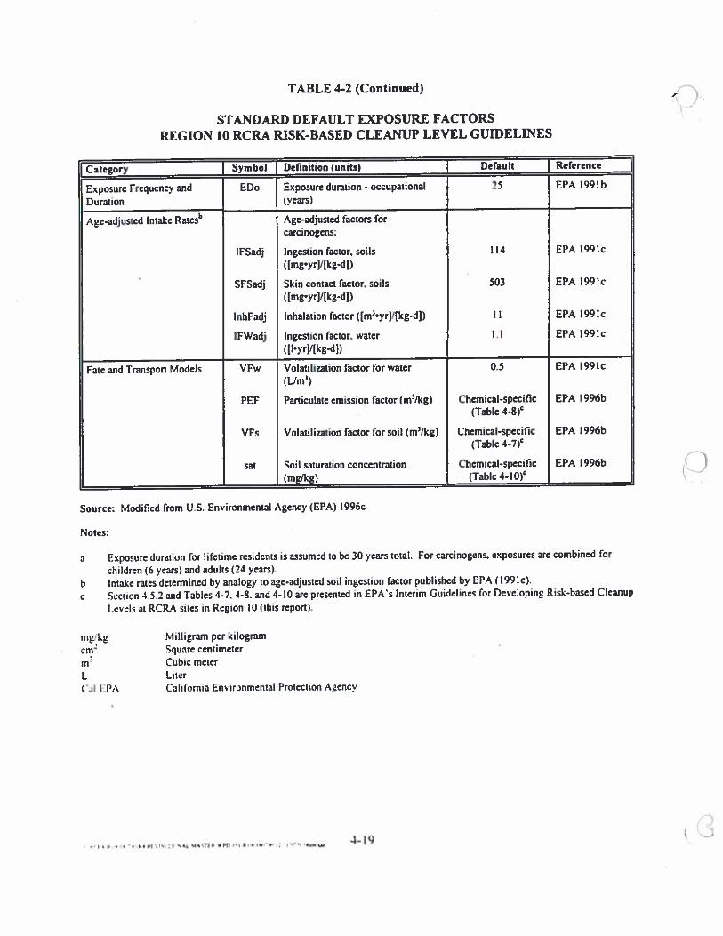
TABLE 4-2 (Continucd)

STANDARD DEFAULT EXPOSURE FACTORSREGION 10 RCRA RISK-BASED CLEANUP LEVEL GUIDELINES

Source; Modified from U.S. Environmental Agency (EPA) 1996c

Notes:

a Exposure duration for lifetime residents is assumed to be 30 years total. For carcinogens, exposures are combined for

children (6 years) and adults (24 years).

b Intake rates determined by analogy to age-adjusted soil inge5tion factor published by EPA (1991 c).

c Section 3.5.2 and Tables 3-7. 3-8. and 4-10 are presented in EPA’s Interim Guidelines for Developing Risk-based Cleanup

Lcvels at RCRA sites in Region 10 (‘his repon).

-1

p

Category j Symbol Definition (units) j Default Reference

Exposure Frequency and EDo Exposure duration - occupational 25 EPA 199 lb

Duration (years)

Age-adjusted Intake Ratesb Age-adjusted factors forcarcinogens:

IFSadj Ingestion factor, soils 114 EPA 199k

([mg-yrj/[kg-d])

. SFSadj Skin contact factor, soils 503 EPA 199 Ic

([mg’yr]/[kg-dj)

InhFadj Inhalation factor ([m3.yr/[kg-d]) II EPA 199k

IFWadj Ingestion factor, water 1.1 EPA 199 Ic

([l-yrj/[kg-d])

Fate and Transport Models VFw Volatilization factor for water 0.5 EPA 199 Ic

(L/m3)

PEF Particulate emission factor (m’&g) Chemical-specific EPA 1996b(Table 4-8)’

VFs Volatilization factor for soil (m’/kg) Chemical-specific EPA 1996b(Table 4-7)’

sat Soil saturation concentration Chemical-specific EPA 1996b

(mglkg) (Table 4-10)’

mg/kg Milligram per kilogramcm Square centimeter

Cubic meterL LtterCal EPA Caitfornia En’ tronmental Protection Agency

4-19

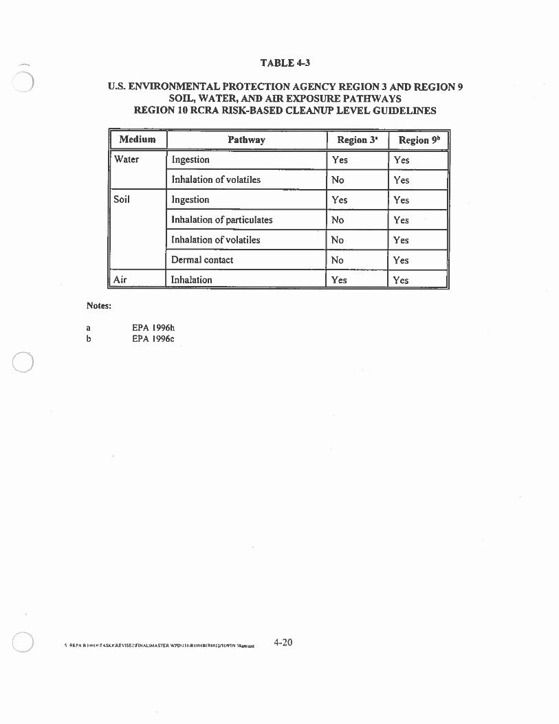
TABLE 4-3

U.S. ENVIRONMENTAL PROTECTION AGENCY REGION 3 AND REGION 9SOIL, WATER, AND AIR EXPOSURE PATHWAYS

REGION 10 RCRA RJSK-BASED CLEANUP LEVEL GUIDELINES

Medium Pathway J Region 3’ Region 9b 1Water Ingestion Yes Yes

Inhalation of volatiles No Yes

Soil Ingestion Yes Yes

Inhalation of particulates No Yes

Inhalation of volatiles No Yes

Dermal contact No Yes

Air Inhalation Yes Yes

Notes:

a EPA 1996hb EPA 1996c

S EPA’.R ikII; TASKNflV1SEZWINAL’MAS1TR Ip,7, 4—20

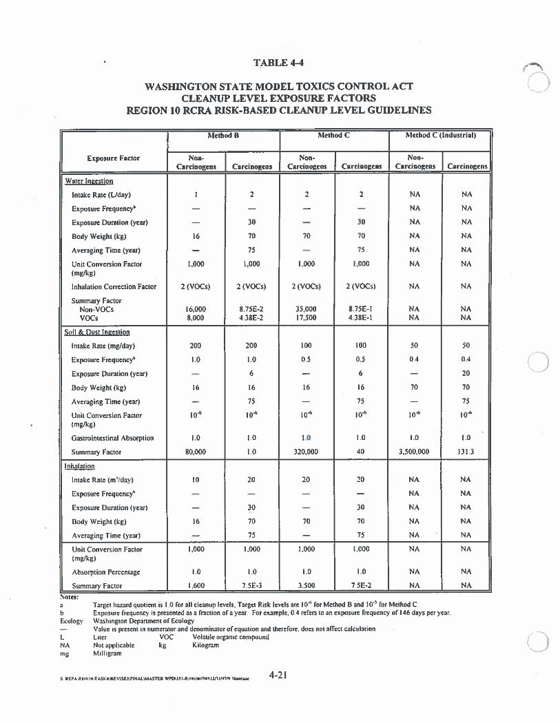
TABLE 4-4

WASHINGTON STATE MODEL TOMCS CONTROL ACTCLEANUP LEVEL EXPOSURE FACTORS

REGION 10 RCR4 RISK-BASED CLEANUP LEVEL GUIDELINES

Method 8 Method C Method C (Industrial)

Exposure Factor Non- Non- Non-Carcinogens Carcinogens Carcinogens Carcinogens Carcinogens Carcinogens

Waler Innestion

Intake Rate (1./day) I 2 2 2 NA NA

Exposure Frequcncy — — — — NA NA

Exposure Duraiion (year) — 30 — 30 NA NA

flody Weight (kg) 16 70 70 70 NA NA

Averaging Time (year) — 75 — 75 NA NA

Unit Conversion Factor 1,000 1,000 (.000 1.000 NA NA(mg/kg)

Inhalation Correction Factor 2 (VOCs) 2 (VOCs) 2 (VOCs) 2 (VOCs) NA NA

Summary FactorNon-VOCs (6,000 8.75E-2 35,000 8.75E-I NA NAVOCs 8.000 4.38E-2 17,500 4.38E-I NA NA

Soil & Dust Ineestion

Intake Rate (mg/day) 200 200 100 100 50 50

Exposure Frequency’ 1.0 1.0 0.5 0.5 04 0.4

Exposure Duration (year) — 6 — 6 — 20

Body Weight (kg) 16 16 16 16 70 70

Averaging Time (year) — 75 — 75 — 75

UnitConversion Factor I0 I0’ l0 i04 lot lo(mg/kg)

Gastrointestinal Absorption 1.0 1,0 1.0 1.0 1.0 1.0

Summary Factor 80.000 1.0 320.000 40 3,500,000 131.3

Inhalat inn

Intake Rate (m’/day) (0 20 20 20 NA NA

Exposure Frequency’ — — — — NA NA

Exposure Duration (year) — 30 — 30 NA NA

Body Weight (kg) (6 70 70 70 NA NA

Averaging Time (year) — 75 — 75 NA ‘ NA

Unit Conversion Factor 1,000 1.000 (.000 1,000 NA NA(mg/kg)

Absorption Percentage (.0 (.0 1.0 1.0 NA NA

Summary Factor (.600 7.5E-3 3.500 7.5E-2 NA NA

0

(:3

Notes:ahEcology

LNAmg

Target hazard quotient is 1.0 for all cleanup levcls, Target Risk levels are 0’ for Method B and I 0” for Method C.Exposure frequency is presented as a fraction of a year. For example, 0.4 refers loan exposure frequency of 146 days per year.

Washington Department of EcologyValue is present in numerator and denominator ofequation and therefore, does not affect calculationLiter VOC Volatile organic compoundNot applicable kg KilogramMilligram

5 RtPA\Ril PW,IASKX’REVI5EI’flNALV.IA5ThR WPO’tli’RI’UlI’J7’fl\ilnifl7fl lbm\,x 4-21

Exposure parameters dictated by MTCA (Methods B and C) are presented in Table 4-4. For soil

exposures, MTCA only considers the ingestion pathway. For water exposures, MTCA considers both

ingestion and volatile organic compound inhalation pathways. MTCA rules do not have to be followed for

EPA-lead corrective actions, but they should be considered in terms of preventing the need of future,

additional corrective action under state authorities. No other EPA Region 10 states have developed

specific exposure assumptions for RCRA facility RBC calculations; exposure parameters recommended by

the EPA guidance should be used.

Additional information on dermal absorption factors is presented in Section 4.5.1. Information on how

fate and transport models are used to incorporate hazardous constituent migration into cleanup levels is

presented in Section 4.5.2.

As stated in Section 4.1, other scenarios including recreational, agricultural, and trespasser may be more

appropriate at a given facility. An exposure parameter source for these and other scenarios is EPA’s

Exposure Factors Handbook I 989d, which EPA is updating [the EPA (I 996e) update was currently

available on the Internet at the time of this printing]. The Exposure Factors Handbook summarizes the

current literature regarding human exposures to contaminated media via a variety of specific exposure

conditions (for example, inhalation rates based on light, medium, and heavy activities). Values from the

handbook can be used in lieu of the default exposure factors when reliable facility-specific exposure

information is available. The Draft Exposure Assessment Guidance, Attachment C ofGuidance for

Performing Screening Level Risk Analyses at Combustion Facilities Burning Hazardous Waste

(EPA 1994i), further described in Section 4.5.2.4, also includes exposure parameters for human food chain

exposure pathways, such as garden produce and fish ingestion rates.

Pew Policy on Evaluating Health Risks to Children (EPA 1995e) requires that exposures to infants and

children be considered separately from adults. Children may be more or less sensitive to specific

constituents. They may also experience different types and rates of exposures; therefore, separate risk and

hazard estimates should be made for infants and children, or it should be clearly stated why this is not

done (for example, demonstrate that infants and children are not expected to be exposed to the constituent

S wpD\I3.IcIJIsrnxnjnIn7RI I’çmne 4—22

of concern). EPA’s Exposure Factors Handbook (1 989d) and the draft I 996e update include information

on infant and children exposure rates.

4.5.1 Dermal Absorption Factors

Dermal absorption of chemicals from soil and water across the skin and into the blood stream may occur.

The rate of absorption may be estimated by dermal absorption factors (for chemicals in soil) and dermal

permeability constants (for chemicals in water). Both dermal absorption factors (ABS) and dermal

permeability constants are used to calculate absorbed doses of chemicals via the dermal exposure route.

Few chemical-specific ABS values are available from EPA. Table 4-5 presents recommended ABS

values. References for these values include literature sources and Dermal Exposure Assessment:

Principles andApplications (EPA 1992d). The ABS value units are percentages (that is, percent absorbed

through skin).

Differences in soil characteristics may affect chemical desorption from soil. For example, EPA (1992d)

compiled an ABS range of 0.001 to 0.03 for dioxins based on experimental data and recommended that the

lower end of the range could be used for soils with high organic content (dioxin less available to desorb)

and the higher end of the range for soils with low organic content (dioxin more available to desorb).

Limited experimental data are available to assign constituent-specific ABS values based on soil

characteristics. To the extent that they are available and scientifically justifiable, constituent-specific ABS

values identified in the literature should be used.

Default ABS values for volatile organic compounds (VOC) recommended by Region III Technical

Guidance Manual, Risk Assessment: Assessing Dermal Exposurefrom Soil (EPA 1995fl may be used for

calculating cleanup levels if constituent-specific values are not available: 0.0005 for volatiles with a vapor

pressure equal to or greater than benzene (approximately 95.2 mm mercury) (Skowronski et al. 1988;

Franz 1984) and 0.03 for volatiles with a vapor pressure lower than benzene.

An EPA workgroup has drafted but not yet published a supplementary Superfund risk assessment guidance

specific to the dermal pathway; when available it should be referenced.

S REP’R ICMIIU\TA5KNRfl1SE2flNALth4ASThR lUamSn. 423

Exposure parameters dictated by MTCA (Methods B and C) are presented in Table 4-4. For soilexposures, MTCA only considers the ingestion pathway. For water exposures. MTCA considers bothingestion and volatile organic compound inhalation pathways. MTCA nles do not have to be followed forEPA-lead corrective actions, but they should be considered in terms of preventing the need of future,additional corrective action under state authorities. No other EPA Region 10 states have developedspecific exposure assumptions for RCRA facility RBC calculations; exposure parameters recommended bythe EPA guidance should be used.

Additional information on dermal absorption factors is presented in Section 4.5.1. Information on howfate and transport models are used to incorporate hazardous constituent migration into cleanup levels ispresented in Section 4.5.2.

As stated in Section 4.1, other scenarios including recreational, agricultural, and trespasser may be moreappropriate at a given facility. An exposure parameter source for these and other scenarios is EPA’sExposure Factors Handbook I 989d, which EPA is updating [the EPA (I 996e) update was currentlyavailable on the Internet at the time of this printing]. The Exposure Factors Handbook summarizes thecurrent literature regarding human exposures to contaminated media via a variety of specific exposureconditions (for example, inhalation rates based on light, medium, and heavy activities). Values from thehandbook can be used in lieu of the default exposure factors when reliable facility-specific exposureinformation is available. The Draft Exposure Assessment Guidance, Attachment C ofGuidance forPerforming Screening Level Risk Analyses at Combustion Facilities Burning Hazardous Waste(EPA l994i), further described in Section 4.5.2.4, also includes exposure parameters for human food chainexposure pathways, such as garden produce and fish ingestion rates.

Neit’ Policy on Evaluating Health Risks to Children (EPA 1995e) requires that exposures to infants andchildren be considered separately from adults. Children may be more or less sensitive to specificconstituents. They may also experience different types and rates of exposures; therefore, separate risk andhazard estimates should be made for infants and children, or it should be clearly stated why this is notdone (for example, demonstrate that infants and children are not expected to be exposed to the constituent

3 9,-.

¶3

of concern). EPAS Exposure Factors Handbook (I 989d) and the draft I 996e update include information

on infant and children exposure rates.

4.5.1 Dermal Absorption Factors U 5 ‘RA-C qf-f

Dermal absorption of chemicals from soil and water across the skin and into thelood stream may occur.

The rate of absorption may be estimated by dermal absorption factors (for chyhicals in soil) and dermal

permeability constants (for chemicals in water). Both dermal absorption factors (ASS) and dermal

permeability constants are used to calculate absorbed doses of chemicals via the dermal exposure route.

Few chemical-specific ABS values are available from EPA. Table 4-5 presents recommended ABS

values. References for these values include literature sources and Dermal Exposure Assessment:

Principles andApplications (EPA l992d). The ABS value units are percentages (that is, percent absorbed

through skin).

Differences in soil characteristics may affect chemical desorption from soil. For example, EPA (1992d)

compiled an ABS range of 0.001 to 0.03 for dioxins based on experimental data and recommended that the

lower end of the range could be used for soils with high organic content (dioxin less available to desorb)

and the higher end of the range for soils with low organic content (dioxin more available to desorb).

Limited experimental data are available to assign constituent-specific ABS values based on soil

characteristics. To the extent that they are available and scientifically justifiable, constituent-specific ABS

values identified in the literature should be used.

Default ABS values for volatile organic compounds (VOC) recommended by Region III Technical

Guidance Manual Risk Assessment: Assessing Dermal Exposure from Soil (EPA I 995fl may be used for

calculating cleanup Levels if constituent-specific values are not available: 0.0005 for volatiles with a vapor

pressure equal tqbr greater than benzene (approximately 95.2 mm mercury) (Skowronski et al. (988;

Franz 1983) a 0.03 for volatiles with a vapor pressure lower than benzene.

An EPA torkroup has drafted but not et published a supplementary Superfund risk assessment guidance

specific to the dermal pathway; when available it should be referenced.

ME.,s[:H%.IIk%—1 PPI)

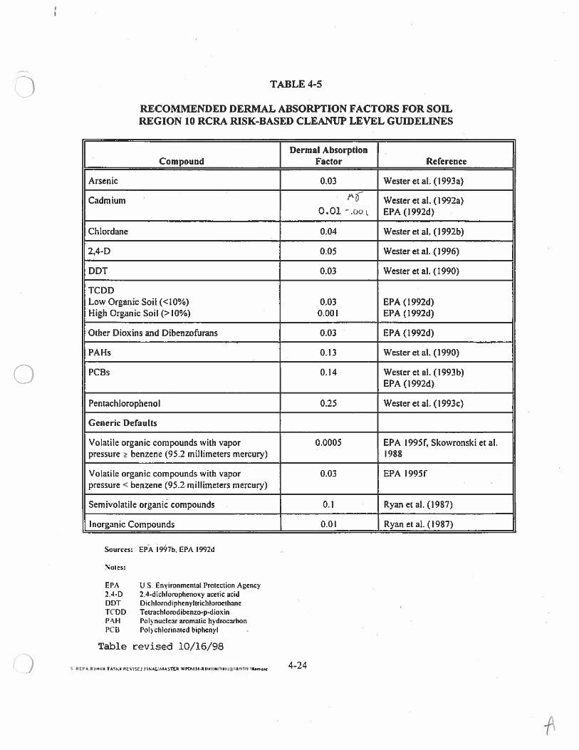
TABLE 4-5

RECOMMENDED DERMAL ABSORPTION FACTORS FOR SOILREGION 10 RCRA RISK-BASED CLEANUP LEVEL GUIDELINES

Dermal AbsorptionCompound Factor Reference

Arsenic 0.03 Wester et al. (1993a)

Cadmium Wester et al. (l992a)0.01 -.oo EPA(l992d)

Chlordane 0.04 Wester et al. (1992b)

2,4-D 0.05 Wester et al. (1996)

DDT 0.03 Westeretal. (1990)

TC DDLow Organic Soil (<10%) 0.03 EPA (1992d)High Organic Soil (>10%) 0.001 EPA (l992d)

Other Dioxins and Dibenzoftarans 0.03 EPA (1992d)

PAHs 0.13 Wester et al. (1990)

PCBs 0.14 Wester et al. (I 993b)EPA (1992d)

Pentachlorophenol 0.25 Wester et aT. (1993c)

Generic Defaults

Volatile organic compounds with vapor 0.0005 EPA 199Sf, Skowronski et al.pressure benzene (95.2 millimeters mercury) 1988

Volatile organic compounds with vapor 0.03 EPA 199Sfpressure < benzene (95.2.millimeters mercury)

Semivolatile organié compounds 0.1 Ryan et al. (1987)

Inorganic Compounds 0.01 Ryan et al. (1987)

Sources: EPA 1997b, EPA 1992d

Notes:

EPA U.S. Enyironmenlal Protection Agency2.4-13 2.4-dichlorophenoxy acetic acidDDT DichlorodiphenyltrichloroethancTCDD Tetrachlorodibenzo-p-dioxinPAR [‘olynuclear aromatic hydrocarbonI’CB Polychlorinated hiphenyl

Table revised 10/16/98

S REPA R I’MIW.TASKW.RE1St FINAL\MkSUR WP0I5$R ICRP$RU7IRHU1Ifl7PI $RImC ——

To evaluate dermal contact with constituents in water, dermal absorption across the skin, barrier is

determined using constituent-specific dermal permeability constants, expressed in units of centimeters per

hour. Equations for calculating dermal permeability constants are presented in Dermal Exposure

Assessment: Principles andApplications (EPA 1992d); EPA recommends calculating permeability

constants for organic compounds using the Potts and Guy equation presented on pages 5-36 through 5-38

(EPA 1992d). EPA recommends the use of the measured permeability constants for inorganic compounds

presented in Table 5-3 of the dennal exposure assessment report (EPA 1992d). The dermal exposure to

constituents in the water pathway was not incorporated into EPA Region 9 PRG equations. Equations for

assessing this pathway are included in Dermal Exposure Assessment: Principles and Applications

(EPA I 992d). Reduced equations for calculating risks or hazards resulting from dermal contact with

constituents in water have been incorporated in the Section 4.7.2 RBC calculation equations. Adult and

child residential exposures (during showering or bathing) are considered.

When evaluating the dermal contact exposure pathway (for both soil and water) the total surface area of

body exposed must be estimated. For showering and bathing, whole-body surface area is assumed. For

soil exposures, portions of the body (for example, hands, arms, lower legs, face, and neck) are assumed to C)contact soil. The duration of exposure must also be estimated (for example, assume a 15-minute-per-day

showering time). EPA-recommended defaults for dermal contact exposure factors are presented in

Table 4-6.

4.5.2 Fate and Transport Models

Table 4-I, discussed in Section 4.1, lists potential exposure pathways for human receptors. Many of the

exposure pathways result from contamination migrating from one medium to another. For example, soil

contamination may migrate into groundwater, subsequently causing exposure to persons using the

contaminated aquifer as a drinking water source and/or discharge to surface waters, which may have both

human health and ecological impacts, depending on use. Cleanup levels for the primary medium may

require an adjustment to be protective of hazardous constituent migration into the secondary medium.

Certain fate and transport modeling equations have been standardized for this purpose.

4-’ 5S PEPAR 1•’ITASKrAE’iSEIIJALMASTtX —

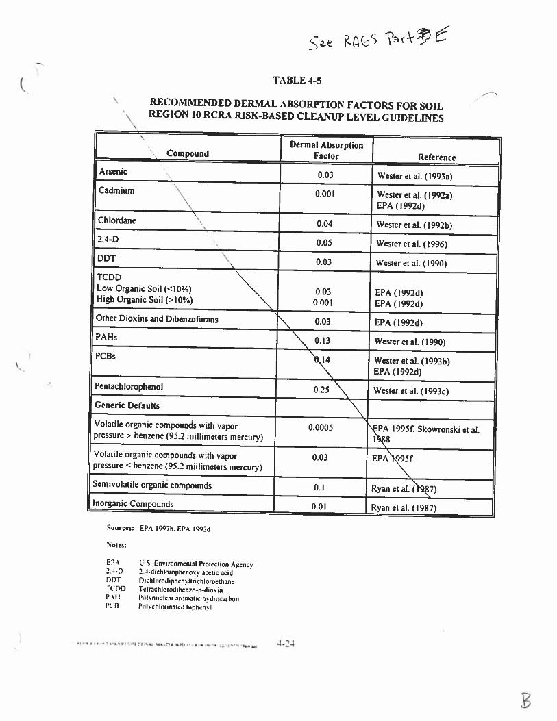
TABLE 4-5

Notes:

EP\2.4-0DDTROD

5’“LII

RECOMMENDED DERMAL ABSORPTION FACTORS FOR SOILREGION 10 RCR4 RISK-BASED CLEANUP LEVEL GUIDELINES

US EnironmcniaI Protection Agency23-dichIorophenov acetic acidDrchInrodiphen irichiorocihaneTcirachiorodihcnzo-p-dioinPok nucear aromatic hdri,ca,honPok chlorinaicd hiphen I

F rermai Absorption JCompound Factor Reference

Arsenic 0.03 Westeret al. (l993a)

Cadmium N 0.001 Wester et a!. ( I 992a)N. EPA(1992d)

Chordane N 0.04 Wesier et a!. (1 992b)

2,4-0 0.05 Wester et al, (1996)

DOT 0.03 Wester ci a). (1990)

TCDD N.Low Organic Soil (<10%) 0.03 EPA (1992d)High Organic Soil (>10%) 0.001 EPA ( I 992d)

Other Dioxins arid Dibenzothrans 0.03 EPA (1992d)

PARs 0.13 Wester et a). (1990)

PCBs \j4 Wester et a!. (199Th)

\ EPA (1992d)

Pentachlorophenol 0.25 Westeret al. (1993c)

Generic Defaults

Volatile organic compounds with vapor 0.0005 \çPA 199Sf, Skowronski et a!.pressure benzene (95.2 millimeters mercury)

Volatile organic compounds with vapor 0.03 EPA”3Q95fpressure < benzene (95.2 millimeters mercury)

Semivolatile organic compounds 0.1 Ryan ci alRN7)

Inorganic Compounds 0.01 Ryan et al. (1987)

Sources: EPA 1997b. EPA 1992d

) 4-23.‘H;[I

To evaluate dermal contact with constituents in water, dermal absorption across the skin barrier is

determined using constituent-specific dermal permeability constants, expressed in units of centimeters per

hour. Equations for calculating dermal permeability constants are presented in De,-mal Lrposure

Assessment: Principles and Applications (EPA 1992d); EPA recommends calculating permeability

constants for organic compounds using the Ports and Guy equation presented on pages 5-36 through 5-38

(EPA 1992d). EPA recommends the use of the measured permeability constants for inorganic compounds

presented in Table 5-3 of the dermal exposure assessment report (EPA 1992d). The dermal exposure to

constituents in the water pathway was not incorporated into EPA Region 9 PRG equations. Equations for

assessing this pathway are included in Dermal Exposure Assessment: Principles a.d Applications

(EPA I 992d). Reduced equations for calculating risks or hazards resulting from dermal contact with

constituents in waler have been incorporated in the Section 4.7.2 RBC calculation equations. Adult and

child residential exposures (during showering or bathing) are considered.

When evaluating the dermal contact exposure pathway (for both soil and water) the total surface area of

body exposed must be estimated. For showering and bathing, whole-body surface area is assumed. For

soil exposures, portions of the body (for example, hands, arms, lower legs, face, and neck) are assumed to

contact soil. The duration of exposure must also be estimated (for example, assume a 15-minute-per-day

showering time). EPA-recommended defaults for denial contact exposure factors are presented in

Table 4-6.

4.5.2 Fate and Transport Models

Table 4-1. discussed in Section 4.1, lists potential exposure pathways for human receptors. Many of the

exposure pathways result from contamination migrating from one medium to another. For example, soil

contamination may migrate into groundwater, subsequently causing exposure to persons using the

contaminated aquifer as a drinking water source and/or discharge to surface waters, which may have both

human health and ecological impacts, depending on use. Cleanup levels for the primary medium may

require an adjustment to be protective of hazardous constituent migration into the secondary medium.

Certain fate and transport modeling equations have been standardized for this purpose.

1”

•“.‘-M,,flH’ ;PO ... .,: ——

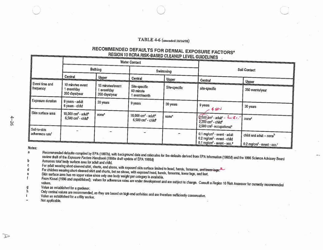
TABLE 4-6 (amended 10/16198)

RECOMMENDED DEFAULTS FOR DERMAL EXPOSURE FACTORS5REGION 10 ACRA RISK-BASED CLEANUP LEVEL GUIDELINESWater Contact

Soil ContactBathing SwimmingCentral Upper Central Upper Central j UpperEvent time and 10 minutes event 15 minutes/event Site-specific Site-specific site-specific 350 events/yearfrequency 1 event/day 1 event/day 60 minute350 days/year 350 days/year I event/month

Exposure duration 9 years - adult 30 years 9 years 30 years 9 years 30 yearsSyears-child4 &‘

Skin surface area 18,000 cm2 - adult” none 18,000 cnf - adult” nones iao)rnz - adult’ — f-” r— non&6,500 cm2 - chil& 6,500 c& - chil& 220 cm2 - chil&2,500 cii?- occupational°

Soil-to-skin —— — — 0.1 mg’cm2 - event - adult child and adult — nonehadherence rat&

0.2 m’cm2 - event - child0.1 m’cm2 - event - occ. 0.2 mg’cm2 - event - ccc)

Notes:a Reconvnended defaults compiled by EPA (1997b), with backound data and rationales (or the defaults derived from EPA information (1992d} and the 1996 Science Advisory Board

review draft of the Exposure Factors Handbook(1996e draft update of EPA 1989d)b Assumes total body surface area For adult and child.c For adult wearing shod-sleeved shirt, shorts, and shoes, with exposed skin surface limited to head, hands, forearms, mld4ewef-legs?’d For chitdren wearing short-sleeved shin and shorts, but no shoes, with exposed head, hands, forearms, lower legs, and feet.a Skin surface area has no upper value since only one body weight per category is available.From Kissel (1996 and unpublished); values for adherence rates are under development and are subject to change. Consult a Region 10 Risk Assessor for currently recommendedvalues.

Value as established for a gardener.-Only central values are recommended, as they are based on high-end activities and are therefore sufficiently conservative.Value as established for a utility worker.

M0-i

9h

— Not applicable.

Models that address volatile and particulate emissions from soil into air are described in Section 4.5.2.1.Fate and transport assumptions that estimate the transfer of VOC from water into indoor air duringhousehold water use are identified in Section 4.5.2.2. A model and partition equation that addressmigration of constituents from soil to groundwater are described in Section 4.5.2.3. Partition equationsthat address migration of constituents from soil into food chain organisms are discussed inSection 4.5.2.4.

Several of the models discussed in this section are recommend by EPA’s Soil Screening Guidance:Users Guide (EPA l996b). These include models for estimating volatile and particulate emissions fromsoil, and a model for estimating soil-to-groundwater constituent migration. EPA’s soil screening levelsand associated models Were developed for screening purposes, for use during early investigativeprocesses such as the RFI. The use of conservative, facility-specific soil and aquifer parametefswillresult in the calculation of health-protective soil screening levels. The facility must adequately justi& allfacility-specific parameters used to calculate soil screening levels.

Although the EPA soil screening guidance (1996b) was developed for the CERCLA program, it can beconsidered for RCRA corrective action facilities. EPA does not intend for soil screening levels to serveas national cleanup standards. The screening levels are very conservative and can be used to determinethat the soil-to-air or soil-to-groundwater pathways are either not significant or that further assessment ofthese pathways is warranted. The soil screening levels could be used as cleanup levels if conditions atthe facility are representative of those assumed during the development of the screening levels. Highercleanup levels that are still he. th protective may be identified using facility-specific fate and transponmodels.

4.5.2.1 Soil-to-Air

Volatilization and particulate emission factors (VF and PEF). which are described in the followingsection, are used in the soil RBC calculations to address long-term inhalation exposures. Equations forderiving these factors are presented in Tables 4-7 and 4-8. Section 4.7 and Exhibit 4-I present how thefactors are incorporated into RBC calculations. VFs should be estimated for VOCs, while PEFs shouldbe estimated for compounds that may exert significant toxicity via dust inhalation. VOCs are defined in

S REPAR ItuittAski .R2VSE2flNAL(MThR WTOt I nin,rt 1I,mun 4—27

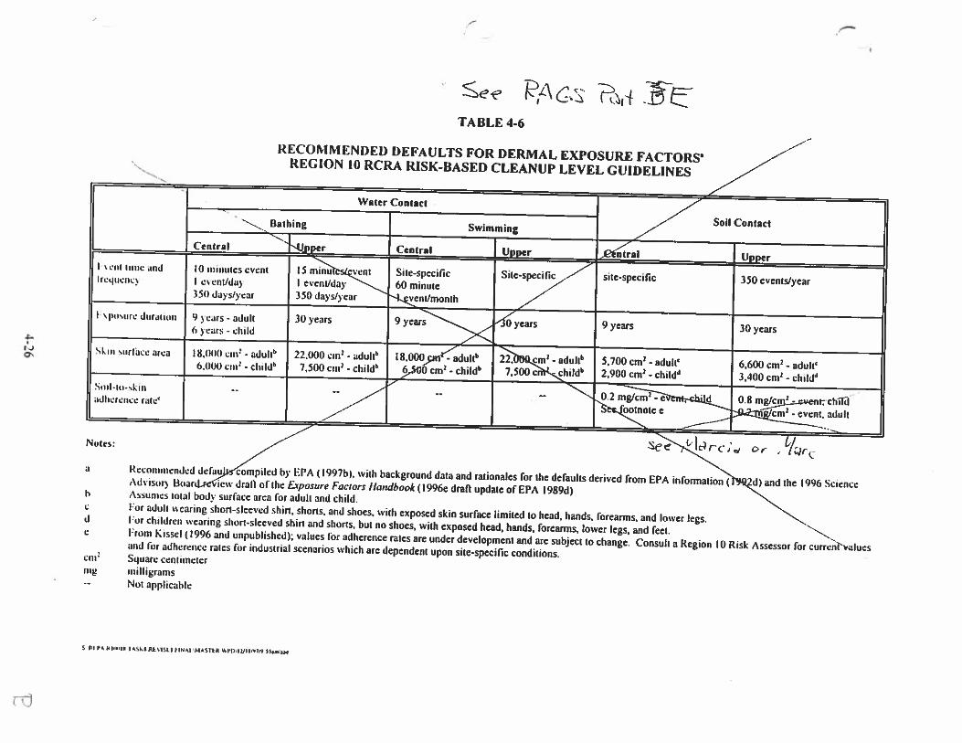
$ee L%s 1:1 wTABLE 4-6

Water Contact•

Soil Contact.Bathing Swimming

Central t-pper Central [upper Q€al UpperI Li1t time and ID nittiles cveni IS minu enl Site-specific Site-specific site-specific 350 events/yearIrcqtici’c’ I eentJda3 I event/day 60 minute

350 days/year 350 days/year EnUmonth77

‘r° duruiion 9 years - adult 30 years 9 years 46’years 9 years 30 years(a years — child

Skin snrtbee area 18,OttO cm1 - adullb 22.000 cm’ - adulL6 l8,000aIdultb boQ.&m- adultb 5,700 cm’ - adult’ 6,600 cm2 - adult’6.000 en” - cluldb 7.500 cm’ - childb 950 cm2 - childb 7,500 c)i.hdd6 2,900 cm’ - childd 3,400 cm’ - childdSuit-to-skits

----

--

— ‘‘-

0.2-e ,d 0.8idlicrejice rule’ectootnote e cm - event, adult

-

.

Notes:

a Recommended defa9jss<mpiled by EPA (1997b). with background data and raLionales for the defaults derived from EPA infonnatiot9çd) and the 1996 ScienceAd’ ison BoariLrdiew draft of the £zposure Factors Handbook (I 996e draft update of EPA l989d)h Assumes total body surface area for adulL and child.c For adult wearing short-sleeved shin, shorts, and shoes, with exposed skin surface limited to head, hands, forearms, and lower legs.LI F children wearing short-sleeved shin and sltons, but no shoes, with exposed head, hands, forearms, lower legs, and feet.e From Kissel (1996 wad unpublished); values for adherence rates are under development and are subject to change. Consult a Region 10 Risk Assessor for currenhaluesand fur adherence rates for industrial scenarios which are dependent upon site-specific conditions.en’1 Square centuneternag ti ill grams-. Not applicable

N

RECOMMENDED DEFAULTS FOR DERMAL EXPOSURE FACToRS’REGION 10 RCRA RISK-BASED CLEANUP LEVEL GUIDELINES

S RIPS iII I SSKi flSISI. I RINM MASfl AYfl.IUSiff*fl i,,...

Models that address volatile and particulate emissions from soil into air are described in Section 4.5.2.1.

Fate and transport assumptions that estimate the transfer ofVOC from water into indoor air during

household water use are identified in Section 4.5.2.2. A model and partition equation that address

migration of constituents from soil to groundwater are described in Section 4.5.2.3. Partition equations

that address migration of constituents from soil into food chain organisms are discussed in

Section 4.5.2.4.

Several of the models discussed in this section are recommend by EPA s Soil Screening Guidance:

Users Guide (EPA 1996b). These include models for estimating volatile and particulate emissions from

soil, and a model for estimating soil-to-groundwater constituent migration. EPA’s soil screening levels

and associated models were developed for screening purposes, for use during early investigative

processes such as the REI. The use of conservative, facility-specific soil and aquifer parameters will

result in the calculation of health-protective soil screening levels. The facility must adequately justify all

facility-specific parameters used to calculate soil screening levels.

Although the EPA soil screening guidance (1996b) was developed for the CERCLA program, it can be

considered for RCRA corrective action facilities. EPA does not intend for soil screening levels to serve

as national cleanup standards. The screening levels are very conservative and can be used to determine

that the soil-to-air or soil-to-groundwater pathways are either not significant or that further assessment of

these pathways is warranted. The soil screening levels could be used as cleanup levels if conditions at

the facility are representative of those assumed during the development of the screening levels. Higher

cleanup levels that are still health protective may be identified using facility-specific fate and transport

models.

4.5.2.1 Soil-to-Air

Volatilization and particulate emission factors (VF and PEF). which are described in the following

section. are used in the soil RBC calculations to address long-term inhalation exposures. Equations for

deriving these factors are presented in Tables 4-7 and 4-8. Section 4.7 and Exhibit 4-1 present how the

factors are incorporated into RBC calculations. VFs should be estimated for VOCs, while PEFs should

be estimated for compounds that may exert significant toxicity via dust inhalation. VOCs are defined in

4 97-k,-p.kk. .PD ——

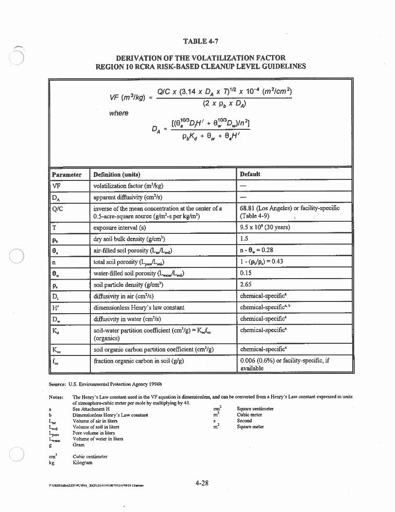
TABLE 4-7

DERIVATION OF THE VOLATILIZATION FAORREGION 10 RCRA RISK-BASED CLEANUP LEVEL GUIDELINES

Q/C x (3.14 x D x 7)1/2 x iO (m2icm2)VF (m3/kg) = A

(2 X Pb X DA)

where

D= [(O°’3DfrI’ +

APbKd + + BJH’

Parameter Definition (units) Default

W volatilization factor (m3/kg) —

DA apparent diffusivity (cm2/s) —

QIC inverse of the mean concentration at the center of a 68.81 (Los Angeles) or facility-specific0.5-acre-square source (gIm2-s per kgl&) (Table 4-9)

T exposure interval (s) 9.5 x 10 (30 years)

1½ dzysoilbu&density(g’/cm3) 1.5

0, air-filled soil porosity (LJL,,,) n -0,, = 0.28

n total soil porosity (LJL,J) I - (pJpj = 0.43

ow water-filled soil porosity (LJL,) 0.15

p, soil particle density (g/cm3) 2.65

D diThisivity in air (cm2/s) chemical-specific’

H’ dimensionless Henry’s law constant chemical-specific’

D diThantvity in water (cm2fs) chemical-specific’

K., soil-water partition coefficient (cm3/g) = KJ0 chemical-specific’(organics)

Pc soil organic carbon partition coefficient (cm3/g) chemical-specific’

f,c fraction organic carbon in soil (gIg) 0.006 (0.6%) or facility-specific, ifavailable

Source: U.S. Environmental Protection Agency 1996b

Notes: The Hairy’s Law constant used in the ‘F equation is dimensionless, and can be converted from a Henry’s Law constant expressed in unitsof atmosphere-cubic meter pa male by multiplying by 41.

a See Attachment H cm’ Square centimeterb Dimensionless Henry’s Law constant in3 Cubic meterL,, Volume of air in liters s Second

L,, Volume of soil in liters In2 Square meterPore volume in liters

L%,, Volume of water in litersg Gram

cm3 Cubic centimeterkg Kilogam

P’aAUEiWLW4) 4-28

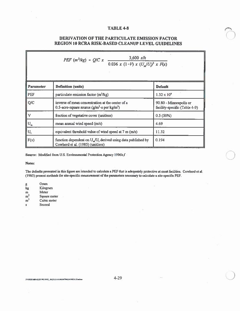
TABLE 4-8

DERIVATION OF THE PARTICULATE EMISSION FACTORREGION 10 RCRA RISK-BASED CLEANUP LEVEL GUIDELINES

PEP (m3/kg) = Q/C 3,600 s/h

0.036 x (14’) x (U,,/L4)3 x F(x)

Parameter Definition (units) Default

PEF particulate emission factor (m3&g) 1.32 x i09

Q/C inverse of mean concentration at the center of a 90.80 - Minneapolis or0.5-acre-square source (g/m2-s per kg/rn3) facility-specific (Table 4-9)

V fraction of vegetative cover (unifless) 0.5 (50%)

Urn mean annual wind speed (mIs) 4.69

U1 equivalent threshold value of wind speed at 7 m (mIs) 11.32

F(x) flmcfion dependent on UjU1 derived using data published by 0.194Cowherd et al. (1985) (unitiess)

Source: Modified from U.S. Environmental Protection Agency 1996b,f ()Notes:

The defaults presented in this figure are intended to calculate a PEF that is adequately protective at most facilities. Cowherd et al.(1985) present methods for site-specific measurement of the parameters necessary to calculate a site-specific PEF.

g Gramkg Kilogramm Meterm2 Square meterm3 Cubic meters Second

P.mA1nW4I3I4UOI.nnWW33 429- U

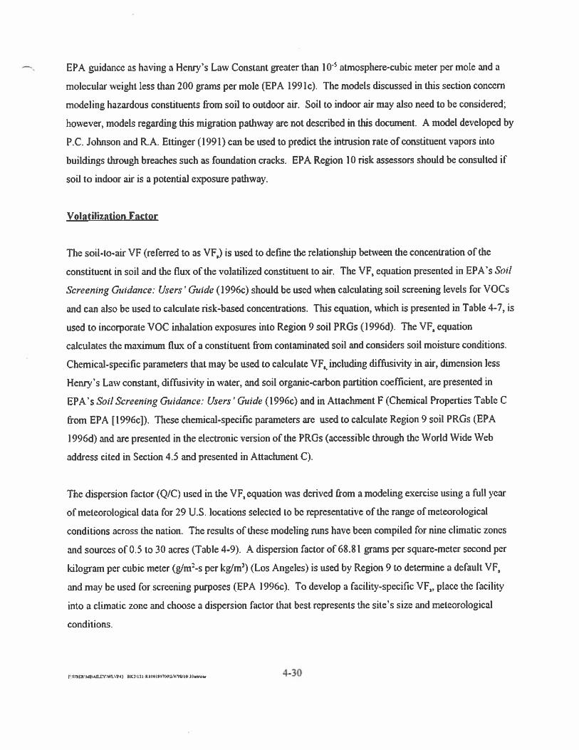
EPA guidance as having a Henry’s Law Constant greater than 10 atmosphere-cubic meter per mole and a

molecular weight less than 200 grams per mole (EPA 1991c). The models discussed in this section concern

modeling hazardous constituents from soil to outdoor air. Soil to indoor air may also need to be considered;

however, models regarding this migration pathway are not described in this document. A model developed by

P.C. Johnson and R.A. Ettinger (1991) can be used to predict the intrusion rate of constituent vapors into

buildings through breaches such as foundation cracks. EPA Region 10 risk assessors should be consulted if

soil to indoor air is a potential exposure pathway.

Volatilization Factor

The soil-to-air VF (referred to as VFJ is used to defme the relationship between the concentration of the

constituent in soil and the flux of the volatilized constituent to air. The VF, equation presented in EPA’s Soil

Screening Guidance: Users’ Guide (1996c) should be used when calculating soil screening levels for VOCs

and can also be used to calculate risk-based concentrations. This equation, which is presented in Table 4-7, is

used to incorporate VOC inhalation exposures into Region 9 soil PROs (1996d). The VF, equation

calculates the maximum flux of a constituent from contaminated soil and considers soil moisture conditions.

Chemical-specific parameters that may be used to calculate VF1 including difflasivity in air, dimension less

Henry’s Law constant, diffusivitv in water, and soil organic-carbon partition coefficient, are presented in

EPA’s Soil Screening Guidance: Users’Guide (1996c) and in Attachment F (Chemical Properties Table C

from EPA [1996c]). These chemical-specific parameters are used to calculate Region 9 soil PROs (EPA

l996d) and are presented in the electronic version of the PROs (accessible through the World Wide Web

address cited in Section 4.5 and presented in Attachment C).

The dispersion factor (Q/C) uscd in the VF,equation was derived from a modeling exercise using a full year

of meteorological data for 29 U.S. locations selected to be representative of the range of meteorological

conditions across the nation. The results of these modeling runs have been compiled for nine climatic zones

and sources of 0.5 to 30 acres (Table 4-9). A dispersion factor of 68.81 grams per square-meter second per

kilogram per cubic meter (gIm-s per kglm3) (Los Angeles) is used by Region 9 to determine a default VF,

and may be used for screening purposes (EPA l996c). To develop a facility-specific VF!, pLace the faciliw

into a climatic zone and choose a dispersion factor that best represents the site’s size and meteorological

conditions.

F .:,a.MOAZZVWL..4) nK:Ln J\& —

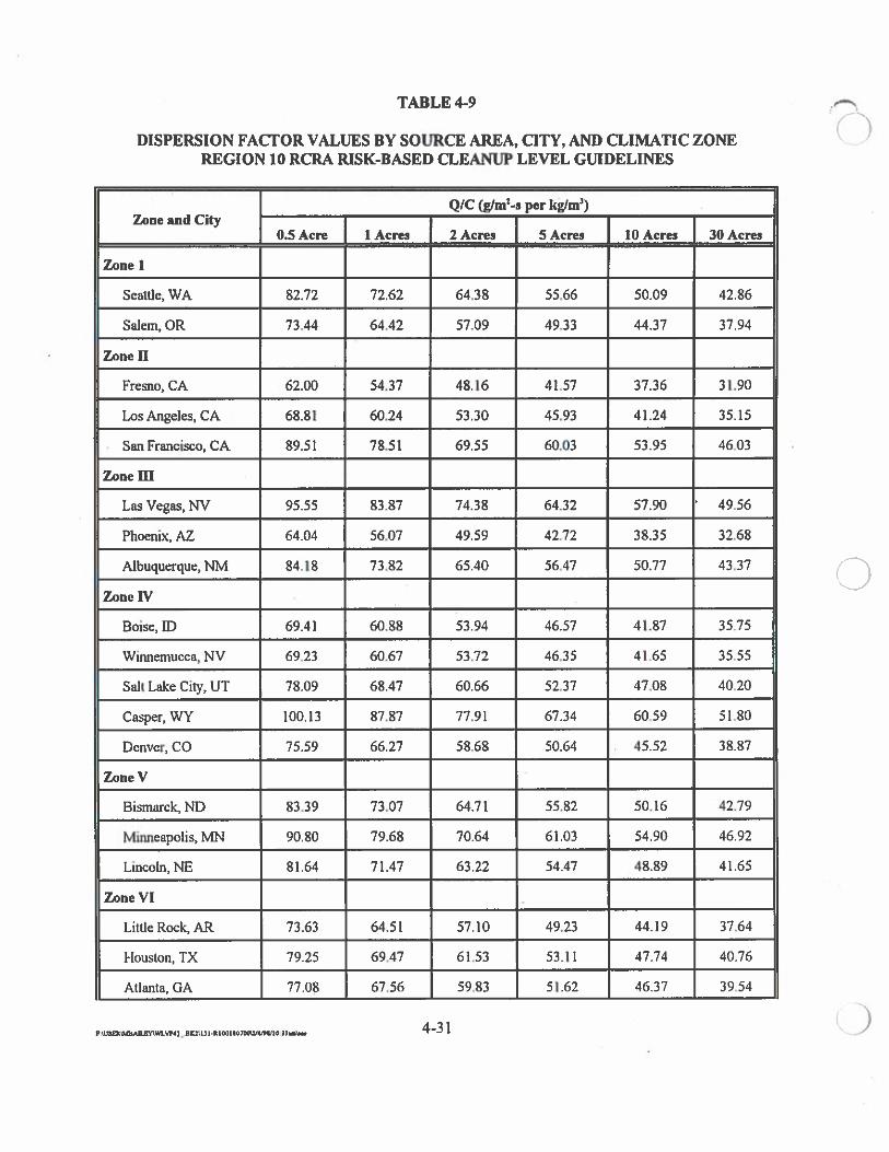
TABLE 4-9

DISPERSION FACTOR VALUES BY SOURCE AREA, CITY, AND CLIMATIC ZONEREGION 10 RCRA RISK-BASED CLEANUP LEVEL GUIDELINES

__ __ __

0

0

__________

QfC (glrn’-s per kg/rn3)Zone and City

0.5 Acre 1 Acres 2 Acres S Acres 10 Acres 30 Acres

Zone I

Seattle, WA 82.72 72.62 64.38 55.66 50.09 4286

Salem, OR 73,44 64.42 57.09 49.33 44.37 37.94

Zone H

Fresno, CA 62.00 54.37 48.16 41.57 37.36 31.90

Los Angeles, CA 68.81 60.24 53.30 45.93 41.24 35.15

• San Francisco, CA 89.51 78.51 69.55 60.03 53.95 46.03

Zone ifi

Las Vegas, NV 95.55 83.87 74.38 64.32 57.90 ‘ 49.56

Phoenix, AZ 64.04 56.07 49.59 42.72 38.35 32.68

Albuquerque, Nl’.’I 84.18 73.82 65.40 56.47 50.77 43.37

ZoneW

Boise, ID 69.41 60.88 53.94 46.57 41.87 35.75

Winnemuccn,NV 69.23 60.67 53.72 46.35 41.65 35.55

Salt Lake City, UT 78.09 68.47 60.66 52.37 47.08 40.20

Casper, WY 100.13 87.87 77.91 67.34 60.59 51.80

Denver, CO 75.59 66.27 58.68 50.64 45.52 38.87

Zone V

Bismarck, ND 83.39 73.07 64.71 55.82 50.16 42.79

Minneapolis, MN 90.80 79.68 70.64 61.03 54.90 4692

Lincoln, NE 81.64 71.47 63.22 54.47 48.89 41.65

Zone VI

LittleRock,AR 73.63 64.51 57.10 49.23 44,19 37.64

Houston, TX 79.25 69.47 61.53 53.11 47.74 40.76

Atlanta, GA 77.08 67.56 59.83 51.62 46.37 39.54

F OSa’IDAflRWLW4-BK1\l5l.RIOiIO7OOW4/WIOi.s\.. 4-31

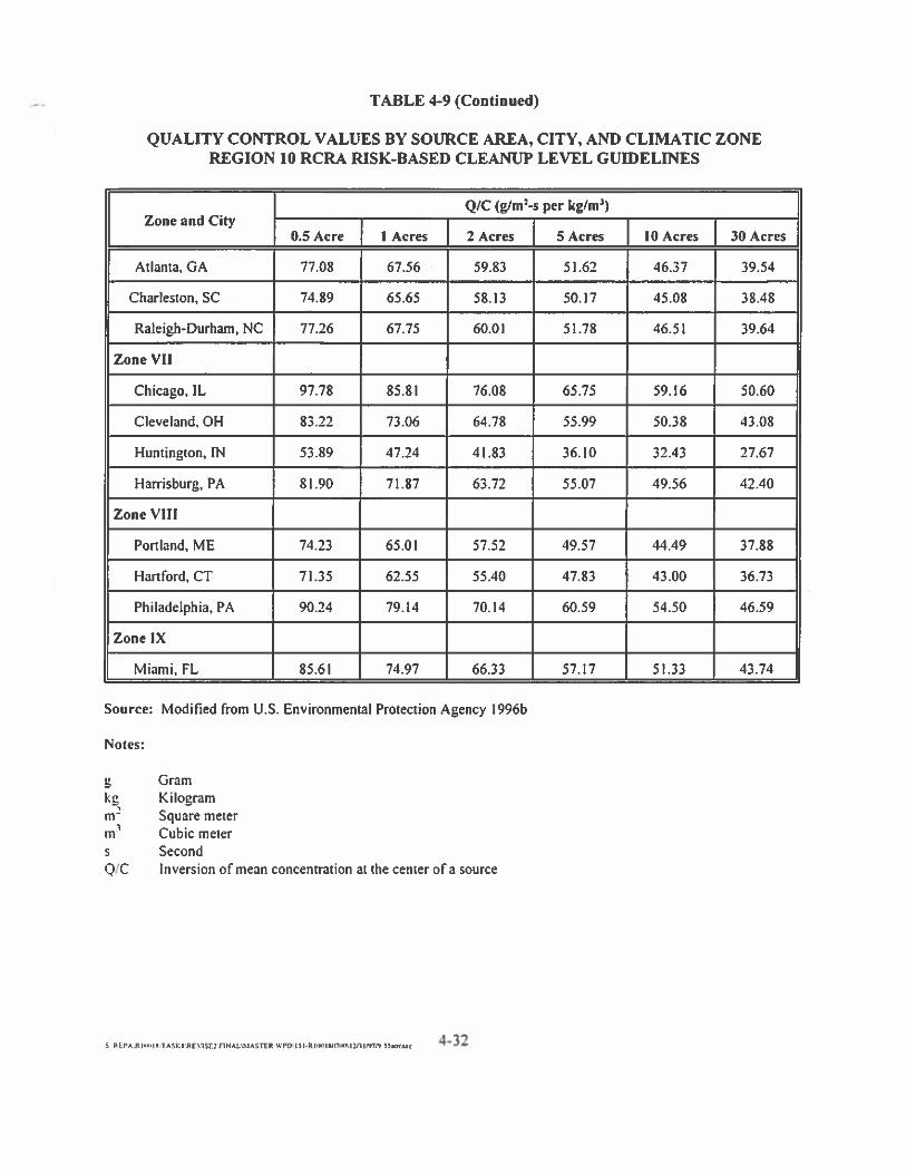
TABLE 4-9 (Continued)

QUALITY CONTROL VALUES BY SOURCE AREA, CITY, AND CLIMATIC ZONEREGION 10 RCRA RISK-BASED CLEANUP LEVEL GUIDELINES

Q/C (g/m-s per kg/rn3)Zone and City I

0.5 Acre I Acres 2 Acres 5 Acres 10 Acres 30 Acres

Atlanta, GA 77.08 67.56 59.83 51.62 46.37 39.54

Charleston, SC 74.89 65.65 58.13 50.17 45.08 38.48

Raleigh-Durham, NC 77.26 67.75 60.01 51.78 46.51 39.64

Zone VII

Chicago, IL 97.78 85.81 76.08 65.75 59.16 50.60

Cleveland, OH 83.22 73.06 64.78 55.99 50.38 43.08

Huntington, [N 53.89 47.24 41.83 36.10 32.43 27.67

Harrisburg, PA 81.90 71.87 63.72 55.07 49.56 42.40

Zone VIII

Portland, ME 74.23 65.01 57.52 49.57 44.49 37.88

Hartford, CT 71.35 62.55 55.40 47.83 43.00 36.73

Philadelphia, PA 90.24 79.14 70.14 60.59 54.50 46.59

Zone IX

Miami, FL 85.61 74.97 66.33 57.17 51.33 43.74

Source: Modified from U.S. Environmental Protection Agency l996b

Notes:

g Gramkg Kilogramm2 Square meterm1 Cubic meters SecondQ/C Inversion of mean concentration at the center of a source

REPA R IIflIkTASK.RE95E3flNALA5flM IP’7PI 1.m’s1. 432

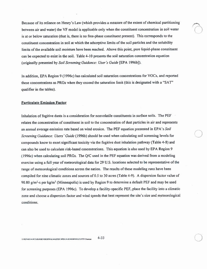
Because of its reliance on Henry’s Law (which provides a measure of the extent of chemical partitioning

between air and water) the VF model is applicable only when the constituent concentration in soil water

is at or below saturation (that is, there is no free-phase constituent present). This corresponds to the

constituent concentration in soil at which the adsorptive limits of the soil particles and the solubility

limits of the available soil moisture have been reached. Above this point, pure liquid-phase constituent

can be expected to exist in the soil. Table 4-10 presents the soil saturation concentration equation

(originally presented by Soil Screening Guidance: Users Guide [EPA I 996bJ).

In addition, EPA Region 9 (1996c) has calculated soil saturation concentrations for VOCs, and reported

these concentrations as PRGs when they exceed the saturation limit (this is designated with a “SAT’

qualifier in the tables).

Particulate Emission Factor

Inhalation of fugitive dusts is a consideration for nonvolatile constituents in surface soils. The PEF

relates the concentration of constituent in soil to the concentration of dust particles in air and represents

an annual average emission rate based on wind erosion. The PEF equation presented in EPA’s Soil

Screening Guidance: Users Guide (1996b) should be used when calculating soil screening levels for

compounds know to exert significant toxicity via the fugitive dust inhalation pathway (Table 4-8) and

can also be used to calculate risk-based concentrations. This equation is also used by EPA Region 9

(1996c) when calculating soil PRGs. The Q/C used in the PEF equation was derived from a modeling

exercise using a full year of meteorological data for 29 U.S. locations selected to be representative of the

range of meteorological conditions across the nation. The results of these modeling runs have been

compiled for nine climatic zones and sources ofo.5 to 30 acres (Table 4-9). A dispersion factor value of

90.80 gJm2-s per kg/m3 (Minneapolis) is used by Region 9 to determine a default PEF and may be used

for screening purposes (EPA 1996c). To develop a facility-specific PEF, place the facility into a climatic

zone and choose a dispersion factor and wind speeds that best represent the site’s size and meteorological

conditions.

S EPMRIIW,PI\TA5ISJEVCflAfl4ASflR WThU3p nhI.Pp,o7npv3t.r., 3!.c -

TABLE 4-10

DERIVATION OF THE SOIL SATURATION LIMITREGION 10 RCRA RISK-BASED CLEANUP LEVEL GUIDEL[NES

C58 = + 0, H’ O)Pb

Parameter Definition (units) Default

C,,, soil saturation concentration (mg/kg) calculated

S solubility in water (mg/L-water) chemical-specific’

Pb dry soil bulk density (kg/L) 1.5

Kd soil-water partition coefficient (L/kg) x f (chemical-specific’)

f fraction organic carbon in soil (g/g) 0.006(0.6%) or facility-specific, if available

ow water-filled soil porosity (L,,5L,01) 0.15

H’ dimensionless Henry’s law constant chemical-specific’

0, air-filled soil porosity (L,,/L1) n -= 0.28

n total soil porosity I- (Pb/Ps) = 0.43

p, soil particle density’ (kg/L) 2.65

Source: Modified from U.S. Environmental Protection Agency 1996b

Notes:

a See Attachment Hmg/kg Milligram per literL Literg GramLWMCr Volume of waterL01 Volume of soil in litersLair Volume of air in litersL01 Pore volume in liters

S REPSR ICM,i,[TASK,Rr3fl5E,’$iNA1iMA5flfl WPO\151.Rii,iiA4i 7CiS I

Both EPA (1 996b) and EPA Region 9 (I 996c) acknowledge that when soil ingestion and fugitive dust

inhalation are evaluated together, the risks and hazards associated with ingestion are significantly greater

than those associated with inhalation. Exceptions are the metals chromium (hexavalent form) and

cadmium; therefore, the inclusion of the fugitive dust inhalation pathway can be limited to these two

metals or other compounds known to exert significant toxicity via dust inhalation. Default PEF

modeling assumptions can normally be assumed; however, if site conditions are such that higher fugitive

dust emissions than the defaults are likely (for example, thy, dusty soils, high average annual wind

speeds, vegetative cover less than 50 percent) and cadmium or hexavalent chromium is present in surface

soils, site-specific parameters should be used in the PEF equation (EPA 1996b).

4.5.2.2 Household Water-to-Indoor Air

A groundwater-to-indoor air VF (VF) of 0.005 x 1,000 L/m3 is used to define the relationship between

the concentration of the constituent in household water and the average concentration of the volatilized

constituent in air (EPA 199 Ic). In the derivation, all uses of household water were considered (for

example, showering, laundering, dish washing). It was assumed that the volume of water used in a

residence for a family of four is 720 Llday, the volume of the home is 150,000 L, and the air exchange

rate is 0.25 m3/hour. Furthermore, it is assumed that the average transfer efficiency weighted by water

use is 50 percent (that is, half of the concentration of each chemical in water will be transferred into air

by all water uses. Note: the range of transfer efficiencies extends from 30 percent for toilets to

90 percent for dishwashers). The VF is used in the groundwater RBC calculation equation (presented in

Section 4.7.2) to assess volatilization of constituents from tap water into indoor air. Use of the EPA

(1991 c) water-to-air Vf results in a conservative estimation of volatilized constituent concentrations.

Updated estimates of water volume use, house volume, and air exchange rate are presented in the 1995

draft revised Exposure Factors Handbook (EPA 1996e) and may be used to recalculate a Vf if

warranted by facility-specific conditions. In addition, the intrusion rate of vapors through building

foundations into enclosed spaces may be predicted using a model developed by Johnson, et al. (1991).

S REPA’RIcIIM’TASKrRE15E2W1NAL9.lAflR WPOU3I.RIIWIlVI7(flI2N7P) SS.m\c 435

4.5.2.3 Soil-to-Groundwater Estimations

)EPA’s Soil Screening Guidance: Users ‘ Guide (EPA I 996b) recommends a dilution factor model and

soil/water partition equation for estimating soil screening levels that are protective of groundwater. The

approach requires that groundwater constituent concentrations at the downgradient edge of contaminated

soil not exceed MCL or risk-based groundwater cleanup levels (that is, cleanup levels for residential

use). The method is applied in step-by-step fashion. A groundwater cleanup level and dilution factor are

identified. The dilution factor is based on facility-specific aquifer characteristics, including hydraulic

conductivity, hydraulic gradient, mixing zone depth, and source length. The dilution factor is multiplied

by the groundwater cleanup level to determine a target soil leachate concentration. The target soil

leachate concentration represents a constituent concentration that, upon dilution in groundwater, will not

result in an exceeded groundwater cleanup level directly beneath the site.

The target soil leachate concentration can be compared directly to leach test results for the site. EPA

(I 996b) provides some guidance on the availability of leach tests and suggests using the EPA Synthetic

Precipitation Leaching Procedure [Method 1312 from the current edition of SW-846 (EPA 1986b)].

EPA (1 996b) also provides a soil/water partitioning equation for converting the target soil leachate

concentration into a total soil concentration. The equation requires that site-specific soil parameters,

including fraction organic carbon, soil porosity, and soil density, be determined. Default soil parameters

are also proposed. The total soil concentration can be used as a soil screening level.

The previous procedures assume an infinite source of contamination. Because this assumption can

violate mass balance considerations, such as for small sources, EPA (1996b) also presents a model for

calculating mass-limit soil screening levels. The mass-limit soil screening level represents a soil

constituent concentration that is still protective of groundwater cleanup levels when the entire volume of

contamination leaches to groundwater over an assumed 30-year exposure duration. The mass-limit soil

screening model can be used when the area and depth of the source are known or can be estimated

reliably. Both standard and mass-limit soil screening levels should be calculated, and the higher of the

two values should be selected (EPA 1996b).

As previously stated, the soil screening concentrations are to be used in preliminary facility

investigations and assume residential exposure circumstances. EPA did not intend that they would serve

S REPAIR 10’Ix WPV\ ‘I-RI rn Ill’ 711111 Ui I ,7r, 33imn. —

as national cleanup standards. More detailed fate and transport models can be used to back-calculate soil

cleanup levels that are protective of groundwater. Additional facility-specific data are required for these ()models. Multimedia models are available that simulate the hazardous constituent transport through both

the vadose zone and the aquifer (for example, MEPAS, GWSCREEN, ROAM, RESRAD, and

MULTIMED). Other models may only simulate vadose zone transport (for example SOLUTE,

BIOPLUME, and AT123D). In this situation, two models should be used to simulate multimedia

transport, and a mass balance conservation approach should be used to connect the models. Qualified

hydrogeologists should be consulted when selecting a fate and transport model, and the use of the model

should be subject to the approval of regulatory personnel overseeing the corrective action or closure

activities. Further modeling and/or monitoring to assess groundwater discharges to surface water may be

required on a facility-specific basis.

Washington State MTCA regulation (WAC 173-340-740) requires that soil cleanup standards be

protective of groundwater. Historically, MTCA has required that the soil concentration be equal to or

less than 100 times the groundwater cleanup standard unless it could be demonstrated that a higher soil

concentration is protective of groundwater at the facility. At this printing, Ecology was preparing to

propose a number of changes to MTCA regulations, including ways to calculate protection of

groundwater from soil contamination. Ecology’s web site should be consulted for proposed and final ()rules (http://www.wa.gov/ecology/tcp/cleanup.html). For further information, contact Charles San Juan

of Ecology at (360) 407-7191.

4.5.2.4 Food Chain Exposure Pathways

Migration of contamination into human food chain pathways may require consideration in facility-

specific situations. For example, if soil contamination is present in areas that are likely to be used for

home gardening, this pathway should be considered when setting soil cleanup levels. EPA RCRA

guidance for assessing indirect exposures at hazardous waste combustion facilities provides useful

intermedia hazardous constituent partitioning equations for estimating constituent migration into the

food chain. The draft Guidance for Performing Screening Level Risk Analyses at Combustion Facilities

Burning Hazardous Wastes (EPA I 994i) compiles and streamlines intermedia partition equations

proposed in earlier RCRA combustion guidance documents (EPA 1990, 1 993d). The EPA (I 994i)

document contains RCRA program guidance issued by the Office of Emergency and Remedial Response,

S ‘REPAm I)ITASKM’EV15E3’$1NAL’MA5ThR WPOSI3I.RHNIIVI7IWI\IVlIfl7N iSim’nc —

while the EPA (1990, l993d, and 1995g) reports are technical support documents. In addition, the draft

Estimating Exposure to Dioxin-Like Compounds (EPA I 994j) presents similar intermedia partition

equations for estimating dioxin uptake into plants, animals, and fish. EPA regional risk assessors should

be contacted for further information on the availability of updated documents.

While much of the RCRA combustion guidance series addresses the fate of constituent air emissions,

partitioning equations presented for secondary migration pathways can be used to derive soil and water

RBCs. The EPA (1994ij) guidance documents address the primary food chain pathways, including

constituent migration into garden produce, fish, beef, and milk. lntermedia constituent partitioning

equations for migration pathways, such as soil-to-root-vegetable and water-to-fish, are recommended.

For example, the equations estimate the concentration of a constituent in a secondary media, such as a

garden plant, that results from constituent uptake into the plant from soil. Similarly, estimates can be

made of constituent concentrations in fish resulting from constituent uptake from water or sediment, or

constituent concentrations in beef cattle and dairy cattle milk resulting from constituent uptake from soil

and plants. These equations rely on constituent-specific biotransfer or bioconcentration factors that

represent the ratio of constituent concentrations in the secondary media (for example, garden produce) to

constituent concentrations in the primary media (for example, soil).

These equations can be used in a KHRA to first calculate constituent concentrations in food chain

pathways resulting from air, soil, or water contamination. Human ingestion rates for these food chain

pathways (for example, garden produce or fish ingestion rates) are then estimated. The dose and

resulting risk or hazard are then calculated. Food chain pathways are not typically considered when

calculating risks or RBCs, and their relevance should be determined on a case-by-case basis. Methods

for assessing food chain exposure pathways are typically conservative and may result in RBCs that are

lower than RBCs based on direct contact. They should not be evaluated at every facility, but should be

considered on a case-by-case basis where the food chain pathway is known to be a complete exposure

pathway. At sites where the plant ingestion pathway may reasonably exist, screening level estimates

may be developed using the EPA Region 10 ASARCO plant uptake data for arsenic, cadmium, and lead.

For other contaminants, applicabLe portions of EPA (1994i) shouLd be used. Special situations where

Food chain organisms such as fish or shellfish are consumed at a subsistence level, such as in Alaska or

for Native American populations, should be incorporated into RBCs. EPA Region 10 risk assessors

should be consulted regarding rates of food consumption for such specific situations (for example, for

S [P5.R P.11K TASLKRE1SE1INALMSThR —

Puget Sound or Columbia River fisheries). EPA Region 10 risk assessors should also be contacted to

confirm the selection of appropriate partitioning equations for use in determining either facility risks and

hazards or facility-specific soil and water RBCs. EPA Region 10 has decided to assume that 10 percent

of the inorganic arsenic in seafood is organic (see Attachment I).

4.6 TOXICITY ASSESSMENT

The toxicity assessment summarizes the toxicologic basis for all chemical-specific toxicity data using

available dose-response information. Toxicity assessments should be conducted as described in

Chapter 7 of Risk Assessment Guidancefor Superfund, Volume I, Human Health Evaluation Manual,

Part A, (EPA 1989c). The following sections present an overview of the types of dose-response

information used to characterize carcinogenic and noncarcinogenic dose responses (Section 4.6.1),

sources of EPA toxicity values (Section 4.6.2), and methods for assessing chemicals without EPA

toxicity values (Section 4.6.3).

4.6.1 Dose-Response Information

In developing F114RA methods, EPA recognizes fundamental differences between carcinogenic and

noncarcinogenic dose-response variables used to estimate risks. Because of these differences, human

health risk is characterized separately for the carcinogenic and noncarcinogenic effects related to

hazardous constituents. Some analytes have both carcinogenic and noncarcinogenic effects, although in

many cases, EPA has published toxicity criteria for only one of them. it should not be assumed that in

all cases this is the more sensitive type of toxic effect. Information sufficient to characterize and/or

quantilv the dose-response relationship may be lacking (for example, in the case of endocrine disruptors,

or when no appropriate animal models exist).

Human epidemiologic data provide the strongest evidence of a positive association between hazardous

constituents and human health effects; however, human health effects data adequate to develop

quantitative dose-response relationships are available for only a few chemicals. As a result, toxicity

information obtained from nonhuman mammalian experiments is often used to predict human

dose-response relationships and to develop chemical-specific toxicity criteria. Animal toxicity data are

typically derived from studies in which animals are exposed to relatively high doses ofa chemical. In

S RE?ARH,Ifl\TA5KAmE5E2’FENA.4A5ThR WPD\33 I.R —

contrast, the chronic exposures evaluated in the HI-IRA are for much lower doses. In addition, the

animals are exposed for relatively short periods of time compared with chronic exposure risk

assessments, which typically assume humans will be exposed for a lifetime. Both of these contribute to

the uncertainties in I-il-IRA (see Section 4.8).

4.6.1.1 Toxicity Information for Carcinogenic Effects

Currently, the key dose-response variable used to evaluate carcinogenic effects is the cancer potency

factor (CPF), which is derived from carcinogenicity studies (typically conducted at high doses). To

evaluate the probability of developing cancer at the lower doses more typically encountered by the

public, the EPA-recommended linearized, multistage model is applied to the data. This mathematical

model expresses individual excess cancer risk as a function of exposure and is based on the conservative

assumption that even a single, low-dose exposure to a carcinogen may result in cancer. The CPF,

expressed as risk per milligrams per kilogram per day [(mg/kg’day)j, quantitatively defines the

relationship between dose and response.

In HI-IRA, chemical-specific CPFs are multiplied by the lifetime average daily dose (LADD) of a

hazardous constituent from a given exposure route to assess the upper-bound cancer risk associated with

that dose. Carcinogenic risk is expressed as the probability of an individual in a population developing

cancer (for example, one in a million or IE-6). Chemical-specific CPFs can be incorporated into RBC

equations along with dose information to back-calculate RBCs that correspond to selected target risks

(Section 4.7).

EPA assigns weight-of-evidence classifications to potential carcinogens. Under this system, chemicals

are classified as belonging to one of six groups (EPA 1997a):

S \REPA\R IIflIU;T4SKWREV5E2S!NAL\MASThR WPD;151.R (%IImI7pIv1 PPJlfl %3.mne — 0

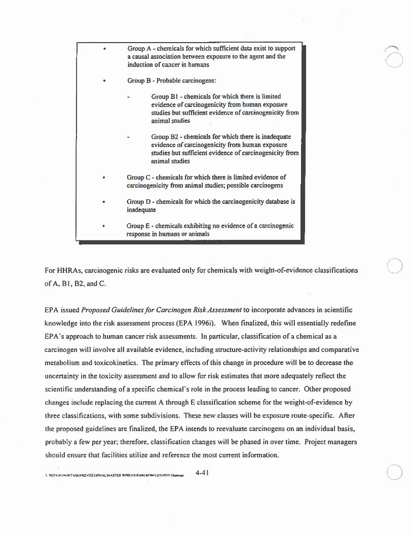
• Group A - chemicals for which sufficient data exist to supporta causal association between exposure to the agent and theinduction of cancer in humans

• Group B - Probable carcinogens:

- Group 81 - chemicals for which there is limitedevidence of carcinogenicity from human exposurestudies but sufficient evidence of carcinogenicity fromanimal studies

- Group 82 - chemicals for which there is inadequateevidence of carcinogenicity from human exposurestudies but sufficient evidence of carcinogenicity fromanimal studies

• Group C - chemicals for which there is limited evidence ofcarcinogenicity from animal studies; possible carcinogens

• Group D - chemicals for which the carcinogenicity database isinadequate

• Group E - chemicals exhibiting no evidence of a carcinogenicresponse in humans or animals

For HHRAs, carcinogenic risks are evaluated only for chemicals with weight-of-evidence classifications

ofA, 81, B2, and C.

EPA issued Proposed Guidelines for Carcinogen Risk Assessment to incorporate advances in scientific

knowledge into the risk assessment process (EPA 1996i). When finalized, this will essentially redefine

EPA’s approach to human cancer risk assessments. In particular, classification of a chemical as a

carcinogen will involve all available evidence, including structure-activity relationships and comparative

metabolism and toxicokinetics. The primary effects of this change in procedure will be to decrease the

uncertainty in the toxicity assessment and to allow for risk estimates that more adequately reflect the

scientific understanding ofa specific chemical’s role in the process leading to cancer. Other proposed

changes include replacing the current A through E classification scheme for the weight-of-evidence by

three classifications, with some subdivisions. These new classes will be exposure route-specific. After

the proposed guidelines are finalized, the EPA intends to reevaluate carcinogens on an individual basis,

probably a few per year; therefore, classification changes will be phased in overtime. Project managers

should ensure that facilities utilize and reference the most current information.

S REPARItMIIRTASKflEV5EflNAL’MASThR WPoI3I-RIrnII’II’IMSImIN7N 33.m,ae 4—41

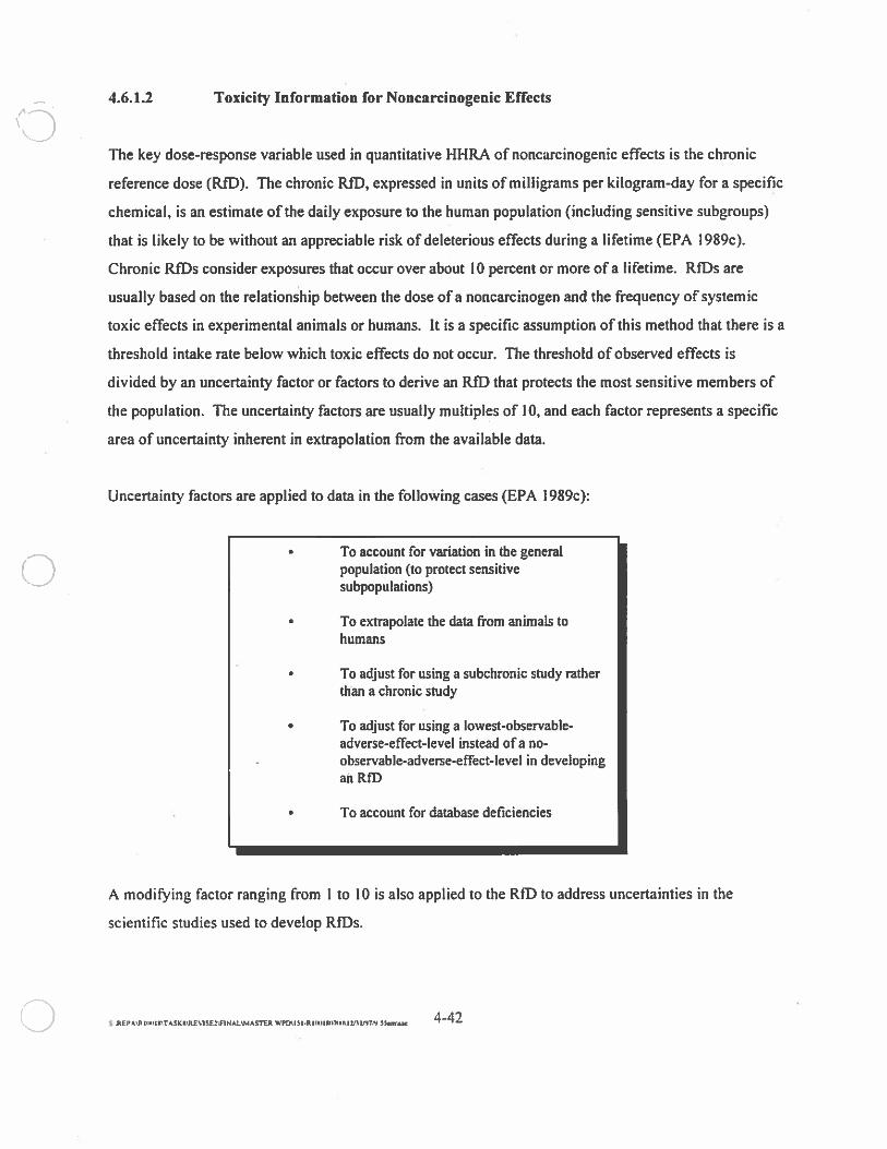
4.6.1.2 Toxicity Information for Noncarcinogenic Effects

The key dose-response variable used in quantitative HI-IRA of noncarcinogenic effects is the chronic

reference dose (RfD). The chronic RID, expressed in units of milligrams per kilogram-day for a specific

chemical, is an estimate of the daily exposure to the human population (including sensitive subgroups)

that is likely to be without an appreciable risk of deleterious effects during a lifetime (EPA 1989c).

Chronic RiDs consider exposures that occur over about 10 percent or more of a lifetime. RtDs are

usually based on the relationship between the dose of a noncareinogen and the frequency of systemic

toxic effects in experimental animals or humans. It is a specific assumption of this method that there is a

threshold intake rate below which toxic effects do not occur. The threshold of observed effects is

divided by an uncertainty factor or factors to derive an RID that protects the most sensitive members of

the population. The uncertainty factors are usually multiples of 10, and each factor represents a specific

area of uncertainty inherent in extrapolation from the available data.

Uncertainty factors are applied to data in the following cases (EPA 1989c):

• To account for variation in the generalpopulation (to protect sensitivesubpopulations)

• To extrapolate the data from animals tohumans

• To adjust for using a subchronic study ratherthan a chronic study

• To adjust for using a lowest-observable-adverse-effect-level instead of a no-observable-adverse-effect-level in developingah RID

- • To account for database deficiencies

A modifying factor ranging from Ito 10 is also applied to the RIO to address uncertainties in the

scientific studies used to develop RIDs.

S .REPARIl.Sa\TASK’REVl5E2\F1NAIS.4ASThR WPDI5I-RISS)IflSflILqI,91N 5Smsat —

Once an RD for a compound has been verified by EPA, it is used to characterize the likelihood of

noncarcinogenic hazards resulting from long-term chemical exposures at a facility. In HHRA, the RD is

compared to the average daily dose (ADD) calculated in the exposure assessment to determine whether

chronic effects might occur. The ratio of the ADD and the RD is called the hazard quotient (HQ). If the

predicted ADD exceeds the RfD, the HQ is greater than 1.0, and there may be concern for potential

noncancer effects (EPA 1989c). HQs for individual constituents can be added to calculate an exposure

pathway or site hazard, referred to as the hazard index (HI). According to Risk Assessment Guidancefor

Superfirnd, Volume 1, Human Health Evaluation Manual, Part A, the addition of HQs from all hazardous

constituents is appropriate as a screening-level approach (EPA 1989c). If the resulting HI is greater than

I .0, however, it would be appropriate to calculate new HIs for hazardous constituents with similar

critical effects and mechanisms of action. Further guidance on segregating COPCs by critical effects and

mechanisms of action is presented in Section 4.7.4. Chemical-specific RIDs can be incorporated into

RBC equations to back-calculate RBCs that corresponded to target hazards (Section 4.7).

EPA has also derived inhalation reference concentrations (RfC), which are estimates of daily exposures

(via inhalation) to the human population including sensitive subgroups that are likely to be without

appreciable risk of deleterious effects. RICs are generally reported as a concentration in air (milligrams

per cubic meter). For purposes of using standard RBC equations, however, RfCs can be converted to a

corresponding inhaled dose (milligram per kilogram-day) by dividing by 70 kilograms (an assumed

human body weight), multiplying by 20 cubic meters per day (an assumed human inhalation rate), and,

preferably, adjusting by an appropriate, chemical-specific absorption factor. This conversion, however,

may often be technically incorrect, and the appropriateness of doing this must be evaluated on a case-by-

case basis (EPA 1997a). RICs can be used in screening risk assessments to determine whether a

constituent may contribute significantly to the HI; however, the appropriateness of RIO conversions and

their use in baseline HHRA’s should be verified by a EPA Region 10 risk assessor (EPA 1997a) prior to

their use.

4.6.2 U.S. Environmental Protection Agency Toxicity Factors

Toxicity factors (RIDs, RfCs, and CPFs) are not always readily available, so multiple sources may need

to be consulted. The EPA Region 10 hierarchy of sources for RIDs, RfCs, and CPFs is as follows:

REPA\R 4—43 3

1. Integrated Risk Information System (IRIS) on-line database (EPA l996g). IRIS is thepreferred EPA source for toxicity information. It provides RfDs, RfCs and CPFs thathave been reviewed and verified by agency-wide work groups. Supporting discussionand references also appear in each chemical file. IRIS User Support at (513)569-7254can provide information about how to access IRIS. IRIS is available to EPA Region 10personnel on its automaxx menu and to the public on EPA’s web site athttp://www.epa.gov/iris.

2. Health Effects Assessment Summary Tables (HEAST) (EPA 1997a). HEASTsummarizes all currently available toxicity factors developed by National Center forEnvironmental Assessment (NCEA) and a bibliography of Health Effects Assessmentsand related documents. These documents contain supporting information for toxicityvalues developed by EPA NCEA. The I-lEAST tables are revised quarterly. Toxicityfactors that appear in IRIS do not appear in HEAST.

3. Provisional values developed byNCEA. Region 10 risk assessment staff should becontacted to obtain information from NCEA.

4. Agency for Toxic Substances and Disease Registry (ATSDR) minimal risk levels(MRL). These MRLs are developed using an approach that is generally consistent withRID methodology. These may be available for acute, intermediate, or chronic exposuredurations and are potentially useful for situations of short-term exposure, for whichverified RfDs are seldom available. They can be found in ATSDR Toxicity Profiledocuments (in the Health Effects Summary section, in the text and/or on the“thermometer” chart). MRLs can also be found on the Internet athftp://atsdrl .atsdr.cdc.gov:8080/mrls.html. Concurrence with use of MRLs for a specificsituation should be sought from Region 10 risk assessment staff.

5. Region 10 risk assessors may have access to additional toxicity numbers from othersources that may be appropriate for a given circumstance.

In addition to the RfDs, RfCs, and CPFs, the EPA weight-of-evidence classifications and the types of

cancers observed in animal testing should be presented for all carcinogenic hazardous constituents, while

the confidence levels, critical effect and target organs, and uncertainty and modifying factors associated

with the available RIDs should also be presented. The identification of critical effects and target organs

becomes important during risk characterization when segregating COPCs for HI calculations.

Since carcinogenic chemicals may also cause noncarcinogenic health effects, RIDs (when available)

should be compiled for carcinogenic chemicals and used to evaluate potential noncarcinogenic effects for

these chemicals. It should not be assumed that noncarcinogenic effects are negligible or even less

important than cancer risks just because RfD or RfCs are not available.

S REPA R c”Ia TAS’RE9SEHNALMA5ThR Wp0s15 I-R3U,I rnnlnJ3ns91n 5.msn —

4.6.3 Chemicals or Exposure Pathways With No U.S. Environmental Protection AgencyToxicity Values

This section identifies key constituents that do not have toxicity values in the EPA IRIS and HEAST

databases. Recommendations for what toxicity values may be used to evaluate these constituents are

presented. Methods for evaluating exposure pathways with limited or no EPA toxicity values are also

presented. If it is determined that provisional or other alternative values may be used, their uncertainties

must be discussed in the risk assessment document (specifically in the risk characterization section) and

should be considered in risk management decisions.

4.6.3.1 Polynuclear Aromatic Hydrocarbons

Polynuclear aromatic hydrocarbons (PAH) are a very extensive group of organic compounds that contain

at least two benzene rings. Sources of PAHs include petroleum and coal tar products. The major source

of PAH releases to the environment is combustion of these products (EPA 1982). PARs may be found at

hazardous waste sites that used or generated these products, such as coal gasification plants, coal tar

generators, power plants, wood treaters that used creosote, and coke manufacturers. Some PARs are

carcinogenic and some are not. Benzo(a)pyrene is currently the only carcinogenic PAR for which a CPF (J)has been verified by EPA. It is recommended that toxicity equivalency factors (TEF) based on the

relative potency of each PAR compound to that of benzo(a)pyrene be used to evaluate the toxicity of the

remaining carcinogenic PARs on the target compound list (see following list). The TEFs presented here

were recommended by EPA’s NCEA and are from the Provisional Guidance for Quantitative Risk

Assessment ofPolycyclic Aromatic Hydrocarbons (EPA 1993e). Concentrations of specific carcinogenic

PARs should be multiplied by their respective TEFs to calculate their concentrations relative to

benzo(a)pyrene potency. This benz(a)pyrene equivalent concentration should then be used for risk

characterization. These TEFs are not in IRIS, and therefore are not necessarily accepted by all states and

maybe revisited by NCEA in the future.

S 445

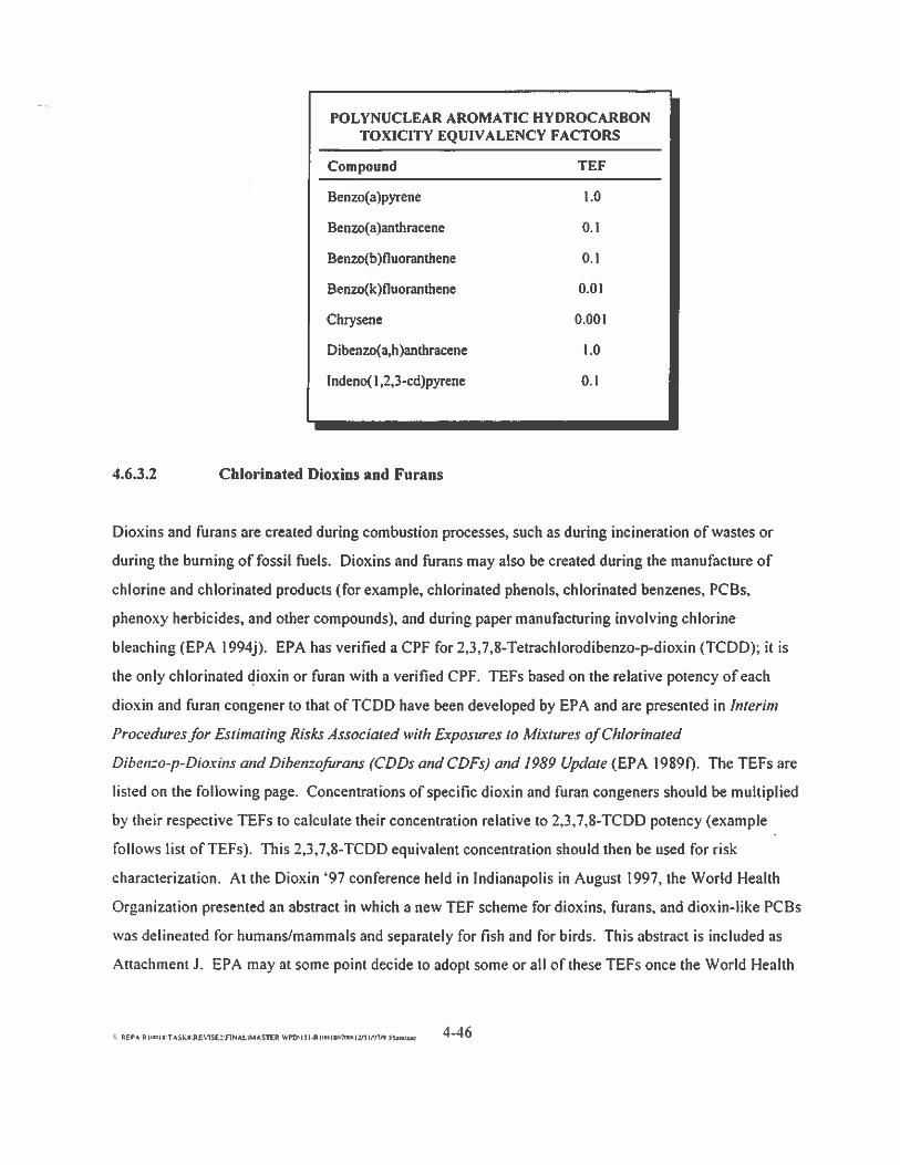
POLYNUCLEAR AROMATIC HYDROCARBONTOXICITY EQUIVALENCY FACTORS

Compound TEF

Benzo(a)pyrene 1.0

Benzo(a)anthracene 0.1

Benzo(b)fluoranthene 0,1

Benzo(k)fluoranthene 0.01

Chrysene 0.001

Dibenzo(a,h)anthracene 1.0

lndeno(1,2,3-cd)pyrene 0.1

4.6.3.2 Chlorinated Dioxins and Furans

Dioxins and furans are created during combustion processes, such as during incineration of wastes or

during the burning of fossil fuels. Dioxins and flirans may also be created during the manufacture of

chlorine and chlorinated products (for example, chlorinated phenols, chlorinated benzenes, PCBs.

phenoxy herbicides, and other compounds), and during paper manufacturing involving chlorine

bleaching (EPA 1994j). EPA has verified a CPF for 2,3,7,8-Tetrachlorodibenzo-p-dioxin (TCDD); it is

the only chlorinated dioxin or furan with a verified CPF. TEFs based on the relative potency of each

dioxin and furan congener to that of TCDD have been developed by EPA and are presented in interim

Proceduresfor Estimating Risks Associated with Exposures to Mixtures ofChlorinated

Dibenzo-p-Dioxins and Dibenzofrrans (‘CDDs and CDFs,) and 1989 Update (EPA I 989fl. The TEFs are

listed on the following page. Concentrations of specific dioxin and furan congeners should be multiplied

by their respective TEFs to calculate their concentration relative to 2,3,7,8-TCDD potency (example

follows list of TEFs). This 2,3,7,8-TCDD equivalent concentration should then be used for risk

characterization. At the Dioxin ‘97 conference held in Indianapolis in August 1997, the World Health

Organization presented an abstract in which a new TEF scheme for dioxins, furans, and dioxin-like PCBs

was delineated for humans/mammals and separately for fish and for birds. This abstract is included as

Attachment J. EPA may at some point decide to adopt some or all of these TEFs once the World Health

REP AR hR K;TASKN\REVISE2’SINALhMA51ER WPD\ II ‘‘RI ER) I 3I)7ERIE I In IflVl i)Jn,Enc —

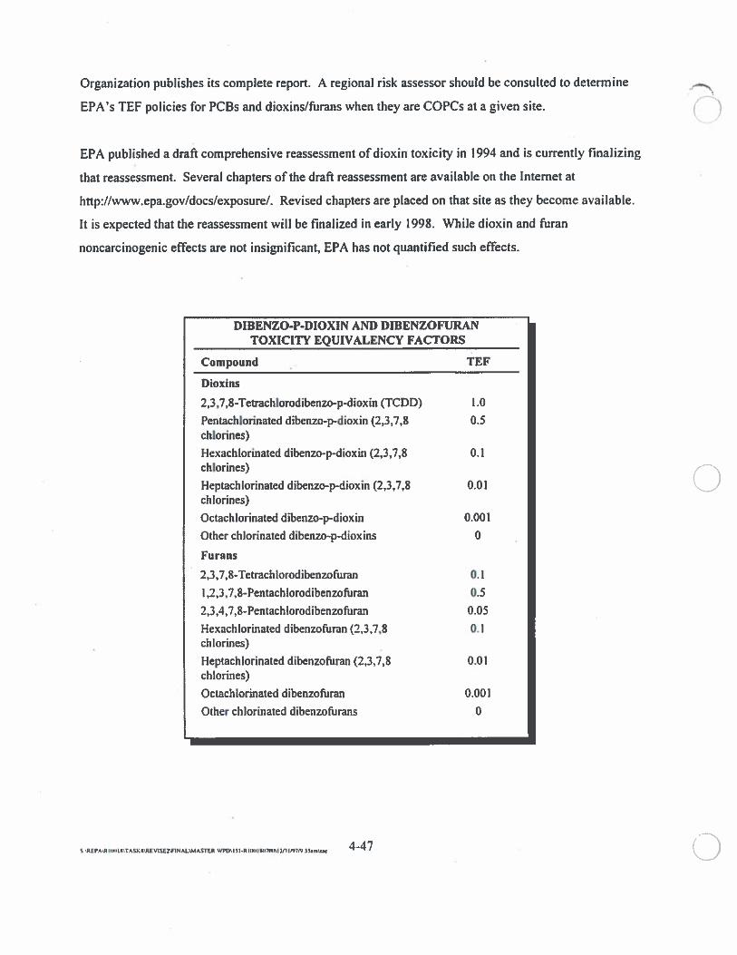
Organization publishes its complete report. A regional risk assessor should be consulted to determine

EPA’s TEF policies for PCBs and dioxins/furans when they are COPCs at a given site.

EPA published a draft comprehensive reassessment of dioxin toxicity in 1994 and is currently finalizing

that reassessment. Several chapters of the draft reassessment are available on the Internet at

hnp://www.epa.gov/docs/exposure/. Revised chapters are placed on that site as they become available.

It is expected that the reassessment will be finalized in early 1998. While dioxin and furan

noncarcinogenic effects are not insignificant, EPA has not quantified such effects.

DIBENZO-P-DIOXIN AND DIBENZOFURANTOXICITY EQUIVALENCY FACTORS

• Compound TEF

Dioxins

2,3,7,8-Tebachlomdibenzo-p-dioxhi (TCDD) 1.0

Pentachlorinated dibenzo-p-dioxin (2,3,7,8 0.5chiorthes)

Hexachlorinated dibenzo-p-dioxin (2,3,7,8 0.1chlorines)

Heptachlorinated dibenzo-p-dioxin (2,3,7,8 0.01chlorines)Octachlorinated dibenzo-p-dioxin 0,001Other chlorinated dibenzo-p-dioxins 0

Fu ra ns

2,3,7,8-Tetrachlorodibenzoftiran 0.1

I ,2,3,7,8-Pentachlorodibenzoftiran 0.5

2,3,4,7,8-Pentachlorodibenzofiiran 0.05

Hexachlorinated dibenzoftran (2,3,7,8 0.1chlorhes)Heptachiorinated dibenzoftran (2,3,7,8 0.01chiorines)

Octachiorinated dibenzofiinn 0.001Other chlorinated dibenzofurans 0

mi ‘ 447

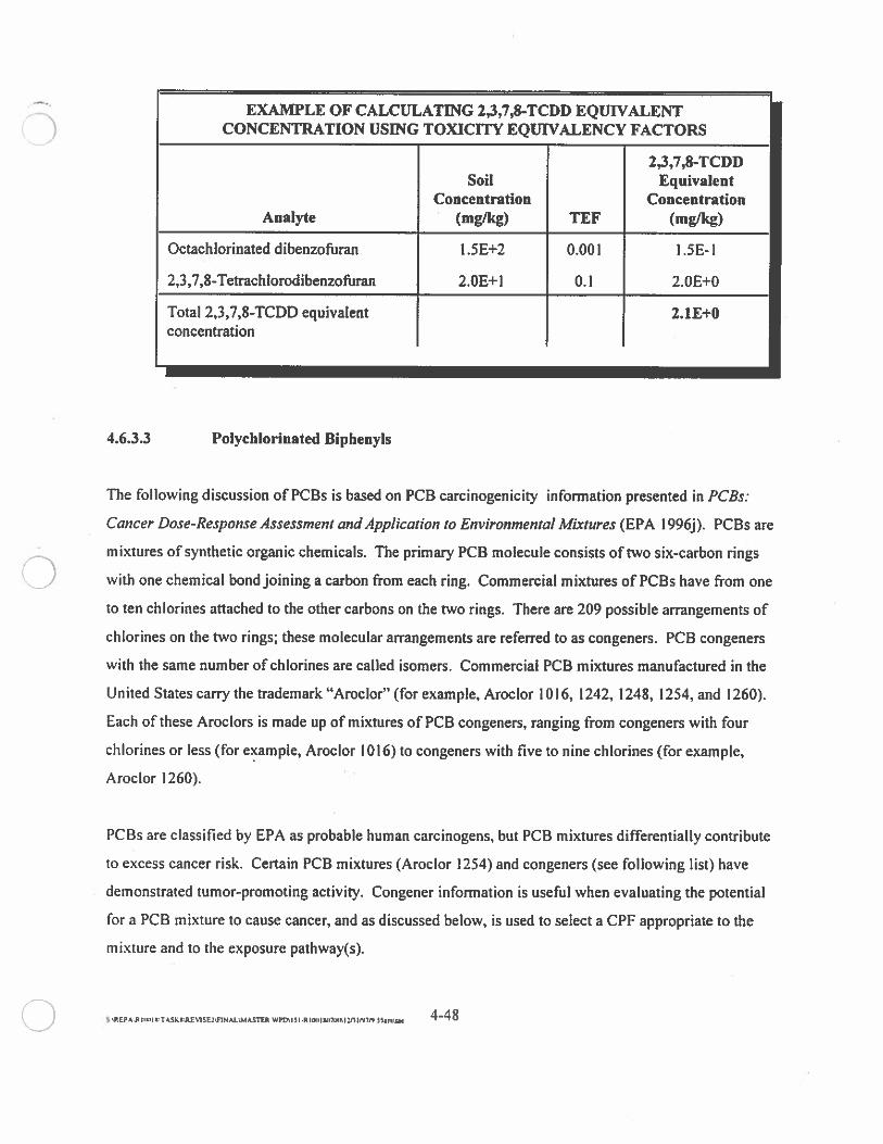
EXAI’i1PLE OF CALCULATING 2,3,7,8-TCDD EQUIVALENTCONCENTRATION USING TOXICITY EQUIVALENCY FACTORS

2,3,7,8-TCDDSoil Equivalent

Concentration ConcentrationAnalyte (mg/kg) TEF (mg/kg)

Octachlorinated dibenzofiiran 1.5E+2 0.00 I 1.5E-l

2,3,7,8-Tetrachlorodibenzofiiran 2.OE+ 1 0.1 2.OE+0

Total 2,3,7,8-TCDD equivalent 2.1E+Oconcentration

4.6.3.3 Polychlorinated Biphenyls

The following discussion of PCBs is based on PCB carcinogenicity information presented in PCBs:

Cancer Dose-Response Assessment and Application to Environmental Mixtures (EPA I 996j). PCBs are

mixtures of synthetic organic chemicals. The primary PCB molecule consists of two six-carbon rings

with one chemical bond joining a carbon from each ring. Commercial mixtures of PCBs have from one

to ten chlorines attached to the other carbons on the two rings. There are 209 possible arrangements of

chlorines on the two rings; these molecular arrangements are referred to as congeners. PCB congeners

with the same number of chiorines are called isomers, Commercial PCB mixtures manufactured in the

United States carry the trademark “Aroclor” (for example, Aroclor 1016, 1242, 1248, 1254, and 1260).

Each of these Aroclors is made up of mixtures of PCB congeners, ranging from congeners with four

chlorines or less (for example, Aroclor 1016) to congeners with five to nine chlorines (for example,

Aroclor 1260).

PCBs are classified by EPA as probable human carcinogens, but PCB mixtures differentially contribute

to excess cancer risk. Certain PCB mixtures (Aroclor 1254) and congeners (see following list) have

demonstrated tumor-promoting activity. Congener information is useful when evaluating the potential

for a PCB mixture to cause cancer, and as discussed below, is used to select a CPF appropriate to the

mixture and to the exposure pathway(s).

£ REPAJ I INmsIamrwsE,s,NALwAsTtR WPOUS IRIIrnIIPIIWM2flIN7N 5.j.iIn. —

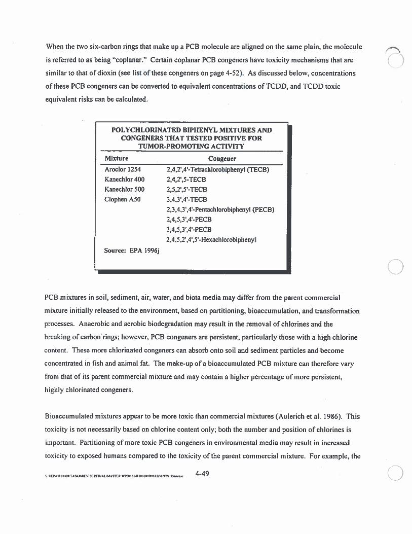
When the two six-carbon rings that make up a PCB molecule are aligned on the same plain, the molecule

is referred to as being “coplanar.” Certain coplanar PCB congeners have toxicity mechanisms that are

similar to that of dioxin (see list of these congeners on page 4-52). As discussed below, concentrations

of these PCB congeners can be converted to equivalent concentrations of TCDD, and TCDD toxic

equivalent risks can be calculated.

POLYCHLORINATED BIPHENYL MIYCrURES ANDCONGENERS THAT TESTED POSITWE FOR

TUMOR-PROMOTING ACTIVITY

Mixture Congener

Aroclor 1254 2,4,2’,4’-Tetrachlorobiphenyl (ThCB)Kanechlor 400 2,4,2’,S-TECBKanechlor 500 2,5,2’,S’-ThCBClophen ASO 3,4,3’,4’-ThCB

2,3,4,3’,4’-Pentachlorobiphenyl (PECH)2,4,5,3’,4-PECB

3,4,5,3’,4’-PECB2,4,5,2’,4’,5’-Hexachlorobiphenyl

Source: EPA 1996j

0PCB mixtures in soil, sediment, air, water, and biota media may differ from the parent commercial

mixture initially released to the environment, based on partitioning, bioaccumulation, and transformation

processes. Anaerobic and aerobic biodegradation may result in the removal of chlorines and the

breaking of carbonrings; however, PCB congeners are persistent, particularly those with a high chlorine

content. These more chlorinated congeners can absorb onto soil and sediment particles and become

concentrated in fish and animal fat. The make-up of a bioaccumulated PCB mixture can therefore vary

from that of its parent commercial mixture and may contain a higher percentage of more persistent,

highly chlorinated congeners.

Bioaccumulated mixtures appear to be more toxic than commercial mixtures (Aulerich et al 1986). This

toxicity is not necessarily based on chlorine content only; both the number and position of chiorines is

important. Partitioning of more toxic PCB congéners in environmental media may result in increased

toxicity to exposed humans compared to the toxicity of the parent commercial mixture. For example, the

REFARIcIIa’TAsKREuErnN1AmR WPDI5I.RI€X’flI2flIMflS3.mc 449

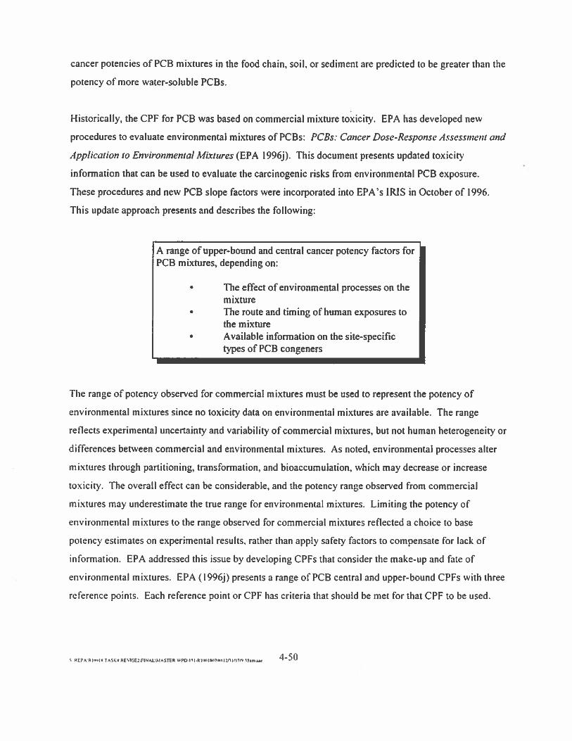
cancer potencies of PCB mixtures in the food chain, soil, or sediment are predicted to be greater than the

potency of more water-soluble PCBs.

Historically, the CPF for PCB was based on commercial mixture toxicity. EPA has developed new

procedures to evaluate environmental mixtures of PCBs: FCBs: Cancer Dose-Response Assessnwnt and

Application to Environmental Mixtures (EPA 1996j). This document presents updated toxicity’

information that can be used to evaluate the carcinogenic risks from environmental PCB exposure.

These procedures and new PCB slope factors were incorporated into EPA’s IRIS in October of 1996.

This update approach presents and describes the following:

A range of upper-bound and central cancer potency factors forPCB mixtures, depending on:

• The effect of environmental processes on themixture

• The route and timing of human exposures tothe mixture

• Available information on the site-specifictypes of PCB congeners

The range of potency observed for commercial mixtures must be used to represent the potency of

environmental mixtures since no toxicity data on environmental mixtures are available. The range

reflects experimental uncertainty and variability of commercial mixtures, but not human heterogeneity or

differences between commercial and environmental mixtures. As noted, environmental processes alter

mixtures through partitioning. transformation, and bioaccumulation, which may decrease or increase

toxicity. The overall effect can be considerable, and the potency range observed from commercial

mixtures may underestimate the true range for environmental mixtures. Limiting the potency of

environmental mixtures to the range observed for commercial mixtures reflected a choice to base

potency estimates on experimental results, rather than apply safety factors to compensate for lack of

information. EPA addressed this issue by developing CPFs that consider the make-up and fate of

environmental mixtures. EPA (1996j) presents a range of PCB central and upper-bound CPFs with three

reference points. Each reference point or CPF has criteria that should be met for that CPF to be used.

S REPAR ‘.‘ITAsg,RES,sunNaS,.Asmn WPDU -RRPM7(WRPL9Jfl 7fl55.nsa, —

Criteria include the human exposure pathway evaluated and specific information on the congener

composition of the mixture that must be obtained through environmental sampling.)

A tiered approach is used that allows different types of information in estimating the potency of

environmental mixtures of PCBs. Total PCBs or congener or isomer analyses are recommended. The

first (default) tier is invoked when congener information is limited. Only the high-risk CPF should

normally be used in the first tier since it is not possible to demonstrate the absence of persistent, dioxin

like, or tumor-promoting congeners without such analysis. The lowest-risk CPFs cannot be used without

specific information on the congener composition of the mixture.

The second tier is invoked when congener or isomer information is available from sampling and

analysis; it can be used to further refine a potency estimate that was chosen to reflect an exposure

pathway. The lowest upper-bound CPF (0.07 [mg/kgldayj’) may be used if congener or isomer analyses

ventS’ that congeners with more than four chlorines comprise less than 0.5 percent of total PCBs. The

higher CPF (2.0 [mg/kg/dayf’) should be used if dioxin-like, tumor-promoting, and persistent congeners

are present. When dioxin-like coplanar congener concentrations are available, the use of CPFs for PCBs

may be supplemented by the calculation of TCDD toxic equivalent risks. Under this method, PCB

congeners that are not dioxin-like are evaluated using the appropriate PCB CPF, while PCB congeners

that are dioxin-like are evaluated using the TCDD CPF. TEFs for the dioxin-like PCB congeners (see the

following list) would be used to estimate TCDD toxic equivalent concentrations by multiplying the

concentrations of individual dioxin-like PCB congeners by the TEFs. TCDD toxic equivalent

concentrations from all dioxin-like PCB congeners are then added together. This sum is used to

calculate a lifetime average daily dose of dioxin, which is then multiplied by the dioxin CPF to estimate

dioxin-like PCB risk. Section 4.6.3.2 describes possible changes in the TEFs for dioxin-like PCBs based

on World Health Organization studies.

S .REPAJ kMIIuTASKrREV,5E,w1NfljA4AS1fl WPD\I3IRICIIPO7tISIZflI,S7N S3amne —

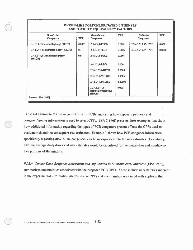
DIOXIN-LIKE POLYCHLORINATED BIPHENYLSAND TOXICITY EQUIVALENCY FACTORS

Non-Ortho Mono-Ortho TEF Di-Ortho TEFCongeaen TEF Congenen Congeners

3,4,3.4-Tetrachlorobiphenyl (FECB) 0.0005 2,3,4,3’,4’-PECB 0.0001 2,3.4.5,2’.3.4’-HPCB 0.0001

3,4.5.3.4’-Pentachlorobiphenyl (PECB) 0.1 2,3,4,S,4’-PECB 0.0005 2,J,4,5,2’.4’,5’-HPCB 000001

3,4,5,3,4,5’-Hexachlowbiphenyl 0.01 2,4,53’,4’-PECB 0.000!(HXCB)

3,4,5,2’,4-PECS 0.0001

2,3,4,5.3,4-KXCB 0.0005

23,4,3’,4’,5’-HXCB 0.0005

2,4,5,Y,4’,S’-HXCB 0.00001

2,3,4,5,3’,4’,5’- 0.0001Hepffichiorobiphenyl(HPCB)

Source: EPA 1995j

Table 4-Il summarizes the range of CPFs for PCBs, indicating how exposure pathway and

congener/isomer information is used to select CPFs. EPA (1996j) presents three examples that show

how additional information regarding the types of PCB congeners present affects the CPFs used to

evaluate risk and the subsequent risk estimates. Example 3 shows how PCB congener information,

specifically regarding dioxin-like congeners, can be incorporated into the risk estimates. Essentially,

lifetime average daily doses and risk estimates would be calculated for the dioxin-like and nondioxin

like portions of the mixture.

PCBs: Cancer Dose-Response Assessment and Application to Environmental Mixtures (EPA I 996j)

summarizes uncertainties associated with the proposed PCB CPFs. These include uncertainties inherent

in the experimental information used to derive CPFs and uncertainties associated with applying the

S REP4.R Ifl’IM’TkSKI’REVlSEIWINAL’MASTtR W?OI5I.RIlkIIllI7i,It1flh’7I9 33rn.,,.t —

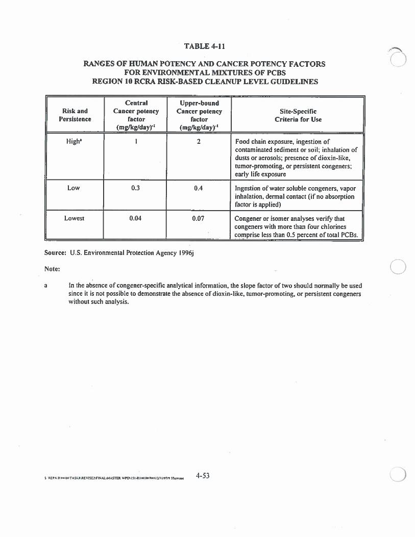
TABLE 4-11

RANGES OF HUMAN POTENCY AND CANCER POTENCY FACTORS C’FOR ENVIRONMENTAL MUCTURES OF PCBS

REGION 10 RCR4 RISK-BASED CLEANTJP LEVEL GUIDELINES

Central Upper-boundRisk and Cancer potency Cancer potency Site-Specific

Persistence factor factor Criteria ror Use(mg/kg/dayy’ (mg/kg/day)-’

High’ I 2 Food chain exposure, ingestion ofcontaminated sediment or soil: inhalation ofdusts or aerosols; presence of dioxin-like,tumor-promoting, or persistent congeners:early life exposure

Low 0.3 0.4 Ingestion of water soluble congeners. vaporinhalation, dermal contact (if no absorptionfactor is applied)

Lowest 0.04 0.07 Congener or isomer analyses veri& thatcongeners with more than four chlorinescomprise_less than 0.5_percent_of total PCBs.

Source: U.S. Environmental Protection Agency 1996j

Note:-

a In the absence of congener-specific analytical information, the slope factor of two should noñnally be usedsince it is not possible to demonstrate the absence of dioxin-like, tumor-promoting, or persistent congenerswithout such analysis.

S ,, 453

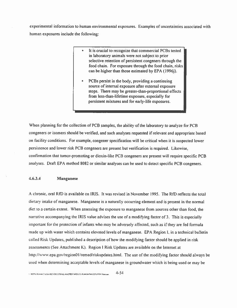
experimental information to human environmental exposures. Examples of uncertainties associated with

human exposures include the following:

ft is crucial to recognize that commercial PCBs testedin laboratory animals were not subject to priorselective retention of persistent congeners through thefood chain. For exposure through the food chain, riskscan be higher than those estimated by EPA (1996j).

PCBs persist in the body, providing a continuingsource of internal exposure after external exposurestops. There may be greater-than-proportional effectsfrom less-than-lifetime exposure, especially forpersistent mixtures and for early-life exposures.

When planning for the collection of PCB samples, the ability of the laboratory to analyze for PCB

congeners or isomers should be verified, and such analyses requested if relevant and appropriate based

on facility conditions. For example, congener specification will be critical when it is suspected lower

persistence and lower risk PCB congeners are present but verification is required. Likewise,

confirmation that tumor-promoting or dioxin-like PCB congeners are present will require specific PCB

analyses. Draft EPA method 8082 or similar analyses can be used to detect specific PCB congeners.

4.6.3.4 Manganese

A chronic, oral RfD is available on IRIS. It was revised in November 1995. The RID reflects the total

dietary intake of manganese. Manganese is a naturally occurring element and is present in the normal

diet to a certain extent. When assessing the exposure to manganese from sources other than food, the

narrative accompanying the IRIS value advises the use of a modifying factor of 3. This is especially

important for the protection of infants who may be adversely affected, such as if they are fed formula

made up with water which contains elevated levels of manganese. EPA Region I, in a technical bulletin

called Risk Updates, published a description of how the modifying factor should be applied in risk

assessments (See Attachment K). Region I Risk Updates are available on the Internet at

littp;//www.epa.gov/regionol/remed!riskupdates.html. The use of the modifying factor should always be

used hen determining acceptable levels of manganese in groundwater which is being used or may be

REP R .,I, TASk’ RrISE17!NALLMASThP “l,,sc —

used in the future as drinking water. A site-specific determination should be made regarding the use of

the modifying factor for soil. If it is a reasonable assumption that infants will not be exposed to the soil, (3the use of the modi’ing factor would not be necessary.

4.6.3.5 Total Petroleum Hydrocarbons

EPA verified toxicity values are not available for total petroleum hydrocarbons (TPH) or for most of the

hundreds of individual chemicals that comprise petroleum products. Cleanup frameworks for TPH that

have been developed and adopted by individual Region 10 states should generally be followed for

petroleum releases in those states. The assessment of risks posed by TPH releases should always include

at a minimum the measurement of benzene and the carcinogenic PAHs (see box in Section 4.6.3.1 for

list). The leaching potential to ground and surface waters and vapor releases to ambient and enclosed

breathing areas such as basements through structural breaches should be considered where applicable.

The federal Water Pollution Prevention Act (also known as the Clean Water Act) prevents the discharge

of oil to navigable waters of the United States such that it causes a film or sheen or causes a sludge or

emulsion beneath the surface of the water (Clean Water Act 31 0(a)( I); 311 (b)(3); and 40 CFR 110.3).

Each state in Region 10 is addressing TPH cleanups differently. For RCRA facilities where TPH

releases are an issue, An EPA Region 10 underground storage tank technical expert in the groundwater

protection unit should be consulted [(206) 553-1587] for the status of each state’s TPH cleanup program.

EPA’s Office of Underground Storage Tanks is also developing guidance for TPH cleanups on Native

American lands; however, the state in which the land is located may have a more sophisticated or more

pertinent TPH cleanup framework. The Native American stakeholders should be consulted in making

decisions about which cleanup framework to follow for petroleum releases on their lands.

4.6.3.6 Dermal Toxicity Factors

No RfDs or CPFs are available for the dermal route of exposure. In some cases, however, risks and

hazards associated with dermal exposure can be evaluated using an oral toxicity factor. This

route-to-route extrapolation assumes that the toxicity of a hazardous constituent is the same whether it is

S REPAR IIS;TASkRflV1SE2ENAtMASThR WP0u51.RI(SIIIJI7IMSImIpfln 5Sm\ae 455

experimental information to human environmental exposures. Examples of uncertainties associated withhuman exposures include the following:

It is crucial to recognize that commercial PCBs testedin laboratory animals were not subject to priorselective retention of persistent congeners through thefood chain. For exposure through the food chain, riskscan be higher than those estimated by EPA (1996j).

• PCBs persist in the body, providing a continuingsource of internal exposure after external exposurestops. There may be greater-than-propoi-tional effectsfrom less-than-lifetime exposure, especially forpersistent mixtures and for early-life exposures.

When planning for the collection of PCB samples, the ability of the laboratory to analyze for PCBcongeners or isomers should be verified, and such analyses requested if relevant and appropriate basedon facility conditions. For example, congener specification will be critical when it is suspected lowerpersistence and lower risk PCB congeners are present but verification is required. Likewise,confirmation that tumor-promoting or dioxin-like PCB congeners are present will require specific PCBanalyses. Draft EPA method 8082 or similar analyses can be used to detect specific PCB congeners.

3.6.3.4 Manganese

A chronic, oral RIO is available on IRIS. It was revised in November 1995. The RID reflects the totaldietary intake of manganese. Manganese is a naturally occurring element and is present in the normaldiet to a certain extent. When assessing the exposure to manganese from sources other than food, thenarrative accompanying the IRIS value advises the use ofa modifying factor of3. This is especiallyimportant for the protection of infants who may be adversely affected, such as if they are fed formulamade up with water which contains elevated levels of manganese. EPA Region I, in a technical bulletincalled Risk Updates. published a description of how the modifying factor should be applied in riskassessments (See Anachment K). Region I Risk Updates are available on the Internet atImp:’ \sw\.epa.ao\ ‘reionOl/remed!riskupdates.html. The use of the modifying factor should always beliNed s\lwn determining acceptable levels of manganese in groundwater which is being used or may be

3-4:1: fl—.

used in the future as drinking Water. A site-specific determination should be made regarding the use of

the modifying factor for soil. If it is a reasonable assumption that infants will not be exposed to the soil.

the use of the modifying factor would not be necessary.

(jse \1C(i4.6.3.5 Total Petroleum Hydrocarbons

/EPAN’efied toxicity values are not available for total petroleum hydrocarbon,(ZPH) or for most of the

hundredsfividual chemicals that comprise petroleum products. Cle,2d$frameworks for TPH that

have been devele4and adopted by individual Region 10 states shoyld generally be followed for

N /petroleum releases in thbçstates. The assessment of risks posefr6y TPH releases should always include

at a minimum the measuremi$benzene and the carcino,Øic PAHs (see box in Section 4.6.3.1 for

list). The leaching potential to ghi4 and surface wate,d’and vapor releases to ambient and enclosed/

breathing areas such as basements throug tructurakbreaches should be considered where applicable.

The federal Water Pollution Prevention Act (a,. known as the Clean Water Act) prevents the discharge

of oil to navigable waters of the United States such at it causes a film or sheen or causes a sludge or

emulsion beneath the surface of the water (Clean Water t 31 0(a)( I); 311 (b)(3); and 40 CFR 110.3).

Each state in Region ID is addressing TPH cleanups differently. RCRA facilities where TPH

releases are an issue, AnPA Region 10 underground storage tank tec ical expert in the groundwater

protection unit shouid’6e consulted [(206) 553-1587] for the status of each te’s TPH cleanup program.

EPAs Office oflihderground Storage Tanks is also developing guidance for cleanups on Native

American ntfs; however, the state in which the landis located may have a mores histicated or more

pertineytPH cleanup framework. The Native American stakeholders should be consilked in making

dccIns about which cleanup framework to follow for petroleum releases on their lands.”

:Th ‘c.,‘7”t’ !

3.6.3.6 Dermal Toxicity Factors -

No RfDs or CPFs are available for thc dermal route of exposure. In some cases, however, risks and

hazards associated with dermal exposure can be evaluated using an oral toxicity factor. This

route-to-route extrapolation assdmes that the toxicity of a hazardous constituent is the same whether it is

•:1—55

oral or dermal route. In certain instances, it may not be appropriate to use oral toxicity factors to evaluate the

dennal pathway (for example, when a toxicant is lmowri to exert a specific point-of-contact [skin) effect). A

risk assessor can assist with the evaluation of the appropriateness of a route-to-route extrapolation.

Exposures via the dermal route are calculated and expressed as absorbed doses, while most oral toxicity

factors are expressed as administered doses. An administered dose is the dose that is presented to a persons

“exchange surfaces” or points of contact with the external world, including the mouth, skin, and nose. An

absorbed dose in the portion of the administered dose that actually enters the general circulation of the body.

For example, because the sldn is an effective bather to many chemicals, only a portion of the dose

administered on the skin’s surface will be absorbed through the skin into the blood stream. When evaluating

dennal exposure to contaminants in water or soil, it may be necessary to adjust an oral toxicity value based on

an administered dose to one based on an absorbed dose using a chemical’s dral absorption efficiency. This

section discusses the method for making this adjustment. If the oral toxicity factor is used unadjusted, the

resulting risk or hazard estimates will be less conservative because adjusted values are more protective than

unadjusted oral values (see examples below).

Information concerning absorption efficiencies may be found in various chemical-specific documents

including ATSDR toxicological profiles and Health Effects Assessments. Mother source of absorption

efficiencies is a list compiled by the Health Sciences Research Division of the Oak Ridge National

Laboratory. This list is included as Attachment L. A Region 10 risk assessor should be consulted before

the adjustment of oral toxicity factors is considered.

The oral absorption efficiencies listed in the box to the right are recommended in Supplemental Guidance to

RAGs:Region 4 Bulletins, Human Health Assessment

and ma be used as rntenm default alues m the absence

of chemical-specific values (EPA 1995h). An exception VOCs -80 percent• SVOC 50 percent

to the default value for inorganics should be made for• Inorganic Chemicals - 20 percent

cadmium. IRIS (EPA 1996g) states that the RID for

cadmium (based on drinking water) assumes an oral

absorption efficiency of 5 percent. A risk assessor should be consulted for a value for arsenic.

4—56

As shown in the box to right, an oral CPF,

expressed as an administered dose, is converted

to an absorbed dose by dividing the oral CPF by

the oral absorption efficiency.

Likewise, an oral RID, expressed as an

administered dose, is converted to an absorbed

dose by multiplying the oral RID by the oral

absorption efficiency (either detennined from

literature or assumed) in the species on which

the oral RID is based.

4.6.3.7 Inhalation Toxicity Factors

Inhalation toxicity factors (RFC) are available for only a select number of hazardous constituents.

Provisional inhalation toxicity values may be available from various sources such as EPA’s NCEA or

chemical-specific ATSDR toxicity profiles. EPA Region 10 risk assessors may be consulted as to the

availability of inhalation toxicity factors.

For eases where EPA-derived toxicity factors are not available for the inhalation route of exposure but are

available for the oral route, a Region 10 toxicologist should be contacted for guidance on route-to-route

extrapolation. If an oral toxicity factor is used to evaluate inhalation risks or hazards, the uncertainty

associated should be discussed. In certain instances, it may not be appropriate to use oral toxicity factors to

evaluate the inhalation pathway (for example, when a toxicant is known to exert a specific point-of-contact

[lung effect). If it is recommended that route-to-route extrapolation not be considered and if no provisional

toxicity values is available, the hazardous constituent in question should be discussed qualitatively, and its

absence should be discussed in the uncertainty section.

4.7 CALCULATION OF RISK-BASED CONCENTRATIONS

EPA intends that contaminated RCRA sites be remediated in a manner consistent with available, protective,

risk-based media cleanup standards (FR 19449, May 1, 1996). When appropriate promulgated standards and

a

0Example: An oral CPF, unadjusted for absorption,

equals 1.6 (mglkg/day)1. Information (oran assmnption) indicates a 20 percent oralabsorption efficiency; therefore, theadjusted CPF would be 1.6 (mgAcg/day’ /0.20 = B (mg/kg/day)1.

Example: An oral RD. unadjusted for absorption,: .: equals 10 mg/kg/day. thfoation (or an

assumption) mdicates a 20 percent oralabsorption efficiency therefore theadjusted RD would be 10 mg/kg/day x

0.20

= 2 mgikglday.

O34BAflEYWLVP4L BK3I5l-RlDOl*O7UOW4/9t/lO:jJ..\,n 4-57

promulgated standards and criteria do not exist, protective media cleanup standards can be developed

using a facility-specific HHRA approach. The primary goal of HHRA is to calculate the chemical dose

that a person may receive when exposed to contaminated media and to determine the type and magnitude

of toxic effects that are known to occur at that dose level. The exposure and toxicity assessment methods

described in Sections 4.5 and 4.6 are the major risk assessment tools used to accomplish this goal.

Standardized risk characterization equations that incorporate exposure and toxicity information can be

adjusted to calculate RBCs that correspond to selected target cancer risks or HQs.

The following subsections describe how target risks and HQs are selected (Section 4.7.1). what HI-IRA

equations are used to calculate RBCs (Section 4.7.2 and Attachment E), how RBCs are calculated

(including an example) (Section 4.7.3), how to calculate RBCs for multiple hazardous constituents

(Section 4.7.4), how fate and transport models are used to determine RBCs for hazardous constituents in

one media that may migrate into another media (Section 4.7.5), and how RBCs can be estimated for lead

(Section 4.7.6).

4.7.1 Selection of Target Risks and Hazard Quotients

EPA’s RCRA program risk reduction goal is to reduce the threat from facility-related carcinogenic

hazardous constituents such that, for any medium, the excess risk of cancer to an individual exposed over

a lifetime generally falls within a range from IE-6 to IE-4 (that is, I in one million to I in one hundred

thousand) (FR 19449, May 1, 1996). Available risk-based media cleanup standards are thus considered

protective if they achieve a level of risk that falls within the IE-6 to lE4 cancer risk range. Program

implementors and facility owners/operators should generally use IE-6 as a point of departure when

initially developing target site-specific media cleanup levels. For noncarcinogens, the HI should

generally not exceed l.O(FR 19449, May 1,1996).

Washington State MTCA regulations prescribe target risks of I E-6 for Method B cleanup levels and

I E-5 for Method C or industrial cleanup levels for carcinogens, and HQ of 1.0 for all scenarios.

Cleanups and closures at EPA-lead RCRA sites in Washington should typically beat least as

conservative as MTCA requires to avoid the need for further action later. The Oregon State approved

RCRA corrective action authorization package states that it will rely upon EPA risk assessment guidance

documents to determine appropriate cleanup levels at RCRA facilities, including the use ofa IE-6 target

S REPAR ‘R’IATASKRREVIsE3FINa{AsmR WPD\I%I.RIIR37RPI2J1 IP)’P) SSRn\ne —

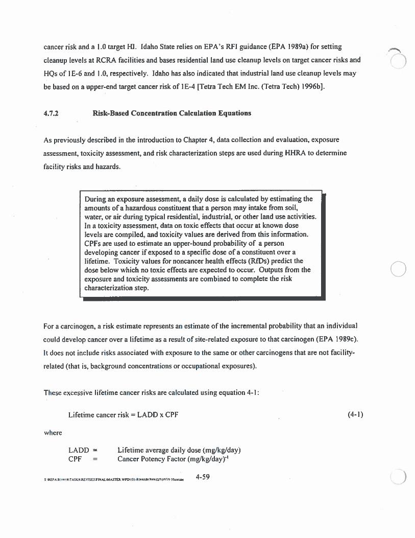
cancer risk and a 1.0 target I-il. Idaho State relies on EPA’s RFI guidance (EPA I 989a) for selling

cleanup levels at RCRA facilities and bases residential land use cleanup levels on target cancer risks and

HQs of IE-6 and 1.0, respectively. Idaho has also indicated that industrial land use cleanup levels may

be based on a upper-end target cancer risk of IE-4 [Tetra Tech EM Inc. (Tetra Tech) l996b].

4.7.2 Risk-Based Concentration Calculation Equations

As previously described in the introduction to Chapter 4, data collection and evaluation, exposure

assessment, toxicity assessment, and risk characterization steps are used during HHRA to determine

facility risks and hazards.

During an exposure assessment, a daily dose is calculated by estimating theamounts of a hazardous constituent that a person may intake from soil,water, or air during typical residential, industrial, or other land use activities.In a toxicity assessment, data on toxic effects that occur at known doselevels are compiled, and toxicity values are derived from this information.CPFs are used to estimate an upper-bound probability of a persondeveloping cancer if exposed to a specific dose of a constituent over alifetime. Toxicity values for noncancer health effects (RfDs> predict thedose below which no toxic effects are expected to occur. Outputs from theexposure and toxicity assessments are combined to complete the riskcharacterization step.

For a carcinogen, a risk estimate represents an estimate of the incremental probability that an individual

could develop cancer over a lifetime as a result of site-related exposure to that carcinogen (EPA 1989c).

It does not include risks associated with exposure to the same or other carcinogens that are not facility-

related (that is, background concentrations or occupational exposures).

These excessive lifetime cancer risks are calculated using equation 4-1:

Lifetime cancer risk = LADD x CPF (4-I)

where

LADD = Lifetime average daily dose (mg/kg/day)CPF = Cancer Potency Factor (mg/kg/day)’

S REPAJ.IIrnTAS..EV1StzF1NALMASThR WPDI3RItXl 7ttSI3fSPiP) i*i,sac —

The LADD expresses the hazardous constituent dose for the facility based on exposure information.

This dose is compared to the constituent’s toxicity per unit dose to calculate the risk from exposure to the

constituent attributed to releases from the facility.

For noncarcinogens, the potential for individuals to develop noncarcinogenic effects is evaluated by

comparing an assumed intake developed over a specific exposure period to an RD developed over a

similar exposure period. This comparison takes the form ofa ratio called an HQ and is expressed in

equation 4-2:

HQ = ADD / RD (4-2)

where

HQ = Hazard quotient (unitless)ADD = Average daily dose (mg/kg/day)RD = Reference dose (mg/kg/day)

The ADD and RD are calculated over the same exposure period. The ADD expresses the constituent

dose for the facility based on exposure information. The facility dose is compared to the RD to estimate

the likelihood of health effects.

Risk can be expressed as a lifetime excess cancer risk or as a noncarcinogenic hazard.

RBCs are calculated by the same methods used to calculate risks. The risk equations are simply reversed

to solve for a daily constituent dose that is equivalent to a selected target risk or hazard level. The

concentration of a hazardous constituent released from a facility that would cause such a dose is

determined based on the site-specific exposure conditions assumed (for example, see Table 4-2) or

measured. This concentration may serve as the basis of a cleanup level unless multiple hazardous

constituents are present in concentrations above screening levels (see Section 4.7.4 for adjustments based

on multiple constituents).

Examples of equations that may be used to calculate RBCs are presented in Exhibit 4-1. The equations

are reduced versions of the PRG equations recommended by EPA Region 9 (1996c). The Region 9

equations are derived from standard EPA equations used to calculate risks or hazards. The standard

S 4114 R lWTASKl PDiiI.Rll)l 7IIJllfli’l —

equations have been rearranged to solve for the soil or water constituent concentration that corresponds

to target risk or HQ levels. The full EPA Region 9 equations and exposure assumptions are presented in

Attachment E.

The ultimate selection of target risks and hazards are risk management decisions. EPA guidance for risk

assessment (1989c, 1995a) anticipates that the risk assessment will proceed independent of and before

risk management decisions. In Washington State, where MTCA is followed, many risk management

decisions are already made by virtue of the exposure assumptions and levels of protectiveness required

by Methods B and C.

Summary, reduced RBC equations are presented in Exhibit 4-I for soil and water media. The reduced

equations consider the primary direct exposure pathways for these media, including ingestion, inhalation,

and demial contact for soil and water. The exposure assumptions for each exposure pathway (presented

in Table 4-2) were incorporated into the original Region 9 risk equation to arrive at the reduced

equations. When available and determined to be appropriate to the facility assessment, chemical-specific

parameters, including ABS values (Section 4.5.!), VF, PEFs (Section 4.5.2.1), and toxicity values

(Section 4.6), must be entered into the reduced equations to calculate RBCs. The exposure pathway for

dermal contact with constituents in water is not included in the Region 9 (l996c) PRG equations. This

exposure pathway was incorporated in the Exhibit 4-I groundwater equations. Depending on site-

specific conditions, it may be determined that one or more exposure pathways are incomplete (that is,

there are no actual or potential receptors to the constituents in questions, via a specific exposure

pathway). In this event, the bracketed portion of the Exhibit 4-1 equations that correspond to that

exposure pathway can be dropped from the equation.

Exhibit 4-2 presents the same reduced equations as Exhibit 4-1; however, in Exhibit 4-2, the equations

are adjusted to solve for risk or HQ levels. Soil and water constituent concentrations and chemical-

specific parameters (the same as those noted for Exhibit 4-1) can be entered into the Exhibit 4-2

equations to calculate risks and hazards for specific constituents. The soil and water constituent

concentrations should represent the average concentration levels to which a human receptor could be

exposed (this is defined as the exposure point concentration). Typically, the 95th percent upper

confidence limit on the arithmetic mean (95th UCL) constituent concentration for the area of exposure is

S !PARuKIIsmsKwnV1SEn,NAL4ASm —

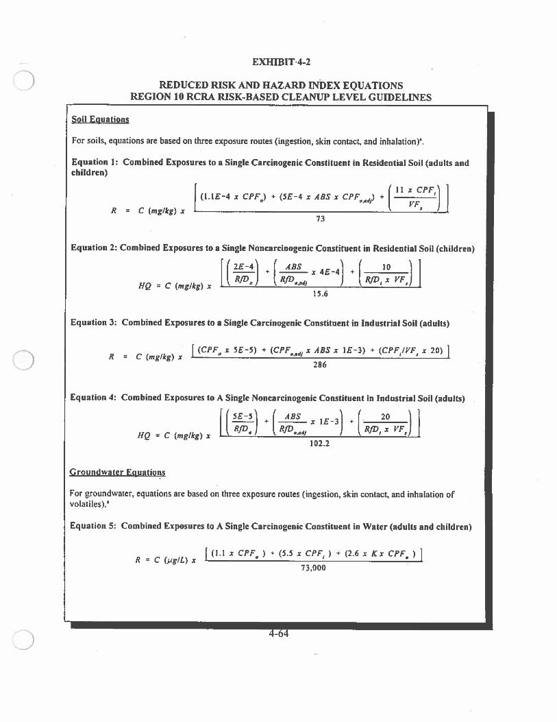
EXWBIT4-2

REDUCED RISK AND HAZARD INDEX EQUATIONSREGION 10 RCRA RISK-BASED CLEANUP LEVEL GUIDELINES

Soil Equations

For soils, equations are based on three exposure routes (ingestion, skin contact, and inhalation)’.

Equation I: Combined Exposures to a Single Carcinogenic Constituent in Residential Soil (adults andchildren)

II x CPF(l.IE-4 x CPF0) + (SE-4 x ABS x CPF)

+ VFR = C(mg/kg)x

73

Equation 2: Combined Exposures to a Single Noncarcinogenic Constituent in Residential Soil (children)

2E-4 ABS 10

____

+ x4E—4 +

RJD0 RJD, x VP’,HQ = C (mg/kg) x

Equation 3: Combined Exposures to a Single Carcinogenic Constituent in Industrial Soil (adults)

(CPF0 x 5E—5) + (CPFOaJJ x ABS x IE-3) + (CPF,/ VP’3 x 20)= C (mg/kg) x

Equation 4: Combined Exposures to A Single Noncarcinogenic Constituent in Industrial Soil (adults)

5E-5 ABS 20

HQ = C (mg/kg) xRffl3 + RPQAdJ + Rifi, x VF,

Groundwater Equations

For groundwater, equations are based on three exposure routes (ingestion, skin contact, and inhalation ofvolatiles).’

Equation 5: Combined Exposures to A Single Carcinogenic Constituent in Water (adults and children)

[(1.1 x CPF ) + (5.5 x CPF ) + (2.6 Kr CPFRC(g/L)x ‘ 0

73,000

4-64

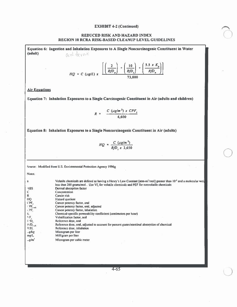
EXHIBIT 4-2 (Continued)

REDUCED RISK AND HAZARD INDEXREGION 10 RCRA RISK-BASED CLEANUP LEVEL GUIDELINES

Equation 6: Ingestion and Inhalation Exposures to A Single Noncarcinogenic Constituent in Water(adult) C’-’

2 10 5.5xK

HQC(g/L)x÷

RID0

Air Equations

Equation 7: Inhalation Exposures to a Single Carcinogenic Constituent in Air (adults and children)

C (jig/rn 3) x CPF

6,600

Equation 8: Inhalation Exposures to a Single Noncarcinogenic Constituent in Air (adults)

HQ= C (pg/rn’)

RJD1 x 3,650

Source: Modified from U.S. Environmental Protection Agency l996g

Noles:

a Volatile chemicals are defined as having a Henry’s Law Constant [atm-m’/mol] greater than 10’ and a molecular weiless than 200 grams/mcI Use Vf, for volatile chemicals and PEF for nonvolatile chemicals

\RS Dermal absorption factorC Concentrationft Cancer riskHQ Itazard quotientCPF, Cancer potency factor, oral

Cancer potency factor, oral, adjustedCancer potency factor, inhalationChemical-specific permeability coefficient (centimeters per hour)Volatilization factor, soil

I-ID,, Reference dose, oralH Reference dose, oral, adjusled to account for percent gastrointestinal absorption of chemicalR:O, Reference dose, inhalation

Microgram per litermg/L Milligram per liter

Microgram per cubic meter

4-65

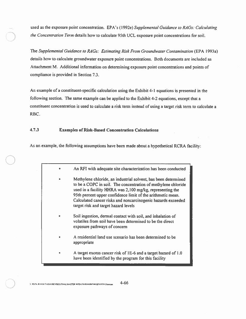
used as the exposure point concentration. EPA’s (1992e) Supplemental Guidance to RAGs: Calculating

the Concentration Term details how to calculate 95th UCL exposure point concentrations for soil.

The Supplemental Guidance to RAGs: Estimating Risk From Groundwater Contamination (EPA I 993a)

details how to calculate groundwater exposure point concentrations. Both documents are included as

Attachment M. Additional information on determining exposure point concentrations and points of

compliance is provided in Section 7.3.

An example of a constituent-specific calculation using the Exhibit 4-I equations is presented in the

following section. The same example can be applied to the Exhibit 4-2 equations, except that a

constituent concentration is used to calculate a risk term instead of using a target risk term to calculate a

RBC.

4.7.3 Examples of Risk-Based Concentration Calculations

As an example, the following assumptions have been made about a hypothetical RCRA facility:

• An RFI with adequate site characterization has been conducted

• Methylene chloride, an industrial solvent, has been detenninedto be a COPC in soil. The concentration of methylene chlorideused in a facility EU-IRA was 2,100 mg/kg, representing the95th percent upper confidence limit of the arithmetic mean.Calculated cancer risks and noncarcinogenic hazards exceededtarget risk and target hazard levels

• Soil ingestion, dermal contact with soil, and inhalation ofvolatiles from soil have been determined to be the directexposure pathways of concern

• A residential land use scenario has been determined to beappropriate

• A target excess cancer risk of I E-6 and a target hazard of 1.0have been identified by the program for this facility

S REPA R TAsLRREVIsflnNAi’MA5TER WPDI I-R lirnimp 7MR rn VI7N 5%rn.Un —

No promulgated federal standards for methylene chloride in soil are available. An RBC can be

calculated using equations I and 2 in Exhibit 4-1.

The following paragraphs discuss the specific information for methylene chloride that is needed to

calculate carcinogenic and noncarcinogenic RBCs. Sections 4.7.3.1 and 4.7.3.2 present example RBC

calculations based on carcinogenic and noncarcinogenic effects, respectively.

The IRIS (EPA 1996g) and I-lEAST (EPA 1997a) databases indicate that methylene chloride has toxicity

values for both carcinogenic and noncarcinogenic effects. The oral CPF is 0.0075 (mgIkgJdayt, the

inhalation CPF is0.0016 (mg/kgIday’, the oral RD is 0.06 mg/kg/day, and the inhalation RfC is

3.0 milligrams per cubic liter, converted to an inhalation RiD by multiplying by 20 cubic meters and

dividing by 70 kilograms (no absorption factor available). As discussed in Section 4.6.3, the oral CPF

and RID are adjusted to account for the oral absorption efficiency of methylene chloride when assessing

the dermal exposure pathway. Following the recommendations in Section 4.6.3, a default oral absorption

efficiency of 80 percent may be assumed for VOCs in the absence of chemical-specific information. The

oral CPF is adjusted for 80 percent oral efficiency to 0.0094 (mglkg/dayY’ to arrive at a dermal CPF.

The oral RD is adjusted for 80 percent oral efficiency to 0.048 mg/kg/day to arrive at a dermal RD.

An ABS is needed to estimate the amount of methylene chloride that is absorbed across the skin. In the

absence of a methylene chloride-specific ABS value, a default ABS value for methylene chloride of

0.05 percent (0.0005) is used. This value is based on recommendations from Region Ill Technical

Guidance Manual, Risk Assessment: Assessing Dermal Exposure from Soil (EPA I 995fl. EPA Region 3

recommends two ABS values for VOCs: 0.05 percent for volatiles having a vapor pressure equal to or

greater than benzene (approximately 95.2 millimeters mercury) and 3 percent for volatiles having a

vapor pressure lower than benzene (EPA 1995fl. Methylene chloride has a vapor pressure of 349

millimeter mercury; therefore, the ABS value of 0.05 percent is used.

Since methylene chloride is a VOC, a VF is derived to assess inhalation exposures. A VF of 2,815 m3/kg

is derived following the method described in Section 4.5.2.1.

S REPARl€IIMT4SKIREV1SE2W1NA1S.lASTER WPD\I5I.RIIEII4I7CNTI1flIMN 5S,m\,a. —

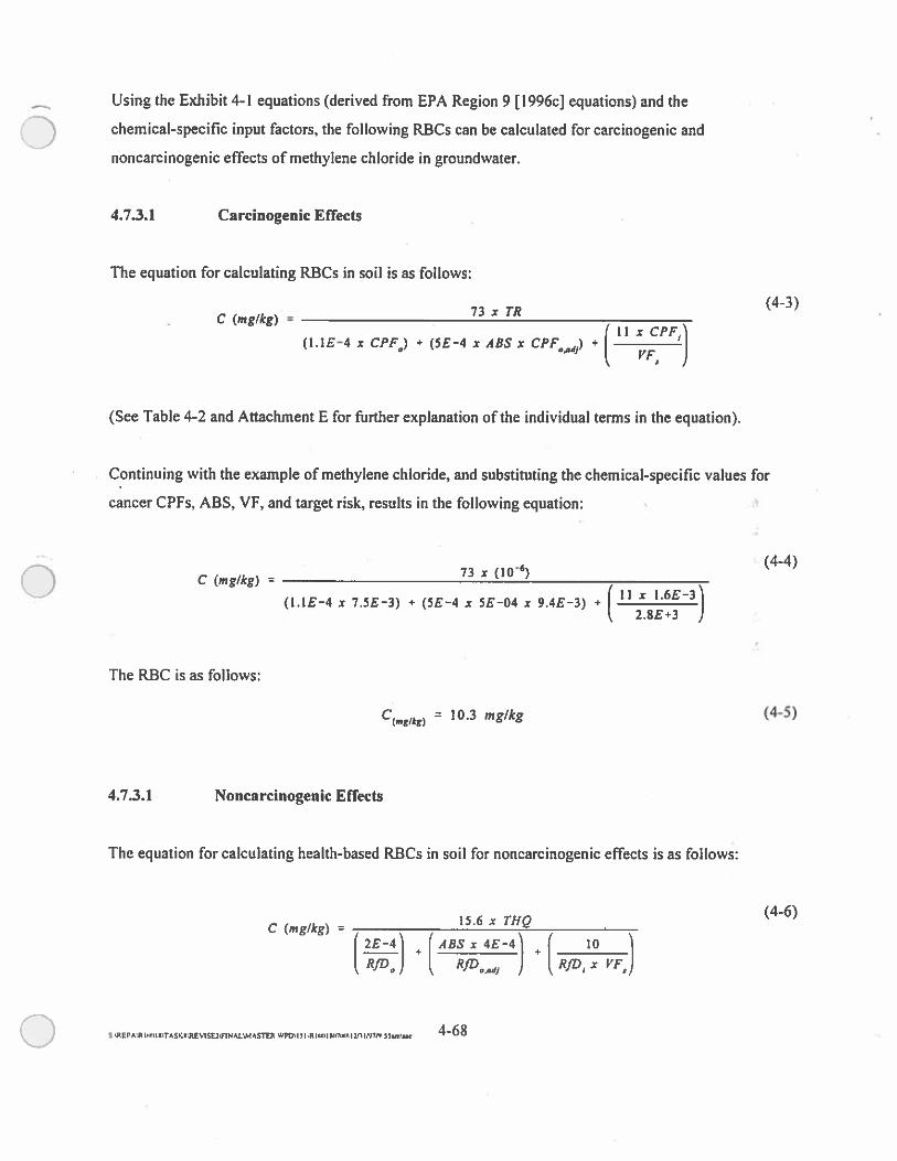
Using the Exhibit 4-I equations (derived from EPA Region 9 [I996c] equations) and the

chemical-specific input factors, the following RBCs can be calculated for carcinogenic and

noncarcinogenic effects of methylene chloride in groundwater.

4.73.1 Carcinogenic Effects

The equation for calculating RBCs in soil is as follows:

73 x TI?(4-3)

- C (mg/kg) =

_________________________________________________

11 x CPF.(1.IE-4 x CPFQ) + (SE-4 x ABS x CPFOAJJ)

+ ( VF )(See Table 4-2 and Attachment E for further explanation of the individual terms in the equation).

Continuing with the example of methylene chLoride, and substituting the chemical-specific values for

cancer CPFs, ASS, VF, and target risk, results in the following equation:

(44)

73 x (10.6)C (mg/kg) =

__________________________________________________________

(1.1E-4 x 7.5E-3) + (SE-4 x 5E-04 x 9.4E-3)+ 11 x l.6E-3

2.SE+3

The RBC is as follows:

C(mg/kg) = 10.3 mg/kg (45)

4.7.3.1 Noncarcinogenic Effects

The equation for calculating health-based RBCs in soil for noncarcinogenic effects is as follows:

(4-6)15.6 x THQC (mg/kg) =

_______________________________________

2E-4 - ABSx4E-4 10

RID, RJD,,JJ Rifi x IT,

S REPA\R I.SNTASKWREVThnY1NALMA&TER WPD’ISIR IlILI7ISI3J13fl7fl ls,.\s.c —

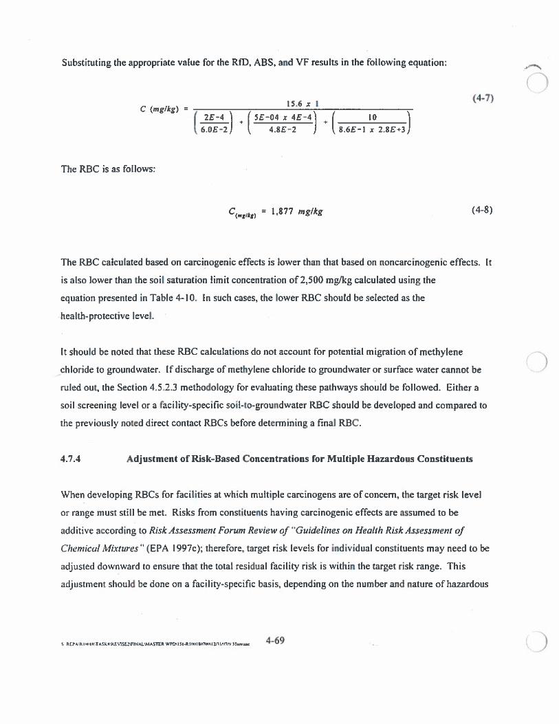
Substituting the appropriate value for the RID, ABS, and VF results in the following equation:

015.6

(4-7)C (mg/kg) =

____________________________________________

2E-4 5E-04 x 4E-4 1 I 10

_____

+ i •16.OE—2 4.8E—2 ) 8.6E—1 x 2.SE+3

The RBC is as follows:

C(,g/jg) = 1,877 mg/kg (48)

The RBC calculated based on carcinogenic effects is lower than that based on noncarcinogenic effects. It

is also lower than the soil saturation limit concentration of 2,500 mg/kg calculated using the

equation presented in Table 4-10. In such cases, the lower RBC should be selected as the

health-protective level.

It should be noted that these RBC calculations do not account for potential migration of methylene

_chloride to groundwater. If discharge of methylene chloride to groundwater or surface water cannot be

ruled out, the Section 4.5.2.3 methodology for evaluating these pathways should be followed. Either a

soil screening level or a facility-specific soil-to-groundwater RBC should be developed and compared to

the previously noted direct contact RBCs before determining a final RBC.

4.7.4 Adjustment of Risk-Based Concentrations for Multiple Hazardous Constituents

When developing RBCs for facilities at which multiple carcinogens are of concern, the target risk level

or range must still be met. Risks from constituents having carcinogenic effects are assumed to be

additive according to Risk Assessment Forum Review of Guidelines on Health RiskAssessment of

CIw,nical Mixtures” (EPA I 997c); therefore, target risk levels for individual constituents may need to be

adjusted downward to ensure that the total residual facility risk is within the target risk range. This

adjustment should be done on a facility-specific basis, depending on the number and nature of hazardous

S RtPAR WPi il-RI IIflhIfllUi IPflP) i5.mc 4—69 0

COPCs present. Exhibit 4-3 demonstrates how RBCs for carcinogens can be adjusted to achieve an

acceptable target risk range.

In general, cleanup levels for the constituent(s) contributing most significantly to total risk can be

adjusted to keep total risk in the target risk range. For example, five carcinogens may be present: four

representing total risks in the l0 range and one representing risk in the lO range. Adjusting the

cleanup level for the single constituent contributing most of the risk may be adequate to achieve a total

facility risk in the target range. This would be more practicable ifa corrective measure could be selected

that is especially effective for the constituent constituting the highest risk (for example, if the constituent

is highly vulnerable to bioremediation); however, this method may not be practicable in all situations. In

that case, the target risk from carcinogens can be established overall and the remediation would continue

until the combined risk from the mixture of the residual carcinogens had been reduced to the target risk

or lower.

HQs from constituents having similar systemic toxic effects and similar mechanisms of action are also

assumed to be additive. The IRIS (EPA 1996g) and HEAST (EPA 1997a) databases provide information

on the types of toxic effects that are the basis for each RID. Hazardous constituents with similar

noncarcinogenic toxic affects should be grouped together to determine cleanup levels for multiple

constituents. For example, many orgaiuic solvents typically affect the central nervous system or the liver.

The target HQ level for individual constituents in each toxic effects group should be adjusted downward

to ensure that the total residual facility HI is Tess than 1.0. This adjustment can be done on a

facility-specific basis, depending on the number of hazardous constituents present. As with carcinogens,

instead of adjusting the target HQ for individual constituents, the remediation results could be monitored

to ensure that the target HI is achieved or surpassed.

Exhibit 4-4 demonstrates how cleanup levels for noncarcinogens can be adjusted to achieve an

acceptable target HI. As was explained for carcinogens, adjusting the cleanup levels for the chemicals

presenting most of the hazard may achieve an acceptable total hazard.

A regional risk assessment specialist should be consulted to confirm how chemicals are grouped

according to types of toxic effects.

S P [PAR IIMIIWT ASKKRE V1SE FIN 11 Acfl R WPV’ fl I-RI WI I X1171Th I 211 IflI I —

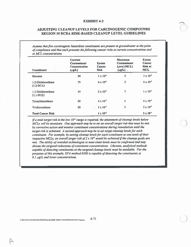
EMIThIT 4-3

ADJUSTING CLEANUP LEVELS FOR CARCINOGENIC COMPOUNDSREGION 10 RCRA RISK-BASED CLEANUP LEVEL GUIDELINES

Assume thatfive carcinogenic hazardous constituents are present in groundwater at the pointofcompliance and that each presents thefollowing cancer risks at current concentrations andat MCL concentrations.

Current Maximum ExcessContaminant Excess Contaminant CancerConcentration Cancer Level (MCL) Risk at

Constituent (pgIL) Risk (pWL) MCI.

Benzene 50 1x10’ 5 1x103

1,2-Dichloroethane 75 óx l0 5 4 x io-(I ,2-DCA)

1,1-Dichloroethene 14 2x io 7 lx l0(l,1-DCE)

Tetrachloroethene 50 4 x 10-’ 5 4 x I0

Trichloroethene 50 3 x 10’ 5 3 x I0

TotalCancerRisk IxIW’ 2x104

Ifa total target risk in the low I o range is required, the attainment ofcleanup levels belowMCLs will be necessary. One approach may be to set an overall target risk that must be metby corrective action and monitor constituent concentrations during remediation until thetarget risk is achieved. A second approach may be to set target cleanup levels for eachconstituent. For example, by setting cleanup levels for each constituent at one-tenth of the irrespective MCLs, an overall target risk of2 x W5 would be achieved Vt/ic cleanup goals aremet. The ability’ ofremedial technologies to meet clean levels must be confirmed and maydictate the targeted reductions ofconstituent concentrations. Likewise, analytical methodscapable ofdetecting constituents at the targeted cleanup levels must be available. For thepurposes of this erample, EPA method 8260 is capable ofdetecting the constituents at0.1 pg/L and lower concentrations.

4-71 ç

COPCs present. Exhibit 4-3 demonstrates how RBCs for carcinogens can be adjusted to achieve anacceptable target risk range.

In general, cleanup levels for the constituent(s) contributing most significantly to total risk can be

adjusted to keep total risk in the target risk range. For example, five carcinogens may be present: four

representing total risks in the 10 range and one representing risk in the I0 range. Adjusting the

cleanup level for the single constituent contributing most of the risk may be adequate to achieve a total

facility risk in the target range. This would be more practicable ifa corrective measure could be selected

that is especially effective for the constituent constituting the highest risk (for example, if the constituent

is highly vulnerable to bioremediation); however, this method may not be practicable in all situations. In

that case, the target risk from carcinogens can be established overall and the remediation would continue

until the combined risk from the mixture of the residual carcinogens had been reduced to the target riskor lower.

HQs from constituents having similar systemic toxic effects and similar mechanisms of action are alsoassumed to be additive. The IRIS (EPA 1996g) and HEAST (EPA 1997a) databases provide informationon the types of toxic effects that are the basis for each RID. Hazardous constituents with similar

noncarcinogenic toxic affects should be grouped together to determine cleanup levels for multiple

constituents. For example, many organic solvents typically affect the central nervous system or the liver.The target HQ level for individual constituents in each toxic effects group should be adjusted downwardto ensure that the total residual facility HI is less than 1.0. This adjustment can be done on afacility-specific basis, depending on the number of hazardous constituents present. As with carcinogens,instead of adjusting the target HQ for individual constituents, the remediation results could be monitoredto ensure that the target HI is achieved or surpassed.

Exhibit 4-4 demonstrates how cleanup levels for noncarcinogens can be adjusted to achieve anacceptable target HI. As was explained for carcinogens, adjusting the cleanup levels for the chemicalspresenting most of the hazard may achieve an acceptable total hazard.

A reinonal risk assessment specialist should be consulted to confirm how chemicals are groupedaccording to types of toxic effects.

4-70

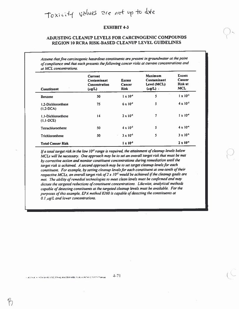
toxic1 \?tU€S 2 ict uj -it J-

EXhIBIT 4-3 oADJUSTING CLEANUP LEVELS FOR CARCINOGENIC COMPOUNDS

REGION 10 RCRA RISK-BASED CLEANUP LEVEL GUIDELINES

Assume that five carcinogenic hazardous constituents are present in groundwater at the point

ofcompliance and that each presents the following cancer risks at current concentrations andat MCL concentrations.

Current Maximum ExcessContaminant Excess Contaminant Cancer

Concentration Cancer Level (MCL) Risk at

Constituent (sgfL) Risk (pg/U) MCL

Benzene 50 I x l0 5 I x io

I 2-Dicbloroethanc 75 6 x I 5 4 x I o-’(I ,2-DCA)

Il-Dichloroethene 14 2x IO’ 7 I x l0’

(I,I-DCE)

Tetnchlorocthcne 50 4 x I0 5 4x I0A

Trichlorocthcne 50 3x 10’ 5 3 x l0

Total Cancer Risk I x 10” 2 x Ifr

Ifa total target risk in the low lfr’ range is required, the attainment ofcleanup levels below C)MCLX will be necessa.’y. One approach may be to set an overall target risk that must be met

by corrective action and monitor constituent concentrations during remediation until the

target risk is achieved. A second approach may be to set target cleanup levelsfor each

constituent. For example, by setting cleanup levelsfor each constituent at one-tenth of their

respective MCLS, an overall target risk of2 x iCY’ would be achieved jithe cleanup goals are

met The ability ofremedial technologies to meet clean levels must be confirmed and may

dictate the targeted reductions ofconstituent concentrations. Likewise, analytical methods

capable ofdetecting constituents at the targeted cleanup levels must be available. For the

purposes of this example, EPA method 8260 is capable ofdetecting the constituents at

0. 1 pg/L and lower concentrations.

4•%T .gI.!J’IIp’’,’,.,—

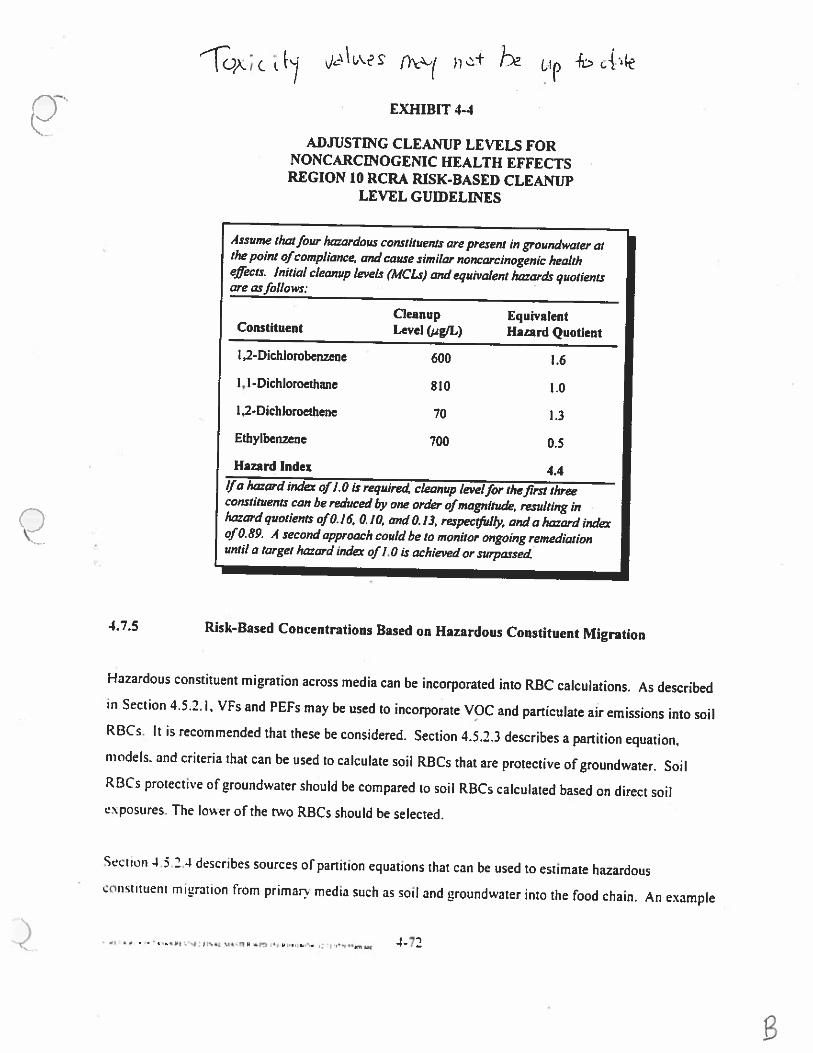
C jLe

EXHIBIT 4-4

ADJUSUNG CLEANUP LEVELS FORNONCARCENOGEMC HEALTH EFFECTSREGION 10 RCRA RISK-BASED CLEANUP

LEVEL GUIDELINES

Assume thatfour hazardous constituents are present in groundwater atthe point ofcompliance, and cause similar noncarcinogenic healtheffects. Initial cleanup levels (MCLs) and equivalent hazards quotientsare asfollows:

Cleanup EquivalentConstituent Level (pgfL) Hazard Quotient

l,2-Dichlombenzene 600 1.6

1,1-Dichloroethane 810 1,0

1,2-Dichloroethene 70 1.3

Ethylbenzene 700 0.5

Hazard Index 4.4Ifa hazard indes of 1.0 is require4 cleanup levelfor thefirst threeconstituents can be reduced by one order ofmagnitude, resulting inhazard quotients of0.16, 0.10, and 0.13, respectfid4’, and a hazard indexof0.89. A second approach could be to monitor ongoing remediationuntil a target hazard index of 1.0 is achieved or surpassel

4.7.5 Risk-Based Concentrations Based on Hazardous Constituent Migration

Hazardous constituent migration across media can be incorporated into RBC calculations. As describedin Section 4.5.2.1, VFs and PEFs may be used to incorporate VOC and particulate air emissions into soilRBCs. It is recommended that these be considered. Section 1.5.2.3 describes a partition equation,models, and criteria that can be used to calculate soil RBCs that are protective of groundwater. SoilRBCs protective of groundwater should be compared to soil RBCs calculated based on direct soilexposures. The loer of the two RBCs should be selected,

Section 4.5.2.4 describes sources of partition equations that can be used to estimate hazardousconstituent migration from priman media such as soil and groundwater into the food chain. An example

4-7,F; •‘.kI’-TT4F) —

of how the partition equations may be used follows. At a site where home gardening is an important

exposure pathway, constituent migration from soil to garden root crops may be estimated using the

partition equations in Guidancefor Performing Screening Level Risk Analvses at Combustion Facilities

Burning Hazardous Wastes, Attachment C, Draft Exposure Assessment Guidance (EPA I 994i). Using

the HHRA equations presented by EPA (19941), the amount of the root crop ingested by a home gardener

would then be estimated, and the risk associated with plant ingestion would be calculated. Soil RBCs

determined after constituent migration into plants has been considered can be back-calculated using the

same HHRA equations. Chemical-specific parameters required for the calculation include oral toxicity

values and soil-to-plant partition coefficients. Partition coefficients for common hazardous waste

combustion facility constituents are included in the EPA (1994i) combustion guidance (that is. for

dioxins, PAHs, PCBs, nitroaromatics, phthalates, and certain metals). Some of the primary sources of

plant partition coefficients cited by the combustion guidance document series include A Review and

Analysis ofParameters for Assessing Transport ofEnvironmentally Released Radionuclides Through

Agriculture (Baes et al. 1984) for inorganic compounds and Bioconcentration of Organics in Beef Milk,

and Vegetation (Travis and Arms 1988) for organic compounds. Evaluation ofDredged Material

Proposedfor Ocean Disposal, Testing Manual (EPA 199 Id) also provides octanol-water partition

coefficients for many chemicals that can be converted to plant partition coefficients using equations

recommended by Travis and Arms (1988).

As previously noted, human food chain exposures are typically not significant pathways of concern at

RCRA facilities, so indirect exposures to food chain organisms require consideration only on a

case-by-case basis. Methods for incorporating food chain exposures into RBCs may also be conservative

(for example. garden produce partitioning equations) and may overestimate actual site risks. If they are

significant exposure pathways and are not included, however, risks would be underestimated,

4.7.6 Cleanup Levels for Lead

Cleanup levels for lead are not calculated using standard EPA risk assessment equations. Rather. EPA

has developed an integrated exposure uptake biokinetic model (IEUBK) that predicts lead blood levels in

ptlsI:rls4L,,snp.poLua473

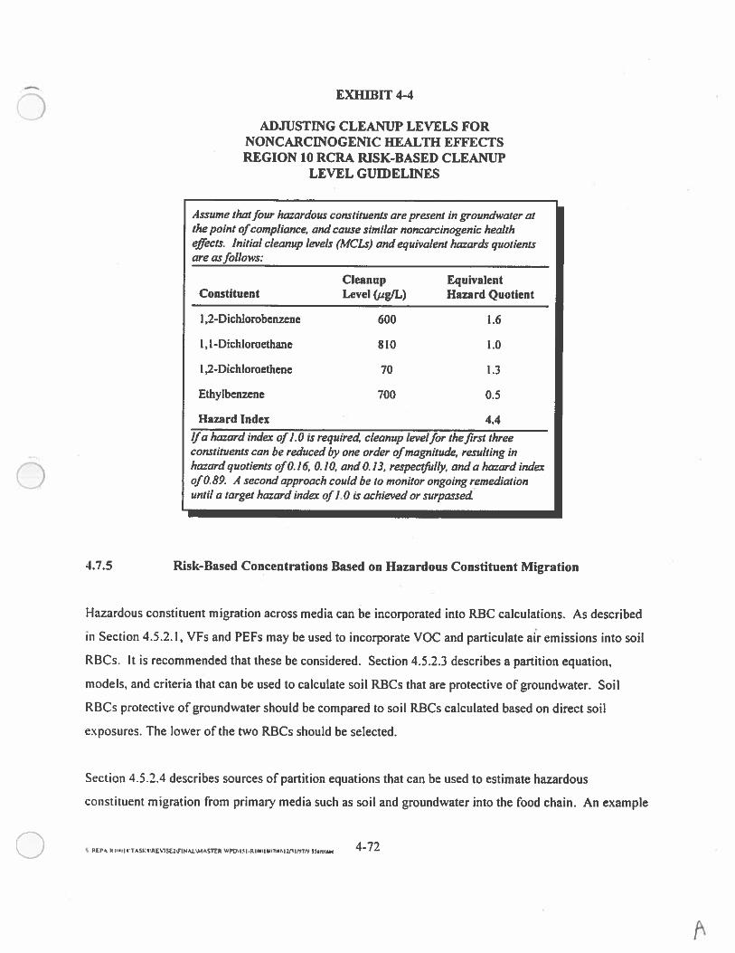
EXHIBIT 4-4

ADJUSTING CLEANUP LEVELS FORNONCAJ{CNOGEMC HEALTH EFFECTSREGION 10 RCRA RISK-BASED CLEANUP

LEVEL GUIDELINES

Assume that four hazardous constituents are present in roundwater atthe point ofcompliance, and cause similar noncarcinogenic healtheffects. Initial cleanup levels (MCLs) and equivalent hazards quotientsare as follows:

Cleanup EquivalentConstituent Level (jigfL) Hazard Quotient

I,2-Dichlorobenzene 600 1.6

1,1-Dichloroethane 810 1.0

1,2-Dichloroethene 70 1.3

Ethylbenzene 700 0.5

Hazard Index 4•4

4.7.5 Risk-Based Concentrations Based on Hazardous Constituent Migration

Hazardous constituent migration across media can be incorporated into RBC calculations. As described

in Section 4.5.2.1, VFs and PEFs may be used to incorporate VOC and particulate air emissions into soil

RBCs. It is recommended that these be considered. Section 4.5.2.3 describes a partition equation,

models, and criteria that can be used to calculate soil RBCs that are protective of groundwater. Soil

RBCs protective of groundwater should be compared to soil RBCs calculated based on direct soil

exposures. The low-er of the two RBCs should be selected.

Section 4.5.2.4 describes sources of partition equations that can be used to estimate hazardous

constituent migration from priman’ media such as soil and groundwater into the food chain. An example

S PEPA R ILMII, T4SKEREWSE,LnNALLMAcWR WEDLI .RIIWflhiIPflIfl MN “an, 4-72

Ifa hazard index of 1.0 is required cleanup levelfor thefirst threeconstituents can be reduced by one order ofmagnitude, resulting inhazard quotients of0.16. 0.10, and 0.13, respectfrlly, and a hazard indexof0.89. A second approach could be to monitor ongoing remediationuntil a target hazard index of 1.0 is achieved or surpassed

1’

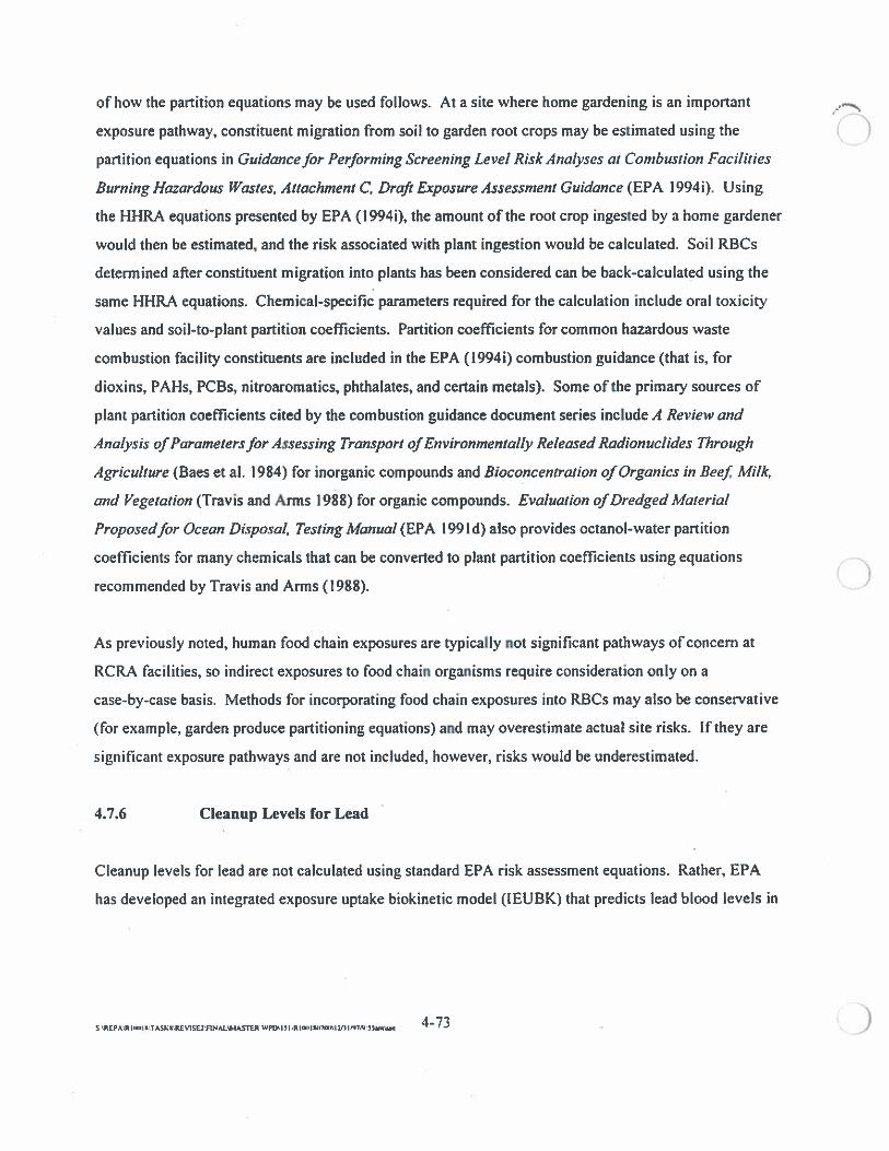
of how the partition equations may be used follows. At a site where home gardening is an important

exposure pathway, consti Went migration from soil to garden root crops may be estimated using the

partition equations in Guidancefor Performing Screening Level Risk Analyses at Combustion Facilities

Burning Hazardous Wastes, Attachment C, Draft Exposure Assessment Guidance (EPA I 994i). Using

the HI-IRA equations presented by EPA (1994i), the amount of the root crop ingested by a home gardener

would then be estimated, and the risk associated with plant ingestion would be calculated. Soil RBCs

determined after constituent migration into plants has been considered can be back-calculated using the

same HHRJ& equations. Chemical-specific parameters required for the calculation include oral toxicity

values and soil-to-plant partition coefficients. Partition coefficients for common hazardous waste

combustion facility constituents are included in the EPA (1994i) combustion guidance (that is, for

dioxins, PAHs, PCBs, nitroaromatics, phthalates, and certain metals). Some of the primary sources of

plant partition coefficients cited by the combustion guidance document series include A Review and

Analysis ofParametersfor Assessing Transport ofEnvironmentally Released Radionuclides Through

Agriculture (Baes et al. 1984) for inorganic compounds and Bioconcentration ofOrganics in Beef Milk,

and Vegetation (Travis and Arms 1988) for organic compounds. Evaluation ofDredged Material

Proposedfor Ocean Disposal, Testing Manual (EPA 199 Id) also provides octanol-water partition

coefficients for many chemicals that can be converted to plant partition coefficients using equations

recommended by Travis and Arms (1988).

As previously noted, human food chain exposures are typically not significant pathways of concern at

RCRA facilities, so indirect exposures to food chain organisms require consideration only on a

case-by-case basis. Methods for incorporating food chain exposures into RECs may also be conservative

(for example, garden produce partitioning equations) and may overestimate actual site risks. If they are

significant exposure pathways and are not included, however, risks would be underestimated.

4.7.6 Cleanup Levels for Lead

Cleanup levels for lead are not calculated using standard EPA risk assessment equations. Rather, EPA

has developed an integrated exposure uptake biokinetic model (IEUBK) that predicts lead blood levels in

S mEPARII,PI,’TASK,RESE3flNALV.lAS1ER WpDI5I.RLlrnIS4IlwIiInIm7I93San, 4’.73

children. The model was developed for children because they are more sensitive to lead effects. The

IEUBK is considered superior to the use of a RID in a standard HHRA equation because the model

(1) recognizes the multimedia nature of lead exposures, (2) incorporates important absorption and

pharmacokinetic information, and (3) considers the potential distributions of exposures and risk likely to

occur at a facility. The model allows for the incorporation of water. soil/dust, air, dietary, paint, and

maternal-blood lead concentration levels into a lead dose estimate.

The Memorandum Regarding Revised Interim Soil Lead Guidancefor CERCL4 Sites and RCK4

Corrective Action Facilities (EPA 1994k) recommends a residential soil lead screening level of

400 mg/kg. This screening level is back-calculated using the IEUBK model, assuming a blood lead

concentration of 10 micrograms per deciliter (yg/dL) in children and standard defaults for water, air,

diet, paint, and maternal-blood lead levels. This target blood level is based on analyses conducted by the

Centers for Disease Control and EPA that associate blood lead levels of 10 Mg/dL or higher with health

effects in children. No comparable soil Lead screening level has been set for a nonresidential adult; the

IEUBK model is designed specifically for children.

EPA is currently considering what industrial soil lead levels may be appropriate. An interim approach is

recommended by EPA (1996k) in Recommendations of The Technical Review Workgroupfor Leadfor

An Interim Approach to Assessing Risks Associated with Adult Exposures to Lead in SoiL This document

recommends the use of a biokinetic slope factor, which relates the increase in typical adult blood lead

concentrations for a women of child-bearing age to average lead uptake from contaminated soils. The

document then recommends the use of a proportionality constant, which relates a fetal blood lead

concentration at birth to a material blood lead concentration. Using a fetal blood lead goal of 10 MgJdL

or less, a soil RBC can be calculated that should not result in an exceeded of the fetal blood lead goal.

Using default parameters summarized in the EPA (1996k) review, RBCs ranging from 743 mg/kg to

1.738 mg/kg can be calculated, depending on the baseline level of adult blood lead and the blood lead

standard deviation associated with adults exposed to similar on-site lead concentrations. EPA 0996k)

should be consulted to confirm a facility-specific industrial soil lead RBC. The Region 10

representatives on the EPA Superfund technical review group should be consulted for information on

current lead policy.

c PEPAR OMPIW.TASktREV1SEflNALM&SThR WPDJP P.R IIEP7n Ivu’pvp 3Pi,nu —

The EPA memorandum recommends using the IEUBK model on a site-specific basis to develop media

cleanup standards at RCRA facilities where site data support modification of model default parameters c--:)(1994k).

4.8 UNCERTAINTY ANALYSIS

Once the HI-IRA process and the step-by-step process for developing cleanup levels are understood,

facility and regulatory officials should be prepared to answer the questions listed in Exhibit 4-5 for a

contaminated facility undergoing corrective action or clean closure under RCRA.

EXHIBIT 4-5

RISK ASSESSMENT AND CLEANUP LEVEL DETERMINATION PROCESSREGION 10 RCR4 RISK-BASED CLEANUP LEVEL GUIDELINES

Have receptors and exposure pathways that are likely affected by facilitycontamination been identified?

• Are data of sufficient quantity and quality available to determine whether and towhat extent on-site and off-site remediation is necessary to protect the health of themaximally exposed individual?

• Have contaminants of concern been identified?

• Are promulgated standards or criteria available? If so, are they sufficientlyprotective?

• Are there state methodologies, regulations, or policies that should be considered?

• Is the corrective action or clean closure being considered subject to a RCRAauthorized state program?

• Have current and future land use scenarios been identified?

• Have risk-based concentrations been calculated using published RiDs and CPFs forany of the COPCs?

• Have risk management decisions regarding target risk and hazard levels beenidentified by the lead regulatory agency?

• Have cleanup levels been adjusted (as appropriate) to account for multiplehazardous constituents?

S WII.RIlMIIw7cflIIN7fl 475

RBCs are associated with varied levels of uncertainty. Uncertainty can be defined as a lack of precise

knowledge of the qualitative or quantitative truth. As part of an ideal risk analysis, a complete

uncertainty analysis would provide a risk manager with the ability to estimate risk for each individual in

a given population in both actual and projected scenarios of exposures; it would also estimate the

uncertainty in each prediction in quantitative, probabilistic terms (see Chapter 6). But even a less

exhaustive treatment of uncertainty will serve a very important purpose: it can reveal whether the

deterministic risk estimate overestimates or underestimates risk and if so, to what extent.

Uncertainties associated with all sections of the human health-based analysis should be discussed in all

HHRAs. This section discusses uncertainty in qualitative terms; for a discussion of quantitative

uncertainty, see Chapter 6 (Probabilistic Risk Assessment Methods). Additional uncertainty discussions

can be found in the National Research Council’s Science and Judgement in Risk Assessment (Chapter 9)

(1994) and in EPA Administrator Carol Browner’s memorandum of risk assessment (EPA I 995a)

(Attachment A). The effect that each eLement of uncertainty has on the final cleanup Levels should be

included. For example, an assumption that future land use will be industrial will lead to less

conservative (that is, higher) cleanup levels.

4.8.1 Data Uncertainty

Issues contributing to uncertainty in data evaluation include the identification of COPCs, data quality,

data useability, adequacy ofquantitation limits (relative to target risk levels), and data coverage.

All data that are used to evaluate compliance with a cleanup level should be reviewed with respect to

data quality standards presented in the site-specific quality assurance project plan. Data that do not meet

the data quality standards should be qualified as necessary, and the uncertainty associated with these data

should be discussed. Uncertainty associated with data quality may result in an underestimation or

overestimation of hazardous constituent concentrations, depending on the specific data quality issue.

By the time the uncertainty section is prepared, data should have been reviewed to ensure that the

detection or quantitation limits achieved for the various analyses were sufficient to evaluate site-specific

hazardous constituents at concentrations equal to or less than the hazardous constituent-specific cleanup

levels. If a chemical’s detection or quantitation limit is greater than its cleanup level, one cannot

S RPA ‘H IllIK I ASKXRE7SL2IIN AL.qActrR WrD’ Ill-RIM) 1W171R11 I 111 I I’?’!’? 51.mit —

determine whether the cleanup level has been met. Detection and quantitation limits should be compared

to cleanup levels before chemical analyses. Chapter 3 of this guidance provides additional information(fl’)

on data evaluation procedures, while Chapter 7 describes how below detection limit data should be

handled in HI-WA.

Data coverage refers to the ability of the sampling plan and associated sample results to completely

characterize the contamination. (Were sufficient data collected to evaluate all potential exposure

pathways? Do the sampling locations adequately represent actual or potential exposure conditions?) For

example, uncertainty would arise if groundwater sample points were not located downgradient of a

source.

Data quality indicators were discussed in Section 3.2: completeness, representativeness, comparability,

precision, and accuracy. Any problems associated with any of the data quality indicators should be

discussed in the uncertainty section. Other issues that could adversely affect data quality are blank

contamination, matrix interferences, sample holding times, and sample preservation.

4.8.2 Exposure Assessment Uncertainty

CDUncertainty is inherent in the evaluation of exposure pathways and in the assumptions used to estimate

exposure doses. Human activity patterns and individual characteristics (for example, body weight) can

vary significantly within a given population. The degree of uncertainty depends to a large extent on the

amount and adequacy of facility-specific data available. Typically, the most significant areas of

uncertainty for the exposure assessment include exposure pathway identification, exposure assumptions,

assumptions of steady-state conditions, environmental chemical characterization, and modeling

procedures. These areas of uncertainty are described as follows:

Exposure pathway identification: To the degree that actual or future human activitypatterns are misrepresented, uncertainty is introduced into the cleanup levels. In mostcases, there is uncertainty regarding future land use at a site. This uncertainty must beconsidered when evaluating exposure estimates developed under the future land usescenarios.

S REPALRlIWPl*\TASKR3RE9SE2\$1NAL’MASThR WPD,I,L.RI,uIml,l.,u21,Ip,7p, SSan\sac —

Exposure assumptions: Standard default assumptions for population characteristics,such as body weight and surface area, life expectancy, period of exposure, and exposurecharacteristics such as frequency, duration, amount of intake or contact and degree ofabsorption or soil adherence may not accurately represent exposure conditions. Theexposure assumptions used may overestimate or underestimate actual exposure.

Assumption of steady-state conditions: Estimated future exposure doses are based on anassumption of steady-state conditions. The inherent assumption is that future chemicalconcentrations are the same as those measured during sampling. This assumptionignores the effects of various fate-and-transport mechanisms, which will alter thecomposition and distribution of most chemicals present in the various media. Theassumption of steady-state conditions usually results in overestimations of futurechemical concentrations and exposure doses.

Hazardous constituent characterization: It is impossible to completely characterize thenature and extent of hazardous constituents in the environment. Instead, the variousenvironmental media are sampled to estimate hazardous constituent concentrations andto identify hazardous constituents actually present as a result of releases at the facility.Because no sampling can completely and accurately characterize environmentalconditions, the exposure dose calculation will be somewhat uncertain. Uncertainties areintroduced into exposure dose calculations during collection, analysis, and evaluation ofenvironmental chemical data. Two areas of uncertainty that should be addressed in arisk assessment are the assumption of uniform concentrations in an exposure area andthe treatment of nondetection results.

Modeling procedures: Modeling assumptions are used to determine hazardousconstituent concentrations in outdoor air resulting from VOC and particulate emissionsand VOC concentrations in indoor air generated by household water use. The numerousassumptions included in these models introduce uncertainty to the degree that they donot reflect actual conditions. Use of models may overestimate or underestimate actualenvironmental concentrations.

Analytical and numerical models are also used to estimate soil-to-groundwatercontaminant migration. There are many soil-to-groundwater models available that havebeen developed by government agencies, universities, and the private sector. Modelscan simulate different fate and transport processes and migration mechanisms such asadvection, dispersion, diffusion, retardation, chemical reactions, and microbial reactions.In addition, different models are designed to account for various phases of contamination(for example, vapor, water, or nonaqueous phase liquids) and various dimensions (one-,two-, or three-dimensional). Some of the models simulate complex geologic andhydrogeologic systems while other models are more appropriate for simple geology andgroundwater flow conditions. The models use assumptions to simplify the real-worldconditions and describe these conditions with mathematical equations (usualLy partial

% REPA\kItIHI,TAStKflV1SE2WINAL1AcTTR WPD’ISIRI4III*lI7IN1flhlV7N $.m’ne —

differential equations). When a model is applied at a site, these assumptions should becarefully evaluated against the site-specific conditions. A sensitivity analysis should beperformed to identi& the most sensitive parameters. The uncertainty of the models canbe determined by evaluating the agreement between model assumptions and siteconditions as well as the accuracy of input parameters.

4.8.3 Toxicity Assessment Uncertainty

RfDs and CPFs must be viewed in light of uncertainties and gaps in toxicological data. For instance,

direct information concerning toxic effects in humans is often limited to historical cases of accidental or

industrial exposures. Animal studies conducted with specially bred homogeneous species are typically

extrapolated to a heterogenous human population. The reliance on animal studies introduces

uncertainties regarding effects on humans including sensitive subpopulations and differences in

physiological characteristics between the animal species studied and humans, such as target organs,

metabolism, organ sensitivity, and detoxification capabilities.

In addition, high-dose, short-term (acute) animal studies may not be applicable to low-level, long-term

(chronic) exposures that humans are more likely to experience. Likewise, the quality of the. animal study

may introduce additional uncertainty if, for example, accepted scientific protocols were not employed.

The uncertainties discussed previously are addressed by dividing the no-observable-adverse-effect level

(NOAEL) for a hazardous constituent from animal studies by uncertainty factors of 10 to 10,000 to

obtain RiDs. The NOAEL is the highest level of a hazardous constituent evaluated in a study that does

not cause statistically significant differences between the experimental and control animals. The lowest-

observable-adverse-effect level (LOAEL), on the other hand, is the lowest level of a hazardous

constituent evaluated in a study that causes statistically significant differences between experimental and

control animals. Uncertainty factors are applied to data in the following cases (EPA l989c):

S REPA;RL*IIST5W WPDIiI.Rh(N’IV’7SSI 1fl719 5am\nc — -

To account for variation in thegeneral population (to protectsensitive subpopulations)

To extrapolate data from animals tohumans

To adjust for using a NOAEL from asubchronic study rather than achronic study

To adjust for using a LOAELinstead of a NOAEL in developingan RD

A modifying factor ranging from Ito 10 is also applied to the RD to address uncertainties in the

scientific studies used to develop RiDs. Published RfDs already contain the necessary uncertainty and

modifying factors.

Unceñainty associated with determining chemical carcinogenicity is reflected in the weight-of-evidence

clasñification groups assigned to carcinogens. In addition, CPFs are derived from the low-dose end of

the dose-response curve. The studies are usually conducted at the high-dose end of the curves. The

selected 95th upper confidence limit of the slope of the dose-response curve is considered an

upper-bound toxicity value (that is, there is only a 5 percent chance that the probability of a response

could be greater than the estimated value on the basis of the experimental data and model used).

The use of oral toxicity factors to evaluate dermal exposures is associated with uncertainty. The use of

oral toxicity factors as surrogates for this pathway is necessary because no dermal toxicity factors have

been approved by EPA. Most of the uncertainty associated with the use of surrogate toxicity factors

exists because the constituents in question are not known to exhibit similar toxicological effects (that is,

degree of toxicity, target organ) during dermal contact and the oral pathway. In addition, dermal

absorption assumptions add to uncertainty. Using surrogate toxicity factors is more conservative than

ignoring the dermal pathway and allows for a quantitative cleanup level rather than a qualitative

discussion.

S ‘.REPMRI,MSTA5 E’,SErFINA1JMASThR WPDI5I.RHrnItA,7,ThI2flIN79 35.m’nc —

4.8.4 Cleanup Level Uncertainty

Since the cleanup level calculations incorporate information from all the previous processes. the

uncertainties associated with the data evaluation, exposure assessment, and toxicity assessment sections

will all directly affect the cleanup level uncertainty.

0

S R[PA lSIIP’ flPI-’ 5nS 4—81 (J

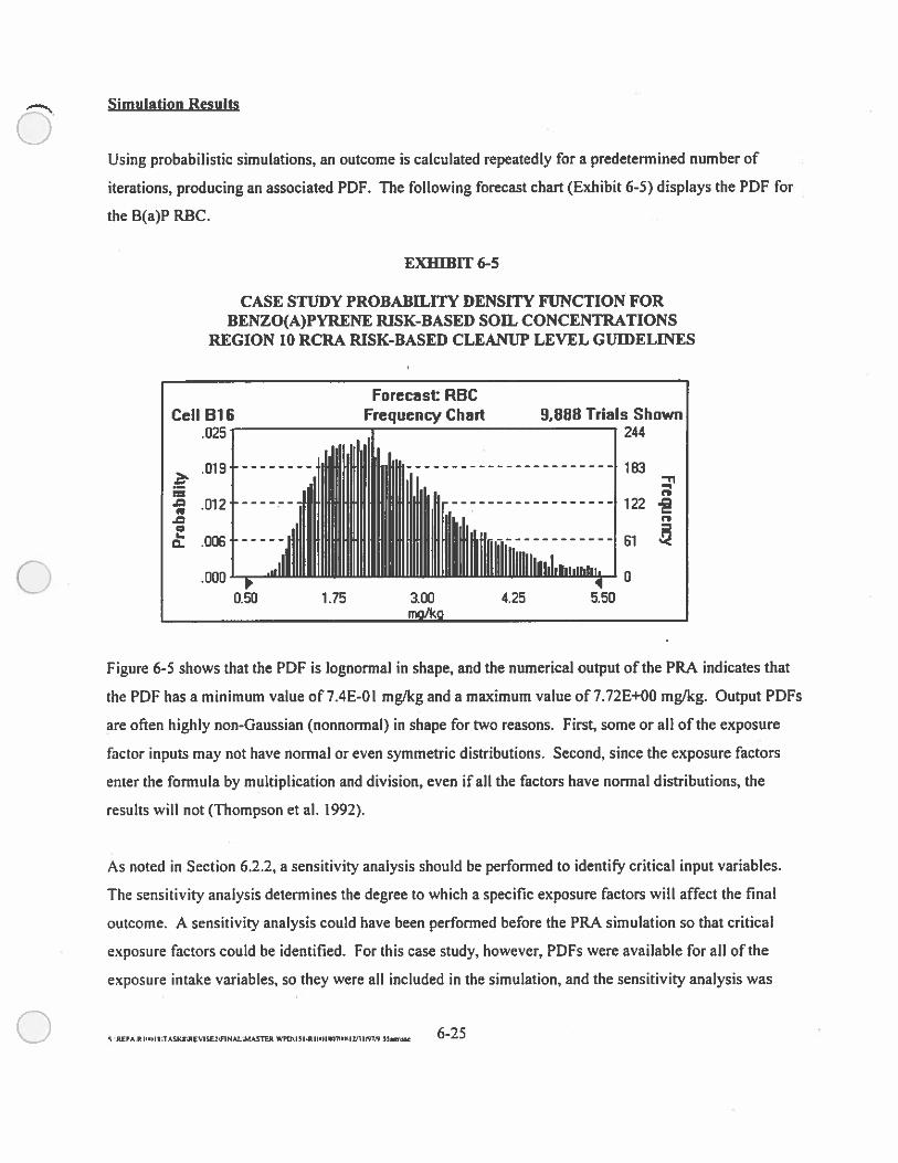
Simulation Results

Using probabilistic simulations, an outcome is calculated repeatedly for a predetermined number of

iterations, producing an associated PDF. The following forecast chart (Exhibit 6-5) displays the PDF for

the B(a)P RBC.

EXHIBIT 6-5

CASE STUDY PROBABILITY DENSITY FUNCTION FORBENZO(A)PYRENE RISK-BASED SOIL CONCENTRATIONS

REGION 10 RCRA RISK-BASED CLEANUP LEVEL GUIDELINES

Forecast: RSCCell 816 Frequency Chart 9.888 Trials Shown

.025 244

.019 183

3.00nw/kg

Figure 6-5 shows that the PDF is lognormal in shape, and the numerical output of the PRA indicates that

the PDF has a minimum value of7.4E-0l mg/kg and a maximum value of 7.72E+OO mg/kg. Output PDFs

are often highly non-Gaussian (nonnormal) in shape for two reasons. First, some or all of the exposure

factor inputs may not have normal or even symmetric distributions. Second, since the exposure factors

enter the formula by multiplication and division, even if all the factors have nonnal distributions, the

results will not (Thompson et al. 1992).

As noted in Section 6.2.2, a sensitivity analysis should be performed to identify critical input variables.

The sensitivity analysis determines the degree to which a specific exposure factors wiLl affect the final

outcome. A sensitivity analysis could have been performed before the PRA simulation so that critical

exposure factors could be identified. For this case study, however, PDFs were available for all of the

exposure intake variables, so they were all included in the simulation, and the sensitivity analysis was

6-25

a’.0

.0CI

0-

.012

.006

r.; ;: : : :.000

0.50

flfI ii1.75

-I,

122 .

61

104.25 5.50

S REMR HW)IW,T4SKI3REV1SE1WINAL.MASThR WPO’I 5 .RLlIlW7InI1 1MM 55amac

performed during the simulation. With Crystal Ball software, sensitivity is calculated by computing

Spearman rank correlation coefficients (a common statistical measure of dependency) between every ()exposure factor and outcome calculation while the simulation is running (Decisioneering 1993). A

positive correlation coefficient indicates that an increase in the exposure factor is associated with an

increase in the outcome. A negative correlation coefficient indicates that an increase in the exposure factor

is associated with a decrease in the outcome (Decisioneering 1993). The larger the absolute value of the

correlation coefficient, the stronger the relationship; however, caution should be applied when interpreting

the sensitivity analysis in simulations where exposure factors are correlated. For example, if a highly

sensitive exposure factor were correlated with an insensitive one, the insensitive exposure factor would

likely have a high sensitivity with regard to the outcome (Decisioneering 1993).

Exposure factors that are identified as being highly sensitive, contributing a high degree of uncertainty to

the outcome, may be further refined so as to decrease the effect on the final outcome. Likewise, it may not

be necessary to spend PRA resources on those factors that have little effect on the risk outcome.

in the Exhibit 6-6 sensitivity chart, exposure factors are listed on the left side, beginning with the exposure

factor with the highest sensitivity.

In this simulation, adult exposure duration has the highest sensitivity ranking and can be considered the

most important assumption in the model. Likewise, the child exposure frequency and the child soil

ingestion rate have the lowest sensitivity rankings and can be considered the least important assumptions in

the model. Considering this, collection of facility-specific exposure durations could be prioritized over the

collection of child soil ingestion rates if further data collection was deemed necessary. Confidence must

also be established in the child exposure frequency and child soil ingestion rate information used in the

sensitivity analysis. For example, if it is believed that facility-specific child soil ingestion rates are

significantly underestimated, further.data collection and a second sensitivity analysis may be warranted.

Descriptive statistics shown in Table 6-1 were calculated for the B(a)P RBC POF. Population percentiles

and corresponding RBCs are also determined for the PDF, as presented in Table 6-2.

S WPThISI.RItW)tKIflIrnljtUfl7m 35.i,n 6—_6

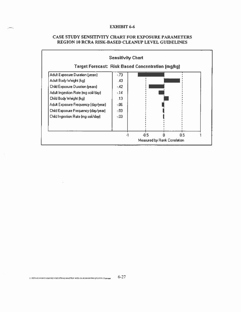
EXUIBIT 6-6

CASE STUDY SENS[WITY CHART FOR EXPOSURE PARAMETERSREGION 10 RCRA RISK-BASED CLEANUP LEVEL GUIDELINES

Sensitivity Chart

Target Forecast: Risk Based Concentration (mg/kg)

Adult Exposure Duration [years) -.73Adult Body Weight (kg) .43 I

Chdd Exposure Duration [years) -.42 I

Adult Ingestion Rate 1mg soL’day] -.14Child Body Weight (kg) .13

Adult Exposure Fcequency (day/year) -06 IChild Exposure Frequency [day/year) -.03Child Ingestion Rate [mg soil/day) -.03

•d.s 0.5Measured by Rank Correlation

6-’ 7S •RrpAnxIInASk!nqSE2nNaAS1tR 35amc —

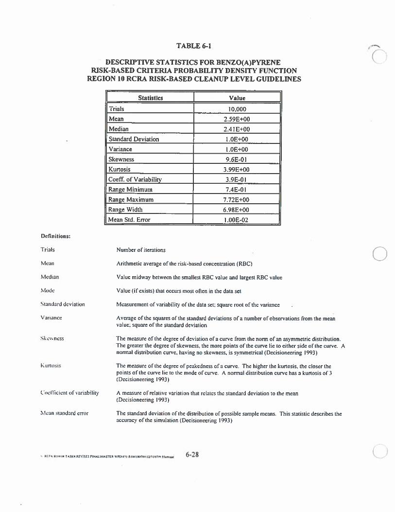
TABLE 6-I

DESCRWTWE STATISTICS FOR BENZO(A)PYRENERISK-BASED CRITERIA PROBABILITY DENSITY FUNCTION

REGION 10 RCRA RISK-BASED CLEANUP LEVEL GUIDELINES

Statistics Value

Trials 10,000

Mean 2.59E+00

Median 2.41E+00

Standard Deviation I .OE+00

Variance I .OE+0O

Skewness 9.6E-01

Kurtosis 3.99E+00

Coeff. of Variability 3.9E-0l

Range Minimum 7.4E-0l

Range Maximum 7.72E+00

Range Width 6.98E+00

Mean Std. Error I .OOE-02

Definitions:

Trials Number of iterations

Mean Arithmetic avenge of the risk-based concentration (RBC)

Median Value midway between the smallest REC value and largest RBC value

Mode Value (if exists) that occurs most ofien in the data set

Standard deviation Measurement of variability of the data set: square root of the variance

Variance Average of the squares of the standard deviations of a number of observations from the meanvalue; square of the standard deviation

Ske ness The measure of the degree of deviation of a curve from the norm of an asymmetric distribution.The greater the degree of skewness, the more points of the curve lie to either side of the curve. Anormal distribution curve, having no skewness, is symmetrical (Decisioneering 1993)

Kurtosts Thc measure of the degree of peakedness of a curve. The higher the kurtosis. the closer thepoints of the curve lie to the mode of curve. A normal distribution curve has a kurtosis of 3(Decisioneering 1993)

Liietiicient of variability A measure of relative variation that relates the standard deviation to the mean(Decisioneering 1993)

Mean standard error The standard deviation of the distribution of possible sample means. This statistic describes theaccuracy of the simulation (Decisioneering 1993)

ri, K IIMIIK TASKK RE’SE2nNI4snR WPD iii R {MiiI7€wfliVflp37pJ 55am 6—28 U

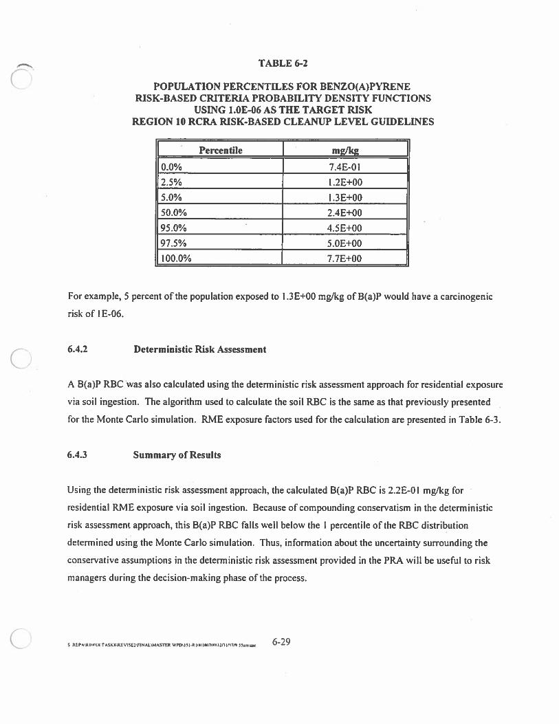
TABLE 6-2

POPULATION PERCENTILES FOR BENZO(A)PYRENERISK-BASED CRITERIA PROBABILITY DENSITY FUNCTIONS

USING 1.OE-06 AS THE TARGET RISKREGION 10 RCRA RISK-BASED CLEANUP LEVEL GUIDELINES

Percentile ) mg/kg

0.0% 7.4E-Ol

2.5% 1.2E+00

5.0% l.3E+00

50.0% 2.4E+00

95.0% 4.5E+O0

97.5% 5.OE+00

100.0% 7.7E+00

For example, 5 percent of the population exposed to I.3E+00 mg/kg of B(a)P would have a carcinogenic

risk of IE-06.

6.4.2 Deterministic Risk Assessment

A B(a)P RBC was also calculated using the deterministic risk assessment approach for residential exposure

via soil ingestion. The algorithm used to calculate the soil RBC is the same as that previously presented

for the Monte Carlo simulation. RME exposure factors used for the calculation are presented in Table 6-3.

6.4.3 Summan’ of Results

Using the deterministic risk assessment approach, the calculated B(a)P RBC is 2.2E-0I mg/kg for

residential RJ’vIE exposure via soil ingestion. Because of compounding conservatism in the deterministic

risk assessment approach, this B(a)P RBC falls well below the I percentile of the RBC distribution

determined using the Monte Carlo simulation. Thus, information about the uncertainty surrounding the

conservative assumptions in the deterministic risk assessment provided in the PR.A will be useful to risk

managers during the decision-making phase of the process.

S REPARItM,IwTASKmfl1SErflNAL\MASThR WPO 31.RIIEflO7IflI3/lIfllfS 33.ms.c —

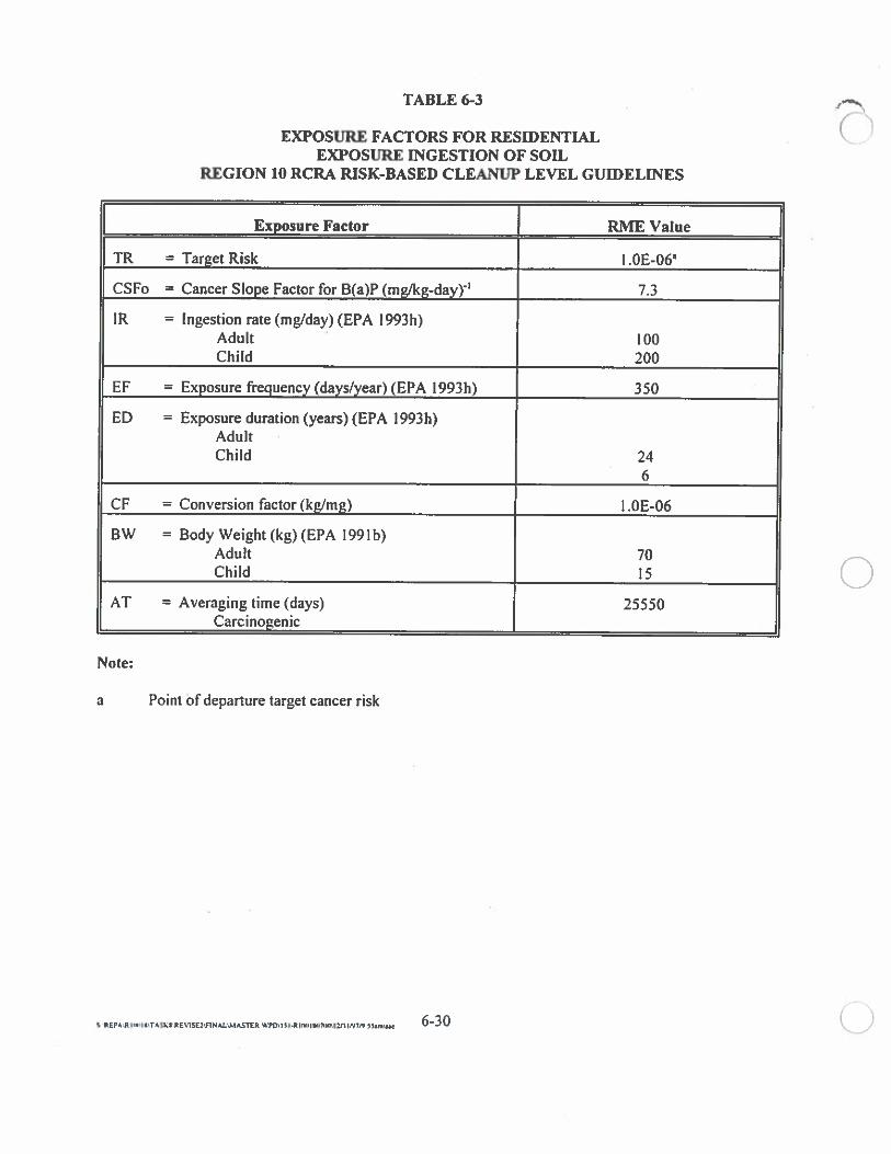
TABLE 6-3

EXPOSURE FACTORS FOR RESIDENTIALEXPOSURE INGESTION OF SOIL

REGION 10 RCRA RISK-BASED CLEANUP LEVEL GUIDELINES

Exposure Factor RME Value

TR = Target Risk I .0E06a

CSFo = Cancer Slope Factor for B(a)P (mg/kg-dayY’ 7.3

IR = Ingestion rate (mglday) (EPA 1993h)Adult 100Child 200

EF = Exposure frequency (days/year) (EPA 1993h) 350

ED = Exposure duration (years) (EPA 1993h)AdultChild 24

6

CF = Conversion factor (kg/mg) I .OE-06

BW = Body Weight (kg) (EPA l99Ib)Adult 70Child 15

AT = Averaging time (days) 25550Carcinogenic

Note:

a Point of departure target cancer risk

0

0REP#RIIIflS’T4SLIflVISE31NALlASflR WPO\I5I.RItflhItI7tI;tV1INTh, innc 6-30

6.5 WORK PLANS, REPORTS, AND PRESENTATIONS

There are several minimal requirements for PRA work plans and reports to ensure sufficient data quality.

In fact, it is important that the facility submit a work plan for EPA review before doing the PRA

simulation. The work plan should include exposure variables for human receptors. Guidance for

application to environmental receptors is not available at this time. The work plan should describe the

software to be used, the exposure routes and models, and input probability distributions and references,

The following good principles of practice should be used to select input data and distributions for the PRA

work plan (EPA 1997d, Items II through 16: page 17).

• A complete and thorough description of the exposure model and its equations should beprovided.

• The presentation of the deterministic point estimate should always accompany a PRAanalysis.

• Where possible, areas of uncertainty should be identified accompanied by an explanationof how it will be dealt with in the report.

• Sensitivity analysis should be used to identify model structures, exposure pathways, andmodel input assumptions and factors that make important contributions to the assessmentendpoint and its overall uncertainty and variability.

• Probabilistic assessment should be restricted to significant pathways and variables.

• Sufficient data should be used to support the choice of input distributions for model inputfactors.

• Surrogate data can be used to develop distributions when they can be appropriatelyjustified.

• Data should be collected to develop input distributions for the exposure model followingthe basic tenets of environmental sampling. Furthermore, particular attention should begiven to the quality of information at the tails of the distribution.

• Expert judgment may be used to select appropriate input distributions, but the reasons andjustification for subjective analysis should be included in detail.

S PEP A R TASKW.Et1SEJflP1ALlASThR WPD SI P lIE I 2/1 I P17fl I inn. —

Presentation of PRA simulation results should be tailored to the targeted audience. Entirely different types

of reports are needed for scientific and nonscientific audiences. For example, descriptive and less detailed

summary presentations may be appropriate for the nonscientific public. Graphs and tables showing and

describing each input distribution, distribution of risk for each exposure route, and distributions of total

risk should be included.

0

REPA.R 55.m.c 6—32 0

CO

MP

LIA

NC

E

CHAPTER 7

DETERMINATION OF COMPLIANCE WITH TARGET CLEANUP LEVELS

Following the selection of target cleanup levels and corrective actions to treat or remove a contaminated

media, additional sampling is performed to determine whether the cleanup levels have been attained. This

sampling is performed using the same data quality objectives (DQO) and data quality assessment (DQA)

procedures described in Chapter 3 of this guidance. The DQO and DQA steps are summarized in

Sections 7.1 through 7.6. Section 7.7 provides additional guidance on how to handle below-detection-limit

(BDL) sampling results when calculating constituent concentrations.

7.1 DATA QUALITY OBJECTIVES STEPS 1 THROUGH 3

Steps I through 3 of the DQO process, as described in Chapter 3, apply directly to compliance

determinations, with the exception that cleanup levels are considered that may differ from the screening

levels or preliminary background levels considered during the Resource Conservation and Recovery Act

(RCRA) facility investigation (RFI) stage. The decision rule is likely to be very similar to the Chapter 3

example (that is, have constituent levels been reduced to a concentration below the selected cleanup level

concentration? If so, no further action would be called for; if not, further remedial action may be

required). The remaining Chapter 7 sections provide additional information on DQO Steps 4 through 7

and the DQA as they apply to determination of compliance with target cleanup levels.

7.2 STEP 4: STUDY BOUNDARIES

In Step 4 of the DQO process, the spatial and temporal boundaries of the problem are defined. To

determine compliance with cleanup levels, facility-specific points of compliance that were earlier

established in the formal RCRA corrective action process should be used. A point of compliance is the

location or locations at which media cleanup levels are to be achieved. No final U.S. Environmental

Protection Agency (EPA) RCRA corrective action regulations defining points of compliance have been

promulgated. In an update to the proposed Subpart S rule, EPA (Federal Register [FRJ 19450, May I,

1996) recommends that points of compliance be determined on a site-specific basis and notes that program

implementors and facility owners have routinely established points of compliance in the following manner:

S RErAR IRIIR rA94an,SEaINa.IAsmR wroISI.RIiiIlIm,nI,nIp.v, 5Sam’s.c

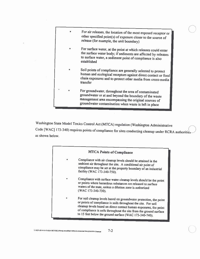
0For air releases, the location of the most exposed receptor orother specified point(s) of exposure closer to the source ofrelease (for example, the unit boundary)

For surface water, at the point at which releases could enterthe surface water body; if sediments are affected by releasesto surface water, a sediment point of compliance is alsoestablished

Soil points of compliance are generally selected to protecthuman and ecological receptors against direct contact or foodchain exposures and to protect other media from cross-mediatransfer

For groundwater. throughout the area of contaminatedgroundwater or at and beyond the boundary of the wastemanagement area encompassing the original sources ofgroundwater contamination when waste is left in place

Washington State Model Toxics Control Act (MTCA) regulation (Washington AdministrativeCode [WACI 173-340) requires points of compliance for sites conducting cleanup under RCRA authoritiesas shown below.

MTCA Points of Compliance

• Compliance with air cleanup levels should be attained in theambient air throughout the site. A conditional air point ofcompliance may be set at the property boundary of an industrialfacility (WAC 173-340-750).

• Compliance with surface water cleanup levels should be the pointor points where hazardous substances are released to surfacewaters of the state, unless a dilution zone is authorized(WAC 173-340-730).

• For soil cleanup levels based on groundwater protection, the pointor points of compliance i5 soils throughout the site. For soilcleanup levels based on direct contact human exposures, the pointof compliance is soils throughout the site from the ground surfaceto 15 feet below the ground surface (WAC 173-340-740).

0S REPAEIIIIITS REVZSE2ICNAL,.t&ct wpo\I,,.RL,I, ‘wvimu’n, SSimix —

MTCA Points of ComplianceContinued

Compliance with groundwater cleanup levels should bedetermined for each groundwater monitoring well or othermonitoring points such as a spring (WAC 173-340-720).

In summary, the study boundaries for compliance decisions are primarily set by points of compliance. The

points of compliance should be determined following EPA guidance or, in Washington, the specified

MTCA regulation.

7.3 STEP 5: DEVELOP DECISION RULE

As described in Chapter 3, Step 5 requires that a decision rule be developed to define the conditions that

would cause the decision maker to choose among alternative actions. The decision rule is an “if. . . then”

statement that incorporates the information determined during DQO Steps I through 4. An example

decision rule for a compliance decisions follows: ifthe parameter of interest (average concentration of

constituent of concern) within the study area (the point of compliance) is less than the cleanup level (a

standard, criterion, risk-based, or background concentration) following remediation, then alternative action

A (no further remedial action) should be taken; otherwise, alternative action B (remove additional

contamination) should be taken.

Note that for the previous example, the average concentration of the constituent was selected as the

statistical parameter to compare with the cleanup level. The statistical parameter selected (for example, the

mean, median, or an upper percentile constituent concentration) will be a measurement of the

contamination present within the study boundaries. Because a receptor is assumed to move randomly

across an exposure area overtime, spending equivalent amounts of time in each location, EPA’s

Supplemental Guidance to RAGs: Calculating the Concentration Term (EPA 1992e) (Attachment M)

recommends the use of the true mean to characterize long-term exposures in a specific study area. To be

reasonably sure that the comparison value is at least as large as the true site mean, EPA (1992e)

recommends use of the 95th upper confidence limit on the arithmetic mean (95th UCL) for the exposure

point concentration and details how to calculate it. The 95 UCL is defined as a value that, when calculated

repeatedly for randomly drawn subsets of site data, equals or exceeds the true mean 95 percent of the time.

S •REPAR IC IWTASKRESE3FINALCMASTtR ‘4PVCI SIRIINIIIC7IWSI2flIfl?CI 35.m’sa. —

The 95 UCL of the mean is used because it is not possible to know the true mean, particularly with limited

sampling data. As sampling data become less limited, uncertainty decreases, and the UCL moves closer to

the true mean (EPA I 992e). Other statistical parameters that characterize the population may be relevant.

For example, an upper percentile of the distribution of constituent measurements in the study area (for

example, the 95th percentile) may be compared to a cleanup level to determine whether a subpopulation

(for example, a potential hot spot) is present. Statistical outlier tests may also be used to identifS’ hot spots.

Statistical Analysis of Ground-Water Monitoring Data at RCRA Facilities, Interim Final Guidance

(EPA 1989k), Guidance for the Data Quality Objectives Process (EPA 1994b), and Determination of

Background Concentrations ofInorganics in Soils and Sediments at Hazardous Waste Sites (EPA I 995c)

provide more detailed guidance on the selection of an appropriate statistical parameter to compare with a

cleanup standard.

Washington State MTCA regulation (WAC 173-340-740) requires that upper percentile constituent

concentrations be used to evaluate compliance with soil cleanup levels based on short-term or acute toxic

effects. For cleanup levels based on chronic or carcinogenic effects, MTCA requires that the mean soil

concentration generally be used to evaluate compliance unless large variations in constituent

concentrations occur. To address hot spots, the MTCA rule also specifies that no single sample

concentration exceed two times the cleanup level and that less than 10 percent of the sample

concentrations exceed the cleanup level.

7.4 STEP 6: SPECIFY TOLERABLE LIMITS ON DECISION ERRORS

Step 6 requires that the decisions maker’s tolerable limits on decision errors be specified. As noted in

Chapter 3. the true value of the population parameter being measured (for example, the average constituent

concentration) can never be exactly defined because of sampling design and measurement design errors. A

decision error occurs when the data mislead the decision maker into concluding that the parameter of

interest is on one side of a cleanup level when the true value of the parameter is on the other side of the

cleanup level. As described in Chapter 3, the EPA DQO guidance (I 994b) explains how the probability of

decisionerrors can be controlled by adopting a scientific approach that incorporates hypothesis testing.

For example, following remediation, the decision maker may want to know whether a hazardous

constituent is present at a solid waste management unit (SWMU) at an average concentration that is now

S PEM’R PIWIIWTASKrRE15E,FINAL.4ASTER WPD’P sI-RIlMIIII.MocntR) ,ipmsac 74

below the cleanup level. Because the extent of contamination is well delineated and is believed to have

been completely removed, the decision maker may view the consequence of deciding that the average

concentration is greater than the cleanup level when it is actually less than the cleanup level as a more

severe decision error than concluding the concentration is less than the cleanup level when it is actually

greater (for example, more cleanup would be required at significant cost when all parties believe the

cleanup was successful). The null hypothesis would then be that the average concentration is less than the

cleanup level. A conclusion that the concentration is greater than the cleanup level when it is actually less

would be a false positive error, while a conclusion that the concentration is less than the screening level

when it is actually greater would be a false negative error. The decision maker then sets allowable decision

error probabilities at points below (false positive errors) and above (false negative errors) the cleanup level.

starting at the boundaries of the grey area near the cleanup level where the consequences of errors are

minor. As described in Section 3.1.6, the grey area is bound by the action level and the concentration

where the decision maker wants to begin to control false negative error. For this example, the grey area

extends from the action level to a concentration above the action level where a false negative error rate is

assigned. Error will not be controlled at the concentration range within the grey area, based on the

minimal consequences of making an error or the expense of collecting enough samples to control error.

Null and alternative hypotheses may be predetermined by regulations. For example, the MTCA cleanup

regulations (WAC 173-340) recommend a confidence interval approach for evaluating compliance that

requires a one-tailed test of the null hypothesis that the true media concentration exceeds the cleanup level.

A tolerable false positive error probability of 5 percent is specified.

Detailed examples of DQO evaluations developed by EPA (EPA 1994b and 1996a) are included in

Attachment C.

7.5 STEP 7: OPTIMIZE THE DESIGN FOR OBTAINING DATA

As noted in Chapter 3. Step 7 includes identifying a resource-effective data collection (sampling) strategy

for generating data that are expected to satisfy the DQOs. The sampling strategy typically will focus on the

sampling design, the sample size, and the analyticaL methods that will be required to meet the DQOs. A

primary requirement of Step 7 will be to define a statistical method for testing the Step 6 hypothesis and a

sample size formula that corresponds to the statistical method and the sample design. EPA has published

S REPA A Wp9IiI.Rltrtfl.r.t9Il71 ,,.,u,.c —)

several guidance documents on the selection of appropriate statistical models for determining sample sizes

and sample designs. These documents are listed and briefly described in the following paragraph; similar

statistical models can be used in both corrective action investigations and compliance determinations.

EPA has published several guidance documents that specify mathematical models for testing statistical

hypotheses. The previously noted Methods for Evaluating the Attainment ofCleanup Standards,

Volume 1: Soils and Soil Media (EPA I 989b) and a follow-up document Statistical Methods for

Evaluating the Attainment ofCleanup Standards, Volume 3: Reference-based Standardsfor Soils and Soil

Media (EPA 1992i) describe statistical models for testing soil cleanup level attainment hypotheses. EPA

(I 989b) describes how to determine whether a mean or upper percentile site concentration is statistically

less than a cleanup standard. The document also describes how the statistical models can be used to

determine the sample size required to meet allowable decision error probabilities. The statistical models

may assume that the data conform to a certain distribution type (for example, normal or lognormal) or that

the data sets being compared (that is, site and background) have equal or unequal variances. Generally, the

variability of constituent concentrations, the tolerable probability of error, and the size of the grey zone will

have the greatest effect on the number of required samples. Guidance on designing a sampling plan is also

presented by EPA (I 989b). Parametric and nonparametric tests for comparing facility concentrations to

cleanup levels are presented. The parametric tests are used when the distribution of contamination is

known or assumed to be normal or lognormal. Otherwise, nonparametric tests (no distribution assumed)

should be used (see Chapter 6 for information on distribution types). EPA (19921) provides additional

guidance on determining soil cleanup level achievement. This document focuses on two nonparametric

statistical tests and a hot spot measurement comparison in addition to addressing other statistical data

analysis issues, such as treatment of below quantitation limit data. In the more recent Geostatistical

Sampling and Evaluation Guidance for Soils and Solid Media (EPA I 996a) review draft document, EPA

proposes detailed guidance on using average, upper percentile, or hot spot facility data to determine

compliance with cleanup levels. The document outlines sampling plans as well as scenarios and provides

guidance on evaluating decision errors and uncertainty versus sampling costs. Guidance for sampling

design and sample sizes for verifying the cleanup of PCB spills is provided in the EPA Office of Toxic

Substances Ver(fication ofFCB Spill Cleanup By Sampling and Analysis (EPA 1985). This document

describes sampling on a hexagonal grid centered on the cleanup area to determine residual PCB

concentrations. The methodology described in this document can be applied to the cleanup of other

constituents released to soils as well.

S REPA R I,.IL,-TSkrRESUS1,jaMA5flR WPOI5I-RI’flhtflRflI2I1I7fl 7—6

Statistical Analysis ofGroundwater Monitoring Data at RC’K1 Facilities. Interim Final Guidance

(EPA 1989k) and a follow-up addendum (EPA 1992k) describe statistical models for testing groundwater

cleanup level attainment hypothesis. EPA (1989k) describes how to determine whether contamination in a

given well exceeds background or target cleanup level concentrations. Sampling sizes are recommended.

and parametric and nonparametric tests are described. The EPA addendum (1992k) provides methods for

determining whether constituent concentrations are normally distributed or whether unequal variances in

constituent concentrations occur between wells. The document also focuses on nonparametric tests (that

is, no distribution is assumed) for comparing compliance well data to background or target cleanup

concentrations and provides recommendations for handling nondetect data. The EPA Statistical Methods

for Evaluating the Attainment ofCleanup Standards, Volume 2: Groundwater (1 992h) document also

provides guidance on selecting statistical tests for determining sample sizes.

Data Quality Objectives Decision Error Feasibility Trials (DQO/DEFT) Users Guide, Version 3,0

(EPA 1994c) software package can be used to iterate through one or more DQO steps to identify a sample

design that will meet the budget and generate adequate data. The DEFT software allows the user to

change DQO constraints such as limits on decision errors or the grey region and evaluate how these

changes affect sample sizes (and resulting costs) for several basic sample decisions.

7.6 DATA USEABILITY AND DATA QUALITY ASSESSMENT

The output of the DQO process will be a sampling strategy that defines sampling design, sample numbers,

and analytical methods. Steps should also be taken to assure that the data collected are useable. Section 3.2

of Chapter 3 describes methods that should be followed to assure that the sample data collected are of

acceptable quality to use in compliance decisions, Following the data useabihty determination, the DQA

process briefly introduced in Section 3.3 of Chapter 3 should be performed. The purpose of the DQA is to

verify DQO assumptions, complete statistical comparisons of target cleanup level concentrations with the

levels measured through field sampling, and determine whether compliance with cleanup goals has been

achieved. Guidance for Data Quality Assessment, Practical Methods for Data Analysis (EPA I 996d)

provides specific details on how to perform the DQA.

REPAR IIMI TASK’ RE V15E2 FIN AtM ASTER WFD\ 151 ‘RI ER)) RSEWR 211 EE’llfl i1.,,El,. —

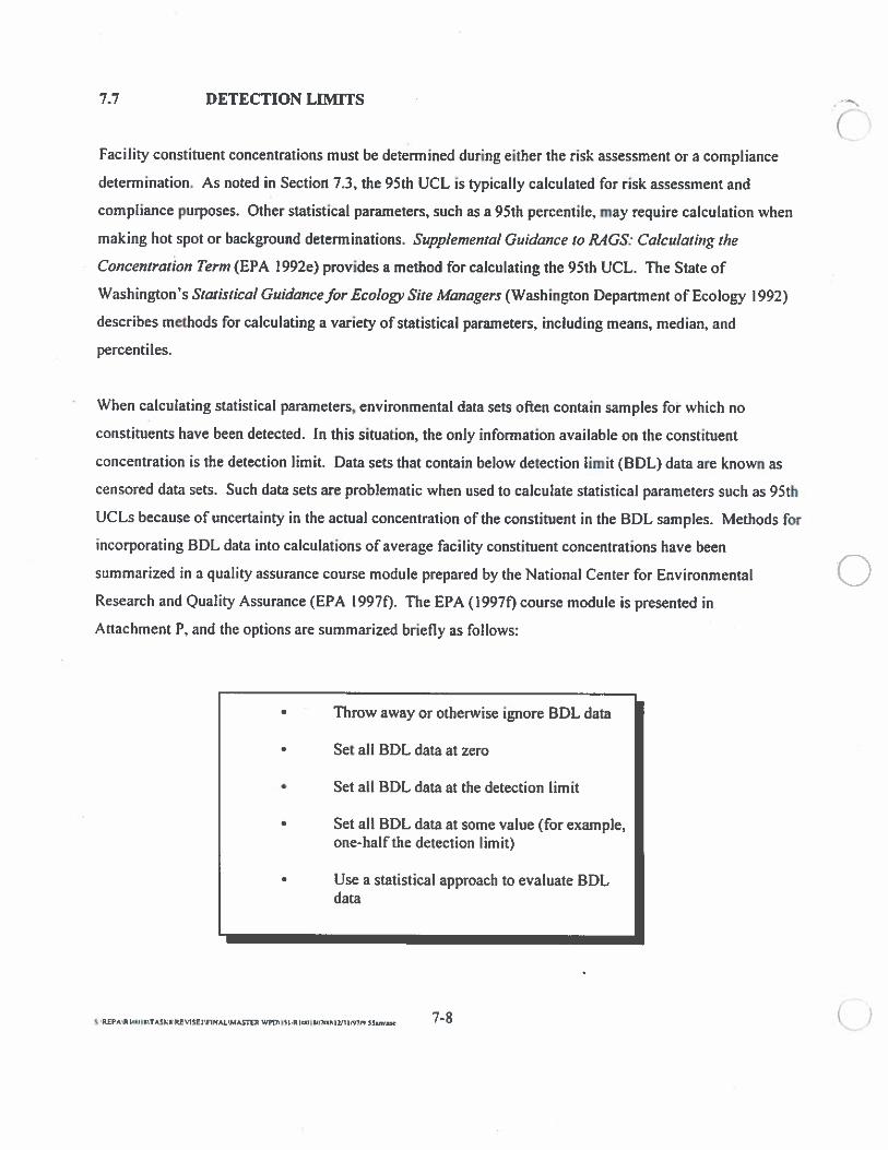
7.7 DETECTION LIMITS

Facility constituent concentrations must be determined during either the risk assessment or a compliance

determination. As noted in Section 7.3, the 95th UCL is typically calculated for risk assessment and

compliance purposes. Other statistical parameters, such as a 95th percentile, may require calculation when

making hot spot or background determinations. Supplemental Guidance to RAGS: Calculating the

Concentration Term (EPA I 992e) provides a method for calculating the 95th UCL. The State of

Washington’s Statistical Guidancefor Ecology Site Managers (Washington Department of Ecology 1992)

describes methods for calculating a variety of statistical parameters, including means, median, and

percentiles.

When calculating statistical parameters, environmental data sets often contain samples for which no

constituents have been detected. In this situation, the only information available on the constituent

concentration is the detection limit. Data sets that contain below detection limit (BDL) data are known as

censored data sets. Such data sets are problematic when used to calculate statistical parameters such as 95th

UCLs because of uncertainty in the actual concentration of the constituent in the BDL samples. Methods for

incorporating BDL data into calculations of average facility constituent concentrations have been

summarized in a quality assurance course module prepared by the National Center for Environmental

Research and Quality Assurance (EPA l997Q. The EPA (1997±) course module is presented in

Attachment P. and the options are summarized briefly as follows:

• Throw away or otherwise ignore BDL data

• Set all BDL data at zero

• Set all BDL data at the detection limit

• Set all BDL data at some value (for example,one-half the detection limit)

• Use a statistical approach to evaluate BDLdata

/

S PAM WFOI5I.R IINIlI’Iflh2fl fl’N 7—8

As noted in Attachment P, application of the first three methods may result in overestimations or

underestimations of the true mean and variance. If BDL data are not used when calculating statistical

parameters, the true mean may be overestimated and variability’ may be underestimated. If BDL data are

all set at zero, the true mean may be underestimated and variability overestimated. If BDL data are all set

at the detection limit, the true mean may be overestimated and variability underestimated.

The fourth method, using one-half the detection limit for BDL data, is frequently assumed in risk

assessments. The one-half detection limit method simply estimates a concentration half-way between that

assumed by Method 2 (zero) or Method 3 (the detection limit). When using any of the first 4 methods

(referred to as substitution methods), the resulting bias in estimating mean and variance is small when the

BDL data make up less than 15 percent of the data set. When the BDL data make up between 15 percent

and 50 percent of the data, however, the biases increase, and statistical approaches such as Cohen’s

adjustment, a trimmed mean, or the Winsorized mean and standard deviation can be applied (EPA I 997fl.

Use of the statistical approaches will reduce the bias associated with BDL data and the use of the

substitution methods. Attachment P presents a further description of the substitution and statistical

methods for handling BDL data.

Guidance for Data Quality Assessment, Practical Methods for Data Analysis (EPA I 996d) provides

additional specific guidance on the statistical methods. Risk Assessment Guidance for Superfluid.

Volume I, Human Health Evaluation ManuaL Part A (EPA I 989c) recommends that sample quantitation

limits be used as the detection limits of first choice when applying BDL methods. If sample quantitation

limits are not available, contract-required or method detection limits should be used.

[PAR PIMIW TASk RfllSEJSINAL MASThR WPD’ IS RI CR1 IRII’CRI’ I 111 I rITR Sm1.c —

-J

RE

FE

RE

NC

ES

REFERENCES

American Society for Testing and Material (ASTM). I 995a. Standard Guidefor DevelopingConceptual Site Models for Contaminated Sites. Standard E- I 689. Philadelphia, Pennsylvania.November.

ASTM. I 995b. Standard Guide for Risk-Based Corrective Action Applied at Petroleum Release Sires.Standard E-l739. Philadelphia, Pennsylvania. November.

ASTM. 1996. Draft Standard Guidefor Probabilistic Risk Assessment and Handling Uncertaimies inRisk Assessmentsfor Contaminated Sites. ASTM, Philadelphia. February.

Aulerich, R.J., R.K. Ringer, J. Safronoff. 1986. Assessment of Primmy Versus Secondan’ Toxicin’ ofAroclor 1254 to Mink Arch. Environ. Contam. Toxicol. 15:393-399.

Baes, C.F., R..D. Sharp, A.L. Sjoreen, R.W. Shor. 1984. A Review andAnalysis ofParameters forAssessing Transport ofEnvironmentally Released Radionuclides Through Agriculture. OakRidge National Laboratory. ORNL-5786. September.

California Environmental Protection Agency (Cal/EPA). 1994. Preliminary Endangerment AssessmentGuidance Manual. Department of Toxic Substances Control. January

Cal/EPA. I 996a. Guidance for Ecological Risk Assessment at Hazardous Waste Sites and PermittedFacilities - Part A: Overview. Department of Toxic Substances Control. Sacramento, California.July.

Cal/EPA. I 996b. Guidance for Ecological Risk Assessment at Hazardous Waste Sites and PermittedFacilities - Part B: ScopingAssessment. Department of Toxic Substances Control. Sacramento,California. July.

Cowherd, C.G., G Muleski, P. Engelhart, and D. Gillette. 1985. RapidAssessment ofExposure ofParticulate Emissions from Surface Contamination. Prepared for U.S. Environmental ProtectionAgency, Office of Health and Environmental Assessment, Washington, D.C. EPA/600/8-85/002.National Technical Information Service (NTIS) PB85-92219 7AS.

Daniel. Wayne W. 1983. Biostatistics: A Foundation for Analysis in the Health Sciences, Third Edition.John Wiley ana Sons, Inc.

Decisioneering, Inc. 1993. Crystal Ball Version 3.0 User Manual. Denver.

Franz. T.J. 1984. Percutaneous Absorption ofBenzene. Advances in Modern Environmental Toxicology.Volume 6, Applied Toxicology ofPetroleum Hydrocarbons. Princeton Scientific Publish, Inc.Pages 6 1-70.

Gilbert. Richard. 1987. Statistical ivIethods for Environmental Pollution Monitoring. Van NostrandReinhold Company, Inc.

S .REPA’RI,NII’TASK*RE1SE2SNAL).IA5TER WPOI5 IR I3III7WSJ2flI,7m ‘am,n —

Gilbert, Richard. 1993. Letter Regarding Background Comparison Methods for Rocky Flats Plant. ToBeverly Ramsey, Systematic Management Services. Inc. July 30. (

Johnson, P.C., and R.A. Eninger. 1991. “Heuristic Mode/for Predicting the Intrusion Rate ofContaminant Vapors into Buildings.’ Environmental Science and Technology: Volume 25.Number 8, pages 1445 -1452.

Kissel, J.C., Richter, K.Y. and Fenske. R.A. Unpublished. Dermal Soil Exposure: Two Investigation ofSoil Contact and Skin Coverage with the Aid ofa Fluorescent Tracer. (Unpublished).

Kissel, J.C., Richter, KY. and Fenske, R.A. 1996. Field Measurement of Dermal Soil Loading Attributedto Various Activities: Implications for Exposure Assessment, Risk Analysis 16: 115-125. /°1 (o

Lloyd, K.J., K.M. Thompson, and D.E. Burmaster. 1992. Probabilistic Techniques for BackcalculatingSoil Cleanup Targets In: Superfisnd Risk Assessment in Soil Contamination Studies, ASTMSTPI 158 (Eds. K.B. Hoddinott, American Society for Testing and Materials, Philadelphia).

Long, E.R. and L.G. Morgan. 1990. The Potentialfor Biological Effects ofSediment-SorbedContaminants Tested in the National Status and Trends Program. Technical Memorandum NOSOMA 52. March.

Massachusetts Department of Environmental Protection (MDEP). 1995. Guidancefor Disposal Site RiskCharacterization. Interim Final Policy. WSC/ORS-95- 141. Boston, Massachusetts. July.

Mckone, T.E., and K.T. Bogen. 1992. “Uncertainties in Health-Risk Assessment: An Integrated CaseStudy Based on Tetrachloroethylene in California Groundwater.” Regulatory Toxicology andPharmacology, Volume 15, pages 86-103.

Morgan, M. Granger and Max Henrion. 1990. Uncertainty, A Guide To Dealing With Uncertainty inQuantitative Risk and Policy Analysis. Cambridge University Press.

National Research Council. .1994. Science and Judgement in RiskAssessment, Prepublication Copy.National Academy Press.

ODEQ. 1996. “Guidance for Ecological Risk Assessment.” Draft. November.

Remington, Richard D., and M. Anthony Schork. 1970. Statistics with Applications to the Biological andHealth Sciences. Prentice-Hall, Inc.

Ryan, L.A., et al. 1987. “Assessing Risk From Dennal Exposure at Hazardous Waste Sites.” InSuperfund 87: Proceedings of the Eight National Conference: November 16-I 8; Wash. D.C.,G. Bennett and J. Bennett (eds). The Hazardous Materials Control Research Institute.pp. 166-8.

Sigal. L.L. and G.W. Suter II. 1989. Potential Effects ofChemicalAgents on TerrestrialResources. Environmental Professionals. Volume 11. Pages 376-384.

S REPS R IflII’.TASK\REVTSE33INAIt45Thk WPDi%Ij II,IIlI’ThtV1U’flfl 5Jm.rn R—2

Skowronski, G.A., R.M. Turkall, and M.S. Abdel-Rahman. 1988. SoilAdsorption Alters Bioavailabilin’of Benzene in Dermally Exposed Male Rats. American Industrial Hygiene Association Journal 49(10). Pages 506-511.

Smith, Roy L. 1994. Use ofMonte Carlo Simulationfor Human Exposure Assessment at a SuperfisndSire. Risk Analysis, Volume 14, Number 4. Pages 433-439.

Suter II, G.W. 1993. Ecological RiskAssessment. ISBN 0-87371-875-5. Lewis Publishers. Chelsea,Michigan.

Tetra Tech. 1996a. Record of Telephone Conversation between Neil Morton of Tetra Tech and RandySteger of Idaho Division of Environmental Quality. August 1.

Tetra Tech. 1996b. Record of Telephone Conversation Between Paul Racene of Tetra Tech and RandyBuckindorf of Alaska Department of Environmental Conservation. October 24.

Thompson, K.M., D.E. Burmaster, and E.A.C. Crouch. 1992. Monte Carlo Techniques for QuantitativeUncertainty Analysis in Public Health Risk Assessments. Risk Analysis, Volume 12, No. 1,pages 53-63.

Travis, C.C., and A.D. Arms. 1988. Bioconcentration of Organics in Beef Milk, and Vegetation. InEnvironmental Science and Technology. Volume 22. Pages 27 1-274.

U.S. Environmental Protection Agency (EPA). 1979. Guidelines and Specjflcationsfor PreparingQuality Assurance Program Plans. QAMS-004/80.

EPA. 1980. Interim Guidelines and Spec{flcationsfor Preparing Quality Assurance Project Plans.Office of Monitoring Systems and Quality Assurance. Office of Research and Development.QAMS-005/80. December.

EPA. 1982. An Exposure and Risk Assessment for Benzo(a)pyrene and Other Polycyclic AromaticHydrocarbons. Volume IV, Final Draft Report, Office of Water. October.

EPA, 1985. Verjfication of PCB Spill Cleanup By Sampling andAnalysis. Office of Toxic Substances.EPA-560/5-85-026. August.

EPA. 1986a. Quality Criteriafor Water 1986. U.S. Environmental Protection Agency, Office of Water,EPA44O/5-86-001. May I.

EPA. I 986b. Test Methods for Evaluating Solid Waste. SW-846. Office ofSolid Waste and EmergencyResponse. November plus updates.

EPA. 1988. Guidance for Conducting Remedial Investigations and Feasibility Studies Under CERCLA,Interim Final. Office of Emergency and Remedial Response. EPA/540/G-89/004. October.

EPA. 1989a. RCRA Facility investigation (RF1) Guidance, Interim Final. EPA 530/SW-89-023 1.Office of Solid Waste and Emergency Response.

REP I.U TA’EVSE IINM.MASThR WPD S3am*ac —

EPA. 19891* Methods for Evaluating the Attainment ofCleanup Standards, Volume 1: Soils and SolidMedia. Office of Policy, Planning, and Evaluation. EPN23O/02-89/042. February.

EPA. I 989c. Risk Assessment Guidancefor Superfund, Volume I, Human Health Evaluation ManuaLPart A, Baseline Risk Assessment. Office of Solid Waste and Emergency Response. OSWERDirective No. 9285.7-OlA. EPA 540/1-89/002.

EPA. I 989d. Exposure Factors Handbook. Office of Health and Environmental Assessment.EPAJ600/8-89/043. http://www.epa.gov/ORD/WebPubs/exposure/

EPA. I 989e. Clean Closure Guidance Manualfor Hazardous Waste Management Units,EPPJ530-SW-87-022. August.

EPA. 1 989f. Interim Procedures for Estimating Risks Associated with Exposures to Mixtures ofChlorinated Dibenzo-p-Dioxins and Dibenzofurans (CDDs and CDFs) and 1989 Update.EPA/625/3-89/0 16. March.

EPA. 1989g. Risk Assessment Guidancefor Superfluid. Volume 2: Environmental Evaluation Manual.Interim Final. EPA/540/1-89/OOIA. Office of Solid Waste and Emergency Response.Washington, D.C. March.

EPA. I 989h. Ecological Assessment of Hazardous Waste Sites: A Field and Laboratory Reference.EPA/600/3-89/013. Office of Research and Development. Corvallis, Oregon.

EPA. 1989 i. The Nature and Extent ofEcological Risks at Superfluid Sites and RCR.A Facilities.EPA-230-03-89-043. Office of Policy Analysis. Washington. D.C. June. ED)

EPA. I 989j. Ecological Risk Assessment ofSuperfund Sites: An Overview. ECO Update. IntermittentBuLletin. VoLume L,Number 2. Office of Emergency and Remedial Response. Washington, D.C.

EPA. 1989k. Statistical Analysis of Ground- Water Monitoring Data at RCRA Facilities, Interim FinalGuidance. Office of Solid Waste. April.

EPA. 1990. Methodologyfor Assessing Health Risks Associated with Indirect Exposure to CombustorEmissions, Interim Final. Office of Health and Environmental Assessment. EPA/600/6-90/003.January.

EPA. 1991 a. EPA Region 10 Supplemental Risk Assessment Guidance for Superfund. August.

EPA. 1991 b. Risk Assessment Guidance for Superfund, Volume I: Human Health Evaluation Manual,Supplemental Guidance: Standard Default Exposure Parameters. OSWER directive 9285.7-05.

EPA. 1991 c. Risk Assessment Guidancefor Superfrnd, Volume I Human Health Evaluation Manual,Part B. Development ofRisk-based Remediation Goals. Office of Solid Waste and EmergencyResponse. OSWER Directive No. 9285.7-018. EPA/5401R-92/003.

EPA. 1991 d. Evaluation ofDredged Material Proposedfor Ocean Disposal, Testing ManuaL Office ofWater, EPA/503/8-9l/00l. Febniarv.

S RLPAR HM)fl’TASkLREVISE3YTNAL’MASTEk WPD\II .RIiwIpmflTThIlJl rn,,’, 35mm., R—4

EPA. I 992a. Interim Final Guidelines for Developing Risk-Based Cleanup Levels at RCRA SUes inRegion JO. EPA Region 10. March.

EPA. I 992b. Final Guidance for Data Useabilijv in Risk Assessment (Part A). Office of Solid Waste andEmergency Response. Publication 9285.7-09A/FS. May.

EPA. I 992c. Exposure Assessment Guidelines. Federal Register, May 29, 1992. 57 FR 22888-22938.

EPA. 1 992d. Dermal Exposure Assessment: Principles and Applications. Office of Health andEnvironmental Assessment. EPA]60018-9 1/0118. January.

EPA. 1 992e. Supplemental Guidance to RAGS: Calculating the Concentration Term. Office of SolidWaste and Emergency Response. Publication 9285.7-081.

EPA. 19921 Frameworkfor Ecological Risk Assessment. EPAJ630IR-92/001. Risk Assessment Forum.Washington, D.C. February.

EPA. 1992g. Guidance for Data Useability in Risk Assessment (Part B). Publication number9265.7-098. Office of Emergency and Remedial Response. Washington, D.C. May.

EPA. 1992h. Statistical Methods for Evaluating the Attainment of Cleanup Standards. Volume 2:Groundwater. Office of Policy, Planning, and Evaluation.

EPA. I 992i. Statistical Methods for Evaluating the Attainment ofCleanup Standards, Volume 3:Reference-Based Standardsfor Soils and Solid Media. Office of Policy, Planning, andEvaluation. EPA/2301R-94/004. December.

EPA. I 992j. Guidance on Risk Characterizationfor Risk Managers and Risk Assessors. Memorandumfrom F. Henry Habicht II, Deputy Administrator. Office of the Administrator. Washington, D.C.February.

EPA. 1992k. Statistical Analysis ofGround-Water Monitoring Data at RCRA Facilities, Addendum toInterim Final Guidance. Office of Solid Waste. July.

EPA. I 993a. Supplemental Guidance to RAGS: Estimating Riskfrom Groundwater Contamination.Office of Solid Waste and Emergency Response. December.

EPA. I 993b. Qualm’ Assurance Project Plans for RCK4 Ground-Water Monitoring and CorrectiveAction Activities. July.

EPA. I 993c. RCK4 Public Involvement Manual, EPA 530-R-93-006.

EPA. 1 993d. Addendum to Methodologyfor Assessing Health Risks Associated with Indirect Exposure toConthustor Emissions, External Review Draft. Office of Health and Environmental Assessment.EPAJ600/AP-93/003. November.

EPA. I 993e. Provisional Guidance for Quantitative Risk Assessment ofPolvcvclic AromaticHvdrocarbons EPA/600/R93/089. July.

REPA R IIHRl TASKWRE,SE:flNALM ASTIR SPOIl SIR ICR’’ RIC TCREI LII TIC’) ‘..wnr —

EPA. 1993 f. Wild!jfe Exposure Factors Handbook - Volume 1 of 2. EPAJ600/R-93/1 87a. Office ofResearch and Development. Washington, D.C. December.

EPA. 1993g. WildlLfe Exposure Factors Handbook - Appendix: Literature Review Database - Volume 2of2. EPAI600IR-9311 87b. Office of Research and Development. Washington. D.C. December.

EPA. I 993h. Superfund c Standard Default Exposure Factors for the Central Tendency and ReasonableMaximum Exposure.

EPA. 1994a. RCRA/CERCLA Interface-Interim Final Guidance. EPA Region 10 Memorandum.August 3.

EPA. I 994b. Guidance for the Data Quality Objectives Process. EPA QA/G-4. Quality AssuranceManagement Staff. Washington, D.C. September.http://www.epa.gov/r I Oearth/offices/oea/aaindex.htm

EPA. I 994c. Data Quality Objectives Decision Error Feasibility Trials (DQO/DEFT) Users Guide,Version 4.0. EPA QAJG-4D. September.hftp://www.epa.gov/rl Oearth/offices/oealaaindex.htm

EPA. I 994d. EPA Requirementsfor Quality Assurance Project Plans for Environmental DataOperations, Draft Interim Final. EPA QAJR-5. August.http:Hwww.epa.gov/rI Oearth/offices/oea/aaindex.htm

EPA. I 994e. Requirements for Quality Management Plans (QA/R-2). August.http://www.epa.gov/rl Oearth/offices/oea/aaindex.htm cD

EPA. I 994f. USEPA Contract Laboratory Program National Functional Guidelines for Organic DataReview. Publication 9240.1-05. February.http://www.epa.gov/r I Oearth/offices/oealaaindex.htm

EPA. 1994g. USEPA Contract Laboratory Program National Functional Guidelines for Inorganic DataReview. Publication 9240.1-05-01. February.http://www.epa.gov/r I Oeanhloffices/oea/aaindex.htm

EPA. I 994h. Region 8 Superfluid Technical Guidance &4-03: Evaluating and Identfving Contaminantsof Concernfor Human Health. Region 8, Denver. September.

EPA. I 994i. Guidance for Performing Screening Level Risk Analyses at Combustion Facilities BurningHazardous Wastes, Attachment C, Draft Exposure Assessment Guidance. Office of Emergencyand Remedial Response. December 14.

EPA. I994j. Estimating Exposure to Dioxin-Like Compounds. Office of Research and Development.EPAI600/6-881005 B. hnp://www.epa.gov/docs/exposure/

EPA. 1994k. Memorandum Regarding Revised Interim Soil Lead Guidance for CERCL4 Sites andRCRA CorrectiveAction Facilities. From Elliott P. Laws, Assistant Administrator. To RegionalAdministrators l-X. July.

S REPAR I...J,TA5Kfl%1SErflNArn4A5ThR WPOU3 I.RI(SHW)7IlzI1 P17?) 3Saainc R— 6

EPA. 19941. Ecological Risk Assessment Guidance for Superfrnd: Processfor Designing andConducting Ecological Risk Assessments. Review Draft. Environmental Response Team. Edison,New Jersey. September.

EPA. I 994m. Region 8 Superfund Technical Guidance: Use ofMonte Carlo Simulation in PerformingRisk Assessments. Region 8, Denver. December.

EPA. I 995a. EPA Risk Characterization Program, Memorandum from Carol Browner, EPAAdministrator. March 21.

EPA. I 995b. Region 5 Ecological Data Quality Levels. Draft Final. Prepared for the Office of RCRA byPRC Environmental Management, Inc. Chicago, Illinois. September.

EPA. I 995c. Determination ofBackground Concentrations ofInorganics in Soils and Sediments atHazardous Waste Sues. Office of Solid Waste and Emergency Response. EPA/54015-96/500.December.

EPA. I 995d. Land use in the CERCL4 Remedy Selection Process, Memorandum from Elliott P. Laws.Office of Solid Waste and Emergency Response Directive No. 9355.7-04. May 25.

EPA. 1995e. New Policy on Evaluating Health Risks to Children. Office of the Administrator.October 20.

EPA. 1995f. Region III Technical Guidance Manual, RiskAssessment: Assessing Dermal Exposure fromSoil. Office of Superfund Programs. December.http://www.epa.gov/reg3hwmd/riskmenu.htm

EPA. 1995g. Memorandum Regarding Further Issuesfor Modeling the Indirect Exposure Impacts fromCombustor Emissions. From Matthew Lorber, Exposure Assessment Group and Glenn Rice,Indirect Exposure Team, Office of Research and Development. To Addressees. January 20.

EPA. I995h. Supplemental Guidance to RAGS: Region 4 Bulletins, Human Health Risk AssessmentWaste Management Division. November.

EPA. I 996a. Geostatistical Sampling and Evaluation Guidance for Soils and Solid Media, Review Draft.Office of Solid Waste. February.

EPA. I 996b. Soil Screening Guidance: Users Guide. Office of Solid Waste and Emergency Response.Publication 9355.4-23. April. http://www.epa.gov/superfund.’oerr/soil/inde>chtml

EPA. I 996c. Region IX Preliminary Remediation Goals (PRGs) 1996. August 1.http ://www.epa. gov/regiono9/wastefsfundlprglindex. html

EPA I 996d. Guidance for Data Quality Assessment. Practical Methods for Data Analysis. EPA QAIG-9,QA96 Version. EPA/600/R-96/084. July.http://www.epa.gov/rI Oearthloffices/oea/aaindex.html

5 REPA R l.tIW,TA5KWRE95EflINAjWASflR wpp\IsI.RIIrnE,tmIncL’,t Ipnsa —

EPA. 1996e. Exposure Factor Handbook, Internet Download, EPA/600/P-95/002A. August.

EPA. I 996f. Supplemental Risk Assessment Guidancefor Superfrnd. Draft. EPA Region 10 Risk CEvaluation Unit. Seattle, Washington. February.

EPA. 1996g. Integrated Risk Information System (IRIS). On-line database.http://www.epa.gov/ORD/dbases/iris/ (monthly updates)http://www.epa.gov/ngigpm3/iris/index.html (web prototype)

EPA. I 996h. Risk-Based Concentration Table, January-June 1996. U.S. Environmental ProtectionAgency, Region III. January.http://www.epa.gov/reg3hwm&riskmenu.htm

EPA. 1996i. Proposed Guidelines for Carcinogen Risk Assessment. Office of Research andDevelopment. EPA/600/P-92/003C. April.hftp://www.epa.gov/ORD/WebPubs/carcinogen/

EPA. I 996j. PCBs: Cancer Dose-Response Assessment and Application to Environmental Mixture.National Center for Environmental Assessment. Office of Research and Development.EPAI600/P-96/00 IA. September.http://www.epa.gov/ORD/WebPubs/pcb/

EPA. 1996k. Recommendations of the Technical Review Work Group for Lead for an Interim Approachto Assessing Risks Associated with Adult Exposures to Lead in Soil. December.

EPA. 19961. Proposed Guidelines for Ecological Risk Assessment. Published in CFR Volume 61,Number 175. Risk Assessment Forum. Washington, D.C. EPM63OIR-95/002B. September.http://www.epa.gov/ORD/WebPubs/ecoriskl

EPA. I 997a. Health Effects Assessment Summary Tables (HEAST), FY 1997 Update. Office of SolidWaste and Emergency Response, EPA-540-R-97-036. NTIS No. PB97-92 1199. July.

EPA. 1997b. Risk Assessment Guidance for Superfund Volume 1: Human Health Evaluation Manual,Supplemental Guidance, Dermal Risk Assessment Interim Guidance. Office of Emergency andRemedial Response. June 19.

EPA. 1997c. Risk Assessment Forum Review of “Guidelines on Health RiskAssessment of ChemicalMixtures ‘, NCEA-C-0 148. June 20.

EPA. 1997d. Guiding Principles for Monte Carlo Analysis, EPA’6301R-97/001. March.hnp://www.epa.gov/ncealmcpolicy.htm

EPA. 1997e. Policy For Use of Probabilistic Analysis in Risk Assessments at the U.S. EnvironmentalProtection Agency. Office of Research and Development. May 15.http://www.epa.gov/ncealmcpolicy.htm

EPA. I997f. Quality Assurance Course Module 492, Dealing with Data Below Detection Limits,National Center For Environmental Research and Quality Assurance. Downloaded March.

S REPAS I,.,IaTASK,R1%1SE2rINALWA3ThR WPD’ISiJ nii.’,,,sim mN R— 8

EPA. 1997g. Rules of Thumbfor Superfund Remedy Selection, OSWER 9355.0-69. August.

EPA. 1997h. The Role of CSG WPPs in EPA Remediation Programs. OSWER Directive 9283.1-09.April 4.

Washington Department of Ecology (Ecology). 1992. Statistical Guidance for Ecology Site Managers.Washington State Department of Ecology, Toxics Cleanup Program. August.

Ecology. 1994. Guidancefor Clean Closure ofDangerous Waste Facilities, Publication No. 94-Ill.August.

Ecology. I 995a. Washington State Comprehensive State Groundwater Protection Program. CoreProgram Assessment Document. July.

Ecology. I 995b. Summary of Guidelines for Cantaminated Sediments. WDOE publication 95-308.March.

Ecology. 1996. Model Toxics ControlAct Cleanup Levels and Risk Calculations (CLARC II Update.Publication No. 94-145. Febmarv.

Wester. R.C.. H.!. Maibach, D.A.W. Bucks, L. Sedik, J. Melendres, CL. Laio, S. DeZio. 1990.Percutaneous absorption of[14C]DDT and [14C]benzo(a)pyrenefrom soil. Fund. Appl.Toxicol15:510-516.

Wester, R.C., H.!. Maibach, L. Sedik, J. Melendres, S. DeZio. M. Wade. I992a. In vitro percutaneousabsorption of cadmium from water and soil into human skin. Fundam. AppI. Toxicol. 19:1-5.

Wester, R.C., HI. Maibach, L. Sedik, J. Melendres, CL. Lab, S. DeZio. 1992b. Percutaneousabsorption of [14C]chlordane from soil. J. Toxicol. Environ. Health 35:269-77.

Wester, R.C., H.1. Maibach, L. Sedik. J. Melendres. M. Wade. 1993a. In vivo and in vitro percutaneousabsorption and skin decontamination ofarsenic from water and soiL Fundam. AppI, Toxicol.20 :3 3 6-40.

Wester, R.C., HI. Maibach, L. Sedik, J. Melendres. M. Wade. 1993b. Percutaneous absorption of PCBsfrom soil: in vivo Rhesus monkey, in vitro human skin, and binding to powered human stratumcorneum. J. Toxicol. Environ. Health 39:375-82.

Wester, R.C.. HI. Maibach, L. Sedik, J. Melendres, M. Wade, S. DeZio. 1993c. Percutaneous absorptionofpentachlorophenolform soil. Fundam. AppI. Toxicology 20:68-7L

Wester. R.C., J. Melendres, F. Logan, X. Hui, H.!. Maibach. 1996. Percutaneous absorption of2, 1-dichlorophenoxyacetic acidfrom soil with respect to the soil load and skin contact time: inrho absorption in Rhesus monkey and in vitro absorption in human skin. J. Toxicol. Environ.Health 47:335-44.

MI MSMIWIIK TASK tREV1 SEI.FINAL\MASThR WrOl I’ .R 1111 MI TIM’. I UT nw 5i.m\sJt —

Wenisel, R.S., T.W. LaPoint, M. Simini, D. Ludwig. and L. Brewer. 1994. Procedural GuidelinesforEcological Risk Assessments at US. Army Sites - Volume I. Report Number ERDEC-TR-22 1.Aberdeen Proving Ground, Maryland. December.

a

R— 1 0 (Q

Name

W1DEX

ABS (see dermal absorption factors)Alaska Department of Environmental Quality (ADEC) 2-2Air 4-9, 4-12, 4-13, 4-14, 4-17, 4-20, 4-27, 4-28, 4-30 thru 4-35. 4-72. 4-78, 7-2

4-13, 4-14. 5-15. 5-173-8,3-11,4-70.6-6, 7-5, 7-7

(see ambient waler quality criteria)4-40 thru 4-53, 4-68. 4-69

4-22, 4-3 7, 4-44. 4-45. 4-723-3, 5-2. 5-9. 5-18

Chapter 1, 3-1,3-14, 4-I, 4-15. 4-43(see constituents of potential concern)

(see cancer potency factor)3-13,7-1,7-7,7-9.

3-1, 3-7, 3-8, 5-22, 7-I, 7-4, 7-71-5. 3-9. 4-75, 7-7

3-6, 3-7, 3-8, 7-4, 7-6, 7-73-2, 3-5, 3-6. 7-I, 7-3

4-23, 4-24, 4-25, 4-62 thru 4-674-23, 4-25

3-11,7-8,7-94-23, 4-24, 4-38, 4-46, 4-47, 4-48, 4-5 1, 4-53

5-261-6, 1-8, Chapter 5, 6-1, 6-8, Attachment N

(see Washington State Department of Ecology)4-I, 4-2, 4-22, 4-25, 4-73

1-7, 4-14, 4-17, 4-22, 4-60, 4-76, 4-77, 5-164-1, 4-2, 4-3, 4-5, 4-16, 4-17, 4-20, 4-22, 4-25, 4-36.

4-74, 4-76, 5-1 thru 5-18, 5-29, 6-11,6-12.6-13, 6-31. Attachment N3-4, 4-19, 4-25, 4-27, 4-36, 4-57, 4-77, 5-5, 5-9, 5-16,

5-20. 5-29, 6-9, Attachment N3-5, 4-2, 4-3, 4-4, 4-6 thru 4-11,4-13,4-14,4-25,4-27.

4-60. 4-65, 4-67, 4-68, 4-70, 4-71, 4-76, 4-77, 5-9, 6-12. 7-2, 7-3, 7-74-15, 4-16,4-42,4-43,4-57,4-63,4-69,4-71,5-26,6-11

3-11,4-18,4-21,4-42,4-59,4-71,5-23, 5-254-28, 4-30, 4-33

(see human health risk assessment)(see hazard index)

3-14, Chapter4, 6-I, 6-5, 6-8, 6-10-6-12. 6-2!

(COPCs)

Ambient water quality criteriaAnalytical methodsAWQCCancer potency factorCombustionConceptual site modelConstituents of potential concernCOPCsCPFData quality assessment (DQA)Data quality objectives (DQO)Data useabilityDecision errorsDecision ruleDermal absorption factorsDermal permeabilityDetection LimitsDioxinEcological adversityEcological risk assessmentEcologyExposure assessmentExposure assumptionsExposure pathways

4-3 7, 4-44, 4-60, 4-65, 4-72,Fate and transport

Groundwater4-34, 4-35, 4-36, 4-53.

Hazard indexHazard quotientHenry’s Law...HHRAHIHuman health risk assessment . .

Idaho Division of Environmental Quality (IDEQ) 2-2Inhalation 4-2 thru 4-5, 4-14, 4-16 thru 4-22, 4-27, 4-30, 4-34, 4-42, 4-52, 4-56, 4-60, 4-65, 4-66,

5-9, 6-12, 6-13

S REPA.R IC’)ITASKWRS95E2$INAL’MASTER WPO’ISI R IIrnIIlI7IMI\I2/1INlr) S5.m’sac I—I

Name

Inhalation reference concentrations 4-42, 4-43. 4-44Land use 1-6, 2-1, 3-3, 4-5 thru 4-9, 4-13, 4-14, 4-58, 4-65, 4-74. 4-75, 4-76Lead 2-1, 4-22, 4-38, 4-57, 4-73, 4-74, 4-75, 5-19, 6-13, 6-17, 6-18. Attachment NLowest adverse effects level (LOAEL)Maximum contaminant levels (MCLs)Measurement endpointsModel Toxics Control Act 2-3, 4-6, 4-7,Monte Carlo simulationMTCANo observed effect level (NOAEL)Oregon Department of Environmental QualityPAHsParticulate emission factorsP035PEFPolychlorinated biphenylsPolycyclic aromatic hydrocarbonsPreliminary remediation goals (PRG)Problem formulationQuality assurance project plan (QAPP)Quantitation limitsRBCsRCRA facility investigation (RFI)Reference Dose 4-4RfCsRfDRFIRisk characterization

Risk management 14, 1-10, 1-11,4-7,Risk-based screening Level (RBSL)Risk-based concentrations Chapter 1,

4-42, 4-57,Safe Drinking Water ActSoil cleanup levelsSolid waste management unitsSurface waterSWMU2,3,7,8-Tetrachlorodibenzo-p-dioxin

4-78. 4-79. 5-224-10, 4-13, 4-14, 4-70, 4-71

5-2, 5-13, 5-14, 5-25, Attachment Nthru 4-14, 4-2 1, 4-22, 4-36, 4-57, 4-60, 7-2 thru 7-5

5-29, Chapter 6(see Model Toxics Control Act)

4-78, 4-79, 5-4, 5-15, 5-21, 5-22, 5-242-2,4-8,4-10,4-15,5-1,5-6

(see polycyclic aromatic hydrocarbons)4-17, 4-19, 4-27, 4-29, 4-30, 4-34

(see polychlorinated biphenyls)(see particulate emission factors)

4-24, 4-46, 4-47, 4-48 thru 4-53, 4-724-24, 4-45, 4-54, 4-73, Attachment N

3-11,4-15,4-17, 4-25, 4-59, 4-60-6, 5-2, 5-4, 5-6, 5-9, 5-10, 5-15, 5-16, 5-22, 5-27

3-10,3-153-11,3-13,3-16,4-75,4-76,7-9

(see risk-based concentrations)3-I, 3-3. 3-4, 4-1, 4-27, 4-57, 4-65, 5-4, 5-5, 5-22, 7-1

4-44,4-53,4-56,4-59,4-66,4-68,4-69,4-73,4-79,6-Il(see inhalation reference concentration)

(see reference dose)(see RCRA facility investigation)

1-9, 3-15, 4-1, 4-2, 4-43,4-44, 4-45, 4-57, 4-58, 5-I, 5-2,5-22 thru 5-27, 6-1, Attachment N

4-44, 4-60, 4-74, 5-2, 5-IS, 5-24. 5-25, 5-27, Attachment N1-8.4-15.4-17

3-4. 3-14, 4-I, 4-2, 4-14, 4-15, 4-17, 4-30, 4-37, 4-38, 4-39,4-59, 4-60, 4-66 thru 4-69, 4-71 thru 4-75, 6-2 1, 6-26, 6-27

1-3,4-10,4-134-5, thru 4-8. 4-14, 7-2

3-3, 3-5, 3-6, 3-7, 5-3, 7-44-2, 4-3, 4-5 thru 4-9,4-Il thru 4-14, 4-36, 4-68, 5-9, 7-2

(see solid waste management units)(see dioxin)

INDEX

4-10

(ODEQ)

.1

I thru0

0S RE?A\Ru.IIrT4S,Inv1SrnNALMASTER 3.m5a. 1-2

IT%DEX

Name

Total petroleum hydrocarbons.4-55Toxicity reference values (TRV) 5-4, 5-15, 5-21, 5-23, 5-24, 5-25TPH (see total petroleum hydrocarbons)TRV (see toxicity reference values)Uncertainty 1-3, 1-9, 1-10, 4-40 thru 4-43, 4-49, 4-56, 4-74 thru 4-80, 5-6, 5-25, 5-26, 5-27.

5-29, 5-30, 6-1, 6-2, 6-5 thru 6-9, 6-13, 6-19, 6-26, 6-3 1, 7-4, 7-6, 7-8, Attachment NVF (see volatilization factor)Volatile organic compounds (VOC) 4-23, 4-27, 4-66, 4-71, 4-77Volatilization factor 4-27, 4-28, 4-30, 4-34, 4-66, 4-67. 4-68Washington Department of Ecology (Ecology) 2-3,4-8,4-10,4-13,4-14,4-21,4-36, 5-17, 7-8

S WPthI5I.R kIImflKIILq Ifl7I 3!sm\sae —

AT

FA

CU

ME

NT

S

ATTACHMENT A

U.S.. ENVIRONMENTAL PROTECTION AGENCYCAROL BROWNER MEMORANDUM ON RISK ASSESSMENT

S REPARnhptTASKrREV1SEflNAtMASTER 1’pi.sac

sr•7

____

UNITED STATES ENVIRONMENTAL PROTECTION AGENCYWASHINGTON. DC. 20450

THE ADMINISTRATOR

MAR 2 11935

RECEIVED

?we4ORANDUM. MAR 2 81995

SUBJECT: EPARISkCharICteriTSUOnPrOWC.. OFFICE OF

REGIONAL ADMINISTRATORTth . AsiAnaonAnodneA&nonRegional AdminiflaonGeneralC—Genud

EPA has achieved dgnifinnt pc&nioareducdoaover the paS2O yean but the challengeswe &ce now at vay &ffa from those of the pa. Many more people at awn ofenvfronmnl keec today than in the — ad their kvd ofsopliicton ad iatst inunderstanding t)w’o kew. cofles to thaesaa We now wuk with a populace which is t,t

only interaed in knowing what EPA tltinke about a pntiadu isme but also how we coat rour conehttions.

• More ad more key subholdn in e&fromtad eein wa enough inhmadon toallow fiwn to indepnvlssiysand nkejudnman.about the dg,fiçstir ofcnvñnnntalrisks and the rnsomh1enen of ow risk reduction acfioa Jfwe at to nrcedI ad build owaedlbility ad vate as a jnd in enviraámcntal protection fir thea ccntáy, EPA beresponsive and resolve to more openly ad hilly - to the mb& Ut complexities andchallenges ofenvfroml dedsioumaking in the 6cc of sdethflc tmcutaiay.

Al the we 6cc became more compla, people both incMt and onnia ofEPA mustbetter understand the basis fat ow deddons as well as our confidence in the data, the sciencepolicy judgmafla we have made, and the uncertainty in the inthrmton base. In order to achievethis better undentandthg we must improve the way in which we characterize and comnn ‘n’cfle

environmental risk. We must embrace certain fiIMamnIt2l ‘jahjt5

frltII i..

-2-

so that we may begin the process of changing the way in which we interact with each other; the- public, and key staktholders on environmental sk k.nje I need your help to ensure that these

values are embraced and that we nhange the way we do bUsiness.

First,’ we must adopt as values flnspannq in our dedioan*king process and deity incomminicon with each other and the public iegarding axvfromnaal risk and the uncertaintiesassociated with ow assesmients ofenvfronnwtal risk. .Thjs nnn that we must filly, openly,and deafly characterize dab. In doing so, we will disde the scientific analyses, uncertainties,assuiupGons, and science policies which underlie ow decisions as they an made throughout therisk nantnnt and risk managesnesit processes. I warn to be sum that key science policy k5

an identified as such during the riskarnrt process, that po&)mahn an filly swan andengaged in thesdection of science policy options, and that that choices and the rationale for

those. choices an dearly articulated and visible ‘mow cocmicatiocs about environmental risk.

-

. 1 understand that some may be concerned aboqt adsfitiiwsl dialln,gn and disputes. Iepec that will see more thlisir. particularly at flit However, I stnngiy bdieve thatmaking this change to a more open ded&’.sking pmcea will led to more meaningfld publicparticipation, better inthrnnfion fir dr.krmsking bpnved dr’w and more public mppoaand respect for EPA positions and dedciont Thenà value in sharing with others thecompletities and challenges we &á in making dedsions in the ftce ofuncertainty.. I view making

this change as essential to the long tam sw’c’ of this-Agency..

Cladtfl am on also means thatwewili su-iveto help the public penvironmental risk in the proper perspective when wattles risk managaitsit aøk’a We mustmeet this dialienga and find legitimate ways to help the public better co...per1iesit4 the relative

signffiëance ofenvironmental dab. -

Second, becsniie trnprq ‘mdecisionmakinglead to more outside questioning ofmit as wziptions and pden polities, we nnre be more

vigilant about ensuring that our core assumptions and science policies an consistent and

comparable sacas programs, well grounded in science, and that they thil within a zone of

reasonableness.” .

0

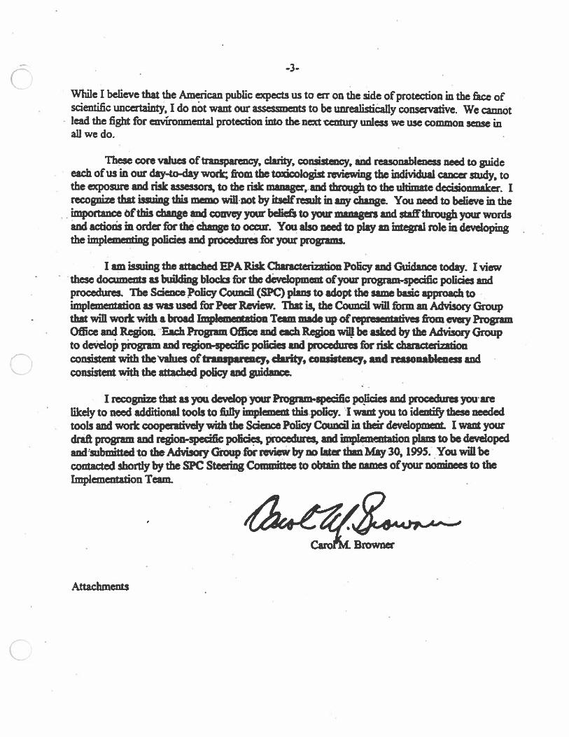
0•

-3-

While I believe that the American public expects us to en on the side of protection in the &ce ofscientific uncertainty, I do not want our assessments to be unrealisfiêally conservative. We cannotlead the fight for environmental protection into the next century unless we use common sense inall we do.

These core values offlnspanncy, clarity, con.ktnry, and reasonableness need to guideeach of us in our day-to-day work; from the toñcologig reviewing the individual cancer study, tothe exposure and risk assessors, to the risk mamger,.and through to the ultimate dedsionmaker. Irecognin that kqring this mnvv willnot by bdfresuh in any change. You need to believe in the

• importance ofthis change and convey your bdth to your managua and staff through your wordsand actions in order for the change to ocar. You also need to play an integral role in developingthe implnnniting policies and procedures for your pmgra

I am issuing the aftaded EPA Risk Characteriation Policy and Guidance today. I view• these doamias as bñlding blocks for the dadopma ofyour program-specific policies and

procedures. The Science Policy Council (SPC) plans to adopt the same basic approach toimplementation as was used for Peer Review. That is, the Council will form an Advisory Groupthat will work with a broad Implementation Team made up ofrepresatves from evny ProgramOffice and Region. Pseh Program Office and each Region will be sske4 by the Advisory Groupto dedop program and region-specific policies at procedures for risk chmaerintionconsistent with thevahies of transparency, dsrfty, consistency, and reasonableness andconsistent with the attached policy and guidance.

I recognize that as you develop your Program-specific p licies and procedures you areikely to need additional tools to folly implement tffis.poliq. I want you to idai, these neededtools and work cooperatively with the Science Policy Council in their devdopnwt I want yourdrift program and region-specific policies, mcedwes, and frTlplnnelltafion plaId to be developedat :mbthted to the Advisory Gtoupfor review by no — than May30, 1995. You will becontacted shortly by the SPC Steering Co..’miftee to obtain the names ofyour nominees to theImplementation Ten

Cam Browner

Attachments

March 1995POLICY FOR RISK QIARAUIERIZATION

at the U.S. Environmental Protection Agency

INTRODUCflON

Many EPA policy decisions are based in part on the results of risk assessment, ananalysis of scientific information on existing and projected risks to human healthand the environment As practiced at EPA, risk assessment makes use of manydifferent kinds of scientific concepts and data (e.g., exposure, toxicity, epidemiology,ecology), all of which are used to “characterize” the expected risk assodated with aparticular agent or action in a particular environmental context. Informed use ofreliable scientific information from many different sources is a central feature of therisk assessment process.

Reliable information may or may not be available for many aspects of a riskassessment. Scientific uncertainty is a fact of life for the risk assessment process, andagency managers almost always must make decisions using assessments that are notas definitive in all important areas as would be desirable. They therefore need tounderstand the strengths and the limitations of each assessment, and. tocommunicate this information to all participants and the public

This policy reaffirms the principles and guidance fdund in the Agency’s 1992 policy(Guidance on Risk Characterization for Risk ManAgers and Risk Assessors, February26, 1992). That guidance was based on EPA’s risk assessment guidelines6 which, areproducts of peer review and public cdmment The 1994 National ReSearck Council(NRC) report “Science and Judgment in Risk Assessment,” addressed the Agency’sapproach to risk assessment, including the 1992 risk thaflcterization policy. TheNRC statement accompanying the report stated, “... EPA’s overall approach toassessing risks is fundamentally sound despite often-heard riticisms, but the.Agency must morn dearly establish the scientific and policy basis for risk estimatesand better describe the uncertainties in its estimates of risk.”

This policy statement and associated guidance for risk characterization is designed toensure that critical information from each stage of a risk assessment is used informing conclusions about risk and that this information is. communicated fromrisk assessors to risk managers (policy makers), from middle to upper manageniait,and from the Agency to the public. Additionally, the policy will provide a basis forgreater clarity, transparency, reasonableness; and consistency in risk assessmentsacross Agency programs. While most of the discussion and examples in this policyare drawn from health risk assessment, these values also apply to ecological riskassessment. A parallel effort by the Risk Assessment Forum to develop EPAecological risk assessment guidelines will include guidance specific to ecological riskcharacterization.

Polkv Statement

Each risk assessment preared in support of decision-making at EPA should• include a risk characterization that follows the principles and reflects the valuesoutlined in this policy. A risk characterization should be prepared in a manner thatis dear, transparent, reasonable ad consistent with other risk characterizations ofsimilar scope prepared across programs in the Agency. Further, discussion of risk inall EPA reports, presentations, decision packages, and other documents should be

• substantively cons stentwith the risk tharactizatioa The nature of the riskcharacterization will depend upon the information available, the regulatoryapplication of the risk information, and the resources. (including time). available. Inall cases, however,, the assessment should identify and discuss all the major ssues

• associated irithdetermining the nature and extent of the risk and provide• cornméntaq on any constraints limiting fuller exposition.. -

Kev Arectc.ofRsChnprtninflnn

Bridging risk assessment and risk managemenLM the.inierfacibebveen riskassessment and risk management, risk characterizations should be dearly presented,

and separate from any risk management considerations. Risk management options

should be developed using the risk characterization and should be based on

consideration of all relevant factors, scientific and nonscientific. C)Discussing confidence and uncertainties. Key scientific concepts, data and

methods (e.g., use of animal or human data for extrapolating from.higfrto low

• doses, uth of pharthacokinetics data, exposure pathways, sampling methods,

• availability of chemical-specific information, quality of data) shoulêbe discussed.

To en,sure transparency, risk characterizations should indudè a statement of

confidence irithe assessment that identifies all major uncertainties alongwith 1.

comment on their influence on the assessment, consistent with thE Guidance on

Risk Oaracterzafton (attached). ••

Presenting several types of risk information. Information should be

presented on the range of exposures derived from posure scenarios and on the use

of multiple risk descriptors (e.g., central tendency, hi end of individual risk,.

population risk, important subgroups, if knowa) consistent with terminology in the

Guidance on Risk Oaracteñzation, Agency risk assessment guidelines, and

program-specific guidance. In dedsion-makiuig, risk managers should use risk

information appropriate to their program legislation.

EPA conducts many types of risk assessments, including screening-level

assessments of new chemicals, in-depth assessments of pollutants such as dioxin

2.• U

S

and environmental tobacco smoke, and site-specific assessments for hazardouswaste sites. An iterative approch to risk assessment, beginning with screeningtechniques, may be used to determine if a more comprehensive assessment isnecessary. The degree to which confidence and bncertainty axe addressed in a riskcharacterization depends largely on the scope of the assessment. In general, thescope of the risk characterization should reflect the information presentçd in therisk assessment and program-specific guidance. When special circumstances (e.g.,lack of data, extremely complex situations, resource limitations, statutory deadlines)preclude a bill assessment such circumstances should be explained and their impacton the risk assessment discussed. .

Risk Characterization in Context .

Risk assessment is on a sales of questions that the assessor asks aboutscientific information that is relevant to human and/or environmental risk Eachqüetion calls for anal’sis and interpretation of the.availáble studies, selection of theconcepts and data that are most sdentiEolly reliable and most relevant to theproblem at hand, and scientific conclusions regarding the question presented. Forexample, health. risk assEssments involve the folowiñg questions:

Hazard Identification — What is known about the capacity of an environmentalagent for causing cancer or other adverse health effects in humans, laboratoryanimals, or wildlife species? What are the related uncertainties and sciencepolicy choices?

Dose-Response AssessmeM — What isiatown about the biological mechanisms• and dose-response relationships underlying any effects observed in the laboratory

or epidemiology studies providing data for the assessment? What are therelated uncertainties and science policy. choices? •*

Exposure Mséssment — What is known about the principal paths, patterns, and

magnitudes of human. or wildlife exposure and. námbers of persons or wildlife

species likely to be exposed? What am the related uncertainties and. science

policy choices?

Corresponding principles and questions for ecological risk assessment are being

discussed as part of the effort to develop ecologcal risk guidelines.

Risk characterizaffoü is the summarizing step of risk assesmtent The risk

characterization integrates information from the preceding components of the risk

assessment and synthesizes an overall conclusion about risk that is complete,

informative and useful for decisionmakers.

3

Risk characterizations should dearly highlight both the confidence and theuncertainty associated with the risk assessment. For”example, numerical riskestimates should always be accompanied by descriptive information carefullyselected to ensure an objective and balanced characterizaffonof risk in risk—assessment reports and regulatory documents. In essence, a risk characterizationconveys the assessor’s judgment as to the nature and existence of (or lack of) humanhealth or ecological risks. Even though a risk characterization describes limitaffânsin an assessment, a balanced discussion of reasonable conclusions and relateduncertainties’ enhances, rather than detracts, from the overall credibility ofeachassessment.

‘Risk characterization” is not synonymous with “risk communicadon.9 Thisrisk characterization policy addresses the interface between ‘risk assessment and riskmanagement.’ Risk communication, in contrast, emphAsizes the process of.exchanging information and opinion with the public - including thdividualsigroups, nd other institutions. The development of a risk assessment may involverisk communication. Forexahiple, in the case of site-specific assessments forhazardous waste:sites discussions with the public rnayinfiuence the exposurepathways included in the risk assessment While the final risk assessmentdocument (including the risk characterization) is .availnble to the public, the riskcommunication process may be better served by separate risk jnformaffondocuments designed for particular audiences.

Promoting Clarity. Cémpanbifity and Consistency -. ‘ ..

There are several reasons that theAgency should strive for greater clarity,

consistency and comparability in risk assessments. One reason is to minimize

confusion. For example, many people have not unde±Stood that a risk estimate of

one in a million foE an “average” individual is not comparable to anothef one in a

million risk estimate for the “most exposed individuaL” Use of such apparently

similar estima without further explanation leads to misunderstandings about the

relative significance of risks and the. protectiveness of risk reduction actions.

EPA’s Exposure Assessment Guidelines pm’tide standard descriptors of -

exposure and risk. Use of these tcrais in all Ageicy risk assessments will promote

consistency and comparability. Use of several descriptors, rather than a single

descriptor, will enable EPA to present a filler picture of risk that cocresponds to the

range of different exposure conditions encountered by various individuals and

populations exposed to most environmental chemicals. .

4 .

0

Legal Effect

This policy statement and associated guidance on risk characterization do notestablish or affect legal rights orobligaffons. Rather, they confirm the importance ofnsk characterization as a component of risk assessment, outline relevant principles,and identify factors Agency staff should consider in implementing the policy.

The polity and assodatedguidance do not’stand alone; nor do they establish abinding norm that Is finally determinative of the issues addressed. Except whenotherwise provided by law, the Agency’s decision on conducting a risk assessment inany particular case is within the Agency’s discredon Variations in the applicationof the policy and associated guidance, therefore, are not a legitimate basis fordelaying or cbmlicatng action on Agency decisions.

Applicability

Except where othexwise provided by law and subject to the limitations on thepolicy’s legal effect discussed above, this policy applies to risk assessments preparedby EPA and to risk assessments prepared by others that are used in support of EPAdecisions.

EPA will consider the principles in this policy in evaluating assessmentssubmitted to EPA to complement dr challenge Agency assessments. Adherence tothis Agency-wide policy will improve understanding of Agency risk assessments,lead to more informed decisions, and heighten the credibility of both asáessmentsand decisions.

Implementation

Assistant Administrators and Regional Administrators are responsible forimplementation of this policy within their organizational units. The Science PolicyCouncil (SPC) is organizing Agency-wide implementation activities. Itsresponsibilities include promoting consistent interpretation, assessing Agency’wideprogress, working with external groups on risk characterization issues and methods,

and developing recommendations for revisions of thepoicy and guidance, asnecessary.

Each Program and Regional office will develop office-specific policies and

procedures for risk characterization that are consistent with this policy and the•

associated guidance. Each Program and Regional office will desiate a risk.

manager or risk assessor as the office representative to the Agency-wide Implementa

5

tion Team, which will coordinate development of office-specific policies andprocedures and other implementation activities. The SPC will also designate asmall cross-Agency Advisory Group that will serve as the liaison between the SECand the Implementation Team. - -

In ensuring coordinafion.and consistency among EPA offices, theImplementation Team will take into account statutory and court deadlines, resourceimplications, and existing Agency and program-specific guidance on riskassessment The group will work closely with staff throughout Headquarters andRegional offices to promote development of iisk thancterizaffons that preseht a fulland complete picture of risk that meets the needs of the risk managers.

AR21S5APPROVED: DATE -

-- C1Broi A tor -

0

& 0

ELEMENTS TO CONSIDER WHEN DRAFTING EPA RISKCHARACTERIZATIONS

March 1995

Background - Risk Chancterizaffon Principles

There are a number of principles which form the basis ior a risk characteriza

• Risk assessments should be transparent, in that the conclusions drawn ftscience are identified separately from policy judgements, and the use of d

• values or methods and the use of assumptions in the risk asseésmeni arearticulated.

• Risk characterizations should include a summary of the ke issues and• ‘conclusions of each of the other components of the risk assessment, as w

describe the likelihood of ham The summary should include a desthptthe overall strengths and the limitationa (including uncertainties) of theassessment and conclusions.

• Risk characterizations should be consistent in genetal format, but recognunique characteristics of each specific situation. -

• Risk characterizations should include, at least in a qualitative sense, a. di• of how a specific risk and its context compares with other similar riska 7

be accomplished by comparisons with other chemicals or situations in wAgency hasdedded to ad, or with other situations which the public may

• familiar whit The discussion should highlight the limitations of such• comparisons. -

• Risk characterization is a key component of risk communication, which isinteractive process invOlving exchange of information and export opinionamong individuals, groups and institutions.

Conceptual Guide for Developing Chemical-Specific Risk Characterizations

The following outline is a guide and formatting aid for developing riskcharacterizations for chemical risk assessments. Similar outlines will be defor other types of risk characterizations, including site-specific assessments zecological risk assessments. A common format will assist risk managers inevaluating and using risk characterization.

The outline has two parts. The first part tracks The risk assessment to bringits major conclusions. The second part draws all of the information togethcharacterize risk. The outline represents the expected findings for a typicalchemical assessment for a single chemical. However, exceptions for the

circumstances of individual assessments exist and should be explained as part of therisk characterization. For example, particular statutory requirements, court-ordereddeadlines, resource limitations, and other specific factors may be described to explainwhy certain elements are incomplete.

This outline does not establish or affect legal rights or obligations. Rather, itconfirms the importance of risk characterization, outlines relevant principles, andidentifies factors Agency staff should consider in implementing the policy. On a

• continuing basis, Agency management is expected to evaluate the policy as well as• the results of its application throughout the.Agency and undertake revisions as

necessary. TherefOre, the pOlicy does not stand alone; nor does it establish a bindingnorm that is finally detemünaffveof the issues addressed. Minor variations in itsapplication from one aistance to another are appropriate and expected; they thus arenot a legitimate basis for delaying or complicating action on otherwise satisfactoryscientific, technical, and regulatory products. :.

PARTONE •

SUMMARIZING MAJOR CONCLUSIONS IN RISK GIARACrERIZATION

L Characterization of Hazard Identification

A. What is the key toxicological study (or studies) that provides the basis for 0health concerns?.

Howgoodisthekeystudyj .

t.

— Are the data from laboratory or field studies? In single species. ormultiplespedes?. . :.

— if the hazard is carcinogenic, comment on issues such as: observation ofsingle or multiple tumor sites; occurrence of benign or malignanttumors; ceitain tumor typei not linked, to cardnogenidty; ,use of themaximum tolerated dose (MTD):

- if the hazard is other than carcinogenic, what endpoints were observed,and what is the basis for the critical effect?’

- Describe other studies that support this flnding.- Disaiss any valid studies which conflict ivth this finding.

B. Besides the health effect observed lii the key study, are there other healthendpoints of concern?— What are the significant data gaps?

C Discuss available epidemiological or clinical data. For epidemiologicalstudies:— What types of studies were used, i.e., ecologic, case-control, cohort?

2

— Describe the degree to which expo5ures were adequately described.— Describe the degree to which confounding factors were adequatelyaccounted for.— Describe the degree to which other causal factors were excluded.

P. How ctu± is awn about how (through what biological medLJlL) thechemical produces adverse effects?— Discuss relevant studies of mechanisms of action or metabolism.— Does this information aid in the interpretation of the toxicity data?— What are the implications for potential health effects?

E. Comment on any non-positive data in animals or people, and whetherthese data were considered in the hazard identification.

F. U adverse health affects have been observed in wildlife species, characterizesuch effects by discussing the relevant issues as in A through E above.C. Summarize the hazard identification and discuss the significance of each ofhe following:

— confidence in conclusions;— alternative conclusions that are also supported by the data;— significant data gaps; and— highlights of major assumptions.

I Characterization of Dose-Response

A. What data were used to develop the dose-response a.ine? Would theresult have been significantly different if based on a different d!b set?- U animal data were used:

— which species were used? most sensitive, average of all species, orother?— were any studies excluded? why?

— If epidemiological data were used:— Which studies were used? only positive studies, all studies, orsome other combination?— Were any studies excluded? why?— Was a mn-analysis performed to combine the epidemiologicalstudies? what approach was used? were studies excluded? why?

B. What model was used to develop the dose-response curve? What rationalesupports this choice? Is chemical-specific information available to supportthis approach?— For non-carcinogenic hazards:

— How was the RED/REC (or the acceptable range) calculated?

3

— ‘That assumptions or uncertainty factors were used?— What is the confidence in the estimates?

— For carcinogenic hazards:— What dose-response üiodel was used? LMS or other linear-at-low-

dose model, a biologically-based model based on metabolism data,or data about possible mechanisms of action?

— What is the basis for the selection of the particulardose-responsemodel used?. Are there other models that could have been usedwith equal plausibility and scientific validity? What is the basis forselection of the model used in this thstance?

C. Discuss the route and level of exposure observed, as compared to expectedhuman exposures.— Are the available data from the same route of exposure as the expected

human exposures? U not are pharmacokinetc data available toextrapolate across route of exposure?

— How far does one need to extrapolate from the observed data toenvironmental expdsures (one to two orders of magnitude? multipleorders of magnitude)? What is the impact of such an extrapolation?

D. U adverse health affects have been observed in wildlife species, characterizedose-response information using the process outlined in A-C.

UI. Cuncterizaffon of Exposure

A. What are the most significant sources of environmental exposure?— Are there data on sources of exposure from different media? What is the

relative contribution of different sources of exposure?— What are the most significant environmental pathways for exposure?

B. Desaibe the populations that were assessed, including as the generalpopulation, highly exposed groups, and highly susceptible groups.

C Describe the basis for the exposure asáessment, including any monitoring,modeling, or other analyses of exposure distributions suth as Monte-Carloor krieging.

0. What are the key descriptors of exposure?- Describe the (range of) exposures to: “average” individuals, “high end”

individuals, general population, high exposure group(s), children,susceptible populations.

— How was the cental tendency estimate developed? What factors and/ormethods were used in developing this estimate?

— How was the high-end estimate developed?

U4

- Is there information on highly-exposed subgroups? Who are they?What are their levels of exposure? How are they accound for in theassessment?

& Is there reason to be covrnrcr about cimuladve or multiple exposuresbecate of ethnic, radar, or socioeconomic reasons?F. U adverse health affects have been observed in wildlife species, characterizewildlife exposure by discussing the relevant issues as in A through E above.C. Summarize exposure conclusions and discuss the following:

— results of different approaches, i.e. modeling, monitoring, probabilitydistributions;— limitations of each, and the range of most reasonable values; and- confidence in the results obtained, and the limitations to the results.

PART TWORISK CONCLUSIONS AND COMPARISONS

IV. Risk Conclusions

A. What is the overall picture of risk, based on the hazard identification, doseresponse and exposure characterizations?

B. W}tat are the major conclusions and sfrengths of the assessment in each ofthe three main analyses (i.e., hazard identification, dose-response, andexposure assessment)?

C. What are the major limitations and uncertainties in the three mainanalyses?

I). What areS the science policy options in each of the three major analyses?- What are the alternative approaches evaluated?— What are the reasons for the choices made?

V. Risk Context

A. What are the qualitative characteristics of the hazard (e.g., voluntary vs.involuntary, technological vs. natural, etc.)? Comment on Endings, if any,from studies of risk perception that relate to this hazard or similar han±ds.B. What are the alternatives to this hazard? How do the risks compare?

5

C. How does this risk compare to other risks?1.; How does this risk compare to other risks in this regulatory program, or

other similar risks that the EPA has made decisions about? k)

2. Where appropriate, can this risk be compared with past Agencydecisions, decisions by other federal or state agencies, or rnmmoa tick5with which people may be familiar?

3. Describe the limitations of making these comparisons.

D. Comment on significant community concerns which influence publicperception of risk?

VI. Existing Risk Infoimaffon

Comment on other risk assessmenb that have been done cr1 this chemical byEPA, other federal agencies, or other organizations. Are there sipificandydifferent conclusions that merit discussion?

VU. Other Information

Is there other thkrmation that would be useful to the risk manager or thepublic in this situation that has not been described above?

•0

6 0

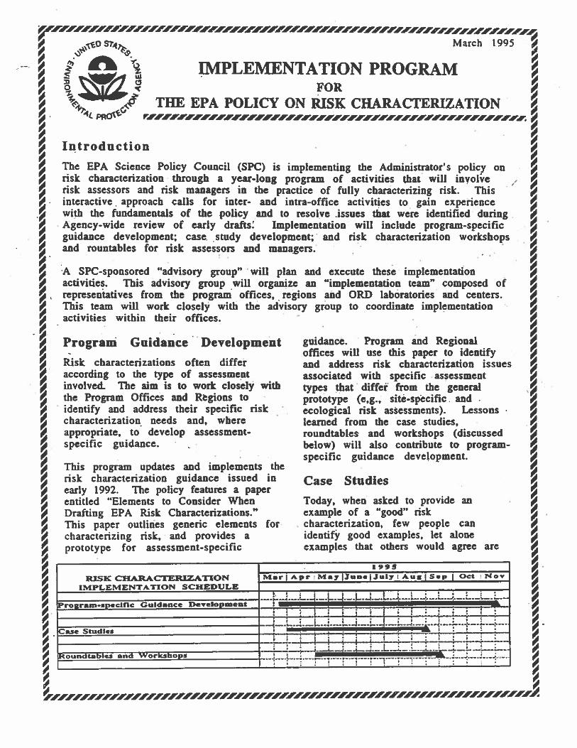
p4 ,Øtosr% March 1995

I C IMPLEMENTATION PROGRAMFOR 0

/ THE EPA POLICY ON RISK CHARACTERIZATION• L pçid- rrrrrrrrrrreerrrrrrrrrrrrrrrrrrrrr_rrrrrrrr,_n. p4

0Introduction

The EPA Science Policy Council (SPC) is implementing the Administrator’s policy ond risk characterization through a year-long program of activities that will involi’e ,,

risk assessors and risk managers in the practice of fully characterizing risk. This4 interactive approach calls for inter- and intra-office activities to gain experience

with the fundamentals of the policy and to resolve issues that were identified during p44 Agency-wide review of early drafts Implementation will include program-specific

guidance development; case study development;• and risk characterization workshops 4p4 and rountables for risk assessors and managers..0* .

.

A SPC-sponsored “advisory group” will plan and execute these implementationp4 activities. This advisory group will organize an “implementation team” composed of

representatives from the program offices, regions and ORD laboratories and centers. 44 This team will work closely with the advisory group to coordinate implementation

activities within their offices. 4Program Guidance Development guidance. Program and Regional

4 - offices will use this paper to identifyRisk characterizations often differ and address risk characterization issues

4 according to the type of assessment associated with specific . assessmentinvolved. The aim is to work closely with types that differ from the general 0the Program Offices and Rtgions to prototype (e.g., sité-spëciflc. and . p4

• identify and address their specific risk ecological risk assessments). Lessonscharacterization needs and, where learned from the ease studies, 4

4 appropriate, to develop assessment- roundtables and workshops (discussed

0. specific guidance. - .

.below) will also contribute to program-

4 .. specific guidance development. p4

This program updates and implements the .

risk characterization guidance issued in Case Studies 44 early 1992. The policy features a paper . .

4 entitled “Elements to Consider When Today, when asked to provide an 4d Drafting EPA Risk Characterizations.” example of a “good” risk4 This paper outlines generic elements for characterization, few people can 44 characterizing risk, and provides a identify good examples, let alone

0 prototype for assessment-specific examples that others would agree are p4

p4

__________

0.

p4 p4-trsrrrnrrrrrrrrrrrsnrnntrnrrrrnrsrrrrrnsnrrtrrnrnrA

RISK CRARACrERIZAnONIMPLEMENTATION SCHEDULE

Progrn-speciflc Guidance Development

Case Studies

Roundtables and Workshops

1995

Mar) Apr May)Sune)Juiy i Aug) Sap Oct Nov

— —

—

— a —

—

— —i •..44—

i

—. - 4... —

ac;:4.E

-

.—H

..—J.——.

—

— — —.--.—.

—— — —

a

—

—

of high quality. As a first step. a selected as to tije adequacy of the original risk p4number of risk characterization case . assessment and risk characterization. % C4 studies will bc developed for use as Examples of case studies may include ateaching tools. A “case study” will, be an chethical assessment, a site-specific

p4 exercise to improve an existing risk assessment1 and a screening-levelcharacterization, using the information assessment The case studies will be p4

4 available in an existing risk assessment, developed by the risk characterization• While based on actual risk assessments, advisory group, working in consultation 4identifying information (e.g., site with the implementation team, and will

4 identification information) will be be used for discussion at the first risk 4removed to avoid any implied judgement characterization workshop.

Roundtables : and .. Workshops‘I . .

‘,•

• EPA. decision-makers will be invited to participató in rOundtable discussions on risk 4. characterization; In addition, a minimum of. two workshops are planned. for EPA risk

assessors and risk managers.‘. . . . . .

• C Risk Decision-maker Rountabies on Risk• Characterization - The goal willS/be to determine the types of risk characterization information needed by managers

4. for effective risk-based decision-making. . .

r. . . . .

Risk Characterization Workshop I - Will focus on identifying the qualities of .

“good” risk characterizations, program-specific plans and guidance development,and case studies. .

0 Risk Characterization Workshop II - Risk assessors. and risk managers will4 meet to wrap-up program-specific plans and guidance, and discuss any necessary p0 updates to the agency-wide risk characterization ‘guidance..

.. I0

‘‘01 2 •

rnrnrrnnrnnnnannneannnrnnrnnrnnnrnnnnri

• GUIDANCE

• RISK CHARACTERIZATION

U.S. Environmental Protectidn AgencySdence Policy Council

February, 1995

CONTENTS

I. The Risk Assessment-Risk Management Interface

II. Risk Assessment and Risk Characterization

Ill. Exposure and Risk Pesaiptors

0

0

PREFACE

This guidance contains principles for developing and describing EPA riskassessments, with a particular emphasis on risk characterization. The currentdocument isan update of the guidance issued with the Agencfl 1992 policy(Guidance onRisk Characterization for Risk Managers and Risk Assessors, February26, 1992). The guidance has not been substantially revised, but includes someclarifications and changes to give more prominence to certain issues, such as theneed to explain the âse of.dthult assumptions.

As in the ±992 policy, some aspects of this guidance kcus on cancer riskassessment, but the guidance applies generally to human health. effects (e:g.,neurotoxidty, developmental toxicity) and, with appropriate modfficaffons, shouldbe used in all health risk assessments. This document has not been revised tospecifically address ecological risk assessment, however, initial guidance forecological risk characterization is included in EPA’s Framework for Ecological RiskAssessments (EPA/630/R-92/OO1). Neither does this guidance address in detail the

ae of risk assessment information (e.g., information from the Tntegrated RiskInformation System (IRIS)) to generate site- or media-specific risk assessments.Additional program-specific guidance will be developed to enable implementationof EPA’s Risk Characterization Policy. Pevelopment of Such guidance will beoverseen by the Science Policy Council and will involve risk assessors and riskmanagers from across the Agency.

L THE RISK ASSESSMENT-RISK MANAGEMENT INTERFACE

URecognizing that for. many people the term risk• assessment has wide meaning, theNational Research Councils 1983 report on risk assessment in the federalgovernment distinguished between risk assessment and risk management.

“Broader uses of the term [risk assessment] than ours also embrace analysis ofperceived risks, comparisons of risks associated with different regulatorystrategies, — occasionally analysis of the. economic and social implications ofregulatory decisions — functions that we assign to risk mahagement(emphasis added). (1) . ..

Ia 1984,. EPA endorsed these distinctions between risk assessment and risk;‘ management for Agency use (2), and later relied onthem in developing risk...

assessment guidelines (3). . Ia 1994, the NRC reviewed the Agencfl approach to anduse of ±kassessmënt and isáued an extensivereport on their findings (4). misdistinction suggests that EPA participants in the process can be grouped into twomain categories, each with somewhat different responsibilities, based on their roles.with respect to risk assessment and risk management.

A. Roles of Risk Assessors and Risk Managers . -

Within the Risk Assessment category there is a group that develops chemical-specific risk assessments by collecting, analyzing, and synthesizing scientific data toproduce the hazard identification, dose-response, and exposure assessment portionof the risk assessment and to characterize rislc This group relies in.pa±t on Agencyriskdssessment guidelines to address science policy issues and scientificuncertainties. . Generally, this group includes scientists and statisticians in the Officeof Rthearch and Develp1sment ti’s Office of Prevention, Pesticides and Toxia andother prograhi offices;the Car&togèn RiskMsessment Verification Endeavor(CRAVE); an&.the Reference Dose (RiD) and Reference Concentration (RK)Workgroups.. - ..

Another group generates site- or media-specific risk assessments for use inregulation development, or site-specific decision-making. These assessors rely onexisting databases (e.g., IRIS, 010 Health.Assessment Documents, CRAVE andRfD/RfC Workgroup documents, and program-specific toxicity information) andmedia- or site-specific exposure information in developing risk assessments. Thisgroup also relies.in part on Agency risk assessment guidelines and program-specificguidance to address science policy issues and scientific uncertainties. Generally, thisgroup includes scientists and analysts in program offices, regional offices, and theOffice of Research and Development.

01

Risk managers, as a separate category, integrate the risk characterization with otherconsiderations specified in applicable statutes to make and justly regulatorydecisions.’ Generally, this group indudes Agency mangers and decision-makers.Risk managers also play a role in determining the scope of risk aisessmmits. Therisk, assessment process involves regular inten±on between risk as essors and riskmanagers, with overlapping responsibffities at various stages in the overall process.Shared responsibilities include initial decisions regarding the planninjand conductof an assessment, discussions as the assessment developé, decisions r garding newdata needed th•complete an assessment and to address significant uncertainties. Atcritical junctures in the assessment, such consultations shape the nature of, andschedule for, the assessment External experts and members of the public may alsoplay a role in determirdng the scope of the assessment for eximple, the public isoften concerned about certain chemicals or exposure pathways in the developmentof site-specific risk assessments. , , ,

B. Guiding Principles , , , ,

The following guidance outlines pdnciplei for those who generate, review, use, andintegrate risk aEsessments for decision-making. ‘

t Risk assessom and risk managers should be sensitive to distinctions betweenrisk assessment and risk managemát ,

The major participants in the risk assessment process have many sharedresponsibilities. Where responsibilities differ, it is important that paftidpantsconfine themselvesto tasks in their, areas of responsibility and not inadvertentlyobscure differences between risk assessmettt and risk management

For the generator of the assessment. distinguishing between risk assessment andrisk management means thaf sdenfffië information is èelected, evaluated, andpresented without considering issues such as cost, feasibility,. or how the Sdaififlcanalysis might influence the regulatory or site-specific decision. Assessors arecharged with (1) genErating a credible, objective, realistic, and sdenti&ally balancedanalysis; (2) presenting information on hazard, dose-response, exposure and risk;and (3) explaining confidence in each assessment by dearly delineating strengths,uncertainties and assumptions, along with the impacts of these factors (e.g.,confldenèe limits, use of conservative/non-conservative assumptions) on theoverall assessment They do not make decisions on the acceptability of any risklevel for protecting public health or selecting procedures for reducing risks.

For users of the assessment and for decision-makers who integrate theseassessments into regulatory or site-specific decisions, the distinction between riskassessment and risk mahagement means refraining from influencing the risk

2

description through consideration of other factors -- e.g.. the regulatory outcome —

and from attempting to shape the risk assessment to avoid statutory constraints,meet reguiatory objectives, or serve political purposes. Such managementconsiderations are often legitimate considerations for the overall regulatory decision(see next principle), but they have no role in estimating or describing riskHowever, decision-makers and risk assessors pahidpate in an Agency process thatestablishes policy directions that determine the overall nature and tone of Agencyrisk assessments and, as appropriate, provide policy guidance on difficult andcontroversial risk assessment issues. Matters such as risk assessment priorities,degree of conservatism, and acceptability of particular risk levels are reserved fordecision-makers who are charged with making decisions regarding protection ofpublic health. .•

2. The risk assessment product, that is, the risk characterization, is only one ofsveral kinds of inioñnaion used forregtilatoq decision-making.

Risk characterization, the last step in risk assessment, is the starting point for riskmanagement considerations: and the foundation for regulatory decision-making, butit is only one of several important comporients in such decisions.. As the laststep inrisk assessment, the risk characterization identifies and Mghlight the noteworthyrisk conclusions and related uncertainties. Each of the environmental lawsadministered by EPA calls for consideration a other factors at various stages itt theregulatory process. As authorized by different statutes, decision-makers evaluatetechnical feasibility (e.g., freatabffity, detection limits), economic, social, political, andlegal factors as part of the analysis of whether or not to regulate and, if so, to whatextent Thus, regulatory decisions arc usually based on a combination of thetechnical analysis used to develop-the risk assessment and information from otherfields. . -

For this reason, risk assessors and managers should undemãnd that the regulatorydecision is usually not determined solely by the ouftome of the risk assessment Forexample, a regulatory decision on the use of a particular pesticide considers not onlythe risk level to affected populations, but also thèagriailthral benefits of its use thatmay be important for the nation’s food supply. Similarly, assessment efforts mayproduce an RID for a particular chemical, but other considerations may result in• aregulatory le’iél that is more or less protective than the RID itself.

For decision-makers, this means that societal considerations (e.g., costs and benefits)that along with the risk assessment shape the regulatory decision should bedescribed as fully as the scientific information set forth in the risk characterization.Information on data sources and analyses, their strengths and limitations,confidence in the assessment, uncertainties, and alternative analyses are asimportant here as they are for the scientific components of the regulatory decision.Decision-makers should be able to expect, for example, the same level of rigor fromthe economic analysis as they receive from the risk analysis. Risk managemtdecisions involve numerous assumptions and uncertainties regarding technology,economics and social factors, which need to be explicitly identified for the C)decision-makers and the public.

3

EL RISK CHARACTERIZATiON

A. Defining Risk Cbaracterizafion in the Context of Risk Assessment

EPA risk assessment principles and practices draw on many sources. Obvioussources include the environmental laws administered by EPA, the NationalResearch Council’s 1983 report on risk assessment-(fl, the Agency’s Risk AssessmentGuidelines (3), and various program specific guidance (e.g., the Risk AssessmentGuidance for Superfund). Twenty years of EPA experience in developing,defending, and enforcing risk assessment-based regulation is another. Togetherthese various sources stress the mportance of.a dear explanation of Agencyprocesses for evaluating hazard, dose-response; exposure, and other data thatprovide the scientific foundation for characterizing risk.

This section focuses on two requirements for fun characterization of risk. First, thecharacterization should address qualitative and quaniftative feajaires of theassessment Second, it should. identify the important strengths and uncertainties inthe assessment as part of a diidthsion of the confidence in the assessmentemphasis on a full description of all elements. of the assessment draws attention tothe importance of the qualitative, as well as the quantitative, dimensions of theassessthent.• The 1983 NRC report carefully distinguished qualitative riskassessment from quantitative assessments, preferring risk statements that are not

- strictly numerical.

The term risk assessment is often given narrower and broader meaningsthan we have adopted here. For some observers, the term is synonymouswith quantitative risk assessment and emphasizes reliance on numericalresults. Our broader definition includes quantification, but also includesqualitative expressions of ±L Quantitative estimates of risk are not, always.feasible6 and they may be schewed by agencies for polic3i reasons. (1)

EPA’s Exposure Assessment Guideli±ws ‘define risk characterization as the final step• in the risk assessment process that

• Integrates the individual characterizations from the hazard identification, dose-response, and exposure assessments;

• Provides an evaluation of the overall quality of the• assessment and the degree,of confidence the authors have in the estimates of risk and conclusions draww

• Describes risks to individuals and populations in terms of extent and severity ofprobable, harm; and

• Communicates results of the risk assessment to the risk manager. (5)

Particularly critical to full characterization of risk is a frank and open discussion ofthe uncertainty in the overall assessment and in each of its components. Theuncertainty discussion is important for several reasons.

4

1. Information from different sources carries different kinds of uncertainty andknowledge of these differences is important when uncertainties are combinedfor characterizing risk.

2. The risk assessment process, with management input, involves decisionsregarding the collection of additional data (versus living with uncertainty); inthe risk characterization; a discussion of the uncertainties will help to identifywhere additional information could contribute significantly to reducing

- uncertainties in risk assessment..

3. A dear and explicit statemEnt of the strengths an& limitations of a risk- assessment requires a dear and eplidt statement of. related uncertainties.

A discussion of-uncertainty requires comment on such issues as thequality and- quantity of available data, gaps hLdw data basE for specific themkals,quality of the

measureddata,usé of default assumptions, incomplete understanding of general• biological phenomena, and scientific judgments pr science policy positions that were

employed to bridge information gaps; *-. :

In short, broad agreement edsft on the importance of a full, picture of riskparticularly including a staflent of confidence in the assessment and theassociated uncertainties. This section discusses information contit and uncertaintyaspects of risk characterization, while Section ifi discusses various descriptors uthdin risktharacterization. . . . -

B. Guiding Principles:. - . .,

1. The risk dianctenabon integrates the information from the banrdidentification, dose-responsE, and eposun assessments, using a combination ofqualitative information, quanfttahve information, and information regardinguncertainties.., . . - . .;

Risk assessment is based on a series of questions that the assessor asks about the dataand the implications of the dab for h iman risk. Each question calls for analysis andinterpretation of the available studies, selection of the data that are mostscientifically reliable and most relevant to the problem at hand, and scientificconclusions regarding the question presented. As suggested below, betause thequestions and analyses are complex, a complete characterization includes severaldifferent kinds of information, carefully selected for reliability and relevance.

a. Hazard Identification. — What is known about the capacity of an environmentalagent for causing cancer (or other adverse effects) in humans and laboratoryanimals?

05

Hazard identification is a qualitative description based on factors such as the kindand quality of data on humans or laboratory animals, the availability of ancillaryinformation (e.g., structure-activity analysis, genetic toxicity, pharmacoidnefics)from other studies, and the weight-of-the-evidence from all of these data sources.For example, to develop this description, the issues addressed include:

1) the nature, reliability, and consistency of the particular studies in humans andin laboratory animals;

2) the available information on the mechanistic basis for activity; and

3) experimental animal responses and their relevance to human outcomes.

These issues nice dear that the task of hazard identification is characterized bydescribing the full range of available infdrmation and the implications of thatinformation for human health.

b. Dose-Response Assessment— What.is known about the biological mechanismsand dose-response relationships underlying any effects observed in thelaboratory or epidaniolqgy studies providing data fur the assessment?

The dose-response assessment examines quantitative relationships betweenexposure (or dose) and effrctá in the studies used to identify and define effects of

Oconcern. This information is later — along with “real world”, exposure

• information (see below) to develop estimates of the likelihood of adverse effects in• populations potentially at risk It should be noted that, in pnctice. hazard

identification for developmental toxicity and other non-cancer health effects isusually done in conjunction with an evaluation of dose-response relationships,since the determination of whether there is a.hanrd is ofterrdependent on whethera dose response relationship is present (6) Also, the framework developed by EPAfor ecological risk assessment does not distinguish between hazard identificationand dose-response assessment, but rather calls fur a t1thancterization of ecologicaleffects.ӯ

Methods fur establishing dose-response relationships often depend on variousassumptions used in lieu of a complete data base, and the method chosen canstrongly influence the ovenll’assessment The Agency’s risk assessment guidelinesoften identify so-called “default assumptions” for use in the absence of otherinformation. The risk assessment should pay careful attention to the choice of ahigh-to-low dose extrapolation procedure. As a result, an assessor who ischaracterizing a dose-response relationship considers several key issues:

1) the relationship between extrapolation. models selected and availableinformation on biological m&hanisms;

6

2) how appropriate data sets were selected from those that show the range ofpossible potatdes both in laboratory animals and humans;

.

3) the basis for selecting interspedes dose scaling factors to account for scaling C)doses from experimental animals to humans;

9

4) the .correspondence between the expected route(s) of exposure and the exposureroute(s) utilized in the studies forming the basis of the dose-responseassessment, as weli as the. interrelationships of potential effects from differentexposure routes;

5) the correspondence between the expected duration of exposure and theexposure durations in the studies used in forming the basis of the dose-responseassessment, e.g., chronic studies would be used to assess long-term, cumulativee)posu_n concentrations, while acute studies would be zsed in assessing peaklevels of exposure; and . .... . .

6) the potential. for differing susceptibilities among population subgroups.

The AgerLqs Integrated RAsk thfomiatioä System (IRIS). is a repository for suchinformation for EPA. EPA program offices also maintain program-specificdatabases, such as the OSWER Health Effects Assessment Summary Tables (NEAST).IRIS indudes data summaries representing Agency consensus on specific chemicals,based on a careflil review of the scientific issues listed above, For specific riskassessments based ondata from source, risk assessors should carefully reviewthe information presented, emphasizing. confidence in the data and uncertainties(see subsection 2 below). Specifically, when WJS data are used, the JR$ statement ofconfidence should be included as an explicit part of therisk characterization forhazar4 and dose-response information. .. .

. .

c. Exposure Assessment — What is known about the principal paths, patterns, andmagnitudes of human exposure and numbers of persons who may be exposed?

The exposure assessment examines a wide range of exposure parameters pertainingto the environmental scenarios of people who may be exposed to the agent understudy. The information considered for the exposure assessment includesmonitoring studies of chemical concentrations in environmental media, food, andother materiAls; modelingof environmental fate and transport of contaminants;and information on different activity patterns of different population subgroups.An assessor who characterizes exposure should address several issues:

1) The basis for the values and input parameters used for each exposure scenario.ffthevaluesarebasedondath,thereshouldbeadiscussionofthequality,purpose, and representativeness of the database. For monitoring data, thereshould be a discussion of the data quality objectives as they are relevant to risk

7

assessment, including the appropriateness of the analytical detection limits, ifmodels are applied, the appropriateness of the models and information on theirvalidation should be presented. When assumptions are made, the source andgeneral logic used to develop the assumptions (e.g., program guidance, analogy,professional judgment) should be described.

2) The confidence in the assumptions made about human behavior and therelative likelihood of the different exposure scenarios.-

• 3).The major factor or factors (e.g., concentration, body uptake, duration/frequencyof exposure) thought-to account for the greatest uncertainty in the exposureestimate, due either to sensitivity or lack of data.

•.

4) The link between. the exposure information and the risk descriptors discussed•

- in Section III of thiE Appendix. Spedflcafly, the risk assessor needs to discuss• the connection between the conservatism or nonëonservaffsm of the

•

. data/assumptions used in the scenarios and’ the choice of descriptors.

5) Other information that may be important for the particular risk assessmentFor example, for many assessments; other sources and background levels in the’environment may contribute significantly to population exposures and shouldbediscussed. ‘ •, L

2) The risk characterization includes a discussion of uncertainty ad variability.

In the risk characterization, conclusions about hnnd and dose response areintegrated’with those from the exposure assessment. In addition, confidence aboutthese conclusions, including information about ‘the uncertainties associated witheach aspect of the assessment inthe final risk ummary, is highlighted. In theprevious assessment steps and hi the risk characterization, the risk assessor mustdisthgtñsh between variabifity and uncertainty. ‘‘

..

Variability arises from true heterogeneity in characteristics such as dose-responsedifferences within a population, or differences in contaminant levels in the’

enviroriment The values of some variables used in an assessment change withtime and space, or across the population whose exposure is being estimated.Assessments should address the resulting variability in doses received by membersof the target population. Individual expdsuze, dose, and risk can vary widely in alarge population. The cent±al tendency and high end individual risk descriptors(discussed in Section III below) am intended to capture the variability in exposure,lifestyles, and other factors that lead to a distribution of risk across a population.

Uncertainty, on the other hand, represents lack of btowlede about factors such asadverse effects or contaminant levels which may be reduced with additional study.Generally, risk assessments carry several categories of uncertainty, and each merits

8

consideration. Measurement uncertainty refers to the usual error that accompaniesscientific measurements—standard statistical techniques can often be used to expressmeasurement uncertainty. A substantial amount of uncertainty is often inherent inenvironmental sampling, and assessments should address these uncertainties.There are likewise uncertainties associated with -the use of scientific models, e.g.,

- dose-response models, models of environmental fate and transport. Evaluation ofmodel uncertainty would consider the scientific basis for the model and availableempirical validation.

A different kind of uncertainty stems from data gaps that is, estimates or - -

assumptions used in the assessment Often, the data gap is broad, such as the:absence of information on the effects. of exposure to a chemical. on humans or. onthe biological mechanism of action of an agent The risk assessog should include astatementof confidence that reflects the degree to which the risk. assessor believesthat the estimates or assumptions adeqátely fill the data gap.- For some common -

and, important data gaps, Agency or program-specific risk assessment guidanceprovidesdefault assumptions ‘QT, valueS.. Riskassessors should carefully consider allavailable datazbekre deciding to rely on default assumptions. H defaults are used,

- the risk assessment should reference the Agency guidance that explains the defaultassumptionsor values. . . . . . • . ... .. .

Often risk assessoS and managers simplify discussion of risk issues by speaking-onlyof the numerical components of an assessment: That is, they refer to the alphanumeric weight-of-the-evidence classification, unit risk the risk-specific dose or theql* for cancer risk, and the RID/RK for health effects other than.cancer, to theexclusion of other information bearing on the risk case. However; since everyassessment carries uncertainties, a simplified numerical presentation of risk isalways incomplete and often misleading. For this reason, the NRC (1) and EPA riskassessment guidelines (2) all for “thanctérithig’ risk to include qualitativeinformation, a related numerical risk -eStimate and a discussion of uncertainties,’limitations, and assumptions—default and otherwise.’• .. ... .•, ..

. .

Qualitative information on methodology, alternative interpretations, and workingassumptions (including defaults) is an important component of riskcharacterization. For example, specifying that animal studies rather than human -

studies were used in an assessment tells others that the risk estimate is based on,assumptions about human response to a particular chemical rather than humandata. Information that human exposure estimates am based on the subjects’presence in the vicinity of a chemical accident rather than tissue measurementsdefines known and unknown aspects of the exposure component of the study..

Qualitative descriptions of this kind provide crucial information that augmentsunderstanding of numerical risk estimates. Uncertainties such as these are expectedin scientific studies and in any risk assessment based on these studies. Such

0

uncertainties do not reduce the validity of the assessment Rather, they shouid behighlighted along with ‘other important risk assessment conclusions to informothers fully on the results of the assessment.

In many cases, assessors must choose among available data, models, or assumptionsin estimating risks. :.E3Qixiliung the impact of selected, plausible alternatives on theconclusions of the assessment is an important part of.the uncertainty discussion.The key words are “selected” and “plausible;” listing all alternatives to a particularassumption, regardless of their merits would be superfluous. Generators of theassessment using best, professional judgment, should outline the strengths and

• weaknesses of the plausible alternative approaches.’

Mt adequate description of the process of alternatives’selection involves several

a. A nifonalefor the choice.I,. Discussion of the effects of alternatives selected on the assessmentc Comparison with other plausible alternatives, where appropriate.

The degree to which variabffity.and uncertainty are a4dressed depends largely onthe scope of the assessment and the resources available. For example, the Agencydoes not aped an assessment to evaluate and assess every conceivable exposurescenario for every possible pollutant to examine all susceptible populationspotentially.at risk, or to characterize every possible environmental scenario to

‘estimate the cause and effect relationships between exposure to pollutants andadverse health effects. Rather, the discussion of uncertainty, and variability shouldreflect the type and complexity of the risk assessment, with the level of effort for

• analysis and discussion of uncertainty corresponding to the level of effort for the.assessment. . ‘ .

3. . Wellebalanced risk characterizations present risk conclusiOns and informationregarding the strengths and limitations of the assessment for other riskassessom, EPA dedsion-maka, and the public.

The risk assessment process calls for identifying and highlighting significant riskconclusions and related uncertainties partly to assure full communication amongrisk assessoñ and partly to assure that edsion-makers are fully ‘ifonned Issuesare identified by acknowledging noteworthy qualitative and quantitative factors thatmake a difference in the overall assessment of hazard and risk, and hence in theultimate regulatory decision. The key word is “noteworthy.” Information that

cases where risk assessments within an Agency program routinely address slut sets of

alternatives, program guidance may be developed to sfreamline and simplify the discussion of thesealternatives.

10

significantly influences the analysis is explicitly noted — in all future presentationsof the risk assessment and in the related decision. Uncertainties and assumptionsthat strongly influence confidence in the risk estimate also require special attention. )Numerical estimatS should not be separated from the descriptive information thatis integral to risk characterization. Documents and presentations supporting

• regulatory or sitespedfic decisions should include both the numerical estimate and• descriptive information; in short reports; this information can be abbreviated. Fully

visible information assures. that important features of the assessment are• immediately available .ateach level of review for evaluating whether risks are

acceptable or unreasonable. •

-A-.

o

U11

EL EXPOSURE ASSESSMENT AND RISK DESCRWrORS•

A. Presentation of Risk Descriptors

The results of a risk assessment are usually communicated to the risk manager inthe risk characterization portion of the assessment. This communication is oftenaccomplished through risk descriptors which convey information and answerquestions about risk, each descriptor providing different information and insights.Exposure assessment plays a key role in developing these risk descriptors since eachdescriptor is based in part on the exposure distribution within the population ofinterest. -

The following, guidance outlines the different descriptors in a convenient order thatshould not be construed as a hierarchy of importance. These descriptors should beused to describe risk in a variety of ways for a given assessment, consistent with theassessment’s purpose, the data available, and the information the risk manager-needs. Use of a range of descriptors instçad of a single descriptor enables Agencyprograms to present a picture of risk that corresponds to the range of differentexposure conditions encountered for most environmental chenilàals. This analysis,in turn, allows risk managers to identify popUlations at greater and lesser risk and toshape regulatory solutions accordingly.

Agency risk assessments will be expected to address or provide descriptions of (1)individual risk that include the central tendency and high end portions of the riskdistribution, (2) population risk, and (3) important subgroups of the population,such as highly exposed or highly susceptible groups. Assessors may also useadditional descriptors of risk as needed when these add to the clarity of thepresentation. With the exception of assessments where particular descriptors dearlydo not apply, some form of these three types of descriptors should be routinelydeveloped and presented for Agency risk assessments2. In other cases, where adescriptor would be relevant, but the program lacks the data or methods to developit, the program office should design and implement a plan, in coordination withother EPA offices, to meet these assessment needs. While gaps continue to exist,risk assessors should make their best efforts to address each risk descriptor, and at aminimum, should briefly discuss the lack of data or methods. Finally, presenters ofrisk assessment information should be prepared to routinely answer questions byrisk managers concerning these descriptors.

It is essential that presenters not only communicate the results of the assessment byaddressing each of the descriptors where appropriate, but that they also

2Program-spedfic guidance will need to address these situations. For example, for sitespedficassessments, the utility and appropriateness of population risk estimates will be determined based onthe available data and program guidance.

12

communicate their confidence that these resuib portray a reasonable picture of theactual or projected exposures. This task will usually be accomplished by franidycommenting on the key assumptions and parameters that have the greatest impacton the results, the basis or rationale for choosing these assumptions/parameters,and the consequences of choosing other assumptions.

B. Relationship Between ExposureDesaiptom and Risk Descriptors

In the risk assessment process, risk is estimated as a function of exposure, with therisk of adverse affects increasing as ecposüre increases. Information on the lçvels ofexposure experieuced by different members of the population is key tounderstanding the range ofrisks that may occur.. Risk assessors and risk managersshould keep in mind, however, that exposure is not synonymous with risk.Differences among individuals in absorption rates, susceptibility, or other factotsmean that individual&with the same level of exposure may be at different levels of±lc lit Moat cases, the state of the science is not yet adequate to define disfrthuffonsof factors such as pópulaffón Susceptlbffity. The guidance principle below discuss a

• variety orisk descriptors that primarily reflect differencesin estimated exposure. if• a full description of the range of susceptibility in the population cannot be

presented, an effort should be wade. to identify subgroups that, for various reasons,may be partidilarly susceptible.

C. Guiding Principles

1. Information about the distribution of individual exposures is important tocommunicating the results of a risk assessment

The risk manager is generally interested in answeñ to questions such as thefollowing:

• Who are the people at the highest risk?

• What riskievels are they subjected to?

• What are they doing, where do they li#ej, etc., that might be puffing them at thishigher risk?

• What is the average risk for individuals in the population of interest?

Individual exposure and risk descriptors are intended to provide answers to thesequestions so as to illuminate the risk management decisions that need to be made.In order to describe the range of risks, both high end and central tendency

013

descriptors are used to convey the variability in risk levels experienced by differentindividuals in the population.

a. High end descriptor

For the Agency’s purposes, high end risk descriptors are plausible estimates of theindividual risk for those persons at the upper end of the risk distribution. Givenlimitations in current understanding of variability in individuals’ sensitivity totoxins, high end descriptors will usually address high end exposure or dose (hereinreferred to as exposure for brevity). The intent of these descriptors is.to conveyestimates of exposure in the upper range of the distribution, but to avoid estimateswhich are beyond the true distribution. Conceptually, high end exposure meansexposure above about the 90th percentile of the population distribution, but nothigher than the individual in the population who has the highest exposure. Whenlarge populations are assessed,.a largenumber of individuals may be. includewithin the “high end” (e.g., above 90th or 95th percentile) and information on therange of exposures received by these individuals should be presented:

• High end descriptors are intended, to estimate the exposures that are expected tooccur in small, but definable, “highend” segments of the subject population) Theindividuals with these exposures may be members of a special population segmentor individuals in the general population who am highly exposed because of theinherent stochasfic.nature of the factors which give rise to exposure. Where

• differences in sensitivity sn be identified within the population, high end estimates• addressing sensitive individuals or subgroups can be developed.

In those few cases in which the complete data on the population distributions ofexposures and doses are available, high end exposure or dose estimates can be

• represented by reporting exposures or dosS at a set of selected percentiles of thedistributions, such as the 90th, 95th, and 98th percentile. High aid ãposumsordoses, as appropriate,, can then be used to calculate high end risk estimates.

In the majority of cases where the complete distributions are not available, severalmethods help estimate a high end exposure or dose. if sufficient information aboutthe variability in chemical concentrations, activity patterns, or. other factors areavailable, the distribution may be estimated through the use of appropriatemodeling (e.g., Monte Carlo simulation or parametric statistical methods). The

3High aid estimates focus on estimates of exposure in the exposed poptiations. Boundingestimates, on the other hand, are constructed to be equal to or greater than the highest actual risk inthe population (or the highest risk that could be expected in a future scenario). A “worst case sceiiafio”refers to a combination of events and conditions such that taken together, produces the highestconceivable risk. Although it is possible that such an exposure, dose, or sensitivity combination mightoccur in a given population of interest the probability of an individual receiving this combination ofevents and conditions is usually small, and often so small that suth a combination will not occur in aparticular, actual population.

14

determination of whether available information is suffidentto support the use ofprobabilistic estimation methods requires careful review and documentation by therisk assessor. if the input distributions are based on limited data, the restiltingdistribution should be evaluated carefully to determine whether it is animprovement over more traditional estimation techniques. if a distribution isdeveloped, it should be described with a eries of percentiles or populationfrequency estimates, particularly in the high end range. The assessor and riskmanager should be aware, however, that unless a great deal is known aboutexposures and doses. at the high ad of the disthbution, these estimates will involveconsiderable uncertainty which the exposure assessor will need to describe. Notethat in this context, the probabilistic analysis addresses variabffit of exposunin thepopulatiort Probabilistic techniques may also be applied to evaluate uncertainty inestimates (see section 5, below).. However, it is generally inappropriate to combinedistributions reflecting both uncertainty and.vanabffity to get a single overalldisthbuffoa Such a result. is not readily interpretable for the concerns ofeniilionmental decision-making. .

If only limited’:informthon on the distribution of the exposure or dose factors iiavailable, the assessor should approach estimAting the high end by identifying the•

•most sensitive variables and using high end values for a subset of these variables,• leaving others at their central valu.4 Tn doing this1 the assessor heeds to avoidcombinations of. parameter values that are inconsistent (e.g., low body weight usedin combination with high dietary intake rates), and must keep in mind the ultimateobjective of being within the distribution of actual expected exposures and doses,and not beyond it

if very little data am available on the ranges for the various variables, it will bedifficult to estimate exposures or doses and associated ±b in the high end withmuch confidence. One method that hasbeen used insuch cases is to start with abounding estimate and “back off’the limits used until the combination of:parameter values is, in the judgment of theassessor, within the disffibutionof.expected exposure, and still lies within the upper 10% of persons exposed.Obviously, this method resiil&tha large uncertainty and requires explanation;

b. Central tendenèy descriptor

Central tendency descriptors generally reflect central estimates of exposure or dose.The descriptor addressing èentral tendency may be based on either the arithmeticmean exposure (avenge estimate) or the median exposure (median estimate), either

4Maximizing all variable will thvirbmlly all cases result in an estimate that is above theactual values seen in the population. When the principal pammeters of the dose equation, e.g.,concentration (appropriately integrated over time), intake rate, and duration, an broken out into subcomponents, it may be necsaxy to use maximum values for more than two of these sub-componentparameters, depending on a sensitivity analysis.

15

of ‘vhich show% be dearly labeled. The average estimate, used to approximate thearithmetic mean, can often be derived by using average values for all the exposurefactors.5 It does not necessarily represent a particular individual on the distribution.Because of the skewness of typical exposure profiles, the arithmetic mean may differsubstantially from the median estimate (i.e., 50th percentile estimate, which is equalto the geometric mean for a log normal distribution). The selection of whichdescriptor(s) to present in the risk characterization wjll depend on the available dataand the goals of the assessment When data are limited, it may .not be possible toconstruct true median or mean estimates, but it is still possible to constructestimates of central ten4ency. The discussion of the use of probabilistic techniquesin Section 1(a) above also applies to estimates of central tendency.

Information about population exposure leads to mother important way toH describe risk. .. I -

PopulAtion risk refers to an assessment of the extent d harm for the population as awhole. In theory, it cat be áakulàted by summing, the individual risks for allindividuals within the subject population. This task, of course, requires a great dealmore i formafion than is normally, if ever, avii1able.

The kiñd&of questions addressed by descriptors of population risk include thefollowing:

• How many cases of a particular health effect might be probabifistically estimatedin this population for a specific time period?

• For non-carcinogens, what portion of the population.is within a specified rangeof some reference level; e.g., exceedance of the RID (a. dose), the RK (aconcentration), or other health concern level?

• For carcinogens, what portion of the population is above a certain risk level,such as 1O? . . .

These questions can lead to two different descriptors of population risk.

a: Probabilistic number of cases

The first descriptor is the probabilistic number of health effect cases estimated in thepopulation of interest over a specified time period. This descriptor can be obtainedeither by (a) summing the individual risks over all the individuals in thepopulation, e.g. using an estimated distribution of risk in the population, when

This holds true when variables are added (e.g., exposures by different routes) or whenindependent variables are multiplied (e.g., concentration x intake). However, it would be incanect forproducts of correlated variables, variables used as divisors, or for formulas involving exponents.

16

such information is available, or (b) through the use of a risk model that assumes alinear non-threshold response to exposure, such as many cardñogerüc models. lEtthese calculations, data will typically be available to address variability in individualexposures. If risk varies linearly with exposure,.multiplying the mean risk by thepopulation size produces an estimate of the number of cases.6 At the present time,most cancer potency values represent plausible upper bounds on rIsk. When such a

• value is used to estimate numbers of cancer Eases,, it is important to understand that• the result is also an upper bound. As with other risk descriptors, this approach maynot adequately address sàisiffve subgroups for which different dose-response curveor exposure estimates might be needed. ‘. •

Obviously, the mdré information one has, the more certain the estimate of this risk• descriptor, but inherent uncertainffes’in risk assessment methodology placelimitations on the accuracy of the estimate; The discusàion of uncertainty involvedin estimatingthEnumberofcasesshoüld indicate that this descriptor is not to beconfused with an actuarial prediction of cases in did. population (which is astatistical prediction baaed oaa great deal àY empirical data).

In general,’ it should be r ognized that when small pôpulatioñs are exposed,population risk estimates may be vety small.. For example, if 100 people am exposed

•

. to an hdMdual lifetiffiecancer risk of 10, the expected number of cases is 0.01.. Insuch situations, individual risk estimates will usually be a more meaningfulparameter for dedion-makers.. . .

b. Estimated percentage of population with risk ream than some level CDFor non-cancer .eff&ts, we generally have not developed the riskassessmenttechniques to the. point of knowing how to add risk probabilities, so a seconddescriptor is usually more appropriata An, estimate of the petcentige of fitpopulation, or the number, of persons, abovea specified level àY risk or within aspecified range of some referernte level, e.g., exceedance of the RD or theRK,LOAEL, or other specific level of interest This.desaipthr must be obtained throughmeasuring or ‘simulating the population distribution. .

3. Information about the distribution of exposure and risk for different subgroupsof the population are important components of a risk assessment

A risk manager might also ask questions about the distribution of the risk burdenamong various segments of the subject population such as the followinç How doexposure and risk impact various subgroups?; and, what is the population risk of a

6However, certain important cautions apply (see EPA’s Exposure Assessment Guidelines). Also,this is not appropriate for non-carcinogenic effects or for other types of cancer models. For non-linearcancer models, an estimate of population risk must be calculated using thedisffibufion of individual C)risks.

17

pa±nilar subgroup? Questions about the distribution of exposure and risk amongsuch population segments require additional risk descriptors.

a. Highly exposed

Highly exposed subgroups can be identified, and where possible, characterized andthe magnitude of risk quantified. This descriptor is useful when there is (or isexpected to be) a subgroup experiencing significantly different exposures or dosesfrom that of the larger population. These sub-populations may be identified by age,sex, lifestyle, economic factors, or other demographic variables. For example,toddlers who play in contaminated soil and high fish consumers represent sub-populations that may have greater exposures to certain agents. -

b. Highly susceptible

Highly susceptible subg±oups can also be identified, and if possthk chañcterized andthe magnitude of risk quantified. This descriptor is useful when the sensitivity orsusceptibility to thIeffect for specific subgroups is (or is expected to be) significantlydifferent fromthat of the larger population. In order to calculate risk for thesesubgroups, it will sometimes be necessaqto use a different dose-responserelationship; e.g., upon exposure to a chemical, pregnant women, elderly people,children, and people with certain illnesses may each be mow sensitive than thepopulation as a whole. For example, children are thought to be both highly exposedand highly susceptible to the effects of environmental lead. A model has beatdeveloped that uses data on lead concentrations in different environmental mediato predict the resulting blood lead leyels in children. Federal agencies are workingtogether to develop specific. guidance on blood lead levels that present risks tochildren.

it is important to note, however, that the Agency’s current methodologies fordeveloping reference doses and reference doncentations (RfOs and RKs) areSdesigned to protect sensitive populaffbns; if data on sensitive human populationsare available (and there is confidence in the quality of the data), then the RD is set atthe dose level at which no adverse effects are observed in the sensitive population(e.g., RDs for fluoride and nitrate). if no such. data are available (for example, if theRH) is developed using data from humans of avenge or unknown sensitivity) thenan additional 10-fold factor is used to account for variability between the averagehuman response and the response of more sensitive individualt

Generally, selection of the population segments is a matter of either a priori interestin the subgroup (e.g., environnental justice considerations), in which case the riskassessor and risk manager can jointly agree on which subgroups to highlight, or amatter of discovery Of a sensitive or highly exposed subgroup during the assessment

18

process. In either case, once identified, the subgroup can be treated as a populationin itself, and characterized in the same way as the larger population using thedescriptors for population and individual risk. (Th)

4. Situation-specific information adds perspective on possible future events orregulatory options.

‘What if...?” questions can be used to examine candidate risk management options.For example, consider the following:

• What if a pesticide applicator applies this, pesticide without using protectiveequipment?

• What if this site becomes residential in the future?

• What risk level will occur if we set thestandard at 100 ppb?

Answering these “What if...?” questions involves a calculation of risk based onspecific Eombinátions of factors postulated within the assessment7. The answers tothese “What if...?” questions do not, by themselves, give information about how

- likely the combination of values might be in the actual population or about howmany (if any) persons might be subjected to the potential future risk. However,information on the likelihood of the postulated scenario would also be desirable hiinclude in the assessment. . - -

When addressing projected changes for a population (either expected futuredevelopments or consideration of different regulatory options), it is usuallyappropriate to calculate and consider all the risk 4esaipton discussed above. When.central tendency or high end -estimates are developed far a future scenario, thesedescriptors should reflect reasonable.expectafions about future activities. Forexample, in site-specific risk assessments, future scenarios should be evaluatedwhen they are supported by realistic forecasts of future land use, -and the risk’••descriptors should be developed within that context

.

5. An evaluation of the uncertainty in the risk descriptors is an importantcomponent of the uncertainty discussion in the assessment

Risk descriptors are intended to address variability of risk within the population andthe overall adverse impact on the- population. In particular, differences betweenhigh end and central tendency estimates reflect variability in the population, but notthe scientific uncertainty inherent in the risk estimates. As discussed above, there

7Some programs routinely develop future scenarios as part of developing a risk assessment.Program-specthc guidance may address future scenarios in more detail than they are described here.

19

will be uncertainty in all estimates of risk. These uncertainties can includemeasurement uncertainties, modeling uncertainties, and assumptions to fill datagaps. Risk assessors should address the impact of each of these factors on theconfidence in the estimated risk values.

Both qualitative and quantitative evaluations of uncertainty provide usefulinformation to users of the assessment. The techniques of quantitative uncertaintyanalysis are evolving iapidly and both the SAB (8) and the NRC (4) have urged theAgency to incorporate these techniques into its risk analyses. However, it should benoted that a probabilistic assessment that uses only the assessor’s best estimates fordistributions of population variables addxesses variability, but not uncertainty...Uncertainties in the estimated risk distribution need to be separately evaluated.

20

REFERENCES

1. National Research Council. Risk Assessment in the Federal Government:Management the Process. 1983.

2. U.S. EPA. Risk Assessment and Management Framework for Decision Making,1984.

3. US. EPA. “Risk Assessment Guidelines.” 51 Federal Register, 33992-34054,September 24, 1986.

4. National Research Council Science and Judgement in Risk Assessment. 1994.

5. US. EPA “Guidelines for Exposure Assessment” 57 Federal Register, 22888-22938, May 29, 1992. ‘ . ‘.

6. US. EPA. “Guidelines for Developmental Toxicity Risk Assessment.”, 56 FederalRegister, 67398-63826, December 5, 1991.

7. US. EPA. Framework for Ecological Risk Assessment 1992.

8. Loehr, R.A., and Matànoski, G.M., Letter to Carol M. Browner, EPAAdministrator, Re: Quantitative Uncertainty Analysis for RadiologicalAssessments EPA SdeñceAdvisory Board, July 23, 1993 (EPA-SAB-RAC-COM93-006).

a21

,1,

ATTACHMENT B

RCRMCERCLA INTERFACE-INTERIM FINAL GUIDANCE,EPA REGION 10 MEMORANDUM, AUGUST 3

EP4 R T’SK’ RESE2 FINAL.M4SThR “I’D S) ml’.; ‘)&r

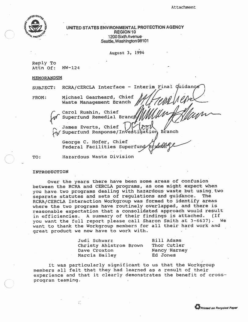
Attachment

UNITED STATES ENVIRONMENTAL PROTECTION AGENCY- REGION 10

1200 Sixth AvenueSeattie.Washington 98101

Reply ToAttn Of: HW—l24

August 3. 1994

MEMORANDUM

SUBJECT:

FROM:

TO:

RCRA/CERCLA Interface - Interim Final

Michael Gearheard, ChiefWaste Management Branch

Carol Rushin, ChiefSuperfund Remedial Bran

James Everts, ChiefSuperfund Response/InVa

George C. Hofer, ChiefFederal Facilities Superfun

Hazardous Waste Division

INTRODUCTION

Over the years there have been some areas of confusionbetween the RCRA and CERCLA programs, as one might expect whenyou have, two programs dealing with hazardous waste but using twoseparate statutes and sets of regulations and guidance. TheRCRA/CERCLA Interaction Workgroup was formed to identify areaswhere the.two programs have routinely overlapped, and there isreasonable expectation that a consolidated approach wauld resultin efficiencies. A summary of their findings is attached. (Ifyou want the full report please call Sharon Smith at 3—6637) - Wewant to thank the Workgroup members for all their hard work andgreat product we now have to work with. . -

Judi SchwarzChristy Ahistrom BrownDave CroxtonMarcia Bailey

Bill AdamsThor CutlerNancy HarneyEd Jones

It was particularly significant to us that the Workgroupmembers all felt that they had learned as a result of theirexperience and that it clearly demonstrates the benefit of cross—program teaming.

QThfnad on Recycled Papa

2

This memo is intended to give greater clarity to and set outour expectations as how these potential overlaps should behandled. If you have general situations that are not coveredhare, please call Judi Schwarz as she is quite knowledgeable inboth program areas. We branch chiefs would also welcome a callas a major part of our job is to work cràss—pogram issues.

This guidance will not answer every question that.may comeup in developing a site—specific comprehensive and non—duplicative solution. We encourage creative solutions anddiscourage rigid interpretation of the regulations and guidance,

but we also recognize that some solutions may require input from

the section. and branch chiefs. We encourage you to involve usearly in the process rather than becoming frustrated by asituation.

We are issuing this guidance as an interim final product.We want to begin to apply this approach, but realize that we maynot have thought of all of.the implications and problems that mayarise. If necessary, this guidance can be revised in the futureto reflect what we will learn about integrating our two EPAprograms. - Other revisions may also-be necessary if and when thisapproach is applied to EPA RCRA/State clean—up program orCERCLA/State RCRA program overlaps.

- PARITY POLICY - THE BIG PICTURE . C)We are committed to doing everything we can to avoid

duplication between the Region 10 RCRA and CERCLA programs. Tothis end, we believe RCRA and CERCLA program managers and staffneed to: (1) be knowledgeable about both programs, (2) maintainclose pommunication where sites may involve, both programs anddevelop a coordinated strategy such as a site management plan forsuch sites, and (3) recognize that either program will producesubstantially equivalent cleanup outcomes. Aétions are set forthbelow to help achieve these goals.

Because we believe that the environmental outcome reached ata site managed under CERCLA or RCRA will be similar, we aredeclaring parity between RCRA corrective action and CERCLAremedial action decisions. Parity means that a site—specificdecision under one program will be considered equivalent to adecision under the other program. The CERCLA and RCRA correctiveaction programs rely on similar risk—based approaches, and theyaddress remediation of past activities/practices. Under parity,one program will normally not recheck or re—open unit—specificdecisions made by the other program.

-U

3

Declaring Parity between the RCRA and CERCLA programs atRCRA regulated units themselves is not as simple. Overlapsbetween these two programs are most likely to occur at facilitiesthat have interim status for either operating. or closing units orhave illegal RCRA regulated units (e.g., they managed hazardouswastes in a unit without having achieved interim status). Forthose RCRA regulated units that have not yet been permitted,there may be RCRA interim status requirements.such as groundwatermonitoring, financial assurance, and closure and post—closurecare that will still have to be met by the facility even ifCERCLA is involved at the site. There may also be issues ofregulatory compliance or violations. However, through the stepsoutlined in this memo, the requirements of both programs can andshould be met with a single coordinated approach.

In summary, for RCRA corrective action and Superfundremedial actions, the actual environmental results achievedthrough cleanup are expected to be environmentally equivalent.In addition, application of RCRA closure and post—closure

“RCRA loin — Definitions: -

A regulated unit is a unit, such as a landfill, surface impoundment,storage area, etc., within a RCRA Treatment, Storage, or Disposal Facility (orTSDF), that managed RCRA hazardous waste at any time after the appropriateregulation went into effect. (Generally this means any’ time after November1980.) A facility cannot be a TSDF unless it has at least one RCRA regulatedunit. A Solid Waste Management Unit (or SWMU) is any discernible unit at aTSDF at which solid wastes have been placed at any time, irrespective ofwhether the unit was intended for the management of solid or hazardous waste.Regulated units are a subset of SWMUs. Areas of Concern (AOC) are areaswithin a facility that are known or suspected to be contaminated’by hazardousconstituents but which were not a location of solid waste management. A onetime product spill is an example.

All TSDFs are required to eventually have RCRA permits or go throughclosure of the regulated units. Permits must include long—term post—closurecare for units that cannot clean close. Until EPA or the delegated statehasissued that permit, or until the facility is clean closed, the TSDF is subjectto the interim status requirements found in 40 CFR 265.

Corrective action is required for all releases from SWMUs. Forfacilities that are being permitted, corrective action requirements must bepart af, the permit. Corrective action can also be repaired at interim statusfacilities through administrative prders.

A facility that only generates RCRA hazardous waste and stores thishazardous, waste for less than 90 days in tanks or containers under certainconditions is a hazardous waste generator subject to the RCRA generatorstandards found in 40 cFR 262 and is conditionally exempt from the storagepermit requirements. Such an exempt storage facility is generally not subjectto RCRA corrective action under a RCRA 3008(h) order. However environmentalproblems could be addressed through RCRA”s imminent hazard prder authority(Section 7003) or RCRA’s investigation authority (Section 3013.)

Please note that these definitions are somewhat simplified and shouldnot be reLied upon to give the correct answer in all situations.

4

processes and Superfund remedial actions are also expected to

achieve environmentally equivalent results. The only exception

to this is that some proposed/potential Superfund No Further

Action decisions at regulated units may require additional steps

to ensure that the RUTh clean closure standards are also met.

PROCEDURES -

Clean—up decisions will continue to be routinely j5resented

in documents such as fact sheets, Statement of Basis, Final

Decision documents, and Records of Decision (RODs) . However,

these decision documents and the related public notices and

Proposed Plans should explain that the selected action will

satisfy the’ requirements for remediation under both statutes. In

addition, as long as the clean-up action fits into the parity

categories described above, the two hazardous waste programs will

not cross—check decisions. The workgroup did recommend that

informal peer review be used to inform and educate (see below).

Either program may perform or postpone some or all of the

cleanup areas as long as there is no duplication and the decision

is reflected in the site-specific coordinated strategy. The

decision should be based on, among other things, timing,

resources and environmental priority, and should involve

consultation with the other program.

Where RCRA corrective action is being incorporated into

Superfund activities, the need for action at all identified Solid

Waste Management Units (SWNUs) and Areas of Concern, (AOCs) will

be considered by the Superfund program. Whenever possible, the

RCRA Facility Assessment (RFA) should be started and completed

early enough so that the results of the RFA cn be factored into

the Superfund process in a timely and coordinated manner. If for

some reason, one or more SWMUs are not identified or considered

in the Superfund evaluation process,- the.RCRA -program may choose

to evaluate the need for further investigation at such units,

particularly where there is or will be a RCRA permit, for

regulated activities. Superfund should document their

evaluations of SWMU5 even if they are not addressed in the ROD.

BUT...

That is not the whole story. - Theèxistence of one or more

RCRA regulated units at an NPL site raises several additional

concerns regarding that regulated unit that must be addressed.

These are: .

1. It the regulated unit is not closing, it must obtain a

RCRA permit. The permit must, by law, include site—

wide corrective action. At NPL sites, this corrective

action requirement can be met in the -permit by

referencing a legally enforceable CERCLA agreement

5

(e.g.,, see the permits for Elmendorf AFB, and FortWainwright).

2. If the regulated unit is closing by clean closure,certain requirements apply and must be considered eventhough the environmental outcome reached under RCRA andCERCLA is substantially equivalent. - The Regulated UnitChecklist that will be developed and the discussionbelow on public participation requirements for closingregulated units will give guidance on how we cansatisfy both programs’ requirements.

3. If the regulated unit will be closed as a landfill —

i.e., with waste in plac.e - then different procedural,timing and substantive requirements may apply. Three

- of these requirements are outlined below. TheRegulated Unit Checklist will provide a complete list.In these situations, the respective site managers needto develop a more detailed site—specific coordinatedstrategy.

USING CERCLA TO CLOSE INTERIM STATUS REGULATED UNITS

The purpose and scope of the RCRA regulatory provisions forclosure and post—closure of regulated hazardous waste managementunits/activities are not identical in scope or purpose to RCRACorrective Action or Superfund cleanup provisions. There may beregulatory obligations and schedules applicable at the facility,as well as procedural requirements, which make it more difficultto declare universal parity when we want CERCLA activities toachieve RCRA closure of regulated units. Nonetheless,.we muststrive for reduction or elimination of duplication of effort.The following addresses the major potential differences inapproach or scope and identify considerations necessary to -

determine that Superfund activities satisfy regulated unitrequirements.2

2”cEPCLA 101” — Applicable or Relevant and Appropriate Requirements

(ARARS)Any remedial action selected under CERCLA must meet two “threshold”

criteria: protectiveness, and ARARs. To comply with the “applicable” part ofARARs requirement, a remedy must meet all substantive promulgatedenvironmental requirements that would apply if the site was not -a Superfundsite. Under the “relevant and approprj.ate” part of the ARARs requirement, aremedy must meet all substantive promulgated environmental requirements thatfit the circumstances at the site, even though those requirements would notapply if the site was not a Superfund site. H superfund decides thatremedial action is necessary at a RCRA regulated unit, the substantive partsof the RcRA regulations, such as landfill closure requirements, would beapplicable and would have to be followed. Superfund could also requireadditional actions beyond the RcRA regulations if necessary to meet the“protectiveness” threshold criteria.

6

1. - Groundwater Monitoring Requirements (40 CFR 265 subpart F)

The RCRA groundwater monitoring requirements for interim

status regulated land—based units are designed to detect unit

specific releases from units that have yet to leak or to assess

the nature, rate and extent of releases which have been detected.

For regulated units that have leaked, there may be little reason

to continue to strictly apply the interim status groundwater

requirements in those cases where the contamination hat been

successfully assessed and where the priority is to remediate such

contamination or to monitor the effectiveness of the remedial

actions. Both Superfund and RCRA Corrective Action groundwater

monitoring are oriented towards effective remediation.

Therefore, in the future, we expect that for each facility where

program overlaps occur, groundwater detection monitoring

requirements will be designed to meet the requirements of both

programs, so that the RCRA groundwater requirements at leaking

regulated units can be sufficiently addressed by CERCLA.

2. Closure (40 CFR 265 Subpart G)3

The respective site managers should develop a coordinated

strategy to determine which ai*thority/program will address which

closing units and to insure that either the closure plan approval

process or CERCLA proposed plan and ROD are designed to satisfy

the, respective administrative and procedural requirements. A

potential Superfund No Further Action decision at a regulated

unit is a special case that requires early cross—program planning

as part of this coordinated strategy.

Both programs have public participation requiremnts. The

public, notices and proposed plans should be written to satisfy

the requirements of both programs.’ It may be also appropriate to

include a’ discussion of this joint approach in documents seeking

public comment.

With the consent of the programs and the facility, Superfund

may manage the closure and post—closure care of a RCRA regulated

unit. In such a case, an enforceable Superfund process may allow

the RCRA program to delay formally processing a post—closure

permit.

3. ‘Financial Assurance Instruments (40 CFR 265 subpart H)

RCRA 101”, continued — Types of permits:

Regulated units that are operating have to get an operating RCRA permit.

Regulated units that are closing (and this is the majority of regulated units)

either go through “clean” closure or “landfill closure.” Clean closed units

require no further controls or actions. “Landfil1,closures are all other

closures, Currently, ‘landfill closure units are required to have a post—

closure permit to ensure long—ten care.

7

This RCRA regulatory requirement is not applicable atfederal facilities. For non—federal facilities, facility

owners/operators should be made aware that even if CERCLA is

taking responsibility for investigation or rejuediation of a

facility with RCRA regulated units, the self-implementing

regulations of RCRA, including financial assurance, still apply.

Depending on the financial viability of the owner/operator, it is

sometimes not possible for them to meet this requirement.Violations may be addressed through various RCRA enforcement

mechanisms.

IMPLEMENTATION

- Identification of facilities/sites where program overlap may

occur. To aid in identifying where areas of overlap and

therefore duplication of effort may occur, attached is alist of facilities which appear on both the CERCT.A NPL andthe RCRA treatment, storage, disposal facility (TSDF) list.This is not a static list so as new RCRA TSDFs arediscovered, or as new sites are listed on the NPL, the RCRAstaff should call David Bennett to see if this site is alsoon the NPL and the CERCLA staff should call Patricia Hanleyto see if the site is a TSDF.

— Develop site—specific coordinated strategy that covers and

integrates the points above. Site managers working on afacility on this list are expected to seek out their.counterpart in the other program and develop a writtencoordinated strategy for the site. Such strategies shouldbe reviewed by both programs’ site managers at leastannually and updated as needed. Our state counterpartsshould also be involved in the development of the site-specific strategies, where appropriate.

The site-specific coordinated strategy may be fairly simpleat those sites where CERCLA is handling only SWMUs and AOCsthat may require corrective action. A more detailed planmay be appropriate where CERCLA is involved with anyregulated units.

When developing a coordinated strategy, it may be helpful tokeep in mind that the differences between approaches to siteremediation between the programs may be primarily a factor

of the individual project managers rather than programspecific differences. The workgroup observed thatdifferences were more likely to be based on individualpractices or philosophies, and less likely due to statutoryor regulatory requirements. The workgroup also felt thatsimilar differences exist among sections of the same branchand among individuals within the same section. In other

B

words, there is frequently room for flexibility when it is

needed.

Management follow—up. Managers should support and follow—up

on the development of the site—specific strategies.

Creative and effective approaches should-be shared. In

addition, managers should regularly ask questions like: Are

there any RCRA regulated units or CERCLA operable .units at

this site? Where are these in relationship to our program’s

concerns? How are we coordinating our approach? What else

might we be doing at this site (or in this document) to

avoid re—work?

Remedy Selection Information Exchanges. It is important

that we do more to share information between our programs on

our remedy selection decisions and our reasons for these

decision. Three steps are planned.

— Regular presentations. There will be three remedy

selection presentation meetings a year, at which each

clean—up branch would present one site or facility

decision, to be followed by a discussion period. A

technical staff group is working on setting up these

presentations.

— Decision summaries. All future remedy/corrective

action decisions will be summarized and distributed on

the LAN to HWD staff. These information exchanges will

focus for now on clean—up level and action (or the “go

do something”) levels. The same technical staff group

is working on setting up a format for these summaries.

— Informal Peer Review. We encourage informal peer

review at the appropriate decision points in the RCRA

and CERCLA remedial processes. This review is intended

to inform and educate both staffs; it is not intended

to force either program to gain technical/regulatory

approval from the other. Such a macro—scale peer

review would not include review of detailed documents.

One way to increase such informal peer review is to

invite staff from other HWD programs to attend internalbriefings or discussions. Jbdi and other workgroip

members are available to help identify interested

staff -

State Delegated RCRA Programs and Other State Clean

up/Remedial Programs. The workgroup was created and this

memo was written.to address EPA Region 10 HWD concerns.

However, this memo and our general approach will be shared

with our state counterparts and discussed during dur annual

meetings.

9

- The states may wish to participate in a similar approach

either with EPA (e.g., at sites where the state has the RCRA

lead and EPA has the CERCLA lead), or between two state-only

programs. For now, a site—by—site decision is the

recommended approach. Such mutual state—EPA decisions

should be memorialized in writing.

OTHER ACTIONS TO IMPROVE RCRA/CERCLA INTERACTION

- Training. RCRA program managers will provide RCRA

orientation training for all interested Superfund staff and

managers. In addition, training which addresses the

implementation and ramifications of this policy will be

provided for CERCLA and RCRA Program Managers and staff.

- Regulated Unit Checklist. RCRA program managers and staff

will develop and distribute to the CERCLA program a

checklist of what, according to the regulations, has to

happen for closure, and where necessary, post—closure care

at regulated unit. This list will font the basis of

negotiations between the programs. This list will aléo be

the minimum list of items that must be addressed in the

coordinated site strategy.

A schedule which outlines when these steps will be taken and

by whom can be found in the second attachment.

We all recognize that improving RCRA/CERCLA interaction will

be a continuing process. It is our hope that this memorandum and

approach will make it easier for Regional RCRA and CERCLA staff

to reduce duplication of effort in the context of remedial

decision—making. Suggestions for further improvements aic always

welcomed and should be sent to any of us or to Judi Schwarz.

Attachments:Summary of workgroup resultsList of TSDF/NPL sites (June 1994 draft)Imlementation and next steps schedule

NOTICE: The policies set out in this document are intended solely as guidance

to EPA Region 10 personnel; they are not final EPA actions and do not

constitute rulemaking. These policies are not intended, nor can they be

relied upon, to create any rights enforceable by any patty in litigation with

the United States. EPA officials may decide to follow the guidance provided

in this document, to act at variance with the guidance, based on an analysis

of specific site circumstances. EPA also reserves the right to change the

guidance at any time without public notice.

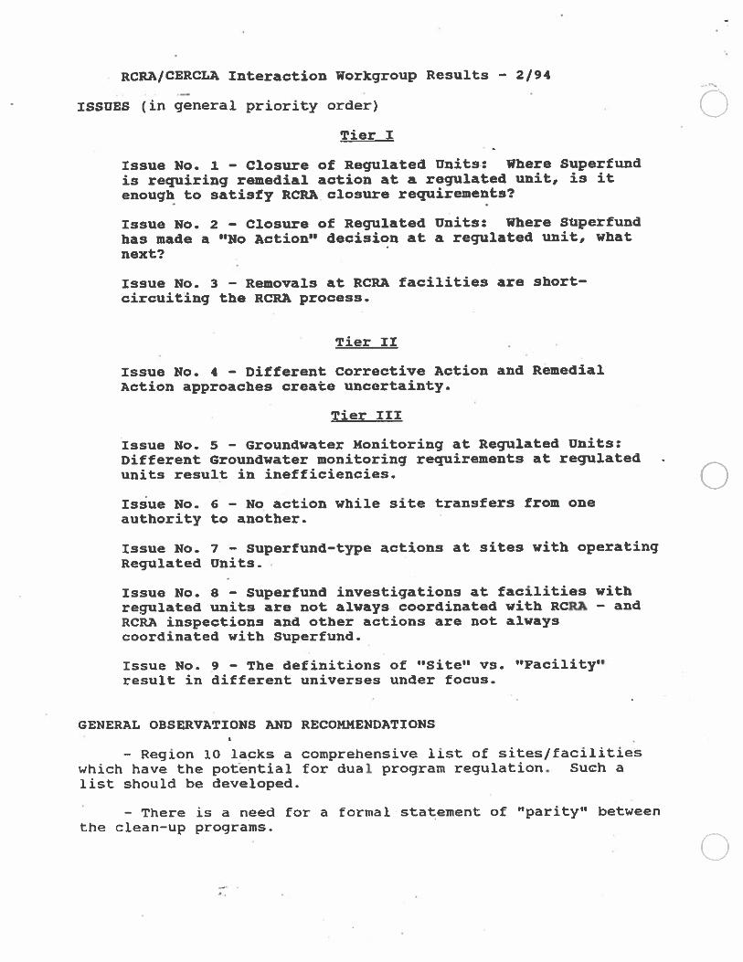
RCRA/CERCLA Interaction Workgroup Results - 2/94

ISSUES (in general priority order)

Tier I

Issue No. 1 — Closure of Regulated Units: Where Superfund

is requiring remedial action at a regulated unit, is itenough to satisfy RCRA closure requirements?

Issue No. 2 — Closure of Regulated Units: Where Superfundhas made a “No Action” decision at a regulated unit, whatnext?

Issue No. 3 — Removals at RCRA facilities are short—circuiting the RCRA process.

Tier II -

Issue No. 4 — Different Corrective Action and Remedial

Action approaches create uncertainty.

Tier III

Issue No. S - Groundwater Monitoring at Regulated Units:Different Groundwater monitoring requirements at regulated

units result in inefficiencies. 0Issue No. 6 — No action while site transfers from one

authority to another.

Issue No. 7 - Superfund-type actions at sites with operating

Regulated Units.

Issue No. 8 - Superfund investigations at facilities withregulated units are not always coordinated with RCRA — and

RCRA inspections and other actions are not alwayscoordinated with Superfund.

Issue No. 9 — The definitions of “Site” vs. “Facility”result in different universes under focus.

GENERAL OBSERVATIONS AND RECOMMENDATIONS

- Region 10 lacks a comprehensive list of sites/facilitieswhich have the potential for dual program regulation. Such alist should be developed.

— There is a need for a formal statement of “parity” betweenthe clean—up programs.

U

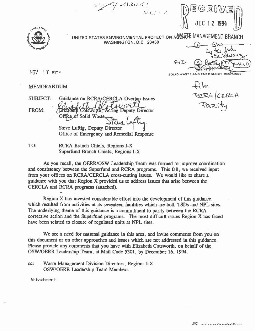
• [U\Vj71)[f\\ DEC12 1994 UIEO

ST,,

£‘ fl iAIACTtAAftjAnr rUNITED STATES ENVIRONMENTAL PROTECTION AGFMfl VItj!’JRtJtMct\JT BRANCH

‘4 I ; WASHINGTON, D.C. 20460

______

‘<4)4p0it

@ . j1\LcSA

NOV I 7 a. SOLIDWAS!EMERGENCE5NSi

MEMORANDUM

SJECT: Guidance on RCCERC Overlap IssuesA

• flag fl9rtLFROM: ffètft1swo$E’Actmg IYeputy Director

• Offf,fi Solid Was

Steve Luftig, Deputy DirectorOffice of Emergency and Remedial Response

TO: RCR4 Branch Chiefs, Regions I-XSuperifind Branch Chiefs, Regions I-X

As you recall, the OERRJOSW Leadership Team was formed to improve coordinationand consistency between the Superfluid and RCRA programs. This fall, we received inputfrom your offices on RCRMCERCIA cross-cutting issues. We would like to share aguidance with you that Region X provided us to address issues that arise between theCERCL4 and RCRA programs (attached).

Region X has invested considerable effort into the development of this guidance,which resulted from activities at its seventeen facilities which are both TSDs and NPL sites.The underlying theme of this guidance is a commitment to parity between the RCRAcorrective action and the Superñrnd programs. The most difficult issues Region X has facedhave been related to closure of regulated units at NPL sites.

We see a need for national guidance in this area, and invite comments from you onthis document or on other approaches and issues which are not addressed in this guidance.Please provide any comments that you have with Elizabeth Cotsworth, on behalf of theOSW/OERR Leadership Team, at Mail Code 5301, by December 16. 1994.

cc: Waste Management Division Directors, Regions I-XOSW/OERR Leadership Team Members

Attachment

£fl .,._... -- ,,___‘_.

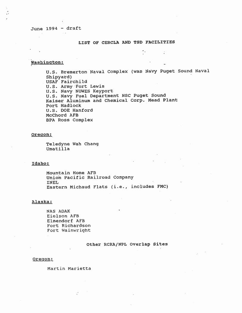
June 1994 — draft

LIST OF CERCLA AND TSD FACILITIES

Washington:

U.S. Bremerton Naval Complex (was Navy Puget Sound Naval

Shipyard)USAP FairchildU.S. Army-Fort LewisU.S. Navy NUWES KeyportU.S. Navy Fuel Department NSC Puget Sound

Kaiser Aluminum and Chemical Corp. Head Plant

Port HadlockU.S. DOE HanfordMcchord AFBBPA Ross Complex

Oregon:

Teledyne Wah ChangUmatilla

Idaho:

Mountain Home AFBUniob Pacific Railroad Company

INELEastern Michaud Flats (i.e., includes FNC)

Alaska:

NAS ADAKEielson AFBElmendorf AFBFort RichardsonFort Wainwright

Other RCRA/NPL Overlap Sites

Oregon:

Martin Marietta

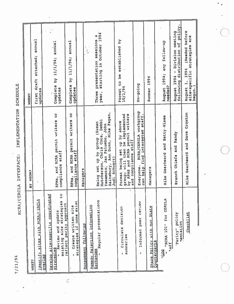
7/2

1/9

4R

CR

A/C

ER

CL

AIN

TE

RF

AC

E;

IMP

LE

ME

NT

AT

ION

SC

HE

DU

LE

WH

AT

?B

YW

HO

M?

-W

HE

N?

Jdenti

fysit

es

wit

hR

CR

A/(

ER

CL

A-

fir

st

dra

ftatt

ached;

annual

overl

ap

update

s

Qevelo

psit

e—

specif

iccoord

inate

d

str

ate

gie

s-

Revie

wan

dupdate

RP

Ms,

and

RC

RA

perm

itw

rite

rsor

Com

ple

teby

11/1

/94;

annual

exis

ting

sit

estr

ate

gie

sto

com

pli

ance

sta

ff

update

s

refle

ct

pari

tyappro

ach

-C

reate

wri

tten

sit

eR

PH

s,and

RC

RA

perm

itw

rite

rsor

Com

ple

teby

11/1

/94;

annual

str

ate

gie

sif

none

exis

tcom

pli

ance

sta

ff

update

s

Man

agem

ent

Fol1

ow

jpM

anagers

Rem

edy

Sele

cti

on

Info

rmati

on

Exchanges

-R

egula

rpre

senta

tions

Bein

gset

up

by

gro

up

(Susa

nT

hre

epre

senta

tion

sessio

ns

a

Hutc

hers

on,

Chri

sC

ora

,D

ebbi

year,

sta

rti

ng

inO

cto

ber

1994

Yam

amoto

,Ja

nP

alu

mbo,

John

Sain

sbury

,A

nnD

unn,

Hik

eF

agan,

Judi_

Schw

arz

)

—C

ircula

tedecis

ion

Form

at

bein

gset

up

by

above

Form

at

tobe

esta

bli

shed

by

sum

mari

es

gro

up;

wil

lth

en

be

imple

mente

d10/1

/94

.by

RPM

San

dR

CR

Aperm

itw

rite

rsand

com

pli

ance

sta

ff

-In

form

al

peer

revie

wE

very

one.

RC

RA

/CE

RC

LA

work

gro

up

On—

goin

g

can

help

find

inte

reste

dsta

ff.

Share

Poli

cy

wit

hour

Sta

teM

anagers

Sum

mer

1994

Counterparts

_______________________________________

—“R

CR

A101”

for

CE

RC

LA

Mik

eG

earh

eard

and

Bett

y-W

iese

August

1994;

any

foll

ow

—up

taft

___________________________________

needed?

Pari

ty”

poli

cy

Bra

nch

Chie

fsand

Ran

dy

August

1994

—D

ivis

ion

meeti

ng

entation

___________________________________

foll

ow

ing

dis

trib

uti

on

of

poli

cy.

Checkli

st

Mik

eG

earh

eard

and

Dav

eC

roxto

nA

ugust

1,

1994

(Nee

ded

befo

resit

e—

specif

icstr

ate

gie

sare

•begun.)

o

ATTACHMENT C

EXAMPLES OF DATA QUALITY ASSESSMENT APPLICATIONS

?H R ‘Al. MS1T ?O IIM

U0

0

Appendix B from EPA (1994a)Guidance for the Data Quality Objectives Process, EPA QAJG-4

UN’I 1SK RE\1s11 HNALMASTER 4POflI-R

APPENDIX B

DQO CASE STUDY: CADMIUM-CONTAMINATEDFLY ASH WASTE

TntroductiQp.

This appendix presents a functional, but realistic example of the DQO outputs for a

decision that could be made within the Resource Consen’afion and Recovery Act (RCLk)

hazardous waste management program. The example is intended to illusa-ate the types of

outputs that axe common to the DQO Process. It is not intended, however, to represent the

policy of the RCRA program for actual situations that may be similar to the example. Please

consult with a knowledgeable representative within the RCRA program office about the

current policy for making waste classification decisions for fly ash or other types of

hazardous waste.

‘lie case study has been chosen because it is simple and stx-aighdbrward, and because

the outputs are uncomplicated. Although some of the outputs from this example may seem

intuitive, this is not often the case in practice. For many studies, the DQO Process is

complicated and thought-provoking. Even so, some steps will require more effort than others.

Keep in mind that fl of the steps in the DQO Process are necessary to develop a data

collection design. Once the first six steps have been pàmpleted and thoroughly thought-out,

then development of the most resource-effective data collection desi can proceed.

Background

A waste incineration facility located in the Midwest routinely removes fly ash from its

flue gas scrubber system and disposes of it in a local sanitary landfill. Previously it was

determined that the ash was not hazardous according to RCRA program regulations. The

incinerator, however, recently began teating a new waste steam.. The representatives of the

incineration company are concerned that the waste fly ash could now contain hazardous levels

of cadmium from the new waste sources. They have decided to test the ash to determine

whether it should be sent to a hazardous waste landfill or continue to be sent to the municipal

landfill. They have decided to employ the DQO Process to help guide their decision making.

Cadmium is primarily used as corrosion protection on metal pans of cam and electrical

appliances. It is also used in some batteries. Cadmium and cadmium saks have toxic effects

for humans through both ingestion and inhalation exposures. Ingestion exposure usually

causes mild to severe in-itation of the gastiointesdnal u-act, which can be caused byconccnuations as low as 0.1 mg/kg/day. Chronic (long-term) inhalation exposure can cause

increased incidence of emohysema and chronic bronchitis, as well as kidney damage.

EPA QAIG-4 47 . Scpwm&r Q4

Under the current Code of Federal Regulations, 40 CFR. Pail 261, a solid waste can

be considered “hazardous” if it meets specific criteria of ignitabthty, conosivity, reactivity,

and toxicity. One method that is used to determine if a solid substance, such as fly ash,

meets the criteria for toxicity under the RCRA program regulations is to test a “representative

sample” of the waste and perform a Toxicity Characteristic Leaching Procedure (TCLP)

described in 40 CFR, Pt 261, App. LI. During this process, the solid fly ash will be

“extracted” using an acid solution. The extraction liquid (the TOY leachate) will then be

subjected to tests for specific metals and compounds. For this example, the only concern is

with the concentratioa of cadmium in the leachate. The primary benefit of the DQO Process

will be to establish the data collection design needed to determine if the waste is hazardous

under RCRA regulations within tolerable decision error rates.

As a precursor to the DQO Process, the incineration company has conducted a pilot

flidy of the fly ash to determine the vañabthty in the concentration of cadmium between

loads of ash leaving the facility. They have determined that each load is fairly homogeneous.

There is a high variability between loads, however, due to the nature of the waste stream.

Most of the fly ash produced is not hazardous and may be disposed of in a sanitary landfill.

Thus, the company has decided that testing each individual waste load before it leaves the

facility would be the most economical, Then they could send loads of ash that exceeded the

regulated standards to the higher cost RCRA landfills and continue to send the others to the

sanitary landfill. -

BOO Development

The following is a representative example of the output from each step of the DQO

Process for the fly ash toxicity problem.

State the Problem — a description of the problem(s) and specifications of available

resources and relevant deadlines for the study.

(1) Jdennh the members of the jlanning team — The members of the planning team will

include the incineration plant manager, a plant engineer, a statistician, a quality

assurance officer, an EPA representative who works within the RCRA program, and a

chemist with sampling experience.

(2) Idennfy she primary &cirion maker — There will not be a primary decision maker,

decisions will be made by consensus.

(3) Develop a concise descripHon of the problem — The problem is to determine which

loads should be sent to a RCRA landfill versus a sanitary landfill.

(4) Specify available resources and relevant deadlines for the study —L While the project

will not by constrained by cost, the waste generator (the incineration company) wishes

to hold sampling costs below 52,500. They have also requested that the waste testing

be completed within 1 week for each container load. (Z)48 Scpembcr 1994

Identify the Decision — a statement of the decision that will use cnviromneatal data and the

actions that could result from this decision.

(1) identify the principal study question — Is the fly ash waste considered hazardous

under RCRA regulations?

(2) Define alternative actions that could result from resolution of the principal study

question —

(a) The waste fly ash could be disposed of in a RCRA landfill.

(b) The waste fly ash could be disposed of in a sanitary landfill.

(3) Combine the principal study question and the alternative actions into a decision

statement — Decide whether or not the fly ash waste is hazardous under RCRA and

requires special disposal procedures.

(4) Organize multiple decisions — Only one decision is being evaluated.

Identify the Inputs to the Decision — a list of.the environmental variables or cliaratteristics

that will be measured and other injoitadon needed to resolve the decision statement.

(1) Identify the information :hat will be required to resolve the decision statement — To

resolve the decision statemenç the planning team needs to obtain measurements of the

cadmium concentration in the leachate resulting from TCLP extraction.

(2) Determine the sources for each item of infornzatinn identified — The fly ash should be

tested to determine if it meets RCRA cgu1ated standards for toxicity using the test

methods listed in 4.0 CFR, Pt. 261, App. U. Existing pilot study data provide

information about variability, but do not provide enough information to resolve the

decision statement

(3) identify the information that is needed to establish the action level — The action leveL

will be based on the RCRA regulations for cadmium in TCLP leachate.

(4) Confirm that appropriate measurement methods exist to provide the necessary data —

Cadmium can be measured in the leachate according to the method specified in 40

CFR. ft 261, App. a The detection limit is below the standard.

Define the Boundarl of the Study — a detailed description of the spatial and temporal

boundaries of the problem, characteristics that define the population of interest, and any

practical considerations for the study.

EPA QAJO4 49 Scpccmbcr I9c

(1) Specify the characteristics that define the population of interest — fly ash waste from

the hazardous waste incinerator will be analyzed. The fly ash should not be mixed

with any other constituents except water that is used for dust control. Each load of

ash should fill at least 70% of the waste trailer. In cases where the trailer is filled less

than 70%. the trailer must wait on-site until more ash is produced and fills the taller

to the appropriate capacity.

(2) Define the spatial boundary of the decision statement

—

(a) Define the geographic area to which the decision statement applies. Decisions

will apply to each container load of fly ash waste.

(b) When appropriate, divide the population into strata that have relatively

homogeneous characteristics. Stratification is not necessary si’ice the waste ash is

relatively homogeneous within each container.

(3) Define the temporal boundary of the decision statement —

(a) Determine the rimeframe to which the iecuion statement applies. It will be

assumed that the sampling data represent both the current and future concentration

of cadmium within the ash. -

(b) Determine when to collect data. Contained in the trucks, the waste does not pose

a threat to hiiminc or the envimnmenL Additionally, since the fly ash is not

subject to change, thsinteaton. or alteration, the. decision about the waste

characteristics does not warrant any temporal constraints. To expedite decision

making, however, the planning team has placed denAlines on sampling and

reporting. The fly ash waste will be tested within 48 hours of being loaded onto

waste hauling trailers. The analytical results from each sampling round should be

completed ad reported within 5 working days of sampling. Until analysis is

complete, the trailer cannot be used.

(4) Define the scale of decision making — The scale of d&ision making will be each

container of waste ash..

(5) I&nnfj practical constraints on data collection — The most important practical

consideration that could interfere with the study is the ability to take samples from the

fly ash that is stored in waste hmiling trailers. Although the trailers have open access.

special procedures and methods will have to be implemented for the samples to be

representative of the entire depth of the ash. It has been suggested that core samples

may be one practical solution to this problem. To get additional samples from each

truck and to minimize the cost, composiUng of core samples has been suggested.

EYF QAJO-4 50 Scptemba 1994

1

Develop a Decision Rule — to define the parameter of interest, specie the action level and

integrate previous DQO outputs into a single statement that describes a logical basis for

choosing among alternative actions.

(1) Specify the statistical parameter that characterizes the population of interest — The

planning team is interested in the true mean concentration of cadmium in the TCLY

leachate for each container. -

(2) Specjfy thaachon level for the study — The action level for the decision will be the

RCRA regulatory standard for cadmium of 1.0 mgfL in the TCLP leachate.

(3) Develop a decision rule (an “:f..then..i’ statement) — U the mean concentration of

cadmium from the fly ash leachate in each container load is geater than 1.0 mg/L

(using the TCLP method as defined in 40 CFR 261), then the waste will be considered

hazardous and will be disposed of at a RCRA landfill. if the mean concentration of

cadmium from the fly ash waste leachate is less than 1.0 mg/L (using the TCLP

method as defined in 40 CFR 261), then the waste will be considered non-hazardous

and will be disposed of in a sanitary landfill.

Specify Tolerable Limits on Decision Errors — the decision mikrr’ tolerable decision

error rates based on a consideration of the consequences of making a decision error.

(1) Determine the possible range of the parameter of interest — From analysis of records

of similar studies of ca&niu’m in environmental msthces, the range of the cadmium

concentrations is expected to be from 0-2 mgIL. Therefore the mean concentration is

expected to be between 0-2 mg/L for this investigation.

(2) Identify the decision errors and choose the null hypothesis —

(a) Define both types of decision errors and establish the true state of nature for each

decision error. The planning team has determined that the two decision errors arc

(i) deciding that the waste is hazardous when it truly is not, and (ii) deciding that

the waste is not hazardous when it truly is.

The true state of nature for decision error (i) is that the waste is not hazardous.

The true state of nature for decision error (ii) is that the waste is hazardous.

(b) Specify and evaluate the potential consequences of each decision error.

The consequences of deciding that the waste is hazardous when it truly is not

will be that the incinerator company will have to pay more for the disposal of

the fly ash at a RCRA facility than at a sanitary landfill.

EPA QAJG-4 Septemba 994

The consequences of deciding that the waste is not hazardous when it wily is

will be that the incinerator company will dispose of the waste in a sanitary

landfill which could possibly endanger human health and the envisonmenL In

this situation, they may also be liable for fiitwc damages and environmental

cleanup costs. Additionally, the reputation of the incinerator company may be

compromised. jeopardizing its future profitability.

(c) Establish which decision error has more severe consequences near the action

leveL Th j,lanning team has concluded that decision error (ii) has the more

seven consequences near the action level since the risk of jeopardizing human

health outweighs the consequences of having to pay more for disposal.

Cd) Define the null hypothesis (baseline condition) and the aUemafive hypothesis and

assign the emtr “false positive” and ‘fake negative” to the appropriate decision

error.

The baseline condition or null hypothesiA (H,) is “the waste is hazardous.”

The alternative hypothesis (H,) is “the waste is not hatardous.”

The false positive decision error occurs when the null hypothesis is rejected when

it is true. For this example, the false positive decision error occurs when the

decision maker decides the waste is not hazardous when it truly is hazardous. The

false negative decision error occurs when the null hypothesis is not rejected when

it is false. For this example, the false negative decision error occurs when the

decision maker decides that the waste is hazardous when it truly is not hazardous.

(3) Speczf a range of possible values of the parameter of interest where the consequences

of decision errors are relatively minor (gray region) — The gray region is the area

adjacent to the action level when the planning team feels that the consequences of a

false negative decision error aic minimal. To decide how to set thc width of the gray

region, the planning team must decide where the consequences of a false negative

decision error are mini rnal• Below the action level, even if the concentration of

cad.tnium were very close to the action level, the monetary costs of disposing of the

waste at a RCRA facility are the same as if the waste bad a much lower concentration

of cadmium. Clearly any false negative decision error (to the left of the action level)

will cause the incinerator company and their customers to bear the cost of unnecessary

expense (i.e., sending nonhazardous waste to a RCRA facility). The planning team.

however, also realizes that they must define a reasonable gray region that balances the

cost of sampling with risk to hurthn health and the environment and the ability of

measurement instruments to detect differences. Therefore the plnnning team has

specified a width of 0.25 mg/L for this gray region based on their preferences to detect

decision errors at a concentration of 0.75 mgfL (see Figure B-i):

EPA QAJG3 52 Sepwmba (994

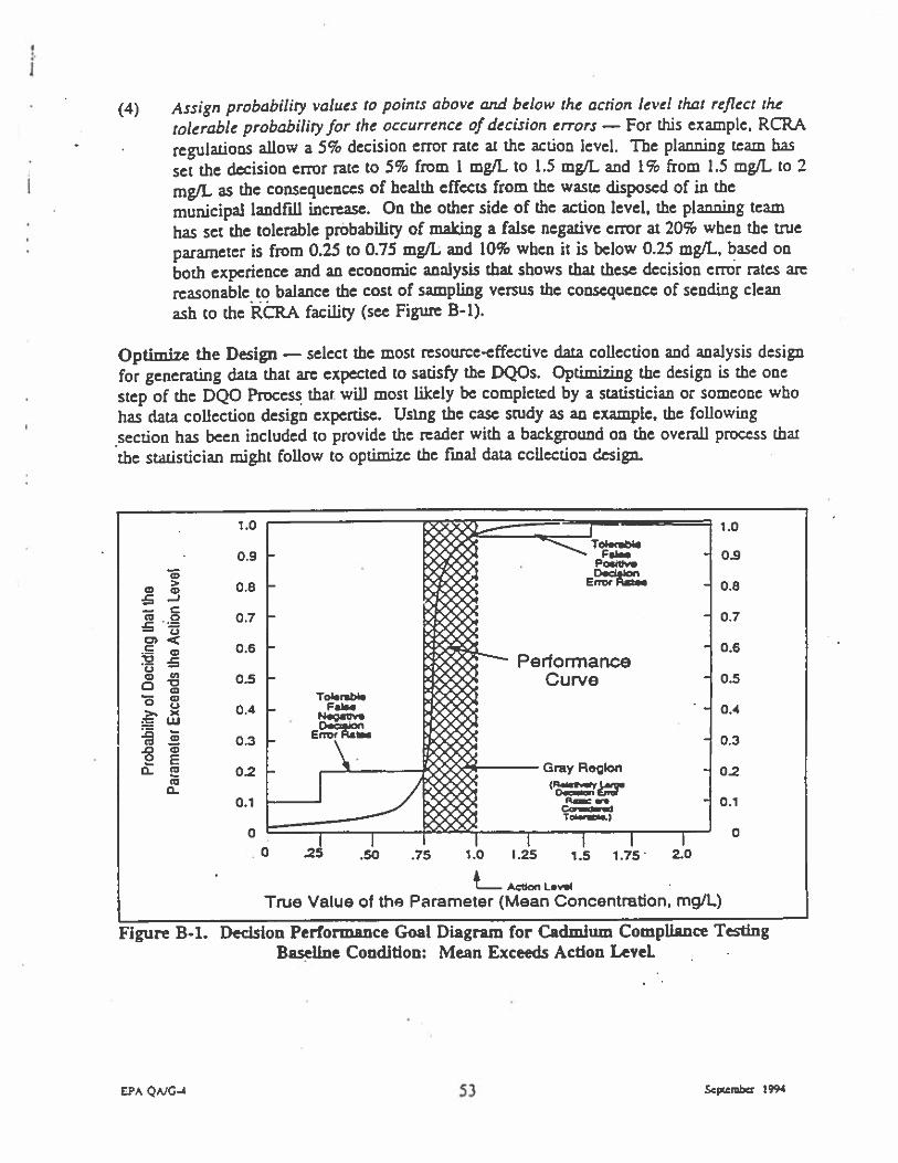
(4) Assign probability values to points above and below the action level that reflect the

tolerable probabiliry for the occurrence of decision errors — For this example, RCRA

regulations allow a 5% decision error rate at the action level. The planning team has

set the decision error rate to 5% from 1 mg/L to 1.5 mgfL and 1% from 1.5 mgfL to 2

mgfL as the consequences of health effects from the waste disposed of in the

municipal landfihi increase. On the other side of the action level, the planning team

has set the tolerable probability of making a false negative error at 20% when the true

parameter is from 0.25 to 0.75 mgfL and 10% when it is below 0.25 mg/L, based on

both experience and an economic analysis that shows that these decision endr rates are

reasonable to balance the cost of sampling venus the consequence of sending clean

ash to the RCL4 facility (sea Figure B-i).

Optimize the Design — select the most resource-effective data collection and analysis design

for generating data that are expected o satisfy the DQOs. Oprimiiing the design is the one

step of the DQO Process that. will most likely be completed by a statistician or someone who

has data collection design expertise. Using the case study as an example, the following

section has been included to provide the reader with a background on the overall process that

the statistician might follow to optimize the final data collection design.

Figure B-i. Decision Performance Goal Diagram for Cadmium Compliance TestingBaseline Condition: Mean Exceeds Action LeveL

1.0

0.9

0.8

0.7

0.6

1.0

0

o o

— CC .0

0

— 00

cca-

0.5

03

0.8

0.4

0.3

0.7

0.6

02

0.5

0.1

0.4

0

0

0.3

02

True Value of the

0.1

0

Acton Len4

Parameter (Mean ConcentmUon, mgJL)

EPA QAIG3 53 Scpwmb 1994

Overview

Developing a data collection design requires an understanding of the sampled medium

and the information that ws generated in previous DQO steps. The statistician’s job is to

review he background information, determine the appropriate statistical application to

adequately solve the problem. and develop one or more appropriate data collection designs.

Once this is complete, the statistician will compare the cost and performance of the different

data collccdon designs. This process can be broken down into five distinct steps:

(1) Review the DQO outputs and existing environmental data.

(2) Develop general data collection design alternatives.

(3) For each data collection design alternative, select the optim2l sample size that

satisfies the DQOs.

(4) Select the most resource-effective data collection design that satisfies th of the

DQOs.

(5) Document the operational details md theoretical assumptions of th: selected

design in the sampling and analysis plan.

Actiñ&s .

(1)(1) Review the DQO outputs and existing environmental data — Because the statistician

has participated in the DQO Process for this problem, there is no need to review the

DQO outputs further. The only existing data relevant to this problem ait the pilot

study data Based on the pilot study, the incineration company has determined that

each load of ash is fairly homogeneous, and has estimated the standard deviation, in

the concentration of cadmium within loads of ash to be 0.6 owL.

(2) Develop general data collection design alternatives — Generally, the design

alternatives are based on a combination of design objectives developed in previous

DQO Process steps and knowledge of statistical parameters about the medium or

cont2minanL Below an four examples of possible designs that could apply to the case

study:

(a) Simple Random Sampling — The simplest type of probability sample is the simple

random sample. With this type of sampling. evety possible point in the sampling

medium has an equal chance of being selected. Simple random samples are used

primarily when the variability of the medium is relatively small and the cost of

analysis is relatively inexpensive. Srnph random sampb locaticr.s are generally

developed through the use of a random r.umber table or through computer

generation of pseudo—random numbers. C)EPA QAIG-4 54 Scpambcr 1994

In the case of the cadmium-contaminated ash, a fixed number of random grab

samples would be selected and analyzed. Standard lab splits and QC samples

would be taken according to standard procedures for the RCRA pmpaa Each

sample would be chosen randomly in three dimensions. A Student’s t-test Es

suggested as a possible method for testing the statistical hypothesis.

(1,) Composite Simple Random Sampling (composite sampling) — This type of

sampling consists of taking multiple samples, physically combining (compositing)

them, and drawing one or more subsamples for analysis. Composite samples are

taken primarily when an average concentration is sought and there is no need to

detect peak concentrations. By compositing the samples, researchers are able to

sample a larger number of locations than if compositing was not used, while

reducing the cost of analysis by combining several samples.

hi the case of the cadmium-contaminated ash, a fixed number of random grab

samples would be taken and composited. The number of grab samples contained

in a composite sample (g) is also fixed. To determine sampling locations within

the composite, a container would be divided into ‘g” equal-volume strata and

samples would be chosen randomly within each strata The use of strata ensure

full coverage of each container. Standard lab splits and QC samples would be

taken according to standard procedures for the RCRA program. A Student’s t-tcst

is suggested as the possible method for testing the statistical hypothesis. -

(c) Sequential Sampling — Sequential sampling involves m2Hng several rounds of

sampling and analysis. A statistical test is performed after each analysis to arrive

at one of three possible decisions: reject the null hypothesis, accept the null

hypothesis,’ or collect more samples. This strategy is applicable when sampling

and/or analysis costs are high, when information concerning sampling and/or

measurement variability is lacking, when the waste and site characteristics of

interest are stable over the timeframe of the sampling effort, and when the

objective of the sampling is to test a single hypothesis. By taking samples in

sequence, the researcher can hold down the cost of sampling and analysis.

In the case of the cadmium-contaminated ash, a sequential probability sample

could be performed. The samples in each sampling round would be chosen

randomly in three dimensions. U the decision to stop sampling has not been made

before the number of samples required for the simple random sample an taken.

sampling would stop at this point and the simple random sample test would be

performed. Standard laboratory splits and QC samplcs would be taken according

to standard procedures for the RCRA program. An approximate ratio test is

‘Decide not to rcject the null bascd on tolerable decision error UnilLS.

EPA QMO-4 55 Scpcember I94

suggested after each round of sampling is complete to decide whether or not to

conclude that the waste is hazardous or to continue sampling.

(d) Stratified Random Sampling — Stratified sampling involves dividing the study

area into two or more non-overlapping subsets (stnta).which cover the entire

volume to be sampled. These strata should be defined so that physical samples

within a stratum are more similar to each other than to samples from other strata.

Sampling depth, concentration level, previous cleanup attempts, and confounding

contamüfthi Is can be used as the basis for creating strata Once the strata have

been defined, each stratum is tlen sampled separately using one of the above

designs. Stratification is often used to ensure that important areas of a site an

represented in the sample. In addition, a stratified random sample may provide

more precise estimates of contaminant levels than those obtained from a simple

random sample. Even with imperfect information, a stratified sample caa be more

resource-effective.

Since the incineration company has already determined that each load of ash is

fairly homogeneous, stratification does not have any advantages over a simple

random sample. In addition, since the company has decided to test each waste

load individually before it leaves the facility, stratifying each waste load would be

difficult and unnecessary. Therefore, this data collection design will not be

considered further. .

.

(N

(3) - For each data collection design ahemafive, select the optimal sample size that

satisfies the DQOs — The formula for determining the sample size (number of

samples to be collected) is chosen based on the hypothesis test and data collection

design. Standard formulas can be found in several references, including:

• Cochran, W. 1977. Sampling Techniques. New Yort John Wiley.

• Desu, M.M., and 0. Raghavano. 1990. Sample Size Methodology. San Diego,

CA: Academic Press.

• Gilbert, Richard 0. 1987. Statistical Methods for Environmental Pollution

Monitoring. New York: Van Nostrand Reinhold.

U.S. Environmental Protection Agency. 1989. Methods for Evaluating the

Attainment of Clewwp Standards: Volume 1: SoiLs and Solid Media

EPA 23C1V2-89-042, Office of Policy, Planning and Evaluation.

• U.S. Environmental Protection Agency. 1992. Methods for Evaluating the

Attainment of Cleanup Standards: Volume 2: Ground Water.

EPA 230-R-92-014, Office of Policy, Planning and Evaluation.

UEPA QAJG-4 55 Scpccmba 1994

• U.S. Environmental Protection Agency. 1994. Statistical Methods for

Evaluating the Attainment of Clean-up Standards: Volume 3: Reference-

Based Standards for Soils and Solid Media EPA 230-R-94-004. Office of

Policy. Planning and Evaiutalon.

These formulas can also be found in many basic statistics textbooks. Different

formulas an necessary for each data collection design, for each parameter, and for

each statistical test These formulas an generally a function of a; ; the detection

difference, A-(delta); and the standard deviation, a. The detection difference, b., is

defined to be the difference between the action level (AL) and the other bound of the

gray region (U); i.e., ê. = AL - U. In this case the standard deviation was derived

from pilot data under approximately the same conditions as expected for the real

facility.

For example, a formula for computing the sample size necessary to meet the DQO

constraints for comparing a mean against a regulatory threshold, when a simple

random sample is selected, is:

where;

& = estimated variance in measurements (from pilot study)

n = number of samples required,= the th percentile of the standard normal distribution (from standard

statistical tables), andA= U-AL

Simple Random Sample — Using the formula above, it was determined thai 37

samples an necessary to achieve the specified limits on decision errors. This

sampling plan satisfies all the DQOs including budget schedule, and practical

constraints.

Composite Sampling — To determine sample sizes for a composite sample, it is

necessary to compute the number of composites samples, n; the number of samples. g.

within each composite; and the number of subsamples, m, to be measured for each

composite. Usually m=1; however, since this design is to be used repeatedly, it is

suggested that two subsamples from each composite sample be measured to estimate

composite variability, which can then be used to re-optimize the number of samples m

and g.

For a composite sample, with random sample locations, it has been determined that

eight composite samples of eight samples each are sufficient to meet the limits on

decision errors that have been specified. This design is more than sufficient to

EPA QNG-4 57 .

1944

achieve the specified limits on decision errors and satisfies all the DQOs including

budget schedule, and practical constraints.

Sequential Sampling — For the purposes of comparing costs, the average number of

samples in a sequential sampling design can be estimated, but these estimnrrs are only

averages. The avenge sample size for concluding that the waste is hazardous is 16

and the average sample size for concluding the waste is not hazardous is 22. The

avenge sizes arc different because the burden of proof is placed on disproving the null

hypothesis, thus, more samples on avenge are required to prove that the alternative

hypothesis (the waste is not hazardous) is true. However, these sample sizes are only

averages. In some cases, fewer samples are necessary; in others, more may be

necessary. This sampling plan satisfies all the DQOs including budget, schedule, and

practical constraints.

(4) Select the most resource-effective data collection design that satisfies the DQOs —

Compare the overall efficiency of each model and choose the one that will solve the

problem most effectively.

Cost Estimates for Each Design

First the costs for the three designs alternatives will be evaluated: -

SimpJe Random Sampling — A simple random sampling scheme can be implemented

for each load of fly ash by first generating three-dimensional random sampling points.

This can most easily be done by using a computer. Samples can then be taken using a

special ab sampler which will be forced into the ash, opened to take the sample.

then closed and removed. The difficulty with this type of sampling scheme is

measuring sampling locations in three dimensions, and it may be difficult to gain

access to the correct sampling locations.

This design meets all of the required limits on dision errors. The cost of this design

is calculated based on the assumed cost of selecting a sample ($10). and the cost of

analyzing a sample ($150). Since 37 samples need to be taken and analyzed, the cost

of this design is:

Cost =37x$l0÷37x$150= $370 + $5550 = $5920

Composite Sampling — Composite sampling will be performed similarly to simple

random sampling except that after eight random samples are collected (one from each

stmmm), they will be combined and homogenized. Two sample aliquots for analysis

will then be drawn from the homogenized mixmrc. This process will be repeated

eight times.

0EPA QMG3 53 Scpiembc 1994

This design meets all of the required limits on decision errors. The cost of this design

is based on the cost of selecting ($10) and analyzing•(S 150) a sample. Eight samples

will be used to make each composite sample for a sampling cost of 580; two

subsamples will be analyzed froth this composite sample for a cost of 5300.

Therefore, each composite sample will cost $380. The total cost of this design is:

Costa = 8 x5380=S3040. -

Sequential Sampling — Sequential sampling will be performed similarly to random

sampling. The primary difference is that the ultimate number of samples will be

determined by the results of one or more sampling rounds.

This design has the potential to reduce the number of samples required in the simple

random sampling design and still meet the decision error limits. The avenge costs of

the two decisions are used below:

The ash is hazardous: 16 x (5160) = 52,560

The ash is non-hazardous: 22 x ($160) = $3,520

To detemüne the expected cost, estimat the number of loads of ash that should be

sent to a RCRA facility venus the number of loads that can be sent to a municipal

facility. Suppose 25% of the loads are hazardous and should be sent to a RCRA

facility. Then the expected cost (ECj of this design should be.

EC = 0.25 x (cost of sampling when ash is h2rndous) + (0.75 x cost of

sampling when ash is non-hazardous)

= 0.25 x ($2,560) + 0.75 x ($3,520) = $ 3,280

Selection of a Design

Because the simple random sampling design requires that many samples be taken and

analyzed, it is inefficient for the goals of this study. Sampling will cost almost as

much to determine whether the waste is hazardous or nonhazardous as it would cost to

send all the waste to a RCRA h7fldOUs waste landfill. Therefore, this decision is not

resource-effective.

The sequential data collection design is more resource-effective than the simple

random sampling design. The potential savings over sending all waste to a RCRA

hazardous waste facility is $6,750 - 53.280 = $3,470. The site owner has expressed.

disapproval for this sampling plan because of the time it may take before a decision

can be made, if the ash was not homogeneous within a cont&incr, however, Uds data

collection design may be the dcsign of choice.

S’AQAJG-3 59 Scpccmba 194*

The composite sample design is the best option. ft is the most resource-effective C)design and requires the least amount of time to implement. In addition, the use of

strata ensures full coverage of each container. It is recommended that each of the

eight composite samples have two subsamples analyzed. In the future, after sufficient

data have been collected to estimate the variability within each composite sample, ft

may be possible to reduce the number of samples that will be necessary to make a

decision about the waste contents.

(5) Document the operational detaiLs and theoretical assumptions of the selected design in

she sampling and analysis plan — A composite sample design should be used to

determine whether each container of ash should be sent to a RCRA landfill or to a

municipal landfill. Eight composite samples, consisting of eight grab samples, should

be taken from each container and two subsamples from each composite should be

analyzed at the laboratory. To form the composite samples, the containers will be

divided into eight strata of equal size and one grab sample will be taken randomly

within each stratum and composited. Sample locations will be generated randomly

using computer-generated random numbers. The model assumes that the variability

within a composite sample is negligible. Data from the subsamples can be used to test

this assumption and make corrections to the model.

Beyond the 1)00 Process - Evaluaflon of the Design using the DOA

For this study, the data were collected using the composite sampling design. Once the C)samples were collected and analyzed, the data were evaluated statistically and scientifically

using the DQA Process to inspect for anomalies, confirm that the model assumptions were

correct, select a statistical test and verify that the test assumptions such as distribution and

independence can be met. For this study, a t-test satisfied the DQOs, and inspection of the

data indicated that there was no reason to believe that the data were not normally distributed

or that there was correlation between data points. It was also verified that the within-

composite variability was negligible.

After three weeks of sampling, appmxmately 30% of the waste loads leaving the

incinerator were found to have hazardous concentrations of cadmium in the fly ash. The data

collection design was determined to be cost-effective because the combined cost of sampling

and disposal was less than sending all of the waste to a RCL4 landfill.

0EPA QAIG-4 Scpwmba 1994

1

APPENDiX C

DERIVATION OF SAMPLE SIZE FORMULA FOR TESTING MEAN

OF NORMAL DISTRIBUTION VERSUS AN ACTION LEVEL

This appendix presents a mathematical derivation df the sample size formula used in

the DQO example-of Appendix B.

Let X1, X )C, denote a random sample from a normal thsthbution with unknown

mean i and known standard deviation a. The decision maker wishes to test the nufl

hypothesis H0: .i = AL versus the alternative HA: p> AL, where AL. the action level, is some

prescribed constant; the false positive (Type I) error rate is a (i.e., probability of rejecting H0

when x = AL is a); and for some fixed constant U> AL (where U is the other bound of the

gray region), the false negative (Type it) error rate is (i.e., probability of rejecting H0 when

p = U is l-). Let X denote the sample mean of the Xs. It will have a normal Wsthbution

with mean p and variance &In. Hence the random variable Z defined by

z=(111 .(1)

will have a standard normal distribution (mean 0, variance 1). Let denote the pth percentile

of the standard normal distribution (available in most statistics books). Recall that the

symmetry of the standard normal disthbution implies that zp =

Case I: Standard De1aUon Known

The test of H0 versus HA is performed by caiculating the test statistic

r= (x4)V7 (2)

If T> z1.0, the null hypothesis is rejected..

Note that

T =[(X—[O÷(P-AL)]c

= Z+a(g)(3)

E’AQMG-L 61 Scp’tmba 1993

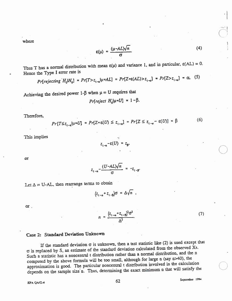
where

2(3.1)(—ALXc (4)

Thus T has a normai thsthbution with mean sQl) and variance 1, and in particular, s(AL) =0.

Hence the Type I error rate is

Prfrejectinil0Lff0] = PrfT>z1.g’AL) = Pr[Z+s(AL)>z1..j - PrIZ>z,j a (5)

Achieving the desired power 1- when i = u requires that

P4reject H0ljs=U) 1-.

Therefore.

PrfTz1l,rU) = PrfZ+s(U) ;..j = Pr[Z z14— ECU)] = (6)

This implies

z1-sCU) = z.

or .

..

0(U-AL)J - -

Zia a

Let A = U-AL. then reamnge terms to obtain

=

= (z1_÷z1_)1& (7)

&

Case 2: Standard Deviation Unknown

U the standard deviation a is unknown, then a test statistic like (2) is used except that

a is replaced by S. an estimate of the standard deviation caiculazed from the observed Xs.

Such a statistic has a nonceotni t distribution rather than a normal distribution, and the n

computed by the above formula will be too small, although for large n (say n>40), the

approximation is good. The particular noncentnl t disthbudon involved in the calculation

depends on the sample sizen. Thus, determining the exact minimum a that will satisfy the

EPA QNG-4 62 Scrxemba 1fl4

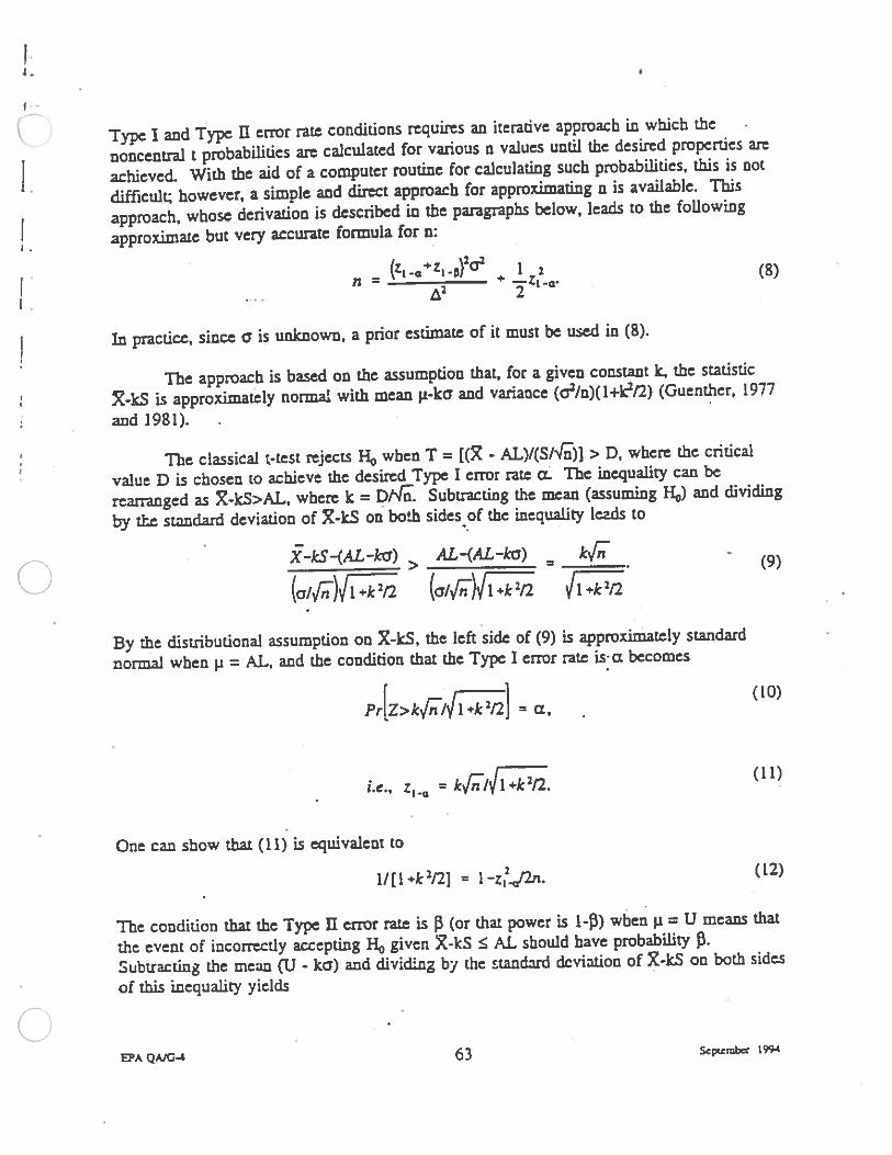
Type I and Type U error rate conditions requires an iterative approach in which the

noncentral t probabilities are calculated for various a values until the desired properties are

actüevei With the aid of a computer routine for calculating such probabilities, this is not

diffzcult however, a simple and direct approach for approximating a is available. This

approach, whose derivation is described in the paragraphs below, leads to the following

approximate but very accurate formula for a:

= (z1 ÷z, )2&

+ !Zi_a.(8)

A’ 2

In practice, since a is unknown, a prior estimate of it must be used in (8).

The approach is based on the assumption that, for a given constant t the statistic

X-kS is approximately normal with mean ji-ka and variance (&In)( 1+k’fl) (Guenther, 1977

and 1981).

The classidal c-test rejects H0 when T = [(X - AL)/(S/’&)] > 0, where the critical

value D is chosen to achieve the desired Type I error rate a.. The inequality can be

rearranged as X-kS>AL, where Ic = PHi Subtracting the an (assuming H0) and dividing

by the standard deviation of X-kS on both sides of the inequality leads to

X-kS-(AL-ka)> AL -(AL-ku) = kF- (9)

(aIFW1 +k2fl (a,i)ji k2n +k’’2

By the ±sthbutional assumption on X-ts, the left side of (9) is approximately standard

normal when p = AL, and the condition that the Type I error rate is-a becomes

pr[z>kF/11+k’nl = a,-

(ID)

i.e., Z10 = kJ/I1+kmfl. (11)

One can show that (11) is equivalent to

1f[1÷k1/21 = I—4J2n. (12)

The condition that the Type U error raze is (or that power is l-) when p = U means that

the event of incorrectly accepting H0 given X-kS AL should have probability .

Subtracting the mean (U - ka) and dividing by the standard dcviafion of X-kS on both sides

of this inequality yields

EPA QAJGA 63 Scpcemba 1994

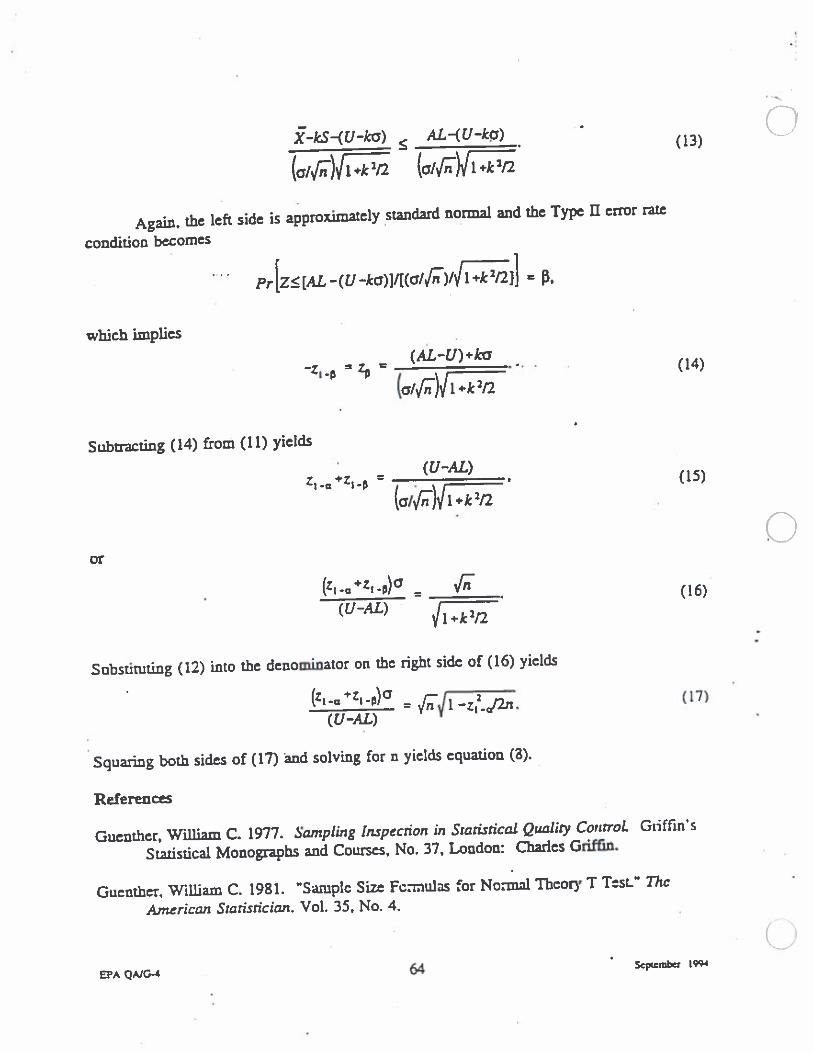
X-kSU-ka) ALU-kq) fl2 (aif,i/i 4272

Again, the left side is approximately standard normal and the Type II error raze

condition becomes

pr[zratL_w_ka)v[(alvc)41.k’,2;l

=

which implies

(AL-U)÷kaZ10 —Z5 =

______

.‘. . (14)

(a,FX/1+k272

Subtracting (14) from (11) yields

(U-AL)= -

________

‘ (15)

(a/6W1+kmn

or.

C)

__________

=

_________

(U-AL) i(1)

Substituting (12) into the denominator on the right side of (16) yields

__________

= Gv’i —z120/2n. (17)

Squaring both sides of (17) and solving for n yields equation (3).

References

Guenther, Wilibim C. 1977. Sampling Inspection in Statistical Quality ControL Griffin’s

Stmistical Monographs and Courses, No. 37, London: Charles Griffin.

Guenther, William C. 1981. “Samplc Size Fcnnulas for Nonnal Thcory T Test” Thc

American Statistician. Vol. 35, No. 4.

0EPA QAJG-4 64 Scptemba 1944

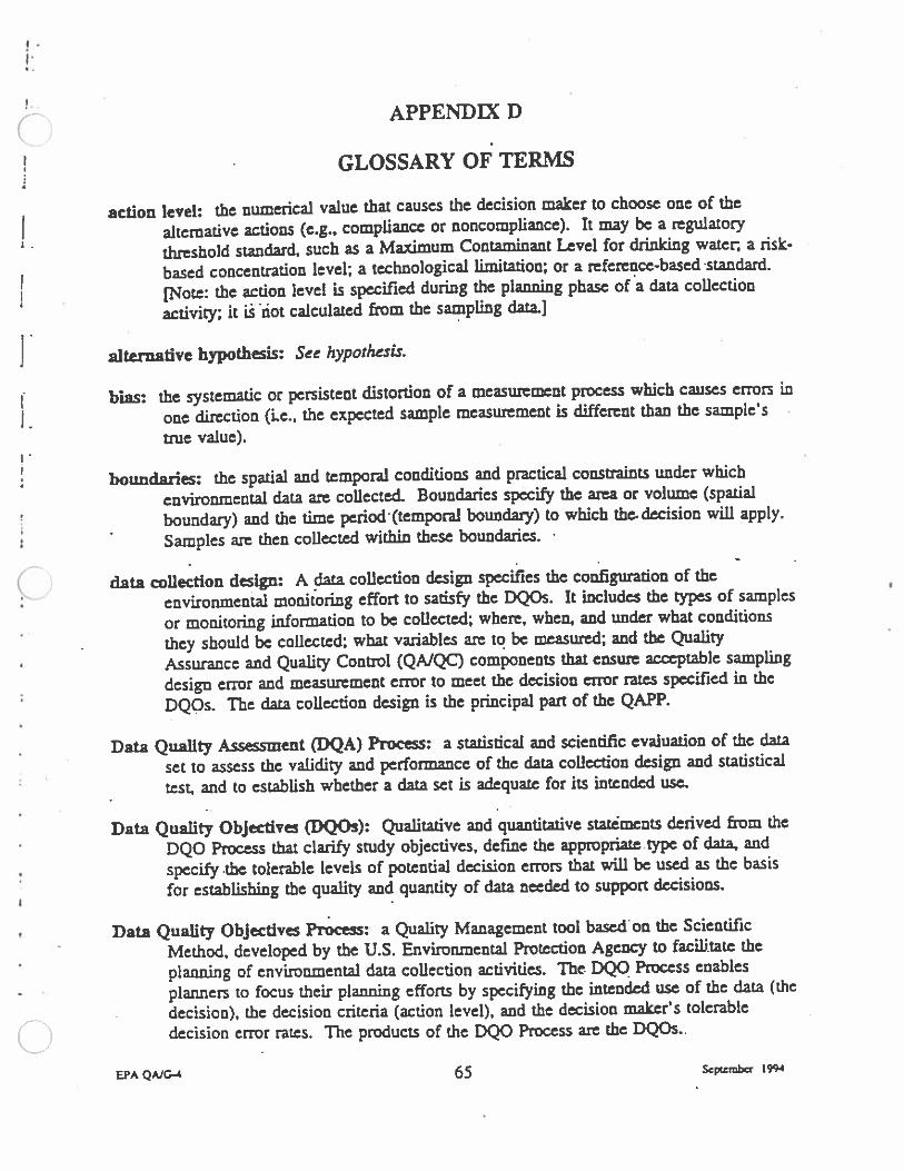
APPENDIX D

GLOSSARY OF TERMS

action level: the numerical value that causes the decision maker to choose one of the

alternative actions (e.g., compliance or noncompliance). It may be a regulatory

threshold standard, such as a Maximum Contaminant Level for drinking water a risk-

based concentration level; a technological limitation; or a reference-based standard.

fNote: the action level is specified during the planning phase of a data collection

activity; it is ñot calculated from the sampling data]

alternative hypothesis: See hypothesis.

bias: the systematic or persistent distortion of a measurement process which causes errors in

one direction (i.e., the expected sample measurement is different than the sample’s

ate value).

boundaries: the spatial and temporal conditions and practical constraints under which

environmental data are collected. Boundaries specify the area or volume (spatial

boundaiy) and the time petiot(temporai boundary) to which the decision will apply.

Samples art then collected within these boundaries.

data collection design: A data collection design specifies the conflgwation of the

environmental monitoring effort to satisfy the OQOs. It includes the types of samples

or monitoring information to be collected; where, when, and under what conditions

they should be collected; what variables are to be measured; and the Quality

Assurance and Quality Control (QNQC) components that ensure acceptable sampling

design error and measurement error to meet the decision error rates specified in the

DQQs. The data collection design is the principal pan of the QAPP.

Data Quality Assessment (DQA) Process: a statistical and scientific evaluation of the data

set to assess the validity and performance of the data collection design and statistical

test, and to establish whether a data set is adequate for its intended use.

Data Quality Objectives (DQOs): Qualitative and quantitative stmdmcnts derived from the

DQO Process that clarify study objectives, define the appropriate type of data, and

specify the tolerable levels of potential decision errors that will be used as the basis

for establishing the quality and quantity of data needed to support decisions.

Data Quality Objectives Proce: a Quality Management tool basedon the Scientific

Method, developed by the U.S. Environmental Protection Agency to facilitate the

planning of environmental data collection activities. The DQQ Process enables

planners to focus their planning efforts by specifying the intended use of the data (the

decision), the decision criteria (action level), and the decision maker’s tolerable

decision error rates. The products of the DQO Process are the DQOs..

EPA QNG-4 65 Scpwmba 1994

decision error: an error made when drawing an inference from data in. the context of Chypothesis testing, such that variability or bias in the data mislead the decision maker

to draw a conclusion that is inconsistent with the true or actual state of the population

under study. See also false negative decision error, fake positive decision error.

defensible: the ability to withstand any reasonable challenge related to the veracity, integrity,

or quality of the logical, technical, or scientific approach taken in a decision m2hing

process.

false negative decision error: a false negative decision error occurs when the decision

maker does not reject the null hypothesis when the null hypothesis actually is faise.

In statistical terminology, a false negative decision error is also called a Type U error.

The measure of the size of the error is expressed as a probability, usually referred to

as “beta (n)”; this probability is also called the complement of power.

false positive decision error: a false positive decision error occurs when a decision maker

rejects the null hypothesis when the null hypothesis actually is true. In statistical

terminology, a false positive decision error is also called a Type I error. The measure

of the size of the error is expressed as a probability, usually referred to as “alpha (a),”

the “level of significance,” or “size of the critical region.”

gray region: a range of values of the population parameter of interest (such as mean

contaminant concentration) where the consequences of riinking a decision error an

relatively minor. The gray region is bounded on one side by the action level.

hypothesis: a tentative assumption made to draw out and test its logical or empirical

consequences. In hypothesis testing, the hypothesis is labeled “null” or “alternative”,

depending on the decision maker’s concerns for makng a decision error.

limits on decision errors: the tolerable decision error probabilities established by the

decision maker. Potential economic, health, ecological, political, and social

consequences of decision errors should be considered when setting the limits.

mean: (1) a measure of central tendency of the population (population mean), or (ii) the

arithmetic avenge of a set of values (sample mean).

measurement erron the differee between the true or actual state and that which is

reported from measurements.

median: the middle value for an ordered set of n values; represented by the central value

when n is odd or by the average of the two most central values when n is even. The

median is the 50th percentile.

medium: a substance (e.g.. air, water, soil) which serves as a carrier of the analytes of

interest.

EPA QMG4 66 Scpcemba 1994

natural variability: the variability that is inherent or natural to the media, objects, or people

being studied.

null hypothesis: See hypothesis.

parameter a numerical descriptive measure of a population.

percentile: the specific value of a distribution that divides the distribution such that p

percent of the distribution is equal to or below that value. Example for p=95: “The

95th percentile is X” means that 95% of the values in the population (or statistical

sample) am less than or equal to X.

plnnning team: the group of people that will carry out the DQO Process. Members include

the decision maker (senior manager), representatives of other data users, senior

proam and technical staff, someone with statistical expcnise, and a QAJQC advisor

(such as a QA Manager).

population: the total collection of objects, media, or people to be studied and from which a

sample is to be drawn.

power function: the probability of rejecting thenull hypothesis CH_J over the range of

possible population parameter values. The power fraction is used to assess the

goodness of a hypothesis test or to compare two competing tests.

quality assurance (QA): an integrated system of management activities involving planning.

quality control, quality assessment, reporting, and quality improvement to ensure that a

product or service (e.g., environmental data) meets defined standards of quality with a

stated level of confidence.

Quality Assurance Project Plan (QAPP): a formal technical document containing the

detailed QA, QC and other technical procedures for assuring the quality of

environmental data prepared for each EPA environnntai data collection activity and

approved prior to collecting the data.

quality control (QC): the. overall system of technical activities that measures the attributes

and performance of a process, item, or service against defined standards to verify that

they meet the stated requirements established by the customer.

Quality Management Plan (QMP): a formal document describing the management policies.

objectives, principles, organizational authority, responsibilities, accountability, and

implementation protocols of an agency, organization, or laboratory for ensuring quality

in its products and utility to its users. in EPA, QMPs are submitted to the Quality

Assurance Management Staff (QAMS) for approval.

range: the numerical difference between the minimum and maximum of a set of values.

EPA OA/04 67 Scpwm 199’

‘sample: a single item or specimen from a larger whole or group, such as any single sample

of any medium (air, water, soil, etc.).

2sample: a set of individual samples (specimens or readings), drawn from a population,

whose properties are studied to gain information about the whole.

sampling: the process of obnining representative samples and/or measurements of a subset

of a population.

sampling design error: the error due to observing only a limited number of the total

possible values that make up the population being studied. It should be distinguished

from errors due to imperfect selection; bias in response; and errors of observation,

measurement, or recording, etc.

scientific method: the principles and processes regarded as necessary for scientific

investigation, including rules for concept or hypothesis formulation, conduct ofexperiments, and validation of hypotheses by analysis of observations.

standard deviation: the square root of the variance.

statistic: a function of the sample measurements; e.g., the sample mean or standarddeviation. (E)

statistical test: any statistical method that is used to determine which of several hypothesesare true.

total study error: the combination of sampling desi error and measurement error.

true: being in accord with the actual state of affairs.

Type I error: A Type I error occurs when a decision maker rejects the null hypothesis whenit is actually true. See false positive decision error.

Type II erron A Type il error occurs when the decision maker fails to reject the nullhypothesis when it is actually false. See false negative decision error.

variable: The attribute of the environment that is indeterminan’t

variance: a measure of Ci) the variability or dispersion in a population (population variance),or (ii) the sum of the squared deviations of the measurements about theft mean dividedby the degrees of freedom (sample variance).

fl’AQAJG4 68 $cvnnbc t994

Appendix A from EPA (1996b)Geostatistical Sampling and Evaluation Guidance for Soils

and Solid Media, Review Draft

RI PR FIL’IN IkSkN RI:’IsI 1 IISALMASThII WPDIiI.R

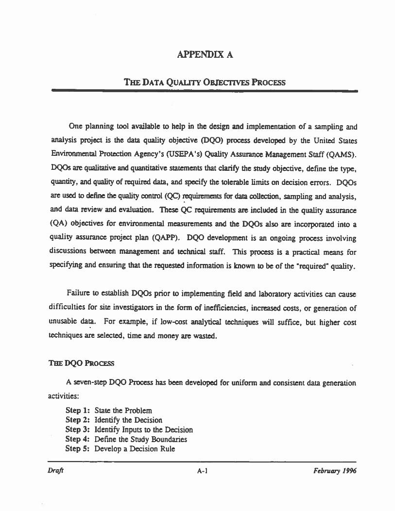
APPENDIX A

THE DATA Quarry Oawcrws PRocEss

One planning tool available to help in the design and implementation of a sampling and

analysis project is the data quality objective (DQO) process developed by the United States

Environmental Protection Agency’s (USEPA’s) Quality Assurance Management Staff (QAMS).

DQOs axe qualitative and quantitative statements that clarify the study objective, define the type,

quantity, and quality of required data, and specify the tolerable limits on decision errors. DQOs

are used to define the quality connvl (QC) requirements for data collection, sampling and analysis,

and data review and evaluation. These QC requirements an included in the quality assurance

(QA) objectives for environmental measurements and the DQOs also are incorporated into a

quality assurance project plan (QAPP). DQO development is an ongoing process involving

discussions between management and technical staff. This process is a practical means for

specifying and ensuring that the requested information is known to be of the required quality.

Failure to establish DQOs prior to implementing field and laboratory activities can cause

difficulties for site investigators in the form of inefficiencies, increased costs, or generation of

unusable data. For example, if low-cost analytical techniques will suffice, but higher cost

techniques are selected, time and money an wasted.

THE DQO PRoass

A seven-step DQO Process has been developed for uniform and consistent data generation

activities:

Step 1: State the ProblemStep 2: Identify the DecisionStep 3: Identify Inputs to the DecisionStep 4: Define the Study BoundariesStep 5: Develop a Decision Rule

Draft A-I February 19%

Geoswtis&& Soil Swnpling Guidance—4ppen&r A

Step 6: Specify Tolerable Limits on Decision Errors

Step 7: Optimize the Design for Obtaining Data.

The DQO process is based on the guidance document issued by QAMS as ‘fmal” in

September 1994. Guidance for the Data Quality Objectives Process (EPA QA/G4) provides

general guidance to organintions for developing data quality criteria and performance

specifications for decision making. Chapter One of the SW-846 Methods Manual also provides

additional guidance on the QA program in the Office of Solid Waste (OSW).

Step 1: Statethefroblem

Thefinstepinanydecision-makingprocessistodeflnethepmblemthathasresukedin the

inception of the study. A planning team is assembled and is tasked with developing the project-

specific DQOs. The planning team comprises personnel representing all phases of the project and

may include technical project managers, QMQC managers, data users, and decision makers. The

primary decision maker, or leader, must be identified. When applicable, field and lab

technicians, chemists, statisticians, and modelers also should be recruited for the planning team.

The responsibilities of each team member should be clearly defined during this initial planning (11)stage.

A concise description of the problem must be developed during this early stage of DQO

development. Existing information should be summarized, and the need for additional

information, should be determined. Performance of literature searches or an evaluation of

historical data or ongoing studies related to the current site can be studied.

Available financial and manpower resources must be identified and project milestones and

deadlines also should be determined, if sufficient information is present

Step 2: Identify the Decision

This step is used to define the decision statement that the study must resolve. The decision

statement is a consolidation of the principal study question and alternative actions. The principal

Draft A-2 . bFebnswy 1996

Geosiau&ai Soil Sonpling Guidance—Appcn&x 4

study question identifies the key unknown conditions or unresolved issues that will be used co

reveal the solution to the problem being investigated. Alternative actions, which are items that

may be taken to solve the problem based on the outcome or on the decisions arrived at from the

study, also are identified.

Step 3: Identify Inputs to the Decision

Specific information rufred to resolve the decision statement must be identified during this

step in the DQO development process. The selected data acquisition dpploach will lead to the next

set of questions that address the specific types of information needed to support the decision

statement. Sources of the necessary information an then developed and can include regulatory

guidance, scientific literature, historical data or past projects that were simiiar in scope to the

current effort.

A bright-line, defined as the threshold value that provides the criterion for choosing between

alternative actions, needs to be established.

Existing analytical methods are evaluated to determine if the method will perform as

published, or if method modification or method development needs to be included in the study.

Each analyte of interest should have a method detection limit or level of quantitation assigned, as

this performance information is used later in the DQO Process (Steps S & 7).

Step 4: Derme the Study Boundaries

Two types of boundaries must be defined and quantified: spatial and temporal. Spatial

boundaries define the physical area to be studied and locations to collect samples. Temporal

boundaries describe the timefmme that the study data will represent and when the samples should

be collected. To arrive at these boundaries, the characteristics that define the population must be

identified. For instance, the compounds of interest and the matrix that should be evaluated might

need to be selected to determine if the compounds an present and at what typical concentrations.

Draft A-3 . February 1996

Geon’’’d Soil Swnptthg Guidance—A ppen&.r A

The spatial boundaries, or the geographic area to be studied, must be specified using some

physical feature or border, such as units of measure. Where possible, the population should be

further segregated into more homogenous subsets, or strata, as a means of reducing variability. C)Step 5: Develop a Decision Rule

A statement must be developed that combines the parameters of interest and the action levels

with the DQO outputs already developed. The combination of these three elements forms the

decision nile and summarizes what attributes the decision maker wants to study and how the

information will assist in solving the central problem. The four elements that form the decision

rule include: (1) the parameter of interest that describes a characteristic of the statistical

population, (2) the scale of decision making defined in Step 4 when boundaries were defined,

(3) the bright-line (action level or a measurement threshold value), used as a criterion to choose

alternative actions through the use of 9f/then statements, and (4) identifying the alternative

actions, as developed in Step 2.

Step 6: Specify Timits on Decision Errors

Decision makers are interested in iowing the true state of some feature of the environment

(e.g., the concentration of the constituent of concern in soil). However, data generated from a

sampling and analysis program can only be used to estimate this state, and there is a chance that

the data aiein cmii and the correct decision win not be made. This step in the DQO development

process allows the decision makers to specify acceptable or tolerable limits on decision errors.

There are at least two primary reasons why the decision maker might not determine the true

value of a population parameter. First, sampling design error occurs when the sampling design

is unable to capture the complete extent of variability that exists in the true state of the

environment. Second, measurement error, which is a combination of random and systematic

errors, results from various steps in the measurement process including sample collection, sample

handling, sample preparation, sample analysis, data reduction, and data handling. The

combination of sampling design error and measurement error can be viewed as the total study

error and may lead to decision errors. C:)Draft A4 Febnswy IL°6

Geossaithcat Soil Sampling Guidance—,kppenthr A

To estimate the probability of decision errors, the anticipated range of results from the

parameters of interest usually must be determined, perhaps through the use of historical data.

Values between the obsexvai upper and lower bounds or perhaps from a distribution modeled after

the historical data can be used to estimate how likely are the various decision errors that might

occur depending on the hypothesis framework that has been constructed. The statistical

hypotheses associated with any decision criterion consist of a null hypothesis, supposed to

represent the initially assumed condition of the site, and the alternative hypothesis, representing

the condition of the the when the null hypothesis is not true. Often the null hypothesis indicates

the location of the center (in terms of concentration levels) of the hypothesized sampling

distribution, but it can describe other characteristics of the sire population (e.g., an upper

percentile). Both the null and alternative hypotheses make statements regarding a characteristic

of the population rather than a characteristic of a sample. The probability of a decision error is

determined by tctimañng the chance that one of the two hypotheses will be accepted when in fact

the opposite hypothesis is true.

To identii5t the decision enors and to consnct the hypothesis framework, performance of

four steps must be acaimplishal. (I) Both types of decision errors must be defined, determining

which occurs above the action level and which occurs below the action level. (2) Potential

consequences of each decision error must be specified and the impact of arriving at the incorrect

decision considered. The severity of the error may affect economic and social costs or have

ramifications to human health and the environment. One of the two types of errors (eg., above

or below the action level) often will have a greater impact than the other. (3) The decision maker

should evaluate which scenario results in more serious consequences. (4) The null hypothesis,

or baseline condition, should be defined and the decision as to what constitutes a false-positive or

false-negative result should be answered. The term false-positive is assigned to the decision error

where the decision maker rejects the null hypothesis when it is true. Conversely, a false-negative

is the resulting decision error if the null hypothesis is not rejected when it is false.

Some decision errors may be considered minor and of minimal impact to use of the data.

This grey region’ should be specified as a range of values having little or no adverse

Draft A-5 February 1996

Geonarictird Soil Swnpling Guidance—Appendix A

consequences to the project. Use of these grey area regions is often important as a tool for

building tolerable limits on the probability of making an incorrect decision.

CStep 7: Optimize the Design for Obtaining Data

The final step addresses the design of a resource-effective data collection system to satisfy

the DQOs. Verify that the DQO outputs produced in all preceding steps are internally consistent.

The design options should have been developed based on cost benefits, versus achieving DQOs.

General data collection designs can then be developed as either a fctoria] design, systematic

sampling, composite sampling, or one of the following random sampling designs: simple,

stratified, or sequential.

In general, three statistical expressions need to be selected to optimize the data collection

design. (1) An appropriate method for.testing the statistical hypothesis framework must be

chosen. (2) A statistical model used to compare measured values to the modeled values must be

developed and tested for consistency with the observed data. Once established, the model also can

be used to more thoroughly describe the components of error or bias that may exist in the

measured values. (3) Finally, a cost evaluation of number of samples venus the total cost of (E)sampling and analysis must be developed. Using these statistical expressions, an optimal sample

size and sampling layout can be chosen to meet the DQOs for each data collection design

alternative.

Quality Assurance Review

Usily, have the document peer reviewed, preferably by personnel experienced in statistical

data collection designs. Ensure that all aspects of the project have been documented to minimize

the numbers of assumptions made during performance of the project.

DQO DrnsIoN ERROR FEASIBHITY ThLus (DEFT) Sornv4utt

The two most intensive steps in the DQO Process am Step 6: Specify Tolerable Limits on

Decision Errors, and Step?: Optimize the Design for Obtaining Data. During Step 7, the entire

set of DQO outputs is incorporated into a sampling design. If the DQO constraints are not

A-6 February 1996

Georfnricrirat Soil Swnpling Guidance—Appendix A

feasible, it is necessary to iterate through one or mare of the earlier steps of the DQO Process to

identify a sampling design that will meet the budget and generate adequate data for the decision.

This iteration cast be time consuming and costly. EPA developed the DEFT User’s Guide and

software (USEPA 1994c) to streamline this iterative process. Users can change DQO constraints

such as limits on decision errors or the grey region and evaluate how these changes affect the

sample size for seven] basic sampling designs. The OUtpUt of the DEFT software can be used to

set upper and lower bounds on the sample size (i.e., the appropriate number of observations).

Through this pmcs, the planning team n evaluate whether these constraints are appropriate or

feasible before the sampling and analysis plan is developed.

Users of the DEFT software axe first prompted to enter information from the DQO outputs

based on a series of amy screens. Specific information requested by the DEFT software includes:

• Parameter of interest

• Minimum and maximum values (range) of the parameter of interest

• Action level (i.e., the bright-line)

• Null and alternative hypothesis

• Bounds of the gray region

• Estimate of the standard deviation

• Cost per sample for sample collection (i.e., field cost per sample)

• Cost per sample for sample analysis (i.e., laboratory cost per sample)

• Probability limits on decision errors for the bounds of the gray region

• Any additional limits on decision errors.

The DEFT software automatically starts with a simple random sampling design, so the

information requested corresponds to this design.

EXAMPLE APPLiCATION OF THE DEFT Sonw*iw

At a site contaminated with polynuclear aromatic hydrocarbons (PAH) compounds,

contaminated soil has been excavated and placed on a pad. Investigators are interested in

Draft A-i Februwy 19%

Geonminird Soil Swnptthg Guidance—Appen&r A

determining whether the mean concentration of benzo(a)pyrene (BAP) exceeds the bright-line

standard of 90 mgfKg. The investigators have decided to use the DEPT software during the DQO

Process to help optimize the study design. (2

Parameter of Interest

The panmetu of interest for this study is the population mean of the concentration of BAP.

Minimum and Maximum Values (Range) of the Parameter of Interest

Based on data gennted during a preliminary study of the contaminated soil, the minimum

concentration of RAP was 62 mg/Kg and the maximum was 120 mg/Kg.

Action Level

The action level, or bright-line, for RAP is 90 mg/Kg.

Null and Akemalive Hypothesis

H0: mean bright-line vs. H: mean < bright-line.

Bounds of the Gray Region

The gray region is bounded on one side by the bright-line (90 mg/Kg). For H0:

mean > bright-line vs. H,: mean < bright-line, DEPT sets a default value for the other bound

of the gray r€gion at the midpoint between the minimum concentration (62 mg/Kg) and the bright-

lint. In this example, the lower bound of the gray region is 76 mglKg.

Estimate of the Standard Deviation

If there is no estimate of the standard deviation available, DEPT calculates a default value

given by:

(Maximum Concentration - Minimum Concentration)/6

0Draft A-8 February 1996

Geonnilnied Soil Swnpling Guidance—,4ppenclix A

In this example, the estimate of the standard deviation is 9.7.

Cost Per Sample for Sample Collection

The cost of sample collection is approximately $67.00 per sample. This estimate is based

on the following assumptions:

• Two field sampling technicians are required.

• Samplers can collect, prepare, and ship 12 samples per 8-hour thy.

• labor raze is $50.00/hour (loaded’ rate).

Cost Per Sample for Sample Analysis

The cost per soil sample analysis for semi-volatile organic compounds, including BAP, is

approximately $480.00 per sample.

Probability Limits on Decision Errors for the Bounds of the Gray Region

For this example, the probability of making a ñlse positive ciiyf is set a a = .01, and the

probability of making a false negative error is set a P = .05.

After the above information is entered into the DEPT software, sampling design and DQO

summary information is provided. For this example, a simple random sampling design would

require ii samples at a total cost of $5,137.00 (see attached ‘Design/DQO Summary Screen’ and

“Decjsion Performance Goal Diagram Screen with the Performance Curve”).

Draft A-9 Febnswy 1996

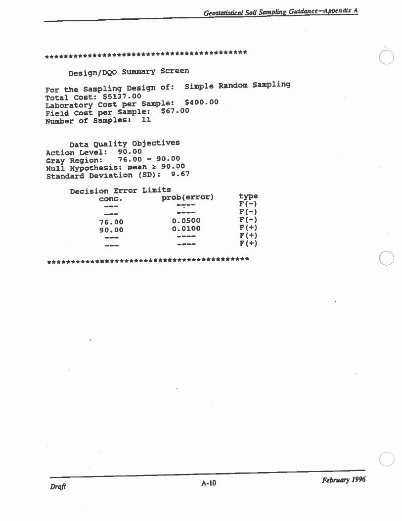
GeouiUis&al Sod Swnpling Guidance—A ppen&s A

Desiqn/DQO Summary ScreenC)

For the Sampling Design of: Simple Random Sampling

Total Cost: $5137.00

Laboratory Cost per Sample: $400.00

Field Cost per Sample: $67.00

Number of Samples: 11

Data Quality Objectives

Action Level: 90.00Gray Region: 76.00 — 90.00

Null Hypothesis: mean .90.00

Standard Deviation (SD): 9.67

Decision Error Limitsconc. prob(error) type

F(-)F (-)

76.00 0.0500 F(—)

90.00 0.0100 F(+)F(+)F(+)

* 0Draft A-10 Februwy 1996

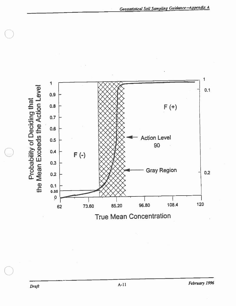
Geonnrinira! Soil Sampling GuWance—Appen&x A

15>a)-JC04-

C

a)-c0

Co0a)a)CxInCCDa)

a)-C4-

4-

CD-C4-

0C00a)00

4-

.0CD.00I.

0

F(+)

1

0.9

0.8

0.7

0.6

0.5

0.4

0.3

02

0.1O.D5

0

Action

I

0.1

02

Level90

Gray Region

62 73.60 85.20 96.80 108.4 120

True Mean Concentration

Draft A-il Febnsary 19%

Geostaösdcal Soil Sampling Guidance—Appen& A

RacvAwr Gumea ON DATA QuALnv OuJFrnns

USEPA. 1994a EPA Reqzdrnnemsfor Qualiiy Assurance Project Plansfor Environmental

Data Operations (lmehm Final). EPA QA/R-5. Quality Assurance Management Staff

(QAMS), Washington, DC.

Presents detailed specifications and instructions for the information that must be contained

in a QAPP for environmental darn operations performed by or on behalf of USEPA and the

procedures for its review and approval.

2. USEPA. 19941,. Gtddanceforthe Data Quality Objectives Process (Final). EPA QA/G4.

Quality Assurance Management Staff (QAMS), Washington, DC.

Offers general guidance on developing data quality criteria and performance specifications

for data operations. The document outlines the seven distinct steps of the DQO Process:

state the problem; identify the decision; identify inputs to the decision; define the decision

boundaries; develop a decision nile; specify limits on decision nile; and optimize the design

for obtaining data. Includes a detailed example and a glossary.

3. USEPA. 1 994e. Data Quality Objectives Decision Error Feasibility That (DQOIDEPT)

Version 4.0 Software and User’s Guide. EPA QA/G4D (Final). Quality Assurance

Management Staff (QAMS), Washington, DC.

The DEPT software uses the outputs from Steps 1 through 6 of the DQO Process to allow

a decision maker or member of the DQO planning team to quickly generate cost information

about several simple sampling designs based on the DQO constraints.

4. USEPA. 1996. Guidance for Data Quality Assannem (Rnd). EPA QAIG-9. Quality

Assurance Management Staff (QAMS), Washington, DC.

The purpose of this guidance is to demonstrate the use of EPAs data quality assessment

(DQA) process in evaluating environmental darn sets and to provide some graphical and

statistical tools that are useful in performing DQA.

0Draft A-12 . February 1996

ATTACHMENT D

DATA USEABILITY WORKSHEETS

HI ‘H H TASKI HFVISL2FCNAL MASTER lYlE) fiR

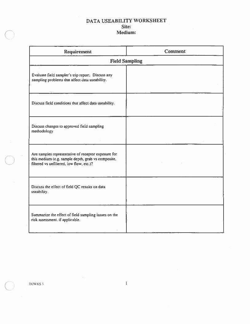
DATA USEABILITY WORKSHEETSite:

Medium:

Requirement I Comment

Field Sampling

Evaluate field sampler’s trip report. Discuss anysampling problems that affect data useability.

Discuss field conditions that affect data useability.

Discuss changes to approved field samplingmethodology

Are samples representative of receptor exposure forthis medium (e.g. sample depth, grab vs composite,filtered vs unfiltered, low flow, etc.)?

Discuss the effect of field QC results on datauseability.

Summarize the effect of field sampling issues on therisk assessment, if applicable.

DUWKS3 1

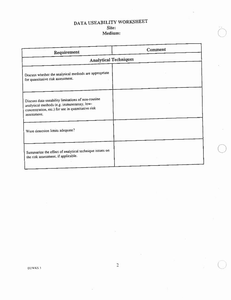
DATA USEABILITY WORKSHEET

Site:Medium: 0

Requirement I Comment

Analytical Techniques

Discuss whether the analytical methods are appropriate

for quantitative risk assessment.

Discuss data useability limitations of non-routine

analytical methods (e.g. immunoassay, low-

concentration, etc.) for use in quantitative risk

assessment.

Were detection limits adequate?

Summarize the effect of analytical technique issues on

the risk assessment, if applicable.0

DUWKS I

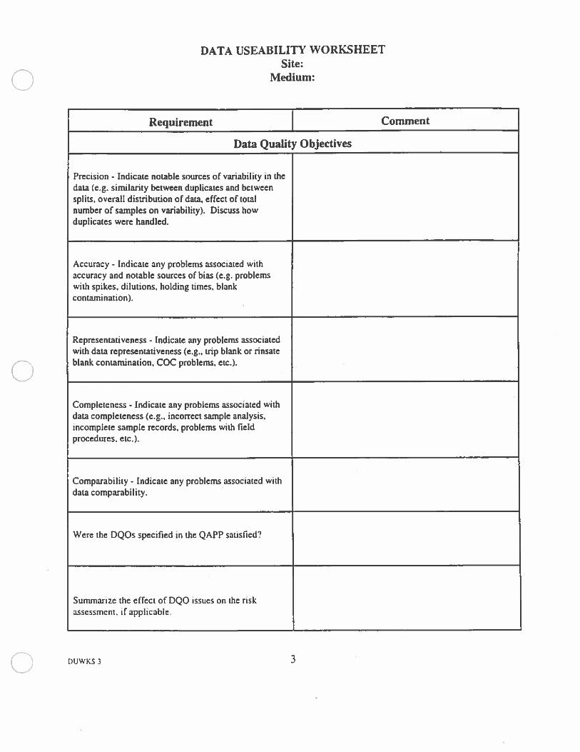
DATA USEABILITY WORKSHEETSite:

Medium:

Requirement I Comment

Data Quality Objectives

Precision - Indicate notable sources of variability in thedarn (e.g. similarity between duplicates and betweensplits, overall distribution of data, effect of totalnumber of samples on variability). Discuss howduplicates were handled.

Accuracy - Indicate any problems associated withaccuracy and notable sources of bias (e.g. problemswith spikes, dilutions, holding times, blankcontamination).

Representativeness - Indicate any problems associatedwith darn representativeness (e.g., trip blank or rinsateblank contamination, COC problems, etc.).

Completeness - Indicate any problems associated withdata completeness (e.g., incorrect sample analysis,incomplete sample records, problems with fieldprocedures. etc.).

Comparability - Indicate any problems associated withdata comparability.

Were the DQOs specified in the QAPP satisfied?

Summarize the effect of OQO issues on the riskassessment, if applicable.

DUWKS 3 3

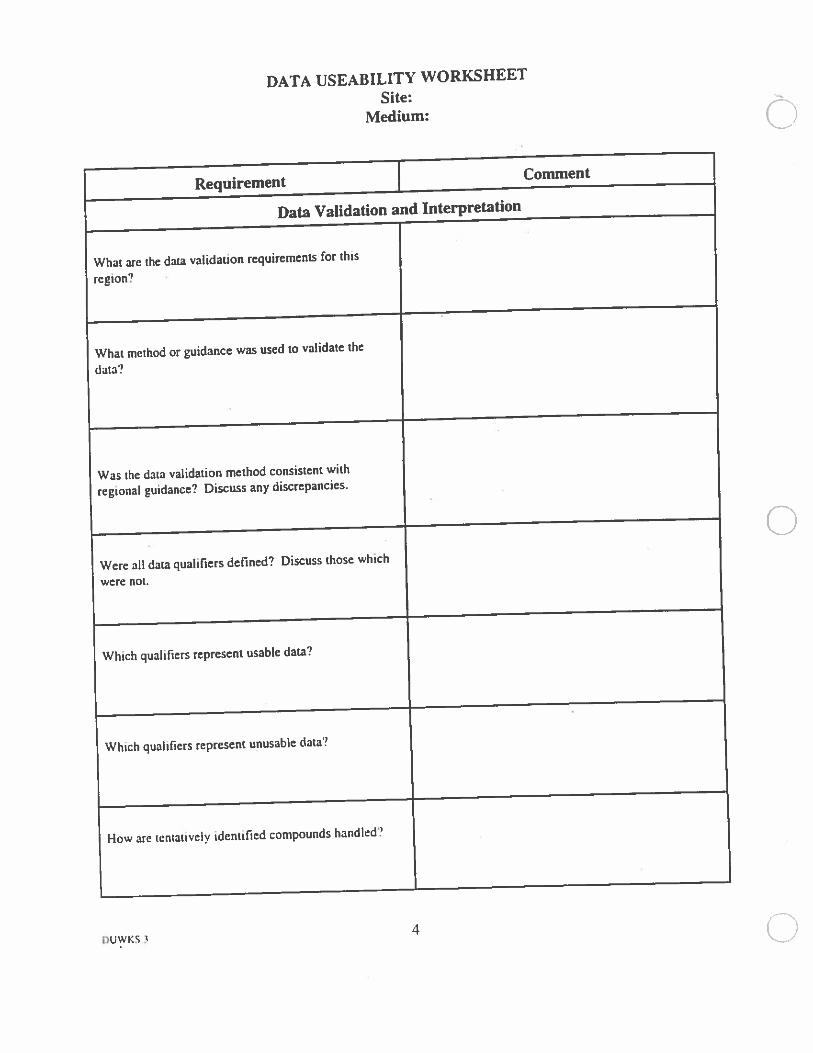
DUWKS 3

DATA USEABIUTY WORKSHEET

Site:Medium:

Requirement I Comment

Data Validation and Interpretation

What are the data validation requirements for this

region?

What method or guidance was used to validate the

data?

Was the data validation method consistent with

regional guidance? Discuss any discrepancies.

Were all darn qualifiers defined? Discuss those which

were not.

Which qualifiers represent usable darn?

Which qualifiers represent unusable data?

How are tentatively identified compounds handled?

0

4

DATA USEABILITY WORKSHEETSite:

Medium:

Requirement Comment

Summarize the effect of data validation andinterpretation issues on the risk assessment, ifapplicable.

Additional notes:

Note. The purpose of this Worksheet is to succinctly summarize the data useability anaiysis and conclusions. Referencespecific pages in the Risk Assessment text to hinher expand on the information presented here.

DUWK.S 3 5

A1TACHMENT E

U.S. ENVTRONMENTAL PROTECTION AGENCY REGION 9PRELIMINARY REMEDIATION GOALS

RLIAR TASkWREVISE1.FINALMASttR WPO 5 SR I!.PIOfl ljf24fl7? lSpms.

AflACHMENT F

U.S. ENVIRONMENTAL PROTECTEON AGENCY REGION 8SUPEREUND TECHNICAL GUTBANCE NUMBER RA-03

EVALUATING AND IDENTIFYING CONTAMINANTS OF CONCERNFOR HUMAN HEALTH

PUPA P1 A TASk4 REVSU p:SAL MASTER WV9 I :5 1 IwI•.SIS4l’-fl

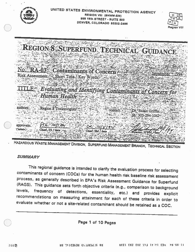
UNiTED STATES ENVIRONMENTAL PROTECTION AGENCYr 1C. REGION VIII (8HWM-SM) .,

______

999 15th STREET - SUITE SOD“%,,.‘ DENVER, COLORADO 80202-2486

Regon VIII

7.. ;:. c

No:Risk,Msessmäñt,

TflLk’

——.-.- — .—- 2. :.-‘

authors - -

.! - Gnffi )--/ -- — 303-294-1062’-

- — - _

:—‘-..,iJ .u.......r.a...:c -—tt’-_-

—:b-.• -.e.t.%f ;........:I

approvals fr1c /cØftz - C’ aô)ç/qcf “9

________

1,

flmbSIS) — CEwL,TS rare - k;’ bf, SM date - — .! ,, ‘:1; :.. .4.-. +r •--$.-‘r’—..

- ;‘:-I -z JJ—

HAZARDOUS WASTE MANAGEMENT DivisioN, SUPERFUNO MMtRGEMEI.r BRANCH, TECHNIC.t SECTION

SUMMARY-

This regional guidance is intended to clarify the evaluation process for selectingcontaminants of concern (COCs) for the human health risk baseline risk assessmentprocess, as generally described in EPA’s Risk Assessment Guidance for Superfund(RAGS). This guidance sets forth objective criteria (e.g., comparison to backgroundlevels, frequency of detections, essentiality, etc.) and provides explicitrecommendations on measuring attainment for each of these criteria in order toevaluate whether or not a site-related contaminant should be retained as a CCC.

Page 1 of 10 Pages

9Ct £8 CCC X TV 03w tb’60LIoo B9 ]V103h3)I oxiS13d.1S SB

BACKGROUND

For certain sites, the list of potentially

site-related contaminants and exposure

pathways may be lengthy. Carrying a

large number of contaminants through a

quantitative risk assessment may be

complex, and may consume significant

amounts of time and resources. In these

cases, a selection process should be used

to further reduce the number of

contaminants of potential concern for each

medium to a reasonable and relevant

amount EPAs Risk Assessment Guidance

for Superfund (RAGS): Pan A (EPA,

1 989a) describes general qualitative

criteria which should be considered when

evaluating contaminants for either

elimination or retention as contaminants of

EPA’s RAGS: Part A (EPA 1989a)

recommends that the following criteria be

evaluated when determinin9 which

chemicals on the Initial list of all potentially

site-related contaminants should be

retained or eliminated as COCs for the

Baseline RIsk Assessment:

1. Essential Nutrients

2. Exceedance of

concentrations

3. Detection frequency

4. MobIlity, persistence,

bloaccumulation

5. Exceedance of ARARs

6. Historical Evidence

7. Concentration and ToxicIty

Page 2 of 10 Pages

C,

EVALUATING AND IDENTIFYING CONTAMINANTS OF CONCERNFOR HUMAN HEALTH

U.S. EPAt_pn_ —r—

OBJECTIVE

The objective of this Regional

Guidance is to outline and describe a

selection process whereby preliminary lists

of potentially site-related contaminants can

be evaluated for elimination or r?tention as

contaminants of concern (COCs) for the

human health baseline risk assessment.

COPS IRA-O3l.ew.S 3li

concern (COCs) for the baseline risk

assessment. The purpose of this Regional

Guidance is to present those criteria in a

selection process which can be applied on

a generic basis to USEPA Superfund sites

in Region 8. This Regional Guidance will

also present detailed examples of how

several criteria presented In the upcoming

flow chart can be quantitatively evaluated.

DISCUSSION

(

C

background

and

lifi 1Y1G3K32 G\JJH3d]S Sd SCZT C6Z Cot VI 9t:tl U3s t6’60/Li

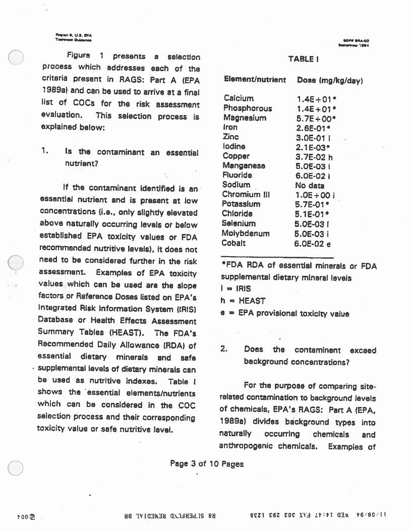
S.e’.,. P. U.S. EPAt.n... au.....

Figure 1 presents a selectionprocess which addresses each of thecriteria present in RAGS: Pan A (EPA1 989a) and can be used to arrive at a finallist of COCs for the risk assessmentevaluation. This selection process isexplained below:

1. Is the contaminant an essentialnutrient?

If the contaminant identified is anessential nutrient and is present at lowconcentrations (i.e., only slightly elevatedabove naturally occurring levels or belowestablished EPA toxicity values or FDArecommended nutritive levels), it does not

Q need to be considered further In the riskassessment. Examples of EPA toxicityvalues which can be used are the slopefactors or Reference Doses listed on EPA’sintegrated Risk information System (IRIS)Database or Health Effects AssessmentSummary Tables (HEAST). The FDA’sRecommended Daily Allowance (RDA) ofessential dietary minerals and safesupplemental levels of dietary minerals canbe used as nutritive indexes. Table Ishows the essential elements/nutrientswhich can be considered in the CCCselection process and their correspondingtoxicity value or safe nutritive level.

‘FDA RDA of essential minerals or FDAsupplemental dietary mineral levelsI = IRIS

h= HEASTEPA provisional toxicIty value

2. Does the contaminant exceedbackground concentrations?

For the purpose of comparing site-related contamination to background levelsof chemicals, EPA’s RAGS: Pan A (EPA,1989a) divides background types intonaturally occurrIng chemicals andanthropogenic chemicals. Examples of

Page 3 of 10 Pages

nnc31i,.ae III’

TABLE I

Element/nutrient Dose (mg/kg/day)

CalciumPhosphorousMagnesiumIronZincIodineCopperManganeseFluorideSodiumChromium IIIPotassiumChlorideSeleniumMolybdenumCobalt

1.4€ + 01’1.4E+015.7E+00’2.6E-01’3.OE-O1 I2.1E-03’3.7E-02 h5.OE-03 I6.OE-02 INo data1.OE+00 i5.7E-01’5.1E-O1’5.OE-O3 I5.OE-03 i6.OE-02 a

too 8 1VIU3R3N a’asaadJs g V3 Lv:vT Q3.ii V6/60’IL

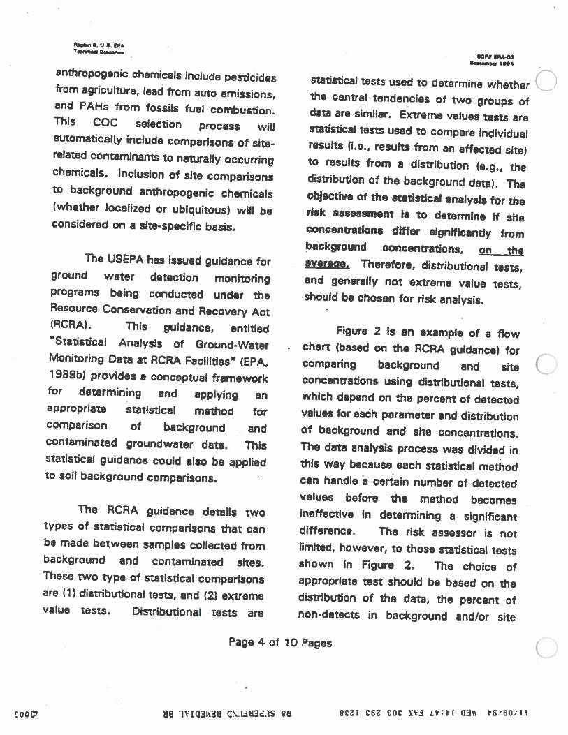
I. U.S. (PAT..n,.a G.an. -

anthropogenic chemicals include pesticidesfrom agriculture, lead from auto emissions,and PANs from fossils fuel combustion.This COC selection process willautomatically include comparisons of site-related contaminants to naturally occurringchemicals. Inclusion of site comparisonsto background anthropogenic chemicals(whether localized or ubiquitous) wilt beconsidered on a site-specific basis.

The USEPA has issued guidance forground water detection monitoringprograms being conducted under theResource Conservation and Recovery Act(RCRA). This guidance, entitled“Statistical Analysis of Ground-WaterMonitoring Data at RCRA Facilities” (EPA,1 989b) provides a conceptual frameworkfor determining and applying anappropriate statistical method forcomparison of background andcontaminated groundwater data. Thisstatistical guidance could also be appliedto soil background comparisons.

The RCRA guidance details twotypes of statistical comparisons that canbe made between samples collected frombackground and contaminated sites.These two type of statistical comparisonsare (1) distributional tests, and (2) extremevalue tests. Distributional tests are

fl n.aai_1_.,_ in’

statistical tests used to determine whetherthe cent-al tendencies of two groups ofdata are similar. Extreme values tests arestatistical tests used to compare individualresults (I.e., results from an affected site)to results from a distribution (e.g., thedistribution of the background data). Theobjective of the statistical analysis for therisk assessment is to determine If sheconcentrations differ significantly frombackground concentrations, on theaverage. Therefore, distributional tests,and generally not extreme value tests,should be chosen for risk analysis.

Figure 2 is an example of a flowchart (based on the RCRA guidance) forcomparing background and siteconcentrations using distributional tests,which depend on the percent of detectedvalues for eadh parameter and distributIonof background and site concentrations.The data analysis process was divided inthis way because each statistical methodcan handle a certain number of detectedvalues before the method becomesineffective In determining a significantdifference. The rl5k assessor is notlimited, however, to those statistical testsshown In Figure 2. The choice ofappropriate test should be based on thedistribution of the data, the percent ofnon-detects in background andlor site

Page 4 of 10 Pages 0

0

oc NH 1V103h38 Q\13a3d35 SM SEtI C6Z COC Xii Lv:VE 0344 ti/Ba/It

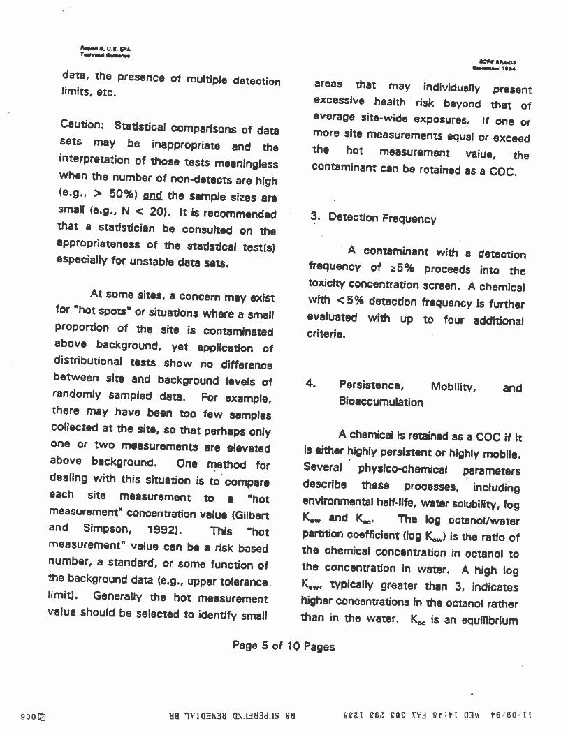
Rma. a. Its. EPA

data, the presence of multiple detectionlimits, etc.

Caution: Statistical comparisons of datasets may be inappropriate and theinterpretation of those tests meaninglesswhen the number of non-detects are high(e.g., > 50%) the sample sizes aresmall (e.g., N < 20). It is recommendedthat a statistician be consulted on theappropriateness of the statistical test(s)especially for unstable data sets.

At some sites, a concern may existfor “hot spots” or situations where a smallproportion of the site is contaminatedabove background, yet application ofdistributional tests show no differencebetween site and background levels ofrandomly sampled data. For example,there may have been too few samplescollected at the site, so that perhaps onlyone or two measurements are elevatedabove background. One method fordealing with this situation is to compareeach sits measurement to a “hotmeasurement” concentration value (Gilbertand Simpson, 1992). This “hotmeasurement” value can be a risk basednumber, a standard, or some function oftie background data (e.g., upper tolerancelimit). Generally the hot measurementvalue should be selected to identify small

_ SR-o3I__as. I •14

areas that may individuetly presentexcessive health risk beyond that ofaverage site-wide exposures. If one ormore site measurements equal or exceedthe hot measurement value, thecontaminant can be retained as a CCC.

3. Detection Frequency

A contaminant with a detectionfrequency of 5% proceeds into thetoxicity concentration screen. A chemicalwith <5% detection frequency Is furtherevaluated with up to four additionalcriteria.

4. Persistence, Mobility,Bicaccumulatlon

A chemical Is retained as a COC if ItIs either highly persistent or highly mobile.Several physlco-chemical parametersdescribe these processes, includingenvironmental half-life, water solubility, logK0 and lç. The log octanol/waterpartition coefficient (log K) Is the ratio ofthe chemical concentration in octanol tothe concentration In water. A high logK0, typically greater than 3, indicateshigher concentrations in the octanot ratherthan in the water. K is an equilibrium

Page S of 10 Pages

and

SOD MR iviU3h3U cSlAd3diS i 8Cr! C6Z LOt Yi 8ttt clan t6’6O’

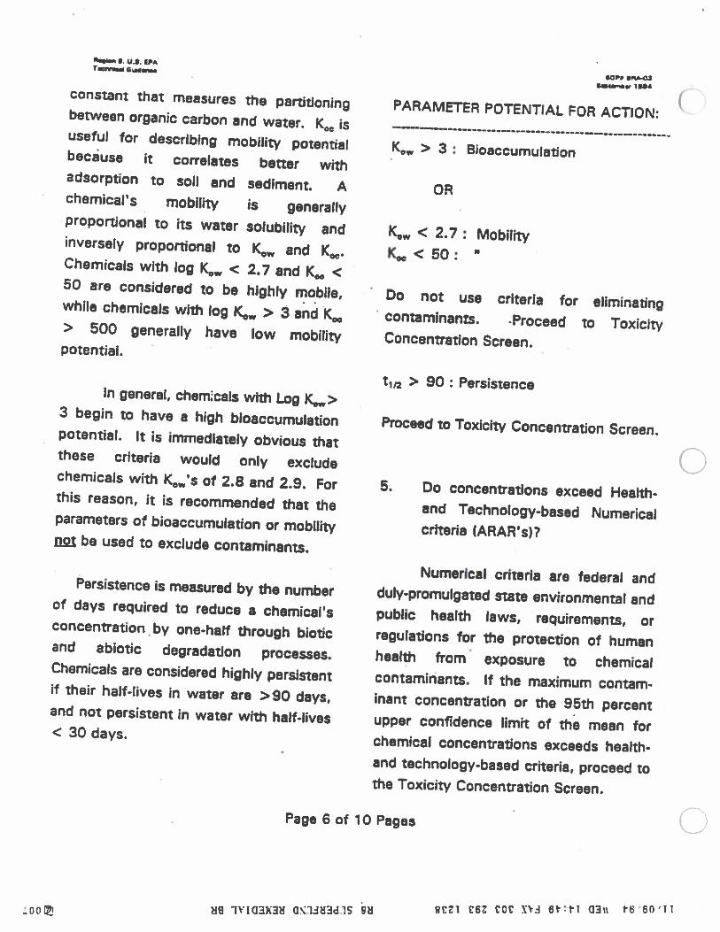
U.S. EPAT.ctn. Gums’s.

constant that measures the partitioningbetween organic carbon and water. K00 isuseful for describing mobility potentialbecuse it correlates better withadsorption to soil and sediment. Achemical’s mobility is generallyproportional to its water solubility andinversely proportional to c and K00.Chemicals with log K0,., < 2.7 and KM <50 are considered to be highly mobile,while chemicals with log iç, > 3 and iç> 500 generally have low mobilitypotential.

In general, chemcals with Log K,,,>3 begin to have a high bloaccumulationpotential. it is immediately obvious thatthese criteria would only excludechemicals with K0’s of 2.8 and 2.9. Forthis reason, ft is recommended that theparameters of bioaccumuiation or mobilitynx be used to exclude contaminants.

Persistence is measured by the numberof days required to reduce a chemical’sconcentration by one-half through bioticand abiotic degradation processes.Chemicals are considered highly persistentif their half-lives in water are >90 days,and not persistent in water with half-lives< 30 days.

criteria for eliminating.Proceed to Toxicity

ti,, > 90 : Persistence

Proceed to Toxicity Concentration Screen.

5. Do concentrations exceed Health-and Technology-based Numericalcriteria (ARAR’s)?

Numerical criteria are federal andduly-promulgated state environmental andpublic health laws, requirements, orregulations for the protection of humanhealth from’ exposure to chemicalcontamihants. If the maximum contaminant concentration or the 95th percentupper confidence limit of the mean forchemical concentrations exceeds health-and technology-based criteria, proceed tothe Toxicity Concentration Screen.

0

Page 6 of 10 Pages

tI C6Z UCE fli 6ttT G3% t5’sO’tT

son ta-Gaseem 15)4

PARAMETER POTENTIAL FOR ACTION:

K0,,. > 3: Bloaccumulation

OR

K0,,. < 2.7: MobilityK0<50:.

Do not usecontamInants.Concentration Screen.

0

LOD WB 1V1G3W3M GS1j3J1S 9)1

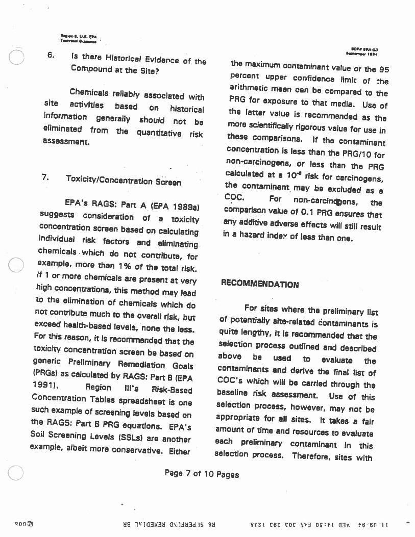
M_... U.S. PAt_..__ a___

6. is there Historical Evidence of theCompound at the Site?

Chemicals reliably associated withsite activities based on historicalinformation generally should not beeliminated from the quantitative riskassessment.

7. Toxicity/Concentration Screen

EPA’s RAGS: Pan A (EPA 1989a)suggests consideration of a toxicityconcentration screen based on calculatingindividual risk factors and eliminatingchemicals which do not contribute, for

C example, more than 1 % of the total risk.if 1 or more chemicals are present at veryhigh concentrations, this method may leadto the elimination of chemicals which donot contribute much to the overall risk, butexceed health-based levels, none the less.For this reason, ft is recommended that thetoxicity concentration screen be based ongeneric Preliminary Remediation Goals(PRGs) as calculated by RAGS: Pan B (EPA1991). Region ll!s Risk-BasedConcentration Tables spreadsheet is onesuch example of screening levels based onthe RAGS: Pan B PRG equations. EPA’sSoil Screening Levels (SSLs) are anotherexample, albeit more conservative. Either

top. IRA.Ola__ac ‘a

the maximum contaminant value or the 95percent upper confidence limit of thearithmetic mean can be compared to thePRG for exposure to that media. Use ofthe latter value is recommended as themore scientifically rigorous value for use inthese comparisons. If the contaminantconcentration Is less than the PRG/10 fornon-carcinogens, or less than the PRGcalculated at e 1 o risk for carcinogens,the contaminant may be excluded as aCOC. For non-carcintens, thecomparison value of 0.1 PAG ensures thatany additive adverse effects will still resultin a hazard index of less than one.

RECOMMENDATION

For sites where the preliminary listof potentially site-related dontaminants isquite lengthy, ft is recommended that theselection process outlined and describedabove be used to evaluate thecontaminants and derive the final list ofCOC’s which will be carried through thebaseline risk assessment. Use of thisselection process, however, may not beappropriate for all sites. It takes a fairamount of time and resources to evaluateeach preliminary contaminant In thisselection process. Therefore, sites with

Page 7 of 10 Pages

rt £6t you X’3 oc:t1 03’\ t6S’ 1!qQo g ]YTG3I(3 uS.U13d.1S M

%e,S. U.S. PA1na Qaad—...

smaller lists of preliminary contaminantsmay find it easier to Just to carry all of theidentified contaminants through thequantitative risk assessment evaluation.

REFERENCES

1. Gilbert, R.O. and Simpson, J.S. (1992).Statistical Methods for Evaluating theAttainment of Cleanup Standards, Volume3: Reference-Based Standards for Soilsand Solid Media, PNL-7409 Vol. 3, Rev. 1,Pacific Northwest Laboratory, Richland,Washington.

2. U.S. Environmental Protection Agency(EPA). 1989a. Risk Assessment Guidancefor Superfund, Volume 1: Human HealthEvaluation Manual. Office of Emergencyand Remedial Response. EPA/540/1-89/002.

3. U.S. Environmental Protection Agency(EPA). 1989b. Statistical Analysis ofGroundwater Monitoring Data at RCRAFacilities, Interim Final Guidance. Office ofSolid Waste, Waste Management Division.EPA/530-SW-89-026, April 1989.

4. U.S. Environmental Protection Adency(EPA). 1991. Risk Assessment Guidancefor Superfund, Human Health Evaluation

Manual, Part B: “Development of Risk-based Preliminary Remediation Goals”.Office of Emergency and RemedialResponse. OSWER Directive 9285.7-01 B.

Sc Pt SG3law’*e 15)8

C

UPage 8 of 10 Pages

gEti £6Z LOt XYi I2tL Q3i\ V6’60 ‘TI600 MU ]Y1G3K3U os.uaaa.Th SM

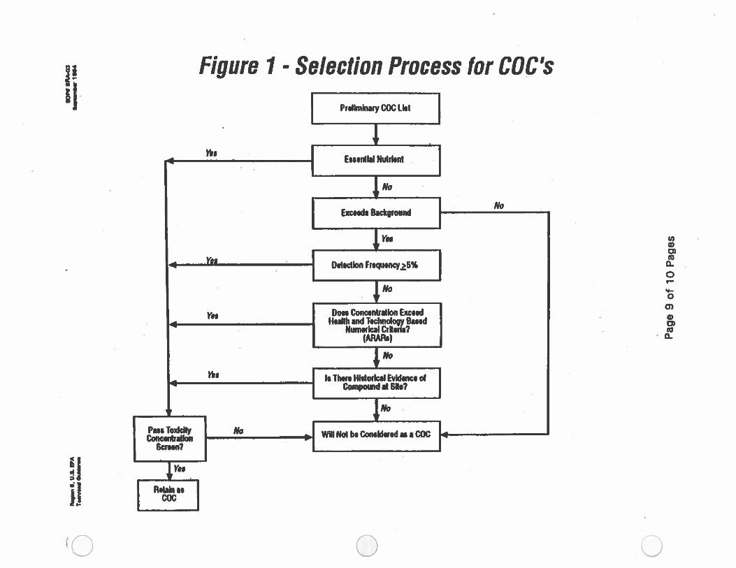
.aL

US

WA

•n

eaA

.

Tfl.i

Gb—

a.4

—1

fl4 baA I Ca

CD CD CD n n

Pag

e9

of10

Pag

es

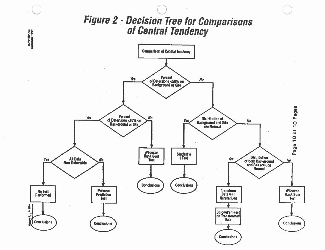
s068d01.

J.O01.

o8e

-I

C’)

C’)

I‘a-mt

I

S

a

pat-r-s

co.n.aim

ATTACHMENT C

U.S. ENVIRONMENTAL PROTECTJON AGENCYLAND USE MEMORANDUM

EP rAsk’RE:sa EI.%LMASThR APD .‘I.’.4fl1 2l!pmst

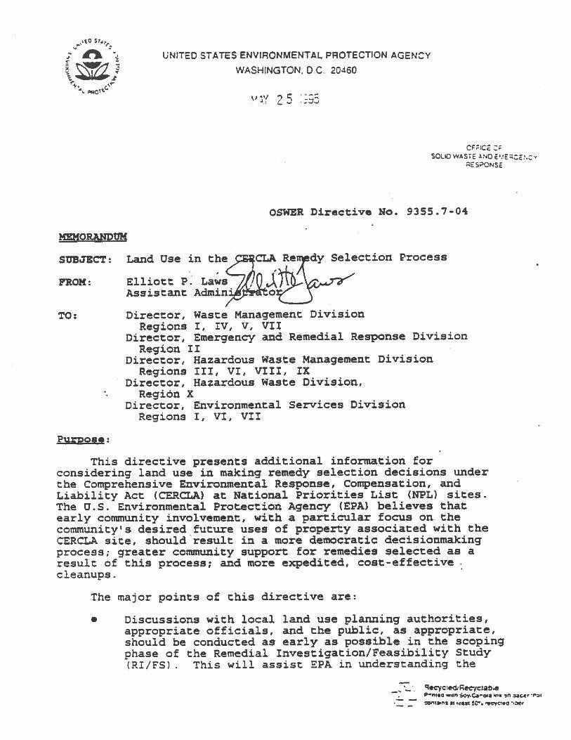
_tc 5T,,_

fl - UNITED STATES ENVIRONMENTAL PROTECTION AGENCY

_____

WASHINGTON, DC. 20460

4’ qtC

25 ::-;5

CFEtESOLID WASTE AND E.’E:E.c

ESONS2

OSWER Directive No. 9355.7-04

(ORA?WUM

SUBJECT: Land Use in the,,cSCIaA Re dy Selection Process

flOM: Elliott P Laws’740J,.Ass is taut Admin,dto

TO: Director, Waste Management DivisionRegions I, IV, V, VII

Director, Emergency and Remedial Response DivisionRegion II

Director, Hazardous Waste Management DivisionRegions III, VI, VIII, IX

Director, Hazardous Waste Division,Regiba X

Director, Environmental Services DivisionRegions I, VI, VII

Purpose:

This directive presents additional information forconsidering land use in making remedy selection decisions underthe Comprehensive Environmental Response, Compensation, andLiability Act (CERcLA) at National Priorities List (NFL) sites.The U.S. Environmental Protection Agency (EPA) believes thatearly conununity involvement, with a particular focus on thecommunity’s desired future uses of property associated with theCERCLA site, should result in a more democratic decisionmakingprocess; greater coimnunity support for remedies selected as aresult of this process; and more expedited, cost-effectivecleanups.

The major points of this directive are:

• Discussions with local laud use planning authorities,appropriate officials, and the public, as appropriate,should be conducted as early as possible in the scopingphase of the Remedial Investigation/Feasibility Study(RI/FS) . This will assist EPA in understanding the

91cyc’ediRecjclab,a— Pn,. win oyCa’o’. Ifl fl macI, rI

—— ,u,.n. at Inst 5 C’% .Cyc’.a ,ae.

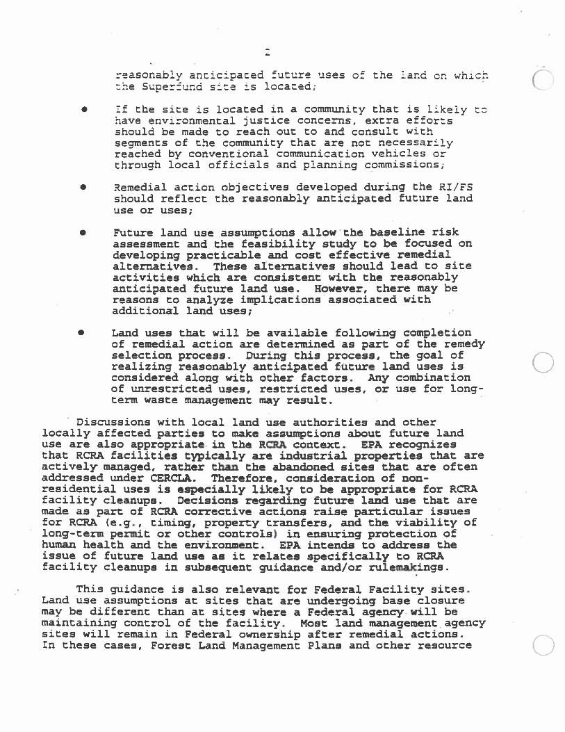
reasonably anticipated future uses of the land on whchthe Superfund site is iccaced;

• If the site is located in a community that is likely tohave environmental justice concerns, extra effortsshould be made to reach out to and consult withsegments of the community that are not necessarilyreached by conventional communication vehicles orthrough local officials and planning commissions;

• Remedial action objectives developed during the RI/FSshould reflect the reasonably anticipated future landuse or uses;

• Future land use assumptions allow’ the baseline riskassessment and the feasibility study to be focused ondeveloping practicable and cost effective remedialalternatives. These alternatives should lead to siteactivities which are consistent with the reasonablyanticipated future land use. However, there may bereasons to analyze implications associated withadditional land uses;

• Land uses that will be available following completionof remedial action are determined as pan of the remedyselection process. During this process, the goal ofrealizing reasonably anticipated future land uses isconsidered along with other factors. Any combinationof unrestricted uses, restricted uses, or use for long-tern waste management may result.

Discussions with local land use authorities and otherlocally affected panics to make assumptions about future landuse are also appropriate, in the RCRA context.. EPA recognizesthat RCRA facilities typically are industrial properties that areactively managed, rather than the abandoned sites that are oftenaddressed under CERa.A. Therefore, consideration of nonresidential uses is especially likely to be anpropriate for RRAfacility cleanups. Decisions regarding future land use that aremade as part of RCRA corrective actions raise particular issuesfor RCRA (e.g., timing, property transfers, and the viability oflong-ten permit or other controls) in ensuring protection ofhuman health and the environment. EPA intends to address theissue of future land use as it relates specifically to RRAfacility cleanups in subsequent guidance and/or rulemakings.

This guidance is also relevant for Federal Facility sites.Land use assumptions at sites that are undergoing base closuremay be different than at sites where a Federal agency will bemaintaining control of the facility. Most land management, agencysites will remain in Federal ownership after remedial actions.In these cases, Forest Land Management Plans and other resource (3

anacernent guidelines may helD develop reasonable assumticnsabout future uses of the land. At all such sites, however, chsdocument1 can focus the land use consideration toward apropriaceoptions.

Background:

Reasonably anticipated future use of the land at ?4PL sitesis an important consideration in determining the appropriateextent of remediation. Future use of the land will affect thecyoes of exposures and the frequency of exposures that may occurto any residual contamination remaining on the site, which inturn affects the nature of the remedy chosen. On the other hand,

the alternatives selected through the National Oil and HazardousSubstance Contingency Plan (NCP) (55 Fed. Reg. 8666, March 8,19901 process for CERCLA remedy selection determine the extent towhich hazardous constituents remain at the site, and thereforeaffect subsequent available land and ground water uses.

The NCP preamble specifically discusses. land use assumptionsregarding the baseline risk assessment. The baseline riskassessment provides the basis for. taking a remedialaction at aSuperfund site and supports the development of remedial actionobjectives. Land use assumptions affect the exposure pathwaysthat are evaluated in the baseline risk assessment. Current landuse is critical in determining whether there is a current riskassociated with a Superfund site, and future land use isimportant in estimating potential future threats. The results ofthe risk assessment aid in determining the degree of remediationnecessary to ensure long-term protection at NPL sites.

EPA has been criticized for too often assuming that futureuse will be residential. 1n many cases, residential use is theleast restricted land use and where human activities areassociated with the greatest potential for exposures. Thisdirective is intended to facilitate future remedial decisions atNfl sites by outlining a public process and sources ofinformation which should be considered in developing reasonableassumptions regarding future land use.

This directive expands on discussions provided in thepreamble to the National Oil and Hazardous Substance ContingencyPlan (NCP); “Risk Assessment Guidance for Superfund Vol. I, HumanHealth Evaluation Manual” (Pan A) CEPA/540/1-89/002, Dec. 1989);“Guidance for Conducting Remedial Investigations and FeasibilityStudies Under cERaSA” (OSNER Directive 9355.3-01, Oct. 1988); and

1Federal agency responsibility under cERItA 120(h) (3),

which relates to additional clean up which may be required toallow for unrestricted use of the property, is not addressed inthis guidance.

“Role the Baseline Risk Assessment in Superfund Remedy (Selection Decisor.s” (QSWER Directive 9355.0-30, April 22, 1991)

This land use directive may have the most relevance insituations where surface soil is the primazy exwosure pathway.Generally, where soil contamination is impacting ground water,protection of the ground water may drive soil cleanup levels.Consideration of future ground water use for CERCLA sites is notaddressed in this document. There are separate expectationsestablished for ground water in the NC? rule section 300.430Ca) (1) (iii) (F) that “EPA expects to return usable ground watersto their beneficial uses wherever practicable, within a timeframethat is reasonable given the particular circumstances of thesite.

0b1 ectiva

This directive has two primary objectives. First, thisdirective promotes early discussions with local land use planningauthorities local officials, and the public regarding reasonablyanticipated future uses of the property on which an NPL site islocated. Second,. this directive promotes the use of thatinformation to formulate realistic assumptions regarding futureland use and clarifies how these assumptions fit in and influencethe baseline risk assessment, the development of alternatives,and the CERCLA remedy selection process.

ImDlcentption

The approach in this guidance is meant to be considered atcurrent and future sites in the RI/FS pipeline, to the extentpossible. This directive is not intended to suggest thatprevious remedy selection decisions should be re-opened.

Devalovkna Anintiong out ‘ut’a. t.nd Usg

In order to ensure use of realistic a.ssumptions regardingfuture land uses at a site, EPA should discuss reasonablyanticipated future uses of the site with local land use ylanninaauthorities, local officials. and the public, as pypropnate. asearly p possible during the scoping phase of the RI/fl. EPAshould gain an understanding of the reasonably anticipated futureland uses at a particular Superfund site to perform the riskassessment and select the appropriate .remedy.

A visual inspection of the site and its surrounding area isa good starting point in developing assumptions regarding futureland use. Discussions with the local land use authorities andappropriate officials should follow. Discussions with the publiccan be accomplished through a public meeting and/or other means.By developing realistic assumptions based on information gathered (from these sources early in the RI/FS process, EPA may develop

remedial aiterratives that are consistent with the anticiDatedfuture use.

The development of assumptirns regarding the reasonablyanticipated future land use should not become an extensive;independent research project. Site managers should use existinginformation to the extent possible, much of which will beavailable from local land use planning authorities. Sources andtypes of information that may aid EPA in determining thereasonably anticipated future land use include, but are notlimited to:

• Current land use• Zoning laws• Zoning maps.• Comprehensive community master plans• Population growth patterns and projections (e.g.,

Bureau of Census projections)• Accessibility of.site to existing infrastructure (e.g.,

transportation and public utilities)• Institutional controls nirrently in place• Site location in relation to urban, residential,

commercial, industrial, agricultural and recreationalareas

• Federal/State land use designation (Federal/statecontrol over designated lands range from establisheduses for the general public, such as national parks orState recreational areas, to governmental facilitiesproviding extensive site access restrictions, such as

• Department of Defense facilities• Historical or recent development patterns• Cultural factors (e.g., historical sites, Native

American religious sites)• r,aturai resources information• Potential vulnerability of ground water to contaminants

that might migrate from soil• Environmental just&ce issues• Location of on-site or nearby wetlnrln• Proximity of site to a floodplain• Proximity of site to critical habitats of endangered or

threatened species• Geographic and geologic information• Location of Wellhead Protection areas, recharge areas,

and other areas identified in a State’s ComprehensiveGround-water Protection Program

These types of information should be considered whendeveloping the assumptions about future land use. Interactionwith the public, which includes all stakeholders affected by the

Q site, should serve to increase the certainty in the assumptionsmade regarding future land use at an NFL site and increase the

confidence exDec:a:Icr.s about an:iciaced future land use are,

fact, reasonable. C)For example, future industrial land use is likely to be a

reasonable assumption where a site is currently used for

industrial purpcses, is located in an area where the surroundings

are zoned for industrial use, and the ccmprehensive plan predicts

the site will continue to be used for industrial purposes.

Counity Involvement

NFL sites are located in diverse areas of the country, with

great variability in land use planning practices. For some NFL

sites, the future land use of a site may have been carefully

considered through local, public, participatory, planning

processes, such as zoning hearings, master plan approvals or

othervehicles. When this is the case, local residents around

the superfund site are likely to demonstrate substantial

agreement with the local land use planting authority on the

future use of the property. Where there is substantial agreement

among local residents and land use planning agencies, owners and

developers, EPA can rely with a great deal of certainty on the

future land use already anticipated for the site. For other NFL

sites, however, the absence or nature of a local planning process

may yield considerably less certainty about what assumptionsregarding future use are reasonable. In some instances the local

residents near the Superfund site may feel disenfranchised from

the local land use planning and development process. This may be

an especially important issue where there are concerns regarding

environmental justice in the neighborhood around the NFL site.Consistent with the principle of fairness, EPA should make an

extra effort to reach out to the local conummity to establishappropriate future land use assumptions at such sites.

Lau4 Use kss=tions in tb. Banline Risk Anesnent

Future land use assumotions allow the baseline riskassessment and the feasibility study to focus on the developmentpf practicable and cost-effective remedial alternatives. leadinato site activities which are consistent with the reasonablyanticipated future land use.

The baseline risk assessment generally needs only toconsider the reasonably anticipated future land use; however, itmay be valuable to evaluate risks associated with other landuses. The NCP preamble (55 Fed. Reg. 8710) states that in thebaseline risk assessment, more than one future land useassumption may be considered when decision makers wish tounderstand the implications of unexpected exposures. Especiallywhere there is some uncertainty regarding the anticipated futureland use, it may be useful to compare the potential risksassociated with several land use scenarios to estimate the impact ()

cn human neal:h and the envlrcr.ment shculd the land use

unexpectedly change. The maitude of such ccren:a.l :pac:s may

be an important consideration in determining whether and how

institutional controls should be used to restrict future uses.

If the baseline risk assessment evaluates a future use under

which exposure is limited, it will not serve the traitonal

role, evaluating a “no action” scenario. A remedy, i.e.

institutional controls to limit future exposure, will be required

to protect human health and the environment. In addition to

analyzing human health exposure scenarios associated with cercan

land uses, ecological exposures may also need to be considered.

Devglpoing Remedial Action Oblectives

Remedial action objectives provide the foundation upon which

remedial cleanup alternatives are developed. In general,

remedial action obiectives should be develooed in order to

develop alternatives that would achieve cleanuo levels associated

with the reasonably anticipated future land use over as much of

the site as possible. EPA recognizes, however, that achieving

either the reasonably anticipated land use, or the land use

preferred by the community, may not be practicable across the

entire site, or in some cases, at all. For example, as RI/FS

data become available, they may indicate that the remedial

alternatives under consideration for achieving a level of cleanup

consistent with the reasonably anticipated future land use arenot cost-effective nor practicable. If this is the case, theremedial action objective may be revised which may result indifferent, more reasonable land use(s).

EPA’s remedy selection expectations described in section300.430 (a) (1) (iii) of the NCP should also be considered whendeveloping remedial action, objectives. Where practicable, EPAexpects to treat principal threats, to use engineering controlssuch as containment for low-level threats, to use institutionalcontrols to supplement engineering controls, to consider the useof innovative technology, and to return usable ground waters tobeneficial uses to protect human health and the environment.(Some types of applicable or relevant and appropriaterequirements (ARARs) define protective cleanup levels which may,in turn, influence post-remediation land use potential.)

In cases where the future land use is relatively certain,the remedial action objective generally should reflect this landuse. Generally, it need not include alternative land usescenarios unless, as discussed above, it is impracticable toprovide a protective remedy that allows for that use. A landfillsite is an example where it is highly likely that the future landuse will remain unchanged (i.e., long-ten waste managementarea), given the NCP’s expectation that treatment of high volumesof waste generally will be impracticable and the fact that EPA’S

presumptive remedy for landfills is containment. In such a case,

$

a remedial action objective could be established with a yendegree of certainty to reflect the reasonably anticipated futureland use.

In cases where the reasonably anticipated future land use ishighly uncertain, a range of the reasonably likely future landuses should be considered in developing remedial actionobjectives. These likely future land uses can be.reflected bydeveloping a range of remedial alternatives that will achievedifferent land use potentials. The remedy selection process willdetermine which alcenative is most appropriate for the site and,consequently, the land use(s) available following remediation.

As discussed in “Role of the Baseline Risk Assessment insuperfund Remedy Selection Decisions’ (OSWER Directive 9355.0-30,April 22, 1991), EPA has established a risk range for carcinogenswithin which EPA strives to manage site risks. EPA recognizesthat a specific cleanup level within the acceptable risk rangemay be associated with mo6re than one land use (e.g., anindus4trial cleanup to 10 may also allow for residential use ata 10 risk level.) It is not EPA’s intent that the risk rangebe partitioned into risk standards based solely on c6ategories ofland use (e.g., with residential cleanups at the 10 level andindustrial cleanups at the 10 risk level.) Rather, the riskrange provides the necessary flexibility to address the technicaland cost limitations, and the performance and risk uncertaintiesinherent in all waste remediation efforts. C)

tand Usø Considerations in Remedy Selection

As a result of the comparative analysis of alternatives withrespect toEPA’s nine evaluation criteria. EPA selects a site-specific remedy. The remedy determines the cleanup levels, thevolume of contaminated material to be treated, and the volume ofcontaminated material to be contained. Consequently, the remedyselection decision determines the size of the area that can bereturned to productive use and the particular types of uäes thatwill be possible following remediation. -

The volume and concentration of contaminants left on-site,and thus the degree of residual risk at a site, will affectfuture land use. For example, a remedial alternative may includeleaving in place contaminants in soil at concentrationsprotective for industrial exposures, but not proteàtin forresidential exposures. In this case, institutional controlsshould be used to ensure that industrial use of the land ismaintained and to prevent risks from residential exposures.Conversely, a remedial alternative may result in no waste left inplace and allow for unrestricted use (e.g., residential use).

C

Results of Remedy Selection Process

Several potential land use situations could result from

EPA’s remedy selection decision. They are:

• The remedy achieves cleanup levels that allow theentire site to be available for the reasonablyanticipated future land use in the baseline riskassessment (or. where future land use is uncertain, alluses that could reasonably be anticipated)

• The remedy achieves cleanup levels that allow most, but

not all, of the site to be available for the reasonablyanticipated future land use. For example, in order to

be cost effective and practicable, the remedy may

require creation of a long-term waste management area

for containment of treatment residuals or low-levelwaste on a small portion of the site- The cleanuplevels in this portion of the site might allow for amore restricted land use.

• The remedy achieves cleanup levels that require a morerestricted land use than the reasonably anticipatedfuture land use for the entira site. This situationoccurs when no remedial alternative that is cost-effective or practicable will achieve the cleanuplevels consistent with the reasonably anticipatedfuture land use. The site may still be used forproductive purposes, but the use would be morerestricted than the reasonably anticipated future landuse. Furthermore, the more restricted use could be along-term waste management area over all or a portionof the site.

Institutional Controls

If any remedial alternative developed during the FS willrequire a restricted land use in order to be protective,, it isessential that the alternative include components that willensure that it remain protective. In particular, institutionalcontrols will generally have to be included in the alternative toprevent an unanticipated change in land use that could result inunacceptable exposures to residual contamination, or, at aminimum, alert future users to the residual risks and monitor forany changes in use. In such cases, institutional controls willplay a key role in ensuring long-term protectiveness and shouldbe evaluated and implemented with the same degree of care as isgiven to other elements of the remedy. In developing remedialalternatives that include institutional controls, EPA shoulddetermine: the type of institutional control to be used, theexistence of the authority to implement the institutionalcontrol, and the appropriate entity’s resolve and ability to

ID

implement the institutional control. An alternative mayanticipate two or more ootlons for establishing instituticflaicontrols, but should fully evaluate all such options. A varietyof institutional controls may be used such as deed restrictionsand deed notices, and adoption of land use controls by a localgovernment. These controls either prohibit certain kinds of siteuses or, at a minimum, notify potential owners or land users ofthe presence of hazardous substances remaining on site at levelsthat are not protective for all uses. Where exposure must belimited to assure protectiveness, a deed notice alone generallywill not provide a sufficiently protective remedy. While the RODneed not always specify the precise type of control to beimposed, sufficient analysis should be shown in the FS and ROD tosupport a conclusion that effective implementation ofinstitutional controls can reasonably be expected.

Suppose, for example, that a selected remedy will beprotective for industrial land use and low levels of hazardoussubstances will remain on site. An industry may still be able tooperate its business with the selected remedy in place.Institutional controls, however, cyenerally will need to be -

established to ensure the land is not used for other, lessrestricted purposes, such as residential use, or to alertpotential buyers of any remaining contamination.

Futurs Changes in Land Us• (DWhere waste is left on-site at levels that would require

limited use and restricted exposure, EPA will conduct reviews atleast every five years to monitor the site for any changes. Suchreviews should analyze the implementation and effectiveness ofinstitutional controls with the same degree of care as otherparts of the remedy. Should land use change, it will benecessary to evaluate the implications of that change for theselected remedy, and whether the remedy remains protective.EPA’s role in any subsequent additional cleanup will bedetermined on a site-specific basis If landowners or othersdecide at a future date to change the land use in such a way thatmakes further cleanup necessary to ensure protectiveness, CERCLAdoes not prevent them from conducting such a cleanup as long asprotectiveness of the remedy is not compromised. (EPA may invokeCERCSA section 122(e) (6), if necessary, to prevent actions thatare inconsistent with the original remedy.) In general, EPAwould not expect to become involved actively in the conduct oroversight of such cleanups. EPA, however, retains its authorityto take further response action where necessary to ensureprotectiveness.

a

Further InformationIf you have any cuestions concerning this d:rective, please

call Sherri Clark at 703-603-9043.

NOTICE: The policies set out in this memorandum are intendedsolely as guidance. They are not intended, nor can they berelied upon, to create any rights enforceable by any party inlitigation with the United States. EPA officials may decide tofollow the guidance provided in this memorandum, or to act atvariance with the guidance, based on an analysis of specific sitecircumstances. Remedy selection decisions are made and justifiedon a case-specific basis. The Agency also reserves the right tochange this guidance at any time without public notice.

ATI’ACHMENT H

SOIL SCREENING GUIDANCECHEMICAL PROPERTIES TABLE C

FP%ALMASThR AN $I.R:.I.,:!.fl!_4’ffi’1 1]pms.C

Attachment C

Chemical Properties for SSL Development

Attachment C

Chemical Properties C)This attachment provides the chemical properties necessary to calculate inhalation and migration toground water SSLs (see Section 2.5.2) for 110 chemicals commonly found at Superfund sites. TheTechnical Background Document for Soil Screening Guidance describes the derivation and sourcesfor these property values.

• Table C-I provides soil organic carbon - water partition coefficients (Krn). air and waterdiffusivities (Dia and D,), water solubilities (S), and dimensionless Henn”s law constants(H’).

• Table C-2 provides pH-specific K. values for organic contaminants that ionize under naturalpH conditions. Site-specific soil pH measurements (see Section 2.3.5) can be used to selectappropriate K0 values for these chemicals. Where site-specific soil pH values are notavailable, values corresponding to a pH or 6.8 should be used (note that the ic values forthese chemicals in Table C-I are for a pH of 6.8).

• Table C-3 provides the physical state (liquid or solid) for organic contaminants. Acontaminant’s liquid or solid state is needed to apply and interpret soil saturation limit (cat)

results (see Section 2.5.2, p.23).

• Table C-4 provides pH-specific soil-water partition coefficients (lCj) for metals. Site-specificsoil pH measurements (see Section 2.3.5) can be used to select appropriate K. values forthese metals. Where site-specific soil pH values are not available, values corresponding to apH of 6.8 should be used.

Except for air and water diffusivities, the chemical properties necessary to calculate SSLs foradditional chemicals may be found in the Superfund Chemical Data Matrix (SCDM). Additional airand water diffusivities may be obtained from the CHEMDAT8 and WATERS models, both of whichcan be downloaded off EPA’s SCRAM electronic bulletin board system. Accessing information is

OAQPS SCRAM BBS(919)541-5742 (24 hr/d, 7 d/wk except Monday AM)Line Settings: 8 bits, no parity, I stop bitTerminal emulation: VTIOO or ANSISystem Operator: (919)541-5384 (normal business hours EST)

CiU

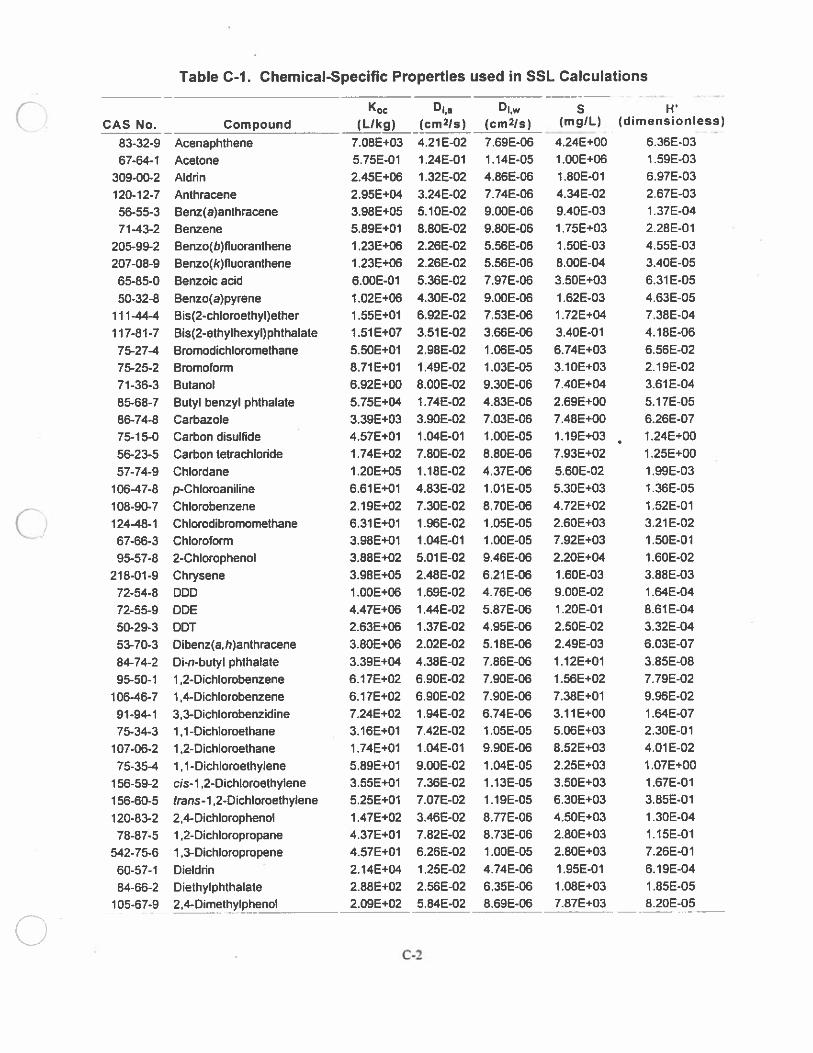
Table C-I. Chemical-Specific Properties used in SSL Calculations

Dia S HCAS No. Compound (LIkg) (cm2ls) (cm2is) (mg!L) (dimensionless)

83-32-9 Acenaphthene 7.08E+03 4,21E-02 7.69E-06 4.242+00 6.362-03

67-64-1 Acetone 5.752-01 1.242-01 1.142-05 1.006+06 1.592-03

309-00-2 Aldrin 2.456+06 1 .32E-02 4.86E-06 1.802-01 6.972-03

120-12-7 Anthracene 2.952÷04 3.246-02 7.746-06 4.346-02 2.676-03

56-55-3 Benz(a)anthracene 3.982+05 5.102-02 9.002-06 9.40E-03 1372-04

7143-2 Benzene 5.892+01 8.SOE-02 9.806-06 1.75E÷03 2.286-01

205-99-2 Benzo(b)fluoranthene I .23E+06 2.262-02 5.56E-06 1 .50E-03 4.55E-03

207-08-9 Benzo(k)fluoranlhene 1.232÷06 2.262-02 5.566-06 8.OOE-04 340E-05

65-85-0 Benzoic acid 6.002-01 5.362-02 7.97E-06 3.502÷03 6.316-05

50-32-8 Benzo(a)pyrene 1.026÷06 4.302-02 9.002-06 1.622-03 4.636-05

111444 Bis(2-chloroethyl)ether 1.55E÷01 6.92E-02 7.532-06 1.726÷04 738E-04

117-81-7 Bis(2-ethylhexyQphthalate 1.51E÷07 3,512-02 3.662-06 3.40E-01 4.18E-06

75-274 Bromodichloromethane 5.50E÷01 2.98E-02 1.062-05 6.74E+03 6,562-02

75-25-2 Bromoform 8.712+01 1.492-02 1.03EM5 3.1OE+03 2.192-02

71-36-3 Butanol 6.922+00 8.002-02 9.30E-06 7.402+04 3.61E-04

85-68-7 Butyl benzyl phthalate 5.752+04 1.742-02 4.832-06 269E÷00 5.17E-05

86-74-8 Carbazole 3.39E+03 3.902-02 7.032-06 748E+00 6.26E-07

75-15-0 Carbon disulfide 4.57E+01 1.042-01 1.002-05 1.192±03 • 1.24E÷00

56-23-5 Carbon tetrachlohde 1 .74E+02 7.80E-02 8.80E-06 7.932+02 1.252÷00

57-74-9 Chlordane 1.202÷05 1.182-02 4.372-06 5.602-02 1.992-03

106-47-8 p-Chloroaniline 6,612*01 4.832-02 1.012-05 5.302+03 1.36E-05

108-90-7 Chlorobenzene 2.19E+02 7.306-02 8.702-06 4.722+02 1.522-01

12448-1 Chlorodibromomethane 6.31E+0i 1.96E-02 lOSE-OS 2.602+03 3.212-02

67-66-3 Chloroform 3.98E+01 1.042-01 1.002-05 7.922+03 1.502-01

95-57-8 2-Chlorophenol 3.882+02 5.OIE-02 9.462-06 2.20E+04 1.60E-02

218-01-9 Chrysene 3.982+05 2.482-02 6.216-06 1.602-03 3.88E-03

72-54-8 DDD I .006+06 1.692-02 4.762-06 9.OOE-02 1.642-04

72-55-9 DDE 4.472+06 1.442-02 5.872-06 l.20E-01 8.612-04

50-29-3 DDT 2.632+06 1.372-02 4.952-06 2.502-02 3.322-04

53-70-3 Dibenz(a,h)anthracene 3.80E+06 2.022-02 5.182-06 2.492-03 6.032-07

84-74-2 Di-n-butyl phthalate 3.39E÷04 4.382-02 7.86E-06 1.122+01 3.852-08

95-50-1 i,2-Dichlorobenzene 6,17E÷02 6.902-02 7.902-06 1.562+02 7.792-02

10646-7 1 ,4-Dichlorobenzene 6.172÷02 6.902-02 7902-06 7.382÷01 9.96E-02

91-94-1 3,3-Dichlorobenzidine 7.242+02 1.94E-02 6.746-06 3.112+00 1.642-07

75-34-3 li-Dichloroethane 3.162+01 7.422-02 1.052-05 5.062+03 2.30E-01

107-06-2 12-Dichloroethane 1.74E÷01 1.046-01 9.902-06 8.52E+03 4.O1E-02

75-354 1,1-Dichloroethylene 5.89E+01 9.002-02 1.04E-05 2.252+03 1.072+00

156-59-2 cis-i ,2-Dichloroethylene 3.55E+01 7.36E-02 1.1 3E-05 3.50E+03 1.672-01

156-60-5 trans-i ,2-Dichloroethylene 5252÷01 7,07E-02 1.1 9E-05 6.302+03 3852-01

120-83-2 2,4-Dichlorophenol 1 .47E+02 3.462-02 8.776-06 4.50E÷03 1.302-04

78-87-5 12-Dichloropropane 4.372+01 7.822-02 8.732-06 2.80E+03 i.15E-0i

542-75-6 1.3-Dichloropropene 4.57E÷0i 6.266-02 1.006-05 2.80E+03 7.262-01

60-57-i Dieldñn 2.146+04 1.252-02 4.742-06 1.952-01 6.196-04

84-66-2 Diethylphihalate 2.886+02 2.56E-02 6.352-06 1.082+03 1.856-05

105-67-9 2,4Dimethylphenoi 2.096+02 5.842-02 8696-06 7.872+03 8.202-05

C-2

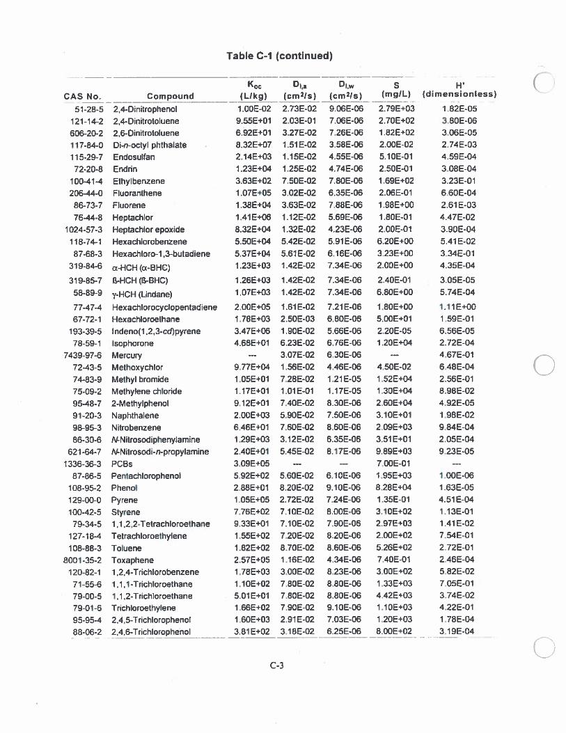
Table C-I (continued)

D — - S H ([CAS No. - Compound (LIkg) (cm2ls) (crn2/s) (mg!L) (dimensionless)

51-28-5 2,4-Dinitrophenol 1.002-02 2.736-02 9.066-06 2.796÷03 1 .82E-05

121-142 2,4-Dinitrotoluene 9.55E+01 2.036-01 7.066-06 2.70E÷02 3.80E-06

606-20-2 2,6-Dinitrotoluene 6,926+01 3.276-02 7262-06 1 .82E+02 3.066-05

117-840 Di-n-octyl phihalate 8.326+07 1.512-02 3.582-06 2.002-02 2.746-03

115-29-7 Endosulfan 2.14E+03 1.152-02 4.55E-06 5.1OE-01 4.592-04

72-20-8 Endrin 1.236+04 1.256-02 4.74E-06 2.50E-01 3.08E-04

100-414 Ethylbenzene 3.63E+02 7.506-02 7.80E-06 1.696+02 3.23E-01

20644-0 Fluoranthene 1.076+05 3.02E-02 6.35E-06 2.066-01 6.60E-04

86-73-7 Fluorene 1,38E÷04 3.636-02 7.88E-06 1.98E÷00 2.612-03

76-44-8 Heptachlor 1.416+06 1.126-02 5.69E-06 1,80E-01 4.47E-02

1024-57-3 Heptachlor epoxide 8.326+04 1.32E-02 4.23E-06 2.OOE-01 1906-04

118-741 Hexachlorobenzene 5,50E÷04 5,42E-02 5916-06 6.20E÷00 5.41 E-02

87-68-3 Hexachloro-1,3-butadiene 5.372+04 5.616-02 6.16E-06 3.236+00 3.34E-01

319-846 a-HCH(a-BHC) 1.236÷03 1.42B02 7.34B06 2.002+00 4.35E04

319-85-7 B-HCH(B-BHC) 1.26E+03 1.426-02 7.346-06 2.402-01 3.056-05

58-89-9 y-HCH (Undane) 1.076+03 1 .42E-02 7.34E-06 6.80E÷00 5.74E-04

77474 Hexachlorocydopentadiene 2.006+05 1.616-02 7.216-06 1.806÷00 1.112÷00

67-72-1 Hexachloroethane 1.786+03 2.50E-03 6.806-06 5.OOE÷01 1.596-01

193-39-5 lndeno(1,2,3-ccpyrene 3.472+06 1.90E-02 5.66E-06 2.202-05 6.56E-05

78-59-1 lsophorone 4.686±01 6.23E-02 6.76E-06 1.206+04 2.72E-04

7439-97-6 Mercury — 3.07E-02 6.306-06 —- 4.67E-01

72-43-5 Methoxychlor 9.776+04 1.566-02 4.462-06 4.50E-02 6.48E-04

74-83-9 Methyl bromide 1 .05E+01 7.286-02 1.21 6-05 1.522÷04 2.562-01

75-09-2 Methylene chloride 1.176+01 1.016-01 1.172-05 1.30E÷04 8.986-02

95-48-7 2-Methylphenol 9.12E+01 7.406-02 8.306-06 2.60E+04 4.926-05

91-20-3 Naphthalene 2.002+03 5.906-02 7.506-06 3.106+01 1.986-02

98-95-3 Nitrobenzene 6.46E+01 7.602-02 8.602-06 2.092+03 9.84E-04

86-30-6 MNitrosodiphenylamine 1.296÷03 3.126-02 6.352-06 3.512+01 2.052-04

621-647 MNitrosodi-n-propylamine 2.402+01 5.45E-02 8.176-06 9.89E÷03 9.23E-05

1336-36-3 PCBs 3.092+05 — — 7.OOE-01 —

87-86-5 Pentactilorophenol 5,92E±02 5.606-02 6.106-06 1.952+03 1.OOE-06

108-95-2 Phenol 2.682+01 8.202-02 9.102-06 8.282+04 1.632-05

129-00-0 Pyrene 1.05E+05 2.722-02 7.242-06 1.35E-01 4.51E-04

10042-5 Styrene 7.76E+02 7.1OE-02 8.006-06 3.102÷02 1.13E-01

79-34-5 1,1,2,2-Tetrachloroethane 9,336÷01 7.1OE-02 7.902-06 2.976÷03 1,41E-02

127-184 Tetrachloroethylene 1.556±02 7.202-02 8.20E-06 2,00E+02 7.54E-01

108-88-3 Toluene 1.822+02 6.706-02 8.606-06 5.26E+02 2,72E-01

8001-35-2 Toxaphene 2.57E05 1.166-02 4.346-06 7.402-01 2.46E-04

120-82-1 1 ,24-Trichlorobenzene 1.782+03 3,006-02 8.236-06 3.006+02 5.826-02

71-55-6 1,1,1-Trichloroethane 1.106+02 7.80E-02 8.802-06 1.332÷03 7.052-01

79-00-5 1,1,2-Trichloroethane 5.012+01 7.80E-02 8.806-06 4.422+03 3,74E-02

79-01-6 Trichloroethylene 1.666÷02 7.902-02 9.102-06 1.106+03 4.226-01

95-95-4 2,4,5-Trichlorophenol 1.606+03 2.912-02 7.036-06 1.206+03 1.782-04

88-06-2 2,4,6-Trichlorophenol 3.816÷02 3.182-02 6.252-06 8.006÷02 3.196-04

C-3-- 0

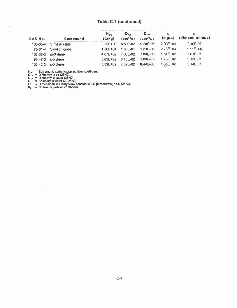
Table C-I (continued)

S HCAS No. Compound (LIkg) (cm2ls) (cmzls) (mgIL) (dimensionless)

108-05-4 Vinyl acetate 5.25E+00 8.505-02 9.205-06 2.005÷04 2.105-02

75-014 Vinyl chloride 1.865+01 1.065-01 1.23E-06 2.76E-03 1.11E+00

108-38-3 m-Xylene 4.07E+02 7.00E-02 7.80E-06 1.61E±02 3.015-01

95-47-6 o-Xylene 3.63E.02 8.70E-02 1.OOE-05 1.78E+02 2.13E-01

10642-3 p-Xylene - - 3.89E+02 7.69E-02 - 8.44E-06 1.855+02 3.145-01

= Soil organic carboaMater partition coefficientD a = Difftisivity in air (25 -C).D = Diffusivity in water (25 C).S = Solubility in water (20-25 -C).H = Dimensionless Henrys law constant (HLC [atm-mD/rnoq 41) (25 C).

= Soil-water partition coefficient.

C-4

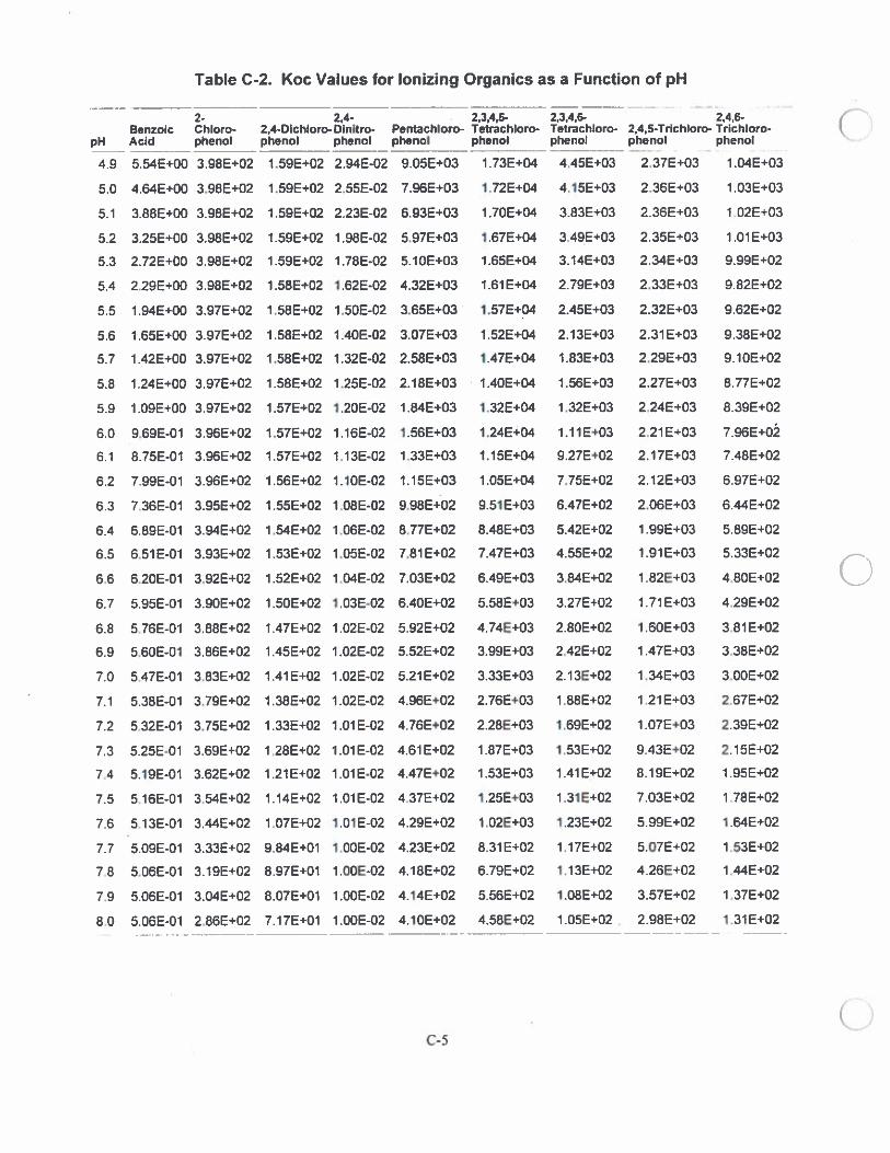
Table C-2. Koc Values for Ionizing Organics as a Function of pH

2- 2,4- 2,345- 2,3,4,6- 2,4,6-Benroic Chloro- 2,4-Dlchioro-Dlnitro- Pentachloro- Tetrachloro- Tetrachloro- 2,4,5-Thchloro- Trichloro

pH Acid phenol phenol phenol — phenol phenol phenol phenol phenol

4.9 5.546±00 3.982+02 1.596±02 2.946-02 9.05E+03 1.736+04 4.456÷03 2.376+03 1.046÷03

5.0 4.54E+00 3.986+02 1.59E+02 2.552-02 7.966+03 1.726+04 4.15E+03 2.362÷03 1.03E±03

5.1 3.882+00 3.986÷02 1.592+02 2.232-02 6.932+03 1.702+04 3.832+03 2.366÷03 1.022÷03

5.2 3.25E÷00 3.986÷02 1.596+02 1.986-02 5.976÷03 1.672+04 3.49E+03 2.352÷03 1.012+03

5.3 2.726+00 3.982÷02 1.596÷02 1.782-02 5.102+03 1.65E÷04 3.146÷03 2.34E÷03 9.996÷02

5.4 2.29E÷00 3.982÷02 1.582+02 1.62E-02 4.326+03 1.612+04 2,79E÷03 2.332÷03 9.822±02

5.5 1.946÷00 3.972+02 1.586÷02 1.506-02 3.656÷03 1.576+04 2.456+03 2.322±03 9.62E02

5,6 1.652÷00 3.97E+02 1.582+02 1.406-02 3.072÷03 1.522+04 2.136+03 2.312+03 9.386÷02

5.7 1.426+00 3.976÷02 1.586+02 1.322-02 2.586÷03 1.472÷04 1.83E÷03 2.296÷03 9.106÷02

5.8 1.246+00 3.97E02 1.58E+02 1.25E-02 2.186÷03 1.406÷04 1.562÷03 2.276÷03 8.776÷02

5.9 1.092+00 3.976+02 1.57E+02 1.206-02 1.846+03 1.32E04 1.326+03 2.246÷03 8.396÷02

6.0 9.696-01 3.966÷02 1.576÷02 1.166-02 1.566+03 1.246÷04 1.116÷03 2.212+03 7.966+02

6.1 8.756-01 3,966+02 1.572+02 1.136-02 1.33E+03 1.152+04 9.276÷02 2.172+03 7.482÷02

6.2 7.996-01 3.966+02 1.566+02 1.106-02 1.15E+03 1.052+04 7.756÷02 2.12E÷03 6.976÷02

6.3 7.362-01 3.956÷02 1.552+02 1,082-02 9.986+02 9.516+03 6.476+02 2.062+03 6.44E+02

6.4 6.896-01 3.946+02 1.546÷02 1.066-02 8.772+02 8.48E+03 5.426+02 1.99E÷03 5.896÷02

6.5 6.51E-01 3.936+02 1.536+02 1.05E-02 7.812+02 7.472+03 4.552+02 1.91E÷03 5.336+02

6.6 6.20E-01 3.926÷02 1.522+02 1.042-02 7.036+02 6.492+03 3.84E+02 1.826÷03 4.806÷02

6.7 5.956-01 3.906÷02 1.506÷02 1.03E-02 6.406+02 5.586+03 3.276+02 1.712+03 4.292+02

6.8 5,766-01 3.886+02 1.472+02 1.026-02 5.926÷02 4.746+03 2.802+02 1.606÷03 3.816÷02

6.9 5.602-01 3.862±02 1.452+02 1.026-02 5.526÷02 3.992+03 2.426÷02 1.47E+03 3.38E+02

7.0 5.476-01 3.832+02 1.412+02 1.02E-02 5.212+02 3.336÷03 2.136÷02 1.346÷03 3.006+02

7.1 5.386-01 3.792+02 1.382+02 1.022-02 4.966+02 2.766÷03 1.886+02 1.21 2+03 2.672+02

7.2 5.326-01 3.75E02 1.33E+02 1.016-02 4.762+02 2.28E+03 1.696÷02 1.07E÷03 2.392+02

7.3 5.256-01 3.696÷02 1.28E÷02 1,012-02 4.612+02 1.872÷03 1.532+02 9.436÷02 2.152+02

7.4 5.196-01 3.626÷02 1.21E÷02 1.016-02 4.472÷02 1.536+03 1.412+02 8.19E÷02 1.952+02

7.5 5.166-01 3.54E+02 1.142+02 1.O1E-02 4.37E+02 1.256±03 1.316+02 7.036+02 1.786÷02

7.6 5.136-01 3.44E÷02 1.076+02 1.016-02 4.296÷02 1.026÷03 1.236+02 5.996÷02 1.64E÷02

7.7 5.096-01 3.336÷02 9.842+01 1.006-02 4.23E÷02 8.316+02 1.176+02 5.076+02 1,532+02

7.8 5.066-01 3.196+02 8.976÷01 1.006-02 4.186÷02 6.792+02 1.136+02 4.262+02 1.446+02

7.9 5.06E-01 3.046÷02 8.076+01 1.OOE-02 4.146+02 5.566+02 1.08E÷02 3.57E÷02 1.376+02

8.0 5.06E-01 2.866÷02 7.176+01 1.002-02 4.1OE±02 4.586÷02 1.056÷02 . 2.98E÷02 1.316±02

C-5‘ C

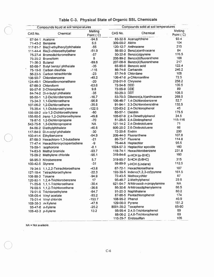
Table C-3. Physical State of Organic SSL Chemicals

Compounds liquid at soil temperatures —- Compounds solid at soil temperatures—

— Melting MeltingCAS No. Chemical Point ( C)

CAS No. Chemical Point ( C)

67-64-1 Acetone -94.8 83-32-9 Acenaphthene 93.47143-2 Benzene 5.5 309-00-2 Aldhn 104

117-81-7 Bis(2-ethylhexyl)phthalate -55 1 20-1 2-7 Anthracene 215

111-444 Bis(2-chloroethyl)ether -51.9 56-55-3 Benz(a)anthracene 8475-274 Bromodichloromethane -57 50-32-8 Benzo(a)pyrene 176.5

75-25-2 Bromoform 8 205-99-2 Benzo(b)fluoranthene 168

71-36-3 Butanol -89.8 207-08-9 Benzo(k)fluoranthene 217

85-68-7 Butyl benzyl phthalate -35 65-85-0 Benzoic acid 122.475-15-0 Carbon disulfide -115 86-74-8 Carbazole 246.256-23-5 Carbon tetrachloride -23 57-74-9 Chlordane 106

108-90-7 Chlorobenzene 45.2 10647-8 p-Chloroaniline 72.512448-1 Chlorodibromomethane -20 218-01-9 Chrysene 258.267-66-3 Chloroform -63.6 72-54-8 DOD 109.595-57-8 2-Chlorophenol 9.8 72-55-9 DDE 8984-74-2 Di-n-butyl phthalate -35 50-29-3 DDT 108.595-50-1 1 ,2-Dichlorobenzene -16.7 53-70-3 Dibenzo(a,h)anlhracene 269.575-34-3 1 ,1-Dichloroethane -96.9 10646-7 1 ,4-Dichlorobenzene 52.7

107-06-2 1 2-Dichloroethane -35.5 91-941 3,3-DicNorobenzidine 132.575-354 1,1 -Dichloroethylene -122.5 120-83-2 2,4-Dichlorophenol 45

156-59-2 cis-i ,2-Dichloroethylene -80 60-57-1 Dieldhn 175.5156-60-5 trans-i ,2-Dichloroethylene 49.8 105-67-9 2,4-Dimethylphenol 24.5

78-87-5 1,2-Dichloropropane -70 51-28-5 2,4-Dinitrophenol 115-116542-75-6 1,3-Dichloropropene NA 121-142 2,4-Dinitrotoluene 71

84-66-2 Diethylphthalate 40.5 606-20-2 2,6-Dinitrotoluene 66117-84-0 Di-n-octyl phthalate -30 72-20-8 Endrin 200100-414 Ethylbenzene -94.9 20644-0 Fluoranthene 107.887-68-3 Hexachloro-1 ,3-butadiene -21 86-73-7 Fluorene 114.877-47-4 Hexachlorocyclopentadiene -9 7644-8 Heptachlor 95.578-59-1 Isophorone -8.1 1024-57-3 Heptachlor epoxide 16074-83-9 Methyl bromide -93.7 118-741 Hexachlorobenzene 231.875-09-2 Methylene chloride -95.1 319-846 a-HCH (a-BHC) 160

98-95-3 Nitrobenzene 5.7 319-85-7 B-HCH (l1-BHC) 31510042-5 Styrene -31 58-89-9 y-HCH (Undane) 112.5

79-34-5 1.1 ,2,2-Tetrachloroethane 43.8 67-72-1 Hexachloroethane 187127-184 Tetrachloroethylene -22.3 193-39-5 lndeno(12,3-cd)pyrene 161.5108-88-3 Toluene -94.9 7243-5 Methoxychlor 87

120-82-1 1.2,4-Trichlorobenzene 17 9548-7 2-Methylphenol 29.871-55-6 1,1,1-Thchloroethane -30.4 621-647 MNitrosodi-n-propylamine NA79-00-5 1.1 ,2-Thchloroethane -36.6 86-30-6 N-Nitrosodiphenylamine 66.5

79-01-6 Thchloroethylene -84.7 91-20-3 Naphthalene 80.2108-054 Vinyl acetate -93.2 87-86-5 Pentachlorophenol 17475-014 Vinyl chloride -153.7 108-95-2 Phenol 40.9

108-38-3 rmXylene 47.8 129-00-0 Pyrene 151.2

95-47-6 o-Xylene -25.2 8001-35-2 Toxaphene 65-90106-42-3 p-Xylene 13.2 95-954 2,4,5-Trichlorophenol 69

88-06-2 2,4,6-Thchlorophenol 69

-

—115-29-7 Endosullfan 106

NA = Not available.

C-6

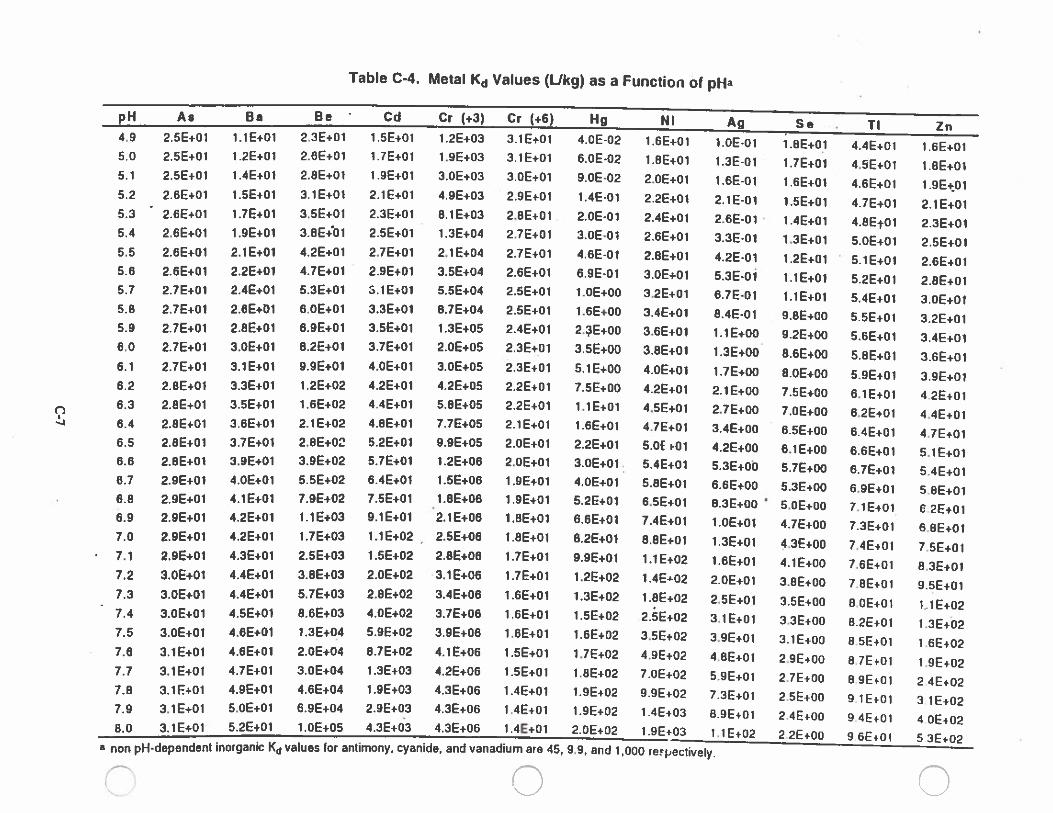
Table C-4. Metal 1d Values (Ukg) as a Function of pHa

Ag Se . TI ZnpH As Ba Cd Cr(+3) Cr(+6) Hg

--

4.9 2.5E÷01 1.1E+01 2.3E+01 1.SE+01 1.2E+03 3.1E+01 4.0E-02 1.6E+01 i.oE-oi 1.8E+oi 44E+01 1.6E+ol5.0 2.5E+01 1.2E+O1 2.6E+01 1.7E+01 1.9E+03 31E+01 6.OE-02 1.AE+01 1.3E-01 1.7E+01 4.5E÷0I 1.BE+0i5.1 2.5E÷01 1.4E+01 2.OE+01 1.9E+01 a.OE+03 3.OE+01 9.OE-02 2.OE+O1 1.6E-o1 1.6E+01 4.6E+01 19E+,015.2 2.6E+01 1.5E+01 a.1E+01 2.1E+01 4.9E+03 2.9E+01 1.4E-01 2.2E+01 2.1E-01 1.SE+01 4.7E+01 2.1E+015.3 - 2.6E+01 1.7E+O1 3.5E+01 2.3E÷01 8.1E+03 2.BE÷0l 2.OE-01 2.4E+01 2.6E-01 1.4E+01 4.8EtOl 2.3E+015.4 2.6E÷01 1.9E+01 3.BE+bl 2.SE+01 1.3E+04 2.7E+01 3.0-01 2.6E+01 3.3E-01 1.3E+01 5.OE+01 2.SE+0I5.5 2.6E+01 2.1E+0l 4.2E+0l 2.7E+Ol 2.1E+04 2.7E+0l 4.6E-01 2.OE+0l 4.2E-01 1.2E+ol 5.1E+01 2.6E+015.6 2.6E+01 2.2E+O1 4.7E+01 2.9E+01 3.SE+04 2.6E+01 6.9E-0l 3.OE+0l 5.3E-Oi 1.1E+0l 5.2E+0l 2.6E+015.7 2.7E+O1 2.4E+0l 5.3E+0l S.1E+01 5.5E+04 2.SE+01 1.OE+00 3.2E+0l 6.7E-0l l.1E+01 5.4E+0l 3.DE+015.8 2.7E+O1 2.6E+O1 6.OE+01 3.3E+0l e.7E+04 2.SE+01 l.6E+0o 3.4E+01 8.4E-01 9.8E+00 5.5E+01 3.2E+015.9 2.7E+01 2.8E+01 6.9E+01 3.5E+01 1.3E+05 2.4E+01 2.?E+00 3.6E+01 i.iE+oo 9.2E+00 5.6E+01 3.4E+016.0 2.7E+01 3.0E+O1 8.2E+01 3.7E+01 2.OE+05 2.SE+O1 3.5E+00 3.8E+01 1.3E+00 8.6E+00 5.8E+01 3.6E+016.1 2.7E+01 3.1E+01 9.9E+01 4.OE+01 3.OE+05 2.3E+01 5.1E+00 4.OE+01 1.7E+oo 8.OE+00 5.9E+O1 3.9E+016.2 2.BE+01 3.3E+01 t2E+02 4.2E+01 4.2E+05 2.2E+01 7.5E+00 4.2E+01 2.IE+00 7.SE+00 6.1E+01 4.2E+0I6.3 2.8E+01 3.SE÷01 1.6E+02 4.4E+01 5.BE+O5 2.2E+01 1.1E+01 4.5E+01 2.7E+00 7.OE+00 6.2E+01 4.4E+01

J 6.4 2.8E+01 3.GE+01 2.1E+02 4.8E+01 77E+05 2.1E+01 1.6E+01 47E+01 3.4E+00 6.5E+00 6AE+01 4.1E+016.5 2.8E+01 3.7E+01 2.8E+02 5.2E+01 9.9E+05 2.OE+01 22E+01 5.0E fOl 4.2E+OO 6.1E+O0 6.6E+O1 s.iE+oi6.6 2.8E+01 3.9E+01 3.9E+02 5.7E+O1 1.2E+06 2.OE+01 3.OE+01. 6.4E+01 s.sE+ob &7E+o0 6.7E+01 5.4E+016.7 2.9E+01 4.OE+01 &SE+02 6.4E+01 1.5E÷06 1.9E+01 4.OE+O1 s.8E+oi 6.6E+00 s.aE+oo 6.9E+01 5.eE+oi6.8 2.9E+01 4.1E+01 7.9E+02 7.SE+01 1.8E+06 i.gE+oi S.2E+01 6.5E+01 8.3E+00 5.OE+oo 7.1E+01 6.2E+016.9 2.9E+01 &2E+O1 1.1E+03 9.1E+01 2.1E+06 1.8E+01 6.6E÷O1 7.4E+01 1.oE+ol 4.7E+00 7.3E+ol 6.BE+017.0 2.9E+01 4.2E+O1 1.7E+03 1.1E+02 2.5E+06 1.8E+01 6.2E+01 8.SE+01 1.3E+01 4.3E+00 7.4E+01 75E+0l7.1 2.9E+01 4.3E+01 2.5E+03 1.5E+02 2.8E+06 1.7E+01 9.9E+01 1.1E+02 1.6E+01 4.1E+00 76E+01 a.3E+oi7.2 3.OE+01 4.4E÷01 3.SE+03 2.OE+02 3.1E+06 1JE+01 1.2E+02 1.4EL02 2.OE+01 3.SE+O0 78E+0l 95E+QI7.3 3.0E+01 4.4E+01 5.7E+03 2.8E+02 3.4E#06 1.GE+o1 1.3E+o2 1.BE+02 2.5E+01 3.SE+O0 a.oF.oi 1..1E+027.4 3.OE+01 4.SE+01 8.6E+03 4.OE+02 3.7E+06 1.6E+oI 1.5E+02 2SE+02 3.iE+oi 3.3L+00 8.2E.o1 1.3E+027.5 3.OE+01 4.6E+01 1.3E+04 5.9E+02 3.9E+06 1.6E+O1 1,6E+02 3.5E+02 3.9E+01 a.IE÷oo 8SE+Oi 1.6E+o27.6 3.1E+01 4.6E+01 2.OE+04 8.7E+02 4.1E+06 i.sE+oi 1.7E+o2 4.9E+02 4.8E+01 2.9E+00 B.1E+01 1.9E+D27.7 3.IE+01 4.7E+01 3.oE+o4 1.3E+03 4.2Et06 1.5E+01 1.OE+02 7OE÷02 5.9Ej-O1 2.7E+00 S 9E01 24E÷027.8 3.1F+01 4.9E+01 4.6E+04 1.9E+03 4.3E+06 1.4E+01 1.9E+02 9.9E÷02 73E+oi 2.SE+00 yiE+oi 3 IE+027.9 3.1E+01 s.OE+01 6.9E+04 2.9E+03 4.3E+06 1.4E÷01 1.9E+02 1.4E+03 8.9E+oi 2.4E+00 94E÷01 4OE+028.0 3.1E+O1 5.2E+0I 1.OE÷05 4.3E+03 4.3E÷06 1.4E÷01 2.OE+02 i.9E+03 1.1E+02 2.2E÷O0 9 GE+01 5 3E+02

non pR-dependent inorganic Kd values tot antimony, cyanide, and vanadium are 45, 9.9, and 1,000 reqiectively.

C

ATTACHMENT I

REGION 10 EPA MEMORANDUM ON INORGANIC ARSENIC

HI F }IL•!I TK HLVRE2 FISU IHSThR WPIIflI-K IIF:24)

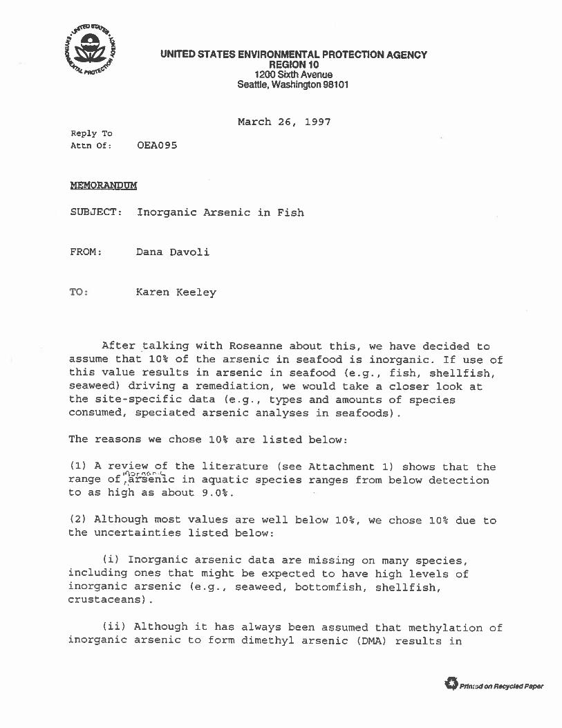
1e44. UNITED STATES ENVIRONMENTAL PROTECTION AGENCY

% / REGION 101200 Sixth Avenue

Seattle, Washington 98101

March 26, 1997Reply To

Attn Of: OEAO9S

MEMORANDUM

SUBJECT: Inorganic Arsenic in Fish

FROM: Dana Davoli

TO: Karen Keeley

After talking with Roseanne about this, we have decided toassume that 10% of the arsenic in seafood is inorganic. If use ofthis value results in arsenic in seafood (e.g., fish, shellfish,seaweed) driving a remediation, we would take a closer look atthe site-specific data (e.g., types and amounts of speciesconsumed, speciated arsenic analyses in seafoods)

The reasons we chose 10% are listed below:

(1) A review of the literature (see Attachment 1) shows that therange offntic in aquatic species ranges from below detectionto as high as about 9.0%.

(2) Although most values are well below 10%, we chose 10% due tothe uncertainties listed below:

(i) Inorganic arsenic data are missing on many species,including ones that might be expected to have high levels ofinorganic arsenic (e.g., seaweed, bottomfish, shellfish,crustaceans)

(ii) Although it has always been assumed that methylation ofinorganic arsenic to form dimethyl arsenic (DMA) results in

Pfimsd on Recycled Paper

2

Cdetoxification, more recent data have shown that DMA may be aprobable human carcinogen (see Attachment 2) . Data that we havefrom a Superfund site in Washington show that the DMA levels aremuch higher than the inorganic levels (see attached report). Wehave no way of including this potential risk in our riskassessments because the Agency has not yet developed a potencyfactor for DMA.

0

0

ATTACHMENT J

WORLD HEALTH ORGANEZATION ABSTRACTON DIOXIN TOXIC EQUIVALENCY FACTORS

I!P’.

‘€J U U

WHO Toxic Equivalency Factors (ThFs) for dioxin-like compoundsfur humans and wildlife

Introduedon

Polychlorinazcd dibenzothoxins (PODs), polychlorinated dibenzofiwans (POFs) andpolychlorinated biphenyls (PCBs) are persistent - and toxic - environmental Chemicals. Theyenter the food chain and accumulate in fatty tissues of humans and other humans. Severalrepresentatives of these groups of chemicals have been shown to cause similar toxic effects as23,7.S-TCDD, the most toxic dioxin. Their health effects include dermal toxicity,immqnotoxicity, reproductive effects and teratogerücity, endocrine effects andcarcinogcnicity. These chemicals are also found in human millç which raises serious healthconcerns.

As a result of their different chemical properties, the relative concentrations of thevarious POD, POP and PCB compounds vary from sample to sample. They also differ&om the mixtures originally released into the environment. This complex situation hampersthe evaluation of the health risk for humans and for the environment and the establishment ofregulatory control of exposure to mixtures of these compounds.

ThF concept

The concept of toxic equivalency fictors (TEFs) has been developed to deal with thisproblem. The TEF concept is based on the evidence that dioxin-like compounds share acommon mechanism of action - binding to the Ah-receptor. By applying this TEF concept,the toxicity of the different compounds relative to that of2,3,7,8-TCDD is determined on thebasis of in vivo and in vitro data.

Several TEE schemes have been developed for PCDDS and PCDFs and for dioxin-likePCBs. Recogniing the need for a harmonized approach in setting intemañonafly agreedThFs, the WHO European Centre for Environment and Health and the InternationalPro-arnme on Chemical Safety (IPCS) have initiated a pmamme to derive consensus TEEsfor compounds with dioxin-like activity for assessing the impact of these compounds onhuman health. The &st Consultation on the Derivation of TEFs for Dioxin-like PCBs wasconvened in December 1993. For this meeting data on the relative toxicity of dioxin-likePCBs for mammalian species were collected and criteria for deriving TEEs were established.

These data were entered into a database set up by the Karolthska Institute inStockholm, Sweden, and evaluated with respect to the applicability for the derivation ofThFs. As a result of this process, consensus TEFs for human intake were derived for 13different PCBs (I). In addition, it became apparent that the database should be extended toinclude PCDDs and PCDFs, as well as data on the relative toxicity of dioxin-like compoundsfor wildlife.

C

09/04/97 ThU 17:08 FAX 2187205539 ID—C0NT ECOL DIV DULUTH OO3

C.Risks for wildlife?

One of the open questions was whether or not the TEFs derived for human risk assessment

purposes were appropriate for estimating the risk for wildlife, or whether a separate set of

TEEs for wildlife should be developed. This was discussed at an initial WHO consultation on

the derivation of TEFs for wildlife for PCBs, PCDDs, PCDFs and other dioxin-like

compounds, convened in August 1996. This WHO meeting identified the type of data

necessary for the derivation of TEEs for wildlife, and defined a workplan and the way data

should be collected. ft decided to combine the effi,rts to derive TEFs for wildlife with the

update of existing TEEs for human risk assessment Funhenuore, ft recommended that ThFs

(or human health and wildlife be harmonized to the extent possible.

Derivation ofltFs

Many scientific articles on PCDDs, PCDFs and PCBs were analysed, o(which 185 flilfihled

the selection criteria. Based on the information available in these articles about 1600 sets of

information have been inserted into the database. Following collection of alt available

information, a WHO meeting on the derivation of toxic equivalency factors (TEEs) for PCBs,

PCDDs, PCDFs and other dioxin-like compounds for humans and wildlife was held at the

Institute of Environmental Medicine of the Karoliuska Institute in June [997. The meeting

evaluated the information in the database and discussed several general issues related to the

TEE concept.

The term TEE was defined to be an order ofmagnitude estimate of the toxicity of a L)compound relative to the toxicity ofTCDD that is derived using careful sciendficjudgement

after considering all available data. The relative potency of a compound obtained in a single

in vivo or in vitro study will be referred to as a relative potency (REP) value. TEEs, in

combination with chemical residue data can be used to calculate toxic equivalent (TEOJ

concentrations in various media, including animal tissues, soil, sediment and water. TEQ

concentrations in samples containing PCDDs, PCDFs and PCBs are calculated using the

following equation:

TEQ = ([PCDP x ThFil11) + (fPCDF TEFJ,) + (fPCB x TEF1]&

Substantial evidence indicated that the TEF approach is equally valid for human risk

assessment as for wildlife, although wildlife risk assessments usually attempt to estimate

population-level effects (unlike traditional human risk assessments, which focus on protecting

individuals) because effects on populations are of greater ecological relevance than are effects

on individuals. The criteria used for including a compound in a wildlife TEF scheme are the

same as those used for human TEEs. Compounds must:

• show a snctuml relationship to the PCDDs and PCDFs

• bind to the Ah receptor• elicit dioxm-specific biochemical and toxic responses

• be pex-szstent and3ccumulate in the food chain.

..3 ..I t,, ,,..,,. n.-...,en,,.,A .knnAqrt in nn,r nr

U/U4Ji till iUO mA LAQILuDaJlj ftflp—j.,Uf.j tUUL Ui’ UlILtlifl IQJUU3

New WHO TEF scheme

Based on the available information ,both the previously established TEPs for PCDDs andPCDFs (2) and the WHO ThFs for POs (1) for human risk assessment were re-evaluated.For revision of the existing TEFs for PCDOs, PCDFs and PCBs it was agreed by the workinggroup that if the available information was considered insufficient to wanant a change, theexisting value would be adopted.

In deriving TEPs for wild mammals it was concluded that there was insufficientevidence to discriminate between laboratory and wild mammalian species, and it was thereforedecided that the ThFs fbr human risk assessment based on laboratory animals would be equallyapplicable for wild mammal species.

The relative potency factors were primarily taken from in viva toxicity data, which weregiven more weight than In vitro and/or QSAR data. In viva toxicity data were pdorizedaccording to the ranking scheme chronic > subcbronic > subacute> acute. In the Enal ‘rEFselection different Ah-receptor specific cndpothts were also ranked according to toxic>biochemical (e.g. enzyme induction) response.

Also for the derivation ofThFs for PCDDs, PCDFs, and coplanar and mono-orthoPCBs for fish, and birds a tieredapproach was followed that gives a higher weight to overttoxicity in vito studies than to biochemical effects. As even lower weight was given tobiochemical effects (enzyme induction) in vitro; In case none of these data were available anestimate was made based on quantitative smicture-activity relationships (QSAR).

When comparing the final TEF values across different taxa the working tup tied toharmonize the ThFs to the extent possible, as this would have a clear advantage from a riskassessment and management perspective. However total synchronisation of ThFs betweenmammals, birds and fish was considered to be not feasible in case of obvious indications oforders of a magnitude difference between the tan.

In line with the already existing lIP values new lIPs were rounded to a value ofeither br 5, irrespective of the order of mafitude difference with the reference compound,TOO. It is imnortant to point out that in this rounding procedure a conservative approachhas been chosen to provide optimal protection of humans and wildlife.

I. Afflborg et aL(1994), Toxic equivalency factors for dioxin-lilce PCBs: Report on a WHOECEH and ]FCS consuLtation, December 1993. Chemosphere, Vol.28, No. 6, 1049-1067.

2. NATO (198$), International toxicity equivalency factor (I-TEE) method of risk assessmentfor complex mixtures of dioxins and related compounds. Report No. 176, Brussels, Belgium.

For more infoutarion please contact F.X.Rolaf van Lecuwen, WHO European Centre forEnvironment and Health, P.O. Box 10, NL.3730 PA Ut BUt, tel. 31 302295 307, fax 31302294 252, email ru@who.nl

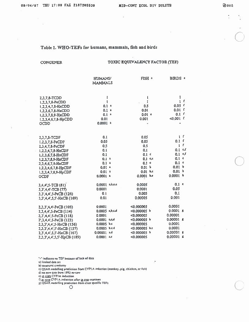
09/04/97 THU 17:09 FAX 2187205539 MID—CONT ECOL DIV DULUTH )005

Table 1. WEO-TEFs fur humans, mammals, fish and birds

CONGENER TOXIC EQUIVALENCY FACTOR çrzrj

mTh4M4si FISH a BIRDS

2.3,7,S-TCDD I IL.2.3,7.8-PeCDD I 1

I2,3,4,7,3-HxCDD 0A a 0.5 0.05l.2,3,6,7,8-HxCDD 0.1 a 0.01 0.01 i

1,2,3.7,3,9-HxCDD 0.1 0.01 C 0.1[.2,3.4,6,7,8-HpCDD 0.01 0.001 <0.001OCDO 0.0001 -

2,3,7,8-TCDF 0.1 0.05 1

l.2,317,S-PeCDF 0.05 0.05 0.1 f

2,3,4.7,8-PcCDF 0.5 0.5 1l,2,3,47,8-HxCDF 0.1 0.1 0.1 cS

I,2,3,6,7,5-kLxCDF 0.1 0.1 c 0.1 c,f

1,2,3,7,8,9-HxDF 0.1 ‘ 0.1 c.c 0.1 c

2,3,4,6.7,E-HzOF 0.1 0.! c 0.1 c

1,2.3,4,6,7,8-HpCDF 0.01 0.01 b 0.01 b

I,2.],4,7.8,9-HpCDF 0.01 0.01 b.c 0.01 6

QOF 0.0001 ‘ 0.0001 b.c 0.0001

3,4,4’,S-TCB (81)’ 0.0001 a.b,c,c 0.0005 0.13,3’.4.4’-TcS (77) 0.0001 0.0001 0.053,3’,4,4’,5-PeCB (126) 0.1 0.005 0.13,3,4,4’,5,5’-KxCB (169) 0.01 0.00005 0.001

2,J,3,4,4’-PeCB (105) 0.0001 <0.000005 0.00012,3,4,4’.S-PcCB (114) 0.0005 g,b,c.d <0.000005 6 0.0001 S

2.3’,4,4’,5.PeCB (118) 0.0001 <0.000005 0.000012,3,4,4,5-PcCB (123) 0.0001 a,c.d <0.000005 6 0.00001 8

2,3,3,4,4’,5-HxCB (156) 0.0005 b.c <0.000005 0.000123.3’.4,4,5’-E4xCB (157) 0.0005 b,c.d <0.000005 b.c 0.00012,3,4.4,5j.HxCB (167) 0.00001 ad <0.000005 t 0.00001 g

2,3,3,4.4.5,5’-HpCB (189) 0.0001 ‘. <0.000005 0.00001 S

indca,n no T bcc3uSr of lack oidaua) Jimjtcd da ci

b) totcuni szmil:htyc) QSAR modclling prediction Itm CYPIA inductiot, (monkey, pig, chicken. or nh)

1) no new Can from I 993 rc’jc%’dc)mzjCYPIA induction0 inm CYPIA ,nduccicn after jcxpoSn:) QSAR ntdcllin! prcdicdon Iron cia,: specific TEF,

0

AflACHMENT K

EPA REGION 1 RISK UPDATES,REVISED MANGANESE REFERENCE DOSE

REF B ‘[“‘tic TSkNREISE2 FI.AL MASThR WPO ilk cllrnlcl 111114/97/1 lvp,,i,ac

flotrkRegion 1, New England RISK UPDATE S

IINm 4 November 1996 iiRISK UPDATES is a periodic Contents

bulletin prepared by EPA - Region I, EPA Ecological GuidanceNew England risk assessors to provide Update Page 1information on new regional guidance.Risk Updates is distributed to contractors Superfund Risk Assessmentsupporting Superfund and RCRA, Reform lnittives Page 2regulators, and interested parties, Risk Risk Characterizationassessment questions may be directedto the following EPA scientists (area Update. Page 3code 617): Mercury Update. Page 3

EPA Finalizes Soil ScreeningRegional Risk Assessment ContactAnn-Made Burke 223-5528 Guidance. Page 3

EPA’s Proposed Cancer GuidanceSuperfund

and Implementation PlanPage 4Human Health Risk AssessmentAnn-Marie Burke 223-5528 Ground Water Use and ValueSarah Levinson 573-9614 Guidance. Page 5Margaret McDonough 573-5714

Lead Risk at CERCLA Sites andJayne Michaud 223-5583RCRA Correction Action

Ecological Risk Assessment Facilities. Page 6Susan Svirsky 573-9649 Revised Manganese ReferencePatti Tyler 8604342

Dose Page 8

RCRA Corrective Action New Cancer Slope Factors forMary Ballew 573-5716 PCB’s. Page 8Stephanie Car 223-5593

Air ModelingBrian Hennessey 565-3572

Combustion Risk IssuesJui-Yu Hsieh 565-3501

Comparative RiskKatrina Kipp 565-3520

Cost Benefit AnalysisRonnie Levin 565-9351

Drinking WaterMaureen McClelIand 565-3543

Air Risk IssuesJerri Weiss 565-9448

ORD Technical LiaisonRuth Bleyler 573-5792

EPA Region I, New England receivesadditional ecological technical supportfrom Ken Finkeistein (223-5537) of theNational Oceanic AtmosphericAdministration (NOAA), and US Fish &Wildlile (Steve Mierzykowski 207/827-5938, Ken Munney 6031225-1411, andTim Prior 4011364-9124).

EditorsStephanie Cart and Jayne MichaudLayout Giona Hume

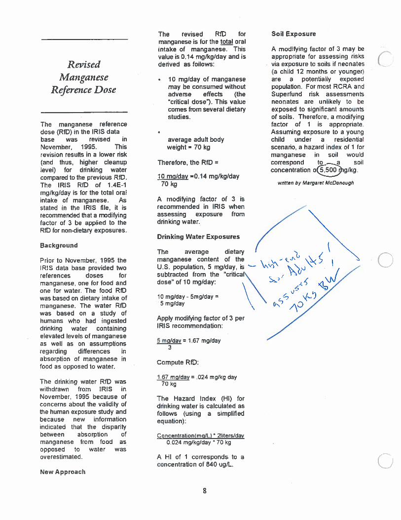
The manganese referencedose (RID) in the IRIS database was revised inNovember, 1995. Thisrevision results in a lower risk(and thus, higher cleanuplevel) for drinking watercompared to the previous RID.The IRIS RID of 1.4E-1mg/kg/day is for the total oralintake of manganese. Asstated in the IRIS file, it isrecommended that a rmdifyingfactor of 3 be applied to theRID for non-dietary exposures.

Bat kg round

Prior to November, 1995 theIRIS data base provided tworeferences doses formanganese, one for food andone for water. The food RIDwas based on dietary intake ofmanganese. The water RIDwas based on a study ofhumans who had ingesteddrinking water containingelevated levels of manganeseas well as on assumptionsregarding differences inabsorption of manganese infood as opposed to water.

The drinking water RID waswithdrawn from IRIS inNovember. 1995 because ofconcerns about the validity ofthe human exposure study andbecause new informationindicated that the disparitybetween absorption ofmanganese from food asopposed to water wasoverestimated.

New Approach

The revised RID formanganese is for the total oralintake of manganese. Thisvalue is 0.14 mg/kg/day and isderived as follows:

10 mg/day of manganesemay be consumed withoutadverse effects (thecrtticaI dose”). This valuecomes (mm several dietarystudies.

average adult bodyweight = 70 kg

Therefore, the RID =

10 mg/day =0.14 mg/kg/day70kg

A modifying factor of 3 isrecommended in IRIS whenassessing exposure fromdrinking water.

Drinking Water Exposures

The average dietarymanganese content of theU.S. population, 5 mg/day, issubtracted from the cdUcaldose’ of 10 mg/day:

Apply modifying factor of 3 perIRIS recommendation:

S mg/day = 1.67 mg/day3

Compute RID:

167 mg/day= .024 mg)kg day70kg

The Hazard Index (HI) fordrinking water is calculated asfollows (using a simplifiedequation):

Concentration(mq/L) 2liters/day0.024 mgikg/day 70 kg

A HI of 1 corresponds to aconcentration of 840 ug/L.

Soil Exposure

A modifying factor of 3 may beappropriate for assessing risksvia exposure to soils if neonates(a child 12 months or younger)are a potentially exposedpopulation. For most RCRA andSuperfund risk assessmentsneonates are unlikely to beexposed to significant amountsof soils. Therefore, a modifyingfactor of 1 is appropriate.Assuming exposure to a youngchild under a residentialscenario, a hazard index of 1 formanganese in soil wouldcorrespond to a soilconcentration og/kg.

wnffen by Margaret Mcoonough

RevisedManganese

Reference Dose

4N10mg/day - 5mg/day =

5 mg/day

a

0

US

AflACHMENT

AN APPROACH FOR DETERMINING TOXICITY VALUESFOR DERMAL EXPOSURE,

OAK RIDGE NATIONAL LABORATORY INTERNAL PAPER

ATTACHMENT L

AN APPROACH FOR DETERMINING TOXICITY VALUESFOR DERMAL EXPOSURE,

OAK RIDGE NATIONAL LABORATORY INTERNAL PAPER

FP’ P Rr1sE:rIs%L.lksThR WPfl :‘vI.lac

A

AN APPROACH FOR DETERM]MNG TOXICITY VALUES FOR DERMAL EXPOSURE.

C. B. Bast and H. T. Borga. Biomedical and Environmental Information Analysis. Health

Sciences Research Division. Oak Ridge National Laboratoty, Oak Ridge, TN.

Managed by Martin Marietta Energy Systems, Inc., for the U.S. Department of Energy under

contract No. DE-ACOS-840R21400.

ABSTRACT

nOral- toxicity data are available for many chemicals allowing for the calculation of Oral Reference

Thzes (RID) for noncarcinogenic effts and slope factors (afl for carcinogenic effects. In contrast,

dermal toxicity data for bog-term apcxuse are not available for mct chemicals which precludes

calculation of dermal RiDs and slope bctoa Health risb from derma] apcure to chemicals may

be estimated by modification of the oral RID or slope factor by a chemical-specific gastrointestinal

absorption factor following SUPEREJND guidelines. This transforms the Rdminictered doses (oral

RIDs and slope factors) into absorbed doses for comparison to intake amounts determined from

dermal aposun A computer program was developed to calculate the dermal RID and slope factors

from absorption data obtained from the published literature. When no quantitative data were

available, estimates were m3de using structural analogs or a scheme developed to assign quantitative

values to qualitative data Wben quantitative data were available, the most conservative absorption

factor from the species phylogenetically closest to the hnmnn was selected. The computer program ()uses t data ban for calculating demal toxicity values. The flat, updated quarterly, contains oral

and inhalation risk values for over 600 chcmicals. The second contains the absorption factor and the

reference citation for over 100 chemicals. The program compares the CAS numbers of all chemicals

in both data ban When a match is found and if oral data and absorption factors are present the

program computes the dermal RID and slope factors, prints the calculated results, the reference

dtatioas, and the source of the oral data (WIS or HEASfl Using this methodob, RIDs ranging

from IOOE-O8 to 4.OOE+00 mg/kg/day and slope factors ranging from 7S9E-03 to 430E+02

(mg/kg/day)4 have been derived for over 60 chemicals.

0

INTRODUCflON

Oral toxicity data are available for many chemicals enabling Oral Reference D (RfD) for

nOncaltlnogenlc effects and slope factors (q1) for carcinogenic effects to be calculated. In contrast

dermal toxicity data for long-tam aposure are not available for most themicaK This precludes the

calculation of dermal RIDS and slope factors. However, die health rib from dermal apaure to

chemicals can be characterized by modification of the on] Rn) or slope factor by a cbcmicai-speciflc

gastxointatmal absorption factor. Thi transforms the adminictered doses (oral RIDs and slope

factors) into absorbed doses which can then be mpared to intake amounts determined from dermal

eiposn

METHOD

Cl7. Jdnzdftcadon ofPotaitialAaae Effect. A flmt step in dermal risk assasment is to review dermal

toxicity of the compound and determine if it causes point of enby effects (direct skin effects). For

aampk, strong acids and bases cause direct skin desthiction, and mercury, chromium, and lead can

cause skin irritation at relad*ly low coniriflation Even if the amount of chemical involved in

dermal aposure is nil compared to the amount inhaled or ingested, dcrmal toxicity may be

important if acute skin effeca aist Also, when applying the following risk equations, it is important

to evaluate the risk value obtained in referein to the conthbution of contact site toxicity.

a I&ntiftcadon of Gasnob#eubwlAbsoepdon Faaaa Absorption data were obtained through on

line literature searches of National bbn’y of Medicine (NLM) databases and from hardcopy sources.

Secondary sources such as monographs, surveys, review articles, and criteria documents were used to

obtain gastrointestinal absorption data when possible. However, if no absorption data were present

in the sndazy sowca or if the absorption data were not clearly presented, primary publications

were consulted..

Gastrointestinal (GD absorption values calculated and reported in the literature were utilized

when the methods anpbyed appeared to be scientifically sound. In C2Cfl where no absorption

factors were reported or where the factors appeared to be derived by inappropriate methods,

attempts were made to estimate absorption factors from the published absorption and excretion data

In these instances, absorption was estimated by adding amounts of compound recovered in all

reported orgain (atiuding the bmhin2l contents of the stomach and intestines) at necmzy and/or

from amounts measured from sampling of plasma, saliva, urine, and bztatk In many ca.sa it was

possible to estimate only a lower limit of absorption since it could not be determined if compound

detected in the feces was actually absorbed. In these r.n, absorption is reported as ‘greater than

or equal to’ a given value.

In some cases qualitative descziptioin olgasunintatinal absorption, such as ‘readily absorbed

or ‘poorly a&orbed are available. When mpañng qualitative and quantitative 0! absorption data,

the tenz ‘rare, little, spane, and low’ tend to zeta to absorptions between 1-20%, readily and

rapidly’ to absorpuom between 20-90%, and ‘well and almost complete’ between 70-100%. Because

terms such as readily and rapidly may refer to ate rather than amount of absorption, it is difficult to

devise • qualitative absorption pinking system based on the terun mat commonly found in theliterature. The following system is suggested when no quantitative data aist but qualitative data arepresent

Negligibly Absothe& <1%Poorly Absotheth 1-20%Moderately Alzothc± 21-50%Well Absorbe& 51-80%Very Well Absorbe& >80%

if no quantitative or qualitative data were available for specific chemicals, an attempt wasmade to estimate absorption factors by smictural analogy.

3. S-krlinn ofGawobzwsthwlAbnpdon Faaarftr Use in Denial RiukAnavnezL The followingscheme w developed to select GI absorption factors for use in damal risk niasmentFor chemicals with quantitative absorption datz

1) Select absorption data from the species whose skin most closely mimics human skin (US.EPA, 1992).

flmnn > Non-human Primate, Pig> Rat, Guinea Pig > Mouse, Rabbit2) Select the most comantive absorption value (lowest p.acatagc absorption) from theappropriate srrw. (When the only value available was apressed a ptatn than or equala given absorption, the value itself was elected)

For chemicals with only qualitative absorption dat

1) Utilize the qualitative system previously presented.

Subjectively celet Ut mat appropriate absorption category, and select the lower limit of therange as the absorption factor.

4. Cawcsinn fran AdmbzLun& to Absorbed Data 01 absorption factors for 135 chemicals of

interat at DOEs Oak Ridge Reservation were identified in the literature and placed into a denim] C)risk database. The CAS numbers of these chemicals acre compared electronicafly with the CAS

numbers of a database containing the RID and Slope Factors of over 600 hundred chemicak When

an aact match wa foun4, the RID and Slope Factor was inserted into the dermal risk database and

converted to toxicity values based on absorbed dosed for dermal aposure follows (U-S EPA, 1992;

US. EPA, 1989):

Rffl1__14 = Rm x ABS01

______

= % .:_j I ABS

C)

0

RESUUS

Using th methodology, Rfl ranging from 3MOE-88 to 4.OOE+0O mg/kg/day and slope factors

ranging from 729E4B to 430E+02 (mg/kgIday’ have been derived for over 60 chemicals. The

computer-generated table pzovila a consistent mathematical method for caloiiaüng dermal toxicity

values and is prented below.

REFERENCES’

_

CUS. EPA 1969. Risk Act.tmcnt Guidance for Supethind. Volume L Human Health Evaluation

Manual (Pan A)- Interim Final Office of Emergency and Remedial Rnponsc, Washington, DC

December, 1969. EPM540Th89,00Z

U.S. EPA 1992 Dermal Ezposure Assasment Prindpla and Applieatious. Interim Report OSce

of Health and Environmental Asssment Washington, DC January, 1992 EPM600/&91,U1 I B.

Refcrnca from which gas#uñztestthat ahwrpdon faar wee o&abwd an listed at the aid of the

wmpaa wb&

C

C

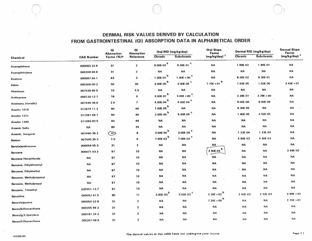
DERMAL RISK VALUES DERIVED BY CALCULATION

FROM GASTROINTESTINAL (GI) ABSORPTION DATA IN ALPHABETICAL ORDER

GI 01 Oral SlopeDermal RID (mg!kglday)

D.rmal Slop.Oral RID mgIkgIdayI Factor

_______________________

FacorAbsorption Absorption

_______________________ _______________________

Chemical CAS Numb.r Factor %i Relerenc. Chronic Subchronlc (mglkgldayl’ Chronic Subchronic (mIkgIdayi’

b cAcenaphihene 000083-32-9 31 2 6.OOE-02 6.OOE-0l NA 1.86E-02 1 86€-Ol NA

Acenaphthylene 000208-96-8 31 2 NA NA NA NA NA NA

b cAcetone 000067-64-1 83 3 - 1.OOE-01 1.00€ +00 NA 8.30E-02 8 30E-O1 NA

b c bAldrln 000309-00-2 50 65 3.OOE-05 3.00€-OS 1.70E+01 1.50€-OS 1.50E-05 3.40E+01

Aluminum 007429-90-5 10 4.5 NA NA NA NA NA NA

b cAnthr.cene 000120-12-7 76 6 3.00€-Ol 3.OOE+00 - NA 2.28E-01 2.28[+oo NA

b cAntimony (metellici 007440-36-0 2.0 7 4.OOE-04 4 OOE-04 NA 8.OOt-06 8 OOE-06 NA

bArocbr ‘016 012674-11-2 90 46 7.OOE-05 NA NA 6.30€-OS NA NA

b cAroclor I24 011097-69-1 90 46 2.00€-05 - 5.00€-OS NA 1.80E-05 4 50E-05 NA

Aroclor 1260 011096-82-5 90 46 NA NA NA NA NA NA

Arsenic Salt. NA 60 26 NA NA NA NA NA NA

Arsenic, InorganIc 007440- 38-2 (1) 8 33:4b 3.OOE-04C

NA 1.23E-04 1 23E-04 NA

b c

Barium 007440-39-3 7.0 9 7.OOE-02 7.OOE-02 NA 4.90E-03 4 90E-03 NA

NA NA NAB.nzialanthracene 000056-55-3 31 2 NA NA NA

B.nzen. 000071-43-2 97 10 NA NA NA NA 2 99€ -02

B.nzane Hexachbnde NA 97 10 NA NA NA NA NA NA

Benzone. EthyWimothyl NA 97 10 NA NA NA NA NA NA

B.nzene. Ethylmethyl NA 97 10 NA NA NA NA NA NA

B.nzene. Mothylpiopenyl NA 97 10 NA - NA NA NA NA NA

Benzene. Mothylpropyl NA 97 10 NA - NA NA NA NA NA

Benzene, Trimothyl 025551-13-7 97 10 NA NA NA NA NA NA

b c b

Benzidine 00009287-5 80 11 3.OOE-03 3.OOE-03 2 30€ +02 2 40€ 03 2 40€ 03 2 86€ .02

b

Benzolalpyrene 000050328 31 2 NA NA 7.30E+00 NA NA 2 35€ +01

Benzo(blfluoisnthene 000205992 31 2 NA NA NA NA NA NA

B.nzofg,h.ilperylene 000191-24-2 31 2 NA NA NA NA NA NA

Benzolkltluoranthene 000207-08-9 31 2 NA NA NA NA NA NA

02/09195The dermal values in this table have not undergone peer review y

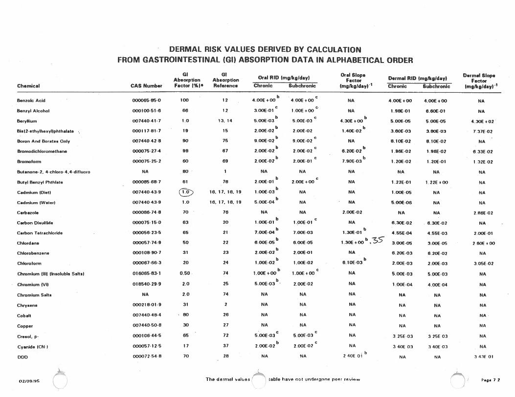
DERMAL RISK VALUES DERIVED BY CALCULATIONFROM GASTROINTESTINAL (GI) ABSORPTION DATA IN ALPHABETICAL ORDER

GI GI Oral Slop.Dermal RID (mg/kg/day) Darmal Sloit.Oral RID (mg/kg/day) Factcr

______________________

FactorAbsorption Absorption

_______________________ _______________________

Chemical CAS Number F.ctor (%) Relerenc. Chronic Subchronic (mg/kg/day)1 Chronic Subchronlc (mg/kg/day)’

b cBmnzolc Acid 000065-85-0 100 12 4.00€ +00 4.00€ +00 NA 4.00€ +00 4.00€ +00 NA

C CBenzylAlcohol 000100-51-6 66 12 3.00€-Of 1.OOE+00 NA 1.98E-01 6.60E-01 NA

b c bBeryllium 007440-41-7 1.0 13. 14 5.00E03 5.00E03 4.30E+00 5.00€-OS 500E-05 4.30€ +02

b bBI.(2-ethylhexyl)phthalate ., 00011781-7 19 15 2.00E02 2.00€02 1.40E02 3.80€03 3.00E03 737E02

Boron And Borate. Only 00744042-8 90 75 9.OOE.02 9.OOE02C

NA 8.10E-02 8.IOE-02 NAb c b

Bromodichloromothane 000075-27-4 98 67 2.00E02 2.00E02 6.20E.02 1.96E02 1.96E.02 633€ 02b c b

Bromofonn 000075-25-2 60 69 2.00E02 2.00E01 7.90E03 1.20E02 1.20E01 1 32€ 02

Butanone-2. 4chioro4.4dilluoro NA 80 1 NA NA NA NA NA NAb c

ButylBenzyl Phthlete - 00008568-7 61 78 2.OOE-01 2.00€ +00 NA 1.22E-01 1 22€ +00 NAb

Cadmium (Diet) 007440-43-9 () 16. 17. 18. 19 1.00E-03 NA NA 100€-OS NA NAb

Cadmium (Water) 007440-43-9 1.0 16. 17. 18. 19 5.OQE-04 NA NA 5.00€-Ofi NA NA

Carbazole 000086-74-8 70 76 NA NA 2.OOE-02 NA NA 2M6EO2b c

CathonDl.ulflde 000075-15-0 63 20 1.00E01 1.OOE-01 NA 6.30E-02 6.30E-02 NAb b

Carbon Totrachbride . 000056-23-5 65 21 7.OOE-04 7.OOE-03 l30t-01 4.55E-04 4.55E-03 2.00€ 01b b

Chlordane 000057-74-9 50 22 6.00€-OS 6.OO€-05 1.30€ +00 3.00€-OS 3.OOE-05 260€ +00b

Chbrobenzene 000108-90-7 31 23 2.00E-02 2.00€-Ol NA 6.20E-03 6.20E-02 NAb b

Chloroform 000067-66-3 20 24 1.00E-02 1.OOE-02 6.1OE-03 2.OOE-03 2.00E-03 305€02b c

Chromium (Ill) (insoluble Salts) 016065-83-1 0.50 74 1.00€ +00 1i)OE+OO NA 5.ooE-o3 5.00E-03 NAb

Chromium (VI) 018540-29-9 2.0 25 5.00€-03 - 2.OOE-02 NA 1.00E-o4 4.OOE-04 NA

Chromium Salt. NA 2.0 74 NA NA NA NA NA NA

Chry.ene 000218-01-9 31 2 NA NA NA NA NA NA

Cobalt 007440-48-4 . 80 26 NA NA NA NA NA NA-

Copper 007440-50-8 30 27 NA NA NA NA NA NA

C C

Cresol. p- 000106-44-5 65 72 5.OOE-03 5.O0E-03 NA 3 25€ 03 3 25€ 03 NA

b cCyanide (CN I 000057125 17 3? 2.00E02 2.OOE02 NA 340€ 03 3 40E-03 NA

ODD 000072-54-8 70 28 NA NA 2 40€ 01 NA NA 3 4’lF 01

The dermal values table have not undergone peer review Page 7 202/09/95

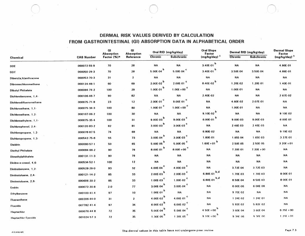
DERMAL RISK VALUES DERIVED BY CALCULATION

FROM GASTROINTESTINAL (GI) ABSORPTION DATA IN ALPHABETICAL ORDER

Ab.orption Ab.orption Oral RID imglkgldayl Or;i SlopeD.rmaI RID imglkgldayi

Dat ial Slop.

Chemical CAS Number Factor (Xi’ Reference Chronic Subchronic (mglkgld.y)’ Chronic Subchronic (mg!kgld.yl’

DDE 000072-55-9 70 26 NA NA 3.40E-01b

NA NA 4 86(01

DDI 000050-29-3 70 28 5.OOE-04b

5.OOE-04 3.40E-0lb

3.50E-04 350(04 4.86(01

Dibenzl.hlanthracene 000053-70-3 31 2 NA NA NA NA NA NA

b c bDibromochloromethane 000124-48-1 60 69 2.OOE-02 2.OOE-01 6.40E-02 1.20E-02 1.2oE-ol 1 40€-Ol

b cDibutyl Phthalate 000084-74-2 100 29 1.OOE-01 1.00€ +00 NA 1.OOE-01 NA NA

Dichbrobenzena. 1.4- 000106-46-7 90 62 NA NA 2.40E-02 NA NA 2 67E-02

C C

DlcNorodifluoromethane 000075-71-8 23 12 2.OOE-01 9.00(01 NA 4.60(02 207(01 NA

C C

Dlchbweth.ne. 1.1- 000075-34-3 100 80 1.OOE-01 1.OOE+00 NA 1.OOE-01 NA NA

bDlchlomothane. 1.2- 000107-06-2 100 30 NA NA 9.10E-02 NA NA 9 10(02

b c bDkhlom.thylene. 1.1- 000075-35-4 100 31 9.OOE-03 9.OOE-03 6.00(-01 9.OOE-03 9.00(03 6 00€ 01

b cDecNorophenol. 2.4- 000120-63-2 62 01 3.OOE-03 3 OOE-03 NA 2,46E-03 2 46E 03 NA

Dichloropropane. 1.2- 000078-87-5 74 66 NA NA 6.OOE-02 NA NA 9 19(02

b cDicNoropropene. 1.3- 000542-75-6 55 73 3.OOE-04 3.OOE-03 1.80(-01 1.65E-04 1 65(03 3 27(01

b c b01.1dm 000060-57-1 50 65 5.00E05 5.00E05 160€ +01 2.50(05 2 50E-05 320€ +0)

b cDiethyl PhIhalate 000084-66-2 90 79 8.OOE-01 6 00€ +00 NA 7.20E-01 7 20€ + 00 NA

Dlmothylphthalate 000131-11-3 90 79 NA NA NA NA NA NA

Dlnitro-o-cresol. 4.6- 000534-52-1 100 12 NA NA NA NA NA NA

C C

Dinltrobenzene. 1.2- 000520-29-0 93 32 4.00E-04 4.OOE-03 NA 3.72(04 3 72(03 NA

b c b.dDinitrotoluene. 2.4- 000121-14-2 85 33 2.OOE-03 - 2.OOE-03 6.OOE-01 1.70(03 1 70(03 000(01

c c b.dDinitrotoluene. 2.6- 000606-20-2 85 33 1 .OOE-03 1 .00E02 6.80(01 6.50E-04 8 50(03 8 00€ 01

b C

Endrln 000072-20-6 2.0 77 3.OOE-04 3.OOE-04 NA 6,00(06 6 OOE 06 NA

bEthylbenzena 000100-41-4 97 10 1 OOE-01 NA NA 9 70€ 02 NA NA

b cFluoranthene 000206-44-0 31 2 4.OOE-02 4.OOE-01 NA 1 24E 02 1 24F 01 NA

b cFluoride 007782 414 97 34 6.00E02 6.00(02 NA 5 62E 02 5 82f 02 NA

b c b

Heptachlor 000076-44 8 72 35 5.OOE-04 5 00(04 4 SOlE + 00 3 60E 04 3 60[ 04 6 7SF + 00

b c b

Heptachlor Epo+ide 001024 57 3 72 35 1 30€ 05 1 30E 05 9 10€ • 0() 9 361 06 9 161 06 1 761 01

nhInaIoc The dermal values in this table have not undergone peer review rage 7 3

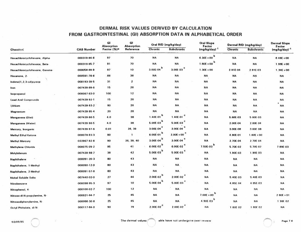
DERMAL RISK VALUES DERIVED BY CALCULATION

FROM GASTROINTESTINAL C GI) ABSORPTION DATA IN ALPHABETICAL ORDER

D.rmal Slop.GI GI Oral SlopeD.rmal RID Imglkgldayi Factor

Oral RID (mglkglday) Factor

_______________________

Absorption Absorption

______________________ ______________________

ChemIc CAS Number Factor %a Reference Chronic Subchronlc imglkgldayl1 Chronic Subchronlc (mglkg!day)’

bHexachbrocyclohe*ane. Alpha- 000319-84-6 97 70 NA NA 6.30€ +00 NA NA 6 49€ +00

bHex.chlorocyclohexaqe. Beta- 000319-85-7 91 70 NA NA 1.80€ +00 NA NA 1.98€ +00

b cH.xachbrocyclohexane. Gamma- 000058-69-9 97 10 3.OOE-04 3.OOE-03 1.30€ +00 2.91E-04 2.91E-03 1.34E+00

Haxanone. 2- 000591-78-6 66 36 NA NA NA NA NA NA

lndenoll.2.3-cdlpyrene 000193-39-5 31 2 NA NA NA NA NA NA

Iron 007439-89-6 15 26 NA NA NA NA NA NA

Icopropanol - 000067-63-0 100 12 NA NA NA NA NA NA

lead And Compounds 007439-92-1 15 26 NA NA NA NA NA NA

lithIum 00743993-2 00 26 NA NA NA NA NA • NA

Magnesium . 007439-95-4 20 26 NA NA NA NA NA NAb c

Manganese (Diet) 007439-96-5 4.0 30 1.40E-01 1.40€-Ol NA 5.60E-03 5 60E03 NA

CManganese Water) 00743996-5 4.0 38 5.OOE-03 5.OOE-03 NA 2.00E-04 2 00€ 04 NA

Mercury. Inorganic 007439-97-6 0.01 26. 39 3.OOE.O4C 3.OOE-04C

NA 3.OOE-00 3.00€ 00 NA

b cMethylEthylketone 000078-93-3 80 1 6.OOE-01 2.OOE+00 NA 4.60€-ol 1.60E+00 NA

C

Methyl Mercury 022967-92-6 90 26. 39. 40 3.00E-04’ 3.00E-04 NA 2.70E-04 2.70E04 NA

c bMethylene Chloride 000075-09-2 95 41 - 6.OOEO2l 6.OOE-02 7.50E-03 5.70E-02 5.70E-02 7.89E-03

C

Molybdenum 007439-98-7 38 42 5.OOE.O3b 5.OOE-03 NA 1.90E-03 1.90E•03 NA

Naphthalena - 000091-20-3 80 43 NA NA NA NA NA NA

Naphthalene. 1Methyl 000090-12-0 00 43 NA - NA - NA NA NA NA

Naphthalane. 2-Methyl 000091-57-6 60 43 NA NA NA NA NA NA

b cNickel Soluble Salt. 007440-02-0 27 44 2.OOE-02 2.00E-02 NA 540E-03 5.40E-03 NA

C

Nitrobenzene 000098-95-3 97 10 5.00E-04’ 5.OOE-03 NA 4 85€ 04 4 HSE-03 NA

Nltrophenol. 4- 000100-02-7 100 12 NA NA NA NA NA NA

bNitroso-dI-N-propylamine. N- 000621-64-7 25 45 NA NA 7.00€ +00 NA NA 2 80€ +01

bNitrosodiphenylamine. N- 000086-30-6 25 45 NA NA 4 90E-03 NA NA 1 961 02

C C

Octyl Phthalate. di-N- 000117-84-0 90 79 2.OOE-02 2.001-02 NA 1 801 02 I 801 02 NA

02/09195 -

- The dermal values able have not undergone peer review Page 7 4

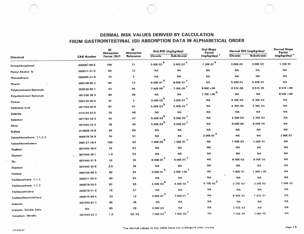
DERMAL RISK VALUES DERIVED BY CALCULATION

FROM GASTROINTESTINAL (GIJ ABSORPTION DATA IN ALPHABETICAL ORDER

GI 01 Oral SlopeD.rm.l RID (mlkgIday) Derm& Slop.

Oral RID (mglkgldey) Factor

_______________________

FactorAbsorption Absorption

______________________ ______________________

Chemical CAS Number Factor (%I Reference Chronic Subchronic (mgIkgldayl’ Chronic Subchronic (mglkg!dayl’

I, c bPent.chbrophenoi 000087-86-S 100 71 3OOE-02 3.OOE-02 l.20E-O1 3.OOE-02 3.00(02 I 20(01

Pontyl Alcohol. N- 000071-41-0 50 12 NA NA NA NA NA NA

Phonanthrono 000065-018 73 2 NA NA NA NA NA NA

b c

Phenol 000108-95-2 90 12 6.OOE-01 6.OOE-01 NA 5.40E-01 5.40E-01 NA

C C

Polybrominated Biphenyls 059536-65-1 93 64 7.OOE-06 7OOE-05 8.90E+00 6.51E-06 6.51E-05 9.S7E +00

b

Polychiorinated Biphenyls 001 336-36-3 90 46 NA NA 7.70E+00 NA NA 8 56E +00

-b c

Pyrene 000129-00-0 31 2 3.OOE-02 3.OOE-01 NA 9.30(03 9.30E 02 NA

-

b c

Selenious Acid 007783-00-8 87 47 5.OOE-03 5.00E-03 NA 4.35E-03 4 35(03 NA

SaI.nite 014124-67-5 70 48 NA NA NA NA NA NA

C

Selenium 007782-49-2 44 67503b

5.00E-03 NA 2.20E-03 2 20E-03 NA

Sliver 007440-22-4 18 49 S.OOE.O3b 5.OOE-03C

NA 9 OOE-04 9 00[ 04 NA

Sulfate 014806-798 20 50 NA NA NA NA NA NA

Tetrachloroeth.no. 1I.22- 000079-34-5 70 51 NA NA 2,00E-01b

NA NA 2 86E-01

b c

T.trechioroothyleno 000127-18-4 100 63 1.OOE-02 1.OOE-01 NA 1.OOE-02 1 00(01 NA

Thallium 007440-28-0 15 52 NA NA NA NA NA NA

Thodum 007446-29-1 1.0 53 NA NA NA NA NA NA

C C

007440-31-5 10 26 6.OOE-01 6.OOE-01 NA 6.00(02 600(02 NA

Titanium 007440-32-6 3.0 28 NA NA NA NA NA NA

b c

Toluene 000108-88-3 80 54 2.OOE-01 2.00( +00 NA 1.60E 01 1 60f +00 NA

Inchloroethane, 11.1- 000071-556 90 55 NA NA NA NA NA NA

b c b

Trichloroothane. 112- 000079-06-5 81 56 4.OOE-03 4.00(02 5.70E02 3 24E 03 3 24E 02 7 04E 02

Trichloroothylene 000079-01-6 15 57 NA NA NA NA NA NA

b £

Trichlorofluoromelbane 000075694 23 12 3.OOE-01 7.OOE-01 NA 6 90E 02 1 OlE 01 NA

Uranium 00744061-1 85 26 NA NA NA NA NA NA

Uranium. Soluble Salts NA 85 26 3 OOE-03 NA NA 2 5SF 03 NA NA

C C

V.nadium. Metallic 007440-62-2 1.0 58. 59 7 OOE 03 700(03 NA ()Jf 05 7001 05 NA

The dermal values in this table have not underqona t)et roviaw 7 5

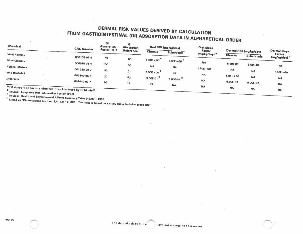
‘09/95

J)

DERMAL RISK VALUES DERIVED BY CALCULATIONFROM GASTROINTESTINAL (GI) ABSORPTION DATA IN ALPHABETICAL ORDERChemical

CAS Number

GI GIOral RID (mglkgldayl Oral SlopeAbsorption Absorption

FactorFactor (%ia R.fer.nc. Chronic Subchronic Imglkgld.y)’Dermal RID (mglkgldsylChronic Subchronlc

CC

Vinyl Acetate000106-054 65 60 1.OOE+00 1.OOE+00 NA 6.50€-Ol 6.50(01 NA

Vinyl Chloride000075-01-4 100 66 NA NA 1.90€ +00 NA NA 1.90(400

b

Xyl.n.. MIxture001330-20-7 92 61 2.00€ +00 NA NA 1.64€ +00 NA NA

b c

Zinc (Metallic). 007440-666 20 62 3.OOE-01 3.OOE-01 NA 6.OOE-02 6 00(02 NA

Zirconium- 007440-67-7 80 12 NA NA NA NA NA NA

D.rmal Slop.Factor

(mglkgIdayt

a GI absoprtion factors obtained from literature by BElA staffSource: Integrated Risk information System IIS)Source: Health and Environmental AUects Summary Table 1EAST) 1993listed as Dinitrotoluene mixture. 2.4-12.6- - In IRIS. The value ii based on a study using technical grade DNT.

The dermal values in thi! iave not undergone fleet review

GI ABSORPTION REFERENCES

R.f.r.nceNumber Reference

1 ATSDR (Agency for Toxic Substances and Disease Registry). 1992. Toxicological Profile for 2-Butanone. ATSDRIU.S. Public Health Service

2 Rahman, A., J.A. Barrowman end A. Rahimtula. 1986. The influence of bile on the bioavailability of polynuclear aromatic hydrocarbons from the ret intestine. Can. i. Physiol.

Pharmacol. 64:12141218

3 ATSDR (Agency for Toxic Substances and Disease Registry). 1992. Toxicological Profile for Acetone. ATSDR/U.S. Public Health Service

4 Venugopal, B. and T.D. Luckey. 1978. Metal Toxicity in Marnmals-2. Chemical Toxicity of Metals and Metalloids. Plenum Press. pp. 104-112

5 . Kortus, J. 1967. The carbohydrate metabolism accompanying intoxication by aluminum salts in the rat. Experiantia 23:912-93 3

6 Rahman, A., J.A. Barrowman and A. Rahimtula. 1986. The influence of bile on the bioavailability of polynuclear aromatic hydrocarbons from the rat intestine. Can. i. Physiol.

Pharmacol. 64:1214-1218

7 Gerber, G.B., J. Maes and B. Eykens. 1982. Transfer of antimony and arsenic to the developing organism. Arch. Toxicol. 49:159-168

8 Bettley. F.R., O’Shea. i.A. 1975. The absorption of arsenic and its relation to carcinoma. Br. J. Dermatology. 92:563. (Cited in Hindmarsh and McCurdy, 1986)

9 ATSDR (Agency for Toxic Substances and Disease Registry). 1992. Toxicological Profile f or Barium. ATSDRIU.S. Public Health Service

10 Sabourin, P.3., B.T. Chen, G. Lucier. at al. 1987. Effects of dose on the absorption and excretion of ll4Clbenzene administered orally or by inhalation in rats and mice. Toxicol.

Appi. Pharmacol. 8.7:325-336

11 ATSDR (Agency for Toxic Substances and Disease Registry). 1993. Toxicological Profile for Benzidine. ATSDR/U.S. Public Health Service

12 HSDB (Hazardous Substances Data Bank). 1994. MEDIARS Online Information Retrieval System, National Library of Medicine. Retrieved March, 1994

13 Furchner, J.E., C.R. Richmond and i.E. London. 1973. Comparative metabolism of radionuclides in mammals: VII. Retention of beryllium in the mouse, rat, nrnrikey and dog.

Health Phys. 24:292-300

11 Reeves, A.L. 1965. The absorption of beryllium from the gastrointestinal tract. Arch. Environ. Health 11:209-214

15 Teirlynck, O.A. and 3. Belpaire. 1985. Disposition of orally administered di(2-ethylhexyl)phthalate and mono(2-ethylhexyl)phthalate in the rat. Arch. Toxicol. 57(41:226-230

16 Foulkes, E.C. 1986. Absorption of cadmium. In: Handbook of Experimental Pharmacology. Vol. 80, E.C. Foulkes, ed., Springer-Verlag, Berlin, pp. 75-100

17 Nordberg, G.F., T. Kjellstrom and M. Nordberg. 1985. Kinetics end metabolism. In: Cadmium and Health: A Toxicological and Epidemiological Appraisal. Vol. 1. Exposure.

Dose, and Metabolism. L. Friberg. C.G. Elinder, T. Kjellstrom and G.F. Nordberg, ads. CRC Press, Boca Raton, FL, pp. 103-178

18 McLallan, i_S., P.R. Flanagan, M.J. Chamberlain and L.S. Valberg. 1978. Measurement of dietary cadmium absorption in humans. 3. Toxicol. Environ. Health 4:13 1 138

19 Shaikh, Z.A. and J.C. Smith. 1980. Metabolism of orally ingested cadmium in humans. In: Mechanisms of Toxicity and Hazard Evaluation, B. Holmstesd, at al., ads.

Elsevier/North Holland. Amsterdam. pp. 569-574

20 ATSOR (Agency for Toxic Substances and Disease Registry). 1992. Toxicological Profile (or Carbon Disulfide. ATSDR/U.S. Public Health Service

21 U.S. EPA. 1989. Updated Health Effects Assessment for Carbon Tetrachloride. Prepared for the Office Emergency aiiU Remedial Response, Washington, DC: Environmental

Criteria and Assessment Office, Cincinnati, OH

22 ATSDR (Agency for Toxic Substances and Disease Registry). 1992. Toxicological Profile for Chlordane. ATSDR/U.S. Public Health Service

02/09/95 Page 9.1

GI ABSORPTION REFERENCESR. ferenceNumber Reference

23 ATSDR (Agency for Toxic Substances and Disease Registry). 1990. Toxicological Profile for Chlorobenzene. ATSDR/U.S. Public Health Service

24 Brown, D.M.. P.F. Langely, 0. Smith. at al. 1974. Metabolism of Chloroform. I. The metabolism of 114C1-chloroform by different species. Xenobiotica 4:151-163

25 U.S. EPA. 1984. Health Effects Assessment for Chromium. Final Report. Environmental Criteria and Assessment Office. Research Triangle Park, NC. EPA 600I8830l4F.

PB851 15905

26 Goyer, R.A. 1991. Toxic Effects of Metals. In: Casarett and Doull’s Toxicology: The Basic Science of Poisons, fourth edition. M. 0. Ammdur, J. Doull, and C.D. Klesseen,

ads. pp. 623680

27 Vonugopal, B. and T.D. Luckey. 1978. Metal Toxicity in Mammals - 2. Chemical Toxicity of Metals and Metalloids. Plenum Press. pp. 104-112.

28 ATSDR (Agency for Toxic Substances and Disease Registry). 1992. Toxicological Profile for p,p’-DDT, DDE, DDD. ATSDR/U.S. Public Health Service

29 ATSDR (Agency for Toxic Substances and Disease Registry). 1990. Toxicological Profile for Din-Butylphthalate. ATSDR/U.S. Public Health Service

30 ATSDR (Agency for Toxic Substances and Disease Registry). 1989. Toxicological Profile for 1,2-Dichloroethane. ATSDR/U.S. Public Health Service

31 ATSDR (Agency f or Toxic Substances and Disease Registry). 1989. Toxicological Profile for 1,1-Dichloroethene. ATSORIU.S. Public Health Service

32 Parke, D. 1961. Studies in detoxification. V. The metabolism of m-dinitro(l4Cjbenzene in the rabbit. Biochem. J. 78:262-27 1

33 U.S. EPA. 1986. Health and Environmental Effects Profile for Dinitrotoluene. Office of Health and Environmental Assessment, Environmental Criteria and Assessment Office.

Cincinnati, OH. ECAO- CIN-P 183

34 ATSDR (Agency for Toxic Substances and Disease Registry). 1991. Toxicological Profile for Fluoride. Hydrogen Fluoride, and Fluorine. ATSDR/U.S. Public Health Service

35 ATSDR (Agency for Toxic Substances and Disease Registry). 1993. Toxicological Profile for Heptachlor/Heptachior Epoxide. ATSDR/U.S. Public Health Service

36 ATSDR (Agency for Toxic Substances and Disease Registry). 1992. Toxicological Profile for 2-Hexanone. ATSDR/U.S. Public Health Service

37 U.S. EPA. 1984. Health Effects Assessment for Cyanides. Prepared by the Environmental Criteria and Assessment Office, Cincinnati, OH for the Emergency and Remedial

Response Office, Washington, DC. EPA/540/1-86-O11

38 U.S. EPA. 1990. Integrated Risk Information System (IRIS). Health Risk Assessment for Manganese. On line. (Verification date 6121/90). Office of Health and Environmental

Assessment, Environmental Criteria and Assessment Office, Cincinnati, OH

39 ATSDR (Agency for Toxic Substances and Disease Registry). 1989. Toxicological Profilé for Mercury. ATSDR/U.S. Public Health Service

40 Miettinen, J.K. 1973. Absorption and elimination of dietary (Hg + +) and methylmercury in man. In: Mercury, Mercurials, and Mercaptans, M.W. Miller and T.W. Clakrson, Eds.

Springfield. IL pp 233243

41 Angelo, MJ., A.B. Pritchard, D.R. Hawkins, at el. 1986. The pharmacokinetics of dichloromethane. I. Disposition in B6C3F1 mice following intravenous and oral administration.

Food Chem. Toxicol. 24:965-974

42 Friberg, C. and J. Caner. 1986. Molybenum. In: Handbook on the Toxicology of Metals. 2nd ad. L. Friberg. G.E. Nordberg arid V.8. Vouk, eds. Elsevier/Nouth Holland Biomedical

Press, New York. pp. 446-461

43 ATSDR (Agency for Toxic Substances and Disease Registry). 1993. Toxicological Profile for Naphthalene. ATSDRIU.S. Public Health Service

02/09/95 Page 9.2

GI ABSORPTION REFERENCES

ReferenceNumber Reference

44 ATSDR (Agency for Toxic Substances and Disease Registry). 1993. Toxicological Profile for Nickel. ATSDR/U.S. Public Health Service

45 ATSDR (Agency for Toxic Substances and Disease Registry). 1989. Toxicological Profile for N-Nitrosodi-n-propylamine. ATSDRIU.S. Public Health Service

46 ATSDR (Agency for Toxic Substances and Disease Registry). 1989. Toxicological Profile for Polychiorinated Biphenyls: Aroclor 1260, 1254, 1248, 1242. 1232, 1221, and

1016. ATSDR/U.S. Public Health Service

47 Medinsky, M.A., R.G. Cuddihy, HO. McClellan. 1981. Systemic absorption of selenious acid and elemental selenium aerosols in rats. J. Toxicol. Environ. Health 8:917-928.

48 Thomson C.D. and RD.H. Stewart. 1974. The metabolism of I7SSel in young women. Br. J. Nutr. 32:47-57

49 East. 8W., K. Boddy, E.D. Williams, et al. 1980. Silver retention, total body silver end tissue silver concentrations in argyria associated with exposure to an anti-smoking remedy

containing silver acetate. Clin. Exp. Dermetol. 5:305-311

50 World Health Organization (WHO). 1984. Guidelines for Drinking Water Quality. Vol. 2. Health Criteria and Other Supporting Information

51 ATSDR (Agency (or Toxic Substances and Disease Registry). 1989. Toxicological Profile for 1,1,2,2-Tetrachloroethane. ATSDR/U.S. Public Health Service

52 ATSDR (Agency for Toxic Substances and Disease Registry). 1992. Toxicological Profile for Thallium. ATSDR/U.S. Public Health Service

53 ATSDR (Agency for Toxic Substances and Disease Registry). 1990. Toxicological Profile for Thorium. ATSDR/U.S. Public Health Service

54 ATSDR (Agency for Toxic Substances and Disease Registry). 1989. Toxicological Profile for Toluene. ATSDR/U.S. Public Health Service

55 ATSDR (Agency for Toxic Substances and Disease Registry). 1993. Toxicological Profile for 1,1,1-Trichloroethane. ATSDRIU.S. Public Health Service

56 ATSDR (Agency for Toxic Substances and Disease Registry). 1989. Toxicological Profile for 1,1,2-Trichloroethane. ATSDRIU.S. Public Health Service

57 Daniel, J.W. 1963. The metabolism of 36C1-lab&led trichloroethylene and tetrachlorethylene in the rat. Biochem. Pharmacol. 12:795-802

58 Curran, G.L. and R.E. Butch. 1967. Biological and health effects of vanadium. In: Proceedings of the Conference on Trace Substances in Environmental Health. DO. Hernphill

Ed. University of Missouri. Columbia, MO, pp. 96-104

59 ICRP (International Commission on Radiological Protection). 1960. Report of Committee II on Permissible Dose for Internal Radiation. Recommendations of the International

Commission on Radiological Protection. ICRP Publ. No. 2. Pergamon Press, Oxford, England, p.163

60 ATSDR (Agency for Toxic Substances and Disease Registry). 1992. Toxicological Profile for Vinyl Acetate. ATSDR/U.S. Public Health Service

61 ATSDR (Agency for Toxic Substances and Disease Registry). 1993. Toxicological Profile for Total Xylenes. ATSDR/U.S. Public Health Service

62 U_S. EPA. 1984. Health Effects Assessment for Zinc and Compounds. U.S. Environmental Protection Agency, Office of Research and Development. Washington, DC.

EPA/540/1 -8 6-048

63 ATSDR (Agency for Toxic Substances and, Disease Registry). 1993. Toxicological Profile for Tetrachloroethylene. ATSDR/U.S. Public Health Service

64 ATSDR (Agency for Toxic Substances and Disease Registry). 1993. Toxicological Profile for Polybrominated biphenyls (PBBs). ATSDR/U.S. Public Health Service

65 ATSDR (Agency for Toxic Substances and Disease Registry). 1993. Toxicological Profile for Aldrin/Dieldrin. ATSDRIU.S. Public Health Service

66 ATSDR (Agency for Toxic Substances and Disease Registry). 1993. Toxicological Profile for Vinyl Chloride. AISDR/U.S. Public Health Service

67 ATSDR (Agency for Toxic Substances and Disease Registry). 1989. Toxicological Profile for Bromodichioromeihane. ATSDR/U.S. Public Health Service

02i09/959 3

GI ABSORPTION REFERENCES

ReferenceNumber Reference

68 ATSDR (Agency for Toxic Substances end Disease Registry). 1989. Toxicological Profile for 1,2-Dichloropropane. ATSDRIU.S. Public Health Service

69 ATSDR (Agency for Toxic Substances and Disease Registry). 1990. Toxicological Profile for BromoformlChlorodibromomethane. ATSDRIU.S. Public Health Service

70 ATSDR (Agency for Toxic Substances and Disease Registry). 1994. Toxicological Profile I or Alpha-, Beta-, Gamma-, end Delta- Hexachlorocyclohexane. ATSDRIU.S. Public

Health Service

71 ATDR (Agency for Toxic Substances and Disease Registry). 1994. Toxicological Profile for Pentachlorophenol. ATSDR/U.S. Public Health Service

72 ATSDR (Agency for Toxic Substances and Disease Registry). 1992. Toxicological Profile for Cresols. ATSDR/U.S. Public Health Service

73 ATSDR (Agency for Toxic Substances and Disease Registry). 1992. Toxicological Profile for 1,3-Dichloropropene. ATSDRIU.S. Public Health Service

74 ATSDR (Agency for Toxic Substances and Disease Registry). 1993. Toxicological Profile for Chromium. ATSDRIU.S. Public Health Service

75 U.S. EPA. 1990. Health end Environmental Effects Document for Boron and Boron Compounds. Prepared for the Office of Solid Waste and Emergency Response, Washington,

DC by the Environmental Criteria and Assessment Office, Cincinnati, OH. ECAO-CIN-G 100

76 U.S. EPA. 1986. Health end Environmental Effects Profile for Carbazole. Prepared for the Office of Solid Waste end Emergency Response, Washington, DC by the Environmental

Criteria and Assessment Office, Cincinnati. OH. ECAO-CIN-P157

77 U.S. EPA. 1987. Health Effects Assessment for Endrin. Prepared for the Office of Solid Waste and Emergency Response, Washington, DC by the Environmental Criteria and

Assessment Office, Cincinnati. OH. ECAO-CIN-H089

78 U.S. EPA. 1989. Health and Environmental Effects Document for Buty) benzyl phthalate. Prepared for the Office of Solid Waste and Emergency Response, Washington, DC by

the Environmental Criteria and Assessment Office, Cincinnati, OH. ECAO-CIN-GOB1

79 U.S. EPA. 1987. Health and Environmental Effects Profile for Phthalic acid alkyl. aryl, and elkyl/aryl esters. Prepared for the Office of Solid Waste and Emergency Response,

Washington, DC by the Environmental Criteria and Assessment Office, Cincinnati, OH. ECAO.CIN-P188

80 U.S. EPA. 1985. Health and Environmental Effects Document for Dichloroethenes. Prepared for the Office of Solid Waste end Emergency Response, Washington, DC by the

Environmental Criteria and Assessment Office, Cincinnati. OH. ECAO-CIN-P139

81 U.S. EPA. 1987. Health and Environmental Effects Profile for Chlorinated phenols. Prepared for the Office of Solid Waste and Emergency Response. Washington, DC by the

Environmental Criteria and Assessment Office, Cincinnati, OH. ECAÔ-CIN-G013

82 U.S. EPA. 1987. Health Effects Assessment for Dichlorobenzenes. Prepared for the Office of Solid Waste and Emergency Response, Washington, DC by the Environmental

Criteria end Assessment Office, Cincinnati, OH. ECAO-CIN-H079

02103!95 94

ATTACHMENT M

EPA GUIDANCE FOR CALCULATING EXPOSURE POINT CONCENTRATIONS

[P E .,I4Pck!RE’IsflFpALMAsmR V,PO II.R:.,I,,.:2s1mL.e

The overarching mandate of the Comprehensive Environmental Response, Compensation, and LiabilityAct (CERCIA) is to protect human health and the environment from current and potential threats posed byuncontrolled releases of hazardous substances. To help meet this mandate, the U.S. Environmental ProtectionAgency’s (EPA’s) office of Emergency and Remedial Response has developed a human health risk assessmentprocess as pan of its remedial response program. This process is described in Risk Assessment Guidance forSuperfimt Volume I — Human Health Evnh,nñnn Manual (RAGS/IfflEM). Pan A of R4GSTh{}{EMaddresses the baseline risk assessment, and describes a general approach for estimating exposure to individualsfrom hazardous substance releases at Superbmd sites.

This bulletin explains the concentration tarn in the exposurenntake equation to remedial projectmanagers (RPMs), risk assessors, statisticians, and other personneL This bulletin presents the general intakeequation as presented in RAGS/FG{EM Pan A, discusses basic concepts concerning the concentration term.describes generally how to calculate the concentration term, presents examples to ifiustrate several importantpoints, and, lastly, identifies where to get additional help.

ThE CONCENTRATION TERM

flow Is the arnctnnfion term used?

RAGSTh{HEM Pan A presents theSuperfund risk assessment process in four steps:(1) data coueaion and nluatiorn (2) exposureassessment (3) toxicity assessment; and (4) fiskcharacterization. The concentration term iscalculated for use in the exposure assessment step.fllghflght 1 presents the general equationSuperftmd uses for calculating exposure, andillustrates that the concentration term (C) is oneof several parameters needed to estimatecontaminant intake for an individuaL

For Superfund assessments, the- concentration term (C) in the intake equation is

an estimate of the arithmetic average concentrationfor a contaminant based on a set of site samplingresults. Because of the uncertainty associated withesUmatinR the true avenge concentration at a sjj.the 95 percent upper confidence limit (UCI3 ofthe arithmetic mean should be used for thisvariable. The 95 patent UCL provides reasonableconfidence that the true site avenge will not beunderestimated.

Why use an average value for the concenflUonterm?

An estimate of avenge concentration is usedbecause:

SupplaraiwJ Guidan m RAGS is a bulletin acm on risk aamt oC Supatind sin That bulletins .aw n suppleuzazb toR1W Arnois Guidonj Supeftat Vohcnc 1— Hwnwt Heat Enbitha, MnaL The akrtion pnented b intended asguidance to EPA sod other ge.fltmat It doa bat nwtuw ru1—i-g by the s’4t5cY. sod may no! be Ftjied OD toante a substantive or produn1 right fwbIe by any other palon. The Govunmt may take salon that is at nnan WiLbtbc bufletina

aC

Unrted Sates Offle ol SoI Waste art Publication 9285.7-081Envimnrrental PmtectEn Emergercy Respocse May 1992Agercy Washirçtn. D.C. 2O6

Supplemental Guidance toRAGS: Calculating theConcentration Term

Office of Emergency ait Remedial ResporseHazardous Site Evahmton Dvn, OS-230

Intenmuent BulletinVolume I Number I

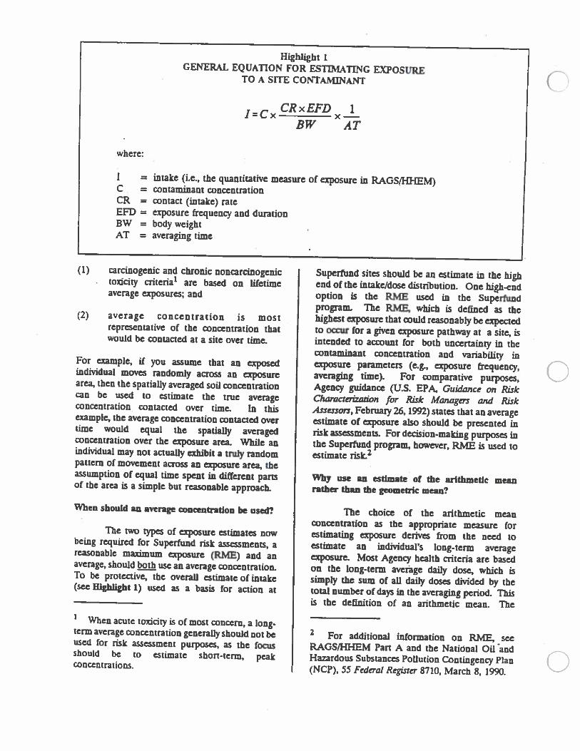
where:

Highlight IGENERAL EQUATION FOR ESTIMATING EXPOSURE

TO A SITE CONTAMINANT

= intake (i.e., the quantitative measure of exposure in RAGS,N}{EM)= contaminant concentration= contact (intake) rate= exposure frequency and duration= body weight= averaging time

(1) carcinogenic and chronic noncarcinogenictoxicity criteria1 are based on lifetimeavenge exposures; and

(2) average concentration is mostrepresentative of the concentration thatwould be contacted at a site over time.

For example, if you assume that an exposedindividual moves randomly across an exposurearea, then the spatially avenged soil concentrationcan be used to estimate the true avengeconcentration contacted over time. In thisexample, the avenge concentration contacted overtime would equal the spatially avengedconcentration over the exposure area While anindividual may not actually exhibit a truly randompattern of movement across an exposure area, theassumption of equal time spent in different partsof the area is a simple but reasonable approach.

When should an avenge concenfration be used?

The two types of exposure estimates nowbeing required for Superfiwd risk assessments, areasonable maximum exposure (RME) and anavenge, should use an avenge concentration.To be protective, the overall estimate of intake(see HIghlight 1) used as a basis for action at

When acute toxicity is of most concern, a long-term avenge concentration generally should not beused for risk assessment purposes, as the focusshould be to estimate short-term, peakconcentrations.

Superfiind sites should be an estimate in the highend of the intake/dose distribution. One high-endoption is the Rlb{E used in the Superfimdprogram. The RME, which is defined as thehighest exposure that amId reasonably be expectedto occur for a given exposure pathy at a site, isintended to account for both uncertainty in thecontaminant concentration and variability inexposure parameters (e.g., exposure frequency,avenging time). For comparative purposes,Agency guidance (U.S. EPA, Guidance on RiskCharacrcünrion for Risk Managers and RiskAssessors, Febniaiy 26, 1992) states that an averageestimate of exposure also should be presented inrisk assessments. For decision-making purposes inthe Supethmd program, however, RMB is used toestimate risk.2

Why use an estimate ot the arithmetic meanrather than the geometric man?

The choice of the arithmetic meanconcentration as the appropriate measure forestimating exposure derives from the need toestimate an individual’s long-term avengeexposure. Most Agency health criteria are basedon the long.term avenge daily dose, which issimply the sum of all daily doses divided by thetotal number of days in the avenging period. Thisis the definition of an arithmetic mean. The

CRxEFD1CxBW AT

ICCREFDBWAT

0

2 For additional information on RME, seeRAGS/FU-IEM Part A and the National Oil andHazardous Substances Pollution Contingency Plan(NC?), 55 Federal Register 8710, March 8, 1990.

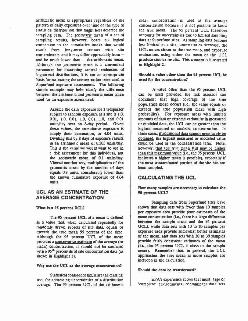
arithmetic mean is appropriate regardless of thepattern of daily exposures over time or the type ofstatistical distribution that might best describe thesampling data. The geometric mean of a set ofsampling results, however, bears no logicalconnection to the cumulative intake that wouldresult from long-term contact with sitecontaminants, and it may differ appreciably from —

and be much lower than — the arithmetic mean.Although the geometric mean is a convenientparameter for describing central tendencies oflognormal distributions, it is not an appropriatebasis for estimating the concentration term used inSupernrnd exposure assessments. The followingsimple example may help clah’ the differencebetween the arithmetic and geometric mean whenused for an exposure assessment:

Assume the daily exposure for a trespassersubject to random exposure at a site is 1.0,0.01, 1.0, 0.01, 1.0, 0.01, 1.0, and 0.01units/day over an 8-day period. Giventhese values, the cumulative exposure issimply their summation, or 4.04 units.Dividing this by 8 days of exposure resultsin an arithmetic mean of 0.505 units/day.This is the value we would want to use ina risk assessment for this individual, notthe geometric mean of 0.1 units/day.Viewed another way, multiplication of thegeometric mean by the number of daysequals 0.8 units, considerably lower thanthe known cumulative exposure of 4.04units.

UCL AS AN ESTIMATE OF ThEAVERAGE CONCENTRATION

What is a 95 percent UCL?

The 95 percent UCL of a mean is deflnedas a value that, when calculated repeatedly forrandomly drawn subsets of site data, equals orexceeds the true mean 95 percent of the time.Although the 95 percent UCL of the meanprovides a conservative estimate of the avenge (ormean) concentration, it should not be confusedwith a 95th percentile of site concentration data (asshown in HIghlight 2).

Why use the UCE as the avenge concentration?

Statistical confidence limits are the classicaltool for addressing uncertainties of a distributionaverage. The 95 percent UCL of the arithmetic

mean concentration isconcentration because itthe true mean. The 95

used as the averageis not possible to knowpercent UCL therefore

accounts for uncertainties due to limited samplingdata at Superfund sites. As sampling data becomeless limited at a site, uncertainties decrease, theUCL moves closer to the true mean, and exposureevaluations using either the mean or the UCLproduce similar results. This concept is illustratedin HIghlight 2.

Should a value other than the 95 percent UCL beused for the concentration?

A value other than the 95 percent UCLcan be used provided the risk assessor candocument that high coverage of the truepopulation mean occurs (i.e., the value equals orexceeds the true population mean with highprobability). For exposure areas with limitedamounts of data or extreme variability in measuredor modeled data, the UCL can be greater than thehighest measured or modeled concentration. Inthese cases, if additional data cannot practicably beobtained, the highest measured or modeled valuecould be used as the concentration term. Note,however, that the true mean still may be higherthan this maximum value (i.e., the 95 percent UCLindicates a higher mean is possible), especially ifthe most contaminated portion of the site has notbeen sampled.

CALCULATING THE UCL

flow many samples an necessary to calculate the95 percent UCL?

Sampling data from Superfimd sites haveshown that data sets with fewer than 10 samplesper exposure area provide poor estimates of themean concentration (i.e., there is a large differencebetween the sample mean and the 95 percentUCL), while data sets with 10 to 20 samples perexposure area provide somewhat better estimatesof the mean, and data sets with 20 to 30 samplesprovide fairly consistent estimates of the mean(i.e., the 95 percent UCL is close to the samplemean). Remember that, in general, the UCLapproaches the true mean as more samples areincluded in the calculation.

Should the data be transformed?

EPA’s experience shows that most large or‘complete’ environmental contaminant data sets

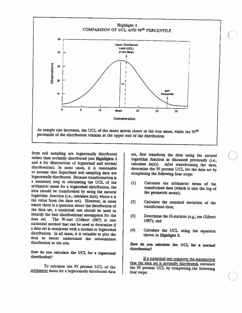
from soil sampling are lopormally distributedrather than normally distributed (see HighlIghts 3and 4 for illustrations of lognormal and normaldistributions). In most cases, it is reasonableto assume that Superfimd soil sampling data arelognormally distributed. Because transformation isa necessasy step in calculating the UCL of thearithmetic mean for a lognormal distribution, thedata should be transformed by using the naturallogarithm function (La, calculate ln(x), where x isthe value from the data set). However, in caseswhere there is a question about the distribution ofthe data set, a statistical test should be used toidentify the best distributional assumption for thedata set The W-test (Gilbert 1987) is onestatistical method that can be used to determine ifa data set is consistent with a normal or lognormaldistribution. In all casa, it is valuable to plot thedata to better understand the contaminantdistribution at the site.

flow do you calculate the UCL for i lopomaldistribution?

To calculate the 95 percent UCL of thearithmetic mean for a lopiormafly distributed data

set, fimt transform the data using the naturallogarithm function as discussed previously (i.e.,calculate ln(x)). After transforming the data,determine the 95 percent UCL for the data set bycompleting the following four steps:

(1) Calculate the arithmetic mean of thetransformed data (which is also the log ofthe geometric mean);

(2) Calculate the standard deviation of thetransformed data;

(3) Determine the H-statistic (e.g., see Gilbert1987); and

(4) Calculate the UCL using the equationshown in HIghlight 5.

How do you calculate the UCL for i normaldistribution?

if a statistical test supports the assumptionthat the data set is normally distributed, calculatethe 95 percent UCL by completing the followingfour steps:

(.)

Highlight 2COMPARISON OF UCL AND 95th PERENTllI

50

Upp.r ConlaraumIt (UCtI

_

ci th Mon

• I

5 30-

S

0200

ID

As sample size increases, the UCL of the mean moves closer to the true mean, while the 95thpercentile of the distribution remains at the upper end of the distribution.

0 5

95PtttI

10 20

Concentration

25 30

C

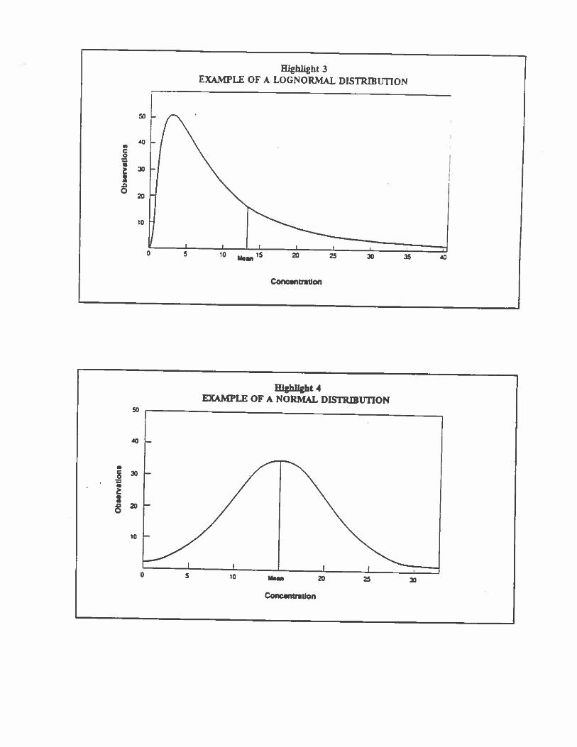
Highlight 3EXAMPLE OF A LOGNORMAL DISTRIBUTION

C0

0

a20

10

0 5 10 _,I5 20 25 X 35 40

Conanfluon

50

Highliflt 4EXAMPLE OF A NORMAL DISTRIBUTION

40

10

0 10 Ibei 25

Concanntion

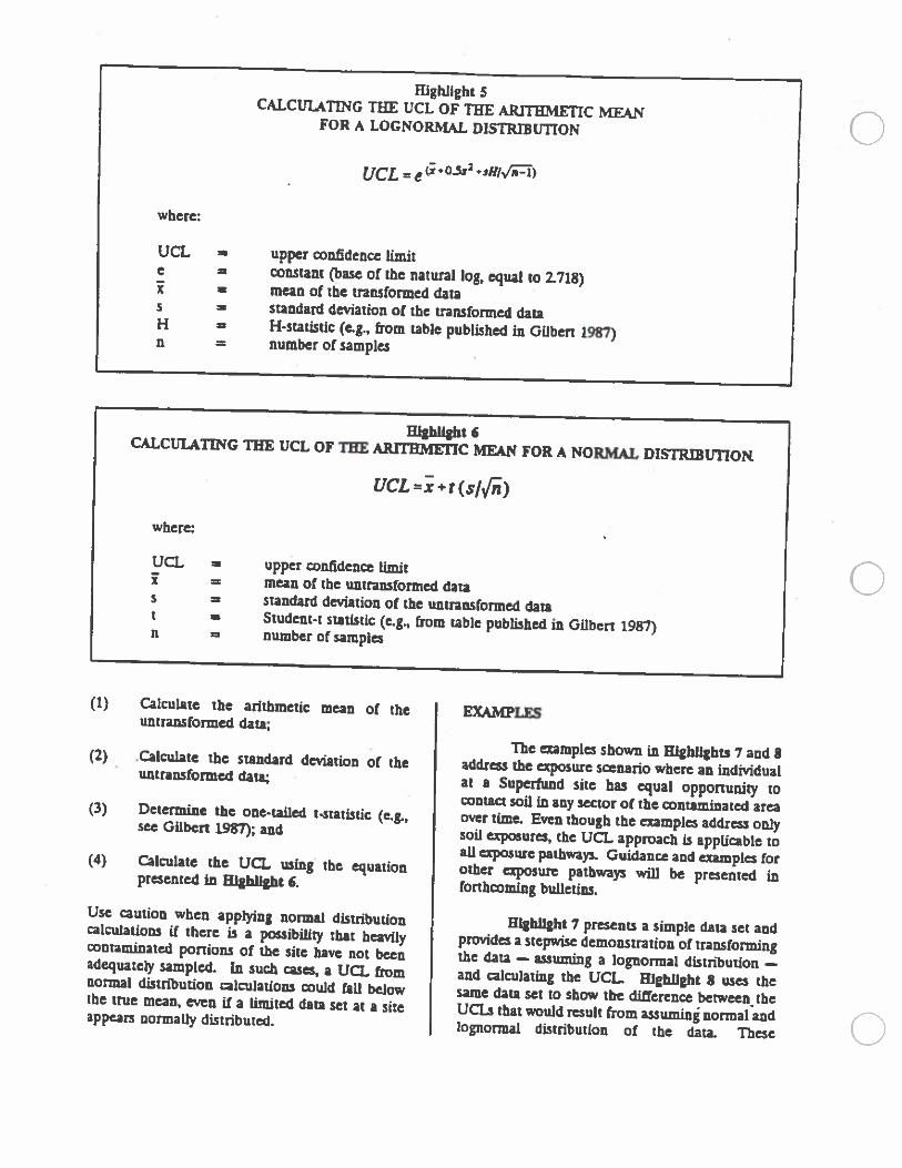
(1) Calculate the arithmetic mean of theuntransformed data;

(2) Calculate the standard deviation of (heuntransfrrmed data;

(3) Determine the one-tailed t-statistic (e.&,see Gilbert 1987); and

(4) Calculate the UC using the equationpresented in HIghlight 6.

Use caution when applying normal distributioncalcuiations if there is a possibility that heavilycontaminated portions of the she have not beenadequately sampled. In such cans, a UC fromnormal distribution calculations could fau belowthe true mean, even if a United data set at a siteappears normally distributed.

EX4MPLFS

The examples shown in BIghIIghts 7 and Saddress the exposure scenario where an individualat a Superfund site has equal opportunity tocontact soil in any sector of the contaminated areaover time. Even though the examples address onlysoil exposures, the UCL approach is applicable toall exposure pathway’s. Guidance and examples forother exposure pathways will be presented inforthcoming bulletins.

Ulghllght 7 presents a simple data set andprovides a stepwise demonstration of transformingthe data — assuming a lognormal distribution —

and calculating the UCL Highlight S uses thesame data set to show the difference between theUCLs that would result from assumini normal andlognonnal distribution of the data. These

HighlightsCAICUMTh4G TilE UCL OF TEE ARIThMETIC MEAN

FOR A LOGNORMAL DISTRIBUTION

where:

UCL upper confidence limite constant (base of the natural log, equal to 1718)

a mean of the transformed data$ a standard deviation of the transformed dataH a H-statistic (e.g., from table published in Gilbert 1987)n = number of samples

Highlight’CALCUlATING VIE UCL OF THE ARITEMEflC MEAN FOR A NORMAL DISI’RIBUTIOK

where:

UCL a upper confidence limit= mean of the untransformed data

s = standard deviation of the untransformed datat a Student-i statistic (e.g.. from table published in Gilbert 1987)11 = number of samples

0

0

0

examples demonszraw the importance of using thecorrect assumptions.

WHERE CAN I GET MORE HELP?

Additional information on Supertund’spolicy and approach to calculating theconcentration term and estimating aposi#es atwaste sites n be obtained in:

• U.S. EPA, Risk Assessment Guidancefor Supcfunth Volume I — HumanHealth Evahw4on Manual (Pan A),EPMS4O/1-29,002, December 1989.

• U.S. EPA, Guidance for DarnUstabWry in Risk Anessmnzt,EPAI54O/G-901008 (OSWERDirective 9285.7-05), October 1990.

• U.S. EPA, Rick Assessment Guidancefor Supefund (PanA —Baseline RiskAssessment) Suppkmaual Guidance!Standard Exposure Factors, OSWERDirective 9285.6-03, May 1991.

Useful statistical guidance can be found in manystandard textbooks. including:

S Gilbert, R.O., SroAs&& Methods forEnvironmental Pc/baton Monitoring,Van Nostrand Reinhold, New York,New York, 1987.

Questions or comments concerningconcentration term can be directed to:

the

• To Integration BranchOffice of Emergency and Remedial

Response401 M Street SWWashington, DC 20460Phone: 202-260-9426

EPA staff can obtain additional copies of thisbulletin by calling EPA’s Center for EntonmennlResearch Information at ETh 684-7562 (513-569-7652). Others can obtain copies by contactingNTIS at 800-336-4700 (703-4874650 in theWashington. DC area).

aCUnited StatesEnvironmental ProtectionAgency (05-230)Washington, DC Z460

Official BusinessPenalty for Private Use$300

flit-Clan MallPostag. and Fees PaidEPAPennft Na G-35

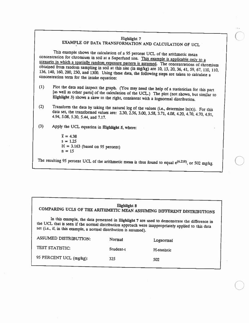
Hhlht 7 1 0EXAMPLE OF DATA TRANSFORMATION AND CALCUL4TION OF UCL

This example shows the calculation of a 95 percent UCL of the arithmetic meanconcentration for chromium in soil at a Superfund site. This example is apylicable only to ascenario in which a spatially random exposure pattern is assumed. The concentrations of chromiumobtained from random sampling in soil at this site (in mg/kg) are 10, 13, 20, 36, 41, 59. 67, 110, 110,136. 140, 160, 200, 230, and 13w. Using these data, the following steps are taken to calculate aconcentration terni for the intake equation:

(1) Plot the darn and inspect the graph. (You may need the help of a statistician for this pan(as well as other pansi of the calculation of the UCL) The plot (not shown, but similar toHighlight 3) shows a skew to the right, consistent with a lognormal distribution.

(2) Transform the data by taking the natural log of the values (i.e., determine ln(x)). For thisdarn set, the transformed values are: 130, 156, 3.00, 3.58, 3.71, 4.08, 4.20. 4.70, 4.70, 4.91,4.94, 5.08, 5.30, 5.44, and 7.17.

(3) Apply the UCL equation in HlghIIht 5, where:

= 4.38s = 1.25H = 3.163 (based on 95 percent)

The resulting 95 pe:cent UCL of the arithmetic mean is thns found to equal e(6218, or 502 mg/kg. C

HIhlIght 8COMPARING UCLS OF TEE ARrrnMunc MEAN ASSUMING DifFERENT DISTRBUfTONS

In this example, the data presented in Highlight 1 are used to demonstrate the difference inthe UCL that is seen if the normal distribution approach were inappropriately applied to this dataset (i.e., iL in this aample, a normal distribution is assumed).

ASSUMED DISThfflIfl1ON: Normal Lngnormal

TEST STATISTIC: Student-t H-statistic

95 PERCENT UCL (mg/kg): 325 502

C

Agency Washington. D.C. 20460- Envronmen:al Protecion Enerqency Response Daccmer 1993

Supplemental Guidance to RAGS:

Estimating Risk from Groundwater

Contamination

Office of Emergency and Remedial ResponseHazardous Site Evaluation Division

Intermittent BulletinVolume X Number X

The Toxics Integration Branch and Regional risk

assessors have formed a Total Quality Management

(TQM) Quality Action Team (QAT), known as the

Concentration Term workgroup, to address the broad

goal of improving the quality of data used in baseline

risk assessments.For this fact sheet, the Concentration Term

workgroup consulted with representatives of the

Groundwater Forum to address the risk assessment

challenges posed by gmundwater, in particular.

Lating Risk

Risk at Superfund sites generally is calculated by

comparing estimates of human exposure with Agency-

verified toxicity criteria. Exposure is calculated by

combining concentration with other parameters, such

as the contact rate, exposure frequency and duration,

and body weight. Current Agency guidance (U.S.

EPA, Guidance on Risk Characterization for Risk

Managers and Risk Assessors, February 26, 1993)

requires risk assessments to present multiple descripton of risk, including estimates for both average and

high-end exposure scenarios. The Superfiind site

manager uses the calculated risk value to help deter

mine the need for and extent of contaminant cleanup.

Since risk and exposure are linearly related, the

pollutant’s concentration has a significant influence on

the risk analysis, and, consequently, the remedial

decision at a given site. The calculation of the concen

tration term is crucial; miscalculation could result in a

false estimate of risk and, ultimately, result in inappro

() pdate cleanup decisions and misdirected Superfiind

actions.The Superfiind program uses a reasonable maxi

mum exposure (R?vfE) or high-end risk calculation as

the basis for remedial decisions. RME is intended to

estimate a conservative case that is both protective of

human health and the environment, while remaining

within the range of potential exposure levels.

Because groundwater is a very complex and

dynamic medium with characteristics that can change

seasonally, it is likely that concentration of a given

contaminant in each well will vary over time. There

fore, the concentration term is best described by an

arithmetic average, regardless of whether the ovenli

exposure estimate is high-end or avenge. Time and

resource considerations generally preclude collecting

enough data to calculate a true avenge; therefore,

Superflind has relied on an upper-confidence limit on

the arithmetic mean (UCLQ5) to represent the average

concentration.

llenge of Groundwater

Risk Assessment

When determining the need for action, there are

both policy and technical issues that set groundwater

apart from other media, such as soil. EPA’s policy is to

consider the maximum beneficial use of groundwater

and to protect it against future contarnirwtion. The

National Oil and Hazardous Substances Pollution

Contingency Plan (NCP) (U.S. EPA Publication

9200.2-14, January 1992) states that groundwater is an

inherently valuable natural resource to be protected and

restored where necessary and pracdeal. as groundwater

that is not cuffently used may be a drinking water

supply in the future. An example of this practice is

where a deeper, uncontaminated aquifer is Iwdrauli

cally connected to a shallow, contaminated aquifer.(continued on p.2)

Paac

a’

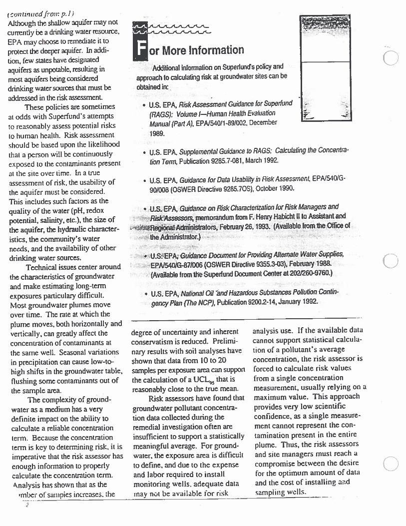
roinsntwdfroa: pi.)Mthough the shallow aquifer may not

currently be a drinking water resource,

EPA may choose to remediate it to

protect the deeper aquifer. In addi

tion, few states have designated

aquifers as unpotable. resulting inmost aquifers being considered

drinking water sources that must be

addressed in the risk assessment.These policies are sometimes

at odds with Superfund’s attempts

to reasonably assess potential risks

to human health. Risk assessment

should be based upon the likelihood

that a person will be continuously

exposed to the contaminants present

at the site overtime. In a true

assessment of risk, the usability of

the aquifer must be considered.This includes such factors as thequaiity of the water (pH, redoxpotential, salinity, etc.), the size ofthe aquifer, the hydraulic character

istics, the community’s waterneeds, and the availability of other

drinking water sources.Technical issues center around

the characteristics of groundwater

and make estimating long-term

exposures parüculaiy difficult.Most groundwater plumes moveover time. The rate at which theplume moves, both horizontally andvertically, can greatly affect theconcentration of contaminants atthe same well. Seasonal variations

in precipitation can cause low-to-high shifts in the groundwater table,flushing some contaminants out ofthe sample area.

The complexity of groundwater as a medium has a verydefinite impact on the ability tocalculate a reliable concentrationterm. Because the concentrationterm is key to determining risk, it isimperative that the risk assessor has

enough information to properlycalculate the concentration term.

Analysis has shown that as the

‘mberof swupies increases, the

degree of uncertainty and inherent

conservatism is reduced. Prelimi

nary results with soil analyses have

shown that data from 10 to 20samples per exposure area can support

the calculation of a UCL95 that isreasonably close to the true mean.

Risk assessors have found that

groundwater pollutant concentra

tion data collected during theremedial investigation often areinsufficient to support a statisticallymeaningful average. For groundwater, the exposure area is difficult

to define, and due to the expenseand labor required to installmonitoring wells, adequate datamay not be available for risk

analysis use. If the available data

cannot support statistical calcula

tion of a pollutant’s average

concentration, the risk assessor is

forced to calculate risk values

from a single concentration

measurement, usually relying on a

maximum value. This approach

provides very low scientific

confidence, as a single measure

ment cannot represent the con

tamination present in the entire

plume. Thus, the risk assessors

and site managers must reach a

compromise between the desire

for the optimum amount of data

and the cost of installing and

sampling wells.

or More InformationAdditional information on Superfunds policy and

approach to calculating risk at groundwater sites can be

obtained in:

U.S. EPA, Risk Assessment Guidance icr Supedund

(RAGS): Volume I—Human Health Evaluation

Manual (Part A), EPN54OI1 -89/002, December

1989.

a

• U.S. EPA, Supplemental Guidance to RAGS: Calculating the Concentra

tion Term, Publication 9285.7-081, March 1992.

• U.S. EPA, Guidance for Data Usability in Risk Assessment, EPNS4WG-

90/008 (OSWER Directive 9285,70S), October 1990.

on Risk Chamctenzation for Risk A1anageis and- - —

- ,HabichtlltoAssistantand- m>theOtfceoh

*

4

ce Document for Providing Altemate Vater Supplies,

bEW54wS$7i0O6 (OSWEH Directive 9355.3-03)Febniary498&

e(Avauable from the Supedund Document Center at202/260-9760.)

• U.S. EPA1 National Oil Sand Hazardous Substances Pollution Contin

gency Plan (The NCP), Publication 92002-14, Januasy 1992.

a

C

C

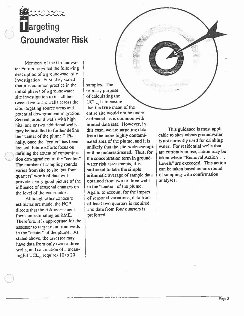
flargetingGroundwater Risk

Members of the Groundwater Forum provided the followingdescription of a grottiidwater siteinvestigation. First, they statedthat it is common practice in the

initial phases of a groundwatersite investigation to install between five to six wells across the

site, targeting source areas and

potential downgradient migration.Second, around wells with highhits, one or two additional wellsmay be installed to further definethe “center of the plume.” Finally, once the “center” has beenlocated, future efforts focus ondefining the extent of contamination downgradient of the “center.”The number of sampling roundsvaries from site to site, but fourquarters’ worth of data willprovide a very good picture of theinfluence of seasonal changes on

the level of the water table.Although other exposure

estimates are made, the NCPdirects that the risk assessmentfocus on estimating an RME.Therefore, it is appropriate for theassessor to target data from wells

in the “center” of the plume. Asstated above, the assessor mayhave data from only two or threewells, and calculation of a meaningful UCL9S requires 10 to 20

samples. Theprimary purposeof calculating theUCL9, is to ensurethat the true mean of theentire site would not be underestimated, as is common withlimited data sets. However, inthis case, we are targeting datafrom the more highly contaminated area of the plume, and it isunlikely that the site-wide averagewill be underestimated. Thus, forthe concentration term in groundwater risk assessments, it issufficient to take the simplearithmetic average of sample dataobtained from two to three wellsin the “center” of the plume.Again, to account for the impactof seasonal variations, data fromat least two quarters is required,

I and data from four quarters ispreferred.

This guidance is most applicable to sites where groundwater

is not currently used for drinkingwater. For residential wells thatare currently in use, action may be

taken where “Removal Action -

Levels” are exceeded. This actioncan be taken based on one roundof sampling with confirmationanalyses.

Page 3

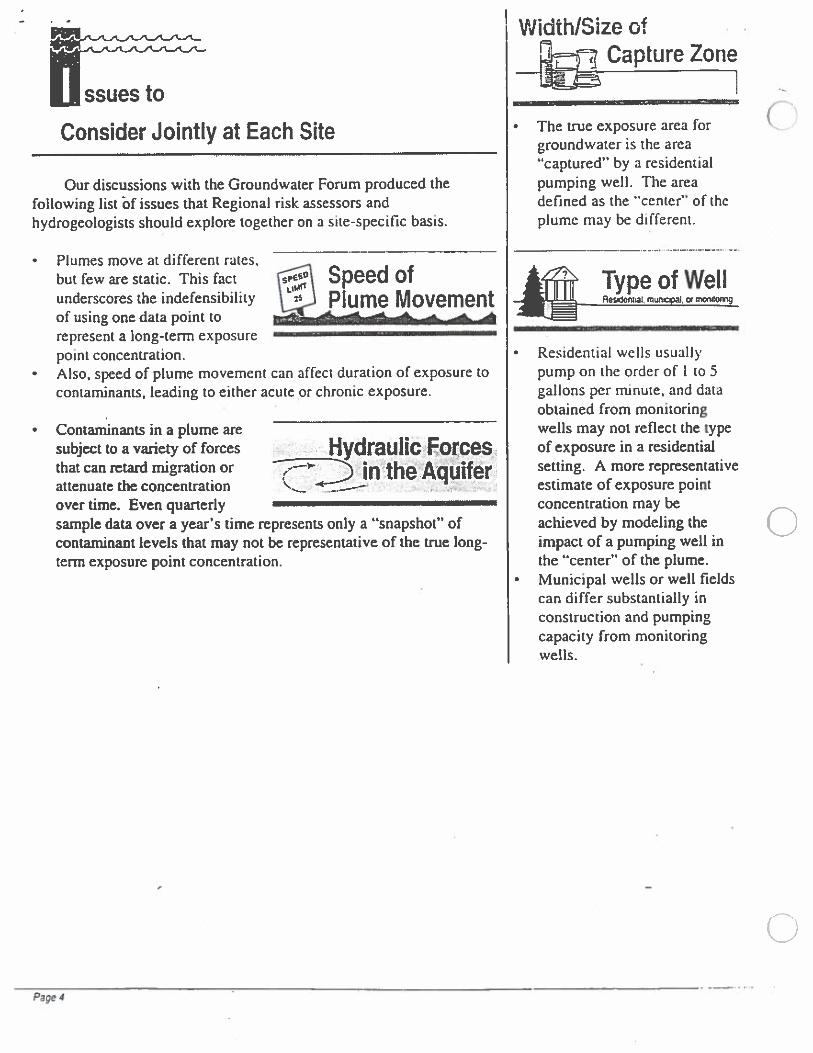
WidthISize of_,Capture Zone

The true exposure area forgroundwater is the area“captured” by a residentialpumping well. The areadefined as the “center” of theplume may be different.

jfffr Type of WellResent2t. muncçal. moiIog

Residential wells usuallypump on the order of I to 5gallons per minute, and dataobtained from monitoringwells may not reflect the typeof exposure in a residentialsetting. A more representativeestimate of exposure pointconcentration may beachieved by modeling theimpact of a pumping well inthe “center” of the plume.Municipal wells or well fieldscan differ substantially inconstruction and pumpingcapacity from monitoringwells,

ssues to

Consider Jointly at Each Site

Our discussions with the Groundwater Forum produced thefollowing list bf issues that Regional risk assessors andhydrogeologists should explore together on a site-specific basis.

• Plumes move at different rates,but few are static. This fact 1\ Speed of

pMfl

underscores the indefensibility \J Plume Movementof using one data point to -a- A

represent a long-term exposurepoint concentration.

• Also, speed of plume movement can affecT duration of exposure tocontaminants, leading to either acute or chronic exposure.

• Contaminants in a plume aresubject to a variety of forces Hydraulic Forcesthat can retard migration or 2”$in!1he Aquiferattenuate the concentrationover time. Even quarterlysample data over a year’s time represents only a “snapshot” ofcontaminant levels that may not be representative of the true long-term exposure point concentration,

C:

U

ATTACHMENT N

A BIBLIOGRAPHY RELATED TO ECOLOGICAL RISK ASSESSMENT

H T4SHJ R[’l5i11INAL MAS11H *PD IiI.R LIh4fl7I

This bibliography is based on a limited literature search and review and is not a complete list of documentsrelated to ecological risk assessment.

U.S. ENVIRONMENTAL PROTECTION AGENCY GUIDANCE

U.S. Environmental Protection Agency. 1994. Ecological Risk Assessment Guidancefor Superfund:Processfor Designing and Conducting Ecological Risk Assessments. Environmental Response Team.Edison, New Jersey. September.

This proposed agency-wide guidance document describes an accepted process for designing andconducting ecological risk assessments under the Superfund program, including methods for calculatingrisk-based cleanup levels. The final version of this guidance document will supersede Risk AssessmentGuidancefor Superfund, Volume II, Environmental Evaluation Manual, which still can be used as a basictutorial on Comprehensive Environmental Response, Compensation, and Liability Act (CERCLA)ecological risk assessment.

EPA. 1993 and 1994. A Review ofEcologicatAssessment Case Studies From a Risk AssessmentPerspective. Volumes 1 and 2. Risk Assessment Forum. Washington, D.C.

EPA scientists present a cross section of ecological assessment case studies. The case studies present avariety of work scopes, ecosystems, ecological endpoints, chemical and nonchemical stressors, andprogrammatic requirements within EPA. The approaches used in the case studies are generally consistentwith some, but not alt, of the principles in the Frameworkfor Ecological RiskAssessment (EPA 1992).While these case studies are useful examples of the “state-of-the-practice,” they should not be regardedmodels to be followed.

EPA. 1992. Frameworkfor Ecological Risk Assessment. EPA/6301R-92/OO1. Risk Assessmentforum. Washington, D.C. February.

This reference should be used in conjunction with other technical guidelines since it is only a conceptualframework and is not considered a “stand alone” guidance document. The framework provides a formatthat facilitates consistent ecological risk assessment formulation at regulated facilities, including ResourceConservation and Recovery Act (RCRA) hazardous waste facilities.

EPA. 1989. The Nature and Extent ofEcological Risks at Superfund Sites and RCRA Facilities.EPA-230-03-89-043. Office of Policy Analysis. Washington, D.C. June.

This report presents the results of a study of ecological risks posed by Superfund sites and RCRA facilities.The report includes discussions of methods used in the identification of sites and review of reports, thenature and extent of ecological threats, and summaries of key findings.

EPA. 1989. Risk Assessment Guidancefor Superfund, Volume II, Environmental EvaluationManual. Interim Final. EPA/540/1-89/OO1. Office of Solid Waste and Emergency Response.Washington, D.C. March.

Risk Assessment Guidance for Superfund (RAGS) Volume II provides conceptual guidance in planningstudies to evaluate the ecology of a site, including RCRA facilities. The draft Ecological RiskAssessmentGuidancefor Superfzind supersedes RAGS Volume II as guidance on how to design and conduct

S REPS R IURIWTSSKS REVISE2 FINALMASThR WPD I I-R IRIIR)7R5 l1111415711 2Spn,, —

ecological risk assessments. RAGS Volume II does include useful information on the regulatory andstatutory bases of ecological risk assessment, basic ecological concepts, and other background informationthat are not presented in RAGS Volume II.

EPA. 1989. Ecological Assessments ofHazardous Waste Sites: A field and Laboratory Reference.EPAJ600/3-891013. Office of Research and Development. Washington, D.C. March.

This document provides introductory discussions on various techniques in ecological risk assessment thatmay be appropriate for RCRA facilities.

The following ECO Updates are ecological risk assessment bulletins intermittently issued by the EPA thatsupplement RAGS Volume II. These bulletins are used to provide technical information that pertains tovarious aspects of ecological risk assessment. The bulletins do not constitute rule making by the EPA.There are currently three volumes of ECO Updates containing specific topics as follows:

Volume 1:

EPA. 1991. The Rote ofBTAGs in Ecological Assessment. Volume 1. Number 1. Office of SolidWaste and Emergency Response. Washington, D.C. September.

This bulletin summarizes the Biological Technical Assistance Group (BTAG) structure and function in theCERCLA process. It explains how the BTAG can assist project managers in evaluating ecological risks. V

EPA. 1991. EcotogicalAssessment ofSuperfund Sites: An Overview. Volume 1. Number 2. Officeof Solid Waste and Emergency Response. Washington, D.C. December.

This bulletin provides an updated framework for ecological assessment in the Superfund (or CERCLA)program. It describes ecological assessment components and how they fit into the remedial investigation V

aI1d feasibility study (RI/FS) process.V

EPA. 1992. The Role ofNatural Resource Trustees in the Superfund Process. Volume 1. Number 3.Office of Solid Waste and Emergency Response. Washington, D.C. March.

This bulletin facilitates the working relationship between project managers involved in site cleanup andnatural resource trustees. It also helps ensure compliance with applicable or relevant and appropriaterequirements (ARAR) and increases understanding of trustee issues relevant to the CERCLA process.

EPA. 1992. Developing a Work Scopefor Ecological Assessments. 1992. Volume 1. Number 4.Office of Solid Waste and Emergency Response. Washington, D.C. May.

This bulletin helps project managers involved in site cleanup to plan and manage ecological assessments aspart of the RI/FS process under CERCLA. It includes information on project scoping, preparingstatements of work, and work plan development.

EPA. 1992. Briefing the BTA G: Initial Description ofSetting, History, and Ecology ofa Site.Volume 1. Number 5. Office of Solid Waste and Emergency Response. Washington, D.C. August.

R[rP RI II T SkI4 REVISE2 FINAL MASTER WPD\I 51 -R 1111 I II7AII IIII4P17/l2IIpDDR —

This bulletin focuses on the first opportunity (usually in the early RI planning stage) that a project managerhas for conferring with the BTAG about possible ecological effects at a site. Pertinent information topresent to the BTAG includes the site’s setting and history, constituents expected. and ecologicalcharacteristics.Volume 2:

EPA. 1994. Using Toxicity Tests in Ecological RiskAssessment. Volume 2. Number 1. Office ofSolid Waste and Emergency Response. Washington, D.C. September.

This bulletin presents measurement endpoints in toxicity testing, elements in a toxicity assessment, andgeneral guidelines for selecting toxicity tests. These tests may help to determine whether concentrations ofCOPECs detected in site media are high enough to cause adverse effects in organisms; demonstratewhether constituents are bioavailable; evaluate the aggregate toxic effects of all hazardous constituents in amedium; and evaluate the toxicity of substances whose biological effects are not well understood.

EPA. 1994. Catalogue ofStandard Toxicity Testsfor Ecological Risk Assessnient. 1994. Volume 2.Number 2. Office of Solid Waste and Emergency Response. Washington, D.C. September.

This bulletin consists of a list of standardized aquatic, sediment, terrestrial, and microbial toxicity testsused at CERCLA sites. It indicates source documents that more fully describe test protocols.

EPA. 1994. Field Studiesfor Ecological Risk Assessment. Volume 2. Number 3. Office of SolidWaste and Emergency Response. Washington, D.C. September.

This bulletin addresses ecological field studies as part of the ecological risk assessment that occur in thearea of ecological concern at a site. It covers important considerations such as the organisms to beevaluated in the field study and elements in the design of a field study. A catalogue of field methods isalso presented.

EPA. 1994. Selecting and Using Reference Information in Superfund Ecological Risk Assessments.Volume 2. Number 4. Office of Solid Waste and Emergency Response. Washington, D.C.September.

This bulletin summarizes methods for identifying and using reference information sources such as existingrelevant data, mathematical models, and new data collected from unimpacted or reference sites.

Volume 3:

EPA. 1996. Ecological Signflcance and Selection of Candidate Assessment Endpoints. Volume 3.Number 1. Office of Solid Waste and Emergency Response. Washington, D.C. January.

This bulletin helps project managers identify ecological elements at a site, estimate their relative value andsignificance in the ecosystem, and identify potential assessment endpoints.

EPA. 1996. Ecotox Thresholds. Volume 3. Number 2. Office of Solid Waste and EmergencyResponse. Washington, D.C. January.

S REPA R IX TASKX RE’.75E2’FINALMASTER WED’ XI .R XXI I XO7IXI’ XI!24IflR 2Opm . —

This bulletin describes how ecotoxicological values are to be used for screening purposes in the Superfundecological risk assessment process. It summarizes the methodologies used to calculate ecotox thresholdsfor each medium and discusses limitations of using ecotox thresholds.

REGION-SPECIFIC U.S. ENVIRONMENTAL PROTECTION AGENCY GUIDANCE

Region 1

EPA. 1989. Supplemental Risk Assessment Guidancefor the Superfund Prograni - Part 2: Guidancefor Ecological Risk Assessments. EPAI9O1/5-69/01. Risk Assessment Work Group. Boston,Massachusetts.

This manual reviews elements of the ecological risk assessment process and the types of data needed toevaluate risks to ecological receptors.

Region 3

EPA. 1994. Interim Ecological Risk Assessment Guidelines. 9107-4431. Hazardous WasteManagement Division. Philadelphia, Pennsylvania.

This draft document briefly summarizes three levels of ecological risk assessment: the screening level, thesemiquantitative level, and the quantitative level.

Region 4

EPA. 1995. Supplemental Guidance to RAGS: Region 4 Bulletins - Ecological Risk Assessment.Draft. Office of Health Assessment. Atlanta, Georgia. November.

This draft document includes bulletins that discuss preliminary risk evaluation or screening-levelecological risk assessment, ecological screening values used to identify COPECs in the screening-levelecological risk assessment, assessment and measurement endpoint selection based on the results of thescreening-level ecological risk assessment, and inclusion of natural resource trustees in the CERCLAprocess.

Region 5

EPA. 1992. Regional Guidancefor Conducting Ecological Assessments. Draft final. Chicago,Illinois. April.

This reference supplements existing CERCLA guidelines; it outlines a framework for conductingecological assessments at Superfund sites.

EPA. 1994. Ecological Risk Assessment Guidancefor RCRA Corrective Action. Interim draft.Waste Management Division. Chicago, Illinois. July.

This is a draft document that discusses ecological risk assessment and how to effectively integrate riskassessment and corrective action processes.

‘ REP R .R I X TASKK REViSE2FINALMASTER WPD’I 5 -R 111R1541711U’ P111-11)7/i 2lpn —

Region 7

EPA. 1995. Assessing Ecological Risk at RCRA Hazardous Waste Treatment, Storage, and Disposalfacilities: A Project Manager’s Guide. Kansas City, Kansas. June.

This guide is design to help project managers and risk managers that are unfamiliar with ecologicalconcepts used in ecological risk assessment. The focus is on evaluating ecological risks posed by RCRAtreatment, storage, and disposal (TSD) facilities in Region 7. The guide relies primarily on CERCLAguidance to provide the framework for ecological risk assessment at RCRA TSD facilities in Region 7.

Region 8

EPA. 1994. Operation ofthe Ecological Technical Assistance Group (ETA G) for EPA Region VIIIEcological Risk Assessments. ER-Ol. Hazardous Waste Management Division. September.

This technical guidance describes the goals of the ETAG (or BTAG) for CERCLA ecological riskassessments in Region 8. ETAGs and BTAGs help EPA achieve better and more consistent ecological riskassessments at CERCLA sites.

Region 10

EPA. 1995. Supplemental Risk Assessment Guidancefor Superfund. Draft. Seattle, Washington.December.

This draft guidance incorporates CERCLA human health and ecological risk assessment guidance. Itsummarizes important concepts for the agency-wide guidance, highlights steps of the CERCLA RI/FSprocess in which risk assessors need to be involved, and identifies specific deliverables required by EPARegion 10 during the development of baseline risk assessments.

DEPARTMENT OF ENERGY GUiDANCE

U.S. Department of Energy (DOE). 1996. Screening Benchmarksfor Ecological Risk Assessment.Version 1.5 (computer database program). Oak Ridge National Laboratory. Oak Ridge,Tennessee. January.

Note: Screening benchmarks approved for use at some DOE facilities are formatted in a computerdatabase format. The database provides screening values for aquatic biota, wildlife, terrestrialplants, sediment-associated organisms, and soil and litter organisms. The sources and derivationof these screening values are presented in the following DOE documents.

Suter II, G.W. and J.B. Mabrey. 1994. Toxicological Benchmarks for Screening ofPotentialContaminants ofConcern for Effects on Aquatic Biota on Oak Ridge Reservation. 1994 Revision.ES/ERJTM-96. Oak Ridge National Laboratory. Oak Ridge, Tennessee.

Opresko, D.M., B.E. Sample, and G.W. Suter II. 1995. Toxicological Benchmarks for Wildlife: 1995Revision. ES/ERJTM-86/R2. Oak Ridge National Laboratory. Oak Ridge, Tennessee.

S REPAR 101110 TASJ REVISE2FINAL MASTER WPD S I -R 0011111700 11024/Sf’S 2Ilpoos.,o —

Will. M.E. and G.W. Suter II. 1995. Toxicological Benchmarksfor Screening Potential Contaminants ofConcernfor Effects on Terrestrial Plants: 1995 Revision. ES/ERJTM-85-R2. Oak Ridge NationalLaboratory. Oak Ridge, Tennessee.

Suter II, G.W., and R.N. Hull. 1994. Toxicological Benchmarks for Screening Contaminants ofPotentialConcern for Effects on Sediment-Associated Biota: 1994 Revision. ESIER/TM-95/R1. Oak RidgeNational Laboratory. Oak Ridge, Tennessee.

Will, M.E. and G.W. Suter II. 1995. Toxicological Benchmarksfor Potential Contaminants of Concernfor Effects on Soil and Litter Invertebrates and Heterotrophic Process. ES/ER/TM- 126/RI. Oak RidgeNational Laboratory. Oak Ridge, Tennessee.

Barnthouse, L.W., et al. 1992. Survey ofEcological Risk Assessment at DOE Facilities. NTISAccession Number: Df93000972/XAB. Oak Ridge National Laboratory. Oak Ridge, Tennessee.

This document is a survey of ecological risk assessment procedures at a subset of major DOE facilities.The survey identifies ecological risk assessment approaches used by DOE and its contractors. Itdocuments lessons learned with these approaches. The survey identifies new technical developments andapproaches that may apply to DOE facilities. The report also identifies major data needs, data resources,and methodological deficiencies.

Suter II, G.W. 1994. Approach and Strategyfor Performing Ecological Risk Assessmentsfor the U.S.Department ofEnergy’s Oak Ridge Reservation. ESIERJTM-33/R1. Oak Ridge NationalLaboratory. Oak Ridge, Tennessee. August.

This document includes guidelines on developing conceptual models for the ecological risk assessmentprocess, selecting assessment and measurement endpoints, specific data requirements, and riskcharacterization.

DEPARTMENT OF DEFENSE GUIDANCE

LaPoint, T.W., M. Simini, J.D. Florian, Jr., and R.S. Wentsel. 1995. Procedural GuidelinesforEcological Risk Assessments at U.S. Army Sites - Volume 2: Research and Biomonitoring Metliodsforthe Characterization ofEcological Effects. Report Number: ERDEC-TR-221. Aberdeen ProvingGround, Maryland. February.

Volume 2 contains information about more than 100 environmental models and test methods used inecological risk assessment. The methodologies are designed to assist risk assessors in selecting appropriatemodels and tests that are relevant to ecological hypotheses and goals of Ris and fSs.

Wentsel, R.S., T.W. LaPoint, M. Simini, D. Ludwig, and L. Brewer. 1994. Procedural Guidelinesfor Ecological Risk Assessments at U.S. Army Sites - Volume 1. Report Number: ERDEC-TR-221.Aberdeen Proving Ground, Maryland. December.

Volume 1 provides ecological risk assessment guidance for U.S. Army National Priority sites and siteslisted under the Base Realignment and Closure program. This report provides an enhanced understandingof CERCLA guidance. cost-effective and tiered procedures, and a conceptual framework to standardize

S REPS 510010 TSSKK’JSE’.7SE2FINALMASThR WPD’ 151.5 100101I71U111U12410713 2l5n —

ecological risk assessments at U.S. Army facilities. The conceptual framework is based on EPA’sagency-wide framework.

NATIONAL OCEANIC and ATMOSPHERIC ADMINISTRATION GUIDANCE

Long, E.R. and L.G. Morgan. 1990. The Potentialfor Biological Effects ofSediment-SorbedContaminants Tested in the National Status and Trends Program. Technical memorandum NOSOMA52. March.

This report assesses the potential for adverse biological effects through exposure of biota to hazardousconstituents in sediments sampled and analyzed under the National Status and Trends Program.Guidelines for assessing potential effects are included and were developed from data assembled for avariety of approaches and many geographic areas.

Long, E.R. 1992. Ranges in chemical concentrations in Sediments Associated with Adverse BiologicalEffects. Marine Pollution Bulletin 24. Volume 1. Pages 38-45.

Data derived from many geographic regions, methods, and approaches are evaluated in this paper toidentify the ranges in chemical concentrations associated with adverse biological effects. Data from threebasic approaches to determining health-based criteria were evaluated: the equilibrium partitioningapproach, the spiked-sediment bioassay approach, and various methods of evaluating biological andchemical data collected during field surveys.

Long, E.R. et al. 1995. “Incidence of Adverse Biological Effects Within Ranges of ChemicalConcentrations in Marine and Estuarine Sediments.” Environmental Management. 19(1): 81-97.

This paper presents effects range-low (ER-L) and effects range-median (ER-M) guideline values forselected chemicals, based on biological and chemical data compiled from numerous modeling, laboratory,and field studies performed in marine and estuarine sediments. The incidence of adverse effects wasquantified within 3 separate concentration ranges for the selected chemicals.

AMERICAN SOCIETY for TESTING and MATERIALS GUIDANCE

American Society for Testing and Materials (ASTM). 1996. Standard Guidefor Selecting and UsingEcological Endpointsfor Contaminated Sites. Draft. ASTM subcommittee E-47.13. January.

This guide presents an approach to identifying, selecting, and using assessment and measurementendpoints that may be affected by direct or indirect chemical and nonchemical stressors associated withwastes and contaminated media at specific sites under current and future land uses. NOTE: According toASTM, this document is a draft and not an ASTM standard. As such, it has not been approved by ASTM.The final approved version of this draft may or may not include the same information as it appears in thisdraft. For more information on this draft, contact ASTM at 100 Barr Harbor Drive, West Conshohocken,Pennsylvania 1942$.

ASTM. 1995. Standard Guidefor Developing Conceptual Site Modelsfor Contaminated Sites.STP 1-1689. ASTM. Philadelphia, Pennsylvania.

S REPS RPSX TASKX REVISE2FINAL).IASThR WPD 9RII 1SI/4,fl1 2n —

This guide assists in the development of conceptual site models used to integrate technical information,support sampling design elements such as identifying data needs and data collection activities, andevaluate risk to human health and the environment posed by a contaminated site.

Gorsuch, J.W., J. Dwyer, C. Ingersoll, and T.W. LaPoint, editors. 1993. Environmental Toxicologyand Risk Assessment - Volume 2. ASTM STP 1216. ISBN 0-8031-1485-0. Philadelphia,Pennsylvania.

This document presents 48 papers on new research techniques, findings concerning various environmentalstressors, and the application of techniques and processes of environmental assessment. Specific topicsinclude aquatic toxicology and the use of experimental ecosystems, plants for toxicity assessments, andsediment toxicology.

Hughes, J.S., G.R. Biddinger, and E. Mones, editors. 1995. Environmental Toxicology and RiskAssessment - Volume 3. ASTM STP 1218. ISBN 0-8031-1485-0. Philadelphia, Pennsylvania.

This text provides a comprehensive overview of the current status of ecological risk assessment andsuggested advances. Also, 22 papers are presented on topics such as models in ecological risk assessment,ecotoxicology and the measurement of ecological effects at various sites, fate and effects of chemicals, andthe development and refinement of new methods to evaluate exposure and toxicity.

Landis, W.G., J.S. Hughes, and M.A. Lewis, editors. 1993. Environmental Toxicology and RiskAssessment. ASTM STP 1179. ISBN 0-8931-1860-0. ASTM. Philadelphia, Pennsylvania.

This document presents 28 papers addressing such topics as evaluating ecological impacts at thepopulation and community levels, biomarkers, and marine toxicity test methods and methods development.Other topics include evaluating regulatory concerns, basic research, risk and hazard assessment, andmethods development in environmental toxicology.

CANADIAN GUIDANCE

Canadian Council of Ministers of the Environment (CCME). 1996. A Frameworkfor EcologicalRisk Assessment-General Guidance. National Contaminated Sites Remediation Program. March.

This document provides general guidance for using the framework for ecological risk assessment atcontaminated sites in Canada. Topics include planning ecological risk assessments, screening-levelassessments, and preliminary and detailed quantitative ecological risk assessments.

CCME. 1996. A Protocolfor the Derivation ofEnvironmental and Human Health Soil QualityGuidelines. National Contaminated Sites Remediation Program. March.

This document includes rationale and guidance for developing environmental and human health soilquality guidelines for contaminated sites in Canada. Topics include derivation of environmental soilquality guidelines, relevant endpoints for deriving soil quality guidelines, potential ecological receptors andexposure pathways of soil contamination, and uncertainties in guidelines derivation.

CCME. 1995. Protocolfor the Derivation of Canadian Sediment Quality Guidelinesfor the ProtectionalAquatic Life. CCME EPC-98E. Environment Canada. Ottawa, Canada. March.

S REPA RI IK TASKS REVISE2FINALMASThR WPD15 I-k lIE ISII7ISSIOI24I17/l 2lm,S, —

These guidelines can be used to assess sediment quality, help set goals for sediment quality that willsustain aquatic system health for the long term, and develop site-specific objectives. The documentoutlines procedures for deriving scientifically defensible sediment quality guidelines for the protection ofaquatic life. The document also discusses the use of sediment quality guidelines as benchmarks, theNational Status and Trends Program (NSTP) approach, the spiked-sediment toxicity approach, andderivation of safety factors.

Gaudet, C. 1994. A frameworkfor Ecological Risk Assessment at Contaminated Sites in Canada:Review and Recommendations. Scientific Series Number 199. Environment Canada. Ottawa,Canada.

This document presents the ecological risk assessment framework for the National Contaminated SitesRemediation Program. The framework includes a tiered approach to ecological risk assessment. Thedocument discusses ecological risk assessment components such as problem definition, exposureassessment, receptor characterization, hazard assessment, and risk characterization.

Jaagumagi, R. 1993. Development of tite Ontario Provincial Sediment Quality Guidelinesfor Arsenic,Cadmium, Chromium, Copper, Iron, Lead, Manganese, Mercury, Nickel, and Zinc. ISBN0-7729-9249-5. Ontario Ministry of the Environment. Canada. August.

This document describes the derivation of the metals guidelines and summarizes data used to derive thevalues listed in the guidelines. The document also summarizes properties and fate of the metals, describesthe forms in which metals can exist in sediments, and provides details of the calculations used to arrive atthe sediment quality guidelines.

Jaagumagi, R. 1994. Development of the Ontario Provincial Sediment Quality GuidelinesforPolycyclic Aromatic Hydrocarbons. ISBN 0-7778-1710-1. Ontario Ministry of the Environment.Canada. January.

This document describes the derivation of the guidelines for 12 individual polycyclic aromatichydrocarbons (PAR) as well as total PAR and summarizes data used to derive these values. The documentalso summarizes the fate of PARs in sediments, and provides details of the calculations of the sedimentquality guidelines.

Keddy, C., J.C. Greene, and M.A. Bonnell. 1994. A Review of Whole Organism BioassaysforAssessing the Quality ofSoil, Freshwater Sediment, and Freshwater in Canada. Scientific SeriesNumber 198. Ecosystem Conservation Directorate. Ontario, Canada.

This report addresses application of recommended bioassays to site assessment and remediation. Thereport identifies potentially suitable test methods, assesses their applicability, and recommends tests forsoil, freshwater sediment, and fresh water. The report also evaluates the future for hazardous constituentassessment using biological organisms, including alternative test endpoints, in situ tests, and assessmentbeyond whole organisms and fresh water, such as methods for assessing impacts to microbial processesand multispecies testing.

Persaud, D., R. Jaagumagi, and A. Hayton. 1993. Guidelinesfor the Protection and Management ofAtiuatic Sediment Quality in Ontario. ISBN 0-7729-9248-7. Ontario Minister of the Environment.Canada. August.

S REPA .R IDA IX TASIX REV1SE1fINALMASThR WPD Ii I-R IDAIDA7IXIID/24/A7I 2pns —

The purpose of the sediment quality guidelines is to protect aquatic systems by setting safe concentrationsfor metals, nutrients, and organic compounds. The guidelines help decision makers with sediment issues,including determining which sediments are contaminated and how to effectively manage the problem. Theguidelines establish three levels of effect: no effect level, lowest effect level, and severe effect level.

ADDITIONAL GUIDANCE

Bartell, S.M., R.H. Gardner, and R.V. O’Neill. 1992. Ecological Risk Estimation. ISBN0-873711637. Lewis Publishers. Chelsea, Michigan.

This publication presents an approach to estimating ecological risks using laboratory toxicity data topredict ecological consequences of toxic chemicals. The text includes discussions of the followingsubjects: toxicological and ecological data for risk analysis, modeling aquatic ecosystems, modelingsublethal toxic effects, predicting risks, evaluating predictive methodology, and comparisons of predictedand measured effects.

Burmaster, D.E. and P.D. Anderson. 1994. “Principles of Good Practice for the Use of MonteCarlo Techniques in Human Health and Ecological Risk Assessment.” Risk Analysis. Volume 14.Pages 477-481.

This paper proposes 14 principles of good practice in performing and reviewing probabilistic or MonteCarlo risk assessments of toxic chemicals in the environment. Monte Carlo risk assessments that followthese principles will be easier to understand, will explicitly distinguish assumptions from data, and willconsider and quantify effects that could otherwise lead to misinterpretation of the results.

Calabrese, E.J. and L.A. Baldwin. 1993. Performing Ecological Risk Assessments. LewisPublishers. Chelsea, Michigan.

This text presents an extensive compilation that addresses components of an ecological risk assessment,including environmental fate modeling and pharmacokinetic factors, uncertainty factors, derivingchemical-specific and species-specific maximum acceptable tissue concentrations, and sediment qualitycriteria.

Cairns, J., B.R. Niederlehner, and P.R. Orvos, editors. 1992. Predicting Ecosystem Risk. VolumeXX. Princeton Scientific Publishing Company. Princeton, New Jersey.

This text includes a series of papers on topics such as predicting ecological risks posed by changes inhydrological regime, forest management, genetically engineered microorganisms and products, highways,and radioactive materials. The use of experimental stream mesocosms in assessing risks is also discussed.

Cardwell, R., et al. 1991. Aquatic Risk: An Assessment Report. Evaluation ofthe ProtocolsforAquatic Ecological Risk Assessment. Water Environment Research Foundation Order Number:D0005. Alexandria, Virginia.

This report evaluates aquatic and ecological risk models. Additional research is identified to help developa conceptual framework to integrate, organize, and validate aquatic ecological risk assessment protocols,and to apply these protocols to water quality issues.

S REPA RI RI S TASKSREVISE2FINALMASThR WPD’ 51-S I(5115117(51k111123117R 2IIpns —

Clifford, P.A., D.E. Barchers, D.F. Ludwig, R.L. Sietken, J.S. Klingensmith, R.V. Graham, and M.LBanton. 1995. “An Approach to Quantifying Spatial Components of Exposure for Ecological RiskAssessment.” Environmental Toxicology and Chemistry. Volume 14. Pages 895-906.

This paper presents an approach to quantifying spatial components of exposure using the GeographicInformation System (GIS). GIS is used to estimate spatially weighted exposure concentrations within anorganism’s foraging or exposure ranges. GIS is also used for comparing exposure concentrations tobenchmark concentrations and presenting site-specific results in a three-dimensional format to effectivelypresent site-specific quantified ecological risks and to provide an effective risk managementdecision-making tool.

International Atomic Energy Agency. 1992. Effects ofIonizing Radiation on Plants and Anintals atLevels Implied by Current Radiation Protection Standards. Technical Report Series Number 332.ISBN 92-0-100992-5. Vienna, Austria.

This report addresses potential effects on plant and animal populations through chronic releases ofradionuclides. The report includes reviews of available information on the effects of ionizing radiation onnatural organisms and determines the doses above which there are adverse effects to plants and animals.The report also establishes whether on not plant and animal populations are adequately protected underradiation protections standards for humans.

Landis, W.G., G.B. Matthews, R.A. Matthews, and A. Sergeant. 1994. “Application of MultivariateTechniques to Endpoint Determination, Selection, and Evaluation in Ecological Risk Assessment.”Environmental Toxicology and Chemistry. Volume 13. Pages 1917 - 1927.

The paper reviews the role of ecological endpoints and introduces and discusses the ramifications ofmultivariate analysis on the assessment of risk to ecological systems. Three methods are discussed in thepaper: the mean strain measurement, the state-space analysis, and the nonmetric clustering method.

MacDonald, D.D. 1994. Approach to the Assessment ofSediment Quality in Florida Coastal Waters,Volume 1 - Development and Evaluation ofSediment Quality Assessment Guidelines. MacDonaldEnvironmental Sciences, Ltd. British Columbia, Canada. November.

This report recommends a scientifically defensible framework for assessing the biological significance ofsediment-associated hazardous constituents. Numerical sediment quality assessment guidelines (SQAG)provide the basis for assessing potential effects of sediment-associated constituents. The report reviews avariety of approaches and recommends an integrated strategy and relevant assessment tools. The SQAGsare derived from a variety of sediment quality data and are based on a weight-of-evidence approach thatlinks constituent concentrations with adverse biological effects.

MacDonald, D.D. 1994. Approach to the Assessment ofSediment Quality in Florida Coastal Waters,Volume 2 - Application of the Sediment Quality Assessment Guidelines. MacDonald EnvironmentalSciences, Ltd. British Columbia, Canada. November.

This document assists potential users in applying SQAGs and other relevant sediment quality assessmenttools. The report lists applications of SQAGs that are considered inappropriate and presents a frameworkfor assessing the significance of sediment-associated constituents.

S REPS R WO IS TASKS REVISE2FINALMASTtR WPD I -R IIRI SS7ISI\ 5524117/1 2Rpnsss. —

MacIntosh, D.L., G.W. Suter II, and F.O. Hoffman. 1994. “Use of Probabilistic Exposure Modelsin Ecological Risk Assessments of Contaminated Sites.” Risk Analysis. Volume 14. Pages 405 -419.

This paper discusses the use stochastic food web models in ecological risk assessment, particularly inestimating exposure to endpoint species as well as subsequent effects and determining cleanup levels byestimating concentrations in environmental media that will not cause significant adverse effects in endpointspecies.

Maughan, J.T. 1993. EcologicalAssessment ofHazardous Waste Sites. ISBN 0-442-01091-5. VanNostrand Reinhold. New York, New York.

Essential technical and regulatory information necessary to plan, prepare, and implement an ecological riskassessment is presented in this text. The ecological risk assessment process is examined along withtechniques for evaluating three important components of ecological risk assessments: terrestrial pathwaysof constituents, sediment quality and contamination, and toxicity testing.

McCarthy, J.F. and L.R. Shugart, editors. 1990. Biomarkers ofEnvironmental Contamination.ISBN 0-87371-284-6. Lewis Publishers. Boca Raton, Florida.

This text provides and introduction and review of the research on biological markers in plants as well asanimals and provides an approach to evaluating ecological and health effects of environmentalcontamination. The focus is on the development, application, and validation of biological markers asindicators of exposure to toxic chemicals or as predictors of the averse consequences of that exposure.

Peterle, T.J. 1991. Witdt[e Toxicology. Van Nostrand Reinhold. New York, New York.

This text provides information on environmental pollution as it affects wildlife. The text covers relevantlaws and regulations, materials found in environmental pollutants, transport and distribution in naturalsystems, accumulation in organisms, lethal and chronic effects on organisms, and effects on ecosystems.

Suter II, G.W. 1993. Ecological Risk Assessment. ISBN 0-87371-875-5. Lewis Publishers. Chelsea,Michigan.

This text emphasizes risks to aquatic systems because of the preponderance of data and modelingtechniques for aquatic systems. There are also more ecological risk assessments that address aquatic ratherthan terrestrial systems. Predictive risk assessments are the main focus because the risk assessmentparadigm is based on predictive assessments. A chapter in the text is dedicated to retrospectiveassessments. Chemical, physical, and biological stressors are discussed in the text. Effects of exposure tochemicals and fate and transport of chemicals are discussed. This text also refers to other literatureconcerning ecological risk assessment.

Suter II, G.W. 1990. “Endpoints for Regional Ecological Risk Assessments.” EnvironmentalManagenwnt. Volume 14. Pages 19 - 23.

This article distinguishes between assessment and measurement endpoints in terms of their roles inecological risk assessment. Topics include endpoint selection criteria and regional ecosystem effects.

S REPS P10015 TSSKN REVISE1FINALMASTER WPDISI-RP5)l$l)71511111/24197fl 2,rnS —

ATTACHMENT 0

EPA GUiDANCE AND POLICY FOR PROBABILISTIC RISK ASSESSMENT

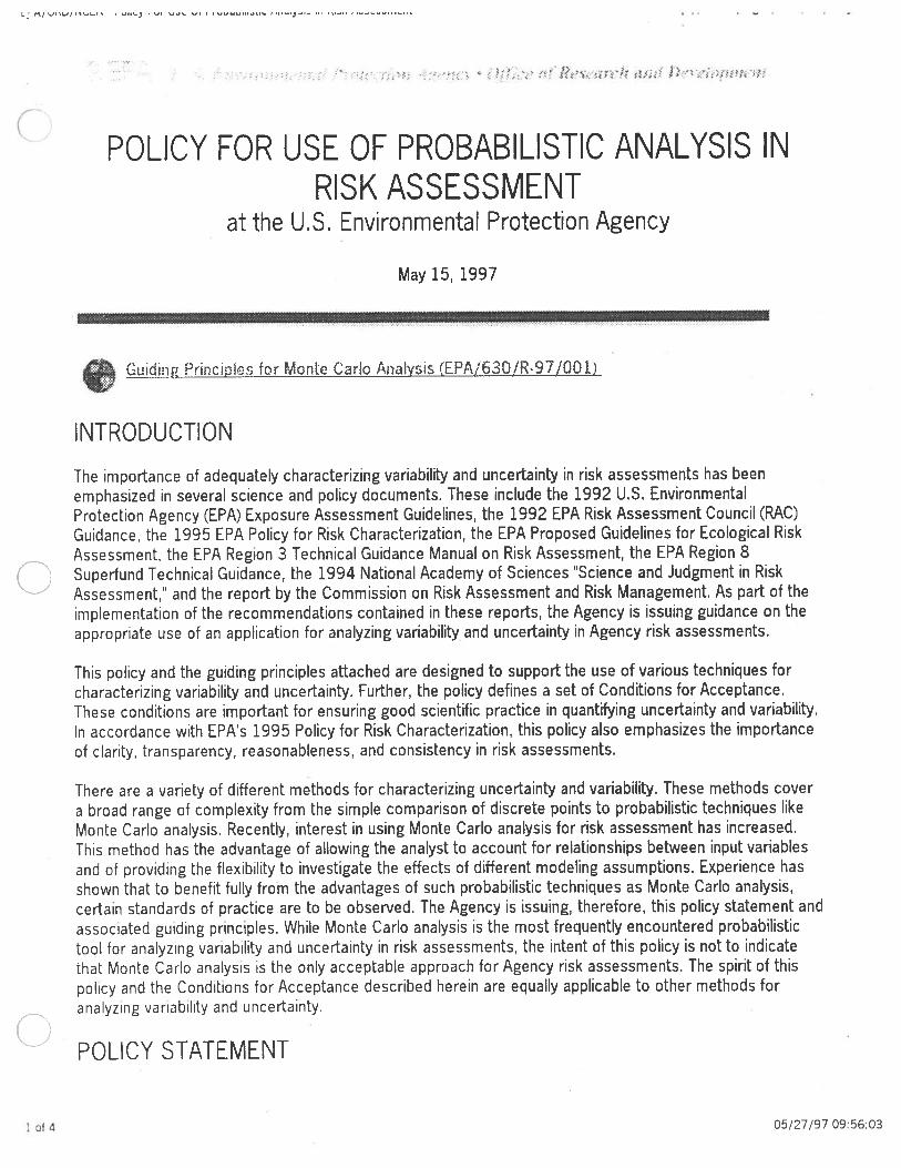
C ‘-“j’- ‘‘•‘.“—

POLICY FOR USE OF PROBABILISTIC ANALYSIS INRISK ASSESSMENT

at the U.S. Environmental Protection Agency

May 15, 1997

Guiding Principles for Monte Carlo Analysis (EPA/63O/R97/OOl)

INTRODUCTION

The importance of adequately characterizing variability and uncertainty in risk assessments has beenemphasized in several science and policy documents. These include the 1992 U.S. EnvironmentalProtection Agency (EPA) Exposure Assessment Guidelines, the 1992 EPA Risk Assessment Council (RAC)Guidance, the 1995 EPA Policy for Risk Characterization, the EPA Proposed Guidelines for Ecological RiskAssessment, the EPA Region 3 Technical Guidance Manual on Risk Assessment, the EPA Region 8Superfund Technical Guidance, the 1994 National Academy of Sciences ‘Science and Judgment in RiskAssessment,” and the report by the Commission on Risk Assessment and Risk Management. As part of theimplementation of the recommendations contained in these reports, the Agency is issuing guidance on theappropriate use of an application for analyzing variability and uncertainty in Agency risk assessments.

This policy and the guiding principles attached are designed to support the use of various techniques forcharacterizing variability and uncertainty. Further, the policy defines a set of Conditions for Acceptance.These conditions are important for ensuring good scientific practice in quantifying uncertainty and variability.In accordance with EPA’s 1995 Policy for Risk Characterization, this policy also emphasizes the importanceof clarity, transparency, reasonableness, and consistency in risk assessments.

There are a variety of different methods for characterizing uncertainty and variability. These methods covera broad range of complexity from the simple comparison of discrete points to probabilistic techniques likeMonte Carlo analysis. Recently, interest in using Monte Carlo analysis for risk assessment has increased.This method has the advantage of allowing the analyst to account for relationships between input variablesand of providing the flexibility to investigate the effects of different modeling assumptions. Experience hasshown that to benefit fully from the advantages of such probabilistic techniques as Monte Carlo analysis,certain standards of practice are to be observed. The Agency is issuing, therefore, this policy statement andassociated guiding principles. While Monte Carlo analysis is the most frequently encountered probabilistictool for analyzing variability and uncertainty in risk assessments, the intent of this policy is not to indicatethat Monte Carlo analysis is the only acceptable approach for Agency risk assessments. The spirit of thispolicy and the Conditions for Acceptance described herein are equally applicable to other methods foranalyzing variability and uncertainty.

POLICY STATEMENT

1 05/27/97 09:56:03

EPA/ORD/NCEA Policy For Use Of Probabilistic Analysis in Risk Assessment http://www.epa.govincea,mcpolicyhtm

It is the policy of the U.S. Environmental Protection Agency that such probabilistic analysis techniques asMonte Carlo analysis, given adequate supporting data and credible assumptions. can be viable statisticaltools for analyzing variability and uncertainty in risk assessments. As such, and provided that the conditionsdescribed below are met, risk assessments using Monte Carlo analysis or other probabilistic techniques willbe evaluated and utilized in a manner that is consistent with other risk assessments submitted to the Agencyfor review or consideration. It is not the intent of this policy to recommend that probabilistic analysis beconducted for all risk assessments supporting risk management decisions. Such analysis should be a part ofa tiered approach to risk assessment that progresses from simpler (e.g., deterministic) to more complex(e.g., probabilistic) analyses as the risk management situation requires. Use of Monte Carlo or other suchtechniques in risk assessments shall not be cause, per Se, for rejection of the risk assessment by theAgency. For human health risk assessments, the application of Monte Carlo and other probabilistictechniques has been limited to exposure assessments in the majority of cases. The current policy,Conditions for Acceptance and associated guiding principles are not intended to apply to dose responseevaluations for human health risk assessment until this application of probabilistic analysis has been studiedfurther. In the case of ecological risk assessment, however, this policy applies to all aspects includingstressor and dose •response assessment.

CONDITIONS FOR ACCEPTANCE

When risk assessments using probabilistic analysis techniques (including Monte Carlo analysis) are submittedto the Agency for review and evaluation, the following conditions are to be satisfied to ensure high qualityscience. These conditions, related to the good scientific practices of transparency, reproducibility, and theuse of sound methods, are summarized here and explained more fully in the Attachment, “Guiding Principlesfor Monte Carlo Analysis.”

1. The purpose and scope of the assessment should be clearly articulated in a “problem formulation”section that includes a full discussion of any highly exposed or highly susceptible subpopulationsevaluated (e.g., children, the elderly). The questions the assessment attempts to answer are to bediscussed and the assessment endpoints are to be well defined.

2. The methods used for the analysis (including all models used, all data upon which the assessment isbased, and all assumptions that have a significant impact upon the results) are to be documented andeasily located in the report. This documentation is to include a discussion of the degree to which thedata used are representative of the population under study. Also, this documentation is to include thenames of the models and software used to generate the analysis. Sufficient information is to beprovided to allow the results of the analysis to be independently reproduced.

3. The results of sensitivity analyses are to be presented and discussed in the report. Probabilistictechniques should be applied to the compounds, pathways, and factors of importance to theassessment, as determined by sensitivity analyses or other basic requirements of the assessment.

4. The presence or absence of moderate to strong correlations or dependencies between the inputvariables is to be discussed and accounted for in the analysis, along with the effects these have onthe output distribution.

5. Information for each input and output distribution is to be provided in the report. This includes tabularand graphical representations of the distributions (e.g., probability density function and cumulativedistribution function plots) that indicate the location of any point estimates of interest (e.g.. mean.median, 95th percentile). The selection of distributions is to be explained and justified. For both theinput and output distributions, variability and uncertainty are to be differentiated where possible.

6. The numerical stability of the central tendency and the higher end (i.e., tail) of the output distributionsare to be presented and discussed.

7. Calculations of exposures and risks using deterministic (e.g., point estimate) methods are to bereported if possible. Providing these values will allow comparisons between the probabilistic analysisand past or screening level risk assessments. Further, deterministic estimates may be used toanswer scenario specific questions and to facilitate risk communication. When comparisons are

2of4 05/2797095603

L’1i1 URU/ INLCfl UIIt t ul Uat csl F I UUQUIIIaLIC nI raryaia iii ii an auja rrrrrt ‘“p., .,,.., . ,

answer scenario specific questions and to facilitate risk communication. When comparisons aremade, it is important to explain the similarities and differences in the underlying data, assumptions,and models.

8. Since fixed exposure assumptions (e.g., exposure duration, body weight) are sometimes embedded inthe toxicity metrics (e.g., Reference Doses, Reference Concentrations, unit cancer risk factors), theexposure estimates from the probabilistic output distribution are to be aligned with the toxicity metric.

LEGAL EFFECT

This policy and associated guidance on probabilistic analysis techniques do not establish or affect legaltights or obligations. Rather, they confirm the Agency position that probabilistic techniques can be viablestatistical tools for analyzing variability and uncertainty in some risk assessments. Further, they outlinerelevant Conditions for Acceptance and identify factors Agency staff should consider in implementing thepolicy.

The policy and associated guidance do not stand alone; nor do they establish a binding norm that is finallydeterminative of the issues addressed. Except where otherwise provided by law, the Agency’s decision onconducting a risk assessment in any particular case is within the Agency’s discretion. Variations in theapplication of the policy and associated guidance, therefore, are not a legitimate basis for delaying action onAgency decisions.

IMPLEMENTATION

Assistant Administrators and Regional Administrators are responsible for implementation of this policy withintheir organizational units. The implementation strategy is divided into immediate and follow-up activities.

Immediate Activities

To assist EPA program and regional offices with this implementation, initial guidance on the use of oneprobabilistic analysis tool, Monte Carlo analysis, is provided in the Attachment, “Guiding Principles for MonteCarlo Analysis” (EPA/630/R.97/OO1). The focus of this guidance is on Monte Carlo analysis because it isthe most frequently encountered technique in human health risk assessments. Additional information may befound in the Summary Report for the Workshop on Monte Carlo Analysis” (EPA/630/R.96/O1O). This reportsummarizes discussions held during the May 1996 Risk Assessment Forum sponsored workshop thatinvolved leading experts in Monte Carlo analysis.

Follow-Up Activities

To prepare for the use and evaluation of probabilistic analysis methods, including Monte Carlo analysis,within the next year, EPA’s Risk Assessment Forum (RAF) will develop illustrative case studies for use asguidance and training tools, Further, the RAF will organize workshops or colloquia to facilitate thedevelopment of distributions for selected exposure factors. EPA’s National Center for EnvironmentalAssessment (NCEA) will develop an Agency training course on probabilistic analysis methods, includingMonte Carlo analysis for both risk assessors and risk managers which will become available during FiscalYear (FY) 1997 or FY 1998. Also, NCEA will develop detailed technical guidance for the quantitative analysisof variability and uncertainty.

In the longer term, various Regions, Programs and the Office of Research and Development (ORD) may needto modify existing or develop new guidelines or models to facilitate use of such techniques as Monte Carloanalysis. Also, the NCEA will revise or update the Exposure Factors Handbook to include distributional

3 4 05/27/97 09:56:03

EPA/ORD/NCEA . Policy For Use Of Probabilistic Analysis in Risk Assessment http://wwwepa.gov/ncea/mcpohcyhtm

information. ORD’s National Exposure Research Laboratory

(NERL) has formed a modeling group that may provide assessment and analysis advice to Program andRegional Offices. The issue of using probabilistic techniques, including Monte Carlo analysis in the doseresponse portion of human health risk assessments requires further study. NCEA will conduct research inthis area and additional guidance will be provided if necessary.

Fred Hansen

Deputy Administrator

Send Comments I Search I NCEA Home Page I ORD Home Page I

Last Revised: May 21, 1997URL: http://www.epa.gov/ncea/mcpoiicy.htm

0

0

4 of 4 05 /27/97 09:5&04

EPA/630/R-97/OO IMarch 1997

Guiding Principles for Monte CarloAnalysis

Technical Panel

Office of Prevention, Pesticides, and Toxic Substances

Michael Firestone (Chair) Penelope fenner-Cnsp

Office of Policy, Planning, and Evaluation

Timothy Barry

Office of Solid Waste and Emergency Response

David Bennett Steven Chang

Office of Research and Development

Michael Callahan

Regional Offices

AnneMane Burke (Region I) Jayne Michaud (Region I)Marian Olsen (Region II) Patricia Cirone (Region X)

Science Advisory Board Staff

Donald Barnes

Risk Assessment Forum Staff

William P. Wood Steven M. Knott

Risk Assessment ForumL.S . Environmental Protection Agency

Washington, DC 20460

DISCLAIMER

This document has been reviewed in accordance with U.S. Environmental Protection

Agency policy and approved for publication. Mention oftrade names or commercial products

does not constitute endorsement or recommendation for use.

..

0

ii 0

TABLE OF CONTENTS

Preface iv

Introduction 1

Fundamental Goals and Challenges 3

When a Monte Carlo Analysis Might Add Value to a Quantitative Risk Assessment 5

Key Terms and Their Definitions 6

Preliminary Issues and Considerations 9

Defining the Assessment Questions 9

Selection and Development of the Conceptual and Mathematical Models . I 0

Selection and Evaluation ofAvailable Data 10

Guiding Principles for Monte Carlo Analysis 1 1

Selecting Input Data and Distributions for Use in Monte Carlo Analysis 1 1

Evaluating Variability and Uncertainty 15

Presenting the Results ofa Monte Carlo Analysis 17

A ppen dix Probabi I ity Di stri buti on Sel ection Issues 22

References Cited in Text 29

111

PREFACE ‘

0The US. Environmental Protection Agency (EPA) Risk Assessment Forum was

established to promote scientific consensus on risk assessment issues and to ensure that this

consensus is incorporated into appropriate risk assessment guidance. To accomplish this. the Risk

Assessment forum assembles experts throughout EPA in a formal process to study and report on

these issues from an Agency-wide perspective. For major risk assessment activities, the Risk

Assessment Forum has established Technical Panels to conduct scientific reviews and analyses.

Members are chosen to assure that necessary technical expertise is available.

This report is part of a continuing effort to develop guidance covering the use of

probabilistic techniques in Agency risk assessments. This report draws heavily on the

recommendations from a May I 996 workshop organized by the Risk Assessment Forum that

convened experts and practitioners in the use ofMonte Carlo analysis, internal as well as external

to EPA, to discuss the issues and advance the development ofguiding principles concerning how

to prepare or review an assessment based on use of Monte Carlo analysis. The conclusions and

recommendations that emerged from these discussiàns are summarized in the report “Summary

Report for the Workshop on Monte Carlo Analysis” (EPA/6301R-96/OlO). Subsequent to the

workshop, the Risk Assessment Forum organized a Technical Panel to consider the workshop

recommendations and to develop an initial set of principles to guide Agency risk assessors in the ‘‘

use ofprobabilistic analysis tools including Monte Carlo analysis. It is anticipated that there will

be need for further expansion and revision ofthese guiding principles as Agency risk assessors

gain experience in their application.

iv . . . C)

IntroductionThe importance of adequately characterizing variability and uncertainty in fate, transport,

exposure. and dose-response assessments for human health and ecological risk assessments has

been emphasized in several U.S. Environmental Protection Agency (EPA) documents and

activities. These inc]ude:

. the 1 986 Risk Assessment Guidelines;

. the 1992 Risk Assessment Council (RAC) Guidance (the Habicht memorandum);

. the 1992 Exposure Assessment Guidelines; and

. the I 995 Policy for Risk Characterization (the Browner memorandum).

As a follow up to these activities EPA is issuing this policy and preliminary guidance on

usin probabilistic analysis. The policy documents the EPA’s position “that such probabilistic

analysis techniques as Monte Carlo analysis, given adequate supporting data and credible

assumptions, can be viable statistical tools for analyzing variability and uncertainty in risk

assessrnents.’ The policy establishes conditions that are to be satisfied by risk assessments that

use probabilistic techniques. These conditions relate to the good scientific practices of clarity,

consistency, transparency, reproducibility, and the use ofsound methods.

The EPA policy lists the following conditions for an acceptable risk assessment that uses

probabilistic analysis techniques. These conditions were derived from principles that are

presented later in this document and its Appendix. Therefore, after each condition, the relevant

pnnciples are noted.

I . The purpose and scope ofthe assessment should be clearly articulated in a ‘problem

formulation” section that includes a full discussion ofany highly exposed or highly

susceptible subpopulations evaluated (e.g., children, the elderly, etc.). The questions

the assessment attempts to answer are to be discussed and the assessment endpoints

are to be well defined.

2 The methods used for the analysis (including all models used, all data upon which the

assessment is based, and all assumptions that have a significant impact upon the

results) are to be documented and easily located in the report. This documentation is

to include a discussion ofthe degree to which the data used are representative ofthe

population under sdy. Also, this documentation is to include the names ofthe C)models and software used to generate the analysis. Sufficient information is to be

provided to allow the results ofthe analysis to be independently reproduced.

(Principles 4, 5, 6, and 1 1)

3. The results ofsensitivity analyses are to be presented and discussed in the report

Probabilistic techniques should be applied to the compounds, pathways, and factors of

importance to the assessment, as determined by sensitivity analyses or other basic

requirements ofthe assessment. (Principles I and 2)

4. The presence or absence of moderate to strong correlations or dependencies between

the input variables is to be discussed and accounted for in the analysis, along with the

effects these have on the output distribution. (Principles I and 14)

5. Information for each input and output distribution is to be provided in the report. This

includes tabular and graphical representations ofthe distributions (e.g., probability

density function and cumulative distribution function plots) that indicate the location

ofany point estimates ofinterest (e.g., mean, median, 95th percentile). The selection

. ofdistributions is to be explained andjustified. for both the input and output

distributions, variability and uncertainty are to be differentiated where possibte.

(Principles 3, 7, 8, 10, 12, and 13)

6. The numerical stability ofthe central tendency and the higher end (i.e., tail) of the

output distributions are to be presented and discussed. (Principle 9)

7. Calculations ofexposures and risks using deterministic (e.g., point estimate) methods

are to be reported ifpossible. Providing these values will allow comparisons between

the probabilistic analysis and past or screening level risk assessments. Further.

deterministic estimates may be used to answer scenario specific questions and to

facilitate risk communication. When comparisons are made, it is important to explain

the similarities and differences in the underlying data, assumptions, and models.

(Principle 15).

0

8. Since fixed exposure assumptions (e.g., exposure duration, body weight) are

sometimes embedded in the toxicity metrics (e.g., Reference Doses, Reference

. Concentrations, unit cancer risk factors), the exposure estimates from the probabilistic

output distribution are to be aligned with the toxicity metric.

The following sections present a general framework and broad set of principles important

for ensuring good scientific practices in the use ofMonte Carlo analysis (a frequently encountered

tool for evaluating uncertainty and variability). Many of the principles apply generally to the

various techniques for conducting quantitative analyses ofvariability and uncertainty; however,

the focus ofthe following principles is on Monte Carlo analysis. EPA recognizes that quantitative

risk assessment methods and quantitative variability and uncertainty analysis are undergoing rapid

development. These guiding principles are intended to serve as a minimum set ofprinciples and

are not intended to constrain or prevent the use of new or innovative improvements where

scientifically defensible.

Fundamental Goals and ChallengesIn the context of this policy, the basic goal of a Monte Carlo analysis is to chatacterize,

quantitatively, the uncertainty and variability in estimates ofexposure or risk. A secondary goal is

to identify key sources of variability and uncertainty and to quantify the relative contribution of

these sources to the overall variance and range of model results.

Consistent with EPA principles and policies, an analysis ofvariability and uncertainty

should provide its audience with clear and concise information on the variability in individual

exposures and risks it should provide information on population risk (extent of harm in the

exposed population), it should provide information on the distribution ofexposures and risks to

hihlv exposed or highly susceptible popuIations it should describe qualitatively and

quantitatively the scientific uncertainty in the models applied, the data utilized, and the specific

risk estimates that are used.

Ultimately, the most important aspect of a quantitative variability and uncertainty analysis

may well be the process of interaction between the risk assessor, risk manager and other

interested parties that makes risk assessment into a dynamic rather than a static process.

Questions for the risk assessor and risk manager to consider at the initiation ofa quantitative

\arlahIIItv and uncertainty analysis include:

. Will the quantitative analysis ofuncertainty and variability improve the riskassessment?

. What are the major sources ofvariahthry and uncertainty? lou’ wi/i iaitahi/iRand uncertainly be kept separate in the analysis?

0 Are there time and resources to complete a complex w,aiysis.?

. Does the project warrant this level ofeffort ?

. Will a quantitative estimate ofuncertainty improve the decision? How u/Il theregulatory decision be affected by this variability and itncertainty analysis?

. What types ofskills and experience are needed to perform the analysis?

. Have the weaknesses and strengths of/he methods been eiahta/ed?

. How will the variability and uncertainty analysis be communicated to the pith/icand decision makers?

One ofthe most important challenges facing the risk assessor is to communicate,

effectively, the insights an analysis ofvañability and uncertainty provides. It is important for the

risk assessor to remember that insights will generally be qualitative in nature even though the

models they derive from are quantitative. Insights can include:

. An appreciation ofthe overall degree ofvariabiiity and uncertainty and theconfidence that can be placed in the analysis and itsfindings.

. An understanding ofthe key sources of variability and key sources of uncertain/iand their impacts on the analysis.

. An itnderstanthng ofthe critical assttmptiotis and their importance to the a/ia!vsisandfindings.

a An understanding ofthe itnimportant assumptions and why they are uI1ll11po1l111

. An understanding of the extent to which plausible alternative assumptions ormodels could affect any conclusions.

. An understanding ofkey scientific controversies related to the assessmeiit atid asense ofwhat difference they might make regarding the conclusions.

4 .. 0

The risk assessor should strive to present quantitative results in a manner that will clearly

communicate the information they contain.

When a Monte Carlo Analysis Might Add Value to a

Quantitative Risk AssessmentNot every assessment requires or warrants a quantitative characterization of variability and

uncertainty. For example, it may be unnecessary to perform a Monte Carlo analysis when

screening calculations show exposures or risks to be clearly below levels ofconcem (and the

screening technique is known to significantly over-estimate exposure). As another example, it

may be unnecessary to perform a Monte Carlo analysis when the costs of remediation are low.

on the other hand, there may be a number of situations in which a Monte Carlo analysis

may be useful. For example, a Monte Carlo analysis may be useftil when screening calculations

using conservative point estimates fall above the levels of concern. Other situations could include

when it Is necessary to disclose the degree of bias associated with point estimates of exposure;

when it is necessary to rank exposures, exposure pathways, sites or contaminants; when the cost

of re’ulatory or remedial action is high and the exposures are marginal; or when the consequences

of si rn p11 stic exposure esti mates are unacceptable.

. , Often, a ‘tiered approach” may be helpful in deciding whether or not a Monte Carlo

analysis can add value to the assessment and decision. In a tiered approach, one begins with a

fairly simple screening level model and progresses to more sophisticated and realistic (and usually

more complex) models only as warranted by the findings and value added to the decision.

Throughout each of the steps in a tiered approach, soliciting input from each of the interested

parties is recommended. Ultimately, whether or not a Monte Carlo analysis should be conducted

is a matter ofjudgment, based on consideration ofthe intended use, the importance of the

exposure assessment and the value and insights it provides to the risk assessor, risk manager, and

other affected individuals or groups.

5

Key Terms and Their DefinitionsThe following section presents definitions for a number of key terms which are used

throughout this document.

Bayesian

The Bayesian or subjective view is that the probability of an event is the degree of belief

that a person has, given some state ofknowledge, that the event will occur. In the classical or

frequentist view, the probability of an event is the frequency with which an event occurs given a

long sequence of identical and independent trials. In exposure assessment situations, directly

representative and complete data sets are rarely available; inferences in these situations are

inherently subjective. The decision as to the appropriateness of either approach (Bayesian or

Classical) is based on the available data and the extent ofsubjectivity deemed appropriate.

Correlation, Correlation Analysis

Correlation analysis is an investigation of the measure of statistical association among

random variables based on samples. Widely used measures include the linear corre/alioti

coefficient (also called the product-moment correlation coefficient or Pearson ‘s correlation

coefficient), and such non-parametric measures as Spearman rank-order correlation coefficient, Qand Kendall’s tau. When the data are nonlinear, non-parametric correlation is generally

considered to be more robust than linear correlation.

Cumulative Distribution Function (CDF)

The CDF is alternatively referred to in the literature as the distrihtttionjitnction,

cumulativefrequencyflinction, or the cumulative probabihtyfiinction. The cumulative

distribution function, F(x), expresses the probability the random variable X assumes a value less

than or equal to some value x, F(x) Prob (X x). For continuous random variables, the

cumulative distribution function is obtained from the probability density function by integration. or

by summation in the case of discrete random variables.

Latin Hypercube Sampling

In Monte Carlo analysis, one oftwo sampling schemes are generally employed: simple

random sampling or Latin Hypercube sampling. Latin hypercube sampling may be viewed as a

stratified sampling scheme designed to ensure that the upper or lower ends ofthe distributions

6

used in the analysis are well represented. Latin hypercube sampling is considered to be more

efficient than simple random sampling. that is. it requires fewer simulations to produce the same

level of precision. Latin hvpercube sampling is generally recommended over simple random

sampling when the model is complex or when time and resource constraints are an issue.

Monte Carlo Analysis, Monte Carlo Simulation

Monte Carlo Analysis is a computer-based method of analysis developed in the 1 940’s that

uses statistical sampling techniques in obtaining a probabilistic approximation to the solution of a

m athem ati cal equation or m odel .

Param eter

Two distinct, but often confusing, definitions for parameter are used. In the first usage

(preferred), parameter refers to the constants characterizing the probability density function or

cumulative distribution function ofa random variable. For example, ifthe random variable W is

known to be normally distributed with mean i and standard deviation a, the characterizing

constants .t and a are called parameters. In the second usage, parameter is defined as the

constants and independent variables which define a mathematical equation or model. for

example. in the equation Z aX + 3Y, the independent variables (X,Y) and the constants (a,3)

are all parameters.. .

Probability Density Function (PDF)

The PDF Is alternatively referred to in the literature as the probabihtyflinction or the

f1eC/llCtlCVflttlCtiOtl. For continuous random variables, that is, the random variables which can

assume any value within some defined range (either finite or infinite), the probability density

function expresses the probability that the random variable falls within some very small interval.

For discrete random variables, that is, random variables which can only assume certain isolated or

fixed values. the term prohahihtv rnassfunctioti (PMF) is preferred over the term probability

density function. PMF expresses the probability that the random variable takes on a specific

value.

Randoni ariable

A random variable is a quantity which can take on any number ofvalues but whose exact

value cannot be known before a direct observation is made. For example, the outcome ofthe toss

.

7

of a pair of dice is a random variable, as is the height or weight of a person selected at random

from the New York City phone book.

Representativeness

Representativeness is the degree to which a sample is characteristic ofthe population for

which the samples are being used to make inferences.

Sensitivity, Sensitivity Analysis

Sensitivity generally refers to the variation in output ofa mathematical model with respect

to changes in the values ofthe model’s input. A sensitivity analysis attempts to provide a ranking

ofthe model’s input assumptions with respect to their contribution to model output variability or

uncertainty. The difficulty ofa sensitivity analysis increases when the underlying model is

nonlinear, nonmonotonic or when the input parameters range over several orders of magnitude.

Many measures of sensitivity have been proposed. for example, the partial rank correlation

coefficient and standardized rank regression coefflcient have been found to be useful. Scatter

plots ofthe output against each ofthe model inputs can be a very effective tool for identifying

sensitivities, especially when the relationships are nonlinear. for simple models or for screening

purposes, the sensitivity index can be helpful.

In a broader sense, sensitivity can refer to how conclusions may change if models, data. or

assessment assumptions are changed . •

Simulation

In the context of Monte Carlo analysis, simulation is the process of approximating the

output of a model through repetitive random application of a model’s algorithm .

8’ 0

Uncertainty

Uncertainty refers to lack ()Jkt1owledg about specific factors, parameters, or models.

For example. we may be uncertain about the mean concentration of a specific pollutant at a

contaminated site or we may be uncertain about a specific measure of uptake (e.g., 95th percentile

fish consumption rate among all adult males in the United States). Uncertainty includes parameter

uncertaitily (measurement errors, sampling errors, systematic errors), model uncertainly

(uncertainty due to necessary simplification ofreal-world processes, mis-specification of the

model structure, model misuse, use of inappropriate surrogate variables), and scenario

uncertainty (descriptive errors, aggregation errors, errors in professional judgment, incomplete

analysi s).

Variability

Variability refers to observed differences attributable to true heterogeneity or diversity in a

population or exposure parameter. Sources of variability are the result of natural random

processes and stem from environmental, lifestyle, and genetic differences among humans.

Examples include human physiological variation (e.g., natural variation in bodyweight, height,

breathing rates, drinking water intake rates), weather variability, variation in soil types and

differences in contaminant concentrations in the environment. Variability is usually not reducible

by further measurement or study (but can be better characterized).

Preliminary Issues and Considerations

Defining the Assessment Questions

The critical first step in any exposure assessment is to develop a clear and unambiguous

statement ofthe purpose and scope ofthe assessment. A clear understanding ofthe purpose will

help to define and bound the analysis. Generally, the exposure assessment should be made as

simple as possible while still including all important sources ofrisk. finding the optimum match

between the sophistication of the analysis and the assessment problem may be best achieved using

a “tiered approach” to the analysis, that is, starting as simply as possible and sequentially

employing increasingly sophisticated analyses, but only as warranted by the value added to the

analysis and decision process.

9

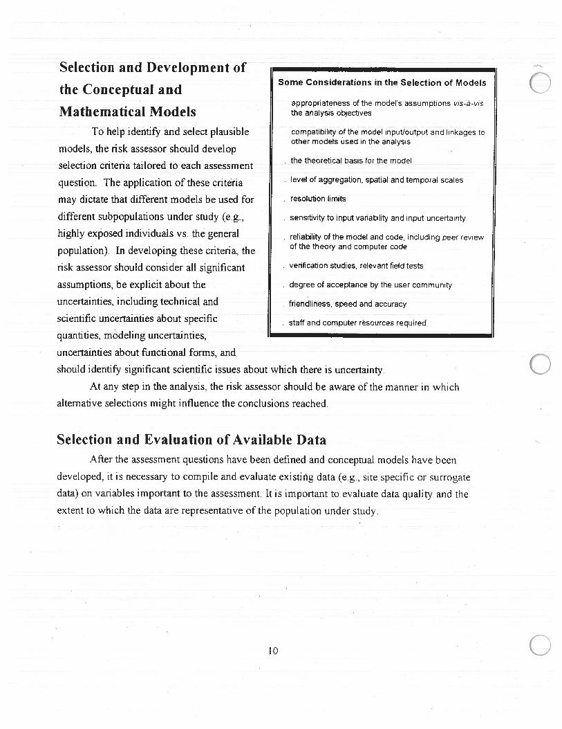
Selection and Development ofSome Considerations in the Selection of Models

the Conceptual and. .

appropriateness ofthe model’s assumptions vis-ä-visMathematical Models the analysis objectives

To help identify and select plausible .compatibility of the model input/output and linkages to

. other models used in the analysismodels, the risk assessor should develop

. . the theoretical basis for the modelselection cntena tailored to each assessment

question. The application of these criteria .

level of aggregation, spatial and temporal scales

may dictate that different models be used for •resolution limits

different subpopulations under study (e.g., . sensitivity to input variability and input uncertainty

highly exposed individuals vs. the general . reliability ofthe model and code, including peer review. . . . of the theory and computer codepopulation). In developing these cntena, the

risk assessor should consider all significant verification studies, relevant field tests

assumptions, be explicit about the .degree of acceptance by the user community

uncertainties, including technical and friendliness, speed and accuracy

scientific uncertainties about specific . staff and computer resources required

quantities, modeling uncertainties,

uncertainties about functional forms, and

should identify significant scientific issues about which there is uncertainty.

At any step in the analysis, the risk assessor should be aware ofthe manner in which

alternative selections might influence the conclusions reached.

Selection and Evaluation ofAvailable DataAfter the assessment questions have been defined and conceptual models have been

developed, it is necessary to compile and evaluate existing data (e.g., site specific or surrogate

data) on variables important to the assessment. It is important to evaluate data quality and the

extent to which the data are representative of the population under study.

10 . 0

Guiding Principles for Monte Carlo AnalysisThis sectionpresents a discussion ofpnnciples ofgood practice for Monte Carlo

simulation as it may be applied to environmental assessments. It is not intended to serve as

detailed technical guidance on how to conduct or evaluate an analysis ofvañability and

uncertainty.

Selecting Input Data and Distributions for Use in Monte Carlo

An alysis

I. Conduct preliminary sensitivity analyses or numerical experiments to identify model

structures, exposure pathways, and model input assumptions and parameters that make

important contributions to the assessment endpoint and its overall variability and/or

uncertainty.

The capabilities of current desktop computers allow for a number of “what if’ scenarios to

be examined to provide insight into the effects on the analysis of selecting a particular model,

including or excluding specific exposure pathways, and making certain assumptions with respect

to model input parameters. The output of an analysis may be sensitive to the structure of the

exposure model . Alternative plausible models should be examined to determine if structural

differences have important effects on the output distribution (in both the region of central

tendency and in the tails).

L Numerical experiments or sensitivity analysis also should be used to identify exposure

pathways that contribute significantly to or even dominate total exposure. Resources might be

saved by excluding unimportant exposure pathways (e.g., those that do not contribute appreciably

to the total exposure) from full probabilistic analyses or from further analyses altogether. For

important pathways. the model input parameters that contribute the most to overall variability and

U ncertai nty should be i dentifi ed . Again, unimportant parameters may be excluded from full

probabilistic treatment. For important parameters, empirical distributions or parametric

distributions may be used. Once again, numerical experiments should be conducted to determine

the sensitivity of the output to different assumptions with respect to the distributional forms of

the input parameters. Identifying important pathways and parameters where assumptions about

distributional form contribute significantly to overall uncertainty may aid in focusing data

atherin efforts

) 11

Dependencies or correlations between mode! parameters also may have a significant

influence on the outcome ofthe analysis. The sensitivity ofthe analysis to various assumptions

about known or suspected dependencies should be examined. Those dependencies or correlations

identified as having a significant effect must be accounted for in later analyses.

Conducting a systematic sensitivity study may not be a trivial undertaking. involving

significant effort on the part ofthe risk assessor. Risk assessors should exercise great care not to

prematurelyor unjustifiably eliminate pathways or parameters from full probabilistic treatment.

Any parameter or pathway eliminated from full probabilistic treatment should be identified and the

reasons for its elimination thoroughly discussed.

2. Restrict the use of probabilistic assessment to significant pathways and parameters.

Although specifying distributions for all or most variables in a Monte Carlo analysis is

useful for exploring and characterizing the full range ofvariability and uncertainty. it is often

unnecessary and not cost effective. Ifa systematic preliminary sensitivity analysis (that includes

examining the effects of various assumptions about distributions) was undertaken and

documented, and exposure pathways and parameters that contribute little to the assessment

endpoint and its overall uncertainty and variability were identified, the risk assessor may simplify

the Monte Carlo analysis by focusing on those pathways and parameters identified as significant.

From a computational standpoint, a Monte Carlo analysis can include a mix of point estimates and

distributions for the input parameters to the exposure model. However, the risk assessor and risk

manager should continually review the basis for “fixing” certain parameters as point values to

avoid the perception that these are indeed constants that are not subject to change.

3. Use data to inform the choice of input distributions for model parameters

The choice of input distribution should always be based on all information (both

qualitative and quantitative) available for a parameter. In selecting a distributional form, the risk

assessor should consider the quality ofthe information in the database and ask a series of

questions including (but not limited to):

. is there any mechanistic hasisfor ChOosing a distriht(t!ona//arni/y?

. Is the shape ofthe distribution likely to he dictated by physical or biologicalproperties or other mechanisms?

. Is the variable discrete or continuotts

12 0

. 1’Jhat are the hoiiiids o/the variable?

. [V the disirthittion skewed or symmetric?

. Ifthe distribution is thotight to he skewed, in which direction?

. What other aspects ofthe shape oft/ic distribution are known?

When data for an important parameter are limited, it may be useful to define plausible

alternative scenarios to incorporate some information on the impact ofthat variable in the overall

assessment (as done in the sensitivity analysis). In doing this, the risk assessor should select the

widest distributional family consistent with the state of knowledge and should, for important

parameters, test the sensitivity ofthe findings and conclusions to changes in distributional shape.

4. Surrogate data can be used to develop distributions when they can be appropriately

j us tilled.

.The risk assessor shou]d always seek representative data ofthe highest quality available.

However, the question of how representative the available data are is often a serious issue. Many

times. the available data do not represent conditions (e.g., temporal and spatial scales) in the

population being assessed. The assessor should identify and evaluate the factors that introduce

uncertainty into the assessment. In particular, attention should be given to potential biases that

may exist in surrogate data and their implications for the representativeness ofthe fitted

di stn buti ons.

When alternative surrogate data sets are available, care must be taken when selecting or

combining sets. The risk assessor should use accepted statistical practices and techniques when

combining data, consulting with the appropriate experts as needed.

Whenever possible, collect site or case specific data (evenin limited quantities) to help

justify the use of the distribution based on surrogate data. The use of surrogate data to develop

distributions can be made more defensible when case-specific data are obtained to check the

reasonableness of the distribution.

5. When obtaining empirical data to develop input distributions for exposure model

parameters, the basic tenets of environmental sampling should be followed. Further,

.13

particular attention should be given to the quality of information at the tails of the

distribution.

As a general rule, the development of data for use in distributions should be carried out

using the basic principles employed for exposure assessments. For example,

. Receptor-based sampling iti which data are obtained oii the receplor or i-ni fhc’exposure fields relative to the receptor;

I Sampling at appropriate spatial or temporal scales using an appropriatestratified random sampling methodology,

. Using two-stage sampling to determine and evaluate the degree oferror,.

statisticalpower, and subsequent sampling needs; and

. Establishing data quality objectives.

In addition, the quality of information at the tails of input distributions often is not as good

as the central values. The assessorshould pay particular attention to this issue when devising data

collection strategies.

6. Depending on the objectives of the assessment, expert ‘ judgment can be included either

within the computational analysis by developing distributions using various methods or

by usingjudgments to select and separately analyze alternate, but plausible, scenarios.

When expert judgment is employed, the analyst should be very explicit about its use.. Expertjudgment is used, to some extent, throughout all exposure assessments. However,

debatable issues arise when applying expert opinions to input distributions for Monte Carlo

analyses. Using expert judgment to derive a distribution for an input parameter can reflect bounds

on the state ofknowledge and provide insights into the overall uncertainty. This may be

particularly useful during the sensitivity analysis to help identify important variables for which

additional data may be needed. However, distributions based exclusively or primarily on expert

judgment reflect the opinion of individuals or groups and, therefore, may be subject to

considerable bias. Further, without explicit documentation of the use of expert opinions. the

I According to NCRP (1996). an expert has (1)training and expenence in the suhiect irea resulting insupenoT knowledge in the field, (2) access to relevant intormation. (3) an ability to process and effectively USC thCintotmation. ind t 4 is recoeruzed by his or her peers or those C(mfldUCtifl! the study as qualitied to pinvide nd inniabout assumptH)ns. models. and model parameters at the level ()t detail equi;ed

.14 . 0

distributions based on thesejudgrnents might be erroneously viewed as equivalent to those based

on hard data. When distributions based on expertjudgement have an appreciable effect on the

outcome ofan analysis, it is critical to highlight this in the uncertainty characterization.

Evaluating Variability and Uncertainty

7. The concepts ofvariability and uncertainty are distinct. They can be tracked and

evaluated separately during an analysis, or they can be analyzed within the same

computational framework. Separating variability and uncertainty is necessary to

provide greater accountability and transparency. The decision about how to track

them separately must be made on a caseby-case basis for each variable.

Variability represents the true heterogeneity or diversity inherent in a well-characterized

population. As such, it is not reducible through further study. Uncertainty represents a lack of

knowledge about the population. It is sometimes reducible through further study. Therefore,

separating variability and uncertainty during the analysis is necessary to identify parameters for

which additional data.are needed. There can be uncertainty about the variability within a

population. For example, ifonly a subset ofthe population is measured or ifthe population is

otherwise under-sampled, the resulting measure ofvanability may differ from the true population

variability. This situation may also indicate the need for additional data collection.

8. There are methodological differences regarding how variability and uncertainty are

addressed in a Monte Carlo analysis.

There are formal approaches for distinguishing between and evaluating variability and

uncertainty. When deciding on methods for evaluating variability and uncertainty, the assessor

should consider the following issues.

. Variability depends on the averaging time, averaging space, or other dimensionsin which the data are aggregated.

. S’tandard data analysis tends to ttnderstate uncertainty byfocusing solely onrandom error within a data set. Conversely, standard data analysis tends tooi ‘erstate ‘ariahi/ii by implicitly including measurement errors.

. I U1IOlt.S Rf)e.V ()/fllode/ e!T0t.V caii represent important sources of tincertainty.,1 liernaiii’e conceJ)tuaI 01 mathematical models are a potentially important sourceof l(flCctiUifltV. A n?cijür threat to the accuracy ofa variability analysis is a lack oft(!J)1e.SetlIUtI 1L11 1eS.S• 0/ the c/ala.

15

9. Methods should investigate the numerical stability of the moments and the tails of the •

distributions.

for the purposes ofthese principles, numerical stability refers to observed nurnerica]

changes in the characteristics (i.e., mean, variance, percentiles) ofthe Monte Carlo simulation

output distribution as the number ofsimulations increases. Depending on the algebraic stRicture

of the model and the exact distributional forms used to characterize the input parameters. sonic

outputs will stabilize quickly, that is, the output mean and variance tend to reach more or less

constant values after relatively few sampling iterations and exhibit only relatively minor

fluctuations as the number of simulations increases. On the other hand, some model outputs may

take longer tostabilize. The risk assessor should take care to be aware of these behaviors. Risk

assessors should always use more simulations than they think necessary. Ideally, Monte Carlo

simulations should be repeated using several non-overlapping subsequences to check for stability

and repeatability. Random number seeds should always be recorded. In cases where the tails of

the output distribution do not stabilize, the assessor should consider the quality of information in

the tails ofthe input distributions. Typically, the analyst has the least information about the input

tails. This suggest two points.

. Data gathering efforts should he sfruciured to provide adecjuate coverage at ihe Ctails of/he input distributions.

. The assessment should include a narrative and qualitative discussion of thequality ofinformation at the tails ofthe input distrihtttions.

10. There are limits to the assessor’s ability to account for and characterize all sources of

uncertainty. The analyst should identify areas of uncertainty and include them in the

analysis, either quantitatively or qualitatively.

Accounting for the important sources ofuncertainty should be a key objective in Monte

Carlo analysis. However, it is not possible to characterize all the uncertainties associated with the

models and data. The analyst should attempt to identify the full range oftypes of uncertainty

impinging on an analysis and clearly disclOse what set ofuncertainties the analysis attempts to

represent and what it does not. Qualitative evaluations ofuncertainty including relative rankins of

the sources of uncertainty may be an acceptable approach to uncertainty evaluation, especially

when objective quantitative measures are not available. Bayesian methods may sometimes be

0

useful for incorporating subjective information into variability and uncertainty analyses in a

manner that is consistent with distinguishing variability from uncertainty.

Presenting the Results ofa Monte Carlo Analysis

I 1. Provide a complete and thorough description ofthe exposure model and its equations

(including a discussion of the limitations of the methods and the results).

Consistent with the Exposure Assessment Guidelines, Model Selection Guidance, and

other relevant Agency guidance, provide a detailed discussion ofthe exposure model(s) and

pathways selected to address specific assessment endpoints. Show all the formulas used. Define

all terms. Provide complete references. If external modeling was necessary (e.g., fate and

transport modeling used to provide estimates of the distribution of environmental concentrations),

identify the model (including version) and its inpUt parameters. Qualitatively describe the major

advantages and limitations ofthe models used.

The objectives are transparency and reproducibility - to provide a complete enough

description so that the assessment might be independently duplicated and verified.

1 2. Provide detailed information on the input distributions selected. This information

should identify whether the input represents largely variability, largely uncertainty,

or some combination of both. Further, information on goodness-of-fit statistics

should be discussed.

It is important to document thoroughly and convey critical data and methods that provide

an important context for understanding and interpreting the results ofthe assessment. This

detailed information should distinguish between variability and uncertainty and should include

graphs and charts to visually convey written information.

The probability density function (PDf) and cumulative distribution function (CDf) graphs

provide different, but equally important insights. A plot ofa PDF shows possible values of a

random variable on the horizontal axis and their respective probabilities (technically, their

densities) on the vertical axis. This plot is useful for displaying:

a the relative pi-ohahilily ofvalues;

. the niü.t like/V i’a/nes (e.g. , modes) ; .

. the shape o/the thstrihittioti (e.g. , skewness, kurtosis) ; and

17

. small changes in probability density. :

A plot of the cumulative distribution function shows the probability that the value of a random

variable is less than a specific value. These plots are good for displaying:

. fractiles, including the median;

. probability intervals, including confidence intervals; .

. stochastic dominance; and

. mixed, continuous, and discrete distributions.

Goodness-of-fit tests are formal statistical tests ofthe hypothesis that.a specific set of

sampled observations are an independent sample from the assumed distribution. Common tests

include the chi-square test, the Kolmogorov-Smirnov test, and the Anderson-Darling test.

Goodness-of-fit tests for normality and lognormality include Lilliefors test, the Shapiro-WUks

test, and DAgostino’s test.

Risk assessors should never depend solely on the results ofgoodness-of-fit tests to select

the analytic form for a distribution. Goodness-of-fit tests have low discriminatory power and are

generally best for rejecting poor distribution fits rather than for identifying good fits. For small to

medium sample sizes, goodness-of-fit tests are not very sensitive to small differences between the

observed and fitted distributions. On the other hand, for large data sets, even small and

unimportant differences between the observed and fitted distributions may lead to rejection of the

null hypothesis. For small to medium sample sizes, goodness-of-fit tests should best be vewed as

a systematic approach to detecting gross differences. The risk assessor should never let

differences in goodness-of-fit test results be the sole factor for determining the analytic form of a

distribution.

Graphical methods for assessing fit provide visual comparisons between the experimental

data and the fitted distribution. Despite the fact that they are non-quantitative, graphical methods

often can be most persuasive in supporting the selection of a particular distribution or in rejecting. the fit ofa distribution. This persuasive power derives from the inherent weaknesses in numerical

goodness-of-fit tests. Such graphical methods as probability-probability (P-P) and quantile

quantile (Q-Q) plots can provide clear and intuitive indications of goodness-of-fit.

,

18 .o

Having selected and justified the selection of specific distributions, the assessor should

provide plots of both the PDF and CDF, with one above the other on the same page and using

identical horizontal scales. The location ofthe mean should be clearly indicated on both curves

[See Figure 1]. These graphs should be accompanied by a summary table ofthe relevant data.

13. Provide detailed information and graphs for each output distribution.

In a fashion similar to that for the input distributions, the risk assessor should provide

plots of both the PDF and CDF for each output distribution, with one above the other on the

same page, using identical horizontal scales. The location ofthe mean should clearly be indicated

on both curves. Graphs should be accompanied by a summary table ofthe relevant data.

1 4. Discuss the presence or absence of dependencies and correlations.

Covanance among the input variables can significantly affect the analysis output. It is

important to consider covariance among the model’s most sensitive variables. It is particularly

important to consider covanance when the focus ofthe analysis is on the high end (i.e., upper

end) àfthe distribution.

When covariance among specific parameters is suspected but cannot be determined due to

lack of data, the sensitivity of the findings to a range of different assumed dependencies should be

evaluated and reported.

15. Calculate and present point estimates.:

Traditi onal determini stic (poi nt) estimates should be calculated using established

protocols Clearly identify the mathematical model used as well as the values used for each inputparameter

in this calculation. Indicate in the discussion (and graphically) where the point estimate

falls on the distribution generated by the Monte Carlo analysis. Discuss the model and parameter

assumptions that have the most influence on the point estimate’s position in the distribution. The

rTiost important issue in comparing point estimates and Monte Carlo results is whether the data

and exposure methods employed in the two are comparable. Usually, when a major difference

between point estimates and Monte Carlo results is observed, there has been a fundamental

change in data or methods. Comparisons need to call attention to such differences and determine

their impact

In some cases, additional point estimates could be calculated to address specific risk

manaitement questions or to meet the information needs ofthe audience for the assessment. Point

estimates can often assist in communicating assessment results to certain groups by providing a

19

scenario-based perspective. For example, if point estimates are prepared for scenarios with which

the audience can identify, the significance ofpresented distributions may become clearer. This

may also be a way to help the audience identify important risks.

16. A tiered presentation style, in which briefing materials are assembled at various levels

of detail, may be helpful. Presentations should be tailored to address the questions

and information needs of the audience.

Entirely different types ofreport are needed for scientific and nonscientific audiences.

Scientists generally will want more detail than non-scientists. Risk managers may need more

detail than the public. Reports for the scientific community are usually very detailed. Descriptive.

less detailed summary presentations and key statistics with their uncertainty intervals (e.g., box

and whisker plots) are generally more appropriate for non-scientists.

To handle the different levels of sophistication and detail needed for different audiences, it

may be useful to design a presentation in a tiered format where the level of detail increases with

each successive tier. For example, the first tier could be a one-page summary that might include a

graph or other numerical presentation as well as a couple of paragraphs outlining what was done.

This tier alone might be sufficient for some audiences. The next tier could be an executive

summary, and the third tier could be a full detailed report. for further information consult Bloom

eta!., 1993.

Graphical techniques can play an indispensable role in communicating the findings from a

Monte Carlo analysis. It is important that the risk assessor select a clear and uncluttered graphical

style in an easily understood format. Equally important is deciding which information to display.

Displaying too much data or inappropriate data will weaken the effectiveness ofthe effort.

Having decided which information to display, the risk assessor should carefully tailor a graphical

presentation to the informational needs and sophistication of specific audiences. The performance

of a graphical display of quantitative information depends on the information the risk assessor is

trying to convey to the audience and on how well the graph is constructed (Cleveland, 1994). The

following are some recommendations that may prove useful for effective graphic presentation:

S Avoid excessively complicated graphs. Keep graphs intended for a glance (e.g.,overhead or slide presentations) relatively simple and uncluttered. Graphsintended for publication can include more complexity. .

. Avoid pie charts, perspective charts (3-dimensional bar and pie charts, ribboncharts), pseudo-perspective charts (2-dimensional bar or line charts).

20 .. 0

. Color and shading can create visual biases and are very difficult to use effectively.Use color or shading only when necessary and then, only very carefully. Consultreferences on the use of color and shading in graphics.

. When possible in publications and reports, graphs should be accompanied by atable ofthe relevant data.

. If probability density or cumulative probability plots are presented, present both,with one above the other on the same page, with identical horizontal scales andwith the location ofthe mean clearly indicated on both curves with a solid point.

. Do not depend on the audience to correctly interpret any visual display of data.

Always provide a narrative in the report interpreting the important aspects of thegraph.

. Descriptive statistics and box plots generally serve the less technically-orientedaudience

well. Probability density and cumulative probability plots are generallymore meaningful to risk assessors and uncertainty analysts.

21

Appendix: Probability Distribution Selection IssUes

Surrogate Data, fitting Distributions, Default DistributionsSubjective Distributions

Identification ofrelevant and valid data to represent an exposure variable is prerequisite toselecting a probability distribution However, often the data available are not a direct measure ofthe exposure variable of interest. The risk assessor is often faced with using data taken in spatialor temporal scales that are significantly different from the scale of the problem underconsideration. The question becomes whether or not or how to use marginally representative orsurrogate data to represent a particular exposure variable. While there can be no hard and fastrules on how to make thatjudgment, there are a number ofquestions risk assessors need to askwhen the surrogate data are the only data available.

Is there Prior Knowledge about Mechanisms? Ideally, the selection of candidate probabilitydisthbutions should be based on consideration ofthe underlying physical processes or mechanismsthought.to be key in giving rise to the observed variability. for example, if the exposure variableis the result ofthe product ofa large number ofother random variables, it would make sense toselect a lognormal distribution for testing. As another example, the exponential distributionwould be a reasonable candidate ifthe stochastic variable represents a process akin to inter-arrivaltimes of events that occur at a constant rate. As a final example, a gamma distribution would be areasonable candidate if the random variable of interest was the sum of independent exponentialrandom variables.

Threshold Question - Are the surrogate data ofacceptabte quality and representativcnc.ss tosupport reliable exposure estimates?

What uncertainties and biases are likely to be introduced by using surrogate data? F orexample, ifthe data have been collected in a different geographic region, the contribution offactors such as soil type, rainfall, ambient temperature, growing season, natural sources ofexposure, population density, and local industry may have a significant effect on the exposureconcentrations and activity patterns. Ifthe data are collected from volunteers or from hot spots,they will probably not represent the distribution of values in the population of interest. Eachdifference between the survey data and the population being assessed should be noted. The

. effects of these differences on the desired distribution should be discussed if possible.

How are the biases likely to affect the analysis and can the biases be corrected? The riskassessor may be able to state with a high degree ofcertainty that the available data over-estimatesor under-estimates the parameter of interest. Use of ambient air data on arsenic collected nearsmelters will almost certainly over-estimate average arsenic exposures in the United States.However. the smelter data can probably be used to produce an estimate of inhalation exposuresthat falls within the high end. In other cases. the assessor may be unsure how unrepresentativedata will affect the estimate as in the case when data collected by a particular State are used in a

22 . 0

national assessment. In most cases, correction of suspected biases will be difficult or not possible.

If only hot spot data are available for example, only bounding or high end estimates may bepossible. Unsupported assumptions about biases should be avoided. Information regarding the

direction and extent ofbiases should be included in the uncertainty analysis.

How SlioUlfi (1fl uncertainty introduced by the surrogate data be represented?

In identifying plausible distributions to represent variability, the risk assessor should examine

the following characteristics ofthe variable:

1 . Mtturc oftl;e variable.Can the variable only take on discrete values (e.g., either on or off; either heads or tails) or is

the variable continuous over some range (e.g., pollutant concentration, body weight; drinkingwater consumption rate)? Is the variable correlated with or dependent on another variable?

2. BOUnfIS ()fthe variable.What is the physical or plausible range ofthe variable (e.g., takes on only positive values,

bounded by the interval [a,b]). Are physical measurements ofthe variable censored due to limitsofdetection or some aspect ofthe experimental design?

3. Si’nznictry ofthe Distribution.Is distribution of the variable known to be or thought to be skewed or symmetric? If the

distribution is thought to be skewed, in which direction? What other aspects ofthe shape of thedistribution are known? Is the shape ofthe distribution likely to be dictated by physical/biologicalproperties (e.g., logistic growth rates) or other mechanisms?

4. SUfIlfllflrV Statistics.

Summary statistics can sometimes be useful in discriminating among candidate distributions.for example, frequently the range ofthe variable can be used to eliminate inappropriatedistributions it would not be reasonable to select a lognormal distribution for an absorptioncoefficient since the range ofthe lognormal distribution is (O,) while the range ofthe absorptioncoefficient is (0,1). If the coefficient of variation is near I .0, then an exponential distributionrniht be appropriate. Information on skewness can also be useful. For symmetric distributions,skewness = O for distributions skewed to the right, skewness > 0; for distributions skewed to theleft. skewness < 0.

5. 6rapltical Methods to Explore the Data.The risk assessor can often gain important insights by using a number ofsimple graphical

techniques to explore the data prior to numerical analysis. A wide variety ofgraphical methodshave been developed to aid in this exploration including frequency histograms for continuousdistributions, stem and Ieafplots, dot plots, line plots for discrete distributions, box and whiskerplots. scatter plots. star representatiqns, glyphs, Chernofffaces, etc. [Tukey (1977); Conover( 1980): du bit et a!. (1986), Morgan and Henrion, (1990)]. These graphical methods are all

23

intended to permit visual inspection ofthe density function corresponding to the distribution ofthe data. They can assist the assessor in examining the data for skewness, behavior in the tails.rounding biases, presence of multi-modal behavior, and data outliers.

Frequency histograms can be compared to the fundamental shapes associated with standardanalytic distributions (e.g., normal, lognormal, gamma, Weibull). Law and Kelton ( I 99 1 ) andEvans et al. (1993) have prepared a useful set of figures which plot many ofthe standard analyticdistributions for a range of parameter values. Frequency histograms should be plotted on bothlinear and logarithmic scales and plotted over a range offrequency bin widths (class intervals) toavoid too muchjaggedness or too much smoothing (i.e., too little or too much data aLzreszation)The data can be sorted and plotted on probability paper to check for normality (or log-normality).Most ofthe statistical packages available for personal computers include histogram andprobability plotting features, as do most ofthe spreadsheet programs. Some statistical packagesinclude stem and leaf, and box and whisker plotting features.

After having explored the above characteristics ofthe variable, the risk assessor has threebasic techniques for representing the data in the analysis. In the first method, the assessor canattempt to fit a theoretical or parametric distribution to the data using standard statisticaltechniques. As a second option, the assessor can use the data to define an empirical distributionfunction (EDf). finally, the assessor can use the data directly in the analysis utilizing randomresampling techniques (i.e., bootstrapping). Each ofthese three techniques has its own benefitsHowever, there is no consensus among researchers (authors) as to which method is generallysuperior. For example, Law and Kelton (1991) observe that EDFs may contain irregularities,especially when the data are limited and that when an EDF is used in the typical manner, valuesoutside the range of the observed data cannot be generated. Consequently, when the data arerepresentative ofthe exposure variable and the fit is good, some prefer to use parametricdistributions. On the other hand, some authors prefer EDFs (Bratley, Fox and Schrage, I 987)arguing that the smoothing which necessarily takes place in the fitting process distorts realinformation. In addition, when data are limited, accurate estimation of the upper end (tail) isdifficult. Ultimately, the technique selected will be a matter ofthe risk assessor’s comfort with thetechniques and the quality and quantity of the data under evaluation.

The following discussion focuses primarily on parametric techniques. For a discussion of theother methods, the reader is referred to Efron and Tibshirani (1993), Law & Kelton (1991 ), andBratley et a! (1987).

Having selected parametric distributions, it is necessary to estimate numerical values for theintrinsic parameters which characterize each of the analytic distributions and assess the quality ofthe resulting fit.

Parameter Estimation. Parameter estimation is generally accomplished using conventionalstatistical methods, the most popular of which include the method of maxi mum Ii keli hood.method of least squares. and the method of moments. See Johnson and Kotz ( I 970). Law and

24 0

Kelton ( 1991 ) Kendall and Stewart (1979), Evans et a!. (1993), Ang and Tang (1975),

Gilbert (1987). and Meyer (1975).

4ssesxing the Representativeness ofthe fitted Distribution. Having estimated the

parameters ofthe candidate distributions, it is necessary to evaluate the qfiy ofthe fit’

and. if more than one distribution was selected, to select the “best” distribution from among

th e can d i dates. Unfortun ate]y, there is no si ngle, unam biguous measure of what constitutes

best fit. Ultimately, the risk assessor mustjudge whether or not the fit is acceptable.

(rapI;icaI Mcthoftsfor Assessing Fit Graphical methods provide visual comparisons

between the experimental data and the fitted distribution. Despite the fact that they are non-

quantitative, graphical methods often can be most persuasive in supporting the selection of a

particular distribution or in rejecting the fit ofa distribution. This persuasive power derives

from the inherent weaknesses in numerical goodness-of-fit tests. Commonly used graphical

methods include: frequency comparisons which compare a histogram of the experimental data

with the density function ofthe fitted data; prohabilityplots compare the observed cumulative

density function with the fitted cumulative density function. Probability plots areoften based

on graphical transformations such that the plotted cumulative density function results in a

straight Iine prohabi/ity-probabililyplots (P-P plots) compare the observed probability with

the fitted probability. P-P plots tend to emphasize differences in the middle ofthe predicted

and observed cumulative distributions, quantile-quantile plots (Q-Q plots) graph the it/i-

c/iiwiti/e of the fitted distribution against the it/i quantile data. Q-Q plots tend to emphasize

differences in the tails ofthe fitted and observed cumulative distributions; and box plots

compare a box plot of the observed data with a box plot ofthe fitted distribution.

Goofiness-of-fit Tests. Goodness-of-fit tests are formal statistical tests of the hypothesis that

the set ofsampled observations are an independent sample from the assumed distribution.

The null hypothesis is that the randomly sampled set of observations are independent,

identically distributed random variables with distribution function F. Commonly used

goodness-of-fit tests include the chi-square test, Kolmogorov-Smimov test, and Anderson-

Darling test. The chi-square test is based on the difference between the square of the

observed and expected frequencies. It is highly dependent on the width and number of

intervals chosen and is considered to have low power. It is best used to reject poor fits. The

Kolmogorov-Smirnov Test is a non-parametric test based on the maximum absolute

difference between the theoretical and sample Cumulative Distribution functions (CDFs).

The Kolmogorov-Smirnov test is most sensitive around the median and less sensitive in the

tails and is best at detecting shifts in the empirical CDF relative to the known CDF. It is less

proficient at detecting spread but is considered to be more powerful than the chi-square test.

The Anderson-Darling test is designed to test goodness-of-fit in the tails of a Probability

Density function (PDF) based on a weighted-average ofthe squared difference between the

observed and expected cumulative densities.

25

Care must be taken not to over-interpret or over-rely on the findings ofgoodness-of-flt testsIt is far too tempting to use the power and speed of computers to mn goodness-of-fit testsagainst a generous list ofcandidate distributions, pick the distribution with the best”goodness-of-fit statistic, and claim that the distribution that fit “best” was not rejected at somespecific level ofsignificance. This practice is statistically incorrect and should be avoided[Bratley et at., 1987, page 134]. Goodness-of-fit tests have notoriously tow power and aregenerally best for rejecting poor distribution fits rather than for identifying good fits. Forsmall to medium sample sizes, goodness-of-fit tests are not very sensitive to small differencesbetween the observed and fitted distributions. On the other hand, for large data sets, evenminute differences between the observed and fitted distributions may lead to rejection of thenull hypothesis. for small to medium sample sizes, goodness-of-fit tests should best beviewed as a systematic approach to detecting gross differences.

Tests ofChoicefor Normality and Lôgnornwlity. Several tests for normality (andlognormality when log-transformed data are used) which are considered more powerful thaneither the chi-square or Komolgarov-Smimoff(K-S) tests have been developed: Lilliefors’test which is based on the K-S test but with ‘normalized” data values, Shapiro-Wilks test (forsample sizes 50), and DAgostino’s test (for sample sizes 50). The Shapiro-Wilks andD’Agostino tests are the tests ofchoice when testing for normality or lognormality.

If the data are not well-fit by a theoretical distribution, the risk assessor should consider theEmpirical Distribution Function or bootstrapping techniques mentioned above.

For those simations in which the data are not adequately representative of the exposure Qvariable or where the quality or quantity of the data are questionable the following approachesmay be considered.

Distributions Based on Surrogate Data. Production of an exposure assessment oftenrequires that dozens offactors be evaluated, including exposure concentrations, intake rates,exposure times, and frequencies. A combination Of monitoring, survey, and experimentaldata, fate and transport modeling, and professional judgment is used to evaluate these factors.Often the only available data are not completely representative of the population beingassessed. Some examples are the use of activity pattern data collected in one geographicregion to evaluate the duration of activities at a Superfund site in another region, use ofnational intake data on consumption of a particular fotd item to estimate regional intake anduse of data collected from volunteers to represent the general population.

In each such case, the question ofwhether to use the unrepresentative data to estimate thedistribution ofa variable should be carefully evaluated. Considerations include how to expressthe possible bias and uncertainty introduced by the unrepresentativeness ofthe data andalternatives to using the data. In these situations, the risk assessor should carefully evaluatethe basis ofthe distribution (e.g., data used, method) before choosing a particular surrogate orbefore picking among alternative distributions for the same exposure parameter. The

. . 26 0

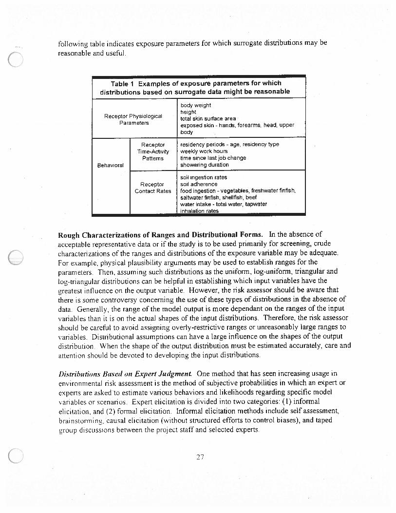
following table indicates exposure parameters for which surrogate distributions may be

reasonable and useful.

Table I Examples of exposure parameters for whichdistributions based on surrogate data might be reasonable

body weight

Receptor Physiological kin surface areaParameters exposed skin - hands, forearms, head, upper

body

Receptor residency periods - age, residency typeTime-Activity weekly work hours

Patterns time since lastjob changeBehavioral showering duration

soil ingestion ratesReceptor soil adherence

Contact Rates food ingestion - vegetables, freshwater finfish,saltwaterfinfish, shellfish, beefwater intake - total water, tapwaterinhalation rates

Rough Characterizations of Ranges and Distributional Forms. In the absence of

acceptable representative data or if the study is to be used primarily for screening, crudecharacterizations ofthe ranges and distributions ofthe exposure variable may be adequate.For example, physical plausibility arguments may be used to establish ranges for theparameters. Then, assuming such distributions as the uniform, log-uniform, triangular andlog-triangular distributions can be helpful in establishing which input variables have thegreatest influence on the output variable. However, the risk assessor should be aware thatthere is some controversy concerning the use ofthese types ofdistñbutions in the absence ofdata. Generally, the range ofthe model output is more dependant on the ranges ofthe inputvariables than it is on the actual shapes of the input distributions. Therefore, the risk assessorshould be careful to avoid assigning overly-restrictive ranges or unreasonably large ranges tovariables. Distributional assumptions can have a large influence on the shapes of the outputdistribution. When the shape of the output distribution must be estimated accurately, care andattention should be devoted to developing the input distributions.

I)istrihutions B(tNCd On Expert Judgment. One method that has seen increasing usage inenvironmental risk assessment is the method ofsubjective probabilities in which an expert orexperts are asked to estimate various behaviors and likelihoods regarding specific modelvan abl es or scenan Os . Expert eli citati on is divided i nto two categories : ( ) informalelicitation, and (2) formal elicitation. Informal elicitation methods include self assessment,brainstormimz, causal elicitation (without structured efforts to control biases), and taped

group discussions between the project staffandselected experts.

27

formal elicitation methods generally follow the steps identified by the US. NuclearRegulatory Commission (USNRC, 1989, Oritz, 1991, also see Morgan and Henrion. 1990:JAEA, 1989; Helton, 1993; Taylor and Burmaster, 1993) and are considerably mote elahorateand expensive than informal methods.

.

C

28 0

References Cited in Text

A. H-S. Ang and W. H. Tang, Probability Concepts in Engineering Planning and Design,

1 ()/tIfllC I, 19(15/C Principles, John Wiley & Sons, Inc., New York ( I 975).

D L. Bloom, et al., Communicating Risk to Senior EPA Policy Makers: A focus Group

Study, U.S. EPA Office ofAir Quality Planning and Standards (1993).

p. Bratley, B. L. fox, L. E. Schrage, A Guide to Simulation, Springer-Verlag, New York

(1987).

w.S. Cleveland, The Elements ofGraphing Data, revised edition, Hobart Press,

Summit, New Jersey (1994). .

w. j. Conover, Practical Nonparameiric Statistics, John Wiley & Sons, Inc., New York

(1980).

S. H. C. du Toit, A. G. W. Steyn, RH. Stumpf, Graphica/Exploraloiy Data Analysis,

Springer-Verlag, New York (1986).

B . Efron and R. Tibshirani, An introduction to the bootstrap, Chapman & Hall, New York

(1993).

M. Evans, N. Hastings, and B. Peacock, Statistical Distributions, John Wiley & Sons, New

York (1993).

R. 0. Gilbert, Statistical Methodsfor Environmental Pollution Monitoring, Van Nostrand

Reinhold, New York (1987).

J. C. Helton, “Uncertainty and Sensitivity Analysis Techniques for Use In Performance

Assessment for Radioactive Waste Disposal,” Reliability Engineering and System Safety,Vol. 42, pages 327-367 (1993).

IAEA, Safety Series 100, Evaluating the Reliability ofPredictions Made Using!n!!Y)n1nenta1 Transfer Models, International Atomic Energy Agency, Vienna, Austria

(1989).

N. L. Johnson and S. Kotz, Continuous Univariate Distributions, volumes I & 2, John Wiley

& Sons. Inc., New York (1970).

M Kendall and A. Stuart, The Ath.’anced Theory ofStatistics, Volume I - Distribution

Theory: Volume 11 - Inference and Relationship, Macmillan Publishing Co., Inc., New York

(1979).

29

A. M. Law and W. D. Kelton, Simulation Modeling & Analysis, McGraw-Hill. Inc.. ( 1 99 1 )

S. L. Meyer, Data Anatysisfor Scientists and Engineers, John Wiley & Sons. Inc.. New York(1975).

M. G. Morgan and M. Henrion, Uncertainty A guide to Dealing with Uncertainii inQuantitative Risk andPolicy Analysis, Cambridge University Press, New York ( I 990).

NCRP Commentary No. 1.4, “A Guide for Uncertainty Analysis in Dose and Risk AssessmentsRelated to Environmental Contaminati on,” National Committee on Radiatlo,, Prorrarns,Scientfic Committee 64-1 7, Washington, D.C . (May, 1 996). •

N. R. Oritz, M. A. Wheeler, R L. Keeney, S. Hora, M. A. Meyer, and R. L. Keeney, “Use ofExpert Judgment in NUREG- 1 1 50, Nuclear Engineering and Design, 1 26 : 3 1 3 -3 3 1 ( I 99 1 )

A. C. Taylor and D. E. Burmaster, “Using Objective and Subjective Information to GenerateDistributions for Probabilistic Exposure Assessment,” U. S. Environmental Protecti on Agency,draft report (1993).

J. W. Tukey, Exploratoty Data Analysis, Addison-Wesley, Boston (1977).

USNRC, Severe Accident Risks. An Assessmentfor Five U. S. Nuclear power Plants (secondpeer review draft), U.S. Nuclear Regulatory Commission, Washington, D.C. (1989). I

30 . ‘ 0

References for Further Reading

B. F Baird, Mwiageria/ DeCISIOnS lint/er Uncertainty, John Wiley and Sons, Inc., New

York ( I 989). V

D. E. Burmaster and P. D. Anderson, “Principles ofGood Practice for the Use of Monte

Carlo Techniques in Human Health and Ecological Risk Assessments,” RiskAna/ysis, Vol.

14(4), pages 477-482 (August, 1994).

R. Clemen, Making Hard Decislons, Duxbury Press (1990). V V

D. C. Cox and P. Baybutt, “Methods for Uncertainty Analysis: A Comparative Survey,” Risk

Analysis, Vol. 1 (4), 251-258 (1981). V

R. D’Agostino and MA. Stephens (eds), Goodness-of-fit Techniques, Marcel Dekker, Inc.,

New York (1986).

L . Devroye, Non-Umforin Random Deviate Generation, Springer-Verlag, (1986).

D. M. Hamby, “A Review of Techniques for Parameter Sensitivity Analysis of Environmental

Models,” Environmental Monitoring andAssessmeni, Vol. 32, 135-1 54 (1994).

D. B . Hertz, and H. Thomas, Risk Analysis and Its Applications, John Wiley and Sons, New

York (1983). V

D. B. Hertz, and H. Thomas, Practical Risk Analysis - An Approach Through Case Studies,John Wiley and Sons, New York (1984).

F . 0. Hoffman and J. S . Hammonds, An Introductory Guide to Uncertainty Analysis inEnvironmental and Health Risk Assessment, ES[ER/TM-3 5 , Martin Marietta (1992).

F. 0. Hoffman and J. S. Hammonds, “Propagation of Uncertainty in Risk Assessments: TheNeed to Distinguish Between Uncertainty Due to Lack ofKnowledge and Uncertainty Due to

Variability,” 1?iskAnalvsis. Vol. 14 (5), 707-712 (1994).

R. L. Iman and I. C. Helton, “An Investigation ofUncertainty and Sensitivity AnalysisTechniques for Computer Models,” RiskAnalysis, Vol. 8(1), pages 71-90 (1988).

R. L Irnan and W. J. Conover, “A Distribution-Free Approach to Inducing Rank CorrelationAmong Input Variables,” Commun. Statistics, Communications and Computation, 1 1 , 3 1 1-331 (1982).

31

R. L. Iman, J. M. Davenport, and D. K. Zeigler, “Latin Hypercube Sampling (A ProgramUsers Guide),” Technical Report SAND 79: 1473, Sandia Laboratories, Albuquerque ( I 980)

M. E. Johnson, Multivariate Statistical Simulation, John Wiley & Sons. Inc., New York(1987).

N. L. Johnson, S. Kotz and A. W. Kemp, Univariate Discrete Distrthtttions, John Wiley &Sons, Inc., New York (1992). .

R. LePage and L. Billard, Exploring the Limits ofBootsfrap, Wiley, New York (1992).

J. Lipton, et al. “Short Communication: Selecting Input Distributions for Use in Monte CarloAnalysis,” Regulatory Toxicology and Pharmacology, 2 1 , 1 92- 1 98 (1995).

w. j. Kennedy, Jr. and J. E. Gentle, Statistical Computing, Marcel Dekker, Inc.. New York(1980).

I. E. McKone and K. T. Bogen, “Uncertainties in.Health Risk Assessment: An IntegratedCase Based on Tetrachioroethylene in California Groundwater,” Regulatory Toxicology atidPharmacology, 15, 86-103 (1992).

R. E. Megill (Editor), Evaluating andlianaging Risk, Penn Well Books, Tulsa, Oklahoma(1985). . .

R. E. Megill, An Introduction to RiskAna/ysis, end Ed. Penn Well Books, Tulsa, Oklahoma(1985).

Palisade Corporation, Risk Analysis and Simulation Add-In for Microsoft Excel or Lotus 1-2-3. Windows Version Release 3.0 User’s Guide, Palisade Corporation, Newfield, New York(1994).

W. H. Press, B. P. flannry, S. A. Teuloisky, and W. T. Vetterling, Numerical Recie.v inPascal: the Art ofScient,fic Computing, Cambridge University Press ( 1 989). .

W. H. Press, S. A. Teuloisky, W. T. Vetterling, and B. P. Flannery, Ntnnerica/ I?ecipc’s inFORTRAN: the Art ofScientific Computing, Cambridge University Press (1992).

W. H. Press, S. A. Teuloisky, W.. T. Vetterling, and B. P. flannery, Nitmerical /p (‘:

the Art ofScientfic Computing, Cambridge University Press (1992).

T. Read and N. Cressie, Goodness-of-fit Statistiesfor Discrete Mit/tivariale Data, Springer-Verlag, New York (1988).

32 0

V K. Rohati. Statistical Inference, John Wiley & Sons, New York (1984).

R. Y. Rubinstein. Sirntt/a/ioti and the Monte Carlo Method, John Wiley and Sons, New York

( 1981).

L Sachs. A/)p/ied £‘aiisiic.’ - A Handbook of Techniqites, Spring-Verlag, New York ( I 984).

A. Saltelli and J. Marivort. “Non-parametric Statistics in Sensitivity Analysis for Model

Output: A Comparison of Selected Techniques,” Reliability Engineering andSystem Safety’,

Vol. 28, 229-253 (1990).

H. Schneider, 7rttncaied atid Censored Distrthutionsform Normal Populations, Marcel

Dekker, Inc., New York (1986).

F. A. Seiler and J. L. Alvarez, “On the Selection of Distributions for Stochastic Variables,”

Risk A iict/.si., Vol . 1 6 ( I ), 5 - 1 8 ( 1 996).

F.A. Seiler, “Error Propagation for Large Errors,” RiskAnalysis, Vol 7 (4), 509-518 (1987).

W. Slob, “Uncertainty Analysis in Multiplicative Models,” RiskAnalysis, Vol. 14 (4), 57 1-576

(1994).

A. E. Smith, PB . Ryan, J. S. Evans, “The Effect of Neglecting Correlations When

Propagati ng Uncertai nty and Estimating the Population Distribution of Risk,” Risk Analysis,

Vol. 12 (4), 467-474 (1992).

U.S. Environmental Protection Agency, Guidelines for Carcinogenic Risk Assessment,

Federal Register 51(185). 33992-34003 (May 29, 1992).

U . S . Envi ronm ental Protection Agency, Source Assessment: Analysis of Uncertainty -

Pri!1Cif)le.S’ and Applicaiions, EPA/600/2-79-004 (August, 1 978)

U.S. Environmental Protection Agency, Guidelines for Exposure Assessment, federal

Register 57(104), 22888-22938 (May 29, 1992).

U S Environmental Protection Agency, Summary Report for the Workshop on Monte Carlo

Analysis. EPAI63O/R-96/0l0 (September, 1996).

2

ii

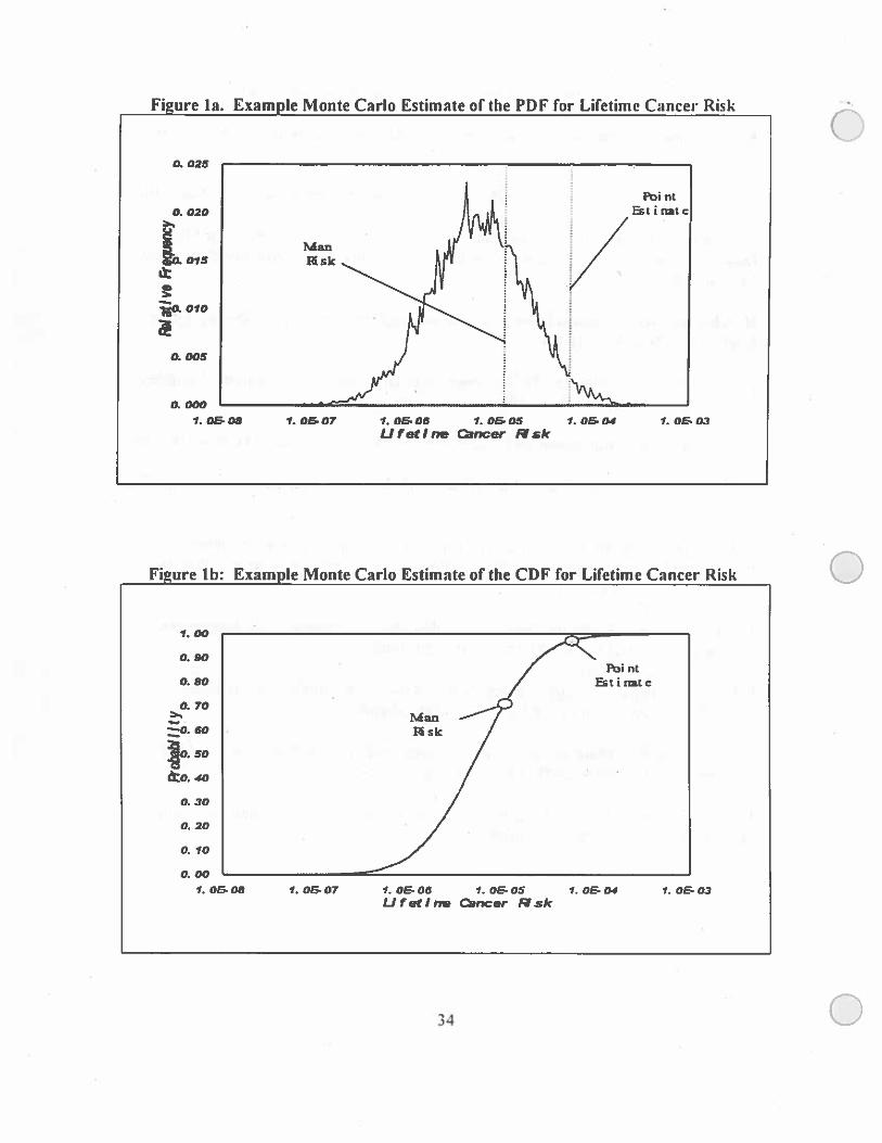
Figure Ia. Example Monte Carlo Estimate of the PDF for Lifetime Cancer Risk a

Figure Ib: Example Monte Carlo Estimate of the COF for Lifetime Cancer Risk C1. 00

0.90

0. 80

a 70

Sd

to. 40

a 30

0. 20

0. 10

a on

C

a 025

a 020a,

L.Ita

010

a oos

0. 000

1.08.08 1. OS 07 1. OS 06 1.06- 05 1.06.04 1. OS 03UfetIne tancer flsk

1. 08-08 1.08-07 1. 08- 06 1. 06- 05 1. 0504 1. 0503Ufetlne cancer flsk

34

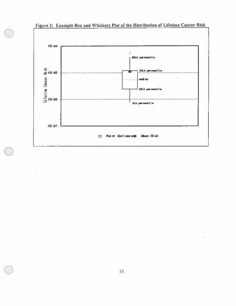
Figure 2: Example Box and Whiskers Plot of the Distribution of Lifetime Cancer Risk

1$O4

16th pcflhl.

t,.di

25thprc.,lI.

1SO65th wcwWHa

1&o7

o Pcint atin.tee Jban Nfl

35

ATTACHMENT P

DEALING WITH DATA BELOW DETECTION LIMITS,QUALITY ASSURANCE COURSE MODULE 492,

EPA NATIONAL CENTER FOR ENVIRONMENTALRESEARCH AND QUALITY ASSURANCE

REPARI:.PtT%SIREV15VFlNAL4A5TER WVflhI5I.RIl,,IIth.PI:IvJ;1 Ip’isae

0 0 0

• 492: Dealing with DataBelow Detection Limits

492- 1095 1

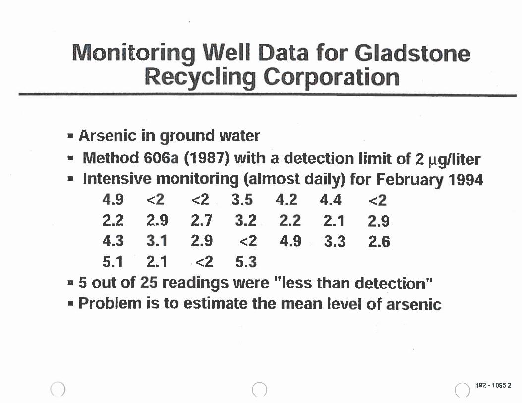
II

II

I

__

-v

u,

—

_ 0k

toa

nI

B-”

za°

.11 0

•A

F’h3A

—z

—I

a)0

C0

-

—ao

a

CD

W-‘

0—

OC

_

BtIc,

-ç—

01

CD0

—I

—

fl—

.0

—

torn

CDF’

)

0 CD LI’ F’)

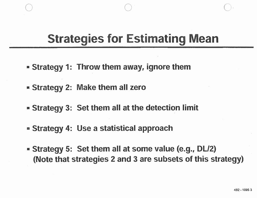
C.,

U,

00(N

C’)

0.j.d

CD

c’J0

Ct

•It

AI

wi

W—

I—

_

OB

C2

‘S

•—EI—

—00

BCC

C4-.

ma

CI— 4-a

ciC

t0

0CD2

>0

0m

aaa

tic2o

•C—

(,,c

1)

N

_

CDw

—S

-—

Ct

Li..

E=

‘9E

=.,-a

Eu

’0

‘a

a;Ia0

-0

0-

0I-

0D

fl

0S

I

Ct

C%J1=

>.,

4n1C

’C

’)0

—Cs,

00

00

4-f

4-P

.4-a

4-I

CDCD

CVCD

4-’

—4

-I—

Z0

00

0a

a

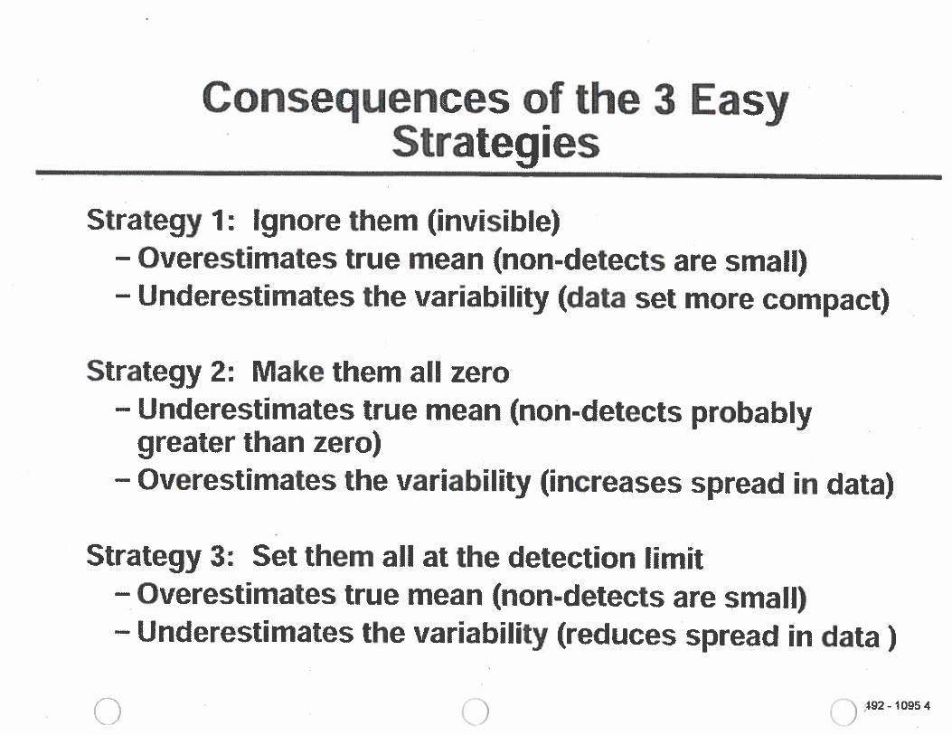
0—

COCa

Ca0

--c

C—

—I—

—I—

.0CaCa

0.0

Ct

oI-

0-

WS

E0

-0

CaOW

—ø

c0

C

.9C

oI—

0O

’5’)C

Wn

——

I—

‘—

—I—

a‘—

—C

.0eC

a.0

.C

CC

aQ

—N

WCa

Cat

tW

Ca

(00

(0E

0C

)E

2C)

S0_C

OC

aC

4.I

aC

aE

(0

CoIO

0_

C“01

0“o

Wo

OD

Do

OO

Di-I

IiI

Ii..I

I—

—0

0

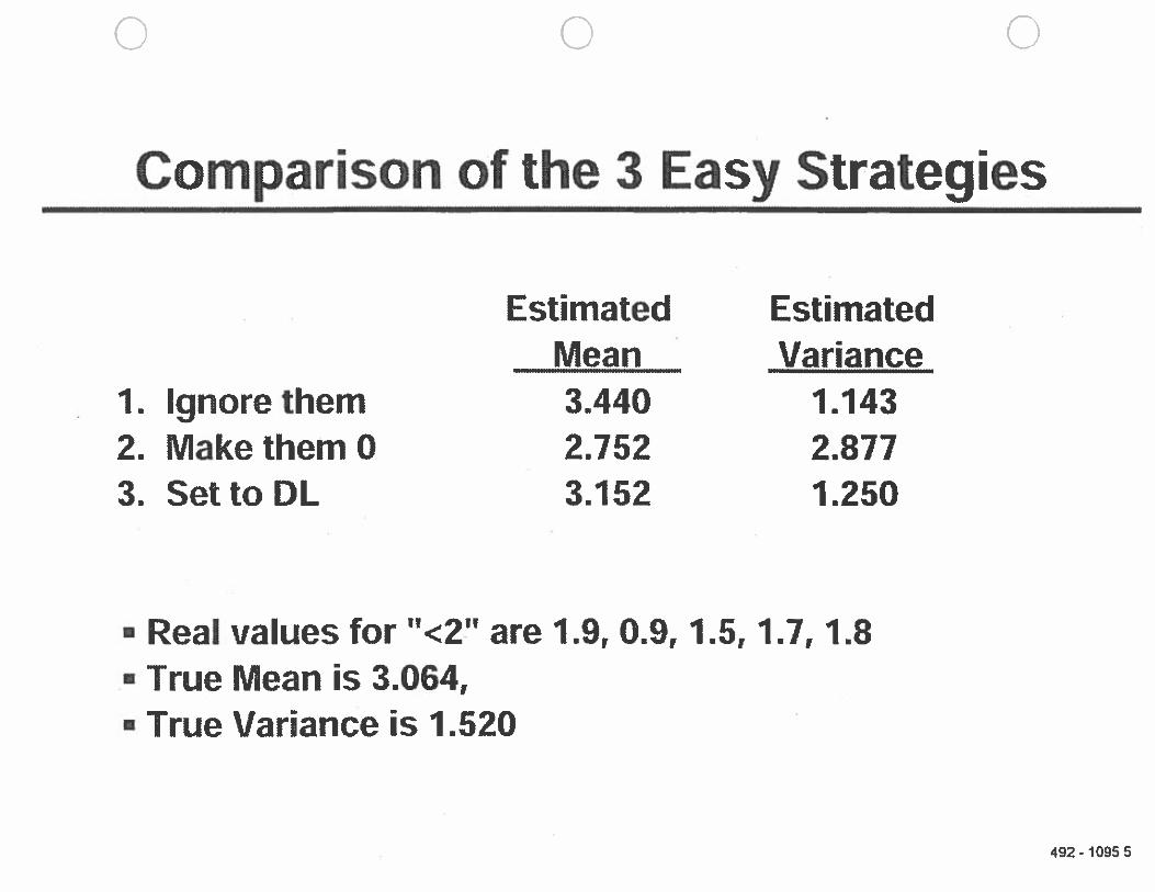
o 0 0

Comparison of the 3 Easy Strategies

Estimated EstimatedMean Variance

1. Ignore them 3.440 1.1432. Make them 0 2.752 2.8773. SettoDL 3152 1.250

Real values for “<2” are 1.9, 0.9, 1.5, 1.7, 1.8• True Mean is 3.064,• True Variance is 1.520

492- 1095 5

Recommendations

Strategy 3: If you want to “nail them”

Strategy 2: II you want to conceal things

Strategy 1: Provided your boss does hot catch youwasting resources!

() (_) C) 492-1095 6

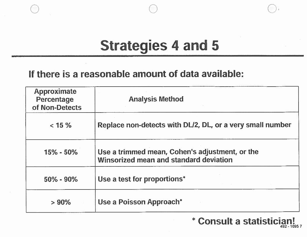
0. 0

Strategies 4 and 5

If there is a reasonable amount of data available:

ApproximatePercentage Analysis Method

of Non-Detects

< 15 % Replace non-detects with DU2, DL, or a very small number

15% - 50% Use a trimmed mean, Cohen’s adjustment, or theWinsorized mean and standard deviation

50% - 90% Use a test for proportions*

> 90% Use a Poisson Approach*

* Consult a statistician!492-10957

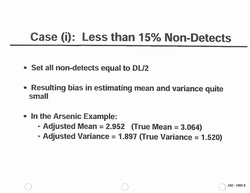
I —0

,00

CDCD

VP

-—

=c

0)CM

aa®

=CD

in

i—

I

cc>

z

aC

aI

P-_C

Dt..

CO

Caaa

—a CD

0—

‘m

m—

*CD

raa)x

gCD

o

CMII3

CDCM

a

3c

0)0)

-01

——

I-p3

Co

p3

CII

-‘C

D

CDa) a

zC

0—

I

0)1

10)

—-‘

SI

—I

nfl

0)I 0

0 CDCD

•

aC

lc

CDo

_0

CDe1 0

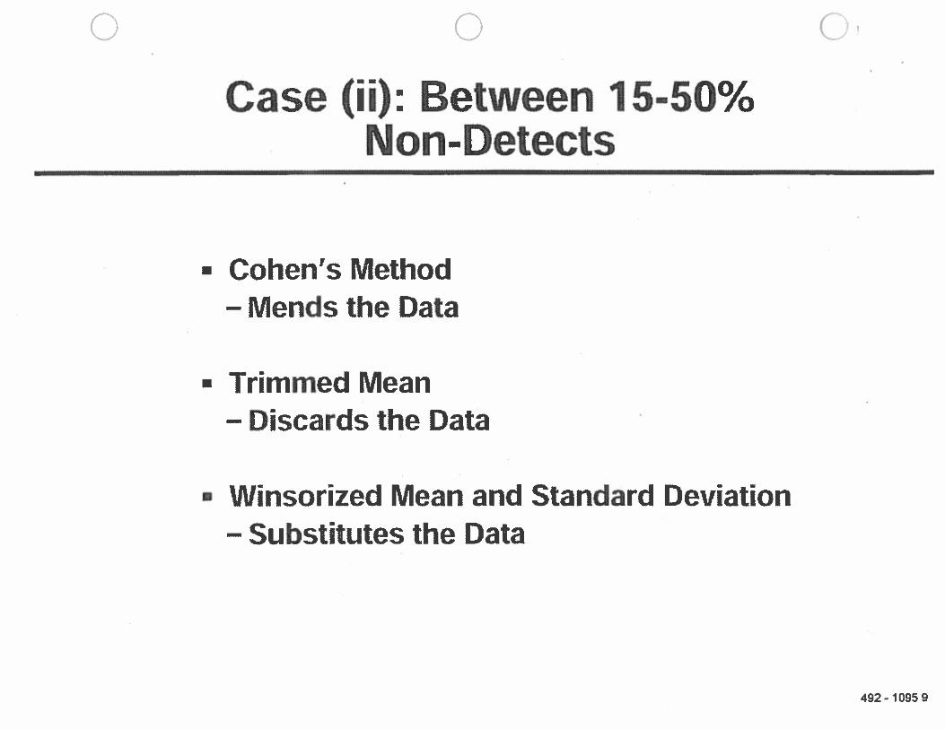
CD M 0 CD U,

CD

0

SS

S

‘—4

‘0

0o

a0)

CD

Z(I

,CD

aD.

——

I

‘m0

CD

a)0

CDa) a 0) -I a

Io

0’

CD0

—I

a) —I

0

.9

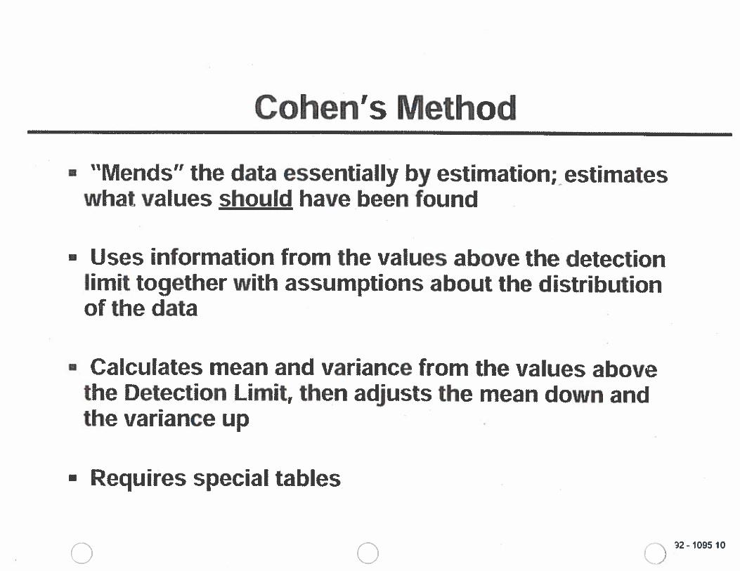
0U,

00c.JC

,

0C

c0

oI.a

•—

CuEon

cuc

•—

Ia

—‘

I_

I—

I-

00•P

ba

z

o>

cu

w.c

oW

VE

.o

cu

Oat

Cfl

WD

C)0

0—

C‘‘

IAvicu

0‘a

C0

C>

00

C)0

3at

.c

00

CCu

o0

t1

oc

cE

•—

0.:

C.)

_

C0

VC

I.

2c0

00

0E

w0

.20

U,

C0

IIflC

Cu

WtC

00Cu

.—

‘—

Ø4

Ø

(VO

W0

0=

_C

QD

•—

I

__

—

II

N

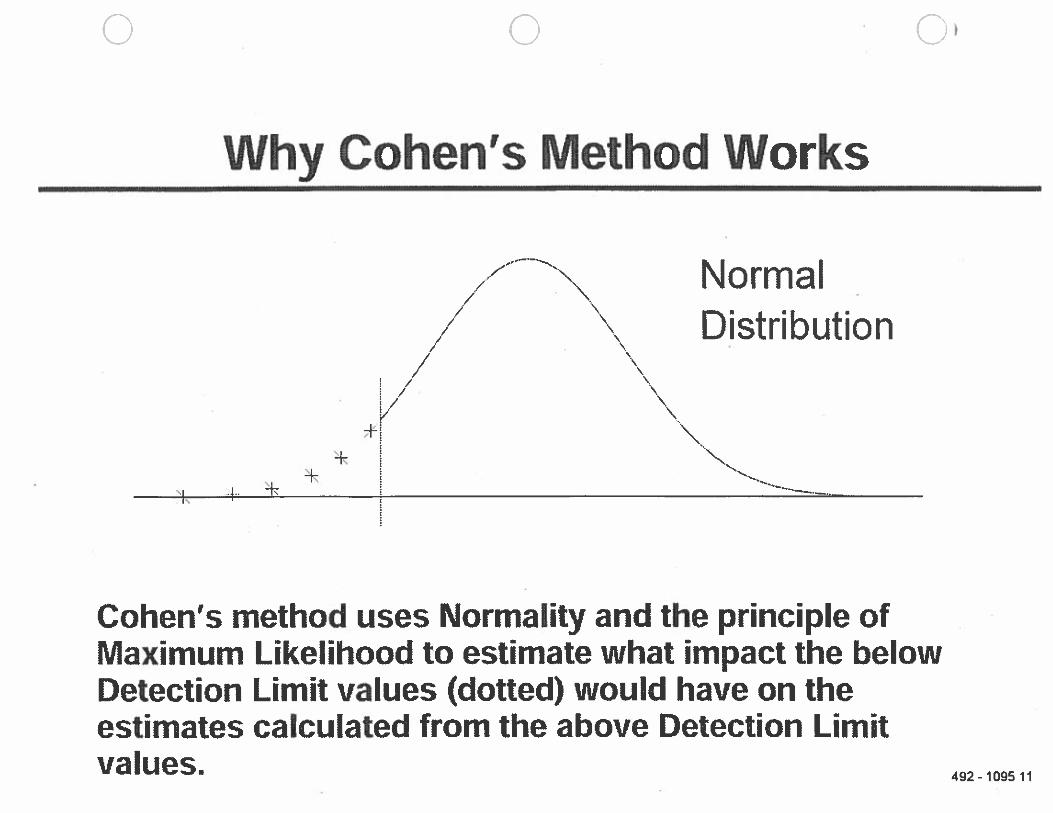
C C

Why Cohen’s Method Works

/ Normal/// Distribution

• N.

//

/

+N

Cohen’s method uses Normality and the principle ofMaximum Likelihood to estimate what impact the belowDetection Limit values (dotted) would have on theestimates calculated from the above Detection Limitvalues. 492-1095 11

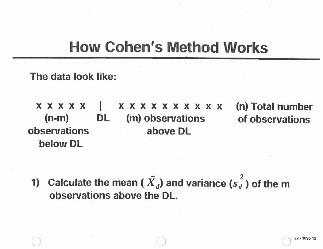
How Cohen’s Method Works

The data look like:

I xxxxxxxxxx (n)Totalnumber(n-rn) DL (m) observations of observations

observations above DLbelow DL

1) Calculate the mean (Xd) and variance (s) of the mobservations above the DL.

C) ED 32-109512

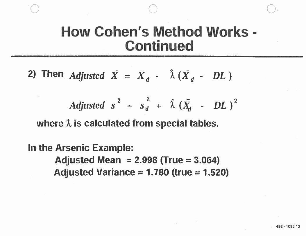
C C) 0

How Cohen’s Method Works -

Continued

2) Then Adjusted X = Xd - (Xd - DL)

2 2— 2Adjusted s = + - DL)

where is calculated from special tables.

In the Arsenic Example:Adjusted Mean = 2.998 (True = 3.064)Adjusted Variance = 1.780 (true 1.520)

492-109513

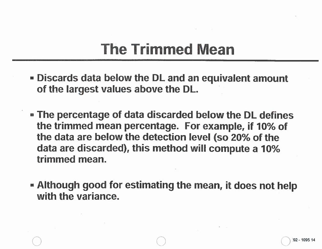
SS

—.

——

03 03

El

3D

DC

DD

)

0(0

—00

CM

—m

-t o Cd,

— —I

(‘)D

33

—I

nfl

nZ (0 —

oo.

CD

m a0

—

— CDC

D0

0CD _0

m—

•30

aco

O0

o 0O

a’i

.....O

C,’

30

0—

—*

C

CD-l.

,0

-Sm0

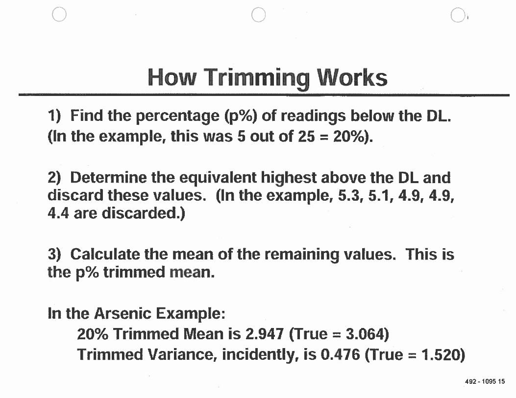
o C)

How Trimming Works

1) Find the percentage (p%) of readings below the DL.(In the example, this was 5 out of 25 = 20%).

2) Determine the equivalent highest above the DL anddiscard these values. (In the example, 5.3, 5.1, 4.9, 4S,4.4 are discarded.)

3) Calculate the mean of the remaining values. This isthe p% trimmed mean.

In the Arsenic Example:20% Trimmed Mean is 2.947 (True = 3.064)Trimmed Variance, incidently, is 0.476 (True 1.520)

492-109515

CD NJ

0 CD a’ 0)

CDa

CD—

I

—z-

—

(In

lo

0 -‘

—l

øsø

N a

Cr

—— Cd

,C

.

z

‘-I

C—

•

CD -‘ 0

<—

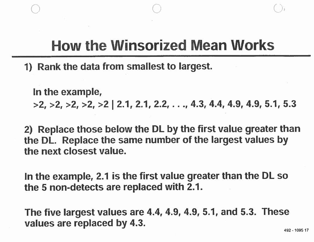
I—

0C

D,-

.0

0E

0zo

vz•

Ox

00

-‘a

fl(I’)

CD

00

®t

O-c._

.1W

——

a

V’

CDO

D)

_

7c

a.’

000

051

—

-I

Co

Dl

a;B

rZ

No

a—

Z’C

Da

-‘

3°-B

CD

’9’

-CD

——

‘a

ZC

OD

)

U’

—C

cD

.0

)-

CD1

•0

CD

)-

00e

Ci

r-‘

-C

0c-I—

,

o9’

0 C”

-a -4

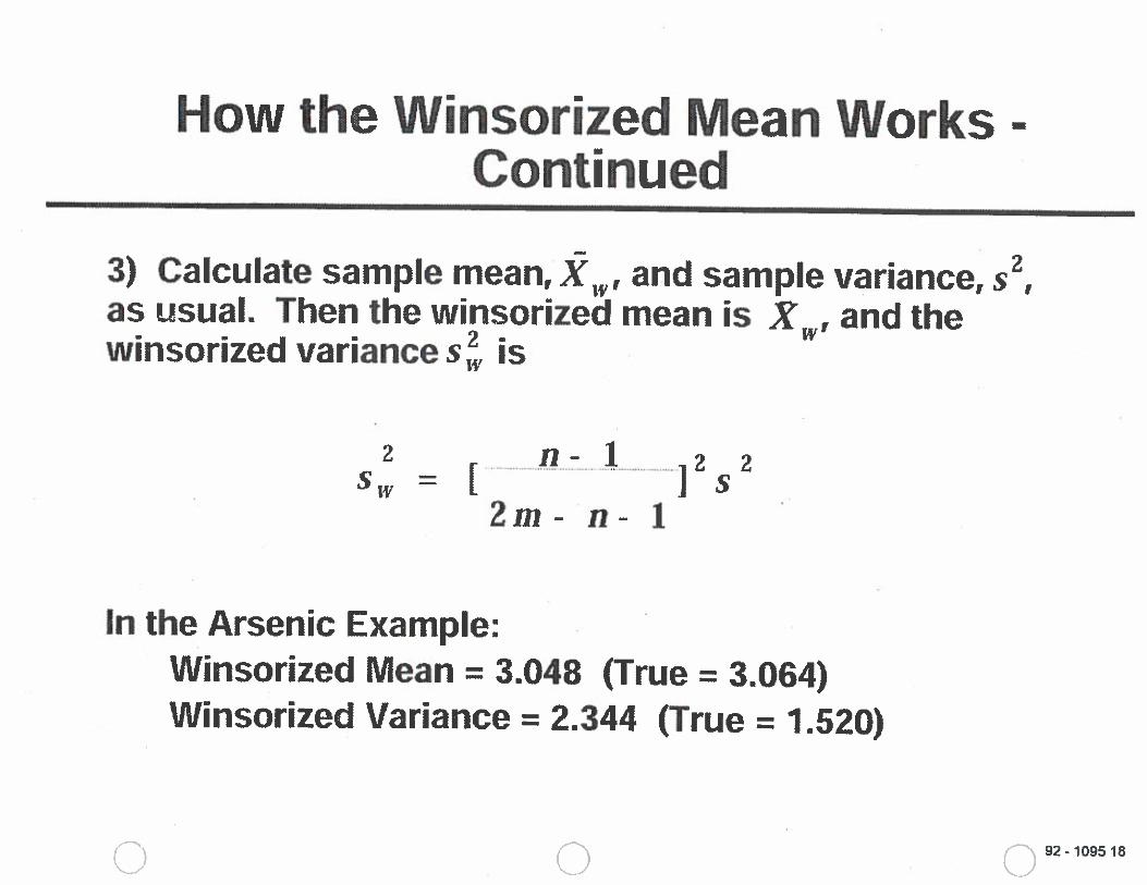
How the Winsorized Mean WorksContinued

3) Calculate sample mean, X, and sample variance, s2as usual. Then the winsorized mean is X , and thewinsorized variance S14, is

2 ii- 1 2 2= [ ] s

2m n- 1

In the Arsenic Example:Winsorized Mean = 3.048 (True = 3.064)Winsorized Variance = 2.344 (True 1.520)

0 . .. Q 92-1095 18

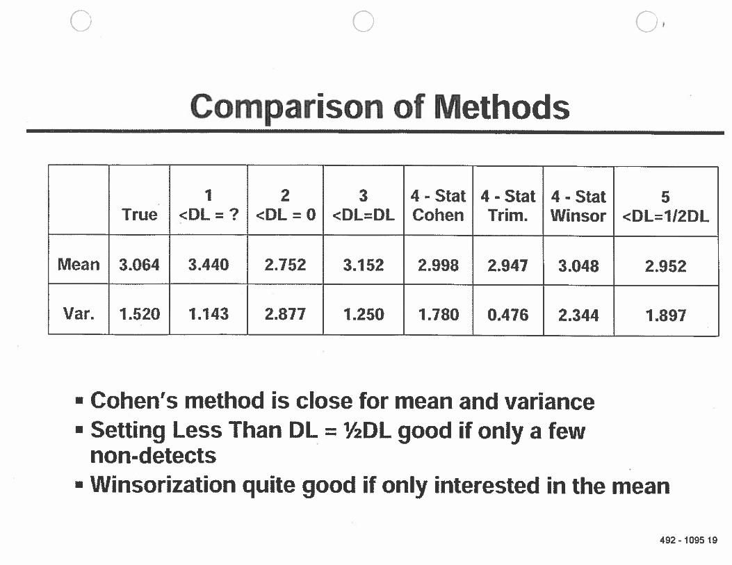
0 0 0

Comparison of Methods

• 1 2 3 4-Stat 4-Stat 4-Stat 5True <DL =? <DL = 0 <DL=DL Cohen Trim. Winsor <DL=1I2DL

Mean 3.064 3.440 2.752 3.152 2.998 2.947 3.048 2.952

Var. 1.520 1.143 2.877 1.250 1.780 0.476 2.344 1.897

• Cohen’s method is close for mean and variance• Setting Less Than DL = ½DL good if only a few

non-detects• Winsorization quite good if only interested in the mean

492-109519

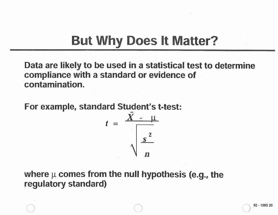
-I’ a C0

= CD r

0 0)0

z0 -1

-1

0a

a ‘C -C 0 z. CD 0 —I

0 42 = a

a •2.

CD 0 0) a 0) a 0

CI

00 — =0

0C

D

aCD —

I

On

,

CD

—C

D,

—I

— —I

aI

ow

a— 0 ‘-

p 0 a a a 5’ CD

-I,

0

0

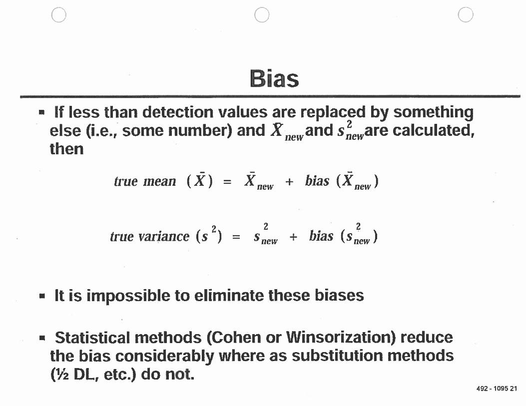
o C. .. C

BiasIf less than detection values are replaced by somethingelse (i.e.; some number) and X,jewand sare calculated,then

true mean (X) = + bias (X,)

true variance(2)

= + bias (sw)

• It is impossible tO eliminate these biases

• Statistical methods (Cohen or Winsorization) reducethe bias considerably where as substitution methods(½ DL, etc.) do not.

492-109521

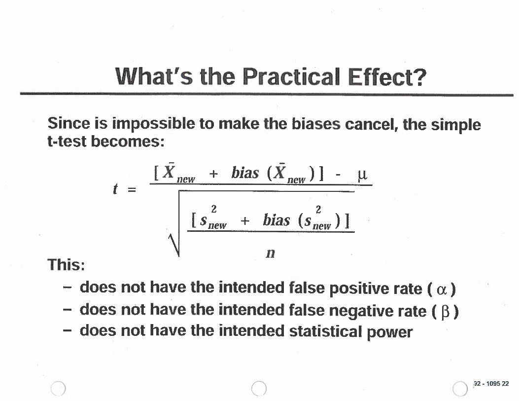
-‘rø

——

I

II

I0

00

aaa”

—®

000

c—

000

000

0—

’0

3C

coo

B’v

Cm

O0

0“0 —

I—

cc.c

____

Cm

om

——

eCD —

—0

00

+0

—‘

‘—

‘

3C’D

,m

oo

+-Q

CDaaa

000

DI)

aaa

m0

C—

—.

00

‘0

00

0CD

_

00

00

_

0m

on

0CD — —

0z.

—CD 0

-P

—I 3 CD

CD M - 0 CD U’

0

21

— ‘V 0

0)—

‘

—.

(fl 0SI

mC

D

z W —I

‘A

—

0—

0)

0)-’ CD

0

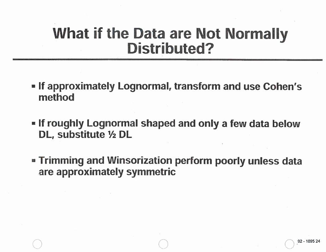
What if the Data are Not NormallyDistributed?

• If approximately Lognormal, transform and use Cohen’smethod

• It roughly Lognormal shaped and only a few data belowDL, substitute ½ DL

• Trimming and Winsorization perform poorly unless dataare approximately symmetric

C) C) ()

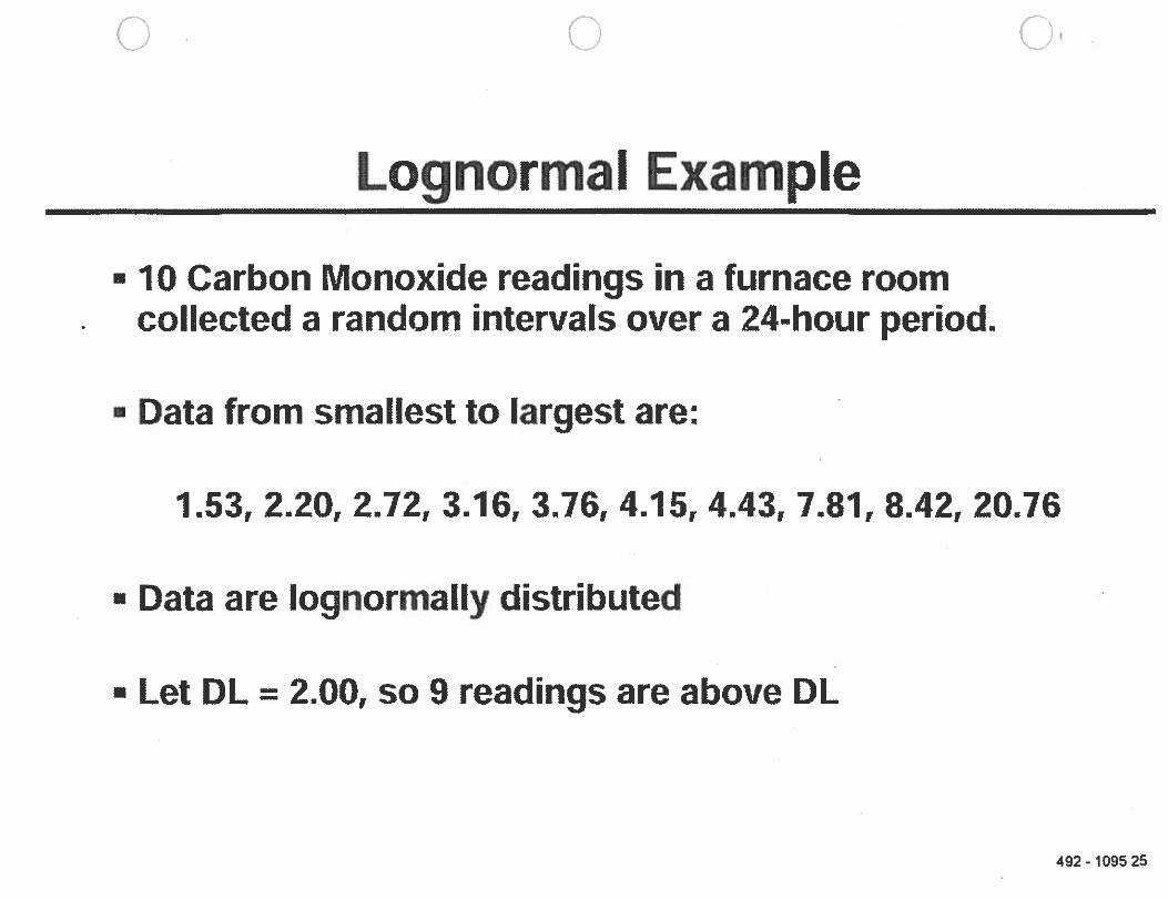
aa

aa

0r

oo

CDp

00

p.

o r ii0

CP

Uao

3o

v_c

CM

r 0CD

—.‘

IA

(iD

WI

—LA

)

aP

—0

a—

.0)

N’

—t

CMLA

)-‘

Li

COC

aCO

—.

CD0

CMU

,,C

_

0)—

A%

a<

—m

aCD

0) U 0 Cr3

C

oC

cm

-a—

‘1

Co

tO

• N)

p.0 Li

0a,

(0 M -A 0 (0 c-n tO UI

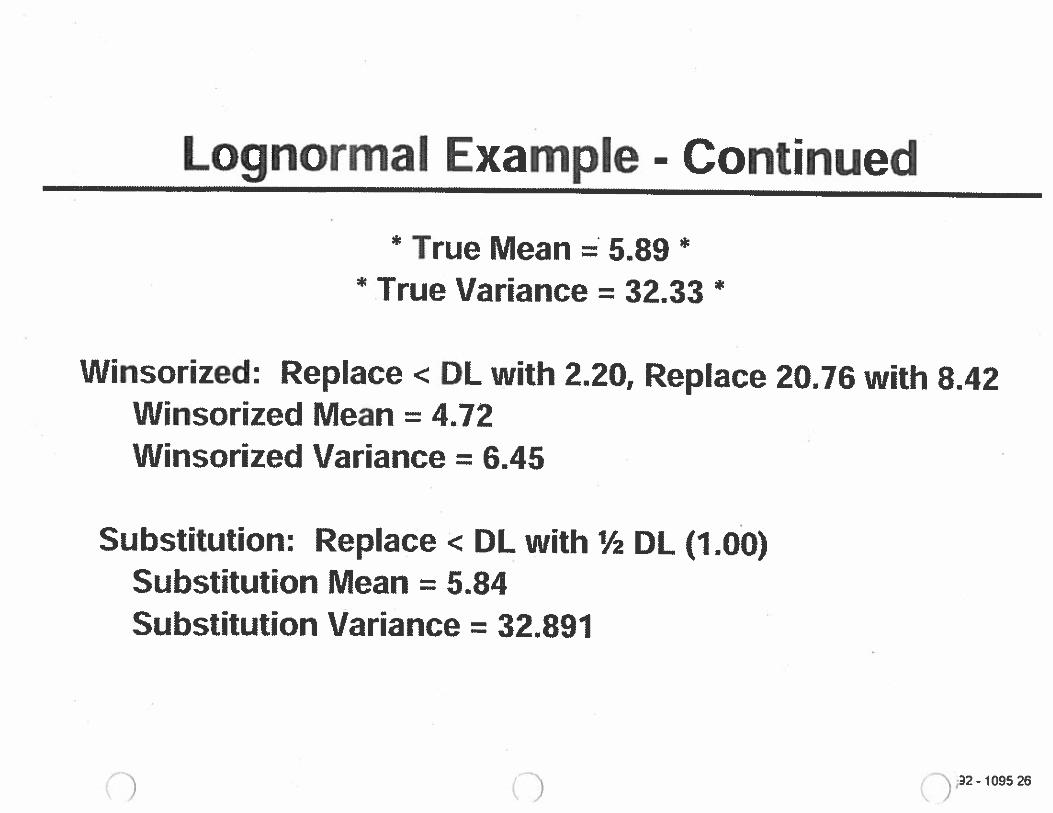
0—

I

00

Cc

—I—

so

IA

IA

—.

00

dW

IW

IN

0—

I—

I— —

aa

acC

——

sN

NCO

—,

—•

CDCD

Go

-.

aa

0C

D-%

CD

D*

3—

IQ

i)—

C—

I0

11

CD

CD

QIA

iiL

fl“C

oo

c• OZ

—.

3N

-aII

CII

o rCD

C,)

*

- -*

a0

oa’

• 0)

m 0.

Co

.

-a 0 CD U,

0)

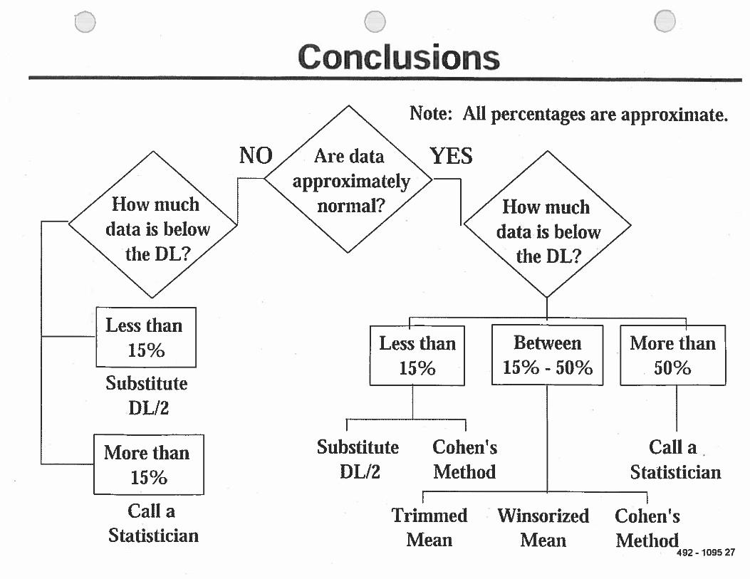
o 0 0Conclusions

Note: All percentages are approximate.

NO Are data YESapproximately

How much normal? How muchdata is below data is below

tile DL? the DL?

Less than Io Less than Between More than15k

15% 15%-50% 50%Substitute

DL/2

______________

1

More than Substitute Cohen’s Call a•

15% DL/2 Method StatisticianI I

Call a Trimmed Winsorized Cohen’sStatistician Mean Mean Method

492-109527