arX

iv:a

stro

-ph/

0201

177v

1 1

1 Ja

n 20

02

Interstellar Deuterium, Nitrogen, and Oxygen Abundances

Toward BD+28◦ 4211: Results from the Far Ultraviolet

Spectroscopic Explorer1

George Sonneborn,2 Martial Andre,3 Cristina Oliveira,3 Guillaume Hebrard,4

J. Christopher Howk,3 Todd M. Tripp,5 Pierre Chayer,3,6 Scott D. Friedman,3

Jeffrey W. Kruk,3 Edward B. Jenkins,5 Martin Lemoine,4 H. Warren Moos,3

William R. Oegerle,2 Kenneth R. Sembach,3 and Alfred Vidal-Madjar4

ABSTRACT

High resolution far-ultraviolet spectra of the O-type subdwarf BD+28◦ 4211 were obtainedwith the Far Ultraviolet Spectroscopic Explorer to measure the interstellar deuterium, nitrogen,and oxygen abundances in this direction. The interstellar D I transitions are analyzed down toLyι at 920.7 A. The star was observed several times at different target offsets in the directionof spectral dispersion. The aligned and coadded spectra have high signal-to-noise ratios (S/N= 50− 100). D I , N I, and O I transitions were analyzed with curve-of-growth and profile fittingtechniques. A model of interstellar molecular hydrogen on the line of sight was derived from H2

lines in the FUSE spectra and used to help analyze some features where blending with H2 wassignificant. The H I column density was determined from high resolution HST/STIS spectraof Lyα to be log N(H I) = 19.846 ± 0.035 (2σ), which is higher than is typical for sight linesin the local ISM studied for D/H. We found that D/H = (1.39 ± 0.21) × 10−5 (2σ) and O/H= (2.37 ± 0.55) × 10−4 (2σ). O/H toward BD+28◦ 4211 appears to be significantly below themean O/H ratio for the ISM and the Local Bubble.

Subject headings: ISM: Abundances — Cosmology: Observations — ISM: Evolution — Ultraviolet: ISM— Stars: Individual (BD+28◦ 4211)

2Laboratory for Astronomy and Solar Physics, Code

681, NASA Goddard Space Flight Center, Green-

belt, MD 20771; george.sonneborn@gsfc.nasa.gov,

oegerle@s2.gsfc.nasa.gov3Dept. of Physics and Astronomy, The Johns Hopkins

University, Baltimore, MD 21218; mandre, oliveira, howk,

chayer, scott, kruk, hwm, and sembach @pha.jhu.edu.5Princeton University Observatory, Princeton, NJ

08544; tripp and ebj@astro.princeton.edu.4Institut d’Astrophysique de Paris, 98bis Blvd. Arago,

75014 Paris, France; alfred, hebrard, and lemoine@iap.fr.6Primary affiliation: Department of Physics and Astron-

omy, University of Victoria, P. O. Box 3055, Victoria, BC

V8W 3P6, Canada.1Based on observations made with the NASA-CNES-

CSA Far Ultraviolet Spectroscopic Explorer. FUSE is op-

erated for NASA by the Johns Hopkins University under

NASA contract NAS5-32985.

1. INTRODUCTION

The abundance ratio of atomic deuterium tohydrogen (D/H) is a key diagnostic of light el-ement production and the baryon-to-photon ra-tio (η) in big bang nucleosynthesis (BBN, Walkeret al. 1991). Significant efforts in recent yearsto measure D/H in high redshift intergalactic gashave generally yielded values in the range D/H= (2.5 − 4.0) × 10−5 (O’Meara et al. 2001 andreferences therein).

In galaxies, D/H is an important indicatorof chemical evolution (Audouze & Tinsley 1974;Boesgard & Steigman 1985; Tosi et al. 1998), asD is easily destroyed in stars (2H + p →3 He + γ)at temperatures of only a few million degrees. In

1

fact, there are no known appreciable sources of Dother than BBN. The interstellar medium (ISM),as the repository of stellar mass loss, holds thekeys to unravelling the chemical history of D overthe age of the galaxy. Measurements of atomicD/H in the ISM were first made by the Coperni-

cus satellite toward bright OB stars within ∼ 500pc of the sun (Rogerson & York 1973; see Vidal-Madjar & Gry 1984 for a review). Significantprogress had been made using the Hubble SpaceTelescope (HST ) to obtain some precise D/H mea-surements in the local ISM (Linsky et al. 1998;Vidal-Madjar et al. 1998), but these have nec-essarily been limited to very low column densitylines of sight (N(H I)∼ 1018 cm−2) where Lyα canbe used to measure the D I column density.

The D/H ratio was measured at high spec-tral resolution (λ/∆λ ∼ 80, 000) with the Inter-stellar Medium Absorption Profile Spectrograph(IMAPS, Jenkins et al. 1988, 1999) toward threeOB stars (δ Ori A, Jenkins et al. 1999; γ2 Veland ζ Pup, Sonneborn et al. 2000) first studiedby Copernicus. These studies showed unequiv-ocally that there is a large spread in D/H (fac-tor of 3) on sight lines toward early type stars atdistances of 300-500 pc. The IMAPS instrumentwas limited to observing very bright OB starsby its instrument design. At that time IMAPScould only observe the lower Lyman series throughLyǫ λ937 because its gratings were coated withlithium-fluoride (LiF).

FUSE provides a new capability to studythe entire Lyman series (except Lyα) in muchfainter stars than were possible with Copernicus

or IMAPS, and hence D/H in the ISM within 200pc can now be studied systematically for the firsttime. This is important because the lines of sightto nearby stars are usually simpler with less blend-ing of different velocity components. FUSE hassufficient sensitivity to perform absorption linestudies of white dwarfs as well as extragalacticobjects. Both categories of targets were inaccessi-ble to Copernicus or IMAPS. The study of D/Hthroughout the Galaxy is one of the primary ob-jectives of the FUSE mission (Moos et al. 2000).

In this paper we report the analysis of D,N, and O abundances toward the O subdwarfBD+28◦ 4211 using high signal-to-noise (S/N) ra-tio spectra obtained with FUSE . BD+28◦ 4211has a very high temperature (∼82,000 K), lies at

a distance of ∼ 100 pc, and has a H I columndensity, N(H I) , of ∼ 1020 cm−2. This columndensity is much higher than those of the otherLISM lines of sight studied previously for D/H,and very similar to that of the D/H sight linesstudied by IMAPS. In this N(H I) regime the Ly-man series shortward of Lyδ λ949 is required tostudy N(D I) .

Because a measurement of D/H requires bothaccurate N(D I) and N(H I) , we use FUSE spec-tra to measure total column densities for N(D I) ,N(N I) , and N(O I) and HST/STIS spectra ofLyα to measure N(H I) . Even in the regimeN(H I)∼ 1020 cm−2, the damping wings of Lyβand higher Lyman series transitions are too weakto obtain an accurate N(H I) measurement.

The observations and data processing are pre-sented in §2 and the stellar atmosphere model andsynthetic spectrum in §3. The measurement ofN(H I) is discussed in §4. In §5 we describe themeasurement of N(D I) , N(N I) , and N(O I) bycurve of growth and profile fitting techniques, aswell as the analysis of interstellar molecular hy-drogen. This H2 model is used in the D I , N I,and O I analysis. The paper concludes in §6 witha discussion of the results and a comparison withother recent D/H studies in the Galaxy.

2. OBSERVATIONS

BD+28◦ 4211 was observed by FUSE throughthe LWRS aperture (30′′×30′′) on 2000 June 13for 2192 s (ObsID=M1080901), 2000 July 16 for16677 s (ObsID=M1040101), and 2000 September19 for 7864 s (ObsID=M1040105). One MDRSaperture (4′′×20′′) observation was made on 2000July 17 for 24795 s (ObsID=M1040102). The firstobservation was a short exposure to establish thefeasibility and safety of using BD+28◦ 4211 for theFUSE calibration program because its far-UV fluxis very close to the bright limit of the FUSE de-tectors (Fλ ∼ 10−10 erg cm−2 s−1 A−1). The sub-sequent observations were made for the purpose oftesting the acquisition of data with the Focal PlaneAssembly (FPA) offset to different positions alongthe dispersion direction as a technique to reducefixed-pattern noise when the observations are latercoaligned and added. This procedure and the re-sults are discussed below. The FUSE instrumentand its performance are described by Moos et al.

2

(2000) and Sahnow et al. (2000).

The data were obtained in “histogram” modebecause of the high far-UV flux of the star. In thisdata acquisition mode a two-dimensional spectralimage is accumulated on board, eliminating anytiming information within individual exposures.The observations were split into four intervals ofapproximately equal exposure time, each with adifferent X-offset of the FPA. The exposure timerequired for the last two LWRS FPA positions wasobtained in part during observation M1040101 andin part during observation M1040105. A shift inFPA X causes a corresponding shift in the locationof the spectrum on the detector along the disper-sion direction. The spectral shifts and exposuretimes are given in Table 1. The FPA is fixed forthe duration of each exposure so that there is noloss in spectral resolution relative to an observa-tion taken at a single FPA location. The offsetsfor the MDRS observations span a smaller rangein FES X than those of the LWRS observationsin order to provide sufficient margin in the FPArange of motion. This margin is needed so thatMDRS peakups can properly adjust the FPA’s tocorrect for image motion caused by small rotationsof the primary mirrors on orbital timescales. Forfurther information on this image motion see Sah-now et al. (2000). The shifts caused by this imagemotion, together with shifts caused by similar ro-tations of the gratings, result in a distribution ofshifts clustered about the mean offsets given in Ta-ble 1. Even for MDRS, these spectral offsets spana range roughly twice the width of typical inter-stellar absorption lines or of the high-frequencycomponents of the detector fixed pattern noise.

Exposure durations varied from 430 s to 535s in order to minimize Doppler smearing of thespectrum by satellite orbital motion so that thereis no degradation of spectral resolution. Most ofthe LWRS exposures were obtained during orbitalnight when O I and N I airglow emission is absentand that of H I is significantly reduced. Whenexposures having both orbital night and day seg-ments are considered, over 70% of the LWRS datawas obtained during orbital night. Over 82% ofthe MDRS data was obtained at night.

The data were processed with the latest ver-sion of the FUSE calibration pipeline (CALFUSE v.1.8.7). For each channel, data for each exposurewere aligned by cross correlation and combined on

a common heliocentric wavelength scale. Part ofthe resulting spectrum for the LWRS observationsis shown in Figure 1. The LWRS LiF co-addedspectra have S/N∼ 100 per 0.05 A resolution el-ement in the LiF channels and S/N∼ 60 in theshort-wavelength silicon-carbide (SiC) channels.The S/N in the MDRS spectra of BD+28◦ 4211are about 25% lower than for LWRS. These S/Nlevels are close to the photon-noise limits. Theanalyses presented in this paper uses primarily SiCchannel spectra. Figure 2 shows small sections ofthe spectrum near several of the Lyman lines anddemonstrates the high quality of our spectra. Ouranalysis of spectral features in the BD+28◦ 4211co-added spectra indicates that the spectral res-olution is consistent with λ/∆λ ∼ 20,000, thenominal spectral resolution obtained by the FUSE

instrument (Sahnow et al. 2000). It is evidentfrom Figures 1 and 2 that airglow has a negligi-ble effect on these spectra. Lyβ is the strongestairglow transition in the FUSE band pass andthe observed Lyβ profile is only weakly affected.O I airglow, if present, would primarily effect thestronger transitions longward of ∼ 950 A, butthe O I column density is determined from muchweaker lines that are unaffected.

Figures 1-3 show that the saturated H I lineshave non-zero residual flux (on the order of a fewpercent). The FUSE instrument has very low lev-els of scattered light (Moos et al. 2000, Sahnowet al. 2000), as shown by the zero flux level belowthe Lyman limit (see Fig. 1). The residual fluxin the Lyman lines is probably the result of wingsof the instrumental line spread function (LSF; seeKruk et al. 2001). The shape of the LSF andits potential effects on the line profile analysis isdiscussed further in §5.1.

3. STELLAR MODEL FOR BD +28◦

4211

MacRae, Fleischer, & Weston (1951) reportedthe first spectral analysis of BD+28◦ 4211 andclassified it as an extremely blue star with pe-culiar spectrum (Op). The optical spectrum ofBD+28◦ 4211 attracted their attention becauseof its very blue continuum and the presence ofBalmer and He II lines. Greenstein (1952) esti-mated the distance to BD +28◦ 4211 and foundout that the star was a subdwarf. BD+28◦ 4211

3

is now classified as sdO, based on the study ofMoehler et al. (1990), in which the class is de-fined as having He II and strong Balmer absorp-tion lines. Although low resolution optical spec-tra show only these lines, high-resolution spectrareveal, in addition, many weak metal lines. Her-big (1999) obtained high-resolution optical spec-tra of BD+28◦ 4211 at the Keck I telescope anddetected a significant number of narrow absorp-tion and emission lines (C IV, N IV, N V, O IV,O V, and Si IV), and also emission cores in Hα,Hβ, and He II λλ6560, 5411, 4685 lines. Us-ing the O IV absorption lines, Herbig (1999) setan upper limit on the star’s rotational velocity,v sin i ≤ 4 km s−1. Even though BD +28◦ 4211 isa well-known spectrophotometric standard star inthe ultraviolet and optical (see, e.g., Bohlin 1986;Massey et al. 1988), its atmospheric parame-ters were investigated only recently by Napiwotzki(1993), Werner (1996), and Haas et al. (1996).

Using H+He NLTE stellar model atmospheres,Napiwotzki (1993) tried to fit the Balmer line pro-files in BD+28◦ 4211’s optical spectrum with nosuccess. He demonstrated that the effective tem-peratures obtained from fits of individual Balmerlines showed large discrepancies. This inconsis-tency, known as the Balmer line problem, was alsoobserved in central stars of old planetary nebu-lae and DAO white dwarfs (see, e.g., Napiwotzki& Schonberner 1993; Napiwozki & Raunch 1994;Bergeron et al. 1994). To overcome this problem,Napiwotzki (1993) modeled the He I λ5876 line,as it is a very sensitive diagnostic of effective tem-perature (Teff ), and obtained Teff = 82,000 K andlog(He/H) = −1.0. He also derived the gravitylog g = 6.2 from the higher Balmer lines.

By analyzing the optical spectra of BD +28◦ 4211and the central star of the planetary nebulaS216, Werner (1996) concluded that the Balmerline problem was caused by the omission or in-adequate inclusion of metal opacities. For in-stance, he matched the Balmer lines (Hα-Hδ)of BD+28◦ 4211 combining Napiwotzki’s (1993)parameters (Teff= 82,000 K, log g = 6.2, andlog (He/H) = −1.0) and the improved Stark-broadened CNO line profiles. He demonstratedthat the effect of this added opacities increasedthe temperature in the deeper layers of the at-mosphere, and decreased the temperature in thesuperficial layers, therefore modifying the Balmer

line formation. He noted that the low Balmer se-ries members cores are deeper as they are formedhigher in the atmosphere, where the temperatureis lower. On the other hand, the high Balmerseries members were less affected because theyoriginate from deeper layers of the atmosphere.This new temperature structure caused by theaddition of more realistic metal line opacities re-solved the Balmer line discrepancy. Interestingly,Bergeron et al. (1993) had reached a similar con-clusion to that of Werner (1996) by analyzing theDAO white dwarf Feige 55 and using a LTE iron-blanketed model.

For the purpose of this study, we adopt the stel-lar atmospheric parameters determined by Napi-wotzki (1993) as they are the best available. Wecompute a grid of H+He NLTE model atmo-spheres with the following atmospheric parame-ters: Teff = 78000 K, 82000 K, and 86000 K;log g = 6.0, 6.2, and 6.4; and log(He/H) = −0.6,−1.0, and −1.4. We also compute a metal-lineblanketed model including the following chemicalcomposition: H, He, C, N, O, Si, S, Fe, and Ni.We then compute a grid of synthetic spectra fromLyα to the Lyman limit using the TLUSTY pro-gram developed by Hubeny & Lanz (1995) andan upgraded version of the program SYNSPEC(I. Hubeny 2000, private communication), whichincorporates the Lemke (1997) Stark broadeningtables for hydrogen. We explored the model pa-rameter space (Teff , log g, and log(He/H)) to eval-uate the uncertainties in the stellar H I Lyman +He II Balmer line profiles. §4 describes in more de-tails the use of stellar models to dermine the H I

column density.

The FUSE spectrum of BD+28◦ 4211 (Fig. 1)shows many stellar and interstellar lines. The stel-lar spectrum displays the Lyman series of hydro-gen from Lyβ up to Ly-9 and the He II Balmerseries from 1084 A up to at least 942 A. The spec-trum also contains many stellar lines of highlyionized species, such as C IV, N V, O IV, O V,O VI, Si IV, P V, S IV, S V, S VI, Fe VI, Fe VII,Ni VI, and Ni VII. The strongest lines are the N IV

λ923.15 sextuplet, S VI λλ933.38, 944.52 doublet,N IV λ955.33, and O VI λλ 1031.91, 1037.61 dou-blet. In order to identify potential blending ofphotospheric and ISM lines, we first performed anabundance analysis of BD+28◦ 4211’s atmosphereand then calculated a synthetic spectrum using the

4

derived abundances. Figure 3 illustrates the com-parison between the synthetic spectrum and theFUSE spectrum for the wavelength range 920–927A.

BD+28◦ 4211 has several strong, narrow metallines in the FUSE range and that made it pos-sible to register the wavelength scale of the stel-lar model with the observed spectrum. In par-ticular, S VI λ944.523 is seen in both SiC chan-nels and has a deep, narrow core. We used thisline to align the model with the spectra. As ex-pected, the zero point wavelengths are differentfrom channel to channel because it depends on theFPA position as well as the location of the starin the aperture. It varied between −60 km s−1

and +60 km s−1 in our data, although larger off-sets were occasionally detected in the first year ofFUSE operations (Sahnow et al. 2000). Once thewavelength offsets are corrected, the best estimatefrom the FUSE data of the velocity of the star rel-ative to the ISM is +34±6 km s−1, a value that isconsistent with our more accurate determinationof +31± 2 km s−1 from HST spectra (see below).We increased the error to ±8 km s−1 to take intoaccount any remaining uncertainties in the FUSE

wavelength calibration.

4. DETERMINATION OF THE H I COLUMN

DENSITY

4.1. Hubble Space Telescope Observations

The determination of the interstellar H I col-umn density along the sight line to BD+28◦ 4211uses an extensive series of archival observationstaken with the Space Telescope Imaging Spectro-graph (STIS) on board the HST . The H I columndensity may in principle be determined using theFUSE observations of this star. However, most ofthe Lyman-series lines in the FUSE bandpass areon the flat part of the curve of growth. In addition,the damping wings of interstellar Lyβ and Lyγ,the strongest H I transitions in the FUSE band-pass are significantly less prominent than those forLyα and comparable in strength with the stellarH I + He II profiles. Therefore, the only reli-able procedure for determining an accurate H I

column density to BD+28◦ 4211 is by fitting theLorentzian wings of the very strong Lyα line. Asillustrated below, the interstellar H I profile ismuch stronger that its stellar counterpart.

BD+28◦ 4211 is a calibration source for STIS,and observations have been acquired over sev-eral years with the E140M echelle grating pro-jecting the two-dimensional spectrum onto theFUV MAMA (Kimble et al. 1998; Woodgateet al. 1998). All data were taken through the0.′′2 × 0.′′2 aperture and cover the spectral range∼ 1150 − 1750 A. This instrumental setup pro-vides a spectral resolution R ≡ λ/∆λ ∼ 45, 000(∆v ∼ 7 km s−1 FWHM), although the line spreadfunction for data taken through this aperture hassignificant power in broad wings that extend wellbeyond this width (see Figure 13.87 in the Cycle 9STIS Instrument Handbook). We used eight suchobservations taken over the time period 1997 Sept.19 to 2000 Nov. 10. Exposure times for the indi-vidual observations were in the range 350–1800 s.Figure 4 shows a coaddition of the data sets usedin our analysis in the region near Lyα. This figuredemonstrates the quality of the data and showsthe importance of high spectral resolution for sep-arating the numerous stellar and interstellar linesin this region.

4.2. Data Calibration and Reduction

The E140M data have been reduced using theCALSTIS pipeline by two different approaches inan attempt to uncover sources of systematic error.One used the pipeline as developed by the STISInstrument Definition Team, the other the stan-dard STSDAS pipeline distributed within IRAF(see Voit 1997). The CALSTIS pipeline removesan estimated dark level, applies a flat field, cor-rects small-scale distortions, identifies the spectraltrace, removes scattered light, extracts the one-dimensional spectrum, and performs the wave-length and flux calibrations. We show below thatboth analysis approaches yield the same result.

The scattered-light removal process is amongthe most important, particularly for our purposeswhere we are interested in the large-scale wingsof the Lyα profile. Because the strength of theechelle-scattered light can be significant in E140Mspectra, the Bowers & Lindler algorithm (seeLandsman & Bowers 1997; Bowers et al. 1998)was used to estimate and remove scattered lightfrom the data in the pipeline procedures. Wefound that this algorithm does a good job of de-termining an appropriate zero-level, as evidencedby the small residual fluxes in the saturated cores

5

of strong lines (e.g., the Lyα profile shown in Fig.4).

After extracting the spectrum, several echellespectral orders in the regions adjacent to Lyαwere combined using a weighted averaging schemewhere the orders overlap. The flux calibration be-tween orders seems good for the E140M data setsused here. Even so, there can be some small fluc-tuations in the final co-added spectrum due to mis-matches at the edges of orders, although in generalthese can be masked out and do not significantlyaffect our analysis.

4.3. Analysis Methodology

The method for deriving the H I column den-sity along this sight line follows Jenkins (1971) andsubsequent work (see discussion, particularly of er-ror analysis, in Vidal-Madjar et al. 1998; Howk,Savage, & Fabian 1999; Jenkins et al. 1999; Son-neborn et al. 2000). The distribution of opticaldepth, τ(λ), with wavelength for Lyα is given bythe product of the absorption cross-section, σ(λ),and the column density. For H I at Lyα this is:

τ(λ) ≡ σ(λ)N = 4.26 × 10−20N(λ − λ0)−2, (1)

where λ0 is the Lyα line center at the velocitycentroid of interstellar hydrogen. The H I col-umn density is determined to be the one that bestmatches the above distribution of optical depthwith the observed profile. This method only givesinformation on the total column of H I , since thedetails of the component structure are all withinthe strongly-saturated core of the Lyα line whichspans a velocity range of ±200 km s−1. It is ex-tremely unlikely that the damping wings are af-fected by low column density H I absorption fea-tures. Any H I absorber that could modify theshape of the damping wings would have to havea heliocentric velocity |v| > 400 km s−1 (see Fig.9 of Sonneborn et al. 2000). The broad damp-ing wings of Lyα are not sensitive to the Dopplerbroadening parameter. We therefore have very lit-tle information about b from the Lyα analysis.

The derivation of N(H I) was performed withtwo independent, though similar, fitting proce-dures. Both vary the important free parameters,which for our purposes include λ0 and N(H I) , tominimize the χ2 statistic between the model, afterconvolution with the instrumental LSF, and the

observed spectra (see, e.g., Jenkins et al. 1999).We note that the specifics of the LSF are rel-atively unimportant for N(H I) as large as isfound on this sight line (see, e.g., Appendix Aof Howk et al. 1999). This insensitivity includesthe possible presence of the broad wings of theSTIS E140M LSF mentioned above, which are ona much smaller scale than that of the H I absorp-tion.

We applied masks to exclude obvious stellar andinterstellar absorption features from the fit. Wealso avoided fitting the very deepest portion of theLyα line core (effectively those regions with flux< 10% of the stellar continuum within ∼ ±2 Aof the line center) because of the possibility thatstellar lines may be unseen in this low signal-to-noise region of the spectrum.

The stellar atmosphere for this type of star alsohas broad Lyα + He II absorption. It is, therefore,important to account for the stellar continuum un-derlying the interstellar absorption in our fittingprocess. For this purpose we used the syntheticspectrum and stellar Lyα + He II line profile de-scribed in §3.

The computed stellar spectrum was shifted toa heliocentric velocity of +20.2 km s−1, the ra-dial velocity of BD+28◦ 4211, for comparison withthe observed Lyα profile. We determined this ra-dial velocity by measuring the velocities of promi-nent stellar lines in the STIS E140M observa-tions, the average of which gives a heliocentricvelocity of vhel = +20.2 ± 0.8 km s−1. Thequoted uncertainty is the 1σ standard deviationof the individual measurements about the meanand does not include the uncertainties in the STISabsolute wavelength scale, which probably corre-spond to ∼ 1.6 to 3.2 km s−1. This determina-tion agrees well with the stellar radial velocityof vhel = +21.4 ± 1.7 km s−1 derived by Her-big (1999), where we use the mean and 1σ stan-dard deviation of his individual measurements.For comparison, the average velocity of interstel-lar material along this sight line is vhel ∼ −9 to−13 km s−1 (stronger lines give more negative ve-locity components due to the presence of weakercomponents on the blue side of the interstellarprofiles). The stellar radial velocity is well con-strained, although we found that offsets from thisbest value as large as 5 km s−1 have no effect onthe derived H I column density.

6

The model stellar spectrum was scaled to bestmatch the observed flux distribution using asecond-order Legendre polynomial, the parame-ters of which are treated as free parameters inthe fitting process. In general, the shape of thecalculated stellar model far from line center fitsthe data relatively well. However, the adoptionof a low-order polynomial correction to the syn-thetic stellar continuum allows for several possiblesystematic effects, including mis-matches betweenthe observed spectrum and the model, slight re-distribution of flux in the scattered light removalprocess, stellar atmospheric variability, and otherproperties of the detector and observations thatcould change the absolute flux distribution onAngstrom scales.

We also allowed for the effects of uncertainty inthe flux zero point, treating it as a free parameterin the fit. This corrects for any small uncertaintyin the background subtraction on scales of severalAngstroms. The derived corrections to the fluxzero point were always less than a percent or twoof the continuum away from the line core.

Because of the possibility that the stellar Lyαprofile could be variable, we fit separately eachof the individual observations taken at differenttimes. No evidence of variability was found. Thisis discussed in more detail below in our discussionof systematic uncertainties.

4.4. Results and Discussion of Systematic

Uncertainties

Figure 4 shows the best fit interstellar H I pro-file on top of the coadded STIS observations. Thefinal estimate for the H I column is log N(H I ) =19.846+0.036

−0.034, where the uncertainties are 95% con-fidence limits (2σ if Gaussian errors are appropri-ate) including systematic effects. This is an aver-age of the results from the two N(H I) determi-nations, which differed by only 0.003 dex (< 1%),and uncertainties, for which we adopted the largerof the uncertainty estimates.

The uncertainties in N(H I) given above in-clude estimates of the statistical (random) andsystematic uncertainties added in quadrature. Be-cause of the high quality of the data and thestrength of the Lyα damping wings, the system-atics dominate the statistical uncertainties in ouranalysis. Given the importance of the systematic

uncertainties, we discuss several below and theirimpact on the N(H I ) determination.

Stellar model uncertainties – The largest iden-tified source of systematic uncertainty for N(H I)is the adopted stellar model. However, fits to theobserved Lyα profile which use only a straight linecontinuum rather than a stellar model for nor-malization produce H I column densities that arelarger by only +0.1 dex (∼ 25%). This sets an up-per bound on the magnitude of the uncertaintiesdue to the stellar models.

The effects of imperfectly-known stellar atmo-spheric parameters on N(H I) were estimated byrefitting the interstellar Lyα absorption profile us-ing model atmospheres with the most extremestellar properties that are still nominally consis-tent with the determination of the atmospheric pa-rameters (see §3). For this purpose we chose thosemodels with the strongest and weakest stellar Lyαabsorption profiles from a grid of atmospheres cov-ering a wide range in parameters: log He/H(−0.6to −1.4), Teff (78,000 to 86,000 K), and log g (6.0to 6.4).

The N(H I) values derived in this way weretreated as extrema corresponding to 95% con-fidence limits (2σ assuming Gaussian statistics)about the best-fit result. While this approach doesnot account for any uncertainties in our knowl-edge of the fundamental physics of stellar atmo-spheres or radiative transfer, the adopted extremeatmospheres encompass a sufficiently large rangeof parameter space that the effects of any sub-tle atmospheric physics are expected to be smallin comparison to the uncertainties estimated inour approach. The uncertainties associated withthe adopted stellar model and our allowance forstronger and weaker stellar Lyα profiles dominatethe uncertainties in the N(H I) determination.

We note that the effects of line-blanketingwithin the model atmosphere will be much smallerthan the effects of the extreme atmospheric pa-rameters investigated above. We verified this as-sumption with appropriate model calculations,and that the variation in the stellar Lyα profileoccurs primarily in the core of the line where theresidual flux in the observed spectrum is zero.

Residual scattered light – In principle, residualscattered light in the STIS E140M spectra couldbias the N(H I) determination. The core of Lyα

7

is indeed very near zero, and we allowed the trueflux zero point to vary as a free parameter in thefits. However, if light were distributed in the linewings in an appropriate way during the scatteredlight removal process, this could potentially be asource of systematic uncertainty in our H I columndensity determination.

As a check of the N(H I) value derivedfrom STIS E140M observations, we also analyzedarchival observations taken with the pre-COSTARGoddard High Resolution Spectrograph (GHRS)first-order G160M grating through the small sci-ence aperture (0.′′25×0.′′25). These spectra have aresolution of ∼ 15, 500 (∼ 19.3 km s−1 FWHM).While the observations do not cover the entire ex-tent of the red wing of Lyα, the holographically-ruled G160M grating had excellent scattered lightproperties (Cardelli, Ebbetts, & Savage 1993).Eight observations with a total exposure time of1152 s were reduced and combined using proce-dures described by Howk et al. (1999). From thesespectra we found log N(H I ) = 19.842±0.020 (2σ,statistical uncertainties only). This value is soclose to the value derived using the STIS E140Mobservations that we believe residual scatteredlight uncertainties are not likely to be a signifi-cant source of error.

Stellar atmospheric variation – The atmo-spheric profile of the star could be variable, andthere is some evidence that BD+28◦ 4211 maybe part of a binary system (see Napiwotzki 1999;Massey & Gronwall 1990). To account for thepossibility that the stellar Lyα profile might vary,we separately calculated the best-fit H I columndensities for each of the eight individual STIS ob-servations. The dispersion in these best-fit mea-surements for the ensemble of observations wassmall and was added in quadrature to the finaluncertainty estimate. The dispersion of the indi-vidual measurements about the mean was muchsmaller than that resulting from the variation ofstellar model parameters described above.

5. COLUMN DENSITIES OF ATOMIC

DEUTERIUM, NITROGEN AND OXY-

GEN

5.1. General Considerations

Both curve of growth (COG) and profile fittingtechniques were used to determine N(D I) and

N(O I) in order to better understand potentialsources of systematic error. Profile fitting alonewas used for N(N I) because there are only threeunsaturated and unblended N I lines available (theλ952 multiplet). The FUSE spectra were also an-alyzed to develop a model for interstellar N(H2)for rotational levels J = 0 − 4. The compari-son of measurements from multiple channels (SiC1and SiC2) and observations (LWRS and MDRS)is a powerful tool that improves our statistics andhelps to identify poor data quality due to instru-mental effects.

In the COG method the equivalent width, Wλ,of several lines of the same species having differentoscillator strengths are measured and their distri-bution in the log(Wλ/λ)− log(Nfλ) plane is com-pared with a theoretical curve of growth for a sin-gle absorption component subject to a Maxwellianvelocity distribution. The free parameters in thefit are the column density, N and Doppler spreadparameter, b. However, if there is a complex ve-locity distribution, b is regarded as an “effective”Doppler spread and as such has no physical mean-ing. Continuum placement and equivalent widthmeasurements are treated in independent stepsand assume some a posteriori conservative errorbars to take into account the uncertainties in con-tinuum placement. The COG method is poten-tially vulnerable to error because of the assump-tion of a single-component profile. In particular,at the FUSE spectral resolution narrow, unre-solved components could be concealed by broaderfeatures, which could result in underestimated col-umn densities (Nachman & Hobbs 1973, Savage &Sembach 1991). Jenkins (1986) showed that col-umn densities accurate to ∼10% can be obtainedwith the COG method provided that the lines arenot heavily saturated (τ0 ≤ 2) and have smoothdistributions of b and τ in their components. Inthe case where all transitions are on the linear partof the COG, the column density is insensitive tothe line-of-sight velocity structure. One of the ad-vantages of the COG method is that it is not toosensitive to the LSF. On the other hand, transi-tions blended with lines from other species shouldbe avoided in this analysis technique. In this case,profile fitting may be more appropriate.

The profile fitting method makes the same basicassumptions as the COG: an interstellar absorp-tion line is formed in a single component and is

8

described by two parameters: N and b. In ad-dition the wavelength centroid of the line, or ra-dial velocity, vr, is also a free parameter. Thefitting technique also assumes that each interstel-lar component produces absorption lines describedby Voigt profiles. We note that in our analysis theDoppler parameter, b, has no unique physical in-terpretation. Normally b2 = 2kT/m+v2

turb. How-ever, from the FUSE spectra alone, with spectralresolution of ∼ 15 km s−1, temperature (T ) andturbulent motion (vturb) effects on the line widthsare not easily separated. We can, however, use bto set an upper limit on T .

Lines of sight with multiple components areoften more reliably analyzed with a fitting tech-nique than it is with the COG. In practice, to fit amultiple-component COG requires a prior knowl-edge of vr and b for each component as well astheir expected relative ratios. This information isnot necessary with profile fitting because in princi-ple it lies in the profiles. For the same reason, theblending of adjacent lines is also easier to modelwith a fitting procedure.

A second significant advantage of our pro-file fitting analysis is that absorption lines andcontinua are fit simultaneously so that contin-uum shape and placement are treated as free pa-rameters. We have used the profile fitting pro-gram Owens.f (Lemoine et al. 2001, Hebrardet al. 2001). Owens.f is a powerful profile fit-ting program that simultaneously models multi-ple spectral lines, species, and absorption com-ponents in an arbitrary number of spectral re-gions, or windows. Many quantities characteriz-ing the fit may be treated as free or fixed param-eters (N, T, vturb, LSF, continuum placement andshape, background level, velocity offset betweenspectral windows, etc.). The program uses an op-timized χ2-minimization algorithm to obtain fastconvergence. The flexibility of Owens.f allowedus to analyze many different cases. As with anyconvergence algorithm, parameter space was ex-plored to verify that a converged solution was thetrue minimum and not a local minimum far fromthe true solution. This was done by changing theinitial parameters and/or conditions and then run-ning the program again to reach a new convergedsolution. A potential disadvantage of profile fit-ting is that knowledge of the instrument LSF isrequired, and errors in the assumed LSF have the

potential to bias the results.

The instrumental LSF is a key parameter inthe profile fitting analysis of interstellar absorp-tion lines. The characterization of the FUSE LSFwas incomplete at the time of this analysis (seeKruk et al. 2001). Although there is evidencethat the FUSE LSF has wings that effect the zerolevel of heavily saturated lines (§2), two indepen-dent analyses (Hebrard et al. 2001, Wood et al.2001) show that modelling of weak unsaturatedlines with a single Gaussian LSF and a doubleGaussian LSF give very consistent results withinthe uncertainties of the FUSE LSF parameters(see the companion papers referenced above forfurther details). For our profile fitting analyseswe used a single gaussian LSF for each componentmodelled.

In the next subsection the interstellar H2 modelis derived. The following subsections describe theCOG analysis of D I and O I and the profile fittinganalysis of D I , O I, and N I.

5.2. Interstellar H2 Column Densities

The FUSE spectra of BD+28◦ 4211 contain alarge number of absorption lines from interstellarmolecular hydrogen. Absorption arising from H2

rotational levels J = 0 − 4 can be clearly seenalong this line of sight. Many H2 lines are blendedwith stellar and other ISM features. For transi-tions corresponding to the rotational level J = 4there are not enough unblended lines to derive areliable column density using either COG or pro-file fitting techniques. However, a 3σ upper limitfor N(H2) J = 4 is derived. A few H2 transi-tions from J = 5 and 6 may also be present. Thebest candidate is Werner 0 − 0 Q(5) at 1017.831A. However, the FUSE spectra of BD+28◦ 4211contain many unidentified stellar features and itis possible that this and other weak transitionscould be stellar in origin, or if actual H2 ISM lines,blended with stellar lines. Due to these uncertain-ties, the column densities for J ≥ 5 could not beestimated. The H2 column densities for rotationallevels J = 0 − 3 were measured using both pro-file fitting and COG methods, using lines that ap-peared free of blending, as judged by the shapeof the absorption profile and with the help of thestellar model.

Profile fitting used only unsaturated lines, i.e.

9

lines for which the absorption profile deconvolvedwith the LSF did not have a residual intensityin the line core < 0.1. The column densityfor each rotational level was determined indepen-dently. The synthetic stellar spectrum gave guid-ance when selecting the H2 lines to be analyzedin order to avoid blending with stellar features.Each spectral region (several Angstroms) was firstnormalized with a spline function. A subset ofthis region, a spectral window of ∼ 1A, was usedby Owens.f where a polynomial (up to 4th order)was fit to the continuum away from the line. Werestricted the size of the spectral windows usedin the Owens.f analysis because of concern aboutsmall nonlinearities in the FUSE wavelength cali-bration on larger scales. The number of lines an-alyzed for each J level are listed in Table 3. Allthe H2 lines analyzed lie away from the H I lines.The background was set to zero for each window.The width of the Gaussian LSF was free to varyfrom window to window and between successivefits. Once the best fit was found, correspondingto a minimum χ2, the error in the column densitywas calculated by fixing N(H2) to a different valueand computing a new optimized fit, which alwayshad a larger χ2. The difference of the new reducedχ2 from χ2

min determined the 1, 2, 3, 4, 5, 6, and7σ deviations from the best fit. The adopted 1σerror was the average of these values to allow forany asymmetry in the ∆χ2 curve. Only an upperlimit was derived for N(H2) J = 4, the result ofits weak transitions being indistinguishable fromweak stellar features. N(H2) and 2σ errors de-rived this way are given in Table 3.

The H2 equivalent widths were measured by di-rectly integrating the area of several lines for eachrotational level for J = 0−3. The continuum neareach line was defined by a Legendre polynomial upto 5th order. Wλ of each transition is the weightedaverage of Wλ measured in each channel wherethe line was present. A single-component Gaus-sian COG was fit to the data for each rotationallevel, and the residuals about the best-fit curvewere minimized (Figure 5). The resulting columndensities are completely consistent with the profilefitting results, although with somewhat larger un-certainties. Assuming the population of the lowerrotational states of H2 is determined by collisionalexcitation and a Boltzmann distribution, the exci-tation temperatures are T1,0 = 313 K , T2,1 = 294

K and T3,2 = 296 K. However, the similarity of Ti,j

for J = 0 − 3 indicates that one or more of theseassumptions may not be correct. The uncertaintyin N(H2) J = 0 may permit a more typical valueof T1,0 ∼ 100 K. The total H2 column density islog(N(H2) )= 15.13+0.20

−0.08 cm−2.

5.3. D I and O I Curve-of-Growth Analy-

ses

The high S/N of the FUSE observations ofBD+28◦ 4211 permits analysis of the D I tran-sitions down to 916 A where the H I profiles startto overlap. However, some of the higher D I Ly-man series lines (916–918 A) have strengths thatvary significantly from line to line and channel tochannel. These inconsistencies probably originatein the fixed pattern noise of the detector and/orin blends with weak stellar features or interstellarH2. Therefore, the COG analysis of D I was lim-ited to the six transitions listed in Table 4. Mostof the D I lines (Lyγ – Lyη) lie in the blue wingof the corresponding H I lines. Four out of the sixtransitions fall on the linear part of the curve ofgrowth. Hence, the velocity structure on the lineof sight does not influence the final column densityestimate (see §5.4).

5.3.1. D I Continuum Normalization

The stellar H I and He II and interstellar H I

absorption profiles dominate the shape of the con-tinuum near the D I feature. A continuum modelwas constructed, where the key parameters areN(H I) , N(H2) , and b for the ISM model com-puted with Owens.f and Teff , log g and He/H forthe stellar model. We adjusted the stellar plus in-terstellar model to fit the data (a small zero-pointshift in the model’s wavelength scale and scalingthe absolute flux of the model to match the ob-served flux level – see Fig. 3). These are discussedfurther below.

The stellar model has been discussed in detail in§3. The uncertainties in Teff and log g consideredin the N(H I) analysis (∼5%) have a negligibleeffect on the shape of the H I + He II profile nearthe D I lines we are studying. While varying theseparameters would change the goodness of the fitfar from the core of the D I lines, the continuumplacement would be similar. As to the He/H ratio,this affects only the two strongest lines (D I Lyγ

10

and Lyδ) where He II is readily apparent in themodel.

The overall shape of the model agrees well withthe spectrum, although we noted some localizeddiscrepancies. The different spectra showed fluxscale differences from the model of up to +5% forLWRS and +10% for MDRS. The latter sufferedfrom small variations in slit transmission due tomirror motion (see Sahnow et al. 2000) and asmall part of the flux was lost in this process. TheMDRS flux calibration is also less well known thanthat of the LWRS channel.

We modelled the interstellar H I profiles by us-ing Owens.f to fit the relevant H I Lyman se-ries transitions (919 – 972 A), forcing the columndensity to log(N(H I) ) = 19.85 and the adoptedthe N(H2) parameters from Table 3. A one-component fit agreed well with the data. A three-component fit was also performed (cf. §5.4) butthere was no improvement in the fit because inH I these components are buried in the saturatedline cores. The purpose of this H I model was tofind a good empirical match with the data to assistin the measurements of D I Wλ, not to determineN(H I) .

5.3.2. Wλ Measurements

The general method for measuring Wλ for theD I lines is illustrated in Figure 6. First, the datawere divided by the stellar model appropriatelyregistered in λ and Fλ (Fig. 6a and d). Thisprocess sometimes produced what was judged tobe a poor fit in the red wing of interstellar H I ,especially for D I λ925. We believe this is due todifferences in the number, location,and strength ofweak stellar lines between the blue and red wings.In spite of the concern about such line blanketingdifferences, Wλ for D I λ925 is consistent with theother D I transitions analyzed.

Second, the normalized spectrum was then cor-rected for interstellar H I (Fig. 6b and e) by us-ing the H I model profiles described above. Wλ ofeach D I feature was measured by fitting a Gaus-sian to the residual D I absorption line (Fig. 6cand f) using all of the profile except the far redwing of where the near-zero flux near the line coreof H I produces large residuals. Since the prin-cipal source of error in this analysis is the stellarcontinuum placement, we adopted a conservative

approach, scaling the continua by ±3% and re-measuring Wλ. This produced noticeably poor fitsthat represent extreme cases. We assumed thatthese fits were 2σ from the best fit. Therefore, theN(D I) errors include the systematic error due tocontinuum placement.

Table 4 gives the D I Wλ values for each chan-nel and aperture. There are four independentmeasurements of W for each DI transition (SiC1and SiC2, LWRS and MDRS). These measure-ments were consistent to within 1σ, except for thethree cases where Wλ was omitted. These mea-surements were discarded because they were in-consistent (discrepant by ≥50%) with the othermeasurements of the same transition. We con-cluded that these cases were probably caused bydetector artifacts (fixed-pattern noise) after care-ful comparison of line profiles in the four apertureand channel combinations. The far right handcolumn in Table 4 is the mean Wλ used in theCOG. The COG fit for D I is shown in Figure7. We found log N(D I)= 14.99 ± 0.10 (2σ) andb = 5.2 km s−1.

5.3.3. O I Curve of Growth

A curve of growth was constructed for O I,for each segment (SiC1 and SiC2, MDRS andLWRS), using the lines and f -values of Table 4.O I λλ924.52, 936.63, and 950.88 were not usedbecause of blending with stellar or H2 features.The general procedure to construct the curve ofgrowth is similar to what was described above forthe H2 COG analysis (§5.2). For the O I COGwe chose lines that are free of blending with otherISM or stellar features. Unlike D I and H2, O I f -values may have relatively higher uncertainties inthe FUSE bandpass, all of them coming from the-oretical calculations (Morton 1991; Morton 2000,private communication; Verner, Barthel, & Tytler1994). Unlike the pathological case of O I λ1026.5pointed out by Jenkins et al. (2000), the otherO I f -values appear to be self-consistent. Wλ

and associated errors measured for the four spec-tra are listed in the Table 4. The COG fit to themean Wλ is shown in Figure 8 and the derivedcolumn densities are given in Table 5. A COGfit to the weighted average of Wλ for the differentchannels and apertures yields log N(O I) COG =16.23 ± 0.08 cm−2 (2σ) and b = 4.5 km s−1.

11

5.4. Profile Fitting Analysis

A profile fitting analysis of D I , N I, and O I

column densities was performed to provide a com-parison with the results of the COG analysis inthe previous subsection. The general technique isidentical to that discussed in §5.2. Since Owens.f

was used to fit D I , N I, and O I simultaneously,the following discussion also applies to N(O I) andN(N I) .

The five D I transitions analyzed (Lyǫ, Lyζ,Lyη, Lyθ, and Lyι) are not saturated. With theuse of a fitting procedure, the choice of the lines toanalyze is different than with the COG technique.An example is Lyζ which was not used in the COGanalysis because it is blended with H2 J = 1 andJ = 2. By adopting the H2 solution (Table 3) asa constraint in the fit, this transition is now partof the fitting analysis and easily deblended fromthe H2. We note that the errors in N(H2) arenot significant for the N(D I) analysis becausethe H2 lines blended with Lyζ are on the flat partof the COG. The two strongest D I transitionsused for the COG (Lyγ and Lyδ) were omittedfrom the profile fits because they are mildly satu-rated (τ0 ∼ 2). Uncertainties in our knowledge ofthe FUSE LSF could influence the results derivedfrom profile fits to such lines. In any case, N(D I)is well constrained by the other five transitions.

Although the continuum close to the O I lines isvery smooth and easily fit with a low-order polyno-mial, some of the O I transitions used in the COGare indeed saturated and for this reason they werenot included in the N(O I) profile fitting analysisusing Owens.f. Only three O I transitions wereused to determine N(O I) : 919.92 A, 925.45 A,and 930.26 A. The strongest of these has τ0 ∼ 1.

There are many N I transitions in the FUSE

range and four multiplets are detected : λλ952,λλ953, λλ964, and λλ1134. The 952 A tripletis free of any blending with H2 or ISM atomiclines and seems clear of stellar features. Sinceall the lines of this triplet are still on the linearpart of the curve of growth, deriving the columndensity is straightforward. This is not the casefor the λλ953, λλ964, or λλ1134. These multi-plets ets are all saturated and much less sensitiveto N than they are to b. The 964 A triplet isthe next strongest after λλ952, but these lines areblended with several H2 lines, P II λ963.8, and

with unidentified stellar features. With only onemultiplet (λλ952) we did not perform a COG anal-ysis of N I. The N I f -values used were providedby D. Morton (2000, private communication).

The Owens.f analysis of the D I , N I, and O I

lines allow many quantities that characterize thefits to be treated as free parameters. These includethe wavelength and flux zero points of each profile,the polynomial coefficients for each spectral win-dow, the LSF parameters (discussed below), thecolumn densities N , and Doppler parameters b. Intotal, there were about 40 spectral windows andabout 1500 degrees of freedom to fit 11 transitions.The H2 column densities (Table 3) were adoptedas a fixed constraint. We fit the five lines of D I ,three of O I, and three of N I in the four data setssimultaneously, providing a global solution.

The continuum for the D I line profiles was de-termined by a different approach than was usedfor the D I Wλ measurements. There is sufficientinformation immediately adjacent to the D I fea-tures to establish the continuum with a polyno-mial without normalizing the spectrum or mod-elling the stellar and interstellar H I . The shoul-der of the blue wing of the interstellar H I profile,excluding the D I feature, was fit by a 4th orderpolynomial. Examples of the continuum and D I

profile fits are shown in Figure 9. The effective bis not tightly constrained in this analysis becausethe true shapes of the D I profiles are unresolvedfor these weak lines.

The effect of simultaneously modelling the in-terstellar H I and D I profiles and fitting apolynomial to the stellar contribution alone wasalso examined. The line-of-sight velocity struc-ture becomes critical when higher Lyman seriesof D I and H I are fit together. In this case forBD+28◦ 4211 the effective b is dominated by H I

and is larger than the D I effective b, much largerthan the expected

√2 difference between H and

D. This is probably the result of very weak H I

components not visible in D I or any other speciesthat become a factor in the width high Lyman se-ries profiles of H I . Overestimating b for D I leadsto an anomalously low N(D I) . When D I and H I

are fit together a larger fitting window (∆λ ∼4A) is also required, forcing D I to be shifted fromits true center as a result of small residual nonlin-earities in the FUSE wavelength calibration. Dueto the introduction of these systematic errors we

12

rejected this fitting approach in favor of the tech-niques described in the previous paragraph andillustrated in Figure 9.

The influence of the LSF assumptions and thevelocity structure were carefully examined. Threecases were considered in the profile fitting anal-ysis. One way of investigating the sensitivity ofthe fit to the assumed LSF was to let Owens.f ad-just it as part of the χ2 minimization. For Case1 we considered a fixed LSF associated with eachchannel/aperture combination, ignoring the possi-ble variations with wavelength. The choice of theLSFs was made after several Owens.f test runswith different parameters. In Case 2, we assumeda LSF modeled by a single Gaussian with FWHMthat varied freely with wavelength and from chan-nel to channel. Case 3 examined the effect of line-of-sight velocity structure as derived from STISFe II profiles on the derived column densities. Thecontinuum was determined in all three cases bythe technique illustrated in Figure 9. For all threecases, the LSF was modelled as a single Gaussianfor reasons discussed at the end of §5.1.

A free LSF (Case 2) clearly improved the fit, asindicated in Table 6, compared with the fixed LSF(Case 1). Only a few spectral windows showedLSF width variations as large as 20% (≤ 2 pixels).Such variations may be the result of fixed patternnoise that is only partly corrected by means ofthe FP-split procedure, or from weak, unresolvedphotospheric features. For Case 2 the reduced χ2

was slightly lower than before but the N(D I) andN(O I) were unchanged. The fit of the N I lines,fit simultaneously with D I and O I, showed slightdifferences but are within the 2σ uncertainty. Al-though the LSF calibration as a function of λ,channel, and aperture is not yet well determined(Kruk et al. 2001), we accounted for this by con-sidering two extreme assumptions (free vs. fixedLSF) and adopting an average column density thatincludes this systematic effect in the errors.

For Case 3 we used high resolution STIS E230Hspectra to provide resolved Fe II λλ2344, 2382line profiles, the only Fe II lines available inthe existing archival high resolution spectra ofBD+28◦ 4211. Profile fits to the STIS spec-tra alone found three components at vhel =−2.4,−9.7, and −17.0 km s−1 (listed in orderof decreasing Fe II column density) and a totalFe II column density of log N(Fe II)= 13.81 cm−2

(see Figure 10). We also performed a simultane-ous fit of FUSE and STIS data using Owens.f.This fit found the velocity separations of thethree components to be 3.5 and 10.9 km s−1

and log N(Fe II)= 13.79 cm−2, compared with 7.3and 7.3 km s−1 for the STIS data alone. Thesedifferences (3 − 4 km s−1) reflect the level of un-certainty of these fits.

For the Case 3 fits, the relative ratios of eachcomponent for the neutral species was very dif-ferent from that in Fe II. Specifically, the weakest(bluest) Fe II component had no contribution fromD I , N I, or O I. This could be due to ionizationeffects or iron might be depleted in different waysin different environments, while N I and O I areonly lightly depleted (Savage & Sembach 1996). Itappears that the fit of the neutral species sufferedfrom the use of the Fe II lines, showing a higher re-duced χ2. We believe that the neutral species arenot fit well by the Fe II velocity structure becausethe b-values and/or the velocity structure appearsto be different. Since we do not resolve the com-ponent structure with FUSE , we rely on the onecomponent solution for D I , N I, and O I.

The column density errors were calculated bycomputing new fits for different fixed values of Naway from the best fit column density and deriving∆χ2 as a function of N . The 3σ error is given by∆χ2= 9. The average gives log N(D I) = 14.99±0.03 cm−2(2σ).

The COG and profile fitting analyses give thesame D I column density and have error estimatesthat differ only slightly at the 2σ level. It is reas-suring that both approaches give results within 5%of each other. The errors from the COG analysisare more conservative than the ones coming fromthe profile fits. The reason for this is that mov-ing the continuum by ±3%, as was done for theCOG, we have probably overestimated the errors.Yet they seem to fairly reflect the scatter seen inthe individual Wλ measurements. Combining theresults, we adopted a straight average of N(D I)from the COG and profile fitting analyses and ar-rive at the final D I column density log N(D I)= 14.99 ± 0.05 cm−2 (2σ) for the BD+28◦ 4211line of sight.

Figure 11 compares the O I fits for SiC2 spec-tra from the LWRS and MDRS observations.Combining the results from the different LSFapproaches (see Table 6) gives log N(O I)=

13

16.21 ± 0.10 cm−2 (2σ) from the profile fittinganalysis.

Most of the O I lines used in the profile fittinganalysis are close to saturation which may makeboth this and the COG method sensitive to thevelocity structure. We investigated this possibil-ity by analyzing the effect of a three-componentvelocity structure on the COG analysis. The goalof this investigation was to see if a one-componentCOG could still be applied with success on thisline of sight. We computed a model for the lineof sight for D I and O I lines with three compo-nents as seen in the STIS Fe II profiles. Perform-ing a one-component COG analysis of the modelline profiles yielded D I and O I column densi-ties within 5% of the model and an average ef-fective b of 5.8 km s−1. Although the velocitystructure found in Fe II is not identical to that forthe neutral species, it is the best available. Forthe BD+28◦ 4211 line of sight a one-componentCOG gives reliable results. We find that the ef-fective b from the analysis of the three-componentsimulated profiles is consistent with the effectiveb from the analysis of the actual data. The finalvalue adopted for the O I column density is logN(O I)= 16.22 ± 0.10 cm−2 (2σ).

Examples of the fits to the N Iλλ952 lines areshown in Figure 12 and the results listed in Ta-ble 6. The mean fit gives log N(N I)= 15.55 ±0.13 (2σ).

6. RESULTS AND DISCUSSION

The abundances derived in the previous sec-tions are summarized in Table 8 along with theirratios. The 2σ errors in the abundance ratiosare those from the individual column densitiescombined in quadrature. We find that D/H =(1.39 ± 0.21) × 10−5 (2σ) toward BD+28◦ 4211.Golz et al. (1998) observed BD+28◦ 4211 with theTubingen echelle spectrograph (λ/∆λ ∼ 10,000)on the ORFEUS-SPAS II mission and found D/H= (0.8+0.7

−0.4) × 10−5(1σ). Our result is at the up-per end of their range. The FUSE result forBD+28◦ 4211 is just marginally consistent withthe higher D/H value found for the more distantsight line toward Feige 110 (D/H = (2.1± 0.70)×10−5) by Friedman et al. al. (2001). The to-tal neutral gas column toward BD+28◦ 4211 isvery similar to that toward γ2 Vel, ζ Pup, and

δ Ori A (at distances of 250–500 pc), the sightlinesstudied with IMAPS to measure D/H (Jenkins etal. 1999, Sonneborn et al. 2000). D/H towardBD+28◦ 4211 is in the middle of the range of val-ues found in the IMAPS studies.

Our result for D/H toward BD+28◦ 4211 issimilar to values found on lines of sight in the Lo-cal Bubble by FUSE (Moos et al. 2001) and HST

(Linsky et al. 1998), even though BD+28◦ 4211lies just outside the Local Bubble. The totalH I column density toward BD+28◦ 4211 is logN(H I)= 19.85, much higher than the other LISMsight lines studied thus far by FUSE for D/H (ex-cept for Feige 110). The Na I contours for theLISM (Sfeir et al. 1999) show that BD+28◦ 4211is located in a region of higher column density justbeyond the edge of the Local Bubble, with muchlower densities in the intervening ∼ 100 pc. TheH I column toward BD+28◦ 4211 is large enoughthat the local cloud is a negligible contribution.Our abundance measurements are therefore dom-inated by the gas ∼ 100 pc from the Sun. Asdiscussed by Moos et al. (2001), there is nowconsiderable evidence for a constant D/H withinthe Local Bubble. Beyond ∼ 100 pc, however, ormore specifically outside the Local Bubble and logN(H I) ge19.5, there appears to be a considerablespread in D/H as larger amounts of gas are probed.

The total H2 column density is ∼ 1.3 ×1015 cm−2, and the molecular fraction f(H2) ∼3.8 × 10−5. This low value of f(H2) is typical oflower H I column density ISM sight lines (Tum-linson et al. 2001). The abundance of H2 at∼ 100 pc indicates that some molecular gas ispresent, but the low column densities and highexcitation temperature are consistent with a lowdensity environment where UV pumping is prob-ably significant.

The profile fitting and COG analyses for D I

and O I consistently found an effective b-value of∼ 5 km s−1. Although FUSE lacks the spectralresolution to sepatate thermal and non-thermaleffects on the neutral gas line profiles, we canset an upper limit to the temperature. For D I

b = 5.0 km s−1 corresponds to T ≤ 6000 K. ForO I, however, the same b corresponds to T ≤40,000K. There must either be a significant non-thermalcontribution to the line broadening of the neu-tral species, or the component structure on theBD+28◦ 4211 line of sight has a significant effect

14

of the line shapes. Very high resolution spectra ofspecies such as Na I are needed to determine thecomponent structure, T and vturb of the neutralgas as a function of velocity.

The O/H ratio toward BD+28◦ 4211 is (2.37±0.55)×10−4 (2σ), a value that is anomalously lowwith respect to the Local Buble and the ISM. TheBD+28◦ 4211 O/H is marginally consistent withthe mean O/H ratio in the ISM (<O/H>ISM )of (3.19 ± 0.28) × 10−4 (2σ) found by Meyer etal. (1998) in a study of O I λ1355 on 13 sightlines toward OB stars at distances of 130 – 1500pc. Recently, however, Meyer (2001) updated<O/H>ISM to (3.43± 0.28)× 10−4 as a result ona revised f -value for the λ1355 transition. TheFUSE O/H ratio toward BD+28◦ 4211 is welloutside the estimated uncertainties in the revised<O/H>ISM . In the Local Bubble <O/H>LB=(3.9±0.3)×10−4 (1σ) (Moos et al. 2001), slightlyhigher than Meyer’s revised value for the ISM, al-though consistent within their respective uncer-tainties. Moos et al. (2001) also finds the samevalue of the mean O/H when the more distantsight line to Feige 110 is included. Of the fivesight lines for which O/H is measured by FUSE ,only BD+28◦ 4211 gives a value that disagreeswith <O/H>ISM and <O/H>LB. If correct, thegas just outside the Local Bubble has a low Oabundance. This implies that the gas towardBD+28◦ 4211 beyond the Local Bubble would ap-pear to have a different chemical history than thatsampled in the Meyer et al. study.

We have searched for other possible explaina-tions for the low O/H ration toward BD +28◦ 4211.O I is not vulnerable to ionization effects (Jenk-ins et al. 2000), so the O I-to-H I ratio shouldaccurately reflect the total O/H abundance ra-tio. If the error is in the H I column den-sity, then correcting O/H to obtain agreementwith <O/H>ISM would result in a large D/Hratio (∼ 2.0 × 10−4). Such a D/H value forBD+28◦ 4211 would be similar to that found forFeige 110 (Friedman et al. (2001) and γ2 Vel (Son-neborn et al. 2000). However, a ∼40% increase inN(H I) would be inconsistent with the availablespectra.

The D/O ratio for BD+28◦ 4211 appears to behigh (Moos et al. 2001, Hebrard et al. 2001), argu-ing for N(O I) as the anomalous quantity. Agree-ment with <O/H>ISM would require a ∼ 40%

increase in N(O I) . One or more of the O I linesanalyzed might actually be saturated, even thoughour analysis shows (Fig. 11) that the three O I

lines are unsaturated. Line saturation, possiblyas the result of narrow (cold gas) componentswould result in an underestimated column density.The effect of potential line saturation in N(O I)was examined by excluding the strongest O I line(λ930) from the fitting analysis, leaving only thetwo weaker O I lines. For this case we found logN(O I) = 16.28, which is within 2σ of the best fit.We cannot determine whether this difference in Nis the result of saturation, fixed pattern noise, LSFuncertainties, component structure, or some othercause. If this were the correct O I column den-sity, the O/H ratio would be 2.72×10−4, still wellbelow <O/H>ISM and <O/H>LB.

The N/H ratio toward BD+28◦ 4211 is (5.08±1.66)× 10−5 (2σ), a value that is marginally con-sistent with the mean ISM value of N/H = (7.5±0.8) × 10−5 (2σ) found for six OB stars by Meyeret al. (1997). However, the N II column den-sity could be significant (see below). If so, thenthe N/H ratio toward BD+28◦ 4211 could well beconsistent with the mean ISM result.

In the local ISM, the abundance of N I has beenfound to be reduced by ionization effects on somesight lines (Jenkins et al. 2000, Moos et al. 2001).N I has a photoionization cross section larger thanthat of H I and a large fraction of it can be ionized.There are only two N II transitions in the FUSE

bandpass (λ915.6 and λ1085.5) and both of themare heavily saturated on all but the lowest columndensity sight lines. We derived a lower limit of logN(N II) > 14.2 using both optical depth techniqueand profile fitting. Since we know that some N II

is associated with the neutral component, we esti-mate an upper limit assuming that the b-value forN II is greater than that of the neutral gas. Theseassumptions give an upper limit of log N(N II)< 15.7. We cannot rule out the possibility thatan apreciable fraction of the nitrogen on the sightline toward BD+28◦ 4211 could be singly ionized.

Objects like the hot subdwarf BD+28◦ 4211 areimportant targets for studying D I and O I in theISM with FUSE because they can sample regionsof space beyond that accessible with white dwarfs(d < 100 pc) and closer that that sampled by thelightly-reddened O stars observable by FUSE (d >1 kpc). Most of the nearer O stars far exceed the

15

FUSE brightness limit.

High-quality spectra of the type shown in Fig-ures 1 and 2 are needed to understand these ob-jects, and the observational techniques to obtainthem with FUSE are now available. Over timeissues like stellar continuum placement and stel-lar line identifications may be better understood,allowing even more precise interstellar abundancemeasurements.

This work is based on data obtained for theGuaranteed Time Team by the NASA-CNES-CSAFUSE mission operated by the Johns Hopkins Uni-versity. Financial support to U. S. participants hasbeen provided in part by NASA contract NAS5-32985 to Johns Hopkins University. Support forFrench participation in this study has been pro-vided by CNES.

REFERENCES

Audouze, J., & Tinsley, B. 1974, ApJ, 192, 487

Bergeron, P., Wesemael, F., Beauchamp, A.,Wood, M. A., Lamontagne, R., Fontaine, G., &Liebert, J. 1994, ApJ, 432, 305

Bergeron, P., Wesemael, F., Lamontagne, R., &Chayer, P. 1993, ApJ, 407, L85

Boesgaard, A. M., & Steigman, G. 1985, ARA&A,23, 319

Bohlin, R. C. 1986, ApJ, 308, 1001

Bowers, C.W., et al. 1998, Proc. SPIE, 3356, 401

Cardelli, J.A., Ebbets, D.C., & Savage, B.D. 1993,ApJ, 413, 401

Friedman, S. D., et al. 2001, ApJ, submitted

Golz, M., et al. 1998, in Proc. IAU Colloq.No. 166, The Local Bubble and Beyond, eds.D. Breitschwerdt, M. J. Freyberg, J. Trumper(Berlin: Springer), 75

Greenstein, J. L. 1952, PASP, 64, 256

Haas, S., Dreizler, S., Heber, U., Jeffery, S., &Werner, K. 1996, A&A, 311, 669

Hebrard, G., et al. 2001, ApJ, submitted

Herbig, G. H. 1999, PASP, 111, 1144

Howk, J.C., Savage, B.D., & Fabian, D. 1999,ApJ, 525, 253

Hubeny, I., & Lanz, T. 1995, ApJ, 439, 875

Jenkins, E. B. 1971, ApJ, 169, 25

Jenkins, E. B. 1986, ApJ, 304, 739

Jenkins, E. B., Joseph, C. L., Long, D., Zucchino,P. M., Carruthers, G. R., Bottema, M., & De-lamere, W. A. 1988, in UV Technology II, ed.R. E. Huffman (Bellingham: International So-ciety for Optical Engineering), 213

Jenkins, E. B. et al., 2000, ApJ, 538, L81

Jenkins, E.B., Tripp, T. M., Wozniak, P. R., Sofia,U. J., & Sonneborn, G. 1999, ApJ, 520, 182

Kidder, K. M., Holberg, J. B., & Mason, P. A.1991, AJ, 101, 579

Kimble, R.A., et al. 1998, ApJ, 492, L83

Kruk, J. W., et al. 2001, ApJ, submitted

Landsman, W., & Bowers, C. 1997, in HST Cal-ibration Workshop with a New Generation ofInstruments, ed. S. Casertano, R. Jedrzejewski,C.D. Keyes, & M. Stevens (Baltimore: STScI),132

Lemke, M. 1997, A&AS, 122, 285

Lemoine, M., et al. 2001, ApJ, submitted

Linsky, J. L., 1998, Sp. Sci. Rev., 84, 285

MacRae, D. A., Fleischer, R., & Weston, E. B.1951, ApJ, 113, 432

Massey, P. , & Gronwall, C. 1990, ApJ, 358, 344

Massey, P., Strobel, K., Barnes, J. V., & Ander-son, E. 1988, ApJ, 328, 315

Meyer, D. M. 2001, in XVIIth IAP Colloquium,Gaseous Matter in Galaxies and IntergalacticSpace, eds. R. Ferlet & M. Lemoine, in press

Meyer, D. M., Cardelli, J. A., & Sofia, U. J. 1997,ApJ, 490, L103

Meyer, D. M., Jura, M., & Cardelli, J. A. 1998,ApJ, 493, 222

Moehler, S., Richtler, T., de Boer, K. S., Dettmar,R. J., & Heber, U. 1990, A&AS, 86, 53

Moos, H. W., et al. 2000, ApJ, 538, L1

Moos, H. W, et al. 2001, ApJ, submitted

Morton, D. C., 1991, ApJS, 77, 119

Nachman, P., Hobbs, L. M., 1973, ApJ, 182, 481

Napiwotzki, R. 1993, Acta Astron., 43, 343

Napiwotzki, R. 1999, A&A, 350, 101

16

Napiwotzki, R., & Rauch, T. 1994, A&A, 285. 603

Napiwotzki, R., & Schonberner, 1993 in WhiteDwarfs: Advances in Observation and Theory,ed. M. A. Barstow, (Dordrecht: Kluwer), 99

O’Meara, J. M., Tytler, D., Kirkman, D., Suzuki,N., Prochaska, J. X., Lubin, D., & Wolfe, A.M. 2001, ApJ, 552, 718

Perryman, M. A. C., et al. 1997, A&A, 323, L49

Rogerson, J. B., & York, D. G. 1973, ApJ, 186,L95

Sahnow, D. J., et al. 2000, ApJ, 538, L7

Savage, B. D. & Sembach, K. R. 1991, ApJ, 379,245

Savage, B. D. & Sembach, K. R. 1996, ARA&A,34, 279

Sfeir, D. M., Lallment, R., & Welsh, B. Y. 1999,A&A, 346, 785

Sonneborn, G., Tripp, T. M., Ferlet, R., Jenk-ins, E. B., Sofia, U. J., Vidal-Madjar, A., &Wozniak, P. 2000, ApJ, 545, 277

Tosi, M., Steigman, G., Matteucci, F., & Chiap-pini, C. 1998, ApJ, 498, 226

Verner, D. A., Barthel, P. D., Tytler D. 1994,A&A, 108, 287

Vidal-Madjar, A., & Gry, C. 1984, A&A, 138, 285

Vidal-Madjar, A., et al. 1998, A&A, 338, 694

Voit, M. 1997, HST Data Handbook, Vol. 1 (ver-sion 3; Baltimore: STScI)

Walker, T. P., Steigman, G., Schramm, D. N.,Olive, K. A., & Kang, H.-S. 1991, ApJ, 376,51

Werner, K. 1996, ApJ, 457, L39

Wood, B. E., et al. 2001, ApJ, submitted

Woodgate, B. E., et al. 1998, PASP, 110, 1183

This 2-column preprint was prepared with the AAS LATEX

macros v5.0.

17

Fig. 1.— FUSE co-added LWRS spectra of BD+28◦ 4211 obtained on 2000 July 16. The spectral region910-990 A is from the SiC1 channel, 1000-1080 A from LiF1, 1080-1095 A from SiC2, and 1095-1160 A fromLiF1. The data have been binned by a factor of 2 for display purposes.

18

Fig. 2.— The higher Lyman lines in BD+28◦ 4211 from the SiC1 LWRS spectra are shown on a velocityscale. The zero point is set to the observed center of the D I feature. The principal interstellar atomictransitions are indicated above the spectrum and stellar transitions below.

19

Fig. 3.— Comparison between a portion of the FUSE spectrum (solid line) and a synthetic spectrum (dashedline) computed with Teff = 82, 000 K, log(He/H) = −1.0, log g = 6.2, and incorporating solar nitrogen andoxygen abundances. The photospheric lines are labelled at the top of the figure. The ISM lines are labelledjust above the spectrum.

20

Fig. 4.— The wavelength region surrounding interstellar Lyα towards BD+28◦ 4211. The histogram showsthe coadded STIS E140M observations of BD+28◦ 4211. The dashed gray line shows the adopted stellarmodel (Teff = 82, 000 K, log g = 6.2, and log He/H = −1.0) modified by a second order Legendre polynomialto bring it into agreement with the observed flux distribution. The two narrow absorption components inthe stellar profile are the cores of H I and He II. The solid line shows the best-fit H I model times this stellarcontinuum. The best-fit interstellar parameters are vhel = −13.3±0.8 km s−1 and log N(H I ) = 19.846+0.034

−0.036

(both 2σ uncertainties).

21

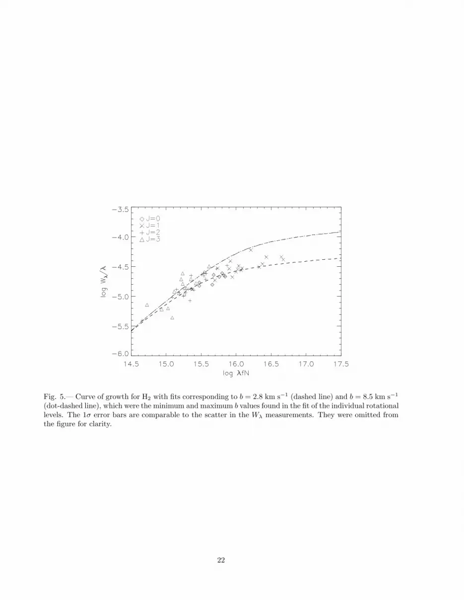
Fig. 5.— Curve of growth for H2 with fits corresponding to b = 2.8 km s−1 (dashed line) and b = 8.5 km s−1

(dot-dashed line), which were the minimum and maximum b values found in the fit of the individual rotationallevels. The 1σ error bars are comparable to the scatter in the Wλ measurements. They were omitted fromthe figure for clarity.

22

Fig. 6.— Continuum normalization for D I Wλ measurements. Panels a) - c) illustrate the method usedto measure Wλ of D I λ925.974 (Lyη) in the SiC2 channel and LWRS aperture. Panel a) shows the stellarmodel placement (smooth, solid line) over the data (histogram-style line). Panel b) shows the ISM model (H I

+ H2 only) relative to the spectrum normalized by the stellar model. Panel c) shows the ISM-normalizedspectrum from b) and the Gaussian fit to the D I Lyη profile used to measure the area of the line underthe continuum. The red side of the reconstructed D I profile is affected by large residuals from dividing bythe near-zero flux in the core of H I . Panels d)-f) show the same method applied to D I Lyγ in the samechannel and aperture. The weak feature in the blue wing of the stellar Lyγ model profile (panel d) is He II,while the stronger feature directly below it in the observed spectrum is interstellar D I .

23

Fig. 7.— The best fit curve of growth for D I (solid line) corresponding to log N(D I) = 14.99 ± 0.10 (2σ)and b = 5.2 km s−1. The dashed lines are the 1σ errors in the fit. The equivalent width data points, shownwith the wavelength of the transition and 1σ error bars, are the weighted average of Wλ from the SiC1 andSiC2 channels and the LWRS and MDRS observations.

24

Fig. 8.— The best fit curve of growth for O I (solid line) corresponding to log N(O I) = 16.23 ± 0.08(2σ)and b = 4.46 km s−1. The dashed lines are the 1σ errors in the fit. The equivalent width data points, shownwith the wavelength of the transition and 1σ error bars, are the weighted average of Wλ from the SiC1 andSiC2 channels and the LWRS and MDRS apertures.

25

Fig. 9.— The fits of D I Lyǫ λ937.5, Lyζ λ930.5, Lyη λ926.0, and Lyι λ920.7 for the SiC2 channel and LWRSaperture are shown on a relative velocity scale. The histogram lines represent the data, the thick solid linesare the final fits to the spectrum, and the dashed lines are the fits after deconvolution with the LSF. Notethat no D I lines stronger than Lyǫ were used since this transition is already optically thick (τ0 ∼ 2). Notealso D I Lyζ is blended with H2(J = 1) and H2(J = 2). The profile fitting technique recovers the informationfor the D I profile contained in the data.

26

Fig. 10.— Fe II λ2344 and λ2382 line profiles from HST/STIS E230H spectra of BD+28◦ 4211 are comparedwith the best fit model and shown on a heliocentric velocity scale. The smooth solid line is the bestfit obtained with three components. The histogram line is the normalized spectrum. 70% of the totalcolumn density is in the dominant component (right), 27% in the middle component, and 3% in the weakestcomponent (left). The two stronger components are separeted by less than 8 km s−1 and are not resolvedin Fe II features present in the FUSE spectra of BD+28◦ 4211.

27

Fig. 11.— Profile fits to three optically thin O I lines (λλ919.92, 925.45, and 930.26). The top panels showsthe fits for the SiC2 channel LWRS aperture spectra. The bottom panel shows the same transitions for thesame channel but MDRS aperture. The definitions of the different line styles are the same as Figure 9. Bothdata sets are very similar, with a LSF FWHM ∼ 20 km s−1 for LWRS and ∼ 18 km s−1 for MDRS.

28

Fig. 12.— Profile fits to the N I λ952 multiplet. The top panels shows the fits to the spectrum for theSiC2 channel and the LWRS aperture. The bottom panel is the same channel for the MDRS aperture. Thedefinitions of the different line styles are the same as Figure 9. The spectral resolution in the two data setsare very similar. Note the H2 L14 − 0 P(3) line on the blue side of the triplet. This N I triplet is the onlyone available in the FUSE bandpass that is not optically thick and free of significant interference by lines ofother species.

29

Table 1

FUSE Observations of BD+28◦ 4211

Program ID Date Aperture FP-split Offset ∆λ Exposures Exp. Timepos No. (pixels) (A) (s)

M1080901 Jun 13 2000 LWRS · · · · · · · · · 1–4 2192M1040101 Jul 16 2000 LWRS 1 −27 −0.17 1–14 6251

2 0 0.00 14–25 50733 +7 +0.04 26–30 24544 +36 +0.23 31–36 2799

M1040105 Sep 19 2000 LWRS 3 +7 +0.04 1–8 36914 +36 +0.23 9–17 4146

M1040102 Jul 17 2000 MDRS 1 −12 −0.08 1–13 62792 0 0.00 14–30 82113 +5 +0.03 31–42 57954 +12 +0.08 43–52 4540

Table 2

Properties of BD +28◦ 4211

Quantity Value Reference

Spectral Type sdO 1l 81.87◦ 2b −19.29◦ 2da (pc) 104 ± 18 2V 10.53 3U − B −1.26 3B − V −0.34 3vhel +20.2 ± 0.8 km s−1 4Teff (K) 82,000 1log g (cm s−2) 6.2 1log(He/H) −1.0 1

aTrigonometric parallax

References.—(1) Napiwotzki 1993; (2) Perry-man et al. 1997; (3) Kidder et al. 1991; (4) Thispaper (§4).

30

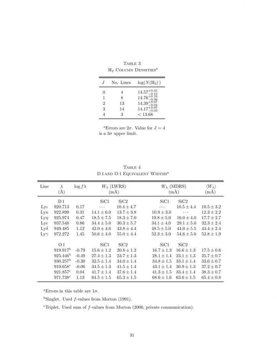
Table 3

H2 Column Densitiesa

J No. Lines log(N(H2) )

0 4 14.57+0.45−0.15

1 8 14.76+0.16−0.06

2 13 14.39+0.07−0.04

3 14 14.17+0.05−0.03

4 3 < 13.68

aErrors are 2σ. Value for J = 4is a 3σ upper limit.

Table 4

D I and O I Equivalent Widthsa

Line λ log fλ Wλ (LWRS) Wλ (MDRS) 〈Wλ〉(A) (mA) (mA) (mA)

D I SiC1 SiC2 SiC1 SiC2Lyι 920.713 0.17 · · · 10.4 ± 4.7 · · · 10.5 ± 4.4 10.5 ± 3.2Lyκ 922.899 0.31 14.1 ± 6.0 13.7 ± 3.8 10.9 ± 3.0 · · · 12.3 ± 2.2Lyη 925.974 0.47 18.5 ± 7.5 18.3 ± 7.0 19.8 ± 5.0 16.0 ± 4.0 17.7 ± 2.7Lyǫ 937.548 0.86 34.4 ± 5.0 30.3 ± 5.7 34.1 ± 4.0 29.1 ± 5.0 32.3 ± 2.4Lyδ 949.485 1.12 42.0 ± 4.6 43.8 ± 4.4 48.5 ± 5.0 44.0 ± 5.5 44.4 ± 2.4Lyγ 972.272 1.45 50.6 ± 4.0 55.0 ± 4.4 52.3 ± 3.0 54.6 ± 5.0 52.8 ± 1.9

O I SiC1 SiC2 SiC1 SiC2919.917b -0.79 15.6 ± 1.2 20.8 ± 1.2 16.7 ± 1.3 16.6 ± 1.3 17.5 ± 0.6925.446b -0.49 27.4 ± 1.3 23.7 ± 1.3 28.1 ± 1.4 23.1 ± 1.3 25.7 ± 0.7930.257b -0.30 32.5 ± 1.4 34.0 ± 1.4 34.8 ± 1.5 33.1 ± 1.4 33.6 ± 0.7919.658c -0.06 34.5 ± 1.3 41.5 ± 1.4 43.1 ± 1.4 30.9 ± 1.3 37.2 ± 0.7921.857c 0.04 41.7 ± 1.4 37.6 ± 1.4 41.3 ± 1.5 33.4 ± 1.4 38.3 ± 0.7971.738c 1.13 64.5 ± 1.5 65.3 ± 1.5 68.6 ± 1.6 63.6 ± 1.5 65.4 ± 0.8

aErrors in this table are 1σ.

bSinglet. Used f -values from Morton (1991).

cTriplet. Used sum of f -values from Morton (2000, private communication).

31

Table 5

N(O I) from Curve of Growtha

Channel Aperture log(N(OI)) b( cm−2) ( km s−1)

SiC1 LWRS 16.22± 0.10 4.46SiC1 MDRS 16.25± 0.06 4.83SiC2 LWRS 16.29± 0.16 4.41SiC2 MDRS 16.18± 0.18 4.24

aErrors in this table are 2σ.

Table 6

D I , N I, and O I Profile Fitting Resultsa

Case No. DOF χ2min b log N(D I) log N(N I) log N(O I)

Windows ( km s−1) ( cm−2) ( cm−2) ( cm−2)

Case 1b 39 1444 1674 4.0 14.99 ± 0.05 15.51 ± 0.05 16.22 ± 0.09Case 2c 39 1405 1441 4.2 14.99 ± 0.07 15.57 ± 0.09 16.22 ± 0.16Case 3d 41 1527 1929 3.8 + 3.3 14.96 ± 0.05 15.49 ± 0.05 16.17 ± 0.06

aErrors in this table are 2σ.

bOne Gaussian component, LSF fixed for each channel (SiC1 or SiC2).

cOne Gaussian component, LSF free to vary from window to window.

dThree Gaussian components as defined by Fe II velocity structure, LSF fixed for eachchannel (SiC1 or SiC2). See text.

Table 7

D I , N I, and O I Column Densities a

Ion Profile Fitting Mean COG AdoptedSolution

log(N(D I) ) ( cm−2) 14.99± 0.03 14.99± 0.10 14.99± 0.05log(N(N I) ) ( cm−2) 15.55± 0.13 · · · 15.55± 0.13log(N(O I) ) ( cm−2) 16.21± 0.10 16.23± 0.08 16.22± 0.10

aErrors in this table are 2σ.

32

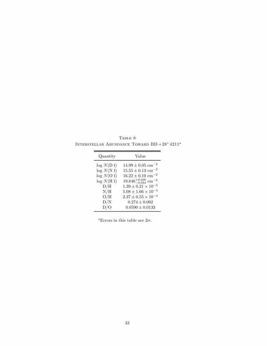
Table 8

Interstellar Abundance Toward BD+28◦ 4211a

Quantity Value

log N(D I) 14.99± 0.05 cm−2

log N(N I) 15.55± 0.13 cm−2

log N(O I) 16.22± 0.10 cm−2

log N(H I) 19.846+0.036−0.034 cm−2

D/H 1.39 ± 0.21 × 10−5

N/H 5.08 ± 1.66 × 10−5

O/H 2.37 ± 0.55 × 10−4

D/N 0.274± 0.092D/O 0.0590± 0.0133

aErrors in this table are 2σ.

33